of gross product and purchasing power , 'f'JS - World Bank ...
316
Public Disclosure Authorized Public Disclosure Authorized Public Disclosure Authorized Public Disclosure Authorized 13386 A system of international comparison~ of gross product and purchasing power , 'f'JS IRVING B. KRAVIS • ZOLTAN KENESSEY • ALAN HESTON • ROBERT SUMMERS liDL~, FILE COPY _ .... ~,,- · 11111........ . .,, ..... ,a.cg.WWW ~~udl _,.,,,, --- Public Disclosure Authorized Public Disclosure Authorized Public Disclosure Authorized Public Disclosure Authorized
-
Upload
khangminh22 -
Category
Documents
-
view
1 -
download
0
Transcript of of gross product and purchasing power , 'f'JS - World Bank ...

Pub
lic D
iscl
osur
e A
utho
rized
Pub
lic D
iscl
osur
e A
utho
rized
Pub
lic D
iscl
osur
e A
utho
rized
Pub
lic D
iscl
osur
e A
utho
rized
13386
A system of international comparison~ of gross product and purchasing power , 'f'JS IRVING B. KRAVIS • ZOLTAN KENESSEY • ALAN HESTON • ROBERT SUMMERS
liDL~, FILE COPY _ .... ~,,- ·
11111........ . .,, ..... ,a.cg.WWW ~~udl _,.,,,, ---
Pub
lic D
iscl
osur
e A
utho
rized
Pub
lic D
iscl
osur
e A
utho
rized
Pub
lic D
iscl
osur
e A
utho
rized
Pub
lic D
iscl
osur
e A
utho
rized


A system of international comparisons of gross product and purchasing power


UNITED NATIONS INTERNATIONAL COMPARISON PROJECT: PHASE ONE
A system of international comparisons of gross product and purchasing power PRODUCED BY THE STATISTICAL OFFICE OF THE UNITED NATIONS, THE
WORLD BANK, AND THE INTERNATIONAL COMPARISON UNIT OF THE
UNIVERSITY OF PENNSYLVANIA
Irving B. Kravis • Zoltan Kenessey • Alan Heston • Robert Summers
with the assistance of SULTAN AHMAD, ALICIA CIVITELLO, SAMVIT P. DHAR,
MICHAEL McPEAK, ALFONSO PARDO-GUTIERREZ, LORENZO PEREZ,
ALFONSO UONG, DONALD WOOD, JR., and ANTONIO YU
PUBLISHED FOR THE WORLD BANK BY
The Johns Hopkins University Press • Baltimore and London

Copyright© 1975 by the International Bank for Reconstruction and Development 1818 H Street, N.W., Washington, D.C. 20433
Library of Congress Catalog Card Number 73-19352 ISBN 0-8018-1606-8 (cloth) ISBN 0-8018-1669-6 (paper)
All rights reserved :Manufactured in the United States of America
Library of Congress Cataloging in Publication data will be found on the last printed page of this book.

Contents
Preface vii
Introduction ix
PART I OBJECTIVES AND MAIN RESULTS
I. The Nature of the Study and the Main Results A. The Nature of the Study . . . . . . . . . . . . . I B. A Thumbnail Sketch of the Methods. . . . . . 4 C. The Main Results . . . . . . . . . . . . . . . . . . 5 D. A Note of Warning and Guidance . . . . . . . 10
PART II METHODS
2. Conceptual Problems A. The Validity of Making International
Comparisons . . . . . . . . . . . . . . . . . . . . . 17 B. Alternative Approaches to International
Comparisons . . . . . . . . . . . . . . . . . . . . . 19 C. The Meaning of Output . . . . . . . . . . . . . . 20 D. The Concept of Price . . . . . . . . . . . . . . . 23
3. Organizing the Basic Data A. The Classification System . . . . . . . . . . . . 26 B. The Sampling of Price Ratios . . . . . . . . . . 28 C. The Matching of Qualities . . . . . . . . . . . . 31 D. Processing the Basic Data . . . . . . . . . . . . . 34 A note on conceptual adjustments needed for MPS countries. . . . . . . . . . . . . . . . . . . . . 34 Appendix: The International Comparison Project Classification System . . . . . . . . . . . . . 37
4. Methods of the Binary Comparisons A. The Desired Properties . . . . . . . . . . . . . . . 46 B. Averaging within Detailed Categories . . . . . 47 C. Aggregation . . . . . . . . . . . . . . . . . . . . . . 49 D. Bridge-Country Binary Comparisons . . . . . 50
5. Methods of the Multilateral Comparisons A. The Desired Properties . . . . . . . . . . . . . . 54 B. Estimating PPPs at the Detailed-Category
Level (Frequency-Weighted CPD) . . . . . . . 55 C. Filling Holes in the Matrix of PPPs for
the Categories (Double-Weighted CPD) 63 D. Alternative Aggregation Methods . . . . . . . 65 E. From Representative Countries to
"Supercountries" . . . . . . . . . . . . . . . . . . 71 F. Comparison of Different Aggregation
Methods . . . . . . . . . . . . . . . . . . . . . . . 75 G. Measures oflmprecision . . . . . . . . . . . . . 77
6. Comparing Consumer-Goods Prices A. General Procedures . . . . . . . . . . . . . . . . . 80 B. Price Collection in Individual Countries . . . 81 C. Special Problems in Particular Consumer-
Goods Categories . . . . . . . . . . . . . . . . . . 85
7. The Role of Quantity Comparisons A. Medical Care . . . . . . . . . . . . . . . . . . . . . 94 B. Education . . . . . . . . . . . . . . . . . . . . . . . 100
8. Matching Qualities by Regression Methods A. Methodological Issues . . . . . . . . . . . . . . . 104 B. The Automobile Price Comparisons . . . . . . I 08
9. Rent Comparisons A. Conceptual Problems . . . . . . . . . . . . . . . 117 B. The Data ..................... 119 C. The Binary Comparisons . . . . . . . . . . . . . 124 D. The Multilateral Comparisons .......... 143 E. Summary of Rent and Quantity Comparisons
for Housing, 1970 ................. 146
V

vi CONTENTS
Contents (Continued)
10. Comparing Prices of Producers' Durables A. Choosing Specifications ............. 147 B. The Collection of Data . . . . . . . . . . . . . . 148 C. Matching Techniques ............... 149 D. Data Processing ................... 152 Appendix 1. Producers' Durable Goods for Which Price Comparisons Were Made . . . . . . . 153 Appendix 2. Imputations for Missing Price Comparisons in Producers' Durable-Goods Categories ......................... 154
11. Comparing the Prices of Construction A. The General Approach ............... 155 B. Matching Procedures ............... 157 C. Data Processing ................... 159
12. Comparison of Government Services A. The Scope of Government Services ....... 160 B. Adjustments for Productivity Differences .. 161 C. Comparison of Compensation of
Government Employees .............. 162 D. Government Purchases of Commodities ... 163 E. Measurement Problems .............. 164
PART III THE RESULTS OF THE COMPARISONS
13. Results of the Binary Comparisons A. The Major Aggregates ............... 169 B. Analysis of Subaggregates ............. 188 Appendix. Detailed Binary Tables ......... 195
14. Results of the Multilateral Comparisons A. An Explanation of the Tables . . . . . . . . . . 228 B. The Results of the Comparisons . . . . . . . . . 229 Appendix. Detailed Multilateral Tables ...... 244
15. Some Applications of the Data A. Similarity Indexes ................. 267 B. Quantities and the Roles of Price and
Income Differences . . . . . . . . . . . . . . . . . 279
Glossary ............................. 287
Index ............................... 291

Preface
International comparisons of production, consumption, and investment are indispensable for the analysis of economic and social development. As a result of work over the past two decades by national statistical offices, the United Nations and other international organizations, data on national income and expenditure are becoming more and more comparable from the standpoint of statistical methodology.
However, even where standard methodology has been adopted to produce national estimates of these aggregates, a major limitation to comparability has been the inadequacy of official exchange rates for purposes of converting estimates in national currencies to a common basis of valuation. Careful estimates by other means require large resources and sustained effort; as a result only a few have so far been made. Studies, such as the pioneering comparisons of the Organisation for Economic Cooperation and Development under Gilbert and Kravis, and the work of the Council for Mutual Economic Assistance and the Economic Commission for Latin America, have been limited to relatively homogeneous groups of countries. Thus, at the end of the 1960s no adequate basis existed for comparisons on a worldwide scale.
The long-term aim of the work begun by the United Nations International Comparison Project in 1968 was to fill this important gap in international statistics by developing detailed intercountry comparisons for gross domestic product and the purchasing power of currencies. The results of the first stage of this effort are presented in this report. An extension of the project to cover additional countries is currently under way.
A number of sources have provided financial support for this work. We are pleased to acknowledge the major contribution made by the Ford Foundation to the initial phases of this project through a grant to the University of Pennsylvania as well as the continuing contribution of the Government of the Netherlands to the United Nations Trust Fund for Development Planning and Projections, which has helped to finance the work, and also directly to the project for its current extension. The International Bank for Reconstruction and Development (World Bank) has provided substantial assistance for the past several years, as has the United States Agency for International Development. Extensive assistance in kind has been provided by the Statistical Office of the European Economic Community. Other important contributors to the extension of this work are: The Danish International Development Agency; the German Bundesministerium filr Wirtschaftliche Zusammenarbeit; the Norwegian Development Agency; and the United Kingdom Ministry of Overseas Development. We also wish to thank statisticians in all the participating countries for their very valuable contributions to this undertaking. Finally, we are especially pleased to introduce this report as the result of a joint effort of the United Nations and the World Bank.
HOLLIS B. CHENERY Vice President, Develop
ment Policy International Bank for
Reconstruction and Development
JACOB L. MOSAK
Deputy to the Undersecretary-General for Economic and Social Affairs
United Nations
vii


Introduction
The past two decades have witnessed the rapid development of work at the national level on the estimation of product, income, and expenditure aggregates. As a result, an increasing number of countries in all regions of the world regularly publish such estimates. 1 These data are widely used at the national level for economic policymaking, planning, and research.
But as yet the use of the same data in the international context has been less successful. There are two main prerequisites for the successful use of the growing wealth of estimates of national product, income, and expenditure-at either the national or the international level-for country-to-country comparisons. The first prerequisite is the adoption of comparable methodological principles (standard definitions, classifications, frameworks, and the like by the estimators in the different countries, or the possibility of rearranging national estimates according to standard methodological procedures. The second is the introduction of comparable valuation with regard to the product, income, and expenditure aggregates, generally estimated in value terms of national currencies.
Significant results have been achieved, and much work is in progress to meet the challenge of the first prerequisite, especially in regard to the United Nations new System of National Accounts (SNA), which was issued at the end of 1968.
At the end of the 1960s, however, the situation was far less satisfactory with respect to comparable valuation. Because official exchange rates could not be relied upon to convert the estimates of different countries, a special effort was required to develop an intercountry set of comparisons of national accounts aggregates on a comparable basis of valuation.
1The 1970 United Nations Yearbook of National Accounts Statistics presented national accounts estimates for ninety-four countries and territories.
The Statistical Commission of the United Nations, at its thirteenth session held in the spring of 1965 in New York, discussed at some length the conversion problem involved in comparing national accounting aggregates expressed in national currencies. In this discussion, the Statistical Commission agreed that this problem was important and that the solution obtained by using currency conversion rates based directly or indirectly on prevailing exchange rates was inadequate for many purposes. At that time, however, the Commission considered that the alternative of exhaustively repricing the relevant product and expenditure flows was not practicable for most countries, "although it might form the basis of a definitive solution for the statistically advanced countries if undertaken at relatively infrequent intervals. " 2
Therefore, the Commission welcomed the proposal of the Secretariat to begin systematic work on this subject as resources permitted, and it recommended, as a first step, that a study should be made of all available experience and data in the field at the international, regional, and national levels, with the aim of formulating more specific proposals for this work.
The recommended study was undertaken in 1967, and a report entitled "International Comparisons of Production, Income and Expenditure Aggregates" was submitted to the fifteenth session of the Statistical Commission, held early in 1968 in New York. The purpose of the report was to outline a project on the subject, which was prepared for the years 1968-71, to carry out comparisons for a selected number of countries and develop, test, and describe suitable techniques for the more comprehensive comparisons to be carried out at subsequent stages of the work. Because of the limited resources available in the U.N. budget for statistical purposes,
2 U.N. Statistical Commission, Report of the Thirteenth Session, April 20-May 7, 1965 (New York: United Nations, 1965), para. 77.
ix

x INTRODUCTION
members of the Commission considered that "the project might be organized on the basis of participation by additional international organizations and considerable assistance from Member States. " 3
The U.N. International Comparison Project, which began its activities later in 1968, indeed became a cooperative undertaking. The central project staff was organized in two units, one located at U.N. headquarters, the other at the University of Pennsylvania. To enable the creation of the latter unit, the Ford Foundation generously made a major contribution in the form of a grant to the university. The World Bank provided substantial financial aid, and the statistical offices of the participating countries made substantial and essential contributions in real terms. Financial support also was provided, mainly for the work in India, by the U.S. Agency for International Development and, for collaboration with Japanese statisticians, by the U.S. Social Science Research Council.
The director of the U.N. Statistical Office maintained general supervision over the development of the project. The immediate responsibility for the undertaking rested with the project director, located in Philadelphia, artd the associate project director, located in New York, who were in continuous communication with each other. For the initiation of the work, helpful advice was obtained from an Advisory Board.4
Detailed proposals for the project, entitled "Plans for International Product and Purchasing Power Comparison," were issued as a separate document in August 1968. As a result of suggestions received from members of the Advisory Board and from statisticians in cooperating international agencies, as well as on the basis of the experience with the beginning of the practical work of the comparisons, an expanded and revised set of proposals was issued in September 1969 under the title "Methods for International Product and Purchasing Power Comparisons." These proposals were discussed at a meeting of the Advisory Board, held in October 1969 in Bellagio, Italy.
In the execution of the project, arrangements were made to draw upon the work and strength of numerous international organizations and bodies. Within the United Nations, personnel from the statistical divisions
3 U.N. Statistical Commission, Report of the Fifteenth Session, February 26-March 8, 1968 (New York: United Nations, 1968), para. 42.
4 The Advisory Board consisted of the following persons: P. J. Loftus, United Nations (chairman); W. Beckerman, Oxford University; R. Bowman, U.S. Bureau of the Budget; U. Chand, Central Statistical Organization, India; M. Gilbert, Bank for International Settlements, Switzerland; E. Krzeczkowska, Central Statistical Office, Poland; S. Kuznets, Harvard University; M. Mod, Central Statistical Office, Hungary; J. Mosak, United Nations; R. Ruggles, Yale University and U.S. National Bureau of Economic Research; R. Stone, Cambridge University; and S. Tsuru, Institute of Economic Research, Japan. The project director was Irving B. Kravis and the associate director was Zoltan Kenessey.
of the Economic Commission for Africa (ECA), the Economic Commission for Europe {ECE), and the Economic Commission for Latin America (ECLA) lent their experience and skills to certain stages of the work. The Statistical Office of the European Economic Community (EEC) agreed to coordinate closely its comparisons among the then six member countries of EEC with the U.N. International Comparison Project and to participate intensively in those comparisons of its member countries with the United States which were carried out in the U.N. project. 5 The Brookings Institution made available its experience in closely related work in Latin America.
In the countries reported on in the present volume, the following national institutions were most active in supplying materials for and participating in the work:
Colombia: mainly the Departamento Administrativo Nacional de Estadistica, but also the Centro de Estudios Desarrollo Econ6mico at the Los Andes University and the Banco de la Republica Hungary: the Hungarian Central Statistical Office India: the Central Statistical Organization of the Government of India Japan: the Bureau of Statistics in the Office of the Prime Minister, the Economic Research Institute of the Economic Planning Agency, and the Institute of Developing Economies Kenya: the Statistical Division in the Ministry of Finance and Planning United Kingdom: the Central Statistical Office in the Cabinet Office, the Economic and Statistics Division of the Department of Trade and Industry, the Statistics Division of the Department of Employment, and the Department of Environment United States: the Statistical Policy Division of the Office of Management and Budget in the Executive Office of the President, the Bureau of Labor Statistics, and the National Income Division of the Office of Business Economics In respect to France, the Federal Republic of Germany, and Italy, the work was carried out in cooperation with the Statistical Office of the European Economic Community in Luxembourg. It is not possible to acknowledge all the individuals
who assisted in the work, but mention should be made of Dorothy Brady, Polibio Cordova, Alan Gleason, Pal Koves, Angus Maddison, Gyorgy Szilagyi, and L. Zienkowski, who rendered valuable advice in the formative stages of the project. In the course of the actual provision of the data, particular appreciation goes to Alvaro Velasquez-Cock, Jorge A. Celis, Ernesto Rojas-Morales, German Botero de los Rios, Jaime Sabogal, Jesus M. Tello, Rafael Isaza, and Rafael Prieto of Colombia; Albert Racz, Margaret Mod, Jozsef Tar, Gyorgy Szilagyi,
5The project methodology was discussed initially by the statistical experts of the EEC countries at a special meeting held in Luxembourg with the participation of the director and the associate director of the U.N. International Comparison Project.

Adam Marton, Szaboles Rath, and Mihaly Zafir of Hungary; B. W. Chavan, R. M. Chatterjee, L. N. Rastogi, N. K. Chandekar, Girdhar Go pal, and R. N. Lal of India; Sadanori Nagayama, Tsu-tomu Noda, and Mytsuru Ide of Japan; Parmeet Singh of Kenya; John Ayris, Bernard Brown, Peter Capell, John Dearman, Jack Hibbert, Rita Maurice, Bill Osborn, Alec Sorrell, and Laurence Surman of the United Kingdom; Milton Moss, John Musgrave, Janet Norwood, and Winifred Stone of the United States; and Guy Bertaud, Phillippe Goybet, Hugo Krijnse-Locker, Vittorio Paretti, and Silvio Ronchetti of the EEC.
Aid with the price collection in various countries was given by Najib Banabila, William Berry, Mary Lou Drake, Wilma Heston, Ethel Hoover, and Karren Wood. Assistance in the work of the central staff was provided by Jill Brethauer, Betsy Burton, Susan Colson, Beatrice Fitch, Mitchell Kellman, Kurt Kendis, Jean Kunkel, Linda Robson, Jane Samuelson, Michelle Turnovsky, and Carl Weinberg. Jorge Salazar and Stanley Braithwaite provided helpful links with the related work of the Brookings Institution and the Economic Commission for Latin America, respectively. Bela Balassa, Wilfred
INTRODUCTION xi
Beckerman, Abram Bergson, J.P. Hayes, Salem Khamis, Moni Mukherjee, Joel Popkin, Nancy Ruggles, and Richard Ruggles gave valuable advice on an earlier draft of this report. From the beginning to the final stage, Laszlo Drechsler was a thoughtful and constructive critic. Peter E. de Janosi of the Ford Foundation and John Edelman and Elinor Yudin of the World Bank provided sympathetic and effective liaison with these supporting organizations. The effective support of the directors of the U .N. Statistical Office, Patrick J. Loftus, Abraham Aidenoff, and Simon Goldberg, made possible the execution of the project.
The active participation of the various national and international authorities in the project and the gracious help continuously enjoyed by the central project staff from these colleagues and from their institutions were of the greatest importance for the success of the work and are most appreciatively acknowledged. Goddard W. Winterbottom provided thoughtful and professional editorial guidance and also prepared the volume's index. Responsibility for the methods applied and the results obtained, of course, rests entirely with the central project staff.


A system of international comparisons of gross product and purchasing power


Part I
Objectives and main results


Chapter 1
The nature of the study and the main results
A. The Nature of the Study
THE PROBLEM The lack of accurate data on comparative levels of
output and income in different countries is an important gap in the knowledge of the world economy. When such comparisons are required, the usual practice is to convert the outputs of the various countries to U.S. dollars or some other common currency through the use of official exchange rates. But as any traveler knows, the official exchange rates do not reflect the relative purchasing powers of different currencies, and thus errors are introduced into the comparisons. These errors often may be small, as is probably the case between the currencies of the United States and Canada, 1 but they can be quite large as well. An earlier study found, for example, that US$1,000, when converted to sterling at the official exchange rate, bought a basket of U.K. goods 64 percent larger than the dollars could have purchased in the United States.2 In the study reported upon here, the purchasing power of sterling was 52 percent greater in terms of the U.K. basket of goods in 1970.
The difficulties of using exchange rates to convert the output of different countries into a common currency are compounded when exchange rates themselves change. For example, in view of the 16.9 percent upward evaluation of the yen in the Smithsonian agreement of late 1971, the use of exchange rates to convert gross domestic product (GDP) of Japan to U.S. dollars would produce for the ensuing year a 16.9 percent increase in the estimate of Japanese per capita GDP relative to that of the United States even if no change had occurred in the per capita GDP of either country in terms of its own currency.
1 See Economic Council of Canada, Second Annual Review (Ottawa: The Council, December 1965), p. 51.
2 M. Gilbert and I. Kravis, An International Comparison of National Products and the Purchasing Power of Cu"encies
Reasonably accurate comparisons of intercountry differences in production, incomes, and purchasing power of currencies are required for a wide variety of purposes. They are useful in any effort to understand the process of economic growth and development. Because product, income, and expenditure aggregates are fundamental variables in most models of growth or development, the lack of internationally comparable data of this kind impairs the validity of cross-sectional comparisons of stages of economic development or judgments on the success of development efforts. This is true whether interest lies in savings or investment ratios, the composition of real output, growth rates, the role of government, or a number of other critical aspects of development.
Such comparisons also are useful for policy purposes at the international and national levels. For example, an appreciation of the differences in the level of income is important in the allocation of aid au'd in the judgment of its efficacy. It is relevant as well to international burden sharing, whether for current costs of international bodies or for developmental or military objectives.
At the national level, it is important for planning purposes that both developed and underdeveloped countries be able to anticipate the patterns of expansion in final demand as income levels rise. Without internationally comparable income, output, and expenditure indicators, it is difficult to use the experience of wealthier countries to anticipate the time pattern of the changes that may be expected to occur in the development of the poorer ones. And, as in Western Europe, Eastern Europe, and Latin America, income and price comparisons may help illuminate potential or actual problems created by regional economic integration.
One evidence of the widespread feeling of need for international comparisons of the kind offered here is the
(Paris: Organization for European Economic Cooperation, 1954), pp. 22-23.

2 OBJECTIVES AND MAIN RESULTS
fact that so many organizations concerned with international economic problems have attempted to produce their own estimates of per capita income relationships between countries: for example, the U.N. Statistical Office, the Organization for European Economic Cooperation (OEEC),3 the Council for Mutual Economic Assistance (CMEA), the International Bank for Reconstruction and Development (World Bank), the Economic Commission for Latin America (ECLA), and a number of governments, including those of Canada, the Federal Republic of Germany, Japan, the Soviet Union, and the United States. In addition, a number of estimates have been made by individuals, and many of these are in the public domain. Virtually all of the private estimates and some of the official ones are based on armchair calculations. Although many of these may come closer to the truth than the simple conversion at official rates of exchange, a more solid and consistent basis for the estimates nonetheless is to be desired. Unfortunately, estimates for which field work has been done vary widely in the intensity and quality of the effort.
From the world standpoint, the aggregate effort that has gone into these comparisons has not been as productive as a well-coordinated effort would have been. The coverage of countries is not narrow, but the studies have been so varied in time and method that an incomplete jigsaw puzzle of comparisons has been the result. No useful worldwide system of consistent, reliable comparisons covering a substantial number of countries has been produced. More than that, no uniform framework has been laid down that can be used as the basis for an expanded and continuing coverage of countries over time.
THE PURPOSE OF THE INTERNATIONAL COMPARISON PROJECT
The U.N. International Comparison Project (ICP) represents a cooperative effort, under the aegis of the U.N. Statistical Office, to establish such a system of comparisons of real product and purchasing power.
The initial phase of the ICP, reported in this volume, had two main purposes: first, to work out the methods for the system of international comparisons, and, second, partly an end in itself and partly an adjunct to the first purpose, actually to make such comparisons for a group of countries selected to provide a variety of countries with respect to income levels, systems of economic organization, and locations.
In light of the latter consideration, we were fortunate to have obtained the cooperation of the following countries for the initial set of comparisons: Colombia, Hungary, India, Japan, Kenya, the United Kingdom, and the
3 Now the Organization for Economic Cooperation and Development (OECD).
United States. In addition, the European Economic Community (EEC), which carried out a comparison among its six constituent countries and with some outside countries for the year 1970, coordinated its work closely with the ICP. The governments of France, the Federal Republic of Germany, and Italy authorized the EEC Statistical Office to provide the ICP with the necessary data for the comparisons. For expository convenience, these three countries are referred to as the "EEC countries," although the passage of time has made the United Kingdom an EEC country as well.
Thus, the countries in the first phase include several major developed market economies, several developing countries, and one centrally planned economy. From the regional point of view, Africa, Asia, Europe, Latin America, and North America are represented. The countries also differ widely with respect to population, area, climate, mores, and degree of dependence on other countries or trading blocs. Finally, the relative importance of the nonmarket sector varies significantly among the countries.
Real product and purchasing-power comparisons are presented herein for these ten countries for 1970 and for six of them for 1967 as well. The comparisons relate not only to GDP as a whole, but also to consumption, capital formation, and government.4 The results for GDP and three main subaggregates for 1970 are summarized in later parts of this chapter. In following chapters, estimates are provided for a more detailed breakdown-for both the ten countries in 1970 and the six countries in 196 7.
In addition to the methodological work itself, a manual for carrying out international comparisons has been prepared. The standardization and systematization thus proposed have important advantages. Standardization helps to ensure that the data for countries added to the system in subsequent phases will be comparable to the data for the first-phase countries. Systematization will reduce greatly the costs of introducing new countries into the present ten-country network of international comparisons. Country coverage already is being extended, and it is hoped that the network will be expanded at a more rapid rate in the future.
RELATION OF THE ICP TO ITS ANTECEDENTS Behind the work of the ICP lies substantial progress
in national accounts work in the world. Not only has the estimation and use of national accounts spread, but also there has been a notable movement toward the adoption of common methods (standard definitions, classifications, and the like) by national-income estimators in different countries.
4 For definitions of these terms, seep. 4.

In addition, a number of international comparisons have been made, at least for groups of relatively homogeneous groups of countries-namely, those of the OEEC,5 the CMEA,6 and the ECLA.7 Some pioneering work in comparisons between centrally planned and market economies has been carried out as well under the auspices of the Conference of European Statisticians.8
The nature of past experience and the character of the new problems have several implications for the design of the ICP. The techniques developed in the past work related mainly to comparisons focusing upon one pair of countries at a time: that is, to "binary" comparisons. Thus, it seemed logical to begin with these kinds of comparisons, although at the same time the project deliberately undertook to deal with a heterogeneous group of countries.
The general framework of the binary comparisons follows the OEEC studies of the early 1950s, but several major improvements over these studies have been made. First, the more extensive cooperation of the countries has enabled ICP to make a larger number of price comparisons with far more control over the comparability of quality than in the earlier studies. Second, for rents and some durable goods, so-called hedonic regression methods of international price comparisons have been employed (see Chapters 8 and 9). These methods, made feasible by the advances in economic theory and statistics and the advent of computers since the OEEC studies, allow us to hold constant across countries a number of different quality variables and thus to improve price comparability. Third, for construction, reliance has been placed almost entirely upon price comparisons for entire construction projects rather than for measured units of building operations (such as the laying of a certain number of bricks), upon which major reliance was placed in the earlier work.
Although the experience gained in the earlier studies provided valuable guidance for the present work, new problems had to be solved. For one thing, the very heterogeneity of countries created some difficult problems. For example, a common list of items for which price comparisons could be made for all countries had to be ruled out. In addition, ways had to be found to meet the problems posed by the existence in some countries
5Gilbert and Kravis, An International Comparison; M. Gilbert and Associates, Comparative National Products and Price Levels: A Study of Western Europe and the United States (Paris: 1958).
6 See L. Drechsler, Ertekbeni mutatoszamok nemzetkozi osszehasonlitasanak mbdszertang (Budapest: Kozgazdasagi es Jogi Konyvkiado, 1966) (with Bibliography).
7"The Measurement of Latin American Real Income in U.S. Dollars," Economic Bulletin for Latin America, XII (October 1967), pp. 107-142.
8Conference of European Statisticians, Comparison of Levels of Consumption in Austria and Poland, Document WG. 22/19, mimeo. (New York: United Nations, 1968).
THE NATURE OF THE STUDY AND THE MAIN RESULTS 3
of a large rural sector having a substantially different content of consumption from the more westernized urban sector.
The large number of countries eventually to be included in the network of comparisons made it clear that binary comparisons alone will not suffice. Binary comparisons between each pair of countries quickly reach an astronomical number; even the ten countries produce forty-five possible pairs (that is, n(n - 1)/2, where n is the number of countries). Therefore, it was important to design the binary comparisons so that they could be fit into a broader framework in which a large number of countries are compared simultaneously. An essential feature of these "multilateral" comparisons, as we refer to these simultaneous comparisons, is that the circular test, or transitivity requirements, is satisfied. That is,/; 1 k
= I;11 -'c-[k/l' where !ilk is a price or quantity index for the jfh country relative to the kth country, and l is a third country. A set of binary comparisons, when each pair of countries is compared directly, will not necessarily possess this property. Chapter 4 returns to this question.
Another consideration arising out of the large number of countries eventually to be included-and also out of the need to keep estimates up to date-was the importance of cost reduction either through the development of shortcut methods or through greater efficiency.
TREATMENT OF DIFFICULT INDEX-NUMBER PROBLEMS
Like all makers of price and quantity indexes, ICP faced a number of methodological choices for which economic and statistical theory offers little or no guidance.
In meeting these issues, we had the benefit of the views of statisticians in the participating countries and in international agencies. These consultations helped the project to arrive at procedures that are more likely to find wide acceptance.
In some areas, however, particularly with respect to the multilateral comparisons, it was necessary to break new ground. The sanction of established usage cannot be claimed here, but, as we have suggested above, the need for a world system of comparisons requires some such development.
Our response to this situation has been along the following lines: First, we have tried to set out these problems, indicating the advantages and disadvantages of each of a number of alternative solutions and our reasons for the choices we made. Second, for the major aggregates, we show more than one set of results. Third, we provide far more detailed data than ordinarily would be regarded as publishable in order to furnish the building blocks for those who wish to handle the data in ways that are different from the ones we finally followed.

4 OBJECTIVES AND MAIN RESULTS
B. A Thumbnail Sketch of the Methods
The methods of the study, as already noted, form the subjects of subsequent chapters. In order to make the main results intelligible to the general user who does not intend to go into the details of the methods however a brief outline is provided here. ' '
GENERAL CONCEPTS Comparisons are made in terms of expenditures on
GDP, its main subdivisions, and detailed subcomponents. The concepts underlying the price and quantity measurements conform closely to the definitions in A System of National Accounts (SNA). 9
In the SNA breakdown of expenditures on GDP, the principle of classification for the main subaggregates is based on the type of transactor. The major transactors are (I) private households, (2) governments, and (3) enterprises purchasing on capital account; the (roughly) corresponding subaggregates are (i) private final consumption expenditure, (ii) government final consumption expenditure, and (iii) gross capital formation. 10 The use of this classification allows comparison for different countries of the real quantity of product purchased by households, the real quantity purchased by governments, and the real amount of capital formation. This is of great interest, of course, and the results on this SNA basis are presented in Chapter 13.
Within private final consumption expenditure, the SNA follows a familiar functional classification, dividing expenditures into such categories as food, clothing, and medical care. Where, as in most countries, both households and governments pay for some of the commodities and services in these functional categories, notably in the medical-care and education categories, the SNA calls for the inclusion of household expenditures only; government expenditure is included under government final consumption expenditure.
As a result, an international comparison of consumption categories that strictly followed SNA lines would not be especially informative for those categories in which the division of payments between households and governments varies from country to country. It would not allow a proper comparison, for example, of the total consumption of educational services by a society, but only of that part purchased by households in each country.
To obtain the desired aggregate amount of these general kinds of final expenditures-food, medical care,
9 U.N. Statistical Office, Studies in Method, Series F, Number 2, Rev. 2 (New York: United Nations, 1968).
1 ° Final expenditures represent purchases for the use of the buyer and not for resale or for embodiment in a product to be sold. "Gross capital formation" is defined for ICP purposes to include changes in stocks and net exports.
and the like-regardless of the varying degrees to which they are paid for by households or governments, we have assigned each general type wholly to "consumption" or to "government" in a uniform manner from country to country. Expenditures for health, education, recreation, and housing have been assigned to ICP "consumption," more formally labeled "Final Consumption Expenditure of the Population" (CEP). Services providing physical, social, and national security-those activities which are found rather consistently to be carried on by public authorities and financed by tax revenues-have been allocated to ICP "government," or, to use the formal term, to "Public Final Consumption Expenditure" (PFC). The line of demarcation between ICP consumption and government is discussed in Chapter 3. The expenditures shifted from SNA government to ICP consumption are tabulated in Table 13.15.
The purchasing-power parities (PPPs) and the price indexes are based in general on market prices: that is, the prices paid by final purchasers. The main exception to this occurs in those areas of consumption in which both households and governments make expenditures. In these cases, an effort has been made to price services rendered at the full cost to society, including payments by households and governments where they have been made by both. Similarly, in housing, an effort has been made to add the governmental subsidy component of rent to the rents paid by tenants.
These matters of classification and definition affect the meaning of the results and the uses to which they may be put. In particular, it should be noted that the ICP PPPs, even for consumption, are not invariably those faced by households. If, for example, a comparison were desired of the per capita or per household incomes of two countries derived from household survey data in each, these PPPs, reflecting the full social costs of important subsidized services, would have to be adjusted to take account of the differences in the provision of free or subsidized goods in the two countries.
THE METHODS OF THE MULTILATERAL COMPARISONS
Multilateral per capita quantity comparisons and price comparisons for GDP, consumption, capital formation, and government for 1970 are presented in the following pages for ten countries. A more detailed report on the comparisons will be found in Chapter 14. The multilateral comparisons represent, in our judgment, the most generally useful estimates that can be produced. Other methods produce somewhat different answers. These alternative results for a number of other methods that have found favor in one place or another are given in Chapters 4 and 5.
The methods we have chosen to produce the multilateral results yield a unique cardinal scaling of countries with respect to GDP and each of its components. They are not influenced by the particular country selected as

the base country. They enable us to present GDP in money terms in an "additive" matrix of numbers in which the rows represent components of GDP and the columns are countries. (By an additive matrix is meant one in which the numbers on any row indicate quantity relationships among the countries, whereas those in any column may be added to form GDP or some subaggregate thereof.) Finally, we have adopted methods based on a conception of the world price structure.
The world price structure comprises a set of average international prices based on the price and quantity structures of the ten countries included. Each of these ten countries plays a role in determining the structure of international prices, with allowances made for the extent to which each may be considered to represent excluded countries. The international prices have been used to value the quantities of each of the ten countries. The international prices and the product values they are used to obtain are expressed in "international dollars" (1$). An international dollar has the same overall purchasing power as a U.S. dollar for GDP as a whole, but the relative prices correspond to average "world" relative prices rather than to U.S. relative prices. Thus, the purchasing power of an international dollar over footwear or transport equipment, for example, is not the same as that of a U.S. dollar. As noted above, the results of the comparisons would have been the same if any other country had been taken as the numeraire country; if the currency of another country had been used as the basis for the computations, the numbers expressing the values of GDP and the like all would have been different only by a constant factor. The multilateral methods, summarized in this and the preceding paragraph, are explained more fully in Chapter 5.
C. The Main Results
THE MAJOR AGGREGATES IN NATIONAL CURRENCIES
Tables 1.l and l.2 show the major aggregates that usually are drawn upon for GDP comparisons. (Data for 1967 also are presented in these tables, although use will not be made of them until Chapter 13.) Table 1.l shows GDP in national currencies, exchange rates, and population figures. These materials lead to the figures on per capita GDP converted to U.S. dollars by means of exchange rates (column 9). According to these exchangerate conversions, the 1970 per capita GDPs of the other nine countries (column 10) varied from 2 percent of that of the United States, in the case of India, to 64 percent, in the case of Germany.
Table 1.2 shows the composition of GDP with respect to consumption, capital formation, and government. Capital formation varied in 1970 from 17 to 20 percent of GDP in Colombia, India, Kenya, the United Kingdom and the United States to about 30 percent in France, the
THE NATURE OF THE STUDY AND THE MAIN RESULTS 5
Federal Republic of Germany, and Hungary and over 40 percent in Japan.
Government, defined according to the ICP concept described above, accounted for 14 percent of U.S. GDP in 1970 and from 5 to 11 percent in other countries. Although separate figures for defense expenditures have not been gathered in the ICP, it seems clear that relatively large U.S. defense expenditures play a significant role in producing the larger governmental share in that country.
THE MAJOR AGGREGATES IN INTERNATIONAL DOLLARS
The results of the ICP's multilateral per capita quantity comparisons and price comparisons for GDP, consumption, capital formation, and government are presented in Tables l.3, 1.4, and 1.5. The ten countries in Table 1.3 have been arrayed from left to right in order of increasing 1970 per capita GDP. GDP per capita varied from 1$275 in Kenya to 1$4,801 in the United States (Table 1.3, line 4); in relative terms, the lowest per capita GDP, that of Kenya was 5.7 percent of that of the United States (line 12).
The results produced by the use of exchange rates are repeated from Table 1.1 for comparison (line 13). The extent of the difference betweep the ICP estimates and the exchange-rate-derived figures is indicated by the "exchange-rate-deviation index" (line 14), which is simply the ratio of the former to the latter .11 The per capita GDP of India, for example, relative to the United States remains quite low when the product of both countries is valued at international prices, but the ratio of the Indian to the U.S. per capita GDP is 3.5 times the ratio indicated by the use of exchange rates. The size of the exchange-rate-deviation indexes tends to decline with rising real GDP. The factors influencing the size of the index and time-to-time changes in it arc discussed in Chapter 13. 12
The investment, or capital formation, quantity ratios (line 10) are strikingly larger than the GDP ratios in the cases of Japan, the Federal Republic of Germany, and France. They are larger as well, though by smaller margins, for Italy, Hungary, the United Kingdom, and Colombia. The ratios for government (line 11), on the other hand, are smaller than the GDP ratios, except for Kenya and India.
The composition of GDP in terms of the three main subaggregates when all quantities are valued at international prices (lines 5-8) may be compared with the composition when each country's own prices are used to value quantities (Table 1.2). When all goods are valued at
11 The use of this term is simply a matter of convenience and is not intended to express any judgment about the appropriateness of the exchange rate. The equilibrium exchange rate is determined by more factors than simply GDP purchasing-power parities. See the comments on this point below.
12See pages 186-188.

6 OBJECTIVES AND MAIN RESULTS
Table 1.1. Gross Domestic Product in National Currencies and in U.S. Dollars at Official Exchange Rates
Official GDP in US$ millions GDP in exchange converted at national rate to official exchange rate Population
Currency unit currency US$ $ millions (U.S.=100) (000)
(1) (2) (3) (4)=(2)-,-(3) (5) (6)
1970: Colombia P millions 130,591(F) 18.56 7,036 0.72 21,363(U) France Fr millions 818,392(F) 5.554 147,352 14.98 50,776(C) Germany, F.R. DM millions 687,466(F) 3.66 187,827 19.09 60,987(C) Hungary Ft millions 321,458(P) 30. 10,715 1.09 10,331(C) Indiat Rs millions 398,900(F) 7.5 53,187 5.41 541,839(C),i Italy L billions 57,903(F) 625. 92,645 9.42 54,504(C) Japan ¥ billions 74,577(F) 360. 207,158 21.06 103,499(U) Kenya Sh millions ll ,556(P) 7.143 1,618 .16 11,24 7(C) United Kingdom £ millions 50,003(P) .4167 119,998 12.20 55,989(U) United States $ millions 983,770(P) 1.00 983,770 100.00 204,900(C)
1967: Hungary P millions 246,849(P) 30. 8,228 1.04 10,217(C) India:j: Rs millions 324,670(F) 7.5 43,289 5.4 7 506,702(C)# Japan ¥ billions 43,725(F) 360. 121,458 15.34 100,243(C) Kenya Sh millions 8,804(P) 7.143 1,233 .16 9,928(C) United Kingdom £ millions 39,707(P) .3571 § 111,193 14.02 55,112(C) United States $ millions 791,614(P) 1.00 791,614 100.00 198, 700(C)
Sources: GDP: (F) refers to estimates based on the 1952 version of the U.N. System of National Accounts (SNA); and (P) to present (1968) version. See U.N., A System of National Accounts, Studies in Methods, Series F, No. 2, Rev. 3 (New York: United Nations, 1968). For the few cases among our countries in which estimates have been available on both the former and present bases, the GDP aggregates have differed by amounts ranging from around 0.3 percent to 1.7 percent, with neither version consistently yielding a higher aggregate than the other.
The GDP figures are those reported to the U.N. Statistical Office, except for the U.S. data for 1967, which were adjusted to present SNA concepts by the ICP staff; for France, Germany (F.R.), and Italy, for which the data were supplied by the Statistical Office of the European Economic Community; and for the 1970 Japanese data, which were provided by Institute of Developing Economies in Tokyo. for reasons explained in the text (seep. 23), rent subsidies have been added to the GDP figures reported by these sources. The amounts added were as follows:
Cu"ency unit 1967 1970
France million francs 229 Germany, F.R. million DM 506 Japan billion yen 73.4 115 United Kingdom million pounds 195 304 United States million dollars 282 533
The figures for France and Germany (F.R.) used for 1970 actually pertain to rent subsidies in 1965, and the 1970 figure for Japan is an estimate.
Exchange rates: Par values as reported in IMF International Financial Statistics, January 1971, except for Hungary, which is from U.N. Statistical Yearbook, 1971, p. 605, and Colombia, which is annual average of end-of-month selling rates as reported in U.N. Monthly Bulletin of Statistics.
Population: Figures followed by (C) were provided to ICP by each country, except for United States, which is from national income issue of Survey of Current Business, July 1972, Table 7.6 (p. 46); and figures for France, Germany (F.R.), and Italy, which were provided to ICP by EEC Statistical Office. Figures followed by (U) represent an unofficial U.N. estimate.
t Reference year April 1970-March 1971. :j: Reference year April 1967-March 1968. § Rate changed from .35 71 to .4167 on November 18, 1967.
a common set of international prices, the share of capital formation in total GDP is lower in Hungary and Kenya by 4 or 5 percentage points and by smaller amounts in Japan and India. International prices push the consumption share up in these countries, except for India, in which it is government that emerges with a substantially larger share. In the other countries, capital formation rises in relative importance in GDP at international prices, most notably in the Federal Republic of Germany, in which there is a 5-point difference from the share at national prices.
,i Reference date for population is October 1970. #Reference date for population is October 1967.
Because the estimates are transitive and invariant with respect to the base country, it is legitimate to compare any pair of countries among the ten. The figures for relative per capita GDP for all pairs have been presented in Table 1.4; they are based on line 4 of Table l.3.
Purchasing-power parities-units of each currency required to purchase the same quantity of goods as a U.S. dollar-are presented in Table 1.5 (lines 1-4). They may be compared with the exchange rate in line 5. They may be converted, more conveniently, to price indexes relative to U.S. prices by dividing them by the exchange

THE NATURE OF THE STUDY AND THE MAIN RESULTS 7
Per capita GDP
United States.) Prices for GDP as a whole varied from about 30 to 85 per cent of U.S. prices. Price levels for governmental services were even lower relative to the United States because of the importance of the compensation of governmental employees in this sector and because of the lower wage levels that prevail in lowerincome countries.
In national currency
Units Amount
(7) (8)=(2)-,-(6)
p 6,113 Fr 16,118 DM 11,272 Ft 31,116 Rs 736
L(OOO) 1,062 ¥(000) 721 Sh 1,027 £ 893 $ 4,801
Ft 24,161 Rs 641 ¥ 436 Sh 887 £ 720 $ 3,984
In US$ at exchange rate
($) U.S.=100
(9)=(8).,-(3) (10)
329 6.85 2,902 60.45 3,080 64.15 1,037 21.60
98 2.04 1,699 35.39 2,003 41.72
144 3.00 2,143 44.64 4,801 100.00
805 20.27 85 2.13
1,211 30.40 124 3.11
2,016 50.60 3,984 100.00
The aggregate categories in Table 1.5 are too broad to enable much more to be said about international price relationships. In Chapters 13 and 14 it will be seen, for example, that prices in construction tend to be quite different from country to country, probably reflecting different wage levels, whereas prices for producers' durables tend to approach much closer to a common world level.
rate (lines 6-9). (The price index form expresses each country's price level-after conversion to dollars at the official exchange rate-as a percentage of that of the
The broad picture of the quantity and price relations presented in Tables 1.3, 1.4, and 1.5 is similar in the main to that which emerges from the binary comparisons discussed in Chapter 4 and presented in Chapter 13. One of the more noticeable differences is in ranking of two of the countries with similar levels of per capita GDP, but the countries involved-the United Kingdom and Japan-have per capita GDPs that are so close that little significance can be attached to the rank of one relative to the other. (Compare line 12 of Table 1.3 with line 4 of Table 13.17 .) The question of the relationship between pairs of countries other than pairs involving the
Table 1.2. Gross Domestic Product and Its Main Subaggregates, in National Currencies and Percent Distribution
Germany, Colombia France F.R. Hungary India Italy Japan Kenya U.K. U.S.
(P (Fr (DM (Ft (Rs (L (¥ (Sh (£ ($ million) million) million) million) million) billion) billion) million) million) million)
(1) (2) (3) (4) (5) (6) (7) (8) (9) (10)
Part A. 1970
In national currencies
Consumption 97,727 523,108 405,077 194,226 301,030 40,414 38,059 7,913 35,517 670,380 Capital formation 26,006 236,691 208,910 102,290 66,320 13,261 30,664 2,322 9,937 171,524 Government 6,858 58,593 73,479 24,942 31,550 4,228 5,854 1,321 4,549 141,866 GDP 130,591 818,392 687,466 321,458 398,900 57,903 74,577 11,556 50,003 983,770
Percentage distribution
Consumption 75 64 59 60 75 70 51 69 71 68 Capital formation 20 29 30 32 17 23 41 20 20 18 Government 5 7 11 8 8 7 8 11 9 14 GDP 100 100 100 100 100 100 100 100 100 100
Part B. 1967
In national currencies
Consumption 155,869 254,648 24,369 6,223 28,547 525,889 Capital formation 74,328 46,430 16,363 1,698 7,135 146,188 Government 16,652 23,592 2,993 883 4,025 119,537 GDP 246,849 324,670 43,725 8,804 34,707 791,614
Percentage distribution
Consumption 63 79 56 71 72 66 Capital formation 30 14 37 19 18 19 Government 7 7 7 10 10 15 GDP 100 100 100 100 100 100

8 OBJECTIVES AND MAIN RESULTS
Table 1.3. Comparisons of Per Capita Gross Domestic Product, Consumption, Capital Formation, and Government, 1970
Kenya India Colombia
Valuation at international prices (I$)
I. Consumption 193 250 555 2. Capital formation 43 49 166 3. Government 39 43 42 4. GDP 275 342 763
Percentages distribution of GDP valued at international dollars
5. Consumption 70 73 73 6. Capital formation 16 14 22 7. Government 14 13 5 8. GDP 100 100 100
Per capita quantity indexes based on international prices (U.S.=100)
9. Consumption 5.84 7.58 16.8 10. Capital formation 4.65 5.34 18.0 11. Government 6.66 7.31 7.2 12. GDP 5.72 7.12 15.9
Conversion to US$ at exchange rates
13. GDP (U.S.=100) 3.00 2.04 6.85
Exchange rate deviation index (12·H3)
14. 1.91 3.49 2.32
Addendum Aggregate GDP (U.S.=lOO)t .31 18.84 1.66
t Line 4 times population, relative to United States.
United States is examined in Chapter 14, and the reasons for preferring the multilateral results are given.
Chapter 14 also includes multilateral comparisons for Hungary, India, Japan, Kenya, the United Kingdom, and the United States for 1967. Binary comparisons involving the same countries and the same reference date can be found in Chapter 13.
A COMPARISON OF 1950 AND 1970 For four of the nine countries compared with the
United States, the present results may be compared with 1950 results of the Gilbert-Kravis study. For this purpose, we draw on the binary comparisons because they are more comparable to the 1950 estimates. (It should be pointed out, however, that the 1950 estimates refer to GNP rather than to GDP.) As already noted, the differences between the multilateral results (summarized in Tables 1.3 and 1.5) and the binary figures are not great.
It can be seen from Table 1.6 that all four of the European countries have gained substantially on the United States in terms of per capita gross product. Gauged by the ideal index-the geometric mean of the U.S.-weighted and the own-weighted indexes-the per capita gross product of the four countries in 1970 ranged from one-half to three-fourths of the U.S. figure. This compares to a range from one-fourth of the U.S.
Germany, Hungary Italy U.K. Japan F.R. France U.S.
1,263 1,516 2,050 1,591 2,015 2,238 3,295 524 558 627 1,139 1,243 1,138 922 148 124 218 222 327 223 584
1,935 2,198 2,895 2,952 3,585 3,599 4,801
65 69 71 54 56 62 69 27 25 22 39 35 32 19 8 6 7 7 9 6 12
100 100 100 100 100 100 100
38.3 46.0 62.2 48.3 61.2 67.9 100.0 56.9 60.5 68.1 123.6 134.8 123.4 100.0 25.4 21.3 37.4 38.1 55.9 38.2 100.0 40.3 45.8 60.3 61.5 74.7 75.0 100.0
21.6 35.4 44.6 41.7 64.2 60.4 100.0
1.87 1.29 1.35 1.47 1.16 1.24 1.00
2.03 12.18 16.48 31.06 22.23 18.58 100.0
per capita to more than one-half, twenty years earlier. Italy and the Federal Republic of Germany improved their position relative to the United States the most, and the United Kingdom, the least. The United Kingdom, with the highest per capita of the four European countries in 1950, clearly is below France and the Federal Republic of Germany in 1970.
The relative rise in the GDP of all four European countries has been especially great in capital formation. It already has been noted that France and the Federal Republic of Germany, devoting nearly twice the proportion of GDP to capital formation as the United States in 1970 (Table 1.2), had substantially more real investment per capita than the United States-a sharp contrast with 1950, when per capita capital formation was only about 35 to 40 percent of the U.S. level. The quantity indexes for government services per capita, on the other hand, show consistent declines between 1950 and 1970.
Prices in the three EEC countries were not, in general, as far below U.S. prices in 1970 as they were in 1950. In the United Kingdom, however, 1970 prices were slightly lower in relation to U.S. prices than they were in 1950, perhaps continuing to reflect the impact of the 16.7 percent devaluation of sterling near the end of 1967.
It also may be of interest to compare the 1970 results with those obtained by extrapolating the 1950 estimates by the changes in real per capita GDP for the United

THE NATURE OF THE STUDY AND THE MAIN RESULTS 9
Table 1.4. Relative Gross Domestic Product Per Capita, All Pairs of Countries, 1970
Numerator country
Denominator Germany, country Kenya India Colombia Hungary Italy U.K. Japan F.R. France
India 80.3 Colombia J5.8 44.7 Hungary 14.1 17.6 Italy 12.4 15.5 U.K. 9.5 11.8 Japan 9.3 11.5 Germany 7.6 9.5 France 7.6 9.5 U.S. 5.7 7.1
States and each other country. The figures are as follows:
France-United States Germany-United States Italy-United States United Kingdom-U.S.
tTable 1.6.
Per capita quantities (U.S.= 100)
1970 l 950t Extrapolated+ ICP resultt
45 36 23 56
68 67 40 57
74 74 48 62
:j:Ratio of 1970 to 1950 real product, estimated by chaining figures in U.N. Yearbook of National Accounts Statistics, 1964 and 1970 editions. The ratios were: France, 2. 722; Germany (F.R.), 3.629; United Kingdom, 1.727; and United States, 2.057. When these ratios were divided by the population change calculated from Table 1.1, the per capita ratios were: France, 2.248; Germany (F.R.), 2.824; Italy, 2.582; United Kingdom, 1.554; and United States, 1.508. The per capita ratios for the first four countries were divided by the U.S. ratio, and the results were used to extrapolate the 1950 figures to 1970.
The extrapolations understate relative French, German (F .R.), and U .K. products by 8 or 9 percent and relative Italian product by 17 percent. 13 There is no
13When the same extrapolators are applied to the U.S.weighted 1950 indexes, the 1970 estimates come close to the
39.5 34.7 88.0 26.4 66.8 76.0 25.9 65.5 74.5 98.0 21.3 53.9 61.3 80.7 82.3 21.2 53.7 61.1 80.4 82.0 99.6 15.9 40.3 45.8 60.3 61.5 74.7 75.0
logical reason to expect identical results. The 1950 real product comparisons are based solely on 1950 prices, the 1970 ones solely on 1970 prices. The extrapolations are based on time series that in principle compare the 1950 and 1970 quantities in each country using current (1970) prices. Actually, data in constant 1970 prices or in the prices of any other single year were not available, and the twenty-year time series in each country had to be strung together from two or three subsets of years each of which had its own base-year prices. This further diminishes the likelihood that the extrapolators will yield answers which are similar to those produced by direct estimates.
Of course, all these comparisons, like the others presented in this study, are based on a single year. The year chosen may not be a representative one for some of the countries. For the United States, for example, 1970 was unusual in that real gross product actually declined slightly (by less than I percent). The impact of cyclical and other temporary influences upon the comparisons
1970 ICP results-within 6 percent in all four comparisons. The extrapolated 1950 own-weighted indexes fall short of the ICP results by about 15 percent for France, Germany (F.R.), and the United Kingdom and by 28 percent for Italy.
Table 1.5. Purchasing-Power Parities and Price Indexes for Gross Domestic Product, Consumption, Capital Formation, and Government, 1970
Germany, Kenya India Colombia Hungary Italy U.K. Japan F.R. France (Sh) (Rs) (P) (Ft) (L) (£) (¥) (DM) (Fr)
Currency units per US$
Purchasing power parities 1. Consumption 3.68 2.24 8.3 15.0 493 .312 233 3.32 4.64 2. Capital formation 5.30 2.74 8.1 20.8 480 .311 286 3.03 4.51 3. Government 2.55 1.15 6.4 13.7 526 .314 215 3.11 4.36 4. GDP 3.74 2.16 8.0 16.1 483 .308 244 3.14 4.48 5. Exchange rate 7.143 7.5 18.56 30.0 625 .4167 360 3.66 5.554
U.S. prices=JOO
Price index 6. Consumption (1+5) 52 30 45 50 79 75 65 91 84 7. Capital formation (2+5) 74 37 44 69 77 75 79 83 81 8. Government (3+5) 36 15 34 46 84 75 60 85 79 9. GDP (4+5) 53 29 43 54 77 74 68 86 81

10 OBJECTIVES AND MAIN RESULTS
for the reference years may be greater for subaggregates such as capital formation. The difficulties of finding a "normal" year or of adjusting the data to offset the peculiarities of the selected reference year have led us to confine ourselves to calling attention to these problems.
D. A Note of Warning and Guidance
THE LIMITATIONS OF THE STUDY It has already been made apparent that the inter
national comparisons reported upon in this volume involve many problems concerning the availability and quality of data and concerning concepts and methods applied. Some of them are intractable. Nonetheless, improvements in the international comparability of national accounting magnitudes can be achieved, and they should not be delayed until the resolution of each and every one of these problems by the further development of statistical theory and practice. Obviously, the valid use of the comparisons depends on the understanding by the readers of both its possibilities and limitations. Use of the results of the comparisons in an inappropriate context or without an understanding of their limitations can lead to erroneous conclusions. A study of this sort reaches persons of varying backgrounds, not all of whom possess the special training in economics and statistics required for the full appreciation of the conceptual and empirical problems encountered in the work. In addition, some readers may not have the time to cover the detailed methodological discussions of the report. For these reasons, the attention of readers is called at this early point to a number of caveats.
First, in the case of the comparisons involving Hungary, the work represents the collaboration of the Hungarian Central Statistical Office and the U.N. ICP staff. For the rest, the study is published on the responsibility of the secretariats involved. The views expressed in it should not be attributed to other organs of the United Nations, the World Bank, or the participating governments. The generous cooperation of the countries in furnishing the data, providing expertise, and offering comments on the work should not be interpreted as approval of the results shown. A significant effort was made to obtain the views of the participating national statistical offices on the draft of the report, but an official approval of the results was neither sought nor received from the governments involved-in fact, it would have been inappropriate for a research project of this nature.
Second, it should be stressed that the purchasingpower parities calculated are not measures of equilibrium exchange rates and, therefore, cannot be relied upon as indicators of overvaluation or undervaluation of
currencies for foreign trade analyses. Equilibrium exchange rates depend upon the supply and demand for each currency; such supply and demand for currencies depend in turn upon their relative purchasing power over some-but far from all-of the commodities and services that constitute GDP, upon transfer costs (including transport costs and the effects upon price of protection), and upon the direction and size of capital flows. 14
Third, it must be pointed out that on the statistical side, the estimates are based upon a necessarily limited set of observations, and thus sampling errors must be reckoned with. Furthermore, despite extensive efforts to avoid them, some incomparabilities remain with regard to prices, quantities, expenditures, and even population sizes gathered from different countries. The quality of the data varies from one country to another, and fitting the country expenditure data into the ICP classification system sometimes required approximations for certain detailed categories. The combined effect of errors of observation and sampling errors is reduced when a number of detailed expenditure categories are aggregated to totals such as consumption or GDP.
Fourth, from the standpoint of economic theory, comparisons of income can be justified rigorously only in terms of the preference system of a given person at a given moment in time. The customary time-series uses within each country of GDP figures in constant prices already involve a large jump from this underlying theoretical formulation. When real GDP per capita rises from one year to the next, the country is regarded as better off in some significant sense. This involves the assumption that the utility of each dollar's ( or other currency unit's) worth of GDP is identical for all persons in the country. It assumes also that welfare comparisons can be made legitimately for the populations at the two dates in terms of the price structure of a selected year. The inappropriateness of such an assumption increases as comparisons are made between more distant points in time. The position with respect to international comparisons is not different in principle. In practice, in country-to-country comparisons (India with the United States, for example) price structures deviate from each other-and therefore (for one or the other or both) from any base price structure that can be selected-to a greater degree than is likely to be true of short-term comparisons within a given country. This is not always the case, however; a comparison of real per capita GDP between France and the Federal Republic of Germany for 1970, for example, may involve less stretching of the
14The relationship between the purchasing power of currencies and equilibrium exchange rates is discussed in most textbooks on international economics. See, for example, C. P. Kindleberger, International Economics, 5th ed. (Homewood, Ill.: Irwin, 1973), pp. 390ff.

THE NATURE OF THE STUDY AND THE MAIN RESULTS 11
Table 1.6. Price and Per Capita Quantity Comparison for France, Germany, Italy, and the United Kingdom with the United States, 1950 and 1970
(U.S.=100)
Price indexes Quantity indexes
ICP Aggregate U.S. weights Own weights Ideal index U.S. weights Own weights Ideal index
Gross Product France
1950 89 64 75 53 39 45 1970 89 74 81 82 68 74
Germany, F.R. 1950 86 60 72 43 30 36 1970 95 80 87 80 67 74
Italy 1950 92 52 70 30 18 23 1970 83 66 74 54 43 48
U.K. 1950 81 61 70 63 49 56 1970 78 66 72 68 58 62
Consumption France
1950 90 63 75 53 39 45 1970 94 74 83 77 60 68
Germany, F.R. 1950 91 62 76 42 28 34 1970 99 82 90 68 56 62
Italy 1950 94 53 71 31 18 24 1970 86 66 76 55 42 48
U.K. 1950 84 63 73 66 52 59 1970 80 66 73 70 58 64
Capital Formation France
1950 92 79 85 41 35 38 1970 81 74 77 136 124 130
Germany, F.R. 1950 81 61 71 39 29 34 1970 87 75 81 150 128 138
Italy 1950 95 74 84 19 15 17 1970 75 68 72 68 60 64
U.K. 1950 79 72 75 35 31 33 1970 79 72 76 70 64 67
Government France
1950 74 52 62 90 62 75 1970 78 74 76 40 39 40
Germany, F.R. 1950 57 46 51 70 57 63 1970 87 83 85 58 55 56
Italy 1950 74 28 45 52 20 32 1970 73 64 68 28 24 26
U.K. 1950 60 43 51 107 77 91 1970 63 51 57 55 45 50
Sources: 1950: M. Gilbert and I. B. Kravis, An International Comparison of National Products and the Purchasing
Power of Currencies (Paris: Organization for European Economic Cooperation, 1954). 1970: Tables 13.16 and 13.18.
Note: The 1950 figures refer to GNP; 1970 figures to GDP.

12 OBJECTIVES AND MAIN RESULTS
underlying theory than a comparison for either country between 1950 and 1970. (For supporting evidence for this last statement, see Chapter 15.)
Fifth, comparisons between countries with levels of economic development and social system as similar as those of France and the Federal Republic of Germany may be considered more reliable than comparisons between countries differing as widely in these respects as the United States and Hungary or the United Kingdom and India. This familiar point is illustrated by the differences between the quantity indexes in Table 1.6 obtained when U.S. price weights are used and when each country's own price weights are used. To illuminate the implications of different assumptions, we present at various points in this volume, alternative estimates based on different methods with respect to weighting and other matters. Of the various estimates presented, the authors believe that the multilateral estimates summarized in Tables 1.3, 1.4, and 1.5 and presented in more detail in Chapter 14 are the ones most generally useful. The reasons for this view are set out in Chapter 5.
A GUIDE FOR THE READER For the reader who wishes to probe beyond this sum
mary of the results, it may be helpful to offer some guidance, beyond the topical table of contents, by drawing together and expanding a little on what already has been said.
Chapters 2 to 12 are mainly methodological. Their purpose is to explain as fully as possible the gathering and processing of data from the standpoint both of the governing principles and of the actual procedures. Where no clear-cut theoretical or practical grounds exist for selecting one procedure over another, we usually experimented with the alternatives. We try to state clearly the grounds, sometimes admittedly narrow, for choosing the method we adopted, and we often give the alternative results.
This series of chapters begins with a discussion in Chapter 2 of conceptual aspects of the comparisons, including problems in the definition of output and price. This is followed in Chapter 3 by a description of the data obtained from the countries and the methods of preparing the materials for the computation of index numbers. The classification system used in the ICP is presented in the Appendix to Chapter 3.
Chapter 4 deals with the methods of calculating the purchasing-power parities (PPPs) and the quantity indexes for binary comparisons. The text sets out, first, the desired properties for the indexes we seek to derive and, then, in the light of these criteria, describes the binary methods we chose. The results of some alternative methods are presented and, to compare them with the results of our preferred methods, some of the overall results of the preferred "original-country" binary com-
parisons are included. 15 (The latter are presented in full in Chapter 13 after all the methodological chapters have been set out.) The first set of alternative quantity indexes found in Chapter 4 (Table 4.1) are obtained by using the United States as a bridge country to derive comparisons between pairs of countries not including the United States. Also shown are original-country comparisons for the three EEC countries,16 and the results of equal weighting and item weighting within detailed expenditure categories are compared17
Chapter 5 is concerned with the methods of multilateral comparisons. Once again, a consideration of the desired properties is followed by a weighing of alternative methods and the reasons for selection of the preferred method. Our method of deriving transitive PPPs for detailed expenditure categories-the "CountryProduct-Dummy" method-is described and its results compared with the results of the binary comparisons in Sections B and C of the chapter. A number of alternative methods of combining price and quantity comparisons for the detailed categories into PPPs and quantity indexes for the major national accounts totals are described in Section D. We choose a formula offered some years ago by R. G. Geary and recently applied by S. H. Khamis.
In addition to the index number formula, the results of the multilateral comparisons depend on the weights assigned to each of the ten countries in deriving the average international prices. 18 Alternative weighting schemes are described and evaluated in Section E.
Throughout the discussion of the alternative methods of obtaining PPPs for categories and of weighting countries-Sections B, C, D, and E-the results both of the method selected and of those rejected are shown in connection with each problem considered. We carry over this practice into Section F, in which the results of aggregation formulas offered by Walsh, by Elteto, Koves, and Szulc (EKS), and by Van Yzeren are compared with the results for our version of the Geary-Khamis formula and with the results of the binary comparisons.
The last section of Chapter 5 discusses the degree of imprecision in the final estimates of relative GDPs per capita.
Chapters 6 through 12 are concerned with methods of comparison within specific expenditure categories: consumers goods (Chapter 6), medical care and education (7), automobiles (8), rents (9), producers durables (10), construction (11), and government services (12). Chapter 6 sets out general methods of quality matching that have applications throughout the study. Three of the other chapters also involve some general methodo-
15 See pages 49-50. 16 See pages 52-53. 17 See pages 4 7-49 and 53. 18 See page 5.

logical issues: the role of quantity comparisons (7) and the use of regression methods in price comparisons (8 and 9). These three chapters also contain alternative results for the categories with which they are primarily concerned. Chapters 8 and 9 will indicate that we have not hesitated to dwell at length on individual categories for which the methodological problems were particularly challenging. In these cases, the importance of the categories in expenditures is not necessarily proportionate to the length of their treatment.
Chapter 13 presents the binary results of the study in full product detail, and Chapter 14 does the same for the multilateral comparisons. Price and quantity comparisons are presented in those chapters for more than thirty subdivisions of GDP and for various aggregations.
Chapter 15 represents a reconnaissance into the possible analytical uses of the new data. We investigate,
THE NATURE OF THE STUDY AND THE MAIN RESULTS 13
first, the extent of similarity of the price and quantity structure of the ten countries. Second, we engage in some limited explorations of demand relationships. The fuller exploration of both of these lines of inquiry must await the addition of more countries to the ICP system of comparisons.
In conclusion, it may not have escaped notice that we have been unable to avoid developing a certain jargon. The text is filled with terms such as "CPD method," "original-country binary comparisons," and qthers that are not exactly terms of everyday household parlance or even terms familiar in statistical offices and classrooms. But to avoid writing a descriptive sentence or two each time we wished to refer to one of these concepts, a resort to such labels became necessary. To give substance to this apology, a glossary is offered at the end of the book.


Part II
Methods


Chapter 2
Conceptual problems
We begin this discussion of some of the theoretical aspects of international comparisons by considering the case for the validity of such comparisons. (In view of the very existence of this book, it is unlikely to surprise anyone that we conclude that such comparisons may validly be made.) We then discuss briefly the alternative broad approaches to international comparisons of prices and quantities. Finally, we cover the definition of output and the concept of price-matters that are fairly standard in the context of the statistics of a single nation but that raise certain problems in the context of international comparisons.
A. The Validity of Making International Comparisons
The interest in international comparisons of real product on the part of major international organizations, governments, and individual scholars has been noted in Chapter 1. So, too, have their uses in judging comparative economic performance, for burden sharing, and for analytical purposes in setting growth targets and in studying growth processes.
The question sometimes has been raised, however, as to whether comparisons are justified in principle. To put in an extreme form a question that is sometimes asked: What meaning can be attached to numbers that purport to compare bundles of commodities and services consumed in the villages of Asia and Africa with the radically different bundles consumed in the cities of Europe and America?
This challenge to international comparisons (unless it is accompanied by an equal challenge to intertemporal comparisons) can be based only on the size of the gap between the quantities and prices in the situations being compared. Nothing in the logic of the objection fails to apply to some degree to comparisons between two closely adjacent periods for a given country. In rigorous theory, comparisons are justified only from the standpoint of a given person at a given moment in time. One can legitimately ask questions about differences in the
money income that would be required to leave a given individual indifferent between the price structure he actually faces at that moment in time and some alternative price structure or structures with which he might be confronted at the same moment. Even comparisons of the welfare of the same individual at two points in time cannot be made rigorously, because it cannot be assumed that his tastes remain identical as he passes through life. 1 Comparisons of the welfare of an entire nation at two points in time are still more difficult to justify.
These niceties, however, generally are ignored in intertemporal comparisons. Problems of interpersonal comparisons are put to one side completely, and money aggregations simply are compared at two points in time without regard to the distribution of gains or losses among individuals and the impact of these changes on aggregate welfare. Also, it is assumed that tastes remain unchanged, an assumption that few persons would regard as unreasonable when the comparison is confined to a short interval of time such as one year to the next or even a period of several years. The hemline may rise or fall and car fenders may change their shape, but if one is prepared to accept the desire for changes in style as an inherent part of the utility function once a certain level of income is reached, then such changes need not be regarded as changes in taste.
Over a longer period of time, however, the style of life appears to change in a more fundamental sense. The clothing worn is apt to be made of different materials; the entertainment enjoyed may be transmitted in different forms; travel from homes to places of work and to friends' homes may be by means of different forms of transport; and in many cases even the food purchased is different from that available in an earlier age.
How do the assumptions required for international comparisons differ? The aggregation assumption that
1 See F. M. Fisher and K. Shell, "Taste and Quality Change in the Pure Theory of the True Cost-of-Living Index," in J. N. Wolfe, ed., Value, Capital and Growth (New York: Academic Press, 1968).
17

18 METHODS
disregards the internal distributional effect on welfare is exactly the same. What is different is that the assumption of similar tastes places a still greater strain on credulity when a comparison is made between distant situations in space at a given moment in time. Are we really warranted in assuming that the taste structure of such different peoples as the French, the Japanese, the Indians, and the Americans are similar?
This question-and the related question involving long-term comparisons within a country-may be answered in two ways. On one level, stress may be placed on the differences in the physical forms of the things people consume in the different situations. French wine, Japanese saki, German beer, and American cola can be regarded as reflecting different tastes. So, too, can the relatively large quantities of automobiles, refrigerators, and other durable goods consumed by Americans as compared with the quantities consumed by people in other countries. Indeed, products can be found in some countries that have no single equivalent or no equivalent at all in the consumption pattern of other countries. For example, next to their persons the Kashmiris use a tiny stove, a kangri, filled with glowing coals to keep off the winter chill. An equivalent in other countries is difficult to think of; some combination of a blanket, pajamas, sweater, and warm stones would be required to serve the same purpose.
On the other hand, it is possible to regard the basic needs and desires of man as fundamentally the same in different periods and different places. In this view, what changes from time to time and what is different from place to place is not so much what men would like to have but what it is that the economy affords them. What differs is, first, the extent to which the economy is capable of satisfying their needs, and, second, the means by which they are satisfied-that is, the physical identity of the goods. Differences in technology and differences in relative factor prices have been mainly responsible for variations in the physical forms in which the economy produces goods that satisfy those basic wants which have remained substantially constant through time and over space.
There are reasons for believing that it is the latter view that, in the main, is the more valid approach to the international differences observed in the real income of nations. Support for this view can be found both in ordinary observation and, to a modest degree, in econometric analyses. Any traveler around the world cannot help but be struck by the similarity of goods found in the shops of the major cities. A person could be in a department store in Tokyo or New York and not be able to tell which was which, were it not for the differences in language and appearance of the people. As economic levels rise, plumbing facilities in housing and the possession of automobiles and other durable goods, once regarded as American idiosyncracies, are becoming common in other parts of the world. Even in parts of Asia in
which material values often are thought to take a second place to the spiritual, emerging middle classes typically pursue the same patterns of consumption that people with equivalent income levels pursue elsewhere in the world.
A reasonable inference is that the consumption patterns of the peasant and subsistence sectors in less developed countries are different from those of middleincome urban dwellers in the same countries and from the consumption patterns prevalent in the richer countries, not because of differences in taste, but because of differences in opportunity. If this is the case, the measurement of relative income levels between the rural and urban sectors of the less developed countries and between the less developed countries as a whole and the wealthy countries as a whole is in principle a valid exercise. The problem then becomes one of finding criteria of equivalence between the different physical forms of goods that are used to satisfy similar wants. This is difficult but not objectionable in principle, and, as we argue subsequently, it is manageable in practice.
In the realm of econometric and statistical materials, no extensive evidence exists on either side on this issue, but the limited materials available support the general view that human tastes are more alike than not. One clue is given by the tendency for price ratios for subcomponents of consumption and of GDP in country-tocountry comparisons to be correlated inversely with the quantity ratios. 2 This at least suggests the existence of international similarities in price and income elasticities In addition, several studies indicate that at least for the United States and the countries of western Europe, great similarities exist between consumption patterns; income elasticities of demand for various categories of goods and ownership patterns for consumers' durables seem to be alike. 3 Chapter 15 shows that the similarities in consumption patterns among France, the Federal Republic of Germany, Italy, the United Kingdom, and the United States at a given time ( 1950 or 1970) tended to be greater than the similarities for the patterns of individual countries at periods separated by 20 years (1950 and 1970). In addition, the simple "demand" equations we present in Chapter 15, based on quantity, price, and income data for our ten countries, including countries as diverse regarding income levels and consumption patterns as India and the United States, generally yield plausible coefficients for prices and incomes.
2 See M. Gilbert and I. B. Kravis, An International Comparison of National Products and the Purchasing Power of Currencies (Paris: Organization for European Economic Cooperation, 1954), pp. 51-57.
3 H. S. Houthakker and L. D. Taylor, Consumer Demand in the United States (Cambridge: Harvard University Press, 1966), pp. 16 7 -172; and L. T. Wells, "Test of a Product Cycle Model of International Trade: U.S. Exports of Consumer Durables," Quarterly Journal of Economics 83 (February 1969), pp. 152-162.

B. Alternative Approaches to International Comparisons
If we focus for the moment on international comparisons of real product per capita, two basic approaches are available. The one followed by ICP and by most of its predecessor studies is to make the comparison in terms of expenditures on GDP and its major subdivisions (consumption, government, and capital formation) and minor subdivisions (food, clothing, and the like). The alternative is to make comparisons from the production aspect of GDP and its subdivisions (net product of individual industries).
The interest in-and significance of-comparisons on the product side would be great.4 For countries with important industrial sectors, however, the statistical difficulties of performing such comparisons are much greater than in the case of the expenditure comparisons. A task of "double deflation" is involved, in which the price comparisons that have to be made for each industry must include comparisons both of output prices and input prices. The great difficulties that this involves made the statistical services of several of the more developed countries reluctant to attempt the production approach, although hope remains that this can be done at some future stage.
Another basic choice in the approach to international comparisons of real product is between "direct" and "indirect" quantity comparisons. In direct quantity comparisons, quantities are compared for each detailed subcomponent of GDP (milk, tractors, and the like) and are aggregated to give quantity ratios for food consumption and the like up to GDP by the use of expenditure weights. In the indirect approach to real product comparisons, price comparisons are made for the detailed subcomponents of GDP, and the resulting price ratios are divided into the corresponding expenditure ratios to derive the quantity ratios. That is,
where p and q are prices and quantities, i refers to the ;th commodity, andj and k are two countries.
Direct quantity comparisons are difficult to make for many categories of products. Apparel, for example, is so heterogeneous that quantity data for each type and quality of product usually are difficult to obtain. Even if quantity information about some variants is available in both or all the countries involved in the comparison, the quantity ratios may be expected to exhibit wide dis-
4 The most notable work utilizing this approach is D. Paige and G. Bombach,A Comparison of National Output and Productivity of the United Kingdom and the United States (Paris: Organization for European Economic Cooperation, 1959).
CONCEPTUAL PROBLEMS 19
p1ersion relative to the corresponding price ratios in the case of categories composed of such varied kinds of products.
The indirect approach to quantity comparisons, which relies as noted upon direct price comparisons, has two advantages. First, price ratios for individual products are easier to obtain. Second, the sampling variance of the indirect quantity ratios will be smaller than the variance of the direct quantity ratios. The latter point follows from the presumed relative sizes of the sampling variances of the price and direct quantity ratios. Primary reliance, therefore, has been placed on: the price comparison approach in the ICP.
In a few detailed categories, however, quantity data lend themselves more readily to international comparisons than do price data. These are categories for which the quantity data are available on a comprehensive basis and in which the contents are relatively homogeneous, at least as far as can be measured for purposes of international comparison. These conditions are met in the service sectors for which national accounting conventionally measures output by the quantity of inputs, as in education.
Furthermore, quantity comparisons not only are possible in some of these cases but also are easier to make because price data pose special problems. For example, in all the countries we have dealt with, it is much easier to obtain information about the number of teachers than it is to obtain national average compensation data for them.
Direct quantity comparisons have been relied upon for personnel in the medical care and education sectors. In these instances, the direct quantity indexes and the indirect price comparisons have been used for purposes of aggregation to obtain quantity and price comparisons for consumption and GDP. (See Chapter 7.)
In some categories, both direct quantity and direct price comparisons can be made. If we had complete knowledge and accurate data, the direct quantity ratio times the direct price ratio would equal the expenditure ratio. 5 That is, the factor reversal test would be met. In most cases, however, these ideal conditions do not exist and the product of the price and quantity ratios deviate~ from the expenditure ratio. This may be taken, as Irving Fisher observed long ago, 6 as a measure of the joint error of the two ratios. The reason is that the expenditure ratio (in the present context, j's expenditure in its currency as a ratio of k's expenditure in its currency) is a datum, whereas the price and quantity indexes are estimates that may be calculated by many different methods.
5 This is clearly true at the level of individual items. For a category in which two or more items have to be aggregated, it is tr~e provided that an index-number formula is used that permits this condition to be satisfied.
6 Irving Fisher, The Making of Index Numbers (Boston: Houghton Mifflin, 1922), pp. 77ff.
20 METHODS
Where the product of the two direct ratios deviates from the expenditure ratio and no source of error can be uncovered, we have two choices. One possibility is to accept the inconsistency in order to obtain, as far as our knowledge permits, the best possible price ratio and the best possible quantity ratio. The alternative is to discard one of the direct ratios, whichever seems less trustworthy after the necessary checks, and to replace it by the one derived from the retained ratio and the expenditure ratio.
We have opted for the latter course. That is, in our main tables in Chapters 1, 13, and 14, we have presented price and quantity ratios that when multiplied together produce the expenditure ratios. With the exceptions mentioned three paragraphs above, the price comparison generally was retained, because the price ratios for individual commodities are subject, as noted earlier, to less dispersion; therefore, the estimates are subject to smaller sampling error than the quantity ratios. The convenience of having consistent price and quantity ratios seemed to be worth the small difference in the result that would be produced at the aggregative levels (for example, food, consumption, and GDP) if the independent price and quantity ratios each were retained consistently. The direct ratios, where both were available, are presented in Chapter 7.
Whatever approach is taken to international comparisons, the reliability of the results depends basically upon the careful matching of the commodities and services with respect to which price or quantity comparisons are made. This is as essential for direct quantity comparisons as for direct price comparisons, for comparisons using the product or income-originating approach as for those such as ours using the expenditure approach.
Another common feature of international comparisons, whatever the approach, is the need to base the work on a sample of representative goods. The sample is stratified by industry in the product approach (iron and steel or machine tools) and by function in the expenditure approach (food or clothing).
The classification of GDP in terms of which the sample is stratified must be common for all the countries compared. The classification used in the ICP is discussed in Chapter 3. We have broken down expenditures on GDP into more than 150 categories that, of course, can be aggregated to varying levels. These 150-plus categories, referred to as "detailed" categories, are the finest subdivision for which we offer any data in this report.
A completely different approach to the international comparison of real consumption is represented by what have come to be known as "shortcut" methods. 7 These methods have in common a reliance upon such various
7 A. Heston, "A Comparison of Some Short-Cut Methods of Estimating Real Product per Capita," Review of Income and Wealth (March 1973), pp. 79-104.
indicators as steel production, number of telephones, and stock of motor vehicles. They differ from one to the other in the selection of indicators, although there is a great deal of overlapping, and in the statistical methods used to derive measures of relative consumption from the indicators. In the work of Wilfred Beckerman, probably the best known of the researchers in this area, regression methods are employed. 8
The attractiveness of the shortcut methods is, of course, that they are economical relative to the large resources required for comparisons such as those reported upon in the current volume. On the other hand, the relative merits of different shortcut methods and the validity of the results produced by them cannot be assessed without a set of benchmark data comprising consistent and careful comparisons for a sufficiently large number of countries to permit statistical testing. The high cost of the full comparisons brings a much richer set of data, of course, including quantity and price comparisons not only for GDP as a whole but also for a large number of subcomponents. Our effort in the next stages of the ICP, therefore, is to reduce the cost of adding additional countries to the network so that in the event that shortcut methods do not prove to be satisfactory or adequate, the full comparisons can be more economically done.
C. The Meaning of Output
CONVENTIONS ABOUT THE PRODUCTION BOUNDARY
The conceptual problems involved in defining GDP so that it constitutes an unduplicated aggregate that distinguishes the results of economic activity from noneconomic activity have been discussed now for the better part of half a century. For some questions, the outcome has been a clear resolution based on underlying theoretical considerations; but for others, where theory could not resolve the issues, conventions commanding international agreement have been developed. These resolutions and conventions have been set out carefully and systematically in the System of National Accounts (SNA).9
In the concept of GDP that has emerged, it is well understood that many aspects of welfare are not measured. Gross domestic product tells nothing about such important aspects of welfare as the pleasantness or unpleasantness of working conditions, the net improve-
8 W. Beckerman, International Comparisons of Real Income (Paris: OECD Development Center, 1966); and W. Beckerman and R. Bacon, "International Comparisons for Income Levels: A Suggested New Measure," Economic Journal 76 (September 1966),p~519-536.
9 U. N. Statistical Office, A System of National Accounts, Studies in Methods, Series F, No. 2, Rev. 3 (New York: United Nations, 1968).

ment or deterioration of the environment, or the equities or inequities of the economic and social organization. 10
What the GDP does is to measure in a reasonably satisfactory way the changes from time to time in the provision of satisfaction-yielding commodities and services, holding constant the production boundary marking off economic activity from other human activities. In the context of international comparisons, the GDP concept enables us to judge the relative flow of outputs of satisfaction-yielding products from the economies of two or more countries in a manner analogous to that in which the relative flows are compared for two or more time periods within a country.
A number of conceptual and practical problems remain, however, when it comes to international comparisons. The SNA, detailed and careful as it is, necessarily leaves some leeway in its practical application, and the possibility arises that two countries may conform to the SNA and still be left with some incomparabilities in their GDPs. International differences in GDP coverage that may be relatively unimportant for measuring timeto-time changes within countries may have to be taken into account in place-to-place comparisons. In addition, a number of problems of implementation of SNA concepts and procedures that have not been fully resolved in time-to-time measurements also are encountered in place-to-place measurement.
ENVIRONMENT AND OUTPUT One set of problems relates to the environment,
including both the impact of production on the environment and thereby on welfare, and the impact of the environment in its pristine state upon welfare.
Were there a way to measure them, the adverse effects of such unfavorable concomitants of high production and economic growth as high noise levels, polluted atmosphere, and congested transport arteries might be regarded as negative goods. As matters stand, our conventions governing the preparation of national accounts do not provide for any deductions from GDP for environmental deterioration, but they do lead to additions for some but not all expenditures designed to improve the environment or to prevent further deterioration.
Expenditures by government, households, or businesses on capital account to reduce pollution or otherwise protect the environment are counted as additions to final product. Expenditures for these purposes by businesses on current account, however, are not regarded as final product, but merely increase the prices of output. This means that efforts to offset the deterioration
1°For a recent attempt to produce another welfare oriented measure, see W. Nurdhaus and J. Tobin, Is Growth Obsolete? in National Bureau of Economic Research, Economic Growth (New York: Columbia University Press, 1972), pp. 1-80.
CONCEPTUAL PROBLEMS 21
of the environment affect the GDP estimates of different countries according to their extent and to the transactors that carry on these efforts. Thus, as between two countries, one of which devoted substantial resources to attempts to combat environmental deterioration and another that used none of its resources for this purpose, the former-other things (resources, productivity, and other influences) being equal-would have a relatively smaller GDP if its environmental efforts were financed through business expenditures on current account. If, on the other hand, its efforts were conducted through governmental expenditures, the two countries would be shown to have equal GDPs.
Given the present stage of international comparisons, we make no effort in the ICP to deal with these problems. At a later point, if environmental costs continue to rise, as seems likely, it may be necessary for nationalincome statisticians to reconsider the treatment of such costs, for time-to-time measurements within the country as well as for country-to-country comparisons.
Differences in environmental conditions raise further questions about the comparisons of real product quite apart from the adverse effects of production. Some of these questions are relatively easy to answer. For example, a cold climate requires men to produce heat for residences and other buildings, but this is unnecessary in a warm climate. The production of heat is an economic activity that adds to welfare and must be counted as a part of the contribution the economy is making to welfare where the heat is produced. Thus, the income of a country that requires and produces heat is higher than the income of a country in a warm climate that does not require or produce heat, the production of all other products being equal in the two countries. It is equally clear, on the other hand, that added inputs or costs to attain a given level of welfare that are necessitated by a harsher environment do not represent more production. A potato remains a potato whether it takes one hour to produce in a rich soil in a hospitable climate or three hours in a barren soil in an unfavorable climate.
MEASUREMENT OF RELATIVE NEW CAPITAL FORMATION
A question arises, however, into which of these two reasonably clear-cut cases-the one representing added outputs necessitated by a cold climate, the other, merely added costs-we should place the extra inputs and costs that may be required to produce capital goods in an unfavorable environment. For example, a mountainous country may have to build largely curved highways at a steep incline, whereas a flat country may be able to build most of its highways straight and level. Is flat land for highways analogous to fertile land for potatoes and mountainous land analogous to barren land? In that case, we should take as our unit of output one mile of highway, regardless of its inclination. Alternatively, we may argue that a mile of mountain road is regarded as

22 METHODS
more output than a mile of flat road within each country and should be counted as such in comparisons between countries. Or, to take another illustration, suppose that in a cold climate a steam power plant has to be built with insulating walls around its boiler room and switchhouse, whereas in a warm climate both may be exposed to the weather. Assuming that all other characteristics are identical, shall we regard inputs and costs required for enclosed construction in the cold climate simply as added costs or shall we regard them as more output?
One line of reasoning in response to such questions is to regard the future flow of services that each capital good would produce in each country as the basis for evaluating the relative amounts of investment. This implies that an international comparison should be made of the present value of the increases in output-ultimately in the form of consumption goods-that new capital goods would contribute in each economy. In the real world, we have no dated list of consumer goods that eventually will flow from new investment, but only the value of investment and the prices of the capital goods themselves in each country's own currency. Furthermore, knotty problems would arise in isolating the differences in the future flow that could be attributed to the input of capital from the differences attributable to other elements, such as other factor inputs and environment. Therefore, it is too difficult to implement the future flow of services approach.
The most common method of measuring time-to-time changes in the quantity of new capital investment is based on the value of the physical inputs at constant prices. The current value series for capital formation is divided by a price index for capital goods, which usually is formulated in terms of changes in the production cost of base-period equipment. This has the disadvantage, both in the time-to-time context and in international comparisons, of ignoring differences in the productivity of capital goods. Capital goods are purchased not to obtain their base-year inputs, but rather for their productive capacity, and price comparisons should be based on the cost after adjustment for improvements in productive capacity.
If the capacity of each new machine or other form of investment to contribute to production could be measured in terms of one dimension, the task would be relatively simple. If, for example, the productivity of a steam power plant could be measured solely by the kilowatts it generates, we would have an unambiguous basis for quantity comparisons. Other things, of course, such as fuel economy, labor requirements, and reliability affect the net contribution of the power plant. The same is true of most other producers' durable goods.
For those kinds of producers' durables which are marketed in a variety of models, it is possible through statistical analysis to relate observed prices to the various physical characteristics that contribute directly (for
example, the horsepower of a tractor) or indirectly (weight as a guide to durability) to the value of the good in production. That is, the presumption is that the prices producers are willing to pay for these characteristics reflect their contribution to production. For certain goods that are available in a variety of models, we have made price comparisons between different countries for models defined in terms of certain combinations of these characteristics. These methods, sometimes referred to as "hedonic indexes," 11 are discussed in Chapter 8.
For other machinery and for construction, when no empirical evidence existed on the relative productivity of different variants, we based our price comparisons on equivalent physical specifications. In the case of highways, for example, we were not able to obtain any basis for assessing productivity; therefore, we compared prices for things with like physical specifications. The cost of a flat road of a given specification in one country was compared with the cost of a road of the same specification in another country, and likewise for a mountainous road. The effect, of course, was to treat the mountainous road as more output than a flat road; in a sense, an adverse environment in this instance required more production, just as low temperatures necessitated the provision of heat and warm clothing. Similarly, insulating walls for power plants in cold climates were regarded as part of output rather than mere additions to cost.
THE "GENERAL" QUALITY OF OUTPUT The basic approach to the treatment of differences in
quality for specific goods is to attempt to avoid such differences between goods for which comparisons are made or to adjust prices where goods of equivalent quality cannot be found. Thus, because quality differences of this type do not affect the output comparisons, they need not be discussed in connection with the definition of output. They are treated in Chapter 3 in Section C, entitled "The Matching of Qualities."
Some kinds of quality differences, however, are associated with the whole aggregate of goods rather than pertaining to specific products. For a given aggregate of goods, to have conveniently located, well-stocked stores with courteous and efficient sales personnel is more advantageous to the population than to be forced to search for supplies and to queue up for service. A similar point applies to such ancillary services as credit, delivery, right to return merchandise, and repairs and adjustments. Generally, a greater variety of goods also is to be preferred to a lesser variety.
A retail distribution system that provides all these conveniences and services is more expensive and absorbs more real resources than one that does not. The GDP of each country includes the value of such services to the extent that they are rendered. Our method of inter-
11 Z. Griliches, ed., Price Indexes and Quality Change (Cambridge: Harvard University Press, 1971 ).

national comparisons, however, does not attempt to measure international differences in their provision. We simply compare the extent to which each economy delivered meat and potatoes, shoes and stockings, and the like to its residents without regard to the extent or nature of the accompanying services.
The direction of the bias that results from the omission of these general quality factors is difficult to judge. There are some reasons to believe, for example, that American output would be higher relative to that of other countries were it possible to measure and include these factors in our comparisons. Variety, availability of goods, convenience of shopping, and the provision of services, including credit sales, all appear to favor this point of view. On the other hand, Americans tend to buy in relatively large quantities, particularly with respect to foods and household supplies, with the consequence that a part of the storage function is transferred from retail establishments to households. In addition, the larger number of sales in small quantities that are more typical of other countries can be regarded as the provision of more distributive services for the same quantity of final product delivered to consumers. Thus, even if it is granted that U.S. shops are more convenient and provide more services in some respects than those of other countries, at least some offsetting factors exist.
D. The Concept of Price
THE USE OF MARKET PRICES The definition of output and the concept of price are
closely related. Thus, the decision to ignore all the differences discussed in the previous paragraphs and to define our commodities primarily in physical terms has direct implications for the concept of price. The concept of price used is influenced also by the final expenditure approach we follow and by SNA definitions.
To start with the latter point, purchasers' values (market prices) are used in valuing the final products that make up GDP. 12 The possibility of systematic factor-cost comparisons either in lieu of, or as supplementary to, the market price comparisons was considered and rejected. Even on theoretical grounds, the case for factor prices is not completely without blemish, because the quantities observed are responses to market prices. The operative reasons behind the decision against factor prices, however, were the great difficulty of ascertaining true factor costs in many countries.
These difficulties arose out of the extensive distortions of market prices from factor costs that characterize nearly all countries. The industrialized market economies subsidize their domestic agriculture, developing countries subsidize industrial production directly or
12 Pinal products are those bought by purchasers for their own use and not for resale.
CONCEPTUAL PROBLEMS 23
through the exchange rate system, 13 and socialist countries also have price structures reflecting the impact of public policies.
In some sectors in which governments paid for substantial portions of the total social cost of a commodity or service, however, we tried to estimate what may be regarded as the total market price-that paid by households plus that paid by governments. This was done, for example, in connection with housing services.
The reason for this treatment is that, in some countries, the use of prices paid by households alone would lead to a gross underestimation of the relative importance of certain categories of expenditures. In Hungary, for example, tenants pay less than 20 percent of the current costs of housing. Thus, in any aggregation of relative real product, the use of Hungarian weights based on tenant prices or expenditures would assign much less importance to housing than it should have.
Although other unusual differences exist between factor costs and market prices, notably in alcoholic beverages and tobacco, expenditures in these categories are much less important. In the OEEC comparisons,14
such distinctions between factor prices and market prices affected the aggregate results little. These comparisons were for similar countries, but high taxation of alcoholic beverages and tobacco is common.
THE NATURE OF THE NATIONAL AVERAGE PRICES
The market price that is sought for each good is the average price for all the units of that product which entered into the nation's GDP in the reference year. As noted above, the way in which this average is estimated is closely related to the definition of the final product to which it applies. We have already ruled out variety and quality of distributive services as elements affecting the definition of the product. Apart from the problems of specifying quality, considered in Chapter 3, decisions have to be made also with respect to such aspects of product definition as seasonality, size of transaction, location, and own-account production.
The basic rule we have applied in all these cases was that products were defined within each country on the basis of their physical characteristics: a potato with given physical characteristics was treated not only as the same product but also as the same quantity, whether it was purchased in the country or in the city, in January or June, by the piece or by the bushel, and whether it was purchased or consumed out of own production. The price of the potato is apt to vary, of course, from one situation to another in each of the cases. The appropri-
13 See B. Balassa and Associates, The Structure of Protection in Developing Countries (Baltimore: Johns Hopkins Press, 1971); and I. Little, T. Scitovsky, and M. Scott, Industry and Trade in Some Developing Countries (London: Oxford University Press, 1970).
14Gilbert and Kravis, An International Comparison.

24 METHODS
ate price for the present study is an average in which the actual price of each unit entering into GDP is given an equal weight; if the country has followed the recommendations of the SNA, this average will correspond to that implicit in the expenditure figure.
Deviations from this a-potato-is-a-potato rule were permitted only when there was clear evidence that physically different products were equivalent in use in two or more countries. The criteria used to identify such cases are described in Chapter 3, in Section C, entitled "The Matching of Qualities."
With respect to the seasonal factor, the ICP takes the view that a country that uses extensive resources to produce fruit out of season simply is obtaining a final product in an expensive way: strawberries in January are not different from strawberries in June, simply more expensive. It can be claimed, on the other hand, that the rare or unusual is not just more costly but confers greater satisfaction, and that strawberries in January really involve more final product than an equal amount of identical strawberries in June. Although the latter point of view may be valid for some aspects of intertemporal measurement of real product within a country, 15 as a practical matter it has less to commend it in the context of international comparisons in which the objective is to compare the amount of product derived by different nations from whatever resources and climatic conditions they face. If one country chooses to use resources to produce some of its fruit under adverse conditions, it should not be counted as more product than an equal quantity of the identical fruit produced under more favorable conditions in another country. Otherwise, we should have to determine continually the conditions of production for each final product with a potentially seasonal character before we could say how much product it really was. We also would have to decide how various seasonals in different countries might be matched.
The treatment of products as identical without regard to international differences in the average quantity purchased per transaction may raise some questions. Many items, particularly foods and pharmaceutical products, are more expensive per unit when bought in small quantities. Rice in the United States, for example, cost 14 percent more per ounce when purchased in a sixteen-ounce bag than when purchased in an eightyounce bag. The price premium per unit on small purchases can be regarded as the price paid by the consumer for more distributive service, and it can be argued that the additional service should be treated as part of final product. Although this view has some validity, it can be argued against it that shoppers, especially those with high income, sometimes may buy larger quantities without any price incentive merely to economize their shopping time.
15 See U.N. Statistical Office, A System, p. 61 (para. 4.68).
The practice we followed in implementing the physical definition of products was to obtain the average price paid per unit for the most common size transaction in each country. If, for example, a certain specification of soap customarily was purchased in packages of three in one country and in packages of six in another, we sought to compare the price per cake for packages of three in the first country with the price per cake for packages of six in the second. This treatment, by the way, has the merit of producing an average price for each country that is consistent with the expenditure figure in the national accounts.
PRICING SELF-PRODUCED GOODS A special problem in the concept of national average
price arises in connection with location, because it is closely related to the treatment of consumption of own production. Like the other price problems, this issue is linked directly to the concept of national product.
Under conditions of optimal resource allocation, goods that absorb more resources represent more output than goods that absorb fewer resources. Potatoes consumed in the city count for more output than potatoes consumed on the farm. This valuation, based on the conditions of static equilibrium, is embedded in national-income accounting practice, and to some extent it is carried over into the time-to-time measurement of changes in income. Thus, in national accounting statistics as usually prepared, a shift from farm to urban consumption, with farm and urban prices constant, raises real product. If we try to match this treatment in international comparisons, we will treat own consumption of potatoes and purchased consumption of potatoes as separate products. This implies pricing the former at producers' prices, the latter, at retail prices.
This method leads to a lower estimate of the relative product for a country with relatively high own consumption and with a relatively large spread between the producers' and retail prices. The following illustration may bring out the way the arithmetic works:
Own consumption of potatoes
Purchased potatoes
Total
Urbanized country
Pu qu Puqu
5 10 50
10 100 1000
110 1050
Rural country Extensions
Pr q, Prqr Puqr Prqu
2 100 200 500 20
8 10 80 100 800 -110 280 600 820
Both countries consume 110 of potatoes, but with very different distributions between own consumption and purchased consumption. The quantity index with the urbanized country's weights is
600
1050 = 57.

The quantity index with the rural country's weights is
280
820 34.
If the difference in price spread is eliminated so that the retail (purchased) price in the rural country is 4 (that is, two times the own-consumption price as in the urbanized country), both indexes come to 57. (Or, if the common spread is four times the own consumption price-for example, Pu for purchased potatoes is 20-both indexes come to 34.)
Whether it is correct or not, to use a method that results in counting the same quantity of potatoes as less output because they are consumed on the farm depends on the reasons for the different distribution of populations between farm and city. In general, a population living close to its points of production will require less transport inputs and, all other things being equal, will enjoy more final product than a population dwelling at a greater average distance from its points of production. Distance involves a cost, and a greater need to overcome it should not be allowed to count as more output any more than the greater need to wrest production from a less fertile soil. Someone might wish to argue that urban dwelling (at a distance from production) is a result of choice rather than necessity, and that the greater costs entailed in this preference constitute a contribution to welfare. There may be an element of truth in this view: the attraction of cities all over the world seems to be powerful and only partly explicable in terms of greater economic opportunity. We cannot gauge the relative roles of choice and necessity in urban concentration, however. We are not trying to assess the relative utilities and disutilities involved in urban dwelling. We do not attempt to deduct the disutilities entailed in urban life such as pollution and commuting time, and we should
CONCEPTUAL PROBLEMS 25
eschew techniques that implicitly ascribe greater utilities in urban living. Counting an urban potato as more product than a rural potato because of the costs of transport and trade margins would be to ascribe more welfare to city than to rural dwelling. It seems preferable, for international comparison purposes, to regard a potato as a potato.
The way to achieve this is to combine own production and purchased output for each product into a single category. This still leaves open the question of how the national average price will be determined, particularly how own consumption will be valued for the purpose of estimating the national average price. There are two possibilities for the valuation of own consumption: one is to value it at retail, the other to value it at producers' prices. In the latter case, the national price is the weighted average of producers' and retail prices, using consumption weights. In either case, once the national average price is determined, both methods treat all units consumed so that they make an equal contribution to each country's relative product: a potato is a potato for comparison purposes, whether consumed on the farm or in the city. What is different is that the relative importance of the product-that is, the price weight assigned to the quantity-will be greater when own consumption is valued at retail prices. The quantity ratio for potatoes will be the same whichever prices are used, because all potatoes are treated as a single category.
There is, however, a clear case for valuing own consumption at producers prices and using a weighted average of producers and retail prices. First, the weighted average prices truly reflect the average resource input in each country. Second, they are the prices that are in each country's expenditure data (if the SNA is followed), and, therefore, they are the prices that will produce price ratios consistent with the appropriate quantity and expenditure ratios.

Chapter 3
Organizing the basic data
The actual work of international comparison falls into three main stages. First, there is the need to work out a common classification of GDP and to break down each country's GDP into the selected categories. This serves two purposes. From a technical standpoint, it provides a stratification within which the sample of commodities for price or quantity comparisons can be chosen. From the standpoint of the utility of the results, such classification enables comparisons to be made for subaggregates of GDP.
The second main task is to choose the sample of items and to match the qualities in different countries. Finally, the price or quantity comparisons made for individual items must be aggregated.
The methods followed in the ICP with respect to the first two of these steps are described in this chapter. The aggregation methods for binary comparisons are set out in Chapter 4 and those for the multilateral comparisons in Chapter 5.
A. The Classification System
The nature of the classification has been alluded to at several points in the foregoing chapters. It has been mentioned that the expenditures on GDP are subdivided into more than 150 detailed categories, and that with certain exceptions, the scheme follows that proposed in the SNA. These and related matters are set out more fully in the following paragraphs, and the classification system itself, with examples of items priced, appears as the Appendix to this chapter.
The SNA is an obvious reference framework for an international comparison of real products. It provides a standard set of definitions and classifications to which all cooperating countries can be asked to conform with respect to the way in which the detailed data necessary to carry out the comparisons are provided: that is, it gives guidance on what should be included and how. The production boundary defined by the SNA is sometimes helpful as well, serving as a reference source to determine in questionable cases what it is that should not be included in the comparisons.
26
We have felt it necessary, however, to introduce one deviation from the SNA concept of GDP. For reasons spelled out in Chapter 2, 1 we have added government subsidies for current housing services to GDP.
With respect to the classification of expenditures, aside from the need to define the detailed expenditure categories more precisely, the modifications in the SNA classification were intended (1) to improve the international comparability of the resulting estimates, (2) to increase the convenience with which the results could be presented, and (3) to facilitate the actual work of making the comparisons.
The modifications for the last two purposes were relatively minor. The main changes to simplify the presentation of results related to the definition of the aggregates into which GDP is initially broken down. For purposes of convenience in the presentation of results, the SNA categories "increase in stocks," "gross fixed capital formation," "exports of goods and services," and "imports of goods and services" (entered with a negative sign) have been consolidated into the ICP category "gross capital formation" (GCF). The other major aggregates used by the SNA are government final consumption expenditure and private final consumption expenditure. Price and quantity comparisons are presented for these three major aggregates drawn from the SNA.
The changes made to facilitate the work of international comparisons consisted chiefly of breaking down the categories shown in the SNA more explicitly into detailed and well-defined categories. The selection of the detailed categories from the SNA classification was guided by several criteria. One was the relative importance of different items in the expenditures of five or six countries for which information was at hand at an early stage when the classification had to be drawn up. Another was the desire to ease the problems of making price comparisons for the detailed categories. This objective could be promoted by defining the categories so as to minimize the dispersion of international price relatives within the categories. 2
1 See page 23. 2See page 30.

A somewhat greater departure from the SNA seemed necessary to make the aggregates and subaggregates more comparable in content from nation to nation. In the SNA, expenditures on final products are classified according to the type of transactor-household, nonprofit institutions serving households, and governmentas well as by functional type-food, clothing, and the like. The comparisons of the three major SNA aggregates corresponding to the main transactors enable us to compare the baskets of goods purchased by households and by governments, respectively. Some types of final products such as education, medical care, and recreation, however, often are paid for by both governments and households, mainly by the former in some countries, by the latter in others. As noted earlier, it seems important to make the country-to-country comparisons of these functional types of product invariant to the institutional arrangements governing their provision; whether they are paid for by households or governments should not affect the quantity comparisons or the weights these types of product receive in quantity comparisons or aggregates in which these types of products are included.
For this reason, each functional type of final product is assigned wholly to "consumption" (ICP's "Consumption Expenditure of the Population," or CEP) or to "government" (ICP's "Public Final Consumption Expenditure," or PFC) in a uniform manner from country to country. So assigning products requires an internationally uniform boundary line between "consumption" and "government."
Such a boundary is not easy to draw. One might look for guidance to materials on standards and levels of living, but soon it will become apparent that the concepts involved here are too broad to be helpful in the present context. An expert committee of the United Nations, for example, included conditions of work, the employment situation, and human freedom, as well as aggregate consumption, as components of the level of living. The other components, which perhaps can be regarded as overlapping with some categories of final product, were: 3
• Health, including demographic conditions • Food and nutrition o Education, including literacy and skills • Transportation • Housing, including household facilities • Clothing • Recreation and entertainment • Social security
Another possibility would be to take as the touchstone of consumption the individual character of the benefits derived from the final product. Commodities
3 United Nations, Report on International Definition and Measurement of Standards and Levels of Living (New York: United Nations, 1954), p. 80.
ORGANIZING THE BASIC DATA 27
and services that are consumed individually ( or by individual households) would be regarded as constituting consumption, whereas those services which are provided to the society as a whole would be treated as government. Education and medical services, for example, provide direct service to immediately identifiable individuals, whether they are furnished by privately operated institutions or private practitioners or by a governmental agency with or without fees. On the other 1
hand, the making of laws and their administration, including police protection, represent services that benefit the society on a group basis. Of course, the society as a whole benefits from the individual's consumption of educational and medical services and the individual is a beneficiary of the administration of justice. Nevertheless, consumption may be distinguished from government in that the individuals directly and immediately benefiting from each specific use of resources can be readily identified in the former case, whereas in the latter case, the main purpose is to serve the group as a whole rather than individuals as individuals.4
The notion of the relatively individual or personal character of consumption as contrasted with the social or group character of government can be carried an additional step by using the distinction between private goods and public or social goods that is made in the theory of public finance. 5 Goods that can be subdivided into units that in principle can be sold to individuals ( or to individual households) and consumed by them without any benefit accruing to any other individual ( or household) are regarded as private goods (a loaf of bread, a tooth extraction). Goods that cannot be so subdivided for exclusive consumption, goods that cannot be consumed by one individual ( or household) without having some of the benefits spill over to others, goods whose use cannot be withheld from those who do not pay, are regarded as public or social goods (defense). If we equate consumption with private goods and government with public goods, all or most commodities and services in the food, clothing, shelter, education, medical care, recreation, and transportation categories would be consumption, whereas the resources devoted to the making of laws and their administration, including police protection, would fall under government. The identification of consumption with private goods would mean that education and medical services would be regarded as personal consumption under whatever arrangements they were provided and however they were paid for. Of
4 Our line of reasoning here recently has been adopted in U.N. Statistical Commission, A Draft System of the Statistics of the Distribution of Income, Consumption and Accumulation, Document E/CN.3/425 (New York: United Nations, February 3, 1972), paragraph 146 ff.
5 R. Musgrave, "Provision for Social Goods," in J. Margolis and H. Guitton, eds., Public Economics (London: Macmillan, 1969). See also the article in the same volume by Paul Samuelson, "Pure Theory of Public Expenditure and Taxation."

28 METHODS
course, the distinction between private and public goods would not resolve all the difficulties, because questions of interpretation, particularly as concerns the administrative feasibility of instituting fees, still remain. In principle, some types of services such as those provided by roads could be withheld from persons who do not pay, and in some instances actually are, but the more usual situation is that they are open to all.
Although the criteria outlined in the three preceding paragraphs provide some helpful guidance, they are not completely consistent with one another, and each leaves open a number of questions of interpretation in actual application. Therefore, to avoid a degree of arbitrariness in the allocation of final goods between consumption and government is impossible. Fortunately, the most important allocations necessary to obtain internationally consistent coverage of "consumption" and "government" do seem fairly clear cut on any of the criteria. Thus, most expenditures on housing, health, education, and recreation seem to fall into the consumption category, whichever of the three bases is used. The inclusion in ICP consumption of current housing subsidies represents a net addition to total GDP as defined in the SNA; the other items involve merely transfers from government to consumption without affecting total GDP.
"Government" is viewed as comprising those final products which most societies, regardless of economic and social system, have found can best be provided through public organizations and financed by tax revenues. These final products take the form largely of services that provide citizens with physical, social, and national security. They include the making of laws, the administration of justice, and the establishment and maintenance of standards where necessary to promote the public welfare, as in foods and drugs, medical practice, and education.
It is less clear where insurance-type expenditures should be classified. Social security is included as part of the level of living by the U.N. experts, and some forms of security, such as life and health insurance, can be and are purchased individually in many western countries. On the other hand, it can be argued that the administrative apparatus required to provide social security is a hallmark of the "welfare" state, and that all states have become welfare states in this sense. In view of this identification of the bulk of these expenditures with governments in most countries, it would have been consistent to classify private and public insurance schemes with government in the International Comparison Project. In practice, household net expenditurespremiums minus benefits-on life insurance were left in consumption as a matter of expediency; in view of the small magnitude of these expenditures in most countries other than the United States, it did not seem worthwhile to make the necessary adjustments.
These definitions of "consumption" and "government" require an allocation between the two of the
expenditures on nonprofit institutions serving households. These are assigned in the last SNA consolidation to household consumption, but for purposes of the ICP, we have assigned to government their expenditures under the categories of professional and labor organizations and civic associations, research and scientific institutes, and welfare services ( exclusive of expenditures for food, clothing, and the like for individual use). Their other expenditures ( education, medical, recreational and cultural, religious, and miscellaneous) are allocated to the appropriate categories of consumption.6
These differences from the SNA are discussed in more specific detail in Chapter 12. For the most part, however, the definitions of the three main components of GDP follow the SNA, and the reader is referred to that source for further details.
For most purposes, the three major subaggregates of GDP are subdivided into detailed categories, as follows:
0 Consumption 110 Capital formation 38
2 Government 5 Total 153
Some further disaggregation sometimes is employed, but when this is the case, explanations are given.
In almost every case, some reallocation was necessary of expenditures on GDP from the classification in use in the country, because the categories are more detailed than, and, in any case, slightly different from, those used in the country's own accounts. Resort to supplementary data such as household surveys and production statistics often was required.
An effort was made to obtain estimates of expenditures for each category in every country and to provide price and quantity ratios for each. This approach helped in the gathering and processing of the basic data in a way that left many alternatives open with respect to methods of aggregation.
The estimation of expenditures on SNA concepts and for the detailed categories pose special problems for countries using the Material Product System (MPS) of accounts. 7 The relation of the MPS to the ICP version of the SNA is discussed in a note immediately following the main text of this chapter and preceding the Appendix.
B. The Sampling of Price Ratios
SAMPLING PRINCIPLES For each of the detailed categories, it was necessary
to select a number of representative goods for which
6 For a description of the composition of the expenditures of these institutions, see U.N. Statistical Office, A System of National Accounts, Studies in Methods, Series F, No. 2, Rev. 3 (New York: United Nations, 1968), p. 89.
7 See U.N. Statistical Office, Basic Principles of the System of Balances of the National Economy, Studies in Methods, Series F, No. 17 (New York: United Nations, 1971).

prices for identical or equivalent specifications could be found in the countries being compared. Before describing what actually was done along these lines, it may be useful to consider what we would do if our resources were unlimited and our knowledge complete. It is convenient to think of these problems, at least initially, in terms of binary comparisons (that is, involving only two countries), although our ultimate objective is a set of consistent multilateral comparisons (involving many countries).
Let us begin with the population of the final purchases, unit by unit, of commodities and services in each of two countries in a binary comparison. Each popula· tion of transactions may be divided into those which are for commodities and services that are common to the other country and those which are for things that are not included in the other country's set. One way or another, it might be possible to establish equivalences between things in the nonoverlapping sets of the two countries, but for present purposes, we will ignore this possibility and concentrate on the items in the overlapping set.
In principle, then, an international price comparison would be based on a random sample of the price relatives-the ratio of one country's price to the other's price 8 -of the commodities and services found in the overlapping set. Of course, the character of such a ran· dom sample and of the population of overlapping items being sampled would be unambiguous only if the frequencies of the purchases of identical products were the same in the two countries. Actually, this is extremely unlikely, and the probability is that some items in the overlapping set are purchased more often in one country than in the other. Let us put this problem aside for the moment, however, and define the overlapping set to include not only the identical items in the two countries but also the identical numbers of each item. In effect, we take the highest common multiple for each item and put the excess into the nonoverlapping set.9
In a random sample of the population of identical items appearing with identical frequencies, each transaction in a final product would have an equal chance of being represented in the sample. Even this approach would have the disadvantage that, from the standpoint of a value aggregate such as GDP, it would lead to an oversampling of items of small value with numerous transactions relative to those of high value with few transactions. This would not bias the estimated purchasing-power ratios between currencies unless relative international prices varied systematically with the size (in value terms) of the transaction unit in which dif-
8 That is, P;/Pb where p is the price of a given specification of a good and/ and k are countries.
9 This is similar to Keynes's "highest common factor." See J.M. Keynes, A Treatise on Money, Vol. I (London: Macmillan, 1950), p. 108.
ORGANIZING THE BASIC DATA 29
ferent goods typically are exchanged. It is more likely than not, however, that relative prices do vary in this way; one would expect durables that tend to come in units carrying larger price tags than do nondurables to be relatively cheaper in higher-income countries.
A more appropriate sampling frame would involve the substitution of values for physical quantities so that the population of final products being considered would be a population of dollars or pounds sterling or rupees worth of transactions. The difficulty here is that the evaluation of the overlapping set of commodities would depend upon which country's prices were used to value them. A valuation in the currency of either country-so as to obtain a sampling of the distribution of, say, dollars' worth or rupees' worth or other currency's worth of final product-would be an improvement over the sampling of the common list of physical items, although the result probably would be to produce higher relative prices for the country whose prices were used than would be produced if the other country's prices were used. This effect can be expected because of the tendency, referred to above, for relative prices to be inversely correlated with relative quantities. The use of one country's prices would tend systematically to assign lower transactions values to those kinds of goods which were most important in that country and therefore to diminish the sampling ratio for such goods.
A preferable way of dealing with the difference between the value and physical unit distributions would be to sample the physical unit distribution and then to weight the different price relatives according to their expenditure weights for one country or the other or for a combination of both countries.
In the real world, to approximate any such ideal scheme for random sampling would be difficult. For one thing, an existing stratification of the transactions is forced upon us. In reality, we are not confronted with a list of individual transactions, but rather with a classification of final· expenditures divided into commodity groups that, although differing in detail, generally are similar from one country to another. There is, first, the division into government, households, and capital formation, and within each of these sectors there are fairly familiar subdivisions (food, clothing, and the like, in consumption). Although the widespread adoption of such a classification attests to its utility, there is little reason to believe that it is optimal from the point of view of international price comparisons. Some of the common classifications, such as dairy products, can be expected to comprise items for which the price relatives will be fairly uniform from one specification to another, whereas others, such as household furnishings (including furniture, household textiles, and household appliances), may contain price relatives that vary widely. We have some control, of course, over the commodity classification by our ability to combine groups-or what generally is more helpful but also more difficult, to subdivide

30 METHODS
them so as to obtain categories that are more likely to have homogeneous price relatives in them.
One suggestion that has been made is to use the dispersion of price relatives as a criterion for the classification of items into commodity groups. 10 The idea is to choose from among alternative classification systems that one which minimizes the variance of price relatives within categories relative to the variance between categories. This is an attractive objective, because small dispersions justify the use of unweighted averages within categories, a practice that sometimes is made necessary by the lack of data for weighting and that always is convenient. 11 If this objective were accepted, it might be implemented on an a priori basis by classifying consumer goods according to similarity in production rather than on a functional basis. Alternatively, experience with international comparisons might make it possible to modify the starting classification so as to reduce the dispersion of price relatives within categories. That progress along these lines will be easier in binary than in multicountry comparisons can be expected, particularly because in the latter, the maintenance of identical detailed categories merits higher priority than the reduction of within-category price dispersion.
A more feasible procedure is, first, to start with the basic classification suggested by the SNA and used by most countries; second, to modify it with some subdivisions designed to improve homogeneity; and, third, to cope with the remaining problems of heterogeneity within classifications by increasing the size of the sample within the more heterogeneous categories. Optimally, the sampling rate within each category would be proportional to the standard deviation of the price relatives in the category. 12
SAMPLING PRACTICE In light of the theoretical and practical problems
facing us, we have worked along three lines in choosing specifications.
First, the classification basically follows traditional final-product classification lines, but it was modified
10 See T. Mizoguchi, "An Application of Variance Analysis for the International Comparison of Price Levels," processed (Tokyo: Hitotsubashi University, 1969); also in Committee for Comparative Research of Levels of Living in Japan and the United States, Comparison of Levels of Living in Real Terms in Japan and the United States (Tokyo: Japan Society for the Promotion of Science, 1971).
11 The convenience arises from the fact that unweighted averages produce single price and quantity comparisons, rather than different ones for each set of weights. Single averages, it is true, can be produced by formulas that take into account the weights of more than one country, but they are less appropriate for bridge-country comparisons that, for example, derive the Country j/Country k comparison from the product of the Country j/Country I and Country k/Country l comparisons. (See Chapter 4.)
12 See L. Kish, Survey Sampling (New York: John Wiley, 1965), p. 92.
with a view toward reducing the dispersion of international price relatives within categories. As already noted, we did not know what the dispersion of price relatives would be in different categories, and we had to base this work on a priori expectations. Nevertheless, some changes in the SNA classification seemed clearly to promise some benefits on this account. For example, the category of purchased transport 13 was broken down into local-distance and long-distance transport, which was further disaggregated into train, bus, and airplane transport in the expectation that the price relatives for local transport would have substantially larger dispersion than the price relatives for other classifications, and that the subcategories would have less dispersion. In a few cases, where similar price relationships seemed likely to prevail, different SNA categories were consolidated. For example, the repair categories in furniture, furnishings, and household equipment and operation, which are included in the SNA separately for each subgroup (that is, for furniture, for appliances, and for other subgroups), were combined into one detailed category, thus reducing the need for pricing work.
Second, the target numbers of specifications for the detailed categories were determined initially on the basis of the relative importance of the categories in the GDPs of five or six countries for which information was available in the early planning stage. The roughly proportional sampling ratios then were modified in the light of the expected degree of dispersion of price relatives within the categories. For example, only one specification was provided for relatively homogeneous categories such as eggs and coffee, whereas five were called for in the case of a heterogeneous category such as men's and boys' hosiery, underwear, and nightwear.
Third, the selection of specific items within the detailed categories was governed by two principles. The first was the criterion of "concentrated selection": that is, the selection of the goods with the largest expenditure weights was adopted. The advantage of this rule is that it produces a large coverage of the expenditures within each category at a low cost, and thus it diminishes the likelihood of sampling error attributable to omitted items.
On the other hand, concentrated sampling has significant disadvantages for our purposes. In the first place, it yields an unambiguous rule for the selection of items only if applied to the expenditure of one country. When used in this fashion, however, it is likely to produce a sample of items some of which will fall outside the overlapping sets referred to above. Even if applied from the standpoint of one country to the items within the overlapping set, concentrated sampling will bias the price comparisons so as to produce lower relative prices for the country whose expenditures are used
13 SNA category 6.3; see United Nations, A System.

as the basis for the selection of items. 14 The reason is, once again, the inverse correlation between price relatives and quantity relatives. The second disadvantage of concentrated selection is that it is likely to lead to an underrepresentation of the items of low importance within each group. 15 If the price relatives are markedly different for low and high volume items, this will bias the results, although it is more difficult to predict the direction of this bias in international comparisons.
The second principle governing the selection of items was that each specification chosen had to be important or at least in common use in the consumption of each country. The idea is to avoid the selection of items that, although they can be found in a given country, will be so uncommon as to provide an unrepresentative basis for price comparisons within the category in which they fall. This means that each specification should be typical for the category in each of the countries with respect to volume of sales, source of supply ( domestic versus foreign), and any other factors that affect relative price formation. It means also that care must be taken to avoid price gathering in outlets catering to the minority of extremely high- or extremely low-income groups in the population. In the case of the United States, for example, goods that can be found readily in stores that cater to mass markets, such as mail-order houses, supermarkets, or department stores, can be taken as satisfying this criterion.
Although an effort was made to keep the representative goods similar as we extended the price collection effort to successive countries, the satisfaction of the criteria of concentrated selection and common use, as well as the practical need to make maximal use of data available without special field work, resulted in a variation from one binary comparison to another in the number and identity of the representative goods chosen for a given detailed category. For example, although four kinds of fish were priced in Japan, the list did not include carp, which was a common fish in Hungary and India, because, with few exceptions, the Japanese consume only sea fish. Again, broadcloth shorts were priced in the European countries, and cotton briefs in Kenya. In this case, both styles were common in both areas, but we took prices that were already available.
C. The Matching of Qualities
MATCHING PROCEDURES After the decisions about the selection of specifi
cations were made, each was subject to close scrutiny to
14D. Brady and A. Hurwitz, Conference on Research in
Income and Wealth, "Measuring Comparative Purchasing Power," in Problems in the International Comparison of Economic Accounts. Studies in Income and Wealth, Vol. 20 (Princeton: Princ_eton University Press, 195 7).
15 Brady and Hurwitz, "Measuring Comparative Purchasing Power."
ORGANIZING THE BASIC DATA 31
ensure that qualities were really equivalent in the countries being compared.
The specification itself was the focal point for this work of quality matching. An example of a simple specification used in the ICP is the one for eggs: "Fresh chicken eggs, large size (weighing at least 680.4 grams per dozen), white or brown shell. Not the best quality, but close to it. The white is less thick and high than the best quality; the yolk must be firm, high, and not easily broken."
Sometimes, as in the case of the egg specification, it could be assumed that anything meeting the specification in one country could be considered equal in quality to anything meeting the specification in another country. This was true for most foods. For most other goods, no brief specification could define the product with sufficient precision to ensure such a result; each specification narrowed the range of products, to be sure, but it still covered a variety of qualities.
An important means of coping with this problem was to organize an interchange of price experts in which the experts from each country had the opportunity to visit the shops of the other country to examine the actual items. 16
These visits helped also to clear away misunderstandings arising from differences in terminology. In Japan, for example, "cashmere" refers to a weave rather than to a yarn, as in the United States and Europe. Again, in England, "ox liver" is used rather than "beef liver," the American terminology.
In the course of their meetings, the experts decided which matchings they could agree upon and for what categories new specifications should be substituted for the ones which had been tentatively agreed upon in advance. Further specifications usually had to be prepared and new prices gathered after these meetings.
The experts often carried samples or sent them ahead, and returned with other samples to aid in the completion of the matching process. The samples usually were for grains, dried vegetables, tobacco, apparel, footwear, textiles, stationery, or small housewares. In the case of consumers' and producers' durables, the brochures of the producers played a large role. The aid of buyers for large stores, manufacturers, and trade associations also was obtained in determining matching specifications.
These efforts do not take long to report, but they were essential to the establishment of comparable quality. Even so, we are conscious of many deficiencies in our price comparisons, in terms both of doubtful matches of qualities and, more important, of inadequate samples of items within detailed categories. An iterative process would have been desirable: visits and revisits by consumer-goods price experts to check on supple-
16 For two of the countries in which experience with specification pricing was less extensive, however, reliance was placed mainly on outside experts.

32 METHODS
mentary specifications and to add further specifications. These deficiencies, however, can be diminished as the ICP is extended to new countries in the future, and as more experience accumulates in matching.
MATCHING METHODS In the process of decision making about matching,
several different methods were relied upon. These are set out in the following paragraphs.
Physical identity. The preferred method was to find goods that were physically identical in each of the countries. As already noted, this was substantially the situation for many foods. Among nonfoods, also, comparison of prices for physically identical goods sometimes could be made, particularly where the same models of a given brand or trademark were sold in the different countries. Commodities for which identity on the basis of brand names or trademark was established included pharmaceuticals, cameras, toys, and consumers' and producers' durables. In some of these cases, such as cameras, the trademark and model number were included in the specification; in others, such as toothpaste, a list was provided of brands or trademarks that met the specification.
Equivalence in quality. More usually, however, exactly identical commodities could not be found. In a number of cases, there were products in different countries that conformed to the same general specification but had small differences in design or composition that seemed to be relatively unimportant or offsetting with respect to cost. If such differences were deemed unlikely to affect the country-to-country price ratios, they were ignored. For example, a Japanese polyester cotton broadcloth with a thread count of 116 by 72 was taken as comparable to a U.S. one with a thread count of 128 by 72. Sometimes larger differences between specifications existed, but the best though incompletely researched judgment of our experts was that they were comparable in terms of relative costs and utilities. For example, a Japanese cocktail table made of verbena wood veneer from Southeast Asia was compared with a U.S. cocktail table of walnut, mahogany, or oak veneer. Ideally, more time and effort should have gone into the establishment of equivalence in certain cases of this kind.
Replication of product. In general, the end product was regarded as the touchstone in assessing equivalence in quality, and different prices were compared for equivalent goods even though different means of production were used in different countries. Ready-made men's suits, for example, are most common in the United States and are cheaper than tailor-made garments, whereas in India the opposite is true. In this case, we sought to identify a U.S. ready-made garment equivalent in quality to each Indian tailored garment. This effort involved an exchange of cloth samples and consultations with cloth manufacturers in both countries, tailors in India, and ready-made clothing manufacturers in the United States. A similar procedure was unnecessary in
other countries, because ready-made garments appear to be displacing tailor-made clothing quite generally. In Japan, for example, two-thirds of the suits sold in 1967 were of the ready-to-wear variety.
The straddle method. In some instances in which the exact matching quality could not be found, prices for a slightly higher and a slightly lower quality product were averaged to make the match. For example, U.S. sliced bacon was regarded as equivalent of the average of "middle cut smoked" and "streaky smoked" in the U.K. price list.
Equivalence in use. A number of cases were encountered in which things were not physically identical but clearly served the same need or use. For example, in the United States, 120-volt light bulbs commonly are used, whereas in Europe, 220-volt bulbs are common. It appears that there would be little or no difference in the cost of production were the two types of bulbs produced under similar conditions in the same country, and because no difference exists in the utility afforded by them, they were treated as equivalent products. In some instances, the establishment of equivalence required a larger leap in judgment than in the case of light bulbs. For example, as is described more fully in Chapter 6, we equated Japanese noodles with U.S. spaghetti despite difference in their physical composition.
Taste equivalence. In a few cases, one variant of a product was cheaper than a second variant in one country, whereas the opposite price relationship prevailed in another country. We regarded these instances as attributable to taste differences, and we made a direct price comparison between the cheaper variants in each country. For example, a standard U.S. wheat sells at a discount in India relative to an indigenous wheat that makes better chapaties, even though, in the outside world, the U.S. wheat sells for a premium. The Japanese have a strong preference for short-grain rice, and there is not even a market for long-grain rice in the country, even though long-grain rice commands a price premium elsewhere. In these and similar cases, national tastes seem to have adapted themselves to a product that is regarded abroad as relatively low in quality. In taking such products as directly comparable to products regarded as higher in quality elsewhere, we are assuming that tastes in these cases are independent and not merely a reflection of relatively low incomes. If the Indians shift from the local wheat to American wheat and the Japanese from short- to long-grain rice as their incomes rise, this will prove to have been the wrong decision.
Price adjustment. In some cases in which qualities were not directly comparable, a price adjustment was made to raise or lower the price in one country by the amount appropriate to the difference in quality. The amount of the adjustment was based on differences between market prices or costs. Ideally, the adjustments should have been made in terms of each country's prices in turn, because the percentage difference in prices or

costs between the two specifications would not necessarily be the same in the two countries. The required information generally was easier to obtain from U.S. sources, however, and the adjustments usually were made in terms of that country's prices. Costs were used widely in construction to adjust for such differences as the presence in the specification of a basement for which a price was estimated in one country and its absence in that of another country. Adjustments were made also on the basis of size, most systematically in construction, where cost estimates for buildings were placed on a persquare-meter basis. (In general, buildings of the same size were compared, but, on the advice of an architectural consultant, small differences such as that between a thirty-two-unit apartment building in the Common Market countries and an otherwise similar thirty-six-unit building in the United States simply were matched on a per-square-meter basis.)
Regression method. Regression methods are a means for achieving a broader and more systematic price adjustment to a common set of specifications for complicated products that appear on the market in many different models, each with its own mix of specifications. These methods are described in Chapter 8 and need not be discussed here.
But before leaving the subject of matching, reference should be made to the problems created for price comparisons when the same goods are packaged differently in different countries. For example, paper containers are cheaper for distribution of cream in the United States, where high wages make the collection and deaning of used bottles expensive, and bottles are cheaper for distribution in Europe, where paper products are costly. Our solution to these cases was to treat cartons and bottles containing the same quality and quantity of cream as equivalent and directly comparable. This could be regarded as an instance of taste equivalence.
On the other hand, where two types of packaging of a product exist side by side in both countries, with one more expensive than the other in both countries, we treat the different packaging as representing different qualities. Rice, for example, is sold in both boxes and bags in Europe and the United States, with the box packaging consistently the more expensive. In such cases, the packaging was part of the specification, and prices were compared only for similarly packaged products.
UNIQUE GOODS AND EMPTY CATEGORIES When price comparisons are made on the basis of a
sample of representative goods of equivalent quality, as outlined above, expenditures on other goods in effect are transferred to the expenditure on the representative goods in the same category. In the case of the direct price comparisons the effect of such transfers is to raise the quantities of the representative goods by the same proportion as their expenditure has been increased. In
ORGANIZING THE BASIC DATA 33
the case of direct quantity comparisons, the quantities must be increased explicitly by the same proportion as expenditures; otherwise, the implicit price relationships would be distorted.
In an earlier study, 17 "unique" goods were defined as goods available only in one of the countries in a binary comparison. Because unique goods are omitted from the list of representative goods, expenditures on them are transferred to representative items, as described in the previous paragraph.
If unique goods are pervasive, special methods for handling them must be developed. Among the developed countries, few unique products are found that play any major role in consumption, and from the standpoint of international comparisons, it is fortunate that such goods are becoming less and less frequent-though it may make for a duller world. One of the few encountered in the developed countries included in the present report is Japan's bean cake, or tofu. (The fact that bean cake can be found in the Oriental restaurants and groceries of the United States and other countries does not alter this view of the product, because it is a massconsumed item in Japan and a specialty item elsewhere.)
The unique-goods problem looms larger and appears in both directions in comparisons between developed and developing countries. The nonmarket sector of the developing country may have goods that are unique as far as the developed country is concerned, and some of the products found on the markets of the developed country may be unique as concerns the developing country. The market goods of the developed country almost surely will be found in the cities of the less developed country, however, and the rural sector may be brought into comparisons through the urban sector rather than directly. For example, rents may be initially compared between India and the United States, on the basis of overlapping types of dwellings found in the United States and in such large Indian cities as Bombay and Calcutta. The large-city rents then can be adjusted to national averages by comparisons of rents in the large cities with rents in small cities and in rural areas. The latter comparisons may be based on types of dwellings that can be found in both the large cities and the other areas in India, though not in the United States. It may be necessary, as in the case of India, to perform this linking operation in more than one step if such large differences exist between rural and big-city levels of living in the less developed country that overlapping specifications cannot be found; in such a case, the rural areas have to be compared with small cities and the small cities with the large cities. It may be desirable to extend this linking procedure to other categories, as was done in India.
17M. Gilbert and I. B. Kravis, An International Comparison of National Products and the Purchasing Power of Cullencies (Paris: Organization for European Economic Cooperation, 1954).

34 METHODS
When multilateral comparisons, those involving a number of countries at once, are considered, the number of unique goods is relatively small, and they are not likely to be important in the expenditure of any country. Small dwellings (with a floor area of, say, 15 square meters) not substantially built and without running water or electricity are unique to India in a binary comparison with the United States, but once the comparison is made multilateral and Kenya is included, the uniqueness disappears. In our multilateral comparisons, we have developed methods to include such specifications that are common to some countries though absent in others; these will be discussed in Chapter 5.
Sometimes, however, there may be no purchases in the entire category. Of course, one of the considerations in selecting the detailed categories was to make them broad enough to minimize this possibility. Nevertheless, any classification that gives reasonable expenditure breakdowns for the industrialized countries may produce some detailed categories that are empty of expenditures in small developing countries. This is particularly likely to happen in the capital-goods sector, because the expenditures of such countries for particular kinds of capital goods tend to be lumpy-that is, large expenditures in one year, zero in others. Thus, zero expenditures were found for some categories of transportation equipment, for example, in one of the developing countries.
The empty-category problem could be met by consolidating the detailed category for which there is a zero expenditure with another for which it is judged that comparative prices would be representative of those of the omitted items. The identical result will be achieved by assigning to the omitted category the price ratio observed for the one thought to be representative of it. We followed the latter method because it preserves the formal symmetry of the multilateral comparisons.
D. Processing the Basic Data
After the prices were received by the ICP, the first processing step was to convert them to a 1967 or a 1970 reference date or to both. Some of the prices already referred to these dates, but a large number did not. Prices collected especially for the ICP usually had to be converted, because usually they were gathered on a current basis in order to maximize the response rate in the field work. Each such price was extrapolated from its individual reference date to annual averages for 1967, 19 70, or both by a price index for a similar item or, if such an in<lex was not available, by an index for the category in which the item belonged. These indexes usually were obtained from the price series maintained by each country for its consumer or wholesale price indexes.
The next step, applicable to all the prices, was to subject them to two computer programs, CLEANSER
and COMP ARE, devised to highlight errors. In CLEANSER, prices for all countries were printed out for each specification. The purchasing-power parity (PPP) -the ratio of the price in local currency to the dollar price-also was printed for each specification. Finally, the prices of the countries other than the United States were converted to U.S. dollars at the official exchange rate and expressed as percentages of the U.S. price. Any unusual price relationships within a particular specification stood out conspicuously for an investigation of possible clerical or other errors. In COMPARE, similar price ratios were printed out for any given pair of countries; here were displayed unusual price relationships from one specification to another for a particular binary comparison. Data cleaning for expenditures consisted chiefly of ensuring that the figures supplied for detailed categories added up correctly to the figures given for aggregates.
These data-cleaning operations helped to reveal clerical errors both at the sending and receiving ends. Equally important, they called attention to errors in matching that previously had escaped notice. Some of these problems could be straightened out by the ICP staff, but most required the advice and sometimes further information from the country's statistical office.
The value and quantity data were entered on a per capita basis, using midyear population estimates. This had the advantages of producing a greater degree of comparability across countries and of calling immediate attention to unusual relationships that might indicate errors or the existence of special problems. (In some instances, the source materials were such that per capita data, based on household surveys, actually were more reliable than aggregate data divided by rough population estimates.)
The concept of resident population, as defined in A System of National Accounts, 18 was used. It includes all persons "whose general center of interest is considered to rest in the given country." In general, all persons living in the domestic territory of the country are included, the main exclusion being tourists, temporary business visitors, foreign seasonal workers, and foreign diplomatic and military personnel.
A Note on Conceptual Adjustments Needed for MPS Countries by Laszlo Drechsler, Economic Commission for Europe
To ensure comparability, data of countries using the Material Product System (MPS) must be adjusted to the SNA concepts adopted for the International Comparison Project. The necessary adjustments are close to those known as SNA-MPS intersystem adjustments. A document of the U.N. Statistical Commission describes in
18 United Nations.A System, p. 93.

detail the conceptual relationship between the revised SNA and MPS. 19 This document gives a detailed inventory on the differences between the various SNA and corresponding MPS concepts and includes a set of adjustment tables, which provide the links between the different indicators of the two systems.
The main conclusions of the document with respect to expenditure categories, together with some further adjustment problems specific to the ICP, are summarized below.
The SNA concept of household consumption can be derived from the personnel (material) consumption of the population of the MPS. The following adjustments are necessary:
1. Add household's consumption of nonmaterial services, financed by themselves.
2. Add consumption (both material and nonmaterial) accruing to households, financed by others ( enterprises, government, and so forth). This consists of the cost of these goods and services minus the amount paid by the population.
3. Deduct depreciation of dwellings.
Among the other possible adjustments with respect to consumption that must be considered are the following:
1. Adjustment from the "consumption in the domestic market" to the "consumption of resident households" basis. This might be negligible in some MPS countries.
2. Adjustment for business travel expenses ( other than food) that are included in MPS personal consumption but not in the ICP consumption.
3. Adjustment for uniforms. The scope of the uniforms that are included in household consumption is different in the SNA and MPS.
4. Adjustment for tips. Tips are included in final consumption in the SNA but not in the MPS. It should be noted that this does not relate to the service charge, entered on the bills, because this is treated as final consumption in the MPS too.
5. Sales of secondhand goods by households. In the SNA, this is negative consumption, whereas it is not deducted in the MPS.
6. Import duties paid by households. In the SNA, they are included in consumption, but not in the MPS.
7. The term "nonmaterial services" is interpreted in a somewhat broader sense in the ICP than in the MPS.
For example, lottery and gambling margins and banking services (but not interest) also are covered under this flow.
19 U.N. Statistical Commission document E/CN.3/397/Rev. 1 (New York: United Nations, 1969). For a brief description of the MPS, see U.N., Yearbook of National Accounts Statistics, 1970 (New York: United Nations, 1970).
ORGANIZING THE BASIC DATA 35
The concept of "gross fixed capital formation" can be derived from the net fixed capital formation as defined in MPS. The required adjustments are:
1. Add depreciation of fixed a~sets as defined in the MPS.
2. Add unforeseen losses in fixed assets. In the MPS, unforeseen losses are charged against capital formation, whereas in the SNA, they are treated as capital losses and do not decrease the capital formation of the given year.
3. Add work in progress in construction. In the MPS, this item is covered by the increase in stocks and not by the fixed capital formation.
There may be some further differences between the MPS and SNA concepts, but they cannot be determined on the basis of the definitions used in the two systems. It would be desirable to devote some attention to the borderline between current and capital repairs and to the borderline between outlays on development that are treated as capital formation and current outlays (treated as intermediate consumption). Differences in this field may exist between countries using the same national accounting system. Differences may exist also in the field of some military expenditures (in the SNA, all military expenditures are excluded from capital formation).
The "increase in stocks" concept can be derived from the same concept of the MPS (generally referred to increase in material circulating assets). The following adjustments are necessary:
1. Deduct work in progress in construction. (In the MPS, this belongs to increase in stocks, whereas in the SNA, it is put with fixed capital formation.)
2. Add unforeseen losses in stocks. In the MPS, these losses are charged against capital formation, whereas in the SNA, they are treated as capital losses.
Some further possible differences may occur in connection with: • The treatment of some military expenditures. • The gold ingots and other financial gold, which are
excluded in the SNA from capital formation-treated as financial assets-whereas in the MPS, presumably not.
• The valuation of the stocks.
Net exports-exports minus imports-can be determined from the corresponding MPS concept by adding the export and import of nonmaterial services in its broader sense. Further adjustments that may be necessary include:
1. Adjustment for purchase of nonresident households (for example, tourists) in the domestic market and purchase of resident households abroad. {In the SNA,

36 METHODS
these flows are covered by exports and imports, but not in the MPS.)
2. Adjustment for the differences in the treatment of financial gold. In the SNA, when industrial gold is converted to financial gold, it is recorded as an export, whereas when financial gold crosses the border, it is considered as a transaction in financial assets and liabilities and not as an export or import; in the MPS, financial gold is covered in export and import when it crosses the border.
There is no MPS concept corresponding to the SNA concept of government. The MPS "consumption of the non-material sphere serving community needs"-generally referred to as "consumption of non-material sphere 11"-is, on the one hand, broader than the SNA government in that it covers also financial institutions insurance, and the like, and, on the other hand, narrowe; in that it relates only to material cost.
The SNA concept of government consumption can be compiled from the following elements:
• Material cost (including depreciation) of these activities
• Purchase on nonmaterial services by thes~ activities • Wages and salaries, employer's contributions to social
security, to pension funds in these activities20
• Minus: value of sales by these activities.
All of the foregoing relate to a restricted part of the nonmaterial sphere II (excluding insurance, banks, and the like) but may include some activities that are in the nonmaterial sphere I-for example, some community and welfare services.21
20 If . d" m uect taxes are paid by these activities, they should be included as well.
21 In this connection, see the discussion on the borderline between "consumption" and "government" in this chapter.

APPENDIX TO CHAPTER 3
The international comparison project: classification system
The classification of final expenditures follows closely the classifications suggested in A System of National Accounts (SNA; United Nations, A System of National Accounts, Studies in Method, Series F, No. 2, Rev. 3 [New York: United Nations, 1968] ). Some modifications have been necessary to meet the special requirements of the International Comparison Project; these are covered in footnotes indicated by letter superscripts. Actually it has been necessary to develop a more detailed classification than that given in the SNA, but in this process, the list of items given in the SNA classifications has been used as guidance. For producers' durables, use has been made of the International Standard Industrial Classification (ISIC; United Nations, International Standard Industrial Classification Statistical Papers, Series M, No. 4, Rev. 2, [New York: United Nations, 1968]) in order to obtain more detailed product breakdowns.
The main categories and their code numbers are as follows:
0 Final Consumption Expenditure of the Population a 01. Food 02. Clothing and footwear 03. Gross rent, fuel and powerb 04. Furniture, furnishings, household equipment,and
operations OS. Medical care and health expensesc 06. Transport and communication 07. Recreation, entertainment, education, and cul-
tural servicesd 08. Other goods and servicese Gross Capital Formationf I 0. Residential buildingsg 11. Nonresidential buildingsh 12. Other constructioni 13. land improvements and plantation and orchard
developmenti 14. Transport equipment IS. Nonelectrical machinery and equipment
16. Electrical machinery and equipment 17. Other durable furnishings and equipment 18. Increase in stocksk 19. Exports less imports of goods and services
2 Public Final Consumption Expenditure 20. Compensation of employees 21. Expenditure on commodities
The most disaggregated categories, which together account for the total GDP, constitute what is referred to in the text as the "detailed categories." The more aggregative "summary categories," which also account for the total GDP are in italics. (Two sets of footnotes are used. The first, using numerical superscripts following category numbers, refers to special groupings of categories in the summary binary tables in Chapters 13 and 14. The second, using letter superscripts following category titles, refers to more detailed explanations of the categories themselves.)
0 Final Consumption Expenditure of the Populationa
01.000 Food, beverages, and tobacco
01.100 Food
0 l . l 00 Bread and Cereals
01.101 Rice, glazed or polished but not otherwise worked (including broken rice)
01.102 Meal and flour of wheat, barley, and other cereals and, maize
01.103 Bread and rolls
01.104 Biscuits, cake, and other bakery products
01 .105 Cereal preparations, preparations of flour, starch or malt extract, used as infant food or for dietetic or culinary purposes; tarts and pies other than meat and fish tarts and substances other than meat
01.106 Other cereals (macaroni, spaghetti, noo dies, vermicelli, and similar products, whether cooked ready for consumption or not; rice cooked ready for consumption; malt, malt
37

38 METHODS
flour, malt extract, potato starch, sago, tapioca, and other starches; etc.)
01.110 Meat
01.111 Fresh beef and veal
01.112 Fresh lamb and mutton
01.113 Freshpork
01.114 Freshpoultry
01.115 Other fresh meat (sheep, goats, horses, game, edible offal, frog meat, and meat of marine mammals such as seals, walruses, and whales)
01.116 Frozen, chilled, dried, salted, smoked, canned meat, meat preparations, bacon, ham, and other dried, salted, or smoked meat and edible offals; meat extracts and meat juices; sausages, meat pies, meat soups in liquid, solid, or powder form, whether or not containing vegetables, spaghetti, rice, or the like; paste products filled with meat, such as canelloni, ravioli, and tortellini
01.120 Fish 01.121 Fresh or frozen fish and other sea food
01.122 Canned and preserved fish and other sea food and fish preparation; tinned fish soup, snails, fish pie
01.130 Milk, cheese, and eggs
01.131 Fresh milk
01.132 Milk products (evaporated, condensed, dried milk, cream, buttermilk, whey, yogurt, cheese, curd)
0 I .133 Eggs, treated eggs, egg products
0 I .140 Oils and fats
01.141 Butter
01.142 Margarine, edible oils, peanut butter, mayonnaise, other edible oils
01.143 Lard and other edible fat
01.1501 Fresh fruits and vegetables ( other than potatoes and similar tubers)
01.151 Fresh fruits, tropical and subtropical ( orange, tangerine, lemon, lime, grapefruit, banana, mango, pineapple, etc.)
01.152 Fresh fruits, other (apple, pear, cherry, grape, melon, plum, prune, nut, strawberry, etc.)
01.153 Fresh vegetables (beans, cabbages, carrots, cauliflowers, cucumbers, eggplants, garlic, ginger, onion, peas, pumpkins, squash, spinach, lettuce, tomatoes, edible seeds, herbs, lentils, pulses, mushrooms, rhubarb, truffles, etc.)
01.1601 Fruits and vegetables other than fresh ( excluding potatoes and similar tubers)
01.161 Dried, frozen, preserved fruits, juices, fruit peel, nuts, and parts of plants preserved by sugar
1 In the summary binary tables, these categories are combined as Fruits and Vegetables.
01.162 Dried, frozen, preserved vegetables, vegetable juices, vegetable soups without meat or meat abstract ( or only traces)
01.1701 Potatoes, manioc, and other tubers (potatoes, manioc, arrowroot, cassava, sweet potatoes, and other starchy roots; tinned and other products such as meal, flour, flakes, chips, except starches)
01.1802 Sugar ( refined sugar and other products of refining beet and cane sugar, not including syrups)
0 l.190 Coffee, tea, and cocoa
01.191 Coffee
01.192 Tea
01.193 Cocoa
01.2002 Other foods
01.201 Jam, preserves, marmalades, jellies, syrup, honey
01.202 Chocolate, sugar confectionery, ice cream
01.203 Salt, spices, vinegar, prepared baking powders, sauces, mixed condiments and mixed seasonings; yeast; substitutes for coffee, tea, and cocoa; and other food n.e.s.
01.300 Beverages
01.310 Nonalcoholic beverages (mineral waters and other soft drinks)
01.320 Alcoholic beverages
01.321 Spirits
01.322 Wine and cider (including cider with low alcohol content)
01.323 Beer (including beer with low alcohol content)
01.400 Tobacco
01.410 Cigarettes
01.420 Other ( cigars, tobacco, snuff, etc.)
02.000 Clothing and footwear
02.100 Clothing other than footwear, including repairs
02.1103 Clothing materials (woolen materials and synthetic materials of woolen character; cotton materials and synthetic materials of cotton character; other materials, silk [natural and synthetic], synthetic fibres [other than woolen and cotton character] , flax, hempen, and the like)
02.1203 Outer clothing other than leather and fur ( coats, suits, trousers, shirts, blouses, skirts, dresses, sweaters, etc., both ready made and custom tailored)
2 In the summary binary tables, these categories are combined as Spices, Sweets, and Sugar.
3 In the summary binary tables, these categories are combined as Clothing, Leather Clothing; expenditures have been treated as a separate category only in the binary comparison of Hungary with the United States.

02.121 Men's (16 years and over)
02.122 Women's (16 years and over)
02.123 Boys' and girls' (15 years and under)
02.1303 Hosiery, underwear, and nightwear
02.131 Men's and boys'
02.132 Women's and girls'
02. 1403 Leather clothing and furs
02.1503 Other clothing (haberdashery, millinery, aprons, smocks, bibs, belts, gloves and mittens other than rubber; handkerchiefs, except paper handkerchiefs; muffs, sleeve protectors, bathing suits, crash helmets, suspenders; accessories for making clothing such as buckles, buttons, fasteners, patterns, zippers, etc.)
02.1603 Rental of clothing, repairs to clothing other than footwear 1
02.200 Footwear including repairs
02.2104 Footwear (includes rubbers, sport shoes [ other than boots and shoes with ice or roller skates attached, gaiters, spats, leggings, puttees])
02.211 Men's (16 years and over)
02.212 Women's (16 years and over)
02.213 Children's (1 S years and under)
02.2204 Repairs to footwear (including shoe cleaning)
03.000 Gross rent, fuel and power
03.100 Gross rents
03.110 Gross rents (excluding indoor repair and upkeep.ac All gross rent in respect of dwellings, actual and imputed in the case of owner-occupied houses, including ground rents and taxes on the property. In general, house rent will be space rent, covering heating and plumbing facilities, lighting fixtures, fixed stoves, wash basins, and similar equipment that customarily is installed in the house before selling or letting. Also included are payments for garbage and sewage disposal. Rents paid for rooms in boardinghouses, but not in hotels, are included. Rents of secondary dwellings such as summer cottages, mountain chalets, etc., also are included.)
03.120 Expenditures of occupants of dwelling units on indoor repair and upkeep (indoor painting, wallpaper, decorating, etc.)m
03.200 Fuel and power
03.210 Electricity
03.220 Gas (natural and manufactured gas, including liquefied, petroleum gases [butane, propane, etc.J) 03.230 Liquid fuels {heating and lighting oils)
03.240 Other fuels, water charges, and ice {coal, coke, briquettes, firewood, charcoal, peat, purchased heat, hot water, water charges, and ice)
4 In the summary binary tables, these categories are combined as Footwear.
ORGANIZING THE BASIC DATA 39
04.000 Furniture, furnishings, household equipment, and operationn
04.1005 Furniture, fixtures, carpets, and other floor coverings
04.110 Furniture and fixtures (beds, chairs, tables, sofas, storage units, and hallboys; cribs, high chairs, playpens; door and dividing screens; sculptures, carvings, figurines, paintings, drawings, engravings, and other art objects; venetian blinds; fireplace equipment; other furniture and fixtures)
04 .120 Floor coverings ( carpets, large ma ts, and linoleum; other floor coverings)
04.2005 Household textiles and other furnishings ( curtains, sheets, tablecloths and napkins, towels, tapestries, bedding mattress, and other coverings, of all materials; furnishings such as ashtrays, candlesticks, and mirrors; awnings, counterpanes, and doormats; flags; garden umbrellas; garment and shoe bags, laundry hampers and bags, and shoe racks; mosquito nets; steamer and traveling rugs; wastepaper baskets and flower and plant boxes and pots)
04.3005 Heating and cooking appliances, refrigerators, washing machines and similar major household appliances including fitting
04.310 Refrigerators, freezers, and cooling appliances (refrigerators, food freezers, ice boxes, room air conditioners, and fans)
04.320 Washing appliances (dishwashers, other washing appliances)
04.330 Cooking appliances (cooking appliances, reflector ovens, camping stoves, and similar appliances, toasters, electric coffee makers)
04.340 Heating appliances other than cooking ( clothes drying and ironing appliances)
04.350 Cleaning appliances ( electric floor-scrubbing, -waxing, and -polishing machines, vacuum cleaners, water-softening machines)
04.360 Other major household appliances (sewing and knitting machines, garden tractors, powerdriven lawnmowers, nonportable safes, water pumps)
04.400 6 Glassware, tableware, and household utensils (pottery, glassware, cutlery, silverware; hand kitchen and garden tools (not power driven); all types of kitchen utensils; portable toilet and sanitary utensils for indoor use; electric bulbs, plugs, wire, cable, and switches; heating pads, saucepans, nonelectric coffeemakers; thermos bottles and flasks; watering cans, wheelbarrows, garden hose and sprinkling devices, lawnmowers (not power driven), and other garden appliances; portable money boxes and strong boxes; household scales; ladders; locksmith's wares)
04.500 Household operation
04.5106 Nondurable household goods (paper products, cleaning supplies [household soap, scourers, polishes, cleaning materials, shoe polish,
5 In the summary binary tables, these categories are combined as Household Furniture and Appliances.
6In the summary binary tables, these categories are combined
as Household Supplies and Operations.

40 METHODS
mops, brooms and brushes, dyes for dyeing clothing and household textile furnishing; washers, insecticides, fungicides, and disinfectants] others [ matches, candles, lamp wicks, clothes hangers, clothespins, rope, string and twine, nails, nuts and bolts, screws, tacks, hooks, knobs, needles, pins, aluminum foil, and so on])
04.5206 Domestic services (total compensation, including payments in kind to domestic servants, cleaners, etc.; includes payments in cash and in kind to babysitters, chauffeurs, gardeners, governesses, tutors, etc.)
04.5306 Household services other than domestic (includes cleaning, dyeing and laundering; hire of furniture, furnishings and household equipment, including payments by subtenants for the use of furniture, etc.; service charge for insurance of household property against fire, theft, and other eventualities; payments for services such as chimney cleaning, window cleaning, snow removal, exterminating, disinfecting and fumigating, etc.)
04.6006 Repair to furniture, furnishings, and household equipment (repairs to all items in categories 04.100 through 04.500)
05.000 Medical care and health expensesaa
05.100 7 Medical and pharmaceutical products (includes medical and pharmaceutical products, whether directly purchased by consumers or by hospitals and independent practitioners, etc., for use in the care of patients)
05.110 Drugs and medical preparations (medicines, vitamins and vitamin preparations, cod and halibut liver oil)
05 .120 Medical supplies ( clinical thermometers, hot-water bottles and ice bags; bandage materials, first aid kits, elastic medical hosiery, and similar goods)
05.2007 Therapeutic appliances and equipment (major appliances and equipment, whether directly purchased by consumers or by hospitals and independent practitioners, etc., for use in the care of patients: eyeglasses; hearing aids; glass eyes, artificial limbs, orthopedic braces and supports; surgical belts, trusses and supports; medical massage equipment and health lamps; wheelchairs and invalid carriages, motorized or not)
05.3007 Services of physicians, dentists, and nurses and related professional and semi-professional personnel ( compensation of employed persons and net income of independent practitioners for services performed, both in and out of the hospital)
05 .310 Physicians
05.320 Dentists
05. 3 30 Nurses, physiotherapists, technicians, midwives, etc.
05.4007 Cu"ent expenditures of hospitals, laboratories, clinics and medical offices, n.e.c. (expenditures other than those covered in 05.100, 05.200, and 05 .300; includes professional expenses of indepen-
7 In the summary binary tables, these categories are combined as Medical Care.
dent practitioners: expenditures related to physical facilities; personnel other than medical and related practitioners; service charges on accident and health insurance)
06.000 Transport and Communication
06.100 Personal transport equipment
06.110 Passenger cars
06.120 Other
06.200 Operation of personal transport equipment
06.210 Tires, tubes, other parts and accessories
06.220 Repair charges
06.230 Gasoline, oils, and greases
06.240 Other expenditures (parking and garaging; bridge, tunnel, ferry, and road tolls; driving lessons; hire of personal transport equipment, service charges on insurance of personal transport equipment)
06.300 Purchased transport services
06.3108 Local transport (fares on trains, buses, and cabs; includes: service charges for special transport accident insurance)
06.3208 Long-distance transport (fares on transport; fees for transporting personal transportation equipment, for baggage transfer; storage and excess charges; tips to porters; service charges for baggage)
06.321 Rail
06.322 Bus
06.323 Air
06.330 8 Miscellaneous transport (household moving and water transport)
06.440 Communication
06.410 Postal
06.420 Telephone and telegraph
07 .000 Recreation, entertainment, education, and cultural services
07.1009 Equipment and accessories, including repairs0
07.110 Radio, television sets, and phonographs (radio, television sets, phonographs, tape recorders, radio transmitting and receiving sets for amateur radio stations, clock radios)
07 .120 Major durables for recreational, entertainment, and cultural purposes (airplanes; boats and outboard motors; cameras, projection equipment, other photographic equipment, binoculars; microscopes and telescopes; pianos, organs, violins, cornets, and other major musical instruments; typewriters; power-driven equipment for woodworking, metalworking, etc.; horses; swimming pools that are not permanent fixtures)
07 .130 Other recreational equipment and goods (semidurable and nondurable goods; harmonicas
8 Jn the summary binary tables, these categories are combined as Purchased Transport.
9 In the summary binary tables, these categories are combined as Recreation.

and other minor musical instruments; records; flowers; all sports equipment and supplies except sports clothing and footwear; camping equipment; films and other photographic supplies; used postage stamps for philatelic purposes; children's outdoor play equipment; pets other than horses; feeding stuffs for pets; exercising equipment)
07.2009 Entertainment, religious, recreational, and cultural services (excluding hotels, restaurants, and cafes)ad
07 .210 Public entertainment (private and public expenditure on places of public amusement and recreation, including theaters, cinemas, sports, museums, art galleries, historical monuments, botanical and zoological gardens, parks, ski facilities, and the like)
07 .220 Other recreational and cultural activities (expenditure on private entertainment such as hiring musicians, clowns, etc., for private parties; bridge, dancing, and sports lessons; gambling; portrait and other services such as film developing and print processing furnished by photographers; hire of radio and television sets, airplanes, boats, horses, and other recreational equipment; veterinary and other services for pets; radio and television licenses where government broadcasting stations exist; religious activities)
07.3009 Books, newspapers, magazines, and stationeryP
07 .310 Books, newspapers, magazines, and other printed matter
07 .320 Stationery supplies (ink, paper clips, pens, pencils; typewriter carbon and stencil paper; pencil sharpeners, paper punches, hand stamps and seals; typewriter ribbons; slide rules, drawing sets, and similar instruments)
07.400 10 Educationab
07.410 Compensation of employees (total expenditure for personnel, whether paid by governments or institutions or directly by households)
07.411 Teachers for primary and secondary school, and administrative personnel with teaching qualifications such as principals and deans should be classified with teachers)
07.412 Teachers for colleges and universities.
07.42010 Expenditures of educational institutions related to physical facilities
07.430 10 Other expenditures of educational institutions
07.431 Books, stationery, and related supplies
07.432 Other
08.000 Other goods and servicese
08.10011 Services of barber and beauty shops, baths, massage parlors, etc.
08.200 11 Goods for personal careq
1 0In the summary binary tables, these categories are combined as Education.
11 In the summary binary tables, these categories appear as Personal Care.
ORGANIZING THE BASIC DATA 41
08.210 Toilet articles and preparations (including shaving equipment; electric hair driers and hair clippers, electric or not; permanent wave sets for home use; tooth and toilet brushes)
08.220 Personal effects (jewelry, watches, rings, and precious stones; travel goods, handbags, and similar goods; umbrellas, walking sticks and canes; pipes, lighters, tobacco pouches; pocket knives, sunglasses; clocks; baby carriages)
08 .300 Expenditures in restaurants, cafes, and hotels
08.310 Restaurants and cafes
08.320 Hotels and similar lodging places
08.500 12 Financial and other services n.e.s. r (service charges for life insurance and for insurance against civil responsibility for injuries to other persons or other persons' property not arising from the operation of personal transport equipment; actual charges for bank services; fees and service charges for brokerage, investment counseling, household finance company loans and services of similar financial institutions; charges for money orders and other financial services provided by the post office; fees to tax consultants; administrative charges of private pension schemes. Fees for legal services and to employment agencies; dealers' margins on purchases from pawnbroke rs; duplicating, blueprinting, photostating, addressing, mailing, and stenographic services; payments for copies of birth, death, and marriage certificates; charges for newspaper notices and advertisements; fees to house agents, etc. Welfare services.ae)
08.90013 Net Expenditures of Residents Abroad
1 Gross Capital Formation
Construction (I0.000 through 13.000)
IO.ODO Residential buildings (Completed buildings consisting wholly or primarily of dwellings, excluding the value of the land before improvement, if this can be separately estimated; major alterations and improvements in residential buildings; and transfer and similar costs in respect of purchase of existing residential buildings. Includes the cost of external and internal painting of new buildings and of all permanent fixtures such as furnaces, fixed stoves, and central-heating, air-conditioning, and water-supply installations, as well as all equipment customarily installed before dwellings are occupied. Hotels, motels, and similar buildings operated on a purely transient basis are considered as nonresidential.)
10.100 One- and two-dwelling buildings (detached, twin, and row houses, including prefabricated units)
I0.200 Multidwelling buildings (apartment buildings with three or more units)
11.000 Nonresidential buildings (Completed buildings and structures wholly or primarily for industrial or commercial use; major alterations and improvements in nonresidential buildings; and transfer and similar costs in respect of purchase of existing nonresidential buildings.
12 In the summary binary tables, these categories appear as Miscellaneous Services.
13 In the detailed multilateral tables, this category appears as Miscellaneous Services. In the summary binary tables, it is included in total consumption only.

42 METHODS
Includes the construction of factories, warehouses, office buildings, stores, restaurants, hotels, farm buildings such as stables and barns, and buildings for religious, educational, recreational, and similar purposes; and the fixtures and nonmovable equipment that are an integral part of these structures.)
11.100 Hotels and other nonhousekeeping units (including dormitories)
11.200 Industrial buildings (factories, mines, and special buildings for utility industries such as power, communications, and transportation)
11.300 Commercial buildings (stores, banks, warehouses, and garages)
11.400 Office buildings
11.500 Educational buildings (including day nurseries, laboratories, libraries, and museums)
11.600 Hospital and institutional buildings
11. 700 Agricultural buildings (barns and storage facilities)
11.800 Other buildings (including buildings for cultural, religious, sports, and social purposes)
12.000 Other construction (Completed new construction and major alterations and renewals of nonmilitary projects such as the permanent ways of railroads; roads, streets, sewers; bridges, viaducts, subways, and tunnels; harbors, piers, and other harbor facilities; car-parking facilities; airports; pipelines, oil wells, and mineshafts; canals and waterways; water-power projects, dams and dikes that are not part of irrigation and flood-control projects; aqueducts; drainage and sanitation projects; athletic fields; electric-transmission lines, gas mains and pipes, telephone and telegraph lines, etc. Includes the cost of raising the surface of future building sites, leveling the sites, and laying out the necessary streets and sewers, but excludes groundwork within the building line, when a start is made on the actual construction, which should be included in residential or nonresidential buildings, as the case may be. Includes as well transfer and similar costs in respect of purchase of existing assets of this type.)
12.100 Roads, streets, and highways (including road bridges and tunnels)
12.200 Transport (other than road) and utility lines (railroad ways; lines for telephone and power; pipes for gas, water, and sewer systems; airplane runways; canals; harbor facilities)
12.300 Other construction (including dams for power; petroleum and gas well drilling and exploration)
13.00014 Land improvement and plantation and orchard developmentss (All land reclamation and land clearance, irrespective of whether it represents an addition to total land availability or not; irrigation and floodcontrol projects and dams and dikes that are part of these projects; forest clearance and afforestation; and transfer costs in connection with transactions in land, mineral and concessions, forests, fishing and concessions, and the like. Includes also planting and cultivation, until they yield products, of new orchards, rubber planta-
14 1n the summary binary tables, this category is included with Other C:onstruction.
tions, and other new holdings of fruit-bearing and sapbearing plants that require more than a year to become productive.)
Producers' Durables1 (14.000 through 17.000)
14.000 Transport equipment [384]
14.10015 Railway vehicles [3842] (locomotives of any type or gauge, and railway and tramway cars for freight and passenger service; specialized parts for locomotive, railroad, and tramway cars [3710, 3829, 3819])
14.110 Locomotives
14.120 Other
14.20015 Passenger cars [3843] (complete passenger automobiles, commercial cars, taxis; specialized passenger automobile parts [3560] and accessories such as engines, brakes, clutches, axles, gears, transmissions, wheels, and frames)
14.300 15 Trucks, buses, and trailers [3843] (complete buses, trucks, and truck trailers, universal carriers, special-purpose motor vehicles [ambulances, fire trucks; trailer and pickup coaches; vehicle-drawn caravans; motorized sleighs]; specialized motorvehicle parts and accessories, except automobile [3560], such as engines, brakes, clutches, axles, gears, transmissions, wheels, and frames)
14.40015 Aircraft [3845] (airplanes, gliders, aircraft, and parts such as engines, propellers, pontoons, and undercarriages; space vehicles and specialized parts [3560])
14.50015 Ships and boats [3841] (ships, barges, lighters, and boats, except rubber boats, specialized marine engine and ship parts [3560] ; the conversion, alteration, and breaking up of ships [6100])
14.60015 Other transport equipment [3844, 3849] (motorcycles, scooters, bicycles, tricycles, pedicabs, and specialized parts such as motors, saddles, seat posts, frames, gears, and handlebars [3844] ; transport equipment not elsewhere classified, such as animal-drawn wagons, carts, and sleighs, hand-drawn pushcarts, wheelbarrows, and baby carriages [3849])
15.000 Nonelectrical machinery and equipment [382]
15.10016 Engines and turbines [3821] (steam and gas engines and steam, gas, and hydraulic turbines; and gas, diesel, and other internal-combustion engines. Complete steam, gas, and hydraulic turbinegenerator sets are classified as electrical industrial machinery and apparatus in category 16.100. Turbines or engines for a given type of transport equipment are classified in the appropriate transport-equipment category.) 15.20016 Agricultural machinery [3822] (machinery and equipment for use in the preparation and maintenance of the soil, in planting and harvesting of the crop, in preparing crops for market on the farm, or in dairy farming and livestock raising; for use in performing other farm operations and processes such
15 In the summary binary tables, these categories are combined as Transport Equipment.
16 Jn the summary binary tables, these categories are combined as Non-Electrical Machinery.

as planting, seeding, fertilizing, cultivating, harvesting: for example, ploughs, harrows, stalk cutters, milking machines, farm tractors, etc.)
15 .210 Tractors
15.220 Other
15.30016 Office machines [3825] (office machines and equipment, such as calculating machines, adding machines, accounting machines; punch-card-system machines and equipment; digital and analog computers and associated electronic data-processing equipment and accessories; cash registers; typewriters; weighing machines except scientific apparatus for laboratories; duplicating machines except photocopying machines; etc.)
15.40016 Metalworking machinery [3823] (metalworking machinery such as lathes and machines for boring, drilling, milling, grinding, shearing, and shaping; drop forges and other forging machines; rolling mills, presses, and drawing machines; extruding, melting, and nonelectrical machines; and machine tools, dies, and jigs, including accessories for metalworking machines.)
15 .50016 Construction, mining, and oil-field machinery [3824] ( cement-making and other heavy machinery and equipment used by construction industries; oil-refining machinery and equipment and heavy machinery and equipment used by mining industries.)
15.60016 Special industry machinery, n.e.s. [3824, 3823] (special industrial machinery and equipment except metalworking machinery: for example, machinery used in the food, textile, paper, printing, chemical, and woodworking industries.)
15.70016 General industry machinery [3829] (machinery and equipment, except electrical machinery, not elsewhere classified, such as pumps, air and gas compressors; blowers, air conditioning and ventilating machinery; fire sprinklers; refrigerators and equipment; mechanical power-transmission equipment; lifting and hoisting machinery, cranes, elevators, moving stairways, industrial trucks, tractors, trailers, and stackers; sewing machines; small arms and accessories, heavy ordnance and artillery; industrial process furnaces and ovens. Included are general-purpose parts of machinery such as ball and roller bearings, piston rings, valves; parts and accessories on a job or order basis.)
15.80016 Service industry machinery [3829] (automatic merchandising machines; washing, laundry, dry-cleaning, and pressing machines; cooking ranges and ovens; etc.)
16.00017 Electrical machinery and appliances [383, 385]
16.10017 Electrical transmission, distribution, and industrial apparatus [3831] (electric motors; generators and complete turbine-generator and enginegenerator sets; transformers; switchgear and switchboard apparatus; rectifiers; other electrical transmission and distribution equipment; electrical industrialcontrol devices such as motor starters and controllers,
1 7 In the summary binary tables, these categories are combined as Electrical Machinery.
ORGANIZING THE BASIC DATA 43
electronic timing and positioning devices, electromagnetic clutches and brakes; electrical welding apparatus; etc.)
16.200 17 Communications equipment [3832] (radio and television receiving sets, sound reproducing and recording equipment, including public address systems, phonographs, dictating machines, and tape recorders; phonograph records and prerecorded magnetic tapes; wire and wireless telephone and telegraph equipment; radio and television transmitting, signalling, and detection equipment and apparatus; radar equipment and installations; parts and supplies specifically classified in this group; semiconductor and related sensitive semiconductor devices; fixed and variable electronic capacitors and condensers; radiographic, fluoroscopic, and other X-ray apparatus and tubes)
16.30017 Other electrical equipment [3839] (other electrical apparatus, accessories, and supplies not elsewhere classified, such as insulated wires and cables; storage and primary batteries, wet and dry; electric lamps and tubes; fixtures and lamp sockets and receptacles; snap switches, conductor connectors, and other current-carrying wiring devices; conduits and fittings; electrical insulators and insulation materials, except porcelain and glass insulators)
16.40017 Instruments [3851, 3852, 3853] (laboratory and scientific instruments and measuring and controlling equipment not elsewhere classified; cyclatrons, betatrons, and other accelerators; surgical, medical, and dental equipment, instruments and supplies and orthopedic and prosthetic appliances [3851] ; optical instruments and lenses, ophthalmic goods, photographic and photocopying equipment and supplies. Included are optical instruments for scientific and medical use [3852]; clocks and watches of all kinds; clock and watch parts and cases; and mechanisms for timing devices [3853] .)
17 .000 Other durable furnishings and equipment
17.10018 Furnitures and fixtures [3320, 3812, 3851, 3901, 3902, 3909] (equipment, furnishings and furniture used by businesses, governments, offices, hotels, boardinghouses, restaurants, hospitals, research institutions, schools, and other services)
17 .20018 Miscellaneous durable goods [3813, 3819, 3811] (all durable goods, n.e.s., such as containers, tanks, and nonelectrical hand tools)
18.000 Increase in stocks
18.10019 Commodity stocks (increase in value of materials and supplies, work in progress, and finished products and goods in the possession of industries; excludes standing timber and crops, but includes logs and harvested crops; excludes partially completed construction works.)
18.20019 Livestock, including breeding stock, dairy cattle and the likek (livestock raised for slaughter; all chicken and other fowl; value of additions to, less disposals of, breeding stocks, draught animals, dairy cattle, sheep, llamas, etc., raised for wool clipping)
18 In the summary binary tables, these categories are combined as Other Durable Equipment.
19 In the summary binary tables, these categories are included in Capital Formation.

44 METHODS
19 .00019 Exports less imports of goods and services (merchandise exports, f.o.b. [free-on-board] and imports, c.i.f. [cost, insurance, and freight] include all transactions [sales and purchases] between the residents of a country and the rest of the world in commodities; include new and used ships and aircraft, though they may not cross the customs frontier of the country, and also electricity, gas, and water. Exclude such items as goods in direct transit through the country, goods not owned by residents for purposes of storage and transshipment only, tourists' and travelers' effects, and goods for exhibition or study, samples that are returnable or of no commercial value, returnable containers and animals for racing or breeding. Data are net of the value of returned goods and in-transit losses. Include freight, passenger, and other transport and communication services; insurance services.)
2 Public Final Consumption Expenditure (PFC)u
20.000 Compensation of employees
20.1002° Compensation of employees having first level of education v
20.2002° Compensation of employees having second level of educationv
20.210 Compensation of "blue-collar" employeesw
20.220 Compensation of "white-collar" employeesx
20.3002° Compensation of employees having third level of educationv
21.000 Expenditure on commodities
acEP (Final consumption expenditure of the Population) is identical with "Household Final Consumption Expenditure" as defined by the SNA except for the following points:
33CEP includes certain expenditures on medical and other health services not included in Household Final Consumption Expenditure by the SNA. The expenditures to be included are defined in terms of SNA Tables 5.3 and 5.4 (SNA, pp. 87-89), as follows:
aaacEP includes government expenditures on Hospitals and clinics and Individual health services (items 4.2 and 4.3 in the SNA classification of the purposes of government-SN A Table 5.3). All expenditures of government on these items, which according to the SNA would be recorded as parts of "Government Final Consumption Expenditure," should be included in CEP.
aabcEP includes expenditures of nonprofit bodies serving households-SNA Table 5 .4. All expenditures of such nonprofit bodies on these items, which according to the SNA would be recorded as parts of "Final Consumption Expenditure of Nonprofit Institutions Serving Households," should be included in CEP.
abCEP includes certain expenditures on schools and other educational facilities not included in Household Final Consumption Expenditure by the SNA. The expenditures to be included are defined in terms of SNA Tables 5.3 and 5.4, as follows:
abacEP includes government expenditures on Schools, universities and other educational facilities and Subsidiary services (items 3.2 and 3.3 in SNA Table 5.3). The inclusion applies to all expenditures of government on these items, which according to the SNA would be recorded as parts of "Government Final Consumption Expenditure."
20 rn the summary binary tables, these categories are combined as Compensation of Government Employees.
abbcEP includes expenditures of private nonprofit bodies on education (item 2 in SNA Table 5.4). The inclusion affects all expenditures of nonprofit bodies on this item, which according to the SNA would be recorded as parts of "Final Consumption Expenditure of Nonprofit Institutions Serving Households."
accEP includes current expenditures of government for provision, assistance, or support of housing (for example, government expenditures to meet current costs of dwellings). Insofar as such expenditures of government constitute part of the compensation of employees in the government sector as income in kind, they are already included in household consumption expenditure (and therefore in CEP); and hence the inclusion of this item does not require additional rearrangement between household and government expenditures. However, government expenditure for provision, assistance, or support of housing other than that included in the compensation of employees of the government sector should be included in CEP and excluded from public final consumption expenditure.
adcEP includes certain expenditures on recreational and related cultural services not included in household final consumption expenditure by the SNA. The expenditures to be included are the following:
adaExpenditures on recreational and related cultural services and religion and services n.e.c. (items 7.1 and 7.2 in SNA Table 5.3), treated as part of Final Government Consumption Expenditure in the SNA.
adbExpenditures on recreational and related cultural services and religious organizations (items 5 and 6 in SNA Table 5.4), treated as part of Final Consumption Expenditure of Nonprofit Institutions Serving Households in the SNA.
aecEP includes expenditures on welfare services by government and by nonprofit institutions serving households. The expenditures to be included are those described in item 5. 2 of SNA Table 5.3 and item 4 of SNA Table 5.4.
bincludes government expenditures for housing, as described in note c•c), above.
cincludes certain expenditures of government and of nonprofit institutions serving households; see note (3 a), above.
dlncludes certain expenditures of government and of private nonprofit bodies on educational, recreational and cultural services; see notes (ab) and (ad), above.
elncludes expenditures of government and of nonprofit institutions serving households on welfare services; see note (ae), above.
f"Gross Capital Formation" is identical with "Gross Capital Formation" as defined by the United Nations System of National Accounts (1968) except that it includes Exports Less Imports of Goods and Services.
gp or the definition of the scope of this category, see item I in Table 6.3 of the SNA (p. 114).
hFor the definition of the scope of this category, see item 2 in Table 6.3 of the SNA (p. 114).
iF or the definition of the scope of this category, see item 3 in Table 6.3 of the SNA (p. 114).
iFor the definition of the scope of this category, see item 4 in Table 6.3 of the SNA (p. 114).
kincludes breeding stocks, draught animals, dairy cattle, and the like, though these are in the SNA as part of Gross Fixed Capital Formation rather than as stocks. 1In the SNA, custom tailoring and hire of clothing are included in the category "clothing other than footwear."
mExpenditures on indoor repair and upkeep are included in gross rents in the SNA.
n1n the SNA, each subcategory of "Furniture, Furnishings, Household Equipment and Operation" includes a separate item for repair. The present classification combines all repairs within category 04. into a single subcategory.

0 In the SNA, repairs are treated as a separate category rather than being added to each breakdown.
PStationery is placed with miscellaneous goods in the SNA.
qlncludes SNA categories "goods for personal care," "jewelry, watches, rings and precious stones," and "other personal goods."
rMembership dues in professional associations, included in this category by the SNA, here are classified with Government. Also, the SNA separates financial services from other services, and both of them are included here.
ssNA separates "land improvement" and "plantation, orchard, and vineyard development."
tBracketed numbers following categories refer to codes of the International Standard Industrial Classification, United Nations (1968). Descriptions, taken over with little or no modification, include some consumers durables that should be excluded, insofar as they are purchased by the consumer. The ISIC codes are used solely to indicate the types of products included in each ICP category. Products used for current repairs rather than for additions or replacements to the stock of capital are excluded, in accordance with the rules of the SNA (see SNA paragraph 6: 23).
u"Public Final Consumption Expenditure" (PFC) is identical with "Government Final Consumption Expenditure," as defined by the SNA, except for the following points:
uaPFC includes, in addition to the expenditures of government (that is, central government, state and local government, social security agencies, and the like) certain expenditures of private nonprofit institutions serving households. The purposes for which expenditures are included are:
uaaResearch and scientific institutes (item I in SNA Table 5.4)
uabprofessional, labor, and civic organizations (item 7 in SNA Table 5.4)
ubPFC excludes some expenditure classified as government final expenditure in the SNA. The excluded categories are:
ubaPFC excludes expenditures for provision, assistance or support of housing (for example, government expenditures to meet current costs of dwellings) unless they are part of the compensation of employees in governments.
ubbHospitals and clinics and individual health services (items 4.2 and 4.3 in the classification of the purposes of government, SNA Table 5.3). All expenditures of government on these items, which according to the SNA would be recorded as parts of "Government Final Consumption Expenditure," should be included in the final consumption expenditure of the population (CEP).
ubcPFC excludes expenditures on recreation and related cultural services and religion and services n.e.c. (items 7. I and 7 .2 in SNA Table 5.3). All expenditures of government on these items, which according to the SNA would be recorded as parts of "Government Final Consumption Expenditure," should be included in CEP.
ubdschools, universities, and other educational facilities and subsidiary services (items 3.2 and 3.3 in SNA Table 5.3). All expenditures of government on these items, which according to the SNA would be recorded as parts of "Government Final Consumption Expenditures," should be included in CEP.
ORGANIZING THE BASIC DATA 45
ubePFC excludes expenditures on welfare services (item 5.2 in SNA Table 5.3). All expenditures of government on this item, which according to the SNA would be recorded as parts of "Government Final Consumption Expenditures," should be included in CEP.
vThe general definitions of the first, second, and third levels of education-as suggested by UNESCO-are as follows:
vaThe first level of education consists of schools such as elementary and primary schools "whose main function is to provide basic instruction in tools of learning."
vbThe second level of education consists of schools such as middle, secondary, high, and vocational schools "which provide general or specialized instruction, or both, based upon at least four years previous instruction at the first level." vcThe third level of education consists of schools such as universities and higher professional schools, "which require, as a minimum condition of admission, completion of ten or more years of previous instruction at the first and second level or equivalent."
For the purposes of the present reporting, the three educational levels should be approximated in the following way: (I) first level, 7 to 9 years of completed education or less; (2) third level, more than 12 years of completed education; and (3) second level, years of completed education above the first and under the third level. In case of lack of adequate data, the educational qualifications usually required for a given grade in government employment should be used for subdividing government employment (and the related PFC expenditures) according to the categories requested.
wGovernment employees at the second level of education whose occupations fall within the following ISCO (International Standard Classification of Occupations, ILO, 1968) major groups can be considered as "blue-collar" employees:
Major group no.
7/8/9
5
6
10
Title
Production and related workers, transport equipment operators, and laborers
Service workers
Agricultural, animal husbandry, and forestry workers, fishermen and hunters
Workers not classifiable by occupation
xGovernment employees at the second level of education whose occupations fall within the following ISCO major groups can be considered as "white-collar" employees:
Major group no.
3
2
0/1
4
Title
Clerical and related workers
Administrative and managerial workers
Professional, technical, and related workers
Sales workers

Chapter 4
Methods of the binary comparisons
The data described in Chapter 3 are the materials from which we constructed first binary and then multilateral comparisons of prices and quantities. In this chapter, we deal with the binary comparisons; the multilateral comparisons are described in Chapter 5. In addition, we anticipate some of the final results of the binary comparisons, which are described in Chapter 13, in order to show how alternative methods would have affected the overall measure of relative per capita GDP.
Three kinds of data were available for each of the ten countries:
I. There were expenditures in domestic currencies for approximately 150 detailed categories. There were some empty boxes-that is, zeros-but for the most part, data were provided for each category by each of the ten countries. Expenditures for the categories added up to GDP.
2. For each category, there was a sample of prices that in almost all cases provided at least one price ratio with the United States and sometimes as many as a dozen or more. The items for which prices were compared with the United States, however, were not always the same items for all countries.
3. For categories that lent themselves to direct comparisons, there were quantity data measured in physical units.
We start with a set of binary comparisons in which each of the other nine countries is compared with the United States as the base country. At a second stage, we present comparisons between other pairs of countries.
A. The Desired Properties
The methods chosen for the binary comparisons should be judged on the basis of several considerations: characteristicity, the country-reversal test, and the factor-reversal test.
46
• Characteristicity. 1 Each binary comparison should be optimal for that pair of countries. This requires that the comparison between each pair should be based on the best sample of representative items that can be obtained for that pair so that the prices will be most directly comparable, and that the weights used in the comparison be based solely on spending patterns of the countries. In a quantity comparison, for example, the relative evaluation of different goods or services used in aggregating the quantities ( that is, the price weights) should be as close as possible to the relative evaluations in the individual countries.
• Country-reversal test. In addition, a set of consistency conditions should be satisfied. One type of desired consistency is that, in a given binary comparison, it should not matter which country is used as the denominator country. Adapting the language of index number theory, the "country-reversal" test should be satisfied: 2 that is, if Ij/k represents the price or quantity index for two countries, j and k, with the base country in the denominator, then Jilk • lk/j should equal 1. (It is assumed, of course, that each index is computed independently.)
• Factor-reversal test. Another consistency requirement is that the product of the price and quantity comparisons should equal the expenditure ratio: that is, the factor-reversal test should be satisfied. In a trivial sense, this test is satisfied whenever a direct price (quantity) index is joined to an indirect quantity (price) index, because the latter is obtained by dividing the former into the expenditure ratio. For the test
1 The term was suggested by L. Drechsler in a thoughtful paper dealing with the desired properties of international com· parisons, among other things. See his "Weighting of Index Numbers in Multilateral International Comparisons," Review of Income and Wealth (March 1973), pp. 17-34.
2 This is the time-reversal test as modified to allow for country comparisons rather than temporal ones. I. Fisher, The Making of Index Numbers (Boston: Houghton Mifflin, 1922), Chap. 13.

to be satisfied meaningfully, both the price and quantity indexes must be computed indepemlently.
Each of these criteria has much to commend it. The first hardly needs further comment. The consistency criteria are important because it is highly desirable to produce, if possible, a single set of unambiguous estimates. In many applications, the utility of the results would be greatly diminished if, for example, it were necessary to provide two estimates of the comparison between the countries depending upon which was taken as the denominator country in the ratio between them.
B. Averaging within Detailed Categories
The first step in making the binary comparisons was to aggregate the data within each detailed category. Because the expenditures were not available below the detailed category level, the first aggregation task consisted of averaging the price relatives or occasionally the quantity ratios relating to different specifications.
The basic method of averaging when more than one price ratio was available for a detailed category was to use a simple, or unweighted, geometric mean of the price relatives. That is, for category i,
1/A
where (p;f Pn) is the average relative price or purchasing power parity (PPP) of the jf h country relative to the nth
country, Pa; is the price of the cxth item in the jth country (stated in the jth country's currency), Pan is the price of the ath good in the numeraire country ( which in the present study is the United States, the last country alphabetically among the ten), and A is the number of items within the category priced in both the jlh and nth
countries. A geometric mean was preferred to an arithmetic one
because the former meets the country-reversal test, whereas the latter does not. The use of a simple rather than a weighted geometric mean represents a departure from widespread practice and, therefore, merits careful consideration. Most of the rest of this section is given over to this question.
The use of a simple mean, or "equal weighting," could be justified easily if the within-category dispersion of price ratios were small. In that case, the results of weighted and simple averages of price relatives would not be different. It would be pleasant to be able to report that this was the case in the binary comparisons presented in this volume. In truth, however, it was not uncommon to find, for different specifications with-
METHODS OF THE BINARY COMPARISONS 47
in a detailed category, that the highest price ratio was two or three times the lowest one.
A simple average can distort the comparison in cases in which two or more specifications are of significantly different importance in the expenditures of the countries being compared. This is particularly true if one item is quite inexpensive relative to another in one country, and the opposite price relationship exists in the other partner country.
Nevertheless, chief reliance was placed on unweighted averages rather than on "item-weighted" averages, in which expenditure weights are assigned to the price relative for each item for which prices are compared within the category. The compelling reason for this procedure was that the data required for weighting usually were lacking. In some categories, greater effort might have uncovered the required data; in others, not.
Note that item weighting requires a knowledge of the final expenditures on each specific item, not just on each detailed commodity category. It calls, for example, for expenditure data on dresses, skirts, jackets, blouses, sweaters, and so forth, rather than merely for women's outer clothing. Data in this degree of detail simply are not available in many countries. In most developing countries, the estimate of final expenditure by households is derived as a residual from gross domestic product after public consumption expenditures (government) and capital formation are estimated directly. Because they do not build up the consumption total from data on individual categories, it is already a major task in these countries to estimate final expenditures for the more than 100 categories of consumption expenditures used in the ICP; data rarely are provided by the countries in this fine detail. Even where the underlying data are available, they usually are not processed and published in a way that matches the national accounts concepts. The United States, for example, publishes personal consumption expenditures subclassified in about 75 categories. One of the more important aggregates, "clothing and accessories, other than footwear," is broken down into three categories: women's and children's, men's and boys', and standard clothing issued to military personnel. The corresponding category in the ICP is subdivided into eight detailed categories.
Basically two kinds of source information exist for the detailed breakdown of consumption expenditures. One consists of household expenditures surveys, which vary considerably in the degree of detail in which they report expenditures. Rarely do they go down to the level of the individual item. "Women's outer clothing," for example, is more frequently to be found than its individual components, "dresses," "skirts," "coats," or the like. The other basic source of information consists of statistics of production, shipments, or sales obtained from surveys or censuses of manufacturers. These materials usually have more product detail than do the

48 METHODS
family expenditure surveys, but too often they stop short of the item level. Even where they do provide information about individual items, further knowledge is required to estimate consumption expenditures. Exports must be subtracted from and imports added to domestic manufacturing production; and shipments or sales intended for direct household use must be separated from those going for intermediate products. For example, to assign an expenditure weight to zippers, an item priced for the ICP in a number of countries as part of the "other clothing" category (ICP 02.150), 3 one would have to know the total domestic absorption (production plus imports minus exports), the division of the domestic absorption of zippers between households, on the one hand, and industry ( for dresses and the like), on the other hand, as well as the trade and transport margins. Of course, such estimates of final consumption expenditures reflecting these considerations often are made for national accounts and input-output purposes, but rarely at such a detailed commodity level.
If all the necessary information were available, itemweighted averages undoubtedly would be preferable to unweighted ones in producing binary comparisons. In the real world, however, some of the requisite data will not be available, and it will be necessary to introduce into the weighting scheme arbitrary elements that reduce the advantages of item weighting. The reason is that, even if we could get the necessary expenditure data in sufficient detail, not all of the major items in a category are priced, and the problem arises of imputing the weights of the omitted items to those which are included. In the women's outerwear category, for example, the Japan- United States comparison is based upon a cotton blouse, a skirt, a street dress, and a raincoat. These items account for about one-half of the U.S. outerwear expenditures total for women and girls 18 and over, with dresses alone making up 36 percent.4
In the method used in the ICP, the weights for the missing items-consisting chiefly of coats, suits, slacks, and sweaters-are assigned equally to the four included items. Weighting, in its ideal form, would assign the weights for the missing items to the included items on the basis of similar price relationships. But we do not know what these similarities are: we do not know, for example, whether the Japan-U.S. price ratio for sweaters is more like the one for a dress than like the ones for a skirt or blouse or raincoat. Under item weighting, in this illustration we would assign over 70 percent
3 For more detailed descriptions of these categories, as well as their contexts, refer to the Appendix to Chapter 3.
4 U.S. Bureau of Labor Statistics, Consumer Expenditure and Income, BLS report 237-238, supplement 3, part B. (Washington: Government Printing Office, July 1964). According to the 1967 Census of Manufactures, the four items accounted for about two-thirds of manufactured shipments of women's outerwear in the United States in 1967, with street dresses alone making up nearly one-half of the total.
of the weights for sweaters and the other missing items to the Japan-U.S. price relative for dresses. It is not at all clear that this is superior to the strategy of assuming that the price relatives we have-four, in this case-represent a random sample of all of those in the category, in which case our procedure of equal weighting may be used.
An intermediate solution would allow each item to receive its own weight plus an equal share of the weight of the excluded items. 5 Considering the impossibility of getting expenditure data in some cases and the added labor involved where it is possible, however, we decided against any general attempt at importance weighting.
Because our rejection of item weighting is purely pragmatic and not a matter of principle, we made a serious effort to review the categories in which substantial dispersion of price ratios occurs. We looked for cases in which some systematic element appeared to be making some kinds of items within a category relatively inexpensive in one country and relatively expensive in the other. Where this seemed to be the case, we made a special effort to obtain weights despite the difficulties involved.
The result is that we have resorted to weighting in the case of the following categories in the consumption sector: (I) rents, in which international differences exist in the price ratios related to the age and facilities of dwelling units (see Chapter 9); (2) potatoes, in which category the price ratios for yams differ substantially from those for potatoes (see Chapter 6); (3) passenger cars, in which category U.S. models become progressively cheaper as size and horsepower rise (see Chapter 8); ( 4) local transport, in which category price relatives for buses and taxis were quite different (see Chapter 6); and (5) purchased meals, in which category price relatives for food and beverages varied widely (see Chapter 6). In some of these cases, it was possible to obtain data for weighting from all or most countries, although even in these instances it cannot be claimed that weights could be assigned in a manner free from arbitrary judgment. In other cases, we used similar weights for all countries based on information available for a few countries. Some illustrations of the difference in results between item weighting and equal weighting are given for EEC countries in the next section.
The methods outlined up to this point were used in the case of most detailed categories to estimate category purchasing-power parities (PPPs), relative to the United States, for each of the nine other countries studied by
5 The smaller the fraction of expenditures represented by the particular commodities for which prices are obtained, the less the advantage of the weighting. Although every effort has been made to select important expenditure items (see Chapter 3), there are some detailed categories, particularly catch-all classifications such as "other clothing" (ICP 02.150), in which the included items are apt to represent a small fraction of total expenditures.

the ICP. The PPP then was divided into the expenditure ratio to derive the quantity ratio to obtain the corresponding quantity index.
In a few cases, notably in medical care and education, direct quantity indexes also were computed on the basis of physical quantities. In a number of these, the direct quantity indexes were retained and indirect PPPs, those derived from the division of the quantity indexes into the expenditure ratios, were used in place of the direct price indexes. We did this because, for various reasons, more credence could be placed in the direct quantity index than in the direct price index. Thus, we maintained the consistency between the product of the price and quantity indexes, on the one hand, and the expenditure ratio, on the other, by adjusting one of the former, rather than the expenditure ratio.6
The PPPs and quantity indexes for the detailed categories are presented in Appendix Tables 13 .1 to 13.14 in Chapter 13. It should be stressed that these data are worksheet data underlying our estimates for the more aggregated categories in Tables 13.1 to 13.14. The data for the detailed categories are subject to errors of observation and sampling with respect to expenditures, prices, and quantities. We cannot fully assess the magnitude of these errors, but we know them to be large in some cases.
The PPPs are subject mainly to sampling errors, but the quantity indexes, obtained by dividing the PPPs into the expenditure ratios, are subject also to some rather obvious errors in the expenditure ratios. For example, substantial differences exist among the countries in their estimates of their distribution of footwear expenditures among men, women, and children. Some of this may reflect true differences in spending patterns, but we suspect a large part arises from country-to-country differences in the allocation of the footwear total to these categories. Incomparabilities in expenditure data are likely to be particularly great for residual categories such as "other household appliances" (ICP 04.360) and "other services" (ICP 08.400), because it is unlikely that national income accountants in different countries assigned difficult-to-classify expenditures to these categories in identical ways. {The incomparabilities in the expenditure data, incidentally, lend support to our decision not to try to break down expenditures to the item level.)
The reader should understand why we make available the worksheet data of the Appendix tables of Chapter 13 when they do not meet the usual standards of publication. We do not believe that they can stand on their own as reliable estimates of price and quantity relationships. We do believe, however, that the numbers are adequate as inputs to an aggregation process. We describe and present the results of our own preferred aggre-
6See page 20.
METHODS OF THE BINARY COMPARISONS 49
gation method in the next section, but we make available the Appendix tables for the use of researchers who wish to pursue an alternative aggregation procedure.
Before describing our own methods of aggregation, it is worth pointing out two reasons why considerably more confidence can be placed in our aggregate results than in the detailed-category data. First, the aggregation of the category PPPs increases the number of price ratios averaged together to give any particular aggregate PPP estimate and thereby reduces the sampling error. Second, the errors in the expenditure ratios are negatively correlated, so consolidation of the detailed categories tends to reduce the errors in the (indirect) quantity ratio. If the German-U.S. expenditure ratio for children's shoes is too high because of an error in either country's expenditure estimate, it is likely that the expenditure ratio for one of the other footwear categories will be too low because of an offsetting error in the expenditure data. Consequently the indirect quantity ratios will be biased in opposite directions and the error in the quantity ratio for footwear as a whole will be reduced.
C. Aggregation
The averaging process within detailed categories left us with PPPs and quantity indexes for each of the nine other countries relative to the United States for each of about 150 detailed categories.
We used these materials to produce two kinds of binary comparisons. One was a straightforward comparison of each of the nine other countries with the United States. We call these "original-country comparisons" because they involve no data other than those of the two countries in the binary comparison. (A more natural term to describe these comparisons would be "direct," but we have already used this adjective to refer to price [ or quantity] comparisons based on a sample of items in contrast to those "indirect" ones derived by dividing the quantity [ or PPP] index into the expenditure ratio.) The other kind of binary comparisons, via "a bridge country," is discussed in the next section.
Standard index number formulas were used to compute the original-country comparisons; to obtain the PPP for GDP or other desired aggregate, weighted arithmetic means of price relatives were employed. Thus, the PPPs for the detailed categories were aggregated first using U.S. expenditure weights and then the partner country's "own" expenditure weights. The formulas for the U.S.-and own-weighted indexes are
i (P;). 'win and------i=t Pn , m (Pn) }l Pj i • W;;

50 METHODS
where index i runs over the categories, n is the subscript for the United States (the numeraire country), and j is the subscript of the partner country. The weights are:
and wii = m Le ..
i= l I/
where e is per capita expenditure in national currency. The same formulas were used in those few cases in which weights were used within a detailed category. 7
We also present the "ideal," or Fisher, index, the geometric mean of the own-weighted and U.S.-weighted indexes. Although this index is not easy to justify in theoretical terms, it is a widely used compromise between the index reflecting one partner's consumption pattern and the index reflecting that of the other. 8
Despite an effort to obtain expenditures and price comparisons for each detailed category for each country, expenditures and/or prices were missing in some cases. In a few instances, the category turned out to be relatively unimportant in all or most countries, and the category was consolidated with another. A miscellaneous cereal category, for example, was merged with meal and flour of wheat, barley, and other cereals.
It was obviously undesirable, however, to merge categories wherever there was missing information. Thus, we reached the aggregation stage with some categories for which expenditure or prices were unavailable in one or a few countries. If price comparisons were missing, the PPP for some other category was selected to represent the missing information. These "imputations" have been mentioned in some of the product chapters (for example, in Chapter 10 dealing with producers' durables).
Missing expenditure data could signify either nil expenditures or simply the unavailability of an estimate. In the former case, no price comparison was available for the category. The problem then posed was how to treat the U.S. expenditure. The solution was simply to include it in the lowest level of aggregation of categories that included the zero expenditure category. For example, in the India- U.S. comparison, India reported a zero expenditure for washing appliances (ICP 04.320); the U.S. expenditure for this category was included in major household appliances (ICP 04.300) for the purpose of aggregating to obtain PPPs for furnishings and, subsequently, for total consumption. The effect of this treatment was, of course, to impute the PPPs of other major appliances, such as refrigerators (04.310), to the U.S. expenditure on washing appliances.
7 These formulas were used in lieu of that given on page 4 7. For the categories in which weights were used, see page 48.
8 See Fisher's reasons for preferring this over near alternatives: Fisher, The Making, p. 221.
In other cases, the zero expenditure was thought to represent missing information rather than nil expenditures (for example, there was no separate expenditure for lard for the EEC countries). In such instances, a price comparison usually was available. No special problem arises here in using the U.S. expenditure weight to obtain the U.S.-weighted PPP. For the PPP employing the weights of the other country, the U.S. expenditure was transferred to that category which was thought to contain the expenditure of the other country on the category for which it reported a zero (U.S. lard expenditures were transferred to fresh pork in the comparisons with the EEC countries). The available price ratios, if any, also were transferred to the selected category (fresh pork in the example), and a geometric mean was calculated of all the price ratios in the newly enlarged category.
The original-country binary comparisons produced by the methods described above are summarized in Tables 13.17 to 13.22 and are shown in more detail in Tables 13.1 to 13.14.
D. Bridge-Country Binary Comparisons
The advantage of the original-country comparisons is that they represent the best comparison that can be made for each pair of countries taken alone; they have the maximal possible degree of characteristicity. One might conceive of preparing such comparisons for each pair of countries, but, as noted earlier, the number of binary pairs quickly becomes large; even for the ten countries in the first phase of the ICP, there are fortyfive possible pairs. The task of obtaining prices for enough matching specifications for all possible pairs would be formidable.
Beyond the problem of numbers, original-country binary comparisons will not yield a transitive system of comparisons. Country j may be shown to have a GDP 15 percent above that of Country k and Country / only 5 percent above that of Country k, but the original-country binary comparison between Countries j and/ could conceivably show j to have a smaller GDP than country /.
Such inconsistencies would be avoided if in all the binary comparisons with the United States, an identical list of items and an identical set of weights were used. The disadvantage of this approach is that such a universal list of goods would exclude many goods that were important in many individual countries. Although a way might be found to represent the total GDP of each country through the goods in the list, there would be some pairs of countries that had more goods in common than those on the universal list; for these pairs, the universal list would provide an inferior comparison to

METHODS OF THE BINARY COMPARISONS 51
Table 4.1. Bridge-Country Binary Comparisons of Gross Domestic Product, 1970
Numerator country
Germany Base country Kenya India Colombia Hungary Italy Japan U.K. (F.R.) France
Part A. Bridging at the level of GDP 1. India 96.7 2. Colombia 38.3 39.6 3. Hungary 14.8 15.3 38.7 4. Italy 12.3 12.8 32.2 83.3 5. Japan 9.7 10.0 25.2 65.2 78.4 6. United Kingdom 9.4 9.8 24.6 63.7 76.5 97.6 7. Germany (F.R.) 8.0 8.3 20.9 54.1 64.9 82.9 84.9 8. France 7.9 8.2 20.7 53.4 64.2 81.9 83.9 98.8 9. (United States)t 5.9 6.1 15.4 39.8 47.8 61.0 62.5 73.6 74.5
Part B. Bridging at the detailed category level 10. India 89.0 11. Colombia 34.6 39.0 12. Hungary 13.2 15.2 40.5 13. Italy 11.9 12.4 31.7 82.2 14. Japan 9.2 9.7 25.9 64.8 84.2 15. United Kingdom 8.8 9.4 24.9 64.8 77.3 95.3 16. Germany (F.R.) 7.7 8.4 20.6 51.0 64.9 79.8 83.7 17. France 7.3 7.6 19.4 50.6 63.0 77.2 80.7 98.1
t Line 9 is obtained from the original-country comparisons with the United States.
that which could be made on the basis of a more comprehensive list of common goods. The use of an identical set of weights also would distort the comparison between individual pairs of countries, particularly if one country's own weights were close to those used, whereas the other country's own weights deviated substantially from them. These disadvantages of a universal list may be small for relatively homogeneous groups of countries, but for any worldwide comparisons, a universal list is bound to provide too small a set of items. Furthermore, the things that are available everywhere conceivably may be important nowhere.
Another alternative is simply to ignore the possibility that an original-country comparison for j and l will produce a different answer from that derived by each country's comparison with Country k. In the context of our study, we could compute the relationship between every pair of countries simply on the basis of the nine original-country comparisons with the United States. These binary comparisons, made by way of another country, are referred to as "bridge-country" binary comparisons.
Bridge-country binary comparisons are presented in Table 4.l. The starting point, the original-country binary comparisons, are shown on line 9 for 1970. These figures represent the Fisher per capita quantity indexes, which are presented in greater detail in Chapter 13. The countries are listed from top to bottom and from left to right according to the size of the Fisher indexes on line 9. We defer a discussion of these original-country binary results to Chapter 13; our concern here is solely methodological. We draw upon them to illuminate the methods of binary comparisons between pairs of countries other
than those for which original-country comparisons have been made.
In Part A of the table, the bridging has been carried out at the level of GDP. All the numbers on lines 1 to 8 have been derived from line 9. For example, the percentage of the per capita GDP of Italy relative to that of Japan, 78.4, is calculated simply by dividing the originalcountry binary percentage of Italy relative to the United States, 47.8, by the corresponding figure for Japan, 61.0. The Japan-Italy GDP relationship is, of course, the reciprocal (127.5) of that for Italy-Japan.
Notice that the result of this method of bridging is to produce a unique cardinal scaling of countries with respect to their GDP. The figures in any column bear a fixed relationship to the figures in any other column, and an analogous point applies to the lines. Transitivity has been achieved, but it is a superficial kind of transitivity: the result simply of taking account only of comparisons relying upon the United States as a bridge country and of ignoring the alternative estimates that would be produced by using any other country as the bridge or by making original-country comparisons.
The United States was taken as the bridge country only because it was easier as a practical matter to start the system of comparisons on a U.S. data base. The central staff of the ICP was located in the United States; there was a wide variety of readily available price and quantity data for matching with other countries; and the official price agency in the United States was able to extend more aid in the price comparisons than were the comparable agencies of other potential base countries.
The basic objection to the bridge-country method remains, however, whatever the country selected as a

52 METHODS
bridge. The objection is that the use of any bridge country interposes its sample of goods and its price weights, neither of which is necessarily characteristic of either of the countries in a binary comparison. The comparison of Kenya and India, for example, by way of the United States or of the United Kingdom may exclude many goods the two countries have in common but that are not found in the bridge country. In addition, the bridge country's pattern of final expenditure may be particularly inappropriate for these countries.
The influence of the bridge country can be reduced but not eliminated by bridging, not as in Part A of Table 4.l at the aggregate level, but at the level of the detailed categories. 9 For each pair of countries, the PPP is derived from each country's PPP relative to the bridge country. In the context of the ICP, where the United States is the bridge country, the PPPj/k for category i for countriesj and k is:
where p stands for prices and n for the bridge country, the United States. The PPPs thus obtained for the individual detailed categories may be aggregated first with j's weights and then with k's weights, and an ideal index finally computed. The results of such a procedure are shown in Part B of Table 4.l.
Bridging at the detailed-category level limits the influence of the bridge country to effects within detailed categories; the bridge country has no impact upon the weights used to aggregate the detailed categories. The within-category effects can be either relatively indirect, as in the case in which representative goods are included in the j/n and k/n comparisons, which are irrelevant to the j/k comparison; or more explicit, as in cases in which within-category weights are used, with the result that the bridge country's weights affect the j/k comparisons.
The use of simple means within categories further reduces the influence of the bridge country, because it obviates the need to use the bridge country's weights. The influence of the bridge country (n) still is not entirely eliminated, however, because items that are important in it play a role in the j/k, k/l, and so on comparisons, even though such items might not have been chosen for original-country comparisons between j and k, k and l, and so on.
When the results of bridging at the detailed level are compared with the results of bridging at the level of GDP, the differences for particular pairs of countries range from - 7 to + 12 percent, with large differences
9 See E. Krzeczkowska, "On the International Comparison of Consumption Level Carried Out by the Polish Centnl Statistical Office," Review of Income and Wealth (December, 1967), pp. 353-366.
being particularly marked in comparisons involving Kenya.
Linking at the detailed category level improves the characteristicity of the comparisons, but the facade of transitivity afforded by bridging at the GDP level is lost. For example, the Italy-Japan relationship in line 14 is shown to be 84.2, whereas that inferred from the ItalyFrance and Japan-France relationships on line 17 is 81.6 (that is, 63.0-,-77.2=81.6).
Using the data gathered by the EEC, we were able to estimate original-country binary comparisons for the three EEC member countries. The results are presented below and compared with the results obtained by bridging by way of the United States at the detailed-category level:
Original-country comparisons
Numerator country weights Denominator country weights
Ideal index
Bridge-country comparisons Ideal index
Germany (F .R.)-
France
98.2 102.3 100.2
101.9
ItalyItaly- Germany
France (F .R.)
62.1 63.0 65.3 66.5 63.7 64.7
63.0 64.9
In these cases, the bridge-country method came close to the original-country results.
The original-country comparisons reported in the previous paragraph were carried out using ICP methods, including the computation of PPPs for most categories by unweighted geometric means. Because the EEC Statistical Office used item weighting in its work, we had the opportunity to calculate the difference between item-weighted results and the results produced by our procedure of equal weighting for the items within categories. The item weights available for consumption enabled us to examine ninety-seven ICP categories accounting for 97 or 98 percent of total consumption in
the three countries. The ratios of the PPPs derived from equal weighting within categories to those derived from item weighting for total included consumption and the major subaggregates (using ideal indexes) are as follows:
PPPs based on equal weighting as% of PPPs based on item weighting
Germany Italy-(F.R.)- Italy- Germany
Consumption France France (F.R.)
100.0 102.2 102.2 Food, beverages,
tobacco 96.4 100.3 102.7 Clothing & footwear 101.7 103.8 101.5 Gross rent & fuel 100.0 102.4 101.1 House furnishings &
operations 101.6 104.0 98.5 Medical care 101.0 99.4 99.4 Transportation &
communications 104.2 106.5 100.1 Recreation &
education 100.0 104.3 108.5 Other 101.6 102.9 105.6

The largest difference, for recreation and education in the Italy-Federal Republic of Germany comparison, was 8.5 percent. All in all, however, the two methods give similar results.
Of course, greater differences were found in the detailed categories. The distribution of the ratios is as follows:
Germany Italy-Ratio, equal to (F.R.)- Italy- Germany item weighted France France (F.R.)
> 1.10 3 9 8 1.05-1.099 11 10 8 1.01-1.049 19 24 26 1.00 37 30 27
.95-.999 13 16 16
.90-.949 9 6 9 < .90 5 2 3
Total 97 97 97
In general, the overall results tend to be close, but, even though more than 70 percent of the ratios in each comparison fall within ± 5 percent of 1.00, some large deviations exist for individual categories. Some of the differ-
METHODS OF THE BINARY COMPARISONS 53
ences in excess of 10 percent, including the largest one of 54 percent, were found in the alcoholic beverage category. This is a sector for which good weights are likely to be available in most countries, and the itemweighted results probably are better than the equalweighted results. (In retrospect, we feel it would have been better to incorporate weights for alcoholic beverages.) On the other hand, big differences occurred also in categories such as women's clothing, in which case it is doubtful, for reasons given above, 10 that item weighting improves the situation.
The methods we have been considering in this chapter, those involving binary comparisons or comparisons based on a single bridge country, cannot achieve genuine transitivity, whether item weighting is or is not used. The methods required to produce transitivity are described in Chapter 5.
10see page 48.

Chapter 5
Methods of the multilateral • comparisons
The binary comparisons discussed in the preceding chapter suffer from the disadvantage that they are not efficient in the sense that they fail to make use of all the relevant price information available in arriving at particular comparisons, and they depend upon the choice of base, or bridge, country. From the standpoint of a comparison involving a single pair of countries, this may not matter. But when a system of international comparisons, one involving many countries at once, is the objective, the lack of efficiency and dependence upon the choice of base country are important deficiencies. This chapter discusses ways of achieving efficiency and base-country invariance and explains the procedure we prefer.
A. The Desired Properties
In some respects, the desired properties we seek in the comparisons are similar to those we wanted in the binary comparisons. Specifically, our concerns about characteristicity and the satisfying of the factor reversal test are unchanged. In other respects, however, the properties we want are altered or new ones are added when many countries are to be compared jointly rather than merely in pairs. The multilateral methods ultimately used should produce indexes which have the following properties:
• Base-country invariance. Symmetry with respect to the countries should be preserved so that in the final comparisons, it makes no difference which country is chosen as the base. The country selected as the base should serve as no more than a numeraire. This is a generalization of the country-reversal test.
• Equality of treatment of countries. Individual countries of the ICP set should be treated in such a way that a lack of representativeness of the ICP set of countries relative to the world as a whole should not unduly influence the final comparisons. This property
54
will be discussed in connection with the discussion of "supercountries" in Section E, below.
• Transitivity. Each index sought, price or quantity, should be a number on a continuous scale such that pairwise comparisons between the indexes of members of any group of countries will be transitive in the sense that Jilk =Jill-:- Ik//· This property, Fisher's "circular test," is relevant only to relationships between more than two countries.
• Additive consistency. Quantities stated in value terms are to be estimated for each category so that (1) the values for any category will be directly comparable between countries, and (2) the values for any country will be directly comparable between categories. The latter requirement is necessary because a country's quantity at any level of aggregation is to be obtained as the sum of the quantities of all the categories comprising that aggregate. If the quantities, measured in physical units, were known for all countries and all categories, the quantity numbers would meet (I), above. Such quantity numbers would not meet (2), however, because they could not be added together meaningfully across categories for a particular country to get the country's aggregate quantity. (No special reference to "additive consistency" was necessary in the discussion of binary comparisons in Chapter 4 because the procedures used there automatically gave estimates possessing this property.)
• Statistical efficiency. Because the underlying data collected by the ICP are subject to sampling errors, the multilateral methods used should give quantity and price indexes that are relatively insensitive to these underlying sampling errors_ (In formal statistical terms: the aggregation method should give estimates of relative quantities and prices that have minimum variance.) Statistical efficiency plays a role in binary as well as multilateral comparisons; but where the methodological choices in the binary case were limited, it did not warrant serious consideration.

In everything that follows, we will insist that our indexes possess base-country invariance and additive consistency, and that they pass the factor-reversal and circular tests. These are the properties most important for a system of comparisons that can be used readily by the scholar and man of affairs who does not wish to make a detailed study of index-number problems before using the comparisons. Characteristicity and statistical efficiency will be sought, but not at the cost of failing to satisfy the other criteria.
It should be clear that the properties are not derived explicitly from economic theory. In fact, economic theory indicates that all desirable properties cannot be possessed by any single set of indexes. Stricter requirements-for example, Slutsky conditions-would flow from the standard theory of consumer behavior, but we have chosen not to attempt to impose such requirements on our data. Economic theory in its present form provides limited guidance on aggregation procedures across individual households, business firms, and governmental units and gives virtually none across diverse geographical regions of countries at different seasons of the year. 1
The ICP accepts as fundamental the notion that, in a basic way, prices faced by purchasers reflect preferences and, therefore, should be helpful in making commensurable different goods and services. Even if the theory did point to a specific index number formula, however, it must be remembered that the prices gathered for the ICP can give no more than a reasonable approximation of the average of prices faced by purchasers within a country. It would, indeed, be making a strong assumption to require in the estimation process that the country quantities be related to the country prices in as restrictive a way as the theory of consumer behavior and investment theory would imply. One of the first investigations of the ICP empirical estimates surely should focus precisely on how closely, given relative prices and GDP, countries' quantity compositions conform to what is implied by the theory of consumer behavior. Chapter 1 S represents a first, quick attempt to do this.
As in the case of the binary comparisons, two stages in making multilateral comparisons may be distinguished: (l) combining item data at the detailed category level to obtain price (quantity) indexes for each category; and (2) averaging in a suitable way the price (quantity) indexes for the different categories to obtain price (quantity) indexes at various levels of aggregation.
1 In special cases, if a person is prepared to assume a common utility function of a sufficiently simple functional form, he may be able to find the exact price or quantity index of the theory of consumer behavior. For example, if all individuals in all countries are assumed to have identical utility functions of the CobbDouglas form and all individuals of each country simultaneously face the same prices, it is easy enough to work out the appropriate aggregation procedure for consumption. In fact, it turns out to involve the Walsh index, described below. The implied unitary elastic demand curves of this index, however, make the CobbDouglas form much too special.
METHODS OF THE MULTILATERAL COMPARISONS 55
These stages will be discussed in turn, the first in Sections Band C, below, and the second in Sections D and E. The results of applying the various methods of these sections are presented in Section F, and estimates of the precision of the results appear in Section G.
B. Estimating PPPs at the DetailedCategory Level (FrequencyWeighted CPD)
One possible way of handling the data at the detailedcategory level in order to derive multilateral comparisons would be simply to use the results of the binary comparisons. The different aggregation methods described below could be applied to the binary PPPs of the detailed categories (that is, those which are set out in the Appendix tables to Chapter 13). These binary results, however, possess neither the transitivity nor base-country invariance properties and, therefore, are not ideal raw materials for multilateral comparisons. If we are to have multilateral comparisons characterized by transitivity and base-country invariance, at each stage we should use methods that produce estimates with these properties. In this section, a procedure we call the Country-Product-Dummy (CPD) method is developed: when applied at the detailed-category level, it gives us the kind of numbers we want. In the following section, we extend the use of CPD in a special way to handle some data deficiencies that remain at the category level. We postpone a discussion of the problem of aggregating the detailed category results until the fourth and fifth sections.
For now, we concentrate exclusively on the problem of estimating the country purchasing-power parities for a detailed category. The data input will be a collection of entries in the price tableau P (S.1).
Country (j)
Item (a) 2 n
1 Pu P12 Pin
2 P21 P22 P2n
(S.1) P:
A PA2
where Pa;, the price of the a,th commodity in the jfh
country, is expressed in the units of the jfh country's national currency. (Example: If A = 9 and N = I 0, p
38 represents the price of the third commodity, out of
nine commodities in the category, in the eighth country of the set of ten countries; the price is stated in the currency unit of the eighth country.) For ease in dis-

56 METHODS
course, we will speak interchangeably of commodities, items, and specifications in referring to the rows of P.
In the second section of Chapter 3, the process of selecting and pricing individual items was discussed in detail. It was noted in particular that the sets of items priced in the various countries were not all identical. 2
This means that the data input for estimating most category PPPs is a P tableau with missing entries. Coping with these holes in making binary comparisons is an easy enough matter: in comparing any two countries, where only the two columns of P corresponding to the countries are relevant, any row containing a hole in either or both columns is ignored. The geometric mean is computed simply for the ratios of "included" items in the columns. The discussion of weighting-or, rather, of nonweighting-in computing the geometric means will not be repeated here. 3 In this chapter's multilateral work, as in the binary case, price-ratio averaging is done without weighting at the detailed category level-with only a few exceptions. The effects of ignoring weights in a binary comparison were described in Chapter 4.4
Category PPPs that are geometric means based upon included entries only (GMi/k' where the jfh and kth
countries are being compared) may be satisfactory for particular pairwise comparisons (though, even here, considerations of statistical efficiency are important), but their fatal flaw is that they do not possess the property of transitivity. If P contains holes, in general it will not
be true5
that GMi/k = GMi/l--;. GMk/l' Transitivity is essential, so some accommodation
must be made. One possibility, a modified binary method based upon the use of a bridge country, already has been discussed in Chapter 4. We shall see presently that our CPD method is another way of satisfying the transitivity requirement.
2 See page 31. 3See pages 4 7-49. 4 See pages 52-53. 5 Suppose the price of the hth good is missing for the fh
country. Then
I =IPtj •...• PAjl I/A
j/k I__P1k PAkj
Jj/l = ~:~ .... ·) ::~(- ...•
and
(The backward parentheses bracket a ratio that is not in the price tableau and, therefore, is not in the product.)
The bridge-country method has the advantage of being easy to implement: a base or bridge country is selected and all price indexes are computed from the binary comparisons of the individual countries with the bridge country-that is, binary comparisons in the form of geometric means of "included price ratios." Let the bridge country be the one numbered n. GMi/n is the geometric mean of included price ratios for the j1h
country relative to the bridge country. Two nonbridge countries, j and k, are compared not by their direct
geometric mean, GMi/k' but rather by the result of the calculation Jilk= GM;;n--;. GMk/n· The direct geometric mean derived from the two original countries will not, in general, be the same as I;7k if there are holes in the j1h
and kth columns of P, but in the bridge-country method any such discrepancy is ignored. Thus, the bridge-country method of treating a P tableau containing holes gives price indexes possessing the transitivity property, but only in an artificial sense.
Its arbitrary way of achieving transitivity makes the bridge-country method a target for criticism on at least two counts. First, the method gives indexes that are not invariant under a change of bridge country. If there are holes in P, and this is the empirical case of interest, then J.1: normally will be different computationally for each tossible bridge country ( other than the j1h and kth
countries).6
Second, the bridge-country method is not statistically efficient, because it fails to make use of all of the information contained in P. To show this, we review why the bridge-country method itself is an improvement in an international sense over original-country binary comparisons. The basic logic underlying the use of the bridge-country method, when appropriately generalized, leads to the Country-Product-Dummy method.
It follows that 1
[PJj • -) ::~ (- ... • PAj 1~
1i!t 7 1k!l P11 P,41
[p1k. -) ::; (- -... PAk}~1 p 11 PA/
= ~ ~: .... -) ::: (- ...
But this latter expression is not quite equal to Jilk' because it is
the geometric mean of the price ratios of all the items of the category except the h 1h one.
6 Under appropriate random sampling assumptions, the bridge-country method will give estimators of relative price levels that are "consistent" as that term is used in statistical estimation theory. For any fixed sample size, however, the method does not define unique estimators. There will be as many distinct consistent estimators as there are countries to be compared less one.

To illustrate the role of a bridge country and its connection with the CPD method, let us imagine three alternative situations with respect to the available price information for a detailed category. We have a set of items from which we can calculate France- United States ratios and a completely different set from which we can calculate Japan- United States price comparisons. Because there is no overlap between the items priced in France and Japan, clearly the only possible way of comparing the two countries is by seeing how they each compare with the United States. If, for example, the geometric mean of price ratios of the Japan - United States set was 400 yen per dollar and that of the France - United States set was 3 .5 francs per dollar, the best estimate of the purchasing power parity of the yen in terms of francs would be 400/3.5 = 114.3 yen per franc. In this case, "increased efficiency" is not the natural term to use in describing the motivation for resorting to the bridge-country method in comparing France and Japan. Its use is a matter of necessity.
Now let us suppose a second situation: there are, say, nine items in the Japan- United States set and ten in the France-United States set, of which two are found in both sets. Two Japan-France price ratios can be calculated, and from these an original-country comparison can be made. Such a comparison is based on only two observations, however, and it ignores seven "pieces" of information contained in the available Japan - United States price ratios and eight pieces in the available France - United States price ratios. On the other hand, the bridge-country method would bring to bear these fifteen additional pieces of information in the estimation process.
So far, the bridge-country method appears better. Pushing the example farther, however, will illustrate its shortcomings. If, in addition to the nine-item and tenitem sets, there was one additional item for which both a Japanese and a French price were available but not a U.S. one, the Japan-France original-country comparison would be based upon three price ratios. Again, the bridge-country comparison would be based upon the 15 price ratios and, therefore, apparently would be the method to choose. But here the bridge-country method actually would ignore one of the Japan-France price ratios. As we will see, the CPD method uses both kinds of information-the original-country and bridge-country price ratios-and more.
The "more" consists of information derived from the use of other bridge countries. If it is sensible to infer relative Japan -France prices by using the United States as a bridge country, as outlined two paragraphs above, the logic applies with equal force to the use of other countries as bridges. This brings us to our third situation. Suppose we have, as before, the set of nine JapanUnited States prices and the set of ten France - United States prices (including the two prices common to both sets), but now we have, in addition, a set of nine Japan-
METHODS OF THE MULTILATERAL COMPARISONS 57
United Kingdom prices and a set of ten France - United Kingdom prices, all of which correspond exactly to the sets involving the United States. If we are going to use a bridge-country approach, we certainly should not ignore this information and similar data from other possible bridge countries. Furthermore if, as is more likely, the elements in the other bridge-country sets varied from one bridge country to another, the relevance of the added data would be enhanced; in fact, the CPD method meets the criterion in this case of being base ( or bridge) country invariant.
The reader should be reminded that, at the category level where no quantity weights are used, gains from introducing a bridge country-or doing anything more than simply comparing countries directly-can result only if there are holes in P. If P is complete, no additional information about the Japan-France comparison can be obtained from prices in other countries.
Clearly, the distinction between binary and multilateral comparisons turns on the nature of the data used in comparing any particular pair of countries. An original-country binary comparison draws upon data relating only to the two countries. The bridge-country method is a half-way step toward a multilateral comparison in that it draws on the data of the two countries in addition to the data of the bridge country. A multilateral comparison, on the other hand, even when only two countries are being considered, draws upon the data of all countries.
The CPD method is a multilateral one that takes advantage of all the information of the P tableau in estimating each of the price indexes. Because the CPD method has been described more fully elsewhere,7 we present only a bare-bones stochastic formulation of the estimating problem and then go directly to a description of the multilateral regression procedure implied by the stochastic formulation.
For the purposes of most of what follows, it will be assumed that conceptually an indefinitely large number of items exist in each category, and that A represents only the actual number of observations in a sample that has been generated by the following model.
Pairs of prices in any row of P are assumed to be related to each other in the manner indicated in equation (5.2):
(5.2) Pa; = P; . wik ~ Pk °'
P/Pk is PPP, with respect to the category in question, of Country j's currency to that of Country k; and w;:_ is a random variable that is lognormally distributed 8 with
7 Robert Summers, "International Comparisons With Incomplete Data," Review of Income and Wealth (March 1973), pp. 1-16.
8 A lognormally distributed random variable is one for which the natural logarithm of the variable is distributed normally. The parameters of the lognormal distribution are the mean and variance of the distribution of logs.

58 METHODS
parameters O and o2• The assumption that the w~"s are
distributed lognormally is a typical one in situations wherein multiplicative relationships are assumed. The assumption that the variance of w~k,02 , needs neither subscripts nor superscripts is a strong one, however; it asserts that the dispersion of the distribution of price ratios is the same for all pairs of countries and categories. Clearly, such an assumption can be defended only on the grounds of expediency; the available data are insufficient in quantity to allow a more realistic distinction to be made empirically between country pairs. Fortunately, violation of this assumption would not cause the estimates to be biased on that account alone. More important, it is assumed that the wi~s for different goods are independent. This is the sense in which random sampling is assumed, and this assumption must be complied with.
Equation (5.2) and the associated specification of the stochastic properties of w~k imply a complicated likelihood function. Fortunately, however, it can be shown that the maximum-likelihood estimators of the PPPs, P;IPk, can be obtained using a straightforward multipleregression approach.
The history of price index construction has been shaped by the fact that what is interesting about price levels-for time-to-time or, place-to-place comparisonsis the level of one set of prices relative to another. As a consequence, price ratios have been the natural element of observation. The fact that price ratios are unitsinvariant seemed to add additional weight to the feeling that the price ratio or some function thereof should be the basic dependent variable. It is possible, however, with no loss of generality either of a statistical or economic character, to devise a multiple regression equation that draws upon individual Pa/s from the P tableau. This is actually an advantage, because then all countries are treated symmetrically.
Equation (5.3), the linear regression equation .that forms the keystone of CPD, involves two sets of dummy variables {xa;, Ya;} j = l, ... , (n ~ I); a == 1, .. , A. (n: number of countries;A: number of1tems).
(5.3) lnPa;==~1Xa1 + ... +~n-1Xa,n-1
t 11 y lj + · · · + IA y Aj + V~,
where In Pa; is the natural logarithm of Pa;, Xaj' = 1 ~f i' = j and O otherwise; Ya';= 1 if a'= a and O otherwise; and vi is a normally distributed variable with mean zero a and variance o2
•
The coefficient of the Xa; dummy, f3;, in equation (5.3) is to be interpreted as the natural log of the PPP of Country j's currency relative to the base country, chosen here to be the nth country. If the regression coefficient estimates are denoted t;, then t; is an estimate of the natural logarithm of the category PPP (that is, of P;f P,), On the assumption of lognormality of the original dis-
turbance ePi will be the maximum likelihood estimate of p./p '. but the expected value of eP; is not P;f Pn-
J n • •
Similarly, eS;-S\is ~n estim~te.of f;IP__k· Clearlyeil;-/Jk equals both l(ef3k-/J; and ef3;-f31/eilk-il1. Therefore, the estimates of relative price levels are both base invariant and circular.
Incidentally, observe that the assumption .of logriormality of the underlying disturbance term, w !\ in equation (5.2) (or, equivalently, that vtin equation [5.3] is normal) is not essential; without that assumption, one can still rely on the optimal properties flowing from t~e Gauss-Markov theorem on Least Squares. That is, the (3;s will remain both unbiased and, if the number of items in the category is not too small, approximately normally distributed.
The coefficients of the Y G'/ dummies have no significance for country price-level comparisons, though conceivably they may be useful in an analysis of the average relative values that purchasers in all n countries put on the individual items within the category.9
A possible disadvantage of this generalized bridgecountry method is that a country for which there are many price observations within the given category will have more influence upon the regression coefficients than a country for which there are few price observations. Because in many of the categories of our data set there are more prices for the United States and other advanced countries than for any other individual country, this is a problem to be reckoned with. Our response to this consideration was to weight each price observation for each country proportional to the reciprocal of the number of price observations for the country. Thus, in the Fresh Vegetables example, (see Table 5.1), below, each of the eleven Colombian observations receives a relative weight of 0.909; each of the twelve French observations, a relative weight of 0.833; and so on. 10
Hence, each country's observations in their totality received equal weight. The consequence of using the frequency-weighted version of CPD rather than the unweighted one is discussed below. 11
9 If, for example, the units of the items are standardized for an attribute-say, caloric content in the case of a fuel category ~r nutritional content in the case of a food category-so that a umt of each item contains the same quantity of the attribute, then c,y1 - -y2 ) is directly relevant to the question of ~ow attractive Item 1 is compared with Item 2 as a way of secunng a standard unit of the attribute. Specifically, if-y7 - -y3 = .21, then the cost of obtaining a unit of the attribute through the purchase of the seventh item would be 23 percent (e·21 = 1.23) greater than if it were obtained through the purchase of the third item. Because a change in the units of an item will lead onl:I'. to a chang~ in the Y coefficient associated with the item, the pnce-level estimates for the various countries will be invariant under a change in units.
IO Actually, these weights were blown up by t_he ratio of the number of observations to the number of countnes (by 105/10 in this category) so that the sum of the weights would equal the number of observations. This was done to avoid bias in the standard errors.
11 See page 62.

In a few cases in which it seemed crucial to weight the items within a category, 12 we used what we refer to as the "double-weighted CPD." Double weighting within categories was confined to house rents (ICP 03 .110), automobiles (ICP 06.110), and restaurant food (ICP 08.310). The main use of double-weighted CPD, however, was to obtain PPPs for some categories for which no items at all had been priced in a particular country. This application of CPD is described in section C. 13
Before passing on to the Fresh Vegetables empirical example, the precision of the price level estimates and the notion of randomness should be discussed. First, the regression procedure delivers estimates of the standard errors of the regression coefficient estimates. These, of course, provide a basis for computing confidence intervals for the true regression coefficients. 14 Because the category PPPs are simply the exponentials of the regression coefficients, to go on to compute confidence intervals for the price-level ratios themselves is an easy matter. Specifically,
where trr is an appropriate entry from a Student's t distribution table and a~; is an estimate of the standard
12 See pages 48-49. 13 See pages 63-65. 14 It should be noted that the inevitable assumption that the
variance of vl does not depend upon either °' or j has implications for these standard errors. Loosely speaking, all of the individual standard errors as computed will be more nearly equal than if the assumption could be relaxed. In the extreme case of a P tableau with no holes, the assumption will lead to identical standard errors for all country-dummy coefficients. See pages 57-58.
METHODS OF THE MULTILATERAL COMPARISONS 59
error of ~;- (One qualification: Equation (5.4] holds strictly only if the disturbance term of equation [ S .3] is normal. If it is not, the Student's t distribution is not the correct source for t'TT. If the number of degrees of freedom of the regression is large, however-that is, the number of prices actually present in the P tableau minus the number of parameters estimated in the regression, A+(n-1), is not too small-then the expression within the brace of equation [ 5 .4] is likely to be an acceptable approximation to a "true" confidence interval.)
Second, the notion of random sampling needs amplification. In regression analysis, it is the disturbances that must be distributed randomly, not the independent variables. Thus, it is not necessary that the holes in P be distributed randomly, provided that the systematic pattern of the holes-with respect to countries and itemsdoes not lead to a systematic pattern among the disturbances. The fact that countries at different stages of development may not consume identical goods and services within a category may give rise to a nonrandom pattern of holes, but this does not necessarily introduce any bias in the regression coefficient estimates. The only concern about the pattern of the holes is that it must not lead to a singular variance-covariance matrix for the independent variables. (Singularity could occur if, to give one example, the set of goods in a detailed category and the set of countries each can be divided into two subsets such that no member of the first goods subset is priced in the first country subset, and no member of the second goods subset is priced in the second country subset. Intuitively, this means simply that country price levels cannot be compared unless some overlap exists in the list of goods that have been priced in the two countries.) To summarize: the random sampling requirement is simply that the price of an item in a country should
Table 5.1. Prices of Fresh Vegetables, Ten Countries, 1970 (prices per kilogram)
Colombia France Germany, Hungary India Italy Japan Kenya U.K. U.S. Item (P) (Fr) F.R. (DM) (Ft) (Re) (L) (¥) (Sh) (£) ($)
1. Artichokes 2.75 3.26 646 2.22 2. Beets 3.90 .07 .42 3. Brussels sprouts 2.35 1.69 485 1.89 4. Cabbage 1.41 .98 .55 2.9 .91 157 75.4 .47 .08 .32 5. Cauliflower 5.33 1.90 1.13 1.27 195 156.6 2.58 .17 .63 6. Carrots 2.10 .93 .86 3.2 .75 172 115 .I 2.58 .07 .39 7. Celery, pascal 4.49 .44 8. Cucumbers 4.7 .87 173.3 .61 9. Eggplant .72 .59
10. Escarole 1.82 .98 212 11. Green peppers 17.40 2.62 2.32 8.7 186 195.4 1.16 12. Kunde greens .56 .79 .67 13. Lettuce 4.82 3.23 2.27 9.3 239 218.1 .62 .53 14. Mushrooms 7.90 5.60 790 .54 1.95 15. Onions, yellow 5.59 1.18 .86 4.8 .67 .27 98.6 .77 .13 .35 16. Radishes .55 .88 17. Red cabbage 1.27 .56 .12 18. Spinach 4.71 133.8 1.24 19. Tomatoes 5.79 2.55 1.85 6.7 1.21 226 160.9 1.19 .31 .92 20. Yellow squash 2.29 1.5 .66
Note: - = Price not available

60 METHODS
(5.5) Zn Pa; :: 1.9623 Xa 1 + .9234 Xa 2 + .5711 Xa 3 + 2.0209 Xa 4 + .3450 Xas + 5.6774 Xa 6 + 5.3201 Xa 1 (.1700) (.1717) (.1717) (.1726) (.1727) (.1724) (.1714)
+ .5658 Xa 8 - 1.5641 Xa 9 + .5556 Y1; - .8904 Y2; - .2257 Y 3; - 1.0174 Y4 ; - .1828 Y 5;
(.1733) (.1738) (.2396) (.2487) (.2396) (.1659) (.1710)
- .6661 Y6; - .5886 Y7; - .3931 Y8; - .6266 Y9 ; - .4095 Y10; + .1357 f 11 ; - .7778 Y12;
(.1659) (.3242) (.2196) (.3093) (.2695) (.1883) (.2433)
- .2061 Y13; + .999 Y14; - .6616 Y15; - .6808 Y16i - 1.2005 Y17i - .2873 Y18; - .0971 Y19;
(.1784) (.2110) (.1659) (.3093) (.2726) (.2579) (.1659)
-l.2171Yw; (.2536)
iP :: .97 Standard error of estimate:= .375
depart from an amount defined by the country's category PPP and by the specific item only by an amount that stochastically does not depend upon either the country or the item.
This discussion of the CDP method ends with the observation that the most commonly used technique in empirical economies, regression analysis, has been harnessed to do category PPP estimating with only a minimum of complications in transforming price data into a regression format. In the limiting case, when there are no missing observations in the price tableau, it can be shown easily that the regression procedure amounts to no more than the computation of a set of geometric means. Because this is what a person normally would compute to estimate relative price levels if he did not introduce stochastic considerations into his framework of analysis-that is, using the original-country method or the bridge-country method-it is reassuring to see that the regression method is consistent with ordinary practice when a full information price tableau is available. Furthermore, the weighting procedure grafted onto CPD15 gives results identical to those given by the unweighted CPD procedure if there are no holes in P. (Note, though, that the estimation of precision is always important, so casting the problem in stochastic terms is useful even in the case of complete data.)
To illustrate these ideas, regressions based upon equation (5.3) are presented for the Fresh Vegetable price tableau given in Table 5 .1. The regression result for the ten countries and twenty items are given in equation (5.5). The numbers in parentheses are the standard errors of the coefficients directly above them. The Xs refer to countries, with the second subscript keyed to the countries as arrayed in Table 5 .1, and the Y s to the vegetables with the first subscript keyed to the list in Table 5.1. When the coefficients of the Xs are exponentiated, the PPPs are obtained. For example, X0/.7
15See page 58.
refers to Japan. The natural antilog of its coefficient is 204.5, and this PPP is entered in the first line of Table 5.2. JP is the coefficient of determination adjusted for degree of freedom. 16
In this and the five following paragraphs, the discussion centers on a detailed example of the Fresh Vegetables category. This category was selected because we had many price observations for it, and because it was expected that price relatives would vary widely from item to item. The frequency-weighted CPD results for Fresh Vegetables in line 1 of Table 5.2 are based on 105 price observations for twenty different vegetables in the ten countries. We investigate the sensitivity of the results to exactly what items and which countries are represented in the data. Our conclusions come from a set of regressions carried out with various omissions of lines and columns of Table 5 .I. The results may be summarized as follows : 1. Regressions based upon all ten countries but with the
deletion of a few randomly chosen items give PPPs that can vary by as much as 15 or 20 percent (see lines 1-4 and 13 of Table 5.2). When the number of items is halved in a random way, even more substantial changes can occur (see lines 5 and 14). This underscores the sampling variability underlying the PPPs (binary as well as multilateral) for individual categories, as well as our strictures17 about the reliability of price and quantity comparisons for the detailed categories.
2. Regressions based upon all twenty items but upon smaller subsets of countries generally do not reveal as much variability in the PPPs (see lines 6-9 and 15).
16If all the prices in Table 5.1 were converted to U.S. dollars at the prevailing exchange rates, the_regression would give the same PPPs and standard errors. The R 2 in that case, however, is smaller (. 78). This is to be expected if the exchange rates are correlated with the Fresh Vegetables PPPs.
17See page 49.

METHODS OF THE MULTILATERAL COMPARISONS 61
Table 5.2. Purchasing-Power Parities Relative to the U.S. Dollar, as Estimated Using the Frequency-Weighted CountryProduct-Dummy, Unweighted Country-Product-Dummy, and Original-Country Methods: Fresh Vegetables, 1970
Colombia France Germany, Hungary India Italy Japan Kenya U.K. U.S. (P) (Fr) F.R. (DM) (Ft) (Re) (L) (¥) (Sh) (£) ($) (1) (2) (3) (4) (5) (6) (7) (8) (9) (10)
(currency units per U.S. dollar)
Part A. Country-Product-Dummy Method, Frequency-Weighted Items, Table 5.1 Countries
1. All 20 All 7.108 2.516 1.768 7.530 1.410 291.9 204.5 1.757 .2092 1.000 2. All but #20 All 7.387 2.649 1.859 8.460 1.485 306.9 215.6 1.857 .2200:j: 1.000 3. All but #19, All
#20 7.480 2.616 1.834 8.670 1.515 311.9 221.8 1.971 .2004 1.000 4. All but #18, All
#19, #20 7.925:j: 2.721:j: 1.907:j: 9.030:j: 1.568:j: 324.4:j: 236.9:j: 2.057:j: .2092 1.000 5. All but #11-20 All 6.032 2.199 1.588 7.710 1.740 353.8 238.3 2.979 .1854 1.000 6. All 20 All but Hungary 7.034 2.594 1.823 1.432 301.2 209.5 1.821 .2134 1.000 7. All 20 All but Colombia,
India, and Kenya 2.655 § 1.866 § 7.786 308.4 § 212.3 .2314 § 1.000 8. All but #20 All but Colombia,
France, Germany (F.R.), and Italy 7 .335 § 1.307 § 193.0 § 1.651 § .2010
9. All but #lOt All but France, Germany (F.R.), 6.942§ 7.407 1.371 199.0 1.745 .2073 and Italy
Part B. Country-Product-Dummy Method, Unweighted
10. All 20 AU 10 7.127 2.616 1.841 7.560 1.418 300.6 208.4 1.800 .2167
Part C. Original.Country Method, All Items, All Countries
11. AU 20 All IO 7.350 3.005 2.163 8.010 1.425 324.4 229.7 2.057 .2538 12. Number of price ratios 11 II 11 8 9 IO 9 7 7
(Pa;f Pa,u.s)
Addendum
13. Maximum percentage deviation of frequency-weighted CPD estimates in lines 2-4 from line 1 :j: 11.5 8.1 7.9 19.9 11.2 11.l 15.8 17.1 5.2
14. Percentage deviation of frequency-weighted CPD estimates in line 5 from line 1 17.8 14.4 11.3 2.4 23.4 21.2 16.5 70.0 12.8
15. Maximum percentage deviation of frequency-weighted CPD estimates in lines 6-9 from line l § 2.1 6.4 6.6 2.3 2.8 6.2 4.1 3.6 11.1
16. Percentage deviation of unweighted CPD estimates (line 10) from frequency-weighted CPD estimates (line 1) 0.3 4.0 4.1 0.4 0.7 3.0 1.9 2.4 3.6
17. Percentage deviation of original-country estimates (line 11) from frequency-weighted CPD estimates (line I) 3.4 19.4 22.3 6.4 1.1 11.l 12.3 17.1 21.3
tPrices for item #10 were available only for France, the Federal Republic of Germany, and Italy. :j:The line entry in lines 2 to 4 deviating most from the line 1 entry is marked by a double dagger. § The line entry in lines 6 to 9 deviating most from the line 1 entry is marked by a section symbol.
1.000
1.000
1.000
1.000
N
105 102
92
89 51 97
78
59
70
105
Line 10 of Table 5.2 shows the estimates of the Fresh Vegetables PPPs obtained from unweighted CPD. The entries on line 16 indicate that it makes little difference whether frequency weighting is used in dealing with Fresh Vegetables. This conclusion is generalized beyond Fresh Vegetables in the fifth paragraph below.
Vegetables category, the CPD estimates are all larger than the original-country estimates. We shall see below that over a large number of categories, frequencyweighted CPD estimates are slightly larger on the average, but the differences are small.
In line 11 of Table 5.2, we give PPP estimates using the original-country binary method. Line 12 gives the number of price ratios that entered into the originalcountry geometric means. (Note that with twenty items represented in the Fresh Vegetable category, the number of ratios could be as high as twenty.) The percentage deviations in line 17 show that the frequency-weighted CPD estimates differ from the original-country estimates by amounts ranging from 1 to 22 percent. In the Fresh
Confidence intervals at the 0.95 probability level for the relative price levels are given in Table 5 .3. The first set of lower and upper limits are CPD ones based upon the regression estimates of equation (5.5) and the confidence interval formula given by equation (5.4). The second set of limits are original-country results based upon the geometric means appearing in line 10 of Table 5 .2 and the variance of the natural logarithms of the Pa;IPo,,to price ratios. Note that the confidence intervals derived from the original-country method are less likely

62 METHODS
Table 5.3 .. 95 Confidence Intervals for Estimates of Relative Price Levels Based on the Frequency-Weighted Country-Product-Dummy Method and on the Original-Country Method: Fresh Vegetables, 1970
Country-product dummyt Original-country :j:
Lower Upper Lower Upper limit limit limit limit (1) (2) (3) (4)
Colombia-United States 5.27 9.99 5.18 10.43 France-United States 1.79 3.55 1.98 4.55 Germany (F.R.)-United States 1.26 2.49 1.58 2.95 Hungary-United States 5.34 10.65 4.86 13.23 India-United States .998 1.995 .998 2.048 Italy-United States 207. 412. 253. 416. Japan-United States 145. 288. 170. 311. Kenya-United States 1.24 2.49 1.09 3.87 United Kingdom-United States .148 .296 .196 .329
t Derived from parameter estimates of equation (5.5) (10 countries, 20 items).
:j:Based upon all "available price ratios." Lower limit=/+ t.9s&rl~,
upper limit =i + t.9s&,f~
l [POl.j ] . 2 1 [ (POl.j ) ]2 where r = N ~ ln -- , .ar = N ~ In -- - r , P01.,10 POl.,10
t.95 is the appropriate entry from the Student's t table, andN is the number of available price ratios.
to be robust with respect to (that is, be more sensitive to) the assumption of lognormality than those derived from the regression.
It was expected that, at least on the average, confidence intervals obtained by the original-country method would be wider than the corresponding intervals of the frequency-weighted CPDs. The efficiency arguments underlying this were (1) the regression approach, taking full advantage of circularity, uses the data more efficiently, and (2) the small numbers of price ratios on which the geometric means are based lead to relatively large t values in the confidence interval formula. The confidence intervals using both methods are distressingly large ( even the frequency-weighted CPD regression estimates twenty-nine paramenters on the basis of only 105 observations), but ilie greater efficiency of CPD does peek through. In five cases, there is a distinct difference between the widths of the confidence intervals, and in four of these the CPD interval is the narrower one. In two cases, ilie differences are small, with the CPD interval and the original-country interval each being smaller in one case. In the two remaining cases, the differences were negligible.
The inferences we drew from Table 5.2 all were based on comparisons involving the United States. We made similar comparisons for non-U.S. pairs of countries and found similar relationships.
The consequences of using frequency-weighted CPD, unweighted CPD, and the original-country binary method have been compared in considerable detail for a single category, Fresh Vegetables. Now we generalize our conclusions by applying the three methods to each of
129 categories to which the CPD methods are relevant.18 Tables 5.4 and 5.5 summarize the results, giving for each country a frequency distribution of the ratio of two different kinds of estimates of each category's PPP. In Table 5.4, the ratio of the unweighted CPD estimate to the frequency-weighted CPD one is examined. The heavy concentration of the frequencies at or near unity indicates that, on the average, the two estimating procedures give practically the same results. Table 5 .4 and the evidence presented below,19 indicate that it makes almost no difference to our final international comparisons which is used. In view of this similarity, the principle of Occam's razor suggests that unweighted CPD should be used. Though it makes virtually no difference, we have opted nevertheless for frequency-weighted CPD on the basis of the logic set out above ensuring that no country will unduly influence the results.
Table 5.5 gives equivalent frequency distributions for comparing frequency-weighted CPD estimates with original-country estimates. Again, there is a concentration of ratios around unity. More than 40 percent of all ratios are within 5 percent of 1.00, and more than 70 percent are wiiliin 15 percent. The means are not as close to unity and standard deviations as close to zero as in the comparison of unweighted CPD with frequency-weighted CPD. The mean of the ratios tends to be greater than unity ( only one being below), but in just three cases are they more than 2 percent.
18See page 65. 19 See the following page.

METHODS OF THE MULTILATERAL COMPARISONS 63
Table 5.4. Comparison of Country-Product-Dummy Method with Frequency-Weighted Country-Product-Dummy Method for 129 Categories, Including Prices Estimated by Double-Weighted Country-Product-Dummy Method, 1970
Purchasing-power-parity estimates Frequency
Ratio of CPD to FCPD estimate Germany,
of PPPt Colombia France F.R. Hungary India Italy Japan Kenya U.K. Total
.6000 to .6999 0 0 0 0 0 0 0 1 0 1
.7000 to .7999 0 0 0 0 0 0 0 0 0 0
.8000 to .8999 4 2 2 3 0 2 0 2 1 16
.9000 to .9999 30 38 36 34 30 38 29 38 28 301 1.0000 52 54 54 58 53 54 55 51 53 484
1.0001 to 1.0999 39 31 33 32 42 32 44 36 45 334 1.1000 to 1.1999 3 4 4 2 3 3 1 0 2 22 1.2000 to 1.2999 1 0 0 0 1 0 0 1 0 3
Mean 1.0032 0.9995 1.0002 1.0014 1.0087 0.9988 1.0035 0.9954 1.0018 Standard deviation 0.0458 0.0413 0.0409 0.0350 0.0379 0.0399 0.0284 0.0523 0.0322 Number 129 129 129 129 129 129 129 129 129 1161
tCPD estimate: PPPs with the United States the base obtained from unweighted CPD. FCPD estimate: PPPs with the United States the base obtained from frequency-weighted CPD.
When the confidence intervals of the binary PPPs are compared with those of the PPPs produced by the frequency-weighted CPD, the expectations expressed in the fourth paragraph above are clearly borne out. The binary confidence intervals are larger than those of the frequency-weighted CPDs in over two-thirds of the cases; for individual countries, they are larger in as few as 57 percent and as many as 83 percent of the cases.
Before leaving the description of our use of frequency-weighted CPD, it should be mentioned that, for reasons associated with the mechanics of handling large quantities of data in two locations, the CPD regressions for the 24 durables categories were carried out on price data in a slightly different format from the one used with the other 105. Only non-U.S. prices entered the regressions, and each country's price for an item was the ratio of its actual price to the U.S. price for the same item. Thus, the dependent variable in the CPD regressions was the natural logarithm of P<Y.;f P<Y., us, and the independent variables did not include item dummies. This alternative can, lead to slightly different regression estimates, but it need not; in any case, the estimates based upon this alternative format also will be unbiased.
C. Filling Holes in the Matrix of PPPs for the Categories (Double-Weighted CPD)
Thus far, we have discussed the use of frequencyweighted CPDs to obtain transitive PPPs from an incomplete matrix of prices for a detailed category. The CPD method at this level overcomes the handicap of missing prices within a given category. CPD has been applied also at a second stage-namely, to deal with situations in which no items have been priced for a particu-
lar country for an entire category. In the binary comparisons, problems posed by missing prices for entire categories were met by imputing prices from other categories or by reassigning expenditures.2° For example, we had no price observations for the category Other Fuels (ICP 03.240) in the case of Colombia. In the binary comparison, we assumed that the Colombia-U.S. price relatives for the three other detailed fuel categories-Electricity (ICP 03.210), Gas (ICP 03.220), and Liquid Fuels (ICP 03.230)-could be averaged to represent the missing Colombia-U.S. PPP.
The second-stage CPD method provides a less arbitrary imputation that, though still ad hoc, is useful for multilateral comparisons. The matrix we are confronted with here is like the P matrix set out earlier,21 except that the row entries refer to detailed categories instead of items. The holes in the matrix occur not because a particular specification within a detailed category was left unpriced in a given country, but because no specification at all was priced in that category in the country. We use this new matrix-call it R-to estimate PPPs for categories for which no pricing was done in a given country. We do this by inference from the relationships among the PPPs in the remainder of R.
The application of the CPD method to this task would be quite straightforward were it not for the fact that we have some important additional information about the R matrix that we did not have about the earlier matrix. Because the R matrix refers to detailed categories, we have expenditure information associated with each price entry. We know the relative importance of each. With few exceptions apart from automobiles and residential housing, we did not have this information for the items in the P matrices.
20 See page 50. 21 See page 55.

64 METHODS
Table 5.5. Comparison of Original-Country Method with Frequency-Weighted Country-Product-Dummy Method for 129 Categories, Including Prices Estimated by Double-Weighted Country-Product-Dummy Method, 1970
Purchasing-power-parity estimates Frequency
Ratio of binary to FCPD estimate Germany,
of PPpt Colombia France F.R. Hungary India Italy Japan Kenya U.K. Total
0 to .3499 1 0 0 0 1 2 0 0 1 5 .3500 to .4499 0 0 0 0 1 0 0 0 0 1 .4500 to .5499 4 0 0 0 0 0 0 1 1 6 .5500 to .6499 6 3 5 3 3 2 0 4 3 29 .6500 to .7499 3 6 5 4 3 4 1 2 1 29 .7500 to .8499 6 11 8 7 3 9 8 13 7 72 .8500 to .9499 19 24 23 18 20 25 15 20 17 181 .9500 to 1.0499 54 53 56 51 50 52 60 48 61 485
1. 0500 to 1.1499 17 13 7 19 20 15 24 17 22 154 1.1500 to 1.2499 10 8 14 11 19 9 8 16 8 103 1.2500 to 1.3499 5 4 5 7 3 5 7 5 3 44 1.3500 to 1.4499 2 2 1 5 1 1 2 0 3 17 1.4500 to 1.5499 1 0 1 0 2 0 0 1 0 5 1.5 500 to 1.6499 1 3 2 0 1 1 2 0 2 12 1.6500 and above 0 2 2 4 2 4 2 2 0 18
Mean 0.9860 1.0089 1.0162 1.0493 1.0638 1.0191 1.0454 1.0068 1.0058 Standard deviation 0.1982 0.2256 0.2275 0.2251 0.4420 0.2453 0.1619 0.1947 0.1832 Number 129 129 129 129 129 129 129 129 129 1161
tBinary estimate: Original-country PPPs with the United States as the base country. FCPD: PPPs obtained from frequency-weighted CPD, with the United States the base country.
Clearly, we should make use of the knowledge of the relative importance of the various cells in the R matrix to allow entries for the more important cells to have a proportionately greater impact in the CPD regressions. There are two possible ways of assessing the relative importance of the cells: one is by columns, the other, by lines. In the former, the importance of each cell is assessed relative to the other cells (for different categories) of the same country. The appropriate weight here (w1) is the proportion of the country's expenditure for the category to which the cell refers. Line importance is assessed relative to the other cells (for different countries) referring to the same category. The desired weight (w2) is obtained by taking the proportion of the quantity in each cell to the total quantity for the line (that is, the "world" quantity).
We resolved the question of which of these weights to use by using them both-hence, the term "double. weighted CPD." Specifically, the weight for each cell is the product of w 1 and w2 normalized by the sum of the products of the two weights in all the cells.
As far as the number of columns is concerned, the size of the R matrix is fixed by the number of countries. With respect to the number of lines, there is room for choice. We can form the R matrix by including a11 the other 151 lines along with the line corresponding to a category for which a PPP is missing. 22 Alternatively, we
22 Jn the multilateral comparisons, the number of categories is 152, one less than in the binary comparisons. Net Expenditures of Residents Abroad (ICP 08.900) has been consolidated into "Other Services" (ICP 08.400). It will be noted that the line number of this category (110) simply has been omitted so that
can include only a selected few lines that are closely related to the problem row in our classification system. The issue is whether missing PPPs can be estimated best from the PPP relation inherent in all 152 categories or from PPP relationships of closely related categories. We have opted for the latter way of constituting the R matrices. Missing PPPs for categories have been estimated by applying the double-weighted CPD method to R matrices consisting of the category for which a PPP is missing and the other categories that, together with the given category, constitute the lowest aggregation level in our summary tables (see Tables 14.1 to 14.5).
The total R matrix consisted of 1,520 PPPs in 152 categories (with all l's in the U.S. column). For reasons to be explained shortly, CPD was used in only 129 of the categories. Of the 1,290 cells for these 129 categories, 89 PPPs in 38 different categories were missing. These holes were filled on the basis of eighteen separate regressions using the double-weighted CPD method. For example, there were seven PPPs missing out of the sixty meat cells in the R matrix (six detailed meat categories times ten countries). The seven were obtained as follows:
all the subsequent line numbers in the multilateral appendix tables correspond to those in the binary appendix tables. See page 70.
It should be mentioned also that the actual Geary-Khamis computations and the other aggregations were carried out with government purchases of commodities subdivided into 13 categories. The expenditure breakdowns were too rough to warrant publication of the results. It was thought simpler to describe our calculations in terms of the number of categories presented in our tables. See page 163.

1. A double-weighted CPD was applied to the elements of the six-line, ten-column R matrix for meat;
2. Each appropriate country dummy and category dummy ( directly analogous to item dummies in the previous CPD discussion) was set equal to 1 and all other dummies were set equal to zero; and then,
3. The right side of the regression equation was evalu-ated for these dummy values.
The rationale for our choice of six meat lines for R is illustrated by considering the missing Japan-U.S. PPP for lamb (ICP 1.112). This PPP, we felt, could be estimated better from the price relationships for various categories of meats in the ten countries than from either (I) some arbitrary selection of another price relationship, perhaps the Japan-U.S. PPP for beef(ICP 1.111); or (2) price relationships for a wider set of goods (that is, from an R matrix including nonmeat as well as meat categories). In principle, of course, the R matrix selected should comprise lines representing categories sharing the production characteristics of the category with the missing price, rather than consumption characteristics.
Reference has already been made several times to the fact that CPD methods were applied to 129 categories, but before moving on to the use made of these PPPs for aggregation purposes, we should explain how the PPPs for the remaining 23 categories were obtained. In 8, only a single item was priced (for example, eggs); in 6, indirect price and direct quantity comparisons were chosen;23 for 8, imputations were made directly rather than by means of CPD methods; and in one, Exports Minus Imports, the exchange rate was used.
In the categories in which there was only one item, the use of CPD was possible but trivial. No confidence intervals could be estimated, however, in these degenerate cases.
The categories for which imputations were made directly were those for which there was reason to believe that the missing price relationships could be approximated better from a selected category than from the more generalized approach represented by the doubleweighted CPD. For example, the PPPs for the expenditures of educational institutions on Books and Supplies (ICP 07.431) were taken to be the same as the PPPs for household purchases of Books, Papers, and Magazines (ICP 07.310). This was preferred over a mechanical application of the double-weighted CPD method in which the missing PPPs ( for I CP 07.431) would have been inferred from the PPPs for other educational categories, such as teachers' salaries (ICP 07.411 and 07.412) and Expenditures on Physical Facilities (ICP 07 .420).
Among the other categories for which imputations were made, two may be singled out for special comment. The PPPs for the Increase in Stocks (ICP 18.000) were taken simply from the original-country binary calcula-
23 See pages 19-20.
METHODS OF THE MULTILATERAL COMPARISONS 65
tions.24 The PPPs for Government Purchases of Commodities (ICP 21.000) were obtained by including thirteen separate subcategories of government purchases in the aggregation procedures described in Section D below. Only the PPPs for total government purchases actually are presented in our final tables (see Chapter 14) because less confidence could be placed in those subdivisions of expenditures. The PPPs for the individual subcategories were the same as those used in the binary comparisons; they were imputed from the PPPs estimated for other categories.25
By these means, PPPs for 152 detailed categories were obtained. A corresponding set of quantity indexes also was obtained. In 146 categories, the PPPs were estimated directly and the quantity indexes derived by the division of the PPPs into the expenditure ratios. In the other six categories, quantity indexes were estimated directly and the PPPs derived by division into the expenditure ratio. These, then, are the PPPs and the quantity indexes that are the inputs for the multilateral aggregations described in Sections D and E.
D. Alternative Aggregation Methods
We now are at the second stage of the estimating procedures outlined earlier.26 Having suitably combined item price data at the category level, we take up the problem of how to combine the various category PPPs and quantity indexes to estimate (1) relative GDPs and their components, and (2) PPPs at the level of both GDP and their components.
FOUR ALTERNATIVE AGGREGATION METHODS Four multilateral methods are considered in detail:
(1) Walsh, (2) EKS, (3) Van Yzeren, and (4) GearyKhamis. Each method goes beyond the binary procedures of Chapter 4 by drawing upon price and quantity data of all countries simultaneously in aggregating up from the category level. They all are base country invariant, have the transitivity property, and can be adapted to a form that gives additive consistency. The EKS method meets the factor-reversal test. The Geary-K.hamis method also satisfies the test at the GDP level. Only in a purely definitional sense (that is, by deriving either the PPPs or the quantity index indirectly) can the Walsh and Van Yzeren methods and the Geary-K.hamis subaggregates be said also to meet the test.
The ignoring of quantity weights in averaging item prices to get category relative prices cannot be repeated when aggregating upward from the category level. The index-number problem of economics calls for an answer to this sort of question: "With what weights should the
24 See page 15 9. 25 See page 164. 26 See page 55.

66 METHODS
various category PPPs be combined to get a single PPP for GDP ( or some subaggregate) so as to reflect in a satisfactory way the importance of each category to the group of countries as a whole?"
Alternatively, the question may be set in these quantity index terms: "How can the quantity indexes for the various individual categories be combined so that a correct cardinal quantum index is obtained for GDP ( or some subaggregate )?"
Economic theory gives no explicit procedure for answering these questions in the sense of providing a specific computing algorithm. Each of the four multilateral methods, however, involves a computing formula that can be used to answer one or the other of these questions. In Chapter 15, we engage in some preliminary demand analysis of the international comparisons generated using the methodology of this chapter. Without attempting to anticipate the Chapter 15 materials here, we wish to acknowledge that, in principle, the economic framework used in the demand analysis should be consistent with the methods of the present chapter. If, for example, a particular utility function is assumed to be common to all countries in the demand analysis, it might be expected that our aggregation method would stem from that utility function, or at least be consistent with it. It will be seen that, in fact, we have proceeded in a much looser fashion. We have selected the Geary-Khamis method for computing our final PPPs and quantity indexes, but each method will be discussed here and computational results for the various methods will be described in Section F.
Average weight methods. The overall quantum index may be obtained for each country by deflating its GDP, expressed in domestic currency units, by a PPP arrived at by an appropriate averaging process-either geometric or arithmetic-of individual category PPPs. The distinguishing feature of "average-weight" methods is not that they are concerned directly with this averaging process; rather, they are directed at the method of arriving at the weights that are used in the process. The weights assigned to each category's PPPs are obtained by assessing the average importance of the category, relative to all other categories, across all of the countries, measured either by quantity27 or expenditure averages. A number of different average-weights methods have been employed experimentally in the ICP computation work, but results are reported only for the Walsh Price Index.
27 Average quantity weights were used in the comparisons made by the Economic Commission for Latin America. See U.N. Economic Commission for Latin America, A Measurement of Price Levels and the Purchasing Power of Cu"encies in Latin America, 1960-62, Document E/CN. 12/653 (New York: United Nations, 1963). See also S. N. Braithwaite, "Real Income Levels in Latin America," Review of Income and Wealth, (June 1968), pp. 113-82. The ICP could not apply the average quantity weight method because it requires prices and quantities at the category levels not available to us. The prices we have at the detailed category level are relative prices (PPPs relative to the dollar).
Walsh method. The distinguishing feature of the Walsh method is that expenditures are used as weights. In the version of the Walsh index used in the ICP, expenditures were averaged arithmetically. 28 The formula is given by equation (5.6):
m V· n P .. 1
i= 1 I/
J n [< m
0 v.= ~ L e .. / Lei,· 1 n j= I If i= I
where m is the number of detailed categories, n is the number of countries, and e is the expenditures. Because the negative correlation between prices and quantities within a country is basically what lies behind the index number problem, it seems plausible that expenditures may be more suitable than quantities, in the Walsh method, in weighting the category PPPs. A modified form of the Walsh index is just right if all demand curves are of unitary elasticity.29
EKS method. 30 As indicated in the discussion of binary methods, in comparing two countries' outputs at any level of aggregation, we should like to make different items commensurable by using price weights that are closely relevant to the two countries. (To spell out further: the index using one country's weights unfortunately neglects the other country's consumption pattern; on the other hand, the index using the second country's weights unfortunately neglects the first country's consumption pattern; average-price weights do not specifically represent the patterns of either country, but rather reflect a compromise pattern.) Although it may be hard to decide just what consumption pattern to refer to in obtaining price weights, most economists would agree that those of a third country markedly different from the first two should not be considered. It may be impossible to decide on theoretical grounds whether to use American prices or Japanese prices in comparing the outputs of the United States and Japan, but almost everyone would consider either set of prices superior to the set of prices prevailing in, say, Colombia-except, of course, Colombians.
28Correa M. Walsh, The Measurement of General Exchange Values (New York: Macmillan, 1910). The ICP did not use the geometric-average weighting procedure because it assigns a negligible weight to a category for which even one country has a tiny expenditure.
29 Richard Ruggles has argued cogently for average-expenditure weights because they allow for price elasticity. Also, in "Price Indexes and International Price Comparisons" (in Ten Economic Studies in the Tradition of Irving Fisher [New York: John Wiley, 1967), p. 200), he develops other arguments for average-expenditure weights.
30 Named for its three independent discoverers, Elteto, Koves, and Szulc. The original publications describing these methods are not in English, but see L. Dreschler, "Weighting of Index Numbers in International Comparisons," Review of Income and Wealth (March 1973), pp. 17-34. This method has been used in some international comparison work by the socialist countries of Eastern Europe.

The EKS method calls for the computation of circular quantity indexes with the property that the full collection of them-that is, the estimate of Country j's output relative to Country k's for all j and k-should deviate "minimally" (in an appropriate logarithmic leastsquares sense) from what would be obtained if Fisher ideal indexes were used. This underlying principle of quadratic minimization leads to a formula for execution:
(5.7)
1
n F.1] ri • TI _1_ 1 =1 F I cfoj,k kl
where Fik is the Fisher quantity index for Country j relative to Country k. (It should be remembered that the Fisher indexes are not circular, and this is one important reason for going beyond them to EKS.)
The EKS method is a multilateral method because a comparison of any two countries makes use of prices in all other countries.31 Certainly, this method gives results in accord with one's intuition. It is to be expected that any sensible method of comparing the outputs of two countries will lean heavily on an original-country binary comparison between the two. But a direct comparison of each of the countries with a third (and fourth, fifth, and so on) country tells something additional about how two countries compare. Suppose one knows that, as measured by the Fisher index, the first country's output is twice that of the third country, and the second country's output is only half again as much as that of the third. These two fragments of information suggest that the first country's output is in the neighborhood of 1.33 (271.5) times as great as that of the second. Now, if those bridge-country comparisons (Country I/Country 3 and Country 2/Country 3) were known along with the original-country Fisher index, say 1.20, for the two countries, how should 1.20 and 1 .33 be combined to get a single estimate?
The EKS method calls for a weighted geometric mean of the two numbers, with the original-country comparison getting a weight of 2 and the bridge-country comparisons each getting a weight of 1. (The EKS method, as outlined, ignores the implications of some countries being larger or more important than others. If such a consideration were deemed important, it would be
31 In principle, at least, the EKS method also could have been used to average item prices to arrive at category PPPs. It may be conjectured that countries with similar quantity structures within categories will exhibit similar pricing patterns. That is, the same items will be priced or will be left unpriced. If this were so, original-country price indexes would be most "characteristic" (in the sense set out early in Chapter 4). Therefore, EKS comparisons might be regarded as a good compromise between conflict· ing desires for characteristicity and efficiency (via bridge-countries). It is easy to show, however, that the EKS method applied to a P matrix with holes does not necessarily give circular PPPs. As a consequence, the EKS method as a way of obtaining category PPPs was rejected almost at the outset.
METHODS OF THE MULTILATERAL COMPARISONS 67
appropriate to take it into account in the least-squares function. The natural way of introducing the importance factor into that function would lead to a formula in which the index is a weighted geometric mean such as the EKS formula above but with weights different from [2,1, ... ,1].)
The Van Yzeren method(s). 32 The Van Yzeren approach, like the Walsh procedure, was designed to measure the purchasing power of various countries' currency. These PPPs could then be used as deflators to obtain quantum indexes. Like the EKS method, it builds up multilateral comparisons out of binary ones. The criterion for combining the binary indexes, however, is based upon Van Yzeren's concept of a complicated set of common market baskets. Thus, it avoids the quite special and arbitrary quadratic minimization principle. (But in the limiting case of two countries, both EKS and Van Yzeren reduce to the Fisher index.) Essentially, the method calls for pricing the goods and services of each of a number of countries in each of the other countries. A set of purchasing-power indexes is computed on the basis of minimizing what Van Yzeren calls a "discordance function," which is "a yardstick for the degree to which the currency ratios are adapted to the price and quantity patterns of the different countries."
Van Yzeren has devised three different methods, each of which can be used with or without weighting, but only his preferred, so-called "balanced," method will be described here. Consider a world consisting of four countries, A, B, C, and D, which have as their national currencies A-francs, B-francs, C-francs, and D-francs. Our problem of finding relative purchasing powers amounts to seeking a set of "exchange rates" (what we call PPPs), rBA, rcA, and r0 A, which will tell how many B-francs, C-francs, and D-francs will be received in exchange for one A-franc. The conditions to be imposed upon 'BA, rcA, and r0 A involve costs incurred by four men, one from each country, buying a basket in the proportions of his own country's basket in each of the other countries. Essentially, rBA, r CA, and r0 A should be such that the total cost of buying three standardized baskets (one of the B-basket type, another of the C-basket type, and a third of the D-basket type) in A with A -francs is equal to the total cost of three standardized A-baskets, one each bought in B, C, and D. Here, payments are made in the currencies of those three countries, the currencies having been obtained by exchanging A-francs at rBA ,r CA, and r DA rates. Similarly, the total cost of buying an A-basket, a C.basket, and a D-basket in B with B-francs must be equal to the total cost of three B-baskets bought in A, C, and D. These two conditions on rBA, rcA, and r0 A, plus the analogous one involving purchases in C,
32 J. van Y zeren, "Three Methods of Comparing the Purchasing Power of Currencies, " Netherlands Central Bureau of Statistics, Statistical Studies (December 1956), pp. 3-34. This method was used by the European Coal and Steel Community.

68 METHODS
together define a set of three equations that the three PPPs must satisfy. (The fourth analogous equation is not independent of the other three, so it may be ignored because of its redundancy.)
Solving the set of equations is a simple matter, even though it is not a linear system, because a convenient a!gorithm has been provided by Van Yzeren. The equation system will not be reproduced here. Suffice to say, the coefficients appearing in it will be indexes in which each country's market basket is valued at each country's
prices. Once we have the 'BA, r CA, and 'DA, it is an easy matter to deflate the national outputs valued in their local currencies to get relative quantum indexes for the four countries.
The Geary-Khamis method. If each country's price for a particular good or service were adjusted for the known purchasing power of the country's currency, it would be easy to find a (weighted) average "international price," denoted 7ri, for the good or service. Similarly, if the international price were known for each good or service, it would be a simple matter to compute for each country the average (weighted) deviation of its prices from the international prices and thereby obtain
the corresponding purchasing power, denoted PPPj, of its currency. That is to say, using the prices and quantities for all countries and all goods and services, p ii and qii• one can obtain all the rr/s if all the PPPis are known; and the PPP;s can be obtained if all the rris are known. Geary has suggested the use of a system of homogeneous linear equations that would make it possible to find the rris and PPP;s simultaneously. 33 Subsequently, Kharnis demonstrated that the equation system can indeed be depended upon to give nonnegative rr/s and PPP;s and, in a number of ways he amplified the method. 34
GDP then can be found for each country in either of two ways: either (1) by valuing the category quantities at the calculated international prices (the ir/s) and aggregating across all 152 categories; or (2) by deflating each country's GDP expressed in domestic currency units, by its calculated purchasing power parity (PPP;), The two procedures give the same amount.
33R. G. Geary, "A Note on Comparisons of Exchange Rates
and Purchasing Power Between Countries," Journal of the Royal Statistical Society 21 (1958), pp. 97-99. The essence of the Geary system was suggested also by Smith and Jablon, as reported in D. Brady and A. Hurwitz, "Measuring Comparative Purchasing Power," in Studies in Income and Wealth (Princeton, N .J.: Princeton University Press, 195 7), p. 307. An iterative method that converges to the Geary-Khamis PPPs is described there.
34 S. H. Khamis, "Some Problems Relating to International Comparability and Fluctuating of Production Volume Indicators," Bulletin of International Statistical Institute 42 (1967), pp. 213-320; "Properties and Conditions for the Existence of a New Type of Index Number," Sankhya 32, (1970), pp. 81-98; "A New System of Index Numbers for National and International Purposes," Journal of the Royal Statistical Society 135 (1972) pp. 96-121. The Geary-Khamis method has been used at the Food and Agriculture Organization and the Indian Statistical Institute.
The Geary-Khamis equation system is as follows:
(5.8)
(5.9)
;=1 PPP; n 'Tfi = !: !!!_ [.!!Jj___j
~ q .. j= 1 1/
m ~ P;;qii i=l
PPP;= ---m L rr-q ..
i= I l l}
i =I, ... , m,
j = 1, ... , n,
where n is the number of countries and m is the number of detailed categories. Note the economic interpretations of the two subsystems: equation (5.8) says that the international price of the fh category is the quantityweighted average of the purchasing-power-adjusted prices of the ith category in the n countries; and equation (5.9) says that the purchasing power of a country's currency is equal to the ratio of the cost of its total bill of goods at national prices to the cost at international prices. 35
Though the system as written consists of (n + m) equations in (n + m) unknowns, one is redundant. After suitable manipulation, the sum over i of equation (5 .8) can be shown to be equal to the sum over j of equation (5.9)36 -and the system is homogeneous. By dropping one equation and setting PPP n = 1, and then rearranging terms, equations (5.8) and (5.9) become:
35 The original Geary conception can be restated easily in terms of weighted geometric averages instead of weighted arithmetic ones. (See D. S. Prasada Rao. Contributions to Methodology of Construction of Consistent Index Numbers [unpublished dissertation, Indian Statistical Institute, Calcutta, 1972 ]). This alternative version does not provide the additivity which is so useful in disaggregation.
36Multiply both sides of equation (5.8) by £ q .. and trans;=1 l/
pose the right-hand side to the left to obtain:
(5.8')
m Similarly, multiply both sides of equation (5.9) by?:: rrfliPPP-
i=l , I and transpose the right-hand side to the left to obtain:
m (5.9') !: qi1· rri - !: P··
i=J i=J I/
I
PPP; j = 1, .... , n.
Now sum equation (5.8') over i from 1 tom to get
m n m n J !: !: q--rr- - !: !: p .. q ..• -- =O.
i=l j=i l} I i=Jj=l I/ If PPP;
This is exactly what is obtained if equation (5.9') is summed over j from 1 to n. Therefore, one equation is redundant.
Note that equation (5.10) in the text is the system given by (5.8') and (5.9') except that the last equation (i=n) of (5.9') has been dropped and PPP n has been set equal to L

(5.10)
where Qi is the total quantity for all countries of the ith
category; q ii is the quantity of the i1h category consumed in the jf h country, ei is the value of the total expenditure of the jlh country in its own domestic prices; and eii is the expenditure of the jfh country on the i1h category in its own currency. Notice that the system is no longer homogeneous because everything is now standardized on the nth country.
The special structure of the (m + n - 1) equation system in as many unknowns given by equation (5.10) requires comment. In the ICP application of GearyKhamis, m is equal to 152 and n is equal to 10, so the system is quite large. 37 Fortunately, the presence of many strategically located zero coefficients in the system, 23,033 out of a total of 26,082, makes easy what otherwise would be a formidable computing exercise. Though modern high-speed computers make possible if awkward the solution of a system of 161 linear equations, the problem of round-off error would be a matter of serious concern in such a large system. Equation (5.10) can be rewritten, however, so that the matrix of left-hand-side coefficients will consist of two diagonal submatrices along the diagonal. By taking advantage of an elementary theorem about the inverse of partitioned matrices, it is possible to solve the 161-equation system with dispatch by engaging in computations no more complicated than various matrix multiplications and the inversion of a nine-by-nine matrix. Furthermore, the location of the zeros makes the round-off problem quite manageable if double-precision arithmetic is used.
As inputs, the Geary-Khamis method requires prices and physical quantities for the sets of goods and services
37The system was even larger, because 164 categories actually were used in the computations. See the latter part of footnote 22.
METHODS OF THE MULTILATERAL COMPARISONS 69
1 - ell PPP
1 - _1_
e21 PPP 1
1 - e 12 PPP
2 1
-e 22 PPP2
1 e 1,11-1 PPP
11-1 1
e2,11-1 PPP 11-1
0
0
....L ' en-1 PPP
11_
11 0,
to be covered. The ICP's data base, after the raw item prices were refined into category PPPs, comprised (1) a set of 152 prices for each of nine countries, denominated in national currency units and expressed relative to the U.S. dollar; and (2) a set of 152 expenditures for each of the ten countries, again denominated in national currency units. Our inputs into Geary-Khamis, then, are not quite those originally envisioned by Geary. We use the category PPPs as prices and a set of "notional" quantities, each obtained as the ratio of expenditure to PPP (the latter derived from a frequency-weighted CPD, or, in the twenty-three instances described above 38 by other methods). If the international prices and purchasing power parities obtained using ICP inputs are denoted rf; and PPP; then their values are determined by the conditions of equations (5 .l 1) and (5.12)
(5.11)
(5.12)
m "'E.P .. Q ..
i= 1 l/ lJ
m "'E, 1T· Q .. i= I I If
_ PPi(qii . where P;f· - P;1/p. u.s and Q .. - = q .. p. It 1s
,, 'f p .. /p. 'f ,,us· 1/ ,,us
easy to show that rf; = rri/Pi, us and PPPi = PPP;. Thus, the ICP's PPP; is indeed correct. The fact that the ICP international price for each category Or) deviates from
38 See page 65.

70 METHODS
the Geary concept (ni) by a factor equal to the U.S. price for that category would appear to be a source of concern. We use international prices, however, only as a basis for valuing ICP notional quantities. They never are used alone, but rather have application only in connection with terms of the form rii Qij· Because this product
is equal to (rrJPi, us) • (qijPi, us)= niqii' the ICP real quantity values coming from Geary-Khamis are correct even though the quantity input was notional rather than physical.
The Geary-Khamis method can be applied at any level of aggregation. We have chosen to apply the method to all 152 categories of GDP, but, alternatively, we could have operated at the level of the major sectors Consumption, Capital Formation, and Government or even at lower levels. The ICP groups all 152 categories together at once because of the special character of the additivity feature of Geary-Khamis quantity indexes. The general approach to finding the quantity indexes for the major sectors, and indeed for subsectors within the major sectors, was foreshadowed in the previous paragraph. The procedure is explained in Chapter 14, and the indexes are presented in Table 14.4. It is sufficient here to observe that a country's quantity index for a grouping of categories is obtained by (1) valuing the country's quantities for each of the categories using the international prices obtained from the 152 category grouping; (2) valuing the U.S. quantities in the grouping in the same way; and (3) computing the ratio of the first value to the second. It should be recognized that, in general, the quantity index obtained this way will not be identical to the quantity index obtained by applying GearyK.hamis to the categories of the grouping alone. In Section F, below ,39 we show that in fact this distinction is unimportant empirically.
THE CHOICE OF GEARY-KHAMIS We chose Geary-Khamis over the other estimating
methods primarily because it is based upon the assumption that is implicit in the question asked whenever international comparisons are made: it assumes that there is a unique price level for each country, and that this can be measured in terms of the weighted average deviation of its prices from average international prices. Looked at from another standpoint, it defines international prices in a straightforward and appropriate manner. It is, in turn, the availability of these international prices that enables us to achieve additivity conjointly with transitivity. Finally, the method makes it possible to pick a base country that will be no more than a numeraire country. That is, the method is base country invariant. In having this clear economic rationale, it compares favorably with the EKS method, which, as noted above, transforms Fisher indexes into transitive indexes so as to minimize the squared deviations of the
39 See pages 76-77.
new indexes from the original ones. Although Fisher indexes have wide acceptance and the EKS indexes exhibit a high degree of characteristicity ,40 the procedure still must be regarded as rather mechanical relative to the Geary-Khamis approach. The Van Yzeren method's complicated interpretation puts it at a substantial disadvantage relative to Geary-Khamis.
The Walsh index is perhaps the most attractive of the alternatives to Geary-Khamis. Expenditure weights have the advantage of implying price elasticities of unity, which probably is more realistic than the zero elasticities implied by quantity weights. (Of course, demand theorists would find the Cobb-Douglas form of the utility function implied by the Walsh index to be unsatisfactory.) This advantage of building some elasticity in the demand functions is offset by the attractiveness of the Geary-Khamis conception of a world price system with country and commodity influences accounting for observed prices, and its being amenable to aggregations over less than full GDP. (Incidentally, it is possible to estimate international prices using the Walsh method by introducing Walsh PPPs into equation[5.8]. The real GDPs of each country valued at these international prices, however, would not be equal to the real GDPs found by deflating domestic GDPs by the Walsh PPPs.)
PROBLEM CATEGORIES In using the Geary-Khamis technique, as well as other
methods, categories that sometimes have negative expenditures-namely, Net Expenditures of Residents Abroad (ICP 08.900), Increase in Stocks (ICP 18.000), and Exports Minus Imports (ICP 19 .000)-need special treatment. In Walsh, for example, it makes no sense to apply a negative expenditure weight to the PPP for a category where expenditures are negative. In the Geary-Khamis method, the presence of negative expenditures implies negative quantities. In addition to having no easy interpretation, negative quantities can lead to meaningless results-as, for example, a negative international price for a category. (Khamis's demonstration that the Geary system will not give negative international prices assumed only positive quantities.)
The category Net Expenditures of Residents Abroad is reported by only three of the ten countries, and comparisons would afford little analytical interest. Therefore, it was consolidated with Other Services (ICP 08.400).
The Increase in Stocks happened to be positive for all ten countries, and this category, therefore, could be treated like all the others. Otherwise, special treatment along the lines accorded to Exports Minus Imports, as described below, would have been required.
The first step in the procedure for dealing with the category Exports Minus Imports, for which four countries had negative signs in 1970, was to exclude it from
40 See L. Drechsler, "Weighting of Index Numbers."

the initial Geary-Khamis calculations. When the nominal U.S. quantities for all the other categories were valued at international prices, they added up to U.S. GDP less the foreign balance (that is, to GDP less Exports Minus Imports). We then performed a special calculation, described in the next paragraph, for the foreign balance to obtain its value in international dollars. The results appear in Appendix Table 14.5 (line 148). They were added to the figures for the other categories in the same table (which were derived by Geary-Khamis formulas) to form the totals for capital formation and GDP in Table 14.5. The relative quantities (that is, U.S.= 100) for capital formation and GDP in Table 14.4 embody these relationships. The PPPs for these two aggregates, reported in Summary Table 14.3, were derived from the ratio of each aggregate in national currency (Table 14.1) to the corresponding aggregate in international dollars (Table 14.5).
The starting point for the estimation of the international price for the foreign balance was to take for each country the ratio of its exchange rate to its PPP, as estimated from the initial Geary-Khamis calculation for GDP excluding the foreign balance. The exchange rate (national currency units per U.S. dollar) was a natural way to view the national price of the foreign balance. A glance at the Geary formulas41 will indicate that it was quite in the spirit of the calculations for the other categories to divide these national prices by the PPPs. The next issue was how to weight these ratios to obtain an average international price. For the other categories, the weights used in calculating average international prices were the category quantities. Because that was not feasible here, the weights were based on the relative importance of the supercountry which each of the ten countries represented (see next section). The prices being averaged, it will be noted, correspond to the exchange rate deviation index (that is, the exchange rate divided by the PPP).
In view of the relationship between the exchange rate deviation index and the level of per capita GDP noted in Chapter 13,42 the expedient of using supercountry importance weights does not seem particularly disadvantageous. Because this estimate of the average international price turns out to be greater than unity, however, the valuation of the U.S. foreign balance at the international price makes it larger than the original U.S. dollar figure. When it is added to the other U.S. categories (those derived through Geary-Khamis), valued at international prices, the U.S. total GDP thus exceeds the original dollar figure for U.S. GDP. Because as a matter of convenience we wished to retain the original U.S. GDP total, all international prices were scaled downward so that the sum of GDP of the United States at international prices equaled U.S. GDP at U.S. prices. This adjustment does
41 See page 68. 42 See page 170.
METHODS OF THE MULTILATERAL COMPARISONS 71
not affect the relation of the GDP of other countries to the U.S. at international prices, because the aggregates and subaggregates for all countries are adjusted in the same proportion.
E. From Representative Countries to "Supercountries"
An essential aspect of the Geary-Khamis method is that the international price of any category is equal to the weighted average of the individual country prices for that category after the country prices have each been made commensurate by division by the various country overall PPPs. But the weight for any country is its share of the "worldwide" quantity of the category good or service. If the ICP countries are not properly representative of the countries of the world, our international prices (and, therefore, our estimates of per capita GDP in international dollars for each country) will depend upon which countries are, fortuitously, in the ICP set. In fact, the ten ICP countries are far from representative (as will be made evident shortly), so some method must devised to take account of this complication. We must decide how to derive from the prices of the ten included countries a set of avernge international prices that will reflect the average price structure prevailing in the world as a whole. Our basic procedure is to weight the price structure of each of the ten countries in accordance with the degree to which each is likely to be representative of the price structures of the countries that are not included in the ICP set.
The computing formulas for the Fisher, Walsh, EKS, and Van Yzeren indexes, by the way, do not depend upon the relative sizes of the ICP countries or the degree of their unrepresentativeness. That is not to say, however, that the results of these methods for each given country will not depend on which other countries are included.
In considering the representativeness of the ten ICP countries-or the lack thereof-one is struck immediately by the fact that, on average, the ICP countries are distinctly more affluent than the world as a whole. In 1970 the total GDP of the developed market economies was US$2,083,200 millions, whereas that of the developing market economies was US$386,600 millions, a ratio of 5.4 to 1.43 In the case of the ICP countries, the total GDP of the six developed market economies was US$1,738,750 millions, as opposed to US$61,841 millions for the three developing market economies (see Table 1.1), a ratio of 28.1 to one. (Because these GDP figures are based upon exchange rate conversions, they overstate the real differences between developed and
43 U.N. Statistical Office, U.N. Yearbook of National Accounts, 1971, Vol. 3 (New York: U.N.).

72 METHODS
developing countries.44 This consideration, however, is equally relevant to both the world and the ICP countries.) In the ICP set, the developing countries clearly are underrepresented. Similarly, the geographic distribution of the ICP set is far from random, with Western Europe overrepresented and Africa, Asia, and Latin America underrepresented.
To achieve a proper balance, a weighting procedure was adopted in which a "supercountry" was constituted with reference to each of our ten lCP countries. That is, ten synthetic supercountries, one for each ICP country, were established, each representing the weight of a group of countries on the basis of income, as well as some other criteria such as geography. The ICP country belonging to a supercountry is called the "representative" country of that supercountry. The ten supercountries account for all 189 countries of the world listed in the World Bank Atlas, 19 72. 45 Each super country is assumed to have the same price and expenditure structure as the countries it represents, but its total GDP is assumed to equal the sum of the 1970 GDPs of the class of countries making up that supercountry.
In the foregoing description of the Geary-Khamis procedure, the unit of analysis was a country. In fact, we apply the procedure to supercountries. The synthetic nature of the country units does not necessitate any special provision in the computing, but the output of Geary-Khamis then will be the international prices and purchasing-power parities of the ten supercountries. We return soon46 to a description of how we apply the supercountry PPP;s and rr;s to the representative countries to make comparisons among the representative countries.
The assumption that the price and expenditure structures of the supercountries match the structures of the corresponding representative countries, along with the weighting procedure that determines total supercountry GDPs, define our inputs for Geary-Khamis. The category prices for each supercountry are merely the category PPPs of its representative country.47 Again, each cate-
Upper tier
US$millions
gory quantity is a notional quantity, but now it is equal to the product of the supercountry's GDP times the proportion of the GDP of its representative country that was spent on the category, all divided by the representative country's category PPP. In effect, we have scaled all of the ICP countries' notional quantities up or down relatively to take account of the degree to which each country type is overrepresented or underrepresented in the ICP set.
It remains to indicate the basis for allocating the countries of the world to the various supercountries in order to arrive at the scaling factors. We have, in fact, partitioned the 189-country list in a number of ways, and, as will be demonstrated below,48 have found the results relatively insensitive to minor changes in the assignments.
In our preferred partitioning, the 189 countries are arrayed by 1970 per capita GNP, as reported in the World Bank Atlas, and then divided into three tiers. (To facilitate exposition, the GNP figures from the Atlas henceforth are referred to simply as "GDP," because the ICP works with the GDP concept. The difference between the two aggregates will be trivial for present purposes, particularly because they are summed over a number of countries.) The 17 most affluent countries were placed in the first tier, the next 32 countries in the array were placed in the second tier, and the 140 least affluent were placed in the third tier. Specifically, the split was made so that all of the upper-tier countries had per capita GDPs above US$2,500, all of the lower-tier countries had per capita GDPs below US$ l ,000, and all of the middle-tier countries had per capita GDPs between US$ l ,OOO and US$2,500. The total GDP of each tier was summed and then divided evenly among the ICP countries assigned to the tier. The United States, the Federal Republic of Germany, and France were in the upper tier; the United Kingdom, Japan, Italy, and Hungary were in the middle tier; and Colombia, Kenya, and India were in the lower tier. The total GDP of each tier and of each supercountry were as follows:
Middle tier Lower tier
US$millions US$millions Total GDP 1,545,930 Total GDP 1,141,800 Total GDP 548,250
Supercountry GDP:
United States 515,310 Germany, F.R. 515,310 France 515,310
44 See page 5. 45 International Bank for Reconstruction and Development,
World Bank Atlas: Population, Per Capita Product and Growth Rates (Washington: IBRD, 1972). The Atlas includes estimates
Supercountry GDP: Supercountry GDP:
United Kingdom 285,450 Colombia 182,750 Japan 285,450 Kenya 182,750 Italy 285,450 India 182,750 Hungary 285,450
for some developing countries that do not report to the United Nations.
46 See the following page. 47 See page 65. 48 See the following page.

Two other partitionings were examined. In the first of these, six tiers were defined. The ICP countries were assigned to the tiers as follows: Tier 1, the United States; Tier 2, the Federal Republic of Germany and France; Tier 3, the United Kingdom and Japan; Tier 4, Italy and Hungary; Tier 5, Colombia; Tier 6, Kenya and India. The first five countries in the World Bank Atlas ( those with per capita GDP above US$3,500) with a total GDP of US$1,090 billion were put in the first tier, and the GNP of the U.S. supercountry was set at the entire $1,090 billion. The next two countries (those with per capita GDP between US$2,500 and US$3,500) with a total GDP of US$456 billion constituted the second tier; and the GDPs of the German (F.R.) and French supercountries were each set at US$228 billion. The other four supercountries were treated in the same manner.
In the second of the alternatives, the partitioning was based primarily upon the geographical regions of the ICP countries. In addition, however, political affiliations or trade relationships were taken into account. All of Latin America was assigned to the Colombian supercountry; all of the developing countries of Asia (and Oceania) and Africa were assigned to the Indian and Kenyan supercountries, respectively; the Commonwealth countries and some other related areas were assigned to the United Kingdom; the Socialist countries were assigned to Hungary ( except that the Peoples' Republic of China was grouped with India); and so on.
Before examining the consequences of these alternative ways of assigning the countries of the world to the ten ICP countries, a reminder about the purpose of applying Geary-Khamis to the supercountries is in order. The PPPs obtained from applying Geary-Khamis to the ten supercountries could be used to find the relative size of a supercountry's GDP compared with that of the United States supercountry, which fact is not without interest. But, the more important application-and, indeed, the point of the entire procedure-is to value the GDPs of the representative countries. In the GearyKhamis method, the weights (total GDPs) of the supercountries directly affect the importance of the individual countries in determining the international prices (see equation [5.8)). Of course, the weights affect the PPPs as well, but only indirectly insofar as they are critical in determining the international prices (see equation [5.9]). It should be emphasized, however, that it is the notional quantities of the representative countries and not the notional quantities of the supercountries that are valued at the international prices. International prices derived through the use of supercountries are preferred because they bring us closer to a price structure like the one that would be obtained if all the countries of the world-or a representative sample of countries-were included in the ICP.
As stated earlier, the three-tier weighting system is the one preferred by the ICP. It combines a correction
METHODS OF THE MULTILATERAL COMPARISONS 73
for unrepresentativeness with simplicity. A more complicated classification such as the one based on six tiers increases the number of cases in which arbitrary decisions must be made about the assignment of countries to one tier or another. In any case, the three classification schemes examined provide some basis for gauging the extent of the differences produced by alternative ways of constituting the supercountries. The following table compares estimates of relative per capita GDP using alternative weighting systems. Columns 1 and 2 show the percentage deviations between the results of the threetier partition and both the six-tier and geography partitions.
Colombia France
Percentage Difference of Each Weighting Method from the Three-Tier Results
Six tiers "Geography" Unweighted Unweighted per capita
(1) (2) (3) (4)
1.9 3.1 17.5 9.4 3.8 4.3 3.9 .2
Germany, F.R. 2.7 3.6 2.8 -.1 Hungary 4.8 2.5 11.2 4.5 India 4.2 2.9 22.5 12.7 Italy 4.2 3.9 7.3 2.8 Japan 2.8 4.2 6.5 1.8 Kenya 6.3 5.3 26.3 17.6 United
Kingdom 3.0 2.0 6.8 2.7
The maximum difference between per capita GDP as estimated by the three-tier partition and either the sixtier or the geography partition is only 6.3 percent.
Another basis for judging the three-tier results is through a Geary-Khamis calculation in which no special supercountry weighting is used. That is, the notional quantities for each country are the actual ones for each country. The difference between these and the three-tier results, shown in column 3, is substantial enough to justify the ICP concern with weighting. Specifically, reliance on the price structures of only the ten ICP countries to derive the average international prices would bias the results for lower-income countries sharply upwards. This is the result of what is often termed the "Gerschenkron effect," to be discussed presently.
Still another weighting scheme of possible interest involves representative countries instead of supercountries, but where GDPs are represented in per capita terms. Such a scheme would reduce the impact of differences in population, and in this sense it would treat the countries as more nearly equal. The entries in column 4 show that per capita weights produce results similar to those in column 3, though in every case they are closer to the three-tier supercountry results.
Geary-Khamis is a multilateral method that must be recalculated every time a new country is added to the system of comparisons. If our supercountries were ideally constituted, however, the average international prices would reflect the average world price structure,

74 METHODS
and they would not change even if recomputed with new countries added. Therefore, the same prices could be used to value the quantities of the new countries. Furthermore, the addition of new countries to the ICP comparisons would not significantly affect the relative GDP standings of the presently included countries-provided, of course, that the same reference year was retained.
The practical question, therefore, is: "To what extent would our international prices change with the addition of new countries?" Until data for additional countries are fully available, the only way a judgment can be made is by dropping some countries and recomputing the international prices.
An experiment was performed in which international prices were computed using the Geary-Khamis supercountry approach applied to the 1970 prices and expenditures for six of the ten countries (Hungary, India, Japan, Kenya, the United Kingdom, and the United States). Two sets of comparisons were then made:
1. The standings of the six countries relative to the United States based upon the six-country data were compared with the standings based upon the tencountry data; and
2. The standings of the other four countries (Colombia, France, the Federal Republic of Germany, and Italy) relative to the United States as calculated from the six-country international prices were compared with the standings based upon the ten-country international prices.
The motivation for picking this particular set of six countries stemmed from the fact that necessarily we had singled out these countries already for our 1967 comparisons on grounds of availability of data. The experiment was flawed because the category PPPs used in calculating the six-country international prices for 1970 were obtained using CPD applied to all ten countries rather than to the six alone. Nevertheless, the table giving the results of this experiment is illuminating:
Kenya India Hungary United Kingdom Japan
Percentage Difference of Results Based on Six Country Prices from Those Based on
Ten Country Prices
International Prices Based on US$2,500 Cutoff US$3,500 Cutoff
(1) (2)
7.0 5.6 6.5 4.0 7.5
3.5 2.8 3.7 2.2 5.0
The percentage difference in per capita GDP relative to the United States is shown for the five countries ( other than the United States) using two variants of the sixcountry application. In the variant reported in column 1, the weights assigned to the supercountry tiers corresponded exactly to those of the first partitioning de-
scribed above: 49 that is, a per capita GDP of US$2,500 was the line of division for assignment of countries to the middle and upper tiers. The differences in column 1 are between 4 and 7.5 percent, with the six-country comparisons always larger.
It is not difficult to understand why this method produces higher per capita GDPs for the five countries relative to the United States than does the corresponding method based on ten-country data. Because the same per capita GDP limits were used to define the tiers, the deletion of France and the Federal Republic of Germany leaves the entire weight of the top tier to the United States. Thus, the U.S. price structure has a great influence upon the international prices, and the nearerU.S. price structure pushes up the quantity indexes. This is the consequence of the well-known tendency, often referred to as the "Gerschenkron effect," for the valuation of a country's quantities to be high when a price structure much different from its own is the basis for the valuation. U.S. prices for domestic services, for example, are high relative to Indian prices and-as one would expect from demand theory-U.S. quantities relatively low (compared to other India-United States quantity ratios). Thus, when U.S. prices are used to value Indian quantities, much higher values result for Indian domestic servies than when Indian prices or prices taken from a price structure closer to that of India are used.
This consideration suggests that if the weight assigned to the U.S. supercountry in the six-country calculation were reduced, the column 1 differences would be reduced. This has been done by expanding the middle tier to cover a per capita GNP range of US$ l ,OOO to US$3,500; in effect, the weights of the missing France and Federal Republic of Germany are shifted from the top to the middle tier. The results shown in column 2, as expected, are closer to the ten-country figures. We have used this alternative way of defining supercountries in the 1967 calculations of Chapter 14 on the grounds that they will produce international prices closer to the world average and also increase the comparability of the 1967 and 1970 results.
The second part of the experiment relating to the effects of the addition of countries used the six-country international prices to compute the relative per capita GDPs of the other four countries-France, the Federal Republic of Germany, Italy, and Colombia. The results were 5 .5 to 9 percent higher than the results of the ten-country, three-tier results with the US$2,500 cut-off and 5 to 6 percent higher with the US$3,500 cut-off.
In general, the results are encouraging with respect to future ICP work; they suggest that the quantity indexes for the present ICP countries will not change greatly when new countries are added and a new set of international prices based on old and new countries is used to value the quantities of the old countries.
49 See page 72.
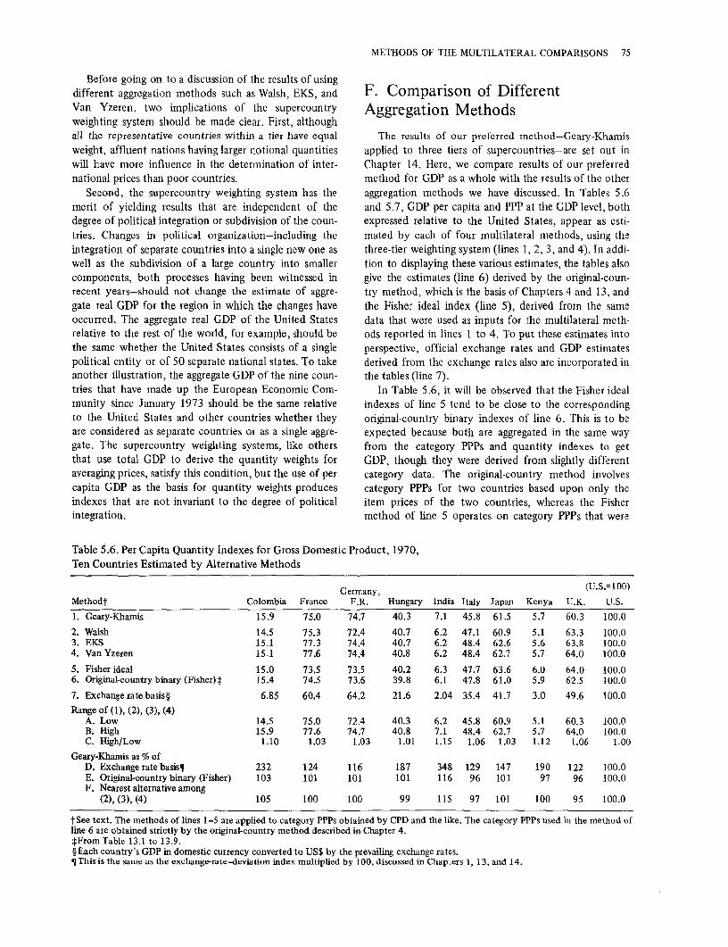
Before going on to a discussion of the results of using different aggregation methods such as Walsh, EKS, and Van Yzeren, two implications of the supercountry weighting system should be made clear. First, although all the representative countries within a tier have equal
weight, affluent nations having larger notional quantities will have more influence in the determination of international prices than poor countries.
Second, the supercountry weighting system has the merit of yielding results that are independent of the degree of political integration or subdivision of the countries. Changes in political organization-including the integration of separate countries into a single new one as well as the subdivision of a large country into smaller components, both processes having been witnessed in recent years-should not change the estimate of aggregate real GDP for the region in which the changes have occurred. The aggregate real GDP of the United States relative to the rest of the world, for example, should be the same whether the United States consists of a single political entity or of 50 separate national states. To take another illustration, the aggregate GDP of the nine countries that have made up the European Economic Community since January 1973 should be the same relative to the United States and other countries whether they are considered as separate countries or as a single aggregate. The supercountry weighting systems, like others that use total GDP to derive the quantity weights for averaging prices, satisfy this condition, but the use of per capita GDP as the basis for quantity weights produces indexes that are not invariant to the degree of political integration.
METHODS OF THE MULTILATERAL COMPARISONS 75
F. Comparison of Different Aggregation Methods
The results of our preferred method-Geary-Khamis applied to three tiers of supercountries-are set out in Chapter 14. Here, we compare results of our preferred method for GDP as a whole with the results of the other aggregation methods we have discussed. In Tables 5 .6 and 5.7, GDP per capita and PPP at the GDP level, both expressed relative to the United States, appear as estimated by each of four multilateral methods, using the three-tier weighting system (lines 1, 2, 3, and 4). In addition to displaying these various estimates, the tables also give the estimates (line 6) derived by the original-country method, which is the basis of Chapters 4 and 13, and the Fisher ideal index (line 5), derived from the same data that were used as inputs for the multilateral methods reported in lines 1 to 4. To put these estimates into perspective, official exchange rates and GDP estimates derived from the exchange rates also are incorporated in the tables (line 7).
In Table 5 .6, it will be observed that the Fisher ideal indexes of line 5 tend to be close to the corresponding original-country binary indexes of line 6. This is to be expected because both are aggregated in the same way from the category PPPs and quantity indexes to get GDP, though they were derived from slightly different category data. The original-country method involves category PPPs for two countries based upon only the item prices of the two countries, whereas the Fisher method of line 5 operates on category PPPs that were
Table 5.6. Per Capita Quantity Indexes for Gross Domestic Product, 1970, Ten Countries Estimated by Alternative Methods
Germany, (U.S.=100)
Methodt Colombia France F.R. Hungary India Italy Japan Kenya U.K. U.S.
1. Geary-Khamis 15.9 75.0 74.7 40.3 7.1 45.8 61.S 5.7 60.3 100.0
2. Walsh 14.S 75.3 72.4 40.7 6.2 47.1 60.9 5.1 63.3 100.0 3. EKS 15.1 77.3 74.4 40.7 6.2 48.4 62.6 5.6 63.8 100.0 4. Van Yzeren 15.1 77.6 74.4 40.8 6.2 48.4 62.7 5.7 64.0 100.0
5. Fisher ideal 15.0 73.5 73.5 40.2 6.3 47.7 63.6 6.0 64.0 100.0 6. Original-country binary (Fisher) :j: 15.4 74.5 73.6 39.8 6.1 47.8 61.0 5.9 62.5 100.0
7. Exchange rate basis§ 6.85 60.4 64.2 21.6 2.04 35.4 41.7 3.0 49.6 100.0 Range of (1), (2), (3), (4)
A. Low 14.5 75.0 72.4 40.3 6.2 45.8 60.9 5.1 60.3 100.0 B. High 15.9 77.6 74.7 40.8 7.1 48.4 62.7 5.7 64.0 100.0 C. High/Low 1.10 1.03 1.03 1.01 1.15 1.06 1.03 1.12 1.06 1.00
Geary-Kharnis as% of D. Exchange rate basis,i 232 124 116 187 348 129 147 190 122 100.0 E. Original-country binary (Fisher) 103 101 101 101 116 96 101 97 96 100.0 F. Nearest alternative among
(2), (3), (4) 105 100 100 99 115 97 101 100 95 100.0
tSee text. The methods of lines 1-5 are applied to category PPPs obtained by CPD and the like. The category PPPs used in the method of line 6 are obtained strictly by the original-country method described in Chapter 4. :j:From Table 13.1 to 13.9. §Each country's GDP in domestic currency converted to US$ by the prevailing exchange rates. 1 This is the same as the exchange-rate-deviation index multiplied by 100, discussed in Chapters 1, 13, and 14.

76 METHODS
Table 5. 7. Purchasing-Power Parities for Gross Domestic Product, 1970, Ten Countries Estimated by Alternative Methods
(U.S.= 1.000)
Germany, Colombia France F.R. Hungary India Italy Japan Kenya U.K. U.S.
Methodt (P) (Fr) (DM) (Ft) (Re) (L) Ci) (Sh) (£) ($)
1. Geary-Khamis 8.01 4.48 3.14 16.07 2.16 483 244 3.74 .308 1.000
2. Walsh 8.76 4.46 3.24 15.92 2.46 47.0 247 4.17 .291 1.000 3. EKS 8.42 4.35 3.16 15.93 2.47 457 240 3.80 .291 1.000 4. Van Yzeren 8.41 4.33 3.16 15.90 2.47 457 239 3.79 .291 1.000
5. Fisher ideal 8.47 4.56 3.19 16.13 2.44 464 236 3.57 .291 1.000 6. Original-country binary (Fisher):j: 8.2 4.51 3.19 16.3 2.53 463 246 3.64 .298 1.000
7. Exchange rate§ 18.56 5.554 3.66 30.0 7.50 625.0 360.0 7.143 .4167 1.000
Range of (1), (2), (3), (4) A. Low 7.96 4.33 3.14 15.90 2.16 457 240 3.76 .291 1.000 B. High 8.76 4.51 3.24 16.10 2.47 484 247 4.17 .308 1.000 C. High/Low 1.10 1.03 1.03 1.01 1.14 1.06 1.03 1.12 1.05 1.000
Geary-Khamis as% of D. Exchange rate 43 81 86 54 29 77 68 52 74 100 E. Original-country binary (Fisher):!: 98 99 98 99 85 104 99 103 103 100 F. Nearest alternative among
(2), (3), (4) 95 100 99 101 8 106 102 99 106 100
tSee text. The methods of lines 1-5 are applied to category PPPs obtained by CPD and the like. The category PPPs used in the method of line 6 are obtained strictly by the original-country method described in Chapter 4. :j:From Table 13.19. § From Table 1.1.
obtained by CPD. We see, then, that the differences between the original-country and the multilateral comparisons are not to be explained by differences in the treatment of the item data within detailed categories.
The differences among Geary-Khamis, Walsh, EKS, and Van Yzeren range from 2 to 15 percent (line C), with the largest differences arising for India, Kenya, and Colombia. Of the nine country comparisons, Geary. Khamis gave the highest estimate of per capita GDP in four instances and the lowest in four. Only in the case of India was Geary-Khamis more than 6 percent away from its nearest alternative (line F).
The Geary-Khamis results were within 4 percent of the original-country estimates except for India, for which they were 16 percent higher. Reasons for this difference are suggested in Chapter 14. so
The discrepancy between the exchange-rate-derived indexes of GDP per capita and the multilateral indexes of real GDP per capita is striking and far overshadows the differences among the multilateral methods. Clearly, the exchange-rate-deviation index as based on the Geary-Khamis results (line D) would not be changed much if another multilateral method were used.
Table 5.7 presents purchasing-power parities as estimated by the various methods just reviewed. No discus-
50 See pages 231, 241.
sion is necessary for this table; it is simply the mirror image of Table 5.6.
Comparative results can be given also for other methodological alternatives discussed in the preceding sections of this chapter. The preferred results in line 1 of Table 5.6 are based on frequency-weighted CPDs. We now make good on a promise given in Section 8 51 to show that frequency-weighted CPD and unweighted CPD give similar Geary-Khamis results. The differences between relative per capita GDP calculated using the two sets of category PPPs are less than 0.6 percent for the nine countries other than the United States. The differences are much smaller than the differences indicated by lines E and F in Table 5 .6.
Another decision we made was to apply GearyKhamis to all 164 categories52 at once rather than sector by sector bases53 (that is, to consumption, capital formation, and government, each in turn). Here, we document our assertion54 that the two methods give virtually the same result. The following table compares our preferred results for consumption, capital formation, and government to results based on a separate application of Geary-Khamis to each of the three major subaggregates:
51 See page 62. 52 With respect to the difference from the usual reference to
15 2 categories, see the latter part of footnote 2 2. 53 See page 70. 54 See page 70.

Consumption
All Consumption categories only
No. of categories 164 109
Colombia 16.8 16.8 France 67.9 67.9 Germany, F .R. 61.2 61.1 Hungary 38.3 38.5 India 7.6 7.5 Italy 46.0 46.0 Japan 48.3 48.4 Kenya 5.8 5.8 United Kingdom 62.2 62.2
The differences are virtually zero for consumption and are quite small in the other two sectors also. The largest difference, 9 percent, is for the Kenya-United States government index.
G. Measures of Imprecision
Line 1 of Table 5 .6 presents our best estimate of GDP per capita relative to the United States for each of the countries of the ICP set. The inevitable question to be asked of such numbers is: "How accurate are they?" The conventional rules governing significant figures would suggest that, in presenting them to three digits, we believe they are correct to that number of digits. We have of course, no such exaggerated confidence in the precision of our results. As is noted several times in this book, there are three sources of error, arising, respectively, from errors in the expenditure data, errors in the prices, and the use of improper aggregation methods.
With respect to the magnitude of errors arising from the expenditure data, we have no basis for quantitative assessment. Incomparabilities undoubtedly affect the classification of expenditures into the detailed categories, especially miscellaneous categories,55 but such classification errors tend to be offsetting. What we do not know and find difficult to judge is the extent to which our relative per capita GDPs in international dollars for different countries may be affected differentially by (1) incorrect aggregate GDP totals in national currencies and (2) improper allocation of GDP to the detailed categories.
Something can be said, however, about the other two sources of imprecision. In considering errors in the prices, we focus on an aspect of the category PPPs that were developed from item prices at the subcategory level using the CPD method. Great care was taken to ensure
55 See page 49.
METHODS OF THE MULTILATERAL COMPARISONS 77
Per Capita Quantity Indexes (U.S.=100)
Capital Formation Government
Derived from Geary-Khamis applied to
All Capital Formation All Government categories only categories only
164 38 164 17
18.0 17.6 7.2 7.5 123.5 123.2 38.2 38.1 134.8 123.8 55.9 55.4 56.9 55.0 25.4 26.4 5.3 5.2 7.3 7.6
60.5 60.2 21.3 21.5 123.6 122.3 38.1 37.3
4.7 4.6 6.7 7.3 68.1 68.2 37.4 38.2
that the item prices were accurate both when they were collected originally in the various countries and during the processing of them by the ICP. But even if all the individual item prices were exactly correct, the fact that they are regarded as sample observations means that the category PPPs based upon them will be subject to error. This source of error can be quantified-for the 128 categories56 examined here-because a by-product of each category CPD regression is an estimate of the variance -covariance matrix of the estimated coefficients of the country dummies.
The nine relative per capita GDP estimates-call them g.-are related in a complicated way to the category PPPs ind the corresponding set of expenditures. In principle, the sampling variances of the gis can be found analytically if one knows the relationship and the joint density function of the category PPPs. In this case, the GearyKhamis method is a relationship too awkward to handle analytically in connection with the lognormal PPPs. However, a numerical method is available to get estimates of the desired variances and covariances of the g;s·
Distribution sampling, or "Monte Carlo," can be used in the following way: From the set of 128 CPD regressions, we know the sampling properties of all the 1,152 category PPPs (128·9). Therefore, we can perturbate the PPPs in accordance with their sampling properties to get a new set of PPPs, to which we apply Geary-Khamis in order to get a new set of g;s, This process can be repeated T times, to get T different sets of gi8· If T is sufficiently large, the calculated variance of each gi will be an adequate estimate of the sampling variance of gi.
An abbreviated description of the perturbation process will suffice here. A replication is calculated by initially generating 1,152 pseudo-random normal deviates, all with means equal to the logs of the estimated PPPs
56 In all, there are 129 CPD categories, but variances and covariances were available for only 128 categories when the computation described in this section was done.

78 METHODS
Table 5.8. Confidence Interval Estimates for Geary-Khamis Quantity Indexes and Precision Intervals
Colombia France Germany, F.R. Hungary India Italy Japan Kenya U.K.
I. g/ 128 categoriest .163 .813 .760 .430 .0697 .501 .608 .0578 .644
2. Mean gj based upon 299 replications .164 .813 .765 .432 .0696 .505 .617 .0582 .649
3. Standard deviation of gj based upon 299 replications .004 .022 .021 .012 .0027 .014 .019 .0028 .017
4. possible deviation of gj at .95 level (in%) 4.81 5.30 5.42 5.47 7.59 5.48 6.13 9.50 5.17
5. gi I52 categories .159 .750 .747 .403 .071 .458 .615 .057 .603
6. confidence interval limits at .95 level:
lower limit .151 .710 .707 .381 .066 .433 .577 .052 .572 upper limit .167 .790 .787 .425 .076 .483 .653 .062 .634
7. Precision interval:j: limits at .95 level:
lower limit .138 .704 .688 .380 .058 .433 .575 .048 .572 upper limit .168 .832 .788 .434 .076 .514 .667 .062 .673
8. Possible deviation taking into account aggregation (in%) 9.4 8.5 6.7 6.7 12.7 8.8 7.5 12.3 8.4
tg/ Per capita GDP of the /h country relative to the United States (U.S.=100)
:j:Precision interval: Lower limit=minimum (lower limits of .95 confidence intervals derived from the Geary-Khamis, Walsh, EKS, and Van Yzeren methods). Upper limit=maximum (upper limits of .95 confidence intervals derived from the Geary-Khamis Walsh EKS and Van Yzeren methods). ' ' '
and variances and covariances equal to the estimated variances and covariances of the estimated PPPs. That is, we let the 1,152 PPPs obtained from the regression coefficients define the location parameters and let the 664,128 variances and covariances of the coefficients (most of the latter being zero because of independence between regressions) define the dispersion parameters of the log normal price world with which we are concerned. When exponentiated, these pseudo-random normal deviates are treated as category PPPs.
To each replication of the PPPs, we apply the GearyKhamis method, always using the same expenditure set, to get nine gis. These T replications give us a basis for estimating the sampling variability ( and covariances, also, though we have not bothered with them) of the gj8, Specifically, we computed 299 replications. The mean and standard deviation of the 299 element samples for the nine g;s are given in lines 2 and 3 of Table 5.8. (Incidentally, the entries of line 1 differ, but not much, from the entries of line 1 in Table 5 .6-repeated in line 4-because all of the catergories of GDP are not covered in the Monte Carlo calculations.)
The quantity indexes (line 2) are close to the quantity indexes produced by our standard application of Geary-Khamis to the same 128 categories (line 1). This need not be so, because the Geary-Khamis method does not constitute a linear transformation of the PPPs; therefore, what differences appear there need not be merely the result of sampling variability. Indeed, the standard errors of the mean are so small (equal to the entries of
line 3 divided by the square root of 299) that the differences are statistically significant in seven out of nine cases.
The sampling variability of the gi estimates relative to the "true" value (that is, the amount of dispersion one can expect around g;) is given in line 3. If these estimates are expressed relative to the elements of line I and then multiplied by 1.96, as in line 4, they give rough idea of the percentage variation to which gi is subject at the .95 confidence level. But note that the g;s in question are the ones derived from 128 categories. If we assume the same percentage error carries over at least approximately to the 152-category case, we can obtain rough estimates of the confidence intervals for the main results of the ICP-that is, for Geary-Khamis applied to 152 categories. These key Geary-Khamis estimates are repeated in line 5 from Table 5.6. Our crude estimates of the .95 confidence interval limits of the gjs for 152 categories appear in line 6. The range of inaccuracy is around 5 percent for six countries and runs a little over 9 percent for one. This amounts to between 2 and 4 percentage points for six of the countries, and is less than 1 percentage point for the other three.
A minor point should be made about the variancecovariance matrices of country-dummy coefficients for categories in which there were holes that were filled by double-weighted CPD. The variances for the hole-filled PPPs and their associated covariances were set at zero, even though non-zero estimates could have been found if the Monte Carlo exercise had warranted a substantial

effort. The variance could have been derived easily from the variance-covariance matrix of the double-weighted CPD regression. The covariances would have been a difficult matter, however, so neither the variances nor covariances were introduced into the Monte Carlo exercise for hole-filled PPPs. In such cases, a row and a column of that category's variance-covariance matrix would consist of zeros.) This resulted in less variance in theg;s than otherwise would have been the case.
Because of (1) these hole-filled PPPs, (2) the possible measurement errors in the item prices, and (3) the possibility that the 128 categories to which CPD was applied were not fully representative of all 152 categories, we must emphasize that the confidence intervals appearing in line 5 should be regarded as a floor to the uncertainty associated with prices.
In addition to the price effects just discussed, we have attempted a broader quantification to cover the cumulative effect of uncertainty arising from the choice of aggregation method. (Unfortunately, we must leave unassessed the possible consequences of expenditure uncertainties.) Table 5.6 showed that each country's gi varied from one aggregation method to another (lines 1 to 4). In no case did the results of a particular method differ from the average for all methods by more than 11 percent (for India), and generally the differences were 3 or 4 percent or less. Although there is no assurance that any one of these methods is correct, the fact that they give results that are fairly close together even though they are dissimilar in their construction leads us to think that the uncertainty associated with the choice of aggregation methods is probably small. There is no clear way of quantifying this uncertainty, but line 7 of Table 5.8 offers a set of intervals that simultaneously take into account this uncertainty and the kind of price uncertainty discussed in previous paragraphs. The Monte Carlo replications that have been described involved the GearyKhamis method, but similar replications were computed for the Walsh, EKS, and Van Yzeren methods. In every case, the sampling variability of gi for these methods was close to the variability of the Geary-Khamis estimates. We have constructed for each country a synthetic inter-
METHODS OF THE MULTILATERAL COMPARISONS 79
val defined as follows: the lower limit is the lowest of the lower confidence interval limits obtained for any of the four methods, and the upper limit is the largest of the four upper confidence interval limits. Of course, the nine new "precision intervals" (presented in line 7) are not confidence intervals in any technical sense, but they do convey a feeling for how accurate our g;5 are. The entries on line 8, half the width of the precision intervals, can be interpreted in the same way as the entries in line 4-except that the term "at .95 level" no longer has a probability meaning, but rather must rest on an intuitive interpretation. The uncertainty band is in the 6 to 9 percent range for seven of the countries and the 12 or 13 percent range for the other two (Kenya and India).
This section has been devoted to an attempt to appraise the accuracy of our estimates of relative per capita GDP for the countries of the ICP set. Because the GearyKhamis estimates of relative PPPs are inversely proportional to the relative per capita GDPs, the confidence intervals for the PPPs will have a width, stated in percentage terms, that is about the same size as the entries in lines 4 and 8 of Table 5.8.
Two final points may put into perspective our guesses about the accuracy of the estimates. First, we hesitate to offer a judgment about the accuracy of estimates of subaggregates because we have not explored this area. Second, we have estimated .95 confidence intervals for no better reason than that this is what is commonly done by statisticians. The "correct" level of confidence to use depends upon the cost to the investigator of being wrong, but normally the statistician sets this consideration aside and falls back on the (.05 hypothesis test, .95 confidence interval) rule of thumb because he does not know his own loss function. If the ICP had used .90 confidence intervals, each of the entries in line 4 and 8 of Table 5.8 would be one-sixth less; for .80 confidence intervals, the entries would have been one-third less; and for .99 confidence intervals, the entries would have been 40 percent more.
A detailed presentation of the results of our use of CPD and the Geary-Khamis methods, at a number of levels of aggregation, can be found in Chapter 14.

Chapter 6
Comparing consumer-goods • prices
The price comparisons for consumers goods reported upon in this chapter were based upon traditional methods utilized in most countries for time-to-time comparisons.
The basic steps in making these comparisons were, first, to select an appropriate sample of items and, second, to ensure that in the actual gathering of prices for these items, identical or equivalent qualities were priced in different countries. The general principles underlying the approach to the sampling and matching problems have been outlined in Chapter 3 and only their application to consumer-goods pricing need be discussed in this chapter. Price collection in individual countries also is described briefly.
Consumers goods for which price comparisons were made by other methods include (1) automobiles and other consumers durables, in Chapter 8, (2) rents, in Chapter 9, and (3) education and health services, in Chapter 7. For the first two, regression methods were employed; for education and health services, for which units of output are difficult to define and therefore to price, the price comparisons for a number of the categories were derived from direct quantity comparisons of labor inputs.
A. General Procedures
OBTAINING THE SAMPLE OF MATCHING COMMODITIES
The design of the sample of prices for the traditional type of comparison began with the establishment of a minimum number of specifications to be sought for each detailed category in the consumption sector. As stated earlier, these target numbers were based initially on the relative importance of the categories in the GDPs of five or six countries. Subsequently, they were modified in the light of the expected degree of dispersion of price relatives within the categories. In the consumption
80
sector, the overall target number of specifications for price comparisons made by traditional methods was nearly 250, of which 67 were in the food categories (see Table 6.1).
The first step in identifying a list of specifications was to draw upon the written specifications prepared by the U.S. Bureau of Labor Statistics (BLS) for use in the U.S. Consumer Price Index (CPI) and for its other retail price work. An effort was made, of course, to select from the BLS list of specifications those which were likely to be found in other countries. In many cases, a number of variants of a specification were included so as to enhance the likelihood that each country would find a suitable one in the BLS list. In the case of a portable electric heater, for example, one variant referred to a 1,320-watt heater, another to one consuming 1,650 watts, and a third to a heater that could be run at either of these wattages.
When each of the other nine countries checked the initial U.S. list to determine which specifications were also common in its markets, it invariably found that a significant number of specifications could be matched. In a number of cases, identical or equivalent specifications actually were being priced for purposes of maintaining time-to-time indexes in the other countries. In other instances, an item identical with, or equivalent to, the BLS specification was not priced but was known to exist in acceptable quantities in the country's markets.
Each other country also was invited to suggest modified or substitute specifications for each detailed category to the extent necessary to provide good coverage of a particular category, especially if items important in that country's expenditures in the category were not on the original list.
There were many cases in which matching products could be found easily, even though they would not have been selected independently in one of the particular countries. In the case of drugs and medical preparations, for example, only a few of the original U.S. specifica-

COMPARING CONSUMER-GOODS PRICES 81
Table6.1 Number of Consumer-Goods Specifications in Sample, Included Countries, 1970
Number of specifications
Number of Number priced
detailed Total Target Ger categories number number Col Fra (FR) Hun Ind !ta Jap Ken U.K. U.S.
01. Food 40 283 67 89 114 113 86 106 111 99 63 103 244 02. Clothing and,
footwear 15 158 so 56 40 40 87 59 38 62 41 79 139 03. Gross rent, t
fuel and power s 33 7 7 18 18 10 10 18 10 12 11 26 04. Furniture and
furnishings 16 178 37 37 47 47 so 51 45 so 32 60 161 05. Medical care 8 81 13 18 16 17 33 14 17 36 19 26 79 06. Transport:j: and
communication 12 42 21 24 21 21 18 20 21 24 18 26 36 07. Recreation and
education 10 125 22 28 54 53 27 40 54 36 27 30 110 08. Other goods and
seIVices 7 91 16 20 27 28 41 38 28 29 20 28 75
Total 113 991 243 279 337 337 352 338 332 346 232 363 870
tAlthough ICP 03. includes rents as well as fuel and power, the rent component has been handled separately, and no accounting is given here of the number of rent specifications; see Chapter 9. :j:Excludes passenger cars (ICP 06.110); see Chapter 8.
tions were widely used in India, but preparations that were important in Indian practice were also commonly used in the United States, even though they were not on the original U.S. list. These included iron salts (for anemia), sulphonomides (for dysentery and other bacterial infections and topically for trachoma), antituberculosis drugs, digitalis, insulin, and antimalarial drugs.
Milk provides an illustration of the opposite situation; that is, the most common Indian specification, for buffalo milk, could not be found in the United States, but cow's milk, accounting for nearly one-half of total Indian consumption, was sufficiently common in India to warrant basing the price comparison on this kind of specification.
In a rough and approximate way, these procedures could be considered as embodying the criterion of concentrated selection described in Chapter 3. The very fact that the specifications were included in the BLS list suggests that they were important items in their categoriesor, at the minimum, widely available ones. The addition of specifications by other countries in effect was applying the criterion from the standpoint of those countries.
The response of other countries resulted in substantial alterations of the original sample chosen from the BLS specifications. Of the original list of about 350 BLS specifications, nearly 300 could be matched in one or more of the other countries. About 700 additional specifications were added, however, to round out the sample in accordance with the criteria set out in Chapter 3. The great bulk of these were selected in the course of developing binary comparisons with the United States, but some were developed by the European Economic Community (EEC) for comparisons among its member
countries, and a few were selected with reference to the India-Japan comparison. About 100 additions were made to the BLS list by Hungary and the EEC and nearly 200 by Japan, these being countries among the other nine for which samples were chosen earliest.
Once a specification was added to round out the sample for one country, it was included in the list of specifications submitted to other countries for which the work of choosing commodity samples came later.
B. Price Collection in Individual Countries
The main burden of price collection in the individual countries fell upon the central statistical offices or other official price-collection agencies. The ICP staff, for the most part, was concerned with coordinating the selection of the appropriate number of specifications in each category and with ensuring that qualities were matched and that national average prices were gathered. The central staff's work in achieving these objectives varied widely from one country to another.
COLOMBIA In Colombia, prices were gathered by the National
Department of Statistical Administration (DANE) in seven cities and adjoining rural areas: Bogota, Baranquilla, Cali, Medellin, Pasto, Manizalez, and Bucaramanga. These seven areas provided broad coverage of the geographic regions of the country, including its diverse climatic and topographical zones. The number of rural prices was limited, however, and their geographical dis-

82 METHODS
tribution, adjacent to the cities, did not produce an optimal sampling frame. Given these circumstances, we decided simply to average the rural and urban prices in each of the seven sets of data and to combine the seven in a national average. Expenditure weights, based on the region represented by each city and its adjacent rural area, were used to compute the national average prices. These weights were from a family expenditure study of 3,000 urban and 500 rural families. The identification of the items to be priced was agreed upon in the course of an exchange of experts between Colombia and the United States.
FRANCE,GERMANY,ANDITALY The prices for the three Common Market countries
were gathered in the course of a survey organized by the Statistical Office of the EEC. The survey, carried out in November 1970, was an expanded version of a long series of consumer-goods price comparisons, the first of which was conducted in the early 1950s. Over the years, a common list of specifications was developed for all of the member countries, although for some products there were variations to permit the pricing of the local brand or trademark. For the November 1970 survey, the sample of items priced was adjusted to include a number of ICP specifications, and, as noted earlier, a number of EEC specifications were incorporated into the ICP list. This was aided by an exchange of experts.
In the Federal Republic of Germany and Italy, prices were gathered in ten different towns, five large and five small. In each town, two department stores, two supermarkets, and two specialized shops were priced. In principle, therefore, sixty observations were obtained in each country for each item. In the case of France, the sample was divided into three geographic groupings: (1) Paris; (2) Lyon, Marseilles, Bordeaux, and Rennes; and (3) small towns. Weights of three, three, and four were assigned to these categories, respectively. More than six French prices were obtained for each item. The specifi. cations and the nature of the sample were determined jointly with the statistical directors of all six EEC countries; the actual price collection was carried out by the statistical offices of the individual countries.
HUNGARY All prices in Hungary were supplied by the Central
Statistical Office (CSO). In 1967, the prices were fixed and were a matter of record. An exchange of experts with the United States helped to identify matching qualities of goods. In 1970, energy and basic foods, such as bread and milk, were still fixed in price. Among the other prices, some were free to fluctuate within minimal and maximal limits, and others were completely free. For most 1970 prices, therefore, the Hungarian CSO relied largely upon the standard kind of price-gathering system.
INDIA Indian prices were supplied by that country's Central
Statistical Organization (CSO), 1 which drew upon other statistical agencies as well as upon its own resources. There was also an exchange of experts, each with some familiarity with the other country's market as well as with his own.
Prices and the content of consumption varied more widely between cities and rural areas and from one region to another in India than in most of the other countries. This problem was resolved by estimating national average prices for India in successive stages, taking account of different price levels in metropolitan India (defined to include Bombay, Calcutta, Delhi, and Madras), urban India (nonmetropolitan cities), and rural India.
Specifically, national average prices for each detailed category were estimated from the following formula:
w p + w p ·-p + w • p .- . -~ Pu) (: Pu Pr) mm um m rm p p
p = m u n
where P = price, n = national average, m = metropolitan (Bombay, Calcutta, Delhi and Madras), u = urban other than metropolitan, r = rural, and w = weights proportional to total expenditure. A completely symmetric treatment of the three different population densities would call for simpler expressions for the last two parenthetical expressions in the numerator on the right. However, the substantial differences in the nature and quality of the items commonly purchased within each detailed category in the rural and urban sectors necessitated the use of urban-metropolitan and rural-urban ratios based upon different sets of specifications.
The specifications used in the urban-metropolitan comparisons were selected to match U.S. goods. The CSO obtained prices both from existing sources and from special surveys. The former included National Sam· pie Survey (NSS) prices from the nonmanual employees consumer price index and Labor Bureau prices from the industrial worker price index. The special surveys were made both by the CSO staff and by the NSS.
The rural-urban prices were taken from those gathered for the consumer price index for agricultural workers and industrial workers and from the consumer price index for nonmanual employees. In addition, prices were specially gathered through the NSS in one urban area and two rural areas in each of the eighteen states. The comparisons were made separately for each
1 The work on the ICP in India benefited from the helpful advice of an advisory working group established by the CSO.

of the states because it was believed that the qualities of goods available differed less within states than across India as a whole; this method, therefore, made it easier to assure pricing of comparable qualities in rural and urban areas.
JAPAN Japanese consumer prices for the ICP were provided
by the Bureau of Statistics of the Office of the Prime Minister.2
The prices were obtained from three existing price surveys and from a special survey. Prices for nearly 200 specifications were taken (1) from the monthly retail price survey covering 170 cities, towns, and villages, which is the basis for the consumer price index; (2) from the National Survey of Retail Prices carried out in 770 cities, towns, and villages in November 1967; and (3) from the monthly department store survey conducted in Tokyo on the price of new products and imported items. The special price survey was carried out in department stores, supermarkets, and other retail outlets in Tokyo during 1970. The Tokyo prices obtained from the department store survey, and the special price survey were adjusted to national averages on the basis of the National Survey of Retail Prices for 1970. By using the most closely related indexes derived from the retail price surveys, prices obtained for 1967 were extrapolated forward to 1970, and prices referring to 1970 were extrapolated backward to 1967.
KENYA In Kenya, the Statistical Department collected prices
regularly only in Nairobi at the time of our reference dates. To obtain national average prices for ICP purposes, special urban and rural price surveys were conducted by the Statistical Department, with the aid of outside experts provided by the Economic Commission for Africa and the ICP.
In the urban sector, additional prices were gathered in several markets in Nairobi, and representative pricing was done in Mombasa and Kisumu to round out the urban sample. (Nairobi and Mombasa account for over three-quarters of the urban population, and with Kisumu they provide representation of each of the three major geographical and ethnic regions of the country.)
Rural prices were collected in thirteen villages chosen to include areas dominated by each of the eight major tribal groups. Because of the cost involved, no effort was made to obtain prices from the Northeastern provinces, inhabited for the most part by nomadic peoples with no
2 See the report by Sadanori Nagayama, Comparison of Levels of Living in Real Terms in Japan and the U.S. (Tokyo: Japan Society for the Promotion of Science, March 1971). This volume is the report of a committee headed by Professor Yuzo Yamada, which was set up to carry on the Japanese side of the work with the ICP.
COMPARING CONSUMER-GOODS PRICES 83
permanent markets and accounting for only about 3 percent of the total population of Kenya. Rural prices were collected for a total of forty-five items, including twenty-one food items, thirteen clothing items, and eleven household products. In markets where bargaining is customary, the purpose of the inquiry was explained to sellers in the local language so actual transaction prices could be obtained. 3
UNITED KINGDOM Prices in the United Kingdom were obtained through
the Statistics Division of the Department of Employment. The specifications to be priced were chosen in collaboration with a U.S. expert. A substantial number of prices, particularly for foods, were obtained directly from records of prices maintained for the cost of living index. Fortunately, the regional variation within the United Kingdom of the other prices needed by the ICP is relatively small, so reliance could be placed on central office price lists of large chains and on prices observed in Watford, central London, and two or three other places. Some mail-order-catalog prices also were used.
UNITED ST A TES Because initially the United States was taken as the
base country in starting this system of consumer-goods prices, an unusually large number of prices was required. National average prices were estimated for nearly 900 specifications of consumer goods.
Nearly three-fourths of the prices were obtained from the U.S. Bureau of Labor Statistics. But only about onethird of the BLS prices, nearly one-half of which were foods, were provided directly in the form of national averages. 4 The others generally were based on prices for a limited number of cities; either only one (usually Philadelphia, New York, or Chicago) or a group of as many as five cities (usually including Chicago, Detroit, Los Angeles, New York, and Philadelphia). The number of observations typically ran from eight to ten per item in each city, but it was sometimes less when quality variations were considered. A substantial number of these prices (approximately 200) especially those pertaining to five cities, were taken from prices collected for the Consumer Price Index (CPI). Others (more than 200) were especially collected for the ICP; the latter usually were for one or two of the following cities: Chicago, New York, or Philadelphia. The balance of the BLS prices were obtained from the agency's miscellaneous records and sources; more than a score were estimated from BLS wholesale prices.
3 For a further description of the price collection in Kenya, see G. Donald Wood, Jr., "Problems of Comparison in Africa with Special Regard to Kenya," Review of Income and Wealth (March 1973), pp. 105-16.
4 A number of the national average prices came from the
Bureau of Labor Statistics City Workers Family Budget Bulletin No. 1570-3 (Washington: Government Printing Office, 1966).

84 METHODS
Two adjustments to the BLS prices usually were necessary. The first was to convert the city prices to national average prices. Fortunately, in the course of preparing standard budgets for city workers, the BLS had done pricing work that made it possible to compare the price level for each type of good in individual cities with the national average price level. Such place-to-place comparisons of clothing costs, for example, existed for a four-person family, separating the purchases made on behalf of the husband, the wife, a boy, and a girl, as well as expenditures on other clothing materials and services in each of thirty-nine metropolitan areas for the spring of 1969.5 For most categories, the budget quantities were identical in all cities. For clothing and certain other categories, however, particularly fuel, the cost comparisons were based on different quantities to allow for climatic differences. The BLS kindly supplied the ICP with data giving the quantity adjustments for climatic conditions, and thus it was possible to estimate the pure price differences for each city relative to the national
average. When more than one city was used to estimate the
national average price, a different answer usually was produced by each city's prices. We estimated the national average price by computing a weighted average of the individual prices, where the weights were the number of price observations in each city. (In principle, the number of obervations was proportional to the appropriate city weight.)
To check on the prices obtained from these procedures, an alternative set of calculations was made based on an earlier version of the city workers' standard budgets, referring to 1966 average prices. These 1966 relationships between city and national average prices were used as a basis for getting national average prices from our 1970 city prices. These estimates of national average prices for 208 items well matched the corresponding prices derived from the 1969 budgets. On the average, they were 1.6 percent lower, but the coefficient of determination, r 2 , between the two sets of prices was
0.966. A second adjustment that had to be made to BLS
prices in many cases was to add sales taxes, which were excluded from the prices provided to the ICP. The national average price was estimated from a city price by the following formula:
5 Bureau of Labor Statistics, Three Budgets for an Urban Family of Four Persons-Final Spring 1969 Cost Estimate (Washington: Government Printing Office, December 1970). The intermediate budget was used for our calculations; the results would have been substantially the same if the budget for the low standard or the one for the high standard had been used.
where Cx = city price exclusive of sales tax, CT= city price inclusive of sales tax, NT= national price inclusive of sales tax, and T = sales tax. (The comparisons between city and national average prices in the standard budgets mentioned above were inclusive of sales taxes, and thus
they provided ratios NT/CT.) In some cases, the prices provided to the ICP were national average prices (rather than prices for individual cities) exclusive of tax, and an average sales tax, taking account of the varying rates and coverages in different states and localities, had to be estimated. This was true, for example, of some drugs and medicines; I percent was added to the 1970 prices of
prescription drugs and 3 percent to the prices of nonprescription medicines to allow for national average sales taxes on these items. In 1970, forty-five of the fifty states and a number of cities had sales taxes, the total rate of which varied between 2 percent and 7 percent.6
Somewhat over one-fourth of the prices were obtained directly by the ICP, over one-half of these from the city of Philadelphia, and most of the remainder from catalogs or through a mail survey of large food chains in the United States. In general, these represented items relatively simple to price, an effort having been made to
leave the pricing of more difficult items to the BLS. Some prices were taken from the U.S. Department of Agriculture price materials and from the U.N. survey of retail prices in New York City.
Although the retail price work of the BLS focuses on clerical workers and wage earners residing in urban places, the BLS prices can be regarded as conforming substantially to national average prices. Well under I 0 percent of retail sales occur outside of the urban areas and standard metropolitan statistical areas covered by the CPI sampling frame. 7 Because they have automobiles, most nonurban families in the United States make the bulk of their purchases in urban areas or in suburban shopping centers that are part of the CPI sample. The rural population also relies heavily on mailorder purchases, some of which enter the BLS sample, and in any case are not thought to be different from other urban prices. Thus, although the U.S. population does not live entirely in urban areas, the prices relevant to national average prices are substantially urban prices as collected for the CPI.
6 John F. Due, State & Local Sales Taxation (Chicago: Public Administration Service, 1971).
7This statement is based on data in the 1963 Census of Business (Retail Trade Summary Statistics Part I (Washington: Government Printing Office, 1966), pp. 135- 38). Actually $26 billion out of a total of $244 billion of retail sales were accounted for by places of less than 2,500 population. About $5 billion of this, however, included purchases of farm equipment, building materials, and lumber, which are not included in consumption. Another $9 billion was spent in gasoline stations and restaurants or in car dealers' establishments.

C. Special Problems in Particular Consumer-Goods Categories
BREAD AND CEREALS (01.100)8
Rice (01.101). The relative importance of rice in consumption patterns varies widely with differences in income levels and with food consumption habits. Among the ten countries included in the present round of comparisons, rice was clearly most important in India, where it accounted for about 20 percent of household expenditures and more than 60 percent of total expenditures on bread and cereals. Rice also is a staple in Japan, where it accounted for seven percent of total consumption expenditures and more than 70 percent of total expenditures on bread and cereals. It is a common product in all the other countries, of course, and plays an important role in the bread and cereal expenditures of Italy (nearly 25 percent) and Kenya (more than 12 percent).
Rice comes in a large number of varieties and qualities. The varieties of rice commonly are classified according to the size and shape of the grain. In the Indian classification, for example, long rice (referred to in India as "fine") is three times as long as it is wide and is small in size. The medium variety has a 2.5 to 3 length-to-width ratio, and the short-grain variety (known in India as "bowled" or "coarse") has a length to breadth ratio of less than 2.5. For the most part, the price of rice varies positively with the length-breadth ratio. In Japan, however, the glutinous short-grain Japonica variety is preferred, and no market exists for long-grain rice. In India, all the varieties of rice are found, with long-grain rice making up about 10 percent of the crop, the medium variety about 30 percent, and short-grain rice the remaining 60 percent. In other countries, long-grain rice commands a price premium, varying from 1 O to 40 percent over that of short-grain rice, with the Indian premium falling in the upper part of the range.
Within each major varietal category of rice there are a number of variants. India has a bewildering variety of kinds, many confined to particular regions of the country. To aid in ensuring proper comparability of the varieties of rice that were priced in India, the United States, Japan, and other countries, samples of six varieties of rice-three from the United States, one from Japan, and two from India as controls-were sent, with the help of the National Sample Survey, to seven Indian centers for matching with local varieties. The samples also were sent to the Food Corporation of India and the Central Rice Research Institute at Cuttack. (The latter did the matching by a scientific classification based on
8 The parenthesized numbers refer to the ICP classification. See the Appendix to Chapter 3.
COMPARING CONSUMER-GOODS PRICES 85
length-breadth ratio.) U.S. and Indian rice samples also were taken to Japan. One important identification problem that the samples helped to resolve related to socalled parboiled rice, which is common in several countries including the United States, where it is marketed under a brand name.
The other major factor affecting rice prices is the quality of the grain. This factor involves moisture content, percentage of damaged or broken kernels, odors (particularly those which are commercially objectionable, such as mustiness), color, presence of insects and other foreign matter, the percentage of rices of mixed types, and the quality of milling. According to a U.S. Department of Agriculture study,9 Japanese rice was, in general, close in quality to U.S. rice, but Indian rice was a lower-grade product. This was mainly because of the presence of foreign matter and the percentage of broken grains, which averaged to 27 percent for raw milled rice and 15 percent for parboiled (selah) rice. The main grade of Indian rice was not found on the U.S. market, but it was thought that it would sell at a discount of 10 to 20 percent below the standard U.S. grade. It has been assumed that the grades of rice in the other countries in the study are similar to that of the United States and Japan, and a discount of 15 percent has been applied to the Indian price to allow for the difference in quality.
The proper method of comparing Japanese rice prices with those of the United States and other countries was discussed at some length with Japanese colleagues. The Japanese considered the difference between short-grain and long-grain rice as a matter of taste and not of quality. In their view, if long-grain rice were marketed in Japan, it would not command any premium price over that of short-grain rice. The appropriate method of price comparisons, therefore, was to disregard the difference between the two kinds of rice and to compare the average price of rice in Japan with the average price of rice in other countries. We accepted this view, although for computational convenience we made the adjustment to the Japanese data (rather than to the data of each other country) simply by treating the Japanese price for shortgrain rice as the price of long-grain rice also. This is one of the instances of what was referred to in Chapter 3 as "taste-equivalence" matching.
We considered subdividing rice into two subcategories, because of its great importance in Indian consumption and because of the small proportion of longgrain rice in the Indian total. This proved unnecessary, however, because the relationship of Indian rice prices to those of other countries was similar for the two subcategories under consideration.
9 USDA Economic Research Services, "Analysis of Selected Varieties and Grades of Rice Moving in World Trade in Terms of Official U.S. Rice Standards" Rice Situation Marketing Research Report No. 460 (Washington: Government Printing Office, March 1969).

86 METHODS
Meal and flour (01.102). The India-United States comparison for wheat flour was another example of matching by taste equivalence. In the United States, an enriched processed white flour is the common product and sells at less per kilo than whole wheat flour. In India, either wheat grain is purchased and taken to a mili for grinding or ground whole wheat is purchased. The exception, though becoming less and less an exception, is purchase of a white bleached flour. The result is that in India, unlike the situation in the United States, brown flour is cheaper than white flour.
Another problem with the wheat flour comparison was to choose the appropriate grade of Indian wheat to which to add grinding charges for comparison with U.S. white flour. What is called in India "American" wheatwhich is the best the United States has to offer and which is marketed throughout the world-is not preferred in India because it makes rather poor chapaties, the standard bread of North India. 10
Although U.S. wheat sells for a discount relative to the medium Indian wheat, its general quality, in terms of foreign matter, moist kernels, and similar characteristics, is higher. A direct price comparison was made between the Indian wheat (plus grinding charges) and U.S. white flour; it was considered that the preferable cooking qualities of the Indian product and its higher internal price seemed to balance the outside view of the higher quality of the U.S. product.
Among products in the flour and meal category, maize flour, which was particularly important in Kenya and Colombia, posed some matching problems. The main difficulties were that countries use different terms and grind maize differently; also, they sometimes add wheat flour. Samples were helpful in clearing up these matters, though in general the price variation of different kinds of maize flour was small.
.Macaroni, spaghetti, noodles, and like products (01.106). A different kind of matching difficulty was posed by Japanese noodles. These are made from hard wheat flour and contain all of the starch from the wheat kernel. They are dull white to gray in color and rather brittle. Spaghetti, the nearest western product, is made from enriched semolina or farina and contains the gluten part of the hard wheat kernel and little starch. Products made from semolina or farina are yellowish, somewhat translucent, and hard but fairly pliable. Thus, Japanese
10 In this connection, an interesting problem arose with the impact of the "green revolution" on Indian wheat prices. Mexican wheat, which is somewhat like American wheat, is the wheat variety with high yields. A local and lower-yielding Punjab wheat, which makes better chapaties, is the variety of wheat in the price index. As the green revolution hit the Indian Punjab, local wheat acreage declined with the introduction of Mexican wheat; consequently, the price of local wheat rose, and the consumer price index for wheat rose as Indians enjoyed the largest increases in domestic wheat production ever experienced. This phenomenon did not affect the particular wheat used for the ICP comparisons.
noodles are not physically identical with noodles in the United States or pasta in Italy. They are, however, roughly similar in appearance and serve the same function, and hence we treated them as equivalent products on grounds of similarity in use.
Other cereals (01.107). Sorghum is grown in India (where it is known asjowar) both as a food crop and for fodder, whereas in the United States and most other countries in the study it was not consumed directly by households but was used, if at all, for fodder or in brewing. A U.S. retail price was estimated from the wholesale sorghum price on the basis of the spread between the wholesale wheat price and the retail price for wheat flour.
MEAT (01.110) It was possible to compare meats for most countries
for common cuts such as veal cutlets, sirloin steak, and the like. In some instances, however, differences exist in the ways in which the animals are butchered for retail distribution. In addition, beef sometimes is sold, as in Japan, by the quality of the animal without much regard to the particular cut. In the latter circumstances, for each quality of animal, we compared the weighted average retail price for which the total carcass was sold.
Unlike a number of other foods, meat appeared to vary significantly in average quality from country to country. Countries with high incomes tended to have highly developed animal husbandry industries catering to a taste for fine meat, whereas countries with lower incomes and lower meat consumption tended to have a lower average quality of meat. Fortunately, grading standards for meat are well developed in countries in which meat is important; these provided a basis for selecting the appropriate quality level for price comparisons with other countries .
FISH (01.120) In the case of fish, some consideration was given to
the possibility of comparing the average price of fish in each country regardless of the type of fish consumed. This would have been an attractive way of proceeding had it been true that each country simply consumed whatever kind of fish were available to it without any special effort to search out varieties regarded as more palatable. But this is a doubtful assumption in any case, and it certainly is no more warranted for a country such as Japan, in which fish is an important source of protein, than a corresponding assumption about the consumption of meat would be for the United States or Western Europe. Accordingly, fish price comparisons were based on identical species, the scientific names proving to be the saving element in an otherwise bewildering variation from one country to another in the common names for identical species of fish. Diagrammatic pictures of the fish on the specifications also proved helpful.

MILK, CHEESE, AND EGGS (01.130) We tried to base price comparisons for cheese on
domestic products, seeking, of course, to find types of cheese common to several countries. One reason for this procedure was that an imported cheese-say, a European cheese in the United States-may be expensive because of both cost of shipment and consumption by only a small percentage of the population. Another factor is that the quality of the exported product may differ from that commonly consumed in the country of origin. A brie in France, for example, may not be equivalent to one that is exported to the United States.
OILS AND FATS (01.140) The most common type of oil purchased in the
United States is so-called salad oil, which is a combination of various kinds of oils, usually soybean, corn, peanut (groundnut), and cottonseed oils. A 100 percent soybean salad oil also is available and sells at the same price as the combination salad oil. Oils commonly consumed in other countries, such as those derived from safflower, cottonseed, corn, rape or mustard, groundnut, and cocoanut, either are not available in U.S. food stores or are sold in small quantities. We have estimated, therefore, the U.S. retail prices for such oils from the relationships of their wholesale prices to the wholesale price of soybean oil. For example, no pure rape oil is sold in the United States at the retail level, except in such a specialty shop as an East Indian grocery, where it would be relatively expensive. The same is true of safflower oil and sunflower oil, the latter being the predominant oil used in Hungary.
FRESH FRUITS AND VEGETABLES (01.150) Quantities of particular fruits and vegetables con
sumed tend to be highly price elastic. This presents serious problems for the ICP, because the growing of particular fruits and vegetables often is highly specialized to particular parts of the world. As a consequence, apples are cheap in Europe and Japan and expensive in Kenya and India, whereas the opposite is true for oranges and bananas.
Seasonality can cause problems, too. The price of fruit we want is the annual average price. Notice the following possible anomaly: strawberries may be cheaper every month of the year in the United States than in the United Kingdom, but because of a larger relative volume of U.S. purchases in months in which they are expensive in both countries, the U.S. annual average price may be higher than that of the United Kingdom.
Vegetable prices exhibit similar problems, though in less dramatic form. Perhaps there are enough universal varieties of vegetables--tomatoes and onions might suf. fice-that a valid comparison could be obtained by restricting the varieties compared. On this point more research is needed.
COMPARING CONSUMER-GOODS PRICES 87
Our method of dealing with these problems has been to seek as large a sample across countries as possible. Thus, an item was eligible for inclusion as long as it was marketed in a sufficiently substantial volume that its price determination was not greatly influenced by factors that were different from those affecting other fruits and vegetables. For example, apples, grown mainly in Himachal Pradesh and Kashmir, meet the test in India.
Of course, a number of other fruits and vegetables were excluded because they were unique products, at least for the present group of countries. For example, the chiku (a fruit that if not allowed to ripen produces chicle for chewing gum and known as sapadilla in Spanish-speaking countries), the guava, the breadfruit or jackfruit, and the lichee fruit, all common in India, have not been included. Perhaps such fruits will be added to the ICP list at such time as new countries are brought into the project.
The fresh fruits and vegetables category also contains a case of matching on a taste-equivalence basis. In the United States, mandarin oranges command premium prices relative to other oranges, but the reverse is true in Japan. A direct price comparison was made between the cheaper of the two variants in each country.
FRUITS AND VEGETABLES OTHER THAN FRESH (01.160)
Considerable variation existed in the names and availabilities of dried peas and beans, and samples were essential to establish comparability. The final list included red kidney beans, lima beans, pinto beans, chick peas (also known as garbanzos and channa), black-eyed peas, green and red gram, and other varieties. Many of these were not known abroad by their U.S. name, and we encountered no nomenclature that seemed to be in international use. Because these items are quite important in countries such as India, several varieties were matched.
POTATOES AND TUBERS (01.170) The importance of root vegetables differs widely
among countries. We planned at first to include potatoes with other vegetables, but it quickly became necessary to separate potatoes. Then, as data came in, it became clear that even potatoes and tubers could not always be treated as a single category. In Kenya, yams are far more important than potatoes, which are common but relatively expensive. Potatoes and yams have quite different price relatives as between Kenya and the United States. Because the expenditure ratios also are different-being larger where prices are cheaper-it was decided to deviate from the usual practice of taking an unweighted geometric mean of the price relatives; instead, potatoes and yams were weighted separately in the Kenya-United States comparisons.

88 METHODS
The problem posed for the multilateral comparisons was that yam prices were not available for the other countries. Because, as was described in Chapter 5, each detailed category is treated as a single product in these comparisons, the simplest procedure would have been to base Kenyan relative prices on potatoes alone. This procedure, however, would not have reflected adequately the substantial consumption of yams and would have produced a lower relative real quantity for the category than seemed warranted. Therefore, we linked the Kenyan price for the category to the prices of the other countries through the United States, using for the Kenya-United States price the Fisher index based on
both potatoes and yams.
ALCOHOLIC BEVERAGES (01.320) The principle problem in matching alcoholic bever
ages is that people tend to drink domestic beers, wines, and liquor rather than imported beverages largely because they are cheaper. The domestic product sometimes varies in type from one country to another. For example, no equivalent of U.S. bourbon or rye is widely distributed in the United Kingdom.
There are, however, branded wines and liquors and, to a more limited degree, beers that enjoy an international reputation and that can be found in the markets of most countries. The fact that they are usually more expensive than the local product is not surprising in view of shipping costs and import duties. A famous brand of U.K. sherry, for example, which the United Kingdom imports, bottles, and exports to the United States, entails shipping costs and import duties, each of which exceeds the value of the barreled wine.
In the sherry example, the alternative exists of matching the U.K. sherry against an equivalent sherry imported into the United States in barrels and bottled domestically. This was the course we followed.
Fortunately, however, matching need not depend entirely on locally bottled beverages having a common provenance. The EEC includes countries that take seriously the differences in wines, and in their wine price comparisons they match ordinary table wines indigenous to each country. To a considerable degree, our compromises have been in the same spirit.
Thus, we matched locally produced table wines and gins, generally seeking a medium quality by Western European standards. This solution also was applied to beer. Relative to the sherries of Portugal, the table wines of France, and the whiskies of the United Kingdom, there appears to be no universal beer. Most countries were quite willing to take a light beer of national origin with alcoholic content of 3 to 5 percent as an internationally comparable item. In addition, ale or heavy beers were priced in a few countries, and some European beers were priced in the United States.
For their internal comparisons, the EEC countries priced a standard Scotch whiskey and a good cognac, the
latter being defined as one imported by the United States. (The U.S. price was about $10.00 for four-fifths of a quart in 1970). Both were priced in the United States as well. If there was a bias in other items selected, it was in the direction of heavy reliance on domestic products, and therefore the inclusion of imported Scotch and cognac served somewhat to balance the sample.
TOBACCO (01.400) Comparability in cigarettes is clouded by the fact
that, in some cases, tastes appear to have adapted them
selves to local or at least readily available types of tobacco. In Hungary, for example, Bulgarian cigarettes long have been preferred; and, although the opposite relationship prevails on world markets, cigarettes made of Virginia tobacco would sell at a discount relative to those made in Bulgaria of Turkish tobaccos. Because Hungary and other countries as well indicated that their national preferences for tobacco did not match international tobacco price relationships, no effort was made to insist upon comparability of type of tobacco.
In the U.S. market, most cigarettes sell at roughly the same price. This is because the production and transportation cost components of the price are very low. Based on Census of Manufactures data, the tobacco, filter, wrapper, and transportation costs averaged 5 .1 cents for a package of twenty in 1967, when the retail price was 36 cents a package. Because marketing costs and taxes, about the same for all brands, are so much larger than production costs, U.S. cigarettes generally have sold at common prices. 11
In Japan as well little variation existed in price, explained by the dominance of a single brand. In other countries in which advertising is less important, however, there are sometimes substantial differentials in price. In India, for example, cigarettes in a price range from about Rs0.70 to Rs2.40 per package of twenty for a largeselling, loosely packed nonfilter as compared with a closely packed filter cigarette.12 In addition, other volume nonfilter cigarettes sell for prices of Rsl .00 to Rs2.40 per package. Our procedure was to use an average of the three principal grades of nonfilter cigarettes in India for comparison with other countries. A similar averaging was performed for other countries, keeping filter and nonfilter cigarettes separate.
11 It is true that, because of duties, imported cigarettes do sell for more in the United States, but they are such a small part of the U.S. market that they have been ignored.
12 Left out of the discussion are beedies, a product widely smoked in both rural and urban areas, which sells for about Rs0.20 to Rs0.50 per package of 25. It would be difficult to match this product in other countries; beedies have been used for the internal price comparisons within India, however, though prices are nearly uniform throughout.

MATERIALS FOR CLOTHING (02.110) The purchase of materials to make up clothing at
home or by a tailor is more important in poor than in wealthy countries. Types of material vary in significant ways from one country to another. In India or Kenya, 100 percent cottons are important because they are inexpensive to purchase and easy to maintain where laundry services are cheap. Cotton blends are relatively cheaper in some industrialized countries such as Japan and the United States. Heavy woolens-say, 400 grams per square meter-are more common in Europe, and especially Hungary, in which central heating is less available than in the United States. Silks are more commonly available in India, Japan, and Italy than other countries. High-thread-count fabrics-say, 150 by 150 per square centimeter-are well known in countries such as Hungary and India. In the wealthier countries, however, as a consequence of blends, bonded fabrics, and special finishes, these high-thread-count fabrics are less important and also less known by retailers. In fact, a major problem with pricing textiles in the United States-and in other countries as well-is that the retailers do not know the technical characteristics of fabrics, particularly weight and thread count, so one cannot ask at a store simply for the price of 40-by-40-count cotton.
A set of cloth samples was developed to aid the identification of common fabrics. The initial set of samples, supplied by the U.S. Bureau of Labor Statistics, comprised mainly fabrics used in ready-made clothing priced for the CPI, but it included as well some materials priced as fabrics. Other countries sent samples: woolens from Hungary, India, Japan, and the United Kingdom; cottons from India and Japan; and silk from India.
The samples were shown to cloth manufacturers and distributors in a number of the countries, and their aid was obtained in matching and pricing. Examinations of the samples by these experts revealed the unavailability of some fabrics in particular countries and/or, in a number of cases, the inherent difficulty of matching fabrics. Fortunately, a number of common fabrics such as wool flannel, cotton and cotton blend broadcloth, lining silk, and nylon and rayon chiffon are available in most countries and provide an adequate basis for comparison.
In the United States for example, several major textile mills and textile jobbers in New York City were able to estimate prices for some of the sample materials of the other countries. One by-product of this consultation with U.S. industry personnel was the conclusion that factors like thread count and weight still loom large in price formation in the U.S. market, even if the technical knowledge is not widely had either by retailers or by consumers.
Several special fabrics are important in the consumption patterns of Kenya and India. Cloth for dashikis is used commonly in Kenya, and this kind of cotton print fortunately is widely available in the United States, so these prices could be compared easily.
COMPARING CONSUMER-GOODS PRICES 89
A more difficult problem was posed by sari and dhoti cloth in India. Sari cloth may be cotton, silk, or any one of a number of synthetics; in India, when it is without a border, it does not sell as a sari at any different price per square meter than it would as material. Therefore, a comparison was sought for a common sari material. Silk was ruled out, and pure synthetic saris seemed inappropriate; synthetics often have a scarcity price in India because both domestic production and imports are limited. This left cotton saris, a heterogeneous group ranging from working saris at perhaps Rs3 per square meter, through office-girl saris at Rs5, to fine cotton saris at Rs8 to Rsl 2. The closest match in material is what is known in the United Kingdom and the United States as cotton voile, which also varies greatly as to quality. In the end, we matched a cotton voile in the United States with an office sari in India.
Another case of matching on the basis of equivalence in use relates to the Indian dhoti. This garment is worn in various styles, but basically it is a six-meter piece of cloth wrapped around the lower part of a man's body. A variation in South India and Ceylon is the lungi, a shorter piece of cloth wrapped at Bermuda short length. The dhoti can be of fine cotton material, but that which usually enters into price indexes is a fairly loosely woven cotton with a thread count of, say, SO by SO per square centimeter. This particular kind of cloth is not available at retail in the United States, nor for that matter are a number of the other common materials. U.S. industry experts, however, were able to make an estimate based on wholesale prices for the type priced in the Indian index.
In these textile comparisons, several factors have simply been ignored. For example, in the United States, a no-iron or "permanent press" finish on a fabric is important to a household that has a clothes dryer; however, without the use of a clothes dryer, a "permanent press" finish has no advantage over a wash-and-wear finish that is now international. Because in Europe and most of the rest of the world, clothes dryers are not common, we have simply ignored the "permanent press" finish on U.S. items: for example, a U.S. "permanent press" shirt was equated with any nonshrinkable finish in other countries. This procedure would be less defensible if "permanent press" finishes commanded a price differential over other finishes in the United States, but they do not. In fact, because "permanent press" finish is close to a wash-and-wear finish in the United States, which is little different in price from a Sanforized finish, the factor of finish frequently was ignored as a quality distinction. 13
13 Cotton grey cloth, which will retail at 70 cents per square meter before shrinkage and finishing, costs about 2 cents to Sanforize and little more to give a wash-and-wear finish. The finish is such a small part of the markup over mill price in the U.S. market that differences in finish can be ignored safely.

90 METHODS
In the markets of the more affluent countries, the quality of materials in ready-made products may have little weight in determining price differences. Therefore, when we matched ready-made clothes, we often have weighted tailoring specifications more heavily as a guide to comparability than the identity of the fabric.
FOOTWEAR (02.210) Typical shoe quality varies greatly between countries,
and substantial quality variation exists as well within countries. The BLS specifications are quite explicit, and exchanges of pricing experts and samples between countries proved useful. In addition, the ICP consulted with a company that is the world's largest manufacturer and that sells its shoes all over the world, either under its own name or through such national distribution channels as large mail-order houses. The company's Indian office was helpful in matching Indian shoes with U.S. models. The same company is important in Kenya also, and their shoes were used for comparisons involving that country.
Reliance on the prices of this company was reviewed carefully with Indian colleagues. It was recognized that the company's shoes are regarded as a prestige item in India and are not typical of mass consumption. Further, the matching Indian item for an ICP specification for a man's shoe was the best in the Indian manufacturer's line; it was a shoe selling for Rs50, wheras the most commonly purchased shoe was about Rs20. 14 (The U.S. shoe matching the ICP specification was priced at $15.) The question was whether we should include the specification in the India- United States comparison in spite of its relatively high quality in terms of the Indian market.
Although it could not be claimed that the Rs50 shoe was representative in itself of Indian footwear expenditures, two considerations led us to include the item. For one thing, there was no way to match the Rs20-grade shoe in the United States. This was not, however, a sufficient reason. In addition, we needed to be convinced that the India- United States price ratio given by the item would fairly represent shoe price relationships for the two countries. The shoe industry in India is competitive, and upon inquiry, the difference in the Indian market between the Rs20 and the Rs50 shoes appeared to be due to more and better materials and workmanship and not to any special factors affecting the production or marketing of the two items, such as economies or diseconomies of scale or a price premium based on snob appeal. Therefore, we felt warranted in including the Rs50 shoe as an item to be considered representative of the price structure for the footwear category.
14 Still more typical is the leather and rubber sandal selling for Rsl O or less. This item, included in the comparisons, was matched with a similar rubber-thonged sandal in the United States.
FURNITURE (04.000) For several reasons, furniture is one of the most dif
ficult categories in the comparison. In India, Japan, and, to a lesser extent, in other low-income or crowded countries, the amount of furniture that can be purchased, the amount that can be used in the available floor area, or both, is limited. In Japan, of course, floor area still is measured in tatamis, which is a mat approximating the space requirements of a person-3 by 6 feet. In general, the Japanese prefer to use their living space in a way that does not lend itself to beds, sofas, heavy chairs, and the like. In India, the situation is similar, and the common rope bed, or charpoy, often used for sleeping usually is stored upright or on the roof during the day. In contrast, a significant portion of expenditures in several of the ICP countries is for quite heavy and space-consuming furniture, in which area quality variations are substantial. For example, in the United States a basic livingroom piece such as a sofa may cost anywhere from $80 to more than $480 for a piece that seats three persons; this price range results from differences in materials and workmanship, as well as from styling.
Another difficulty with furniture is the material. In Japan, it is less expensive to make a kitchen or diningroom table of any type of wood base, including plywood or pressed wood with a plastic- or Formica-type finish, than to make a solid wood or hardwood veneer table. Further, in India, a metal desk would be much more expensive than wood, but not so in Japan. Woods also will differ by country, rosewood being more common in Europe, walnut more usual in the United States, and teak quite common in Asia. In India, a common material for a table is solid teak, which would be expensive in other countries.
Marketing of furniture is also quite different among the ICP countries. The household purchaser is close to the craftsman in India or Kenya but far removed in the U.S. In consequence, it is easy to get a price quotation of a piece of furniture in the United States because the outlet probably owns the piece and has limits within which it can quote prices and continue in business. In India, the quotations on furniture items for price indexes come from the craftsman, not necessarily for items available in the workshop (capital and space are too small for much inventory) but for items he would make. This presented a significant limitation on special price collection for the ICP, because investigators had little check on the accuracy of the estimates from different furniture shops, especially because the investigators themselves customarily would not own or deal much in furniture. Fortunately, cooperatives existed in Bombay and Delhi that carry a fair inventory of furniture, and considerable reliance had to be placed on quotations from these sources.
Another difficulty is the distinction involving styling and quality. A feature such as the joining of furniture by dovetail joints rather than flush attachment often com-

mands a substantial premium in the U.S. market, but not in other countries. In practice, we tried to take account of such differences, which often meant that the best furniture in some countries was equated with mediumquality furniture in the United States. Even with such adjustments, of course, furniture is relatively expensive in the United States.
Because of these problems, special care was required for the furniture price comparison. For example, a particular sofa and chair set in Japan was identified as comparable with a BLS item in the United States by a visiting expert from the BLS; the Japanese then obtained brochures for these items, as well as upholstery samples. These carefully defined specifications then were used in India. Unfortunately, it was not possible to take such care with each furniture item. It is generally agreed that in this area, far more effort in identifying appropriate items for comparison appears to be warranted in the future.
HOUSEHOLD APPLIANCES (04.300) Often the matching of appliances proved difficult
because older and simpler models disappear rapidly in wealthy countries and, therefore, are unavailable for comparison with such items still common in poor countries. Matching often was attempted with simple products. For example, kerosene stoves are common in India and have had a wide use in Japan and the United States at various times. In Japan, however, the only kerosene stove available in 1970 was a specialty item for camping that was quite expensive, so no comparison was attempted. In the United States, the kerosene stove is also a camping item, but its more extensive use made it sufficiently common to justify including a U.S. price for it.
To take another example, in Hungary, the usual washing machine is a wringer style rather than the semiautomatic or automatic model that spins clothes dry. Several manufacturers still make wringer washers in the United States, so it seemed appropriate to use these models for the Hungary comparison, especially because they still must compete with spin-dry models in the U.S. market.
TRANSPORTATION AND COMMUNICATION (06.000)
Although quantity comparisons had been contemplated for the Transporation and Communication category, it was decided finally to rely on price comparisons. The possibility of quantity comparisons seemed attractive because within most of these detailed categories there tends to be one major type of homogeneous service for which quantity data are readily available. In local transport the number of passengers can be obtained, and for long distance transport the number of passenger kilometers. For communications, the number of letters and the number of telephones or telephone messages usually are reported in standard statistical
COMPARING CONSUMER-GOODS PRICES 91
sources. The difficulty, however, is that most of these services are used by businesses as well as households. Therefore, without precise information on the way in which the national accountants have estimated the division of these expenditures between personal consumption and business use, it is difficult to place great reliance on the quantity ratios.
A complicating factor in the case of local transport and long distance transport by rail and bus is the existence in many countries of variegated fare structures, in which reduced fares are given to special groups in the population, such as students and the aged. In addition, for long-distance transport there often are special fares, such as those for excursions, that vary in importance from one country to another. The most appropriate resolution of this problem would be to obtain the average fare paid by all groups of passengers for a given distance on a local journey and for a given number of kilometers on a long-distance journey. With respect to local transport, we lacked the data to make this possible, and therefore we had to use price comparisons based on standard fares.
Another problem was that within the local transport category the price ratios varied widely for taxi and bus ( or streetcar) fares. In Italy, for example, the PPP for taxis was almost four times that for bus fares, whereas for the United Kingdom it was only 1.2 times. Because of these great differences, we decided to apply rough weights in combining the PPPs for taxis and buses; the weights were based on the scattered expenditure data we could obtain for the United States, the Common Market countries, and India.
In the case of long-distance rail transport, it was possible to obtain both the number of passenger kilometers and passenger revenues for a number of the countries. Price comparisons for this category were based, therefore, on the average fare per kilometer in each country. Class II travel in France and air-conditioned Class III travel in India were equated to coach travel in the United States. For the other countries, the average revenue per kilometer was available only for all classes of travel combined, and comparisons were made in these terms. The extent of first-class travel, however, was small (around 5 percent) in all the countries for which we had data, and the error because of different composition of travel with respect to class seems likely to be small.
In the communications sector, price comparisons for the postal service were based on the cost of first-class mail; those for telephones and telegraph were based on the geometric average of PPPs for three telephone specifications-calls from public telephones and from home telephones and long-distance calls-and one telegraph specification.
RECREATION AND ENTERTAINMENT (07.000) Recreational goods include a number of products that
are marketed throughout the world under brand names

92 METHODS
or trademarks. We took advantage of this by including in the items to be compared certain German (F.R.), Japanese, and U.S. cameras, giving in each instance the model number and main features. The same was true for certain toys (including a matchbox-size car, a toy electric locomotive, and building blocks) and for a board game.
For other recreational and cultural activities, including religious activities, price comparisons were based both on output and inputs. In the former category were such things as the developing and printing of film and lessons in sewing, driving, or foreign language. The latter category, used as proxies for the wide variety of miscellaneous services in the category, included comparisons of the annual salaries of a television camera operator, a radio announcer, and a journalist. These occupations are involved in the production of radio and television services included in the category, although the persons in the occupations are paid in different countries variously from government funds, advertising revenues, or license fees. For the countries for which separate expenditures for religious activities were available, a PPP for religious expenditure was derived from the PPPs for teachers' salaries ( representing personnel expenditures) and for indoor repair and upkeep and fuels (representing physical facilities).
SERVICES OF BARBER AND BEAUTY SHOPS (08.100)
Even so simple a service as the cutting of men's hair posed a number of difficulties for the price comparisons. In India, many barbers ply their trade on the sidewalks; having no overhead costs, they ask for their haircuts and cold-water shaves a low price relative to those charged by shops. We used the sidewalk prices for the internal Indian comparisons (rural-urban and urbanmetropolitan), but the comparisons with the United States were based on prices in shops. The internal comparisons indicate that shop prices in an Indian village would be less than in metropolitan areas because barbers earn less in a village; they also enable us to make the appropriate adjustment to metropolitan shop prices to obtain the national average.
A different problem for price comparisons in this category arose in Japan because of the practice of treating a shave, a haircut, and a shampoo as a single item. In Japan, a haircut seldom is the sole service provided; when it is, there is relatively little reduction from the price for the package of services. (A haircut alone is about 75 percent of the price of a shave, shampoo, and haircut.) In the United States, a haircut, a shampoo, and a shave represent separate transactions, each with its own price. A haircut, by far the most frequent service rendered in barber shops, usually costs less than half of the combined cost of the three services. Lacking a better solution, we compromised by using the geometric mean of the ratio of the Japan-United States haircut price and
the Japan- United States haircut, shampoo, and shave price. This was a price adjustment matching in which we were able to make the adjustment in terms of the prices of both countries (see Chapter 3).
RESTAURANTS AND CAFES (08.310) We have made restaurant price comparisons in the
standard way by comparing prices of the same items in similar outlets. 15 Most countries collect prices of awayfrom-home food, but comparability, except for snack items such as a cup of coffee or a soft drink, is limited. This is mainly because price relatives are calculated at the level of the individual restaurant for time-to-time price indexes. Thus, there is no necessary comparability between meals between outlets of a city or country.
It was easier to establish comparable meals between countries than to establish comparability of outlets. A set of en tree items, sandwich items, and snack items was developed for all countries: although the menu is very much U.S. in name, latitude of interpretation was encouraged. For example, a chicken curry in India was equated with the same item in Japan, though the spices are different. In fact, almost all chicken preparations involving the same pieces of chicken were treated as substitutes. The number of items compared between countries usually was more than ten, and sometimes as large as thirty, so the error because of coverage of items should not be large.
Portion sizes also were collected for the United States, and adjustments for portion size proved possible and desirable for several entree items in comparisons of the United States with Hungary, Japan, and the United Kingdom.
Obviously, great differences exist in restaurant prices within countries, determined both by quality of food and service and by location. Some of this variability was eliminated by excluding restaurants with live entertainment ( except such solo performers as an organist) and those associated with large hotels, even though the latter include international chains that offered matching items,
15 Several indirect approaches also were considered, but participating countries did not regard them with favor. An example of an indirect method is to assume that the ratio of the quantity of food (QF) to nonfood services (QN) in the restaurants of the first country is the same as in the restaurants of the second country, whose quantities of food and nonfood are denoted by Qf and Qn respectively. Symbolically, the basic assumption is
QN = QQfn . We may derive a quantity and price ratio for nonfood QF services as follows. From other parts of the study, we know the
ratio ;f , this being the ratio of the food prices in the two
countries. For the quantity of restaurant foods, we can then
derive the ratio ~, because we know the ratio of food expendi-
. · . PfQf Q!!_ tures m restaurants m both countnes, namely, Pp Q F Because QN
=~~,we can estimate ;~(the price ratio for nonfood expendi-
PnQn Qn tures in restaurants) by dividing Pp/)N by QN ·

but at unusually high prices, in India, Japan, and Kenya. This still left a wide range of restaurants in all countries. In the case of India, except for hill areas, the sample was confined to restaurants with air conditioning, a criterion used to promote comparability with other countries in the physical aspects of the restaurant. In the case of Colombia, visiting Colombian experts identified outlets in Bogota comparable to those in the U.S. sample. Members of the ICP staff identified sample outlets in Kenya and the United Kingdom, while Hungarian experts chose their sample outlets after discussion in the United States. The possibility of error because of lack of comparability in outlets remains substantial.
Because price relationships varied widely for foods and beverages, the price relatives were weighted. We assigned a weight of 60 percent to food items, 20 percent to nonalcoholic beverages, and 20 percent to alcoholic beverages. These weights were chosen after the inspection of the available expenditure data for five countries.
HOTELS AND SIMILAR LODGING PLACES (08.320) The hotel price comparisons are based on specifica
tions designed to describe medium-quality accommodations using European standards. It was necessary to price a room with a private bath as well as one without bath. The latter, more usual in Europe, is not common in the United States or in this quality of hotel in India or Kenya.
For the comparisons of the EEC countries with the United States, the EEC prices, reported for rooms without bath, were multiplied by 1.66 to place them on a room-with-bath basis. The adjustment factor was based on rates for rooms with and without baths in comparable hotels as reported by two guidebooks that give extensive coverage of Europe.
The U.S. price for the ICP specification was based on prices reported by two guidebooks, each of which covered ten U.S. cities, some by both books. An unweighted average of the prices in each city was computed, and the prices for the cities then were combined with the aid of population weights to derive a national average price. From each guidebook, we selected the level of accommodation that appeared to match most closely the ICP specification; in one case, we had to choose among five categories, in the other among three. The average prices calculated from the two guidebooks were close, differing only by a few pennies.
One issue that had to be resolved was the treatment of tipping. In Japan, there is a service charge and no
COMP ARING CONSUMER-GOODS PRICES 93
tipping. In Europe, India, and Kenya, hotels frequently levy service charges, but tipping often is expected for services whether or not a service charge is included in the bill. In the United States and the United Kingdom, usually there is no service charge, and tipping is expected for individual services and sometimes for total services; the total tip, however, does not necessarily amount to more than in countries in which a service charge is levied. Thus, it seems that if tipping is ignored, but the service charge is included, the only country in which the direction of the error is clear is Japan. Therefore, we have added a service charge of 15 percent to the basic rate in all the countries except Japan, for which only 10 percent has been added.
Because of the great difficulty of controlling quality in the international price comparisons for hotels, we checked the results obtained through the ICP work against price comparisons based on data in a worldwide travel guide issued by an international airline. We computed national average price for accommodations described in the guide as "modest" and "budget" by a method similar to that described above for getting average U.S. prices.
In many cases, the price relationships were similar to those derived from the ICP work. There were three important differences. First, the French prices based upon the airline guide were 10 to 20 percent higher than German (F.R.) prices, though the ICP data obtained from the EEC Statistical Office indicated that French prices were about one-third lower than the German (F.R.). Because the prices gathered by the Statistical Office could be presumed to be more widely applicable than those gathered by the airline, we retained them.
Second, the airline guide suggested a higher relative price for hotels in Colombia and Kenya than did the ICP results. Here again, we opted for the latter on the grounds that the airline was likely to have in mind the needs of international travelers rather than both domestic and foreign patrons.
Third, and more surprising, the airline source suggested a lower relative price for Indian hotels than the one we obtained directly. The Indian data were based on rates on more than thirty hotels, excluding the very top ones catering to high-income persons. The specification of a hotel with bath, however, was expensive by Indian standards, even though most of the hotels included were widely used by Indian clientel as well as by foreign tourists. Nevertheless, it was felt that the resulting price was high, and a price based on the ratio suggested by the airline travel guide was used.

Chapter 7
The role of quantity • comparisons
For medical care and education, both price and quantity comparisons were attempted. These sectors are singled out for separate treatment because much greater reliance was placed on direct quantity comparisons. For most other sectors such as food, clothing, and construction, primary reliance was placed on price comparisons: that is, direct price comparisons were used in the aggregation to get PPPs for consumption and for GDP, and the corresponding indirect quantity indexes were used for the quantity aggregations. For many of the detailed categories in medical care and education, however, the direct quantity indexes and the indirect price comparisons were employed for aggregation purposes.
A. Medical Care
For the commodity components of medical care, including drugs (05.110), medical supplies (05.120), and therapeutic equipment (05.220), no special theoretical problems arose, so price comparisons were made along the lines described in Chapter 6. On the data-gathering level, however, it is doubtful that the objective of obtaining full-cost prices was achieved fully in some countries in which the state pays part or all of the costs. Failure in these instances distorted the purchasing power parities (PPPs). Because the expenditure estimates were on the same valuation basis as the prices, however, the correct quantity ratios nonetheless were obtained when the PPPs were divided into the expenditure ratios. For drugs, the sample of items for which prices were compared generally included from ten to a score of items, but the samples were much less satisfactory for the other two categories, and the possibility of errors was correspondingly greater.
For the service categories of medical care-including physicians' services (05 .310), dentists' services (05 .320), the services of other professional personnel such as nurses (05 .330), and hospital services (05 .400)-both
94
direct price and direct quantity comparisons were made. It is with these categories that the remainder of this section is concerned. Starting with professional services, we use these categories as a vehicle for setting out the general problems and methods relating to the categories in which both direct price and direct quantity comparisons could be made.
To obtain data for price comparisons, specifications for a visit to a physician, an appendectomy, a heart attack treated in a hospital, a tonsillectomy, and several other medical and dental services were circulated among the countries. Matching prices were obtained in most countries only for house calls, office visits, hospitalbed-days, and the filling of a cavity. For Hungary, Japan, and the United Kingdom, the price for these services was less than the factor cost of the service because of various programs to make medical care widely available at little or no cost to the patient. In Kenya, on the other hand, prices were obtained from only a few practitioners, and were probably above average prices.
A further difficulty with price comparisons based on specific services is the quality problem. The great differences among countries in the length of the training of the average physician and in the quality of medical education generally create a presumption that differences also must exist in the average quality of services rendered. Even the most common medical services, such as a visit to a physician, therefore are difficult to standardize for purposes of price comparisons.
An alternative basis for pricing services is to take the annual average earnings of the professionals. This does not avoid the quality problem referred to above, but it does have two advantages. First, it results in price comparisons that, in a sense, are more comprehensive than those based on a limited number of specific services. Second, national average compensation for professionals, at least for some countries, may be estimated with less error and with greater coverage of both private and

government expenditures than estimates of national average prices for specific services. Even if it were assumed that there are no international differences in the quality of the practitioners, however, price comparisons based on annual compensation would be valid only if it could be assumed also that the productivity of each group of professionals ( doctors, dentists, and so on) was the same in each country or if the differences in productivity were known and corrections were made for them.
The assumption of equal productivity is the simplest to make, though there is little evidence that it is correct. For example, dentists may see more patients per day by the use of extra offices and chairs, assigning tasks to assistants, sending out certain operations such as casting to specialized firms, and the use of high-speed equipment. According to one estimate for the United States, the real output per active dentist rose about 44 percent between 1953 and 1963. This was accomplished in part by an increased number of patient visits per dentist, 1
with a 4 percent increase in work hours playing a small role. It is doubtful that common levels of dental technology prevail in all the ICP countries. If, as the above illustration for dentists suggests, wealthier countries with higher real wages may have higher real output per professional, a comparison of salaries would make the relative price of services appear unduly inexpensive in lowincome countries relative to high-income countries.
The problem of comparing the productivity of physicians is greater still, for the medical field has no simple and widely dispensed service, such as filling a cavity, that might conceivably serve as a quantity indicator. The office visit may come the closest, but as already noted, the qualifications of the practitioner may vary widely from country to country. Furthermore, even the time spent by the physician per office visit is different, especially as between private and publicly supplied services. One of the most striking differences is found between private practitioners in the United States and health center doctors in India. With 1.56 doctors per 1,000 persons in the United States and an average of 4.5 annual visits per person to physicians, there are roughly 2,885 visits per physician per year.2 Taking 150 full working days devoted fully to visits as typical ( excluding hospital visits), a U.S. doctor may average 20 visits in a full day, perhaps more if allowance is made for specialists. But however much we inflate the U.S. figure, it could never approach that of health center doctors in India, of whom 90 percent (in a Johns Hopkins survey) had less than five minutes per patient and one-third, between 30 and 60 seconds. 3 The Indian medical center
1 Rashi Fein, The Doctor Shortage: An Economic Diagnosis (Washington: Brookings Institution, 1967) p. 120.
2 Fein, The Doctor Shortage, pp. 68, 174. 3 H. S. Takulia, Carl E. Taylor, S. Prakash Sangal, and Joseph
D. Alter, The Health Center Doctor in India (Baltimore: The Johns Hopkins Press, 1967).
THE ROLE OF QUANTITY COMPARISONS 95
doctor is the first to say~and loudly~that he does not get enough time per patient. But is his two minutes per patient to be equated minute for minute with the U.S. visits, which may average 20 minutes? It might be argued that two minutes for rural Indian patients with obvious needs represent, in terms of contribution to welfare (and productivity?), the equal of a 20-minute visit to a U.S. physician by relatively healthy patients.4
If reliance is placed on direct comparisons either of prices of services or of annual earnings, quantity comparisons can be made indirectly by dividing the PPPs into the expenditure ratio. The alternative is to make direct quantity comparisons of the number of services or of the numbers of professional personnel. The number of services can be used in the case of hospitals, where a bed or bed-day can be identified as a quantity unit, but for the services of physicians, dentists, and other medical personnel, no unit is feasible other than such time units of input as man-years.
All the problems of quality and productivity mentioned earlier in connection with direct price comparisons are encountered as well in making direct quantity comparisons. As a practical necessity, we have assumed that the quality of each specified service ( office visit, hospital-bed-day) and of each type of professional (doctor, dentist) is the same from one country to another, except for a crude adjustment for the amount of capital used in the provision of health care.5 We know that this assumption is not warranted, but it would take a special effort, backed up by considerable financial and technical resources, to calibrate the differences. Further improvements of a modest nature are possible without such a large investment of resources, and it is hoped that they can be undertaken in the future development of the ICP. For example, the data on the value of the capital used in medical care may be improved, and rough quality adjustments for medical personnel may be based on length of education and training.
The quantity data come from sources that arc completely independent of the price data. Because the product of the price and quantity ratios should yield the expenditure ratios, an opportunity exists to check the consistency of the two approaches. When, as is all too often the case, the product of the two direct ratios does
4 It may be of interest to note that the average fee of a doctor in India for an office visit in 1969 was Rs4.26, as compared with a fee of Rs20.0 paid by the U.N. employees in India. U.N. Statistical Office, Retail Price Comparisons for International Salary Determination (New York: United Nations, 1971.) The difference probable reflects in part the longer visits of more affluent patients to physicians having more equipment and facilities than their counterparts charging lower fees. This situation within India probably is analogous to the difference between physicians in India and the United States. It may also be mentioned that the earlier reference to the large number of patients seen by the Indian Health Center doctor does not carry over to private physicians in India; the latter, who constitute the largest group, probably see fewer patients than U.S. doctors.
5 See pages 97-98.

96 METHODS
not equal the original expenditure ratio, we are confronted with a problem.
One possible course is to accept all three ratios, even though they are inconsistent. We reject this possibility because, for the study as a whole, we want to present final results in which this consistency test is met. If in most categories it were possible to produce direct quantity and direct price comparisons, it might be worthwhile to aggregate each separately in order to show the best possible estimate of the overall PPP and also the best possible estimate of the GDP quantity ratio. In fact, there are not many such categories, and independent estimates of PPPs and of the quantity ratios would add still another set of results-these not much different from others-to a study already surfeited with alternative answers.
If we opt for consistency, we have to choose two of the ratios and derive the third from them, rather than accept the independent estimate of it. As a practical matter, we have little choice but to include the expenditure ratio as one of the two that we accept. Each country's expenditures must add up to its GDP, and we cannot alter its expenditure in any one category without changing its expenditures in another category by an offsetting amount. The total GDP is not sacrosanct, but usually it is estimated by alternative approaches; thus, it seems wiser to accept the total as correct, even though one of the breakdowns looks suspicious.
The decisions (1) to maintain consistency and (2) to retain the expenditure ratio require that a choice be made between the direct price ratio and the indirect quantity ratio, on the one hand, and the direct quantity ratio and indirect price ratio, on the other hand.
One consideration governing this choice is the decision to give priority to obtaining the best possible quantity ratios wherever a conflict exists between accurate quantity and accurate price ratios. This is based on the view that the more important analytical and policy uses of the measures we are producing involve the quantity rather than the price ratios. The direct price ratios, however, are presented in this chapter; if anyone wishes to do so, they may be aggregated to form better estimates of the overall PPP than those we offer.
A second consideration in the choice between the use of the direct price versus the direct quantity ratios is the relative availability and trustworthiness of the data. Generally, in the health and education sectors, reliable information on quantities is more readily available than equally good information on national average prices. In the United States, for example, it is possible to place more confidence in the data on the total number of teachers at each educational level than it is on the national average salary of teachers. Salaries are different in private and public schools; each private school and each locality operating a public school system generally establishes its own salary scales. Earnings figures also are
difficult to obtain in some countries in which private practitioners are important in the provision of medical care. Resort might be had to comparisons of earnings for certain subgroups of professionals who are salaried in all countries, such as public health officers. In some countries such as the United States, however, a public health officer earns less than the average physician, whereas in India and other countries, he earns more. Furthermore, the salaries of public doctors are total earnings in some countries, whereas in others these salaries may be augmented by earnings from private practice.
The results of the alternative approaches to price and quantity comparisons that we have been discussing are set out for physicians' services in Table 7.1. The price comparisons on the simplest basis-the price of an office visit-are shown in column 2a. In most of the cases, a house call was the only additional service for which comparative prices were available, but in three cases there also were comparative prices of three to five other services. In one of these cases, Hungary- United States, the price index drops from 26 percent of the U.S. price to 12 percent (column 2b). For four comparisons, annual earnings data also were available:
Colombia India Japan United Kingdom
(U.S.=100) 12 5
16 34
The earnings ratio is different from the price ratios for services in all four cases, radically so in the case of Colombia. All in all, the price data offer a slender reed upon which to base our comparisons; few services are priced, and the addition of others or the use of earnings sometimes changes the results substantially.
This conclusion points to the use of quantity indicators. The number of physicians per capita is the basis of the direct quantity ratios in column 4a. These figures are not corrected, as they should be, for differences in average hours of work, let alone for differences in quality. An attempt was made to limit the data to physicians engaged in providing services to patients, bu~ this proved not to be feasible.
The use of the number of personnel has the disadvantage of measuring only one component of the service rendered, although an important one. Each physician in a wealthy country is apt to be able to work with equipment and facilities that enhance the value of his services to his patients relative to the equipment and facilities available to the physician in a poor country.
Differences in the availability of equipment can have such a large impact on the quality of the services rendered by the professional staff that it seemed important to make some allowances for this factor, even though they had to be very crude. Therefore, we have introduced an extremely rough correction to the quan-

THE ROLE OF QUANTITY COMPARISONS 97
Table 7.1. Direct and Indirect Price and Quantity Comparisons, Physicians' Services (ICP 05 .310), 1970 (U.S. = 100)
Expenditure Country ratiot Price index Quantity index Derived expenditure ratio
Direct:j: Indirect Direct Indirect (6)
(1) (2) (3)=(1)+(4b) (4) (5)=(1).;-(2) (a}= (b)= (a)§ (b),r (a)# (b)tt (a) (b) (2a) X (4b) (2b) X (4b)
Colombia 7.6 66 68 30 29 26 12 11 19.1 19. 7 France 105.3 48 46 128 85 82 219 229 40.8 39.1 Germany, F.R. 112.5 40 43 100 118 113 281 262 47.2 50.7 Hungary 7.6 26 12 7 122 112 29 63 31. 7 14.6 India 0.34 10 3 13 11 3 1.3 Italy 49.5 57 27 68 79 73 87 183 45.0 21.3 Japan 9.1 19 11 14 70 66 48 83 13.3 7.7 Kenya 1.5 38 37 21 8 7 4 4 3.0 3.0 United Kingdom 28.6 40 41 43 71 67 72 70 28.4 29.1
tExpenditures converted to dollars at the official exchange rate (column 3 of Table 1.1) and expressed as percentage of the U.S. expenditure, which was $47.38. :j:Price converted to dollars at official exchange rate (column 3 of Table 1.1) and expressed as percentage of U.S. price. § Price ratio for office visit. ,r Average of ratios for house call and office visits except as follows: Hungary, house call, office visit, hernia, tonsillectomy, and obstetrical service; Japan, office visit, house call, office visit to pediatrican, hernia operation, tonsillectomy; Colombia, office visit, obstetrical service, appendectomy. In these three comparisons the average price ratio for office visits and house calls was averaged with the average price ratio for the other services, no weights being used other than those implicit in the averaging procedure. #Figures are based on the number of physicians per capita in 1970, except for India (1969-70), Colombia (1969), Italy (1968), and France (1968); in these cases, the U.S. quantities refer also to the corresponding year. ttThe physicians' quantity ratios have been adjusted downward to allow for capital in medicine, as discussed in the text (pp. 97-98).
tity ratios to allow for the amount of capital used in the provision of health care.6
We had estimates of capital used in providing medical care only for two countries, Hungary and the United States. For the former, the 1970 per capita estimate was Ft2,148.9 for the latter, $219.74. 7 Drawing upon the PPPs for construction and producers durable goods estimated below (Table 13.4), we find that the overall
PPP in 1970 was Ft22.3 per dollar (ideal index). Dividing this into the ratio of the per capita capital stocks (2148.9/219.74), a real Hungary-United States quantity ratio for per capita medical capital of 43.9 percent is obtained.
This quantity ratio applies to all components of medical care taken together. The global ratio already is crude, and still more arbitrariness would have had to be introduced to make separate estimates for the capital quantity ratio for the four components of medical services: physicians, dentists, nurses, and hospitals. We propose, therefore, to work out the impact of allowing
6 The case for adjustments for capital inputs is perhaps less clear in connection with bed-days for hospital services because to a large degree these already reflect physical capital. The comfort provided, however, as well as the quality of medical care, depend on the amount of capital per bed.
7The estimate for Hungary was provided by the Hungarian Central Statistical Office. The estimate for the United States is based on an estimated capital stock of $8.9 billion for profitseeking entities providing health care and hospital assets of $36,159 million. The former figure was estimated with the aid of Jack G. Faucett Associates of Chevy Chase, Md.; the latter figure was taken from "Hospital Statistics," Journal of the American Hospital Association 45 (August I, 1971 ), p. 463.
for the use of capital equipment for these four components taken together.
To do this, we must anticipate somewhat and make use of the Hungary-United States quantity ratios not only for physicians but also for the other three components. When the quantity ratios are based solely on service inputs (numbers of professionals for physicians, dentists, and nurses, and the number of bed-days for hospitals), the ideal index comes to 95.1.
To include both the service and capital inputs, we combine the capital index of 43.9 and the service index of 95. I with weights of 1 for capital and 6 for labor services. (The weights are based on the ratio of labor income to income from nonresidential structures and equipment in the United States and eight European countries.8
) The result is an overall quantity index of 87 .8. The adjustment on account of capital is 8 percent (87.8 7 95.l = 0.92). We apply thls adjustment to the Hungary-United States quantity indexes based on service inputs (column 4a) for each of the four components to derive the quantity index based on both service and capital inputs ( column 4b ). In the case of physicians' services, for example, the Hungary-United States quantity ratio based on the numbers of physicians per capita is 122, but taking account of capital inputs, it is 112.
8Compare E. Denison, Why Growth Rates Differ (Washington: Brookings Institution, 1967), p. 38. Denison's 1960-62 figures were used, although it would make little difference if his figures for other dates were used.

98 METHODS
In the absence of capital estimates for the other countries, we have used the 8 percent adjustment for Hungary as a benchmark for making adjustments for the other countries based on preliminary estimates of the per capita GDPs relative to Hungary and the United States. The assumption was that the relative enhancement of physicians' services attributable to the provision of capital was related to per capita GDP level. Thus, for Italy, which has a per capita GDP only slightly higher than that of Hungary, the adjustment also was 8 percent. The adjustments for France and the Federal Republic of Germany, with about three-fourths of the U.S. per capita GDP, were 4 percent; for Japan and the United Kingdom, with nearly two-thirds of the U.S. GDP, 5 percent; and for the poorer countries, 10 percent for Colombia and 14 percent for India and Kenya.
If the direct price and direct quantity ratios for physicians' services were both correct, their product (shown in column 6) would equal the expenditure ratio (column 1). Only for Italy, Japan, and the United Kingdom is this condition met for the direct quantity comparison and at least one of the direct price comparisons. For the other countries, no more than two of the three ratios-price, quantity, or expenditure-can be correct. In some instances, as in the cases of France and the Federal Republic of Germany, the expenditure data seem doubtful; no plausible margins of error assigned to the underlying prices or quantities will alter either the price ratio (column 2) or the quantity ratio (column 4b) sufficiently to account for the extent of the shortfall in the derived expenditure ratio ( column 6) relative to the original expenditure ratio ( column 1 ). Nevertheless, for reasons given above, we accept the expenditure ratios and use them together with the direct quantity compari-
sons to derive the indirect PPPs in column 3. These may be compared with the direct PPPs (column 2), or the analogous comparison may be made between the direct quantity indexes (column 4b) and the indirect ones (column 5). For most of the countries, the answers are quite different, but it is difficult to see how the data on the number of physicians can be as likely to be in error as the price ratios or the expenditure ratios.
The comparisons for dental services and services of nurses and other professional personnel, shown in Tables 7.2 and 7.3, involve similar problems. The latter group of personnel is more heterogeneous than doctors or dentists, and the mix of skills probably varies widely from one country to another. Part of the problem for this category is that expenditures for nurses should in principle be separated from hospital expenditures, but in practice this breakdown has not been easy for some countries to provide.
The other major portion of medical expenditures is on hospitals, excluding professional personnel. In Table 7.4, direct per capita quantity ratios based on the number of beds ( column 4a) and on the number of bed-days (column 4b) are shown. From the standpoint of measuring the flow of services to consumers, the latter seems more appropriate; in the seven instances in which both measures are available, the latter is larger in five cases, ranging from 69 to 142 percent of the former.
Even wider differences result when the quantity ratios are derived from the price ratios. These indirect quantity ratios (column 5) are substantially lower than the direct ones, being one-half or less in four out of the five cases in which they are available. The direction of the difference is explicable in terms of the quality difference that the direct price comparison tries to control
Table 7.2. Direct and Indirect Price and Quantity Comparisons, Dentists' Services (ICP 05.320), 1970
Country
Colombia France Germany, F.R. Hungary India Italy Japan Kenya United Kingdom
Expenditure ratiot
(I)
3.6 199.6 142.9
2.0 0.01
74.9 6.7 0.4
31.5
Price index
Direct:j: Indirect
(2) (3)=(1)~(4b)
40 33 50 266
129 146 24 5 49 6 72 79 18 10 35 45 35 66
(U.S. = 100)
Derived expenditure Quantity index ratio
Direct Indirect
(4) (5)=(1H2) (6)=(2) X (4b) (a)§ (b),r
17 15 12 6.8 78 75 399 39.0
102 98 111 131.6 47 43 8 11.3
2 2 0.02 1.0 103 95 104 74.2
73 69 37 13.2 1 1 1 0.4
50 48 90 1 7.5
tExpenditures converted to dollars at the official exchange rate (column 3 of Table 1.1) and expressed as percentage of the U.S. expenditure, which is $13.88. :j:Price for filling converted to dollars at official exchange rate (column 3 of Table 1.1) and expressed as percentage of U.S. price. §Number of dentists for 1970, except 1969 (Colombia) and 1967 (United Kingdom, France, India, and Italy), where comparisons have been made with the United States for the appropriate year. fj The dentists' quantity ratios have been adjusted downward to allow for capital in medicine, as discussed in the text (pp. 97-98).

THE ROLE OF QUANTITY COMPARISONS 99
Table 7.3. Direct and Indirect Price and Quantity Comparisons, Services of Nurses and Related
Personnel (ICP 05 .330)
(U.S.= 100)
Expenditure Derived expenditure Country ratiot Price index Quantity index ratio
Direct:j: Indirect Direct Indirect
(1) (2) (3)=(1)-,-(4b) (4) (5)=(1H2) (6)=(2) X (4b) (a)§ (b),J
Colombia 0.3 19 1.6 7 6 1 1.1 France 6.9 11 68 65
Germany, F .R. 14.5 19 79 76 Hungary 4.6 6 80 74 India 0.3 6 6 5 Italy 3.3 10 37 34 Japan 4.6 34 9 57 54 14 19.4 Kenya 0.9 6 18 16 United Kingdom 27. 7 44 27 107 102 63 47.1
tExpenditures converted to dollars at the official exchange rate (column 3 of Table 1.1) and expressed as percentage of the U.S. expenditure, which is $82.89. :j:Based on nurses' salaries. Price converted to dollars at official exchange rate (column 3 of Table 1.1) and expressed as percentage of U.S. price. § Based on figures for number of nurses, midwives, practical nurses, and auxilliary nurses per capita relative to the United States. Figures refer to 1970. ,i The nurse quantity ratios have been adjusted downward to allow for capital in medicine, as discussed in the text (pp. 97-98).
Table 7.4. Direct and Indirect Price and Quantity Comparisons for Hospital Services (ICP 05 .410), 1970
(U.S.= 100)
Expenditure Derived expenditure Country ratiot Price index Quantity index ratio
Direct:j: Indirect Direct Indirect
(1) (2) (3)=0H4b) (4) (5 )=(1 )-,-( 2) (6) (a) (b) (a)§ (b),J (a)= (b)=
(2) X (4a) (2) X (4b)
Colombia 1.5 14 6 8 26 18 11 4.2 3.3 France 5.8 10 7 57 81 Germany, P.R. 10.2 38 8 7 129 140 27 50.9 55.1 Hungary 12.6 15 13 86 96 India 0.2 4 3 7 5 0.3 Italy 8.0 27 7 7 114 116 30 33.5 31.9 Japan 12.4 10 9 9 141 131 124 14.8 13.1 Kenya 2.1 14 15 United Kingdom 25.5 39 26 22 97 115 65 39.8 24.8
tExpenditures converted to dollars at the official exchange rate (column 3 of Table 1.1) and expressed as percentage of the U.S. expenditure, which is $117 .82. :j:Price converted to dollars at official exchange rate (column 3 of Table 1.1) and expressed as percentage of U.S. price. § Number of beds per capita in 1968 relative to the United States, except Colombia, Kenya, and India figures, which are for 1967, and have been compared with U.S. 1967 figures. ,i Number of bed-days per capita in 1968 relative to the United States, except for Colombia and Japan, where the comparisons are for 1967 and 1966, respectively. The bed-day ratios have been adjusted downward to allow for capital in medicine, as discussed in the text (pp. 97-98). Figures are for total beds, except France, which excludes mental hospitals; the latter were excluded from total U.S. beds to obtain the France- United States ratio.
and that the direct quantity comparison ignores in this
case. Large variations exist in the provision of hospital
facilities in different countries.9 In some countries, a
member of the family may stay with the patient, per-
9Brian Abel-Smith, as part of his studies of international health, examined data on the cost of hospital-bed-days in several countries, but the United States was the only ICP coun-
haps cooking and serving the food for the patient; in
others, meals are prepared and served by the hospital
staff and included in the per diem price of the stay. The
size of the room, the degree of privacy, and the quality
try included. See his An International Study of Health Expend/. ture, Public Health Papers No. 32 (Geneva: World Health Organization, 1967).

100 METHODS
of the facilities and furnishings also vary; on the latter point, for example, private baths, telephones, and television are provided in some rooms in high-income countries. The type of hospital also affects the kind and quantity of services provided with a room; general hospitals are much more expensive than long-term hospitals, and the mix varies considerably between countries.
We would have preferred to use the direct price ratios, which have the advantage that, in principle, they reflect the quality differences between hospital rooms within the countries and thus yield a (indirect) quantity comparison for a comparable facility. Two reasons, however, led us to rely instead on the direct quantity comparisons in terms of bed-days. First, we did not have the data to make satisfactory price comparisons between the United States and three of the other nine countries. Second, in two or three of the remaining cases ( the Federal Republic of Germany, Italy, and, to a lesser degree, the United Kingdom) the indirect quantity ratio ( column 5) derived from the direct price ratio deviated so much from the direct (bed-day) quantity ratio as to make its plausibility questionable. In these instances, it seemed likely that the expenditure data were at fault, because the probable margins of error in neither the price nor quantity ratios could have been large enough to account for the fact that their product (column 6) is so far off from the expenditure ratio (column 1). Following the rule we have explained above,1° we nevertheless retain the expenditure ratios and use the direct quantity ( column 4b) and indirect price ( column 3) ratios. For Kenya and India, for which no data on beddays were available, we have used the number of beds as the quantity indicator (column 4a), which is equivalent to assuming the same utilization rate per bed as in the United States.
B. Education
As in the case of health care, some educational inputs were handled by means of direct price comparisons. These included expenditures related to physical facilities (ICP 07.420) and other expenditures of educational institutions (ICP 07.430). But for the greater part of educational expenditures, which refer to personnel (ICP 07.410), reliance has been placed on comparisons of the numbers of persons engaged in providing the services. We have made an effort, however, to produce direct price comparisons as well as direct quantity comparisons, even though it is the latter we finally use.
The simplest approach to this task was to compare the number of teachers per capita at each level of education. Following UNESCO definitions, teaching personnel have been divided into three levels of education: primary schools (first seven to nine years of education), secondary schools (years following the primary years up to and
1 O See pages 95 -96.
including the twelfth year of education), and colleges and universities. Another category comprises administrative, clerical, and service personnel.
Upon further examination of the data on primary and secondary education, it appeared that if the education of the teacher is held constant, there was little difference in the salary of teachers at the first two levels. For example, in analysis of the data on 1,500 teachers from all parts of the United States, it was found that, holding constant the education of a teacher, secondary teachers earned less than 5 percent more than primary teachers.11 Salaries rose by 8.4 percent for each year of additional schooling, holding other factors constant. In the United Kingdom, the salary scales for primary and secondary teachers are the same. 12
In Kenya and India, large salary differences between secondary and primary teachers were reported-in I 967, £880 versus £216 in Kenya, and Rs2584 versus Rs1464 in India. But upon examination of these data, it was clear that large differences existed also in the education of teachers; in Kenya, the primary teacher averaged only nine years of education, the secondary school teacher, fifteen years. In India, only 14 percent of the primary teachers in 1965 had education beyond the high school level, whereas 91 percent of the secondary teachers had advanced education.
In what follows, we have assumed that for teachers of a given level of education, salaries in primary and secondary schools are the same. We have defined a "standard teacher" in all countries as one who has completed two years of study at the college or university level and have compared salaries between countries for such a teacher. We did not have the data necessary to estimate accurately the national average salary for a standard teacher in every country, and in some cases we had to resort to a considerable degree of approximation. 13
11 The analysis of U.S. teachers' salaries was made on the data underlying the National Education Association's American Public School Survey of 1965-66 (Washington: National Education Association, 1967). The difference between primary and secondary salaries was not a result of secondary teachers having more experience, because this variable also was held constant.
12 See, for example, Department of Education and Science, Scales of Salaries for Teachers in Primary and Secondary Schools, England and Wales 1969 (London: Her Majesty's Stationery Office, 1969).
13 For the United States, the estimated salary of a standard teacher was $8,110 in 1970. This was based on the analysis of the National Education Survey mentioned in footnote 9, above.
The reported salary of a secondary teacher in India in 1970 was Rs3040 and for primary teachers, Rsl 781. The average years of education for secondary teachers was reported as fourteen years, so the salary of Rs3040 is taken as an estimate of a teacher with two years of college education. The ratios of teachers with different qualifications are from Ministry of Education, Second All-India Educational Survey 1967 (New Delhi: Government of India, 1967), p. 66, and refer to 1965.
For Kenya, we simply interpolated the salary of teachers of fourteen years on the basis of their salaries for nine and fifteen years of education. This yields a salary of £800 for 196 7 and £987 for 1970.

THF ROLF OF QUANTITY COMPARISONS 101
Table 7.5. Direct and Indirect Price and Quantity Comparisons for Primary and Secondary Education (ICP 07.411), 1970
Country
Colombia France Germany, F.R. Hungary India Italy Japan Kenya United Kingdom
Expenditure ratiot
Dircct:j:
(1) (2)
4.1 60.1 50.0
9.2 0.8
37.0 18.1 3.0
30.8
15.5 44.7 63.9 12.7
2.3 42.7 36.4 34.1 64.1
Price index
Indirect
(3)
Teachers Pupils (a) = (b) = OH- (4a) (1)-;- (4b)
7.2 7.7 77.2 64.3 69.4 77.4 12.6 15.6
0.3 1.5 42.7 63.4 25.6 26.4 10.6 2.2 45.9 47.8
(U.S. = 100)
Derived expenditure Quantity index ratio
Direct§ Indirect ---
(4) (S) = (6) (1)-;- (2)
Teachers Pupils Teachers Teachers Pupils (a)= (b) =
(a) (b) (2) X (4a) (2) X (4b)
57.0 59.3 26.5 8.8 9.2 77.8 93.S 134.S 34.8 41.8 72.0 64.6 78.2 46.0 41.3 72.8 58.9 72.4 9.2 7.5 34.3 59.0 16.0 1.7 3.0 86.6 58.4 73.3 43.7 29.5 70.7 68.6 49.7 25.7 25.0 28.3 58.1 8.8 9.7 19.8 67.1 64.5 48.0 43.0 41.3
tExpenditures converted to dollars at the official exchange rate (column 3 of Table 1.1) and expressed as percentage of the U.S. expenditure, which is $185.05. :j:Based on salaries for teachers with two years of college education, salaries converted to dollars at official exchange rate (column 3 of Table 1.1) and expressed as percentage of U.S. salary. Sources for salary data are described in the text. § Pupil and teacher data refer to 1969 and are from UNESCO Statistical Yearbook, 1971.
The price ratios based on the salary estimates for a standard teacher are given in column 2 of Table 7 .5, and the indirect quantity ratios they yield are shown in column 5. Because the price comparisons are derived
Por France, secondary teachers range across the civil service grades 243 to 451, and we have taken the grade of 390 as an estimate for a four-year teacher, that grade referring to a sanitary engineer. A two-year teacher in France was assumed to be the grade of inferior schoolmaster. The former grade of civil servant received total earnings of Fr20,148, whereas the average earnings of teachers in secondary education was Fr23,018.
For the Federal Republic of Germany, data were not available to find teacher grades in any simple way. We took the ratio of the average German secondary salary (DM18,959) to the salary of sanitary engineers, yielding an estimate of DM21,309 for secondary teachers with four years of college, and used the above ratio for two- and four-year teachers for France (20,148/23,0l 8 = .875) to estimate the German teacher with two years of education at DM18,965.
For Italy the same type of adjustment was made as described for the Federal Republic of Germany, the average secondary salary being L2,560,560 and the estimated salary for teachers with two years of college being L2,561,400, all for 1970.
For the United Kingdom, Statistics of Education, 1967 (vol. 4, Teachers, p. 69) gives the average salary of graduates in primary or secondary education as £2,494; we made similar adjustments to the scale of nongraduates, who we assumed had two years of college, to estimate the salary for two years of college at £2,165 in 1970.
For Japan, the average salary for primary and secondary teachers was supplied as ¥918,943 for a teacher with an average of 14.7 years of education. The salary scale for Japanese teachers suggests that between two and four years of college, salary goes up 11.4 percent per year of education. This ratio has been applied to estimate for a teacher with two years of college education a salary of ¥814,482 for 1967, which was adjusted on the basis of government salaries to ¥1,062,360 for 1970.
For Hungary, primary teachers with fourteen years of education earned Ft30,800.
For Colombia, we took the average secondary salary of P23,400 to be that for a teacher with two years of education.
with the aid of a good deal of rough estimation, it seems preferable to rely upon the direct quantity comparisons. Such reliance upon the raw quantity data, however, would assume that the average quality of teachers is the same in all countries. We know that large differences exist in the education of teachers in Colombia, India, and Kenya, as compared with the other countries. Therefore, a basis had to be found for making quality adjustments for these countries.
Because the data for India seem fairly reliable, and because of the rather special situation in Kenya, where foreign nationals with higher salaries teach in secondary schools, we have taken India as a base for the adjustment. In India, the average salary of a primary teacher was Rs1781 in 1970, and the probable years of schooling was between 12 and 13 .14 For the United States and other countries, except Colombia and Kenya, the average education of teachers appears higher. For example, compared to a U.S. average of 15.2 years of education for all primary and secondary teachers, India was 13 .3 years, 15 which we believe warrants an adjustment of the Indian quantity figures in column 4a.
We would have preferred to use the Indian price data to make this adjustment, but it was felt that the regres-
14As mentioned earlier, the Second All-India Educational Study 196 7, reported only 14 percent of the primary teachers as having education beyond high school in 1965. Even if this percentage had doubled in 1970 and, say, 30 percent of the teachers had two years of college, the average years of education of primary teachers would be 12.6 years, and the average for both primary and secondary ( taking the latter as all having two years of college) teachers would be 13.3 years.
15 For estimate of Indian figure, see footnote 14.

102 METHODS
sion analysis of teacher salaries we were able to make for the United States isolated the influence of teacher education in a way that could not be done with the Indian data available to us. Therefore, we applied the estimate of 8.4 percent more salary per additional year of schooling16 to adjust the Indian quantity data to a standard level. The adjusted quantity estimate for India in column 4 of Table 7 .5 is thus 8.4 x (I 5.2 - 13.3) = 16 percent less than actual. Although we did not have a basis for estimating the average years of education of teachers in Colombia, we have assumed that it would be the same as India, and we also adjusted their quantity by 16 percent. For Kenya, however, the average years of education for all primary and secondary teachers in 1967 was between nine and ten years. Application of the 8.4 percent adjustment factor thus would result in a near halving of the Kenyan quantity (the difference in education levels of approximately 5.5 years times 8.4). This seemed extreme, particularly because nine to ten years of teacher education is beyond the U.S. sample range from which the adjustment factor was derived. It was clear, however, that Kenya warranted a larger adjustment than India and Colombia, and therefore we reduced the Kenyan quantity ratio in column 4a by one-third.
Another reason for combining primary and secondary education is that the breakdown of pupils, teachers, and expenditures is not uniform across the countries, the end of primary education being anywhere from four to eight years. It would be possible to adjust the number of students to reflect a common definition of primary education, say grades 1 to 8, but this is not so easily done for expenditures on teachers. Because little difference exists in salaries between primary and secondary teachers of the same educational level, little disadvantage accrues from combining the two levels of education.
With respect to the category of administrative, clerical, and service personnel, several countries had rather large expenditures, equal to those for secondary education. Because the data for independent price or quantity comparisons for this category generally were lacking, it was assumed that the quantities of these personnel were proportional in each country to teaching personnel. Thus, the expenditures for this category were included with expenditures for teachers in primary and secondary education in column 1 of Table 7.5, and the price and quantity ratios in the table may be regarded as inclusive of these ancillary personnel.
As a matter of information, Table 7.5 also provides quantity indicators based on the number of pupils (column 4b). When the number of pupils rather than the number of teachers is used to form the quantity ratios, the relative quantities rise for Colombia, France, India, and Kenya. As incomes go up across countries, a rise occurs in both the affluence to support smaller classes and the cost of those smaller classes; the impact of
16 See page 100.
affluence can be expected to reduce class size (the income effect), and the influence of the higher price of teachers in the wealthier countries can be expected to increase class size (the substitution effect). Thus, the substantially lower incomes of Colombia, Kenya, and India seem to explain their relatively larger quantity of students compared to teachers. (Some of the differences result from the fact that the teacher ratio has been reduced by the quality adjustment, but the pupil-based quantity ratios for Kenya and India would be higher than the teacher-based quantity ratio without the quality adjustment.) Because the income and substitution effects are working in opposite directions, however, it is not surprising to find that, in at least one of the higher income countries, France, the quantity ratio based on pupils also is larger.
For grades I to 12 in general, Italy had smaller class sizes than Hungary, the Federal Republic of Germany, Japan, and the United States, in which the averages were about twenty-four students per teacher in 1967. 17 In Colombia, France, India, and Kenya, class sizes were closer to thirty per teacher.
The underlying assumption in our use of the teacherbased quantity ratios is that the productivity of a teacher with the same training is the same whether he is teaching a class of twenty-five or fifty. In this connection, it should be borne in mind that it is not solely the amount of learning that our quantity ratios should reflect but the total services rendered by teachers, including personal attention to pupils that may add to their well-being in ways other than learning. If it were assumed that a teacher of fifty produced more output than a teacher of twenty-four, some combination of pupil- and teacher-based quantity ratios would be appropriate.
It may be mentioned that quantity ratios based on pupils may be less reliable than those based on teachers because pupils are overcounted in some countries. This sometimes occurs when school administrators are motivated to register as many students as possible because the allocation of funds to local schools from central or state sources is on the basis of registered students rather than attendance. Measuring the number of teachers is also difficult because of the frequent use of part-time personnel in some countries such as Colombia.
The ratios of the reported expenditures in column 1 of Table 7.5 may be compared with the expenditure ratios in column 6 obtained by taking the product of the per capita quantity ratios and the price ratios. With the exception of France, the Federal Republic of Germany, and Hungary, the product of the price and quantity ratios yields higher expenditure ratios than those in column 1. In accordance with our general rule, we accept the expenditure figures in column 1, and as be-
17 Data have been taken from UNESCO Statistical Yearbook (Paris: UNESCO, 1971).

THE ROLE OF QUANTITY COMPARISONS 103
Table 7.6. Direct and Indirect Price and Quantity Comparisons for Third-Level Education (ICP 07.412)
(U.S. = 100)
Expenditure Derived expenditure Country ratiot Price index Quantity ratio
Direct:j: Indirect Direct§ Indirect
(1) (2) (3)=(l}c-(4) (4) CS)=OH2) (6) Teachers Students Teachers Students Teachers Students
(a) (b) (a) (b) (a)= (b) = (2) X (4a) (2) X (4b)
Colombia 5.5 25.l 11.8 18.3 16.0 10.4 7.5 4.0 2.6 France 46.8 32.9 241.8 148.9 19.4 31.5 142.6 6.4 10.4 Germany, F.R. 52.7 41.7 206.7 281.8 25.5 18.7 126.3 10.6 7.8 Hungary 5.0 11.4 17. 7 38.2 28.3 13.1 43.9 3.2 1.5 India 0.6 5.2 7.0 3.8 8.6 15.8 11.6 0.4 0.8 Italy 23.1 32.2 94.3 78.0 24.5 29.6 71.6 7.9 9.5 Japan 17.1 24.6 38.3 41.8 44.7 40.9 69.5 11.0 10.1 Kenya 0.9 38.9 75.0 69.0 1.2 1.3 2.3 0.5 0.5 United Kingdom 32.6 45.7 67.2 291.1 48.5 11.2 71.4 22.2 5.1
tExpenditures converted to dollars at the official exchange rate (column 3 of Table 1.1) and expressed as percentage of the U.S. expenditure, $35.19. :j:Based on teachers' salaries, salaries converted to dollars at official exchange rate (column 3 of Table 1.1), and expressed as percentage of U.S. salary. Sources for salary data are described in the text. §Pupil and teacher data refer to 1969 and are from UNESCO Statistical Yearbook, 1971.
tween the combination of the direct price and indirect quantity ratios and the combination of indirect price and direct quantity ratios, we have already indicated that we opt for the latter. Therefore, the figures in columns 3a and 4a represent our final results.
We do make use, however, of the direct price comparisons ( column 2) for certain other categories such as welfare services, in which salaries of primary and secondary teachers could be taken as representative of the level of salaries for occupations involving related educational and other qualifications.
Table 7.6 shows that most of the same problems exist for higher education as for primary and secondary education. The expenditures for France and the Federal Republic of Germany yield high derived price and quantity ratios, suggesting they may be too large. Large differences exist in student and teacher quantities, particularly for the United Kingdom, with its high teacherstudent ratio. Again, we have chosen to work with teachers instead of pupils as the quantity indicator and
have used columns 3a and 4a as our preferred results for purposes of aggregation to obtain PPPs and quantity comparisons for consumption and GDP.
In education as in health, it can be expected that physical facilities will be better in a wealthy than in a poor country. More space per pupil and more comfortable or attractive facilities do not necessarily betoken more learning, but nevertheless they should be included as added product even if they represent only higher consumption in the form of a more pleasant environment for learning. In principle, therefore, the quantity indicators for education should be amplified to include measures of educational plant and equipment in each country. Because of the difficulty of obtaining the required data, however, we did not adjust the quantity ratios for capital inputs as we did in connection with health care. This reflects the judgment-perhaps mistaken-that international differences in capital inputs have a greater impact on differences in the delivery of health services than on the delivery of educational services.

Chapter 8
Matching qualities by regression methods
Regression methods were used to make international price comparisons for rents and for a number of producers and consumer goods. Their most extensive use was in connection with rents, to which the next chapter is devoted, and with automobiles, dealt with in this chapter.
The following section on methodological issues can be brief in view of the growing body of literature dealing with the multivariate analysis of price differences between two situations. 1
A. Methodological Issues
Regression analysis provides a convenient method of international price comparison for complex products that are differentiated by their producers. 2 Each of these products may be regarded as a cluster of characteristics (for example, weight, horsepower, engine displacement, and so on), and each model produced by a given firm is apt to be unique in the sense that no other model has exactly the same combination of characteristics in the same proportions. The traditional method of price comparison-that is, the matching of identical or equivalent models in different countries-is easy to apply to such products only when a given model of a given producer commonly is consumed in the two or more countries for which prices are being compared. In many situations, identical brands and models are found in different countries, as, for example, the many kinds of producers' durables in Latin American countries and the United States. In other instances, however, overlap is only limited or nonexistent.
1 See, for example, Z. Griliches, ed., Price Indexes and Quality Change (Cambridge: Harvard University Press, 1971).
2 Compare I. Kravis and R. Lipsey, Price Competitiveness in World Trade (New York: Columbia University Press for the National Bureau of Economic Research, 1971 ), Chap. 5.
104
Where there are no identical models, the traditional method of price comparison involves matching pairs of models (one from each country) as closely as possible and making ad hoc adjustments in the price of one of the models to take account of the differences in characteristics. For example, in the Japanese- U.S. price comparison, if we wish to avoid basing the entire result on Japanese cars imported into the United States, the problem posed by the need to match cars from the two countries may be i!lustrated in terms of one of the closest matchings that was available:
Japanese U.S. (Model C)3 (Model V)3
Horsepower (SAE) 115 115 Displacement (cu. in.) 137 170 RPM 5200 4400 Weight (lbs.) 2767 2836 Length (in.) 184 188 Width (in.) 67 70 Price($) 2788 2337
The rated horsepower of the two cars was the same, but the U.S. car had a larger engine and a larger, heavier body. Should the U.S. price be adjusted downward by 24 percent on the basis of the larger displacement or by 2 to 4 percent on the basis of weight, length, or width? By some intermediate amount?
In Chapter 3, we described some of the methods by which we have tried to cope with these problems of matching qualities of goods in different countries. In Chapter 10, we describe a method we worked out for the rough interpolation of prices in just such a case as is posed in the preceding paragraph.
Such methods have the great advantage of requiring less comprehensive data than regression methods, but necessarily they are based on arbitrary assumptions
3 Actual models found in each country.

about the relative importance of the key price-determining variables.
The advantage of the regression method is that it avoids the arbitrary and ad hoc character of such a rough interpolation. The price in each country can be expressed as a function of these several characteristics at the same time. The assumption underlying the use of a regression equation to estimate price is that the differences in prices for various models of a given product at a moment in time in a given market are accounted for by differences in the mix of the characteristics. The identity and relative importance of these characteristics can be uncovered by a systematic statistical investigation in which a search is conducted for those which best explain the observed variation in prices. Once the preferred equation is selected for the given country, it can be used to estimate the price for a car that matches a car found in the market of another country.
ALTERNATIVE WAYS OF DEFINING THE PRODUCT
One of the problems in using regression methods for international price comparisons is how to define the product for comparative purposes. The choices are ( 1) to define it in terms of identical price-determining characteristics for all countries (the "universal" definition); (2) to have identical variables for pairs of countries in binary comparisons (the "binary" definition); or (3) to select these variables in a separate and independent way for each country (the "national" definition).
Universal product definition. In a neat and tidy world with technological knowledge the same everywhere, the same price-explaining elements would be found in each market for a given product ( though as indicated below, some of these elements might be of negligible im· portance in some countries). This happy set of circumstances would enable us to include identical characteristics for each country as the independent variables in the regressions in which price was the dependent variable. The coefficients of the independent variables, which can be interpreted as marginal prices for the characteristics, might differ, of course, from one country to another. Indeed, they could be expected to differ, because relative prices of the factors of production differ between countries and because a different mix of factors may be required to produce an increment of a particular characteristic in the various countries. A larger automobile, for example, may require mainly more metal, whereas an automobile with greater gasoline economy may require more skilled labor. If materials are relatively inexpensive and labor relatively expensive in the United States, one would expect the coefficient of weight to be smaller, and the coefficient of gasoline economy (if we could measure gasoline economy satisfactorily) would be higher than, say, in Europe. It is conceivable, though not likely, that factor prices and substitution possibilities
MATCHING QUALITIES BY REGRESSION METHODS 105
could produce zero or near zero prices for some characteristics in some countries. By and large, however, in a perfect world the variables contributing to the explanation of price would be the same in all countries.
The universal approach has the advantage that the product is defined unequivocally as a given cluster of characteristics, and that all of these characteristics are priced in each country. Because a unique price can be obtained for any given cluster for each country, then of course the universal approach also will produce intercountry comparisons that meet the circularity test (that is, Ii/I -;- Ik/l = Ii/k).4 These advantages are sufficiently attractive that imposing an identical list of variables upon the countries is worth considering, even though the statistical evidence leaves the choice of variables somewhat arbitrary. In the automobiles case, for example, we might decide-after examination of the correlations involving different combinations of variables in each of the countries-that weight, displacement, and pressure represented the best compromise combination of variables, and we would therefore use these three for all the countries. The disadvantage is that many or most of the price estimates and hence the intercountry comparisons will be subject to larger errors than they would be if the choice of the variables were tailored to each country individually. Thus, a strong statistical case exists against the universal definition, however attractive it is on conceptual grounds.
Binary product definition. A less sweeping constraint and one that would reduce the apparent errors of price estimates for the individual countries involves the selection of the cluster of independent variables solely on the basis of the data for each pair of countries. For the United Kingdom-United States comparison, for example, the selected characteristics might turn out to be weight and horsepower, whereas for a Japan-United States comparison, the characteristics might turn out to be weight, displacement, and pressure. In one sense, this binary approach corresponds to our treatment of the selection of specifications in the ICP where we are relying on the traditional method of price comparison: it is similar in that we are allowing the cluster of characteristics to differ from one pair of countries to another.
Although the binary approach reduces errors (in the standard error sense) arising from the misspecification of independent variables, it has the disadvantage of giving price ratios that fail the circularity test. Because the price for each country will be estimated from an equation that may differ according to the particular partner country with which it is compared, there is no necessity for the binary comparisons to be mutually consistent.
National product definition. A third possible approach is to specify independently the explanatory vari-
4 Where I is a price index, and j, k, and/ are countries. See Chapter 2.

106 METHODS
ables for each country. A search is made in each market for the characteristics that best explain the variation of prices in the market of that nation. In the case of automobiles, for example, this may prove to be weight and horsepower in one country, length and displacement in the second country, and still other combinations of variables in other countries. The rationale of this approach is that we, as general economists, do not have the technical knowledge required really to understand the connection between prices and various independent variables and the relations among those independent variables. In view of this lack of knowledge, it is better simply to allow the data to determine which variables will be used, even though the variables selected may turn out to differ from one country to another. Price comparisons then can be made by estimating the price of a given model of the product (a Volkswagen 1600, a Fiat 850, or whatever) from each country's equation, even though the price, in the automobile illustration, may be based on the weight and horsepower of the selected model in one country, on length and displacement in another country, and on still different combinations of variables in other countries. Because in each country only one price will be estimated for each model, the circularity test is met. 5 The national definition has the additional merit of simplicity and ease of application, particularly in relation to the binary approach, and we have opted for it.
POOLING VERSUS SEPARATE REGRESSIONS FOR EACH COUNTRY
The national definition lends itself to computing separate regressions for each country, but it is not necessarily inconsistent with pooling data for several different countries.
The disadvantage of separate equations is that the coefficients of some of the variables may be estimated less reliably than would be the case if the data were pooled. If, for example, all U.K. cars are produced within a narrow range of displacements, the estimate of the coefficient for displacement based on U.K. data will be subject to substantial sampling error and therefore may tum out to be statistically insignificant. This should not be interpreted, however, as meaning that displacement is to be ignored in estimating the relative price of U.K. cars, especially if there is reason to believe that displacement is positively correlated with price and other independent variables (as, for example, if such a relationship is revealed in data in countries where cars with greater variability in displacement are produced). In such instances, a coefficient that is not statistically significant is to be construed as a reflection of poor resolving power
5 This is true, however, only with respect to the countries for which the same set of models is priced. See the following section on the choice of representative models.
of the data rather than as an indication that displacement plays no role in determining price. Omitting displacement may lead to a biased price estimate.
An alternative is to rely on what has been called flexible pooling.6 In this method, the data of two or more countries are used in a single regression, but one country is taken as the base country and dummy variables are inserted for the other(s) in connection with the intercept term and each independent variable. When the regression is run with the full set of these dummies, the results are substantially equivalent to running a separate regression for each country. The coefficients for the base country, the same as those obtained in a regression based upon that country's data alone, will be the coefficients of the basic variables (that is, those not involving dummy terms). If, for a given country, each dummy coefficient is added to the corresponding base-country coefficient, the result will be the coefficient that would be obtained from a regression based on the data of the second country alone.
When the coefficient of a dummy variable is not statistically significant, however, the implication is that the marginal price of that characteristic is the same in both countries included in the regression. Where that is the case, we are justified in dropping the dummy term for that characteristic from the equation. Thus, in flexible pooling, we pool the data of the two countries completely with respect to independent variables that turn out to have coefficients that are not significantly different in the two countries, but we retain dummy variables for those characteristics which the data show to be different in price in the two countries.
The attractiveness of the flexible-pooling procedure diminishes as we move from binary comparisons to those involving many countries. The reason is that the need to insert dummy variables for more than one country quickly increases the number of possible combinations of the basic variables with the dummy variables. As a practical matter, it is probably is desirable to work with binary pairs even if-keeping with the universal approach-it is desired to keep the basic variables always the same from one binary pair to another. It cannot be claimed that complete transitivity really will be achieved when the work is carried on with pairs of countries, because the dummy variables retained for a given country may well be different from those which would be retained were all the countries included in the regression at the same time. But it becomes extremely cumbersome, to say the least, to include as many as eight or ten countries at once, and it is doubtful that much would be gained by working with groups of three or four. Therefore, we have worked with separate equations for each country.
6see I. Kravis and R. Lipsey,Price Competitiveness.

THE CHOICE OF REPRESENTATIVE MODELS Whatever the approach used, the relative prices esti
mated for any pair of countries generally will differ according to the characteristics of the model of the product that is selected for pricing. The way in which relative prices arc affected by the values of the characteristics depends, of course, upon the mathematical form employed. When, as in the regressions employed below, the dependent variable is in log form, the countries being compared must have identical independent variables with identical coefficients for these variables if the results are not to depend upon the particular model selected for pricing. Because, in fact, the coefficients often differ substantially even when identical variables are used, the choice of the model to be compared can have a large impact on the outcome. In the case of automobiles, for example, large, powerful cars are relatively inexpensive in the United States and expensive in France, whereas the opposite is true for small, low-horsepower cars; that is, the coefficient for horsepower in an equation for French cars will be much larger than the comparable coefficient in an equation for U.S. cars. Thus, a price comparison based on the specifications of a standard size U.S. car will make French prices much higher than U.S. prices, whereas a comparison based on the specifications of a small, low-horsepower car will make French prices much lower than U.S. prices.
In principle, this problem should be met by applying the guidelines for the selection of representative items used elsewhere in the ICP for price comparisons of the traditional type (see Chapter 3, Section B). In general, the population of overlapping specifications should be sampled. In choosing the sample, an effort should be made to avoid items that are used infrequently in any of the countries and, consequently, are relatively high in price; and, instead, to select the items so as to match at least roughly the relative importance of expenditures of the classes of items found in the overlapping range. In the latter connection, if the relative importance differs from one country to another, each country's weights will have to be used in turn.
The implementation problems that arise in connection with binary comparisons are particularly great when the overlapping models available for a pair of countries are limited in number and, in one or both of the countries, are produced on a smaller-than-typical scale of production. The scale factor is important because, in the case of the durable goods to which we are applying regression analysis, it can be expected to have a significant influence upon price. Imports as well may involve a scale factor in terms of distribution costs within the importing country, although production-lot sizes in the country of manufacture may be the more important influence on price.
The case of no overlapping production. The problem of implementation is most difficult when there are no overlaps in consumption between pairs of countries. In
MATCHING QUALITIES BY REGRESSION METHODS 107
the case of automobiles, for example, overlaps were found between the U.S. and French markets only if imported cars were included in the U.S. regression. Because our price comparisons are based on the final expenditure approach, imported products should be included. In some cases, however, even imports will not save the day. In India, for example, none of the three automobiles on its market was over 50 horsepower, and even imported cars in the U.S. market had higher horsepower ranges than this.
Two methods are available to deal with such cases in binary comparisons. One is to extrapolate the regression equation for one or both countries so as to estimate prices in the overlapping range. The disadvantage of this approach is that in the absence of any observations in this range, one's confidence in the extrapolations necessarily is limited.
The second solution is to compare the two countries through the medium of a third country that has some models falling within the range of each of the other two. In the automobiles case, for example, England has substantial production across a wide range of automobiles, and it could be used for the India-United States comparison. The disadvantage of this method is that its results will depend critically on which particular bridge country is used.
The case of overlapping models. There may be some cases in which the models found in the overlapping range can be regarded as representative of the whole range of models in each country. In the more usual situations, however, the models in the overlapping range are purchased infrequently in one or both of the countries and consequently may be relatively high in price. Several methods may be used to avoid the distortions from possibly atypical prices:
First, the size of output may be added as an independent variable in the equation for each country. The inclusion of this variable would make it possible to identify the effect of scale upon the prices. It would be appropriate, however, to estimate for each country the prices for the selected specifications within the overlapping range at the average scale of output typical for that country rather than at the scale associated with the particular specification. This method has the advantage of including all the observations; if those in the overlapping range are high in price because of low scale of output, this will not affect the results more than it should. The price estimate we make will be for the typical scale of output for the country, the latter being influenced, of course, by the number of models produced in small volume. A feature of this method is that it treats variety as a cost-increasing factor. Though this may be a disadvantage within a broad framework of welfare comparisons, it is consistent with our disregard of the benefits of variety elsewhere in our comparisons. 7
7 See Chapter 2, Section C.

108 METHODS
A more compelling practical disadvantage of this approach is that often it will be difficult to ascertain what the scale of output is for a particular model. This is particularly true when, as in the case of automobiles, different models often share a commonality of design and parts.
Second, if it is not feasible to obtain a measure of scale of production, the comparisons may be based on the extrapolation of results derived from the main range of observations. This method meets the problem posed by the high prices of the infrequently consumed models in the overlapping range by excluding the observations in that range altogether. The extrapolation of the equation into that range then can be justified on the ground that if the country really produced such models on its typical scale, its costs and prices probably would lie along the line predicted by the equation. The disadvantage, here again, is that there is no experience that can be used to back up this expectation. It is possible, of course, that relationships in other countries may support the hypothesis that the functional relationship between price and the independent variables will continue into the range in which extrapolation may be more warranted. Even so, this method has the further disadvantage that, for purposes of price comparison, it does not capture that part of the country's output which is low in volume and high in cost and price. Ideally, this portion of the country's output should be included with its appropriate weight; the comparison will be biased if it is left out altogether, just as it will be biased if the comparison is too heavily influenced by it or based entirely upon it.
Third, weighted equations may be fitted to all observations in each country. Relative to the preceding method, this has the advantage of getting the highpriced, low production models into the regression without allowing them to influence it as much as they would without weighting. Weighted regressions also have advantages with respect to the models found within the middle ranges of a country's models. In principle, we would like to obtain the relationship between price and such independent variables as horsepower and weight based on a random sample of sales of each model in the market. The unweighted regressions considered in the first two methods weight each model equally, regardless of its volume of sales. In a market in perfect long-run equilibrium, this method could be expected tu yield the proper relationship between price and the independent variables. Actually, however, the situation we observe may be one in which some prices are unduly high relative to their equilibrium levels and others unduly low, and we have no way of identifying these. Because we are interested in obtaining some sort of average price for a particular specification, it seems worthwhile to try to obtain a sample that reflects the structure of the market, and this implies weighting the observations in proportion to their sales. Sales data, incidentally, are more readily available than are reasonably reliable data on scale.
THE PROCEDURES ADOPTED The national product definition and its concomitant
of running a separate regression for each country were chosen because of their ease and simplicity. Were pooled regressions less awkward, the balance might have weighed in favor of a universal product definition. As already noted, however, even with national product definitions and separate regressions for each country, price comparisons between pairs of countries still will be estimated on the basis of the specifications of selected models that are held constant across all countries.
The preferred way to cope with the sensitivity of the results to the selection of these models would be to use a weighted regression fitted to all observations in the country and to include the volume of output of each model as an independent variable. Then it would be possible to estimate the price of any model within the range of observation of a given country that was found also in the market of another country. The price of each such model would be estimated on the assumption that it was produced on the scale that was typical for the given country. Because of the difficulty of finding a satisfactory scale variable, however, the weighted regressions used in the ICP only infrequently include a scale variable, and even in these cases it is doubtful that it catches the scale effects very fully.
Finally, mention should be made of cases in which the number of models or the information available is too limited for the use of regressions in one or more countries, though adequate data are available in others. In some of these instances, the actual prices for the few models available in the one country have been compared with estimated prices for models with the same characteristics derived from regression equations in the other country (or countries). In the case of automobiles, for example, the relatively few models available in the Indian and Kenyan markets were priced in the United States by means of the U.S. regression equation. A similar method has been used for a number of producers' durable goods for which regression equations were estimated for the United States but not for other countries.
B. The Automobile Price Comparisons
THE DATA Retail list prices of all automobiles having any signifi
cant volume of sales were obtained for seven countriesFrance, the Federal Republic of Germany, Hungary, Italy, Japan, the United Kingdom, and the United States-for the reference year 1969. The prices were converted into U.S. dollars at exchange rates prevailing in June 1969 .8 In most instances, the data on prices and on
8 The results were adjusted to 1967 and 1970 on the basis of indexes or prices in each c0untry. The number of units of domestic currency equivalent to a dollar, taken from the U.N.

the physical characteristics of cars-including displacement, horsepower, RPM, weight, length, width, and number of cylinders-were obtained from trade journals or from the statistical offices of the cooperating countries. The latter also are the main source of data on the number of new registrations for each model. The prices include excise taxes, but special transportation charges such as those added to list prices in the United States were not included. The prices refer to cars with standard equipment. The major difference that came to our attention with respect to standard equipment was that radios, treated as an optional, extra-charge item in other countries, were included in the list price as standard equipment in the United States and Japan. An effort was made to include every domestic and imported model that was sold in any significant volume (1 percent of total sales) in each country. This criterion produced a number of models in each country, ranging from eleven in Hungary to eighty in the United States. Sports cars, station wagons, and luxury versions of models available in standard form were not included.
THE REGRESSION For reasons described in the previous section, it was
decided to work with weighted regressions. This was accomplished by replicating some of the observations so that the number of observations included in the regression of each model was roughly proportionate to the importance of that model in new-car registrations within the country concerned.9
A number of different regression forms were tried for each country. The inverse semilog form, in which logarithmic price is the dependent variable and the
, independent variables are in arithmetic form, was chosen partly because it performed as well as, or better than, other mathematical forms, and partly because a form in which the dependent variable is expressed as a logarithm has the advantage of minimizing the squares of percentage deviations rather than the squares of absolute deviations.10 Because many of the U.S. models were hardtops (models in which the roofs were not supported by exterior columns immediately behind the front doors), and because these were known to be more costly than other
Statistical Office, Monthly Bulletin of Statistics (New York: United Nations, December 1969), except for Hungary, were as follows: Colombia, 17.38 pesos; France, 4.969 francs; Federal Republic of Germany, 4.003 Deutschmarks; Hungary, 30.0 forints; India, 7.550 rupees; Italy, 626.5 lira; Japan, 359.0 yen; Kenya, 7 .143 shillings; United Kingdom, 0.4182 pounds.
9 The t-ratios as computed using standard regression pro
cedures were adjusted by the factor ~ where n is the
number of unduplicated observations, N the number including duplications, and k the number of coefficients including the constant.
10That is, a larger absolute error is acceptable in estimating the price of an expensive automobile than the price of an inexpensive one. See I. Kravis and R. Lipsey, Price Competitiveness, p. 109.
MATCHING QUALITIES BY REGRESSION METHODS 109
models, a dummy variable for hardtop models was included in all the equations in which U_S. data were involved. 11 In addition to the variables enumerated earlier (horsepower, weight, length, and the like), mean effective pressure 12 also was used in some regressions as an independent variable.
It quickly became clear that the relationships between price and the independent variables differed significantly from one country to another, and there was little point in trying to pool the data for different countries with respect to some or all of the variables. For this as well as for reasons discussed in the earlier section on methodology, the results that are discussed are confined to separate country equations.
Only a few of the equations that were estimated are reported upon here. The criteria for selecting sets of independent variables for each equation were as follows:
1. Each coefficient should have a sign that is consistent with expectations;
2. Each coefficient should be equal to, or larger than, its standard error; and
3. Subject to the foregoing conditions, the included vari-ables should give the highest iP.
When these criteria were used to select the best equation for each country separately, the results were those shown in Table 8.1.
THE CHOICE OF MODELS FOR PRICING Once the equations were selected, the next task was
to choose the representative models for which prices were to be compared. For this purpose, a cross-classification was prepared of all the models in the sample with respect to weight and horsepower. Tables 8.2 and 8.3 show the resulting distributions, the first giving the original numbers in the sample, the second, the number inclusive of the duplications necessary to obtain the proper weighting. Ten cells were selected from the matrix of cells in these tables; the selected cells, heavily outlined in the two tables, were distributed over the various horsepower and weight categories to provide representatives of the entire overlapping range of weight and horsepower models consumed in the various countries. The smallest cars ranged from 26 to 50 horsepower and were below 1,401 pounds in weight; the largest were from 176 to 225 horsepower and from 2,901 to 3,200 pounds in weight. Although the United States produced many cars that were larger and more powerful than those in this range, including them was not worthwhile
11 The dummy variable was included in the regressions with the value of 1 for hardtops and with the value of O for other models. The coefficient of the dummy variable therefore indicated the amount that was added to the price because of the hardtop feature.
12 This was computed by the formula: Mean effective presHorsepower • number of cycles
sure = • 198,000. Displacement • RPM
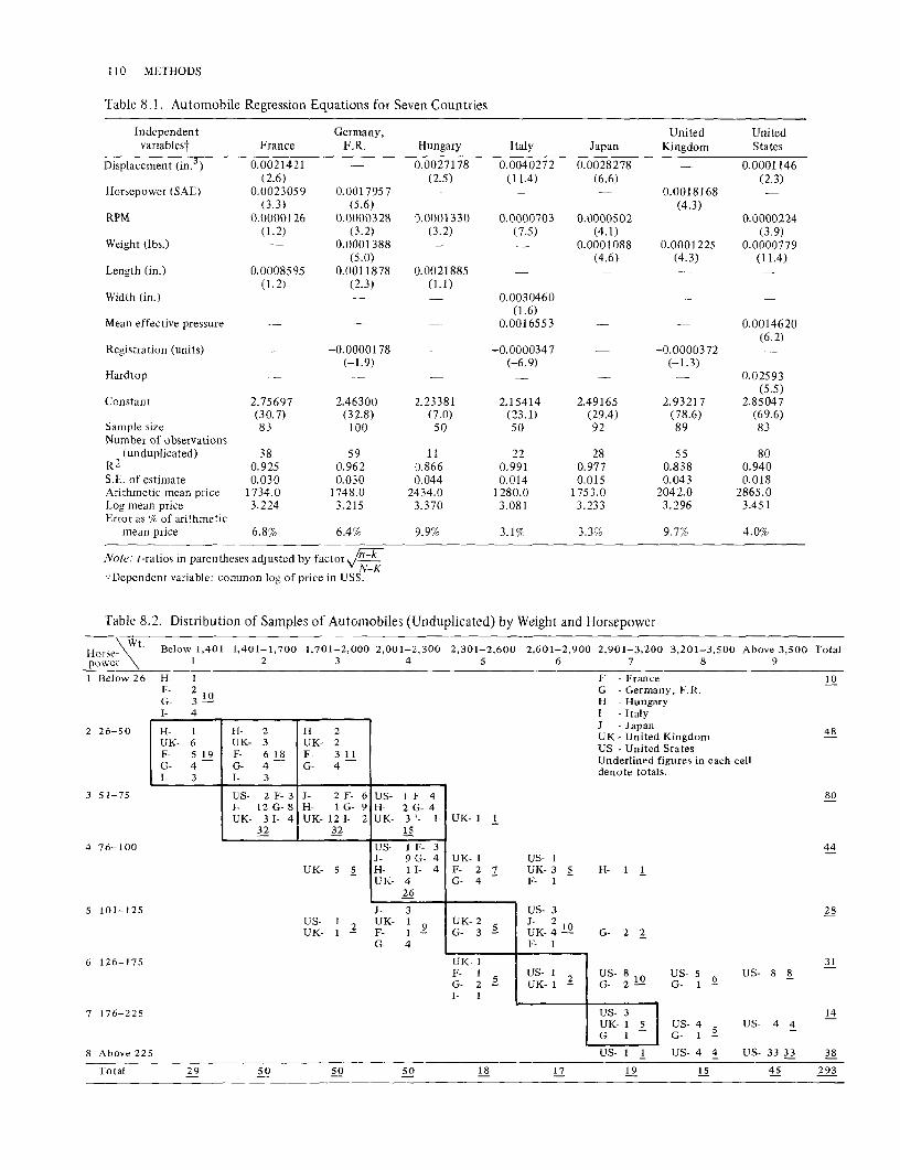
110 METHODS
Table 8.1. Automobile Regression Equations for Seven Countries
Independent Germany, United United variablest France F.R. Hungary Italy Japan Kingdom States
Displacement (in. 3) 0.0021421 0.0027178 0.0040272 0.0028278 0.0001146 (2.6) (2.5) (11.4) (6.6) (2.3)
Horsepower (SAE) 0.0023059 0.0017957 0.0018168 (3.3) (5.6) (4.3)
RPM 0.0000126 0.0000328 0.0001330 0.0000703 0.0000502 0.0000224 (1.2) (3.2) (3.2) (7.5) ( 4.1) (3.9)
Weight (lbs.) 0.0001388 0.0001088 0.0001225 0.0000779 (5.0) (4.6) (4.3) (11.4)
Length (in.) 0.0008595 0.0011878 0.0021885 (1.2) (2.3) (1.1)
Width (in.) 0.0030460 (1.6)
Mean effective pressure 0.0016553 0.0014620 (6.2)
Registration (units) -0.0000178 -0.0000347 -0.0000372 (-1.9) (-6.9) (-1.3)
Hardtop 0.02593 (5.5)
Constant 2. 75697 2.46300 2.23381 2.15414 2.49165 2.93217 2.8504 7 (30. 7) (3 2.8) (7.0) (23.1) (29.4) (78.6) (69.6)
Sample size 83 100 50 50 92 89 83 Number of observations
(unduplicated) 38 59 11 22 28 55 80 R2 0.925 0.962 0.866 0.991 0.977 0.838 0.940 S.E. of estimate 0.030 0.030 0.044 0.014 0.015 0.043 0.018 Arithmetic mean price 1734.0 l 748.0 2434.0 1280.0 1753.0 2042.0 2865.0 Log mean price 3.224 3.215 3.370 3.081 3.233 3.296 3.451 Error as % of arithmetic
mean price 6.8% 6.4% 9.9% 3.1% 3.3% 9.7% 4.0%
Note: t-ratios in parentheses adjusted by factor~ N-K
tDependent variable: common log of price in US$.
Table 8.2. Distribution of Samples of Automobiles (Unduplicated) by Weight and Horsepower
t. Horsc Below 1,401 1,401-1,700 1,701-2,000 2,001-2,300 2,301-2,600 2,601-2,900 2,901-3,200 3,201-3,500 Above 3,500 Total
powe_r ~~-1 Below 26 H
FGI-
2 26-50 H-UK-F-G-I-
3 51-75
4 76-100
5 101-125
6 126-175
7 176-225
8 Above 225
Total
1 2 3 4 5 6 7 8 9
I 2 10 3-4
1 6 5 19 4 3
29
H- 2 UK- 3 F- 6 18 G- 4 I- 3
US- 2 F- 3 J- 12 G- 8 UK- 3 I- 4
32
H- 2 UK- 2 F- 3 11 G- 4
J- 2 F-H- 1 G-UK- 12 I-
32
UK- 5 i
US- I l UK- I
6 US- I F- 4 9 H- 2 G- 4 2 UK- 3 I- 1
!.2 US- 1 F- 3 J- 9 G- 4 H- I I- 4 UK- 4
26
J- 3 UK- I
2 F- I G- 4
UK- 1 l
UK- 1 US- I F- 2 7. UK- 3 i G- 4 F- 1
US- 3 UK-2
§.. J- 2
G- 3 UK- 4 .!.Q F- 1
UK-1 F- I
i US- I
l G- 2 UK- I I- I
18
F - France G - Germany, F.R. H - Hungary I - Italy J - Japan UK- United Kingdom US - United States Underlined figures in each cell
s. denote total
H- I !.
G- 2 ~
US- 8 10 G- 2-US- 5
§_ US-
G- I
US- 3 UK- I .?_ G- I
US- 4 l
US-G- I
8 ~
4 '.!.
US- 1 I US- 4 '.!. US- 33 ll
!.2 !§. ~
10
48
80
44
28
31
14
38
293

MATCHING QUALITIES BY REGRESSION METHODS 111
Table 8.3. Distribution of Samples of Automobiles (with Duplications) by Weight and Horsepower
Horsepower
Wt. Below 1,401 1,401-1,700 1,701-2,000 2,001-2,300 2,301-2,600 2,601-2,900 2,901-3,200 3,201-3,500 Above 3,500 Total l 2 3 4 5 6 7 8 9
1 Below 26 H- 1 F- 3 23 G- 4-1- 1 S
2 26-50 H- 11 H- 12 UK- 8 UK- 4 F- 21 53 F- 9 39 G- 7 G- 8 I- 6 I- 6
3 51-75 US- 2 F- 5 J- 40 G- 9 UK- 9 I- 9
74
4 76-100
H- 5 UK- 2 27 F- 4-G- 16
J- 2 F-19 US- 4 F-11 H- 9 G-17 H- 8 G- 7 UK- 26 I- 4 UK- 6 I- 4
77 40
US- 1 F- 3 J- 32 G- 5
UK- 1 .!.
UK- 1 US- 1
F - France G - Germany, F. R. H - Hungary I - Italy J - Japan UK- United Kingdom US - United States Underlined figures in each cell
s. denote total
23
119
192
83
UK- 12 12 H- 1 I- 5 F- 3 10 UK-4 2 H- 3 3 -UK- 4 G- 6 F- 2 ll
5 101-125 J- 9 US- 3 47 US- 1
~ UK- l 17 UK- 2
~ J- 9
UK- I F- 1 - G- 4 UK- 4 .!.2 G- 5 2. G- 6 F- 1
6 126-175 UK- 1 31 F- I US- I
1.. US- 8 lO G- 22 UK- 1 G- 2-
US- 5 £.
US- 8 .§_ UK- 1
I-
7 176-225
8 Above 225
Total 76 113 118 108
because virtually no overlapping observations were available for other countries. For each of the ten cells, a particular car falling within the cell was selected to represent it. An effort was made to select cars from the production of different countries, preferably those which were used in other countries as well. The result of this is shown in the list of cars included in Table 8.4. This table also shows the prices of each car as estimated from each country's best equation. Prices followed by the symbol ( §) represent those estimated for cars that were beyond the range of sample observations in the country. The Japanese sample, for example, does not have any car under 51 or over 125 horsepower, and therefore the prices for the first two models in the list and for the last three had to be estimated by extrapolating the Japanese regression beyond the range of observation of the Japanese sample. Prices for models followed by the symbol (e;\) lie outside the middle 90 percent of the country's ( duplicated) sample.
ORIGINAL-COUNTRY BINARY PRICE COMPARISONS
Some alternative sets of results of the international price comparisons are presented in the upper half of Table 8.5. The first three columns show simple geometric means of prices relative to the United States based on different selections of the models to be included in the comparisons. The first column shows the
1
22
US- 3 UK- 1 j_
US- 4 ..i.
US- 4 ~ 14 G- 1
G- 1
US- 1 _!_ US- 4 4 US- 33 ll_ 38
26 24 15 45 547
results when all ten cars are included. The next column shows the results of including in each comparison with the United States only those which were common to the pair of countries.13 The indexes for the Federal Republic of Germany and the United Kingdom are higher than when all cars were included because, in the overlapping comparisons, the small cars, which are relatively expensive in the United States, are excluded. The indexes for the other countries are lower because of the exclusion of very large cars that turn out to be very expensive when the regressions are extrapolated to estimate them.
The comparisons in the third column also are based on overlapping models but exclude those at the extreme ( 5 percent on each end) of the country's distribution. 14
The deletion of some of these models has a marked effect in some instances, most notably in the United Kingdom.
The next two columns of the table show weighted arithmetic mean price relatives for the overlapping observations when they are weighted first with U.S. expenditure weights and then with the other countries' weights.
13That is, the mqdels followed by ( §) in Table 8.4 were
excluded. An alternative to the exclusion of these items would have been to weight them (and other items) inversely to the standard error of forecast.
14 Models followed by either ( §) or (,i) in Table 8.4 were excluded.

112 METHODS
Table 8.4. Estimated Automobile Prices by Country and Model, 1969 (US$)
Germany, United United Cellt Model France F.R. Hungary Italy Japan Kingdom States:j:
2, I Renault R4-40V 1,281 1,061 1,991 988 1,017§ 1,398 1,602§ 2,2 Fiat 85 0 Berlina 1,373 1,125 1,962 1,105 1,065 § 1,501 1,769§ 2,3 Volkswagen 1300 1,714 1,369 2,544 1,338 1,371 1,718 1,740§ 3,2 Escort 1100 DX 2D 1,695 1,405 3,097 1,438 1,367 1,667 1,798,r 3,3 Opel Kadett LS 45 PS 1,728 1,484 3,304 1,468 1,397 1,706 1,840,r 3,4 Peugeot 404 Berlina 2,063 1,833 3,544 1,665 1,765 2,106 1,982 4,4 Corona Mk!I 1600 DX 40 2,463 1,990 3,970 2,068 1,882 2,247 2,123 5,5 Vauxhall Victor 2000 40 3,028,r 2,340 5,265 § 2,593,r 2,402§ 2,509,r 2,112 6,6 American 6 5,288 § 2,581,i 5,575§ 4,807§ 3,940§ 3,098,i 2,004 7,7 Chevy II Nova VS 12,479§ 4,296,i 12,405 § 12,164 § 8,665 § 4,751,i 2,249
tFirst figure applies to row number and second figure to column number in Tables 8.2 and 8.3. :j:These prices have been adjusted from those estimated from the regression to allow for discounts from listed prices received by consumers. The adjustments were 10. 7 percent for the last two cars in the list and 5 .4 percent for the others. They are based on a Federal Trade Commission analysis of approximately 10,000 invoices for the model year 1969. (Memorandum by Steven R. Nelson dated September 10, 1969, entitled "Public Hearing Relating to Price Advertising of New Automobiles.") §Outside of country's range of observations. ,i Outside of middle 90 percent of country's observations.
The geometric mean of these two indexes (Fisher's "ideal" index) is shown in the following column. As is to be expected, the U.S. weights tend to result in higher price relatives for other countries than any other form of computation.
The U.S. and other individual-country-weighted indexes (columns 4 and 5) are the results that are easiest to relate to the underlying economic theory of demand. In each index, prices are compared for the mix of automobiles in the consumption pattern of one of the countries. But the need to confine the comparison to overlapping models introduces an arbitrary element into the assignment of weights. In the case of the United States, for example, the largest car of the ten, the Chevy Nova, was assigned 62 percent of the U.S. weights in the comparison with the United Kingdom, because it seemed preferable to assign the weights of the larger cars to this one rather than to distribute them in part to still smaller models. Nevertheless, given the great differences in the types of automobiles purchased, these results represent the best price comparisons we can make between each country and the United States.
If a single answer is desired, the Fisher index is to be preferred at least marginally over unweighted indexes in columns 1 to 3 because it provides an explicit compromise between the indexes corresponding to each country's weights. Among the three unweighted indexes, the last one ( column 3) is superior to the others because it is not affected by high prices associated with atypically small volume. It would be felicitous if the results of the Fisher index ( column 6) and the simple geometric mean of overlapping models excluding extreme values (column 3) were in close agreement. The difference between them, however, is 30 percent for the United Kingdom- United States comparison and nearly 25 percent for the Germany (F.R.)-United States comparison.
BRIDGE-COUNTRY COMPARISONS One way to compare the prices for pairs of countries
other than pairs involving the United States is by using the United States as the bridge country. For example, the Fisher indexes for France-United States and Germany (F.R.)-United States, 119 and 123, respectively, imply a France-Germany (F.R.) price index of 97 (119--c-123==97). The France-United States and Germany (F.R.)- United States Fisher indexes, however, like all the indexes in Table 8.5, are based on a set of cars that varies from one row of the table to another depending upon the overlap of models of each country, with the United States as the base country. Because the United States has missing observations for the three small cars, and most of the other countries have missing observations for at least two of the big cars, none of the indexes in columns 2 to 6 is based on more than seven cars, and some are based on as few as two. This means that although the index numbers under discussion may
provide reasonable alternative estimates of each country's relation with the United States, it would be unwise to try to draw inferences about the relationships between pairs of countries other than the United States.
But the United States, which in most categories of goods has a broad range of varieties and thus provides a good market in which to find matching products for almost all other countries, clearly does not serve this function nearly as well when it comes to automobiles. Both the Federal Republic of Germany and the United Kingdom have all ten observations and, consequently, represent better base countries than does the United States.
Accordingly, the United Kingdom has been used as the base country in the second bank of figures in Table 8.5. The differences between the column 3 and column 6 indexes are much reduced as compared with the earlier

MATCHING QUALITIES BY REGRESSION METHODS 113
Table 8.5. Binary Automobile Price Comparisons, Based on Prices Estimated from Each Country's "Best" Index, 1969
France Germany, F.R. Hungary Italy Japan United Kingdom United States
France Germany, F.R. Hungary Italy Japan United Kingdom United States
set of figures; aside from the United States, they are all within 6 percent. The shift to the new base country does not affect the relationship between the United States and the United Kingdom (because the comparison is identical except that numerator and denominator are reversed), but for the other countries, the relationships do change in relation both to the United States and to each other. With respect to comparisons of each country with the United States, the first bank of figures must be regarded as superior; but with respect to comparisons between other pairs (for example, France-Germany [F.R.] ), the figures in the second bank are better because they are based on more observations (four to ten). It can be seen that the index number spread is smaller, and that results of the various indexes are much more in accord with one another-except, of course, for the row representing the United States. The implicit Fisher index for France-Germany (F .R.) using the United Kingdom as the bridge country is 120 ( 103 7 86 = 120).
No bridge country, of course, can produce a binary comparison that is optimal purely from the standpoint of the two countries involved; only a direct comparison based on the models that overlap for the two countries can do that. But even a full set of direct binary comparisons would not be fully satisfactory from the standpoint of the ICP. What is desired is circularity and independence of the choice of a bridge-country, which neither binary indexes nor the Fisher indexes based on a single country will yield. This is a general problem in the ICP that has been resolved for other product categories by the Country-Product-Dummy method (CPD).
Simple geometric mean Weighted mean for all of price relatives overlapping cars
Overlapping cars Base Other All Except country country Fisher cars All extreme weights weights index
(1) (2) (3) (4) (5) (6)
Part A. United States the base country 130 109 110 140 101 119 93 106 99 163 93 123
195 179 183 186 177 181 109 92 90 120 85 101 102 88 96 111 89 99 111 121 106 184 104 138 100 100 100 100 100 100
Part B. United Kingdom the base country 118 101 99 106 100 103 84 84 82 87 85 86
173 162 162 177 158 168 99 83 80 89 80 84 92 85 83 86 86 86
100 100 100 100 100 100 90 83 94 96 54 72
MULTILATERAL COMPARISONS The Country-Product-Dummy method as explained
in Chapter 5 assumes that the prices observed for the various models in different countries are related systematically to the countries and to the models. In a tableau of prices such as that which would be found in Table 8.4 if the prices followed by ( §) were deleted ( they are really missing observations and were obtained by extrapolation), the price in any cell may be regarded as depending, in one part, on the intercountry difference in prices and, in the other part, on the intermodel difference in prices. Accordingly, the log of prices is taken as the dependent variable in a regression in which the independent variables consist of two sets of dummy variables: in one set, there is a dummy variable for each model car in the tableau; and in the other set, there is a dummy variable for each country other than the numeraire country. The coefficient of the dummy variable for each country (strictly speaking, it is the antilog of the coefficient) provides a direct estimate of the car prices in that country relative to prices of the numeraire country. It may illuminate the underlying method to point out that when the regression equation is fitted to a completely filled-in tableau, the antilog of each country coefficient will be equal to the simple geometric mean of the price ratios for the individual cars.
The results of the CPD method are presented in columns 1 and 2 of Table 8.6, the first based on the treatment of the cells outside of the range of observation of the country sample (prices in Table 8.4 followed by

114 METHODS
Table 8.6. Multilateral Automobile Price Comparisons, 1969
Unweighted CPD Weighted CPD
55 46 55 46 o bservationst observations :j: observationst observations :j:
(1) (2) (3) (4)
Part A. United States the numeraire country France Germany, F.R. Hungary
123 117 167 127 105 97 137 104 199 191 278 212
Italy 100 95 139 106 Japan 97 95 134 102 United Kingdom United States
125 118 154 119 100 100 100 100
Part B. United Kingdom the numeraire country France Germany, F.R. Hungary
99 99 108 107 84 83 89 87
160 162 181 178 Italy 81 80 90 89 Japan 78 80 87 86 United Kingdom United States
100 100 100 100 80 85 65 84
tCells in Table 8.4 followed by ( § ), representing cells outside of range of sample observations, are not included in the regression. 4:Cells in Table 8.4, followed by ( §) or (11), representing cells not falling within middle 90 percent range of observations, are not included in the regression.
[ §]) as missing observations or holes, and the second treating the cells outside of the middle 90 percent of the country sample (prices followed by [ §] and [~]) as holes. These indexes are most comparable, respectively, to the simple geometric mean for all overlapping cars and to the simple geometric mean for the overlapping cars excluding the extremes in Table 8.5. Because these indexes are unweighted, it is probably better to base them on the middle 90 percent range, and the column 2 version therefore would be preferred over column 1.
An advantage of the CPD method, which was compelling for product categories other than automobiles, is that it uses all the information in the available set of prices to gauge the price level relationship between each pair of countries. The weakness of the method, which becomes important in the automobile context, is that it is based on a kind of averaging of country-to-country price differences across models which assumes that no systematic element exists in the behavior of the price ratios for different models. In fact, the country-tocountry price differences do vary in a systematic way with the characteristics of the models. For example, the France- United States price ratio rises from around 89 for the smallest car found in both countries to 110 for the largest.
This difficulty may be mitigated by the use of the double-weighted version of the CPD. 15 Each price in the tableau (Table 8.4) is weighted by the product of two importance factors-one based on the relative importance of each model in the expenditures of the country, the other based on the relative importance of a given
15 See pages 63-65.
model in each country compared with the "world" (that is, seven-country) total for that model.
The results of the double-weighted CPD method are shown in columns 3 and 4 of Table 8.6. The underlying prices once again are those of Table 8.4. In column 3, the fifteen prices for cars beyond the range of observations in a given country (that is, the entries followed by [ §]) are excluded, whereas in column 4, all the models outside the middle 90 percent range of observations are excluded.
Weighting raises the indexes for all countries relative to the United States. This effect is particularly notable in the case of the results based on fifty-five observations; the use of weights in conjunction with the inclusion of extreme observations has a large impact. In accordance with the basic approach outlined in our discussion of sampling, 16 we accept the results based on forty-six observations that exclude models not widely consumed.
These results in columns 3 and 4 in Part A of Table 8.6 differ substantially in some instances from the Fisher indexes in column 6 of Part A of Table 8.5. The comparison of the weighted CPD indexes and the Fisher indexes, however, can be better made by taking the United Kingdom as the numeraire country. From the CPD standpoint, it does not matter which country is used as the numeraire. The figures in Part B of Table 8.6 do serve, however, to call attention to the fact that the difference between the weighted calculations based on forty-six observations and those based on fifty-five observations concern mainly the United States; aside from the United States, there is little difference be-
16 See Chapter 3, especially page 31.

tween the figures in columns 3 and 4 when they are expressed relative to the United Kingdom. That is, the relationships among countries other than the United States are quite similar in columns 3 and 4-and this is true whatever country is taken as the numeraire.
From the standpoint of the Fisher indexes, however, the U .K.-based estimates are clearly superior to those based on the United States, because they are derived from a larger and more similar list of cars. With the United Kingdom as the base country, the weighted CPD results are, with the exception of United States, not much different from the Fisher results of Table 8.5.
PRICE COMPARISONS FOR NONREGRESSION COUNTRIES
For three countries-Colombia, India, and Kenyainformation was gathered for only a few models. Actually, only three models are available in India on any scale. Because regressions were not feasible for these countries, the method adopted was to use the equations in Table 8.1 to estimate U.S. and U.K. prices for cars comparable to the Colombian, Indian, and Kenyan models. The results are set out in Table 8.7.
Unweighted geometric means of the price ratios for the three or four models have been taken. In the case of India, where the three included models account for the great bulk of Indian cars, the method is about as satisfactory as can be found. For the other countries, regression methods might have been used, but they would have required a greater data-collection effort. The results suggest, however, the advantages of using regression methods. For Kenya the ratios range from 6.9 to 10.2, a spread of 45 percent, and for Colombia the range is still
MATCHING QUALITIES BY REGRESSION METHODS 115
greater. Some other selection of three or four models for price comparison might produce very different averages. The regression approach has the merit of taking into account the entire range of models in the marketplace in estimating the price for any particular model.17
Because the small cars for which prices must be estimated for comparisons with Colombia, India, and Kenya are within the range of observations for the United Kingdom but not for the United States, the former provides a better bridge country. Therefore, although the average price ratios relative to the United States are used as the automobile entries in the binary comparison of each country with the United States, the price ratios relative to the United Kingdom are used for the multilateral comparisons.
CONCLUSION The final indexes selected are set out in Table 8.8.
For the regression countries, the U.S.-weighted and own-weighted indexes based on regression estimated prices ( columns 4 and 5, Table 8.5) are used for the binary comparisons with the United States. The weighted CPD indexes based on forty-six observations are used for these countries to accomplish the multilateral comparisons.
For the nonregression countries, the indexes are simple geometric means relative to the United States for the binary comparisons and simple geometric means relative to the United Kingdom for the multilateral compari-
17The comparisons involving Kenya and Colombia could have been improved by weighting, but the data requiied for this purpose are hardly less troublesome to gather than the data req uiied for regressions.
Table 8.7. Comparison of Prices of Passenger Cars in Colombia, India, and Kenya with Estimated Prices for Comparable Cars in the United States and the United Kingdom, 1969
Pricest Price ratios
Weight Domestic Est. Est. U.S.= U.K.= HP (lbs.) market U.S. U.K. 100 100
Colombian cars Renault 4 37.5 1,367 2,181 1,751 1,438 125 152 Simca 1000 49.5 1,576 2,748 1,901 1,609 145 171 Zastava 72 2,116 3,952 2,289 2,070 173 191 Dodge Dart Big 6 145 3,013 7,102 2,440 3,649 291 195
Geometric mean 174 176 Indian cars
Herald Mark Ill Standard 40 1,929 2,090 1,903 1,717 110 122 Fiat 1100 Delight 43 1,896 2,410 1,852 1,721 130 140 Ambassador Mark III 50 2,563 2,553 2,025 2,164 126 118
Geometric mean 122 126 Kenyan cars:j:
Volkswagen 1200 Deluxe 41.5 1,675 1,916 1,762 1,604 109 119 Volkswagen 1500 Deluxe 53 1,918 2,110 1,840 1,805 115 117 Toyota Corolla 1200 4-door 73 1,611 1,875 2,073 1,785 90 105 Ford Cortina 1600 DX 4-door 76 1,973 2,690 2,031 2,015 132 134
Geometric mean 110 118
tConverted to U.S. dollars at the following exchange rates per US$: Colombia, 17.38 pesos (principal selling rate); India, 7.550 rupees; Kenya, 7.143 shillings; U.K., 0.4182 pounds sterling. :j:The Kenyan prices represent list prices reduced by 7 percent to allow for discounts.

116 METHODS
Table 8.8. Final Automobile Price Comparisons, 1969
Binary comparisons
Weighted arithmetic Simple mean
geometric U.S. Own mean weights weights
(1) (2) (3)
France 140 IOI Germany, F.R. 163 93 Hungary 186 177 Italy 120 85 Japan 111 89 United Kingdom 184 104 United States 100 100 Colombia 174 India 122 Kenya 110
sons. In the latter case, the indexes are converted to a U.S. base using the United Kingdom as the bridge country. Relative automobile prices for these countries appear lower when the comparison is based on U.S. prices than when they are made by way of the United Kingdom. This is attributable to the fact that the models involved in the comparisons are mainly small cars, which tend to be relatively expensive in the United States. This, together with the fact that some of the U.S. prices must be estimated by extrapolation of the U.S. equation
(U.S." 100)
Multilateral comparisons
(4)
127 104 212 106 102 119 100 209 150 140
into a range for which there are no U.S. observations, may point to a preference for the use of the results obtained by way of the United Kingdom even for the binary comparisons of each country with the United States. In this view, the figures in column 4 may give a better indication of what the relative prices of cars might be in each of the last three countries, assuming that country and the United States produced the same type of car, each maintaining its 1969 scale and other conditions of production.

Chapter 9
Rent comparisons
A. Conceptual Problems
The comparison of the cost of housing services posed special difficulties for the International Comparison Project. For one thing, a substantial number of dwelling units are owner-occupied in most countries (see Table 9.1). Market prices for housing services are available only for rented dwellings, and our price comparisons for housing services are necessarily based on rent comparisons. In this respect we do not deviate from standard national accounts practice, in which the intertemporal estimation of price changes for housing services within individual countries also is based on changes in rents.
Even within this framework, however, price comparisons involved some problems rather different from those encountered for the general run of consumer commodities and services.
First, it was not possible to obtain price information from a relatively few key sellers, as could be done for most consumer goods. In most countries, a substantial fraction of rented units is let out by landlords who have only a few units to rent.
Second, a much greater dispersion of rents around the national average probably exists for each given type of dwelling than is the case for most other commodities and services. In some measure, this is the result of limited knowledge of the market on the part of amateur landlords and on the part of tenants, who tend to rent with little and infrequent market research. What is even more important in making the market imperfect from a national standpoint is the limited possibility of substitution between houses in different localities: housing markets are uniquely local markets.
Third, most countries have a great variety of dwellings with respect to type of structure, condition, size, facilities, and location or neighborhood. Taken in conjunction with the imperfection of markets, this range increases the need for rent comparisons based on as wide a variety of dwellings as possible.
Fourth, housing tends to be one of the categories in which the difference between high- and low-income
countries is great. As a result, the degree of overlap in the types of housing between a very poor country and a very wealthy country is apt to be much smaller than is the case for most other commodities and services.
One consequence of these difficulties is that even if we were able to measure every rent-determining quality of a housing unit, we would be able to estimate the rent of any particular unit only with a considerable margin of error.
Actually, we cannot measure or even identify with certainty all of the important quality variables. Only those that are capable of objective description and measurement fall within our reach: for example, size (floor area or number of rooms) and facilities or amenities ( the presence or absence of electricity, inside running water, flush toilet, and tub or shower).
Thus, our matching of dwellings in different countries is necessarily approximate. It is based on key quantitative (floor area) and qualitative (presence or absence of facilities) characteristics. Other important variables such as the general quality of the neighborhood, which often has a major impact on rents, could not be taken into account. But, with some major exceptions, which will be pointed out, the estimates do not involve large elements of judgment, and it is unlikely that other analysts relying also upon available indicators of housing quantity and quality would come to substantially different results. Furthermore, a substantial fraction of the variation in rents within a country, generally about 0.6 or better, can be explained by the variables with which we work.
The objective variables we want to use are not always readily available. One of those sometimes difficult to obtain in a satisfactory form relates to the size of dwelling units. For countries to use the number of rooms as the measure of size in their housing statistics is common. This is understandable, because it is easier for the occupant or interviewer to count rooms than to measure floor area. But the definition of rooms and their average size on any standard definition may vary widely from country to country. Therefore, whenever information on floor area was not available directly, it was necessary in each country to obtain some estimate of the floor area
117

118 METHODS
Table9.l. Indicators of Quantity of Housing, Eight Countries
Colombia France Germany (F.R.) Hungary India Italy Japan C.K. U.S. 1964 1968 1968 1970 1960 1961 1968 1966 1970
Population (000) 17,485 49,655 60,842 10,295:j: 434,885 50,625 98,275 53,789 203,185 Number of dwellings
Total (000) 1,258 15,190 19,347 3,035 79,194 13,032 24,198 17,016 63,450 Per 100 persons 7.2 30.6 31.8 29.5 18.2 25.7 24.6 31.6 31.2
Percent owner occupied 61 43 34 63 85 46 60 48 63 Average floor area (sq. m.)
Per dwelling n.a. 52.4 62.3 43.9 27.1 54.4 62.5 84.5 95.6 Per person n.a. 16.0 19.8 13.0 4.9 14.0 15.4 26.7 29.8
Percent of dwellings with: 42 Flush toilet 52 86 33 2 17 98 96
Inside piped water 41 91 99 36 5 62 95 98
±Figure for 1969. Sources: Population, number of dwellings, and precentage owner-occupied, U.N. Statistical Yearbook, 1972, Table 203, Summary of Housing Condition. Average floor area: France, the Federal Republic of Germany, and Italy: number of rooms per dwelling unit reported in the U.N. Statistical Yearbook, 1972 multiplied by the average size of rooms in dwellings occupied by iron and steel workers reported in Situation des Logements des Travailleurs C.E. C.A., Statistiques Socia/es, No. 2, 1961, Office Statistique des Communautes Europeennes. Hungary: estimated from data provided by the Central Statistical Office. India: estimated from the distribution of dwellings by room size as given in the Census of India, 1961, 1, part IV (B), Housing and Establishment Tables: and from average floor area of dwellings of different room sizes reported for 1968-69 in the Quick Tabulation Schedule, National Sample Survey, 23rd Round, and specially provided to the ICP. Japan: from tables relating to the 1968 Census of Housing, specially prepared for the ICP by the Bureau of Statistics. United Kingdom: based on 5.35 rooms per dwelling computed from U.N. Statistical Yearbook, 1972, and on estimated floor area for that number of rooms. The latter figure is derived from data on dwellings subject to registered rents provided by the Department of the Environment. United States: estimated floor area of a five-room unit, reported as the median size in the 1970 Census of Housing. Percentage of dwellings with flush toilet and with inside piped water: from U.N. Statistical Yearbook, 1972, except for India, which is from the National Sample Survey, 15th Round.
associated on the average with dwellings having different numbers of rooms.
Another variable that is an important indicator of the quality of housing, at least in some countries, is the age of the dwelling unit. In the United States, higher-income families tend to occupy newer and more expensive quarters; older dwellings tend to rent for relatively diminished amounts, partly because they are sometimes allowed to deteriorate and are found in declining neighborhoods, partly because newness itself commands a premium. It is also possible that newer buildings contain other desirable features not measured by the variables we use to explain rents-for example, more efficient heating systems. Thus, as can be seen from Table 9.2, dwellings built in the 1960s rented in the United States for 20 percent more than dwellings with the same physical characteristics built in the 1950s. The age factor also seemed to be an important influence on rents in Japan and India, although for the latter, the figures refer to Bombay alone. In Europe, on the other hand, age seems to have a smaller impact on rents. In England, the premium on ten-years age difference was much larger in the Greater London area (17 percent) than elsewhere (9 percent), but in Japan the premium in urban areas (18 percent) was lower than that in rural areas (35 percent).
A variable that we know to affect rents but that we have not utilized is location. Rents in London, for example, are 1.5 times the rents elsewhere in England and
Wales for recently constructed (post-1939) dwellings. Rents in Budapest tend to be 1.5 to 2 times those in rural communities in Hungary for dwellings with equal physical characteristics. Similar premiums for rents in large urban centers are found in India, Japan, and the United States and doubtless would be revealed in the other countries were the data available.
It seems clear that the rent differences attributable to location within a country reflect quality differences from the standpoint of consumers: a dwelling in London, Budapest, or Manhattan is more valuable than one with the same physical characteristics in a rural area in the same country. In the ICP, however, these locational scarcity values are not being taken into account. We regard these differences as price differences and seek merely the average national price for selected types of dwellings ( that is, ones with given physical specifications). This has the advantage of simplicity; it avoids the need to match places in different countries having equivalent scarcity values. (From a land-scarcity standpoint, what U.S. cities are matching to London? To Budapest?) More important, it is consistent with our treatment of farm and urban consumption in other sectors (the "a potato is a potato" approach set out in Chapter 2). Taking account of scarcity values would lead
us to regard, as between two countries with identical housing stocks, the country with the more concentrated population as having a larger real quantity of housing.
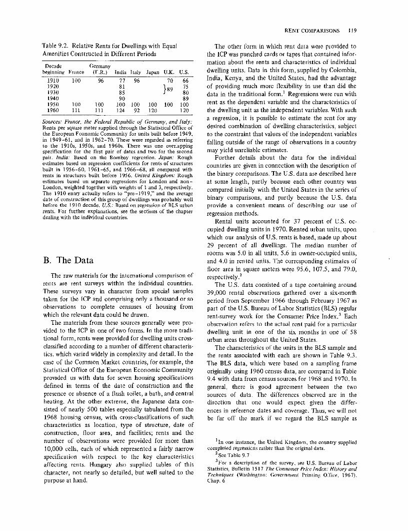
Table 9.2. Relative Rents for Dwellings with Equal Amenities Constructed in Different Periods
Decade Germany beginning France (F.R.) India Italy Japan U.K.
1910 100 96 77 96 70 1920 81
}89 1930 85 1940 90 1950 100 100 100 100 100 100 1960 111 111 124 92 120
U.S.
66 75 80 89
100 120
Sources: France, the Federal Republic of Germany, and Italy: Rents per square meter supplied through the Statistical Office of the European Economic Community for units built before 194 9, in 1949-61, and in 1962-70. These were regarded as referring to the 1910s, 1950s, and 1960s. There was one overlapping specification for the first pair of dates and two for the second pair. India: Based on the Bombay regression. Japan: Rough estimates based on regression coefficients for rents of structures built in 1956-60, 1961-65, and 1966-68, all compared with rents in structures built before 1956. United Kingdom: Rough estimates based on separate regressions for London and nonLondon, weighted together with weights of 1 and 3, respectively. The 1910 entry actually refers to "pre-1919," and the average date of construction of this group of dwellings was probably well before the 1910 decade. U.S.: Based on regression of BLS urban rents. For further explanations, see the sections of the chapter dealing with the individual countries.
B. The Data
The raw materials for the international comparison of rents are rent surveys within the individual countries. These surveys vary in character from special samples taken for the ICP and comprising only a thousand or so observations to complete censuses of housing from which the relevant data could be drawn.
The materials from these sources generally were provided to the ICP in one of two forms. In the more traditional form, rents were provided for dwelling units crossclassified according to a number of different characteristics, which varied widely in complexity and detail. In the case of the Common Market countries, for example, the Statistical Office of the European Economic Community provided us with data for seven housing specifications defined in terms of the date of construction and the presence or absence of a flush toilet, a bath, and central heating. At the other extreme, the Japanese data consisted of nearly 500 tables especially tabulated from the 1968 housing census, with cross-classifications of such characteristics as location, type of structure, date of construction, floor area, and facilities; rents and the number of observations were provided for more than 10,000 cells, each of which represented a fairly narrow specification with respect to the key characteristics affecting rents. Hungary also supplied tables of this character, not nearly so detailed, but well suited to the purpose at hand.
RENT COMPARISONS 119
The other form in which rent data were provided to the ICP was punched cards or tapes that contained information about the rents and characteristics of individual dwelling units. Data in this form, supplied by Colombia, India, Kenya, and the United States, had the advantage of providing much more flexibility in use than did the data in the traditional form. 1 Regressions were run with rent as the dependent variable and the characteristics of the dwelling unit as the independent variables. With such a regression, it is possible to estimate the rent for any desired combination of dwelling characteristics, subject to the constraint that values of the independent variables falling outside of the range of observations in a country may yield unreliable estimates.
Further details about the data for the individual countries are given in connection with the description of the binary comparisons. The U.S. data are described here at some length, partly because each other country was compared initially with the United States in the series of binary comparisons, and partly because the U.S. data provide a convenient means of describing our use of regression methods.
Rental units accounted for 37 percent of U.S. occupied dwelling units in 1970. Rented urban units, upon which our analysis of U.S. rents is based, made up about 29 percent of all dwellings. The median number of rooms was 5.0 in all units, 5.6 in owner-occupied units, and 4.0 in rented units. The corresponding estimates of floor area in square meters were 95.6, 107.5, and 79.0, respectively .2
The U.S. data consisted of a tape containing around 39,000 rental observations gathered over a six-month period from September 1966 through February 1967 as part of the U.S. Bureau of Labor Statistics (BLS) regular rent-survey work for the Consumer Price Index. 3 Each observation refers to the actual rent paid for a particular dwelling unit in one of the six months in one of 58 urban areas throughout the United States.
The characteristics of the units in the BLS sample and the rents associated with each are shown in Table 9 .3. The BLS data, which were based on a sampling frame originally using 1960 census data, are compared in Table 9.4 with data from census sources for 1968 and 1970. In general, there is good agreement between the two sources of data. The differences observed are in the direction that one would expect given the differences in reference dates and coverage. Thus, we will not be far off the mark if we regard the BLS sample as
1 In one instance, the United Kingdom, the country supplied completed regressions rather than 'the original data.
2 See Table 9.7 3 For a description of the survey, see U.S. Bureau of Labor
Statistics, Bulletin 1517 The Consumer Price Index: History and Techniques (Washington: Government Printing Office, 1967), Chap. 6

120 METHODS
Table 9.3. United States: Characteristics of Dwelling Units in BLS Urban Rent Sample, September 1966-February 1967
Average Number of Percentage monthly Standard
observations of samplet rent deviation
Total sample 39,107 100 $ 84.60 $ 44.42 Type of house 39,081 100
Single detached 6,234 16.0 72.82 34.76 Single semidetached 2,549 6.5 69.82 30.20 Single attached 1,335 3.4 74.56 32. 76 Multiple unit 28,606 73.2 89.16 47.19 Other 357 0.9 66.79 25.12
Condition 39,063 100 Sound 34,134 87.4 88.54 45.33 Deteriorating 4,188 10.7 58.61 23.36 Dilapidated 741 1.9 49.63 28.54
Year built 38,689 100 Pre-1920 14,513 37.5 64.78 28.24 1920-29 6,434 16.6 77.51 36.19 1930-39 3,485 9.0 77.58 33.37 1940-49 4,527 11. 7 87.80 34.64 1950-54 2,881 7.4 99.90 39.49 1955-60 3,137 8.1 109.25 47.95 1961-66 3,712 9.6 142.69 60.08
Number of rooms 39,058 100 One 1,338 3.4 73.37 33.30 Two 4,355 11.1 72.94 33.15 Three 11,512 29.5 82.23 39.33 Four 11,290 28.9 89.62 46.19 Five 6,506 16.7 87.77 46.48 Six 2,995 7.7 86.28 55.62 Seven 691 1.8 93.18 58.23 Eight or more 371 0.9 103.97 81.44
Number of private bathrooms 39,065 100 None or shared 2,061 5.3 54.42 27.40 Flush toilet only 510 1.3 40.36 34.47 Half bath 651 1.7 53.12 36.63 One complete bath 34,194 87.5 83.86 36.83 One-and-a-half baths 850 2.2 130. 75 65.36 Two baths or more 799 2.0 198.88 106.93
Heating equipment 39,021 100 None 1,366 3.4 103.05 55.80 Central 25,464 65.3 91.94 46.48 Other installed 11,273 28.9 68.48 32. 74 Other not installed 948 2.4 52.82 23. 70
Included in rent Refrigerator 39,097 100
Yes 20,208 51.7 100.02 50.97 No 18,889 48.3 68.16 28.77
Stove 39,098 100 Yes 23,676 60.6 97.14 49.57 No 15,422 39.4 65.42 25.98
Electricity 39,096 100 Yes 8,524 21.8 91.28 50. 73 No 30,572 78.2 82.76 42.65
Heat 39,019 100 Yes 19,447 49.8 94.15 48.97 No 19,572 50.2 74.97 37.41
Garage 39,078 100 Yes 8,427 21.6 95.43 46.09 No 30,651 78.4 81.58 43.64
tFor each characteristic, the number of observations providing information about that characteristic is taken as l 00.
indicating the most common characteristics of U.S. renter-occupied urban housing. The 1970 census data in the table, showing the characteristics of all dwellingsurban and rural, as well as rental and owner-occupiedwill be useful for weighting purposes.
The rents in Table 9.3 refer to the payments actually made by the tenants to landlords, whether or not equipment or services as well as housing space were covered by the payments. About one-fifth of these "contract" rental payments, for example, included garages, about

RENT COMPARISONS 121
Table 9.4. United States: Characteristics of Dwellings
Number of rooms one and two three four five or more
Number of housing units in structure
one two three or four five or more
Year built 1939 or earlier 1940-49 1950-59 196 0 or later
Median rent Mean rent
tRenter and owner occupied.
BLS urban sample 1966-67
(%) 100
14 30 29 27
100 27 16 15 42
100 63 12 14 11
$75.55 $84.60
Renter occupied
Bureau of Census sample, urban & rural
1968 (%)
100 11 24 31 34
100 31 19 13 37
100 58 13 12 17
$78
All d wellingst
Census of Housing 1970 (%)
100 5
11 21 63
100 68
9 5
15 100 41 13 21 25
$89
Source: BLS data from special tabulation. (The median BLS rent is based on the geometric mean. See text.) Census sample data from U.S. Bureau of the Census, Current Housing Reports, Series H-111, No. 55 (July 1969), Tables 17 and 18. 1970 Census of Housing data from Detailed Housing Characteristics, Final Report HC (1 )-B 1, U.S. Summary (July 1972), Tables 30, 31, and 32.
one-half included heat, and well over one-half included the use of stoves and refrigerators supplied by the landlord. The data that are required for the ICP represent "space" rents: they should exclude all such payments for equipment and for service and should cover the use of dwelling space alone.
THE GENERAL APPROACH The exclusion of these payments was achieved in the
course of a multivariate analysis in which facilities and services other than space were taken as explanatory variables and rent as the dependent variable. At the same time, other key quantitative and qualitative characteristics of the dwelling units, such as the number of rooms, bathroom facilities, and age of the dwelling also were included as explanatory variables. With the inclusion of such added variables as regional location, population size of the community in which the dwelling was located, and structural characteristics of the dwelling unit, the number of independent variables examined increased to forty.
A number of equations were estimated, using alternative combinations of independent variables. Most of the coefficients obtained seemed plausible and, despite some multicollinearity, proved in general to be quite stable with alternative combinations of the independent variables. The large size of the sample used in the regressions, 38,349, helped make it possible to isolate the
separate effects on rent of the various variables despite the high correlation between some of them.
THE PREFERRED EQUATION The preferred equation is summarized in Table 9.5.
The percentage of explained variation (JP= 0.64) is not as high as we would like, of course, probably reflecting the omission from the data of important quality variables associated with neighborhood and structure that are difficult to measure. Our inability to control these variables is not unique to the regression technique, however, and in the same manner would limit traditionaltype rent comparisons. All of the coefficients in the equation are more than twice their standard errors. The merit of the preferred equation is that its coefficients provide plausible estimates of the separate effects of the different variables.
The natural logarithm of rent was taken as a function of thirty-three independent variables, of which only the log of population was a continuous variable. The coefficient for population indicates that the log of monthly rent was .OS 19 higher, holding everything else constant, for each increase of 1 million in city size. This works out to a 5.3 percent increase in rent for every rise of 1 million in city size ( that is, the antilog of .OS 19 is 1.053).
All the other variables are dummy variables taking on a value of 1 if a given observation was characterized by

122 METHODS
Table 9.5. United States: Coefficients of Regression Equation for Urban Rents, September 1966-February 1967
Standard Variable Coefficientt error
Population (log of millions) 0.0519 .0010 Location variables:j:
North Central states 0.0674 .0040 Western states 0.0710 .0052 Southern states -0.0134 .0049 Alaska 0.6273 .0116 Hawaii 0.3960 .0105
Inclusious in rental payment§ Refrigerator 0.1448 .0054 Cooking stove 0.0707 .0053 Electricity 0.0304 .0043 Heat 0.1320 .0044 Garage 0.0996 .0037 Furniture 0.0245 .0044
Structural characteristics Central heating,i 0.1449 .0039 Multiple unit# 0.0449 .0040 Conditiontt
Deteriorating -0.0879 .0049 Dilapidated -0.1627 .0107
Year built:j:t 192(}-29 0.0886 .0043 193(}-39 0.1463 .0055 194(}-49 0.2444 .0053 195(}-54 0.3250 .0062 1955-60 0.4237 .0060 1961-66 0.5634 .0059
Number of rooms§ § two 0.0850 .0088 three 0.2243 .0084 four 0.3440 .0086 five 0.4551 .0092 six 0.5121 .0101 seven 0.5887 .0139 eight or more 0.6648 .0174
Bathroom facilities,i ,i One-half bath 0.0646 .0124 One complete bath 0.2270 .0062 One-and-one-half baths 0.4058 .Oll8 Two or more baths 0.6419 .0123
Intercept 3.2413
iF =.64 SEE= .2769
Mean of logs of rent: 4.3248
Definitions: Number of rooms: A room has four (permanent) walls to the ceiling; is finished; and is used regularly for living quarters. Other spaces not completely separated from an adjoining room and with less than four walls to the ceiling are counted as half rooms. Bathrooms are not counted as rooms. Condition of dwelling unit: A sound house has no defects or only slight defects, which normally are corrected during the course of regular maintenance: whereas a deteriorating housing needs more repairs than would be provided in the course of regular maintenance. A dilapidated house does not provide safe and adequate shelter. Shacks, huts, or other structures with makeshift walls or roofs or with dirt floors are considered to represent inadequate construction. Bathroom: A complete bathroom contains (1) a flush toilet, (2) a wash bowl, and (3) a bathtub and/or shower. A half-bathroom consists of any two of these three standard fixtures. Multiunit structures: A structure containing two or more housing units.
tNatural logarithms. :j:Northeast the base. § Exclusion from rent the base in each case.
the specified characteristic and O if it was not. In this method, a dummy variable is included for each of a given set of characteristics except one.4 The coefficient of each dummy variable then indicates the amount by which the lo-g of rent for that characteristic differs from the log of rent for the omitted characteristic. In the case of rooms, for example, the omitted, or "base," characteristic is a one-room dwelling unit, and the coefficient for each room size indicates the amount by which the log of rent for that number of rooms exceeds the log of rent for one-room units, holding everything else constant. The number of rooms could have been treated as a continuous variable, but this would have implied an equal log rent increase for each unit increase in the number of rooms. Our coefficients show the increase is not really uniform; from one to two rooms, for example, the log of rent rises by .0850 (equivalent to 8.9 percent), but a third room adds another .l 393 to the log of rent, equivalent to 14.9 percent. Incidentally, the continuous rise in rents with room size indicated by these coefficients is in contrast to the more erratic movement of rents in Table 9.3, the difference being that in Table 9.3 each room size group contains a different mix of the other rent-influencing characteristics, whereas in Table 9.5, all other characteristics are held constant and only the difference in the number of rooms is allowed to influence the coefficients.
In a similar way, the coefficients for the bathroom facilities indicate the increases for each type of bathroom facility over the rent for units with no bathroom, a shared bathroom, or private bathroom containing a flush toilet only. The dummies for date of construction show the difference in the log of rent for dwellings constructed at various periods after 1920 and those built before I 920. The coefficient of the dummy for multiunit buildings shows the difference between log of rent for dwellings in structures containing two or more units and that of single-unit structures, whereas the coefficients of the dummies for deteriorating and dilapidated units estimate the average amounts by which the log of rent in such structures fell below the log of rent in sound structures. Population, which was based on 1960 census figures, varied from 4,000 to 10.7 million for the fiftyeight urban areas; the average for all the places was
4 See D. B. Suits, "Use of Dummy Variables in Regression Equations," Journal of the American Statistical Association (December 1957), pp. 548-51.
,i No heat or heating other than central heating the base. #Dwelling in single structure the base. ttSound structure the base. :j: :j:Prc-1920 the base. § §One room the base. ,i 'I No bathroom, shared bathroom, or private bathroom containing only a flush toilet the base.

2,177,000. The coefficients for the regional (South, West, and on on) dummies indicate the amount by which the log of rent differs, all other things held constant, from the log of rent in the base area, the Northeast-for which no dummy variable is included.
THE USE OF THE EQUATION TO ESTIMATE RENTS
The equation was used in the first instance to estimate the space rent for a standard dwelling; that is, one close to the average in size, facilities, and the like. It then was used to provide adjustment factors to modify this rent so that other specifications, as required for comparisons with other countries, could be matched.
By setting equal to zero the variables reflecting the service and equipment variables such as electricity and heating included in the rent, we obtained the space-rent estimates. We assumed that the dwelling unit was in an average size urban place (population 2,177,000), and we estimated the average rent in such a place over all regions of the United States. For the latter purpose, we calculated an average ( weighted by population) of the regional coefficients. This calculation, including the Northeast, with its implicit zero coefficient, indicates that the average urban log rent in the United States as a whole was .0276 more than in the Northeast.
With respect to the characteristics as well, we selected for our standard dwelling those specifications which are the most common in the United States: a dwelling with a complete bathroom in a sound, centrally heated structure. Because the impact upon rents of the number of dwellings in the structure could not be judged clearly in different countries, we simply took the average U.S. mix of single- and multiple-unit dwellings in estimating the urban rent for our standard dwelling. Assuming further that the dwelling had three rooms and was in a structure built in the 1920s, the calculation of the monthly space rent in the period September 1966 to February 1967 is:
1. Standardization for city size and region
City size (log of 2.177 X .0519) Region
2. Standardization for specification of dwelling unit
Three rooms Private complete bathroom Built in 1920-29 Mix of multi- and single-unit structures Central heating
3. Constant term
Total
Antilog: $60.21
Log of rent
.1130
.0276
.2243
.2270
.0886
. 0312
.1449
3.2413
4.0979
RENT COMPARISONS 123
One further adjustment is necessary before reaching the mean urban rent for our standard dwelling. The dollar rents obtained from our double log equation (by taking the antilogs of the estimated log rents) should be considered as estimates of the median rather than mean rents. 5 If the data available for another country being compared with the United States are in terms of median rents, the rents represented by the antilogs of the results produced by the equation will be appropriate. If, however, the other country's figures are means, the U.S. medians can be converted to means by applying an adjustment factor based on the relationship between the arithmetic and geometric means.6 This factor turns out to be 1.04, and the mean standard urban rent thus becomes $62.62.7
RURAL RENTS Both the median and mean rents estimated above
apply to urban rents. We need a basis for adjusting them to national averages inclusive of rural rents. About 30 percent of U.S. housing units were in rural areas in 1960, most of them (24 out of the 30 percent) being rural nonfarm dwellings. 8 Unfortunately, little information exists about rural rents, and we had to base our estimates on tenuous evidence.
The 1960 census gives the following information about urban and rural nonfarm dwellings:
Urban Rural nonfarm9
Median number of rooms in renter-occupied dwellings
Flush toilet, exclusive use (%)
Median gross rent
3.8
94.2 $73.
4.2
75.7 $55.
5 The reason is that if it is assumed, as seems plausible, that rents for any given type of dwelling (specified by particular values of our independent values) are lognormally distributed, the estimate produced by the equation is the mean value of the log of rent for that kind of dwelling. The antilog of the mean value of the log of rent (the geometric mean) corresponds to the median rent when the distribution is lognormal. See J. Aitchison and J. A. C. Brown, The Lognormal Distribution (Cambridge: Cambridge University Press, 1957), p. 9.
2 6 The relationship is A = Ge'l,a , where, for our purposes, A is the arithmetic estimate, G the antilog of the log rent estimated from the equation, e = 2. 7128, and u is the standard error of estimate. As can be seem from Table 9.5, u = .2769. Therefore,
'/: 2 the log of the expression e ,u works out to .0383, and the antilog is 1.04 .
7 1.04 · 60.21 = 62.62. 8 See Table W, P. XLIII, Vol. I, Part I, U.S. Bureau of the
Census, U.S. Census of Population, 1960 (Washington: Government Printing Office, 1963). In urban areas, 42 percent of dwellings were renter occupied, in rural areas, 29 percent.
9 Ibid. Our comparisons are confined to rural nonfarm dwellings because the census gave no rental data for farm dwellings.

124 METHODS
Median gross rent, which includes the rent actually paid plus the costs of utilities (gas, electricity, and water) and fuel if these items were not included in the rent, was about 75 percent of the urban level in rural nonfarm areas. Although slightly larger, rural nonfarm dwellings were of lower quality in that they more often lacked such facilities as flush toilets, bathtubs, central heating, and the like. It is difficult to say, therefore, to what extent the difference in gross rents represents lower rural prices.
An attempt to throw additional light on this question was made by means of a special tabulation of data from a one-in-a-thousand sample of the 1960 census. We compared monthly contract rents 10 in urban and rural nonfarm areas for dwellings of four different room sizes in sound, centrally heated structures. The results, shown in Table 9.6, indicate an average ratio, subject to considerable variability, of rural nonfarm rents to urban rents of 0.85. The number of observations is small, totaling only a little over 500 for rural nonfarm, but we have assumed that rural rents are 85 percent of urban rents for equivalent dwelling units.
The results of the 1970 Census of Housing were not fully available at the time of writing, and more current calculations of these relationships could not be made. Figures were available, however, indicating that 26 percent of U.S. housing units were in rural areas in 1970. Using the 1970 rural-urban proportions for the number of housing units and assuming ttat the 0.85 rural-urban rent ratio derived from the 1960 census figures was still applicable in 1970, the adjustment factor necessary to convert the urban rents produced by our regression is 0.96.11 This brings the national mean rent for the standard dwelling to $60.12. 12 A final adjustment was made for rent subsidies: 0.4 percent for 1967 and 0.6 percent for 1970. 13
This rent estimate for a standard dwelling unit was used as the basis for estimating, with the aid of the equation, rents for other specifications so as to match those available in other countries. Central heating, for ex-
10Contract rent, as noted above, refers to rent actually paid regardless of utilities and other services or equipment included or not included. Space rents, it has been estimated by the BLS, are about 81 percent of contract rents. This estimate, which was based on October 1966 worksheets for "City Workers Family Budgets," involved, first, the application of the percentage of families having each utility included in its rent to the average dollar cost of that utility for families that did not have it included in the rent. Second, the estimated average values of rentincluded utilities were aggregated and deducted from contract rent to get space rent. The average ratio of space to contract rent came out to 0.8093.
II (1.00 • .76) + (.85 • .24) = .96. 12 62.62 · .96 = 60.12. 13The adjustments were based on the proportion of rent
subsidies to household expenditures for housing space. The estimates of the subsidies were based on data provided by the Department of Housing and Urban Development. See notes to Table I. I.
ample, is not usual in a number of the ICP countries (Colombia, India, and Kenya). Where all other features of the standard specification were present, comparability was attained by deducting 0.1449 from the log of U.S. rent. This is equivalent to 15.6 percent (the antilog of 0.1449 is 1.156), and the adjustment may be made by multiplying the standard rent by 0.87 ( the reciprocal of 1.156). Similar adjustments were made for differences from the standard in the size of the dwelling unit, bathroom facilities, and date of construction. The adjustment factors are summarized in convenient form in Table 9.7.
Data on floor area, estimated on the basis of the number of rooms, are included in the table because, as noted earlier, they provide a better basis for international comparisons than the number of rooms. The floor area associated with each room size was estimated on the basis of (1) Federal Housing Administration (FHA) data relating to one-family houses on which the FHA insured mortgages, (2) census data relating to size of new houses sold, and (3) data provided by a private constructionstatistics company indicating the relative floor areas both of newly built apartments and of one- or twofamily dwellings.
Following is an illustrative use of Table 9.7 to adjust the standard rent to obtain the estimated monthly urban rent in 1967 for a two-room dwelling in a sound, not centrally heated, structure with a half bathroom, built in 1960-66.
Standard rent14 $60.12 Adjustment for:
Two rooms X .87 Construction in 1960-66 X 1.59 Absence of central heating X .87 Half-bathroom X .85 I 96 7 ( calendar year) X 1.011 Subsidy X 1.004
Estimated mean rent $62.43
C. The Binary Comparisons
Initially, a series of binary comparisons was made between the United States and each other country. The first step in this work was to examine the distribution of housing in each country according to the various characteristics such as floor area, plumbing facilities, and so forth, for which data were available. On this basis, a number of specifications for dwelling units were selected, an effort being made (along the lines suggested in Chapter 3) to obtain a good sampling of the range within which housing of the two countries overlapped.
14 Monthly rent for period September 1966 to February 1967 for three-room unit with one full private bathroom in sound, centrally heated structure built in 1920-29.

RENT COMPARISONS 125
Table 9.6. Monthly Contract Rents, Urban and Rural Nonfarm Dwellings in Sound, Centrally Heated Structures, 1960
Urban Rural nonfarm Rural Number of Rent/ Number of Rent/ nonfarm as
Number of rooms observations (Ii) observations (Ii) % of urban
two 787 68.20 19 60.00 88 (26.56) (42.61)
three 2,350 73.73 78 57.31 78 (29.40) (21.86)
four 2,464 78.19 238 62.29 80 (31.53) (26.44)
five 1,624 80.43 182 74.64 93 (31.31) (34.33)
Source: Special tabulation of one-in-a-thousand sample of 1960 U.S. Census of Population and Housing.
As noted earlier, when a poor country is compared with a wealthy country, the overlapping housing is apt to be found near the bottom of the high-income country's housing distribution and near the top of the low-income country's distribution. Thus, it was more difficult in the case of housing than in most other categories to avoid basing price comparisons on specifications that were unusual in either country. The best we were able to do was to try to avoid including in the rent comparisons specifications that fell outside the middle 90 percent of each country's housing.
Once these specifications were chosen, rents were estimated for each country either from a regression or from cross-classification tables. The number of specifications used in the binary comparisons varied from four in the case of the Colombia-United States and KenyaUnited States comparisons to eighteen for United Kingdom- United States. The rent relatives for the selected specifications were averaged in turn (1) without any weighting, (2) with U.S. weights, and (3) with the other country's weights; in addition, (4) a Fisher index was computed of the U.S.-weighted and other-country -weighted indexes.
COLOMBIA-UNITED ST ATES The rents for Colombia consisted of about 1,500
observations of tenant-occupied dwellings drawn from a household survey conducted by the Departamento Administrativo Nacional de Estadistica (DANE). The survey, which was carried out in July 1971 , covered seven different cities and their surrounding rural areas. In addition to the rent, the information about each dwelling included location ( city and region), type of dwelling (house, apartment, rooms, hut, improvised housing unit, or other), number of rooms, facilities (flush toilet, shower, electricity, kitchen, and the like), and things other than space provided with the dwelling (light, water, furnishings, and so on) and included in the rent.
As in the case of the U.S. data, a multivariate analysis of the data was carried out in which the natural log rent was the dependent variable and the characteristics of the
dwellings were the independent variables. Each independent variable was expressed in dummy form, taking on a value of 1 if the dwelling unit had the specified characteristic and O if it did not. The equation selected as the basis for estimating rents is set out in Table 9.8. The more important variables omitted from this regression were data indicating whether unit had (1) a shared flush toilet, (2) a private shower, (3) a shared shower, ( 4) a system for waste disposal, (5) whether the kitchen was private or shared, and, finally, (6) whether light and water were included in the rent. Most of these variables were discarded because their coefficients turned out not to be significant, either because they were highly correlated with variables included in the selected equation or because the coefficients appeared implausible for other reasons. The presence of the shower, for example, was highly correlated with the presence of a toilet. Again, for both the shower and toilet, the coefficients for shared facilities were higher than those for private facilities-for reasons that could not be determined.
A major difficulty in using the results for international rent comparisons was that, in the sample survey, the size of the dwelling units was expressed in terms of number of rooms. It proved difficult to obtain any reliable information on the average size of rooms in rented dwellings. We had to use data on the average floor area and number of rooms in newly constructed dwellings to produce rough estimates of the floor areas associated with each number of rooms reported in the survey. DANE reported that the floor areas in two typical urban dwellings used in the calculation of the construction-cost index were 4 7 .60 square meters for a three-room unit and 74.48 square meters for a six-room unit (the room counts excluded kitchens). We then estimated the areas for the four- and five-room units by simple interpolation.
Another missing ingredient for the international comparison is the average age of Colombian dwellings. Census data indicate a 51 percent increase in the number of residential buildings in Colombia between 1951 and 1964. This fact, together with construction statistics for

126 METHODS
Table 9. 7. United States: Adjustment Factors to Convert the Rent for a Standard Dwelling to Rents for Other Specifications and Dates
Reason for adjustment
Size of dwelling unit Number of roomst
Multiply standard rent by
I 2 3 4 5 6
Absence of central heatingt Bathroom facilitiest
Average floor areat
(sq. ft.) (sq. m.) 375 34.8 600 55.8 700 65.1 850 79.0
1,030 95.6 1,240 115.5
No private bath or flush toilet only Half-bathroom
Single structure Multiunit structuret Date of construction
Before 1920 1920-29 1930-39 1940-49 1950-54 1955-60 1961-66 1950-5 9§ 1960-66 § 1960-69 §
Date of reference~ 1967 1968 1969 1970
Rent subsidies 1967 1970
.80
.87 1.00 1.13 1.26 1.32
.87
.80
.85
.97 1.01
.92 1.00 1.06 1.17 1.27 1.40 1.61 1.33 1.59 1.66
1.011 l.035 1.068 1.112
1.004 1.006
Note: The "standard" in the table title refers to the mean national rent for September 1966-February 1967 for a dwelling with three rooms, one full private bathroom, in a sound, centrally heated structure built in 1920-29. tf'or definitions, see Table 9.5. tFloor area refers to the interior area of living space, including kitchens, bathrooms, closets, and hallways; excluded are attics and basements not used for living quarters, balconies. terraces, and garages. See text. §Estimated from the date of construction coefficient in Table 9.3 with the aid of the equation log C = -2.4468 7 .0470 T, where C is the natural log of the desired coefficient and Tis the midpoint of the period measured in years, taking 1924-25 as 1. (f' = .998). The antilog of log C produces an interpolated or extrapolated coefficient similar to the date of construction coefficient in Table 9.3. The adjustment factor is the antilog of this coefficient. The adjustment factor for 1950-59, for example, is calculated in the following steps: (I) Tis set equal tu 31; (2) lug C is computed at -0.9898; (3) the antilog of log C is 0.3720; the estimated coefficient analogous to those in Table 9.3; and (4) the adjustment factor is the antilog of the difference between this coefficient and the coefficient of the base period (1920-29): that is, antilog (.3720 - .0886) = 1.33. 11 Computed from BLS rent index.
the period 1964-70 suggests that the median dwelling was built in the 1940s.
Comparisons of rents between Colombia and the United States were made for fully equipped ( complete bath, private kitchen) dwellings of four sizes (see Table 9.9). The floor areas of these units were selected so as to provide a spread within the range of overlapping sizes found in the two countries. The smallest of these sizes, 47.6 square meters, is not much if at all above the fifth percentile from the bottom of the U.S. size distribution,
but we have ample observations (roughly 9 percent of the BLS sample ). 15 Units with less than complete facilities had to be excluded because the Colombian equation permitted us to estimate rents for dwellings with a full bath or without any bath but not for units with a half bath, whereas in the United States, units without any bath fell outside of the middle 90 percent range of
15 Estimated by interpolating the room frequencies in Table 9.3 with the aid of the room sizes in Table 9.7.

Table 9.8. Colombia: Coefficients of Regression Equation for Rents, 1970
Variable
Intercept House Apartment Two rooms Three rooms Four rooms Five rooms Six or more rooms Private toilet Liquid cooking fuel Gas cooking fuel Electric cooking fuel Public electricity Gas included in rent Telephone included in rent Furniture included in rent Atlantic region Oriental region Central region Pacific region Sublet
Coefficientt
4.6989 0.2655 0.5323 0.3087 0.6858 0.8648 1.14 75 1.2827 0.1509 0.0033 0.6337 0.4 716 0.4587 0.2200 0.1960 0.0200
-0.6804 -0.3786 -0.7022 -0.4994
0.2837
Standard Error
0.1288 0.1450 0.1444 0.0471 0.0571 0.0645 0.0715 0.0769 0.1432 0.0633 0.7163 0.0732 0.1245 0.1253 0.1316 0.0787 0.0612 0.0714 0.0495 0.04 74 0.0916
R2 = .6290
SEE= .5956
Arithmetic mean rent= 599
Mean of logs of rent= 5.910
t Natural logarithrms. Note: The coefficients for house and apartment indicate the log of the amounts by which the rents of such dwellings exceed those of dwellings consisting of rooms, huts, or improvised units with equal space and facilities. The number of rooms is exclusive of kitchens. Over 60 percent of the sample dwellings had private kitchens, and nearly 30 percent shared kitchens.
dwellings to which we wished to confine the project's price comparisons.
The Colombian rents estimated from the equation referred to July 1971; they were adjusted to the annual average for 1970 on the basis of the rent component of the Colombian consumer price index (417.0 in July 1971 and 370.7 in 1970). U.S. rents were estimated by adjusting the standard rents to conform to the required specifications by the methods set out in the preceding section. 16
It can be seen from Table 9.9 that the purchasingpower parities (PPPs) varied from 9.5 to 13.4 pesos per dollar. The overall results may be set out as follows:
A. Simple geometric mean Weighted arithmetic means:
B. Colombian weights C. U.S. weights
D. Fisher index
E. Exchange rate
F. Price ratio (D-,-E)
16 See pages 124-125.
Pesos per dollar
11.5
10.9 11.8
11.4
18.56 U.S.= 100
64
RENT COMPARISONS 127
Table 9.9. Comparison of Rents in Colombia and the United States, 1970
Colombia United States Square meters (pesos) ($) Peso/Dollar
(1) (2) (3)
47.60 549 57.59 9.53 56.56 657 60.19 10.92 65.52 872 68.59 12. 71 74.48 998 74.33 13.43
The first row (A) shows the unweighted geometric mean of the PPPs for the four specifications for which prices are given in Table 9.8. Next, average PPPs are calculated with Colombian weights, B, and then with U.S. weights, C. In row D, the geometric mean of these two weighting systems-the Fisher index-is shown. Row F gives the price ratio derived by dividing the PPP based on the Fisher index by the official exchange rates. The difficulty of assigning weights to individual specifications, alluded to in Chapter 4, is particularly serious in binary rent comparisons. The necessarily approximate character of these weights is discussed more fully in connection with the following EEC comparisons.
FRANCE,GERMANY,ANDITALY The rent data for France, the Federal Republic of
Germany, and Italy were provided by the Statistical Office of the European Economic Community. Like the other EEC materials used in the ICP, the data were gathered as part of the internal-purchasing-power and product comparisons carried out by the Common Market in close cooperation with the U.N. International Comparison Project. Rents were gathered for units with a floor area ranging from 40 to 80 square meters. For the internal Common Market country comparison, rents were reduced to a per square meter basis.
A cross-classification of the characteristics for which data were collected-namely, date of construction and the presence or absence of a flush toilet, bathtub, and central heating-gave a total of seven specifications. The specifications are indicated in columns 2 to 5 of Table 9.10, and the rents in the European countries in columns 6 to 8.
It has been assumed that the median date of construction for buildings "built before 1949" fell in the decade from 1910 to 1919. This is a guess based only on the fact that the U.S. median for this group was around 1920 and on the assumption that European buildings still in existence and having been built before 1949 are probably older than the corresponding U.S. buildings.
Of the seven EEC specifications, the one referring to a dwelling unit without any toilet, tub, or central heating was regarded as too unusual in the United States for pricing (less than 5 percent of the U.S. units fell in this category). The U.S. prices for the other six specifica-

128 METHODS
Table 9.10. Rents in France, the Federal Republic of Germany, Italy, and the United States, 1970, for Dwellings with Specified Characteristics
Specifications Specifications Date of Central France
# construction Toilet Bathtub heating (Fr)
(1) (2) (3) (4) (5) (6)
13 Before 1949 no no no 104 14 Before 1949 yes no no 140 15 Before 1949 yes yes no 196 19E 1949-61 yes yes no 194 29E 1949-61 yes yes yes 235 24E 1962-70 yes yes no 212 34E 1962-70 yes yes yes 266
tions, entered in column 9, were calculated by adjusting the standard rent 17 with the aid of the regression equation data in Table 9.7 in the manner described in a pre
ceding section. U.S. rents were calculated for dwellings with a floor area of 60 square meters.
In Table 9.11, the rent data are used to calculate PPPs for all the binary pairs among the six countries. The PPPs for the three European countries relative to the United States all show the effects of the age factor referred to earlier (see columns I to 3). The premium on newness or the discount on aged dwellings is greater in the United States than it is in Europe. Therefore, as the eye travels down the column in the direction of newer dwellings, a tendency becomes apparent for fewer European currency units to be required to command $1.00 worth of rental service. Among the Common Market countries, newness makes much less difference in Italy than in France or the Federal Republic of Germany (see columns 4 to 6). Within each age group, however, there is a tendency for the European countries to be slightly more expensive relative to the United States for the specifications involving better facilities.
One of the difficulties is the need to assign weights for types of dwellings for which we have no prices to those for which we do. In the EEC-United States comparisons, the six specifications priced exclude several major groups of U.S. dwelling units. The most important of these consists of units built before 1949 having central heating and full bathrooms. It seems likely that this group constituted well over one-third of all U.S. dwelling units in 1970, including owner-occupied and tented and urban and rural. 18 If we assign their weight to one of the specifications for the period before 1949, it has to be allocated to units having no central heating.
If, on the other hand, we allocate their weight to the correct category with respect to facilities, it has to be the wrong category as far as year of construction is con-
17 See page 124. 18 DweJ!ings with central heating and full bathrooms ac
counted for 46 percent of the BLS sample which refers to rented urban units in the latter part of 1966 and early 1967.
Monthly rent
Germany, Italy United States F.R. (DM) (L) ($)
(7) (8) (9)
97 10,920 115 17,820 40.70 139 17,160 47.89 145 17,760 73.35 198 25,500 83.81 167 16,260 91.42 213 23,520 105.08
cerned. We took an average of one allocation g1vmg primacy to the age of the dwelling unit and one giving primacy to heating. Our estimates of the U.S. weights were derived with the aid of a special cross-classification of the BLS rent sample, which was then adjusted by using 1970 census data as the control distribution for dwelling units with respect to their age and to their heating facilities.
Despite the weighting difficulties, the weighted average PPPs probably deserve more credence than the simple averages. If we hase our conclusions on the Fisher indexes, Italian, French, and German (F.R.) rents were 49, 55 and 64 percent, respectively, of U.S. rents in I 970. Italian rents were about 30 percent below German (F.R.) rents and 15 to 20 percent below French rents. There is relatively little variability around these averages in the PPPs for individual specifications, and the spread between the numerator- and denominator-weighted average PPPs is small.
HUNGARY-UNITED STATES The data on rents in Hungary were provided by the
Hungarian Central Statistical Office in the form of a series of tables giving the average monthly rents in 1967 for various categories of state-owned dwellings. The rents included both payments made by tenants and subsidies allocated by the state to communal management enterprises. Of the national average rent of 416 forints, only 80 forints was paid by tenants. The 1967 rents were still in effect during the calendar year 1970.
State-owned units included around 85 percent of all rented units and nearly one-forth of the total housing stock. About two-thirds of the privately owned dwelling units were room-and-kitchen flats without facilities, found mainly in rural villages.
The categories of state-owned dwellings for which rents were given were established in terms of location, size of dwelling, and facilities. Disregarding the classifications based on location for reasons given above, 19 we made use of the cross-classifications involving facilities
19 See page 118.

RENT COMPARISONS 129
Table 9 .11. Comparison of Rents in France, the Federal Republic of Germany, Italy and the United States, 1970
Part A. Purchasing-power parities for individual specifications
Specification # France/U.S. Ger.(F.R.)- ltaly-U.S. France/Ger. (F.R.) Italy /Ger. Italy /France (Fr/$) U.S. (DM/$) (L/$) (Fr/DM) (F.R.)(L/DM) (L/Fr).
(I) (2) (3) (4) (5) (6) 13 1.06 112 104 14 3.44 2.82 437 1.21 114 126 IS 4.10 2.90 358 1.40 122 87 !9E 2.64 1.98 243 1.33 121 91 29E 2.80 2.37 304 1.18 128 108 24E 2.32 1.83 178 1.26 96 77 34E 2.53 2.03 224 1.24 109 87
Part B. Average PPPs
A. Unweighted geometric mean 2.5 I 2.29 277 1.24 119 96.2 Arithmetic means
I with weights of: B. Numerator country 2.94 2.29 311 1.22 125 100.6 c. Denominator country 3.12 2.43 300 1.27 122 97.8 D. Fisher index 3.03 2.36 305 1.24 123 99.2 E. Exchange rate 5.554 3.66 625 1. 52 173 114.0
(Rent in numerator country as% of rent in denominator country) F. Price ratio (D -;- E) 54.6 64.4 48.8 81. 7 71.3 87.0
Note: Lines A to D based on six specifications for comparisons involving the United States and on seven for other countries. Most intra-EEC results based on the six specifications used in the U.S. comparions were within l percent of those shown in the table; the maximal difference was 3 percent.
and room size. This yielded 24 specifications, of which 8 fell within the middle 90 percent range of the types of dwellings found both in Hungary and the United States.
The specifications of these dwellings and the Hungarian rents are shown in Table 9.12. The rents are taken directly from the information described above. U.S. rents once again were estimated by adjusting the standard rent20 with the coefficients set out in Table 9.7.
In order to estimate the U.S. rent on a comparable basis, however, we had to form some estimate of the average age of Hungarian dwellings, about which information was lacking. On the basis of construction statistics and statistics on the housing stock, we have assumed the median date of construction to have fallen in the 1920s.21 This corresponds to the median of the BLS sample of urban rental units, but it is 20 years earlier than the median for all U.S. dwellings-urban and rural,
20 see pages 124-125. 21 The basis for the assumption that the median construction
date of Hungarian dwellings falls in the 1920s lies in a comparison of the number of newly constructed dwellings and the housing stock. From 1949 through 1967, 911,000 new dwellings were constructed in Hungary. (Hungarian Central Statistical Office, Statistical Yearbook, 1970 [Budapest: Hungarian Central Statistical Office, 1972], p. 417 and Hungarian-language version of same for 1966, p. 310.) Assuming all of these units were still in existence in 1967, they accounted for 29.4 percent of the stock of 3,095,000 dwellings. The question is whether the proportion built in 1930-48 is greater or less than 20.6 percent. If at least 11,500 new dwellings per year had been built in the 1930-48 period, and if they were all still in existence in 1967, the proportion would be greater than 20.6 and the median would fall after 1930. The 1930-48 period, however, consisted largely of depression and war years, and our guess is that construction did not average as high as 11,500 per year. This rate would have been about 40 percent of the annual average rate for 1949-53, the earliest postwar years for which we have data.
owner occupied, and rented-occupied in 1968.22 Our guess about the median age is unlikely to be off by more than a decade, which, if the data for the other European countries in Table 9.2 are any guide, would not make much difference in the Hungarian rent. U.S. rents for units built a decade earlier (the 1910s) were 8 percent less, and rents for those built a decade later (the 1930s) were 6 percent more than the rents for the dwellings built in the 1920s.
In Table 9.13, the forint/dollar purchasing powers are shown for each of the types of dwellings set out in the previous table. They vary from 7 to around 12 forints per dollar in a fairly regular pattern, rising from smaller to larger units and from units with few facilities to those with many. The simple geometric mean is 10.27 forints per dollar.
Once again, weighting posed difficulties. For neither country was it easy to develop a completely satisfactory weighting pattern for combining the PPPs in a way that took due account of the relative importance of the different types of dwelling units. In the case of Hungary, it was necessary to prorate the number of privately owned dwellings, which account for more than three-quarters of the total, to the various room size categories in accordance with the proportions for state-owned units with similar facilities. For the United States, dwellings with central heating but without complete facilities, which were not directly represented by our specifications, had to be allocated between the categories having heating with complete facilities (the only with-heating category included) and those without heating and less
22 See Bureau of the Census, Current Housing Reports, Housing_Vacancies, Series H-111, No. 55 (July 1969), Table 16.

130 METHODS
Table 9.12. Hungary: Monthly Rents of State-owned Dwellings, 1967
Size Without central heating With central heating Number of rooms (sq. m.) Half bath Full bath and full bath
2.5 48.1 313 480 583 3 63.6 313 545 702 3.5 78.6 686 847
Source: Central Statistical Office of Hungary, special tabulation for the ICP.
than complete facilities. Because the BLS sample referred only to urban dwellings, a distribution of all occupied U.S. dwellings for 1968, based on a census sample survey ,23 was taken as the control; and the BLS survey frequencies were used to distribute each room size to the different facilities categories.
The results of applying these distributions to calculate PPPs for rents are shown below.
Forints per dollar
1967 1970 A. Simple geometric mean 10.27 9.31
Weighted arithmetic means: B. Hungarian weights 8.80 7.98 C. U.S. weights 11.98 10.86
D. Fisher index 10.27 9.31
E. Exchange rate 30 30 U.S.= 100
F. Price ratio (D-,-E) 34.2 31.0
The 1970 rents simply were extrapolated from 1967 by the change in U.S. rents as measured by the BLS rent index, there having been no change in Hungarian rents during the time between l 967 and 1970. Thus, Hungarian rents were about one-third of U.S. rents when converted to a common currency by means of the exchange rate.
INDIA-UNITED STATES As in the case of comparisons for other consumers
goods and services, the problem of comparing Indian rents with those of the United States and other countries
23 Bureau of the Census, Current Housing Reports. Housing Vacancies. Series H-111, No. 63, Pt. II, March 1971, p. 41.
turned largely on the great differences in quality within India. In India's great cities such as Delhi and Bombay, substantial numbers of dwellings are similar to those found in metropolitan centers throughout the world: that is, dwellings with amenities such as electricity and bathrooms with flush toilets and bathtubs or showers. There are also dwelling units in India that are very small, almost entirely without amenities, and simply constructed. These far outnumber the others because they characterize the rural sector in which more than 80 percent of the dwelling units are found (see Table 9.14).
Our method of meeting this great diversity of qualities and the incomparability of housing in rural India with that of other countries followed the same lines as our treatment of consumers goods in general. Prices for "metropolitan India" ( defined as Bombay, Calcutta, Delhi, and Madras), in which qualities matching those in other countries could be found, were adjusted to national average prices on the basis of independent comparisons for metropolitan with "urban" India (defined as all urban places excluding the four metropolitan areas) and for urban with rural India.
Rural-urban and urban-metropolitan rent comparisons based on dwelling sizes. Published data on rural and urban rents made possible comparisons on the basis of type of construction and the number of rooms.24 The difficulty with these data is that construction type was categorized only as pucca (good) or kucha (bad) on the basis of general criteria, which did not necessarily result in uniform evaluations in different parts of India. In addition, floor areas, a more reliable measure of size than rooms, were not provided.
24 See, for example, National Sample Survey. 17th Round, Sept. 1961-July 1962, No. 150, Tables with Notes on Housing Conditions, Cabinet Secretariat, Government of India (New Oelhi: Government of India Press, 1969).
Table 9.13. Hungarian-United States Rent Comparisons, 1967
(forints per dollar)
Size Without central heating Central heating Number of rooms (sq. m.) Half bath Full bath and full bath
2.5 48.1 8.26 10.77 11.37 3 63.6 7.08 10.48 11. 74 3.5 78.6 11.43 12.28

RENT COMPARISONS 131
Table 9.14. India: Number and Average Size of Households, Facilities, and Material of Structure for Urban and Rural Areas
All India All Urban Metropolitant Urbant Rural
Facilities
Number of households (000) 83,553 14,842 2,001 12,841 68,711 Average size (persons per household) 5.2 5.1 5.2 Percentage of households having
facilities for Piped water
Inside 5.1 24.6 0.9 Outside 11.4 34.9 6.3
Bath 12.9 23.1 7.9 Toilet
Flush 2.3 12.4 0.1 Other 10.4 41.6 3.7
Electricity 5.8 27.9 1.0 Material of structure
Mud 50.6 21.5 10.2 23.2 56.9 Brick 23.7 56.1 70.6 53.9 16. 7 Stone 11.9 11.6 0.8 13.2 12.0 Grass, leaves, reeds, or bamboo 11.3 6.0 4.2 6.3 12.5 Metal sheet 0.4 1.5 5.6 0.9 0.1 Cement, concrete 0.4 1.7 5.9 1.1 0.1
Total 100.0 100.0 100.0 100.0 100.0
Sources: Facilities: Data on Housing Condition collected in National Sample Survey, 15th Round (July 1959-June 1960), draft report. Cabinet Secretariat (New Delhi: Government of India, 1970). Material: Census of India 1961, Vol. I, Part IV(B)-Housing and Establishment Tables from the Office of the Registrar General of India. In computation, the relative weights were Delhi (.22), Madras (.16), Bombay (.32), and Calcutta (.30), with the four cities being .13 of urban India. These weights are based on the number of sample households underlying the census tables. t "Metropolitan" comprises Bombay, Calcutta, Delhi, and Madras; "urban" comprises all other cities.
Fortunately, the Quick Tabulation Schedule of the 23rd Round (July 1968-June 1969) of the National Sample Survey (NSS) did contain a question asking both number of rooms and square meters for the rural and urban areas of each of the 15 states. The NSS did a tabulation of these results for the ICP, and these data provided a basis for comparing rural and urban rents, holding constant the size of dwellings. The data are limited in that they tell us nothing of such amenities as electricity, water, or plumbing nor about the type of structure. Further, few rural houses are rented (a total of 282 observations, or about 3 percent of households sampled in rural India, as opposed to 3,851 urban households, or about 45 percent of households sampled), so the nature of the sample is rather special. There is reason to suppose, however, that most rural renters will be people such as teachers, government officers, or other salaried individuals who probably rent better-thanaverage rural accommodations. 25 This means that the rural centers have a type of accommodation that more closely approximates the urban sample than would be
25 Money payments for haircuts and laundry were made mainly by such persons, who are residents of, but not native to, the village. This was reported by price collectors when they were asked how prices could be obtained in view of the prevalence of barter. It is inferred, and supported by prevailing opinion, that a similar situation applies where rents are paid.
the case if the rented houses in rural areas were the average of rural houses.
The Central Statistical Organization (CSO) tabulated the monthly rural rents per square meter, as reported by the NSS, for different size dwellings (see Table 9.15). The average monthly rent per square meter was Rs .046 in rural areas, Rs0.80 in urban areas, and Rs! .77 in the four metropolitan cities. Though the rents are subject to wide sampling errors, especially for the rural sector, the premium on space in the more crowded areas is indicated clearly by the tendency for the ratio of urban to metropolitan rents and of rural to urban rents to fall as the size of the dwelling increases. Holding floor area constant, rural rents are from 77 to 37 percent of urban rents and urban rents from 67 to 38 percent of metropolitan rents. But these differences in rent per square meter between the areas reflect differences in facilities, as well as the space premium for urban and metropolitan areas.
Rural-urban comparisons with identical amenities. To compare rural rents with urban rents for dwellings with identical facilities, we utilized the rural rent data cited in Table 9.15 and urban rent data collected by the NSS for the middle-class consumer price index.
For each dwelling unit in the sample, the latter provided the 1969 rent, room size, floor area, and information about the presence or absence of various amenities.

132 METHODS
Table 9.15. India: Monthly Rent per Square Meter, in Rupees, 1969
Number of square meters in dwelling
Up to 5 5-10 10-15 15-20 20-30 30-40 40-50 Above 50 All
Rents: Rural 2.35 I.OJ 0.70 0.34 0.62 0.30 0.32 0.24 0.46 All urban 2.71 1.35 1.25 1.05 1.12 0.94 0.86 0.49 0.92
Urban 2.63 1.29 1.15 0.93 1.07 0.85 0.73 0.44 0.80 Metropolitan 3.03 1.54 1.69 1.75 1.45 1.65 1.93 1.48 1.97
Rent ratios: Rural-urban .894 .783 .609 .366 .579 .353 .438 .545 .525 Urban-metropolitan .868 .838 .680 .531 . 738 .515 .378 .297 .452
Number of observations: Rural 8 64 62 55 41 25 9 18 282 All urban 202 877 834 607 606 295 138 292 3,851
Urban 165 681 669 521 519 261 122 274 3,212 Metropolitan 37 196 165 86 87 34 16 18 639
Source: National Sample Survey, 23rd Round (July 1968-June 1969), Quick Tabulation Schedule. Note: For definitions of "metropolitan" and "urban," see Table 9.14.
There were 3,333 observations from 36 cities in the sample; 696 of them were from the four metropolitan cities.26 Regression equations were estimated, with rent as the dependent variable and with independent variables consisting of living area and area per room and, in dummy form, the presence of a flush toilet system, electricity, water, and a veranda.27 Furthermore, allowance was made for different rent levels in different cities by introducing intercept dummies. In the final equation, these coefficients were not retained in cases in which they were not significant at the 5 percent level. In the case of the four metropolitan cities, which we wished to distinguish from the others if the data warranted, we tested to determine whether they displayed a significant difference in the coefficients of the independent variables representing rent-determining factors from the corresponding coefficients of the other cities. The method was to fit equations with dummy slope coefficients for area, area per room, and the four amenities distinguishing the metropolitan cities from the others. Only the metropolitan slope coefficient for area proved to be statistically significant, and hence it is the only one retained in the equation finally selected. The equation is shown in Table 9.16.
In order to use the equation to estimate average rents
for urban areas, account had to be taken of the different rent levels, indicated by these coefficients, in different
26 There was no systematic factor related to the exclusion of nine of the forty-five cities for which middle-class rent data are collected; the original schedules or the punch cards were not readily available for these cities when the work was organized.
27 All of the equations were double log in form, so the dummy variables were additive in the logs. The colinearity between living area and number of rooms was reduced by taking area and area per room as the variables. The total explained variance, however, remains the same because, in logs, the variables are linear combinations of floor area and number of rooms.
cities. We combined these coefficients, using as weights the number of observations in the original sample. 28
We used the equation to estimate an average urban rent for a dwelling corresponding to the average rural dwelling. This was a dwelling with 1.44 rooms and a floor area of 22.18 square meters (15 .40 per room) and with the average proportion of facilities, shown in Table 9.11, for water (.009), electricity ( .01 O), and flush toilet (.001). We set the proportion of verandas at 0.5. This is about the average for the middle-class sample, and it does not seem likely that rural areas have a smaller proportion of verandas than urban areas.
It turns out that the urban rent for a dwelling corresponding to the average rural dwelling is Rs0.75 per square meter. This result is a little surprising because it is not as much below the Rs0.80 figure for average urban rents in Table 9.15 as might have been expected. The average urban dwelling, however, is not so much better equipped as to make the result entirely implausible. Therefore, we take the rural-urban rent ratio as 0.61 (the rural rent of Rs0.46 per square meter from Table 9 .15 divided by Rs0.75).
Urban-metropolitan rent comparisons. The same equation was used to estimate urban and metropolitan rents for dwellings with the average characteristics of
urban dwellings. That is, the dwelling units were assumed to have, on the average, .246 piped water, .279 electricity, .124 flush toilets, and 0.5 verandas. In addition, it was assumed that the area per room was 5 .88 square meters, the average for urban and metropolitan centers, and rents were estimated for six different size classes. The results are shown in Table 9 .17.
28 The city samples varied from 60 to 240 dwellings, with small centers such as Simla having 60, moderate centers such as Madurai having 90 dwellings, major centers such as Bangalore having 120, and Madras and Delhi having 180, Bombay and Calcutta 240.

RENT COMPARISONS 133
Table 9.16. India: Rent Regression, Middle-Class Workers Sample, 1969
Coefficien tt Standard error
Area .748 Area per room Veranda
-.443 .041 .122 .152 .090 .113 .789
.021
.024
.009
.011
.011
.010
.035
.024
Flush toilet Electricity Inside piped water Area slope dummy for metropolitan Constant
Intercept dummies for Average urban:j: -.096 Bombay Delhi Calcutta Madras
-.226 -.168 -.067 -.182
.050
.047
.050
.048
R:2 = o.53
SEE= .232
Mean oflogs of rent: 1.484
t In common logarithms. :j:Average for cities; see text.
In obtaining these estimates, the intercept coefficients for the various urban centers were averaged as they were for the rural-urban comparisons, but the intercept coefficients for the four metropolitan cities posed special problems. The difficulty is that reported rents in Bombay and Delhi do not correspond to average market rents. In Bombay, rents are controlled, and renters often make substantial additional payments to landlords every two or three years. (Bombay was said to be the only city in which such payments were common.) The Delhi rents are those actually paid by tenants, but for a substantial number of dwellings owned by the government of India and rented to government employees, the rents paid are below the market value. It was felt that if true market rents could be observed, rents in Bombay would be the hrghest, followed by rents in Delhi, Calcutta, and Madras. In these circumstances, we decided to take the Calcutta rents as the closest approximation to market rents that could be obtained for the metropolitan areas.
The urban-metropolitan rent ratios shown in Table 9 .1 7 were averaged, using as weigh ts the average of the urban and metropolitan sample distributions (Table 9.15). The final result is an urban-metropolitan ratio of 0.69.
Comparison of metropolitan India with the United States. For purposes of international comparisons, it seemed desirable to have information on more specifications of the dwelling unit than could be obtained from the data gathered in connection with the middle-class consumer price index. Accordingly, the CSO arranged for a special survey to be conducted by the NSS in Greater Bombay; it sampled heavily in areas that had a high proportion of large concrete apartment dwellings of the type of construction found in all the world's large cities. Nearly 1,500 usable observations were obtained in the survey, which was conducted over the period from
July 1970 to June 1971. In addition to information on the floor area and the presence or absence of inside water, flush toilets, and electricity-all contained in the middle-class rent data-information was obtained on the average age of the dwelling, the main material of construction, and the presence or absence of a private bathroom.
This sample provided a unique link between rents and date of construction. Although age of structure was a variable tabulated for the middle-class cost of living survey in the early 1960s, it had not been collected in 1969. Bombay is a good choice from the standpoint of the age variable: it has had a population nearly 1 million for more than a century, so there is a large stock of older dwellings and room as well for newer dwellings on reclaimed land and in the northern and eastern suburbs. We already have noted that age of structure is important because newness itself may command a premium or new buildings may have more amenities, and rents may be higher in part because features are available that are not captured by other variables. Another factor, important in India, is that rent controls and lease rights tend to make rents less expensive for the same accommodation the longer the same tenant has occupied a given rental unit. Because tenants turn over slowly in India, old structures will have a higher proportion of tenants of long residence than new buildings and, hence, lower rents.29 This phenomenon is not unusual in other countries, but it is pronounced in India.
29 Two types of evidence from the middle-class rent sample support these propositions. First, the turnover of persons in the sample dwellings in 1961-69 was estimated by the NSS to be under 5 percent. Second, in the 1961 middle-class sample, there was a direct question asking how long the tenant had rented the accommodation. This variable was not available for all centers.

134 METHODS
Table 9.17. India: Estimated Rents per Square Meter for Urban and Metropolitan Areas, Urban-Type Dwelling, 1969
Area Square meters in dwelling °' 5-10
1. 70 2.28
10-15 15-20 20-30 30-40 40-50
1.08 1.77
.61
(rupees per square meter) Urban 1.49 1.37 1.25 1.15 Metropoli tant Urban/Metropolitan
2.13 2.03 1.93 1.84 .75 . 70 .68 .65 .62
t Based on Calcutta; see text.
Table 9.18 gives the results of a regression equation in which Bombay rents were taken as the dependent variable and the various characteristics of the dwellings as independent variables. Among the latter, floor area and age were treated as continuous variables, and the others were incorporated by means of the dummy variable technique. A reasonably high proportion of the total variation in rents is explained, and the coefficients seem plausible.
For purposes of comparing metropolitan Indian rents with U.S. rents, we seek specifications of dwelling units that are common both in India and in the United States. This means that, with respect to size and facilities, we had to pick units that are near the upper limits of the Indian sample and near the lower limits of the U.S. sample. The comparative distribution of dwellings by size is shown in Table 9.19. By stretching a little our rule of avoiding observations outside of a country's middle 90 percent range, we may compare units with floor areas of 45 and 60 square meters. The 45-square meter size is probably a little below the fifth percentile from the bottom of the U.S. size distribution, but we have ample observations (11 percent of the BLS sample 30
). The 45-square meter size is well within the middle 90 percent range of all Indian housing but is near the top size for rental housing. For each of these sizes, we distinguish four different dates of construction. We compare Indian dwellings in concrete buildings having private bathrooms but without flush toilets to U.S. dwellings with a half bath. Thus, we compare rents for eight specifications. The specifications and the Bombay rents may be seen in Table 9.20.
Two adjustments are necessary to obtain national average rents from the Bombay rents. First, the Bombay rents have to be adjusted to the Calcutta level to represent our best judgment about the metropolitan average. The coefficients in Table 9.16 indicate that this requires a 44 percent increase in the Bombay rents.
The other adjustment is to correct the metropolitan rents to national averages. The formula, given in Chapter 6, is:
Whenever it could be included in an equation estimating rent for individual centers, however, the coefficients were negative and significant, meaning that for the same amenities, rent would be less the longer one had rented the same accommodation.
30see footnote 15.
where R is rent, n national, m metropolitan, u urban, r
rural, and w weights. We R
R have estimated it- to be .69
m
and Rr to be .61. 31 The weights, which are expressed as u
proportions so that their sum equals 1, are derived from the number of households in Table 9.14 and the rent data underlying Table 9.15. The formula indicates that national average rents are 53 percent of metropolitan rents. Taking account of this adjustment and of the Bombay-Calcutta adjustment, national average rents are 76 percent of the estimates yielded by the Bombay equation.
The resulting Indian national average rents are shown in column 2 of Table 9.20, together with the corresponding U.S. rents estimated from the U.S. regression equation. The averages for the eight purchasing-power equivalents are as follows:
Rupees per dollar
A. Simple geometric mean Weighted arithmetic means:
B. India weight C. U.S. weight
D. Fisher index
E. Official exchange rate
F. Price ratio (Ir-E)
1.75
1.72 1.78
1.75
7.5 U.S. = 100
23.4
Because the percentage change in rents between 1967 and 1970 was identical in the two countries, these estimates apply to both years.
JAPAN-UNITED STATES The data. The Japanese data were derived from
special tabulations of the 1968 housing census in which separate tables were prepared for (I) privately owned rented dwelling units with exclusive facilities, (2) privately owned dwelling units sharing facilities, and (3)
31 wm = .07; Wu= .25; and wr = .68.

RENT COMPARISONS 135
Table 9.18. India: Coefficients of Regression Equation for Bombay Rents, 1970-71
Standard Independent variables Coefficientt error
1. Space in sq. ft. 2. Age of building 3. Concrete structure 4. Water in residence 5. Bathroom
With tub Without tub
6. Own flush toilet 7. Electricity
.5836 .0176 -.1969 .0162
.0789 .0132
.0544 .0144
.1389 .0484
.0679 .0248
.0837 .0256
Electricity and fan Electricity
.3071
.0868 .0275 .0154
8. Intercept (nonconcrete constructions, new building, without water, bathroom, latrine or electricity in
dwelling) .1346 .0449
iF =. 72 Arithmetic mean rent: 28. 78
SEE= .41 Mean of logs of rent: 1.240
tCommon logarithms.
owner-occupied dwelling units. Only the first of these tabulations was used as a source of rental data for the comparisons. The relative importance, size, and average rents of these units may be compared with those in the other categories as follows:
Number of Average Average dwellings floor area rent
(000) (sq. m.) (yen)
All dwelling units 24,198 Privately owned
Rented Exclusive facilities 4,527 37.64 7,191 Shared facilities 2,000 17.51 5,479 Owner-occupied 14,594 85.36
Publicly owned 1,403 37.57 3,838 Issued 1,674 49.67 1,850
The tabulations for privately owned rented dwelling units with exclusive facilities included cross-classifications according to area (for example, rural versus urban), structural type (wooden detached house, wooden apartment) and water supply and bathroom installations. As a result of these cross-classifications, there were 240 tables, each of which provided data on the number of units, the floor area, and average rent for dwelling units further cross-classified by size (under 30 square meters, 30 to 50 square meters, and so on), and by date of construction (before 1955, 1956-60, and so on). Thus, privately owned rental dwelling units having exclusive facilities were cross-classified into 5,760 cells, each of which provided a fairly narrow specification with respect to the key characteristics affecting the rent of dwelling units.
Selection of the specifications. It was decided also to concentrate on a comparison of units that enjoyed pri-
vate facilities, because shared facilities are rare in the United States. In the United States, units with no bathroom facilities were lumped with those sharing some facilities, and the combination of the two accounted for only nine percent of rented dwellings; the other 91 percent had at least one full bathroom ( three fixtures including sink, flush toilet, and tub). 32
In Japan, on the other hand, units with shared facilities made up about one-third of the privately owned rented dwellings, and even among those with exclusive
32 U.S. Bureau of the Census, 1970 Census of Housing (Washington: Government Printing Office, 1971).
Table 9.19. Comparative Distribution of Indian and U.S. Dwellings by Size
India United States
All Rental All Rental No. of Area housing housing Area housing housing rooms (M2) (%) (%) (M2) (%) (%)
One 15.5 49.0 57.3 34.8 1.8 4.0 Two 31.l 26.4 28.3 55.8 3.5 7.5 Three 41.4 11.3 9.1 65.1 11.0 22.8 Four 42.7 5.9 3.6 70.0 20.8 30.1 Five plus 68.3 6.0 1.8 95.6 75.1 20.0 Six 115.5 20.1 10.1 Seven 9.5 3.3 Eight or more 8.2 2.2
Total 27.1 100.0 100.0 95.6 100.0 100.0
Sources: India: Area and rental housing estimated from 1968-69 National Sample Survey; 23rd Round; all housing from Census of India, 1961, Vol. 1, Part IV (B), Housing and Establishment Tables, Table E-V.l. Office of Registrar General. (New Dehli: 1967). United States: Area estimated (see text); all housing and rental housing, 1970 Census of Housing, Detailed Housing Characteris· tics, U.S. Summary, Table 30.

136 METHODS
Table 9.20. Comparison of Indian and U.S. Rents, 1970-71
Monthly rents
India National U.S. India-U.S. Bombay (Rs) ($) Rs/$
(1) (2) (3) (4) = (2).;. (3) 45 M2
191 Os 192.34 70.18 37.17 1.89 1930s 100.88 76.67 44.78 1.71 1950s 119.26 90.64 56.19 1.61 1960s 148.08 112.54 70.12 1.60
60 M2 1910s 109.24 83.02 41.65 2.00 1930s 119.32 90.68 50.17 1.81 1950s 141.06 107.21 62.96 1.70 1960s 1 75 .12 133.09 78.57 1.69
facilities, only 6.5 percent had both a flush toilet and a tub. Owner-occupied dwellings in Japan were only a little better equipped; about 8 percent had both flush toilet and tub. More than 80 percent of owner-occupied dwellings, however, and nearly 40 percent of rental units had tubs. Thus, it seemed warranted to take two overlapping specifications between Japanese and U.S. units with respect to bathroom facilities: one, in Japan, referring to a full bathroom and the other to a bathroom with no tub; and another, in the United States, to a bathroom with any two of the three fixtures.
The Japanese data were subdivided into four types of structures: wooden detached houses, wooden apartments, concrete apartments, and "others." It seemed likely that the concrete apartments were most similar to American dwelling units; 90 percent of them had flush toilets and two-thirds had both toilets and tubs. The mix of these structures between those made with reinforced concrete and those simply of fire-resistant concrete block is unknown. The latter approximate the structural qualities of most U.S. dwelling units that are built of brick, concrete block, or wood with insulation, lath, and plaster. The former are more substantial than the average U.S. dwelling, although some reinforced concrete structures are found in the United States as well. But taking account of the fact that concrete apartments in the Japanese setting, constituting only 2.5 percent of the privately owned rented units with exclusive facilities, represent luxury or semiluxury units that tend to be found in desirable locations, it is not unlikely that, on the average, they are of somewhat higher quality than the average U.S. rental unit with equal facilities. On the other hand, the wooden structures, which constitute over three-quarters of all privately owned Japanese rented dwellings with exclusive facilities, are clearly built less sturdily and with less insulation than the average U.S. structure.
In the U.S. data, the distinction is made between dwellings in multiple unit structures and various kinds of single units ( detached, semidetached, and attached).
Other things being held constant, the rents for dwellings in multiple unit structures are about 4.5 percent higher than those for the others.
Because the Japanese concrete structures are probably above the overall U.S. average, a reasonable structural matching is to set rents for Japanese concrete units against rents for U.S. dwellings in multiple-unit structures. The disadvantage of this procedure is that it bases the comparison upon a small, high-quality segment of Japanese housing.
Thus, it was desirable to find a way to draw into the comparisons the wooden structures that are so important in Japanese housing, even though they cannot be matched in the United States. One method considered was to find a basis for adjusting the rents of these structures to represent rents for fireproof structures that would correspond more closely to the types found in the United States. We experimented with construction-cost data referring to 1958 for three types of structureswooden buildings, simple fire-resistant structures (with concrete-block outer walls or comparable structure), and reinforced-concrete structures. 33 Japanese costs for the simple fire-resistant structures were about one-third more than for the wooden structures. 34 It seems likely, however, that the cost of fireproof structures fell relative to the cost of wooden structures in the period after 1958, particularly because the price of lumber rose sharply relative to the prices of other building materials. Therefore, a quality adjustment factor of 25 rather than 33 percent seemed more appropriate: that is, an increase of 25 percent was necessary to make the rents on J apanese dwellings in wooden structures comparable to the rents of U.S. dwellings other than those in multiple-unit structures. We made some preliminary calculations of PPPs based on such estimates of Japanese rents: for an urban dwelling of 5 5 .8 square meters ( 600 square feet) with toilet and tub 1968 PPPs were 229 and 256 yen per dollar for buildings constructed in 1961-65 and in 1966-68, respectively. When Japanese concrete apartments were compared with U.S. dwellings in multipleunit structures, the corresponding PPPs were 275 and 25 2 yen per dollar.
This adjustment factor, however, is subject to unsatisfactorily wide margins of error, and we finally adopted another approach to the estimation of Japanese rents based on the concrete apartment specification but taking into account the rents on wooden dwellings.
The method consisted of using the data for wooden dwellings to help determine the rent differentials for dwellings of different floor area, facilities, and dates of
33 Housing Bureau, Ministry of Construction, Housing in Japan, 1960 (Tokyo: Bureau of Statistics, 1961 ), p. 8.
34Estimated on the basis of midrange costs for dwellings with 35 square meters of floor area. The reinforced concrete dwellings were 25 percent more expensive than the simple fire-resistant structures.

Table 9.21. Japan: Coefficients of Regression Equation for Rents, 1968
Standard Variable Coefficien tt error
Intercept+ 7.0582 .1132 Floor area (sq. m.) .3016 .0249 Year built
1956-60 .4924 .0450 1961-65 .5879 .0436 1966-68 . 7039 .0454
Presence of Running water .0177 .0471 Flush toilet .4554 .0352 Tub .2517 .0351
Concrete apartment .2917 .0466
iF = .76 Arithmetic mean rent= 9646 yen
SEE = . 241 Mean of logs of rent = 9. 034
tNatural logarithms. +Refers to wooden apartments or houses, built before 1956, and without running water, flush toilet, and tub.
construction. This was done by means of a regression based on 237 cells in the census tables, all relating to Japan as a whole. The observations were taken from twelve separate tables (four each) for wooden detached houses, wooden apartments, and concrete apartments. For each type of construction, the separate tables related to ( 1) dwellings without running water and (2) dwellings with running water with (a) a flush toilet, (b) a tub, and (c) both a toilet and a tub. In each of these twelve tables, average rents, average floor area, and number of dwellings were presented in a cross-classification for six floor-area categories (ranging from under 30 square meters to 150 square meters or greater) and for four periods of construction (1955 or before, 1956-60, 1961-65, and 1966-68). By using all the cells in the twelve tables that contained information for at least I 00 dwellings, we obtained the 237 observations used in our regression work.
The dependent variable was the log of rent and the independent variables consisted of the log of floor area and dummy variables for (1) concrete apartments,35 (2, 3, 4) three of the four age classes, and for the presence of (5) running water, (6) flush toilet, and (7) a bathtub. The equation is presented in Table 9 .21.
This method may be compared with the most direct way of utilizing the Japanese census data, which is to take the rents for particular cells and to match them in each instance with U.S. rents for the same specification as that represented by the cell. The method we em-
35 When a separate dummy variable for wooden apartments was added, it indicated that rents for wooden apartments were about 4 percent lower than rents for wooden houses, holding size, facilities, and date of construction constant. The coefficient was less than twice its standard error, however, and the equation we selected for use in estimating rents does not contain this variable.
RENT COMPARISONS 137
ployed has the advantage of drawing upon more information to estimate the Japanese rent for each specification. Data about wooden and concrete apartments and apartments with and without toilet and tub are used to tell us what the difference in rent was for apartments of different sizes. Data relating to apartments with and without toilet and tub are used to tell us what the difference in rent was for wooden versus concrete apartments and so on .
We have indicated already that we would match Japanese concrete apartments with U.S. multiple-unit dwellings, in one series with full bath and in another series without a tub in Japan and with a half bath in the United States. It remains to choose the floor areas for which the matching will be done; the Japanese and U.S. rents can then be estimated from the regression equation for each country.
The distribution of Japanese dwelling units with respect to floor area is set out below for comparison with the U.S. distribution in Table 9 .16:
Class limits Mean All housingt Rental housing (sq. m) (sq. m) (%) (%)
Under 30 21.1 21.8 55.1 30-50 36.1 20.0 29.4 50-70 56.9 21.7 10.4 70-100 83.7 18.8 3.6
100-150 119.9 12.3 1.1 Over 150 197.1 5.4 0.3
Total 100.0 100.0
tExcludes publicly owned and issued housing, which accounts for about one-eighth of dwellings.
By stretching a little our rule of avoiding observations outside of a country's middle 90 percent range, we may compare units with floor areas of 45, 60, and 75 square meters. As already noted, we have ample observations for the 45-square-meter size, although it is probably a little below the fifth percentile from the bottom of the U.S. size distribution. 36 The 75-square-meter size is well within the middle 90 percent range of all Japanese housing but is near the top size for rental housing.
A final criterion used to increase the degree of comparability between Japanese and American units was the date of construction. The two more recent date-of-construction categories, 1961-65 and 1966-68, had certain advantages for the comparison: first, about half of Japanese privately owned rental dwelling units with exclusive facilities were built in these two periods; second, less than 0.1 percent of recently built units were in need of major repair and thus could be compared with "sound" units in the United States; and, third, there is some presumption that recently built units in Japan and the United States are more alike than are old units.
36 See footnote 15, page 126.

138 METHODS
Table 9.22. Comparison of Urban Rents, Japan and the United States, Selected Specifications, 1968
Japan United Statest Japan-United States Variable (¥) ($) (¥-$)
With flush toilet and bathtub 1961-65
4 5 square meters 18,730 69.85 268.1 60 square meters 20,427 78.27 261.0 75 square meters 21,850 91. 73 238.2
1966-68 45 square meters 21,015 78.47 267.8 60 square meters 22,920 87.92 260.7 75 square meters 24,516 103.05 237.9
With flush toilet, no bathtub:j: 1961-65
45 square meters 14,516 59.37 244.5 60 square meters 15,831 66.53 238.0 75 square meters 16,933 77.97 217.2
1966-68 45 square meters 16,288 66.70 244.2 60 square meters 17,763 74.73 237. 7 7 5 square meters 19,000 87.59 216.9
Note: Apartments in concrete buildings in Japan; dwellings in multiunit buildings in the United States. t Excludes U.S. subsidies, which added 0.4 percent to rents in 1967 and 0.6 percent in 1970. :j:Dwellings without tub in Japan and without one of three fixtures (sink, toilet, or tub) in the United States.
The comparisons. The result of these considerations was the selection of the twelve specifications of dwelling units, defined in terms of facilities, date of construction, and size. The specifications and the Japanese and U.S. rents for them are set out in Table 9.22. The estimation of U.S. rents for these specifications was based on the U.S. regression equation described earlier.
Average PPPs based on the twelve specifications are as follows:
Yen per dollar 1968 extrap
olated to 1968 1967 1970
A. Simple geometric mean 244 237 263 Weighted arithmetic means:
B. Japanese weights 236 229 254 C. U.S. weights 243 237 262
D. Fisher index 240 233 258
E. Exchange rate 360 360 360 U.S. = 100
F. Price ratio (D7E) 67 64.7 71.8
The 1968 figures have been extrapolated to the other years on the basis of the rent components of the consumer price index of each country. The 1967 and 1970 figures, unlike the 1968 data in Table 9.22, include the effects of U.S. rent subsidies, which added 0.4 and 0.7
percent, respectively, to the rents in the two years. Japanese rents were 65 percent of U.S. rents in 1967, 72 percent in 1970.
KENYA-UNITED ST ATES The basic source of information on Kenyan rents was
an expenditure survey of African households in Nairobi, Mombassa, and Kisumu conducted in mid-1970. A regression analysis was performed for 763 households reporting rental payments, following methods similar to those described in connection with the United States, Colombia, and India.
For a number of the characteristics of the dwelling units, answers to the questionnaire were consolidated; this left a maximum of twenty-six independent variables. In the equation adopted-see Table 9.23-twenty-two independent variables were used, including those indicating whether the landlord was an employer or public authority, as well as the characteristics of the dwelling relating to kitchen, plumbing, heating, and roofing and wall materials. The following variables were deleted because they did not produce significant coefficients and also, in one case (shared water pipe), yielded an untoward sign: (1) a house (rather than a flat), (2) a shared bathroom (or shower room), and (3) a shared inside water pipe or lack of water pipe (rather than a private inside water pipe). Owing to multicollinearity, the contribution to rent of these omitted variables could not be distinguished from that of the included variables. In any

RENT COMPARISONS 139
Table 9.23. Kenya: Coefficients of Regression Equation for Urban Rents, 1970
Variable Coefficien tt Standard error
Intercept Employer-owned dwelling Government-owned dwelling
5.0661 -0.6838 -0.4031
0.1133 0.0556 0.0642 0.0438 0.0615 0.0663 0.0851 0.0927 0.0703 0.0893 0.04 72 0.0644 0.0552 0.0823 0.0545 0.0598 0.0817 0.1076 0.1725 0.2340 0.0552 0.0612
Unit shared with another household Shared kitchen
-0.1140 -0.1172
No kitchen -0.2797 Charcoal cooking fuel -0.2503 Firewood or paraffin cooking fuel Shared flush toilet
-0.1407 -0.0340
No flush toilet or no toilet No electricity
-0.2003 -0.3904
Walls other than stone, brick, or concrete Roof or iron
-0.4697 0.0650
Roof of aluminum Roof other than tiles, iron, or aluminum Two rooms
-0.1001 0.0342 0.3159 0.6269 1.1018 1.1012 0.8922
Three rooms Four rooms Five rooms Six or more rooms Unit located in Mombassa Unit located in Kisumu
-0.1905 -0.4101
iF = o.6266
SEE= 0.5023
tNatural logarithm.
case, the rent estimates did not differ much when these variables were included.
Rents were estimated from the selected equation for two-, three-, and four-room dwelling units of two types likely to be found in the United States. The characteristics of the units were a private house or flat having a private kitchen; running water; electricity in the dwelling; gas or electricity as cooking fuel; walls of stone, brick, or concrete; and a roof of tile. In addition, the unit could not be one that was shared or rented from an employer or from the government. Rents were estimated for (1) a unit meeting these requirements and having in addition a private toilet, and (2) for units having the given characteristics without the private toilet.
The rents in Kenyan shillings for these units in Nairobi were as follows:
Two rooms Three rooms Four rooms
All facilities No toilet
217 297 477
178 243 391
It can be seen from the regression equation that rents for identical facilities in Mombassa were 82.6 percent and rents in Kisumu 66.4 percent of those in Nairobi. In deriving national average urban rents, it was assumed that the level of Kisumu rents was representative of all excluded urban areas. Using population statistics from the 1969 census of weights, the rents of Nairobi, Mombassa, and Kisumu were averaged, assigning weights
Arithmetic mean rent= 100.4
Mean of logs of rent = 4. 25 0
of roughly 47, 23, and 30 percent, respectively. The result was that national average urban rents were estimated to be 86 percent of those of Nairobi.
Modern dwellings of the kind we have been considering are not found in rural Kenya. Rural housing consists of mud and wattle dwellings constructed by the family from local materials-mud and wood-obtained by family labor. Imputed rents on rural housing, which consist solely of owner-occupied units, are estimated for national-accounts purposes on the basis of the capital values of the units, which, in turn, are based on their imputed labor cost. To estimate the difference between imputed rents for mud-and-wattle dwellings in rural areas and such dwellings in urban areas is possible, therefore, on the basis of differences in labor rates and in location-scarcity values.
Some indication of rural-urban wage differences is given by the spread in minimum wages between Nairobi and one of the smallest towns, Naivasha: 175 versus 160 shillings per month, a difference of 8.6 percent. Other evidence is the difference in the housing allowance an employer had to pay in the same two cities if he did not provide an employee with housing: 35 versus 30 shillings per month, a difference of 14.3 percent.37 In view of these differences between urban areas, we have taken 20
37 Both comparisons refer to July 1968 and are reported in Ministry of Economic Planning and Development, Statistical Division, Statistical Abstract, 1969 (Nairobi: Statistical Division, 1969), p. 172.

140 METHODS
percent as the urban-rural rent spread for equivalent types of dwelling units, thus making some allowance for location-scarcity values. Hence, taking into account that 10 percent of the population is urban and 90 percent rural, national average rents are around 70 percent of the Nairobi rents that were derived from the equation.38 A final adjustment is needed such as the one required for the U.S. equation 39 to convert the rents derived from the double log equation from an estimate of median to mean rents. With a standard error of .5023, the adjustment factor comes to 1.14. Therefore, the Nairobi rents given in the previous text table must be multiplied by .80 to obtain our estimates of mean national rents.40
In addition to these urban averages, it was necessary to have some estimate of the floor area associated with each room size. The survey itself provided information only on the number of rooms (living rooms, dining rooms, and bedrooms) but not on floor area. Therefore, a means had to be found for estimating the floor areas associated with each number of rooms. This was done on the basis of about a score of different floor plans in Homes for Kenya. 41
The average room sizes and the national urban average rents in Kenyan shillings estimated by the foregoing means42 may be set out as follows:
All facilities Without
flush toilet43
Number of rooms Square feet Rent Square feet Rent
Two Three Four
300 450 600
174 238 382
250 400 545
142 194 313
We need not again describe the source of the U.S. rent estimates, but can confine ourselves to a discussion of the problems of matching the specifications for which we estimated Kenyan rents.
In the end, it seemed inadvisable to attempt to estimate a U.S. rent for the smallest of the Kenyan specifications originally selected-that is, for the two-room Kenyan unit. Our estimated size for the two-room unit in Kenya, 300 square feet, was smaller than the smallest U.S. dwelling unit for which we could make any rent estimates. The smallest unit recorded in the U.S. statistics is a "one-room unit" in U.S. terms, and our estimated floor area for it is 375 square feet. But units this small accounted for only a little more than 3 percent of the BLS sample and only about 2 percent of all occupied
38 (.JO • .86) + (.90 • .86 · .80) = .705. 39 See page 123. 40
. 705 · 1.14 = .804. 41 National Housing Corporation, Homes for Kenya (Nairobi:
University Press of Africa, 1969). 42 The Nairobi rents given on the preceding page have been
multiplied by .80. 43 It has been assumed that dwellings without flush toilets did
not have separate bathrooms.
dwellings, urban and rural, rented and owner occupied, in the 1970 housing census.44 Therefore, we confined the comparisons to the three- and four-room units.
Unfortunately, the Kenyan data do not include any information on date of construction. As already pointed out, the median construction date for the 1970 stock of U.S. dwellings fell in the early 1940s. We have assumed arbitrarily that the median for the Kenyan dwellings was in the mid-1930s. This may be too early, because the accumulation of durable housing units may be a relatively recent development in Kenya. If so, the error may offset that arising from what may be surmised to be the less substantial construction of Kenyan dwellings, even when all the features we can control are taken into account.
Table 9.24 shows the PPPs of Kenyan shillings to U.S. dollars for each of the four specifications. The PPPs vary between 4.54 and 7.08 shillings per dollar, with the smaller quarters being inexpensive in Kenya relative to the larger ones. Consequently, when weights are assigned to these four specifications based on the distribution of Kenyan and U.S. dwelling units, there is a large spread between the results produced by Kenyan weights and those produced by U.S. weights.
The results may be summarized as follows:
Kenyan shillings per dollar
1967 1970
A. Simple geometric mean 6.28 5.70 Weighted arithmetic means:
B. Kenyan weights 5.69 5.16 C. U.S. weights 7.67 6.95
D. Fisher index 6.60 5.98
E. Official exchange rate 7.143 7.143
U.S. = 100 F. Price ratio (D-c-E) 92.4 83.7
The 1967 estimates were derived by applying an appropriate index to adjust each country's rents from 1970 to 1967.45 Rents in Kenya on the average were around 8 percent less than those in the U.S. in 1967 and 16 percent less in 1970.
UNITED KINGDOM-UNITED STATES The market for rental dwellings in the United King
dom is stratified into a number of sectors between which
44 U.S. Bureau of the Census, 1970 Census of Housing, HC (I )-B 1, Table 30.
45 Between 1967 and 1970 rents in the United States increased by 11.2 percent according to the BLS rent index. For Kenya, no rent index is available. Rents were controlled, although small increases could occur in connection with new dwelling units. The change in the wage-earner consumer price index between December 1967 and December 1970 was 2.3 percent. It was assumed that rents increased by l percent.

Table 9.24. Comparison of Rents in Kenya and the United States, 1970
Dwelling and facilities
450-square-foot dwelling All facilities No toilet
600-square-foot dwelling All facilities No toilet
Kenya (Sh)
(1)
238 194
382 313
U.S. ($)
(2)
50.85 42.70
53.96 44.81
Sh/$
(3)
4.68 4.54
7.08 6.99
rents differ substantially. There is also a marked difference in rents between Greater London and the remainder of England and Wales. (Price comparisons for rents are based on data for England and Wales, but the expenditure data include Scotland and Northern Ireland as well.)
At the end of 1970, the most important sector of the market consisted of council houses, dwellings built and rented by local authorities, which accounted for less than one-half of the rented dwellings in London and about two-thirds of those in the rest of England and Wales. The next most important sector was the uncontrolled private sector, which provided about one-third of rental units in London and less than one-fifth of those in other parts of England and Wales. At the end of 1970, about one-eightth of these units were "registered." Registered rents are set by government authority upon application of either landlord or tenant, usually the former; such a rent is intended to be a fair rent that reflects market price excluding scarcity value. The remaining rental units, less than one-fifth of the London dwellings and about 15 percent of those outside of London, were rent controlled. The distribution of these types of units, in and out of London, are shown in Table 9.25.
Information relating rents to physical facilities was most readily available in connection with registered rents. A systematic sample of 517 registrations was selected from a 1970 total of around 29,000 registrations for analysis by the U.K. Department of the Environment (Statistics Housing). The department treated rents as the dependent variable in regressions in which the independent variables were number of rooms, state of repair, age of building, type of premise (flat, detached house, or whatever), location, and amenities (hot water, bath, and the like). The estimates for registered rents, shown in Table 9.26, are derived from two regressions, one for Greater London and the other for the remainder of England and Wales, selected by the department from among those it estimated. For pricing, we chose 18 various specifications of four-, five-, and six-room dwellings, each being a frequently encountered type of rental unit. These sizes are common as well in the United States.
RENT COMPARISONS 141
The rent estimates refer to rents of registered dwellings, and our need is for average national rents, inclusive of rates (taxes paid by occupants) and subsidies.
The first step in converting the rents estimated from the regression to national average rents was to calculate a weighted average rent for the eighteen specifications. The average came to £18.4 per month.
This average for registered rents, exclusive of rates, compares with an estimated £17.2 per month for the national average rent, inclusive of subsidies and of imputations of owner-occupied dwellings.46 This national average is suitable for our purposes in that it includes rates. It has the disadvantage, however, of including owner-occupied dwellings, which, on the average, are larger than rental units, and it spreads the subsidies that are paid on rental units over all dwellings. The national average rent figure we are seeking would be lower on the first count and higher on the second count-in the latter case, because the ICP includes both private and public payments for current housing costs. It turns out, however, that these two factors are almost precisely offsetting, and therefore we have retained this average figure.47
Having this national average in hand, the conversion of regression estimates in Table 9 .26 was accomplished in two stages. First, the London and non-London figures were combined with weights of 1 and 3, respectively, reflecting the relative proportions of dwelling units.48 Second, the resulting figures were adjusted by
46 This estimate was based on rents and subsidies from national accounts data and on the number of occupied dwelling units reported in the General Register Office, Sample Census 1966 (London: Her Majesty's Stationery Office, 1968), extrapolated in 1970 on the basis of the change in population.
47 According to the Department of Employment and Productivity Family Expenditure Survey, Report for 1969 (London: Her Majesty's Stationery Office, 1970), p. 9, owner-occupied payments for housing were about 22 percent higher than payments made by renters of unfurnished dwellings. This difference, taken in conjunction with an average rent per dwelling unit derived from national accounts data when subsidies are excluded, suggests a difference of around £3 per month in the cost of owner-occupied and rented dwelling units. The subsidies on rented dwelling units average out to about the same amount.
48 Based on data in General Register Office, Sample Census 1966, England and Wales, Housing Tables, Part 1, Table 6.
Table 9.25. Estimated Number of Tenancies, England and Wales, April 1971
Greater London Other England & Wales
(000)
Council tenants 690 4,130 4,820 Private tenants 910 2,140 3,050
Controlled 300 1,000 1,300 Uncontrolled 610 1,140 1,750 Registered (80) (140) (220)
Total 1,600 6,270 7,870
Source: U.K. Department of the Environment (Statistics Hous-ing).

142 METHODS
Table 9.26. Estimation of Registered Rents from Regression Equations, 1970
Intercept Good state of repair Number of rooms Sole use of bath Type of premise Pre-1919 Post-1939
4 rooms (61.8 sq. m.) Pre-1919 1919-39 Post-1939
5 rooms (82.8 sq. m.) Pre-1919 1919-39 Post-1939
6 rooms (87.6 sq. m.) Pre-1919 1919-39 Post-1939
Part A: Coefficients of equations
Part B: Estimated Rents§
London
London Other
(£ per year) 91.6 125.4 45.9 30.l 46.2 18.3 73.2 39.6
-103.9t -86.3t -102.7 -43.6
67.0 20.0:t:
Other
Shared or no bath Sole use of bath Sha1ed or no bath Sole use of bath (£ per year)
115. 7 188.9 98.8 138.4 218.4 291.6 142.4 182.0 285.4 358.6 162.4 202.0
161. 9 235.1 117.1 156.7 264.6 337.8 160.7 200.3 331.6 404.8 180. 7 220.3
208.1 281.3 135.4 l 75.0 310.8 384.0 179.0 218.6 377.8 45 l.O 199.0 238.6
Source: Regressions from the U.K. Department of the Environment (Statistics Housing). The sample was taken from a total of 28,952 rent registrations. The Greater London regression was based on 190 observations and the regression for the rest of England and Wales on 327. The R's were 0.48 and 0.57, respectively. The standard errors of estimate were 6.0 (mean rent of 302.7) and 7.7 (mean rent of 167.7). Each equation had a couple of other variables that were not used for present purposes (terrace houses and flats in converted houses in the London equation, and detached houses and a particular location in the othe1). All of the coefficients were larger than two times their standard errors.
tRepresents average mix of flats and houses in Greater London (20-80 percent) and in the rest of England and Wales (6-94 percent). The effect of this treatment is to produce the average rent in each area for the existing mix. Coefficients for terrace houses in the regression equation were -129.9 and -9 l.8, respectively. :j:Not included in regression. Arbitrary estimate. Coefficient for this variable in a regression, including all England and Wales (rejected in favor of separate equations for London and non-London), was £26. § Each rent is estimated by summing coefficients from the appropriate equation. For example, the London rent of a four-room dwelling with private bath and built before 1919 is the sum of the intercept (91.6) and the coefficients for good state of repair (45.9), number of rooms (4 X 46.2), private bath (73.2), and type of premise (- !03.9), and pre-19 l 9 construction (-102. 7 ).
r:mltiplying by the ratio 17.2/18.4 and dividing by 12 to obtain the monthly average. The results are entered in Table 9.27 for comparison with U.S. rents of similar dwelling units. It should be added that all the calculations refer to unfurnished accommodations.
As in the other binary comparisons, we computed weighted rent PPPs even though the assignment of weights involved arbitrary elements. The resulting rent comparisons are as follows:
Estimates of average floor area required for the comparisons with the United States were taken from a Department of the Environment analysis of the registered rent sample cross-classifying room size and floor area.
It can be seen from the table that the PPPs range from £0.2206 to £0.3204 per U.S. dollar. The simple geometric mean is £0.2737. Aside from the fact that more sterling consistently was required to match the purchasing power of a dollar over accommodations built in 1919-39 than was needed for dwellings constructed earlier or later, there is no marked systematic variation in the PPPs.
Pounds sterling per dollar
1967 1970
A. Simple geometric mean .2561 .2737 Weighted arithmetic means:
B. United Kingdom weights .2530 .2704-C. United States weights .2544 .2719
D. Fisher index .2542 .2716
E. Exchange rate .3571 .4167 U.S. = 100
F. Price ratio (D-s-E) 71 65

RENT COMPARISONS 143
Table 9.27. Comparison ofU.K. and U.S. Rents, Selected Specifications, 1970
United Kingdom United States United Kingdom -United States Specifications (£) ($) (£/$)
4 rooms, private bath Pre-1919 11.76 45.50 .2584 1919-39 16.32 50.94 .3204 Post-1939 18.78 65.78 .2855
4 rooms, shared or no bath Pre-1919 8.03 36.40 .2206 1919-39 12.5 7 40.75 .3084 Post-1939 15.05 5 2.62 .2860
5 rooms, private bath Pre-1919 13. 73 56.18 .2444 1919-39 18.28 62.90 .2906 Post-1939 20.75 81.20 .2556
5 rooms, shared or no bath Pre-1919 9.99 44.94 .2223 1919-39 14.55 50.31 .2892 Post-1939 17.02 64.97 .2619
6 rooms, private bath Pre-1919 15.70 58.09 .2703 1919-39 20.25 65.04 .3191 Post-1939 22.72 83.98 .2706
6 rooms, shared or no bath Pre-1919 11.96 46.47 .2574 1919-39 16.51 52.03 .3173 Post-1939 18.98 67.18 .2825
Sources: U.K. rents calculated from Table 9.26 and adjusted to national average (see text). U.S. rents from regression equation. See pp. 124-125.
The 1967 comparisons are derived from those for 1970 on the basis of the relative changes in the U.K. housing component of the general index of retail prices and the U.S. rent component of the consumer price index.
The spread between the U.K. and the U.S. weighted averages is small, reflecting both the relatively small dispersion of the PPPs and the similarity in the distribution of weights in the two countries. The PPFs (£ per S) rose slightly between 1967 and 1970, but because of the depreciation of sterling, the U.K.-U.S. price ratio (that is, relative rents in dollar terms) declined between the two dates.
D. The Multilateral Comparisons
The binary comparisons were based on specifications of dwelling units that were tailored to obtain overlapping specifications for the United States and each other country with which it was compared individually. Excluded were specifications that were common to other countries but were rare or not to be found in the United States. Thus, dwellings with 35 square meters of floor area (about equivalent to one-room units in the United States) or less, and dwellings without such facilities as running water and electricity, do not figure among the specifications upon which the binary comparisons are based, although they are quite important in India, Japan, and Kenya.
THE USE OF ST AND ARD SPECIFICATIONS One way to remedy this defect is to make a series of
binary comparisons involving each possible pair of countries, selecting specifications most suited to each pair in turn. That would be the way to get the best binary comparisons for each pair, but it would be quite arduous because it would involve 36 additional pairs of countries.
What has been done instead is to make multilateral rent comparisons on the basis of 34 standard specifications of dwelling units drawn up so as to cover the entire range of kinds of dwelling units found in the ten countries with respect to size, date of construction, and presence or absence of running water, flush toilet, a bathtub or shower, electricity, and central heating. These specifications and the rents estimated for them may be seen in Table 9.28. (The original list included 38 specifications, but 4 of them-numbers 32, 33, 35, and 36-were not used in the analysis because rents for them were not available in at least two countries).
In general, an effort was made to estimate a rent for every one of the multilateral specifications that fell within the middle 90 percent of the type of dwelling units found in the country. The problems encountered in accomplishing this varied somewhat from country to country.
ESTIMATING THE RENTS IN INDIVIDUAL COUNTRIES
For France, the Federal Republic of Germany, and Italy, the only data available were the rents for seven

144 METHODS
Table 9.28. Multilateral Rents, 1970
Colombia France Germany Hungary India Italy Japan Kenya U.K. U.S. Size Date Facilities (P) (Fr) (F.R.)(DM) (Ft) (Rs) (L) (¥) (Sh) (£) ($)
1 15 1930 None 2 25 1930 None 3 35 1930 None 112t 4 15 1930 Electricity only 5 25 1930 EJectrici ty only 6 35 1930 Electricity only l 77t 7 25 1950 Electricity only 8 35 1950 Electricity only 217 § 9 25 1930 All except heat
10 35 1930 All except heat 442t 11 45 1930 All except heat 535t 12 60 1930 AU except heat 735t 13 60 1910 Electricity only 104.4 96.6 14 60 1910 Electricity, toilet only 139.8 115.2 15 60 1910 AU except heat 196.2 16 25 1950 All except heat 17 35 1950 All except heat 540§ 18 45 1950 All except heat 653 § 19 60 1950 AU except hca t 899§ 193.8 20 75 1950 All except heat 1257 § 21 90 1950 AU except heat 22 35 1960 All except heat 23 45 1960 All except heat 24 60 1960 All except hca t 212.4 25 75 1960 All except heat 26 90 1960 All except heat 27 35 1950 All including heat 28 45 1950 All including heat 29 60 1950 All including heat 234.6 30 75 1950 All including heat 31 90 1950 All including heat 32 35 1960 All including heat 33 45 1960 All including heat 34 60 1960 All including heat 265.8 35 75 1960 All including heat 36 90 1960 All including heat 37 75 1930 All including heat 38 90 1930 All including heat
tEstimated rent for 1940s date of construction less 10 percent. :j:Probably 1920s, but no adjustment made.
138.6
144.6
166.8
198.0
213.0
§ Estimated rent for 1940s date of construction plus 10 percent. 11 Estimated rent for 191 Os date of construction less 5 percent. #Estimated rent for 1950s date of construction plus 10 percent.
specifications selected by the Statistical Office of the Common Market for its own PPP comparisons. These specifications simply were included among the 38 standard ones. As noted earlier, we assumed that the pre-1949 dwellings had a median date of construction that fell in the 1910s. We assumed also that the other dates of construction given in the EEC specifications,
1949-61 and 1962-70, fell squarely in the nearest decades, the 1950s and the 1960s, respectively.
One quality of the dwelling units that we would have liked to have been able to measure more adequately related to the quality of construction. We had some information about construction materials of dwelling units in some countries, but in others it was missing. In any case, we could not assess fully those differences in comfort- for example, in protection from wind, rain, and sounds of neighbors~which were afforded by differences in construction; but we did make a rough divi-
10.64 31.8 14.34 41.0 17.46 54.8 13.00 51.9 17.51 3,679 67.0
192+ 21.32 4,073 89.5 20.69 5,846 25.18 6,467
10,182 163.4 408+ 11,270 206.3 23.99 463:j: 12,156 280.8 12. 73 51.48 530:j: 13,258 410.6 15.95 57.67 26611 53.19 10,920 8.03 29711 73.10 17,820 13.06 40.70 50411 17,160 16.74 47.89
16,163 449# 17,891 26.11 509# 19,299 13.85 64.59 583# 17,760 21,049 17.36 72.37 717# 22,515 21.57 84.82 833# 23,785 23.31 94.94
21,487 23,180 80.62
16,260 25,281 90.33 27,042 105.87 28,567 118.50
568# 74.24 624# 83.19 741# 25,500 97.49 893#
1024# 109.12
92.66 23,520 103.82
121.69 136.19
652:j: 14,182 19.83 67.60 757+ 14,982 21.42 75.66
sion of the multilateral specifications into three classes according to quality of construction. The standard quality that prevails on the average in Europe and the United States was taken for all the specifications beginning with number (9). All the countries had some dwellings that met these specifications, but in addition, some had important components of their housing stock that represented a simpler type of construction.
Japan, for example, had concrete apartments that were clearly similar in construction to those found in Europe and the United States, but it also had wooden detached houses and wooden apartments that were much less substantial. Kenya also had some dwellings in its towns and cities that matched the standard ones, but it had others, with aluminum roofs and mud and wattle walls, that clearly were of a lower quality.
Therefore, we set aside some specifications, generally small in size and with few facilities or none, and spec-

ified lower standards of construction for them. Specifications number (I) through {3) represent very simple types of construction. In the case of Kenya, these dwellings were assumed to have aluminum roofs rather than the standard tile roofs and walls other than the standard stone, brick, or concrete. An intermediate quality of construction was represented by specifications four through eight. In this category were assumed to fall the Japanese wooden detached houses and Kenyan dwellings with standard roofs but walls other than the standard stone, brick, and concrete.
In India, on the other hand, the comparable quality distinction appeared to be, on the one hand, between concrete structures and, on the other hand, those of brick, mud, or stone. When a dummy variable was added for structures of brick, there was no significant difference in the rent from that of mud and stone dwellings. The brick dwellings in the rent sample probably are closer to the quality of the mud and stone dwellings than to the brick dwellings of Western Europe and the United States. Although brick construction of the latter quality is found in India, it is much more likely to represent an owner-occupied bungalow than a rented dwelling. Accordingly, we took concrete dwellings for the standard quality and those of brick, mud, or stone for the specifications calling for simple construction. For the intermediate quality of construction, we took brick, mud, or stone dwellings with electricity; the jump in rent with the addition of electricity, holding all else constant, suggests that electricity is serving as a proxy for other aspects of quality. At the next stage upwards in quality, an electric fan plays a similar role, and we included it, as well as the specification of a concrete structure, for the standard quality of construction.
In Colombia, a rent estimate for the lower standard of construction was taken as referring to a dwelling other than a house or apartment: that is, to rented rooms, a hut, or an improvised shelter. As in the case of India, the addition of electricity alone was used as a proxy for quality to provide the jump to the intermediate standard of construction.
The main problem in estimating Hungarian rents for multilateral specifications was the dating problem discussed earlier ,49 where we gave our reasons for placing the median date of construction for Hungarian dwellings in the 1920s. For the multilateral specifications calling for construction in the 1930s, we made no adjustment for the small difference it probably would make in the rent-a course recommended by our uncertainty about whether the median may not actually fall in the 1930s anyway. We simply deducted S percent to obtain the estimates for the 191 Os and added 10 percent to derive those for the 1950s, these percentages being rough guesses based on data for other European countries (see
49See page 129.
RENT COMPARISONS 145
Table 9.2). Rents were adjusted to the standard floor areas called for by the multilateral specifications by interpolation from data on rents for dwellings of different room sizes and on the average floor area associated with each room size.
For Kenya, the rent estimates for the multilateral specifications were derived in the same way as those for the binary specifications, except that interpolation was necessary to adjust rents for different room sizes to the desired floor areas.
In the case of Colombia, it was necessary both to estimate the average date of construction and to interpolate for floor areas. It seems reasonably clear that the average age of Colombian residences falls in the 1940s. We assumed, on the basis of the data in Table 9.2, that the rents would be 10 percent less for dwellings built in the 1930s and 10 percent more for those built in the 1950s. For the interpolations-and, in the case of the 35-square-meter size, the extrapolation-we used the {linear log) relationship between sizes as estimated for the binary comparison and the regression coefficients for dwellings with different numbers of rooms.
For the United Kingdom, national average rents were estimated for dwellings with two, three, four, five, and six rooms by the methods outlined in connection with the binary comparisons. These rents were used to estimate by interpolation the rents of the floor areas called for by the standard multilateral specifications. Adjustment factors for the dates of construction and the presence or absence of facilities were estimated, in some cases roughly, from the coefficients of the equations.
THE COMPARISONS Once having assembled the rent estimates for the
multilateral specifications, we were in a position to apply the Country-Product-Dummy method described in Chapter S to derive multilateral rent comparisons. These rent comparisons, unlike those derived in the binary comparisons, are transitive and base invariant.
We used the double-weighted form of the CPD method. The weights were a product of two sets of weights. The first was determined by the relative importance within each country of the dwelling units for which rents were available. That is, these weights were based upon the percentage distribution of the dwelling units in each column in Table 9.28. The second set of weights took account of the relative importance of each country in the "world" total of the dwellings for each specification. That is, these weights were based upon percentage distribution of the quantities of housing in each row of Table 9.28. The quantities were obtained by dividing the binary rent comparisons into the expenditures. The PPPs resulting from these calculations are shown in Table 9.29, column 3.
For convenience in comparing these rents with those of the binary comparisons, the ideal index calculated in

146 METHODS
Table 9.29. Comparisons of Rents and per Capita Housing Quantities, 1970
Quantity per capita
Ratio of Purchasing power parity Direct Indirect
Country Currency unit expenditures Binary Multilateral Floor area Binary Multilateral
(Currency units for $US) (U.S.= 100)
(1) (2) (3) (4) (5) (6) Colombia (Peso) 1.144 11.4 10.64 10 11 France (Franc) 1.870 3.03 3.48 54 61 54 Germany (F.R.) (Deutschmark) 1.540 2.36 2.69 66 65 57 Hungary (Forint) 1.518 9.31 8.54 44 17 18 India (Rupee) .0506 1. 75 1.66 16 2.9 3.0 Italy (Lire) 149.5 305 348 47 49 43 Japan (Yen) 97.30 258 242 52 31 40 Kenya (Shilling) .1399 5.98 4.96 2.4 2.8 United Kingdom (Pound) .1451 .2716 .255 90 53 57 United States (Dollar) 1.00 1.00 1.00 100 100 100
Notes: Column (1): Ratio of rent expenditures (ICP 03.11) in columns (3) and (4), line 5 2, Appendix Tables 13.1 to 13.9. Imputed rents on owner-occupied dwellings are included, but expenditures on repair and upkeep are not. For quantity comparisons including the latter, see summary binary tables, 13.1 to 13. 7, lines 5 2 to 53. Column (2): Fisher indexes; see Section C, this chapter. Column (3): Double-weighted CPD results; see Section D, this chapter. Column (4): Floor area per person reported in Table 9.1. Not corrected for quality differences in housing. Reference dates are as much as l O years apart. Column (5): The binary PPP for rent (ideal index) in column (2) is divided into the expenditure ratio for rent. The PPPs and therefore the quantity ratios refer to comparable qualities of housing in the United States and each partner country. Column (6): As in (5) except that the multilateral PPPs of column (3) are divided into the expenditure ratio.
the binary comparisons has been tabulated in column (2). It can be seen that the multilateral PPPs for Colombia, Hungary, India, Japan, and the United Kingdom are within ten percent of the binary estimates. The largest difference, 17 percent, is for Kenya. Here, more credence surely should be attached to the multilateral result that is based on ten observations for Kenya than to the binary comparison, for which it was possible to find only four overlapping Keyan-U.S. specifications-even with some straining of the 90 percent rule. Indeed, the Kenyan case illustrates the advantage of using a generalized bridge-country method such as the CPD. An examination of Table 9.28 will indicate that no single country provides a good bridge for all the other countries. The CPD method does not restrict us to specifications available in a single bridge country; thus more rent observations generally can be utilized for each country.
E. Summary of Rent and Quantity Comparisons for Housing, 1970
Table 9.29 also contains (indirect) quantity per capita ratios ( columns 5 and 6) derived by dividing the PPPs into the ratio of expenditures. In addition, the direct
quantity per capita ratios ( column 4) derived from the estimated floor area figures in Table 9.1, are presented. The latter clearly are less appropriate quantity indicators than the indirect measures; not only are they subject to large errors as measures of floor area, but also they are deficient for our purposes because they do not contain any quality adjustment for amenities. We already have indicated our methodological reasons for preferring the multilateral rent estimates, and they carry over to a preference for the corresponding quantity estimates. Each reader will have to judge for himself whether the indirect quantity measures produced by the multilateral approach are likely, in fact, to be closer to the mark than those produced by the binary approach. The chief difference between the two sets of results is that the binary approach indicates that the Federal Republic of Germany and France enjoy a significant margin of superiority in the per capita quantity of housing services relative to the United Kingdom. The multilateral estimates-which by method of construction make such comparisons among countries other than the United States more warranted-suggest that there is little or no difference. The French and German results (like those for Italy) are sensitive to the weighting scheme because the price ratios vary substantially among the seven specifications (see Table 9.11).

Chapter 10
Comparing prices of · producers' durables
This chapter deals with the overall experience of the International Comparison Project in connection with the comparison of producers' durables; it includes discussions on the following topics:
• The characteristics of the detailed expenditure categories
• The specifications, their origins, and the present sample
• The collection of data • The types of comparisons performed • Data processing and the adjustment of prices to
purchasers' values
The only feasible way to approach international comparisons of real capital formation is through direct price comparisons from which the quantity comparisons can be derived with the aid of expenditure ratios (see Chapter 2, Section B). This method has been followed for producers' durables, covered in this chapter, and for construction, covered in the next. In both cases, the general principles followed in selecting the specifications and in matching qualities were those outlined in Chapter 3, and discussion is confined to matters that are unique to these sectors.
In many respects, the international comparison of producers' durable goods prices presented greater difficulties than the comparisons for consumer goods. In many countries, price statistics on producers' durables are virtually nonexistent; where they do exist, they are invariably weaker than those available in the consumergoods area. The evaluation of differences in technical specifications is more difficult than in the case of relatively simple consumer goods. Ascertaining market prices for producers' goods presents many more problems than for items that are widely sold to a large number of consumers. In countries in which price statistics are relatively good in the area of producers' durables, prices rarely are published, as is the case for some consumer-goods prices. Indeed, the national statistical
authorities usually obtain price and specification information on a voluntary basis, with the understanding that price and other data will not be identified or disclosed to outside users. As a result, in most instances statistical offices were able to provide less extensive assistance to the ICP in the comparison of producers' durable goods prices.
This forced the ICP staff to devote a great deal of time to learning about producers' durables. Statisticians as consumers are fairly well acquainted with the nature of a wide variety of consumer goods: they may not be able to grade oranges or gauge the number of threads per square inch in a coat, but they certainly know what each item is. In connection with producers' durables, it may be possible for a statistician to identify a grader and a scraper that, in most countries of the study, are fairly common items in the road-building sector (they are used outside and therefore are observable), but items such as a dobby loom, a warper creel, a Banbury mixer, or a flexitray are not likely to be so readily identified-or, for that matter, explained.
A. Choosing Specifications
The first task, as in the case of consumer goods, was to identify specifications that could be priced in dif. ferent countries. A tentative list of specifications was drawn up with the help of the U.S. Bureau of Labor Statistics (BLS); it provided at least several specifications in each of the score or so detailed categories within the producers' durable-goods sector.
The specifications provided the product name and a brief technical description of the item, listing the measurements or other attributes for what were felt to be the price-important or -critical variables. We had attempted to determine, through research and discussions with industry experts, those variables which played a critical role in price determination and which, therefore,
147

148 METHODS
were important to a valid comparison of products between countries.
These specifications were intended as a starting point in developing the products to be priced for each binary comparison. Each partner country involved in a binary comparison with the United States was asked (1) to determine which specifications were appropriate to its expenditure pattern for producers' durables, (2) to suggest desirable modifications in these specifications, and (3) to offer supplementary or substitute specifications as necessary.
A revised, expanded, and more detailed set of specifications, with illustrations for most of the items, was prepared, incorporating the suggestions of the participating countries. The addition of an illustration to accompany the specification was intended to provide a visual interpretation of the item to be compared because, in some areas, there were sometimes difficulties associated with the interpretation of technical terms.
It was hoped that each participating country would provide prices for a minimal number of specifications included in the revised list. Countries were invited, of course, to offer their comments on the suitability of the specifications (as with the first list), but we hoped that out of the enlarged list of items a significant number could be priced in all countries. We found almost im
mediately that a list comprising mainly products identical across all of the countries in the study was even less possible than in the case of consumer goods.
One difficulty was that the physical size of an item chosen to typify U.S. goods often was too large for the other countries. For example, track-type tractors are usually sold in the over-90-horsepower range in the United States, whereas in other countries, smaller horsepower is more common. Furthermore, the average size in other countries, although consistently smaller than in the United States, tends to vary from country to country. Operationally, this meant that if track-type tractors were to be included in the comparison, the size supplied by partner countries had to be found in the United States. We tried, of course, to compare prices for as large a range of overlapping sizes as was available for a given type of machine in both the United States and the partner-country markets. Often, however, only one size ( or a small-size range) was to be found in the other country's market.
In other respects as well, the U.S. variant of the item was not typical in the partner country. In the case of agricultural equipment and implements, for example, different types of soils, terrains, and crops determine the type of equipment purchased by the farmer. Often this meant that a particular type of harrow or plow would not be suitable as a representative item for a particular country. Only because the agricultural output, terrain, and soil are so diversified in the United States was it
possible to accept, as items to be compared, almost all types of agricultural equipment.
Finally, some items simply are not to be found in some countries, are unimportant in terms of expenditures, or are extremely difficult to price because there is only one purchaser. Examples included textile machinery in Kenya, some types of service-industry machinery in India, aircraft in Hungary, and telephone-switching equipment in the EEC countries.
As already suggested, the basic way of minimizing these difficulties was to attempt to match with U.S. prices virtually all specifications offered by other countries. To have insisted upon a set of specifications that were common across all countries would have meant a very small number of comparisons: in fact, it would have made any significant comparison of producers' durables impossible.
The outcome was that a reasonably common list of general kinds of items were included in all the binary comparisons, but the particular variant of the items differed from one binary comparison to another. Thus, farm tractors are found in all of the comparisons, but the farm tractors in one comparison may be of 50 horsepower, for another, 75 horsepower, and for a third, JOO horsepower.
Altogether, a total of 1,000 variants of over 100 different producers' durable goods were included in the various binary comparisons. The types of items are listed by ICP detailed category in Appendix 1 at the end of this chapter. Not all items or identified variants of the same items appeared in each comparison, because either some were not available in each country or the expenditure on the item was insignificant.
B. The Collection of Data
For most of the countries in the study, the collection of prices and specifications was undertaken by the national statistical offices. The main exceptions were in the case of the Federal Republic of Germany, France, and Italy, for which the data collection was organized by the Statistical Office of the European Economic Community, and the United States, for which the data collection was undertaken by the ICP directly.
In the initial stages of the work, a list was drawn up of major U.S. suppliers covering all the ICP detailed producers' durable-goods categories. Data on specifications and list prices were requested from each firm. Care was taken to canvass suppliers in general rather than only domestic producers: in a number of cases, the products representative of U.S. expenditures are produced abroad. Over 300 manufacturers or other suppliers were contacted for information. The response on the part of the firms was extremely good, with informative replies received from roughly 90 percent.
At this stage, we had not requested information that was not generally in the public realm. That is, we limited

our requests basically to information published by firms without restrictions as to dissemination.
Most U.S-. companies make available current price sheets, either .as information for potential buyers or as aids for their own sales representatives and/or distributors. These sheets "list the prices" (hence "list price" or "suggested list price") at the factory for the basic machine and for all additional equipment that may be added or that may replace (as an option) the basic equipment. For example, a price sheet for a truck with a gasoline engine may list as an option a diesel engine at additional cost. It may list also the additional cost for such items as nonstandard tires. Because a truck with many possible variations can be priced as may be required from comparison to comparison, these price sheets allow considerable flexibility in the approach to the comparison of producers' durables.
Furthermore, and of major importance, the price sheets helped the ICP staff to determine those components which were price important in relation to total cost. In other words, they assisted in defining the specification for the product so that when a comparison actually was performed, we could be reasonably sure that we had covered the major part of the cost-or at least not overlooked price-important components. During the initial collection, we acquired prices for over 50,000 items {including variations to basic items) from the 300 companies. Most of the prices collected were current (1969) prices. We requested current prices because this reduced the burden on the respondent, and for the United States, detailed price indexes are available for adjusting the prices to the reference periods of the ICP.
Most U.S. companies also supply detailed technical specifications of the products they sell (sometimes technical specifications appear on the same sheets as the prices). These "spec sheets" provide physical dimensions and performance or capacity data ( usually under different conditions) for the products. The actual comparisons were made on the basis of the published technical descriptions that were collected, and the price data for components were used to build up an overall price that corresponded to the technical specification.
The ICP staff member in charge of the producers' durable-goods price comparisons visited some of the other countries to facilitate agreement on matching specifications, and experts on producers' durable goods from several of the other countries visited the United States. Specification sheets of the products commonly used in other countries were obtained whenever they were available.
To supplement the data originally collected, additional price and specification information was collected during later stages in the comparison. This supplementary collection was necessary because the United States was involved in the nine basic binary comparisons reported on herein, and thus U.S. prices had to be
COMPARING PRICES OF PRODUCERS' DURABLES 149
obtained to match all specifications received from partner countries (see Section A). The additional collection was relatively small in scale. It involved mainly the sending of foreign specifications to the major producers or suppliers in the United States for assistance in comparison. Usually the specifications that were sent to manufacturers and suppliers were for fairly complex types of procucts for which the ICP staff had not developed an expertise. In such cases, we found the assistance provided by industry experts to be substantial (see Section Con matching).
Information also was requested on the amount of discount that the producer offered final purchasers. This type of information usually is not available to the public, and less than half of the companies that replied to our request for data supplied a discount rate. We were able, however, to acquire a fairly good indication of the average discount to final purchasers for every ICP detailed category. Some products, of course, receive no discount from the producers' or distributors' list price, and others are discounted at different rates according to either the class of buyer or the size of shipment, or to both. Discounts were required, along with price indexes and other information (see Section D on data processing), in order to derive final users' prices from the list prices that were collected originally.
The producers' durable-goods prices gathered from the United States and other countries were collected under a pledge of confidentiality. In accordance with the advance understanding, no country has received the prices of any other country, and the prices have been used in a way that prevents the disclosure of the price of any individual firm.
C. Matching Techniques
The most difficult and time-consuming part of the producers'-durables segment of the study was the actual matching of the products for which prices were received from the countries. Virtually every product comparison raised some questions that had to be resolved through the collection of additional information, either from U.S. companies or from the country that supplied the price.
The main matching methods used were physical identity and quality equivalence. In certain cases estimation by using a single critical variable was used (see Chapter 3).
Only in cases where brand name and model number were the same in both countries could we be certain of physical identity. For many of the binary pairs, comparisons based on identical brand and model were made mainly for office machinery, agricultural tractors, and construction machinery.
Major kinds of office machinery are supplied on the world market by a relatively few manufacturers, and

150 METHODS
model numbers across countries are the same. Furthermore, there is little or no variation possible in the configuration ( that is, the combination of specifications) of a given piece of office machinery ( with the exception of computers) for a given model number. Thus, given the brand name and model number of a product, we were reasonably sure that a valid technical comparison was being made.
In the case of agricultural tractors as well, there is a relatively small number of worldwide producers. Although the model numbers are the same across countries, tractors are more complex in the sense that more variants can exist for a particular model than office machinery. For example, utility, row crop, and orchard tractors with the same model number can be found-but with a significant difference in price. Therefore, in this particular area and even though we were dealing with a relatively few brand names and model numbers, it was important to have as precise a description of the configuration as possible in order to make a valid comparison. Once they were adequately specified, however, no adjustments were deemed necessary for tractors. On the other hand, other agricultural equipment, though also produced by the tractor manufacturers, tends to vary in model number and basic type from region to region, and therefore it could not be compared on the basis of physical identity.
Neither are there many international producers of construction machinery and equipment: in fact, U.S. manufacturers and their licensees supply 85 to 90 percent of the world market ( excluding Eastern European countries) for this type of equipment. In general, therefore, we were comparing a limited number of products, and the main problem, as for agricultural tractors, was simply one of adequate specification.
By far the most usual type of matching involved products produced by different firms. Overall, about three-quarters of all the comparisons fell into this category; in the case of Hungary, the percentage was much greater, and in Kenya and Colombia, it was much lower because of their high dependence on imports of producers' durables that could be compared on a brand
name basis. Often it was possible to find nearly identical specifi
cations despite production by different manufacturers. This occurred mainly in the case of such relatively simple types of machinery and equipment as electric
motors, pumps, and compressors. In many cases, however, products were similar but not enough alike to be regarded as equivalent. Where large differences existed, of course, the products had to be dropped from the comparison.
Where the differences were not fundamental, various ways were used to estimate the price for an equivalent product. In a few cases, a specification in one country fell between two similar but not identical specifications in a second country. The application of the straddle
method (see Chapter 3) in such cases permitted the comparison of the average price of the two specifications in the second country with the single price of the first country. The straddle method was advantageous, for example, in the comparison of flexitrays having slight differences in diameter but otherwise of the same quality characteristics.
Equivalence was established in a number of cases by averaging price comparisons obtained by matching the specification of one country with a number of similar specifications in the second country, each of the latter matching the former with respect to one price-determining influence. Assume, for example, that the priceimportant variables for an electric motor are (1) the horsepower (HP), (2) the revolutions per minute (RPM), and (3) the weight. Assume also that we have prices for one specification from Country A and for three specifications from the United States, as follows:
HP RPM Weight
Country A
25 1800
50
U.S. I U.S. 2 U.S. 3
25 1750
48
26 1800
52
24 1850
50
None of the U.S. motors is much different from the Country A motor, but none is exactly the same. Each of the U.S. specifications has one element that matches the Country A specification: the first motor matches in horsepower; the second, in RPM; and the third, in weight. Three different price ratios can be formed with the Country A specification, each based on an exact match for one of the critical variables, with the other variables not being much different. An unweighted geometric mean of the three price ratios then may be formed to represent the comparison of the electric motor.
This method was extremely useful for utilizing price observations for nearly matching specifications. The possible drawbacks are that, first, equal weight is assigned to each price-determining characteristic on which models are aligned, although some may be more important than others; and second, the variables not used in each matching may bias the price comparison (for example, if a 90-horsepower luxury car were compared with a 90-horsepower compact).
But these potential disadvantages were minimized in our procedures. We usually did not apply the method where differences in key specifications were as large as IO percent. In addition, we usually based the averaging on five to ten different characteristics and tried to avoid the bias referred to above by matching products with equal or offsetting values for the remaining characteristics that were not taken as the specifications to be matched in the particular case.
In the case of Hungary, however, some deviations occurred from the JO percent rule. The weight of the machinery and equipment in relation to other variables

tends to be higher in Hungary, even when the specifications are comparable to those of the United States and the other countries in other respects. We ignored the weight differences in these instances and concentrated on matching all other variables.
Specifications sometimes were matched on a one-toone basis, and the price of one was adjusted to take account of the differences between them. Also, averaging occasionally was used when it was difficult to determine which of two specifications matched one in another country. In some cases the adjusted price could be estimated by the use of a single variable. For example, within certain technical limits, cotton-roving machines and spinning frames may be priced accurately according to the number of spindles, ovens by the square feet of heating surface, and cooling cabinets by cubic capacity.
In other instances, outside experts were relied upon to make quality adjustments. The outside experts whose aid was sought were involved almost routinely with the products on a day-to-day basis for complex specifications ranging from locomotives to transformers.
The guidance of the industry experts usually led us to use one of the matching methods described above, but in a few cases we relied directly upon their knowledge and judgment for quality adjustments. For example, in the comparison of locomotive prices, the experts' knowledge of the usual configuration of the locomotives that one of our countries purchased led us to adjust the U.S. price in order to account for features that usually would not be picked up in a technical specification. In another instance, because the quality of the output of a particular company differed from that of other competitors in a way that was well known in the industry but not apparent from the technical descriptions, expert judgement was used as the basis for adjusting prices for a quality difference.
On the other hand, it must be pointed out that, in some instances, industrial experts expressed skepticism at the validity of comparisons for producers' durables on the grounds that there were too many variables, both technical and nontechnical, that must be considered. In the area of machine tools, for example, an industry expert considered that one company's machines were unique and could not be compared meaningfully with machines of another manufacturer. In a strict sense he was correct: the technical specifications in all elements would not be exact matches, nor would the quality of the machines be precisely the same. In the market for machine tools, however, it is apparent that there are machines that do compete on the basis of their specifications and performance, and that a meaningful comparison of the prices for these alternative machines can be made.
The derivation of price ratio of producers' durables by means of regression methods described in Chapter 8 was applied to sixteen products, mainly to generate U.S.
COMPARING PRICES OF PRODUCERS' DURABLES 151
prices for a variety of specifications. The products in the producers' durables sample studied by regression methods included railroad boxcars and hoppers; passenger cars and trucks; utility aircraft; diesel and gasoline engines; tractors, balers, and combines; compressors and pumps; forklift trucks; and electric motors.
The work included the preparation of descriptions (including key quantifiable characteristic variables) of the above producers' durables. For purposes of data collection, it was necessary to define the scope of the sample to be used for the regressions, as well as the individual variables for which data were required in the case of each item.
In connection with the scope of the sample, we tried to avoid the inclusion of very different kinds of models so as to keep the number of variables affecting price within easily manageable limits. For example, for purposes of the regression sample, a diesel engine was defined, to include all the equipment between "the fan and flywheel" that is necessary for the operation of the engine: engine, air cleaners (one stage), alternator, oil cooler; electric starter and generator; oil, fuel and jacketwater pumps; flywheel and housing; turbo charger and aftercooler, when standard; and the exhaust manifold. We specifically excluded two-stage air cleaners, specialized exhaust fittings, specialized governors, radiators or heat exchangers, and clutch or gear boxes. Diesel engines with these additional features could have been included and handled by intercept and slope dummies, of course; but, unless many observations were added to take account of these features, the regression only would have been complicated with no concomitant increase in the precision of the estimates of prices for particular specifications.
According to our experience with the United States, most of the information necessary to compile the samples is available from those brochures, catalogs, and price sheets which manufacturers normally would issue (see Section C) for marketing purposes; this information can be gathered from the major producing firms. Most often, those features which are included in the standard models and those which are offered as options differ from one firm to another. As a result, considerable time and care were required to prepare the data for regression analysis.
The result of these procedures was that the number of different kinds of producers' durable goods for which prices were matched in the binary comparisons with the United States ranged from 33 to 63, except for Japan, for which comparisons were available for only 18 different types. Comparisons usually were made for more than one specification of a good. A total of 41 specifications ( of the 18 goods) were compared for Japan and the United States, more than 80 in the case of the comparisons involving the Common Market countries, and from more than 100 to 200 each in the comparisons of Colombia, Hungary, India, Kenya, and the United Kingdom with the United States. For each binary compari-

152 METHODS
son, price ratios were unavailable for some detailed categories, and for aggregation purposes, the price relative for one or more other categories had to be assigned to the category for which price comparisons were missing. In the Hungary-United States comparison, for example, there were no price comparisons for aircraft (ICP 14.400), ships and boats ( 14.500), and other transport equipment (14.600), so for purposes of aggregation the geometric mean of the price relatives for locomotives (14.110), passenger cars (14.200), and trucks, buses, and trailers ( 14.300) was taken as the price relative for the missing categories. Sometimes, as in this instance, the missing information betokened small expenditures in the U.S. partner country, but this was not always the case. For most comparisons, imputations for missing price comparisons were necessary for less than half a dozen of the twenty-two producers' durable-goods detailed categories. The gaps were greatest for the Japan-United States comparison. The imputations are listed in part 2 of the Appendix to this chapter.
D. Data Processing
In the United States and in some of the other countries, price data were gathered on a current basis, and wholesale price indexes were used to adjust the prices to 1967 and 1970, our reference dates. The price data for the producers' durable-goods sectors generally are among the weakest price statistics, and it cannot be said that the extrapolating series used to adjust our prices to the required dates were always satisfactory.
The domestic indexes tend to be least satisfactory for commodities undergoing rapid technological change; these sometimes undergo large and sudden price movements. In one six-month period, for example, the U.S. price of one of the office machines in our sample was cut in half. A new, greater-capacity model had been introduced in the same price range, and consequently the stock of the old model was being unloaded at half price. This is not an isolated example: the office-machine category in particular has been marked by rapid change. During the few years we have been engaged in this study, we have seen the introduction, on a large scale, of electronic desk machines with transistorized circuits to replace electric desk machines; and, subsequently of electronic desk machines with integrated circuits to replace those with transistorized ones. It is difficult for ongoing wholesale price series to catch these kinds of changes, and in such cases we had to try to obtain prices for the reference period directly.
The adjustment of prices to purchasers' value (final users' prices) was left to the individual countries, except for the United States, for which the ICP staff adjusted the prices to the correct level and reference period, and for France, the Federal Republic of Germany, and Italy, for which that task was performed by the Statistical Office of the EEC.
In some cases the producers'-durables prices we obtained referred to final user prices and no adjustments were necessary. Often, however, the price data were on the basis of "factory FOB list price." Such prices do not include transport costs or retail taxes, which should be included for ICP purposes. On the other hand, they are not reduced, as is necessary for ICP use, for those discounts which, depending on industry practice and prevailing market conditions, may be offered to final users. In connection with U.S. farm machinery, for example, it was found recently that the price paid by the farmer, omitting retail taxes and transportation costs, was 14.5 percent below the suggested retail price.1 Thus, where we had FOB list prices, adjustments had to be made for (I) transport costs, (2) retail taxes, where applicable, and (3) discounts from the list price given to final purchasers.
For the United States, the Office of Business Economics (QBE) input-output data were used to estimate transport costs and retail taxes. These data were available in value terms for entire categories of goods rather than for individual products, and it was necessary, therefore, to develop ratios that could be applied to the list prices we obtained for individual products.
Once the prices from the various countries were assembled and adjusted to the appropriate basis and dates, they were subjected to data-cleaning operations such as those described in connection with consumers goods in Chapter 5. A procedure such as that involved in COMPARE was used to scan the data; it involved the formation of price ratios for each pair of matched specifications in each binary comparison. The price ratios then were tabulated, each within its appropriate detailed expenditure category. Extreme price ratios stood out and led to a further in-house inquiry into the nature of the specifications being compared; to the staff's identification of the key price-determining characteristics of the product; and in many cases, to a request for additional and clarifying information from the individual countries themselves.
1 The Royal Commission on Farm Machinery, Special Report on Prices (Ottawa: The Commission, 1969).

APPENDIX TO CHAPTER 10
1. Producers' Durable Goods for Which Price Comparisons Were Made
ICP category ICP category ICP category 14.000 Transport equipment Drilling machine 16.000 Electrical machinery and 14.100 Railway vehicles Milling machine ( vertical) appliances 14.110 Locomotives Milling machine (horizontal) 16.100 Electrical transmission and
Diesel electric Lathe dis tri bu tion 14.120 Other railway vehicles Band saw Motor (open drip proof)
Boxcar Grinder Motor (enclosed) Flatcar Open back inclina ble press Motor (explosion proof)
14.200 Passenger car Hacksawing machine Transformer (10/ 12 kv) 14.300 Trucks, buses, and trailers 15.500 Construction and mining Transformer (20/24 kv)
Truck machinery Transformer (30/40.5 kv) 14.400 Aircraft Three-wheel roller Transformer (current)
Commercial jetliner Track-type tractor Transformer (potential) Utility aircraft Dozer blade Welding equipment
14.500 Ships and boats Wheel tractor scraper Diesel genera tor set Ship Power shovel (crawler) 16.200 Communication equipment
14.600 Other transport equipment Hydraulic excavator (crawler) Telephone Bicycle Wheel loader Telex Motorcycle Motor grader Electron tube
15.000 Nonelectrical machinery Crawler loader X-ray and equipment 15.600 Special industry machinery TV receiver (black and
15.100 Engines and turbines 15.610 Special industry machinery white, closed circuit)
Diesel engine other than chemical TV camera (portable)
Gasoline engine (large) industry machinery 16.300 Other electrical equipment Gasoline engine (small)
Warper Incandescent lamp 15.200 Agricultural machinery and Knitting machine Fluorescent lamp equipment Wool-spinning frame Flush tumbler switch 15.210 Tractors
Tractor Cotton-roving machine Auto battery
15.220 Other agricultural machinery Loom Cable for telephone
and equipment Cotton-spinning frame Coaxial cable for TV Offset press 16.400 Instruments Moldboard plow Monotype keyboard Watt-hour meter Rake
Rotary cultivator Line casting machine Voltmeter
Grain drill Automatic platen press Ammeter
Manure spreader Roll mills Digital voltmeter
Baler Homogenizer Linc recorder
Combine Bread oven Centrifuge
Disc plow Combing machine Oscilloscope
Scarifier 15.620 Chemical-industry machinery Photocopier
Disc harrow 15. 700 General industry machinery 17.000 Other durable furnishings 15.300 Office machinery Stationary compressor and equipment
Electric typewriter Portable compressor 17.100 Furniture and fixtures Electronic calculator Pump Desk Copier Forklift truck (diesel) File cabinet Adding machine Forklift truck (electric) Storage cabinet Manual typewriter Forklift truck (gasoline) Medical furniture Electric calculator 15.800 Service-industry machinery Fixed armchair Addressing machine Soft-drink vending machine Shelves Computer Gasoline dispenser High cupboard Accounting machine Freezer (food) 17.200 Other durable goods
15.400 Metalworking machinery and Freezer (meat) Oil drum equipment Cooling cabinet Steamboiler (building)
153

154 METHODS
2. Imputations for Missing Price Comparisons in Producers' Durable-goods Categories
Category used for binary
Country Missing category comparisonst
Colombia 14.120 Index of 14.110 14.500 All other 14
France 14.400 All other 14 15.1 All other 15
Germany, (F.R.) 14.300, 14.500 All other 14 15.100 All other 15
Hungary 14.400, 14.500 All other 14 India 14.400, 14.500 All other 14
16.200 All other 16 17.200 Index of 17.100
Italy 14.300, 14.500 All other 14 15.100 All other 15
Japan 14.100, 14.300, 14.400, Index of 14.200 14.500, 14.600 15.100, 15.200, 15.300, All other 15 15.800 16.100, 16.200 All other 16 17.000 All other pro-
ducers' durables Kenya 14.400, 14.500 All other 14 United l(jngdom 14.100, 14.300, 14.400, All other 14
14.500 15.800 All other 15 16.100 All other 16 17. 200 Index of 17.100
tFor multilateral imputations, see discussion in Section C of Chapter 5.

Chapter 11
Comparing the prices of construction
A. The General Approach
Construction costs can be compared internationally in a number of different ways, each of which has its advantages and disadvantages.
In a sense, the most direct method is to compare the costs for complete construction projects. This is much in the spirit of the other price comparisons we have made in the consumption and producers' durable-goods sectors, for which we selected a representative sample of specifications for each detailed category and tried to price matching versions of the specification in each country. The advantage of this "complete-project" approach is that it provides a direct estimate of the price comparison we are really seeking: namely, of construction final products purchased by private and public transactors in each country. The difficulties of the approach are, first, that of identifying specifications of construction projects that are common in every detail to the countries being compared, and second, of finding a means of obtaining cost estimates or prices for these specifications in each country.
An approach that played a large role in earlier cornparisons I is one based on price comparisons for component units of work that go into construction, such as laying a certain number of bricks or pouring a certain amount of concrete. The great advantage of this "component-unit-of-work" approach over the complete-project method is that the specifications are simpler to prepare, easier to understand, and more readily priced in different countries. Even where the method of doing a particular unit of work is different from country to country, as in earth excavation, it usually is simpler to cope with the necessary adjustments than when an entire
1 See M. Gilbert and I. Kravis, An International Comparison of National Products and the Purchasing Power of Currencies (Paris: Organization for European Economic Cooperation, 195 4), p. 193.
construction project is being considered. But this approach also has significant limitations. First, to cover a large part of the total cost of most construction projects with such simple operations is difficult. Second, the approach excludes a possibly significant aspect of productivity, namely, the efficiency with which various operations are combined to produce the whole. This is an important deficiency from the standpoint of international comparisons, one that is avoided by the complete-project approach.
Regression methods, used in connection with durable goods and rents,2 also could be applied in principle to construction. In the case of residential buildings, for example, prices of individual units constructed in each country could be related to such physical characteristics as size, number of stories, and number of bathrooms. This method currently is being used in the United States as a means of measuring time-to-time changes in construction costs. 3 This is an attractive approach that may become feasible in the future, but the possibility of obtaining sufficient data in each country to relate the price of each construction project with key physical characteristics, even on a sample basis, seemed small.
Another possible way of comparing construction costs in different countries is to base the comparison on bills of inputs of materials and hours of work.4 It is difficult, however, to see what advantages this approach has for our purposes over that based on the cost or price comparison for completed construction projects. If the bundle of inputs is used to define the quality of a construction project and therefore is held constant from one country to another, the implicit assumption becomes
2 See Chapters 8 and 9. 3 U.S. Department of Commerce, Bureau of the Census,
"Housing Starts," Construction Reports (Washington: Government Printing Office, 1968), c20-69-5.
4 Compare Douglas C. Dacey, "A Price and Productivity Index for a Nonhomogeneous Product," Journal of the American Statistical Association (June 1964), pp. 469-80.
155

156 METHODS
that the productivity with which materials and labor are applied is identical in different countries; the price comparison in this case becomes one between weighted bundles of inputs. If, on the other hand, what is held constant is the quality of the final product, and the bundle of inputs required to produce that final product is allowed to vary from one country to another, we are really back to price comparisons based on completed construction units.
Thus, the practical choice boiled down to the complete-project approach versus the component-unit-ofwork approach. The objections to the latter were sufficiently compelling to lead us to choose to work with entire construction projects. Our comparisons thus are based on the costs of specified building projects such as houses or factories and nonbuilding construction projects such as roads or dams as explained below.
The first problem was to identify specifications that represented common kinds of construction projects in different countries. It proved difficult to find published sources that were helpful on this point, and the initial selections were based on the opinions of persons familiar with conditions in a number of different countries. An effort also was made to provide a relatively large number of specifications so that each country would be able to find, in each of the fourteen detailed construction categories, at least some that were matched in its own construction activity. Countries were invited to suggest modifications or, if necessary, to provide supplementary specifications, bearing in mind the need to select specifications that could be found as well in other countries.
The specifications for buildings were drawn up initially from U.S. construction-cost manuals5 with the aid of outside experts. Modifications and additions were suggested by Colombia, Hungary, Kenya, the United Kingdom, and the EEC Statistical Office. The specifications are abbreviated descriptions of buildings, usually less than a page in length (a point to which we will return).
The specifications for nonbuildings, initially provided by the Central Statistical Office (CSO) of Hungary, consist of worksheets that follow closely those supplied by the CSO. The worksheets, usually three or four pages in length, set out the main operations, tasks, or components involved in the project. They describe briefly the work to be performed in each operation-sometimes, as in the movement of earth, in quantitative terms-and call for a cost estimate for each item. The operations listed account for a large part, though not all, of the total cost of the project. Operations for which it is more
5 These manuals, designed for use by assessors, engineers, and architects, give detailed descriptions for a large variety of buildings and other forms of construction, with factors enabling the costs of a number of variants of each to be estimated. The ICP is grateful to the Chicago Real Estate Board for permission to use specifications from the Chicago Building Cost Manual and to the American Appraisal Company for permission to use specifications from the Boeckh Building Valuation Manual.
difficult to compare costs, for one reason or another, are not listed explicitly; rather, respondents are asked to provide cost estimates for the unenumerated balance of the project. As in the case of buildings, countries were requested to provide supplementary specifications, and some additions were made to the original list.
The outcome was a list of about I 00 specifications, although the target number actually sought for price comparisons was less than half of this number (see Table I I. I). More than two-thirds of the specifications were for buildings ( of these, about one-fourth were for residences and the rest were for other buildings) and the balance for highways, utility lines, dams, and the like.
The obvious obstacle to carrying out a scheme of pricing finished construction projects was the very great cost. The specifications and plans prepared for a builder by an architect might run 50 to I 00 pages for a building and far more for some complicated nonbuilding construction projects. They would have been expensive to prepare and to have priced in the different countries, particularly because some require modification to meet local practices in particular countries. Even if the target number of projects had been limited to one for each of fourteen detailed categories, this would have involved a major effort that would have absorbed a substantial part, if not all, of the resources available for the ICP.
We met this problem by relying upon abbreviated descriptions of buildings, usually about a page in length, and on simplified descriptions of nonbuilding projects that indicated the major operations involved in them. Our strategy was to provide a broad description of a building or other construction project, but one detailed enough to ensure that any project meeting the description would be at least roughly comparable to any other one meeting it.
An important advantage of this approach is that the economical character of the estimates makes it more feasible to obtain costs for each of a large number of projects from alternative sources in each country.
It certainly is to be expected that cost comparisons from country to country will be more reliable if they are based upon a large number of different projects. One reason is that on any particular project, an unusual local material or local building practice may lead to an atypical cost comparison. It is desirable, too, to have estimates from alternative sources in each country in view of the unusual within-country variation of construction costs. Anyone who has ever examined bids for a particular project, even bids based on very detailed specifications, cannot help but be impressed with the large dispersion that characterizes construction pricing.
The ease with which the national statistical offices were able to obtain the cost data varied from one construction category to another and from country to country. Every government is itself a major final purchaser of construction. Knowledge of costs and prices for the kinds of construction financed by governments them-

COMPARING THE PRICES OF CONSTRUCTION 157
Table 11.1. Number of Construction Specifications
Number of specifications
Minimum ICP Code Expenditure category Total desired
10.000 Residential buildings 18 6 9 3 10.100 One- and two-dwelling buildings
10.200 Multidwelling buildings 9 3 11.000 Nonresidential buildings 56 19
8 3 11.100 Hotels and other nonhousekeeping units 11.200 Industrial buildings 8 3 11.300 Commercial buildings 11 3 11.400 Office buildings 6 2 11.500 Educational buildings 5 2 11.600 Hospital buildings 4 2 11.700 Agricultural buildings 11 3 11.800 Other buildings 3 2 12.000 Other construction 24 10 12.100 Roads, streets, and highways 5 3 12.200 Transport and utility lines 14 5 12.300 Other construction 5 2 13.000 Land improvement and plantation and
orchard development 6 l 4 13.100 Land improvement 2
13.200 Plantation and orchard development 2 1
selves-highways, office buildings, and the like-is available within the government, and the national statistical offices had little difficulty obtaining the desired estimates for such projects.
In most of the included countries, however, much of the information required related to projects usually carried out in the private sector. Knowledge about such costs was not readily available to the statistical offices, so it was necessary to consult private sources.
The success of the complete-project approach to construction cost comparisons is greatly facilitated when in the various countries there are groups of men whose business it is to make such shortcut estimates of building costs. In the United States, a number of professionals, including architects, builders, and engineers, customarily make such estimates as part of their work. In addition, several companies that specialize in keeping track of construction costs do so in terms of specified types of buildings or construction projects. U.S. cost estimates were obtained from three such companies, several construction companies, a few government agencies, and several utility companies doing own-account construction. A Philadelphia architectural firm provided guidance, not only by giving the ICP some cost estimates, but also, and more important, by advising us on specifications and on matching problems as data came in from the various countries. U.S. prices were obtained for all specifications, usually from three or four sources.
In the United Kingdom, a well-established professional group, the quantity surveyors, specialize in making cost estimates. Estimates for virtually all specifications were provided by quantity surveyors in the Department of Environment.
Total 104 38
In the Common Market countries, on the other hand, the Statistical Office of the EEC concentrated its resources upon obtaining a smaller number of carefully prepared estimates conforming to detailed specifications agreed upon among the countries. Most of the specifications selected for this work were chosen from the ICP list, and the few exceptions subsequently were added to the ICP list.
By resort to government sources, companies, architects, and engineers, the statistical offices of the other countries generally were able to provide the desired estimates. These data sometimes represented the realized costs for actual construction projects, particularly in Colombia and Hungary. In some of these cases, the project deviated from the specification, and ways had to be found to make appropriate cost adjustments. The following section covers these matching problems.
B. Matching Procedures
The price sought was the national average cost of each project to its purchaser. Thus, overhead and profit were included. It was recognized that bid prices for construction projects vary widely with the location, site conditions, and other factors, but respondents were asked to approximate realized costs for the average circumstances in their country.
To standardize the estimation of costs, certain rules were laid down. For buildings, cost estimates were to apply to substructures and superstructures only. The estimates were to exclude architectural and engineering fees, expenditure on site development, external works

158 METHODS
within the curtilage such as pavings, walks, and landscaping, and movable furnishings and equipment unless specifically noted within the technical characteristics.
In some cases, estimators work in terms of costs per square meter. We found that, in preparing such estimates, different sources treated basement areas in different ways. We requested that per-square-meter estimates for the cost of buildings that include basements be obtained by dividing the total cost of the building including basement by the total floor area excluding the basement area.
In terms of the matching techniques listed in Chapter 3, the chief methods used in construction were equivalence in use and price adjustment.
In general, an effort was made to compare the prices of construction that was equivalent in the utility provided the purchaser. In the case of buildings, prices were compared for units that provided equivalent space and comfort, even though the materials and equipment used to achieve the given result might differ from one country to another. Thus, local materials or local construction methods that differed from those provided in the specification could be used in estimating costs, with the proviso that the overall quality of the end result was not to differ from that called for in the specification. Respondents were asked to describe any such changes.
In the case of nonbuilding projects, a similar principle was applied. Each respondent was invited to consider whether the relative quantities provided in the specification for each step of the project corresponded to those commonly employed in the country. If this was not the case, the quantities considered more typical were to be noted and estimates based on them provided.
A striking example of a substitution involving factors of production rather than merely materials was provided in Kenya. An architect reported using larger reinforcedconcrete columns than were necessary to support the weight they had to carry; his purpose was to avoid the need for the skilled carpenters and supervisors who wuukl have been required to make smaller columns with more accurately fixed steel and more careful shuttering. Relative to concrete, he observed, good carpenters and supervisors were at a premium in Kenya.6
Our experience suggests that the degree of similarity in the materials and methods used in construction in different parts of the world varies widely from one type of construction to another. The differences are great in the construction of individual residences, whereas the construction of apartment buildings and office buildings tends to be more alike.
In a number of cases, the cost estimates obtained from the individual countries referred to specifications
6 See D. Wood, "Problems of Comparisons in Africa, with Special Regard to Kenya," Review of Income and Wealth (March 1973), p. 105-16.
that deviated in some respects from those that have been provided. The deviations were sometimes small and unlikely to have any significant impact upon relative costs. In other instances, the differences could be taken care of by reducing costs to a per-square-meter basis. For example, EEC specification for an apartment building related to a structure one story higher than that of the ICP specification. Because the building was of steel frame and did not have load-bearing walls, our architectural consultant advised us that a direct comparison could be made on a per-square-meter basis.
In some cases, however, the deviations were of a size and character that clearly would affect the cost comparison. The basic procedure in these instances was to align the deviant estimate to the ICP specification by making appropriate adjustments in costs. It would have been preferable to make these cost adjustments on the basis of the prices in the country that offered the deviant specification. The information usually was not available to carry out this procedure, however, sometimes because the ICP specification called for a feature that was not prevalent in the country concerned, as, for example, central heating in India.
In most cases, therefore, adjustment factors based on U.S. data had to be used. The U.S. price for the ICP specification was raised or lowered as necessary to match the deviant specification provided by another country. The PPP ratio for the comparable specification then was computed by dividing the other country's price by the U.S. dollar price. This PPP ratio then was used to standardize the other country's cost estimate by multiplying it by the U.S. price estimate for the original ICP specification. For example, the Japanese supplied a cost estimate for a chimney that excluded two job steps called for in the ICP specification. The U.S. estimate was reduced to eliminate the cost of these two steps. The PPP ratio of the yen versus the dollar for the comparable chimney was 186.7. Using this ratio and the complete U.S. cost for the original ICP specification, we obtained a Japanese cost estimate for the complete ICP specification. The advantage of standardizing all prices to a common set of specifications was simply the ease of handling the data in subsequent operations, particularly those involved in the multilateral comparisons.
The establishment of equivalence for buildings and other construction projects was necessarily very rough. We certainly could not take account of the relative future flows of utilities from the projects (see the discussion of the comparison of prices for capital goods in Chapter 2, Section C). In some instances, we were aware of such differences but did not undertake to adjust for them because of the complex factors involved. For example, in the comparison of U.S. and European school buildings, it came to our attention that the United States tends to use unit or modular heating, whereas in Europe central-heating systems installed in basements are still

being used. Costs are about the same, and we treated them as equivalent, even though the maintenance costs on modular heating are lower.
C. Data Processing
Once the cost data were assembled, they were subjected to data-cleaning operations, including the use of CLEANSER and COMPARE, described in Chapter 3, Section D.
We fell farther short of the target number of specifications in construction than in the other major sectors. The shortfalls affected only some of the countries, however; data for Hungary, Japan, the United Kingdom, and the United States were available for almost all the specifications. For France, the Federal Republic of Germany, and Italy, there were costs for only eleven building and eight nonbuilding specifications, for reasons given above. The other countries fell in intermediate positions: India and Colombia had good coverage of buildings and fair
COMPARING THE PRICES OF CONSTRUCTION !59
coverage of nonbuilding specifications, and Kenya had only fair coverage of buildings and good coverage of nonbuilding specifications.
The lack of complete data in the case of some countries left some detailed categories without PPP estimates. In these instances, we assigned PPPs from other categories as seemed most appropriate. In the case of the missing data for railways, for example, we applied the PPPs for roads to railways as well.
Before leaving the subject of capital formation, mention should be made of two other components-net change in stocks and exports minus imports. PPPs for stocks were estimated as the weighted average of the PPPs for all the commodity components of consumption ( that is, excluding services) and producers' durables. Admittedly, this is a makeshift device, but the special effort involved in identifying the composition of stock changes did not seem warranted in view of the small importance of the category and the methodological difficulties that were likely to be encountered. For net exports, we used exchange rates as the PPPs.

Chapter 12
Comparison of government • services
The comparisons of government services in the ICP were greatly dependent on the decisions taken regarding the allocation of final consumption expenditures to householders and to government. In Chapter I, Section B, and Chapter 3, Section A, reference was made to the general considerations regarding the scope of the government sector. This chapter begins by providing more specific detail on this matter; it then discusses the questions of productivity differences and the classification of government employees into major categories to facilitate adjustments in this respect. The comparisons of selected government occupations is described next. Finally, the treatment of government expenditures on goods and services, as well as other questions, are dealt with.
A. The Scope of Government Services
As noted earlier, the services provided by the government sector as defined by the ICP consist primarily of general public services-general administration, external affairs, public order and safety, defense, and research. The general administration component includes the carrying out of such governmental functions as setting standards: for example, in connection with health and education, whose major expenses are included elsewhere.
In more specific terms, the concept employed by the ICP called "Public Final Consumption Expenditure" (PFC) is identical with "Government Final Consumption Expenditure" as defined by the U.N. System of National Accounts (SNA), 1 except for certain inclusions and exclusions. The inclusions are the expenditures of the following private nonprofit institutions serving households:
1 United Nations Statistical Office, A System of National Accounts, Studies in Methods, Series F, No. 2, Rev. 3 (New York: United Nations, 1968).
160
• Research and scientific institutes (item 1 in SNA Table 5.4)
• Professional and labor organizations and civic organizations (item 7 in SNA Table 5.4)
On the other hand, the Public Final Consumption Expenditure concept of the ICP excludes some expenditures classified as Government Final Consumption Expenditure in the SNA. The excluded categories were expenditures for:
• Provision, assisrance, or support of housing (for example, governmental expenditures to meet current costs of dwellings) unless they were part of the compensation of employees in governments
• Hospitals and clinics and individual health services (items 4.2 and 4.3 in SNA Table 5.3)
• Recreation and related cultural services and religion and services n.e.s. (items 7.1 and 7.2 in SNA Table 5.3)
• Schools, universities, and other educational facilities and subsidiary services (items 3.2 and 3.3 in Table 5.3) .
• Welfare services (item 5.2 in SNA Table 5.3)
All expenditures of government on these items were included in the ICP "Final Consumption Expenditure of the Population" (CEP). As set out more fully in Chapter 3, Section A, the purpose was to provide a basis for comparing personal consumption that was invariant to institutional differences in the way in which nations finance expenditures on health, education, and like areas. These expenditures are set out in detail in Chapter 13, Appendix Table 13.14.
From the point of view of the various levels of government ( central, state, local) and in respect to the handling of social security administrations, the scope of government was identical with the concept of "general government" in the SNA. In the ICP, "government" included all departments, offices, organizations, and

other bodies that were agencies or instruments of the central, state, or local public authorities. Also included were nonprofit institutions that, though not an integral part of a government, were wholly or mainly financed and controlled by the public authorities or primarily served government bodies.
The concept of government in the project extended also to all social security arrangements for large sections of the population established, controlled, or financed by a government and to government enterprises that mainly produce goods and services for government itself or primarily sell goods and services to the public on a small scale. Other government enterprises and public corporations were excluded.
Because the SNA is concerned primarily with international standardization of the national accounting practices within countries and is not specifically concerned with international comparisons of the type undertaken by the ICP, the subdivisions of the government services for the ICP needed further thought. The SNA makes no suggestion on comparing government output between countries, but it does comment upon measuring government output at constant costs within a country. These comments were relevant to the ICP because of the similarities between the two problems. "Perhaps the suitable, feasible procedure in most instances is to base the constant price estimates of final consumption expenditure on the sum of estimates of real intermediate consumption and real primary inputs, reduced by real sales of goods and services, if significant. When compiling indicators of real primary inputs it would be desirable to take into account the consumption of fixed capital and changes in the mix of the employees .... It is questionable whether reliable adjustments can be made for other factors contributing to labor productivity. " 2
For practical reasons, we decided not to attempt to make real comparisons of government sales. Instead, government sales were deducted from government expenditures in national currencies before comparisons were made. Government capital consumption was not treated separately but was included with government expenditures on commodities. In all other respects, we followed the spirit of the SNA.
With respect to final consumption expenditure of the population and to gross capital formation, the SNA provided specific guidelines for disaggregating the main expenditure categories. As noted earlier, we used these guidelines in determining the detailed expenditure categories. In most instances the only change made in the
2 SNA, p. 144. Some countries recently have attempted to adjust for changes in labor productivity arising from sources other than employee mix. See, for instance, H. Bartels, "National Product at Constant Prices in the Federal Republic of Germany," Review of Income and Wealth (December, 1968), pp. 387-402.
COMPARISON OF GOVERNMENT SERVICES 161
SNA system was to divide its most detailed expenditure categories into additional subaggregates.
The SNA, however, does not give comparable guidelines for disaggregating public final consumption by type of commodity or service purchased. Among the supporting and supplementary tables recommended in the SNA are tables suggesting a subdivision of government final consumption according to cost composition and purpose. The cost elements separated are ( 1) compensation of employees, (2) consumption of fixed capital, (3) the consumption of goods and services, and ( 4) other net outlays. The classification by purpose shows nine sectors (education, health, defense, and so on). 3 The only additional SNA recommendation with a bearing on the classification of government purchases was the one quoted above, which recommends that capital consumption and the mix of employees be taken into account.
The significance of an appropriate classification of government expenditures for the comparison assumed added importance because at an early stage it became clear that the comparison of government outputs among countries was hardly feasible. As is well known, national accounts practice generally values the output of the government sector at the cost of providing government services, because of the difficulty in obtaining any other meaningful measure of the output of this sector. The measurement of government output in this manner meant that international comparisons for this sector unavoidably are input comparisons that serve as proxies for the output comparisons being sought.
For the ICP comparisons, we divided government expenditures into a number of expenditure categories. The two major categories are Compensation of Employees (ICP 20) and Expenditures on Commodities (ICP 21 ). Compensation of employees was subdivided further into a number of detailed expenditure categories. Expenditures on commodities were not subdivided further into detailed expenditure categories, but additional information was requested from the countries concerning the composition of this category.
B. Adjustments for Productivity Differences
Because it was decided to compare the measures for government services among the countries on the basis of inputs rather than outputs, one possible procedure was to perform quantity comparisons in terms of one major element of input, personnel. Such comparisons are facilitated by the fact that most countries have detailed statistics of government employment.
3 See SNA, tables 4 (p. 170), 13 (p. 185), 21 (p. 195), and 22 (p. 197).

162 METHODS
Obviously, any comparison of the quantity of labor between countries must involve, explicitly or implicitly, assumptions about the difference in labor productivity between countries. The simplest hypothesis would be that the productivity of government employees is the same everywhere; in which case, the quantity ratio would be determined by the number of government employees in each country.
Although to adjust for different labor productivity of government employees between countries is not possible in any exact sense, one measurable aspect of potential or expected differences in productivity may arise from different levels of education. Accordingly, we assumed not that the productivity of all government employees was the same internationally, but rather that the productivity of government employees having the same level of education was the same. Thus, the comparisons were made for three levels of education, as defined by UNESC0.4 Employees having a second level of education were further subdivided into blue- and white-collar workers. The definitions are as follows:
• Education at the first level, as in elementary, or primary, school, provides basic instruction in the tools of learning.
• Education at the second level-as in middle, secondary, or high school, vocational school, or teachertraining school-is based upon at least four years of previous instruction at the first level; it provides general or specialized instruction or both.
• Education at the third level-as in a university, teachers' college, or higher professional school-requires, as a minimal condition of admission, the successful completion of education at the second level or evidence of the attainment of an equivalent level of knowledge.
Employees with a second-level education were allocated between blue- and white-collar workers on the basis of the International Standard Classification of Occupation (lSC0).5 Thus, quantity (and price) comparisons were made for the following detailed categories of government employment:
I. Employees having first-level education (ICP 20.100) 2. Employees having second-level education: blue-collar
workers (ICP 20.210) 3. Employees having second-level education: white
collar employees (ICP 20.220) 4. Employees having third-level education (ICP 20.300)
4 Recommendation Concerning the International Standardization of Educational Statistics adopted by the General Conference of UNESCO at its Tenth Session (Paris, 1958).
5 International Standard Classification of Occupations, rev. 1968 (Geneva: International Labor Organization, 1969).
This treatment means that in the ICP aggregation process, the within-country differences in productivity between the various types of employees are measured by the differences in their compensation.
A further modification that was considered and rejected is to assume that the level of productivity of government employees of a given degree of education differs internationally in the same way as productivity in the commodity-producing sectors. Because estimates of productivity per worker in the commodity-producing industries could be derived readily from the consumplion and capital-goods sectors treated above, this is a feasible alternative. The correction could not be properly made, however, unless commodity productivity also was adjusted for education and for differences in capital equipment. In any case, it would be equally arbitrary to assume that the international differences in productivity in one economic sector are exactly the same as the differences in productivity in another sector.
C. Comparison of Compensation of Government Employees
As mentioned earlier, the category "Compensation of Employees" was one for which both direct quantity and direct price comparisons could be made. In most other instances, the quantity comparisons are indirect in that the quantity comparison is obtained by dividing the expenditure ratio by the price comparison. Indirect price comparisons in the government sector can be made by dividing the quantity comparisons into the appropriate expenditure ratios, but it was decided to make direct price comparisons instead.
For the sake of these price comparisons, twenty-two detailed job specifications were drawn up on the basis of the international classification of occupations. At least five specifications were provided for each detailed expenditure category. Insofar as possible, the jobs were selected so as to represent relatively standard occupations likely to be common in all governments and to involve similar qualifications and duties in all countries. The need for adequate coverage of each category was also a consideration.
The specific job categories selected were as follows: For the category comprising employees with first
level education and including jobs requiring little education or training, the selections were watchman, messenger, charworker, laborer, and postman.
The blue-collar category consisted of jobs that require some training and more than the first level of education (but no more than twelve years of completed education) and that falls within the following ISCO major groups: production and related workers (7), transport equipment operators (8), and laborers (9); service workers (5); agriculture, animal husbandry and forestry workers, fisher-

men, and hunters ( 6); and workers not classified by occupation (10). The jobs selected for this group were those of a maintenance electrician, offset pressman, bulldozer operator, cabinetmaker, and telephone and telegraph installer.
The white-collar category included jobs that also require second level of education and some training and that fall within the following ISCO major groups: clerical and related workers (3); administrative and managerial workers (2); professional, technical, and related workers (0/1 ); and sales workers ( 4). The jobs compared in this category were stenographer, secretary, office cashier, card- and tape-punching machine operator, bookkeeping clerk, statistical clerk, and policeman.
The jobs requiring third level of education were sanitary engineer, accountant, public health physician, farming adviser, and surveyor general.
For each of these jobs, a detailed description was furnished to the countries. These job specifications were based on ISCO, with the exception of the specifications for the accountant and the director of personnel, which were based on U.S. government job descriptions.
Each country was asked to supply average annual compensation for employees of each job description. In some instances a country could not provide th pensation for every one of the twenty-two spec1t1c" tions. In these cases the comparisons were made with fewer price ratios or other job specifications were substituted. Colombia, the United Kingdom, and the United States provided wages for all the twenty-two specifications requested; Kenya and Hungary furnished all but one. For the Federal Republic of Germany, France, and Italy, nine out of the twenty-two were obtained. In these countries government employees with a given level of education and a given number of years of experience are located at a certain point in the salary scale: consequently, it was considered of no benefit to make more comparisons with the same salary rates.
In all these comparisons, the price was the SNA concept of average compensation of employees. This includes all payments by resident producers of wages and salaries to their employees, in kind and in cash, and of contributions, paid or imputed, for their employees to social security, private pension, family allowance, casualty insurance,. life insurance, and similar schemes. 6
The compensation refers to the work year in the country reporting the information; no attempt was made to adjust to standard work years to take account of annual differences in working hours.
D. Government Purchases of Commodities
In the case of the other major part of government spending-that is, for government expenditures on com-
COMPARISON OF GOVERNMENT SERVICES 163
modities-only price comparisons could be made. The simplest means of making price comparisons for government purchases of commodities would have been to classify all government purchases into the expenditure categories used by the ICP for the consumption expenditure of the population and for capital goods. This was not completely feasible even in principle, because some government purchases were for products that would be classified as intermediate rather than final products from the standpoint of consumers and purchasers on capital account. Furthermore, no data are available in any country giving this kind of subdivision of government purchases of commodities.
Indeed, breakdowns of such expenditures are generally available, if at all, only in connection with inputoutput tables. The classifications employed usually follow the International Standard Industrial Classification (ISIC)7 or a national industrial classification usually closely related to it. In the ICP, therefore, each country was asked to provide the estimated breakdown of government expenditures on commodities for certain categories of goods based on ISIC classifications.
These groupings, referred to below as G categories, were as follows:
ICP Code Industry (ISIC Code)
G31 Food, beverages, and tobacco (ISIC Division 31)
G32 Textiles, wearing apparel, and leather (ISIC Division 32)
G33 Wood and wood products, including furniture (ISIC Division 33)
G34 Paper and paper products, printing, and publishing (ISIC Division 34)
G35 Chemicals and chemical, petroleum, coal, rubber, and plastic products (ISIC Division 35)
G36 Nonmetallic mineral products except products of petroleum and coal (ISIC Division 36)
G37 Basic metal products (ISIC Division 37) G38 Fabricated metal products, machinery, and
equipment (ISIC Division 38) G39 Products of other manufacturing industries
(ISIC Division 39) G40 Electricity, gas, and water (ISIC Major Division
4) G50 Construction (ISIC Major Division 5) G70 Transport, storage, and communication (ISIC
Major Division 7) G80 All other (ISIC Major Division 0,1,2,6,8, and 9)
6 SNA, p. 231, and p. 121, paragraphs 7.11-7.14. 7 United Nations Statistical Office, In ternotional Standard In
dustrial Classification of All Economic Activities, Statistical Papers, Series M, No. 4, Rev. 2 (New York: United Nations. 1968).

164 METHODS
The breakdown available from an earlier year, corresponding to the reference year for an input-output or other special study, often was applied to the expenditures for the ICP reference year. For some countries, special inquiries were required to obtain the desired distributions. In India, for example, the estimates were based in part on sample data from some states and localities. Even though accurate estimates of government expenditures on detailed commodities could not be obtained in some cases, it was believed that even rough weights for different types of expenditures would be better than equal weighting in calculating the purchasing-power parity (PPP) for this category.
The grouping of all ISIC categories into thirteen categories for the purpose of the ICP was done in large part on a conjectural basis, because little objective information was available. On the basis of the data available in the ICP now, it can be seen that in countries studied the bulk of expenditures are concentrated in two or three categories. In most countries, expenditures on fabricated metal products, machinery, and equipment (G38) and on the all other (GSO) categories8 account for more than 60 percent of total expenditures. Other categories such as textiles (G32) and wood products (G33) often account for less than 1 percent of expenditures. It seems clear that a grouping in which expenditures were more equally divided between the categories would be better for international comparisons, and work is currently under way to develop an improved classification for future comparisons.
The expenditure data provided half of the required information; the other part of the task was to find a means for making price comparisons for each of the thirteen categories. This was done by selecting, to the greatest extent possible, those PPPs from other parts of the study which could be regarded as representative of the ISIC . industries in each of our G categories. An unweighted geometric mean was taken of the PPPs selected for each G category, and the expenditure weights then were used to aggregate the G categories to obtain the PPPs for government purchases of commodities. In a few cases, PPPs from other parts of the study were directly relevant. For example, it was obviously advantageous to apply the results obtained from the food, beverages, and tobacco category in consumption to the similar G category in government. Similarly the results obtained from the construction comparisons (ICP 10, 11, and 12) described in Chapter 9 were used for category GSO.
E. Measurement Problems
Although many difficulties were encountered in obtaining the prices, quantities, and expenditures required
8 Capital consumption of government was included in item G80.
for all the countries in order to make the comparisons outlined above, this discussion is confined to those which were general for most or all countries and to problems that have some bearing on the reliability and the accuracy of the estimates.
ESTIMATING EXPENDITURES Relatively little difficulty was encountered in adjust
ing government expenditures as prepared for the country's own use to the expenditures required by the ICP. The major adjustment required involved the health, education, and investment sectors. These sectors usually are of particular interest to governments, and generally there is a great deal of supplementary informationthough usually not organized and assembled precisely for ICP needs. This is true of the developing countries as well as the developed countries. To the extent that difficulties arose, they usually were concerned with the detailed categories rather than with the aggregates. In all cases, for example, good data were available for the estimate of government expenditures on personnel engaged in educational activities. In some cases, however, less satisfactory data had to be used to make the allocations between the various types of labor (that is, to the three educational levels and between the blue- and white-collar groups). In addition, the detailed government expenditures to be transferred to CEP had to be subtracted from the G groups by using assumptions that could not be verified empirically. For instance, it had to be assumed in some cases that expenditure on commodities of a particular sector (health, education, or the like) was distributed among the G categories in the same manner as total government expenditures on commodities.
ESTIMATING QUANTITIES OF LABOR A number of difficulties were associated with obtain
ing an estimate of the total quantity of labor employed by the government sector. First, obtaining complete coverage was more difficult than expected. All countries had good statistics on central, or national, government employment, but countries have a hierarchy of governments, and employment data covering local governments were difficult to estimate in some instances. (To avoid confusion, the term "local government" is used to designate all forms and types of government below the level of the central government.) The problem of allocating the employment of local government to the four detailed categories was particularly serious. The difficulties sometimes were increased by the fact that the bulk of government expenditures on health and education are undertaken by local authorities in a number of countries.
Even at the level of central government, information on the educational level of the employees sometimes was not available, although the distribution of employees by

type of job-manual laborer, skilled blue-collar, secretarial, professional, and so on-was available. Furthermore, a clear and well-known relation usually existed between type of job and educational level for a number of job classifications. Accordingly, estimates of employment by educational attainment were made in these cases by associating a particular job with a certain level of education.
Difficulties were created, however, by the fact that a number of countries have educational systems that do not mesh well with the UNESCO education classification used by the ICP. This sometimes led to a certain amount of ambiguity as to what educational level should be associated with a particular job. For instance, a number of countries have a final degree that falls about halfway between the first and second levels of the UNESCO classification. Employees with this kind of intermediate degree often are found in the same type job-say, secretarial-as those with a second-level education. The allocation of employees in jobs of this nature between the two detailed expenditure categories-the one for first-level education and the other for second-level educationoften had to be based upon the expert knowledge of individuals in the countries.
Another problem was posed by part-time government employees. All levels of government usually hire some part-time employees, but the relative importance of such employment appears to increase at the lower levels of the government structure. Part-time employees who were enumerated as such were adjusted to full-time equivalent employees according to the work year appropriate to the country. We believe that most part-time employees of the government sector have been properly treated, but it is doubtful that all part-time employees have been counted correctly: a few may have been included as full-time employees, whereas others may not have been enumerated at all. The errors in the comparisons caused on this account, however, are thought not to be substantial. Consultants, incidentally, are not counted as part-time employees; they are self-employed, and government expenditures on their services are treated as government expenditures on goods and services.
ESTIMATING THE COMPENSATION OF LABOR The problems associated with estimating the com
pensation of particular types of labor were relatively minor compared to those involved in estimating the quantities. Most central governments have a general grading system for employees and a set of detailed job descriptions for employees within each grade. For each grade and job specification it was possible to find the exact wage paid. One difficulty was that, from a practical standpoint, the ICP specifications often were not as detailed as the national job descriptions. In these cases, several national specifications, each with a different compensation level, often fell within a given ICP specifi-
COMPARISON OF GOVERNMENT SERVICES 165
cation. When this occurred, an average of the highest and lowest national compensation was taken as the price.
Because the job specifications used were chosen by the ICP, the specifications could be selected so as to minimize any ambiguity as to which expenditure category the job belonged to; an effort was made to avoid job specifications that could be filled by either someone with a first-level education or by someone with a secondlevel education.
As in the case of the quantity data, the major difficulty was securing price data related to local government employees. To derive the national average price for each job specification, it was necessary to obtain compensation for the same type of employee for whom the central government's compensation had been obtained. In some cases, the relationship between central government and state and local government compensation could be approximated only on the basis of partial information. Because the work was done by each national statistical office, it had the benefit of expert judgement in each case.
Compensation of military personnel was not compared. Because of the possibility that information about military expenditures and personnel would be regarded as sensitive information, it was decided from the start not to seek such data. Expenditures on military employees and the quantities were included with the corresponding entries for civilian employees in the appropriate ICP detailed categories. To the extent that the relative compensation levels of military and civilian employees differ from country to country, the failure to make comparisons of military salaries will introduce an error into the overall price and quantity comparisons for government employees. Even comparisons of military salaries, which might be a less sensitive matter, would not remove this difficulty altogether because information on military expenditures on personnel, on the quantity of military personnel, or on both would also be needed.
ESTIMATING PRICES OF COMMODITIES If the general procedures used by the ICP in other
categories of expenditure were employed for the government expenditure on commodities, then actual prices paid by the government for well-specified items in each category would have been collected. This procedure had so many practical difficulties associated with it that it could not be employed. As described above, price comparisons from other ICP categories were used instead. The insurmountable difficulty in obtaining prices actually paid by government is that most governments simply do not know the actual average price that they pay for individual items. The complex methods of purchasing used are such that it is not possible for the countries to calculate such prices without a great deal of special

166 METHODS
effort. In this particular case, the information available at the level of central government usually is no better than that at the local level.
In principle, therefore, the procedures we have used will yield the price ratio that would exist if the commodities purchased by the governments had been purchased by private transactors. It is often thought that the government pays prices for commodities different from those paid by private transactors, although there is no agreement as to whether prices paid by government are, on the average, higher or lower. One argument states that the government can obtain discounts and other favorable conditions of sale because it is a large purchaser, and because of its special position. The counterargument is that the individual government purchasing agent has little incentive to save on prices, but that a considerable incentive exists for the seller to cultivate the purchasing agent. But whatever the difference in the price paid for a given commodity by the government and the price paid in the private sectors, the PPP calculated by relying on prices paid in the private sector will be
inaccurate only to the extent that the prices paid in the private sector relative to prices paid by the government differ in direction or magnitude between countries.
Some consideration was given to collecting an entirely new set of prices for comparing the government sector. The prices collected would be prices paid by private transactors, but the items to be priced would be selected according to the G categories rather than the categories used for the other parts of the comparison. Although this would be more feasible than the process of obtaining prices actually paid by governments for standard specifications, the burden placed on the national statistical offices still would be great and the feasible sample of items small. Given these limitations, it was felt that PPPs selected from the other ICP sectors, supplemented by a few new PPPs collected for intermediate goods, would provide a better measure of the relative price level of items purchased by the government sector than would a PPP based upon a much smaller number of prices from a specially designed sample of government transactions.

Part III
The results of the •
comparisons


Chapter 13
Results of the binary • comparisons
The full results of the binary comparisons are presented in the summary tables of this chapter. Tables 13.1 to 13.9 present original-country binary comparisons between the United States and each of nine other countries for 1970. 1 Tables 13.10 to 13.14 show the same kind of comparisons for five of the nine countries for 1967. Per capita expenditures in national currencies, purchasing-power parities (PPPs), and per capita quantity ratios, with the United States as 100, are shown for more than thirty subdivisions of GDP and for various aggregations.
A. The Major Aggregates
For the major aggregates, the results are shown both in terms of ICP and SNA concepts, the latter as addendum items. The ICP concepts, it will be recalled from Chapter 3, enable us to compare "consumption" and "government," each defined with a standard product coverage in different countries. The SNA concepts, on the other hand, correspond approximately to the sense of household purchases and of public purchases, respectively. No addendum items are included for the SNA concepts for investment and GDP. The ICP concept of investment is identical with that of the SNA, and the ICP concept of GDP differs only by the addition of rent subsidies, which affect the GDP comparisons only marginally. The categories that have been transferred from SNA "government" to ICP "consumption" and the expenditures of each country for these categories are given in Table 13.15.
The summary tables contain three sets of PPPs. The first set is aggregated from the PPPs for 153 detailed categories with the use of U.S. expenditure weights. The second is aggregated from the same materials using the partner country's own weights. The third set is the
1 In the case of India, the actual reference date is April 1970-March 1971.
geometric mean of the first two ( that is, the Fisher, or ideal, index).
There are also three sets of per capita quantity indexes, each based on the United States as 100. These indexes usually are derived by dividing the PPPs into the expenditure ratio on each row of the tables. ("Usually," because there are, as described in Chapter 7, some direct quantity comparisons.) As is well known in index-number work, the division of the expenditure ratio by U.S.weighted PPPs yields "own"-weighted quantity indexes:
where the ps are prices, qs are quantities, n refers to the United States and j to one of the nine other countries, and the summation runs over the is, which refer to the detailed categories. Similarly, division of the expenditure ratio by "own"-weighted PPPs yields U.S.-weighted quantity indexes.
The methods by which these results have been produced have been described in previous chapters: the aggregation methods appear in Chapter 4, and methods for the various product sectors in Chapters 6 to 12.
Corresponding to each of the fourteen summary binary tables is an appendix table giving price and quantity comparisons for the 15 3 detailed categories. It has been pointed out several times, but it bears repeating: these data are worksheet materials; they do not meet the ordinary standards of publication, but they are made available for the use of statisticians and economists who wish to aggregate the data in ways different from those which we have chosen.
The figures in the summary binary tables can be subjected to many kinds of analysis. In this chapter, we confine ourselves mainly to pointing out some of the major features of the results. In Chapter 15, some simple analytical uses of the data are illustrated. [Text resumes on page 184.]
169

170 THE RESULTS OF THE COMPARISONS
Table 13.1. Summary Binary Table: Expenditures per Capita, Purchasing-Power Parities, and Quantity per Capita, Colombia-U.S., 1970
Per Capita Purchasing-Power Parities Quantity per Capita Expenditure Peso/Dollar (U.S.= 100)
Colombia U.S. U.S. Colombia U.S. Colombia Category Line Number (Peso) (Dollar) Weight Weight Ideal Weight Weight Ideal
(!) (2) (3) (4) (5) (6) (7) (8) (9) (IO)
Consumetion, ICP l to 110 4574.6 3271.73 I 1.5 6.0 8.3 23.3 12.2 16.8 Food, beverages, tobacco I to 39 1518.7 564.14 13.0 9.1 10.8 29. 7 20. 7 24.8
Food I to 33 1425.1 446.80 14.4 9.2 I I. 5 34.5 22.1 27.6 Bread and cereals I to 6 240.4 55.88 17.6 13.2 15.2 32.5 24.5 28.2 Meat 7 to 12 400.2 150.82 I I. 7 10.2 10.9 26.0 22.6 24.3 Fish 13 to 14 14.4 11.98 13.7 15.0 14.3 8.0 8.8 8.4 Milk, cheese, eggs 15 to 17 169.4 67.34 11.5 10.2 10.8 24.8 2 1.8 23.2 Oil and fats 18 to 20 88.5 16.13 18.1 17.6 17.8 3 1.2 30.3 30.8 Fruits and vegetables 21 to 26 332.9 98.42 19.6 6.0 10.8 56.7 17.2 31.3 Coffee, tea, cocoa 27 to 29 56.8 14.64 12.5 1 I. 7 12.1 33.2 30.9 32.1 S12ices and sweets, sugar 30 to 33 122.5 31. 59 10.6 9.2 9.9 42.3 36.5 39.3
Beverages 34 to 37 64.3 62.21 I 1.2 11.5 1 I. 3 9.0 9.2 9.1 Tobacco 38 to 39 29.3 55.12 3.6 3.7 3.7 14.3 14.6 14.5
Clothing and footwear 40to 51 257.1 256.37 12.0 10.2 I 1.0 9.8 8.4 9.1 Clothing 40 to 47 205.0 214.57 12.9 I 1.5 12.2 8.3 7.4 7.8 Footwear 48 to 5 I 52.1 41.80 7.0 7.1 7.0 17.6 I 7.8 17. 7
Gross rent, fuel 52 to 57 631.3 5 60. 2 5 10.8 9.8 10.3 I 1.5 I 0.4 10.9 Gross rents 52 to 53 559.9 455.04 11.6 10.4 11.0 11. 9 10.6 11.2 Fuel and 12ower 54 to 57 71.4 105.21 7.2 7.1 7.1 9.6 9.4 9.5
House furnishings, operation 58 to 71 394.8 252.07 13.8 3.5 6.9 44.8 I 1.4 22.6 Furniture, appliances 58 to 66 204.6 15 I. 97 18.1 13.2 15.4 10.2 7.5 8.7 Sueelies and oeeration 67 to 71 190.2 I 00.10 7.3 2.0 3.8 97.4 26.0 50.3
Medical care 72 to 78 124.4 314.74 3.6 2.9 3.2 13.8 I 0.9 12.2 Transport and communication 79 to 91 535.6 446.09 20.5 6.2 I I. 3 19.4 5.9 10.7
Equipment costs 79to 80 208.3 158.16 38.2 17.9 26.1 7.4 3.5 5.0 Operation costs 81 to 84 127.4 201.28 13.6 5.9 9.0 10.7 4.6 7.1 Purchased transport 85 to 89 175.1 30.68 5.5 4.0 4.7 143.7 102.9 121.6 Communication 2Q 1Q 91 24.8 55.97 3.2 2.8 3.0 16.0 13.8 14.8
Recreation and education 92 to 103 450.3 506.75 9.1 3.1 5.3 28.5 9.7 16.7 Recreation 92 to 98 21 I. 3 241.44 15.3 7.6 10.8 11.6 5. 7 8.1 Education 99 to 103 239.1 265.30 3.5 2.1 2. 7 43.9 25.9 33.7
Other expenditure 104 to 110 662.4 347.63 6.5 5.6 6.1 33.9 29.3 31. 5 Person al care 104to 106 79.3 80.05 9.7 9.1 9.4 10.8 I 0.3 10.6 Miscellaneous services 107 to 109 583.0 267.58 5.6 5.3 5.5 40.7 39.1 39.9
Capital formation 111 to 148 1217.3 837.11 14.8 6.4 9.7 22.7 9.8 14.9 Construction 111 to 124 724.1 463.96 4.3 4.3 4.3 36.3 36.7 36.5
Residential llltoll2 189.7 147.14 4.3 4.4 4.4 29.2 29.9 29.6 Non-residential 113 to 120 179.8 171.55 4.1 3.9 4.0 26.6 25.7 26.1 Construction other than buildings 121 to 124 354.6 145.27 4.4 4.4 4.4 55. l 5 5.3 55.2
Producers' durables 125 to 146 485.9 349.12 28.8 24.9 26.8 5.6 4.8 5.2 Transport equipment 125 to 131 154.1 105.85 31.2 3 I. 3 31.3 4.6 4. 7 4.7 Nonelectrical machinery !32tol40 203.5 144.83 31.4 25 .5 28.3 s. 5 4.5 5.0 Electrical machinery 141 to 144 96.0 59.47 25.0 19.7 22.2 8.2 6.5 7.3 Other durables 145 to 146 32.3 38.97 18.4 18.5 18.4 4.5 4.5 4.5
Government 149 to I 5 3 321.0 692.37 7.7 4.0 5.5 I 1. 7 6.0 8.4 Compensation 149 to 152 200.5 354.32 3.3 3.1 3.2 18.2 17.3 17.7 Commodities 153 to 153 120.5 338.05 12.3 7.1 9.4 5.0 2.9 3.8
Gross domestic product I to 153 6112.8 4801.20 11.5 5.9 8.2 2 I. 5 I I. I 15.4 Aggregates
ICP Concepts
Consumption (CEP) I to 110 4574.6 3271.73 I 1.5 6.0 8.3 23.3 12.2 16.8 Capital formation (GCF) 111 to 148 1217.3 837.11 14.8 6.4 9.7 22.7 9.8 14.9 Government (PFC) 149tol53 321.0 692.37 7.7 4.0 5.5 11. 7 6.0 8.4 GDP I to I 53 6112.8 4801.20 11. 5 5.9 8.2 21.5 I I. I 15.4
SNA Concepts
Consumption (PFCE) I to 110 4429.3 3019.73 12.2 6.4 8.8 22.9 12.0 16.6 Capital formation (GCF) llltol48 1217.3 837.11 14.8 6.4 9.7 22.7 9.8 14.9 Government (GFCE) I to 153 466.3 944.37 6.4 3.1 4.4 16.1 7.7 I I. I GDP I to I 5 3 6112.8 4798.59 I 1.5 5.9 8.2 2 I. 5 I I. I 15.4
Notes: 1. Line numbers refer to Appendix Table 13.1 and show the detailed categories that are included in each aggregation. 2. Above expenditures for lines 1 to 110 include both household and government expenditures. The latter are shown separately in Appendix Table 13.15. SNA consumption excludes these government expenditures. 3. Consumption aggregate (lines 1 to 110) includes net expenditure of residents abroad (line ll 0) not shown separately above. Similarly, capital formation aggregate (lines 111 to 148) includes increase in stocks (line 14 7) and net exports (line 148). See appendix table for these items. 4. Ideal or Fisher Index is the geometric mean of the indexes with weights of the United States and of Colombia. 5. Letters in parentheses are first letters of official terms. See Glossary. 6. Exchange rate: P18.56=US$1.00 (see Table 1.1).

RESULTS OF THE BINARY COMPARISONS 171
Table 13.2. Summary Binary Table: Expenditures per Capita, Purchasing-Power Parities and Quantity per Capita, France-U.S., 1970
Per Capita Purchasing-Power Parities Quantity per capita Expenditure Franc/Dollar (U.S.= 100)
France U.S. U.S. France U.S. France Category Line Number (Franc) (Dollar) Weight Weight Ideal Weight Weight Ideal
(I) (2) (3) (4) (5) (6) (7) (8) (9) (! 0)
Consum12tion, ICP I to 110 10302.14 3271.73 5.20 4.11 4.62 76.7 60.S 68.1 Food, beverage, tobacco I to 39 2841.57 564.14 5.27 3.89 4.52 129.6 95.6 111. 3
Food I to 33 2310.67 446.80 S.75 4.54 5.11 113.8 89.9 101.2 Bread and cereals I to 6 325. 74 SS.88 7.12 4.06 5.38 143.5 81.8 108.4 Meat 7 to 12 796.81 IS 1.66 5.27 5.10 5.18 103.1 99.6 101.4 Fish 13 to 14 112.06 11.98 6.71 6.23 6.46 ISO. I 139.4 144.7 Milk, cheese, eggs 15 to 17 302.01 67.34 3.74 3.70 3.72 121. 3 120.0 120.6 Oils and fats 18 to 20 IS 5. 76 15.30 4.78 5.47 5.12 186.2 212.8 199.1 Fruits and vegetables 21 to 26 427.37 98.42 5.64 3.59 4.50 120.8 76.9 96.4 Coffee, tea, cocoa 27 to 29 61.74 14.64 8.34 8.19 8.26 51. 5 50.5 51.0 S12ices and sweets, sugar 30 to 33 129.18 31.59 9.15 7.39 8.22 55.4 44.7 49.8
Beverages 34 to 37 384.65 62.21 3.21 2.13 2.61 290.5 192.4 236.4 Tobacco 38 to 39 146.25 55.12 3.67 3.50 3.58 75.8 72.3 74.0
Clothing and footwear 40 to 5 I 954.41 256.37 6.88 6.35 6.61 58.7 54. \ 56.3 Clothing 40 to 47 804.36 214.57 7.24 6. 71 6.97 55.9 51.8 53.8 Footwear 48 to 51 150.05 41.80 5.00 4.93 4.96 72.9 71.8 72.3
Gross rent, fuel 52 to 57 1266.70 560.25 3.96 3.46 3.70 65.4 57.0 61.1 Gross rents 52 to 53 966.62 45 5.04 3.13 2.98 3.05 71.2 68.0 69.6 Fuel and power 54 to 57 300.08 105.21 7.59 7.08 7.33 40.3 37.6 38.9
House furnishings, operation 58 to 71 722.70 252.07 5.76 5.26 5. 51 54.5 49.8 52.1 Furniture, appliances 58 to 66 475. 79 15 I. 97 5.64 5.42 5.53 57.8 55.5 56.6 Su1212lies and 012eration 67 to 71 246.91 I 00.10 5.95 4.99 5.45 49.4 41.5 45.3
M~,li~al ~am 72 to 78 912.97 314. 74 2.60 2.65 2.62 109.4 111.8 110.6 Transport and communication 79 to 91 1030.45 446.09 7.83 5.35 6.47 43.2 29.5 35.7
Equipment 79 to 80 264.99 158.16 6.99 5.22 6.04 32.1 24.0 27.7 Operation costs 81 to 84 552.72 201.28 9.41 6.20 7.64 44.3 29.2 36.0 Purchased transport 85 tu 89 161.45 30.68 4.79 3.83 4.28 137.6 109.9 123.0 Communication 90 to 91 51.28 55.97 6.20 4.89 5.51 18.8 14.8 16.6
Recreation and education 92tol03 1477.49 506.75 5.31 4.59 4.94 63.5 54.9 59.0 Recreation 92 to 98 720.85 241.44 4.87 4.46 4.66 66.9 61.3 64.0 Education 99 to 103 756.64 265.30 5. 71 4.73 5.20 60.3 49.9 54.9
Other expenditure 104 to 110 1095.97 347.63 4.27 4.14 4.21 76.1 73.9 75.0 Personal care I 04 to 106 336.20 80.05 5.19 4.71 4.94 89.2 81.0 85.0 Miscellaneous services 107 to 109 759.77 267.58 3.99 3.94 3.97 72.1 71.1 71.6
Capital formation 111 to 148 4661.46 837.11 4.50 4.09 4.29 136.3 123.8 129.9 Construction Ill to 124 2403.30 463.96 3.80 3.49 3.64 148.3 136.3 142.2
Residential 1 11 to 112 1114. 11 147.14 4.71 4.11 4.40 184.3 160.7 172.1 Nonresidential bldgs. 113 to 120 794.86 171.55 4.12 3.79 3.95 122.2 112.4 117.2 Construction exc. bldgs. 121 to 124 494.33 145.27 2.49 2.38 2.44 142.9 136.4 139.6
Producers' durables 125 to 146 1760.71 349.12 5.36 4.92 5.14 102.6 94.0 98.2 Transport equipment 125 to 131 382.76 105.85 5.53 5.50 5.52 65. 7 65.4 65.6 Nonelectrical n1achinery 132 to 140 793.98 144.83 5.52 5.05 5.28 108.5 99.4 103.8 Electrical machinery 141 to 144 397.22 59.47 4.43 3.98 4.20 167.7 150.8 159.0
Other durables 145 to 146 186.76 38.97 5.79 5.88 5.83 81.5 82.8 82.2 Government 149to 153 1153.95 692.37 4.32 4.12 4.22 40.5 38.6 39.5
Compensation 149 to 152 630.06 354.32 3.77 3.76 3.76 47.3 47.2 47.2 Commodities 153 tu 153 523.89 338.05 4.90 4.65 4.77 33.3 31.6 32.5
Gross domestic J:lroduct I to I 5 3 16117.49 4801.20 4.95 4.10 4.51 81.8 67.8 74.5 Aggregates
ICP Concepts
Consumption (CEP) I to 110 10302.14 3271.73 5.20 4.11 4.62 76.7 60.5 68.1 Capital formation (GCF) 111 to 148 4661.46 837.11 4.50 4.09 4.29 136.3 123.8 129.9 Government (PFC) 149tol53 1153.95 692.37 4.32 4.12 4.22 40.5 38.6 39.5 GDP I to I 5 3 16117.49 4801.20 4.95 4.10 4.51 81.8 67.8 74.5
SNA Concepts
Consumption (PFCE) 1 to 110 9497.08 3019.73 5.25 4.17 4.68 7 5.5 59.9 67.2 Capital formation (GCF) 111 to 148 4661.46 837.11 4.50 4.09 4.29 136.3 123.8 129.9 Government (GFCE) I to 15 3 1959.03 944.37 4.40 3.84 4.11 54.0 47.1 50.4 GDP I to 153 16112.98 4798.59 4.95 4.10 4.51 81.8 67.8 74.5
Notes: 1. Line numbers refer to Appendix Table 13.2 and show the detailed categories that are included in each aggregation. 2. Above expenditures for lines 1 to llO include both household and government expenditures. The latter are shown separately in Appendix Table 13.15. Consumption, SNA excludes these government expenditures. 3. Consumption aggregate (lines 1 to 110) includes net expenditure of residents abroad (line 110) not shown separately above. Similarly capital formation aggregate (lines 111 to 148) includes increase in stocks (line 14 7) and net exports (line 148). See appendix table for these items. 4. Ideal or Fisher Index is the geometric mean of the indexes with weights of the United States and of France. 5. Letters in parentheses are first letters of official terms. See Glossary. 6. Exchange rate: Fr5.554=US$ l.OO.

172 THE RESULTS OF THE COMPARISONS
Table 13.3. Summary Binary Table: Expenditures per Capita, Purchasing-Power Parities and Quantity per Capita, Federal Republic ofGermany-U.S., 1970
Per Capita Purchasing-Power Parities Quantity Per Capita Expenditure D. Mark/Dollar (U.S.= 100)
Germany, Germany, Germany, F.R. U.S. U.S. F.R. U.S. F.R.
Category Line Number (D Mark) (Dollar) Weight Weight Ideal Weight Weight Ideal (I) (2) (3) (4) (5) (6) (7) (8) (9) ( 10)
ConsumEtion, ICP I to 110 6641.94 3271. 73 3.62 3.01 3.30 67.5 56.0 61.5 Food, beverage, tobacco I to 39 1590.79 564.14 4.03 3.59 3.81 78.S 69.9 74.1
Food 1 to 33 1265.25 446.80 4.25 3.81 4.02 74.4 66. 7 70.4 Bread and <.:creals I to 6 227.49 55.88 4.54 3.32 3.88 122.7 89.6 104.9 Meat 7 to 12 335.24 IS 1.66 3.88 3.83 3.86 57. 7 57.0 57.3 Fish 13 to 14 19.97 11.98 4.01 4.44 4.22 37.6 41.6 39.S Milk, cheese, eggs IS to 17 144.01 67.34 2.79 2.88 2.83 74.3 76.7 75.S Oils and fats 18 to 20 124.65 15.30 4.15 4.08 4.11 199.8 196.3 198.1 Fruits and vegetables 21 to 26 196.06 98.42 4.10 3.34 3.70 59.7 48.S 53.8 Coffee, tea, cocoa 27 to 29 99.23 14.64 10.43 10.05 10.24 67.4 65.0 66.2 SEices and sweets, sugar 30 to 33 118.60 31.59 6.34 5.22 5.75 72.0 59.3 65.3
Beverages 34 to 37 164.59 62.21 2.46 2.40 2.43 110.2 107.6 108.9 Tobacco 38 to 39 160.95 55.12 4.05 3.84 3.94 76.1 72. l 74.1
Clothing and footwear 40 to 51 691.57 256.37 4.07 3.86 3.96 70.0 66. 2 68.l Clothing 40 to 47 569.35 214.57 4.30 4.19 4.24 63.3 61. 8 62.6 Footwear 48 to 5 1 122.22 41.80 2.94 2.81 2.88 104.0 99.5 101. 7
Gross rent, fuel 52 to 57 947.96 560. 25 2.90 2.60 2.75 65.1 58.3 61.6 Gross rents 52 to 53 715.59 45 5.04 2.43 2.29 2.36 68.5 64.8 66.6 Fuel and 12ower 54 to 57 232.36 105.21 4.96 4.38 4.66 50.5 44.S 47.4
House furnishings, operation 58 to 71 611.72 252.07 3.84 3.38 3.60 71.8 63.2 67.4 Furniture, appliances 58 to 66 386.62 151.97 3.87 3.64 3. 75 69.9 65.8 67.8 Su1212Iies and 012eration 67 to 71 225.10 100.10 3.81 3.01 3.38 74.8 59.1 66.S
Medical care 72 to 78 614.95 314.74 1.63 1.64 1.64 119.1 119.8 119. 5 Transport and communication 79 to 91 726.66 446.09 5.83 3.82 4.72 42.7 27.9 34.5
Equipment 79 to 80 184.53 158.16 6.15 3.72 4.79 31.3 19.0 24.4 Operation costs 81 to 84 363.04 201. 28 6.58 5.16 5.83 34.9 27.4 30.9 Purchased transport 85 to 89 124.63 30.68 3.41 2.63 3.00 154.3 119.2 135.6 Communication 90 to 91 54.45 55.97 3.54 2.36 2.89 41.3 27.S Jn
Recreation and education 92 to 103 994.87 506.75 3.25 3.03 3.14 64.8 60.4 62.6 Recreation 92 to 98 498.5 3 241.44 3.07 3.07 3.07 67.2 67.3 67.3 Education 99 to 103 496.33 265.30 3.42 2.99 3.19 62.6 54.8 58.6
Other expenditure 104tol!O 463.49 347.63 3.15 3.19 3.17 41.9 42.3 42.1 Personal care 104 to 106 17 1.84 80.05 3.48 3.04 3.25 70.6 61.6 66.0 Miscellaneous services 107 to 109 291.65 267.58 3.05 3.28 3.16 33.3 35.7 34.5
Capital formation 111 to 148 3425.48 837.11 3.20 2.74 2.96 149.5 127.9 138.3 Construction 111 to 124 1609.85 463.96 2.44 2.12 2.27 163.8 142.1 152.6
Residential 111 to 112 608.98 147.14 3.08 2.25 2.64 183.6 134.2 157.0 Nonresidential bldgs. 113to120 574.55 171.55 2.46 2.35 2.41 142.6 135.9 139.2 Construction exc. bldgs. 121 to 124 426.32 145.27 I. 76 1.74 1. 75 If!!! 8 166.6 167.7
Producers' durables 125 to 146 1359.30 349.12 4.16 3.65 3.90 106.7 93.6 99.9 Transport equipment 125 to 131 310. 72 105.85 4.82 4.86 4.84 60.4 61.0 60.7 Nonelectrical machinery 132 to 140 578.98 144.83 3.99 3.40 3.69 117.6 100.1 108.5 Electrical machinery 141 to 144 311. 98 59.47 3.15 3.02 3.08 173.9 166.3 170.1 Other durables 145 to 146 157.62 38.97 4.53 4.5J 4.53 89.4 89.3 89.3
Government 149 to 153 1204.83 692.37 3.18 3.03 3.10 57.5 54.7 56.1 Compensation 149 to 152 527.74 354.32 3.03 2.85 2.94 52.3 49.1 so. 7 Commodities 15 3 to 15 3 677.09 338.05 3.34 3.18 3.26 63.0 60.0 61.4
Gross domestic l'roduct 1 to 153 11272.17 4801.20 3.49 2.92 3.19 80.3 67.3 73.6 Aggregates
ICP Concepts
Consumption (CEP) 1 to 110 6641.94 3271.73 3.62 3.01 3.30 67.5 56.0 61.5 Capital formation ( GC F) lllto148 3425.48 837.11 3.20 2.74 2.96 149.S 127.9 138.3 Government (PFC) 149 to 153 1204.83 692.37 3.18 3.03 3.10 57.5 54. 7 56.1 GDP I to 153 11272.17 4801.20 3.49 2.92 3.19 80.3 67.3 73.6
SNA Concepts
Consumption (PFCE) 1 to 110 6050.57 3271.73 3.69 3.26 3.47 61.S 54.3 57.8 Capital formation (GCF) lllto148 3425.48 837.11 3.20 2.74 2.96 149.5 127.9 138.3 Government (GFCE) l to 153 1796.22 944.37 3.08 2.40 2.72 79.2 61.8 69.9 GDP 1 to 153 11263.87 4798.59 3.49 2.92 3.19 80.3 67.3 73.5
Notes: 1. Line numbers refer to Appendix Table 13.3. and show the detailed categories that are included in each aggregation. 2. Above expenditures for lines 1 to 110 include both household and government expenditures. The latter are shown separately in Appendix Table 13.15. Consumption, SNA excludes these government expenditures. 3. Consumption aggregate (lines 1 to 110) includes net expenditure of residents abroad (line 110) not shown separately above. Similarly capital formation aggregate (lines 111 to 148) includes increase in stocks (line 147) and net exports (line 148). See appendix table for these items. 4. Ideal or Fisher Index is the geometric mean of the indexes with weights of the United States and of the Federal Republic of Germany. 5. Letters in parentheses are fiist letters of official terms. See Glossary. 6. Exchange rate: DM3.66=US$1.00.

RESULTS OF THE BINARY COMPARISONS 173
Table 13.4. Summary Binary Table: Expenditures per Capita, Purchasing-Power Parities and Quantity per Capita, Hungary-U.S., 1970
Per Capita Purchasing-Power Parities Quantity Per Capita Expenditure Forint/Dollar (U.S. = 100)
Hungary U.S. U.S. Hungary U.S. Hungary Category Line Number (Forint) (Dollar) Weight Weight Ideal Weight Weight Ideal
(1) (2) (3) (4) (5) (6) (7) (8) (9) (10)
Consumption, ICP 1 to 110 18800.1 3271. 73 19.4 11.6 15.0 49.5 29.7 38.3 Food, beverage, tobacco I to 39 6686.6 564.14 27.0 17.4 21. 7 68.1 43.9 54.7
Food I to 33 5693.1 446.80 30.1 18.5 23.6 69.0 42.4 54.1 Bread and cereals I to 6 742.6 55.88 13. 7 8.4 10.7 158.3 97.0 123.9 Meat 7 to 12 1660.3 150.82 35.4 33.7 34.6 32.6 31. I 31.9 Fish 13 to 14 43.8 11.98 33.5 20.3 26.1 18.0 10.9 14.0 Milk, cheese, eggs 15 to 17 693.9 67.34 16.9 17.1 17.0 60.2 61.0 60.6 Oils and fats 18 to 20 561.9 16.13 28.5 35.5 31.8 98.2 122.2 109.6 Fruits and vegetables 21 to 26 998.4 98.42 30.5 12.5 19.5 81.3 33.2 52.0 Coffee, tea, cocoa 27 to 29 229.8 14.64 102.3 101.6 101.9 15.4 15. 3 I 5.4 S12ices and sweets, sugar 30 to 33 762.5 31.59 26.2 25.5 25.9 94.6 92.0 93.3
Beverages 34 to 37 702.0 62.21 20.9 17.1 18.9 66.1 53.9 59.7 Tobacco 38 to 39 291.5 55.12 9.1 8.4 8.8 62.9 57.9 60.3
Clothing and footwear 40 to 51 2175.7 256.37 23.8 21.8 22.8 38.9 35.7 37.2 Clothing 40 to 47 1738.8 214.57 25.0 23.0 24.0 35.2 32.4 33.8 Footwear 48 to 51 436.8 41.80 17.8 18.0 17.9 58.0 58.8 58.4
Gross rent, fuel 52 to 57 1434.4 560.25 14.2 8.7 11.1 29.5 18.1 23.1 Gross rents 52 to 53 835.3 455.04 10.7 7.6 9.0 24.1 17.2 20.3 Fuel and 12ower 54 to 57 599.2 105.21 29.2 10.7 17.7 53.2 19.5 32.2
House furnishings, operation 58 to 71 1548.0 252.07 23.9 21.2 22.5 29.0 25.7 27.3 Furniture, appliances 58 to 66 930.4 15 I. 97 26.4 24.2 25.3 25.3 23.2 24.2 Su1212Hes and 012eration 67 to 71 617.6 100.10 20.1 17.9 19.0 34.5 30.7 32.5
Medical care 72 to 78 1092.9 314.74 3.9 3.9 3.9 89.6 90.0 89.8 Transport and communication 79 to 91 1100. 7 446.09 30.3 I 5.1 21.4 16.3 8.1 11. 5
Equipment 79 to 80 346.1 15 8.16 50.5 37.3 43.4 5.9 4.3 5.0 Operation costs 81 to 84 182.6 20 I. 28 23.9 18.3 20.9 4.9 3.8 4.3 Purchased transport 85 to 89 504.2 30.68 12.8 11.4 12.1 144.3 128.5 136.2 Communication 90 to 91 67.8 55.97 5.9 7.2 6.5 16. 7 20.6 18.6
Recreation anc.l edu<.:ation 92 to 103 2087.5 506.75 13.6 6.1 9.1 67.8 30.4 45.4 Recreation 92 to 98 1093.0 241.44 20.4 6.1 11.1 74.3 22.2 40.6 Education 99 to 103 994.S 265.30 7.3 6.1 6.7 61.9 51.0 56.2
Other expenditure 104 to 110 2674.5 347.63 16.6 13.5 15.0 57.0 46.3 51.4 Personal care 104 to 106 432.3 SO.OS 19.4 10.1 14.0 53.5 27.8 38.6 Miscellaneous services 107 to 109 2242.2 267.58 15.8 14.4 IS.I 58.1 53.2 55.6
Capital formation 111 to 148 9901.2 837.11 25.1 20.0 22.4 59.2 47.1 52.8 Construction Ill to 124 5800.0 463.96 16.4 16.3 16.4 76.5 76.3 76.4
Residential 11 I to 112 1526.9 147.14 16.6 15.9 16.3 65.2 62.4 63.8 Nonresidential bldgs. 113tol20 2442.8 171.55 16.8 19.5 18.1 73.2 84.8 78.8 Construction exc. bldgs. 121 to 124 1830.3 145.27 15.6 13. 7 14.6 91.8 80.6 86.0
Producers' durables 125 to 146 3815.9 349.12 36.8 31.9 34.2 34.3 29. 7 31.9 Transport equipment 125 to 131 939.2 105.85 44.8 35.7 40.0 24.8 19.8 22.2 Nonelectrical machinery 132tol40 1988.7 144.83 36.2 34.4 35.3 39.9 37.9 38.9 Electrical machinery 141 to 144 407.7 50.47 22.6 22.9 22.8 29.9 30.3 30.1 Other durables 145 to 146 480.3 38.97 38.4 26.9 32.1 45.9 32. l 38.4
Government 149 to 153 2414.3 692.37 15.3 11.6 13.3 30.1 22.9 26.2 Compensation 149 to 152 624.4 354.32 5.5 5.2 5.4 33.6 32.2 32.9 Commodities 15 3 to 15 3 1789.9 338.05 25.5 20.0 22.6 26.5 20.8 23.5
Gross domestic 12roduct 1 to 15 3 31115.6 4801.19 19.8 13.4 16.3 48.4 32.8 39.8 Aggregates
ICP Concepts
Consumption (CEP) I to 110 18800.1 3271.73 19.4 11.6 15.0 49.5 29.7 38.3 Capital formation (GCF) lllto148 9901.2 837.11 25.1 2().0 22.4 59.2 47.1 52.8 Government (PFC) 149 to 153 2414.3 692.37 15.3 11.6 13.3 30.1 22.9 26.2 GDP 1 to 15 3 31115.6 4801.19 19.8 13.4 16.3 48.4 32.8 39.8
SNA Concepts
Consumption (PFCE) 1 to 11 O 16341.6 3019.73 20.5 14.8 17.4 36.6 26.4 31.1 Capital formation (GCF) lllto148 9901.2 837.11 25.1 20.0 22.4 59.2 47.1 52.8 Government (GFCF) I to 15 3 4872.8 944.37 12.9 6.7 9.3 76.7 40.0 55.4 GDP 1 to 15 3 30772.9 4798.59 19.8 13.5 16.3 47.5 32.4 39.2
Notes: 1. Line numbers refer to Appendix Table 13.4 and show the detailed categories that are included in each aggregation. 2. Above expenditures for lines 1 to 110 include both household and government expenditures. The latter are shown separately in Appendix Table 13.15. Consumption, SNA excludes these government expenditures. 3. Consumption aggregate (lines 1 to 110) includes net expenditure of residents abroad (line 110) not shown separately above. Similarly capital formation aggregate (lines 111 to 148) includes increase in stocks (line 147) and net exports (line 148). See appendix table for these items. 4. Ideal or fisher Index is the geometric mean of the indexes with weights of the United States and of Hungary. 5. Letters in parentheses are first letters of official terms. See Glossary. 6. Exchange rate: Pt30.=US$1.00.

174 THE RESULTS OF THE COMPARISONS
Table 13.5. Summary Binary Table: Expenditures per Capita, Purchasing-Power Parities and Quantity per Capita, India-U.S .. 1970
Per Capita Purchasing-Power Parities Quantity Per Capita Expenditure rupee/Dollar (U.S.= 100)
India U.S. U.S. India U.S. India Category Line Number (Rupee) (Dollar) Weight Weight Ideal Weight Weight Ideal
(1) (2) (3) (4) (S) (6) (7) (8) (9) ( I 0)
Consumption, ICP I to 110 555.56 3271.73 3.79 2.04 2.78 8.3 4.5 6.1 Food, beverage, tobacco I to 39 365.11 564.14 5.48 3.54 4.40 18.3 11.8 14.7
Food I to 33 349.67 446.80 4.63 3.56 4.06 22.0 16.9 19.3 Bread and cereals I to 6 191.84 55.88 5.27 3.69 4.41 93.0 65.2 77.8 Meat 7 to 12 6.77 I 50.82 4.29 4.43 4.36 1.0 1.0 1.0 Fish 13 to 14 6.28 11.98 3.54 1.34 2.18 39.2 14.8 24.1 Milk, cheese, eggs IS to 17 24.92 67.34 3.87 3.08 3.45 12.0 9.6 10.7 Oils and fats 18 to 20 37.57 16.13 5.63 5.09 5.35 45.8 41.3 43.5 Fruits and vegetables 21 to 26 37.99 98.42 4.05 2.96 3.46 13.0 9.5 11. 2 Coffee, tea, cocoa 27 to 29 6.23 14.64 9.58 3.38 5.69 12.6 4.4 7.5 Spices and sweets, sugar 30 to 33 38.07 31.59 6.14 3.87 4.88 31. I 19.6 24.7
Beverages 34 to 37 2.50 62.21 9.69 11.39 IO.SI 0.4 0.4 0.4 Tobacco 38 to 39 12.94 5 5.12 7.67 2.68 4.53 8.8 3.1 5.2
Clothing and footwear 40 to 51 23.08 256.37 3.93 4.07 4.00 2.2 2.3 2.3 Clothing 40 to 47 21.06 214.57 4.00 4.13 4.06 2.4 2.5 2.4 Footwear 48 to 51 2.02 41.80 3.56 3.59 3.58 I. 3 1.4 1.4
Gross rent, fuel 52 to 57 54.36 560.25 2.90 2.36 2.61 4.1 3.3 3.7 Gross rents 52 to 53 24.31 455.04 I. 74 1.57 1.65 3.4 3.1 3.2 Fuel and J::>Ower 54 to 57 30.06 105.21 7.91 3.97 5.60 7.2 3.6 5.1
House furnishings, operation 58 to 71 21.98 252.07 3.80 1.19 2.12 7.3 2.3 4.1 Furniture, appliances 58 to 66 7.13 151. 97 4.54 2.35 3.27 2.0 I.U 1.4 Sueplies and operation 67 to 71 14.85 JOO.IO 2.67 0.96 1.60 I 5.5 5.6 9.3
Medical care 72 to 78 16.24 314.74 0.62 0.74 0.68 7.0 8.3 7.6 Transport and communication 79 to 91 31.61 446.09 7.06 1.96 3.71 3.6 1.0 I. 9
Equipment 79 to 80 2.18 158.16 11.18 6.82 8.74 0.2 0.1 0.2 Operation costs 81 to 84 3.83 201.28 5.96 2.50 3.86 0.8 0.3 0.5 Purchased transport 85 to 89 23.73 30.68 3.66 1.84 2.59 42.1 2 I. I 29.8 Communication 90 to 91 1.87 55.97 1.20 1.34 1.27 2.5 2.8 2.6
Recreation and education 92tol03 21.90 506.75 2.50 0.30 0.86 14.6 I. 7 5.0 Recreation 92 to 98 6.49 241.44 4.19 2.18 3.03 1.2 0.6 0.9 Education 99 to 103 I 5.41 265.30 0.96 0.22 0.46 26.9 6.0 12.7
Other expenditure 104 to I JU 2 1.29 347 .63 2.71 2.12 2.40 2.9 2.3 2.6 Personal care 104 to I 06 7.42 80.05 3.77 3.28 3.52 2.8 2.5 2.6 Miscellaneous services I 07 to I 09 13.87 267. 58 2.39 I. 78 2.06 2.9 2.2 2.5
Capital formation 111 to 148 122.40 837.11 3.97 2.10 2.89 7.0 3.7 5.1 Construction 111 to 124 72.26 463.96 1.63 I.SO 1.56 10.4 9.6 10.0
Residential 111 to 112 28.11 147.14 1.57 1.60 1.58 12.0 12.2 12.1 Nonresidential bldgs. 113tol20 13.14 171.55 1.87 1.75 1.81 4.4 4.1 4.2 Construction exc. bldgs. 121 to 124 31.01 145.27 1.40 1.35 1.37 15.8 15.3 15.6
Producers' durables 125tol46 35.95 349.12 7.03 6. 78 6.90 1.5 1.5 I. 5 Transport equipment 125 to 131 10.89 l 05.85 8.F1 8.15 8.38 1.3 1.2 I. 2 Nonelectrical machinery 132 to 140 1I.85 144.83 7.16 7.23 7.20 I. I I. I I. I Electrical machinery 141 to 144 9.64 59.47 5. 74 6.53 6.12 2.5 2.8 2.6 Other durables 145 to 146 3.57 38.97 4.18 4.18 4.18 2.2 2.2 2.2
Government 149tol53 58.23 692.37 2.02 0.74 1.23 11.3 4.2 6.9 Compensation 149 to 152 33.60 354.32 0.74 0.5 I 0.61 18.8 12.8 I 5. 5 Commodities 153 to 153 24.63 338.05 3.36 2.08 2.65 3.5 2.2 2.8
Gro~~ d_c,mestic J::>roduct I to 15 3 736.18 4801.20 3.57 1.80 2.53 8.5 4.3 6.1 Aggregates
ICP Concepts
Consumption (CEP) 1 to 11 O 555.56 3271.73 3.79 2.04 2.78 8.3 4.5 6.1 Capital formation (GCF) llltol48 122.40 837.11 3.97 2.10 2.89 7.0 3.7 5.1 Government (PFC) 149to 153 58.23 692.37 2.02 0.74 1.23 I 1.3 4.2 6.9 GDP 1 to I 5 3 736.18 4801.20 3.57 I.SO 2.53 8.5 4.3 6.1
SNA Concepts
Consumption (PFCE) I to 110 543.60 3019.73 4.04 2.48 3.17 7.2 4.5 5.7 Capital formation (GCF) llltol48 122.40 837.11 3.97 2.10 2.89 7.0 3.7 5.1 Government (GFCE) I to I 5 3 70.19 944.37 1.70 0.53 0.95 14.0 4.4 7.8 GDP I to I 5 3 736.18 4798.59 3.57 1.80 2.53 8.5 4.3 6.1
Notes: I. Line numbers refer to Appendix Table 13.5 and show the detailed categories that are included in each aggregation. 2. Above expenditures for lines 1 to 110 include both household and government expenditures. The latter are shown separately in Appendix Table 13.15. Consumption, SNA excludes these government expenditures. 3. Consumption aggregate (lines 1 to 110) includes net expenditure of residents abroad (line 110) not shown separately above. Similarly capital formation aggregate (lines 111 to 148) includes increase in stocks (line 147) and net exports (line 148). See appendix table for these items. 4. Ideal or Fisher Index is the geometric mean of the indexes with weights of the United States and of India. 5. Letters in parentheses are first letters of official terms. See Glossary. 6. Exchange rate: Rs7.5=US$1.00.

RESULTS OF THE BINARY COMPARISONS 175
Table 13.6. Summary Binary Table: Expenditures Per Capita, Purchasing-Power Parities and Quantity Per Capita, Italy-U.S., 1970
Per Capita Purchasing-Power Parities Quantity Per Capita Expenditure Lira/Dollar (U.S. = 100)
Italy U.S. U.S. Italy U.S. Italy Category Line Number (Lira) (Dollar) Weight Weight Ideal Weight Weight Ideal
(I) (2) (3) (4) (5) (6) (7) (8) (9) (JO)
Consumption, ICP 1 to 110 741489. 3271.73 540. 412. 472. 55.0 42.0 48.1 Food, beverage, tobacco 1 to 39 279879. 5 64.14 658. 498. 572. 99.7 7 5.4 86. 7
Food 1 to 33 229742. 446.80 701. 5 21. 604. 98.7 73.3 85.1 Bread and cereals 1 to 6 31666. 55.88 645. 394. 504. 143.8 87.8 112.4 Meat 7 to 12 70795. 151.66 641. 614. 628. 76.0 72.8 74.4 Fish 13 to 14 8548. 11. 98 741. 732. 737. 97.5 96.3 96.9 Milk, cheese, eggs 15 to 17 29000. 67.34 575. 592. 583. 72.8 75.0 73.9 Oils and fats 18 to 20 13883. 15.30 693. 647. 670. 140.2 131.0 135.S Fruits and vegetables 21 to 26 53690. 98.42 653. 375. 495. 145.S 83.5 100.2 Coffee, tea, cocoa 27 to 29 6770. 14.64 1738. 1811. 1774. 25.5 26.6 26.1 Spices and sweets, sugar 30to 33 15 392. 31.59 1013. 952. 982. 51.2 48.1 49.6
Beverages 34 to 37 29823. 62.21 430. 347. 387. 138.1 111.4 124.0 Tobacco 38 to 39 20314. 5 5.12 570. 51 !. 570. 64.6 64.6 64.6
Clothing and footwear 40 to 51 611 so. 256.37 623. 532. 576. 44.8 38.3 41.4 Clothing 40to 47 50616. 214.57 65 1. 546. 596. 43.2 36.2 39.6 Footwear 48 to 51 l 05 33. 41.80 481. 474. 478. 53.1 52.4 52.8
Gross rent, fuel 52 to 57 88443. 560. 25 402. 362. 382. 43.6 39.3 41.4 Gross rents 52 to 53 66691. 455.04 296. 308. 302. 47.6 49.S 48.S Fuel and 12ower 54 to 57 217 5 3. 105.21 857. 795. 826. 26.0 24.1 25.0
House furnishings, operation 58 to 71 38984. 252.07 55 5. 509. 5 31. 30.4 27.9 29.1 Furniture, appliances 58 to 66 21064. 151. 97 554. 496. 524. 27.9 25.0 26.4 Su1212Jies and 012eration 67 to 71 17920. 100.10 556. 525. 540. 34.1 32.2 33.1
Medical care 72 to 78 S 1666. 314. 74 188. 191. 190. 85.9 87.2 86.6 Transport and communication 79 to 91 69492. 466.09 864. 476. 641. 32. 7 18.0 24.3
Equipment 79 to 80 18057. 158.16 753. 555. 646. 20.6 15.2 17. 7 Operation costs 81 to 84 31532. 201.28 1131. 591. 818. 26.5 13.9 19.2 Purchased transport 85 to 89 13542. 30.68 441. 294. 360. 150. l 100.2 122.6 Communication 90 to 91 6361. 55.97 449. 450. 450. 25.2 25.3 25.3
Recreation and education 92 to 103 92026. 5 06. 7 5 459. 346. 399. 52.S 39.5 45.6 Recreation 92 to 98 39333. 241.44 5 53. 439. 492. 37.1 29.S 33.1 Education 99 to 103 52693. 265.30 375. 299. 334. 66.5 53.0 59.4
Other expenditure 104 to 110 5 985 1. 347.63 514. 500. 507. 34.4 33.S 34.0 Personal care 104 to 106 19835. SO.OS 611. 429. 512. 57.7 40.6 48.4 Miscellaneous services 107 to 109 40015. 267.58 485. 545. 514. 27.4 30.8 29.1
Capital formation 111 to 148 243302. 837.11 481. 42.4 452. 68.5 60.S 64.4 Construction 111 to 124 142984. 463.96 342. 358. 350. 86.2 90.2 88.2
Residential 111 to 112 74760. 147.14 396. 390. 393. 130.4 128.2 129.3 Nonresidential bldgs. 113 to 120 44239. 171.55 368. 378. 373. 68.3 70.0 69.1 Construction exc. bldgs. 12ltol24 23985. 145.27 25 5. 264. 259. 62.5 64.8 63.7
Producers' durables 125 to 146 82724. 349.12 656. 572. 613. 41.4 36.1 38.7 Transport equipment 125 to 131 31803. 105.85 811. 795. 803. 37.8 37.1 37.4 Nonelectrical machinery 132 to 140 22962. 144.83 582. 488. 533. 32.5 27.3 29.8 Electrical machinery 141 to 144 17523. 59.47 508. 402. 452. 73.3 58.0 65.2 Other durables 145 to 146 10436. 38.97 739. 753. 746. 35.6 36.2 35.9
Government 149tol53 77567. 692.37 458. 398. 427. 28.1 24.4 26.2 Compensation 149 to 152 47358. 354.32 407. 385. 395. 34.9 32.9 33.8 Commodities 153 to 153 30209. 338.05 512. 424. 466. 2 I. 1 17.4 19.2
Gross domestic 2roduct 1 to 153 1062357. 4801. 20 S 18. 414. 463. 53.5 42.7 47.8 Aggregates
ICP Concepts
Consumption (CEP) 1 to 110 741489. 3271. 73 540. 412. 472. 55.0 42.0 48.1 Capital formation (GCF) 111 to 148 24)302. 837.11 481. 424. 452. 68.5 60.5 64.4 Government (PFC) 149tol53 77567. 692.37 458. 398. 427. 28.1 24.4 26.2 GDP 1 to 15 3 1062 35 7. 4801. 20 518. 414. 463. 53.S 42.7 47.8
SNA Concepts
Consumption (PFCE) 1 to 11 O 683983. 3019.73 559. 453. 503. 50.0 40.5 45.0 Capital formation (GCF) 111 to 148 243302. 837.11 481. 424. 452. 68.5 60.S 64.4 Government (GFCE) 1 to 15 3 135072. 944.37 420. 279. 342. S 1. 3 34.1 41.8 GDP 1 to 15 3 1062357. 4798.59 518. 414. 463. 53.5 42.7 47.8
Notes: 1. Line numbers refer to Appendix Table 13.6 and show the detailed categories that are included in each aggregation. 2. Above expenditures for lines 1 to 110 include both household and government expenditures. The latter are shown separately in Appendix Table 13.15. Consumption, SNA excludes these government expenditures. 3. Consumption aggregate (lines 1 to 110) includes net expenditure of residents abroad (line 110) not shown separately above. Similarly capital formation aggregate (lines 111 to 148) includes increase in stocks (line 147) and net exports (line 148). See appendix table for these items. 4. Ideal or Fisher Index is the geometric mean of the indexes with weights of the United States and of Italy. 5. Letters in parentheses are first letters of official terms. See Glossary. 6. Exchange rate: L625=US$1.00.

176 THE RESULTS OF THE COMPARISONS
Table 13.7. Summary Binary Table: Expenditures Per Capita, Purchasing-Power Parities and Quantity Per Capita,
Japan-U.S., 1970
Per Capita Purchasing-Power Parities Quantity Per Capita Expenditure Yen/Dollar (U.S.= JOO)
Japan U.S. U.S. Japan U.S. Japan Category Line Number (Yen) (Dollar) Weight Weight Ideal Weight Weight Ideal
(I) (2) (3) (4) (5) (6) (7) (8) (9) ( 10)
Consumption, ICP 1 to 110 367718. 3271. 73 282. 199. 237 56.4 39.9 47.4 Food, beverage, tobacco 1 to 39 120286. 564.14 390. 316. 35 I. 67.5 54.6 60.7
Food I to 33 97590. 446.80 424. 330. 374. 66.3 5 I. 5 58.4 Bread and cereals 1 to 6 29245. 55.88 314. 365. 338. 143.6 166.9 154.8 Meat 7 to 12 10684. I 50.82 507. 474. 490. I 5.0 14.0 14.5 Fish 13 to 14 16854. 11.98 311. 320. 315. 440.1 45 I. 7 445.9 Milk, cheese, eggs IS to 17 8116. 67.34 359. 319. 338. 37.7 33.6 35.6 Oils and fats 18 to 20 1260. 16.13 411. 394. 402 .. 19.8 19.0 19.4 Fruits and vegetables 21 to 26 20905. 98.42 382. 308. 343. 68.9 55.7 61.9 Coffee, tea, cocoa 27 to 29 1633. 14.64 622. 291. 425. 38.4 17.9 26.2 SQices and sweets, sugar 30 to 33 8893. 31.59 457. 230. 324. 122.2 61. 7 86.8
Beverages 34 to 37 17813. 62.21 310. 292. 301. 97.9 92.3 95.0 Tobacco 38 to 39 4884. 55.12 208. 208. 208. 42.6 42.6 42.fi
Clothing and footwear 40 to S 1 29886. 256.37 234. 252. 243. 46.3 49.8 48.0 Clothing 40 to 47 27538. 214.57 244. 260. 252. 49.3 52.5 50.9 Footwear 48 to SI 2347. 41.80 182. 182. 182. 30.9 30.9 30.9
Gross rent, fuel 52 to 57 53846. 560.25 328. 266. 295. 36.2 29.3 32.S Gross rents 52 to 53 44541. 45 5.04 259. 250. 25 s. 39.1 37.8 38.4 Fuel and QOwer 54 to 57 9304. 105.21 628. 378. 487. 23.4 14.1 18.1
House furnishings, operation 58 to 71 18252. 252.07 308. 280. 294. 25.8 23.5 24.6 Furniture, appliances 58 to 66 9859. 15 I. 97 364. 363. 363. 17.9 17.8 17.9 SUQQlies and OQeration 67 to 71 8393. 100.10 224. 221. 223. 37.9 37.4 37.6
Medical care 72 to 78 26164. 314.74 54. 76. 64. 109.5 I 54.1 129.9 Transport and communication 79 to 91 24526. 446.09 413. 110. 214. 49.8 13.3 25.8
Equipment 79 to 80 3291. 158.16 419. 359. 388. 5.8 5.0 5.4 Operation costs 81 to 84 4686. 20 I. 28 483. 447. 464. 5.2 4.8 5.0 Purchased transport 85 to 89 14560. 30.68 147. 74. 105. 637.9 322.0 453.2 Communication 90 to 91 1988. 55.97 291. 290. 290. 12.2 12.2 12.2
Recreation and education 92to 103 49106. S 06. 7 5 203. 184. 193. 52.6 47.8 SO. I Recreation 92 to 98 29404. 241.44 266. 281. 273. 43.3 45.8 44.S Education 99 to 103 19701. 265.30 145. 122. 133. 61.0 SI. I 55.9
Other expenditure 104 to 110 44592. 347.63 192. 184. 188. 69.6 66.9 68.2 Personal care I 04 to 106 10842. 80.05 211. 191. 201. 71.0 64. l 67.5 Miscellaneous services I 07 to 109 33750. 267.58 186. 182. 184. 69.1 67.8 68.S
Capital formation 111 to 148 296272. 837.11 303. 280. 292. 126.4 116.6 121.4 Construction 111 to 112 145817. 463.96 277. 244. 260. 128.7 113.6 120.9
Residential Ill to 122 50509. 147.14 2 51. 248. 250. 138.2 137.0 137.6 Nonresidential bldgs. 113 to 120 41686. 171.55 354. 334. 344. 72.7 68.7 70.6 Construction exc. bldgs. 121 to 124 53623. 145.27 212. 199. 205. 185.2 174.4 179.7
Producers' durables 12Sto146 109899. 349.12 337. 324. 330. 97.1 93.4 95.2 Transport equipment 125 to 131 32342. 105.85 374. 374. 374. 81.6 81.6 81.6 Nonelectrical machinery 132 to 140 47328. 144.83 305. 288. 296. 113.S 107.2 110.3 Electrical machinery 141 to 144 22006. 59.47 362. 354. 358. 104.S 102.2 103.4 Other durables 145 to 146 8224. 38.97 316. 316. 316. 66.8 66.8 66.8
Government 149tol53 56558. 692.37 208. 153. 179. 53.3 39.2 45.7 Compensation 149 to 152 40511. 354.32 168. 136. 151 84.3 68.0 75.7 Commodities 153 to l53 16047. 338.05 250. 228. 239. 20.8 19.0 19.9
Gross domestic 12roduct 1 to 153 720548. 4801.20 275. 220. 246. 68.1 54.6 61.0 Aggregates
ICP Concepts
Consumption (CEP) 1 to 110 367718. 3271. 73 282. 199. 237. 56.4 39.9 47.4 Capital formation (GCF) 111 to 148 296272. 837 .11 303. 280. 292. 126.4 116.6 121.4 Government (PFC) 149 to 153 56558. 692.37 208. I 53. 179. 53.3 39.2 45.7 GDP I to 153 720548. 4801.20 275. 220. 246. 68.1 54.6 61.0
SNA Concepts
Consumption (PFCE) 1 to 110 345 106. 3019.73 294. 214. 2 S l. 53.4 38.9 45.5 Capital formation (GCF) Ill to 148 296272. 837.11 303. 280. 292. 126.4 116.6 121.4 Government (GFCE) 1 to I 5 3 79170. 944.37 188. 131. 157. 63.8 44.6 53.3 GDP I to 15 3 719437. 4798.59 275. 220. 246. 68.1 54.6 61.0
Notes: 1. Line numbers refer to Appendix Table 13.7 and show the detailed categories that are included in each aggregation. 2. Above expenditures for lines 1 to 110 include both household and government expenditures. The latter are shown separately in Appendix Table 13.15. Consumption, SNA excludes these government expenditures. 3. Consumption Aggregate (lines 1 to 110) includes net expenditure of residents abroad (line 110) not shown separately above. Similarly capital formation aggregate (line 111 to 148) includes increase in stocks (line 147) and net exports (line 148). See appendix table for these items. 4. Ideal or hsher Index is the geometric mean of the indexes with weights of the United States and of Japan. 5. Letters in parentheses are first letters of official terms. See Glossary. 6. Exchange rate: ¥360=US$1.00.

RESULTS OF THE BINARY COMPARISONS 177
Table 13.8. Summary Binary Table: Expenditures Per Capita, Purchasing-Power Parities and Quantity Per Capita, Kenya-U.S., 1970
Per Capita Purchasing-Power Parities Quantity Per Capita Expenditure Shilling/Dollar (U.S.= 100)
Kenya U.S. U.S. Kenya U.S. Kenya Category Line Number (Shilling) (Dollar) Weight Weight Ideal Weight Weight Ideal
(I) (2) (3) (4) (5) (6) (7) (8) (9) (JO)
Consumption, ICP 1 to 11 O 703.58 3271. 73 5.50 2.70 3.85 8.0 3.9 5.6 Food, beverage, tobacco 1 to 39 343.80 564.14 6.06 3.65 4.70 16.7 10.0 13.0
Food I to 33 312.17 446.80 5.86 3.48 4.52 20.1 11.9 15. S Bread and cereals 1 to 6 125.34 55.88 4.03 5.18 4.57 43.3 55.7 49.1 Meat 7 to 12 31.04 150.82 4.39 3.32 3.82 6.2 4.7 5.4 Fish 13 to 14 7.52 11.98 6.52 4.49 5.41 14.0 9.6 11.6 Milk, cheese, eggs 15 to 17 42.05 67.34 4.94 4.27 4.60 14.6 12.6 13.6 Oils and fats 18 to 20 11.39 16.13 7.54 6.09 6.78 11.6 9.4 10.4 Fruits and vegetables 21 to 26 68.10 98.42 5.28 1.82 3.10 37.9 13.1 22.3 Coffee, tea, cocoa 27 to 29 4.72 14.64 6.99 3.44 4.90 9.4 4.6 6.6 S[>ices and sweets, sugar 30 to 33 22.01 31.59 18.19 5.49 10.00 12. 7 3.8 7.0
Beverages 34 to 37 22.11 62.21 9.11 9.10 9.11 3.9 3.9 3.9 Tobacco 38 to 39 9.53 5 5.12 4.31 4.34 4.32 4.0 4.0 4.0
Clothing and footwear 40 to SI 27.56 256.37 6.24 4.39 5.23 2.4 1.7 2.1 Clothing 40 to 47 22.48 214.57 7.04 5.47 6.20 1.9 1.5 1. 7 Footwear 48 to SJ 5.08 41.80 2.11 2.35 2.23 5.2 5.8 5.5
Gross rent, fuel 52 to 57 72.39 560.25 7.46 4.27 5.64 3.0 1.7 2.3 Gross rents 52 to 53 61.35 455.04 6.80 5.15 5.92 2.6 2.0 2.3 Fuel and ['Ower 54 to 57 11.04 I OS. 21 10.32 2.18 4.75 4.8 1.0 2.2
House furnishings, operation 58 to 71 43.58 252.07 5.90 2.65 3.95 6.5 2.9 4.4 Furniture, appliances 58 to 66 13.02 IS 1. 97 7.23 5.35 6.22 1.6 1.2 1.4 Supplies and operation 67 to 71 30.56 100.10 3.87 2.18 2.91 14.0 7.9 10.5
lvlechcal care 72 to 78 36.31 314.74 1.34 0.98 1.1 S 11.7 8.6 10.0 Transport and communciation 79 to 91 5 l. 21 466.09 7.21 4.28 5.55 2.7 1.6 2.1
Equipment 79 to 80 11.26 15 8.16 10.04 6.94 8.35 1.0 0.7 0.9 Operation costs 81 to 84 6.37 201.28 6.36 3.25 4.55 1.0 0.5 0.7 Purchased transport 85 to 89 32.16 30.68 5.97 4.06 4.92 25.8 17.6 21.3 Communication 90 to 91 1.43 55.97 2.94 3.05 3.00 0.8 0.9 0.9
Recreation and education 92 to 103 82. 78 506. 75 4.51 1.31 2.43 12.4 3.6 6.7 Recreation 92 to 98 28.66 241.44 6.88 3.67 5.02 3.2 1.7 2.4 Education 99 to 103 54.12 265.30 2.36 0.98 1.52 20.8 8.7 13.4
Other expenditure 104 to 110 45.96 347.63 3.45 3.21 3.32 4.1 3.8 4.0 Personal care 104 to 106 5.70 80.05 5.93 5.93 5.93 1.2 1.2 1.2 Miscellaneous services 107 to 109 40.26 267.58 2.70 3.01 2.85 5.0 5.6 5.3
Capital formation llltol48 206.45 837.11 5.80 4.97 5.37 5.0 4.3 4.6 Construction 111 to 124 112.41 463.96 4.14 4.03 4.09 6.0 5.8 5.9
Residential 111 to 1 12 42.61 147.14 3.37 3.31 3.34 8.7 8.6 8. 7 Nonresidential bldgs. 113 to 120 30.89 171.55 3.5 I 3.66 3.58 4.9 5.1 5.0 Construction exc. bld~s. 121 to 124 38.91 145.2 7 5.68 5.92 5.80 4.5 4.7 4.6
Producers' durables 125tol46 87.99 349.12 7.97 7.45 7.71 3.4 3.2 3.3 Transport equipment 125 to 131 33.38 I 05.85 7.65 7.69 7.67 4.1 4.1 4.1 Nonelectrical machinery 132 to 140 37.66 144.83 8.38 7.70 8.03 3.4 3.1 3.2 Electrical machinery 141 to 144 9.61 59.47 8.70 6.74 7.66 2.4 1.9 2.1 Other durables 145 to 146 7.35 38.97 6.24 6.40 6.32 2.9 3.0 3.0
Government 149to 153 117.42 692.37 3.80 1.07 2.01 I 5.9 4.5 8.4 Compensation 149to 152 89.22 354.32 2.52 0.87 1.48 28.9 10.0 17.0 Commodities I 5 3 to 15 3 28.21 338.05 5. J 5 3.67 4.35 2.3 1.6 1. 9
Gross domestic product 1 to 15 3 102 7.46 4801.20 5.30 2.50 3.64 8.6 4.0 5.9 Aggregates
ICP Concepts
Consumption (CEP) I to 110 703.58 3271.73 5.50 2.70 3.85 8.0 3.9 5.6 Capital formation (GCF) 111 to 148 206.45 837.11 5.80 4.97 5.37 5.0 4.3 4.6 Government (PFC) 149 to 153 11 7.42 692.37 3.80 1.07 2.01 15.9 4.5 8.4 GDP I to I 5 3 1027.46 4801.20 5.30 2.50 3.64 8.6 4.0 5.9
SNA Concepts
Consumption (PFCE) I to 110 653.32 3019. 73 5.79 3.19 4.30 6.8 3. 7 5.0 Capital formation (GCF) 111 to 148 206.45 837.11 5.80 4.97 5.37 5.0 4.3 4.6 Government (GFCE) I to I 5 3 167.69 944.37 3.30 1.0 I 1.83 17.5 5.4 9.7 GDP I to I 5 3 1027.46 4798.59 5.30 2.50 3.64 8.6 4.0 5.9
Notes: 1. Line numbers refer to Appendix Table 13.8 and show the detailed categories that are included in each aggregation. 2. Above expenditures for lines 1 to 110 include both household and government expenditures. The latter are shown separately in Appendix Table 13.15. Consumption, SNA excludes these government expenditures. 3. Consumption aggregate (lines 1 to 110) includes net expenditure of residents abroad (line 110) not shown separately above. Similarly capital formation aggregate (lines 111 to 148) includes increase in stocks (line 147) and net exports (line 148). See appendix table for these items. 4. Ideal or Fisher Index is the geometric mean of the indexes with weights of the United States and of Kenya. 5. Letters in parentheses are first letters of official terms. See Glossary. 6. Exchange rate: Sh7.143=US$1.00.

178 THE RESULTS OF THE COMPARISONS
Table 13.9. Summary Binary Table: Expenditures Per Capita, Purchasing-Power Parities and Quantity Per Capita, U.K.-U.S., 1970
Per Capita Purchasing-Power Parities Quantity Per Capita Expenditure Pound/Dollar (U.S.= 100)
U.K. U.S. U.S. U.K. U.S. U.K. Category Line Number (Pound) (Dollar) Weight Weight Ideal Weight Weight Ideal
{I) (2) (3) (4) (5) (6) (7) (8) (9) (10)
Consumetion, ICP I to 110 634.348 3271.73 0.335 0.277 0.305 70.0 57.9 63.6 Food, beverage, tobacco I to 39 182.429 564.14 0.372 0.360 0.366 89.9 86.9 88.4
Food I to 33 111.200 446.80 0.314 0.288 0.301 86.4 79.2 82.7 Bread and cereals I to 6 15.342 55.88 0.260 0.233 0.246 117.7 105.5 111.4 Meat 7 to 12 32.363 150.82 0.277 0.270 0.273 79.6 77.6 78.6 Fish 13 to 14 3.894 11.98 0.347 0.325 0.336 100.0 93.6 96.8 Milk, cheese, eggs 15 to 17 16.950 67.34 0.329 0.318 0.324 79.1 76.5 77.8 Oils and fats 18 to 20 4.930 16.13 0.362 0.265 0.310 115.5 84.3 98. 7 Fruits and vegetables 21 to 26 20.325 98.42 0.340 0.314 0.326 65.8 60.8 63.3 Coffee, tea, cocoa 27 to 29 4.233 14.64 0.337 0.212 0.267 136.5 85.9 108.2 Seices and sweets, sugar 30 to 33 13.163 31.59 0.432 0.416 0.424 100.3 96.5 98.4
Beverages 34 to 37 40.526 62.21 0.500 0.525 0.513 124.0 130.2 127.1 Tobacco 38 to 39 30.702 55.12 0.695 0.696 0.695 80.1 80.2 80.1
Clothing and footwear 40 to 51 48.706 256.37 0.353 0.321 0.336 59.3 53.9 56.5 Clothing 40 to 47 39.883 214.5 7 0.379 0.360 0.369 SI. 7 49.0 50.3 Footwear 48 to 51 8.823 41.80 0.215 0.215 0.215 98.2 98.0 98.1
Gross rent, fuel 52 to 57 102.699 560.25 0.319 0.302 0.310 60.7 57.4 59.1 Gross rents 52 to 53 76.122 455.04 0.275 0.281 0.278 59.S 60.8 60.1 Fuel and 12ower 54 to 57 26.577 105.21 0.508 0.381 0.440 66.2 49.7 57.4
House furnishings, operation 58 to 71 44.044 252.07 0.363 0.330 0.346 52.9 48.2 50.5 Furniture, appliances 58 to 66 24.023 I 5 I. 97 0.407 0.376 0.391 42.1 38.8 40.4 Su1212lies and 012eration 67 to 71 20.022 l 00. l 0 0.295 0.289 0.292 69.3 67.8 68.6
Medical care 72 to 78 39.115 314. 74 0.131 0.124 0.128 100.2 94.S 97.3 Transport and communication 79 to 91 71.960 446.09 0.500 0.315 0.397 5 1.3 32.3 40.7
Equipment 79 to 80 18.075 158.16 0.728 0.434 0.562 26.4 15.7 20.3 Operation costs 81 to 84 30.345 201.28 0.428 0.328 0.374 46.0 35.2 40.3 Purchased transport 85 to 89 17.843 30.68 0.347 0.266 0.304 218.8 167.6 191.5 Communication 90 to 91 5.698 55.97 0.198 0.209 0.203 48.8 5 1.5 SO. I
Recreation and education 92 to 103 87.356 506. 75 0.287 0.224 0.253 77.0 60.1 68.0 Recreation 92 to 98 47.456 241.44 0.347 0.224 0.279 87.7 56.6 70.4 Education 99 to 103 39.901 265.30 0.232 0.223 0.228 67.3 64.9 (i6. l
Other expenditure I 04 to 110 58.386 347.63 0.305 0.261 0.282 64.2 5 5.1 59.5 Personal care 104 to 106 12.860 80.05 0.267 0.205 0.234 78.6 60.1 68.7 Miscellaneous services 107 to 109 45.527 267.58 0.316 0.284 0.299 60.0 53.9 56.8
Capital formation 111 to 148 177.481 837.11 0.330 0.302 0.316 70.2 64.3 67.2 Construction 111 to 124 81.123 463.96 0.25 1 0.248 0.250 70.4 69.5 70.0
Residential I 11 to 11 2 27.005 147.14 0.193 0.193 0.193 95.2 95.0 95.1 Nonresidential bldgs. 113tol20 36.329 171.55 0.320 0.324 0.322 65.3 66.1 65.7 Construction exc. bldgs. 121 to 124 17.789 145.2 7 0.229 0.239 0.234 51.2 53.5 52.3
Producers' durables 12Stol46 82. 713 349.12 0.430 0.364 0.396 65.0 55. l 59.9 Transport equipment 12 5 to 131 18.182 I 05.85 0.648 0.624 0.636 27.S 26.S 27.0 Nonelectrical machinery 132tol40 43. 705 144.83 0.357 0.338 0.347 89.3 84.S 86.9 Electrical machinery 141 to 144 18.486 59.47 0.363 0.322 0.342 96.6 85.6 90.0 Other durables 145 to 146 2.340 38.97 0.210 0.210 0.210 28.6 28.6 28.6
Government 149 to 153 81.248 692.37 0.262 0.212 0.236 55.2 44.8 49.8 Compensation 149 to 152 50.581 354.32 0.212 0.178 0.194 80.3 67.4 73.6 Commodities 15 3 to I 5 3 30.667 338.05 0.314 0.313 0.313 29.0 28.9 28.9
Gross domestic product I to 153 893.073 4801.20 0.324 0.274 0.298 67.9 57.5 62.S Aggregates
ICP Concepts
Consumption (CEP) I to 110 634.348 3271. 73 0.335 0.277 0.305 70.0 57.9 63.6 Capital formation (GCF) 111 to 148 177.481 837.11 0.330 0.302 0.316 70.2 64.3 67.2 Government (PFC) 149tol53 81.248 692.37 0.262 0.212 0.236 55.2 44.8 49.8 GDP I to 153 893.073 4801.20 0.324 0.274 0.298 67.9 57.5 62.5
SNA Concepts
Consumption (PFCE) I to 110 552.619 3019.73 0.346 0.312 0.328 58.7 52.9 55.7 Capital formation (GCF) 111 to 148 177.481 837.11 0.330 0.302 0.316 70.2 64.3 67.2 Government (GFCE) I to 15 3 162.979 944.37 0.247 0.181 0.211 95.3 70.0 81. 7 GDP 1 to 15 3 887.643 4798.59 0.324 0.274 0.298 67.5 57.2 62.1
Notes: 1. Line numbers refer to Appendix Table 13.9 and show the detailed categories that are included in each aggregation. 2. Above expenditures for lines 1 to 110 include both household and government expenditures. The latter are shown separately in Appendix Table 13.15. Consumption, SNA excludes these government expenditures. 3. Consumption aggregate (lines 1 to 110) includes net expenditure of residents abroad (line 110) not shown separately above. Similarly capital formation aggregate (lines 111 to 148) includes increase in stocks (line 147) and net exports (line 148). See appendix table for these items. 4. Ideal or Fisher Index is the geometric mean of the indexes with weights of the United States and of the United Kingdom. 5. Letters in parentheses are first letters of official terms. See Glossary. 6. Exchange rate: £0.417=US$ l .OO.

RESULTS OF THE BINARY COMPARISONS 179
Table 13. l 0. Summary Binary Table: Expenditures Per Capita, Purchasing-Power Parities and Quantity Per Capita, Hungary-U.S., 1967
Per Capita Purchasing-Power Parities Quantity Per Capita Expenditure Forint/Dollar (U.S. = 100)
Hungary U.S. U.S. Hungary U.S. Hungary Category Line Number (Forint) (Dollar) Weight Weight Ideal Weight Weight Ideal
(1) (2) (3) (4) (5) (6) (7) (8) (9) ( 10)
Consumetion, ICP 1 to 110 15255.7 2646.63 22.0 12.1 16.3 47.6 26.2 35.3 Food, beverage, tobacco I to 39 5419.0 475.64 31.0 18.4 23.9 61.9 36. 7 47. 7
Food 1 to 33 4702.8 376.67 34.6 19.2 25.8 65.0 36.1 48.5 Bread and cereals I to 6 724.0 47.11 14.5 9.5 11. 7 162.6 106.3 131.4 Meat 7 to 12 1291.1 127.15 41.8 39.9 40.9 25.5 24.3 24.9 Fish 13 to 14 36.4 10.10 34.2 20.9 26.8 17.2 10.5 13. 5 Milk, cheese, eggs IS to 17 594.0 56.77 20.5 19.3 19.9 54.2 51.0 52.6 Oils and fats 18 to 20 492.2 13.59 32.7 42.1 37.1 86.1 110.7 97.6 Fruits and vegetables 21 to 26 768.7 82.98 31.3 11.6 19.0 80.1 29.6 48.7 Coffee, tea, cocoa 27 to 29 147.6 12.34 133.S 119.9 126.5 10.0 9.0 9.5 Seices and sweets, su~ar 30 to 33 648.8 26.64 30.9 26.9 28.8 90.6 78.9 84.6
Beverages 34 to 37 475.0 52.20 23.1 18.0 20.4 50.S 39.3 44.6 Tobacco 38 to 39 241.2 46.77 11.4 10.4 10.8 49.8 45.4 47.6
Clothing and footwear 40 to 51 1813.4 210.62 25.6 22.7 24.1 38.0 33.7 35.8 Clothing 40 to 47 1408.7 177.12 26.8 24.4 25.6 32.5 29.7 31.1 Footwear 48 to 51 404.7 33.5 I 19.0 18.1 18.6 66.6 63.6 65.1
Gross rent, fuel 52 to 57 1176. 7 45 5. 21 16.5 9.2 12.3 28.1 15. 7 21.0 Gross rents 52 to 53 685.1 365.08 11.8 8.3 9.9 22.7 16.0 19.0 Fuel and 12ower 54 to 57 491.5 90.13 35.S 10.9 19.7 50.0 15.4 27.7
House furnishings, operation 58 to 71 1203. S 217.32 25.8 22.0 23.8 25.2 21.5 23.3 Furniture, appliances 58 to 66 700.9 127.92 28.9 26.2 27.5 20.9 19.0 19.9 Su1rnlies and oeeration 67 to 71 502.6 89.40 21.3 18.0 19.6 31.2 26.4 28.7
Medical care 72 to 78 846.7 229.55 4.3 4.3 4.3 86.3 85.5 85.9 Transport and communication 79 to 91 862.l 363. 71 34.l 15.2 22.8 15.6 6.9 10.4
Equipment 79 to 80 195.3 136.10 55.3 36.9 45.2 3.9 2.6 3.2 Operation costs 81 to 84 140.6 15 8. 74 27.0 16.3 21.0 5.4 3.3 4.2 Purchased transport 85 to 89 462.1 25.12 13.9 14.2 14.0 129.4 132.5 130.9 Communication 90 to 91 64.1 43.75 5.4 6.2 5.8 23.6 27.2 25.3
Recreation and education 92 to 103 1621.5 383.00 15.0 5.7 9.2 74.6 28.3 45.9 Recreation 92 to 98 854.7 193.94 22.1 6.4 11. 9 69.3 19.9 37.1 Education 99 to 103 766.9 189.07 7.6 5.1 6.2 BO.O 53.3 65.3
Other expenditure 104 to 110 2312.9 292.13 18.4 14.3 16.2 55.2 43.0 48.7 Personal care 104 to 106 324.9 69.85 22.1 9.8 14.7 47.3 21.1 31.6 Miscellaneous services 107 to 109 1988.1 222.27 17.2 15.5 16.4 57.7 51.9 54.7
Capital formation 111 to 148 7274.9 735. 72 25.5 20.5 22.8 48.3 38.8 43.3 Construction llltol24 3687.0 391.17 16.4 15.9 16.1 59.4 57.4 58.4
Residential 111 to I 1 2 936.8 122.30 15. 7 15. l 15.4 50.6 48.6 49.6 Nonresidential bldgs. 113to 120 1341.8 149.84 17.2 19.3 18.2 46.3 52.1 49.2 Construction exc. bldgs. 121 to 124 1408.4 119.03 16.2 13.9 15.0 84.9 73.0 78.8
Producers' durables 125 to 146 2688.3 306. 5 I 37.1 32.3 34.6 27.1 23.6 25.3 Transport equipment 125 to 131 655.9 90.33 46.9 38.6 42.5 18.8 15.5 17. I Nonelectrical machinery 132 to 140 1453.9 132.32 34.9 33.6 34.2 32. 7 31. 5 32.1 Electrical machinery 141 to 144 339.0 51.38 22.6 22.4 22.5 29.5 29.2 29.3 Other durables 145 to 146 239.5 32.48 41.7 30.8 35.9 23.9 17. 7 20.6
Government 149 to 153 1629.8 601.60 17.9 12.3 14.9 22.0 IS. 1 18.2 Compensation 149 to 152 467.5 271.90 6.li 6.2 6.3 27.7 26.7 27.2 Commodities I 53 to 153 1162.4 329. 70 27.4 20.4 23.6 17.3 12.9 14.2
Gross domestic product l to 15 3 24160.3 3983.95 22.1 13.8 17.5 43.8 27.5 34.7 Aggregates
ICP Concepts
Consumption (CEP) 1 to 110 15255.7 2646.63 22.0 12.1 16.3 47.6 26.2 35.3 Capital formation (GCF) 111 to 148 7274.9 735.72 25.5 20.5 22.8 48.3 38.8 43.3 Government (PFC) 149 to 153 1629.8 601.60 17.9 12.3 14.9 22.0 15 .1 18.2 GDP I to 15 3 24160.3 3983.95 22.l 13.8 17.5 43.8 27.5 34. 7
SNA Concepts
Consumption (PFCE) 1 to 110 13345.6 2466.88 23.2 15.5 18.9 34.9 23.4 28.6 Capital formation (GCF) 111 to 148 7274.9 735.72 25.5 20.5 22.8 48.3 38.8 43.3 Government (GFCE) 1 to 153 3539.9 781.35 15.3 6.7 10.1 67.8 29.6 44.8 GDP I to 15 3 23895.5 3982.53 22.1 13.9 17 .5 43.1 27.2 34.2
Notes: 1. Line numbers refer to Appendix Table 13.10 and show the detailed categories that are included in each aggregation. 2. Above expenditures for lines 1 to 110 include both household and government expenditures. The latter are shown separately in Appendix Table 13.15. Consumption, SNA excludes these government expenditures. 3. Consumption aggregate (lines 1 to 110) includes net expenditure of residents abroad (line 110) not shown separately above. Similarly capital formation aggregate (lines 111 to 148) includes increase in stocks (line 14 7) and net exports (line 148). See appendix table for these items. 4. Ideal or Fisher Index is the geometric mean of the indexes with weights of the United States and of Hungary. 5. Letters in parentheses are first letters of official terms. See Glossary. 6. Exchange rate: Ft30~US$l.00.

180 THE RESULTS OF THE COMPARISONS
Table 13.11. Summary Binary Table: Expenditures Per Capita, Purchasing-Power Parities and Quantity Per Capita,
India-U.S., 1967
Per Capita Purchasing-Power Parities Quantity Per Capita Ex pen di ture Rupee/Dollar (U.S.= JOO)
India U.S. U.S. India U.S. India Category Line Number (Rupee) (Dollar) Weight Weight Ideal Weight Weight Ideal
(1) (2) (3) (4) (5) (6) (7) (8) (9) ( 10)
Consum11tion, ICP 1 to 11 o 502.55 2646.63 3.92 2.30 3.00 8.3 4.8 6.3 Food, beverage, tobacco 1 to 39 340.72 475.64 5.42 3.45 4.32 20.8 13.2 16.6
Food 1 to 33 327.32 376.67 4.68 3.47 4.03 25.0 18.6 21.6 Bread and cereals I to 6 188.87 47.11 5.65 3.82 4.64 105.0 71.0 86.3 Meat 7 to 12 6.22 127.15 4.38 4.50 4.44 I. I I. I I. I Fish 13 to 14 4.91 10.10 3.71 1.47 2.33 33.1 13.1 20.8 Milk, cheese, eggs 1 S to 17 21.85 56.77 3.82 3.08 3.43 12.5 I 0.1 11.2 Oils and fats 18 to 20 29.36 13.59 4.92 4.44 4.67 48.6 43.9 46.2 Fruits and vegetables 21 to 26 40.45 82.98 3.90 2.99 3.42 16.3 12.5 14.3 Coffee, tea, cocoa 27 to 29 4.80 12.34 10.27 2.94 5.49 13.2 3.8 7.1 SQices and sweets, sugar 30 to 33 30.87 26.64 6.28 2.77 4.17 41.8 18.5 27.8
Beverages 34 to 37 1.65 52.20 8.54 11.81 10.04 0.3 0.4 0.3 Tobacco 38 to 39 I I. 74 46.77 7.90 2.65 4.58 9.5 3.2 5.5
Clothing and footwear 40 to 5 1 24.88 210.62 4.07 4.23 4.15 2.8 2.9 2.8 Clothing 40 to 47 22.15 177.12 4.14 4.30 4.22 2.9 3.0 3.0 Footwear 48 to SI 2.73 33.S I 3.72 3.73 3.73 2.2 2 .1 22
Gross rent, fuel 52 to 57 45.40 455.21 2.88 2.51 2.69 4.0 3.5 3. 7 Gross rents 52 to 53 20.56 365.08 I. 74 1.5 8 I.66 3.6 3.2 3.4 Fuel and 12ower 54 to 57 24.84 90.13 7.48 4.92 6.07 5 Q 3.7 4.S
House furnishings, operation 58 to 71 18.41 217.32 3.76 l.33 2.23 6.4 2.3 3.8 Furniture, appliances 58 to 66 6.30 127.92 4.52 2.58 3.41 I. 9 1.1 1.4 SUQQlies and 012eration 67 to 71 12.11 89.40 2.68 1.06 1.69 12.8 5.0 8.0
Medical care 72 to 78 12.48 229.55 0.68 0.75 0.72 7.3 7.9 7.6 Transport and communication 79 to 91 23.80 363. 71 7.08 2.42 4.14 2. 7 0.9 1.6
Equipment 79 to 80 1.88 136.10 11.04 6.90 8.73 0.2 O.l 0.2 Operation costs 81 to 84 2.5 I 15 8. 74 5.82 2.83 4.06 0.6 0.3 0.4 Purchased transport 85 to 89 18.04 25.12 3.63 2.31 2.90 31.1 19.8 24.8 Communication 90 to 91 1.37 43.75 1.36 1.57 1.46 2.0 2.3 2.1
Recreation and education 92 to 103 17.46 383.00 2.67 0.37 0.99 12.4 1.7 4.6 Recreation 92 to 98 5.12 193.94 4.19 2.12 2.98 1.2 0.6 0.9 Education 99 to 103 12.34 189.07 1.12 0.27 0.55 23.9 5.8 11.8
Other expenditure 104 to 110 19.41 292.13 3.11 2.37 2.72 2.8 2.1 2.4 Personal care 104 to 106 6.59 69.85 3.87 3.43 3.64 2.8 2.4 2.6 Miscellaneous services I 07 to I 09 12.81 222.27 2.88 2.05 2.43 2.8 2.0 2.4
Capital formation lllto148 91.63 735.72 4.18 2.10 2.97 5.9 3.0 4.2 Construction llltol24 62.26 391. l 7 1.81 1.63 1.72 9.7 8.8 9.3
Residential llltol12 25.72 122.30 1.71 I. 76 1.73 12.0 12.3 12.1 Nonresidential bldgs. Il3tol20 12.23 149.84 2.11 1.99 2.05 4.1 3.9 4.0 Construction exc. bldgs. 121 to 124 24.31 119.03 1.52 1.40 1.46 14.5 13.5 14.0
Producers' durables 125 to 146 34.36 306.5 I 7.13 6.32 6.71 1.8 1.6 I. 7 Transport equipment 125 to 131 9.95 90.33 8.68 8.32 8.50 1.3 1.3 1.3 Nonelectrical machinery 132to140 12.03 132.32 7.18 6.56 6.86 1.4 1.3 I. 3 Electrical machinery !41tol44 6.72 51.38 6.30 6.83 6.56 1.9 2.1 2.0 Other durables 145 to 146 5.66 32.48 3.97 3.97 3.97 4.4 4.4 4.4
Government 149 to 15 3 46.56 601.60 2.32 0.81 1.37 9.6 3.3 5.7 Compensation 149 to 152 27.35 271. 90 0.82 0.56 0.68 18.0 12.3 14.9 Commodities 153 to 153 19.21 329. 70 3.56 2.25 2.83 2.6 1.6 2.1
Gross domestic product I to I 5 3 640.73 3983.95 3.73 2.00 3.73 8.0 4.3 5.9 Aggregates
ICP Concepts
Consumption (CEP) I to 110 502.55 2646.63 3.92 2.30 3.00 8.3 4.8 6.3 Capital formation (GCF) 111 to 148 91.63 735.72 4.18 2.10 2.97 5.9 3.0 4.2 Government (PFC) 149 to 153 46.56 601.60 2.32 0.81 1.37 9.6 3.3 5. 7 GDP I to 153 640.73 3983.95 3.73 2.00 2.73 8.0 4.3 5.9
SNA Concepts
Consumption (PFCE) I to 110 493.00 2466.88 4.14 2.68 3.33 7.5 4.8 6.0 Capital formation (GCF) 111 to 148 91.63 735.72 4.18 2.10 2.97 5.9 3.0 4.2 Government (GFCE) I to 153 56.11 781.35 2.01 0.61 1.10 11.8 3.6 6.5 GDP I to 153 640.73 3982.53 3.73 2.00 2. 73 8.0 4.3 5.9
Notes: 1. Line numbers refer to Appendix Table 13.11 and show the detailed categories that are included in each aggregation. 2. Above expenditures for lines I to 110 include both household and government expenditures. The latter are shown separately in Appendix Table 13.15. Consumption, SNA excludes these government expenditures. 3. Consumption aggregate (lines 1 to 110) includes net expenditure of residents abroad (line 110) not shown separately above. Similarly capital formation aggregate (lines 111 to 148) includes increase in stocks (line 147) and net exports (line 148). See appendix table for these items. 4. Ideal or Fisher Index is the geometric mean of the indexes with weights of the United States and of India. 5. Letters in parentheses are first letters of official terms. See Glossary. 6. Exchange rate: Rs7.5=US$1.00.
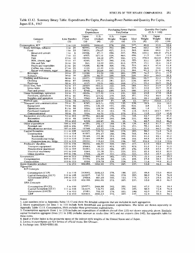
RESULTS OF THE BINARY COMPARISONS 181
Table 13.12. Summary Binary Table: Expenditures Per Capita, Purchasing-Power Parities and Quantity Per Capita, Japan-U.S., 1967
Per Capita Purchasing-Power Parities Quantity Per Capita Expenditure Yen/Dollar (U.S.= 100)
Japan U.S. U.S. Japan U.S. Japan Category Line Number (Yen) (Dollar) Weight Weight Ideal Weight Weight Ideal
(1) (2) (3) (4) (5) ( 6) (7) (8) (9) ( 10)
Consumption, ICP 1 to 110 243092. 2646.63 278. 184. 227. 49.8 33.0 40.6 Food, beverage, tobacco 1 to 39 85991. 475.64 393. 300. 344. 60.2 45.9 52.6
Food 1 to 33 70921. 376.67 427. 31 l. 364. 60.6 44.1 51. 7 Bread and cereals 1 to 6 24506. 47.11 280. 327. 303. 159.1 185.8 171.9 Meat 7 to 12 6957. 127.15 524. 469. 496. 11. 7 10.4 11.0 Fish 13 to 14 10152. 10.10 277. 266. 271. 378.4 363.0 370.7 Milk, cheese, eggs 15 to 17 6245. 56.77 380. 332. 355. 33.1 28.9 30.9 Oils and fats 18 to 20 961. 13.59 425. 413. 419. 17.1 16.6 16.9 Fruits and vegetables 21 to 26 14308. 82.98 364. 286. 323. 60.3 47.4 53.4 Coffee, tea, cocoa 27 to 29 1113. 12.34 619. 250. 394. 36.0 14.6 22.9 SQices and sweets, sugar 30to 33 6678. 26.64 487. 272. 364. 92.3 5 1. 5 68.9
Beverages 34 to 37 11200. 52.20 318. 28 l. 299. 76.3 67.5 71. 7 Tobacco 38 to 39 3870. 46.77 209. 209. 209. 39.5 39.5 39.5
Clothing and footwear 40to 5 I 25977. 210.62 231. 22 l. 226. 55. 7 53.3 54.5 Clothing 40 to 47 24460. 177.12 241. 227. 234. 60.9 57.3 59.1 Footwear 48 to 51 1 S 17. 33.51 182. 160. 17 1. 28.3 24.9 26.S
Gross rent, fuel 52 to 57 35059. 455.21 322. 244. 280. 31.5 23.9 27.5 Gross rents 52 to 53 26790. 365.08 231. 222. 227. 33.0 31. 7 32.4 Fuel and QOwer 54 to 57 8268. 90.13 688. 363. 500. 25.2 13.3 18.3
House furnishings, operation 58 to 71 18894. 217.32 313. 291. 302. 29.8 27.8 28.8 Furniture, appliances 58 to 66 8932. 127.92 379. 364. 371. 19.2 18.4 18.8 SUQQlies and OQeration 67 to 71 9962. 89.40 220. 247. 233. 45.1 S0.7 47.8
Medical care 72 to 78 16717. 229.55 57. 68. 62. 107.6 128.8 117.7 Transport and communication 79 to 91 8797. 363.71 432. 132. 239. 18.4 5.6 10.1
Equipment 79 to 80 1991. 136.10 455. 383. 418. 3.8 3.2 3.5 Operation costs 81 to 84 1026. 158.74 499. 476. 488. 1.4 1. 3 1. 3 Purchased transport 85 to 89 4253. 25.12 163. 79. 114. 214.2 103.7 149.1 Communication 90 to 91 1526. 43. 75 272. 273. 272. 12.8 12.8 12.8
Recreation and education 92 to 103 25786. 383.00 178. 123. 148. 54.7 37. 7 45.4 Recreation 92 to 98 19476. 193.94 260. 206. 231. 48.9 38.6 43.4 Education 99 to 103 6310. 189.07 94. 55. 72. 60.7 35.4 46.3
Other expenditure 104 to 110 25201. 292.13 140. 139. 139. 62.2 61. 7 61.9 Personal care 104 to 106 9441. 69.85 210. 173. 191. 78.1 64.3 70.9 Miscellaneous services 107 to 109 I 5760. 222.27 118. 124. 121. 57.2 60.2 58.7
Capital formation 111 to 148 163237. 735.72 305. 274. 289. 80.9 72.8 76.8 Construction 111 to 124 81057. 391.17 285. 246. 265. 84.3 72.6 78.2
Residential 111 to 112 28169. 122.30 253. 252. 252. 91.4 91.1 91.2 Nonresidential bldgs. 113to120 23365. 149.84 364. 348. 356. 44.8 42.8 43.8 CQnstruction exc. bldgs. 121 to 124 29522. 119.03 220. 196. 207. 126.8 112.8 119.6
Producers' durables 125 to 146 58256. 306.51 328. 307. 317. 61.9 58.0 59.9 Transport equipment 125 to 131 19663. 90.33 423. 423. 423. 51.5 5 1. 5 51. 5 Nonelectrical machinery 132to140 2646 l. 132.32 306. 287. 296. 69.8 65.4 67.5 Electrical machinery 141 to 144 9364. 51.38 221. 221. 221. 82.5 82.5 82.5 Other durables 145 to 146 2768. 32.48 322. 322. 322. 26.5 26.5 26.5
Government 149tol53 29860. 601.60 202. 153. 175. 32.5 24.6 28.3 Compensation 149 to 152 21276. 2 71. 90 156. 135. 145. 57.8 50.2 53.9 Commodities 153 to 153 8584. 329. 70 239. 224. 231. 11.6 10.9 11. 3
Gross domestic Qroduct 1 to 153 436188. 3983.95 272. 207. 237. 53.0 40.3 46.2 Aggregates
ICP Concepts
Consumption (CEP) I to 110 243092. 2646.63 278. 184. 227. 49.8 33.0 40.6 Capital formation (GCF) llltol48 163237. 7 35. 72 305. 274. 289. 80.9 72.8 76.8 Government (PFC) 149to 153 29860. 601.60 202. 153. 175. 32.5 24.6 28.3 GDP I to I 5 3 436188. 3983.95 272. 207. 237. 53.0 40.3 46.2
SNA Concepts
Consumption (PFCE) I to 110 234971. 2466.88 292. 201. 242. 47.5 32.6 39.4 Capital formation (GCF) 111 to 148 163237. 735.72 305. 274. 289. 80.9 72.8 76.8 Government (GFCE) 1 to 15 3 37981. 781.35 176. 111. 140. 43.9 27.6 34.8 GDP I to 153 43545 5. 3982.53 272. 207. 237. 52.9 40.3 46.1
Notes: 1. Line numbers refer to Appendix Table 13.12 and show the detailed categories that are included in each aggregation. 2. Above expenditures for lines 1 to 110 include both household and government expenditures. The latter are shown separately in Appendix Table 13.15. Consumption, SNA excludes these government expenditures. 3. Consumption aggregate (lines I to 110) includes net expenditure of residents abroad (line 110) not shown separately above. Similarly capital formation aggregate (lines 111 to 148) includes increase in stocks (line 147) and net exports (line 148). See appendix table for these items. 4. Ideal or Fisher Index is the geometric mean of the indexes with weights of the United States and of Japan. 5. Letters in parentheses are first letters of official terms. See Glossary. 6. Exchange rate: ¥360=US$1.00.

182 THE RESULTS OF THE COMPARISONS
Table 13.13. Summary Binary Table: Expenditures Per Capita, Purchasing-Power Parities and Quantity Per Capita, Kenya-U.S., 1967
Per Capita Purchasing-Power Parities Quantity Per Capita Expenditure Shilling/Dollar (U.S.= 100)
Kenya U.S. U.S. Kenya U.S. Kenya Category Line Number (Shilling) (Dollar) Weight Weight Ideal Weight Weight Ideal
(!) (2) (3) (4) (5) (6) (7) (8) (9) (IO)
Consumetion, ICP I to 110 626.79 2646.63 5.96 2.90 4.15 8.2 4.0 5. 7 Food, beverage, tobacco I to 39 313.12 475.64 6.43 4.14 5.16 15.9 10.2 12.8
Food I to 33 278.99 376.67 6.12 3.94 4.91 18.8 12.1 15.1 Bread and cereals I to 6 99.77 47.11 4.07 5.29 4.64 40.0 52.0 45.6 Meat 7 to 12 38.51 127.15 4.77 3.70 4.20 8.2 6.3 7.2 Fish 13 to 14 8.58 10.10 7.39 5.24 6.22 16.2 11. 5 13.6 Milk, cheese, eggs 15 to 17 39.17 56.77 5.29 4.56 4.91 15.1 13.0 14.0 Oils and fats 18 to 20 10.44 13.59 7.83 6.18 6.96 12.4 9.8 11.0 Fruits and vegetables 21 to 26 58.37 82.98 5.31 2.40 3.57 29.3 13.3 19.7 Coffee, tea, cocoa 27 to 29 6.10 12.34 6.97 3.43 4.88 14.4 7.1 IO. I SQices and sweets, sugar 30to 33 18.05 26.64 18.79 5.18 9.86 13. l 3.6 6.9
Beverages 34 to 37 20.54 52.20 9.84 9.25 9.54 4.3 4.0 4.1 Tobacco 38 to 39 13.59 46.77 5.06 5.11 5.09 5.7 5.7 5. 7
Clothing and footwear 40 to SI 20.05 210.62 6.91 4.52 5.58 2.1 1.4 I. 7 Clothing 40 to 47 15.87 177.12 7.78 5.71 6.67 1.6 1.2 I. 3 Footwear 48 to 51 4.17 33.51 2.26 2.52 2.39 4.9 5.5 5.2
Gross rent, fuel 52 to 57 64.91 455.21 8.07 5.15 6.45 2.8 1.8 2.2 Gross rents 52 to 53 55.61 365.08 7.50 5.68 6.52 2.7 2.0 2.3 Fuel and 12ower 54 to 57 9.29 90.13 10.36 3.32 5.87 3.1 1.0 I. 8
House furnishings, operation 58 to 71 36.42 217.32 5.91 2.54 3.87 6.6 2.8 4.3 Furniture, appliances 58 to 66 8.38 127.92 7.04 4.49 5.62 I. 5 0.9 1.2 SUQJ2lies and 012eration 67 to 71 28.04 89.40 4.30 2.24 3.11 14.0 7.3 IO. I
Medical care 72 to 78 25.62 229.55 1.38 1.00 1.17 11.2 8.1 9.5 Transport and communication 79 to 91 57.97 363. 71 8.09 5.88 6.90 2.7 2.0 2.3
Equipment 79 to 80 10.38 136.10 11. 21 7. 71 9.30 1.0 0.7 0.8 Operation costs 81 to 84 16.13 158. 74 6.97 5.82 6.37 1. 7 1.5 1.6 Purchased transport 85 to 89 30.32 25.12 6.61 5.61 6.09 21.5 18.3 19.8 Communication 90 to 91 1.15 43. 75 3.34 3.43 3.38 0.8 0.8 Q l!
Recreation and education 92 to 103 65.90 383.00 4.65 1.07 2.23 16.1 3.7 7.7 Recreation 92 to 98 22.62 193.94 7.10 3.47 4.97 3.4 1.6 2.3 Education 99 to 103 43.28 189.07 2.13 0.78 1.29 29.2 10.8 17.7
Other expenditure 104toll0 42.81 292.13 3.82 3.56 3.68 4.1 3.8 4.0 Personal care 104 to I 06 4.04 69.85 6.19 5.65 5.91 1.0 0.9 1.0 Miscellaneous services 107 to I 09 38.77 222.27 3.07 3.42 3.24 5.1 5.7 5.4
Capital formation llltoI48 171.03 735.72 5.80 5.38 5.59 4.3 4.0 4.2 Construction 111 to 124 81.41 391.17 4.13 4.16 4.14 5.0 5.0 5.0
Residential 111 to 112 25.44 122.30 3.53 3.50 3.52 5.9 5.9 5.9 Nonresidential bldgs. 113 to 120 20. 73 149.84 3.75 3.37 3.56 4.1 3.7 3.9 Construction exc. bldgs. 121 to 124 35.24 119.03 5.21 5.72 5.46 5.2 5.7 5.4
Producers' durables 125 to 146 84.18 306.51 7.91 7.60 7. 75 3.6 3.5 3.5 Transport equipment 125 to 131 37.26 90.33 7.87 7.88 7.87 5.2 5.2 5.2 Nonelectrical machinery 132 to 140 32.35 132.32 7.89 7.57 7. 73 3.2 3.1 3.2 Electrical machinery 141 to 144 8.25 51.38 8.74 7.17 7.91 2.2 1.8 2.0 Other durables 145 to 146 6.31 32.48 6.78 6.85 6.82 2.8 2.9 2.9
Government 148 to 153 88.95 601.60 4.25 1.16 2.22 12.7 3.5 6.7 Compensation 149 to 152 67.58 271. 90 2.75 0.95 1.62 26.2 9.0 15.4 Commodities 15 3 to 153 21.37 329. 70 5.48 3.99 4.68 1.6 1.2 1.4
Gross domestic product 1 to 15 3 886.77 3983.95 5.67 2.73 3.93 8.2 3.9 5.7 ggregates
ICP Concepts
Consumption (CEP) 1 to 110 626. 79 2646.63 5.96 2.90 4.15 8.2 4.0 5.7 Capital formation (GCF) 111 to 148 171.03 735.72 5.80 5.38 5.59 4.3 4.0 4.2 Government (PFC) 149 to 153 88.95 601.60 4.25 1.16 2.22 12.7 3.5 6.7 GDP 1 to 15 3 866.77 3983.95 5.67 2. 73 3.93 8.2 3.9 5.7
SNA Concepts
Consumption (PFCE) 1 to 110 590.44 2466.88 6.26 3.48 4.67 6.9 3.8 5.1 Capital formation (GCF) 111 to 148 171.03 735. 72 5.80 5.38 5.59 4.3 4.0 4.2 Government (GFCE) I to 15 3 125.30 781.35 3.69 1.01 1.93 15.8 4.3 8.3 GDP 1 tu I 53 886.77 3982.53 5.67 2. 73 3.93 8.2 3.9 5.7
Notes: 1. Line numbers refer to Appendix Table 13.13 and show the detailed categories that are included in each aggregation. 2. Above expenditures for lines 1 to 110 include both household and government expenditures. The latter are shown separately in Appendix Table 13.15. Consumption, SNA excludes these government expenditures. 3. Consumption aggregate (lines 1 to 110) includes net expenditure of residents abroad (line 110) not shown separately above. Similarly capital formation aggregate (lines 111 to I 48) includes increase in stocks (line I 4 7) and net exports (line 148). See appendix table for these items. 4. Ideal or Fisher Index is the geometric mean of the indexes with weights of the United States and of Kenya. 5. Letters in parentheses are first letters of official terms. Sec Glossary. 6. Exchange rate: Sh7.143=US$1.00.

RESULTS OF THE BINARY COMPARISONS 183
Table 13.14. Summary Binary Table: Expenditures Per Capita, Purchasing-Power Parities and Quantity Per Capita, U.K.-U.S., 1967
Per Capita Purchasing-Power Parities Quantity Per Capita Expenditure Pound/Dollar (U.S.= 100)
U.K. U.S. U.S. U.K. U.S. U.K. Category Line Number (Pound) (Dollar) Weight Weight Ideal Weight Weight Ideal
(I) (2) (3) (4) (5) (6) (7) (8) (9) ( 1 O)
ConsumEtion, ICP 1 to 110 517.973 2646.63 0.332 0.274 0.302 71.5 58.9 64.9 Food, beverage, tobacco 1 to 39 156.499 47 5.64 0.367 0.346 0.357 95.0 89.6 92.3
Food 1 to 33 97.420 376.67 0.302 0.276 0.289 93.8 85.5 89.6 Bread and cereals 1 to 6 13.500 47.11 0.236 0.215 0.225 133.6 12 l.3 127.3 Meat 7 to 12 27.798 127. l 5 0.263 0.259 0.261 84.5 83.0 83.8 Fish 13 to 14 3.556 10.10 0.334 0.319 0.326 110.6 105.4 108.0 Milk, cheese, eggs 15 to 17 14. 788 56.77 0.317 0.308 0.313 84.5 82.1 83.3 Oils and fats 18 to 20 4.573 13.59 0.355 0.257 0.302 13 l. l 94.7 11 l.4 Fruits and vegetables 21 to 26 18.163 82.98 0.334 0.309 0.321 70.9 65.6 68.2 Coffee, tea, cocoa 27 to 29 3.647 12.34 0.364 0.207 0.274 143.1 81.3 107.9 Seices and sweets, sugar 30 to 33 11. 395 26.64 0.409 0.388 0.398 110.3 104.6 107.4
Beverages 34 to 37 31.717 52.20 0.493 0.510 0.501 119.2 123.3 12 l.2 Tobacco 38 to 39 27.362 46.77 0.749 0.748 0.749 78.2 78.1 78.1
Clothing and footwear 40 to 51 41.134 210.62 0.375 0.338 0.356 57.7 52.l 54.9 Clothing 40 to 47 33.695 177.12 0.402 0.380 0.391 50.0 47.3 48.6 Footwear 48 to 51 7.439 33.51 0.227 0.225 0.226 98.6 97.8 98.2
Gross rent, fuel 52 to 57 81.362 45 5. 21 0.300 0.281 0.291 63.6 59.5 61.5 Gross rents 52 to 53 59.497 365.08 0.258 0.266 0.262 61.3 63.2 62.3 Fuel and QUWer 54 to 57 21. 865 90.13 0.472 0.334 0.397 72.6 S 1.4 61. l
House furnishings, operation S8 to 71 37.687 217.32 0.3S 1 0.323 0.337 53.8 49.4 51. 5 Furniture, appliances 58 to 66 20.867 127.92 0.395 0.357 0.376 45. 7 41.3 43.4 SuEElies and oEeration 67 to 71 16.820 89.40 0.288 0.288 0.288 65.3 65.4 65.3
Medical care 72 to 78 29.014 229.5 5 0.131 0.125 0.128 101.0 96.4 98.7 Transport and communication 79 to 91 55.777 363.71 0.507 0.326 0.406 47.l 30.3 37.8
Equipment 79 to 80 14.661 136.10 0.742 0.435 0.568 24.8 14.5 19.0 Operation costs 81 to 84 21.556 158. 74 0.412 0.316 0.361 43.0 33.0 37.6 Purchased transport 85 to 89 l 5.133 25.12 0.369 0.307 0.337 196.0 163.2 178.8 Communication 90 to 91 4.427 43.75 0.197 0.220 0.208 45.9 51.3 48.5
Recreation an ct education 92 to 103 67.553 383.00 0.266 0.211 0.237 83.5 66.4 74.5 Recreation 92 to 98 37.215 193.94 0.311 0.210 0.255 91.5 61.7 75.2 Education 99 to 103 30.338 189.07 0.219 0.213 0.216 75.2 73.3 74.2
Other expenditure 104 to 110 47.594 2 92.13 0.309 0.256 0.281 63.6 52.7 57.9 Personal care 104 to 106 10. 742 69.85 0.241 0.198 0.219 77.6 63.7 70.3 Miscellaneous services 107 to 109 36.852 222.27 0.330 0.280 0.304 59.2 50.2 54.5
Capital formation J 11 to 148 129.463 7 35. 72 0.322 0.283 0.302 62.2 54.6 58.3 Construction llltol24 69.168 391.17 0.263 0.254 0.258 69.7 67.3 68.5
Residential 111 to 112 26.981 122.30 0.206 0.209 0.207 105.7 107.0 106.3 Nonresidential bldgs. 113 to 120 29.377 149.84 0.330 0.331 0.331 59.2 59.4 59.3 Construction exc. bldgs. 121 to 124 12.810 119.03 0.236 0.234 0.235 46.0 45.7 45.8
Producers' durables 125 to 146 64.723 306.51 0.394 0.328 0.359 64.5 53.6 58.8 Transport equipment 12S to 131 12.284 90.33 O.S88 0.566 0.577 24.0 23.l 23.6 Non electrical machinery 132 to 140 35.165 132.32 0.341 0.310 0.325 85.8 78.0 81.8 Electrical machinery 141 to 144 15.242 51.38 0.312 0.292 0.302 101.6 95.2 98.4 Other durables 145 to 146 2.032 32.48 0.200 0.200 0.200 31.3 31.3 31.3
Government 149 to 153 73.033 601.60 0.271 0.231 0.250 52.5 44.8 48.5 Compensation 149 to 152 39.011 271.90 0.235 0.193 0.213 74.2 61.0 67.3 CQmmodities 153 to 153 34.022 329. 70 0.301 0.298 0.299 34.6 34.3 34.5
Gross domestic )2roduct l to 153 720.465 3983.95 0.321 0.270 0.295 66.9 56.3 61.4 Aggregates
ICP Concepts
Consumption (CEP) 1 to 110 517.973 2646.63 0.332 0.274 0.302 71.5 58.9 64.9 Capital formation (GCF) lllto148 129.463 735.72 0.322 0.283 0.302 62.2 54.6 58.3 Government (PFC) 149to 153 73.033 601.60 0.271 0.231 0.250 52.5 44.8 48.5 GDP 1 to 15 3 720.465 3983.95 0.321 0.270 0.295 66.9 56.3 61.4
SNA Concepts
Consumption (PFCE) 1 to 110 458.006 2466.88 0.342 0.303 0.322 61.2 54.2 57.6 Capital formation (GCF) 111 to 148 129.463 735. 72 0.322 0.283 0.302 62.2 54.6 58.3 Government (GFCE) 1 to 153 133.002 781.3S 0.254 0.190 0.220 89.5 67.1 77.5 GDP 1 to 15 3 716.927 3982.S3 0.321 0.270 0.295 66.6 56.0 61.1
Notes: 1. Line numbers refer to Appendix Table 13.14 and show the detailed categories that are included in each aggregation. 2. Above expenditures for lines 1 to 110 include both household and government expenditures. The latter are shown separately in Appendix Table 13.15. Consumption, SNA excludes these government expenditures. 3. Consumption aggregate (lines 1 to 110) includes net expenditure of residents abroad (line 110) not shown separately above. Similarly capital formation aggregate (lines 111 to 148) includes increase in stocks (line 14 7) and net exports (line 148). See appendix table for these items. 4. Ideal or Fisher Index is the geometric mean of the indexes with weights of the United States and of the United Kingdom. 5. Letters in parentheses are first letters of official terms. See Glossary. 6. Exchange rate: £0.357=US$1.00.

184 THE RESULTS OF THE COMPARISONS
Before attempting to describe the main results of the comparisons, we present as a useful background Table 13.16, a summary breakdown of the expenditures of each of the ten countries. We do not stop now to describe the relationships depicted in this table, but will draw upon them as they become relevant to the illumination of the quantity and price comparisons.
The main results of the binary quantity comparisons are summarized in Table 13.17, which is composed of figures from Tables 13.1 to 13.14. Part A refers to 1970 and Part B to 1967. The countries are arrayed from left to right in order of ascending real GDP per capita, as measured by the ideal index (line 4).
The 1970 per capita GDP for the nine countries varies from 4 percent to 68 percent of that of the United States when valued in each country's own prices, and from 8.5 to 82 percent when valued in United States prices. Kenya and India have the lowest per capita GDP. Colombia's, although notably higher, is still low. Hungary and Italy are at the next level, followed by Japan and the United Kingdom. The Federal Republic of Germany and France, with almost identical indexes, are closest to the United States level of per capita GDP. Although this broad picture applies regardless of the basis of evaluation, the ordinal rankings of Kenya and India are different for the two sets of valuations.
The per capita quantity indexes for the major subaggrcgates-consumption, capital formation, and government-generally show a rather similar pattern. The main exception is the high level of per capita capital formation in Japan, France, and the Federal Republic of Germany. These are the only cases in the table in which the figures exceed 100-indicating, of course, that the per capita product is greater than that of the United States. The per capita capital formation figures for France and the Federal Republic of Germany contrast sharply with the corresponding figures that were estimated for 1950 in a predecessor study. 2 As was noted in Chapter 1, the per capita quantity indexes for these two countries were only 30 to 40 percent of that of the United States at the earlier date; in 1970, they exceeded the United States by 20 to 50 percent. This reflects in large part the high proportion of GDP that these countries devoted to investment in 1970 relative to the U.S. proportion; around 30 percent of French and German GDP went for capital expenditures, compared with 17 percent in the United States (see Table 13.16). In Japan, 1970 real per capita investment was substantially higher than in the United States, and Japan devoted a high proportion of its GDP-41 percent-to capital formation. The United Kingdom did not have high levels of investment. Instead, its consumption accounted for a high share of total
2 M. Gilbert and I. Kravis, An International Comparison of National Products and the Purchasing Power of Currencies (Paris: Organization for European Economic Cooperation, 1954).
GDP; in real terms, U.K. per capita consumption was about the same as that of France and the Federal Republic of Germany, even though its total per capita GDP was smaller.
For seven of the nine countries, the government indexes computed on the ICP basis (lines 13 to 15) are smaller than those for consumption. The ICP does not provide a breakdown for defense expenditures, but it seems clear that higher U.S. expenditures of this type, accounting in 1970 for about one-third of government purchases of goods and services (SNA concept), contribute to this result. (Note that the smaller government indexes mean that real per capita government services relative to the United States are smaller than real per capita consumption relative to the United States.)
A convenient way to evaluate the differences between the results for the ICP and SNA concepts of consumption and government is to compare the two sets of indexes for government. The fact that the SNA government figures are uniformly larger than those of the ICP indicates that in most other countries expenditures for education, medical care, and the like are financed by government to a greater degree than is the case in the United States. Among categories, the differences tend to be largest for medical care (see Table 13.15), and among countries, the difference is most marked for Hungary, the United Kingdom, and Italy (Table 13.17).
Large differences exist even among subsets of countries that sometimes are treated as though they were homogeneous. For example, among the three developing countries, the per capita GDP of Colombia is approximately 2.5 times that of Kenya or India, and among the Common Market countries, the per capita GDPs of France and the Federal Republic of Germany are 1.5 times that of Italy.
Fewer comparisons are available for 1967. The most notable difference revealed by these data is the remarkable rise in the relative position of Japan between 1967 and 1970. Hungary also gained ground relative to the United States. The differences between the two years for the other countries were marginal.
As expected, the gap (line 3) between own-weighted and U.S.-weighted quantity indexes (lines 1 and 2, respectively) is inversely correlated with GDP per capita (see Figure 13.1). For lowest-income countries-Kenya, India, and Colombia-valuation at U.S. prices produces a quantity index about twice as great as valuation at own prices. For the highest-income countries, the gap is only about 20 percent.
The economic reasons for the gap are, of course, well understood, as frequent references in the literature to the "Gerschenkron effect" testify. The structure of each country's quantities adapts to its own price structure: expensive commodities are consumed in relatively small amounts, and cheap ones are consumed in relatively large amounts. Thus, the size of the index spread is likely to be a function of the degree of similarity be-

RESULTS OF THE BINARY COMPARISONS 185
Figure 13.1. Index-Number Spread in Relation to Real Per Capita GDP
2.2
• 2.1
2.0 • 1.9
1.8 ~ .....
<l) s 1.7 'O
"' C)
0. 1.6 C/l
"' <!l 'O ..s
1.5
1.4
1.3
1.2
1.1
1.0
•
•
•
10 20 30 40
• •
50 60 70
• •
80
Ideal Index (Ii ne 4)
Source: Table 13.17
tween the price structure of the base country and that of the given country. It may be argued that, in turn, similarity in price structure is inversely associated with the size of the difference in real GDP per capita (see Chapter 15 for our findings on this point).
Among the countries included in the present study, labor-intensive commodities and services, for example, tend to be cheap in Kenya and India, both low GDP countries, so relatively large quantities are apt to be consumed. On the other hand, capital-intensive goods are likely to be expensive and therefore consumed in lesser quantities. In the United States, the opposite price and quantity relationships tend to prevail. Thus, when the quantities of a low-income country such as Kenya or India are valued at U.S. prices, the country's GDP is much larger relative to the U.S. GDP than when the country's own prices are used in the valuation.
The size of the index spread does not reflect merely economic factors, however. Its magnitude is also very much a function of the methods of aggregation. In the
ICP, unweighted price relatives within each of 153 categories were used to derive indirect quantity indexes (with a few exceptions in which direct quantity indexes were estimated). The two sets of prices, U.S. and "own," were applied to these relative quantities to obtain the aggregates for the binary comparisons summarized in Table 13.17. The index spread would have been different if we had applied the weights at a different level of aggregation: it would have been larger if we had applied weights at a more disaggregated level, smaller if we had applied them at a more aggregated level. Because the methods were the same for all fourteen comparisons, the index spread may legitimately be compared for different binary comparisons, as was done three paragraphs above. But comparisons of the spreads reported in Table 13.17 with those of the Gilbert-Kravis and other studies must take this source of difference into account.
To simplify the rest of our discussion, we work with the ideal index. The own-weighted and U.S.-weighted indexes have a clear economic rationale that the ideal

186 THE RESULTS OF THE COMPARISONS
Table 13.15. Government Components of Final Consumption Expenditure of Population
Part A. Per Capita Expenditure, 1970
Germany ICP category Colombia France F.R. Hungary India Italy Japan Kenya U.K. U.S.
(Peso) (Franc) (D. Mark) (Forint) (Rupee) (Lira) (Yen) (Shilling) (Pound) (Dollar)
3 I lOG Rents o.o 4.51 8.30 342. 7 0.0 0. 1111. 0.0 5.430 2.60 2 5 11 OG Drugs, medical 0.0 0.06 12.30 261.1 0.23 92. 783. 0.36 4.465 0.89
preparations 3 5 120G Medical supplies 0.0 0.0 4.66 80.6 0.10 18. 793. 0.12 0.464 0.12 4 5 200G Therapeutic 0.0 0.75 5.21 0.0 0.13 73. 159. 0.00 1.268 0.21
equipment 5 5 31 OG Physicians' services 9.5 33.09 29.25 101.4 0.42 1934. 944. 2.19 5.180 1.65 6 5 3 2 OG Dentists' services I. 9 0.0 o.o 7.9 0.00 0. 203. 0.0 1.482 0.51 7 5 330G Services, nurses, etc. 0.2 31. 71 43.94 106.8 0.62 1734. 834. 2.97 9.466 14. 76 8 5 41 OG Hospitals 3.5 5.89 30.71 413.5 1.05 3831. 676. 8.40 12.395 15.77 9 7 21 OG Public entertainment 0.0 0.0 o.o 126.3 0.09 0. o. 0.13 3.054 7.95
10 7 2 30G Other recreational 0.0 0.0 o.o 46.9 0.11 0. o. 0.0 0.0 0.0 cultural activities
11 7 411G Teachers, 1st and 2nd 75.5 595.58 311. 95 453.8 7.57 40463. 11144. 27.52 20.290 152.49 12 7 412G Teachers, college 21. 7 88.23 62.46 46.6 0.62 4798. 902. 1.36 3.179 19.87 13 7 420G Educational physical 12.1 34.39 58.75 237.8 0.37 2675. 2198. 3.81 5.358 19.19
facilities 14 7 431 G Educational books, 2.2 5.30 2.75 24.7 0.22 457. 806. 1.5 7 1.947 4.58
supplies 15 7 432G Other education 4.7 5.59 21.10 103.1 0.42 1431. 955. 1.83 3.644 4.87
expenditures 16 8 400G Other services 14.0 0.0 o.o 105.3 0.0 0.0 1103. 0.0 4.108 6.52
Part B. Per Capita Expenditure, 1967
ICP category Hungary India Japan Kenya U.K. U.S. (Forint) (Rupee) (Yen) (Shilling) (Pound) (Dollar)
3 l lOG Rents 264.9 2 5 llOG Drugs, medical preparation 210.6 3 5 120G Medical supplies 36.7 4 5 200G Therapeutic equipment 0.0 5 5 31 OG Physicians' services 93.2 6 5 320G Services of dentists 7.4 7 5 330G Services, nurses, etc. 97.9 8 5 4 1 OG Hospitals 317.0 9 7 210G Public entertainment 80.7
10 7 2 30G Other recreational, cultural activities 44.2 11 7 41 lG Teachers, 1st and 2nd 364.3 12 7 412G Teachers, college 38.4 13 7 420G Educational, physical facilities 168.7 14 7 431 G Educational books, supplies 17.2 1 S '· 7 432G Other education expenditures 83.0 16 '8 400G Other services 85.7
index lacks, but the convenience of a single number that
is a compromise between the two is responsible for its
widespread use and for our use here. (Actually, the
multilateral indexes presented in the next chapter are to
be preferred over the ideal index as single-number esti
mates of relative GDP per capita, but our task in this
chapter is to summarize the results of the more familiar
binary comparisons.) Little if anything that we have to
say would be much altered if we worked with the two
more basic sets of indexes: we would just have to say it
in a more cumbersome way.
The first question to which we address ourselves is
the difference between the relative per capita GDPs ob
tained by the ICP and those derived by the use of ex
change rates. This is important because the major reason
for this entire undertaking rests on the proposition that
exchange rates are not the proper basis for making GDP
commensurable.
Per capita comparisons of GDP that have been
derived from exchange rates are entered on line 5 of
0.0 0.21 0.09 0.11 0.33 0.00 0.49 0.86 0.02 0.08 6.03 0.50 0.31 0.18 0.36 0.0
732. 0.0 3.538 1.42 1665. 0.23 3.429 0.91
193. 0.09 0.345 0.12 52. 0.00 0.962 0.13
302. 1.66 3. 702 2.72 13. 0.0 1.052 0.28
254. 1.93 6.750 10.44 600. 4.89 9.145 12.18
0. 0.12 2.214 5.58 0. 0.0 0.0 0.0
2628. 21.01 15.151 108.58 207. 1.00 2.377 11. 33 819. 2.87 4.137 15.20 300. 1.18 1.506 3.63 356. 1.37 2.812 3.86
0. 0.0 2.849 3.39
Table 13.17. The per capita GDP of Japan, for example,
has been converted to dollars (by dividing its value in
yen by 360), and taken as a percentage of the U.S. per
capita GDP. The underlying data for these conversions
aggregate GDP, population, and exchange rates-may be
found in Table 1.1. (The exchange rates are shown also
in line 4 of Table 13.19.) As a convenient means of indicating the difference
between these exchange-rate- derived comparisons and
the ICP results, an "exchange-rate -deviation index"3
has been calculated and entered in line ( 6). The index is
obtained by dividing the per capita GDP of each country
relative to the United States, as measured by the ideal
index, by the exchange-rate-derived comparisons. The
exchange rate deviation index of 1.97 for Kenya, for
30ur use of this term is simply a matter of convenience; it is not intended to express any judgment about the appropriateness of the exchange rate. The "equilibrium" exchange rate is determined by more factors than simply the PPP for GDP. (See pages 9-10.

example, results from the division of the real per capita GDP of Kenya relative to the United States, 5 .9 percent, by the exchange-rate-derived per capita GDP of Kenya relative to the United States, 3.0 percent. The exchange rate distortion index of nearly 2 reflects the fact that the real per capita GDP of Kenya relative to the United States is twice as high as would be inferred from exchange rates. (The own-weighted or U.S.-weighted quantity indexes also might have been used to calculate an exchange rate deviation index, but, as already noted, the use of the ideal index represents a useful compromise that serves the interests of brevity.)
Relative to the United States, the 1970 per capita GDPs of the other countries range from about 15 percent higher than that indicated by the exchange rate to three times greater. The differences tend to be larger for low-income countries, but factors other than income level are at work as well (see Figure 13.2). For example, among the industrialized market economies, the exchange-rate -deviation index is highest for Japan, though its per capita GDP is substantially greater than that of Italy; and among the developing countries, Kenya's index is lower than that of Colombia despite the fact that Kenya has a substantially lower per capita GDP.
RESULTS OF THE BINARY COMPARISONS 187
The nature of the underlying structural relationship that may exist between the exchange-rate-deviation index and the level of real per capita GDP has attracted the attention of a number of investigators,4 but it cannot be understood fully until more observations such as those we offer in this study have been accumulated. However, some a priori hypotheses about the identity of some of the other factors affecting this relationship receive some hints of support in the present set of results. As between two countries with equal per capita GDP, the one with closer trading ties with other countries may be expected to have a lower exchange-ratedeviation index than one whose economy is less influ-
4 Gi!bert and Kravis, An International Comparison, pp. 50-57; E. E. Hagen, "Comment," Problems in the International Comparison of Economic Accounts, Studies in Income and Wealth, Vol. XX (Princeton, N. J.: Princeton University Press, 1957), pp. 381-85; B. Balassa, "The Purchasing Power Parity Doctrine: A Reappraisal," Journal of Political Economy 72 (December 1964), pp. 584-96;C. Clague and V. Tanzi, "Human Capital, Natural Resources and the Purchasing Power Parity Doctine: Some Empirical Results," Economia Internazionale 25 (February 1972), pp. 3-18; and P.A. David, "Just how Misleading Are Official Exchange Rates?", Economic Journal 82 (September 1972), pp. 979-90.
Figure 13.2. Exchange-Rate Deviation Index in Relation to Real Per Capita GDP
3.5 r------.-,-----.-,-----,-,-----.,-----.,-----.,------.,------,
3.0 - • -
G <lJ
2 >< <D 2.5 - --0
..:; C .2 • ~ ·;;
<lJ a <lJ 2.0 -~ • ex: Cj Oil • C
"' ..c u ><
UJ
1.5 - • • • • •
1.0 I I I I I I I
10 20 30 40 50 60 70 80
Ideal Index (line 4) Source: Table 13.17

188 THE RESULTS OF THE COMPARISONS
Table 13.16. Percentage Distribution of Expenditures on Gross Domestic Product, Ten Countries, 1970
Kenya India Colombia
Consumptiont 68.5 75.5 74.8 Food, beverages, tobacco 33.5 4cf"6 -24-:S Clothing and footwear 2. 7 3.1 4.2 Housing and household 11.3 10.4 16.8 Medical care 3.5 2.2 2.0 Education 5.3 2.1 3.9 Transport and communication 5.0 4.3 8.8 All other 7.3 3.8 14.3
Capital formation:j: 20.1 16.6 19.9 Construction 16:-§ ?Ji 11.8 Producers durables 8.6 4.9 7.9
Government 11.4 _1:1 5.3 GDP 100.0 100.0 100.0
tincludes net expenditure of residents abroad. :j:lncludes changes in stocks and net exports.
enced by world prices through trade. The relationships among our three less developed countries are consistent with this expectation. Exports plus imports as percentages of GDP for India, Colombia, and Kenya were 8.5, 20.9, and 39.1 percent, respectively, and the exchangerate-deviation indexes were 3.05, 2.25, and 1.97, respectively .5 Some support for the hypothesis is found also among the market economies; Japan's high index is matched by a relatively low trade proportion (19 .3 percent), and the Federal Republic of Germany, with a lower index than France, has a higher trade proportion as well (34.2 percent, as against 28.2 percent for France). The United Kingdom, on the other hand, has both a higher exchange-rate -deviation index and a higher trade proportion (34.4 percent) than France and the Federal Republic of Germany.
The relationship between the exchange-rate-deviation index and the level of GDP also may be expected to alter at least for a time because of changes in exchange rates or, if exchange rates are left fixed, because of differential internal rates of inflation. For example, the shift in the exchange-rate-deviation index for the United Kingdom from 1.21 in 1967 to 1.40 in 1970 was influenced by changes in both of these factors, one working to increase the index, the other to reduce it. The change in the exchange rate from $2.80 per pound to $2.40 near the end of 1967 (a 16.7 percent rise in the sterling price of dollars) operated to diminish the dollar value of the U.K. GDP when converted at the exchange rate and thus to raise the exchange-rate-deviation index. At the same time, the internal rate of inflation between 1967 and 1970 was 17 percent in the United Kingdom and 6 percent in the United States, gauged by the change in each country's implicit price deflator for GDP. This factor, by raising the relative valuation placed on U .K. GDP when converted to dollars at a given exchange rate,
5 Trade figures from U.N. Monthly Bulletin of Statistics (August 1972); GDP figures from Table 1.1.
Germany, Hungary Italy Japan U.K. F.R. France U.S.
60.4 69.8 51.0 71.0 58.9 63.9 68.1 21.S 26.3 16.7 -20.4 14.1 17];" TT:-'7
7.0 5.8 4.1 5.5 6.1 5.9 5.3 9.6 12.0 10.0 16.4 13.8 12.3 16.9 3.5 4.9 3.6 4.4 5.5 5.7 6.6 3.2 5.0 2. 7 4.5 4.4 4.7 5.5 3.5 6.5 3.4 8.1 6.4 6.4 9.3
12.1 9.3 10.3 11.9 8.5 11.3 12.3 31.8 22.9 41.1 19.9 30.4 28.9 17.4 18.6 Tfs 20.2 -9-:T -T43° 14.9 ~ 12.3 7.8 15.3 9.3 12.1 10.9 7.3
7.8 7.3 7.8 9.1 10. 7 7.2 14.4 100.0 1<fo.o iocfo 100.0 100.0 100.0 100.0
had the effect of lowering the exchange-rate-deviation index. If these two sets of influence were the only factors at work, a 5 percent increase in the index would have occurred instead of the 16 percent increase that did occur. We do not attempt to explain the difference, particularly because our main purpose is merely to call attention to the impact of exchange-rate changes and differential rates of inflation on exchange-rate -based comparisons of GDP.
B. Analysis of Subaggregates
So much for the broad picture in terms of GDP and its three main subaggregates. We turn now to the examination of further product detail on the composition of real GDP per capita. For this purpose, ideal indexes for some of the more important product categories have been taken from column 10 of Tables 13.l to 13.9 and gathered in Table 13.18.
One notable feature of the table is the tendency for the per capita quantities relative to those of the United States to be larger for foods than for most other categories of consumption. For the lowest-income countries, Kenya and India, per capita food consumption is 16 and 19 percent, respectively, of the U.S. level whereas for consumption as a whole, the corresponding percentages are 5.6 and 6.1. At the other income extreme, French per capita food consumption is at practically the same level as that of the United States. All of the countries, it may be seen in Table 13.16, spend a higher proportion of GDP on food than does the United States. As Engel's law predicts, the proportion tends to be inversely related to income level: it is highest in India, in which food, beverages, and tobacco account for half of the expenditures.
Another consumption sector in which high quantity ratios are found is purchased transport services. These figures, which even exceed the food ratios, reflect the

RESULTS OF THE BINARY COMPARISONS 189
Table 13.17. Per Capita Quantity Indexes of Gross Product and Its Main Subdivisions (U.S.= 100)
Part A. 1970
Germany, Kenya India Colombia Hungary Italy Japan United Kingdom F.R. France
GDP, ICP 1. Own weights 4.0 4.3 11 33 43 55 58 67 68 2. U.S. weights 8.6 8.5 22 48 54 68 68 80 82 3. Index spread 2.15 1.98 l.94 1.48 1.25 1.25 1.18 1.19 1.21
(line 2 .;. line l )t 4. Ideal index 5.9 6.1 15 40 48 61 63 74 74
(.JTinei><line 2) 5. At exchange rates 3.0 2.0 6.9 22 35 42 45 64 60 6. Exchange-rate-deviation 1.97 3.05 2.25 l.84 1.3 5 1.47 1.40 1.15 1.23
index (line 4.;. line 5)t Consumption, ICP
7. Own weights 3.9 4.5 12 30 42 40 58 56 60 8. U.S. weights 8.0 8.3 23 so 55 56 70 68 77 9. Ideal index 5.6 6.1 17 38 48 47 64 62 68
Capital formation l 0. Own weights 4.3 3.7 10 47 60 117 64 128 124 11. U.S. weights 5.0 7.0 23 59 68 126 70 150 136 12. Ideal index 4.6 5.1 15 53 64 121 67 138 130 Government, ICP 13. Own weights 4.5 4.2 6 23 24 39 45 55 39 14. U.S. weights 15.9 11.3 12 30 28 53 55 58 41 15. Ideal index 8.4 6.9 8 26 26 46 50 56 40
Addendum Consumption, SNA
16. Own weights 3.7 4.5 12 26 40 39 53 54 60 17. U.S. weights 6.8 7.2 23 37 50 53 59 62 76 18. Ideal index 5.0 5.7 17 31 45 46 56 58 67
Government, SNA 19. Own weights 5.4 4.4 8 40 34 45 70 62 47 20. U.S. weights 17.5 14.0 16 77 51 64 96 79 54 21. Ideal index 9.7 7.8 11 55 42 53 82 70 50
Part B. 1967
Kenya India Hungary Japan U.K. GDP, ICP
1. Own weights 3.9 4.3 28 40 56 2. U.S. weights 8.2 8.0 44 53 67 3. Index spread (line 2.;. line 1) 2.10 1.86 1.59 1.3 2 1.19 4. Ideal index(.../ line 1 X line 2) 5.7 5.9 35 46 61 5. At exchange rates 3.1 2.1 20 30 51 6. Exchange-rate-deviation index (line 4.;. line 5) 1.84 2.81 1.72 1.52 1.21
Consumption, ICP 7. Own weights 4.0 4.8 26 33 59 8. U.S. weights 8.2 8.3 48 50 72 9. Ideal index 5.7 6.3 35 41 65
Capital formation 10. Own weights 4.0 3.0 39 73 55 11. U.S. weights 4.3 5.9 48 81 62 12. Ideal index 4.2 4.2 43 77 58 Government, ICP 13. Own weights 3.5 3.3 15 25 45 14. U.S. weights 12.7 9.6 22 32 52 15. Ideal index 6.7 5.7 18 28 48
Addendum Consumption, SNA
16. Own weights 3.8 4.8 23 33 54 17. U.S. weights 6.9 7.5 35 48 61 18. Ideal index 5.1 6.0 29 39 58
Government, SNA 19. Own weights 4.3 3.6 30 28 67 20. U.S. weights 15.8 11.8 68 44 90 21. Ideal index 8.3 6.5 45 35 78
tLines 3 and 6 actually computed from Table 13.1 to 13.14 and from Table 1.1, in which one more digit usually was available.
relative decline of public transport in the United States and expansion in the use of the automobile. Medical care ratios also are high; in Japan, the Federal Republic of Germany, and France, per capita medical services exceed those of the United States.
Attention already has been called to the large ratios for capital formation. Table 13.18 indicates that as between the two major components of capital formation, the ratios are uniformly higher for construction than they are for producers' durables.
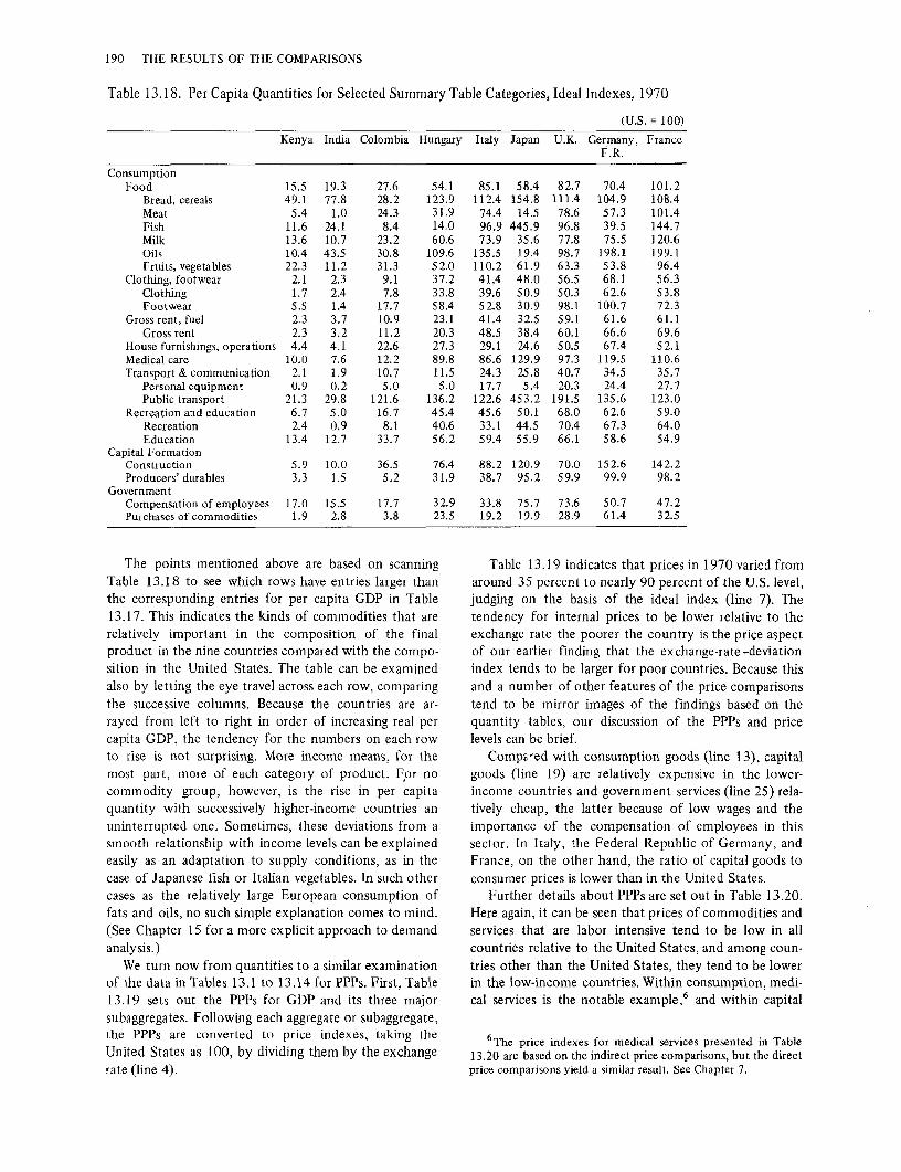
190 THE RESULTS OF THE COMPARISONS
Table 13.18. Per Capita Quantities for Selected Summary Table Categories, Ideal Indexes, 1970
Kenya India Colombia Hungary
Consumption Food 15.5 19.3 27.6 54.1
Bread, cereals 49.1 77.8 28.2 123.9 Meat 5.4 1.0 24.3 31.9 Fish 11.6 24.1 8.4 14.0 Milk 13.6 10.7 23.2 60.6 Oils 10.4 43.5 30.8 109.6 Fruits, vegetables 22.3 11.2 31.3 52.0
Clothing, footwear 2.1 2.3 9.1 37.2 Clothing 1.7 2.4 7.8 33.8 Footwear 5.5 1.4 17.7 58.4
Gross rent, fuel 2.3 3.7 10.9 23.1 Gross rent 2.3 3.2 11.2 20.3
House furnishings, operations 4.4 4.1 22.6 27.3 Medical care 10.0 7.6 12.2 89.8 Transport & communication 2.1 1.9 10. 7 11.5
Personal equipment 0.9 0.2 5.0 5.0 Public transport 21.3 29.8 121.6 136.2
Recreation and education 6.7 5.0 16.7 45.4 Recreation 2.4 0.9 8.1 40.6 Education 13.4 12.7 33.7 56.2
Capital Formation Construction 5.9 10.0 36.5 76.4 Producers' durables 3.3 1.5 5.2 31.9
Government Compensation of employees 17.0 15.5 17. 7 32.9 Purchases of commodities 1.9 2.8 3.8 23.5
The points mentioned above are based on scanning Table 13.18 to see which rows have entries larger than the corresponding entries for per capita GDP in Table 13.17. This indicates the kinds of commodities that are relatively important in the composition of the final product in the nine countries compared with the composition in the United States. The table can be examined also by letting the eye travel across each row, comparing the successive columns. Because the countries are arrayed from left to right in order of increasing real per capita GDP, the tendency for the numbers on each row to rise is not surprising. More income means, for the most part, more of each category of product. F,or no commodity group, however, is the rise in per capita quantity with successively higher-income countries an uninterrupted one. Sometimes, these deviations from a smooth relationship with income levels can be explained easily as an adaptation to supply conditions, as in the case of Japanese fish or Italian vegetables. In such other cases as the relatively large European consumption of fats and oils, no such simple explanation comes to mind. (See Chapter 15 for a more explicit approach to demand analysis.)
We turn now from quantities to a similar examination of the data in Tables 13.1 to 13.14 for PPPs. First, Table 13.19 sets out the PPPs for GDP and its three major subaggregates. Following each aggregate or subaggregate, the PPPs are converted to price indexes, taking the United States as 100, by dividing them by the exchange rate (line 4).
(U.S.= 100)
Italy Japan U.K. Germany, France F.R.
85.1 58.4 82.7 70.4 101.2 112.4 154.8 111.4 104.9 108.4
74.4 14.5 78.6 57.3 101.4 96.9 445.9 96.8 39.5 144.7 73.9 35.6 77.8 75.5 120.6
135.5 19.4 98.7 198.1 199.1 110.2 61.9 63.3 53.8 96.4 41.4 48.0 56.5 68.1 56.3 39.6 50.9 50.3 62.6 53.8 52.8 30.9 98.1 100. 7 72.3 41.4 32.5 59.1 61.6 61.1 48.5 38.4 60.1 66.6 69.6 29.1 24.6 50.5 67.4 52.1 86.6 129.9 97.3 119.5 110.6 24.3 25.8 40.7 34.5 35.7 17. 7 5.4 20.3 24.4 27.7
122.6 453.2 191.5 135.6 123.0 45.6 50.1 68.0 62.6 59.0 33.1 44.5 70.4 67.3 64.0 59.4 55.9 66.1 58.6 54.9
88.2 120.9 70.0 152.6 142.2 38. 7 95.2 59.9 99.9 98.2
33.8 75. 7 73.6 50.7 47.2 19.2 19.9 28.9 61.4 32.5
Table 13 .19 indicates that prices in 1970 varied from around 35 percent to nearly 90 percent of the U.S. level, judging on the basis of the ideal index (line 7). The tendency for internal prices to be lower relative to the exchange rate the poorer the country is the price aspect of our earlier finding that the exchange-rate -deviation index tends to be larger for poor countries. Because this and a number of other features of the price comparisons tend to be mirror images of the findings based on the quantity tables, our discussion of the PPPs and price levels can be brief.
Comp2red with consumption goods (line 13), capital goods (line 19) are relatively expensive in the lowerincome countries and government services (line 25) relatively cheap, the latter because of low wages and the importance of the compensation of employees in this sector. In Italy, the Federal Republic of Germany, and France, on the other hand, the ratio of capital goods to consumer prices is lower than in the United States.
Further details about PPPs are set out in Table 13.20. Here again, it can be seen that prices of commodities and services that are labor intensive tend to be low in all countries relative to the United States, and among countries other than the United States, they tend to be lower in the low-income countries. Within consumption, medical services is the notable example,6 and within capital
6 The price indexes for medical services presented in Table 13.20 are based on the indirect price comparisons, but the direct price comparisons yield a similar result. See Chapter 7.

RESULTS OF THE BINARY COMPARISONS 191
Table 13.19. Purchasing Power Parities and Relative Price Levels, GDP and Its Main Subdivisions
Part A. 1970
Kenya Germany, (Shil- India Colombia Hungary Italy Japan U.K. F.R. France ling) (Rupee) (Peso) (Forint) (Lira) (Yen) (Pound) (D. Mark) (Franc)
Currency units per US$
GDP, ICP 1. Own weights 2.50 1.80 5.9 13.4 414 220 .274 2.92 4.10 2. U.S. weights 5.30 3.57 11.5 19.8 518 275 .324 3.49 4.95 3. Ideal index 3.64 2.53 8.2 16.3 463 246 .298 3.19 4.51 4. Exchange rates 7.143 7.50 18.56 30.0 625 360 .4167 3.660 5.554
Price indexes (U.S.= 100)
5. Own weights 35 24 32 45 66 61 66 80 74 6. U.S. weights 74 48 62 66 83 76 78 95 89 7. Ideal index 51 34 44 54 74 68 72 87 81
Currency units per US$
Consumption, ICP 8. Own weights 2.70 2.04 6.0 11.6 412 199 .277 3.01 4.11 9. U.S. weights 5.50 3.79 11.5 19.4 540 282 .335 3.62 5.20
10. Ideal index 3.85 2.78 8.3 15.0 472 237 .305 3.30 4.62 Price indexes (U.S.= 100)
11. Own weights 38 27 32 39 66 55 66 82 74 12. U.S. weights 77 51 62 65 86 78 80 99 94 13. Ideal index 54 37 45 50 76 66 73 90 83
Currency units per US$
Capital formation 14. Own weights 4.97 2.10 6.4 20.0 424 280 .302 2.74 4.09 15. U.S. weights 5.80 3.97 14.8 25.1 481 303 .330 3.20 4.50 16. Ideal index 5.37 2.89 9. 7 22.4 452 292 .316 2.96 4.29
Price indexes (U.S.= 100)
17. Own weights 70 28 34 67 68 78 72 75 74 18. U.S. weights 81 53 80 84 77 84 79 87 81 19. Ideal index 75 39 52 75 72 81 76 81 77
Currency units per US$
Government, ICP 20. Own weights 1.07 0.74 4.0 11.6 398 153 .212 3.03 4.12 21. U.S. weights 3.80 2.02 7. 7 15.3 458 208 .262 3.18 4.32 22. Ideal index 2.01 1.23 5.5 13.3 427 179 .236 3.10 4.22
Price indexes (U.S.= 100)
23. Own weights 15 10 22 39 64 42 51 83 74 24. U.S. weights 53 27 41 51 73 58 63 87 78 25. Ideal index 28 16 30 44 68 50 57 85 76
Part B. 1967
Kenya India Hungary Japan U.K. Kenya India Hungary Japan U.K. Currency units 12er US$
GDP, ICP Currency units per US$
1. Own weights 2.73 2.00 13.8 207 .270 Capital formation 2. U.S. weights 5.67 3.73 22.1 272 .321 14. Own weights 5.38 2.10 20.5 274 .283 3. I deal index 3.93 2. 73 17.5 237 .295 15. U.S. weights 5.80 4.18 25.5 305 .322 4. Exchange rate 7.143 7.5 30.0 360.0 .3571 16. Ideal index 5.59 2.97 22.8 289 .302
Price indexes (U.S. = 100) Price indexes (U.S.= 100)
5. Own weights 38 27 46 58 76 17. Own weights 75 28 69 76 79 6. U.S. weights 79 50 74 76 90 18. U.S. weights 81 56 85 85 90 7. Ideal index 55 36 58 66 83 19. Ideal index 78 40 76 80 85
Currency units per US$ Currency units per US$
Consumption, ICP Government, ICP 8. Own weights 2.90 2.30 12.1 184 .274 20. Own weights 1.16 0.81 12.3 153 .231 9. U.S. weights 5.96 3.92 22.0 278 .332 21. U.S. weights 4.25 2.32 17.9 202 .271
10. Ideal index 4.15 3.00 16.3 227 .302 22. Ideal index 2.22 1.37 14.9 175 .250 Price indexes (U.S. = 100) Price indexes (U.S.= 100)
11. Own weights 41 31 40 51 77 23. Own weights 16 11 41 42 65 12. U.S. weights 83 52 73 77 93 24. U.S. weights 59 31 60 56 76 13. Ideal index 58 40 54 63 85 25. Ideal index 31 18 50 49 70
Note: Price levels derived by dividing PPPs (i.e., the currency units per U.S. dollar) by the exchange rate.

192 THE RESULTS OF THE COMPARISONS
Table 13 .20. Price Indexes for Selected Summary Table Categories, Ideal Indexes, 1970
Kenya India Colombia Hungary
Consumption Food 63 54 62 79
Bread, cereals 64 59 82 36 Meat 53 58 59 115 Fish 76 29 77 87 Milk 64 46 58 57 Oils 95 71 96 106 Fruits, vegetables 43 46 58 65
Clothing & footwear 73 53 59 76 Clothing 87 54 66 80 Footwear 31 48 38 60
Gross rent, fuel 79 35 55 37 Gross rent 83 22 59 30
House furnishing, operation 55 28 37 75 Medical care 16 9 17 13 Transport & communication 78 49 61 71
Personal equipment 117 117 141 145 Public transport 69 35 25 40
Capital formation Construction 57 21 23 55 Producers' durables 108 92 144 114
Government Compensation employees 21 8 17 18 Purchases of commodities 61 35 51 75
Exchange rate 7.143 7.50 18.56 30.0
formation, the generalization applies to construction as compared with producers' durables. Producers' durables are the most nearly uniform in price in all countries, doubtless reflecting the large role that international trade plays in the markets for these goods.
We close this chapter with a brief description of our exploration-admittedly rather gross-of a few systematic relationships between the quantity ratios or PPPs of various subaggregates derived from categories classified in special ways.
1. How is GDP per capita related to the differences between the service aggregates and commodity aggregates?7
2. How is GDP per capita related to the difference between aggregates of categories of goods entering into international trade and aggregates of those unlikely to enter into international trade? 8
3. How is GDP per capita related to the difference between aggregates of categories of goods and services which are valued by cost of labor inputs and aggregates valued by market prices of outputs? 9
7 The classification of categories into service and nonservice categories was suggested by M. Mukherjee, director of the Indian Statistical Institute, who thought it would be of particular analytic significance for the low-income countries.
8 The second classification of the categories, into those traded and not traded, is suggested by the literature on PPPs. For example, Balassa (see footnote 4) suggested that the different price levels for traded and nontraded production played a significant role in explaining differences between exchange rates and PPPs (for example, exchange-rate deviations).
(U.S.= 100)
Italy Japan U.K. Germany,
F.R. France
97 104 72 110 92 81 94 59 106 97
100 136 66 105 93 118 88 81 115 116 93 94 78 77 67
107 112 74 112 92 79 95 78 101 81 92 68 81 108 119 95 70 89 116 125 76 51 52 79 89 61 82 74 75 67 48 71 67 64 55 85 82 83 98 99 30 18 31 45 47
103 59 95 129 116 103 108 135 131 109 58 29 73 82 77
56 72 60 62 66 98 92 95 107 93
63 42 47 80 68 75 66 75 89 86
62.5 36.0 .4167 3.660 5.554
Tables 13.21 and 13 .22 present the results of aggregating the categories by these three classification schemes. In each table, the countries are arranged from top to bottom in order of increasing per capita GDP. The first classification ( columns 1 and 2) separates the service categories from the commodity categories. "Services" consist of categories in which expenditures are entirely on personnel (for example, domestic services, teachers, and government employees), repairs of various kinds (footwear, autos), rents, public transport and communication, public entertainment, and household services. We already have noted that service prices tend to be low in low-income countries, a tendency evident in the table. The PPPs for commodities ( column 2) are about 5 times the PPPs for services (column 1) in the case of India, mostly in the range of 2.5 to 3 times for Kenya, Colombia, and Hungary, about 2 times for Japan, and less than 2 times for the United Kingdom, the Federal Republic of Germany, and France.
The relative quantities of services, shown in Part A of Table 13.22, rise with income level, but not as sharply or as consistently as commodities. The division of expenditures between services and commodities, set out in the
9 The third classification is suggested by the work of Edward E. Denison, Why Growth Rates Differ (Washington: Brookings Institution, 1967). Our assumption of equal productivity for labor inputs relates to inputs with a given level of education. Also, there is a notable difference in our treatment of medical personnel in that an allowance has been made for differences in the input of capital.

RESULTS OF THE BINARY COMPARISONS 193
Table 13.21. Relative Price Levels for Selected Classifications of Final Expenditures, 1970
Price indexes (U.S.= 100) Traded Nontraded Equal
Services Commodities goods goods productivity Other
(1) (2) (3) (4) (5) (6)
Kenya Own weights 18.2 58.1 58.5 22.3 11.8 54.9 U.S. weights 46.5 90.0 96.7 48.9 24.9 84.7 Fisher index 29.l 72.7 75.2 32.9 17.1 68.2
India Own weights 8.0 40.4 46.8 10.3 4.4 35.7 U.S. weights 16.1 66.3 74.4 17.3 6.1 56.3 Fisher index 11.3 51. 7 59.1 13.3 5.2 44.9
Colombia Own weights 19.9 45.8 57.6 21.0 11.9 37.2 U.S. weights 29.6 81.4 91.6 28.6 13.5 72.2 Fisher index 24.2 60.9 72.7 24.2 12.4 51.7
Hungary Own weights 21. 7 60.7 62.7 30.7 12.3 53.3 U.S. weights 27.3 89.0 95.0 33.0 14.3 77.0 Fisher index 24.3 73.3 77.3 31.7 13.3 64.0
Italy Own weights 47.7 77.3 84.0 50.4 39.2 72.8 U.S. weights 55.7 99.0 107.0 55.5 48.0 90.2 Fisher index 51.5 87.5 94.9 53.0 43.5 81.0
Japan Own weights 36.9 77.8 82.5 46.4 25.6 70.6 U.S. weights 49.1 92.5 95.3 55.0 30.3 86.1 Fisher index 42.8 85.0 88.6 50.6 27.8 78.1
U.K. Own weights 47.8 79.0 83.3 50.2 38.2 73.2 U.S. weights 54.7 91.2 97.0 55.9 43.9 84.7 Fisher index 51.1 85.0 89.8 52.8 40.8 78.7
Germany, F.R. Own weights 62.8 87.4 99.2 60.9 56.6 84.4 U.S. weights 75.4 107.1 114.5 73.5 70.2 100.5 Fisher index 68.9 96.7 106.6 66.9 63.1 92.1
France Own weights 63.7 78.l 83.4 63.4 64.1 75.4 U.S. weights 70.9 100.1 105.9 70.4 69.7 93.3 Fisher index 62.2 88.4 93.8 66.8 66.8 83.9
Table 13.22. Relative Quantities and Expenditures for Selected Classifications of Final Expenditures, 1970
Part A. Ideal Quantity Indexes (U.S.= 100)
Traded Non traded Equal Services Commodities goods goods productivity Other
(1) (2) (3) (4) (5) (6)
Kenya 8.4 4.6 4.4 8.0 15.7 4.5 India 8.2 5.2 4.8 8.7 15.7 5.1 Colombia 25.4 11.9 9.7 27.5 23.9 14.8 Hungary 47.3 37.6 32.4 55.8 55.8 38.4 Italy 49.8 47.1 41.9 57.7 54.6 46.7 Japan 64.8 59.0 48.8 79.0 75.5 59.1 U.K. 72.7 57.7 56.1 72.2 76.3 60.3 Germany, F.R. 60.1 80.4 70.1 78.2 66.9 74.7 France 61.9 81.0 72.1 78.2 59.3 77.3
Part B. Expenditure as Percent of GDP
Kenya 30.4 69.6 58.7 41.3 15.6 84.4 India 17.0 83.0 73.2 26.8 7.0 93.0 Colombia 33.7 66.3 54.4 45.6 7.6 92.4 Hungary 19.9 80.1 61.5 38.5 6.0 94.0 Italy 27.1 72.9 59.5 40.5 11.7 88.3 Japan 24.7 75.3 55.0 45.0 8.8 91.2 U.K. 31.1 68.9 59.8 40.2 12.2 87.8 Germany, F.R. 24.0 76.0 61.7 38.3 11.4 88.6 France 25.7 74.3 59.4 40.6 11.4 88.6 U.S. 37.3 62.7 53.0 47.0 17.4 82.6

* x 0)
"Cl
E C
.!:: _§ ;, CJ
C CJ ;;; ::,:
"
194 THE RESULTS OF THE COMPARISONS
Figure 13.3. Exchange-Rate Deviation Index compared to Ratio of PPPs for Traded Goods to PPPs for Nontraded Goods
3.5 ,------,i-----.-1-----1.------.... 1-----r-,-----,,-----..,.-,------,
3.0 >- •
2.5 >-
• "° C
" ..c :., x
u.;
2.0 -
1.5 ._
• •
• ••
• •
1.0 .__ ____ ....J1,___ ____ _._1 _____ ,__, ____ _.1 _____ .J.._ i _____ ,L_ ____ ...1.r ____ ___J
1.5 2.0 2.5 3.0 3.5 4.0 4.5 5.0
Ratio of Traded to Nontraded PPPst
Sources: Tables 13.17* and 13.2lt
lower part of the table, does not seem to vary systematically with per capita GDP. It is possible that the in· come and substitution effects are working in opposite directions. The rise in service prices associated with rising incomes restrains the increase in the quantity of services consumed.
The next two columns (3 and 4) in Tables 13.21 and 13.22 show price and quantity indexes for traded and nontraded goods. The latter are intended to refer to categories that are unlikely to enter into international trade; they consist of the service categories plus the construction categories. In view of the importance of the service categories in the total, it is not surprising that the price and quantity indexes do not behave much differently from those described earlier.
In Figure 13.3, the exchange-rate-deviation index is plotted against the ratio of the PPPs for traded goods to the PPPs for nontraded goods (using the Fisher index). As expected, the relationship is positive: India, for example, with a large difference between its overall PPP for GDP and the exchange rate, has a large difference as well between its PPP for traded goods and its PPP for nontraded goods.
The final distinction is between the categories that were compared on the basis of personnel inputs and all others. For categories compared on the basis of inputs, consisting of medical, educational, and government personnel, the assumption was made of equal productivity for equally educated personnel. As we would expect, the prices of these inputs are lower in low-income countries. The PPPs for all other categories ( column 6) are 8 or 9 times as high as the PPPs for the "equal productivity" categories ( column 5) in the case of India, 3 to 5 times as high for Kenya, Colombia, and Hungary, nearly 3 times as high for Japan, nearly 2 times as high for Italy and the United Kingdom, and about 1.5 times as high for the Federal Republic of Germany and France. Once again, we find that the increase in the relative quantities (for the "equal productivity" categories) is not continuous as income rises.
We have stretched the valid limits of the originalcountry binary comparisons to the extent that we have said things about the relationships not involving the United States. The multilateral comparisons in the next chapter provide a more appropriate basis for the analysis of such relationships.

APPENDIX TO CHAPTER 13
Detailed binary tables
Appendix Table 13.1. Expenditures per Capita, Purchasing-Power Parities, and Quantity per Capita for Detailed Categories, Colombia-U.S., 1970
Per capita expenditure Purchasing- Quantity Colombia U.S. power parities per capita Line
Code Category (peso) (dollar) peso/dollar (U.S.=100) number
(1) (2) (3) (4) (5) (6) (7)
01.101 Rice 77.5 1.49 12.1 429.0 1 01.102 Meal, other cereals 63.9 6.49 17.2 57.1 2 01.103 Bread, rolls 46.4 17.96 11.8 21.8 3 01.104 Biscuits, cakes 16.7 19.79 22.9 3.7 4 01.105 Cereal preparations 16.8 8.32 20.8 9.7 5 01.106 Macaroni, spaghetti, related foods 19.1 1.84 7.4 141.4 6 01.111 Fresh beef, veal 286.9 69.83 10.1 40.9 7 01.112 Fresh lamb, mutton 4.7 2.83 3.1 53.1 8 01.113 Fresh pork 24.2 16.96 8.9 16.0 9 01.114 Fresh poultry 26.1 19.12 21.!l 6 S IQ 01.115 Other fresh meat 23.4 3.00 9.8 79.9 11 01.116 Frozen, salted meat 34.8 39.08 12.2 7.3 12 01.121 Fresh, frozen fish 5.2 8.15 11.6 s.s 13 01.122 Canned fish 9.2 3.83 18.1 13.2 14 01.131 Fresh milk 93.1 36.25 7.8 32.9 15 01.132 Milk products 35.1 16.79 14.6 14.3 16 01.133 Eggs, egg products 41.3 14.30 17.4 16.6 17 01.141 Butter 15.8 4.82 15.6 21.0 18 01.142 Margarine, edible oil 66.4 10.48 17 .1 37.0 19 01.143 Lard, edible fat 6.3 0.83 44.6 17.Q 2!l 01.151 Fresh fruits, tropical, subtropical 111.0 7.97 3.1 443.1 21 01.152 Other fresh fruits 4.9 12.13 22.8 1.8 22 01.153 Fresh vegetables 74.7 25.44 7.3 40.0 23 01.161 Fruit other than fresh 5.2 20.61 30.3 0.8 24 01.162 Vegetables other than fresh 68.2 20.78 34.6 9.5 25 01.170 Potatoes, manioc, other tubers 68.9 11.48 8.6 69.6 26 01.191 Coffee 33.4 11.64 11.4 25.1 27 01.192 Tea 0.8 2.16 18.9 1.9 28 01.193 Cocoa 22.7 0.83 11.9 227.6 29 01.180 Sugar 78.1 4.49 10.2 170.9 30 01.201 Jam, syrup, honey 9.2 4.99 13.4 13.8 31 01.202 Chocolate, ice cream 5.4 15.13 11.7 3.1 32 01.203 Salt, spices, sauces 29.8 6.98 6.6 65.0 33 01.310 Nonalcoholic beverages 10.4 13.13 9.4 8.4 34 01.321 Spirits 33.3 19.91 10.8 15.5 35 01.322 Wine, cider 11. 7 4.25 35.4 7.7 36 01.323 Beer 8.9 24.92 8.3 4.3 37 01.410 Cigarettes 22.1 50.83 3.1 14.2 38 01.420 Other tobacco 7.3 4.29 10.S 16.2 39 02.110 Clothing materials 21.0 5.81 17 .1 21.1 4Q 02.121 Men's clothing 73.9 49.80 10.1 14.7 41 02.122 Women's clothing 33.3 78.29 15.9 2.7 42 02.123 Boys', girls' clothing 22.5 23.88 11.5 8.2 43 02.131 Men's, boys' underwear 11.9 10.72 13.6 8.2 44 02.132 Women's, girls' underwear 20.6 28.86 12.2 5.8 45 02.150 Other clothing 15.2 12.94 10.1 11.6 46 02.160 Clothing rental, repair 6.6 4.28 5.6 27.9 47 02.211 Men's footwear 19.6 11.97 7.9 20.8 48 02.212 Women's footwear 15.5 15.77 6.4 1 5 .4 49 02.213 Children's footwear 13.4 11.99 1.0 1 ~.8 SQ 02.220 Footwear repairs 3.5 2.07 6.3 26.9 SI 03.110 Gross rents 499.8 437.06 11.3 10.1 52 03.120 Indoor repair, upkeep 60.2 17.98 7.3 45.6 53 03.210 Electricity 35.2 48.39 7.2 10.1 54
195

196 THE RES UL TS OF THE COMP ARI SONS
Appendix Table 13.l. Continued
Per capita expenditure Purchasing- Quantity Colombia U.S. power parities per capita Line
Code Category (peso) (dollar) peso/dollar (U.S.=100) number
(l) (2) (3) {4) (5) (6) (7)
03.220 Gas 11.9 29.45 4.4 9.1 55 03.230 Liquid fuels 18.0 22.93 10.8 7.3 56 03.240 Other fuels, ice 6.3 4.44 57 04.110 Furniture, fixtures 103.7 52.56 11.0 18.0 58 04.120 Floor coverings 6.6 18.29 59 04.200 Household textiles, etc. 37.9 38.57 10.3 9.5 60 04.310 Refrigerators, etc. 7.9 14.79 31.9 1.7 61 04.320 Washing appliances 9.3 8.29 56.4 2.0 62 04.330 Cooking appliances 20.3 9.13 23.0 9.7 63 04.340 Heating appliances 4.3 4.44 20.8 4.7 64 04.350 Cleaning appliances 9.7 2.44 59.4 6.7 65 04.360 Other household appliances 4.9 3.47 54.2 2.6 66 04.400 Household utensils 13.9 20.13 10.2 6.8 67 04.510 Nondurable household goods 71.9 27.34 12.1 21.8 68 04.520 Domestic services 85.3 23.23 1.0 374.2 69 04.530 Household services 19.1 21.53 5.9 l s.o 70 04.600 Household furnishing repairs 7.87 71 05.110 Drugs, medical preparations 32.7 38.26 14.7 5.8 72 05.120 Medical supplies 5.22 73 05.200 Therapeutic equipment 4.3 9.28 9.4 4.9 74 05.310 Physicians' services 41.7 47.38 26.2 75 05.320 Den tis ts' services 9.2 13.88 14.8 76 05.330 Services, nurses, other personnel 3.9 82.89 6.1 77 05.410 Hospitals, etc. 32.7 11 7 .82 18.0 78 06.110 Personal cars 207.6 137.80 26.4 5.7 79 06.120 Other personal transport 0.7 20.36 30.9 O.l 80 06.210 Tires, tubes, accessories 22.9 27.50 16.7 5.0 81 06.220 Repair charges 40.6 37.82 5. l 20.9 82 06.230 Gasoline, oil, etc. 31.3 112.64 18.0 1.5 83 06.240 Parking, tolls, etc. 32.5 23.32 84 06.310 Local transport 59.5 12.41 2.3 204.2 85 06.321 Rail transport 31.S 0.73 3.7 1167.3 86 06.322 Bus transport 6.4 1.95 4.0 81. 7 87 06.323 Air transport 77.8 11.92 9.0 72.3 88 06.330 Miscellaneous transport 3.67 89 06.410 Postal communication 2.1 7.49 7 .1 3.9 90 06.420 Telephone, telegraph 22.7 48.49 2.6 17.9 91 07 .110 Radio, TV, phonograph, etc. 53.1 40.62 29.0 4.5 92 07.120 Major durable recreation equipment 6.8 26.29 21.6 1.2 93 07 .130 Other recreation equipment 14.9 39.81 24.5 1.5 94 07.210 Public entertainment 85.4 28.80 4.5 66.5 95 07.230 Other recreation, cultural events 16.6 57.68 6.3 4.6 96 07 .310 Books, papers, magazines 32.1 37.14 10.0 8.6 97 07.320 Stationery 2.3 11.10 10.8 2.0 98 07.411 Teachers, I st, 2nd 140.6 185.05 56.9 99 07.412 Teachers1 college 36.0 35.19 16.0 100 07.420 Educational facilities 12.1 29.04 101 07.431 Educational supplies 19.5 7.54 102 07.432 Other education expenditures 30.8 8.48 103 08.100 Barber, beauty shops 14.6 19.91 4.3 17.2 104 08.210 Toilet articles 48.9 29.85 14.9 11.0 105 08.220 Other personal-care goods I 5.9 30.29 8.0 6.6 106 08.310 Restaurants, cafes 253.9 140.16 6.3 28.6 107 08.320 Hotels, etc. 19.0 8.67 8.1 27.0 108 08.400 Other services 310.2 118. 76 109 08.900 Expenditures of residents abroad 23.70 110 10.100 I- and 2-dwelling buildings 168.0 I 03.98 4.5 36.0 Ill 10.200 Multidwelling buildings 21.7 43.16 3.9 13.0 112 11.100 Hotels, etc. 5.6 6.69 3.8 22.2 113 11.200 Industrial buildings 57.3 36.17 6.5 24.5 114 11.300 Commercial buildings 18.0 25.28 4.2 17.0 115 11.400 Office buildings 36.1 32.68 2.8 39.9 116 11.500 Educational buildings 16.9 32.17 2.7 19.6 117 11.600 Hospital buildings 6.3 16.81 118 11.700 Agricultural buildings 33.1 3.36 119 11.800 Other buildings 6.5 18.38 120 12.100 Roads, highways 107.1 51.45 4.5 46.6 121 12.200 Transmission, utility lines 89.3 70.11 4.4 29.1 122 12.300 Other construction 62.4 13.57 123 13.000 Land improvement 95.9 10.14 124 14.110 Locomotives 0.1 1.16 16.5 0.7 125 14.120 Other 2.0 6.33 126 14.200 Passenger cars 42.2 34.27 35.0 3.5 127 14.300 Trucks, buses, trailers 60.0 44.01 31.6 4.3 128 14.400 Aircraft 19.3 14.40 28.1 4.8 129 14.500 Ships, boats 29.0 3.96 130

RESULTS OF THE BINARY COMPARISONS I97
Appendix Table 13.1. Continued
Per capita expenditure Purchasing- Quantity Colombia U.S. power parities per capita Line
Code Category (peso) (dollar) peso/dollar (U.S.=100) number
(1) (2) (3) (4) (5) (6) (7)
14.600 Other transport 1.5 1.71 34.3 2.5 131 15.100 Engines and turbines 9.1 6.46 28.7 4.9 132 15.210 Tractors 8.8 8.24 19.5 5.4 133 15.220 Other agricultural machinery 12.1 11.81 32.7 3.1 134 15.300 Office machinery 12.1 32.00 45.8 o.s 135 15.400 Metalworking machinery 23.1 17.83 14.2 9.1 136 15.500 Construction, mining 32.4 16.37 31.6 6.3 137 15.600 Special ind us trial 44.6 15.33 22.7 12.8 138 15.700 General industrial 59.2 19.79 31.0 9.6 139 15.800 Service industrial 2.2 17.01 36.4 0.4 140 16.100 Electrical transmission 27.1 13.62 30.8 6.4 141 16.200 Communication equipment 17.7 25.45 142 16.300 Other electrical 33.3 3.88 143 16.400 Instruments 17.9 16.52 144 17 .JOO Furniture, fixtures 17.8 19.45 20.2 4.5 145 17.200 Other durable goods 14.5 19.52 16.7 4.4 146 18.000 Increase in stocks 106.7 16.60 14.0 45.9 147 19.000 Exports less imports -99.4 7.42 18.6 -72.2 148 20.100 Blue-collar, unskilled 39.1 18.33 2.3 92.4 149 20.210 Blue-collar skilled 8.7 94.41 3.0 3.1 150 20.220 White-collar 52.7 108.62 3.6 13.6 151 20.300 Professional 100.0 132.96 3.4 22.4 152 21.000 Government expenditure on commodities 120.5 338.05 9.4 3.8 153
Notes: 1. Above expenditures for lines 1 to 110 include both household and government expenditures. The latter are shown separately in Table 13.15. 2. Sugar (1 180) is intentionally out of order; the purpose is to facilitate aggregation. 3. The purchasing-power parities are direct except for the following: Purchasing-power parities are indirect and the quantity ratios are direct in lines 75,76,77,78,99, and 100. Blanks in columns (5) and (6) indicate no direct price or quantity comparisons were made. Where neither comparison was made, purchasing-power parities from other selected categories were imputed to these categories for aggregation purposes. 4. Exchange rate: P18.56=US$1.00 (see Table 1.1).
Appendix Table 13.2. Expenditures per Capita, Purchasing-Power Parities, and Quantity per Capita for Detailed Categories, France-U.S., 1970
Per capita expenditure Purchasing- Quantity France U.S. power parities per capita Line
Code Category (franc) (dollar) franc/dollar (U.S.=100) number
(1) (2) (3) (4) (5) (6) (7)
01.101 Rice 4.75 1.49 4.81 66.1 1 01.102 Meal, other cereals 13.29 6.49 6.98 29.3 2 01.103 Bread, rolls 1 SO.OS 17.96 2.47 337.8 3 01.104 Biscuits, cakes 138.67 19.79 11.36 61.7 4 01.105 Cereal preparations 1.89 8.32 8.28 2.7 5 01.106 Macaroni, spaghetti, related foods 17.09 1.84 4.08 228.2 6 01.111 Fresh beef, veal 300.10 69.83 4.48 96.0 7 01.112 Fresh lamb, mutton 24.70 2.83 8 01.113 Fresh pork 84.53 16.96 4.42 112.7 9 01.114 Fresh i2oultr~ 94.97 19.12 7.37 62.4 IQ 01.115 Other fresh meat 109.22 3.00 4.91 741.9 11 01.116 Frozen, salted meat 183.30 39.08 6.08 77.1 12 01.121 Fresh, frozen fish 77.87 8.1 S 5.42 176.3 13 01.122 Canned fish 34.19 3.83 9.45 94.S 14 01.131 Fresh milk 81.67 36.25 3.05 74.0 15 01.132 Milk products 166.20 16.79 3.69 268.4 16 01.133 Eggs, egg products 54.14 14.30 5.54 68.3 17 01.141 Butter 114.92 4.82 6.17 386.8 18 01.142 Margarine, edible oil 40.85 10.48 4.15 94.0 19 01.143 Lard, edible fat 0.83 2Q 01.151 Fresh fruits, tropical, subtropical 56.03 7.97 7.71 91.2 21 01.152 Other fresh fruits 94.97 12.13 2.95 265.6 22 01.153 Fresh vegetables 160.51 25.44 3.00 210.1 23 01.161 Fruit other than fresh 17.09 20.61 8.18 10.1 24 01.162 Vegetables other than fresh 52.23 20.78 8.83 28.5 25 01.1 70 Potatoes, manioc, other tubers 46.54 11.48 2.59 156.6 26 01.191 Coffee 52.23 11.64 8.90 50.4 27 01.192 Tea 2.86 2.16 6.49 20.4 28 01.193 Cocoa 6.66 0.83 5.40 147.7 29 01.1 so Sugar 30.39 4.49 4.77 141.9 30

198 THE RESULTS OF THE COMPARISONS
Appendix Table 13.2. Continued
Per capita expenditure Purchasing- Quantity France U.S. power parities per capita Line
Code Category (franc) (dollar) franc/dollar (U.S.=100) number
(I) (2) (3) (4) (5) (6) (7)
01.201 Jam, syrup, honey I 5.20 4.99 4.67 65.2 31 01.202 Chocolate, ice cream 72.18 l S .13 10.39 45.9 32 01.203 Salt, spices, sauces 11.40 6.98 12.47 13.1 33 01.310 Nonalcoholic beverages 33.24 13.13 3.25 77.8 34 01.321 Spirits 48.43 19.91 3.79 64.2 35 01.322 Wine, cider 279.23 4.25 1.86 3522.1 36 01.323 Beer 23.75 24.92 2.96 32.2 37 01.410 Cigarettes 125.35 50.83 3.78 65.3 38 01.420 Other tobacco 20.90 4.29 2.43 200.6 39 02.110 Clothing materials 34.15 5.81 6.54 89.8 40 02.121 Men's clothing 244.07 49.80 5.53 88.6 41 02.122 Women's clothing 188.04 78.29 8.93 26.9 42 02.123 Boys', girls' clothing 28.50 23.88 4.86 24.S 43 02.131 Men's, boys' underwear 76.93 10.72 6.95 I 03.3 44 02.132 Women's, girls' underwear 146.25 28.86 8.77 57.8 45 02.150 Other clothing 72.18 12.94 6.64 84.0 46 02.160 Clothing rental, repair 14.24 4.28 2.81 118.2 47 02.211 Men's footwear 46.54 11.97 5.71 68.1 48 02.212 Women's footwear 56.03 15.77 5.41 65.7 49 02.213 Children's footwear 37.05 11.99 3.76 82.2 50 02.220 Footwear repairs 10.44 2.07 5.00 100.8 SI 03.110 Gross rents 817 .51 437.06 3.03 61.8 52 03.120 Indoor repair, upkeep 149.11 17.98 3.26 254.7 53 03.210 Electricity 98.77 48.39 7.67 26.6 54 03.220 Gas 82.62 29.45 9.26 30.3 55 03.230 Liquid fuels 56.98 22.93 5.61 44.3 56 03.240 Other fuels, ice 61.72 4.44 5.93 234.4 57 04.L 10 Furniture, fixtures 208.94 52.56 4.48 88.7 58 04.120 F1oor coverings 26.59 18.29 5.80 25.1 59 04.200 Household textiles, etc. 84.53 38.57 6.23 35.2 60 04.310 Refrigerators, etc. 26.59 14.79 4.86 37.0 61 04.320 Washing appliances 48.43 8.29 9.13 64.0 62 04.330 Cooking appliances 28.50 9.13 5.12 60.9 63 04.340 Heating appliances 20.90 4.44 7.75 60.7 64 04.350 Cleaning appliances 14.24 2.44 7.81 74.7 65 04.360 Other household appliances 17.09 3.47 7.90 62.5 66 04.400 Household utensils 82.62 20.13 3.81 107.8 67 04.5 JO Nondurable household goods 119.66 27.34 5.60 78.1 68 04.520 Domestic services 23.23 69 04.530 Household services 44.63 21.53 6.95 29.8 70 04.600 Household furnishing repairs 7.87 71 05.110 Drugs, medical preparations 382.82 38.26 2.77 361.6 72 05.120 Medical supplies 7.60 5.22 7.13 20.4 73 05.200 Therapeutic equipment 21.64 9.28 3.77 61.9 74 05.310 Physicians' services 277.16 47.38 82.0 75 05.320 Den tis ts' services 153.85 13.88 75.0 76 05.330 Services, nurses, other personnel 31.71 82.89 64.9 77 05 .410 Hospitals, etc. 38.19 117 .82 81.4 78 06.110 Personal cars 245.04 137.80 6.11 29.1 79 06.120 Other personal transport 19.95 20.36 5.63 17.4 80 06.210 Tires, tubes, accessones 81.67 27.50 6.38 46.6 81 06.220 Repair charges 174.75 37.82 8.92 51.8 82 06.230 Gasoline, oil, etc. 209.88 112.64 11.81 15.8 83 06.240 Parking, tolls, etc. 86.42 23.32 2.21 167.4 84 06.310 Local transport 60.78 12.41 3.40 144.1 85 06.321 Rail transport 45.38 0.73 3.22 1924.9 86 06.322 Bus transport 47.13 1.95 5.23 462.S 87 06.323 Air transport 8.17 11.92 6.62 10.4 88 06.330 Miscellaneous transport 3.67 89 06.410 Postal communication 21.84 7.49 3.62 80.7 90 06.420 Telephone, telegraph 29.44 48.49 6.60 9.2 91 07.110 Radio, TV. phonograph, etc. 134.87 40.62 8.70 38.2 92 07.120 Major durable recreation equipment 34.19 26.29 6.23 20.9 93 07.130 Other recreation equipment 180.44 39.81 6.03 75.2 94 07.210 Public entertainment 40.85 28.80 1.85 76.8 95 07.230 Other recreation, cultural events 58.89 57.68 3.02 33.9 96 07.310 Books, papers, magazines 173.80 37.14 4.07 114.8 97 07.320 Stationery 97.82 11.10 3.71 237.4 98 07.411 Teachers, 1st, 2nd 618.09 185.05 77.9 99 07.412 Teachers, colle~e 91.56 35.19 19.4 100 07.420 Educational facilities 35.69 29.04 101 07.431 Educational supplies 5.49 7.54 102 07.432 Other education expenditures 5.81 8.48 103 08.100 Barber, beauty shops 7 3.13 19.91 2.62 140.2 104 08.210 Toilet articles 118.38 29.85 5.72 69.3 105 08.220 Other personal-care goods 144.69 30.29 6.35 75.3 106 08.310 Restaurants, cafes 520.44 140.16 4.49 82.7 107

RESULTS OF THE BINARY COMPARISONS 199
Appendix Table 13.2. Continued
Per capita expenditure Purchasing Quantity France U.S. power parities per capita Line
Code Category (franc) (dollar) franc/dollar (U.S.=100) number
(1) (2) (3) (4) (5) (6) (7)
08.320 Hotels, etc. 207.99 8.67 3.03 793.0 108 08.400 Other services 31.33 118.76 109 08.900 Expenditures of residents abroad 23.70 110 10.100 1- and 2-dwelhng butldrngs 362.38 103.98 5.11 68.2 111 10.200 Multidwelling buildings 751.73 43.16 3.76 463.8 112 11.100 Hotels, etc. 22.85 6.69 1.97 173.4 113 11.200 Industrial buildings 143.77 36.17 4.04 98.4 114 11.300 Commercial buildings 115 .21 25.28 2.47 184.6 115 11.400 Office buildings 121.12 32.68 3.45 107.3 116 11.500 Educational buildings 129.98 32.17 6.45 62.6 117 11.600 Hospital buildings 43.33 16.81 118 11.700 Agricultural buildings 88.62 3.36 6.00 439.4 119 11.800 Other buildings 129.98 18.38 120 12.100 Roads, highways 128.01 51.45 2.45 101.7 121 12.200 Transmission, utility lines 331.65 70.11 2.37 199.9 122 12.300 Other construction 22.85 13.57 1.83 92.0 123 13.000 Land improvement 11.82 10.14 4.51 25.8 124 14.110 Locomotives 15.16 1.16 8.93 146.2 125 14.120 Other 23.48 6.33 9.22 40.2 126 14.200 Passenger cars 125.06 34.27 4.65 78.5 127 14.300 Trucks, buses, trailers 183.30 44.01 128 14.400 Aircraft 11.30 14.40 4.91 16.0 129 14.500 Ships, boats 23.16 3.96 130 14.600 Other transport 1.30 I. 71 5.49 13.9 131 15.100 Engines and turbines 10.83 6.46 132 15.210 Tractors 55.95 8.24 4.89 138.8 133 15.220 Other agricultural machinery 94.53 11.81 5.39 148.6 134 I 5.300 Office machinery 121.77 32.00 5.54 68.7 135 15.400 Metalworking machinery 56.21 17.83 2.78 113.4 136 15.500 Construction, mining 160.5 3 16.37 7.88 124.5 137 15.600 Special ind us trial 186.86 15.33 4.79 254.5 138 15.700 General industrial 89.57 19.79 3.98 113.7 139 15.800 Service industrial 17.72 17 .01 8.99 11.6 140 16.100 Electrical transm1ss1on 146.51 13.62 3.61 298.0 141 16.200 Communication equipment 100.28 25.45 5.46 72.2 142 16.300 Other electrical 28.34 3.88 3.60 202.6 143 16.400 Instruments 122.09 16.52 3.71 199.2 144 17.100 Furniture, fixtures 69.91 19.45 4.96 72.5 145 17.200 Other durable goods 116.85 19.52 6.61 90.6 146 18.000 Increase in stocks 464.67 16.60 5.26 532.1 147 19.000 Exports less imports 32.79 7.42 5.55 79.5 148 20.100 Blue-collar, unskilled 23.48 18.33 3.53 36.3 149 20.210 Blue-collar skilled 139.24 94.41 3.09 47.7 150 20.220 White-collar 266.07 108.62 3.96 61.9 151 20.300 Professional 201.28 132.96 4.13 36.6 152 21.000 Government expenditure on commodities 523.89 338.05 4.77 32.5 153
Notes: 1. Above expenditures for lines I to 110 include both household and government expenditures. The latter are shown separately in Table 13.15. 2. Sugar (1180) is intentionally out of order; the purpose is to facilitate aggregation. 3. The purchasing-power parities are direct except for the following: Purchasing-power parities are indirect and the quantity ratios are direct in lines 75,76,77,78,99, and 100. Blanks in columns 5 and 6 indicate no direct price or quantity comparisons were made. Where neither comparison was made purchasing-power parities from other selected categories were imputed to these categories for aggregation purposes. 4. Exchange rate: Fr5.554=US$1.00.
Appendix Table 13.3. Expenditures per Capita, Purchasing-Power Parities, and Quantity per Capita for Detailed
Categories, Federal Republic of Germany-U.S., 1970
Per capita expenditure Purchasing Quantity Germany U.S. power parities per capita Line
Code Category (D. mark) (dollar) D. mark/dollar (U.S.=100) number
(1) (2) (3) (4) (5) (6) (7)
01.101 Rice 4.85 1.49 5.20 62.5 I OJ.I 02 Meal, other cereals 40.53 6.49 5 .51 113.4 2 01.103 Bread, rolls 117.99 17.96 2.45 267.6 3 01.104 Biscuits, cakes 49.01 19.79 6.17 40.1 4 01.105 Cereal preparations 2.41 8.32 4.56 6.4 5 01.106 Macaroni, spaghetti, related foods 12.69 1.84 3.38 204.9 6 01.111 Fresh beef, veal 69.59 69.83 3.20 31. I 7

200 THE RESULTS OF THE COMPARISONS
Appendix Table 13.3. Continued
Per capita expenditure Purchasing- Quantity Germany U.S. power parities per capita Line
Code Category (D. mark) (dollar) D. mark/dollar (U.S.=100) number
(!) (2) (3) (4) (5) (6) (7)
01.112 Fresh lamb, mutton 2.83 8 01.113 Fresh pork 96.82 16.96 3.38 168.8 9 01.114 Fresh poultry 18.76 19.12 5.85 16.8 1 !l 01.115 Other fresh meat 5.44 3.00 3.68 49.3 II 01.116 Frozen, salted meat 144.62 39.08 4.38 84.5 12 01.121 Fresh, frozen fish 7.26 8.15 3.27 27.3 13 01.122 Canned fish 12.71 3.83 5.58 59.4 14 01.131 Fresh milk 52.04 36.25 2.28 62.8 IS 01.132 Milk products 44.78 16.79 3.04 87.6 16 01.133 Eggs, egg products 47.19 14.30 3. 76 87.8 17 01.141 Butter 80.48 4.82 4.01 417.0 18 01.142 Margarine, edible oil 44.17 10.48 4.22 100.0 19 01.143 Lard, edible fat 0.83 20 01.151 Fresh fruits, tropical, subtropical 24.20 7.97 5.03 60.4 21 01.152 Other fresh fruits 36.30 12.13 2.13 140.5 22 01.153 Fresh vegetables 37.52 25.44 2.16 68.2 23 01.16) Fruit other than fresh 23.00 20.61 4.88 22.9 24 0 J.162 Vegetables other than fresh 44.78 20.78 6.73 32.0 25 01.170 Potatoes, manioc, other tubers 30.25 ll.48 3.71 71.l 26 01.191 Coffee 85.31 11.64 11.17 65.6 27 01.192 Tea 6.66 2.16 8.55 36.0 28 01.193 Cocoa 7.26 0.83 4.98 174.6 29 01.180 Sugar 41.76 4.49 4.54 204.9 30 01.20 I Jam, syrup, honey 12.10 4.99 3.26 74.3 31 02.202 Chocolate, ice cream 61.11 15.13 6.47 62.4 32 02.203 Salt, spices, sauces 3.62 6.98 9.40 5.5 33 01.310 Nonalcoholic beverages 19.36 13.13 2.82 52.4 34 01.321 Spirits 44.78 19.91 2.52 89.1 35 01.322 Wine, cider 38.12 4.25 2.39 375 .4 36 01.323 Beer 62.32 24.92 2.23 112.2 37 01.410 Cigarettes 145.21 50.83 4.21 67.8 38 01.420 Other tobacco 15.74 4.29 2.10 174.1 39 02.110 Clothing materials 27.83 5 .81 3.97 120.6 40 02.121 Men s clothing 130.08 49.80 3.14 83.3 41 02.122 Women's clothing 148.24 78.29 4.67 40.5 42 02.123 Boys', girls' clothing 47.80 23.88 4.25 47.1 43 02.131 Men's, boys' underwear 44.17 10.72 5.62 73.3 44 02.132 Women's, girls' underwear 108.30 28.86 4.97 75.5 45 02.150 Other clothing 55.06 12.94 4.44 95.7 46 02.160 Clothing rental, repair 7.87 4.28 3.26 56.5 47 02.211 Men's footwear 24.20 11.97 3.52 57.5 48 02.212 Women's footwear 33.29 15.77 2.68 78.6 49 02.213 Children's footwear 39.32 11.99 2.77 118.4 50 02.220 Footwear repairs 25.42 2.07 2.55 482.2 51 03.110 Gross rents 673.24 437.06 2.36 65.3 52 03.120 Indoor repair, upkeep 42.35 17.98 2.38 99.1 53 03.210 Electricity 99.23 48.39 4.19 48.9 54 03.220 Gas 38.71 29.45 7.56 17.4 55 03.230 Liquid fuels 41.76 22.93 3.34 54.6 56 03.240 Other fuels, ice 52.65 4.44 4.47 265.0 57 04.110 Furniture, fixtures 158.53 52.56 2.86 105.6 58 04.120 Floor coverings 33.89 18.29 3.65 50.8 59 04.200 Household textiles, etc. 93.77 38.57 5.42 44.8 60 04.310 Refrigerators, etc. 14.53 14.79 2.65 37.1 61 04.320 Washing appliances 31.45 8.29 5.22 72.7 62 04.330 Cooking appliances 11.49 9.13 3.56 35.3 63 04.340 Heating appliances 12.10 4.44 3.97 68.6 64 04.350 Cleaning appliances 11.49 2.44 4.94 95.3 65 04.360 Other household appliances 19.36 3.47 4.86 115.0 66 04.400 Household utensils 88.95 20.13 2.41 183.1 67 04.510 Nondurable household goods 100.45 27.34 3.33 110.4 68 04.520 Domestic services 23.23 69 04.530 Household services 35.70 21.53 4.59 36.2 70 04.600 Household furnishing repairs 7.87 71 05.110 Drugs, medical preparations 189.56 38.26 3.35 147.8 72 05.120 Medical supplies 19.18 5.22 4.61 79.7 73 05.200 Therapeutic equipment 50.60 9.28 2.71 201.2 74 05.310 Physicians' services 195.04 47.38 113.0 75 05.320 Dentists' services 72.61 13.88 98.0 76 05 .330 Services, nurses, other personnel 43.94 82.85 75.9 77 05.410 Hospitals, etc. 44.01 117.82 140.4 78 06.110 Personal cars 174.86 137.80 4.99 25.4 79 06.120 Other personal transport 9.67 20.36 3.04 I S.6 80 06.210 Tires, tubes, accessories 43.57 27.50 4.99 31.8 81 06.220 Repair charges 87.74 37.82 6.42 36.1 82 06.230 Gasoline, oil, etc. 188.78 112.64 8.02 20.9 83 06.240 Parking, tolJs, etc. 42.96 23.32 1.76 104.7 84 06.310 Local transport 30.86 12.41 2.56 97 .2 85

RESULTS OF THE BINARY COMPARISONS 201
Appendix Table 13.3. Continued
Per capita expenditure Purchasing- Quantity Germany U.S. power parities per capita Line
Code Category (D. mark) (dollar) D. mark/dollar (U.S.= 100) number
(I) (2) (3) (4) (5) (6) (7)
06.321 Rail transport 63.47 0.73 2.62 3309.3 86 06.322 Bus transport 27.61 1.95 2.63 538.5 87 06.323 Air transport 2.69 11.92 4.73 4.8 88 06.330 Miscellaneous transport 3.67 89 06.410 Postal communication 34.50 7.49 1.94 238.0 90 06.420 Telephone, telegraph 19.96 48.49 3.78 10.9 91 07 .110 Radio, TV, phonograph, etc. 54.45 40.62 4.01 33.5 92 07.120 Major durable recreation equipment 40.53 26.29 3.75 41.1 93 07 .130 Other recreation equipment 196.63 39.81 4.09 120.9 94 07.210 Public entertainment 31.45 28.80 1.20 91.1 95 07.230 Other recreation, cultural events 61.72 57.68 2.19 48.8 96 07.310 Books, papers, magazines 83.49 37.14 3.30 68.1 97 07.320 Stationery 30.25 11.10 2.99 91.0 98 07.411 Teachers, 1st, 2nd 338.78 185.05 72.0 99 07.412 Teachers, college 67.83 35.19 25.5 100 07.420 Educational facilities 63.83 29.04 101 07.431 Educational supplies 2.98 7.54 102 07.432 Other education expenditures 22.91 8.48 103 08.100 Barber, beauty shops 45.98 19.91 1.81 127.4 104 08.210 Toilet articles 56.64 29.85 3.89 48.7 105 08.220 Other personal-care goods 69.23 30.29 4.18 54.7 106 08.310 Restaurants, cafes 178.48 140.16 3.63 35.1 107 08.320 Hotels, etc. 78.67 8.67 3.06 296.5 108 08.400 Other services 34.50 118. 76 109 08.900 Expenditures of residents abroad 23.70 110 10.100 1- and 2-dwelling buildings 149.87 103.98 3.53 40.9 111 10.200 Multidwelling buildings 459.11 43.16 2.02 527.6 112 11.l 00 Hotels, etc. 23.61 6.69 1.39 253.5 113 11.200 Industrial buildings 218.08 36.17 2.44 247.5 114 11.300 Commercial buildings 65.59 25.28 1.65 156.8 115 11.400 Office buildings 81.98 32.68 2.03 123.6 116 11.500 Educational buildings 96.74 32.17 3.60 83.5 117 11.600 Hospital buildings 45.91 16.81 2.41 113.5 118 11. 700 Agricultural buildings 32.79 3.36 4.35 224.l 119 11.800 Other buildin11;s 9.84 18.38 2.41 22.2 120 12.100 Roads, highways 172. l 7 51.45 1.72 194.1 121 12.200 Transmission, utility lines 221.36 70.11 1.96 161.3 122 12.300 Other construction 24.60 13.57 0.89 203.2 123 13.000 Land improvement 8.20 10.14 124 14.110 Locomotives 2.05 1.16 4.95 35.6 125 14.120 Other 9.99 6.33 3.83 41.2 126 14.200 Passenger cars 104.46 34.27 5.61 54.3 127 14.300 Trucks, buses, trailers 113.24 44.01 128 14.400 Aircraft 23.50 14.40 3.35 48.7 129 14.500 Ships, boats 57.01 3.96 130 14.600 Other transport 0.48 1.71 4.11 6.8 131 15.100 Engines and turbines 5.66 6.46 132 15.210 Tractors 19.40 8.24 3.41 69.0 133 15.220 Other agricultural machinery 25.83 11.81 3.90 56.l 134 15.300 Office machinery 88.63 32.00 3.67 75.5 135 15.400 Metalworking machinery 67.93 17.83 2.66 143.2 136 15.500 Construction, mining 74.39 16.37 5.63 80.7 137 15.600 Special industrial 109.27 15.33 3.18 224.2 138 15.700 General industrial 168.20 19.79 2.99 284.3 139 l 5.800 Service industrial 19.68 17.01 6.80 17.0 140 16. l 00 Electrical transmission 102.79 13.62 2.83 266.8 141 16.200 Communication equipment 101.76 25.45 3.67 108.9 142 16.300 Other electrical 22.40 3.88 2.97 194.1 143 16.400 Instruments 85.03 16.52 2.67 192.8 144 17 .100 Furniture, fixtures 78.74 19.45 4.39 92.2 145 17.200 Other durable goods 78.89 19.52 4.67 86.6 146 18.000 Increase in stocks 250.87 16.60 3.98 379.6 147 19.000 Exports less imports 205.45 7.42 3.66 756.2 148 20.100 Blue-collar, unskilled 34.20 18.33 3.01 61.9 149 20.210 Blue-collar, skilled 95.50 94.41 2.45 41.2 150 20.220 White-collar 333.60 108.62 2.85 107.7 l 5 l 20.300 Professional 64.44 132.96 3.60 13.5 152 21.000 Government expenditure on commodities 677.09 338.05 3.26 61.4 153
Notes: 1. Above expenditures for lines 1 to 110 include both household and government expenditures. The latter are shown separately in Table 13.15. 2. Sugar (l 180) is intentionally out of order; the purpose is to facilitate aggregation. 3. The purchasing-power parities are direct except for the following: Purchasing-power parities arc indirect and the quantity ratios are direct in lines 75,76,77,78,99, and 100. Blanks in columns 5 and 6 indicate no direct price or quantity comparisons were made. Where neither comparison was made purchasing-power parities from other selected categories were imputed to these categories for aggregation purposes. 4. Exchange rate: DM3.66=US$ l.OO.

202 THE RESULTS OF THE COMPARISONS
Appendix Table 13.4. Expenditures per Capita, Purchasing-Power Parities, and Quantity per Capita for Detailed Categories, Hungary-U.S., 1970
Per capita expenditure Purchasing- Quantity Hungary U.S. power parities per capita Line
Code Category (forint) (dollar) forint/dollar (U.S.=100) number
(t) (2) (3) (4) (5) (6) (7)
01.101 Rice 51.4 1.49 49.4 69.7 1 01.102 Meal, other cereals 179.8 6.49 19.3 143.4 2 01.103 Bread, rolls 301.0 17.96 5.4 312.8 3 01.104 Biscuits, cakes 96.7 19.79 20.0 24.S 4 01.1 OS Cereal preparations 81.1 8.32 5 01. l 06 Macaroni, spaghetti, related foods 32.S 1.84 16.S 107.4 6 01.111 Fresh beef, veal 81.9 69.83 40.4 2.9 7 01.112 Fresh lamb, mutton 17.1 2.83 13.0 46.4 8 01.113 Fresh pork 713.0 16.96 45.7 92.1 9 01.114 Fresh poultry 400.3 19.12 35.6 58.7 10 01.115 Other fresh meat 48.9 3.00 16.0 102.2 11 01.116 Frozen, salted meat 399.2 39.08 25.0 40.8 12 01.121 Fresh, frozen fish 29.1 8.15 14.9 24.0 13 01.122 Canned fish 14.6 3.83 73.1 5.2 14 01.131 Fresh milk 272.2 36.25 11.9 63.0 15 01.132 Milk products 129.4 16.79 15.5 49.7 16 01.133 Eggs, egg products 292.3 14.30 31.1 65.7 17 01.141 Butter 88.S 4.82 26.2 70.1 18 01.142 Margarine, edible oil 37.0 10.48 28.7 12.3 19 01.143 Lard, edible fat 436.5 0.83 39.1 1339.2 20 01.15 1 Fresh fruits, tropical, subtropical 102.8 7.97 5 1.5 25.0 21 01.152 Other fresh fruits 323.4 12.13 11.6 230.2 22 01.153 Fresh vegetables 283.8 25.44 8.0 139.3 23 01.161 Fruit other than fresh 52.1 20.61 63.9 4.0 24 01.162 Vegetables other than fresh 55.7 20.78 36.7 7.3 25 01.170 Potatoes, manioc, other tubers 180.6 11.48 14.7 106.9 26 01.191 Coffee 206.9 11.64 l l 5.7 15.4 27 01.192 Tea 11.6 2.16 52.1 10.3 28 01.193 Cocoa 11.3 0.83 45.2 30.0 29 01.180 Sugar 228.0 4.49 33.7 150.7 30 01.201 Jam, syrup, honey 6.1 4.99 18.6 6.6 31 01.202 Chocolate, ice cream 359.4 15.13 31.9 74.6 32 01.203 Salt, ;pices, sauces 169.0 6.98 14.7 165.0 33 01.310 Nonalcoholic beverages 36.3 13.13 22.4 12.4 34 01.321 Spirits 183.1 19.91 26.1 35.2 35 01.322 Wine, cider 357.4 4.25 14.2 593.1 36 01.323 Beer 125.2 24.92 17.2 29.2 37 01.410 Cigarettes 287.1 50.83 8.3 67.7 38 01.420 Other tobacco 4.5 4.29 18.6 5.6 39 02.110 Clothing materials 168.1 5.81 56.S 5 1.2 40 02.121 Men's clothing 413.4 49.15 23.7 35.S 41 02.122 Women's clothing 318.1 71.81 26.9 16.S 42 02.123 Boys', girls' clothing 223.9 23.80 21.6 43.5 43 02.131 Men's, boys' underwear J 38.0 10.72 27.0 47.7 44 02.132 Women's, girls' unden,vear 140.8 28.86 24.7 19.7 45 02.150 Other clothing 224.6 12.94 18.2 95.2 46 02.160 Clothing rental, repair 72.6 4.28 9.3 182.3 47 02.211 Men's footwear 141.9 11.97 21.0 56.S 48 02.212 Women's footwear 188.9 15.77 20.3 59.1 49 02.213 Children's footwear 67.3 11.99 l 1.4 49.0 so 02.220 Footwear repairs 38.7 2.07 16.9 110.8 51 03.110 Gross rents 663.S 437.06 9.3 16.3 52 03.120 Indoor repair, upkeep 171.7 17.98 6.5 147.1 53 03.210 Electricity 160.9 48.39 30.3 11.0 54 03.220 Gas 84.0 29.45 20.8 13.7 55 03.230 Liquid fuels 45.6 22.93 41.9 4.8 56 03.240 Other fuels, ice 308.7 4.44 6.8 1024.7 57 04.110 Furniture, fixtures 377.3 52.56 22.9 31.4 58 04.120 Hoor coverings 54.7 18.29 28.7 10.4 59 04.200 Household textiles etc. 214.0 38.57 24.6 22.6 60 04.310 Refrigerators, etc. 90.3 14.79 44.0 13.9 61 04.320 Washing appliances 43.6 8.29 29.S J 7.8 62 04.330 Cooking appliances 79.7 9.13 14.3 60.8 63 04.340 Heating appliances 39.2 4.44 34.9 25.3 64 04.350 Cleaning appliances 15.8 2.44 29.1 22.2 65 04.360 Other household appli~nces 15.9 3.47 24.4 18.8 66 04.400 Household utensils 205.7 20.13 20.8 49.0 67 04.S 10 Nondurable household goods 232.9 27.34 36.1 23.6 68 04.520 Domestic services 36.7 23.23 9.3 17 .1 69 04.530 Household services 24.4 21.53 14.9 7.6 70 04.600 Household furnishing repairs 117.9 7.87 9.4 159.6 71 05.110 Drugs, medical preparations 330.1 38.26 10.7 80.S 72 05.120 Medicial supplies 86.0 5.22 21.5 76.5 73 05.200 Therapeutic equipment 9.28 74

RESULTS OF THE BINARY COMPARISONS 203
Appendix Table 13.4. Continued
Per capita expenditure Purchasing- Quantity Hungary U.S. power parities per capita Line
Code Category (forint) (dollar) for int/ dollar (U.S.=lOO) number
(l) (2) (3) (4) (5) (6) (7)
05.310 Physicians' services 108.l 47.38 l 12.1 75 05.320 Dentists' services 8.4 13.88 43.0 76 05.330 Services, nurses, other personnel 113.9 82.89 73.7 77 05.410 Hospitals, etc. 446.4 117.82 96.2 78 06.110 Personal cars 254.4 137 .80 53.6 3.4 79 06.120 Other eersonal transeort 91.8 20.36 20.8 21.7 80 06.210 Tires, tubes, accessories 48.l 27.50 29.S 5,9 81 06.220 Repair charges s5.2 37.82 13.6 10.8 82 06.230 Gasoline, oil, etc. 72.0 112.64 30.l 2.1 83 06.240 Parking, tolls, etc. 7.3 23.32 3.9 8.0 84 06.310 Local trans port 147.I 12.41 7.9 150.6 85 06.32 l Rail transport 141.3 0.73 11.9 1619.S 86 06.322 Bus trans port 162.6 1.95 I 5.0 556.7 87 06.323 Air transport 24.2 11.92 88 06.330 Miscellaneous transport 28.9 3.67 25.3 31.1 89 06.410 Postal communication 37.3 7.49 11.2 44.5 90 06.420 Telephone, telegraph 30.5 48.49 5.1 12.4 91 07.110 Radio, TV, phonograph, etc. 253.5 40.62 43.5 14.3 92 07.120 Major durable recreation equipment 9.7 26.29 19.3 1.9 93 07 .130 Other recreation equipment 84.9 39.81 26.9 7.9 94 07.210 Public entertainment 236.5 28.80 3.1 265.0 95 07.230 Other recreation, cultural events 248.5 57.68 4.3 100.3 96 07.310 Books, papers, magazines 194.9 37.14 I 5.2 34.6 97 07.320 Stationery 65.I 11.10 52.5 11.2 98 07.411 Teachers, I st, 2nd 510.4 185.05 72.8 99 07.412 Teachers, college 52.6 35.19 28.2 100 07.420 Educational facilities 272.8 29.04 101 07.431 Educational supplies 28.3 7.54 102 07.432 Other education expenditures 130.5 8.48 103 08.100 Barber, beauty shops 94.4 19.91 3.4 138.8 104 08.210 Toilet articles 135.l 29.85 14.4 31.4 105 08.220 Other personal-care goods 202.8 30.29 34.9 19.2 106 08.310 Restaurants, cafes 1726.8 140.16 17 .9 68.8 107 08.320 Hotels, etc. 64.6 8.67 16.8 44.4 108 08.400 Other services 450.8 118.76 109 08.900 Exeenditures of residents abroad 23.70 110 10.100 I- and 2-dwelling buildings 730.8 103.98 17.4 40.3 Ill 10.200 Multidwelling buildings 796.1 43.16 14.7 125.1 112 11.100 Hotels, etc. 106.6 6.69 17.0 93.6 113 11.200 Industrial buildings 1030.7 36.17 22.1 129.0 114 11.300 Commercial buildings 163.6 25.28 19.3 33.5 115 11.400 Office buildings 176.7 32.68 12.6 42.9 116 11.500 Educational buildings 140.6 32.17 14.6 29.9 117 11.600 Hospital buildings 49.I 16.81 12.1 24.1 118 11. 700 Agricultural buildings 725.6 3.36 21.6 998.0 119 11.800 Other buildings 49.9 18.38 17 .s 15.6 120 12.100 Roads, highways 287.1 51.4 5 19.3 28.9 121 12.200 Transmission, utility lines 926.7 70.11 14.6 90.7 122 12.300 Other construction 485.7 13.57 11.8 302.4 123 13.000 Land improvement 130.8 10.14 9.5 136.4 124 14.110 Locomotives 71.9 1.16 62.2 99.6 125 14.120 Other 149.8 6.33 42.5 55.6 126 14.200 Passenger cars 61.3 34.27 69.S 2.6 127 14.300 Trucks, buses, trailers 389.4 44.01 27.8 31.9 128 14.400 Aircraft 28.9 14.40 129 14.500 ShiQs, boats 16.0 3.96 130 14.600 Other transport 221.9 l. 71 39.7 326.8 131 15 .100 Engines and turbines 80.4 6.46 50.6 24.6 132 l 5.210 Tractors 124.8 8.24 30.7 49.3 133 1 S.220 Other agricultural machinery 184.1 11.81 24.9 62.7 134 15.300 Office machinery 119.6 32.00 45.1 8.3 135 15 .400 Metalworking machinery 199.7 17.83 33.6 33.3 136 l 5.500 Construction, mining 210.1 16.37 31.7 40.5 137 15.600 Special ind us trial 777.6 15.33 36.0 140.8 138 15.700 General industrial 254.3 19.79 33.5 38.3 139 15.800 Service ind us trial 38.0 17.01 37.4 6.0 14Q 16.100 Electrical transmission 81.4 13.62 22.4 26.6 141 16.200 Communication equipment 110.5 25.45 21.2 20.5 142 16.300 Other electrical 21.3 3.88 27.1 20.2 143 16.400 Instruments 194.5 16.52 23.8 49.4 144 17.100 Furniture, fixtures 435.4 19.45 25.6 87.4 145 17.200 Other durable goods 44.9 19.52 51.2 4.5 146 18.000 Increase in stocks 1193.1 16.60 23.4 307.1 147 19.000 Exports less imports -907.8 7.42 30.0 407.6 148

204 THE RESULTS OF THE COMPARISONS
Appendix Table 13.4. Continued
Code
(1)
20.100 20.210 20.220 20.300 21.000
Notes:
Category
(2)
Blue-collar, unskilled Blue-collar, skilled White-collar Professional Government expenditure on commodities
Per capita expenditure Hungary U.S. (forint) (dollar)
(3) (4)
220.4 18.33 12.5 94.41
205.S 108.62 186.0 132.96
1789.9 338.05
Purchasing- Quantity power parities per capita Line forint/dollar (U.S.=100) number
(5) (6) (7)
4.7 258.5 149 s.o 2.6 150 5.4 34.9 151 5.9 23.5 152
22.6 23.5 153
I. In other comparisons, lines 41-43 include leather clothing. In the Hungary-U.S. comparison, leather clothing has been treated as a separate category. The figures for columns 3 to 6 inclusive are: 2 140 Leather clothing 39.3 7.20 19.9 27.4 2. For purposes of the Hungary-U.S. comparison, special-industry machinery has been split into two categories: one for chemicalindustry machinery and the other for all other. The purchasing-power parity shown above is the ideal index of the two. The purchasing power parities for chemical machinery and for all others were 50.00 and 32.66 respectively. In the United States, 4.6 percent of special industry machinery expenditures were for chemical machinery; in Hungary, 35.0 percent. 3. Above expenditures for lines I to 110 include both household and government expenditures. The latter are shown separately in Table 13.15. 4. Sugar (I 180) is intentionally out of order: the purpose is to facilitate aggregation. 5. The purchasing-power parities are direct except for the following: Purchasing-power parities are indirect and the quantity ratios are direct in lines 75,76,77,78,99, and 100. Blanks in columns 5 and 6 indicate no direct price or quantity comparisons were made. Where neither comparison was made, purchasing-power parities from other selected categories were imputed to these categories for aggregation purposes. 6. Exchange rate: Ft30=US$1.00.
Appendix Table 13.5. Expenditures per Capita, Purchasing-Power Parities, and Quantity per Capita for Detailed
Categories, lndia-U.S., 1970
Per capita expenditure Purchasing- Quantity India U.S. power parities per capita Line
Code Category (rupee) (dollar) rupee/dollar (U.S.=100) number
(I) (2) (3) (4) (5) (6) (7)
OJ.JOI Rice IH,.07 1.49 4.50 1726.8 I 01.102 Meal, other cereals 74.34 6.49 2.88 398.2 2 0 I. I 03 Bread, rolls 0.32 17.96 3.12 0.6 3 01.104 Biscuits, cakes 0.30 19.79 8.54 0.2 4 01.105 Cereal preparations 0.40 8.32 2.96 1.6 5 01.106 Macaroni, spaghetti, related foods 0.41 1.84 10.56 2.1 6 01.111 Fresh beef, veal 0.66 69.83 3.78 0.3 7 01.112 Fresh lamb, mutton I.OS 2.83 4.69 7.9 8 01.113 Fresh pork 0.20 16.96 1.86 0.6 9 01.114 Fresh eoultr~ 1.66 19.12 7.64 1.1 10 01.115 Other fresh meat 3.19 3.00 11 01.116 Frozen, salted meat 39.08 12 01.121 Fresh, frozen fish 6.28 8.15 1.34 57.6 13 01.122 Canned fish 3.83 14 01.131 Fresh milk 20.95 36.25 2.88 20.1 IS 01.132 Milk products 3.13 16.79 4,75 3.9 16 01.133 Eggs, egg products 0.84 14.30 5.35 1.1 17 01.141 Butter 17 .55 4.82 4.00 91.2 18 01.142 Margarine, edible oil 20.02 10.48 6.69 28.6 19 01.143 Lard, edible fat 0.83 20 OJ.ISi Fresh fruits, tropical, subtropical 3.97 7.97 2.95 16.9 21 01.152 Other fresh fruits 0.74 12.13 3.37 1.8 22 01.153 Fresh vegetables 10.03 25.44 1.43 27.6 23 01.161 Fruit other than fresh 0.28 20.61 6.02 0.2 24 01.162 Vegetables other than fresh 17.96 20.78 6.23 13.9 25 01.170 Potatoes, manioc, other tubers 5.01 11.48 3.81 11.S 26 01.19) Coffee l.69 11.64 10.46 1.4 27 01.192 Tea 4.54 2.16 2.70 77.7 28 01.193 Cocoa 0.83 29 01.180 Sugar 18.98 4.49 7.37 57.4 30 01.201 Jam, syrup, honey 0.54 4.99 8.49 1.3 31 01.202 Chocolate, ice cream 1.52 15.13 6.71 1.5 32 01.203 Salt, spices, sauces 17.03 6.98 2.44 99.8 33 01.310 Nonalcoholic beverages 0.43 13.13 4.96 0.7 34 01.321 Spirits 0.15 19.91 10.34 0.1 35 01.322 Wine, cider I.SO 4.25 19.73 1.8 36 01.323 Beer 0.41 24.92 9.95 0.2 37 01.410 Cigarettes 1.20 50.83 8.11 0.3 38 01.420 Other tobacco 11.75 4.29 2.50 109.2 39 02.110 Clothing materials 8.50 5.81 7.02 20.8 40

RESULTS OF THE BINARY COMPARISONS 205
Appendix Table 13.5. Continued
Per capita expenditure Purchasing- Quantity India U.S. power parities per capita Line
Code Category (rupee) (dollar) rupee/dollar (U.S.=100) number
(1) (2) (3) (4) (5) (6) (7)
02.121 Men's clothing 4.66 49.80 3.24 2.9 41 02.122 Women's clothing 6.55 78.29 3.87 2.2 42 02.123 Boys', girls' clothing 0.68 23.88 2.39 1.2 43 02.131 Men's, boys' underwear 0.04 10.72 1.94 0.2 44 02.132 Women's, girls' underwear 0.04 28.86 5.88 0.0 45 02. l so Other clothing 0.02 12.94 7.72 0.0 46 02.160 Clothing rental, repair 0.55 4.28 1.25 10.3 47 02.211 Men's footwear 0.75 11.97 4.00 1.6 48 02.212 Women's footwear 0.75 15.77 4.02 1.2 49 02.213 Children's footwear 0.38 11.99 2.54 1.2 so 02.220 Footwear repairs 0.14 2.07 3.53 2.0 51 03.110 Gross rents 22.14 437.06 1.75 2.9 52 03.120 Indoor repair, upkeep 2.17 17.98 0.83 14.6 53 03.210 Electricity 1.15 48.39 6.98 0.3 54 03.220 Gas 0.04 29.45 6.15 0.0 55 03.230 Liquid fuels 5.29 22.93 13.00 1.8 56 03.240 Other fuels, ice 23.57 4.44 3.37 157.6 57 04.110 Furniture, fixtures 0.54 52.56 4.20 0.2 58 04.120 Floor coverings 1.99 18.29 59 04.200 Household textiles, etc. 3.83 38.57 1.82 5.5 60 04.310 Refrigerators, etc. 0.69 14.79 12.26 0.4 61 04.320 Washing appliances 8.29 62 04.330 Cooking appliances 0.01 9.13 6.11 0.0 63 04.340 Heating appliances 0.01 4.44 5.35 0.1 64 04.350 Cleaning appliances 2.44 65 04.360 Other household appliances 0.06 3.47 4.92 0.3 66 04.400 Household utensils 4.07 20.13 4.16 4.9 67 04.510 Nondurable household goods 3.91 27.34 5.40 2.6 68 04.520 Domestic services 2.22 23.23 0.24 39.6 69 04.530 Household services 3.50 21.53 1.10 14.7 70 04.600 Household furnishing repairs 1.16 7.87 71 05.110 Drugs, medical preparations 10.33 38.26 2.53 10.7 72 05.120 Medical supplies 0.96 5.22 2.40 7.6 73 05.200 Therapeutic equipment 0.24 9.28 1.44 1.8 74 05.310 Physicians' services 1.21 47.38 11.0 75 05.320 Dentists' services 0.01 13.88 1.0 76 05.330 Services, nurses, other personnel 1.79 82.89 4.8 77 05.410 Hospitals, etc. 1.71 11 7 .82 6.8 78 06.110 Personal cars 0.99 137 .80 9.47 0.1 79 06.120 Other personal transport 1.19 20.36 6.33 0.9 80 06.210 Tires, tubes, accessories 0.57 27.50 8.10 0.3 81 06.220 Repair charges 0.87 37.82 1.1 S 2.0 82 06.230 Gasoline, oil, etc. 1.57 112.64 7.95 0.2 83 06.240 Parking, tolls, etc. 0.81 23.32 84 06.310 Local trans port 3.66 12.41 1.23 23.9 85 06.321 Rail trans port 3.92 0.73 2.19 244.8 86 06.322 Bus trans port 12.61 1.95 2.10 308.4 87 06.323 Air transport 0.08 11.92 7.17 0.1 88 06.330 Miscellaneous transport 3.46 3.67 89 06.410 Postal communication 0.84 7.49 1.88 6.0 90 06.420 Telephone, telegraph 1.03 48.49 1.09 1.9 91 07.110 Radio, TV, phonograph, etc. 1.10 40.62 7.89 0.3 92 07 .120 Major durable recreation equipment 0.08 26.29 93 07 .130 Other recreation equipment 0.15 39.81 5.57 0.1 94 07.210 Public entertainment 0.35 28.80 2.05 0.6 95 07.230 Other recreation, cultural events 1.55 57.68 1.34 2.0 96 07.310 Books, papers, magazines 2.53 37.14 2.68 2.5 97 07.320 Stationery 0.72 11.10 1. 76 3.7 98 07.411 Teachers, 1st, 2nd 11.63 185.05 36.S 99 07.412 Teachers, college 1.58 35.19 8.6 100 07.420 Educational facilities 0.73 29.04 101 07.431 Educational supplies 0.65 7.54 102 07.432 Other education expenditures 0.82 8.48 103 08.100 Barber, beauty shops 1.16 19.91 1.31 4.5 104 08.210 Toilet articles 3.13 29.85 5.07 2.1 105 08.220 Other personal-care goods 3.13 30.29 4.11 2.5 106 08.310 Restaurants, cafes 5.14 140.16 3.65 1.0 107 08.320 Hotels, etc. 5.14 8.67 3.79 15.6 108 08.400 Other services 3.59 118.76 109 08.900 Ex£enditures of residents abroad 23.70 110 10.l 00 1- and 2-dwe\ling buildings 14.05 103.98 1.53 8.8 111 10.200 Multidwelling buildings 14.05 43.16 1.67 19.5 112 I I.JOO Hotels, etc. 0.51 6.69 1.64 4.7 113 11.200 Industrial buildings 1.1 7 36.17 2.57 1.3 114 11.300 Commercial buildings 3.13 25.28 11 S 11.400 Office buildings 1.30 32.68 1.5 5 2.6 116

206 THE RESULTS OF THE COMPARISONS
Appendix Table 13.5. Continued
Per capita expenditure Purchasing- Quantity India us power parities per capita Line
Code Category (rupee) (dollar) rupee/dollar (U.S =JOO) number
(!) (2) (3) (4) (5) (6) (7)
11.500 Educational buildings 0.79 32.17 1.72 1.4 117 11.600 Hospital buildings 0.50 16.81 1.35 2.2 118 11.700 Agricultural buildings 4.64 3.36 119 11.800 Other buildings 1.10 18.38 120 12.100 Roads, highways 3.84 51.45 1.62 4.6 121 12.200 Transmission, utility lines 11.11 70.11 1.24 12.8 122 12.300 Other construction 7.93 13.57 1.40 41.9 123 13.000 Land improvement 8.13 10.14 1.37 58.6 124 14.110 Locomotives 0.38 1.16 8.34 4.0 125 14.120 Other 0.85 6.33 6.79 2.0 126 14.200 Passenger cars 0.38 34.27 8.81 0.1 127 14.300 Trucks, buses, trailers 7.01 44.01 8.96 1.8 128 14.400 Aircraft 0.25 14.40 129 14.500 Ships, boats 0.76 3.96 130 14.600 Other transport 1.26 1.71 131 15.100 Engines and turbines 1.09 6.46 10.58 1.6 132 15.210 Tractors 0.62 8.24 5.15 1.5 133 15.220 Other agricultural machinery 0.12 11.81 6.88 0.1 134 15.300 Office machinery 0.19 32.00 135 l 5.400 Metalworking machinery 1.11 17.83 S .31 1.2 136 15.500 Construction 0.75 16.37 10.39 0.4 137 15.600 Special ind us trial 2.02 15.33 5.88 2.2 138 15.700 General industrial 5.53 19.79 8.04 3.5 139 15.800 Service industrial 0.42 17.01 7.63 0.3 140 16.100 Electrical transmission 4.28 13.62 8.24 3.8 141 16.200 Communication equipment 4.15 25.45 142 16.300 Other electrical 0.75 3.88 143 16.400 lnstrumen ts 0.46 16.52 3.07 0.9 144 17 .100 Furniture, fixtures 0.13 19.45 4.18 0.2 145 17 .200 Other durable goods 3.44 19.52 146 18.000 Increase in stocks 19.10 16.60 3.45 33.3 147 19.000 Exports less imports -4.91 7.42 7.50 -8.8 148 20.100 Blue-collar, unskilled 11.38 18.33 0.33 185.4 149 20.210 Blue-collar skilled 0.93 94.41 0.37 2.7 150 20.220 White-collar 12.79 108.62 0.56 21.2 151 20.300 Professional 8.50 132.96 1.20 5.3 152 21.000 Government expenditure on commodities 24.63 338.05 2.65 2.8 153
Notes: 1. Above expenditures for lines 1 to llO include both household and government expenditures. The latter are shown separately in Table 13.15. 2. Sugar (1 180) is intentionally out of order; the purpose is to facilitate aggregation. 3. The purchasing-power parities are direct except for the following: Purchasing-power parities are indirect and the quantity ratios are direct in lines 75,76,77,78,99, and 100. Blanks in columns 5 and 6 indicate no direct price or quantity comparisons were made. Where neither comparison was made, purchasing-power parities from other selected categories were imputed to these categories for aggregation purposes. 4. Exchange rate: Rs7.500=US$ l .OO.
Appendix Table 13.6. Expenditures per Capita, Purchasing-Power Parities, and Quantity for Detailed Categories, Italy-U.S., 1970
Per capita expenditure Purchasing- Quantity Italy U.S. power parities per capita Line
Code Category (Ura) (dollar) lira/dollar (U.S.=! 00) number
(1) (2) (3) (4) (5) {6) (7)
01.101 Rice 752. 1.49 590. 85.4 I 01.102 Meal, other cereals 1710. 6.49 875. 30.1 2 01.103 Bread, rolls 14911. 17.96 293. 283.7 3 01.104 Biscuits, cakes 5950. 19.79 704. 42.7 4 01.105 Cereal preparations 136. 8.32 1137. 1.4 s 01.l 06 Macaroni, spaghetti, related foods 8207. 1.84 467. 958.3 6 01.111 Fresh beef, veal 36458. 69.83 573. 91.1 7 01.112 Fresh lamb, mutton 1437. 2.83 s 01.113 Fresh pork 6088. 16.96 611. 58.7 9 01.114 Fresh [lOUltry 9370. 19.12 935. 52.4 10 01.115 Other fresh meat 4242. 3.00 474. 298.5 11 01.116 Frozen, salted meat 13201. 39.08 641. 52.7 12 01.121 Fresh, frozen fish 5745. 8.15 677. 104.0 13 01.122 Canned fish 2803. 3.83 877. 83.5 14 01.131 Fresh milk 8139. 36.25 507. 44.3 IS 01.132 Milk products 15047. 16.79 609. 147.3 16

RESULTS OF THE BINARY COMPARISONS 207
Appendix Table 13.6. Continued
Per capita expenditure Purchasing- Quantity Italy U.S. power parities per capita Line
Code Category (lira) (dollar) lira/dollar (U.S.=100) number
(I) (2) (3) (4) (5) (6) (7)
01.133 Eggs, egg products 5814. 14.30 707. 57.5 17 01.141 Butter 3214. 4.82 904. 73.8 18 01.142 Margarine, edible oil 10669. 10.48 596. 170.8 19 01.143 Lard edible fat 0.83 20 01.151 Fresh fruits, tropical, subtropical 7113. 7.97 870. 102.5 21 01.152 Other fresh fruits 12858, 12.13 272. 390.3 22 01.153 Fresh vegetables 24349. 25.44 324. 295.0 23 01.161 Fruit other than fresh 3693. 20.61 961. 18.7 24 01.162 Vegetables other than fresh 25.30 20.78 970. 12.S 25 01.1 70 Potatoes, manioc, other tubers 3147, 11.48 508. 54.0 26 01.191 Coffee 6291. 11.64 1902. 28.4 27 01.192 Tea 273, 2.16 1087. 11.6 28 01.193 Cocoa 205, 0.83 1145. 21.5 29 01.180 Sugar 5200, 4.49 887. 130.6 30 01.201 Jam, syrup, honey 1163. 4.99 527. 44.2 31 01.202 Chocolate, ice cream 5882. 15.13 125 I. 31.1 32 01.203 Salt, spices, sauces 3147. 6.98 925. 48.7 33 01.310 Nonalcoholic beverages 3147. 13.13 609. 39.4 34 0 I. 321 Spirits 4651. 19.91 366. 63.8 35 01.322 Wine, cider 19015. 4.25 314. 1426.7 36 01.323 Beer 3011. 24.92 408. 29.6 37 01.410 Cigarettes 19015. 50.83 572. 65.4 38 01.420 Other tobacco 1299. 4.29 549. 55.1 39 02.110 Clothing materials 5541. 5.81 40 02.121 Men's clothing 12107. 49.80 525. 46.3 41 02.122 Women's clothing 6293. 78.29 792. 10.2 42 02.123 Boys', girls' clothing 5060. 23.88 464. 45.7 43 02.131 Men's, boys' underwear 12381. 10.72 689. 167.6 44 02.132 Women's, girls' underwear 5473. 28.86 740. 25.6 45 02. l so Other clothing 1299. 12.94 586. 1 7 .1 46 02.160 Clothing rental, repair 2462. 4.28 182. 316.7 47 02.211 Men's footwear 4719- 11.97 622. 63.4 48 02.212 Women's footwear I 915. 15.77 449. 27.0 49 02.213 Children's footwear 2803. 11.99 410. 57.0 so 02.220 Footwear repairs 1095. 2.07 311. 170.2 51 03.I 10 Gross rents 65 324. 437.06 305. 48.9 52 03.120 Indoor repair, upkeep I 367, 17.98 207. 36.7 53 03.210 Electricity 9781. 48.39 752. 26.9 54 03.220 Gas 5609. 29.45 1224. 1 5.6 55 03.230 Liquid fuels 45 IS. 22.93 645. 30.S 56 03.240 Other fuels, ice 1848. 4.44 665. 62.6 57 04.110 Furniture, fixtures 9575. 52.56 415. 43.9 58 04.120 F1oor coverings 890. 18.29 659. 7.4 59 04.200 Household textiles, etc. 4446. 38.57 714. 16.2 60 04.310 Refrigerators, etc. 958. 14.79 421. 15.4 61 04.320 Washing appliances 2257. 8.29 591. 46.0 62 04.330 Cooling appliances 1299. 9.13 355. 40.1 63 04.340 Heating appliances 752. 4.44 790. 21.4 64 04.350 Cleaning appliances 341. 2.44 926. I 5.1 65 04. 360 Other household appliances 547. 3.47 769. 20.5 66 04.400 Household utensils 3556. 20.13 332. 5 3.3 67 04.510 Nondurable household goods 5677. 27.34 686. 30.3 68 04.520 Domestic services 23.23 69 04.530 Household services 8687. 21.53 S74. 70.3 70 04.600 Household furnishing repairs 7.87 71 OS.I 10 Drugs, medical preparations 22393. 38.26 396. 147.7 72 05.120 Medical supplies 154. 5.22 309. 9.6 73 05.200 Therapeutic equipment 347. 9.28 588. 6.4 74 05.310 Physicians' services 14656. 47.38 73.0 75 05.320 Dentists' services 6499. I 3.88 95.0 76 05.330 Services, nurses, other personnel 1734. 82.89 34.5 77 05.410 Hospitals, etc. 5884. 117.82 115.9 78 06.110 Personal cars 17235. I 37 .80 660. 18.9 79 06.120 Other personal transport 822. 20.36 539. 7.5 80 06.210 Tires, tubes, accessories 2394. 27.50 513. 17.0 81 06.220 Repair charges 6361. 37.82 654. 25.7 82 06.230 Gasoline, oil, etc. 18125. 112.64 1641. 9.8 83 06.240 Parking, tolls, etc. 4651. 23.32 167. 119.5 84 06.310 Local transport 6293. 12.41 296. I 71.3 85 06.321 Rail transport 4205. 0.73 255. 225 0.0 86 06.322 Bus transport 2651. 1.95 343. 396.5 87 06.323 Air transport 393. I 1.92 662. s.o 88 06.330 Miscellaneous transport 3.67 89 06.410 Postal communication 2462. 7.49 453. 72.6 90 06.420 Telephone, telegraph 3899. 48.49 449. 17.9 91 07.1 IO Radio, TV, phonograph, etc. 5335. 40.62 824. I 5.9 92 07 .120 Major durable recreation equipment 205. 26.29 697. 1.1 93

208 THE RESULTS OF THE COMPARISONS
Appendix Table 13.6. Continued
Per capita expenditure Purchasing- Quantity Italy U.S. power parities per capita Line
Code Category (lira) (dollar) lira/dollar (U.S.=!OO) number
(I) (2) (3) (4) (5) (6) (7)
07 .130 Other recreation equipment 6431. 39.81 643. 25.1 94 07 .210 Public entertainment 11150. 28.80 287. 134.9 95 07 .230 Other recreation, cultural events 3214. 57.68 422. 13.2 96 07 .310 Books, papers, magazines 111 so. 37.14 525. 57.2 97 07.320 Stationery 1848. 11.10 354. 47.0 98 07.411 Teachers, 1st, 2nd 42795. 185.05 86.6 99 07.412 Teachers, collelle 5073. 35.19 24.5 100 07.420 Educational fac1lit1es 2829. 29.04 IOI 07.431 Educational supplies 483. 7.54 102 07.432 Other education expenditures 1 S 14. 8.48 103 08.100 Barber, beauty shops 7113. 19.91 247. 144.6 104 08.210 Toilet articles 5724. 29.85 732. 26.2 105 08.220 Other personal-care goods 6998. 30.29 730. 31.6 106 08.310 Restaurants, cafes 25993. 140.16 645. 28.7 107 08.320 Hotels, etc. 12243. 8.67 446. 316.4 108 08.400 Other services 1780. 118.76 109 08.900 Ex enditures of residents abroad 23.70 II 10.100 1- an 2- welling bui ings 56084. 103.98 441. 122.2 111 10.200 Multidwelling buildings 18676. 43.16 288. 150.1 112 I I. I 00 Hotels, etc. 1831. 6.69 229. 119.7 113 11.200 Industrial buildings 1936. 36.17 413. 129.5 114 11.300 Commercial buildings 2747. 25.28 257. 42.3 115 11.400 Office buildings 7691. 32.68 327. 72.1 116 11.500 Educational buildings 3662. 32.17 460. 24.8 117 11.600 Hospital buildings 2563. 16.81 118 11. 700 Agricultural buildings 4S78. 3.36 542. 251.1 119 11.800 Other buildin~ 1831. 18.38 120 12.100 Roads, highways 9045. 51.45 232. 75.9 121 12.200 Transmission, utility lines 8752. 70.11 262. 47.7 122 12.300 Other construction 695. 13.57 83. 61.8 123 13.000 Land improvement 5493. 10.14 552. 98.1 124 14.110 Locomotives 750. 1.16 986. 65.5 125 14.120 Other 769. 6.33 1328. 9.1 126 14.200 Passenger cars 12285. 34.27 783. 45.8 127 14.300 Trucks, buses, trailers 12304. 44.01 128 14.400 Aircraft 2180. 14.40 660. 22.9 129 14.500 Ships, boats 2343. 3.96 130 14.600 Other trans port 1172. l.71 821. 83.6 131 15.100 Engines and turbines 732. 6.46 132 15.210 Tractors 1393. 8.24 557. 30.3 133 15.220 Other agricultural machinery 1831. 11.81 868. 17.9 134 15.300 Office machinery 2106. 32.00 669. 9.8 135 15 .400 Metalworking machinery 3460. 17.83 300. 64.6 136 15.500 Construction, mining 2070. 16.37 842. 15.0 137 15.600 Special industrial 5090. 15.33 519. 64.0 138 15.700 General industrial 5365. 19.79 433. 62.6 139 15.800 Service industrial 916. 17.01 522. 10.3 140 16.100 Electrical transmission 8020. 13.62 401. 146.8 141 16.200 Communication equipment 3150. 25.45 591. 20.9 142 16.300 Other electrical 3460. 3.88 272. 327.6 143 16.400 Instruments 2893. 16.52 522. 33.5 144 17 .100 Furniture, fixtures 3442. 19.45 693. 25.S 145 17.200 Other durable goods 6994. 19.52 786. 45.6 146 18.000 Increase in stocks 16586. 16.60 606. 164.8 147 19.000 Exports less imports 1009. 7.42 625. 21.8 148 20.100 Blue-collar, unskilled 13955. 18.33 378. 201.2 149 20.210 Blue-collar, skilled 6148. 94.41 341. 19.1 150 20.220 White-collar 23314. 108.62 387. 55.5 I 51 20.300 Professional 3941. 132.96 473. 6.3 152 21.000 Government expenditure on commodities 30209. 338.05 466. 19.2 15 3
Notes: 1. Above expenditures for lines 1 to 110 include both household and government expenditures. The latter are shown separately in Table 13.15. 2. Sugar (1180) is intentionally out of order; the purpose is to facilitate aggregation. 3. The purchasing-power parities are direct except for the following: Purchasing-power parities are indirect and the quantity ratios are direct in lines 75,76,77,78,99, and 100. Blanks in columns 5 and 6 indicate no direct price or quantity comparisons were made. Where neither comparison was made purchasing-power parities from other selected categories were imputed to these categories for aggregation purposes. 4. Exchange rate: L625=US$1.00.
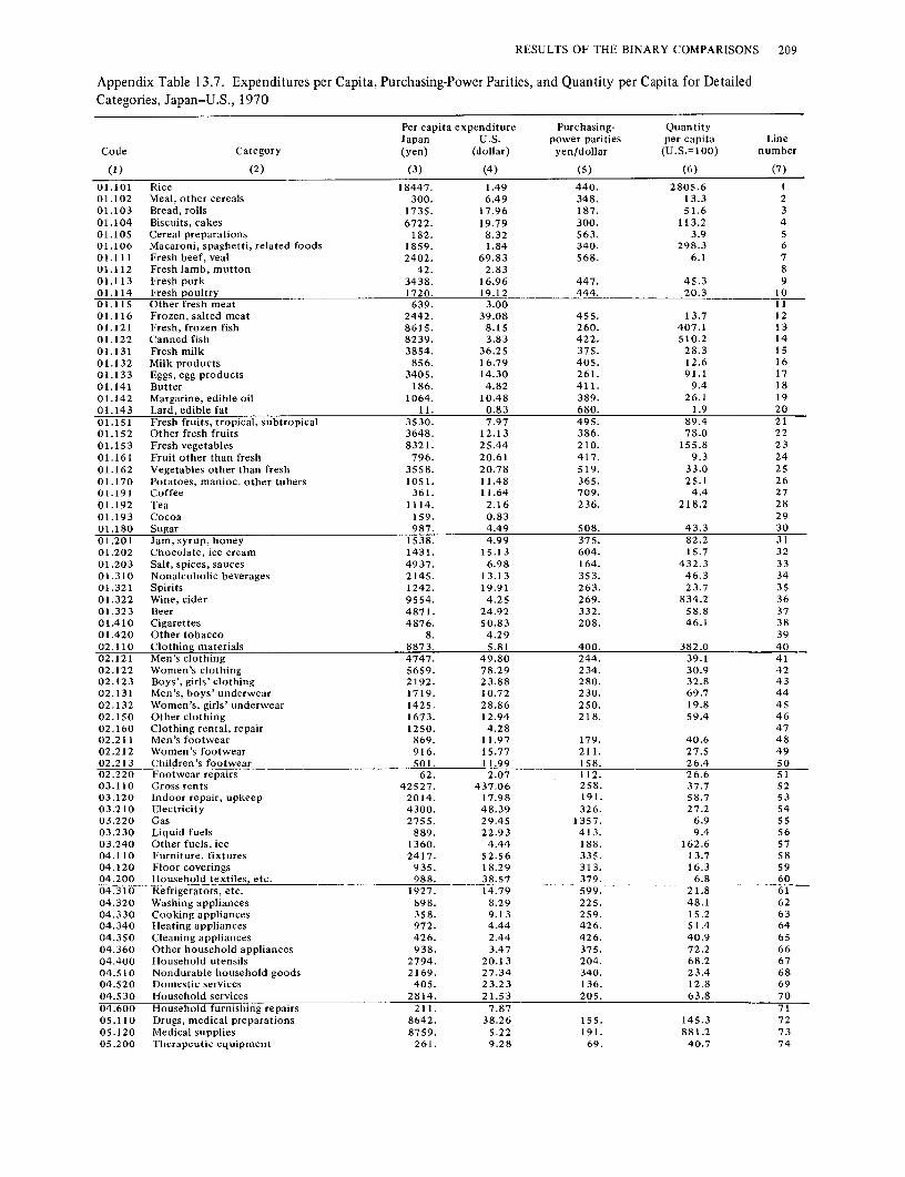
RESULTS OF THE BINARY COMPARISONS 209
Appendix Table 13.7. Expenditures per Capita, Purchasing-Power Parities, and Quantity per Capita for Detailed Categories, Japan-U.S., 1970
Per capita expenditure Purchasing- Quantity Japan U.S. power parities per capita Line
Code Category (yen) (dollar) yen/dollar (U.S.=100) number
(l) {2) (3) {4) (5) (6) (7)
01.101 Rice 18447. 1.49 440. 2805.6 I 01.102 Meal, other cereals 300. 6.49 348. 13.3 2 01.103 Bread, rolls 1735. 17.96 187. 51.6 3 01.104 Biscuits, cakes 6722. 19.79 300. 113.2 4 01.105 Cereal preparations 182. 8.32 563. 3.9 5 01.106 Macaroni, spaghetti, related foods 1859. 1.84 340. 298.3 6 01.111 Fresh beef, veal 2402. 69.83 568. 6.1 7 01.112 Fresh lamb, mutton 42. 2.83 8 01.113 Fresh pork 3438. 16.96 447. 45.3 9 01.114 Fresh poultry 1720. 19.12 444. 20.3 10 Ol.ll5 Other fresh meat 639. 3.00 11 01.116 Frozen, salted meat 2442. 39.08 455. 13.7 12 01.121 Fresh, frozen fish 8615. 8.15 260. 407.l 13 01.122 Canned fish 8239. 3.83 422. 510.2 14 01.131 Fresh milk 3854. 36.25 375. 28.3 I 5 01.132 Milk products 856. 16.79 405. 12.6 16 01.133 Eggs, egg products 3405. 14.30 261. 91.l 17 01.141 Butter 186. 4.82 41 l. 9.4 18 01.142 Margarine, edible oil 1064. 10.48 389. 26.l 19 01.143 Lard, edible fat 11. 0.83 680. 1.9 20 01.151 Fresh fruits, tropical, subtropical 3530. 7.97 495. 89.4 21 0 I. I 52 Other fresh fruits 3648. 12.13 386. 78.0 22 01.153 Fresh vegetables 8321. 25.44 210. l 55.8 23 01.161 Fruit other than fresh 796. 20.61 417. 9.3 24 01.162 Vegetables other than fresh 3558. 20.78 519. 33.0 25 01.170 Potatoes, manioc, other tubers 105 I. 11.48 365. 25.1 26 01.191 Coffee 361. 11.64 709. 4.4 27 01.192 Tea 1114. 2.16 236. 218.2 28 01.193 Cocoa 159. 0.83 29 01.180 Sugar 987. 4.49 508. 43.3 30 01.201 Jam, syrup, honey l 538. 4.99 375. 82.2 31 01.202 Chocolate, ice cream 1431. 15.13 604. 15.7 32 01.203 Salt, spices, sauces 4937. 6.98 164. 432.3 33 01.310 Nonalcoholic beverages 2145. 13.13 353. 46.3 34 01.321 Spirits 1242. 19.91 263. 23.7 35 01.322 Wine, cider 9554. 4.25 269. 834.2 36 01.323 Beer 4871. 24.92 332. 58.8 37 01.410 Cigarettes 4876. 50.83 208. 46.l 38 01.420 Other tobacco 8. 4.29 39 02.110 Clothing materials 8873. 5.81 400. 382.0 40 02.121 Men's clothing 4747. 49.80 244. 39.l 41 02.122 Women's clothing 5659. 78.29 234. 30.9 42 02.123 Boys', girls' clothing 2192. 23.88 280. 32.8 43 02.131 Men's, boys' underwear 1719. 10.72 230. 69.7 44 02.132 Women's, girls' underwear 1425. 28.86 250. 19.8 45 02.150 Other clothing 1673. 12.94 218. 59.4 46 02.160 Clothing rental, repair 1250. 4.28 47 02.211 Men's footwear 869. 11.97 179. 40.6 48 02 .212 Women's footwear 916. 15.77 21 l. 27.5 49 02.213 Children's footwear 501. 11.99 158. 26.4 50 02.220 Footwear repairs 62. 2.07 112. 26.6 51 03.llO Gross rents 42527. 437.06 258. 37.7 52 03.120 Indoor repair, upkeep 2014. 17.98 191. 58.7 53 03.210 Electricity 4300. 48.39 326. 27.2 54 03.220 Gas 2755. 29.45 1357. 6.9 55 03.230 Liquid fuels 889. 22.93 413. 9.4 56 03.240 Other fuels, ice 1360. 4.44 188. 162.6 57 04.110 Furniture, fixtures 2417. 52.56 335. 13.7 58 04.120 floor coverings 935. 18.29 313. 16.3 59 04.200 Household textiles, etc. 988. 38.57 379. 6.8 60 04.310 Refrigerators, etc. 1927. 14.79 599. 21.8 61 04.320 Washing appliances 898. 8.29 225. 48.1 62 04.330 Cooking appliances 358. 9.13 259. l 5.2 63 04.340 Heating appliances 972. 4.44 426. 51.4 64 04.350 Cleaning appliances 426. 2.44 426. 40.9 65 04.360 Other household appliances 938. 3.47 375. 72.2 66 04.400 Household utensils 2794. 20.13 204. 68.2 67 04.510 Nondurable household goods 2169. 27.34 340. 23.4 68 04.520 Domestic services 405. 23.23 136. 12.8 69 04.530 Household services 2814. 21.53 205. 63.8 70 04.600 Household furnishing repairs 211. 7.87 71 05.110 Drugs, medical preparations 8642. 38.26 l 5 5. 145.3 72 05.120 Medical supplies 8759. 5.22 191. 881.2 73 05.200 Therapeutic equipment 261. 9.28 69. 40.7 74

210 THE RESULTS OF THE COMPARISONS
Appendix Table 13.7. Continued
Per capita expenditure Purchasing· Quantity Japan U.S. power parities per capita Line
Code Category (yen) (dollar) yen/dollar (U.S.=100) number
(1) (2) (3) (4) (5) (6) (7)
05.310 Physicians' services 155 3. 47.38 66.0 75 05.320 Dentists' services 334. 13.88 68.9 76 05.330 Services, nurses, other personnel 1372. 82.89 54.0 77 05 .410 Hospitals, etc. 5243. 11 7 .82 130.6 78 06.110 Personal cars 2291. 137 .80 373. 4.5 79 06.120 Other personal transport 1000. 20.36 436. 11.3 80 06.210 Tires, tubes, accessories 173. 27.50 304. 2.1 81 06.220 Repair charges ll08. 37.82 362. 8.1 82 06.230 Gasoline, oil, etc. 2314. 112.64 591. 3.5 83 06.240 Parking, tolls, etc. 1090. 23.32 370. 12.6 84 06.310 Local transport 9945. 12.41 63. 1276.1 85 06.321 Rail transport 3059. 0.73 117. 3583.9 86 06.322 Bus transport 818. 1.95 147. 285.7 87 06.323 Air transport 328. 11.92 253. 10.9 88 06.330 Miscellaneous transport 410. 3.67 89 06.410 Postal communication 254. 7.49 257. 13.2 2!! 06.420 Telephone, telegraph 1734. 48.49 296. 12.1 91 07.110 Radio, TV, phonograph, etc. 6169. 40.62 210. 72.4 92 07.120 Major durable recreation equipment 970. 26.29 21 I. 17.4 93 07.130 Other recreation equipment 4299. 39.81 269. 40.2 94 07.210 Public entertainment 10173. 28.80 408. 86.5 95 07 .230 Other recreation, cultural events 2310. 57.68 181. 22.2 96 07 .310 Books, papers, magazines 4566. 37.14 367. 33.5 97 07.320 Stationery 917. 11.10 261. 31.6 98 07.411 Teachers, 1st, 2nd 12083. 185.05 70.8 99 07.412 Teachers, college 2170. 35.19 44.8 100 07.420 Educational facilities 2632. 29.04 101 07.431 Educational supplies 877. 7.54 102 07.432 Other education exependitures 1939. 8.48 103 08.100 Barber, beauty shops 4165. 19.91 135. 154.4 104 08.210 Toilet articles 5260. 29.85 279. 63.0 105 08.220 Other personal-care goods 1417. 30.29 194. 24.I 106 08.310 Restaurants, cafes 13038. 140.16 214. 43.5 107 08.320 Hotels, etc. 5056. 8.67 267. 218.5 108 08.400 Other services I 5656. 118.76 109 08.900 Expenditures of residents abroad 1064. 23.70 110 10.100 1- and 2-dwelling buildings 34424. 103.98 261. 126.7 111 10.200 Multidwelling buildings 16084. 43.16 225. 165.8 112 11.100 Hotels, etc. 2233. 6.69 272. 122.6 113 11.200 Industrial buildings 7091. 36.17 536. 36.6 114 11.300 Commercial buildings 7092. 25.28 446. 62.9 115 11.400 Office buildings 7845. 32.68 282. 85.0 116 I 1.500 Educational buildings 4918. 32.17 208. 73.6 117 11.600 Hospital buildings 1715. 16.81 180. 56.8 118 1 I. 700 Agricultural buildings 1200. 3.36 622. 57.4 119 11.800 Other buildings 9592. 18.38 393. 132.8 120 12.100 Roads, highways 14244. 51.45 288. 96.0 121 12.200 Transmission, utility lines 167 36. 70.11 167. 143.0 122 12.300 Other construction 22127. 13.57 191. 856.1 123 13.000 Land improvement 516. 10.14 160. 31.8 124 14,110 Locomotives 782. 1.16 125 14.120 Other 89. 6.33 126 14.200 Passenger cars 11408. 34.27 374. 88.9 127 14.300 Trucks, buses, trailers 14279. 44.01 128 14.400 Aircraft 364. 14.40 129 14.500 Ships, boats 3924. 3.96 130 14.600 Other transport 1497. 1.71 131 15.100 Engines and turbines 2070. 6.46 132 15.210 Tractors 410. 8.24 133 15.220 Other agricultural machinery 1916. 11.81 134 15.300 Office machinery 5508. 32.00 135 I 5 .400 Metalworking machinery 7482. 17.83 427. 98.2 136 15.500 Construction, mining 4720. 16.37 302. 95.5 137 15.600 Special industrial 12427. l 5.33 230. 351.9 138 15.700 General industrial 11 744. 19.79 292. 203.0 139 15.800 Service industrial 1052. 17.01 140 16.100 Electrical transmission 7658. 13.62 141 16.200 Communication equipment 8000. 25.45 142 16.300 Other electrical 2203. 3.88 143 16.400 Instruments 4144. 16.52 144 17.100 Furniture, fixtures 5359. 19.45 316. 87.2 145 17.200 Other durable goods 2864. 19.52 146 18.000 Increase in stocks 31443. 16.60 326. 580.9 147 19.000 Exports less imports 9113. 7.42 360. 341.0 148 20.100 Blue-collar, unskilled 9844. 18.33 142. 377.6 149 20.210 Blue-collar, skilled 19445. 94.41 118. 174.2 150

RESULTS OF THE BINARY COMPARISONS 211
Appendix Table 13.7. Continued
Per capita expenditure Purchasing- Quantity Japan U.S. power parities per capita Line
Code Category (yen) (dollar) yen/dollar (U.S.=100) number
(1) (2) (3) (4) (5) (6) (7)
20.220 White-collar 4780, 108.62 124. 35.5 151 20.300 Professional 6441. 132.96 244. 19.9 152 21.000 Government expenditure on commodities 16047. 338.05 239. 19.9 153
Notes: 1. Above expenditures for lines 1 to 110 include both household and government expenditures. The latter are shown separately in Table 13.15. 2. Sugar (1180) is intentionally out of order; the purpose is to facilitate aggregation. 3. The purchasing-power parities are direct except for the following: Purchasing-power parities are indirect and the quantity ratios are direct in lines 75,76,77,78,99, and 100. Blanks in columns 5 and 6 indicate no direct price or quantity comparisons were made. Where neither comparison was made, purchasing-power parities from other selected categories were imputed to these categories for aggregation purposes. 4. Exchange rate: ¥360=US$1.00.
Appendix Table 13.8. Expenditures per Capita, Purchasing-Power Parities, and Quantity per Capita for Detailed Categories, Kenya-U.S., 1970
Per capita expenditure Purchasing- Quantity Kenya U.S. power parities per capita Line
Code Category (shilling) (dollar) shilling/ dollar (U.S.=100) number
(1) (2) (3) (4) (5) (6) (7)
01.101 Rice 1.80 1.49 4.14 29.l l 01.102 Meal, other cereals 115.79 6.49 S.74 310.9 2 01.103 Bread, rolls 4.76 17.96 3.05 8.7 3 01.104 Biscuits, cakes 2.02 19.79 1.06 9.7 4 01.105 Cereal preparations 0.83 8.32 10.22 1.0 s 01.106 Macaroni, spaghetti, related foods 0.15 1.84 11.42 0.7 6 01.111 Fresh beef, veal 22.43 69.83 3.14 10.2 7 01.112 Fresh lamb, mutton 2.74 2.83 2.76 35.1 8 01.113 Fresh pork 0.54 16.96 6.83 o.s 9 01.114 Fresh 12oultr:i:: Q.2!! 12 12 S 12 IQ IQ 01.115 Other fresh meat 2.39 3.00 11 01.116 Frozen, salted meat 1.98 39.08 5.35 0.9 12 01.121 Fresh, frozen fish 6.54 8.15 4.11 19.5 13 01.122 Canned fish 0.99 3.83 11.63 2.2 14 01.131 Fresh milk 37.64 36.23 4.13 25.2 15 01.132 Milk products 4.07 16.79 6.11 4.0 16 01.133 Eggs, egg products 0.33 14.30 5.64 0.4 17 01.141 Butter 5.48 4.82 4.48 25.4 18 01.142 Margarine, edible oil 4.76 10.48 8.51 5.3 19 01.143 Lard, edible fat 1.lS Q,83 13 Q2 IQ S 2Q 01.151 Fresh fruits, tropical, subtropical 13.27 7.97 2.48 67.0 21 01.152 Other fresh fruits 0.32 12.13 15.77 0.2 22 01.153 Fresh vegetables 19.72 25.44 2.06 37.7 23 01.161 Fruit other than fresh 0.11 20.61 4.92 0.1 24 01.162 Vegetables other than fresh 3.61 20.78 5.90 2.9 25 01.1 70 Potatoes, manioc, other tubers 31.07 11.48 2.01 134.9 26 01.191 Coffee 0.96 11.64 7.63 1.1 27 01.192 Tea 3.49 2.16 2.88 56.1 28 01.193 Cocoa 0.26 0.83 8.70 3.6 29 01.180 Sugar 13.46 4.49 5.48 54.7 30 01.201 Jam, syrup, honey 2.69 4.99 3.49 l S.4 31 01.202 Chocolate, ice cream 1.96 l 5.13 32.72 0.4 32 01.203 Salt, spices, sauces 3.90 6.98 5.40 10.4 33 01.310 Nonalcoholic beverages 5.86 13.13 14.68 3.0 34 01.321 Spirits 2.05 19.91 6.85 1.5 35 01.322 Wine, cider 0.47 4.25 7.79 1.4 36 01.323 Beer 13.73 24.92 8.22 6.7 37 01.410 Cigarettes 9.33 50.83 4.35 4.2 38 01.420 Other tobacco 0.20 4.29 3.82 1.2 39 02.110 Clothing materials 5.31 5.81 7.94 11.~ ~Q 02.121 Men's clothing 7.92 49.80 4.66 3.4 41 02.122 Women's clothing 4.59 78.29 11.28 0.5 42 02.123 Boys', girls' clothing 2.36 23.88 2.80 3.5 43 02.131 Men's, boys' underwear 0.55 10.72 8.06 0.6 44 02.132 Women's, girls' underwear 0.47 28.86 4.17 0.4 45 02.150 Other clothing 0.66 12.94 4.73 1.1 46 02.160 Clothing rental, repair 0.62 4.28 3.56 4.0 47 02.211 Men's footwear 3.34 11.97 2.72 10.3 48 02.212 Women's footwear 0.83 15.77 1.80 2.9 49 02.213 Children's footwear 0.65 11.99 1.59 3.4 so

212 THE RESULTS OF THE COMPARISONS
Appendix Table 13.8. Continued
Per capita expenditure Purchasing- Quantity Kenya U.S. power parities per capita Line
Code Category (shilling) (dollar) shilling/dollar (U.S.=100) number
(I) (2) (3) (4) (S) (6) (7)
02.220 Footwear repairs 0.27 2.07 4.01 3.2 SI 03.110 Gross rents 61.15 437.06 5.99 2.3 52 03.120 Indoor repair, upkeep 0.20 17.98 3.15 0.4 53 03.210 Electricity 1.43 48.39 9.11 0.3 54 03.220 Gas 0.11 29.45 8.30 0.0 55 03.230 Liquid fuels 1.38 22.93 17.13 0.4 56 03.240 Other fuels, ice 8.12 4.44 1.69 108.2 57 04.110 Furniture, fixtures 6.00 52.56 3.77 3.0 58 04.120 Floor coverings 0.98 18.29 8.63 0.6 59 04.200 Household textiles, etc. 3.85 38.57 7.36 1.4 6Q 04.310 Refrigerators, etc. 0.59 14.79 8.93 0.4 61 04.320 Washing appliances 0.08 8.29 62 04.330 Cooking appliances 0.62 9.13 10.41 0.7 63 04.340 Heating appliances 0.56 4.44 64 04.350 Cleaning appliances 0.10 2.44 65 04.360 Other household appliances 0.24 3.47 16.48 0.4 66 04.400 Household utensils 6.79 20.13 3.25 10.4 67 04.510 Nondurable household goods 16.19 27.34 7 .73 7 .7 68 04.520 Domestic services 6.37 23.23 0.67 40.7 69 04.530 Household services 1.14 21.53 4.09 1.3 70 04.600 Household furnishing repairs 0.08 7.87 0.89 I. I 71 05.110 Drugs, medical preparations 7.06 38.26 3.31 5.6 72 05.120 Medical supplies O.S5 5.22 3.68 2.9 73 05.200 Therapeutic equipment 0.09 9.28 1.44 0.7 74 05.310 Physicians' services s.os 47.38 7.0 75 05.320 Dentists' services 0.40 13.88 1.0 76 05.330 Services, nurses, other personnel 5.36 82.89 77 05 .410 Hospitals, etc. 17.79 117.82 15.1 78 06.110 Personal cars 11.14 137.80 8.43 1.0 79 06.120 Other personal transport 0.11 20.36 8.61 0.1 80 06.210 Tires, tubes, accessones 2.18 27.50 10.76 0.7 81 06.220 Repair charges 2.18 37.82 1.77 3.3 82 06.2 30 Gasoline, oil, etc. 1.16 112.64 7.68 0.1 83 06.240 Parking, tolls, etc. 0.86 23.32 84 06.310 Local transport 2.24 12.41 1.93 9.4 85 06.321 Rail transport 1.40 0.73 3.16 60.5 86 06.322 Bus transport 13.24 1.95 2.67 254.9 87 06.323 Air transport 15.06 11.92 12.03 10.5 88 06.330 Miscellaneous transport 0.22 3.67 89 06.410 Postal communication 0.41 7.49 4.33 1.3 90 06.420 Telephone, telegraph 1.02 48.49 2.73 0.8 91 07.110 Radio, TV, phonograph, etc. 3.75 40.62 11.25 0.8 92 07.120 Major durable recreation equipment 5.43 26.29 10.06 2.1 93 07.130 Other recreation equipment 3.72 39.81 7.33 1.3 94 07.210 Public entertainment 5.61 28.80 1.35 14.4 95 07.230 Other recreation, cultural events 4.06 57.68 2.96 2.4 96 07.310 Books, papers, magazines 6.oo 37.14 6.85 2.4 97 07.320 Stationery 0.09 11.10 16.16 0.0 98 07.411 Teachers, 1st, 2nd 40.04 185.05 28.6 99 07 .412 Teachers, colle11e 2.22 35.19 1.2 JOO 07.420 Educational facilities s.n 29.04 IOI 07.431 Educational supplies 2.35 7.54 102 07.432 Other education expenditures 3.79 8.48 103 08.100 Barber, beauty shops 0.46 19.91 2.55 0.9 104 08.210 Toilet articles 2.62 29.85 8.65 1.0 105 08.220 Other personal-care goods 2.62 30.29 5.47 1.6 106 08.310 Restaurants, cafes 13.80 140.16 2.84 3.5 107 08.320 Hotels, etc. 14.48 8.67 4.01 41.7 108 08.400 Other services 11.97 118.76 109 08.900 Exeenditures of residents abroad 23.70 110 JO.I 00 I- and 2-dwelling buildings 37.06 I 03.98 3.27 10.9 111 10.200 Multidwelling buildings 5.56 43.16 3.61 3.6 112 11.100 Hotels, etc. 0.78 6.69 4.77 2.4 113 11.200 Industrial buildings 14.s 1 36.17 5.14 7.8 114 11.300 Commercial buildings 2.37 25.28 3.73 3.0 115 11.400. Office buildings 3.71 32.68 2.62 4.3 l 16 I 1.500 Educational buildings 3.64 32.17 2.52 4.5 117 11.600 Hospital buildings 3.7 J 16.81 3.01 7.4 118 l l.700 Agricultural buildings 0,74 3.36 2.23 9.9 119 11.800 Other buildin11s 0.93 18.38 120 12.100 Roads, highways 11.60 S 1.45 121 12.200 Transmission, utility lines 8.76 70.11 122 12.300 Other construction 13.96 13.57 8.84 11.6 123 13.000 Land improvement 4.59 10.14 3.54 12.8 124 14.110 Locomotives 2.79 1.16 6.84 35.2 125 14.120 Other 4.95 6.33 9.46 8.3 126

RESULTS OF THE BINARY COMPARISONS 213
Appendix Table 13.8. Continued
Per capita expenditure Purchasing- Quantity Kenya U.S. power parities per capita Line
Code Category (shilling) (dollar) shilling/ dollar (U.S."100) number
(1) (2) (3) (4) (5) (6) (7)
14.200 Passenger cars 10.22 34.27 8.15 3.7 127 14.300 Trucks, buses, trailers 11. 71 44.01 6.99 3.8 128 14.400 Aircraft 2.71 14.40 129 14.500 Ships, boats 0.46 3.96 130 14.600 Other transport 0.54 1.71 8.21 3.8 131 15.100 Engines and turbines 2.18 6.46 8.42 4.0 132 l 5 .210 Tractors 2.40 8.24 6.82 4.3 133 15.220 Other agricultural machinery 3.39 11.81 9.56 3.0 134 15.300 Office machinery 1.87 32.00 9.85 0.6 135 15.400 Metalworking machinery 1.15 17.83 4.39 1.5 136 15.500 Construction, mining 4.75 16.37 9.29 3.1 137 15.600 Special industrial 10.20 15.33 6.60 10.1 138 15.700 General industrial 9.64 19.79 7.84 6.2 139 15.800 Service industrial 2.07 17.01 11.09 1.1 140 16.100 Electrical transmission 4.12 13.62 5.48 5.5 141 16.200 Communication equipment 2.93 25.45 142 16.300 Other electrical 1.12 3.88 143 16.400 Instruments 1.43 16.52 7.28 1.2 144 17.100 Furniture, fixtures 2.00 19.45 5.82 1.8 145 17.200 Other durable goods 5.35 19.52 6.65 4.1 146 18.000 Increase in stocks 23.83 16.60 5.51 26.0 147 19.000 Exports less imports -17.78 7.42 7.14 -33.5 148 20.100 Blue-collar, unskilled 44.13 18.33 0.51 471.1 149 20.210 Blue-collar, skilled 3.12 94.41 1.18 2.8 150 20.220 White-collar 12.07 108.62 1.91 5.8 151 20.300 Professional 29.90 132.96 4.26 5.3 152 21.000 Government expenditure on commodities 28.21 338.05 4.35 1.9 153
Notes: 1. Above expenditures for lines 1 to 110 include both household and government expenditures. The latter are shown separately in Table 13.15. 2. Sugar (1 180) is intentionally out of order; the purpose is to facilitate aggregation. 3. The purchasing-power parities are direct except for the following: Purchasing-power parities are indirect and the quantity ratios are direct in lines 75,76,77,78,99, and 100. Blanks in columns 5 and 6 indicate no direct price or quantity comparisons were made. Where neither comparison was made purchasing-power parities from other selected categories were imputed to these categories for aggregation purposes. 4. In the Kenya-U.S. comparison, yams and potatoes were treated as separate categories, although for mechanical convenience they are printed above as a single category; the price ratio for potatoes was 3.350 and for yams, sweet potatoes, and cassava, 1.157. 75.0 percent of ICP 1 170 expenditure in Kenya was for yams and 9.1 percent in the United States. 5. Exchange rate: Sh7.143=US$1.00.
Appendix Table 13.9. Expenditures per Capita, Purchasing-Power Parities, and Quantity per Capita for Detailed Categories, U.K.-U.S., 1970
Per capita expenditure Purchasing- Quantity U.K. U.S. power parities per capita Line
Code Category (pound) (dollar) pound/dollar (U.S."100) number
(1) (2) (3) (4) (5) (6) (7)
01.101 Rice 0.107 1.49 0.390 18.4 1 01.102 Meal, other cereals 0.714 6.49 0.355 31.0 2 01.103 Bread, rolls 17.96 0.203 182.7 3 01.104 Biscuits, cakes 6.430 19.79 0.247 131.6 4 O 1.1 OS Cereal preparations l.12S 8.32 0.291 46.5 5 01.106 Macaroni, spaghetti, related foods 0.304 1.84 0.384 43.1 6 01.111 Fresh beef, veal 8.39S 69.83 0.214 56.2 7 01.112 Fresh lamb, mutton 4.447 2.83 0.207 759.0 8 01.113 Fresh pork 2.018 16.96 0.347 34.3 9 01.114 Fresh 11ou1trr 2.876 19.12 0.351 42.8 10 01.115 Other fresh meat 1.268 3.00 0.324 130.6 II 01.116 Frozen, salted meat 13.360 39.08 0.323 105.8 12 01.121 Fresh, frozen fish 2.500 8.15 0.270 113.6 13 01.122 Canned fish 1.393 3.83 0.511 71.2 14 01.131 Fresh milk 9.180 36.25 0.361 70.2 15 01.132 Milk products 3.786 16.79 0.220 102.5 16 01.133 Eggs, egg products 3.983 14.30 0.376 74.1 17 01.141 Butter 3.161 4.82 0.217 302.4 18 01.142 Margarine, edible oil 1.179 10.48 0.421 26.7 19 01.143 Lard edible fat 0.589 0.83 0.467 151.2 20 01.151 Fresh fruits, tropical, subtropical 1.840 7.97 0.447 51.6 21 01.152 Other fresh fruits 2.608 12.13 0.368 58.4 22

214 THE RESULTS OF THE COMPARISONS
Appendix Table 13.9. Continued
Per capita expenditure Purchasing- Quantity U.K. U.S. power parities per capita Line
Code Category (pound) (dollar) pound/dollar (U.S.=100) number
(1) (2) (3) (4) (S) (6) (7)
01.153 Fresh vegetables 5.037 25.44 0.254 78.0 23 01.161 Fruit other than fresh 2.233 20.61 0.365 29.7 24 01.162 Vegetables other than fresh 3.983 20.78 0.407 47.1 25 01.170 Potatoes, manioc, other tubers 4.626 11.48 0.259 I 55.6 26 01.191 Coffee 1.161 11.64 0.369 27.0 27 01.192 Tea 2.965 2.16 0.180 761.9 28 01.193 Cocoa 0.107 0.83 0.293 43.8 29 01.180 Sugar 2.21 S 4.49 0.291 169.S 30 01.201 Jam, syrup, honey 1.143 4.99 0.189 121.1 31 01.202 Chocolate, ice cream 8.805 I 5.13 0.567 102.6 32 01.203 Salt, spices, sauces 1.000 6.98 0.403 35.6 33 01.310 Nonalcoholic beverages 2.947 13.13 0.395 56.8 34 01.321 Spirits 10.431 19.91 0.440 119. l 35 01.322 Wine, cider 4.930 4.25 0.690 168.1 36 01.323 Beer 22.219 24.92 0.572 155.9 37 01.410 Cigarettes 26.845 50.83 0.693 76.2 38 01.420 Other tobacco 3.858 4.29 0.714 125.8 39 02.110 Clothing materials 1.286 5.81 0.382 57.9 40 02.121 Men's clothing 7.573 49.80 0.317 48.0 41 02.122 Women's clothing 12.556 78.29 0.457 35.1 42 02.123 Roy's, girls' clothing 2.483 23.88 0.311 33.4 43 02.131 Men's, boys' underwear 4.019 10.72 0.497 75.4 44 02.132 Women's, girls' underwear 5.412 28.86 0.351 53.4 45 02.1 so Other clothing 5.698 12.94 0.258 170.6 46 02.160 Clothing rental, repair 0.857 4.28 0.331 60.5 47 02. 211 Men's footwear 2.590 11.97 0.208 104.0 48 02.212 Women's footwear 3.554 I 5.77 0.252 89.4 49 02.213 Children's footwear 1.929 11.99 0.174 92.S so 02.220 Footwear repairs 0.750 2.07 0.220 164.8 SI 03.110 Gross rents 63.423 437.06 0.271 53.S 52 03.120 Indoor repair, up keep 12.699 17.98 0.356 198.4 53 03.210 Electricity l l.770 48.39 0.330 73.7 54 03.220 Gas 6.876 29.45 0.890 26.2 55 03.230 Liquid fuels 1.107 22.93 56 03.240 Other fuels, ice 6.823 4.44 0.287 535.3 57 04.110 Furniture, fixtures 6.162 52.56 0.494 23.7 58 04.120 Floor coverings 5.001 18.29 0.303 90.3 59 04.200 Household textiles, etc. 4.912 38.57 0.288 44.2 60 04.310 Refngerators, etc. 1.429 14.79 0.438 22.1 61 04.320 Washing appliances 1.875 8.29 0.344 65.8 62 04.330 Cooking appliances 1.661 9.13 0.382 47.6 63 04.340 Heating appliances 1.554 4.44 0.556 62.9 64 04.350 Cleaning appliances 1.107 2.44 0.730 62.2 65 04.360 Other household appliances 0.321 3.47 0.643 14.4 66 04.400 Household utensils 6.716 20.13 0.351 95.0 67 04.510 Nondurable household goods 6.090 27.34 0.418 53.3 68 04.520 Domestic services 2.822 23.23 0.185 65.7 69 04.530 Household services 3.590 21.53 0.272 61.3 70 04.600 Household furnishing repairs 0.804 7.87 0.111 92.0 71 05.110 Drugs, medical preparations 6.555 38.26 0.164 104.5 72 05.120 Medical supplies 1.107 5.22 0.207 102.S 73 05.200 Therapeutic equipment 1.911 9.28 0.171 120.4 74 05.310 Physicians' services 5.644 47.38 66.9 75 05.320 Den tis ts' services 1.822 13.88 48.1 76 05.330 Services, nurses, other personnel 9.573 82.89 102.2 77 05.410 Hospitals, etc. 12.502 11 7 .82 11 5.3 78 06.110 Personal cars 17 .003 137.80 0.570 21.6 79 06.120 Other personal transEort 1.072 20.36 0.522 10.1 80 06.210 Tires, tubes, accessories 4.465 27.50 0.240 67.7 81 06.220 Repair charges 4.21 S 37.82 0.172 64.8 82 06.230 Gasoline, oil, etc. 14.146 112.64 O.S87 21.4 83 06.240 Parking, tolls, etc. 7.519 23.32 0.296 108.9 84 06.310 Local transport 9.609 12.41 0.214 361.9 85 06.321 Rail transport 2.518 0.73 0.283 1215.6 86 06.322 Bus transport 0.500 1.95 0.233 110.2 87 06.323 Air transport 3.394 11.92 0.393 72.4 88 01.101 Miscellaneous transport 1.822 3.67 0.720 68.9 89 06.410 Postal communication 1.947 7.49 0.268 97.0 90 06.420 Telephone, telegraph 3.751 48.49 0.187 41.4 91 07.110 Radio, TV, phonograph, etc. 3.215 40.62 0.576 13.7 92 07 .120 Major durable recreation equipment 1.661 26.29 0.414 15.3 93 07 .130 Other recreation equipment 11.002 39.81 0.437 63.2 94 07.210 Public entertainment 6.876 28.80 0.084 284.2 95 07 .2 30 Other recreation, cultural events 14.485 57.68 0.355 70.8 96 07.310 Books, papers, magazines 8.269 37.14 0.166 134.1 97

RESULTS OF THE BINARY COMPARISONS 215
Appendix Table 13.9. Continued
Per capita expenditure Purchasing- Quantity UK US. power parities per capita Line
Code Category (pound) (dollar) pound/ dollar (U.S =100) number
(I) (2) (3) (4) (5) (6) (7)
07.320 Stationery 1.947 11.10 0.339 51.7 98 07.411 Teachers, 1st, 2nd 23.719 185.05 67.1 99 07.412 Teachers, college 4.787 35.19 48.6 100 07.420 Educational facilities 5,590 29.04 101 07.431 Educational supplies 2.054 7.54 102 07.432 Other education expenditures 3.751 8.48 103 08.100 Barber, beauty shops 4.037 19.91 0.118 171.8 104 08.210 Toilet articles 4.251 29.85 0.366 38.9 105 08.220 Other personal-care goods 4.512 30.29 0.268 56.3 106 08.310 Restaurants, cafes 16.289 140.16 0.394 29.5 107 08.320 Hotels, etc. 10.413 8.67 0.285 421.5 108 08.400 Other services 18.825 118.76 109 08.900 Expenditures of residents abroad -0.339 23.70 0.417 -3.4 110 1 o. l 00 1- and 2-dweJling buildmgs 18.414 103.98 0.183 96.8 ll l 10.200 Multidwelling buildings 8.591 43.16 0.218 91.3 112 11.100 Hotels, etc. 0.643 6.69 0.399 24.1 113 11.200 Industrial buildings 13.663 36.17 0.373 101.3 114 11.300 Commercial buildings 4.626 25.28 0.343 53.3 115 11.400 Office buildings 3.126 32.68 0.258 37.1 116 11.500 Educational buildings 6.055 32.17 0.308 61.1 117 11.600 Hospital buildings 2.983 16.81 0.242 73,3 118 11. 700 Agricultural buildings 1.643 3.36 0.250 195.S 119 11.800 Other buildings 3.590 18.38 0.373 52.4 120 12.100 Roads, highways 8.216 51.45 0.243 65.7 121 12.200 Transmission, utility lines 4.858 70.11 0.185 37.5 122 12.300 Other construction 2.572 13.57 0.308 61.5 123 13.000 Land improvement 2,143 10.14 0.357 59.2 124 14.110 Locomotives 0.143 1.16 125 14.120 Other 0.232 6.33 126 14.200 Passenger cars 6.090 34.27 0.670 26.5 127 14.300 Trucks, buses, trailers 0.625 44.01 128 14.400 Aircraft 1.804 14.40 129 14.500 Ships, boats 5.698 3.96 130 14.600 Other transport 3.590 1.71 131 15.100 Engines and turbines 0.107 6.46 0.310 5.3 132 15.210 Tractors 0,929 8.24 0.320 35.2 133 15.220 Other agricultural machinery 1.375 11.81 0.390 29.9 134 15.300 Office machinery 3.108 32.00 0.410 23.7 135 15 .400 Metalworking machinery 4.376 17.83 0.300 81.8 136 15.500 Construction, mining 4.590 16.37 0.370 75.8 137 15.600 Special industrial 7.591 15.33 0.370 133.8 138 15.700 General industrial 2 J.058 19.79 0.320 332.6 139 15.800 Service industrial 0.572 17.01 140 16.100 Electrical transmission 6.483 13.62 141 16.200 Communication equipment 8.502 25.45 142 16.300 Other electrical 1.786 3.88 0.1 so 306.5 143 16.400 Instruments 1.715 16.52 0.160 64.9 144 17 .100 Furniture, fixtures 1.911 19.45 0.210 46.8 145 17.200 Other durable goods 0.429 19.52 146 18.000 Increase in stocks 6.626 16.60 0.381 104.7 147 19.000 Exports Jess imports 7.019 7.42 0.417 226.8 148 20.200 Blue-collar unskilled 25,005 112.74 0.149 148.9 149 20.220 White-collar 17 .575 108.62 0.201 80.5 151 20.300 Professional 8.002 132.96 0.274 22.0 152 21.000 Government expenditure on commodities 30.667 338.05 0.313 28.9 153
Notes: 1. Above expenditures for lines 1 to 110 include both household and government expenditures. The latter are shown separately in Table 13.15. 2. Sugar (1180) is intentionally out of order; the purpose is to facilitate aggregation. 3. The purchasing-power parities are direct except for the following: Purchasing-power parities are indirect and the quantity ratios are direct in lines 75,76,77,78,99, and 100. Blanks in columns 5 and 6 indicate no direct price or quantity comparisons were made. Where neither comparison was made, purchasing-power parities from other selected categories were imputed to these categories for aggregation purposes. 4. Blue-collar workers (line 149) include both first- and second-level blue-collar workers. In other binary comparisons, these are found in lines 149 and 150, respectively. 5. Exchange rate: £0.417=US$1.00.
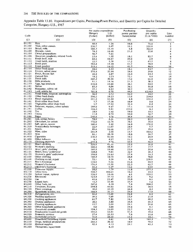
216 THE RESULTS OF THE COMPARISONS
Appendix Table 13.10. Expenditures per Capita, Purchasing-Power Parities, and Quantity per Capita for Detailed Categories, Hungary-U.S., 1967
Per capita expenditure Purchasing- Quantity Hungary U.S. power parities per capita Line
Code Category (forint) (dollar) forint/dollar (U.S.=100) number
(I) (2) (3) (4) (5) (6) (7)
01.101 Rice 48.9 1.26 50.8 76.6 I OJ.I 02 Meal, other cereals 231.7 5.47 19.1 221.9 2 0 I. I 03 Bread, rolls 285.3 15.14 5.8 322.4 3 OJ.I 04 Biscuits, cakes 78.3 16.68 21.3 22.0 4 01.105 Cereal preparations 56.7 7.01 5 01.106 Macaroni, spaghetti, related foods 23.1 1.55 18.1 82.7 6 01.111 Fresh beef, veal 84.4 58.87 49.0 2.9 7 01.112 Fresh lamb, mutton 12.7 2.39 I 1.2 47.7 8 01.113 Fresh pork 583.4 14.30 5 1.7 78.9 9 01.114 Fresh poultry 315.2 16.12 41.7 46.9 10 01.115 Other fresh meat 20.0 2.53 18.1 43.7 11 01.116 Frozen, salted meat 275.4 32.94 28.8 29.0 12 01.121 Fresh, frozen fish 26.2 6.87 16.4 23.3 13 01.122 Canned fish 10.2 3.23 72.1 4.4 14 01.131 Fresh milk 269.3 30.56 13.2 66.6 15 01.1 32 Milk products 91.1 14.16 21.3 30.2 16 0 I.I 33 Eggs, egg products 233.6 12.05 38.1 50.9 17 01.141 Butter 83.3 4.06 36.1 56.8 18 01.142 Margarine, edible oil 27 .1 8.83 30.2 10.2 19 01.143 Lard, edible fat 381.8 0.70 44.9 1214.9 20 01.151 Fresh fruits, tropical, subtropical 56.9 6.73 56.9 14.9 21 01.152 Other fresh fruits 296.2 10.23 13.5 214.0 22 01.153 Fresh vegetables 221.2 21.44 6.8 I 52.2 23 01.161 Fruit other than fresh 7 .7 17 .38 68.9 0.6 24 01.162 Vegetables other than fresh 2.7 17.52 32.4 0.5 25 01.170 Potatoes, manioc, other tubers 184.0 9.67 17 .I 111.4 26 01.191 Coffee 125.3 9.81 153.2 8.3 27 01.192 Tea 10.9 1.82 59.0 IO.I 28 01.193 Cocoa 11.5 0.70 50.0 32.7 29 01.180 Sugar 245.6 3.78 39.9 162.8 30 01.201 Jam, syrup, honey 70.9 4.21 20.3 82.9 31 01.202 Chocolate, ice cream 172.0 12.76 38.5 35.0 32 01.203 Salt, spices, sauces 160.4 5.89 16.0 170.0 33 01.310 Nonalcoholic beverages 22.9 11.07 26.9 7.7 34 01.321 Spirits 89.6 16.68 27 .7 19.4 35 01.322 Wine, cider 281.4 3.56 I 5.7 503.2 36 01.323 Beer 81.1 20.39 18.8 20.7 37 01.410 Cigarettes 235.1 41.90 10.2 54.9 38 01.420 Other tobacco 6.1 4.97 21.2 5.9 39 02.110 Clothing materials 145.4 4.76 65.9 46.4 40 02.121 Men's clothing 328.8 41.31 25.6 31.0 41 02.122 Women's clothing 288.S 58.80 27 .7 17.7 42 02.123 Boys', girls' clothing 165.S 19.68 23.6 35.6 43 02.131 Men's, boys' underwear 104.8 9.01 32.9 35.3 44 02.132 Women's, girls' underwear 106.8 23.63 27.8 16.3 45 02.1 so Other clothing 169.9 10.70 20.4 78.0 46 02.160 Clothing rental, repair 72.1 3.29 9.1 239.9 47 02.211 Men's footwear 114.5 9.56 21.8 54.9 48 02.212 Women's footwear 176.4 12.59 22.3 62.7 49 02.213 Children's footwear 55.3 9.57 13.2 43.9 so 02.220 Footwear repairs 58.S 1.79 11.8 277.3 51 03.110 Gross rents 558.7 350.61 10.3 15.5 52 O 3.170 Indoor repair, upkeep 126.5 14.46 6.5 133.S 53 03.210 Electricity 123.4 37 .73 35.5 9.2 54 03.220 Gas 45.8 25.67 22.0 8.1 55 03.230 Liquid fuels 15.3 22.40 56.4 1.2 56 03.240 Other fuels, ice 307.0 4.34 7.8 904.2 57 04.110 Furniture, fixtures 294.8 45.02 24.6 26.6 58 04.120 Floor coverings 35.0 15.29 26.8 8.5 59 04.200 Household textiles etc. 166.9 31.17 29.9 17 .9 60 04.310 Refrigerators, etc. 54.4 12.65 52.8 8.2 61 04.320 Washing appliances 39.2 7.09 25.9 21.4 62 04.330 Cooking appliances 61.7 7.82 16.1 49.2 63 04.340 Heating appliances 30.2 3.80 35.8 22.3 64 04.350 Cleaning appliances 12.7 2.09 29.1 21.0 65 04.360 Other household appliances 6.0 3.00 24.6 8.1 66 04.400 Household utensils 154.3 16.09 22.7 42.1 67 04.S 10 Nondurable household goods 192.6 23.81 41.5 19.5 68 04.520 Domes tic services 27.4 22.53 7.8 15.6 69 04.S 30 Household services 31.9 20.35 I 5.5 IO.I 70 04.600 Household furnishing repairs 96.4 6.61 8.8 165.3 71 05.110 Drugs, medical preparations 261.5 30.32 10.9 79.5 72 05.120 Medical supplies 42.1 4.13 24.1 42.3 73 05.200 Therapeutic equipment 8.10 74

RESULTS OF THE BINARY COMPARISONS 217
Appendix Table 13.10. Continued
Per capita expenditure Purchasing- Quantity Hungary U.S. power parities per capita Line
Code Category (forint) (dollar) forin t/ dollar (U.S.=100) number
(1) (2) (3) (4) (5) (6) (7)
05.310 Physicians' services 97.l 38.71 111.5 75 05.320 Den tis ts' services 7.7 11.69 41.3 76 05.330 Services, nurses, other personnel 102.0 56.23 72.6 77 05.410 Hospitals, etc. 336.3 80.38 96.0 78 06.110 Personal cars 134.1 125.38 56.8 1.9 79 06.120 Other 12ersonal trans12ort 61.2 10.71 21.3 26.8 80 06.210 Tires, tubes, accessories 39.2 19.37 33.4 6.1 81 06.220 Repair charges 36.0 29.57 12.9 9.4 82 06.230 Gasoline, oil, etc. 55.7 88.67 36.1 1.7 83 06.240 Parking, tolls, etc. 9.8 21.13 3.1 14.7 84 06.310 Local transport 137.0 11.l 5 9.4 130.0 85 06.321 Rail transport 146.8 1.04 15.0 942.2 86 06.322 Bus transport 137 .0 1.80 22.5 338.0 87 06.323 Air transport 14.7 8.14 88 06,330 Miscellaneous transport 26.5 2.99 23.5 37.7 89 06.410 Postal communication 29.9 5.85 11.0 46.6 90 06.420 Telephone, telegraph 34.3 37.91 4.5 20.0 91 07.110 Radio, TV, phonograph, etc. 169.6 36.42 53.5 8.7 92 07.120 Major durable recreation equipment 8.2 19.68 18.7 2.2 93 07.130 Other recreation equipment 75.2 29.65 24.3 10.4 94 07.210 Public entertainment 171.9 23.84 3.2 222.l 95 07.230 Other recreation, cultural events 221.l 46.49 4.8 98.4 96 07.310 Books, papers, magazines 148.4 29.67 14.7 33.9 97 07.320 Stationery 60.3 8.18 52.4 14.l 98 07.411 Teachers, 1st, 2nd 407.1 133.01 97.8 99 07.412 Teachers, colle!le 42.9 21.84 37.3 100 07.420 Educational facilities 191.2 22.12 101 07.431 Educational supplies 19.5 5 .71 102 07.432 Other education expenditures 106,3 6.39 103 08.100 Barber, beauty shops 82.2 18.63 3.4 130.4 104 08.210 Toilet articles 97,0 24.44 20.1 19.8 105 08.220 Other personal-care goods 145.6 26.78 36.9 14.7 106 08.310 Restaurants, cafes 1624.4 116.93 19.2 72.4 107 08,320 Hotels, etc. 33,0 7.60 14.6 29.7 108 08.400 Other services 330.6 97.75 109 08.900 Expenditures of residents abroad 19.45 110 10.100 1- and 2-dwelling buildings 508.5 96.22 16.2 32.6 111 10.200 Multidwelling buildings 428.3 26.08 14.0 117.3 112 11.l 00 Hotels, etc. 82.9 6.17 16.4 82.1 113 11.200 Industrial buildings 676.7 35.22 22.4 85.9 114 11.300 Commercial buildings 82.7 18.74 18.9 23.3 115 11.400 Office buildings 84.6 23.03 12.6 29.2 116 11.500 Educational buildings 97.5 35.94 l 5.3 17.8 117 11.600 Hospital buildings 30.5 10.09 12.3 24.7 118 11.700 Agricultural buildings 250.1 3.18 20.8 378.0 119 11.800 Other buildings 36.8 17.47 17.4 12 .1 120 12.100 Roads, highways 192.6 44.65 20.2 21.4 121 12.200 Transmission, utility lines 743.5 52.01 15.0 95.6 122 12.300 Other construction 277.6 10.67 12.7 204.8 123 13.000 Land improvement 194.8 11.70 9.7 170.8 124 14.110 Locomotives 82.3 1.31 65.5 96.0 125 14.120 Other 143.4 7.08 44.S 45.5 126 14.200 Passenger cars 29.6 30.68 68.0 1.4 127 14.300 Trucks, buses, trailers 214.4 29.14 27.8 26.5 128 14.400 Aircraft 12.3 16.72 129 14.500 ShiJ2s, boats 29.3 3.68 130 14.600 Other transport 144.6 1.72 42.4 198.6 131 15.100 Engines and turbines 70.8 5.04 53.6 26.2 132 15.210 Tractors 57 .7 9.45 37.5 16.3 133 15.220 Other agricultural machinery 122.6 12.00 29.4 34.8 134 15.300 Office machinery 71.5 27.54 43.5 6.0 135 15.400 Metalworking machinery 225.3 18.98 28.4 41.9 136 15.500 Construction, mining 122.6 12.93 31.1 30.5 137 l 5.600 Special ind us trial 596.6 15.64 33.7 113.2 138 15.700 General industrial 147 .5 16.17 33.7 27.0 139 15.800 Service ind us trial 39.2 14.57 32.2 8.3 140 16.100 Electrical transmission 116.3 12.37 20.0 46.9 141 16.200 Communication equipment 78.9 19.64 22.3 18.1 142 16.300 Other electrical 13.9 3.71 24.1 15.6 143 16.400 Instruments 130.0 15.66 24.8 33.S 144 17.100 Furniture, fixtures 204.0 16.93 28.6 42.1 145 17.200 Other durable goods 35.5 15.55 S 6.1 4.1 146 18.000 Increase in stocks 1373.4 34.50 24.6 161.8 147 19.000 Exports less imports -473.7 3.54 30.0 -446.3 148

218 THE RESULTS OF THE COMPARISONS
Appendix Table 13.10. Continued
Code
(1)
20.100 20.210 20.220 20.300 21.000
Notes:
Category
(2)
Blue-collar, unskilled Blue-collar, skilled White-collar Professional Government expenditure on commodities
Per capita expenditure Hungary US. (forint) (dollar)
(3) (4)
165.2 13.82 9.5 72.12
153.7 82.97 139.1 102.98
1162 .4 329.70
Purchasing- Quantity power parities per capita Line forint/dollar (U.S.=l 00) number
(5) (6) (7)
5.6 215.3 149 5.9 2.2 150 6.4 29.0 151 7.0 19.3 1S2
23.6 14.9 1S3
1. In other comparisons, lines 41-43 include leather clothing. In the Hungary-U.S. comparison, leather clothing has been treated as a separate category. The figures for columns 3 to 6 inclusive are: 2 140 Leather clothing 26.8 5.93 13.9 32.5 2. For purposes of the Hungary-U.S. comparison, special-industry machinery has been split into two categories, one for chemicalindustry machinery and the other for all other. The purchasing-power parity shown above is the ideal index of the two. The purchasingpower parities for chemical machinery and for all other were 50.03 and 30.03, respectively. In the United States, 4.6 percent of special industry machinery expenditures were for chemical machinery; in Hungary, 35.0 percent. 3. Above expenditures for lines 1 to 110 include both household and government expenditures. The latter are shown separately in Table 13.15. 4. Sugar (1 180) is intentionally out of order; the purpose is to facilitate aggregation. 5. The purchasing-power parities are direct except for the following: Purchasing-power parities are indirect and the quantity ratios are direct in lines 75,76,77,78,99, and 100. Blanks in columns Sand 6 indicate no direct price or quantity comparisons were made. Where neither comparison was made, purchasing-power parities from other selected categories were imputed to these categories for aggregation purposes. 6. Exchange rate: Ft30=US$1.00.
Appendix Table 13.11. Expenditures per Capita, Purchasing-Power Parities, and Quantity per Capita for Detailed
Categories, India-U .S., 1967
Per capita expenditure Purchasing- Quantity India U.S. power parities per capita Line
Code Category (rupee) (dollar) rupee/dollar (U.S.=100) number
(1) (2) (3) (4) (5) (6) (7)
01.101 Rice 111.45 1.26 4.79 1850.8 1 01.102 Meal, other cereals 76.18 5.47 2.94 474.1 2 01.103 Bread, rolls 0.30 15.14 3.46 0.6 3 ·01.104 Biscuits, cakes 0.35 16.68 8.99 0.2 4 01.105 Cereal preparations 0.29 7.01 3.36 1.2 s 01.106 Macaroni, spaghetti, related foods 0.29 1.55 11.76 l.6 6 01.111 Fresh beef, veal 0.54 58.87 3.94 0.2 7 01.112 Fresh lamb, mutton 0.98 2.39 4.81 8.5 8 01.113 Fresh pork 0.19 14.30 1.85 0.7 9 01.114 Fresh poultry l.67 16.12 7.32 1.4 10 01.115 Other fresh meat 2.84 2.53 11 01.116 Frozen, salted meat 32.94 12 01.121 Fresh, frozen fish 4.91 6.87 1.47 48.6 13 01.122 Canned fish 3.23 14 01.131 Fresh milk 18.25 30.56 2.88 20.8 15 01.132 Milk products 2.82 14.16 4.68 4.3 16 01.133 Eggs, egg products 0.79 12.05 5.22 1.2 17 01.141 Butter 14.79 4.06 3.63 100.3 18 01.142 Margarine, edible oil 14.56 8.83 5.75 28.7 19 01.143 Lard, edible fat 0.70 20 01.151 Fresh fruits, tropical, subtropical 4.21 6.73 2.62 23.9 21 01.152 Other fresh fruits 0.64 10.23 2.97 2.1 22 01.153 Fresh vegetables 10.67 21.44 1.44 34.6 23 01.161 Fruit other than fresh 0.30 17.38 5.20 0.3 24 01.162 Vegetables other than fresh 19.39 17 .52 6.65 16.7 25 01.170 Potatoes, manioc, other tubers 5.23 9.67 3.96 13.6 26 01.191 Coffee 0.80 9.81 11.34 0.7 27 01.192 Tea 4.00 1.82 2.56 85.8 28 01.193 Cocoa 0.70 29 01.180 Sugar 16.93 3.78 7.82 57.2 30 01.201 Jam, syrup, honey 0.33 4.21 7.37 I.I 31 01.202 Chocolate, ice cream 1.60 12.76 7.72 1.6 32 01.203 Salt, spices, sauces 12.01 5.89 1.38 148.2 33 01.310 Nonalcoholic beverages 0.16 11.07 5.26 0.3 34 01.321 Spirits 0.11 16.68 8.80 0.1 35 01.322 Wine, cider 1.08 3.56 17.64 1.7 36 01.323 Beer 0.30 20.89 8.51 0.2 37 01.410 Cigarettes 0.86 41.90 8.53 0.2 38 01.420 Other tobacco 10.88 4.87 2.52 88.9 39 02.110 Clothing materials 8.92 4.76 7.41 25.3 40

RESULTS OF THE BINARY COMPARISONS 219
Appendix Table 13.11. Continued
Per ca pita expenditure Purchasing- Quantity India U.S. power parities per capita Line
Code Category (rupee) (dollar) rupee/dollar (U.S.=!OO) number
(!) (2) (3) (4) (5) (6) (7)
02.121 Men's clothing 4.89 4!.8S 3.29 3.6 41 02.122 Women's clothing 6.87 64.13 4.09 2.u 42 02.123 Boys', girls' clothing 0.72 19.74 2.44 1.5 43 02.131 Men's, boys' underwear 0.07 9.01 2.04 0.4 44 02.132 Women's, girls' underwear 0.06 23.63 5.97 0.0 45 02.150 Other clothing 0.03 10.70 8.01 0.0 46 02.160 Clothing rental, repair 0.60 3.29 1.37 13.4 47 02.211 Men's footwear 1.03 9.56 4.13 2.6 48 02.212 Women's footwear 1.03 12.59 4.28 1.9 49 02.213 Children's footwear 0.52 9.57 2.62 2.1 so 02.220 Footwear repairs 0.15 1.79 3.48 2.3 51 03.110 Gross rents 18.72 350.61 1.75 3.1 52 03.120 Indoor repair, upkeep 1.84 14.46 0.86 14.8 53 03.210 Electricity 0.85 37.73 6.95 0.3 54 03.220 Gas 0.03 25.67 4.27 0.0 55 03.230 Liquid fuels 4.61 22.40 12.65 1.6 56 03.240 Other fuels, ice 19.35 4.34 4.25 10.4 57 04.110 Furniture, fixtures 0.28 45.02 4.34 0.1 58 04.120 Floor coverings 1.83 15.29 59 04.200 Household textiles etc. 3.52 31.17 2.07 5.4 60 04.310 Refrigerators, etc. 0.55 12.65 10.98 0.4 61 04.320 Washing appliances 7.09 62 04.330 Cooking appliances 0.01 7.82 5.64 0.0 63 04.340 Heating appliances 0.01 3.80 4.86 0.1 64 04.350 Cleaning appliances 2.09 65 04.360 Other household appliances 0.10 3.00 4.71 0.7 66 04.400 Household utensils 2.92 16.09 4.24 4.3 67 04.510 Nondurable household goods 3.41 23.81 5.70 2.5 68 04.520 Domestic services 2.00 22.53 0.31 29.0 69 04.530 Household services 2.77 20.35 1.15 11.8 70 04.600 Household furnishing repairs 1.02 6.61 71 05.110 Drugs, medical preparations 7.77 30.32 2.53 10.1 72 05.120 Medical supplies 0.73 4.13 2.71 6.5 73 05.200 Therapeutic equipment 0.21 8.10 1.53 1.7 74 05.310 Physicians' services 0.93 38.71 11.7 75 05.320 Dentists' services 0.00 11.69 1.8 76 05.330 Services, nurses, other personnel 1.38 56.23 5.0 77 05.410 Hospitals, etc. 1.46 80.38 7.0 78 06.110 Personal cars 0.94 125.38 9.09 0.1 79 06.120 Other eersonal transeort 0.94 10.71 6.59 1.3 80 06.210 Tires, tubes, accessories 0.47 19.37 7.76 0.3 81 06.220 Repair charges 0.56 29.57 1.25 1.5 82 06.230 Gasoline, oil, etc. 0.98 88.67 7.83 0.1 83 06.240 Parking, tolls, etc. 0.50 21.13 84 06.310 Local transport 2.25 11.15 1.39 14.5 85 06.321 Rail transport 3.63 1.04 2.46 142.2 86 06.322 Bus trans port 9.41 1.80 2.80 186.5 87 06.323 Air transport 0.06 8.14 7.65 0.1 88 06.330 Miscellaneous transport 2.69 2.99 89 06.410 Postal communication 0.64 5.85 3.00 3.7 90 06.420 Telephone, telegraph 0.73 37 .91 1.11 1.7 91 07.110 Radio, TV, phonograph, etc. 0.85 36.42 7.42 0.3 92 07.120 Major durable recreation equipment 0.07 19.68 93 07 .130 Other recreation equipment 0.12 29.65 5.66 0.1 94 07.210 Public entertainment 0.26 23.84 2.40 0.5 95 07.230 Other recreation, cultural events 1.50 46.49 1.32 2.4 96 07.310 Books, papers, magazines 1.81 29.67 2.97 2.1 97 07.320 Stationery 0.52 8.18 1.80 3.5 98 07.411 Teachers, 1st, 2nd 9.26 133.01 31.9 99 07.412 Teachers, college 1.26 21.84 9.9 100 07.420 Educational facilities 0.60 22.12 101 07.431 Educational supplies 0.54 5.71 102 07.432 Other education expenditures 0.68 6.39 103 08.100 Barber, beauty shops 1.02 18.63 1.36 4.0 104 08.210 Toilet articles 2.78 24.44 5.26 2.2 105 08.220 Other personal-care goods 2.79 26.78 4.33 2.4 106 08.310 Restaurants, cafes 4.83 116.93 4.35 0.9 107 08.320 Hotels, etc. 4.83 7.60 4.28 14.8 108 08.400 Other services 3.16 97 .75 109 08.900 Expenditures of residents abroad 19.45 110 10.100 1- and 2-dwelling buildings 12.86 96.22 1.68 8.0 111 10.200 Multidwelling buildings 12.86 26.08 1.84 26.7 112 11.100 Hotels, etc. 0.42 6.17 1.81 3.8 113 11.200 Industrial buildings 1.11 35.22 2.82 1.1 114 11.300 Commercial buildings 2.96 18.74 115 11.400 Office buildings 1.21 23.03 1.71 3.1 116 11.500 Educational buildings 0.67 35.94 1.90 1.0 117

220 THE RESULTS OF THE COMPARISONS
Appendix Table 13 .11. Continued
Per capita expenditure Purchasing- Quantity India U.S power parities per capita Line
Code Category (rupee) (dollar) rupee/dollar (U.S.=100) number
(1) (2) (3) (4) (5) (6) (7)
11.600 Hospital buildings 0.40 10.09 1.49 2.7 118 11.700 Agricultural buildings 4.43 3.18 119 11.800 Other buildin~ 1.02 17.47 120 12.100 Roads, highways 2.87 44.65 1.75 3.7 121 12.200 Transmission, utility lines 8.80 52.01 1.35 12.6 122 12.300 Other construction 4.79 10.67 123 13.000 Land improvement 7.86 11.70 1.37 49.0 124 14.110 Locomotives 0.64 1.31 9.15 5.4 125 14.120 Other 1.27 7.08 7.26 2.5 126 14.200 Passenger cars 0.41 30.68 8.91 0.1 127 14.300 Trucks, buses, trailers 5.84 29.14 9.03 2.2 128 14.400 Aircraft 0.35 16.72 129 14.500 Ships, boats 0.54 3.68 13Q 14.600 Other transport 0.91 1.72 131 15.100 Engines and turbines 0.96 5.04 11.44 1.7 132 15.210 Tractors 0.33 9.45 5.94 0.6 133 15.220 Other agricultural machinery 0.27 12.00 6.30 0.4 134 15.300 Office machinery 0.23 27.54 135 15.400 Metalworking machinery 1.93 18.98 5.64 1.8 136 15.500 Construction, mining 0.39 12.93 12.20 0.2 137 15.600 Special industrial 3.45 15.64 5.17 4.3 138 15.700 General ind us trial 3.93 16.17 7.76 3.1 139 15.800 Service industrial Q,53 14.51 8,07 0.5 140 16.100 Electrical transmission 3.07 12.37 8.96 2.8 141 16.200 Communication equipment 2.12 19.64 142 16.300 Other electrical 0.74 3.71 143 16.400 Instruments 0.79 15.66 3.51 1.4 144 17.100 Furniture, fixtures 0.16 16.93 3.97 0.2 145 17.200 Other durable goods 5.49 15 .55 146 18.000 Increase in stocks 8.93 34.50 4.63 5.6 147 19.000 Exports less imports -13.91 3.54 7 .so -52.4 148 20.100 Blue-collar, unskilled 9.26 13.82 0.36 184.0 149 20.210 Blue-collar skilled 0.84 72.12 0.43 2.7 150 20.220 White-collar 9.71 82.97 0.61 19.2 151 20.300 Professional 7.54 102.98 1.32 5.5 152 21.000 Government expenditure on commodities 19.21 329.70 2.83 2.1 153
Notes: 1. Above expenditures for lines 1 to 110 include both household and government expenditures. The latter are shown separately in Table 13.15. 2. Sugar (1 180) is intentionally out of order; the purpose is to facilitate aggregation. 3. The purchasing-power parities are direct except for the following: Purchasing-power parities are indirect and the quantity ratios are direct in lines 75,76,77,78,99, and 100. Blanks in columns 5 and 6 indicate no direct price or quantity comparisons were made. Where neither comparison was made, purchasing-power parities from other selected categories were imputed to these categories for aggregation purposes. 4. Exchange rate: Rs7.5=US$l.OO.
Appendix Table 13.12. Expenditures per Capita, Purchasing-Power Parities, and Quantity per Capita for Detailed Categories, Japan-U.S., 1967
Per capita expenditure Purchasing- Quantity Japan U.S. power parities per capita Line
Code Category (yen) (dollar) yen/dollar (U.S.=100) number
{l) (2) (3) (4) (5) {6) (7)
01.101 Rice 16702. 1.26 377. 3521.2 1 01.102 Meal, other cereals 360. 5.47 335. 19.6 2 01.103 Bread, rolls 1244. 15.14 169. 48.7 3 01.104 Biscuits, cakes 4671. 16.68 267. 105.0 4 01.105 Cereal preparations 102. 7.01 484. 3.0 s 01.106 Macaroni, spaghetti, related foods 1428. 1.55 320. 289.2 6 01.111 Fresh beef, veal 1599. 58.87 594. 4.6 7 01.112 Fresh lamb, mutton 25. 2.39 8 01.113 Fresh pork 2289. 14.30 402. 39.9 9 01.114 Fresh poultry 1077. 16.12 460. 14.5 10 01.115 Other fresh meat 447. 2.53 11 01.116 Frozen, salted meat 1519. 32.94 488. 9.5 12 01.121 Fresh, frozen fish 5837. 6.87 208. 407.7 13 01.122 Canned fish 4315. 3.23 423. 316.2 14 01.131 Fresh milk 2777. 30.56 384. 23.6 15 01.132 Milk products 587. 14.16 456. 9.1 16 01.133 Eggs, egg products 2882. 12.05 281. 85.2 17

RESULTS OF THE BINARY COMPARISONS 221
Appendix Table 13 .12. Continued
Per capita expenditure Purchasing- Quantity Japan U.S. power parities per capita Line
Code Category (yen) (dollar) yen/dollar (U.S.=100) number
(1) (2) (3) (4) (5) (6) (7)
01.141 Butter 169. 4.06 432. 9.6 18 01.142 Margarine, edible oil 784. 8.83 407. 21.8 19 01.143 Lard, edible fat 8. 0.70 613. 1.9 20 01.151 Fresh fruits, tropical, subtropical 2228. 6.73 511. 64.7 21 01.152 Other fresh fruits 2504. 10.23 309. 79.1 22 01.153 Fresh vegetables 5631. 21.44 196. 133.7 23 01.161 Fruit other than fresh 617. 17.38 431. 8.2 24 01.162 Vegetables other than fresh 2609. 17.52 464. 32.1 25 01.170 Potatoes, manioc, other tubers 719. 9.67 390. 19.0 26 01.19] Coffee 248. 9.81 715. 3.5 27 01.192 Tea 730. 1.82 195. 205.1 28 01.193 Cocoa 135. 0.70 29 01.180 Sugar 874. 3.78 500. 46.2 30 01.201 Jam, syrup, honey 795. 4.21 406. 46.S 31 01.202 Chocolate, ice cream 1095. 12.76 641. 13.4 32 01.203 Salt, spices, sauces 3914. 5.89 204. 325.7 33 01.310 Nonalcoholic beverages 896. 11.07 402. 20.2 34 01.321 Spirits 6874. 16.68 254. 161.9 35 01.322 Wine, cider 407. 3.56 292. 39.1 36 01.323 Beer 3023. 20.89 329. 44.0 37 01.410 Cigarettes 3855. 41.90 209. 44.0 38 01.420 Other tobacco 14. 4.87 39 02.110 Clothing materials 8375. 4.76 395. 444.8 40 02.121 Men's clothing 2743. 41.85 231. 28.4 41 02.122 Women's clothing 1600. 64.13 234. 10.7 42 02.123 Boys', girls' clothing 721. 19.74 292. 12.5 43 02.131 Men's, boys' underwear 3121. 9.01 236. 146.7 44 02.132 Women's, girls' underwear 2259. 23.63 230. 41.6 45 02.1 so Other clothing 2434. 10.70 229. 99.3 46 02.160 Clothing rental, repair 3208. 3.29 47 02.211 Men's footwear 517. 9.56 182. 29.7 48 02.212 Women's footwear S 13. 12.59 213. 19.1 49 02.213 Children's footwear 171. 9.57 155. 11.5 so 02.220 Footwear repairs 316. 1.79 101. 174.9 51 03.110 Gross rents 23043. 350.61 231. 28.5 52 03.120 Indoor repair, upkeep 3747. 14.46 187. 138.4 53 03.210 Electricity 3544. 37 .73 334. 28.1 54 03.220 Gas 2187. 25.67 1483. 5.7 55 03.230 Liquid fuels 702. 22.40 470. 6.7 56 03.240 Other fuels, ice 1835. 4.34 200. 211.5 57 04.110 Furniture, fixtures 2964. 45.02 361. 18.2 58 04.120 Floor coverings 247. 15.29 274. 5.9 59 04.200 Household textiles etc. 301. 31.17 402. 2.4 60 04.310 Refrigerators, etc. 1649. 12.65 656. 19.9 61 04.320 Washing appliances 747. 7.09 270. 39.0 62 04.330 Cooking appliances 795. 7.82 233. 43.6 63 04.340 Heating appliances 1013. 3.80 436. 61.2 64 04.350 Cleaning appliances 192. 2.09 369. 24.9 65 04.360 Other household appliances 1024. 3.00 327. 104.4 66 04.400 Household utensils 2458. 16.09 191. 80.0 67 04.510 Nondurable household goods 5354. 23.81 354. 63.5 68 04.520 Domestic services 333. 22.53 123. 12.0 69 04.530 Household services 188. 20.35 202. 4.6 70 04.600 Household furnishing repairs 1629. 6.61 71 05.110 Drugs, medical preparations 9340. 30.32 135. 228.2 72 05.120 Medical supplies 95 3. 4.13 179. 128.9 73 05.200 Therapeutic equipment 256. 8.10 70. 45.2 74 05.310 Physicians' services 1521. 38.71 66.0 75 05.320 Den tis ts' services 343. 11.69 66.3 76 05.330 Services, nurses, other personnel 1348. 56.23 54.0 77 05.410 Hospitals, etc. 2956. 80.38 130.8 78 06.110 Personal cars 1396. 125.38 409. 2.7 79 06.120 Other Qersonal transQOrt 596. 10.71 430. 12.9 80 06.210 Tires, tubes, accessories 35. 19.37 287. 0.6 81 06.220 Repair charges 178. 29.57 342. 1.8 82 06.230 Gasoline, oil, etc. 560. 88.67 617. 1.0 83 06.240 Parking, tolls, etc. 253. 21.13 418. 2.9 84 06.310 Local transport 2906. 11.15 65. 402.0 85 06.321 Rail transport 855. 1.04 136. 607.9 86 06.322 Bus transport 279. 1.80 216. 71.7 87 06.323 Air transport 79. 8.14 306. 3.2 88 06.330 Miscellaneous transport 134. 2.99 89 06.410 Postal communication 297. 5.85 330. 15.4 90 06.420 Telephone, telegraph 1230. 37 .91 262. 12.4 91 07.110 Radio, TV, phonograph, etc. 3315. 36.42 222. 41.0 92 07.120 Major durable recreation equipment 1635. 19.68 182. 45.6 93 07.130 Other recreation equipment 1408. 29.65 270. 17.6 94

222 THE RESULTS OF THE COMPARISONS
Appendix Table 13.12. Continued
Per capita expenditure Purchasing- Quantity Japan US. power parities per capita Line
Code Category (yen) (dollar) yen/dollar (U.S.=100) number
(1) (2) (3) (4) (5) (6) (7)
07.210 Public entertainment 453. 23.84 407. 4.7 95 07.230 Other recreation, cultural events 7529. 46.49 174. 93.1 96 07 .310 Books, papers, magazines 4320. 29.67 343. 42.4 97 07.320 Stationery 815. 8.18 230. 43.2 98 07.411 Teachers, 1st, 2nd 2919. 133.01 73.6 99 07.412 Teachers, college 346. 21.84 37.9 100 07.420 Educational facilities 1276. 22.12 101 07.431 Educational supplies 375. 5.71 102 07.432 Other education expenditures 1393. 6.39 103 08.100 Barber, beauty shops 3984. 18.63 115. 185.3 104 08.210 Toilet articles 4414. 24.44 302. 59.7 105 08.220 Other personal-care goods 1042. 26.78 192. 20.3 106 08.310 Restaurants, cafes 7526. 116.93 102. 63.4 107 08.320 Hotels, etc. 2921. 7.60 305. 125.9 108 08.400 Other services 5313. 97.75 44.4 109 08.900 Expenditures of residents abroad 673. 19.45 306. 9.6 110 10.100 1- and 2-dwelling buildings 22005. 96.22 260. 88.0 111 10.200 Multidwelling buildings 6164. 26.08 227. 104.2 112 11.100 Hotels, etc. 918. 6.17 277. 53.7 113 11.200 Industrial buildings 6686. 35.22 550. 34.5 114 11.300 Commercial buildings 3967. 18.74 456. 46.4 115 11.400 Office buildings 4360. 23.03 287. 66.0 116 11.500 Educational buildings 2858. 35.94 210. 37.9 117 11.600 Hospital buildings 1053. 10.09 182. 57.3 118 11.700 Agricultural buildings 574. 3.18 612. 29.5 119 11.800 Other buildings 2949. 17.47 401. 42.1 120 12.100 Roads, highways 7393. 44.65 297. 55.8 121 12.200 Transmission, utility lines 12633. 52.01 171. 141.8 122 12.300 Other construction 5650. 10.67 196. 270.3 123 13.000 Land improvement 3847. 11.70 165. 199.9 124 14.110 Locomotives 121. 1.31 125 14.120 Other 749. 7.08 126 14.200 Passenger cars 4611. 30.68 423. 35.5 127 14.300 Trucks, buses, trailers 107 5 5. 29.14 128 14.400 Aircraft 158. 16.72 129 14.500 Ships, boats 2599. 3.68 130 14.600 Other transport 670. 1.72 131 15.100 Engines and turbines 1198. 5.04 132 15.210 Tractors 518. 9.45 133 15.220 Other agricultural machinery 982. 12.00 134 15.300 Office machinery 1815. 27.54 135 15.400 Metalworking machinery 3649. 18.98 410. 46.9 136 15.500 Construction, mining 3611. 12.93 338. 82.6 137 15.600 Special industrial 8804. 15.64 252. 223.0 138 15.700 General industrial 3810. 16.17 242. 97.4 139 15.800 Service ind us trial 2074. 14.57 140 16.100 Electrical transmission 4306. 12.37 141 16.200 Communication equipment 4067. 19.64 221. 93.8 142 16.300 Other electrical 269. 3.71 143 16.400 Instruments 722. 15.66 144 17 .I 00 Furniture, fixtures 1533. 16.93 322. 28.1 145 17.200 Other durable goods 1234. 15.55 146 18.000 Increase in stocks 22907. 34.50 313. 212.1 147 19.000 Exports less imports 1018. 3.54 360. 79.9 148 20.100 Blue-collar, unskilled 5164. 13.82 144. 259.2 149 20.210 Blue-collar, skilled 10217. 72.12 120. 118.4 150 20.220 White-collar 2519. 82.97 130. 23.4 151 20.300 Professional 3376. 102.98 204. 16.1 152 21.000 Government expenditure on commodities 8584. 329.70 231. 11.3 153
Notes: 1. Above expenditures for lines 1 to 110 include both household and government expenditures. The latter are shown separately in Table 13.15. 2. Sugar (1 180) is intentionally out of order; the purpose is to facilitate aggregation. 3. The purchasing-power parities are direct except for the following: Purchasing-power parities are indirect and the quantity ratios are direct in lines 75,76,77,78,99, and 100. Blanks in columns 5 and 6 indicate no direct price or quantity comparisons were made. Where neither comparison was made, purchasing-power parities from other selected categories were imputed to these categories for aggregation purposes. 4. Exchange rate: ¥360=US$ l.OO.

RESULTS OF THE BINARY COMPARISONS 223
Appendix Table 13.13. Expenditures per Capita, Purchasing-Power Parities, and Quantity per Capita for Detailed Categories, Kenya-U.S., 1967
Per capita expenditure Purchasing- Quantity Kenya U.S. power parities per capita Line
Code Category (shilling) (dollar) shilling/dollar (U.S.=100) number
(1) (2) (3) (4) (5) (6) (7)
01.101 Rice 1.25 1.26 4.45 22.3 1 01.102 Meal, other cereals 90.96 5.47 6.00 277.3 2 01.103 Bread, rolls 4.75 15.14 3.07 10.2 3 01.104 Biscuits, cakes J.89 16.68 1.07 10.6 4 01.105 Cereal preparations 0.77 7.01 9.99 1.1 s 01.106 Macroni, spaghetti, related foods 0.1 S 1.5 5 12.35 0.8 6 01.111 Fresh beef, veal 28.l 7 58.87 3.53 13.6 7 01.112 Fresh lamb, mutton 3.31 2.39 3.10 44.7 8 01.113 Fresh pork 0.66 14.30 7.55 0.6 9 01.114 Fresh eoultry 1.39 16.12 5.27 1.6 10 01.115 Other fresh meat 2.73 2.53 11 01.116 Frozen, salted meat 2.26 32.94 5.68 1.2 12 01.121 Fresh, frozen fish 7.45 6.87 4.81 22.5 13 Ol.122 Canned fish l.12 3.23 12.88 2.7 14 01.131 Fresh milk 34.72 30.56 4.40 25.8 15 01.132 Milk products 3.92 14.16 6.19 4.5 16 01.133 Eggs, egg products 0.53 12.05 6.51 0.7 17 01.141 Butter 5.05 4.06 4.49 27.7 18 01.142 Margarine, edible oil 4.34 8.83 8.83 5.6 19 01.143 Lard, edible fat 1.05 0.70 14.68 10.2 20 01.151 Fresh fruits, tropical, subtropical 12.41 6.73 2.54 72.6 21 01.152 Other fresh fruits 0.29 10.23 15.65 0.2 22 Ol.153 Fresh vegetables 18.38 21.44 2.20 38.8 23 01.161 Fruit other than fresh 0.08 17.38 4.89 0.1 24 01.162 Vegetables other than fresh 2.96 17.52 6.21 2.7 25 01.170 Potatoes, manioc, other tubers 24.32 9.67 2.29 109.6 26 01.191 Coffee 1.27 9.81 7.65 1.7 27 01.192 Tea 4.50 1.82 2.86 86.4 28 01.193 Cocoa 0.34 0.70 8.11 5.9 29 01.180 Sui;ar 6.9 l 3.78 5.79 31.6 30 01.201 Jam, syrup, honey 3.46 4.21 4.01 20.5 31 01.202 Chocolate, ice cream 2.52 12.76 34.44 0.6 32 01.203 Salt, spices, sauces 5.16 5.89 3.81 23.0 33 01.310 Nonalcoholic beverages 4.39 11.07 16.88 2.4 34 01.321 Spirits 2.07 16.68 7.17 1.7 35 01.322 Wine, cider 0.22 3.56 8.77 0.7 36 01.323 Beer 13.85 20.89 8.42 7 .9 37 01.410 Cigarettes 13.35 41.90 5.13 6.2 38 01.420 Other tobacco 0.23 4.87 4.52 1.1 39 02.110 Clothing materials 2.59 4.76 8.91 6.1 40 02.121 Men's clothing 5.93 41.85 4.95 2.9 41 02.122 Women's clothing 3.49 64.13 12.87 0.4 42 02.123 Boys', girls' clothing 1.84 19.74 2.94 3.2 43 02.131 Men's, boys' underwear 0.52 9.01 8.76 0.7 44 02.132 Women's, girls' underwear 0.44 23.63 4.21 0.4 45 02.150 Other clothing 0.64 10.70 5.01 1.2 46 02.160 Clothing rental, re pair 0.43 3.29 4.19 3.1 47 02.2 l l Men's footwear 2.74 9.56 2.89 9.9 48 02.212 Women's footwear 0.68 12.59 2.00 2.7 49 02.213 Children's footwear 0.53 9.57 1.72 3.2 so 02.220 Footwear repairs 0.22 1.79 3.67 3.4 51 03.110 Gross rents 55.43 350.61 6.61 2.4 52 03.120 Indoor repair, upkeep 0.18 14.46 3.35 0.4 53 03.210 Electricity 1.33 37.73 8.39 0.4 54 03.220 Gas 0.10 25.67 9.00 0.0 55 03.230 Liquid fuels 1.29 22.40 16.74 0.3 56 03.240 Other fuels, ice 6.58 4.34 2.58 58.8 57 04.110 Furniture, fixtures 3.91 45.02 2.87 3.0 58 04.120 Floor coverings 0.64 15.29 9.07 0.5 59 04.200 Household textiles etc. 2.00 31.17 7.65 0.8 60 04.310 Refrigerators, etc. 0.49 12.65 9.45 0.4 61 04.320 Washing appliances 0.07 7.09 62 04.330 Cooking appliances 0.52 7.82 9.43 0.7 63 04.340 Heating appliances 0.47 3.80 64 04.350 Cleaning appliances 0.08 2.09 65 04.360 Other household appliances 0.20 3.00 17 .1 S 0.4 66 04.400 Household utensils 5.68 16.09 3.50 10.l 67 04.510 Nondurable household goods 13.54 23.81 8.83 6.4 68 04.520 Domestic services 7.43 22.53 0.83 39.8 69 04.530 Household services 1.33 20.35 4.59 1.4 70 04.600 Household furnishing repairs 0.06 6.61 0.87 1.1 71 05.110 Drugs, medical preparations 5.19 30.32 3.20 5.3 72 05.120 Medical supplies 0.41 4.13 4.06 2.4 73 05.200 Therapeutic equipment 0.07 8.10 1.55 0.5 74

224 THE RESULTS OF THE COMPARISONS
Appendix Table 13.13. Continued
Per capita expenditure Purchasing- Quantity Kenya U.S. power parities per capita Line
Code Category (shilling) (dollar) shilling/dollar (U.S.= 100) number
(I) (2) (3) (4) (5) (6) (7)
05.310 Physicians' services 4.18 38.71 7.1 75 05.320 Dentists' services 0.29 11.69 1.0 76 05.330 Services, nurses, other personnel 3.73 56.23 16.0 77 05.410 Hospitals, etc. 11.75 80.38 15 .1 78 06.110 Personal cars 10.22 125.38 9.35 0.9 79 06.120 Other eersonal transEort 0.16 10.71 9.31 0.2 80 06.210 Tires, tubes, accessories 1.22 19.37 11.57 0.5 81 06.220 Repair charges 2.09 29.57 2.14 3.3 82 06.230 Gasoline, oil, etc. 11.93 88.67 8.48 1.6 83 06.240 Parking, tolls, etc. 0.89 21.13 84 06.310 Local transport 2.11 11.15 2.47 7.7 85 06.321 Rail transport 1.32 1.04 3.38 37.6 86 06.322 Bus transport 12.48 1.80 4.00 173.2 87 06.323 Air transport 14.20 8.14 14.55 12.0 88 06.330 Miscellaneous transport 0.21 2.99 89 06.410 Postal communication 0.33 5.85 6.00 0.9 90 06.420 Telephone, telegraph 0.82 37.91 2.92 0.7 91 07.110 Radio, TV, phonograph, etc. 2.25 36.42 11.00 0.6 92 07.120 Major durable recreation equipment 2.54 19.68 8.97 1.4 93 07,130 Other recreation equipment 1.74 29.65 7.77 0.8 94 07.210 Public entertainment 6.13 23.84 1.66 I 5.5 95 07.230 Other recreation, cultural events 4.45 46.49 3.21 3.0 96 07.310 Books, papers, magazines 5.42 29.67 8.02 2.3 97 07.320 Stationery 0.08 8.18 16.97 0.1 98 07.411 Teachers, 1st, 2nd 32.05 133.01 40.0 99 07.412 Teachers, college 1.72 21.84 2.5 100 07.420 Educational facilities 4.55 22.12 101 07.431 Educational supplies 1.87 5.71 102 07.432 Other education expenditures 3.09 6.39 103 08.100 Barber, beauty shops 0.70 18.63 2.85 1.3 104 08.210 Toilet articles 1.67 24.44 9.20 0.7 105 08.220 Other personal-care goods 1.67 26.78 5.78 1.1 106 08,310 Restaurants, cafes 12.49 116.9 3 3.36 3.2 107 08.320 Hotels, etc. 13.64 7.60 5.01 35.8 108 08.400 Other services 12.64 97 .75 109 08.900 Expenditures of residents abroad 19.45 110 JO.I 00 I- and 2-dwelling buildings 22.12 96.22 3.45 6.7 111 10.200 Multidwelling buildings 3.32 26.08 3.83 3.3 112 11.100 Hotels, etc. 0.67 6.17 5.07. 2.1 113 11.200 Industrial buildings 5.28 35.22 5.42 2.8 114 11.300 Commercial buildings 2.74 18.74 3.97 3.7 115 11.400 Office buildings 2.39 23.03 2.78 3.7 116 11.500 Educational buildings 5.35 35.94 2.67 5.6 117 11.600 Hospital buildings 2.07 10.09 3.19 6.4 118 11.700 Agricultural buildings 1.33 3.18 2.35 17.9 119 11.800 Other buildings 0.89 17.47 120 12.100 Roads, highways 10.64 44.65 121 12.200 Transmission, utility lines 8.04 52.01 4.94 3.1 122 12.300 Other construction 12.81 10.67 9.35 12.8 123 13.000 Land improvement 3.75 11.70 3.74 8.6 124 14.110 Locomotives 3.12 1.31 7.32 32.6 125 14.120 Other 5.53 7.08 10.12 7.7 126 14.200 Passenger cars 11.41 30.68 7.86 4.7 127 14.300 Trucks, buses, trailers 13.07 29.14 7.32 6.1 128 14.400 Aircraft 3.02 16.72 129 14.500 Shies, boats 0.52 3.68 130 14.600 Other transport 0.60 1.72 8.54 4.1 131 15.100 Engines and turbines 1.87 5.04 9.05 4.1 132 15.210 Tractors 2.06 9.45 6.43 3.4 133 I 5.220 Other agricultural machinery 2.92 12.00 9.08 2.7 134 15.300 Office machinery 1.61 27.54 8.60 0.7 135 1 5.400 Metalworking machinery 0.99 18.98 4.42 1.2 136 1 5.500 Construction, mining 4.08 12.93 9.37 3.4 137 I 5.600 Special industrial 8.76 15.64 7.24 7.7 138 I 5.700 General industrial 8.28 16.17 6.86 7.5 139 I 5.800 Service industrial 1.78 14.57 11.19 I.I 140 16.100 Electrical transmission 3.54 12.37 5.74 5.0 141 16.200 Communication equipment 2.52 19.64 142 16.300 Other electrical 0.96 3.71 143 16.400 Instruments 1.23 15.66 7.59 1.0 144 17. I 00 Furniture, fixtures 1.72 16.93 6.66 1.5 145 17.200 Other durable goods 4.59 15.55 6.92 4.3 146 18.000 Increase in stocks 13.50 34.50 5.96 6.6 147 19.000 Exports less imports -8.06 3.54 7.14 -31.9 148 20.100 Blue-collar, unskilled 33.43 13.82 0.56 434.9 149 20.210 Blue-collar, skilled ~.3!:i 12,12 I 28 2 S 1S!l

RESULTS OF THE BINARY COMPARISONS 225
Appendix Table 13.13. Continued Per capita expenditure Purchasing- Quantity Kenya U.S power parities per capita Line
Code Category (shilling) (dollar) shilling/dollar (U.S.=100) number
(1) (2) (3) (4) (S) (6) (7)
20.220 White-collar 9.14 82.97 2.07 5.3 151 20.300 Professional 22.65 102.98 4.63 4.8 152 21.000 Government expenditure on commodities 21.37 329.70 4.68 l.4 153
Notes: 1. Above expenditures for lines 1 to 110 include both household and government expenditures. The latter are shown separately in Table 13.15. 2. Sugar (1180) is intentionally out of order; the purpose is to facilitate aggregation. 3. The purchasing-power parities are direct except for the following: Purchasing-power parities are indirect and the quantity ratios are direct in lines 75,76,77,78,99, and 100. Blanks in columns 5 and 6 indicate no direct price or quantity comparisons were made. Where neither comparison was made, purchasing-power parities from other selected categories were imputed to these categories for aggregation purposes. 4. In the Kenya-U.S. comparison, yams and potatoes were treated as separate categories, although for mechanical convenience they are printed above as a single category. The price ratio for potatoes was 3.780 and for yams, sweet potatoes, and cassava, 1.462. 75.0 percent of ICP 1 170 expenditure in Kenya was for yams and 9.1 percent in the United States. 5. Exchange rate: Sh7.143=US$1.00.
Appendix Table 13.14. Expenditures per Capita, Purchasing-Power Parities, and Quantity per Capita for Detailed Categories, U.K.-U.S., 1967
Per capita expenditure Purchasing- Quantity U.K. U.S. power parities per capita Line
Code Category (pound) (dollar) pound/dollar (U.S.=100) number
(1) (2) (3) (4) (5) (6) (7)
01.101 Rice 0.091 1.26 0.347 20.8 1 01.102 Meal, other cereals 0.635 5.47 0.313 37.1 2 01.103 Bread, rolls 5.843 15.14 0.190 203.1 3 01.104 Biscuits, cakes 5.661 16.68 0.224 151.5 4 01.105 Cereal preparations 0.998 7.01 0.259 55.0 5 01.106 Macaroni, spaghetti, related foods 0.272 1.55 0.357 49.3 6 01.111 Fresh beef, veal 7.204 58.87 0.207 59.1 7 01.112 Fresh lamb, mutton 3.829 2.39 0.200 802.5 8 01.113 Fresh-pork 1.742 14.30 0.331 36.8 9 01.114 Fresh ~oultrr 2.468 16.12 0.315 48.6 10 01.115 Other fresh meat 1.089 2.53 0.304 141.8 11 01.116 Frozen, salted meat 11.468 32.94 0.311 111.9 12 01.121 Fresh, frozen fish 2.286 6.87 0.270 123.3 13 01.122 Canned fish 1.270 3.23 0.471 83.6 14 01.131 Fresh milk 8.020 30.56 0.349 75.2 IS 01.132 Milk products 3.284 14.16 0.216 107.4 16 01.133 Eggs, egg products 3.484 12.05 0.356 81.2 17 01.141 Butter 2,921 4.06 0.208 345.8 18 01.142 Margarine, edible oil 1.107 8.83 0.411 30.S 19 01.143 Lard, edible fat 0.544 0.70 0.503 154.7 20 01.151 Fresh fruits, tropical, subtropical 1.742 6.73 0.433 59.8 21 01.152 Other fresh fruits 2.468 10.23 0.375 64.3 22 01.153 Fresh vegetables 4.373 21.44 0.245 83.2 23 01.161 Fruit other than fresh 2.105 17.38 0.373 32.5 24 01.162 Vegetables other than fresh 3.466 17.52 0.383 51.6 25 01.170 Potatoes, manioc, other tubers 4.010 9.67 0.256 161.9 26 01.191 Coffee 0.998 9.81 0.404 25.2 27 01.192 Tea 2,558 1.82 0.172 816.5 28 01.193 Cocoa 0.091 0.70 0.295 44.0 29 01.180 Sugar 1.923 3.78 0.252 201.7 30 01.201 Jam, syrup, honey 0.998 4.21 0.175 135.:5 31 01.202 Chocolate, ice cream 7,657 12,76 0,555 108.1 32 01.203 Salt, spices, sauces 0.817 5.89 0.361 38.4 33 01.310 Nonalcoholic beverages 2,540 11.07 0.433 53.0 34 01.321 Spirits 8,056 16.68 0.418 11 S.5 35 01.322 Wine, cider 3.792 3.56 0.720 147.8 36 01.323 Beer 17.328 20.89 0.545 152.2 37 01.410 Cigarettes 23.860 41.90 0.753 75.6 38 01.420 Other tobacco 3.502 4.87 0.719 100.1 39 02.110 Clothing materials 1.089 4.76 0.426 53.7 40 02.121 Men's clothing 6.460 41.85 0.332 46.5 41 02.122 Women's clothing 10.524 64.13 0.495 33.2 42 02.123 Boys', girls' clothing 2.105 19.74 0.324 32.9 43 02.131 Men's, boys' underwear 3.448 9.01 0.527 72.6 44 02.132 Women's, girls' underwear 4.536 23.63 0.354 54.2 45

226 THE RESULTS OF THE COMPARISONS
Appendix Table 13.14. Continued
Per capita expenditure Purchasing- Quantity U.K. U.S. power parities per capita Line
Code Category (pound) (dollar) pound/dollar (U.S.=100) number
(l) (2) (3) (4) (S) (6) (7)
02.1 so Other clothing 4.808 10.70 0.277 162.2 46 02.160 Clothing rental, repair 0.726 3.29 0.347 63.6 47 02.21 l Men's footwear 2.177 9.56 0.217 105.0 48 02.212 Women's footwear 2.994 12.59 0.271 87 .8 49 02.213 Children's footwear 1.633 9.57 0.182 93.7 so 02.220 Footwear repairs 0.635 1.79 0.213 166.4 51 03.110 Gross rents 49.481 350.61 0.253 55.7 52 03.120 Indoor repair. upkeep 10.016 14.46 0.353 196.2 53 03.210 Electricity 9.417 37.73 0.298 83.8 54 03.220 Gas 4.681 25.67 0.825 22.1 55 03.230 Liquid fuels 1.089 22.40 56 03.240 Other fuels, ice 6.677 4.34 0.262 587.5 57 04.110 Furniture, fixtures 5.716 45.02 0.473 26.8 58 04.120 floor coverings 4.627 15.29 0.256 118.2 59 04.200 Household textiles etc. 3.992 31.17 0.319 40.1 60 04.310 Refrigerators, etc. 1.179 12.65 0.417 22.4 61 04.320 Washing appliances I.542 7.09 0.333 65.4 62 04.330 Cooking appliances I.361 7.82 0.336 51.8 63 04.340 Heating appliances 1.270 3.80 0.510 65.5 64 04.350 Cleaning appliances 0.907 2.09 0.678 64.1 65 04.360 Other household appliances 0.272 3.00 0.601 15.1 66 04.400 Household utensils 5.534 16.09 0.347 99.1 67 04.510 Nondurable household goods 5.353 23.81 0.407 55.2 68 04.520 Domestic services 2.450 22.53 0.198 54.9 69 04.530 Household services 2.849 20.35 0.259 54.0 70 04.600 Household furnishing repairs 0.635 6.61 0.108 89.0 71 05.110 Drugs, medical preparations 5.153 30.32 0.137 124.1 72 05.120 Medical supplies 0.889 4.13 0.200 107.6 73 05.200 Therapeutic equipment 1.506 8.10 0.174 106.9 74 05.310 Physicians' services 4.064 38.71 66.9 75 05.320 Dentists' services 1.325 11.69 45.9 76 05.330 Services, nurses, other personnel 6.841 56.23 102.2 77 05.410 Hospitals, etc. 9.236 80.38 114.9 78 06.110 Personal cars 13.790 125.38 0.574 19.1 79 06.120 Other Eersonal transEort 0.871 10.71 0.483 16.8 80 06.210 Tires, tubes, accessories 3.175 19.37 0.224 73.2 81 06.220 Repair charges 2.994 29.57 0.176 57.5 82 06.230 Gasoline, oil, etc. 10.034 88.67 0.563 20.l 83 06.240 Parking, tolls, etc. S.353 21.13 0.279 90.8 84 06.310 Local transport 8.601 11.15 0.239 322.7 85 06.321 Rail transport 1.996 1.04 0.608 316.6 86 06.322 Bus transport 0.454 1.80 0.250 100.7 87 06.323 Air transport 2.450 8.14 0.420 71.7 88 06.330 Miscellaneous transport 1.633 2.99 0.705 77.4 89 06.410 Postal communciation 1.960 5.85 0.303 110.6 90 06.420 Telephone, telegraph 2.468 37.91 0.181 36.0 91 07.110 Radio, TV, phonograph, etc. 2.631 36.42 0.513 14.l 92 07 .120 Major durable recreation equipment 1.270 19.68 0.308 21.0 93 07 .130 Other recreation equipment 8.419 29.65 0.379 74.9 94 07.210 Public entertainment 5.316 23.84 0.085 262.3 95 07 .230 Other recreation, cultural events 11.486 46.49 0.351 70.4 96 07.310 Books, papers, magazines 6.550 29.67 0.139 158.8 97 07.320 Stationery 1.542 8.18 0.307 61.4 98 07.411 Teachers, 1st, 2nd 17.873 133.01 72.6 99 07.412 Teachers, college 3.647 21.84 63.0 100 07.420 Educational facilities 4 . .318 22.12 101 07.431 Educational supplies 1.597 5.71 102 07.432 Other education expenditures 2.903 6.39 103 08.100 Barber, beauty shops 3.212 18.63 0.117 147.4 104 08.210 Toilet articles 3.629 24.44 0.328 45.3 105 08.220 Other personal-care goods 3.901 26.78 0.249 58.5 106 08.310 Restaurants, cafes 13.572 116.93 0.426 27.2 107 08.320 Hotels, etc. 8.691 7.60 0.282 405.3 108 08.400 Other services 14.588 97.75 109 08.900 Expenditures of residents abroad 1.361 19.45 0.357 19.6 110 10.100 1- and 2-dwelling buildings 18.399 96.22 0.199 96.1 111 10.200 Multidwelling buildings 8.583 26.08 0.233 141.2 112 11.100 Hotels, etc. 0.472 6.17 0.406 18.8 113 11.200 Industrial buildings 1 l.849 35.22 0.378 89.0 114 11.300 Commercial buildings 3.520 18.74 0.348 54.0 115 11.400 Office buildings 2.304 23.03 0.262 38.2 116 11.500 Educational buildings 5.135 35.94 0.312 45.8 117 11.600 Hos pi ta! buildings 2.268 10.09 0.246 91.4 118 11.700 Agricultural buildings 1.107 3.18 0.252 138.3 119 11.800 Other buildings 2.722 17.47 0.379 41.1 120 12.100 Roads, highways 4.772 44.65 0.242 44.2 121 12.200 Transmission, utility lines 4.627 52.01 0.187 47.6 122

Appendix Table 13.14. Continued
Code Category
( 1) (2)
12.300 Other construction 13.000 Land improvement 14.110 Locomotives 14.120 Other 14.200 Passenger cars 14.300 Trucks, buses, trailers 14.400 Aircraft 14.500 Ships, boats 14.600 Other transport 15.100 Engines and turbines 15 .210 Tractors 15.220 Other agricultural machinery 15.300 Office machinery 15.400 Metalworking machinery 15.500 Construction, mining 15.600 Special industrial 15.700 General industrial 15.800 Service industrial 16.100 Electrical transmission 16.200 Communication equipment 16.300 Other electrical 16.400 Instruments 17.100 Furniture, fixtures 17.200 Other durable goods 18.000 Increase in stocks 19.000 Exports less imports 20.100 Blue-collar unskilled 20.220 White-collar 20.300 Professional 21.000 Government expenditure on commodities
Notes:
RESULTS OF THE BINARY COMPARISONS 227
Per capita expenditure U.K. U.S.
(pound) (dollar)
(3) (4)
1.760 10.67 1.651 11.70 0.181 1.31 0.272 7.08 4.990 30.68 0.526 29.14 0.671 16.72 2.685 3.68 2.958 1.72 0.091 5.04 0.744 9.45 1.107 12.00 2.486 27.54 3.520 18.98 3.702 12.93 6.097 15.64
16.947 16.17 0.472 14.57 5.371 12.37 7.022 19.64 1.470 3.71 1.379 15.66 1.651 16.93 0.381 15.55 3.956 34.50
-8.383 3.54 19.270 85.94 13.591 82.97
6.151 102.98 34.022 329.70
Purchasingpower parities pound/dollar
(5)
0.312 0.359
0.610
0.300 0.320 0.360 0.410 0.280 0.360 0.360 0.280
0.140 0.150 0.200
0.361 0.357 0.161 0.218 0.311 0.299
Quantity per capita (U.S.=100)
(6)
52.8 39.3
26.7
6.0 24.6 25.6 22.0 66.2 79.5
108.3 374.3
282.7 58.7 48.8
31.8 -663.7
139.3 75.1 19.2 34.5
Line number
(7)
123 124 125 126 127 128 129 130 131 132 133 134 135 136 137 138 139 140 141 142 143 144 145 146 147 148 149 151 152 153
1. Above expenditures for lines 1 to 110 include both household and government expenditures. The latter are shown separately in Table 13.15. 2. Sugar (1180) is intentionally out of order; the purpose is to facilitate aggregation. 3. The purchasing-power parities are direct except for the following: Purchasing-power parities are indirect and the quantity ratios are direct in lines 75,76,77,78,99, and 100. Blanks in columns 5 and 6 indicate no direct price or quantity comparisons were made. Where neither comparison was made purchasing-power parities from other selected categories were imputed to these categories for aggregation purposes. 4. Blue-collar workers (line 149) include both first- and second-level blue-collar workers. In other binary comparisons, these are found in lines 149 and 15 0, respectively. 5. Exchange rate: £0.375=US$ l .OO.

Chapter 14
Results of the multilateral • comparisons
The results of the multilateral comparisons for ten countries in 1970 are presented in this chapter. Per capita expenditures in national currencies are given in Table 14.1 and then repeated in terms of a percentage distribution in Table 14.2. In these tables and the ones to follow, GDP and 4 7 subaggregates are given. Three multilateral tables complete the 1970 descriptions: PPPs in Table 14.3, real per capita quantities relative to the United States in Table 14.4, and quantities in inter· national prices in Table 14.5, all presented at the aggregate and disaggregate levels. Corresponding results for 1967 for six countries are presented in an equivalent set of tables-Tables 14.6 to 14.10. The discussion that follows will be addressed to the 1970 tables. By adding five to each table number and following the 1970 discussion, the reader should have no difficulty threading through the 1967 tables.
A. An Explanation of the Tables
Chapter 5 described the methods by which these comparisons have been made. The key steps in the methodology are (1) the production of transitive, base· invariant PPPs at the detailed category level through the Country-Product-Dummy method, and (2) aggregation by means of the Geary-Khamis formulas, which also incorporate transitive and base-invariant properties. The methods may be illuminated further by setting out the mechanical operations by which some of the tables are derived from others.
For this purpose, it is convenient to refer to the set of appendix tables, which are similar in content and num· bering to the main tables except that they refer to 152 detailed categories1 rather than to aggregations. Once
1 In the multilateral comparisons, the number of categories is 15 2, one less than in the binary comparisons. Expenditures of residents abroad (ICP 89.00) has been consolidated into "Other services" (ICP 84.00) for reasons explained on page 70. The
228
again, we remind the reader that these tables are to be regarded as worksheet materials rather than as publishable estimates of price and quantity relations. 2
Tables 14.1 and 14.2 and the corresponding appendix tables, representing simply the expenditure data, are identical with the corresponding data in the summary binary tables, Tables 13.1 through 13.9, and in the detailed binary tables, Appendix Tables 13.1 through 13.9.
The starting point for the preparation of the other tables was the PPPs for the detailed categories. Most of these were obtained by means of the CPD method outlined in the preceding portions of Chapter 5. 3 The PPPs set out in Appendix Table 14.3 are expressed in terms of national currency units per U.S. dollar, but, as was brought out in the presentation of the method, the United States serves simply as a numeraire country in this procedure. The relative purchasing powers would be the same if another country had been chosen for this role.
Once the PPPs have been determined in this manner, the quantity comparisons are obtained by dividing the PPP for each category for each country into the corresponding expenditure ratio.4 For example, the French quantity index for bread was obtained by dividing the ratio of French to U.S. expenditures on bread (150.05-d 7 .96=8.355) from Appendix Table 14.1 by the PPP for bread (2.65) from Appendix Table 14.3. The result (8.40-:-2.65=3. I 5) is entered (multiplied by 100 to place it in percentage form) in Appendix Table 14.4.
line number of this category (110) simply has been omitted so that all the subsequent line numbers in the multilateral appendix tables correspond to those in the binary appendix tables.
2 See page 49. 3 See page 65.
4 '!..E....!!.E._ p F q F For a given category: p q -;. -p = ~ , where p us us us qus
represents price, q quantity, and the subscripts, France and the United States.

Each row of this table shows the real quantity for a detailed category as a percentage of the U.S. quantity.
The next step is to combine the PPPs and the quantity comparisons for these detailed categories into the desired levels of aggregation ("rice," "bread," and so on into "bread and cereals"; then "bread and cereals," "meat," and so on into "food"; and so on to "consumption" and "GDP").
The procedures used to produce the aggregations in Tables 14.3 and 14.4 are based on the Geary-Khamis method described in Chapter 5. As stated there, the essence of the Geary-Khamis method is that PPPs relative to a set of "international" prices are determined simultaneously with the international prices themselves by means of a system of linear equations. One set of equations defines the international price of the ith good or service as the quantity-weighted average of the purchasing-power -adjusted prices of the ith good in the M countries. A second set makes the purchasing power of a country's currency equal to the ratio of the cost of its output at prices in national currency to the cost at international prices. The supercountry weighting system used in connection with the Geary-Khamis procedure is described in Section E of Chapter 5.
The inputs for the estimation of the Geary-Khamis equations are the expenditures of Appendix Table 14.1 rescaled by the supercountry weights and the PPPs of Appendix Table 14.3. The qs are notional qs obtained by dividing the PPPs into expenditures for each detailed category in each country, the expenditures being denominated in each country's own national currency.5
The quantity for French bread (56.6), for example, was obtained by dividing the French expenditure on bread (150.05 francs) from Appendix Table 14.1 by the PPP for bread (2.65) from Appendix Table 14.3. (These notional quantities are not shown in our tables because they represent only intermediate data.)
The solution of the equations yields an international price for each detailed category. This set of prices, which has been entered in the right-most column of Appendix Table 14.3, can be used to value each country's quantities. The international price of bread, for example, is 0.581. The quantities are the notional quantities described above. Thus, in the French bread illustration, the notional quantity 56.6 is multiplied by the international price of bread (0.581) to obtain the value of French bread consumption at international prices. This turns out to be 32.9 and is entered in Appendix Table 14.5.
Appendix Table 14.5 is in a form that enables us to aggregate real quantities simply by addition over whatever categories we choose. That is, the quantities for the
s pFqF pFqF For a given category: PPP = - 1- = q F' because
F/S Pp Ps Ps = 1. It may be noted that for purposes of the multilateral comparisons, each detailed category is treated as a single commodity with a price, quantity, and expenditure for each country.
RESULTS OF THE MULTILATERAL COMPARISONS 229
detailed categories have been made commensurable from row to row as well as from column to column by valuing them at international prices. This simple additivity is the key to the derivation of the summary tables, particularly Table 14.4 and, more indirectly, Table 14.3
Before turning to the summary tables in the main part of the chapter, we call attention to Appendix Table 14.4. The relationships along any row of this table are identical to those along the corresponding row of Appendix Table 14.5: that is, relative quantities among the different countries for any given category are the same in both tables. The figures are expressed with the United States = 100 in Appendix Table 14.4 to facilitate comparisons with the United States.
To explain the PPP and quantity comparisons in the summary tables, it is convenient to start with Table 14.5. The values in this table represent merely selected aggregations of the figures in the corresponding Appendix Table 14.5. The values are in terms of "international dollars" (1$), which have the same purchasing power over total GDP as a U.S. dollar (US$). For subaggregates and for the detailed categories, however, the purchasing power of an 1$ differs from that of a US$ because it depends upon the structure of average international prices rather than upon the U.S. relative price structure.
Because the aggregations of Table 14.5 are summations at international prices of the quantities of a given set of goods consumed by the different countries, they may be recast in index number form. This has been done with the United States taken as 100 in Table 14.4. For example, U.K. expenditure on meat at international prices comes to I$133.8, whereas that of the United States is I$192.5 (Table 14.5). The ratio between the two is 0.695, which is entered in percentage form in Table 14.4.
The PPPs for the aggregated categories have been obtained by dividing the quantity ratios in Table 14.4 into expenditure ratios taken from Table 14.1. For example, when the United Kingdom-United States expenditure ratio for meat (32.363·H50.82) is divided by the quantity ratio (0.695), the result is a PPP of .309 pounds per dollar, which is entered in Table 14.3.
B. The Results of the Comparisons
The main results of the multilateral comparisons have been set out in Chapter 1. On a more detailed level, the multilateral comparisons show the same broad features about the quantity and price comparisons that emerged from the binary comparisons discussed in the last chapter. Within consumption, food and purchased transportation show high quantity ratios relative to the United States, particularly with respect to food in the poorer countries. Medical services per capita are high in the European countries and Japan. Within capital formation,

230 THE RESULTS OF THE COMPARISONS
Summary Multilateral Table 14.1 Per Capita Expenditures in National Currencies, 1970
Ger-Colom- many, Hun-
bia France F.R. gary India Line number (peso) (franc) (D. mark) (forint) (rupee)
1 Consumption, ICP 1 to I 09 4,574.6 10,302.16 6,641.95 18,800.1 555.56 2 Food, beverage, tobacco 1 to 39 1,518.7 2,841.57 1,590.79 6,686.6 365.11 3 Food 1 to 33 1,425.1 2,310.67 1,265.25 5,693.1 349.67 4 Bread & cereals 1 to 6 240.4 325.74 227.49 742.6 191.84 5 Meat 7 to 12 400.2 796.81 335.24 1,660.3 6.77 6 Fish 13 to 14 14.4 112.06 19.97 43.8 6.28 7 Milk, cheese, eggs 15 to 17 169.4 302.01 144.01 693.9 24.92 8 Oils & fats 18 to 20 88.5 155.76 124. 76 561.9 37.57 9 Fruits & vegetables 21 to 26 332.9 427.37 196.06 998.4 37.99
10 Coffee, tea, cocoa 27 to 29 56.8 61.74 99.23 229.8 6.23 11 Spices & sweets, sugar 30 to 33 122.5 129.18 118.60 762.5 38.07 12 Beverages 34 to 37 64.3 384.65 164.59 702.0 2.50 13 Tobacco 38 to 39 29.3 146.25 160.95 291.5 12.94 14 Clothing & footwear 40 to 51 257.1 954.41 691.57 2,175.7 23.08 15 Clothing 40 to 47 205.0 804.36 569.35 1,738.8 21.06 16 Footwear 48 to 51 52.1 150.05 122.22 436.8 2.02 17 Gross rent, fuel 52 to 57 631.3 1,266.70 947.96 1,434.4 54.36 18 Gross rents 52 to 53 559.9 966.62 715.59 835.3 24.31 19 Fuel & power 54 to 57 71.4 300.08 232.36 599.2 30.06 20 House furnishings, operation 58 to 71 394.8 722.70 611.72 1,548.0 21.98 21 Furniture, appliances 58 to 66 204.6 475.79 386.62 930.4 7.13 22 Supplies & operation 67 to 71 190.2 246.91 225.10 617.6 14.85 23 Medical care 72 to 78 124.5 912.97 614.95 1,092.9 16.24 24 Transport & communications 79 to 91 535.6 1,030.45 726.66 1,100.7 31.61 25 Equipment 79 to 80 208.3 264.99 184.53 346.1 2.18 26 Operation costs 81 to 84 127.4 552.72 363.04 182.6 3.83 27 Purchased transport 85 to 89 175.1 161.45 124.63 504.2 23.73 28 Communication 90 to 91 24.8 51 .28 54.45 67.8 1.87 29 Recreation & education 92 to 103 450.3 1,477.49 994.87 2,087.5 21.90 30 Recreation 92 to 98 211.3 720.85 498.53 1,093.0 6.49 31 Education 99 to 103 239.1 756.64 496.33 994.5 15.41 32 Other expenditure 104 to 109 662.4 1,095.97 463.49 2,674.5 21.29 33 Personal care 104 to 106 79.3 336.20 171.84 432.3 7.42 34 Miscellaneous services 107 to 109 583.0 759. 77 291.65 2,242.2 13.87 35 Capital formation 111 to 148 1,217.3 4,661.46 3,425.48 9,901.2 122.40 36 Construction 111 to 124 724.1 2,403.30 1,609.85 5,800.0 72.26 37 Residential 111 to 112 189.7 1,114.11 608.98 1,526.9 28.11 38 Nonresidential bldgs. 113tol20 179.8 794.86 574.55 2,442.8 13.14 39 Other construction 121 to 124 354.6 494.33 426.32 1,830.3 31.01 40 Producers' durables 125 to 146 485.9 1,760.71 1,359.30 3,815.9 35.95 41 Transport equipment 125 to 131 154.1 382.76 310.72 939.2 10.89 42 Nonelectrical machinery 132 to 140 203.5 793.98 578.98 1,988.7 11.85 43 Electrical machinery 141 to 144 96.0 397.22 311.98 407.7 9.64 44 Other durables 145 to 146 32.3 186.76 157.62 480.3 3.57 45 Government 149 to 153 321.0 1,153.95 1,204.83 2,414.3 58.23 46 Compensation 149 to 152 200.5 630.06 527 .74 624.4 33.60 47 Commodities 15 3 120.5 523.89 677.09 1,789.9 24.63 48 Gross domestic product 1 to 15 3 6,112.9 16,117.48 11,272.15 31,115.6 736.18
Note: Line numbers refer to the Appendix Table 14.1 and show the detailed categories that are included in each aggregation.

Italy (lira)
741,489. 279,879. 229,742.
31,666. 70,795.
8,548. 29,000. 13,883. 53,690.
6,770. 15,392. 29,823. 20,314. 61,150. 50,616. 10,533. 88,443. 66,691. 21,753. 38,984. 21,064. 17,920. 51,666. 69,492. 18,057. 31,532. 13,542. 6,361.
92,026. 39,333. 52,693. 59,851. 19,835. 40,015.
243,302. 142,984.
74.760. 44,239. 23,985. 82,724. 31,803. 22,962. 17,523. 10,436. 77,567. 47,358. 30,209.
1,062,356.
Japan (yen)
367,719. 120,286. 97,590. 29,245. 10,684. 16,854.
8,116. 1,260.
20,905. 1,633. 8,893.
17,813. 4,884.
29,886. 27,538.
2,347. 53,846. 44,541.
9,304. 18,252. 9,859. 8,393.
26,164. 24,526.
3,291. 4,686.
14,560. 1,988.
49,106. 29,404. 19,701. 45,655. 10,842.
34,814. 296,272. 145,817. 50,509. 41,686. 53,623.
109,899. 32,342. 47,328. 22,006.
8,224. 56,558. 40,511. 16,047.
720,548.
Kenya (shilling)
703.58 343.80 312.1 7 125.34
31.04 7.52
42.05 11.39 68.10
4.72 22.01 22.11
9.53 27.56 22.48
5.08 72.39 61.35 11.04 43.58 13.02 30.56 36.31 51.21 11.26
6.37 32.16
1.43 82.78 28.66 54.12 45.96
5.70 40.26
206.45 112.41 42.61 30.89 38.91 87.99 33.38 37.66
9.61 7.35
117.42 89.22 28.21
1,027.46
U.K. (pound)
634.350 182.429 111.200
15.342 32.363
3.894 16.950 4.930
20.325 4.233
13.163 40.526 30.702 48.706 39.883 8.823
102.699 76.122 26.577 44.044 24.023 20.022 39.115 71.960 18.075 30.345 17 .843 5.698
87.356 47.456 39.901 58.047 12.860 45.187
177.481 81.123 27.005 36.329 17.789 82.713 18.182 43.705
18.486 2.340
81.248 50.581 30.667
893.073
U.S. (dollar)
3,271.73 564.14 446.80
55.88 150.82
11.98 67.54 16.13 98.42 14.64 31.59 62.21 55.12
256.37 214.57
41.80 560.25 455.04
105 .21 252.07 151.97 100.10 314.74 446.09 158.16 201.28
30.68 55.97
506.75 241.44 265.30 371.33
80.05 291.28 837.11 463.96 147.14 171.55 145.27 349.12 105.85 144.83 59.47 38.97
692.37 354.32 338.05
4,801.18
RESULTS OF THE MULTILATERAL COMPARISONS 231
the other countries tend to have larger quantity indexes, relative to the United States, for construction than for producers' durables.
It is of interest to examine the differences as well as the similarities between the multilateral and binary comparisons, using Fisher indexes for the latter. We begin with a simple comparison of the estimates of per capita GDP relative to that of the United States:
Kenya India Colombia Hungary Italy U.K. Japan Germany, P.R. France U.S.
Binary comparison
Rank
(1)
1 2 3 4 5 7 6 8 9
10
%
(2)
5.9 6.1
15.4 39.8 47.8 62.5 61.0 73.6 74.5
100.0
Multilateral comparison
Rank
(3)
1 2 3 4 5 6 7 8 9
10
%
(4)
5.7 7 .1
15.9 40.3 45.8 60.3 61.5 74.7 75.0
100.0
Ratio multilateral
to binary percent
(5)=(4)7(2)
0.97 1.16 1.03 1.01 0.96 0.96 1.01 1.01 1.01 1.00
The overall differences are small except for India. The rankings of the United Kingdom and Japan change, but these countries are so close on either measure that not much significance can be attributed to a ranking of one ahead of the other. (See Section G of Chapter 5 for a discussion of the precision of our numerical comparisons.) But the extent to which the multilateral basis pushes up the relative GDP of India-the multilateral result is 16 percent higher than the binary result-indicates that the differences can be substantial. Therefore, the possible sources of the differences between the binary and multilateral methods are worth considering.
An examination of the details of the multilateral and binary comparisons (using the categories of Table 13.18) indicates that most of the large differences occur in the food categories. The largest difference between the two sets of results for India, for example, is for bread and cereals. In the binary comparison, the Indian per capita quantity is 77 .8 percent of that of the U.S. (Table 13.5); in the multilateral, it is 153.5 (Table 14.4). This difference seems to be an extreme observation, but it is worth exploring because it reflects one of the major sources of the difference between the two approaches.
The binary approach values all quantities at own prices and U.S. prices in turn and then offers the geometric mean of the two results as a compromise answer. The multilateral approach values the quantities of each and every country at a single set of international prices. These prices are the average prices of all the included countries, with due account-by way of the supercountry technique-of the extent to which each of the countries can be regarded as being representative of the excluded countries of the world. [Text resumes on page 241.]

232 THE RESULTS OF THE COMPARISONS
Summary Multilateral Table 14.2. Percentage Distribution of Expenditures in National Currencies, 1970
Ger-Colom- many, Hun-
Line number bia France F.R. gary India Italy Japan Kenya U.K. U.S.
Consumption, ICP l to 109 74.8 63.9 58.9 60.4 75.5 69.8 51.0 68.5 71.0 68.1 2 Food, beverage, tobacco 1 to 39 24.8 17.6 14.1 21.5 49.6 26.3 16.7 33.5 20.4 11.7 3 Food 1 to 33 23.3 14.3 11.2 18.3 47.5 21.6 13.5 30.4 12.5 9.3 4 Bread & cereals 1 to 6 3.9 2.0 2.0 2.4 26.1 3.0 4.1 12.2 1.7 1.2 5 Meat 7 to 12 6.5 4.9 3.0 5.3 0.9 6.7 1.5 3.0 3.6 3.1 6 Fish 13 to 14 0.2 0.7 0,2 0.1 0.9 0.8 2.3 0.7 0.4 0.2 7 Milk, cheese, eggs 15 to 17 2.8 1.9 1.3 2.2 3.4 2.7 1.1 4.1 1.9 1.4 8 Oils & fats 18 to 20 1.4 1.0 1.1 1.8 5 .1 1.3 0.2 1.1 0.6 0.3 9 Fruits & vegetables 21 to 26 5.4 2.7 1.7 3.2 5.2 5.1 2.9 6.6 2.3 2.0
10 Coffee, tea, cocoa 27 to 29 0.9 0.4 0.9 0.7 0.8 0.6 0.2 0.5 0.5 0.3 11 Spices & sweets, sugar 30 to 33 2.0 0.8 1.1 2.5 5.2 1.4 1.2 2.1 1.5 0.7 12 Beverages 34 to 37 1.1 2.4 1.5 2.3 0.3 2.8 2.5 2.2 4.5 1.3 13 Tobacco 38 to 39 0.5 0.9 1.4 0.9 1.8 1.9 0.7 0.9 3.4 1.1 14 Clothing & footwear 40 to 51 4.2 5.9 6.1 7.0 3.1 5.8 4.1 2.7 5.5 5.3 15 Clothing 40 to 47 3.4 5.0 5.1 5.6 2.9 4.8 3.8 2.2 4.5 4.5 16 Footwear 48 to 51 0.9 0.9 1.1 1.4 0.3 1.0 0.3 0.5 1.0 0.9 17 Gross rent, fuel 52 to 57 10.3 7.9 8.4 4.6 7.4 8.3 7.5 7.0 11.5 11.7 18 Gross rents 52 to 53 9.2 6.0 6.3 2.7 3.3 6.3 6.2 6.0 8.5 9.5 19 Fuel & power 54 to 57 1.2 1.9 2.1 1.9 4.1 2.0 1.3 1.1 3.0 2.2 20 House furnishings, operation 58 to 71 6.5 4.5 5.4 5.0 3.0 3.7 2.5 4.2 4.9 5.3 21 Furniture, appliances 58 to 66 3.3 3.0 3.4 3.0 1.0 2.0 1.4 1.3 2.7 3.2 22 Supplies & operation 67 to 71 3.1 1.5 2.0 2.0 2.0 1.7 1.2 3.0 2.2 2.1 23 Medical care 72 to 78 2.0 5.7 5.5 3.5 2.2 4.9 3.6 3.5 4.4 6.6 24 Transport & communications 79 to 91 8.8 6.4 6.4 3.5 4.3 6.5 3.4 5.0 8.1 9.3 25 Equipment 79 to 80 3.4 1.6 1.6 1.1 0.3 1.7 0.5 1.1 2.0 3.3 26 Operation costs 81 to 84 2.1 3.4 3.2 0.6 0.5 3.0 0.7 0.6 3.4 4.2 27 Purchased transport 85 to 89 2.9 1.0 1.1 1.6 3.2 1.3 2.0 3.1 2.0 0.6 28 Communication 90 to 91 0.4 0.3 0.5 0.2 0.3 0.6 0.3 0.1 0.6 1.2 29 Recreation & education 92tol03 7.4 9.2 8.8 6.7 3.0 8.7 6.8 8.1 9.8 10.6 30 Recreation 92 to 98 3.5 4.5 4.4 3.5 0.9 3.7 4.1 2.8 5.3 5.0 31 Education 99 to 103 3.9 4.7 4.4 3.2 2.1 5.0 2.7 5.3 4.5 5.5 32 Other expenditure 104 to 109 10.8 6.8 4.1 8.6 2.9 5.6 6.3 4.5 6.5 7.7 33 Personal care 104 to 106 1.3 2.1 1.5 1.4 1.0 1.9 1.5 0.6 1.4 1.7 34 Miscellaneous services 107 to 109 9.5 4.7 2.6 7.2 1.9 3.8 4.8 3.9 5.1 6.1 35 Capital formation 111 to 148 19.9 28.9 30.4 31.8 16.6 22.9 41.1 20.1 19.9 17.4 36 Construction 111 lo 124 11.8 14.9 14.3 18.6 9.8 13.5 20.2 10.9 9.1 9.7 37 Residential Ill to 112 3.1 6.9 5.4 4.9 3.8 7.0 7.0 4.1 3.0 3.1 38 Nonresidential bldgs. 113 to 120 2.9 4.9 5.1 7.9 1.8 4.2 5.8 3.0 4.1 3.6 39 Other construction 121 to 124 5.8 3.1 3.8 5.9 4.2 2.3 7.4 3.8 2.0 3.0 40 Producers' durables 125 to 146 7.9 10.9 12.1 12.3 4.9 7.8 15 .3 8.6 9.3 7.3 41 Transport equipment 125 to 131 2.5 2.4 2.8 3.0 1.5 3.0 4.5 3.2 2.0 2.2 42 Nonelectrical machinery 132 to 140 3.3 4.9 5.1 6.4 1.6 2.2 6.6 3.7 4.9 3.0 43 Electrical machinery 141 to 144 1.6 2.5 2.8 1.3 1.3 1.6 3.1 0.9 2.1 1.2 44 Other durables 145 to 146 0.5 1.2 1.4 1.5 0.5 1.0 1.1 0.7 0.3 0.8 45 Government 149 to 153 5.3 7.2 10.7 7.8 7.9 7.3 7.8 11.4 9.1 14.4 46 Compensation 149 to 152 3.3 3.9 4.7 2.0 4.6 4.5 5.6 8.7 5.7 7.4 47 Commodities 153 2.0 3.3 6.0 5.8 3.3 2.8 2.2 2.7 3.4 7.0 48 Gross domestic product 1 to 15 3 100.0 100.0 100.0 100.0 100.0 100.0 100.0 100.0 100.0 100.0
Note: Line numbers refer to the Appendix Table 14.2 and show the detailed categories that are included in each aggregation.

RESULTS OF THE MULTILATERAL COMPARISONS 233
Summary Multilateral Table 14.3. Purchasing-Power Parities per U.S. Dollar, 1970
Ger-Colom- many, Hun-
bia France F.R. gary India Italy Japan Kenya U.K. U.S. Line number (peso) (franc) (D.mark) (forint) (rupee) (lira) (yen) (shilling) (pound) (dollar)
1 Consumption, ICP 1 to 109 8.3 4.64 3.32 15.0 2.24 493. 233. 3.68 0.312 1.00
2 Food, beverage, tobacco 1 to 39 9.5 4.78 3.78 20.0 3.08 622. 339. 4.29 0.369 1.00 3 Food 1 to 33 9.8 5.24 3.96 21.2 3.13 645. 343. 4.19 0.301 1.00 4 Bread & cereals 1 to 6 9.3 5.33 3.78 11.3 2.24 523. 238. 3.34 0.232 1.00
5 Meat 7 to 12 10.1 5.33 3.95 28.0 4.41 677. 430. 4.03 0.309 1.00 6 Fish 13 to 14 12.6 6.18 3.43 15.1 1.43 691. 326. 4.06 0.423 1.00
7 Milk, cheese, eggs 15 to 17 10.7 3.92 2.95 17.3 3.20 619. 288. 4.71 0.307 1.00
8 Oils & fats 18 to 20 14.9 6.15 4.61 30.0 5.73 649. 361. 6.35 0.286 1.00
9 Fruits & vegetables 21 to 26 8.5 4.94 3.94 18.5 3.43 571. 410. 3.44 0.315 1.00 10 Coffee, tea, cocoa 27 to 29 12.1 7.85 9.70 95.5 6.55 1657. 578. 6.59 0.373 1.00 11 Spices & sweets, sugar 30 to 33 8.7 6.24 4.36 24.9 4.55 786. 316. 5.10 0.333 1.00 12 Beverages 34 to 37 11.6 3.25 2.50 23.3 13.19 474. 381. 8.43 0.516 1.00 13 Tobacco 38 to 39 4.1 4.00 4.41 8.4 2.80 667. 211. 5.13 0.640 1.00 14 Clothing & footwear 40 to 51 11.1 6.69 4.07 23.9 3.48 577. 240. 4.64 0.334 1.00 15 Clothing 40 to 47 12.2 6.98 4.26 25.0 3.57 591. 251. 5.41 0.360 1.00 16 Footwear 48 to 51 7.3 5.19 3.09 18.3 3.26 494. 188. 2.46 0.227 1.00 17 Gross rent, fuel 52 to 57 10.6 3.86 2.86 9.5 2.19 367. 289. 4.68 0.331 1.00 18 Gross rents 52 to 53 10.8 3.16 2.43 8.1 1.32 290. 257. 4.92 0.277 1.00 19 Fuel & ~wer 54 to 57 7.8 7.71 4.87 15.1 5.28 853. 414. 3.73 0.457 1.00 20 House furnishings, operation 58 to 71 9.0 4.91 3.21 21.5 1.83 493. 258. 4.76 0.342 1.00 21 Furniture, appliances 58 to 66 13.7 5.78 3.77 23.3 1.63 551. 308. 5.87 0.407 1.00 22 Supplies & operation 67 to 71 5.5 3.63 2.40 18.3 1.64 395. 191. 3.58 0.254 1.00 23 Medical care 72 to 78 3.0 2.06 1.53 4.4 0.69 181. 67. 1.37 0.133 1.00 24 Transport & communications 79 to 91 11.5 7.25 4.84 26.4 3.52 695. 240. 6.14 0.439 1.00 25 Equipment 79 to 80 37.5 6.23 4.23 46.2 8.76 643. 404. 10.39 0.519 1.00 26 Operation costs 81 to 84 9.9 8.62 6.01 21.5 3.34 852. 490. 3.87 0.397 1.00 27 Purchased transport 85 to 89 5.4 5.66 3.68 16.9 2.32 458. 127. 4.22 0.399 1.00 28 Communication 90 to 91 2.8 4.52 2.25 9.5 1.71 405. 200. 3.49 0.236 1.00 29 Recreation & education 92 to 103 5.5 5.39 3.31 8.4 0.61 523. 195. 2.53 0.253 1.00 30 Recreation 92 to 98 12.4 4.92 3.36 9.7 2.60 595. 249. 5.46 0.288 1.00 31 Education 99 to 103 2.9 6.59 3.37 7.2 0.34 523. 145. 1.51 0.220 1.00 32 Other expenditure 104 to 109 7.5 3.80 2.72 15.1 2.31 453. 169. 3.06 0.281 1.00 33 Personal care 104 to 106 11.1 5.84 3.85 12.6 3.74 591. 255. 4.91 0.269 1.00 34 Miscellaneous services 107 to 109 6.8 3.27 2.37 15.5 1.91 414. 150. 2.76 0.286 1.00 35 Capital formation lll to 148 8.1 4.51 3.03 20.8 2.74 480. 286. 5.30 0.3ll 1.00 36 Construction 111 to 124 4.6 3.96 2.40 15.4 1.69 377. 249. 4.06 0.244 1.00 37 Residential l ll to 112 4.3 4.71 2.60 16.9 1.69 437. 254. 3.23 0.192 1.00 38 Nonresidential bldgs. 113 to 120 4.1 3.77 2.31 18.1 1.85 363. 328. 3.45 0.309 1.00 39 Other construction 121 to 124 4.8 3.19 2.32 11.6 1.54 293. 196. 7.70 0.257 1.00 40 Producers' durables 125 to 146 22.8 5.04 3.81 29.9 7.92 595. 329. 7.19 0.395 1.00 41 Transport equipment 125 to 131 21.9 4.86 4.67 29.2 7.96 739. 382. 7.16 0.572 1.00 42 Nonelectrical machinery 132 to 140 25.9 5.17 3.50 32.8 7.31 530. 291. 7.78 0.356 1.00 43 Electrical machinery 141 to 144 20.5 4.43 3.22 21.7 8.23 453. 327. 7.30 0.350 1.00 44 Other durables 145 to 146 17.7 5.44 4.21 29.1 8.40 679. 351. 6.07 0.252 1.00 45 Government 149 to 153 6.4 4.36 3.11 13.7 1.15 526. 215. 2.55 0.314 1.00 46 Compensation 149 to 152 4.9 3.88 3.38 6.8 0.67 532. 166. 1.79 0.285 1.00 47 Commodities 153 8.0 4.63 3.16 21.2 2.45 472. 254. 4.19 0.309 1.00 48 Gross domestic product 1 to 153 8.0 4.48 3.14 16.1 2.16 483. 244. 3.74 0.308 1.00
Note: Line numbers refer to the Appendix Table 14.4 and show the detailed categories that are included in each aggregation.

234 THE RESULTS OF THE COMPARISONS
Summary Multilateral Table 14.4. Quantities per Capita with U.S.=100, 1970
Ger-Colom- many, Hun-
Line number bia France F.R. gary India Italy Japan Kenya U.K. U.S.
1 Consumption, ICP 1 to 109 16.8 67.9 61.2 38.3 7.6 46.0 48.3 5.8 62.2 100.0 2 Food, beverage, tobacco 1 to 39 28.4 105.4 74.6 59.2 21.0 79.8 62.9 14.2 87.5 100.0 3 Food 1 to 33 32.7 98.8 71.5 60.2 25.0 79.7 63.6 16.7 82.6 100.0 4 Bread & cereals 1 to 6 46.l 109.3 107.8 117 .3 153.5 108.3 220.3 67.2 118.6 100.0 5 Meat 7 to 12 26.2 99.2 56.3 39.3 1.0 69.3 16.5 5.1 69.5 100.0 6 Fish 13 to 14 9.6 151.3 48.7 24.1 36.6 103.2 431.8 15.5 76.8 100.0 7 Milk, cheese, eggs 15 to 17 23.6 114.3 72.5 59.4 11.6 69.5 41.8 13.3 82.0 100.0 8 Oils & fats 18 to 20 36.8 157.0 167.8 116.0 40.6 132.7 21.6 11.1 106.9 100.0 9 Fruits & vegetables 21 to 26 39.8 87.9 50.5 54.9 11.3 95.6 51.9 20.1 65.6 100.0
10 Coffee, tea, cocoa 27 to 29 32.2 53.7 69.9 16.4 6.5 27.9 19.3 4.9 77.5 100.0 11 Spices & sweets, sugar 30 to 33 44.7 65.5 86.1 96.9 26.5 62.0 89.1 13.7 125.2 100.0 12 Beverages 34 to 37 8.9 190.2 106.0 48.4 0.3 101.1 75.2 4.2 126.2 100.0 13 Tobacco 38 to 39 12.9 66.3 66.3 62.9 8.4 55.2 42.0 3.4 67.0 100.0 14 Clothing & footwear 40 to 51 9.0 55.7 66.4 35.5 2.6 41.3 48.5 2.3 56.9 100.0 15 Clothing 40 to 47 7.8 53.7 62.3 32.4 2.7 39.9 51.2 1.9 51.7 100.0 16 Footwear 48 to 51 17.2 69.1 94.6 57.2 1.5 51.1 29.9 4.9 93.0 100.0 17 Gross rent, fuel 52 to 57 10.6 58.6 59.2 27.1 4.4 43.0 33.3 2.8 59.0 100.0 18 Gross rents 52 to 53 11.4 67.3 64.8 22.8 4.0 50.6 38.1 2.7 60.4 100.0 19 Fuel & power 54 to 57 8.7 37.0 45.4 37.8 5.4 24.2 21.3 2.8 55.3 100.0 20 House furnishings, operation 58 to 71 17 .5 58.4 75.5 28.6 4.8 31.4 28.1 3.6 51.2 100.0 21 Furniture, appliances 58 to 66 9.9 54.1 67.5 26.3 2.9 25.2 21.0 1.5 38.9 100.0 22 Supplies & operation 67 to 71 34.6 68.0 93.6 33.6 9.0 45.3 43.9 8.5 78.8 100.0 23 Medical care 72 to 78 13.2 141.l 127.7 79.7 7.5 90.6 124.8 8.4 93.7 100.0 24 Transport & communications 79 to 91 10.5 31.8 33.7 9.3 2.0 22.4 22.9 1.9 36.7 100.0 25 Equipment 79 to 80 3.5 26.9 27.6 4.7 0.2 17.8 5.2 0.7 22.0 100.0 26 Operation costs 81 to 84 6.4 31.9 30.0 4.2 0.6 18.4 4.8 0.8 38.0 100.0 27 Purchased transport 85 to 89 106.1 93.0 110.3 97.4 33.3 96.3 374.3 24.8 145.9 100.0 28 Communication 90 to 91 15.7 20.3 43.3 12.8 2.0 28.1 17.8 0.7 43.2 100.0 29 Recreation & education 92 to 103 16.1 54.1 59.2 48.8 7 .1 34.8 49.7 6.5 68.3 100.0 30 Recreation 92 to 98 7.1 60.7 61.5 46.6 1.0 27.4 48.8 2.2 68.3 100.0 31 Education 99 to 103 31.0 43.3 55.5 52.4 17 .l 46.9 51.1 13.5 68.2 100.0 32 Other expenditure 104 to 109 23.8 77.7 45.9 47.8 2.5 35.6 72.5 4.0 55.7 100.0 33 Personal care 104 to 106 8.9 71.9 55.7 42.9 2.5 41.9 53.1 1.4 59.8 100.0 34 Miscellaneous services l 07 to 109 29.3 79.8 42.2 49.7 2.5 33.2 79.8 5.0 54.2 100.0 35 Capital formation 111 to 148 18.0 123.5 134.8 56.9 5.3 60.5 123.6 4.7 68.1 100.0
36 Construction 111 to 124 33.9 130.9 144.5 81.4 9.2 81.8 126.3 6.0 71.6 100.0 37 Residential 111 to 112 29.9 160.8 159.3 61.5 11.3 116.4 135.0 9.0 95.6 100.0
38 Nonresidential bldgs. 113 to 120 25.3 122.9 144.8 78.8 4.1 71.0 74.l 5.2 68.6 100.0 39 Other construction 121 to 124 50.4 106.8 126.7 108.3 13.9 56.3 188.3 3.5 47.7 100.0 40 Producers' durables 125 to 146 6.1 100.0 102.1 36.5 1.3 39.8 95.7 3.5 60.0 100.0
41 Transport equipment 125 to 131 6.6 74.4 62.8 30.4 1.3 40.7 80.0 4.4 30.l 100.0 42 Nonelectrical machinery 132 to 140 5.4 106.1 114.2 41.9 1.1 29.9 112.3 3.3 84.7 100.0 43 Electrical machinery 141 to 144 7.9 150.6 162.9 31.7 2.0 65.0 113.1 2.2 88.8 100.0 44 Other durables 145 to 146 4.7 88.1 96.1 42.4 1.1 39.5 60.l 3.1 23.8 100.0 45 Government 149 to 153 7.2 38.2 55.9 25.4 7.3 21.3 38.1 6.7 37.4 100.0 46 Compensation 149 to 152 11.6 45.8 44.0 26.0 14.2 25.1 68.9 14.1 50.1 100.0 47 Commodities 153 4.5 33.5 63.4 25.0 3.0 18.9 18.7 2.0 29.4 100.0 48 Gross domestic product I to 153 15.9 75.0 74.7 40.3 7.1 45.8 61.5 5.7 60.3 100.0
Note: Line numbers refer to the Appendix Table 14.4 and show the detailed categories that are included in each aggregation.

RESULTS OF THE MULTILATERAL COMPARISONS 235
Summary Multilateral Table 14.5. Quantities per Capita Valued at International Prices, 1970 (1$)
Ger-Line Colom- many, Hun-
number bia France F.R. gary India Italy Japan Kenya U.K. U.S.
1 Consumption, ICP 1 to 109 555.1 2,238.0 2,015.4 1,262.8 249.7 1,516.1 1,590.7 192.6 2,049.6 3,295.3 2 Food, beverage, tobacco l to 39 198.5 735.4 520.4 413.2 146.4 556.5 439.0 99.2 610.6 697.7 3 Food 1 to 33 184.1 556.6 402.7 339.3 141.0 449.1 358.5 94.1 465.4 563.5 4 Bread & cereals 1 to 6 25.7 60.9 60.1 65.4 85.5 60.3 122.7 37.4 66.1 55.7 5 Meat 7 to 12 50.5 190.9 108.4 75.7 2.0 133.4 31.7 9.8 133.8 192.5 6 Fish 13 to 14 1.3 20.0 6.4 3.2 4.8 13.6 57.0 2.0 10.1 13.2 7 Milk, cheese, eggs 15 to 17 18.3 88.6 56.2 46.0 9.0 53.9 32.4 10.3 63.5 77.5 8 Oils & fats 18 to 20 11.0 46.8 50.0 34.6 12.l 39.5 6.5 3.3 31.9 29.8 9 Fruits & vegetables 21 to 26 45.7 101.0 58.l 63.1 12.9 109.9 59.6 23.1 75.4 114.9
10 Coffee, tea, cocoa 27 to 29 10.4 17.3 22.6 5.3 2.1 9.0 6.2 1.6 25.0 32.3 11 Spices & sweets, sugar 30 to 33 21.3 31.2 41.0 46.1 12.6 29.5 42.4 6.5 59.6 47.6 12 Beverages 34 to 37 6.4 137.8 76.8 35.1 0.2 73.2 54.5 3.1 91.5 72.5 13 Tobacco 38 to 39 7.9 41.0 40.9 38.9 5.2 34.1 26.0 2.1 53.7 61.8 14 Clothing & footwear 40 to 51 29.2 180.6 215.3 115.3 8.4 134.0 157.4 7.5 184.5 324.4 15 Clothing 40 to 47 22.2 152.4 176.6 91.9 7.8 113.1 145.2 5.5 146.5 283.5 16 Footwear 48 to 51 7.0 28.3 38.7 23.4 0.6 20.9 12.2 2.0 38.0 40.9 17 Gross rent, fuel 52 to 57 56.7 313.3 316.6 144.8 23.7 229.9 177.9 14.8 315.1 534.5
18 Gross rents 52 to 53 43.3 256.6 247.1 86.8 15.4 192.7 145.2 10.5 230.3 381.2 19 Fuel & power 54 to 57 13.3 56.7 69.6 58.0 8.3 37.2 32.7 4.3 84.8 153.3 20 House furnishings, operation 58 to 71 47.2 157.7 204.0 77.1 12.9 84.7 75.9 9.8 138.2 270.0
21 Furniture, appliances 58 to 66 18.4 101.2 126.1 49.2 5.4 47.0 39.3 2.7 72.6 186.9 22 Supplies & operation 67 to 71 28.8 56.6 77.9 28.0 7.5 37.7 36.5 7.1 65.5 83.2 23 Medical care 72 to 78 17.4 185.8 168.1 105.0 9.8 119.2 164.2 11.1 123.3 131.6 24 Transport & communications 79 to 91 64.2 195.0 206.2 57.2 12.3 137.2 140.6 11.5 225.1 612.6
25 Equipment 79 to 80 8.9 68.2 70.0 12.0 0.4 45.0 13.1 1.7 55.9 53.7 26 Operation costs 81 to 84 18.5 91.8 86.6 12.2 1.6 53.0 13.7 2.4 109.5 288.2 27 Purchased transport 85 to 89 30.1 26.4 31.3 27.6 9.5 27.3 106.3 7.1 41.4 28.4
28 Communication 90 to 91 6.6 8.6 18.3 5.4 0.8 11.9 7.5 8.3 18.2 42.2
29 Recreation & education 92 to 103 63.2 212.5 232.7 191.6 27.9 136.5 195.1 25.4 268.1 392.8
30 Recreation 92 to 98 17.3 148.4 150.3 113.9 2.5 66.9 119.3 5.3 166.9 244.4
31 Education 99 to 103 46.0 64.2 82.4 77.7 25.4 69.6 75.8 20.1 101.2 148.3 32 Other expenditure 104 to 109 78.8 257.6 152.1 158.6 8.2 118.0 240.7 13.4 184.7 331.7 33 Personal care 104 to 106 8.0 64.9 50.2 38.7 2.2 37.8 47.9 1.3 53.9 90.2 34 Miscellaneous services 107 to 109 70.8 192. 7 101.9 119.9 6.0 80.2 192.7 12.1 130.8 241.5 35 Capital formation 111 to 148 165.6 1,138.2 1,242.6 524.2 49.2 557 .8 1,138.6 42.9 627.3 921.6
36 Construction 111 to 124 132.9 513.4 566.8 319.2 36.2 320.8 495.4 23.4 280.8 392.3 37 Residential 111 to 112 38.6 207.8 205.8 79.4 14.6 150.3 174.4 11.6 123.5 129.2
38 Nonresidential bldgs. 113 to 120 38.7 187.7 221.1 120.2 6.3 108.3 113.1 8.0 104.7 152.6
39 Other construction 121 to 124 55.7 118.0 139.9 119.6 15.3 62.2 207.9 3.8 52.7 ll0.4 40 Producers' durables 125 to 146 30.3 495.6 505.8 181.1 6.4 197.4 474.0 17.4 297.5 495.5 41 Transport equipment 125 to 131 11.1 124.1 104.8 50.6 2.2 67.8 133.5 7.3 50.l 166.8 42 Nonelectrical machinery 132 to 140 10.8 211.4 227.4 83.4 2.2 59.6 223.7 6.7 168.7 199.2 43 Electrical machinery 141 to 144 5.8 110.8 119.9 23.3 1.5 47.8 83.2 1.6 65.4 73.6 44 Other durables 145 to 146 2.6 49.2 53.7 23.7 0.6 22.1 33.6 1.7 13.3 55.9 45 Government 149 to 153 42.2 223.3 326.7 148.3 42.7 124.5 222.4 38.9 218.5 584.3
46 Compensation 149 to 152 26.1 103.3 99.2 58.6 32.0 56.7 155 .4 31.7 113.0 225.5 47 Commodities 153 16.0 120.1 227.4 89.7 10.7 67.9 67.0 7.2 105.5 358.8 48 Gross domestic product l to 15 3 762.8 3,599.5 3,584.8 1,935.3 341.6 2,198.5 2,951.8 274.4 2,895.4 4,801.1
Note: Line numbers refer to the Appendix Table 14.5 and show the detailed categories that are included in each aggregation.

236 THE RESULTS OF THE COMPARISONS
Summary Multilateral Table 14.6. Per Capita Expenditures in National Currencies, 1967
Hun- Kenya Line gary India Japan (shil- U.K. U.S.
number (for int) (rupee} (yen) ling) (pound) (dollar) I Consumption, ICP 1 to 109 15,255.7 502.55 243,092. 626.80 517.975 2 646.64 2 Food, beverage, tobacco I to 39 5,419.0 340.72 85,991 313.12 156.499 475.64 3 Food 1 to 33 4,702.8 327 .32 70,921. 278.99 97.420 376.67 4 Bread & cereals I to 6 724.0 188.87 24,506. 99.77 13.500 47.11 5 Meat 7 to 12 1,291.1 6.22 6,957. 38.51 27 .798 127.15 6 Fish 13 to 14 36.4 4.91 10,152. 8.58 3.556 IO.IO 7 Milk, cheese, eggs 15 to 17 594.0 21.85 6,245. 39.17 14.788 56.77 8 Oils & fats 18 to 20 492.2 29.36 961. 10.44 4.573 13.59 9 Fruits & vegetables 21 to 26 768.7 40.45 14,308. 58.37 18.163 82.98
10 Coffee, tea, cocoa 27 to 29 147.6 4.80 1,113. 6.10 3.647 12.34 11 Spices & sweets, sugar 30 to 33 648.8 30.87 6,678. 18.05 11.395 26.64 12 Beverages 34 to 37 475.0 1.65 11,200. 20.54 31.717 52.20 13 Tobacco 38 to 39 241.2 11.74 3,870. 13.59 27.362 46.77 14 Clothing & footwear 40 to 51 1,813.4 24.88 25,977. 20.05 41.134 210.62 15 Clothing 40 to 47 1,408.7 22.15 24,460. 15.87 33.695 177 .12 16 Footwear 48 to 51 404.7 2.73 1,517. 4.17 7.439 33.51 17 Gross rent, fuel 52 to 57 1,176.7 45.40 35,059. 64.91 81.362 455.21 18 Gross rents 52 to 53 685.1 20.56 26,790. 55.61 59.497 365 .08 19 Fuel & power 54 to 57 491.5 24.84 8 268. 9.29 21.865 90.13 20 House furnishings, operation 58 to 71 1,203.5 18.41 18,894. 36.42 37.687 217.32 21 Furniture, appliances 58 to 66 700.9 6.30 8,932. 8.38 20.867 127.92 22 Supplies & operation 67 to 71 502.6 12.11 9,962. 28.04 16.820 89.40 23 Medical care 72 to 78 846.7 12.48 16 717. 25.62 29.014 229.55 24 Transport & communications 79 to 91 862.l 23.80 8,797. 57.97 55.777 363. 71 25 Equipment 79 to 80 195.3 1.88 1,991. 10.38 14.661 136.10 26 Operation costs 81 to 84 140.6 2.51 1,026. 16.13 21.556 158.74 27 Purchased transport 85 to 89 462.1 18.04 4,253. 30.32 15.133 25.12 28 Communication 90 to 91 64.1 1.37 1,526. 1.15 4.427 43.75 29 Recreation & education 92 to 103 1,621.5 17.46 25,786. 65.91 67.553 383.00 30 Recreation 92 to 98 854.7 5.12 19,476. 22.62 37 .215 193.94 31 Education 99 to 103 766.9 12.34 6,310. 43.29 30.338 189.07 32 Other expenditure 104 to 109 2,312.9 19.41 25,874. 42.81 48.955 311.58 33 Personal care 104 to 106 324.9 6.59 9,441. 4.04 10.742 69.85 34 Miscellaneous services 107 to 109 1,988.1 12.81 16,434. 38.77 38.213 241.72 35 Capital formation 111 to 148 7,274.9 91.63 163,237. 171.03 129.463 735.72 36 Construction 111 to 124 3,687.0 62.26 81,057. 81.41 69.168 391.1 7 37 Residential Ill to 112 936.8 25.72 28,169. 25.44 26.981 122.30 38 Nonresidential bldgs. 113 to 120 1,341.8 12.23 23,365. 20.73 29.377 149.84 39 Other construction 121 to 124 1,408.4 24.31 29,522. 35.24 12.810 119.03 40 Producers' durables 125 to 146 2,688.3 34.36 58,256. 84.18 64.723 306.51 41 Transport equipment 125 to 131 655.9 9.95 19,663. 37.26 12.284 90.33 42 Nonelectrical machinery 132 to 140 1,453.9 12.03 26,461. 32.35 35.165 132.32 43 Electrical machinery 141 to 144 339.0 6.72 9,364. 8.25 15 .242 51.38 44 Other durables 145 to 146 239.5 5.66 2,768. 6.31 2.032 32.48 45 Government 149tol53 1,629.8 46.56 29,860. 88.95 73.033 601.59 46 Compensation 149 to 152 467.5 27.35 21,276. 67.58 39.011 271.90 47 Commodities 153 1,162.4 19.21 8.584. 21.37 34.022 329.70 48 Gross domestic product 1 to 153 24,160.3 640.73 436,188. 886.78 720.465 3,983.95
Note: Line numbers refer to the Appendix Table 14.6 and show the detailed categories that are included in each aggregation.

RESULTS OF THE MULTILATERAL COMPARISONS 237
Summary Multilateral Table 14. 7. Percentage Distribution of Expenditures in National Currencies, 1967
Hun-Line number gary India Japan Kenya U.K. U.S.
Consumption, ICP 1 to 109 63.1 78.4 55.7 70.7 71.9 66.4 2 Food, beverage, tobacco 1 to 39 22.4 53.2 19.7 35.3 21.7 11.9 3 Food 1 to 33 19.5 51.l 16.3 31.5 13.5 9.5 4 Bread & cereals 1 to 6 3.0 29.5 5.6 11.3 1.9 1.2 5 Meat 7 to 12 5.3 1.0 1.6 4.3 3.9 3.2 6 Fish 13 to 14 0.2 0.8 2.3 1.0 0.5 0.3 7 Milk, cheese, eggs 15 to 17 2.5 3.4 1.4 4.4 2.1 1.4 8 Oils & fats 18 to 20 2.0 4.6 0.2 1.2 0.6 0.3 9 Fruits & vegetables 21 to 26 3.2 6.3 3.3 6.6 2.5 2.1
10 Coffee, tea, cocoa 27 to 29 0.6 0.7 0.3 0.7 0.5 0.3 11 Spices & sweets, sugar 30 to 33 2.7 4.8 1.5 2.0 1.6 0.7 12 Beverages 34 to 37 2.0 0.3 2.6 2.3 4.4 1.3 13 Tobacco 38 to 39 1.0 1.8 0.9 1.5 3.8 1.2 14 Clothing & footwear 40 to 51 7.5 3.9 6.0 2.3 5.7 5.3 15 Clothing 40 to 47 5.8 3.5 5.6 1.8 4.7 4.4 16 Footwear 48 to 51 1.7 0.4 0.3 0.5 1.0 0.8 17 Gross rent, fuel 52 to 57 4.9 7.1 8.0 7.3 11.3 11.4 18 Gross rents 52 to 53 2.8 3.2 6.1 6.3 8.3 9.2 19 Fuel & power 54 to 57 2.0 3.9 1.9 1.0 3.0 2.3 20 House furnishings, operation 58 to 71 5.0 2.9 4.3 4.1 5.2 5.5 21 Furniture, appliances 58 to 66 2.9 1.0 2.0 0.9 2.9 3.2 22 Supplies & operation 67 to 71 2.1 1.9 2.3 3.2 2.3 2.2 23 Medical care 72 to 78 3.5 1.9 3.8 2.9 4.0 5.8 24 Transport & communications 79 to 91 3.6 3.7 2.0 6.5 7 .7 9.1 25 Equipment 79 to 80 0.8 0.3 0.5 1.2 2.0 3.4 26 Operation costs 81 to 84 0.6 0.4 0.2 1.8 3.0 4.0 27 Purchased transport 85 to 89 1.9 2.8 1.0 3.4 2.1 0.6 28 Communication 90 to 91 0.3 0.2 0.3 0.1 0.6 1.1 29 Recreation & education 92 to 103 6.7 2.7 5.9 7.4 9.4 9.6 30 Recreation 92 to 98 3.5 0.8 4.5 2.6 5.2 4.9 31 Education 99 to 103 3.2 1.9 1.4 4.9 4.2 4.7 32 Other expenditure 104 to 109 9.6 3.0 5.9 4.8 6.8 7.8 33 Personal care 104 to 106 1.3 1.0 2.2 0.5 1.5 1.8
34 Miscellaneous services 107 to 109 8.2 2.0 3.8 4.4 5.3 6.1
35 Capital formation 111 to 148 30.1 14.3 37.4 19.3 18.0 18.5
36 Construction 111 to 124 15.3 9.7 18.6 9.2 9.6 9.8 37 Residential 111 to 112 3.9 4.0 6.5 2.9 3.7 3.1
38 Nonresidential bldgs. 113 to 120 5.6 1.9 5.4 2.3 4.1 3.8
39 Other construction 121 to 124 5.8 3.8 6.8 4.0 1.8 3.0 40 Producers' durables 125 to 146 11.1 5.4 13.4 9.5 9.0 7.7 41 Transport equipment 125 to 131 2.7 1.6 4.5 4.2 7 2.3 42 Nonelectrical machinery 132 to 140 6.0 1.9 6.1 3.6 ~.9 3.3 43 Electrical machinery 141 to 144 1.4 1.0 2.1 0.9 2.1 1.3
44 Other durables 145 to 146 1.0 0.9 0.6 0.7 0.3 0.8 45 Government 149 to 153 6.7 7.3 6.8 10.0 10.1 15.1 46 Compensation 149 to 152 1.9 4.3 4.9 7.6 5.4 6.8 47 Commodities 153 4.8 3.0 2.0 2.4 4.7 8.3 48 Gross domestic product 1 to 153 100.0 100.0 100.0 100.0 100.0 100.0
Note: Line numbers refer to the Appendix Table 14.7 and show the detailed categories that are included in each aggregation.

238 THE RESULTS OF THE COMPARISONS
Summary Multilateral Table 14.8. Purchasing-Power Parities per U.S. Dollar, 1967
Hun- Kenya gary India Japan (shil- U.K. U.S.
Line number (forint) (rupee) (yen) ling) (pound) (dollar)
1 Consumption, ICP 1 to 109 15.1 2.37 212. 3.81 0.294 1.00 2 Food, beverage, tobacco 1 to 39 20.6 3.24 309. 4.59 0.352 1.00
3 Food 1 to 33 21.6 3.19 315. 4.34 0.287 1.00 4 Bread & cereals 1 to 6 10.7 2.03 175. 2.97 0.220 1.00 5 Meat 7 to 12 29.6 4.38 375. 4.66 0.292 1.00
6 Fish 13 to 14 14.4 1.62 301. 5.70 0.397 1.00
7 Milk, cheese, eggs 15 to 17 19.8 3.36 296. 4.80 0.283 1.00 8 Oils & fats 18 to 20 32.8 5.05 393. 6.45 0.288 1.00 9 Fruits & vegetables 21 to 26 15.6 3.38 349. 3.19 0.287 1.00
10 Coffee, tea, cocoa 27 to 29 109.5 6.50 578. 6.96 0.394 1.00 11 Spices & sweets, sugar 30 to 33 29.8 3.89 426. 5.51 0.316 1.00 12 Beverages 34 to 37 20.8 11.84 330. 8.74 0.504 1.00 13 Tobacco 38 to 39 10.3 2.72 213. 6.06 0.683 1.00 14 Clothing & footwear 40 to 51 25.0 3.44 227. 4.74 0.342 1.00 15 Clothing 40 to 47 26.5 3.48 235. 5.79 0.370 1.00 16 Footwear 48 to 51 19.1 3.45 178. 2.48 0.235 1.00 17 Gross rent, fuel 52 to 57 10.3 2.48 278. 5 .62 0.291 1.00 18 Gross rents 52 to 53 8.7 1.41 240. 5 .45 0.259 1.00 19 Fuel & power 54 to 57 16.1 6.80 445. 5.45 0.421 1.00 20 House furnishings, operation 58 to 71 22.1 1.85 230. 4.40 0.332 1.00
21 Furniture, appliances 58 to 66 24.6 1.73 281. 6.92 0.425 1.00 22 Supplies & operation 67 to 71 18.5 1.71 177. 3.36 0.238 1.00
23 Medical care 72 to 78 4.8 0.72 59. 1.17 0.123 1.00 24 Transport & communications 79 to 91 21.7 3.02 209. 6.16 0.405 1.00
25 Equipment 79 to 80 42.2 7.87 421. 11.80 0.529 1.00
26 Operation costs 81 to 84 20.9 3.67 510. 6.07 0.351 1.00
27 Purchased transport 85 to 89 21.4 2.82 143. 5.40 0.458 1.00
28 Communication 90 to 91 6.8 1.68 211. 3.46 0.215 1.00
29 Recreation & education 92 to 103 8.3 0.88 153. 2.46 0.232 1.00
30 Recreation 92 to 98 9.5 2.65 228. 5.96 0.256 1.00
31 Education 99 to 103 6.8 0.49 76. 1.37 0.206 1.00 32 Other expenditure 104 to 109 13.2 2.41 157. 3.24 0.260 1.00
33 Personal care 104 to 106 13.4 3.79 238. 6.65 0.266 1.00
34 Miscellaneous services 107 to 109 12.8 2.02 132. 2.93 0.258 1.00
35 Capital formation llltol48 21.0 2.56 285. 5.48 0.303 1.00
36 Construction 111 to 124 16.1 1.82 268. 4.72 0.253 1.00
37 Residential 111 to 112 15.5 1.75 269. 3.47 0.203 1.00
38 Nonresidential bldgs. 113 to 120 18.3 1.89 360. 3.59 0.322 1.00
39 Other construction 121 to 124 14.3 1.69 205. 8.17 0.244 1.00
40 Producers' durables 125 to 146 29.5 5.58 302. 6.43 0.355 1.00
41 Transport equipment 125 to 131 35.2 4.67 369. 6.27 0.517 1.00
42 Nonelectrical machinery 132 to 140 29.3 6.50 268. 7.04 0.331 1.00 43 Electrical machinery 141 to 144 20.8 6.45 283. 6.71 0.296 1.00
44 Other durables 145 to 146 30.5 5.32 295. 6.48 0.263 1.00
45 Government 149 to 153 14.6 1.45 212. 2.84 0.314 1.00
46 Compensation 149 to 152 8.0 0.88 163. 1.97 0.311 1.00
47 Commodities 153 20.5 2.52 236. 4.38 0.295 1.00
48 Gross domestic product 1 to 15 3 16.1 2.31 227. 3.94 0.296 1.00
Note: Line numbers refer to the Appendix Table 14.8 and show the detailed categories that are included in each aggregation.

RESULTS OF THE MULTILATERAL COMPARISONS 239
Summary Multilateral Table 14.9. Quantities per Capita with U.S.=100, 1967
Hun-Line number gary India Japan Kenya U.K. U.S.
1 Consumption, ICP 1 to 109 38.3 8.0 ~3 3 6.2 66.6 IQQ Q 2 Food, beverage, tobacco 1 to 39 55.2 22.1 58.5 14.3 93.6 100.0 3 Food 1 to 33 57.7 27.2 59.9 17.1 90.1 100.0 4 Bread & cereals 1 to 6 143.8 197.6 296.5 71.3 130.1 100.0 5 Meat 7 to 12 34.3 1.1 14.6 6.5 74.8 100.0 6 Fish 13 to 14 25.0 29.9 334.0 14.9 88.7 100.0 7 Mille, cheese, eggs 15 to 17 52.9 11.5 37 .1 14.4 92.0 100.0 8 Oils & fats 18 to 20 110.6 42.7 18.0 11.9 116.8 100.0 9 Fruits & vegetables 21 to 26 59.3 14.4 49.5 22.0 76.1 100.0
10 Coffee, tea, cocoa 27 to 29 10.9 6.0 15.6 7.1 75.1 100.0 11 Spices & sweets, sugar 30 to 33 81.7 29.8 58.8 12.3 135.3 100.0 12 Beverages 34 to 37 43.8 0.3 64.9 4.5 120.4 100.0 13 Tobacco 38 to 39 50.0 9.2 38.8 4.8 85.7 100.0 14 Clothing & footwear 40 to 51 34.4 3.4 54.4 2.0 57.1 100.0 15 Clothing 40 to 47 30.1 3.6 58.9 1.5 51.4 100.0 16 Footwear 48 to 51 63.1 2.4 25.5 5.0 94.3 100.0 17 Gross rent, fuel 52 to 57 25.2 4.0 27.7 2.5 61.4 100.0 18 Gross rents 52 to 53 21.6 4.0 30.5 2.8 62.9 100.0 19 Fuel & power 54 to 57 33.9 4.1 20.6 1.9 57.7 100.0 20 House furnishings, operation 58 to 71 25.0 4.6 37.9 3.8 52.3 100.0 21 Furniture, appliances 58 to 66 22.2 2.9 24.9 0.9 38.4 100.0 22 Supplies & operation 67 to 71 30.4 7.9 63.0 9.3 79.1 100.0 23 Medical care 72 to 78 76.7 7.5 123.9 9.5 103.0 100.0 24 Transport & communications 79 to 91 10.9 2.2 11.6 2.6 37.9 100.0 25 Equipment 79 to 80 3.4 0.2 3.5 0.6 20.4 100.0 26 Operation costs 81 to 84 4.2 0.4 1.3 1.7 38.6 100.0 27 Purchased transport 85 to 89 86.0 25.5 118.6 22.4 131.4 100.0 28 Communication 90 to 91 21.6 1.9 16.5 0.8 47.1 100.0 29 Recreation & education 92 to 103 50.9 5.2 43.9 7.0 75.9 100.0 30 Recreation 92 to 98 46.6 1.0 44.0 2.0 74.9 100.0 31 Education 99 to 103 59.3 13.4 43.8 16.7 77.9 100.0 32 Other expenditure 104 to 109 56.2 2.6 52.8 4.2 60.4 100.0 33 Personal care 104 to 106 34.6 2.5 56.8 0.9 57.8 100.0 34 Miscellaneous services 107 to 109 64.0 2.6 51.4 5.5 61.3 100.0 35 Capital formation 111 to 148 47.1 4.9 78.0 4.2 58.1 100.0 36 Construction 111 to 124 58.6 8.7 77.4 4.4 70.0 100.0 37 Residential 111 to 112 49.3 12.0 85.7 6.0 108.7 100.0 38 Nonresidential bldgs. 113 to 120 48.9 4.3 43.3 3.9 61.0 100.0 39 Other construction 121 to 124 82.9 12.1 120.8 3.6 44.1 100.0 40 Producers' durables 125 to 146 29.7 2.0 63.0 4.3 59.5 100.0 41 Transport equipment 125 to 131 20.6 2.4 59.0 6.6 26.3 100.0 42 Nonelectrical machinery 132 to 140 37.5 1.4 74.5 3.5 80.3 100.0 43 Electrical machinery 141 to 144 31.7 2.0 64.4 2.4 100.1 100.0 44 Other durables 145 to 146 24.2 3.3 28.9 3.0 23.7 100.0 45 Government 149 to 153 18.6 5.3 23.4 5.2 38.7 100.0 46 Compensation 149 to 152 21.5 11.4 48.1 12.6 46.1 100.0 47 Commodities 153 17.2 2.3 11.0 1.5 35.0 100.0 48 Gross domestic product 1 to 153 37.6 7.0 48.3 5.6 61.0 100.G
Note: Line numbers refer to the Appendix Table 14.9 and show the detailed categories that are included in each aggregation.

240 THE RESULTS OF THE COMPARISONS
Summary Multilateral Table 14.10. Quantities per Capita Valued at International Prices, 1967 (1$)
Hun-Line number gary India Japan Kenya U.K. U.S.
I Consumption, ICP 1 to 109 988.6 206.5 1,119.0 160.5 1,718.2 2,581.4
2 Food, beverage, tobacco 1 to 39 331.4 132.6 351.3 86.0 561.3 600.0
3 Food 1 to 33 270.0 127.2 279.9 79.9 421.3 467.6
4 Bread & cereals 1 to 6 55.6 76.4 114.7 27.6 50.3 38.7
5 Meat 7 to 12 56.9 1.9 24.2 10.8 123.9 165.7
6 Fish 13 to 14 2.8 3.4 37.6 1.7 10.0 11.3
7 Mille, cheese, eggs 15 to 17 36.1 7.8 25.4 9.8 62.9 68.3
8 Oils & fats 18 to 20 27.7 10.7 4.5 3.0 29.3 25.1
9 Fruits & vegetables 21 to 26 54.3 13.2 45.3 20.2 69.8 91.6
10 Coffee, tea, cocoa 27 to 29 2.8 1.5 4.0 1.8 19.4 25.8
11 Spices & sweets, sugar 30 to 33 33.6 12.3 24.2 5.1 55.7 41.2
12 Beverages 34 to 37 33.5 0.2 49.7 3.4 92.1 76.5
13 Tobacco 38 to 39 27.9 5.2 21.7 2.7 47.9 55.9
14 Clothing & footwear 40 to 51 87.0 8.7 137.6 5.1 144.3 252.7
15 Clothing 40 to 47 65.9 7.9 129.1 3.4 112.8 219.3
16 f'ootwear 48 to 51 21.1 0.8 8.5 1.7 31.5 33.4
17 Gross rent, fuel 52 to 57 114.0 18.2 125.5 11.5 278.3 453.4
18 Gross rents 52 to 53 69.6 12.9 98.5 9.0 202.7 322.4
19 Fuel & power 54 to 57 44.5 5.3 27.0 2.5 75.5 131.0
20 House furnishings, operation 58 to 71 57.7 10.6 87.3 8.8 120.5 230.5
21 f'urniture, appliances 58 to 66 33.8 4.3 37.8 1.4 58.3 151.9
22 Supplies & operation 67 to 71 23.9 6.2 49.5 7.3 62.2 78.6
23 Medical care 72 to 78 70.1 6.9 113.2 8.7 94.2 91.4
24 Transport & communications 79 to 91 46.8 9.3 49.5 11.1 162.2 427.8
25 Equipment 79 to 80 6.2 0.3 6.4 1.2 37.3 183.3
26 Operation costs 81 to 84 7.6 0.8 2.3 3.0 69.6 180.2
27 Purchased transport 85 to 89 25.4 7.5 35.1 6.6 38.8 29.5
28 Communication 90 to 91 7.5 0.6 5.8 0.3 16.4 34.8
29 Recreation & education 92 to 103 131.5 13.4 113.5 18.0 196.2 258.3
30 Recreation 92 to 98 79.4 1.7 75.0 3.3 127.7 170.5
31 Education 99 to 103 52.1 11.7 38.5 14.7 68.4 87.8
32 Other expenditure 104 to 109 150.2 6.9 141.2 11.3 161.4 267.3
33 Personal care 104 to 106 24.7 1.8 40.5 0.6 41.2 71.3
34 Miscellaneous services 107 to 109 125.5 5 .1 100.7 10.7 120.2 195.9
35 Capital formation 111 to 148 412.3 42.5 682.6 37.1 509.1 875.6
36 Construction 111 to 124 227.9 33.9 300.8 17.1 272.2 388.8
37 Residential 111 to 112 55.4 13.5 96.2 6.7 122.1 112.3
38 Nonresidential bldgs. 113 to 120 81.8 7.2 72.3 6.4 101.9 167 .1
39 Other construction 121 to 124 90.8 13.2 132.8 4.0 48.3 109.5
40 Producers' durables 125 to 146 128.2 8.7 272.1 18.5 256.9 431.7
41 Transport equipment 125 to 131 29.1 3.3 83.1 9.3 37.0 140.8
42 Nonelectrical machinery 132to140 67.5 2.5 134.2 6.3 144.7 180.1
43 Electrical machinery 141 to 144 20.3 1.3 41.3 1.5 64.l 64.0
44 Other durables 145 to 146 11.3 1.5 13.5 1.4 11.1 46.8
45 Government 149to153 98.1 28.2 123.3 27.4 204.0 526.9
46 Compensation 149 to 152 37.7 20.1 84.5 22.2 81.0 175.7
47 Commodities 153 60.4 8.1 38.8 5.2 123.0 351.2
48 Gross domestic product l to 153 1,499.0 277.2 1,924.9 225.0 2,431.2 3,98B
Note: Line numbers refer to the Appendix Table 14.10 and show the detailed categories that are included in each aggregation.

The bread and cereal case illustrates the factors at work. In low-income countries, cereal products loom large in total expenditures, and the quantity comparisons that are obtained are influenced significantly by the prices assigned to these products. In India, rice alone accounted for nearly 16 percent of 1970 GDP in national currency, and in Kenya, meal and flour accounted for 11 percent. Thus, the per capita quantity of GDP, of consumption of food, and, most of all, of bread and cereals (ICP O 1.100), the food group that includes rice and meal and flour, is sensitive to the prices used to value the quantities of these grains and related products. The great difference between the multilateral and binary results in the case of India suggests a high international price of rice relative to the price of rice in the Indian and U.S. price structures. Of course, the sensitivity of the resulting quantity indexes to the prices used is greater when we focus upon a narrow category such as bread and cereals than it is for a broader aggregate such as food or consumption.
In order to show the role of price structure in producing the difference in the results, we start with the international price of rice, which Appendix Table 14.3 tells us is 2.00. The position of this price in the international price structure is established by other prices. We note that the average price of all 152 categories is 1.0 and, more particularly, that the average international price for the six detailed categories making up the bread and cereals group ( of which rice is one) is 1.19. Thus, rice is 68 percent higher than the price of breads and cereals in general. (This calculation is very approximate because the bread and cereal prices were averaged without weighting.)
If our explanation is correct-that is, that the prices used to value quantities have pushed up the Indian multilateral bread and cereal quantity ratio-then the relative price of rice should be much less in the United States and still less in India. In order to examine the relative position of rice in the bread and cereal sector of the Indian and U.S. price structures, we first compute an average rupee price and an average dollar price for those specifications in each of the six categories for which both Indian and U.S. prices are available. Next, an overall average price for the six bread and cereal categories is computed by averaging the average prices for the six detailed categories. It turns out that rice in India is 41 percent of the Indian average, and rice in the United States, 52 percent of the U.S. average.
Thus, the relatively high international prices of rice in conjunction with relatively large Indian consumption of rice produces a high Indian/U.S. quantity ratio in the multilateral comparison. In the binary comparison, the lower U.S. relative price produces a lower ratio, and the Indian price structure, in which rice is cheaper still, yields the lowest ratio.
The relative price of rice in the United States thus is seen to be closer to the Indian than to the international
RESULTS OF THE MULTILATERAL COMPARISONS 241
relative price. The United States, as a producer and exporter of rice and only a moderate consumer, has a lower internal relative rice price than most of the other countries in the study. Japan, Germany, and Hungary have higher rice prices than the United States even when converted at the exchange rate; when account is taken of the fact that prices of most goods in all three of these countries are well below the level implied by the exchange rate, rice can be seen to be a relatively highpriced item in the price structures of those countries. Even in countries in which the price of rice converted to dollars by means of the exchange rate is not higher than the U.S. price, its price relative to other goods is often high.
The question arises whether the result produced by international prices or that produced by the ideal index is a better general purpose measure of relative GDP. It is natural to be inclined to use the binary results as a standard against which to assess the reasonableness of the multilateral results. One may ask, however, whether this does not depend mainly or even completely upon a natural tendency to rely on the familiar to assess the new. If we wish to measure the per capita GDP of India relative to that of 9 or 19 or 49 or any other number of countries, there is more logic in using average international prices to value the quantities of all the countries than there is in a procedure that allows U.S. prices, but no other outside country's prices, to help determine the GDP of India relative to Kenya. If rice is expensive in the world relative to the U.S. and Indian prices, that is the relevant input into the evaluation of Indian product relative to the world of other countries-and if rice were cheaper in the world than in India, in the United States, or in both, that would be the appropriate input.
Another way of examining the effect of valuing each country's quantities at international prices is to compare the distribution of its expenditures at such a valuation (that is, the percentage distribution of the international dollar figures in Table 14.5) with the distribution at its own prices (Table 14.2). A comparison along these lines was offered earlier for the three main subaggregates of GDP.6 The comparison with respect to more disaggregated data is offered in Table 14.11.
Among the most interesting differences are those found within the capital formation sector. The proportion of GDP for which producers' durable goods accounted is much lower in India, Kenya, Colombia, and Hungary when international prices are used than when local prices are the basis of valuation: for India the percentage is only 1.9 at international prices and 4.9 at national prices. This, of course, is a reflection of the high price of these goods in the Indian price structure compared with the relative prices of such goods in the average price structure of the "world" (that is, the ten super-
6 See pages 5-6.

242 THE RESULTS OF THE COMPARISONS
Table 14.11. Comparison of Percentage Distribution of Expenditures at National and at International Prices, 1970
Colombia France Germany, F .R. Hungary India
Nat'!. Int'!. Nat'!. Int'!. Nat'!. Jnt'L Nat'!. Int'!. Nat'!. Int'!.
ConsumEtion 74.8 72. 7 63.9 62.2 58.9 56.2 60.4 65.2 75.5 73.1 Food, beverage, tobacco 24.8 26.0 17.6 20.4 14. l 14.5 21.5 21.4 49.6 42.9
Food 23.3 24.1 14.3 15.5 11.2 11.2 18.3 17.5 47.5 41.3 Bread and cereals 3.9 3.4 2.0 1.7 2.0 I. 7 2.4 3.4 26.1 25.0 Meat and fish 6.8 6.8 5.6 5.9 3.2 3.2 5.5 4.1 1.8 2.0 Milk, cheese, eggs 2.8 2.4 1.9 2.5 1.3 1.6 2.2 2.4 3.4 2.6 Oils and fats 1.4 1.4 1.0 1.3 1.1 1.4 1.8 1.8 5.1 3.5 Fruits and vegetables 5.4 6.0 2. 7 2.8 1. 7 1.6 3.2 3.3 5.2 3.8 Other foods 2.9 4.2 1. 2 1.3 1.9 1.8 3.2 2. 7 6.0 4.3
Beverages 1.1 0.8 2.4 3.8 1.5 2.1 2.3 1.8 0.3 0.1 Tobacco 0.5 1.0 0.9 1.1 1.4 1.1 0.9 2.0 1.8 1.5
Clothing and footwear 4.2 3.8 5.9 5.0 6.1 6.0 7.0 6.0 3.1 2.5 Gross rents, fuel 10.3 7.4 7.9 8. 7 8.4 8.8 4.6 7.5 7.4 6.9
Gross rents 9.2 5.7 6.0 7.1 6.3 6.9 2. 7 4.5 3.3 4.5 Fuel and eower 1. 2 1.7 1.9 1.6 2.1 1.9 1.9 3.0 4.1 2.4
House furnishings, oEeration 6.5 6.2 4.5 4.4 5.4 5.7 5.0 4.0 3.0 3.8 Medical care 2.0 2.3 5.7 5.2 5.5 4.7 3.5 5.4 2.2 2.9 Transport and communication 8.8 8.4 6.4 5.4 6.4 5.8 3.5 3.0 4.3 3.6
Personal transport 5.5 3.6 5.1 4.4 4.9 4.4 1. 7 1.2 0.8 0.6 Purchased transport 2.9 3.9 1.0 0.7 1.1 0.9 1.6 1.4 3.2 2.8 Communication 04 0.9 0.3 0.2 0.5 0.5 0.2 0.3 0.3 0.2
Recreation and education 7.4 8.3 9.2 5.9 8.8 6.5 6. 7 9.9 3.0 8.2 Recreation 3.5 2.3 4.5 4.1 4.4 4.2 3.5 5.9 0.9 0.7 Education 3.9 6.0 4.7 1.8 4.4 2.3 3.2 4.0 2.1 7.4
Other exeendi ture 10.8 10.3 6.8 7.2 4.1 4.2 8.6 8.2 2.9 2.4 Capital formationt 19.9 21.7 28.9 31.6 30.4 34.7 31.8 27.1 16.6 14.4
Construction 11.8 1 7.4 14.9 14.3 14.3 15.8 18.6 16.5 9.8 10.6 Producers' durables:j: 7.9 4.0 10.9 13.8 12.1 14.l 12.3 9.4 4.9 1.9
Transport equipment 2.5 1.5 2.4 3.4 2.8 2.9 3.0 2.6 1.5 0.6 Machinerl'. 4.9 2.2 7.4 9.0 7.9 9.7 7.7 5.5 2.9 1.1
Government 5.3 5.5 7.2 6.2 10. 7 9.1 7.8 7.7 7.9 12.5
Gross domestic product 100.0 100.0 100.0 100.0 100.0 100.0 100.0 100.0 100.0 100.0
Source: Distribution at national prices from Table 14. 2; distribution at international prices derived from Table 14.5. tincludes net exports and increase in stocks. :j:lncludes miscellaneous producers durables.
countries) as a whole. For construction, the relationship is less systematic; some low-income countries (Kenya and Hungary) also have high construction prices, but others (Colombia and India) have low ones. The result is that for capital formation as a whole, India, Kenya, and Hungary-but not Colombia-have lower GDP proportions at international than at national prices. There are also some notable differences in the consumption sector. U.S. medical care, for example, accounts for 2.7 percent
of GDP at international prices versus 6.6 percent at U.S. prices.
It would be possible, of course, to extend further this verbal description of the multilateral results. Beyond the main features we have highlighted already, however, what is noteworthy will depend largely upon the interests of each reader. Therefore, we turn to Chapter 15, in which we apply some simple statistical techniques to the data.

RESULTS OF THE MULTILATERAL COMPARISONS 243
United Italy Japan Kenya Kingdom United States
Nat'!. Int'!. Nat'!. Int'!. Nat'!. In t'l. Nat'!. Int'!. Nat'!. Int'!.
Consum,etion 69.8 69.0 51.0 53.9 68.5 70.2 71.0 70.8 68.l 68.6 Food, beverage, tobacco 26.3 25.3 16. 7 14.9 33.5 36.2 20.4 21.1 11.7 14.5
Food 21.6 20.4 13.5 12.l 30.4 34.3 12.5 16.1 9.3 11.7 Bread and cereals 3.0 2.7 4.1 4.2 12.2 13.6 1.7 2.3 1.2 1.2 Meat and fish 7.5 6.7 3.8 3.0 3.8 4.3 4.1 5.0 3.4 4.3 Milk, cheese, eggs 2.7 2.5 1.1 1.1 4.1 3.8 1.9 2.2 1.4 1.6 Oils and fats 1.3 1.8 0.2 0.2 1.1 1.2 0.6 1.1 0.3 0.6 Fruits and vegetables 5.1 5.0 2.9 2.0 6.6 8.4 2.3 2.6 2.0 2.4 Other foods 2.1 1.8 1.5 1.6 2.6 3.0 1.9 2.9 1.0 1.7
Beverages 2.8 3.3 2.5 1.8 2.2 1.1 4.5 3.2 1.3 1.5 Tobacco 1.9 1.6 0.7 0.9 0.9 0.8 3.4 1.9 1.1 1.3
Clothing and footwear 5.8 6.1 4.1 5.3 2.7 2.7 5.5 6.4 5.3 6.8 Gross rents, fuel 8.3 10.5 7.5 6.0 7.0 5.4 11.5 10.9 11.7 11.1
Gross rents 6.3 8.8 6.2 4.9 6.0 3.8 8.5 8.0 9.5 7.9 Fuel and power 2.0 1.7 1.3 1.1 1.1 1.6 3.0 2.9 2.2 3.2
House furnishings, o,eeration 3. 7 3.9 2.5 2.6 4.2 3.6 4.9 4.8 5.3 5.6 Medical care 4.9 5.4 3.6 5.6 3.5 4.0 4.4 4.3 6.6 2.7 Transport and communication 6.5 6.2 3.4 4.8 5.0 4.2 8.1 7.8 7.3 12.8
Personal transport 4. 7 4.5 1.1 0.9 1.7 1.5 5.4 5.7 7.5 11.3 Purchased transport 1. 3 1.2 2.0 3.6 3.1 2.6 2.0 1.4 0.6 0.6 Communication 0.6 0.5 0.3 0.3 0.1 0.1 0.6 0.6 1.2 0.9
Recreation and education 8.7 6.2 6.8 6.6 8.1 9.3 9.8 9.3 10.6 8.2 Recreation 3.7 3.0 4.1 4.0 2.8 1.9 5.3 5.8 5.0 5.1 Education 5.0 3.2 2.7 2.6 5.3 7.3 4.5 3.5 5.5 3.1
Other expenditure 5.6 5.4 6.3 8.2 4.5 4.9 6.5 6.4 7. 7 6.9 Capital Formationt 22.9 25.4 41.1 38.6 20.1 15.6 19.9 21.7 17.4 19.2
Construction 13.5 14.6 20.2 16.8 10.9 8.5 9.1 9.7 9. 7 8.2 Producers' dtuables:j: 7.8 9.0 15.3 16.1 8.6 6.3 9.3 10.3 7.3 10.3
Transport equipment 3.0 3.1 4.5 4.5 3.2 2.7 2.0 1. 7 2.2 3.5 Machinery 3.8 4.9 9.6 10.4 4.6 3.0 7.0 8.1 4.3 5.7
Government 7.3 5.7 7.8 7.5 11.4 14.2 9.1 7.5 14.4 12.2
Gross domestic product 100.0 100.0 100.0 100.0 100.0 100.0 100.0 100.0 100.0 100.0

APPENDIX TO CHAPTER 14
Detailed multilateral tables
Appendix Table 14.1 Per Capita Expenditures in National Currencies, 1970
Ger-Colom- many, Hun- Kenya
bia France F.R. gary India Italy Japan (shil- U.K. U.S. (peso) (franc) CD.mark) (forint) (rupee) (lira) (yen) ling) (pound) (dollar)
I 01.101 Rice 77.S 4.75 4.85 S 1.4 ll6.07 752. 18,447. 1.80 0.107 1.49 2 01.102 Meal, other cereals 63.9 13.29 40.53 179.8 74.34 1,710. 300. 115.79 0.714 6.49 3 01.103 Bread, rolls 46.4 150.05 117.99 301.0 0.32 14,911. 1,735. 4.76 6.662 17.96 4 OJ. I 04 Biscuits, cakes 16.7 138.67 49.01 96.7 0.30 5,950. 6,722. 2.02 6.430 19.79 5 0 I. I OS Cereal preparations 16.8 1.89 2.41 81.1 0.40 136. 182. 0.83 1.125 8.32 6 01.106 Macaroni, spaghetti, related foods 19.1 17.09 12.69 32.5 0.41 8,207. 1,859. 0.15 0.304 1.84 7 01.111 Fresh beef, veal 286.9 300.10 69.59 81.9 0.66 36,458. 2,402. 22.43 8.395 69.83 8 01.112 Fresh lamb, mutton 4.7 24.70 0.0 17.1 I.OS 1,437. 42. 2.74 4.447 2.83 9 01.113 Fresh pork 24.2 84.53 96.82 713.0 0.20 6,088. 3,438. 0.54 2.018 16.96
10 !ll lH Frnsb i;ioyUry 26.1 94.97 18. 76 400.3 1.66 9,370. 1,720. 0.96 2 872 19 12 II 01.115 Other fresh meat 23.4 109.22 5.44 48.9 3.19 4,242. 639. 2.39 1.268 3.00 12 01.116 Frozen, salted meat 34.8 183.30 144.62 399.2 0.0 13,201. 2,442. 1.98 13.360 39.08 13 01.121 Fresh, frozen fish 5.2 77.87 7.26 29.1 6.28 5,745. 8,615. 6.54 2.500 8.15 14 01.122 Canned fish 9.2 34.19 12. 71 14.6 0.0 2,803. 8,239. 0.99 1.393 3.83 15 01.131 Fresh milk 93.1 81.67 52.04 272.2 20.95 8,139. 3,854. 37.64 9.180 36.25 16 01.132 Milk products 35.1 166.20 44.78 129.4 3.13 15,047. 856. 4.07 3.786 16.79 17 01.133 Eggs, egg products 41.3 54.14 47.19 292.3 0.84 5,814. 3,405. 0.33 3.983 14.30 18 01.141 Butter 15.8 114.92 80.48 88.S 17.55 3,214. 186. 5.48 3.161 4.82 19 01.142 Margarine, edible oil 66.4 40.85 44.17 37.0 20.02 10,669. 1,064. 4.76 1.179 10.48 20 Ill 1113 I atd edible fal 6.3 0.0 0.0 436.S 0.0 o. 11. I, I 5 !l.~ll2 !l !!J 21 01.151 Fresh fruits, tropical, subtropical 111.0 56.03 24.20 102.8 3.97 7,113. 3,530. 13.27 1.840 7.97 22 OJ. I 52 Other fresh fruits 4.9 94.97 36.30 323.4 0.74 12,858. 3,648. 0.32 2.608 12.13 23 01.153 Fresh vegetables 74.7 160.51 37.52 283.8 10.03 24,349. 8,321. 19.72 5.037 25.44 24 01.161 Fruit other than fresh 5.2 17.09 23.00 52.1 0.28 3,693. 796. 0.11 2.233 20.61 25 01.162 Vegetables other than fresh 68.2 52.23 44.78 55.7 17.96 2,530. 3,558. 3.61 3.983 20.78 26 01.170 Potatoes, manioc, other tubers 68.9 46.54 30.25 180.6 5.01 3,147. 1,051. 31.07 4.626 11.48 27 01.191 Coffee 33.4 52.23 85.31 206.9 1.69 6,291. 361. 0.96 1.161 11.64 28 01.192 Tea 0.8 2.86 6.66 11.6 4.54 273. 1,114. 3.49 2.965 2.16 29 01.193 Cocoa 22.7 6.66 7.26 11.3 0.0 205. 159. 0.26 0.107 0.83 30 01.180 Sugar 78.1 30.39 41.76 228.0 18.98 s,200. 2!11 13.46 2.215 4,42 31 01.201 Jam, syrup, honey 9.2 lS.20 12.10 6.1 0.54 1,163. 1,538. 2.69 1.143 4.99 32 01.202 Chocolate, ice cream 5.4 72.18 61.11 359.4 1.52 5,882. 1,431. 1.96 8.805 15.13 33 01.203 Salt, spices, sauces 29.8 11.40 3.62 169.0 17.03 3,147. 4,937. 3.90 1.000 6.98 34 01.310 Nonalcoholic beverages 10.4 33.24 19.36 36.3 0.43 3,147. 2,145. 5.86 2.947 13.13 35 01.321 Spirits 33.3 48.43 44.78 183. l 0.15 4,651. 1,242. 2.05 10.431 19.91 36 01.322 Wine, cider 11. 7 279.23 38.12 357.4 I.SO 19,015. 9,554. 0.47 4.930 4.25 37 01.323 Beer 8.9 23.75 62.32 125.2 0.41 3,011. 4,871. 13.73 22.219 24.92 38 01.410 Cigarettes 22.1 125.35 145.21 287.1 1.20 19,015. 4,876. 9.33 26.845 50.83 39 01.420 Other tobacco 7.3 20.90 15.74 4.5 11.75 1,299. 8. 0.20 3.858 4.29 40 02.110 Clothin& materials 21.0 34.15 27.83 168.1 8.50 5,541. ll,llL! 5.31 1,2ll2 HI 41 02.121 Men's clothing 73.9 244.07 130.08 417.0 4.66 12,107. 4,747. 7.92 7.573 49.80 42 02.122 Women's clothing 33.3 188.04 148.24 353.4 6.55 6,293. 5,659. 4.59 12.556 78.29 43 02.12 3 Boys', girls' clothing 22.5 28.50 47.80 224.3 0.68 5,060. 2,192. 2.36 2.483 23.88 44 02.131 Men's·, boys' underwear 11. 9 76.93 44.17 138.0 0.04 12,381. 1,719. 0.55 4.019 10.72 45 02.132 Women's, girls' underwear 20.6 146.25 108.30 140.8 0.04 5,473. 1,425. 0.47 5.412 28.86 46 02.150 Other clothing 15.2 72.18 SS.06 224.6 0.02 1,299. 1,673. 0.66 S.698 12.94 47 02.160 Clothing rental, repair 6.6 14.24 7.87 72.6 0.55 2,462. 1,250. 0.62 0.857 4.28 48 02.211 Men's footwear 19.6 46.54 24.20 141.9 0.75 4,719. 869. 3.34 2.590 11.97 49 02.212 Women's footwear 15.5 56.03 33.29 188.9 0.75 1,915. 916. 0.83 3.554 15.77 so 02.213 Children's footwear 13.4 37.05 39.32 67.3 0.38 2,803. 501. 0.65 1.929 11.99 51 02.220 Footwear repairs 3.5 10.44 25.42 38.7 0.14 1,095. 62. 0.27 0.750 2.07 52 03.110 Gross rents 499.8 817.51 673.24 663.S 22.14 65,324. 42,527. 61.15 63.423 437.06 53 03.120 Indoor repair, upkeep 60.2 149.11 42.35 171. 7 2.17 1,367. 2,014. 0.20 12.699 17.98 54 03.210 Electricity 35.2 98.77 99.23 160.9 1.15 9,781. 4,300. 1.43 11. 770 48.39 55 03.220 Gas 11. 9 82.62 38.71 84.0 0.04 5,609. 2,755. 0.11 6.876 29.45
244

RESULTS OF THE MULTILATERAL COMPARISONS 245
Appendix Table 14.1. Continued
Ger-Colom- many, Hun- Kenya
bia France F.R. gary India Italy Japan (shil- U.K. U.S. (peso) (franc) CD.mark) (forint) (rupee) (lira) (yen) ling) (pound) (dollar)
56 03.230 Liquid fuels 18.0 56.98 41.76 4S.6 5.29 4,S 15. 889. 1.38 1.107 22.93 57 03.240 Other fuels, ice 6.3 61.72 52.65 308.7 23.57 1,848. 1,360. 8.12 6.823 4.44 58 04.110 Furniture, fixtures 103.7 208.94 I S8.53 377.3 0.54 9,575. 2,417. 6.00 6.162 52.56 59 04.120 Floor coverings 6.6 26.59 33.89 54.7 1.99 890. 935. 0.98 5.001 18.29 60 04.200 Household textiles, etc. 3:Z !l 8!! SJ 23 22 2HQ J,!lJ !lHfi 988. H~ !1212 38 52 61 04.310 Refrigerators, etc. 7.9 26.59 14.53 90.3 0.69 958. 1,927. 0.59 1.429 14.79 62 04.320 Washing appliances 9.3 48.43 31.45 43.6 0.0 2,257. 898. 0.08 1.875 8.29 63 04.330 Cooking appliances 20.3 28.50 11.49 79.7 0.01 1,299. 358. 0.62 1.661 9.13 64 04.340 Heating appliances 4.3 20.90 12.10 39.2 0.01 752. 972. 0.56 1.554 4.44 65 04.350 Cleaning appliances 9.7 14.24 11.49 15.8 0.0 341. 426. 0.10 1.107 2.44 66 04.360 Other household appliances 4.9 17.09 19.36 15.9 0.06 547. 938. 0.24 0.321 3.47 67 04.400 Household utensils 13.9 82.62 88.95 205.7 4.07 3,556. 2,794. 6.79 6.716 20.13 68 04.510 Nondurable household goods 71.9 119.66 100.45 232.9 3.91 5,677. 2,169. 16.19 6.090 27.34 69 04.520 Domestic services 85.3 0.0 0.0 36.7 2.22 0. 405. 6.37 2.822 23.23 70 04.530 Household services l!l l !If! 63 JS 2Q 24 4 3.50 8.~!!7- 2,814. I l:'I 3 S2Q 21 SJ 71 04.600 Household furnishing repairs 0.0 0.0 0.0 117.9 1.16 o. 211. 0.08 0.804 7.87 72 05.110 Drugs, medical preparations 32.7 382.82 189.56 330.1 10.33 22,393. 8,642. 7.06 6.555 38.26 73 05.120 Medical supplies 0.0 7.60 19.18 86.0 0.96 154. 8,759. 0.55 1.107 5.22 74 05.200 Therapeutic equipment 4.3 21.64 50.60 0.0 0.24 347. 261. 0.09 1.911 9.28 75 05.310 Physicians' services 41.7 277.16 195.04 108.1 1.21 14,656. 1,553. 5.05 5.644 47.38 76 05.320 Dentists' services 9.2 153.85 72.61 8.4 0.01 6,499. 334. 0.40 1.822 13.88 77 05.330 Services, nurses, other personnel 3.9 31.71 43.94 113.9 1.79 1,734. 1,372. 5.36 9.573 82.89 78 05.410 Hospitals, etc. 32.7 38.19 44.01 446.4 1.71 5,884. 5,243. 17.79 12.502 117.82 79 06.110 Personal cars 207.6 245.04 174.86 254.4 0.99 17,235. 2,291. 11.14 17.003 137.80 80 06.120 Other I!ersonal trans11ort Q2 12 2S 2 22 21 8 I 12 822 1,000. Q 11 I Q22 2!l Jfl 81 06.210 Tires, tubes, accessories 22.9 81.67 43.57 48.1 0.57 2,394. 173. 2.18 4.465 27.50 82 06.220 Repair charges 40.6 174.75 87.74 55.2 0.87 6,361. 1,108. 2.18 4.215 37.82 83 06.230 Gasoline, oil, etc. 31.3 209.88 188. 78 72.0 1.57 18,125. 2,314. 1.16 14.146 112.64 84 06.240 Parking, tolls, etc. 32.5 86.42 42.96 7.3 0.81 4,651. 1,090. 0.86 7.519 23.32 85 06.310 Local transport 59.5 60.78 30.86 147.1 3.66 6,293. 9,945. 2.24 9.609 12.41 86 06.321 Rail transport 31.5 45.38 63.47 141.3 3.92 4,205. 3,059. 1.40 2.518 0.73 87 06.322 Bus transport 6.4 47.13 27.61 162.6 12.61 2,651. 818. 13.24 0.500 1.95 88 06.323 Air transport 77.8 8.17 2.69 24.2 0.08 393. 328. 15.06 3.394 11.92 89 06.330 Miscellaneous transport 0.0 0.0 0.0 28.9 3.46 0. 410. 0.22 1.822 3.67 90 06.410 Postal communication 2.1 21.84 34.50 37.3 0.84 2 !162 254. 0.41 1.947 7.42 91 06.420 Telephone, telegraph 22.7 29.44 19.96 30.5 1.03 3,899. 1,734. 1.02 3.751 48.49 92 07.110 Radio, TV, phonograph, etc. 5 3.1 134.87 54.45 253.5 1.10 5,335. 6,169. 3.75 3.215 40.62 93 07.120 Major durable recreation equip. 6.8 34.19 40.53 9.7 0.08 205. 970. 5.43 1.661 26.29 94 07.130 Other recreation equipment 14.9 180.44 196.63 84.9 0.15 6,431. 4,299. 3.72 11.002 39.81 95 07.210 Public entertainment 85.4 40.85 31.45 236.5 0.3S 11,150. 10,173. 5.61 6.876 28.80 96 07.230 Other recreation, cultural events 16.6 58.89 61.72 248.5 1.55 3,214. 2,310. 4.06 14.485 57.68 97 07. 310 Books, papers, magazines 32.1 173.80 83.49 194.9 2.53 11,150. 4,566. 6.00 8.269 37.14 98 07.320 Stationery 2.3 97.82 30.25 65.1 0.72 1,848. 917. 0.09 1.947 11.10 99 07.411 Teachers, 1st, 2nd 140.6 618.09 338.78 510.4 11.63 42,795. 12,083. 40.04 23.719 185.05
100 07.412 Teachers, college 36.0 91.56 67.83 52.6 1.58 5 073. 2,170. 2.22 4.787 35.19 101 07.420 Educational facilities 12.1 35.69 63.83 272.8 0.73 2,829. 2,632. 5.72 5.590 29.04 102 07.431 Educational supplies 19.5 5.49 2.98 28.3 0.65 483. 877. 2.35 2.054 7.54 103 07.432 Other education expenditures 30.8 5.81 22.91 130.5 0.82 1,514. 1,939. 3.79 3.751 8.48 104 08.100 Barber, beauty shops 14.6 73.13 45.98 94.4 1.16 7,113. 4,165. 0.46 4.037 19.91 105 08.210 Toilet articles 48.9 118.38 56.64 13S.1 3.13 5,724. 5,260. 2.62 4.251 29.85 106 08.220 Other personal-care goods 15.9 144.69 69.23 202.8 3.13 6,998. 1,417. 2.62 4.572 30.29 107 08.310 Restaurants, cafes 253.9 520.44 178.48 1726.8 5.14 25,993. 13,038. 13.80 16.289 140.16 108 08.320 Hotels, etc. 19.0 207.99 78.67 64.6 5.14 12,243. 5,056. 14.48 10.413 8.67 109 08.400 Other services 310.2 31.33 34.50 450.8 3.59 1,78Q. 16,720. 11.97 18.486 142.45 111 l 0.100 1- and 2-dwelling buildings 168.0 362.38 149.87 730.8 14.05 56,084. 34,424. 37.06 18.414 103.98 112 10.200 Multidwelling buildings 21.7 751.73 459.11 796.1 14.05 18,676. 16,084. 5.56 8.591 43.16 113 11.100 Hotels, etc. 5.6 22.85 23.61 106.6 0.51 1,831. 2,233. 0.78 0.643 6.69 114 11.200 Industrial buildings 57.3 143.77 218.08 1030.7 1.17 19,336. 7,091. 14.51 13.663 36.17 115 11. 300 Commercial buildings 18.0 115.21 65.59 163.6 3.13 2,747. 7,092. 2.87 4.626 25.28 116 11.400 Office buildings 36.1 121.12 81.98 176.7 1.30 7,691. 7,845. 3.71 3.126 32.68 117 11.500 Educational buildings 16.9 129.98 96.74 140.6 0.79 3,662. 4,918. 3.64 6.055 32.17 118 11.600 Hospital buildings 6.3 43.33 4S.91 49.1 0.50 2,563. 1,715. 3.71 2.983 16.81 119 11. 700 Agricultural buildings 33.1 88.62 32.79 725.6 4.64 4,578. 1,200. 0.74 1.643 3.36 120 11. 800 Other buildin!ls 6.5 129.98 9.84 49.9 1.10 1,831. 9,592. Q.93 J S2Q l!LHI 121 12.100 Roads, highways 107.1 128.01 172.17 287.1 3.84 9,045. 14,244. 11.60 8.216 51 .45 122 12.200 Transmission, utility lines 89.3 331.65 221.36 926.7 11.11 8,752. 16,736. 8.76 4.858 70.11 123 12.300 Other construction 62.4 22.85 24.60 485.7 7.93 695. 22,127. 13.96 2.572 13.57 124 13.000 Land improvement 95.9 11.82 8.20 130.8 8.13 5,493. 516. 4.59 2.143 10.14 125 14.110 Locomotives 0.1 15.16 2.05 71.9 0.38 750. 782. 2.79 0.143 1.16 126 14.120 Other 2.0 23.48 9.99 149.8 0.85 769. 89. 4.95 0.232 6.33 127 14.200 Passenger cars 42.2 125.06 104.46 61.3 0.38 12,285. 11,408. 10.22 6.090 34.27 128 14.300 Trucks, buses, trailers 60.0 183.30 113.24 389.4 7.01 12,304. 14,279. 11. 71 0.625 44.01 129 14.400 Aircraft 19.3 11.30 23.50 28.9 0.25 2,180. 364. 2.71 1.804 14.40 130 14.500 ShiJ:!s, boats 22 Q 2J I fi SZQI HiQ Q.2fi 2,343. 3,924. Q.46 H28 J 2'2 131 14.600 Other transport 1.5 1.30 0.48 221.9 1.26 1,172. 1,497. 0.54 3.590 1.71 132 15.100 Engines and turbines 9.1 10.83 5.66 80.4 1.09 732. 2,070. 2.18 0.107 6.46

246 THE RESULTS OF THE COMPARISONS
Appendix Table 14.1. Continued
Ger-Colom- many, Hun- Kenya
bia France F.R. gary India Italy Japan (shit- U.K. U.S. (peso) (franc) (D.mark) (forint) (rupee) (lira) (yen) ling) (pound) (dollar)
133 15.210 Tractors 8.8 55.95 19.40 124.8 0.62 1,393. 410. 2.40 0.929 8.24 134 15.220 Other agricultural machinery 12.1 94.53 25.83 184.1 0.12 1,831. 1,916. 3.39 1.375 1 I.Bl 135 15.300 Office machinery 12.1 121.77 88.63 119.6 0.19 2,106. 5,508. 1.87 3.108 32.00 136 15.400 Metalworking machinery 23.1 56.21 67.93 199.7 1.11 3,460. 7,482. 1.15 4.376 17.83 137 15.500 Construction, mining 32.4 160.53 74.39 210.1 0.75 2,070. 4,720. 4.75 4.590 16.37 138 15.600 Special industrial 44.6 186.86 109.27 777.6 2.02 5,090. 12,427. 10.20 7.591 15.33 139 l 5. 700 General industrial 59.2 89.57 168.20 254.3 5.53 5,365. 11,744. 9.64 21.058 19.79 140 15.800 Service industrial 2.2 17.72 19.68 38.0 0.42 916. 1,052. 2 !!7 0.572 17.01 141 16.100 Electrical transmis~ion 27.1 146.51 102.79 81.4 4.28 8,020. 7,658. 4.12 6.463 13.62 142 16.200 Communication equipment 17.7 100.28 101.76 110.5 4.15 3,150. 8,000. 2.93 8.502 25.45 143 16.300 Other electrical 33.3 28.34 22.40 21.3 0.75 3,460. 2.203. 1.12 1.786 3.88 144 16.400 Instruments 17.9 122.09 85.03 194.S 0.46 2,893. 4,144. 1.43 1.71 S 16.52 145 17.100 Furniture, fixtures 17.8 69.91 78.74 435.4 0.13 3,442. 5,359. 2.00 l.911 19.45 146 17.200 Other durable goods 14.5 116.85 78.89 44.9 3.44 6,994. 2,864. 5.35 0.429 19.52 147 18.000 Increase in stocks 106.7 464.67 250.87 1193.1 19. l 0 16,586. 31,443. 23.83 6.626 16.60 148 19.000 Exports less imports -99.4 32.79 205.45 -907.8 -4.91 1,009. 9,113. -17 .78 7.019 7.42 149 20.100 Blue-collar, unskilled 39.1 23.48 34.20 220.4 11.38 13,955. 9,844. 44.13 22.254 18.33 150 20.210 Blue-collar skilled 8.7 139.24 95.50 12.5 0.93 6,148. 19 445. 3.12 2.751 94.41 151 20.220 White-collar 52.7 266.07 333.60 205.5 12.79 23,314. 4,780. i2.07 17 .575 108.62 152 20.300 Professional 100.0 201.28 64.44 186.0 8.50 3,941. 6,441. 29.90 8.002 132. 96 153 21.000 Government expenditure 120.5 523.89 677.09 1789.9 24.63 30,209. 16,047. 28.21 30.667 338.05
commodities
Note: The net expenditure of residents abroad, line 110 in the binary tables, has been consolidated with other services (line 109) in the multilateral compartsons. Thus, there are 152 categories in this table. See page 70.
Appendix Table 14.2. Percentage Distribution of Expenditures in National Currencies, I 970
Ger-Colom- many, Hun-
bia France F.R. gary India Italy Japan Kenya U.K. U.S.
I OJ.IOI Rice 1.27 0.03 0.04 0.17 I 5.77 0.07 2.56 0.18 0.01 0.03 2 01.102 Meal, other cereals I.OS 0.08 0.36 0.58 10.10 0.16 0.04 I 1.27 0.08 0.14 3 01.103 Bread, rolls 0.76 0.93 I.OS 0.97 0.04 1.40 0.24 0.46 0.75 0.37 4 01.104 Biscuits, cakes 0.27 0.86 0.43 0.31 0.04 0.56 0.93 0.20 0.72 0.41 5 Ol.105 Cereal preparations 0.27 0.01 0.02 0.26 0.05 0.01 0.03 0.08 0.13 0.17 6 01.106 Macaroni, spaghetti, related foods 0.31 0.11 0.11 0.10 0.06 0.77 0.26 0.01 0.03 0.04 7 01.1 l I Fresh beef, veal 4.69 1.86 0.62 0.26 0.09 3.43 0.33 2.18 0.94 1.45 8 01.112 Fresh lamb, mutton 0.08 0.1 S 0.0 0.06 0.14 0.14 0.01 0.27 0.50 0.06 9 01.113 Fresh pork 0.40 0.52 0.86 2.29 0.03 0.57 0.48 0.05 0.23 0.35
JO 01.114 Fresh 12oultrr 0.43 0.59 0.17 1.29 0.23 0.88 0.24 0.09 0.32 0.40 II 01.115 Other fresh meat 0.38 0.68 0.05 0.16 0.43 0.40 0.09 0.23 0.14 0.06 12 01.116 Frozen, salted meat 0.57 1.14 1.28 1.28 0.0 1.24 0.34 0.19 1.50 0.81 13 01.121 Fresh, frozen fish 0.08 0.48 0.06 0.09 0.85 0.54 1.20 0.64 0.28 0.17 14 01.122 Canned fish 0.15 0.21 0.11 0.05 0.0 0.26 1.14 0.10 0.16 0.08 15 01.131 Fresh milk 1.52 0.51 0.46 0.87 2.85 0.77 0.53 3.66 1.03 0.75 16 01.132 Milk products 0.57 1.03 0.40 0.42 0.43 1.42 0.12 0.40 0.42 0.35 17 01.133 Eggs, egg products 0.68 0.34 0.42 0.94 0.11 0.55 0.47 0.03 0.45 0.30 18 01.141 Butter 0.26 0.71 0.71 0.28 2.38 0.30 0.03 0.53 0.35 0.10 19 01.142 Margarine, edible oil 1.09 0.25 0.39 0.12 2.72 1.00 0.15 0.46 0.13 0.22 20 01.143 Lard edible fat 0.10 0.0 0.0 1.40 0.0 o.o 0.00 0.11 0.07 0.02 21 01.151 Fresh fruits, tropical, subtropical 1.82 0.35 0.21 0.33 0.54 0.67 0.49 1.29 0.21 0.17 22 01.152 Other fresh fruits 0.08 0.59 0.32 1.04 0.10 1.21 0.51 0.03 0.29 0.25 23 01.153 Fresh vegetables 1.22 1.00 0.33 0.91 1.36 2.29 1.15 1.92 0.56 0.53 24 01.161 Fruit other than fresh 0.09 0.11 0.20 0.17 0.04 0.35 0.11 0.01 0.25 0.43 25 01.162 Vegetables other than fresh 1.11 0.32 0.40 0.18 2.44 0.24 0.49 0.35 0.45 0.43 26 0 I. I 70 Potatoes, manioc, other tubers 1.13 0.29 0.27 0.58 0.68 0.30 0.15 3.02 0.52 0.24 27 01.191 Coffee 0.55 0.32 0.76 0.66 0.23 0.59 0.05 0.09 0.13 0.24 28 01.192 Tea 0.01 0.02 0.06 0.04 0.62 0.03 0.15 0.34 0.33 0.05 29 01.193 Cocoa 0.37 0.04 0.06 0.04 0.0 0.02 0.02 0.03 0.01 0.02 30 01.180 Sugar 1.28 0.19 0.37 0.73 2.58 0.49 0.14 1.31 0.25 0.09 31 01.201 Jam, syrup, honey 0.15 0.09 0.11 0.02 0.07 0.11 0.21 0.26 0.13 0.10 32 01.202 Chocolate, ice cream 0.09 0.45 0.54 1.16 0.21 0.55 0.20 0.19 0.99 0.32 33 01.203 Salt, spices, sauces 0.49 0.07 0.03 0.54 2.31 0.30 0.69 0.38 0.11 0.15 34 01.310 Nonalcoholic beverages 0.17 0.21 0.17 0.12 0.06 0.30 0.30 0.57 0.33 0.27 35 01.321 Spirits 0.54 0.30 0.40 0.59 0.02 0.44 0.17 0.20 1.17 0.41 36 01.322 Wine, cider 0.19 1.73 0.34 1.15 0.20 1.79 1.33 0.05 0.55 0.09 37 01.323 Beer 0.15 0.15 0.55 0.40 0.06 0.28 0.68 1.34 2.49 0.52 38 01.410 Cigarettes 0.36 0.78 1.29 0.92 0.16 1.79 0.68 0.91 3.01 1.06

RESULTS OF THE MULTILATERAL COMPARISONS 247
Appendix Table 14.2. Continued
Ger-Colom- many, Hun-
bia France F.R. gary India Italy Japan Kenya U.K. U.S.
39 01.420 Other tobacco 0.12 0.13 0.14 0.01 1.60 0.12 0.00 0.02 0.43 0.09 40 02.110 Clothing materials 0.34 0.21 0.25 0.54 1.15 0.52 1.23 0.52 o.r4 0.12 41 02.121 Men's clothing 1.21 1.5 I I. I 5 1.34 0.63 1.14 0.66 0.77 0.85 1.04 42 02.122 Women's clothing 0.55 1.17 1.32 1.14 0.39 0.59 0.79 0.45 1.41 1.63 43 02.123 Boys', girls' clothing 0.37 0.18 0.42 0.72 0.09 0.48 0.30 0.23 0.28 0.50 44 02.131 Men's, boys' underwear 0.19 0.48 0.39 0.44 0.01 1.17 0.24 0.05 0.45 0.22 45 02.132 Women's, girls' underwear 0.34 0.91 0.96 0.45 0.01 0.52 0.20 0.05 0.61 0.60 46 02.1 so Other clothing 0.25 0.45 0.49 0.72 0.00 0.12 0.23 0.06 0.64 0.27 47 02.160 Clothing rental, repair 0.11 0.09 0.07 0.23 0.08 0.23 0.17 0.06 0.10 0.09 48 02.211 Men's footwear 0.32 0.29 0.21 0.46 0.10 0.44 0.12 0.32 0.29 0.25 49 02.212 Women's footwear 0.25 0.35 0.30 0.61 0.10 0.18 0.13 0.08 0.40 0.33 so 02.213 Children's footwear 0.22 0.23 0.35 0.22 0.05 0.26 0.07 0.06 0.22 0.25 51 02.220 Footwear repairs 0.06 0.06 0.23 0.12 0.02 0.10 0.01 0.03 0.08 0.04 52 03.110 Gross rents 8.18 5.07 5.97 2.13 3.01 6.15 5.90 5.95 7.10 9.10 53 03.120 Indoor repair, upkeep 0.98 0.93 0.38 0.55 0.30 0.13 0.28 0.02 1.42 0.37 54 03.210 Electricity 0.58 0.61 0.88 0.52 0.16 0.92 0.60 0.14 1.32 1.01 55 03.220 Gas 0.20 0.51 0.34 0.27 0.01 0.53 0.38 0.01 0.77 0.61 56 03.230 Liquid fuels 0.29 0.35 0.37 0.15 0.72 0.43 0.12 0.13 0.12 0.48 57 03.240 Other fuels, ice 0.10 0.38 0.47 0.99 3.20 0.17 0.19 0.79 0.76 0.09 58 04.110 Furniture, fixtures 1.70 1.30 1.41 1.21 0.07 0.90 0.34 0.58 0.69 1.09 59 04.120 Floor coverings 0.11 0.16 0.30 0.18 0.27 0.08 0.13 0.10 0.56 0.38 60 04.200 Household textiles etc. 0.62 0.52 0.83 0.69 0.52 0.42 0.14 0.37 0.55 0.80 61 04.310 Refrigerators, etc. 0.13 0.16 0.13 0.29 0.09 0.09 0.27 0.06 0.16 0.31 62 04.320 Washing appliances 0.15 0.30 0.28 0.14 0.0 0.21 0.12 0.01 0.21 0.17 63 04.330 Cooking appliances 0.33 0.18 0.10 0.26 0.00 0.12 0.05 0.06 0.19 0.19 64 04.340 Heating appliances 0.07 0.13 0.11 0.13 0.00 0.07 0.13 0.05 0.17 0.09 65 04.350 Cleaning appliances 0.16 0.09 0.10 0.05 0.0 0.03 0.06 0.01 0.12 0.05 66 04.360 Other household appliances 0.08 0.11 0.17 0.05 0.01 0.05 0.13 0.02 0.04 0.07 67 04.400 Household utensils 0.23 0.51 0.79 0.66 0.55 0.33 0.39 0.66 0.75 0.42 68 04.510 Nondurable household goods 1.18 0.74 0.89 0.75 0.53 0.53 0.30 1.58 0.68 0.57 69 04.520 Domestic services 1.40 0.0 0.0 0.12 0.30 0.0 0.06 0.62 0.32 0.48 70 04.530 Hou5ehold services 0.31 0.28 0.32 0.08 0.48 0.82 0.39 0.11 0.40 0.45 71 04.600 Household furnishing repairs 0.0 0.0 0.0 0.38 0.16 0.0 0.03 0.01 0.09 0.16 72 OS.I I 0 Drugs, medical preparations 0.54 2.38 1.68 1.06 1.40 2.11 1.20 0.69 0.73 0.80 73 05.120 Medical supplies 0.0 0.05 0.17 0.28 0.13 0.01 1.22 0.05 0.12 0.11 74 05.200 Therapeutic equipment 0.07 0.13 0.45 0.0 0.03 0.03 0.04 0.01 0.21 0.19 75 05.310 Physicians' services 0.68 1.72 1.73 0.35 0.16 1.38 0.22 0.49 0.63 0.99 76 05.320 Dentists' services 0.15 0.95 0.64 0.03 0.00 0.61 0.05 0.04 0.20 0.29 77 05 .330 Services, nurses, other personnel 0.06 0.20 0.39 0.37 0.24 0.16 0.19 0.52 1.07 1.73 78 05.410 Hospitals, etc. 0.54 0.24 0.39 1.43 0.23 0.55 0.73 1.7 3 1.40 2.45 79 06.110 Personal cars 3.40 1.52 1.55 0.82 0.13 1.62 0.32 1.08 1.90 2.87 80 06.120 Other ~rsonal transEort 0.01 0.12 0.09 0.29 0.16 0.08 0.14 0.01 0.12 0.42 81 06.210 Tires, tubes, accessories 0.38 0.51 0.39 0.1 S 0.08 0.23 0.02 0.21 0.50 0.57 82 06.220 Repair charges 0.66 1.08 0.78 0.18 0.12 0.60 0.15 0.21 0.47 0.79 83 06.230 Gasoline, oil, etc. 0.51 1.30 1.67 0.23 0.21 1.71 0.32 0.11 1.58 2.35 84 06.240 Parking, tolls, etc. 0.53 0.54 0.38 0.02 0.11 0.44 0.15 0.08 0.84 0.49 85 06.310 Local transport 0.97 0.38 0.27 0.47 0.50 0.59 1.38 0.22 1.08 0.26 86 06.321 Rail trans port 0.51 0.28 0.56 0.45 0.53 0.40 0.42 0.14 0.28 0.02 87 06.322 Bus transport 0.10 0.29 0.24 0.52 1.71 0.25 0.11 1.29 0.06 0.04 88 06.323 Air transport 1.27 0.05 0.02 0.08 0.01 0.04 0.05 1.47 0.38 0.25 89 06.330 Miscellaneous transport 0.0 0.0 0.0 0.09 0.47 0.0 0.06 0.02 0.20 0.08 90 06.410 Postal con1munication Q.Q;i Q.14 0.31 0.12 0.11 0.23 0.04 0.04 0.22 0.16 91 06.420 Telephone, telegraph 0.37 0.18 0.18 0.10 0.14 0.37 0.24 0.10 0.42 1.01 92 07.110 Radio, TV, phonograph, etc. 0.87 0.84 0.48 0.81 0.1 S 0.50 0.86 0.37 0.36 0.85 93 07 .120 Major durable recreation equip. 0.11 0.21 0.36 0.03 0.01 0.02 0.13 0.53 0.19 0.55 94 07 .130 Other recreation equipment 0.24 1.12 1.74 0.27 0.02 0.61 0.60 0.36 1.23 0.83 95 07 .210 Public entertainment 1.40 0.25 0.28 0.76 0.05 I.OS 1.41 0.55 0.77 0.60 96 07.230 Other recreation, cultural events 0.27 0.37 0.55 0.80 0.21 0.30 0.32 0.40 1.62 1.20 97 07.310 Books, papers, magazines 0.52 1.08 0.74 0.63 0.34 I.OS 0.63 0.58 0.93 0.77 98 07 .320 Stationery 0.04 0.61 0.27 0.21 0.10 0.17 0.13 0.01 0.22 0.23 99 07.411 Teachers, 1st, 2nd 2.30 3.83 3.01 1.64 1.58 4.03 1.68 3.90 2.66 3.85
JOO 07.412 Teachers, college 0.59 0.57 0.60 0.17 0.21 0.48 0.30 0.22 0.54 0.73
101 07.420 Educational facilities 0.20 0.22 0.57 0.88 0.10 0.27 0.37 0.56 0.63 0.60 102 07.431 Educational supplies 0.32 0.03 0.03 0.09 0.09 0.05 0.12 0.23 0.23 0.16 103 07.432 Other education expenditures 0.50 0.04 0.20 0.42 0.11 0.14 0.27 0.37 0.42 0.18 104 08.100 Barber, beauty shops 0.24 0.45 0.41 0.30 0.16 0.67 0.58 0.04 0.45 0.41 105 08.210 Toilet articles 0.80 0.73 0.50 0.43 0.43 0.54 0.73 0.26 0.48 0.62 106 08.220 Other personal-care goods 0.26 0.90 0.61 0.65 0.43 0.66 0.20 0.26 0.51 0.63 107 08.310 Restaurants, cafes 4.15 3.23 1.58 5.55 0.70 2.45 1.81 1.34 1.82 2.92 108 08.320 Hotels, etc. 0.31 1.29 0.70 0.21 0.70 I.IS 0.70 1.41 1.17 0.18 109 08.400 Other services 5.07 0.19 0.31 1.45 0.49 0.17 2.32 1.17 2.07 2.97
111 JO.JOO 1- and 2-dwelling buildings 2.75 2.25 1.33 2.35 1.91 5.28 4.78 3.61 2.06 2.17 112 10.200 Multidwelling buildings 0.35 4.66 4.07 2.56 1.91 1.76 2.23 0.54 0.96 0.90 113 11.100 Hotels, etc. 0.09 0.14 0.21 0.34 0.07 0.17 0.31 0.08 0.07 0.14 114 1 1.200 Industrial buildings 0.94 0.89 1.93 3.31 0.16 1.82 0.98 1.41 1.53 0.75 115 11.300 Commercial buildings 0.29 0.71 0.58 0.53 0.43 0.26 0.98 0.28 0.52 0.53 116 l l .400 Office buildings 0.59 0.75 0.73 0.57 0.18 0.72 1.09 0.36 0.35 0.68

248 THE RESULTS OF THE COMPARISONS
Appendix Table 14.2. Continued
Ger-Colom- many, Hun-
bia France F.R. gary India Italy Japan Kenya U.K. U.S.
117 11.500 Educational buildings 0.28 0.81 0.86 0.45 0.11 0.34 0.68 0.35 0.68 0.67 118 11.600 Hospital buildings 0.10 0.27 0.41 0.16 0.07 0.24 0.24 0.36 0.33 0.35 119 11.700 Agricultural buildings 0.54 0.55 0.29 2.33 0.63 0.43 0.17 0.07 0.18 0.07 120 11.800 Other buildings 0.11 0.81 0.09 0.16 0.15 0.17 1.33 0.09 0.40 0.38 121 12.100 Roads, highways 1.75 0.79 1.53 0.92 0.52 0.85 1.98 1.13 0.92 1.07 122 12.200 Transmission, utility lines 1.46 2.06 1.96 2.98 1.51 0.82 2.32 0.85 0.54 1.46 123 12.300 Other construction 1.02 0.14 0.22 1.56 1.08 0.07 3.07 1.36 0.29 0.28 124 13.000 Land improvement 1.57 0.07 0.07 0.42 1.10 0.52 0.07 0.45 0.24 0.21 125 14.110 Locomotives 0.00 0.09 0.02 0.23 0.05 0.07 0.11 0.27 0.02 0.02 126 14.120 Other 0.03 0.15 0.09 0.48 0.11 0.07 0.01 0.48 0.03 0.13 127 14.200 Passenger cars 0.69 0.78 0.93 0.20 0.05 1.16 1.58 0.99 0.68 0.71 128 14.300 Trucks, buses, trailers 0.98 1.14 1.00 1.25 0.95 1.16 1.98 1.14 0.07 0.92 129 14.400 Aircraft 0.32 0.07 0.21 0.09 0.03 0.21 0.05 0.26 0.20 0.30 130 14.500 Shies, boats 0.47 0.14 0.51 0.05 0.10 0.22 0.54 0.04 0.64 0.08 131 14.600 Other transport 0.02 0.01 o.oo 0.71 0.17 0.11 0.21 0.05 0.40 0.04 132 15.100 Engines and turbines 0.15 0.07 0.05 0.26 0.15 0.07 0.29 0.21 0.01 0.13 133 15.210 Tractors 0.14 0.35 0.17 0.40 0.08 0.13 0.06 0.23 0.10 o.:. 134 15.220 Other agricultural machinery 0.20 0.59 0.23 0.59 0.02 0.17 0.27 0.33 0.15 0.25 135 15 .300 Office machinery 0.20 0.76 0.79 0.38 0.03 0.20 0.76 0.18 0.35 0.67 136 l S .400 Metalworking machinery 0.38 0.35 0.60 0.64 0.15 0.33 1.04 0.11 0.49 0.37 137 15 .500 Construction, mining 0.53 1.00 0.66 0.68 0.10 0.19 0.66 0.46 0.51 0.34 138 I 5 .600 Special industrial 0.73 1.16 0.97 2.50 0.27 0.48 1.72 0.99 0.85 0.32 139 15.700 General industrial 0.97 0.56 1.49 0.82 0.75 0.50 1.63 0.94 2.36 0.41 140 15.800 Service industrial 0.04 0.11 0.J 7 0.12 0.06 0.09 0.15 0.20 0.06 0.35 141 16.100 Electrical transmission 0.44 0.91 0.91 0.26 0.58 0.75 1.06 0.40 0.73 0.28 142 16.200 Commul).ication equipment 0.29 0.62 0.90 0.36 0.56 0.30 1.11 0.29 0.95 0.53 143 16.300 Other electrical 0.55 0.18 0.20 0.07 0.10 0.33 0.31 0.11 0.20 0.08 144 16.400 Instruments 0.29 0.76 0.75 0.62 0.06 0.27 0.58 0.14 0.19 0.34 145 17.100 Furniture, fixtures 0.29 0.43 0.70 1.40 0.02 0.32 0.74 0.19 0.21 0.41 146 17 .200 Other durable goods 0.24 0.72 0.10 0.14 0.47 0.66 0.40 0.52 0.05 0.41 147 18.000 Increase in stocks 1.75 2.88 2.23 3.83 2.59 1.56 4.36 2.32 0.74 0.35 148 19.000 Exports less imports 1.63 0.20 1.82 2.92 0.67 0.09 1.26 1.73 0.79 0.15 149 20.100 Blue-collar, unskilled 0.64 0.15 0.30 0.71 1.55 1.31 1.37 4.29 2.49 0.38 150 20.210 Blue-collar skilled 0.14 0.86 0.85 0.04 0.13 0.58 2.70 0.30 0.31 1.97 151 20.220 White-collar 0.86 1.65 2.96 0.66 1.74 2.19 0.66 1.17 1.97 2.26 152 20.300 Professional 1.64 1.25 0.57 0.60 1.1 5 0.37 0.89 2.91 0.90 2.77 153 21.000 Government expenditure on 2.0 3.3 6.0 5.8 3.3 2.8 2.2 2.7 3.4 7.0
commodities
Note: The net expenditure of residents abroad, line 110 in the binary tables, has been consolidated with other services (line 109) in the multilateral comparisons. Thus, there are 15 2 categories in this table. See page 70.
Appendix Table 14.3. Purchasing-Power Parities per U.S. Dollar, Nine Countries, and International Prices, 1970
Ger-Colom- many, Hun- Kenya Inter-
bia France F.R. gary India Italy Japan (shil- U.K. national (peso) (franc) (D.mark) (forint) (rupee) (lira) (yen) ling) (pound) prices
1 01.101 Rice 12.0 4.80 5.20 49.7 4.50 589. 440. 4.16 0.390 2.00 2 01.102 Meal, other cereals 1 5.4 8.32 6.56 19.9 3.07 1,042. 311. 4.86 0.317 1.39 3 01.103 Bread, rolls 11.4 2.65 2.14 5.1 2.56 321. 178. 2.50 0.153 0.58 4 01.104 Biscuits, cakes 22.2 8.65 4.43 22.3 8.58 759. 314. 1.06 0.243 1.21 5 01.105 Cereal preparations 16.4 6.53 3.60 8.2 3.05 896. 352.t 8.06 0.240 0.90 6 01.106 Macaroni, spaghetti, related foods 7 .1 4.30 3.67 15.9 10.96 456. 352. 11.85 0.384 I.OS 7 01.111 Fresh beef, veal 8.7 4.97 4.16 40.4 2.48 65 I. 597. 3.41 0.241 1.10 8 01.112 Fresh lamb, mutton 4.3 4.42t 3.66 13.0 4.01 542.t 377.t 3.30 0.247 0.93 9 01.113 Fresh pork 8.9 5.02 3.84 45.7 2.11 696. 448. 6.01 0.347 1.60
10 01.114 Fresh Qoultrl'. 18.0 6.31 5.01 30.5 6.55 801. 480. 4.39 C!.351 1.61 11 01.115 Other fresh meat 9.8 4.92 3.68 16.0 4.39t 474. 410.t 3.I9t 0.324 1.19 12 01.116 Frozen, salted meat 13.4 5.79 4.53 23.2 4.28 676. 438. 6.21 0.340 1.31 13 01.121 Fresh, frozen fish 11.7 4.99 3.18 8.5 1.06 648. 299. 2.79 0.387 0.81 14 01.122 Canned fish 17.4 8.07 4.77 62.4 7.93 749. 421. 12.64 0.490 1.71 15 01.131 Fresh milk 8.1 3.17 2.37 12.4 2.77 526. 375. 4.29 0.375 1.06 16 01.132 Milk products 14.3 3.86 3.30 15.4 5.06 643. 348. 5.17 0.186 1.09 17 01.133 Eggs, egg products 17.4 5.54 3.77 31.2 5.35 706. 261. 5.64 0.376 1.44 18 01.141 Butter 15.6 6.16 4.03 26.2 4.00 906. 410. 4.48 0.217 I.SO 19 01.142 Margarine, edible oil 14.3 4.25 4.33 28.8 7.11 612. 364. 7.49 0.347 1.96 20 01.143 Lard, edible fat 40.4 8.36 5.53 39.1 7.50 1,069. 616. 11.85 0.423 ,.4·1 21 01.151 Fresh fruits, tropical, subtropical 3.S 7.01 4.58 56.9 3.16 793. 548. 2.74 0.433 0.82 22 01.152 Other fresh fruits 22.6 2.92 2.12 11.2 3.43 270. 373. 14.77 0.370 0.74 23 01.153 Fresh vegetables 7 .1 2.60 1.83 7.5 1.42 299. 203. 1.79 0.215 0.62 24 01.161 Fruit other than fresh 28.4 8.70 5.18 49.2 6.00 1,022. 337. 3.59 0.294 1.44

RESULTS OF THE MULTILATERAL COMPARISONS 249
Appendix Table 14.3. Continued
Ger-Colom- many, Hun- Kenya Inter-
bia France F.R. gary India Italy Japan (shil- U.K. national (peso) (franc) (D.mark) (forint) (rupee) (lira) (yen) ling) (pound) prices
25 01.162 Vegetables other than fresh 27.8 8.91 6.79 29.4 6.48 979. sos. 5.13 0.348 2.20 26 01.170 Potatoes, manioc, other tubers 6.7 2.01 2.88 11.4 2.95 394. 283. 2.02 0.201 0.69 27 01.191 Coffee 11.1 8.67 10.88 109.9 10.46 1,853. 709. 7.82 0.369 2.50 28 01.192 Tea 16.6 5.72 7.53 45.9 2.38 957. 236. 2.54 0.159 0.89 29 01.193 Cocoa 11.9 5.40 4.98 45.3 7.50 1,144. 312.t 8.70 0.293 1.49 30 01.180 Sugar 10.2 4.77 4.54 33.7 7.37 886. 508. 5.49 0.291 1.92 31 01.201 Jam, syrup, honey 14.3 4.75 3.31 17.9 8.20 536. 367. 3.37 0.193 1.13 32 01.202 Chocolate, ice cream 13.9 9.45 5.88 29.0 6.10 1,137. 512. 18.05 0.349 1.77 33 01.203 Salt, spices, sauces 5.4 5.99 4.51 14.7 2.23 444. 159. 5.22 0.343 0.93 34 01.310 Nonalcoholic beverages 9.4 3.00 2.87 24.4 5.41 517. 328. 12.59 0.345 1.18 35 01.321 Spirits 10.3 3.98 2.48 26.1 9.95 396. 266. 6.51 0.418 1.12 36 01.322 Wine, cider 60.0 1.93 2.03 15.3 18.49 304. 292. 13.21 0.896 0.70 37 01.323 Beer 8.3 2.96 2.23 17.2 9.97 408. 332. 8.21 0.571 1.27 38 01.410 Cigarettes 3.6 4.46 4.97 8.3 8.10 676. 211. 5.14 0.638 1.12 39 01.420 Other tobacco 7.4 2.47 2.14 17.1 2.63 559. 157.t 4.59 0.658 1.12 40 02.110 Clothing materials 13.2 8.39 5.24 57.7 7.27 747. 410. 7.71 0.380 2.09 41 02.121 Men's clothing 10.1 5.32 3.02 21.4 2.95 sos. 243. 4.64 0.313 1.13 42 02.122 Women's clothing 17.2 9.81 5.00 26.8 3.30 859. 235. 9.46 0.441 1.46 43 02.123 Boys', girls' clothing 12.9 4.84 4.23 22.7 2.46 461. 268. 3.09 0.299 1.15 44 02.131 Men's, boys' underwear 12.7 6.16 4.98 26.8 1.78 611. 264. 8.85 0.432 1.36 45 02.132 Women's, girls' underwear 13.3 9.13 5.17 24.7 5.53 769. 255. 4.39 0.350 1.47 46 02.150 Other clothing 10.0 5.14 3.44 18.4 6.73 453. 191. 4.14 0.245 1.02 47 02.160 Clothing rental, repair 6.2 3.94 4.56 9.0 l.19 254. 112. t 3.02 0.320 0.65 48 02.211 Men·~ footwear 7.7 5.18 3.19 22.9 3.52 566. 195. 2.99 0.237 I.OS 49 02.212 Women's footwear 6.9 5.84 2.90 19.5 3.40 484. 202. 1.73 0.242 1.01 50 02.213 Children's footwear 7.3 4.47 3.30 11.7 2.68 488. 177. 1.89 0.195 0.89 51 02.220 Footwear repairs 6.4 5.00 2.55 16.9 3.52 311. 112. 4.01 0.220 0.86 52 03.110 Gross rents 10.6 3.02 2.42 8.6 1.38 292. 261. 4.94 0.264 0.84 53 03.120 Indoor re pair, upkeep 13.2 4.02 2.49 6.1 0.87 228. 184. 3.59 0.348 0.78 54 03.210 Electricity 7.3 7.76 4.24 31.8 7.39 761. 303. 9.34 0.338 1.29 55 03.220 Gas 6.1 9.76 7.91 15.9 7.22 1,359. 1,039. 11.33 0.823 1.69 56 03.230 Liquid fuels 10.8 5.61 3.34 41.9 12.97 644. 414. 17.14 0.413 1.61 57 03.240 Other fuels, ice 5.3t 5.85 4.38 6.9 2.89 739. 192. 1.86 0.292 0.91 58 04.110 Furniture, fixtures 10.5 4.67 2.77 19.l 3.19 469. 239. 3.71 0.530 1.07 59 04.120 Floor coverings 10.3t 6.22 3.91 28.7 0.49 706. 313. 8.71 0.303 0.73 60 04.200 Household textiles etc. 11.2 6.66 5.69 28.0 2.39 744. 323. 8.11 0.269 1.34 61 04.310 Refrigerators, etc. 25.9 4.82 2.62 53.3 9.95 417. 599. 10.81 0.531 1.51 62 04.320 Washing appliances 64.2 9.14 5.22 29.5 7.50 591. 285. 12.14t 0.435 1.60 63 04.330 Cooking appliances 16.2 6.29 4.38 11.9 6.02 436. 211. 11.16 0.357 1.14 64 04.340 Heating appliances 36.6 10.78 5.52 43.7 4.99 1,099. 566. 14.3St 0.814 2.13 65 04.350 Cleaning appliances 65.l 7.57 4.79 32.8 7.50 897. 427. 13.26t 0.823 2.02 66 04.360 Other household appliances 45.1 7.90 4.86 24.4 4.09 769. 312. 13.71 0.643 1.59 67 04.400 Household utensils 7.8 4.03 2.70 23.2 3.98 369. 212. 3.59 0.376 I.OS 68 04.510 Nondurable household goods 10.4 5.45 3.65 28.3 4.39 549. 266. 6.66 0.278 1.30 69 04.520 Domestic services 1.0 5.55 3.66 9.3 0.24 625. 136. 0.67 0.185 0.17 70 04.530 Household services 5.7 5.90 4.14 13.9 1.10 526. 219. 3.72 0.242 0.85 71 04.600 Household furnishing repairs 18.6 s.ss 3.66 10.4 0.61 t 625. 178.t 1.70 0.138 0.51 72 05.110 Drugs, medical preparations 18.5 2.76 3.35 11.5 2.44 396. 140. 3.55 0.152 0.79 73 05.120 Medical supplies 9.3 3.50 2.27 21.5 2.32 152. 194. 4.25 0.211 0.86 74 05.200 Therapeutic equipment 10.4 2.77 1.99 3.2 1.06 432. 69. 1.90 0.171 0.65 75 05.310 Physicians' services 3.4 7.13 3.65 2.0 0.23 424. 50. 1.53 0.178 0.60 76 05.320 Dentists' services 4.5 14.78 5.34 1.4 0.04 492. 35. 2.86 0.273 1.17 77 05 .330 Services, nurses, other personnel 0.8 0.59 0.70 1.9 0.45 61. 31. 0.40 0.113 0.25 78 05.410 Hospitals, etc. 1.5 0.40 0.27 3.9 0.22 43. 34. 1.00 0.092 0.22 79 06.110 Personal cars 38.2 6.26 4.32 62.1 11.93 652. 363. 10.57 0.520 1.63 80 06.120 Other personal transenrt 35.9 6.54 3.53 24.1 6.33 626. 507. 10.01 0.608 1.40 81 06.210 Tires, tubes, accessories 17.9 5.30 4.15 14.6 7.36 436. 279. 9.77 0.216 1.13 82 06.220 Repair charges 4.5 7.51 4.29 18.1 1.10 487. 347. 1.36 0.164 0.95 83 06.230 Gasoline, oil, etc. 17.1 11.81 8.02 28.6 7.57 1,642. 590. 7.31 0.587 1.82 84 06.240 Parking, tolls, etc. 4.4t 3.06 2.43 5.4 l.34t 231. 273. 2.04 0.298 0.71 85 06.310 Local transport 2.7 3.91 2.95 9.0 1.42 338. 58. l.97 0.223 0.45 86 06.321 Rail transport 3.7 3.22 2.62 11. 9 2.19 255. 117. 3.15 0.283 0.69 87 06.322 Bus transport 4.0 5.23 2.63 15.0 2.10 343. 147. 2.66 0.233 0.87 88 06.323 Air transport 8.8 6.19 4.42 20.l t 7.22 619. 237. 11.98 0.417 1.46 89 06.330 Miscellaneous transport 6.3 4.52 2.79 25.3 l.61 340. 96. 2.26 0.720 0.86 90 06.410 Postal communication 7.1 4.15 2.22 12.8 1.97 519. 257. 4.96 0.308 0.87 91 06.420 Telephone, telegraph 2.6 5.47 3.13 7.8 l.69 372. 192. 3.16 0.217 0.74 92 07.110 Radio, TV, phonograph, etc. 24.8 10.45 4.81 37.9 7.12 991. 198. 10.51 0.560 1.61 93 07 .120 Major durable recreation equip. 23.8 6.04 3.37 26.3 7.l2t 621. 198. 11.57 0.444 1.28 94 07 .130 Other recreation equipment 24.2 6.16 4.12 25.2 5.63 653. 266. 7.25 0.408 1.30 95 07 .210 Public entertainment 6.8 2.98 1.68 4.8 2.34 459. 362. 2.08 0.130 0.65 96 07.230 Other recreation, cultural events 5.9 3.24 3.35 2.5 1.02 380. 153. 2.53 0.25 l 0.50 97 07 .310 Books, papers, magazines 10.2 3.92 3.18 11.9 2.66 sos. 332. 6.06 0.159 0.92 98 07.320 Stationery 10.1 4.49 3.62 44.6 1.55 429. 282. 13.74 0.319 1.08 99 07.411 Teachers, 1st, 2nd 1.3 4.29 2.54 3.8 0.17 267. 92. 0.76 0.191 0.33
100 07.412 Teachers, college 6.4 13.40 7.57 5.3 0.52 589. 138. 5.36 0.280 0.88

250 THE RESULTS OF THE COMPARISONS
Appendix Table 14.3. Continued
Ger-Colom- many, Hun- Kenya Inter-
bia France F.R. gary India Italy Japan (shil- U.K. national (peso) (franc) CD.mark) (forint) (rupee) (lira) (yen) ling) (pound) prices
IOI 07.420 Educational facilities 9.3 S.65 3.74 24.1 5.02 690. 356. 7.09 0.417 1.32 102 07.431 Educational supplies 10.7 3.94 3.20 11.1 2.70 507. 322. 5.81 0.154 0.95 103 07.432 Other education expenditures 12.7 5.39 4.08 23.2 3.53 595. 381. 4.97 0.330 1.33 104 08.100 Barber, beauty shops 4.8 2.97 2.05 3.4 1.33 280. 135. 2.89 0.133 0.53 105 08.210 Toilet articles IS. I 5.34 3.76 11. 7 5.52 694. 307. 12.81 0.352 1.26 106 08.220 Other personal-care goods 9.4 8.39 4.95 28.9 4.09 692. 194. 3.76 0.279 1.39 107 08.310 Restaurants, cafes 10.5 3.93 2.90 19.7 3.15 520. 130. 2.56 0.387 1.00 108 08.320 Hotels, etc. 8.1 3.72 2.47 16.8 3.79 451. 267. 4.01 0.285 0.97 109 08.400 Other services 4.6 3.61 2.40 10.4 0.76 304. 148. 2.44 0.227 0.65
111 JO.JOO J - and 2-dwelling buildings 4.5 5.85 4.04 17.0 1.68 506. 256. 3.27 0.188 0.91 112 10.200 Multidwelling buildings 3.9 3.93 2.11 15. 7 1.60 302. 247. 3.61 0.199 0.79 113 11. J 00 Hotels, etc. 3.8 1.97 1.39 16.8 1.70 229. 290. 4.86 0.399 0.69 114 11.200 Industrial buildings 6.4 4.04 2.44 24.5 2.31 413. 435. 4.48 0.379 1.06 115 11.300 Commercial buildings 4.3 2.47 1.65 19.6 1.64t 257. 426. 3.59 0.339 0.78 116 11.400 Office buildings 2.8 3.45 2.03 12.4 I. 55 327. 284. 2.59 0.258 0.72 117 I 1.500 Educational buildings 2.8 6.45 3.60 14.1 1.72 460. 206. 2.63 0.306 0.94 118 11.600 Hospital buildings 3.6t 3.34t 2.06t 11. 7 1.34 333.t 181. 3.19 0.242 0.74 119 11.700 Agricultural buildings S.6t 6.00 4.35 21.8 2.5 It 542. 765. 2.38 0.245 1.19 120 11.800 Other buildings 4.4t 4.lOt 2.S3t 21.4 l.99t 408.t 393. 4.04t 0.373 1.09
121 12.100 Roads, highways 4.3 2.95 1.99 17.0 1.61 244. 291. 8.95t 0.249 0.77 122 12.200 Transmission, utility lines 5.5 3.54 3.41 10.7 1.63t 409. 154. 7.05 0.209 0.78 123 12.300 Other construction 4.3 1.83 0.89 10.6 1.5 l 83. 188. 8.96 0.324 0.70 124 13.000 Land improvement 4.4 3.30 1.82 11.7 1.10 309. 149. 3.59 0.386 0.61 125 14.110 Locomotives 16.5 8.93 4.95 62.2 11. 74t 986. 549t 6.84 0.800 2.35t 126 14.120 Other 13.6t 4.85t 4.SOt 3J.6t 6.80 739.t 384.t 9.46 0.560t 1.72 127 14.200 Passenger cars 35.0 4.65 5.61 69.5 8.81 783. 374. 8.15 0.670 1.59 128 14.300 Trucks, buses, trailers 31.6 4.93t 4.57t 27.8 9.01 75 I.t 390.t 6.99 0.569t 1.61 129 14.400 Aircraft 28.1 4.92 3.35 31.1 t 8.11 t 661. 379.t 6.76t O.SS3t 1.46 130 14.500 Shies, boats S.6t 3.83t 2.60t 16.9! 3.46t 405.! 267,! 5.49! 0.335! 0.92 131 14.600 Other transport 36.9 5.49 4.11 32.9t 8.57t 821. 401.t 7.59 0.584t 2.02 132 15.100 Engines and turbines 29.3 S.60t 3.45t 45.8 9.34 51 S.t 304.t 8.21 0.308 1.75 133 15.210 Tractors 19.S 4.89 3.41 30.7 5.14 557. 288.t 6.81 0.322 1.35 134 15.220 Other agricultural machinery 32.3 5.38 3.90 23.0 6.77 868. 301.t 9.56 0.378 1.38 135 15.300 Office machinery 44.0 5.57 3.68 45.1 6.31 670. 303.t 9.98 0.43 J 1.32 136 15.~oo Metalworking machinery 13.9 3.04 2.74 29.0 5.32 327. 410. 4.48 0.283 1. 11 137 15.500 Construction, mining 32.1 7.89 5.66 36.5 9.20t 881. 303. 9.92 0.357 1.73 138 15 .600 Special industrial 21.8 4.89 3.38 34.3 5.83 521. 217. 6.64 0.366 1.34 139 15.70:J General industrial 29.9 3.59 2.57 27.8 7.53 422. 292. 7.54 0.314 1.19 140 15.800 Service industrial 36.S 9.13 6.80 37.3 7.63 523. 302.! 11.09 0.363! 1.53 141 16.100 Electrical transmission 32.3 3.60 2.83 22.1 9.08 401. 260.t 5.44 0.3 lOt 1.09 142 16.200 Communication equipment 23.7 5.46 3.66 15.8 9.08t 59 I. 347.t 11.93 0.540 1.43 143 16.300 Other electrical I I. It 3.60 2.96 27. I S.78t 272. 35 I. 4.89t 0.214 1.00 144 16.400 Instruments 24.9 4.23 2.89 25.6 3.38 577. 395. 7.28 0.164 1. 12 145 17.100 Furniture, fixtures 18.3 4.24 3.71 23.9 6.30 568. 314.t 5.91 0.199 1.22 146 17 .200 Other durable goods 16.7 6.61 4.67 51.2 9.68t 786. 370.t 6.65 0.442t 1.65 147 18.000 Increase in stocks 14.0 5.26 3.98 23.4 3.45 606. 326. 5.51 0.381 1.36 148 19.000 Exports less imports 18.6 5.55 3.66 30.0 7.50 625. 360. 7.14 0.417 I.SO 149 20.100 Blue-collar, unskilled 2.3 3.23 2.75 4.4 0.34 346. 142. 0.48 0.153 0.23 150 l.!!-l.lQ Bll!e-collar ~killed 3.0 3.12 2.48 5.0 0.37 345. 118. 1.18 0.145 0.60 ISi 20.220 White-collar 3.6 4.00 2.89 5.3 0.38 391. 124. 1.91 0.201 0.51 152 20.300 Professional 6.4 4.03 3.56 5.9 1.21 492. 243. 4.26 0.274 0.83 153 21.000 Government expenditure on 8.0 4.63 3.16 21.2 2.45 472. 254. 4.19 0.309 1.06
commodities
Note: The net expenditure of residents abroad, line 110 in the binary tables, has been consolidated with other services (line 109) in the multilateral comparisons. Thus there are 152 categories in this table. See page 70. tThe PPPs for these items where price and quantity data were missing have been estimated by applying the double-weighted CPD method and are considered less reliable than direct estimates. The corresponding quantity estimates in Table 14.5 share the same weakness.
Appendix Table 14.4. Quantities per Capita with U.S.=l 00, 1970
Ger-Colom- many, Hun-
bia France F.R. gary India Italy Japan Kenya U.K. U.S.
I 0 I.I 01 Rice 432.0 66.2 62.4 69.2 1,727.2 85.5 2,805.5 29.0 18.4 100.0 2 0 I. I 02 Meal, other cereals 63.9 24.6 95.3 139.1 373.4 25.3 14.9 366.7 34.7 100.0 3 01.103 Bread, rolls 22.7 315.4 306.8 330.6 0.7 258.4 54.3 10.6 243.2 100.0 4 OJ.I 04 Biscuits, cakes 3.8 81.0 55.9 21.9 0.2 39.6 108.4 9.6 133.8 100.0 s 01.105 Cereal preparations 12.3 3.5 8.1 118.7 1.6 1.8 6.2 1.2 56.S 100.0 6 0 I. I 06 Macaroni, spaghetti, related foods 146.8 216.7 188.6 111.S 2.1 980.2 287.4 0.7 43.1 100.0

RESULTS OF THE MULTILATERAL COMPARISONS 251
Appendix Table 14.4. Continued
Ger-Colom- many, Hun-
bia France F.R. gary India Italy Ja!)an Kenya U.K. v.s.
7 01.111 Fresh beef, veal 47.4 86.5 24.0 2.9 0.4 80.2 5.8 9.4 49.9 100.0 8 01.112 Fresh lamb, mutton 38.8 197.6 0.0 46.5 9.2 93.6 4.0 29.3 635.8 100.0 9 01.113 Fresh pork 16.0 99.2 148.5 92.0 0.6 S 1.6 45.3 o.s 34.3 100.0
10 01.114 Fresh poultry 7.6 78.6 19.6 68.5 1.3 61.2 18.7 1.1 42.9 100.0 11 01.115 Other fresh meat 79.9 741.6 49.3 102.0 24.2 298.4 52.0 25.1 130.S 100.0 12 01.116 Frozen, salted meat 6.7 81.0 81. 7 43.9 0.0 50.0 14.3 0.8 100.4 100.0 13 01.121 Fresh, frozen fish 5.4 191.6 28.0 42.0 72.9 108.7 353.7 28.8 79.3 100.0 14 01.122 Canned fish 13.7 110.6 69.5 6.1 0.0 97.6 S 10.6 2.0 74.3 100.0 15 01.131 Fresh milk 31. 7 71.2 60.5 60.6 20.9 42.7 28.3 24.2 67.5 100.0 16 01.132 Milk products 14.6 256.5 80.9 50.1 3.7 139.4 14.7 4.7 12 l. l 100.0 17 01.133 Eggs, egg products 16.6 68.4 87.5 65.5 l. l 57.6 91.2 0.4 74.1 100.0 18 01.141 Butter 21.0 387.0 415.0 70.1 91.1 73.6 9.4 25.4 302.3 100.0 19 01.142 Margarine, edible oil 44.2 91.6 97.4 12.3 26.9 166.4 27.9 6.1 32.4 100.0 2(; 01.143 Lard, edible fat 18.7 0.0 0.0 1 338.9 0.0 0.0 2.1 11.6 167.0 100.0 21 01.151 Fresh fruits, tropical, subtropical 398.9 100.2 66.3 22.6 15.8 112.5 80.9 60.7 53.3 100.0 22 01.152 Other fresh fruits 1.8 267.9 141.4 238.2 1.8 392.5 80.6 0.2 58. l 100.0 23 01.15 3 Fresh vegetables 41.4 242.8 80.6 148.2 27.7 319.7 160.8 43.2 91.9 100.0 24 01.161 Fruit other than fresh 0.9 9.5 21.5 5.1 0.2 17.5 11.5 0.1 36.9 100.0 25 01.162 Vegetables other than fresh 11.8 28.2 31.7 9.1 13.3 12.4 33.9 3.4 55.0 100.0 26 01.170 Potatoes, manioc, other tubers 89.6 201.6 91.6 137.7 14.8 69.6 32.3 133.9 200.6 100.0 27 01.191 Coffee 25.8 51. 7 67.3 16.2 1.4 29.2 4.4 1.1 27.0 100.0 28 01.192 Tea 2.2 23.l 40.9 11.7 88.1 13.2 218.4 63.7 863.8 100.0 29 01.193 Cocoa 228.2 147.8 174.9 30.0 0.0 21.5 60.9 3.6 43.8 100.0 30 01.180 Sugar 170.7 141.9 204.9 150.6 57.3 130.7 43.2 54.7 169.3 100.0 31 01.201 Jam, syrup, honey 12.9 64.1 73.2 6.8 1.3 43.4 84.0 16.0 118.7 100.0 32 01.202 Chocolate, ice cream 2.6 50.S 68.7 82.0 1. 7 34.2 18.5 0.7 132.6 100.0 33 01.203 Salt, spices, sauces 78.6 27.3 11.5 164.7 109.5 101.6 445.6 10.7 41.8 100.0 34 01.310 Nonalcoholic beverages 8.4 84.2 51.3 11.3 0.6 46.4 49.9 3.5 65.1 100.0 35 01.321 Spirits 16.3 61.1 90.S 35.2 0.1 59.1 23.S 1.6 125.2 100.0 36 01.322 Wine, cider 4.6 3408.4 440.7 548.4 1.9 1,469.7 770.8 0.8 133.4 100.0 37 01.323 Beer 4.3 32.2 112.2 29.2 0.2 29.6 58.9 6.7 156.2 100.0 38 01.410 Cigarettes 12.0 55.3 57.4 67.7 0.3 55.3 45.5 3.6 82.8 100.0 39 01.420 Other tobacco 22.9 196.9 170.9 6.1 104.2 54.1 1.2 1.0 136.S 100.0 40 02.110 Clothin!!, materials 27.4 70.0 91.4 50.2 20.1 127.6 372.6 11. 9 58.2 100.0 41 02.121 Men's clothing 14.6 92.1 86.6 39.1 3.2 48.l 39.2 3.4 48.S 100.0 42 02.122 Women's clothing 2.5 24.S 37.9 16.8 2.5 9.4 30.8 0.6 36.4 100.0 43 02.123 Boys', girls' clothing 7.3 24.7 47.4 41.4 1.2 45.9 34.3 3.2 34.8 100.0 44 02.131 Men's, boys' underwear 8.8 116. 5 82.7 48.0 0.2 189.2 60.7 0.6 86.9 100.0 45 02.132 Women's, girls' underwear 5.4 55.S 72.6 19.8 0.0 24.6 19.4 0.4 53.6 100.0 46 02.150 Other clothing 11.7 108.6 123.8 94.S 0.0 22.1 67.6 1.2 179.4 100.0 47 02.160 Clothing rental, repair 25. l 84.4 40.3 189. l 10.8 226.1 260.9 4.8 62.7 100.0 48 02.21 l Men's footwear 21.2 75.0 63.4 51.8 l. 8 69.7 37.3 9.3 91.4 100.0 49 02.212 Women's footwear 14.2 60.9 72.9 61.S l.4 25.l 28.8 3.l 93.3 100.0 so 02.213 Children's footwear 15.2 69.1 99.4 48.l 1.2 47.9 23.6 2.9 82.5 100.0 SI 02.220 Footwear repairs 26.7 100.8 482.l 110.8 2.0 170.4 26.6 3.2 164.8 100.0 52 03.110 Gross rents 10.8 62.0 63.7 17.7 3.7 51.2 37.2 2.8 5 5.0 100.0 53 03.120 Indoor repair, upkeep 25.4 206.2 94.8 156.l 13.9 33.3 60.8 0.3 202.7 100.0 54 03.210 Electricity 10.0 26.3 48.4 10.5 0.3 26.6 29.3 0.3 72.1 100.0 55 03.220 Gas 6.7 28.7 16.6 17.9 0.0 14.0 9.0 0.0 28.4 100.0 56 03.230 Liquid fuels 7.3 44.3 54.5 4.7 1.8 30.6 9.4 0.4 11. 7 100.0 57 03.240 Other fuels, ice 26.9 237.6 270.6 1,007.3 183.3 56.3 159.6 98.0 525.9 100.0 58 04. l l 0 Furniture, fixtures 18.8 85. l 108.7 37.6 0.3 38.9 19.2 3.1 22.1 100.0 59 04.120 Floor coverings 3.5 23.4 47.4 10.4 22.0 6.9 16.3 0.6 90.1 100.0 60 04.200 Household textiles, etc. 8.8 32.9 42.7 19.8 4.1 15.5 7.9 I. 2 47.3 100.0 61 04.310 Refrigerators, etc. 2. l 37.3 37.4 l l.5 0.5 ls. 5 2I.8 0.4 18.2 100.0 62 04.320 Washing appliances I. 7 64.0 72.7 17.8 0.0 46. l 38.1 0.1 52.1 100.0 63 04.330 Cooking appliances 13.8 49.6 28.8 73.l 0.0 32.7 18.6 0.6 50.9 100.0 64 04.340 Heating appliances 2.7 43.6 49.3 20.2 0.1 15.4 38.7 0.9 43.0 100.0 65 04.350 Cleaning appliances 6.l 77.l 98.3 19.7 0.0 15.6 40.9 0.3 55.2 100.0 66 04.360 Other household appliances 3.l 62.5 115.0 18.8 0.4 20.5 86.7 0.5 14.4 100.0 67 04.400 Household utensils 8.8 101.8 163.8 44.l 5.1 47.9 65.3 9.4 88.7 100.0 68 04.510 Nondurable household goods 25.2 80.3 100.8 30.0 3.3 37.8 29.9 8.9 80.0 100.0 69 04.520 Domestic services 373.2 ().0 0.0 17.0 39.8 0.0 12. 8 40.8 65.7 100.0 70 04.530 Household services 15.6 35. l 40.0 8. l 14.7 76.8 59.8 1.4 69.0 100.0 11 04.600 Household furnishing repairs 0.0 ().0 0.0 143.5 24.2 0.0 15.1 0.6 73.8 100.0 72 05.110 Drugs, medical preparations 4.6 362.S 148.1 75.3 11.0 147.9 160.9 5.2 112.6 100.0 73 05.120 Medical supplies 0.0 41.6 162.0 76.5 7.9 19.5 863.6 2.5 100.7 100.0 74 05.200 Therapeutic equipment 4.4 84.3 274.3 0.0 2.5 8.6 40.8 o.s 120.2 100.0 75 05.310 Physicians' services 26.2 82.0 112.9 l l 1. 9 10.9 73.0 66.0 7.0 66.9 100.0 76 05.320 Dentists' services 14.8 75.0 98.0 43.0 I. I 95.0 68.9 1.0 48.1 100.0 77 05 .330 Services, nurses, other personnel 6.0 65.0 75.8 73.9 4.8 34.5 54.1 16.2 102.3 100.0 78 05 .410 Hospitals, etc. 18.0 81.1 139.8 96.4 6.7 115. 8 130.l 15.1 115.2 100.0 79 06.110 Personal cars 3.9 28.4 29.4 3.0 O. l 19.2 4.6 0.8 23.7 100.0 80 06.i20 Other Qersonal trans11ort 0.1 15.0 13.5 18.7 0.9 6.4 9.7 O.l 8.7 100.0 Bl 06.210 Tires, tubes, accessories 4.7 56.0 38.2 12.0 0.3 20.0 2.3 0.8 75.2 100.0 82 06.220 Repair charges 23.6 61.5 54.1 8.1 2.1 34.5 8.5 4.3 67.9 100.0 83 06.230 Gasoline, oil, etc. 1.6 15. 8 20.9 2.2 0.2 9.8 3.5 0.1 21.4 100.0

252 THE RESULTS OP THE COMPARISONS
Appendix Table 14.4. Continued
Ger-Colom- many, Hun-
bia France F.R. gary India Italy Japan Kenya U.K. U.S.
84 06.240 Parking, tolls, etc. 31.5 121.1 75.7 5.8 2.6 86.5 17.2 1.8 108.2 100.0 BS 06.310 Local transport 177.0 125.3 84.3 131.8 20.7 150.3 1391. 7 9.2 346.8 100.0 86 06.321 Rail transport 1,169.3 1,924.2 1,620.9 1,620.9 244.5 2,252.7 3,582.6 60.6 1,215.8 100.0 87 06.322 Bus transport 81.5 462.6 538.8 556.7 308.4 396.8 285.9 255.1 110.3 100.0 88 06.323 Air transport 74.5 11.1 5.1 IO.I 0.1 5.3 11.6 10.5 68.2 100.0 89 06.330 Miscellaneous transport 0.0 0.0 0.0 31.1 58.4 0.0 116.3 2.7 69.0 100.0 90 06.410 Postal communication 3.9 70.3 207.4 38.8 5.7 63.3 13.2 I. I 84.6 100.0 91 06.420 Telephone, telegraph 17.9 11.1 13.1 8.0 1.3 21.6 18.6 0.7 35.6 100.0 92 07 .110 Radio, TV, phonograph, etc. 5.3 31.8 27.9 16.5 0.4 13.3 76.6 0.9 14.1 100.0 93 07 .120 Major durable recreation equip. 1.1 21.5 45.8 1.4 0.0 1.3 18.6 1.8 14.2 100.0 94 07 .] 30 Other recreation equipment 1.6 73.S 119. 7 8.5 0.1 24.7 40.6 1.3 67.7 100.0 95 07 .210 Public entertainment 43.3 47.6 64.9 172.1 0.5 84.4 97.6 9.4 184.2 100.0 96 07.230 Other recreation, cultural events 4.9 31.S 32.0 173.0 2.6 14.7 26.2 2.8 100.1 100.0 97 07.310 Books, papers, magazines 8.5 119.3 70.8 43.9 2.6 59.4 37.0 2.7 140.2 100.0 98 07 .320 Stationery 2.1 196.2 75.2 13.1 4.2 38.8 29.3 0.1 55.0 100.0 99 07 .411 Teachers, 1st, 2nd 56.9 77.9 72.1 73.0 36.4 86.7 70.9 28.6 67.2 100.0
100 07.412 Teachers, college 16.0 19.4 25.S 28.1 8.5 24.5 44.7 1.2 48.6 100.0
101 07.420 Educational facilities 4.5 21. 7 58.8 39.0 0.5 14.1 25.S 2.8 46.2 100.0 102 07.431 Educational supplies 24.2 18.S 12.4 33.9 3.2 12.6 36.1 5.4 176.7 100.0 103 07.432 Other education expenditures 28.7 12.7 66.2 66.5 2.8 30.0 60.0 9.0 134.2 100.0 104 08.100 Barber, beauty shops I 5.2 123.8 112.S 137.4 4.4 127.6 154.5 0.8 152.0 100.0 105 08.210 Toilet articles 10.9 74.2 50.5 38.6 1.9 27.6 57.4 0.7 40.4 100.0 106 08.220 Other personal-care goods 5.6 56.9 46.2 23.2 2.5 33.4 24.1 2.3 54.2 100.0 107 08.310 Restaurants, cafes 17.3 94.6 43.9 62.6 1.2 3S.7 71.8 3.8 30.0 100.0 108 08.320 Hotels, etc. 27.0 645.8 367.9 44.3 15.6 313.0 218.4 41.7 421.S 100.0 109 08.400 Other services 47.7 6.1 IO.I 30.6 3.3 4.1 79.3 3.4 57.2 100.0
Ill 10.100 1- and 2-dwelling buildings 36.0 59.6 35.7 41.3 8.0 106.7 129.3 10.9 94.0 100.0 112 10.200 Multidwelling huildings 12.9 442.9 503.7 117.5 20.4 143.3 150.7 3.6 99.9 100.0 113 I 1.100 Hotels, etc. 22.0 173.7 253.7 95.0 4.5 119.6 115.0 2.4 24.1 100.0 114 11.200 Industrial buildings 24.8 98.3 247.3 116.4 1.4 129.4 45.0 9.0 99.6 100.0 115 11.300 Commercial buildings 16.7 184.4 156.8 32.9 7.5 42.3 65.8 3.2 53.9 100.0 116 11.400 Office buildings 39.2 107.3 123.7 43.4 2.6 72.0 84.4 4.4 37.1 100.0 117 11.500 Educational buildings 18.7 62.7 83.5 31.0 1.4 24.7 74.1 4.3 61.4 100.0 118 11.600 Hospital buildings 10.5 77.1 132.6 25.0 2.2 45.9 56.2 6.9 73.4 100.0 119 11.700 Agricultural buildings 176.8 439.4 224.1 990.7 54.9 250.9 46.6 9.3 199.4 100.0 120 11.800 Other buildings 8.0 172.5 21.2 12.7 3.0 24.4 132.8 1.2 52.4 100.0
i21 12.100 Roads, highways 49.0 84.4 168.1 32.9 4.6 72.1 95.1 2.5 64.1 100.0 122 12.200 Transmission, utility lines 23.3 133.7 92.7 123.1 9.7 30.S 155.3 1. 8 33.2 100.0 123 12.300 Other construction 108.1 91.9 203.0 337.1 38.6 61. 7 869.5 11.S 58.5 100.0 124 13.000 Land improvement 213.1 35.3 44.4 110.5 72.7 175.4 34.1 12.6 54.8 100.0 125 14.110 Locomotives 0.7 146.2 35.6 99.6 2.8 65.S 122.6 35.1 15.4 100.0 126 14.120 Other 2.3 76.3 35.0 74.9 2.0 16.4 3.7 8.3 6.5 100.0 127 14.200 Passenger cars 3.5 78.S 54.3 2.6 0.1 45.8 89.0 3.7 26.S 100.0 128 14.300 Trucks, buses, trailers 4.3 84.4 56.3 31.8 1.8 37.2 83.2 3.8 2.5 100.0 129 14.400 Aircraft 4.8 16.0 48.7 6.5 0.2 22.9 6.7 2.8 22.7 100.0 130 14.500 ShiQs, boats 130.7 152.5 552.8 23.9 5.5 146.0 370.7 2.1 429.7 100.0 131 14.600 Other transport 2.3 13.9 6.8 394.3 8.6 83.6 218.7 4.2 359.7 100.0 132 15.100 Engines and turbines 4.8 29.9 25.4 27.2 1.8 22.0 105.5 4.1 5.4 100.0 133 15.210 Tractors 5.5 138.7 69.1 49.3 1.5 30.3 17.3 4.3 35.0 100.0 134 15.220 Other agricultural machinery 3.2 148.8 56.1 67. 7 0.2 17.9 54.0 3.0 30.9 100.0 135 IS .300 Office machinery 0.9 68.3 75.2 8.3 0.1 9.8 56.7 0.6 22.S 100.0 136 I 5.400 Metalworking machinery 9.3 103.8 139.2 38.6 1.2 59.3 102.3 1.4 86.9 100.0 137 15.500 Construction, mining 6.2 124.3 80.3 35.2 0.5 14.3 95.1 2.9 78.6 100.0 138 15.600 Special industrial 13.4 249.4 210.8 147.8 2.3 63.8 374.0 10.0 135.3 100.0 139 15.700 General industrial 10.0 126.0 330.4 46.2 3.7 64.2 203.0 6.5 338.7 100.0 140 15 8!l!l Service ind u~trial 0.4 11.4 17.0 6.0 0.3 10.3 20.4 I. I 9.2 100.0 141 16.100 Electrical transmission 6.1 298.S 266.8 27.1 3.5 146.8 216.4 5.6 153.4 100.0 142 16.200 Communication equipment 2.9 72.2 109.1 27.S 1.8 20.9 90.7 1.0 61.9 100.0 143 16.300 Other electrical 77.0 202.7 194.7 20.2 3.3 327.6 161.6 5.9 214.7 100.0 144 16.400 Instruments 4.4 174.8 178.2 46.1 0.8 30.4 63.5 1.2 63.2 100.0 145 17.100 Furniture, fixtures 5.0 84.7 109.0 93.6 0.1 31.1 87.8 1.7 49.3 100.0 146 17.200 Other durable goods 4.4 90.6 86.S 4.5 1.8 45.6 39.7 4.1 5.0 100.0 147 18.000 Increase in stocks 45.9 532.1 379.8 307.1 33.3 164.8 580.6 26.1 104.8 100.0 148 19.000 Exports less imports 149 20.100 Blue-collar, unskilled 92.8 39.7 67.8 274.S 184.0 220.3 377.7 503.0 793.9 100.0 ISO ~Q-:V Q Blue-collar, skilled 3.1 47.3 40.8 2.6 2.7 18.9 174,4 2.!! 2Q I IQQ Q IS 1 20.220 White-collar 13.6 61.2 106.4 35.8 30.8 54.9 35.5 5.8 80.4 100.0 152 20.300 Professional 11.8 37.6 13.6 23.6 5.3 6.0 19.9 5.3 22.0 100.0 153 21.000 Government expenditure on 4.5 33.S 63.4 25.0 3.0 18.9 18.7 2.0 29.4 100.0
commodities
Notes: l. The net expenditure of residents abroad, line 110 in the binary tables, has been consolidated with other services (line 109) in the
multilateral comparisons. Thus there are 15 2 categories in this table. See page 70. 2. The quantity ratios for line 148 are not printed because they would not have a clear economic meaning. The iuternational dollar values are given in Table 14.5.

RESULTS OF THE MULTILATERAL COMPARISONS 253
Appendix Table 14.5. Quantities per Capita Valued at International Prices, 1970 (1$)
Ger-Colom- many, Hun-
bia France F.R. gary India Italy Japan Kenya U.K. U.S.
1 01.101 Rice 12.9 2.0 1.9 2.1 51.6 2.6 83.9 0.9 0.5 3.0 2 01.102 Meal, other cereals 5.8 2.2 8.6 12.5 33.6 2.3 1.3 33.0 3.1 9.0 3 01.103 Bread, rolls 2.4 32.9 32.0 34.5 0.1 27.0 5. 7 1.1 25.4 10.4 4 01.104 Biscuits, cakes 0.9 19.3 13.3 5.2 0.0 9.5 25.9 2.3 31.9 23.9 5 01.105 Cereal preparations 0.9 0.3 0.6 8.9 0.1 0.1 0.5 0.1 4.2 7.5 6 01.106 Macaroni, spaghetti, related foods 2.8 4.2 3.6 2.2 0.0 18.9 5.5 0.0 0.8 1.9 7 01.111 Fresh beef, veal 36.6 66.7 18.5 2.2 0.3 61.9 4.4 7.3 38.5 77.2 8 01.112 Fresh lamb, mutton 1.0 S.2 0.0 1.2 0.2 2.S 0.1 0.8 16.7 2.6 9 01.113 Fresh pork 4.3 26.9 40.2 24.9 0.2 14.0 12.2 0.1 9.3 27.1
10 01.114 Fresh poultry 2.3 24.2 6.0 21.1 0.4 18.8 5.8 0.4 13.2 30.8 11 01.115 Other fresh meat 2.8 26.4 1.8 3.6 0.9 10.6 1.8 0.9 4.6 3.6 12 01.116 Frozen, salted meat 3.4 41.6 41.9 22.5 0.0 25.6 7.3 0.4 51.5 51.3 13 01.121 Fresh, frozen fish 0.4 12.7 1.9 2.8 4.8 7.2 23.5 1.9 5.3 6.6 14 01.122 Canned fish 0.9 7.3 4.6 0.4 0.0 6.4 33.5 0.1 4.9 6.6 15 01.131 Fresh milk 12.2 27.4 23.3 23.4 8.0 16.4 10.9 9.3 26.0 38.S 16 01.132 Milk products 2.7 47.1 14.8 9.2 0.7 25.6 2.7 0.9 22.2 18.3 17 01.133 Eggs, egg products 3.4 14.1 18.0 13.5 0.2 11. 8 18.8 0.1 15.3 20.6 18 01.141 Butter 1. 5 27.9 30.0 5.1 6.6 5.3 0.7 1.8 21.8 7.2 19 01.142 Margarine, edible oil 9.1 18.8 20.0 2.5 5.5 34.2 s. 7 1.2 6.7 20.6 20 01.143 Lard, edible fat 0.4 0.0 0.0 27.0 0.0 0.0 0.0 0.2 3.4 2.0 21 01.151 Fresh fruits, tropical, subtropical 26.2 6.6 4.4 1.5 1.0 7.4 5.3 4.0 3.5 6.6 22 01.l 52 Other fresh fruits 0.2 24.1 12.7 21.4 0.2 35.2 7.2 0.0 5.2 9.0 23 01.153 Fresh vegetables 6.6 38.6 12.8 23.5 4.4 50.8 25.5 6.9 14.6 15.9 24 01.161 Fruit other than fresh 0.3 2.8 6.4 1.5 0.1 5.2 3.4 0.0 11.0 29.8 25 01.162 Vegetables other than fresh 5.4 12.9 14.5 4.2 6.1 5.7 15.5 1.6 25.2 45.8 26 01.170 Potatoes, manioc, other tubers 7.1 16.0 7.3 10.9 1.2 5.5 2.6 10.6 16.0 7.9 27 01.191 Coffee 7.5 I 5.1 19.6 4.7 0.4 8.5 1.3 0.3 7.9 29.1 28 01.192 Tea o.o 0.4 0.8 0.2 I. 7 0.3 4.2 1.2 16.6 1.9 29 01.193 Cocoa 2.8 1.8 2.2 0.4 0.0 0.3 0.8 0.0 0.5 1.2 30 01.180 Su&ar 14.7 12.2 17.7 13.0 4.9 11.3 3.7 4.7 14.6 8.6 31 01.201 Jam, syrup, honey 0.7 3.6 4.1 0.4 0.1 2.4 4.7 0.9 6.7 5.6 32 01.202 Chocolate, ice cream 0.7 13.6 18.4 22.0 0.4 9.2 5.0 0.2 35.6 26.8 33 01.203 Salt, spices, sauces 5.1 I. 8 0. 7 10.7 7.1 6.6 29.0 0.7 2.7 6.5 34 01.310 Nonalcoholic beverages 1. 3 13.1 8.0 1.8 0.1 7.2 7.7 0.5 IO.I 15.5 35 01.321 Spirits 3.6 13.6 20.2 7.8 0.0 13.1 5.2 0.4 27.9 22.3 36 01.322 Wine, cider 0.1 100.0 13.0 16.2 0.1 43.S 22.8 0.0 4.0 3.0 37 01.323 Beer 1.4 10.2 35.6 9.3 0.1 9.4 18.7 2.1 49.6 31.7 38 01.410 Cigarettes 6.8 31.5 32.7 38.6 0.2 31.5 25.9 2.0 47.2 56.9 39 01.420 Other tobacco 1.1 9.5 8.2 0.3 5.0 2.6 0.1 0.0 6.6 4.8 40 02.110 Clothin& materials 3.3 8.5 11.1 6.1 2.4 15.S 45.2 1.4 7.1 12.1 41 02.121 Men's clothing 8.2 5 I. 7 48.6 22.0 1.8 27.0 22.0 1.9 27.3 56.2 42 02.122 Women's clothing 2.8 28.0 43.4 19.3 2.9 10.7 35.3 0.7 41. 7 114.6 43 02.123 Roys', girls' clothing 2.0 6.8 13.1 11.4 0.3 12.7 9.4 0.9 9.6 27.6 44 02.131 Men's, boys' underwear 1.3 17.0 12.1 7.0 0.0 27.6 8.8 0.1 12. 7 14.6 45 02.132 Women's, girls' underwear 2.3 23.6 30.9 8.4 0.0 10.5 8.2 0.2 22.8 42.5 46 02.1 so Other clothing 1.6 14.4 16.4 12.S 0.0 2.9 9.0 0.2 23.7 13.2 47 02.160 Clothing rental, repair 0.7 2.3 1.1 5.2 0.3 6.3 7.2 0.1 1.7 2.8 48 02.211 Men's footwear 2.7 9.4 8.0 6.5 0.2 8.8 4.7 1.2 11.S 12.6 49 02.212 Women's footwear 2.3 9.7 11.6 9.8 0.2 4.0 4.6 0.5 14.8 15.9 so 02.213 Children's footwear 1.6 7.4 10.6 5.1 0.1 5.1 2.5 0.3 8.8 10.7 51 02.220 Footwear repairs 0.5 1.8 8.5 2.0 0.0 3.0 0.5 0.1 2.9 1.8 52 03.110 Gross rents 39.8 227.8 233.8 65.0 13.5 188.1 136.7 10.4 202.0 367.2 53 03.120 Indoor repair, upkeep 3.5 28.8 13.2 21.8 1.9 4.7 8.5 0.0 28.3 14.0 54 03.210 Electricity 6.2 16.4 30.2 6.5 0.2 16.6 18.3 0.2 45.0 62.5 55 03.220 Gas 3.3 14.3 8.3 8.9 0.0 7.0 4.5 0.0 14.1 49.9 56 03.230 Liquid fuels 2.7 16.3 20.1 1.7 0.7 11. 3 3.5 0.1 4.3 36.9 57 03.240 Other fuels, ice 1.1 9.6 11.0 40.8 7.4 2.3 6.5 4.0 21.3 4.0 58 04.110 Furniture, fixtures 10.6 47.7 61.0 21.1 0.2 21.8 10.8 I. 7 12.4 56.1 59 04.120 Floor coverings 0.5 3.1 6.3 1.4 2.9 0.9 2.2 0.1 12.0 13.3 60 04.200 Household textiles etc. 4.5 17.0 22.0 10.2 2.1 8.0 4.1 0.6 24.4 51.6 61 04.310 Refrigerators, etc. o.s 8.3 8.4 2.6 0.1 3.5 4.9 0.1 4.1 22.4 62 04.320 Washing appliances 0.2 8.5 9.6 2.4 0.0 6.1 5.0 0.0 6.9 13.3 63 04.330 Cooking appliances J.4 5.2 3.0 7.6 0.0 3.4 1.9 0.1 5.3 10.4 64 04.340 Heating appliances 0.3 4.1 4.7 1.9 0.0 1.5 3.6 0.1 4.1 9.4 65 04.350 Cleaning appliances 0.3 3.8 4.8 1.0 0.0 0.8 2.0 0.0 2.7 4.9 66 04.360 Other household appliances 0.2 3.4 6.3 1.0 0.0 I. I 4.8 0.0 0.8 5.5 67 04.400 Household utensils 1. 9 21.5 34.6 9.3 I. I 10.1 13.8 2.0 18.7 21.1 68 04.510 Nondurable household goods 9.0 28.6 35.9 10.7 1.2 13.5 10.6 3.2 28.S 35.6 69 04.520 Domestic services 15.1 0.0 0.0 0.7 1.6 0.0 0.5 1.6 2.7 4.0 70 04.530 Household services 2.9 6.4 7.3 1.5 2.7 14.1 11.0 0.3 12.6 18.3 71 04.600 Household furnishing repairs 0.0 o.o 0.0 5.8 1.0 0.0 0.6 0.0 3.0 4.0 72 05.110 Drugs, medical preparations 1.4 109.1 44.6 22.6 3.3 44.5 48.4 1.6 33.9 30.1 73 05.120 Medical supplies 0.0 1.9 7.2 3.4 0.4 0.9 38.S 0.1 4.5 4.5 74 05.200 Therapeutic equipment 0.3 5.1 16.5 0.0 0.1 0.5 2.4 0.0 7.2 6.0 75 05.310 Physicians' services 7.4 23.2 32.0 31.7 3.1 20.7 18.7 2.0 19.0 28.3 76 05.320 Dentists' services 2.4 12.2 15.9 7.0 0.2 15.4 11.2 0.2 7.8 16.2 77 05.330 Services, nurses, other personneJ 1.2 13.3 I 5.5 15.1 1.0 7.1 11. 1 3.3 20.9 20.4

254 THE RESULTS OF THE COMPARISONS
Appendix Table 14.5. Continued
Ger-Colom- many, Hun-
bia I'rance I'.R. gary India Italy Japan Kenya U.K. U.S.
78 05.410 Hospitals, etc. 4.7 21.1 36.4 25.1 1.7 30.2 33.9 3.9 30.0 26.1 79 06.110 Personal cars 8.9 64.0 66.2 6.7 0.1 43.2 10.3 I. 7 53.4 225.2 80 06.120 Other 12ersonal transQort 0.0 4.3 3.8 5.3 0.3 1.8 2.8 0.0 2.5 28.5 81 06.210 Tires, tubes, accessories 1.4 17.4 11.9 3.7 0.1 6.2 0.7 0.3 23.4 31.1 82 06.220 R~pair charges 8.5 22.0 19.3 2.9 0.7 12.3 3.0 1.5 24.3 3S.8 83 06.2 30 Gasoline, oil, etc. 3.3 32.3 42.8 4.6 0.4 20.1 7.1 0.3 43.8 204.8 84 06.240 Parking, tolls, etc. 5.2 20.1 12.6 1.0 0.4 14.4 2.9 0.3 18.0 16.6 85 06.310 Local transport 9.9 7.0 4.7 7.4 1.2 8.4 77.7 0.5 19.4 5.6 86 06.321 Rail transport 5.9 9.7 16.6 8.1 1.2 l l.3 18.0 0.3 6.1 0.5 87 06.322 Bus transport 1.4 7.8 9.1 9.4 5.2 6.7 4.8 4.3 I. 9 I. 7 88 06.323 Air transport 13.0 1.9 0.9 1.8 0.0 0.9 2.0 1.8 11. 9 17.5 89 06.330 Miscellaneous transport 0.0 0.0 0.0 1.0 1.8 0.0 3.7 0.1 2.2 3.2 90 06.410 Postal communication 0.3 4.6 13.6 2.5 0.4 4.1 0.9 0.1 5.5 6.5 91 06.420 Telephone, telegraph 6.4 4.0 4.7 2.9 0.4 7. 7 6.6 0.2 12.7 35.7 92 07 .110 Radio, TV, phonograph, etc. 3.4 20.7 18.2 10.8 0.2 8. 7 50.0 0.6 9.2 65.3 93 07 .120 Major durable recreation equip. 0.4 7.3 15.4 0.5 0.0 0.4 6.3 0.6 4.8 33.7 94 07 .130 Other recreation equipment 0.8 38.2 62.2 4.4 0.0 12.8 21.1 0.7 35.l 51.9 95 07.210 Public entertainment 8.1 8.9 12.l 32.2 0.1 I 5.8 18.3 1.8 34.5 18.7 96 07.230 Other recreation, cuftural events 1.4 9.0 9.1 49.5 0.8 4.2 7.5 0.8 28.6 28.6 97 07.310 Books, papers, magazines 2.9 40.8 24.2 15.0 0.9 20.3 12.7 0.9 48.0 34.2 98 07 .320 Stationery 0.2 23.4 9.0 1.6 0.5 4.6 3.5 0.0 6.6 11.9 99 07.411 Teachers, 1st, 2nd 34.3 47.0 43.5 44.0 22.0 52.3 42.7 17.2 40.5 60.3
JOO 07.412 Teachers, college 5.0 6.0 7.9 8.7 2.7 7.6 13.9 0.4 I 5.1 31.1 IOI 07.420 Educational facilities I. 7 8.4 22.6 15.0 0.2 5.4 9.8 I. I 17.8 38.5 102 07.431 Educational supplies I. 7 1.3 0.9 2.4 0.2 0.9 2.6 0.4 12.7 7.2 103 07.432 Other education expenditures.- 3.2 1.4 7.4 7.5 0.3 3.4 6.8 1.0 l 5.1 11. 3 104 08.100 Barber, beauty shops 1.6 13.0 11.8 14.4 0.5 13.4 16.2 0.1 I 5.9 10.5 105 08.210 Toilet articles 4.1 28.0 19.1 14.6 0.7 10.4 21. 7 0.3 1 5.3 37. 7 106 08.220 Othec personal-care goods 2.3 23.9 19.4 9.7 I. I 14.0 10.1 1.0 22.7 42.0 107 08.310 Restaurants, cafes 24.2 132.6 61.5 87.8 1.6 50.0 100.7 5.4 42.1 140.2 108 08.320 Hotels. etc. 2.3 54.4 31.0 3.7 1. 3 26.4 18.4 3.5 35.5 8.4 109 08.400 Other services 44.3 5.7 9.3 28.4 3.1 3.8 73.6 3.2 53.1 92.8
111 10.100 I· and 2-dwelling buildings 34.2 56.7 33.9 39.3 7.6 101.4 123.0 10.4 89.4 95.1 112 10.200 Multidwelling buildings 4.4 I 51.2 171.9 40.1 7.0 48.9 51.4 1.2 34.1 34.1 113 I I. I 00 Hotels, etc. 1.0 8.0 11.7 4.4 0.2 5.5 5.3 0.1 I. I 4.6 114 11.200 Industrial buildings 9.S 37.6 94.5 44.5 0.5 49.5 17.2 3.4 38.1 38.2 Ii 5 11. 300 Commercial buildings 3.3 36.3 30.8 6.5 1.5 8.3 12.9 0.6 10.6 19.7 116 11.400 Office buildings 9.2 25.3 29.2 10.2 0.6 17.0 19.9 1.0 8.7 23.6 117 11.500 Educational buildings 5.7 18.7 25.3 9.4 0.4 7.5 22.4 1.3 18.6 30.2 118 11.600 Hospital buildings 1.3 9.5 16.4 3.1 0.3 5. 7 7.0 0.9 9.1 12.4 119 11. 700 Agricultural buildings 7.1 17.6 9.0 39.7 2.2 10.0 1.9 0.4 8.0 4.0 120 11.800 Other buildings 1.6 34.5 4.2 2.5 0.6 4.9 26.S 0.2 10.5 20.0
121 12.100 Roads, highways 19.s 33.6 66.9 13.1 1.8 28.7 37.9 1.0 25.5 39.8 122 12.200 Transmission, utility lines 12.8 73.5 50.9 67.6 5.3 16.8 85.3 1.0 18.2 54.9 123 12.300 Other construction 10.3 8.7 19.3 32.0 3.7 5.9 82.6 I. I 5.6 9.5 124 13.000 Land improvement 13.1 2.2 2.7 6.8 4.5 10.8 2.1 0.8 3.4 6.1 125 14.110 Locomotives 0.0 4.0 1.0 2.7 0.1 1.8 3.4 1.0 0.4 2.7 126 14.120 Other 0.3 8.3 3.8 8.1 0.2 1.8 0.4 0.9 0.7 10.9 127 14.200 Passenger cars I. 9 42.7 29.5 1.4 0.1 24.9 48.4 2.0 14.4 54.4 128 14.300 Trucks, buses, trailers 3.0 59.8 39.9 22.6 I. 3 26.4 59.8 2.7 1.8 70.8 129 14.400 Aircraft 1.0 3.3 10.2 1.4 0.0 4.8 1.4 0.6 4.8 21.0 130 14.500 Shi[!s bol!t~ 4.8 5.6 20.1 0.9 0.2 5.3 13.5 0.1 I 5.6 3.6 131 14.600 Other transport 0.1 0.5 0.2 13.6 0.3 2.9 7.5 0.1 12.4 3.5 132 15.100 Engines and turbines 0.5 3.4 2.9 3.1 0.2 2.5 11.9 0.5 0.6 11.3 133 15.210 Tractors 0.6 15.4 7.7 5.5 0.2 3.4 1.9 0.5 3.9 11.1 134 15.220 Other agricultural machinery 0.5 24.2 9.1 11.0 0.0 2.9 8.8 o.s 5.0 16.2 135 15.300 Office machinery 0.4 28.8 31.8 3.5 0.0 4.1 24.0 0.2 9.5 42.2 136 15.400 Metalworking machinery 1.9 20.6 27.7 7.7 0.2 11.8 20.3 0.3 17.3 19.9 137 I 5.500 Construction, mining I. 7 35.2 22.7 9.9 0.1 4.1 26.9 0.8 22.2 28.3
138 I 5.600 Special ind us trial 2.7 5 I. I 43.2 30.3 0.5 13.1 76.6 2.1 27. 7 20.5 139 15.700 General ind us trial 2.4 29.8 78.0 10.9 0.9 I 5.2 48.0 1.5 80.0 23.6 140 15 l3!l!l S5i:IYh:e ind11stcia1 0.1 3.0 4.4 1.6 0.1 2.7 ~.3 0.3 2.4 26.1 141 16.100 Electrical transmission 0.9 44.5 39.7 4.0 0.5 21.9 32.2 0.8 22.8 14.9
142 16.200 Communication equipment I. I 26.3 39. 7 10.0 0.7 7.6 33.0 0.4 22.5 36.4
143 16.300 Other electrical 3.0 7.9 7.6 0.8 0.1 12.8 6.3 0.2 8.4 3.9
144 16.400 Instruments 0.8 32.2 32.9 8.5 0.2 5.6 11. 7 0.2 11. 7 18.4
145 17.100 Furniture, fixtures 1.2 20.1 25.9 22.3 0.0 7.4 20.9 0.4 11.7 23.8
146 17 .200 Other durable goods 1.4 29.1 27.8 1.4 0.6 14.7 12.8 I. 3 1.6 32.1 147 18.000 Increase in stocks 10.4 120.2 85.8 69.4 7.5 37.2 131.2 5.9 23.7 22.6 148 19.000 Exports less imports -8.0 8.9 84.3 -45.4 -1.0 2.4 38.0 -3.7 25.3 11.1 149 20.100 Blue-collar, unskilled 3.9 1.7 2.8 11.5 7.7 9.3 15.9 21.1 33.4 4.2
150 20.21Q Blue-i;.~ll~[ skill~~ 1. 7 26.6 23.0 1.5 1.5 10.6 98.1 1.6 11.3 56.2

RESULTS OF THE MULTILATERAL COMPARISONS 255
Appendix Table 14.5. Continued
Ger-Colom- many, Hun-
bia France F.R. gary India Italy Japan Kenya U.K. U.S.
151 20.220 White-collar 7.5 33.6 58.5 19.7 16.9 30.2 19.5 3.2 44.2 55.0 152 20.300 Professional 13.0 41.4 15.0 25.9 5.8 6.6 21.9 5.8 24.2 110.1 153 21.000 Government expenditure on 16.0 120.1 227.4 89.7 10.7 67.9 67.0 7.2 105.5 358.8
commodities
Note: The net expenditure of residents abroad, line 110 in the binary tables, has been consolidated with other services (line 109) in the multilateral comparisons. Thus there are 152 categories in this table. See page 70.
Appendix Table 14.6. Per Capita Expenditures in National Currencies, 1967
Hun-gary India Japan Kenya U.K. U.S.
(forint) (rupee) (yen) (shilling) (pound) (dollar)
l 01.101 Rice 48.9 111.45 16,702. 1.2 5 0.091 1.26 2 0 I. I 02 Meal, other cereals 231.7 76.18 360. 90.96 0.635 5.47 3 01.103 Bread, rolls 285.3 0.30 1,244. 4.75 5.843 I 5.14 4 01.104 Biscuits, cakes 78.3 0.35 4,671. l.89 5.661 16.68 5 01.105 Cereal preparations 56.7 0.29 102. 0.77 0.998 7.01 6 01.106 Macaroni, spaghetti, related foods 23.l 0.29 1,428. 0.15 0.272 1.55 7 01.111 Fresh beef, veal 84.4 0.54 1,599. 28.17 7.204 58.87 8 01.112 Fresh lamb, mutton 12. 7 0.98 25. 3.31 3.829 2.39 9 01.113 Fresh pork 583.4 0.19 2,289. 0.66 1.742 14.30
10 01.114 Fresh 12oultrx 31 S :I. I 6:Z I 011 1.39 2.468 16.12 11 01.115 Other fresh meat 20.0 2.84 447. 2.73 l.089 2.53 12 01.i l 6 Frozen, salted meat 275.4 0.0 1,519. 2.26 11.46 8 32.94 13 01.121 Fresh, frozen fish 26.2 4.91 5,837. 7.45 2.286 6.87 14 01.122 Canned fish 10.2 0.0 4,315. 1.12 1.270 3.23 IS 01.131 Fresh milk 269.3 18.25 2,777. 34.72 8.020 30.56 16 0 I. I 32 Milk products 91.l 2.82 587. 3.92 3.284 14.16 17 01.133 Eggs, egg products 233.6 0.79 2,882. 0.53 3.484 12.05 18 01.141 Butter 83.3 14.79 169. 5.05 2.921 4.06 19 01.142 Margarine, edible oil 27. l 14.56 784. 4.34 1.107 8.83 :I.Q 01.143 Lard, edible fat 38] 8 QQ 8 I Q5 Q SH Q 7Q 21 01.151 Fresh fruits, tropical, subtropical 56.9 4.21 2,228. 12.41 1.742 6.73 22 01.152 Other fresh fruits 296.2 0.64 2,504. 0.29 2.468 10.23 23 01.153 Fresh vegetables 221.2 10.67 5,631. 18.30 4.373 21.44 24 01.161 Fruit other than fresh 7.7 0.30 617. 0.08 2.105 17.38 25 01.162 Vegetables other than fresh 2.7 19.39 2,609. 2.96 3.466 17.52 26 01.170 Potatoes, manioc, other tubers 184.0 5.23 719. 24.32 4.010 9.67 27 01.191 Coffee 125.3 0.80 248. 1.27 0.998 9.81 28 01.192 Tea 10.9 4.00 730. 4.50 2.558 1.82 29 01.193 Cocoa 11.5 0.0 135. 0.34 0.091 0.70 JO 01.180 Su!,ar 2,156 16 23 8H 6 21 I 223 3. 78 31 01.201 Jam, syrup, honey 70.9 0.33 795. 3.46 0.998 4.21 32 01.202 Chocolate, ice cream 172.0 1.60 1,095. 2.52 7.657 12.76 33 01.203 Salt, spices, sauces 160.4 12.01 3,914. 5.16 0.817 5.89 34 01.310 Nonalcoholic beverages 22.9 0.16 896. 4.39 2.540 11.07 35 01.321 Spirits 89.6 0.11 6,874. 2.07 8.056 16.68 36 01.322 Wine, cider 281.4 1.08 407. 0.22 3.792 3.56 37 01.323 Beer 81.1 0.30 3,023. 13.85 17.328 20.89 38 01.410 Cigarettes 235.1 0.86 3,855. 13.35 23.860 41.90 39 01.420 Other tobacco 6.1 10.88 14. 0.23 3.502 4.87 40 02.110 Clothin!! materials 145.4 !l 2i !l J'.ZS 2 :i9 1.089 4.76 41 02.121 Men's clothing 33 l.2 4.89 2,743. 5.93 6.460 41.85 42 02.122 Women's clothing 312.6 6.87 1,600. 3.49 10.524 64.13 43 02.123 Boys', girls' clothing 165.8 0.72 721. 1.84 2.105 19.74 44 02.131 Men's, boys' underwear 104.8 0.07 3,121. 0.52 3.448 9.01 45 02.132 Women's, girls' underwear 106.8 0.06 2,259. 0.44 4.536 23.63 46 02.150 Other clothing 169.9 0.03 2,434. 0.64 4.808 10.70 47 02.160 Clothing rental, repair 72.1 0.60 3,208. 0.43 0.726 3.29 48 02.211 Men's footwear 114.S 1.03 517. 2. 74 2.177 9.56 49 02.212 Women's footwear 176.4 1.03 S 13. 0.68 2.994 12.59 so Q:I. :I.I J Children's footwear 55.3 Q,52 1'.ZI Q.53 1.633 9.57 SI 02.220 Footwear repairs 58.S 0.15 316. 0.22 0.635 I. 79 52 03.110 Gross rents 558.7 18.72 23,043. 55.43 49.481 350.61 53 03.120 Indoor repair, upkeep 126.S l.84 3,747. 0.18 10.016 14.46 54 03.210 Electricity 123.4 0.85 3,544. 1.33 9.417 37.73 55 03.220 Gas 45.8 0.03 2,187. 0.10 4.681 25.67 56 03.230 Liquid fuels I 5.3 4.61 702. 1.29 1.089 22.40

256 THE RESULTS OF THE COMPARISONS
Appendix Table 14.6. Continued
Hun-gary India Japan Kenya U.K. U.S.
(forint) (rupee) (yen) (shilling) (pound) (dollar)
57 03.240 Other fuels, ice 307.0 19.35 1,835. 6.58 6.677 4.34 58 04.110 Furniture, fixtures 294.8 0.28 2,964 3.91 5.716 45.02 59 04.120 Floor coverings 35.0 1.83 2-l7. 0.64 4.627 15.29 60 04.200 Household textiles etc. 166.9 3.52 301. 2.00 3.992 31.17 61 04.310 Refrigerators, etc. 54.4 0.55 1,649. 0.49 1.179 12.65 62 04.320 Washing appliances 39.2 0.0 747. 0.07 1.542 7.09 63 04.330 Cooking appliances 61.7 0.01 795. 0.52 1.361 7.82 64 04.340 Heating appliances 30.2 0.01 1,013. 0.47 1.270 3.80 65 04.350 Cleaning appliances 12.7 0.0 192. 0.08 0.907 2.09 66 04.360 Other household appliances 6.0 0.10 1,024. 0.20 0.272 3.00 67 04.400 Household utensils 154.3 2.92 2,458. 5.68 5.534 16.09 68 04.S 10 Nondurable household goods 192.6 3.41 5,354. 13.54 5.353 23.81 69 04.520 Domestic services 27.4 2.00 333. 7.43 2.450 22.53 70 04.530 Ho use hold services 31.9 2.77 188. 1.33 2.849 20.35 71 04.600 Household furnishing repairs 96.4 1.02 1,629. 0.06 0.635 6.61 72 05.110 Drugs, medical preparations 261.5 7.77 9,340. 5.19 5.153 30.32 73 05.120 Medical supplies 42.1 0.73 953. 0.41 0.889 4.13 74 05.200 Therapeutic equipment 0.0 0.21 256. 0.07 1.506 8.10 75 05.310 Physicians' services 97.1 0.93 1,521. 4.18 4.064 38.71 76 05.320 Dentists' services 7.7 0.00 343. 0.29 1.325 11.69 77 05.330 Services, nurses, other personnel 102.0 1.38 1,348. 3.73 6.841 56.23 78 05.410 Hospitals, etc. 336.3 1.46 2,956. 11.75 9.236 80.38 79 06.110 Personal cars 134. l 0.94 1,396. 10.22 13. 740 125.38 8.0 06.120 Other personal transport 61.2 0.94 596. 0.16 0.871 10. 71 81 06.210 Tires, tubes, accessories 39.2 0.47 35. 1.22 3.175 19.37 82 06.220 Repair charges 36.0 0.56 178. 2.09 2.994 29.57 83 06.230 Gasoline, oil, etc. 55.7 0.98 560. 11.93 10.034 88.67 84 06.240 Parking, tolls, etc. 9.8 0.50 253. 0.89 5.353 21.13 85 06.310 Local transport 137.0 2.25 2,906. 2.11 8.601 11. l 5 86 06.321 Rail transport 146.8 3.63 855. 1.32 J.996 J.04 87 06.322 Bus transport 137.0 9.41 279. 12.48 0.454 1.80 88 06.323 Air trans port 14.7 0.06 79. 14.20 2.450 8.14 89 06.330 Miscellaneous transport 26.5 2.69 134. 0.21 1.633 2.99 90 06.410 Postal communication 29.9 0.64 297. 0.33 1.9§0 ~ !!~ 91 06.420 Telephone, telegraph 34.3 0.73 1,230. 0.82 2.468 37.91 92 07.110 Radio, TV, phonograph, etc. 169.6 0.85 3,315. 2.25 2.631 36.42 93 07 .120 Major durable recreation equip. 8.2 0.07 1,635. 2.54 1.270 19.68 94 07.130 Other recreation equipment 75.2 0.12 1,408. 1.74 8.419 29.65 95 07 .210 Public entertainment 171.9 0.26 453. 6.13 5.316 23.84 96 07 .230 Other recreation, cultural events 221.1 I.SO 7,529. 4.45 11.486 46.49 97 07 .310 Books, papers, magazines 148.4 1.81 4,320. 5.42 6.550 29.67 98 07 .320 Stationery 60.3 0.52 815. 0.08 1.542 8.18 99 07.411 Teachers, 1st, 2nd 407.1 9.26 2,919. 32.06 17.873 133.01
100 07.412 Teachers, college 42.9 1.26 346. 1.72 3.647 21.84 IOI 07.420 Educational facilities 191.2 0.60 1,276. 4.55 4.318 22.12 102 07.431 Educational supplies 19.5 0.54 375. 1.87 1.597 5. 71 103 07.432 Other education expenditures 106.3 0.68 1,393. 3.09 2.903 6.39 104 08.100 Barber, beauty shops 82.2 1.02 3,984. 0.70 3.212 18.63 105 08.210 Toilet articles 97.0 2.78 4,414. l.67 3.629 24.44 106 08.220 Other personal-care goods 145.6 2.79 1,042. 1.67 3.901 26.78 107 08.310 Restaurants, cafes 1,624.4 4.83 7,526. 12.49 13.572 116. 93 108 08.320 Hotels, etc. 33.0 4.83 2,921. 13.64 8.691 7.60 109 08.400 Other services 330.6 3.16 5,987. 12.64 15.949 117.19
111 10.100 !- and 2-dwelling buildings 508.5 12.86 22,205. 22.12 16.709 96.00 112 10.200 MultidweJling buildings 428.3 12.86 6,164. 3.32 8.583 26.08 113 11.100 Hotels, etc. 82.9 0.42 918. 0.67 0.472 6.17 114 11.200 Ind us trial buildings 676.1 1.11 6,686. 5.28 11.849 35.22 115 11.300 Commercial buildings 82.7 2.96 3,967. 2.74 3.520 18. 74 116 11.400 Office buildings 84.6 1.21 4,360. 2.39 2.304 23.03 117 11.500 Educational buildings 97.5 0.67 2,858. 5.35 5.135 35.94 118 11.600 Hospital buildings 30.5 0.40 1,053. 2.07 2.268 10.09 119 11.700 Agricultural buildings 250.1 4.43 574. 1.33 l.107 3.18 120 11.800 Other buildings 36.8 1.02 2,949. 0.89 2.722 17.47
121 12.100 Roads, highways 192.6 2.87 7,393. 10.64 4,772 44.65 122 12.200 Transmission, utility lines 743.5 8.80 12,633. 8.04 4.627 52.01 123 12 .300 Other construction 277.6 4.79 5,650. 12.81 1.760 10.67 124 13.000 Land improvement 194.8 7.86 3,847. 3.75 1.65 l 11.70 125 14.110 Locomotives 82.3 0.64 121. 3.12 0.181 l. 31 126 14.120 Other 143.4 1.27 749. 5.53 0.272 7.08 127 14.200 Passenger cars 29.6 0.41 4,611. 11.41 4.990 30.68 128 14.300 Trucks, buses, trailers 214.4 5.84 10,755. 13.07 0.526 29.14 129 14.400 Aircraft 12.3 0.35 158. 3.02 0.671 16.72 130 14.500 Ships, boats 29.3 0.54 2 599. 0.52 2.685 3.68 HI 14.600 Other transport 144.6 0.91 670. 0.60 2.958 1.72 132 15.100 Engines and turbines 70.8 0.96 1,198. 1.87 0.091 5.04 133 15.210 Tractors 57.7 0.33 518. 2.06 0.744 9.45

RESULTS OF THE MULTILATERAL COMPARISONS 257
Appendix Table 14.6. Continued
Hun-gary India Japan Kenya U.K.
(forint) (rupee) (yen) (shilling) (pound)
134 15.220 Other agricultural machinery 122.6 0.27 982. 2.92 1.107 13S 1 S.300 Office machinery 71.S 0.23 1,81 s. 1.61 2.486 136 I S.400 Metalworking machinery 225.3 1.93 3,649. 0.99 3.520 137 1S.SOO Construction, mining 122.6 0.39 3,611. 4.08 3.702 138 I 5.600 Special industrial 596.6 3.45 8,804. 8.76 6.097 139 1 S.700 General industrial 147.S 3.93 3,810. 8.28 16.947 140 I 5.800 Service ind us trial 39.2 0.53 2 074. 1.78 0.472 141 16.100 Electrical transmission 116.3 3.07 4,306. 3.54 5.371 142 16.200 Communication equipment 78.9 2.12 4,067. 2.52 7.022 143 16.300 Other electrical 13.9 0.74 269. 0.96 1.470 144 16.400 Instruments 130.0 0.79 722. 1.23 1.379 145 17.100 Furniture, fixtures 204.0 0.16 1,533. 1.72 1.65 I 146 17.200 Other durable goods 35.S 5.49 1,234. 4.59 0.381 147 18.000 Increase in stocks 1,373.4 8.93 22,907. 13.50 3.956 148 19.000 Exports less imports -473.7 -13.91 1,018. -8.06 -8.383 149 20.100 Blue-collar, unskilled 165.2 9.26 5,164. 33.43 17.147 150 20.210 Blue-collar skilled 9.5 0.84 10217. 2.36 2.123 ISi 20.220 White-collar I 53. 7 9.71 2,519. 9.14 13.591 152 20.300 Professional 139.1 7.54 3,376. 22.6S 6.151 153 21.000 Government expenditure on 1,162.4 19.21 8,584. 21.37 34.022
commodities
Note: The net expenditure of residents abroad, line 110 in the binary tables, has been consolidated with other services (line 109) in the multilateral comparisons. Thus there are I52 categories in this table. See page 70.
Appendix Table 14.7. Percentage Distribution of Expenditures in National Currencies, 1967
Hun-gary India Japan Kenya U.K.
I 01.101 Rice 0.20 17.39 3.83 0.14 0.01 2 01.102 Meal, other cereals 0.96 11.89 0.08 10.26 0.09 3 01.103 Bread, rolls 1.18 0.05 0.29 0.54 0.81 4 01.104 Biscuits, cakes 0.32 0.05 1.07 0.21 0.79 5 01.105 Cereal preparations 0.23 0.05 0.02 0.09 0.14 6 01.106 Macaroni, spaghetti, related foods 0.10 0.05 0.33 0.02 0.04 7 01.111 Fresh beef, veal 0.35 0.08 0.37 3.18 1.00 6 01.112 Fresh lamb, mutton 0.05 0.15 0.01 0.37 0.53 9 01.113 Fresh pork 2.41 0.03 0.52 0.07 0.24
10 01.114 Fresh eouttri:: 1.30 0.26 0.25 0.16 Q J4 11 01.115 Other fresh meat 0.08 0.44 0.10 0.31 0.15 12 01.116 Frozen, salted meat 1.14 0.0 0.35 0.25 1.59 13 01.121 Fresh, frozen fish 0.11 0.77 1.34 0.84 0.32 14 01.122 Canned fish 0.04 0.0 0.99 0.13 0.18 IS 01.131 Fresh milk 1.11 2.85 0.64 3.91 1.11 16 01.132 Milk products 0.38 0.44 0.13 0.44 0.46 17 01.133 Eggs, egg products 0.97 0.12 0.66 0.06 0.48 18 01.141 Butter 0.34 2.31 0.04 0.57 0.41 19 01.142 Margarine, edible oil 0.11 2.27 0.18 0.49 0.15 20 01.143 Lard edible fat 1.58 0.0 0.00 0.12 0.08 21 01.151 Fresh fruits, tropical, subtropical 0.24 0.66 0.5 l 1.40 0.24 22 01.152 Other fresh fruits 1.23 0.10 0.57 0.03 0.34 23 01.153 Fresh vegetables 0.92 1.66 1.29 2.06 0.61 24 01.161 Fruit other than fresh 0.03 0.05 0.14 0.01 0.29 25 01.162 Vegetables other than fresh 0.01 3.03 0.60 0.33 0.48 26 01.170 Potatoes, manioc, other tubers 0.76 0.82 0.16 2.74 0.56 27 01.191 Coffee 0.52 0.12 0.06 0.14 0.14 28 01 192 Tea 0.04 0.62 0.17 0.5 I 0.36 29 01.193 Cocoa 0.05 0.0 0.03 0.04 0.01 30 01.180 Sugar 1.02 2.64 0.20 0.78 0.27 31 01.201 Jam, syrup, honey 0.29 0.05 0.18 0.39 0.14 32 01.202 Chocolate, ice cream 0.71 0.25 0.25 0.28 1.06 33 01.203 Salt, spices, sauces 0.66 1.87 0.90 0.58 0.11 34 01.310 Nonalcoholic beverages 0.09 0.03 0.21 0.50 0.35 35 01.321 Spirits 0.37 0.02 1.58 0.23 1.12 36 01.322 Wine, cider 1.16 0.17 0.09 0.02 0.53
U.S. (dollar)
12.00 27.S4 18 .. 98 12.93 IS.64 16.17 14.57 12.37 19.64
3.71 15.66 16.93 15.55 34.SO
3.54 13.82 72.12 82.97
102.98 329.70
U.S.
0.03 0.14 0.38 0.42 0.18 0.04 1.48 0.06 0.36 0.40 0.06 0.83 0.17 0.08 0.77 0.36 0.30 0.10 0.22 0.02 0.17 0.26 0.54 0.44 0.44 0.24 0.25 0.05 0.02 O.Q9 0.11 0.32 0.15 0.28 0.42 0.09

258 THE RESULTS OF THE COMPARISONS
Appendix Table 14.7. Continued
Hun-gary India Japan Kenya U.K. U.S.
37 01.323 Beer 0.34 0.05 0.69 1.56 2.41 0.52 38 01.410 Cigarettes 0.97 0.13 0.88 1.51 3.31 I.OS 39 01.420 Other tobacco 0.03 I. 70 0.00 0.03 0.49 0.12 40 02.110 Clothing materials !!.fiO 1.39 1.92 Q ~2 Q.l~ 0.12 41 02.12 l Men's clothing l.37 0.76 0.63 0.67 0.90 1.05 42 02.122 Women's clothing 1.29 1.07 0.37 0.39 1.46 1.61 43 02.123 Boys', girls' clothing 0.69 0.11 0.17 0.21 0.29 0.50 44 02.131 Men's, boys 1 underwear 0.43 0.01 0.72 0.06 0.48 0.23 45 02.132 Women's, girls' underwear 0.44 0.01 0.52 0.05 0.63 0.59 46 02.150 Other clothing 0.70 0.00 0.56 0.07 0.67 0.27 47 02.160 Clothing rental, repair 0.30 0.09 0.74 0.05 0.10 0.08 48 02.211 Men's footwear 0.47 0.16 0.12 0.31 0.30 0.24 49 02.212 Women's footwear o. 73 0.16 0.12 0.08 0.42 0.32 so 02.213 Children's footwear 0.23 0.08 0.04 O.Of! 0.23 0.24 S 1 02.220 Footwear repairs 0.24 0.02 0.07 0.02 0.09 0.04 52 03.J 10 Gross rents 2.31 2.92 5.28 6.25 6.87 8.80 53 03.120 Indoor repair, upkeep 0.52 0.29 0.86 0.02 I. 39 0.36 54 03.210 Electricity 0.51 0.13 0.81 0.15 1.31 0.95 55 03.220 Gas 0.19 0.00 0.50 0.01 0.65 0.64 56 03.230 Liquid fuels 0.06 0.72 0.16 0.14 0.15 0.56 57 03.240 Other fuels, ice 1.27 3.02 0.42 0.74 0.93 0.11 58 04.110 Furniture, fixtures 1.22 0.04 0.68 0.44 0.79 1.13 59 04.120 Floor coverings 0.15 0.29 0.06 0.07 0.64 0.38 60 Q4.;rn!l 1:iou~~b2l!i texrn~~ ~t~ 0.69 0.55 0.07 0.23 0,55 0.78 61 04.310 Refrigerators, etc. 0.23 0.09 0.38 0.06 0.16 0.32 62 04.320 Washing appliances 0.16 0.0 0.17 0.01 0.21 0.18 63 04.330 Cooking appliances 0.26 0.00 0.18 0.06 0.19 0.20 64 04.340 Heating appliances 0.13 0.00 0.23 0.05 0.18 0.10 65 04.350 Cleaning appliances 0.05 0.0 0.04 0.01 0.13 0.05 66 04.360 Other household appliances 0.02 0.02 0.23 0.02 0.04 0.08 67 04.400 Household utensils 0.64 0.46 0.56 0.64 0.77 0.40 68 04.5 I 0 Nondurable household goods 0.80 0.53 1.23 1.5 J 0.74 0.60 69 04.520 Domestic services 0.11 0.31 0.08 0.84 0.34 0.57 70 04.5 30 Household services 0.13 0.43 0.04 0.1 S 0.40 0.51 71 04.600 Household furnishing repairs 0.40 0.16 0.37 0.01 0.09 0.17 72 05.110 Drugs, medical preparations 1.08 1.2 1 2.14 0.59 0.72 0.76 73 05.120 Medical supplies 0.17 0.11 0.22 0.05 0.12 0.10 74 05.200 Therapeutic equipment 0.0 0.03 0.06 0.01 0.21 0.20 75 05.310 Physicians' services 0.40 0.15 0.35 0.47 0.56 0.97 76 05.320 Dentists' services 0.03 0.00 0.08 0.03 0.18 0.29 77 05.330 Services, nurses, other personnel 0.42 0.22 0.31 0.42 0.95 1.41 78 05.410 Hospitals, etc. 1.39 0.23 0.68 1.33 1.28 2.02 79 06.110 Personal cars 0.56 0.15 0.32 1.15 1.91 3.15 80 06.120 Other Qersonal transQort 0.25 0.15 0.14 0.02 0.12 0 2:Z 81 06.210 Tires, tubes, accessories 0.16 0.07 0.01 0.14 0.44 0.49 82 06.220 Repair charges 0.15 0.09 0.04 0.24 0.42 0.74 83 06.230 Gasoline, oil, etc. 0.23 0.15 0.13 1.35 1.39 2.23 84 06.240 Parking, tolls, etc. 0.04 0.08 0.06 0.10 0.74 0.53 85 06.310 Local transport 0.57 0.35 0.67 0.24 1.19 0.28 86 06.321 Rail transport 0.61 0.57 0.20 0.15 0.28 0.03 87 06.322 Bus transport 0.57 1.47 0.06 1.41 0.06 0.05 88 06.32 3 Air transport 0.06 0.01 0.02 1.60 0.34 0.20 89 06.330 Miscellaneous transport 0.11 0.42 0.03 0.02 0.23 0.08 90 Q6.41Q Po~tal ~ommunicatioll 0.12 0.10 0.07 0.04 0.27 Q IS 91 06.420 Telephone, telegraph 0.14 0.11 0.28 0.09 0.34 0.95 92 07.l 10 Radio, TV, phonograph, etc. 0.70 0.13 0.76 0.25 0.37 0.91 93 07.120 Major durable recreation equip. 0.03 0.01 0.37 0.29 0.18 0.49 94 07.l 30 Other recreation equipment 0.31 0.02 0.32 0.20 I. l 7 0.74 95 07.210 Public entertainment 0.71 0.04 0.10 0.69 0.74 0.60 96 07.230 Other recreation, cultural events 0.92 0.23 I. 73 0.50 1.59 1.1 7 97 07 31( Books, papers, magazines 0.61 0.28 0.99 0.61 0.91 0.74 98 07. 32( Stationery 0.25 0.08 0.19 0.01 0.21 0.21 99 07.41' Teachers, 1st, 2nd 1.68 1.45 0.67 3.62 2.48 3.34
100 07.41 'l Teachers, college 0.18 0.20 0.08 0.19 0.5 I 0.55
101 07.420 Educational facilities 0.79 0.09 0.29 0.5] 0.60 0.56 102 07.4,,1 Educational supplies 0.08 0.08 0.09 0.21 0.22 0.14 103 07.432 Other education expenditures 0.44 0.11 0.32 0.35 0.40 0.16 104 08.100 Barber, beauty shops 0.34 0.16 0.91 0.08 0.45 0.47 105 08.210 Toilet articles 0.40 0.43 I.OJ 0.19 0.50 0.61 106 08.220 Other personal-care goods 0.60 0.43 0.24 0.19 0.54 0.67 107 08.310 Restaurants, cafes 6.72 0.75 1.73 1.41 1.88 2.93 108 08.320 Hotels, etc. 0.14 0.75 0.67 1.54 1.21 0.19 109 08.400 Other services 1.37 0.49 1.37 1.43 2.21 2.94
111 10.100 I- and 2-dwelling buildings 2.10 2.01 5.04 2.49 2.55 2.42 112 10.200 M ultidwelling buildings 1.77 2.01 1.41 0.37 I.I 9 0.65 113 11.100 Hotels, etc. 0.34 0.07 0.21 0.08 0.07 0.15

RESULTS OF THE MULTILATERAL COMPARISONS 259
Appendix Table 14.7. Continued
Hun-gary India Japan Kenya U.K. U.S.
114 11.200 Ind us trial buildings 2.80 0.17 1.53 0.60 1.64 0.88 115 11.300 Commercial buildings 0.34 0.46 0.91 0.31 0.49 0.47 116 11.400 Office buildings 0.35 0.19 1.00 0.27 0.32 0.58 117 11.500 Educational buildings 0.40 0.11 0.66 0.60 0.71 0.90 118 11.600 Hospital buildings 0.13 0.06 0.24 0.23 0.31 0.25 119 11.700 Agricultural buildings 1.04 0.69 0.13 0.15 0.15 0.08 120 11.800 Other buildings 0.15 0.16 0.68 0.10 0.38 0.44 121 12.100 Roads, highways 0.80 0.45 1.69 1.20 0.66 1.12 122 12.200 Transmission, utility lines 3.08 1.37 2.90 0.91 0.64 1.31 123 12.300 Other construction 1.15 0. 75 1.30 1.44 0.24 0.27 124 13.000 Land improvement 0.81 1.23 0.88 0.42 0.23 0.29 125 14.110 Locomotives 0.34 0.10 0.03 0.35 0.03 0.03 126 14.120 Other 0.59 0.20 0.17 0.62 0.04 0.18 127 14.200 Passenger cars 0.12 0.06 1.06 1.29 0.69 0.77 128 14.300 Trucks, buses, trailers 0.89 0.91 2.47 1.47 0.07 0.73 129 14.400 Aircraft 0.05 0.05 0.04 0.34 0.09 0.42 130 14.500 ShiJ2s, boats 0.12 0.08 0.60 0.06 0.37 0.09 131 14.600 Other transport 0.60 0.14 0.15 0.07 0.41 0.04 132 15.100 Engines and turbines 0.29 0.1 S 0.27 0.21 0.01 0.13 133 15.210 Tractors 0.24 0.05 0.12 0.23 0.10 0.24 134 15.220 Other agricultural machinery 0.51 0.04 0.23 0.33 0.15 0.30 135 15 .300 Office machinery 0.30 0.04 0.42 0.18 0.35 0.69 136 15 .400 Metalworking machinery 0.93 0.30 0.84 0.11 0.49 0.48 137 15.500 Construction, mining 0.51 0.06 0.83 0.46 0.51 0.32 138 15.600 Special industrial 2.47 0.54 2.02 0.99 0.85 0.39 139 15.700 General industrial 0.61 0.61 0.87 0.93 2.35 0.41 140 I 5 .800 Service industrial 0.16 0.08 0.48 0.20 0.07 0.37 141 16.100 Electrical transmission 0.48 0.48 0.99 0.40 0.75 0.31 142 16.200 Communication equipment 0.33 0.33 0.93 0.28 0.97 0.49 143 16.300 Other electrical 0.06 0.12 0.06 0.11 0.20 0.09 144 16.400 Instruments 0.54 0.12 0.17 0.14 0.19 0.39 145 17.100 Furniture, fixtures 0.84 0.03 0.35 0.19 0.23 0.42 146 17.200 Other durable goods 0.15 0.86 0.28 0.52 0.05 0.39 147 18.000 Increase in stocks 5.68 1.39 5.25 1.52 0.55 0.87 148 19.000 Exports less imports -1.96 -2.17 0.23 -0.91 -1.16 0.09 149 20.100 Blue-collar, unskilled 0.68 1.44 1.18 3.77 2.38 0.35 150 20.210 Blue-collar, skilled !l !l~ O.lJ 2 J1 !l 21 Q,22 1,81 151 20.220 White-collar 0.64 1.52 0.58 1.03 1.89 2.08 152 20.300 Professional 0.58 1.18 0.77 2.55 0.85 2.58 153 21.000 Government expenditure on 4.8 3.0 2.0 2.4 4.7 8.3
commodities
Note: The net expenditure of residents abroad, line 110 in the binary tables, has been consolidated with other services (line 109) in the multilateral comparisons. Thus there are 152 categories in this table. See page 70.
Appendix Table 14.8. Purchasing-Power Parities per U.S. Dollar, Five Countries, and International Prices, 1967
Hun- Inter-gary India Japan Kenya U.K. national
(forint) (rupee) (yen) (shilling) (pound) prices
1 01.101 Rice 51.9 4.78 377. 4.49 0.347 l.97 2 01.102 Meal, other cereals 16.3 3.32 242. 4.97 0.227 1.33 3 01.103 Bread, rolls 5.5 2.77 162. 2.46 0.167 0.48 4 01.104 Biscuits, cakes 24.7 8.85 268. 0.99 0.202 0.90 5 01.105 Cereal preparations 6.6 3.49 289.t 7.71 0.208 0.65 6 01.106 Macaroni, spaghetti, related foods 17.4 12.22 332. 12.83 0.357 1.39 7 01.111 Fresh beef, veal 49.0 3.94 594. 3.61 0.207 I.OJ 8 01.112 Fresh lamb, mutton 11. 2 3.85 400.t 4.04t 0.260 0.99 9 01.113 Fresh pork 51.7 2.04 401. 6.86 0.330 2.18
10 01.114 Fresh 12oultry 35.9 6.30 126, 4 54 Q J15 1,61 11 01.115 Other fresh meat 18.1 4.92 432.t 3.89 0.304 1.41 12 01.116 Frozen, salted meat 26.8 4.45 504. 7.54 0.330 1.29 13 01.121 Fresh, frozen fish 8.3 1.16 241. 3.89 0.360 0.80 14 01.122 Canned fish 64.6 8.16 423. 13.35 0.462 1.79 15 01.131 Fresh milk 13.2 2.87 384. 4.41 0.349 1.11 16 Ol.132 Milk products 24.S 5.87 382. 4.74 0.166 1.14

260 THE RESULTS OF THE COMPARISONS
Appendix Table 14.8. Continued
Hun- Inter-gary India Japan Kenya U.K. national
(for int) (rupee) (yen) (shilling) (pound) prices
17 01.133 Eggs, egg products 38. I 5.22 280. 6.50 0.356 1.52 18 01.141 Butter 36.1 3.63 432. 4.49 0.209 1.39 19 01.142 Margarine, edible oil 30.0 5.72 397. 7.13 0.330 1.99 20 OJ.143 Lard, edible fat 44.9 7.50 55~. 13.19 0 4~2 2 ji!"! 21 OJ.I SI Fresh fruits, tropical, subtropical 58.5 2.63 526. 2.61 0.418 1.08 22 01.152 Other fresh fruits 13.1 3.31 299. 14.21 0.346 0.96 23 01.15 3 Fresh vegetables 5.9 1.36 182. I. 79 0.196 0.56 24 OJ.161 Fruit other than fresh 57.1 5.32 337. 4.09 0.289 1.10 25 01. l 62 Vegetables other than fresh 29.3 7.12 461. 5.53 0.312 2.05 26 01.170 Potatoes, manioc, other tubers 13.6 3.16 312. 2.29 0.205 0.77 27 01.191 Coffee 133.0 11.69 715. 8.21 0.416 2.36 28 OJ.192 Tea 48.6 2.11 195. 2.36 0.142 0. 73 29 01.193 Cocoa 50.0 15.29 525.t 8.11 0.295 1.89 30 0\.180 Suj!ar 39.8 7.82 500. 5. 79 0.252 2.38 31 01.201 Jam, syrup, honey 20.5 7.58 416. 4.12 0.190 1.16 32 01.202 Chocolate, ice cream 37.4 7.50 594. 25.02 0.474 1.85 33 01.203 Salt, spices, sauces I 5. 7 l.l4 172. 3.08 0.310 0.63 34 01.310 Nonalcoholic beverages 29.6 5.80 370. 13.91 0.372 1.48 35 01.321 Spirits 29.9 7.84 319. 7.55 0.440 1.40 36 OJ .322 Wine, cider I 5. 7 14.61 292. 8.76 0.655 1.20 37 OJ.323 Beer 18.8 8.50 329. 8.42 0.545 1.56 38 01.410 Cigarettes 10.2 8.53 214. 6.10 0.690 1.20 39 01.420 Other tobacco 18.6 2.52 207.t 4.93 0.630 1.16 40 02.110 Clothing materials 67.7 6.93 397. 8.86 0.435 2.19 41 02.121 Men's clothing 22.3 3.14 237. 5.19 0.320 1.18 42 02.122 Women's clothing 27.6 3.50 230. 10.71 0.483 1.33 43 02.123 Boys', girls' clothing 24.4 2.65 292. 3.41 0.307 1.18 44 02.131 Men's, boys' underwear 33.4 1.72 262. 10.14 0.452 1.35 45 02.132 Women's, girls' underwear 28.0 5.54 229. 4.69 0.348 1.15 46 02.150 Other clothing 20.9 6.08 177. 5.75 0.230 0.96 47 02.160 Clothing rental, repair 8.7 1.28 101.t 3.52 0.330 0.52 48 02.211 Men's footwear 24.4 3.85 204. 2.95 0.232 1.08 49 02.212 Women's footwear 21.5 3.55 206. 1.85 0.262 1.10 so 02.213 Children's footwear 13.2 2.85 172. 1.93 0.201 0.84 SI 02.220 Footwear repairs 11.8 3.49 101. 3.67 0.214 0.71 52 03.110 Gross rents 9.5 1.40 237. 5.50 0.243 0.89 53 03.120 Indoor repair, upkeep 4.9 1.22 214. 4.84 0.319 0.67 54 03.210 Electricity 3S.7 6.79 334. 8.39 0.298 l.23 55 03.220 Gas 17.4 4.16 1,175. 7.78 0.855 1.57 56 03.230 Liquid fuels 56.4 12.65 470. 16.74 0.412 1. 79 57 03.240 Other fuels, ice 7.8 3.91 200. 2.81 0.262 0.91 58 04.110 Furniture, fixtures 19.2 2.89 215. 4.73 0.530 1.13 59 04.120 Floor coverings 26.8 0.43 274. 9.76 0.256 0.54 62 o4.ioo Household textile~ etc. 3S. 1 2.46 J18, 10.16 0.285 1 22 61 04.310 Refrigerators, etc. 66.3 8.91 656. 11.86 0.523 1.83 62 04.320 Washing appliances 25.9 7.50 270. 10.85 0.333 1.19 63 04.330 Cooking appliances 13.4 5.65 186. 9.73 0.351 0.94 64 04.340 Heating appliances 46.8 4.32 625. 14.53 0.815 2.12 65 04.350 Cleaning appliances 34.3 7.50 369. 13.54 0.801 I. 71 66 04.360 Other household appliances 24.7 4.69 326. 17.09 0.601 1.38 67 04.400 Household utensils 29.0 3.89 216. 4.18 0.406 1.26 68 04.510 Nondurable household goods 31.4 4.94 264. 7.34 0.263 1.34 69 04.520 Domestic services 7.8 0.31 123. 0.83 0.197 0.32 70 04.530 Household services 13.0 1.23 241. 3.42 0.194 0.73 71 04.600 Household furnishing repairs 10.4 1.04 160. 1.98 0.139 0.65 72 05.110 Drugs, medical preparations 12.1 2.39 128. 3.63 0.138 0.71 73 05.120 Medical supplies 24.1 2.56 181. 4.49 0.202 0.98 74 OS.ZOO Therapeutic equipment 2.9 1.09 70. 1.94 0.174 0.64 75 05.310 Physicians' services 2.2 0.20 59. 1.53 0.157 0.32 76 05.320 Dentists' services 1.6 0.02 44. 2.57 0.247 0.46 77 05.330 Services, nurses, other personnel 2.5 0.49 44. 0.41 0.119 0.32 78 05.410 Hospitals, etc. 4.3 0.26 28. 0.97 0.100 0.31 79 06.110 Personal cars 65.8 11.45 398. 11.72 0.524 1.33 80 06.120 Other eersonal transeort 2!i Q !i ~2 526 II 36 0.591 I ~2 81 06.210 Tires, tubes, accessories 33.4 7.94 287. 11.85 0.222 1.08 82 06.220 Repair charges 18.1 1.24 340. 1.80 0.175 0.80 83 06.230 Gasoline, oil, etc. 36.4 7.90 617. 8.56 0.563 1.32 84 06.240 Parking, tolls, etc. 3.2 2.34 418. 5.66 0.279 0.89 85 06.310 Local transport 10.9 1.60 62. 2.44 0.239 0.55 86 06.321 Rail transport 15.0 2.46 136. 3.38 0.608 0.97 87 06.322 Bus transport 22.S 2.80 216. 4.00 0.250 1.16 88 06.323 Air transport 36.5t 7.65 284. 14.54 0.453 2.12 89 06.330 Miscellaneous transport 23.S 1.97 118. 3.14 0.705 1.03 90 06.410 Postal communication 12.1 3.04 330 666 0.336 l !!1 91 06.420 Telephone, telegraph 5.3 1.29 193. 2.92 0.181 0.76 92 07.110 Radio, TV, phonograph, etc. 50.8 7.50 230. 10.55 0.538 1.36 93 07 .120 Major durable recreation equip. 19.6 7.50 171. 7.74 0.328 0.99

RESULTS OF THE MULTILATERAL COMPARISONS 261
Appendix Table 14.8. Continued
Hun- Inter-gary India Japan Kenya U.K. national
(forint) (rupee) (yen) (shilling) (pound) prices
94 07 .130 Other recreation equipment 21.3 6.72 261. 7.26 0.341 1.13 95 07.210 Public entertainment 5.7 2.95 338. 2.91 0.149 0.55 96 07 .230 Other recreation, cultural events 2.2 1.09 135. 2.95 0.222 0.41 97 07 .310 Books, papers, magazines 12.3 3.14 301. 7.44 0.141 0.89 98 07.320 Stationery 33. l 1.47 263. 10.74 0.244 1.10 99 07.411 Teachers, 1st, 2nd 3.1 0.22 30. 0.60 0.185 0.24
100 07.412 Teachers, college 5.3 0.59 42. 3.11 0.265 0.54 101 07.420 Educational facilities 27.6 5.31 369. 7.96 0.378 1.40 102 07.431 Educational supplies 12.3 3.14 301. 7.44 0.141 0.87 103 07.432 Other education expenditures 24.9 4.37 378. 5.50 0.318 1.36 104 08.100 Barber, beauty shops 3.4 1.39 115. 3.31 0.136 0.46 105 08.210 Toilet articles 16.1 5.17 298. 10.82 0.310 1.22 106 08.220 Other personal-care goods 28.l 4.39 197. 6.13 0.299 1.23 107 08.310 Restaurants, cafes 14.1 3.54 122. 2.82 0.402 0.88 108 08.320 Hotels, etc. 14.6 4.28 305. 5.01 0.282 1.22 109 08.400 Other services 11.0 0.88 122. 2.58 0.216 0.72
111 IO.JOO 1- and 2-dwelling buildings 15.7 1.66 279. 3.45 0.199 0.93 112 10.200 Multidwelling buildings 14.7 1.77 236. 3.83 0.207 0.86 113 11.100 Hotels, etc. 16.2 1.90 301. 5.14 0.406 1.07 114 11.200 Industrial buildings 23.1 2.79 581. 5.19 0.389 1.43 115 11.300 Commercial buildings 19.0 l.60 432. 3.98 0.342 1.12 116 11.400 Office buildings 12.3 l. 71 284. 2.82 0.262 0.97 117 11.500 Educational buildings 14.8 l.90 208. 2.77 0.309 0.03 118 11.600 Hospital buildings 11.8 l.48t 185. 3.39t 0.246 0.84 119 11.700 Agricultural buildings 21.6 l.94 747. 2.32 0.244 1.07 120 11.800 Other buildings 21.3 l.94t 401. 3.44t 0.379 1.23
121 12.100 Roads, highways 19.0 l.76 297. 9.84 0.232 1.13 122 12.200 Transmission, utility lines 13.3 1.46 164. 7.66 0.215 0.80 123 12.300 Other construction 11.4 l.60 193. 9.53 0.328 0.88 124 13.000 Land improvement 10.1 1.36 158. 3.56 0.364 0.68 125 14.110 Locomotives 65.0 3.21 378.t 7.32 0.520 2.24t 126 14.120 Other 44.0t 7.26t 451.t 10.12t 0.620t 2.14 127 14.200 Passenger cars 68.0 8.91 422. 7.86 0.610 1.58 128 14.300 Trucks, buses, trailers 36.1 5.92t 358.t 4.91 t 0.491t 1.5 S 129 14.400 Aircraft 42.4t 8.52 423.t 7.87 o.580t I. 31 130 14.~00 Shi12s, boats 18.31 1.831 250.:t 7.69:t 0.334:t 1.08 131 14.600 Other transport 37.6t 3.28 386.t 7.53 0.530t 1.89 132 I 5.100 Engines and turbines 47.5 11.21t 303.t 8.71 0.300 1.83 133 l 5.210 Tractors 37.5 5.93 276.t 6.43 0.320 1.39 134 15.220 Other agricultural machinery 27.1 6.10 287.t 9.06 0.352 1.39 135 15.300 Office machinery 43.4 6.69 282.t 8.46 0.427 1.29 136 I 5.400 Metalworking machinery 24.8 5.60 377. 4.77 0.326 1.40 137 I 5.500 Construction, mining 27.4 12.18 322. 9.49 0.361 1.43 138 l 5.600 Special industrial 32.2 5.73 238. 6.11 0.363 1.44 139 I 5.700 General industrial 29.2 6.88 242. 6.50 0.283 1.22 140 15.80Q Service industrial 21 J 8.07 283.:t 11.18 0.324:t 1.25 141 16. l 00 Electrical transmission 19.6 9.08 292.t 5.56 0.34lt 1.34 142 16.200 Communication equipment 16.9 6.26 302.t 10.70 0.352 1.27 143 16.300 Other electrical 27.2 4.39 212. 5.30 0.182 1.00 144 16.400 Instruments 26.6 3.84 286. 7.57 0.173 1.19 145 17 .100 Furniture, fixtures 26.7 2.86 291.t 6.76 0.225 1.27 146 17 .200 Other durable goods 35.6 6.13 295.t 6.92 0.345t 1.63 147 18.000 Increase in stocks 24.6 4.63 313. 5.96 0.361 1.44 148 19.000 Exports less imports 00.0 0.00 000. 0.00 0.000 0.00 149 20.100 Blue-collar, unskilled 5.3 0.37 144. 0.53 0.165 0.23 150 2Q.ZlQ Blue-collar, skilled ~ 2 0.43 120. 1.29 0.157 0.61 151 20.220 White-collar 6.1 0.61 130. 2.07 0.218 0.51 152 20.300 Professional 7.0 1.32 204. 4.63 0.311 0.83 153 21.000 Government expenditure on 20.5 2.52 236. 4.38 0.295 1.00
commodities
Notes: 1. The net expenditure of residents abroad, line 110 in the binary tables, has been consolidated with other services (line 109) in the multilateral comparisons. Thus there are 15 2 categories in this table. See page 70. 2. The quantity ratios for line 148 are not printed because they would not have a clear economic meaning. The international dollar values are given in table 14.10. tThe PPPs for these items where price and quantity data were missing have been estimated by applying the double-weighted CPD method and are considered less reliable than direct estimates. The corresponding quantity estimates in 14.10 share the same weakness.

262 THE RESULTS OF THE COMPARISONS
Appendix Table 14.9. Quantities per Capita with U.S.=100, 1967
Hun-gary India Japan Kenya U.K. U.S.
1 01.101 Rice 75.0 1,851.2 3,521.0 22.1 20.8 100.0 2 01.102 Meal, other cereals 260.0 419.1 27.1 334.4 51.2 100.0 3 01.103 Bread, rolls 339.5 0.7 50.8 12.7 230.9 100.0 4 01.104 Biscuits, cakes 19.0 0.2 104.4 11.4 167.9 100.0 5 01.105 Cereal preparations 122.5 1.2 5.0 1.4 68.5 100.0 6 01.106 Macaroni, spaghetti, related foods 85.8 1.6 278.2 0.7 49.3 100.0 7 01.11 I Fresh beef, veal 2.9 0.2 4.6 13.3 59.2 100.0 8 01.112 Fresh lamb, mutton 47.7 10.6 2.6 34.3 616.5 100.0 9 01.113 Fresh pork 78.9 0.7 39.9 0.7 36.9 100.0
10 01.114 Fresh poultry 54.4 1.6 13.5 1.9 48.6 100.0 11 01.115 Other fresh meat 43.7 22.8 41.0 27.7 142.0 100.0 12 01.116 Frozen, salted meat 3).2 0.0 9.1 0.9 105.4 100.0 13 01.121 Fresh, frozen fish 46.1 61.5 352.8 27.9 92.4 100.0 14 01.122 Canned fish 4.9 0.0 316.2 2.6 85.1 100.0 15 01.131 Fresh milk 66.6 20.8 23.7 25.8 75.1 100.0 16 01.132 Milk products 26.2 3.4 10.8 5.8 140.0 100.0 17 01.1 33 Eggs, egg products 50.9 1.2 85.3 0.7 81.2 100.0 18 01.141 Rutter 56. 8 100.3 9.6 27.7 344.9 100.0 19 01.142 Margarine, edible oil 10.2 28.9 22.3 6.9 38.0 100.0 20 01.143 Lard, edible fat 1 214.5 0.0 2.1 11.4 172.1 100.0 21 01.151 Fresh fruits, tropical, subtropical 14.4 23.9 62.9 70.5 61.9 100.0 22 01.152 Other fresh fruits 221.3 I. 9 81.9 0.2 69.8 100.0 23 01.153 Fresh vegetables 173.7 36.6 144.4 47.6 104.2 100.0 24 01.l 61 Fruit other than fresh Q.8 0.3 10.5 0.1 41.9 100.0 25 01.162 Vegetables other than fresh o.5 15.5 32.3 3.1 63.4 100.0 26 01.1 70 Potatoes, manioc, other tubers 139.7 17.1 23.8 109.7 202.6 100.0 27 01.191 Coffee 9,6 0.7 3.5 1.6 24.4 100.0 28 01.192 Tea 12,3 104.1 205.0 104.7 990.6 100.0 29 01.193 Cocoa 32.7 0.0 36.9 5.9 44.0 100.0 30 01.180 Sugar 162,9 57.2 46.2 31.6 201.6 100.0 31 01.201 Jam, syrup, honey 82, l 1.0 45.4 19.9 124.6 100.0 32 01.202 Chocolate, ice cream 36.0 1.7 14.4 0.8 126.6 100.0 33 01.203 Salt, spices, sauces 173,0 178.9 386.3 28.S 44.7 100.0 34 01.310 Nonalcoholic beverages 7.0 0.3 21.9 2.9 61. 7 100.0 35 01.321 Spirits 17,9 0.1 129.2 1.6 109.9 100.0 36 01.322 Wine, cider 503.3 2.1 39.1 0.7 162.5 100.0 37 01.323 Beer 20.7 0.2 44.0 7.9 I 52.2 100.0 38 01.410 Cigarettes 54,8 0.2 43.0 5.2 82.5 100.0 39 01.420 Other tobacco 6,7 88.7 1.4 1.0 114.2 100.0 40 02.110 Clothing materials 45.1 27.0 443.0 6.1 52.6 100.0 41 02.121 Men's clothing 35.5 3.7 27. 7 2.7 48.3 100.0 42 02.122 Women's clothing 11,7 3.1 10.8 0.5 34.0 100.0 43 02.123 Boys', girls' clothing 34.4 1.4 12.S 2.7 34.7 !00.0 44 02.131 Men's, boys' underwear 34.8 0.4 132.3 0.6 84.5 100.0 45 02.132 Women's, girls' underwear 16,) 0.0 41.7 0.4 55.1 100.0 46 02.1 so Other clothing 76,l 0.0 128.4 1.0 195. 7 100.0 47 02.160 Clothing rental, repair 252,3 14.3 968.3 3.8 66.9 100.0 48 02.211 Men's footwear 49,0 J.-8 26.5 9.7 98.0 100.0 49 02.212 Women's footwear 65.2 2.3 19.8 2.9 90.6 100.0 50 02.213 Children's footwear 43,9 I. 9 10.4 2.9 84. 7 100.0 SI 02.220 Footwear repairs 271.1 2.3 175.1 3.4 166.0 100.0 52 03.110 Gross rents 16.8 3.8 27.7 2.9 58.1 100.0 53 03.120 Indoor repair, upkeep 171.7 10.4 121.2 0.3 217.2 100.0 54 03.210 Electricity 9.2 0.3 28.1 0.4 83.8 100.0 55 03.220 Gas 10.2 0.0 7.3 0.0 21.3 100.0 56 03.230 Liquid fuels 1.2 1.6 6.7 0.3 11.8 100.0 57 03.240 Other fuels, ice 903.9 114.l 211.4 54.1 588.0 100.0 58 04.110 Furniture, fixtures 34,l 0.2 30.6 1.8 24.0 100.0 59 04.120 floor coverings 8,5 28.0 5.9 0.4 118.0 100.0 60 04.200 Household textiles etc. 15.2 4.6 3.0 0.6 45.0 100.0 61 04.310 Refrigerators, etc. 6.5 0.5 19.9 0.3 17.8 100.0 62 04.320 Washing appliances 21.4 0.0 39.1 0.1 65.4 100.0 63 04.330 Cooking appliances 58.7 0.0 54.7 0.7 49.6 100.0 64 04.340 Heating appliances 17.0 0.1 42.7 0.9 41.0 100.0 65 04.350 Cleaning appliances 17.8 0.0 24.9 0.3 54.2 100.0 66 04.360 Other household appliances 8.1 0.7 104.8 0.4 15.1 100.0 67 04.400 Household utensils 33.1 4.7 70.6 8.4 84.6 100.0 68 04.510 Nondurable household goods 25.8 2.9 85.1 7.8 85.4 100.0 69 04.520 Domestic services 15.6 28.8 12.0 39.8 55.1 100.0 70 04.530 Household services 12.1 11.1 3.8 1.9 72.3 100.0 71 04.600 Household furnishing repairs 141,0 14.8 154.3 0.5 69.2 100.0 72 05.110 Drugs, medical preparations 71,2 10.7 240.4 4.7 123.3 100.0 73 05.120 Medical supplies 42,3 6.9 127.4 2.2 106.7 100.0 74 05.200 Therapeutic equipment o.o 2.4 45.2 0.4 106.7 100.0 75 05.310 Physicidns' services 111.5 11. 9 66.2 7.1 66.8 100.0

RESULTS OF THE MULTILATERAL COMPARISONS 263
Appendix Table 14.9. Continued
Hun-gary India Japan Kenya U.K. U.S.
76 05.320 Dentists' services 41.6 1.5 66.3 1.0 45.8 100.0 77 05.330 Services, nurses, other personnel 72.8 5.0 54.1 16.0 102.3 100.0 78 05.410 Hospitals, etc. 96.2 6.9 130.9 15.0 114.9 100.0 79 06.110 Personal cars 1.6 0.1 2.8 0.7 21.0 100.0 80 06.120 Other eersonal transeort 22.0 1.3 10.6 0.1 13.8 100.0 81 06.210 Tires, tubes, accessories 6.0 0.3 0.6 0.5 73.7 100.0 82 06.220 Repair charges 6.7 1.5 1.8 3.9 57. 7 100.0 83 06.230 Gasoline, oil, etc. 1.7 0.1 1.0 1.6 20.1 100.0 84 06.240 Parking, tolls, etc. 14.7 1.0 2.9 0.7 90. 7 100.0 85 06.310 Local transport 112. 8 12.7 420.8 7.7 322.3 100.0 86 06.321 Rail transport 942.2 142.2 607.5 37.6 316.6 100.0 87 06.322 Bus transport 338.0 186.7 71.7 173.2 100.7 100.0 88 06.323 Air transport 4.9 0.1 3.4 12.0 66.5 100.0 89 06.330 Miscellaneous transport 37. 7 45.5 37.7 2.2 77.3 100.0 90 06.410 Pm,tal communication 42.0 3.6 15.4 0.8 99.6 100.0 91 06.420 Telephone, telegraph 17.2 I. 5 16.8 0.7 36.0 100.0 92 07.110 Radio, TV, phonograph, etc. 9.2 0.3 39.6 0.6 13.4 100.0 93 07.120 Major durable recreation equip. 2.1 0.0 48.5 I. 7 19.7 100.0 94 07.130 Other recreation equipment 11.9 0.1 18.2 0.8 83.2 100.0 95 07.210 Public entertainment 126.5 0.4 5.6 8.8 149.7 100.0 96 07.230 Other recreation, cultural events 214.2 3.0 119. 7 3.2 111.1 100.0 97 07 .310 Books, papers, magazines 40.8 l.9 48.3 2.5 156.1 100.0 98 07.320 Stationery 22.3 4.3 37.9 0.1 77.3 100.0 99 07.411 Teachers, 1st, 2nd 98.1 32.0 73.5 40.2 72.6 100.0
100 07 .412 Teachers, college 37.4 9.8 38.0 2.5 63.0 100.0
101 07.420 Educational facilities 31.3 0.5 15.6 2.6 51.6 100.0 102 07.431 Educational supplies 27.8 3.0 21.8 4.4 197.9 100.0 103 ()7.432 Other education expenditures 66.9 2.4 57. 7 8.8 142.8 100.0 104 08.100 Barber, beauty shops 127.9 4.0 185. 7 1.1 126.7 100.0 105 08.210 Toilet articles 24.6 2.2 60.5 0.6 47.9 100.0 106 08.220 Other personal-care goods 19.3 2.4 19.8 1.0 48.7 100.0 107 08.310 Restaurants, cafes 98.7 I. 2 52.6 3.8 28.9 100.0 108 08.320 Hotels, etc. 29.7 14.8 125.8 35.8 404.6 100.0 109 08.400 Other services 25.6 3.0 41.7 4.2 63.0 100.0 Ill IO.JOO 1- and 2-dwelling buildings 33.7 8.1 82.1 6.7 96.1 100.0 112 10.200 Multidwelling buildings 111.5 27.0 100.2 6.7 158.9 100.0 113 11.100 Hotels, etc. 82.9 3.6 49.S 2.1 18.8 100.0 114 11.200 Industrial buildings 83.2 I. I 32.7 2.9 86.6 100.0 115 11.300 Commercial buildings 23.3 9.8 49.0 3.7 54.9 100.0 116 11.400 Office buildings 29.8 3.1 66.6 3.7 38.2 100.0 117 11.500 Educational buildings 18.3 1.0 38.3 5.4 46.2 100.0 118 11.600 Hospital buildings 25.6 2.7 56.4 6.1 91.5 100.0 119 I I. 700 Agricultural buildings 364.6 71. 8 24.2 18.0 143.1 100.0 120 11.800 Other buildings 9.9 3.0 42.1 I. 5 41.2 100.0 121 12.100 Roads, highways 22.8 3.7 55.7 2.4 46.0 100.0 122 12.200 Transmission, utility lines 107.6 11.6 148.3 2.0 41.5 100.0 123 12.300 Other construction 228.1 28.0 274.3 12.6 50.3 100.0 124 13.000 Land improvement 164.2 49.2 208.6 9.0 38.8 100.0 125 14.110 Locomotives 96.8 15.3 24.4 32.6 26.7 100.0 126 14.120 Other 46.0 2.5 23.5 7. 7 6.8 100.0 127 14.200 Passenger cars 1.4 0.1 35.6 4.7 26.6 100.0 128 14.,00 Trucks, buses, trailers 20.4 3.4 103.1 9.1 3.7 100.0 129 14.400 Aircraft I. 7 0.2 2.2 2.3 6.9 100.0 130 14.500 Shies, boats 43.5 8.0 282.4 1.8 218.4 100.0 131 14.600 Other transport 223.9 16.2 101.2 4.7 325.2 100.0 132 15.100 Engines and turbines 29.5 I. 7 78.4 4.3 6.0 100.0 133 I 5.210 Tractors 16.3 0.6 19.9 3.4 24.6 100.0 134 15.220 Other agricultural machinery 37.7 0.4 28.5 2.7 26.2 100.0 135 15.300 Office machinery 6.0 0.1 23.4 0. 7 21.1 100.0 136 15.400 Metalworking machinery 47.8 1.8 51.0 1.1 56.8 100.0 137 15.500 Construction, mining 34.6 0.2 86.8 3.3 79.4 100.0 138 15.600 Special industrial 118.4 3.9 237.0 9.2 107.4 100.0 139 15.700 General industrial 31.3 3.5 97.4 7.9 370.6 100.0 140 15 .800 Service industrial 12.6 0.5 50.3 I. I 10.0 100.0 141 16.100 Electrical transmission 48.l 2.7 119.1 5.2 127.2 100.0 142 16.200 Communication equipment 23.8 1.7 68.6 1.2 101.4 100.0 143 16.300 Other electrical 13.7 4.6 34.2 4.9 217.7 100.0 144 16.400 Instruments 31.2 I. 3 16.1 1.0 50.9 100.0 145 17.100 Furniture, fixtures 45.2 0.3 31.2 1.5 43.4 100.0 146 1 7 .200 Other durable goods 6.4 5.8 26.9 4.3 7.1 100.0 147 18.000 Increase in stocks 161. 8 5.6 212.2 6.6 31.8 100.0 148 19.000 Exports less imports -446.3 -52.4 79.9 -31.9 -663.5 100.0 149 20.100 Blue-collar, unskilled 227.6 182.2 259.4 457.4 753.4 100.0 150 20.210 Blue-collar skilled 2.2 2.7 118.5 2.5 18.7 100.0

264 THE RESULTS OF THE COMPARISONS
Appendix Table 14.9. Continued
Hun-gary India Japan Kenya U.K.
151 20.220 White-collar 30.1 19.3 23.4 5.3 75. l 152 20.300 Professional 19.3 5.5 16.1 4.8 19.2 153 21.000 Government expenditure on 17.2 2.3 11.0 1.5 35.0
commodities
Note: The net expenditure of residents abroad, line 110 in the binary tables, has been consolidated with other services (line I 09) in the multilateral comparisons. Thus there are 152 categories in this table. See page 70.
Appendix Table 14.10. Quantities per Capita Valued at International Prices, 1967 (I$)
Hun-gary India Japan Kenya U.K.
1 01.101 Rice 1.9 45.8 87.1 o.s o.s 2 01.102 Meal, other cereals 18.9 30.S 2.0 24.3 3.7 3 01.103 Bread, rolls 24.6 0.1 3.7 0.9 16.7 4 01.104 Biscuits, cakes 2.9 0.0 15.7 1.7 25.2 5 01.105 Cereal preparations 5.6 0.1 0.2 0.1 3.1 6 01.106 Macaroni, spaghetti, related foods 1.8 0.0 6.0 0.0 1.1 7 01.111 Fresh beef, veal I. 7 0.1 2.7 7.9 35.1 8 01.112 Fresh lamb, mutton 1.1 0.3 0.1 0.8 14.5 9 01.113 Fresh pork 24.6 0.2 12.4 0.2 11. S
IO 01.114 Fresh eoultr;i:: 14.7 0.4 3.6 o.s 13.1 II 01.115 Other fresh meat 1.6 0.8 1.5 1.0 5.1 12 01.116 Frozen, salted meat 13.2 0.0 3.9 0.4 44.7 13 01.121 Fresh, frozen fish 2.S 3.4 19.4 !.S 5.1 14 01.122 Canned fish 0.3 0.0 18.3 0.2 4.9 15 01.131 Fresh milk 22.6 7.0 8.0 8.7 25.S 16 OJ. I 32 Milk products 4.2 0.5 1.7 0.9 22.5 17 01.133 Eggs, egg products 9.3 0.2 15.6 O.l 14.8 18 01.141 Butter 3.2 S.6 o.s 1.6 19.4 19 01.142 Margarine, edible oil 1. 8 S. l 3.9 1.2 6.7 20 01.143 Lard, edible fat 22.7 0.0 0,0 0.2 ~.2 21 01.151 Fresh fruits, tropical, subtropical I. I 1.7 4.6 5.1 4.5 22 01.152 Other fresh fruits 21.7 0.2 8.0 0.0 6.8 23 01.153 Fresh vegetables 20.8 4.4 17.3 5.7 12.5 24 01.161 Fruit other than fresh 0.1 0.1 2.0 o.o 8.0 25 01.162 Vegetables other than fresh 0.2 S.6 11.6 1.1 22.7 26 01.170 Potatoes, manioc, other tubers 10.4 1.3 1.8 8.2 IS. I 27 01.191 Coffee 2.2 0.2 0.8 0.4 5.7 28 01.192 Tea 0.2 1.4 2.7 1.4 13.2 29 01.193 Cocoa 0.4 0.0 o.s 0.1 0.6 30 01.180 ;;iugar 14.7 S.2 41 .I,§ I B 2 31 01.201 Jam, syrup, honey 4.0 0.1 2.2 1.0 6.1 32 01.202 Chocolate, ice cream 8.S 0.4 3.4 0.2 29.8 33 01.203 Salt, spices, sauces 6.S 6.7 14.4 1.1 I. 7 34 01.310 Nonalcoholic beverages I. I 0.0 3.6 o.s IO.I 35 01.321 Spirits 4.2 0.0 30.1 0.4 25.6 36 01.322 Wine, cider 21.S 0.1 1. 7 0.0 6.9 37 01.323 Beer 6.7 0.1 14.3 2.6 49.5 38 01.410 Cigarettes 27.S 0.1 21.6 2.6 41.4 39 01.420 Other tobacco 0.4 s.o 0.1 0.1 6.S 40 02.110 Clothing materials 4.7 2.8 46.2 !Mi 2 s 41 02.121 Men's clothing 17.S 1.8 13.6 1.3 23.8 42 02.122 Women's clothing 15.0 2.6 9.2 0.4 28.9 43 02.123 Boys', girls' clothing 8.0 0.3 2.9 0.6 8.1 44 02.131 Men's, boys' underwear 4.2 0.1 16.1 0.1 10.3 45 02.132 Women's, girls' underwear 4.4 0.0 11.4 0.1 15.0 46 02.150 Other clothing 7.8 0.0 13.2 0.1 20.1 47 02.160 Clothing rental, repair 4.3 0.2 16.5 0.1 1.1 48 02.211 Men's footwear 5.1 0.3 2.7 1.0 JO. I 49 02.212 Women's footwear 9.0 0.3 2.7 0.4 12.5 50 02.213 Children's footwear 3.5 0.2 Q,B Q,2 6 8 SI 02.220 Footwear repairs 3.5 0.0 2.2 0.0 2.1 52 03.110 Gross rents 52.4 11.9 86.8 9.0 181.7 53 03.120 Indoor repair, upkeep 17.2 1.0 11.7 0.0 21.0 54 03.210 Electricity 4.3 0.2 13.1 0.2 39.0
U.S.
100.0 100.0 100.0
U.S.
2.S 7.3 7.3
15.0 4.5 2.2
59.2 2.4
31. I 26.9
3.6 42.4
S.5 S.8
33.9 16.I 18.3
S.6 17.6
1.9 7.3 9.8
12.0 19.2 35.9 7.S
23.2 1.3 1.3 2 ll 4.9
23.6 3.7
16.4 23.3 4.3
32.S 50.2
S.7 IQ !l 49.2 85.1 23.2 12.2 27.3 10.2
1. 7 10.3 13.8 B !l 1.3
312.7 9.7
46.6

RESULTS OF THE MULTILATERAL COMPARISONS 265
Appendix Table 14.10. Continued
Hun-gary India Japan Kenya U.K. U.S.
55 03.220 Gas 4.1 0.0 2.9 0.0 8.6 40.4 56 03.230 Liquid fuels 0.5 0.7 2.7 0.1 4.7 40.2 57 03.240 Other fuels, ice 35.6 4.5 8.3 2.1 23.2 3.9 58 04.110 Furniture, fixtures 17.3 0.1 15.6 0.9 12.2 50.8 59 04.120 Floor coverings 0.7 2.3 0.5 0.0 9.8 8.3 60 04.200 Household textiles, etc. 5.8 1. 7 1.2 !l 2 17.1 Ja I 61 04.310 Refrigerators, etc. 1. 5 0.1 4.6 0.1 4.1 23.2 62 04.320 Washing appliances 1.8 0.0 3.3 0.0 5.5 8.4 63 04.330 Cooking appliances 4.3 0.0 4.0 0.1 3.7 7.4 64 04.340 Heating appliances 1.4 0.0 3.4 0.1 3.3 8.0 65 04.350 Cleaning appliances 0.6 0.0 0.9 0.0 1.9 3.6 66 04.360 Other household appliances 0.3 0.0 4.3 0.0 0.6 4.1 67 04.400 Household utensils 6.7 0.9 14.3 1.7 17.2 20.3 63 04.510 Nondurable household goods 8.2 0.9 27.2 2.5 27.3 32.0 69 04.520 Domestic services 1.1 2.1 0.9 2.8 3.9 7.2 70 04.5 30 Household services La 1. 7 !Hi !l 3 I!! a H2 71 04.600 Household furnishing repairs 6.0 0.6 6.6 0.0 3.0 4.3 72 05.110 Drugs, medical preparations 15.3 2.3 51.6 1.0 26.5 21.5 73 05.120 Medical supplies 1. 7 0.3 5.1 0.1 4.3 4.0 74 05.200 Therapeutic equipment 0.0 0.1 2.4 0.0 5.6 5.2 75 05.310 Physicians' services 13.7 1.5 8.1 0.9 8.2 12.3 76 05.320 Dentists' services 2.2 0.1 3.6 0.1 2.5 5.4 77 05.330 Services, nurses, other personnel 13.2 0.9 9.8 2.9 18.6 18.1 78 05.410 Hospitals, etc. 23.9 1.7 32.6 3.7 28.6 24.9 79 06.110 Personal cars 2.7 0.1 4.7 1. 2 35.1 167.3 80 06.120 Other (!ersonal trans(!ort 3.5 0.2 1.7 Q,Q 2.2 16.0 81 06.210 Tires, tubes, accessories 1.3 0.1 0.1 0.1 15.4 20.9 82 06.220 Repair charges 1.6 0.4 0.4 0.9 13.7 23.7 83 06.230 Gasoline, oil, etc. 2.0 0.2 1.2 1.8 23.5 116.8 84 06.240 Parking, tolls, etc. 2.8 0.2 0.5 0.1 17.1 18.8 85 06.310 Local transport 6.9 0.8 25. 7 0.5 19.7 6.1 86 06.321 Rail transport 9.4 1.4 6.1 0.4 3.2 1.0 87 06.322 Bus transport 7.1 3.9 1.5 3.6 2.1 2.1 88 06.323 Air trans port 0.9 0.0 0.6 2.1 11. 5 17.3 89 06.330 Miscellaneous transport 1.2 1.4 1.2 0.1 2.4 3.1 90 06.410 Postal communication 2.6 0,2 0,9 !l,I {i.1 6.1 91 06.420 Telephone, telegraph 4.9 0.4 4.8 0.2 10.3 28.7 92 07.110 Radio, TV, phonograph, etc. 4.5 0.2 19.7 0.3 6.7 49.6 93 07.120 Major durable recreation equip. 0.4 0.0 9.5 0.3 3.8 19.5 94 07.130 Other recreation equipment 4.0 0.0 6.1 0.3 28.0 33.6' 95 07.210 Public entertainment 16.7 0.0 0.7 1.2 19.8 13.2 96 07.230 Other recreation, cultural events 41.0 0.6 22.9 0.6 21.2 19.1 97 07.310 Books, papers, magazines 10.8 0.5 12.8 0.6 41.3 26.4 98 07.320 Stationery 2.0 0.4 3.4 0.0 7.0 9.0 99 07.411 Teachers, 1st, 2nd 30.8 10.1 23.1 12.6 22.8 31.4
100 !l'.Z :112 Iea,ll!m ~Qll1a:t 4.4 1.2 4.4 !l 3 1,4 11. 7 101 07.420 Educational facilities 9.7 0.2 4.9 0.8 16.0 31.1 102 07.431 Educational supplies 1.4 0.1 1.1 0.2 9.8 5.0 103 07.432 Other education expenditures 5.8 0.2 5.0 0.8 12.4 8. 7 104 08.100 Barber, beauty shops 11.0 0.3 16.0 0.1 10.9 8.6 105 08.210 Toilet articles 7.3 0.7 18.0 0.2 14.3 29.8 106 08.220 Other personal-care goods 6.4 0.8 6.5 0.3 16.0 32.9 107 08.310 Restaurants, cafes 101.1 1.2 53.8 3.9 29.6 102.4 108 08.320 Hotels, etc. 2.8 1.4 11.7 3.3 37.5 9.3 109 08.400 Other services 21.6 2.6 35.2 3.5 53.1 84.3
111 10.100 1- and 2-dwelling buildings 30.3 7.2 73.7 6.0 86.3 89.8 112 10.200 Multidwelling buildings 25.1 6.3 22.5 0.7 35.7 22.5 113 11.100 Hotels, etc. 5.5 0.2 3.3 0.1 1.2 6.6 114 11.200 Ind us trial buildings 41.9 0.6 16.5 1. 5 43.7 50.4 115 11.300 Commercial buildings 4.9 2.1 10.3 0.8 11.6 21.0 116 11.400 Office buildings 6.6 0.7 14.8 0.8 8.5 22.3 117 11.500 Educational buildings 6.1 0.3 12.8 1.8 15.4 33.4 118 11.600 Hospital buildings 2.2 0.2 4.8 0.5 7.8 8.5 119 11.700 Agricultural buildings 12.4 2.4 0.8 0.6 4.9 3.4 120 11.800 Other buildings 2.1 0.6 9.0 0.3 8.8 21.4
121 12.100 Roads, highways 11.5 1.8 28.2 1.2 23.3 50.5 122 12.200 Transmission, utility lines 44.7 4.8 61.6 0.8 17.2 41.6 123 12.300 Other construction 21.5 2.6 25.9 1.2 4.7 9.4 124 13.000 Land improvement 13.0 3.9 16.6 0.7 3.1 7.9 125 14. 110 Locomotives 2.8 0.4 0.7 1.0 0.8 2.9 126 14.120 Other 7.0 0.4 3.6 1.2 0.9 15.1 127 14.200 Passenger cars 0.7 0.1 17.2 2.3 12.9 48.4 128 14.300 Trucks, buses, trailers 9.2 1.5 46.6 4.1 1.7 45.2 129 14.400 Aircraft 0.4 0.1 0.5 0.5 1.5 21.9 130 14.500 Shies, boats 1.7 0.3 11.3 0.1 87 :1 !l

266 THE RESULTS or THE COMPARISONS
Appendix Table 14.10. Continued
Hun-gary India Japan Kenya U.K.
131 14.600 Other transport 7.2 0.5 3.3 0.2 10.5 132 15.100 Engines and turbines 0.4 0.2 2. 7 7.2 0.6 133 I 5.210 Tractors 0.4 0.1 2.1 2.6 3.2 134 I 5.220 Other agricultural machinery 0.4 0.1 6.3 4.8 4.4 135 15.300 Office machinery 0.2 0.0 2.1 8.3 7.5 136 1 5 .400 Metalworking machinery 0.3 0.5 12.7 13.6 15.1 137 1 s.:;oo Construction, mining 0.6 0.0 6.4 16.0 14.6 138 I 5.600 Special industrial 2.1 0.9 26.6 53.2 24.1 139 15.700 General indt•strial 1.6 0.7 6.2 19.3 73.3 140 15.800 Service industrial 0.1 2.3 9.2 1.8 141 16.100 Electrical transmission 0.9 0.5 8.0 19.f 21.2 142 16.200 Comn1unication equipment 0.3 0.4 6.0 17.2 25.4 143 16.300 Other electriral 0.2 0.2 0.5 l.3 8.1 144 16.400 Instruments 0.2 0.2 5.8 3.0 9.5 145 17.100 Furniture, fixtures 0.3 0.1 9.7 6.7 9.3 146 17.200 Other durable goods I. I 1.5 1.6 6.8 1.8 147 18.000 Increase in stocks 3.3 2.8 80.4 105.4 15.8 148 19.000 Exports less imports -1.7 -2.8 -24.1 4.3 -35.9 149 20.100 Blue-collar, unskilled 14.8 5.9 7.3 8.4 24.3 150 20.210 Blue-collar, skilled l I 1.2 1.0 52.4 8.3 151 20.220 White-collar 2.3 8.2 12.9 10.0 32.1 152 20.300 Professional 4.1 4.7 16.5 13.7 16.4 153 21.000 Government expenditure on 5.2 8.1 60.4 38.8 123.0
commodities
Note: The net expenditure of residents abroad, line 110 in the binary tables, has been consolidated with other services (line I 09) in the multilateral comparisons. Thus there are 152 categories in this table. See page 70.
U.S.
3.2 9.2
13.1 16.7 35.5 26.6 18.5 22.5 19.8 18 16.6 25.0
3.7 18.7 21.4 25.3 49. 7
5.4 3.2
44.2 42.7 85.6
351.2

Chapter 15
Some applications of the data
A detailed analysis of the results of the ICP described in Chapters 13 and 14 is beyond the scope of the present volume, but we cannot resist the temptation now to engage in some simple analyses of the data. In part, we are curious to see what the data tell us about the structure of prices and quantities in relation to incomes. At the same time, we are interested in checking on the plausibility of our results by determining whether quantities, prices, and incomes appearing in the tables are tied together-at least approximately--in the way that economic theory would suggest.
Certain well-known elementary facts about consumption behavior in the ten ICP countries can be verified without reference to the "science" of economics: for example, that beef consumption is minimal in India; that the relatively cold countries of Western Europe consume much larger quantities of residential heating fuel than do tropical countries; that the French eat in restaurants more than do the residents of other countries; and so on. But what deeper observations can be made after a few such propositions are shown to hold? We discussed in Chapter 2 the plausibility of treating these numbers as though they were generated by a group of ten populations that share common tastes. Their tastes certainly are not truly identical, but we now wish to see if we can tell if they are similar enough for us to be able to explain a part of the differences in expenditure behavior in the ten ICP countries by differences in relative prices and relative per capita incomes.
We start out by comparing five of the 1970 ICP countries with that information which we have about them from the Gilbert-Kravis study done in the early 1950s. 1
We go on to throw light on the fundamental question of whether the hypothesis of common tastes is tenable. This is done by applying a "similarity-index" analysis, first to the five-country-two-time-point data, then to the data of the ten ICP countries of 1970. The results are sufficiently encouraging to embolden us to attempt
1 M. Gilbert and I. B. Kravis, An International Comparison of National Products and the Purchasing Power of Currencies (Paris: Organization for European Economic Cooperation, 1954).
to estimate regressions that might loosely be called "demand functions." However, our reservations about the extent to which these crude regressions refer to actual structural relationships cause us to shrink from employing here the sophisticated methods implied by the theory of consumer behavior (for example, the Geary-Stone linear expenditure system). Nevertheless, partly to facilitate our narrative when we describe the regressions, we shall write of coefficients as price and income elasticities when it is convenient. The fairly strong tendency for the regression estimates to conform to a priori expectations, we feel, adds to the weight of evidence from the similarity-index analysis.
A. Similarity Indexes
In Chapters 13 and 14, we summarized the results of our study in terms of quantity and PPP comparisons for GDP and various subcomponents of GDP. Here, we go one step further and investigate the similarity of the countries with respect to quantity and price structures. Underlying the comparisons given in the main bodies of the previous chapters were appendix tables in which vectors of both PPPs and relative quantities were presented for each of the ten countries. The PPP vectors are representations of relative prices (with U.S. prices as the numeraire ), and it is in this sense that we use them here. The quantity structures of the countries are reflected in the quantity vectors. Thus, the price and quantity vectors provide a basis for positioning the countries with respect to their degrees of similarity with one another.
FIVE COUNTRIES, 1950 AND 1970 For five of the ten countries, we have vectors of
quantities and PPPs not only from the 1970 study upon which we have been reporting, but also from the 1950 study of the OEEC. 2 Although both the 1950 and 1970 studies provided considerable detail on the composition of GDP, there were differences in classification. As a
2 See Table 1.6.
267

268 THE RES UL TS OF THE COMPARISONS
result, it is convenient for present purposes to work with a twenty-category classification consisting of sixteen consumption, two capital formation, and two government groupings. 3 Some further breakdown would have been possible, but the errors in both studies increase with disaggregation, and it was not obvious that the extra work would have been warranted. The matching of even twenty categories required a fair amount of reclassification of ICP data. It should also be borne in mind that the 1950 data referred to the consumption in the territory of the country, whereas those of 1970 referred to the consumption of residents.
First, we address relatively simple but interesting questions:
• To what extent did the quantity structures of the four European countries-France, the Federal Republic of Germany, Italy, and the United Kingdom-draw closer to that of the United States?
• To what extent did the quantity structures of the European countries draw together over the twentyyear period? (It may be seen in Table 1.6 that their per capita GDP levels in 1970 are more tightly clustered than in 1950. The coefficients of variation for 1950 and 1970 are, respectively, 0.30 and 0.17 for the ideal indexes.)
• To what extent has the price structure of the five countries come closer together over twenty years?
Comparisons of similarity indexes. We examine the degree of similarity between all the pairs of situations involving the five countries in 1950 and 1970-that is, ten pairs of different countries in 1950, ten pairs of different countries in 1970, five pairs involving the same country in the two different years, and ten pairs of different countries in different years. The index we have used as our measure of similarity between the vectors of category quantities ( or prices) referring to any pair of situations is the weighted "raw correlation" coefficientthat is, the ratio of the cross moment to the square root of the product of the two second moments, each moment being computed relative to the origin rather than the mean. This is the same as the cosine of the angle between the two situation quantity ( or price) vectors located in the commodity (or price) space. 4 Because the
3The 20 categories, which represent combinations of the more detailed 152-category breakdown of earlier chapters, are: food, alcoholic beverages, tobacco, clothing and footwear, rent, fuel and power, household furnishings and operations, household and personal services, personal transport equipment, operation of personal transport equipment, public transportation, communication, recreation and entertainment, health, education, miscellaneous consumption, construction, producers' durable goods, government personnel, and government purchases of commodities and services.
4 A similar index for the composition of imports and exports was used by H. Linneman, An Econometric Study of International Trade Flows (Amsterdam: North Holland, 1966), pp. 141ff.
quantities (and prices) are all in index form (with the United States 1970= 100), the weights applied to the individual categories in calculating the raw moments were expenditures. In fact, U.S. expenditure weights have been used. In addition, the quantity (and price) indexes that make up the vectors being compared are those obtained using U.S. price (or quantity) weights in the binary comparisons. 5 The similarity indexes are invariant with respect to the units of the groupings.
This similarity measure has been applied to the quantity vectors of sixteen categories of consumption and twenty categories of GDP in order to compare each of the European countries with the United States, with the following results:
United States Consumption GDP and 1950 1970 1950 1970
France .81 .86 .82 .86 Germany, F.R. .86 .93 .87 .90 Italy .83 .87 .82 .87 United Kingdom .84 .93 .84 .94
The increase in the quantity similarity index between 1950 and 1970 in every case indicates that European consumption patterns and overall quantity patterns for GDP both have become more like that of the United States.6 Whether this is caused by the shrinkage of the income gap or to other influences, these data alone cannot tell us.
When the same type of analysis is applied to the various pairs of European countries, the results are somewhat more equivocal. The similarity indexes for the per capita quantities, still using U.S. price and expenditure weights, are:
Consumption GDP
Germany, Germany, F.R. Italy U.K. F.R. Italy U.K.
France 1950 .91 .99 .86 .88 .99 .87 1970 .93 .97 .93 .95 .96 .92
Germany, F.R. 1950 .93 .96 .90 .94 1970 .94 .95 .92 .91
Italy 1950 .88 .89 1970 .95 .94
5 Although the subsequent analysis is in terms of these U.S.
weighted quantity (and price) similarity indexes, the results of using own-weighted and ideal quantity (and price) indexes also were examined. The similarity indexes for these quantity indexes were computed with weights derived as the geometic averages of the expenditures that were used to weight the quantity (and price) indexes of the pair of countries being compared.
6 When the own-weighted or Fisher indexes are analyzed in a similar way, we find the changes in the similarity index are in the same direction, with only one exception-Italy, own-weighted index for consumption.

There is a clear tendency for the degree of similarity of pairs of countries to increase between 1950 and 1970 wherever it was relatively low in the earlier period. In every case in which the 1950 index was less than 0.90, the index increased by at least 0.05 over the next twenty years. On the other hand, in cases in which the similarities already were high in 1950, little further increase occurred, and in a few cases there was a slight diminution. The already great similarity in quantity patterns in 1950 and the relatively small relative income changes among the four European countries (as compared with their income changes relative to the United States) probably accounts for this result. 7
The preceding text table indicates that the similarity in quantity patterns tends to be greater in both periods for Consumption than for GDP as a whole. This suggests that those factors which determine consumption patterns operate more consistently across countries than those factors which determine quantity patterns in capital formation and government.
When our measure of similarity is applied to the 1950 and 1970 price (PPP) data, the same kind of finding emerges. We need not present the individual similarity indexes for prices, but such a conclusion is clear from the following summary data:
Means of similarity indexes
Pairs of Consumption GDP countries Quantities Prices Quantities Prices
(1) (2) (3) (4)
U.S. and a European country
1950 .835 .872 .838 .900 1970 .898 .928 .892 .940
All pairs 1950 .887 .935 .882 .939 1970 .926 .955 .917 .961
The means of similarity indexes for the quantities ( columns 1 and 3) are simple averages of the data presented in the preceding text tables. The data in columns 2 and 4 are the means of the corresponding similarity indexes (again using U.S. expenditure weights) for prices. The country price structures, like those of quantities, tended to converge between 1950 and 1970; convergence with the United States was greater than convergence among the already similar European countries. The table shows also that the similarity of price structures is greater than that of quantity structures in each pair of comparisons in the text table. With only two exceptions, a higher level of similarity indexes for prices than for quantities characterizes all the individual pairwise comparisons between the countries for both dates. This confirms a common view of international
7Comparable results are obtained from the own-weighted and Fisher indexes.
SOME APPLICATIONS OF THE DATA 269
trade theory: the international market mechanism can be expected to bring about conformance in price while leaving the structure of quantities more differentiated.
In the preceding paragraphs, we have suggested that the increased similarity in quantities and prices may be a consequence of the rise in per capita real income in Europe relative to the United States. Now we articulate a more general formulation, drawing somewhat informally on economic theory. We begin with the following strong assertion of the economist's creed: If relative prices and income are the critical determinants of economic choices, then if in two countries all relative prices are the same and their per capita incomes are the same, identity of tastes in the two countries would lead to (virtual) identity of per capita quantities. 3 This is simply a reflection of the economist's belief in the existence of systems of demand equations. Because no one would suggest seriously that prices and income are the sole determinants of choices, it is to be expected that demand equations are stochastic and, therefore, that the assertion should be interpreted in stochastic terms. A proximity version of the "quantity depends upon prices and income" proposition is as follows: The more similar relative prices and income are in two countries, the more similar the countries' quantity compositions will be. The stochastic character of this statement, too, should be recognized.
Regression analysis. The proximity statement can be prepared for statistical test by translating it into mathematical form. The general relationship hypothesized is given in equation (15 .1)
(15.1)
where Qik' Pjk• and Y;k are measures of similarity of quantity composition, price structure and incomes per capita respectively in the jfh and kth countries, and u is a stochastic disturbance term. More specifically, a linear version that can be adapted to regression analysis is given in equation (15.2).
(15.2)
By using the similarity indexes defined earlier9 for Qik
and P;k, and using IY; - Ykl as an income similarity measure, it is possible to use the five-country-two-timepoint data (and, in the next section, the ten-country ICP data for 1970) to estimate the regression coefficients and make a judgment about the proximity proposition. Some specific modifications of equation (15.2) will be
8The parenthetical insert signals that hedging should b"
introduced. For example, even if all individuals in both countries had the same tastes in the sense of identical preference functions, differences in the countries' distribution of income would lead to different per capita quantity selections.
9See the preceding page.

270 THE RESULTS OF THE COMPARISONS
introduced, but basically it is this equation which will concern us throughout the rest of this section. Only one further remark need be made here: The proximity proposition is to be judged by the signs and sizes of the estimated coefficients and by the amount of noise (that is, variance of u) in the various regression equations.
We begin with the consumption categories. We work with all forty-five of the possible paired comparisons afforded by the five countries for the two time points. Because in original form the 1950 OEEC data were based on U.S. 1950=100 and the 1970 ICP data on U.S. 1970= 100, they could not be compared without an adjustment of the quantity data. To place all the data on a comparable basis, a rough deflation of the U.S. data was performed so that the U.S. quantity in each of the 16 categories for 1950 could be expressed as a ratio of the corresponding U.S. quantity in 1970. 10 (For per capita consumption as a whole, the U.S. 1950 level was 64.5 percent of the 1970 level.) The 1950 quantities for the four European countries then were adjusted by the appropriate proportion for each category so that they, too, were expressed as percentages of the corresponding U.S. 1970 quantities.
For each pair of situations ( each country in each year being paired with itself in the other year and with each other country in both years), we have three variables: two indexes of similarity (for quantities and prices) and an income similarity variable. For the analysis of consumption behavior, the income-difference variable is defined in terms of consumption; it is the absolute value of the difference between the two real per capita consumption indexes (based on U.S. price weights). For F.R. Germany70 /U.S. 70 , for example, the consumptiondifference variable is 0.32, obtained by subtracting 0.68 for the Federal Republic of Germany from 1.00 for the United States; the F .R. Germany 70 /Italy 70 value is 0.13, obtained by subtracting 0.55 for Italy from 0.68 for Germany (see Table 13.17).
We rewrite equation (15.2) in the first of two forms we will examine.
(15.3)
Qtt = a ptt + f3 I c - c1 I + o + u tt t l = 1950 1970 jk jk j k jk' ' ,
where Q([ and pt[ are the similarity measures for quan-' ' ·th . tity and price, respectively, between the J country m
the rth year and the kth country in the 7th year; and 1ct - Cf I is the absolute value of the difference between the total per capita consumption of the jfh country in
10CPI component series found in U.S. Department of Commerce, Business Statistics, 1971 (Washington: Government Printing Office, 1972) were used as deflators for the categories in Table 3 except for education, for which the annual earnings of full-time employees in public education (1950 from U.S. Income and Output, p. 213, and 1970 from Survey of Current Business [July 1973], p. 42) were used.
th'e tth year and the kth country in the rth year. The
proximity proposition can be thought of as an assertion about the parameter values of equation ( 15 .3). If the proposition is true, then a should be greater than 0, /3 less than 0, and ll'. + o should equal unity. (This latter restriction on the _coefficients is the conseque~ce of Pf[ = 1 and IC/ - Cl I = 0 together implying Q}f = 1.) In addition, the importance of the economic variables relative to noneconomic ones is greater the smaller the standard error of estimate, au-
An easy thing to look at first is the simple correlation matrix for the three variables given by the tableau (15 .4).
ptt jk IC}- C}I
Qt"i jk .81 -.67
(15.4) ptt jk -.85
We expect to find the correlation between Qtt andPtf to be positive and the correlation between Q~! and \Ct - q.1 to be negative. The coefficients in the first row ccinfirm these expectations; moreover, they are statistically significant.
The ~trong negative correlation between Pf [ and IC! - Cf I should make us cautious in trying to guess the tr~e separate effects of the variables and the extent of the combined explanatory power of the two variables. For this, we turn to the regression results given in Table 15.1. Even though each coefficient is of the right sign and is highly significant when taken alone (see regressions 1 and 2), 11 the separate effect of IC/ - c£1 is submerged completely in the combined regression (regression 3). We note that the hypothesized linear relationship among the coefficients referred to two paragraphs above (a: + o = 1) holds in regressions I and 3. 12
The fact that JP is less than I in Table 15.1 means that price and income variation do not by themselves explain all variation in quantity composition. The fact that R.. 2 is significantly greater than O means the variables definitely make a difference. The fact that R.2 is in the neighborhood of 0.50 to 0.70 means that, at the level of this kind of econometric analysis, a very substantial part of the difference in quantity compositions among countries can be explained in terms of the economic conditions in which the countries find themselves rather than of differences in taste.
11 The degrees of freedom adjustment of R 2 in Table 14.1 accounts for the small differences between the square roots of the R. 2 values in the table and the correlation coefficients shown in the above paragraph.
12 The test of this statement was carried out as follows: Under the null hypothesis that °' + b = l, the statistic (1 - ~, -So)/[&~; + &s! + 2&s, So] is distributed as Student's t with 42 degrees of freedom. This statistic is less than 1 in both regressions l and 3, so the null hypothesis should be accepted.

SOME APPLICATIONS OF THE DATA 271
Table 15.1. Regression Coefficients for Various Variants of
Q tt = =Ptt + a 1ct_ ct1 + -,n·tt + "Dtt + 0 + u!f. jk UC jk /J j k I jj I\ jk ]k •
Comparisons of Five Countries, 1950 and 1970
Regression pft jk le/- ct1 D~~ Dtt
jk Constant R.2
//
(1) 1.4203* -.4577* .642 (.1590) (.1479)
(2) -.00265* .9398* .440 (.00044) (.0156)
(3) 1.4903* .00018 -.5281 .634 (.3062) (.00068) (.3019)
(4) 1.1915* .0341 .0515 * -.2719 .721 (.1531) (.0205) (.0137) (.1396)
(5) -.00214* .0683* .0573* .8916* .566 (.00043) (.0249) (.0173) (.0196)
(6) 1.4095 * .00058 .0280 .0537* -.4919 .719 (.2909) (.0066) (.0216) (.0139) (.2860)
Pit. jk'
lcf-c!I=
Index of similarity of consumption quantity-compositions of the/h and kth countries in the t and t periods, respectively.
Index of similarity of price structures of the fh and kth countries in the t and 7 periods, respectively.
Absolute value of the difference between per capita consumption of the /h and kth countries in the t and l periods, respectively (taking U.S. 1970 as 100).
Dummy variable that takes on a value of 1 if the two country subscripts are the same and the year superscripts are different; and a value of O otherwise.
Dummy variable that takes on a value of 1 if the two country subscripts are different and if the year superscripts are the same; and a value of O otherwise.
Coefficient of determination (adjusted for degrees of freedom).
Note: Numbers in parentheses are coefficient standard errors. *: Coefficient is significantly different from Oat the .OS level; one-tail test except for constant, where two-tail tests used.
Similarities for different times and for different countries. To check on the appropriateness of a simple pooling of all forty-five pairwide situations, two dummy variables are introduced to distinguish between the comparisons involving (1) the two years for the same country (for example, France 1950 and France 1970); (2) the same year for two different countries (France 1950 and the Federal Republic of Germany 1950); and (3) different countries and different years (France 1950 and the Federal Republic of Germany 1970). The dummy variables are ntt, which refers to the first of these cases, and
tt . // tt D.k, which refers to the second. D .. takes on a value of 1
1 when the country subscripts are Jentical but the years
are different, a value_ of O when either of these conditions is not met. n;; takes on a value of I when the years are the same and the country subscripts are different, a value of O when either of these conditions is not met. The case of different countries and different years is covered by both dummies taking on the value of 0. The empirical results appear as regressions 4, 5 ,_and 6. 13
As before, the coefficients of Pf% and IC/ -- C~I are of
the right sign and significant when they appear in the regression alone, but IC~ - Ckt / becomes an insignificant
I -variable when it appears along with 11r
The positive sign and significance of the coefficient of the two-country, same-year dummy variable, DfI, in each regression indicates that, other things being equal, two countries in the same year are more similar than they are for different years (France and the Federal Republic of Germany in 1970 are more similar, for example, than France in 1950 and the Federal Republic of Germany in 1970). The positive coefficient of the same-country, different-year dummy variable in the equations indicates-again, other things being equal-that
131n working with pairwise comparisons, it must be expected that the disturbance terms might not all be mutually independent. Dummy variables for individual countries were introduced into the regression, but the results were erratic. The
conclusions with respect to pf[ and 1c/ - cJ1 were still supported. The loss of degrees of freedom resulting from increasing the number of parameters to be estimated by nine was not warranted by the two significant country dummies that were found.

272 THE RESULTS OF THE COMPARISONS
there is a tendency for greater similarity to show up between two years for the same country than between the two years for two different countries (France in 1970 is more similar to France in 1950, for example, than the Federal Republic of Germany in I 970 is to France in 1950). The effect is quite weak, however, and only in regression 5 is the coefficient significant. But the most interesting finding is the relationship between the coefficient of DJ{ and the coefficient of DJJ. Regressions 4 and 6 are directly relevant here. Regress10n 5 appears in the table only for completeness, because clearly PJI should be included in the regression. In both regressions 4 and 6, the coefficient of DJ{ is larger than DJ/, though the differences are not statistically significant. (The coefficient is only nine-tenths of the standard error of the difference in the first case and I. I 6 times as great in the second.) This suggests-but does not prove-that, other things being equal, the five different countries tended to be more similar at a given time than individual countries were at times twenty years apart. We return to this point in the next section.
The significance of the coefficient of D ;; warns against relying upon the coefficients in the correlation matrix. However, our a priori expectations of the effects of price and income, which were confirmed by the signs and significance of the correlation coefficients, still are borne out by the signs and significance of the coefficients of these variables in the equations in which the dummy variables have been added. It is unclear just how the linear restriction on the coefficients should be interpreted when the dummies are included in the regression. Because the dummy coefficients are quite small, however, the general sense of the linear restriction seems to be confirmed in regressions 4 and 6.
Perhaps this regression exercise suffers from the inadequate treatment of prices as exogenous rather than endogenous. It may be argued that although such a cavalier treatment of prices would be subject to question in a standard international demand analysis, it is not obvious that the similarity index for prices must be regarded as endogenous. We return in the next section to the problems of endogeneity.
A final point that may be made about these results relates to the claims set out earlier that international comparisons do not necessarily place any greater strain on the underlying economic rationale than comparisons for dates widely separated in time for a given country. Support for this claim already has been provided in the discussion of the regressions. There was some indication that greater similarity existed with respect to the quantity composition of consumption between countries in a given year than between the composition for a given country in different periods twenty years apart. This result was obtained holding price and income constant, but the outcome is the same when price and income are allowed to vary .14
Recourse once again to a table displaying the similar-ity indexes will make the latter result more transparent. Consider the following indexes of similarity of quantity composition:
Germany, France F.R. Italy U.K. 1970 1970 1970 1970
France 1950 .92 1970 .93 .97 .93
Germany, F.R. 1950 .81 1970 .93 .94 .95
Italy 1950 .88 1970 .97 .94 .95
U.K. 1950 .87 1970 .93 .95 .95
For each of the four countries, the 1970 quantity structure was more like the 1970 quantity structure of the other three countries than its own 1950 quantity structure.15 The picture is mixed, however, when the United States is introduced. The U.S. 1970 quantity structure is more like the 1970 quantity structures of the Federal Republic of Germany (.93) and the United Kingdom (.93) than its own 1950 quantity structure (.92), but is less like that of France (.86) and Italy (.87).
The regressions summarized in Table 15 .1 and the entire discussion surrounding them was based on the sixteen categories of consumption. We estimated similar equations adding the four categories of capital formation and government to the sixteen consumption categories. The results are so similar that it is not worth displaying them. The only notable difference is that the gap in GDP per capita turns out to be a slightly stronger variable in these regressions than was the gap in consumption per capita in the earlier ones. In the equivalent of regression (3) in Table 15.1, the coefficient of the variable measuring the difference in per capita GDP was nearly twice its standard error, whereas the corresponding coefficient in regression (3) is less than its standard error. When the variable reflecting the income gap between the two countries is taken as the only independent variable (regression 2), R. 2 is higher in the GDP regressions (.49) than in the consumption regressions (.44). In the other
-2 regressions, however, the R declines.
14Qtt = 070Dft+ 093D~t + 812 R. 2 = .325 jk · JI · Jk · '
(.031) (.020) (.014) _
The difference between the coefficients of DJJ and DJI is 0.57 times the standard error of the difference.
15 The same conclusion emerges if intercountry similarity indexes for 1950 are compared with the intertemporal similarity indexes for given countries (though a little less uniformly) or if own-weighted and Fisher indexes are used.

Once again, these results correspond to expectations. We would expect differences in income levels to be a more powerful influence than relative prices on the determination of the capital formation component of per capita GDP and, perhaps, of the government component as well. Thus, when the four nonconsumption categories are included in the regressions, the explanatory power of income rises and that of prices declines.
The proximity proposition does not imply a particular functional form for equation (15.1 ). Those alternatives to the linear forms described in Table 15.1 which were examined (for example, linear in the angles between the country vectors in the quantity and price spaces rather than linear in the cosines;16 and also linearin-the-logs of the cosines) led to essentially the same substantive conclusions relating to the price and income variables.
TEN COUNTRIES IN 1970 The analysis of the data for five countries in 1950
and 1970 necessarily was based on binary comparisons. Of the forty-five pairs, only eight involved the United States. The other pairs consisted of countries other than the United States whose quantity ( and price) vectors were compared through use of the United States as a bridge country. As noted in Chapter 4, 17 bridge-country comparisons are subject to the distortions that we have minimized but not avoided entirely by bridging at the detailed-category level in establishing the quantity and price vectors.
In the analysis of similarities for the ten ICP countries in 1970, we are able to avoid these difficulties by drawing upon the multilateral comparisons in which pairs of countries not including the United States are on the same theoretical and statistical basis as pairs involving the United States. In calculating the similarity indexes, the various categories were weighted in accordance with their importance in "world GDP." 18 Because we were not confined by the problem of reconciling the classification used in the ICP with an earlier one, we were able to base the similarity indexes on all 152 categories in principle. In fact, however, we deleted two categories in which expenditures can be negative-Exports Minus Imports and Increases in Stocks. Thus, we were left with 150 categories, of which 109 are in consumption, 36 in capital formation, and 5 in government.
16 See page 268. 17 See page S2. 18 For each category of GDP, each representative country's
quantity (in international dollars) was blown up to represent the corresponding supercountry's quantity. (This was done by multiplying the international dollar quantity of the representative country by the ratio of the supercountry GDP to representative country GDP.) These totals were then summed across the ten representative countries to get the category's "world" total, which could be compared with world GDP.
SOME APPLICATIONS OF THE DATA 273
Comparisons of similarity indexes. The similarity indexes for quantities and prices are set out for GDP, consumption, and capital formation in Tables 15 .2, 15.3, and 15.4. The countries are arrayed in both the lines and the columns in order of increasing size of real per capita GDP. An easy confirmation of the role of per capita income in determining the quantity compositions can be obtained merely by glancing along the lines or down the columns of the quantity matrices of Tables 15.2 and 15.3. There is a distinct tendency for the size of the similarity indexes to diminish as one moves along a line or column away from the principal diagonal-from upper left to lower right. That is, similarity in quantity composition diminishes as the per capita income gap between the countries increases. The corresponding tendency in the price matrices for GDP and consumption is clearly weaker. Table 15.4, relating to capital formation, does not show the same tendency; income differences apparently play a small role in explaining investment patterns.
The patterns exhibited by the similarity indexes in Tables 15.2, 15.3, and 15.4 can be summarized in different ways. Table 15.5 gives the averages of each country's similarity index with respect to each other country. These averages depend on the composition of the sample countries, so generalizations made from these averages strictly apply only to similarities within the sample of ten countries.
It can be seen that India has the most dissimilar quantity structure from that of the other countries in the consumption sector and for GDP as a whole. There is some tendency for countries to be more alike in the quantity composition of capital formation than in the quantity composition of consumption. But on average, the Federal Republic of Germany and France differ more from other countries in the structure of their capital formation than they do in the structure of their consumption. Once again, it can be seen that the similarity of price structure is consistently greater than the similarity in the composition of quantities. Even Kenya and India, with consumption patterns very dissimilar from the other countries, have price structures that are not so radically different. Similarities in price structure seem to be greater within capital formation than within consumption.
The sets of mean similarity indexes of Table 15 .5 represent only one of a number of possible ways of setting out the relationships between the countries. Formal dimension-reducing methods for facilitating comparisons across countries can provide a visual representation of the relationships among the countries. One such nonmetric, multidimensional scaling procedure was devised by Torgerson utilizing the so-called TORSCA algorithm.19 It is designed to position a group of entities,
19W. S. Torgerson, Theory and Methods of Scaling (New York: John Wiley, 1960); P. E. Green, and V. R. Rao, Applied

274 THE RESULTS OF THE COMPARISONS
Table 15.2. Indexes of Similarity for Quantity Structures and Price Structures for GDP, 150 Categories, 1970
Part A. Quantities Germany,
Kenya India Colombia Hungary Italy Japan U.K. F.R. France U.S.
Kenya 1.000 0.665 0.633 0.557 o.546 0.505 0.540 0.467 0.489 0.484 India 0.665 1.000 0.534 0.441 0.423 0.549 0.419 0.412 0.399 0.391 Colombia 0.633 0.534 1.000 0.759 o.836 0.833 0.820 0.690 0.763 0.750 Hungary 0.557 0.441 0.759 1.000 o.ns 0.824 0.799 0.845 0.850 0.821 Italy 0.546 0.423 0.836 0.775 1.000 0.845 0.955 0.875 0.932 0.872 Japan 0.505 0.549 0.833 0.824 0.845 1.000 0.839 0.774 0.846 0.775 U.K. 0.540 0.419 0.820 0.799 0.955 0.839 1.000 0.908 0.908 0.924 Germany, F.R. 0.467 0.412 0.690 0.845 0.875 0.774 0.908 1.000 0.929 0.923 France 0.489 0.399 0.763 0.850 0.932 0.846 0.908 0.929 1.000 0.879 U.S. 0.484 0.391 0.750 0.821 0.872 0.775 0.924 0.923 0.879 1.000
Part B. Prices
Kenya India Colombia Hungary Italy Kenya 1.000 0.872 0.853 0.822 0.849 India 0.872 1.000 0.898 0.842 0.818 Colombia 0.853 0.898 1.000 0.798 0.785 Hungary 0.822 0.842 0.798 1.000 o.873 Italy 0.849 0.818 0.785 0.873 1.000 Japan 0.856 0.811 0.769 0.881 o.922 U.K. 0.903 0.880 0.846 0.851 0.905 Germany, F.R. 0.847 0.798 0.778 0.871 0.979 France 0.840 0.768 0.759 0.832 0.959 U.S. 0.850 0.763 0.763 0.809 0.598
each described by an n-dimensional vector within an m-dimensional space (m < n) in such a way that the Euclidean distance between entity points may be interpreted as a representation of their relative similarity. In the present ICP applications, we work with ten countries (entities), each described by its quantities or prices for each of the l 09 consumption categories (that is, n = 109). We wish to pass to a two-dimensional representation ( that is, m = 2) for each country such that the distance between country points in the two-dimensional space will indicate the relative degree of similarity between the countries with respect to quantity composition or price structure.20
We are interested in the spatial configuration of Figures 15.l and 15.2 without being concerned about the coordinates ( or meaning of the coordinates) of the specific points. We see in Figure 15. I that, with respect
Multidimensional Scaling (New York: Holt, Rinehart and Winston, 1972).
20 Because the object of the present discussion is merely to provide some visual feeling for the relative closeness of the ICP countries to each other, the TORSCA method will be treated here as a black box. It involves a modified (that is, nonmetric) factor analysis, and here only the first two factors are computed and graphed. The first factor in Figures 15.1 and 15.2 appears on the horizontal axis and the second on the vertical one. The distance between any two country points is a measure of the similarity between the two countries, which reflects not only the appropriate direct similarity index of Table 15.3 but also takes account (through factor analysis) of all the indirect similarities implied by all the other entries in the table.
Germany, Japan U.K F.R. France U.S. 0.856 0.903 0.847 0.840 0.850 0.811 0.880 0.798 0.763 0.763 0.769 0.846 0.778 0.759 0.763 0.881 0.851 0.871 0.832 0.809 0.922 0.905 0.979 0.959 0.898 1.000 0.898 0.916 0.882 0.899 0.898 1.000 0.907 0.892 0.921 0.916 0.907 1.000 0.974 0.926 0.882 0.892 0.974 1.000 0.917 0.899 0.921 0.926 0.917 1.000
to quantity compositions, India and Kenya are quite dissimilar and also are quite different from each of the other eight countries, including even Colombia. On the other hand, the United States, France, the Federal Republic of Germany, Italy, and the United Kingdom are all much alike. Hungary, Japan, and Colombia are dissimilar between themselves and are unlike the EEC countries and the United States to about the same degree; however, there is far greater similarity among them than there is between them and India and Kenya.
The points of Figure 15.2 represent price structures of countries. The fact that they are more widely scattered than those of the quantity points of Figure IS.I does not mean price structures are more dissimilar. In fact, we have seen above that the opposite is true. The distances of Figure 15 .l are not comparable with the distances of Figure 15.2. Again, the same four countries of Western Europe and the United States are close together, with Japan away slightly and, off farther in the same direction, Hungary. The three developing countries are together. Interestingly enough, the United Kingdom is close relatively to its Commonwealth partners, India and Kenya.
One may expect that the degree of similarity will be in part a function of the degree of disaggregation. Substitutions are more likely to occur between similar products serving the same function than between broad categories of goods. Thus, when we compare the results of Table 15.2, based on 150 detailed categories, with
similarity indexes based on a 34-category classification

SOME APPLICATIONS OF THE DATA 275
Figure 15.1. Relationship between Country Quantity Compositions, ICP 1970
F.R. Germany
-1.4 -1.2 -1.0 -.8 -.6
United States
Hungary
• France
UK
·.2
Italy
Factor 2
.7
.6
.5
.4
.3
.2
.1
r ·.1
Colombia
Japan• ·.2
-.3
-.4
-.5
·,6
-,7
of GDP used in the summary tables of Chapter 14,21 we find that the latter yields measures of similarity that generally are higher. Table 15.6, which presents the ratios of the 34-category indexes to the ! SO-category indexes, shows that the use of the more aggregative classification increased the quantity similarity most in the cases of Kenya and Hungary. Aggregation or disaggregation has smaller effects on indexes of price similarity.
21 The thirty-four summary categories are those selected from the stubs of the summary multilateral tables in Chapter 14 so as to obtain a set of categories that account for the entire GDP without duplication and without the use of any data in the table that represent aggregations of other data in the table.
• Kenya
Factor 1 .2 .4 .6 .8 1.0 1.2 1.4
e India
Regression analysis. The preceding paragraphs have been devoted to a description of the ten ICP countries couched in terms of our similarity indexes. Following the approach used above in the analysis of 1950 and 1970 data for five countries, we now examine by regression analysis the relationship between quantity similarity, on the one hand, and price and income similarity, on the other. Once again, the index of quantity similarity is taken as the dependent variable, and the index of price similarity and the gap in GDP per capita are treated as independent variables. The forty-five pairs that can be formed from the ten countries are our observations. The results of the regressions based on similarity indexes for 150 categories of GDP and 109 categories of consump-

-.8
276 THE RESULTS OF THE COMPARISONS
Figure 15.2. Relationship between Country Price Structures, ICP 1970
• Hungary
eJapan
Italy
~ -.4\ -.3 .1 -.7 -.6 -.2 -.5
F.R. Germany
Factor 2
.8
.7
.6
.5
.4
.3
.2
.1
-.1
.1 .2
• United Kingdom
-.2
.3 .4 .5
e Kenya
e India
Factor .6 .7 .8 .9 1.0
• France • Colombia -.3
-.4
• United States
-.5
-.6
-.7
-.8
tion are presented in Table 15. 7, as well as results based on similarity indexes drawn from more aggregative data (34 categories of GDP and 25 of consumption).
Once again, our expectations are confirmed by the data. In every regression the coefficient of Pik is positive and that of IGi - Gkl or ICi - Ckl is negative; with only two exceptions, they are all statistically significant. Even when both price and income similarity appear in the regressions (regressions 3, 4, 7, 8, 11, 12, 15, and 16) the separate effects of the two variables show up clearly. Unmistakably, countries with similar price structures and with relatively small differences in per capita GDP
have more similar quantity structures than countries that are not so much alike in these two respects. More than that, the a + o == I relationship also holds statistically. We observe that when the detailed categories are used (150 for GDP and 109 for consumption), the proportion of the total variation in the similarity indexes for quantities that is explained by similarities in prices and incomes is only around one-third, both for GDP and for consumption (see regressions 3 and 11 ). Matters are improved substantially, however, when the similarity indexes are based on more aggregated categories. Price and income similarities explain nearly one-half of the
1

SOME APPLICATIONS OF THE DATA 277
Table L 5 .3. Indexes of Similarity for Quantity Structures and Price Structures for Consumption,
109 Categories, 1970
Part A. Quantities Germany,
Kenya India Colombia Hungary Italy Japan U.K. F.R. France U.S.
Kenya 1.000 0.664 0.612 0.562 0.505 0.466 0.482 0.4 79 0.4 79 0.455 India 0.664 1.000 0.507 0.384 0.367 0.554 0.351 0.355 0.335 0.327 Colombia 0.612 0.507 1.000 0.800 0.817 0.843 0.816 0.777 0.795 0.801 Hungary 0.582 0.384 0.800 1.000 0.798 0.852 0.798 0.796 0.854 0.781 Italy 0.505 0.367 0.817 0.798 1.000 0.862 0.966 0.974 0.969 0.938 Japan 0.466 0.554 0.843 0.852 0.862 1.000 0.867 0.862 0.884 0.851 U.K. 0.482 0.351 0.816 0.798 0.966 0.867 1.000 0.980 0.941 0.961 Germany, F.R. 0.4 79 0.355 0.777 0.796 0.974 0.862 0.980 1.000 0.959 0.961 France 0.4 79 0.335 0.795 0.854 0.969 0.884 0.941 0.959 1.000 0.931 U.S. 0.455 0.327 0.801 0.781 0.938 0.851 0.961 0.961 0.931 1.000
Part B. Prices Germany,
Kenya India Colombia Hungary Italy Japan U.K. F.R. France U.S.
Kenya 1.000 0.872 0.857 0.799 0.838 0.852 0.895 0.835 0.830 0.833 India 0.872 1.000 0.875 0.817 0.806 0.814 0.881 0.789 0.758 0.767 Colombia 0.857 0.875 1.000 0.765 0.776 0.779 0.853 0.778 0.767 0.784 Hungary 0.799 0.817 0.765 1.000 0.862 0.877 0.820 0.863 0.817 0.791 Italy 0.838 0.806 0.776 0.862 1.000 0.926 0.894 0.977 0.954 0.890 Japan 0.852 0.814 0.779 0.877 0.926 1.000 0.887 0.917 0.869 0.885 U.K. 0.895 0.881 0.853 0.820 0.894 0.887 1.000 0.900 0.884 0.920 Germany, F.R. 0.835 0.789 0.778 0.863 0.977 0.917 0.900 1.000 0.970 0.921 France 0.830 0.758 0.767 0.817 0.954 0.869 0.884 0.970 1.000 0.906 U.S. 0.833 0.767 0.784 0.791 0.890 0.885 0.920 0.921 0.906 1.000
variation in the similarity indexes when the similarity was based on a still larger degree of aggregation (that is, indexes are based on 34 categories of GDP and 25 cate- on 20 categories for GDP and 16 for consumption). We gories of consumption (see regressions 7 and 15). These find again that the regressions meet the test suggested JPs (.477 and .493) are smaller than the corresponding earlier: 22 that the predicted value of Qik should be unity R2 s derived from the earlier analysis of the four Euro- when P;k is unity and IG; - Gkl (or IC; - Ckl) is 0. pean countries and the United States (.551 and .634),
but it should be borne in mind t:iat the earlier analysis 22 See page 270.
Table 15 .4. Indexes of Similarity for Quantity Structures and Price Structures for Capital Formation, 36 Categories, 1970
Part A. Quantities Germany,
Kenya India Colombia Hungary Italy Japan U.K. F.R. France U.S.
Kenya 1.000 0.760 0.918 0.644 0.946 0.846 0.887 0.421 0.529 0.875 India 0.760 1.000 0.830 0.840 0.864 0.867 0.779 0.715 0.832 0.808 Colombia 0.918 0.830 1.000 0.726 0.907 0.860 0.846 0.454 0.546 0.863 Hungary 0.644 0.840 0.726 1.000 0.750 0.849 0.706 0.753 0.820 0.804 Italy 0.946 0.864 0.907 0.750 1.000 0.862 0.911 0.662 0.733 0.905 Japan 0.846 0.867 0.860 0.849 0.862 1.000 0.857 0.628 0.756 0.924 U.K. 0.887 0.779 0.846 0.706 0.911 0.857 1.000 0.647 0.668 0.847 Germany, F.R. 0.421 0.715 0.454 0.753 0.662 0.628 0.647 1.000 0.939 0.638 France 0.529 0.832 0.546 0.820 0.733 0.756 0.668 0.939 1.000 0.752 U.S. 0.875 0.808 0.863 0.804 0.905 0.924 0.847 0.638 0.752 1.000
Part B. Prices Germany,
Kenya India Colombia Hungary Italy Japan U.K. F.R. France U.S.
Kenya 1.000 0.869 0.846 0.874 0.900 0.856 0.923 0.894 0.884 0.922 India 0.869 1.000 0.955 0.906 0.902 0.807 0.900 0.869 0.833 0.801 Colombia 0.846 0.955 1.000 0.878 0.862 0.745 0.848 0.821 0.777 0.748 Hungary 0.874 0.906 0.878 1.000 0.934 0.886 0.934 0.922 0.895 0.880 Italy 0.900 0.902 0.862 0.934 1.000 0.915 0.939 0.985 0.971 0.929 Japan 0.856 0.807 0.745 0.686 0.915 1.000 0.913 0.913 0.922 0.940 U.K. 0.923 0.900 0.848 0.934 0.939 0.913 1.000 0.919 0.906 0.926 Germany, F.R. 0.894 0.869 0.821 0.922 0.985 0.913 0.919 1.000 0.981 0.940 France 0.864 0.833 0.777 0.895 0.971 0.922 0.906 0.981 1.000 0.957 U.S. 0.922 0.801 0.748 0.880 0.929 0.940 0.926 0.940 0.957 1.000

278 THE RESULTS OF THE COMPARISONS
Table 15.5. Means of Similarity Indexest
GDP Consumption Capital formation
Quantities Prices Quantities Prices Quantities Prices
Kenya .54 .85 .52 .85 .76 .89 India .4 7 .83 .43 .82 .81 .87 Colombia .74 .81 .75 .80 .77 .83 Hungary .74 .84 .74 .82 .77 .90 Italy . 78 .89 .80 .88 .84 .93 Japan .75 .87 .78 .87 .83 .88 U.K. .79 .89 .80 .88 .79 .91 Germany .76 .89 .79 .88 .65 .92 France .78 .87 .79 .86 . 73 .90 U.S. .76 .86 .78 .86 .82 .89
t For each country, average of its indexes relative to the other nine countries.
We explored the possibility that countries linked by close cultural or political ties might have more similar quantity structures for a given level of similarity in price structures and in incomes. We inserted intercept dummies into the equations for the countries that were members of the British Commonwealth (India, Kenya, and the United Kingdom) and for countries that were members of the European Economic Community (France, the Federal Republic of Germany, and Italy). We also included three dummy variables for comparisons involving two low-income countries ( that is, pairs including India, Kenya, and Colombia), for those involving two medium-income countries (Hungary, Italy, Japan, and the United Kingdom), and for those involving two highincome countries (France, the Federal Republic of Germany, and the United States). It turns out that the dummy variable for low-income countries has the great-
est explanatory power, and regressions including it appear in Table 15.7 (regressions 4, 8, 12, and 16). The dummy variable for the Commonwealth countries also proved to be significant in some cases. It had less explanatory power than the dummy for the low-income countries, however, and we have not thought it worthwhile to include it in the tables, particularly because two of the three Commonwealth countries, India and Kenya, are in the low-income group. The dummy for EEC pairs was not significant in any of the equations.
One possible reason for the significance of the dummy for pairs of low-income countries is that poor countries tend to rely largely upon traditional factors of production that reflect their particular environment and history, and they tend to transform these resources into traditional patterns of output. Only after industrialization and modernization begin do similarities in quan-
Table 15.6. Ratios of 34-Category to 150-Category Similarity Indexes
Part A. Quantities Germany,
Kenya India Colombia Hungary Italy Japan U.K. F.R. France U.S.
Kenya 1.000 1.355 1.145 1.266 1.249 1.424 1.252 1.276 1.288 1.258 India 1.355 1.000 1.009 1.222 1.175 1.038 1.148 1.053 1.065 1.056 Colombia 1.145 1.009 1.000 1.188 1.037 1.004 1.017 1.142 1.121 1.056 Hungary 1.266 1.222 1.188 1.000 1.157 1.126 1.146 1.095 1.098 1.060 Italy 1.249 1.175 1.037 1.157 1.000 1.000 .991 1.058 1.033 1.014 Japan 1.424 1.038 1.004 1.126 1.000 1.000 1.048 1.151 1.072 1.041 U.K. 1.252 1.148 1.017 1.146 .991 1.048 1.000 1.043 1.066 1.027 Germany, F.R. 1.276 1.053 1.142 1.095 1.058 1.151 1.043 1.000 1.038 .997 France 1.288 1.065 1.121 1.098 1.033 1.072 1.066 1.038 1.000 1.034 U.S. 1.258 1.056 1.056 1.060 1.014 1.041 1.027 .997 1.034 1.000
Average 1.279 1.125 1.080 1.151 1.079 1.100 1.082 1.095 1.091 1.060
Part B. Prices Germany,
Kenya India Colombia Hungary Italy Japan U.K. F.R. France U.S. Kenya 1.000 1.024 1.093 1.100 1.052 1.076 1.044 1.064 1.058 1.075 India 1.024 1.000 1.000 1.040 1.008 1.060 .977 1.016 1.023 1.015 Colombia 1.093 1.000 1.000 1.118 1.082 1.133 1.041 1.098 1.108 1.090 Hungary 1.100 1.040 1.118 1.000 1.056 1.047 1.048 1.049 1.067 1.063 Italy 1.052 1.008 1.082 1.056 1.000 1.046 1.054 1.014 1.016 1.051 Japan 1.076 1.060 1.133 1.04 7 1.046 1.000 1.059 1.050 1.076 1.042 V.K. 1.044 .977 1.041 1.048 1.054 1.059 1.000 1.055 1.057 1.036 Germany, F.R. 1.064 1.016 1.098 1.049 1.014 1.050 1.055 l.000 1.011 1.031 France 1.058 1.023 1.108 1.067 1.016 1.076 1.057 1.011 1.000 1.046 U.S. 1.074 1.015 1.090 1.063 1.051 1.042 1.036 1.031 1.046 1.000
Average 1.065 1.018 1.085 1.065 1.042 1.065 1.041 1.043 1.051 1.050

tities become closely geared to price structure and income similarities. An alternative explanation is that, though in all countries the individual demand functions are the same, the stochastic element has a larger variance for low-income countries. This kind of heteroscedasticity in the demand functions would lead to the need for dummies such as Din Table 15.7.
B. Quantities and the Roles of Price and Income Differences
The encouraging results concerning the explanatory power of prices and incomes for quantities lead naturally to demand analysis of the more traditional form, in which the quantity of a specific product or group of products is taken as a function of own and other prices and of income or overall level of consumption. We are handicapped in following this avenue by our having observations on only ten countries, a limitation that will be eased as additional countries are brought into the ICP system of comparisons. In order to make available without delay the basic results set out in Chapters 13 and 14, we confine ourselves here to a simple investigation involving a very loose formulation of a demand system. This continues our efforts to document our position that quantities demanded depend significantly on relative prices and income, and that commonality of tastes around the world is plausible.
At a later time, a far more elaborate econometric analysis of a system of demand relationships will be carried out. The similarity-index exploration just described constitutes a rough approach to the analysis of the full system. It involves relating-admittedly, in a very special way-all of the elements of the matrix of detailed category ( or summary category) quantities to all of the entries of the matrix of detailed category ( or summary category) prices and to all of the individual country incomes or levels of consumption. This is what is done in, say, the linear-expenditure-system approach to consumption data, though that very different system specification draws far more on the implications of the theory of consumer behavior for a single consumer. 23
Our basic demand function takes the form of equation (15.4):
(15.4) Zn qCY.i = {3(Y_ 1 zn(::;)+ {3(Y_ 2 ln Ci+ {3(Y_ 0 + u(Y_;,
a= 1, ... , m; j= 1, ... , 10,
23 As is generally acknowledged, market demand equations need not meet the restrictions implied for individuals by the theory of consumer behavior. See H. Wold and L. Jureen, Demand Analysis (New York: John Wiley, 1953), p. 120, Theorem I; or R. A. Pollak and T. J. Wales, "Estimation of the Linear Expenditure System," Econometrica 37 (October 1969), pp. 611-12.
SOME APPLICATIONS OF THE DATA 279
Table 15.7. Regression Coefficients for Various Variants
of Qik = aP;k + {3 IG; - Gk!+ ')'D + D + U;k: Comparisons of Ten Countries, 1970
Regression Pjk D Constant 'i?.2
(1)
(2)
(3)
(4)
(5)
(6)
(7)
(8)
(9)
(10)
(11)
(12)
(13)
(14)
(15)
(16)
Qjk:
pjk:
IGi- Gk!:
IC;- Ckl:
D:
1.511* (.4246)
.7332 (.4898) .5050
(.4592)
2.1948* (.3671)
1.6340* (.4540) 1.3858* (.45 23)
1.9109* (.4925)
1.2650* (.5404) 1.1284* (.5090)
2.4403* (.4224)
1.8643* (.4532) 1.6911 * (.4495)
GDP: 150 Categories -.5874
-.00413* (.00095) -.00312* (.0012) -.00435* (.00115)
-.2597* (.0904)
(.365 7) .8670*
(.0424) .1986
(.4484) .4583
(.4 238)
GDP: 34 Categories -1.2022*
-.00411* (.00086) -.00193* (.00097) -.00284* (.00103)
(.3324) .9367*
(.0385) -.6227 (.4346)
-.1643* -.3531 (.0782) (.4372)
Consumption: 109 Categories
-.00472* (.00121) -.00317* (.00133)
-.00428* (.00131)
-.9103* (.4207) .8826*
(.0505) -.2496 (.4861)
-.2781 * -.0759 (.1062) (.4602)
Consumption: 25 Categories -1.4208*
-.00462* (.00103) -.00262* (.00100) -.00336* (.00105)
(.3821) .944J*
(.0429) -.8093 (.4 278)
-.1610* -.6166 (.0853) (.4277)
.210
.291
.311
.412
.441
.332
.477
.516
.242
.245
.317
.400
.424
.305
.493
.522
Index of similarity of quantity compositions of the jfh and kfh countries. Index of similarity of price structure of the jth and kth countries. Absolute value of the difference between per capita GDP of thejth and kth countries, taking U.S. as 100 Absolute value of the difference between per capita consumption of the jfh and k th countries, taking U.S. as 100. A dummy variable that has a value of 1 when both countries are low-income countries (Colombia, India, or Kenya); 0 otherwise.
Note: Numbers in parentheses are coefficient standard errors. *: Coefficient is significantly different from O at the .05 level: one-tail test except for constant, where two-tail test used.
where ln stands for the natural logarithm, Qaf is the real quantity per capita of the ath good consumed in the jlh
country ( denominated in international dollars, and given in either Table 14.5 or Appendix Table 14.5); p CY.i is the PPP for the ex.th good in the jlh country (as given in either Table 14.3 or Appendix Table 14.3), p cj is the purchasing power parity for consumption in the j1h
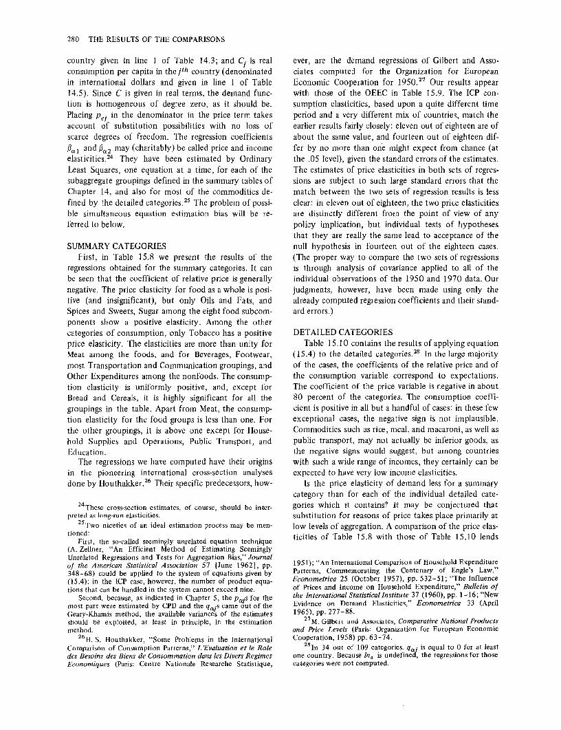
280 THE RESULTS OF THE COMPARISONS
country given in line I of Table 14.3; and C; is real consumption per capita in the jlh country ( denominated in international dollars and given in line 1 of Table 14.5). Since C is given in real terms, the demand function is homogeneous of degree zero, as it should be. Placing p cj in the denominator in the price term takes account of substitution possibilities with no loss of scarce degrees of freedom. The regression coefficients (3"' 1 and (3°' 2 may (charitably) be called price and income elasticities. 24 They have been estimated by Ordinary Least Squares, one equation at a time, for each of the subaggregate groupings defined in the summary tables of Chapter 14, and also for most of the commodities defined by the detailed categories. 25 The problem of possible simultaneous equation estimation bias will be referred to below.
SUMMARY CATEGORIES First, in Table 15.8 we present the results of the
regressions obtained for the summary categories. It can be seen that the coefficient of relative price is generally negative. The price elasticity for food as a whole is positive (and insignificant), but only Oils and Fats, and Spices and Sweets, Sugar among the eight food subcomponents show a positive elasticity. Among the other categories of consumption, only Tobacco has a positive price elasticity. The elasticities are more than unity for Meat among the foods, and for Beverages, Footwear, most Transportation and Communication groupings, and Other Expenditures among the nonfoods. The consumption elasticity is uniformly positive, and, except for Bread and Cereals, it is highly significant for all the groupings in the table. Apart from Meat, the consumption elasticity for the food groups is less than one. For the other groupings, it is above one except for Household Supplies and Operations, Public Transport, and Education.
The regressions we have computed have their origins in the pioneering international cross-section analyses done by Houthakker. 26 Their specific predecessors, how-
24 These cross-section estimates, of course, should be interpreted as long-run elasticities.
25 Two niceties of an ideal estimation process may be mentioned:
First, the so-called seemingly unrelated equation technique (A. Zellner, "An Efficient Method of Estimating Seemingly Unrelated Regressions and Tests for Aggregation Bias," Journal of the American Statistical Association 57 (June 1962], pp. 348-68) could be applied to the system of equations given by (15.4); in the ICP case, however, the number of product equations that can be handled in the system cannot exceed nine.
Second, because, as indicated in Chapter 5, the Po,js for the most part were estimated by CPD and the qo,j5 came out of the Geary-Khamis method, the available variances of the estimates should be exploited, at least in principle, in the estimation method.
26 H. S. Houthakker, "Some Problems in the International Comparison of Consumption Patterns," L 'Evaluation et le Role des Besoins des Biens de Consommation dans /es Divers Regimes Economiques (Paris: Centre Nationale Researche Statistique,
ever, are the demand regressions of Gilbert and Associates computed for the Organization for European Economic Cooperation for 1950. 27 Our results appear with those of the OEEC in Table 15.9. The ICP consumption elasticities, based upon a quite different time period and a very different mix of countries, match the earlier results fairly closely: eleven out of eighteen are of about the same value, and fourteen out of eighteen differ by no more than one might expect from chance (at the .05 level), given the standard errors of the estimates. The estimates of price elasticities in both sets of regressions are subject to such large standard errors that the match between the two sets of regression results is less clear: in eleven out of eighteen, the two price elasticities are distinctly different from the point of view of any policy implication, but individual tests of hypotheses that they are really the same lead to acceptance of the null hypothesis in fourteen out of the eighteen cases. (The proper way to compare the two sets of regressions is through analysis of covariance applied to all of the individual observations of the 1950 and 1970 data. Our judgments, however, have been made using only the already computed regression coefficients and their standard errors.)
DETAILED CATEGORIES Table 15 .10 contains the results of applying equation
(15.4) to the detailed categories. 28 In the large majority of the cases, the coefficients of the relative price and of the consumption variable correspond to expectations. The coefficient of the price variable is negative in about 80 percent of the categories. The consumption coeffident is positive in all but a handful of cases: in these few exceptional cases, the negative sign is not implausible. Commodities such as rice, meal, and macaroni, as well as public transport, may not actually be inferior goods, as the negative signs would suggest, but among countries with such a wide range of incomes, they certainly can be expected to have very low income elasticities.
Is the price elasticity of demand less for a summary category than for each of the individual detailed categories which it contains? lt may be conjectured that substitution for reasons of price takes place primarily at low levels of aggregation. A comparison of the price elasticities of Table 15.8 with those of Table 15.10 lends
1951); "An International Comparison of Household Expenditure Patterns, Commemorating the Centenary of Engle's Law," Econometrica 25 (October 1957), pp. 532-51; "The Influence of Prices and Income on Household Expenditure," Bulletin of the International Statisticallnstitute 37 (1960), pp. 1-16; "New Evidence on Demand Elasticities," Econometrica 33 (April 1965), pp. 277-88.
27 M. Gilbert and Associates, Comparative National Products and Price Levels (Paris: Organization for European Economic Cooperation, 1958) pp. 63-74.
28 In 34 out of 109 categories, qOI.. is equal to O for at least one country. Because In O is undefined, the regressions for those categories were not computed.
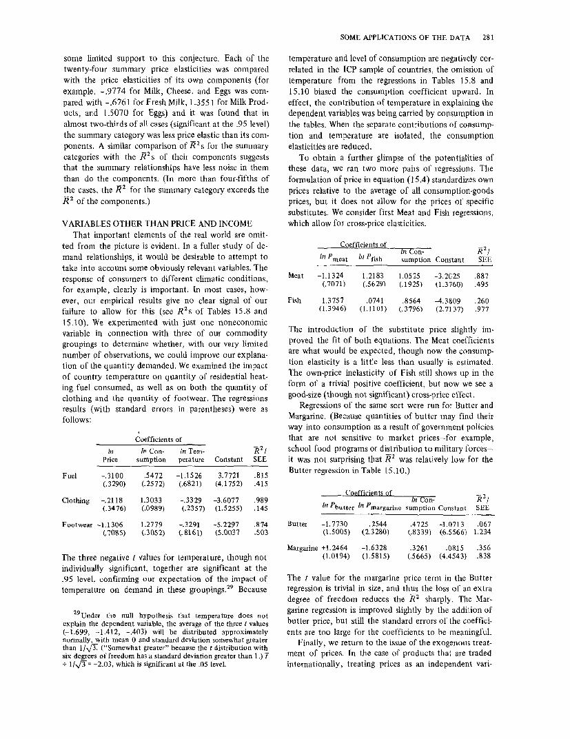
some limited support to this conjecture. Each of the twenty-four summary price elasticities was compared with the price elasticities of its own components (for example, -.9774 for Milk, Cheese, and Eggs was compared with -.6761 for Fresh Milk, 1.3551 for Milk Products, and 1.5070 for Eggs) and it was found that in almost two-thirds of all cases (significant at the .95 level) the summary category was less price elastic than its components. A similar comparison of R. 2 s for the summary categories with the R. 2 s of their components suggests that the summary relationships have less noise in them than do the components. (In more than four-fifths of the cases, the R2 for the summary category exceeds the R. 2 of the components.)
VARIABLES OTHER THAN PRICE AND INCOME That important elements of the real world are omit
ted from the picture is evident. In a fuller study of demand relationships, it would be desirable to attempt to take into account some obviously relevant variables. The response of consumers to different climatic conditions, for example, clearly is important. In most cases, however, our empirical results give no clear signal of our failure to allow for this (see R. 2 s of Tables 15 .8 and 15.10). We experimented with just one noneconomic variable in connection with three of our commodity groupings to determine whether, with our very limited number of observations, we could improve our explanation of the quantity demanded. We examined the impact of country temperature on quantity of residential heating fuel consumed, as well as on both the quantity of clothing and the quantity of footwear. The regressions results (with standard errors in parentheses) were as follows:
Coefficients of
In In Con- In Tern- R.2/ Price sumption perature Constant SEE
Fuel -. 3100 .5472 -1.1526 3.7721 .815 (. 3290) (.2572) (.6821) (4.1752) .415
Clothing -.2118 1.3033 -.3329 -3.6077 .989 (.3476) (.0989) (.2357) (1.5255) .145
Footwear -1.1306 1.2779 -.3291 -5.2297 .874 (. 7085) (.3052) (. 8161) (5.0037 .503
The three negative t values for temperature, though not individually significant, together are significant at the .95 level, confirming our expectation of the impact of temperature on demand in these groupings. 29 Because
29 Under the null hypothesis that temperature does not explain the dependent variable, the average of the three t values (-1.699, -1.412, -.403) will be distributed approximately normally, with mean O and standard deviation somewhat greater than 1/.)3. ("Somewhat greater" because the t distribution with six degrees of freedom has a standard deviation greater than 1.) t .;- 1/.J'f = -2.03, which is significant at the .05 level.
SOME APPLICATIONS OF THE DATA 281
temperature and level of consumption are negatively correlated in the ICP sample of countries, the omission of temperature from the regressions in Tables 15 .8 and 15.10 biased the consumption coefficient upward. In effect, the contribution of temperature in explaining the dependent variables was being carried by consumption in the tables. When the separate contributions of consumption and temperature are isolated, the consumption elasticities are reduced.
To obtain a further glimpse of the potentialities of these data, we ran two more pairs of regressions. The formulation of price in equation (15.4) standardizes own prices relative to the average of all consumption-goods prices, but it does not allow for the prices of specific substitutes. We consider first Meat and Fish regressions, which allow for cross-price elasticities.
Coefficients of ·1F1
In p meat In pfish In Con-sumption Constant SEE
Meat -1.1324 1.2183 1.0525 -3.2025 .887 (. 7071) (.5629) (.1925) (1.3760) .495
Fish 1.3757 .0741 .8564 -4.3809 .260 (1.3946) (1.1101) (. 3796) (2.7137) .977
The introduction of the substitute price slightly improved the fit of both equations. The Meat coefficients are what would be expected, though now the consumption elasticity is a little less than usually is estimated. The own-price inelasticity of Fish still shows up in the form of a trivial positive coefficient, but now we see a good-size (though not significant) cross-price effect.
Regressions of the same sort were run for Butter and Margarine. (Because quantities of butter may find their way into consumption as a result of government policies that are not sensitive to market prices-for example, school food programs or distribution to military forcesit was not surprising that JP was relatively low for the Butter regression in Table 15.10.)
Coefficients of In Con- R. 2
/ In Pbutter In Pmargarine sumption Constant SEE
Butter -1. 7730 .2544 (l.5005) (2.3280)
Margarine +l.2464 (l.0194)
-1.6328 (l.5815)
.4 725 -1.0713 .067 (.8339) (6.5566) 1.234
.3261 .0815 .356 (.5665) (4.4543) .838
The t value for the margarine price term in the Butter regression is trivial in size, and thus the loss of an extra degree of freedom reduces the R.2 sharply. The Margarine regression is improved slightly by the addition of butter price, but still the standard errors of the coefficients are too large for the coefficients to be meaningful.
Finally, we return to the issue of the exogenous treatment of prices. In the case of products that are traded internationally, treating prices as an independent vari-

282 THE RESULTS OF THE COMPARISONS
Table 15.8. Regressions of Real Per Capita Quantities on Relative Price and Per Capita Consumption, 1970 (Summary Groupings)
(Paj) In qi = {31 In p cj + (3 2 lnCj + (3 0 + Uj j=l, ... ,10
Coefficient of
zn(P~~) lnCj Constant R. 2 /SEE 'Pc1
l Food, beverage, tobacco 0.1949 0.7215* 0.8275 0.9586 (0.4660) (13. 7635) (2.0577) 0.1428
2 Food 0.1843 0.6339* 1.2613* 0.9583 (0.6030) (13.9561) (3.6872) 0.1257
3 Bread and cereals -0.4464 0.1396 3.0959* -0.1246 (-0.4 732) (0.9049) (2.8398) 0.4472
4 Meat -1. 7066* 1.2081* -4.0063* 0.8272 (-2.1075) (5.4772) (-2.4475) 0.6120
5 Fish -0.1173 0.7708* -3.3697 0.2523 (-0.0852) (2.1023) (-1.3380) 0.9820
6 Milk, cheese, eggs -0.9774 0.6884* -1.1320 0.9402 (-1.7092) (6.5757) (-1.4420) 0.2013
7 Oils and fats 0.8016 r: 9130* -3.7312 0.4705 (0. 7233) (2.5690) (-1.3118) 0.6783
8 Fruits and vegetables -0.8248 0.6482* -0.3890 0.8455 (-1.8104) (6.8310) (-0.5748) 0.2751
9 Coffee, tea, cocoa -0.5918* 0.8899* -3.5773* 0.8504 (-2.4480) (6.4305) (-3.5027) 0.3972
10 Spices and sweets, sugar 0.1509 0.6708* -1.3863 0.8032 (0.2543) (5.6644) (-1.5162) 0.3057
11 Beverages -1.5221 * 1.1783* -4.5545 0.8789 (-2.5189) (3.0353) (-1.5698) 0. 7181
12 Tobacco 0.0390 1.1534* -5.0298* 0.9355 (0.1744) (11.5112) (-7.1125) 0.2908
13 Clothing and footwear -0.1198 1.3976* -5.3751 * 0.9872 (-0.3365) (22.9010) (-11.3466) 0.1551
14 Clothing -0.1609 1.4114* -5.6403* 0.9877 (-0.4360) (21.0865) (-10.4482) 0.1543
15 Footwear -1.1316 1.3792* · -7.1865* 0.8896 {-1.7023} {8.4 784} (-6.2552} 0.4721
16 Gross rent, fuel -0.1350 1.2280* -3.6962* 0.9917 (-0.7971) (29.5862) (-12.7587) 0.1095
17 Gross rents -0.0083 1.2823* -4.3763* 0.9819 (-0.0487) (21.5743) (-10.5847) 0.1680
18 Fuel and power -0.2090 l.l 205* -4.2667* 0.9213 (-0.6277) {10.3389! (-5.5192} 0.3145
19 House furnishings, operation -0.2669 1.1194* -3.5441 * 0.9502 (-0.5015) (13.1509) (-5.8781) 0.2470.
20 Furniture, applicances -0.1850 1.3855* -6.0600* 0.9578 (-0.4885) (14.3240) (-8.7818) 0.2805
21 Supplies and operation -0. 7938* 0.8908* -2.8841 * 0.9357 (-1. 9368) (11.5111) (-5.1659) 0.2233
22 Medical care -0.7944* 1.3240* -5.777* 0.9354 {-2.4541) (10.9346! (-5.5920! 0.3030
23 Transport and communication -1.3125* 1.1480* -3.0428* 0.9489 (-2.2275) (I 0.0276) (-3.3030) 0.2887
24 Equipment -0.8243 1.5046* -7.0920 0.8628 (-1.0696) (3.5842) (-2.0919) 0.7152
25 Operation costs -1.7632* 1.7503* -8.3228* 0.8778 (-2.1529) (8.1565) (-5.7344) 0.5936
26 Purchased transport -1.5 227* 0.5824* -0.8489 0.8136 (-3.9628) (5.2633) (-1.0860) 0.3207
27 Communication -1.1977* 1.5343* -9.2525* 0.9307 (-2.8368} (11.0804} (-9.1518} 0.3920
28 Recreation and education -0.1731 1.0294* -2.4005* 0.9712 (-0.9323) (12.6271) (-3.9213 0.1620
29 Recreation -0.5951 1.5 259* -6.6558* 0.9393 (-0.9095) (9.3825) (-5.6753) 0.3936
30 Education -0.3189* 0. 7845 * -1.5372 0.9425 (-2.3138) (8.4638) (-2.1618) 0.1461

SOME APPLICATIONS OF THE DATA 283
Table 15.8. Continued
Coefficient of
Inc~~) lnC; Constant R. 2 /SEE Pc1
31 Other expenditure -1.4185 1.2167* -4.0808* 0.9013 (-1.1867) (8.84 71) (-4.2446) 0.3953
32 Personal care -0.4113 1.4 772* -7.1932 0.9841 (-1.0189) (16.8362) (-10.9551) 0.1889
33 Miscellaneous services -0.5197 1.1821 * -4.0541 0.8253 (-0.4695) (6.6676) (-3.1355) 0.5117
Notes: t: Student t value for the regression coefficient appears within parentheses. R 2 : Coefficient of determination (adjusted for degrees of freedom). SEE: Standard error ot estimate. *: Coefficient is significantly different from O at the .05 level; one-tail test except for constant, where two-tail tests used.
able is quite plausible. In that case, differences in price from country to country may represent simply differences in transfer costs and government policies. No problems of simultaneous equation estimation arise in this situation. When, however, commodities or, more particu-
larly, services are produced domestically, price should be treated as a jointly determined variable. Simultaneous equation estimation methods then are called for. Some experimentation was attempted with the use of a number of "general-purpose" exogenous variables-rate of
Table 15 .9. Comparison of Price and Consumption Elasticities Obtained in a 1950 OEEC Study and Corresponding ICP Elasticities for 1970
Price elasticity Consumption elasticity
ICP OEEC ICP OEEC
Food .18 (.31) - .27 (.27) .63 (.05) .54 (.05) Breads and cereals - .45 (.94) - .59 (.34) .14(.15) .20 (.14) Meat -1.71 (.81) - .19 (.39) 1.21 (.22) .86 (.18) Fish - .12 (1.38) -1.03 (.49) . 77 (.37) .62 (.39) Dairy products - .98 (.57) - .43 (.26) .69(.10) .60 (.10) Oils and fa ts .80 (1.11) - .60 (.32) .91 (.36) .37 (.17) Fruits and vegeta blest - .82 (.46) -2.10 (.46) .65 (.09) .73 (.21) Spices and sweets, sugar - .15 (.51) -1.62 (.55) .67 (.12) .42 (.25) Tobacco .04 (.22) - .26 (.29) 1.15 (.10) .88 (.28) Clothing - .16 (.37) - .63 (.61) 1.41 (.07) .84 (.15) Footwear -1.13 (.66) - .62 (.20) 1.38 (.16) 1.01 (.09) Fuel and eower - .21 (.33) - .86 (.40) 1.12 (.II) 1.19 (.32) Medical care - .79 (.32) -1.59 (.80) 1.32 (.12) 1.80 (.33) Transport equipment - .82 (.77) -3.84 (1.66) 1.50 (.42) .71 (.78) Purchased transport -1.52 (.38) -1.79 (.39) .58 (.11) 1.10 (.17) Communication -1.20 (.42) - .92 (.31) 1.53 (.14) 2.03 (.20) Recreation - .60 (.65) - .99 (.50) 1.53 (.17) 1.15 (.23) Education - .32 (.14) - .49 (.22) . 78 (.09) .75 (.13)
Source: OEEC: M. Gilbert and Associates, Comparative National Products & Price Levels: A Study of Western Europe & the United States (Paris: Organization for European Economic Cooperation, 1958). ICP: present study. Note: Numbers in parentheses are standard errors. tThe OEEC study gives the elasticities separately for Fruits and for Vegetables. In the absence of the detailed OEEC data necessary for pooling the two categories, the elasticities and standard errors simply were averaged together for the purposes of this table. [Price elasticities: Fruits -2.06 (.29); Vegetables -2.15 (.64 ). Consumption elasticities: Fruits, .71 (.15); Vegetables, .75 (.27).]
FND

284 THE RESULTS OF THE COMPARISONS
Table 15.10. Regressions of Real per Capita Quantities on Relative Price and per Capita
Consumption, 1970 (seventy-five detailed categories)
ra) /nqoj=(Ji In ~ +f32lnCj+f30 +ui; i=l, ... ,10
Coefficient of
tn(~) lnCi Constant R. 2 /SEE
01.101 Rice 1.5798 -0.3224 3.0652 -0.0551 (0.9998) (-0.5328) (0.6929) 1.7264
2 01.102 Meal, other cereals -1.1019 -0.8166* 8.0007* 0.4100 (-1.0150) (-2. 7422) (3.6947) 0.8628
3 01.103 Bread, rolls -1.9904* 1.3772* -8.3429* 0.8235 (-2.8559) (4.6215) (-4.1074) 0.8109
4 01.105 Cereal preparations -2.7740* 0.4146 -2.6311 0.5954 (-2.8195) (0.9371) (-0.8129) 1.1133
5 01.111 Fresh beef, veal -2.2725* 1.3086* -6.0428 0.5455 (-2.2876) (3.0729) {-2.0288) 1.2209
6 01.113 Fresh pork 0.8163 2.0603* -12.8175* 0.8799 (1.2264) (8.1816) (-7.1468) 0.7305
7 01.114 Fresh poultry 0.0205 1.5696* -9.2218* 0.8347 (0.0283) (6.1481) (-4.6572) 0.6599
8 01.115 Other fresh meat -1.0696 0.6314* -3.0889 0.3314 (-0.9545) (2.0759) (-1.4106) 0.8595
9 01.121 Fresh, frozen fish -0.6347 0.6547 -3.1924 0.0186 (-0.5436) (1.4582) (-1.0007) 1.1298
10 01.131 Fresh milk -0.6761 * 0.4091 * -0.0003 0. 7946 (-2.1090) (4.6788} (-0.0005} 0.2396
11 01.132 Mille products -1.3551 0.9603* -4.5380 0. 7951 (-1.6409) (2.9281) (-1.8862) 0.6668
12 01.133 Eggs, egg products 1.5070 2.3094* -15.0642* 0.9298 (1.8284) (8.7980) (-7.2502) 0.5242
13 01.141 Butter -1.7013 0.3963 -0.4591 0.1985 (-1.3602) (0.935 7) (-0.1454) 1.1433
14 01.142 Margarine, edible oil -0. 7879 0.4540 -0.7470 0.3105 (-0.5 352) (0. 7880) (-0.1640) 0.8673
15 01.151 Fresh fruits, tropical, subtropical -1.2648* 0.5097* -1.6755 0.5755 (-3.61152 (2.3511} (-1.1219} 0.5833
16 01.15 3 Fresh vegetables -1.0685 0.6843* -2.5115 0.5165 (-1.3607) (3.3984) (-1.6105) 0.5520
17 01.162 Vegetables other ·:.han fresh -0.2865 0.7667* -2.9717 0.5677 (-0.4651) (3. 1559) (-1.5614) 0.6406
18 01.170 Potatoes, manioc, other tubers -1.9742* 0.2763* -0.4644 0.7969 (-5.5242) (2.1933) (-0.5236) 0.3646
19 01.191 Coffee -0.4214 1.3390* -7.4943* 0.6895 (-0.8877) (4.2432) (-3.1661) 0.8875
20 01.180 Sugar -0.5249 o. 1676 1.2829 0.1673 (-1.1013) {0.8246} {0.8311} o.~QZ4
21 01.201 Jam, syrup, honey -1.3485* o. 7673* -4.5930 0.7111 (-2.2192) (2.5530) (-2.1039) 0.7409
22 01.202 Chocolate, ice cream 0.0720 1.8842* -11.5948* 0.8656 (0.0803) (4.8539) (-3.5767) 0.6970
23 01.203 Salt, spices, sauces -3.6895* 0.1750 0.1969 0.6157 (-3.9715) (0.6914) (0.1101) 0.7345
24 01.310 Nunalcuhulic beverages -0.2638 1.4879* -9.1861 * 0.8438 (-0.3134) (3.4669) (-2.8696) 0.6542
25 01.323 Beer -0.2537 1.5654* -8.9524 0.6661 {-0.2942) (2.9333) {-2.2974} 1.0917
26 01.410 Cigarettes -0.8098* 1.5633* -8.2004 0.8576 (-2.1186) (6.4771) (-4.7753) 0.6802
27 02.110 Clothing materials 0.1485 0.8490* -4.0537 0.5177 (0.2189) (2.9580) (-1.7871) 0.6934
28 02.121 Men's clothing 0.1540 1.3160* -6.4305* 0.9608 (0.1988) (11.3575) (-7.3313) 0.2532
29 02.122 Women's clothing -1.4551* 1.3085* -5.8512* 0.9577 (-3.4804) (9.8546) (-5.5537) 0.3247
30 02.123 Boys', girls' clothing 0.0250 1.3670* -7.9029* 0.8406 (0.0270) (7.0192) (-5.7592) 0.5642

SOME APPLICATIONS OF THE DATA 285
Table 15 .10. Continued
Coefficient of
Inca~) Pc1
In Ci Constant R. 2 /SEE
31 02.160 Clothing rental, repair -2.3781 * 1.4377* -10.3312* 0.9536 (-7.8080) (13.1858) (-12.8840) 0.2983
32 02.211 Men's footwear -1.1526 1.1567* -6.6091 * 0.8163 (-1.5343) (5.9792) (-4.8257) 0.5545
33 02.212 Women's footwear -0.7493 1.5150* -9.2551* 0.8893 (-1.4399) (8.5876) (-7.3898) 0.4955
34 02.213 Children's footwear -1.0682 1.6231 * -10.5320* 0.8952 (-1.5268) (8.8634) (-7.9584) 0.5171
35 03.110 Gross rents 0.1025 1.2870* -4.4828* 0.9643 {0.4070} (15.1770) {-7.6314) 0.2368
36 03.210 Electricity -1.6019* 1.5924* -8.4243* 0.9889 (-7.2455) (16.3745) (-11.2615) 0.2163
37 03.230 Liquid fuels -1.2139 0.9755* -4.7700 0.8306 (-1.6694) (2.0499) (-1.2860) 0.7276
38 03.240 Other fuels, ice -0.6645 0.4152 -1.0724 -0.1048 (-0.0713) (1.0124) (-0.3663) 1.1039
39 04.110 Furniture, fixtures -2.2482 1.4809* -7.6702* 0.7876 (-1.7329) (5.1219) (-3.6869) 0.8155
40 04.120 Floor coverings -1.4457* 1.3416* -8.4893* 0.875 l !-5.12632 {7.1928) (-6.4872) 0.5283
41 04.200 Household textiles, etc. -0.9108 1.1642* -5.7893* 0.8494 (-1.4636) (6.2356) (-4.1462) 0.5117
42 04.310 Refrigerators, etc. -0.1863 1.8238* -11.9242* 0.9792 (-0.9256) (13.4142) (-11.3810) 0.2697
43 04.400 Household utensils -0.4565 1.1149* -5.6665* 0.8531 (-0.7625) (6.4576) (-4.6219) 0.4618
44 04.510 Nondurable household goods -1.0422 0.8210* -3.0106 0.8431 (-1.2494) (3.2935) (-1.6129) 0.4391
45 04.530 Household services -1.8758* 1.3919* -8.3599* 0. 7368 (:...2.0510) 5.1100 -4.2487 0.6502
46 05 .110 Drugs, medical preparations -1.4878 1.1139* -5.1785* 0.8815 (-3.1403) (5 .3398) (-3.5945) 0.5358
47 05 .310 Physicians' services -0.1958 1.0840* -5.1245* 0.9046 (-1.4362) (8.3744) (-5.25 23) 0.3070
48 05.320 Dentists' services 0.0488 1.6802* -10.2355* 0.9086 (0.3744) (8.0635) (-6.7334) 0.5221
49 05.330 Services, nurses, other personnel 0.0890 0.9741 * -4.6818 0.6598 (0.2524) (3. 7229) (-2.1305) 0.6632
50 05.400 Hospitals, etc. -0.1012 1.0559* -4.8734* 0. 7906 t-0.4674) {5 .9784} (-3.5953) 0.5061
51 06.110 Personal cars -1.3168 1.4060* -6.2400 0.7953 (-1.4 742) (2.4877) (-1.3835) 1.0140
52 06.210 Tires, tubes, accessories -0.9520 1.3614 -8.0936 0.7485 (-0.6723) (1.8234) (-1.4429) 0.9859
53 06.220 Repair charges -1.2965* 1.6847* -10.0348* 0.75 33 (-2.0237) (4.8334) (-3.9689) 0.6637
54 06.230 Gasoline, oil, etc. -0.7495 1.9928* -11.1687* 0.9173 (-1.2125 (8.9744) (-6.2330) 0.6044
55 06.240 Parking, tolls, etc. 0.1377 1.4252* -8.4675* 0.6639 (Q H62l (3.9643} (-3.1125) 0.9451
56 06.310 Local transport -2.3458* 1.3485* -8.7903* 0.9146 (-7.1342) (9.0255) (-7.8117) 0.4036
57 06.321 Rail transport -2.8520* 0.7324* -4.6232 0.4648 (-2.3421) (1.9751) (-1.7578) 1.0751
58 06.322 Bus transport 1.3314 -0.0836 2.3560 -0.0153 (1.3642) (-0.3245) (1.244 7) 0. 7173
59 06.410 Postal communication -2.2426* 1.3497* -9.0119* 0.8399 (-1.8658) (5.8070) (-5.5622) 0.6389
60 06.420 Telephone, telegraph -1.4140* 1.5887* -10.2007* 0.8547 (-2.5437) (7.4125) (-6.4860) 0.5878

286 THE RESULTS OF THE COMPARISONS
Table 15.10. Continued
Coefficient of
In (Pa~) lnC; Constant R. 2 /SEE Pc1
61 07.110 Radio, TV, phonograph, etc. -1.2408* 1.3524* -6.6658* 0.8857 (-1.9454) (4.4824) (-2.7420) 0.6218
62 07.210 Public entertainment -0.9290 1.3942* -8.0152* 0.5918 (-1.1968) (3.6131) (-2.9454) 1.11 79
63 07.230 Other recreation, cultural even ts -1.1984* 1.4688* -8.9886* 0.8427 (-3.0656) (6.9608) (-5.8248) 0.5921
64 07.310 Books, papers, magazines -0.9086* 1.3391* -7.0177* 0.9714 (-2.8169) (12.1590) (-9.0231) 0.2559
65 07.411 Teachers, 1st, 2nd -0.15 31 0.4993* -0.0041 0.9032 {-1.495 21 {5.5758} (-0.0057} Q.1 iQl
66 07.412 Teachers, college -0.6824* 1.2801* -7.1719* 0.9291 (-4.6925) (10.9402) (-8.6383) 0.3138
67 07.420 Educational facilities -0.5315 1.424 7* -8.0425* 0.7923 (-0.3582) (3.6534) (-2.5620) 0.7383
68 07.431 Educational supplies -1.1213 0.7127* -4.5429 0.4867 (-1.0336) (l.8768) (-1.6985) 0.8903
69 07.432 Other education expenditures 0.4839 1.0288* -6.0716 0.4809 (0.2328) (2.7222) (-2.0072) 0.8839
70 08.100 Barber, beauty shops -1.2886* l.7096* -11.1280* 0.9452 !-3.5636} (11.8156} HO 726'.Zl 0.4123
71 08.210 Toilet articles -0.8936 1.2754* -6.5537* 0.9632 (-1.7388) (5 .36 79) (-3.5856) 0. 3116
72 08.220 Other personal-care goods 0.0657 1.3668* -7.4666* 0.9729 (0.2798) (17.9598) (-13.6755) 0.2197
73 08.310 Restaurants, cafes -0.871 7 1.3553* -5.8934* 0.8288 (-1.2897) (6.4648) (-3.9853) 0.6054
74 08.320 Hotels, etc. -2.7291 0.6273 -2.0542 0.6367 (-1.8099) (1. 7680) (-0.5186) 0.7913
75 08.400 Other services 0.8034 0.5842 -0.9899 0.0924 (0.3539) (0.8930) (-0.1853) 1.3067
Notes: t: Student t value for the regression coefficient appears within parentheses. JF: Coefficient of dete1mination (adjusted for degrees of freedom). SEE: Standard error of estimate. •: Coefficient is significantly different from Oat the .05 level; one-tail test except for constant, where two-tail tests used.
growth of real output, proportion of the population in the labor force, and proportion of population to arable land---to apply the estimating method known as Two
Stage Least Squares. With such a small number of observations, however, the price elasticity estimates varied
over an extremely wide range depending upon just which combination of the three exogenous variables was introduced into the system. For the most part, the consumption elasticities were insensitive to changes in the set of
exogenous variables. This indicates that the price elasticities of Tables 15.8 and 15.10 are even more imprecise
than their standard errors there would suggest, but that the consumption elasticities are fairly robust (insensi-
tive) with respect to the problem of simultaneous equa
tion bias. Although a definitive assessment of the role of rela
tive prices and income levels in explaining relative quantities from country to country must await a more careful
formulation of the underlying model, as well as the accumulation of data from more countries, the regression coefficients in Tables 15.8 and 15.10 indicate clearly that relative prices and income levels work with
sufficient power and persistence that their influence shows through-despite the imperfections of the under
lying data and of the theoretical framework in which
these equations are formulated.

Glossary
Additivity: The property that makes it possible to have correct country-to-country quantity relationships for each detailed category, and, at the same time, to obtain the correct country-to-country quantity relationships for any desired aggregation of categories simply by summing the quantities for the included categories. This requires that the quantities be stated in value terms so that (1) the values for any category are directly comparable between countries and (2) the values for any country are directly comparable between categories.
Binary comparison: A price or quantity comparison between two countries without regard to the consistency of this comparison with comparisons of each of the countries with any third countries. (See Circularity or transitivity.)
Bridge-country binary comparison: A price or quantity comparison between a pair of countries derived from the comparison of each country with a third country. For example, if we have I; 1 k and 111 :c, the bridge-country method of obtaining Ji/1 is to divide Ii/k by I 1/k' where I
is a price or quantity index and j, k, and/ are countries. (See also Original-country binary comparison.)
CEP (consumption expenditures of the population): The ICP concept of "consumption" that includes both household expenditures and expenditures of government on such categories as health and education. (See Table 13.15.)
Characteristicity: The property whereby the sample of prices or quantities and the weights used in an international comparison conform closely to a representative sample of items and to the weights of each of the countries included in the comparison.
Circularity or transitivity: There is circularity or transitivity if the indexes expressing the price or quantity relationships between any two among three or more countries are the same whether derived (I) from an originalcountry comparison between them or (2) from the comparison of each country with any third country. In the case of three countries, where I is a price or quantity index and j, k, and / are countries, the circular test is satisfied if: Ii/k = I;;t 7 Ik/f· When this test is satisfied, there is a unique cardinal scaling of countries with respect to relative quantities and prices.
Country-product-dummy (CPD) method: A generalized bridge-country method employing regression analysis to obtain transitive price comparisons for each detailed category. The basic data for a given category consist of all the prices available for the various specifications for the entire collection of countries. The prices are regressed against two sets of dummy variables; one set contains a dummy for each specification; the second set, a dummy for each country other than the numeraire country. The transitive price comparisons are derived from the coefficients of the country dummies. (See Chapter 5.)
Country-reversal test: This test is satisfied if, when country j is taken as the base country, the price or quantity index for countries j and k is the reciprocal of the index when country k is the base country. For example, I; 1 k • I k Ii == I , where I is a price or quantity index.
Detailed categories: The subdivisions of final expenditure for which the first aggregation of price ( or quantity) ratios for individual specifications or items takes place. (See appendix tables of Chapters 13 and 14.)
Direct price or quantity comparison: One made by comparing for two or more countries the prices or quantities for a representative sample of equivalent commodities. (See also Indirect price or quantity comparison.)
Double-weighted CPD: A weighted CPD method in which the weights are the products of (1) the importance of each cell in the column in which it falls (the percentage of the country's expenditure) and (2) the importance of the cell in the row in which it falls (the percentage of the total quantity of the category in the ten countries). The double-weighted CPD is used to obtain PPPs for categories for which no price comparisons were made. The CPD is applied in this case to the matrix of PPPs in which the columns represent countries and the rows detailed categories. (See Country-productdummy method.)
Exchange-rate-deviation index: The ratio of the real GDP per capita relative to the United States as estimated by the ICP to the GDP per capita relative to the United States when the exchange rate is used to convert nondollar currencies to dollars.
287

288 GLOSSARY
Equal weighting: Used in the ICP to refer to the practice of applying simple or unweighted averages to all the price ratios within a category to derive the PPP for the category. (See Item weighting.)
Factor-reversal test: The condition that, for any given item, category, or aggregate and for any given pair countries, the product of the price ratio ( or index) and the quantity ratio ( or index) be equal to the expenditure ratio.
Final products: Products purchased for own use and not for resale or for embodiment in a product for resale; those purchased by households, by government, or by business on capital account.
Fisher, or "ideal," index: The geometric mean of two indexes, one the harmonic mean of price ( or quantity) relatives weighted by the numerator country's expenditures, the other, the arithmetic mean weighted by the denominator country's expenditures.
Frequency-weighted CPD: The CPD method applied to a detailed category with each price weighted by 1/nj, where ni is the number of price observations for country j. (See Country-product-dummy method.)
GCF (gross capital formation): Includes fixed capital formation, change in stocks, and net exports. Definitions of these three components correspond to SNA concepts, although the SNA does not include net exports in its definition of GCF.
Geary-Khamis method: An aggregation method in which category international prices (reflecting relative category values) and country PPPs ( depicting relative country price levels) are estimated simultaneously from a system of linear equations. (See pp. 68-70.)
GFCE(government final consumption expenditure): The SNA concept of "government" which includes public expenditures on education, health, and similar categories. (See Table 13.15.)
ICP: International Comparison Project
"Ideal" index: See Fisher, or "ideal," index.
Index spread: The ratio of a U.S.-weighted quantity index to an own-weighted quantity index.
Indirect price or quantity comparison: A comparison made by dividing the price or quantity ratio into the expenditure ratio. That is, the indirect quantity comparison between country j and country k for commodity i,
q ·· Pi; qii . Pi; qii .....:1.., is obtained from: --- ..,. - = - , where the qik Pik qik Pik q ik
ps are the commodity prices. (See also Direct price or quantity comparison.)
International prices: Average prices based on the prices of the ten included countries, each weighted by the GDP of the supercountry to which it is assigned.
International dollars (1$): Dollars with the same purchasing power over total GDP as the U.S. dollar, but with a purchasing power over subaggregates and over detailed categories determined by average international prices rather than by U.S. relative prices.
Item weighting: The assignment of individual weights to each specification for which prices are compared within a detailed category. (See Equal weighting.)
Multilateral comparison: A price or quantity comparison of more than two countries simultaneously that produces consistent relations among all pairs; that is, satisfies the circular test or the transitivity requirement.
Original-country binary comparison: A price or quantity comparison between two countries based on the data of the two countries and no others. (See also Bridge-country binary comparison.)
Own weights: The weights of the numerator country: that is, the weights of country j in the index lj/k· We use the term to refer mainly to the weights of a country other than the United States in comparisons in which the United States is the base country, k.
PFC (public final consumption expenditure): The ICP concept of "government" that excludes public expenditures for education, health, and like categories. (See Table 13.15.)
PFCE (private final consumption expenditure): The SNA concept of "consumption" that excludes public expenditures on education, health, and similar categories. (See Table 13.15.)
PPP: See Purchasing-power parity.
Price index: The price level for a category or aggregate of goods in one country expressed as a percentage of the price level for the same category or aggregate in another country, when prices in both countries are expressed in a common currency, usually the U.S. dollar, with the official exchange rate being used for currency conversions. A price index may be derived from a purchasing power parity by dividing by the exchange rate. (See Purchasing-power parity.)
Price ratio or price relative: The purchasing power parity for a single specification.
Purchasing-power parity (PPP): The number of currency units required to buy goods equivalent to what can be bought with one unit of the currency of the base country, usually the U.S. dollar in the present study.
Quantity index: The quantity per capita of a category or aggregate of goods in one country expressed as a percentage of the quantity per capita in another country.
Quantity ratio: The quantity of a particular commodity in one country as a percentage of the quantity of the same commodity in another country.

Real product or real quantity: The final product or quantity in two or more countries which is valued at common prices and, therefore, valued in comparable terms internationally.
Representative country: One of the ten included countries regarded as a representative of a larger group of countries that together with it form a supercountry. All the countries in the world are assigned to one of the ten supercountries. (See also Supercountry.)
Similarity index: The weighted "raw correlation" coefficient between the price ( or quantity) vectors of two countries. Expenditures are used as the weights. The coefficient is the ratio of the cross moment to the square root of the product of the two second moments, where
GLOSSARY 289
each moment is computed relative to the origin rather than to the mean.
Specification: A description of an item for which a price comparison is to be made. The description is designed to ensure that goods of equivalent quality are compared.
Supercountry: A group of countries assumed to have the price and quantity structure of the representative country. The aggregate GDP of the supercountry is used to weight the prices of the representative country in the process of deriving average international prices. (See also Representative country.)
Transitivity requirement: See Circularity or transitivity.


Index
Abel-Smith, B., 98n Additivity, 4-5; defined, 28 7; as method-
ological criterion, 54-55 Aggregation methods, 49-53, 65-79 Aitchison, J., 123n Alcoholic Beverages category, 38; match
ing qualities within, 88 Alter, J. D., 95n Automobiles: data for regressions, 108-11;
matching qualities of, 104-08; price comparisons of, 111-16
Bacon, R., 20n Balassa, B., 23n, 187n, 192n Barber and Beauty Shops category, 41;
matching qualities within, 92 Base-country invariance, as methodologi
cal criterion, 54-55 Beckerman, W., 20 Binary comparisons: aggregation methods
in, 49-53, 154; of automobile prices, 111-13; defined, 287; methods of, 3, 46-53, 169, 184-93;of 1950 and 1970, 8-9; properties of, 46-4 7; of rents, 124-43; results of, 169-227. See also specific categories,: specific countries
Binary product definition, 105 Bambach, G., 19n Brady, D., 31n, 68n Braithwaite, S. N., 66n Bread and Cereals category, 37; matching
qualities within, 85-86 Bridge-country binary comparison, 5 O-
S 3; of automobile prices, 112-13; and CDP method, 56-57; defined, 287
Brown, J. A. C., 123n Buildings, nonresidential, category, 41-42 Buildings, residential, category, 41
Capital formation. See Gross capital formation
Categories: filling holes in, 63-65, 78-79; negative expenditures in, 70; particular matching difficulties in, 85-93. See also Classification system; specific categories
CEP. See Consumption expenditures Characteristicity, 50, 54-55; defined, 287;
as methodological criterion, 46 Circularity or transitivity, 51, 56; defined,
287; as methodological criterion, 3, 54-55
Clague, C., 187n Classification system: description of, 26-
28; product categories and code numbers within, 3 7-45; public v. private goods, 27; selection of specifications for, 30-31; unique goods and empty categories within, 33-34, 50
CLEANSER, 34, 159
Clothing and Footwear category, 38-39; matching qualities within, 89-90
Cobb-Douglas form, 55n Colombia: automobile price comparisons
for, 115-16; detailed binary comparisons for, 195-97; detailed multilateral comparisons for, 244-55; education pricequantity comparisons for, 100-03; medical price-quantity comparisons for, 94-100; price collection in, 81-82; summary binary comparisons for, 170; summary multilateral comparisons for, 230-35, 241-43;-U.S. rent comparisons, 125-27
Commodities, Expenditure on, category, 44
Commodity Stocks category, 43 Communication and Transport category,
40; matching qualities within, 91 Communication Equipment category, 43 COMPARE, 34,152,159 Comparisons. See Binary comparisons;
Bridge-country binary comparison; Consumer-goods prices; International comparisons; Multilateral comparisons; Original-country binary comparison; Similarity indexes
Compensation of Employees category, 44, 161-65
Conference of European Statisticians, 3 Construction category, 41-4 2 Construction prices, methods of compar-
ing, 155-59 Consumer behavior, judged by results of
comparisons, 26 7 -86; theory of, 5 5 Consumer-goods prices, methods of com
paring, 28-34, 80-93, 104-16. See also specific categories
Consumption: classification of, 4, 24-28; patterns of, 18
Consumption expenditures: classifications of, 37-41; defined, 287; government components of, 160-62, 169, 186; in MPS-SNA conversion, 34-36; similarity indexes of, 267-79; sources of data on, 47-48. See also Public final consumption expenditure; specific categories; specific countries
Council for Mutual Economic Assistance, 2, 3
Country-Product-Dummy method: defined, 287; double-weighted, 63-65; frequency-weighted, 55-63
Country-reversal test: defined, 287; as methodological criterion, 46-4 7
CPD. See Country-Product-Dummy method
Cultural services. See Recreation, Entertainment, Education, and Cultural Services category
Currencies. See National currencies
Dacey, D. C., 155n Data: basic organization of, 26-36; pro-
cessing operations on, 34, 152, 159 David, P.A., 187 Denison, E., 97n, 192n Dentists. See Medical Care category Detailed categories: aggregation within,
49-50, 65-75; binary comparisons of, 195-227; bridging at level of, 52-53; and consumption behavior, 280-81; defined, 287; holes in, 34, 50, 55-65; multilateral comparisons of, 244-66
Developing countries. See Colombia; India; Kenya; Supercountries
Direct price or quantity comparison, 5-8, 19-20;defined, 287
Doctors. See Medical Care category Double-weighted Country-Product
Dummy method, 59, 63-65; defined, 287
Drechsler, L., 3n, 34-36, 46n, 66n, 70n Due, J. F., 84n Durable Furnishings and Equipment cate
gory, 43
Earnings: categories, 44; as matching criterion, 94-95, 100-03, 161-63, 165
Economic Commission for Latin America, 2, 3
Economic development, level of, 12. See also Colombia; India; Kenya; Supercountries
Education category, 41; matching qualities within, I 00-03; price and quality comparisons, 100-03
EEC countries. See France; Germany, Federal Republic of; Italy
EKS method, 66-67, 70, 75-76 Entertainment. See Recreation, Enter·
tainment, Education, and Cultural Services category
Environment: and consumption, 281; and output, 21-22
Equality of treatment of countries, as methodological criterion, 54
Equal weighting, 47-48, 5 2-5 3, 58; defined, 288
Error, measures of, 77 - 79 European Economic Community, 2. See
also France; Germany, Federal Republic of; Italy
Exchange-rate-deviation index, 5, 71, 75-76, 186-88, 194; defined, 287
Exchange rates: and GDP, 5 -8; limitations of, 1
Expenditures per capita: binary comparisons of, 170-83, 195-227; multilateral comparisons of, 230-66. See also Consumption expenditures
Exports. See Gross capital formation
291

292 INDEX
Exports Less Imports category, 44; matching qualities within, 70-71
Factor cost, 23 Factor-reversal test, 19; defined, 288; as
methodological criterion, 46-4 7, 5 5 Fein, R., 95n Final products, defined, 288 Financial Services category, 41 Fish category, 38; matching qualities
within, 86 Fisher, F. M., 17n Fisher, I., 19n, 46n, 50n Fisher, or "ideal," index, 50-51, 54, 67,
70, 75-76; defined, 288 Food, Beverages, and Tobacco category,
37-38 Footwear category, 39; matching qualities
within, 90 France: automobile price comparisons
for, 108-16; detailed binary comparisons for, 197-99; detailed multilateral comparisons for, 244-55; education price-quantity comparisons for, 100-03; medical price-quantity comparisons for, 94-100; price collection in, 82; summary binary comparisons for, 171; summary multilateral comparisons for, 230-35, 241-43; -U.S. rent comparisons, 127-28
Frequency-weighted Country-ProductDummy method, 55 -63; defined, 288
Fruits and Vegetables category, 38; matching qualities within, 87
Furniture. See Durable Furnishings and Equipment category; Household Furniture category
GCF. See Gross capital formation GDP. See Gross domestic product Geary, R. G., 12, 68n Geary-Khamis method, 65-79, 228-29;
defined, 288; and supercountries, 72-77 Germany, Federal Republic of: automobile
price comparisons for, 108-16; detailed binary comparisons for, 199-201; detailed multilateral comparisons for, 244-55; education price-quantity comparisons for, 100-03; medical price-quantity comparisons for, 94-100; price collection in, 82; summary binary comparisons for, 1 72; summary multilateral comparisons for, 230-35, 241-43; -U.S. rent comparisons, 127-28
Gerschenkron effect, 74, 184 GFCE. See Government final consumption
expenditure Gilbert, M., In, 3n, 8, 1 ln, 18n, 23n, 33n,
155n,184n, 187n,267n,280n,283n Goods and Services, Other, category, 4 2 Government Expenditures on Commodi
ties category, 44-45, 161, 163-64 Government final consumption expendi·
ture: classification of, 4, 26-28, 160-61; defined, 288. See also Public final consumption expenditure
Government services: employee productivity and compensation within, 161-63; expenditures for, 163-64; measurement of, 164-65; scope of, 160-61
Griliches, Z., 22n, 104n Gross capital formation, 26, 159; classi
fications of, 4, 41, 44; defined, 288;
measurement of new, 21-22; in MPSSNA conversion, 35-36; and producers' durables, 147-54; quantity ratios of, 5-6; similarity indexes of, 273, 277
Gross domestic product: bridging at level of, 4 9-5 0, 51; difficulties in defining, 20-23; and environment, 21-22, 281; and exchange-rate-deviation index, 5, 186-88; percentage of distribution of expenditures, 188, 242; similarity indexes of, 267-79; temporal influences on, 10
-comparisons of: limitations of, 10-11; methods of binary, 46-5 3; methods of multilateral, 54-79; results of binary, 169-94; results of multilateral, 228-43; through super country concept, 71-77
Gross national product, 72
Health care. See Medical Care category Hedonic indexes, 22. See also Regression
methods Heston, A., 20n Hospitals and related institutions, costs of,
98-100 Hotels and Similar Lodging Places cate
gory, 41; matching qualities within, 93 Household Appliances category, 39; match
ing qualities within, 91 Household Furniture category, 39-40;
matching qualities within, 90-91 Household Services category, 40 Housing, 117-46; and subsidies, 23, 26.
See also Rents Houthakker, H. S., 18n, 280n Hungary: automobile price comparisons
for, l 08-16; detailed binary comparisons for, 202-04, 216-18; detailed multilateral comparisons for, 244-66; education price-quantity comparisons for, 100-0 3; medical price-quantity comparisons for, 94-100; price collection in, 82; summary binary comparisons for, 173, 179; summary multilateral comparisons for, 230-40; -U.S. rent comparisons, 128-30
Hurwitz, A., 31n, 68n
ICP. See International Comparison Project "Ideal" index. See Fisher, or "ideal," index Income effect, in education, 102 Incomes: comparison of teachers', 100-03;
and expenditures, 26 7 -68; of government employees, 162-63, 165. See also Com· pensation of Employees category
Indexes. See specific indexes Index spread, 171; defined, 288 Jndia: automobile prke comparisons for,
115-16; detailed binary comparisons for, 204-16, 218-20; detailed multi· lateral comparisons for, 244-66; educa· tion price-quantity comparisons for, 100-03; medical price-quantity comparisons for, 94-100; price collection in, 82-83; summary binary comparisons for, 174-80; summary multilateral comparisons for, 230-43; -U.S. rent comparisons for, 130-34; washing appliance expenditures, 5 0
Indirect price ot quantity comparison, 19, 20; defined, 288
Innovation, problems of, 15 2 International Bank for Reconstruction
and Development, 2, 10
International Comparison Project: classification system of, 37-45; limitations of, 10-12; nature and results of, 1-13
International comparisons, 1-2, 17-20; alternative approaches to, 18-20; validity of,17-18
International dollars, 5-6; defined, 288 International prices: defined, 288; from
multilateral comparisons, 228-66 International Standard Classification of
Occupation, 162 International Standard Industrial Classi
fication, government expenditures on components of, 163-64
Intervals, precision, 77-79 Investment. See Gross capital formation Italy: automobile price comparisons for,
108-16; detailed binary comparisons for, 206-08; detailed multilateral comparisons for, 244-55; education pricequantity comparisons for, 100-03; medical price-quantity comparisons for, 94-100; price collection in, 82; sum· mary binary comparisons for, 175; summary multilateral comparisons for, 230-35, 241-43; -U.S. rent comparisons, 127-28
Item weighting, 4 7-48; defined, 288
Jablon, S., 68n Japan: automobile price comparisons for,
108-16; detailed binary comparisons for, 209-11, 220-22; detailed multi· lateral comparisons for, 244 -66; education price-quantity comparisons for, 100-03; medical price-quantity comparisons for, 94-100; price collection in, 83; summary binary comparisons for, 176, 181; summary multilateral com· parisons for, 230-43; -U.S. rent comparisons, 134-38
Jureen, L., 279n
Kenya: automobile price comparisons for, 108-16; detailed binary comparisons for, 211-13, 223-25; detailed multilateral comparisons for, 244-66; education pricequantity comparisons for, 100-03; medical price-quantity comparisons for, 94-100; price collection in, 83; summary binary comparisons for, 177, 18 2; summary multilateral comparisons for, 230-43; -U.S. rent comparisons, 138-40
Keynes, J.M., 29n Khamis, S., 12, 68n Kindleberger, C. P., !On Kish, L., 30n Kravis, I., ln, 3n, 8, lln, 18n, 23n, 33n,
104n, 106n, 109n, 155n, 184n, 187n, 267n
Krzeczkowska, E., 5 2n
Labor. See Government services; Person-nel; Productivity
Land Improvement category, 42 Linneman, H., 268n Lipsey, R., 104n, 106n, 109n Little, I.M.D., 23n Livestock category, 43

Machinery, Electrical, category, 43 Machinery, Nonelectrical, category, 42-43 Margolis, J., 27n Matching of qualities. See Qualities of
goods and services; specific categories Material Product System, 28; and detailed
categories, 34-36 Materials for Clothing category, 38; match
ing qualities within, 89-90 Meat category, 38; matching qualities
within, 86 Medical Care category, 40; matching
qualities within, 94-100; price and quality comparisons, 94-100
Milk, Cheese, and Eggs category, 38; match-ing qualities within, 87
Mizoguchi, T., 30n Monte Carlo exercise, 77-79 MPS. See Material Product System Mukherjee, M., 192n Multilateral comparisons: aggregation
methods in, 65-79; of automobile prices, 113-16; average weight methods for, 66; defined, 288; EKS method for, 66; Geary-Khamis method for, 68-70; of major aggregates, 5 -8, 12; methods of, 3, 4-S, 54-79; properties of, 54-55; of rents, 143-46; results of, 228-66; Van Y zeren method for, 6 7 -68; Walsh method for, 66. See also specific categories
Musgrave, R., 27n
Nagayama, S., 83n National currencies, expenditures in, 230-
33, 236-37, 244-48, 255-59 National product definition, 105 -06 National Sample Survey, 131,133 Negative expenditures, 70 Noneconomic variables, regression results
of, 281 Nonprofit institutions, classification of,
28
Occupations, International Standard Classification of, 45
Oils and Fats category, 38; matching qualities of, 87
Organization for Economic Cooperation and Development, 2, 3, 23
Organization for European Economic Cooperation. See Organization for Economic Cooperation and Development
Original-country binary comparison, 49-50, 52-53, 75-76; of automobile prices, 111-12; defined, 288; results of, 169-94
Output, measurement of, 20-23. See also Gross domestic product
Own consumption, 24-25 Own weights, 49-53; defined, 288
Paige, D., 19n Paramedical personnel and services. See
Medical Care category Personnel: military, 165; number as match
ing criterion, 96, 100-03, 164-65. See also Incomes
PFC. See Public final consumption expenditure
PFCE. See Private final consumption expenditure
Pollak, R. A., 279n
Pooling of data, 106 Potatoes and Tubers category, 38; match-
ing qualities of, 87-88 PPP. See Purchasing-power parity Prasada Rao, D. S., 68n Price, concept of, 23-26. See also Price
collection; Price indexes; Price ratios or price relatives
Price collection, 81-84 Price indexes: averaging of, 4 7-50, 65-75;
bases of, 4; defined, 288; desired properties for, 46-4 7, 54-55; of detailed categories,47-49, 55-65, 195-227, 244-66; processing of data on, 34
Price ratios or price relatives, 4 7; defined, 288; sampling of, 28-31; as units of observation, 5 8
Price relative. See Price ratios or price relatives
Private final consumption expenditure, 186; classification of, 4, 27-28, 160; defined, 288
Producers' durables: categories of, 153-54; comparison of prices of, 14 7-54; matching qualities of, 149-52; specification for, 14 7-48. See also Gross capital formation
Product definition, alternative ways of, 105-06
Productivity: in government services, 161-62; as matching criterion, 95
Public final consumption expenditure: classifications of, 44-45; defined, 288; government components of, 186; methods of comparing prices in, 160-66; in MPS-SNA conversion, 36; scope of services under, 160-66
Purchasing-power parity: bases of, 4; combining of, 65-77; defined, 288; for detailed categories, 5 2-5 3, 55 -79, 195-227, 248-50, 259-61; estimation of, 48-50, 55-63; limitations of estimates of, 10-11; and similarity indexes, 26 7-79; for summary categories, 170-83, 238. See also specific categories
Qualities of goods and services: of automobiles, 104; of construction prices, 155-59; in housing, 118-19; matching of, 22, 31-34; of producers' durables, 149-52; use of regression methods, 104-46
Quantity comparison: direct v. indirect, 19; in education, 100-03; for housing, 117-46; in medical care, 94-100
Quantity indexes: averaging of, 49-50, 65-77; of categories, 47-49, 55-65, 169-266; confidence interval estimates for, 77 - 79; defined, 288; desired properties of, 46-47, 54-55; as related to price and income, 279-86; and similarity indexes, 267 -79
Quantity ratio, 47, 49; defined, 288
Real product or real quality: alternative comparisons of, 19; defined, 289
Real quality. See Real product or real quality
Recreation, Entertainment, Education, and Cultural Services category, 40-41; matching qualities within, 91-92
Regression methods, 33, 269-70, 275-79, 281-82; for automobiles, 104-16; for
INDEX 293
rents, 119-24. See also Country-ProductDummy method
Rent, Fuel, and Power category, 39 Rents: binary comparisons of, 124-43;
comparisons of, 33, 117-46; multilateral comparisons of, 143-46; U.S. data, 119-24
Representative country, defined, 289. See also Supercountries
Resident population, concept of, 34 Restaurants and Cafes category, 41; match
ing qualities within, 92-93 Ruggles, R., 66n Rural-urban differences. See Urban-rural
differences
Salaries. See Incomes Sampling: concentrated, 30-31; errors
in, 49; matching qualities in, 31-34, 80-81; of price ratios, 28-31; of prices in specific countries, 81-84, 124-43; principles of, 28-30; in problem categories, 85-93; and qualities, 31-34; random, 59-60; representativeness of, 20, 31, 107-11; specifications in, 30-34, 117-24, 147-48, 156-57; of unique goods, 33-34
Samuelson, P., 27n Sangal, S. P., 95n Scitovsky, T., 23n Services categories, relative price levels of,
192-94. See also specific categories Shell, K., 17n Short-cut methods, 20 Similarity indexes: defined, 289; of ex-
penditure behavior, 267-79 Slutsky conditions, 55 Smith, J. H., 68n SNA. See System of National Accounts Social security, 160-6 l Specification, defined, 289. See also
Sampling Statistical efficiency, 54; as methodologi-
cal criterion, 54-55 Stock Increases category, 43 Substitution effect, in education, 102 Suits, D. B., 122n Summary categories: binary comparisons
of, 170-84; multilateral comparisons of, 230-40. See also Gross domestic product
Summers, R., 57n Supercountries: concept of, 71-77; de
fined, 289 System of National Accounts, 23; classifi
cation system of, 4; limitations of, 21; and Material Product System, 34-36; and product classification system, 26-28, 37-45, 160-61
Takulia, H. S., 95n Tanzi, V., 187n Taste: comparison of, 17-18, 24, 32,
85-93; and expenditure behavior, 267-86
Taylor, C. E., 95n Taylor, L. D., 18n Time-reversal test, 46n Tobacco category, 38; matching qualities
within, 88 Torgerson, W. S., 273n Transitivity. See Circularity or transitivity Transport, 25

294 INDEX
Transport and Communication category, 40; matching qualities within, 91
Transport Equipment category, 42
UNESCO, definitions of educational level, 162
Unique goods. See Classification system United Kingdom: automobile price com
parisons for, 108-16; detailed binary comparisons for, 213-15, 225-27;detailed multilateral comparisons for, 244-66; education price-quantity comparisons for, 100-03; medical pricequantity comparisons for, 94-100; price collection in, 83; summary binary comparisons for, 178, 183; summary multilateral comparisons for, 230-40; -U.S. rent comparisons, 140-43
United Nations, 1 O; Statistical Office, 2. See also System of National Accounts
United States: automobile data for, 108-16; binary rent comparisons for, 119-43; detailed binary comparisons for, 195 -227; detailed multilateral comparisons for, 244-66; price collection in, 83-84; summary binary comparisons for, 1 70-83; summary multilateral comparisons for, 230-43
Unit-of-work pricing technique, 155-56 Universal product definition, 105 Urban-rural differences, 24-25, 123-24,
130-32
Van Yzeren, J., 67n Van Yzeren method(s), 67-68, 70, 75-76 Vegetable category, as empirical examples
of CPD, 60-62
Wages. See Incomes Walsh, C. M., 66n Walsh method, 55n, 66, 70, 75-76 Weighting. See Equal weighting; Index
spread; Item weighting; Own weights Welfare, 20-21, 28 Wells, L. T., 18n Wiles, T. J., 'J,79n Wold, H., 279n Wolfe, J. N., 17n Wood, G.D., 83n, 158n World Bank. See International Bank for
Reconstruction and Development
Yamada, Y., 83n
Zellner, A., 280n

THE JOHNS HOPKINS UNIVERSITY PRESS
This book was set in Press Roman text and display type
by Jones Composition Company, from a design by
Susan Bishop. It was printed on Westvaco 60-lb. Clear
Spring paper and bound in Columbia Bayside cloth by
Universal Lithographers, Inc.

Library of Congress Cataloging in Publication Data
Main entry under title:
A System of international comparisons of gross product and purchasing power.
Includes bibliographical references and index. 1. Income. 2. Gross national product. 3. Purchasing power.
I. Kra vis, Irving B. HC79.I5S97 339.2'01'8 73-19352
ISBN 0-8018-1606-8 ISBN 0-8018-1669-6 pbk.


This book presents both binary and multilateral comp<1risons of the gross domestic product per capita and currency purchasing power for ten countries in 1970, and for six of the same countries in 1967. Because an important part of the study was methodological, the countries were selected to reflect a variety of income levels, geographical locations, and economic systems. In order of increasing real income per capita, they are: Kenya, India, Colombia, Hungary, Italy, the United Kingdom, Japan, the Federal Republic of Germany, France, and the United States. The study shows that, relative to the United States, per capita incomes are higher than the figures obtained through the usual practice of converting gross domestic products to a common currency by means of exchange rates, in amounts ranging from 16 to 249 percent.
The methodological chapters examine the problems of binary and multilateral comparisons. They explain the new methods adopted to achiieve the bflse-invariant transitive results of the multilateral comparisons. These methods are being used in the extension of the comparisons to other 1~ountries.
About the authors: Irving B. Kravis is professor of economics at the University of Pennsylvania. Zoltan Kenessey is assistant director of the Statistical Office of the United Nations. Alan Heston is associate professor of South Asian economics at the University of Pennsylvania. Robert Summers. is professor of economics at the University of Pennsylvania.
ISBN 0-8018-1669-6