Interannual variability of wheat yield in the Argentine Pampas ...

Agriculture, Ecosystems and Environment 103 (2004) 177–190

Interannual variability of wheat yield in the Argentine Pampasduring the 20th century

Santiago R. Veróna,∗, José M. Parueloa, Gustavo A. Slaferb,1

a Departamento de Recursos Naturales y Ambiente and IFEVA, Facultad de Agronom´ıa, Universidad de Buenos Aires-CONICET,Av. San Mart´ın 4453 (C1417DSE), Buenos Aires, Argentina

b Departamento de Producción Vegetal and IFEVA, Facultad de Agronom´ıa, Universidad de Buenos Aires,Av. San Mart´ın 4453 (C1417DSE), Buenos Aires, Argentina

Received 11 February 2003; received in revised form 7 October 2003; accepted 9 October 2003

Abstract

National long-term agricultural records offer an unique opportunity to improve our understanding of the patterns of variabil-ity of crop yield. In this paper, our objectives were: (i) to describe yield and yield stability of wheat crops (Triticum aestivumL.) and (ii) to identify some controls for their spatial and temporal variability. Their environmental controls (precipitation(PPT), photothermal coefficient and drainage type) were explored using a database covering the period between 1923 and2000 and the main subregions of the Pampas.

Linear or bi-linear regression models were fitted to the relationship between yield and year for each of the 97 countiesanalyzed. Two traits derived from the temporal dynamics of wheat yield were used to characterize the spatial variability inyield trends: the inflection point (IP, the year at which the rate of increase in yield changed) and the difference between yieldat the beginning and at the end of time-period considered (�yield). Wheat variability trends were analyzed by plotting theabsolute residuals and relative residuals of the regression models (absolute residual expressed as percentage of predictedyield) against year.

Forty counties displayed linear relationships between yield and time, while in the other 57 counties the relationship wasbi-linear. On average, the IP occurred in 1970. Only a small portion of the overall variance in the IP, 11%, was explained byenvironmental variables (photothermal quotient (PTQ), as the ratio between mean monthly incident short-wave radiation andmean monthly temperature) suggesting that the modernization of agriculture was driven mainly by local factors (such as riskaversion or land tenure). The difference in yield between 1923 and 2000 was positively associated with the average precipitationduring the crop cycle and the photothermal quotient between September and November. These variables accounted for 34% ofthe total spatial variability. Ninety-six counties showed higher yield variability at the end than at the beginning of last century.However, in 92 counties the increase in yield variability was lower than the increase in grain yield. This finding suggests thatduring the last century wheat production systems of the Pampas have been successful in increasing yield while maintaining orincreasing relative yield stability. Absolute variability was associated with the photothermal quotient (13%), and precipitation(7%). The proportion of the spatial variance in the relative variability explained by the proportion of the county without drainageproblems (DREN) was 31%, while PPT and PTQ explained 10 and 9%, respectively. Our results provide evidence against

∗ Corresponding author. Tel.:+54-114-524-8070; fax:+54-114-514-8730.E-mail address:[email protected] (S.R. Veron).

1 Present address: Departament de Produccio Vegetal i Ciencia Forestal, Universitat de Lleida, Centre UdL-IRTA, Alcalde Rovira Roure 191,25198 Lleida, Spain.

0167-8809/$ – see front matter © 2003 Elsevier B.V. All rights reserved.doi:10.1016/j.agee.2003.10.001

178 S.R. Ver´on et al. / Agriculture, Ecosystems and Environment 103 (2004) 177–190

the trade-off between yield and yield stability, demonstrating empirically that simultaneous improvement of cultivars andmanagement strategies may provide increases in both, yield and yield stability, in either low- or high-yielding environments.© 2003 Elsevier B.V. All rights reserved.

Keywords:Wheat; Grain yield; Yield variability; Environmental controls; Argentina; Agricultural statistics

1. Introduction

Agricultural systems, for which data are available,provide an ideal system to study environmental andhuman effects on primary production. Analyses of na-tional long-term yield records have been used to de-scribe two important crop attributes: yield and, to alesser extent, yield variability. During the 20th centuryglobal wheat (Triticum aestivumL.) yield increasedconsiderably, from less than 1 to ca. 2.5 Mg ha−1. Thisincrease in yields was the most remarkable feature ofthe intensification of the wheat cropping system dur-ing last century. Two factors were largely responsiblefor the production levels achieved by farmers: bet-ter management practices (technological componentof yield gains) and new improved genotypes (geneticcomponent of yield gains) (Slafer and Kernich, 1996;Cassman, 1999).

The impact of crop management and its changesthrough time are difficult to assess because of its multi-dimensional nature. The components of the technolog-ical improvement are diverse (optimal sowing dates ordensities, type and availability of machinery, amountof fertilizers and pesticides, irrigation, etc.) (Hall et al.,1992; Calderini and Slafer, 1999) and their importancevaries spatially and temporally. The impact of technol-ogy depends on government policies and social condi-tions necessary to promote technological developmentand use (Cassman, 1999).

The contribution of genetic improvements on yieldhas been thoroughly analyzed in several cereals suchas wheat (T. aestivumL.) (e.g.Austin et al., 1980), bar-ley (Hordeum vulgare) ( e.g.Riggs et al., 1981) oats(Avena sativa) (e.g.Wych and Stuthman, 1983) maize(Zea maysL.) (e.g. Duvick, 1984) and rice (OrizyasativaL.) (e.g.Ashraf et al., 1994). In general, the in-crease in yield of modern cultivars was mainly due tochanges in the harvest index. A negative relationshipbetween yield and yield stability was also reported,as modern cultivars were more responsive to environ-mental conditions than older cultivars (Calderini and

Slafer, 1999). Despite the negative effects of geneticimprovements on yield stability, it would be incorrectto expect more variable yields under cropping condi-tions. The net result of the opposing effects of man-agement and genetic improvement will depend on howsuccessful was the former to promote higher yieldsand to avoid the decrease in yield stability producedby the latter. Resource levels will also control theseeffects generating regional patterns of wheat yield.

Yield variability has received much less attentionthan yield trends (Slafer and Kernich, 1996). Calderiniand Slafer (1998)showed that in 14 of the 21 coun-ties analyzed in their study, wheat yield variabilityincreased over the last century. However, this increasewas relatively small compared to the increase in yield.Therefore, these authors suggested that wheat produc-tion systems have been, in general, highly successfulin increasing yield without a concomitant increasein yield variability. However, analyzing data fromcounties or very large agricultural areas prevents theidentification of particular environmental patterns re-sponsible for, or associated with, the long-term trendsin yield and yield stability.

Yield and yield variability (or its opposite: yieldstability) of wheat crops in the Pampas region of Ar-gentina were analyzed using long-term records at thecounty level. Our objective was to describe yield andyield stability of wheat crops and to identify somecontrols for their spatial and temporal variability. Thisstudy provides evidence to evaluate the existence of atrade off between yield and yield stability.

2. Methods

2.1. Study area

The Pampas of Argentina (located between 28 and40◦S and 68 and 57◦W) covers approximately 34million hectares (Mha) encompassing five Provinces(Buenos Aires and parts of the provinces of Entre

S.R. Ver´on et al. / Agriculture, Ecosystems and Environment 103 (2004) 177–190 179

Fig. 1. Map of the study area and its location in South America. Each province (Buenos Aires, Cordoba, Santa Fe, La Pampa and EntreRios) is subdivided into its counties. Gray colored counties had missing data and will appear white in the following maps. Dots correspondto the meteorological stations from which climatic variables were extrapolated. Isohiets (mm) are also depicted in the map.

Rios, Santa Fe, Cordoba and La Pampa) and ca. 250counties (departments) (Fig. 1). The area includes fivesubregions of the Rio de la Plata grasslands, whichextend over 70 Mha of Argentina, Brazil and Uruguay(Ghersa and Leon, 1999). Mean annual precipitation(PPT) ranges from 400 mm in the southwest to morethan 1200 mm at the northeast. The rainfall regimetends to be monsoonal at the northwest and evenlydistributed in the southeast (Hall et al., 1992). Meanannual temperature displays a north–south gradientof approximately 5◦C, from 13.5 to 18.5◦C. Mollisolis the dominant soil order over the area (SAGPyA,1990) and Argiudols and Haplustols are the mostrepresentative soils of the region. However, the soilsof large areas of some of the subregions of the Pam-pas (e.g. flooding Pampa) show important constraintsfor agriculture (alkalinity and salinity). In general,the soils, which developed from aeolian sediments,display a gradient in texture, being coarser at thesouthwest and finer at the northeast.

2.2. Wheat crops

During the last century important changes tookplace in wheat production on the Pampas. At the

beginning of the 20th century, wheat crops occu-pied an area of ca. 4.5 Mha and yielded on average0.65 Mg ha−1 per year. Wheat production was carriedout mainly by immigrant farmers who rented the landfor short periods (3–4 years) from landowners tradi-tionally devoted to cattle and sheep rising (Barskyand Gelman, 2001). In these systems, productivitywas low mainly because sowing and harvest were notmechanized and insecticides, fertilizers or herbicideswere not used. By the end of the century wheat pro-duction was 4.5 times greater than in 1900, primarilybecause of a four-fold increase in yields (averaged2.5 Mg ha−1 in 2000) and a rather modest (ca. 20%)growth of the sown area devoted to wheat (5.4 Mha)(SAGPyA, 2000).

At present, wheat crops are mostly grown as partof a 4-year agriculture/6-year pasture rotation with anincreasing area of continuous agriculture (Satorre andSlafer, 1999). Tillage systems have changed radicallyfrom the conventional moldboard to less aggressivedouble disc seeders, reducing the number of tillagesnecessary. Direct-drill or no tillage systems havebecome more popular in recent years. By the endof the last decade ca. 1.7 Mha of wheat crops weredirect-drilled (AAPRESID online report). Depending


on the genetic material and location, wheat crops aresown from late May to early August and floweringtakes place between late September and early Novem-ber (Hall et al., 1992; Satorre and Slafer, 1999).Fertilization has not been common until recent yearsand the mean application rate during the 1980s wasabout 25–30 kg N ha−1 (Obschatko and del Bello,1986). Pesticide use has been limited (Satorre andSlafer, 1999). This description applies for the averagewheat cycle throughout the region, though differencescertainly exist between sites.

2.3. Data selection

A database of wheat crop, climate and soil in-formation was constructed. The spatial resolution ofthe database corresponds to the county level (de-partment). Wheat crop information included wheatgrain yield and harvested area. Data were digitalizedfrom the archives of the Secretarıa de AgriculturaGanaderıa Pesca y Alimentación (The National Sec-retary of Agriculture and Fishery, SAGPyA) for theperiod 1923–2000. Counties with less than 76 yearsof data or less than 10,000 ha of harvested area onaverage were not included in this study to avoid biasassociated with missing values or local phenomena.Application of this criterion resulted in a total of 97counties for subsequent analyses (ca. 60% of the areacomprised by the five provinces). Most of the coun-ties not considered were from the flooding Pampasubregion where soil constraints prevent commercialcrops from being grown in large areas, and from theneighborhood of Buenos Aires, a metropolitan areawith ca. 13 million people.

Climatic information was taken fromFAO (1985). Itconsisted of mean monthly precipitation, temperatureand radiation obtained from 38 stations located in,or close to, the area under study. Data points wereinterpolated to obtain spatial continuous values usingArc View GIS 3.2 Spatial Analyst Module. The inversedistance weighted (IDW) interpolation method, whichassumes that each input point has a local influence thatdiminishes with distance, was used. Values assignedto each county corresponded to the average value ofall the pixels that lay within its area.

Guerschman et al. (2003)database was used for soilinformation. These authors calculated the proportionof the country occupied by soils belonging to each of

the seven classes of drainage defined in the Soil At-las of Argentina (SAGPyA, 1990). This variable wasselected because it synthesizes many edaphic charac-teristics of the soil, such as texture, profile depth andlandscape position.

2.4. Analyses

An already published method for estimating yieldgains and yield stability (Calderini and Slafer, 1999)based on previous studies (Finlay and Wilkinson,1963; Eberhardt and Russell, 1966), was followed.Briefly, bi-linear regression models were fitted to therelationships between yield and year to characterizeyield trends for the entire region and for each of the 97counties. The residuals of this relationship were usedto describe changes in yield stability. The followingmodel was used:

Yw = (b1 × y + b0) × (y ≤ b3) + ((b1 − b2)

× b3 + b0 + b2 × y) × (y > b3) (1)

whereYw is wheat yield,y is the year after 1900 andb0, b1, b2 andb3 correspond to four parameters thatdescribe the model shape: the intercept, the rate ofgrain yield increase during the first period, the rate ofgrain yield increment during the second period andthe year at which the inflection point (IP) occurred,respectively. The termsy ≤ b3 andy > b3 state con-ditions that, if true the term equals to 1 or 0 if false.The model requires initial values for the parametersb0, b1, b2 and b3 to start iterating until it finds thevalues that minimize the square of the difference be-tween the observed and predicted values. To avoid bi-ases associated with the initial values, broad rangesof values for each parameter were assigned. For eachcounty, the PROC NLIN routine (SAS Institute, 1996)evaluated each of the possible combinations of start-ing values using the secant method (DUD,Ralston andJennrich, 1978). The final criteria used to accept thebi-linear model was based on three premises: (i) thereshould be at least 10 years (points) between the in-flection point and the beginning/end of the time-seriesconsidered; (ii) the slopes of each phase of the bilinearmodel should be significantly different; and (iii) theiteration should have converged to a set of parametersvalues that minimize the error sum of squares. When-ever one of these premises was not achieved, a linear


Fig. 2. Examples of the methodology used to obtain yield residuals and the absolute and relative residuals’ slope for the counties of Azul,Buenos Aires province (left) and Catrilo, La Pampa province (right). Parts (A) and (B): we fitted the bi-linear relationship between yieldand year. The absolute residues of this relationship (the difference between the observed and predicted value) were our estimators of theabsolute yield variability. Parts (C) and (D): the modules of the absolute residuals (averaged over three years periods—moving average)were plotted against year. The slope of this relationship (slope of the absolute residuals) was used to identify changes in wheat grain yieldstability. Parts (E) and (F): the ratio of the absolute residuals and predicted yield was plotted against year to compare the magnitude ofthe changes in yield and yield variability.


model was fitted to the relationship between countyyield and year. The difference between average yieldof the last and the first decade of the period considered(�yield; �(1991–2000);�(1923–1932)) and the yearat which the rate of increase in wheat yield changed(IP) were used to characterize yield trends.

Fig. 2 shows, for two contrasting counties, themethodology followed to estimate yield variabilitytrends. The absolute residuals were used to estimatevariability independently from the impact of geneticand management improvement (Slafer and Kernich,1996). Absolute residuals were computed as the dif-ference between values observed and predicted by themodel fitted,—Eq. (1)—(Fig. 2A and B). Negativeabsolute residuals were multiplied by−1 because wewere only interested in absolute deviations from themean. As average yield and yield gains differed be-tween counties, the relative variability of wheat yieldwas also calculated. Relative variability was equal tothe difference between actual and predicted yield val-ues expressed as a percentage of the predicted value.In order to smooth the impact of abnormal years bothtypes of residuals—absolute and relative—were av-eraged over 3-year periods (moving average). Finallystraight-line regression models were fitted for therelationship between averaged absolute and averagerelative residuals and year. The slopes of these re-gressions were our estimates of wheat yield stabilityin absolute and relative terms (slope of the abso-lute residuals—SAR—and the slope of the relativeresiduals—SRR) (Fig. 2C and D, and E and F, respec-tively). A negative SAR indicates that yield variabilitydecreased (the stability increase) with time, while anegative SRR, for cases with positive SAR, meansthat the increase in yield variability (numerator) waslower than the increase in yield (denominator).

Stepwise regression analysis (Kleinbaum andKupper, 1978) was used to study the relationshipbetween environmental variables and parameters re-lated to yield trend and yield variability. Climatic andedaphic data were the independent variables, and thedescriptors of yield trend and yield variability (IP,�yield, SRR, and SAR) the dependent ones (n = 94counties). For the specific case of the inflection pointonly counties whose yield trends fitted a bilinearmodel were considered(n = 57). To minimize theeffect of the correlation between single environmentalvariables (temperature, precipitation and radiation),

they were condensed into three variables: mean pho-tothermal quotient (PTQ) between September andNovember (Fischer, 1985a; Savin and Slafer, 1991;Magrin et al., 1993), mean precipitation between Julyand December and the proportion of county’s areaoccupied by well drained soils (DREN). PTQ wascalculated as the ratio between mean monthly incidentshort-wave radiation and mean monthly temperature−4.5◦C (base temperature,Fischer, 1985a,b) for theperiod between September and November. PPT wasequal to the sum of mean precipitation between Julyand December. DREN was the sum of the proportionof the county area occupied with soils belonging tothe “well drained” and “moderately well drained”classes, as defined in the Soil Atlas of Argentina(SAGPyA, 1990). A multicollinearity analysis wasalso performed to detect correlations between inde-pendent variables using the SAS PROC REC routine(SAS Institute, 1996). For every regression model,the four variables presented a variance inflation fac-tor (VIF) lower than 10. This value is considered athreshold above which the variances’ increase in theparameter estimates are large enough to affect thepredicted values.

3. Results

3.1. Yield trends

All the counties analyzed showed higher wheatyields at the end than at the beginning of the 20th cen-tury. The temporal dynamics of yield varied amongcounties. Forty counties, out of the 97 analyzed, dis-played linear relationships between yield and time,while in the other 57 counties the relationship wasbi-linear (Fig. 3). In general, the slope of the first por-tion of the period was lower than that of the secondand, with the exception of three cases for the firstslope, they were always positive. When each yearyield was averaged for the entire region (i.e. regionalscale) the slope of the first part of the period was10.3 kg ha−1 per year, while at county level it rangedfrom −7.3 kg ha−1 per year (Pehuajo, Buenos Aires)to 27.0 kg ha−1 per year (Balcarce, Buenos Aires).The slope of the second part of the bilinear relation-ship was 34.5 kg ha−1 per year for the entire region,and varied between 25.3 kg ha−1 per year (San Justo,


Fig. 3. Map showing the spatial variability in the year of the inflection point (IP) of the relationship between yield and year among counties.

Santa Fe) and 138.0 kg ha−1 per year (25 de Mayo,Buenos Aires) among counties.

The inflection point for the entire region occurred in1970. At county level the IP exhibited a large variabil-ity, ranging from 1945 (San Justo, Sante Fe) to 1990(Benito Juarez, Buenos Aires) (Fig. 3). The differencein yield between the first and the last decade con-sidered (�yield) spanned from 0.6 Mg ha−1 (Villar-ino, Buenos Aires) to almost 2.1 Mg ha−1 (Necochea,Buenos Aires). The area of lowest�yield was foundalong a pheripherical band extending across northernEntre Rios, southeastern Cordoba, eastern La Pampaand southwestern of Buenos Aires (Fig. 4). The area ofhighest�yield occurred along a northwest-southeastoriented axis between southern Santa Fe and southernBuenos Aires.

The results from the stepwise regression analysisshowed that from the overall variance in�yield, 34%was explained by climatic variables. The average pre-cipitation during the crop cycle showed the highest

association with�yield (20%) while the average pho-tothermal quotient between September and Novemberaccounted for the other 14% (Table 1). The inflectionpoint was positively associated to the PTQ. However,this variable only explained 11% of the spatial vari-ability in the IP.

3.2. Yield variability trends

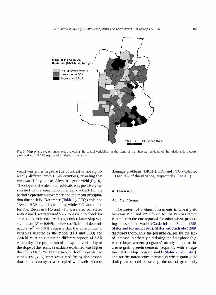
At the regional level, the slope of the relationshipbetween the absolute residuals and the year after 1900(SAR) was positive(P < 0.05), indicating an increasein yield variability. At a more detailed spatial reso-lution, SAR was positive for 95 counties (approxi-mately 94% of the area considered) and negative forthe other 2 counties (Fig. 5). For 75 counties the slopeof the absolute residuals was statistically higher than0 (P < 0.05), while none showed a significantly neg-ative slope(P < 0.05). The slope of the relative resid-uals (residuals expressed as percentage of predicted


Fig. 4. Map showing the spatial variability in the difference in average yield (�yield) between the last 10 years (1991–2000) and the first10 years of the period considered (1923–1932). Values are expressed in Mg ha−1.

Table 1Relationships between the traits derived from the temporal dynamics of wheat yields to characterize yield and yield variability patternsand environmental variables

Dependent variable Intercept R2 F Independentvariables

Regressioncoefficient

R2 partial P

Inflection pointa 41.71 0.11 6.64 PTQ 18.68 0.11 <0.05�Yieldb −909.1 0.34 23.9 PPT 2.3 0.20 <0.001

PTQ 842.44 0.14 <0.001Slope absolute residuals (SAR)b −6.32 0.20 11.46 PTQ 3.54 0.13 <0.001

PPT 0.006 0.7 <0.001Slope relative residu als (SRR)b −0.01 0.50 27.65 DREN 0.001 0.31 <0.001

PPT 0.00001 0.10 <0.001PTQ 0.0034 0.09 <0.001

Notes: The analysis were performed by stepwise multiple regression. Variables left in the model were significant at 0.15 level. Independentvariables include the percentage of soils without drainage problems within a county (DREN), mean precipitation (PPT) occurred duringwheat cycle (July–December) and mean photothermal quotient (PTQ) between September and November.

a n = 57.b n = 94.


Fig. 5. Map of the region under study showing the spatial variability in the slope of the absolute residuals of the relationship betweenyield and year (SAR) expressed in Mg ha−1 per year.

yield) was either negative (52 counties) or not signif-icantly different from 0 (45 counties), revealing thatyield variability increased less than grain yield (Fig. 6).The slope of the absolute residuals was positively as-sociated to the mean photothermal quotient for theperiod September–November and the mean precipita-tion during July–December (Table 1). PTQ explained13% of SAR spatial variability while PPT accountedfor 7%. Because PTQ and PPT were also correlatedwith �yield, we regressed SAR to�yield to check forspurious correlations. Although this relationship wassignificant(P = 0.049) its low coefficient of determi-nation (R2 = 0.04) suggests that the environmentalvariables selected by the model (PPT and PTQ) and�yield must be explaining different aspects of SARvariability. The proportion of the spatial variability ofthe slope of the relative residuals explained was higherthan for SAR, 50%. Almost two thirds of the explainedvariability (31%) were accounted for by the propor-tion of the county area occupied with soils without

drainage problems (DREN). PPT and PTQ explained10 and 9% of the variance, respectively (Table 1).

4. Discussion

4.1. Yield trends

The pattern of bi-linear increments in wheat yieldbetween 1923 and 1997 found for the Pampas regionis similar to the one reported for other wheat produc-ing areas of the world (Calderini and Slafer, 1998;Slafer and Kernich, 1996). Slafer and Andrade (1989)discussed thoroughly the possible causes for the lackof increase in wheat yield during the first phase (e.g.wheat improvement programs’ mainly aimed to in-crease grain protein content, frequently with a nega-tive relationship to grain yield (Slafer et al., 1990))and for the noteworthy increase in wheat grain yieldduring the second phase (e.g. the use of genetically


Fig. 6. Map of the region under study showing the spatial variability in the slope of the relative residuals of the relationship between yieldand year (SRR) expressed in % per year. Slope values were multiplied by 10,000.

improved varieties (with semi-dwarfing genes), betteragronomic practices, etc.).

The large variability found for the year of the in-flection point at the county level may be an indica-tion that the modernization of agriculture has beena local phenomenon, being more influenced by bothsocio-economic aspects (such as risk aversion or landtenure among others) than environmental variables.The low proportion of the spatial variance in the IPexplained by environmental variables (11% by PTQ)supports this hypothesis.

The positive relationship found between precipita-tion and the photothermal quotient and the differencein yield (�yield) agrees with the hypothesis that theimpact of the agricultural intensification upon yieldis higher at favorable than unfavorable environments(Slafer and Kernich, 1996; Cassman, 1999). Thisobservation confirms for the first time at a county

level what has been recognized from comparisonsamong whole counties (Araus et al., 2002). In thePampas, water availability has been identified as oneof the main climatic controls of crop yield (Satorreand Slafer, 1999). Under no water or nutrient limita-tions,Magrin et al. (1993)found a strong relationshipbetween wheat yield and the photothermal quotientcalculated for the 3 weeks prior to anthesis. The pho-tothermal quotient reflects the opposing effects ofradiation and temperature on grain number, and thuson wheat yield. Radiation increases spike weight atanthesis and hence kernel number while temperaturedecreases the duration of spike growth by speedingdevelopment rate, thus reducing spike weight andkernel number (Fischer, 1985a,b). The proportion ofthe explained�yield variability rose to 79% whenthe average of the three highest yields of the countywas used as an estimator of potential environmental


quality (i.e. the degree of correspondence betweenwheat environmental requirements and the actuallevel of environmental factors).

4.2. Yield variability

The trends in wheat yield variability were differ-ent for the absolute and relative descriptors. In abso-lute terms yield variability increased as implied fromthe positive slope of the absolute residuals regressedagainst time while in relative terms yield variabilitydecreased (negative slope of the relative residuals).This pattern was evident at the regional level as wellas at the county level. The increase in absolute resid-uals would be expected if yield and yield variabilitywere not totally independent. For example, if the er-ror associated with the attainment (e.g. harvesting ma-chine) or determination (i.e. weight) of yield had beena percentage of yield, the higher yields of the end oflast century would appear more variable than those ofthe beginning. Relative residuals, by expressing yieldvariability as percentage of yield, avoid this limitationand provide a more suitable/adequate approach to un-derstand the changes in yield variability (Francis andKannenberg, 1978; Calderini and Slafer, 1998). Thesignificant negative SRR found for the region, as wellas for the majority of the counties, indicates that, eventhough both yield and yield variability increased dur-ing the 20th century, grain yield increment was higherthan the increase in yield variability. Thus, the wheatcropping systems of the Pampas have been successfulin increasing yields while maintaining or increasingyield stability.

These results differ from those reported by other au-thors.Hazell (1984)andAnderson et al. (1988)con-cluded that cereal yield gains were associated with anincrease in yield variability. The methodology used bythese authors may have been responsible for these dif-ferences. They restricted the analysis to the compari-son between two specific periods of time. As pointedout by Calderini and Slafer (1998)this methodologypresents two problems: it does not show trends and,more importantly, it confounds yield trends with yieldvariability changes. Moreover, the results from such amethodology are highly susceptible to the occurrenceof an abnormal year.

Long-term weather changes may have played animportant role in determining the observed pattern of

yield variability. Our weather data (unpublished) andprevious reports (Roberto et al., 1994; Viglizzo et al.,1995) showed a significant increase in rainfall in thedriest part of the region during the last 75 years (LaPampa province, data not shown). Such changes mayhave important effects on yield and on yield stabil-ity. As precipitation variability is negatively relatedto mean annual precipitation (Lauenroth and Burke,1995; Davidowitz, 2002), an increase in precipita-tion would not only have increased wheat yields butalso would make them more stable; particularly inthe subhumid areas where precipitation has increasedmarkedly (Le Houérou, 1996). We also checked for apossible effect of changes in harvested area and theobserved changes in yield variability. However, whenthe slope of the harvested area (the rate at which theharvested area changed per year) was regressed againstSAR or SRR, the relationship was not significant (P =0.16 for SAR andP = 0.26 for SRR).

The positive association between SAR and PTQand PPT suggests that at favorable environments theincrease in yield variability was higher than in siteswhere resources were less available. As counties withhigher yield may have higher variability—simply be-cause a site that yields, for example, 4 Mg ha−1 peryear, may show a difference of up to 4 Mg ha−1 peryear (if there is no yield) while a site with an av-erage yield of 1 Mg ha−1 per year will only displaya difference of 1 Mg ha−1 per year under the samesituation—there is a possibility that this relationshipmay be due to statistical artifacts. However, the weakrelationship between SAR and�yield or averagecounty yield suggests that this is not the case. Rel-ative variability decreased less at favorable than atunfavorable environments meaning that, at marginalareas, the difference between the increase in yield andthe increase in yield variability was higher than forareas best suited for wheat production. The patternof response of both estimators of yield variability toenvironmental variables may be related to the relativecontribution of genetic and technological contribu-tions to grain yield gains in different environments.

4.3. Relative importance of genetic andtechnological contributions to yield gains

Previous studies have dealt with the difficult taskof estimating the relative contribution of genetic and


technological contributions to grain yield gains. Ingeneral, these studies have come to a convergent result:genetic and technological contributions were almostthe same (Jensen, 1978; Silvey, 1979; Deckerd et al.,1985; Slafer and Andrade, 1991). Would this patternbe maintained for different environments? Should weexpect that the relative importance of these two com-ponents of yield gains vary in space?

Genetic improvements and agronomic practices ex-ert opposing effects over yield variability. Modernwheat cultivars are more responsive to improvementsin environmental conditions than their older counter-parts (e.g.Hucl and Baker, 1987; Ledent and Stoy,1988; Cox et al., 1988). Calderini and Slafer (1999)confirmed this result in a study performed using dataof cultivars released at different times in different en-vironments. They found that the slope of the relation-ship between grain yield and an environmental indexwas higher in modern than in old cultivars and thatmodern cultivars out-yielded their older counterpartsin virtually all conditions for counties with extremelydifferent conditions. Thus, it is possible to expect ahigher impact of genetic improvement on yield and ab-solute variability of yield on sites with adequate envi-ronmental conditions for wheat crops (those with highvalues of both photothermal quotient and precipita-tion). On the other hand, agronomic practices such asirrigation, fertilization, herbicides and pesticides use,date and rate of sowing, etc. not only improve yieldby modifying the environment perceived by the cropbut also make this environment less variable from yearto year (Hazell, 1989; Tivy, 1989). For example, inwheat–rice double cropping systems in several Asiancounties, differences in N supply in similar soils wereidentified as responsible for variations in rice yields of3.6 Mg ha−1 when no N was applied (Cassman et al.,1998). Paruelo et al. (2001)found that, in the Cen-tral Plains of USA, irrigation not only increased cropproduction but also decoupled the system from theenvironmental factors that controlled its variability,making the system more stable. In addition, modernmanagement practices aim to provide the required re-sources for crop growth and crop protection withoutdeficiency or excess at each point in time and space.

The relative importance of the impact of geneticand agronomic improvement on wheat yield and onits temporal variability would differ spatially. The im-pact of genetic improvements would be highest at sites

with good environmental conditions while the impactof better agronomic practices would be more impor-tant in less adequate sites for wheat production. Ourresults support this hypothesis. In the Argentine Pam-pas wheat grain yield of 97 counties increased duringthe 20th century. This increase in yield was related toa decrease in yield stability. However, in marginal ar-eas of this study, the increase in yield was higher thatthe increase in yield variability while in the core areasthe opposite tended to occur.

5. Conclusion

The mechanisms by which agroecosystems copedwith the increasing demand on food and fiber in thepast, now seem exhausted. Recent works have high-lighted that grain yield increase through genetic im-provement may be approaching its ceiling (Cassman,1999). There is little possibility for expansion of agri-cultural lands due to the human demographic growthand actual availability of arable land for sustainableproduction. On the contrary, a reduction of the mostfertile lands is the most likely scenario because of ur-banization and land degradation. In this context, main-taining high and stable grain production is essential.

Our results showed that the impact of genetic andmanagement improvement contributions on wheatgrain yield and yield variability varied among sites.In low resource areas grain yield increased at a higherrate than yield variability. In contrast, in high re-sources areas the increase in yield variability tended tobe higher (though not significantly) than the increasein grain yield. This finding highlights a “win–win”solution for the generalized idea of a trade off be-tween grain yield and yield stability. To identify andto understand the underlying mechanisms responsiblefor this pattern constitutes an important prerequisitefor the design of agricultural policies that may al-low an adequate food supply as well as preserve ournatural, social and economic capital.

Acknowledgements

We are grateful to Daniel Calderini for providinguseful comments and suggestions. S.R.V. wish tothank Lucas Borrás and Juan Pablo Guerschman for


the discussion of ideas. The Secretarıa de AgriculturaPesca y Alimentación, who kindly gave us accessto the wheat data, is also recognized. Our work wasfunded on grants from UBACyT, CONICET andFONCyT (Argentina), Inter-American Institute (IAI,ISP3-077, CNR 012) and Fontagro. S.R.V. has a grantfrom CONICET.

References

Anderson, J.R., Dillon, J.L., Hazell, P.B.R., Cowie, A.J., Wang,G.H., 1988. Changing variability in cereal production inAustralia. Rev. Market. Agric. Econ. 56, 270–286.

Araus, J.L., Slafer, G.A., Reynolds, M.P., Royo, C., 2002. Plantbreeding and drought in C3 cereals: what should we breed for?Ann. Bot. 89, 925–940.

Ashraf, M., Akbar, M., Salim, M., 1994. Genetic improvementin physiological traits of rice yield. In: Slafer, G.A. (Ed.),Genetic Improvements of Field Crops. Marcel Dekker, NewYork, pp. 413–455.

Austin, R.B., Bingham, J., Blackwel, R., Evans, L., Ford, M.,Morgan, C., Taylor, M., 1980. Genetic improvement in winterwheat since 1900 and associated physiological changes. J.Agric. Sci. Camb. 94, 675–689.

Barsky, O., Gelman, J., 2001. Historia del Agro Argentino. GrijalboMondador, Buenos Aires.

Calderini, D.F., Slafer, G.A., 1998. Changes in yield and yieldstability in wheat during the 20th century. Field Crops Res. 57,335–347.

Calderini, D.F., Slafer, G.A., 1999. Has yield stability changed withgenetic improvement of wheat yield? Euphytica 107, 51–59.

Cassman, K.G., 1999. Ecological intensification of cerealproduction systems: yield potential, soil quality, and precisionagriculture. Proc. Natl. Acad. Sci. U.S.A. 96, 5952–5959.

Cassman, K.G., Peng, S., Olk, D.C., Ladha, J.K., Reichardt, W.,Dobermann, A., Singh, U., 1998. Opportunities for increasednitrogen-use efficiency from improved resource management inirrigated rice systems. Field Crops Res. 56, 7–39.

Cox, T.S., Shroyer, J.P., Ben-Hui, L., Sears, R.G., Martin, T.J.,1988. Genetic improvement in agronomic traits of hard redwinter wheat cultivars from 1919 to 1987. Crop Sci. 28, 756–760.

Davidowitz, G., 2002. Does precipitation variability increase frommesic to xeric biomes? Global. Ecol. Biog. 11, 143–154.

Deckerd, E.L., Busch, R.H., Kofoid, K.D., 1985. Physiologicalaspects of spring wheat improvement. In: Hasper, J., Scrader,L., Howel, R. (Eds.), Exploitation of Physiological and GeneticVariability to Enhance Crop Productivity. American SocietyPlant Physiologists, Rockland, MD, pp. 45–54.

Duvick, D.N., 1984. Genetic contributions to grain gains of UnitedStates hybrid maize, 1930–1980. In: Fehr, W.R. (Ed.), GeneticContributions to Yield Gains of Five Major Crop Plants.CSSA Special Pub. No. 7. Crop Sci. Soc. Am., Madison, WI,pp. 15–47.

Eberhardt, S., Russell, W.E., 1966. Stability parameters forcomparing varieties. Crop Sci. 6, 36–40.

FAO, 1985. FAO Yearbooks and FAO Processed Statistical Series.Food and Agriculture Organization of the United Nations,Rome, Italy.

Finlay, K., Wilkinson, G., 1963. The analysis of adaptation in aplant-breeding program. Aust. J. Agric. Res. 14, 742–754.

Fischer, R.A., 1985a. Number of kernels in wheat crops and theinfluence of solar radiation and temperature. J. Agric. Sci. 105,447–461.

Fischer, R.A., 1985b. Physiological limitations to producing wheatin semitropical and tropical environments and possible selectioncriteria. In: Proceedings of the Wheats for more TropicalEnvironments. Centro Internacional de Mejoramiento del Maizy Trigo (CIMMYT), México D.F., pp. 209–230.

Francis, T.R., Kannenberg, L.W., 1978. Yield stability inshort-season maize. Part I. A descriptive method for groupinggenotypes. Can. J. Plant Sci. 58, 1029–1034.

Ghersa, C.M., Leon, R.J.C., 1999. Successional changes inagroecosystems of the Rolling Pampa. In: Walker, L.R.(Ed.), Ecosystems of Disturbed Ground. Elsevier, Amsterdam,pp. 487–502.

Guerschman, J.P., Paruelo, J.M., Burke, I.C., 2003. Land useimpacts on the normalized difference vegetation index intemperate Argentina. Ecol. Appl. 13, 616–628.

Hall, A.J., Rebella, C.M., Ghersa, C.M., Culot, J., 1992. Field-cropsystem of the Pampas. In: Pearson, C.J. (Ed.), Ecosystemsof the World. Field Crop Ecosystems. Elsevier, Amsterdam,pp. 413–450.

Hazell, P.B.R., 1984. Sources of increased instability in Indiancereal production. Am. J. Agric. Econ. 66, 302–311.

Hazell, P.B.R., 1989. Changing patterns of variability in worldcereal production. In: Anderson, J.R., Hazell, P.B.R. (Eds.),Variability in Grain Yields. John Hopkins University Press,Baltimore, pp. 13–34.

Hucl, P., Baker, R.J., 1987. A study of ancestral and modernCanadian Spring wheats. Can. J. Plant Sci. 67, 87–97.

Jensen, N.F., 1978. Limits to growth in the world food production.Ceilings for wheat yields are coming in developed counties.Science 201, 317–320.

Kleinbaum, D., Kupper, L.L., 1978. Applied Regression Analysisand other Multivariate Methods. North Scituate, MA, DuxburyPress.

Lauenroth, W.K., Burke, I.C., 1995. Great Plains, ClimateVariability. Encyclopedia of Environmental Biology. AcademicPress, London.

Ledent, J.F., Stoy, V., 1988. Yield of winter wheat. A comparisonof genotypes from 1910 to 1976. Cereal Res. Commun. 16,151–156.

Le Houérou, H.N., 1996. Climate change, drought anddesertification. J. Arid Environ. 34, 133–185.

Magrin, G.O., Hall, A.J., Baldy, C., Grondona, M.O., 1993. Spatialinterannual variations in the photothermal quotient: implicationfor the potential kernel number of wheat crops in Argentina.Agric. For. Meteor. 67, 29–41.

Obschatko, E.S., del Bello, J.C., 1986. Tendencias Productivas yEstrategia Tecnológica para la Agricultura Pampeana. CISEA,Buenos Aires.


Paruelo, J.M., Burke, I.C., Lauenroth, W.K., 2001. Land-use impacton ecosystem functioning in eastern Colorado, USA. GlobalChange Biol. 7, 631–639.

Ralston, M.L., Jennrich, R.I., 1978. DUD, a derivative-freealgorithm for nonlinear least squares. Technometrics 20, 7–14.

Riggs, T.J., Hanson, P.R., Start, N.D., Miles, D.M., Morgan, C.L.,Ford, M.A., 1981. Comparison of spring barley varieties grownin England and Wales between 1880 and 1980. J. Agric. Sci.Camb. 97, 599–610.

Roberto, Z.E., Casagrande, G., Viglizzo, E.F., 1994. Lluvias de laPampa Central: tendencias y variaciones en el siglo. CambioClimático y Agricultura Sustentable en la región Pampeana.Publicación INTA CR LP-SL, No. 2, p. 26.

SAGPyA, 1990. Atlas de Suelos de la República Argentina.Secretarıa de Agricultura Ganaderıa Pesca y Alimentación,Buenos Aires.

SAGPyA, 2000. Estimaciones Agrıcolas. Secretarıa de AgriculturaGanaderıa Pesca y Alimentación, Buenos Aires.

Satorre, E.H., Slafer, G.A., 1999. Wheat production systems of thePampas. In: Satorre, E.H., Slafer, G.A. (Eds.), Wheat: Ecologyand Physiology of Yield Determination. The Haworth PressInc., New York, pp. 333–348.

Savin, R., Slafer, G.A., 1991. Shading effects on the yield of anArgentinian wheat cultivar. J. Agric. Sci. 116, 1–7.

Silvey, V., 1979. The contribution of new varieties to increasingcereal yield in England and Wales. J. Natl. Inst. Agric. Bot.14, 367–384.

Slafer, G.A., Andrade, F.H., 1989. Genetic improvement in breadwheat (Triticum aestivumL.) yield in Argentina. Field CropsRes. 21, 289–296.

Slafer, G.A., Andrade, F.H., 1991. Changes in physiologicalattributes of the dry matter economy of bread wheat (Triticumaestivum L.) through genetic improvement of grain yieldpotential at different regions of the world. Euphytica 58, 37–49.

Slafer, G.A., Andrade, F.H., Feingold, S.E., 1990. Geneticimprovement of bread wheat (Triticum aestivum L.) inArgentina: relationships between nitrogen and dry matter.Euphytica 50, 63–71.

Slafer, G.A., Kernich, G., 1996. Have changes in yield(1900–1992) been accompanied by a decreased yield stabilityin Australian cereal production? Aust. J. Agric. Res. 478, 323–334.

Statistical Analysis Systems Institute (SAS) Inc., 1996. SAS User’sGuide Statistics, Version 6. p. 1028

Tivy, J., 1989. Agricultural Ecology. Longman Scientific &Technical, Wiley, New York.

Viglizzo, E.F., Roberto, Z.E., Filippin, M.C., Pordomingo, A.J.,1995. Climate variability and agroecological change in theCentral Pampas of Argentina. Agric. Ecosyst. Environ. 55, 7–16.

Wych, R.D., Stuthman, D.D., 1983. Genetic improvement inMinnesota adapted oat cultivars released since 1923. Crop Sci.23, 879–881.

Interannual variability of wheat yield in the Argentine Pampas ...

Documents

Transcript of Interannual variability of wheat yield in the Argentine Pampas ...