Geographical variation of diversity in Argentine passerine birds

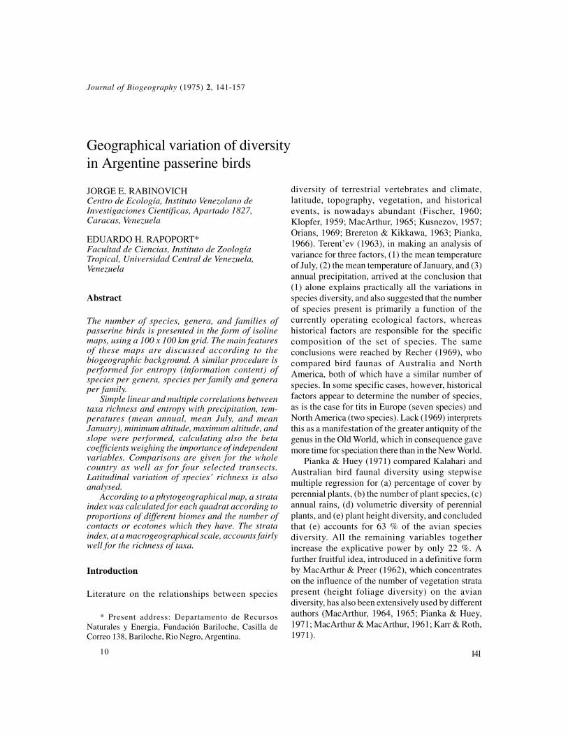
Journal of Biogeography (1975) 2, 141-157

Geographical variation of diversityin Argentine passerine birds

JORGE E. RABINOVICHCentro de Ecología, Instituto Venezolano deInvestigaciones Científicas, Apartado 1827,Caracas, Venezuela

EDUARDO H. RAPOPORT*Facultad de Ciencias, Instituto de ZoologíaTropical, Universidad Central de Venezuela,Venezuela

Abstract

The number of species, genera, and families ofpasserine birds is presented in the form of isolinemaps, using a 100 x 100 km grid. The main featuresof these maps are discussed according to thebiogeographic background. A similar procedure isperformed for entropy (information content) ofspecies per genera, species per family and generaper family.

Simple linear and multiple correlations betweentaxa richness and entropy with precipitation, tem-peratures (mean annual, mean July, and meanJanuary), minimum altitude, maximum altitude, andslope were performed, calculating also the betacoefficients weighing the importance of independentvariables. Comparisons are given for the wholecountry as well as for four selected transects.Latitudinal variation of species’ richness is alsoanalysed.

According to a phytogeographical map, a strataindex was calculated for each quadrat according toproportions of different biomes and the number ofcontacts or ecotones which they have. The strataindex, at a macrogeographical scale, accounts fairlywell for the richness of taxa.

Introduction

Literature on the relationships between species

* Present address: Departamento de RecursosNaturales y Energia, Fundación Bariloche, Casilla deCorreo 138, Bariloche, Rio Negro, Argentina.

10

diversity of terrestrial vertebrates and climate,latitude, topography, vegetation, and historicalevents, is nowadays abundant (Fischer, 1960;Klopfer, 1959; MacArthur, 1965; Kusnezov, 1957;Orians, 1969; Brereton & Kikkawa, 1963; Pianka,1966). Terent’ev (1963), in making an analysis ofvariance for three factors, (1) the mean temperatureof July, (2) the mean temperature of January, and (3)annual precipitation, arrived at the conclusion that(1) alone explains practically all the variations inspecies diversity, and also suggested that the numberof species present is primarily a function of thecurrently operating ecological factors, whereashistorical factors are responsible for the specificcomposition of the set of species. The sameconclusions were reached by Recher (1969), whocompared bird faunas of Australia and NorthAmerica, both of which have a similar number ofspecies. In some specific cases, however, historicalfactors appear to determine the number of species,as is the case for tits in Europe (seven species) andNorth America (two species). Lack (1969) interpretsthis as a manifestation of the greater antiquity of thegenus in the Old World, which in consequence gavemore time for speciation there than in the New World.

Pianka & Huey (1971) compared Kalahari andAustralian bird faunal diversity using stepwisemultiple regression for (a) percentage of cover byperennial plants, (b) the number of plant species, (c)annual rains, (d) volumetric diversity of perennialplants, and (e) plant height diversity, and concludedthat (e) accounts for 63 % of the avian speciesdiversity. All the remaining variables togetherincrease the explicative power by only 22 %. Afurther fruitful idea, introduced in a definitive formby MacArthur & Preer (1962), which concentrateson the influence of the number of vegetation stratapresent (height foliage diversity) on the aviandiversity, has also been extensively used by differentauthors (MacArthur, 1964, 1965; Pianka & Huey,1971; MacArthur & MacArthur, 1961; Karr & Roth,1971).

141

142 Jorge E. Rabinovich and Eduardo H. Rapoport

Another way of focusing on changes in speciesdiversity is that initiated by Simpson (1964) for NorthAmerican mammals, and followed by Hagmeier &Stults (1964) and Wilson (1974), and for birds byCook (1969) and Kikkawa & Pearse (1969), whichuses a pictorial and analytical descriptive method.Simpson (1964), as well as Cook (1969), observeda ‘peninsular effect’ and a ‘topographic effect’, aswell as a latitudinal one, the latter being characterizedby a decrease in species diversity with an increase inlatitude.

With the exception of Cody’s (1970) paper, allthese studies have been limited to the geographicalvariation of diversity in the Palearctic, Nearctic andAustralian regions. Accordingly it seemed valuableto carry out a similar study for the Neotropical region,so as to verify whether the conclusions reachedelsewhere might also be applicable in the Neotropics.

When compared with the above mentioned papers,the present study includes two main extensions. Oneinvolves the inclusion of an H index, used by Kikkawa(1968) and Cody (1970) for ecological purposes, andrecently introduced by Wilson (1974) intobiogeography, which is an entropy index derived frominformation theory, as a measure of diversity ofspecies per genus, species per family, and genera perfamily. The other involves relating variations ofgeographic diversity to variations in the number ofplant strata, taking the latter as a function ofvegetation types, not at point samples but at thebiome scale.

Due to the fact that detailed knowledge of theavifauna of South America was incomplete duringthe original period of data processing,* we have beenforced to restrict the present study to an analysis ofthe passerine birds of Argentina, a country whoseavifauna is relatively well known. This limitationobviously modifies the strength of our conclusionsand the overall degree of generalization which wewere seeking, and has caused us to make manyreservations with respect to how far one may drawuseful comparative inferences for the Neotropicalregion as a whole from the data presented below.

Methods

The basic source of information on the geographical

* Data were processed between 1967 and 1968, beforeOlrog’s book entitled Las Aves Sudamericanas, Una Gaiade Campo, U.N.T. (1968) was published.

distribution of Argentine passerine birds is Olrog(1959), who provided maps of both the breeding andnon-breeding ranges for each species. Although thesemaps do not provide all the details which aredesirable, they allow a satisfactory first approxima-tion of relevant data. The Argentine passerine faunaincludes a total of 434 breeding species, which aredistributed in 247 genera and twenty-six families. Thebreeding range of each species has been mapped ona squared Lambert’s azimuthal equal-area pro-jectionof continental Argentina, including the Malvinas(Falkland) Islands and Tierra del Fuego, which hadbeen previously reticulated in a grid of 336 quadratsof 100 x 100 km each (approximately 3900 squaremiles). The size of each quadrat in this grid isappreciably smaller than that used by Simpson (1964)and Cook (1969) for Central and North America,thus compensating to some extent for the largergeographical scale of Argentina.

Such a mapping procedure yields informationabout the number of species on each quadrat (speciesrichness), and the distribution of the species amonggenera and families; the latter is a measure oftaxonomic diversity of the avian community, whichwe estimated by means of the Shannon & Weaverformula (H= - Σi Pi log2pi). Thus, for each quadrat,we were not evaluating specific diversity in the usualmanner, in which each species is weighed by thenumber of individuals, but rather were weighing thedistribution of species in genera and families, andthe distribution of genera in families. In other words,in the first case pi =(number of species of genus i)/(total number of genera); in the second case Pi=(number of species of family i)/(total number offamilies); and in the third case pi=(number of generaof family i)/(total number of families). This type ofcalculation of diversity indices without theknowledge of the number of individuals has beenperformed previously by Kikkawa (1968) and byWilson (1974).

The climatic and topographic information usedwas obtained from precipitation, temperature andrelief maps which provided rainfall and temperatureisolines, and the height contour lines; and from these,by interpolation, each of the 336 quadrats wasassigned a value for precipitation, temperature andaltitude.

The relief maps had enough detail to providecontour lines for maximum and minimum altitude,and an estimation of mean altitude and ‘slope’. By‘slope’, we mean the difference between maximumand minimum altitude as a percentage of the mean

Geographical variation of diversity in passerine birds 143

Fig. 1. Natural regions of Argentina, after Ragonese (1966). See Table 7 for translation.


value: S= [(maximum altitude-minimum altitude)/(mean altitude)] x 100. This index was used so as totake into consideration the hypothesis that a givendifference between maximum and minimum altitudecould affect bird diversity differentially, dependingupon the mean altitude.

Information about the natural vegetation regionsof Argentina was obtained from a modified versionof a 1968 map by Ragonese (Fig. 1). Dr G. Sarmientocomplemented that map with information about thetype of vegetation included in each natural region,and the number of plant strata typical of each typeof vegetation. A more detailed explanationconcerning the manner in which this information wasprocessed is given in our discussion on therelationship between bird diversity and number ofplant strata.

The computation of the presence or absence ofeach species, and the calculation of the diversityindices which had to be carried out for each of the336 quadrats, and the simple and multiple correla-tions, were processed in the IBM 360/50 System ofthe Facultad de Ciencias of the Universidad Centralde Venezuela.

Results

(1) Patterns of richness and geographical diversity

One of the basic ways of expressing the results is tojoin with a line those quadrats with the same richnessvalues (‘isorichness’ lines), so giving a visual pictureof the main geographical changes in richness. Mapsare given in Figs 2-4, from which an immediategeneral pattern emerges. First, in the cases of thenumber of species and genera, there are three mainbreaks, or sudden changes in richness, as representedby those areas where the lines are very close together:(a) south of the province of Misiones in the northeast;(b) in the northwest; (c) in the centre of the country.However, in the case of the number of families, thereare only two of the breaks (a and c). Secondly,isorichness lines run roughly north-south in Pata-gonia.

The sudden fall in richness south of Misiones,which involves a decrease from 220 to 150 species,is not surprising for it represents a change from thesubtropical rain forest (‘selva misionera’) to thesavanna (‘parque mesopotdmico’) of CorrientesProvince. A similar explanation might be invoked toexplain the change in richness from 200 to 120species in the northwest, in that it represents a

Fig. 2. Number of passerine bird species per quadrat of100 km x 100 km.

change from the subtropical forest of TucumánProvince (‘selva tucumano-oranense’) to the dryforest (‘parque chaqueño occidental’). The thirdbreak, in the centre of the country, apparentlyreflects a biogeographic change, for it correspondsmore or less to the limits between the Guyano-Brazilian and Andean-Patagonian biogeographicregions; this is however only a hypothesis, for there


Fig. 3. Number of passerine bird genera per quadrat of100 km x 100 km.

is not always a change in species richness betweentwo biogeographical subregions (Kaiser, Lefkovitch& Howden, 1972).

Another peculiarity is the species, genera andfamilies density plateau which is found in the areabetween the Uruguay River and the western side ofthe Parand River (Mesopotamia and Western ChacoSavanna). This perhaps reflects local plant speciesdistributional patterns, in that the distribution ofmany subtropical species extends southwards along

Fig. 4. Number of passerine bird families per quadrat of100 km x 100 km.

gallery vegetation as far as the Rio de la Plata delta,so producing a sort of corridor for animals. In thisway, vegetation may ‘push’ to the south sometropical bird species along the margins of the ParandRiver.

One surprising result is the east west direction ofthe density lines along much of the western borderof Argentina; this is probably due primarily to the


inclusion of both lowland and highland species inthe same quadrats. In part, however, it is also theresult of a lack of precision in the original speciesdistribu-tion maps, a difficulty which also presentsitself in the analysis of correlations betweendistributional patterns, precipitation, temperature andvegetation strata.

As noted previously, the isodensity lines of species(as well as of genera and families) richness run north-south in western Patagonia. We have to bear in mindthat this mainly reflects a sharp gradient ofprecipitation, for while eastern Patagonia lies underdesertic conditions, western Patagonia (or moreproperly Araucania) is densely covered with forests.The data presented in Fig. 2 do not completely agreewith Vuilleumier (1972), who found that the avifaunalrichness, as based on three samples, decreased fromthe steppe to the open forest, and to the closed forest,both in terms of the number of individuals and thenumber of species. This result is perhaps due to thefact that the steppe sampled by Vuilleumier nearBariloche is for all practical purposes an ecotonebetween the Patagonian semidesert and the Arau-canian forest. It is not unusual that ecotones presenthigher diversities than contiguous biomes due, in part,to the overlap factor. According to Vuilleumier(1972), the total number of species in the Araucanianforest is forty-three to forty-four, against 122 in thesteppes. In our map (Fig. 2), the Araucanian forestis crossed by the density line of seventy passerinespecies, and this figure is in good agreement withthe field data obtained by the Estación Biológica dela Isla Victoria (Fundación Bariloche) over a periodof several years (J. L. Contreras, personalcommunication).

A further map, which depicts the geographicalvariation of diversity measured by means of theinformation theory index (Fig. 5), shows two typesof patterns in different regions within Argentina. Inthe northern half, there is no well defined pattern,but rather a confused indication of ‘heterogeneity’dispersed in a series of unconnected peaks. Incontrast, in the southern half of the country, andparticularly in its centre (Buenos Aires and La Pampaprovinces), the ‘isoentropy’ lines are con-tinuous andalmost parallel, showing more general trends. Sincethe entropy index indicates how species aredistributed in genera, without considering the actualnumber of genera, a high H value indicates morebalance or ‘equitability’ in the distribution of speciesamong higher categories, while a low H valueindicates that a few genera contain most of the

Fig. 5. Entropy values of species per genera.

species, while the rest are represented by only oneor a few species per genus. Thus the striking changebetween the areas north and south of the Provincesof La Pampa and Buenos Aires means that thereduction in the number of species is not accom-panied by a proportional reduction in the number ofgenera. As the entropy index does not indicate


whether some genera are replaced by others, we donot dare to state at present the tempting conclusionthat some genera show a higher capacity to occupya greater variety of niches than others. However, wehope to solve this question with cluster analysistechniques in work that is under way.

(2) Correlations of species richness and diversitywith climate and topography

(a) For the whole country. As each quadrat hasinformation on richness, temperature, precipitation,and altitude, simple linear and multiple correlationsmay be carried out, in which richness is considered

by selecting those quadrats with the sametemperature and, among them, performing a simplelinear correla-tion between entropy of speciesin genera and ‘slope’ we obtained: r=-0431 at10°C, r=-0730 at 12°C, r=-0262 at 14°C, r=-0508at 16"C, r= -0493 at 18°C, and so on. Of these, mostof the coefficients are statistically significant, and inall cases they are negative. We expected that thereshould be a larger number of niches, and a higherdegree of diversity with an increase in the ‘slope’; asthe results suggest the opposite, we think thatsomehow mountainous areas in Argentina have anegative effect on richness, which is an apparentcontradiction of what happens in North America,

Table 1. Simple correlation coefficients of diversity against climatic and topographic factors

as the dependent variable. In Tables 1 and 2, wepresent the correlation coefficients (simple andmultiple, respectively), with the several forms ofdiversity calculated for each quadrat. In spite of theapparently low values of the coefficients (particu-larly among the coefficients of simple correlation)most of them are statistically significant. One of theresults of these correlations that goes against allexpectations is the correlation between diversity and‘slope’, with a statistically significant negativecoefficient. This negative correlation still holds whenthe effect of temperatures is eliminated; for example,

where mountains are an important factor in specia-tion. A possible explanation for this fact is that thenorthern half of the Andes is practically an aviandesert. In their southern half the Andes are no morea desert, but their relatively lower number of speciesas compared to elsewhere in the country is notenough to compensate for the deleterious effect ofthe northern part, and thus change the negativecorrelation values into positive values.

In respect of the effect of temperature, the coeffi-cients are highly significant in all cases, and thecorrelation coefficients with the mean temperature

With the exception of the marked values (x), all coefficients are statistically significant.

Table 2. Multiple correlation coefficients between diversity, rain, temperature and altitude


Table 3. Average beta coefficients weighing the importance of rain, temperature, and altitude in the multiplecorrelation on different measures of diversity, and their ratios to indicate the relative importance

of January (which is a summer month in Argentina)are in general the lowest. Temperatures seem to be amore important factor than precipitation, and thelatter more important than altitude in relation todiversity. Although the number of species increaseswith maximum altitude, there is a proportionallysmaller increase in the number of families, a factwhich is corroborated when looking at the H valueof species in families with maximum altitude.

In respect of multiple correlations, Table 2 is selfexplanatory. It is surprising to find the high degreeof significance of all the coefficients of multiplecorrelation: F values run from a minimum of 113.78to a maximum of 523.78, while the critical value ofF tabulated for P=0001 and with 3 and 333 degreesof freedom is 5.68.

(b) Along transects. Some further trends wereexamined along selected transects which cross

Argentina north-south (transect A-A’, Fig. 2), andeast west at three different latitudes (transects B-B’,C-C’, and D-D’, Fig. 2). The change in the numberof species along transect A-A’ (Fig. 6) shows anexpected decrease towards the south and also reflectsthe sudden fall when passing from Jujuy to San Juan(shown as the very close lines in Fig. 2) which webelieve represents the rapid loss of influence of theavifauna of the Guyano-Brazilian subregion. Alongtransect B-B’ (Fig. 7) we observed two peaks in thenumber of species, which correspond to twosubtropical rainforest regions, the Tucumano-Oranense and the Misiones forests. Along transectA-A’ all coefficients were highly significant whencorrelating climatic and topographic factors withnumber of species, whereas in transect B-B’ the onlystatistically significant r value is the one betweennumber of species and the ‘slope’ index; it is sur-

Fig. 6. Species richness along transect A-A’.


Table 4. Simple correlation coefficients of number of species against climatic and topographic factors along straight transects

Fig. 7. Species richness along transects B-B’, C-C’ and D-D’.

Table 5. Multiple correlation coefficients, probability of significance, and beta coefficientsbetween number of species versus mean annual temperature, mean annual rainfall, and meanaltitude, along transects

Table 6. Multiple correlation coefficients, probability of significance, and beta coefficients betweennumber of species per family versus mean annual temperature, mean annual rainfall and mean attitude,along transects


Fig. 8. Latitudinal variation of the ratio species/family.

Fig. 9. Entropy values of species per genera (black line) and entropy values of species per families (brokenline) along transect A-A’.

prising that in this case the correlation coefficient ispositive, and the only reasonable explanation is thatthe two subtropical forests (which have a very largenumber of species) are found in mountainous areas.Along transect C-C’ there are several statisticallysignificant correlations, while along transect D-D’only precipitation is correlated with the number ofspecies (Table 4).

Along these transects multiple correlations werecarried out between the number of species and meanannual temperature, rainfall, and mean altitude. TheR value is statistically significant for transects A-A’,B-B', and D -D’, but not for transect C-C’. A similarmultiple correlation, in which the number of speciesper family was used, resulted in an R value whichwas statistically significant only for transect A-A’(Tables 5 and 6).

Graphical results of the changes in number of

species per family, and of the different entropy valuesalong the transects, show the following.

(1) Along transect A-A’ the number of speciesper family decreases in a fashion similar to the totalnumber of species, although with a smaller slope (Fig.8).

(2) Also in transect A-A’, the entropy of speciesper genera and species per families (Fig. 9) decreasessouthward with a very small slope, particularly forthe latter, which is almost completely horizontal.

(3) In transect B-B´ the change in number ofspecies per family follows a pattern almost identicalto the change in the total number of species.

(4) Also in transect B-B´, the entropy values ofspecies per genera and species per families, althoughchanging slightly along the transect, show someinteresting pecularities (Fig. 10): for example, thereis a peak of entropy of species per genera in the


Fig. 10. Entropy values of species per genera (black lines) and entropy values of species per families (brokenlines) along transacts.

Tucumano-Oranense rainforest, and there are twopeaks of entropy of species per family, one inSantiago dal Estero, and the other in the Misionesrainforest. It is curious that in Santiago dal Esterothis transact shows a minimum total number ofspecies, while the number of families stays almostconstant along the transact; as entropy is a measure-ment that weighs the distribution of species infamilies, a peak value in the middle of Santiago dalEstero that has a low number of species (118) relativeto the number of species in Misiones (227), but asimilar number of families (twenty-one and twenty-four respectively) indicates that the decrease in thenumber of species occurs relatively uniformly amongall families.

(5) A similar phenomenon can be observed alongtransact C-C’, where the entropy value of speciesper genera shows a peak in the Province of La Pampa,in Central Argentina, although it is associated withthe minimum number of species along the transact(Fig. 10).

(6) In transact C-C’, the entropy of species infamilies remains practically constant (Fig. 10).

A few hundred kilometres north of the C-C’transact, on the western side of the country, there isan interesting feature of the species-density lines. Atthe higher cordillera (from 4500 to 5000 m) thereare perhaps only four to five species, but species’numbers increase to the east until a hundred speciesare present, following which numbers decrease evenfurther east to ninety and eighty species, so pro-ducing three parallel lines oriented north-south. Thereis moreover not only an increase of the speciesnumber at the piedmont but also an increase inindividuals (V. G. Roig, personal communication).

There are several valleys in the Piedmont(Uspallata, Tunuyan, Calingasta) with grasslandvegetation, which contain a large number of passerinespecies, whose numbers decrease to the west(cordillera), to the east (monte ‘hardwoods’) and tothe south (Patagonian semi-desert). The hundredspecies’ density line is recovered only in easternArgentina, where the monte is replaced by the morehumid pampean steppe.

(3) Latitudinal variations in the number of species

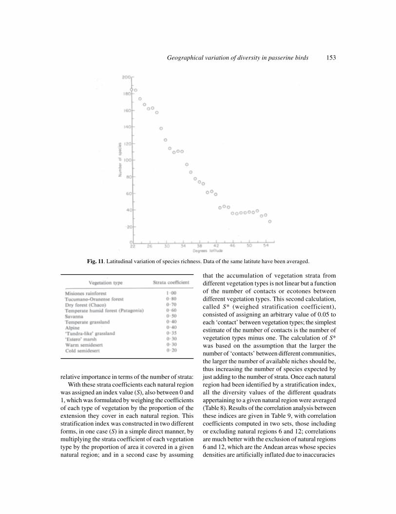
The results of transact A-A’ fit the pattern of adecrease in the number of species with an increasein latitude, which has been analysed by Fisher (1960).To verify more precisely this phenomenon weaveraged the number of species per quadrat for allthose quadrats lying at the same latitude. To theseresults (Fig. 11) we added data for the rest of thecontinent and for North America, as taken from theliterature, and obtained a bell-shaped curve with theinflexion point near the Equator, but this wasasymmetric, with a strong slope at the southern endof South America, and a smaller slope for thenorthern hemisphere. We suggest that this asymmetryresults from the triangular shape of both continents,which produces a large-scale ‘peninsular effect’, sothat the latitudinal decrease in the number of speciesin South America is accentuated by the decrease inthe width of the continent, while the opposite wouldbe occurring in North America.

It is worth mentioning that data concerning thenumber of species in southern latitudes in the vicinityof Argentina, where three important islands are


Table 7. Natural regions, types of vegetation, number of strata and % of area that eachtype of vegetation covers in each natural region, in Argentina

located, seem to support MacArthur & Wilson’s(1963) equilibrium theory of island zoogeography.While mainland Patagonia has an average of 36.2species per quadrat, its nearest neighbour and largestisland (Tierra del Fuego) has an average of thirtyspecies, the close but small island of Los Estadoshas only twenty-one species, and the rela-tively large,and more distant group of islands of the Malvinas(Falkland Islands) has only ten species.

(4) Correlation with the number of vegetation strata

As seen in Tables 1 and 2, there is a statisticallysignificant correlation between the number of speciesand the climatic and topographic factors. However,we felt that this might be a spurious effect, wherebythe climatic and topographic factors would be actingupon the vegetation, the latter being the determinantwhich affected bird species diversity, as alreadysuggested by Moreau (1935). We decided to checkthis by using an approach formulated by MacArthur

(1960, 1964) which related bird diversity to thenumber of vegetation strata, but with a different typeof information: instead of using ‘in situ’ observationsof plant strata, we obtained our data from ourknowledge of the distribution of biomes and vegeta-tion types in Argentina. We felt that this approachwas appropriate for two reasons. First, there is aconvergence of vegetation types for given tempera-ture and rainfall conditions, as pointed out bySarmiento (1968). Secondly, since we are analysingspecies whose distributional patterns occur in largegradients, the analysis of vegetation should be onthe same scale.

Figure 1 depicts the natural regions of Argentina,modified from Ragonese (1968). In Table 7, thevegetation types included in each natural region aregiven, along with the number of strata in eachvegetation type, and the approximate percentage ofsurface that each vegetation type covers in eachnatural region. In order to utilize this information, aheuristic coefficient was assigned to each type ofvegetation (between 0 and 1), indicating their


Fig. 11. Latitudinal variation of species richness. Data of the same latitute have been averaged.

relative importance in terms of the number of strata:With these strata coefficients each natural region

was assigned an index value (S), also between 0 and1, which was formulated by weighing the coefficientsof each type of vegetation by the proportion of theextension they cover in each natural region. Thisstratification index was constructed in two differentforms, in one case (S) in a simple direct manner, bymultiplying the strata coefficient of each vegetationtype by the proportion of area it covered in a givennatural region; and in a second case by assuming

that the accumulation of vegetation strata fromdifferent vegetation types is not linear but a functionof the number of contacts or ecotones betweendifferent vegetation types. This second calculation,called S* (weighed stratification coefficient),consisted of assigning an arbitrary value of 0.05 toeach ‘contact’ between vegetation types; the simplestestimate of the number of contacts is the number ofvegetation types minus one. The calculation of S*was based on the assumption that the larger thenumber of ‘contacts’ between different communities,the larger the number of available niches should be,thus increasing the number of species expected byjust adding to the number of strata. Once each naturalregion had been identified by a stratification index,all the diversity values of the different quadratsappertaining to a given natural region were averaged(Table 8). Results of the correlation analysis betweenthese indices are given in Table 9, with correlationcoefficients computed in two sets, those includingor excluding natural regions 6 and 12; correlationsare much better with the exclusion of natural regions6 and 12, which are the Andean areas whose speciesdensities are artificially inflated due to inaccuracies


Table 8. Uncorrected (S), and corrected (S*) trata coefficients, averagenumber of species with one standard deviation, and number of quadrats(N), for each natural region

Table 9. Linear correlation coefficients between uncorrected (S) and corrected (S*) vegetation strata index anddifferent diversity measurements for all natural regions

* Significant at the 0.05 level.** Significant at the 0.01 level.

Fig. 12. Regression lines between the number of species and uncorrected (circles and black line) and corrected (triangles,broken line) vegetation strata indices. In the former case r = 0.859 and in the latter case r = 0.912 (P<0.002).


in the range maps, as explained before. Fig. 12 givesthe graphical relationship between the averagenumber of species and the stratification indices andthe regression lines. There is an improvement ofcorrelation in S* with respect to S, which could betaken as an indicator of the importance of the contactzones in the measure of diversity, a fact fairly well-established in ecological theory (Mac-Arthur, 1964;Watt, 1968).

Having calculated the stratification indices for the

different natural regions it was then possible toevaluate the relationship between the S* values andthe number of species along the four transects.Table 10 gives the correlation coefficients for eachtransect between the S* and the number of species,genera, and families. There are two interestingresults: (1) coefficients are statistically significantwith the number of species in all transects excepttransect A-A’; (2) the number of species shows aninverse relationship with the vegetation strata index

Fig. 13. 95 % confidence limits for the regression line between the number of species and corrected vegetation strataindex (S*).

Fig. 14. 95 % confidence limits for the regression line between the entropy values of species per families andcorrected vegetation strata index (S*). Correlation coefficient r=0.874 (0.001 <P < 0.01).


Table 10. Linear correlation coefficients between correctedstrata coefficients (S*) and number of species, genera, andfamilies, along transects

* Significant at the 005 level.** Significant at the 001 level.

in transect C-C’. Although we cannot explain thenegative sign in transect C-C’ we think there is areasonable explanation for the absence of correlationin transect A-A’, in that this transect crosses a vastnatural region (Monte) which is oriented north-south,and in which the assigned S* remains constant alongmany degrees of latitude, while the number of speciesdecreases rapidly southward (away from the area ofmixture between the fauna of the Guyano-Brazilianand Andean-Patagonian subregions).

In Fig. 13 the confidence band (95 %) of S* isgiven for practical purposes; and in Fig. 14, aremarkable fact is that the number of vegetation strataaccounts fairly well for the distribution of species infamilies, expressed as entropy values. This factsuggests that in some way an increase in vege-tationalstratification produces a higher equitability in thedistribution of species per family.

Conclusions

Bird species’ richness in the southern part of theNeotropical Region shows similarities and differ-ences with respect to other regions of the world. Forinstance, the richness of species, genera, and familiesis strongly correlated with temperature, and weaklycorrelated with rain and altitude. However, it isnegatively correlated with slope [(maximum altitude-minimum altitude) x 100/mean altitude]. If, insteadof taking values for all the country, we concentrateon local ones, along transects, we can appreciate thatdifferent variables affect diversity in different ways.Moreover, correlations can even change their signs.This is clear evidence that in each locality thenumber of species, genera, and families, and thedistribution of species in genera, species in families,and genera in families, strongly depends on localfactors. Abrupt changes of species’ richness generallymark the limits between biogeographical regions;however, the maximum rate of change is produced

at the borders of the subtropical rainforest biome.The number of species in a given region depends notonly on temperature, rain, and topography but alsoon vegetation type accounted as the number of strataof vegetation plus a coefficient which weighs thenumber of ecotones existing therein.

Acknowledgments

We deeply appreciate the valuable collaboration givenby Professors J. Kikkawa, C. Olrog, G. Orians, V.Roig and G. Sarmiento.

ReferencesBRERETON, J.L. & KIKKAWA, J. (1963) Diversity of avian species. Austr.

J. Sci. 26, 12-14.CODY, M.L. (1970) Chilean bird distribution. Ecology, 51, 455-464.COOK, R.E. (1969) Variations in species density of North American

birds. Syst. Zool. 18, 63-84.FISCHER, A.G. (1960) Latitudinal variations in organic diversity.

Evolution, 14, 64-81.HAGMEIER, E.M. & Stults, C.D. (1964) A numerical analysis of the

distributional patterns of North American mammals. Syst. Zool.13, 125-152.

KAISER, G.W., LEFKOVITCH, L.P. & HOWDEN, H.F. (1972) Faunalprovinces in Canada as exemplified by mammals and birds: amathematical consideration. Can. J. Zool. 50, 1087-1104.

KARR, J.R. & ROTH, R.R. (1971) Vegetation structure and aviandiversity in several New World areas. Am. Nat. 105, 423-435.

KIKKAWA, J. (1968) Ecological associations of bird species andhabitats in Eastern Australia: similarity analysis. J. Anim. Ecol.37, 143-165.

KIKKAWA, J. & Pearse, K. (1969) Geographical distribution of landbirds in Australia-a numerical analysis. Aust. J. Zool. 17, 821-840.

KLOPFER, P. H. (1959) Environmental determinants of faunal diversity.Am. Nat. 93, 337-342.

KUNEZOV, N. (1957) Numbers of species of ants in faunae of differentlatitudes. Evolution, 11, 298-299.

LACK, D. (1969) Tit niches in two worlds; or homage to EvelynHutchinson. Am. Nat. 103, 43-50.

MACARTHUR, R.H. (1960) On the relative abundance of species. Am.Not. 94, 25-36.

MACARTHUR, R.H. (1964) Environmental factors affecting birdspecies diversity. Am. Nat. 98, 387-398.

MACARTHUR, R.H. (1965) Patterns of species diversity. Biol. Rev.40, 510-533.

MACARTHUR, R.H. & MACARTHUR, J.W. (1961) On bird speciesdiversity. Ecology, 42, 594-598.

MACARTHUR, R.H., MACARTHUR, J.W. & PREER, J. (1962) On birdspecies diversity: 11. Prediction of bird censuses from habitatmeasurements. Am. Nat. 96, 167-174.

MACARTHUR, R.H. & WILSON, E.O. (1963) An equilibrium theory ofinsular zoogeography. Evolution, 17, 373-387.

MOREAU R.E. (1935) A critical analysis of the distribution of birdsin a tropical area in Africa. J. Anim. Ecol. 4, 167-191.

OLROG, C.C. (1959) Las Aves Argentinas: Una Guia de Campo.Univ. Nac. Tucumán, Argentina.


Orians, G. (1969) The number of bird species in some tropical forests.Ecology, 50, 765-783.

Pianak, E. (1966) Latitudinal gradients in species diversity: a reviewof concepts. Am. Nat. 100, 33-46.

Pianka, E. P. & Huey, R. B. (1971) Bird species density in theKalahari and the Australian deserts. Koedoe, 14, 123-130.

Ragonese, A.E. (1968) Vegetación y Ganaderia en la RepúblicaArgentina. INTA, Buenos Aires.

Recher, H. (1969) Bird species diversity and habitat diversity inAustralia and North America. Am. Nat. 103, 75-80.

Sarmiento, G. (1968) Correlación entre los tipos de vege-tación deAmérica y dos variables climáticas simples. Bol. Soc. Venez.Cienc. Nat. 27, 113-114.

SIMPSON, G.G. (1964) Species density of North American recentmammals. Svst. Zool. 13, 57-73.

TERENT’EV, P.V. (1963) Attempt at application of analysis of variationto the qualitative richness of the fauna of terrestrial vertebrates ofthe U.S.S.R. Vest. Leningr. Univ. No. 21: 19-26 (transl.Smithsonian Herpetol. Inform. Serv. 1968).

VUILLEUMIER, F. (1972) Bird species diversity in Patagonia (TemperateSouth America). Am. Nat. 106, 266-271.

WATT, K.E.F. (1968) Ecology and Resource Management. McGraw-Hill, New York.

WILSON, J. W. (1974) Analytical zoogeography of North Americanmammals. Evolution, 28, 124-140.

Geographical variation of diversity in Argentine passerine birds

Documents

Transcript of Geographical variation of diversity in Argentine passerine birds