Webthesis - Politecnico di Torino
115
POLITECNICO DI TORINO Department of Control and Computer Engineering (DAUIN) Master of Science in Mechatronic Engineering Master Degree Thesis Actuator Position Control of Dual Clutch Transmission Systems using Model Predictive Control Techniques Supervisors: Author: Prof. Vito Cerone Stefano Coretti Prof. Massimo Canale Prof. Diego Regruto December 2018
-
Upload
khangminh22 -
Category
Documents
-
view
0 -
download
0
Transcript of Webthesis - Politecnico di Torino

POLITECNICO DI TORINO
Department of Control and Computer Engineering(DAUIN)
Master of Science in Mechatronic Engineering
Master Degree Thesis
Actuator Position Controlof Dual Clutch Transmission Systems using
Model Predictive Control Techniques
Supervisors: Author:Prof. Vito Cerone Stefano CorettiProf. Massimo CanaleProf. Diego Regruto
December 2018

Contents
Introduction 1
1 The Dry Dual Clutch Transmission System 41.1 Overview of Transmission Systems . . . . . . . . . . . . . . . . . . . . . 4
1.1.1 The Dual Clutch Transmission for AMT systems . . . . . . . . . 51.2 The C635 Dry Dual Clutch Transmission System . . . . . . . . . . . . . 7
1.2.1 System Architecture and Features . . . . . . . . . . . . . . . . . 71.2.2 Control Unit . . . . . . . . . . . . . . . . . . . . . . . . . . . . . 81.2.3 Electro-hydraulic Actuation System . . . . . . . . . . . . . . . . 9
1.3 The C635 even gear Actuator . . . . . . . . . . . . . . . . . . . . . . . . 111.3.1 Essential elements of Proportional Pressure Control Valves . . . 111.3.2 K2 Actuator position control objectives . . . . . . . . . . . . . . 13
2 Adaptive Model Predictive Control for K2 Actuator 142.1 MPC Overview . . . . . . . . . . . . . . . . . . . . . . . . . . . . . . . . 14
2.1.1 Prediction Model . . . . . . . . . . . . . . . . . . . . . . . . . . . 162.1.2 Cost Function and Optimization Problem . . . . . . . . . . . . . 172.1.3 Control Input and State Constraints . . . . . . . . . . . . . . . . 182.1.4 Quadratic Programming . . . . . . . . . . . . . . . . . . . . . . . 202.1.5 Receding Horizon Control . . . . . . . . . . . . . . . . . . . . . . 22
2.2 Adaptive MPC Principles . . . . . . . . . . . . . . . . . . . . . . . . . . 252.2.1 Least Square Method . . . . . . . . . . . . . . . . . . . . . . . . 262.2.2 Recursive Least Square . . . . . . . . . . . . . . . . . . . . . . . 27
2.3 Adaptive MPC for K2 Actuator . . . . . . . . . . . . . . . . . . . . . . . 302.3.1 K2 Actuator linear model Identification . . . . . . . . . . . . . . 302.3.2 Observer for non measurable disturbance . . . . . . . . . . . . . 342.3.3 Augmented prediction model . . . . . . . . . . . . . . . . . . . . 35
I

2.3.4 Cost Function and Optimization Problem for K2 Actuator . . . . 382.4 MPC tuning and simulations results . . . . . . . . . . . . . . . . . . . . 41
2.4.1 Tuning of the MPC Prediction Horizon . . . . . . . . . . . . . . 422.4.2 Tuning of the MPC Cost Function Weights . . . . . . . . . . . . 432.4.3 Tuning of the RLS adaptation gain . . . . . . . . . . . . . . . . . 442.4.4 Scheduling Algorithm . . . . . . . . . . . . . . . . . . . . . . . . 46
3 Adaptive Linear Quadratic Control for K2 Actuator 523.1 LQR Overview . . . . . . . . . . . . . . . . . . . . . . . . . . . . . . . . 52
3.1.1 Finite Horizon LQR . . . . . . . . . . . . . . . . . . . . . . . . . 533.1.2 Infinite Horizon LQR . . . . . . . . . . . . . . . . . . . . . . . . 55
3.2 Adaptive LQ for K2 Actuator . . . . . . . . . . . . . . . . . . . . . . . . 583.2.1 K2 Actuator Hammerstein model identification . . . . . . . . . . 583.2.2 Adaptive LQ control architecture . . . . . . . . . . . . . . . . . . 60
3.3 Adaptive LQ tuning and simulations results . . . . . . . . . . . . . . . . 653.3.1 Tuning of the LQ Cost Function Weights . . . . . . . . . . . . . 663.3.2 Tuning of the dead zone amplitude . . . . . . . . . . . . . . . . . 663.3.3 Tuning of the RLS adaptation gain . . . . . . . . . . . . . . . . . 673.3.4 Scheduling Algorithm . . . . . . . . . . . . . . . . . . . . . . . . 69
3.4 Numerical implementation of the infinite horizon DARE . . . . . . . . . 763.4.1 DARE and matrix pencils . . . . . . . . . . . . . . . . . . . . . . 763.4.2 DARE solution by means of a structured doubling algorithm . . 77
4 Virtual Sensor based Control for K2 Actuator 804.1 Virtual sensor Overview . . . . . . . . . . . . . . . . . . . . . . . . . . . 804.2 Virtual Sensor Modelling . . . . . . . . . . . . . . . . . . . . . . . . . . 82
4.2.1 Static feedforward Neural Network model structure . . . . . . . . 824.2.2 Robust Hammerstein-Wiener model structure . . . . . . . . . . . 85
4.3 Virtual sensor based Control Architectures . . . . . . . . . . . . . . . . 884.3.1 Single feedback Loop Control . . . . . . . . . . . . . . . . . . . . 884.3.2 Nested feedback Loops Control . . . . . . . . . . . . . . . . . . . 93
4.4 Final Comparisons and Results . . . . . . . . . . . . . . . . . . . . . . . 100
5 Conclusions 103
Bibliography 106
II

List of Figures
1.1 General configuration of Dry Dual Clutch Transmission System. . . . . . . . . . . 61.2 C635 MT and DDCT versions. . . . . . . . . . . . . . . . . . . . . . . . . . . 71.3 C635 DDCT cross section. . . . . . . . . . . . . . . . . . . . . . . . . . . . . 81.4 C635 DDCT Hydraulic Power Unit (a) and Actuation Module (b). . . . . . . . . . 91.5 C635 DDCT complete actuation circuit. . . . . . . . . . . . . . . . . . . . . . . 101.6 Schematic section of a PPV. . . . . . . . . . . . . . . . . . . . . . . . . . . . 111.7 Pressure current characteristic of a PPV. . . . . . . . . . . . . . . . . . . . . . 12
2.1 General Scheme of Model Predictive Control . . . . . . . . . . . . . . . . . . . 152.2 Receding Horizon Principle . . . . . . . . . . . . . . . . . . . . . . . . . . . . 232.3 General Scheme of RH controller as a solution of the QP . . . . . . . . . . . . . . 242.4 General Scheme of an Adaptive MPC Control System . . . . . . . . . . . . . . . 252.5 General Overview of the MPC position control for the K2 Actuator . . . . . . . . 302.6 Validation data set for single single linear model identification strategy. . . . . . . . 312.7 Different position ranges highlighted on the given data set. . . . . . . . . . . . . . 322.8 General Scheme of the State Observer. . . . . . . . . . . . . . . . . . . . . . . 342.9 Adaptive MPC position control architecture for K2 Actuator. . . . . . . . . . . . 382.10 Position response with Gear shift reference profile adopting Adaptive MPC for different
values of Hp. . . . . . . . . . . . . . . . . . . . . . . . . . . . . . . . . . . 432.11 Position response with slow Gear shift reference profile adopting Adaptive MPC for
different values of Qy. . . . . . . . . . . . . . . . . . . . . . . . . . . . . . . 442.12 (Top) Position response and model parameters variation (Bottom) with Stairs reference
profile adopting Adaptive MPC for different values of γ. . . . . . . . . . . . . . 452.13 (Top) Position response and Input Current (Bottom) with Gear Change profile adopt-
ing Adaptive MPC and Adaptive scheduled MPC. . . . . . . . . . . . . . . . . . 482.14 (Top) Position response and Input Current (Bottom) with slow Gear Change reference
profile adopting Adaptive MPC and Adaptive scheduled MPC. . . . . . . . . . . . 49
III

2.15 (Top) Position response and Input Current (Bottom) with ramp reference profile adopt-ing Adaptive MPC and Adaptive scheduled MPC. . . . . . . . . . . . . . . . . . 49
2.16 (Top) Position response and Input Current (Bottom) with slow ramp reference profileadopting Adaptive MPC and Adaptive scheduled MPC. . . . . . . . . . . . . . . 50
2.17 (Top) Position response and Input Current (Bottom) with stairs reference profileadopting Adaptive MPC and Adaptive scheduled MPC. . . . . . . . . . . . . . . 50
3.1 General Overview of the LQR position control for the K2 Actuator . . . . . . . . . 583.2 Hammerstein System block diagram representation for the K2 Actuator. . . . . . . 593.3 Static non-linear function N(·) represented as a dead zone of amplitude D. . . . . . 593.4 Static map N−1(·) for dead zone compensation. . . . . . . . . . . . . . . . . . . 623.5 Adaptive LQ position control architecture for K2 Actuator. . . . . . . . . . . . . 643.6 Position response with 3rd Gear shift reference profile adopting Adaptive LQ for dif-
ferent values of Qy. . . . . . . . . . . . . . . . . . . . . . . . . . . . . . . . 663.7 Position response with 2nd Gear shift reference profile adopting Adaptive LQ for dif-
ferent values of dead zone amplitude D. . . . . . . . . . . . . . . . . . . . . . . 673.8 (Top) Position response and model parameters variation (Bottom) with 4th Gear shift
reference profile adopting Adaptive LQ for different values of γ. . . . . . . . . . . 683.9 (Top) Position response and Input Current (Bottom) with Gear Change profile adopt-
ing Adaptive LQ and Adaptive scheduled LQ. . . . . . . . . . . . . . . . . . . . 713.10 (Top) Position response and Input Current (Bottom) with slow Gear Change reference
profile adopting Adaptive LQ and Adaptive scheduled LQ. . . . . . . . . . . . . . 713.11 (Top) Position response and Input Current (Bottom) with ramp reference profile adopt-
ing Adaptive LQ and Adaptive scheduled LQ. . . . . . . . . . . . . . . . . . . . 723.12 (Top) Position response and Input Current (Bottom) with slow ramp reference profile
adopting Adaptive LQ and Adaptive scheduled LQ. . . . . . . . . . . . . . . . . 723.13 (Top) Position response and Input Current (Bottom) with 2nd Gear Change reference
profile adopting Adaptive LQ and Adaptive scheduled LQ. . . . . . . . . . . . . . 733.14 (Top) Position response and Input Current (Bottom) with 3rd Gear Change reference
profile adopting Adaptive LQ and Adaptive scheduled LQ. . . . . . . . . . . . . . 733.15 (Top) Position response and Input Current (Bottom) with 4th Gear Change reference
profile adopting Adaptive LQ and Adaptive scheduled LQ. . . . . . . . . . . . . . 743.16 (Top) Position response and Input Current (Bottom) with 5th Gear Change reference
profile adopting Adaptive LQ and Adaptive scheduled LQ. . . . . . . . . . . . . . 743.17 (Top) Position response and Input Current (Bottom) with stairs reference profile
adopting Adaptive LQ and Adaptive scheduled LQ. . . . . . . . . . . . . . . . . 753.18 Converging trend of the SDA error related to the DARE solution analytical evaluation. 79
4.1 Black box model of the Virtual Sensor for the K2 Actuator. . . . . . . . . . . . . 804.2 Pressure-Position curve shape for the given data set. . . . . . . . . . . . . . . . . 81
IV

4.3 Neural Network Anatomy for the K2 Actuator Virtual Sensor. . . . . . . . . . . . 834.4 Neural Network based Virtual Sensor validation. . . . . . . . . . . . . . . . . . . 844.5 Hammerstein-Wiener block diagram representation for the K2 Actuator Virtual Sensor. 854.6 Hammerstein-Wiener model based Virtual Sensor validation. . . . . . . . . . . . . 864.7 General block scheme of the single feedback loop Virtual Sensor based control archi-
tecture for the K2 Actuator. . . . . . . . . . . . . . . . . . . . . . . . . . . . 894.8 Position response, position estimate, output pressure, command input with Up shift
reference profile adopting a Virtual Sensor based LQ control. . . . . . . . . . . . . 904.9 Position response, position estimate, output pressure, command input with Up shift
reference profile adopting a Virtual Sensor based MPC control. . . . . . . . . . . . 924.10 General block scheme of the nested feedback loops Virtual Sensor based control archi-
tecture for the K2 Actuator. . . . . . . . . . . . . . . . . . . . . . . . . . . . 934.11 Adaptive 1dof inner pressure control architecture for K2 Actuator. . . . . . . . . . 954.12 Position response, position estimate, output pressure, command input with Up shift
reference profile adopting a Virtual Sensor based nested control (LQ outer loop - 1dofinner loop). . . . . . . . . . . . . . . . . . . . . . . . . . . . . . . . . . . . 96
4.13 Adaptive MPC inner pressure control architecture for K2 Actuator. . . . . . . . . 974.14 Position response, position estimate, output pressure, command input with Up shift
reference profile adopting a Virtual Sensor based nested control (LQ outer loop - MPCinner loop). . . . . . . . . . . . . . . . . . . . . . . . . . . . . . . . . . . . 99
4.15 Position response and Input Current with an Up shift reference profile adopting Adap-tive LQ techniques when either a real position sensor or a Virtual Sensor are employed. 101
4.16 Position response and Input Current with an Up shift reference profile adopting Adap-tive MPC techniques when either a real position sensor or a Virtual Sensor are employed.101
V

List of Tables
2.1 System parameters in the different working regions. . . . . . . . . . . . . . . . . 332.2 Adaptive MPC controller performance resume with different reference profiles. . . . 462.3 Adaptive MPC (MPC 1st) and Adaptive scheduled MPC (MPC 2nd) controller per-
formance resume with different reference profiles. . . . . . . . . . . . . . . . . . 51
3.1 System parameters in the different working regions. . . . . . . . . . . . . . . . . 603.2 Adaptive LQ controller performance resume with different reference profiles. . . . . 693.3 Adaptive LQ (LQ 1st) and Adaptive scheduled LQ (LQ 2nd) controller performance
resume with different reference profiles. . . . . . . . . . . . . . . . . . . . . . . 70
4.1 Neural Network parameters values. . . . . . . . . . . . . . . . . . . . . . . . . 84
VI

Introduction
S ince the early nineties, interest in fuel efficency and driving comfort has increaseddramatically in the automotive industry to enhance the vehicle commercial success.
Improvements in these two aspects have been achieved thanks to several researches forthe developement of advanced transmision and powertrain systems.
In this context, a remarkable result is represented by the Automated ManualTransmission (AMT) systems. They offer the Automated Transmission (AT) effi-cency preserving the Manual Transmission (MT) low fuel consumption. This is becausein the AMT systems, the advantages of traditional torque mechanic transmission arecombined with an automatic clutch actuation performed by a control unit during thegear shifting operations.
Moreover, the AMT systems are nowadays equipped with the Dual Clutch Trans-mission (DCT) technology yielding further improvements regarding the driving com-fort. Indeed, a DCT systems between the engine and the gear transmission is able toalternate torque demands from one clutch to the other clutch without power interrup-tion during the shift process. The result is a rapid gear shifting with an efficient fuelconsumption and riding comfort. Furthermore, the use of dry clutches is less expensivesince they are actuated by a low cost electromechanical system.
In such a Dry Dual Clutch Transmission (DDCT) system, the clutch engagementtorque is proportional to the stroke of the actuator. As a consequence, the positioncontrol effectiveness of the clutch servo system determines the overall performance inrelation to the driving behaviour. A mismatch between the command from the trans-mission control unit and the actual position signal results in an ineffective clutch torque.Thus, an accurate position control of the clutch actuator is needed for effortless drivingwithout any torque interruption.
1

In this regard, the following thesis proposes a position control strategy for theeven gear actuator (K2 Actuator) of a DDCT system. The aim of the project, de-veloped in collaboration with Centro Ricerche Fiat (CRF), is to design a controllerto track different position trajectories guaranteeing smoothness during the gear shiftingprocess with a continue torque transmission.
The thesis is organized as follows.
First of all, a brief overview of the DDCT system and its components, with a focuson the K2 Actuator structure, is introduced. The physical relationships between theinvolved variables are outlined and the control objectives are defined along with theperformance requirements.
In the second Chapter, a Model Predictive Control (MPC) strategy is proposedfor the position control of the K2 Actuator. This decision has been motivated by thewide versatility of the optimization problem formulation offered by the MPC frameworkand by the possibility of explicitly considering physical constraints on the input vari-ables during the design procedure.Once provided a compact overview of the MPC main theoretical aspects, a mathemati-cal model of the K2 Actuator is achieved by means of a system identification procedure.The obtained results have highlighted a large variability of the K2 Actuator dynamicswith respect to the operating region. For this reason, an Adaptive Model Predictivecontroller has been designed on the basis of a real time varying state space representa-tion of the system. Moreover, it is shown how the MPC cost function and optimizationproblem can be suitably customized for the K2 Actuator position control problem. Thetuning procedure of the controller design parameters has been performed by carryingout extensive simulations until satisfactory performances are obtained. These perfor-mances have been further improved by means of a real time adjustment of the controllerdesign parameters on the basis of the working situation.Finally, simulations results are presented in order to test the effectiveness of the pro-posed control strategy.
The third Chapter deals with the application of a Linear Quadratic Regulator(LQR) control technique to the K2 Actuator position control problem. Even if con-straints on the involved variables are not handled, this approach allows to evaluate theoptimal control action in a static state feedback form so that computational aspectscan be enhanced. Indeed, a possible numerical implementation is proposed in the finalsection of this Chapter.
2

In this case, the identification methodology has been performed considering an Ham-merstein model structure for the K2 Actuator plant. As for the MPC, an adaptiveapproach and a dynamic tuning of the controller design parameters has been developedto maintain the same level of control system performances despite the plant model dy-namics are quickly changing on the basis of the working region.
In the fourth Chapter, the absence of a real position sensor in the described DDCTsystem is considered by exploiting a Virtual Sensor based Control architecture.Two types of virtual sensor are considered to provide the best position estimate on thebasis of the K2 Actuator pressure actual value. Their inclusion in different control ar-chitectures is discussed by comparing several simulations results in order to decide themost suitable virtual sensor model structure and control technique.
The last Chapter reports some overall concluding considerations about the wholethesis work. Possible future developements are suggested in order to improve the ob-tained results.
3

Chapter 1The Dry Dual Clutch TransmissionSystem
This Chapter provides a brief outlook of the Dry Dual Clutch Transmission systemwith a particular address to the involved even gear actuator. In regard to the
actuator position control of such a transmission system, the objectives and performancerequirements of the whole thesis work are outlined in the last section.
1.1 Overview of Transmission Systems
The transmission system of an automotive vehicle represents the connection betweenthe engine and the driver. Indeed, according to the driver’s request, the internal en-gine power is converted and adapted to the wheels yielding the overall vehicle traction.Because of their outstanding importance, transmission systems have to be designed en-suring an efficient trade off between speed, climbing performance, acceleration and fuelconsumption without never overlooking the driving comfort.
Nowadays, passengers vehicles are commonly equipped with Manual Transmis-sion (MT) or Automated Transmission (AT) systems. Their geographic diffusionis different with respect to market demands. In particular, European consumers preferthe low cost and the full driving control offered by the manual transmission whereas inUS and Japan, where comfort and ergonomics are promoted, the automatic transmis-sion is more popular.
A good compromise between these two technologies is represented by the Auto-mated Manual Transmission (AMT) systems. Thanks to the fusion between the
4

1 - The Dry Dual Clutch Transmission System
traditional torque mechanic transmission and an automatic clutch actuation, AMT sys-tems are able to offer the AT efficiency still preserving the MT low fuel consumption.Nevertheless, one of the most important problem of the AMT systems during the gearshifting phase, is the presence of torque interruption that affects the driving comfort.For this reason, the Dual Clutch Transmission (DCT) has been developed to overcomesuch a drawback in the AMT systems.
1.1.1 The Dual Clutch Transmission for AMT systems
The Dual Clutch Transmission system was introduced in the first half of the twentiethcentury by the french military engineer Adolphe Kgresse. With the aim of providing acontinue torque transmission, two input shafts are employed in the DCT system suchthat the torque demand is alternated from one clutch to the other without power inter-ruption.
The DCT systems are characterized by the following features
• Gear pre-selection: the synchronization of the oncoming gear has been completedbefore the actual gear shifting procedure starts.
• Overlapping mechanism: the two clutches are wrinkled each other such that theneeded torque is transferred from the engine to the driving wheels without anyinterruption during gear shifting.
The gear shifting process is usually handled in a fully automatic manner but alsothe driver manual selection is possible.Specifically, the traditional torque converter is shelved in favour of a continue torquetransmission with a low fuel consumption. This is because, unlike the disconnection be-tween the engine and the wheels during the gear change, the DCT maintain a constanttraction yielding excellent power transmission and efficiency.
As for the DCT types, two forms are employed with respect to the gears meshingmethod. Wet Dual Clutch Transmissions (WDCT) use oil bathed clutches forcooling and are able to provide torque values up to 350 Nm. On the contrary, frictionbetween the clutches is used as meshing strategy in Dry Dual Clutch Transmission(DDCT) systems. The advantage of employing dry clutches with respect to the wetDCT is motivated by the capability of reducing pump losses and by the opportunity touse a low cost actuation system.
The general configuration of a DDCT system is showed in Figure 1.1.
5

1 - The Dry Dual Clutch Transmission System
contactplates
crankshaft
flywheel
clutch discs
lever springs engagementbearings
movablesupport
lever
springpre-stressedthrust ring
clutch cover
Figure 1.1: General configuration of Dry Dual Clutch Transmission System.
The showed common layout is composed of two independent electromechanical actu-ators that handle the twin clutches during a gear shift. The clutch engagement pressureforce is related to the longitudinal position of the moveable support between the pre-stressed spring and the lever ratio.
However, unlike the described general configuration, modern Dry Dual Clutch Trans-missions are actuated by means of fast electro-hydraulic systems as in the case of theFiat Power-train C635 DDCT, presented in the following section.
6

1 - The Dry Dual Clutch Transmission System
1.2 The C635 Dry Dual Clutch Transmission System
In this thesis project, the Dry Dual Clutch Transmission system, developed and releasedin 2010 by Fiat Power-train Technologies, is considered. This kind of DDCT systemis part of the the new C635 transmission family. They consist of a range of manual ortransversal DDCT transmissions, characterized by a 6-speed and all wheel drive with amaximum input torque of 350 Nm and output torque of 4200 Nm.
Figure 1.2: C635 MT and DDCT versions.
1.2.1 System Architecture and Features
The C635 DDCT system architecture, showed in Figure 1.3, is composed by three inputshafts and contained in a two piece aluminium structure.In particular, due to installation constraints, the gear set housing presents a reducedlength of the upper secondary shaft yielding an efficient packaging even in the lowersegment vehicles.
Moreover, it is worth to highlight the different actuation systems involved in theC635 DCCT. A coaxial pull-rod is adopted for the actuation of the odd-gear Clutch(K1), while the even-gear Clutch (K2) is actuated by means of a rather conventionalhydraulic Concentric Slave Cylinder (CSC).
In such a C635 DDCT, the torque transmission mechanism is related to the overlapbetween the engagement of the on-going clutch and the release of the off-going clutch.Both the twin clutches are installed on the proper housing by means of a single main
7

1 - The Dry Dual Clutch Transmission System
support bearing. This compact mounting solution is favoured by the low thickness ofthe chosen K1 actuation system.
Figure 1.3: C635 DDCT cross section.
Another remarkable feature is the fact that a contact-less linear position sensor canbe integrated in the odd gears actuation system, hence allowing the position controlof the K1 clutch. On the contrary, the even gear clutch must be controlled in forceby means of the hydraulic pressure provided by the CSC. The just outlined aspect iscrucial for this thesis work since affects the K2 Actuator position control strategy.
1.2.2 Control Unit
The different algorithms, involved in the C635 DDCT control unit, run in a multitaskingenvironment so that the Main Micro Controller resources are suitably managed. Thefollowing control problems are considered
• Actuator Control: the aim is to improve the electro-hydraulic clutch actuation.
– Engagement Actuators Control: the desired trajectories are evaluated bycommanding the relevant pressure valves one against the other.
– Shifter Control: the command action is able to push the shifter piston againstthe proper spring in order to reach the desired position level.
– Odd Gears Clutch Control: a position closed loop controls the first and thereverse gears clutch (K1).
– Even Gears Clutch Control: the even gear clutch (K2) is controlled in forcethanks to the pressure feedback provided by the associated sensor.
8
1 - The Dry Dual Clutch Transmission System
• Self-Tuning Control: with the aim of guaranteeing the same high-level calibra-tions to all vehicles, different self tuning control algorithms have been developedmainly concerning the transmitted torque conversion to the K1 position and K2pressure.
• Launch and Gear Shift strategies: different shift patterns are consideredand exploited by specific control and calibration strategies both in automatic andmanual driving mode.
1.2.3 Electro-hydraulic Actuation System
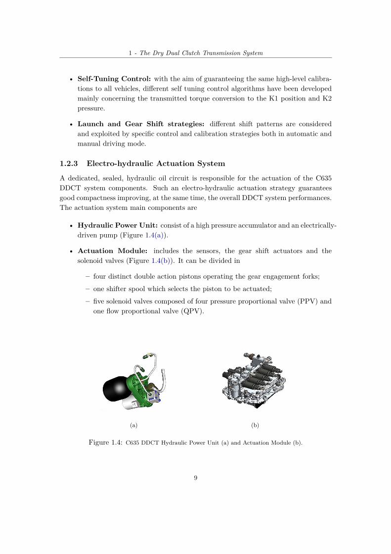
A dedicated, sealed, hydraulic oil circuit is responsible for the actuation of the C635DDCT system components. Such an electro-hydraulic actuation strategy guaranteesgood compactness improving, at the same time, the overall DDCT system performances.The actuation system main components are
• Hydraulic Power Unit: consist of a high pressure accumulator and an electrically-driven pump (Figure 1.4(a)).
• Actuation Module: includes the sensors, the gear shift actuators and thesolenoid valves (Figure 1.4(b)). It can be divided in
– four distinct double action pistons operating the gear engagement forks;
– one shifter spool which selects the piston to be actuated;
– five solenoid valves composed of four pressure proportional valve (PPV) andone flow proportional valve (QPV).
(a)
(b)
Figure 1.4: C635 DDCT Hydraulic Power Unit (a) and Actuation Module (b).
9

1 - The Dry Dual Clutch Transmission System
Specifically, as far as the Actuation Module is concerned, two PPVs are related tothe the gear engagement, while the third commands the spool valve that selects theassociated piston. Finally, the clutches K2 and K1 are, respectively, controlled by thefourth PPV and the QPV.
Different contact-less position sensor are also included in the C635 Actuation Mod-ule, one for each engagement piston and one for the shifter pool. One pressure sensoris related to the K2 clutch control system and one exploits monitoring functions.
The overall hydraulic circuit of the C635 DDCT Actuation System is showed inFigure 1.5 below.
Figure 1.5: C635 DDCT complete actuation circuit.
10

1 - The Dry Dual Clutch Transmission System
1.3 The C635 even gear Actuator
Referring to the whole actuation module described in section 1.2.3, the fourth pro-portional pressure control valve (PPV), associated with the K2 Clutch, is speciallyconsidered here. The choice is motivated by the aim of this thesis project, that is todevelop a control strategy for the even gear actuator of the C635 DDCT system.
In this regard, the basic physical properties are described along with the PPV generalstructure and components. Finally, control objectives and requirements of this thesiswork are presented.
1.3.1 Essential elements of Proportional Pressure Control Valves
As already mentioned in section 1.2.3, the K2 Clutch, associated with the even gearengagement, is controlled by a proportional control valve. Specifically, these kind ofelectro-hydraulic valves can be considered as a trade-off between the cheaper solenoidvalves and the outperforming servo valves in the sense that they preserve low manu-facturing costs with the only drawback of a slight performance worsening. Anyway,PPVs provide an economical and satisfactory alternative for many applications and aretherefore commonly employed in transmission systems.
The K2 Actuator working principle is essentially based on the mechanical forces de-riving from magnetic interactions. That is, a proper solenoid is able to exert an outputforce, hence an output pressure, that is related to the current flowing through its wires.The reason behind the choice of a current based PPV, is to reduce temperature leakagesassociated with a voltage control system so that the overall efficiency is preserved.
The general configuration of a PPV is showed in Figure 1.6 below.
controlled flow
solenoid
supply
controlspring
Figure 1.6: Schematic section of a PPV.
11

1 - The Dry Dual Clutch Transmission System
The output pressure is regulated by controlling the flow of the hydraulic fluid throughthe orifice of the PPV. More precisely, the valve spool is seated between a compressionspring and a proportional solenoid. In this way, the orifice size is controlled via thespring deflection by modifying the mechanical force produced by the solenoid and re-lated to the input current. This strategy leads to an almost proportional relationshipbetween the valve output pressure and the input current flowing through the solenoid.
Concerning the possible drawbacks associated with these PPVs, overlapped spoolshave to be used because of the difficulties in producing a zero lap spool. This meansthat no output pressure is obtained until the input current exceeds a proper value thatis required to overcome the spring pre-load and the spool overlap. Figure 1.7 graphicallyexpress this aspect by showing the dead zone that is present between the input currentand the output pressure.
dead zone
Input Current (mA)
Out
put
Pres
sure
(bar
)
Figure 1.7: Pressure current characteristic of a PPV.
Another important feature of proportional pressure valves is the hysteresis effect.In fact, depending on whether the current is increasing or decreasing, a considerabledifference in the valve output pressure takes place. This is because the valve relies onthe force exerted by the solenoid acting against the spring to move the spool.
Both the dead zone and the hysteresis are crucial aspects in regard to the even gearactuator control strategy. The former is specifically accounted by one of the proposedcontrol strategies (details in section 3.2.1), the latter is treated in [1].
12

1 - The Dry Dual Clutch Transmission System
1.3.2 K2 Actuator position control objectives
With the aim of improving driving comfort and guaranteeing a smooth gear shift process,a position control strategy for the even gear actuator is proposed in this thesis work.Different position reference trajectories have been considered and the tracking problemhas been addressed by accounting the following performance requirements, provided byCentro Ricerche Fiat (CRF).
• Position Overshoot: s ≤ 5%
• Rise Time: 50 ≤ tr ≤ 120 ms
• Steady State Error for step reference: |e∞r | ∼= 0
• Input Current: 0 ≤ Icmd ≤ 1000 mA
• Pressure: 0 ≤ p ≤ 40 bar
In the following Chapters, different control architectures and model identificationapproaches are proposed to develop an efficient position controller for the K2 Actuator.
13

Chapter 2Adaptive Model Predictive Control forK2 Actuator
T he main purpose of this chapter is to provide a compact overview of the essentialelements of model predictive control (MPC) along with its application to the K2
Actuator Control problem.
2.1 MPC Overview
Control systems based on the MPC concept have gained popularity in a wide range ofapplications in different engineering fields due to their ability to yield high performancecontrol systems together with the facility of flexible constraints handling.These peculiarities are conditioned by explicitly considering the model of the system toobtain the control action as a result of a constrained optimization problem. A numericaloptimization problem has to be solved at each sampling time and the computationaleffort is consequently quite high. For this reason, originally, MPC was mainly employedfor systems with slow dynamics and large computational resources such as chemical oraerospace processes. However, in the last years, significant improvements of micropro-cessors and computer power allowed Model predictive control to be applied in fastersystem like mechatronic and automotive applications.
Model predictive control has its roots in optimal control. The key idea of MPC isto use a mathematical model to forecast the system behavior, in order to determine thebest control actions to apply over some period as a result of a constrained optimizationproblem [10], [8].The MPC architecture is composed of (see Figure 2.1)
14

2 - Adaptive Model Predictive Control for K2 Actuator
• the prediction model;
• the cost function and the constraints;
• the optimizer;
• the controlled system.
All these aspects will be discussed in the following sections of this chapter.
Optimizer System
Model
Prediction
Cost Function Constraints
MPC
Figure 2.1: General Scheme of Model Predictive Control
The most relevant benefits of exploiting MPC strategy can be outlined in
• The opportunity to explicitly include both control input and state variables con-straints;
• The capacity to manage multi-variable control problems;
• The possibility to trade off between different control objectives by tuning somecritical parameters.
15

2 - Adaptive Model Predictive Control for K2 Actuator
2.1.1 Prediction Model
Discrete time prediction models are often suitable if the considered system is sampledat discrete times. If the sampling rate is properly chosen, the behaviour between thesamples can be safely ignored and the model describes exclusively the behaviour at thesample times.
The more general representation for the prediction model is a non linear, time in-variant state space system of the following form
x(k + 1) = f(x(k), u(k)
)f ∈ C1
y(k) = g(x(k), u(k)
)g ∈ C1
(2.1)
where x(k) ∈ Rn is the state variable, y(k) ∈ Rp is the system output, u(k) ∈ Rm is thecontrol input.
Assuming that all the system state variables x(k) are measurable, the prediction ofthe model expressed in (2.1) consists in considering the states evolution from a timeinstant k over a certain number of time steps in the future.The length Hp of the finite optimization horizon is referred as prediction horizon.
In order to easily approximate and analyse physical systems, the prediction model(2.1) often consists in a Linear Time Invariant (LTI) discrete time system, described bythe following state space representation
x(k + 1) = Ax(k) +Bu(k)
y(k) = Cx(k)(2.2)
where A ∈ Rn,n, B ∈ Rn,m, C ∈ Rn,p.
For such a LTI System the ith step ahead state prediction x(k+i|k) can be expressedas
x(k + i|k) = Aix(k|k) +Ai−1Bu(k|k) +Ai−2Bu(k + 1|k) + · · ·+Bu(k + i− 1|k)
= Aix(k|k) +i−1∑j=0
Ai−j−1Bu(k + j|k).
(2.3)
Therefore, the prediction model (2.2) depends only on the current state x(k|k) and on
16

2 - Adaptive Model Predictive Control for K2 Actuator
the control sequence U(k) = [u(k|k) u(k + 1|k) ... u(k +Hp − 1|k)].
2.1.2 Cost Function and Optimization Problem
The MPC strategy is related to the minimization, over a specified finite predictionhorizon Hp, of a cost function whose general expression is
J(x(k|k), U(k)) = Φ(x(k +Hp|k)
)+
Hp−1∑i=0
L(x(k + i|k), u(k + i|k)
)(2.4)
where
- x(k|k) is the state measurement at current time k.
- x(k + i|k) is the ith step ahead state prediction.
- U(k) = [u(k|k) u(k + 1|k) ... u(k +Hp − 1|k)] is the command input sequence tobe optimized.
- L(·) is the per-stage weighting function.
- Φ(·) is the terminal state weighting function.
The weighting functions L(·) and Φ(·) are assumed to be continuous in their ar-guments and are considered as design parameters to be suitably chosen according tothe desired control performances.
Therefore, considering the generic non linear system expressed in (2.1), the con-strained finite time optimization problem assumes the following form
U∗ = argminU
J(x(k|k), U(k))
subject tox(k + 1) = f
(x(k), u(k)
)x(k + i|k) ∈ X , i = 1...Hp − 1
u(k + i|k) ∈ U , i = 1...Hp − 1
x(k +Hp|k) ∈ Xf
(2.5)
where
- X ∈ Rn and U ∈ Rm are polyhedra representing respectively the states and theinput constraints invariant sets (details in [10]).
17

2 - Adaptive Model Predictive Control for K2 Actuator
- Xf is the terminal polyhedral region introduced in the optimization problem toensure asymptotic stability (details in [19]).
- U∗(k) = [u∗(k|k) u∗(k + 1|k) ... u∗(k + Hp − 1|k)] is the optimal input controlsequence.
2.1.3 Control Input and State Constraints
The possibility to handle input and state constraints is the main quality that distin-guishes MPC from the standard linear quadratic (LQ) control.
For systems subject to external inputs such as (2.1) and (2.2), the two regions X ∈ Rn
and U ∈ Rm are referred as control invariant sets ( [10], [20], [3]). These two convexregions are useful to answer questions such as: Find the set of initial states for whichthere exists a controller such that the system constraints are never violated. For the sakeof simplicity, in the following it will be assumed that both X and U are reachable poly-tope containing the origin in their interior so they will be modeled as sets of inequalities.
Regarding control input constraints, the set U is usually chosen to take care of theactuator devices physical limitations. For this reason, input actuator saturationand slew rate constraints can be managed with the following formulation
Umin ≤ u(k + i|k) ≤ Umax, i = 1...Hp − 1
∆Umin ≤ u(k + i|k) ≤ ∆Umax, i = 1...Hp − 1(2.6)
where
- Umin and Umax are respectively the constraint vector associated with the mini-mum and maximum control input value.
- ∆Umin and ∆Umax are respectively the constraint vector associated with theminimum and maximum control input variation rate.
In order to clarify this aspect, a prediction horizon Hp = 2 is considered and thecontrol input vector becomes simply U(k) = [u(k|k) u(k + 1|k)]. The set of constraintson the control input value can be rewritten as
18

2 - Adaptive Model Predictive Control for K2 Actuator
umin ≤ u(k|k) ≤ umax
umin ≤ u(k + 1|k) ≤ umax⇒
[1 0
0 1
][u(k|k)
u(k + 1|k)
]≤
[umax
umax
][−1 0
0 −1
][u(k|k)
u(k + 1|k)
]≤
[umin
umin
]
⇒
[I
−I
]| {z }LUv
[u(k|k)
u(k + 1|k)
]≤
umax
umax
umin
umin
| {z }
WUv
⇒ LUvU(k) ≤ WUv (2.7)
In a similar way the matrix inequalities for the slew rate constraints are obtained inthe following form
LUsrU(k) ≤ WUsr (2.8)
Therefore, combining (2.7) and (2.8) the overall input actuator constraints of theform (2.6) can be rearranged as
LUU(k) ≤ WU (2.9)
As to the state constraints, the set X is often related to the performance require-ments. More precisely state constraints are useful to impose limitations on outputvariables e.g. to mitigate overshoots or inverse behaviour in the system response. Stateconstraints can be managed with the same above formulation
xmin ≤ x(k + i|k) ≤ xmax, i = k...Hp (2.10)
where xmin and xmax are respectively the constraint vector associated with the mini-mum and maximum value of each state.
Considering the LTI prediction model (2.2) the state constraints can be expressedas linear constraints in U(k). In fact, choosing again a prediction horizon Hp = 2, thestate boundaries are
Lx1x(k + 1|k) ≤ Wx1
Lx2x(k + 2|k) ≤ Wx2
⇒Lx1
(Ax(k|k) +Bu(k|k)
)≤ Wx1
Lx2
(A2x(k|k) +ABu(k|k) +Bu(k + 1|k)
)≤ Wx1
19

2 - Adaptive Model Predictive Control for K2 Actuator
where the step ahead prediction state expression (2.3) has been applied. Further, theabove expression of the state constraints can be written as a linear matrix inequality inU(k)
LxU(k) ≤ Wx (2.11)
where
Lx =
[Lx1 0
0 Lx2
][B 0
AB B
]
Wx =
[−Lx1 0
0 −Lx2
][A
A2
]x(k|k) +
[Wx1
Wx2
] (2.12)
2.1.4 Quadratic Programming
As discussed in section 2.1 Model Predictive Control strategy is based on solving a con-strained optimization problem related to the minimization of a cost function. Therefore,a suitable choice for the weighting functions L(·) and Φ(·) expressed in (2.4) guaranteean efficient set up for the MPC control problem.For instance, for output or states regulations, the following quadratic form is commonlychosen
L(·) = x(k + i|k)TQx(k + i|k) + u(k + i|k)TRu(k + i|k), i = 0...Hp − 1
Φ(·) = x(k +Hp|k)TPx(k +Hp|k)
where Q ⪰ 0, P ⪰ 0 and R ≻ 0 are symmetric weighting matrices to consider astunable design parameters to reach the control objectives.
By substituting the above weighting functions in (2.4), the cost function to be min-imized in the MPC optimization problem can be rewritten as
J(x(k|k), U(k)) = x(k +Hp|k)TPx(k +Hp|k) +Hp−1∑i=0
(x(k + i|k)TQx(k + i|k)
+ u(k + i|k)TRu(k + i|k)) (2.13)
An optimization problem is called quadratic program (QP) if the constraint functions
20

2 - Adaptive Model Predictive Control for K2 Actuator
are affine and the cost function is a convex quadratic function ([10], [13]).
In order to show that the just presented cost function (2.13) is quadratic with re-spect to the optimization variable U(k), the LTI System (2.2) is considered as predic-tion model. Recalling the equation (2.3), the vector of the predicted states X(k) =
[x(k|k) x(k + 1|k) ... x(k +Hp − 1|k)] can be written as
X(k) = AX(k) + BU(k) (2.14)
where
A =
A
A2
...AHp
∈ Rn·Hp×n, B =
B 0 · · · 0
AB. . . . . . ...
... . . . . . . ...AHp−1B · · · · · · B
∈ Rn·Hp×Hp
and by defining also the weighting matrices
Q =
Q 0 · · · 0
0. . . . . . ...
... . . . Q...
0 · · · 0 P
∈ Rn·Hp×n·Hp , R =
R 0 · · · 0
0. . . . . . ...
... . . . R...
0 · · · 0 R
∈ Rm·Hp×m·Hp
the cost function (2.13) assumes the following compact matrix form
J(x(k|k), U(k)) = X(k)TQX(k) + U(k)TRU(k) (2.15)
After some mathematical manipulations and substituting the (2.14) in (2.15), sucha quadratic form of the cost function is obtained
J(x(k|k), U(k)) =1
2U(k)THU(k) + x(k)TFU(k) + J (2.16)
where
- H = 2(BTQB +R) ≻ 0 is the Hessian of the quadratic form.
- F = 2ATQB is the mixed term of the quadratic form.
21

2 - Adaptive Model Predictive Control for K2 Actuator
- J = x(k)TATQAx(k) is the vertical offset of the quadratic form.
Regarding the affinity of the constraint function, the expression (2.6) of the inputconstraints and (2.11) of the state constraints can be combined in the following singleset of linear constraints
LU(k) ≤ W (2.17)
where L = [LxLU ] and W = [WxWU ].
In conclusion, the MPC constrained optimization problem (2.5) can be expressed asa QP.
U∗ = argminU
(12U(k)THU(k) + x(k)TFU(k) + J
)subject to LU(k) ≤ W
(2.18)
The just expressed formulation ensure the convexity of the QP problem, therefore theunique optimal solution can be efficiently computed by different numerical algorithmssuch as
- "active" set algorithms [4], [11], [22].
- "primal-dual" interior point algorithms [4], [22].
Moreover, new algorithms have been recently introduced improving the MPC onlinecomputation. Some of these method are
- the partial enumerator methodology [4], [19].
- the modified active set method [11].
- the approximate primal barrier method [28].
2.1.5 Receding Horizon Control
The solution of the finite horizon QP (2.18) results in an optimal control move U∗(k) =
[u∗(k|k)... u∗(k+Hp−1|k)] which starts at current time t = k and ends at t = k+Hp−1.The application of this sequence over the time interval [t, t+Hp] gives rise to an open loopcontrol strategy. However, it is well known that modeling errors, parameter uncertain-ties or disturbances may lead to poor control performances with an open loop technique.
22

2 - Adaptive Model Predictive Control for K2 Actuator
To overcome such a drawback, a feedback control action can be obtained through theReceding Horizon (RH) principle. An infinite horizon sub-optimal controller is designedby repeatedly solving finite time optimal control problems in a receding horizon fashionas described next.
t t+ 1 t+Hc t+Hp
reference
u(t+ k)
predicted outputs y(t+ k|t)
t+ 1 t+ 2 t+ 1 +Hc t+ 1 +Hp
predicted outputs y(t+ k + 1|t+ 1)
u(t+ k + 1)
Figure 2.2: Receding Horizon Principle
Starting at current time t = k, the following open-loop optimal control problem issolved over a finite horizon (top graph in Figure 2.2)
minUt→t+Hc|tJt(x(t), Ut→t+Hc|t)
subject to LUt→t+Hc|t ≤ W(2.19)
where Ut→t+Hc|t = [ut|t, · · · , ut+Hc−1|t] is the reduced number of input sequence. Thechosen Hc ≤ Hp, referred as Control Horizon, is often used to reduce the numberof variables involved in the optimization problem in order to tone down the com-putational effort. In case Hc < Hp, the remaining Hp − Hc control input sequence[ut+Hc|t, · · · , ut+Hp−1|t], needed to evaluate the state prediction until the time t = Hp,can be chosen as
- u(k + i|k) = 0 with Hc ≤ i ≤ Hp − 1.
- u(k + i|k) = u(k +Hc|k) with Hc ≤ i ≤ Hp − 1.
Let U∗t→t+Hc|t = [u∗t|t, · · · , u
∗t+Hc−1|t] be the optimal solution of (2.19) at time t. Then,
the Receding Horizon strategy can be explained by the following iterative procedure
23

2 - Adaptive Model Predictive Control for K2 Actuator
I) only the first element u∗t|t is applied as control action to the system during thesampling interval [t, t+ 1].
II) At the next time step t + 1 a new optimal control problem (2.19) based on newmeasurements of the state x(t+1) is solved over a shifted horizon (bottom graphin Figure 2.2).
The resulting Receding Horizon Controller (RHC) evaluates, at each sampling time, anoptimal control input which depends only on the current state x(k). The computedcontrol input at time t = k can be expressed as
u∗(k) = u∗(k|k) = u∗(x(k|k)
)= u∗
(x(k)
)(2.20)
Moreover, since in the considered optimization problem (2.19) either the system ei-ther the constraints and the cost function are time invariant, also the solution (2.20) isa time invariant function of the state. That is, the RHC implicitly defines a non-lineartime invariant static state feedback control law of the form u(k) = K
(x(k)
).
xk+1 = Axk +Buk
K(x(k)
)
QP[I 0 · · · 0]
x(k)
xk|kuk|k
u∗k|k...
u∗k+Hc−1|k]
u(k)
K(x(k)
)
Figure 2.3: General Scheme of RH controller as a solution of the QP
In conclusion, a receding horizon controller where the finite time optimal control lawis computed by solving a QP problem on-line is usually referred as Model PredictiveControl (MPC). Figure 2.3 resumes the MPC strategy.
24

2 - Adaptive Model Predictive Control for K2 Actuator
2.2 Adaptive MPC Principles
In the previous section 2.1 the general set up of the MPC strategy has been discussed.In particular, it has been highlighted how the optimal control law is strongly related tothe model parameters as well as to the imposed constraints.
Adaptive Control covers a set of techniques based on a real time adjustment ofthe controller parameters, in order to maintain a desired level of control systemperformance despite the plant dynamic model parameters are changing in time.At each sampling time, a suitable on-line estimator updates the model parameters onthe basis of the collected data and the MPC control law is consequently adjusted in realtime yielding a closed loop tuning procedure [17].
MPC Controller Plant
Online Estimator
θ
u y
Figure 2.4: General Scheme of an Adaptive MPC Control System
The Adaptive MPC idea, as generally displayed in the Figure 2.4 above, is based onthe following procedure
I) Collect the Plant input u(k) and output y(k) measurements.
II) Estimate the plant dynamic model parameters θ(k) in real time using a suitableestimator algorithm.
III) Adjust the MPC optimal control law by updating, with the real time estimateθ(k), the state space representation of the plant prediction model.
The effectiveness of the just presented Adaptive MPC control strategy occurs in aparticular way when dealing with non-linear systems or with systems whose behaviouris strongly influenced by the working point.Recursive least square (RLS) is a common estimator to be employed for estimating
25

2 - Adaptive Model Predictive Control for K2 Actuator
the system parameters in real time. The RLS is fundamentally based on solving aLeast Square estimation problem in a recursive fashion. For this reason, in the nextparagraphs the main conceptual aspects of the Least Square criterion will be highlightedand the RLS estimation algorithms will be presented.
2.2.1 Least Square Method
The Least Square method has its roots in the linear regression problem i.e.the problemof finding the values of n real parameters θ1, ..., θn such that the sum of the squares ofthe differences between the output y(k) of the plant and the output y(k) of the predic-tion model is minimized [27].
Considering for the Plant model the equation error or ARX model structure, theinput-output relationship can be described by the following difference equation
y(k) + a1y(k − 1) + ...+ anay(k − na) =b0u(k + na − nb) + b1u(k + na − nb − 1)+
...+ bnbu(k − nb) + e(k)
where
- y(k)...y(k − na) are the collected output measurements for k = 1, 2 ...N .
- u(k + na − nb)...u(k − nb) are the collected input measurements for k = 1, 2 ...N .
- e(k) is a white noise term entering the process for k = 1, 2 ...N .
In discrete-time domain
Y (z) =B(z)
A(z)+H(z)E(z) (2.21)
where
B(z) = b0 + b1z−1 + b2z
−2 + ...+ bnbz−nb
A(z) = 1 + a1z−1 + a2z
−2 + ...+ anaz−na
H(z) =1
A(z)
In order to evaluate the prediction error norm ∥y(k)− y(k)∥2 the ARX model ex-pression (2.21) need to be written in prediction form
Y (z) =
(1− 1
H(z)
)Y (z) +
G(z)
H(z)U(z) =
(1−A(z)
)Y (z) +B(z)U(z) (2.22)
26

2 - Adaptive Model Predictive Control for K2 Actuator
which leads to the following difference equation for the predicted output
y(k) = −a1y(k− 1)− ...− anay(k−na)+ b0u(k+na −nb)+ ...+ bnbu(k−nb) = φT (k)θ
(2.23)where
- φT (k) = [−y(k− 1) ... − y(k− na) u(k+ na − nb) ... u(k− nb)] is the regressionvector.
- θ = [a1 a2 ... ana b0 b1 ... bnb] are the model parameters to be identified.
Finally, the quadratic optimality criterion related to the Least Square problem canbe written as
JN (θ) =1
N
N∑k=1
(y(k)− φT (k)θ
)2 (2.24)
and the unique optimal parameter vector θLS is given by
θLS = arg minθ∈Rna+nb
(JN (θ)
)=
N∑k=1
(φ(k)φT (k)
)−1
·N∑k=1
φ(k)y(k) (2.25)
2.2.2 Recursive Least Square
The Recursive Least Square estimation method is based on minimizing the one-step pre-diction error in a recursive fashion on the basis of the previously acquired input-outputdata [25].
The least square estimate solution (2.25) at a generic time instant t is considered
θt =t∑
k=1
(φ(k)φT (k)
)−1
| {z }S(t)−1
·t∑
k=1
φ(k)y(k) = S(t)−1t∑
k=1
φ(k)y(k)
where
S(t) =t∑
k=1
φ(k)φT (k) = S(t− 1) + φ(t)φT (t)
27

2 - Adaptive Model Predictive Control for K2 Actuator
After some manipulations the general structure of the RLS algorithm can be writtenas
θt = θt−1 + S(t)−1φ(t)| {z }K(t)
(y(t)− φT (t)θt−1
)| {z }ϵ(t)
= θt−1 +K(t)ϵ(t) (2.26)
where
- θt−1 is the old parameter vector.
- K(t) is a gain term related to the new parameters sensitivity with respect to theold parameters estimate.
- ϵ(t) is the prediction error.
As highlighted by the above equation (2.26), the RLS procedure is mainly performedby updating the old parameter vector estimate θt−1 with a correction term related tothe actual prediction error ϵ(t). In this sense, the gain term K(t) can be seen as aweighting function which decides how much the new parameters are influenced eitherby the previous parameters estimate or by the new measurements.
Different forms of the gain term K(t) are associated with the following estimationalgorithms
- Unnormalized and Normalized Gradient.
- Forgetting Factor.
- Kalman Filter.
Among the just exposed procedures the most commonly used is the NormalizedGradient Algorithm. This method is capable of guaranteeing good performances interms of parameters estimation preserving the system stability thanks to the normal-ization term.
More precisely, the gain term K(t) is evaluated through the ratio between an adap-tation factor γ and the norm of the regression vector φ(t), as expressed by the followingequation
K(t) =γ
∥φ(t)∥2 + εφ(t) (2.27)
where
28

2 - Adaptive Model Predictive Control for K2 Actuator
- 0 ≤ γ ≤ 1 is the adaptation factor related to the parameters sensitivity withrespect to the variations of the plant dynamics.
- ∥φ(t)∥2 is the normalization term that maintains the system stability.
- ε is a small bias term that prevents sudden jumps in the gain term value whenthe normalization term is almost null.
In conclusion, collecting the expressions (2.26) and (2.27), the RLS iterative proce-dure can be resumed as
I) Collect the Plant input u(k) and output y(k) measurements.
II) Build the regression vector φ(t).
III) Evaluate the gain term K(t) according to (2.27).
IV) Evaluate the prediction error ϵ(t).
V) Update the old parameter vector θt−1 according to (2.26).
29

2 - Adaptive Model Predictive Control for K2 Actuator
2.3 Adaptive MPC for K2 Actuator
In the previous sections 2.1 and 2.2 the main conceptual aspects of the Adaptive ModelPredictive control technique have been discussed. In the following, the practical appli-cation to the K2 Actuator position control will be exploited.
The goal of the project is to control the proportional pressure valve (PPV) thatactuates the K2 Clutch for the even gears. As long as the K2 Actuator is concerned,the output variables are the pressure valve p and the clutch position Xcsc whereas theonly control input variable is the actuation current Icmd that should be provided by thecontroller in such a way that the position tracking error is minimized.
MPC Controller K2 ActuatorIcmd
Xrefcsc
Xcsc
p
Figure 2.5: General Overview of the MPC position control for the K2 Actuator
Assuming that an ideal position measurement is available, a model predictive controlarchitecture has been developed (general scheme in Figure 2.5).
MPC is a particularly suitable control strategy to handle such a problem because itis capable to manage different objectives even taking into account the physical limits ofthe K2 Actuator, including its saturation constraint in the control computation.
2.3.1 K2 Actuator linear model Identification
As discussed in section 2.1, the chosen MPC strategy needs a mathematical model ofthe plant to control, so the K2 Actuator dynamics has been identified on the basis ofthe measured data provided by Centro Ricerche Fiat (CRF).
The relationship between the input current Icmd and the output position Xcsc isrepresented by a first order model described by the following LTI discrete time transferfunction
G(z) =β
z + α=
Y (z)
U(z)(2.28)
30

2 - Adaptive Model Predictive Control for K2 Actuator
where Y = Xcsc and U = Icmd.
The identification of the model parameters α and β has been performed throughMATLAB System Identification Toolbox. Different strategies have been adopted asdescribed next.
Single linear model
The K2 Actuator dynamics has been preliminarily considered as a single linear modelof the form (2.28).A single data set, composed by eighteen different ascending position steps, has beenused both for identifying the K2 Actuator and for validating the identified model.
From now on, the presented Figures, as well as the physical variables numerical data,will be normalized with respect to their maximum value.
0 100 200 300 400 500 6000
0.1
0.2
0.3
0.4
0.5
0.6
0.7
0.8
0.9
1
Figure 2.6: Validation data set for single single linear model identification strategy.
Such an identification strategy shows the following results for the model parameters
α = −0.9828
β = 1.8208 · 10−4
As highlighted by Figure 2.6 above, it is quite evident that the estimated output isnot able to track the measured output data for the whole working conditions. This is
31

2 - Adaptive Model Predictive Control for K2 Actuator
because the Plant position responses are so variable in their static and dynamic proper-ties, with respect to the different working regions, that a single identified model is notenough to catch these variations.
For this reason, a local multiple identification has been exploited as described next.
Multiple linear model
On the basis of the K2 Actuator static and dynamic properties, the whole provideddata set, composed of eighteen ascending set points, has been previously divided in 4different position ranges as highlighted by Figure 2.7 below.
0 100 200 300 400 500 6000
0.1
0.2
0.3
0.4
0.5
0.6
0.7
0.8
0.9
1
Figure 2.7: Different position ranges highlighted on the given data set.
- Low Position Range: [8 - 21] %
- Medium - Low Position Range: [21 - 57] %
- Medium - High Position Range: [57 - 85] %
- High Position Range: [85 - 100] %
For each of the chosen position region, a single linear model of the form (2.28) hasbeen identified. More precisely, the local identification has been performed considering
32

2 - Adaptive Model Predictive Control for K2 Actuator
as output data the corresponding position responses when the K2 Actuator Plant re-ceives as input a suitable input current.
The static and dynamic properties in the different position ranges are resumed inthe following table.
Range (%) DC Gain(mm
A)
β α
8 to 21 0.73 ≤ KDC ≤ 5 2.6962 · 10−6 −0.999721 to 57 6.2 ≤ KDC ≤ 7.96 4.6775 · 10−5 −0.996457 to 85 8.29 ≤ KDC ≤ 8.64 1.1522 · 10−4 −0.986585 to 100 7.23 ≤ KDC ≤ 8.05 2.3719 · 10−4 −0.9740
Table 2.1: System parameters in the different working regions.
As highlighted in Table 2.1, high position ranges are related to fast position re-sponses whereas small position ranges correspond to slow system dynamics. That is,the model behaviour is highly variable with respect to the operating range.
For the above considerations, a recursive estimation strategy has been exploited inorder to have an adaptive Model Predictive Controller designed on the basis of a realtime varying state representation of the system.
Recursive Estimation
The parameters α and β, related to the first order model describing the K2 Actuatordynamics, are estimated in real time through a recursive Least Square method on thebasis of the collected current Icmd and position Xcsc measurements.
Recalling the expression (2.21) for the ARX model structure, the K2 Actuator inputoutput relationship can be written in the following form
G(z−1) =βz−1
1 + αz−1=
Y (z−1)
U(z−1)(2.29)
where Y = Xcsc and U = Icmd.
In time domain
Xcsc(t) = −αXcsc(t− 1) + βIcmd(t− 1) = φT (t) θ
33

2 - Adaptive Model Predictive Control for K2 Actuator
where
- φT (t) = [−Xcsc(t− 1) Icmd(t− 1)] is the regression vector.
- θ = [α β] are the model parameters to be identified.
As previously discussed in section 2.2.2, the parameters recursive estimation is basedon the normalized gradient algorithm. The overall recursive equation can be written as
θt = θt−1 +γ
∥φ(t)∥2 + εφ(t)ϵ(t) (2.30)
Tuning and implementation details are discussed in section 2.4.
2.3.2 Observer for non measurable disturbance
The identification results, discussed in section 2.3.1, have brought out some importantaspects related to the K2 Actuator system dynamics.
Especially in the low position ranges, when the system response is much slower, astatic non-linear effect takes places due to the dead-zone relating the input current andthe position of the clutch. This non-linearity, together with other internal physical effectinducing a mismatch from the nominal linear model (2.28), can be taken into accountwith a non measurable disturbance seen by the controller as an extra state variable.In the MPC control architecture this can be exploited by means of a state Observer ableof providing the controller the disturbance estimate needed for the prediction yieldingan implicit feed-forward action in the control architecture.
The main idea of the state Observer is to use the actual position Xcsc and currentIcmd measurements in order to provide the state estimate x = [Xcsc d]. The observergeneral structure is resumed in Figure 2.8 below.
K2 Actuator
State Observerx
Icmd Xcsc
Figure 2.8: General Scheme of the State Observer.
34

2 - Adaptive Model Predictive Control for K2 Actuator
The state observer dynamics can be associated to a MISO system according to thefollowing state equations
x(k + 1) = Aobsx(k) +Bobsu(k)
y(k) = Cobsx(k)(2.31)
where
- u(k) = [Xcsc(k) Icmd(k)] is the is the Observer input vector.
- Bobs = [Bred L], Aobs = Ared − LCred and Cobs = [1 0] are the observer statematrices.
The matrix L, referred as the Observer Gain, has been suitably chosen in order toensure the matrix Aobs asymptotic stability.
In particular, the Luenberger Observer has been adopted as state estimationstrategy and a suitable tuning for the observer convergence speed has been exploitedby means of a reasonable allocation of the gain matrix L eigenvalues.According to the dominant dynamics of the model (2.28) associated to the K2 Actuator,the following eigenvalues have been assigned
λobs1 = 0.5
λobs2 = 0.05(2.32)
2.3.3 Augmented prediction model
As discussed in section 2.1.1, the Model Predictive Control architecture is related to thestate-space representation of the system. In this case, the following LTI discrete timeform is adopted
x(k + 1) = Ax(k) +Bu(k)
y(k) = Cx(k)(2.33)
where x = Xcsc, u = Icmd, and A = −α, B = β, C = 1.
35

2 - Adaptive Model Predictive Control for K2 Actuator
Explicit integral Action
A standard approach to improve tracking performance for a constant reference and toreduce tracking errors even in presence of constant disturbances, is to use an explicitintegral action in the control architecture.
For the considered MPC strategy, the explicit integral action can be taken into con-sideration by adding in the prediction model (2.33) the integral of the tracking errorq(k) as an extra state variable.Therefore, the new state variable becomes x = [Xcsc Xref
csc q] and the augmented pre-diction model can be described by the following state equations
x(k + 1) = Ax(k) +Bu(k)
Xrefcsc (k + 1) = Xref
csc (k)
q(k + 1) = q(k)− TsCx(k) + TsXrefcsc (k)
(2.34)
where Ts = 0.002 s.
In matrix form
x(k + 1) =
A 0 0
0 1 0
−TsC Ts 1
x(k) +
B00
u(k)
y(k) =[C 0 0
]x(k)
(2.35)
Implicit integral Action
In the MPC architecture the control input variation ∆u can be considered as optimiza-tion variable for the QP problem. This is another method to include an integral actionin the control formulation and it can even give further improvements to the Systemresponse. In particular, by tightening the control input variations the transient oscilla-tions can be reduced by means of a smooth control action.
In this context, implicit integral action is exploited by considering the previouscontrol input value u(k−1) as an extra state variable. Therefore, the new state variablebecomes x = [Xcsc Icmd(k − 1)] and the augmented prediction model can be describedby the following state equations
36

2 - Adaptive Model Predictive Control for K2 Actuator
x(k + 1) = Ax(k) +Bu(k)
∆u(k) = u(k)− u(k − 1)(2.36)
In matrix form
x(k + 1) =
[A B
0 1
]x(k) +
[B
1
]∆u(k)
y(k) =[C 0
]x(k)
(2.37)
In conclusion, taking into account the equations (2.34) and (2.36), and considering,for the sake of simplicity, a constant additive disturbance d(k + 1) = d(k), the overallaugmented prediction model for the K2 Actuator is described by the following stateequations
x(k + 1) = Ax(k) +Bu(k) +Bdd(k)
u(k) = u(k − 1) + ∆u(k)
d(k + 1) = d(k)
Xrefcsc (k + 1) = Xref
csc (k)
q(k + 1) = q(k)− TsCx(k) + TsXrefcsc (k)
(2.38)
where x = Xcsc, u = Icmd, and A = −α, Bd = B = β, C = 1.
In matrix form
x(k + 1)
u(k)
d(k + 1)
Xrefcsc (k + 1)
q(k + 1)
=
A B Bd 0 0
0 1 0 0 0
0 0 1 0 0
0 0 0 1 0
−TsC 0 0 Ts 1
| {z }
A
x(k)
u(k − 1)
d(k)
Xrefcsc (k)
q(k)
| {z }
x
+
B
1
0
0
0
| {z }
B
∆u(k)
y(k) =[C 0 0 0 0
]| {z }
C
x(k)
(2.39)
37

2 - Adaptive Model Predictive Control for K2 Actuator
where
- x(k) is the augmented state variable.
- A, B and C are the augmented state matrices.
The general control architecture of the adaptive MPC position control for the K2 Ac-tuator is resumed in Figure 2.9 below.
∑ MPCController
∑K2 Actuator
Observer
Recursive ParametersEstimation
z−1
Xrefcsc
Xcsc(k)
Icmd(k)θ(k)
d
Icmd(k)
Icmd(k − 1)
q(k) ∆Icmd
p
Xcsc
Xcsc
−
Figure 2.9: Adaptive MPC position control architecture for K2 Actuator.
2.3.4 Cost Function and Optimization Problem for K2 Actuator
As already mentioned in section 2.1.5, the MPC optimal control law is computed bysolving the QP problem (2.18) on-line and by applying the Receding Horizon Principle.For this reason, the choice of a suitable cost function is crucial for the MPC set up.
38

2 - Adaptive Model Predictive Control for K2 Actuator
In particular, the quadratic form (2.13) is selected and a proper weights and con-straints design has been performed in order to guarantee the position reference Xref
csc
tracking without any steady state offset and the input current Icmd oscillations attenu-ation in the K2 Actuator.Therefore, considering the K2 Actuator augmented prediction model (2.39), the justmentioned control objectives can be fulfilled by expressing the cost function in the fol-lowing tracking form
J(x(k|k),∆Icmd(k)) =
Hp−1∑i=0
Qy(Xcsc(k + i|k)−Xrefcsc (k + i|k)
)2+R∆I2cmd(k + i|k)+
+Qqq2(k + i|k)
(2.40)
where
- Qy is the scalar weight for the position tracking.
- R is the scalar weight for the command input variation ∆Icmd.
- Qq is the scalar weight for the integral state q(k) .
Such a tracking problem has been treated as a regulation problem through the costfunction below
JK2(x(k|k),∆Icmd(k)) =
Hp−1∑i=0
(x(k + i|k)T Q x(k + i|k) + R∆I2cmd(k + i|k)
)(2.41)
where
Q =
Qy 0 0 −Qy 0
0 0 0 0 0
0 0 0 0 0
−Qy 0 0 Qy 0
0 0 0 0 Qq
Note that, in order to regulate the tracking error to zero and to add an explicit
integral action in the control formulation, the weights Qy and Qq are introduced in theproper positions with respect to the augmented state vector x(k) = [Xcsc(k) Icmd(k −1) d(k) Xref
csc (k) q(k)].The just mentioned weighting factors Qy, Qq and R are MPC project parameters that
39

2 - Adaptive Model Predictive Control for K2 Actuator
have to be suitably chosen in order to perform the desired control action. Tuning andimplementation details are discussed in section 2.4.
Once defined the proper cost function, the complete MPC optimization problemformulation can be obtained by considering the control input and state constraints. Inthis context, only the input constraint due to the K2 Actuator physical limitation hasto be included.More precisely, the actuation current must remain inside the following range
0 ≤ Icmd ≤ 1000 mA (2.42)
Besides, the control input variation rate ∆Icmd has been bounded as well in orderto avoid sudden jumps in the control action.
− 800 ≤ ∆Icmd ≤ 800mATs
(2.43)
In conclusion, considering the just expressed linear inequalities, the augmented pre-diction model (2.39) and the cost function (2.41), the final expression of the QP problemfor the K2 Actuator is given by
∆I∗cmd = arg min∆Icmd
JK2(x(k|k),∆Icmd(k)),∆Icmd)
subject tox(k + 1) = Ax(k) + Bu(k)
− Icmd(k + i|k) ≤ 0, i = 1...Hp − 1
Icmd(k + i|k) ≤ 1000, i = 1...Hp − 1
−∆Icmd(k + i|k) ≤ 800, i = 1...Hp − 1
∆Icmd(k + i|k) ≤ 800, i = 1...Hp − 1
(2.44)
40

2 - Adaptive Model Predictive Control for K2 Actuator
2.4 MPC tuning and simulations results
The following section covers the MPC tuning procedure exploited to reach the bestperformance in the position control for the K2 Actuator.
Several simulation results using different position reference profiles will be presentedin order to show the effectiveness of the proposed MPC control strategy. In particular,the following position profiles, provided by CRF, reasonably represent the K2 Actuatorin different situations
- Slow Gear Change profile.
- Gear Change profile.
- Slow Ramp profile.
- Ramp profile.
- Stairs profile.
The tuning procedure of the Adaptive MPC controller is related to the choice ofthe prediction horizon Hp and the scalar weights Qy, Qq and R of the quadratic costfunction (2.40) reminded below
J(x(k|k),∆Icmd(k)) =
Hp−1∑i=0
Qy(Xcsc(k + i|k)−Xrefcsc (k + i|k)
)2+R∆I2cmd(k + i|k)+
+Qqq2(k + i|k)
Moreover, since in the proposed control architecture a recursive estimator (section2.2.2) provides a real time estimate of the model parameters, the adaptation gain γ canbe considered as tuning parameters as well.
In a preliminary design procedure, the prediction horizon Hp is selected to be suf-ficiently long with respect to the K2 Actuator dominant dynamics, while the controlhorizon Hc is assumed to be equal to Hp. The scalar weights Qy, Qq and R are orig-inally chosen in order to equally weight each term of the cost function. Afterwards,each coefficient has been properly tuned by means of a trial and error procedure untilsatisfactory control performances have been achieved.Such a trial and error procedure involves extensive simulation tests developed throughthe Multi-Parametric Toolbox 3.0 (MPT) [15]. The just named Toolbox guarantees a
41

2 - Adaptive Model Predictive Control for K2 Actuator
wide versatility in the MPC optimization problem formulation as well as a fully cus-tomizable way of handling input and state constraints.
The following design parameters values have been chosen to guarantee a satisfactorytrade-off between the performance requirements
R = 1
Qy = 1.3 · 103
Qq = 1
Hp = 31
γ = 0.005
θ(0) = [−0.9865 1.1522 · 10−4]
(2.45)
where θ(0) = [α0 β0] is the initial model parameters vector assumed to be inside themedium - high position range identified in section 2.3.1.
The proper values of the just expressed design parameters have been achievedthrough a suitable tuning procedure as described next.
2.4.1 Tuning of the MPC Prediction Horizon
From a computational point of view short prediction horizons are desirable, since thenumber of decision variables of the optimization problem is reduced. However, choos-ing a long prediction horizon induce intrinsic robustness in the control system and isrequired to achieve the desired closed-loop performances and to maintain the systemstability.
Figure 2.10 clarifies the above considerations by showing the influence of the pre-diction horizon variation in the position response when the other design parameters arekept constant as in (2.45).In the reported plot the value of the prediction horizon Hp is changed from Hp = 25 toHp = 40 in one between the different reference profiles. It is evident that a too smallprediction horizon is not able to handle the K2 Actuator dominant dynamics leading toposition oscillations in the system response. On the contrary, a long prediction horizonguarantees the system stability but also affects the response speed and the computa-tional effort as a side effect. Therefore, a prediction horizon Hp = 31 is selected.
42

2 - Adaptive Model Predictive Control for K2 Actuator
0 0.5 1 1.5 2 2.5 3 3.5 4 4.5 5 5.50
0.14
0.28
0.42
0.57
0.71
0.85
1
1.14
0.8 0.85 0.9 0.95 1 1.051.2
1.4
1.6
1.8
2
2.2
2.4
2.4 2.5 2.6 2.7 2.8 2.9 3
6.96
6.97
6.98
6.99
7
7.01
7.02
7.03
7.04
Figure 2.10: Position response with Gear shift reference profile adopting Adaptive MPC for differentvalues of Hp.
2.4.2 Tuning of the MPC Cost Function Weights
The tuning procedure of the cost function weighting matrices is a crucial aspect in theMPC control design since it allows to find a suitable trade-off between performancesand command activity.
Referring to the cost function (2.40), the scalar weights Qy, Qq and R have to beconsidered.
- The weight Qy is related to the tracking error minimization.
- The weight Qq gives penalty to the explicit integral action.
- The weight R is related to the command effort minimization.
Extensive simulations have been performed in which each of the three weights hasbeen individually changed while the other two are kept fixed . These tests have broughtout some important considerations about the MPC control law sensitiveness with re-spect to the single weight variation.
In practice, the MPC control action mainly depends on the ratio between theweights. More precisely, a scaling factor that affects all the weighting factor resultsin the same control action computed without scaling the weights.
43

2 - Adaptive Model Predictive Control for K2 Actuator
For the above considerations, both the input weight R and the integral action weightQq are chosen to be equal as in (2.45). However, the tuning procedure for the trackingweight Qy is reported in Figure 2.11 below.
0 0.5 1 1.5 2 2.5 3 3.5 4 4.5 5 5.50
0.14
0.28
0.42
0.57
0.71
0.85
1
1.14
0.4 0.45 0.5 0.55 0.6 0.65 0.7 0.75 0.8
1
1.2
1.4
1.6
1.8
2
2.2
2.5 2.6 2.7 2.8 2.9 36.98
6.99
7
7.01
7.02
7.03
Figure 2.11: Position response with slow Gear shift reference profile adopting Adaptive MPC fordifferent values of Qy.
It is evident that small values of the output weight Qy cause a slight worsening of theposition tracking performances. On the other hand a too high value increases excessivelythe system reactivity inducing oscillations in the transient. The value Qy = 1.3 · 103
has been chosen as a reasonable trade off between the control objectives.
2.4.3 Tuning of the RLS adaptation gain
As discussed in section 2.2.2, for the chosen adaptive MPC control strategy the adapta-tion gain γ of the recursive estimator is an important parameter that has to be accountedin the design procedure.The adaptation gain tuning allows to regulate the algorithm convergence speed but atthe same time it affects the output behaviour.
The optimal suggested approach to estimate in real time the K2 Actuator modelparameters is to use γ = 1 so that, whatever are the chosen initial conditions, thealgorithm converges to the actual system dynamics as soon as possible.However, several simulations results pointed out that the K2 Actuator system is really
44

2 - Adaptive Model Predictive Control for K2 Actuator
sensitive with respect to the model parameters variation so a small adaptation gainγ = 0.05, 0.005, 0.0005 should be chosen.
0 0.5 1 1.5 2 2.5 3 3.5 4 4.5 5 5.50
0.1
0.2
0.3
0.4
0.5
0.6
0.7
0.8
0.9
1
1.1
0.5 0.6 0.7 0.8 0.9 1
0.8
0.9
1
1.1
1.2
1.3
2.5 2.6 2.7 2.8 2.9 3
4.94
4.96
4.98
5
5.02
5.04
5.06
0 0.5 1 1.5 2 2.5 3 3.5 4 4.5 5 5.5
-0.986546
-0.986545
-0.986544
-0.986543
-0.986542
-0.986541
0 0.5 1 1.5 2 2.5 3 3.5 4 4.5 5 5.5
0.5
1
1.5
210-4
Figure 2.12: (Top) Position response and model parameters variation (Bottom) with Stairs referenceprofile adopting Adaptive MPC for different values of γ.
Figure 2.12 shows the effects of the adaptation gain γ variation on the position re-sponse and on the model parameters α and β. According to the above considerations,the value γ = 0.005 has been selected as adaptation gain of the recursive algorithm.
45

2 - Adaptive Model Predictive Control for K2 Actuator
In conclusion, an overall review of the adaptive MPC tuning procedure can be made.The most important project parameter is the prediction horizon Hp. In fact, choosinga short prediction horizon leads to system instability whereas a too long horizon causea significant performance worsening in terms of rise time. Instead, as long as the costfunction weighting matrices are concerned, they have been changed in order to havea more precise and finer tuning. In this sense, the fact that an excessive increase ofthe tracking weight Qy and of the integral action weight Qq makes the system moreaggressive, has been taken into account.
For the just discussed MPC controller (2.45) some transient and steady-state track-ing indices have been evaluated in the presence of different position reference profiles.Table 2.2 below resumes the obtained results.
Range (%) Overshoot (%) Rise Time (ms) Steady State Error (mm)
8 to 21 s ≤ 17 tr ≤ 70 ∼= 1 · 10−2
21 to 57 s ≤ 10 tr ≤ 60 ∼= 1 · 10−2
57 to 85 s ≤ 4 tr ≤ 60 ∼= 5 · 10−3
85 to 100 s ≤ 4 tr ≤ 80 ∼= 2 · 10−3
Table 2.2: Adaptive MPC controller performance resume with different reference profiles.
The chosen MPC parameters setting ensures quite satisfactory performance in termsof steady state tracking and rise time for all the identified position ranges. However, itis quite evident that the system response is characterized by a still too high overshoot,especially in low position ranges.
In order to improve the performance of the just described predictive controller, thedesign parameters have been dynamically tuned by means of a scheduling algorithmbased on the actual value of the position reference and the tracking error.
2.4.4 Scheduling Algorithm
As discussed in section 2.3.1, the K2 Actuator dynamics is strongly variable with respectto the position range. In such a non-linear system it is a reasonable approach to designa specific controller on the basis of the working point in order to maintain a desiredlevel of control system performance in all the tracking situations.
46

2 - Adaptive Model Predictive Control for K2 Actuator
The Gain Scheduling control strategy consists in a real time adjustment of the con-troller design parameters on the basis of the measurements of some relevant systemvariables. In this context, the Gain scheduling approach is exploited by a suitablescheduling algorithm.
The position reference Xrefcsc and the tracking error ecsc = Xref
csc − Xcsc have beenconsidered as input measurements whereas the prediction horizon Hp, the output weightQy and the control input variation rate ∆Icmd as the adjustable controller design pa-rameters. In the following the operations computed by the scheduling algorithm aredescribed (detailed MATLAB code in appendix)
1. MEASURE the reference Xrefcsc (k) and the tracking error ecsc(k) actual values.
2. CHECK the position range on the basis of Xrefcsc (k).
3. IF(ecsc(k) ≤ ecsc
)3.1 SET the prediction horizon Hp on the basis of the position range.
3.2 IF(ecsc(k) ≤ emin
csc
)INCREASE the output weight Qy and DECREASE the control inputvariation rate ∆Icmd.
3.3 ELSE
SET the output weight Qy and the control input variation rate ∆Icmd
on the basis of the position range.
4. IF(ecsc(k) > ecsc
)4.1 SET the prediction horizon Hp on the basis of the position range.
4.2 SET the output weight Qy = Qminy .
4.3 SET the control input variation rate ∆Icmd = ∆Imaxcmd .
where ecsc is a suitable threshold adopted to handle sudden variations in the positionreferences.
Referring to the above pseudo-code, the main aspects of the adopted scheduling al-gorithm can be clarified. The basic idea is to perform different tuning procedures on thecontroller design parameters with respect to the working region. More precisely, a largerprediction horizon Hp is needed when the system dynamics are slower, on the contrary,it can be decreased in the high position ranges where the system is characterized by
47

2 - Adaptive Model Predictive Control for K2 Actuator
a faster dynamics. Furthermore, in the neighbourhood of tracking error minima emincsc ,
the output weight Qy is increased and the constraint on ∆Icmd is tightened in orderto mitigate oscillations and guarantee good tracking performances without significantlydecreasing the response speed. The effectiveness of the just presented control strategyhas been tested by carrying out several simulations with different position referenceprofiles as illustrated in Figures 2.13, 2.14, 2.15, 2.16 and 2.17.
0 0.5 1 1.5 2 2.5 3 3.5 4 4.5 5 5.50
0.14
0.28
0.42
0.57
0.71
0.85
1
1.14ReferenceAdaptive MPC ControllerAdaptive scheduled MPC Controller
0 0.5 1 1.5 2 2.5 3 3.5 4 4.5 5 5.50
0.5
1
0.82 0.84 0.86 0.88 0.9 0.92 0.94 0.96 0.98 1
1.85
1.9
1.95
2
2.05
2.1
2.15
2.2
2.25
2.5 2.6 2.7 2.8 2.9 36.99
6.995
7
7.005
7.01
7.015
7.02
Figure 2.13: (Top) Position response and Input Current (Bottom) with Gear Change profile adoptingAdaptive MPC and Adaptive scheduled MPC.
A final comparison between the Adaptive MPC and the Adaptive scheduled MPCcontrol strategies can be made by evaluating both tracking and steady-state perfor-mances. Table 2.3 resumes the obtained results.
48

2 - Adaptive Model Predictive Control for K2 Actuator
0 0.5 1 1.5 2 2.5 3 3.5 4 4.5 5 5.50
0.14
0.28
0.42
0.57
0.71
0.85
1
1.14ReferenceAdaptive MPC ControllerAdaptive scheduled MPC Controller
0 0.5 1 1.5 2 2.5 3 3.5 4 4.5 5 5.50
0.5
1
0.55 0.6 0.65 0.7 0.75 0.81.9
1.95
2
2.05
2.1
2.15
2.2
2.5 2.6 2.7 2.8 2.9
6.99
6.995
7
7.005
7.01
7.015
Figure 2.14: (Top) Position response and Input Current (Bottom) with slow Gear Change referenceprofile adopting Adaptive MPC and Adaptive scheduled MPC.
0 0.5 1 1.5 2 2.5 3 3.5 4 4.5 50
0.16
0.33
0.5
0.66
0.83
1
1.16ReferenceAdaptive MPC ControllerAdaptive scheduled MPC Controller
0 0.5 1 1.5 2 2.5 3 3.5 4 4.5 50
0.5
1
1.05 1.1 1.15 1.2 1.250
0.5
1
1.5
2
3.82 3.84 3.86 3.88 3.9 3.92 3.943.5
3.6
3.7
3.8
3.9
4
Figure 2.15: (Top) Position response and Input Current (Bottom) with ramp reference profile adoptingAdaptive MPC and Adaptive scheduled MPC.
49

2 - Adaptive Model Predictive Control for K2 Actuator
0 1 2 3 4 5 6 7 8 9 100
0.16
0.33
0.5
0.66
0.83
1
1.16ReferenceAdaptive MPC ControllerAdaptive scheduled MPC Controller
0 1 2 3 4 5 6 7 8 9 100
0.5
1
0.05 0.1 0.15 0.2 0.25 0.3 0.35 0.4 0.45 0.50
0.1
0.2
0.3
0.4
0.5
0.6
6.75 6.8 6.85 6.9 6.953.6
3.65
3.7
3.75
3.8
3.85
3.9
Figure 2.16: (Top) Position response and Input Current (Bottom) with slow ramp reference profileadopting Adaptive MPC and Adaptive scheduled MPC.
0 0.5 1 1.5 2 2.5 3 3.5 4 4.5 5 5.50
0.2
0.4
0.6
0.8
1
1.2ReferenceAdaptive MPC ControllerAdaptive scheduled MPC Controller
0 0.5 1 1.5 2 2.5 3 3.5 4 4.5 5 5.50
0.5
1
0.5 0.55 0.6 0.65 0.7 0.75 0.8 0.85 0.9 0.95
0.9
0.95
1
1.05
1.1
1.15
3.55 3.6 3.65 3.7 3.75 3.8 3.85 3.9 3.95
2.85
2.9
2.95
3
3.05
3.1
Figure 2.17: (Top) Position response and Input Current (Bottom) with stairs reference profile adopt-ing Adaptive MPC and Adaptive scheduled MPC.
50

2 - Adaptive Model Predictive Control for K2 Actuator
Range (%)Overshoot (%) Rise Time (ms) Steady State Error (mm)
MPC 1st MPC 2nd MPC 1st MPC 2nd MPC 1st MPC 2nd
8 to 21 s ≤ 20 s ≤ 4 tr ≤ 70 tr ≤ 140 ∼= 1 · 10−2 ∼= 2 · 10−3
21 to 57 s ≤ 10 s ≤ 8 tr ≤ 60 tr ≤ 100 ∼= 1 · 10−2 ∼= 1 · 10−2
57 to 85 s ≤ 4 s ≤ 5 tr ≤ 60 tr ≤ 80 ∼= 5 · 10−3 ∼= 4 · 10−3
85 to 100 s ≤ 4 s ≤ 3 tr ≤ 80 tr ≤ 95 ∼= 2 · 10−3 ∼= 2 · 10−3
Table 2.3: Adaptive MPC (MPC 1st) and Adaptive scheduled MPC (MPC 2nd) controller performanceresume with different reference profiles.
Referring the above table, significant performance improvements, especially in lowposition ranges, are visible. The adopted Adaptive scheduled MPC control strategy isable to guarantee a smooth transient behaviour still maintaining the almost equal re-sponse speed. Besides, input current oscillations have been mitigated and a satisfactorysteady state tracking has been assured thanks to the dynamic tuning of the controllerdesign parameters.
As long as the computational effort is concerned, such design parameters (2.45) needquite high resources to compute in real time the optimal control action. This is mainlybecause a long prediction horizon is necessary to properly handle the K2 Actuatordominant dynamics.For this reason, a LQR control strategy has been considered in order to enhance thecomputational aspects. This approach allows to evaluate the optimal control action ina static state feedback form as the solution of an unconstrained optimization problem.In the following Chapter the detailed implementation of the LQR control strategy isexplained.
51

Chapter 3Adaptive Linear Quadratic Control forK2 Actuator
T his chapter will cover the main theoretical aspects of the Linear Quadratic Reg-ulator (LQR) control pointing out some relevant differences and similarities with
respect to the MPC technique discussed in Chapter 1. The LQR application to the K2Actuator position control problem will be exploited together with several simulationsresults. Moreover, a final section is devoted to the numerical implementation of theproposed LQ control strategy.
3.1 LQR Overview
Linear optimal control is a particular branch of optimal control. The plant to control isassumed to be modelled by a LTI transfer function while the controller that generatesthe optimal control move is constrained to be linear. Moreover, in linear optimal con-trol, the cost function adopted as performance index is quadratic either in the controlaction ether in the optimization variable. However, with this strategy, constraints on theinvolved variables are not accounted so an explicit saturation has to be exploited off-line.
Some advantages of the just presented linear optimal control can be outlined [2].
• In practice, all linear optimal control problems have readily computable solutionswhereas, on the contrary, many generic optimal control problems require highcomputational effort to obtain a usable solution.
• Linear optimal control may be also applied to non-linear systems operating in arestricted working region.
52

3 - Adaptive Linear Quadratic Control for K2 Actuator
• Linear optimal controller yield to possess some attractive properties such as goodgain margin,good phase margins and good tolerance of non-linearities.
• Linear optimal control is related to the same framework of the control problemsstudied via classical methods.
As previously mentioned, the LQR control architecture is related to the mathemati-cal description of the plant to control. For such a linear case, the following LTI discretetime model is considered
x(k + 1) = Ax(k) +Bu(k)
y(k) = Cx(k)(3.1)
where A ∈ Rn,n, B ∈ Rn,m, C ∈ Rn,p.
The associated performance index is the quadratic function defined over a finitehorizon of Hp steps
J(x(k), U(k)) = x(k +Hp)TPx(k +Hp) +
Hp−1∑i=0
(x(k + i)TQx(k + i)
+ u(k + i)TRu(k + i)) (3.2)
where Q ⪰ 0 and P ⪰ 0 are respectively the state and terminal state penalties whileR ≻ 0 is the input penalty. The LQR optimal control action U∗(k) = [u∗(k) u∗(k +
1) ... u∗(k +Hp − 1)] is obtained as the solution of the following optimization problem
U∗ = argminU
(J(x(k), U(k))
)subject to x(k + 1) = Ax(k) +Bu(k)
(3.3)
Once described the general framework, two different LQR approaches are presented.
3.1.1 Finite Horizon LQR
The finite horizon LQR can be considered as a QP problem with the absence of con-straints. Therefore, recalling section 2.1.4, the states vector X(k) = [x(k) ... x(k+Hp−1)] are expressed in a compact matrix form
X(k) = AX(k) + BU(k)
53

3 - Adaptive Linear Quadratic Control for K2 Actuator
where
A =
A
A2
...AHp
∈ Rn·Hp×n, B =
B 0 · · · 0
AB. . . . . . ...
... . . . . . . ...AHp−1B · · · · · · B
∈ Rn·Hp×Hp
and the cost function (3.2) can be written in a suitable quadratic form
J(x(k), U(k)) =1
2U(k)THU(k) + x(k)TFU(k) + J (3.4)
where
- H = 2(BTQB +R) ≻ 0 is the Hessian of the quadratic form.
- F = 2ATQB is the mixed term of the quadratic form.
- J = x(k)TATQAx(k) is the vertical offset of the quadratic form.
with the following weighting matrices
Q =
Q 0 · · · 0
0. . . . . . ...
... . . . Q...
0 · · · 0 P
∈ Rn·Hp×n·Hp , R =
R 0 · · · 0
0. . . . . . ...
... . . . R...
0 · · · 0 R
∈ Rm·Hp×m·Hp
Since the just presented cost function (3.4) is quadratic with respect to the opti-mization variable, the minimizer vector U∗(k) = [u∗(k)... u∗(k +Hp − 1)] can be foundby computing its gradient and setting it to zero. This Batch Approach yields thefollowing closed form for the optimal vector of control input
U∗(k) = −(BTQB +R
)−1(ATQB)T
x(k) = −H−1FTx(k) (3.5)
As this expression implies, the finite horizon LQR optimal control law is a linearfunction of the measured state x(k). More precisely, the optimal control move at thegeneric time instant t = k + i depends on the ith step ahead predicted state x(k + i)
obtained starting from the measured state x(k). Hence, as a matter of fact, it does not
54

3 - Adaptive Linear Quadratic Control for K2 Actuator
depends on the actual state x(k + i).
As a consequence, it can be said that the finite horizon LQR optimal control law(3.5) is provided in an open-loop fashion leading to a quite weak control action. This isbecause the model (3.1) for predicting the system states may be inaccurate and subjectto not accounted disturbances [10], [2].
The LQR control strategy can be improved by considering the optimization problem(3.3) operating over a long time period as described next.
3.1.2 Infinite Horizon LQR
The LQR optimization problem (3.2) is carried out to infinity leading to the followingcost function
J(x(k), U(k)) =
∞∑i=0
(x(k + i)TQx(k + i) + u(k + i)TRu(k + i)
)(3.6)
In this case the Batch approach can not be applied and the optimal solution has tobe found with a Recursive Method [10], [12].Starting from the previously described finite horizon LQR, the Hamiltonian functioncan be defined as
H(k) =1
2
(x(k)TQx(k) + u(k)TRu(k)
)+ λ(k + 1)T
(Ax(k) +Bu(k)
)(3.7)
where λ(k) are the Lagrange multiplier vectors associated with the LQR performanceindex.
The optimality and stationary conditions can be written as
∂H(k)
∂λ(k + 1)= Ax(k) +Bu(k) = x(k + 1)
∂H(k)
∂x(k)= Qx(k) +ATλ(k + 1) = λ(k)
∂H(k)
∂u(k)= Ru(k) +BTλ(k + 1) = 0
(3.8)
55

3 - Adaptive Linear Quadratic Control for K2 Actuator
These lead to the following expression for the control input sequence
u(k) = −R−1BTλ(k + 1) (3.9)
As this expression implies, the optimal control input is determined only if the co-state sequence λ(k+1) is known. Therefore, it is necessary to find a relationship betweenthe co-states λ(k) and the states x(k) of the System.
The final state weighting function is Φ = 12x(k + Hp)
TPHpx(k + Hp). Hence, theboundary condition implies that
∂Φ
∂x(k +Hp)= PHpx(k +Hp) = λ(k +Hp)
Using the sweep method [12], the above linear relation is supposed to hold for allk ≤ Hp so that
λ(k) = Pkx(k) (3.10)
Using (3.10) in (3.9) and then in (3.8) the dependencies from the co-states sequencecan be eliminated. After some manipulations, the following time-variant expression forthe optimal control sequence is obtained
u∗(k) = −(R+BTPk+1B)−1 ·BTPk+1Ax(k), for k = 0...Hp − 1 (3.11)
where
Pk = ATPk+1A+Q−ATPk+1B · (R+BTPk+1B)−1 ·BTPk+1A (3.12)
referred as Riccati Difference Equation (RDE), is a recursive equation initializedwith PHp = Q and solved backwards.In case of the infinite horizon LQR strategy, the following conditions are sufficient forthe RDE to converge [10], [12]
• the pair (A,B) is stabilizable.
• the pair (Q1/2, B) is observable.
Assuming that Pk→∞ = P , the (3.12) becomes the Discrete-time Algebraic Ric-cati Equation (DARE)
56

3 - Adaptive Linear Quadratic Control for K2 Actuator
P = ATPA+Q−ATPB · (R+BTPB)−1 ·BTPA (3.13)
As a consequence, the time-variant control law (3.11) assumes the following time-invariant form
u∗(k) = − (R+BTPB)−1 ·BTPA| {z }K
x(k) = −Kx(k) (3.14)
where the constant matrix K is referred as steady-state Kalman Gain [12].
The equation (3.14) is a static state feedback control law, which express theoptimal control sequence u∗(k) as a linear function of the measured state x(k) at thecurrent time t = k. Therefore, in the infinite horizon LQR, or asymptotic LQR, theoptimal control move is applied in a closed loop manner resulting in a more robustcontrol action.Moreover, since the Kalman Gain K is expressed in terms of the DARE solution P andthe system and weighting matrices, it can be computed off-line and stored in memorybefore the control action is ever applied to the system.
57

3 - Adaptive Linear Quadratic Control for K2 Actuator
3.2 Adaptive LQ for K2 Actuator
The previous section 3.1.2 has highlighted the advantages, from the control action ro-bustness point of view, of the infinite horizon LQR control law (3.14) with respect tothe classical LQR approach.The application of the just presented LQR design technique to the K2 Actuator positioncontrol problem will be exploited in the following section.
Assuming that the K2 Actuator position measurement is available, a LQR controlarchitecture has been developed.
LQR Controller K2 ActuatorIcmd
Xrefcsc
Xcsc
p
Figure 3.1: General Overview of the LQR position control for the K2 Actuator
As Figure 3.1 shows, an explicit saturation of the actuation current Icmd has tobe performed. This is to handle the K2 Actuator physical limitations that cannot bemanaged by the chosen LQR control strategy.
3.2.1 K2 Actuator Hammerstein model identification
As for the MPC, also in the LQR control architecture a mathematical model for the K2Actuator is needed.However, a preliminary design and simulation study showed that the disturbance com-pensation strategy (section 2.3.2) employed in MPC does not introduce significant per-formance improvements for LQ controller. As a consequence, plant non-linearity havebeen explicitly included in the model through an Hammerstein structure as describednext.
The same four different position ranges presented in section 2.3.1 have been consid-ered
- Low Position Range: [8 - 21] %
- Medium - Low Position Range: [21 - 57] %
- Medium - High Position Range: [57 - 85] %
58

3 - Adaptive Linear Quadratic Control for K2 Actuator
- High Position Range: [85 - 100] %
For each position range, the relationship between the input current Icmd and theoutput position Xcsc has been represented by a static non-linear function N(·) followedby a discrete-time LTI System as shown in the below Figure 3.2.
N(·) G(z)w(k)Icmd(k) Xcsc(k)
Figure 3.2: Hammerstein System block diagram representation for the K2 Actuator.
where the intermediate variable w(k) is the output of the non-linear function such thatw(k) = N(Icmd(k)) has the same dimensions of Icmd(k).More precisely, the static non linear part has been associated to a current dead zone D
(see Figure 3.3), while the LTI part is assumed to be represented by the following firstorder discrete time transfer function
G(z) =β
z + α=
Y (z)
U(z)(3.15)
where Y = Xcsc and U = Icmd.
0.2 D 0.6 0.8 10
0.1
0.2
0.3
0.4
0.5
0.6
Icmd/Imaxcmd
w/w
max
Figure 3.3: Static non-linear function N(·) represented as a dead zone of amplitude D.
MATLAB System Identification Toolbox has been employed to identify the model
59

3 - Adaptive Linear Quadratic Control for K2 Actuator
(3.15) parameters α and β. Table 3.1 below resumes the model characteristics in thedifferent position ranges
Range (%) Deadzone β α
8 to 21 [0; 0.39] 9.1452 · 10−6 −0.9999821 to 57 [0; 0.28] 5.8677 · 10−5 −0.9999657 to 85 [0; 0.26] 7.0651 · 10−5 −0.996985 to 100 [0; 0.2] 4.7817 · 10−4 −0.9837
Table 3.1: System parameters in the different working regions.
As confirmed by the above Table, the model dynamic properties as well as the deadzone amplitude are strongly variable with respect to the operating working region. Forthis reason, an adaptive LQR controller has been designed on the basis of a real timevarying state representation of the system.More precisely, similarly as for the MPC (section 2.3.1), the Normalized Gradient tech-nique has been employed to estimate the model (3.15) parameters.
θt = θt−1 +γ
∥φ(t)∥2 + εφ(t)ϵ(t)
where
- φT (t) = [−Xcsc(t− 1) Icmd(t− 1)] is the regression vector.
- θ = [α β] are the model parameters to be identified.
- ϵ(t) = y(t)− φT (t)θt−1 is the estimation error.
Tuning and implementation details are discussed in section 3.3.
3.2.2 Adaptive LQ control architecture
As already pointed out in section 3.1, the Linear Quadratic control architecture is basedon the state space representation of the plant to control. In this context, the linear part(3.15) of the Hammerstein system, representing the K2 Actuator model, is representedby the following LTI discrete time form
x(k + 1) = Ax(k) +Bu(k)
y(k) = Cx(k)(3.16)
60

3 - Adaptive Linear Quadratic Control for K2 Actuator
where x = Xcsc, u = w = N(Icmd), and A = −α, B = β, C = 1.
Integral Action
As for the MPC, in the LQ control architecture an explicit integral action is necessary toimprove the steady state tracking performances in the presence of constant references.This can be accounted by considering the integral term q(k) as an extra state variable.
The augmented model is described by the following state equations
x(k + 1) = Ax(k) +Bu(k)
q(k + 1) = q(k)− TsCx(k) + TsXrefcsc (k)
(3.17)
where Ts = 0.002 s.
In matrix form
x(k + 1) =
[A 0
−TsC Ts
]x(k) +
[B
0
]u(k)
y(k) =[C 0
]x(k)
(3.18)
Dead zone compensation
Since the K2 Actuator has been represented by a Hammerstein system (section 3.2.1),a two stage approach is needed to provide the correct LQ control action. Due to itsparticular structure, the LQ controller is firstly designed taking only into account thelinear model, and then the non-linearity is removed by inverting the non-linear staticblock N(·).
In this case, the static non-linear function N(·), represented by a dead zone D, canbe described by he following piecewise linear relationship
N(Icmd) : w =
{mIcmd − q Icmd ≥ D
0 Icmd ≤ D(3.19)
61

3 - Adaptive Linear Quadratic Control for K2 Actuator
where m = 1 and q = D is the dead zone amplitude.
Therefore, the inversion of such a function has been performed by adopting thefollowing piecewise linear expression
N−1(w) : Icmd =
{qm + w
m w ≥ 0
D w ≤ 0(3.20)
In practice, the dead zone compensation in the control architecture is performed, ateach sampling time, by a static map that associates the command input Icmd(k) withthe intermediate variable w(k) produced by the controller. Figure 3.4 below graphicallyshows the just presented inverting function N−1(w).
0 0.1 0.2 0.3 0.4 0.5 0.6
0.2
D
0.6
0.8
1
w/wmax
I cm
d/I
max
cm
d
Figure 3.4: Static map N−1(·) for dead zone compensation.
Cost function and LQ control Law
As discussed in section 3.1, the infinite horizon LQR control strategy is related tothe minimization of a quadratic performance index. In this context, the K2 Actua-tor augmented model (3.18) is considered and the infinite horizon LQR unconstrainedoptimization problem can be written as
62

3 - Adaptive Linear Quadratic Control for K2 Actuator
w∗ = arg minWk, k∈[0, ∞)
(J(x(k),W k)
)subject to x(k + 1) = Ax(k) + Bu(k)
(3.21)
with the associated quadratic cost function
JK2(x(k),Wk) =
∞∑i=0
(x(k + i)T Qx(k + i) +Rw2(k + i)
)(3.22)
where
Q =
[Qy 0
0 Qq
]
The scalar terms Qy and Qq are, respectively, weighting factors for position Xcsc
tracking and for the integral state q(k). These have to be considered as LQR projectparameters whose choice is related to the control action effectiveness. Tuning and im-plementation details are discussed in section 3.3.
Referring to section 3.1.2, such a tracking problem is exploited by the infinite horizonLQR control strategy through the following static state feedback control law
w∗(k) = N(I∗cmd(k)) = −KxXcsc(k)−Kqq(k) +KrXrefcsc (k) (3.23)
where
K = [Kx Kq] = (R+ BTPB)−1 · BTPA
Kr =(C ·
(1− (A−BKx)
)−1 ·B)−1
Note that the expression (3.23) is on the form of an affine state feedback controllaw whose gains depends on the solution P of the DARE (3.13). More precisely, thefeedforward gain Kr has been included in the control formulation in order to guaranteethe position reference Xref
csc tracking without any steady state offset.
The general control architecture of the adaptive LQR position control for the K2Actuator is resumed in Figure 3.5 below.
63
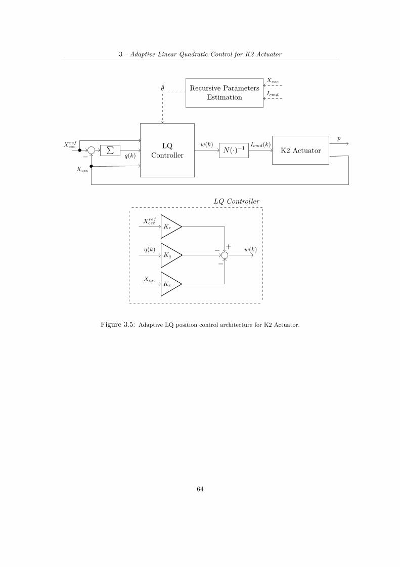
3 - Adaptive Linear Quadratic Control for K2 Actuator
∑ LQController
N(·)−1 K2 Actuator
Recursive ParametersEstimation
Xrefcsc
θ
Xcsc
Icmd
Icmd(k)
q(k)
w(k)p
Xcsc
−
Kr
Kq
Kx
+−
−
w(k)
Xrefcsc
q(k)
Xcsc
LQ Controller
Figure 3.5: Adaptive LQ position control architecture for K2 Actuator.
64

3 - Adaptive Linear Quadratic Control for K2 Actuator
3.3 Adaptive LQ tuning and simulations results
This section will describe the tuning procedure of the adaptive LQ controller designparameters. Numerical simulations results will be presented in order to evaluate theeffectiveness of the adopted control strategy. In particular, a wider spectrum of work-ing situations has been considered. That is, some other position trajectories have beenaccounted in addition to the position reference profiles previously expressed in section2.4.
The infinite horizon LQ controller design parameters are the weighting scalar factorsQy, Qq and R of the quadratic performance index (3.22) reminded below in trackingform
JK2(x(k),Wk) =
∞∑i=0
Qy
(Xcsc(k + i)−Xref
csc (k + i))2
+Rw2(k + i) +Qqq(k + i)2
Note that, in the chosen LQ control architecture, an adaptive approach has beendeveloped (section 3.2.1) and an explicit compensation of the static non-linearity hasbeen performed (section 3.2.2) through the dead zone inverting function. As a conse-quence, the adaptation gain γ and the dead zone amplitude D can be considered astuning parameters as well.Similarly as for the MPC, a trial and error procedure has been necessary to ensure asatisfactory trade off between the control performances.
The following settings have been considered for the adaptive LQ controller design
R = 1
Qy = 2 · 105
Qq = 1
Dead zone = [0; 37] %
γ = 0.012
θ(0) = [−0.9969 7.0651 · 10−5]
(3.24)
where θ(0) = [α0 β0] is the initial model parameters vector assumed to be inside themedium - high position range identified in section 3.2.1.
The just expressed design parameters values have been achieved by means of a
65

3 - Adaptive Linear Quadratic Control for K2 Actuator
suitable tuning procedure as described in the following paragraphs.
3.3.1 Tuning of the LQ Cost Function Weights
For the same considerations expressed in section 2.4.2,both the input weight R and theintegral action weight Qq are chosen to be equal as in (3.24). About the output weightQy, several simulations have been performed keeping fixed the other design parameters.These have pointed out that a high value of the output weight is responsible for a steadystate tracking error reduction especially in high position ranges whereas it induces smalloscillations in low position tracking situations. On the contrary, a too small value forQy causes a slight worsening of the position tracking performances.
0 0.5 1 1.5 2 2.5 3 3.5 4 4.5 5 5.50
0.14
0.28
0.42
0.57
0.71
0.85
1
1.14
0.6 0.7 0.8 0.9 1
1.5
1.6
1.7
3.4 3.5 3.6 3.74.4
4.45
4.5
Figure 3.6: Position response with 3rd Gear shift reference profile adopting Adaptive LQ for differentvalues of Qy.
In Figure 3.6 the output weight Qy is changed from Qy = 1 ·105 to Qy = 9 ·105 whenone of the difference position trajectories is adopted as reference profile. A suitable tradeoff between the control objectives has been assured selecting the value Qy = 2 · 105 forthe output weight.
3.3.2 Tuning of the dead zone amplitude
In section 3.2.2, the Hammerstein model representation of the K2 Actuator has pointedout the need for a two stage control approach. That is, an explicit inversion of the
66

3 - Adaptive Linear Quadratic Control for K2 Actuator
static non linear function, represented as a dead zone, has to be performed before thecommand input is applied to the plant.For this reason, the proper choice of the dead zone amplitude D becomes crucial in theadopted control architecture.
On the basis of the local identification results discussed in section 3.2.1, it is evidentthat the more the system is demanded to track high values of position references Xref
csc ,the less is the dead zone between the command input Icmd and the output position Xcsc.
0 0.5 1 1.5 2 2.5 3 3.5 4 4.5 5 5.50
0.15
0.3
0.46
0.61
0.76
0.92
1.07
1.4 1.6 1.8 24.3
4.4
4.5
4.6
4.7
2.6 2.8 36.4
6.45
6.5
Figure 3.7: Position response with 2nd Gear shift reference profile adopting Adaptive LQ for differentvalues of dead zone amplitude D.
Figure 3.7 confirms the above discussion by showing the influence of the dead zoneamplitude variation in the position response when the other design parameters are keptconstant as in (3.24).According to the obtained results, the value D = 37 % has been considered as deadzone amplitude in order to ensure satisfactory performances in all the position ranges.
3.3.3 Tuning of the RLS adaptation gain
Similarly as for the adaptive MPC, the recursive algorithm adaptation gain γ plays akey role in the adopted LQ control architecture. This is because the plant parametersestimation speed is related to the adaptive LQ control action, hence, it affects the systemresponse, too.
67

3 - Adaptive Linear Quadratic Control for K2 Actuator
0 0.5 1 1.5 2 2.5 3 3.5 4 4.5 5 5.50
0.14
0.28
0.42
0.57
0.71
0.85
1
1.14
0.8 0.85 0.9 0.95 1
2
2.2
2.4
3.4 3.6 3.8 44.9
5
5.1
5.2
0 0.5 1 1.5 2 2.5 3 3.5 4 4.5 5 5.5
-0.9995
-0.999
-0.9985
-0.998
-0.9975
-0.997
0 0.5 1 1.5 2 2.5 3 3.5 4 4.5 5 5.5
123456
10-4
Figure 3.8: (Top) Position response and model parameters variation (Bottom) with 4th Gear shiftreference profile adopting Adaptive LQ for different values of γ.
Figure 3.8 above outlines how an high adaptation gain implies a too reactive positionresponse, whereas a small adaptation gain leads to a significant steady state trackingerror.
For the same considerations expressed in section 2.4.3, the K2 Actuator high sensi-tivity with respect to the model parameters variation has been properly handled witha small adaptation gain γ = 0.012.
68

3 - Adaptive Linear Quadratic Control for K2 Actuator
The just presented tuning procedure can be resumed with a more general consid-eration. A crucial role is assumed by the proper choice of the dead zone amplitude D
between the command input Icmd and the position output Xcsc of the K2 Actuator. Thisis because a biased compensation of the static non linear function leads to an ineffectivecontrol action.The cost function weights and the RLS adaptation gain tuning has been necessary inorder to refine the obtained control action.
On the basis of the obtained results, the LQ controller performances have beenoutlined in the following Table
Range (%) Overshoot (%) Rise Time (ms) Steady State Error (mm)
8 to 21 s ≤ 8 tr ≤ 32 ∼= 5 · 10−3
21 to 57 s ≤ 15 tr ≤ 34 ∼= 2 · 10−2
57 to 85 s ≤ 3 tr ≤ 38 ∼= 8 · 10−3
85 to 100 s ≤ 1 tr ≤ 45 ∼= 6 · 10−3
Table 3.2: Adaptive LQ controller performance resume with different reference profiles.
Referring Table 3.2, the proposed LQ controller design (3.24) is able to guaranteea fast position response with a small steady state tracking error. However, as for theMPC, significant performance improvements, especially in terms of position overshoots,can be obtained by means of a suitable scheduling algorithm as described in the nextparagraph.
3.3.4 Scheduling Algorithm
A suitable trade off between a non oscillating input current and a fast position responsewith small overshoots has been obtained by dynamically tuning the LQ controller pa-rameters on the basis of the working situations.More precisely, the developed scheduling algorithm exploits a real time adjustment ofthe dead zone amplitude D and the output weight Qy considering as input measurementthe position reference Xref
csc and the tracking error ecsc = Xrefcsc −Xcsc actual values. The
generic strategy is resumed in the following steps (detailed MATLAB code in appendix)
1. MEASURE the reference Xrefcsc (k) and the tracking error ecsc(k) actual values.
69

3 - Adaptive Linear Quadratic Control for K2 Actuator
2. CHECK the position range on the basis of Xrefcsc (k).
3. SET the dead zone amplitude D on the basis of the position range.
4. IF(ecsc(k) ≤ ecsc
)4.1 INCREASE the output weight Qy.
5. IF(ecsc(k) > ecsc
)5.1 SET the output weight Qy = Qmin
y .
where ecsc is a suitable threshold adopted to handle position references characterizedby fast variations in their set point amplitudes.
The just presented pseudo code can be further clarified. Different dead zone ampli-tudes are adopted in order to assure an efficient non linearity compensation in all theworking regions guaranteeing a fast position response. Moreover, a significant steadystate error reduction is achieved by increasing the output weight when the position isapproaching the set point.
Several simulations have been carried out to test the effectiveness of the adoptedscheduled LQ controller and to evaluate some transient and steady-state tracking indicesin the presence of different position trajectories. Figures from 3.9 to 3.17 and Table 3.3resume the obtained results.
Range (%)Overshoot (%) Rise Time (ms) Steady State Error (mm)
LQ 1st LQ 2nd LQ 1st LQ 2nd LQ 1st LQ 2nd
8 to 21 s ≤ 8 s ≤ 5 tr ≤ 32 tr ≤ 38 ∼= 5 · 10−3 ∼= 3 · 10−3
21 to 57 s ≤ 15 s ≤ 7 tr ≤ 34 tr ≤ 40 ∼= 2 · 10−2 ∼= 2 · 10−2
57 to 85 s ≤ 3 s ≤ 2 tr ≤ 38 tr ≤ 42 ∼= 8 · 10−3 ∼= 5 · 10−3
85 to 100 s ≤ 1 s ≤ 1 tr ≤ 45 tr ≤ 51 ∼= 6 · 10−3 ∼= 5 · 10−3
Table 3.3: Adaptive LQ (LQ 1st) and Adaptive scheduled LQ (LQ 2nd) controller performance resumewith different reference profiles.
Referring the above Table, significant performance improvements have been obtainedthanks to the adopted scheduling technique. In fact, the proposed adaptive LQ con-troller guarantees a slight reduction of the steady state tracking error and an evidentposition overshoots mitigation. Besides, the almost equal response speed has been pre-served.
70

3 - Adaptive Linear Quadratic Control for K2 Actuator
0 0.5 1 1.5 2 2.5 3 3.5 4 4.5 5 5.50
0.14
0.28
0.42
0.57
0.71
0.85
1 ReferenceAdaptive LQ ControllerAdaptive scheduled LQ Controller
0 0.5 1 1.5 2 2.5 3 3.5 4 4.5 5 5.50
0.5
1
0.8 0.9 1
2
2.1
2.2
2.4 2.6 2.8 36.7
6.8
6.9
7
Figure 3.9: (Top) Position response and Input Current (Bottom) with Gear Change profile adoptingAdaptive LQ and Adaptive scheduled LQ.
0 0.5 1 1.5 2 2.5 3 3.5 4 4.5 5 5.50
0.14
0.28
0.42
0.57
0.71
0.85
1
1.14ReferenceAdaptive LQ ControllerAdaptive scheduled LQ Controller
0 0.5 1 1.5 2 2.5 3 3.5 4 4.5 5 5.50
0.5
1
0.5 0.6 0.7 0.8
2
2.1
2.2
2.4 2.6 2.8 3
6.96
6.98
7
7.02
Figure 3.10: (Top) Position response and Input Current (Bottom) with slow Gear Change referenceprofile adopting Adaptive LQ and Adaptive scheduled LQ.
71
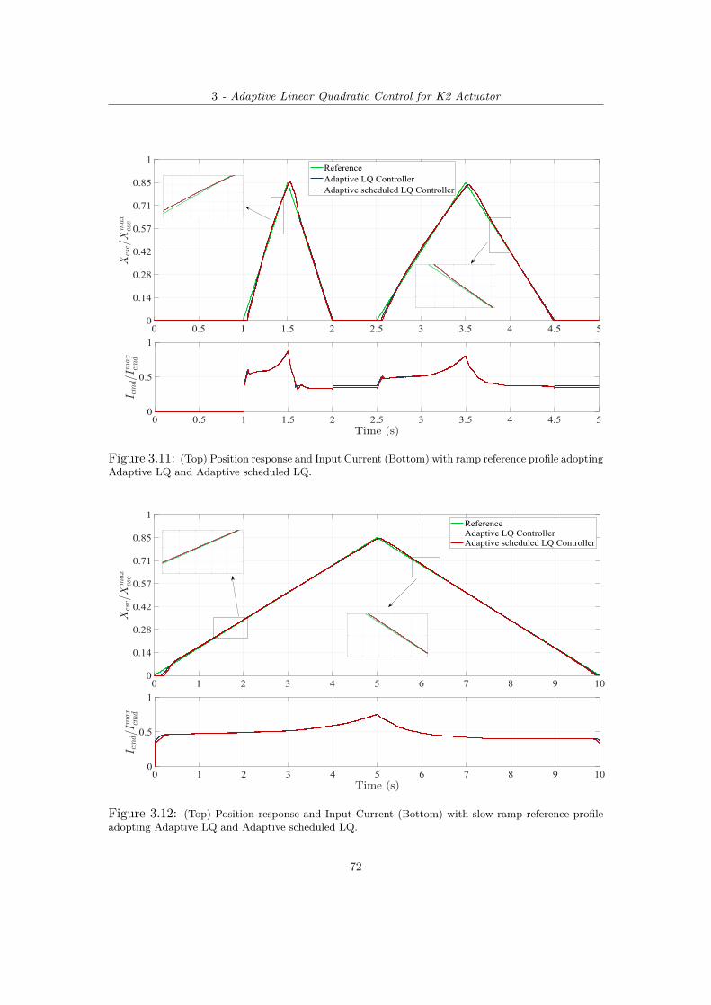
3 - Adaptive Linear Quadratic Control for K2 Actuator
0 0.5 1 1.5 2 2.5 3 3.5 4 4.5 50
0.14
0.28
0.42
0.57
0.71
0.85
1ReferenceAdaptive LQ ControllerAdaptive scheduled LQ Controller
0 0.5 1 1.5 2 2.5 3 3.5 4 4.5 50
0.5
1
1.3 1.35 1.4 1.45
3.54
4.55
5.5
3.7 3.8 3.9 43
3.5
4
4.5
Figure 3.11: (Top) Position response and Input Current (Bottom) with ramp reference profile adoptingAdaptive LQ and Adaptive scheduled LQ.
0 1 2 3 4 5 6 7 8 9 100
0.14
0.28
0.42
0.57
0.71
0.85
1ReferenceAdaptive LQ ControllerAdaptive scheduled LQ Controller
0 1 2 3 4 5 6 7 8 9 100
0.5
1
1.2 1.4 1.6 1.8 2
1.5
2
2.5
5.8 6 6.2 6.4 6.64
4.5
5
Figure 3.12: (Top) Position response and Input Current (Bottom) with slow ramp reference profileadopting Adaptive LQ and Adaptive scheduled LQ.
72

3 - Adaptive Linear Quadratic Control for K2 Actuator
0 0.5 1 1.5 2 2.5 3 3.5 4 4.5 5 5.50
0.15
0.3
0.46
0.61
0.76
0.92
1.07
1.23ReferenceAdaptive LQ ControllerAdaptive scheduled LQ Controller
0 0.5 1 1.5 2 2.5 3 3.5 4 4.5 5 5.50
0.5
1
0.6 0.7 0.8 0.9 1
2.5
2.6
2.7
2.3 2.4 2.5 2.6 2.7
6.4
6.45
6.5
Figure 3.13: (Top) Position response and Input Current (Bottom) with 2nd Gear Change referenceprofile adopting Adaptive LQ and Adaptive scheduled LQ.
0 0.5 1 1.5 2 2.5 3 3.5 4 4.5 5 5.50
0.14
0.28
0.42
0.57
0.71
0.85
1
1.14ReferenceAdaptive LQ ControllerAdaptive scheduled LQ Controller
0 0.5 1 1.5 2 2.5 3 3.5 4 4.5 5 5.50
0.5
1
1.4 1.6 1.85.4
5.45
5.5
5.55
2.4 2.6 2.86.9
6.95
7
Figure 3.14: (Top) Position response and Input Current (Bottom) with 3rd Gear Change referenceprofile adopting Adaptive LQ and Adaptive scheduled LQ.
73

3 - Adaptive Linear Quadratic Control for K2 Actuator
0 0.5 1 1.5 2 2.5 3 3.5 4 4.5 5 5.50
0.14
0.28
0.42
0.57
0.71
0.85
1
1.14ReferenceAdaptive LQ ControllerAdaptive scheduled LQ Controller
0 0.5 1 1.5 2 2.5 3 3.5 4 4.5 5 5.50
0.5
1
0.6 0.7 0.8 0.9 1
1.451.5
1.551.6
2.2 2.4 2.6 2.8
6.8
6.9
7
Figure 3.15: (Top) Position response and Input Current (Bottom) with 4th Gear Change referenceprofile adopting Adaptive LQ and Adaptive scheduled LQ.
0 0.5 1 1.5 2 2.5 3 3.5 4 4.5 5 5.50
0.18
0.36
0.54
0.72
0.9
1.09
1.27ReferenceAdaptive LQ ControllerAdaptive scheduled LQ Controller
0 0.5 1 1.5 2 2.5 3 3.5 4 4.5 5 5.50
0.5
1
0.6 0.8 1 1.23.4
3.6
3.8
2 2.5 3
5.45
5.5
5.55
Figure 3.16: (Top) Position response and Input Current (Bottom) with 5th Gear Change referenceprofile adopting Adaptive LQ and Adaptive scheduled LQ.
74
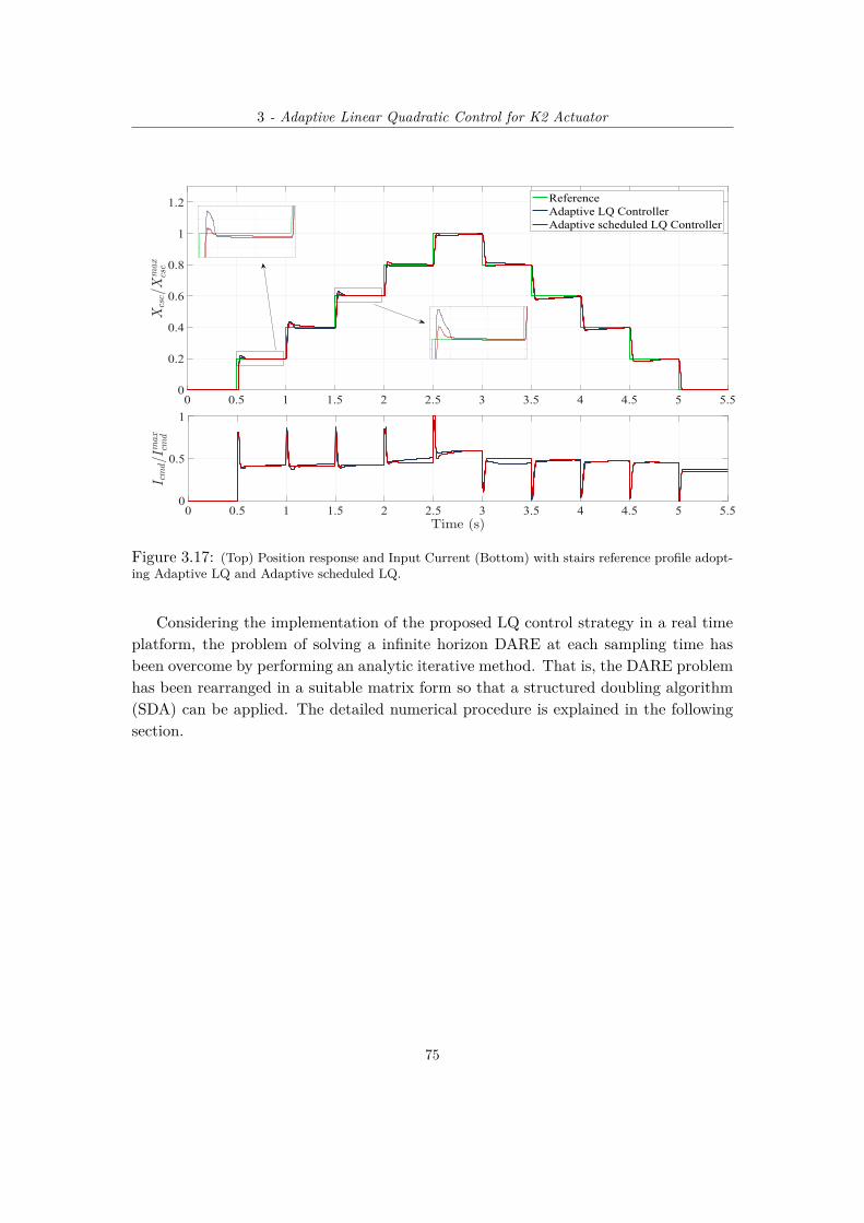
3 - Adaptive Linear Quadratic Control for K2 Actuator
0 0.5 1 1.5 2 2.5 3 3.5 4 4.5 5 5.50
0.2
0.4
0.6
0.8
1
1.2 ReferenceAdaptive LQ ControllerAdaptive scheduled LQ Controller
0 0.5 1 1.5 2 2.5 3 3.5 4 4.5 5 5.50
0.5
1
0.6 0.8 1
0.95
1
1.05
1.1
1.6 1.8 2
2.953
3.053.1
3.15
Figure 3.17: (Top) Position response and Input Current (Bottom) with stairs reference profile adopt-ing Adaptive LQ and Adaptive scheduled LQ.
Considering the implementation of the proposed LQ control strategy in a real timeplatform, the problem of solving a infinite horizon DARE at each sampling time hasbeen overcome by performing an analytic iterative method. That is, the DARE problemhas been rearranged in a suitable matrix form so that a structured doubling algorithm(SDA) can be applied. The detailed numerical procedure is explained in the followingsection.
75

3 - Adaptive Linear Quadratic Control for K2 Actuator
3.4 Numerical implementation of the infinite horizon DARE
Solving discrete time algebraic Riccati equations (DARE) is essential in many compu-tational problems for different engineering applications. However, a detailed analysis ofthe DARE mathematical properties is needed in order to find more effective algorithms.The following section is focused on the DARE application to the infinite horizon LQproblem related to the position control of the K2 Actuator. The needed mathemat-ical structures will be briefly presented together with the chosen structured doublingalgorithm adopted to find the DARE analytical solution.
3.4.1 DARE and matrix pencils
As discussed in section 3.1.2, the infinite horizon LQ controller, adopted for the K2Actuator position control problem, is related to the DARE solution X. The followinggeneral form is considered
ATXA+ Q− (N + BTXA)T · (R+ BTXB)−1 · (N + BTXA)− ETXE = 0
where A, B are the system augmented state matrices, Q is the cost function augmentedweighting matrix, R is the control input weighting factor. In this context, it can beassumed that E = I and N = 0 since no mixed term is present in the adopted costfunction (3.6). Hence, the DARE can be written as
X = ATXA+Q− ATXB · (R+ BTXB)−1 · BTXA (3.25)
According to [7] and [5], the above DARE solution P can be expressed in terms ofdeflating subspaces of a suitable matrix pencil (definitions in appendix) L− zK. A 0 B
−Q I 0
0 0 R
− z
I 0 0
0 −AT 0
0 −BT 0
(3.26)
Hence, the (almost) d-stabilizing solution P is such that A 0 B
−Q I 0
0 0 R
I
X
Z
=
I 0 0
0 −AT 0
0 −BT 0
I
P
Z
Φ (3.27)
where ρ(Φ) ≤ 1 and Z is associated with the solution of the dual DARE.
76

3 - Adaptive Linear Quadratic Control for K2 Actuator
According to [7] and [5], if W is a Hermitian matrix such that R = R+RTWB is nonsingular, the above equation (3.27) can be rearranged as E0 0 0
−P0 I 0
BTWA 0 R
I
X −W
Z
=
I −G0 0
0 ET0 0
0 −BT 0
I
P −W
Z
Φ (3.28)
where
P0 = Q−W + ATWE0
G0 = −BR−1BT
E0 = (I +G0W )A
(3.29)
The result (3.28) is useful to define the new matrix pencil N − zK[E0 0
−P0 I
]− z
[I −G0
0 ET0
](3.30)
whose form is referred as to standard structured form-I (SSF-I) [7]. Therefore, thefollowing equation holds[
E0 0
−P0 I
][I
X −W
]=
[I −G0
0 ET0
][I
X −W
]Φ (3.31)
and a special structured doubling algorithm can be applied in order to find an analyticalexpression for the DARE solution X.
3.4.2 DARE solution by means of a structured doubling algorithm
The structured doubling algorithm (SDA) is a recent and advanced technique whoseframework is independent from the the DARE application. SDA can be seen as aniterative method for generating a sequence of matrix pencils belonging to the same de-flating subspaces and such that their eigenvalues are squared at each step [16], [7].
The application of this class of algorithm to the DARE problem is based of the factthat, there is a one-to-one correlation between the graph invariant deflating subspacesof a matrix pencil and the solutions of the corresponding DARE.More precisely, the (3.30) is assumed to be the starting matrix pencil with initial values
77

3 - Adaptive Linear Quadratic Control for K2 Actuator
(3.29). Then, according to [7] and [5], the following sequence Nk−zKk can be generated[Ek 0
−Pk I
]− z
[I −Gk
0 ETk
](3.32)
with
Pk+1 = Pk + ETk (I − PkGk)
−1PkEk
Gk+1 = Gk + Ek(I − PkGk)−1GkE
Tk
Ek+1 = Ek(I − PkGk)−1Ek
(3.33)
Therefore, assuming that limk→∞ Pk = P , the analytical expression for the DAREsolution X can be evaluated in the following way
X = P +W (3.34)
where W is simply chosen as W = σI, with σ a real small positive number such thatdet(R+ BTσIB) = 0.
For the sake of clarity, a simple pseudo code of the adopted SDA algorithm isreported below (detailed MATLAB code in appendix)
1. BUILT the matrices W = σI and R = R+RTWB.
2. SET the initial matrices P0, E0 and G0 as in (3.29).
3. FIX the iterative algorithm exit conditions
3.1 SET the minimum error tolerance emin and the error initial value estart = 1.
3.2 SET the maximum number of iterations kmax.
4. WHILE((ek > emin)&(k < kmax)
)4.1 UPDATE the matrices Pk, Ek and Gk as in (3.33).
4.2 EVALUATE the error actual value ek = ∥Ek∥1.
4.3 CHECK the exit conditions.
5. EVALUATE the DARE solution X = P +W .
78

3 - Adaptive Linear Quadratic Control for K2 Actuator
1 4 7 10 13 16 19 22 24
0
0.2
0.4
0.6
0.8
1
Figure 3.18: Converging trend of the SDA error related to the DARE solution analytical evaluation.
Considering kmax = 30 as maximum number of iterations and emin = 10−13 as errortolerance, the SDA algorithm takes approximately 24 iterations to converge. Figure3.18 above shows one of the possible error trend when the sub-routine is stopped duringthe program execution.
79

Chapter 4Virtual Sensor based Control for K2Actuator
I n this Chapter, the absence of a real position sensor in the described DDCT systemis considered. A Virtual Sensor is employed such that the needed clutch position
estimate can be obtained on the basis of available measurements.The last section presents several simulation results in order to decide the most suitablevirtual sensor model structure and control architecture.
4.1 Virtual sensor Overview
A virtual sensing system uses information available from other measurements and pro-cess parameters to calculate an estimate of the quantity of interest. Empirical methodsbase the calculus of the needed estimate on historical measurements of the same quan-tity, and on its correlation with other available measurements or parameters [21], [26].
In this context, the K2 Actuator virtual sensor to be modelled is considered as aSISO black box model that transforms, in real time, the actual measure of the outputpressure p in the clutch position estimate Xcsc.
A preliminary analysis of the data sets, provided by Centro Ricerche Fiat, showed thepresence of a dead zone between the pressure and the position. The relationship betweenthe involved variables is showed in Figure 4.2.
As highlighted by the above curve shape, the K2 Actuator position values are relatedto the output pressure in a non linear manner. For this reason, in the following section
80

4 - Virtual Sensor based Control for K2 Actuator
K2 Actuator Virtual Sensorp(k)
Xcsc(k)
Icmd(k) Xcsc(k)
Figure 4.1: Black box model of the Virtual Sensor for the K2 Actuator.
0 0.12 0.25 0.37 0.5 0.62 0.75 0.87 10
0.14
0.28
0.42
0.57
0.71
0.85
1
Figure 4.2: Pressure-Position curve shape for the given data set.
different non linear model structures are proposed to represent the Virtual Sensor.
81

4 - Virtual Sensor based Control for K2 Actuator
4.2 Virtual Sensor Modelling
The non linear characteristic between the K2 Actuator output pressure and the clutchposition value has been reproduced by considering two different strategies to develop aVirtual Sensor.The first method, whose description can be found in section 4.2.1, involves the use ofMultilayer Feedforward Neural Networks to describe the static relationship between thepressure p(k) and the position Xcsc(k) [1].The second approach, presented in section 4.2.2, tries to simplify such a Neural Networkbased Virtual Sensor by means of a block-structured model design. The Hammerstein-Wiener has been demonstrated to be the most suitable model and the Set-Membershipidentification methodology has been exploited to determine the proper parameters val-ues [9].
4.2.1 Static feedforward Neural Network model structure
The chosen class of Neural Network is based on a layer-by-layer forward propagationof the pressure input signal. The training procedure, exploited through the MAT-LAB Neural Network Toolbox, is based on the error back-propagation algorithm andimplemented in a supervised manner following the Levenberg-Marquardt optimizationmethod (for more details see [1], [14], [24], [18]).
The following network anatomy, showed in Figure 4.3, has been selected
• Input Layer: acquires the input pt at each sampling time Ts = 2 ms.
• Hidden Layer: in each neuron the input pt is weighted by the term wj and biasedby bj . Then, the Hyperbolic Tangent Function is chosen as activation function toobtain the output vector y = [y1 ... y10] as reported in the equation below.
yj =2
1 + e−2φj− 1 for j = 1...10
where φj = wj · pt + bj
• Output Layer: produces the Neural Network output by adjusting the HiddenLayer output vector [y1 ... y10] with the weighting terms [wx1 ... wx10 ] and the biasterm bx. The resulting Virtual Sensor’s position estimate Xcsc is given by
82

4 - Virtual Sensor based Control for K2 Actuator
Xcsc(t) = f(pt) =[wx1 · · · wx10
] y1...
y10
+ bx (4.1)
Note that, the use of the hidden layer allows the network to learn more complex tasksor, in this context, to perform a more accurate identification of the K2 Actuator nonlinear dynamics. Indeed, this kind of Neural Network, referred as Multilayer Percep-trons (MLPs), is able to extract more meaningful features from the input patterns [14].
pt Xcsc
Hiddenlayer
y
Inputlayer
Outputlayer
Figure 4.3: Neural Network Anatomy for the K2 Actuator Virtual Sensor.
The Neural Network parameters values are resumed in Table 4.1.
83

4 - Virtual Sensor based Control for K2 Actuator
Hidden Layer Output Layer
Neuron Weights wj Bias bj Weights wxjBias bx
1 10.833 -11.631 0.03
2 11.826 -10.641 0.023
3 10.47 -7.141 0.039
4 -10.569 4.553 -0.05
0.0195 -223.276 2.895 -0.048
6 4.755 0.959 0.123
7 37.33 14.2855 0.046
8 22.656 12.156 0.054
9 10.122 7.688 0.751
10 237.94 198.521 -0.133
Table 4.1: Neural Network parameters values.
The validation procedure, performed on the given data set and portrayed in Figure4.4, shows a quite good tracking of the measured output position. Therefore, it canbe stated that the developed Virtual Sensor, represented by a static Neural Network,is able to provide an accurate position estimate Xcsc on the basis of the K2 Actuatoroutput pressure actual value.
0 100 200 300 400 500 6000
0.14
0.28
0.42
0.57
0.71
0.85
1
Figure 4.4: Neural Network based Virtual Sensor validation.
84

4 - Virtual Sensor based Control for K2 Actuator
However, despite of the good tracking performances, such a developed Virtual Sensoris not easy to be deployed in a real time platform because of the complexity relatedto the Neural Networks inherent estimation approach. For this reason, in the followingparagraph, a simplified Virtual Sensor has been developed to obtain the needed positionestimate by means of manageable block structures.
4.2.2 Robust Hammerstein-Wiener model structure
The aim of this strategy is to build a Virtual Sensor by considering an uncertain systemidentified through a robust identification method. That is, the given experimental mea-surements are assumed to be affected by unknown but bounded (UBB) error so thatthe Set-membership identification technique can be applied to evaluate the ParametersUncertainty Intervals (PUIs) of the pre-defined model structures.Once computed the proper bounding sets, the central estimate has been considered asthe most suitable parameter value for all the chosen model structures.
According to [9], the following Hammerstein-Wiener model has been chosen
NDZ(·) Gvs(z) Npoly(·)λ(k)pD(k)p(k) Xcsc(k)
Figure 4.5: Hammerstein-Wiener block diagram representation for the K2 Actuator Virtual Sensor.
where NDZ(·) and Npoly(·) are, respectively, the input non liner block represented by adead zone and the output non linear block modelled by a finite polynomial. Moreover,the dynamic part between the dead zone processed pressure pD(k) and the inner signalλ(k) is represented by the discrete time transfer function Gvs(z).
The identification procedure has been formulated in terms of optimization problemsas asserted by the Set-membership methodology. Linear programming methods as wellas convex relaxation techniques have been applied in order to handle such a diverseoptimization framework. More precisely, linear programming and convex optimizationproblems have been solved by MATLAB routines whereas the global optima of the nonconvex polynomial optimization problems have been evaluated through the SparsePOPMATLAB toolbox.
Referring to Figure 4.5, the adopted Hammerstein-Wiener Virtual Sensor settingscan be resumed in the following way (details are explained in [9])
85

4 - Virtual Sensor based Control for K2 Actuator
• Input non linear block NDZ(·): as already mentioned, data analysis has confirmedthe presence of a pressure dead zone according to which positive pressure valuesresult in null position response. The identified range is found to be
Dead Zone = [0− 3.89] bar (4.2)
• Output non linear block Npoly(·): under the assumption of invertible non linearity,the polynomial coefficients have been evaluated by considering the inverse identi-fication problem. That is, the experimental steady state operating conditions pssDand Xss
csc have been exploited yielding the following fourth degree polynomial
pssD = N−1(Xsscsc) = 0.5766 ·Xss
csc − 0.6147 · (Xsscsc)
3 + 0.02174 · (Xsscsc)
4 (4.3)
• Linear dynamic Model Gvs(z): the identification procedure has been carried outin the output error model framework considering the known input samples pD(k)
and the uncertain output signal λ(k). Additional constraints have been includedin the optimization problem in order to ensure the system BIBO stability andunitary steady-state gain. The identified transfer function is characterized by afirst order dynamics expressed as
Gvs(z) =0.3132
z − 0.6868(4.4)
Figure 4.6 illustrates the validation procedure performed on the given data set.
0 100 200 300 400 500 6000
0.14
0.28
0.42
0.57
0.71
0.85
1
Figure 4.6: Hammerstein-Wiener model based Virtual Sensor validation.
86

4 - Virtual Sensor based Control for K2 Actuator
As can be seen from the above image, this Virtual Sensor modelling strategy representsa trade off between the tracking accuracy and the ease of implementation. However,the reduction of the position estimate oscillations is a considerable achievement for ourfinal control purpose since the estimated position is directly fed back to track a givenreference trajectory.
87

4 - Virtual Sensor based Control for K2 Actuator
4.3 Virtual sensor based Control Architectures
The previous section has dealt with two different modelling strategies to obtain theproper clutch position estimate by means of the available K2 Actuator output pressure.In the following, both the developed Virtual Sensors are included in different architec-tures that are based on single or nested feedback loops control techniques.Several simulations results are presented with the aim of comparing and testing eachcontrol strategies in terms of different performance criteria such as the real positiontracking behaviour, the command input oscillations reduction, the smoothness of theposition estimate.
Specifically, an Up shift manoeuvre is considered as the typical working situation.This is to properly test the effectiveness of the control techniques when a congenial po-sition reference, and hence pressure trajectory, is involved in the Virtual Sensor basedarchitecture.
Moreover, such a Virtual Sensor based control strategy causes the need to adopt thefollowing adjustments
- the plant model, needed for the controller design, has been re-identified by forcingthe K2 Actuator with a suitable input sequence and collecting as output thecorresponding position estimate Xcsc provided by the Virtual Sensor.
- the command input Icmd and output position Xcsc closed loop data have beenacquired and considered as training data set for the Neural Network based VirtualSensor.
A more appropriate initial model parameters vector improves the recursive algorithmaccuracy. Besides, a more consistent training data set enhances the accuracy of theVirtual Sensor position estimation thanks to the inherent auto-learning capability thatdistinguishes the Neural Networks.
4.3.1 Single feedback Loop Control
A Virtual Sensor based control technique using a single feedback loop is treated in thefollowing paragraph. That is, a position control strategy , based on the position esti-mate Xcsc provided by the Virtual Sensor, has been exploited such that the real K2Actuator output position Xcsc follows a suitable reference profile.
The general control architecture is showed in Figure 4.7.
88

4 - Virtual Sensor based Control for K2 Actuator
Controller Virtual SensorK2 ActuatorIcmd
Xrefcsc
p
XcscXcsc
Figure 4.7: General block scheme of the single feedback loop Virtual Sensor based control architecturefor the K2 Actuator.
As to the Controller, both the MPC and the LQR control methods have beenemployed while, as to the Virtual Sensor, either the Neural Network or the RobustHammerstein-Wiener modelling procedures have been considered.
LQ position Control
The LQ controller design strategy is the same discussed in Chapter 3.However, since the position estimate provided by the Virtual Sensor is characterizedby sudden jumps in low position ranges, some modifications have been necessary. Afine tuning of the weighting matrices, as well as the other involved design parameters,has been exploited until satisfactory control performances are achieved. The trackingweight Qy has been dynamically adjusted on the basis of the working region so thatsudden jumps of the position estimate values are properly reduced.
The chosen parameters settings are
R = 1
Qy = [0.5÷ 9] · 105
Qq = 1
Dead zone = [0; 37] %
γ = 0.0065
θ(0) = [−0.9872 1.1069 · 10−4]
(4.5)
where θ(0) = [α0 β0] is the initial model parameters vector re-identified considering theVirtual Sensor.
Figure 4.8 depicts the K2 Actuator position response, the Virtual sensor positionestimate, the output pressure and the LQ controller command action when the positionestimate Xcsc is provided by three types of different modelled Virtual Sensors.
89

4 - Virtual Sensor based Control for K2 Actuator
0 0.5 1 1.5 2 2.5 3 3.50
0.28
0.57
0.85
1.14ReferenceOpen Loop trained Neural NetworkClosed Loop trained Neural NetworkRobust Hammerstein-Wiener model
0 0.5 1 1.5 2 2.5 3 3.50
0.28
0.57
0.85
1.14
1.6 1.7 1.8 1.9 25.4
5.5
5.6
3 3.1 3.2 3.36.9
6.95
7
1.6 1.8 2
5.45
5.5
5.55
2.8 3 3.26.9
6.95
7
7.05
0 0.5 1 1.5 2 2.5 3 3.50
0.25
0.5
0.75
1
0 0.5 1 1.5 2 2.5 3 3.50
0.2
0.4
0.6
0.8
1
Figure 4.8: Position response, position estimate, output pressure, command input with Up shiftreference profile adopting a Virtual Sensor based LQ control.
90

4 - Virtual Sensor based Control for K2 Actuator
From the reported image it is evident that, adopting such a LQ position controlstrategy, satisfactory trade off results are obtained when the closed loop trained NeuralNetwork is adopted as Virtual Sensor. A significant ripple attenuation is achieved to-gether with an appreciable steady state tracking behaviour indeed.
However, it is worth to highlight that the best results in terms of smoothness areobtained by means of the robust Hammerstein-Wiener Virtual Sensor. This can berelated to the dynamic part of the adopted model structure that, acting as a filter, isable to reduce the output oscillations.
MPC position Control
The same approach described in Chapter 2 is adopted to design the MPC positioncontroller.On the other hand, the fact that the Virtual Sensor position estimate is directly fedback to the controller has caused the need to adjust the involved design parameters,and to exploit a dynamic tuning of the tracking weight Qy and the prediction horizonHp yielding the following settings
R = 1
Qy = [1÷ 25] · 102
Qq = 1
Hp = [28÷ 36]
|∆Imaxcmd | = 500 mA
Ts
γ = 0.01
θ(0) = [−0.9872 1.1069 · 10−4]
(4.6)
where θ(0) = [α0 β0] is the initial model parameters vector re-identified considering theVirtual Sensor.
Figure 4.9 confirms the considerations made in the previous paragraph. The filteringproperties associated with the Hammerstein-Wiener Virtual Sensor lead to a remarkableripple mitigation. Moreover, the inclusion of state and input constraints in the controlproblem formulation has given further benefits in terms of smoothness with respect tothe previously presented Virtual Sensor based LQ control strategy.
However, the best compromise between the response speed and the steady state errorminimization is still obtained by means of the closed loop trained Neural Network.
91

4 - Virtual Sensor based Control for K2 Actuator
0 0.5 1 1.5 2 2.5 3 3.50
0.28
0.57
0.85
1.14ReferenceOpen Loop trained Neural NetworkClosed Loop trained Neural NetworkRobust Hammerstein-Wiener model
0 0.5 1 1.5 2 2.5 3 3.50
0.28
0.57
0.85
1.14
1.7 1.8 1.9 25.35.45.55.65.7
3 3.1 3.2 3.3 3.46.85
6.96.95
77.05
1.4 1.5 1.65.4
5.5
5.6
2.8 2.9 3 3.1 3.26.95
7
7.05
0 0.5 1 1.5 2 2.5 3 3.50
0.25
0.5
0.75
1
0 0.5 1 1.5 2 2.5 3 3.50
0.2
0.4
0.6
0.8
1
Figure 4.9: Position response, position estimate, output pressure, command input with Up shiftreference profile adopting a Virtual Sensor based MPC control.
92

4 - Virtual Sensor based Control for K2 Actuator
For the sake of completeness, in the next section a Virtual Sensor based nested loopcontrol approach is described. The intent is to study if an inner loop that controls theK2 Actuator output pressure can give benefits in terms of the position estimation, henceimproving the overall control performances.
4.3.2 Nested feedback Loops Control
For nested feedback loops control it is intended a control architecture in which twocascade controllers are implemented. More precisely, they are functionally wired in thesense that the outer loop literally commands the inner loop by adjusting its set point.
In this context, a secondary pressure control is nested inside a primary position con-trol which is designed on the basis of the position estimate Xcsc provided by the VirtualSensor. The aim is to improve the control action effectiveness by refining the positionestimate by means of a controlled pressure response.
Figure 4.10 shows the general control architecture.
PositionController
VirtualSensor
PressureController K2 Actuator
Icmdpcmd
Xrefcsc
p
XcscXcsc
Figure 4.10: General block scheme of the nested feedback loops Virtual Sensor based control archi-tecture for the K2 Actuator.
As to the outer position loop, only the Virtual Sensor based LQ control strategyhas been implemented. This decision is motivated by the fact that, as presented inthe previous paragraph, the explicit feed forward action, provided by the LQ controllaw, guarantees a fast position response without significantly increasing overshoots andsteady state errors.On the contrary, two different strategies are proposed for the inner pressure loop asdescribed in the following paragraphs.
93

4 - Virtual Sensor based Control for K2 Actuator
Outer LQ position Control
The LQ position control has been designed observing the same principles described inChapter 3. However, since the relationship between the clutch position and the outputpressure can be well represented by a linear first order model with gain β and pole α
(details in [1]), an explicit dead zone compensation is not needed any more. Besides,the tracking weight has to be adjusted on the basis of the working point to guarantee asmooth behaviour.
A suitable trade off between a non oscillating command pressure and a satisfac-tory position reference tracking has been achieved by setting the following controllerparameters values.
R = 1
Qy = [0.5÷ 9] · 102
Qq = 1
γ = 0.03
θ(0) = [−0.7489 0.098]
(4.7)
where θ(0) = [α0 β0] is the initial model parameters vector as in [1].
Inner pressure Control using Pole Placement techniques
The key idea of this approach is to design a controller for the K2 Actuator such thatthe closed loop poles lays in assigned positions on the complex plane.In this regard, since the linear model that relates the command input with the outputpressure is represented by a first order transfer function GIp(details in [1]), a one de-gree of freedom (1dof) controller is needed. Figure 4.11 shows the adopted 1dof controlarchitecture.
According to [6] and [23], the associated diophantine equation leads to the followingstructure for the 1dof controller with built-in integrator
C(z) =s0 (z + σ)
z − 1=
U(z)
E(z)
where U = Icmd, E = pcmd − p is the tracking error, σ = −9.83 · 10−3 is the pole of theplant model GIp.
94

4 - Virtual Sensor based Control for K2 Actuator
C(z) K2 Actuator
Recursive ParametersEstimation
pref
σ, ρ
p
Icmd
e(k) Icmd(k)Xcsc
p−
Figure 4.11: Adaptive 1dof inner pressure control architecture for K2 Actuator.
Specifically, on the basis of the plant model GIp dominant dynamics, the closed loopcharacteristic polynomial is chosen to be
Am(z) = z + λCL = z − 0.96 (4.8)
Hence, the controller design parameter is fixed according to
s0 =1 + λCL
ρ
where ρ = 5.3 · 10−2 is the gain of the plant model GIp.
Moreover, an adaptive approach has been exploited so that the plant model param-eters σ, ρ and, consequently, the controller design parameter s0, are adjusted in realtime on the basis of the command input Icmd and output pressure p actual values.
The resulting control action that guarantees an adaptive pole cancellation is
Icmd(k) = Icmd(k − 1) + s0(e(k) + σ e(k − 1)
)(4.9)
Finally, employing the LQ position controller 4.7 and the Virtual Sensor in the outerloop, the just described nested control strategy has been adopted to track an Up shiftposition reference profile. Figure 4.12 shows the K2 Actuator position response Xcsc,the position estimate Xcsc, the output pressure p and the command input Icmd in thepresence of three different Virtual Sensor modelling approaches.
95

4 - Virtual Sensor based Control for K2 Actuator
0 0.5 1 1.5 2 2.5 3 3.50
0.28
0.57
0.85
1.14ReferenceOpen Loop trained Neural NetworkClosed Loop trained Neural NetworkRobust Hammerstein-Wiener model
0 0.5 1 1.5 2 2.5 3 3.50
0.28
0.57
0.85
1.14
1.6 1.7 1.8 1.9 2
5.4
5.6
5.8
3 3.1 3.2 3.3 3.4
6.96.95
77.05
1.6 1.7 1.8 1.95.45
5.5
5.55
2.8 3 3.2 3.46.95
7
7.05
0 0.5 1 1.5 2 2.5 3 3.50
0.25
0.5
0.75
1
0 0.5 1 1.5 2 2.5 3 3.50
0.2
0.4
0.6
0.8
1
Figure 4.12: Position response, position estimate, output pressure, command input with Up shiftreference profile adopting a Virtual Sensor based nested control (LQ outer loop - 1dof inner loop).
96

4 - Virtual Sensor based Control for K2 Actuator
As confirmed by the reported simulation results, the inclusion of the 1dof inner pres-sure loop gives particular benefits in terms of position estimate smoothness for all theVirtual Sensor models employed in the outer position loop.Secondly, in comparison with the feedback position control discussed in the previous sec-tion, a faster response is achieved without significantly increasing the position overshoot.
Improvements are proposed in the next paragraph by enhancing the internal pressurecontrol loop with a MPC control architecture.
Inner pressure Control using MPC techniques
On the basis of the same procedures described in Chapter 2, an adaptive Model Pre-dictive Control architecture has been exploited for the inner pressure loop of the K2Actuator.
Figure 4.13 resumes the general MPC layout.
∑ MPCController
∑K2 Actuator
Observer
Recursive ParametersEstimation
z−1
pref
p(k)
Icmd(k)σ, ρ
d
Icmd(k)
Icmd(k − 1)
q(k) ∆Icmd
Xcsc
p
p
−
Figure 4.13: Adaptive MPC inner pressure control architecture for K2 Actuator.
In this different scenario and according to [1], the relationship between the com-mand input and the output pressure is assumed to be modelled by a first order transfer
97

4 - Virtual Sensor based Control for K2 Actuator
function GIp with pole σ and gain ρ. Again, a non linearity model compensation is ex-ploited by performing a state observer based feed forward action. The current variationrate ∆Icmd has been adopted as optimization variable and a suitable variation rate con-straint has been imposed. The chosen controller parameters settings are listed in (4.10).
Once designed the pressure inner loop, the LQ controller 4.7 and the Virtual Sensorhave been included in the outer loop of the overall nested control architecture.Simulations results, in the presence of an Up shift position reference profile, are illus-trated in Figure 4.14.
R = 1
Qy = 1.2 · 102
Qq = 1
Hp = 10
|∆Imaxcmd | =500 mA
Ts
γ = 0.01
θ(0) = [−9.83 · 10−3 5.3 · 10−2]
(4.10)
where θ(0) = [σ0 ρ0] is the initial model parameters vector as in [1].
The reported plots highlight the effectiveness of the just presented nested controlarchitecture. In comparison with the previous approaches, each of the three VirtualSensor modelling strategies presents quite good results. More precisely, a smootherbehaviour of the real output position along with significant improvements in terms ofresponse speed have been obtained, especially when the Hammerstein-Wiener VirtualSensor is included in the outer loop.
However, as long as the Virtual Sensor based control is concerned, and with theaim of providing a general consideration on the proposed control strategies, an overallperformance resume is presented in the following section.
98
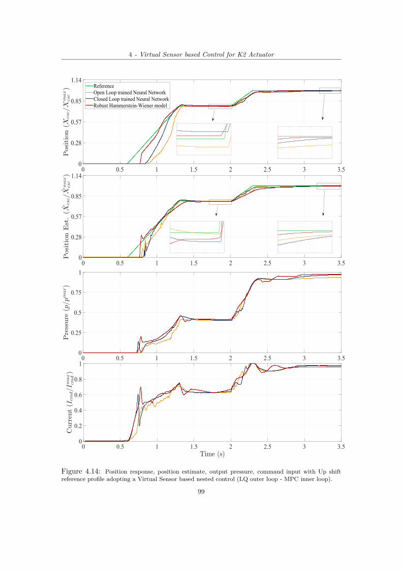
4 - Virtual Sensor based Control for K2 Actuator
0 0.5 1 1.5 2 2.5 3 3.50
0.28
0.57
0.85
1.14ReferenceOpen Loop trained Neural NetworkClosed Loop trained Neural NetworkRobust Hammerstein-Wiener model
0 0.5 1 1.5 2 2.5 3 3.50
0.28
0.57
0.85
1.14
1.7 1.8 1.9 2
5.45
5.5
5.55
3 3.1 3.2 3.3 3.46.8
6.9
7
1.7 1.8 1.9 2
5.445.465.48
5.55.52
3.2 3.3 3.46.94
6.96
6.98
7
7.02
0 0.5 1 1.5 2 2.5 3 3.50
0.25
0.5
0.75
1
0 0.5 1 1.5 2 2.5 3 3.50
0.2
0.4
0.6
0.8
1
Figure 4.14: Position response, position estimate, output pressure, command input with Up shiftreference profile adopting a Virtual Sensor based nested control (LQ outer loop - MPC inner loop).
99

4 - Virtual Sensor based Control for K2 Actuator
4.4 Final Comparisons and Results
In the previous section two modelling strategies for the Virtual Sensor development havebeen described. Their inclusion in different control architectures has been analysed bymeans of simulations results. Besides, control performances have been discussed for eachof the adopted methodologies by taking into account not only the real position responsebehaviour, but also the position estimate accuracy along with the output pressure andcommand input signals.
In the following, dealing with the Virtual Sensor based approaches, and consideringboth the MPC and LQR position controllers developed in Chapter 2 and Chapter 3,the K2 Actuator position response is studied. This is to investigate and compare theachievable control performances when a Virtual Sensor, and not a real position sensor,provides the controller the needed samples of the K2 Actuator output position.Specifically, regarding the previous section results, only the control architectures, andthe associated Virtual Sensor, that provide satisfactory performances in terms of realposition output behaviour, are selected to be compared.
The first plot, reported in Figure 4.15, shows the command input and the positionoutput behaviours when either a real position sensor or a Virtual Sensor is employed inboth the single and nested control architectures. The LQ approach is here investigatedand the closed loop trained Neural Network is assumed to be the best Virtual Sensormodelling strategy for this position control purpose.These simulation results outline the fact that an inner 1dof pressure controller guar-antees an effortless control action and a good tracking behaviour of the K2 Actuatoroutput position. Nevertheless, these improvements in terms of smoothness are obtainedat the cost of slowing down the system response.
In Figure 4.16 the same scenarios as before are considered but, in this case, MPCtechniques are inspected and the Hammerstein-Wiener Virtual Sensor is chosen to bethe more performing one with the nested control architecture.As confirmed by the reported plots, if the K2 Actuator output pressure is controlled bya MPC internal loop, significant advancements of the response speed as well as of theinput current smoothness are appreciable with the only drawback of a slightly largerposition overshoot.
Generally speaking, and with reference to the just discussed simulation results, itis evident that the inclusion of the Virtual Sensor in the control architecture entailssome oscillations in the command input. These are responsible, particularly with ramp
100

4 - Virtual Sensor based Control for K2 Actuator
0 0.5 1 1.5 2 2.5 3 3.50
0.14
0.28
0.42
0.57
0.71
0.85
1
1.14ReferenceAdaptive LQ ControlVirtual Sensor based adaptive LQ ControlVirtual Sensor based adaptive LQ nested Control
0 0.5 1 1.5 2 2.5 3 3.50
0.5
1
1.6 1.7 1.8 1.95.45
5.5
5.55
2.5 2.6 2.7 2.8 2.96.9
6.95
7
7.05
Figure 4.15: Position response and Input Current with an Up shift reference profile adopting AdaptiveLQ techniques when either a real position sensor or a Virtual Sensor are employed.
0 0.5 1 1.5 2 2.5 3 3.50
0.14
0.28
0.42
0.57
0.71
0.85
1
1.14
0 0.5 1 1.5 2 2.5 3 3.50
0.5
1
1.8 1.9 25.46
5.48
5.5
5.52
5.54
3.2 3.25 3.3 3.35 3.4
6.98
7
7.02
Figure 4.16: Position response and Input Current with an Up shift reference profile adopting AdaptiveMPC techniques when either a real position sensor or a Virtual Sensor are employed.
101

4 - Virtual Sensor based Control for K2 Actuator
position trajectories, of a delayed or slightly biased reference tracking.Enhancements about these aspects are proposed by means of different nested approachesthat, however, represent a trade-off between the overall control objectives.
However, as expected and confirmed by the above plots, when the DDCT systemcan be equipped with a real sensor, the position control of the even gear actuator isnaturally far more effective.
102

Chapter 5Conclusions
T his thesis has dealt with the even gear actuator control of a dry dual clutch transmis-sion system. More precisely, the aim of the project has been to design a controller
that, using the clutch position measurement, is able to guarantee a smooth referencetracking and a continue torque transmission.
With the purpose of improving driving comfort, different control architectures, re-lated to the optimal control methodologies, have been exploited. Moreover, due to thelack of an a priory model for the considered K2 Actuator, identification procedures,performed on the basis of the given experimental data, have been necessary to evaluatea mathematical relationship between the involved variables.
Specifically, identification results have shown that the system dynamic and steadystate properties are strictly related to the working region. For this reason, a recursiveleast square estimation algorithm has been developed so that all the proposed controlstrategies are designed on the basis of a real time varying state space model represen-tation.
First of all, an Adaptive Model Predictive Control approach has been considered.Physical constraints and multiple control objectives have been handled through a con-venient customization of the cost function and the control problem formulation. A nonlinear effect has caused the need to perform an implicit feed forward action by including,among the state variables, an unmeasurable disturbance whose estimate is provided bya suitable state observer.
Different position reference profiles, that reasonably represent the K2 Actuator work-ing situations, have been considered.
103

5 - Conclusions
The Adaptive MPC controller parameters setting, whose choice has been reasoned byextensive tuning simulations results, ensures quite satisfactory performances in termsof steady state tracking and rise time. The proposed MPC control action is able toguarantee an accurate tracking even if the reference profile is characterized by suddenset point variations. More precisely, the minimum tracking error is obtained in thepresence of constant references while, with ramp trajectories, a small offset occurs inthe position response.Motivated by the huge variability of the system behaviour with respect to the workingpoint, a real time adjustment of the controller design parameters have been proposed bymeans of a scheduling algorithm. Thanks to this approach, significant improvements,especially in terms of position overshoots, have been achieved.However, due to the long prediction horizon, such an Adaptive MPC method need quitehigh resources to compute in real time the optimal control action.
Therefore, with the aim of improving computational aspects, an Adaptive LinearQuadratic Control strategy has been exploited. An analytic iterative method has beendeveloped to overcame the problem of solving, at each sampling time, the infinite hori-zon Discrete Time Riccati equation that is related to the proposed LQ approach.As for the MPC, a wide spectrum of working situations has been considered to test theeffectiveness of the developed control architecture and a suitable scheduling algorithmhas been proposed to ensure the same level of control performances in all the positionregions.
Simulations results have shown that also an adaptive LQ control action, result-ing from an unconstrained optimization problem, is able to guarantee a fast positionresponse without significantly increasing position overshoots and steady state errors.This is due to the affine static state feedback form of the LQ control action that, thanksto the explicit feed forward loop, ensures satisfactory performances in terms of rise timeand reference tracking.
It is worth to highlight that, both the MPC and the LQ controllers have been de-veloped assuming the availability of a real position sensor in the considered Dry DualClutch Transmission System.In this regard, the last Chapter of this thesis work deals with the lack of a real sensorby including a Virtual Sensor into the control architecture. Extensive simulations andseveral comparisons have proved that the best trade-off between a smooth input cur-rent and a fast position response is obtained by means of a nested control architecturedesigned with an inner MPC pressure loop and an outer LQ position loop.
104

5 - Conclusions
In conclusion, considering the overall DDCT system, the clutch torque effectivenessis strictly related to the gear actuator control accuracy, especially in high position ranges.Therefore, the position response smoothness is of paramount importance in regard tothe driving comfort.With this in mind, among the different proposed approaches for the position controlof the K2 Actuator, the adaptive LQ showed outstanding results in terms of achievedperformances and computational effort. Besides, it offers the possibility of an effectivedeployment in a real time platform thanks to the closed form of the LQ control action.
Future Work
Starting from the results presented in this thesis project, further investigations can becarried out.
The position estimate accuracy can be improved by designing the Hammerstein-Wiener Virtual Sensor on the basis of the proper closed loop data. Hence, the proposedLQ controller can be implemented on the transmission control unit in order to test theachievable performances on the real vehicle.
Another interesting aspect that deserves a more thorough study, is to develop aVirtual Sensor based MPC controller by accounting at first the inclusion of the VirtualSensor into the control problem formulation.
105

Bibliography
[1] Talal Almutaz Almansi Abdalla. Modelling and identification of a dual clutchactuator. Master’s thesis, Politecnico di Torino, April 2018.
[2] J.B. Moore B.D.O. Anderson. Optimal Control. Prentice-Hall, 1 edition, 1989.
[3] F. Blanchini. Set invariance in control a survey. In Automatica, number 35(11),page 1747 1768. November 1999.
[4] S. Boyd and L. Vandenberghe. Convex optimization. Cambridge University Press,2004.
[5] H. Fan C. Chiang and W. Lin. A structured doubling algorithm for discretetimealgebraic riccati equations with singular control weighting matrices. In TaiwaneseJournal Math, number 14(3A), page 933954. 2010.
[6] R.Zanasi C.Bonivento, C.Melchiorri. Sistemi di Controllo digitale. ProgettoLeonardo - Esculapio, 1995.
[7] B.Meini D.B.Bini, B.Iannazzo. Numerical Solution of Algebraic Riccati Equation.SIAM, 2012.
[8] C.Bordons E.F.Camacho. Model Predictive Control. Springer, 2 edition, 2007.
[9] Beccani Eva. Virtual sensor feedback control of a clutch actuator. Master’s thesis,Politecnico di Torino, December 2018.
[10] M. Morari F. Borrelli, A. Bemporad. Predictive Control for linear and hybridsystems. Cambridge, 2011.
[11] H. J. Ferreau. An online active set strategy for fast solution of parametric quadraticprograms with applications to predictive engine control. Technical report, Univer-sity of Heidelberg, 2006.
106

[12] V.L. Syrmos F.L. Lewis, D.L. Vrabie. Optimal Control. Wiley, 3 edition, 2012.
[13] L. El Ghaoui G. C. Calafiore. Optimization Models. Cambridge University Press,2014.
[14] S. Haykin. Neural Networks: a Comprehensive Foundation. Pearson Education,2005.
[15] M. Herceg, M. Kvasnica, C.N. Jones, and M. Morari. Multi-Parametric Toolbox 3.0.In Proc. of the European Control Conference, pages 502–510, Zürich, Switzerland,July 17–19 2013. https://www.mpt3.org/pmwiki.php.
[16] H.K.Wimmer. Normal forms of symplectic pencils and the discrete-time algebraicriccati equation. Mathematisches Znstitut, D-8700 Würzburg, Germany, August1990.
[17] M. MSaad A. Karimi I. D. Landau, R. Lozano. Adaptive Control Algorithms,Analysis and Applications. Springer, 2 edition, 2011.
[18] R.A. Flauzino L.H. Barocci S. dos Reis Alves I.N. da Silva, D.H. Spatti. ArtificialNeural Networks: a Practical Course. Springer, 2017.
[19] David Q. Mayne James B. Rawlings. Model Predictive Control: Theory and Design.Nob Hill, 2013.
[20] E. C. Kerrigan. Robust Constraints Satisfaction: Invariant Sets and PredictiveControl. PhD thesis, University of Cambridge,Cambridge, England, 2000.
[21] L. Ljung. Black-box models from input-output measurements. IEEE, 2001.
[22] R. Milman and E.J. Davison. A fast mpc algorithm using nonfeasible active setmethods. In Journal of Optimization Theory and Applications, number 139(3),page 591 616. 2008.
[23] Kannan M.Moudgalya. Digital Control. Wiley, 2007.
[24] R.Rojas. Neural Networks: a Systematic Introduction. Springer, 1996.
[25] P. Colaneri S. Bittanti. Periodic Systems Filtering and Control. Springer, 2008.
[26] T. Söderström. Discrete-time Stochastic Systems Estimation and Control. Springer,2002.
[27] B.Hassibi T.Kailath, A.H.Sayed. Linear Estimation. Prentice Hall, 2000.
107

[28] Y.Wang and S. Boyd. Fast model predictive control using online optimization.control systems technology. In Control Systems Technology, IEEE Transactionson, number 18(2), pages 267 – 278. 2010.
108