Numerical study of railway track ballast behaviour - Webthesis

POLITECNICO DI TORINO

Corso di Laurea Magistrale in Ingegneria Edile

Tesi di Laurea Magistrale

Numerical study of railway track ballast behaviour

Relatore prof.ssa Marta Castelli

Candidato

Matteo Franco

A.A. 2017 - 2018

AbstractThe railway companies use faster and faster trains and can carry more and more peopleand goods, increasing maintenance requirements needs due to the increased loads inducedby the train. This is due to two main reasons: the rails are welded together and thelongitudinal expansion is prevented, causing a buckling that pushes the ballast outwards.In addition, the trainloads apply forces on the sleeper causing it to settle and deform theballast.

With this thesis, a numerical study of the behaviour of the track ballast is developed sothat it can be effectively compared with the results obtained through laboratory tests. Forthis to happen, it was decided to use the LMGC90 software developed by the Universitéde Montpellier, which is dedicated to the modelling of granular material, such as therailway ballast.

Although over the years there have been numerous improvements in the elements thatmake up the track, the ballast has not undergone particular changes. This was modelledusing the granular model, the one that best describes the behaviour of the ballast andthe resistance to lateral forces and its settlement caused by the application of sinusoidalforces on the sleeper.

In the first part, as for the lateral resistance, simulations have been carried out whichhave shown the validity of the modelling, according to the different profiles of the ballastbed, its compactness, and the friction coefficients. Moreover, the graph of the lateralresistance as a function of the movements of the sleeper was found to have a consistentbehaviour with the tests carried out in the laboratory.

In the second part, graphs were obtained showing the settlement of the sleeper as afunction of the stiffness and the number of elastic layers, as well as of the type of forceapplied to the sleeper. These were compared with curves in the literature, demonstratingthe constant presence of three phases in the graphs. Furthermore, the field of accelerations,velocities, and frequencies in the ballast has been studied.

Finally, this thesis mentions possible improvements for future developments.

RiassuntoLe compagnie ferroviarie utilizzano treni sempre più veloci e che possano trasportareun numero di persone e una quantità di merci sempre più elevata, causando problemidi manutenzione dovuti al costante deterioramento dei binari del treno. Questo si deveper due principali motivi: le rotaie sono saldate fra di loro e la dilatazione longitudinaleè impedita, causando un buckling che spinge la massicciata verso l’esterno. Inoltre, icarichi del treno applicano delle forze sulla traversina causandone il suo cedimento e ladeformazione della massicciata.

Con questa tesi si vuole sviluppare uno studio numerico del comportamento della mas-sicciata del binario, affinché esso sia efficacemente confrontabile con i risultati ottenutiattraverso prove di laboratorio. Affinché ciò avvenga è stato scelto di utilizzare il softwareLMGC90 sviluppato dall’Université de Montpellier, che sfrutta degli script in Python.

Seppur negli anni vi siano state numerosi miglioramenti negli elementi che compongono ilbinario, la massicciata non ha subito particolari cambiamenti. Questa è stata modellatautilizzando la modellazone granulare, quella che meglio descrive il comportamento dellamassicciata e ne sono state studiate la resistenza agli sforzi laterali e il suo cedimentocausato dall’applicazione di forze sinusoidali sulla traversina.

Per quanto riguarda la resistenza laterale, sono state eseguite delle simulazioni che hannodimostrato la validità della modellazione, in funzione dei diversi profili di massicciata,della sua compattezza e dei coefficienti di attrito. Inoltre il grafico della resistenza lateralein funzione degli spostamenti della traversina è risultato avere un comportamento coerentecon delle prove effettuate in laboratorio.

Nella seconda parte, sono stati ottenuti delle curve mostranti il cedimento della traversinain funzione della rigidezza e del numero dei sottostrati elastici, nonché del tipo di forzaapplicata sulla traversina. Queste sono state confrontate con delle curve presenti inletteratura, dimostrando la presenza costante di tre fasi nei grafici. Inoltre si è studiato ilcampo delle accelerazioni, delle velocità e delle frequenze nella massicciata.

Questa tesi, infine, accenna a dei possibili miglioramenti per degli sviluppi futuri.

i

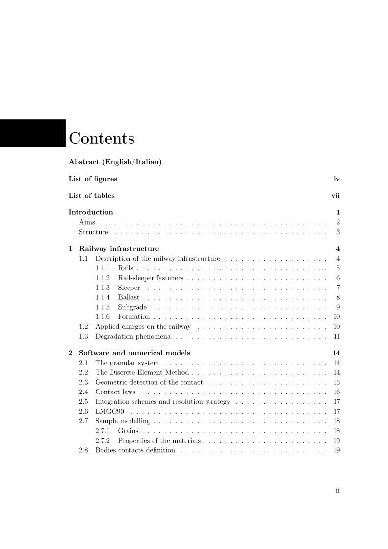
ContentsAbstract (English/Italian)

List of figures iv

List of tables vii

Introduction 1Aims . . . . . . . . . . . . . . . . . . . . . . . . . . . . . . . . . . . . . . . . . . 2Structure . . . . . . . . . . . . . . . . . . . . . . . . . . . . . . . . . . . . . . . 3

1 Railway infrastructure 41.1 Description of the railway infrastructure . . . . . . . . . . . . . . . . . . . 4

1.1.1 Rails . . . . . . . . . . . . . . . . . . . . . . . . . . . . . . . . . . . 51.1.2 Rail-sleeper fasteners . . . . . . . . . . . . . . . . . . . . . . . . . . 61.1.3 Sleeper . . . . . . . . . . . . . . . . . . . . . . . . . . . . . . . . . . 71.1.4 Ballast . . . . . . . . . . . . . . . . . . . . . . . . . . . . . . . . . . 81.1.5 Subgrade . . . . . . . . . . . . . . . . . . . . . . . . . . . . . . . . 91.1.6 Formation . . . . . . . . . . . . . . . . . . . . . . . . . . . . . . . . 10

1.2 Applied charges on the railway . . . . . . . . . . . . . . . . . . . . . . . . 101.3 Degradation phenomena . . . . . . . . . . . . . . . . . . . . . . . . . . . . 11

2 Software and numerical models 142.1 The granular system . . . . . . . . . . . . . . . . . . . . . . . . . . . . . . 142.2 The Discrete Element Method . . . . . . . . . . . . . . . . . . . . . . . . . 142.3 Geometric detection of the contact . . . . . . . . . . . . . . . . . . . . . . 152.4 Contact laws . . . . . . . . . . . . . . . . . . . . . . . . . . . . . . . . . . 162.5 Integration schemes and resolution strategy . . . . . . . . . . . . . . . . . 172.6 LMGC90 . . . . . . . . . . . . . . . . . . . . . . . . . . . . . . . . . . . . 172.7 Sample modelling . . . . . . . . . . . . . . . . . . . . . . . . . . . . . . . . 18

2.7.1 Grains . . . . . . . . . . . . . . . . . . . . . . . . . . . . . . . . . . 182.7.2 Properties of the materials . . . . . . . . . . . . . . . . . . . . . . . 19

2.8 Bodies contacts definition . . . . . . . . . . . . . . . . . . . . . . . . . . . 19

ii

Contents

3 Track’s lateral resistance 223.1 Experimental method . . . . . . . . . . . . . . . . . . . . . . . . . . . . . 223.2 Lateral resistance simulation . . . . . . . . . . . . . . . . . . . . . . . . . . 243.3 Creation of the models . . . . . . . . . . . . . . . . . . . . . . . . . . . . . 243.4 Comparison of compactness . . . . . . . . . . . . . . . . . . . . . . . . . . 273.5 Comparison of the lateral resistance . . . . . . . . . . . . . . . . . . . . . 293.6 Influence of the mass . . . . . . . . . . . . . . . . . . . . . . . . . . . . . . 363.7 Comparison with experimental results . . . . . . . . . . . . . . . . . . . . 38

4 Vertical settlement 404.1 Experimental models . . . . . . . . . . . . . . . . . . . . . . . . . . . . . . 404.2 Implementation of the model in the software . . . . . . . . . . . . . . . . . 404.3 Acceleration analysis . . . . . . . . . . . . . . . . . . . . . . . . . . . . . . 444.4 Settlement of the sleeper . . . . . . . . . . . . . . . . . . . . . . . . . . . . 464.5 Comparison of the compactness . . . . . . . . . . . . . . . . . . . . . . . . 484.6 Comparison with a theoretical model . . . . . . . . . . . . . . . . . . . . . 504.7 Results for the ballast in the box . . . . . . . . . . . . . . . . . . . . . . . 524.8 Comparison with the experiences . . . . . . . . . . . . . . . . . . . . . . . 53

Conclusions and perspective 54General conclusions . . . . . . . . . . . . . . . . . . . . . . . . . . . . . . . . . . 54Perspectives . . . . . . . . . . . . . . . . . . . . . . . . . . . . . . . . . . . . . . 55

Bibliography 57

Appendices 58

A Profiles of the ballast 59

B Oscillations of a two mass spring system 60

C Paraview 64

iii

List of Figures1 How the speed and the mass of the trains increased over time . . . . . . . 1

1.1 Cross section of a railway track . . . . . . . . . . . . . . . . . . . . . . . . 41.2 Division between infrastructure and superstructure . . . . . . . . . . . . . 51.3 Distribution of the charges, from the wheel to the formation . . . . . . . . 51.4 Flat bottomed (Vignoles) rail is the dominant rail profile in worldwide use 61.5 An example of how an extreme heat can cause rails to buckle . . . . . . . 61.6 Scheme of a free body diagram . . . . . . . . . . . . . . . . . . . . . . . . 81.7 First profile of the ballast . . . . . . . . . . . . . . . . . . . . . . . . . . . 91.8 Second profile of the ballast . . . . . . . . . . . . . . . . . . . . . . . . . . 91.9 Third profile of the ballast . . . . . . . . . . . . . . . . . . . . . . . . . . . 91.10 Scheme of a tamping process . . . . . . . . . . . . . . . . . . . . . . . . . 121.11 A tamping machine used by Infrabel . . . . . . . . . . . . . . . . . . . . . 131.12 Ballast regulator machine . . . . . . . . . . . . . . . . . . . . . . . . . . . 13

2.1 Tasks of a contact resolver . . . . . . . . . . . . . . . . . . . . . . . . . . . 152.2 No-penetration laws . . . . . . . . . . . . . . . . . . . . . . . . . . . . . . 162.3 Interpenetration law . . . . . . . . . . . . . . . . . . . . . . . . . . . . . . 172.4 The difference between a real stone and a modelled stone . . . . . . . . . 182.5 Simplified 2D grain modelling for simulation . . . . . . . . . . . . . . . . . 182.6 Deformability of the elastic layer . . . . . . . . . . . . . . . . . . . . . . . 21

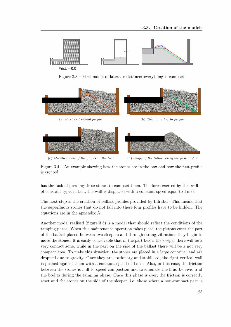
3.1 Cross section of test track during lateral testing with downward load . . . 233.2 Test on the lateral resistance of the ballast . . . . . . . . . . . . . . . . . . 233.3 First model of lateral resistance: everything is compacted . . . . . . . . . 253.4 An example showing how the stones are in the box and how the first profile

is created . . . . . . . . . . . . . . . . . . . . . . . . . . . . . . . . . . . . 253.5 Second model studying the lateral resistance: compacted zone below the

sleeper and not compacted zone beside the sleeper . . . . . . . . . . . . . 263.6 Third model studying the lateral resistance: compacted zone below the

sleeper and beside the sleeper . . . . . . . . . . . . . . . . . . . . . . . . . 263.7 Fourth model studying the lateral resistance: the compaction is everywhere 273.8 Representation of the ballast provided by the Python script . . . . . . . . 273.9 Representation of the ballast provided by Paraview . . . . . . . . . . . . . 28

iv

List of Figures

3.10 First model studying the lateral resistance . . . . . . . . . . . . . . . . . . 283.11 Second model studying the lateral resistance . . . . . . . . . . . . . . . . . 293.12 Third model studying the lateral resistance . . . . . . . . . . . . . . . . . 293.13 Fourth model studying the lateral resistance . . . . . . . . . . . . . . . . . 303.14 Lateral resistance of a ballast compacted below and beside the sleeper,

subjected to a constant displacement . . . . . . . . . . . . . . . . . . . . . 313.15 Lateral resistance of a ballast compacted below, subjected to a constant

displacement . . . . . . . . . . . . . . . . . . . . . . . . . . . . . . . . . . 323.16 Lateral resistance of a ballast compacted below the sleeper, subjected to a

constant displacement . . . . . . . . . . . . . . . . . . . . . . . . . . . . . 323.17 Lateral resistance of a ballast not compacted beside the sleeper, subjected

to an incremental force . . . . . . . . . . . . . . . . . . . . . . . . . . . . . 333.18 Lateral resistance of a ballast not compacted beside the sleeper, subjected

to a constant displacement . . . . . . . . . . . . . . . . . . . . . . . . . . . 343.19 Lateral resistance of a ballast not compacted beside the sleeper, subjected

to a constant displacement . . . . . . . . . . . . . . . . . . . . . . . . . . . 343.20 Lateral resistance of a ballast not compacted beside the sleeper, subjected

to an incremental force . . . . . . . . . . . . . . . . . . . . . . . . . . . . . 353.21 Lateral resistance of a ballast not compacted beside the sleeper, subjected

to an incremental force . . . . . . . . . . . . . . . . . . . . . . . . . . . . . 353.22 Scheme of the mass beside and below the sleeper (red) and beside the

sleeper (cyan) . . . . . . . . . . . . . . . . . . . . . . . . . . . . . . . . . . 363.23 Comparison of the masses of each profile with the total mass of the ballast

with the not compacted zone . . . . . . . . . . . . . . . . . . . . . . . . . 363.24 Comparison of the masses of each profile with the total mass of the ballast

where everything is compact. . . . . . . . . . . . . . . . . . . . . . . . . . 373.25 Velocities of the different bodies in a ballast compacted everywhere . . . . 373.26 A ballast compacted only below the sleeper after the 10 mm displacement 38

4.1 Numerical model to simulate the settlement of the sleeper . . . . . . . . . 404.2 First phase: placement of the stones in the box . . . . . . . . . . . . . . . 424.3 Second phase: compaction of the stones in the box . . . . . . . . . . . . . 424.4 Third phase: hiding of the stones to create the ballast profile . . . . . . . 424.5 Fourth phase: a vertical force is imposed to the sleeper . . . . . . . . . . . 434.6 Numerical model to simulate the settlement of the sleeper . . . . . . . . . 434.7 Force graph with a frequency sweep . . . . . . . . . . . . . . . . . . . . . . 444.8 Accelerations of the stones in the ballast . . . . . . . . . . . . . . . . . . . 454.9 Velocities of the stones in the ballast . . . . . . . . . . . . . . . . . . . . . 454.10 Acceleration, velocity and settlement of the sleeper pushed by a constant

frequency force . . . . . . . . . . . . . . . . . . . . . . . . . . . . . . . . . 464.11 Zoom of the vertical settlement of the sleeper pushed by a constant fre-

quency force . . . . . . . . . . . . . . . . . . . . . . . . . . . . . . . . . . . 47

v

List of Figures

4.12 Settlements of the sleepers pushed by a constant frequency force, for thecases with no elastic layers, one elastic layer, two elastic layers . . . . . . . 47

4.13 Settlements of the sleepers pushed by a frequency sweep force . . . . . . . 484.14 Compactness of the ballast before applying the force to the sleeper . . . . 494.15 Compactness of the ballast after applying the force to the sleeper . . . . . 494.16 Movement of the stones in the ballast after applying the force to the sleeper 494.17 Compactness of the ballast before applying the force to the sleeper . . . . 504.18 Compactness of the ballast after applying the force to the sleeper . . . . . 504.19 Movement of the stones in the ballast after applying the force to the sleeper 504.20 Scheme of a two mass spring system . . . . . . . . . . . . . . . . . . . . . 514.21 Frequency response functions . . . . . . . . . . . . . . . . . . . . . . . . . 514.22 Acceleration of the sleeper loaded by a frequency sweep . . . . . . . . . . 524.23 Settlement of a sleeper placed in a box . . . . . . . . . . . . . . . . . . . . 524.24 Vertical settlement of the sleeper as a function of the number of cycles in

the experimental model . . . . . . . . . . . . . . . . . . . . . . . . . . . . 53

C.1 Velocity of the stones, respectively at t = 1.000 s, 1.025 s, 1.100 s . . . . 64C.2 Velocity of the stones, respectively at t = 100.000 s, 100.025 s, 100.100 s 65C.3 Velocity of the stones, respectively at t = 199.000 s, 199.925 s, 200.000 s 65

vi

List of Tables1.1 Classification of the loads . . . . . . . . . . . . . . . . . . . . . . . . . . . 11

2.1 Materials used in the simulations . . . . . . . . . . . . . . . . . . . . . . . 20

3.1 Summary of the simulations for the lateral resistance . . . . . . . . . . . . 30

vii

Introduction

Context

Figure 1 – How the speed and the mass of the trains increased over time (translated [10])

Over the years, the train transport capacity has increased significantly. Trains are gettingfaster and faster, carrying ever-increasing masses and are required by ever-increasingnumbers of travellers. These three factors cause a continuous deterioration of the tracks,which require constant and well-planned maintenance. The tracks, in fact, must be moreresistant and maintenance operations must above all consider the problem related to thesettlement of the sleepers.

In order to resist these phenomena, the components of the track have become moreperforming: the sleepers are made of prestressed concrete, with a lifetime that is threetimes longer than those of the wooden sleepers. The rails use different profiles, such asUIC 60, to withstand greater traffic.

1

Introduction

Elastic layers can be placed under the sleeper to better dissipate loads and dampen theireffect. Geo-textiles or bituminous layers can be applied to the base of the formation toimprove drainage. However, the only component that has not undergone major changesis the ballast, which in fact remains the component that degrades faster. Some railwaycompanies have tried to replace this layer with reinforced concrete slabs, which has ahigher initial cost, but a lower maintenance in the long run. Since it is not a componentthat has been studied for a long time, to date the ballast is the one most used by railwaycompanies.

Aims

The ballast layer must have periodic maintenance, whatever the traffic in circulation, toensure adequate safety and comfort. The maintenance process most used today is thetamping, an operation similar to what is commonly done with goose down pillows whenyou want to give a new shape before falling asleep. The difference, obviously, betweenthe two materials is notable because the ballast is composed of irregularly shaped solidswith frictions and their displacement must take place in a very short time consideringthat the tracks on which this operation is to be carried out are long several kilometres.

The tamping is an operation that has existed for over sixty years and its effects havetherefore been studied for a long time. Its biggest drawback is that of degrading thecomponents of the ballast: the hammers of the railway tamping machines are insertedbetween the sleepers and with their high-frequency vibrations they round the stonesand break the edges. The degradation is then accelerated and after some operation oftamping, the ballast must be replaced. The study of these operations is very complexand the aim of this thesis is to create a model based on the discrete element methodto perform computer simulations that will then be compared with laboratory tests andscientific texts. The thesis is part of the WholeTrack industrial project of the UniversitéCatholique de Louvain, while the software used is LMGC90, developed by the Universitéde Montpellier. In particular, this thesis is a continuation of the thesis written by RaülAcosta Suñé. I started from his final tips for simulation improvements and I tried to geta more valid model.

The models created use granular modelling and for this type of simulation, they are two-dimensional. With them the lateral resistance of the ballast and the vertical settlementsare studied, evaluating how the settlements vary through the use of elastic components.The final aim is to compare the results obtained with experimental results present in theliterature or with tests carried out in the laboratory.

2

Introduction

Structure

This thesis is divided into four main parts. The first part embraces all the informationthat allows us to understand how a railway track works, which elements it is composed ofand why every element is important. The second part explains what kind of modellingwas used to represent the elements of the track, the software and the contact laws thatallow starting the simulations. In the third part, there is the study of the lateral resistanceof the railway ballast, for each profile and according to the coefficients of friction andcompactness. The fourth chapter contains the study of the settlement of the sleeper,connected to the study of accelerations, velocities, and frequencies of the stones in theballast. Finally, the thesis ends with a summary of the results obtained in this researchand some suggestions for the improvement of the simulations already carried out.

3

1 Railway infrastructure

1.1 Description of the railway infrastructure

Figure 1.1 – Cross section of a railway track (translated [17])

The term railway (or railway track) generally refers to the land transport infrastructure,suitable for the movement of trains. It is composed of two parts: the superstructure andthe infrastructure (fig. 1.1). The former defines the constructive complex composed ofall the elements that should guide and support the train and its wheels. The latter isbelow these elements and it is in general only composed of the ground, in this case calledformation.

There are two types of railway lines in Europe: conventional lines and high-speed lines.As defined by the European Union, the latter has been designed to be used by high-speedtrains and they include: [17, 13]

• Lines specially built for high-speed trains travelling at speeds generally equal to orgreater than 250 km/h;• Lines specially adapted for high speed, where trains travels for speeds of the order

of 200 km/h;• Specially upgraded high-speed lines, linked to topographic constraints. The optimal

speed has to be calculated.

4

1.1. Description of the railway infrastructure

Figure 1.2 – Division between infrastructure and superstructure (translated [15])

The elements of the railway have to bring the train charges from the rails to the formation.The distribution of loads leads to a progressive increase of the distribution area, passingto a reduction of the effort of about 20000 times between the wheel-rail contact pointsand the formation, [2, 9, 14] in order to reduce the risk that the formation could reachthe limit value of the shear strength.

Figure 1.3 – Distribution of the charges, from the wheel to the formation (translated [2])

1.1.1 Rails

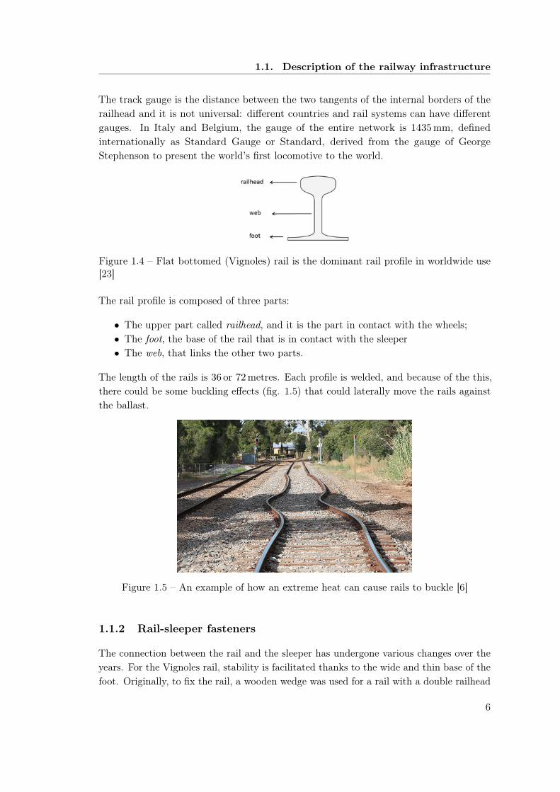
Rails are the fundamental element of a track because they are the first element belowthe trains’ wheels and they have to support and guide them. Their section is a doubleasymmetric T, installed in parallel over a bearing structure called sleeper. The most usedprofile is the one called "Vignoles" (figure 1.4). Its characteristic shape offers a highvertical inertia and an optimal distribution of the shear stresses. Its essential characteristicis its mass per linear meter. The UIC, the worldwide rail organisation, has standardisedtwo profiles: 54 or 60 kg per linear meter, in rolled steel.

5


The track gauge is the distance between the two tangents of the internal borders of therailhead and it is not universal: different countries and rail systems can have differentgauges. In Italy and Belgium, the gauge of the entire network is 1435 mm, definedinternationally as Standard Gauge or Standard, derived from the gauge of GeorgeStephenson to present the world’s first locomotive to the world.

Figure 1.4 – Flat bottomed (Vignoles) rail is the dominant rail profile in worldwide use[23]

The rail profile is composed of three parts:

• The upper part called railhead, and it is the part in contact with the wheels;• The foot, the base of the rail that is in contact with the sleeper• The web, that links the other two parts.

The length of the rails is 36 or 72 metres. Each profile is welded, and because of the this,there could be some buckling effects (fig. 1.5) that could laterally move the rails againstthe ballast.

Figure 1.5 – An example of how an extreme heat can cause rails to buckle [6]

1.1.2 Rail-sleeper fasteners

The connection between the rail and the sleeper has undergone various changes over theyears. For the Vignoles rail, stability is facilitated thanks to the wide and thin base of thefoot. Originally, to fix the rail, a wooden wedge was used for a rail with a double railhead

6


and when the part in contact with the wheels was worn, the rail could be rotated to usethe non-worn part. Today the fastening system is mechanised to ensure good elasticityand faster times. Fastening is done with mechanical machines that automatically connectthe sleeper and the rail.

It is also important to place elastic rubber layers under the sleeper to dampen vibrationscaused by passing trains.

1.1.3 Sleeper

The sleeper is an element that has the role of transmitting train loads from the rail tothe ballast, ensuring a constant track gauge and inclination between the rails. [17]

The two most commonly used materials for the sleeper are wood, almost exclusivelyused years ago, and concrete, which makes the sleeper heavier, improving stability, noiseisolation and giving the track a longer life. In some areas of Italy, wooden sleepers arepreferred to those in concrete because environmental conditions such as the heat and saltcarried by the sea can corrode the armature of the sleeper.

There are two types of concrete sleepers:

• Monoblock: sleepers made of a single piece of concrete. They are characterised bya good stability and they could last around 50 years;• Bi-block: sleepers composed of two concrete parts connected by a metal bar. Theiradvantage is the reducing damage from torsional forces on the sleeper centre duethe more flexible steel connections. They cost less but they last less (30-40 years)because of the possible corrosion of the metal bar.

The lateral anchoring of the sleeper in the ballast is very important for the lateral stabilityof the track. It could help to reduce the buckling effect of a welded rail subjected to heatdilatation.

The sleepers have been made increasingly heavy and stable as a result of the invention ofreinforced concrete, but the disadvantage is in the low vibration damping capacity.

Weight is an important element. The greater the weight of the sleeper, the greater theforce to be applied to move this sleeper.{

F ≤ µ ·m · gT ≤ µ ·N

(1.1)

Where:

• F is the applied force;

7


Figure 1.6 – Scheme of a free body diagram

• T is the friction force;• µ is the friction coefficient;• N is the normal force;• g is the gravity acceleration.

1.1.4 Ballast

The main purpose of the ballast is to ensure a solid and stable support base for heavystructures that must rest directly on the ground. Soils are often unsuitable to directlysupport the structures because they can be wet, yielding and rich in vegetation andparticularly they can undergo considerable changes as a result of floods, winds etc.

The ballast, thanks to its composition of small and medium-size stones, protects thestructure from humidity and lets the water pass underneath, so that it can subsequentlyevaporate.

The crushed stone is regulated by EN 13450:2003 norm which defines mechanical andphysical properties. For Italian standards, the gravel is considered suitable if its densityis higher than 2550 kg/m3. The particle size fraction, comprised between two sieves ofdimensions 31.5 and 50.0 mm, must have a number of stones equal or greater than 50%.[18]

The ballast is not only the base of the train tracks but it also anchors the sleeper reducingthe longitudinal and transversal effects.

In Belgium, Infrabel has defined three profiles of ballast to be used for its tracks. [3, 17]

1. The first profile (fig. 1.7) has a small protuberance of 0.10 m. It is used for speed:

• v < 200 km/h and v ≥ 40 km/h;• v > 200 km/h and the presence of particular elements on the track, such as

expansion devices;

2. The second profile (fig. 1.8) is the one used on the high-speed line, i.e. for trainspeeds above 200 km/h and it does not have the protuberance of 10 centimetres to

8


avoid the risk of flying stones;

3. The third profile (fig. 1.9) is used for low speeds, for example for the accessoriestracks.

Obviously the first profile has a greater lateral resistance compared to the third profile,because it has a greater number of stones and therefore a greater mass on the side of thesleeper. The sleeper finds a greater difficulty in moving the ballast.

The figures 1.7, 1.8, 1.9 provided by the Infrabel track design studio show the three ballastprofiles. [3]

Figure 1.7 – First profile of the ballast (translated [3])

Figure 1.8 – Second profile of the ballast (translated [3])

Figure 1.9 – Third profile of the ballast (translated [3])

1.1.5 Subgrade

In transport engineering, subgrade is the native material underneath a constructed road,pavement or railway track. [22] The aim of this layer is to avoid the reaching of theshear strength in the formation. It also improves the protection against the frost and itimproves the draining.

9

1.2. Applied charges on the railway

The subgrade is generally composed of gravels with a size of 20−40 mm. In order toimprove the lifespan it is possible to add a bituminous concrete or a geotextile. [14]

1.1.6 Formation

The formation constitutes the infrastructure of the track and can be built with anembankment or it can be a bridge or a tunnel. Its most important feature is the weightcapacity: the formation is the last element that makes up the track, takes the remainingloads and influences the long-term behaviour of the sustained superstructure.

Another important aspect is the stiffness, which in some cases can help to decrease thesettlement of the tracks. For this reason, recent research studies the settlement of thetracks analysing the use of elastic layers placed on the formation.

1.2 Applied charges on the railway

The stresses to be taken into account during train transit are as follows: [24]

• Lengthways in the wagon:– Up to four times the mass of the load for goods that are rigidly secured;– Up to once the mass of the load for goods that can slide lengthways in the

wagon;They are mainly due to train’s acceleration and deceleration and temperaturevariations, especially for welded bars. They are generally negligible compared tovertical and horizontal efforts;• Crosswise in the wagon up to 0.5 times the mass of the load. They are caused by

the centrifugal effect when cornering and by forces of thermal origin due to weldingof the tracks. They should not be underestimate in order to prevent the bucklingphenomenon. In fact, the ballast is less rigid in the lateral direction;• Vertically up to 0.3 times the mass of the load, which encourages the displacement

of the goods. They are divided into static loads, such as the mass of the train, anddynamic loads, due to the interaction between vehicle and track.

The UIC classifies the line types based on the load. The lines of each railway are classifiedinto categories per the permissible mass per axle and mass per linear metre, as shown intable 1.1.

The load limits are marked on the wagon and it is that one from the lowest line categoryon the route in question. This limit must not be exceeded. [24]

10

1.3. Degradation phenomena

Table 1.1 – Classification of the loads. [24]

Line category Maximum mass per axle Maximum mass per linear metre

A 16.0 t 5.0 t/m

B1 18.0 t 5.0 t/mB2 18.0 t 6.4 t/m

C2 20.0 t 6.4 t/mC3 20.0 t 7.2 t/mC4 20.0 t 8.0 t/m

D2 22.5 t 6.4 t/mD3 22.5 t 7.2 t/mD4 22.5 t 8.0 t/m

E4 25.0 t 8.0 t/mE5 25.0 t 8.8 t/m

1.3 Degradation phenomena

The train loads induce a slow degradation of the track, both in terms of geometry andthe state of the materials. For this reason it is necessary to carefully design the line bychoosing the appropriate materials.

The type of train and the type of rolling material circulating on the track can influence thedegradation status of the track. A regional train, for example, travels much slower than ahigh-speed train, with much less important dynamic loads. If there are any imperfectionsin the contact between the train wheel and the rail, dynamic overload effects occur,implying a faster degradation.

Atmospheric phenomena must also be considered during track design. For example, insome Italian lines, RFI, the owner of Italy’s railway network, has decided to apply a whitepaint over the rails, in order to decrease the value of the thermal expansion coefficient,thus decreasing the dilatation efforts.

There most important maintenance process is called tamping and it is used when therails no longer satisfy the tolerance thresholds. The machine takes a measure in the firstphase where it detects everything in terms of trajectory, levelling and inclination. A trackin comparison to the other must be flat without any inclination. If there is an error of 3-5millimetres, this must be zero. Information are transmitted to the system and the railwill be straightened or re-aligned. The machine vibrates at high frequency to compressthe ballast under the sleepers and the track remains in its new position.

The hammers break the stones and smooth the edges. Breaking the stones means reducingthe compaction of the ballast and therefore also decreasing its lateral resistance also

11


Figure 1.10 – Scheme of a tamping process [20]

because only the zone below the sleeper is compacted and not on the sides, which willthen need to be especially studied in the curves of the tracks. [17, 14]

Approximately, a tamping is effective for 40-50 million tons of passage, or more or less4-5 years of traffic, depending on the the number of tampings realised. [14]

Generally, this operation can be accompanied by the use of another machine: a ballastregulator, also known as a sweeper, that is used to shape the different ballast profiles andto compact these profiles pushing from the top of the protuberance (figure 1.12).

12


(a) View of the hammers fromthe platform

(b) Internal view of the tampingmachine

Figure 1.11 – A tamping machine used by Infrabel

Figure 1.12 – Ballast regulator machine [21]

13

2 Software and numerical models

2.1 The granular system

A granular material is a conglomeration of discrete solid, macroscopic particles charac-terised by a loss of energy whenever the particles interact and they are not chemicallylinked. They are use in different fields, from agriculture to pharmacy industry. [1]

The behaviour of a solid material divided into very small grains is different from thebehaviour of its material in the solid, liquid or gas state and depends on the appliedenergy, which is dissipated very rapidly.

The granular materials are difficult to study because there are complex limit conditionsand many contacts laws. A granular system is stable if low-stress increases inducesmall deformations, therefore the modelling of quasi-static behaviour assumes that theseincrements have a finite value and that the fluctuations of these values can be neglected.[16] In addition, the friction forces should be calculated because they are the stabilisingelements and they can’t be neglected. The calculation of these forces makes the processlonger.

Thanks to the properties of the granular systems, the stability of the track is also analysedthrough numerical simulations.

2.2 The Discrete Element Method

The principle of the discrete element method (DEM) is to integrate the motion equationsby analysing the interactions of the particles by contact or friction. In general, on onestep [t, t+ h[, three main phases can be identified: [11]

• Contact detection;• The resolution of contact forces: the speeds and/or rotations that each particle will

14

2.3. Geometric detection of the contact

Figure 2.1 – Tasks of a contact resolver (translated [11])

undergo are calculated;• The movement of each particle.

Today the two most used approaches are the following:

• The regular approach, or Smooth: the relative displacements between two particlesat the contact point or the interpenetration are used in correlation with a law whichregulates the contact force;• The non-regular, or Non-Smooth approach: it considers the contact and friction

interactions, using the laws of motion and the dissipation equation.

The NSCD (Non-Smooth Contacts Dynamics) doesn’t allow the overlapping of twoparticles and it considers the perfect rigidity of contacts. Trough the Signorini-Coulomblaw is possible to determine the speed and the force of each stone, avoiding the penetrations.This method is commonly used because it allows different shapes, convex and concave,with bigger time steps.

2.3 Geometric detection of the contact

The contacts can have different types of polyhedral particles such as the ballast. Thesecontacts can be represented by a point, a line or a surface.

In the LMGC90 software, the contacts between two bodies always have a candidate bodyA and an antagonist body B. The aim of the software is to make the contact happenbut A does not have to penetrate the body B. Both have a local reference point andthe direction between these two points must be considered. [16] Through the distancebetween these two points, the distance between the two bodies is calculated and whetheror not the overlap occurred. As a first step, an alert distance is established, which consistsin estimating the proximity of two stones and if this distance is sufficiently high, otherbodies are analysed.

15

2.4. Contact laws

(a) No-penetration law (b) Fiction law

Figure 2.2 – No-penetration laws [17]

The problem of this type of simulation is the large number of cycles, and therefore oftime, to be performed. If, as in the case in question, there are many bodies, it is necessaryto calculate the contact that occurs in a certain step between all the bodies in question.[16] In this thesis, only two-dimensional bodies were used.

2.4 Contact laws

To study the behaviour of the ballast, the choice of the contact law is fundamental,because it regulates the contacts between the grains and therefore their positions. It waschosen to use the Signorini-Coulomb law, with the following constraints:

if g ≤ 0 ⇒

{Rn ≥ 0; Vn ≥ 0

Vn ·Rn = 0(2.1)

Where:

• g is the gap between the two particles. If this space is null it means that a contactreaction is present;• Rn is the normal reaction of the particle;• Vn is the relative normal speed of the particle.

However, the space g is always positive because there is no grain penetration. Theonly case where there could be the interpenetration is with the analysis of the verticalsettlement, where a interpenetration is needed to study the elasticity of some elasticbodies. The law is shown in figure 2.3

if g ≤ 0 ⇒ Rn = −kn · g (2.2)

Where kn is the stiffness.

With regard to the friction law that should regulate the frictional contact between the

16

2.5. Integration schemes and resolution strategy

Figure 2.3 – Interpenetration law [17]

bodies, the Coulomb law was used:{‖dRt‖ ≤ µ · dRn, if Vt = 0

dRt = −µ · dRn‖dRn‖ , if Vt 6= 0

(2.3)

Where:

• Rt is the tangential reaction of the particle;• Rn is the normal reaction of the particle;• Vt is the tangential speed;• µ is the friction coefficient.

The two bodies move only if the tangential force exceeds the value µ ·Rn.

2.5 Integration schemes and resolution strategy

The goal of time integration schemes is to discretise the movement of a particle whenthere are some contacts, in order to have a better precision.

Two approaches are possible: [16]

• Trough the event-driven method: the time is not uniformly divided, but the intervalis adapted in such a way that the collision moment falls in this time step. It is notused in this thesis because there would be an high number of contacts and it wouldrequire an high number of interactions;• Trough the time-stepping : the time is divided into many steps of equal duration. It

is implemented in LMGC90 and it is used in this thesis.

2.6 LMGC90

The software used during the simulations is LMGC90. The LMGC90 is a multipurposesoftware developed in the Université de Montpellier, in France, capable of modelling a

17

2.7. Sample modelling

(a) The real shape of a stone placed in theballast

(b) How the stones are seen by LMGC90[19]

Figure 2.4 – The difference between a real stone and a modelled stone

collection of deformable or non-deformable interacting through simple interaction (friction,cohesion, . . . ) or complex multi-physics coupling (fluid, thermal, . . . ). [11]

LMGC90 can use bodies with different shapes, from polygons to spheres, in two or threedimensions.

In this thesis, only irregular polygons where used to model the stones placed in the ballast,and, in addiction, rectangular elements such as walls, sleeper, formation and elastic layers.

2.7 Sample modelling

2.7.1 Grains

(a) Real shape (b) Real shape vs modelled shape (c) Modelled shape

Figure 2.5 – Simplified 2D grain modelling for simulation [17]

The most difficult track’s component to model is the ballast: in fact, it is necessary todefine the shape of each stone and then place the sleeper on it. The ballast must try tolook as much as possible to an existing ballast, that is, with the area compacted under the

18

2.8. Bodies contacts definition

sleeper and a less compact area on the sides. It is also important so have some differentshape for the stones because a model with only one shape will not be enough accurate.

Also appropriate friction coefficients and appropriate interaction laws must be provided.Moreover, due to the great number of calculations to be performed through the computer,it was decided to use 2D models, giving a prismatic shape to all the components of themodel, with a depth of one meter for each body (figure 2.4).

The shape of the stones used for the simulations was obtained from the stones thatthe Sagex company supplied to the WholeTrack group. Through a video-granulometryprocess, different shapes were taken, obtaining a polygonal line and then simplified toobtain a convex shape (fig. 2.5) [17]. The Non-Smooth Conctacts Dynamics method canconsider concave shapes but it would take more time, it would be more difficult to resolvethe contact and it requires a specific algorithm for the contact detection.

2.7.2 Properties of the materials

It would be impossible to run a simulation with the discrete element method if, in additionto the shape, a material with its mechanical properties was not assigned. It is necessaryto specify that the bodies are considered rigid, that is with an elastic modulus tendingto infinity, [17, 11] except for the elastic layer placed below the sleeper and above theformation.

Through the first simulation model, the lateral resistance of the ballast is studied andtherefore it is necessary to insert the properties of the stones, the sleeper, the formationand some artificial walls that help to realise the compaction. For the second model, thatstudies the vertical settlement of the sleeper, an elastic layer is added. The assignedmaterial is the caoutchouc, a material commonly used in the construction of the railwaytracks because it helps to reduce the acoustic and mechanical vibrations, with a densityof 930 kg/m3.

2.8 Bodies contacts definition

For the properties of granular materials, the definition of friction coefficients is a veryimportant aspect because it affects the behaviour of the structure.

Maynar Melis calculated a friction coefficient between the grains that falls in a rangethat goes from 0.577 to 0.839. Different coefficients were used, in order to evaluate thechanges in the results of the simulation and to study the different behaviours. [17, 12]

For the case of the friction between the grains, only 0.7 and 0.8 were used, in order to bein that range. The contact of the grains with the formation is equal to 1, because, in

19


Table 2.1 – Materials used in the simulations

Simulation that study the lateral resistance

Element Material Density Type(kg/m3)

Stone Porphiry 2800 Rigid

Sleeper Concrete 2500 Rigid

Wall Concrete 2500 Rigid

Simulation that study the settlement

Stone Porphiry 2800 Rigid

Sleeper Concrete 2500 Rigid

Wall Concrete 2500 Rigid

Elastic layer Caoutchouc 930 Elastic

reality, the stones meet a wrinkled soil and there is more adherence.

For the contact between the grains and the sleeper, 0.5 and 0.7 as friction coefficientswere used to check if the lateral resistance of the ballast profiles increases as in the reality.

For the second model that studies the vertical settlement, there could be two elasticlayers.

In addition to the contacts explained above, two other laws are added: [11]

• ELASTIC_ROD: the law used for the elastic layer places below the sleeper. It addsa spring rod to some specified points and its importance it is in the fact that thelayer doesn’t fall because of the gravity, but it is glued to the sleeper. The reactionforce is proportional to the deformation;• ELASTIC_REPELL_CLB: it describes a normal reaction force proportional tothe gap, otherwise the reaction force vanishes when the contactors separate. Thefriction law is Coulomb’s law and it is useful when there are physical reasons totake elasticity into consideration.

The elastic layers have one degree of freedom and their behaviour is shown in the figure2.6.

20


Figure 2.6 – Deformability of the elastic layer

21

3 Track’s lateral resistance

3.1 Experimental method

As already mentioned in section 1.1.1, in addition to the longitudinal and vertical loads,it is important to study the influence of lateral loads on the resistance of the ballast. Ifbefore this study was not necessary, today it is essential because of the increase in thenumber of passengers and the number of goods transported.

The TU Delft Roads and Railways Research Laboratory conducted a series of full-scalethree-dimensional ballast resistance tests using a rail track panel. For our objectives,only the results of the tests regarding the lateral resistance are compared with the resultsobtained in this thesis. [25]

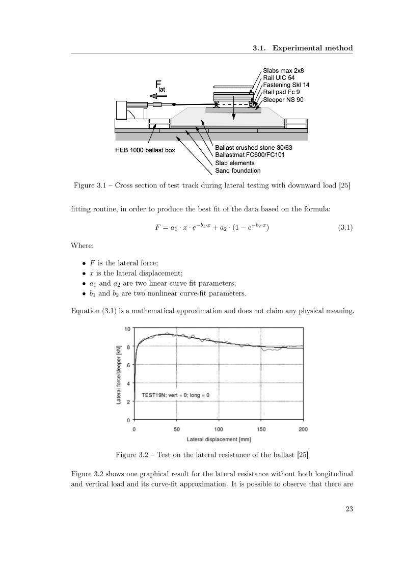
The components that make up the instrumentation used to perform the test, shown infigure 3.1, are: [25]

• Two rail pieces, UIC 54 section;• Five NS90 concrete sleepers;• Ballast bed of crushed stone 30/63, a thickness under sleeper of 30 cm;• Ballast mat, James Walker type (FC600/FC101);• Concrete slabs (Stelcon): 2 m × 2 m × 10 cm, total 120 m2;• Sand foundation (subgrade).

The load introduction in the lateral direction is achieved through two diagonal rodsconnecting the hydraulic actuator, to the track section with a force of 150 kN. Twoconnecting beams are welded between the rails to reinforce the track panel enabling amore uniform load introduction. The actuators are programmed under displacementcontrol to fulfil a complete measurement with a constant low velocity of 10 mm/min. [25]

All measurements in the test were automatically and digitally recorded and importedinto the Matlab environment, where the research team has obtained an automatic curve

22

3.1. Experimental method

Figure 3.1 – Cross section of test track during lateral testing with downward load [25]

fitting routine, in order to produce the best fit of the data based on the formula:

F = a1 · x · e−b1·x + a2 · (1− e−b2·x) (3.1)

Where:

• F is the lateral force;• x is the lateral displacement;• a1 and a2 are two linear curve-fit parameters;• b1 and b2 are two nonlinear curve-fit parameters.

Equation (3.1) is a mathematical approximation and does not claim any physical meaning.

Figure 3.2 – Test on the lateral resistance of the ballast [25]

Figure 3.2 shows one graphical result for the lateral resistance without both longitudinaland vertical load and its curve-fit approximation. It is possible to observe that there are

23

3.2. Lateral resistance simulation

three main parts: [25, 17]

• A phase where the displacements are very small compared to the lateral forces;• A logarithmic phase that ends with an inflection point;• An asymptotic line that reaches a lateral resistance value.

3.2 Lateral resistance simulation

The results of lateral resistance of the track mentioned above are compared with somenumerical simulations carried out with LMGC90. Although in reality the physical modelto move a sleeper is very complex, in simulations it is very simple: a force or a speed isdirectly imposed on the sleeper. The simulations are carried out for four different profiles,in order to compare them and to evaluate the different lateral resistance and, in general,a simulation stops when the sleeper is displaced for 10 mm.

The force imposed is an increasing horizontal force, and for each time step it is possibleto store the reactions of the sleeper (or other selected bodies) and a plot studying thecorrelation between the force and the displacement is the final output.

The increasing horizontal forces are:

• ∆F = 1.0 N each time step, that is every millisecond;• ∆F = 1.5 N/ms;• ∆F = 2.0 N/ms.

When a force is imposed, probably there is a kinetic absorption on the grains of theballast and in the graphs there is not the first linear phase mentioned in section 3.1. Inorder to better understand this phenomenon, an imposed constant velocity was appliedto the sleeper, with a value of vx = 2 mm/s.

In addition, it was decided to evaluate the lateral resistance in the different sides ofthe sleeper, with the respective percentages, to better understand the influence of thecompaction. Below the sleeper, where there is a compacted zone, the forces should bemore influential than the forces in a not compacted zone.

3.3 Creation of the models

In the first simulation of the lateral resistance (figure 3.3), half-track is modelled. It hasbeen chosen to have a very compact ballast, both below the sleeper and on its sides, whichgenerally does not represent reality. In order for this to happen, numerous stones havebeen placed in a large box representing the ballast in a railway track. All these stoneshave been dropped due to gravity and once they are stable, a vertical wall on the right

24

3.3. Creation of the models

Figure 3.3 – First model of lateral resistance: everything is compact

(a) First and second profile (b) Third and fourth profile

(c) Modelled view of the grains in the box (d) Shape of the ballast using the first profile

Figure 3.4 – An example showing how the stones are in the box and how the first profileis created

has the task of pressing these stones to compact them. The force exerted by this wall isof constant type, in fact, the wall is displaced with a constant speed equal to 1 m/s.

The next step is the creation of ballast profiles provided by Infrabel. This means thatthe superfluous stones that do not fall into these four profiles have to be hidden. Theequations are in the appendix A.

Another model realised (figure 3.5) is a model that should reflect the conditions of thetamping phase. When this maintenance operation takes place, the pistons enter the partof the ballast placed between two sleepers and through strong vibrations they begin tomove the stones. It is easily conceivable that in the part below the sleeper there will be avery contact zone, while in the part on the side of the ballast there will be a not verycompact area. To make this situation, the stones are placed in a large container and aredropped due to gravity. Once they are stationary and stabilised, the right vertical wallis pushed against them with a constant speed of 1 m/s. Also, in this case, the frictionbetween the stones is null to speed compaction and to simulate the fluid behaviour ofthe bodies during the tamping phase. Once this phase is over, the friction is correctlyreset and the stones on the side of the sleeper, i.e. those where a non-compact part is

25

3.3. Creation of the models

Figure 3.5 – Second model studying the lateral resistance: compacted zone below thesleeper and not compacted zone beside the sleeper

expected, are hidden. Later, other grains are put back into the container and droppeddue to gravity. The wall no longer pushes the grains, leaving them in their stabilisedposition and many more empty between them. Figure 3.5 shows the compact area, belowthe sleeper, and the non-compact area on its side.

Figure 3.6 – Third model studying the lateral resistance: compacted zone below thesleeper and beside the sleeper

Figure 3.6 shows another compaction that is very similar to that of belonging to firstmodel (fig. 3.3). In this case, at one-third of the simulation, the right vertical wall pushesthe stones through a sinusoidal movement with the following equation:

vx = A · sin(2 · π · f · t) (3.2)

Where:

• A is the amplitude: 0.2512 ;

• f is the frequency: 40 Hz;• t is the time.

In this way, the grains are pushed to the left with a less abrupt but still effective movement.

In this model, as for the first and the third model, there is a compaction in every zone ofthe ballast. The horizontal upper wall falls due to gravity and it is pushed against the

26

3.4. Comparison of compactness

Figure 3.7 – Fourth model studying the lateral resistance: the compaction is everywhere

track stones. At one-third of the simulation, the software adds an incremental force of500 N and the simulation stops until it reaches 50 kN. In addition to this, like the previousmodel, the right vertical wall tries to compact the stones with a sinusoidal movement(figure 3.7).

3.4 Comparison of compactness

Figure 3.8 – Representation of the ballast provided by the Python script. The unit ofmeasure is the meter

For all the simulations carried out, the compactness of the ballast on the side and belowthe sleeper was studied with the aim of analysing the variation of compaction during thismodel creation process. The compaction of the ballast has been studied in three differentphases with the use of Python scripts. Figure 3.8 is the graphic result of a script thatchecks for each point of the ballast whether there is a stone or not: if it is, it draws alittle black square, otherwise a small white square. For reasons related to the complexityof the calculation, it was decided to use a 5 mm step, so that the result is fairly reliable.In fact, there is not a big difference with the image provided by the LMGC90 software(figure 3.9).

Then, it was chosen to represent squares of size 45 mm × 45 mm, so that each squarecontains a value that is the mean of a square containing 9 × 9 points. For each cell acolour was identified representing the percentage of points, i.e. the percentage of spacecovered by one or more in that square. The dark blue indicates that the area is verycompact, while the dark red indicates that there is a gap in the ballast.

27

3.4. Comparison of compactness

Figure 3.9 – Representation of the ballast provided by Paraview

Figure 3.10 – First model studying the lateral resistance. The unit of measure is themeter

The figures 3.3 and 3.5 show two opposite cases: the ballast with a compaction carriedout everywhere and the ballast which has not undergone a compaction on the side of thesleeper. As expected, there is an obvious difference in compaction in the latter area, sothe script used is valid.

The fourth model (fig. 3.7) has a greater compaction than the third (fig. 3.6) because inaddition there is the presence of a wall that pushes from the top towards the bass. It canbe said, however, that the compaction is not so evident, probably due to the fact that thesimulation was not carried out for a sufficient duration or was not carried out adequately.

The influence of the compactness, and therefore of the mass of the ballast, is shown laterin the graphs of the sections 3.5 and 3.6.

28

3.5. Comparison of the lateral resistance

Figure 3.11 – Second model studying the lateral resistance. The unit of measure is themeter

Figure 3.12 – Third model studying the lateral resistance. The unit of measure is themeter

3.5 Comparison of the lateral resistance

In the first model represented in figure 3.14, the studied ballast presents a practicallyuniform compaction, even on the side of the sleeper. In the graph below, the relation

29


Figure 3.13 – Fourth model studying the lateral resistance. The unit of measure is themeter

Table 3.1 – Summary of the simulations for the lateral resistance

Name Compaction Type of imposed Value Friction Frictiondisplacement (grains) (ballast-sleeper)

Fig. 3.14 Below Velocity 10 mm 0.7 0.5and beside (2 mm/s)

Fig. 3.15 Below Velocity (2 mm/s) 10 mm 0.7 0.5


Fig. 3.17 Below Incremental force 10 mm 0.7 0.5(∆F = 1.5 N)



Fig. 3.20 Below Incremental force 10 mm 0.8 0.7(∆F = 2 N)

Fig. 3.21 Below Incremental force 10 mm 0.8 0.7(∆F = 1 N)

between the applied force and the movement of the sleeper was represented, that is theforce necessary for the sleeper to overcome the resistance of the ballast to its side andbe able to move. The lines represent the four different profiles of the ballast and the

30


0 2 4 6 8 10Sleeper displacement (mm)

0

1000

2000

3000

4000

5000

6000

F x (N)

TotalBelow: 66.05%

Side: 20.62%Corner: 13.33%

Distribution of the lateral forces - 1st profile

(a) Influence of the forces in the different zones ofthe ballast


0

1000

2000

3000

4000

5000

6000

F x (N

)

1st profile2nd profile3rd profile4th profile

Displacement imposed (vx=2 mm/s)

(b) Lateral resistance of the ballast

Figure 3.14 – Lateral resistance of a ballast compacted below and beside the sleeper,subjected to a constant displacement

differences are not high.

In the second model, the ballast is compact below the sleeper while it has a lot of emptyspaces on the side and therefore less resistance of the ballast is expected. As can be seenin figure 3.15, the resistance that this ballast opposes to the movement of the sleeper ismuch lower than the values of the previous model.

Through a Python script, the forces applied by the sleeper are studied in order tounderstand which forces act under the sleeper, on the side or in the corner. It has beendecided to insert also the force corresponding to the corner because if a stone is presentin that position it is not known with certainty if this stone is below the sleeper or beside.In the following graphs, it has been chosen to represent only the first profile.

To calculate the percentage of forces in the different zones, a different procedure is usedfor longer time intervals, making the calculation of the graph on the left less accurate.In fact, not always the blue line of the graphs on the left coincides perfectly with theyellow line of the first profile of the graph on the right. However, the calculation of thepercentages proves to be accurate.

Obviously, since the area of the base of the sleeper is greater, the forces applied underthe sleeper have a greater percentage, followed by the forces on the side of the sleeperand those on the corner.

The graph in figure 3.15 analyses the forces applied in another ballast with compactionunder the sleeper and not compacted on the side. As might be expected, a ballast of

31



0

1000

2000

3000

4000

5000

F x (N

)

TotalBelow: 85.78%

Side: 7.51%Corner: 6.71%




0

1000

2000

3000

4000

5000

F x (N

)




Figure 3.15 – Lateral resistance of a ballast compacted below, subjected to a constantdisplacement

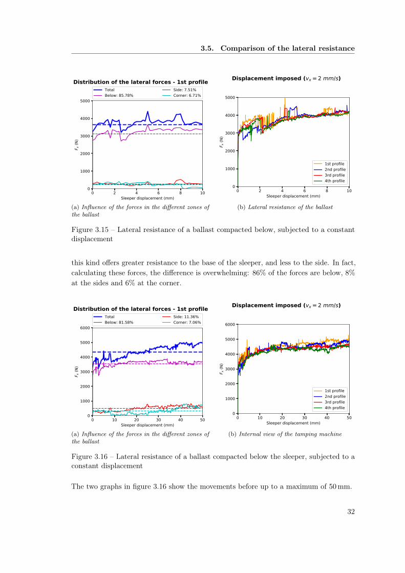
this kind offers greater resistance to the base of the sleeper, and less to the side. In fact,calculating these forces, the difference is overwhelming: 86% of the forces are below, 8%at the sides and 6% at the corner.


0

1000

2000

3000

4000

5000

6000

F x (N

)

TotalBelow: 81.58%





0

1000

2000

3000

4000

5000

6000

F x (N

)



(b) Internal view of the tamping machine

Figure 3.16 – Lateral resistance of a ballast compacted below the sleeper, subjected to aconstant displacement

The two graphs in figure 3.16 show the movements before up to a maximum of 50 mm.

32


The ballast is particularly compact and at first sight, it would seem that the side of thesleeper is more compact than the part below. Looking at the graphs it can be noticed aconstantly increasing shift at the side of the sleeper for the first 15 mm, after which thereis a constant trend of the force. Also, in this case, the difference between the first ballastprofile and the last one is clear, while the difference between the first and the second isnot particularly evident. Indeed, for short moments the values of the second profile reachthose of the first and in some instants are even greater.


0

1000

2000

3000

4000

5000

6000

F x (N

)

TotalBelow: 84.47%





0

1000

2000

3000

4000

5000

6000

F x (N

)


Force imposed (ΔF=1Δ5 N/ms)


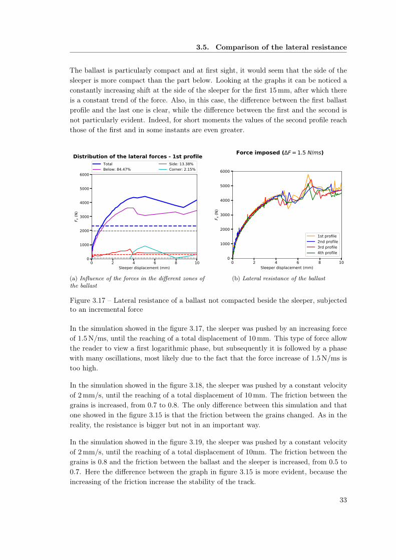
Figure 3.17 – Lateral resistance of a ballast not compacted beside the sleeper, subjectedto an incremental force

In the simulation showed in the figure 3.17, the sleeper was pushed by an increasing forceof 1.5 N/ms, until the reaching of a total displacement of 10 mm. This type of force allowthe reader to view a first logarithmic phase, but subsequently it is followed by a phasewith many oscillations, most likely due to the fact that the force increase of 1.5 N/ms istoo high.

In the simulation showed in the figure 3.18, the sleeper was pushed by a constant velocityof 2 mm/s, until the reaching of a total displacement of 10 mm. The friction between thegrains is increased, from 0.7 to 0.8. The only difference between this simulation and thatone showed in the figure 3.15 is that the friction between the grains changed. As in thereality, the resistance is bigger but not in an important way.

In the simulation showed in the figure 3.19, the sleeper was pushed by a constant velocityof 2 mm/s, until the reaching of a total displacement of 10mm. The friction between thegrains is 0.8 and the friction between the ballast and the sleeper is increased, from 0.5 to0.7. Here the difference between the graph in figure 3.15 is more evident, because theincreasing of the friction increase the stability of the track.

33



0

1000

2000

3000

4000

5000

F x (N

)

TotalBelow: 82.93%





0

1000

2000

3000

4000

5000

F x (N

)




Figure 3.18 – Lateral resistance of a ballast not compacted beside the sleeper, subjectedto a constant displacement


0

1000

2000

3000

4000

5000

6000

F x (N

)

TotalBelow: 87.33%





0

1000

2000

3000

4000

5000

6000

F x (N

)




Figure 3.19 – Lateral resistance of a ballast not compacted beside the sleeper, subjectedto a constant displacement

In the simulation showed in the figure 3.20, the sleeper was pushed by a constant force of2 N/ms, until the reaching of a total displacement of 10 mm. The friction between thegrains is 0.8 and the friction between the ballast and the sleeper is 0.7. As in the figure3.17, there is a main phase with a logarithmic behaviour, followed by some oscillations.The step of the incremental force is even bigger and should be rejected, but it is possible

34



0

1000

2000

3000

4000

5000

6000

7000

F x (N

)

TotalBelow: 76.72%





0

1000

2000

3000

4000

5000

6000

7000

F x (N

)


Force imposed (ΔF=2 NΔms)



to observe that the resistance reach bigger values.


0

1000

2000

3000

4000

5000

6000

7000

F x (N

)

TotalBelow: 86.94%





0

1000

2000

3000

4000

5000

6000

7000

F x (N

)


Force imposed (ΔF=1 NΔms)



In the simulation showed in the figure 3.21, the sleeper was pushed by a constant force of1 N/ms, until the reaching of a total displacement of 10 mm. The friction between thegrains is 0.8 and the friction between the ballast and the sleeper is 0.7. In this graphs

35

3.6. Influence of the mass

there are no oscillations and also in this case there is a logarithmic phase followed by alinear one.

A summary that helps to understand the simulations performed is included in the table3.1.

3.6 Influence of the mass

Figure 3.22 – Scheme of the mass beside and below the sleeper (red) and beside thesleeper (cyan)

The profiles of the ballast are important because the lateral resistance of the ballastdepends on them. But in this simulation, how much do they affect? Is it normal thatthere is not a big difference between the profiles?

The problem is that there is a visible difference in some graphs, for example in the figure3.16, but it is not so evident. In this phase of the work the linear mass of the total ballast(beside and below the sleeper) was computed and it was compared with the mass next tothe sleeper of the four profiles.

The stones located in the red area are the stones belonging to the mass of the total ballast,while the stones in the cyan area belongs to the stones analysed for the four differentprofiles beside the sleeper. As an example, the first profile is shown in figure 3.22.

0 500 1000 1500 2000 2500Mass (kg/m)

Ballast: 2245 kg/m1st profile: 382 kg/m (+55%)2nd profile: 338 kg/m (+37%)3d profile: 286 kg/m (+16%)4th profile: 247 kg/m

Masses in the ballast

Figure 3.23 – Comparison of the masses of each profile with the total mass of the ballastwith the not compacted zone

36

3.6. Influence of the mass

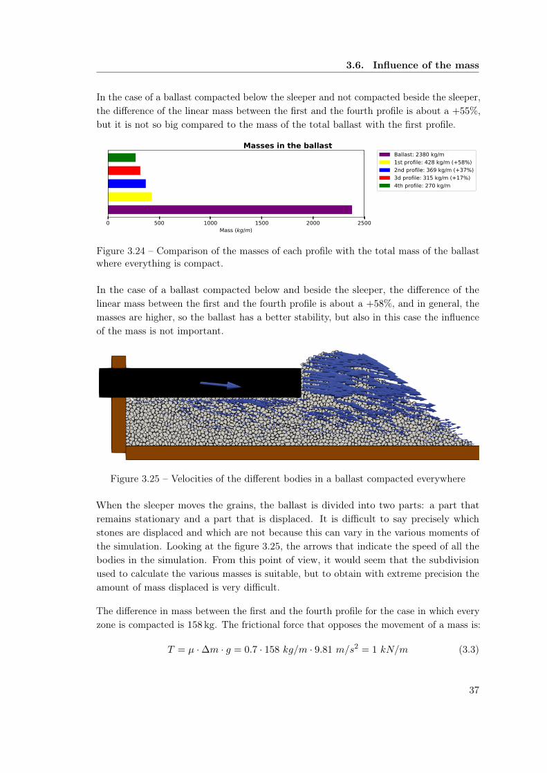
In the case of a ballast compacted below the sleeper and not compacted beside the sleeper,the difference of the linear mass between the first and the fourth profile is about a +55%,but it is not so big compared to the mass of the total ballast with the first profile.

0 500 1000 1500 2000 2500Mass (kg/m)

Ballast: 2380 kg/m1st profile: 428 kg/m (+58%)2nd profile: 369 kg/m (+37%)3d profile: 315 kg/m (+17%)4th profile: 270 kg/m

Masses in the ballast

Figure 3.24 – Comparison of the masses of each profile with the total mass of the ballastwhere everything is compact.

In the case of a ballast compacted below and beside the sleeper, the difference of thelinear mass between the first and the fourth profile is about a +58%, and in general, themasses are higher, so the ballast has a better stability, but also in this case the influenceof the mass is not important.

Figure 3.25 – Velocities of the different bodies in a ballast compacted everywhere

When the sleeper moves the grains, the ballast is divided into two parts: a part thatremains stationary and a part that is displaced. It is difficult to say precisely whichstones are displaced and which are not because this can vary in the various moments ofthe simulation. Looking at the figure 3.25, the arrows that indicate the speed of all thebodies in the simulation. From this point of view, it would seem that the subdivisionused to calculate the various masses is suitable, but to obtain with extreme precision theamount of mass displaced is very difficult.

The difference in mass between the first and the fourth profile for the case in which everyzone is compacted is 158 kg. The frictional force that opposes the movement of a mass is:

T = µ ·∆m · g = 0.7 · 158 kg/m · 9.81 m/s2 = 1 kN/m (3.3)

37

3.7. Comparison with experimental results

The coefficient of friction, for this short calculation, is set equal to 0.7, but this is a greatapproximation.

As shown in figure 3.14, the difference between the resistance of the first and fourthprofiles is around 1 kN, so the model seems valid.

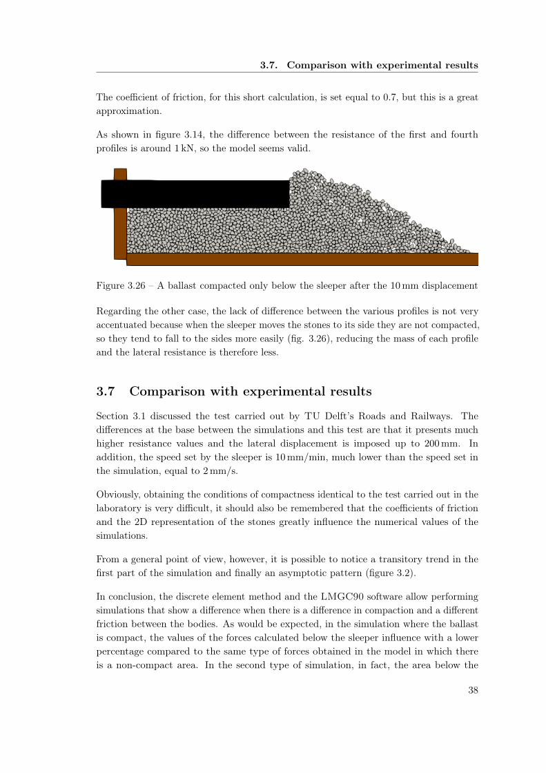
Figure 3.26 – A ballast compacted only below the sleeper after the 10 mm displacement

Regarding the other case, the lack of difference between the various profiles is not veryaccentuated because when the sleeper moves the stones to its side they are not compacted,so they tend to fall to the sides more easily (fig. 3.26), reducing the mass of each profileand the lateral resistance is therefore less.

3.7 Comparison with experimental results

Section 3.1 discussed the test carried out by TU Delft’s Roads and Railways. Thedifferences at the base between the simulations and this test are that it presents muchhigher resistance values and the lateral displacement is imposed up to 200 mm. Inaddition, the speed set by the sleeper is 10 mm/min, much lower than the speed set inthe simulation, equal to 2 mm/s.

Obviously, obtaining the conditions of compactness identical to the test carried out in thelaboratory is very difficult, it should also be remembered that the coefficients of frictionand the 2D representation of the stones greatly influence the numerical values of thesimulations.

From a general point of view, however, it is possible to notice a transitory trend in thefirst part of the simulation and finally an asymptotic pattern (figure 3.2).

In conclusion, the discrete element method and the LMGC90 software allow performingsimulations that show a difference when there is a difference in compaction and a differentfriction between the bodies. As would be expected, in the simulation where the ballastis compact, the values of the forces calculated below the sleeper influence with a lowerpercentage compared to the same type of forces obtained in the model in which thereis a non-compact area. In the second type of simulation, in fact, the area below the

38

3.7. Comparison with experimental results

sleeper, being more compact, opposes a greater resistance to the sliding of the sleeperand therefore influences with percentages around 80-90%.

39

4 Vertical settlement

4.1 Experimental models

In this second part of the thesis, the behaviour of the ballast and the elastic layers placedbelow the sleeper and above the platform are studied under vertical loads with the discreteelement method. The results of a real model are compared to the results obtained fromthe software.

The model is that one realised by the Centre d’Essais et d’Expertises of the SNCF, theFrance’s national state-owned railway company, linked to the Juan Carlos Quezada’sthesis. [17, 16] There is a vertical load over a track placed between two monoblockconcrete sleepers, with an elastic layer placed under the ballast. The loads applied gofrom a minimum of 48.5 kN to a maximum of 68.1 kN, with an average value of 59.7 kN,trying to simulate the forces behaviour during a train transition. Juan Carlos Quezadaused two values of stiffness for the elastic layer: 12 and 500 MPa. In regards to thefrequencies of the charge, he used 3.3 , 4.5 , 5.4 and 6.0 Hz, that are the equivalent of thespeeds 220 , 300 , 360 and 400 km/h. [17, 16]

4.2 Implementation of the model in the software

Figure 4.1 – Numerical model to simulate the settlement of the sleeper

The second simulation model analyses the vertical settlement of the sleeper. This is a

40

4.2. Implementation of the model in the software

much longer simulation because it lasts 320 seconds. In addition, the entire ballast isstudied and therefore no longer its half. On average, the time to perform a simulation ofthis type is one and a half days but it varies depending on the number of stone to besaved. For this simulation, it was decided to model three different tracks:

• A track with an elastic layer in the bottom of the ballast;• A track with an elastic layer in the bottom of the ballast and below the sleeper;• A track without elastic layers.

Two values of stiffness were then added to the simulation, each for each layer above andbelow the ballast. From the technical documents of Infrabel the following values havebeen used: [4, 5]

• k1 = 0.035 N/mm3 for the elastic layer positioned above the platform;• k2 = 0.300 N/mm3 for the elastic layer positioned under the sleeper.

In the model, being a discrete element simulation, each elastic layer is modelled withsmall squares of 20 mm on each side, and being in the two-dimensional model, the depthis equal to one meter. So the values entered in the simulation are the following:

• k1 = 0.035 N/mm3 · 20 mm · 1000 = 7 · 105 N/m

• k2 = 0.300 N/mm3 · 20 mm · 1000 = 6 · 106 N/m

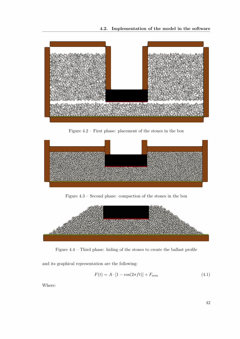
These samples representing the various types of track were created by first placing allthe stones in a large container (fig. 4.2) where this time the whole track is representedand not just half the portion. The upper artificial walls and the stones are allowed to fallby gravity, while all the other bodies remain fixed (fig. 4.3). The upper walls, therefore,apply a constant force equal to its weight, or 2575 N.

The second profile (fig. 1.8) of the Infrabel ballast is assigned to each track, i.e. the onefor high-speed trains. The upper and lateral artificial walls and the stones outside thisprofile are therefore rendered invisible (fig. 4.4). The last step is the application of thevertical load (fig. 4.5) on the concrete sleeper: it is the passage that undergoes morevariations between one simulation and the other because it can be chosen to study onlythe settlement, that is the vertical displacement of the sleeper, or even the horizontaldisplacement and its rotation.

The force applied to the sleeper is applied for a duration of 200 seconds, which identifiesthis step as the longest one. The force is sinusoidal and has two different equations. Thefirst oscillates between 3 and 32 kN, with a frequency of 10 Hz. It is obviously applieddownwards and starts at a value of 3 kN to not immediately have a situation too loaded,which could damage the model. [17] The equation of force introduced in the simulation

41


Figure 4.2 – First phase: placement of the stones in the box

Figure 4.3 – Second phase: compaction of the stones in the box

Figure 4.4 – Third phase: hiding of the stones to create the ballast profile

and its graphical representation are the following:

F (t) = A · [1− cos(2πft)] + Fmin (4.1)

Where:

42


Figure 4.5 – Fourth phase: a vertical force is imposed to the sleeper

• A is the amplitude: (Fmax − Fmin)/2

• Fmax is the maximum force: 32 kN;• Fmin is the minimum force: 3 kN;• f is the frequency: 10 Hz;• t is the time, in seconds.

0 1 2 3 4 5Time (s)

10000

20000

30000

Force (N

)

Figure 4.6 – Numerical model to simulate the settlement of the sleeper

The second force used for the application of the load has the following equation:

F (t) =Fmax

2·[1 +

(2π ·

(f0 +

f1 − f0

t1 − t0· t

2

)· t)]

(4.2)

This is the frequency sweep equation, and unlike the previous one, it was used to studythe behaviour at various frequencies.

Where:

• Fmax is the maximum force: 32 000 N;• f0 is the initial frequency: 20 Hz;• f1 is the final frequency: 50 Hz;• t0 is the initial time: 0 s;• t1 is the final time: 200 s.

The graph in figure 4.7 shows the force graph for the first 20 seconds.

43

4.3. Acceleration analysis

0.0 2.5 5.0 7.5 10.0 12.5 15.0 17.5 20.0Time (s)

0

10000

20000

30000

Force (N

)

Figure 4.7 – Force graph with a frequency sweep

4.3 Acceleration analysis

Through the LMGC90 software, it is possible to choose which elements to study ingreater detail. In particular, by indicating the number that identifies the body, it ispossible to visualise the time step, the x, y and z positions of the body and the velocitiesalong the three axes.

It has been chosen to derive the accelerations of some stones at specific points, to analysehow the acceleration varies in the different areas of the ballast and subsequently tocompare them with a theoretical model, using only the equations of mechanical physics.

The software does not directly store accelerations, so central-difference formulas needto be used. [8] In particular, it is possible to obtain the value of the acceleration in aspecific point, knowing that acceleration is the first derivative of velocities, and using thevalue in that given time step as a step h.

u′(0) =−U2h + 8Uh − 8U−h + U−2h

12h(4.3)

With these equations, accelerations of the stones in the different zones of the ballast canbe plotted (figure 4.8). In this example the ten stones’ accelerations were studied and foreach studied stone a number was assigned (figure 4.1). It can be immediately seen thatthe stones with the greatest accelerations are under the sleeper, and for the stones awayfrom it, the accelerations decrease. The stones placed above platform do not have a highacceleration, probably due to the fact that most of the force applied to the sleeper doesnot contribute to the profile of the ballast at the sides of it. Also in the graph showingthe speed distribution (figure 4.9), there is a tendency similar to that of accelerations: thestones near the sleeper have a greater velocity than those placed far from it. In addition,the six stones placed under the sleeper have an average value almost equal.

44

4.3. Acceleration analysis

Figure 4.8 – Accelerations of the stones in the ballast

Figure 4.9 – Velocities of the stones in the ballast

In the previous graphs the root mean square (RMS) was calculated:

xRMS =

√1

n·(x2

1 + x22 + · · ·+ x2

n

)=

√1

n·∑n=1

x2n (4.4)

The value is positioned above each graph and is represented with a dashed white line. Ithas been chosen to use this type of mean because both accelerations and velocities have awaveform, and therefore the only arithmetic mean would not have been suitable.

Through Paraview, a software to visualise the data obtained from the simulations withLMGC90, it is possible to obtain a scale representation of the speeds of the stones

45

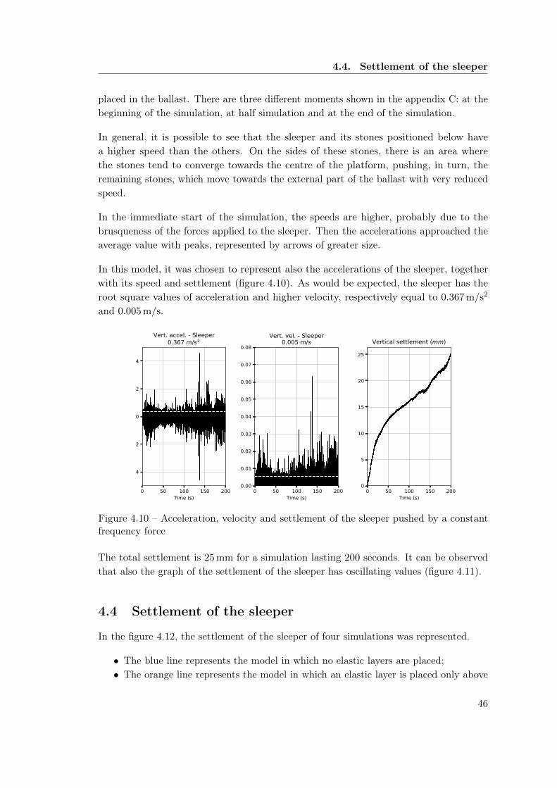
4.4. Settlement of the sleeper

placed in the ballast. There are three different moments shown in the appendix C: at thebeginning of the simulation, at half simulation and at the end of the simulation.

In general, it is possible to see that the sleeper and its stones positioned below havea higher speed than the others. On the sides of these stones, there is an area wherethe stones tend to converge towards the centre of the platform, pushing, in turn, theremaining stones, which move towards the external part of the ballast with very reducedspeed.

In the immediate start of the simulation, the speeds are higher, probably due to thebrusqueness of the forces applied to the sleeper. Then the accelerations approached theaverage value with peaks, represented by arrows of greater size.

In this model, it was chosen to represent also the accelerations of the sleeper, togetherwith its speed and settlement (figure 4.10). As would be expected, the sleeper has theroot square values of acceleration and higher velocity, respectively equal to 0.367 m/s2

and 0.005 m/s.

0 50 100 150 200Time (s)

−4

−2

0

2

4

Vert. accel. - Sleeper0.367 m/s2

0 50 100 150 200Time (s)

0.00

0.01

0.02

0.03

0.04

0.05

0.06

0.07

0.08

Vert. vel. - Sleeper0.005 m/s

0 50 100 150 200Time (s)

0

5

10

15

20

25

Vertical settlement (mm)

Figure 4.10 – Acceleration, velocity and settlement of the sleeper pushed by a constantfrequency force

The total settlement is 25 mm for a simulation lasting 200 seconds. It can be observedthat also the graph of the settlement of the sleeper has oscillating values (figure 4.11).

4.4 Settlement of the sleeper

In the figure 4.12, the settlement of the sleeper of four simulations was represented.

• The blue line represents the model in which no elastic layers are placed;• The orange line represents the model in which an elastic layer is placed only above

46

4.4. Settlement of the sleeper

Figure 4.11 – Zoom of the vertical settlement of the sleeper pushed by a constant frequencyforce

0 25 50 75 100 125 150 175 200Time (s)

0

5

10

15

20

25

30Vertical settlement (mm)

No layersk1=7 ⋅ 105 N/mk2= N.A.k1=7 ⋅ 105 N/mk2=6 ⋅ 106 N/m

Figure 4.12 – Settlements of the sleepers pushed by a constant frequency force, for thecases with no elastic layers, one elastic layer, two elastic layers

the platform;• The green line represents the model in which there are two elastic layers: the first

above the platform and the second below the sleeper;

First of all it is necessary to specify that the different thickness of the lines is due tothe fact that one or more elastic layers is placed. In these cases, with a one-millisecondstep, it can be seen that the sleeper has a high oscillatory behaviour, unlike the firstmodel in which it seems that it always has a settlement downward. The model with thegreatest settlement is the last one, i.e. the one in which the sleeper suffers a verticalforce downwards by frequency sweep. This, in all probability, is due to the fact that thefrequency sweep equation goes from a frequency of 20 Hz to 50 Hz, and then in the final

47

4.5. Comparison of the compactness

part receives a greater boost. It can be also noticed, as it could be expected in reality,that increasing the frequency also increases the slope of the graph of the settlement.

The difference with the graph of the settlement of the third model is not so high, only2 mm. This model has a frequency of 10 Hz and probably the frequency of loading doesnot have a great influence on the settlement of the sleeper.

0 25 50 75 100 125 150 175 200Time (s)

0

5

10

15

20

25

30Vertical settlement (mm)

k1=7 ⋅ 105 N/mk2=6 ⋅ 106 N/m(Frequency sweep)

Figure 4.13 – Settlements of the sleepers pushed by a frequency sweep force

The line in figure 4.13 represents the model in which, unlike the others, the frequencysweep equation is used. Like the previous model, it has two elastic layers.

4.5 Comparison of the compactness

Also for this second model, the compactness of the ballast on the sides and below thesleeper has been studied with the aim of analysing the variation of the compaction duringthis process of creating the model. The images below are the graphic result of the samescript used above for the lateral resistance model. Also in this case, there is not a bigdifference with the image provided by the LMGC90 software.

Figure 4.14 shows the level of compaction preceding the beginning of the application ofthe vertical force on the sleeper.

Then a force is applied and it is possible to notice that the height of the layer of stonesbelow the sleeper is smaller. The greater compaction occurs at one side of the sleeper(the right side) and below (figure 4.15). This is probably due to the fact that the ballastis not perfectly symmetric, so there is a tendency for stones to move more to one side.

Figure 4.16 shows the movements of the stones before the application of the force andafter its application. The green value, with its maximum at 100 %, means that in that

48

4.5. Comparison of the compactness

Figure 4.14 – Compactness of the ballast before applying the force to the sleeper. Theunit of measure is the meter

Figure 4.15 – Compactness of the ballast after applying the force to the sleeper. The unitof measure is the meter

Figure 4.16 – Movement of the stones in the ballast after applying the force to the sleeper.The unit of measure is the meter

area the stone was not there before the application of the force and it is in that positionafter the compaction. The red values, with its minimum at −100 %, means that the stonewas there only before the application of the force.

As it can seen, the differences are not too high because in the graph there are almost onlylight colours. Generally, at first glance, the green colour is the most present, therefore witha greater compaction, especially on the sides of the ballast. In fact, after the applicationof a load on the sleeper, it should be expected a compaction below the sleeper andthe movement of the grains to the sides of the ballast. The dark green colour presentdiagonally on the sides of the ballast represents just this. This concept is also confirmedby the files displayed in Paraview (see appendix C), where it is clearly seen that thevectors of the velocities of the external stones tend to always move outwards, while thosenear the sleeper tend to fall down. These images also show the oscillations that thebodies have: in a first moment the speeds are directed downwards, then upwards andthen immediately downwards again.

49

4.6. Comparison with a theoretical model

Figure 4.17 – Compactness of the ballast before applying the force to the sleeper. Theunit of measure is the meter

Figure 4.18 – Compactness of the ballast after applying the force to the sleeper. The unitof measure is the meter

Figure 4.19 – Movement of the stones in the ballast after applying the force to the sleeper.The unit of measure is the meter

4.6 Comparison with a theoretical model

Another aim of this thesis is to find a relationship between a theoretical model, calculablewith simple dynamics equations, and a model that can be calculated using the LMGC90software. For this reason, it is necessary to consider the model consisting of two masses:m2, i.e. the mass of the sleeper, and m1, the mass of the ballast. Two elastic componentshave been added to this model: k1 or the equivalent elastic component of the elastic layerplaced just above the platform, and k2, the equivalent elastic component of the elasticlayer placed just below the sleeper (fig. 4.20).

It is, therefore, a 2D model with only one degree of freedom and through which the verticaldisplacements were studied, from which the accelerations were subsequently obtained.The latter were compared with the accelerations obtained with the models applied onLMGC90. The demonstration of the calculation of the eigenmodes has been included inthe appendix B.

50

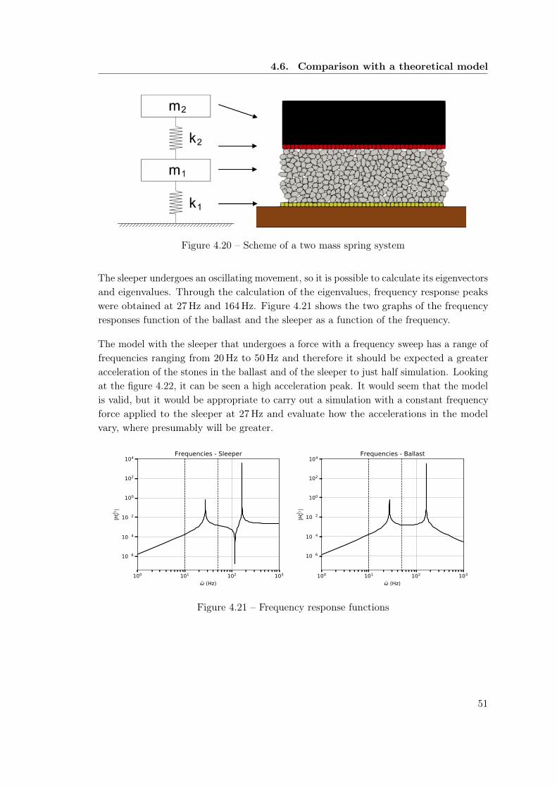
4.6. Comparison with a theoretical model

Figure 4.20 – Scheme of a two mass spring system

The sleeper undergoes an oscillating movement, so it is possible to calculate its eigenvectorsand eigenvalues. Through the calculation of the eigenvalues, frequency response peakswere obtained at 27 Hz and 164 Hz. Figure 4.21 shows the two graphs of the frequencyresponses function of the ballast and the sleeper as a function of the frequency.

The model with the sleeper that undergoes a force with a frequency sweep has a range offrequencies ranging from 20 Hz to 50 Hz and therefore it should be expected a greateracceleration of the stones in the ballast and of the sleeper to just half simulation. Lookingat the figure 4.22, it can be seen a high acceleration peak. It would seem that the modelis valid, but it would be appropriate to carry out a simulation with a constant frequencyforce applied to the sleeper at 27 Hz and evaluate how the accelerations in the modelvary, where presumably will be greater.

100 101 102 103

ω(Hz)

10−6

10−4

10−2

100

102

104

|H z 2 F|

Frequencies- Sleeper

100 101 102 103

ω Hz)

10−6

10−4

10−2

100

102

104

|H z 1 F|

Frequencies- Ballast

Figure 4.21 – Frequency response functions

51

4.7. Results for the ballast in the box

0 25 50 75 100 125 150 175 200Time (s)

−30

−20

−10

0

10

20

30

Vertical acceleration - Sleeper1.721 m/s2

Figure 4.22 – Acceleration of the sleeper loaded by a frequency sweep

4.7 Results for the ballast in the box

In Raül Acosta Suñé’s thesis, [17] the settlement of the ballast was simulated in a box withvertical walls, for a duration of 360 seconds, with and without the addition of an elasticlayer above the platform. Figure 4.23 shows the vertical displacements as a function oftime for situations with and without the elastic layer. Also in this case the settlementsare considered positive.

Figure 4.23 – Settlement of a sleeper placed in a box (translated [17])

It can be observed a more oscillatory behaviour for the situation with the layer placedabove the platform because that has an elastic behaviour. This is the reason why thestones undergo a more oscillating movement contrary to the situation without the elasticlayer. At the end of the simulation, the blue curve without continuing to increase, while,for the red curve, the displacement seems to have stopped. [17] It is possible to noticethat the settlements obtained are lower than the settlements shown in figure 4.12. Thisis due to the fact that the stones are placed in a large box and therefore the wall-stone

52

4.8. Comparison with the experiences

(a) Settlement curves for each test (b) Three phases of settlement in the curve

Figure 4.24 – Vertical settlement of the sleeper as a function of the number of cycles inthe experimental model (translated [16])

friction plays a fundamental role.

4.8 Comparison with the experiences

As it can be seen in the figure 4.24, the shape of the curve obtained from the Juan CarlosQuezada’s thesis [16] is very similar to the curve obtained from the software LMGC90(fig. 4.12). It could be seen that there are three main phases in a settlement curve, asexplained before: a first linear phase, the logarithmic phase with a point of inflexion andthe linear phase. All these phases can be found in the simulations carried out and shownpreviously.

Obviously the numerical results are not the same. This is due to the friction coefficients,the type of compaction, the type of force applied to the sleeper and also due to the factthat the model is 2D.

53

Conclusions and perspective

General conclusions

A plenty of simulations were carried out during these months through the softwareLMGC90, with a high number of data as results. The simulations focused on theimportance of the ballast layer of the track and, as explained in the previous chapters,some parameters can totally change the results.

In the first part, the simulations studied the lateral resistance of the ballast that in generalis caused by the buckling effects of the welded rails subjected to a prevented dilatation.Afterward, the settlement of the sleeper is studied because it is caused by the train traffic.

For what concerns the first analysis, the software has shown that there is a differencebetween the four profiles of studied ballast and the effect of compaction. When thereis a ballast reinforced with a protuberance, a graph has been obtained and it showeda greater resistance. Moreover, it has been shown that a compact ballast has a greaterresistance than a not-compacted ballast and that increasing the compactness decreasesthe influence of forces below the sleeper.

The software also showed that by increasing the friction coefficient, the lateral resistanceof the ballast was also increased. Finally, for the case of the sleeper with a greaterdisplacement, a graph was obtained with a curve that resembles the curves obtained inthe laboratory.

However, the analysis has some limitations, and obviously, the values obtained do notcorrespond to reality. This is due to the fact that the simulations are two-dimensional, sothe bodies are considered as prisms and the two faces in the z direction are not takeninto account.

For the study of the settlement of the sleeper, various cases have been studied, in whichthe number of elastic elements have been changed.

Through numerous simulations, graphs have been provided and they demonstrate howthe stones move at certain points of the ballast after a load applied to the sleeper.

54

Conclusions and perspective

Automatically, graphs that show how the field of accelerations and speeds varies from thepoint most loaded to the less loaded point are plotted.

The software also allowed to demonstrate that there is an oscillatory behaviour due tothe presence of elastic elements. Regarding the settlement of the sleeper, graphs that aresimilar to those seen in the literature are obtained.

The models seem therefore valid, albeit with values far from reality, but the results arevery consistent.

Perspectives

After all the results explained in the previous sections, it is possible to say that thediscrete element method and LMGC90 are reliable for the studies of the lateral resistanceand the vertical settlement.

For the former, it is recommended to improve the compaction of the different zones ofthe ballast, trying to have a distribution very similar to the ballast after the tampingprocess. This is possible trying to create a high number of simulations.

For the latter, a simulation that lasts 300 seconds could not be enough. Future researcherscould try to increase the time of the simulation, changing the friction coefficient andthe compaction of the ballast. After that, it could be possible to correlate the resultswith the graph of the settlements, where the behaviour should be more or less the same.Furthermore, frequency response diagrams were also studied and it will be interesting tostudy the accelerations by a force with a constant frequency approaching the frequencypeaks mentioned before.

The reader should not forget that all the simulations were carried out through 2D models,that doesn’t represent perfectly the reality. 3D models are possible but they require alarge amount of memory space as well as a large amount of time. If it took two days toanalyse the settlement of a sleeper in 2D, in 3D it would take an entire week.

55

Bibliography

[1] Jacques Duran. Sands, powders, and grains: an introduction to the physics ofgranular materials. Springer Science & Business Media, 2012.

[2] Coenraad Esveld. Modern railway track, 2001.

[3] Infrabel. Circulaire sur les traverses en béton M41.

[4] Infrabel. Spécification technique: fabrication et fourniture des traverses en bétonmonoblocs.

[5] Infrabel. Specification technique: fourniture de tapis amortisseurs sous ballast.

[6] Sarah Knapton. Heatwave could buckle train tracks and melt roads, travellerswarned.

[7] KTH Royal Institute of Technology. Rail vehicle dynamics.

[8] Vincent Legat. Méthodes numériques, 2011.

[9] Bernhard Lichtberger. Track compendium, 2005.

[10] Bernhard Lichtberger. Railway manual, 2010.

[11] LMGC90. LMGC90 documentation.

[12] Manuel Melis Maynar. Apuntes de introducción a la dinámica vertical de la vía yalas señales digitales en ferrocarriles: con 151 programas en Matlab, Simulink, VisualC++, Visual Basic y Excel. 2008.

[13] Official Journal of the European Union. Directive 2004/50/EC of the EuropeanParliament and of the Council, April 2004.

[14] Chiara Paderno. Comportement du ballast sous l’action du bourrage et du traficferroviaire, 2010.

[15] Vassilios A Profillidis. Railway engineering, 2000.

[16] Juan-Carlos Quezada. Mécanismes de tassement du ballast et sa variabilité. PhDthesis, Université Montpellier II-Sciences et Techniques du Languedoc, 2012.

56

Bibliography

[17] Raül Acosta Suñé. Analyse numérique de la stabilité des voies ferrées, 2017.

[18] RFI. Specifica tecnica: pietrisco per massicciata ferroviaria.

[19] Gilles Saussine, C Cholet, PE Gautier, Frédéric Dubois, Claude Bohatier, and Jean-Jacques Moreau. Modelling ballast behaviour under dynamic loading. Part 1: A2D polygonal discrete element method approach. Computer methods in appliedmechanics and engineering, 195(19-22):2841–2859, 2006.

[20] Ernest Theodore Selig and John M Waters. Track geotechnology and substructuremanagement. Thomas Telford, 1994.

[21] Shaishav Shah. BRM Kershaw - Ballast regulator machine.

[22] CJ Summers. The idiots guide to highways maintenance. 2005.

[23] Rayl System. Rail profile.

[24] UIC. Loading Guidelines - Code of practice for the loading and securing of goods onrailway wagons.

[25] J van’t Zand and J Moraal. Ballast resistance under three dimensional loading, 1997.

57

Appendices

58

A Profiles of the ballast

First profile:

y > 0.58 ∧ 0.362 < (x− 1.50)2 + (y − 0.32)2 ∨ y > −0.73x+ 1.81 (A.1)

Second profile:

y > 0.33x+ 0.14 ∧ y > 0.56 ∨ y > −0.67x+ 1.69 (A.2)

This profile is a simplification of the first and in theory, they should have almost equalvalues.

Third profile:y > 0.56 ∨ y > −0.67x+ 1.69 (A.3)

Fourth profile:y > 0.56 ∨ y > −0.67x+ 1.63 (A.4)

59

B Oscillations of a two mass springsystem

Another aim of this thesis is to find a relationship between a theoretical model, calculablewith simple dynamics equations, and a model that can be calculated using the LMGC90software. For this reason, it is necessary to consider the model consisting of two masses:m2, i.e. the mass of the sleeper, and m1, the mass of the ballast. Two elastic componentshave been added to this model: k1, or the equivalent elastic component of the elasticlayer placed just above the platform, and k2, the equivalent elastic component of theelastic layer placed just below the sleeper, as shown in figure 4.20.

A 2D model with only two degrees of freedom and his vertical displacements are studied,obtaining also the accelerations and the frequencies of the bodies.

With the following equations, taken from a course in the KTH Royal Institute ofTechnology, in Stockholm, the procedure for obtaining the frequency response functionsis described. [7] {

m2x2 + c2x2 + c2x1 + k2x2 + k2x1 = 0

m1x1 − c2x2 + (c1 + c2)x1 + k2x2 + k2x1 = 0(B.1)

In a short form:Mx+ Cx+Kx = F (B.2)

The values of the eigenvectors and eigenvalues must be found because they give importantinformation about the dynamic properties of a track. The solution is found starting fromthe homogeneous equation:

Mx+ Cx+Kx = 0 (B.3)

The solution of this equation should be in the form:

x(t) = γ · eλt (B.4)

Where γ are the eigenvalues and λ are the eingevectors of the system. Substituting this

60

into the equation (B.3):det(λ2M + λC + k) = 0 (B.5)

It is possible to obtain:

m2m1λ4+(m2c1+m2c2+m1c2)λ3+(m2k1+m2k2+m1k2+c1c2)λ2+(c1k2+c2k1)λ+k1k2 = 0

(B.6)In this case, the model is considered undamped:

c1 = 0, c2 = 0 (B.7)

From which it is obtained:

λ21, 2 = −1

2

k1

m1+k2

m2·(

1 +m2

m1

)±

√[k1

m1+k2

m2·(

1 +m2

m1

)]2

− 4k1k2

m1m2

(B.8)

The eigenvectors are important because they give information on the amplitude ofdisplacements and on the phase shift between the oscillations of the different masses.

Through the eigenvectors and the eigenvalues, it is possible to obtain the frequencyresponse function: the quantitative measure of the output spectrum of a system inresponse to a stimulus, and it is used to characterise the dynamics of the system. It ispossible to compute, for example, the behaviour of the accelerations for various frequenciesand, through the graph, the frequency peaks can be analysed.

The excitation in the system has the equation:

F (t) = F · est (B.9)

Consequently, the system respects with an equation like:

x(t) = x · est (B.10)

By replacing this in (B.3):(Ms2 + Cs+K)x = F (B.11)

It was decided to study the frequency response between force and acceleration, which hasthe form:

HxjFk

(s) =s2 · xjFk

= s2 ·HxjFk

(s) (B.12)

Where:

• xj is the acceleration;• Fk is the input;• s = iω is the frequency of the acceleration;

61

• xj is the output;

With: (z2

z1

)=

(z2

z1

)est (B.13)

equation (B.1) becomes:∣∣∣∣∣m2s2 + c2s+ k2 −c2s− k2

−c2s− k2 m1s2 + (c1 + c2)s+ (k1 + k2)

∣∣∣∣∣ (B.14)

The frequency response function between the applied force F and z2 is written in theform:

Hz2F (s) =

z2

F(B.15)

Remembering Cramer’s rule: [a1 b1a2 b2

]·(x

y

)=

(c1

c2

)(B.16)

the solutions are:

x =

det

∣∣∣∣∣c1 b1c2 b2

∣∣∣∣∣det

∣∣∣∣∣a1 b1a2 b2

∣∣∣∣∣y =

det

∣∣∣∣∣a1 c1

a2 c2

∣∣∣∣∣det

∣∣∣∣∣a1 b1a2 b2

∣∣∣∣∣(B.17)

It is possible to obtain:

Hz2F (s) =

m1s2 + (c1 + c2)s+ (k1 + k2)

m2m1s4 + (m2c1 +m2c2 +m1c2)s3 + (m2k1 +m2k2 +m1k2 + c1c2)s2 + (c1k2 + c2k1)s+ k1k2(B.18)

The frequency response function between F and the acceleration of the second body is:

H z2F =

s2 · z2

F= s2 ·Hz2

F (s) (B.19)

It could be done the same with the first body:

Hz1F (s) =

z1

F=

det

∣∣∣∣∣m2s2 + c2s+ k2 1

−c2s− k2 0

∣∣∣∣∣det

∣∣∣∣∣m2s2 + c2s+ k2 −c2s− k2

−c2s− k2 m1s2 + (c1 + c2)s+ (k1 + k2)

∣∣∣∣∣(B.20)

Hz1F (s) =

c2s+ k2

m2m1s4 + (m2c1 +m2c2 +m1c2)s3 + (m2k1 +m2k2 +m1k2 + c1c2)s2 + (c1k2 + c2k1)s+ k1k2

(B.21)

62

The frequency response function between the imposed force and the first body is givenby:

H z1F =

s2 · z1

F= s2 ·Hz1

F (s) (B.22)

A system with two degrees of freedom has two frequency peaks, as shown in figure 4.21.

63

C Paraview

Figure C.1 – Velocity of the stones, respectively at t = 1.000 s, 1.025 s, 1.100 s

64



65

Rue Archimède, 1 bte L6.11.01, 1348 Louvain-la-Neuve www.uclouvain.be/epl

Numerical study of railway track ballast behaviour - Webthesis

Documents

Transcript of Numerical study of railway track ballast behaviour - Webthesis