Aursudkij, Bhanitiz (2007) A laboratory study of railway ballast behaviour under traffic loading and tamping maintenance. PhD thesis, University of Nottingham.

Access from the University of Nottingham repository: http://eprints.nottingham.ac.uk/10321/1/Thesis.pdf

Copyright and reuse:

The Nottingham ePrints service makes this work by researchers of the University of Nottingham available open access under the following conditions.

· Copyright and all moral rights to the version of the paper presented here belong to

the individual author(s) and/or other copyright owners.

· To the extent reasonable and practicable the material made available in Nottingham

ePrints has been checked for eligibility before being made available.

· Copies of full items can be used for personal research or study, educational, or not-

for-profit purposes without prior permission or charge provided that the authors, title and full bibliographic details are credited, a hyperlink and/or URL is given for the original metadata page and the content is not changed in any way.

· Quotations or similar reproductions must be sufficiently acknowledged.

Please see our full end user licence at: http://eprints.nottingham.ac.uk/end_user_agreement.pdf

A note on versions:

The version presented here may differ from the published version or from the version of record. If you wish to cite this item you are advised to consult the publisher’s version. Please see the repository url above for details on accessing the published version and note that access may require a subscription.

For more information, please contact eprints@nottingham.ac.uk

A Laboratory Study of Railway Ballast

Behaviour under Traffic Loading and

Tamping Maintenance

by

Bhanitiz Aursudkij, MEng (Hons)

Thesis submitted to The University of Nottingham

for the degree of Doctor of Philosophy

September 2007

I

Abstract

Since it is difficult to conduct railway ballast testing in-situ, it is important to

simulate the conditions experienced in the real track environment and study

their influences on ballast in a controlled experimental manner. In this

research, extensive laboratory tests were performed on three types of ballast,

namely granites A and B and limestone. The grading of the tested ballast

conforms to the grading specification in The Railway Specification

RT/CE/S/006 Issue 3 (2000). The major laboratory tests in this research were

used to simulate the traffic loading and tamping maintenance undertaken by the

newly developed Railway Test Facility (RTF) and large-scale triaxial test

facility.

The Railway Test Facility is a railway research facility that is housed in a 2.1

m (width) x 4.1 m (length) x 1.9 m (depth) concrete pit and comprises subgrade

material, ballast, and three sleepers. The sleepers are loaded with out of phase

sinusoidal loading to simulate traffic loading. The ballast in the facility can

also be tamped by a tamping bank which is a modified real Plasser tamping

machine. Ballast breakage in the RTF was quantified by placing columns of

painted ballast beneath a pair of the tamping tines, in the location where the

other pair of tamping tines squeeze, and under the rail seating. The painted

ballast was collected by hand and sieved after each test.

It was found from the RTF tests that the amount of breakage generated from

the tests was not comparable to the fouling in the real track environment. This

is because the external input (such as wagon spillage and airborne dirt) which

is the major source of fouling material was not included in the tests.

Furthermore, plunging of the tamping tines caused more damage to the ballast

than squeezing. The tested ballast was also subjected to Los Angeles Abrasion

(LAA) and Micro-Deval Attrition (MDA) tests. It was found that the LAA and

MDA values correlated well with the ballast damage from tamping and could

indicate the durability of ballast.

The large-scale triaxial test machine was specially manufactured for testing a

cylindrical ballast sample with 300-mm diameter and 450-mm height and can

perform both cyclic and monotonic tests with constant confining stress. Instead

of using on-sample instrumentations to measure the radial movement of the

sample, it measures sample volume change by measuring a head difference

between the level of water that surrounds the sample and a fixed reference

water level with a differential pressure transducer.

The test results from cyclic tests were related to the simulated traffic loading

test in the RTF by an elastic computer model. Even with some deficiencies, the

model could relate the stress condition in the RTF to cyclic triaxial test with

different confining stresses and q/p� stress ratios.

II

Acknowledgements

I would like to thank my main supervisor, Professor Glenn McDowell, for his

invaluable guidance and supervision throughout the whole research. This thesis

would not have been completed without his support. I would also like to

express my sincere gratitude to the following people for their advice and help:

• Professor Andy Collop, my co-supervisor, for his helpful advice.

• Mr. Barry Brodrick, Chief experimental officer, for his thoughts on

both experiments and the thesis. His suggestions have always been

excellent and helpful.

• Dr. Nick Thom and Mr. Andrew Dawson from the University of

Nottingham, Dr. David Thompson from Balfour Beatty Rail

Technologies Limited, and Mr. Eric Hornby from Micron Hydraulics

for their technical support.

• Mr. John Bradshaw-Bullock from Foster Yeoman Ltd. for his help on

providing the ballast for the experiments and Mr. John Harris from

Lafarge Aggregates Ltd. for performing various ballast index tests.

• All technicians and experimental officers in the School of Civil

Engineering for their help with the experiments, in particular Ian

Richardson, Andrew Maddison, Bal Loyla, and Michael Langford.

• My fellow researchers in the School of Civil Engineering, in particular

Wee Loon Lim, Cho Kwan, and Pongtana Vanichkobchinda.

• The Engineering and Physical Science Research Council (EPSRC) for

funding this project.

• Finally, my greatest gratitude goes to my family and Ms. Napaon

Chantarapitak for their constant support, belief, and encouragement.

III

Table of contents

Abstract............................................................................................ I

Acknowledgements ...................................................................... III

Table of contents ...........................................................................IV

List of figures............................................................................. VIII

List of tables................................................................................XVI

Notation..................................................................................... XVII

1. Introduction .............................................................................. 1

1.1. Background and problem definition ................................................... 1

1.2. Aims and objectives............................................................................ 2

1.3. Thesis outline...................................................................................... 3

2. Literature review...................................................................... 5

2.1. Introduction ........................................................................................ 5

2.2. Rail track............................................................................................. 5

2.2.1. Track components....................................................................... 5

2.2.2. Track forces ................................................................................ 6

IV

2.2.3. Track geometry maintenance...................................................... 8

2.3. Ballast ............................................................................................... 14

2.3.1. Ballast specification and testing............................................... 14

2.3.2. Ballast fouling........................................................................... 16

2.4. Particle breakage............................................................................... 20

2.4.1. Griffith theory ........................................................................... 20

2.4.2. Single particle under compression and Weibull statistics........ 22

2.4.3. Particle breakage in aggregate ................................................ 26

2.5. Behaviour of aggregate under monotonic loading............................ 29

2.6. Behaviour of aggregate under cyclic loading ................................... 32

2.6.1. Resilient behaviour ................................................................... 32

2.6.2. Permanent deformation of cyclically loaded aggregate........... 42

2.7. Laboratory tests on ballast ................................................................ 50

2.7.1. Box test ..................................................................................... 50

2.7.2. Triaxial test............................................................................... 53

2.8. Summary........................................................................................... 58

3. Ballast properties and strength............................................. 62

3.1. Introduction ...................................................................................... 62

3.2. Ballast properties .............................................................................. 62

3.3. Ballast strength ................................................................................. 65

3.3.1. Test procedure .......................................................................... 65

3.3.2. Test Programme ....................................................................... 69

3.3.3. Weilbull probability plots ......................................................... 69

3.3.4. Strength comparison by two-sample unpaired t-test ................ 72

V

4. Railway Test Facility ............................................................. 76

4.1. Introduction ...................................................................................... 76

4.2. Test facilities..................................................................................... 76

4.3. Instrumentation................................................................................. 84

4.4. Installation of materials .................................................................... 89

4.4.1. Subgrade................................................................................... 89

4.4.2. Ballast ....................................................................................... 92

4.5. Test procedures................................................................................. 96

4.6. Test Programme................................................................................ 99

4.7. Results ............................................................................................ 101

4.7.1. Subgrade Stiffness and Moisture Content .............................. 101

4.7.2. Vertical stress on subgrade .................................................... 101

4.7.3. Settlement................................................................................ 104

4.7.4. Ballast degradation ................................................................ 111

4.8. Discussion....................................................................................... 116

4.9. Conclusions .................................................................................... 124

5. Triaxial Test.......................................................................... 126

5.1. Introduction .................................................................................... 126

5.2. Triaxial test apparatus..................................................................... 126

5.3. Test sample ..................................................................................... 130

5.3.1. Materials and Grading ........................................................... 130

5.3.2. Dimensions ............................................................................. 130

5.3.3. Top platen, pedestal and sample discs ................................... 132

5.3.4. Preparation............................................................................. 132

VI

5.4. Test development............................................................................ 135

5.4.1. Initial problems....................................................................... 136

5.4.2. Image analysis ........................................................................ 138

5.4.3. Ultrasonic level measurement ................................................ 148

5.5. Test Procedures............................................................................... 152

5.6. Test Programme.............................................................................. 153

5.7. Results ............................................................................................ 157

5.7.1. Series 1 � Repeatability of cyclic triaxial test ........................ 157

5.7.2. Series 2 � Monotonic triaxial tests on limestone .................... 166

5.7.3. Series 3 � Cyclic triaxial tests on limestone ........................... 171

5.8. Discussion....................................................................................... 183

5.9. Conclusion ...................................................................................... 187

6. Comparison of results for RTF and triaxial tests ............. 191

7. Conclusions and recommendations for further research.201

7.1. Conclusions .................................................................................... 201

7.2. Recommendation for further research ............................................ 203

References .................................................................................... 208

VII

List of figures

Figure 1.1. Substructure contributions to settlement (Selig and Waters, 1994) .

....................................................................................................... 2

Figure 2.1. Layout of a typical ballasted track (Selig and Waters, 1994) ........ 7

Figure 2.2. Typical wheel load distribution into the track structure (Selig and

Waters, 1994)................................................................................. 8

Figure 2.3. Self-propelled tamping machine (Selig and Waters, 1994) ........... 9

Figure 2.4. Tamping tines (Selig and Waters, 1994)........................................ 9

Figure 2.5. Tamping sequence (Selig and Waters, 1994)............................... 10

Figure 2.6. Effect of ballast memory (Selig and Waters, 1994) ..................... 12

Figure 2.7. Sleeper settlement as a function of tamping lift (Selig and Waters,

1994) ............................................................................................ 12

Figure 2.8. Stoneblowing wagon (Selig and Waters, 1994) ........................... 13

Figure 2.9. The stoneblowing process (Selig and Waters, 1994) ................... 14

Figure 2.10. Specification for ballast particle size distribution (RT/CE/S/006

Issue 3, 2000)............................................................................... 15

Figure 2.11. Sources of ballast fouling from all sites in North America (Selig

and Waters, 1994)........................................................................ 18

Figure 2.12. Weibull p.d.f. and normal p.d.f with same mean and standard

deviation (a) m = 1.5, (b) m = 2, (c) m = 3, (d) m = 4 (McDowell,

2001) ............................................................................................ 23

Figure 2.13. Weibull distribution of strengths (Ashby and Jones, 1998) ......... 24

VIII

Figure 2.14. 37 % strength against average particle size at failure (McDowell

and Amon, 2000) ......................................................................... 26

Figure 2.15. Large coordination numbers are less helpful for more angular

particles (McDowell et al., 1996) ................................................ 27

Figure 2.16. Evolving particle size distribution curves for one-dimensionally

compressed Ottawa sand (Fukumoto, 1992) ............................... 28

Figure 2.17. Relationship between mean coordination number and voids ratio

(Oda, 1977) .................................................................................. 28

Figure 2.18. One-dimensional compression plots for carbonate and silica sands

(Golightly, 1990) ......................................................................... 29

Figure 2.19. Discrete element simulation of an array of photoelastic discs

FH/FV = 0.43 (Cundall and Strack, 1979) .................................... 30

Figure 2.20. Compression plots for different uniform gradings of sand

(McDowell, 2002) ....................................................................... 31

Figure 2.21. Yield stress predicted from single particle crushing tests, assuming

yield stress = (37% tensile strength)/4 (McDowell, 2002) .......... 31

Figure 2.22. Strains in granular materials during one cycle of load application

(Lekarp et al., 2000a)................................................................... 32

Figure 2.23. Partially crushed gravel and crushed rock in Hicks and Monismith

(1971)........................................................................................... 37

Figure 2.24. Effect of particles passing 0.075 mm sieve (sieve number 200) on

resilient modulus (Hicks and Monismith, 1971) ......................... 38

Figure 2.25. Four types of response of elastic/plastic structure to repeated

loading cycles (Collins and Boulbibane, 2000)........................... 40

Figure 2.26. Effect of stress ratio on permanent strain (Knutson, 1976) ......... 44

IX

Figure 2.27. Stress rotation beneath moving wheel load (Lekarp et al., 2000a)

..................................................................................................... 44

Figure 2.28. Permanent deformation as a linear function of logarithm of

number of load cycle (Shenton, 1974)......................................... 45

Figure 2.29. Effect of stress history on permanent strain (Brown and Hyde,

1975) ............................................................................................ 47

Figure 2.30. Effect of loading sequence on permanent strain (Selig & Waters,

1994) ............................................................................................ 48

Figure 2.31. Effect of density and grading on permanent strain (Thom and

Brown, 1988) ............................................................................... 49

Figure 2.32: Particle size distribution of different samples in Thom and Brown

(1988)........................................................................................... 49

Figure 2.33. Effect of loading frequency on permanent strain (Shenton, 1974)

..................................................................................................... 50

Figure 2.34. Diagram of a box test (Selig and Waters, 1994) .......................... 51

Figure 2.35. Plan of rail and sleepers showing section represented by the box

test (Lim, 2005) ........................................................................... 51

Figure 2.36. Effect of repeated load on horizontal stress in box test (Selig and

Waters, 1994)............................................................................... 52

Figure 2.37. Vertical stress at the sleeper base contact .................................... 56

Figure 3.1. Ballast grading and specification ................................................. 63

Figure 3.2. Configuration of a single particle crushing test ........................... 67

Figure 3.3. Weibull probability plots for different types and sizes of ballast (a)

� (e).............................................................................................. 72

X

Figure 3.4. Example of TTEST function.......................................................... 74

Figure 4.1. End view diagram of the facility .................................................. 78

Figure 4.2. Testing frame in the pit ................................................................ 78

Figure 4.3. RTF control system ...................................................................... 79

Figure 4.4. RTF loading arrangement ............................................................ 79

Figure 4.5. Loading pattern used in this project ............................................. 79

Figure 4.6. Load distributions along successive sleepers (a) suggested by

Awoleye (1993) and used in this project and (b) suggested by

Watanabe (see Profillidis, 2000) ................................................. 80

Figure 4.7. Bombardier BiLevel passenger rail vehicle (Bombardier Inc.,

2007) ............................................................................................ 81

Figure 4.8. Tamping bank............................................................................... 82

Figure 4.9. Tamping tine insertion ................................................................. 83

Figure 4.10. Tamping tine movement before and during squeezing ................ 84

Figure 4.11. Pressure cell ................................................................................. 86

Figure 4.12. Positions of pressure cells, accelerometer, and fines collector .... 86

Figure 4.13. Fines collector .............................................................................. 89

Figure 4.14. German Dynamic Plate measuring subgrade stiffness................. 90

Figure 4.15. GDP sampling points ................................................................... 91

Figure 4.16. Measurement of subgrade profile................................................. 92

Figure 4.17. Ballast sampling points ................................................................ 94

Figure 4.18. Dimensions of a G44 sleeper ....................................................... 95

Figure 4.19. Sleeper arrangement in the RTF .................................................. 95

Figure 4.20. Setup for extra confinement tamping test .................................... 98

XI

Figure 4.21. Subgrade stiffness and moisture content.................................... 101

Figure 4.22. Average vertical stresses on subgrade at different positions for the

first 500,000 cycles (a) and last 500,000 cycles (b) .................. 103

Figure 4.23. Effect of ballast compaction after 600,000 cycles in test 5........ 104

Figure 4.24. Settlements from RTF (a) � (g) .................................................. 108

Figure 4.25. Settlements of middle sleeper from tests 1 to 6 ......................... 108

Figure 4.26. Collapsed corner......................................................................... 109

Figure 4.27. Level of subgrade before and after test 7 ................................... 109

Figure 4.28. Repeatability of settlements ....................................................... 111

Figure 4.29. Particle breakage from RTF from different types of damage .... 111

Figure 4.30. Particles smaller than 22.4 mm from tests 4 to 7 and T (a) � (e) .....

................................................................................................... 114

Figure 4.31. Particles smaller than 22.4 mm from each sampling point (a) � (d)

................................................................................................... 116

Figure 4.32: Sleeper restraint in the RTF ....................................................... 119

Figure 4.33. Correlation between breakage and LAA/MDA values (a) � (h) ......

................................................................................................... 123

Figure 5.1. The triaxial apparatus ................................................................. 128

Figure 5.2. Schematic diagram of the triaxial apparatus .............................. 129

Figure 5.3. Grading of triaxial samples and ballast specification ................ 131

Figure 5.4. Deviatoric stress and random pattern of volumetric strain in a

cycle........................................................................................... 137

Figure 5.5. Test sample for the test with image analysis.............................. 139

Figure 5.6. Meshes on the sample at the beginning of the test..................... 140

XII

Figure 5.7. 25-pixel mesh with search zone of 50 pixels ............................. 140

Figure 5.8. Meshes on the sample at the end of the test ............................... 141

Figure 5.9. Strain results from the first triaxial test with image analysis (a) �

(c)............................................................................................... 143

Figure 5.10. Axial strain results from the second triaxial test with image

analysis ...................................................................................... 144

Figure 5.11. Effect of mesh size and search zone on axial strain from image

analysis ...................................................................................... 145

Figure 5.12. Arrangement of the cameras and LVDTs in the third test with

image analysis............................................................................ 146

Figure 5.13. Axial strain results from the third triaxial test with image analysis

................................................................................................... 147

Figure 5.14. Horizontal movement of the meshes in the image analysis ....... 148

Figure 5.15. Ultrasonic proximity transducer (UPT) ..................................... 149

Figure 5.16. q-p� stress paths of cyclic triaxial tests (Series 1 and 3) ............ 157

Figure 5.17. Permanent axial strain in Series 1 .............................................. 159

Figure 5.18. Permanent volumetric strain in Series 1..................................... 161

Figure 5.19. Resilient modulus in Series 1 ..................................................... 162

Figure 5.20. Poisson�s ratio in Series 1 .......................................................... 163

Figure 5.21. Particles smaller than 22.4 mm from the tests in Series 1 ......... 166

Figure 5.22. Deviatoric stress vs axial strain from monotonic triaxial tests on

limestone (Series 2) ................................................................... 167

Figure 5.23. q-p� stress paths in Series 2 ........................................................ 168

Figure 5.24. Definition of tangent modulus at zero axial strain (Et) and secant

modulus (Es) .............................................................................. 169

XIII

Figure 5.25. Volumetric strain vs axial strain from Series 2 .......................... 170

Figure 5.26. Mohr-Coulomb failure envelope of the limestone ballast for Series

2 ................................................................................................. 170

Figure 5.27. Particles smaller than 22.4 mm from the tests in Series 2 ......... 171

Figure 5.28. Permanent axial strain from the tests in Series 3 (a) � (d) ......... 174

Figure 5.29. Permanent volumetric strain from the tests in Series 3.............. 176

Figure 5.30. Resilient modulus from the tests in Series 3 .............................. 177

Figure 5.31. Resilient modulus vs sum of principle stress ............................. 178

Figure 5.32. Poisson�s ratio in Series 3 .......................................................... 179

Figure 5.33. Particles smaller than 22.4 mm from the tests in Series 3 (a) � (d)

................................................................................................... 182

Figure 5.34. Effect of confining pressure on particle degradation (Indraratna et

al, 2005) ..................................................................................... 183

Figure 5.35. Ballast breakage index in Indraratna et al. (2005) ..................... 183

Figure 5.36. Correlation between mass passing 14 and 1.18 mm and volumetric

strain at 12 % axial strain from Series 2 (monotonic tests on

limestone) .................................................................................. 186

Figure 5.37. Correlation between mass passing 14 and 1.18 mm and volumetric

strain from Series 3 (cyclic tests on limestone) ......................... 187

Figure 6.1. Loading arrangement for the analysis in BISAR ....................... 192

Figure 6.2. Simplification of sleeper base contact pressure distribution

(Shenton, 1974) ......................................................................... 192

Figure 6.3. Structural details for the analysis in BISAR .............................. 194

XIV

Figure 6.4. Equivalent confining stress vs depth below top of ballast from

BISAR analysis.......................................................................... 196

Figure 6.5. Stress conditions from BISAR analysis and Series 3 triaxial tests

................................................................................................... 197

Figure 6.6. Permanent axial strains from triaxial tests in Series 3 and RTF test

6 ................................................................................................. 198

Figure 6.7. Particles smaller than 14 mm from triaxial tests in Series 3 and

RTF test 6 .................................................................................. 199

Figure 7.1. Use of alternative ultrasonic proximity transducer to measure

volume change........................................................................... 206

Figure 7.2. Alternative method of volume change measurement by the

ultrasonic proximity transducer ................................................. 207

XV

List of tables

Table 2.1. British railways sources of fouling (Selig and Waters, 1994)...... 18

Table 2.2. Fouling indices ............................................................................. 19

Table 2.3. Weibull modulus and 37% strength for each grain size (McDowell

and Amon, 2000) ......................................................................... 25

Table 3.1. Coefficient of uniformity and D50 of each ballast type in this

project .......................................................................................... 63

Table 3.2. LAA, MDA, water absorption, and flakiness index..................... 64

Table 3.3. Programme of single particle crushing test .................................. 70

Table 3.4. Summary of strength comparison................................................. 75

Table 4.1. List of tests on the RTF .............................................................. 100

Table 5.1. List of triaxial tests performed in this project............................. 156

Table 5.2. Tangent modulus at zero axial strain and secant moduli from

Series 2 ...................................................................................... 169

XVI

Notation

a Crack length

d Particle size or distance between two flat platens

DPT Differential pressure transducer

d0 Reference particle size

Dy Particle size at y percentage passing

D/dmax Ratio of triaxial sample diameter and maximum particle size

E Young�s modulus

Es Secant modulus

Et Tangent modulus at zero axial strain

εa,r Resilient axial strain

εa,p Permanent axial strain

εv,r Resilient volumetric strain

εv,p Permanent volumetric axial strain

F Force

FID Ballast fouling index (Ionescu, 2004)

FI Ballast fouling index (Selig and Waters, 1994)

FIP Modification of ballast fouling index of Selig and Waters (1994)

GDP German dynamic plate

GC Toughness

H/D Height to diameter ratio of triaxial test sample

K Stress intensity factor

KIC Fracture toughness

k1 and k2 Empirical constants

XVII

XVIII

LAA Los Angeles abrasion

LVDT Linear variable differential transformer

m Weibull modulus

MDA Micro-Deval attrition

Mr Resilient modulus

ν Poisson�s ratio

ODZ Optimum degradation zone

p.d.f. Probability density function

p� Mean principal stress or stress invariant p�

PS Survival probability

Px Percentage passing at x mm sieve / 100

q Deviatoric stress or stress invariant q

θ Sum principal stresses

R2 Correlation coefficient

RTF Railway Test Facility

S Standard deviation

S.E. Standard error

σ Stress

σ0 Characteristic stress at which 37 % of particles survive

σ0,d Characteristic stress at which 37 % of particles of size d survive

σ1 Major principal stress

σ2 Intermediate principal stress

σ3 Minor principal stress

σav Average strength

UPT Ultrasonic proximity transducer

1. Introduction

1.1. Background and problem definition

The rail network is one of the most important transportation systems in

everyday life. It provides a fast means of transportation by a durable and

economical system. To achieve optimum performance of the rail track, it is

necessary to understand how track structure components work. Railway

maintenance is also inevitable in order to attain this goal.

In the past, the train and track superstructure, such as rails and sleepers were

the focus of attention of railway engineers. Less attention was given to the

substructure such as ballast, subballast and subgrade even though they are as

important as the superstructure. While the superstructure provides the main

function of the railway, the substructure provides the foundation to support the

superstructure and to help the superstructure to reach its optimum performance.

Track settlement occurs after long-term service. According to Selig and Waters

(1994), ballast contributes the most to track settlement as shown in Figure 1.1

even though one of the functions of ballast is to restrain track geometry.

Excessive settlement can cause poor passenger comfort, speed restriction, and

potential derailment. The most conventional method of restoring the settlement

is tamping. However, tamping also deteriorates the ballast in addition to the

damage from traffic loading. Thus, it is important to study the degradation of

ballast to increase and predict ballast life on the track, reduce waste ballast,

minimise the frequency and cost of ballast replacement, and lead to further

developments in the railway industry.

1

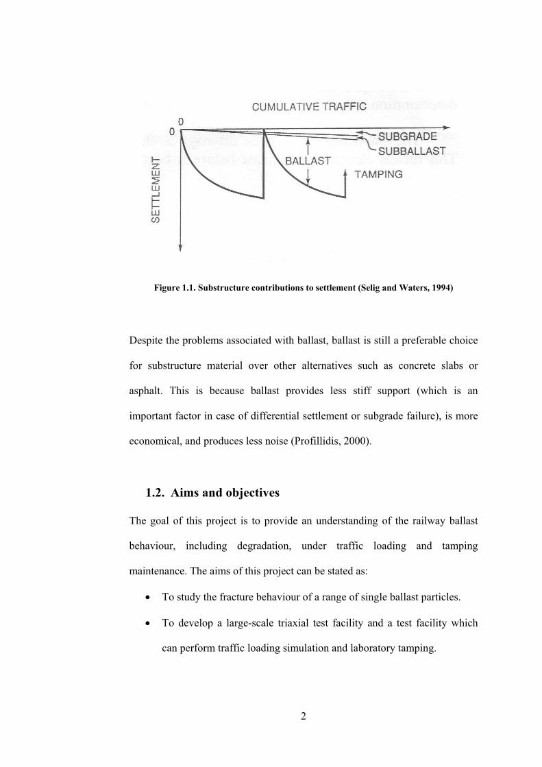
Figure 1.1. Substructure contributions to settlement (Selig and Waters, 1994)

Despite the problems associated with ballast, ballast is still a preferable choice

for substructure material over other alternatives such as concrete slabs or

asphalt. This is because ballast provides less stiff support (which is an

important factor in case of differential settlement or subgrade failure), is more

economical, and produces less noise (Profillidis, 2000).

1.2. Aims and objectives

The goal of this project is to provide an understanding of the railway ballast

behaviour, including degradation, under traffic loading and tamping

maintenance. The aims of this project can be stated as:

• To study the fracture behaviour of a range of single ballast particles.

• To develop a large-scale triaxial test facility and a test facility which

can perform traffic loading simulation and laboratory tamping.

2

• To study ballast behaviour and degradation under stresses induced by

traffic loading and tamping.

To achieve these aims, there are seven specific objectives:

1. A literature review on the behaviour of crushable soil and performance

and degradation of ballast.

2. Measurement of the tensile strengths of single grains of ballast by

single particle crushing tests, and the application of Weibull Statistics.

3. Design, build, and operation of a Railway Test Facility (RTF) for

tamping tests and traffic loading simulation.

4. Simulation of traffic loading and tamping tests on ballast in the RTF to

study ballast degradation.

5. Development of a large-scale triaxial test facility.

6. Large triaxial tests on ballast to study degradation and stress-strain

behaviour as a function of stress level and stress ratio.

7. Relation of the triaxial test results to the simulated traffic loading test

results.

1.3. Thesis outline

This thesis is divided into seven chapters. The brief outline of each chapter is

given below.

A review of background knowledge and literature relevant to this work is

presented in Chapter 2. It covers information on rail track environment, ballast,

3

4

particle breakage, behaviour of aggregates under monotonic and cyclic loading,

and laboratory tests on ballast.

Chapter 3 focuses on the material properties and strength of three types of

ballast that were used in all experiments in this project. Ballast was sent to

Lafarge Aggregates Ltd. for Los Angeles abrasion, micro-Deval attrition,

flakiness index, and water absorption tests. The strengths of ballast particles

were also measured by compressing a ballast particle between two flat platens

and analysed by Weibull statistics and the two-sample unpaired t-test.

The development of the Railway Test Facility (RTF) and large-scale triaxial

test facility are described in Chapters 4 and 5. These chapters also include test

procedures, analysis of test results, and a discussion of the findings.

Chapter 6 attempts to draw together the data from the RTF and triaxial tests.

Lastly, Chapter 7 presents the conclusions of the work and recommendations

for further research.

2. Literature review

2.1. Introduction

Railway ballast is one of the most important components in a rail track. It is a

crushed granular material that supports the rails and sleeper. Various types of

materials are used as ballast such as granite, limestone, or basalt. The chosen

type of ballast material usually depends on the local availability.

This chapter presents a literature review related to ballast and its mechanical

properties. The six sections of this literature review focus on

• Rail track environment

• Ballast in the track

• Particle breakage

• Behaviour of granular materials under monotonic loading

• Behaviour of granular materials under cyclic loading

• Previous laboratory tests on ballast

2.2. Rail track

2.2.1. Track components

Track components are divided into two parts, namely the superstructure and

substructure which are the top and bottom parts as shown in Figure 2.1. The

superstructure includes the rails, fastening system, and sleepers. The

substructure includes the ballast, subballast, and subgrade.

5

The rails are a pair of longitudinal steel members which are in contact with the

train wheels. Their functions are to guide the train in the desired direction and

to transfer the traffic loading to the sleepers which are joined to the rails by the

fastening system. The sleepers then transfer the load from the rails to the

ballast and also restrain the rail movement by anchorage of the superstructure

in the ballast.

Ballast is a crushed granular material placed as the top layer of the substructure

and between sleepers in a track and has many functions. The most important

ones are to resist vertical, lateral, and longitudinal forces applied to the sleepers

and to provide resiliency and energy absorption for the track. Moreover, voids

provide drainage of water in the track. However, the voids in the ballast will

eventually be filled with fouling material and thus the ballast will need to be

cleaned or replaced.

Similar to ballast, subballast is also a granular material but is generally finer

and more broadly-graded than ballast. The subballast further reduces the stress

levels on the subgrade and prevents the upward migration of fine material from

the subgrade into the ballast. Subgrade is the foundation for the track structure

and can be existing natural soil or placed soil. As with all foundations,

excessive settlement should be avoided.

2.2.2. Track forces

Forces in the vertical, lateral, and longitudinal directions act on the track

structure. These forces can be due to moving traffic and changing temperature.

6

The longitudinal force is usually due to acceleration and braking of trains and

thermal expansion or contraction of the rails. The lateral force usually comes

from the lateral wheel force due to the friction between the rail and wheel

especially when a train goes round corners. It also comes from the buckling

reaction force of the rail which is usually caused by a high longitudinal force in

the rail.

Figure 2.1. Layout of a typical ballasted track (Selig and Waters, 1994)

The vertical force can be subdivided into the downward and upward force. In

reaction to the downward force, the upward force is induced by the rail as

7

shown in Figure 2.2. The downward force is a combination of a static load and

a dynamic component. The static component is the weight of the train while the

dynamic component is a function of track conditions, train characteristics,

operating conditions, train speed, and environmental conditions. It is the

dynamic component that usually causes an adverse effect to the track as it can

be much larger than the static load. According to Selig and Waters (1994), the

magnitude of the dynamic component can be up to 2.4 times the static load.

Figure 2.2. Typical wheel load distribution into the track structure (Selig and Waters,

1994)

2.2.3. Track geometry maintenance

Settlement occurs in a railway subjected to long-term traffic loading. In the

UK, normal maintenance intervals for main line and branch line tracks are one

to two years and three to four years, respectively. There are two methods of

8

track geometry maintenance; tamping and stoneblowing. Tamping is used to

correct long wavelength faults caused by repeated traffic (Selig and Waters,

1994). The tamping wagon, shown in Figure 2.3, contains several tamping

tines as shown in Figure 2.4.

Figure 2.3. Self-propelled tamping machine (Selig and Waters, 1994)

Figure 2.4. Tamping tines (Selig and Waters, 1994)

9

Figure 2.5 shows the operating sequence of the tamping machine, where:

(A) The track and sleeper are in an arbitrary position before tamping

begins.

(B) The track and sleeper are raised by the machine to the target level. As a

result, there is an empty space under the sleeper.

(C) The tamping tines are inserted into the ballast on both sides of the

sleeper. This step can cause ballast breakage.

(D) The tamping tines squeeze the ballast into the empty space under the

sleeper. Therefore, the correct position of the rail and sleeper is

recovered. This might also cause ballast breakage.

(E) The tamping tines are lifted from the ballast. They will then move on to

tamp around the next sleeper.

Figure 2.5. Tamping sequence (Selig and Waters, 1994)

10

Ballast should be pushed into the void under the sleepers to support the

sleepers at the required profile. However, the ballast will soon return to its pre-

maintenance profile. This phenomenon is called �ballast memory� and is

shown in Figure 2.6. The tamping process disturbs and dilates the compacted

ballast. Therefore, the ballast that fills the space under the sleeper is loose and

hence under trafficking, the settlement increases at a faster rate and the ballast

will soon return to its previous compacted profile.

The ballast memory effect can be reduced by changing the amount of sleeper

lift (Selig and Waters, 1994). Figure 2.7 shows a plot between the sleeper lift

given by the tamper and the settlement in the subsequent 66 weeks of

trafficking. It can be seen that for relatively small lifts, the settlement is

approximately equal to the lift. Therefore, there is no lasting change in the

inherent track shape. On the other hand, the settlement corresponding to the

higher lifts are not as large as the lift i.e. this indicates more lasting

improvement in the inherent track shape. Selig and Waters (1994) define a high

lift as a lift which exceeds the D50 size of the ballast, i.e. the sieve size that will

retain 50% of a representative sample of the ballast.

According to Selig and Waters (1994), the tamping tines squeeze the ballast

which in turn expands upwards to fill the void for low lifts. On the other hand,

high lifts allow maximum dilation to occur as the squeezed ballast expands

upwards, additional ballast particles will also be added to the ballast skeleton

underneath the sleeper as there is now sufficient room for them. The new

11

ballast skeleton will then be compacted by the subsequent traffic loading and

will adopt a new geometry.

Figure 2.6. Effect of ballast memory (Selig and Waters, 1994)

Figure 2.7. Sleeper settlement as a function of tamping lift (Selig and Waters, 1994)

For short wavelength geometric faults, the stoneblowing maintenance is more

suitable (Selig and Waters, 1994). According to the current normal practice in

12

the UK, stoneblowing is used only on the section of track with high tamping

frequency as it causes less damage to the ballast. Test results of Wright (1983)

showed that both tamping and stoneblowing caused ballast breakage during the

insertion into the ballast layer. However, stoneblowing produced up to eight

times fewer particles smaller than 14 mm than tamping. A stoneblowing wagon

is shown in Figure 2.8.

Figure 2.8. Stoneblowing wagon (Selig and Waters, 1994)

The operating sequence of stoneblowing maintenance is shown in Figure 2.9,

where:

(A) The track and sleeper are in an arbitrary position before tamping

begins.

(B) The track and sleeper are raised by the machine to the target level. As a

result, there is an empty space under the sleeper.

(C) The stoneblowing tubes are inserted into the ballast layer.

(D) A measured quantity of stone is blown by compressed air into the space

between the sleeper and the ballast.

(E) The tubes are withdrawn from the ballast layer.

13

(F) The sleeper is lowered onto the top of the blown stone which will be

compacted by subsequent traffic.

Figure 2.9. The stoneblowing process (Selig and Waters, 1994)

2.3. Ballast

2.3.1. Ballast specification and testing

To ensure that ballast is of good quality, ballast needs to be tested after the

manufacturing process at the quarry. Railway engineers are mainly interested

in mechanical and dimensional properties. RT/CE/S/006 Issue 3 (2000)

specifies the recommended properties of ballast to be used from the 1st April

2005. It follows the European railway ballast specification BS EN 13450

(2002). This specification focuses on five ballast properties: ballast grading,

14

Los Angeles Abrasion (LAA) value, micro-Deval attrition (MDA) value,

flakiness index, and particle length. The specification requires ballast to

conform the particle size distribution shown in Figure 2.10.

0

10

20

30

40

50

60

70

80

90

100

0 10 20 30 40 50 60 7

Size (mm)

% p

as

sin

g

0

Square Mesh Sieve (mm) Cumulative % by mass

passing BS sieve

63 100

50 70-100

40 30-65

31.5 0-25

22.4 0-3

32-50 50≥

Figure 2.10. Specification for ballast particle size distribution (RT/CE/S/006 Issue 3,

2000)

The procedure of the LAA test is described in BS EN 1097-2 (1998). This

procedure is modified by Annex C of BS EN 13450 (2002) to suit the size of

ballast as the usual test sample for the LAA test is 10 � 14 mm i.e. much

smaller than the ballast. The test involves rotating five kilograms of 31.5 � 40

mm ballast and five kilograms of 40 � 50 mm ballast with twelve spherical

steel balls weighing 5.2 kilograms in total in a steel drum. The drum rotates on

a horizontal axis at 31 to 33 revolutions per minute for 1,000 revolutions. The

LAA value is the percentage by mass of particles passing 1.6 mm sieve after

the test. The specification requires the LAA values to be below or equal to 20

%.

15

The micro-Deval test is carried out as specified in BS EN 1097-1 (1996) with

modification specified in Annex E of BS EN 13450 (2002). This test involves

rotating five kilograms of 31.5 � 40 mm ballast and five kilograms of 40 � 50

mm ballast with two litres of water in a steel drum. The drum rotates at 100

revolutions per minute for 14,000 revolutions. The MDA value is the

percentage by mass of particles passing 1.6 mm sieve after the test. The

specification limits the MDA value to 7 %.

BS EN 933-3 (1997) describes a procedure of the flakiness index test. The test

consists of two sieving operations. The first operation is to sieve the test

sample into various particle size fractions. The second is to sieve each fraction

by bar sieves with parallel slots. The width of each slot is half the larger sieve

size of each fraction. The flakiness is the percentage by mass of the particles

passing the bar sieves. The specification limits the flakiness index to 35 %.

The particle length index test is performed by measuring each ballast particle

from a ballast sample of mass exceeding 40 kg with a gauge or callipers. The

length index is the percentage by mass of ballast particles with length larger

than or equal to 100 mm. The specification requires the particle length index to

be less than or equal to 4 %.

2.3.2. Ballast fouling

After long term service, ballast becomes damaged and contaminated and its

gradation changes. As a result, its performance reduces. This process is called

16

�fouling�. According to Selig and Waters (1994), there are five causes of

ballast fouling. They are:

Ballast breakdown

Infiltration from ballast surface

Sleeper wear

Infiltration from underlying granular layers

Subgrade infiltration

Table 2.1 shows the percentage of fouling component according to the

estimates of British Railways. According to the table, the biggest source of

fouling is external. British Railways has also found that after removing the

fouling material, ballast particles are still in good working condition after 15

years of service. This agrees with the estimates in the table that ballast

breakdown is not the main source of fouling. On the contrary, the main source

of ballast fouling in North America is ballast breakdown as shown in Figure

2.11.

Ballast fouling prevents ballast from fulfilling its functions. The effect of

ballast fouling depends on the size and amount of ballast fouling. As the mass

of sand and fine-gravel-sized fouling particles (0.075 � 19 mm) increases, the

resiliency to vertical deformation of the ballast and void space decreases. This

makes surface and lining operations more difficult and drainage decreases. As

the voids become filled or nearly filled, ballast becomes denser and tamping

then loosens the ballast. This will lead to a higher rate of ballast settlement

after tamping.

17

Degradation No. Source

kg/sleeper % of

total

1 Delivered with ballast (2 %) 29 7

2 Tamping:

7 insertions during renewal and

1 tamp/yr for 15 years at 4 kg/tamp

88 20

3 Attrition from various causes including

traffic and concrete sleeper wear

(Traffic loading: 0.2 kg/sleeper/million tons of

traffic)

90 21

4 External input at 15 kg/yr

(Wagon spillage: 4.0 kg/m2/yr)

(Airborne dirt: 0.8 kg/m2/yr)

225 52

Total 432 100

Table 2.1. British railways sources of fouling (Selig and Waters, 1994)

Figure 2.11. Sources of ballast fouling from all sites in North America (Selig and Waters,

1994)

18

An increase in the mass of clay and silt-sized fouling particles (smaller than

0.075 mm) also reduces drainage which then leads to erosion of ballast and

subgrade attrition. Fine particles can also combine with water to form an

abrasive slurry. Also, if the content of clay- and silt-sized fouling particles is

high, it is difficult for the tamping machine to penetrate and rearrange the

ballast.

Different researchers proposed different ballast fouling indices to quantify the

foulness of the ballast, shown in Table 2.2.

Fouling index

FI = P0.075 + P4.75

(Selig and Waters,

1994)

FIP = P0.075 + P13.2

(Ionescu, 2004)

FID = D90 / D10

(Ionescu, 2004)

Classification

< 1 < 2 < 2.1 and P13.2 ≤ 1.5 % Clean

1 to < 10 2 to < 10 2.1 to < 4 Moderately

clean

10 to < 20 10 to < 20 4 to < 9.5 Moderately

fouled

20 to < 40 20 to < 40 9.5 < 40 Fouled

≥ 40 ≥ 45 ≥ 40, P13.2 ≥ 40 %, P0.075 > 5 % Highly fouled

Px = Percentage passing at x mm / 100

Dy = Particle size at y percentage passing (mm)

Table 2.2. Fouling indices

19

Selig and Waters� fouling index (FI) is used to quantify the foulness of ballast

in North America. Ionescu (2004) proposed FIP as a modification of Selig and

Waters� fouling index to suit the condition of the ballast in Australia and FID as

the field sample in the study showed little variation in D90 but a large variation

in D10.

In the UK practice, ballast becomes fully fouled when there are about 30 % by

weight of particles smaller than 14 mm in the ballast (Selig and Waters, 1994)

and ballast is regarded as acceptable if:

1. It retains the geometry such that only a normal level of maintenance is

needed (i.e. annual or bi-annual tamping/stone blowing).

2. There are few wet spots, i.e. track sections with trapped water, or the

wet spots that exist can be traced to factors other than the ballast.

Even if both criteria are present, the ballast condition is however not acceptable

if greater than 30 % of particles smaller than 14 mm are found in the track.

2.4. Particle breakage

2.4.1. Griffith theory

Griffith crack theory is widely used by many materials scientists and engineers

to explain and determine the fracture behaviour of solids. Examples of solids

containing flaws or cracks are ceramics, glasses, and rocks. When a stress is

intensified at a crack, the material will have a little plasticity to resist the crack

propagation and fail by fast fracture. According to Griffith theory, the fast

fracture criterion is given by the following equation:

20

CEGa =πσ (2.1)

where σ = applied stress

a = crack length

E = Young�s modulus

GC = Toughness

Toughness (GC) is the energy required to generate a unit area of crack. Its unit

is energy per unit area i.e. J/m2 and is a material property. From the left hand

side of the equation, the fast fracture can occur when either;

a. A crack grows and reaches the critical size a when a material

is under stress σ, or

b. A material with a crack of length a is under a stress which

increases to the critical stress σ.

The right hand side of the equation is dependent on material properties only.

The constant on the right side of the equation is defined as the fracture

toughness or KIC ( CIC EGK = ). The term in the left hand side of the equation

is normally known as the �stress intensity factor� or K ( aK πσ= ) e,

the critical combination of the stress and the crack length must reach a certain

value in order for a fast fracture to occur. In other words, fast fracture will

occur when K = KIC.

. Therefor

21

2.4.2. Single particle under compression and Weibull statistics

McDowell and Amon (2000) defined an induced stress (σ) of a particle of size

d loaded between two flat platens under a force F as:

2d

F=σ (2.2)

The strength of a particle can be taken as the force at failure divided by the

square size of the particle at failure i.e. the distance between the platens at

failure.

Griffith theory states that failure of a brittle solid is caused by the propagation

of one or more cracks. Hence, the strength of a ballast particle depends on the

size and distribution of cracks and flaws in it. Different particles have different

sizes and distributions of crack sizes even though they look alike. Therefore,

statistical analysis is necessary to determine the distribution of strengths of

ballast particles.

According to Hertzberg (1996), Weibull statistics (Weibull, 1951) gives a more

accurate characterisation of property values for brittle materials than the

normal distribution. Figure 2.12 shows the difference between the normal

probability density function (p.d.f.) and Weibull p.d.f. for the same mean and

standard deviation (McDowell, 2001). The value of m in the figure is the

Weibull modulus which will be explained below. As the Weibull modulus

increases, the similarity between the normal p.d.f. and Weibull p.d.f. increases.

22

Figure 2.12. Weibull p.d.f. and normal p.d.f with same mean and standard deviation (a)

m = 1.5, (b) m = 2, (c) m = 3, (d) m = 4 (McDowell, 2001)

According to McDowell and Amon (2000), a particle of size d loaded between

two flat platens under an induced tensile stress σ has a survival probability

(Ps(d)) given by

⎥⎥⎦

⎤

⎢⎢⎣

⎡

⎟⎟⎠

⎞⎜⎜⎝

⎛−=

⎥⎥⎦

⎤

⎢⎢⎣

⎡⎟⎟⎠

⎞⎜⎜⎝

⎛⎟⎟⎠

⎞⎜⎜⎝

⎛−=

m

do

m

o

sd

ddP

,

3

0

exp

exp)(

σσ

σσ

(2.3)

where

do = Reference particle size

σo = Characteristic stress at which 37 % of particles of size do survive

σo,d = Characteristic stress at which 37 % of particles of size d survive

m = Weibull modulus

23

The Weibull modulus (m) decreases with increasing variability in strength.

(Ashby and Jones, 1998; McDowell and Bolton, 1998). Figure 2.13 shows the

variability in strength for different Weibull modulus. McDowell (2001) showed

that m relates to the coefficient of variation (standard deviation / mean).

Figure 2.13. Weibull distribution of strengths (Ashby and Jones, 1998)

McDowell and Amon (2000) derived an equation defining average tensile

strength (σav) for particles of size d as shown in Equation 2.4.

( ) doav m ,11 σσ +Γ= (2.4)

Γ is the Gamma function and can be calculated by using GAMMALN and EXP

functions in Microsoft Excel or can be found in standard statistics texts. It can

be seen that the average tensile strength is proportional to σo,d. The value of the

gamma function is approximately 1 for a wide range of Weibull modulus

values. Therefore, it can also be said that the average tensile strength is

24

approximately equal to σo,d. Moreover, it can be inferred from Equations 2.3

and 2.4 that

m

doav d 3

,

−∝∝ σσ (2.5)

The above equation shows that there is a size effect in single particle crushing

tests, i.e. the larger the particle, the lower the strength. It can also be seen that

m determines the size effect on σο and hence, on σav. The size effect is small in

a material with small variability since m is large.

McDowell and Amon (2000) performed single particle crushing tests on Quiou

sand grains of different sizes. The results are shown in Table 2.3 and Figure

2.14. The average Weibull modulus from the table is 1.51. According to the

plot in Figure 2.14, -3/m is �1.9647 therefore m is 1.53. This proves that

Equation 2.5 is correct for this material.

Nominal size

/mm

Average size at

failure /mm

Weibull modulus

m

37% tensile

strength /MPa

1 0.83 1.32 109.3

2 1.72 1.51 41.4

4 3.87 1.16 4.2

8 7.86 1.65 0.73

16 15.51 1.93 0.61

Table 2.3. Weibull modulus and 37% strength for each grain size (McDowell and Amon,

2000)

25

Figure 2.14. 37 % strength against average particle size at failure (McDowell and Amon,

2000)

A sufficient number of tests is necessary for obtaining the mean strength and

standard deviation to within a degree of acceptable accuracy. According to

McDowell (2001), for a population Weibull modulus of 1.5, the sample mean

strength can only be determined to with about 25% of the true mean at 95%

confidence level with thirty test particles.

2.4.3. Particle breakage in aggregate

According to McDowell et al. (1996), the probability of particle breakage in an

aggregate increases with an increase in applied macroscopic stress, increase in

particle size, and reduction in coordination number (number of contacts with

neighbouring particles).

According to the size effect, the larger the particle, the lower its strength.

Therefore, the probability of particle breakage increases with an increase in

particle size. A high coordination number can reduce the induced tensile stress

in a particle. This is because loads are distributed through many contact points

26

on the particle surface and hence reducing the induced tensile stress. However,

this also depends on the shape of the particles as shown in Figure 2.15.

Figure 2.15. Large coordination numbers are less helpful for more angular particles

(McDowell et al., 1996)

Therefore, the size and coordination number are two opposing effects on

particle survival. Smaller particles are stronger but have fewer contacts than

larger particles and vice-versa. If the size effect dominates over the effect of

coordination number, large particles are more likely to break, meaning, a

uniform matrix of fine particles will be left at the end of any one-dimensional

compression test. However, no evidence of this has been found. On the other

hand, if the effect of coordination number dominates over the size effect, the

small particles are more likely to break. Hence, a distribution of particle sizes

evolves, such that some of the initial large particles remain, protected by the

many finer particles produced. An example of this behaviour is shown in

Figure 2.16. The figure shows the evolution of particle size for Ottawa sand in

one-dimensional compression tests under increasing macroscopic stress.

27

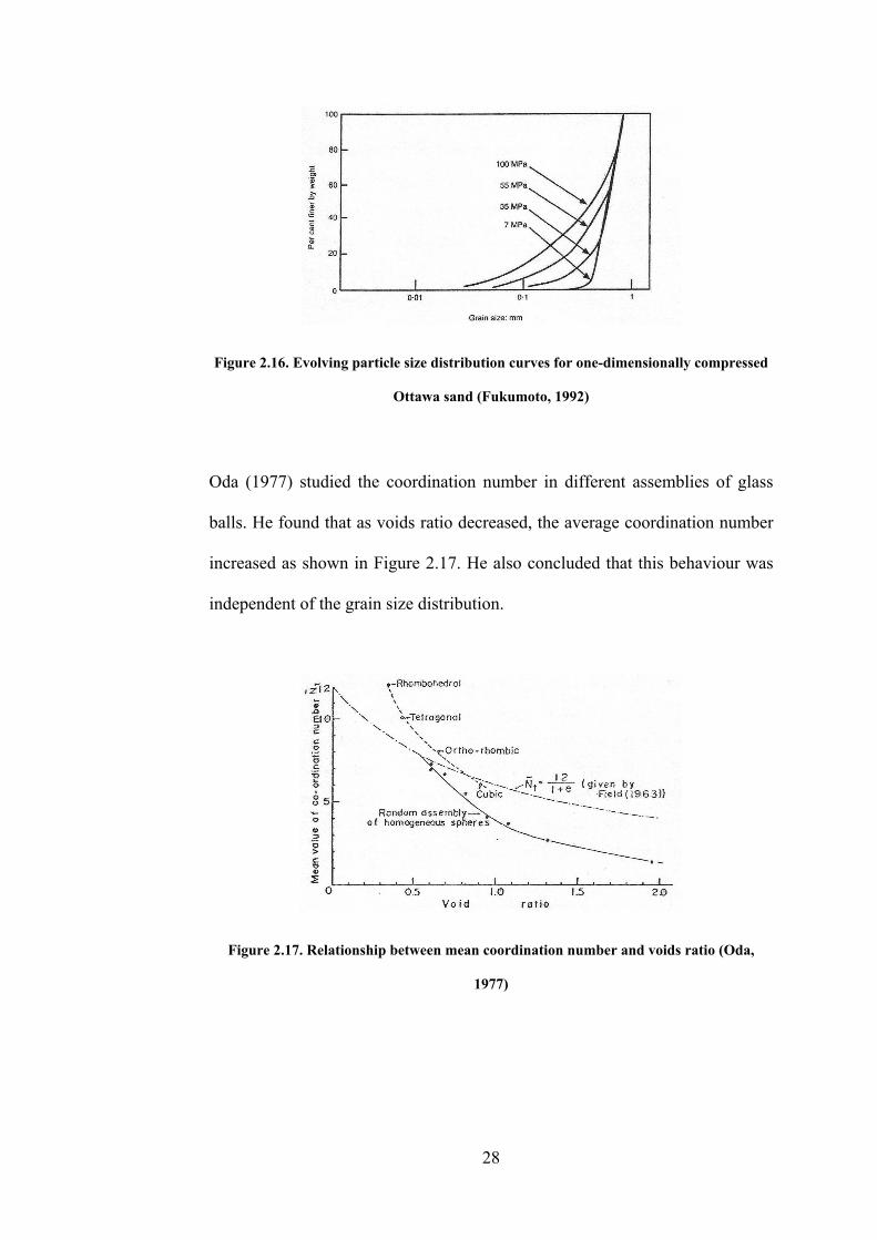
Figure 2.16. Evolving particle size distribution curves for one-dimensionally compressed

Ottawa sand (Fukumoto, 1992)

Oda (1977) studied the coordination number in different assemblies of glass

balls. He found that as voids ratio decreased, the average coordination number

increased as shown in Figure 2.17. He also concluded that this behaviour was

independent of the grain size distribution.

Figure 2.17. Relationship between mean coordination number and voids ratio (Oda,

1977)

28

2.5. Behaviour of aggregate under monotonic loading

The typical behaviour of granular materials subject to one-dimensional

compression is shown by the plot of voids ratio against the logarithm of

vertical effective stress in Figure 2.18.

Figure 2.18. One-dimensional compression plots for carbonate and silica sands

(Golightly, 1990)

The behaviour in region 1 of the dense silica sand is quasi-elastic with some

irrecoverable deformation due to particle rearrangement. The sand yields in

region 2 where the behaviour is plastic and forms a straight line beyond region

2, known as the normal compression line. Since the material has undergone all

possible rearrangement at the end of region 1, particle breakage must then

occur to achieve further compaction. It is clear that all particles are not loaded

in the same direction or orientation. However, it can be assumed that many

particles will eventually be in the paths of the columns of strong force that

carry the applied macroscopic stress. Cundall and Strack (1979) studied the

29

paths of strong force using discrete element simulations as shown in Figure

2.19.

Figure 2.19. Discrete element simulation of an array of photoelastic discs FH/FV = 0.43

(Cundall and Strack, 1979)

The columns of strong force change as breakage and/or rearrangement of

particles occur. The loading geometry of the particles in the force columns is

similar to the loading geometry of the single particle crushing test (i.e. a

particle is loaded between two flat platens) but there are also some smaller

force chains in other directions acting on the particles from the neighbouring

particles. McDowell and Bolton (1998) suggested that the yield stress must be

proportional to the average tensile strength of particles and defined yield stress

as macroscopic stress that causes the maximum rate of grain fracture under

increasing stress. McDowell (2002) analysed single particle crushing tests on

various grain sizes of Leighton Buzzard sand and one-dimensional

compression tests on the same type of sand of various uniform gradings. Figure

2.20 shows the one-dimensional compression test results. It can be seen that the

larger the grain size, the smaller the yield stress. From Figure 2.19, McDowell

(2002) noted that the array is approximately 12 particles wide and

30

approximately three columns of strong force are formed to pass on the stress.

Hence, the stress induced in the particles in the paths of the strong force should

be approximately four times the macroscopic stress. He then predicted that the

yield stress equalled ¼ of 37% tensile strength of the grain (σo). The

comparison of the predicted and true yield stress found in one-dimensional

compression tests is shown in Figure 2.21.

Figure 2.20. Compression plots for different uniform gradings of sand (McDowell, 2002)

Figure 2.21. Yield stress predicted from single particle crushing tests, assuming yield

stress = (37% tensile strength)/4 (McDowell, 2002)

31

It can be seen from Figure 2.21 that the prediction gives a good approximation

of yield stress. This also confirms the suggestion by McDowell and Bolton

(1998) that yield stress should be proportional to the average tensile strength of

the constituent particles.

2.6. Behaviour of aggregate under cyclic loading

2.6.1. Resilient behaviour

Under cyclic loading, the deformation of granular materials is divided into

resilient deformation and permanent deformation. Figure 2.22 (Lekarp et al.,

2000a) shows the stress-strain curve of granular material during one cycle.

Figure 2.22. Strains in granular materials during one cycle of load application (Lekarp et

al., 2000a)

The resilient behaviour of granular material is characterised by the resilient

modulus (Mr) and Poisson�s ratio (ν) defined in Equations 2.6 and 2.7.

32

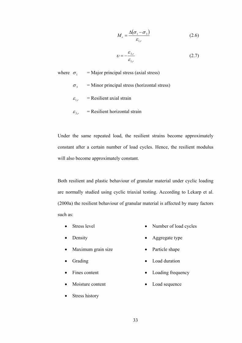
( )r

rM,1

31

εσσ −Δ

= (2.6)

r

r

,1

,3

εε

υ −= (2.7)

where 1σ = Major principal stress (axial stress)

3σ = Minor principal stress (horizontal stress)

r,1ε = Resilient axial strain

r,3ε = Resilient horizontal strain

Under the same repeated load, the resilient strains become approximately

constant after a certain number of load cycles. Hence, the resilient modulus

will also become approximately constant.

Both resilient and plastic behaviour of granular material under cyclic loading

are normally studied using cyclic triaxial testing. According to Lekarp et al.

(2000a) the resilient behaviour of granular material is affected by many factors

such as:

• Stress level

• Density

• Maximum grain size

• Grading

• Fines content

• Moisture content

• Stress history

• Number of load cycles

• Aggregate type

• Particle shape

• Load duration

• Loading frequency

• Load sequence

33

The effect of each parameter will now be discussed.

2.6.1.1.Effect of stress level

According to Lekarp et al. (2000a), many researchers accepted that stress level

had the most significant effect on the resilient behaviour of granular materials.

Monismith et al. (1967) and Uzan (1985) both found that the resilient modulus

increased considerably with confining pressure. On the other hand, the resilient

modulus is affected to a much smaller extent by the magnitude of deviatoric

stress. Uzan (1985) stated that the resilient modulus slightly decreased as the

deviatoric stress increased. Meanwhile, Hicks and Monismith (1971) found

that resilient modulus slightly increased with the deviatoric stress. Ping and

Yang (1998) concluded that the resilient modulus of Panama sand either did

not change, or slightly increased with the deviatoric stress but found the

opposite result on Alachua sand.

Very few studies have concentrated on characterisation of Poisson�s ratio

compared to the resilient modulus (Lekarp et al., 2000a). However, some

researchers found that the effect of the stress level on the value of Poisson�s

ratio is the opposite to the resilient modulus. Hicks and Monismith (1971) and

Brown and Hyde (1975) both showed that the Poisson�s ratio increased with

decreasing confining pressure and increasing deviatoric stress.

Granular materials in pavements are normally subjected to a variety of cyclic

principal stresses as a result of moving traffic. Therefore, it is reasonable to

mutually cycle both the axial and confining stresses in a triaxial test. However,

34

Brown and Hyde (1975) suggested that it was not necessary to cycle both axial

and confining stresses as they obtained similar values of resilient modulus from

cyclic and constant confining stress when the constant stress was equal to the

mean of the cyclic value.

Since applied stress level has the most significant effect on resilient modulus, it

is therefore necessary to model it as correctly as possible. According to the

review of Lekarp et al. (2000a), many researchers have been developing the

resilient modulus model based on curve fitting procedure of the results from

their experiments. Even though it has been generally agreed that the effect of

deviatoric stress is not as pronounced as the confining stress, some researchers

found that the effect of deviatoric stress should be included in the model as

shown in Equation 2.8. The equation however contradicts the findings of Hick

and Monismith (1971) and Ping and Yang (1998) who said that the resilient

modulus slightly increased with the deviatoric stress.

2

1

k

rq

pkM ⎟⎟

⎠

⎞⎜⎜⎝

⎛= (2.8)

where Mr = Resilient modulus

k1 and k2 = Empirical constants

p = Mean principal stress

q = Deviatoric stress

However, the simplest model which is widely accepted for analysis of stress

dependence of material stiffness is commonly known as the K-θ model as

35

shown in Equation 2.9 where θ is the sum of principle stresses. Furthermore,

this model is also used with the triaxial test results in this project (see Section

5.7.3).

2

1

k

r kM θ= (2.9)

2.6.1.2.Effect of density

According to the experiments of Thom and Brown (1988), density has almost

no influence on the properties of the aggregate. However, Hicks and

Monismith (1971) and Kolisoja (1997) found that the resilient modulus

increased with increasing density. This might be because an increase in density

results in an increase in the co-ordination number (the average number of

contacts per particle) and a decrease in the average contact stress between

particles. This then leads to a decrease in the total deformation and, hence, an

increase in resilient modulus.

Hicks and Monismith (1971) concluded from their experiments that the effect

of density was more significant in partially crushed gravel than crushed rock.

The particle size distributions of both aggregate are shown in Figure 2.23. The

resilient modulus was found to increase with the relative density in partially

crushed gravel. The effect of the density on the resilient modulus in fully

crushed rock was negligible. This is probably because the partially crushed

gravel is less angular than the crushed rock.

36

Unlike the behaviour of granular materials under monotonic loading where

density plays an important role, it can be seen from the above findings that the

effect of density of the resilient properties of granular material is still unclear.

This agrees with the conclusion from Lekarp et al. (2000a).

Figure 2.23. Partially crushed gravel and crushed rock in Hicks and Monismith (1971)

2.6.1.3.Effect of maximum particle size, grading, and fines content

For aggregates with the same amount of fines and similar particle size

distribution, the resilient modulus increases with the maximum particle size.

Kolisoja (1997) explained that the load was transmitted through fewer particles

in the aggregates with larger material grains. This leads to smaller deformation

between the particles and hence an increase in the resilient modulus.

The grading of granular materials has a minor effect on resilient modulus.

Thom and Brown (1988) found that for aggregates with the same maximum

37

particle size, uniformly graded aggregate had slightly larger resilient modulus

than well graded aggregate. Heydinger et al. (1996) also found that the poorly-

graded limestone showed higher resilient modulus than the well-graded one.

According to Lekarp et al. (2000a), the effect of the fines content on the

resilient modulus is still unclear. According to Hicks and Monismith (1971),

the influence of amount of particles passing 0.075 mm sieve (sieve number

200) was not very well defined as shown in Figure 2.24.

Figure 2.24. Effect of particles passing 0.075 mm sieve (sieve number 200) on resilient

modulus (Hicks and Monismith, 1971)

2.6.1.4.Effect of moisture content

According to the literature review of Lekarp et al. (2000a), the resilient

behaviours of dry and most partially saturated granular materials are similar.

But as complete saturation is approached, the resilient behaviours are

significantly affected. Many researchers, such as Hicks and Monismith (1971),

Ping and Yang (1998), and Heydinger et al. (1996), agreed that the resilient

38

modulus decreases with increasing saturation level because excess pore-water

pressure is developed under repeated loading. The effective stress in the

material decreases as the pore-water pressure is developed. As a result, the

strength, stiffness, and hence resilient modulus decreases.

2.6.1.5.Effect of stress history and number of load cycles

The effect of stress history is mainly compaction, rearrangement and breakage

of particles. The previous number of load cycles also affects the resilient

behaviour. To eliminate the effect of stress history, Hicks and Monismith

(1971) suggested that specimens should be loaded for 1,000 cycles prior to

repeated load resilient test to condition them into the same level of compaction.

However, Brown and Hyde (1975) concluded that the resilient properties of

granular materials were unaffected by stress history provided that the applied

stress did not cause failure.

With increasing number of load applications, the material gets stiffer and

hence, the resilient modulus increases. However, after a certain number of load

applications, it becomes approximately constant. According to the triaxial tests

on railway ballast of Shenton (1974) where applied maximum deviatoric stress

levels were closed to the failure level, the resilient modulus increased rapidly

during the first 10 cycles and became approximately constant after 100 cycles.

Similarly, Hicks and Monismith (1971) reported that the resilient modulus of

partially crushed gravel and crushed rock becomes constant after 50 to 100

load cycles provided that the ratio between maximum axial stress and

confining stress does not exceed 6 or 7.

39

Collins and Boulbibane (2000) explained the concept of shakedown in four

stages as shown in Figure 2.25. At first, when the cyclic loading is sufficiently

small, there are no permanent strains. If the load then exceeds the elastic load,

the permanent strains will be induced (Stage 2 in Figure 2.25). After the finite

number of cycles, the behaviour becomes purely elastic, i.e. no further

permanent strain. At this point, the material structure is said to have

�shakedown� and the resilient strain becomes constant resulting in constant

resilient modulus.

Figure 2.25. Four types of response of elastic/plastic structure to repeated loading cycles

(Collins and Boulbibane, 2000)

At higher loads, shakedown does not occur and the behaviour will be either

�cyclic plasticity� where a closed cycle of permanent strain is formed (Stage 3

in Figure 2.25) or �ratchetting� where permanent strain increases indefinitely

(Stage 4 in Figure 2.25). If either of these situation occurs, the structure will

40

fail. The critical load below which the structure shakes down and above which

can cause failure is called the shakedown load.

2.6.1.6.Effect of aggregate type and particle shape

Different granular materials give different resilient responses to cyclic loading.

Heydinger et al. (1996) found that gravel had a higher resilient modulus than

crushed limestone and slag.

Hicks and Monismith (1971) and Thom and Brown (1989) showed that the

resilient modulus increased with surface roughness and angularity of the

material. This is because angular particles have better load spreading

properties, i.e. better interlock than the rounded particles. Hicks and Monismith

(1971) also showed that the Poisson�s ratio increased under the same

conditions.

2.6.1.7.Effect of load duration, frequency and load sequence

Many researchers, such as Boyce et al. (1976), Shenton (1974), and Thom and

Brown (1987), agreed that the load duration and frequency had little or no

significant effect on the resilient properties of granular materials. However,

Lekarp et al. (2000a) stated that an increase in the frequency could result in the

reduction of resilient modulus when the moisture content was close to

saturation. This is because as the pore pressure increases, the effective stress

decreases. The literature review of Lekarp et al. (2000a) also showed that the

41

order in which the stresses were applied to a specimen had minimal effect on

the resilient properties of granular materials.

2.6.2. Permanent deformation of cyclically loaded aggregate

Permanent deformation of granular materials in a rail track is normally in the

form of settlement. Unlike resilient behaviour, not enough research has been

focused on permanent deformation of granular materials. This is due to the fact

that it takes a long time to perform thousands of cycles of load. However, it is

known that permanent deformation of granular materials under cyclic loading

is affected by many factors, such as:

• Stress level

• Principal stress rotation

• Number of load cycles

• Moisture content

• Stress history

• Loading sequence

• Density

• Grading

• Loading frequency

The effect of each factor is reviewed below.

2.6.2.1.Effect of stress level

Similar to resilient properties, stress level is one of the most important factors

that affect the amount of permanent deformation of granular materials. Morgan

(1966) concluded that permanent deformation increased with increasing

deviatoric stress or decreasing confining stress. Since then, several researchers

have been using some form of stress ratio that consists of both deviatoric and

42

confining stresses (Lekarp et al, 2000b). Brown and Hyde (1975) found that the

permanent strain was directly proportional to the ratio of deviatoric stress to

confining pressure. However, the same stress ratio can result in a different

permanent strain if the deviatoric stress is larger. Figure 2.26 (Knutson, 1976)

shows that stress ratio 60/15 causes larger permanent strain than 20/5 while

both correspond to the ratio of 4.

2.6.2.2.Effect of principal stress rotation

Principal stress rotation occurs in pavements under moving traffic as shown in

Figure 2.27. According to the literature review of Lekarp et al. (2000b), the

effect of principal stress rotation is still unclear. However, test samples

subjected to principal stress rotation showed larger permanent strain than the

samples without principal stress rotation.

Lim (2004) noted that there was no principal stress rotation for ballast near

sleepers. The traffic load is transferred through the sleeper onto the ballast with

the load being more concentrated near the sleeper. Therefore, the major

principal stress of the ballast near the sleepers suddenly increases as the wheels

are directly on top and rapidly decreases as the wheels move away. However,

deeper ballast or subgrade will be subjected to principal stress rotation

depending on the load spreading capability of the ballast.

43

Figure 2.26. Effect of stress ratio on permanent strain (Knutson, 1976)

Figure 2.27. Stress rotation beneath moving wheel load (Lekarp et al., 2000a)

2.6.2.3.Effect of number of load cycles

Each load application, in a series of cyclic loading, contributes a small amount

of accumulative permanent deformation. Figure 2.26 shows that permanent

strain increases with the number of load cycles. According to Morgan (1966),

the permanent strain can still increase after 2,000,000 load cycles. Barksdale

(1972) and Shenton (1974) both found that permanent deformation is a linear

function of logarithm of the number of load cycles as shown in Figure 2.28.

44

The figure also shows that the rate of permanent deformation accumulation

decreases with increasing number of load cycles. However, Lekarp and

Dawson (1998) stated that this could happen when the applied stresses were

low. High stresses will result in an increasing rate of permanent strain

accumulation according to the ratchetting period of the shakedown theory

explained in Section 2.6.1.5 (Stage 4 in Figure 2.25).

Figure 2.28. Permanent deformation as a linear function of logarithm of number of load

cycle (Shenton, 1974)

2.6.2.4.Effect of moisture content

It is widely known that as moisture content increases and saturation is

approached, the deformation resistance in granular materials decreases. This is

because it leads to the development of excessive pore water pressure under

rapid loading. As a consequence, it reduces the effective stress, stiffness and

permanent deformation resistance. Researchers, such as Barksdale (1972) and

Thom and Brown (1987) have confirmed this finding.

45

However, this is not generally true. For truly dynamic events e.g. very high

speed triaxial test, the material strength can increase dramatically. This then

might compensate for the reduction in deformation resistance from the

increased moisture content.

2.6.2.5.Effect of stress history and loading sequence

Limited research focused on the effect of stress history on the permanent

deformation of granular materials under repeated loading. However, the widely

accepted finding is that each load application stiffens the material and results in

more deformation resistance in subsequent loading applications. Brown and

Hyde (1975) studied this effect by applying cyclic loading with maximum

deviatoric stress of 650 kPa on two specimens. However, one specimen was

subjected to the maximum deviatoric stress of 650 kPa immediately while in

the other specimens, the maximum deviatoric stress successively increased

from 250, 350, 450, 550, to 650 kPa. The permanent strain from a successive

increase in the stress level was significantly smaller than the strain that

occurred when the highest stress level was applied immediately as shown in

Figure 2.29.

According to Selig and Waters (1994), the loading sequence has no effect on

permanent strain accumulation. Figure 2.30 shows the permanent strain of

different samples under different loading sequences where the deviator stresses

were changed after every 1,000 cycles. It can be seen that the final permanent

strains are approximately equal.

46

Figure 2.29. Effect of stress history on permanent strain (Brown and Hyde, 1975)

2.6.2.6.Effect of density and grading

Many researchers such as, Barksdale (1972), Thom and Brown (1988), and

Knutson and Thompson (1978) agree that permanent deformation decreases

with increasing density of granular materials.

Thom and Brown (1988) also found that the effect of density was more

significant than the effect of grading as shown in Figure 2.31. The grading

parameter in Figure 2.31 was used in their experiment to define the particle

size distribution of each sample as shown in Figure 2.32. Furthermore, the

sample compaction in their tests was performed by tamping in five layers each

of 30 mm thickness with a 38-mm diameter rod. The compactive effort was

controlled manually.

47

However, Dawson et al. (1996) found that the effect of grading was more

significant but this may be material dependent.

2.6.2.7.Effect of loading frequency

Very limited research focused on the effect of loading frequency on permanent

deformation. However, Shenton (1974) found that loading frequency has no

effect on permanent deformation of ballast as shown in Figure 2.33.

Figure 2.30. Effect of loading sequence on permanent strain (Selig & Waters, 1994)

48

Figure 2.31. Effect of density and grading on permanent strain (Thom and Brown, 1988)

0

10

20

30

40

50

60

70

80

90

100

0.00001 0.0001 0.001 0.01 0.1 1 10

Particle size (mm)

% p

assin

g

% passing = 100 x (d / 10)n

where d = particle size in mm

n = 0.25

n = 5

Figure 2.32: Particle size distribution of different samples in Thom and Brown (1988)

49

Figure 2.33. Effect of loading frequency on permanent strain (Shenton, 1974)

2.7. Laboratory tests on ballast

2.7.1. Box test

A box test simulates ballast behaviour and performance under field conditions.

Ballast is placed in a box with a sleeper segment shown in Figure 2.34. The test

can simulate traffic loading on the rail section shown in Figure 2.35. It is also

versatile as various types of results can be measured form the test such as,

sleeper settlement, horizontal stress in the ballast, and ballast stiffness and

density for a range of different ballasts.

50

Figure 2.34. Diagram of a box test (Selig and Waters, 1994)

300mm 700mm

Sleeper

Rail

Simulation Area

Figure 2.35. Plan of rail and sleepers showing section represented by the box test (Lim,

2005)

The sleeper settlement can be measured by attaching an LVDT (Linear variable

differential transformer) displacement transducer to the sleeper. Selig and

Waters (1994) measured the horizontal stress in the ballast by installing stress

sensors on the wall. Figure 2.36 shows the horizontal stress from one of the

51

sensors in their test. It can be seen from the figure that both horizontal stresses

of ballast at loaded and unloaded states (at maximum and minimum load of the

cyclic loading, respectively) eventually reached 30 kPa. The ballast stiffness

from the box test is very similar to the resilient modulus. The stiffness can be

calculated by dividing the applied deviatoric stress by the resilient

displacement of ballast in a cycle.

The breakage of the ballast in the box test usually occurs in the area under the

sleeper segment as the ballast in this area is vertically loaded. Lim (2004)

observed the ballast degradation of the whole box and confirmed that the

ballast degradation in the other areas was negligible. Selig and Waters (1994)

dyed the ballast under the sleeper to aid breakage observation.

Figure 2.36. Effect of repeated load on horizontal stress in box test (Selig and Waters,

1994)

The effect of track maintenance can also be observed in the box test. Lim

(2004) simulated tamping maintenance by lifting the sleeper level with the top

52

of the box. Then, a one-inch-wide chisel was inserted into the ballast using a

Kango hammer. This was only to rearrange and loosen the ballast under the

sleeper as it usually happens after tamping. However, it could not simulate the

impact of tamping tines and the squeezing operation.

2.7.2. Triaxial test

Many researchers such as Shenton (1974), Raymond and Buthusrt (1994),

Skoklund (2002), Key (1998) and Fair (2003) performed triaxial tests on

ballast to study its properties. Monotonic (static) triaxial tests on ballast

determine its angle of friction and strength. Cyclic (repeated loading) triaxial

tests on ballast simulate traffic loading in a controlled manner. Different

aspects of triaxial tests on ballast are discussed below.

2.7.2.1.Specimen compaction

Many researchers compacted triaxial test specimens in layers. Shenton (1974)

compacted his ballast specimens by tamping it in four layers. However,

Kolisoja (1997) commented that this compaction method was not

recommended even with other types of granular material. This is because the

compaction effort may cause particle crushing and the result of compaction

depends on the operator.

Skoglund (2002) pressed a vibrating compaction plate against each layer of his

specimen. Key (1998) and Fair (2003) are the only researchers who compacted

their specimens by dropping ballast particles into a mould which is on a

vibrating table. This is because they thought that compaction in layers was not

53

suitable for a ballast sample, because with material of this size, compaction in

layers will cause unusual levelling and orientation of the particles with the flat

face against the compaction tool. This perhaps creates artificial planes of

weakness in the sample and alters the sample�s behaviour.

2.7.2.2.Specimen size

According to Skoglund (2002), the typical value of D/dmax ratio is 5-7 (where D

= specimen diameter and dmax = maximum particle size). The reason behind is

that the diameter must be sufficiently large so that there are enough particles

across the diameter to give a sufficiently representative sample. According to

the literature review of Fair (2003), the D/dmax ratios from different researchers

varied from 4.7 to 10.

The recommended H/D (height to diameter) ratio of a sample by Bishop and

Green (1965) was 2. This is to eliminate the effect of friction at both ends of

the sample. Duncan and Dunlop (1968) concluded that end friction caused an

insignificant increase in the angle of shearing resistance in their drained triaxial

tests on sand. Furthermore, they added that lubrication at both ends was

necessary when volumetric strain needed to be calculated because end friction

usually causes the triaxial specimen to bulge into a barrel shape. This means

the diameter of the specimen is not uniform through the whole height of the

sample and therefore affects the calculation of volumetric strain.

According to the review of Key (1998), the most successful method of

reducing end friction is to sandwich layers of silicone grease between thin

54

rubber membranes. However, end lubrication also has some drawbacks. In a

sample with coarse particles, the particles could penetrate through the cushion

and bear on the platen. Furthermore, the grease might be squeezed from the

ends under the load.

2.7.2.3.Instrumentation

According to Key (1998), load and deformation of the sample should be

monitored inside the triaxial cell to reduce errors. Measuring load with a load

cell inside the triaxial cell will measure the force applied on the sample directly

while the reading from a load cell outside the triaxial cell can be affected by

friction between the loading ram and its bearing. Skoglund (2002) measured

axial deformation between both ends of his samples while Key (1998) used an

LVDT to read the deformation against the cell top. Many researchers such as

Shenton (1974), Key (1998) and Skoglund (2002) used on-sample

instrumentations to measure radial strain. However, they may cause an error in

ballast triaxial testing as they may measure grain movement instead of radial

strain. This is due to the large grain size of ballast.

2.7.2.4.Cyclic loading

According to Shenton (1975), the maximum vertical stress in the ballast at the

sleeper contact varied between 200 and 250 kPa under a 100 kN load on the

sleeper as shown in Figure 2.37. This is in agreement with Raymond and

Buthurst (1994) who reported that the average vertical stress at the sleeper-

55

ballast interface was 140 kPa. Key (1998) varied the deviator stress between

12.5 kPa and 250 kPa.

Figure 2.37. Vertical stress at the sleeper base contact

According to Selig and Alva-Hurtado (1982), in-situ confining pressure of self

standing ballast perpendicular to the rail was approximately 5 � 40 kPa based

on assumed ballast coefficients of lateral earth pressure. Furthermore, the box

tests of Selig and Waters (1994) showed that the horizontal stress at the loaded

and unloaded states would eventually reach approximately 30 kPa as

previously shown in Figure 2.36.

Loading frequency varies between different researchers. Key (1998) applied

0.16 Hz for the first 50 cycles and then used 0.5 Hz for the rest of the test.

Shenton (1974) varied the loading frequency from 0.1 to 30 Hz. However, he

used 0.1 Hz for the first eight cycles in all of his tests. The reason for applying

56

low frequency during the beginning of the test is that the deformations during

the first few cycles are generally large and they might exceed the capacity of a

testing machine in terms of the hydraulic oil flow required to give the required

deformation rate.

However, the typical loading frequency of traffic loading in the track is

normally around 8 � 10 Hz for normal train and may reach 30 Hz for high

speed train. It can be seen that the frequency that Key (1998) used in his

experiment (0.5 Hz) was much smaller than typical frequency. This was

because his volume change measurement would not work with higher

frequency.

2.7.2.5.Membrane correction

Thick rubber membrane can provide extra confining pressure to a triaxial test

sample. However, both Indraratna et al. (1998) and Key (1998) agreed that the

confinement provided by the membrane was negligible compared to the

confining stress. Indraratna et al. (1998) stated that with their 4-mm-thick

membranes, they found that the membrane correction was negligible. In their

tests with 1 kPa confining pressure, the maximum correction was below 8 %,

i.e. negligible. The membrane correction can be calculated according to the

derivation by Kuerbis and Vaid (1990) and is shown in Equations 2.10 and

2.11.

57

)2(3

)2(4''

0

0

Mav

vMavmrrm

D

tE

εεεεεσσ

+−++

−= (2.10)

)2(3

)3)(2(4''

0

0

Mav

vMaMavmaam

D

tE

εεεεεεσσ

+−+++

−= (2.11)

where rm'σ and am'σ = Corrected radial and axial stresses

r'σ and a'σ = Uncorrected radial and axial stresses

= Young�s modulus of the rubber membrane mE

= Initial thickness of the membrane 0t

vε and Maε = Volumetric and axial strains in the specimen

= Initial diameter of the membrane 0D

2.8. Summary

Ballast is a crushed granular material placed as the top layer of substructure in

a rail track. The properties of ballast in the UK are specified in RT/CE/S/006

Issue 3 (2000) which follows the European standard BS EN 13450 (2002). The

main functions of ballast are to resist vertical, lateral, and longitudinal forces in

the track. Ballast also has to provide resiliency and energy absorption for the

track from vertical traffic loading. After long-term service, track settlement

occurs and can be restored in the ballast layer. This is done by first lifting the

sleeper to create the void between the sleeper and the ballast. Tamping tines or

a stoneblowing tube are then inserted into the ballast layer to squeeze the

ballast or blow stones into the void. However, ballast can become fouled by

small particles after subjecting the ballast to long-term traffic loading and track

geometry maintenance. The fouling materials can reduce ballast performance

58

and cause severe track deterioration if the degree of fouling is high and water is

presented.

The strength of a soil particle can be found by compressing the particle

between two flat platens. The strength is the applied force divided by the

square of the size of the particle at failure. Different literature suggests that

particle strengths follow Weibull statistics (Weibull, 1951). According to

Weibull statistics, the particle survival probability is a function of applied

stress, characteristic strength at which 37 % of tested particles survive, and the

Weibull modulus. The characteristic strength is approximately equal to the

particle average strength and the Weibull modulus indicates the variability of

strength i.e. it increases as the variability decreases. Weibull statistics can also

explain the size effect on strength of particles i.e. larger particles have lower

strengths. McDowell (2001) suggested that to use Weibull statistics in a single

particle crushing test, at least thirty test particles are needed.

McDowell et al. (1996) suggested that the probability of particle breakage in an

aggregate increases with an increase in applied stress, increase in particle size,

and a decrease in the coordination number (average number of contact per

particle). The size and coordination number are two opposing effects as small

particles are stronger but have fewer contacts than large particles. However, it

has usually been found in literature that the effect of coordination number

dominates over the size effect as small particles are more likely to break.

59

When an aggregate is subject to one-dimensional compression, the void ratio

decreases with increasing applied stress. During the early stage of compression,

the behaviour is quasi-elastic where there is some irrecoverable deformation

due to particle rearrangement. After the quasi-elastic period, the behaviour

changes to plastic where both particle breakage and rearrangement occur to

achieve further compaction. During compression, the columns of strong force

pass through different particles but change direction when the particles break

and rearrange.

Under cyclic loading, the behaviour of the granular material can be divided

into resilient and permanent behaviour. The resilient behaviour is characterised

by the resilient modulus and Poisson�s ratio and the permanent behaviour is

characterised by permanent deformation. Both types of behaviour are affected

by various factors. The factor that has the most significant effect is stress level.

It has been found that the resilient modulus increases considerably with

confining pressure but is almost unaffected by deviatoric stress. On the other

hand, Poisson�s ratio increases with decreasing confining stress and increasing

deviatoric stress. The permanent deformation also increases with decreasing

confining stress and increasing deviatoric stress.

Box tests and triaxial tests have been used by many researchers to observe

mechanical properties of ballast. For the box test, ballast is placed in a box with

a sleeper segment and cyclically loaded to simulate a loaded section of a

sleeper in a rail track. For the triaxial test, researchers have generally agreed

that the sample has to be sufficiently large. The ratio of the sample diameter to

60

61

the maximum particle size varies between 4.7 and 10. The recommended ratio

of height to diameter of a sample is 2 as this eliminates the effect of friction at

both ends for the bulk of the sample. The maximum vertical stress at the

sleeper contact and the confining pressure of ballast perpendicular to the rail in

a track were approximated to be 200 � 250 kPa and 5 � 40 kPa, respectively

(Shenton, 1975 and Selig and Alva-Hurtado, 1982). Hence, the stress level in

triaxial tests should be comparable to these values. Lastly, different researchers

agree that the extra confinement provided by rubber membrane is negligible

compared to the applied confining stress in triaxial tests.

Different researchers have performed cycling loading in a box test which is a

reduced scale traffic loading simulation. It would be interesting to observe

ballast behaviour under both simulated traffic loading and tamping

maintenance at the full scale. Furthermore, the triaxial testing of ballast has not

been widely studied compared to other types of granular materials. Therefore,

more triaxial tests on ballast and comparisons with the full-scale simulated

traffic loading test would shed some light in this field of research. However,

particle strength analysis and other ballast index properties such as LAA and

MDA values should be studied prior to those tests as the strength or the index

properties are the fundamental properties of ballast particles and might explain

the behaviours of ballast in those tests.

3. Ballast properties and strength

3.1. Introduction

This chapter focuses on the properties and strength of the three types of ballast

used in this project namely; granites A and B and limestone. Granite A is the

only ballast among the three that is still in use on the UK rail network. Granite

B and limestone were used in the past but can no longer pass the specification.

The properties that were of interest are particle size distribution, Los Angeles

abrasion (LAA), micro-Deval attrition (MDA), flakiness index, and water

absorption. These properties except water absorption are used to define the

specification for track ballast as explained in the previous chapter. The ballast

strength was tested by single particle crushing tests following Lim (2004).

Some of ballast strengths in this project are compared with the ones in Lim

(2004). Furthermore, the strength of painted ballast used in the Railway Test

Facility (RTF) was tested and compared to the strength of normal ballast i.e.,

unpainted. The ballast strength was analysed by Weibull statistics and two-

sample unpaired t-test.

3.2. Ballast properties

When the ballast first arrived in the laboratory, the physical appearance of

ballast was observed. Most granite A particles were rounded and had rough

surface. Granite B was relatively smooth but was flat and long. Limestone was

angular compared to the other two types of ballast. The broken pieces of

limestone were usually sharp.

62

After that, the ballast was then sieved to find its grading and then compared to

the grading specification (RT/CE/S/006 Issue 3, 2000). This is shown in Figure

3.1. It can be seen from the figure that the all three types of ballast are within

the specification. Furthermore, Table 3.1 shows the coefficient of uniformity

and D50 of each ballast.

0

10

20

30

40

50

60

70

80

90

100

0 10 20 30 40 50 60 70

Size (mm)

% p

as

sin

g

Granite A

Granite B

Limestone

Specification

Figure 3.1. Ballast grading and specification

Ballast type Coefficient of

uniformity (D60/D10)

D50 (mm)

Granite A 1.47 37.6

Granite B 1.32 40.7

Limestone 1.53 39.2

Table 3.1. Coefficient of uniformity and D50 of each ballast type in this project

The ballast was also sent to Lafarge Aggregates Ltd. which is an industrial

partner of the School of Civil Engineering, University of Nottingham for Los

63

Angleles abrasion, micro-Deval attrition, flakiness index, and water absorption

tests. The procedures of these tests except the water absorption test were

explained in Section 2.3.1.

For water absorption test, the test ballast is soaked in water for 24 hours. After

that, it is wiped and heated until all visible films of water are removed but the

test ballast still has a damp appearance. The test ballast is then dried in an oven

until a constant mass is reached. The water absorption is the percentage of

water mass that is removed from the test ballast by the oven relative to the

mass of the oven-dried ballast (BS EN 1097-6, 2000).

The results from those tests are presented in Table 3.2. The table also shows if

each property of the ballast passes the specification.

LAA MDA Water

absorption

Flakiness

index

Specification Not exceed

20 %

Not exceed 7

%

N/A Not exceed

35 %

Granite A 9 % (pass) 6 % (pass) 0.5 % 5 % (pass)

Granite B 13 % (pass) 8 % (fail) 0.5 % 35 % (pass)

Limestone 22 % (fail) 12 % (fail) 1.0 % 6 % (pass)

Table 3.2. LAA, MDA, water absorption, and flakiness index

64

3.3. Ballast strength

3.3.1. Test procedure

The tensile strength of a ballast particle can be measured by the single particle

crushing test. In this test, a ballast particle is compressed between two flat

platens until it reaches failure. The particle fails by fast fracture and breaks into

two or more pieces. This test has four main assumptions. They are:

i) Fracture of testing particles was caused by the induced tensile stress, i.e.,

the fracture initiates within the bulk of the material.

ii) Testing particles are homogeneous and isotropic. McDowell and Amon

(2000) and McDowell (2002) showed that inhomogeneous and

anisotropic material did not follow Weibull statistics.

iii) All loading geometries are similar. This is the assumption of Weibull

analysis for soil particles (McDowell and Amon, 2000).

iv) The contact areas between the testing particles and the platens are small.

Shipway and Hutchings (1993) concluded that bulk fracture was more

likely to occur than the surface fracture if the contact areas were small.

The ballast was sieved to obtain particles of the required size (10 � 14 mm and

37.5 � 50 mm in this project). Then, thirty ballast particles had to be chosen for

each test. The criteria for the chosen particles were:

i. The particles must be quasi-spherical. This is to minimise the

contact areas.

ii. The contact area between the particle and the top plate should

be approximately at the centre of the particle and should be

small. It is ideal for the same to apply to the contact area

65

between the particle and the bottom platen. However, this is

very difficult because the particle must remain in equilibrium,

and this necessitates a larger contact area.

iii. The particle must not have two or more obvious contact points

on the bottom platen i.e. no arches formed by contact points at

the bottom. This is to avoid failure in bending.

In some tests, ballast particles needed to be painted (see Section 3.3.2 and

Table 3.3 for more details). Painting was performed by dipping ballast particles

into a mixture of emulsion paint and water with ratio of 1: 3 (paint: water). The

particles were then placed on a sieve to drain the paint for a few minutes. They

were then put in a metal tray and dried in an oven overnight to ensure that they

were completely dried.

Figure 3.2 shows the test configuration. The particle stands on the bottom

platen which is fixed in position. The top platen is attached to a Zwick testing

machine. Both platens are made from case-hardened mild steel to avoid plastic

deformation of the platens and minimise the contact areas. They have

diameters of 140 mm. A hollow Perspex cylinder which has a slightly larger

diameter is used to confine both platens and broken fragments. As the particle

is loaded, load and displacement are recorded by a computer and can be plotted

in real time on the computer monitor.

66

Figure 3.2. Configuration of a single particle crushing test

The loading rate of the test is 1 mm/min. The loading rate of 1 mm/min was

chosen because at high loading rates, the broken fragments might still be

attached to the bulk particle and loaded (Lim, 2004). This means that two or

more particles are crushed. However, the loading rate of 1 mm/min does not

guarantee that the broken fragments will fall away from the bulk particle.

Therefore, if there is a drop in the load, the test should be stopped (if failure is

suspected to have occurred) and the particle taken out and checked to see if

failure has occurred. Failure of a particle is defined such that the total size of

broken fragments is at least one-third of the original size of the particle (Lim,

2004). If the particle has not reached failure yet, small broken fragments will

be removed before the particle is put back in the same configuration and then

loaded until it reaches failure. The results of the tests were analysed by Weibull

statistics following McDowell and Amon (2000). The governing equation of

Weibull statistics is shown in Equation 3.1

67

⎥⎥⎦

⎤

⎢⎢⎣

⎡⎟⎟⎠

⎞⎜⎜⎝

⎛−=

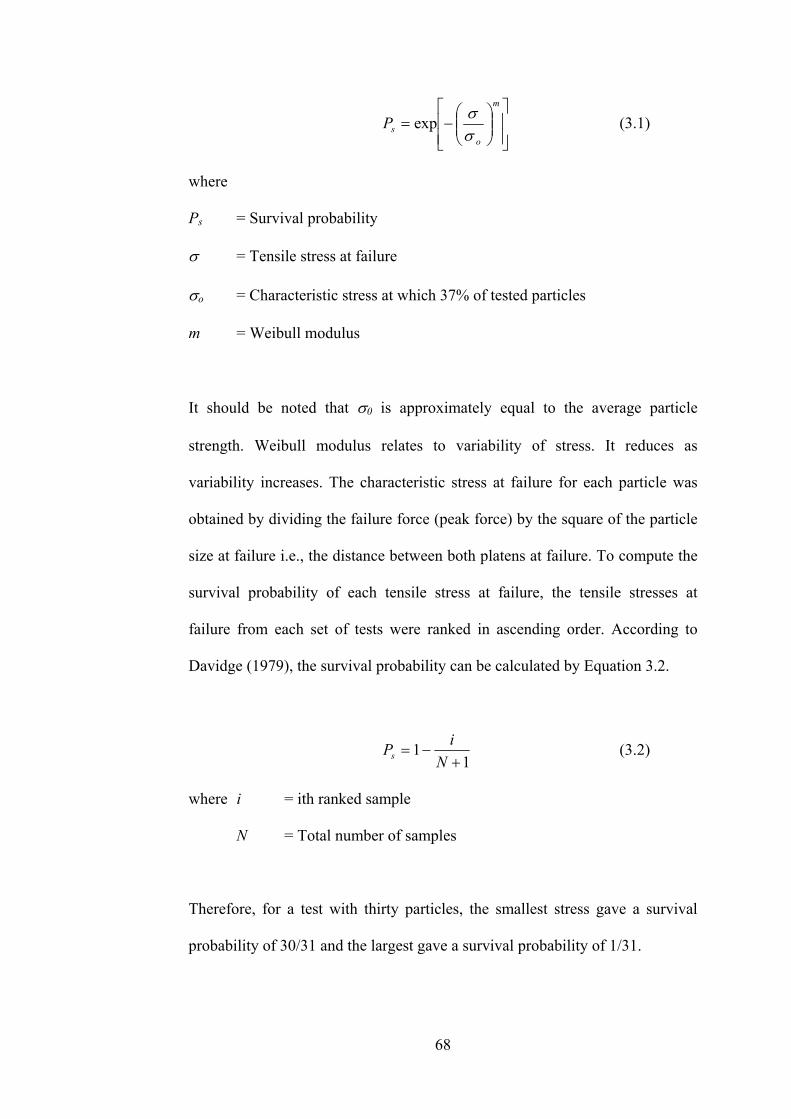
m

o

sPσσ

exp (3.1)

where

Ps = Survival probability

σ = Tensile stress at failure

σo = Characteristic stress at which 37% of tested particles

m = Weibull modulus

It should be noted that σ0 is approximately equal to the average particle

strength. Weibull modulus relates to variability of stress. It reduces as

variability increases. The characteristic stress at failure for each particle was

obtained by dividing the failure force (peak force) by the square of the particle

size at failure i.e., the distance between both platens at failure. To compute the

survival probability of each tensile stress at failure, the tensile stresses at

failure from each set of tests were ranked in ascending order. According to

Davidge (1979), the survival probability can be calculated by Equation 3.2.

11

+−=

N

iPs (3.2)

where i = ith ranked sample

N = Total number of samples

Therefore, for a test with thirty particles, the smallest stress gave a survival

probability of 30/31 and the largest gave a survival probability of 1/31.

68

To use Equation 3.1 in the test, it must be re-written as shown in Equation 3.3.

o

s

mmP

σσ lnln1

lnln −=⎟⎟⎠

⎞⎜⎜⎝

⎛⎟⎟⎠

⎞⎜⎜⎝

⎛ (3.3)

By plotting ln(ln(1/Ps)) against lnσ, the Weibulll modulus can be determined

from the slope of the line of best fit and σo is the value of σ when ln(ln(1/Ps)) =

0. The plots from different tests are shown in Section 3.3.3.

3.3.2. Test Programme

Eight single particle crushing tests were performed in this project. The details

of the tests are shown in Table 3.3. Each test contained thirty particles. The

ballast in tests 4, 6, and 8 were painted like the ballast in the Railway Test

Facility (Chapter 4). This is to check if painting affects ballast strength.

3.3.3. Weilbull probability plots

The Weibull probability plots are shown in Figure 3.3. As Lim (2004)

performed the test on 10-14 mm and 37.5-50 mm granite A, the results of tests

1, 2, and 3 are plotted together with his results. Furthermore, the results of

normal and painted ballasts of the same type are also plotted together for

comparative purposes.

69

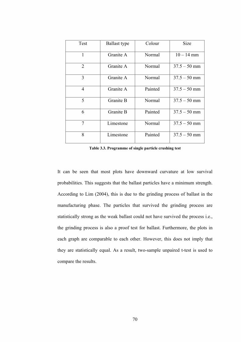
Test Ballast type Colour Size

1 Granite A Normal 10 � 14 mm

2 Granite A Normal 37.5 � 50 mm

3 Granite A Normal 37.5 � 50 mm

4 Granite A Painted 37.5 � 50 mm

5 Granite B Normal 37.5 � 50 mm

6 Granite B Painted 37.5 � 50 mm

7 Limestone Normal 37.5 � 50 mm

8 Limestone Painted 37.5 � 50 mm

Table 3.3. Programme of single particle crushing test

It can be seen that most plots have downward curvature at low survival

probabilities. This suggests that the ballast particles have a minimum strength.

According to Lim (2004), this is due to the grinding process of ballast in the

manufacturing phase. The particles that survived the grinding process are

statistically strong as the weak ballast could not have survived the process i.e.,

the grinding process is also a proof test for ballast. Furthermore, the plots in

each graph are comparable to each other. However, this does not imply that

they are statistically equal. As a result, two-sample unpaired t-test is used to

compare the results.

70

Granite A 10-14 mm (Test 1 and Lim (2004))

Test 1

y = 2.6x - 8.5

R2 = 0.96

m = 2.6

σ0 = 26.3 MPa

Lim (2004)

y = 3.2x - 10.2

R2 = 0.94

m = 3.2

σ0 = 24.0 MPa

-4

-3

-2

-1

0

1

2

3

0.0 0.5 1.0 1.5 2.0 2.5 3.0 3.5 4.0 4.5

ln (σ)

ln(l

n(1

/Ps

))

Test 1

Lim (2004)

Figure 3.3a. Weibull probability plots for 10 � 14 mm granite A

Granite A 37.5-50 mm (Tests 2 and 3 and Lim (2004))

Test 2

y = 3.1x - 8.7

R2 = 0.87

m = 3.1

σ0 = 16.3 MPa

Test 3

y = 3.2x - 8.9

R2 = 0.96

m = 3.2

σ0 = 16.1 MPa

Lim (2004)

y = 3.2x - 8.2

R2 = 0.89

m = 3.2

σ0 = 13.1 MPa

-4

-3

-2

-1

0

1

2

3

0.0 0.5 1.0 1.5 2.0 2.5 3.0 3.5

ln (σ)

ln(l

n(1

/Ps

))

Test 2

Test 3

Lim (2004)

Figure 3.3b. Weibull probability plots for 37.5 � 50 mm granite A

Granite A 37.5 - 50 mm, Normal and Painted (Tests 2 to 4)

Test 4 - Painted

y = 4.0x - 10.7

R2 = 0.98

m = 4.0

σ0 = 14.2 MPa

Test 3 - Normal

y = 3.2x - 8.9

R2 = 0.96

m = 3.2

σ0 = 16.1 MPa

Test 2 - Normal

y = 3.1x - 8.7

R2 = 0.87

m = 3.1

σ0 = 16.3 MPa

-4

-3

-2

-1

0

1

2

0.0 0.5 1.0 1.5 2.0 2.5 3.0 3.5ln (σ)

ln(l

n(1

/Ps

))

Test 2 - Normal

Test 3 - Normal

Test 4 - Painted

Figure 3.3c. Weibull probability plots for 37.5 � 50 mm normal and painted granite A

71

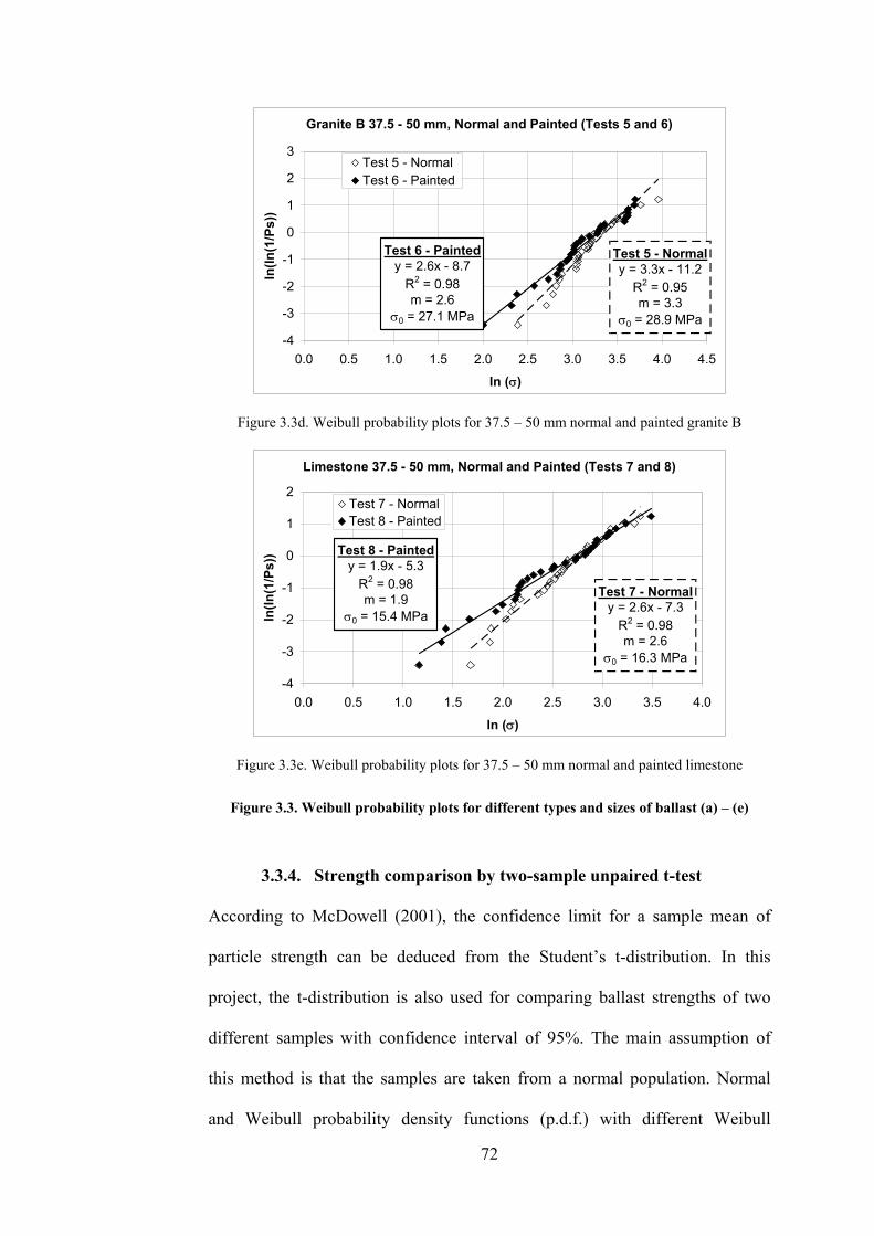
Granite B 37.5 - 50 mm, Normal and Painted (Tests 5 and 6)

Test 6 - Painted

y = 2.6x - 8.7

R2 = 0.98

m = 2.6

σ0 = 27.1 MPa

Test 5 - Normal

y = 3.3x - 11.2

R2 = 0.95

m = 3.3

σ0 = 28.9 MPa

-4

-3

-2

-1

0

1

2

3

0.0 0.5 1.0 1.5 2.0 2.5 3.0 3.5 4.0 4.5

ln (σ)

ln(l

n(1

/Ps))

Test 5 - Normal

Test 6 - Painted

Figure 3.3d. Weibull probability plots for 37.5 � 50 mm normal and painted granite B

Limestone 37.5 - 50 mm, Normal and Painted (Tests 7 and 8)

Test 7 - Normal

y = 2.6x - 7.3

R2 = 0.98

m = 2.6

σ0 = 16.3 MPa

Test 8 - Painted

y = 1.9x - 5.3

R2 = 0.98

m = 1.9

σ0 = 15.4 MPa

-4

-3

-2

-1

0

1

2

0.0 0.5 1.0 1.5 2.0 2.5 3.0 3.5 4.0

ln (σ)

ln(l

n(1

/Ps

))

Test 7 - Normal

Test 8 - Painted

Figure 3.3e. Weibull probability plots for 37.5 � 50 mm normal and painted limestone

Figure 3.3. Weibull probability plots for different types and sizes of ballast (a) � (e)

3.3.4. Strength comparison by two-sample unpaired t-test

According to McDowell (2001), the confidence limit for a sample mean of

particle strength can be deduced from the Student�s t-distribution. In this

project, the t-distribution is also used for comparing ballast strengths of two

different samples with confidence interval of 95%. The main assumption of

this method is that the samples are taken from a normal population. Normal

and Weibull probability density functions (p.d.f.) with different Weibull

72

moduli were previously shown in Figure 2.13. It can be seen from the figure

that the Weibull p.d.f. is very similar to normal p.d.f. when the Weibull

modulus is close to three which reflects the values of Weibull moduli from the

tests. Further details of the two-sample unpaired t-test can be found in most

statistics textbook such as Devore and Farnum (1999).

This test can be easily performed by the TTEST function in Microsoft Excel.

An example of the analysis by TTEST function is shown in Figure 3.4. With

the confidence interval of 95%, it can be concluded that both samples are equal

if the number that the function returns is larger than 0.05 (Aitken, 2006). In the

figure, the returned value is 0.424. Therefore, it can be concluded that both

samples has the same strength. All strength comparisons by TTEST function

with 95% confidence interval are summarised in Table 3.4.

It can be concluded from Table 3.4 that painting does not affect the strength of

the particles and the strengths of 37.5-50 mm granite A from this project (tests

2 and 3) are not statistically equal to that of Lim (2004). The discrepancy may

be because the ballast from both tests came from a different production batch.

However, tests 2 and 3 gave statistically equal results at the 95% confidence

level. In addition, it must be remembered that for the t-test, it must be assumed

that the strengths are normally distributed which might not be true for every

test.

73

Figure 3.4. Example of TTEST function

74

75

Tests to compare Description

Strength comparison (with

95% confidence interval)

Test 1 and Lim (2004) 10 � 14 mm granite A Equal

Test 2 and Lim (2004) 37.5 � 50 mm granite A Not equal

Test 3 and Lim (2004) 37.5 � 50 mm granite A Not equal

Tests 2 and 3 37.5 � 50 mm granite A Equal

Tests 2 and 4 37.5 � 50 mm granite A

(normal and painted)

Equal

Tests 3 and 4 37.5 � 50 mm granite A

(normal and painted)

Equal

Tests 5 and 6 37.5 � 50 mm granite B

(normal and painted)

Equal

Tests 7 and 8 37.5 � 50 mm Limestone

(normal and painted)

Equal

Table 3.4. Summary of strength comparison

4. Railway Test Facility

4.1. Introduction

Performing experiments on ballast in a railway track is desirable since results

can be obtained for real site conditions. However, it is very difficult to control

test variables and to collect data on site. The Railway Test Facility (RTF) was

designed to produce dynamic loading and tamping cycles in the laboratory at a

realistic level and could be related to site conditions. It is located over a pit

filled with a subgrade material and railway ballast. The main purpose of this

facility in this project is to study ballast deformation from traffic loading and

degradation resulting from both traffic loading and tamping. Three actuators

were used to supply traffic loading through three sleepers onto the ballast. A

tamping bank, which was modified from a real tamper, was used for tamping.

Seven tests were performed on this facility in this project. This facility was also

used in another project which investigated the effect of geogrid on ballast

settlement under traffic loading (Kwan, 2006).

4.2. Test facilities

The whole test facility was housed in a concrete pit with dimensions of 2.1 m

(width) x 4.1 m (length) x 1.9 m (depth). An end view of the facility is shown

in Figure 4.1. The geogrid in the figure is optional. The reaction test frame was

placed in the pit as shown in Figure 4.2. The upper half of the frame was

removable to give access to the pit during placement of track bed material and

tamping. Four 150-mm-deep hollow core concrete slabs were positioned on the

base of the frame to provide support for the subgrade. Polythene sheets were

used to waterproof the floor and the walls. Water could be added to the pit via

76

vertical perforated tubes placed at each corner of the pit to lower the subgrade

stiffness if necessary.

Three servo hydraulic actuators were bolted to cross plates under the top two

beams in the upper part of the reaction test frame. Each actuator had a built-in

displacement transducer to measure its vertical shaft movement. A 100-kN

load cell was screwed to the end of each actuator shaft. A three-channel

controller and computer in an adjacent room controlled the actuators and

collected the data from the displacement transducers and load cells as shown in

Figure 4.3. The assembled test facility is shown in Figure 4.4 and loading is

transmitted to the sleepers by means of spreader beams (the three steel beams

on top of the sleepers in Figure 4.4) located on rollers on the rail seatings. The

axial alignment of the actuators is maintained through shallow spherical

bearings (mated horizontal curved surfaces) placed at the centre of the spreader

beams.

The simulated traffic loading on the sleepers was achieved by applying

sinusoidal loading up to 94 kN with a 90° phase lag between each actuator.

This is shown in Figure 4.5. This loading pattern was suggested by Awoleye

(1993). It simulated a train running over three sleepers with 50% of the wheel

load on the middle sleeper and 25% of the wheel load on the outer sleepers.

With this load magnitude and distribution, the test in the RTF simulated an axle

load of approximately 20 tonnes which is comparable to a typical heavy axle

load. However, the finite-element analysis of Watanabe (see Profillidis, 2000,

p.81) showed that the sleeper under the loading wheel took 40% of the load,

77

the adjacent sleepers each took 23% of the load, and the next sleepers each

took 7% of the load. Both loading distributions are shown in Figure 4.6 but

distribution (b) could not be adopted for the current arrangement of the RTF.

Subgrade

Concrete slabs

Ballast

Geogrid

(optional)

Sleepers

Load

actuators

Loading

frame

I-beam

I-beam

2.10 m

0.90 m

0.30 m

0.20 m

0.15 m

123

Simulated direction of traffic

Figure 4.1. End view diagram of the facility

Figure 4.2. Testing frame in the pit

78

Figure 4.3. RTF control system

Simulated direction of traffic

Sleeper

number

13 2

Potentiometer / LVDT

(front end)

Figure 4.4. RTF loading arrangement

0

20

40

60

80

100

0 0.2 0.4 0.6 0.8 1 1.2 1.4

Time (s)

Lo

ad

(k

N)

Actuator 1

Actuator 2

Actuator 3

Figure 4.5. Loading pattern used in this project

79

Figure 4.6. Load distributions along successive sleepers (a) suggested by Awoleye (1993)

and used in this project and (b) suggested by Watanabe (see Profillidis, 2000)

The seating load of the cyclic loading was originally 2 kN but it was later

changed to 4 kN. This was to accommodate any electrical drift of the feedback

load cells. If this occurred in the tensile direction, it could cause the actuator to

lose contact with the packing on the spreader beam. The safety trip for all

actuators was set to 97 kN.

The loading frequency of each test was 3 Hz. This frequency is very low

compared to the usual frequency in the track of approximately 8 � 10 Hz. This

frequency was however dictated by the pressure and flow capacity of the

hydraulic pump. With the above loading pattern and 3-Hz loading frequency,

actuator 2 started loading 1/12 seconds after actuator 1 started loading. This

simulated a wheel moving from one sleeper to another in 1/12 of a second. The

sleeper spacing in the RTF was 0.65 m. Therefore, the test simulated a train

speed of 7.8 m/s (0.65 m ÷ 1/12 s) or 28 km/h. The loading frequency of 3-Hz

also implied that the time taken for the maximum load to be repeated again on

the same sleeper was 1/3 of a second. This indicated that the next wheel would

80

be on top of the same sleeper in 1/3 of a second. With 7.8 m/s train speed, this

meant that the test simulated a 2.6 m axle spacing (7.8 m/s × 1/3 s). Unlike the

frequency, this axle spacing is realistic. The spacing of the front pair of axle of

a Bombardier BiLevel passenger rail vehicle in Montreal, Canada is also 2.6 m

as shown in Figure 4.7 (Bombardier Inc., 2007).

Figure 4.7. Bombardier BiLevel passenger rail vehicle (Bombardier Inc., 2007)

Another part of this facility is the tamping bank which is used to simulate

tamping maintenance in a real track (Figure 4.8). When in use, the upper part

of the test frame must be removed. It incorporated a refurbished Plasser

tamping bank with a vibrating hydraulic cylinder replacing the standard

vibrator. The tamping bank was fitted to a frame which spans the pit and runs

along longitudinal beams so that it can be located and clamped into position

above the location of the rail seating.

81

Figure 4.8. Tamping bank

The tamping bank was used to simulate tamping maintenance in a real track.

The tamping procedures can be found in Section 2.2.3. The 35-Hz tamping tine

vibration of the real system can be achieved in this tamping bank by a

hydraulic actuator which could be controlled by a waveform generator to

simulate the same vibration. The pressure and oil flow required for this

frequency of displacement was maintained by a large accumulator which was

connected to the actuator and would partially discharge during the tamping

cycle. Another accumulator was used for the lowering, squeezing, and lifting of

the tines. These measures were necessary because there was insufficient flow

capacity in the laboratory ring main. The system then automatically recharged

the accumulators ready for the next cycle. There was also a manual facility

which could raise, lower, squeeze and vibrate the tamping tines as individual

operations. The vertical movement of the tamping tines could be controlled by

proximity detectors on the lowering and lifting cylinders.

Tamping was only performed about the middle sleeper as the tamping bank

could not be moved laterally. The middle sleeper was lifted by 20 mm to create

82

a space between it and the ballast and held at this height by clamping it to a

cross beam. The 20-mm lift was chosen because a lift greater than 20 mm

results in little additional improvement of ballast settlement as previously

shown in Figure 2.7 (Selig and Waters, 1994). After that, the tamping tines

were plunged into the ballast so that the bottom part of the tines was about 20

mm below the sleeper as shown in Figure 4.9. Then, the tines squeezed the

ballast into the void by rotating around pivot points in the body of the tamping

bank shown in Figure 4.10. This tamping process takes approximately 5

seconds starting from tine insertion until the tines are completely lifted off

from the ballast layer.

Sleeper

Tamping

tine

20 mm

Figure 4.9. Tamping tine insertion

83

Pivots

Tines

Before

squeezing

During

squeezing

555 mm 275 mm

605 mm

710 mm

Figure 4.10. Tamping tine movement before and during squeezing

4.3. Instrumentation

The primary instruments used in the RTF were the three actuator load cells and

integral stroke transducers to measure the load applied to the sleepers and

average sleeper deflection respectively, displacement transducers to measure

sleeper settlement and pressure cells to measure stresses near the top of the

subgrade.

A secondary exercise was carried out to look at the feasibility of using an

accelerometer to measure subgrade movement just below the ballast and to try

and develop a means of collecting fines at the bottom of the ballast layer during

a test. This will be described later.

The load cells and stroke transducers were fitted to the shafts of the actuators

and were connected to the control system. Additionally, their outputs were

84

connected to an external data acquisition system with 100-Hz logging rate. It

was also used to read the pressure cells and displacement transducers because

there were insufficient channels on the control system for this purpose. The

accelerometer output was monitored on a digital storage oscilloscope so that

any extraneous high frequency signals could be seen but it could also be fed to

the data acquisition system.

The pressure cells consist of a recessed disc with 65-mm diameter and 11-mm

thickness. The bottom of the disc forms a 2-mm-thick diaphragm which has

strain gauge in a Wheatstone bridge configuration. A voltage is applied across

the bridge and pressure on the diaphragm causes a change in resistance of the

gauge which can be used to give a voltage output proportional to the pressure.

The cell is buried with the diaphragm upwards in the subgrade taking care that

there are no stones in contact with the diaphragm and its cable run out of the

surrounding material for accessibility as shown in Figure 4.11. The cells were

installed 25 mm below the subgrade surface to measure vertical stress under

the centre of the middle sleeper, under one loading point of the middle sleeper

and between the sleepers as shown in Figure 4.12.

85

Figure 4.11. Pressure cell

P. cell 3

Acc. meter /

Fines collector

Sleeper

1

2

3

P. cell 2P. cell 1

Simulated

direction

of travel

Figure 4.12. Positions of pressure cells, accelerometer, and fines collector

The central sleeper settlement for the first test was measured with a linear

potentiometer placed at approximately 20 � 40 mm from the end of the middle

sleeper by mounting onto a steel beam spanning over the pit so that the

measured settlement was not affected by the movement of the loading system

as shown in Figure 4.4. The potentiometer comprises a rod moving in and out

of a case containing a resistor. The rod is connected to a wiper on the resistor

which has a D.C. voltage applied to each end. As the rod moves the wiper

along the resistor an output is obtained between the wiper and one end of the

resistor which is proportional to the rod movement. This transducer was

86

replaced after the first test with two LVDTs (Linear variable differential

transformer) displacement transducers, one at each end of the middle sleeper,

which were more accurate. Each consists of a case containing primary and

secondary windings with a ferrite core moving between the windings. The

primary winding is powered with an A.C. voltage and when the core moves a

voltage is induced into the secondary windings to give an output proportional

to the position of the core.

An accelerometer, which had been used in another project for measuring the

response of a pavement surface to an impact, was tried as a means of

measuring dynamic subgrade deflection. This small device contains a quartz

crystal under a small weight. When it moves, a force is exerted on the crystal

which produces a charge. This can be converted to a voltage which is

proportional to acceleration and when double intergrated should give a

deflection reading. It is important that this type of device makes a solid

mechanical contact with the material under the test so that it was fitted to a disc

prior to compacting it into the subgrade. It was placed at the same level as the

pressure cells but under the other end of the middle sleeper as shown in Figure

4.12 for the first two tests. However, the deflection reading obtained from the

tests was many times higher than expected. On removal, the accelerometer was

checked. It was noted that during handling of the connecting cable, a large

signal occurred which was independent of the movement of the accelerometer.

This may have been the problem as the signal obtained during testing was the

correct frequency so it was possible that the cable was disturbed in phase with

the loading by the actuator.

87

The accelerometer was replaced by a fines collector in the third test. It was a

device that can weigh fines as the test was progressing, i.e. its function is

different from the accelerometer. Figure 4.13 shows the top and side views of

the fines collector. It was a 150 mm x 150 mm x 55 mm box buried in the

subgrade. There was an 80 mm x 80 mm opening on the top lid of the box. A

steel mesh with 5 mm x 5 mm aperture was bolted on to the top lid. Ballast

fines could fall onto a rectangular tray inside the box through the mesh. The

tray was supported by four springs at the four corners of the tray. An LVDT

was attached to the middle of the tray and was connected to a multimeter

outside the pit. As the fines fell into the tray, the multimeter could read the

movement of the LVDT which then could be converted to the mass of the fines

using a calibration factor based on this movement. However, it was found that

it did not give realistic results probably due to electrical instability. It is

recommended that the weighing tray needs to be guided in linear bearings to

prevent tilt if the fines fall unevenly on the tray. Furthermore, the electrical

supply and monitoring equipment for the fines collector needs to be very stable

and the alignment of the cone in the LVDT must be effectively perfect. Both

the accelerometer and fines collector required further development and this was

not possible within the timescale of the project.

88

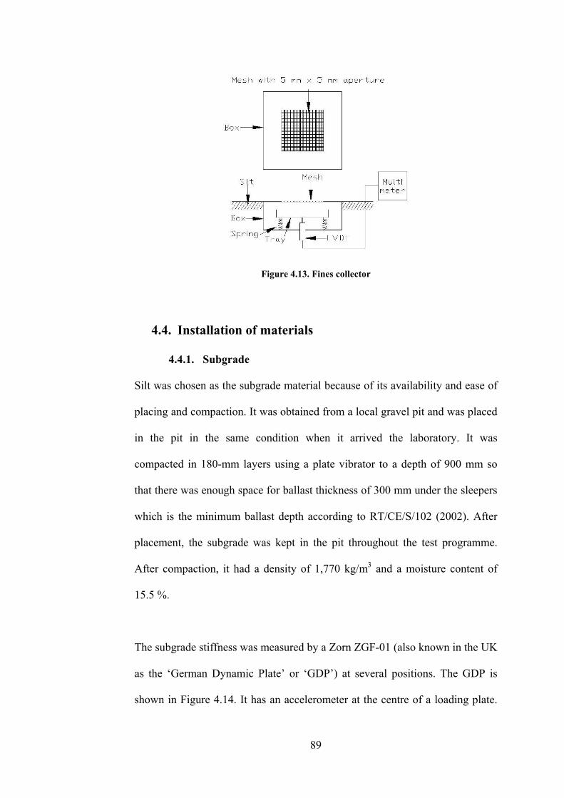
Figure 4.13. Fines collector

4.4. Installation of materials

4.4.1. Subgrade

Silt was chosen as the subgrade material because of its availability and ease of

placing and compaction. It was obtained from a local gravel pit and was placed

in the pit in the same condition when it arrived the laboratory. It was

compacted in 180-mm layers using a plate vibrator to a depth of 900 mm so

that there was enough space for ballast thickness of 300 mm under the sleepers

which is the minimum ballast depth according to RT/CE/S/102 (2002). After

placement, the subgrade was kept in the pit throughout the test programme.

After compaction, it had a density of 1,770 kg/m3 and a moisture content of

15.5 %.

The subgrade stiffness was measured by a Zorn ZGF-01 (also known in the UK

as the �German Dynamic Plate� or �GDP�) at several positions. The GDP is

shown in Figure 4.14. It has an accelerometer at the centre of a loading plate.

89

The load is dropped three times onto a 300-mm diameter steel base sitting on

the surface of the subgrade. The acceleration of the loading plate is measured

and converted to the stiffness of the subgrade which is an approximation of the

surface stiffness of the subgrade (Rahimzadeh et al., 2004). The stiffness was

measured at twenty points on the subgrade as shown in Figure 4.15.

Next, the subgrade profile was measured with a rule up to a straight edge using

the top of the pit as a datum as shown in Figure 4.16. Although it was difficult

to obtain repeatable results due to some disturbance of subgrade between tests,

it was concluded that the maximum settlement of the subgrade was about 0.4

mm and was negligible compared to the ballast settlement. Hence, the

settlement from each test was predominantly in the ballast.

Figure 4.14. German Dynamic Plate measuring subgrade stiffness

90

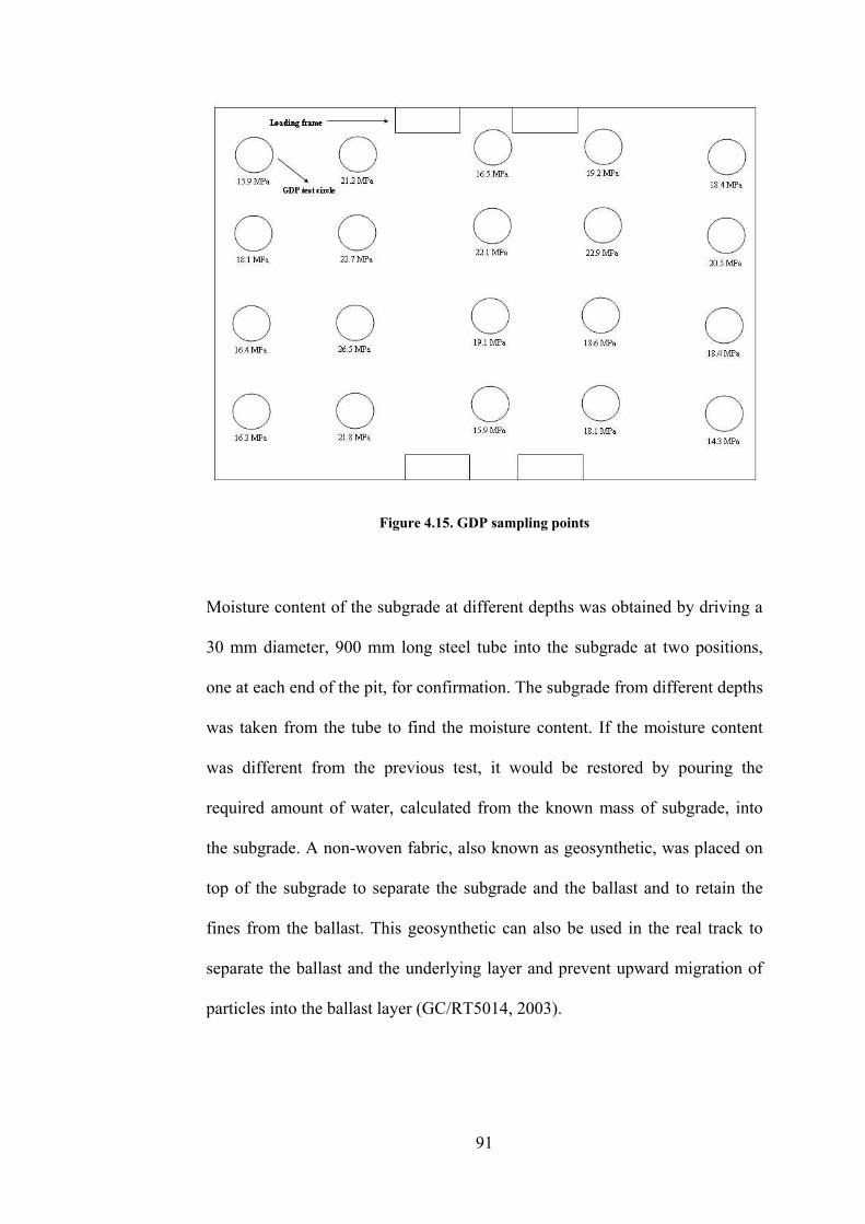
Figure 4.15. GDP sampling points

Moisture content of the subgrade at different depths was obtained by driving a

30 mm diameter, 900 mm long steel tube into the subgrade at two positions,

one at each end of the pit, for confirmation. The subgrade from different depths

was taken from the tube to find the moisture content. If the moisture content

was different from the previous test, it would be restored by pouring the

required amount of water, calculated from the known mass of subgrade, into

the subgrade. A non-woven fabric, also known as geosynthetic, was placed on

top of the subgrade to separate the subgrade and the ballast and to retain the

fines from the ballast. This geosynthetic can also be used in the real track to

separate the ballast and the underlying layer and prevent upward migration of

particles into the ballast layer (GC/RT5014, 2003).

91

Figure 4.16. Measurement of subgrade profile

4.4.2. Ballast

The pit was then filled with ballast. From test 4 onwards, ballast particles at

four critical positions were painted to ease the observation of degradation and

sample collection. This is similar to the dyed ballast approach in the box tests

in Selig and Waters (1994). The strengths of the painted ballast are statistically

equal to the normal ballast according to the single particle crushing test

(Section 3.3.4). These sampling points are called Traffic, Squeezed, T1 and T2.

Their positions are shown in Figure 4.17. The traffic sampling point was

underneath the right rail seat of the middle sleeper. T1 and T2 sampling points

were located under one pair of tamping tines. The squeezed sampling point was

where the other pair of tamping tines squeezed. The particles were placed in

the sampling points using 100 mm deep by 300 mm diameter tubes. To fill the

other places in the pit with ballast, large bags of ballast, hoisted over the pit by

92

a crane, were cut in the form of a flap to let the ballast fall into the pit. The

ballast was placed and compacted in 100-mm layers by the same plate vibrator

to a depth of 300 mm. The tubes were removed before each compaction. The

approximate amount of ballast was 4,500 kg for all tests resulting in ballast

density of 1,742 kg/m3.

Care was taken to ensure that the ballast under the rail seats was slightly higher

than under the centre of the sleeper. A straight edge was used to get the ballast

as level as possible before placing the three sleepers. They were placed

lengthways with 650-mm spacing centre-to-centre. If the sleepers were

rocking, they were then lifted and the ballast high spots were levelled. The

sleepers were repositioned and checked for stability. A vibrating chisel was

then used to settle the ballast material under the sleeper by working it in from

the sides and ends of the sleepers. The depth of the ballast and the sleeper

spacing were chosen to reflect the current UK practice (RT/CE/S/102 Issue 5,

2002). The sleepers used in the RTF were G44 sleepers. This type of sleeper is

used in the mainline track nowadays. The dimensions of the sleeper are shown

in Figure 4.18.

Then, more ballast was added to fill up the pit as shown in Figure 4.19. Two

thin wire ropes were used to prevent tilting of the sleepers and link the sleepers

and the frame together. This was to maintain the positions of the sleepers

during installation and testing. The ropes had sufficient slack to allow vertical

movement so that they would not restrain the settlement of the sleepers during

93

the test. However, it was found in the first test that they could not prevent

tilting of the sleepers so they were not used in the later tests.

It should be noted that the ballast compaction method in the RTF was different

from the normal procedure on site. In a real track, ballast is compacted by a

dynamic track stabiliser which applies horizontal vibration and static vertical

load to the track while running on the track (Selig and Waters, 1994). This

method might break the ballast in the track. The plate vibrator was therefore a

preferable choice for compacting the ballast in the RTF as it was much less

likely to break the ballast. Furthermore, this method was easy and convenient

and did not require any sophisticated equipment.

T1

T2

1

Sleeper

2.10 m

4.10 m

2.50 m

0.60 m 2

3

0.55 m

Squeezed

TrafficRail seats

Simulated

direction

of travel

Figure 4.17. Ballast sampling points

94

Figure 4.18. Dimensions of a G44 sleeper

Figure 4.19. Sleeper arrangement in the RTF

The arrangement of the track bed material in test 7 was different from the

others in that concrete slabs were placed on the subgrade to provide a stiff

support to the ballast. The subgrade surface and sides of the pit were also

covered with polythene so that water could be added to the ballast. This was

because it was believed that a stiff subgrade and water would increase the

amount of breakage from the test. As a result, the ballast thickness under the

sleepers was 200 mm in test 7. It should be noted that the use of polythene

might affect the ballast settlement in the test.

95

4.5. Test procedures

After the installation of the ballast and the sleepers, the facility was assembled

as shown in Figure 4.4. The sleeper height was such that the actuator stroke

had a remaining travel of about 70 mm at the start of loading to ensure

sufficient movement to accommodate the expected settlement.

In general, a million cycles of traffic loading were completed and then three

tamps were carried out by the tamping bank either side of the rail seating at one

end of the middle sleeper. However, in two tests, a tamp around each end of the

middle sleeper was performed halfway (after 500,000 cycles) followed by the

usual three tamps around one end of the middle sleeper after one million

cycles. According to Key (1998), one million cycles of traffic is approximately

equivalent to a year of trafficking.

Before the cyclic loading began, each sleeper was held at 1 kN load to ensure

that it was in contact with the actuator. Then, the readings from the actuator

stroke transducers and the LVDTs at both ends were recorded at this initial

position. The test was stopped after cycles 100; 1,000; 2,000; 5,000; 10,000;

20,000; 50,000; 100,000; 150,000; 200,000; 250,000; 300,000; 400,000;

500,000;�; and 1,000,000 to record the readings at 1 kN. These positions

readings were then used to calculate the settlement. The pressure cell readings

were also taken just before completing the above numbers of cycles. It should

be noted that the dynamic movement of the loading frame would not affect the

settlement reading because each reading was taken when the sleepers were held

at 1 kN.

96

After each test, the ballast for all sampling points was taken for analysis. The

tubes which were used to place the painted ballast were used again during

sampling by placing them on top of the sampling points. The painted ballast

inside the ring was picked out by hand, and the ring was pushed down as the

painted ballast was collected until the bottom was reached. During sampling,

some of the ballast outside the ring was disturbed and would fall into the ring.

This was not collected as the dyed ballast distinguished between the ballast

inside and outside the sampling points.

As the breakage from tamping after traffic loading was not as high as expected,

due to a suspected lack of ballast confinement, i.e. too much space for ballast

to move around to avoid the damage from tamping and low horizontal stress.

Therefore, an additional test with extra confinement on limestone was setup for

tamping after test 7. No trafficking was performed in this test. A box was

formed at the end of the pit near the tamping bank as shown in Figure 4.20.

The steel walls were wedged against both sides of the pit to prevent them from

moving. The width and length of the box were 990 and 1,240 mm. The ballast

was placed in the box by the same method except that the depth of ballast

changed from 300 mm to 445 mm due to the large subgrade settlement in test 7

(see Section 4.7.3 for more details). After that, the sleeper was placed on top of

the ballast. One end of the sleeper was supported by the ballast in the box while

the other end was placed on a steel beam outside the box. Then, the ballast was

added to fill up the box. The tamping bank was then brought into position and

the sleeper was held by clamping to the cross beam. There was no space

97

between the ballast and sleeper in this test. Three tamps were performed and

the painted ballast was taken for sieve analysis after the tamping. After the

sieve analysis, each sample was placed back in the box with particles smaller

than 22.4 mm removed. The same test setup was built again and ten tamps

were performed this time. This was to observe the development of breakage

under different number of tamps. It should be noted that during the ten tamp

test, the tamping bank cannot squeeze the ballast after five tamps. This is

because the ballast in the squeezed location became so compacted that it

prevented the squeezing operation. The squeezing pressure was then increased

to achieve successful squeezing after the fifth tamp.

(a)

(b)

Figure 4.20. Setup for extra confinement tamping test

98

4.6. Test Programme

Seven tests were performed in the RTF. The first four were the joint tests with

the geogrid project (Kwan, 2006). A geogrid was placed at 50 mm above the

bottom of ballast layer in test 2 and at the bottom of ballast layer in test 3 to see

the effect of geogrid position on settlement. The tests are listed in Table 4.1.

The effect of ballast type and subgrade stiffness on settlement and degradation

would be examined from the tests in the table. Repeatability of the test can be

checked during the first 500,000 cycles of tests 1 and 4 (without geogrid) and

tests 2 and 3 (with geogrid) as the same procedure was carried out for all of

them up to this point.

99

Test

No.

Description Intermediate

tamping after cycle*

Final tamping

after cycle**

1 Granite A N/A 1,000,000

2 Granite A + Geogrid at 50

mm above bottom of ballast

N/A 1,000,000

3 Granite A + Geogrid at

bottom of ballast

500,000 1,000,000

4 Granite A 500,000 1,000,000

5 Granite B 600,000***

1,000,000

6 Limestone N/A 1,000,000

7 Limestone + concrete slab

base

N/A 320,000****

T Tamping with extra

confinement but without

trafficking+

N/A N/A

* One tamp at each end of the middle sleeper

** Three tamps at one end of the middle sleeper

*** Hand tamp under the rail seat, see section 4.7.2

**** Test was stopped due to excessive settlement

+ Three tamps followed by ten tamps

Table 4.1. List of tests on the RTF

100

4.7. Results

4.7.1. Subgrade Stiffness and Moisture Content

Figure 4.21 shows subgrade stiffness values and moisture contents for the tests

in the RTF. The subgrade stiffness after test 7 could not be measured because

concrete slabs were used as the base.

The increase in moisture content for test 7 was associated with water which

was added to the ballast finding a way through the polythene above the

subgrade. This is discussed in Section 4.7.3.

0

5

10

15

20

25

30

Su

bg

rad

e s

tiff

ne

ss (

MP

a)

an

d

mois

ture

co

nte

nt

(%)

Subgrade stiffness (MPa)

Moisture content (%)

Before

Test 1

Before

Test 2

Before

Test 3

Before

Test 4

Before

Test 5

Before

Test 6

Before

Test 7

After

Test 7

Figure 4.21. Subgrade stiffness and moisture content

4.7.2. Vertical stress on subgrade

Figure 4.22 shows the average vertical stress reading from the pressure cells

for tests 1 to 6 for the first and last 500,000 cycles. There were no results from

test 7 because the pressure cells could not read the vertical stress due to the

presence of the concrete slabs under the ballast. The distribution of the vertical

101

stresses due to the loading depends on the way in which the sleeper is seated on

the ballast and the compaction of the ballast. The procedure for placing the

sleepers is described in Section 4.4.2 and this method was used for consistency.

However, from analysis of the subgrade stress readings, it can be seen that the

location of the highest stress varied from test to test. To be representative of the

site condition, the highest stress should be below the rail seating as the ballast

will be raised at the position during sleeper installation and tamping. It can be

seen that this is not the case for tests 2, 4, and 5.

The vertical stress under the rail seat for test 5 was found to be particularly

low. After 600,000 cycles, the middle sleeper was lifted and the ballast under

both rail seats was re-compacted by using a vibrating chisel to push it under the

sleeper. This was to increase the vertical stress under the rail seat as this should

increase the degradation due to traffic loading. The effect of the ballast

compaction is shown in Figure 4.23. It can be seen that the stresses under the

centre and between sleepers drop after the compaction and quickly rise

afterwards. On the contrary, the stress under the rail seat rises and drops below

the stress under the centre. This shows that the re-compaction by this method

only gave short term benefit and the sleeper resettled. It would be

recommended in future work that the ballast under the sleeper at the rail

seating should be at a slightly higher level than under the middle portion of the

sleeper.

102

0

10

20

30

40

50

60

70

80

Pressure cell positions

Vert

ica

l str

es

s o

n s

ub

gra

de (

kP

a) Test 1

Test 2

Test 3

Test 4

Test 5

Test 6

Middle

sleeper

Centre

Between

First 500,000 cycles

Rail seat Centre Between

Rail

seat

Figure 4.22(a). Average vertical stresses on subgrade for the first 500,000 cycles

0

10

20

30

40

50

60

70

80

Pressure cell positions

Ve

rtic

al

str

ess

on

su

bg

rad

e (

kP

a) Test 1

Test 2

Test 3

Test 4

Test 5

Test 6

Middle

sleeper

Centre

Between

Last 500,000 cycles

Rail seat Centre Between

Rail

seat

Figure 4.22(a). Average vertical stresses on subgrade for the last 500,000 cycles

Figure 4.22. Average vertical stresses on subgrade at different positions for the first

500,000 cycles (a) and last 500,000 cycles (b)

103

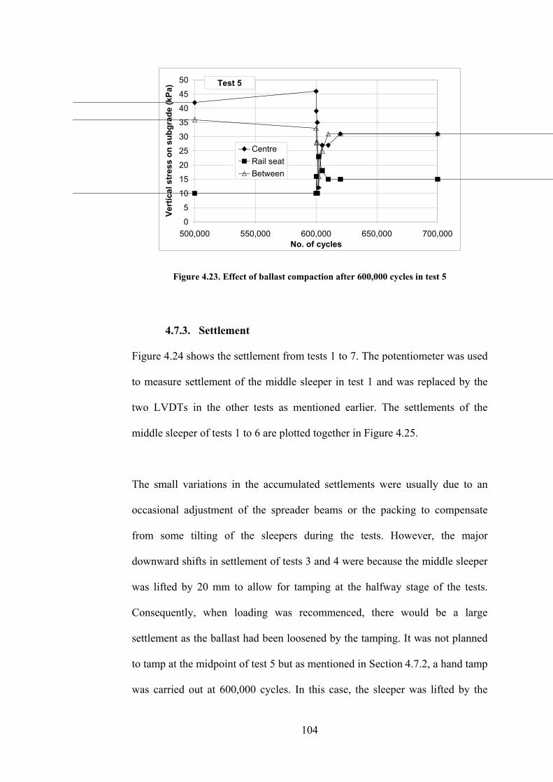
0

5

10

15

20

25

30

35

40

45

50

500,000 550,000 600,000 650,000 700,000

No. of cycles

Vert

ica

l s

tres

s o

n s

ub

gra

de (

kP

a)

Centre

Rail seat

Between

Test 5

Figure 4.23. Effect of ballast compaction after 600,000 cycles in test 5

4.7.3. Settlement

Figure 4.24 shows the settlement from tests 1 to 7. The potentiometer was used

to measure settlement of the middle sleeper in test 1 and was replaced by the

two LVDTs in the other tests as mentioned earlier. The settlements of the

middle sleeper of tests 1 to 6 are plotted together in Figure 4.25.

The small variations in the accumulated settlements were usually due to an

occasional adjustment of the spreader beams or the packing to compensate

from some tilting of the sleepers during the tests. However, the major

downward shifts in settlement of tests 3 and 4 were because the middle sleeper

was lifted by 20 mm to allow for tamping at the halfway stage of the tests.

Consequently, when loading was recommenced, there would be a large

settlement as the ballast had been loosened by the tamping. It was not planned

to tamp at the midpoint of test 5 but as mentioned in Section 4.7.2, a hand tamp

was carried out at 600,000 cycles. In this case, the sleeper was lifted by the

104

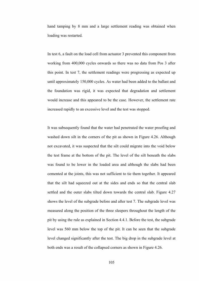
hand tamping by 8 mm and a large settlement reading was obtained when

loading was restarted.

In test 6, a fault on the load cell from actuator 3 prevented this component from

working from 400,000 cycles onwards so there was no data from Pos 3 after

this point. In test 7, the settlement readings were progressing as expected up

until approximately 150,000 cycles. As water had been added to the ballast and

the foundation was rigid, it was expected that degradation and settlement

would increase and this appeared to be the case. However, the settlement rate

increased rapidly to an excessive level and the test was stopped.

It was subsequently found that the water had penetrated the water proofing and

washed down silt in the corners of the pit as shown in Figure 4.26. Although

not excavated, it was suspected that the silt could migrate into the void below

the test frame at the bottom of the pit. The level of the silt beneath the slabs

was found to be lower in the loaded area and although the slabs had been

cemented at the joints, this was not sufficient to tie them together. It appeared

that the silt had squeezed out at the sides and ends so that the central slab

settled and the outer slabs tilted down towards the central slab. Figure 4.27

shows the level of the subgrade before and after test 7. The subgrade level was

measured along the position of the three sleepers throughout the length of the

pit by using the rule as explained in Section 4.4.1. Before the test, the subgrade

level was 560 mm below the top of the pit. It can be seen that the subgrade

level changed significantly after the test. The big drop in the subgrade level at

both ends was a result of the collapsed corners as shown in Figure 4.26.

105

Test 1 (Granite A)

0

2

4

6

8

10

12

14

0 200,000 400,000 600,000 800,000 1,000,000

No. of cycles

Sett

lem

en

t (m

m)

Sleeper 1

Sleeper 2

Sleeper 3

Pot

Figure 4.24(a). Settlement from test 1 (granite A)

0

2

4

6

8

10

12

14

0 200,000 400,000 600,000 800,000 1,000,000

No. of cycles

Se

ttle

me

nt

(mm

)

Sleeper 1

Sleeper 2

Sleeper 3

LVDT fr

LVDT re

Test 2 (Granite A, Geogrid at 50 mm

above bottom of ballast)

Figure 4.24(b). Settlement from test 2 (granite A, geogrid at 50 mm above bottom of ballast)

-15

-10

-5

0

5

10

0 200,000 400,000 600,000 800,000 1,000,000No. of cycles

Sett

lem

en

t (m

m)

Sleeper 1

Sleeper 2

Sleeper 3

LVDT fr

LVDT re Tamp after 500,000 cycles

Test 3 (Granite A, Geogrid

at bottom of ballast)

Figure 4.24(c). Settlement from test 3 (granite A, geogrid at bottom of ballast, tamp at halfway)

106

Test 4 (Granite A)

-15

-10

-5

0

5

10

15

0 200,000 400,000 600,000 800,000 1,000,000

No. of cycles

Sett

lem

en

t (m

m)

Sleeper 1

Sleeper 2

Sleeper 3

LVDT fr

LVDT re Tamp after 500,000 cycles

Figure 4.24(d). Settlement from test 4 (granite A, tamp at halfway)

Test 5 (Granite B)

-2

0

2

4

6

8

10

12

0 200,000 400,000 600,000 800,000 1,000,000

No. of cycles

Se

ttle

me

nt

(mm

)

Sleeper 1

Sleeper 2

Sleeper 3

LVDT fr

LVDT re Hand tamp after 600,000

Figure 4.24(e). Settlement from test 5 (granite B)

Test 6 (Limestone)

0

2

4

6

8

10

12

0 200,000 400,000 600,000 800,000 1,000,000

No. of cycles

Sett

lem

en

t (m

m)

Sleeper 1

Sleeper 2

Sleeper 3

LVDT Fr

LVDT Re

Figure 4.24(f). Settlement from test 6 (limestone)

107

Test 7 (Limestone, Concrete slab base)

0

10

20

30

40

50

60

70

80

0 200,000 400,000 600,000 800,000 1,000,000

No. of cycles

Sett

lem

en

t (m

m)

Sleeper 1

Sleeper 2

Sleeper 3

LVDT Fr

LVDT Re

Test was stopped after 320,000

cycles

Figure 4.24(g). Settlement from test 7 (limestone, concrete slab base)

Figure 4.24. Settlements from RTF (a) � (g)

-20

-15

-10

-5

0

5

10

15

0 200,000 400,000 600,000 800,000 1,000,000

No. of cycles

Sle

ep

er

se

ttle

men

t (m

m)

Test 1 (Granite A)

Test 2 (Granite A, Geogrid)

Test 3 (Granite A, Geogrid)

Test 4 (Granite A)

Test 5 (Granite B)

Test 6 (Limestone)

Settlement from the middle sleeper

Figure 4.25. Settlements of middle sleeper from tests 1 to 6

As water was added during the testing, the early part of the test (up to 50,000

cycles) should be valid as the washing out process would not occur

immediately. By measuring down to the slabs after the test, it was calculated

that on average of about 20 mm of settlement had occurred in the ballast at the

rail seating location for the central sleeper.

108

Figure 4.26. Collapsed corner

-1000

-900

-800

-700

-600

-500

-400

-300

-200

-100

0

0.0 0.5 1.0 1.5 2.0 2.5 3.0 3.5 4.0 4.5Distance from the tamping bank end of the pit (m)

Dep

th f

rom

to

p o

f th

e p

it (

mm

)

Sleeper 1

Sleeper 2

Sleeper 3

Before test 7

Figure 4.27. Level of subgrade before and after test 7

The following points can be drawn from Figure 4.24.

• The settlement from the middle sleeper is always smaller than the other

two. This might be due to the boundary effect between the walls and the

ballast i.e., low shearing resistance between the wall and the ballast.

However, the middle sleeper should be unaffected as it is adequately far

away from the pit walls.

109

• Tamping causes a faster rate of settlement ((c) and (d)). This matches

the findings in Section 2.2.3.

• The settlement from Pos 2 is approximately the average between the

settlements from both LVDTs. This is because the middle sleeper tilted

during the tests.

• The settlements of different ballast are similar to each other (h).

• Field data from Federal Railroad Administration Research Track

(FAST) in Selig and Waters (1994) showed 17 mm of settlement after

the same amount of traffic. Therefore, the settlements obtained from the

tests were about 60 % of the settlement that would be expected on site.

This might be due to the large dynamic load on site. However, it should

be noted that Selig and Waters (1994) did not report test parameters

such as track condition, train speed, ballast type, or ballast density.

Hence, the test results might not be compared on the same basis.

• Tests 1 and 4 (granite A without geogrid) show good repeatability of

the first 500,000 cycles. For easier observation, the settlements from the

middle sleeper of tests 1 and 4 are shown in Figure 4.28.

• According to Kwan (2006), the geogrid reduced the total settlement of

10.1 mm in test 1 (unreinforced) to 7.7 mm in test 2 (reinforced).

However, in tests 3 and 4 where tamping was performed halfway, the

post-tamping settlement in test 4 (unreinforced) is smaller than test 3.

This is likely to be due to a tilt of the middle sleeper, observed visually

during tamping.

110

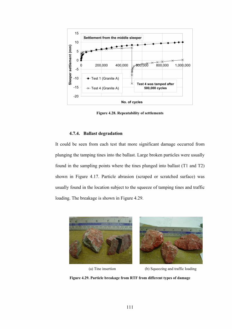
-20

-15

-10

-5

0

5

10

15

0 200,000 400,000 600,000 800,000 1,000,000

No. of cycles

Sle

ep

er

se

ttle

men

t (m

m)

Test 1 (Granite A)

Test 4 (Granite A)

Settlement from the middle sleeper

Test 4 was tamped after

500,000 cycles

Figure 4.28. Repeatability of settlements

4.7.4. Ballast degradation

It could be seen from each test that more significant damage occurred from

plunging the tamping tines into the ballast. Large broken particles were usually

found in the sampling points where the tines plunged into ballast (T1 and T2)

shown in Figure 4.17. Particle abrasion (scraped or scratched surface) was

usually found in the location subject to the squeeze of tamping tines and traffic

loading. The breakage is shown in Figure 4.29.

(a) Tine insertion (b) Squeezing and traffic loading

Figure 4.29. Particle breakage from RTF from different types of damage

111

The ballast degradation from each test is shown by particle size distribution of

particles smaller than 22.4 mm in Figure 4.30. Similarly, the breakage from

each sampling point is shown in Figure 4.31.

Only the results from test 4 onwards are shown because the system of painted

ballast without particles smaller than 22.4 mm was used after the development

in the first three tests. Furthermore, the particle size distribution is shown in

terms of mass passing instead of the usual percentage passing. This is because

not all particles in the sampling points are damaged from trafficking, tine

insertion, or squeezing mechanisms. As percentage passing is calculated from

the total mass of ballast in each sampling point, the mass of the undamaged

ballast would be included in the calculation and the percentage of small

particles can be negligibly small. It should be noted that as test 4 was tamped

halfway, it had one extra tamp at each end of the middle sleeper.

The following points can be drawn from the degradation results.

• Traffic loading and squeezing action of the tines generally produce

similar amount of degradation and cause lower degradation than tine

insertion.

• Degradation of granite B in traffic and squeezed samples is greater than

the other two ballasts. This is probably because the flat and long shape

of granite B.

• Test 7 does not have more fines than test 6. It seems that the increased

stiffness from the concrete slab base does not increase the amount of

degradation as expected.

112

• The degradation from T1 and T2 samples is always greater than Traffic

sample except test 4 (Figure 4.30a). This might be because of the extra

tamp at the trafficked end.

• Even the degradation from ten tamps in test T (extra confinement

tamping on limestone) is smaller than test 6 (limestone).

Test 4 (Granite A, Tamp at halfway)

0

200

400

600

800

1,000

1,200

0 5 10 15 20 25Sieve Size (mm)

Mas

s p

ass

ing

(g

)

Traffic

Squeezed

T1

T2

Figure 4.30(a). Particles smaller than 22.4 mm from test 4 (granite A, tamp at halfway)

Test 5 (Granite B)

0

200

400

600

800

1,000

1,200

0 5 10 15 20 25

Sieve Size (mm)

Ma

ss p

as

sin

g (

g)

Traffic

Squeezed

T1

T2

Figure 4.30(b). Particles smaller than 22.4 mm from test 5 (granite B)

113

Test 6 (Limestone)

0

200

400

600

800

1,000

1,200

0 5 10 15 20 25

Sieve Size (mm)

Mas

s p

ass

ing

(g

)

Traffic

Squeezed

T1

T2

Figure 4.30(c). Particles smaller than 22.4 mm from test 6 (limestone)

Test 7 (Limestone, Concrete slab base)

0

200

400

600

800

1,000

1,200

0 5 10 15 20 25

Sieve Size (mm)

Ma

ss

pa

ss

ing

(g

)

Traffic

Squeezed

T1

T2

Figure 4.30(d). Particles smaller than 22.4 mm from test 6 (limestone, concrete slab base)

Test T (Extra confinement tamping)

0

200

400

600

800

1,000

1,200

0 5 10 15 20 25

Sieve Size (mm)

Ma

ss p

as

sin

g (

g)

Squeezed - 3 tamps

T1 - 3 tamps

T2 - 3 tamps

Squeezed - 10 tamps

T1 - 10 tamps

T2 - 10 tamps

Figure 4.30(e). Particles smaller than 22.4 mm from test T (Extra confinement tamping)

Figure 4.30. Particles smaller than 22.4 mm from tests 4 to 7 and T (a) � (e)

114

Traffic sample

0

200

400

600

800

1,000

1,200

0 5 10 15 20 25

Size (mm)

Mas

s p

as

sin

g (

g)

Test 4 (Granite A,Tamp at halfway)

Test 5 (Granite B)

Test 6 (Limestone)

Test 7 (Limestone,Concrete slab base)

Figure 4.31(a). Particles smaller than 22.4 mm of Traffic sample

Squeezed sample

0

200

400

600

800

1,000

1,200

0 5 10 15 20 25

Size (mm)

Ma

ss

pa

ssin

g (

g)

Test 4 (Granite A, Tamp athalfway)

Test 5 (Granite B)

Test 6 (Limestone)

Test 7 (Limestone,Concrete slab base)

Test T (Extra confinementtamping test) with threetamps

Test T (Extra confinementtamping test) with tentamps

Figure 4.31(b). Particles smaller than 22.4 mm of Squeezed sample

T1 sample

0

200

400

600

800

1,000

1,200

0 5 10 15 20 25

Size (mm)

Ma

ss

pa

ss

ing

(g

)

Test 4 (Granite A, Tampat halfway)

Test 5 (Granite B)

Test 6 (Limestone)

Test 7 (Limestone,Concrete slab base)

Test T (Extraconfinement tampingtest) with three tamps

Test T (Extraconfinement tampingtest) with ten tamps

T1 sample

Figure 4.31(c). Particles smaller than 22.4 mm of T1 sample

115

T2 sample

0

200

400

600

800

1,000

1,200

0 5 10 15 20 25

Size (mm)

Ma

ss p

as

sin

g (

g)

Test 4 (Granite A, Tamp athalfway)

Test 5 (Granite B)

Test 6 (Limestone)

Test 7 (Limestone,Concrete slab base)

Test T (Extra confinementtamping test) with threetamps

Test T (Extra confinementtamping test) with tentamps

Figure 4.31(d). Particles smaller than 22.4 mm of T2 sample

Figure 4.31. Particles smaller than 22.4 mm from each sampling point (a) � (d)

4.8. Discussion

The actuators in the RTF simulated the axle load of 20 tonnes. Even though the

magnitude of this axle load is comparable to a typical heavy axle load, this is

just the static component of the vertical load in the track. According to Selig

and Waters (1994), the dynamic load in the track can be more than twice the

static load. To simulate the worst case scenario, the simulated load in the RTF

should be larger. Another point that should be noted regarding the capacity of

the actuators is the loading frequency that simulated the train speed. The

simulated train speed in the RTF was 28 km/h which was very low and

unrealistic. In the real track, higher loading frequency or train speed causes

larger dynamic load due to track geometrical irregularities and wheel impact

(Selig and Waters, 1994). However, this was not present in the RTF because of

the constant magnitude of traffic loading. Furthermore, frequency has no effect

on the cyclic triaxial test results of ballast according to Shenton (1974).

116

Therefore, it can be concluded that the low and unrealistic simulated train

speed of the RTF had no effect on the test results as the dynamic components

of loading is not presented.

The maximum amounts of particles passing 14 mm produced from traffic

loading in the RTF is 135 g. The maximum amount of particles passing 14 mm

from traffic loading of Awoleye (1993) was 96 g. This is of comparable

magnitude with the amount obtained from the RTF. However, it should be

noted that Awoleye (1993) performed the test using a half-sleeper rig in a box

measuring 900 mm x 402 mm x 150 mm which is smaller than the size of the

RTF. Furthermore, he did not compact the ballast but carefully placed it in the

box instead. This resulted in ballast density of approximately 1,400 � 1,470

kg/m3 which is smaller than the predicted ballast density in the RTF.

The maximum amounts of particles passing 14 mm produced from tamping

from all tests is 548.5 g. However, the amount of particles passing 14 mm from

tamping contradicts with Wright (1983). The maximum amount of particles

passing 14 mm from ten tamps of Wright (1983) was approximately 40 kg.

This was approximately 4 kg per tamp. This contradiction was initially thought

to be due to the void between the ballast and sleeper and lack of ballast

confinement in the RTF. This is because the system in Wright (1983) had no

void underneath the tamped sleeper and had a restraint on top of the tamped

sleeper provided by the weight of the tamping machine (approximately 35

tonnes) through a pair of rails according to Mr. Eric Hornby (Hornby, 2007)

who is the principal technical officer of the company who modified and

117

maintained the tamping facility for Wright (1983). However, the degradation

from the extra confinement tamping test in the RTF was smaller even with ten

tamps.

As a result, some more consideration was given to try and understand where

the differences between the test in the RTF and the test in Wright (1983) arose.

The major differences were the restraint on the tamped sleeper and the

mechanical means of generating vibration.

The RTF was supported by a reaction frame which was clamped to the side

beams fixed to the laboratory floor. So it was necessary to hold down the

sleeper at positions either side of the sleeper with beams which spanned the pit

and were held by jacks against the side beams as shown in Figure 4.32. On the

contrary, the system in Wright (1983) had a large mass to react against and this

may direct the force from the tamping bank more effectively into the ballast

compared to the lighter frame for the RTF. Furthermore, the frame

arrangement used to the RTF tamping bank is not as heavy as the tamping

facility in Wright (1983) so some of the vibration may be transmitted into the

lighter frame.

118

Figure 4.32: Sleeper restraint in the RTF

However, the different ways of producing vibration probably have more

significance with regard to the amount of damage to the ballast. The

mechanical system which is used in Wright (1983) and the real tamping

maintenance is only capable of producing a fixed amplitude of vibration and so

will be more damaging to the ballast when the ballast resistance to penetration

increases due to ballast compaction (Hornby, 2007). On the other hand, the

hydraulic method of developing vibration of the RTF may result in a decrease

in amplitude if the tines meet a high level of resistance during insertion and

especially during squeezing. This is because the resistance of the ballast can

overcome the forces generated by the vibrating cylinder. This reason can also

be used to explain the small degradation from the extra confinement test. As

the ballast is more confined in a small space, the amplitude of the vibration of

the tamping tines may decrease resulting in less breakage. This type of vibrator

may be advantageous as it is less likely to damage the ballast than the fixed

amplitude mechanical vibrator. This is worth exploring in the future in terms of

the damage to the ballast, performance of settlement improvement, and post-

tamping settlement rate.

119

The rate of lowering the tamping tines into ballast is also thought to affect the

ballast breakage. If the tines plunge more slowly into the ballast, the breakage

should reduce. However, this still needs to be studied in more detail.

Lim (2004) found that the breakage from his box tests correlates well with the

Los Angeles Abrasion (LAA) and Micro-Deval Attrition (MDA). Similarly, an

attempt was made to correlate the Los Angeles Abrasion (LAA) and Micro-

Deval Attrition (MDA) to percentage passing 14 mm and 1.18 mm from the

tests as shown in Figure 4.33.

From Figure 4.33, it can be seen that only good correlation can be obtained

from T1 ((e) and (f)). The correlation from percentage passing 1.18 mm of T2

((g) and (h)) is not as good but, similar to T1 correlation, it shows that

breakage increases with increasing LAA and MDA values. It also can be seen

that the percentage passing 14 mm of test 5 does not follow the trend ((g) and

(h)) and is suspected to be an anomaly. This is probably because the tamping

tines did not plunge evenly into the ballast. The correlation from Traffic and

Squeezed are not as good as T1 and they show an opposite trend. This might be

because traffic loading and squeeze action produce minimal amount of

damage. As a result, the scatter of degradation results can be large and affect

the observed trend.

According to Selig and Waters (1994), ballast becomes fully fouled when the

percentage passing 14 mm is about 30%. The ballast degradation from the

120

RTF, Awoleye (1993), and Wright (1983) is not comparable to the fully fouled

ballast. One of the reasons might be because the major source of ballast fouling

in the UK is from external input such as wagon spillage and air borne dirt

(Selig and Waters, 1994). Furthermore, the tests could not simulate the similar

level of dynamic force and degree of attrition and were in a controlled

environment.

Mass passing 14 mm

y = -3.2x + 125.8

Mass passing

1.18 mm

y = -1.9x + 78.0

0

20

40

60

80

100

120

140

160

0 5 10 15 20 25

LAA value

Ma

ss

pa

ssin

g 1

4 a

nd

1.1

8 m

m o

f

Tra

ffic

sa

mp

le (

g)

14 mm

1.18 mm

Granite A

(from test 4)

Granite B

(from test 5)

Limestone (from test 6)

Figure 4.33(a). Correlation between ballast breakage from Traffic sample and LAA value

Mass passing 14 mm

y = -6.5x + 135.5

Mass passing 1.18 mm

y = -4.0x + 85.5

0

20

40

60

80

100

120

140

160

0 5 10 15

MDA value

Ma

ss p

as

sin

g 1

4 a

nd

1.1

8 m

m o

f

Tra

ffic

sa

mp

le (

g)

14 mm

1.18 mm

Granite A

(from test 4)

Granite B

(from test 5)

Limestone (from test 6)

Figure 4.33(b). Correlation between ballast breakage from Traffic sample and MDA value

121

Mass passing 14 mm

y = -1.5x + 102.6

Mass passing

1.18 mm

y = 0.5x + 29.0

0

20

40

60

80

100

120

140

160

180

200

0 5 10 15 20 25

LAA value

Ma

ss

pa

ssin

g 1

4 a

nd

1.1

8 m

m o

f

Sq

uee

ze

d s

am

ple

(g

)

14 mm

1.18 mm

Granite B

(from test 5)

Limestone (from test 6)

Granite A

(from test 4)

Figure 4.33(c). Correlation between ballast breakage from Squeezed sample and LAA value

Mass passing 14 mm

y = -2.5x + 102.3

Mass passing

1.18 mm

y = 1.2x + 26.0

0

20

40

60

80

100

120

140

160

180

200

0 5 10 15

MDA value

Ma

ss

pa

ssin

g 1

4 a

nd

1.1

8 m

m o

f

Sq

uee

ze

d s

am

ple

(g

)

14 mm

1.18 mm

Granite B

(from test 5)

Limestone (from test 6)

Granite A

(from test 4)

Figure 4.33(d). Correlation between ballast breakage from Squeezed sample and MDA value

Mass passing 14 mm

y = 39.8x - 295.2

Mass passing

1.18 mm

y = 9.5x - 40.1

0

100

200

300

400

500

600

700

0 5 10 15 20 25

LAA value

Ma

ss

pa

ssin

g 1

4 a

nd

1.1

8 m

m o

f T

1

sam

ple

(g

)

14 mm

1.18 mm

Granite A

(from test 4)

Granite B

(from test 5)

Limestone (from test 6)

Figure 4.33(e). Correlation between ballast breakage from T1 sample and LAA value

122

Mass passing 14 mm

y = 86.8x - 463.8

Mass passing 1.18 mm

y = 20.9x - 81.6

0

100

200

300

400

500

600

700

0 5 10 15

MDA value

Mas

s p

as

sin

g 1

4 a

nd

1.1

8 m

m o

f T

1

sa

mp

le (

g)

14 mm

1.18 mm

Granite A

(from test 4)

Granite B

(from test 5)

Limestone (from test 6)

Figure 4.33(f). Correlation between ballast breakage from T1 sample and MDA value

Mass passing 14 mm

y = 20.9x + 44.6

Mass passing

1.18 mm

y = 5.4x + 19.1

0

100

200

300

400

500

600

0 5 10 15 20 25

LAA value

Mas

s p

as

sin

g 1

4 a

nd

1.1

8 m

m o

f T

2

sa

mp

le (

g)

14 mm

1.18 mm

Granite A

(from test 4)

Granite B

(from test 5)Limestone (from test 6)

Figure 4.33(g). Correlation between ballast breakage from T2 sample and LAA value

Mass passing 14 mm

y = 47.5x - 60.2

Mass passing 1.18 mm

y = 11.9x - 5.2

0

100

200

300

400

500

600

0 5 10 15

MDA value

Mas

s p

as

sin

g 1

4 a

nd

1.1

8 m

m o

f T

2

sa

mp

le (

g)

14 mm

1.18 mm

Granite A

(from test 4)

Granite B

(from test 5)

Limestone (from test 6)

Figure 4.33(g). Correlation between ballast breakage from T2 sample and MDA value

Figure 4.33. Correlation between breakage and LAA/MDA values (a) � (h)

123

4.9. Conclusions

The Railway Test Facility (RTF) was a newly developed equipment to simulate

train traffic loading and tamping maintenance for observing the settlement and

ballast breakage. The whole facility was housed in a concrete pit which was

filled with silt and ballast as the track bed material. Three concrete sleepers

were placed on top of the ballast. Three servo hydraulic actuators, contained in

the loading frame, supplied the cyclic loading which was transferred to the rail

seats of the three sleepers. Tamping was performed in the RTF by a tamping

bank which was modified from a real Plasser tamping machine. The loading

frame could be removed for the tamping bank to be positioned for the tamping

operation.

It can be concluded from the test results that

• The settlements of the outer sleepers are larger than the middle one

probably because of the boundary effect between the pit walls and the

ballast. However, the boundary effect should not affect the settlement

of the middle sleeper as its location should be adequately far away from

the pit walls.

• The settlements from different ballasts are similar to each other but are

lower than the settlement in the real track. This is probably due to the

large dynamic loading on site.

• With the same amount and magnitude of traffic loading, different

ballast types had similar amount of settlement.

124

125

• Tamping can improve settlement but cause faster rate of settlement

afterwards.

• Tamping tine insertion was the main source of degradation in this

project.

• LAA and MDA values can predict the durability of ballast as the

breakage from tamping increases with increasing LAA and MDA.

While the degradation from the traffic loading matches previous researches, the

degradation from the tamping in the RTF does not. This is probably due to the

restraint on the tamped sleeper and the means of vibration. The sleeper restraint

in the RTF was small compared to Wright (1983) and the real tamping in

which a tamping wagon is used. Also, the amplitude of vibration of the

tamping tines in the RTF may decrease during the tamping operation due to the

use of the hydraulic system rather than a mechanical system. Therefore, the

hydraulic vibrating system may be more preferable than the mechanical

vibrating system as it is less likely to damage the ballast. However, the reduced

amplitude tamping needs to be further studied to ensure that similar

performance can be achieved. Furthermore, the overall degradation from the

test in the RTF is not comparable to the actual degree of fouling in the track.

This is because the major source of fouling in the track was not included in the

tests.

5. Triaxial Test

5.1. Introduction

A good understanding of ballast behaviour and the geotechnical parameters

that control its performance will help in reducing ballast maintenance cost.

Since ballast cannot easily be taken from the track in its in-situ condition and

since controlled tests are difficult in the field, laboratory ballast testing that can

simulate loading conditions in a railway is desirable. Cyclic triaxial testing is

the most suitable test for this job as it is used extensively for testing

geotechnical materials. However, triaxial tests on ballast have to be performed

on large samples so that the aggregate sizes for the specified grading can be

used. Triaxial tests using servo hydraulics can apply cyclic axial stresses to

ballast to simulate the stresses due to traffic. Also, lateral stress on the ballast

can be applied as a cell confining stress via pressurised air and water to

simulate the effect of the surrounding ballast.

5.2. Triaxial test apparatus

The triaxial apparatus in this project, shown in Figure 5.1, was used to

investigate the behaviour of ballast under static loading and repeated loading

under different stress conditions. It was designed for a sample of 300-mm

diameter and 450-mm height. It was manufactured by GDS Instrument Ltd.

Figure 5.2 shows the schematic diagram of the apparatus. It utilises the triaxial

apparatus system presented in Ng et al. (2002) based on a differential pressure

measurement for volume change instead of on sample axial and radial

displacement measurements. This method was preferred due to the irregular

126

outer surface profile of the sample caused by the large size and angular shape

of the ballast.

The principle of this system is to use water in an inner cell which is in direct

contact with the sample (Figure 5.2). Air at a specified pressure is directed to

an outer cell so that the water in the neck is pressurised and consequently a

confining pressure is applied to the sample. As the pressures in the inner and

outer cells are equal, the inner cell volume remains constant so any change in

the volume of the sample will displace an equivalent volume of water in the

inner cell.

The volume change is measured by recording the differential pressure between

the water in the neck of the inner cell and the water inside a reference tube

using a differential pressure transducer. At the beginning of each test, the water

levels in both the inner cell and the reference tube are equal. If the sample in

the inner cell expands, the water level in the inner cell rises while the water

level in the reference tube stays the same. The differential pressure transducer

reading is converted to a volume change based on the known cross-sectional

areas of the inner cell neck and the reference tube. Average radial strain can be

calculated from the axial and volumetric strains. Furthermore, a scale was

attached to the neck of the inner cell to double check the accuracy of the

volume change measurement. The differential pressure transducer cannot

register the differential pressure instantaneously. It was found that it was able

to accurately read the volume change at the frequency of 0.2 Hz. As previously

mentioned, a conventional on-sample measuring system such as strain collars

127

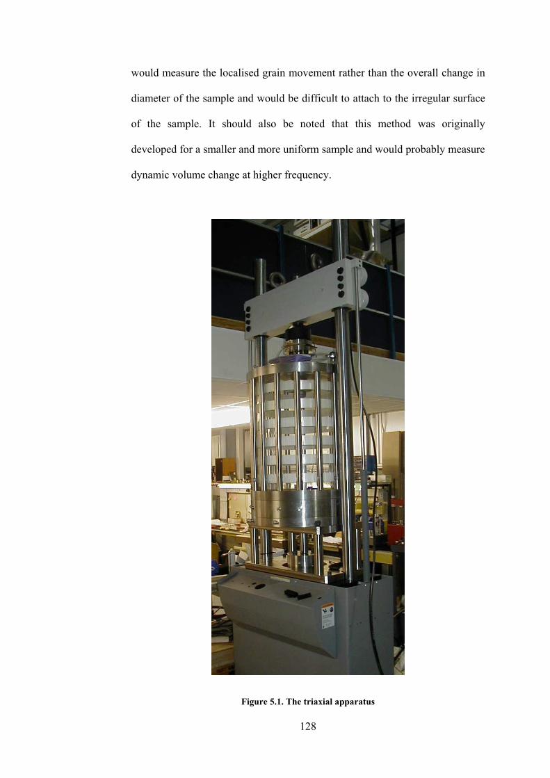
would measure the localised grain movement rather than the overall change in

diameter of the sample and would be difficult to attach to the irregular surface

of the sample. It should also be noted that this method was originally

developed for a smaller and more uniform sample and would probably measure

dynamic volume change at higher frequency.

Figure 5.1. The triaxial apparatus

128

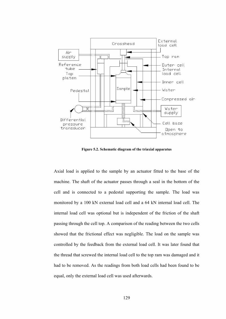
Figure 5.2. Schematic diagram of the triaxial apparatus

Axial load is applied to the sample by an actuator fitted to the base of the

machine. The shaft of the actuator passes through a seal in the bottom of the

cell and is connected to a pedestal supporting the sample. The load was

monitored by a 100 kN external load cell and a 64 kN internal load cell. The

internal load cell was optional but is independent of the friction of the shaft

passing through the cell top. A comparison of the reading between the two cells

showed that the frictional effect was negligible. The load on the sample was

controlled by the feedback from the external load cell. It was later found that

the thread that screwed the internal load cell to the top ram was damaged and it

had to be removed. As the readings from both load cells had been found to be

equal, only the external load cell was used afterwards.

129

Axial deformation was measured by an LVDT (Linear Variable Differential

Transformer) displacement transducer connected to the loading actuator. This

applied upward load thereby lifting the sample against the upper fixed

crosshead so the LVDT was in direct contact with the sample. The

displacement range of the system was 100 mm. This upward movement in the

inner cell means that the actuator shaft displaces the water in the inner cell and

this was subtracted from the total volume change to obtain the sample volume

change.

5.3. Test sample

5.3.1. Materials and Grading

The same granite A and limestone were used in the triaxial tests. Different

sample gradings were used with the different ballasts. This depended on the

grading of each ballast when it was delivered to the laboratory. The sample

gradings are shown in Figure 5.3.

5.3.2. Dimensions

The sample had a diameter and height of 300 mm and 450 mm. As the

maximum grain size of a sample was 50 mm, the ratio of the sample diameter

to maximum particle size (D/dmax) is six which is within the typical range of

five and seven according to Skoglund (2002).

130

0

10

20

30

40

50

60

70

80

90

100

0 10 20 30 40 50 60 70Particle size (mm)

% P

assin

g

Granite A

Limestone

Specification

Figure 5.3. Grading of triaxial samples and ballast specification

The ratio of the height to diameter of the sample (H/D) was 1.5. However,

Bishop and Green (1965) suggested the H/D ratio of two to eliminate the effect

of friction at both ends of the sample. Nevertheless, the ratio of 1.5 enabled

easier and more economical design of the cells in this project. Duncan and

Dunlop (1968) concluded that end friction caused an insignificant increase in

the angle of shearing resistance in their drained triaxial tests on sand.

Furthermore, they added that lubrication at both ends was necessary when

volumetric strain needed to be calculated. This was because end friction

usually caused the triaxial sample to bulge into a barrel shape. This meant the

diameter of the sample was not uniform through the whole height of the sample

and therefore affected the calculation of volumetric strain. However, this was

not a problem in this project since the volumetric strain could be measured

directly. However, an effort was made to lubricate the ends of samples in this

project. This will be explained in the later section.

131

5.3.3. Top platen, pedestal and sample discs

Stainless steel top platen, pedestal and sample discs were used in the sample

preparation which is discussed in the next section. The top platen and pedestal

each had a groove around their edges for sealing membranes around the sample

by O-rings. The pedestal was screwed onto the lower ram with a vacuum line

routed through the lower ram and the pedestal into the sample. The top platen

made direct contact with the top ram when the sample was raised.

The top and bottom sample discs were in direct contact with the sample to

protect the top platen and pedestal from damage by the sharp ballast particles.

The discs were 310 mm in diameter, 8-mm thick, and had twenty 1.5-mm-

diameter holes in the middle for drainage purpose.

5.3.4. Preparation

The sample preparation method in this project was changed several times to

obtain an air/water-tight seal on the sample and optimum sample density. The

method below is the final one that was found to work well.

Fifty five kilograms of ballast with the required grading was mixed on the floor

by a shovel. Care was taken not to break the ballast. It was necessary to make

the sample on the cell base which was bolted onto a vibrating table.

A 2-mm latex membrane was put inside and folded over the top and bottom of

a split aluminium mould which has an internal diameter of 304 mm. The mould

was made of two halves, joined with six bolts.

132

Next, a circular sheet of filter paper was placed on top of the pedestal to

prevent fines from blocking and entering the drainage hole. The bottom sample

disc was then placed on the filter paper and the mould plus the membrane was

placed on the pedestal and the disc. Then, two circular latex sheets

sandwiching silicon grease were put on the disc. They were used at both

sample ends to reduce the friction. The bottom latex sheets had a 50-mm-

diameter hole at the centre for drainage purpose while the top ones had no

holes for drainage as there was no drainage path through the top platen.

The mould was then filled with the ballast in three layers. Each layer was

vibrated for 30 seconds with a surcharge of 20 kg on top of the layer. While the

mould was being filled, some small and flat particles were kept for levelling

the final surface. On the top layer, the top cap was used instead of the 20 kg

weight. The top of the sample was levelled by hand with the small and flat

particles followed by another vibration with the top platen on top. This was

repeated until the top of the sample was level.

After it was levelled, the top platen was removed and the remaining test

material was weighed so that the mass of the sample could be found. The

quantity and size of the surplus material varied with different samples so the

grading of different samples could vary. Then, the lubricated latex sheets were

placed on the top of the sample followed by the top sample discs and the top

platen. With this method of sample preparation, the usual sample mass ranges

between 48 and 52 kg. This is associated with bulk density of 1,500 � 1,630

133

kg/m3 and void ratio of 0.6 � 0.7. This density is slightly lower than the

approximated ballast density in the RTF.

Silicone grease was then applied in both the top and bottom grooves of the

sample. The folded membrane ends were pulled over the grooves and two o-

rings were used to seal the membrane into the grooves. Next, a vacuum pump

was used to apply a partial vacuum of approximately 20 � 30 kPa vacuum to

the sample via the hole at the bottom of the cell base. Full vacuum had been

used but this would cause puncture of the membrane particularly with the

limestone. There was a detachable tap connection between the vacuum pump

and the drainage hole and this was used during transportation of the sample to

the testing frame. The mould was then removed and the sample was covered by

another membrane. This membrane had a thickness of 1 mm. It should be

noted that even if there are holes in the inner membrane but none on the outer

one, the seal can be maintained. Furthermore, due to frequent membrane

puncturing, it was found that a bicycle puncture repair kit could be used to fix

the holes in membranes. Both o-rings were removed from both grooves and

immediately placed again in the grooves over the two layers of membrane.

Insulating tape was put around both o-rings and two jubilee clips were used to

cover the o-rings. The jubilee clips held the position of the o-rings during a test

while the tape helped to maintain an even pressure on the o-rings.

To check if there was a leak in the sample, the inner cell was bolted onto the

cell base and filled with water to the neck so that the sample would be

surrounded by the water. The water level on the neck can be observed by

134

reading the scale on the neck. If the water level did not drop for approximately

five minutes, it could be assumed that there was no leak on the sample. If there

was a leak, the membrane and the seals at the sample ends should be checked

and care taken to ensure that water did not enter the vacuum pump via the

connecting pipe otherwise the vacuum pump could be damaged.

The outer cell was then bolted onto the cell base. The cell base was then

positioned and bolted onto the testing frame. The air and water pipelines were

connected to the cell base and the top of the outer cell. The air supply was then

switched on and the required air pressure was supplied to the system. The

vacuum was removed when the air pressure reached 30 kPa. The pressure was

then adjusted to the required level of the test. After the required air pressure

was reached, a seating load of 1 kN was put on the sample. More water was

added into the inner cell as the water in the inner cell would go into the

reference tube via the cross-drained valve which must be open at this stage.

During this process, all pipelines should be free of air bubbles. If there were

any, they should be released immediately. At the end of this process, the air

pressure should be checked and the water level in the neck should be the same

as the reference tube. The cross-drained valve was then closed. The sample was

now ready for testing.

5.4. Test development

This type of large triaxial testing equipment is more difficult to use than a

standard triaxial test as mechanical aids to manual handling are necessary. The

sample is heavy and irregular in shape requiring non-standard membranes for

135

sealing. Consequently, certain difficulties were encountered when

implementing the test programme.

5.4.1. Initial problems

At the start of the triaxial testing programme, the membrane was punctured

every time the sample was pressurised. As a result, water entered the sample.

To overcome this problem different membrane thicknesses and a doubling of

the number of membranes were tried on granite A samples but the membrane

was still punctured. It was found that the control system reading for the cell

pressure was significantly under-registering which would contribute to the

puncturing of the membrane as the real cell pressure would be too high.

However, after the cell pressure set up was corrected, the water still entered the

sample. The problem was traced to the seals at both ends of the sample letting

in water. Different sealing methods were tried until good seals at both sample

ends were obtained. The final sealing method was previously described in

Section 5.3.4.

During the early stage of the test programme, it was found that the differential

pressure transducer output, which was converted to sample volume change,

sometimes did not follow the expected sinusoidal response as shown in Figure

5.4. The device is extremely sensitive and measures, in terms of pressure, the

difference in a head of water which is changing by less than a millimetre per

cycle up to long term changes of about 40 mm. It is possible that the electrical

drift of the transducer output may have distorted the volumetric strain results.

Sometimes, the electrical drift does not distort the waveform but causes an

136

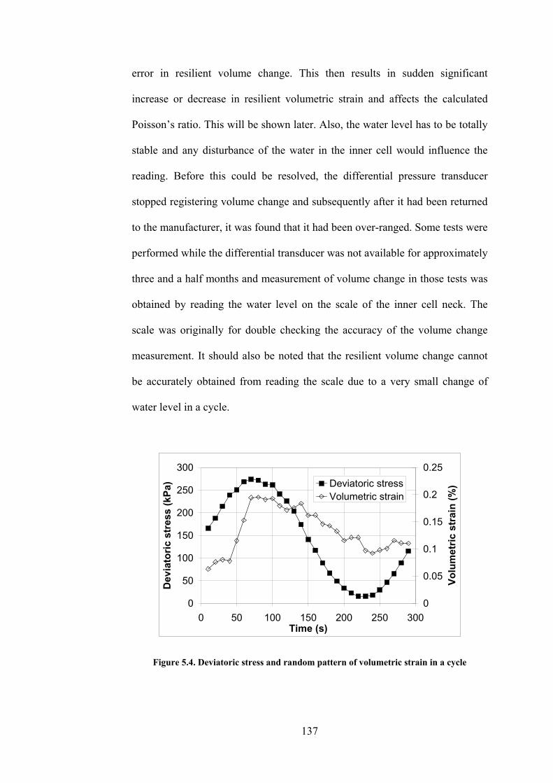
error in resilient volume change. This then results in sudden significant

increase or decrease in resilient volumetric strain and affects the calculated

Poisson�s ratio. This will be shown later. Also, the water level has to be totally

stable and any disturbance of the water in the inner cell would influence the

reading. Before this could be resolved, the differential pressure transducer

stopped registering volume change and subsequently after it had been returned

to the manufacturer, it was found that it had been over-ranged. Some tests were

performed while the differential transducer was not available for approximately

three and a half months and measurement of volume change in those tests was

obtained by reading the water level on the scale of the inner cell neck. The

scale was originally for double checking the accuracy of the volume change

measurement. It should also be noted that the resilient volume change cannot

be accurately obtained from reading the scale due to a very small change of

water level in a cycle.

0

50

100

150

200

250

300

0 50 100 150 200 250 300Time (s)

Dev

iato

ric

str

ess

(kP

a)

0

0.05

0.1

0.15

0.2

0.25

Vo

lum

etr

ic s

train

(%

)Deviatoric stress

Volumetric strain

Figure 5.4. Deviatoric stress and random pattern of volumetric strain in a cycle

137

After the differential pressure transducer was repaired, it was calibrated and

found to be usable again. Up to this point tests had been carried out on granite

A without further membrane failures. Tests were then started using limestone

ballast. However, the differential pressure transducer did not register the

change in volume again. Therefore, another calibration was then performed and

it was found that it registered the volume change but its sensitivity had to be

doubled from the previous value to give the correct volume change reading. It

was then found that the new sensitivity did not stay constant so it was sent back

to the manufacturer for the second time. While it was away for repair for

approximately two months, two alternative methods of volume change

measurement were tried. These are an image analysis and ultrasonic level

measurement.

5.4.2. Image analysis

A test was performed without both the inner and outer cells and was held by a

partial vacuum instead of the cell pressure. A digital camera with image

resolution of 7.1 megapixels was used to remotely take pictures of the sample

during a test. However, White et al. (2003) reported that image resolution of 2

megapixels was adequate for this type of analysis. The camera was connected

to a power supply as the test would last for approximately ten hours and the

camera battery has insufficient power for this purpose. The picture of the

sample is shown in Figure 5.5.

138

Figure 5.5. Test sample for the test with image analysis

The pictures were taken at the beginning of the test and at maximum and

minimum load of cycles 1 � 25, 100, 200, 500, 1000, 2000, 5000, 10000,

20000, 50000, and 100000. They were then analysed by a program called

�GeoPIV� run under MATLAB to obtain the sample movement from the test

(White and Take, 2002 and White et al., 2003). This program is usually used in

geotechnical experiments to track the movement of a fine grain soil over a

series of images. The membrane must be spray-painted so that it has a suitable

texture for the program to track the movement. Three columns of square

meshes were placed on the vertical edges of the sample shown in Figure 5.6.

The program searches around each mesh to detect the movement and, hence,

obtain the displacement. The search area around each mesh is called a search

zone. The sizes of a mesh and search zone are measured in pixels. As an

example, the sizes of mesh and search zone used in the first test (25 and 50

pixels) are shown in Figure 5.7. The movement of the meshes was detected

from each picture and then converted to axial and radial strains. The vertical

139

displacement of the sample was obtained by detecting the vertical movement of

the bottom meshes i.e., the meshes in the bottom row shown in Figure 5.6

relative to the top meshes which were placed near the stationary top platen. The

horizontal displacement was obtained by comparing the average horizontal

distance between the left and right meshes to the original distance. The pictures

of the meshes on the sample at the end of the test are shown in Figure 5.8.

Figure 5.6. Meshes on the sample at the beginning of the test

Figure 5.7. 25-pixel mesh with search zone of 50 pixels

140

Figure 5.8. Meshes on the sample at the end of the test

It can be seen from the figure that the meshes are scattered at the end of the

test. A few of them are even outside the sample. That was probably because the

load was increased from the seating load (1 kN) to the mean load (4.25 kN) in

one minute. During this short period, not enough number of images was taken

for the program to correctly detect the sample movement. Also, this loading

rate was probably too quick for the strength of the sample. As a result, the

sample was overly compressed i.e., axial strain increased to 12 % in one

minute during this stage.

The plot of axial and radial strains against number of cycles from the test is

shown in Figure 5.9. There was no physical measurement of the radial strain on

the test. It can be seen from the figure that the axial strain from the image

analysis was significantly different to the strain from the physical

measurement. However, the slopes of both lines are the same. Therefore, the

difference may be from the fast load build up at the start of the test again.

141

Furthermore, the permanent radial strain was expected to be negative rather

than positive because the sample bulged.

For the second test, radial measurement using two LVDTs was tried by

attaching them to rigid rods screwed into the base. Discs were fitted to the end

of the spring loaded LVDT shafts so that they would rest against the membrane

covered ballast at mid height of the specimen. However, this system of

measurement could not accommodate the vertical movement of the sample

during loading and the discs tilted and even became detached. Consequently, it

was very difficult to obtain a direct measurement of the radial strain so the

validation of the image analysis was limited to axial strain measurement from

the actuator LVDT. Figure 5.10 shows the axial strain results from this test. As

the load was built up too quickly in the previous test, this time it was built up

from the seating load (1 kN) to the mean load (6.88 kN) at approximately 0.5

kN per minute. According to the figure, the discrepancy between the

permanent axial strain from the image analysis and physical measurement was

smaller than the previous test. Therefore, the reduction in loading rate

improved the performance of the measurement technique. Furthermore, this

loading rate prevented the sample from being overly compressed.

142

0.0

2.0

4.0

6.0

8.0

10.0

12.0

14.0

0 20,000 40,000 60,000 80,000 100,000Number of cycles

Perm

an

en

t a

xia

l s

train

(%

)

Image analysis

Physical measurement

Figure 5.9(a). Permanent axial strain from the first test with image analysis

-0.1

0.0

0.1

0.2

0.3

0.4

0 20,000 40,000 60,000 80,000 100,000

Number of cycles

Resil

ien

t axia

l str

ain

(%

)

Image analysis

Physical measurement

Figure 5.9(b). Resilient axial strain from the first test with image analysis

-1.5

-1.0

-0.5

0.0

0.5

1.0

1.5

2.0

2.5

0 20,000 40,000 60,000 80,000 100,000

Number of cycles

Ra

dia

l s

train

(%

)

Permanent Resilient

Figure 5.9(c). Permanent and resilient radial strains from the first test with image analysis

Figure 5.9. Strain results from the first triaxial test with image analysis (a) � (c)

143

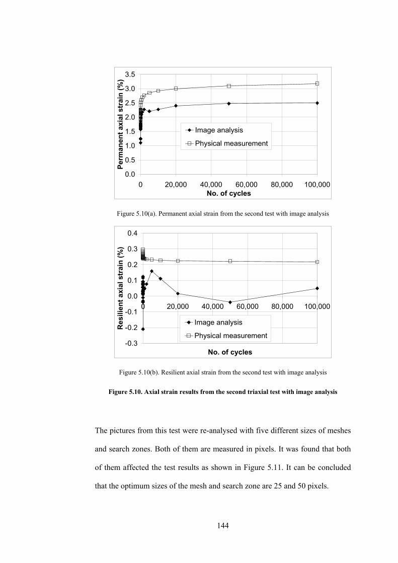
0.0

0.5

1.0

1.5

2.0

2.5

3.0

3.5

0 20,000 40,000 60,000 80,000 100,000

No. of cycles

Perm

an

en

t ax

ial

str

ain

(%

)

Image analysis

Physical measurement

Figure 5.10(a). Permanent axial strain from the second test with image analysis

-0.3

-0.2

-0.1

0.0

0.1

0.2

0.3

0.4

0 20,000 40,000 60,000 80,000 100,000

No. of cycles

Re

sil

ien

t ax

ial str

ain

(%

)

Image analysis

Physical measurement

Figure 5.10(b). Resilient axial strain from the second test with image analysis

Figure 5.10. Axial strain results from the second triaxial test with image analysis

The pictures from this test were re-analysed with five different sizes of meshes

and search zones. Both of them are measured in pixels. It was found that both

of them affected the test results as shown in Figure 5.11. It can be concluded

that the optimum sizes of the mesh and search zone are 25 and 50 pixels.

144

-1.0

-0.5

0.0

0.5

1.0

1.5

2.0

2.5

Ax

ial

str

ain

(%

)

Physicalmeasurement

10-pixel mesh

25-pixel mesh

50-pixel mesh

75-pixel mesh

100-pixel mesh

Seating

load

Max

load -

cycle 1

Min

load -

cycle 1

Max

load -

cycle 2

Min

load -

cycle 2

Tests

performed

with 50-pixel

search zone

Figure 5.11(a). Effect of mesh size on axial strain

0.0

0.5

1.0

1.5

2.0

2.5

Ax

ial s

tra

in (

%)

Physicalmeasurement

25-pixel searchzone

50-pixel searchzone

75-pixel searchzone

100-pixel searchzone

200-pixel searchzone

Seating

load

Max

load -

cycle 1

Min

load -

cycle 1

Max

load -

cycle 2

Min

load -

cycle 2

Tests

performed

with 50-pixel

mesh

Figure 5.11(b). Effect of search zone on axial strain

Figure 5.11. Effect of mesh size and search zone on axial strain from image analysis

The third test with the image analysis was performed with two cameras and

three LVDTs around the sample as shown in Figure 5.12. While the load was

built up from the seating load (1 kN) to the mean load (6.88 kN), pictures of

the sample were taken as many times as possible. These pictures would then be

included in the analysis to help the program to cope with the large movement

of meshes. Even though the discs were fixed to the LVDT shafts in this test to

prevent tilting and detachment of the discs, it was still difficult to obtain the

145

measurement from the LVDTs and the LVDT setup did not stay rigid enough

to accommodate the sample movement. Furthermore, it was found later that the

sample rotated during the test. The rotation of the sample will have an adverse

effect on the calculation of radial strain on the image analysis as the meshes

will move horizontally by rotation instead of expansion and some meshes

might move outside the sample. This might be due to the rotation of the bottom

loading ram or because the screw between the ram and platen became loose or

because of a combination of both. As a result, the radial strain measurements

from both the cameras and the LVDTs were invalid. The axial strain results

from this test are shown in Figure 5.13. It can be seen that permanent axial

strain from the image analysis is very similar to the physical measurement

while the same level of discrepancy of the resilient axial strain can still be seen.

Back Camera

LVDT BLVDT A

LVDT C

Front Camera

Figure 5.12. Arrangement of the cameras and LVDTs in the third test with image

analysis

146

0.0

0.2

0.4

0.6

0.8

1.0

1.2

1.4

0 20,000 40,000 60,000 80,000 100,000No. of cycle

Perm

an

en

t axia

l str

ain

(%

)Image analysis (average from both cameras)

Physical measurement

Figure 5.13(a). Permanent axial strain from the third test with image analysis

0.0

0.1

0.1

0.2

0.2

0.3

0 20,000 40,000 60,000 80,000 100,000No. of cycle

Re

sil

ien

t ax

ial

str

ain

(%

)

Image analysis (average from both cameras)

Physical measurement

Figure 5.13(b). Resilient axial strain from the third test with image analysis

Figure 5.13. Axial strain results from the third triaxial test with image analysis

Later, it was realised that the calculation of the radial strain from the image

analysis was not correct as the horizontal movement of the meshes in the

pictures is not exactly equal to the movement along the diameter of the sample

as shown in Figure 5.14. A new idea of measuring radial strain was initiated.

Different points on a sample can be marked by stickers. The horizontal

movement of each point from a camera can then be detected. However, if a

147

point moves toward the camera, the component of horizontal movement

directly towards the camera cannot be detected. This can be solved by placing

another camera at a different angle. Therefore, at least two cameras are needed

in the test to ensure that all directional components of the horizontal movement

of each point are obtained. However, the radial strains obtained from this

method are from discrete points and the rotation of the sample is still a problem

with this approach. Before the alternative method for measuring radial strain

with the image analysis was tried, another test method was explored and found

to be more promising and to have a simpler principle than the image analysis.

Therefore, the test method was changed.

Figure 5.14. Horizontal movement of the meshes in the image analysis

5.4.3. Ultrasonic level measurement

The second method used an ultrasonic proximity transducer (UPT) shown in

Figure 5.15. This type of transducer uses ultrasonics, i.e. sound wave above the

148

audible limit, to measure the distance from a transmitter to a surface. It

measures the time lag between the transmitted sound waves and the return

sound waves and converts this to voltage. It is ideally suited to provide a non

contact switching device or an analogue device to measure fluid level. The

model used had a range of 30 to 250 mm and was calibrated by positioning it

over a beaker of water and raising the beaker in increments which was

measured by a dial gauge. The output was found to be linear with a sensitivity

of 0.045 V/mm and a resolution of 0.5 mm.

140 mm long

Wave transmitter

located at the tip

of the transducer

Figure 5.15. Ultrasonic proximity transducer (UPT)

Initially, the UPT was fitted to the top of the water level in the reference tube.

Normally, this cylinder is locked off with a valve so that the differential

pressure transducer can measure the change in head of the water in the neck of

the inner cell relative to the fixed head in the reference tube. However, without

using the differential pressure transducer it was possible to keep the valve open

so that the water level in the reference tube would follow the water level in the

inner cell. The volume change measurement accuracy of the UPT was done

149

with the triaxial cell assembled without a sample in place. The inner cell was

filled with water and the connection made to the reference tube to equalise its

water level with the inner cell. The actuator was raised to a fixed amount and

this displaced a known volume of water in the inner cell. Confirmation of this

volume change was checked with a scale attached to the neck of the inner cell.

It was found that the UPT measured this volume change accurately but there

was a time delay before the water level in the reference tube equalised with the

level in the neck of the inner cell. This lag would be a problem for dynamic

volume change measurement and it was clear that a direct measurement of the

change in water level in the neck was necessary.

The only way of fitting the UPT above the neck of the inner cell without a

significant modification to the cell top was to carry out a test with the cell top

(outer cell) removed. It was clamped to a shaft supporting the load cell so that

it could look directly down to the water in the inner cell. This was done

initially without a sample and the UPT worked satisfactorily when calibrated

by raising the actuator to simulate a known volume change.

A test was then carried out with a sample under vacuum in the inner cell as the

external pressure could not be applied with the outer cell removed. This system

appeared to be working well for the low frequency up to 1 cycle per minute.

However, at 4 Hz the upper shaft supporting the load cell could be seen to be

moving laterally, because the top platen was tilted due to uneven settlement of

the ballast. This would not happen when the cell top is in place as it acts as a

support for the upper shaft and keeps the top platen level. The test was stopped

150

at this stage and only limited results from the UPT were obtained. However,

the differential pressure transducer had now been returned from the

manufacturer and was used in the remaining part of this test and the later tests.

After that, the differential pressure transducer was used in the later tests.

However, its sensitivity did not stay constant again even though the

manufacturer said that it was working fine. As testing needed to continue, it

was calibrated before and after every test by pushing the bottom ram upwards

to displace a known volume to the water in the inner cell. The volume change

reading from the differential pressure transducer was then plotted against the

known volume change to obtain the conversion factor. The average conversion

factor for the calibrations before and after each test was used to convert the

reading to the real volume change. It was found that the factor varies between

different tests but the factors obtained before and after each test were equal.

The use of the image analysis technique and the UPT to measure volume

change were not readily adaptable because the triaxial cell arrangement had

been designed to work with the differential pressure transducer as described in

section 5.2. It was essential that testing should continue preferably with the

outer cell fitted as maintaining a vacuum on a sample continually puts an

unacceptable demand on a vacuum pump if a robust vacuum system is not

available.

151

5.5. Test Procedures

Both monotonic and cyclic triaxial tests were performed in the project. After

both types of tests, the sample was sieved to obtain the particle size

distribution. For the monotonic tests, the sample was put under a seating load

of 1 kN at the beginning. The sample was then loaded at 1 mm/min until the

axial strain reached approximately 12 %. This was to prevent the sample from

touching the inner cell according to an observation in the first monotonic test.

Cyclic tests on granite A and limestone were performed by slightly different

methods. For cyclic tests on granite A, the sample was put under a seating load

of 1 kN. The load was brought to the mean load and cyclic loading was started

with the frequency of 0.2 Hz for the first 99 cycles. The rest of the test would

be loaded with a frequency of 4 Hz until cycle 100,000. However, cycles 100,

200, 500, 1000, 2000, 5000, 10000, 20000, 50000, and 100000 were loaded

with a duration of 5 minutes per cycle. This was to obtain the resilient sample

volume change in the test. It should be noted that before and after these slow

cycles, the test was paused for 10 minutes to wait for the water level in the

inner cell to stabilise as unstable water in the inner cell would cause errors in

the volume change reading. During the pauses, the load was dropped to the

seating load of 1 kN.

For cyclic tests on limestone, the sample was also put under the seating load of

1 kN. However, the load was slowly built to the mean load with the rate of

approximately 0.5 kN per minute to avoid the sample being overly compressed.

Furthermore, cycles 1 to 5 and 6 to 30 were loaded with a duration of 5

152

minutes per cycle and 1 minute per cycle, respectively. After that, most parts of

the test were performed with the frequency of 4 Hz until cycle 100,000.

However, cycles 31-100, 181-200, 481-500, 981-1000, 1981-2000, 4981-5000,

9984-10000, 19981-20000, 49981-50000, and 99981-100000 were loaded at

0.2 Hz to obtain the resilient sample volume change.

The speed (or frequency) of the slow cycles for obtaining the sample volume

change was changed from 5 minutes/cycle to 0.2 Hz because the electrical drift

of the differential pressure transducer may distort the sample volume change

over an individual cycle in some cyclic tests on granite A as shown in Section

5.4.1. Therefore, having a group of slow cycles is more accurate than having an

individual cycle as the volume change measurement response can stabilise.

5.6. Test Programme

The triaxial tests in this project were divided into three test series and are

summarised in Table 5.1 and the q-p� stress paths of cyclic tests are shown in

Figure 5.16. As a sample is loaded until axial strain reaches approximately 12

% in monotonic test (Series 2), the maximum deviatoric stress is unknown

before the test. Hence, the q-p� stress path from this series cannot be plotted. It

should be noted that the name of each test includes the test series, cell pressure,

and q/p�max (for only Series 1 and 3). There are special terms in some tests in

Series 3: (I) and (UPT). These indicate that image analysis and ultrasonic

proximity transducer were used to measure volume change, respectively.

153

Series 1 was to observe the repeatability of the cyclic triaxial test. The tests in

this series were performed only on granite A as it was the only available

material at that time. According to the visual observation, breakage from the

tests in Series 1 is minimal probably due to the material properties of granite A.

As the main theme of the project is ballast degradation, a larger amount of

ballast breakage was needed. Therefore, the material was changed to limestone

due to its larger values of LAA and MDA compared to those of granite A.

The tests in Series 2 were monotonic triaxial tests on limestone ballast. It

should be noted that all tests in Series 2 were performed without the

differential pressure transducer as it was sent for repair. Furthermore, the

image analysis and the UPT had not been developed for testing at that time. As

a result, the sample volume change was obtained from reading the water level

on the scale of the inner cell neck.

The first test of Series 2 was performed without the inner cell. This was to

check if the sample was going to touch the inner cell due to its radial

expansion. As a result, sample volume change cannot be obtained. In this test,

air was used as the confining medium as water would distort the visual

observation of the radial expansion. The cell pressure of 10 kPa was chosen to

obtain a large radial expansion. It was found that the sample can be loaded to

12 % axial strain without touching the inner cell. After this test, three more

monotonic tests with cell pressures of 10, 30, and 60 kPa were performed.

154

Different cyclic triaxial tests were performed on limestone in Series 3. Three

tests in this series were performed with image analysis. One test in this series

was performed with the UPT. However, the transducer was used until cycle

2,000 as it was found that the upper shaft supporting the load cell was moving

laterally as it was not supported by the cell top bearing. At that time, the

differential pressure transducer had just come back from repair. It was

therefore used to measure the sample volume change in the later part of the test

and the other tests in this series.

155

Test series No.

of

test

Test number Cell

pressure

(kPa)

Maximum

deviatoric

stress

(kPa)

q/p�max Volume

change

measure

-ment

method

Density

(kg/m3)

S1-90/1.5a 90 270 1.5 DPT* 1,506

S1-90/1.5b 90 270 1.5 DPT* 1,579

S1-90/1.5c 90 270 1.5 DPT* 1,554

S1-90/1.5d 90 270 1.5 DPT* 1,509

S1-90/1.5e 90 270 1.5 DPT* 1,515

S1-90/1.5f 90 270 1.5 Scale** 1,515

S1-90/1.5g 90 270 1.5 Scale** 1,515

1

(Cyclic test

on granite

A)

8

S1-90/1.5h 90 270 1.5 Scale** 1,515

S2-10a 10 N/A N/A None 1,551

S2-10b 10 N/A N/A Scale** 1,511

S2-30 30 N/A N/A Scale** 1,539

2

(Monotonic

test on

limestone)

4

S2-60 60 N/A N/A Scale** 1,545

S3-30/1.7(I) 30 117.7 1.7 Image

analysis

1,517

S3-

30/2.0a(I)

30 180 2.0 Image

analysis

1,549

S3-

60/1.5a(I)

60 180 1.5 Image

analysis

1,553

S3-30/2.0b

(UPT)

30 180 2.0 UPT

and

DPT***

1,559

S3-60/1.5b 60 180 1.5 DPT* 1,600

S3-60/2.0a 60 360 2.0 DPT* 1,575

S3-10/2.0 10 60 2.0 DPT* 1,539

3

(Cyclic test

on

limestone)

8

S3-60/2.0b 60 360 2.0 DPT* 1,592

* Volume change is measured by the differential pressure transducer.

** Volume change is measured by reading water level on scale of the inner cell neck.

*** The volume change during the first 2,000 cycles was measured by the ultrasonic

proximity transducer. After that, the differential pressure transducer was used instead due to

the problem mentioned in Section 5.4.3.

Table 5.1. List of triaxial tests performed in this project

156

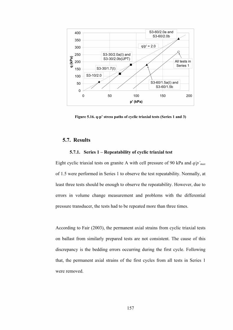
0

50

100

150

200

250

300

350

400

0 50 100 150 200

p' (kPa)

q (

kP

a)

q/p' = 2.0

S3-60/1.5a(I) and

S3-60/1.5b

S3-60/2.0a and

S3-60/2.0b

S3-30/2.0a(I) and

S3-30/2.0b(UPT)

S3-10/2.0

S3-30/1.7(I)

All tests in

Series 1

Figure 5.16. q-p� stress paths of cyclic triaxial tests (Series 1 and 3)

5.7. Results

5.7.1. Series 1 � Repeatability of cyclic triaxial test

Eight cyclic triaxial tests on granite A with cell pressure of 90 kPa and q/p�max

of 1.5 were performed in Series 1 to observe the test repeatability. Normally, at

least three tests should be enough to observe the repeatability. However, due to

errors in volume change measurement and problems with the differential

pressure transducer, the tests had to be repeated more than three times.

According to Fair (2003), the permanent axial strains from cyclic triaxial tests

on ballast from similarly prepared tests are not consistent. The cause of this

discrepancy is the bedding errors occurring during the first cycle. Following

that, the permanent axial strains of the first cycles from all tests in Series 1

were removed.

157

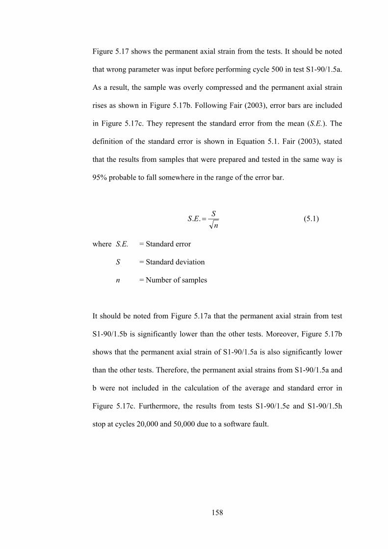
Figure 5.17 shows the permanent axial strain from the tests. It should be noted

that wrong parameter was input before performing cycle 500 in test S1-90/1.5a.

As a result, the sample was overly compressed and the permanent axial strain

rises as shown in Figure 5.17b. Following Fair (2003), error bars are included

in Figure 5.17c. They represent the standard error from the mean (S.E.). The

definition of the standard error is shown in Equation 5.1. Fair (2003), stated

that the results from samples that were prepared and tested in the same way is

95% probable to fall somewhere in the range of the error bar.

n

SES =.. (5.1)

where S.E. = Standard error

S = Standard deviation

n = Number of samples

It should be noted from Figure 5.17a that the permanent axial strain from test

S1-90/1.5b is significantly lower than the other tests. Moreover, Figure 5.17b

shows that the permanent axial strain of S1-90/1.5a is also significantly lower

than the other tests. Therefore, the permanent axial strains from S1-90/1.5a and

b were not included in the calculation of the average and standard error in

Figure 5.17c. Furthermore, the results from tests S1-90/1.5e and S1-90/1.5h

stop at cycles 20,000 and 50,000 due to a software fault.

158

0.0

0.5

1.0

1.5

2.0

2.5

0 20,000 40,000 60,000 80,000 100,000

No. of cycles

Perm

an

en

t axia

l s

tra

in (

%)

S1-90/1.5a

S1-90/1.5b

S1-90/1.5c

S1-90/1.5d

S1-90/1.5e

S1-90/1.5f

S1-90/1.5g

S1-90/1.5h

S1-90/1.5e and h stopped at cycles 20,000

and 50,000 due to a software fault.

Figure 5.17(a). Permanent axial strain in Series 1

0.0

0.5

1.0

1.5

2.0

2.5

0 200 400 600 800 1,000

No. of cycles

Perm

an

en

t a

xia

l str

ain

(%

)

S1-90/1.5a

S1-90/1.5b

S1-90/1.5c

S1-90/1.5d

S1-90/1.5e

S1-90/1.5f

S1-90/1.5g

S1-90/1.5hWrong input parameter in

S1-90/1.5a

Figure 5.17(b). Permanent axial strain in Series 1 (up to cycle 1,000)

0.0

0.2

0.4

0.6

0.8

1.0

1.2

1.4

1.6

1.8

0 20,000 40,000 60,000 80,000 100,000

No. of cycles

Ave

rag

e p

erm

en

en

t ax

ial

str

ain

(%

)

� S1-90/1.5a and b are not included in the calculation of

average permanet axial strain and error bar due to their

strain anomaly.

� Permanent axial strains of S2-90/1.5e and h after cycles

20,000 and 50,000 are not included in the calculation as

the tests stopped due to a software fault.

Figure 5.17(c). Average permanent axial strain in Series 1 with error bars

Figure 5.17. Permanent axial strain in Series 1

159

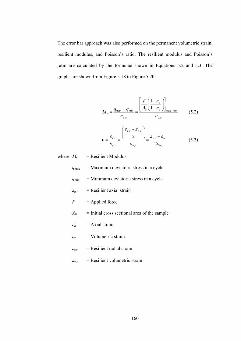
The error bar approach was also performed on the permanent volumetric strain,

resilient modulus, and Poisson�s ratio. The resilient modulus and Poisson�s

ratio are calculated by the formulae shown in Equations 5.2 and 5.3. The

graphs are shown from Figure 5.18 to Figure 5.20.

ra

v

a

ra

r

A

F

qqM

,

minmax0

,

minmax1

1

ε

εε

ε−

⎥⎦

⎤⎢⎣

⎡⎟⎟⎠

⎞⎜⎜⎝

⎛−−

=−

= (5.2)

ra

rarv

ra

rarv

ra

rr

,

,,

,

,,

,

,

2

2

εεε

ε

εε

εε

ν−

=⎟⎟⎠

⎞⎜⎜⎝

⎛ −

== (5.3)

where Mr = Resilient Modulus

qmax = Maximum deviatoric stress in a cycle

qmin = Minimum deviatoric stress in a cycle

εa,r = Resilient axial strain

F = Applied force

A0 = Initial cross sectional area of the sample

εa = Axial strain

εv = Volumetric strain

εr,r = Resilient radial strain

εv,r = Resilient volumetric strain

160

0.0

0.2

0.4

0.6

0.8

1.0

1.2

1.4

1.6

1.8

0 20,000 40,000 60,000 80,000 100,000

No. of cycles

Pe

rma

nen

t v

olu

me

tric

str

ain

(%

)

S1-90/1.5a

S1-90/1.5d

S1-90/1.5e

S1-90/1.5f

S1-90/1.5g

Volumetric strain from tests S1-90/1.5f

and g was obtained from reading the

scale of the inner cell neck.Compression

Figure 5.18(a). Permanent volumetric strain in Series 1

0.0

0.2

0.4

0.6

0.8

1.0

1.2

1.4

1.6

1.8

0 20,000 40,000 60,000 80,000 100,000

No. of cycles

Av

era

ge p

erm

an

en

t

vo

lum

etr

ic s

train

(%

)

Compression

Figure 5.18(b). Average permanent volumetric strain in Series 1 with error bars

Figure 5.18. Permanent volumetric strain in Series 1

161

0

20

40

60

80

100

120

140

0 20,000 40,000 60,000 80,000 100,000

No. of cycles

Res

ilie

nt

mo

du

lus (

MP

a)

S1-90/1.5a

S1-90/1.5d

S1-90/1.5e

Figure 5.19(a). Resilient modulus in Series 1

0

20

40

60

80

100

120

140

0 20,000 40,000 60,000 80,000 100,000

No. of cycles

Av

era

ge r

esilie

nt

mo

du

lus (

MP

a)

Error bars at cycles 50,000 and

100,000 cannot be shown as there is

only one data point at cycles 500,000

and 100,000 (from S1-90/1.5d).

Figure 5.19(b). Average resilient modulus in Series 1 with error bars

Figure 5.19. Resilient modulus in Series 1

162

0.0

0.1

0.2

0.3

0.4

0.5

0.6

0 20,000 40,000 60,000 80,000 100,000

No. of cycles

Po

isso

n's

ra

tio

S1-90/1.5a

S1-90/1.5d

S1-90/1.5e

Figure 5.20(a). Poisson�s ratio in Series 1

0.00

0.05

0.10

0.15

0.20

0.25

0.30

0.35

0.40

0.45

0.50

0 20,000 40,000 60,000 80,000 100,000

No. of cycles

Av

era

ge P

ois

so

n's

rati

o

Error bars at cycles 50,000 and

100,000 cannot be shown as there is

only one data point at cycles 500,000

and 100,000 (from S1-90/1.5d).

Figure 5.20(b). Average Poisson�s ratio in Series 1 with error bars

Figure 5.20. Poisson�s ratio in Series 1

It should be noted from Figure 5.18 that

• The results from test S1-90/1.5a stop at cycle 10,000. This is because as

the sample contracted, water needed to be added into the inner cell

during the test to keep the water level in the measurable range of the

differential pressure transducer. In this test, cycles 10,001 to 19,999

were performed with frequency of 4 Hz which was too fast for the

163

differential pressure transducer to register the sample volume change.

After cycle 19,999, the water level was almost out of the measurable

range. Water was then added right away before reading the volume

change due to cycles 10,000 to 19,999. Therefore, the track of volume

change was lost and later volume change of the sample could not be

obtained.

• The results from tests S1-90/1.5b and c are not presented because the

sample volume changes in these tests did not follow the expected

sinusoidal response. An example was shown in Figure 5.4. As a result,

the volumetric strain could not be obtained from both tests. This

behaviour was found to occur randomly and did not happen in any other

tests in this Series.

• The results from test S1-90/1.5e stop at cycle 20,000 because the test

stopped itself due to a software fault.

• The volumetric strain could not be measured in test S1-90/1.5h because

the water in the inner cell dropped below the measurable range

somewhere between cycle 1 and 99. As a result, the track of volume

change was lost and the volume change could not be measured

afterwards.

It should be noted from Figure 5.19 (resilient modulus) and Figure 5.20

(Poisson�s ratio) that

• Only test results from S1-90/1.5a, d and e are presented in both figures.

This is because these three tests are the only tests that the resilient

volumetric strain could be measured.

164

• The big drop in Poisson�s ratio in test S1-90/1.5d was probably due to

the electrical drift from the differential pressure transducer as explained

in Section 5.4.1.

Figure 5.21 shows the particle size distribution after the tests. Similar to the

RTF results, no particles smaller than 22.4 mm were in each sample before the

test and only the particle size distribution of particles smaller than 22.4 mm is

shown in mass passing instead of percentage passing. As the initial mass of

each test is similar, the behaviour from Figure 5.21 is similar to a degradation

plot using percentage passing. Only the first four tests of Series 1 are presented

because after the first four tests, the degradation on the sample could not be

seen by visual observation and it was felt that the subsequent tests needed to be

performed as quickly as possible. As a result, the same material was used for

all subsequent tests (tests S1-90/1.5e to h) and was thrown away afterwards as

the degradation obtained after the test would be the accumulation from those

tests.

It can be seen from Figure 5.21 that the degradation from test S1-90/1.5b are

much larger than the others. Both permanent axial strain and degradation from

this test are significantly different from the other tests in this series. The cause

of this discrepancy is still unknown but the degradation from this test will also

be treated as an anomaly. Even though the sample in S1-90/1.5a was overly

compressed, the degradation is not significantly different from S1-90/1.5c and

d and it can be concluded that the degradation from the tests is also repeatable.

165

0

100

200

300

400

500

0 5 10 15 20 25

Size (mm)

Mas

s p

ass

ing

(g

)

S1-90/1.5a

S1-90/1.5b

S1-90/1.5c

S1-90/1.5d

Figure 5.21. Particles smaller than 22.4 mm from the tests in Series 1

5.7.2. Series 2 � Monotonic triaxial tests on limestone

Four monotonic tests on limestone ballast have been carried out in Series 2,

two with confining pressure of 10 kPa (S2-10a and S2-10b), one with

confining pressure of 30 kPa (S2-30), and the last one with confining pressure

of 60 kPa (S2-60). Initially, the confining stresses of 10, 30, and 90 kPa were

intended to be used in both monotonic and cyclic triaxial tests on limestone

(series 2 and 3) to cover a big range of confining stress. However, limestone

sample usually punctured the membrane when the confining stress was 90 kPa.

Therefore, the confining stresses were then changed to 10, 30, and 60 kPa.

It should be noted that test S2-10a was performed without the inner cell and

water to check if the sample was going to touch the inner cell when it bulged.

Therefore, the volumetric strain cannot be obtained from that test.

166

Figure 5.22 and Figure 5.23 show the plot of deviatoric stress against axial

strain and q-p� stress paths from the tests in Series 2. Test S2-10a is not

included in the figures because volumetric strain is required to calculate the

deviatoric stress according to Equation 5.2. It can be seen from Figure 5.22 that

the deviatoric stress eventually becomes stable but does not significantly drop.

This suggests that each sample reached its peak strength but not the ultimate

strength.

0

50

100

150

200

250

300

350

400

0 5 10 15

Axial strain (%)

Devia

tori

c s

tre

ss

(kP

a)

S2-10b (10 kPa)

S2-30 (30 kPa)

S2-60 (60 kPa)

Figure 5.22. Deviatoric stress vs axial strain from monotonic triaxial tests on limestone

(Series 2)

167

10 kPa

q/p' max = 2.29

30 kPa

q/p' max = 2.20

60 kPa

q/p' max = 2.04

0

50

100

150

200

250

300

350

400

0 50 100 150 200

p' (kPa)

q (

kP

a)

Figure 5.23. q-p� stress paths in Series 2

The stiffness of a test sample is defined by two parameters; the tangent

modulus at zero axial strain and secant modulus. Tangent modulus (Et) at zero

axial strain is the slope at the initial portion of the curve of deviatoric stress

against axial strain (i.e., Figure 5.22) and secant modulus is the slope of the

line joining the origin to any point of the curve. Both moduli are illustrated in

Figure 5.24. Secant modulus (Es) was calculated at deviatoric stresses of 60,

117.7, 180, and 360 kPa as these were the maximum deviatoric stresses in the

cyclic tests on limestone (Series 3). Table 5.2 summarises the moduli obtained

from the curves in Figure 5.22.

Figure 5.25 shows the plot between volumetric strain and axial strain. The

volumetric strain was obtained from reading the scale of the inner cell as the

differential pressure transducer was sent for repair at that time. It can be seen

from the figure that after a short period of volumetric compression, the sample

began to dilate. The test with 10 kPa has the largest dilation corresponding to

168

its largest q/p�max according to Figure 5.23. Also, Figure 5.26 shows the Mohr-

Coulomb curved envelope attributed to dilation for the tests in Series 2.

Axial strain

De

via

tori

c s

tre

ss

Tangent modulus at

zero axial strain (Et)

Secant modulus

(Es)

Figure 5.24. Definition of tangent modulus at zero axial strain (Et) and secant modulus

(Es)

Secant moduli at different deviatoric stress (MPa) Test Cell

pressure

(kPa)

Tangent

modulus at

zero axial

strain

(MPa)

At 60 kPa

deviatoric

stress

At 117.7

kPa

deviatoric

stress

At 180 kPa

deviatoric

stress

At 360 kPa

deviatoric

stress

S2-10b 10 16 2 N/A N/A N/A

S2-30 30 21 17 12 7 N/A

S2-60 60 45 45 35 19 5

Table 5.2. Tangent modulus at zero axial strain and secant moduli from Series 2

169

-7.0

-6.0

-5.0

-4.0

-3.0

-2.0

-1.0

0.0

1.0

0 2 4 6 8 10 12 14 16

Axial strain (%)

Vo

lum

etr

ic s

tra

in (

%)

S2-10b (10 kPa)

S2-30 (30 kPa)

S2-60 (60 kPa)

Compression

Dilation

Figure 5.25. Volumetric strain vs axial strain from Series 2

0

50

100

150

200

250

0 50 100 150 200 250 300 350 400 450

Normal effective stress (kPa)

Sh

ear

str

ess

(k

Pa

)

Figure 5.26. Mohr-Coulomb failure envelope of the limestone ballast for Series 2

Figure 5.27 shows the particle size distributions of the samples after the

monotonic tests. The particle size distribution of test S2-10a is also shown in

the figure as this result does not relate to the volume change measurement. It

can be seen from the figure that the breakage increases with increasing cell

pressure. This finding agrees with Key (2003) and Indraratna et al. (1998).

170

0

100

200

300

400

500

0 5 10 15 20 25

Size (mm)

Mas

s p

ass

ing

(g

)

S2-10a (10 kPa)

S2-10b (10 kPa)

S2-30 (30 kPa)

S2-60 (60 kPa)

Figure 5.27. Particles smaller than 22.4 mm from the tests in Series 2

5.7.3. Series 3 � Cyclic triaxial tests on limestone

Eight cyclic triaxial tests on limestone were carried out in Series 3. Similar to

Series 1, the first cycle permanent axial strains from all tests in Series 3 were

removed. For comparative purposes, the eight tests are grouped in different

ways in the figures namely, results from tests with cell pressure of 30 kPa, cell

pressure of 60 kPa, q/p�max of 2, and maximum deviatoric stress of 180 kPa. It

should be noted that there are no separate plots for the results from tests with a

cell pressure of 10 kPa in the figures as there was only one such test in Series

3. Furthermore, there are no separate plots for permanent volumetric strain,

resilient modulus, and Poisson�s ratio from tests with cell pressure of 30 kPa.

This is because these parameters are related to the volume change

measurement as mentioned earlier and there was only one test in Series 3 a

with cell pressure of 30 kPa that had a valid volume change measurement (S3-

30/2.0b(UPT)). The other tests with 30 kPa cell pressure (S3-30/1.7(I) and S3-

171

30/2.0(I)) were performed with image analysis which could not measure

volume change accurately.

It can be seen from Figure 5.28 (permanent axial strain against number of

cycles) that:

• It should be noted that the permanent axial strain results presented in

the image analysis section (Section 5.4.2) are from tests S3-30/1.7(I),

S3-30/2.0a(I), and S3-60/1.5a(I). However, the permanent axial strains

from those tests presented in Figure 5.9a, Figure 5.10a, and Figure

5.13a are different. This is because the first cycle permanent axial

strains were not removed from those results.

• For tests with the same cell pressure and stress ratio (e.g. S3-30/2.0a(I)

and S3-30/2.0b(UPT) or S3-60/1.5a(I) and S3-60/1.5b), there are some

discrepancies in permanent axial strain. However, the level of

discrepancy is the same as the permanent axial strains from the tests in

Series 1.

• With the same cell pressure, permanent axial strain increases with

q/p�max.

• With the same q/p�max, the sample contracts more with increasing cell

pressure.

• With the same maximum deviatoric stress, permanent axial strain

increases with increasing q/p�max.

172

0.0

0.5

1.0

1.5

2.0

2.5

0 20,000 40,000 60,000 80,000 100,000

No. of cycles

Perm

an

en

t axia

l str

ain

(%

)

S3-30/1.7(I)

S3-30/2.0(I)

S3-30/2.0b(UPT)

Figure 5.28(a). Permanent axial strains from tests with cell pressure of 30 kPa

0

1

2

3

4

5

6

7

0 20,000 40,000 60,000 80,000 100,000

No. of cycles

Perm

an

en

t ax

ial

str

ain

(%

)

S3-60/1.5a(I)

S3-60/1.5b

S3-60/2.0a

S3-60/2.0b

Figure 5.28(b). Permanent axial strains from tests with cell pressure of 60 kPa

0

1

2

3

4

5

6

7

0 20,000 40,000 60,000 80,000 100,000

No. of cycles

Perm

an

en

t ax

ial str

ain

(%

)

S3-10/2.0, qmax = 60 kPa

S3-30/2.0a(I), qmax = 180 kPa

S3-30/2.0b(UPT), qmax = 180 kPa

S3-60/2.0a, qmax = 360 kPa

S3-60/2.0b, qmax = 360 kPa

Figure 5.28(c). Permanent axial strains from tests with q/p�max of 2.0

173

0.0

0.5

1.0

1.5

2.0

2.5

0 20,000 40,000 60,000 80,000 100,000

No. of cycles

Perm

an

en

t ax

ial

str

ain

(%

)S3-30/2.0a(I)

S3-30/2.0b(UPT)

S3-60/1.5a(I)

S3-60/1.5b

Figure 5.28(d). Permanent axial strains from tests with max deviatoric stress of 180 kPa

Figure 5.28. Permanent axial strain from the tests in Series 3 (a) � (d)

It can be seen from Figure 5.29 (permanent volumetric strain against number of

cycles) that:

• The samples from S3-60/2.0a and b dilated at the beginning of the tests

(negative permanent volumetric strain). This might be because the

maximum deviatoric stress in these tests (360 kPa) was equal to the

maximum deviatoric stress in the monotonic test with 60 kPa (S2-60).

After the first few cycles, the samples started to contract.

• The permanent volumetric strain from S3-60/2.0a was found to dilate

again after 20,000 cycles. Theoretically, this is not possible. Therefore,

test S3-60/2.0b was performed to check if this behaviour was

repeatable. It was found that this behaviour was not seen in S3-60/2.0b.

Even though the behaviours of permanent volumetric strains of both

tests are different, the permanent axial strains are the same (Figure

5.29a).

174

• According to Figure 5.29a, the permanent volumetric strain seems to

increase with decreasing q/p�max under the same confining stress.

However, Suiker et al. (2005) found that with the same cell pressure,

there is no definite trend for permanent volumetric strain against

q/p�max.

• Only S3-10/2.0 shows dilative behaviour.

• With the same q/p�max, the permanent volumetric strain should increase

with increasing cell pressure. However, the strain from S3-60/2.0b is

less than S3-30/2.0b (Figure 5.29b). This is probably due to the dilation

at the beginning of S3-60/2.0b.

• With the same maximum deviatoric stress, the permanent volumetric

strain here seems to increase with decreasing cell pressure in Figure

5.29c. This contradicts with the findings of Indraratna et al. (2005) as

they found that the sample became more compressive with increasing

cell pressure. However, this is not generally true as Fair (2003) found

that there was no definite trend for permanent volumetric strain against

cell pressure with the same maximum deviatoric stress.

175

-0.6

-0.4

-0.2

0.0

0.2

0.4

0.6

0.8

1.0

1.2

1.4

0 20,000 40,000 60,000 80,000 100,000No. of cycles

Pe

rma

ne

nt

vo

lum

etr

ic s

tra

in (

%)

S3-60/1.5b

S3-60/2.0a

S3-60/2.0b

Figure 5.29(a). Permanent volumetric strains from tests with cell pressure of 60 kPa

-0.6

-0.4

-0.2

0.0

0.2

0.4

0.6

0.8

1.0

1.2

1.4

0 20,000 40,000 60,000 80,000 100,000

No. of cycles

Perm

an

en

t vo

lum

etr

ic s

train

(%

)

S3-10/2.0

S3-30/2.0b(UPT)

S3-60/2.0a

S3-60/2.0b

Figure 5.29(b). Permanent volumetric strains from tests with q/p�max of 2.0

-0.6

-0.4

-0.2

0.0

0.2

0.4

0.6

0.8

1.0

1.2

1.4

0 20,000 40,000 60,000 80,000 100,000

No. of cycles

Pe

rma

ne

nt

vo

lum

etr

ic s

tra

in (

%)

S3-30/2.0b(UPT)

S3-60/1.5b

Figure 5.29(c). Permanent volumetric strains from tests with max deviatoric stress of 180 kPa

Figure 5.29. Permanent volumetric strain from the tests in Series 3

176

Figure 5.30 shows the resilient modulus from the tests in Series 3. As the

resilient modulus was found to follow the K-θ model as stated in Section

2.6.1.1, the sum of principle stresses (θ) for each test is also indicated in the

plot. Also, the final resilient modulus is plotted against the sum of principal

stress together with the K-θ model in Figure 5.31. According to the figure, both

empirical constants k1 and k2 are 9.2 and 0.5.

Figure 5.32 shows the plots between Poisson�s ratio and the number of cycles.

It can be seen that the Poisson�s ratio increases with increasing maximum

deviatoric stress (Figure 5.32a) and decreasing cell pressure (Figure 5.32b).

This matches the findings from many researchers in the review of Lekarp et al.

(2000a). However, the definite trend of Poisson�s ratio cannot be found from

the tests with q/p�max of 2.0 (Figure 5.32c). The drift from S3-60/2.0b was

probably due to the electrical drift from the differential pressure transducer

again.

0

50

100

150

200

250

300

0 20,000 40,000 60,000 80,000 100,000

No. of cycles

Resilie

nt

mo

du

lus (

MP

a)

S3-10/2.0, ș = 90kPa

S3-30/2.0b(UPT),ș = 270 kPa

S3-60/1.5b, ș =360 kPa

S3-60/2.0a, ș =540 kPa

S3-60/2.0b, ș =540 kPa

Figure 5.30. Resilient modulus from the tests in Series 3

177

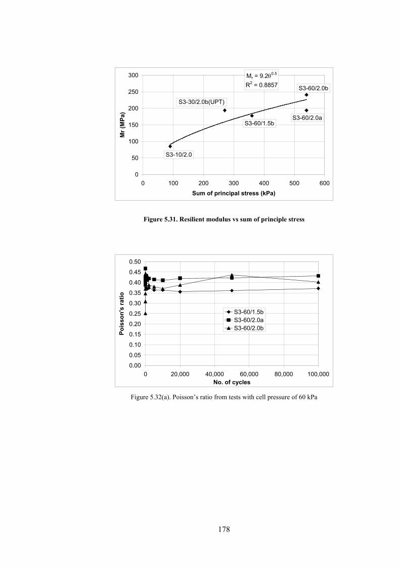
Mr = 9.2θ0.5

R2 = 0.8857

0

50

100

150

200

250

300

0 100 200 300 400 500 600

Sum of principal stress (kPa)

Mr

(MP

a)

S3-10/2.0

S3-30/2.0b(UPT)

S3-60/1.5bS3-60/2.0a

S3-60/2.0b

Figure 5.31. Resilient modulus vs sum of principle stress

0.00

0.05

0.10

0.15

0.20

0.25

0.30

0.35

0.40

0.45

0.50

0 20,000 40,000 60,000 80,000 100,000

No. of cycles

Po

iss

on

's r

ati

o

S3-60/1.5b

S3-60/2.0a

S3-60/2.0b

Figure 5.32(a). Poisson�s ratio from tests with cell pressure of 60 kPa

178

0.00

0.05

0.10

0.15

0.20

0.25

0.30

0.35

0.40

0.45

0.50

0 20,000 40,000 60,000 80,000 100,000

No. of cycles

Po

isso

n's

rati

o

S3-30/2.0b(UPT)

S3-60/1.5b

Figure 5.32(b). Poisson�s ratio from tests with max deviatoric stress of 180 kPa

0.00

0.05

0.10

0.15

0.20

0.25

0.30

0.35

0.40

0.45

0.50

0 20,000 40,000 60,000 80,000 100,000

No. of cycles

Po

iss

on

's r

ati

o

S3-10/2.0

S3-30/2.0b(UPT)

S3-60/2.0a

S3-60/2.0b

Figure 5.32(c). Poisson�s ratio from tests with q/p�max of 2.0

Figure 5.32. Poisson�s ratio in Series 3

Figure 5.33 shows the particle size distribution after the tests in Series 3. It can

be seen that with the same confining stress, breakage increases with increasing

maximum deviatoric stress (Figure 5.33a and b). However, breakage from S3-

30/1.7(I) is probably larger than it should have been (Figure 5.33a). This is

because the sample was overly compressed due to the fast loading rate as stated

in Section 5.4.2 (the first test with the image analysis).

179

It can be seen from Figure 5.33c that the breakage levels from all tests with

maximum deviatoric stress of 180 kPa are not significantly different regardless

of the confining pressure. This matches the findings of Indraratna et al. (2005).

According to their triaxial tests on ballast, minimal breakage occurred when the

confining pressure is between 30 and 75 kPa as shown in Figure 5.34. They

defined this region as the optimum degradation zone or ODZ. It should be

noted that the ballast breakage index in the figure indicates the breakage level

based on calculation of area under the particle size distribution before and after

each test as shown in Figure 5.35. It also can be seen from the Figure 5.34 that

the breakage levels at different confining pressure in ODZ (zone II in the

figure) are not significantly different.

The reason proposed by Indraratna et al. (2005) for the minimal breakage in the

ODZ is that ballast particles are held together with sufficient confinement to

provide optimum coordination number i.e., average number of contacts with

neighbouring particles. Large breakage occurs when confining pressure is

below 30 kPa due to dilative behaviour of the sample under small average

coordination number. Moreover, breakage level increases when the confining

pressure is above 75 kPa because of the increase in confining stress and

because the coordination number has reached it maximum level.

According to Figure 5.33d, the breakage from tests with 60 kPa confining

stress (S3-60/2.0a and S3-60/2.0b) is larger than the one with 30 kPa (S3-

30/2.0a(I) and S3-30/2.0b(UPT)) due to large deviatoric stress in the tests with

60 kPa. Furthermore, the breakage from S3-10/2.0 is approximately equal to

180

S3-30/2.0a(I) even though the maximum deviatoric stress in S3-10/2.0 is much

lower. This is because with dilative behaviour from test S3-10/2.0, the resulting

breakage is large and comparable to the breakage from a test with higher

deviatoric stress but in the optimum degradation zone.

0

50

100

150

200

250

300

350

400

450

0 5 10 15 20 25

Size (mm)

Ma

ss

pa

ss

ing

(g

)

S3-30/1.7(I), qmax = 118 kPa

S3-30/2.0a(I), qmax = 180 kPa

S3-30/2.0b(UPT), qmax = 180 kPa

Figure 5.33(a). Particles smaller than 22.4 mm from tests with cell pressure of 30 kPa

0

50

100

150

200

250

300

350

400

450

0 5 10 15 20 25

Size (mm)

Mass

pa

ssin

g (

g)

S3-60/1.5a(I), qmax = 180 kPa

S3-60/1.5b, qmax = 180 kPa

S3-60/2.0a, qmax = 360 kPa

S3-60/2.0b, qmax = 360 kPa

Figure 5.33(b). Particles smaller than 22.4 mm from tests with cell pressure of 60 kPa

181

0

50

100

150

200

250

300

350

400

450

0 5 10 15 20 25

Size (mm)

Ma

ss

pa

ss

ing

(g

)

S3-30/2.0a(I), qmax = 180 kPa

S3-30/2.0b(UPT), qmax = 180 kPa

S3-60/1.5a(I), qmax = 180 kPa

S3-60/1.5b, qmax = 180 kPa

Figure 5.33(c). Particles smaller than 22.4 mm from tests with max deviatoric stress of 180 kPa

0

50

100

150

200

250

300

350

400

450

0 5 10 15 20 25

Size (mm)

Ma

ss p

as

sin

g (

g)

S3-10/2.0, qmax = 60 kPa

S3-30/2.0a(I), qmax = 180 kPa

S3-30/2.0b(UPT), qmax = 180 kPa

S3-60/2.0a, qmax = 360 kPa

S3-60/2.0b, qmax = 360 kPa

Figure 5.33(d). Particles smaller than 22.4 mm from tests with q/p�max of 2

Figure 5.33. Particles smaller than 22.4 mm from the tests in Series 3 (a) � (d)

182

Figure 5.34. Effect of confining pressure on particle degradation (Indraratna et al, 2005)

Figure 5.35. Ballast breakage index in Indraratna et al. (2005)

5.8. Discussion

The accuracy of the volume change measurement in this project was dependent

on the differential transducer. The principle of using the water filled sample

within an air pressurised outer cell so that sample volume change displaces

183

water in the inner cell is sound. However, the pressure differential caused by

this volume change relative to the reference is very small so a sensitive

transducer is necessary to detect the pressure change. The air pressure in the

cell has to be well-controlled as varying air pressure can cause fluctuation of

the water in the inner cell neck. Also, the free water surface in the neck will

eventually become unstable with increasing loading frequency and surface

tension where the water contacts the neck will cause drag on the movement of

the water. These factors influence the response of the differential pressure

transducer but it seemed to work reasonably well when used with extreme care.

The image analysis and ultrasonic level measurement were considered to have

a potential to measure radial/volumetric strains. For the image analysis,

GeoPIV could be adapted to analyse the permanent axial strain from the test

very satisfactorily even though it is usually used with fine grain soil. However,

further development is still needed for this method to analyse the resilient axial

strain and both resilient and permanent radial strain.

It is difficult to observe the condition of the sample as the water in the inner

cell distorts its shape particularly when trying to see if it has expanded against

the wall of the inner cell or if the membrane is punctured. Furthermore, the

outer cell is reinforced by circumferential strips of fibre (shown in Figure 5.1)

and the top strip can be in the eye line for the reading of the water level in the

inner cell neck.

184

An attempt was made to correlate the breakage and volumetric strain from the

tests in Series 2 (monotonic tests on limestone) and 3 (cyclic tests on

limestone). In Series 2, the correlation was made between mass passing 14 and

1.18 mm and the volumetric strain at 12 % axial strain as shown in Figure 5.36

while a correlation between mass passing 14 and 1.18 mm and the final

permanent volumetric strain was made in Series 3 as shown in Figure 5.37.

Due to the error in sample volume change of S3-60/2.0a (dilation after

contraction of sample, see Figure 5.29), the results from this test are not

included in the correlation. It also should be noted that all samples in Series 2

(monotonic tests on limestone) dilated while most samples in Series 3 (cyclic

tests on limestone) contracted.

It can be seen from Figure 5.36 that a good correlation was obtained for the

monotonic test results. Larger dilation is associated with smaller breakage. This

matches the findings from Indraratna et al. (1998). This is probably because

with large dilation, the particles in the sample can move around or rearrange

more freely to avoid breakage. Particles in a monotonic test sample constantly

rearrange themselves during the test as the diameter and volume of sample

increase to compensate for the reduction of sample height. This is unlike a

cyclic triaxial test where the particle rearrangement does not occur as much

because maximum deviatoric stress is constant and permanent axial strain stay

constant after a certain amount of load applications due to the shakedown

concept.

185

The correlation from Series 3 (cyclic tests on limestone) in Figure 5.37 shows

an opposite behaviour. If the results from the only dilative sample in this series

(S3-10/2.0, see Figure 5.29b) are ignored in the correlation, it could be seen

that the larger the compression, the smaller the breakage even though the

correlation is not as good. However, the degradations from those tests are

probably too small for its trend against the permanent volumetric strain to be

observed as they are in the optimum degradation zone i.e., the middle zone in

Figure 5.34.

Mass passing 14 mm

y = 106.9x + 645.9

Mass passing 1.18 mm

y = 27.4x + 170.1

0

50

100

150

200

250

-6.0 -5.0 -4.0 -3.0 -2.0 -1.0 0.0

Volumetric strain at 12 % axial strain (%)

Ma

ss

pa

ssin

g 1

4 a

nd

1.1

8 m

m (

g)

14 mm

1.18 mm

S2-10b

S2-30

S2-60

Dilation

Figure 5.36. Correlation between mass passing 14 and 1.18 mm and volumetric strain at

12 % axial strain from Series 2 (monotonic tests on limestone)

186

Mass passing 1.18 mm

y = -33.6x + 63.8

(Ignoring dilative sample)

Mass passing 14 mm

y = -170.5x + 242.3

(Ignoring dilative sample)

0

50

100

150

200

250

-0.5 0.0 0.5 1.0 1.5

Final permanent voluemetric strain (%)

Ma

ss

pa

ssin

g 1

4 a

nd

1.1

8 m

m (

g)

14 mm

1.18 mmCompressionDilation

S3-10/2.0

(Dilative)

S3-60/2.0b

S3-60/1.5b

S3-30/2.0b(UPT)

Figure 5.37. Correlation between mass passing 14 and 1.18 mm and volumetric strain

from Series 3 (cyclic tests on limestone)

5.9. Conclusion

The triaxial apparatus in this project was used to investigate the ballast

behaviour under various monotonic and cyclic conditions. Unlike normal

triaxial apparatus, the system in this project measures axial displacement and

volume change instead of axial and radial displacements. The volume change

measurement is measured by a differential pressure transducer that records the

head difference between the water that surrounds the sample in the inner cell

and the fixed water level in the reference tube as shown in Figure 5.2. As the

sample volume changes, the water level in the inner cell changes. The

differential pressure transducer registers the change in head and converts it to

the volume change reading. However, the differential pressure transducer is a

major problem in this project as it was highly sensitive and easily damaged.

187

While the differential pressure transducer was damaged and sent for repair,

three alternative methods of volume change measurement were tried. The first

method is simply reading the change of water level from the scale on the inner

cell neck. The scale was originally for double checking the accuracy of the

volume change measurement from the differential pressure transducer. The

reading from this method cannot be expected to be highly accurate.

Furthermore, resilient volume change cannot be obtained from this method due

to a very small change of water level in a cycle.

The second method was an image analysis. Many photographs of the sample

were taken during a test. The sample movement could then be analysed from

the series of photographs by a computer program called �GeoPIV� to obtain

axial and radial strains of the sample from the vertical and horizontal

movements. Even though a reasonably accurate permanent axial strain could be

obtained from this method, it was later realised that the horizontal movement

of the sample was not the true radial strain. The volume change measurement

was therefore changed to the third one.

The third method used an ultrasonic proximity transducer. This transducer uses

sound wave above the audible limit to measure the distance from the transducer

to a surface. It was used in the system to look directly down to the water in the

inner cell by clamping it to the shaft supporting the load cell with the outer cell

removed. However, the shaft was found to be moving laterally due to uneven

settlement of ballast. Therefore, the volume change measurement had to be by

the differential pressure transducer as it came back from repair at that time.

188

The uses of the image analysis and UPT have potential for volume change

measurement. However, they still need further development. This cannot be

done in this project as the testing needed to continue and the current test system

is not readily compatible with other methods of volume change measurement.

After the differential pressure transducer was used again, it was found that its

sensitivity did not stay constant. This problem was temporary solved by

calibrating the differential pressure transducer before and after each test to

obtain a calibration factor that converted the volume change reading to the real

volume change. Even though the sensitivity did not stay constant from different

tests, it did not change within a test.

The triaxial tests in this project were grouped into three series. Series 1 was to

observe the test repeatability by performing cyclic loading on granite A. All

tests in Series 1 were performed with cell pressure of 90 kPa and q/p�max of 1.5.

It was found from this series that:

• The tests were repeatable as the permanent axial and volumetric strains,

resilient modulus, Poisson�s ratio, and breakage could be reproduced

with small discrepancies from different tests.

• The electrical drift from the differential pressure transducer affected the

measurement of volume change and calculation of Poisson�s ratio.

• The breakage from granite A was small probably due to small LAA and

MDA values. Therefore, limestone, which has larger LAA and MDA,

was used in the other series of tests.

189

190

Series 2 was monotonic tests on limestone with three different cell pressures

(10, 30, and 60 kPa). The samples were loaded at 1 mm per minute to

approximately 12% axial strain to ensure that the sample would not touch the

inner cell due to the expansion. It was found that the peak strength was reached

in each sample. The volume change in this series was measured by reading the

inner cell neck as the differential pressure transducer was sent for repair.

Various cyclic tests on limestone were performed in Series 3. The volume

change of most tests in this series was measured by the differential pressure

transducer. The image analysis and UPT were used in the other tests. The

volume change measurement could not be obtained from the test with image

analysis due to the problem with radial strain measurement.

An attempt was made to correlate the breakage with volumetric strain in both

Series 2 (monotonic tests on limestone) and 3 (cyclic tests on limestone). It was

found in Series 2 that larger dilation leads to smaller breakage probably

because particles in a sample can rearrange themselves better with larger

dilation. However, Series 3 shows the opposite finding as the larger contraction

of sample leads to smaller breakage (ignoring the dilative sample in the series)

even though the correlation is not as good as Series 2. This is because the

sample behaviour in Series 2 was dilative while it was compressive in Series 3.

6. Comparison of results for RTF and triaxial tests

To compare the test results from the RTF to triaxial tests, the stress conditions

under the loading area of the RTF should be known and are approximated by

the Shell BISAR computer program following Kwan (2006) who used the

program to approximate the settlement from the RTF. This program is

normally used to compute elastic stresses, strains, and deflections in a

pavement structures with up to ten layers of material from circular uniformly

distributed loads at the surface. It assumes that the pavement structure has an

infinite horizontal extent. This program was chosen to approximate the stress

conditions in the RTF due to its simplicity. The results from RTF test 6 and

Series 3 triaxial tests will be compared as they all were performed on limestone

and various stress conditions were examined in Series 3 triaxial tests.

As BISAR can only simulate conditions under a circular load, a series of

circular loads is arranged as shown in Figure 6.1 to simulate the load from the

sleeper. The figure also indicates four points where stresses are computed at

various depths below. These are located at x = 190, 722.5, 960, and 1,440 mm.

The total area of the circular loads is equal to the area of the sleeper and the

diameter of each circle is not much different from the sleeper width.

Furthermore, the circles do not overlap to avoid stress concentration. As a

result, nine circular loads were used to represent the load from the sleeper.

Each circle has a diameter of 320 mm.

According to the contact pressure at the sleeper base (Shenton, 1974),

previously shown in Figure 2.36, the distribution can be simplified as shown in

191

Figure 6.2. The simplified stress under the middle third of the sleeper is

approximately 3.33 times smaller than the stress on both of its sides. To

represent the maximum load of 94 kN in the RTF and keep the loading

proportion, each circle in the middle third area applies 51.7 kPa (i.e., low stress

area) while each of the other circles applies 155 kPa (i.e., high stress area) as

shown in Figure 6.1.

Figure 6.1. Loading arrangement for the analysis in BISAR

Figure 6.2. Simplification of sleeper base contact pressure distribution (Shenton, 1974)

192

There are three layers of materials in this analysis to simulate the ballast,

subgrade, and concrete floor below the subgrade in the RTF. Under each of the

four points shown in Figure 6.1, stresses are calculated at 15, 45, 75, �, 255,

and 285 mm below the top of the ballast layer and at 50 mm below the top of

the subgrade as shown in Figure 6.3. The figure also shows the pavement

structural details with Young�s modulus and Poisson�s ratio for each layer. The

Young�s moduli and Poisson�s ratios of the subgrade and concrete floor are the

same values used in the BISAR analysis in Kwan (2006). A relatively large

number of Young�s modulus is chosen for concrete floor to represent a very

stiff base. The Young�s modulus and the Poisson�s ratio of ballast are 175 MPa

and 0.4. These are the average values of the resilient modulus and Poisson�s

ratio from the triaxial tests in series 3 (cyclic tests on limestone) and are also

comparable to the values used by Kwan (2006) which are 100 MPa and 0.3.

The average vertical stress at 50 mm below the top of the subgrade under the

rail seat from the pressure cell in the RTF is 43 kPa while the vertical stress at

the same place from BISAR analysis is approximately 38 kPa. It can be seen

that the values from the pressure cell and analysis are comparable.

193

Ballast

300 mm

E = 175 MPa

ν = 0.4

Subgrade

800 mm

E = 25 MPa

ν = 0.35

Concrete floor

E = 1,000,000,000 MPa

ν = 0.2

Stresses calculated at 15, 45, 75,

105, 135, 165, 195, 225, 255, and

285 mm below the top of the

ballast layer

Stresses calculated at

50 mm below the top of

the subgrade layer

Load

Figure 6.3. Structural details for the analysis in BISAR

Principal stresses obtained from each point in the ballast layer are converted to

the three-dimensional stress invariants q and p� as shown in Equations 6.1 and

6.2 (Powrie, 1997). Even though the directions of the principal stresses

obtained from the calculation are not vertical and horizontal due to the effect of

principal stress rotation, these stress invariants calculated from the principal

stresses are used as the equivalents of the deviatoric stress and average

principal stress in a triaxial test. After obtaining both stress invariants, the

equivalent confining stress and q/p�max for a triaxial test can, hence, be

calculated. The equivalent confining stress is shown in Equation 6.3 and the

equivalent q/p�max is simply dividing the stress invariant q by the stress

invariant p�.

194

2

)''()''()''( 2

32

2

31

2

21 σσσσσσ −+−+−=q (6.1)

3

'''' 321 σσσ ++=p (6.2)

3

'3' ,

qpec

−=σ (6.3)

where σ�1 = Major principal stress

σ�2 = Intermediate principal stress

σ�3 = Minor principal stress

σ�c,e = Equivalent confining stress in triaxial test

Figure 6.4 shows the plot between the equivalent confining stress and ballast

depth. Each line of the plot represents the confining stress under each point in

Figure 6.1. It can be seen that below 150 mm, the confining stress starts to

become negative. This is because the program assumes an infinite horizontal

extent of the pavement structure. It can be seen that the stress conditions at x =

190 and 722.5 mm are the same and significantly different from the stress

conditions at the other two points. This is because one of those other two points

is at the point where the stress magnitude drops and the other is in the middle

of the low stress area (see Figure 6.1). As both x = 190 and 722.5 mm are equal

in the high stress area, the stress conditions from these points will therefore be

used as the prediction of the stress conditions under the rail seat in the RTF.

195

-100

-50

0

50

100

150

200

0 50 100 150 200 250 300

Depth below top of ballast (mm)

Eq

uiv

ale

nt

co

nfi

nin

g s

tre

ss (

kP

a) x = 190 mm

x = 722.5 mm

x = 960 mm

x = 1,440 mm

Figure 6.4. Equivalent confining stress vs depth below top of ballast from BISAR analysis

Figure 6.5 shows the plot of equivalent q/p�max against confining stress from

the predicted stress conditions under the rail seat using BISAR together with

the stress conditions from Series 3 triaxial tests. Only confining stresses

between 0 and 60 kPa are shown in the plot for comparative purposes. It can be

seen that the stress conditions from the triaxial tests except those with 60 kPa

confining stress and q/p�max of 2.0 (S3-60/2.0a and b) are reasonable compared

to the prediction.

It should be noted that BISAR predicted q/p�max over 3 when the confining

stress is low. This is practically impossible as q/p�max over 3 results in negative

confining stress. Such condition was obtained from BISAR because it assumed

an infinite horizontal extent of pavement.

196

0.0

0.5

1.0

1.5

2.0

2.5

3.0

0 10 20 30 40 50

Confining stress (kPa)

q/p

' ma

x

60

S3-10/2.0 S3-30/1.7(I)

S3-30/2.0a(I) and

S3-30/2.0b(UPT) S3-60/2.0a and b

S3-60/1.5a(I) and

S3-60/1.5b

Figure 6.5. Stress conditions from BISAR analysis and Series 3 triaxial tests

The permanent axial strains from all triaxial tests in Series 3 are compared to

the strain from the RTF test 6 (settlement divided by the initial ballast height).

This is because both Series 3 triaxial tests and RTF test 6 were performed on

limestone. The strains from those tests are plotted against the number of cycle

and shown in Figure 6.6. It should be noted that the strain from the RTF after

cycle 100,000 is not included in the plot as the triaxial tests were performed for

100,000 cycles. Also, to compare the results on the same basis, unlike the

comparison of results in Chapter 5, the first cycle permanent axial strains are

not removed from all test results. This is because the first data point of the

settlement from the RTF is at cycle 100 instead of cycle 1 as the settlement

data from the RTF was collected manually unlike the automatic data collection

in the triaxial tests. Therefore, the strain from the first cycle of loading in the

RTF cannot be removed. It can be seen that the strain from S3-30/1.7(I) is very

large. This is because the sample was overly compressed due to the fast initial

loading rate in the test as explained in Section 5.4.2 (Image analysis section).

197

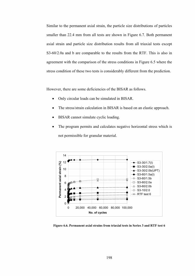
Similar to the permanent axial strain, the particle size distributions of particles

smaller than 22.4 mm from all tests are shown in Figure 6.7. Both permanent

axial strain and particle size distribution results from all triaxial tests except

S3-60/2.0a and b are comparable to the results from the RTF. This is also in

agreement with the comparison of the stress conditions in Figure 6.5 where the

stress condition of these two tests is considerably different from the prediction.

However, there are some deficiencies of the BISAR as follows.

• Only circular loads can be simulated in BISAR.

• The stress/strain calculation in BISAR is based on an elastic approach.

• BISAR cannot simulate cyclic loading.

• The program permits and calculates negative horizontal stress which is

not permissible for granular material.

0

2

4

6

8

10

12

14

0 20,000 40,000 60,000 80,000 100,000

No. of cycles

Perm

an

en

t axia

l s

tra

in (

%)

S3-30/1.7(I)

S3-30/2.0a(I)

S3-30/2.0b(UPT)

S3-60/1.5a(I)

S3-60/1.5b

S3-60/2.0a

S3-60/2.0b

S3-10/2.0

RTF test 6

Figure 6.6. Permanent axial strains from triaxial tests in Series 3 and RTF test 6

198

0

50

100

150

200

250

300

350

400

450

0 5 10 15 20 25

Size (mm)

Ma

ss p

as

sin

g (

g)

S3-30/1.7(I)

S3-30/2.0a(I)

S3-30/2.0b(UPT)

S3-60/1.5a(I)

S3-60/1.5b

S3-60/2.0a

S3-60/2.0b

S3-10/2.0

RTF test 6

Figure 6.7. Particles smaller than 14 mm from triaxial tests in Series 3 and RTF test 6

A simple analysis can be performed to compare the results from the RTF test

with the triaxial test. This analysis is based on the findings from Selig and

Waters (1994) and Shenton (1978). According to the box test results of Selig

and Waters (1994), the observed horizontal stress in ballast eventually reached

30 kPa as previously shown in Figure 2.35. And from Figure 6.2, Shenton

(1974) found that the maximum contact pressure at sleeper base was

approximately 200 � 250 kPa

From both findings, it is reasonable to simulate the condition of ballast under

traffic loading in the RTF by a cyclic triaxial test with constant confining stress

of 30 kPa and maximum axial stress of 200 � 250 kPa. The values of constant

confining stress and maximum axial stresses result in q/p�max from 1.96 to 2.13.

And it is shown that the permanent axial strain (Figure 6.6) and particle size

distribution (Figure 6.7) from cyclic triaxial tests on limestone with 30 kPa

confining stress and q/p�max of 2.0 are comparable to the traffic loading test on

199

200

limestone (RTF test 6). Even though this analysis method is simple and gives a

quick estimation of a stress condition, it might be doubtful as it is based on

others� research and the conditions of those research projects are not fully

understood.

Therefore, it can be concluded that even though BISAR has some deficiencies,

it can estimate the stress condition in the RTF. Also, triaxial tests with the

conditions that match the line in Figure 6.5 are recommended for further

research.

7. Conclusions and recommendations for further

research

7.1. Conclusions

The conclusions that can be drawn from this research are:

• LAA and MDA values correlate well with the breakage from tamping.

• Index tests such as LAA and MDA are economical and easy to perform.

They can also assess ballast performance well in terms of durability.

• The settlements of different ballast types from the traffic loading

simulation in the RTF are similar to each other. The settlement from the

RTF unreinforced tests were about 60 % of the settlement that would be

expected on site. This is probably because the traffic loads on site are

larger particularly if dynamic effects are present. However, this

comparison might not be on the same basis as the researchers did not

report all test conditions and parameters.

• The overall degradation from the RTF tests is lower than the site

degradation because of the higher traffic loads and also there are

fouling materials mixing with the ballast such as wagon spillage and

airborne dirt which would exacerbate degradation.

• The level of ballast degradation from RTF traffic loading is similar to

the previous research (Awoleye, 1993). However, it should be noted

that the scale and ballast density in that research is smaller than the

RTF.

• Tamping can improve track settlement but cause faster rate of

settlement afterwards.

201

• The results from the RTF tamping bank suggest that plunging of the

tamping tines into the ballast layer is more damaging than squeezing.

• Ballast degradation was much less from the tamping tests in this project

compared to the work done by Wright (1983).

o Although the tamping bank was a refurbished full-scale device,

it utilised a hydraulic vibrating actuator instead of a mechanical

vibrator and was mounted in a frame which did not have the

same mass as a 35-tonne tamping machine carriage.

o These differences may have contributed to a reduction in

damage to the ballast for tamping tests.

o This type of vibrator may be advantageous as it is less likely to

damage the ballast than the fixed amplitude mechanical

vibrator. However, this should be further studied in more detail.

• Using painted ballast in columns beneath the tamping tines, in the

squeezed location, and under the rail seating was a successful means of

quantifying breakage.

• The triaxial test on the ballast was repeatable. The permanent axial and

volumetric strains, resilient modulus, Poisson�s ratio, and breakage

could be quantified with small discrepancies between tests.

• According to the monotonic triaxial test results, larger dilation is

accompanied by smaller breakage. This is probably because the

particles in the sample can rearrange more freely with larger dilation.

• With the same confining stress, the breakage of the ballast sample

increases with increasing deviatoric stress.

202

• The range of confining stresses in the cyclic triaxial tests was not large

enough to observe the effect of confining stress on ballast breakage.

The confining stresses used in the tests are in the optimum degradation

zone (30 � 75 kPa, Figure 5.34) according to Indraratna et al. (2005).

• Even with some deficiencies, the BISAR elastic model can predict the

stress condition under traffic loading in the RTF as shown in the line in

Figure 6.5.

7.2. Recommendation for further research

The recommendations for the RTF are to make its performance more

representative of the in service loading conditions. A feature of the laboratory

tamping bank is that it has the facility to vary parameters which can influence

the damage to the ballast. Modifications to the triaxial tests are also

recommended to improve performance. These points and ideas for further

experiments are outlined below.

• Ballast of each size does not need to be prepared to make up a specified

grading for the samples in both the RTF and triaxial test. Instead,

particles smaller than 22.4 mm should be removed from the sample.

However, it should be ensured that the samples conform to the grading

specification.

• In the RTF, the ballast under the sleeper at the rail seating should be at

a slightly higher level than under the middle portion of the sleeper to

ensure that the stress on ballast under the rail seating is higher than the

centre.

203

• The magnitude and frequency of traffic loading in the RTF can be

increased to simulate the effect of the dynamic loading and to reduce

the test duration. However, the capacity of the facility has to be

increased to achieve this.

• The arrangement for the extra confinement test in the RTF could be

extended by dividing the pit into four sections. More test results can be

generated with this type of installation. For example, each section can

be filled with different sizes of ballast to observe the resulting breakage.

• Ballast gradings used for testing in both the RTF and triaxial tests can

be varied to observe its effect on the settlement and degradation.

• The fines collector and accelerometer could be further developed to

measure the fines generated during each test and the resilient

displacement of the subgrade in the RTF.

• The amplitude of tamping tine vibration should be monitored and

recorded during each tamp to detect any changes in response to the

ballast behaviour.

• The amplitude of tamping tine vibration, hydraulic oil pressure, rate of

lowering tamping tines, and shape of tamping tines can all be varied in

the RTF tamping bank to observe the resulting breakage, the

performance of settlement improvement, and the rate of settlement from

subsequent traffic loading.

• As the tamping bank in this project caused reduced particle breakage, it

could be tried on site.

204

• Triaxial tests with stress conditions matching the line in Figure 6.5

should be performed and compared with traffic loading tests from the

RTF.

• The image analysis can be further developed to measure the radial

strain of a sample by placing a series of stickers on the sample and

using two cameras. More details can be found in Section 5.4.2.

• Another model of ultrasonic proximity transducer can be used to

measure the sample volume change. This model is a flat transducer with

a transmitter that operates at right angles from the end rather than the

axial cylindrical type used in this project. This would be easier to locate

above the neck of the inner cell as shown in Figure 7.1. This method

does not require a significant modification to the system.

• The ultrasonic proximity transducer can also be used to measure sample

volume change in a different way as shown in Figure 7.2.

o This method does not use the inner cell. The outer cell is fully

filled with water. The transducer is placed above the pipe that

connects to the outer cell. As the volume of sample changes, the

transducer can register the change of water level in the pipe. The

change of the water level can be converted to the volume

change by the known cross-sectional area of the pipe.

o Since the water is open to the atmosphere, the sample must be

under vacuum. The limitation of this method is that a

modification of the outer cell is required and a robust vacuum

system is also required and the maximum equivalent confining

pressure from the vacuum is 100 kPa.

205

o This limitation can be overcome by using pressurised water to

apply the confining pressure instead of using vacuum but the

system has to be sealed above the water surface in the pipe and

compressed air with equal pressure must be supplied between

the water surface and the seal (Figure 7.2).

o Direct measurement of the water surface level is used in this

method instead of measuring the water head difference, which

can fluctuate with the air pressure in the arrangement used in

this project. Also, the water level in this recommended system

will not oscillate with the rapid movement in the system.

Therefore, the response during a cyclic test should improve.

Figure 7.1. Use of alternative ultrasonic proximity transducer to measure volume change

206

Figure 7.2. Alternative method of volume change measurement by the ultrasonic

proximity transducer

207

References

1. Aitken, P. (2006). Exploring Excel�s function part 6: TTEST(). [online], 14

April. Available at

<URL:http://www.quepublishing.com/articles/article.asp?p=461631&rl=1> [Accessed

2 Dec 2006].

2. Ashby, M. F. and Jones, D. R. H. (1996). Engineering materials 1. Oxford:

Butterworth-Heinemann.

3. Ashby, M. F. and Jones, D. R. H. (1998). Engineering materials 2. Oxford:

Butterworth-Heinemann.

4. Awoleye, E. O. A. (1993). Ballast type - ballast life predictions. Derby,

British rail research LR CES 122, October 1993.

5. Barksdale, R. D. (1972). Laboratory evaluation of rutting in basecourse

materials. Proc., 3rd Int. Conf. on Struct. Des. of Asphalt Pavements, pp.

161-174.

6. Brown, S. F. and Hyde, A. F. L. (1975). Significance of cyclic confining

stress in repeated-load triaxial testiing of granular material. Transportation

research record 537, pp. 49-58.

7. Bishop, A. W. and Green, G. E. (1965). The influence of end restraint on

the compression strength of a cohesionless Soil. Geotechnique 15, pp. 243-

266.

8. Bombardier Inc. (2007). Commuter trains. [online], Available at

<URL:http://www.bombardier.com> [Accessed 24 Aug 2007].

208

9. Boyce, J. R., Brown, S. F. and Pell, P. S. (1976). The resilient behaviour of

granular material under repeated loading. Eighth conference of Australian

road research board, pp. 1-12.

10. British Standard: BS EN 933-3 (1997). Determination of particle shape-

Flakiness index.

11. British Standard: BS EN 1097-1 (1996). Tests for mechanical and physical

properties of aggregates- Determination of the resistance to wear (micro-

Deval).

12. British Standard: BS EN 1097-2 (1998). Tests for mechanical and physical

properties of aggregates- Methods for the determination of resistance to

fragmentation.

13. British Standard: BS EN 13450 (2002). Aggregates for railway ballast.

14. British Standard: BS EN 1097-6 (2000). Determination of particle density

and water absorption.

15. Collins, I. F. and Boulbibane, M. (2000). Geomechanical analysis of

unbound oavements based on shakedown theory. Journal of geotechnical

and geoenvironmental engineering, ASCE. Vol. 126, No. 1, pp. 50-59.

16. Cundall, P. A. and Strack, O. D. L. (1979). A discrete numerical model for

granular assemblies. Géotechnique 29, No. 1, pp. 47-65.

17. Davidge, R. W. (1979). Mechanical behaviour of ceramics. Cambridge

university Press.

18. Dawson, A. R., Thom, N. H. and Paute, J.-L. (1996). Mechanical

characteristics of unbound granular materials as a fucntion of condition.

Flexible pavements. A. G. Correia ed. Rotterdam, A. A. Balkema. pp. 35-

44.

209

19. Devore, J. and Farnum, N. (1999). Applied statistics for engineers and

scientists. Belmont, California, Brooks/Cole publishing company.

20. Duncan, J. M. and Dunlop, P. (1968). The significance of cap and base

restraint. Journal of the soil mechanics and foundation division, Proceeding

of ASCE. Vol. 94(SM1), pp. 271-290.

21. Fair, P. (2003). The geotechnical behaviour of ballast materials for railway

track maintenance. Ph.D. dissertation, University of Sheffield.

22. Fukumoto, T. (1992). Particle breakage characteristics in granular soils.

Soils and foundations 32, No. 1, pp. 26-40.

23. Golightly, C. R. (1990). Engineering properties of carbonate sands. Ph.D.

dissertation, Bradford University.

24. Hertzberg, R. W. (1996). Deformation and fracture mechanics of

engineering materials. New York: John Wiley & Sons.

25. Heydinger, A. G., Xie, Q., Randolph, B. W. and Gupta, J. D. (1996).

Analysis of resilient modulus of dense- and open-graded aggregates.

Transportation research record 1547, pp. 1-6.

26. Hicks, R. G. and Monismith, C. L. (1971). Factors influencing the resilient

properties of granular materials. Highway research record 345, pp. 15-31.

27. Hornby, E. (2007). Personal communication, 11 June, University of

Nottingham.

28. Indraratna, B., Ionescu, D., and Christie, H. D. (1998). Shear behaviour of

railway ballast based on large-scale triaxial tests. Journal of geotechnical

and geoenvironmental engineering 124, No. 5, pp. 439-449.

210

29. Indraratna, B., Lackenby, J. and Christie, D. (2005). Effect of confining

pressure on the degradation of ballast under cyclic loading. Geotechnique

55, No. 4, pp. 325-328.

30. Ionescu, D. (2004). Ballast degradation and measurement of ballast fouling.

Seventh railway engineering conference, Commonwealth Institute, London.

31. Key, A. (1998). Behaviour of two layer railway track ballast under cyclic

and monotonic loading, Ph.D. dissertation, University of Sheffield.

32. Knutson, R. M. (1976). Factors influencing the repeated load behaviour of

railway ballast, Ph.D. dissertation, University of Illinois Urbana-

Champaign.

33. Knutson, R. M. and Thompson, M. R. (1978). Permanent-deformation

behavior of railway ballast. Transportation Research Record 694, pp. 47-

53.

34. Kolisoja, P. (1997). Factors affecting deformation properties of coarse

grained granular materials. International conference on soil mechanics and

foundation engineering, pp. 337-342.

35. Kwan, Cho Ching. (2006). Geogrid Reinforcement of railway ballast,

Ph.D. dissertation, University of Nottingham.

36. Lekarp, F. and Dawson, A. R. (1998) Modelling permanent deformation

behaviour of unbound granular materials. Construction and building

materials 12, No. 1, pp. 9-18.

37. Lekarp, F., Isacsson, U. and Dawson, A. (2000a). State of the art I:

Resilient response of unbound aggregates. Journal of transportation

engineering, ASCE. Vol. 126, No. 1, pp. 66-75.

211

38. Lekarp, F., Isacsson, U. and Dawson, A. (2000b). State of the art II:

Permanent strain response of unbound aggregates. Journal of

transportation engineering, ASCE. Vol. 126, No. 1, pp. 76-83.

39. Lim, W. L. (2004). Mechanics of railway ballast behaviour. Ph.D.

dissertation, University of Nottingham.

40. McDowell, G. R. (2001). Statistics of soil particle strength. Geotechnique

51, No. 10, pp. 897-900.

41. McDowell, G. R. (2002). On the yielding and plastic compression of sand.

Soils and foundations 42, No. 1, pp. 139-145.

42. McDowell, G. R. and Amon, A. (2000). The application of Weibull

statistics to the fracture of soil particles. Soils and foundations 40, No. 5,

pp. 133-141.

43. McDowell, G. R. and Bolton, M. D. (1998). On the micromechanics of

crushable aggregates. Géotechnique 48, No. 5, pp. 667-679.

44. McDowell, G. R., Bolton, M. D. and Robertson, D. (1996). The fractal

crushing of granular materials. J. Mech. Phys. Solids 44, No. 12, pp. 2079-

2102.

45. Monismith, C. L., Seed, H. B., Mitry, F. G. and Chan, C. K. (1967).

Prediction of pavement deflections from laboratory tests. Second Int. Conf.

Struct. Des. of Asphalt Pavements, pp. 109-140.

46. Morgan, J. R. (1966). The response of granular materials under repeated

loading Proceeding of ARRB. 3rd

conference, pp. 1178-1192.

47. Ng, C. W. W., Zhan, L. T. and Cui, Y. J. (2002). A new simple system for

measuring volume changes in unsaturated soils. Canadian geotechnical

journal 39, No. 3, pp. 757-764.

212

48. Oda, M. (1977). Co-ordination number and its relation to shear strength of

granular material. Soils and foundations 17, No. 2, pp. 29-42.

49. Pappin, J. W. (1979). Characteristics of a granular material for pavement

analysis. Ph.D. dissertation, University of Nottingham.

50. Ping, W. V. and Yang, Z. (1998). Experimental verification of resilient

deformation for granular subgrades. Transportation Research Record 1639,

pp. 12-22.

51. Powrie, W. (1997). Soil mechanics: Concepts and Applications. London, E

& FN Spon.

52. Profillidis, V. A. (2000). Railway Engineering. Aldershot: Ashgate

Publishing Limited.

53. Rahimzadeh, B., Jones, M., Hakim, B., and Thom, N. (2004). Performance

testing of unbound materials within the pavement foundation. In: Dawson,

A. R., ed. Pavement Unbound. London, Taylor & Francis group.

54. Railtrack Line Specification (2000). RT/CE/S/006 Issue 3. Track Ballast.

55. Railtrack Line Specification (2002). RT/CE/S/006 Issue 5. Track

Construction Standards.

56. Railway Group Standard (2003). GT/RT5014 Issue 2. Trackbed and Track

Drainage.

57. Raymond, G. P. and Bathurst, R. J. (1994). Repeated-load response of

aggregates in relation to track quality index. Canadian Geotechnical

Journal 31, No. 4, pp. 547-554.

58. Selig, E. T. and Alva-Hurtado, J. E. (1982). Predicting effects of repeated

wheel loading on track settlement. Proceeding of the 2nd

International

Heavy Haul Conference, Colorado Springs, pp. 476-487.

213

59. Selig, E. T. and Waters, J. M. (1994). Track Geotechnology and

Substructure Management. London: Thomas Telford.

60. Shenton, M. J. (1974). Deformation of railway ballast under repeated

loading conditions. British Railways Research and Development Division.

61. Shipway, P. H. and Hutchings, I. M. (1993). Fracture of brittle spheres

under compression and impact loading I. Elastic stress distributions.

Philosophical Magazine A 67, No. 6, pp. 1389-1404.

62. Skoglund, K. A. (2002). A study of some factors in mechanistic railway

track design. Ph.D. dissertation, Norwegian University of Science and

Technology.

63. Suiker, A. S. J., Selig, E. T., and Frenkel, R. (2005). Static and cyclic

triaxial testing of ballast and subballast. Journal of geotechnical and

geoenvironmental engineering, ASCE. Vol. 131, No. 6, pp. 771-782.

64. The American Society for Testing and Materials: ASTM D 1557-78

(1978). Standard test methods for moisture density relations of soil-

aggregate mixtures using 10-lb (4.54 kg) rammer and 18-in (457-mm)

drop.

65. Thom, N. H. and Brown, S. F. (1987). Effect of moisture on the structural

performance of a crushed-limestone road base. Transportation Research

Record 1121, pp. 50-56.

66. Thom, N. H. and Brown, S. F. (1988). The effect of grading and density on

the mechanical properties of a crushed dolomitic limestone. Proceeding of

the Australian Road Research Board 14, No. 7, pp. 94-100.

214

215

67. Thom, N. H. and Brown, S. F. (1989). The mechanical properties of

unbound aggregates from various sources. Unbound Aggregates in Roads.

R. H. Jones and A. R. Dawson eds. London, Butterworth: pp. 130-142.

68. Uzan, J. (1985). Characterization of granular material. Transportation

Research Record 1022, pp. 52-59.

69. Weibull, W. (1951). A statistical distribution function of wide applicability.

Journal of Applied Mechanics 18, pp. 293-297.

70. White, D. J. and Take, W.A. (2002). GeoPIV: Particle Image Velocimetry

(PIV) software for use in geotechnical testing. Cambridge University

Engineering Department Technical Report, D-SOILS-TR322.

71. White, D. J., Take, W. A., and Bolton, M. D. (2003). Soil deformation

measurement using particle image velocimetry (PIV) and photogrammetry.

Géotechnique 53, No. 7, pp. 619-631.

72. Wright, S. E. (1983). Damage caused to ballast by mechanical maintenance

techniques. British Rail Research Technical Memorandum TM TD 15, May

1983.