POLITECNICO DI TORINO

Faculty of Engineering

International Master's Degree course in Mechanical Engineering

Master's Degree thesis

Thermal and mechanical design of a steam generator for the petrochemical refinery service

Thesis Coordinator: Eng. Chiavazzo Eliodoro

Company Tutor: Eng. Cortassa Daniele

Thesis Advisor: Eng. Asinari Pietro

Thesis Advisor: Eng. Bergamasco Luca

Candidate: Gallo Alessandro

INDEX

1. INTRODUCTION .............................................................................................................................. 1

2. LEGISLATIVE FRAMEWORK FOR PRESSURE VESSELS ......................................................................... 3

2.1. LAWS, DIRECTIVES AND TECHNICAL REGULATIONS ......................................................................... 3

2.2. STANDARDS AND CODES .................................................................................................................. 4

2.3. TECHNICAL STANDARDS SPECIFICATIONS ........................................................................................ 7

3. GENERALITIES ON HEAT EXCHANGERS ............................................................................................. 8

3.1. CLASSIFICATION AND MOST COMMERCIAL CONFIGURATIONS........................................................ 8

3.2. SHELL-AND-TUBES CONFIGURATION AND TERMINOLOGY BY TEMA ............................................. 10

3.3. CONSTRUCTION PECULIARITY......................................................................................................... 19

4. CONCEPTS OF HEAT TRANSFER AND THERMAL DESIGN .................................................................. 25

4.1. FOUNDAMENTALS OF CONDUCTION.............................................................................................. 25

4.2. HEAT CONVECTION AND HEAT TRANSFER COEFFICIENT COMPUTATION ...................................... 30

4.3. LOGARITMIC MEAN TEMPERATURE DIFFERENCE AND CORRECTION FACTOR ............................... 32

4.4. EFFECTIVENESS – NTU METHOD ..................................................................................................... 35

4.5. HEAT TRANSFER IN PHASE CHANGE CONFIGURATIONS ................................................................. 37

5. THERMAL DESIGN OF THE HEAT EXCHANGER: CASE STUDY ............................................................ 47

5.1. INTRODUCTION TO THE THERMAL DESIGN .................................................................................... 47

5.2. CUSTOMER INPUT DATA ................................................................................................................. 49

5.3. INTRODUCTION TO ASPEN EXCHANGER DESIGN AND RATING V.11 .............................................. 51

5.4. DESIGN MODE: IMPLEMENTATION OF THE INPUT DATA AND EXPLANATIONS .............................. 52

5.5. DESIGN MODE: RESULTS SECTION .................................................................................................. 72

5.6. RATING MODE ................................................................................................................................ 87

6. CONCEPTS OF PRESSURE VESSELS MECHANICAL DESIGN ................................................................ 89

6.1. PRELIMINARY CONSIDERATIONS .................................................................................................... 89

6.2. GENERAL CALCULATION CRITERIA .................................................................................................. 96

6.3. CYLINDERS UNDER INTERNAL PRESSURE ...................................................................................... 106

6.4. THERMAL STRESS OF CYLINDERS UNDER INTERNAL PRESSURE .................................................... 112

7. MECHANICAL DESIGN OF THE HEAT EXCHANGER: CASE STUDY .................................................... 117

7.1. INTRODUCTION TO MECHANICAL DESIGN ................................................................................... 117

7.2. ANALYSIS AND IMPLEMENTATION OF THE INPUT DATA .............................................................. 118

7.3. ITERATIVE CORRECTIONS AND RESULTS SECTION ........................................................................ 144

8. CONCLUSIONS ............................................................................................................................ 155

9. APPENDIX I: TECHNICAL DRAWINGS ............................................................................................ 159

10. APPENDIX II: CALCULATION REPORT ............................................................................................ 173

11. ACKNOWLEDGEMENTS ............................................................................................................... 223

12. BIBLIOGRAPHY ........................................................................................................................... 224

1

1. INTRODUCTION

In the refinery process the energy recovery can be a real challenge for the engineering activity and it has a

major economic and technological importance. Indeed, achieving substantial falls in the temperature of very

high flows may not be immediate, especially when the tubeside fluid is a mixture of hydrocarbons, which can

be corrosive and hard to handle. On the other hand, a refinery facility can have an in-house power generation

plant or some petrochemical processes which require vapour to be kept operational, as example the steam

cracking method. The steam generation can be maintained exploiting the unnecessary available heat by

means of a heat exchanger, and the situation mentioned above can occur. Heat exchangers, which at a first

glance may seem simply to build, are actually very complex and full of peculiarities. Furthermore, when

special materials have to be used, even a small error in design can be reflected in thousands of euros of

damage. Design and simulation programs, as the one used in the study case, perform the pre-set

computations with the indicated design code. However, to obtain the best configuration for the case under

analysis and to avoid errors, a correct and conscious management performed by the engineer is required.

Generally, given the magnitude of this sector, this is possible only with a fair amount of experience.

The goal of this thesis is to develop the thermal and mechanical design of a heat exchanger, being conscious

of the theories on which the calculus codes are based and the manufacturing and financial problems. The

objective of the heat exchanger’s thermal design is to find the necessary exchange area that allows the

required heat flux between the fluids. Moreover, the best heat exchanger configuration for the case have to

be analysed and found. The mechanical design, instead, aims to ensure the physical resistance of each

component against the internal stress generated from both thermal and pressure gradients. In addition, a

host of traditional considerations must be addressed in designing heat exchangers. As example, the

minimization of fixed cost and some manufacturing considerations have to be taken into account during the

design activity. I decided to write this thesis in collaboration with SIMIC.Spa, which recently received a steam

generator commission from an important EPC contractor (“Engineering, Procurement, Construction”), with

intended use in one of the biggest Indian Petroleum refineries. However, due to the confidentiality

agreement that has been signed, the name of the interested parts and of the project cannot be exposed. In

order to develop the design procedure, I’ve thoroughly studied the regulations framework, the heat

exchange science and the mechanical resistance theories applied to pressure vessels. Therefore, I’ve carried

out an important in-deep analysis of heat exchanger configurations and design options to provide a complete

overview of the topic.

A significant problem for those who approach for the first time to the sector of the pressure vessels is the

regulatory framework. A non-standard scenario is present in the world, in which there are laws, directive and

regulations depending on the delivery place. Very often, also plant requirements or preferences dictated by

the client are present. Due to the possible overlay between the laws, preferences and codes used during the

design activity, I decided to insert a chapter regarding the regulatory framework and the hierarchical order

that must be observed. In the proposed study case, the ASME code and TEMA technical standard have to be

observed. Subsequently, the chapter number three introduces the heat exchangers devices, the classification

and the terminology used during design and construction. In this section all the important features and

construction peculiarity are described. Even if the most used classification method is analysed, it can be

noticed how every device can have its peculiar configuration in order to accomplish the different goals and

settings required by the final working layout. Indeed, the reader will realize how every device requires to be

carefully analysed and designed with particular and dedicated considerations.

2

The following chapters are the core of the thesis and they approach the thermal and mechanical design of

the heat exchanger. For both sections there is a first theoretical part in which the most important concepts

are presented. The thermal theoretical part begins with the popular concepts about conduction and

convection. After the explanations of the thermal design methods, the chapter continues with the in-deep

analysis of the heat transfer in boiling and other phase change configurations. This technical difficulty is also

present in the study case and introduces some tricky concepts that generally are not analysed during the

degree course. Follows a thermal design chapter in which the design activity of the study case, accomplished

with the support of ASPEN shell and tubes, is reported. Starting from the data provided by the client, the

inputs are implemented and all the design choices are explained. Here, many important parameters have

been analysed and some interesting technical considerations can be found. Subsequently, the computational

design procedure has been launched, and the program provides the first set of results. This group of possible

configurations will be thoroughly analysed with respect to the parameters of selection that have to be

satisfied. The best design will be chosen among them, and it will set the heat exchanger geometry and

characteristics. At the end, the vibrational analysis, with both the HTFS and the TEMA methods, have been

carried out in order to verify the acceptability of the design. Afterwards, the thermal design refinement,

called Rating mode, is made and the dimensions of the interface pieces are set at standard values, e.g. the

nozzle diameters. Follows the complete simulation of the last solution, which leads the final thermal output

to be ready for the upload in the mechanical part of the program. In this way, the whole thermal design is

fixed, and the output will be used for the mechanical design activity of the study case.

Before the second part of the study case just mentioned, a mechanical theory chapter reports some insights

and theories about pressure vessel and heat exchanger design. Starting from some preliminary

considerations regarding the admissible stress and the most common used theories of failure, the

verifications criteria with plasticity collaboration has been analysed. Afterwards, a chapter regarding the

general calculation criteria have been reported. Some general considerations about membrane stress in

revolution shell, edge effects and stress concentration around holes have also been carried out. The theories

of cylinders under internal pressure have more deeply been developed and reported as example. However,

many theories and analysis could be incorporated to complement the theoretical approach. The main goal

of this section, as well as for the previously reported thermal theoretical part, is to demonstrate how the

calculation codes are science-based and derive from globally approved theories. In the same conceptual way,

the calculation report of the program, present in the second appendix, includes all the passages and

computation done during the mechanical design, which in turn are based on the calculation codes. Also, it

can be seen how the designer can always maintain the control on the design activity checking calculations

that the program have been done. The last chapter completes the design activity of the study case, discussing

the mechanical design of the heat exchanger under consideration. An important mention to the materials,

and examples of the ASME designation, has been done in this section. At the end some iterative procedures,

similar to the rating mode of the thermal part, were necessary in order to uniform the plate thickness and

pipe dimensions. All the vessel dimensions resulting from the last program calculation have been reported in

the final chapter, while the discussion is concluded with the technical drawings and the calculation report

that have been inserted in the appendices.

3

2. LEGISLATIVE FRAMEWORK FOR PRESSURE VESSELS

Manufacturers must comply with the jurisdictional or government regulations for different product

standards, each targeting specific types of equipment. The heat exchanger devices, independently from their

type or purpose, fall into the pressure vessels category. Due to the potential dangers and associated risk

connected with the high working pressure and temperature of these devices, the reference directives and

the standards design codes are complex and articulate. As a result, an overview of the main classes of

regulations is reported below in the order of priority.

2.1. LAWS, DIRECTIVES AND TECHNICAL REGULATIONS

The laws, directives and technical regulations are continental or national documents with the highest level

of priority. That’s why they are predominant over the standards and technical standard specification. They

are issued by legislative authorities, like governments or committees and they set out goals that must be

achieved by the country in which they are effective. All the contained requirements are not specific or

technical, but they deal with safety or general-purpose issues. So, every device which will be installed in a

country must satisfy the local laws in force. The national legislation can impose a specific design code or

require the designed device to be verified in accordance with a specific one. As example, the European

directive is commented below.

EUROPE - PED 2014/68/EU: Pressure Equipment Directive

The European Pressure Equipment Directive (PED) 2014/68/EU is a pre-requisite for CE-Marking and a

guideline for the design and manufacture of pressure equipment. This means that it has substituted all the

pre-existent national laws about pressure equipment inside the EU. It applies to pressure vessels, steam

boilers, pipelines, heat exchangers, storage tanks, pressure relief devices, valves, regulators and other

pressure equipment with a maximum allowable pressure superior to 0.5 bar. All devices are classified in

different risk categories (Category I, II, III, IV) in function of their maximum allowable pressure and the danger

and amount of fluid they have to process. According to the PED risk category of the product, it can be chosen

the procedure to obtain the CE marking. All the devices that will be installed in the European country shall

mandatorily have the CE marking and so comply with all the requirement of the PED.

Nevertheless, some pressure equipment that present a relatively low hazard from pressurization could be

covered by other directive as the Transportable Pressure Equipment Directive (TPED 2010/35/EU), the Simple

Pressure Vessels Directive (SPVD 2009/105/EC) or other directives, e.g. ATEX Directive, Machinery Equipment

Directive, Electro Magnetic Compatibility Directive or the Low Voltage Directive.

Summarizing, the Pressure Equipment Directive does not impose a specific regulation to follow during the

design activity. However, if the device will be installed inside EU it needs the CE certification, so it shall comply

with all the requirement of the PED. If a code different from EN is used, a document demonstrating that all

the PED’s requirements have been satisfied must be issued. Contrariwise, if the EN regulations are used

during the design activity, the PED requirements are automatically assumed to be observed and the CE

certification can be directly obtained.

4

2.2. STANDARDS AND CODES

Standards, also called codes, are documents issued and approved by a recognized and official standardization

organization. They provide rules, guidelines or characteristics for products or related processes and

production methods for common and repeated use, with which compliance is not mandatory. However, laws

and regulations may refer to standards and compulsory have to make compliance with them. [1] These

documents may also include or deal with symbols, terminology, packaging and marking or labelling

requirements, as they apply to a product, process or production method. For the knowledge of the reader, it

is reported that it is generally named “code” the standard in which all the main rules and guidelines of

product’s sector are contained. Of course, during the design activity, the code is not the only standard

considered. A section with the principal organizations and codes for the pressure vessels is commented

below.

ASME – Boiler & Pressure Vessel Code (BPVC)

ASME, the American Society of Mechanical Engineers, is an international developer of codes and standards

associated with the science, and practice of mechanical engineering. Starting with the first issuance, in 1914,

of the Boiler & Pressure Vessel Code, ASME's codes and standards have grown to more than 500 offerings

currently in print. These offerings are accepted for use in more than 100 countries around the world and

cover a breadth of topics, including pressure technology, nuclear plants, elevators, construction, engineering

design, standardization, and performance testing. [2] The code developed from ASME that regulate the

pressure vessels, in which vapor generator heat exchangers are contained, is the Boiler & Pressure Vessel

Code (BPVC). The following is the structure of the January 2019 Edition of the BPV Code:

• ASME BPVC Section I - Rules for Construction of Power Boilers

• ASME BPVC Section II – Materials

o Part A - Ferrous Material Specifications

o Part B - Nonferrous Material Specifications

o Part C - Specifications for Welding Rods, Electrodes and Filler Metals

o Part D - Properties (Customary)

o Part D - Properties (Metric)

• ASME BPVC Section III - Rules for Construction of Nuclear Facility Components

o Subsection NCA - General Requirements for Division 1 and Division 2

o Appendices

o Division 1

▪ Subsection NB - Class 1 Components

▪ Subsection NC - Class 2 Components

▪ Subsection ND - Class 3 Components

▪ Subsection NE - Class MC Components

▪ Subsection NF – Supports

▪ Subsection NG - Core Support Structures

o Division 2 - Code for Concrete Containments

o Division 3 - Containment Systems for Transportation and Storage of Spent Nuclear Fuel and High-Level Radioactive Material

o Division 5 - High Temperature Reactors

• ASME BPVC Section IV - Rules for Construction of Heating Boilers

• ASME BPVC Section V - Nondestructive Examination

5

• ASME BPVC Section VI - Recommended Rules for the Care and Operation of Heating Boilers

• ASME BPVC Section VII - Recommended Guidelines for the Care of Power Boilers

• ASME BPVC Section VIII - Rules for Construction of Pressure Vessels

o Division 1

o Division 2 - Alternative Rules

o Division 3 - Alternative Rules for Construction of High-Pressure Vessels

• ASME BPVC Section IX - Welding, Brazing, and Fusing Qualifications

• ASME BPVC Section X - Fiber-Reinforced Plastic Pressure Vessels

• ASME BPVC Section XI - Rules for Inservice Inspection of Nuclear Power Plant Components

o Division 1 - Rules for Inspection and Testing of Components of Light-Water-Cooled Plants

o Division 2 - Requirements for Reliability and Integrity Management (RIM) Programs for Nuclear Power Plants

• ASME BPVC Section XII - Rules for the Construction and Continued Service of Transport Tanks

• ASME BPVC Code Cases - Boilers and Pressure Vessels

The study case developed in this thesis refers to the ASME BPVC Section VIII for pressure vessels and the

accessory section II, V and IX, respectively for the materials, non-destructive examination and welding

qualifications.

Particular attention must be adopted for the section II which provides specifications for the materials suitable

for the construction of pressure vessels. It consists in four parts:

▪ Part A - Ferrous Material Specifications

The specifications contained in this Part specify the mechanical properties, heat treatment, heat and

product chemical composition and analysis, test specimens, and methodologies of testing for ferrous

material. The designation of the specifications starts with 'SA' and a number which is taken from the

ASTM 'A' specifications. [2]

▪ Part B - Nonferrous Material Specifications

The specifications contained in this Part specify the mechanical properties, heat treatment, heat and

product chemical composition and analysis, test specimens, and methodologies of testing for

nonferrous materials. The designation of the specifications starts with 'SB' and a number which is

taken from the ASTM 'B' specifications. [2]

▪ Part C - Specifications for Welding Rods, Electrodes, and Filler Metals

It provides mechanical properties, heat treatment, heat and product chemical composition and

analysis, test specimens, and methodologies of testing for welding rods, filler metals and electrodes

used in the construction of pressure vessels. The specifications contained in this Part are designated

with 'SFA' and a number which is taken from the American Welding Society (AWS) specifications. [2]

▪ Part D - Properties (Customary/Metric)

It provides tables for the design stress values, tensile and yield stress values as well as tables for

material properties (Modulus of Elasticity, Coefficient of heat transfer, et al.) [2]

6

EUROPEAN STANDARDS EN13445 – Unfired Pressure Vessels

A European Standard is a standard developed by one of the three recognized European Standardization

Organizations (ESOs): CEN, CENELEC or ETSI. Each Standard is identified by a unique reference code

containing the letters 'EN'. After the emission by the CEN, a European Standard must be receipt from a

National Regulatory Authority, e.g. UNI, and inserted into the National Technical Rules. Then, the name of

the National Regulatory Authority is added to the name of the standard. For instance, the European code

that contains all the main rules and guidelines for the pressure vessels is the EN13445 – Unfired Pressure

Vessels, that becomes UNI-EN 13445 after been inserted into the Italian regulation. As I have introduced, the

European code is harmonized with the Pressure Equipment Directive (2014/68/EU or "PED"), so, if the

equipment is designed following the EN code, automatically the European PED directive is satisfied. The EN

13445 is divided in:

• EN 13445-1: Unfired pressure vessels - Part 1: General

• EN 13445-2: Unfired pressure vessels - Part 2: Materials

• EN 13445-3: Unfired pressure vessels - Part 3: Design

• EN 13445-4: Unfired pressure vessels - Part 4: Fabrication

• EN 13445-5: Unfired pressure vessels - Part 5: Inspection and testing

• EN 13445-6: Unfired pressure vessels - Part 6: Requirements for the design and fabrication of

pressure vessels and pressure parts constructed from spheroidal graphite cast iron

• EN 13445-8: Unfired pressure vessels - Part 8: Additional requirements for pressure vessels of

aluminum and aluminum alloys

• EN 13445-10:2015: Unfired pressure vessels - Part 10: Additional requirements for pressure vessels

of nickel and nickel alloys. PUBLISHED 2016.6.30

• Parts 7 and 9 do exist but they are merely technical reports.

NATIONAL CODES

Before CEN issued the EN standards, every country in Europe had its own national codes, regularly updated.

Nowadays, with the implementation of the EN standards, some country like Italy and Netherlands have

stopped updating their national codes, Ispesl VSR and Stoomwezen respectively, that are now dismissed.

Despite that, other countries continue evolving their standards. Due to the fact that sometimes these

procedures could be expressively required by the client or for legislative issues, the national codes have to

be taken into account. Some important national codes still valid for the pressure equipment are:

▪ AD 2000 MERKBLATTER: Germany

▪ CODAP: France

▪ PD 5500: United Kingdom

▪ Gost: Russia

▪ JIS: Japan

An example in which a national code must be taken into account is when the piece’s final destination is the

Russia. The Russian legislation does not impose a standard for the design. So, you can design the equipment

following any codes but, at the end, you need to verify that the resulting thicknesses are bigger than the

result that you would be obtained if designed using the GOST Russian national codes.

7

2.3. TECHNICAL STANDARDS SPECIFICATIONS

A technical standard is a document issued by clients, engineering companies or manufacturers containing

some technical requirements. They don’t need to be satisfied for some juridical reason, but for some

technical purpose. For example, if many orders for a big project have to be split between different firms, a

technical standard can be released in order to fix the geometry end the dimensions of the items’ interface

part. In this way the compatibility with the other pieces of the project or interchangeability is guarantee.

TEMA (Tubular Exchanger Manufacturers Association) standards is probably the most famous example of

these collection of requirements. It’s not issued by an official organization, but it was created by the

association of the major American companies of heat exchanger in order to compensate where the standards

did not contain methods for design some specialized parts. Now a days, they aren’t something of juridical

recognized, but sometime, for the design activity, they are asked by the clients in association with a code.

8

3. GENERALITIES ON HEAT EXCHANGERS

3.1. CLASSIFICATION AND MOST COMMERCIAL CONFIGURATIONS

A heat exchanger is a heat-transfer device that is used to transfer internal thermal energy between two or

more fluids available at different temperatures. In most heat exchangers, the fluids are separated by a heat-

transfer surface, and ideally they do not mix. On the other hand, if the two flows are directly in contact

because no element of thermal resistance is present between them, the device is named direct-contact heat

exchanger (e.g. steam bubbled into water,Figure 1).

Inside this document only the heat exchangers with a dividing

wall between the fluids will be analysed. The classification of a

heat exchanger can be done according to different parameters.

Below a scheme of the different possibility of heat exchangers’

classification is reported. There are an enormous variety of

configurations, but most commercial exchangers reduce to one

of the three basic types treated in the next page.

Figure 1: A direct-contact heat exchanger. [16]

9

The simple parallel or counterflow configuration. These arrangements are versatile and can have different

shape.Figure 2 shows how the counterflow arrangement is bent around in a so-called Heliflow compact

heat exchanger.

The cross-flow configuration. Figure 3 shows a typical cross-flow configurations in which the two fluid are

not mixed together. If baffles are present each flow must stay in the prescribed path through the exchanger

and is not allowed to “mix” to the right or left.

The shell-and-tube configuration. Most of the large heat exchangers are of the shell-and-tube form, and

them will be study in deep during the next paragraphs. An example is reported in the Figure 4 that shows

an exchanger with tube-bundle removed from shell.

Figure 3: two kind of cross-flow exchangers scheme. on the right a typical plate-fin cross-flow elemet. [16]

Figure 4: typical commercial one-shell-pass, two-tube-pass heat exchangers. [16]

Figure 2: Parallel and counterflow heat exchanger scheme. On the right: Heliflow compact counterflow heat exchanger. [16]

10

3.2. SHELL-AND-TUBES CONFIGURATION AND TERMINOLOGY BY TEMA

1. Stationary head – channel

2. Stationary head – bonnet

3. Stationary head flange – channel or bonnet

4. Channel cover

5. Stationary head nozzle

6. Stationary tubesheet

7. Tubes

8. Shell

9. Shell cover

10. Shell flange – stationary head end

11. Shell flange – rear head end

12. Shell nozzle

13. Shell cover flange

14. Expansion joint

15. Floating tubesheet

16. Floating head cover

17. Floating head flange

18. Floating head backing device

19. Split shear ring

20. Slip-on backing flange

21. Floating head cover – external

22. Floating tubesheet skirt

23. Packing box flange

24. Packing

25. Packing gland

26. Lantern ring

27. Tie rods and spacers

28. Transverse baffles or support plates

29. Impingement plate

30. Longitudinal baffle

31. Pass partition

32. Vent connection

33. Drain connection

34. Instrument connection

35. Support saddle

36. Lifting lug

37. Support bracket

38. Weir

39. Liquid level connection

40. Floating Head Support

All the images present in this chapter, except where properly indicated, have been taken from [3].

11

12

With the purpose of establishing standard nomenclature and terminology, the TEMA has introduced some

frequently used standards. As a matter of fact, it is recommended that heat exchanger type has to be

designated by a number of letters as described below.

13

SHELL TYPES

E-shell: this is the most common type, where the shellside fluid enters

at one end of the shell and leaves at the other in one pass. Generally it

is considered to be the standard. If a single tube pass is used, providing

there are more than two or three baffles, near to counter current flow

is attainable and temperature crosses (cold fluid exit temperature is

higher than hot fluid outlet temperature) can be handled, i.e., low Log

Mean Temperature Difference (LMTD).

F-shell: this shell has longitudinal baffle extending most of the way

along the shell, dividing it into two halves. The shellside fluid enters at

one end of the shell, flows in the top half to the other end and then

back in the lower half, thus giving two shellside passes. In most F types

there are also two passes on the tubeside, thus ensuring

countercurrent flow. If a fixed tubesheet construction is used, then the

longitudinal baffles can be seal welded to the inside of the shell, thus

preventing leakage from the first shell pass to the second. If a

removable bundle is fitted, then leakages can be controlled (but not eliminated) by fitting packing material.

Note than removing and re-inserting the bundle can damage this seal and result in significant leakage across

the baffle from one shell pass to the other. If an F-shell is acceptable to the customer, then a two-tube pass

version is an alternative to a single pass E-shell. Also, if two or more tube passes are used (even number), any

given number of E-shells in series may be replaced by half the number of F-shells, avoiding very long

exchangers.

G-shell: this is sometime known as the “split flow” shell. Fluid enters

the shell through a nozzle placed at the center of the shell. The shell

has a central longitudinal baffle that divides the flow into two, so that

each half makes two passes in its half of the shell before combining

and exiting through a central nozzle. The main advantage, compared

to an E-shell, is that a single G-shell will often handle terminal

temperatures which would often require two E-shells in series. Note

then the minimum number of baffles that may be specified for a G-

shell is five. This is to maintain the crossflow path. Limiting the number of baffles to five ensures that there

is a baffle under the nozzle plus two baffles on each leg of the longitudinal baffle (i.e., 2+1+2 for G shell).

H-shell: sometimes called the “double split flow” type, this shell has

two inlet and exit nozzles located ¼ and ¾ the way along the shell.

There is a longitudinal baffle in each half of the exchanger, so that on

entry each half of the flow is split again, either going to the end of the

shell and back, or to the middle and back. Because of this flow split,

this type has a low shellside pressure drop, and it is normally used in

horizontal thermosyphon reboilers. Note then the minimum number

of baffles that may be specified for a H-shell is 10. This is to maintain the crossflow path. Limiting the number

of baffles to 10 ensure that there is a baffle under the nozzle plus two baffles on each leg of the longitudinal

baffle (i.e., 2(2+1+2) for H shell)

14

I- or J-shell: also known as “divided flow”, this shell has a single central

inlet nozzle and two outlet nozzles, one at each end of the exchanger.

After entering the exchanger, the flow is split into half by a centrally

located baffle. Since half the fluid flows through each half of the

exchanger, the shellside pressure drop for a given service is much

lower than an equivalent E-shell. Thus J-shell are commonly used for

low pressure condensers and other services with low allowable

pressure drop. They are also known as J12 (or 1 nozzle in, 2 nozzles out). Although this type is usually depicted

as having one inlet and two outlets, shell with two inlet and one exit (called “I-shell”, or J21) are also used.

K-shell: these are “Kettle” reboilers and in practice are used

exclusively for vaporizing service. The inlet of the fluid to be vaporized

normally is at the bottom of the shell. The shell diameter is larger than

the bundle and boiling liquid flows up through the bundle, with any

unevaporated liquid falling back to the bottom of the shell, before

recirculating up through the bundle. The liquid level is maintained

above the bundle by a weir plate (a level control valve may be used

instead of a weir plate). The vapour formed is separated from the

liquid in the enlarged shell and leaves through a nozzle at the top. Demister pads are sometimes placed at

the vapour outlet to remove any entrained liquid.

X-shell: this is usually known as a “cross flow” shell, where the

shellside fluid makes one pass diametrically across the shell. Some

have single central nozzles at the top of the shell and a single exit

nozzle at the bottom. Others can have multiple nozzles at the top and

bottom. The shellside pressure drop for an X-shell is very low, and

therefore is used for services where the shellside volumetric flow rate

is high or where the allowable pressure drop is very low, such as

vacuum condenser. Also, an X-shell with four or more tube passes in ribbon band layout approximates to

pure countercurrent flow. Therefore, depending on the pass layout, it can have a superior effective

temperature difference with respect to an E-shell.

There are number of different shell types that are not covered officially by TEMA. These are:

• Double pipe exchanger: These consist of a long, small diameter shell, with a single tube placed within

it. The tube usually has longitudinal fins extending to the shell to increase the heat transfer area.

Double pipe heat exchanger often has a hairpin inner tube, with a separate shell on each leg.

• Multi-tool hairpin exchanger: these consist of a bundle of hairpin tubes, with a separate shell on

each leg of the hairpin and a special cover over the U-bend of the hairpin. The tubes may be

longitudinally finned, but usually they are plain tubes with baffles to give cross flow. The number of

tubes in the bundle is usually much less than in a conventional heat exchanger.

15

FRONT HEAD TYPES

The choice of the front head depends upon the pressure of the tubeside fluid and whether or not the tubeside

requires frequent mechanical cleaning. It mainly affects the mechanical design, the cost and the weight; while

it has little effects on the thermal design activity. The front end is the tubeside inlet end. If an even number

of tubeside passes is specified, it can also be the tubeside exit end. For this reason, the front end always has

at least one nozzle and it is also referred to as the stationary head.

A-type (channel and removable cover): in this type the channel barrel is flanged at both

ends. One flange is bolted to the tubesheet and a usually flat cover plate is bolted to the

other, thereby permitting cleaning of the inside tubes without removing the whole

channel or associated piping. For inspection or repairs of the tube-to-tubesheet joints,

particularly those near the edge, the removal of the channel is usually necessary.

Disassembly of the whole channel is only necessary if the bundle has to be removed for

the shell tube cleaning. In spite of the relative high cost due to two flanges joints, the A-

type is widely used, especially in petroleum refineries where it tends to be regarded as

standard.

B-type (bonnet – integral cover): the channel barrel is flanged at one end only, the other end being

permanently closed by either a welded-in flat plate or semi-elliptical head. This head is

cheaper and lighter than the A-type but is not recommended for exchangers which

require frequent tubeside cleaning, since the entire head must be removed and the

piping connection dismantled. B-types are generally used for exchangers with clean

tubeside fluids or for small fixed tubesheet units where removal is relatively easy. Note:

the difference between A- and B-type is the removable cover, not the shape.

C-type (channel integral with tube sheet – removal cover): this is similar to the A-type,

except for the tubesheet end of the channel is not flanged, but is welded directly to the

tubesheet, which is then bolted to the shell flange. This enables the whole channel and

tube bundle assembly, complete with piping connections to be left in place whilst the

shell is drawn away, usually on wheels specially fitted for this purpose. This head type is

used when the bolted joints must be minimized for hazardous tubeside fluids or for

heavy high-pressure bundles where it is easier to remove the shell and where cleaning

of the shellside is more frequent than the tubeside. One major disadvantage is that

having removed the cover plate for access to the tubesheet it is extremely difficult to

make repairs to the outer tubes. For this reason, it is usually necessary to specify a large

bundle-shell clearance than would otherwise be necessary, thus making this a costly option.

N-type (channel integral with shell): this type is similar to the C-type except for the

integral tubesheet that is not extended to form a flange, but it is welded to the shell.

Like the A-type, it has the advantage that piping connections do not have to be broken

to clean the inside of the tubes, but it does have the same disadvantage of the C-type

for maintenance of the tube-to-tubesheet joints. Mechanical shellside cleaning is

impossible.

16

D-type: the D-type in TEMA is used to describe a specially designed, non-bolted, closure for high pressure

(>150 bar / 2100 psi). It is a generalized term since there are several such designs and some of them are

patented. A common alternative for high-pressure exchangers is to use a B-type head, welded to the

tubesheet, thus eliminating bolted joints. Providing the exchanger is large enough, access to the tubesheet

may be achieved via a nozzle fitted with a manway cover.

Although not given a TEMA designation, conical heads are often used for exchangers with one pass on the

tubeside. They consist of a single cone, flanged on both ends, the flange at the larger end being bolted to the

tubesheet and the other flange being bolted to the piping.

REAR HEAD TYPES

Although there are eight rear head types for a shell and tube heat exchanger designated by TEMA, in practice

they correspond to three general types:

• Fixed tube sheet (L, M, N)

• U-tube

• Floating head (P, S, T, W)

The choice of the rear head is primarily a mechanical design consideration, where it affects whether the

bundle and the tubesheet are fixed or can be withdrawn from the shell for the mechanical cleaning. It can

impact on the thermal design due to the clearance between the bundle and the shell.

For the exchangers operating at average pressures, the fixed tubesheet is the cheapest of the three and

hence the most commonly used. At higher pressures, the U-tubes, which have only one tubesheet, are the

cheapest type. Floating head types are more expensive and are used when fixed tubesheets or U-tubes

exchangers cannot be accommodated. The various rear end types will be described. Note that the rear head

will only be fitted with a nozzle if there is an odd number of tubeside passes.

The rear end is often referred to as the return head, particularly when there are two or more tube passes.

L-, M- and N-type: these are fixed tube sheet exchanger and correspond to an A, B and N-type front end

heads. L and N types would normally only be used for single (or odd) tube-pass exchangers, where they

permit access to the tubes without dismantling the connections. For exchangers with an even number of

tubeside passes generally an M-type is considered.

17

P-type (outside packed floating head): the gap between the shell and the

floating tubesheet is sealed by compressing packing material contained

between the rear head and an extended shell flange, by means of a ring

bolted to the latter. The packed joint is prone to leakage and is not suitable

for hazardous or high-pressure service on the shellside.

S-type (floating head with backing device): this type is usually referred to as

a “split ring floating head” or sometimes abbreviated to SRFH. The backing

ring is made in two halves to allow removal, so, the floating tubesheet can be

pulled through the shell.

T-type (pull through floating head): this is referred to as “pull through”.

Unlike the S-type, the rear end can be pulled through the shell without first

having to remove the floating head. To achieve this, the shell diameter has

to be greater than that of the corresponding S-type, making the T-type more

expensive, except for kettle reboilers. This concept also affects the thermal

design. T-type are easier to be dismantled than S-types. Because of the split

backing ring, the rear tubesheet can be smaller than the one used with a T

type, meaning the shell diameter is smaller. Although it is still larger than with

fixed heads.

W-type (externally sealed floating tubesheet): sometimes referred to as an

“O-ring” or “lantern ring” type due to the lantern ring seals between the

floating tubesheet and the shell and channel respectively. The packed joints

are almost certain to show some leakage and therefore are suitable for low

pressure, non-hazardous fluids on the shell and tubeside.

U-type (U-tube bundles): with the U or “hairpin” tubes only one tubesheet

is required. Two pass U-tube units are also useful for handling tubeside two

phase mixtures which could separate with consequent misdistribution in the

return headers of two pass straight tube types. Attention must be payed if

tubeside mechanical cleaning is required, because many company

specifications do not consider U tubes as mechanically cleanable.

18

Summarizing:

• Types of shell: o E- and F-shell are standards o G- and H-shell normally are only used for horizontal thermosyphon reboilers o J- and X-shell are employed if allowable pressure drop cannot be achieved in an E-shell o K-shell is only used as reboilers

• Types of front head o A-type is standards for dirty tubeside fluids o B-type is standards for clean tubeside fluids o C-type have to be considered for hazardous tubeside fluids, heavy tube bundles or frequent

shellside cleaning o N-type must be considered for fixed tubesheet exchangers with hazardous shellside fluids o D-type (or bonnet welded to tubesheet) is used for high pressure o Conical heads have to be considered for single tube pass (axial nozzle)

• Types of rear head: o L, M and N are chosen if there is no overstressing due to differential expansion and shellside does

not need mechanical cleaning o Fixed tubesheet with bellows can be selected if the shellside fluid is not hazardous, has low

pressure (lower than 80 bar) and it does not lead to need of mechanical cleaning. o U-tube is used when countercurrent flow is not required (unless F shell) and the tubeside will not

require mechanical cleaning. o S-type (Split Backing Ring Floating Head) o T, P, W floating head

19

3.3. CONSTRUCTION PECULIARITY

TUBE DIMENSION AND PATTERN

Inside TEMA standard it is possible to find the conventional lengths for each

application case, the tube pitch and the number of recommended passes. Sometime

particular attention must be payed selecting the tube pattern. The main concern is

the consideration for shellside mechanical cleaning. Bundles with 90- or 45-degree

layouts are much easier to clean with respect to a 30- or 60-degree layout, but a

larger shell diameter is required to house the same number of tubes. Therefore, for

removable bundles (which implies the need to be able to mechanically clean the

shellside) it would normally be used the 45/90°. Instead, for non-removable bundles,

the 30/60° would normally be used. Moreover, 45-degree layouts are slightly more

prone to vibration problems (acoustic resonance) with gasses on the shellside.

As last remark, we can say that generally there is a little difference between 30 and

60 degrees and 45 and 90 degrees. Therefore, 30 and 90 degrees are normally used,

while 60 and 45 can be adopted where the other configuration results in vibrational

problem.

FINNED PIPES AND TUBE INSERTS

Sometime, in order to increase the shellside heat transfer coefficient U and reduce the required area, fin

pipes are used. The pipes can be internally or externally finned, radially or longitudinally, low or high fin

height. The finned tubes can be found on the market in a lot of configurations, but, especially if the fins are

internal, an increment in pressure drop must be considered. The finned tubes theory will not be treated

because the study case will not require this solution.

Figure 5: on the left, eight example of externally finned tubing: 1) and 2) typical commercial circular fins of constant thickness; 3) and 4) serrated circular fins and dimpled spirally-wound circular fins, both intended to improve convection; 5) spirally-wound copper coils outside and inside; 6) and 8) bristle fins, spirally wound and machined from base metal; 7) a spirally indented tube to improve convection and increase surface area. On the right an array of a commercial internally finned tubing. [5]

20

On the other hand, any obstacle placed inside a tube will cause a local increase in the fluid velocity. Some

enhancement devices, for example the twisted insert, can increase the relative velocity between the fluid

and the surface by imparting a rotational component to the fluid flow. Centrifugal force acts on the density

gradients along the tube radius. For a fluid being heated, the centrifugal force tends to move the cooler dense

fluid from the centre to the tube wall, enhancing heat transfer. For a fluid being cooled the opposite effect

will occurs.

NOOZLES PROTECTION AND IMPINGEMENT PLATE

Generally, the nozzle sizes have to be as smaller as

possible to keep costs down. However, it should be

remembered that any pressure loss in the nozzle would

be used more effectively in the shell or tubes. Checks

should be made to ensure pressure drop is not wasted in

the nozzles, where it could be used, for instance, to

decrease the baffle pitch or to increase the number-of-

tube passes in order to enhance tube transfer. Where

pressure drop is not a consideration, then the maximum

allowable fluid velocity usually limits the minimum nozzle

size. This is a metallurgical problem since excessive

velocities can lead to erosion, especially if the fluid

contains solid in suspension. The velocities tolerated are

much higher for gases than liquids and is more helpful to

consider the 𝜌𝜐2 value.

In order to protect the first tube row from high velocity fluid “jetting” onto the tube bundle, an impingement

plate is placed just below the inlet nozzle of the shellside. It is usually a square or circular plate, solid or

perforated, tack welded to the first tube row in the bundle.

Vapour belt, instead, are used for high volumetric gas flows to uniformly distribute the vapour around the

bundle. The aim is to reduce the velocity at the inlet and hence to reduce the pressure drop and the likelihood

of vibration and erosion. The example shown in the image consists of an outer annulus on the shell where

itself acts as an impingement plate. The vapour flows circumferentially around and longitudinally towards

the shell lip before entering the bundle region.

An alternative arrangement consists of an annulus placed around the shell, where the fluid enters into the

exchanger through a series of slots placed circumferentially around the shell. In this case the open end of the

shell is not needed as shown in the picture at bottom right. The last possible configuration is the impingement

roads. They consist in rods bolted on two supports, or baffles, that have the same role of the impingement

plate. However, they cause a lower pressure drop in the shellside.

As reference, some rules laid down by TEMA for the addition of impingement plates are reported:

▪ 𝜌𝜐2 should not exceed 2232 𝑘𝑔/𝑚𝑠2 for non-corrosive, non-abrasive, single phase fluids

▪ 𝜌𝜐2 should not exceed 744 𝑘𝑔/𝑚𝑠2 for liquids which are corrosive, abrasive, or at their boiling point

▪ Always required for saturated vapours and two-phase mixtures

▪ Shell or bundle entrance or exit area to be such that 𝜌𝜐2 does not exceed 5953 𝑘𝑔/𝑚𝑠2 [3]

21

BAFFLES

Baffles are installed on the shellside to give a higher heat transfer rate by means of the increment of the

turbulence of the shellside fluid. They also support the tubes, thus reducing the chance of damage due to

vibration. Most of the several different baffles types will be reported below. It must be observed that, beside

increasing turbulence, baffles are also able to impose the right angles of flow with respect to the tubes, e.g

cross flow.

Single segmental: this is the most common baffles type. They may be arranged to provide side-flow (e.g.

horizontal condenser) or up and over-flow (e.g. single pass units). The baffle cut normally ranges from 15 to

45%.

Double segmental: these baffles are normally used when there is a requirement for a low shellside pressure

drop which cannot be met by a single segmental baffle even with a large baffle cut (e.g. 45%). The lower

pressure drop is achieved by splitting the shellside flow into two paths through the exchanger. The baffle cut

is normally in the range of 15 to 25%.

Figure 6: Example of single segmental baffle installation in the heat exchanger shell. The shellside flow path varies in accordance to the baffle position and cut, generating an up and down flow. The image has been taken from [5].

Figure 7: Single and double segmental baffles. The image has been taken from [5].

22

Orifice baffle: here, there is sufficient clearance between the tube and the baffle hole to allow flow past the

baffle without excessive pressure drop. The baffles do not support the tubes, or at least provide limited

support to the few tubes they touch. This arrangement should either be used with vertical tubes or some of

the baffle raised to press the tubes against the sides of the holes (i.e., baffle offset so touch tubes support).

Helical baffle: in this design the baffles are not positioned perpendicular to the shell wall. Indeed, they are

quadrants at an angle such that the shellside flow follows a spiral path along the heat exchanger. This design

has the advantage of giving a lower shellside pressure drop and reducing the susceptibility to fouling.

However, the velocity at the centre of the shell is very low and basically longitudinal along the exchanger. At

the outside of the bundle, instead, the flow velocity is relatively high. This leads to a significant difference in

heat transfer between the fluid at the centre and the outside of the bundle.

Triple segmental: triple segmental baffles result in a low crossflow, such that the

resulting flow is mainly longitudinal. The pressure drop is therefore very low. [4]

Disc and doughnut baffle: similar to the double segmental baffle they are primarily used for process with a

low side pressure drop. However, in practice it is not used as much as the double segmental.

Rod baffle: this is a technique for supporting tubes with

a matrix of rods instead of the conventional perforated

baffle plate. One Rod Baffle consists of a set of rods

welded to a ring of diameter just greater than the

bundle. A baffle sets consist of four of these baffles,

spaced along the exchanger axis, providing positive 4-

point support of the tubes. An exchanger will then have

a number of these baffle set according to the tube

length.

The rods are arranged so that there are two rows of tubes between each pair of rods in the baffle, with the

next baffle being offset by one row of tubes. The rods pass between the tubes row with minimal clearance,

so that a rod passing a tube provides support.

This baffle was designed principally to eliminate tube damage due to vibration, since it gives primarily axis

flow along the bundle, rather than crossflow.

No-tubes-in-window: this refers to single segmental baffles which have no tubes I the so-called “window”

left by the baffle cut. As it can be seen in the Figure 8, every tube is therefore supported by every baffle,

unlike tubes-in-window setup where tubes in the window region are only supported by every other baffle.

This lead to have a lower length of the tubes not supported and to reduce the risk of vibration problems.

Intermediate baffles can also be inserted if a further modification of the vibrational modes is required.

Figure 8: No tubes in the windows - with intermediate support baffles.

23

BAFFLE CUT ORIENTATION

The term ‘Orientation’ means the position of the cut edge of the baffle with respect to the shell inlet nozzle

centre line. Even if any orientation is theoretically possible, the two are generally used are:

▪ Baffle cut parallel to shell nozzle centre line (0 degree cut angle, side-to-side flow).

▪ Baffle cut perpendicular to shell nozzle centre line (90 degree cut angle, up-and-down flow).

For horizontal shells with top or bottom inlet nozzles, 0 degree cut angle is generally referred to as “vertical

cut” (or side-to-side flow) and 90 degree cut angle as “horizontal cut” (or up-and-down flow). In case of

horizontal condensers, 0 degree cut angle (vertical cut) is often chosen since its use allow reasonable liquid-

vapour separation. In most other cases, including all vertically mounted exchangers, the preferred

arrangement is 90 degree cut angle since the use of 0-degree results in a larger bypass area and require the

installation of sealing strips.

The maximum permissible baffle cut instead is determined by consideration of the maximum allowable

unsupported span since, above a given cut, some of the tubes in the centre of the bundle will not be fully

supported by any of the baffles. The exact value of the maximum possible cut depends on the geometry of

the tube bundle, but is usually taken as 45% for single segmental, and 25% for double segmental. Baffle cuts

below the maximum are usually chosen such that the free flow area in the baffle window is roughly equal to

the crossflow area at the exchanger centre line since it avoids excessive turn-around pressure losses. Small

baffle cuts can lead to poor shellside flow distribution and minimum values of 15% (tubes in window) and

10% (no-tubes-in-window) are recommended. [5]

BAFFLE SPACING

If the calculated shellside pressure drop exceeds the maximum allowable the design engineer will usually

increase the baffle spacing and/or baffle cut until the pressure drop is reduced to an acceptable value. As the

baffle spacing is increased, however, the resulting larger unsupported tube span renders the tubes

increasingly susceptible to damage due to sagging or flow induced vibration. Inside TEMA standards there

are reported some maximum unsupported length for various tube size and materials, but they should in no

way be regarded as a safe limit for avoiding flow induced vibration.

For baffles with no tubes in the window, there is no theoretical limit on the baffle spacing. This because

intermediate supports can be employed to reduce the unsupported span to any required value. If, however,

baffle spacing with no tubes in the window is increased to the point where only one baffle is possible, then

the design engineer should consider using ‘rod baffle’ design instead.

Not only a small baffle cut, as already discussed, can lead to have a poor shellside flow distribution, but also

a small baffle spacing. In the days before computer aided shellside flow analysis, the minimum spacing

traditionally used was one fifth of the shell diameter. Now the design engineer can check whether low baffle

spacing are going to lead in turn to an excessively low crossflow fraction and act accordingly. Note that an

exchanger with large number of closely spaced baffles could be difficult to fabricate. For this reason, TEMA

standard also recommends an absolute minimum space between the baffle. As usual, spacing lower than the

specified can be used, especially in the small heat exchanger, if the installation requirements are taken into

account.

24

CLEARANCE, LEAKAGES AND BYPASS

Clearances between various components of a heat exchanger are required for their construction, even if their

presence lead to have leakages and bypass.

Leakage and bypass reduce the cross flow and hence lower the heat exchange coefficient. They also cause

axial mixing which may reduce the LMTD with close temperature approach. Sealing strips often are used to

reduce bypass, while the computer programmes nowadays estimate how much flow will pass along the

various leakage ad by-pass path.

In particular, we can have:

A) Baffle hole – tube OD

B) Crossflow

C) Shell ID – bundle OTL

E) Baffle OD – shell ID

F) Pass Ianes

W) Window

NOTE ON THE REMOVABLE BUNDLE

An important requirement that can be foreseen is the removable bundle. This configuration choice would

have the following advantages:

▪ the external tubes surface will be easy to clean after a disassembly procedure;

▪ because the tubes are not bonded on both sides, the necessary thickness of the stationary tubesheet is

reduced. This lead to have less internal stress on the internal pipe and a considerable reduction in the cost

of the heat exchanger.

Contrariwise, we can have the below reported disadvantages:

▪ The internal tubes surface cannot be clean in the classical U shape removable bundle;

▪ A removable bundle requires a flanged joint in order to merge the stationary tubesheet with the

stationary head and the shell. This flanged joint is one of the most critical part of the heat exchanger with

removable bundle due to the higher stress induced by the thermal and pressure gradient. These gradients

are generated from the necessity to have the inlet and outlet nozzles of the piping fluid on the same

stationary head, as a consequence of the U shape of the bundle.

25

4. CONCEPTS OF HEAT TRANSFER AND THERMAL DESIGN

4.1. FOUNDAMENTALS OF CONDUCTION

FOURIER LAW AND GENERAL EQUATION FOR THERMAL CONDUCTION

Considering a three-dimensional body as in Figure 9, the general

space- and time-dependent temperature distribution field T is

represented by a scalar 𝑇 = 𝑇(𝑥, 𝑦, 𝑧, 𝑡) or 𝑇(𝑟, 𝑡) and defines

instantaneous isothermal surfaces: T1, T2, and so on.

In association with the scalar field T a very important vector,

called temperature gradient 𝛻T, is also considered. It has

magnitude and direction of the maximum increase of

temperature at each point, and it is defined as:

𝛻𝑇 ≡ 𝑖𝜕𝑇

𝜕𝑥+ 𝑗

𝜕𝑇

𝜕𝑦+ �⃗⃗�

𝜕𝑇

𝜕𝑧

In order to analyze the thermal exchange that occur between the body and the environment we need a

phenomenological equation that links the heat flux exchanged by the surface, q (𝑾 𝒎𝟐⁄ ), with the

temperature in every point. This empirical equation is called Fourier’s Law, can be written using the three

space components, and take into account the material of the body by means of a constant λ.

The heat flux is so defined as a vector quantity, proportional to the magnitude of the temperature gradient

and opposite to it in sign. The previous equation resolves itself in three components:

𝑞𝑥 = −𝜆𝑥𝜕𝑇

𝜕𝑥 𝑞𝑦 = −𝜆𝑦

𝜕𝑇

𝜕𝑦 𝑞𝑧 = −𝜆𝑧

𝜕𝑇

𝜕𝑧

The constant, 𝜆 or k, is called the thermal conductivity [𝑾 𝒎𝑲⁄ ] and depends on temperature, position and

direction. Because most materials are very nearly homogeneous and most of the time isotropic, the

assumption of k=constant is generally taken. However, in each case the reliability of this assumption must be

proven assessing whether or not λ is approximatively constant in the range of interest.

In the next page the approximate range and the temperature dependence of thermal conductivity will be

showed for various substances. In the Figure 10 the thermal conductivity of some representative substance

is reported in scale. Matter with lower thermal conductivity are classified as insulant material, while the more

conductive substances, that can be seen on the right, presents a value of λ many orders of magnitude larger

than insulants. In the Figure 11, instead, the dependence of λ from the temperature can be approximately

seen. A preliminary consideration of the material behavior can be done. As a matter of fact, a constant

thermal conductivity could be considered for most of the materials in a small high temperature rage, while

its value changes a lot for negative temperature range.

Figure 9: A three-dimensional, transient temperature field. The image has been taken from [16].

�̅� = (𝑞𝑥, 𝑞𝑦, 𝑞𝑧) = −𝜆𝛻𝑇

26

Figure 10: The approximate ranges of thermal conductivity of various substances. [16]

Figure 11: Temperature dependence of thermal conductivity of metallic solids (left) and liquid and gases (saturated or at 1atm, right). [16]

27

Given that two dependent variables, T and �̅�, are involved in the Fourier’s law, some passages are required

to find a solution. To eliminate �̅�, and first solve for T, the First Law of Thermodynamics is introduced.

Applying it on a three-dimensional control volume,

as shown in Figure 12, an element of the surface dS

is identified and two vectors are shown on it. One is

the unit normal vector, �⃗⃗� (𝑤𝑖𝑡ℎ |�⃗⃗�| = 1), and the

other is the heat flux vector, �̅� = −𝜆𝛻𝑇, at a point

on the surface. A volumetric heat release

�̇�(�⃗⃗�) 𝑾 𝒎𝟑⁄ is distributed through the region. This

might be the result of chemical or nuclear reaction,

of external radiation into the region, of electrical

resistance heating or of still other causes.

The total heat flux Q in Watts can be written as the sum of the heat flux conduced out of dS and the

volumetric heat flux generated (or consumed) within the region dR, integrated in the surface and in the

volume respectively.

𝑄 = −∫(−𝜆𝛻𝑇) ∙ (�⃗⃗�𝑑𝑆)𝑆

+ ∫�̇�𝑅

𝑑𝑅

Writing the First Law of Thermodynamic the rate of internal energy of the region R can be modified and

expressed as:

𝑄 =𝑑𝑈

𝑑𝑡= ∫ 𝜌𝑐 (

𝜕𝑇(𝑟, 𝑡)

𝜕𝑡) 𝑑𝑅

𝑅

Combining the last two equations we get an expression in which a surface integral must be converted into a

volumetric one by means of the Gauss’s theorem. Because the region R is arbitrary, also the integrand inside

the brackets of the equation obtained must be equal to zero.

∫𝜆𝛻𝑇 ∙ �⃗⃗�𝑑𝑆𝑆

= ∫ [𝜌𝑐𝜕𝑇

𝜕𝑡− �̇�]

𝑅

𝑑𝑅 → ∫ (𝛻 ∙ 𝜆𝛻𝑇 − 𝜌𝑐𝜕𝑇

𝜕𝑡+ �̇�)

𝑅

𝑑𝑅 = 0 → 𝛻 ∙ 𝜆𝛻𝑇 + �̇� = 𝜌𝑐𝜕𝑇

𝜕𝑡

Re-writing it and introducing the thermal diffusivity 𝒂 = 𝝀 𝝆𝒄⁄ [𝒎𝟐 𝒔⁄ ] we get the more complete version of

the three-dimensional heat diffusion equation:

Where 𝛻2𝑇 is called Laplacian and, in the various coordinate systems, can be expressed as

𝐶𝑎𝑟𝑡𝑒𝑠𝑖𝑎𝑛 𝑐𝑜𝑜𝑟𝑑𝑖𝑛𝑎𝑡𝑒 𝛻2𝑇 =𝜕2𝑇

𝜕𝑥2+𝜕2𝑇

𝜕𝑦2+𝜕2𝑇

𝜕𝑧2

𝐶𝑦𝑙𝑖𝑛𝑑𝑟𝑖𝑐𝑎𝑙 𝑐𝑜𝑜𝑟𝑑𝑖𝑛𝑎𝑡𝑒 𝛻2𝑇 =1

𝑟

𝜕

𝜕𝑟(𝑟𝜕𝑇

𝜕𝑟) +

1

𝑟2𝜕2𝑇

𝜕𝜗2+𝜕2𝑇

𝜕𝑧2

𝑆𝑝ℎ𝑒𝑟𝑖𝑐𝑎𝑙 𝑐𝑜𝑜𝑟𝑑𝑖𝑛𝑎𝑡𝑒 𝛻2𝑇 =1

𝑟

𝜕

𝜕𝑟(𝑟2

𝜕𝑇

𝜕𝑟) +

1

𝑟2 sin 𝜗

𝜕

𝜕𝜗(sin𝜗

𝜕𝑇

𝜕𝜗) +

1

𝑟2 sin2 𝜗

𝜕2𝑇

𝜕ø2

Figure 12: Control volume in a heat4-flow field. [16]

𝛻2𝑇 +�̇�

𝜆=𝜌𝑐

𝜆

𝜕𝑇

𝜕𝑥=1

𝑎

𝜕𝑇

𝜕𝑡

28

SOLUTION OF THE HEAT EQUATION AND THERMAL RESISTANCE VALUES

In every case of application, at first, the temperature field is computed integrating the heat equation. Then,

if also the heat flux has to be calculated, T is differentiated and inserted in the Fourier’s Law to get q. Q,

expressed in Watt, can be simply obtained multiplying q for the respective area A, e.g. the formula on the

right. Comparing the shape of the last formula obtained, with the Ohm’s Law, a similitude can be noticed.

𝑂ℎ𝑚′𝑠

𝑙𝑎𝑤 𝐼 =

𝐸

𝑅

𝑒𝑥𝑎𝑚𝑝𝑙𝑒 𝑜𝑓 ℎ𝑒𝑎𝑡

𝑐𝑜𝑛𝑑𝑢𝑐𝑡𝑖𝑜𝑛 𝑠𝑜𝑙𝑢𝑡𝑖𝑜𝑛 𝑄 =

𝛥𝑇

𝐿𝜆𝐴⁄

=𝛥𝑇

𝑅𝑡

By means of this procedure, called electrical analogy in which Q=I and ΔT=E, we are able to define the specific

thermal resistance Rt [𝑲 𝑾⁄ ]. A brief summary of some standard case is reported in the table below.

IMAGE THERMAL RESISTANCE [K/W] NOTES

SIN

GLE

SLA

B

𝑅𝑡 =𝐿

𝜆𝐴

The resistance is inversely proportional to λ and it depends by the geometry of the problem.

INTE

RST

ICES

𝑅𝑡 =1

ℎ𝑐𝐴

The interfacial conductance ℎ𝑐 [𝑊 𝑚2⁄ 𝐾] describe the behavior of the gas filled interstices present between two solids in contact.

DO

UB

LE S

LAB

S

𝑅𝑡 =𝐿

𝜆𝐴+

1

ℎ𝑐𝐴+𝐿

𝜆𝐴

The total thermal resistance of the case can be computed by the sum of all the resistances present inside the configuration. So, in the final formula, two resistance for the slabs and one for the interstices are present.

CYL

IND

RIC

AL

TUB

E

𝑅𝑡 =𝑙𝑛(𝑟𝑜𝑟𝑖⁄ )

2𝜋𝑙𝜆

Comparing to the linear case of a single slab, the resistance is still inversely proportional to λ, but it reflects a different geometry, since A=2πrl.

CO

NV

ECTI

ON

𝑅𝑡 = 𝑅𝑐𝑜𝑛𝑑 + 𝑅𝑐𝑜𝑛𝑣

=𝑙𝑛(𝑟𝑜𝑟𝑖⁄ )

2𝜋𝑙𝜆 +1ℎ̅𝐴

The presence of convection on the outside of a cylinder causes a new thermal resistance that must be added at the tube resistance.

29

THE

RM

AL

RA

DIA

TIO

N

𝑅𝑡 =1

ℎ𝑟𝑎𝑑𝐴

Given the radiation Q exchanged by two objects and the radiation heat transfer coefficient, ℎ𝑟𝑎𝑑 =4𝜎𝑇𝑚

3Ғ1−2, the radiation thermal resistance has the same shape of the convective one. The symbols Ғ1−2 is the view factor from surface 1 to surface 2.

FOU

LIN

G R

ESIS

TAN

CE

The empirical fouling resistance Rf must be summed at the others in order to take into account the resistance of the layer of scale that has been formed with the time. 𝑅𝑡 = 𝑅𝑓

Introducing this concept, we can write the total heat flux Q by means of the overall heat transfer coefficient

U [𝑾 𝒎𝟐𝑲⁄ ] as:

𝑄 = 𝑈𝐴𝛥𝑇 𝑤ℎ𝑒𝑟𝑒 𝑈 =1

𝐴∑𝑅𝑡=

1

[(1ℎ𝑜+ 𝑟𝑓,𝑜) (

1𝐸𝑓) + 𝑟𝑤 + 𝑟𝑓,𝑖 (

𝐴0𝐴𝑖) +

1ℎ𝑖(𝐴0𝐴𝑖)]

The overall heat transfer coefficient is very convenient because based on the composite resistance concepts.

However, attention must be paid at which area is referred to. The reference area of U, and so the reference

areas of all the thermal resistances that compound it, must be the same area used for the computation of Q,

so, the formula 𝑄 = 𝑈𝐴𝛥𝑇 must be consistent. The last equality is the application to a tube of a general heat

exchanger. Ef is the fin efficiency of the tubes if this construction peculiarity is present.

As already said, in a fairly general use of the word, a heat exchanger is anything that lies between two fluid

masses at different temperatures. In this sense a heat exchanger might be designed either to impede or to

enhance heat exchange. If the heat exchanger is intended to improve heat exchange, U will generally be

much greater than 40 (𝑊 𝑚2𝐾⁄ ). If it is intended to impede heat flow, it will be less than 10 (𝑊 𝑚2𝐾⁄ ).

30

4.2. HEAT CONVECTION AND HEAT TRANSFER COEFFICIENT COMPUTATION

The convection is a process in which a moving fluid carry heat away from a warm body with which it is in

contact. When cold air moves on a warm body, it constantly sweeps away the one that has been warmed by

the body and replaces it with cold air. The aim of the heat convection analysis is to predict the heat transfer

coefficients h and ħ, [𝑊 𝑚2⁄ 𝐾]. Their prediction is necessary, in order to find out the heat exchange, when it

happens in a system in which the motion of a fluid around the body is present. So, in the cases in which there

is the replacement of hot fluid with cold, or vice versa.

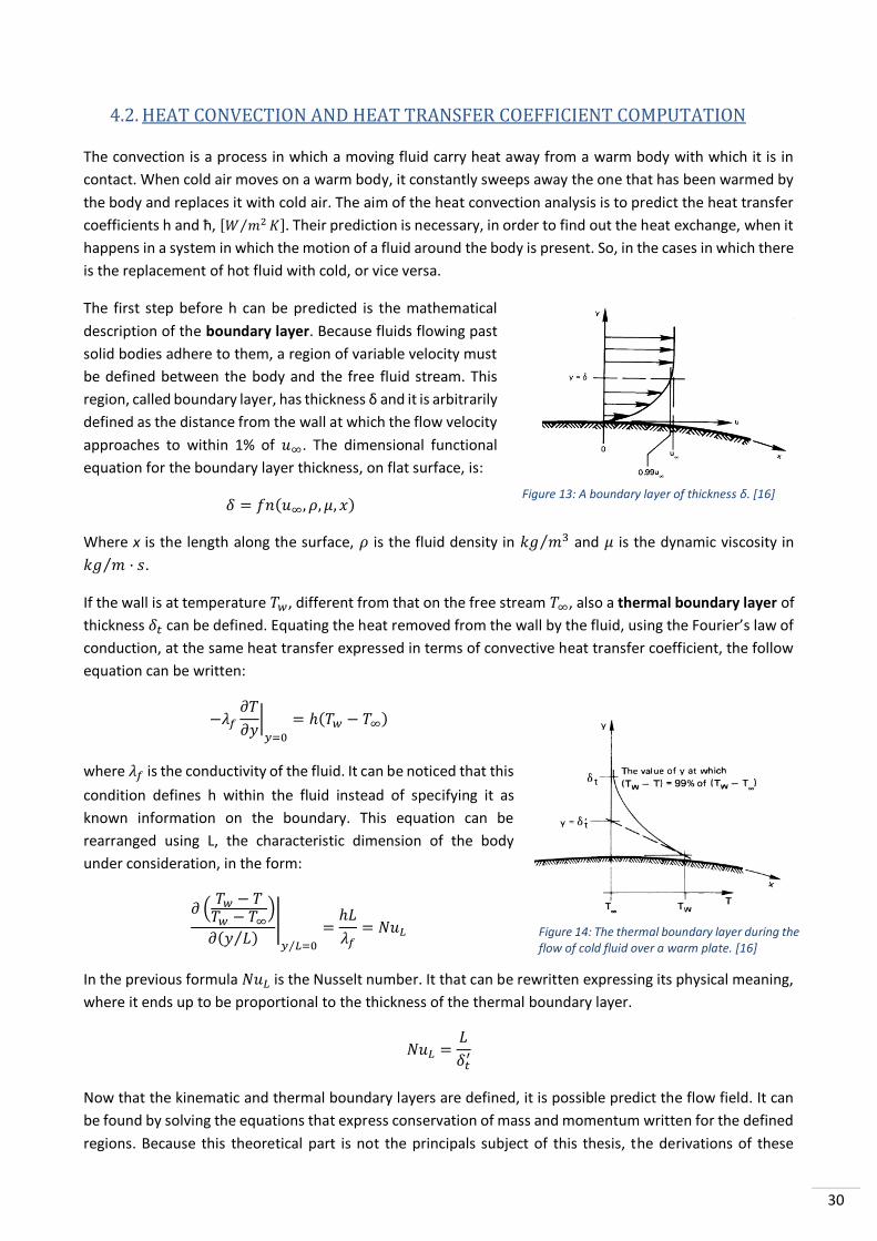
The first step before h can be predicted is the mathematical

description of the boundary layer. Because fluids flowing past

solid bodies adhere to them, a region of variable velocity must

be defined between the body and the free fluid stream. This

region, called boundary layer, has thickness δ and it is arbitrarily

defined as the distance from the wall at which the flow velocity

approaches to within 1% of 𝑢∞. The dimensional functional

equation for the boundary layer thickness, on flat surface, is:

𝛿 = 𝑓𝑛(𝑢∞, 𝜌, 𝜇, 𝑥)

Where x is the length along the surface, 𝜌 is the fluid density in 𝑘𝑔 𝑚3⁄ and 𝜇 is the dynamic viscosity in

𝑘𝑔 𝑚 · 𝑠⁄ .

If the wall is at temperature 𝑇𝑤, different from that on the free stream 𝑇∞, also a thermal boundary layer of

thickness 𝛿𝑡 can be defined. Equating the heat removed from the wall by the fluid, using the Fourier’s law of

conduction, at the same heat transfer expressed in terms of convective heat transfer coefficient, the follow

equation can be written:

−𝜆𝑓𝜕𝑇

𝜕𝑦|𝑦=0

= ℎ(𝑇𝑤 − 𝑇∞)

where 𝜆𝑓 is the conductivity of the fluid. It can be noticed that this

condition defines h within the fluid instead of specifying it as

known information on the boundary. This equation can be

rearranged using L, the characteristic dimension of the body

under consideration, in the form:

𝜕 (𝑇𝑤 − 𝑇𝑇𝑤 − 𝑇∞

)

𝜕(𝑦 𝐿⁄ )|

𝑦 𝐿⁄ =0

=ℎ𝐿

𝜆𝑓= 𝑁𝑢𝐿

In the previous formula 𝑁𝑢𝐿 is the Nusselt number. It that can be rewritten expressing its physical meaning,

where it ends up to be proportional to the thickness of the thermal boundary layer.

𝑁𝑢𝐿 =𝐿

𝛿𝑡′

Now that the kinematic and thermal boundary layers are defined, it is possible predict the flow field. It can

be found by solving the equations that express conservation of mass and momentum written for the defined

regions. Because this theoretical part is not the principals subject of this thesis, the derivations of these

Figure 13: A boundary layer of thickness δ. [16]

Figure 14: The thermal boundary layer during the flow of cold fluid over a warm plate. [16]

31

formulas are not reported. What follow is the two-dimensional continuity equation for incompressible flow

and the two forms of momentum equation for the steady, two-dimensional and incompressible flow.

𝜕𝑢

𝜕𝑥+𝜕𝑣

𝜕𝑦= 0

𝜕𝑢2

𝜕𝑥+𝜕𝑢𝑣

𝜕𝑦= −

1

𝜌

𝜕𝑝

𝜕𝑥+ 𝜈

𝜕𝑢2

𝜕𝑦2 𝑜𝑟 𝑢

𝜕𝑢

𝜕𝑥+ 𝑣

𝜕𝑢

𝜕𝑦= −

1

𝜌

𝜕𝑝

𝜕𝑥+ 𝜈

𝜕2𝑢

𝜕𝑦2

A complete derivation of the last equation would reveal that the result is valid for compressible flow as well.

Therefore, if there is no pressure gradient in the flow, it can be rewritten as:

𝜕𝑢2

𝜕𝑥+𝜕𝑢𝑣

𝜕𝑦= 𝑢

𝜕𝑢

𝜕𝑥+ 𝑣

𝜕𝑢

𝜕𝑦= 𝜈

𝜕2𝑢

𝜕𝑦2

This equation can be solved by means of the introduction of a stream function, 𝜓(𝑥, 𝑦) , that allows to reduce

the number of dependent variables, or by means of the momentum integral method. The first procedure

lead to the Exact solution that, for a flat surface where 𝑢∞ remains constant, can be defined as:

𝛿

𝑥=

4.92

√𝑢∞ 𝑥 𝜈⁄=4.92

√𝑅𝑒𝑥

𝑅𝑒𝑥 is called Reynolds number and it characterizes the relative influences of the inertial and viscous forces

in a fluid problem. This formula means that if the velocity is great or the viscosity is low, 𝛿 𝑥⁄ will be relatively

small, and the heat transfer will be relatively high.

The second one, instead, is an approximated method that simplify the solution given the boundary layers

similarity, and leads to a

𝛿

𝑥=4.64

√𝑅𝑒𝑥

The exact solution for 𝑢(𝑥, 𝑦) reveals that u can be expressed as a function of a single variable, η, and it leads

to what it is called the similarity solution:

𝑢

𝑢∞= 𝑓 (𝑦√

𝑢∞𝜈𝑥) = 𝑓(𝜂)

Now that the flow field in the boundary layer has been determined, the heat conduction equation must be

extended to take into account the motion of the fluid. Starting from the conservation of energy, it is possible

to write the energy equation for incompressible fluids reported on the left. After, it can be modified for a

two-dimensional flow without heat sources in a boundary layer, obtaining the equation on the right.

𝜌𝑐𝑝 (𝜕𝑇

𝜕𝑡+ �⃗⃗� · 𝛻𝑇) = 𝑘𝛻2𝑇 + �̇� 𝑎𝑛𝑑 𝑢

𝜕𝑇

𝜕𝑥+ 𝑣

𝜕𝑇

𝜕𝑦= 𝛼

𝜕2𝑇

𝜕𝑡2

The temperature field in the boundary layer is the solution of the equation on the right and it can be inserted

in the Fourier’s law in order to compute h as follow

ℎ =𝑞

𝑇𝑤 − 𝑇∞= −

𝜆

𝑇𝑤 − 𝑇∞

𝜕𝑇

𝜕𝑦|𝑦=0

32

4.3. LOGARITMIC MEAN TEMPERATURE DIFFERENCE AND CORRECTION FACTOR

In general cases U vary with the position in the exchanger and with the local temperature. At first, we can

suppose it as a constant value, still reasonable assumption in compact single-phase heat exchangers. In these

cases, the overall heat transfer can be written in term of mean temperature difference between the two fluid

streams:

𝑄 = 𝑈𝐴𝛥𝑇𝑚𝑒𝑎𝑛

The problem then reduces to finding the appropriate mean temperature that will make this equation true.

Analysing the simple parallel and counterflow configurations, the temperature variation can be plotted for

both, as reported in Figure 15. Notice that temperatures change more rapidly in the parallel-flow

configuration and so less length is required. However, the counterflow arrangement achieves generally more

complete heat exchange from one flow to the other. The determination of 𝛥𝑇𝑚𝑒𝑎𝑛 for such arrangements

proceeds as follows. Defining the differential heat

transfer within either arrangement as:

𝑑𝑄 = 𝑈𝛥𝑇𝑑𝐴 = −(�̇�𝑐𝑝)ℎ𝑑𝑇ℎ = ±(�̇�𝑐𝑝)𝑐

𝑑𝑇𝑐

Introducing the total heat capacity of the hot and cold

streams, 𝐶ℎ = (�̇�𝑐𝑝)ℎ 𝑎𝑛𝑑 𝐶𝑐 = (�̇�𝑐𝑝)𝑐

[W/K], we

find the below reported equation. If we integrate it for

both cases, parallel and counterflow, it gives us the

relations between the hot and cold fluid temperature

in every point:

∓𝐶ℎ𝑑𝑇ℎ = 𝐶𝑐𝑑𝑇𝑐 →

𝑝𝑎𝑟𝑎𝑙𝑙𝑒𝑙 𝑓𝑙𝑜𝑤 [−𝐶ℎ]

𝐵. 𝐶.: 𝑇ℎ = 𝑇ℎ,𝑖𝑛 𝑇𝑐 = 𝑇𝑐,𝑖𝑛

𝑐𝑜𝑢𝑛𝑡𝑒𝑟𝑓𝑙𝑜𝑤 [+𝐶ℎ]

𝐵. 𝐶.: 𝑇ℎ = 𝑇ℎ,𝑖𝑛 𝑇𝑐 = 𝑇𝑐,𝑜𝑢𝑡

→ 𝑇ℎ = 𝑇ℎ,𝑖𝑛 −𝐶𝑐𝐶ℎ(𝑇𝑐 − 𝑇𝑐,𝑖𝑛) = 𝑇ℎ,𝑖𝑛 −

𝑄

𝐶ℎ

→ 𝑇ℎ = 𝑇ℎ,𝑖𝑛 −𝐶𝑐𝐶ℎ(𝑇𝑐,𝑜𝑢𝑡 − 𝑇𝑐) = 𝑇ℎ,𝑖𝑛 −

𝑄

𝐶ℎ

Where Q is the total heat transfer from the entrance to the point of interest. The above equations can be

solved for the local temperature differences:

𝛥𝑇𝑝𝑎𝑟𝑎𝑙𝑙𝑒𝑙 = 𝑇ℎ − 𝑇𝑐 = 𝑇ℎ,𝑖𝑛 − (1 +𝐶𝑐𝐶ℎ) 𝑇𝑐 +

𝐶𝑐𝐶ℎ𝑇𝑐,𝑖𝑛

𝛥𝑇𝑐𝑜𝑢𝑛𝑡𝑒𝑟 = 𝑇ℎ − 𝑇𝑐 = 𝑇ℎ,𝑖𝑛 − (1 +𝐶𝑐𝐶ℎ)𝑇𝑐 −

𝐶𝑐𝐶ℎ𝑇𝑐,𝑖𝑛

Replacing the founded formulas in 𝑑𝑄 = 𝐶𝑐𝑑𝑇𝑐 = 𝑈𝛥𝑇𝑑𝐴 and making further integration, shall be obtained:

𝑄 = 𝑈𝐴(𝛥𝑇𝑎 − 𝛥𝑇𝑏ln (𝛥𝑇𝑎 𝛥𝑇𝑏⁄ )

)

The 𝛥𝑇𝑚𝑒𝑎𝑛 for use in the initial equation is thus the logarithmic mean temperature difference (LMTD):

𝛥𝑇𝑚𝑒𝑎𝑛 = 𝐿𝑀𝑇𝐷 =𝛥𝑇𝑎 − 𝛥𝑇𝑏

ln (𝛥𝑇𝑎𝛥𝑇𝑏

)

Figure 15: Temperature variation through parallel and counterflow single-pass heat exchanger. [16]

33

It must be observed than, if U were variable the integration of the total heat transfer Q would give a different

expression as result. This means that, as already said, in most of the cases the variability of U would have to

be considered and it changes the value of the 𝛥𝑇𝑚𝑒𝑎𝑛. As example of this phenomenon, the vaporization

phase showed in Figure 16 is a typical situation in which the variation of U within a heat exchanger might be

great, and so it cannot be considered constant. The figure

below shows a typical situation, e.g. vaporization phase, in

which the variation of U within a heat exchanger might be

great. In this case, the heat exchange mechanism on the

water side is completely altered when the liquid is finally

boiled away. If U where uniform in each portion of the heat

exchanger, then we could treat it as two different

exchangers in series. However, in the heat exchangers in

which U varies continuously with position, as in large

industrial shell-and-tube configurations, the analysis

presented must be done using an average value of U,

defined as:

𝑈 =∫ 𝑈𝑑𝐴𝐴

0

𝐴

Another limitation in the use of an LMTD is its restriction to single-pass parallel and counterflow

configurations. As a matter of fact, each configuration must be analysed separately and the results are

generally more complicated than the expression reported in the previous investigation. All the calculations

for every possible configurations have been already done in 1940 by Bowman, Muller and Nagle, and after

by TEMA. Now a day, thanks to the organization of these data, the restriction given from different layout can

be simply overcome multiplying the LMTD by a coefficient F.

𝑄 = 𝑈𝐴(𝐿𝑀𝑇𝐷) · 𝐹(𝑃, 𝑅)

Where:

𝑃 =𝑇𝑡,𝑜𝑢𝑡 − 𝑇𝑡,𝑖𝑛𝑇𝑠,𝑖𝑛 − 𝑇𝑡,𝑖𝑛

=𝑟𝑒𝑙𝑎𝑡𝑖𝑣𝑒 𝑖𝑛𝑓𝑙𝑢𝑒𝑛𝑐𝑒 𝑜𝑓 𝑡ℎ𝑒 𝑜𝑣𝑒𝑟𝑎𝑙𝑙 𝑡𝑒𝑚𝑝𝑒𝑟𝑎𝑡𝑢𝑟𝑒 𝑑𝑖𝑓𝑓𝑒𝑟𝑒𝑛𝑐𝑒 (𝑇𝑠,𝑖𝑛 − 𝑇𝑡,𝑖𝑛)

𝑜𝑛 𝑡ℎ𝑒 𝑡𝑢𝑏𝑒 𝑓𝑙𝑜𝑤 𝑡𝑒𝑚𝑝𝑒𝑟𝑎𝑡𝑢𝑟𝑒. 𝐼𝑡 𝑚𝑢𝑠𝑡 𝑜𝑏𝑣𝑖𝑜𝑢𝑠𝑙𝑦 𝑏𝑒 𝑙𝑒𝑠𝑠 𝑡ℎ𝑎𝑛 𝑢𝑛𝑖𝑡𝑦.

𝑅 =𝑇𝑠,𝑖𝑛 − 𝑇𝑠,𝑜𝑢𝑡𝑇𝑡,𝑜𝑢𝑡 − 𝑇𝑡,𝑖𝑛

= 𝑒𝑞𝑢𝑎𝑙𝑠 𝑡ℎ𝑒 ℎ𝑒𝑎𝑡 𝑐𝑎𝑝𝑎𝑐𝑖𝑡𝑦 𝑟𝑎𝑡𝑖𝑜 𝐶𝑡 𝐶𝑠⁄

𝑇𝑡 = 𝑡𝑒𝑚𝑝𝑒𝑟𝑎𝑡𝑢𝑟𝑒 𝑜𝑓 𝑡ℎ𝑒 𝑡𝑢𝑏𝑒 𝑓𝑙𝑜𝑤

𝑇𝑠 = 𝑡𝑒𝑚𝑝𝑒𝑟𝑎𝑡𝑢𝑟𝑒 𝑜𝑓 𝑡ℎ𝑒 𝑠ℎ𝑒𝑙𝑙 𝑓𝑙𝑜𝑤

Therefore, the factor F is an LMTD correction that varies from unity to zero. It is defined in such a way that

the LMTD temperature should always be calculated for the equivalent counterflow single-pass exchanger

with the same hot and cold temperatures. In the case in which one flow remains at constant temperature,

then either P or R will be equal to zero, and the configuration of the heat exchanger becomes irrelevant. In

this case the simple LMTD will be the correct 𝛥𝑇𝑚𝑒𝑎𝑛 and F must go to unit. As example, two curves taken by

TEMA are presented below. Please note than the Figure 17 and Figure 18 only include the curves for R≤1,

and them must be modified if the tube-and-shell heat exchanger, given its large number of baffles, behave

Figure 16: A typical case of a heat exchanger in which U varies dramatically. [16]

34

like a series of cross-flow exchangers. For the curves with R>1 has been noticed than the value of F may be

obtained using a simple reciprocal rule: F(P,R)=F(PR,1/R)

Figure 17: F for a one-shell-pass, four-, six-,…-tube-pass exchanger. [16]

Figure 18: F for a two-shell-pass, four or more tube-pass exchanger. [16]

35

4.4. EFFECTIVENESS – NTU METHOD

During design activity often the heat exchanger

configuration is known, while the outlet temperatures of

the pipes are unknown. In this case we cannot proceed

with the LMTD method because we don’t know the

temperature difference, consequently the computation of

the LMTD result impossible. The only analytical way to

solve the problem is to adopt an iterative method in which

the outlet temperatures are estimated such as to make

𝑄ℎ = 𝑄𝑐 = 𝐶ℎ𝛥𝑇ℎ = 𝐶𝑐𝛥𝑇𝑐. The correct outlet

temperatures will be find when 𝑄ℎ is equal to the heat

exchanged computed by the LMTD, 𝑄 = 𝑈𝐴𝐹(𝐿𝑀𝑇𝐷).

Since in the compact heat exchangers the overall heat transfer coefficient is far more likely to remain

uniform, the effectiveness-NTU method can be used to simplify the problem.

Defining the number of transfer unit NTU as dimensionless group that can be viewed as a comparison of the

heat capacity of the heat exchanger, expressed in W/K, with the heat capacity of the flow. It can be written

physically as:

𝑁𝑇𝑈 =𝑈𝐴

𝐶𝑚𝑖𝑛

Where 𝐶𝑚𝑖𝑛 is the smallest of 𝐶ℎ and 𝐶𝑐.

The effectiveness instead can be founded graphically in function of the 𝐶𝑚𝑖𝑛 𝐶𝑚𝑎𝑥⁄ ratio and NTU

휀 =𝑎𝑐𝑡𝑢𝑎𝑙 ℎ𝑒𝑎𝑡 𝑡𝑟𝑎𝑛𝑠𝑓𝑒𝑟

𝑚𝑎𝑥𝑖𝑚𝑢𝑚 ℎ𝑒𝑎𝑡 𝑡ℎ𝑎𝑡 𝑐𝑜𝑢𝑙𝑑 𝑝𝑜𝑠𝑠𝑖𝑏𝑙𝑦 𝑏𝑒 𝑡𝑟𝑎𝑛𝑠𝑓𝑒𝑟𝑟𝑒𝑑 𝑓𝑟𝑜𝑚 𝑜𝑛𝑒 𝑠𝑡𝑟𝑒𝑎𝑚 𝑡𝑜 𝑡ℎ𝑒 𝑜𝑡ℎ𝑒𝑟

=𝐶ℎ(𝑇ℎ,𝑖𝑛 − 𝑇ℎ,𝑜𝑢𝑡)

𝐶𝑚𝑖𝑛(𝑇ℎ,𝑖𝑛 − 𝑇𝑐,𝑖𝑛)=𝐶𝑐(𝑇𝑐,𝑜𝑢𝑡 − 𝑇𝑐,𝑖𝑛)

𝐶𝑚𝑖𝑛(𝑇ℎ,𝑖𝑛 − 𝑇𝑐,𝑖𝑛)= 𝑓𝑛 (

𝐶𝑚𝑖𝑛𝐶𝑚𝑎𝑥

, 𝑁𝑇𝑈)

Figure 20: The effectiveness of parallel and counterflow heat exchangers. [16]

Figure 19: Example of a design problem. [16]

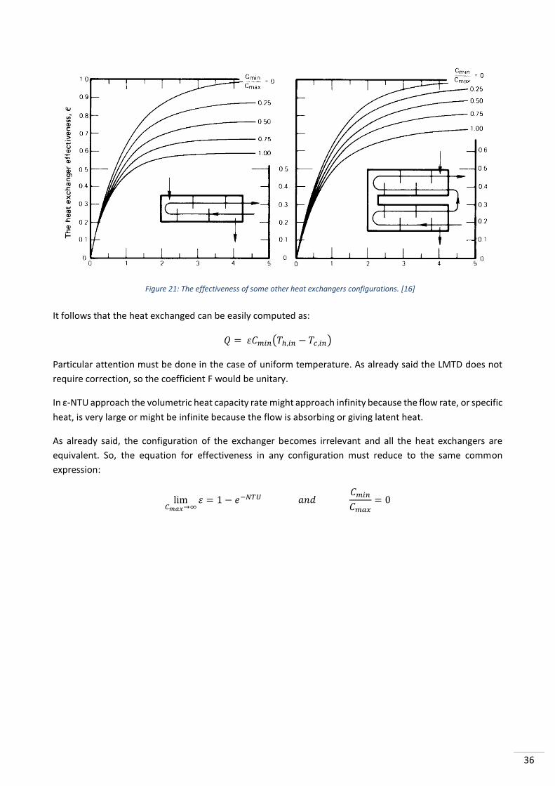
36

It follows that the heat exchanged can be easily computed as:

𝑄 = 휀𝐶𝑚𝑖𝑛(𝑇ℎ,𝑖𝑛 − 𝑇𝑐,𝑖𝑛)

Particular attention must be done in the case of uniform temperature. As already said the LMTD does not

require correction, so the coefficient F would be unitary.

In ε-NTU approach the volumetric heat capacity rate might approach infinity because the flow rate, or specific

heat, is very large or might be infinite because the flow is absorbing or giving latent heat.

As already said, the configuration of the exchanger becomes irrelevant and all the heat exchangers are

equivalent. So, the equation for effectiveness in any configuration must reduce to the same common

expression:

lim𝐶𝑚𝑎𝑥→∞

휀 = 1 − 𝑒−𝑁𝑇𝑈 𝑎𝑛𝑑 𝐶𝑚𝑖𝑛𝐶𝑚𝑎𝑥

= 0

Figure 21: The effectiveness of some other heat exchangers configurations. [16]

37

4.5. HEAT TRANSFER IN PHASE CHANGE CONFIGURATIONS

MODES OF POOL BOILING

The Figure 22 shows, at atmospheric pressure, a complete

boiling curve for saturated water. It has been divided into

five regimes of behavior which will be now discussed,

including the transition phases that divide them.

Natural convection

If water is not in contact with its own vapour, it does not boil

at the so-called normal boiling point, Tsat. Indeed, the heat

continue to be removed by natural convection, and it

continues to rise in temperature until bubbles finally begin

to form. This occurs when a conventional machined metal

surfaces is a few degrees above Tsat.

Nucleate boiling

The nucleate boiling regime embraces the two distinct

regimes that lie between bubble inception and first

transition point.

• The region of isolated bubbles: in this range, bubbles rise from isolated nucleation sites. As q and ΔT

increase, more and more sites are activated. Figure 23.a is a photograph of this regimes as it appears

on horizontal plate.

• The region of slugs and columns: when the activate sites become very numerous, the bubble start to

merge one to another, and an entirely different vapour escape path comes into play. Vapour formed

at the surface joint into jets that feed into large overhead bubbles or “slugs” of vapour. This process

is shown as it occurs on a horizontal cylinder in Figure 23.b.

Peak heat flux

At the upper end of slugs and columns region the temperature difference is low, while the heat flux is very

high. Clearly this means that the heat transfer coefficients in this range are enormous and it is very desirable

be able to make heat exchange equipment work in this point. However, it is very dangerous to run equipment

near qmax in system for which q is the independent variable. If q is raised beyond the upper limit of the

nucleate boiling regime, such a system will suffer a sudden and damaging increase of temperature. This

transition is called by a variety of name: the burnout point; the peak heat flux; the boiling crisis; the DNB

(Departure from Nucleate Boiling) or the CHF (Critical Heat Flux).

Transitional boiling regime

It is a curious fact that the heat flux actually diminishes with ΔT after qmax is reached. In this regime the

effectiveness of the vapour escape process become worse and worse. Furthermore, the hot surface becomes

completely blanketed in vapour and q reaches a minimum heat flux, qmin. Figure 23.c shows two typical

instances of traditional boiling just beyond the peak heat flux.

Figure 22: Typical boiling curve and regimes of boiling for an unspecified heat surface. [16]

38

Film boiling

Once a stable vapor blanket is established, q again increases with increasing ΔT. The mechanics of the heat

removal process during film boiling, and the regular removal of bubbles, has a great deal in common with

film condensation but heat transfer coefficients are much lower because het must be conducted through a

vapour film instead of through a liquid film. In Figure 23.d an instance of film boiling can be seen.

Figure 23: Typical photographs of boiling in the four regimes identified in Figure 22. [16]

39

NUCLEATE BOILING

INCEPTION OF BOILING

The analysis of the inception of boiling starts from the highly enlarged sketch of a heater surface, shown in

Figure 24. Most metal finishing operations engrave tiny grooves on the surface. Moreover, some chattering

or bouncing action leave small holes on the plane that has been worked. When a surface is wetted, the

surface tension prevents the liquid from entering these holes. So, small gas or vapor pockets, representing

the sites at which bubble nucleation occurs, are formed.

The problem can be highly idealized supposing a spherical bubble of pure saturated steam in equilibrium with

an infinite superheated liquid. The p–v diagram in Figure 25 shows the state points of the internal vapor and

external liquid for a bubble at equilibrium. Notice that the external liquid is superheated to (Tsup-Tsat)·K above

its boiling point at the ambient pressure. However, the vapor inside, being held at just the right elevated

pressure by surface tension, is just saturated. To determine the size of such a bubble, the conditions of

mechanical and thermal equilibrium have been imposed. The bubble will be in mechanical equilibrium when

the pressure difference between the inside and the outside of the bubble is balanced by the forces of surface

tension, σ. Thermal equilibrium, instead, requires that the temperature must be the same inside and outside

of the bubble. Since the vapor inside must be saturated at Tsat because it is in contact with its liquid, the force

balance takes the form

(𝑝𝑖𝑛 − 𝑃𝑜𝑢𝑡)𝜋𝑅𝑏2 = (2𝜋𝑅𝑏)𝜎

Which allow to find an expression for the radius

of the equilibrium bubble.

𝑅𝑏 =2𝜎

𝑝𝑖𝑛 − 𝑝𝑜𝑢𝑡=

2𝜎

(𝑝𝑠𝑎𝑡 𝑎𝑡 𝑇𝑠𝑢𝑝) − 𝑝𝑎𝑚𝑏𝑖𝑒𝑛𝑡

Note that the equilibrium bubble is unstable.

Indeed, if its radius is less than this value,

surface tension will overbalance [𝑝𝑠𝑎𝑡(𝑇𝑠𝑢𝑝) −

𝑝𝑎𝑚𝑏𝑖𝑒𝑛𝑡]. Thus, vapor inside will condense at

this higher pressure and the bubble will

collapse. If the bubble radius is slightly larger

than the one specified by the equation, liquid at the interface will evaporate and the bubble will begin to

grow. Thus, as the heater surface temperature is increased, higher and higher values of [𝑝𝑠𝑎𝑡(𝑇𝑠𝑢𝑝) −

𝑝𝑎𝑚𝑏𝑖𝑒𝑛𝑡] will result and the equilibrium radius, Rb, will decrease in accordance with the previous equation.

It follows that smaller and smaller vapor pockets will be triggered into active bubble growth as the

temperature is increased. As an approximation, we can use the equation that describe the radius of the

equilibrium bubble to specify the radius of those vapor pockets that become active nucleation sites.

Figure 24: Enlarged sketch of a typical metal surface. [16]

Figure 25: the conditions required for simultaneous mechanical and thermal equilibrium of a vapour bubble. [16]

40

More accurate estimates can be made using Hsu’s bubble inception theory, or the still more recent technical

literature. In order to present all the data necessary for the discussion, the value of the surface tension σ for

several substances are reporter in the table below.

Figure 26: Surface tension of various substances from the collection of Jasper [22] and other sources [21] [24] [25].

41

REGION OF ISOLATED BUBBLES AND NUCLEATE POOL BOILING HEAT FLUX CORRELATION

In the last century the mechanism of heat transfer enhancement in the isolated bubble regime was hotly

argued. The conclusion that have been made was that the bubbles “act as small pumps” that keep replacing

liquid heated at the wall with cool liquid. The real problem is to specify the correct mechanism thanks to

which this happens. Figure 27 shows the way bubbles probably act to remove hot liquid from the wall and

introduce cold liquid to be heated. The two images on the left show a bubble growing and departing in

saturated liquid. To grows, the bubble needs to absorb heat from the superheated liquid on its periphery.

When the bubble leaves, the cold liquid is entrained onto the plate, which then warms up until nucleation

occurs and the cycle repeats. On the right, instead, a bubble growing in subcooled liquid is shown. When the

bubble protrudes into cold liquid, a short-circuit for cooling the wall is provided. Indeed, the steam can

condense on the top while evaporation continues on the bottom. Then the cold liquid is brought to the wall

when the bubble caves in.

It is evident that the number of active nucleation sites generating bubbles will strongly influence q. So, a

direct dependence can be written in the following ways:

𝑞 ∝ 𝛥𝑇𝑎𝑛𝑏

Where 𝛥𝑇 = 𝑇𝑤 − 𝑇𝑠𝑎𝑡 and n is the site density or number of active sites per square meter. The exponents

turn out to be, approximately, a=1,2 and b=1/3. The problem with this formulation is that n is a nuisance

variable because it varies from system to system and cannot easily be evaluated. Indeed, normally n increase

with ΔT, but it can increase in different way. If all sites were identical in size, they would be activated

simultaneously, and q would be a discontinuous function of ∆T. When the sites have a typical distribution of

sizes, n and q can increase very strongly with ΔT. Luckily, for a large class of factory-finished materials, n

varies between ΔT5 and ΔT 6, so q varies roughly as ΔT3. This makes possible to correlate q approximately for

a large variety of materials with a formulation like the following

𝑐𝑝(𝑇𝑤 − 𝑇𝑠𝑎𝑡)

ℎ𝑓𝑔𝑃𝑟𝑠 = 𝐶𝑠𝑓 [

𝑞

𝜇ℎ𝑓𝑔−√

𝜎

𝑔(𝜌𝑓 − 𝜌𝑔)]

0.33

where all properties are for liquid at Tsat. The hfg is the latent heat of vaporization and the constant Csf is an

empirical correction for typical surface conditions. Figure 28 includes a set of values of Csf for common

surfaces as well as the Prandtl number exponent, s.

Figure 27: Heat removal by bubble action during boiling. Dark regions denote locally superheated liquid. [16]

42

As initially denoted, there are two nucleate boiling regimes, the region of isolated bubble and the region of

slugs and columns. While the first correlation applied only to the first of them, this last equation represents

q(ΔT) in both. This happens because it is empirical and it is not depending from the rational analysis of either

nucleate boiling process. However, it is not very accurate for either of them. Thus, the ability to predict the

nucleate pool boiling heat flux is poor due to the dependence of the nuisance variable n, and there is still not

achieved a reliable heat transfer design relationship for nucleate boiling. Generally, the major problem in the

nucleate boiling regime is to avoid exceeding qmax, rather than to calculate q given ∆T, which is not often

required.

Figure 28: Selected values of the surface correction factor and Prandtl number exponent. [16]

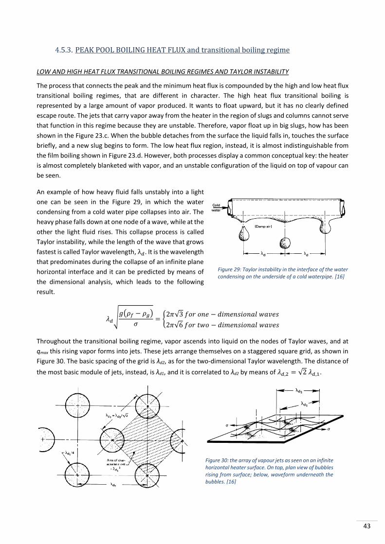
43

PEAK POOL BOILING HEAT FLUX and transitional boiling regime

LOW AND HIGH HEAT FLUX TRANSITIONAL BOILING REGIMES AND TAYLOR INSTABILITY

The process that connects the peak and the minimum heat flux is compounded by the high and low heat flux

transitional boiling regimes, that are different in character. The high heat flux transitional boiling is

represented by a large amount of vapor produced. It wants to float upward, but it has no clearly defined

escape route. The jets that carry vapor away from the heater in the region of slugs and columns cannot serve

that function in this regime because they are unstable. Therefore, vapor float up in big slugs, how has been

shown in the Figure 23.c. When the bubble detaches from the surface the liquid falls in, touches the surface

briefly, and a new slug begins to form. The low heat flux region, instead, it is almost indistinguishable from

the film boiling shown in Figure 23.d. However, both processes display a common conceptual key: the heater

is almost completely blanketed with vapor, and an unstable configuration of the liquid on top of vapour can

be seen.

An example of how heavy fluid falls unstably into a light

one can be seen in the Figure 29, in which the water

condensing from a cold water pipe collapses into air. The

heavy phase falls down at one node of a wave, while at the

other the light fluid rises. This collapse process is called

Taylor instability, while the length of the wave that grows

fastest is called Taylor wavelength, λ𝑑. It is the wavelength

that predominates during the collapse of an infinite plane

horizontal interface and it can be predicted by means of

the dimensional analysis, which leads to the following

result.

𝜆𝑑√𝑔(𝜌𝑓 − 𝜌𝑔)

𝜎= {

2𝜋√3 𝑓𝑜𝑟 𝑜𝑛𝑒 − 𝑑𝑖𝑚𝑒𝑛𝑠𝑖𝑜𝑛𝑎𝑙 𝑤𝑎𝑣𝑒𝑠

2𝜋√6 𝑓𝑜𝑟 𝑡𝑤𝑜 − 𝑑𝑖𝑚𝑒𝑛𝑠𝑖𝑜𝑛𝑎𝑙 𝑤𝑎𝑣𝑒𝑠

Throughout the transitional boiling regime, vapor ascends into liquid on the nodes of Taylor waves, and at

qmax this rising vapor forms into jets. These jets arrange themselves on a staggered square grid, as shown in

Figure 30. The basic spacing of the grid is λd2, as for the two-dimensional Taylor wavelength. The distance of

the most basic module of jets, instead, is λd1, and it is correlated to λd2 by means of 𝜆𝑑,2 = √2 𝜆𝑑,1.

Figure 30: the array of vapour jets as seen on an infinite horizontal heater surface. On top, plan view of bubbles rising from surface; below, waveform underneath the bubbles. [16]

Figure 29: Taylor instability in the interface of the water condensing on the underside of a cold waterpipe. [16]

44

HELMHOLTZ INSTABILITY OF VAPOUR JETS

The Helmholtz instability, which can be seen in Figure 31, explain how the jets become unstable at the peak

and why they cave in when the vapour velocity in them reaches a critical value. It is a fluid dynamic instability

caused by different layers of the fluid in relative motion one with respect to one other. A high-pressure zone

is present where the fluid velocity is low, while a lower pressure zone is the result of higher velocity layer.

The state of collapse occurs when the interface that divides two regions undergoes small disturbance. Indeed,

particles of fluid that before was at rest end

up being in a one where there is a velocity

field. This phenomenon generally leads to

instability, which, however, does not always

occur in vapour jets. Indeed, the surface

tension in the jet walls tends to balance the

flow-induced pressure forces that bring

about collapse. As a matter of fact, since the

vapor velocity in the jet must reach a limiting

value, ug, before state of collapse occurs, the

jet is not always unstable. The following expression has been taken from [6] and exhibit the relation between

the vapor flow, ug, and the wavelength of a disturbance in the jet wall, λH.

𝑢𝑔 = √2𝜋𝜎

𝜌𝑔𝜆𝐻

However, a real liquid–vapor interface will usually be irregular, and therefore it can be viewed as containing

all possible sinusoidal wavelengths superposed on one another. Then, in order to develop the most

representative wavelength, the one more liable to collapse must be guessed. So, the Helmholtz instability is

a theory that only approximate the problem of vapour jets collapse.

PREDICTION OF qmax

In order to write a general expression for qmax, it has to be observed that the heat flux must be balanced by

the latent heat carried away in the jets when the liquid is saturated. Thus, the following formula can be

immediately written:

𝑞𝑚𝑎𝑥 = 𝜌𝑔ℎ𝑓𝑔𝑢𝑔 (𝐴𝑗

𝐴ℎ)

where Ah is the heater area that supplies each jet and Aj is the cross-sectional area of a jet. The problem of

qmax prediction in any pool boiling configuration always comes down to the determination of two parameters.

One is the length of the perturbation in the jet wall, λH, which will trigger Helmholtz instability and fix ug. So,

the value of ug that must be inserted in the above equation can be found from the Helmholtz one. The other

is the ratio 𝐴𝑗 𝐴ℎ⁄ . The specific expression for every heater configuration can be found imposing a correct

value of the jet radius or by means of the dimensional analysis. This last procedure leads to have two pi-

groups in function of the Bond number, Bo, used to compare buoyant force with capillary force. Attention

must be paid in the case in which 𝐵𝑜 < 1 44⁄ , where the process become completely dominated by surface

tension and the Helmholtz wave mechanism no longer operate. In this particular case the mechanism of heat

removal passes directly from natural convection to film boiling.

Figure 31: Helmholtz instability of vapour jets. [16]

45

FILM BOILING AND RADIATION CONTRIBUTION

The similarity between the film boiling and the film condensation is so great that, in 1950, Bromley was able

to adapt the equation for condensation on cylinders to the film boiling prediction. Indeed, modifying the

boundary conditions in the film condensation analysis and changing k and ν from liquid to vapor properties,

he writes the following equation for the 𝑁𝑢̅̅ ̅̅ 𝐷. D is the characteristic dimension of the body under

consideration, so, in this formulation it is the diameter of the cylinder.

𝑁𝑢̅̅ ̅̅ 𝐷 = 0.62 [(𝜌𝑓 − 𝜌𝑔)𝑔ℎ𝑓𝑔

′ 𝐷3

𝑣𝑔𝑘𝑔(𝑇𝑤 − 𝑇𝑠𝑎𝑡)]

14⁄

The vapor and liquid properties should be evaluated at Tsat + ΔT/2 and at Tsat respectively. The constant value

of 0.62 was fixed by means of the comparison between the equation with experimental data values.

However, when the Prandtl number is large, e.g. Pr≥0.6, the latent heat needs to be corrected using the

formulation below:

ℎ𝑓𝑔′ = ℎ𝑓𝑔[1 + (0.968 − 0.163 𝑃𝑟𝑔⁄ )𝐽𝑎𝑔] 𝑤ℎ𝑒𝑟𝑒 𝐽𝑎𝑔 = 𝑐𝑝𝑔(𝑇𝑤 − 𝑇𝑠𝑎𝑡) ℎ𝑓𝑔⁄

Is there also reported the formulation for the film boiling on the spheres

𝑁𝑢̅̅ ̅̅ 𝐷 = 0.67 [(𝜌𝑓 − 𝜌𝑔)𝑔ℎ𝑓𝑔

′ 𝐷3

𝑣𝑔𝑘𝑔(𝑇𝑤 − 𝑇𝑠𝑎𝑡)]

14⁄

In these expressions only the heat transfer by convection through the vapor film is present. Radiation,

instead, can be enormous when film boiling occurs much beyond qmin in water. In this case is not sufficient

to add a radiation heat transfer coefficient ℎ̅𝑟𝑎𝑑 to ℎ̅𝑏𝑜𝑖𝑙𝑖𝑛𝑔because this phenomenon will increase the vapor

blanket thickness, reducing the convective contribution. One approximate relation for the cylinder

application is reported below. However, an accurate correction for every specific case would be needed.

ℎ̅𝑡𝑜𝑡𝑎𝑙 = ℎ̅𝑏𝑜𝑖𝑙𝑖𝑛𝑔 +3

4ℎ̅𝑟𝑎𝑑 , 𝑤ℎ𝑒𝑟𝑒 ℎ̅𝑟𝑎𝑑 =

𝑞𝑟𝑎𝑑𝑇𝑤 − 𝑇𝑠𝑎𝑡

=휀𝜎(𝑇𝑤

4 − 𝑇𝑠𝑎𝑡4 )

𝑇𝑤 − 𝑇𝑠𝑎𝑡< ℎ̅𝑏𝑜𝑖𝑙𝑖𝑛𝑔

Where ε is a surface radiation property of the heater called emittance. It is worth noting that radiation is

seldom important when the heater temperature is less than 300°C.

The analogy between film condensation and film boiling cannot be assumed as valid during film boiling on a

vertical surface, because on the liquid-vapour interface the Helmholtz instability occurs for a certain distance

from the leading edge. However, it has been proved that using 𝜆𝑑,1 √3⁄ in place of D in the first equation, it

can be obtained a very satisfactory prediction of ℎ̅ for rather tall vertical plates. The analogy adopted also

deteriorates when it is applied to small curved bodies. This happens because the vapor film in boiling is

thicker than the liquid film during condensation. Consequently, in curved bodies a correction is needed even

if it could be ignored in film condensation. This curvature correction, to be made when R < 1.86, is:

𝑁𝑢̅̅ ̅̅ 𝐷′ = [(0.715 +

0.263

𝑅′) (𝑅′)1 4⁄ ]𝑁𝑢̅̅ ̅̅ 𝐷

46

MINIMUM HEAT FLUX

For the prediction of the minimum heat flux qmin it is assumed that, as (𝑇𝑤 − 𝑇𝑠𝑎𝑡) is reduced in the film

boiling regime, the rate of vapor generation becomes too small to support the Taylor wave action which

characterizes film boiling. The equation for horizontal heaters was firstly predicted from Zuber and after

corrected, on the basis of experimental data, by Berenson in the following formula

𝑞𝑚𝑖𝑛 = 0.09𝜌𝑔ℎ𝑓𝑔√𝜎𝑔(𝜌𝑓 − 𝜌𝑔)

(𝜌𝑓 − 𝜌𝑔)2

4

The parallel prediction of the equation for horizontal wires was made by Lienhard and Wong, and lead to the

below correction

𝑞𝑚𝑖𝑛,𝑤𝑖𝑟𝑒𝑠 = 0.515 [18

𝑅′2(2𝑅′2 + 1)]1 4⁄

𝑞𝑚𝑖𝑛

The problem with all these expressions is that, when the film boiling heat fluxes are higher than the minimum,

some contact frequently occurs between the liquid and the heater wall. In this case, the boiling curve deflects

above the film boiling curve finding a higher minimum than the ones reported above. The values of the

constants shown above should therefore be viewed as practical lower limits of qmin.

47

5. THERMAL DESIGN OF THE HEAT EXCHANGER: CASE STUDY

5.1. INTRODUCTION TO THE THERMAL DESIGN

In order to obtain the required heat flux between the fluids, a certain amount of exchange area is needed.

The goal of the heat exchanger’s thermal design is to find that value and the best heat exchanger

configuration for the case. Apart from predicting heat transfer, a host of traditional considerations must be

addressed in design heat exchangers, for example the minimization of pumping power and the minimization

of fixed cost. After a brief introduction on thermal design, the document will be focus only on the used

program. In this section are provided all the explanation about the choice that has been taken during the

thermal design activity.

LOGICAL APPROACH TO THE MANUAL THERMAL DESIGN

To better understand the curse of the design process, faced with such an array of trade-offs of advantages

and penalties, a list of design considerations for a large shell-and-tube exchanger design is here reported:

- Decide which fluid should flow on the shellside and which one should flow in the tubes. Normally,

this decision will be made to minimize the cost. Later some useful advices are listed:

o Put dirty stream on the tubeside because is easier to clean inside the tube;

o Put high pressure stream on the tubeside to avoid thick and expensive shell;

o When special materials are required for one stream, put that one on the tubeside to avoid

expensive shell;

o Cross flow gives higher coefficients than in plain tubes, hence put the fluid with lowest

coefficient on the shellside;

o The more viscous oil would flow in the shell in order to minimize the pumping cost;

o Corrosion behaviour, fouling, and problems of cleaning fouled tubes also weigh heavily in

this decision.

- Early in the process, the designer should assess the cost of the calculation comparison with:

o The converging accuracy of computation;

o The investment in the exchanger;

o The cost of miscalculation.

- Make a rough estimate of the heat exchanger size using, for example, U values taken from tables

and/or anything else that might be known from experience. This serves to circumscribe the

subsequent trial-and-error calculations. It will help to size flow rates and anticipate temperature

variations, avoiding again subsequent errors.

- Evaluate the heat transfer and pressure drop.

- Evaluate the needed exchange area imposing the required value in the heat transfer formula.

- Evaluate the cost of various exchanger configurations that appear reasonable for the application.

These are the steps generally followed by the process engineers to optimize the preliminary design of a heat

exchanger.

48

APPROACH TO THE COMPUTER AIDED THERMAL DESIGN

The manual thermal design was used in the small exchangers’ design, typically compact cross flow used in

transportation equipment. Larger shell and tube exchangers pose two kinds of difficulty in relation to U,

which nowadays make the use of computer program necessary. The first one is the variation of U through

the exchanger, which we have already discussed. The second difficulty is that convective heat transfer

coefficients are very hard to predict for the complicated flows that move through a baffled shell. As

introduced before, the determination of ħ in a baffled shell remains a problem that cannot be solved

analytically. Instead, it is normally computed with the help of empirical correlations, or with the aid of large

computer programs that include relevant experimental correlations. The problem of predicting ħ when the

flow is boiling, or condensing, is even more complicated.

As already introduced, nowadays computer programs are used to overcome these problems. All of them are

based on one of two main algorithms for thermal design:

- HTFS, Heat Transfer and Fluid flow Service method: (e.g. Aspen Shell and Tube Exchanger)

- HTRI, Heat Transfer Research, Inc: (e.g. Xist)

During the study case, the heat exchanger thermal design will be done using the Aspen Shell and Tube

Exchanger. This program uses an HTFS algorithm and allow us to make the thermal design optimization

applying a series of refining steps.

49

5.2. CUSTOMER INPUT DATA

The thermal design of the heat exchanger begins from the evaluation of the customer input data. As

previously said the whole real heat exchanger’s document cannot be inserted or attached, due to the

confidentiality agreement that have been signed. However, the summary table of the necessary input data

is reported below.

50

OTHER REQUIREMENTS AND PRELIMINARY INPUT COMMENTS

In addition to the datasheet, three further requirements useful for the thermal design and for the choice of

the configuration has been expressed from the client. In particular, these are the specifications:

• The heat exchanger must be a horizontal shell and tube type;

• Due to the impurity of both liquid the heat exchanger shall present removable bundle in order to

guarantee the possibility of the shellside mechanical cleaning;

• The tubes of diameter 25,4mm and 2,4mm minimum thickness would be appreciate if used in the

removable bundle;

• It is not required the vacuum working condition, so no vacuum design parameters were indicated.

Given all the input data necessary to proceed with the thermal design, some preliminary comments on it can

be done. The aim of this heat exchanger, given the liquid and steam outlet mass flow rate, is clearly the

production of saturated vapour. The water that is converted in steam represents the cold fluid, and it will be

of course placed in the shellside in order to guarantee the correct behaviour of the steam generator. A Kettle

shell type, when well designed, would allow the correct expansion of the steam before the injection in the

pipeline. The HCBN in liquid and vapour physical state represent the hot fluid and has been placed in the

tubeside. While the corrosion characteristics of HCBN depends on the fluid, in the datasheet there is not

specified which hydrocarbon is. Crude oil for example can be a problem due to the high Sulphur content.

Reacting with hydrogen molecules it forms hydrogen sulphide [H2S]. This compound release again hydrogen

during the time that, being in forms of ions, will cause problem of hydrogen embrittlement. Other HCBN

instead can be very low corrosive or even increase the corrosion resistance of the steel. Whereas the

indications provided in the datasheet underline carbon steel as material for all the heat exchanger parts, it is

appropriate to think that if the HCBN would be crude oil it would probably be de-sulphured in a previous

instance. Common practice in such cases is to add three millimeters of oversize. This value come from the

0,1 millimeters of average corrosion per year estimated for a not high-aggressive hydrocarbon. Since during

design activity the estimated life of a heat exchanger is 30 years, the three millimeters are the result of the

obvious calculation. However, the properties of the HCBN fluid are provided in the table, while in the

datasheet the fouling resistance of 0,0004 m2°Ch/kcal is reported. Because both fluids, in the shellside and

tubeside, have a high fouling coefficients, the heat exchanger correctly requires a removable bundle in order

to allow the cleaning procedure in the shellside. While the U shape of tubes can be selected in order to have

a cheap detachable bundle, it doesn’t allow the mechanical cleaning inside the tubes. For this reason, it is

important to make sure that chemical cleaning is possible from the tubeside. The other possible solution is

the straight removable bundle that would allow the mechanical cleaning in the tubeside, but would be more

expensive giving the prevented thermal expansion. Indeed, if the bundle would not be free to expand,

internal stress due to thermal gradient will be introduced and taken into account during the mechanical

design. This would lead to a very thick tubesheets that always have a high influence on the cost of the device.

With regards to the horizontal orientation of the heat exchanger it of course depends from the position of

the device inside at the plant. It has been decided from the process engineers that have been probably

considered all the variables finding the most comfortable solution for the case. For what concern the thermal

and mechanical design, this configuration lead to have a lower hydrostatic head, being the heat exchanger a

pool boiling type. Indeed, given the level of the water constantly present in the shell a fairly lower hydrostatic

pressure is generated in the horizontal configuration. The main design possibilities will be thoroughly

discussed when the correspondent input of the program used in the design activity will be presented.

51

5.3. INTRODUCTION TO ASPEN EXCHANGER DESIGN AND RATING V.11

In the following paragraphs the program Aspen Exchanger Design and Rating is presented. This section would

not be a complete guide for the use of the program, but only a brief overview in order to understand how it

works and how the design choices, presented in the following sections, have been implemented in the

program.

Launching the program and selecting a new project, the choice of the software section to be used is required.

The possibilities are:

Shell & Tube: section of the program that will be used in the first

part of the study case. It allows the thermal design of the shell and

tube heat exchanger.

Shell & Tube Mechanical: allow to draft the mechanical design

useful to estimates the overall cost. It is the section that will be

used during the second part of the study case.

Plate, Plate Fin, Air cooled, Fired Heater and Coil Wound: leads

to the thermal design of plate, fin plate and air-cooled heat

exchanger respectively. For thermal design of boiler with flame

the Fired Heater section must be chosen, while coil wound is a

new functionality that has been added in the latest versions that

allow to design coil wound heat exchanger. All these modules will

not be necessary during the study case.

Budget Cost Estimation: it is a very practical section that allow to

estimate the cost of the heat exchanger.

Component Mechanical Design: to select in case of preliminary

mechanical design of a single component. It turn to be useful in

the case of replacement part design.

Metals and Property of Chemical: are modules that contain all the

property of the metals and chemical substance in tables of data.

These modules can be automatically recalled from the program

during the design computations.

Selecting the Shell & Tube module and clicking on “create” a new project is open, and a navigation pane with

different form is made available on the left. The hierarchically higher forms are:

Console: automatically filled resume of the data implemented in the project

TEMA input: because the TEMA recommended a standard format of datasheet,

this card offers the possibility to input all the data in the TEMA datasheet frame

shape.

Input and Result: these sections have a lot of subcases. They are used for the implementation of the input

data and design choices. Every used sheet and function will be presented in the next section and place side

by side with the inserted data and choice explanation.

52

5.4. DESIGN MODE: IMPLEMENTATION OF THE INPUT DATA AND EXPLANATIONS

PROBLEM DEFINITION

As first step, going in Home/Set_units, the correct unit of measure must be

set as SI, International System. Since the program has an American origin,

the default choice is US, United States customary units.

Before starting to explain the program features, is useful to remark some

graphical and logical characteristics. In particular, red crosses are shown on

the icons of the schedule in which mandatory data are required. They

change in function of the selected calculation mode and allow to see,

graphically, where are placed the missing data to start the design process.

Another visual feature of the program is the meaning associated with the

text graphics. When a choice is made, or data is inserted, the text becomes

bold, and the program cannot automatically change that feature when the

calculation is performed. The program’s default choices, instead, are

written in italic font and can be always modified, also by the program,

during the design activity.

The first form of the input section is the problem definition, which has the three following subtabs:

HEADING/REMARKS

Heading/Remarks is the place where all the company and project data are inserted in order to store correctly

the devices during the years. It also allows to add some remarks, that will be shown in the final datasheet,

and notes, which instead are designer annotation not shown anywhere.

53

APPLICATION OPTIONS

Application Options is the first important schedule in which choices must be done.

Calculation mode allows to choose the design step used by the program. In function of the design accuracy

selected, always more input parameters are required. In particular, the four calculation modes are:

• Design/Sizing: it is the first mode required at the begin. It requires very low amount of input and it makes

a draft design of the project, with the logic of exploiting the following step as refinement. In this first

stage the heat exchanger type is defined.

• Rating/Checking: this step is a refinement of the Design mode. The selected output of the previous mode

is taken, and a verification design is made considering more input data.

• Simulation: it is an application in which all the input data are required, and a complete simulation of the

designed heat exchanger is launched. It is useful to find the causes of a problem in a heat exchanger

already existent or to evaluate other possible use, e.g. working with other fluids or mass flow rates.

• Find Fouling: it is a different calculation mode used when there is a heat exchanger completely modelled

that must be allocated to another use, e.g. employing other liquids. During the simulation all the

parameter must be inserted as input, unless the fouling factor. The aim of this simulation is to find the

maximum allowable fouling factor that, with that device, still allow the indicated heat exchange. After, it

must be verified that the fouling factors of the new fluids are lower than the maximum allowable fouling

factor obtained from the simulation.

Design mode is therefore the first option to be selected in order to proceed with the first step of the thermal

design.

Talking about the Location of hot fluid the study case is a steam generator, so, I known that the water will

be the cold fluid, and it will be placed in the shellside because it must have the space to expand during the

phase change. Therefore, in this case the hot fluid is the HCBN, and it will be placed in the tubes side. Note

that once the tubes side is selected, the text becomes bold with all the previously done consideration.

54

After the choice of the unit of measure, the calculation method has to be selected between advanced or

standard. This function was inserted in order to solve the very long computation time required in the past

decades. Nowadays, with more powerful computers, the advanced method choice can be always done, due

to the fact that this first step will not require more than some minutes of calculation.

Now the Hot and Cold Side parameters must be inserted. The hot side, represented by the tubes side, is

characterized by the HCBN in liquid and vapour physical state for both, inlet and outlet, despite the

condensation process. In this case, is useful to allow the program to set the best option by itself during

calculation. So, the default option has not to be changed and Program, in italic font, is shown. The cold side

instead is characterized by the evaporation of the water in the shell; therefore, vaporization is selected in the

application menu. Another choice that can be done is the vaporizer type. Given the required fluid and steam

mass flow rate, the heat exchanger must be a kettle reboiler, so, kettle type can be selected.

Note than in the section application options there is also a secondary sheet named Application Control. In

this section are collected the setting that govern the mathematical passages of the design, and there are no

parameters to be entered here.

55

PROCESS DATA

This is the section in which the parameters from datasheet must be implemented. Indeed, fluids name, flow

rates, temperature and pressure must be inserted. About temperature, we decide to not force the outlet

temperature of the water, in order to allow at the program to change it. This decision has been taken because

the value contained in the datasheet is slightly different from the value contained inside at the database

program. This difference in the data can lead to miscalculations if not properly managed. Talking about

pressure instead I can have two indication on the datasheet: (a) or (g).

(a) Stands for Absolute pressure, and it indicates that the value takes into account the atmospheric

pressure (so, it will be 101325 Pa higher than relative pressure, e.g. inner pressure measured in

vacuum environment);

(g) Stands for Gauge pressure, and it indicates that the value is the measure of the difference between

the inner pressure and the external-atmospheric one. (e.g. inner pressure measured in air

environment).

The program always indexes with the label “(absolute)” where absolute pressure is expected, while, where

there is not specification, the gauge pressure must be inserted. The output pressures are automatically

computed by the program, which base the calculation on the pressure drop, estimated in function of the

inlet pressure. The allowable pressure drop, instead, must be manually inserted in the correct field after

having choice the coherent unit of measure.

In this case, the tubeside and shellside fouling coefficients was been provided inside the datasheet. However,

when it is not, the values can be taken by TEMA’s tables in function of the types of fluids.

Note the presence of the label “adjust if over-specified”. It asks to specify which parameter the program will

force if the heat exchanged result to be higher than the one indicated. In this case the client does not have

provided that data, so it will be one of the outputs of the design procedure.

56

PROPERTY DATA

The following group of forms is designed to accept the input data of the

fluids flowing in the shell and in the tubes. Attention must be paid

because the program refers to them with the “hot and cold” adjectives,

instead of the flowing position. In this study case both fluid property

entry possibilities will be presented. In order to make the next

screenshots more visible, the list of selectable forms is shown on the

right as it can be seen in the real program.

HOT STREAM COMPOSITION AND PROPERTIES

In ASPEN there are two methods to indicate the composition of a fluid.

The first is seen in this paragraph, because it allows the insertion of the

fluid property manually. For the water, instead, the second method,

explained in the following paragraph, will be used.

The hot stream is represented by a mixture of hydrocarbons (HCBN) of which we don’t know the component

substances and the quantity of them. However, the customer has provided us a table with all the properties

values at the inlet pressure in function of the temperature. These values can be inserted manually in the

program selecting “user specified properties” in the Hot Stream (1) compositions form. Then, the table visible

in Hot Stream (1) Properties can be

filled with the provided values. Note

than the value has been inserted for

seven temperature steps, each of

which refers to the inlet pressure

level.

57

COLD STREAM COMPOSITION AND PROPERTIES

The second method is used when the fluid,

or the percentual values of mixed fluids,

are known. Every fluid present in the

mixture can be chosen from one of the

three database present on ASPEN: ASPEN

Properties, COMThermo and B-JAC. Once

that the substances have been loaded from

the database, the molecular percentage

composition, or the mass weight

percentage composition, has to be

provided. In this case, being the cold fluid

that vaporizes compounded by water only,

one unique component has been selected, using the B-JAC database. Clicking on “get properties” the program

interrogates the previously presented modulus and it loads automatically the property of the fluid. The

updated data are reported in the next form, Cold stream (2) Properties, in function of the temperature and

for the indicated set of pressure (e.g. inlet and outlet pressure). Also, the phase composition and the graphs

of all the inserted property data can be visualized in the other forms.

58

EXCHANGER GEOMETRY

The following group of forms and sub-forms is designed to accept the

input data of the shell and tubes heat exchanger geometry and

configuration. In particular will be possible to implement all the

characteristic regarding the shell and bundle type, the flanges, the

tubesheet, the baffles and the nozzles. In order to make the next

screenshots more visible, the list of selectable forms is shown on the

right as it can be seen in the real program.

GEOMETRY SUMMARY

This is a summary sheet in order to make the data acquisition easier.

However, some data can be directly edit from here. The following

forms are more specific and allow the insertion of very detailed data.

It is appropriate to remember that not all the possible insertions will

be thoroughly investigated, while someone will be considered during

the subsequent design step.

59

SHELL/HEADS/FLANGES/TUBESHEET

In this form, the first statements on the heat exchanger geometry have to be done. In particular, the first

section requires to insert the front and rear head type and the shell type. On the shell, type the choice is

mandatory. Since the heat exchanger type is a vapour generator, it must be a “K – Kettle” type in order to

allow the correct expansion of the steam. Because both fluids, in the shellside and tubeside, have a higher

fouling coefficient, the heat exchanger requires a removable bundle in order to allow the cleaning procedure

in the shellside. Notice that the U shape of the tubes is the classic one adopted in removable bundle

configurations, mainly for economical reason. Indeed, it is the default choice of the program if K-kettle type

is selected. The most important drawback of this configuration is that it doesn’t allow the mechanical cleaning

inside of the tubes. For this reason, it is important to make sure that chemical cleaning is possible from the

tubeside. Straight removable bundle can be done, but they don’t allow the thermal expansion of the tube,

resulting in very thick and expensive tubesheets. The U removable bundle carries with him the classical

ellipsoidal weld shell cover, that cannot be dismounted. The chemical cleaning can be done flushing the

whole device without opening the head. However, have the full access at the tubesheet represent a high

advantage. Indeed, it is one of the points in which the dirt concentrates more. Moreover, the tubesheet-tube

joint is also a critical point for the welds, so, frequent inspections are generally planned. Due to these

considerations, and the possibility to access at the tubesheet without disconnect the inlet and outlet pipes,

the A configuration has been chosen over B. The C type, instead, was excluded because it allows a less

practical dismounting with the impossibility to exclude and remove the head channel before the bundle. For

this reason, the A – channel & removable cover has been selected in the menu. As last operation, in

conformity with the specified requirements, horizontal heat exchanger position have to be inserted. All the

other grey spaces do not require input because are parameters further implemented in the other steps or

60

resulting as output from design step. Note than the program would allow me to insert manually the inner

and outer shell diameter. This enable the simulation of leakages and by-pass computing the gap between the

baffles and the shell. With the insertion of this parameters, the leakages and by-pass simulation lead to

introduce coefficients that, taking into account during calculation, will reduce the heat exchange.

The parameter described above are the only parameters mandatorily required in this form during “Design

(sizing)” calculation mode. In the other section the tubesheet type preferences could be selected but the

classic type is generally used with exception for very specific cases. However, the tubesheet joints

configuration is a parameter on which may be important to linger. Indeed, the tubes can be connected at the

tubesheet in different way. In particular, they can be:

- Expanded only: During the assembly phase the tube is inserted in the tubesheet hole, on which some

circular locations may have been already machined. After, an internal working produces one or more

annular relieves that lead the tube to expand in the pre-worked locations. The joint is created by means

of the generated internal stresses and the corresponding deformations. This method results great for the

mechanical coupling resistance and sealing capacity, but only until a certain value of pressure.

- Seal weld: with this choice a simple weld is indicated. Conceptually it does not provide high joint

mechanical resistance, but a complete sealing capability. It is only used for application at atmospheric

pressure.

- Strength welding: indicates a weld performed with characteristics such that, other than a complete

sealing, also the mechanical resistance of the joint is ensured.

- Expanded and seal welding: it characterizes a joint in which both, a weld and the expanded reliefs are

present. In this case the weld takes care of the sealing capability of the coupling, while the forced

engagement ensures the mechanical resistance.

- Strength welding and expansion reliefs: it is the opposite case of “Expanded and seal welding” in which

the weld ensure the mechanical resistance and sealing, while the expansion reliefs act as support. This is

used for high pressure equipment.

Because of the high shell and tubeside pressures in the study case, a “Strength welding with expansion reliefs”

is required. This will ensure the mechanical resistance of the joint and the complete separation of the water

from HCBN. Moreover, the expanded reliefs are also useful because allow the tubes to stay in correct position

during the welding procedure. Also, different types of weld are possible. Where possible, the simplest

method is to leave three millimetres of the tubes protruding the tubesheet and made fillet welds. However,

this method can be adopted only in case of mid-lower pressure devices. In case of high-pressure devices, the

machining of welding bevels and a full penetration weld is required. Another application in which this

procedure is not allowed is, for example, in the case of device working it the plastic polymerization (e.g.

polyethylene). Indeed, the three millimetres protruding the tubesheet can represent an obstacle for the

stream that solidify around the obstacle, leading to the passages’ obstruction. However, the study case is not

one of this cases, so the three millimetres solution can be adopted, and this information must be

implemented in the program. In this section, if required, also the expansion joint parameters can be inserted.

The expansion joint is a shaped part to be inserted in the middle of the shell, and that allows the thermal

expansion of the shell. Generally, it is used in the double welded tubesheet in order to insert a degree of

freedom and reduce the thickness of the tubesheet. It is important try to reduce the use of expansion joints

because they introduce a weak point in the heat exchanger, e.g. fatigue crack. Moreover, they can only be

used for low pressure equipment, e.g. lower than 20 bar. For the U-shape reboiler the expansion joint is not

necessary because the bundle already has the required degree of freedom that allow thermal expansion.

61

TUBES

In the Tubes form the tubes characteristics and dimensions can be implemented. Since we are in Design

(sizing) calculation mode Plain tubes have to be selected. Indeed, finned tubes will be inserted, only in the

case of necessity, during a further step. Later on, the customer preferences of 25,4 mm diameter and 2,4 mm

thickness must be inserted instead of the most used 19,05x2,11mm tubes, that has been proposed by default.

The next choice is depending from the specification of the tubes that are going to be bought. Average or

Minimum wall can be selected. With the Average wall option, the supplier will provide a tube with a tolerance

plus-minus 12,5% on the thickness. This means that it could vary between the 2,1÷2,7mm range. Minimum

wall option, instead, means that the tube only has the upper tolerance. So, in the previous example its

thickness could vary between 2,4÷2,7mm. Given the customer request, minimum wall option must be

chosen.

The differences among tube patterns have already been discussed during the “Generality on heat exchanger”

section. Despite the higher volume that this layout requires, a 90° square pattern must be implemented in

order to allow the external mechanical cleaning. For the thermal design the carbon steel indication it is

enough for the material. Further specification will be inevitably done during mechanical design.

The smooth tube surface parameter refers to the finishing degree level. The label “smooth”, that will be our

indication, refers to a great surface finishing; “commercial” instead to a rough one. A specific roughness

degree level can also be specified in cases of very smoothly surfaces. This last option lead to a more accurate

computation of a tubeside pressure drop if a specific level of roughness has been inserted. A curiosity to be

notice is that in English with the word tube is indicated the heat exchanger pipes, that present also an

accurate external surface in order to reduce the pressure loss. This requirement it is not present on the

general use pipes, that have rough (e.g. commercial) external surfaces.

62

BAFFLES/SUPPORTS

It must be noticed that the program makes distinctions between baffles and tube supports. While with the

term baffles are indicated the part responsible for the guidance of the fluid, the supports only have the to

carry the tubes in their correct position. Because this device is a Kettle pool boiling, so, it doesn’t have a real

shell stream. Only the tube supports will be present, and “unbaffled” must be chosen.

63

Changing the form from “Baffles” to “Tube Supports”, no special inlet nozzle must be selected. It can be

observed that the tubed curvature present at the end of the U-type bundle is a very critical point for vibration.

So, a baffle must be inserted there selecting “support only” for the second space.

The number of supports and the length between them instead have to be left uncompleted. Them will be

freely choice by the program or be subjected to further refinement in case of vibrational problem. Also,

several extra supports for the U-bend can be inserted in order to avoid vibrational problem at the end. These

devices are angular support placed in the turning of the bundle, as can be seen in the image below. Their aim

is to divide the critical part in some smaller segments, changing in this way the vibrational mode of the

bundle.

The other cards contained in this level are used only in the case in which variable pitches are required. This

arrangement is used only if no one of the other remedy solve the vibrational problem in the bundle, so, they

will not be described during the design step.

64

BUNDLE LAYOUT

In this form, always present in the “Exchanger Geometry” section, it is possible to implement the bundle

configurations. A first parameter that can be selected is Full or Normal bundle. The difference between these

two types is that, in the first one, the whole bundle is filled with tubes, while in the second one the tubes are

not present in the area towards the nozzles. Generally, this is an important choice because the tubes placed

suddenly before the shell nozzles may generate a pressure drop. On the other hand, as already discussed,

the flow coming from the nozzle can lead to a high erosion of the piping. Being this a kettle reboiler, where

the shellside fluid is almost stationary, a full bundle configuration can be adopted.

Now, the pass layout can be analysed. Being a U bundle, at least two passes of tubes will be present. More

passes can be done, and they would allow a better exploitation of the temperature difference. However, the

shellside pressure drop will be increased, and the same thing will happen at the cost. Furthermore, the

software, Aspen Shall and Tubes, does not allow to insert more passages if the allowable pressure drop has

been exceeded. These considerations lead to an analysis of convenience whether it is better to increase the

number of passes or change the heat exchanger configuration. Also, a different type of pass layout can be

chosen between Quadrant, Ribbon or Mixed. Quadrant is the most common configuration, while Ribbon and

Mixed are merely used in order to solve vibration problems. Indeed, the bundle layout does not influence in

a significant way the heat exchanged, despite the tube passes. As last observation, the default choice,

Horizontal orientation of the U-bend, can be left.

65

NOZZLES

The Nozzle module is the last form in the “Exchanger geometry” set. It contains four sub-forms, two of which

will be analysed now. The first is the “Shell Side Nozzles”. Being the heat exchanger a kettle reboiler, it

vaporizes the water with the pool boiling configuration. The pool boiling is a layout in which the bundle is

always completely covered with the water that, contained in the shellside, represents the cold fluid. The

vaporizing fluid enters from an inlet nozzle placed at the bottom, and it will exit from the shell in both the

liquid and the vapour phase. The liquid outlet, also placed at the bottom, has the function of guarantee the

correct recirculation of the water and to adjust its level. The control of the water level is an important aspect

of the configuration because it must always be above the tubes level, but it cannot increase too much. As a

matter of fact, an excess of water in liquid phase would occupy the space required by the vapour to expand,

leading to a dangerous increment in the shellside pressure. A simple but functional method to regulate the

outlet flow rate, and so the level of the water, is to insert a weir. When the elevation of the fluid overcomes

the obstruction, it flows out through the liquid outlet nozzle placed beyond. Nowadays this method is less

used, because the regulation is assigned at the pumps that, guided by level sensors, regulate the inlet flow

rate. In every case, some blowdown nozzles are always present. The choice that has been done is to use

separate outlet nozzles for the liquid and vapour flows. The vapour phase outlet has been placed upward,

and it can be compounded by several nozzles. In this case the mass flow rate in the shellside is not excessively

large, so, probably only one nozzle will be required. However, if more than one outlet will be necessary, the

program will generate a warning. In the image below, the choices already discussed are shown. The

dimensions of the nozzles have been left free, and will be optimized by Aspen. However, most of the time

the heat exchanger to be designed will be inserted in a plant already working. In that case the dimensions of

the nozzle are dictated by those already mounted.

66

The impingement plates, already discussed during the theory part, are inserted to avoid the damage of the

tubes caused by the inlet flow of the shellside. However, its presence will increase the pressure loss. For this

reason, their insertion is postponed at the following steps, in the case in which the ρν2 index will be too high

or vibration problems will be found. Regarding the flange type, the possible choices are “Weld neck”, “Slip

on” or “Lap joint”. In petrochemical context the choice almost always falls on “Weld neck”. As last thing, the

preferences on the location of the nozzles can be pointed out. In particular, for the shellside, the inlet and

the outlet nozzles are delineated to be opposite in side, rather than on the same side. Furthermore, the

indication “before the U-bend” will ensure that the flow will not be disturbed by the presence of the bundle.

Moving on the “Tube Side Nozzles” form, more or less the same decision has to be done. In this case, the hot

fluid is flowing. It is represented by HCBN in liquid and vapour physical state for both, inlet and outlet.

However, separate nozzles cannot be used because it flows in the bundle, entering from the top, and going

out from the bottom. In the same way of shellside argumentation, the dimensions of the nozzle have been

left free and the weld neck flanges have been denoted. In the image below can be seen how these choices

were implemented. Please note that also other parameters can be inserted, and some other forms would be

available in the case in which impingement devices were selected.

67

CONSTRUCTION SPECIFICATIONS

The construction specification set is compounded by the “Materials of

Construction” and “Design Specifications” forms.

MATERIAL CONSTRUCTION

In “Material of Construction” the materials for all the heat exchanger parts

can be outlined. In the program setting the default value can be inserted,

and it will automatically be assigned at all the components. However,

several times different parts require different materials, and each value

must be inserted manually. In the case study, all the parts will be made of

carbon steel, so, if the default value has been set in a proper way,

modifications are not required. Other forms allow to insert the accessory

parts, e.g. gasket, which will not influence the thermal design, but will be

inserted inside the final database. If a particular material is required for the

tubes, and it is not present in the database, the property needed for the

thermal calculation can be specified manually in this section.

DESIGN SPECIFICATION

The values which can be inserted here have a minor importance for the thermal calculation, due to the fact

that their influence is not very high. “Normal” service class have been inserted because the application of the

heat exchanger cannot be considerable as “Lethal” or for “Cryogenic temperatures”. “TEMA class R” means

that the intended use is for petrochemical refinery service, as stated from the client. Some important

parameters, instead, are the design Pressure and Temperature. These values are different from the operative

temperature, and they are used to make a preliminary sizing of the device. The minimum Design Metal

Temperature, as well as the test parameters and the 3mm of corrosion allowance, will be faced soon.

However, as already said, they are not parameters that strongly influence the thermal design. As last

declaration, the full radiography controls on the tubeside and shellside can be assigned.

68

PROGRAM OPTIONS

Until now the process and the heat exchanger parameters have been set.

The program options section allows to insert the limits within whom the

program will operate. Many forms and sub-forms are available in this part.

DESIGN OPTIONS

Starting from the first sub-form, “Geometry Option”, it can be specified on

which diameter the program must base its calculation for the preliminary

mechanical design. Indeed, if the heat exchanger is a small size device, the

shell would be obtained from a pipe, and the external diameter must be

designed as reference. The maximum diameter of commercial pipe easy to

find on the market is 609.6mm, 24 inch, so, if the shell exceeds this

dimension, a rolled plate would be necessary, and the inlet diameter would

be the concern. The last possible option is that the device has a shell so

thick that must be made from a machine worked forged piece. At this point,

some nozzle configuration options are proposed again, and some new one

can be implemented. As example, the choice of don’t “allow the presence of baffle under nozzles” can be

done. In this way, the inlet or outlet flow will not be disturbed. An interesting discussion can be done on the

parameter “percentage of tube to be plugged”. This value indicates the number of tubes which can be

plugged, ensuring the required heat exchange, when failure occurs on them. As a matter of fact, it could

happen that some tubes, during the years, can break, corrode, fail for welding crack or for erosion, and they

need to be excluded in order to guarantee the correct operation of the device.

69

The second sub-form is “Geometry Limits”. A very important parameter, here, is the possible range for the

diameter computation and its increment. The program, during the design activity, will iteratively calculate

the possible solutions in this interval of values. The same conceptual thing must be inserted for the tube

length, where in the case of U bundle, it refers at the length of the bended tube. Indeed, in this case, it is

recommended not to exceed the six meters, due to the fact that the maximum length of the commercial

tubes is about fifteen meters, and they must be bend in the U shape. Proceeding, the tube passes, and the

number of possible shell in series or parallel can be set or limited. Being a U bundle, the minimum number

of passes must be two, while the maximum is left at the default value, eight. Once that all these parameters

have been set, and the calculation have been launched, the program will iterate the computation in order to

search for all the possible solutions in the inserted ranges. In case in which no solution will be possible, or

convenient, it will consider the possibility to make more devices working in series or in parallel. Two devices

in series divide among themselves the heat drop, so it is useful when high difference in temperature fluid

must be managed. Two devices in parallel, instead, allow to split the mass flow rate. It is worth to observe

that a kettle device cannot be made by more shells in series, because in the further stages the water will

enter already in the vapour phase. Indeed, in the case in which superheated steam would be produced in

more stages, the second one can simply be a BEU heat exchanger type. So, the range of the possible shell in

series has to be limited to one, while the number of parallel devices can be left as proposed by default.

Proceeding, the “Process Limit” sub-form can be selected. The minimum and maximum fluid velocity

becomes an important parameter only in case of very dirty fluids. Indeed, the velocity of the fluids impacts

on the heat transfer coefficient, on the tube erosion and on the possibility of fouling. For this reason, a

minimum velocity of 1 m/s must be always inserted, with exception for very dirty fluids, which require a

higher value. Please note that, giving the kettle configuration, the shellside velocities are not required. Next

parameter allows to set the percentage of the pressure drop that will be present in the nozzle. Usually it is

around 10÷15% of the total pressure drop, so a concordant value has been laid down. Now, the entrainment

ratio value must be analysed. This option only applies to pool boiling configuration and it conceptually

expresses the percentage value of the outlet mass which can be in liquid phase. This value is very important

because it leads to compute the difference between the shell diameter and the bundle one. Indeed, higher

is the difference between them, lower will be the liquid droplet in the outlet steam. Or, in other words, lower

is the entrainment ratio, higher will be the diameter of the shell, in order to allow the steam to expand more

and to release the water droplets. Its value can be set at 0,02 if dry steam is required, as in this case. The

discussion of this section closes with the temperature cross that can be accepted in a steam generator like

this, so, its value will be left on “yes”.

70

The last sub-form is the “Optimization Options” in which some parameters can be inserted to discard the

possible configurations. The first decision to be implemented is if the design is devoted to minimizing the

heat exchanger volume or the cost. This will influence the choice of the program between different output

possibilities, e.g. it decides whether to use one big heat exchanger or two smaller device in parallel. A bunch

of other important parameters can be set in order to limit the possible outputs. In particular, it can be chosen

to visualize only the solution that offers, at least, a well-defined higher percentage of exchange area with

respect to the one required. On the other hand, the user can require also to show the solutions that would

have, within certain limits, an exchange area lower that the required one, or a higher pressure drop. This

allows to take them in consideration as “Near” option, considering that some modifications can be done in

the further steps.

71

THERMAL ANALYSIS

In the “Thermal Analysis” set of sub-forms, the thermal property of the fluid can be inserted. Inside “Heat

Transfer” the fluids heat transfer coefficients can be added. In that case the program will skip the steps to

find them out from the fluids property already indicated. The next important parameter gives the possibility

to choose if the U-bend portion of the bundle must be considered as heat exchanging or not. In the kettle

configuration the whole tubes area is covered by water, so the whole area must be considered. However, in

some other configurations the area is only partially exchanging, so it should be neglected. A last useful

parameter is the elevation of the weir above the bundle in order to keep the tubes always covered. However,

this value can only be implemented in the rating mode. All the other forms in this section allow to choose

some criteria for the mathematical models which will be used in order to develop the simulations. These

procedures allow to develop and take into account the variables, e.g pressure drop, thermal gradient and

fouling, during the computational step.

METHODS/CORRELATIONS AND CALCULATION OPTIONS

It is now time to set the vibration

analysis method. Three options based

on two algorithms are possible. The

alternatives are to perform an

analysis built on the HTFS method, on

TEMA or using both of them. The Heat

Transfer and Fluid flow Service, HTFS,

is a recent and complex method with

respect to TEMA. It is more reliable

but requires more computation time.

Generally, since TEMA standards is required, both analyses are used. The use of the TEMA analysis only is

discouraged due to the approximations that would lead to not consider possible cases of vibration. The

remaining forms are dedicated to the mathematical method to implement the calculations, and the

explanation will require an in-deep analysis of them, which would not be the argument of this thesis.

72

5.5. DESIGN MODE: RESULTS SECTION

Now that all the input parameters have been inserted, the button “RUN” can be pressed. In this phase the

program found all the possible solutions in the ranges that have been designed. During the calculation it is

possible to click on “RUN Status” and a screen with all the configuration analysed in real time is shown. In

the last column of this “in-motion” screen, the sentence of the relative configuration is written. Indeed, in

this place can be present one of the following statements:

• “OK”: it refers to a possible design configuration in which the required heat exchange flux and exchange

area are satisfied. Furthermore, the device is present inside the restrictions field, e.g. pressure loss, and

all the parameters enter in the specified range.

• “NEAR”: represents a design arrangement in which the target parameters are not achieved, e.g. exchange

area. The program provides the possibility to proceed with one of these configurations as long as some

input parameters are changed. Most of the times it can happen that the best economical configuration

is represented as a near one. However, the modification of the input value that leads to an acceptable

device greatly increase its price, e.g. finned tubes, making it a no more convenient design.

• “(OK)”: is a possible solution that present some vibration problems. Also in this case, one of these

solutions can be uploaded for the next steps, provided that further analysis and modifications will be

done to solve the issue. Generally, the modifications proposed here don’t increase a lot the price.

At the end, the result part of the program is compiled. As for the input, it is compounded by several sections,

each of which can be divided in forms and sub-forms. In the first section, “Input Summary”, a resume of the

input data is reported. The other sections proceed gradually to exhibit the results. Indeed, the second “Result

Summary” shows the output of the iteration, while the others allow to enter in the selected output in a more

detailed way. All the important views and explanations of the obtained result are now reported.

RESULT SUMMARY

WARNING & MESSAGES

The first form of the “Result Summary” section refers to the warnings and

messages that the program generates during the computation. In the study

case, only one “Result warning” has been generated. It can be seen at the end

of the page and it points out that the Design 4, that will be shown in the next

section, can be a good alternative to the one proposed by the program. Indeed,

it declares that it satisfies the area ratio and pressure loss constraints, and it

would be cheaper, being its cost 95% of the chosen output. However, it has

been marked as (OK) because it presents some vibration problems. As already

explained, it could be selected instead of the given output and some

modifications can be done in order to solve that problem. As it can be seen, no

input or operational warnings have been issued. This means that the program

was able to find solutions in the indicated range, without serious conflicts in

input data. The notes, instead, refers to minor changes in input data that have

been done automatically by the program.

73

OPTIMIZATION PATH

In this form, a table shows the best configurations chosen by the program. The candidate number one is

highlighted and placed at the bottom. These solutions are preferable to the others because they satisfy in a

better way the parameters of selection previously described, e.g. heat exchanger cost or volume. Here is

reported the output table of the study case, divided in two different image, in order to make it more visible.

74

The solution automatically chosen is the Design 6. It respects all the requirements and is the cheaper one

with respect to the other “OK” solutions. Notice that the estimation of the price is made by the program

using some very accurate tables of costs, customizable in the “Customize” section of the program, that take

into account all the parameters, e.g. material, labor cost, etc. As already discussed, one of the other

possibilities can be chosen. For example, the solutions number 9, 10 and 11 respect all the requirements, and

could be selected if a shell with a lower diameter is preferred. It is nevertheless true that, they would provide

a smaller margin on the exchange area, as can be seen from the lower value of the area ratio. Several “Near”

and solutions with vibration problems can be seen. Some of them have a minor cost than the Design 6 but,

during the design activity, the input data was already optimized for the cheapest solution. A modification of

the input parameters, in order to make one of them compliant with the requirements, would lead to an

increment of the price for that solution. This makes the Design 6 the best overall design. Since the maximum

value inserted in input data for the area ratio was 1,02, no one of the solutions presents a higher value than

the indicated one. In the case, a more expensive configuration could have been preferred if more margin

would be needed. Sometime only solutions with vibration problems, or pressure drop higher than the limit,

are found by the program. In such cases, the modifications of the input data are mandatory to find out a

possible solution.

RECAP OF DESIGN

In this form a general view of the adopted solution is shown.

75

THEMA SHEET

In this part of the program, the output datasheet in TEMA frame shape is provided, and it will be necessary

as input for the mechanical design.

76

In the first panel can be seen the shellside inlet diameter and the kettle inner diameter, 1200mm and

1591mm respectively, and the length of the tubes, 5400mm. The device is only one and it is an AKU horizontal

type, as specified in the input. The first new output shown in the datasheet is the effective heat exchange

area, which amounts to 449,4 m2. Please note that the effective area is different from the required one; it

will be analysed later, in the “Thermal/Hydraulic Summary” section.

Proceeding, it can be observed that the panel called “performance of one unit” represents, in this case, the

operation condition of the whole heat exchanger, being it composed by one device only. Comparing the mass

flow rate of the liquid with the design that have been inserted, it can be noticed that the inlet mass flow rate

of the water is the same. The outlet, instead, is slightly different, 8438 kg/h of steam with respect to 8404

kg/h provided as input. However, this difference represents only the 0,004% of the input value, so it is

negligible, and can be assumed as a calculation refinement due to the integration procedure. The same

corrections have been done on the mass flow rate divisions between the liquid and vapour phases of the

HCBN. Also in this case the percentual differences between the output and the input, being it approximately

0,005%, can be accepted as modification. As required, the vaporization is practically complete, while the

HCBN condenses in part during the path. The same minor alteration has been made on the temperature

outlet of the steam. Below these values, the fluids properties have been reported from the database.

Furthermore, a preliminary check on the pressure drop can be done in this section. The computed pressure

drop in the shellside is lower than the maximum allowed, and the same comparison can be made for the

tubeside. Some important values to be observed are the outputs of the velocity. In the shellside, the velocity

of the water is very low, but it can be acceptable due to the pool boiling configuration. In the tubeside,

instead, it represents a very important value. In order to enhance the heat transfer, a lower speed would be

better. However, low velocities lead to increase the fouling, while a too high speed can generate erosion or

vibration problems. As already said, a value higher than 1 m/s should be adopted if the fluid would be water.

However, the HCBN is a dirty fluid, and at least a velocity of 2÷3 m/s should be present. In this case, the

configuration leads to have 7 m/s, so it would be fine. Then, the heat exchanged, which amounts to

5418,3kW, and the MTD of 16,49°C are reported. The transfer rates are the performance values called

thermal conductance, h, inside the theoretical part. Three different values are here reported. The first is the

“Service”, 731,3 [W/m2K], computed with a fouling factor that has been corrected, 0,00042 [m2K/W], based

on the external diameter of the tube. This is the most conservative, and it is the one used for the calculations.

The second is the “Dirty”, 731,3 [W/m2K], and represents the thermal conductance which takes into account

a fouling factor of 0,00034 [m2K/W]. The last, instead, is the “Clean”, 1724,8 [W/m2K], computed without

inclusion of the fouling effect. From here, it can be noticed how the fouling can decrease the capacity to

transfer heat in the device. After the corrosion allowance value, that has been reported from the input, there

are the dimensions of the connections. As it had been indicated, for the water there are one input and two

outputs, one for the steam and one to drain the non-vaporized water. For the HCBN, instead, only two nozzles

are present, but the dimensions are much greater due to the higher mass flow rate. The following data

reported is the number of the forks and their length of 5400mm. They are in total 502 and they lead to have

1004 holes in the tubesheet. Note that in order to produce one fork, a tube of more than 10800mm is

required. In the datasheet are also reported the approximate dimensions of the tubes and shell outer

diameters. However, the correct values will be determined with the mechanical design program in the next

sections of the thesis. As previously said, the program recognizes the heat exchanger as a unbaffled type,

being the devices present in the kettle supports only. Indeed, in this kind of design, the shell diameter is farly

greater than the bundle one. This leads to have some unbaffled space on its sides. Correctly, a support on

the U-bend has been placed, while the suplementar angular supports are not needed in this case. As last

parameters, the ρv2 and an estimation of the weight are reported.

77

OVERALL SUMMARY

The “Overall Summary” is a more detailed summary of the thermal data, fluid properties, pressure drops and

velocities.

In addition to the data previously analysed, also shown here for convenience, the area ratio is reported. This

parameter is the ratio between the effective and the required area in order to have the necessary heat

transfer. Analysing the areas, the gross surface, 464.6 m2, is the total tubes area that has been calculated.

The effective one, 449,4 m2, is the corrected one at the net of the portion that does not effectively transfer

heat, e.g. the confined area in the tubesheet. Note that, in the case in which the U-bend would be indicated

78

as not transferring, its whole area too would be subtracted. The finned area is not present because normal

plain tubes are required in this design, while the required area will be analysed inside the section

“Thermal/Hydraulic Summary”. However, the area ratios between the effective and the required surface for

fouled and clean state are 1,02 and 2,36 respectively. This means that this design has an oversized area of

2% in fouled condition, and it would not be considered in the case in which a higher percentage had been

requested in the input parameter. In the clean state, instead, the effective area is more than two times the

required one. Again the high influence of the fouling can be seen, indeed, without fouling the heat exchanged

would be fairly higher and the required area lower. Always in this panel there are all the thermal conductance

and film coefficients for the fouled and cleaned cases. A preliminary analysis of the pressure drop division

can be done. It will be reported in a more detailed version in a future form, but it can be seen that, in the

shellside, the 80,52% of the drop is done by the outlet nozzle. The critical part of the tubeside, instead, is the

losses inside at the tubes, which account for the 83,22%. As already analysed, the total pressure drop for

both sides can be accepted because within the limits. If not so, these critical parts would be the ones on

which going to act. Proceeding a detailed analysis of the velocity along the path is reported, and some

geometrical data are repeated.

79

THERMAL / HYDRAULIC SUMMARY

Inside this set of forms, very detailed outputs are reported. However, a

lot of results are repeated

PERFORMANCE

“Overall performance” sub-form is the performance part already

presented in the “Overall Summary”. In the “Resistance Distribution”

module, instead, the required area can be seen. It amounts to 190.5 m2

in the cleaning condition, and 442,7 m2 in the fouled one. Inside the

“Shell by Shell Condition”, the parameters that have been split between

series or parallel devices can be analysed in deep. Since the solution

adopted for the design consists in only one device, this card reports a

merely repetition of the data.

80

HEAT TRANSFER

In addition to the thermal coefficients already seen, in this form there are reported the Prandtl and Reynolds

numbers, as well as the thermal flux. The shell and the tubes mean metal temperatures are very important

parameters for the mechanical design. Given that the metal has a high coefficient of thermal conductivity, it

will tend to stabilize more or less at the same temperature, regardless of fluid’s one that varies point by point.

In other words it is the mean of the temperature gradient present in the shell or tubes metal, that is lower

than the fluid’s one due to the thermal conductivity. Please note that the tubeside mean temperature is

increased by the high temperature of the head zone, that is taken into account. A high difference in these

two values leads to a high internal stress in the heat exchanger with a double welded tubesheet. Indeed, the

prevented dilatation induced by that configuration will lead to a high thickness of tubesheet. These cases are

even worsened when the tubes and the shell must be made in different materials, due to the different

thermal conductivity coefficients. In the study case the thermal dilatation is not prevented, so this problem

will not be present. “Duty Distribution” analyses how and where the thermal exchange happens. It can be

seen that the 74,23% of the total heat exchange is latent heat, while only the 25,8% is used to bring the water

at the boiling temperature. These are reasonable values since the aim of the device is to provide saturated

vapour. Indeed, the steam will not be oversaturated, or even a percentage in “vapour only” would be shown.

In the tubeside the fluid is biphasic either at the inlet and at the outlet, but during the process condenses

given the heat released. So, in this case, the HCBN gas release the 16,54% of the total heat released, while

the liquid the 27,2%. The remaining 56,26% is provided by the condensing process that transform the vapour

into liquid.

81

PRESSURE DROP

This is the form in which the whole pressure drop analysis is presented in detail. The difference between the

gravitational, frictional and momentum change is also reported. The gravitational one is a contribution of the

pressure losses at the inlet of the water flow. As a matter of fact, the water already present in the shell

generate a hydrostatic head that acts as an obstruction. Another great contribution is the frictional one,

generated by the roughness of the materials in contact. Finally, the momentum change contribution is

completely negligible since it has two orders of magnitude less. The value and the percentage distribution of

the pressure drop already analysed is here reported in a more exhaustive way.

FLOW ANALYSIS

In the pool boiling heat exchanger configuration, the flow analysis of the shellside is not consistent, but it is

still shown because the output table of the program is standard. In other cases where the baffles are present,

it would constitute an important analysis and every type of leakage would be showed here.

82

The second table instead reports the ρv2 analysis that allows to understand if the nozzles are correctly

designed and if some problems of erosion will occur. The values of ρv2 obtained in the study case are far

minor than the limit reported in the theoretical part. This means that no modifications on the nozzle

diameters or impingement plates are required.

In the second sub-form the thermosiphons and knockback condenser

sections are empty since the device is a Kettle. Indeed, in the

correspondent part some important parameters are reported. The

recirculation ratio is the ratio between the mass flow rate recirculated

around to the bundle, MR in the image, and the inlet mass flow rate, M.

The quality of the vapour at the top of the bundle, instead, have to be

as lower as possible, because the tubes must always be covered by

water. A value of 0,0172 can be accepted. The same is needed for the

entrainment fraction, already discussed in the program input part. In

the case in which the quality of vapour would be to high, an

intervention on a process parameter is required, e.g. enhancing the

water mass flow rate, or decreasing the hot fluid one. Differently, if the

problem is represented by the entrainment fraction, an increment of

the inner shell diameter must be done.

83

VIBRATION & RESONANCE ANALYSIS

As already introduced, in the input section two vibration analysis methods are possible, HTFS and TEMA, and

both of them have to be performed in this case. During every analysis, two type of vibrations are evaluated.

The first is the fluid elastic instability, while the second one is an evaluation of the resonance. Focusing on

the HTFS method, which, as already said, is a complex mathematical based analysis, it performs the

calculations for all the points along the tubes. In the output of the study the more critical tubes are reported,

e.g. tube 3 and 4, which positions can be seen in the “Mechanical summary” sub-form. For every tube the

ratio between the actual shellside flowrate and the critical flow rate is reported for different values of

damping. All these values must be far from 1, due to the fact that having a critical flow rate causes fluid elastic

instability. In this case also in the tube 3 and 4, highlighted as the most dangerous, the values are acceptable.

Notice that all the values are the same, being the observed critical tubes mirrored. In case in which these

values are coming closer to 1, the configuration would be labelled with (OK), and possible vibration can occur.

Proceeding, the natural frequency of the tubes and the method used to compute them are reported.

The second sub-form, always concerning the HTFS method, is dedicated to the resonance analysis. At first

the dangerous location is delineated, e.g. the midspace, and the distance between the supports, called span

length, is reported. However, in the adopted design, resonance does not occur in neither tubes. Also in this

case a ratio allows to estimate the distance between the real case and the one in which resonance would

occur. Indeed, the proportion between the tube frequency and the tube natural frequency is reported, and

it must be as far as possible from one. In a more detailed way, the program reports both values: the natural

frequency and the acoustic frequency that will cause resonance in motion and sonorous respectively. In case

in which resonance occurs, the problem can be solved in two ways. The first is to modify the mass flow rate,

84

solution particularly suitable when the device is already working, while the second one is to act on some

geometrical characteristics, e.g. the span length.

Moving on the TEMA analysis, conceptually the same evaluations have to be done. The strongest difference

between this method and the HTFS one is that, being the TEMA an old procedure developed for the manual

computation, a lot of coefficients must be roughly taken from experimental tables and the values are

evaluated only in some critical points. This generates a situation in which a configuration can present fluid

elastic instability, or resonance problems, that cannot be identified if the point in which it happens is not

considered as critical by TEMA. The explored critical points are the inlet, the baffle window and overlap, the

outlet and the U-bend. Notice that in the study case the baffles only have the support task, so the windows

are not present, and the overlap represents the whole area.

85

METHODS & CONVERGENCE

In this form and sub-forms all the used mathematical method indicated during the input, e.g. inside “Program

options”, or automatically adopted during the computation phase, are reported. For the shake of

completeness the image of this part is reported, but, as already said, it will not be thoroughly analysed

because it is not one of the central arguments of this thesis.

86

MECHANICAL SUMMARY AND CALCULATION DETAILS

In the mechanical summary all the dimensions of the heat exchanger parts are reported in a detailed way by

means of tables and sketches. The whole basic geometry, tube, support and bundle characteristics are

presented again in a compact form. Furthermore, a preliminary estimation of the cost, weight and tubesheet

layout is reported. An important explanation which needs to be done is that this mechanical summary reports

the dimensions of the equipment resulting from the thermal design, but not their thicknesses. Indeed, the

mechanical design of the heat exchanger has not been performed yet, and will be the topic of the next

chapters.

In “Calculations details”, similarly to “Mechanical summary”, the tables of the thermal analysis and the 2D

and 3D plots of the manually inserted and automatically computed fluid properties are reported in a great

detail. Finally, it is worth observing that most of these data are inserted in the tables after the rating mode

has been launched.

87

5.6. RATING MODE

Now that the first mode of calculation has been performed, generating a range of proposals from the input

data, the selected geometry, Design 6, can be uploaded in the rating mode of the program. After the selection

of “Rating mode” in the upper bar and after having followed the instructions to upload the chosen design, a

preliminary simulation can be launched in order to verify if some basic problems occur. Indeed, it can happen

that, being the simulation carried out in this part of the program more accurate, some difficulties that had

not been identified during the design mode can be figured out. As result, the Design 6 without any further

modification does not have produced warnings in this further simulation. Only a note of calculation

refinement, saying that the outlet temperature of the steam has been modified from 251,5°C to 251,7°C,

have been provided by the program, while the other results have been accepted from the design mode.

Once that the design has been verified in the Rating mode, some further modifications can be done in order

to adapt the dimension to some standard values. Indeed, after having inserted the input parameters and

launched the Design mode, the output parameters associated to the selected configuration, e.g. Design 6,

could not be modified before. Now that this operation can be done, the size of the nozzles must be verified.

Going inside the form “Exchanger geometry - Nozzles” their diameters must be equal to the standard

diameters of the pipes on the market, otherwise they would be difficult to find. All the sizes selected by the

program already correspond to a standard in the ASME code, but its name has not already been selected.

This can appear as a useless procedure since the dimensions was already correct, however, it indicates to the

program to base the mechanical design on the standard tubes, and not only on a generic tube with those

dimensions. Furthermore, the nozzle of the shellside vapour outlet measures 3,5 inches, that is not a very

common dimension. For this reason it has been increased to 4 inches, erasing the bold text with the

unwanted measure and selecting the desired one.

88

The same passages have to be done for the tubeside nozzles, which already have standard and common

dimensions, but have to be designed with the standard models. After the nozzle modification, the geometry

configuration must be processed again. Notice that it can only lead to improvements as a decrement of the

pressure drop and of the ρv2. Indeed, no further warnings or notes have been issued, and the thermal design

can be considered completed and ready to export the data in the mechanical part.

All the other parameters have not been modified, accepting the final thermal design as proposed from the

last rating mode.

89

6. CONCEPTS OF PRESSURE VESSELS MECHANICAL DESIGN

6.1. PRELIMINARY CONSIDERATIONS

ALLOWABLE STRESS AND SAFETY FACTORS

The following stresses are typically considered to determine the basic allowable stress of steel:

• 𝜎𝑅= minimum value of the unitary maximum load during the tensile test at room temperature. It is also

called rupture stress.

• 𝜎(0.2) 𝑡⁄ = minimum value of the unitary load during the tensile test at temperature t that causes a

permanent deformation equal to 0,2% of the initial length between references after removal of load. It

practically replaces the yield strength 𝜎𝑠 when the steel does not exhibit the classic yielding

phenomenon. If, in the other hand, it would be easy to determine, the value of 𝜎(0,2) coincides with the

lower value of the yield strength. The symbol 𝜎𝑠 and the term “yield strength” will be used to refer to

them, even though they are formally incorrect.

• 𝜎𝑅 100000 𝑡⁄⁄ =average value of the unitary rupture stress for creep after 100,000 h at temperature t.

In the case of austenitic steel there is general agreement that, instead of a permanent deformation of 0,2%,

allows to take as a reference value the deformation of 1%. Note that the temperature t is the average wall

temperature.

Limiting to focus on the values of 𝜎(0,2) and 𝜎𝑅, in Figure 32 can be noticed that 𝜎(0,2) decreases with the

temperature rise, while 𝜎𝑅 increases initially within a moderate range of temperatures and then decreases.

Moreover, the reduction of 𝜎(0,2) has an important impact on the sizing of the vessel and, under certain

conditions, on the selection of steel to be used. In fact, the decrease in 𝜎(0,2) can be more or less substantial

for steel with different compositions.

The rupture stress during the tensile test refers to room temperature. This may sound surprising since the

resistance verification must be executed at design temperature t, to which the other two values above in fact

refer. But, has pointed out before, the value of the rupture stress at moderate temperatures is greater than

Figure 32: Representative curves of carbon steel as a reference. [17]

90

the one at room temperature. Within this temperature range, the adoption of this last value addresses basic

safety criteria. The use of this value is in fact justified within the range of moderate temperatures: the goal

here is to guarantee, through an adequate safety factor, that stresses acting upon the vessel do not cause a

dangerous situation leading to rupture. Moreover, when steel with high levels of yield strength are adopted

and the design temperature is either room temperature or anyway moderate, the value of 𝜎(0.2) 𝑡⁄ is very

close to 𝜎𝑅. The determination of the allowable stress solely based on 𝜎(0.2) 𝑡⁄ may lead to a value that does

not sufficiently protect against rupture. Finally, as far as the rupture stress per creep at 100,000h is

concerned, its importance is evident if the design temperature is high. For such stress, given the dispersion

of values present even for similar types of steel, one refers to the mean value of the range, generally assuming

that the size of the range itself does not go beyond ±20%.

In order to obtain the allowable stress, f, the three characteristic stresses are associated to safety factors.

The values of these ones lack of a general consensus, and they have undergone numerous modifications over

time. The basic allowable stress of the material, f, is given by the smallest of the following values:

𝑓 = 𝑚𝑖𝑛 (𝜎𝑅2,4

; 𝜎(0.2) 𝑡⁄

1,5; 𝜎𝑅 100000 𝑡⁄⁄

1,5)

From a conceptual point of view, the basic value is the one derived from 𝜎(0.2) 𝑡⁄ . The other two values

mentioned above occur in special instances, even though 𝜎𝑅 100000 𝑡⁄⁄ is found quite frequently. It is critical

for f when its value is lower than the yield strength, since the safety factor has the same value of the one

relative to 𝜎(0.2) 𝑡⁄ . Finally, note that the stress f has been defined as basic allowable stress of the material.

This does not necessarily mean that it corresponds to the allowable stress during resistance verification of a

specific piece in a specific position. In some cases, it is acceptable that the ideal stress may reach the yield

strength or even twice it, from the point of view of calculation in the elastic field, as will be analyzed during

the plasticity collaboration concept. The stress f, which in other cases actually corresponds to the maximum

stress allowable for the piece, and at any rate to the maximum ideal stress of the membrane, represents a

reference point, since it is present in all equations to compute the thickness of the various components.

91

THEORIES OF FAILURE

Given that it is not necessary nor relevant to examine all failure theories, only those directly related to

resistance verification of pressure vessels will be briefly introduced in order to understand what follow next.

Pressure vessels are characterized by the existence of stresses along three axes. First of all, due to pressure,

there is a principal stress orthogonal to the wall of the vessel, while two additional principal stresses act on

the plane orthogonal to the previous one. In the case of cylindrical elements the first of such stresses is radial,

the other two are directed, respectively, along the circumference and along the axis of the cylinder. This calls

for a failure theory that allows one to correlate such state of stress with the resistance values of the material,

derived from the tensile test that in turn is based on a single stress directed along the axis of the specimen.

The most generally accepted failure theories for ductile materials, such as steel used to build pressure vessels,

are the well-known theory of maximum shear stress or Guest–Tresca, and the one known as distortion energy

theory or Huber–Hencky.

According to Guest–Tresca the level of danger is captured by the maximum shear stress, in other words all

states having the same maximum shear stress are equivalent with respect to danger. The state of stress

relative to the specimen being subjected to single tensile stress is represented in Mohr’s plane by the only

circle shown in Figure 33. The maximum shear stress acting at 45° with respect to the only principal stress

𝜎𝐼𝐼𝐼 is equal to 𝜎𝐼𝐼𝐼 2⁄ . Therefore, if a dangerous condition is associated to the yielding of the material and

the corresponding stress is 𝜎𝑠, the shear stress can be computed as

𝜏𝑠 =𝜎𝑠2

If the state of stress is along three axis, 𝜎𝐼 , 𝜎𝐼𝐼 and 𝜎𝐼𝐼𝐼 are the three principal stresses, and conventionally

they increase in value from 𝜎𝐼to 𝜎𝐼𝐼𝐼. This condition is represented in Figure 34. The three maximum shear

stresses on the three planes where they operate are hence given, respectively, by

𝜏𝐼𝐼𝐼,𝐼 = (𝜎𝐼𝐼𝐼 − 𝜎𝐼) 2⁄

𝜏𝐼𝐼𝐼,𝐼𝐼 = (𝜎𝐼𝐼𝐼 − 𝜎𝐼𝐼) 2⁄

𝜏𝐼𝐼,𝐼 = (𝜎𝐼𝐼 − 𝜎𝐼) 2⁄

With the above agreement the maximum value of the shear stress is given by 𝜏𝐼𝐼𝐼,𝐼 . Therefore, the condition

of danger is represented by the following

𝜏𝐼𝐼𝐼,𝐼 =(𝜎𝐼𝐼𝐼 − 𝜎𝐼)

2= 𝜏𝑠 =

𝜎𝑠2

Figure 33: Mohr’s circle of a single tensile stress. [17]

Figure 34: Mohr’s circle of a multidimensional state of stress. [17]

92

From a formal point of view a conventional stress, also called ideal stress or stress intensity, is defined as

𝜎𝑖𝑑 = 𝜎𝐼𝐼𝐼 − 𝜎𝐼

Such stress, in the case of stress condition along more than one axis, takes over the same function that the

only applied axial stress has inside the specimen, i.e., it can pinpoint the examined fiber’s working condition

with respect to danger. In fact, when the ideal stress reaches the value of yield strength, according to the

failure theory adopted here, a situation of danger is faced.

According to Huber and Hencky, the level of danger is captured by the distortion energy, i.e., all conditions

of stress that produce the same distortion energy are equivalent to the condition of danger. Defining again

the three principal stresses as 𝜎𝐼 , 𝜎𝐼𝐼 and 𝜎𝐼𝐼𝐼, such energy is given by the following equation:

𝐿 =1

6𝐺(𝜎𝐼

2 + 𝜎𝐼𝐼2 + 𝜎𝐼𝐼𝐼

2 − 𝜎𝐼𝜎𝐼𝐼 − 𝜎𝐼𝐼𝜎𝐼𝐼𝐼 − 𝜎𝐼𝐼𝐼𝜎𝐼)

In the specific case of the specimen since 𝜎𝐼 = 𝜎𝐼𝐼 = 0, the condition of danger is characterized by 𝜎𝐼𝐼𝐼 = 𝜎𝑠,

and the distortion energy is

𝐿𝑠 =1

6𝐺𝜎𝐼𝐼𝐼2 =

1

6𝐺𝜎𝑠2

For a state stress along more than one axis, the condition of danger is obtained equating the last two

equation. This operation leads to find the following ideal stress:

𝜎𝑠 = 𝜎𝑖𝑑 = √𝜎𝐼2 + 𝜎𝐼𝐼

2 + 𝜎𝐼𝐼𝐼2 − 𝜎𝐼𝜎𝐼𝐼 − 𝜎𝐼𝐼𝜎𝐼𝐼𝐼 − 𝜎𝐼𝐼𝐼𝜎𝐼

This ideal stress allows to identify the working condition of the fiber under scrutiny. As for the previously

discussed theory, when σid reaches the value of the yield strength, a dangerous condition takes place.

Similarly, the sizing of the piece is obtained by making sure that 𝜎𝑖𝑑 does not go beyond the allowable stress.

Von Mises’ theory formally corresponds to the Huber–Hencky’s one, even though they start from completely

different assumptions under the conceptual point of view. Today this theory is the most generally accepted

for resistance verification of pieces for which ductile materials are used, more than the Guest–Tresca theory.

However, it can be noted that codes in the most important industrialized countries are based on the theory

of Guest–Tresca, given that it is more conservative than that of Huber–Hencky and easier to apply as well.

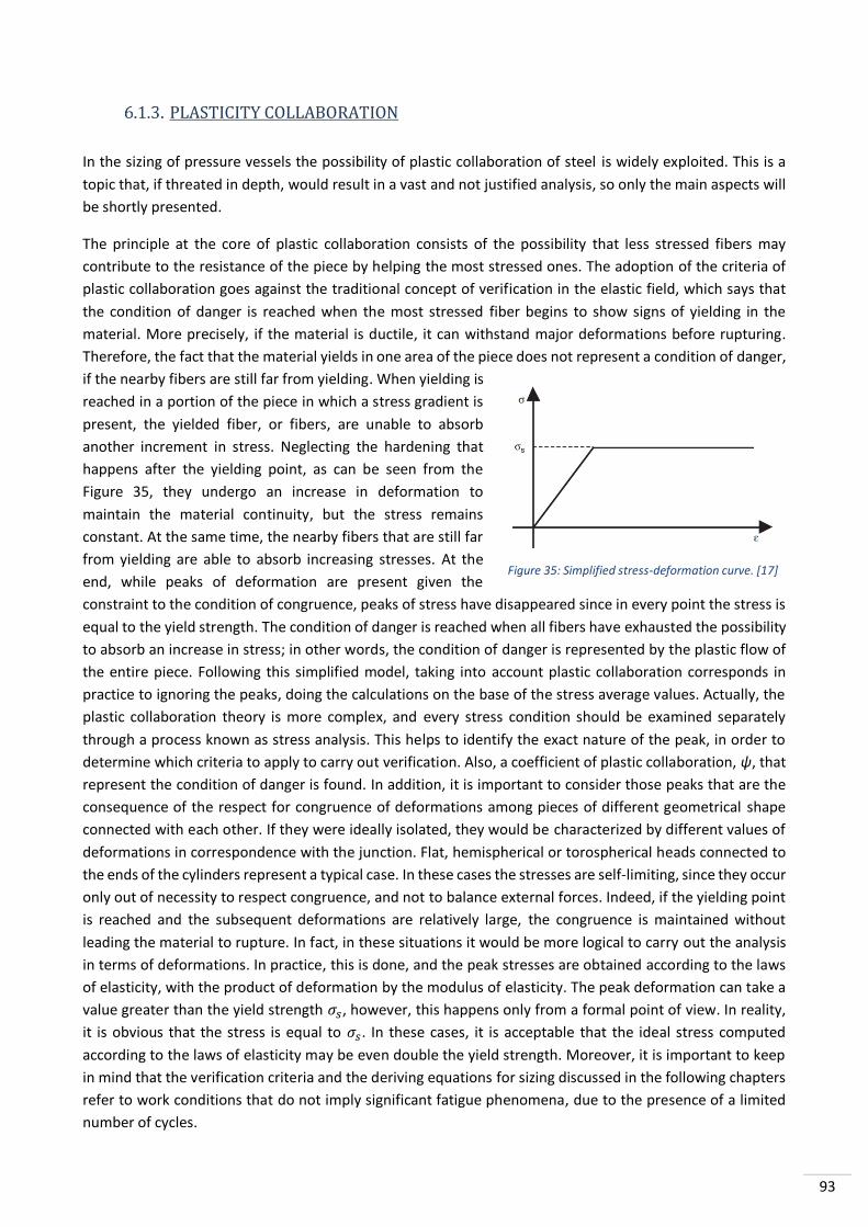
93

PLASTICITY COLLABORATION

In the sizing of pressure vessels the possibility of plastic collaboration of steel is widely exploited. This is a

topic that, if threated in depth, would result in a vast and not justified analysis, so only the main aspects will

be shortly presented.

The principle at the core of plastic collaboration consists of the possibility that less stressed fibers may

contribute to the resistance of the piece by helping the most stressed ones. The adoption of the criteria of

plastic collaboration goes against the traditional concept of verification in the elastic field, which says that

the condition of danger is reached when the most stressed fiber begins to show signs of yielding in the

material. More precisely, if the material is ductile, it can withstand major deformations before rupturing.

Therefore, the fact that the material yields in one area of the piece does not represent a condition of danger,

if the nearby fibers are still far from yielding. When yielding is

reached in a portion of the piece in which a stress gradient is

present, the yielded fiber, or fibers, are unable to absorb

another increment in stress. Neglecting the hardening that

happens after the yielding point, as can be seen from the

Figure 35, they undergo an increase in deformation to

maintain the material continuity, but the stress remains

constant. At the same time, the nearby fibers that are still far

from yielding are able to absorb increasing stresses. At the

end, while peaks of deformation are present given the

constraint to the condition of congruence, peaks of stress have disappeared since in every point the stress is

equal to the yield strength. The condition of danger is reached when all fibers have exhausted the possibility

to absorb an increase in stress; in other words, the condition of danger is represented by the plastic flow of

the entire piece. Following this simplified model, taking into account plastic collaboration corresponds in

practice to ignoring the peaks, doing the calculations on the base of the stress average values. Actually, the

plastic collaboration theory is more complex, and every stress condition should be examined separately

through a process known as stress analysis. This helps to identify the exact nature of the peak, in order to

determine which criteria to apply to carry out verification. Also, a coefficient of plastic collaboration, ψ, that

represent the condition of danger is found. In addition, it is important to consider those peaks that are the

consequence of the respect for congruence of deformations among pieces of different geometrical shape

connected with each other. If they were ideally isolated, they would be characterized by different values of

deformations in correspondence with the junction. Flat, hemispherical or torospherical heads connected to

the ends of the cylinders represent a typical case. In these cases the stresses are self-limiting, since they occur

only out of necessity to respect congruence, and not to balance external forces. Indeed, if the yielding point

is reached and the subsequent deformations are relatively large, the congruence is maintained without

leading the material to rupture. In fact, in these situations it would be more logical to carry out the analysis

in terms of deformations. In practice, this is done, and the peak stresses are obtained according to the laws

of elasticity, with the product of deformation by the modulus of elasticity. The peak deformation can take a

value greater than the yield strength 𝜎𝑠, however, this happens only from a formal point of view. In reality,

it is obvious that the stress is equal to 𝜎𝑠. In these cases, it is acceptable that the ideal stress computed

according to the laws of elasticity may be even double the yield strength. Moreover, it is important to keep

in mind that the verification criteria and the deriving equations for sizing discussed in the following chapters

refer to work conditions that do not imply significant fatigue phenomena, due to the presence of a limited

number of cycles.

Figure 35: Simplified stress-deformation curve. [17]

94

VERIFICATION CRITERIA

According to modern verification criteria, stresses can be divided into three categories: primary, secondary,

and peak stresses. Then, primary stresses can be further divided into general membrane stresses, local

membrane stresses, and primary bending stresses. In summary, there are five types of stresses that now will

be analyzed: general membrane, local membrane, primary bending, secondary, and peak.

GENERAL MEMBRANE STRESSES (σm)

They correspond to stresses derived from calculation when one considers the element under test as a

membrane. More generally, they correspond to the average value of the stresses through the thickness of

the vessel. In contrast to local membrane stresses, that we will discuss shortly, the fundamental characteristic

of these stresses is that a potential yielding of the material does not cause a redistribution of the stresses,

since the same stress is present in all the surrounding fibers. A typical example of general membrane stresses

is represented by the average values of the stresses acting in a cylinder area that is not influenced by holes

or by the junction with the heads.

LOCAL MEMBRANE STRESSES (σml)

In this case the average values of the stresses are studied through the thickness in the analyzed section. In

contrast with the previous ones, they involve a limited area of the component, and this means that the

surrounding fibers are subject to membrane stress of lower value. A potential yielding of the material

happens together with a redistribution of the stresses to the surrounding fibers that are still able to

contribute to the local resistance of material, since they are not yielded. Typical examples of stresses of this

kind are the membrane stresses produced in the cylinder and in the dished heads in correspondence with

their junction. Even the membrane stresses that occur in the cylinder and in the nozzle welded together

represent an example. As already said, these are the average values of the stresses. In both cases, junction

cylinder-heads and in correspondence of the nozzles, stress peaks are generated but they do not fall into

this kind of stress category.

PRIMARY BENDING STRESSES (σf)

These stresses belong to the category of primary stresses, such as the ones mentioned above, but they are

characterized by the fact that their value is proportional to the distance of the fiber from the neutral axis of

the section. As the previous ones, they derive from the balance conditions between internal stresses and

external forces acting upon the vessel, e.g. pressure or mechanical loads. A typical example is represented

by the stresses at the center of a flat head. The stresses produced by bending moments exerted on a vessel

with a quadrangular section fall into this category, as well.

SECONDARY STRESSES (σsec)

Their fundamental characteristic is not to be involved in balancing the forces applied to the vessel, but their

only purpose is to guarantee the congruence of the deformations. Once the required deformations are

produced, even though this happens through the yielding of the material, they do neither cause further

deformations nor do they force the intervention of the surrounding fibers, as is the case instead for the local

membrane stresses. The stresses in correspondence of the junction between cylinder and heads belong to

this category, but not the membrane ones because in that case they are local membrane stresses. The

stresses still not related to membranes in the cylinder or in the sphere and in the welded nipple in

correspondence of a hole belong to this category, as well. In this last case local peaks due to the presence of

sharp edges are excluded, as they belong to the next category.

95

The stresses due to thermal flux are secondary, as well. In fact, they are also self-limiting, since they are

produced solely to re-establish the congruence of the deformations that differ in the various fibers because

of the temperature gradient.

PEAK STRESSES (σpic)

Generally speaking, a peak stress is any type of stress that will show a maximum in the section under test.

From this point of view peak stresses are the local membrane stresses, as they are locally greater than the

general membrane stresses, and the secondary stresses. Going back to the division of stresses in three

categories (primary, secondary, and peak), peak stresses do have a different characterization. Only the

stresses present in a limited area of section under test, that do not produce significant deformations, and

that represent a potential liability only as long as the possibility of rupture is due to fragility or fatigue, belong

to this category. They are peaks induced by special geometrical characteristics of the coupled elements that

can often be eliminated or at least reduced through an appropriate management of the couplings. Moreover,

the stresses due to a rapid variation in the temperature of the fluid inside the vessel belong to this category.

It is important to notice that the stress to be compared with the allowable stress is in any case the ideal stress

or the comparison stress according to the Guest–Tresca failure theory. The allowable stresses for the various

categories are shown in Figure 36, where the basic allowable stress of the material has been identified with

f, as already done during its definition. As one can see, the allowable stress is obviously equal to the basic

allowable stress of the material for the general membrane stress. Is possible to assume an allowable stress

equal to 1.5f, therefore generally equal to the yield strength, for local membrane stress and for primary

bending stresses. If there are secondary stresses besides primary ones, the resulting maximum ideal stress

must not be greater than 3f, a value which is generally equal to twice the yield strength. The peak stresses

can be neglected if a significant fatigue phenomenon has been ruled out. If this has not been possible, a

specific analysis of stresses under fatigue must be performed.

Figure 36: Allowable stress for each stress category. [17]

96

6.2. GENERAL CALCULATION CRITERIA

MEMBRANE STRESS IN REVOLUTION SHELL

In pressure vessels design, the knowledge of membrane stresses in revolution shells is particularly interesting

for the analysis of stress conditions. Indeed, the stresses in cylinders, bended pipes, spheres, spherical heads

and cones, provided they are thin, correspond to the membrane stresses. Moreover, they represent the

average values of the stresses in vessels of great thickness. Figure 37 shows an element of a generic

revolution shell, where 𝑅1 is the radius of curvature according to the meridian and 𝑅2 is the radius of

curvature on the plane orthogonal to the meridian. Calling 𝜎𝑡 and 𝜎𝑚 the stresses along the parallel and the

meridian, respectively, and s the thickness, the forces 𝐹𝑡 are on sides A–B and C–D, and can be written as:

𝐹𝑡 = 𝜎𝑡𝑠𝑑𝑙1

Their resultant orthogonal to the element is

𝐹1 = 2𝜎𝑡𝑠𝑑𝑙1𝑑𝜗22

On the sides A − D and B – C, instead, the forces 𝐹𝑚 are

𝐹𝑚 = 𝜎𝑚𝑠𝑑𝑙2

The resultant orthogonal to the element is

𝐹2 = 2𝜎𝑚𝑠𝑑𝑙2𝑑𝜗12

Given a pressure p which produces a force in the same direction of 𝐹1 and 𝐹2, it can be developed as

𝐹3 = 𝑝𝑑𝑙1𝑑𝑙2

In order to have balance in the direction orthogonal to the element, it must be satisfied

𝐹3 = 𝐹1 + 𝐹2

Entering the previously founded equations in the balance one, and rewriting it by means of the geometrical

relations below reported, it can be obtained

{𝜎𝑡𝑠𝑑𝑙1𝑑𝜗2 + 𝜎𝑚𝑠𝑑𝑙2𝑑𝜗1 = 𝑝𝑑𝑙1𝑑𝑙2𝑑𝑙1 = 𝑅1𝑑𝜗1𝑑𝑙2 = 𝑅2𝑑𝜗2

→ 𝜎𝑡𝑠

𝑅2𝑑𝑙1𝑑𝑙2 + 𝜎𝑚

𝑠

𝑅1𝑑𝑙1𝑑𝑙2 = 𝑝𝑑𝑙1𝑑𝑙2 →

𝜎𝑚𝑅1

+𝜎𝑡𝑅2=𝑝

𝑠

The last equation is completely general, regardless if the axis crosses the membrane or not. However, two

generally valid equations that allow to calculate the meridian and circumferential stresses directly can be

derived from it if the axis crosses the membrane. Taking the circular area above A – B, as can be seen from

Figure 38, the thrust due to the pressure on the portion of the membrane is balanced by the vertical

components of the stresses 𝜎𝑚.

𝜋𝑅2𝑝 = 2𝜋𝑅𝑠𝜎𝑚 sin 𝛼

Figure 37: Element of a generic revolution shell. [17]

97

Inserting in this balance the geometrical relation

𝑅 = 𝑅2 · sin 𝛼, the equation for 𝜎𝑚 can be

found. Afterwards, this last formula can be

placed in the general one that has been deduced

previously in order to find the expression for 𝜎𝑡.

Both results are here reported below.

𝜎𝑚 =𝑝𝑅

2𝑠 sin𝛼=𝑝𝑅22𝑠

𝜎𝑡 =𝑝𝑅2𝑠(1 −

𝑅22𝑅1

)

These equations, as previously said, allow to compute the meridian and circumferential stresses of a

revolution membrane with respect to the axis that crosses itself. For instance, in the case of a cylinder we

have 𝑅2 = 𝐷 2⁄ and 𝑅1 = ∞, where D is the diameter of the cylinder. The meridian stress in the cylinder is

more appropriately indicated as longitudinal or axial stress 𝜎𝑎, and therefore

𝜎𝑎 = 𝜎𝑚 =𝑝𝐷

4𝑠 𝑎𝑛𝑑 𝜎𝑡 =

𝑝𝐷

2𝑠

Even if the axis of the cylinder does not actually cross it, the cylinder is enclosed by the heads that release

the thrust F on the cylinder itself. Therefore, the conditions leading to the general formulas of the two

components are still valid.

In the case of sphere 𝑅1 = 𝑅2 = 𝐷 2⁄ , and the resulting equation is

𝜎𝑚 = 𝜎𝑡 =𝑝𝐷

4𝑠

For the cone, a sketch can be seen in Figure 39. Geometrically can

be identified 𝑅1 = ∞ and 𝑅2 = 𝑟 cos 𝛼⁄ , where r is the radius of the

generic parallel and α the half angle at the tip of the cone. Therefore

𝜎𝑚 =𝑝𝑟

2𝑠 cos 𝛼 𝑎𝑛𝑑 𝜎𝑡 =

𝑝𝑟

𝑠 cos 𝛼

Indicating with D the diameter at the base of the cone, the maximum

values of the meridian and the circumferential stresses are

𝜎𝑚 =𝑝𝐷

4𝑠 cos 𝛼 𝑎𝑛𝑑 𝜎𝑡 =

𝑝𝐷

2𝑠 cos 𝛼

Comparing these equations with those of the cylinder it can be noticed that only the cos 𝛼 is missing.

Therefore, if the parameter α would be equal to zero, the equations of the cone would correspond to the

cylinder ones.

Figure 38: Side view of the area above A - B. [17]

Figure 39: Application of the general equations of the stresses at the cone. [17]

98

EDGE EFFECTS IN CYLINDERS AND SEMISPHERES

The analysis of edge effects in cylinders and semispheres is fundamental for the study of pressure vessels.

Indeed, the state of stress, caused by forces and moments applied in a radial way to the edge of a cylinder or

a semisphere, determine the characteristics of the constraint at the junction between cylinder and heads.

Moreover, the laws that regulate the distribution of stresses and deformation allow to determine the extent

of the collaborating area around a hole and along a nozzle

welded to the cylinder. Figure 40 shows a cylinder, with

ideally infinite length in the x direction, and r as average

radius. As can be seen, radial forces and moments are evenly

distributed on its edge x=0.

Isolating a beam of unitary width from the cylinder, the force

F0 and the bending moment 𝑀0on the edge of the beam, and

per unitary length of the circumference, can be indicated as

shown in Figure 41. 𝐹0 and 𝑀0 bend the beam generating a

deflection y that is a function of x. Due to this deflection the

radius undergoes a variation in length 𝛥𝑟, equal to y,

accompanied by a circumferential deformation 휀𝑡and a

stress 𝜎𝑡

휀𝑡 =𝛥𝑟

𝑟=𝑦

𝑟

𝜎𝑡 = 𝐸휀𝑡 =𝐸𝑦

𝑟

Considering the beam element of unitary length, has shown in

Figure 42, the forces 𝐹𝑡 on the radial sides, due to the 𝜎𝑡, are

represented by

𝐹𝑡 = 𝜎𝑡𝑠 =𝐸𝑠

𝑟𝑦

A radial force 𝐹𝑟 results from the presence of those forces, which

form the angle φ between them

𝐹𝑟 = 2𝐹𝑡𝜑

2= 𝐹𝑡𝜑 =

𝐸𝑠

𝑟2𝑦

As it can be seen, the radial force 𝐹𝑟 is proportional to y, and the

cylinder behaves similarly to a beam.

Considering now an element of length dx, shown in Figure 43, the shear forces 𝑇 and 𝑇 + 𝑑𝑇, as well as the

moments 𝑀𝑥 and 𝑀𝑥 + 𝑑𝑀𝑥 are on the sides perpendicular to the x-axis. In addition, the radial force 𝑑𝐹𝑟 is

exerted on the element

𝑑𝐹𝑟 = 𝐹𝑟𝑑𝑥 =𝐸𝑠

𝑟2𝑦𝑑𝑥

Figure 41: Beam of unitary width. [17]

Figure 42: Beam of unitary width and unitary length. [17]

Figure 40: Infinite length cylinder of radius r with forces and moments applied to itself. [17]

99

Finally, the moments 𝑀𝑧 act upon the radial sides and

are derived from congruence requirements. It is now

possible to proceed with the balance along the y-axis and

the one referred to rotation. Note that the last passage

in the moment equation reports the formula obtained by

neglecting the terms of higher order.

𝑇 −𝐸𝑠

𝑟2𝑦𝑑𝑥 − (𝑇 + 𝑑𝑇) = 0 →

𝑑𝑇

𝑑𝑥= −

𝐸𝑠

𝑟2𝑦

𝑇𝑑𝑥 −𝐸𝑠

𝑟2𝑦𝑑𝑥2

2+ 𝑑𝑀𝑥 = 0 → 𝑇 = −

𝑑𝑀𝑥

𝑑𝑥

Deriving the result of the second equation and inserting it in the first one, the following formula can be

obtained

−𝑑𝑇

𝑑𝑥=𝑑2𝑀𝑥

𝑑𝑥2=𝐸𝑠

𝑟2𝑦

Being the moments of inertia 𝐼 = 𝑠3 12⁄ , identical with respect to x and z direction, the maximum stresses

𝜎𝑥 and 𝜎𝑧, produced by 𝑀𝑥 and 𝑀𝑧 respectively, can be written as

𝜎𝑥 =𝑀𝑥𝑠

2𝐼 𝑎𝑛𝑑 𝜎𝑧 =

𝑀𝑧𝑠

2𝐼

The deformation 휀𝑧, given by the first following formula, can be elaborated and set equal to zero, since the

radial sides must stay radial.

휀𝑧 =1

𝐸(𝜎𝑧 − 𝜇𝜎𝑥) =

1

𝐸(𝑀𝑧𝑠

2𝐼− 𝜇

𝑀𝑥𝑠

2𝐼) =

𝑠

2𝐸𝐼(𝑀𝑧 − 𝜇𝑀𝑥) = 0

where μ is the Poisson’s ratio. This elaboration leads to find the following relation

𝑀𝑧 = 𝜇𝑀𝑥

Now, 휀𝑥 can be written in function of 𝑀𝑥 only

휀𝑥 =1

𝐸(𝜎𝑥 − 𝜇𝜎𝑧) =

1

𝐸(𝑀𝑥𝑠

2𝐼− 𝜇

𝑀𝑧𝑠

2𝐼) =

𝑀𝑥𝑠

2𝐸𝐼(1 − 𝜇2)

Given the last equality, it can be written:

𝑑2𝑦

𝑑𝑥2= −

휀𝑥𝑠2⁄= −

𝑀𝑥

𝐸𝐼(1 − 𝜇2)

Twice deriving and combining it with the equation of 𝑑2𝑀𝑥 𝑑𝑥2⁄ previously obtained, leads to

{

𝑑4𝑦

𝑑𝑥4= −

𝑑2𝑀𝑥

𝑑𝑥2(1 − 𝜇2)

𝐸𝐼

𝑑2𝑀𝑥

𝑑𝑥2=𝐸𝑠

𝑟2𝑦

→ 𝑑4𝑦

𝑑𝑥4= −

𝑠(1 − 𝜇2)

𝑟2𝐼𝑦 = −

12(1 − 𝜇2)

𝑟2𝑠2𝑦

where the last passage has been obtained substituting the moment of inertia I of the unitary width beam.

Figure 43: Element of unitary width and dx length. [17]

100

This last equation can be rewritten in function of a factor β

𝑑4𝑦

𝑑𝑥4= −4𝛽4𝑦

That, for the general value μ=0,3 of the steel, can be written as follow

𝛽 = √3(1 − 𝜇2)

𝑟2𝑠2

4

=√3(1 − 𝜇2)4

√𝑟𝑠=1,285

√𝑟𝑠=1,817

√𝐷𝑠

The general solution of the differential equation is

𝑦 = 𝑒−𝛽𝑥(𝐶1 sin 𝛽𝑥 + 𝐶2 cos 𝛽𝑥) + 𝑒𝛽𝑥(𝐶3 sin 𝛽𝑥 + 𝐶4 cos 𝛽𝑥)

with 𝐶1, 𝐶2, 𝐶3 and 𝐶4 integration constants. However, for x=∞, y=0 follows, and therefore 𝐶3 = 𝐶4 = 0.

Therefore, the general solution of the equation becomes

𝑦 = 𝑒−𝛽𝑥(𝐶1 sin 𝛽𝑥 + 𝐶2 cos 𝛽𝑥)

This equation allows to calculate the behavior of both the shear force and the bending moment along the

axis of the cylinder, once the values of 𝐶1 and 𝐶2 have been determined according to the boundary

conditions. In fact, from the equations obtained during the discussion, the following one can be written

𝑀𝑥 = −𝐸𝑠3

12(1 − 𝜇2)

𝑑2𝑦

𝑑𝑥2 𝑤𝑖𝑡ℎ

𝑑2𝑦

𝑑𝑥2= 2𝛽2𝑒−𝛽𝑥(−𝐶1 cos 𝛽𝑥 + 𝐶2 sin𝛽𝑥)

𝑇 =𝐸𝑠3

12(1 − 𝜇2)

𝑑3𝑦

𝑑𝑥3 𝑤𝑖𝑡ℎ

𝑑3𝑦

𝑑𝑥3= 2𝛽3𝑒−𝛽𝑥[(𝐶1 − 𝐶2) sin 𝛽𝑥 + (𝐶1 + 𝐶2) cos 𝛽𝑥]

From here on, the value of 𝑀𝑥=0 will be named 𝑀0, and the same will be done for 𝐹𝑥=0 and 𝐹0. As boundary

condition, 𝑀0 = 0 can be now considered. It follows that the second derivative of y must be zero for 𝑥 = 0,

and 𝐶1 = 0 can be found. Inserting 𝐶1 = 0 in the third derivative of y, the following statement can be written

𝑑3𝑦

𝑑𝑥3= 2𝛽3𝐶2

Furthermore, given that 𝑇 = 𝐹0 for 𝑥 = 0, its expression can be rewritten as

𝑇 =𝐸𝑠3

12(1 − 𝜇2)

𝑑3𝑦

𝑑𝑥3= 𝐹0 =

𝐸𝑠3

6(1 − 𝜇2)𝛽3𝐶2

And it leads to find the value of the last constant 𝐶2

𝐶2 =6(1 − 𝜇2)

𝐸𝑠3𝛽3𝐹0

At this point, the moment can be written as

𝑀𝑥 = −𝐹0𝛽𝑒−𝛽𝑥 sin 𝛽𝑥

101

The product (−𝐹0𝑥) represents the moment at distance x from the edge, if the elementary beam discussed

earlier were not laterally constrained to the other elementary beams that make up the cylinder.

On the other hand, if 𝐹0 = 0 is considered as boundary condition, the third derivative of y must be zero for

𝑥 = 0, and therefore

𝐶1 + 𝐶2 = 0

It follows that, collecting 𝐶1, the expression of the moment 𝑀𝑥 becomes

𝑀𝑥 =𝐸𝑠3𝐶1

6(1 − 𝜇2)𝛽2𝑒−𝛽𝑥(sin𝛽𝑥 + cos 𝛽𝑥)

As already said, for 𝑥 = 0 the notation 𝑀𝑥 = 𝑀0 is accepted, and consequently

𝐶1 =6𝑀0(1 − 𝜇

2)

𝐸𝑠3𝛽2

Inserting the value of 𝐶1 in the last moment equation, it can be rewritten as

𝑀𝑥 = 𝑀0𝑒−𝛽𝑥(sin𝛽𝑥 + cos 𝛽𝑥)

Where the value of 𝛽𝑥 is can be easily obtained from the previous definition of 𝛽.

𝛽𝑥 =1,817

√𝐷𝑠 𝑥

As can be seen, the two framed equations are functions of the parameter 𝑥 √𝐷𝑠⁄ only, which is present in

β. The representative curves of these functions are shown in Figure 44 and they show the peculiar

characteristic of the phenomenon. Indeed, it can be noticed the rapid damping of the bending moments, and

therefore of the stresses, when

moving from the edge of the

cylinder inward. Moreover, the

curves lead to the following

considerations. Regarding the

damping of the edge effect, the

parameter √𝐷𝑠 plays a crucial role:

at a distance 𝑥 = √𝐷𝑠 from the

edge, the moments present in the

cylinder are already reduced to

about 1/10 compared to those

without the damping; while for 𝑥 =

1,5 √𝐷𝑠 the edge effect becomes

𝑀𝑥

−𝐹0𝑥=𝑒−𝛽𝑥 sin 𝛽𝑥

𝛽𝑥

𝑀𝑥

𝑀0= 𝑒−𝛽𝑥(sin 𝛽𝑥 + cos 𝛽𝑥)

Figure 44: Representative curves of the two framed equations. [17]

102

almost insignificant. Note that if the thickness 𝑠 = 0,02𝐷, the parameter √𝐷𝑠 = 0,14𝐷, and at a distance

from the edge equal to 𝑥 = 1,5 √𝐷𝑠 = 0,20𝐷 the edge effect has practically vanished. This has important

implications as far as the plastic collaboration and the junctions between elements of different geometrical

shape, e.g. cylinder and flat head or dished head. Indeed, in correspondence of the junction mentioned above

there are internal forces and moments induced by the need to restore the congruence of deformations.

These internal forces and moments at the edges of both elements cause stress peaks of relatively reduced

extension due to the damping discussed above. As far as plastic collaboration is concerned, the conclusions

resulting from the study of edge effects highlight the need to set limits to the extent of the collaborating

area. In fact, it is intuitively clear that if deformations undergo rapid damping when moving away from peaks,

the collaboration of too distant fibers could only occur at the expense of undesirably high deformations in

correspondence of the peak. In conclusion, it can be stated that the extent of the collaborating area is

correlated to the parameter √𝐷𝑠.

Up to this point the discussion has focused only on the edge effects of the cylinder. Now it can move on the

semisphere. In Figure 45 a generic parallel plane has been identified through the angle φ that the tangent to

the sphere forms with the equatorial plane. By indicating with y the radial deflection generated by the forces

𝐹0 and by the moments 𝑀0, the variation of radius of the parallel is equal to 𝑦 sin𝜑. If 𝑟𝑝 is the radius of the

parallel plane, the deformation 휀𝑡 and a stress 𝜎𝑡 can be written as

휀𝑡 =𝑦

𝑟𝑝sin 𝜑

𝜎𝑡 = 𝐸휀𝑡 =𝐸𝑦

𝑟𝑝sin 𝜑

On the other hand, if r is the radius of the sphere, 𝑟𝑝 =

𝑟 sin𝜑, and the formulation obtained will be the same as the

one analysed at the begin of the discussion

𝜎𝑡 =𝐸𝑦

𝑟

Consequently, the forces 𝐹𝑡 and the radial forces 𝐹𝑟 do not depend on the position of the parallel and coincide

with those of the cylinder of equal radius. The discussion about the cylinder is therefore equally valid for the

semisphere. It can be argued that in the case of the cylinder has been assumed an infinite length, which does

not hold in the case of a semisphere. However, the edge effects rapidly vanish and the discussion about the

cylinder is true for the semisphere as well, with the only exception of very thick heads.

Figure 45: Generic parallel plane has been identified through the angle φ. [17]

103

STRESS CONCENTRATION AROUND HOLES

Consider a hole with a radius r in a plate of ideally infinite size undergoing a uniform stress σ along the y-axis,

as shown in Figure 46. The generic element at distance ρ from the center of the hole that is located at an

angle ϑ with the y-axis, undergoes the following stresses:

𝜎𝑡 =𝜎

2(1 +

𝑟2

𝜌2) −

𝜎

2(1 +

3𝑟4

𝜌4) cos 2𝜗

𝜎𝜌 =𝜎

2(1 −

𝑟2

𝜌2) +

𝜎

2(1 −

4𝑟2

𝜌2+3𝑟4

𝜌4) cos 2𝜗

𝜏 = −𝜎

2(1 +

2𝑟2

𝜌2−3𝑟4

𝜌4) sin 2𝜗

Specifically, for:

• 𝜗 = 𝜋 2⁄ , and hence along the x-axis

𝜎𝑡𝑥 =𝜎

2(2 +

𝑟2

𝜌2+3𝑟4

𝜌4)

𝜎𝜌𝑥 =3𝜎

2(𝑟2

𝜌2−𝑟4

𝜌4)

𝜏𝑥 = 0

• 𝜗 = 0, and hence along the y-axis

𝜎𝑡𝑦 =𝜎

2(𝑟2

𝜌2−3𝑟4

𝜌4)

𝜎𝜌𝑦 =𝜎

2(2 −

5𝑟2

𝜌2+3𝑟4

𝜌4)

𝜏𝑦 = 0

Figure 47 (a) and (b) shows 𝜎𝑡𝑥, 𝜎𝜌𝑥 , 𝜎𝑡𝑦and 𝜎𝜌𝑦. Notice that for 𝜌 = ∞, 𝜎𝑡𝑥 = 𝜎, 𝜎𝜌𝑥 = 0, 𝜎𝑡𝑦 = 0 and 𝜎𝜌𝑦 =

𝜎. For 𝜌 = 𝑟, therefore at the edge of the hole, can be determined that 𝜎𝑡𝑥 = 3𝜎 and 𝜎𝑡𝑦 = −𝜎. So, in the

direction of the σ active on the plate, and in correspondence of the edge of the hole, the stress peak is equal

to three times the stress in areas that are not influenced by the hole, and it rapidly decreases.

Figure 47: Graphical representation of 𝜎𝑡𝑥, 𝜎𝜌𝑥 , 𝜎𝑡𝑦and 𝜎𝜌𝑦. [17]

Figure 46: Generic element at distance ρ from center. [17]

104

If two identical stresses σ are active in the plate along both x- and y-

axis, as shown in Figure 48, the following stresses can be determined

𝜎𝑡𝑥 = 𝜎𝑡𝑦 = 𝜎 (1 +𝑟2

𝜌2)

𝜎𝜌𝑥 = 𝜎𝜌𝑦 = 𝜎 (1 −𝑟2

𝜌2)

𝜏𝑥 = 𝜏𝑦 = 0

They are represented in the Figure 49, and, in correspondence of the

edge of the hole, their values are 𝜎𝑡𝑥 = 𝜎𝑡𝑦 = 2𝜎.

Finally, if two stresses are on the plate, one equal to σ along the y-axis and the other equal to 𝜎 2⁄ along the

x-axis, as shown in Figure 50, the values turn to be

𝜎𝑡𝑥 =𝜎

4(4 +

3𝑟2

𝜌2+3𝑟4

𝜌4)

𝜎𝜌𝑥 =𝜎

4(2 +

𝑟2

𝜌2−3𝑟4

𝜌4)

𝜏𝑥 = 0

𝜎𝑡𝑦 =𝜎

4(2 +

3𝑟2

𝜌2−3𝑟4

𝜌4)

𝜎𝜌𝑦 =𝜎

2(4 −

7𝑟2

𝜌2+3𝑟4

𝜌4)

𝜏𝑦 = 0

The pattern of behavior of such stresses is shown in Figure 51.

Figure 49: Graphical representation of 𝜎𝑡𝑥, 𝜎𝜌𝑥 , 𝜎𝑡𝑦and 𝜎𝜌𝑦 if two

identical stresses σ are active in perpendicular directions. [17]

Figure 50: Plate with two stresses, one equal to σ along the y-axis and the other equal to 𝜎 2⁄ along the x-axis. [17]

Figure 51: Graphical representation of 𝜎𝑡𝑥, 𝜎𝜌𝑥 , 𝜎𝑡𝑦and 𝜎𝜌𝑦 if two stresses σ and 𝜎 2⁄ are active in perpendicular directions. [17]

Figure 48: Plate with two identical stresses σ active along both the x- and y-axis. [17]

105

Notice that, in correspondence of the edge of the hole the stresses are 𝜎𝑡𝑥 = 2,5𝜎 and 𝜎𝑡𝑦 = 0,5𝜎.

Figure 48 indicatively represents the situation in correspondence of a hole on a spherical head, or at the

center of a torospherical head under pressure. In fact, as already discussed, the meridian and circumferential

stresses are equal in the sphere. A stress peak equal to twice the circumferential, or meridian, stress would

be generated in correspondence of the hole on a spherical head.

Similarly, Figure 50 may describe the situation in correspondence of a hole in a cylinder, with the y-axis along

the circumference and the x-axis along the axis of the cylinder. In fact, as shown in the previous chapter, the

longitudinal stress in the cylinder is equal to half the hoop stress. Therefore, a stress peak twice and a half

the hoop stress in the cylinder would occur in correspondence of the hole.

From this point of view, there would be no difference between a hole with a small or large diameter

compared to the diameter of the cylinder or the sphere, with respect to the amount of increase in membrane

stress in correspondence of the hole. Given that this peak stress is a local membrane stress, it is necessary to

limit its value to 1,5𝑓 that corresponds to the yield strength. Therefore, the thickness of the cylinder needs

to be locally increased, regardless of the diameter of the hole. Specifically, it can be observed that in the case

of cylinder it would be necessary to increase the thickness and make it equal to 5/3 of the required thickness

in the absence of holes. The hoop stress of reference σ would thus be equal to 3/5 of the basic allowable

stress of the material. The value of the peak stress would therefore decrease to 2,5 · 3 5⁄ = 1,5𝑓, as required.

The size of the reinforced area may be quite small. It can be noticed that for 𝜌 = 1,5𝑟 the value of the peak

is already lower than 1,5𝜎. Therefore, the reinforcement may be limited to a distance from the edge of the

hole equal to 0,5𝑟, this notwithstanding the influence that local variations in thickness may exert on

deformations and on the stress behavior. However, I can be noticed that increasing the thickness of the

cylinder by 66% for a width equal to 0.5r, as required, the missing area due to the presence of the hole would

not be compensated. In fact, the reinforcement area is equal to 0.5r × 0.66s = 0.33rs, where s is the thickness

of the wall, while the corresponding area of half the hole is equal to rs.

In the case of a hole on a cylinder, a sphere, or at the center of a torospherical head, the curvature of the

plate cannot be neglected. In fact, the peak at the hole’s edge corresponds to a local increase in deformations

that results in a local increase in radius greater than in the remaining component. The fibers around the hole

go against a greater radial deflection in a similar way to what analyzed for the edge effects discussed in the

previous chapter. Moreover, if a nozzle is welded in correspondence of a hole, the axial rigidity of the nipple

counteracts the local increase in radius.

Experimental tests have shown that the area of the collaborating plate around the hole does not depend on

its diameter, as the previous discussion about the flat plate would lead one to believe. However, similarly to

the edge effects, being D the diameter of the cylinder or the sphere, and s its thickness, the area of the

collaborating plate around the hole depend on √𝐷𝑠. In addition, the diameter of the hole strongly influences

the entity of the peaks. In the case of a small hole, the phenomenon is localized to a limited area. The increase

in radius, which goes with a local increase in hoop membrane stress, is counteracted by the surrounding

areas, that maintain their rigidity with minor changes versus the component without holes. If the hole is

large, the cylinder or the sphere turn out to be weaker, and at the edge of the hole variations in radius that

cause the stress peak are more likely. The widely accepted calculation criterion consists of compensating for

the area of the hole by correlating the thickness of the reinforcement to the diameter of the hole. Even if this

argument will be again mentioned during the study case, the whole discussion of the correlation is not

proposed inside this thesis.

106

6.3. CYLINDERS UNDER INTERNAL PRESSURE

Three principal stresses are generated by internal pressure: a hoop stress 𝜎𝑡, a radial stress 𝜎𝑟, and a

longitudinal stress 𝜎𝑎. The latter is due to the thrust of pressure on the heads of the cylinder. The values of

the stresses 𝜎𝑡 and 𝜎𝑟, differently from the value of 𝜎𝑎, are not constant through the cylinder wall. In the

design phase it is therefore necessary to derive the ideal stress considering the stresses of the triaxial state.

This procedure can be done by means of the theories of failure described in the section “Preliminary

Considerations”. Assuming that the ideal stress is equal to the basic allowable stress, an equation to compute

the minimal required thickness can be obtained. In the first place, considering the semi-cylinder of unitary

length shown in Figure 52, it may be useful recall the Mariotte’s method. The resultant force along y it is

obviously zero, while the one along x can be written as 𝐹 = 𝑝𝐷𝑖. Two identical forces equal to F/2 at the ends

of the semi-cylinder have to be applied to balance this thrust. If the hoop stress in the cylinder is assumed as

constant through the thickness, it can be expressed by

means of the following formula:

𝜎𝑡 =𝐹 2⁄

𝑠=𝑝𝐷𝑖2𝑠

While, if the hoop stress is equal to the basic allowable

stress f, the following formula, called Mariotte’s formula, is

obtained.

𝑠 =𝑝𝐷𝑖2𝑓

However, given the assumption, it does not consider the variation of 𝜎𝑡 through the thickness, as well as the

presence of the other two principal stresses 𝜎𝑟 and 𝜎𝑎. Therefore, even if it is simply and practical, it cannot

be used for the sizing of the cylinder. Anyhow, this procedure remains important because the value of 𝜎𝑡

obtained through this equation represents the hoop stress in a membrane. Indeed, considering the cylinder

as a membrane reducing its thickness to a point, 𝜎𝑡 would no longer be a function of the radius, being the

radius a unique value. Therefore, the obtained value is constant, and it corresponds to the average value,

which is not dependent on the thickness.

Considering now the generic element shown in Figure 53. It has unitary dimension in the direction orthogonal

to the figure itself, and it can be defined by means of the radius r, its thickness dr and the angle dφ. The stress

𝜎𝑡, constant along the circumference, is exercised on sides A–B and C–D. Therefore, the equilibrium in this

direction is assured in any case.

𝐹𝐴𝐵 = 𝐹𝐶𝐷 = 𝜎𝑡𝑑𝑟

The resulting, based on such two forces in the radial

direction, is:

𝐹𝐴𝐵,𝑟 = 2𝐹𝐴𝐵𝑑𝜑

2= 𝜎𝑡𝑑𝑟𝑑𝜑

Regarding the equilibrium in the radial direction, the

presence of the force 𝐹𝐴𝐶 on the A–C side can be noticed.

𝐹𝐴𝐶 = 𝜎𝑟𝑟𝑑𝜑

Figure 52: Semi-cylinder of unitary length. The image has been taken from [17].

Figure 53: Element determined by dimensions dr, dφ and unitary thickness. [17]

107

Similarly, on the B–D side, a force can be developed neglecting the terms of higher order

𝐹𝐵𝐷 = −(𝜎𝑟 + 𝑑𝜎𝑟)(𝑟 + 𝑑𝑟)𝑑𝜑 = −𝜎𝑟𝑟𝑑𝜑 − 𝜎𝑟𝑑𝑟𝑑𝜑 − 𝑟𝑑𝜎𝑟𝑑𝜑

The equation of equilibrium with reference to the radius must be expressed by the sum of the following

forces. According to the previous equations, and with dφ having a nonzero value, the formula can be

rewritten as in the second passage.

𝐹𝐵𝐷 + 𝐹𝐴𝐶 + 𝐹𝐴𝐵,𝑟 = 0 → −𝜎𝑟𝑑𝑟 − 𝑟𝑑𝜎𝑟 + 𝜎𝑡𝑑𝑟 = 0

At the end, the equilibrium equation of the cylinder is

Regarding the congruence of deformations, consider the circular ring of thickness dr shown in Figure 54. Due

to the circumferential deformation 휀𝑡 the radii of circles α and β have a respective elongation 𝛥𝑟𝛼 and 𝛥𝑟𝛽

𝛥𝑟𝛼 = 휀𝑡𝑟 𝑎𝑛𝑑 𝛥𝑟𝛽 = (휀𝑡 + 𝑑휀𝑡)(𝑟 + 𝑑𝑟 )

To impose the congruence, the difference between these two

elongations must correspond to the increment of thickness in

the ring.

𝛥𝑠 = 휀𝑟𝑑𝑟 = 𝛥𝑟𝛽 − 𝛥𝑟𝛼 = 휀𝑡𝑑𝑟 + 𝑑휀𝑡𝑟

From this last equality it can be obtained the equation of

congruence of the cylinder.

The expressions of the deformations obtained in the section “General Calculation Criteria”, where E was the

normal modulus of elasticity and μ was the Poisson’s ratio, can be recalled

휀𝑡 =1

𝐸(𝜎𝑡 − 𝜇(𝜎𝑟 + 𝜎𝑎))

휀𝑟 =1

𝐸(𝜎𝑟 − 𝜇(𝜎𝑡 + 𝜎𝑎))

휀𝑎 =1

𝐸(𝜎𝑎 − 𝜇(𝜎𝑡 + 𝜎𝑟))

Inserting they in the previous obtained congruence equation of the cylinder, the formula in the first line can

be obtained. Subsequently, a second formulation can be written starting from it.

𝜎𝑟 − 𝜎𝑡 − 𝑟𝑑𝜎𝑡𝑑𝑟

− μ(𝜎𝑡 − 𝜎𝑟 − 𝑟𝑑𝜎𝑟𝑑𝑟) + μ𝑟

𝑑𝜎𝑎𝑑𝑟

= 0

(1 − μ) (𝜎𝑡 − 𝜎𝑟 − 𝑟𝑑𝜎𝑟𝑑𝑟) − 𝑟

𝑑𝜎𝑟𝑑𝑟

− 𝑟𝑑𝜎𝑡𝑑𝑟

+ μ𝑟𝑑𝜎𝑎𝑑𝑟

= 0

Figure 54: Circular rings of thickness dr. [17]

𝜎𝑡 − 𝜎𝑟 − 𝑟𝑑𝜎𝑟𝑑𝑟

= 0

휀𝑟 − 휀𝑡 − 𝑟𝑑휀𝑡𝑑𝑟

= 0

108

Given that the part expressed inside the brackets of the previous equation represent the equilibrium

equation of the cylinder, which is equal to zero, and the radius r is a non-zero value, it can be rewritten as

𝑑𝜎𝑟𝑑𝑟

+𝑑𝜎𝑡𝑑𝑟

= μ𝑑𝜎𝑎𝑑𝑟

Deriving the third of the before recalled expressions of the deformations, and substituting the term 𝑑𝜎𝑎 𝑑𝑟⁄

with the above achieved equation, the following expressions can be developed

𝑑휀𝑎𝑑𝑟

=1

𝐸[𝑑𝜎𝑎𝑑𝑟

− μ (𝑑𝜎𝑡𝑑𝑟

+𝑑𝜎𝑟𝑑𝑟)] →

𝑑휀𝑎𝑑𝑟

=1 − 𝜇2

𝐸

𝑑𝜎𝑎𝑑𝑟

For the sections of the cylinder to remain flat, 휀𝑎 must be constant and therefore the derivative of 𝜎𝑎 is zero,

according to the last equation. The longitudinal stress 𝜎𝑎 is therefore constant, and the previously found

equation becomes

𝑑𝜎𝑟𝑑𝑟

+𝑑𝜎𝑡𝑑𝑟

= 0

As last passage, the equilibrium equation of the cylinder can be derived and introduced in the above equation

𝑑𝜎𝑡𝑑𝑟

−𝑑𝜎𝑟𝑑𝑟

−𝑑𝜎𝑟𝑑𝑟

− 𝑟𝑑2𝜎𝑟𝑑𝑟2

= 0

𝑑2𝜎𝑟𝑑𝑟2

= −3

𝑟

𝑑𝜎𝑟𝑑𝑟

Assuming that 𝑦 = 𝑑𝜎𝑟 𝑑𝑟⁄ , it can be rewritten as a differential equation with separable variables.

𝑦′ = −3

𝑟𝑦

Which general integral, with Z and K constants, can be written as follow

∫𝑑y

𝑦= −∫

3

𝑟𝑑𝑟 + 𝑍 → log𝑒 𝑦 = −3 log𝑒 𝑟 + 𝑍 = log𝑒

𝐾

𝑟3 → 𝑦 =

𝑑𝜎𝑟𝑑𝑟

=𝐾

𝑟3

Finally, integrating the last equality and inserting the result in the above equations, being A and B constants,

the expressions for 𝜎𝑟 and 𝜎𝑡 are obtained as follow.

𝜎𝑟 = 𝐴 −𝐵

𝑟2 𝑎𝑛𝑑 𝜎𝑡 = 𝐴 +

𝐵

𝑟2

Note that if 𝑟 = 𝑟𝑒, with 𝑟𝑒 the external radius, 𝜎𝑟 must be equal to zero, and therefore:

𝐴 =𝐵

𝑟𝑒2 , 𝑡ℎ𝑒𝑛 𝜎𝑟 = 𝐵 (

1

𝑟𝑒2 −

1

𝑟2)

On the other hand, if 𝑟 = 𝑟𝑖, with 𝑟𝑖 the inside radius, the radial compressive stress is equal to the pressure

p, and therefore

−p = 𝐵 (1

𝑟𝑒2 −

1

𝑟𝑖2) → 𝐵 =

𝑝𝑟𝑒2

𝑟𝑒2

𝑟𝑖2 − 1

109

Assuming 𝑎 = 𝑟𝑒2 𝑟𝑖

2⁄ the three principal stresses can be finally written as follow. Please note that, as already

said, 𝜎𝑎 is constant, and based on the thrust on the heads.

𝜎𝑡 =𝑝

𝑎2 − 1(1 +

𝑟𝑒2

𝑟2)

𝜎𝑟 =𝑝

𝑎2 − 1(1 −

𝑟𝑒2

𝑟2)

𝜎𝑎 =𝜋𝑝𝑟𝑖

2

𝜋(𝑟𝑒2 − 𝑟𝑖

2)=

𝑝

𝑎2 − 1

These equations are known as Lamè’s equations. Figure 55 and Figure 56 illustrate the diagrams of the three

principal stresses and deformations, respectively. it is evident that 𝜎𝑡 reaches its maximum value in

correspondence to the internal fibers. The same applies to the absolute value of 𝜎𝑟, while the longitudinal

stress has a value in between the two.

Therefore, the maximum value of the ideal stress, according to Guest, must be found in correspondence to

the internal fibers, and it can be computed from 𝜎𝑡 and 𝜎𝑟.

𝜎𝑡𝑖 = 𝑝𝑎2 + 1

𝑎2 − 1 𝑎𝑛𝑑 𝜎𝑟𝑖 = −𝑝

𝜎𝑖𝑑(𝑖) = 𝜎𝑡𝑖 − 𝜎𝑟𝑖 =2𝑎2

𝑎2 − 1

As shown in section “Preliminary Considerations”, there is general consensus that one should not look at the

peak stress located in the internal fiber during the design, but instead take into account the possibility that

other less stressed fibers may cooperate with the latter. According to this criterion, the calculation can be

carried out in different ways. In this thesis only the approach which account for plastic collaboration in a

streamlined and global way will be examined. However, the other method leads to a practically coincident

equations which, even if 𝜎𝑎 is no more constant, slightly overestimate the thickness. In the analyzed method

the danger is no longer linked to the maximum stress value, so at the yielding of the internal fiber, but rather

to the whole plastic flow of the cylinder, which takes place when the ideal stress is equal to the yield strength

everywhere. In other words, following Guest’s theory the dangerous situation is represented by

𝜎𝑖𝑑 = 𝜎𝑡 − 𝜎𝑟 = 𝜎𝑠

Figure 55: Stresses in the elastic condition. [17] Figure 56: Deformations in the elastic condition. [17]

110

where 𝜎𝑠 is the yield strength. Therefore, the equilibrium equation of the cylinder, and its integration, are

𝜎𝑠 − 𝑟𝑑𝜎𝑟𝑑𝑟

= 0 → 𝜎𝑟 = 𝜎𝑠 log𝑒 𝑟 + A

Where A is a constant which, recalling that 𝜎𝑟 = 0 if 𝑟 = 𝑟𝑒, is equal to

𝐴 = −𝜎𝑠 log𝑒 𝑟𝑒

Inserting the value of A the equation of the radial stress can be written.

𝜎𝑟 = 𝜎𝑠 log𝑒𝑟

𝑟𝑒

On the other hand, for 𝑟 = 𝑟𝑖, 𝜎𝑟 = −𝑝, and therefore

𝑝 = 𝜎𝑠 log𝑒𝑟𝑒𝑟𝑖= 𝜎𝑠 log𝑒 𝑎 → 𝑎 =

𝑟𝑒𝑟𝑖= 𝑒𝑝 𝜎𝑠⁄

This last equation means that, given a certain pressure p and a material having a yield strength equal to 𝜎𝑠,

if the ratio between outside and inside radii is equal to the value given by the exponential, the cylinder is

completely plasticized. Of course, this approaches a danger condition and therefore a safety factor must be

applied. The safety condition can be obtained by replacing 𝜎𝑠 with the allowable stress f.

𝑎 =𝑟𝑒𝑟𝑖= 𝑒𝑝 𝑓⁄

The equation obtained allow to safely size the cylinder while taking into account the plastic collaboration. So,

the minimum required thickness can be obtained from it

Now, an alternative equation, called the average diameter equation can be founded. The average of 𝜎𝑟 can

be computed from the extreme values, obtained for 𝑟 = 𝑟𝑖 and 𝑟 = 𝑟𝑒, and it results

𝜎𝑟𝑚 = −𝑝

2

The average value of 𝜎𝑡 is simply the membrane stress 𝜎 mentioned at the beginning, thus recalling

𝜎𝑡𝑚 =𝑝𝐷𝑖2𝑠

=𝑝𝑟𝑖

𝑟𝑒 − 𝑟𝑖=

𝑝

𝑎 − 1

The ideal average stress that that represents the general membrane stress according to the section

“Preliminary considerations – Verification criteria”, will be given by

𝜎𝑖𝑑(𝑚) = 𝜎𝑡𝑚 − 𝜎𝑟𝑚 =𝑝

𝑎 − 1+𝑝

2=𝑝

2

𝑎 + 1

𝑎 − 1

𝑠 =𝑒𝑝 𝑓⁄ −1

2𝑒𝑝 𝑓⁄𝐷𝑒

111

With 𝜎𝑖𝑑(𝑚) = 𝑓 the following equality can be written

𝑎 + 1

𝑎 − 1=

𝑟𝑒𝑟𝑖+ 1

𝑟𝑒𝑟𝑖− 1

=𝑟𝑒 + 𝑟𝑖𝑟𝑒 − 𝑟𝑖

=2f

p

The following equation, where 𝐷𝑚 is the average diameter, can be now obtained

𝐷𝑚𝑠=2f

p →

This equation is the so-called average diameter equation, even if, it can also be rewritten considering the

outside dimeter

𝑝(𝐷𝑒 − 𝑠) = 2fs →

This last equation is used in many national codes, e.g. in the ISO Code. It is more conservative than the

Mariotte’s formula seen at the begin, and therefore definitely acceptable. It is easier to use and results in

walls only slightly thicker than strictly required. Until now it has been implicitly assumed that the cylinder

does not have holes, or that the holes are completely compensated for, and that welding does not cause a

reduction of the cylinder’s resistance in the seams. Even though the influence of holes should be analyzed,

and welded joints can generally be less resistant compared to the basic metal that constitutes the cylinder.

It is therefore introduced a weld joint efficiency, here defined as z, which identifies the allowable stress at

the weld joint as a function of the allowable stress of the basic metal through the relationship

𝑓′ = 𝑓𝑧

Where 𝑓′ is the allowable stress in the weld joint, and z is always less than or equal to one. Therefore, the

equation of the thickness obtained from the outside diameter can be written in more general terms as follow.

𝑠 =𝑝𝐷𝑒

2fz + p

𝑠 =𝑝𝐷𝑒2f + p

𝑠 =𝑝𝐷𝑚2f

112

6.4. THERMAL STRESS OF CYLINDERS UNDER INTERNAL PRESSURE

If the wall of the cylinder is subjected to a thermal flux, stresses are created to re-establish the congruence

of deformations. However, the congruence is perturbed by thermal dilations that vary throughout the wall.

In fact, due to the heat transmission, the temperature of the metal is a function of the radius. The law of

variations in temperature can be found via the following considerations.

Examining the cylinder of unitary length shown in Figure 57, the generic surface S corresponding to radius r

is 𝑆 = 2𝜋𝑟. The heat q that crosses this surface can be written as

𝑞 = 𝜆𝑆𝑑𝑇

𝑑𝑟

where 𝑑𝑇 𝑑𝑟⁄ is the temperature gradient and λ is the

thermal conductivity. Inserting the formula of the surface

inside it, dT can be made explicit as:

𝑑𝑇 =𝑞

2𝜋𝜆

𝑑𝑟

𝑟

Therefore, by integrating, the formula for the temperature

is obtained. Being C a constant, it turns out to be

𝑇 =𝑞

2𝜋𝜆log𝑒 𝑟 + 𝐶

By indicating with 𝑇𝑒 and 𝑇𝑖 the temperatures corresponding to 𝑟𝑒 and 𝑟𝑖 respectively, their difference 𝛥𝑇

can be expressed as:

𝛥𝑇 = 𝑇𝑒 − 𝑇𝑖 =𝑞

2𝜋𝜆log𝑒

𝑟𝑒𝑟𝑖

As usual, 𝑎 = 𝑟𝑒 𝑟𝑖⁄ is imposed, and the following formulation of the temperature gradient can be obtained

𝑑𝑇

𝑑𝑟=

𝛥𝑇

𝑟 log𝑒 𝑎

To compute the stresses on the cylinder due to the effect of 𝛥𝑇, the equations of equilibrium and congruence

discussed in the previous chapter have to be recalled

𝜎𝑡 − 𝜎𝑟 − 𝑟𝑑𝜎𝑟𝑑𝑟

= 0 𝑎𝑛𝑑 휀𝑟 − 휀𝑡 − 𝑟𝑑휀𝑡𝑑𝑟

= 0

Contrariwise, the expressions of the deformations previously obtained in the section “General Calculation

Criteria” can be now written in the following different way.

휀𝑡 =1

𝐸(𝜎𝑡 − 𝜇(𝜎𝑟 + 𝜎𝑎)) + 𝛼𝑇

휀𝑟 =1

𝐸(𝜎𝑟 − 𝜇(𝜎𝑡 + 𝜎𝑎)) + 𝛼𝑇

휀𝑎 =1

𝐸(𝜎𝑎 − 𝜇(𝜎𝑡 + 𝜎𝑟)) + α𝑇

Figure 57: Cylinder of unitary length. [17]

113

Inserting the expressions of the deformations, in which α represent the thermal expansion coefficient of the

material, in the equation of congruence, the first formulation that follow can be obtained. The second one,

instead, has been found using the equation of equilibrium.

−(1 + μ) (𝜎𝑡 − 𝜎𝑟 − 𝑟𝑑𝜎𝑟

𝑑𝑟) − 𝑟

𝑑𝜎𝑟

𝑑𝑟− 𝑟

𝑑𝜎𝑡

𝑑𝑟+ μ𝑟

𝑑𝜎𝑎

𝑑𝑟− 𝐸𝑟𝛼

𝑑𝑇

𝑑𝑟= 0 →

𝑑(𝜎𝑡 + 𝜎𝑟)

𝑑𝑟= μ

𝑑𝜎𝑎

𝑑𝑟− 𝐸𝛼

𝑑𝑇

𝑑𝑟

Deriving the third expression of the deformations, and imposing 𝑑휀𝑎 𝑑𝑟⁄ = 0, given that the sections of the

cylinder orthogonal to the axis remain flat, the following expression can be developed

𝑑휀𝑎𝑑𝑟

=1

𝐸(𝑑𝜎𝑎𝑑𝑟

− μ𝑑(𝜎𝑡 + 𝜎𝑟)

𝑑𝑟) + 𝛼

𝑑𝑇

𝑑𝑟 →

𝑑𝜎𝑎𝑑𝑟

= μ𝑑(𝜎𝑡 + 𝜎𝑟)

𝑑𝑟− 𝐸𝛼

𝑑𝑇

𝑑𝑟

Inserting the last equation in the previous result, the following expression can be found

𝑑(𝜎𝑡 + 𝜎𝑟)

𝑑𝑟= 𝜇2

𝑑(𝜎𝑡 + 𝜎𝑟)

𝑑𝑟− 𝐸𝛼μ

𝑑𝑇

𝑑𝑟− 𝐸𝛼

𝑑𝑇

𝑑𝑟 →

𝑑(𝜎𝑡 + 𝜎𝑟)

𝑑𝑟= −

𝐸𝛼

1 − μ

𝑑𝑇

𝑑𝑟

Using the expression of the thermal gradient previously developed, and setting 𝐾 =𝐸𝛼𝛥𝑇

2(1−μ), the last

expression can be modified and integrated, with A=constant, as follow

𝑑(𝜎𝑡 + 𝜎𝑟)

𝑑𝑟= −

2𝐾

𝑟 log𝑒𝑎 → 𝜎𝑡 + 𝜎𝑟 = −

2𝐾

log𝑒𝑎 log

𝑒𝑟 + 2𝐴 → 𝜎𝑡 = −

2𝐾

log𝑒𝑎 log

𝑒𝑟 + 2𝐴 − 𝜎𝑟

Inserting the expression for 𝜎𝑡 inside the equations of equilibrium shown earlier and integrating

2𝜎𝑟 − 𝑟𝑑𝜎𝑟

𝑑𝑟+

2𝐾

log𝑒𝑎 log

𝑒𝑟 − 2𝐴 = 0 → 𝜎𝑟 = 𝐴 −

𝐵

𝑟2+

𝐾

2 log𝑒𝑎 (1 − 2 log

𝑒𝑟)

where B is constant. For to 𝑟 = 𝑟𝑖 and 𝑟 = 𝑟𝑒, 𝜎𝑟 = 0 have to be respected, and therefore

𝐴 −𝐵

𝑟𝑒2 +

𝐾

2 log𝑒 𝑎 (1 − 2 log𝑒 𝑟𝑒) = 0

𝐴 −𝐵

𝑟𝑖2 +

𝐾

2 log𝑒 𝑎 (1 − 2 log𝑒 𝑟𝑖) = 0

By subtracting the second of those equations from the first one, and inserting the obtained expression, the

values for B and A can be found.

𝐵 = (1

𝑟𝑒2 −

1

𝑟𝑖2) + 𝐾 = 0 → 𝐵 = −

𝐾

1𝑟𝑒2 −

1𝑟𝑖2

=𝐾𝑟𝑒

2

𝑎2 − 1

𝐴 = 𝐾𝑎2

𝑎2 − 1−

𝐾

2 log𝑒𝑎 (1 − 2 log

𝑒𝑟𝑖)

114

Now, the value of the constants A and B can be inserted in the formulas derived so far, and new formulations

of 𝜎𝑟 and 𝜎𝑡 can be found.

𝜎𝑟 = 𝐴 −𝐵

𝑟2+

𝐾

2 log𝑒𝑎 (1 − 2 log

𝑒𝑟) → 𝜎𝑟 = 𝐾 [

𝑎2 − (𝑟𝑒𝑟 )

2

𝑎2 − 1−log

𝑒

𝑟𝑟𝑖

log𝑒𝑎]

𝜎𝑡 = −2𝐾

log𝑒𝑎 log

𝑒𝑟 + 2𝐴− 𝜎𝑟 → 𝜎𝑡 = 𝐾 [

𝑎2 + (𝑟𝑒𝑟 )

2

𝑎2 − 1−1 + log

𝑒

𝑟𝑟𝑖

log𝑒𝑎

]

The expression of 𝜎𝑎, instead, can be obtained recalling a previous developed expression, and rewriting it by

substituting the second term

𝑑𝜎𝑎𝑑𝑟

= μ𝑑(𝜎𝑡 + 𝜎𝑟)

𝑑𝑟− 𝐸𝛼

𝑑𝑇

𝑑𝑟= −

1

1 − μ𝐸𝛼

𝑑𝑇

𝑑𝑟= −

2𝐾

2 log𝑒 𝑎

Integrating and calling C the constant, the formulation for the longitudinal stress is achieved

𝜎𝑎 = −2𝐾

log𝑒 𝑎log𝑒 𝑟 + 𝐾𝐶

On the other hand, the resultant of 𝜎𝑎 must be zero given the absence of external forces. Therefore, the

value of C can be found.

2𝜋 ∫ 𝜎𝑎𝑟𝑑𝑟𝑟𝑒

𝑟𝑖

= 2𝜋𝐾∫ (𝐶𝑟 −2𝑟 log𝑒 𝑟

log𝑒 𝑎)𝑑𝑟

𝑟𝑒

𝑟𝑖

= 0

∫ (𝐶𝑟 −2𝑟 log𝑒 𝑟

log𝑒 𝑎)𝑑𝑟

𝑟𝑒

𝑟𝑖

= |𝐶𝑟2

2−𝑟2 log𝑒 𝑟 −

12𝑟2

log𝑒 𝑎|

𝑟𝑖

𝑟𝑒

𝐶

2(𝑟𝑒2 − 𝑟𝑖

2) =𝑟𝑒2 log𝑒 𝑟𝑒

2 − 𝑟𝑖2 log𝑒 𝑟𝑖

2 −𝑟𝑒2

2+𝑟𝑖2

2log𝑒 𝑎

→ 𝐶 =2𝑎2

𝑎2 − 1+2 log𝑒 𝑟𝑖 − 1

log𝑒 𝑎

Inserting the value of C, the new formulation for 𝜎𝑎 is

𝜎𝑎 = −2𝐾

log𝑒 𝑎log𝑒 𝑟 + 𝐾𝐶 → 𝜎𝑎 = 𝐾 [

2𝑎2

𝑎2 − 1−1 + 2log𝑒

𝑟𝑟𝑖

log𝑒 𝑎]

By recalling the meaning of K, the final expressions for 𝜎𝑡, 𝜎𝑎 and 𝜎𝑟 can be written

𝜎𝑡 =𝐸𝛼𝛥𝑇

2(1 − μ)[𝑎2 + (

𝑟𝑒𝑟)2

𝑎2 − 1−1 + log𝑒

𝑟𝑟𝑖

log𝑒 𝑎]

𝜎𝑎 =𝐸𝛼𝛥𝑇

2(1 − μ)[2𝑎2

𝑎2 − 1−1 + 2log𝑒

𝑟𝑟𝑖

log𝑒 𝑎]

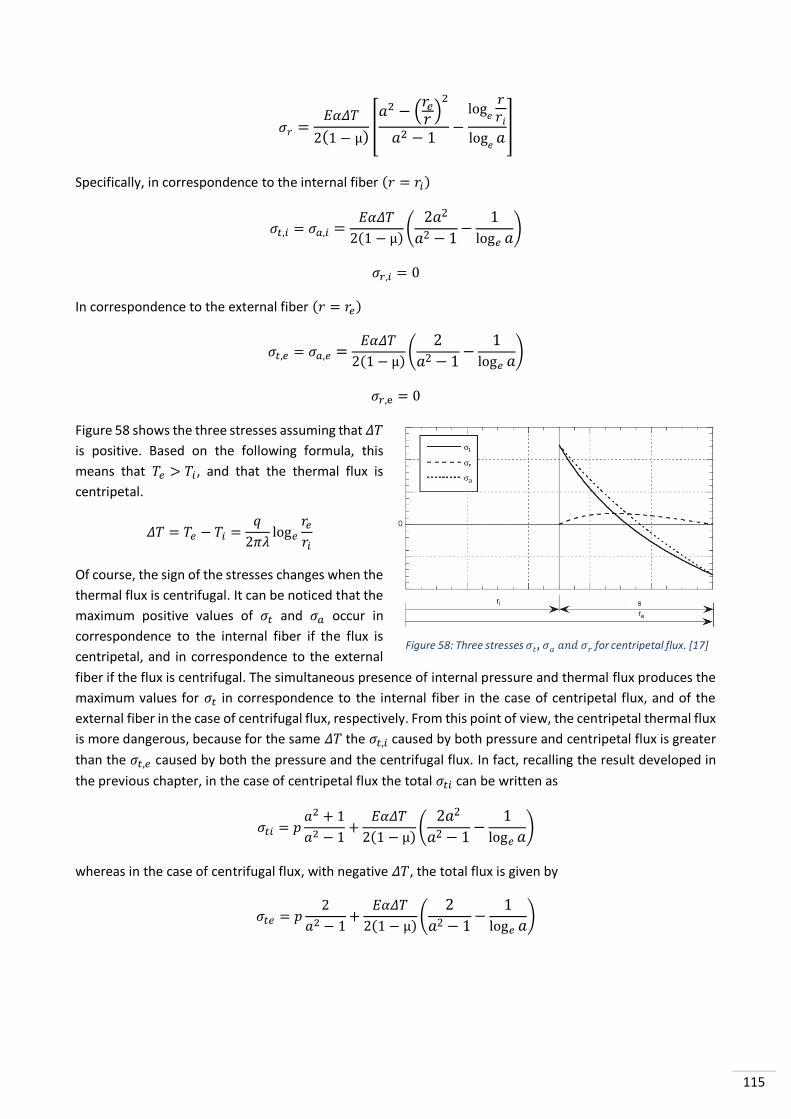
115

𝜎𝑟 =𝐸𝛼𝛥𝑇

2(1 − μ)[𝑎2 − (

𝑟𝑒𝑟 )

2

𝑎2 − 1−log

𝑒

𝑟𝑟𝑖

log𝑒𝑎]

Specifically, in correspondence to the internal fiber (𝑟 = 𝑟𝑖)

𝜎𝑡,𝑖 = 𝜎𝑎,𝑖 =𝐸𝛼𝛥𝑇

2(1 − μ)(2𝑎2

𝑎2 − 1−

1

log𝑒 𝑎)

𝜎𝑟,𝑖 = 0

In correspondence to the external fiber (𝑟 = 𝑟𝑒)

𝜎𝑡,𝑒 = 𝜎𝑎,𝑒 =𝐸𝛼𝛥𝑇

2(1 − μ)(

2

𝑎2 − 1−

1

log𝑒 𝑎)

𝜎𝑟,e = 0

Figure 58 shows the three stresses assuming that 𝛥𝑇

is positive. Based on the following formula, this

means that 𝑇𝑒 > 𝑇𝑖, and that the thermal flux is

centripetal.

𝛥𝑇 = 𝑇𝑒 − 𝑇𝑖 =𝑞

2𝜋𝜆log𝑒

𝑟𝑒𝑟𝑖

Of course, the sign of the stresses changes when the

thermal flux is centrifugal. It can be noticed that the

maximum positive values of 𝜎𝑡 and 𝜎𝑎 occur in

correspondence to the internal fiber if the flux is

centripetal, and in correspondence to the external

fiber if the flux is centrifugal. The simultaneous presence of internal pressure and thermal flux produces the

maximum values for 𝜎𝑡 in correspondence to the internal fiber in the case of centripetal flux, and of the

external fiber in the case of centrifugal flux, respectively. From this point of view, the centripetal thermal flux

is more dangerous, because for the same 𝛥𝑇 the 𝜎𝑡,𝑖 caused by both pressure and centripetal flux is greater

than the 𝜎𝑡,𝑒 caused by both the pressure and the centrifugal flux. In fact, recalling the result developed in

the previous chapter, in the case of centripetal flux the total 𝜎𝑡𝑖 can be written as

𝜎𝑡𝑖 = 𝑝𝑎2 + 1

𝑎2 − 1+

𝐸𝛼𝛥𝑇

2(1 − μ)(2𝑎2

𝑎2 − 1−

1

log𝑒 𝑎)

whereas in the case of centrifugal flux, with negative 𝛥𝑇, the total flux is given by

𝜎𝑡𝑒 = 𝑝2

𝑎2 − 1+

𝐸𝛼𝛥𝑇

2(1 − μ)(

2

𝑎2 − 1−

1

log𝑒 𝑎)

Figure 58: Three stresses 𝜎𝑡, 𝜎𝑎 𝑎𝑛𝑑 𝜎𝑟 for centripetal flux. [17]

116

Calling 𝛾 the highlighted part, with the positive sign for the centripetal flux and the negative for the

centrifugal sign, last expressions can be written as follows:

𝛾 = ±𝐸𝛼𝛥𝑇

2(1 − μ)

𝜎𝑡𝑖𝑝=𝑎2 + 1

𝑎2 − 1+ γ(

2𝑎2

𝑎2 − 1−

1

log𝑒 𝑎)

𝜎𝑡𝑒𝑝=

2

𝑎2 − 1+ γ(

2

𝑎2 − 1−

1

log𝑒 𝑎)

The parameters 𝜎𝑡𝑖 𝑝⁄ and 𝜎𝑡𝑒 𝑝⁄ derived from the equations above are graphically depicted in Figure 59 and

Figure 60. The values for 𝜎𝑡𝑖 and 𝜎𝑡𝑒 for the two types of flux show the greatest differences for large values

of 𝑎, as well as for γ. Some portions of the curves have been dashed in Figure 60, since the stress 𝜎𝑡𝑒 does

not show the highest absolute value under certain conditions. In fact, that portions are not significant for the

identification of the most dangerous stress. Indeed, it may be the case that the longitudinal stress with

negative sign is greater in absolute value than 𝜎𝑡𝑒 in correspondence to the internal fiber.

It would be possible thoroughly analyze when the conditions required for this occur, however, this will not

do in this document. As it is customary, steady-state conditions have been assumed, while the analysis of the

phenomenon can be generalized for thermal transient conditions. These considerations would lead to

observe the importance of having a gradual heating in order to avoid the onset of high stresses during

transient.

A peculiar characteristic of stresses due to the thermal flux consists of having a zero-average value, since they

are not generated to balance external forces, but only to re-establish the congruence of deformations. Based

on the computation criterion that takes only the average values of the stresses into account and neglects

peaks, the stresses generated by flux should not be taken into consideration. Such criterion is often, and

rightfully, adopted when the values of 𝛥𝑇 are modest, and the cylinders are thin. Remember, however, that

the presence of flux sometimes leads to an increase in peaks that cannot be ignored. In conclusion, it is worth

to remember that such peaks, as well as the ones caused by pressure, are crucial whenever the working

conditions of the vessel are such to require a fatigue analysis.

Figure 59: Values of 𝜎𝑡𝑖 𝑝⁄ in function of a and 𝛾. [17] Figure 60: Values of 𝜎𝑡𝑒 𝑝⁄ in function of a and 𝛾. [17]

117

7. MECHANICAL DESIGN OF THE HEAT EXCHANGER: CASE STUDY

7.1. INTRODUCTION TO MECHANICAL DESIGN

After the section of the theoretical concepts about mechanical design, it is now possible proceed with the

second part of the study case. In order to develop the mechanical design of the steam generator, the program

ASPEN Shell and Tubes Mechanical will be used. All the formulation and theories used by the program are

taken from the designed calculation code, which in this case is the ASME code. However, the design

procedure and computations recommended in the ASME codes are developed from the mechanical theories,

some of which reported in the previous chapter. For this reason, in order to better understand the logical

approach of the mechanical design, the theory has been reported before the study case. It is worth to observe

that most of the mechanical equations to be solved during the design are simpler than the thermal one,

which, instead, are usually of differential nature. This lead to require a more complex mathematical methods

in order to solve the thermal equations, that in turn reflects in a higher cost of the licences for the thermal

design programs.

Being the ASPEN Shell and Tubes Mechanical another section of the same program used for the thermal

design, the procedure required to upload the configuration obtained with the previous passages is very

simply. Indeed, selecting the correct section using the bar on top of the screen and following the instructions,

the design developed with the thermal part and all the preliminary data of the configuration are uploaded.

As for the thermal part, the mechanical one is divided in inputs and results, and new sections of the menu

are created on the left of the program. As usual, the menu shows all the sections and the forms of the

mechanical design, and it will be analysed in this chapter.

Finally, some new inputs and specifications, which were not previously required, are now used for the

mechanical part. However, many clarifications and analysis will still be made in order to identify the necessary

and appropriate parameters not provided by the customer. Concluding, it is worth remembering that is not

required the vacuum working condition, so no vacuum design parameters will be indicated.

118

7.2. ANALYSIS AND IMPLEMENTATION OF THE INPUT DATA

PROBLEM DEFINITION

The first section of the input is the “Problem Definition”, which present three

forms. The first, “Description”, is a module dedicated for the description of the

project, as already seen in the thermal design. The second, “Application

Options”, allow to insert the codes and the standards to be used. ASME Code

Section VIII Division 1 must be inserted, and the TEMA class have to be

defined. The TEMA standards identifies the heat exchanger in three classes in

function of their use. The three sections are R, which is the one needed for the

study case with intended use in the refinery service, C and B for the chemical

and general service respectively. Notice that the requirements are always less

restrictive from R to B, and the refinery service is the one in which a more complex approach is required.

However the API 660, standards for the heat exchanger of the American Petroleum Institute, has not to be

taken into account, given that was not in the client requirements. Regarding the service class is a parameter

to declare the working conditions of the heat exchanger, and for the ASME the choice must be done between

Normal, Lethal service or Low temperature. The inputs generally needed to design a heat exchanger’s

component are the temperature, the pressure, and the joint efficiency. The last one is a factor that can

assume three different values in function of the designated mode of defect controls, and its aim is to increase

the thickness of the piece with the increment of the probability to have defects. Indeed, its value is 1 in case

of full radiography control, 0,85 if spot control are indicated or 0,7 if no control are done. Moreover, the

ASME forces to make the full radiography, in the case in which the thickness overcome a certain value or in

case of lethal service. Indeed, when the heat exchanger contains a fluid that has been classified as lethal by

ASME, the lethal service has to be declared so that the program cannot accept an input of joint efficiency

different than one. Another consequence that this option will dictate involves the Post Weld Heat Treatment,

PWHT. Being the welds a thermal procedure that implies a modification of the crystal lattice, they leave a

residual stress in the material. This residual stress can be removed by means of a stress relieving thermal

treatment. The entity of these tensions depend by

the material, hardest the material higher the

residual stress, and from the thickness, that causes

an increment of them. Some studies performed

during the years have delineated the limits within

the stress relief thermal treatment is mandatory or

not. As introduced, these limits depends from the

material and the thickness, but the treatment is

always mandatory in case of lethal service. The low

temperature class implies some complex

obligations of materials to be used and heat

treatments if the Minimum Design Metal Temperature, MDMT, is lower than -29°C. At the end, it can be

resumed that the service class is a very important parameter because it influences the joint efficiency, so the

welding inspections and the thickness of the material, and establishes the obligation of the thermal

treatment. At the end of the sub-form the ASME and the ANSI-American standards have been implemented

for the materials and dimensional standard respectively.

119

The third form, “Design Specifications”, starts with the project inputs design pressures and design

temperatures, already provided in the thermal part. The vacuum design pressure must be inserted if the

device has to perform under vacuum operation. In the input data there was indicated that it is not required

the vacuum working condition, so no vacuum design parameters have to be inserted. Note that they are not

mandatory fields to be filled, otherwise they would be highlighted in light blue and the red cross would

appear on the icon of the form. The test pressure is the one at which the heat exchanger will be subjected

during the final test. It does not correspond to the design pressure to compensate for the fact that the test

will be made at room temperature. In order to take into account the higher temperature during the working

condition, a higher test pressure will be determined based on the ASME code. The minimum test pressure of

the water is done by 1,3 · 𝑀𝐴𝑊𝑃 · 𝐿𝑆𝑅 where the MAWP is the Maximum Allowable Working Pressure of

the shellside, or of the tubeside, and the LSR is the Lowest Stress Ratio. This last parameter is a conversion

factor used to convert the ASME material stress value at the test temperature to the stress value at the design

temperature. It is obtained dividing the 𝜎𝑎𝑚𝑚, the admissible stress at room temperature, by the 𝜎𝑎𝑚𝑚,𝑇 ,

that is the one at the design temperature. Attention must be paid in case in which the test pressure that will

be really used is, for technological or process reasons, higher than the one computed. In that case the

expected pressure must be inserted in order to make de design properly, or a further verification calculation

must be performed. As already seen, all the values not inserted and not strictly necessary for the design will

be computed by the program and provided in the mechanical design output. Because in the inlet datasheet

the Minimum Design Metal Temperature, MDMT, of 5°C and a corrosion allowance of 3 millimeters have

been provided, these values have been inserted. Contrariwise, if the MDMT would not be inserted, the

program would provide it basing the computation on the material characteristics and thickness. Being this

project in a Normal service class, any type of radiography can be chosen at the begin. However, the high

120

pressure will probably lead to high metal thickness that, as previously discussed, will require the full

radiography. The same logic was applied for the Post Welding Heat Treatment, PWHT. Indeed, the full

radiography and the PWHT requirements had already been implemented. The plate tolerance represent the

tolerance that will be used by the program to compute the minimum thickness of the plates for the design.

Indeed, the supplier always provides the pieces that present the required tolerances or the general tolerance

requirements dictated by the standard. In this case, the lower limit of 0,3 millimetres has been provided. The

static head of the water contained in the shell, or eventually some addition due to an external device, can be

implemented by the voices “add static head to design pressure” and “static pressure – override program”.

Proceeding, the actual difference design pressure is an important concept that allow to design the device for

a difference in pressure between the shell and the tubeside, and provide a load procedure in which that

pressure will not be overcome. Generally the components subjected to both the pressures, e.g. tubesheet

and tubes, are designed twice using the shell and the tubeside one, and after the resulting greater thickness

is assumed. However, they never have to withstand all the pressure for one side and nothing from the other.

For this reason, in case in which expensive materials have to be used, it can be thought to design this pieces

to withstand only the difference in pressure, and make this difference the maximum load that will be

provided. In order to provide a better explanation of this design logic, an example of a pressure vessel that

have to be designed with a shellside pressure of 7,8 MPa and a tubeside pressure of 6 MPa can be reported.

Given that the heat exchanger in nominal conditions of working undergoes both the pressure together, the

design can be made taking into account the only difference between them, increased for the safety, e.g. 2

MPa. This can be done because the compression stress given by both the pressure together is negligible with

respect the stresses caused by the difference of them. This leads to mandatorily provide a load procedure

which does not allow to occur more than 2 MPa of difference in pressure in every moment of the heat

exchanger’s life.

Concluding, the last option to be chosen regards the difference between the Class 1 and Class 2 of the BPVC

VIII division 2, which is represented by the admissible stress used for the design activity. Indeed, the Class 1

foreseen an admissible stress lower than Class 2, due to the fact that it has been computed with a higher

safety factor. However, the Class 2 can be used only if the design will be approved from an American or

Canadian engineer. Even if the design will be based on the BPVC VIII division 1 as before indicated, this choice

is presented, and the program have automatically set no as parameter.

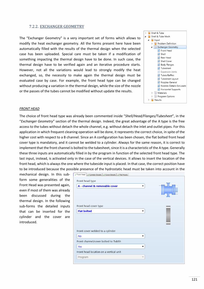
121

EXCHANGER GEOMETRY

The “Exchanger Geometry” is a very important set of forms which allows to

modify the heat exchanger geometry. All the forms present here have been

automatically filled with the results of the thermal design when the selected

case has been uploaded. Special care must be taken if a modification of

something impacting the thermal design have to be done. In such case, the

thermal design have to be verified again and an iterative procedure starts.

However, not all the variations would lead to strongly modify the heat

exchanged, so, the necessity to make again the thermal design must be

evaluated case by case. For example, the front head type can be changed

without producing a variation in the thermal design, while the size of the nozzle

or the passes of the tubes cannot be modified without update the results.

FRONT HEAD

The choice of front head type was already been commented inside “Shell/Head/Flanges/Tubesheet”, in the

“Exchanger Geometry” section of the thermal design. Indeed, the great advantage of the A type is the free

access to the tubes without detach the whole channel, e.g. without detach the inlet and outlet pipes. For this

application in which frequent cleaning operation will be done, it represents the correct choice, in spite of the

higher cost with respect to a B channel. Since an A configuration has been chosen, the flat bolted front head

cover type is mandatory, and it cannot be welded to a cylinder. Always for the same reason, it is correct to

implement that the front channel is bolted to the tubesheet, since it is a characteristic of the A type. Generally

these three inputs are automatically filled in by the program in function of the selected front head type. The

last input, instead, is activated only in the case of the vertical devices. It allows to insert the location of the

front head, which is always the one where the tubeside input is placed. In that case, the correct position have

to be introduced because the possible presence of the hydrostatic head must be taken into account in the

mechanical design. In this sub-

form some generalities of the

Front Head was presented again,

even if most of them was already

been discussed during the

thermal design. In the following

sub-forms the detailed inputs

that can be inserted for the

cylinder and the cover are

introduced.

122

The next sub-form, called “Cylinder Details”, refers to the cylinder of the channel, and not to the kettle’s one.

If both, inside and outside front head cylinder diameters, are not inserted, the program set the front head

inside diameter equal to the inner shellside one, and compute the minimum required thickness. Notice that,

as already said, the inner shellside is different from the kettle one. It follows that all the parameters contained

in the details section can be implemented if some restriction are presents. However, if no special

requirements have to be set, it is always better do not add constraints to the program in order to reduce the

crash prospective. Despite this, other possible inputs are the length of the cylinder and the length for external

pressure. The first is the simple length of the head cylinder, and it will be automatically computed in order

to allow the assembly of all the component. However, a final check about the feasibility is a good habit. The

second one is a value that refers to the devices that work under vacuum conditions, and so they must

withstand the external pressure not balanced. As can be learned from scientific literature, the resulting

thickness of shells under external pressure depends from its non-supported length. Differently, the length of

the shell does not influence the thickness in case of design against internal pressure. The possibility to insert

some stiffening rings allow to reduce the non-supported length, and so to decrease the required thickness

against the external pressure. Indeed, if the thickness required for the vacuum working condition is higher

than the normal one, the values can be matched adding some stiffening rings. This have not too much sense

on the channel as much on the shell, but it could be necessary. Proceeding the joint efficiency for

circumferential and longitudinal welds can be inserted. However, because the full radiography indication has

already been inserted, the program will complete automatically these fields with the relatives correct values

of one. The next parameters are useful only for the production of the technical drawing and for the cost

analysis. They express the distance and the angle at which the girth weld and the longitudinal weld are

located. However these values will be present only in the case in which the cylinder head is very long and

have to be done from more pieces welded together or from a rolled plates.

Sometime, due to the necessity to avoid corrosion, expensive materials like Inconel are required for the

shellside. In order to avoid excessive cost, only a few millimetres of coating are generally deposited. These

clad cannot be considered as

thickness for the mechanical

resistance of the shell. However, in

order to prevent difficulties during

the bundle insertion, it must be

considered as encumbrance for the

inside shell diameter. Typically,

three millimetres of pure coating

guaranteed by a chemical analysis

must be applied, unless in cases in

which they represent a limitation

for the thermal exchange.

Proceeding, the last part of inputs

contains the data about the

material of the cylinder. It is used if

the material is not present in the

program database and it must be

manually implemented. If filled

out, the values specified in the

paragraph 7.2.3 will be overridden.

123

As already presented, the cover in this case must be a flat bolted, so the “Cover Details” sub-form has not to

be compiled. Indeed, it refers only to other covers, e.g. torispherical and hemispherical, which can be used

in a different type of heat exchangers. A very common one is the torispherical, in which a semi-ellipse is

simulated by means of two curvature radii. The first is a large curvature radius present in the center of the

cover, while the second is a smaller radius on the edge. The proportions between the two radii can change,

leading to a family of possible torispherical covers. Returning to the sub-form an important input which is

worth to be analysed is the percentage of thickness for forming allowance. The plate formed to obtain the

cover undergoes a shrinkage, so the minimum thickness required from the mechanical design must be

guarantee at the end of the procedure. The percent value of shrinkage must be inserted in this input.

However, generally during the purchase of the formed cover the minimum thickness is specified, and this

value can be left free. To report some common values, even if highly conservative, a shrinkage of 10% for the

torispherical and a 15% for the hemispherical cover can be considered.

As previously assigned, the study case present a flat bolted head. For this reason the previous sub-form,

“Cover Details”, has not to be considered, while the following, “Flat Heads”, is the important one. Given the

TEMA Class R, the confined type of the flanges have to be mandatorily used. These joints present one or two

recesses to accommodate a gasket, as in the upper figure on the right. 𝐷0 and 𝐷𝑏 represent the outside

diameter of the cover and the bolt circle diameter respectively. The nominal thickness of the cover is 𝑡𝑛 while

𝐶𝑎 is the corrosion allowance. In the image there is also present the groove depth for the partition plate and

the mean gasket diameter 𝑑𝑔. The program allow to insert manually the dept and the diameter for the first

and second recess as well as the maximum deflection value. Notice that the first recess refers to the

dimensions of the cavity which the gasket is located, while the second to the bolt one. The following entry

allow to insert the flat head type regarding to the welds. The image below on the right shows the choice of

the case study, the f type, which presents two welds and an associated factor C=0,33m, used to compute the

thickness of the flat cover. The last two inputs do not have interest for the study case because they are a

command to avoid the empirical reinforcement for the nozzle if it would be placed on the cover, and the

factor Z, that it is used to compute the not circular covers.

124

SHELL

All the data, as the kettle shell type and the horizontal orientation, was already been inserted in the thermal

calculation, and the mechanical one have automatically upload them. Please notice that, as already

mentioned, the shell inlet and outlet diameters don’t refer to the kettle diameter but to the one of the

cylinder connected between the flange and the reducer.

Referring to the image below, it can be noticed that also the kettle inner diameter has been automatically

uploaded. Furthermore, the same input parameters already analyzed for the front head cylinder are now

reported for the kettle. Attention must be paid since they refers to the kettle cylinder only and not to the

cone, e.g. the kettle length. Differs, instead, the section of the stiffening rings, which in this case are not

intended to add stiffness at the cylinder for the design against the external pressure. Given that the

connections between the cone and the cylinders, for both the shellside and the kettle one, are two areas of

high stress concentration and buckling risk, two possibilities can be adopted to avoid problems. The first is to

form the cone in order to avoid the welds to be in the changes of slope. Making a knuckle and a flare on the

cones, the welding joints will be a butt weld, avoiding problems but introducing a higher cost. The parameters

of this solution can be inserted in the next sub-form which refers to the reducer. The second remedy, and

less expensive solution, would be an increment in stiffening produced by placing some rings close to the

joints. All the data to define them manually can be inserted here, however, as already said, it is important do

not insert to much constraints in the first instance.

125

Focusing now on the reducer, the cone between the shellside cylinder and the kettle one, always the same

parameters can be implemented. The diameters from both sides are constrained from the cylinders, while

the geometrical parameters as the thickness, the angles and the radius have to be left empty. The input that

refers to the cone section refers to the already presented discussion to avoid high stress concentration areas

and buckling risk. Some possible solutions of formed cone with knuckle and flare are reported in the following

image, which represent the figure UG-33.1(c)(d)(e) of the ASME Section VIII Division 1.

The possibility to control the flow by means of the weir method has already been discussed. If it has to be

adopted, as in this case, the affirmative statement in the weir part of this sub-form has to be inserted. As all

the devices present in the kettle, it will be considered in the weight and cost estimation of the whole heat

exchanger.

126

REAR HEAD

Various sub-forms are activated or

disabled in function of the selected rear

head. As already discussed, the U type is

necessary for this application, and all the

input parameters are practically turned

off. In the other rear head cases, the inputs

would be the same already seen for the

front head. The only exceptions are the

two sub-forms S and W type, dedicated at

the floating heads. Notice that the W

floating head is rarely used, but the S type

can also be adopted with the kettle

configuration as analysed in the next

paragraph.

SHELL COVER

Talking about the shell cover, a lot of different situations could be analysed. For example, a very particular

case would be the necessary to have a removable bundle in which the mechanical cleaning inside of the tubes

must be ensured. In this situation the S floating rear head must be used, but it will be located inside the kettle

cylinder. An ellipsoidal cover would be used as in the case of the U bundle, however it should be bolted to

the shell rather than welded. This would allow the possibility to remove the shell cover in order to dismount

of the inner S head during the bundle extraction. This

example has been reported to demonstrate how this

input should be carefully analysed case by case. The last

choice proposed in this card is very important for the

study case, because if not correctly inserted the program

can generate an AKU heat exchanger without the

removable bundle. Indeed, obviously the tubesheet

cannot be welded to the shell if the bundle must be

removable. The geometrical details of the shell cover can

be inserted in the dedicated “Cover Details” sub-form if

needed.

127

BODY FLANGES

The first thing to be noticed about the body flange section is that all the inputs present in it do not influence

the thermal design, even if there they were already specified during the first part. Indeed, the Hub type of

flanges was already set given the refinery service TEMA class that forces to use the butt welds. Optimized

has been indicated for the design

standard because the dimensions have

not been determined yet, so the standard

cannot be selected. The confined type of

flanges also must be used, and they have

already been commented. These settings

apply to all the flanges of the tube and

shellside present on the body, and not on

the nozzles’ flanges.

Proceeding, the “Individual Standard” sub-form presents a standard table of all the possible body flanges

that can be present. In the analysed configuration there will be two flanges on the front head channel, the

“Front Head Flange at Cover” and the “Front Head Flange at Tubesheet”, and the one on the shell, the “Front

Shell Flange”. This table can be used to implement the characteristics of the individual flange if different from

the general values expressed above. In this case all the flanges have the characteristics already delineated,

and so no further specifications are required.

In the following two sub-forms all the geometrical details of the flanges, the characteristics of the material,

of the nubbin and gaskets can be inserted by means of two tables. Some important parameters that still were

not analysed are the m and y coefficients of the gaskets. The principal aim of the flanges is to counteract the

forces, given by the internal pressure, that tend to open the joint and to provide the correct preload if not

self-energizing gasket type are used. To design a flanged joint, two required bolting areas are found from the

previously mentioned forces, and the major one is used. Indeed, the selected higher bolting area will be

provided from a combination of number and size of bolts, taking into account that they must have enough

space to be mounted and that more the bolt circle is enlarged, more the bending moment on the flange

increases. The bolting area required to ensure the preloading is called gasket seating, while the force that

must be provided can be determined from the coefficients m and y, given by the manufacturer, and from the

gasket width. So, it is worth to observe that the gasket can have a principal role in the sizing of the bolts. As

presented, the preload necessary for the correct behaviour of the gasket depends also from its width.

However, this dimension cannot be reduced more than a certain limit in order to ensure the resistance of

the gasket, that otherwise would break during the assembly. To overcome the problem of the high preload

needed in the past, without reducing to much the width, the nubbin was used. It is a worked relief on the

128

flange that, closing on the gasket, allow to reduce the effective area considered for the calculation of the

preload, and allow to use wider and handy gasket. As discussed, in first instance it is better do not insert

parameters that will produce some constraints at the calculation performed by the program. For this reason,

and due the simplicity and the redundancy of the other inputs that would be present, the images of the sub-

forms related to the topics just discussed have not been reported.

Analysing instead the “Options” sub-form, the first data reported are the design temperatures for the

shellside and tubeside flanges, automatically uploaded from the thermal design. Just below these, an option

to design the flanges according to the ASME rigidity rules can be activated. This allow to obtain stiffer

components when the design loading conditions do not require too much in term of resistance, leading to a

thin components. KI and KL are two factors used in the above-mentioned verification of the rigidity, and they

refers to the integral and loose flange type respectively. Some standard values, KI=0,3 and KL=0,2, are

provided from the ASME code. They will be automatically filled from the program, given the specification to

follow the ASME code. However, these values are extremely precautionary, and the ASME code allow at the

designer to insert personalized values if properly documented by technical verification. Changing section, a

part of this sub-form is dedicated to the inputs required for

some particular types of gaskets, e.g. the spiral wound gasket

that can be seen in the image on the right. These device are

delicate and difficult to handle, so an inner and outer rings

provide the necessary stiffness and the centring simplicity.

Proceeding, there is an option to activate the full-face gasket,

which extends the gasket external diameter until the

external diameter of the flange, and present the holes for the

bolt passing through. In the last section the type of bolts, US in accordance with ASME standard, and the

minimum bolts diameter can be selected. Finally, the clearance for the bolt tensioner can be foreseen. The

last sub-forms have not been reported because not connected with the study case. However, to be thorough,

the first one is “Backing”, that allows to insert the input for the backing rings of the S type floating heads,

while the second is “PCC-1”, that refers to a good practice rules based on ASME for the bolt tightening.

129

TUBESHEET

Moving on the tubesheet form, six sub-forms are present and now will be analysed. The first one is called

“Tubesheet”, as the general form, and an image of it is reported in the next page. At the begin, the tube to

tubesheet joint type is recalled. It was already presented in the thermal design part, “Exchanger Geometry –

Shell/heads/Flanges/Tubesheet”, where the difference between the possible joint types was explained.

However, most specific input have to be inserted here, defining completely the connections and

guaranteeing a correct mechanical design. As already discussed, a “Strength welding with expansion reliefs”

is required in this case. This is traduced here with the inputs “e – Welded, 𝑎 ≥ 1,4𝑡, and expanded” and “Full

Strength”. They means that the tubes are connected to the tubesheet with a weld that ensure the mechanical

resistance, being the coefficient 𝑎 ≥ 1,4𝑡. However, a mechanical expansion, which acts as support only, is

present and it is not enhanced with particular groves. The tubesheet extension type input allow to choose

between three different tubesheet configurations, among which only the last two are interesting for the

analysed application:

- Welded on both side: this configuration has to be used in the case of N head type only, and it expects a

tubesheet welded on both sides, at the channel and at the shell. In the other cases, in which only one

side can be welded on the shell, it is convenient to leave “Program” and specify the welding type in the

following sub-form. In this way the tubesheet will be mounted on the channel by means of bolted joint,

while on the other side, it will be welded to the shell.

- Pinched or Not-bolted through: the tubesheet is clamped between the flanges and the bolts are external.

This allow to design the tubesheet exclusively to withstand the load provided by the pressure, and it is

not influenced by the bolting preload, which acts only on the flanges. Generally it is cheaper than the full

diameter configuration because it has the same thickness, or it is even thinner, and have a lower

diameter. They are mostly used with smaller pressure devices given that generally, in these cases, the

tubesheet required thickness would be imposed by the bolt preload. However, a strong disadvantage

presented by this configuration is that when the channel have to be dismounted, also the tubesheet is

detached, and the shellside have to be depressurized. Moreover, during the assembling, the whole

bundle must be kept in position while tightening takes place, and this can represent a difficult operation.

- Full diameter or Bolted through: the tubesheet is clamped between the flanges and the bolts pass through

it. This requires the design of the tubesheet considering the load provided by the pressure and by the

bolting preload. Indeed, if the load on the flanged

extension, which is the tubesheet part clamped between

the flanges and subjected to the bolting preload, requires

a higher thickness to be withstood, the whole tubesheet

have to be oversized, even if the part subjected to the

pressure would require a lower thickness. This happens

because the recess must be present to accommodate the

gasket, but conceptually it will be made adding material

in the center rather than machining it. Generally it is

more expensive because it has at least the same

thickness of the pinched one, and it has a larger diameter.

However it can be used in concomitance with the collar

bolts, which allow to dismount the channel without

detach the tubesheet from the shell.

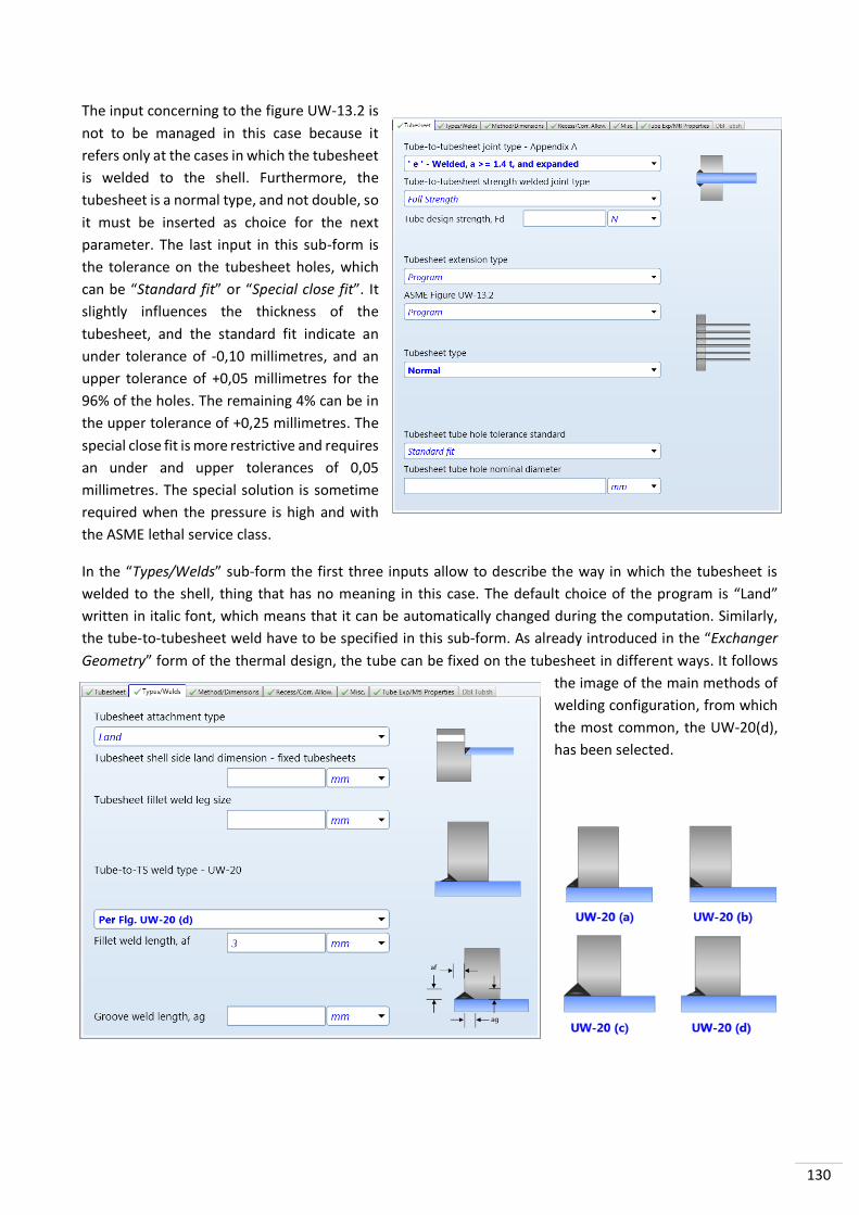
130

The input concerning to the figure UW-13.2 is

not to be managed in this case because it

refers only at the cases in which the tubesheet

is welded to the shell. Furthermore, the

tubesheet is a normal type, and not double, so

it must be inserted as choice for the next

parameter. The last input in this sub-form is

the tolerance on the tubesheet holes, which

can be “Standard fit” or “Special close fit”. It

slightly influences the thickness of the

tubesheet, and the standard fit indicate an

under tolerance of -0,10 millimetres, and an

upper tolerance of +0,05 millimetres for the

96% of the holes. The remaining 4% can be in

the upper tolerance of +0,25 millimetres. The

special close fit is more restrictive and requires

an under and upper tolerances of 0,05

millimetres. The special solution is sometime

required when the pressure is high and with

the ASME lethal service class.

In the “Types/Welds” sub-form the first three inputs allow to describe the way in which the tubesheet is

welded to the shell, thing that has no meaning in this case. The default choice of the program is “Land”

written in italic font, which means that it can be automatically changed during the computation. Similarly,

the tube-to-tubesheet weld have to be specified in this sub-form. As already introduced in the “Exchanger

Geometry” form of the thermal design, the tube can be fixed on the tubesheet in different ways. It follows

the image of the main methods of

welding configuration, from which

the most common, the UW-20(d),

has been selected.

131

Moving on the next sub-form “Method/Dimensions”, a section about the design methods can be noticed.

Since the tubesheet design can be done following different approaches, a choice must be taken between:

- Code only: the tubesheet design has to be done basing on the code rules only, ASME in this case. Please

note that until 2005 the ASME did not contain the rules for the tubesheets design, and an external code

or an internationally recognized standard, e.g. TEMA, had to be used.

- TEMA only: the tubesheet design has to be done basing on the TEMA rules. Since nowadays the ASME

have inserted the design procedure for the tubesheet, the design rules contained in the TEMA have been

moved in the appendix, and they have to be considered as good practicing.

- Code/TEMA thicker or thinner: this choice is used when the customer ask specifically for the TEMA

verification. Indeed, even if the requirements are to design following the ASME code in concomitance

with the TEMA rules as support, the TEMA no longer require the verification of the tubesheet. So the

TEMA check nowadays represent something more than the ASME and TEMA requirements.

For the reason above described, the choice of the tubesheet design method can be “Code only”. The

tubesheet design temperature has been uploaded automatically from the thermal design since it is equal to

the one of the tubeside. Instead, the tubesheet mean metal temperature is different from the tubeside and

shellside ones, and has not been placed. This happened because it does not enter in the mechanical design

calculations, since the U configuration of the tubes allow the thermal dilatation. The normal design of the

tubesheet is done taking the higher thickness given by the worst loading condition. The two cases that are

conceptually analysed are the ones resulting from the shellside or the tubeside subjected at the design

pressure and temperature, and not counterbalanced on the other side. Indeed, the other ambient is

considered as subjected at the normal conditions, or the vacuum if foreseen in the design conditions. This

lead to consider an overestimated design condition due to the consideration of higher pressure and

temperature, e.g. design versus the operative ones, and the neglection of the pressure and temperature

effects in the other ambient that would counteract the gradients. The higher thickness given from one of

these conditions would be assigned at the tubesheet. However, considering a case in which the thermal

dilatation is prevented, the mean metal temperature of the components would have an important role, and

the thickness resulting from this

computation would be higher. The internal

stress given from the thermal load and

prevented thermal expansions, as can

happen in a N head channel type, can be

compensated in different ways. The first is

to increase the thickness of the tubesheet,

while the last two are to increase the shell

or the channel thickness at welded

junctions. Depending from the position of

the stress concentration, one or a

combination of these solutions can be

required. This information may be

provided in the input “Tubesheet/Cylinder

optimization”, where leaving the choice at

the program means optimize the solution

in function of the case. The following

inputs allow to better specify these

increases in thickness. However, the

132

allowed thermal dilatation present in this case make these inputs unnecessary, and they will be left avoid in

order to not provide wrong constraints. Notice that only as last chance a designer will insert an inconvenient

component as an expansion joint. The two inputs that have not been analysed, since they are not foreseen

in the datasheet, are the vacuum design temperature and the effect of radial differential thermal expansion.

Changing sub-form, the first inputs presented in “Recess/Corrosion Allowance” are the tubesheet corrosion

allowances in the shellside and tubeside. They have to be specified if they have different values from the

general ones already inserted in “Problem Definition - Design Specifications”. If nothing is entered the values

inserted in the general specifications will be automatically upload. In this case, three millimetres on each

sides will be taken into account as already indicated. Proceeding, the recesses dimensions for the gasket

accommodation, already discussed talking about the body flanges in the “Front Head” sub-form, can be

specified for the tubesheet sides. They are represented here because the recesses are present even in the

tubesheet, as counterpart of the flange’s ones. All the remaining inputs, e.g. backing flanges, are useful only

in case of floating heads.

In the case in which the thermal dilatation would be prevented and the program cannot find a great solution

automatically, some warning will be generated. In that case it is useful to insert manually some dimensional

or technical constraints, e.g. one of the inputs contained in the “Adjacent Tubesheet Data” section of the

“Miscellaneous” sub-form. The ASME code imposes that the design of the tubesheets, especially the cases in

which the thermal expansion is prevented, must be based on the operative temperature, instead on the

design ones. These because the thermal contribution on the sizing of the tubesheet is driven by the difference

between the shellside and tubeside temperatures, which generally is higher for the operative temperatures.

Reassuming, by default the ASME imposes to consider the operative temperature, however, it leaves the

possibility to consider the design ones in case they will generate a greater gradient. All the rules to design

the tubesheets in the ASME code are contained in the UHX, and the possible options can be selected in these

sub-form, e.g. use the UG-34 (c)(3) option: for the thickness of the non-circular tubesheet. A lot of other

option can be specified in the section “Other”. For example if the tubesheet design has to be made using the

differential design pressure, or if consider an interior or an exterior tube of the bundle as reference for the

thermal stress. Since the tubes have different thermal stress in function of their position, the interior tubes

133

are generally used as reference, given that they have an higher thermal load. The values of the flanged

extension thickness must be made explicit and known when the collar bolts have to be used, while the elastic-

plastic option can be disabled, even if the tubesheet is the only part that can be designed by means of its

adoption.

At the end of the tubesheet form, a last sub-form

named “Tube Expansion/Material Properties” is

present. Parameters regarding the expansion of

the tubes in the bundle can be set here, e.g. the

maximum length that they can reach. Finally, two

sections dedicated at the material are displayed.

The first is the same at those previously analysed,

and it will override the data inserted in the material

section that will be examined. The second one

allow to insert the properties of the material

adjacent to the tubesheet which is used where

reinforcement is required. Even in this case, the

properties inserted here will override the ones

present in the general databank of the program.

134

TUBES/BAFFLES

In this part of the program, “Tubes/Baffles”, as well as in the following one, “Tubesheet Layout”, most of the

inputs are locked because the variation of their values could modify the heat exchanger thermal design and

the global configuration. They can be modified only if the user goes in the sub-form “Tubesheet Layout”,

present in the homonymous form, and sets “Create a new layout”. In this case a new layout can be

implemented, but it will not be taken automatically from the program. Indeed, all the data must be exported

from the mechanical part and

uploaded again in the thermal

one, in order to update the

results and the configuration.

Given the necessity to make the

mechanical design on the real

heat exchanger configuration,

these passages lead to a sort of

iterative procedure. However, all

the parameters here have been

already explained and have been

uploaded automatically from the

thermal design. The only

observation that can be done is

on the corrosion allowance.

Indeed, differently from all the

other heat exchanger parts, the

tubes generally are not oversized

by the corrosion allowance,

being the heat transfer in

function of the thickness.

Regarding the second sub-form,

“Baffles”, only some inputs are

consistent in this case. As a

matter of fact, being the device a

kettle, the baffles have a support

function only, and the flow is not

guided. The specification

“Unbaffled”, the number of

supports, and the input

regarding the ending one have to

be set here. In the analysed

application, three supports plus the ending one have been implemented as input. Some particular entries

are the ones regarding the space around the heat exchanger required to remove the bundle. These inputs

are not useful for the heat exchanger design, but they are present because the data will be provided to the

program packs which allow the whole plant layout design. This is because the ASPEN is a suite compounded

by a lot of program packs interacting one each other, not only intended to the mere heat exchanger design.

135

Same things happen in the sub-form “Baffle Details” in which no baffles are outlined. The tube unsupported

spans, reported from the thermal design, are the only consistent parameters. They are three, the first is the

unsupported span of the tubes between the supports, while the second and the third are the distances of

the first and last baffle from the tubesheet and the U bend support respectively. If the heat exchanger is not

a kettle, the baffle would have the purpose of deviating the flow. This means that the distances between the

baffles would be a design parameter for the thermal computation, and they could not be modified unless the

thermal design is done again. The only problems that the span length can introduce are the fluid elastic

instability or an acoustic resonance problems. So, the distances between the supports are simply obtained

dividing equally the length of the tubes.

As last sub-form the “Double/Triple Cuts” can be chosen. It allows to insert all the percentages of length

cutting, needed to define the baffles in the case of double or triple segmental cuts, and to choose which

segment is the starting one. These baffles have already been presented in the “Generalities on heat

exchanger” chapter, however, being this part of the program pointless for the analysed case, they will not be

thoroughly analysed in the thesis.

TUBESHEET LAYOUT

As already introduced, in “Tubesheet Layout” a lot of inputs are locked because depending on the layout

generated in the thermal design, while the other inputs have already been analysed. Only the equivalent

diameter, a service parameter used by the program to compute the shear stress, can be imposed. Proceeding,

in the “Thermal Layout” sub-form, a first technical drawing of the support is shown. On it, the most dangerous

tubes, analysed inside the “Vibrational & Resonance Analysis” form, have been outlined. Moreover, the

square tube pattern, the ribbon and horizontal pass layout orientation and the tie rods holes can be seen.

Notice that the horizontal pass layout determines the orientation of the U curvature of the bundle, which

does not influence the heat exchange, but can be very important for the vibrational and resonance problems.

At the end, the outer tube limit diameter, which cannot be modified, is shown in light blue in the image.

136

NOZZLES-GENERAL

In this set of sub-forms the parameters regarding the nozzles can be set. In the first two, “Shell Side Nozzles”

and “Tube Side Nozzles”, the general parameters can be selected. ANSI nozzle flange with an elevation of 200

mm above the vessel and without couplings have been chosen. The couplings, attachments for devices and

sensors on the tube, were used in the past in a configuration of one or two per tube. Nowadays they are

inserted only in particular cases and

only if required. Talking about the

flange design, an empirical method is

the historical Taylor Forge, that highly

overestimate the dimensions. While

the DIN standards have developed a

more scientific method for the flange

design, the classical numerical method

based on finite element analysis can

always be used. However, if standard

flanges have been selected, only the

rating have to be verified. The ratings,

expressed in pounds [lb], represent the classes in which the flanges are classified in function of the working

pressure and temperature, e.g. 150 lb, 300 lb; 600 lb; 900 lb; 1500 lb; 2500 lb. So, a flange is chosen from a

table, or automatically by the program, in function of its working pressure and temperature. Conceptually

the same process would have been done using the metric units of measure in the case of ISO standards.

Furthermore, talking about the whole pipe and flange coupling, different methods can be used in order to

obtain the reinforcement for the cut area of the hole. In this case the classic one is adopted, where a “Weld

neck” type of joint is used and the required compensation is made with a reinforcing pad. Notice that in this

case the flange can be of every type explained before, e.g. weld neck or slip on, while the “Weld neck” type

refers to the shape of the joints, which have a bevel to reach the standard dimension of the pipe. The “Long

welding neck” option instead does not present the bevel, allowing the pipe to be thicker, maintaining the

same internal diameter. Both the flange and the non-standard pipe are obtained from the same forging piece,

then welded at the end with the shell. If the long welding neck option does not allow enough increment of

tube’s area needed to satisfy the required reinforcement, the remaining area can be computed and added

at the end of the tube, by means of a local increment in thickness. In this case, a “Self-reinforcing” coupling

is obtained. Notice that, as already introduced, in some particular cases the reinforcing pad is not allowed,

e.g. hydrogen service, and one of the other solutions have to be mandatorily chosen. The “Code flange type”

is a parameter to be set in case of long welding neck or self-reinforcing nozzles, while the “Flange facing” can

be “Raised Face”, “Flat Face” or with

“Tongue and Groove”. The most

common choice is the raised face,

which presents a prominence on the

face to support the gasket, while the

flat face are generally used in

conjunction with the full diameter

gaskets. The last parameter, “Code

flange face type”, represents the way

in which the face of the flange have to

be worked, e.g. plane or grooved.

137

In the following sub-form, “Nozzles”, the dimension of the single nozzle and the angle of position can be

changed. These are the only parameters that would influence the thermal design of the device, e.g. changing

the ρν2 or the vibrational behaviour. Notice that the images on the right of the table serves as a guide for the

location number and for the positioning angle. The name and description of every nozzles must be manually

inserted, basing on the function, position and dimension. Finally it can be said that the coupling, the dome

and the distributor belts settings cannot be modified due to the fact that they was not present in the

application under exam.

NOZZLES-DETAILS-EXTERNAL LOADS

In this form, all the tables presented allow to customize every single nozzle and flange. Indeed, if the previous

section sets the general characteristics, here, all the geometrical dimensions, positions, as well as the joint

efficiency and corrosion allowance can be specified for every nozzle. Also the dimensions of the reinforcing

pads and the parameters of every nozzle’s flanges, e.g. type, rating and face, can be implemented. However,

in this section, as in some others already faced, it is not convenient insert values in the first attempt. Different

is the case in which the device has some geometrical clearances to be observed, or some external loads acting

on the nozzles. In that case, the input value have to be inserted using the last two sub-forms, named “Nozzle

clearances/Miscellaneous” and “External Loads”. The first has been reported below, and it presents the

possibility to insert some other parameter. As examples can be reported the possibility to insert the nozzle

reinforcing ring, previously named reinforcing pad, or “100% Metal replacement in pad” which allow to do

not consider the corrosion in the reinforcing pad.

138

HORIZZONTAL SUPPORTS

The heat exchanger is generally supported by means of two saddles which allow to fix it at the ground, always

leaving a degree of freedom for the thermal expansion, or to stack more device one to another. Location,

distances and orientation, as well as the parameters for the friction of the contact with the ground can be

specified. Given that the contact with the saddles induces a higher mechanical stress on the shell, particularly

in the case in which the internal pressure is not to high and the thickness will not be too much, stiffening ring

on the junctions are inserted. This will change the moment of inertia and increase the stiffness of the part

subjected at the stress, which can be computed with the method of Zick. As last parameters, the total loads

on the saddles can be inserted manually if other devices would be present on the heat exchanger, e.g. a

device that discharge its weight on a nozzle.

In the sub-forms “Details” and “Gussets/Bolts” the insertion of all the geometrical parameters of the parts

that compound the saddles take places. Entering more in detail and providing some terminology, a support

is formed by a wear plate welded to the shell and supported by some vertical internal rib which are indicated

as gussets. The plate that cover the gussets is named web, and the one on which all is placed is the base

plate. Last sub-form “Stacked Units” allow to choose if admit the stacking of more device whereas more than

one would be present. However, the configuration on one only heat exchanger was an output provided from

the thermal design.

139

MATERIALS

In the thermal design part only the class of the material, e.g. carbon steel, was

implemented as input. Indeed, it was the only information required in that part

in order to compute the thermal conductance, which, as delineated, it is also in

function of the material class. In the mechanical design, instead, the material

type and the grade, in concomitance with the standard specification of the used

code have to be denote.

Starting with the first form “Main Materials”, and clicking on the button “Search

Databank”, the correct type of material and grade can be found and assigned at

every part of the heat exchanger. In order to make the research easier, the first section allows to type the

name of the standard specification. The second section, instead, provide the list of all the materials contained

in the selected code. Choosing a material type, e.g. Plate, a filter is applied to the whole list, and the correct

specification can be selected among those who remain displayed. In the third part, the material chosen above

can be assigned at every selected component of the heat exchanger by means of the “Set” button.

Please notice that the experience cover a high role in the selection of the correct standard specification.

Indeed, all the specification should be opened, read, and evaluated in order to find the correct one. Have

experience in this field means that the designer can easily determine the approximative range of the final

thickness and made the correct choice of the specification at the first attempt. This allow to avoid incredible

efforts and time spent to research the correct specification. Taking as example the regulation of the plates,

a lot of them are available in the ASME code, which moreover insert also the low-alloyed steels in the carbon

140

steel class. The standard specification generally used for the plates of not alloyed carbon steel, for the

refinery service in-pressure applications, is the SA-516. It presents three options:

- SA-516 K01800 Grd 55 Plate

- SA-516 K02100 Grd 60 Plate

- SA-516 K02700 Grd 70 Plate

These three options differs from the grade, indicated with the number that represents the KSI, Kilopound per

Square Inc, of the yield strength. So, increasing the grade, the yield strength of the material increase due to

the high percentage of carbon inside of the steel. Again the experience can suggest that the grade 70 is the

best because, even if the material is more expensive, there is a saving given by the less material required.

However, if this concept is correct for a normal condition of working, the higher content of carbon present

in the grade 70 makes it more prone to crack in working conditions in which high level of hydrogen, or

hydrogen sulphide, is present.

Those are the cases in which plates

of grade 55 or 60 are used for the

refinery service in-pressure

applications. Returning on the

program, it index all the materials,

and the corresponding standard

specification, with an internal

number. All the selected materials

chosen for the study case, and the

relative internal numbers, can be

seen in the following image.

All the materials assigned was

outlined by an ASME technical

specification, given that it is the

code used in the project. However,

even if each codes define the

materials using different technical

standards, they are conceptually

similar setting the minimum

characteristics that the material

must accomplish in order to be sell

with a certain name.

It is now possible move on the second sub-form “Normalized/Clad Materials”. Based on the provided

technical standard, one or more heat treatments can be necessary if the thickness overcome a certain value.

For example, the SA-516 Grd 70 foresees the mandatory normalization in case of plate thicker than 40mm,

while they can be provided “as rolled” in the other cases. These heat treatment bring back the material grains

to the original condition, before the rolling. This is particularly important for the carbon steel which will

operate at medium or low temperature. In the ASME paragraph UCS-66, where UCS indicate a Carbon Steel

requirement, the curves for every material allow to obtain the Rated Minimum Design Metal Temperature

in function of the thickness. Conceptually, during the design activity the Rated MDMT of the material used

must be lower or equal than the MDMT of the input data, 5°C in this case. As example, a material SA-516 of

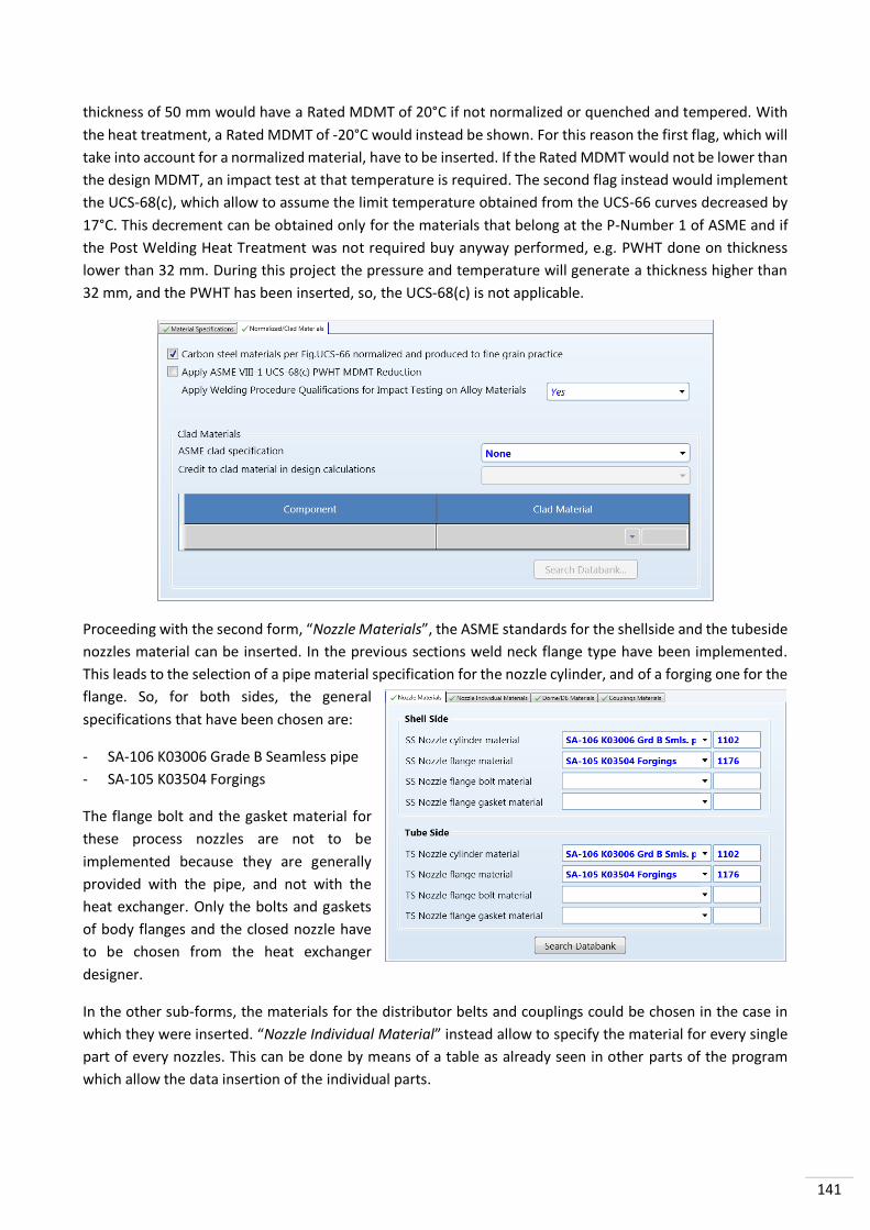
141

thickness of 50 mm would have a Rated MDMT of 20°C if not normalized or quenched and tempered. With

the heat treatment, a Rated MDMT of -20°C would instead be shown. For this reason the first flag, which will

take into account for a normalized material, have to be inserted. If the Rated MDMT would not be lower than

the design MDMT, an impact test at that temperature is required. The second flag instead would implement

the UCS-68(c), which allow to assume the limit temperature obtained from the UCS-66 curves decreased by

17°C. This decrement can be obtained only for the materials that belong at the P-Number 1 of ASME and if

the Post Welding Heat Treatment was not required buy anyway performed, e.g. PWHT done on thickness

lower than 32 mm. During this project the pressure and temperature will generate a thickness higher than

32 mm, and the PWHT has been inserted, so, the UCS-68(c) is not applicable.

Proceeding with the second form, “Nozzle Materials”, the ASME standards for the shellside and the tubeside

nozzles material can be inserted. In the previous sections weld neck flange type have been implemented.

This leads to the selection of a pipe material specification for the nozzle cylinder, and of a forging one for the

flange. So, for both sides, the general

specifications that have been chosen are:

- SA-106 K03006 Grade B Seamless pipe

- SA-105 K03504 Forgings

The flange bolt and the gasket material for

these process nozzles are not to be

implemented because they are generally

provided with the pipe, and not with the

heat exchanger. Only the bolts and gaskets

of body flanges and the closed nozzle have

to be chosen from the heat exchanger

designer.

In the other sub-forms, the materials for the distributor belts and couplings could be chosen in the case in

which they were inserted. “Nozzle Individual Material” instead allow to specify the material for every single

part of every nozzles. This can be done by means of a table as already seen in other parts of the program

which allow the data insertion of the individual parts.

142

PROGRAM OPTIONS

The program options of the mechanical design part will not be

thoroughly analysed, as it had been done for the thermal part.

During the pressure vessel design, different load types have to

be taken into account, and these are the subjects to which the

first form refers. Generally they are categorized in external

loads, wind and seismic loads, earthquake loads, weight and

insulation load. Common external loads to be considered are

the thrusts given from thermal dilatation of the connection

pipes. The best way to verify the resistance of the connection

area in this case is to make a stress analysis with the loads

provided from the pipe designer, or with the standard load

estimated for the type of pipe. The Welding Research Council issues empirical methods, e.g. WRC 537, to

verify the external loads, firstly developed to overcome the absence of the stress analysis method. However,

given the possibility to provide fast result, they are still in use, even if the results are overestimated. However,

attention must be paid because these methods have some applicability limits defined by the nozzle’s tube to

shell ratio and from their relative stiffness. If these limits are not respected, other methods, or the time

expensive stress analysis, have to be evaluated. The wind loads should be taken into account for the pressure

vessel designed for an outdoor working environment. However, given the commonly compact shape of the

heat exchangers, this load only impacts on the supports size rather than on the shell design. Different would

be the case in which a tall and wide device have to be designed, where the possibility of high moments

induced by the wind have to be carefully considered. Similar considerations can be done for the seismic loads.

The evaluation of these loads must be done using the different codes generally applied in the civil engineering

field, e.g. ASCE, IBC o the Eurocodes. It is important to remark that every case can be different and can

present some peculiar external loads to be considered. For example, due to the situation, it may happen that

the weight of the snow or of the insulation have to be considered, as well as the external loads given from

the sea or ground pressure if the device will be placed undersea or underground respectively. All these stress

have been thoroughly considered in the real design of the heat exchanger associated at this study case.

However, they would require a deep analysis of the situation and the development of many considerations

not pertinent on the subject of this thesis. For this reason, the importance of these considerations have been

outlined in this paragraph, but they will not be inserted explicitly.

A last important consideration to make

is about the pressure of the water

during the final test. As explained in the

paragraph “Problem Definition”, the

minimum test pressure of the water is

done by 1,3 · 𝑀𝐴𝑊𝑃 · 𝐿𝑆𝑅 where the

MAWP is the Maximum Allowable

Working Pressure, and the LSR is the

Lowest Stress Ratio. However, due to

technical approximations or by a client

requirements, the real value of the test

can be higher than the minimum one

explained above. If this happens, it means that a pressure higher than the minimum one computed by the

143

program has been inserted in the field “Test Pressure” in “Problem Definition – Design Specification”. In this

case, a verification calculation have to be done using this pressure, which means to run one extra time the

mechanical design inserting Yes in “Hydro test calculation case”. Anyhow, being this pressure computed using

the MAWP and highly overestimated with respect to the real pressure of working, but supported only for

once time from the device, and at ambient temperature, a higher percent of the yield stress can be used for

the calculation with respect to the one used in the design. The ASME code admit using the 90% of the

theoretical yield stress as limit for this verification. Last but not least, the drawings to be produced as output

have to be selected, and some technical parameter for the calculation of the cost can be implemented.

144

7.3. ITERATIVE CORRECTIONS AND RESULTS SECTION

Once that all the input parameters have been inserted, the button “RUN” can be pressed. In this phase,

similarly to what has already been done for the thermal design, the program will solve all the formulas taken

from the selected code of calculation and fill the output of the mechanical design. As for the input, even the

result part of the program is compounded by several sections, each of which can be divided in forms and sub-

forms. In the first section, “Input Summary”, a resume of the input data is reported. Given the simplicity of

the mechanical design results, represented mainly by the dimensions of every heat exchanger’s parts, this

section will not be analysed following the exact division proposed by the program. However, all the results

can be found in the output tables reported in the next chapter, as well as the technical drawings and the

calculation report can be seen it the dedicated appendices. In this first chapter, instead, the analysis of the

warnings developed by the program for the first obtained result will be done. Moreover, in order to solve

them, further implementations of the input data will be presented where necessary.

FIRST RESULT AND MODIFICATIONS

The “Warning/Messages” form, contained in the section “Design Summary”, can be taken as reference for

this procedure of final checks and modifications. Given that the software executes a mathematical approach

to define the minimum thicknesses, the first thing that a designer have to do is to check the compatibility

between the resulting dimensions and the pieces present on the market, or simply a conscious observation

of the results. No input or result warnings have been generated, so the input section has been completed

correctly and with all the mandatory data so that the program was able to calculate a result. However, some

advisory and notes have been produced. Even if they do not compromise the design, they must be

considered.

Starting from the two “Notes 711”, they explain why the thicknesses of the two tubeside nozzles, T1 and T2,

have been increased. As already presented, the compensation for the resistance decrement caused by the

holes is achieved by an empirical method. Following the ASME code, this method implies to increment the

transversal area present in the so-called reinforced limit in order to compensate the area of the shell that

has been removed. With this purpose the program has increased the thicknesses of the cylinders that

compound the nozzles. Checking the thicknesses of the plates from the correspondent drawing it can be

noticed that the front head cylinder plate, which minimum thickness was been computed as 31 mm, must

be set at 32 mm for market compatibility reasons. This should solve the “Note 711” because it results in an

addition of compensation material for the nozzles T1 and T2. On the other hand, the thickness of the plate

for the shell diameter can be set as the one of the starting plate from which the shell cover will be formed,

145

e.g. 55 mm considering the 10% of shrinkage. In this way, no step will be present in the joint, and the same

plate can be used for both parts. Notice than given the input provided at the program, the shell cover plate

in the drawing is represented with the final thickness, and not with the one that will be necessary to purchase.

To implement all the required modification, it is enough to go in the section correspondent at that input, and

insert the value in the correct field. Running again the program with the new inserted constraints leads to a

solution in which the two notes regarding the nozzles are no more present, and the plates thicknesses are

acceptable.

The four “Advisory 83” show the possibility of the Post Weld Heat Treatment to be required for the shell

cylinder and cover, as well as for the eccentric reducer and for the kettle cylinder. These advisory are only

remainders, and given that the PWHT has already been requested in the input, they do not imply any further

modification.

The “Note 909”, instead, regards the after forming heat treatment of the shell cover. The ASME code impose

always the heat treatment in case of hot forming, while, in case of cold forming, it is mandatory only if fiber

elongation is higher than 5%. So, given the fiber elongation of 12,78%, this note is a reminder of this

requirement if cold forming will be performed. No modification in the design parameters are required, but

attention must be paid to comply with this requirement when the forming procedure will be done or

subcontracted.

The last remaining note is the 487, which warns for the insertion of a cone compression ring. Due to the fact

that, sometime, the compression ring leads to manufacturing problems given the lack of space for welding,

it may not be desired. In this case, the plate thickness of the cone can be increased, from 58 mm to 60 mm,

in order to intensify the stiffness of the cone and no longer make the ring necessary.

Last modifications before than the final mechanical design will be produced regard the nozzles and the

reinforcing pads dimensions. Indeed, the standard pipes for the nozzles have to be selected in order to avoid

further verifications with stress analysis methods. Given the outside diameters already inserted in “Nozzles-

General” during the implementation of the inputs, the program have computed a possible solution for each

pipe. However, standard pipes would be appreciated. In order to get this result, the inner diameter of each

tube can be carefully chosen and inserted as input. Observing the minimum thickness of each tube computed

by the program, a tube schedule that ensure a thickness higher than it can be chosen for each tube. This can

be done because the standard tubes are organized in schedule which fix all the dimensions of the tubes in

function of the outer diameter. It is now reported a table in which the results of this procedure can be seen.

NAME DESCRIPTION OUTER DIAMETER MINIMUM THK. SCHEDULE THICKNESS INNER DIAMETER

S1 Water IN 88,9 mm 9,19 mm Schedule 160 11,13 mm 66,64 mm

S2 Water OUT 48,26 mm 7,11 mm Schedule 160 7,12 mm 34,02 mm

S3 Vapour OUT 114,3 mm 9,66 mm Schedule 120 11,13 mm 92,04 mm

T1 HCBN IN 457,2 mm 16,55 mm Schedule 60 19,15 mm 418,90 mm

T2 HCBN OUT 508,0 mm 17,99 mm Schedule 60 20,62 mm 466,76 mm

As before explained, the computed inner diameters can be inserted as input in the respective sub-form. In

this way the dimensions of the pipes are fixed and they will be found on the market since they belong to

standard schedules.

146

Running the program with the addition of the inner diameters as constraints, the variations of thicknesses

will lead to modifications on their respective reinforcing pad. Please notice that if the imposed thicknesses

by the inner and outer diameters would not satisfy the minimum ones, a warning would be issued. The

reinforcing pads can be analized and checked by means of the drawings. Particularly a pad of 31 mm of

thickness can be increased to 32 mm given that a plate of that dimension has been already uses. This lead to

a reduction of different material type to be purchased. In order to fix the thickness of that reinforcing pad,

its value have to be inserted in the “ExchangerGeometry - Nozzle Dettails”. Same procedure can be done for

all the reinforcing pads with thickness different from the plates already used. Running for the last time, the

final design of the heat exchanger is issued with the correspondant drawings, calculation report and the

results that will be listed in the next chapter.

147

OUTPUT TABLES

DESIGN SUMMARY

148

149

150

VESSEL DIMENSIONS: CYLINDERS AND COVERS

151

VESSEL DIMENSIONS: NOZZLES – NOZZLE FLANGES

152

VESSEL DIMENSIONS: BODY FLANGES

VESSEL DIMENSIONS: TUBESHEETS – TUBES – BAFFLES

153

154

VESSEL DIMENSIONS: SUPPORTS

155

8. CONCLUSIONS

As it has been introduced during some thesis’ passages, the design and simulation programs perform the pre-

set computations based on the indicated design code. Even if its use makes the computation phase easier,

the only way to obtain, avoiding errors, the best configuration for the case under analysis is by a correct and

careful management by the engineer. The first personal observation that is worth to do concerns the

previously introduced approach the designer must have with the program. Often the problem is not

represented by which input value have to be assigned, but rather by the necessity to do not insert too many

constraints. Indeed, to insert an input means to add constraints to the configuration. This can lead to the

impossibility to achieve a final design, to the issue of warning notifications or to the program crash.

Furthermore, if this last option occurs and many inputs have been introduced, the designer might find hard

to understand which value is causing the problem. As example, the heat exchanger of the study case has a

removable U-shape bundle, in which there are not thermal expansions prevented. In this case the insertion

of input parameters in a function which have the goal to balance the thermal stress will produce a constraint,

which in turn will not allow to reach a possible configuration. It is therefore necessary to understand the

possibilities of the program, the meaning of its functions, and which inputs are mandatory to obtain the

desired configuration. Hence, the first computation phase of the program has to be launched with as few

inputs as possible, and the needed constraints must be inserted gradually during the steps. This generates

an iterative procedure, still allowing to maintain the control over the project activity.

Resuming the thermal study case, further observation and analysis can be pointed out. The configuration

that has been chosen as the best one is named Design 6 in the study case. Among those analysed, it was the

one which better satisfies the parameter of selection, as the heat exchanger cost, the area ratio and the

feasibility of the device. Only the Design 4, which also satisfies the area ratio and the pressure loss

constraints, could be seriously considered as an alternative option, being its estimated cost 5% lower than

the Design 6. However, it presents some vibration problems which lead it to be discharged given that, during

the design activity, the input data was already optimized for the cheapest solution. Indeed, a modification of

the input parameters to make it compliant with the requirements would probably lead to an increment of

the price for that solution. In the other cases, depending on the location in which resonance occurs, a

modification on the supports, like increasing their number or the spacing between them, could solve the

problem. Other solutions like using a different tube pattern, e.g. 45° instead of 90°, or modifications that

change the fluid dynamic of the system can also be examined. However, given the pool boiling configuration

with almost absent shellside flow, the adjustments of the baffles like the type and the cut orientation cannot

be made. All these considerations lead to the definitive choice of the Design 6, which configuration presents

a single AKU horizontal device as solution. As it has been indicated, for the shellside there are one input and

two outputs, one for the steam and one to drain the non-vaporized water. For the HCBN in the tubeside,

instead, only two nozzles are present, but the dimensions are much greater due to the higher mass flow

rates. An acceptable number of 502 tubes, with length of 5400 mm and two passages are required. Being the

bundle a U-type, the two passages are mandatory and the number of tubes lead to have 1004 holes in the

tubesheet, while the total minimum straight length of the tube required to produce one fork turns to be

10800 mm. This allows to define a gross surface exchange area of 464,6 m2, which at the net of the portion

that does not effectively transfer heat, evolves into the effective heat exchange area of 449,4 m2. Note that

being in this case the U-bend totally immersed, its area has been indicated as transferring and therefore it

has not been subtracted. The required area, instead, can be found from the analysis of the heat transfer

resistances for both conditions, clean and fouled. Once that all these data are available, the area ratio can be

computed by means of the proportion between the effective and the required area. In particular, in the

156

cleaned condition, a greatly overestimated area ratio of 2,36 can be computed by means of a required area

of 190.5 m2. In the fouled one, instead, an area ratio of 1,02 can be computed with a required area of 442,7

m2. This means that this design has an oversized area of 2% in fouled condition, which is within the range of

the minimum percentage of overestimation requested in the input parameters. Here, the high influence of

the fouling can be seen. Indeed, in fouled state the required area is more than twice the one required in clean

state. This happens because the fouling decreases the capacity to transfer heat in the device changing the

effective values of the thermal conductance ℎ [𝑊 𝑚2⁄ 𝐾], and so the overall heat transfer coefficient

𝑈 [𝑊 𝑚2𝐾⁄ ]. It is worth to recall that, as analysed during the thesis, all these aspects are in function of the

fluid velocity. In order to enhance the heat transfer, a lower speed would be better. However, poor velocities

lead to increase the fouling, while a too high speed can generate erosion or vibration problems. In the

shellside, the velocity of the water is very low, but it can be acceptable due to the pool boiling configuration.

In the tubeside, instead, the configuration leads to have 7 m/s, which is higher than the minimum 2÷3 m/s

required for dirty fluid as the HCBN. On the other hand, as it was analysed in the “Flow Analysis” form, the

values of ρv2 obtained in the study case are far minor than the limit reported in the theoretical part, so no

modifications on the nozzle diameters was required.

Comparing the mass flow rates present in the output with the design parameters inserted as input, it can be

noticed that some calculation refinements have been done. In particular the mass flow rates divisions of the

outing phases are slightly different due to the integration procedure. Despite that, they can be accepted

being the variations in the order of 0,004% ÷ 0,005% with respect to the values indicated in the inputs. As

demanded, the vaporization is practically complete, while the HCBN partially condenses during the path. The

same minor alteration has been made on the outlet temperature of the steam. As already said, it was possible

to choose the Design 6 because the computed pressure drops were lower than the maximum allowed.

Indeed, the 0,12487 bar in the shellside is less than 0,3 bar, while in the tubeside 0,41924 bar is minor than

0,7 bar. Analysing more in detail the subdivisions of the pressure drop, it can be noticed that the higher

contribution in the shellside is given from the outlet nozzle which is responsible for the 80,52% of the whole

value. In the tubeside, instead, the critical part is represented by the losses inside the tubes, which account

for the 83,22%.

Moreover, a brief summary of how the total thermal exchange of 5418,3 kW is divided among the process

can be discussed. In the tubeside the fluid is biphasic either at the inlet and at the outlet, but during the

process it condenses providing heat. In particular, it can be seen from the results that the HCBN gas phase

releases the 16,54% of the total heat emitted, while the liquid the 27,2%. The remaining 56,26% is provided

during the condensing process that transforms the vapour into liquid. In the shellside, where the heat is

received, it can be seen that the 74,23% of the total heat exchange is latent heat, while only the 25,8% is

used to bring the water at the boiling temperature. These are reasonable values since the aim of the device

is to provide saturated vapour. Indeed, the steam will not be oversaturated, and the percentage of the heat

absorbed by the vapour phase is nil. Another parameter which allows to observe the quality of the vapour at

the outlet is the already explained entrainment ratio. Expressing the percentage of the outlet mass which

can be in liquid phase, it links the quality of the vapour at the outlet with the difference between the shell

diameter and the bundle one. The estimated diameters values for this configuration produce an entrainment

fraction of 0,0001, which is much lower than the maximum limit of 0,02 prescribed for dry steam. Regarding

the quality of the vapour at the top of the bundle, instead, it has to be as lower as possible, because the tubes

must always be covered by water. The resulting value of 0,0172 can be accepted. If the quality of the vapour

had been too high, an intervention on the process parameters would have been required, e.g. an increment

of the water mass flow rate, or a decrement of the hot fluid one. Differently, if the problem had been

represented by the entrainment fraction, an increment of the inner shell diameter must have been done.

157

In order to evaluate the configuration generated with the thermal design, two vibration & resonance analysis

have been performed, and the results have been analysed. With both the analysis methods, HTFS and TEMA,

either the fluid elastic instability and the evaluation of the resonance have not shown any problems. The

assessment of the fluid elastic instability was done computing the ratio between the actual shellside flowrate

and the critical flow rate which causes it. For all the points and for all the values of damping adopted in the

computation, the resulting ratio was correctly far from 1. The acoustic resonance, instead, was investigated

using the ratio between the tube frequency and the tube acoustic natural frequency. In the same way, this

ratio must be as far as possible from 1. In a more detailed way, the program reports both values of the two

riskiest tubes: the natural frequency 𝐹𝑛 and the acoustic natural frequency 𝐹𝑎, that will cause resonance in

motion and sonorous respectively. After the selection of the configuration, the rating mode was made

available and modifications of the output parameters in a iterative way was made possible. The size of the

nozzles have therefore been compared to the ASME standard diameters of the pipes on the market. Nothing

has been changed except for the nozzle of the shellside vapour outlet, which was increased from 3,5 inches,

which is not a very common dimension, to 4 inches. After the nozzle modification, the geometry configuration

must be processed again. Notice that all the results reported in the thesis for the thermal design are the ones

obtained in the first passage, and not in this last iteration. However, the modification of this nozzle have only

produced some slightly improvements as a decrement of the pressure drop and of the ρv2. It is worth to

specify that the used input of the mechanical design was the last iteration of the thermal part, as it should

be.

After the insertion of the still required inputs explained during the thesis, also the mechanical output has

been made available. A first aspect that can be analysed in this final presentation is that, given the thicknesses

over 40 mm, the normalization after rolling requested by the SA-516 Grd 70 plates have to be satisfied, as it

was foreseen during the implementation of the inputs. This heat treatment brings back the material grains

in the original condition, before the rolling. As explained, this is a particularly important factor because it

allows to obtain, from the ASME paragraph UCS-66, a Rated Minimum Design Metal Temperature of -10°C

for the higher thickness of 55 millimetres, which is lower than the 5°C of MDMT provided as input.

Contrariwise, given that some parts in P number 1 material mandatorily require the PWHT because their

thicknesses are higher than 32 millimetres, the UCS-68(c) would have been inapplicable, and an impact test

at that temperature would have been required in order to further investigate the material resistance. Indeed,

please note how, if the carbon steel had not been normalized, the Rated Minimum Design Metal

Temperature obtained from the UCS-66 would have increased quickly with the thickness, so the impact test

would have been required. During this test the specimens should have shown an amount of energy absorbed

higher than the limits provided by the code in use, so as to certify that a ductile-brittle transition has not

happened until that temperature.

Going back to the analysis, in the inputs and during the design process enhanced problems of corrosion or

hydrogen embrittlement have not been indicated or foreseen. So, the canonical three millimeters of oversize,

resulting from the 0,1 millimeters of average corrosion per year estimated for a not high-aggressive

hydrocarbon on a lifetime of 30 years, have been inserted as corrosion allowance. However, unlike all the

other heat exchanger parts, the tubes generally are not oversized, being the heat transfer in function of the

thickness. Indeed, it is generally preferable to adopt more efficient materials, e.g. stainless steel, than to

increase the thickness of the tubes. Totally different is the case of the tubesheet, which is in contact with

fluids on both sides. As explained, in this case three millimeters have been added on both sides, resulting in

6 millimeters of oversize. Being this project in the ASME Normal service class, any mode of defect control

could be designated. However, given that large thicknesses were foreseen, and the code forces to make the

full radiography over a certain value, this control mode was already inserted from the beginning. This choice

158

led to the possibility to adopt the joint efficiency equal to one in the thickness’ formulas of the components,

with the consequence that they have not been increased, given the total control of the welding joints and

the impossible presence of not found defects. Still in the mechanical output the Maximum Allowable Working

Pressures can be seen and compared with the respective design pressures. The MAWP of the shellside and

of the tubeside are represented by the lowest MAWP of the single side-component. In this case, each side

has the MAWP determined by the Front Head Bolting, which in particular is equal to 78,03 bar for the

shellside, and to 60,01 bar for the tubeside. Notice that their values are really close to the design pressures

of 78 and 60 bar respectively. This situation is correct and indicates a well-done design, without waste of

material. Indeed, these values already contain the necessary precautions, being the design pressure a large

overestimation of the working one and the yield strength of the material assumed as the minimum indicated

in the standard specification. Furthermore, the computation of the allowable stress is subjected at the safety

factors of 1,5, as indicated by the ASME section VIII Division I. The hydrostatic test pressures, used in the final

test, are higher than the design ones to compensate the fact that the test will be made at room temperature.

The resulting values, computed with the formula 1,3 · 𝑀𝐴𝑊𝑃 · 𝐿𝑆𝑅 contained in the ASME code, are 101,4

bar for the shellside, and 78,0 bar for the tubeside. Notice that once that the 𝑀𝐴𝑊𝑃 of the shellside and

tubeside have been fixed, the Stress Ratio, value obtained dividing the admissible stress at room temperature

by the one at the design temperature, being in function of the materials, is the only parameter that can

change in the formula. The Lower Stress Ratio for both hydrostatic tests, the shellside and the tubeside ones,

results to be 1. In each cases it is given from the material of the pipes, SA-106 K03006 Grd B Seamless Pipe,

which generally degrades less than the other. Indeed, for the ASME, the lower ratio is always provided by the

material which less suffers from the variation of the temperature, excluding the bolting materials whose

admissible stress value practically doesn’t change. Notice that, even if the vacuum working condition is not

foreseen, the tubes of the bundle are designed also against the external pressure, and after the higher

thickness is chosen. Even in this case, as well as for the tubesheet, it could be possible to adopt the differential

pressure approach, providing that a loading procedure would be associated with the device. Finally, the

discussion of the mechanical output can be concluded with the control on the component dimensions, which

are all acceptable, and allow enough space to perform the welds during the production of the piece.

Now that the noteworthy results have been commented, it is possible to investigate the limitations of the

study. During the thermal design the thickness of the tubesheet is roughly estimated, given that it influences

the heat exchange. However, only the dimension evaluated in the mechanical design can be accepted as safe

for the piece resistance. This value, even if moderately, is generally different than the one estimated, and

leads to a slightly variation in the heat exchanged. In order to make a precise design, a verification of the

thermal design with the new thickness of the tubesheet must be made reloading the results of the

mechanical part in the thermal one. In case of a larger thickness difference and a small area ratio margin the

new thermal design could result unacceptable. Please, note that during this procedure the configuration and

the dimensions of the heat exchanger are set. However, it is worth to remember that in the study case the

thermal design was overestimated of the 2% in the fouled conditions, and the variation of the tubesheet

thickness was negligible. So even if slightly approximated, since it was the version before the rating mode

and the refinement of the dimensions, the thermal design reported in the thesis results to be valid and truly

representative.

The last remarks to conclude the discussion regard the technical drawings, reported in the Appendix I. Being

automatically generated by the software, they are not enough accurate to be used during the production

phase or to be provided to the client. However, they are an excellent starting point for a designer to produce

the final version.

159

9. APPENDIX I: TECHNICAL DRAWINGS

160

161

162

163

164

165

166

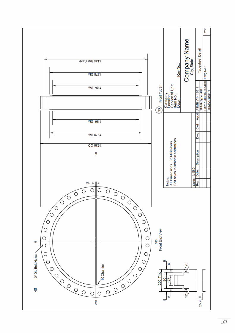
167

168

169

170

171

172

173

10. APPENDIX II: CALCULATION REPORT

Component: Shell Cylinder

ASME Section VIII-1 2017 UG-27 Thickness of Shells under Int. Pressure

--- Calculations --- Cylinder Internal Pressure

Material: SA-516 K02700 Grd 70 Plate

Design pressure P = 7.8 N/mm2 Design temperature T = 280 C

Radiography = Full Joint eff.circ str. E = 1

Design stress S = 136.406 N/mm2 Joint eff.long str. E = 1

Design stress, long S = 136.406 N/mm2 Min thk. UG-16(b) tmin = 4.89 mm

Inside corr.allow. CAI = 3 mm Outside corr. all. CAO = 0 mm

Material tolerance Tol = 0.3 mm TEMA min. thickness tm = 12.7 mm

Outside diameter OD = 1280 mm Corroded radius IR = 603 mm

Required wall thickness of the cylinder , greater of:

Circumferential stress

t = (P*IR / (S*E-0.6*P))+cai+cao+tol = 39.01 mm UG-27(c)(1)

Longitudinal stress

t = (P*IR / (2*S*E+0.4*P))+cai+cao+tol = 20.35 mm UG-27(c)(2)

Actual wall thickness of cylinder: tnom = 40 mm

(Required wall tks. for nozzle attachments, E=1 , tri = 36.01 mm )

Component: Front Head Cylinder

ASME Section VIII-1 2017 UG-27 Thickness of Shells under Int. Pressure

--- Calculations --- Cylinder Internal Pressure

Material: SA-516 K02700 Grd 70 Plate

Design pressure P = 6 N/mm2 Design temperature T = 300 C

Radiography = Full Joint eff.circ str. E = 1

Design stress S = 134.917 N/mm2 Joint eff.long str. E = 1

Design stress, long S = 134.917 N/mm2 Min thk. UG-16(b) tmin = 4.89 mm

Inside corr.allow. CAI = 3 mm Outside corr. all. CAO = 0 mm

Material tolerance Tol = 0.3 mm TEMA min. thickness tm = 12.7 mm

Outside diameter OD = 1264 mm Corroded radius IR = 603 mm

Required wall thickness of the cylinder , greater of:

Circumferential stress

t = (P*IR / (S*E-0.6*P))+cai+cao+tol = 30.85 mm UG-27(c)(1)

Longitudinal stress

t = (P*IR / (2*S*E+0.4*P))+cai+cao+tol = 16.59 mm UG-27(c)(2)

Actual wall thickness of cylinder: tnom = 32 mm

(Required wall tks. for nozzle attachments, E=1 , tri = 27.85 mm )

174

Component: Shell Cover

ASME Section VIII-1 2017 UG-32 Formed Heads, and Sections,

Pressure on Concave Side

--- Calculations --- Ellipsoidal Cover Internal Pressure with t/L >= 0.002

Material: SA-516 K02700 Grd 70 Plate

Design pressure P = 7.8 N/mm2 Design temperature T = 280 C

Radiography = Full Joint efficiency E = 1

Design stress S = 136.406 N/mm2 TEMA min. thk tm = 12.7 mm

Min thk UG-16(b) tmin = 4.59 mm

Inside corr.all. CAI = 3 mm Outside corr.all. CAO = 0 mm

Major/minor rat. D/2h = 2.0 Forming tolerance Tol = 0 mm

Corroded min. thk t = 45.92 mm Equiv.dish radius L = 1437.3 mm

tnom-CAI-CAO-Tol ts = 46.7 mm Ratio ts/L ts/L = 0.03249

K =0.1667*(2+(D/2h)**2) = 1.0 Material tol. Tol = 0.3 mm

Outside diameter OD = 1691 mm Corroded diameter ID = 1597 mm

Required wall thickness of the cover:

t = (P*ID*K / (2*S*E-0.2*P))+cai+cao+tol = 49.22 mm App. 1-4(c)

Actual wall thickness of cover: tnom = 50 mm

(Required wall tks. for nozzle attachments, E=1 , tri = 46.22 mm )

(If opening & reinf. are within 80% of head diameter, tri = 41.63 mm )

Component: Eccentric Reducer

ASME Section VIII-1 2017 UG-32 Formed Heads and Sections,

Pressure on Concave Side

--- Calculations --- Conical Cover Internal Pressure

Material: SA-516 K02700 Grd 70 Plate

Design pressure P = 7.8 N/mm2 Design temperature T = 280 C

Radiography = Full Joint efficiency E = 1

Design stress S = 136.406 N/mm2 TEMA min. thickness tm = 12.7 mm

Inside corr.allow. CAI = 3 mm Outside corr. all. CAO = 0 mm

Material tolerance Tol = 0.3 mm

Large outside dia. Do = 1711 mm Large inside dia. ID = 1597 mm

Cone length L = 678 mm Conical angle Alpha = 30 Deg

Required wall thickness of the conical cover:

t = (P*ID/(2*COS(Alpha)*(S*E-0.6*P))+cai+cao+tol = 57.9 mm App.1-4(e)

Actual wall thickness of cover: ta = 60 mm

175

Component: Eccentric Reducer

ASME Section VIII-1 2017 App.1-5 Rules for Conical Reducer Sect. and

Conical Heads Under Internal Pressure

--- Design conditions

Design pressure P = 7.8 N/mm2 Design temperature T = 280 C

Inside cor.allow. CAI = 3 mm Outside corr.all.CAO = 0 mm

Large cylinder: Small cylinder:

SA-516 K02700 Grd 70 Plate SA-516 K02700 Grd 70 Plate

Design stress Ss = 136.41 N/mm2 Design stress Ss = 136.41 N/mm2

Joint efficiency E1 = 1 Joint efficiency E1 = 1

Mod. of elasticity Es = 185110 N/mm2 Mod. of elast. Es = 185110 N/mm2

Min len 2.0*SQRT(R*t) = 406.52 mm Min len 1.4*SQRT(R*t)= 209.12 mm

Actual length = 4865 mm Actual length = 210 mm

Cone material: SA-516 K02700 Grd 70 Plate

Design stress Sc = 136.4 N/mm2 Mod. of elast. Ec = 185110 N/mm2

Joint efficiency E2 = 1 Halfapex angle Alpha = 30

Reinforcement ring material: ---

Design stress Sr = - Mod. of elasticity Er = -

Large cyl. Small cyl.

Inside corroded Radius RL = 794.5 mm RS = 603 mm

Axial force FL = 0 N FS = 0 N

Bending moment ML = 0 N*m MS = 0 N*m

f = F/(2*pi*R)+-M/(pi*R**2)

Axial load (wind+dead loads) f1 = 0 N/mm f2 = 0 N/mm

(P*RL /2.)+f1 & (P*RS/2.)+f2 QL = 3098.55 N/mm QS = 2351.7 N/mm

Cylinder corroded thickness ts = 52.0 mm ts = 37.0 mm

Minimum required thk. of cylinder t = 47.3 mm t = 35.7 mm

Thickness of cone tc = 56.7 mm tc = 56.7 mm

Minimum required thk. of cone tr = 54.6 mm tr = 41.2 mm

Pressure/stress ratio P/Ss*E1 = 0.0572 P/Ss*E1 = 0.0572

Angle for reinforcement (deg) DeltaL = 30 DeltaS = 20.29

Reinforcement required when Delta is less than Alpha

176

Component: Eccentric Reducer

Cross sectional area requirement cone to large cylinder junction:

Cone to cyl. factor (reinf. ring on cyl.) yL = Sl*Es yL = 25250152

Reinforcement factor (minimum=1) kL = yL/Sr*Er Calculated kL = 1

Minimum kL = 1

Area required for reinforcement element:

ArL = (kL*QL*RL/(Sl*E1))*(1-DeltaL/Alpha)*tan(Alpha) ArL = 0 mm2

Excess area available in large cylinder:

AeL = (ts-t)*(RL*ts)**0.5+(tc-tr)*(RL*tc/Cos Alpha)**0.5 AeL = 1366.9 mm2

*** Enough area available - reinforcing not required per area rules ***

Reinforcing element width: w = -

Reinforcing element thickness: t = -

Reinforcing element area required = ArL - AeL = -

Reinforcing element area: Ar = w * t Ar = -

Reinforcing element within this dist.from junction SQRT(RL*ts) = -

Centroid reinf. elem. within this dist. junction 0.25*SQRT(RL*ts) = -

Cross sectional area requirement cone to small cylinder junction:

Cone to cyl. factor (reinf. ring on cyl.) yS = Ss*Es yS = 25250152

Reinforcement factor (minimum=1) kS = yS/Sr*Er Calculated kS = 1

Minimum kS = 1

Area required for reinforcement element:

ArS = (kS*QS*RS/(Ss*E1)) * (1-DeltaS/Alpha) * tan(Alpha) ArS = 1942.3 mm2

Excess area available in small cylinder:

AeS = 0.78*(RS*ts)**0.5 * ( (ts-t)+(tc-tr)/Cos Alpha ) AeS = 2188.1 mm2

*** Enough area available - reinforcing not required per area rules ***

Reinforcing element width: w = -

Reinforcing element thickness: t = -

Reinforcing element area required = ArS - AeS = -

Reinforcing element area: Ar = w * t Ar = -

-

Reinforcing element within this dist.from junction SQRT(Rs*ts) = -

Centroid reinf. elem. within this dist. junction 0.25*SQRT(Rs*ts) = -

177

Component: Kettle Cylinder

ASME Section VIII-1 2017 UG-27 Thickness of Shells under Int. Pressure

--- Calculations --- Cylinder Internal Pressure

Material: SA-516 K02700 Grd 70 Plate

Design pressure P = 7.8 N/mm2 Design temperature T = 280 C

Radiography = Full Joint eff.circ str. E = 1

Design stress S = 136.406 N/mm2 Joint eff.long str. E = 1

Design stress, long S = 136.406 N/mm2 Min thk. UG-16(b) tmin = 4.89 mm

Inside corr.allow. CAI = 3 mm Outside corr. all. CAO = 0 mm

Material tolerance Tol = 0.3 mm TEMA min. thickness tm = 12.7 mm

Outside diameter OD = 1693 mm Corroded radius OR = 846.5 mm

Required wall thickness of the cylinder , greater of:

Circumferential stress

t = (P*OR / (S*E+0.4*P))+cai+cao+tol = 50.62 mm APP.1-1(A)

Longitudinal stress

t = (P*IR / (2*S*E+0.4*P))+cai+cao+tol = 25.76 mm UG-27(c)(2)

Actual wall thickness of cylinder: tnom = 55 mm

(Required wall tks. for nozzle attachments, E=1 , tri = 47.62 mm )

178

Component: Tubes

ASME Section VIII-1 2017 UG-27 Thickness of Shells under Int. Pressure

--- Calculations --- Cylinder Internal Pressure

Material: SA-179 K01200 Smls. tube

Design pressure P = 6 N/mm2 Design temperature T = 300 C

Radiography = - Joint eff.circ str. E = 1

Design stress S = 91.893 N/mm2 Joint eff.long str. E = -

Design stress, long S = - Min thk. UG-16(b) tmin = -

Inside corr.allow. CAI = 0 mm Outside corr. all. CAO = 0 mm

Material tolerance Tol = 0 mm TEMA min. thickness tm = 0 mm

Outside diameter OD = 25.4 mm Corroded radius OR = 12.7 mm

Required wall thickness of the cylinder , greater of:

Circumferential stress

t = (P*OR / (S*E+0.4*P))+cai+cao+tol = 0.81 mm APP.1-1(A)

Longitudinal stress

t = (P*IR / (2*S*E+0.4*P))+cai+cao+tol = - UG-27(c)(2)

Actual wall thickness of cylinder: tnom = 2.4 mm

(Required wall tks. for nozzle attachments, E=- , tri = - )

TEMA RCB-2.31 U-Bend Requirements - Minimum tube wall thk in the bent portion

to = t1 * (1 + do / (4*R)) + c to = 2.34 mm

Min. Code wall thk t1 = 2.01 mm Outside diameter do = 25.4 mm

Min. Code wall thickness: Corrosion allowance c = 0 mm

Internal press t1i = 0.81 mm External pressure t1e= 2.01 mm

Min. mean bend radius R = 38.1 mm

ASME Section VIII-1 2017 UG-28 Thickness of Shells under Ext. Pressure

--- Calculations --- Cylinder External Pressure

Material: SA-179 K01200 Smls. tube

Design pressure PE = 7.8 N/mm2 Design temperature T = 300 C

Inside corr. allow. CAI = 0 mm Corrosion allow. CAO = 0 mm

Radiography = - Material tol. Tol = 0 mm

Cyl. outside dia. Do = 25.4 mm Cylinder length EP L = 5400 mm

Max length EP Lmax = 16256 mm

Nominal thickness tnom = 2.4 mm (tnom-CAI-CAO-Tol) t = 2.4 mm

L/Do ratio Ldo = 212.6 Do/t Dot = 10.58

(2*S) or (0.9*yield) SE = - Mod. of elasticity ME = 184255 N/mm2

A factor SII-D-FigG A = 0.010377 B factor CS-1 B = 77.54

Max allowed external pressure: Pa = 4*B / (3*Dot) = 9.7684 N/mm2

Actual external design pressure: PE = 7.8 N/mm2

(Required cyl. tks. for nozzle attachments at PE, tre = 2 mm )

179

Component: Tube-to-Tubesheet Welds

ASME Section VIII Div.1 2017 UW-20 Tube-To-Tubesheet Welds

--- Calculations --- Fig UW-20.1 Sketch (d) Full Strength

Tubesheet material: SA-266 K03506 Grd 2 Forgings

Tubesheet clad mtl: -

Tubes material: SA-179 K01200 Smls. tube

Allowable stress TubS St = 129.18 N/mm2 All. stress tubes Sa = 91.893 N/mm2

Allowable stress weld Sw = 91.893 N/mm2 Tube OD do = 25.4 mm

Tubes yield stress Syt = 139.715 N/mm2Tube thickness t = 2.4 mm

Design temperature TubSh = 300 C Design temp. tubes = 300 C

Appendix A weld size a = 3.36 mm

Fillet weld leg af = 3 mm Groove weld leg ag = 1.62 mm

Minimum length ac acmin = 2.92 mm Total length ac = af+ag = 4.62 mm

Fillet weld strength = Ff = 0.55*Pi*af*(do+0.67*af)*Sw Ff = 13057 N

Groove weld strength = Fg = 0.85*Pi*ag*(do+0.67*ag)*Sw Fg = 10529 N

Tube strength Ft = Pi * t * (do - t) * Sa Ft = 15936 N

Design Strength Fd Fd = 15936 N

Fillet weld strength, Ff = min (Ff, Ft) Ff = 13057 N

Groove weld strength, Fg = min (Fg, Ft) Fg = 10529 N

Weld strength factor fw = Sa / Sw fw = 1

Ratio fd = Fd / Ft fd = 1

Ratio ff = 1 - Fg / (fd * Ft) ff = 0.339

Minimum required length of the weld leg(s), ar

ar = SQRT((0.75*do)**2 + 2.73*t*(do-t)*fw*fd*ff) - 0.75*do ar = 1.3 mm

UW-18(d) - Allowable load on fillet/groove welds Weld Leg = 4.62 mm

Allowable Load = PI * do * Weld Leg * Sw * 0.55 = 18633 N

Maximum Allowable Axial Loads, Lmax

Pressure only = LmaxP = Ft LmaxP = 15936 N

Other loads = LmaxO = 2*Ft LmaxO = 31872 N

Total weld throat dimension = 3.27 mm

Component: Front Pass Partition

Pass Partition Plate Max. Allowed Pressure Differential (TEMA 2007 RCB-9.132)

Pass plate material: SA-516 K02700 Grd 70 Plate

Thickness t = 14 mm Pressure drop qa = 0.419 bar

TEMA min thk tmin = 12.7 mm

Corrosion allowance c = 0 mm Minimum thickness, tm

Design stress S = 134.92 N/mm2 tm = b*SQRT((qa*B)/(1.5*S)) + c

Max. allowable pressure drop: q = (1.5*S*((t-c)/b)**2)/B = see table below

Sides fixed Dim a Dim b a/b B factor q tm Selected

mm mm N/mm2 mm

a & b 1616 1200 1.347 0.468 0.0589 11.8

a 1616 1200 1.347 0.48 0.0574 12

b 1616 1200 1.347 0.578 0.0477 13.1 *

180

Component: Front Head Flng At Cov

ASME Section VIII-1 2017 ------- App.2 Bolted Flange With Ring Type Gaskets

Flange type: Integral tapered hub - ASME fig.2-4(6)

Flange material: SA-266 K03506 Grd 2 Forgings

Int. design pressure PI = 6 N/mm2 Design temperature T = 300 C

Ext. design pressure PE = 0 N/mm2 B1 = B+g1 or B+go B1 = -

Inside corr. allow CAI = 3 mm Outside corr. all. CAO = 0 mm

Stress (operating) SFO = 129.18 N/mm2 Stress (atmos.) SFA = 137.9 N/mm2

Outside diameter A = 1472 mm Inside spherical rad. L = -

Inside diameter B = 1206 mm Hub thickness g1 = 37.4 mm

Bolt circle diameter C = 1389 mm Hub tks. at attach. go = 29 mm

Mean gasket diameter G = 1247.47 mm Weld leg/hub length h = 48 mm

Hub to bolt circle R = 54.1 mm Bolt circle to OD E = 41.5 mm

Flange thickness t = 174 mm

Overlay thickness OL = -

Gasket material: Flat Metal Jacket Fiber Stainless Steel

Gasket outside dia. ODG = 1263 mm Gasket width N = 19 mm

Gasket thickness tks = 3.17 mm Gasket eff. width b = 7.77 mm

Gasket seating stress y = 62.05 N/mm2 Gasket factor m = 3.750

Gasket rib seat. str. yr = 62.05 N/mm2 Gasket rib factor mr = 3.750

Gasket unit stress Sg = 120.77 N/mm2 W = 0 mm factor f = 0 mm

Gasket rib length Rib = 1225 mm Seating width bo = 9.5 mm

Gasket rib eff width Br = 4.76 mm (Table 2-5.2 facing 1a/1b Col. II )

Bolt material: SA-193 G41400 Grd B7 Bolt(<= 2 1/2)

Bolt diameter db = 41.27 mm No. of bolts n = 48

Bolt root area Area = 1083.87 mm2 Sg = Ab*Sa/((Pi/4)*((do-f)**2-di**2))

Bsmax = 2*db+6*t/(m+0.5) Actual bolt spacing Bs = 90.9 mm

Max bolt spacing BsMax = 328.2 mm Min bolt spacing BsMin = 88.9 mm

Cf = SQRT(Bs/Bsmax) Cf = 0.526 Cf used Cf = 1

Stress (operating) SB = 172.37 N/mm2 Stress (atmos.) SA = 172.37 N/mm2

Bolting calculations:

Joint-contact compr. load HP = 6.2832*b*G*PI*m+2*Br*mr*PI*RIB= 1632281 N

Hydrostatic end force H = 0.7854*G*G*PI = 7333303 N

Hydrostatic end force H = 0.7854*G*G*PE = 0 N

Operating conditions:

Min. calc. bolt load WM1 = HP+H = 8965584 N

Min. used bolt load WM1 = max of 2 mating flanges = 8965584 N

Bolting up conditions:

Minimum bolt load WM2 = 3.1416*b*G*y+Br*yr*RIB = 2250832 N

Min. used bolt load WM2 = max of 2 mating flanges = 2250832 N

Required bolt area AM = WM2/SA or WM1/SB = 52013.9 mm2

Available bolt area AB = No.Bolt*Area = 52025.7 mm2

Ratio of bolt areas AB/AM = 1

Design bolt load W = 0.5*(AM+AB)*SA = 8966599 N

Minimum gasket width NMIN = AB*SA/(6.283*y*G) = 18.44 mm

Gasket compression stress Gcst = AB*SA/((Pi*G*N)+(Br*RIB)) = 111.68 N/mm2

181

Loads: Integral Flange Calculations

Operating conditions:

Hydrostatic end load HD = 0.785*B*B*PI = 6853884 N

Hydrostatic end load HDe= 0.785*B*B*PE = 0 N

Gasket load HG = WM1-H = 1632281 N

Result. hydrostatic force HT = H-HD = 479419 N

Result. hydrostatic force HTe= He-HDe = 0 N

Bolting up conditions:

Gasket load HG = W = 8966599 N

Operating conditions:

Hydrostatic lever arm hd = R+0.5*g1 = 72.8 mm

Gasket load lever arm hg = (C-G)/2 = 70.77 mm

Result. hydro. lever arm ht = (R+g1+hg)/2 = 81.13 mm

Bolting up conditions:

Gasket load lever arm hg = (C-G)/2 = 70.77 mm

Operating conditions:

Hydrostatic moment MD = HD*hd = 498963 N*m

Gasket moment MG = HG*hg = 115512 N*m

Result. hydro. moment MT = HT*ht = 38897 N*m

Total operating moment MOP = MD+MG+MT = 653371 N*m

MOPe = HDe(hd-hg)+HTe(ht-hg) = 0 N*m

Bolting up conditions:

Bolt up moment MATM = W*hg = 634539 N*m

Effective bolt moment MB = MATM*SFO/SFA = 594436 N*m

Total moment MO = MOP or MB = 653371 N*m

Bolt spacing correction M = MO*Cf = 653371 N*m

(TEMA 2007 RCB-11.23) Cf= 1

Flange shape constants:

K = A/B = 1.2206 ho = SQ(B*g0) = 187.0134

T = Fig.2-7.1 = 1.8306 h/ho = h/ho = 0.2567

Z = Fig.2-7.1 = 5.0835 F = Fig.2-7.2 = 0.8921

Y = Fig.2-7.1 = 9.8551 V = Fig.2-7.3 = 0.4349

U = Fig.2-7.1 = 10.8298 f = Fig.2-7.6 = 1.0

g1/g0 = g1/g0 = 1.2897 e = F/ho = 0.0048

t = = 174 mm

d = U*ho*g0*g0/V = 3916780 Alpha = t*e+1.0 = 1.83

Beta = 1.333*t*e+1.0 = 2.1064 Gamma = Alpha/T = 0.9997

Delta = t*t*t/d = 1.345 Lambda = Gamma+Delta = 2.3447

Stress calculations: Allowable stress:

Long. hub SH = (f*M)/(Lambda*g1**2*B) =165.19 N/mm2 1.5*SFO =193.77 N/mm2

Radial SR = Beta*M/(Lambda*t**2*B) = 16.08 N/mm2 SFO =129.18 N/mm2

Tangential ST1 = M*Y/(t**2*B)-(Z*SR) = 94.63 N/mm2 SFO =129.18 N/mm2

(greater) ST2 = (SH+SR)/2 or (SH+ST1)/2 = 129 N/mm2 SFO =129.18 N/mm2

182

Component: Channel Cover

ASME Section VIII-1 2017 ------- UG-34 Unstayed Flat Heads and Covers

--- Calculations --- Channel Cover Internal Pressure

Material: SA-266 K03506 Grd 2 Forgings

Design pressure P = 6 N/mm2 Design temperature T = 300 C

Stress (operating) SO = 129.18 N/mm2 Stress (atmos.) SA = 137.9 N/mm2

Corr. allowance CAI = 3 mm

Outside diameter OD = 1472 mm

Bolt circle diameter C = 1389 mm

Mean gasket diameter G = 1247.47 mm

Mod. of elasticity ME = 183373 N/mm2

Required thickness t = 170.78 mm Nominal thickness tn = 176 mm

Gasket load lever arm hg = (C-G)/2 = 70.77 mm

ASME Section VIII-1 2017 ------- UG-34 Unstayed Flat Heads and Covers

--- Calculations --- Channel Cover Internal Pressure

Operating bolt load Wo = 8965584 N Factor 'C' C = 0.3

Gasket seating load Wb = 8966599 N Joint efficiency E = 1

Available bolt area Ab = 52025.7 mm2 Factor x per UG-39(d)(2) = 1

Bolt stress (oper.) Sb = 172.37 N/mm2 Nominal diameter ND = 1200 mm

Code required cover thickness:

Operating: t = G*sqrt(x*(C*P/SO*E+1.9*Wo*hg/(SO*E*G**3))) = 170.78 mm

Bolting: t = G*sqrt(x*(1.9*Wb*hg/(SA*E*G**3))) = 83.72 mm

TEMA 2007 RCB-9.21 (cover deflection)

Y = G*(0.0435*G**3*P+0.5*Sb*Ab*hg)/(ME*tn**3) = 1.13 mm

Ymax = 0.03 in. (0.076 mm) or ND/800 or User specified = 1.5 mm

t = (G*(0.0435*G**3*P+0.5*Sb*Ab*hg)/(ME*Ymax))**.333 = 155.18 mm

Thicknesses do NOT include corrosion or recesses.

183

Component: Front Head Flng At Cov

ASME Section VIII Div.1 2017, Appendix 2, 2-14 Flange Rigidity

--- Calculations ---

Operating moment, Mo = 653371 N*m Gasket seat. moment Ma = 634539 N*m

Factor VI VI = 0.4349 Factor L L = 2.3447

Mod. elast.design T Ed = 183373 N/mm2 Mod.elast.atm. temp Ea = 201327 N/mm2

Thickness g0 g0 = 29 mm Factor h0 h0 = 187 mm

Factor KI KI = 0.3 Factor KL KL = 0.2

Corrosion allowance ca = 3 mm Factor K K = 1.2206

Thickness, T T = 174 mm

Flange Rigidity

Loose type flanges without hubs and optional flanges designed as loose type

Gasket seating J = 109.4 * Ma / (E * T ** 3 * Ln(K) * KL) = -

Operating J = 109.4 * Mo / (E * T ** 3 * Ln(K) * KL) = -

Integral type flanges and optional type flanges designed as integral and

Loose type flanges with hubs

Gasket seating J = 52.14 * Ma * VI/ (L*E*G0**2 * ho * KI) = 0.646

Operating J = 52.14 * Mo * VI/ (L*E*G0**2 * ho * KI) = 0.7303

ASME appendix 2 calculation of hub thickness 'go' as a cylinder

Design pressure P = 6 N/mm2 Allowable stress S = 129.18 N/mm2

Outside radius OR = - Inside radius IR = 603 mm

Joint efficiency E = 1 Corr.Allow or OL c = 3 mm

Material tolerance tol = 0 mm

Min hub thk / small end = P*IR / (S*E - 0.6*P)+c+Tol UG-27(c)(1)

= 31.81 mm

Hub thk / small end = 32 mm

New thickness 'go = 32 mm New thickness 'g1' = 40.4 mm

Corroded thickness 'go' = 29 mm Corroded thk 'g1' = 37.4 mm

184

Component: Front Head Flng At TS

ASME Section VIII-1 2017 ------- App.2 Bolted Flange With Ring Type Gaskets

Flange type: Integral tapered hub - ASME fig.2-4(6)

Flange material: SA-266 K03506 Grd 2 Forgings

Int. design pressure PI = 6 N/mm2 Design temperature T = 300 C

Ext. design pressure PE = 0 N/mm2 B1 = B+g1 or B+go B1 = -

Inside corr. allow CAI = 3 mm Outside corr. all. CAO = 0 mm

Stress (operating) SFO = 129.18 N/mm2 Stress (atmos.) SFA = 137.9 N/mm2

Outside diameter A = 1536 mm Inside spherical rad. L = -

Inside diameter B = 1206 mm Hub thickness g1 = 33.8 mm

Bolt circle diameter C = 1434 mm Hub tks. at attach. go = 29 mm

Mean gasket diameter G = 1260.18 mm Weld leg/hub length h = 48 mm

Hub to bolt circle R = 80.2 mm Bolt circle to OD E = 51 mm

Flange thickness t = 230 mm

Overlay thickness OL = -

Gasket material: Flat Metal Jacket Fiber Stainless Steel

Gasket outside dia. ODG = 1278 mm Gasket width N = 25 mm

Gasket thickness tks = 3.17 mm Gasket eff. width b = 8.91 mm

Gasket seating stress y = 62.05 N/mm2 Gasket factor m = 3.750

Gasket rib seat. str. yr = 62.05 N/mm2 Gasket rib factor mr = 3.750

Gasket unit stress Sg = 119.87 N/mm2 factor f = 0 mm

Gasket rib length Rib = 1228 mm Seating width bo = 12.5 mm

Gasket rib eff width Br = 4.76 mm (Table 2-5.2 facing 1a/1b Col. II )

Bolt material: SA-193 G41400 Grd B7 Bolt(<= 2 1/2)

Bolt diameter db = 50.8 mm No. of bolts n = 40

Bolt root area Area = 1710.96 mm2 Sg = Ab*Sa/((Pi/4)*((do-f)**2-di**2))

Bsmax = 2*db+6*t/(m+0.5) Actual bolt spacing Bs = 112.6 mm

Max bolt spacing BsMax = 426.3 mm Min bolt spacing BsMin = 107.9 mm

Cf = SQRT(Bs/Bsmax) Cf = 0.514 Cf used Cf = 1

Stress (operating) SB = 172.37 N/mm2 Stress (atmos.) SA = 172.37 N/mm2

Bolting calculations:

Joint-contact compr. load HP = 6.2832*b*G*PI*m+2*Br*mr*PI*RIB= 1850400 N

Hydrostatic end force H = 0.7854*G*G*PI = 7483561 N

Hydrostatic end force H = 0.7854*G*G*PE = 0 N

Operating conditions:

Min. calc. bolt load WM1 = HP+H = 9333961 N

Min. used bolt load WM1 = max of 2 mating flanges = 11792021 N

Bolting up conditions:

Minimum bolt load WM2 = 3.1416*b*G*y+Br*yr*RIB = 2551607 N

Min. used bolt load WM2 = max of 2 mating flanges = 2551607 N

Required bolt area AM = WM2/SA or WM1/SB = 68411.5 mm2

Available bolt area AB = No.Bolt*Area = 68438.6 mm2

Ratio of bolt areas AB/AM = 1

Design bolt load W = 0.5*(AM+AB)*SA = 11794352 N

Minimum gasket width NMIN = AB*SA/(6.283*y*G) = 24.01 mm

Gasket compression stress Gcst = AB*SA/((Pi*G*N)+(Br*RIB)) = 112.54 N/mm2

185

Loads: Integral Flange Calculations

Operating conditions:

Hydrostatic end load HD = 0.785*B*B*PI = 6853884 N

Hydrostatic end load HDe= 0.785*B*B*PE = 0 N

Gasket load HG = WM1-H = 4308460 N

Result. hydrostatic force HT = H-HD = 629677 N

Result. hydrostatic force HTe= He-HDe = 0 N

Bolting up conditions:

Gasket load HG = W = 11794352 N

Operating conditions:

Hydrostatic lever arm hd = R+0.5*g1 = 97.1 mm

Gasket load lever arm hg = (C-G)/2 = 86.91 mm

Result. hydro. lever arm ht = (R+g1+hg)/2 = 100.45 mm

Bolting up conditions:

Gasket load lever arm hg = (C-G)/2 = 86.91 mm

Operating conditions:

Hydrostatic moment MD = HD*hd = 665512 N*m

Gasket moment MG = HG*hg = 374445 N*m

Result. hydro. moment MT = HT*ht = 63254 N*m

Total operating moment MOP = MD+MG+MT = 1103211 N*m

MOPe = HDe(hd-hg)+HTe(ht-hg) = 0 N*m

Bolting up conditions:

Bolt up moment MATM = W*hg = 1025039 N*m

Effective bolt moment MB = MATM*SFO/SFA = 960257 N*m

Total moment MO = MOP or MB = 1103211 N*m

Bolt spacing correction M = MO*Cf = 1103211 N*m

(TEMA 2007 RCB-11.23) Cf= 1

Flange shape constants:

K = A/B = 1.2736 ho = SQ(B*g0) = 187.0134

T = Fig.2-7.1 = 1.8086 h/ho = h/ho = 0.2567

Z = Fig.2-7.1 = 4.2147 F = Fig.2-7.2 = 0.8979

Y = Fig.2-7.1 = 8.1651 V = Fig.2-7.3 = 0.4744

U = Fig.2-7.1 = 8.9726 f = Fig.2-7.6 = 1.0

g1/g0 = g1/g0 = 1.1655 e = F/ho = 0.0048

t = = 230 mm

d = U*ho*g0*g0/V = 2974446 Alpha = t*e+1.0 = 2.1043

Beta = 1.333*t*e+1.0 = 2.472 Gamma = Alpha/T = 1.1635

Delta = t*t*t/d = 4.0905 Lambda = Gamma+Delta = 5.254

Stress calculations: Allowable stress:

Long. hub SH = (f*M)/(Lambda*g1**2*B) = 152.4 N/mm2 1.5*SFO =193.77 N/mm2

Radial SR = Beta*M/(Lambda*t**2*B) = 8.14 N/mm2 SFO =129.18 N/mm2

Tangential ST1 = M*Y/(t**2*B)-(Z*SR) = 106.9 N/mm2 SFO =129.18 N/mm2

(greater) ST2 = (SH+SR)/2 or (SH+ST1)/2 = 129 N/mm2 SFO =129.18 N/mm2

186

Component: Front Head Flng At TS

ASME Section VIII Div.1 2017, Appendix 2, 2-14 Flange Rigidity

--- Calculations ---

Operating moment, Mo = 1103211 N*m Gasket seat. moment Ma = 1025039 N*m

Factor VI VI = 0.4744 Factor L L = 5.254

Mod. elast.design T Ed = 183373 N/mm2 Mod.elast.atm. temp Ea = 201327 N/mm2

Thickness g0 g0 = 29 mm Factor h0 h0 = 187 mm

Factor KI KI = 0.3 Factor KL KL = 0.2

Corrosion allowance ca = 3 mm Factor K K = 1.2736

Thickness, T T = 230 mm

Flange Rigidity

Loose type flanges without hubs and optional flanges designed as loose type

Gasket seating J = 109.4 * Ma / (E * T ** 3 * Ln(K) * KL) = -

Operating J = 109.4 * Mo / (E * T ** 3 * Ln(K) * KL) = -

Integral type flanges and optional type flanges designed as integral and

Loose type flanges with hubs

Gasket seating J = 52.14 * Ma * VI/ (L*E*G0**2 * ho * KI) = 0.5081

Operating J = 52.14 * Mo * VI/ (L*E*G0**2 * ho * KI) = 0.6003

ASME appendix 2 calculation of hub thickness 'go' as a cylinder

Design pressure P = 6 N/mm2 Allowable stress S = 129.18 N/mm2

Outside radius OR = - Inside radius IR = 603 mm

Joint efficiency E = 1 Corr.Allow or OL c = 3 mm

Material tolerance tol = 0 mm

Min hub thk / small end = P*IR / (S*E - 0.6*P)+c+Tol UG-27(c)(1)

= 31.81 mm

Hub thk / small end = 32 mm

New thickness 'go = 32 mm New thickness 'g1' = 36.8 mm

Corroded thickness 'go' = 29 mm Corroded thk 'g1' = 33.8 mm

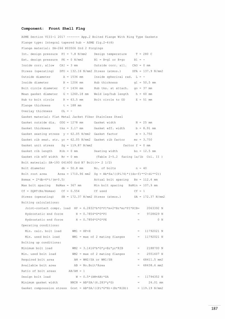
187

Component: Front Shell Flng

ASME Section VIII-1 2017 ------- App.2 Bolted Flange With Ring Type Gaskets

Flange type: Integral tapered hub - ASME fig.2-4(6)

Flange material: SA-266 K03506 Grd 2 Forgings

Int. design pressure PI = 7.8 N/mm2 Design temperature T = 280 C

Ext. design pressure PE = 0 N/mm2 B1 = B+g1 or B+go B1 = -

Inside corr. allow CAI = 3 mm Outside corr. all. CAO = 0 mm

Stress (operating) SFO = 132.16 N/mm2 Stress (atmos.) SFA = 137.9 N/mm2

Outside diameter A = 1536 mm Inside spherical rad. L = -

Inside diameter B = 1206 mm Hub thickness g1 = 50.5 mm

Bolt circle diameter C = 1434 mm Hub tks. at attach. go = 37 mm

Mean gasket diameter G = 1260.18 mm Weld leg/hub length h = 60 mm

Hub to bolt circle R = 63.5 mm Bolt circle to OD E = 51 mm

Flange thickness t = 188 mm

Overlay thickness OL = -

Gasket material: Flat Metal Jacket Fiber Stainless Steel

Gasket outside dia. ODG = 1278 mm Gasket width N = 25 mm

Gasket thickness tks = 3.17 mm Gasket eff. width b = 8.91 mm

Gasket seating stress y = 62.05 N/mm2 Gasket factor m = 3.750

Gasket rib seat. str. yr = 62.05 N/mm2 Gasket rib factor mr = 3.750

Gasket unit stress Sg = 119.87 N/mm2 factor f = 0 mm

Gasket rib length Rib = 0 mm Seating width bo = 12.5 mm

Gasket rib eff width Br = 0 mm (Table 2-5.2 facing 1a/1b Col. II )

Bolt material: SA-193 G41400 Grd B7 Bolt(<= 2 1/2)

Bolt diameter db = 50.8 mm No. of bolts n = 40

Bolt root area Area = 1710.96 mm2 Sg = Ab*Sa/((Pi/4)*((do-f)**2-di**2))

Bsmax = 2*db+6*t/(m+0.5) Actual bolt spacing Bs = 112.6 mm

Max bolt spacing BsMax = 367 mm Min bolt spacing BsMin = 107.9 mm

Cf = SQRT(Bs/Bsmax) Cf = 0.554 Cf used Cf = 1

Stress (operating) SB = 172.37 N/mm2 Stress (atmos.) SA = 172.37 N/mm2

Bolting calculations:

Joint-contact compr. load HP = 6.2832*b*G*PI*m+2*Br*mr*PI*RIB= 2063392 N

Hydrostatic end force H = 0.7854*G*G*PI = 9728629 N

Hydrostatic end force H = 0.7854*G*G*PE = 0 N

Operating conditions:

Min. calc. bolt load WM1 = HP+H = 11792021 N

Min. used bolt load WM1 = max of 2 mating flanges = 11792021 N

Bolting up conditions:

Minimum bolt load WM2 = 3.1416*b*G*y+Br*yr*RIB = 2188700 N

Min. used bolt load WM2 = max of 2 mating flanges = 2551607 N

Required bolt area AM = WM2/SA or WM1/SB = 68411.5 mm2

Available bolt area AB = No.Bolt*Area = 68438.6 mm2

Ratio of bolt areas AB/AM = 1

Design bolt load W = 0.5*(AM+AB)*SA = 11794352 N

Minimum gasket width NMIN = AB*SA/(6.283*y*G) = 24.01 mm

Gasket compression stress Gcst = AB*SA/((Pi*G*N)+(Br*RIB)) = 119.19 N/mm2

188

Loads: Integral Flange Calculations

Operating conditions:

Hydrostatic end load HD = 0.785*B*B*PI = 8910049 N

Hydrostatic end load HDe= 0.785*B*B*PE = 0 N

Gasket load HG = WM1-H = 2063392 N

Result. hydrostatic force HT = H-HD = 818580 N

Result. hydrostatic force HTe= He-HDe = 0 N

Bolting up conditions:

Gasket load HG = W = 11794352 N

Operating conditions:

Hydrostatic lever arm hd = R+0.5*g1 = 88.75 mm

Gasket load lever arm hg = (C-G)/2 = 86.91 mm

Result. hydro. lever arm ht = (R+g1+hg)/2 = 100.45 mm

Bolting up conditions:

Gasket load lever arm hg = (C-G)/2 = 86.91 mm

Operating conditions:

Hydrostatic moment MD = HD*hd = 790767 N*m

Gasket moment MG = HG*hg = 179328 N*m

Result. hydro. moment MT = HT*ht = 82230 N*m

Total operating moment MOP = MD+MG+MT = 1052325 N*m

MOPe = HDe(hd-hg)+HTe(ht-hg) = 0 N*m

Bolting up conditions:

Bolt up moment MATM = W*hg = 1025039 N*m

Effective bolt moment MB = MATM*SFO/SFA = 982397 N*m

Total moment MO = MOP or MB = 1052325 N*m

Bolt spacing correction M = MO*Cf = 1052325 N*m

(TEMA 2007 RCB-11.23) Cf= 1

Flange shape constants:

K = A/B = 1.2736 ho = SQ(B*g0) = 211.2392

T = Fig.2-7.1 = 1.8086 h/ho = h/ho = 0.284

Z = Fig.2-7.1 = 4.2147 F = Fig.2-7.2 = 0.886

Y = Fig.2-7.1 = 8.1651 V = Fig.2-7.3 = 0.4063

U = Fig.2-7.1 = 8.9726 f = Fig.2-7.6 = 1.0

g1/g0 = g1/g0 = 1.3649 e = F/ho = 0.0042

t = = 188 mm

d = U*ho*g0*g0/V = 6386791 Alpha = t*e+1.0 = 1.7886

Beta = 1.333*t*e+1.0 = 2.0512 Gamma = Alpha/T = 0.9889

Delta = t*t*t/d = 1.0404 Lambda = Gamma+Delta = 2.0293

Stress calculations: Allowable stress:

Long. hub SH = (f*M)/(Lambda*g1**2*B) = 168.6 N/mm2 1.5*SFO =198.24 N/mm2

Radial SR = Beta*M/(Lambda*t**2*B) = 24.95 N/mm2 SFO =132.16 N/mm2

Tangential ST1 = M*Y/(t**2*B)-(Z*SR) = 96.41 N/mm2 SFO =132.16 N/mm2

(greater) ST2 = (SH+SR)/2 or (SH+ST1)/2 = 132 N/mm2 SFO =132.16 N/mm2

189

Component: Front Shell Flng

ASME Section VIII Div.1 2017, Appendix 2, 2-14 Flange Rigidity

--- Calculations ---

Operating moment, Mo = 1052325 N*m Gasket seat. moment Ma = 1025039 N*m

Factor VI VI = 0.4063 Factor L L = 2.0293

Mod. elast.design T Ed = 185110 N/mm2 Mod.elast.atm. temp Ea = 201327 N/mm2

Thickness g0 g0 = 37 mm Factor h0 h0 = 211.2 mm

Factor KI KI = 0.3 Factor KL KL = 0.2

Corrosion allowance ca = 3 mm Factor K K = 1.2736

Thickness, T T = 188 mm

Flange Rigidity

Loose type flanges without hubs and optional flanges designed as loose type

Gasket seating J = 109.4 * Ma / (E * T ** 3 * Ln(K) * KL) = -

Operating J = 109.4 * Mo / (E * T ** 3 * Ln(K) * KL) = -

Integral type flanges and optional type flanges designed as integral and

Loose type flanges with hubs

Gasket seating J = 52.14 * Ma * VI/ (L*E*G0**2 * ho * KI) = 0.6126

Operating J = 52.14 * Mo * VI/ (L*E*G0**2 * ho * KI) = 0.684

ASME appendix 2 calculation of hub thickness 'go' as a cylinder

Design pressure P = 7.8 N/mm2 Allowable stress S = 132.16 N/mm2

Outside radius OR = - Inside radius IR = 603 mm

Joint efficiency E = 1 Corr.Allow or OL c = 3 mm

Material tolerance tol = 0 mm

Min hub thk / small end = P*IR / (S*E - 0.6*P)+c+Tol UG-27(c)(1)

= 39.9 mm

Hub thk / small end = 40 mm

New thickness 'go = 40 mm New thickness 'g1' = 53.5 mm

Corroded thickness 'go' = 37 mm Corroded thk 'g1' = 50.5 mm

190

Component: Front Tubesheet

Tubesheet Details - ASME VIII-1 2017 - UHX - U-tube Construction

Materials of construction Fig UHX-12.1 U-Tube Tubesheet configuration (d)

Tubesheet: SA-266 K03506 Grd 2 Forgings

Tubes: SA-179 K01200 Smls. tube

Shell: SA-516 K02700 Grd 70 Plate

Channel: SA-516 K02700 Grd 70 Plate

Design conditions Shell side Tube side Tubes Tubesheet

Design pressure N/mm2 7.8 6

Vacuum N/mm2 - -

Design temperature C 280 300 300 300

All.stress tubesheet S = 129.18 N/mm2 All.stress tubes St = 91.893 N/mm2

All.stress shell Ss = 136.406 N/mm2 All.stress channel Sc = 134.917 N/mm2

Yield stress shell Sys = 209.021 N/mm2 Yield stress chann. Syc = 204.305 N/mm2

Mod.of elas.tubesheet E = 183373 N/mm2 Mod.of elas. tubes Et = 184255 N/mm2

All.str.tubes at T Stt = 91.893 N/mm2 Mod.of E.tubes at T Ett = 184255 N/mm2

Mod.of elas.shell Es = 185110 N/mm2 Mod.of elas. channel Ec = 183373 N/mm2

Poisson Ratio shell vs = 0.3 Poisson ratio chan. vc = 0.3

Shell diameter Ds = 1206 mm Channel diameter Dc = 1206 mm

Shell thickness ts = 37 mm Channel thickness tc = 29 mm

191

Tube OD dt = 25.4 mm Tube thickness tt = 2.4 mm

Number of tube holes Nt = 1004 Tube pitch p = 31.75 mm

Outer tube limit Do = 1187.3 mm Outer tube radius ro = 580.95 mm

Tube expan. ratio rho = 0.985 Tube expanded len. ltx = 191 mm

Gasket Gs diameter Gs = 1260.18 mm Gasket Gc diameter Gc = 1260.18 mm

Center distance UL = 76.2 mm Gasket G diameter G = 1260.18 mm

Tubesheet cor.all. ct = 3 mm Pass groove depth hgt = 5 mm

Tubesheet cor.all. cs = 3 mm Pass groove depth hgs = 0 mm

Tubes cor.all. c = - Effective groove depth:

h'g = MAX[(hgt-ct),(0)] h'g = 2 mm

Bolt circle diameter C = 1434 mm Bolt load W* = 11792021 N

Shell bolt load Wm1s = 11792021 N Channel bolt load Wm1c = 9333961 N

Tubesheet diameter A = 1536 mm DL = (4*Ap/Cp) DL = 873.35 mm

Tubesheet thickness h = 194 mm Actual tubesheet thk ha = 200 mm

UHX-12.5.1 Step 1. Determnie Do, Mu, Mu* and h'g from UHX-11.5.1

Basic ligamente efficiency, mu = (p - dt) / p mu = 0.2

Effective tube hole diameter d* = dt-2*tt*(Et/E)*(St/S)*rho = 22.02 mm

(maximum of) d* = dt-2*tt = 20.6 mm

d* = 22.02 mm

Pass lane area limit 4*Do*p = 150787.11 mm2

Actual pass lane area, AL AL = 90472.26 mm2

Effective tube pitch = p/SQRT(1-(4*MIN[AL,4*Do*p]/Pi*Do**2)) p* = 33.13 mm

Effective ligament efficiency, mu* = (p*-d*)/p* mu* = 0.3353

UHX-12.5.2 Step 2. Calculate diameter ratios rhos and rhoc. For each loading

case, calculate moment Mts due to pressures Ps and Pt acting on the

unperforated tubesheet rim.

Rhos = Gs / Do Rhos = 1.0614 Rhoc = Gc / Do Rhoc = 1.0614

MTS = (Do**2/16)*((rhos-1)*(rhos**2+1)*Ps - (rhoc-1)*(rhoc**2+1)*Pt)

Load case 1 2 3 4

Shell Pressure, N/mm2 0 7.8 7.8 0

Tubes Pressure, N/mm2 6 0 6 0

Moment MTS, N*mm/mm -69005 89707 20702 0

UHX-12.5.3 Step 3. Calculate h/p. If rho changes, recalculate d* and mu* from

figure UHX-11.5.1. Determin E*/E and v* relative to h/p from UHX-11.5.2.

Determine E*/E and v* from Fig UHX-11.4 h/p = 6.2992

Ratio E*/E = 0.3822 Factor v* = 0.3237

192

Tubesheet Details - ASME VIII-1 2017 - UHX - U-tube Construction

UHX-12.5.5 Step 5. Calculate diameter ratio K and coefficient F

K = A/Do K = 1.2937

F = ((1-v*)/E*)*E*Ln(K)) F = 0.4557

Load case 1 2 3 4

Factor F 0.46 0.46 0.46 0.46

UHX-12.5.6 Step 6. For each loading case, calculate moment M* acting on the

unperforated tubesheet rim.

M* = Mts + ((Gc-Gs)/ (2*Pi*Do)) * W*

Load case 1 2 3 4

Effective W, N 9333961 11792021 11792021 0

Moment M*, N*mm/mm -69005 89707 20702 0

Component: Front Tubesheet

Tubesheet Details - ASME VIII-1 2017 - UHX - U-tube Construction

UHX-12.5.7 Step 7. For each loading case, calculate the maximum bending

moments acting on the tubesheet at the periphery Mp and at the center Mo

At the periphery:

Mp = (M* - (Do**2/32) * F * (Ps - Pt)) / (1 + F)

At the center:

Mo = Mp + (Do**2/64) * (3+v*) * (Ps-pt)

M = MAX[|Mp|,|Mo|]

Load case 1 2 3 4

Mp, N*mm/mm 35340 -45942 -10602 0

Mo, N*mm/mm -403914 525088 121174 0

M , N*mm/mm 403914 525088 121174 0

UHX-12.5.8 Step 8. For each loading case, calculate the tubesheet bending

stress sigma.

sigma = 6 * M / (mu* * (h - h'g)**2)

Load case 1 2 3 4

sigma, N/mm2 196.05 254.86 58.81 0

Allowable stress, N/mm2 258.36 258.36 258.36 258.36

Min tubesheet thk, mm 169.25 192.7 93.61 2

UHX-12.5.9 Step 9. For each loading case, calculate the average shear stress

in the tubesheet at the outer edge of the perforated region.

Tau = 1/(4*mu)*(Diam/h)*|Ps-Pt|

Load case 1 2 3 4

|Ps-Pt|, N/mm2 6 7.8 1.8 0

3.2*S*Mu*h/Do 13.51 13.51 13.51 13.51

Diam = DL or Do, mm 1187.3 1187.3 1187.3 1187.3

Tau, N/mm2 45.9 59.67 13.77 0

Allowable stress, N/mm2 103.34 103.34 103.34 103.34

Min tubesheet thickness, mm 86.17 112.02 25.85 0

193

Component: Nozzle S1

ASME VIII-1 2017 UG-27 Thickness of Cylinders under Internal Pressure

--- Calculations --- Cylinder Internal Pressure

Material: SA-106 K03006 Grd B Smls. pipe

Design pressure P = 7.8 N/mm2 Design temperature T = 280 C

Radiography = Full Joint efficiency E = 1

Design stress S = 117.9 N/mm2

Inside corr.allow. cai = 3 mm Outside corr. all. cao = 0 mm

Material tolerance tol = 1.391 mm Minimum thickness tmin = 9.19 mm

Outside diameter OD = 88.9 mm Corroded radius IR = 36.32 mm

- Minimum thickness t(UG-45) = max(ta,tb,UG-16(b)):

- ta = internal pressure:

t = (P*IR / (S*E-0.6*P))+cai+cao+tol = 6.89 mm UG-27(c)(1)

- ta = external pressure+cai+cao+tol t = 0 mm

- tb = min(tb3,max(tb1,tb2,UG-16(b)) t = 9.19 mm

tb3 = Table UG-45+cai+cao+tol = 9.19 mm

max(tb1,tb2,UG-16(b)) t = 52.01 mm

- tb1+cai+cao+tol = 52.01 mm

- UG-16(b)+cai+cao+tol = 5.98 mm

- tb2+cai+cao+tol = 0 mm

Minimum thickness: tmin = 9.19 mm

Nominal thickness: tnom = 11.13 mm

194

Component: Reinforcement Nozzle S1

ASME Section VIII-1 2017 UG-37 Reinforcement Required for Openings in

Shells and Formed Heads

--- Design Conditions:

Int. design pressure PI = 7.8 N/mm2 Ext. design press. PE = 0 N/mm2

Design temperature T = 280 C Fig.UW-16.1 Sketch (h)

Vessel material: SA-516 K02700 Grd 70 Plate

Inside corr. allow. CAI = 3 mm Outside corr.allow.CAO = 0 mm

Vessel design stress Sv = 136.41 N/mm2 Joint efficiency E = 1

Vessel outside dia Do = 1693 mm Corroded radius OR = 846.5 mm

Nominal thickness tnom = 55 mm Reinforcement limit lp = 96.45 mm

Req. tks. int.pres. tr = 47.62 mm Req. tks.ext.pres. tre = 0 mm

Corroded thickness t = 51.7 mm Reinf. efficiency E1 = 1.0

Attachment Material: SA-106 K03006 Grd B Smls. pipe

Inside corr. allow. CAI = 3 mm Outside corr.allow.CAO = 0 mm

Nozzle design stress Sn = 117.9 N/mm2 Joint efficiency E = 1

Nozzle outside dia. Don = 88.9 mm Corroded radius IR = 36.32 mm

Nominal thickness tnom = 11.13 mm Reinforcement limit ln = 52.33 mm

Req.tks. int.pres. trn = 2.8 mm Req.tks.ext.pres. trne = 0 mm

Corroded thickness tn = 8.13 mm Nozzle Projection ha = 0 mm

Nozzle Proj. used h = 0 mm

Reinforcement element material: SA-516 K02700 Grd 70 Plate

Limit of reinf. Dp = 163 mm Nominal thickness te = 32 mm

Outside diameter = 163 mm Design stress Se = 136.41 N/mm2

Minimum weld size tmin = 19.05 mm Weld leg (1/2*tmin) = 20.07 mm

Weld throat (1/2*tmin) = 9.52 mm Weld throat (1/2*tmin) = 14.05 mm

Weld throat tw (min) = 5.69 mm Weld throat tw = 5.69 mm

Weld throat tc (min) = 5.69 mm Weld throat tc = 5.69 mm

smaller |6.35 mm | Weld leg tw = 8.13 mm

tc of |0.7 * tmin| Weld leg tc = 8.13 mm

Outward nozzle weld L1 = 8.13 mm fr1 = Sn/Sv = 0.8643

Outer element weld L2 = 20.07 mm fr2 = Sn/Sv = 0.8643

Inward nozzle weld L3 = 0 mm fr3 = Sn/Sv or Se/Sv = 0.8643

Inward nozzle weld new = 0 mm fr4 = Se/Sv = 1.0

Corroded int.proj.thk ti = 0 mm

195

Corroded inside diameter d = 72.64 mm

Vessel wall length available for reinforcement 2*Lp-d = 120.26 mm

Plane correction factor (Fig.UG-37) F = 1

Offset distance from centerline doff = 0 mm

Reinforcement areas (internal pressure condition) ASME 2017 UG-37

A1 = Vessel wall. Larger of:

|(2*Lp-d)*(E1*t-F*tr)-2*tn*(E1*t-F*tr)*(1-fr1)| = 481.38 mm2

|2*(t+tn)*(E1*t-F*tr)-2*tn*(E1*t-F*tr)*(1-fr1)| = 478.93 mm2

A1 = 481.38 mm2

A2 = Nozzle wall outward | 5*(tn-trn)*fr2*t | = 1190.4 mm2

Smaller of: | 2*(tn-trn)*(2.5*tn+te)*fr2 | = 481.92 mm2

A2 = 481.92 mm2

A3 = Nozzle wall inward | 5*t*ti*fr2 | = 0 mm2

Smallest of: | 5*ti*ti*fr2 | = 0 mm2

| 2*h*ti*fr2 | = 0 mm2

A3 = 0 mm2

A41 = Outward nozzle weld = (L1**2)*fr3 = 57.13 mm2

A42 = Outer element weld = (L2**2)*fr4 = 402.74 mm2

A43 = Inward nozzle weld = (L3**2)*fr2 = 0 mm2

A4 = 459.87 mm2

JE = pad joint efficiency = 1

A5 = Reinforcement pad Area = (Dp-d-2*tn)*te*fr4*JE A5 = 2371.2 mm2

Aa = Area Available = A1+A2+A3+A4+A5 Aa = 3794.37 mm2

A = Area required = (d*tr*F)+2*tn*tr*F*(1-fr1) A = 3564.34 mm2

196

Nozzle attachment weld loads - UG-41 - Strength of reinforcement

-

Total weld load (UG-41(b)(2))

W = (A-A1+2*tn*fr1*(E1*t-F*tr))*Sv W = 428352 N

Weld load for strength path 1-1 (UG-41(b)(1)

W(1-1) = (A2+A5+A41+A42)*Sv W(1-1) = 451911 N

Weld load for strength path 2-2 (UG-41(b)(1)

W(2-2) = (A2+A3+A41+A43+2*tn*t*fr1)*Sv W(2-2) = 172641 N

Weld load for strength path 3-3 (UG-41(b)(1)

W(3-3) = (A2+A3+A5+A41+A42+A43+2*tn*t*fr1)*Sv W(3-3) = 551023 N

Reinforcing element strength = A5 * Se = 323446 N

Nozzle attachment weld loads - ASME 2017 UG-41-Strength of reinforcement

Unit stresses - UW15(c)and UG-45(c)

Inner fillet weld shear = 57.77 N/mm2

Outer fillet weld shear = 66.84 N/mm2

Groove weld tension = 87.25 N/mm2

Groove weld shear = 70.74 N/mm2

Nozzle wall shear = 82.53 N/mm2

Strength of connection elements

Inner fillet weld shear = 65555 N

Nozzle wall shear = 85086 N

Groove weld tension = 629563 N

Outer fillet weld shear = 343266 N

Possible paths of failure

1-1 85086 + 343266 = 428352 N

2-2 65555 + 629563 = 695118 N

3-3 629563 + 343266 = 972829 N

Welds strong enough if path greater than the smaller of W or W(path)

Path 1-1 > W or W11

428352 N > 428352 N OK

Path 2-2 > W or W22

695118 N > 172641 N OK

Path 3-3 > W or W33

972829 N > 428352 N OK

197

Component: Nozzle S2

ASME VIII-1 2017 UG-27 Thickness of Cylinders under Internal Pressure

--- Calculations --- Cylinder Internal Pressure

Material: SA-106 K03006 Grd B Smls. pipe

Design pressure P = 7.8 N/mm2 Design temperature T = 280 C

Radiography = Full Joint efficiency E = 1

Design stress S = 117.9 N/mm2

Inside corr.allow. cai = 3 mm Outside corr. all. cao = 0 mm

Material tolerance tol = 0.892 mm Minimum thickness tmin = 7.11 mm

Outside diameter OD = 48.26 mm Corroded radius IR = 20.01 mm

- Minimum thickness t(UG-45) = max(ta,tb,UG-16(b)):

- ta = internal pressure:

t = (P*IR / (S*E-0.6*P))+cai+cao+tol = 5.27 mm UG-27(c)(1)

- ta = external pressure+cai+cao+tol t = 0 mm

- tb = min(tb3,max(tb1,tb2,UG-16(b)) t = 7.11 mm

tb3 = Table UG-45+cai+cao+tol = 7.11 mm

max(tb1,tb2,UG-16(b)) t = 51.51 mm

- tb1+cai+cao+tol = 51.51 mm

- UG-16(b)+cai+cao+tol = 5.48 mm

- tb2+cai+cao+tol = 0 mm

Minimum thickness: tmin = 7.11 mm

Nominal thickness: tnom = 7.12 mm

198

Corroded inside diameter d = 40.02 mm

Vessel wall length available for reinforcement 2*Lp-d = 112.24 mm

Plane correction factor (Fig.UG-37) F = 1

Offset distance from centerline doff = 0 mm

Reinforcement areas (internal pressure condition) ASME 2017 UG-37

A1 = Vessel wall. Larger of:

|(2*Lp-d)*(E1*t-F*tr)-2*tn*(E1*t-F*tr)*(1-fr1)| = 453.11 mm2

|2*(t+tn)*(E1*t-F*tr)-2*tn*(E1*t-F*tr)*(1-fr1)| = 450.66 mm2

A1 = 453.11 mm2

A2 = Nozzle wall outward | 5*(tn-trn)*fr2*t | = 545.5 mm2

Smaller of: | 5*(tn-trn)*fr2*tn | = 43.47 mm2

A2 = 43.47 mm2

A3 = Nozzle wall inward | 5*t*ti*fr2 | = 0 mm2

Smallest of: | 5*ti*ti*fr2 | = 0 mm2

| 2*h*ti*fr2 | = 0 mm2

A3 = 0 mm2

A41 = Outward nozzle weld = (L1**2)*fr3 = 14.67 mm2

A42 = Outer element weld = (L2**2)*fr4 = 0 mm2

A43 = Inward nozzle weld = (L3**2)*fr2 = 0 mm2

A4 = 14.67 mm2

JE = pad joint efficiency = 1

A5 = Reinforcement pad Area = (Dp-d-2*tn)*te*fr4*JE A5 = 0 mm2

Aa = Area Available = A1+A2+A3+A4+A5 Aa = 511.25 mm2

A = Area required = (d*tr*F)+2*tn*tr*F*(1-fr1) A = 1959.08 mm2

Per UG-36(c)(3)(a), this opening does NOT require additional reinforcement

other than that inherent in the construction.

Nozzle attachment weld loads per UG-41 not required per UW-15(b).

199

Component: Nozzle S3

ASME VIII-1 2017 UG-27 Thickness of Cylinders under Internal Pressure

--- Calculations --- Cylinder Internal Pressure

Material: SA-106 K03006 Grd B Smls. pipe

Design pressure P = 7.8 N/mm2 Design temperature T = 280 C

Radiography = Full Joint efficiency E = 1

Design stress S = 117.9 N/mm2

Inside corr.allow. cai = 3 mm Outside corr. all. cao = 0 mm

Material tolerance tol = 1.391 mm Minimum thickness tmin = 9.66 mm

Outside diameter OD = 114.3 mm Corroded radius IR = 49.02 mm

- Minimum thickness t(UG-45) = max(ta,tb,UG-16(b)):

- ta = internal pressure:

t = (P*IR / (S*E-0.6*P))+cai+cao+tol = 7.77 mm UG-27(c)(1)

- ta = external pressure+cai+cao+tol t = 0 mm

- tb = min(tb3,max(tb1,tb2,UG-16(b)) t = 9.66 mm

tb3 = Table UG-45+cai+cao+tol = 9.66 mm

max(tb1,tb2,UG-16(b)) t = 52.01 mm

- tb1+cai+cao+tol = 52.01 mm

- UG-16(b)+cai+cao+tol = 5.98 mm

- tb2+cai+cao+tol = 0 mm

Minimum thickness: tmin = 9.66 mm

Nominal thickness: tnom = 11.13 mm

200

Component: Reinforcement Nozzle S3

ASME Section VIII-1 2017 UG-37 Reinforcement Required for Openings in

Shells and Formed Heads

--- Design Conditions:

Int. design pressure PI = 7.8 N/mm2 Ext. design press. PE = 0 N/mm2

Design temperature T = 280 C Fig.UW-16.1 Sketch (h)

Vessel material: SA-516 K02700 Grd 70 Plate

Inside corr. allow. CAI = 3 mm Outside corr.allow.CAO = 0 mm

Vessel design stress Sv = 136.41 N/mm2 Joint efficiency E = 1

Vessel outside dia Do = 1693 mm Corroded radius OR = 846.5 mm

Nominal thickness tnom = 55 mm Reinforcement limit lp = 109.15 mm

Req. tks. int.pres. tr = 47.62 mm Req. tks.ext.pres. tre = 0 mm

Corroded thickness t = 51.7 mm Reinf. efficiency E1 = 1.0

Attachment Material: SA-106 K03006 Grd B Smls. pipe

Inside corr. allow. CAI = 3 mm Outside corr.allow.CAO = 0 mm

Nozzle design stress Sn = 117.9 N/mm2 Joint efficiency E = 1

Nozzle outside dia. Don = 114.3 mm Corroded radius IR = 49.02 mm

Nominal thickness tnom = 11.13 mm Reinforcement limit ln = 75.33 mm

Req.tks. int.pres. trn = 3.68 mm Req.tks.ext.pres. trne = 0 mm

Corroded thickness tn = 8.13 mm Nozzle Projection ha = 0 mm

Nozzle Proj. used h = 0 mm

Reinforcement element material: SA-516 K02700 Grd 70 Plate

Limit of reinf. Dp = 178 mm Nominal thickness te = 55 mm

Outside diameter = 178 mm Design stress Se = 136.41 N/mm2

Minimum weld size tmin = 19.05 mm Weld leg (1/2*tmin) = 25.78 mm

Weld throat (1/2*tmin) = 9.52 mm Weld throat (1/2*tmin) = 18.04 mm

Weld throat tw (min) = 5.69 mm Weld throat tw = 5.69 mm

Weld throat tc (min) = 5.69 mm Weld throat tc = 5.69 mm

smaller |6.35 mm | Weld leg tw = 8.13 mm

tc of |0.7 * tmin| Weld leg tc = 8.13 mm

Outward nozzle weld L1 = 8.13 mm fr1 = Sn/Sv = 0.8643

Outer element weld L2 = 25.78 mm fr2 = Sn/Sv = 0.8643

Inward nozzle weld L3 = 0 mm fr3 = Sn/Sv or Se/Sv = 0.8643

Inward nozzle weld new = 0 mm fr4 = Se/Sv = 1.0

Corroded int.proj.thk ti = 0 mm

201

Corroded inside diameter d = 98.04 mm

Vessel wall length available for reinforcement 2*Lp-d = 120.26 mm

Plane correction factor (Fig.UG-37) F = 1

Offset distance from centerline doff = 0 mm

Reinforcement areas (internal pressure condition) ASME 2017 UG-37

A1 = Vessel wall. Larger of:

|(2*Lp-d)*(E1*t-F*tr)-2*tn*(E1*t-F*tr)*(1-fr1)| = 481.38 mm2

|2*(t+tn)*(E1*t-F*tr)-2*tn*(E1*t-F*tr)*(1-fr1)| = 478.93 mm2

A1 = 481.38 mm2

A2 = Nozzle wall outward | 5*(tn-trn)*fr2*t | = 994.92 mm2

Smaller of: | 2*(tn-trn)*(2.5*tn+te)*fr2 | = 579.82 mm2

A2 = 579.82 mm2

A3 = Nozzle wall inward | 5*t*ti*fr2 | = 0 mm2

Smallest of: | 5*ti*ti*fr2 | = 0 mm2

| 2*h*ti*fr2 | = 0 mm2

A3 = 0 mm2

A41 = Outward nozzle weld = (L1**2)*fr3 = 57.13 mm2

A42 = Outer element weld = (L2**2)*fr4 = 664.52 mm2

A43 = Inward nozzle weld = (L3**2)*fr2 = 0 mm2

A4 = 721.65 mm2

JE = pad joint efficiency = 1

A5 = Reinforcement pad Area = (Dp-d-2*tn)*te*fr4*JE A5 = 3503.5 mm2

Aa = Area Available = A1+A2+A3+A4+A5 Aa = 5286.34 mm2

A = Area required = (d*tr*F)+2*tn*tr*F*(1-fr1) A = 4773.95 mm2

202

Nozzle attachment weld loads - UG-41 - Strength of reinforcement

-

Total weld load (UG-41(b)(2))

W = (A-A1+2*tn*fr1*(E1*t-F*tr))*Sv W = 593350 N

Weld load for strength path 1-1 (UG-41(b)(1)

W(1-1) = (A2+A5+A41+A42)*Sv W(1-1) = 655426 N

Weld load for strength path 2-2 (UG-41(b)(1)

W(2-2) = (A2+A3+A41+A43+2*tn*t*fr1)*Sv W(2-2) = 185996 N

Weld load for strength path 3-3 (UG-41(b)(1)

W(3-3) = (A2+A3+A5+A41+A42+A43+2*tn*t*fr1)*Sv W(3-3) = 754538 N

Reinforcing element strength = A5 * Se = 477898 N

Nozzle attachment weld loads - ASME 2017 UG-41-Strength of reinforcement

Unit stresses - UW15(c)and UG-45(c)

Inner fillet weld shear = 57.77 N/mm2

Outer fillet weld shear = 66.84 N/mm2

Groove weld tension = 87.25 N/mm2

Groove weld shear = 70.74 N/mm2

Nozzle wall shear = 82.53 N/mm2

Strength of connection elements

Inner fillet weld shear = 84285 N

Nozzle wall shear = 111843 N

Groove weld tension = 809438 N

Outer fillet weld shear = 481507 N

Possible paths of failure

1-1 111843 + 481507 = 593350 N

2-2 84285 + 809438 = 893723 N

3-3 809438 + 481507 = 1290945 N

Welds strong enough if path greater than the smaller of W or W(path)

Path 1-1 > W or W11

593350 N > 593350 N OK

Path 2-2 > W or W22

893723 N > 185996 N OK

Path 3-3 > W or W33

1290945 N > 593350 N OK

203

Component: Nozzle T1

ASME VIII-1 2017 UG-27 Thickness of Cylinders under Internal Pressure

--- Calculations --- Cylinder Internal Pressure

Material: SA-106 K03006 Grd B Smls. pipe

Design pressure P = 6 N/mm2 Design temperature T = 300 C

Radiography = Full Joint efficiency E = 1

Design stress S = 117.9 N/mm2

Inside corr.allow. cai = 3 mm Outside corr. all. cao = 0 mm

Material tolerance tol = 2.394 mm Minimum thickness tmin = 16.55 mm

Outside diameter OD = 457.2 mm Corroded radius IR = 212.45 mm

- Minimum thickness t(UG-45) = max(ta,tb,UG-16(b)):

- ta = internal pressure:

t = (P*IR / (S*E-0.6*P))+cai+cao+tol = 16.55 mm UG-27(c)(1)

- ta = external pressure+cai+cao+tol t = 0 mm

- tb = min(tb3,max(tb1,tb2,UG-16(b)) t = 13.73 mm

tb3 = Table UG-45+cai+cao+tol = 13.73 mm

max(tb1,tb2,UG-16(b)) t = 33.25 mm

- tb1+cai+cao+tol = 33.25 mm

- UG-16(b)+cai+cao+tol = 6.98 mm

- tb2+cai+cao+tol = 0 mm

Minimum thickness: tmin = 16.55 mm

Nominal thickness: tnom = 19.15 mm

204

Component: Reinforcement Nozzle T1

ASME Section VIII-1 2017 UG-37 Reinforcement Required for Openings in

Shells and Formed Heads

--- Design Conditions:

Int. design pressure PI = 6 N/mm2 Ext. design press. PE = 0 N/mm2

Design temperature T = 300 C Fig.UW-16.1 Sketch (h)

Vessel material: SA-516 K02700 Grd 70 Plate

Inside corr. allow. CAI = 3 mm Outside corr.allow.CAO = 0 mm

Vessel design stress Sv = 134.92 N/mm2 Joint efficiency E = 1

Vessel outside dia Do = 1264 mm Corroded radius IR = 603 mm

Nominal thickness tnom = 32 mm Reinforcement limit lp = 424.9 mm

Req. tks. int.pres. tr = 27.85 mm Req. tks.ext.pres. tre = 0 mm

Corroded thickness t = 28.7 mm Reinf. efficiency E1 = 1.0

Attachment Material: SA-106 K03006 Grd B Smls. pipe

Inside corr. allow. CAI = 3 mm Outside corr.allow.CAO = 0 mm

Nozzle design stress Sn = 117.9 N/mm2 Joint efficiency E = 1

Nozzle outside dia. Don = 457.2 mm Corroded radius IR = 212.45 mm

Nominal thickness tnom = 19.15 mm Reinforcement limit ln = 71.75 mm

Req.tks. int.pres. trn = 11.45 mm Req.tks.ext.pres. trne = 0 mm

Corroded thickness tn = 16.15 mm Nozzle Projection ha = 0 mm

Nozzle Proj. used h = 0 mm

Reinforcement element material: SA-516 K02700 Grd 70 Plate

Limit of reinf. Dp = 789 mm Nominal thickness te = 32 mm

Outside diameter = 789 mm Design stress Se = 134.92 N/mm2

Minimum weld size tmin = 19.05 mm Weld leg (1/2*tmin) = 17.49 mm

Weld throat (1/2*tmin) = 9.52 mm Weld throat (1/2*tmin) = 12.24 mm

Weld throat tw (min) = 11.31 mm Weld throat tw = 11.31 mm

Weld throat tc (min) = 6.35 mm Weld throat tc = 6.35 mm

smaller |6.35 mm | Weld leg tw = 16.15 mm

tc of |0.7 * tmin| Weld leg tc = 9.07 mm

Outward nozzle weld L1 = 16.15 mm fr1 = Sn/Sv = 0.8739

Outer element weld L2 = 17.49 mm fr2 = Sn/Sv = 0.8739

Inward nozzle weld L3 = 0 mm fr3 = Sn/Sv or Se/Sv = 0.8739

Inward nozzle weld new = 0 mm fr4 = Se/Sv = 1.0

Corroded int.proj.thk ti = 0 mm

205

Corroded inside diameter d = 424.9 mm

Vessel wall length available for reinforcement 2*Lp-d = 424.9 mm

Plane correction factor (Fig.UG-37) F = 1

Offset distance from centerline doff = 0 mm

Reinforcement areas (internal pressure condition) ASME 2017 UG-37

A1 = Vessel wall. Larger of:

|(2*Lp-d)*(E1*t-F*tr)-2*tn*(E1*t-F*tr)*(1-fr1)| = 356.97 mm2

|2*(t+tn)*(E1*t-F*tr)-2*tn*(E1*t-F*tr)*(1-fr1)| = 72.63 mm2

A1 = 356.97 mm2

A2 = Nozzle wall outward | 5*(tn-trn)*fr2*t | = 589.11 mm2

Smaller of: | 2*(tn-trn)*(2.5*tn+te)*fr2 | = 594.24 mm2

A2 = 589.11 mm2

A3 = Nozzle wall inward | 5*t*ti*fr2 | = 0 mm2

Smallest of: | 5*ti*ti*fr2 | = 0 mm2

| 2*h*ti*fr2 | = 0 mm2

A3 = 0 mm2

A41 = Outward nozzle weld = (L1**2)*fr3 = 227.93 mm2

A42 = Outer element weld = (L2**2)*fr4 = 305.99 mm2

A43 = Inward nozzle weld = (L3**2)*fr2 = 0 mm2

A4 = 533.92 mm2

JE = pad joint efficiency = 1

A5 = Reinforcement pad Area = (Dp-d-2*tn)*te*fr4*JE A5 = 10617.6 mm2

Aa = Area Available = A1+A2+A3+A4+A5 Aa = 12097.6 mm2

A = Area required = (d*tr*F)+2*tn*tr*F*(1-fr1) A = 11947.67 mm2

206

Nozzle attachment weld loads - UG-41 - Strength of reinforcement

-

Total weld load (UG-41(b)(2))

W = (A-A1+2*tn*fr1*(E1*t-F*tr))*Sv W = 1567007 N

Weld load for strength path 1-1 (UG-41(b)(1)

W(1-1) = (A2+A5+A41+A42)*Sv W(1-1) = 1584006 N

Weld load for strength path 2-2 (UG-41(b)(1)

W(2-2) = (A2+A3+A41+A43+2*tn*t*fr1)*Sv W(2-2) = 219527 N

Weld load for strength path 3-3 (UG-41(b)(1)

W(3-3) = (A2+A3+A5+A41+A42+A43+2*tn*t*fr1)*Sv W(3-3) = 1693300 N

Reinforcing element strength = A5 * Se = 1432490 N

Nozzle attachment weld loads - ASME 2017 UG-41-Strength of reinforcement

Unit stresses - UW15(c)and UG-45(c)

Inner fillet weld shear = 57.77 N/mm2

Outer fillet weld shear = 66.11 N/mm2

Groove weld tension = 87.25 N/mm2

Groove weld shear = 70.74 N/mm2

Nozzle wall shear = 82.53 N/mm2

Strength of connection elements

Inner fillet weld shear = 669715 N

Nozzle wall shear = 922940 N

Groove weld tension = 1797359 N

Outer fillet weld shear = 1432491 N

Possible paths of failure

1-1 922940 + 1432491 = 2355431 N

2-2 669715 + 1797359 = 2467074 N

3-3 1797359 + 1432491 = 3229850 N

Welds strong enough if path greater than the smaller of W or W(path)

Path 1-1 > W or W11

2355431 N > 1567007 N OK

Path 2-2 > W or W22

2467074 N > 219527 N OK

Path 3-3 > W or W33

3229850 N > 1567007 N OK

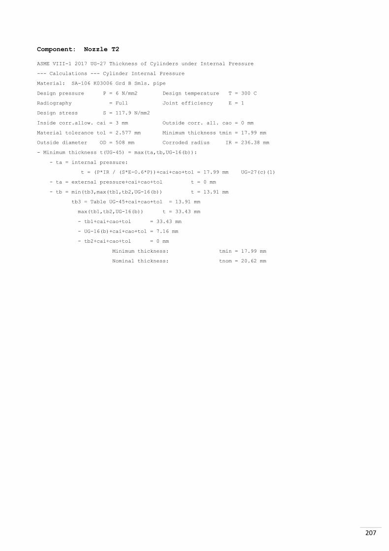
207

Component: Nozzle T2

ASME VIII-1 2017 UG-27 Thickness of Cylinders under Internal Pressure

--- Calculations --- Cylinder Internal Pressure

Material: SA-106 K03006 Grd B Smls. pipe

Design pressure P = 6 N/mm2 Design temperature T = 300 C

Radiography = Full Joint efficiency E = 1

Design stress S = 117.9 N/mm2

Inside corr.allow. cai = 3 mm Outside corr. all. cao = 0 mm

Material tolerance tol = 2.577 mm Minimum thickness tmin = 17.99 mm

Outside diameter OD = 508 mm Corroded radius IR = 236.38 mm

- Minimum thickness t(UG-45) = max(ta,tb,UG-16(b)):

- ta = internal pressure:

t = (P*IR / (S*E-0.6*P))+cai+cao+tol = 17.99 mm UG-27(c)(1)

- ta = external pressure+cai+cao+tol t = 0 mm

- tb = min(tb3,max(tb1,tb2,UG-16(b)) t = 13.91 mm

tb3 = Table UG-45+cai+cao+tol = 13.91 mm

max(tb1,tb2,UG-16(b)) t = 33.43 mm

- tb1+cai+cao+tol = 33.43 mm

- UG-16(b)+cai+cao+tol = 7.16 mm

- tb2+cai+cao+tol = 0 mm

Minimum thickness: tmin = 17.99 mm

Nominal thickness: tnom = 20.62 mm

208

Component: Reinforcement Nozzle T2

ASME Section VIII-1 2017 UG-37 Reinforcement Required for Openings in

Shells and Formed Heads

--- Design Conditions:

Int. design pressure PI = 6 N/mm2 Ext. design press. PE = 0 N/mm2

Design temperature T = 300 C Fig.UW-16.1 Sketch (h)

Vessel material: SA-516 K02700 Grd 70 Plate

Inside corr. allow. CAI = 3 mm Outside corr.allow.CAO = 0 mm

Vessel design stress Sv = 134.92 N/mm2 Joint efficiency E = 1

Vessel outside dia Do = 1264 mm Corroded radius IR = 603 mm

Nominal thickness tnom = 32 mm Reinforcement limit lp = 472.76 mm

Req. tks. int.pres. tr = 27.85 mm Req. tks.ext.pres. tre = 0 mm

Corroded thickness t = 28.7 mm Reinf. efficiency E1 = 1.0

Attachment Material: SA-106 K03006 Grd B Smls. pipe

Inside corr. allow. CAI = 3 mm Outside corr.allow.CAO = 0 mm

Nozzle design stress Sn = 117.9 N/mm2 Joint efficiency E = 1

Nozzle outside dia. Don = 508 mm Corroded radius IR = 236.38 mm

Nominal thickness tnom = 20.62 mm Reinforcement limit ln = 71.75 mm

Req.tks. int.pres. trn = 12.71 mm Req.tks.ext.pres. trne = 0 mm

Corroded thickness tn = 17.62 mm Nozzle Projection ha = 0 mm

Nozzle Proj. used h = 0 mm

Reinforcement element material: SA-516 K02700 Grd 70 Plate

Limit of reinf. Dp = 878 mm Nominal thickness te = 32 mm

Outside diameter = 878 mm Design stress Se = 134.92 N/mm2

Minimum weld size tmin = 19.05 mm Weld leg (1/2*tmin) = 17.53 mm

Weld throat (1/2*tmin) = 9.52 mm Weld throat (1/2*tmin) = 12.27 mm

Weld throat tw (min) = 12.33 mm Weld throat tw = 12.33 mm

Weld throat tc (min) = 6.35 mm Weld throat tc = 6.35 mm

smaller |6.35 mm | Weld leg tw = 17.62 mm

tc of |0.7 * tmin| Weld leg tc = 9.07 mm

Outward nozzle weld L1 = 17.62 mm fr1 = Sn/Sv = 0.8739

Outer element weld L2 = 17.53 mm fr2 = Sn/Sv = 0.8739

Inward nozzle weld L3 = 0 mm fr3 = Sn/Sv or Se/Sv = 0.8739

Inward nozzle weld new = 0 mm fr4 = Se/Sv = 1.0

Corroded int.proj.thk ti = 0 mm

209

Corroded inside diameter d = 472.76 mm

Vessel wall length available for reinforcement 2*Lp-d = 472.76 mm

Plane correction factor (Fig.UG-37) F = 1

Offset distance from centerline doff = 0 mm

Reinforcement areas (internal pressure condition) ASME 2017 UG-37

A1 = Vessel wall. Larger of:

|(2*Lp-d)*(E1*t-F*tr)-2*tn*(E1*t-F*tr)*(1-fr1)| = 397.26 mm2

|2*(t+tn)*(E1*t-F*tr)-2*tn*(E1*t-F*tr)*(1-fr1)| = 74.81 mm2

A1 = 397.26 mm2

A2 = Nozzle wall outward | 5*(tn-trn)*fr2*t | = 615.92 mm2

Smaller of: | 2*(tn-trn)*(2.5*tn+te)*fr2 | = 652.84 mm2

A2 = 615.92 mm2

A3 = Nozzle wall inward | 5*t*ti*fr2 | = 0 mm2

Smallest of: | 5*ti*ti*fr2 | = 0 mm2

| 2*h*ti*fr2 | = 0 mm2

A3 = 0 mm2

A41 = Outward nozzle weld = (L1**2)*fr3 = 271.31 mm2

A42 = Outer element weld = (L2**2)*fr4 = 307.27 mm2

A43 = Inward nozzle weld = (L3**2)*fr2 = 0 mm2

A4 = 578.58 mm2

JE = pad joint efficiency = 1

A5 = Reinforcement pad Area = (Dp-d-2*tn)*te*fr4*JE A5 = 11840 mm2

Aa = Area Available = A1+A2+A3+A4+A5 Aa = 13431.76 mm2

A = Area required = (d*tr*F)+2*tn*tr*F*(1-fr1) A = 13290.98 mm2

210

Nozzle attachment weld loads - UG-41 - Strength of reinforcement

Total weld load (UG-41(b)(2))

W = (A-A1+2*tn*fr1*(E1*t-F*tr))*Sv W = 1743102 N

Weld load for strength path 1-1 (UG-41(b)(1)

W(1-1) = (A2+A5+A41+A42)*Sv W(1-1) = 1758571 N

Weld load for strength path 2-2 (UG-41(b)(1)

W(2-2) = (A2+A3+A41+A43+2*tn*t*fr1)*Sv W(2-2) = 238945 N

Weld load for strength path 3-3 (UG-41(b)(1)

W(3-3) = (A2+A3+A5+A41+A42+A43+2*tn*t*fr1)*Sv W(3-3) = 1877814 N

Reinforcing element strength = A5 * Se = 1597413 N

Nozzle attachment weld loads - ASME 2017 UG-41-Strength of reinforcement

Unit stresses - UW15(c)and UG-45(c)

Inner fillet weld shear = 57.77 N/mm2

Outer fillet weld shear = 66.11 N/mm2

Groove weld tension = 87.25 N/mm2

Groove weld shear = 70.74 N/mm2

Nozzle wall shear = 82.53 N/mm2

Strength of connection elements

Inner fillet weld shear = 811859 N

Nozzle wall shear = 1119571 N

Groove weld tension = 1997065 N

Outer fillet weld shear = 1597413 N

Possible paths of failure

1-1 1119571 + 1597413 = 2716984 N

2-2 811859 + 1997065 = 2808924 N

3-3 1997065 + 1597413 = 3594478 N

Welds strong enough if path greater than the smaller of W or W(path)

Path 1-1 > W or W11

2716984 N > 1743102 N OK

Path 2-2 > W or W22

2808924 N > 238945 N OK

Path 3-3 > W or W33

3594478 N > 1743102 N OK

Component: Nozzle Flange Details

Flange, Gasket and Bolting Details

Dimensional data mm

Flg Flg Flg Neck Flg Bolt Gaskets Bolts

Nozzle Type Dia.(*) Rating tks tks Cir. O.D. Width No Dia.

S1 ANSI WN 88.90 600 11.13 31.75 168.27 127.00 9.65 8 19.05

S2 ANSI WN 48.26 600 7.12 22.35 114.30 73.15 9.65 4 19.05

S3 ANSI WN 114.30 600 11.13 38.10 215.90 157.23 12.70 8 22.23

T1 ANSI WN 457.20 600 19.15 82.55 654.05 533.40 22.35 20 41.27

T2 ANSI WN 508.00 600 20.62 88.90 723.90 584.20 25.40 24 41.27

* Dia. = Nozzle O.D. if standard flange

= Flange O.D. if non-standard flange

211

Horizontal Vessels on Saddles

Saddle material: SA-285 K02801 Grd C Plate

Wear plate mtl: SA-516 K02700 Grd 70 Plate

Shell mean radius R = 820.5 mm Total force Q = W + WS = 473667 N

Weight used W = 473667 N From wind/seismic WS = 0 N

Shell length L = 5801 mm Angle alpha Alpha = 1.8669 rad

Angle beta Beta = 112.6 deg Angle delta Delta = 1.504 rad

Vessel thickness TS = 55 mm Wear plate tks. w = 20 mm

Vessel corr.allowance CA = 3 mm Vessel thk TS+w-CA tsw = 72 mm

Saddle depth b = 400 mm Effective depth b1 = 722.2 mm

Wear plate width bw = 420 mm Angle theta Theta = 134.8 deg

Pressure P = 7.8 N/mm2 Inside diameter ID = 1589 mm

Joint efficiency JE = 1 Head joint eff. JEH = 1

Front head thickness TH = 176 mm Rear head thickness TH = 50 mm

Head diameter D = 1597 mm Head corr.allowance CAH = 3 mm

b1 = b+1.56*(R*(TS-CA))**0.5)

Saddle A Saddle B

Loads on saddles Q = 394024 79643 N

Distance from ref. point A = 967 314 mm

Head length H = 0 498 mm

Ratio A/R A/R = 1.1785 0.3827

Bending moment factor K7 = 0.0414 0.0104

Shell pressure stress PS = P*R/(2*tsw) = 65.51 N/mm2

Fr. head press. stress = P*D+0.2*P*(TH-CAH)/(2*(TH-CAH)) = ---

Re. head press. stress = P*D+0.2*P*(TH-CAH)/(2*(TH-CAH)) = 133.3 N/mm2

Alpha = Pi-(Pi/180)*(Theta/2+Beta/20) Delta = (Pi/180)*(5*Theta/12+30)

S11 = (3*Q*L/(Pi*(TS-CA)*R**2)) S12 = 1-(1-A/L+(R**2-H**2)/(2*A*L))/(1+4*H/3*L)

S13 = Pi*(Sin(Delta)/Delta-Cos(Delta)) S13/S14=1 if shell is

S14 = Delta+Sin(Delta)*Cos(Delta)-2*Sin(Delta)**2/Delta stiffened

Stresses in N/mm2 *** Saddles ***

Bending stress at saddle + pressure A B Allowable

S1 = S11*(4*A/L)*S12*S13/S14 + PS 68.32 65.52 136.41

Bending stress at midspan + pressure

S21 = (1+2*(R**2-H**2)/L**2)/(1+4*H/(3*L))

S2 = S11*(S21-4*A/L) + PS 67.45 66.25 136.41

Tangential shear in shell (unstiffened)

S41 = Sin(Alpha)/

(Pi-Alpha+Sin(Alpha)*Cos(Alpha))

S42 = L-H-2*A/(L+H)

S4 = (Q/R*(TS-CA))*S42*S41 5.91 0 109.12

212

Tangential shear in shell (stiffened)

S61 = Sin(Alpha) * Cos(Alpha)

S62 = (Sin(Alpha)/Pi)*(Alpha-S61)/

(Pi-Alpha+S61)

S6 = (Q/(R*(TS-CA)))*S62 0 1.22 109.12

Circumferential stress at horn, N/mm2

S71 = 12 * Q * K7 * R/(L *tsw**2)

S72 = 4 * tsw * b1

S7 = -Q/S72 - S71 -7.24 -0.65 -170.51

Ring compression in shell over saddle, N/mm2

S91 = 1+Cos(Alpha)/

(Pi-Alpha+Sin(Alpha)*Cos(Alpha))

S92 = (TS-CA)*(B+1.56*(R*(TS-CA))**0.5)

S9 = (Q/S92) * S91 5.39 1.09 104.51

Tangential shear stresses in head, N/mm2

S51 = Sin(Alpha) * Cos(Alpha)

S52 = (Sin(Alpha)/Pi)*(Alpha-S51)/

(Pi-Alpha+S51)

S5 = (Q/(12*R*(TH-CAH)))*S52 0 1.36 109.12

Head stresses, N/mm2

S81 = 3*Q/(8*12*R*(TH-CAH))

S82 = (Sin(Alpha))**2

S83 = Pi-Alpha+Sin(Alpha)*Cos(Alpha)

S8 = S81*(S82/S83) 0 0.71

Head stresses + pressure, N/mm2

S8 + PH 0 134.01 170.51

213

Saddle Geometry Verification

Saddle width A = 1600 mm Saddle depth F = 400 mm

Rib thickness J = 13 mm Web thickness tw = 13 mm

Base plate thk tb = 40 mm Wear plate thk tra = 20 mm

Min saddle height h = 583.5 mm Corr.Shell thk ts = 52 mm

Number of ribs n = 4 Vessel CL to base B = 1430 mm

Angle alpha,rad alpha = 1.8669 Angle beta, rad beta = 1.9651

Angle theta,rad theta = 2.3529 Rib depth G = 400 mm

Yield saddle mtl fy = 164.76 N/mm2 Inside radius Ri = 3 mm

Outside radius Ro = 846.5 mm

Max. load/saddle Qm = 394024 N Friction factor mu = 0.1

Saddle to foundation surface type: Teflon to Teflon

Expansion load mu*Qm = FL1 = 39402 N

Max wind or seismic load = Fws = 0 N

Bundle pull load = Fbl = -

Maximum horizontal load = FL = MAX[FL1,Fws,Fbl] FL = 39402 N

Saddle coefficient K1

K1 = (1+Cos(beta)-0.5*(Sin(beta))**2)/

(Pi-Beta+Sin(Beta)*Cos(Beta)) K1 = 0.2307

Saddle splitting force, fh = K1*Qm fh = 90916 N

Cross sectional area of saddle, As As = 30530 mm2

Web tension stress, sigmaT = fh/As sigmaT = 2.98 N/mm2

Max web tension stress, sigmaTmax = 0.6*fy sigmaTmax = 98.85 N/mm2

Distance centroid of saddle to base plate, d

d = h - C1 d = 181 mm

Web moment M = fh*d M = 16451514 N*mm

Saddle centroid, C1 C1 = 402.5 mm

Saddle moment of inertia, I I = 0.3650E+10 mm4

Web bending stress, fbweb = M*C1/I fbweb = 1.81 N/mm2

fbweb <= fbMax = 0.66*fy fbwebMax = 109.84 N/mm2

Base plate with center web

Base plate area, Ab = A*F Ab = 640000 mm2

Bearing pressure, Bp = Q/Ab Bp = 0.62 N/mm2

Base plate moment, M = Q*F/8 M = 19701208 N*mm

Section modulus, Z = A*tb**2/6 Z = 426666.66 mm3

Base plate bending stress, fbc = M/Z fbc = 46.17 N/mm2

fbc <= fbcMax = 0.66*fy fbcMax = 109.84 N/mm2

214

Base plate with offset web

Distance edge base plate to web, d2 d2 = 13 mm

Weld leg size, base to web, ww ww = 13 mm

Web length, Lw = A - 2*j Lw = 1574 mm

Ribs length, Lr = 2*(G-tw)+2*G Lr = 1574 mm

Overall length, L = Lw + Lr L = 3148 mm

Unit load, fu = Q/L N/mm fu = 125.17

Distance l1 = d2+tw+ww+tb l1 = 79 mm

Distance l2 = F - l1 l2 = 321 mm

Linear load, Omega = Fu/(l1+0.5*l2) Omega = 0.52 N/mm2

Base plate linear moment, M = (omega*l2**2)/6 M = 8975 N

Base plate bending stress, fbo = 6*M/tb**2 fbo = 33.66 N/mm2

fbo <= fboMax = 0.66*fy fboMax = 109.84 N/mm2

fb = MAX(fbweb,fbc,fbo) fb = 46.17 N/mm2

Minimum depth of saddle at top, Gtm

Gtm=SQRT((5.012*Fl/(J*(n-1)*Fb))*

(h+(A/1.96)*(1-Sin(Alpha)))) Gtm = 168.9 mm

Actual depth of saddle at top, Gt Gt = 400 mm

Minimum wear plate width, H = Gt + 1.56*SQRT(Ri*ts) H = 419.5 mm

Actual wear plate width, Ha Ha = 420 mm

Minimum wear plate thickness, tr = (Ha-Gt)**2/(2.43*Ro) tr = 0.2 mm

Actual wear plate thickness, tra tra = 20 mm

Anchor bolts

Bolt material: SA-325 Carbon steel Bolt

Longitudinal load, QL = 13353 N Operating load, Qo = 211035 N

Bolt diameter, d d = 29 mm Bolt area at = 660.5 mm2

Bolt mtl allow st Sb = 139.3 N/mm2 Number of bolts N = 2

Bolt mtl yield st Sy = 558.5 N/mm2 Yield str factor yf = 0.4

If Qo>QL, no uplift occurs. Uplift load per bolt: QL-Qo/N = -

Shear load/bolt = FL/N = 19701 N Allow force Sy*yf*at = 147554 N

Bolt transverse load

Maximum transverse load (seismic or wind), Ftr Ftr = 0 N

Bolt transverse moment, MtransB = Ftr * B MtransB = 0 N*mm

Critical bolt distance, e = MtransB / Q e = 0 mm

If e < A/6, no uplift occurs A/6 = 266.7 mm

Uplift bolt tension force = -

215

Inside ribs/web design

Saddle rib width Gb = 400 mm Base length e = 533.3 mm

Pressure area F*e Ap = 213333 mm2 Axial load Bp*Ap P = 131341 N

Area rib and web Ar = 12133 mm2 Comp. str P/Ar fa = 10.82 N/mm2

Mom.iner.J*Gb**3/12 I = 69333336 mm4 Rad gyr SQRT(I/Ar) r = 75.6 mm

Compression dist. l2 = 586.6 mm Slender ratio K*l2/r = 15.5

Unit force Fl/2*A fu = 12.31 N Moment fu*l2*e M = 3852245 N*mm

Moment arm C2 C2 = 200 mm Bend.str. M*C2/I fb = 11.11 N/mm2

Max. comp.stress Fa = 141.62 N/mm2 Max.bending str. Fb = 109.84 N/mm2

K end connection coeff= 2

Combined stress (must be less than one) fa/Fa + fb/Fb = 0.18

Outside ribs/web design

Press.area 0.5F*e Ap = 106667 mm2 Axial load Bp*Ap P = 65671 N

Area rib and web Ar = 8667 mm2 Comp. str P/Ar fa = 7.58 N/mm2

Compression dist. l1 = 1113.3 mm Slender ratio K*l1/r = 29.5

Unit force Fl/2*A fu = 12.31 N Moment 0.5*fu*l1*e M = 3655563 N*mm

Moment arm C1 C1 = 200 mm Bend.str. M*C1/I fb = 10.54 N/mm2

Max. comp.stress Fa = 137.49 N/mm2 Max.bending str. Fb = 109.84 N/mm2

Combined stress (must be less than one) fa/Fa + fb/Fb = 0.15

Wind loads - ANSI/SEI/IBC-2009/ASCE 7-10

Equipment Risk Category - wind design = II (1.5.1)

Vessel outside diameter, OD OD = 1280 mm

Vessel effective length, EL EL = 8476 mm

Vessel effective diameter, EOD EOD = 1753.6 mm

Effective wind area, Af = EOD*EL Af = 15 m2

Velocity pressure exposure, Kz Kz = 0.85 (29.3.1)

Topographic factor, Kzt Kzt = 1 (26.8)

Directionality factor, Kd Kd = 1 (26.6)

Wind speed, Vkm/h V = 160.9 (26.5)

Velocity pressure, qz, N/m2

qz = 0.04727*Kz*Kzt*Kd*V**2 qz = 1040.64 (29.3-1)

Gust effect factor, G G = 0.85 (26.9)

Force coefficient, Cf Cf = 1 (29.5)

Wind force, F F = qz*G*Cf*Af = 13147 N (29.5-1)

User entered wind force, F F = -

Moment arm, L L = 1.046 m

Overturning moment, OM, m-N OM = F*L = 13758

Seismic Loads - ANSI/SEI/IBC-2009/ASCE 7-10

Equipment Risk Category - earthquake design = II (1.5.1)

Equipment earthquake site class = B (11.4.2)

Response modification factor, Rp Rp = 3 (13.3.1)

Earthquake importance factor, Ip Ip = 1 (13.3.1)

Vessel amplification factor, Ap Ap = 1 (13.3.1)

Mapped MCEr,5% damped spectral resp acceleration Ss = 0.5 (11.4.1)

Mapped MCEr,5% damped spectral resp acceleration,1s S1 = 0.2 (11.4.1)

Site coefficient Fa - Table 11.4-1 Fa = 1 (11.4.3)

216

Site coefficient Fv - Table 11.4-2 Fv = 1 (11.4.3)

Adjusted MCEr,5% damped spectral resp acc Sms = Fa*Ss = 0.5 (11.4.3)

Adjusted MCEr,5% damped spectral resp acc,1s Sm1 = Fv*S1 = 0.2 (11.4.3)

Design,MCEr,5% damped spectral resp acc Sds=(2/3)*Sms = 0.333 (11.4.4)

Design,MCEr,5% damped spectral resp acc,1s Sd1=(2/3)*Sm1 = 0.133 (11.4.4)

Height ratio z/h z/h = 0.5 (13.3.1)

Weight of vessel, operating, Wo Wo = 422069 N

Vertical seismic force, Fv = 0.2*Sds*Wo Fv = 28138 N (13.3.1)

Horizontal seismic force, Fp

Fp =0.4*Ap*Sds*Wp*(1+2*(z/h))/(Rp/Ip) Fp = 37517 N (13.3-1)

Max horizontal force, Fpmax = 1.6*Sds*Ip*Wo Fpmax = 225104 N (13.3-2)

Min horizontal force, Fpmin = 0.3*Sds*Ip*Wo Fpmin = 42207 N (13.3-3)

Horizontal seismic design force, F F = 42207 N

User entered horizontal seismic design force, F F = -

Moment arm, L L = 1.43 m

Overturning moment, OM, m-N OM = F*L = 60356

Wind and Seismic Loads - Effect on Saddles

Dist.between saddles Ls = 4.52 m

Saddle width E = 1.6 m

Horizontal seismic design force F = 42207 N

Projected area of vessel Af=PI*EOD**2/4 Af = 2.415 m2

Longitudinal wind force Fl=Af*Cf*G*qz Fl = 2136 N

Longitudinal seismic load Qls=F*L/Ls Qls = 13353 N

Longitudinal wind load Qlw=Fl*L/Ls Qlw = 676 N

Projected area of vessel Af=EOD*EL Af = 14.863 m2

Transversal wind force Ft=0.5*Af*Cf*G*qz Ft = 6574 N

Transverse seismic load Qts=3*F*L/E Qts = 113167 N

Transverse wind load Qtw=3*Ft*L/E Qtw = 17625 N

Seismic load (compression) Qs1 = MAX[Qls,Qts]+Fv Qs1 = 141305 N

Seismic load (tension) Qs2 = MAX[Qls,Qts]-Fv Qs2 = 85029 N

Maximum seismic load Qs = MAX[Qs1,Qs2] Qs = 141305 N

Maximum wind load Qw = MAX[Qlw,Qtw] Qw = 17625 N

Maximum load Q = max(Qs,Qw) Q = 141305 N

Seismic and wind loads have NOT been applied to supports design.

217

Weights, surface area, Insulation

Shell side Tube side

Volume m3 8.86 3.63

Volume - Operating m3 7.29 3.63

Avg. fluid density kg/m3 942.03 99.7

Fluid weight kg 6866 362

Surface area m2 32.82 6.42

Insulation thk mm - -

Insulation type - -

Insulation density kg/m3 - -

Insulation weight kg - -

Weight, seals and jackets - -

Weight ext.piping kg - -

Total surface Area 39.23 m2

Weight of Accessories -

Bundle weight 10853 kg

Empty weight 35809 kg

Full weight (test) 48299 kg

Operating weight 43038 kg

Tube Heat Transfer Surface Area

Tube Bundle 416.36 m2

Front Head Tubesheet 16.02 m2

Rear Head Tubesheet 0 m2

Rear Head (after Full Diameter Support) 0.8 m2

U-Bend 32.93 m2

218

Maximum Allowable Working Pressures

* = Shell Side MAWP + = Tube Side MAWP

--Design conditions-- ---- New and cold ---

Component Side Temp Stress MAWP Temp Stress MAWP

C N/mm2 bar C N/mm2 bar

Shell Cylinder S 280 136.41 80.09 21.1 137.9 88.39

Front Head Cylinder T 300 134.92 62.43 21.1 137.9 71.26

Front Head Cover T 300 129.18 60.16 21.1 137.9 68.03

Shell Cover S 280 136.41 79.82 21.1 137.9 85.81

Front Tubesheet S 300 129.18 80.73 21.1 137.9 91.58

Front Tubesheet T 300 129.18 80.73 21.1 137.9 91.58

Front Head Flng At TS T 300 129.18 76.04 21.1 137.9 81.84

Front Head Flng At Cov T 300 129.18 61.32 21.1 137.9 67.87

Front Shell Flng S 280 132.16 78.29 21.1 137.9 84.24

Tubes T 300 91.89 187.86 21.1 92.39 188.87

Nozzle S1 S 280 117.9 232.66 21.1 117.9 328.07

Nozzle S2 S 280 117.9 216.06 21.1 117.9 394.44

Nozzle S3 S 280 117.9 177.84 21.1 117.9 249.01

Nozzle T1 T 300 117.9 85.72 21.1 117.9 102.19

Nozzle T2 T 300 117.9 84.12 21.1 117.9 98.93

Nozzle Flng S1 S 280 132.16 81.35 21.1 137.9 102.05

Nozzle Flng S2 S 280 132.16 81.35 21.1 137.9 102.05

Nozzle Flng S3 S 280 132.16 81.35 21.1 137.9 102.05

Nozzle Flng T1 T 300 129.18 79.61 21.1 137.9 102.05

Nozzle Flng T2 T 300 129.18 79.61 21.1 137.9 102.05

Nozzle Reinforcement S1 S 280 136.41 79.17 21.1 137.9 85.45

Nozzle Reinforcement S3 S 280 136.41 81.52 21.1 137.9 87.87

Nozzle Reinforcement T1 T 300 134.92 60.83 21.1 137.9 66.07

Nozzle Reinforcement T2 T 300 134.92 60.83 21.1 137.9 65.93

Front Hd Bolting At TS T 300 172.37 75.83 21.1 172.37 75.83

Front Hd Bolting At TS S 300 172.37 78.03* 21.1 172.37 78.03*

Front Hd Bolting At Cov T 300 172.37 60.01+ 21.1 172.37 60.01+

Eccentric Reducer S 280 136.41 81.31 21.1 137.9 86.36

Kettle Cylinder S 280 136.41 85.40 21.1 137.9 91.99

Nozzle Flng Bolting S1 S 280 172.37 81.35 21.1 172.37 102.05

Nozzle Flng Bolting S2 S 280 172.37 81.35 21.1 172.37 102.05

Nozzle Flng Bolting S3 S 280 172.37 81.35 21.1 172.37 102.05

Nozzle Flng Bolting T1 T 300 172.37 79.61 21.1 172.37 102.05

Nozzle Flng Bolting T2 T 300 172.37 79.61 21.1 172.37 102.05

219

Minimum Design Metal Temperature for Impact Test Exemption

* Indicates the controlling components + Indicates compliance with UG-20(f)

Component Curve Temp ******* UCS-66.1 *******

C Ratio Reduction Temperature

Shell Cylinder D -24 0.97 1 -25

Front Head Cylinder D -29 0.96 2 -31

Front Head Cover C -6 0.88 6 -12

Shell Cover D -20 - - -

Front Tubesheet C -3 0.88 6 -9 *

Front Head Flng At TS C -14 0.93 3 -17

Front Head Flng At Cov C -14 0.90 5 -19

Front Shell Flng C -8 0.93 3 -11

Tubes C -48 0.34 77 -125

Front Head Partitions D -46 0.94 3 -49

Nozzle S1 C -39 0.42 49 -88

Nozzle S2 C -48 0.52 28 -76

Nozzle S3 C -39 0.55 26 -65

Nozzle T1 C -26 + 0.83 9 -35

Nozzle T2 C -24 + 0.84 8 -32

Nozzle Flng S1 - -28 0.76 13 -41

Nozzle Flng S2 - -28 0.76 13 -41

Nozzle Flng S3 - -28 0.76 13 -41

Nozzle Flng T1 - -28 0.59 22 -50

Nozzle Flng T2 - -28 0.59 22 -50

Nozzle Reinforcement S1 D -29 0.96 2 -31

Nozzle Reinforcement S3 D -18 0.96 2 -20

Nozzle Reinforcement T1 D -29 0.96 2 -31

Nozzle Reinforcement T2 D -29 0.92 4 -33

Front Hd Bolting At TS A -48 - - -

Front Hd Bolting At Cov A -48 - - -

Eccentric Reducer D -16 0.96 2 -18

Kettle Cylinder D -18 0.92 4 -22

Nozzle Flng Bolting S1 A -48 - - -

Nozzle Flng Bolting S2 A -48 - - -

Nozzle Flng Bolting S3 A -48 - - -

Nozzle Flng Bolting T1 A -48 - - -

Nozzle Flng Bolting T2 A -48 - - -

220

Minimum Design Metal Temperature for Impact Test Exemption

Ratio = smaller of [tr*je/(tn-corr),MDP/MAP] UCS-66(b)(1)(b)

Component Ratio tr je tn corr Ratio MDP MAP

Shell Cylinder 0.97 35.71 1 39.7 3 - - -

Front Head Cylinder 0.96 27.55 1 31.7 3 - - -

Front Head Cover 0.97 167.78 1 176 3 0.88 6.02 6.8

Shell Cover 0.98 45.92 1 49.7 3 - - -

Front Tubesheet 1.00 193.21 1 197 3 0.88 8.07 9.16

Front Head Flng At TS - - - - - 0.93 7.6 8.18

Front Head Flng At Cov - - - - - 0.90 6.13 6.79

Front Shell Flng - - - - - 0.93 7.83 8.42

Tubes 0.34 0.81 1 2.4 0 - - -

Front Head Partitions 0.94 13.13 1 14 0 - - -

Nozzle S1 0.42 2.8 1 9.74 3 - - -

Nozzle S2 0.52 1.68 1 6.23 3 - - -

Nozzle S3 0.55 3.68 1 9.74 3 - - -

Nozzle T1 0.83 11.45 1 16.76 3 - - -

Nozzle T2 0.84 12.71 1 18.04 3 - - -

Nozzle Flng S1 - - - - - 0.76 7.8 10.2

Nozzle Flng S2 - - - - - 0.76 7.8 10.2

Nozzle Flng S3 - - - - - 0.76 7.8 10.2

Nozzle Flng T1 - - - - - 0.59 6 10.2

Nozzle Flng T2 - - - - - 0.59 6 10.2

Nozzle Reinforcement S1 - - - - - - - -

Nozzle Reinforcement S3 - - - - - - - -

Nozzle Reinforcement T1 - - - - - - - -

Nozzle Reinforcement T2 - - - - - - - -

Front Hd Bolting At TS - - - - - - - -

Front Hd Bolting At Cov - - - - - - - -

Eccentric Reducer 0.96 54.6 1 59.7 3 - - -

Kettle Cylinder 0.92 47.32 1 54.7 3 - - -

Nozzle Flng Bolting S1 - - - - - - - -

Nozzle Flng Bolting S2 - - - - - - - -

Nozzle Flng Bolting S3 - - - - - - - -

Nozzle Flng Bolting T1 - - - - - - - -

Nozzle Flng Bolting T2 - - - - - - - -

221

Hydrostatic Test Pressure - ASME VIII-1 2017 UG-99 Factor: 1.3

Shell Side: 101.4 bar Tube Side: 78 bar

Design Test Stress

Component Material Side Temp Stress Stress Ratio

C N/mm2 N/mm2

Shell Cylinder SA-516 K02700 Grd 70 Plate S 280 136.41 137.9 1.0109

Front Head Cylinder SA-516 K02700 Grd 70 Plate T 300 134.92 137.9 1.0221

Front Head Cover SA-266 K03506 Grd 2 Forgin T 300 129.18 137.9 1.0675

Shell Cover SA-516 K02700 Grd 70 Plate S 280 136.41 137.9 1.0109

Front Tubesheet SA-266 K03506 Grd 2 Forgin S 300 129.18 137.9 1.0675

Front Tubesheet SA-266 K03506 Grd 2 Forgin T 300 129.18 137.9 1.0675

Front Head Flng At TS SA-266 K03506 Grd 2 Forgin T 300 129.18 137.9 1.0675

Front Head Flng At Cov SA-266 K03506 Grd 2 Forgin T 300 129.18 137.9 1.0675

Front Shell Flng SA-266 K03506 Grd 2 Forgin S 280 132.16 137.9 1.0434

Tubes SA-179 K01200 Smls. tube T 300 91.89 92.39 1.0054

Nozzle S1 SA-106 K03006 Grd B Smls. S 280 117.9 117.9 1

Nozzle S2 SA-106 K03006 Grd B Smls. S 280 117.9 117.9 1

Nozzle S3 SA-106 K03006 Grd B Smls. S 280 117.9 117.9 1

Nozzle T1 SA-106 K03006 Grd B Smls. T 300 117.9 117.9 1

Nozzle T2 SA-106 K03006 Grd B Smls. T 300 117.9 117.9 1

Nozzle Flng S1 SA-105 K03504 Forgings S 280 132.16 137.9 1.0434

Nozzle Flng S2 SA-105 K03504 Forgings S 280 132.16 137.9 1.0434

Nozzle Flng S3 SA-105 K03504 Forgings S 280 132.16 137.9 1.0434

Nozzle Flng T1 SA-105 K03504 Forgings T 300 129.18 137.9 1.0675

Nozzle Flng T2 SA-105 K03504 Forgings T 300 129.18 137.9 1.0675

Nozzle Reinforcement S1SA-516 K02700 Grd 70 Plate S 280 136.41 137.9 1.0109

Nozzle Reinforcement S3SA-516 K02700 Grd 70 Plate S 280 136.41 137.9 1.0109

Nozzle Reinforcement T1SA-516 K02700 Grd 70 Plate T 300 134.92 137.9 1.0221

Nozzle Reinforcement T2SA-516 K02700 Grd 70 Plate T 300 134.92 137.9 1.0221

Front Hd Bolting At TS SA-193 G41400 Grd B7 Bolt( T 300 172.37 172.37 -

Front Hd Bolting At CovSA-193 G41400 Grd B7 Bolt( T 300 172.37 172.37 -

Eccentric Reducer SA-516 K02700 Grd 70 Plate S 280 136.41 137.9 1.0109

Kettle Cylinder SA-516 K02700 Grd 70 Plate S 280 136.41 137.9 1.0109

Nozzle Flng Bolting S1 SA-193 G41400 Grd B7 Bolt( S 280 172.37 172.37 -

Nozzle Flng Bolting S2 SA-193 G41400 Grd B7 Bolt( S 280 172.37 172.37 -

Nozzle Flng Bolting S3 SA-193 G41400 Grd B7 Bolt( S 280 172.37 172.37 -

Nozzle Flng Bolting T1 SA-193 G41400 Grd B7 Bolt( T 300 172.37 172.37 -

Nozzle Flng Bolting T2 SA-193 G41400 Grd B7 Bolt( T 300 172.37 172.37 -

Hydrostatic Test Pressure - UG-99 - Bolting exception

Component Material 1.3*LSR*All.Stress 90% Yield

N/mm2 N/mm2

Front Hd Bolting At TS SA-193 G41400 Grd B7 Bolt( 224 651.55

Nozzle Flng Bolting S1 SA-193 G41400 Grd B7 Bolt( 224 651.55

222

*** Extreme Fiber Elongation - UG-79 ***

Cylinders formed from plate, ef = (50t/Rf)(1-Rf/Ro) (Ro = infinity)

Double curvature parts (heads) ef = (75t/Rf)(1-Rf/Ro) (Ro = infinity)

Component Material * governing geometry * thk,t Radius,Rf Elong,e

mm mm % Max

Shell Cylinder SA-516 K02700 Grd 70 Plate 40 620 3.13 5

Front Head Cylinder SA-516 K02700 Grd 70 Plate 32 616 2.53 5

Shell Cover SA-516 K02700 Grd 70 Plate 50 293.49 12.78 5 *

* Warning - Heat treating may be required per UG-79

223

11. ACKNOWLEDGEMENTS

At the end of this paper, I would like to mention all the people without whom this thesis work would not

even exist. Remembering that a great tutor teaches both about his discipline and about life, you have been

a very special person. For this reason the first thanks is dedicated to the company tutor Ing. Cortassa Daniele.

He consistently let this paper to be my own work, but with his passion for teaching he steered me in the right

direction every time I needed it. Simic.Spa, with the commercial manager Ph.D. Marianna Ginola, deserves

my heartfelt thanks for allowing me to finish my course of study within its production spaces. On the other

hand, my university supervisors Ph.D. Asinari Pietro, Ph.D. Chiavazzo Eliodoro and Ph.D. Bergamasco Luca

merit all my gratitude for their willingness and timeliness. A special acknowledgement goes to my girlfriend

Sara, which in addition to be the second reader of my thesis, have supported me during this intense period

and rejoice with me for the achievements. Thanks for all the time you have dedicated to me. Thanks because

you've always been there. Follow all the friends who during these years allowed me to see the word in a

better light. In particular Ivan, Sina and Maria Désirée, which deserve all my gratefulness. Today I probably

wouldn’t be who I am if I hadn’t known you. Finally, I must express my very profound gratitude to my parents

and to my brothers for having always supported me and let me be free in all the decisions of my life, since

the choice of my course of study. In conclusion, I would like to dedicate this milestone to myself, which could

be the beginning of a long and brilliant professional career.

224

12. BIBLIOGRAPHY

[1] «CEN,» [Online]. Available: https://www.cencenelec.eu/Pages/default.aspx.

[2] ASME, «The American Society of Mechanical Engineers,» [Online]. Available: https://www.asme.org/.

[3] TEMA 9th edition, Standards of The Tubular Exchanger Manufacturers Association, 2007.

[4] E. Akpabio, I. Oboh e E. O. Aluyor, «The Effect of Baffles in shell and Tube Heat Exchangers,» Advanced Materials

Research, vol. 62, pp. 694-699, 2009 Trans Tech Publications, Switzerland.

[5] Aspen Technology, Inc., «Thermal Design of Shell and Tube Heat Exchanger using Aspen Tasc+,» 2007.

[6] H. Lamb, Hydrodynamics, New York: Dover Publications, Inc., 6th edition, 1945.

[7] ASME Boiler & Pressure Vessels Code 2017, Section II, Part A - Ferrous Material Specifications Volume 1.

[8] ASME Boiler & Pressure Vessels Code 2017, Section II, Part A - Ferrous Material Specifications Volume 2.

[9] ASME Boiler & Pressure Vessels Code 2017, Section II, Part B - Non-Ferrous Material Specifications.

[10] ASME Boiler & Pressure Vessels Code 2017, Section II, Part C - Specifications for Welding Rods Electrodes and

Filler Materials.

[11] ASME Boiler & Pressure Vessels Code 2017, Section II, Part D - Material Properties [Metric].

[12] ASME Boiler & Pressure Vessels Code 2017, Section V, Non-Destructive Examinations.

[13] ASME Boiler & Pressure Vessels Code 2017, Section VIII, Division 1- Rules for Construction of Pressure Vessels.

[14] ASME Boiler & Pressure Vessels Code 2017, Section IX - Welding, Brazing and Fusing Qualifications.

[15] D. Q. Kern, Process Heat Transfer, Mc Graw Hill, 2011.

[16] J. H. Lienhard IV e J. H. Lienhard V, A Heat Transfer Textbook, Third edition, Phlogiston Press, 2008.

[17] D. Annaratone, Pressure Vessel Design, Springer, 2007.

[18] T. Kuppan, Heat Exchanger Design Handbook, Marcel Dakker Inc., 2000.

[19] B. E. Ball e W. J. Carter, CASTI Guidebook to ASME Section VIII, Div.1 - Pressure Vessels, CASTI Publishing Inc.,

2002.

[20] D. Moss, Pressure Vessel Design Manual, Gulf Professional Publishing , 2004.

[21] M. Okada e K. Watanabe, «Surface tension correlations for several fluorocarbon refrigerants,» Heat transfer.

Japanese Research, vol. 17, n. 1, pp. 35-52, 1988.

225

[22] J. J. Jasper, «The surface tension of pure liquid compounds,» J. Phys. Chem. Ref. Data, vol. 1, n. 4, pp. 841-1010,

1972.

[23] J.Taborek, «Evolution of Heat Exchanger Design Tecniques,» Heat transfer Engineering, vol. 1, n. 1, pp. 15-29,

1979.

[24] A. P. Froba, S. Will e A. Leipertz, «Saturated liquid viscosity and surface tension of alternative refrigerants,» Intl.

J. Thermophys., vol. 2, n. 6, pp. 1225-1253, 2000.

[25] V. G. Baidakov e I. I. Sulla, «Surface tension of propane and isobutane at near-critical temperatures,» Russ. J. Phys.

Chem., vol. 50, n. 4, pp. 551-554,, 1985.

[26] W. M. Rohsenow, «A method of correlating het transfer data for surface boiling of liquids.,» Trans. ASME, pp. 74-

969, 1951.

[27] J. A. Farr e M. H. Jawad , Guidebook for the Design of ASME Section VIII Pressure Vessels, ASME Press, 2001.