Faculty of Engineering, Lakehead University In Partial ... - CORE

MODELLING SOIL TEMPERATURE ON THE BOREAL PLAIN

WITH AN EMPHASIS ON THE RAPID COOLING PERIOD

Thesis Presented to:

Faculty of Engineering, Lakehead University

In Partial Fulfillment of the Requirements for the Degree:

Masters in Environmental Engineering

by

Josiane A. Bélanger

15 September 2009

brought to you by COREView metadata, citation and similar papers at core.ac.uk

provided by Lakehead University Knowledge Commons

https://core.ac.uk/display/51418748?utm_source=pdf&utm_medium=banner&utm_campaign=pdf-decoration-v1

iii

SUPERVISORY COMMITTEE MEMBERS AND EXAMINERS Supervisor: Dr. Ellie Prepas Faculty of Forestry and the Forest Environment Lakehead University, Thunder Bay, ON Supervisory Committee: Dr. Lionel Catalan Faculty of Engineering Lakehead University, Thunder Bay, ON

Mr. Tim McCready, R.P.F.T. Planning Forester Millar Western Forest Products Ltd., Whitecourt, AB

Dr. Gordon Putz Department of Civil and Geological Engineering

University of Saskatchewan, Saskatoon, SK Examiners: Dr. Bruce Kjartanson (Internal) Faculty of Engineering Lakehead University, Thunder Bay, ON Dr. Jian Wang (External) Faculty of Forestry and the Forest Environment Lakehead University, Thunder Bay, ON

iv

ABSTRACT

To accurately model soil temperatures on the Boreal Plain, factors that influence fine-grained

soils during the rapid cooling period must first be identified. The effects of air temperature, soil

moisture and snow depth were quantified at 0.1 and 0.5 m depths for 14 sites encompassing five

treatment types: three upland burned, three upland harvested, three upland conifer, three upland

deciduous and two wetland. In the absence of snow from September to October at the 0.1 m

depth, air temperature was identified as the most important parameter, explaining approximately

70% of the variation in soil temperature for upland and wetland sites. At the same depth in the

presence of snow from November to December, soil moisture was more important. At a deeper

soil depth (0.5 m), soil moisture was identified as the most important parameter regardless of

snow cover, explaining from 63 to 91% of the variation in soil temperatures for upland and

wetland sites. The presence of snow was a significant factor influencing soil temperatures, but

snow depth was not. Further, the soil temperature algorithms of SWAT were tested using one

site of each treatment type at 0.1, 0.5 and 1.0 m depths. The algorithms utilized by SWAT were

able to reproduce seasonal trends in soil temperatures adequately for the spring, summer and

autumn seasons, with only a slight increase in the lag coefficient parameter. During winter

months, the SWAT algorithms tended to predict soil temperatures that were consistently lower

than measured data. Further development to the SWAT soil temperature algorithms is required to

represent better the important insulating effect of snowpack.

v

ACKNOWLEDGEMENTS

I would like to thank Millar Western Forest Products Ltd. and the Natural Sciences and

Engineering Research Council of Canada (NSERC) for their contributions to my NSERC

Industrial Postgraduate Scholarship.

The FORWARD project is funded by the NSERC Collaborative Research and Development

Program and Millar Western Forest Products Ltd., as well as Blue Ridge Lumber Inc. (a division

of West Fraser Timber Company Ltd.), Alberta Newsprint Company (ANC Timber), Vanderwell

Contractors (1971) Ltd., AbitibiBowater Inc. (formerly Bowater Canadian Forest Products Ltd.),

Buchanan Forest Products Ltd. (Ontario), Buchanan Lumber (a division of Gordon Buchanan

Enterprises) (Alberta), Talisman Energy Inc., TriStar Oil & Gas Ltd., the Canada Foundation for

Innovation, the Alberta Forestry Research Institute, the Forest Resource Improvement

Association of Alberta, FedNor, the Ontario Innovation Trust and the Living Legacy Research

Program.

I would like to gratefully acknowledge the following people:

my supervisor: Dr. Ellie Prepas,

my supervisory committee: Dr. Lionel Catalan, Mr. Tim McCready and Dr. Gordon Putz,

my fellow graduate students: Zachary Long, Becky MacDonald and David Pelster,

for help with fieldwork and/or data: Nicole Fraser, Steve Nadworny Dr. Douglas

MacDonald, Mark Serediak, Éric Thériault, Dr. Brett Watson and Dr. Ivan Whitson,

for administrative help: Virginia Antoniak,

for reviews and comments on countless versions of this document: Janice Burke,

and finally, for their love and support, ma mère, ma famille et mes amis, merci.

vi

CONTENTS

CHAPTER 1: INTRODUCTION ............................................................................................ 1

1.1 Research Objectives............................................................................................................ 1

1.2 Thesis Outline ..................................................................................................................... 2

1.3 References........................................................................................................................... 2

CHAPTER 2: MODELLING THE ANNUAL FREEZE-THAW CYCLE OF BOREAL PLAIN SOILS: A REVIEW ............................................................................. 4

2.1 Introduction......................................................................................................................... 4

2.2 Soil Characteristics ............................................................................................................. 5

2.3 Vegetation Biomass ............................................................................................................ 7

2.4 Climate................................................................................................................................ 9

2.5 Modelling the Freeze-thaw Process .................................................................................. 14

2.6 The Soil and Water Assessment Tool............................................................................... 16

2.7 Conclusion ........................................................................................................................ 22

2.8 References......................................................................................................................... 22

CHAPTER 3: QUANTIFYING THE EFFECTS OF AIR TEMPERATURE, SOIL MOISTURE AND SNOW DEPTH ON SOIL TEMPERATURES DURING THE RAPID COOLING PERIOD, ON THE BOREAL PLAIN................... 30

3.1 Introduction....................................................................................................................... 30

3.2 Site Description................................................................................................................. 33

3.3 Data Collection ................................................................................................................. 35

3.4 Data Analysis .................................................................................................................... 37

3.5 Results............................................................................................................................... 39 3.5.1 Soil Temperature at 0.1 m Depth...........................................................................39 3.5.2 Soil Temperature at 0.5 m Depth...........................................................................45

3.6 Discussion......................................................................................................................... 49

vii

3.7 References......................................................................................................................... 53

CHAPTER 4: ANNUAL FREEZE/THAW TEMPERATURE CYCLE IN SOILS ON THE CANADIAN BOREAL PLAIN: COMPARISON OF SWAT PREDICTIONS TO MEASURED DATA ................................................................................ 57

4.1 Introduction....................................................................................................................... 57

4.2 Model Description ............................................................................................................ 58

4.3 SWAT Soil Temperature Submodel ................................................................................. 59

4.4 Model Testing ................................................................................................................... 62

4.5 Site Description................................................................................................................. 63

4.6 Data Collection ................................................................................................................. 65

4.7 Data Analysis .................................................................................................................... 66

4.8 Results and Discussion ..................................................................................................... 67

4.9 Conclusion ........................................................................................................................ 72

4.10 References......................................................................................................................... 73

CHAPTER 5: CONCLUSIONS AND RECOMMENDATIONS ......................................... 76

APPENDIX: ......................................................................................................................... 79

viii

LIST OF TABLES Table 2-1: Summary of modifications made to SWAT as reported in the literature. ....................21

Table 3-1: Climate data for each study year and long-term means from 1 September to

31 December, followed by annual means in brackets..................................................34

Table 3-2: Sample site descriptions ...............................................................................................35

Table 4-1: SWAT soil temperature model input parameters .........................................................62

Table 4-2: Sample site descriptions ...............................................................................................63

Table 4-3: Maximum differences in summer and winter soil temperatures, and error

measurements between predicted and observed model outputs for original

and modified SWAT model outputs at 0.1, 0.5 and 1.0 m depths for each

site ................................................................................................................................69

ix

LIST OF FIGURES Figure 2-1: Swan Hills study area location on the Boreal Plain of Canada.....................................5

Figure 2-2: Soil phase diagram. .......................................................................................................7

Figure 2-3: Vegetation biomass in a mixed-forest setting ...............................................................8

Figure 2-4: Ground temperature regimes for cold regions ............................................................10

Figure 2-5: Schematic demonstrating the general relationship between various factors

and snow depth.. ..........................................................................................................13

Figure 2-6: Location of study area near Whitecourt, Alberta, study area where SWAT

model was developed near Temple, Texas and other North American sites

where SWAT and EPIC have been applied. ................................................................20

Figure 3-1: Location of study sites within the FORWARD study area.........................................33

Figure 3-2: Vertical profile of soil temperature, air temperature and soil moisture

probes...........................................................................................................................36

Figure 3-3: Relationship between measured snow depth at study sites and Environment

Canada Whitecourt A station. ......................................................................................37

Figure 3-4: Mean air temperature from 1 September to 31 December 2006-2008 under

five vegetation cover types. .........................................................................................39

Figure 3-5: Mean soil temperature from 1 September to 31 October 2006-2008 and 1

November to 31 December 2006-2008, under five vegetation cover types at

0.1 and 0.5 m soil depths. ............................................................................................40

Figure 3-6: Mean daily soil temperature at 0.1 m depth versus mean daily air

temperature at 2 m above ground surface for burned and harvested sites in

2006, 2007 and 2008....................................................................................................41


temperature at 2 m above ground surface for disturbed, treed and wetland

sites in the absence and presence of snow from 1 September to 31 December

2006-2008 ....................................................................................................................42

Figure 3-8: Mean soil moisture from 1 September to 31 December 2006-2008 under

five vegetation types. ...................................................................................................44

Figure 3-9: Percentage of contribution to soil temperature for upland conifer and

wetland sites at 0.1 m and 0.5 m depths. .....................................................................45

x


temperature at 2 m above ground surface for burned and harvested sites in

2006, 2007 and 2008....................................................................................................46

Figure 3-11: Mean daily soil temperature at a 0.5 m depth versus mean daily air

temperature at 2 m above ground for disturbed, treed and wetland sites in

the absence and presence of snow from 1 September to 31 December 2006-

2008..............................................................................................................................48

Figure 3-12: Relationship between wetland soil temperature and soil moisture at 0.5 m

depth.............................................................................................................................52

Figure 4-1: Schematic of SWAT soil temperature submodel ........................................................62

Figure 4-2: Location of burned, harvested, conifer, deciduous and wetland soil sites

within the FORWARD study area ...............................................................................64

Figure 4-3: Vertical profile of soil temperature, air temperature and soil moisture

probes...........................................................................................................................66

Figure 4-4: Observed data and original and modified SWAT model outputs for the

burned site at 0.1 m, conifer site at 0.5 m and wetland site at 1.0 m...........................70

Figure 4-5: Example of sensitivity analysis for the lag coefficient for a conifer site at

0.5 m depth...................................................................................................................72

Figure A-1: Observed data and original and modified SWAT model outputs for the

burned site at 0.1, 0.5 and 1.0 m .................................................................................80


harvested site at 0.1, 0.5 and 1.0 m..............................................................................81


conifer site at 0.1, 0.5 and 1.0 m..................................................................................82


deciduous site at 0.1, 0.5 and 1.0 m.............................................................................83


wetland site at 0.1, 0.5 and 1.0 m.................................................................................84

1

CHAPTER 1: INTRODUCTION

1.1 RESEARCH OBJECTIVES

When studying the hydrology, nutrient cycles and bioindicators in forested watersheds with cold

climates, it is important to understand the annual freeze-thaw (FT) cycles within the soils.

However, to model soil temperatures in cold climates, one must first understand which factors

influence soil temperatures during the rapid cooling period, when air temperatures fall below

freezing for long periods of time.

This research was conducted as part of the Forest Watershed and Riparian Disturbance

(FORWARD) project, which is a collaboration of researchers, forestry industries, First Nations

communities and both Federal and Provincial government agencies. FORWARD participants

have been working in the Swan Hills study area, in northern Alberta on the Boreal Plain for over

ten years. The main objectives of FORWARD are to: 1) collect watershed data (vegetation, soils,

meteorology, surface water quality and quantity and bioindicators) to adapt an appropriate

hydrological model to predict the effects of watershed disturbance (MacDonald et al., 2008;

Watson et al., 2008), and 2) apply this knowledge to decision support tools to aid in watershed

and forest management planning (Smith et al., 2003; Prepas et al. 2008). FORWARD researchers

have been collecting hourly soil temperature data at multiple depths and at 14 sites across the

study area, along with climate data, which provides an ideal dataset for an in-depth study on the

fine-grained forested soils of the Boreal Plain. Data from selected sites were used to model soil

temperatures throughout the year, along with the algorithms from the Soil and Water Assessment

Tool (SWAT), which was developed for the Blackland Prairies ecoregion in southeast Texas.

The objectives of this study were to: (1) identify differences and similarities between the

agricultural sites where the SWAT model was developed and the study area in the Swan Hills,

(2) identify and quantify factors that influence soil temperature during the rapid cooling period,

(3) explain differences in soil temperatures among burned, harvested, conifer and deciduous

stands, and between upland and wetland sites, and (4) test and modify as needed the soil

temperature submodel within SWAT for northern climates.

2

1.2 THESIS OUTLINE

The following provides an outline of subsequent chapters:

Chapter 2 presents a summary of the literature that identifies similarities and differences between

soil characteristics, vegetation biomass and climate in the Swan Hills and southeast Texas where

SWAT was developed. This will aid in determining if the soil temperature model will work in

cold climates and if modifications to the model will likely be required.

Chapter 3 deals with identifying and quantifying factors which influence soil temperatures

during the rapid cooling period from September to December. All 14 study sites were used to

determine the effect of air temperature, soil moisture and snow depth. Differences among

treatment types (upland burned, upland harvested, upland conifer, upland deciduous, and

wetland) were also studied.

Chapter 4 studies the suitability of the SWAT soil temperature algorithms to model soil

temperatures on the Boreal Plain. One representative site for each of the five treatments was

selected and a sensitivity analysis was conducted. Sensitive parameters were modified to

increase the efficiency of the model for Boreal Plain conditions.

Chapter 5 provides a general conclusion of the findings within this work and recommendations

for further studies.

1.3 REFERENCES

MacDonald, J.D., Kiniry, J.R., Putz, G., and Prepas, E.E. 2008. A multi-species, process based

vegetation simulation module to simulate successional forest regrowth after forest

disturbance in daily time step hydrological transport models. J. Environ. Eng. Sci. 7 (Suppl.

1): 127-143.

Prepas, E.E., Putz, G., Smith, D.W., Burke, J.M., and MacDonald, J.D. 2008. The FORWARD

Project: Objectives, framework and initial integration into a Detailed Forest Management

Plan in Alberta. For. Chron. 84: 330-337.

3

Smith, D.W., Prepas, E.E., Putz, G., Burke, J.M., Meyer, W.L., and Whitson, I. 2003. The Forest

Watershed and Riparian Disturbance study: a multi-discipline initiative to evaluate and

manage watershed disturbance on the Boreal Plain of Canada. J. Environ. Eng. Sci. 2

(Suppl. 1): 1-13.

Watson, B.M., McKeown, R.A., Putz, G., and MacDonald, J.D. 2008. Modification of SWAT

for modelling streamflow from forested watersheds on the Canadian Boreal Plain. J.

Environ. Eng. Sci. 7 (Suppl. 1): 145-159.

4

CHAPTER 2: MODELLING THE ANNUAL FREEZE-THAW CYCLE OF BOREAL PLAIN SOILS: A REVIEW

2.1 INTRODUCTION

In forested watersheds where air temperatures fall below freezing for long periods of time,

particularly those with deep, fine soils, a thorough knowledge of the annual FT cycle of the soils

is a key requirement when modelling hydrology, nutrient cycles and bioindicators. Similarly, this

information is essential for planning forestry-related operations (e.g., harvesting, replanting)

during FT periods. Although several soil freezing models are readily available (Flerchinger and

Hardegree, 2004; Bond-Lamberty et al., 2005; Vattenteknik, 2008), a model has yet to be

identified that can accurately model soil temperatures on the Canadian Boreal Plain with

minimal input data requirements. The deterministic modelling efforts within the FORWARD

project have focused on adapting SWAT for northern climates. SWAT was developed in

southeast Texas (Blackland Prairies ecoregion) and is a physically-based model designed for

large agricultural watersheds to predict hydrological, sediment and nutrient exports over long

periods of time (Neitsch et al, 2005). SWAT can predict soil temperature; however conditions

where the model was developed differ significantly from the FORWARD study area, which is

located on the Boreal Plain ecoregion in the Swan Hills, approximately 225 km northwest of

Edmonton, Alberta (Figure 2-1). A thorough understanding of both agricultural and forested site

conditions is required to determine if the SWAT soil temperature submodel is suitable for

application in the northern climate of the boreal forest. The following is a compilation of

literature that describes the soil characteristics, vegetation biomass and climatic conditions for

agricultural and forested sites, as well as provides an overview of other soil temperature models.

5

Figure 2-1: Swan Hills study area location (star) on the Boreal Plain of Canada (shaded area).

2.2 SOIL CHARACTERISTICS

Many countries have developed their own systems to identify major soil characteristics and

classify soils. For example, the United States Soil Classification System classifies soils based on

mineral, metal and organic content, moisture, fertility, morphology and texture (Pidwirny, 2006).

In the Blackland Prairies of Texas where SWAT was developed, soils are mainly chernozemic

(highly fertile organic soils that are sometimes referred to as black soils) and vertisolic (highly

expansive dark clays that retain large amounts of water) (World Wildlife Fund, 2001; Texas

Parks and Wildlife Department, 2007). The Canadian System of Soil Classification is based on

parameters similar to the United States, with the inclusion of permafrost (Pidwirny, 2006). On

the Boreal Plain, dominant soils are luvisolic; these are phosphorus-rich, have a high clay content

and are derived from eluvial (in situ weathering) and illuvial (movement of soil particles to

deeper soil horizons by water percolating downward) processes (Government of Canada, 1994).

Soils play an important role in agricultural systems, because they act as the foundation for

vegetation growth. Certain key characteristics are required for a soil to be used for agricultural

purposes: a good balance of nutrients, moisture and microorganisms, and an absence of

6

unsuitable chemicals (Acton and Gregorich, 1995). Farming practices will affect these

characteristics over time, as nutrients and soil moisture are absorbed by crops and percolate out

through runoff. Agricultural soils have a tendency to be more homogenous and their

characteristics are better known than forest soils, which can vary significantly on a spatial scale.

Many other factors that affect soil health occur naturally, however some of these are exaggerated

by tillage and other farming practices. These include erosion from wind and water, salinization

(Acton and Gregorich, 1995), soil respiration (Han et al., 2007) and soil compaction. Temporal

variations (daily, seasonally, or yearly) commonly occur, resulting in additional changes to soils.

For example, the quantity of soil erosion is much higher in the initial stages of crop growth and

after cultivation, when there is less vegetation to protect the bare soil (Kilmer, 1982). Seasonal

variation in soil respiration follows the same pattern as fluctuation in soil temperature, indicating

that soil temperature is a controlling factor (Valentini et al., 2000; Han et al., 2007). The soil

temperature-respiration relationship is also influenced by biotic factors during the growing

season: when soil temperatures are high, crop roots and microbes also contribute to the overall

soil respiration process (Han et al., 2007). Forest soils are also affected by these factors.

However, management practices take place over much longer periods of time. For a forested site

on the Boreal Plain, the crop rotation age is a minimum of 55 years, depending on the region and

stand type (Millar Western Forest Products Ltd., 2007). By comparison, cultivation occurs one to

several times a year on agricultural sites, depending on the crop and weather patterns.

Consequently, conventional farming practices tend to negatively affect soil health more than

harvesting of forested sites on the Boreal Plain.

Differences exist between agricultural soils and mineral boreal forest soils, based upon

morphology of the sites, texture, organic matter content, bulk density and water-retention

capability (Wall and Heiskanen, 2003). For instance, agricultural soils in Finland tend to have

higher organic matter content, be more fine-textured, be better sorted and have lower air-filled

porosity than forest soils (Wall and Heiskanen, 2003). Low air-filled porosity in agricultural soils

with high clay content causes drainage problems and reduces crop yield (Schlenker et al., 2007).

Low air-filled porosity also has a detrimental effect on tree growth because there is not enough

oxygen available for uptake by vegetation, although with proper drainage systems in place, this

7

problem can be overcome. Both sufficient aeration and moisture content are important for

agricultural, as well as forest soils, to sustain growth.

When studying soil temperatures, certain soil characteristics are important. For example, soil

density (weight over volume, W/V) and porosity (volume of air and water over total volume,

( ) VVV wa + ) affect the damping (wetting) depth of a soil (Das, 2004) (Figure 2-2). Although

freezing enlarges pore sizes to some extent, thawing causes soils to shrink. The shrinkage rate is

higher for fine-grained soils than for coarse-grained soils (Aluko and Koolen, 2001). This

shrinking effect could reduce infiltration of water in fine-grained soils, decrease soil temperature,

and reduce porosity. In forests, the air-filled porosity needed to support tree growth must be at

least 20% (Warkentin, 1984). Harvested sites during snowmelt tend to have slightly higher

moisture content while soil temperature has a tendency to be higher when compared to treed sites

(Whitson et al., 2005). Forest removal is also known to increase soil moisture by reducing the

rate of evapotranspiration (Bosch and Hewlett, 1982).

Ww

Ws

air

water

soil

Va

Vw

Vs

W

V

Figure 2-2: Soil phase diagram (V = volume, W = weight, a = air, w = water, s = soil).

Modified from Das (2004).

2.3 VEGETATION BIOMASS

On agricultural fields, vegetation biomass refers to the crop, but in forests this term could refer to

trees, shrubs, lower vegetation, litter, as well as downed woody debris (Figure 2-3). Agricultural

sites are generally monocultures; therefore the amount of vegetation biomass is similar from one

location to the next for a given crop. However in forested sites, the diversity of trees, shrubs and

8

lower vegetation communities is much higher, which leads to a more complex environment

across both the horizontal and vertical landscape. The understory in forests, which includes

lower vegetation and litter, insulates soils since it reduces the amount of light that reaches the

soil surface. Its proximity to the ground also traps long wave radiation being emitted at ground

level. Stand height, structure and leaf-area index (LAI) also affect soil temperature regimes

(Bond-Lamberty et al., 2005). Generally, vegetation biomass is most abundant and provides the

most insulation in summer months on shallow south- or west-facing slopes.

Lower Vegetation

Litter

Soil

Trees

Shrubs

Figure 2-3: Vegetation biomass in a mixed-forest setting.

The amount of vegetation biomass varies temporally and spatially on the Boreal Plain. For

example, canopy cover increases for most plant species during the spring months (April to May),

peaks in the summer (June to August) and has a decreasing transition period in the autumn

(September to October) (Barr et al., 2004). During the winter months (November to March), the

canopy cover is appreciably lower after leaf off, an effect that is more pronounced in deciduous-

dominated sites. Lower vegetation also changes with the seasons, with an increase in biomass in

summer months, a decline during the autumn and relatively low biomass in winter (Barr et al.,

2004). Other factors affecting differences in vegetation biomass from one site to another include

slope, aspect, type of disturbance (e.g., wildfire, forest harvest, disease and insect outbreaks),

time since disturbance and type of treatment applied after disturbance (Fowler and Helvey,

9

1981). Wildfire is the most important landscape-scale disturbance on the Boreal Plain. For

example, in the province of Alberta between 2003 and 2007, wildfires burned an average of

nearly 119 000 ha of land each year (Government of Alberta, 2008a). The wood products

industry is also important. Of the 38 million ha of forested land in Alberta, more than 21 million

ha are leased to forestry companies under the terms of Forest Management Agreements

(Government of Alberta, 2008b). In the study area, the mean annual vegetation biomass for three

plots during the first three years after harvest ranged from 338 to 1343 kg ha-1 (MacDonald et al.,

2007), whereas for a mature forest stand of the same study area, the biomass was 30 to 800 times

higher (MacDonald et al., 2007). These considerable ranges are a good example of the spatial

variation within a region.

2.4 CLIMATE

Climate and weather each play a role in defining the environment of a site, because they affect

the soils, vegetation biomass, hydrology and wildlife. Climate can be defined as weather

averages and variations over a long period of time, whereas weather can vary on a daily basis.

For example, long-term climate normals (1971-2000) for Whitecourt, Alberta, indicate that it has

a cool-temperate climate with an annual average daily temperature of 2.6oC and 201 days of

below 0oC temperature (Environment Canada, 2008). The average annual precipitation in

Whitecourt is 578 mm, 24 percent of which falls as snow (Environment Canada, 2008). By

comparison, the region for which the SWAT model was developed in southeast Texas has an

average annual temperature of 18.8oC and only 31 days of below 0oC temperatures throughout

the year (based on 1959-2004 climate normals) (National Weather Service Forecast Office,

2007). The average annual precipitation in Texas is 910 mm (1971-2000 climate normals)

(Southern Regional Climate Center, 2008).

Dynamics involved in FT cycles affect thermal and geotechnical properties of soils. When soils

freeze in the autumn and thaw in the spring, an active layer forms (the depth at which soil

temperatures fluctuate above and below freezing (Andersland and Ladanyi, 1994; Smith, 1996))

(Figure 2-4). The depth of this layer varies according to its location and can vary from

centimetres to metres in both warm and cold regions (Zhang et al., 1997). Multiple FT cycles

10

within the active layer will increase the hydraulic permeability, diffusivity and void ratio

(volume of voids divided by the volume of solids) for dense soils, and decrease the resilient

modulus (a measure of elasticity), undrained shear strength and thermal conductivity (Efimov et

al., 1980; Qi et al., 2006).

Active layer

Soil surface

Dep

th, z

Mean annual soil temperature

Temperature, T (oC) Decreasing Increasing

Maximum mean temperature

Minimum mean temperature

Figure 2-4: Ground temperature regimes for cold regions. Modified from Smith (1996).

Climate and seasonal temperature variations play an important role in the management of

agricultural crops, because they affect hydrology and nutrient availability, which have a direct

influence on crop yield. To maximize farm income, agricultural sites are managed to produce the

highest crop yield; this includes selecting the best suited crop for the site characteristics. In New

Zealand, climate and soils data were used to design maps to aid in the selection of appropriate

locations for specific crops, to facilitate agricultural decision making for various climate change

scenarios (Wratt et al., 2006). Climate trends in Alberta from 1950 to 1998 show an increase in

air temperature, a decreased in precipitation (as opposed to the 5 to 35% increase for the rest of

Canada) and a decrease in winter and spring snowfall (Zhang et al., 2000). These trends result in

less spring and early-summer runoff coming from snowmelt available for the growing season.

11

Opportunities may arise from a warmer climate such as longer growing seasons and the

possibility for diversified crops, however there are many risks associated with a warmer climate.

These include more expensive irrigation and increased incidence of fires and pest infestations

(Government of Alberta, 2007).

Climate variations are also important factors for the management of forested regions. If climate

warming leads to shorter and warmer winters, the incidence of pest infestations may increase

(Government of Alberta, 2007). For example, the elevational and latitudinal range of the

mountain pine beetle (Dendroctonus ponderosae (Hopkins)) in western Canada is limited by

winter air temperatures below -40°C (Safranyik and Linton, 1998). In Alberta, it has been

estimated that 97.5% of the beetle population must die from cold weather each year to maintain

the population at current levels, and this level of mortality cannot be achieved with warmer

winters (Government of Alberta, 2009). Climate change can also increase the frequency, length

of season, size, intensity (measure of vegetation mortality) and severity (measure of heat transfer

to soils) of wildfires (Li et al., 2000; Westerling et al. 2006; Government of Alberta, 2007).

Warming temperatures, increased risk of drought frequency and early spring snowmelt were

strongly associated with an increased risk of wildfires across the western United States

(Westerling et al., 2006). In terms of management of forests for timber supply, climate not only

interacts with these natural disturbances, but it influences the ability to mitigate the effects of

forest operations. In the forestry industry, compaction due to machinery operating on deep fine-

grained soils, such as the Luvisols that dominate Boreal Plain uplands, has been a concern for

half a century in North America (McNabb et al., 2001). Therefore, harvesting is often conducted

during winter months on frozen ground, and thus climate warming would shorten the window of

opportunity for heavy machinery to access the fibre supply. A warming climate could not only

promote pest infestations and wildfire, which would limit the amount of wood available for

harvest, but it could shift forests (that are considered to be carbon sinks) toward acting as sources

of carbon dioxide to the atmosphere.

Snow cover has a critical role to play in cold regions because it creates an insulating layer over

the soil, but snow cover patterns are projected to be altered by climate change. As discussed

earlier, vegetation biomass provides insulation for the soil but, in the winter months, the

12

insulating effect of snow is greater than that of vegetation biomass. Snow is a good insulator

because of its low thermal conductivity and because of its ability to reflect light (Zhang et al.,

1997). Further, the insulation from a snowpack is nonlinear and a threshold snow depth exists in

which any additional snow does not provide an increased insulation effect (Henry, 2008). A

warmer climate is widely believed to decrease the depth of snowpack and decrease the snow-

covered period and in turn cause average soil temperatures to decrease during winter months

(Zhang et al., 1997; Hardy et al., 2001; Whitson et al., 2004; Mellander et al., 2006; Mellander et

al., 2007; Henry, 2008). A survey of weather station data from 31 sites across Canada (3 of

which are within 330 km of the study area) suggests that warmer winters will increase the

number of FT cycles over a period of one year (Henry, 2008). A two-year experimental study in

New Hampshire, which involved removing accumulated snow in early winter months to simulate

the delayed onset of snowfall in winter projected to occur with climate change, showed a strong

relationship between snow depth and frost depth (Hardy et al., 2001). For all measured depths,

treated sites were substantially colder than the reference sites, supporting the hypothesis that

snow could maintain soil temperature above the freezing point (Hardy et al., 2001) (Figure 2-5).

The environment can also modify the snowpack via mechanisms associated with albedo, a

unitless measure of a surface’s reflectivity that ranges from 0 to 1, as well as via physical

mechanisms. For fresh snow, albedo ranges between 0.8 and 0.9 (Gray and Landine, 1987; Pohl

and Marsh, 2006), indicating high reflectivity. However, impurities in snow like dust and forest

litter can decrease snow albedo (Melloh et al., 2001). Thin and discontinuous forest litter on and

within snow can reduce albedo to as low as 0.3 for aged snow (Barry et al., 1990). This reduction

for aged snow relative to fresh snow is quite substantial, since the albedo of a ground surface was

reported to be 0.17 by Gray and Landine (1987) and 0.27 by Flerchinger et al. (1996). Since

spectral irradiance of littered snow is reduced when compared to that of clean snow, littered

snow melts more rapidly (Melloh et al., 2001). The percentage of forest cover also affects albedo

values and for fresh and non-littered snow, the albedo in an open area is higher than in forests

(Melloh et al., 2002). Forest cover and slope direction affect snowpack temperature (Wu and

Johnston, 2007). Snow depth also increases with increasing openness of a stand and with

decreasing LAI and tree height (Mellander et al., 2007) (Figure 2-5). The snowpack can be as

much as 37% deeper in open sites than forested sites, because tree branches and leaves intercept

13

snowfall, and either retain snow or provide a site for sublimation of snow (Troendle and Reuss,

1997; Pomeroy et al., 2002). This is especially true for conifers (Parviainen and Pomeroy, 2000).

Snow Depth

Tree

hei

ght

Leaf

-are

a in

dex

Ope

nnes

s of

stan

d Fr

ost d

epth

Figure 2-5: Schematic demonstrating the general relationship between various factors and snow depth as

described in Hardy et al. (2001) and Mellander et al. (2007).

When considering snowmelt, the albedo of the snow is a key factor, but albedo is difficult to

predict because its value changes over time. Snow albedo decreases as the snow pack ages due to

changes in wetness, particle size, surface roughness and direction of radiation, but when new

snow falls, the albedo returns to the 0.8 to 0.9 range. An albedo decay function, based upon

measurements and point estimates of incoming and reflected shortwave radiation, provided

reasonably good agreement between predicted and observed data for pre-melt, melt and post-

melt periods and for deep (> 20 cm) and shallow (≤ 20 cm) snow cover in the Canadian prairies

(Gray and Landine, 1987). This model was also used to simulate the variability of snowmelt over

14

an arctic catchment. It provided accurate results, except in shrub-dominated tundra, which was

attributed to the high spatial variability and different snow accumulation patterns in this region

(Pohl and Marsh, 2006). The simultaneous heat and water (SHAW) model was tested against

data from Minnesota. It consistently overestimated snow albedo, but predicted the surface

temperature of the soil well (Flerchinger et al., 1996). Although many attempts have been made

to model the variation in snow albedo over time, none have yet found an efficient solution.

2.5 MODELLING THE FREEZE-THAW PROCESS

When modelling soil temperature, air temperature is a key input parameter. The two main

approaches for quantifying the influence of air temperature on soil temperature are termed

previous-day and degree-day. The previous-day approach uses the temperature from the previous

day or a weighted value of the previous few days (Neitsch et al., 2005). In some cases, a lagging

factor between the previous and current days’ temperatures is used. The degree-day approach is a

measure of heating or cooling (Schlenker et al., 2007). A base temperature is selected and each

degree above or below that base temperature accounts for one positive or negative unit,

respectively. These units are summed for a given period of time to calculate the total heating or

cooling degree-days.

Several models have been developed for cold regions to predict the freezing and thawing of soils.

In the past, researchers have generally opted to develop simple models that focus on a few

specific components of the overall system, rather than developing complex models which require

definition of more data inputs and parameters. A recent approach to modelling the freezing and

thawing of soils is to capture the spatial and temporal variations within a specified geographical

area, which should improve model precision compared to conventional models (Sadler et al.,

2007). However, this approach is more involved and requires larger data sets. In addition, many

models focus mainly on frost heaving, to support efforts to protect pipelines, buildings, roadways

and other infrastructure (Jumikis, 1982; Thomas and Tart, 1984; Kudryavtsev, 2004;

Michalowski and Zhu, 2006). Many of these models utilize the Stefan equation, which is a

simple method to estimate the depth of frost in soils (Jumikis, 1982; Smith, 1996; Neitsch et al.,

2005; Hayashi et al., 2007). The Stefan equation was derived from the Neumann equation, which

15

predicts the movement of the thawing interface based on a large range of parameters. The

simplified Stefan equation (Eq. 2-1) estimates the thaw depth, z (m), as a function of unfrozen

thermal conductivity, ku (W⋅m-1oC-1), air thawing (or freezing) index, TI or FI (oC⋅day), a surface

correction factor for the thawing index, n and specific volumetric latent heat of fusion, L (kJ⋅m-3)

(Smith, 1996).

Eq. 2-1 5.0

15.13 ⎟⎠⎞

⎜⎝⎛ ⋅⋅

=L

TInkz u

The modified Berggren formula also calculates frost depth in multi-layered soil systems by

applying a correction factor to the Stefan equation that accounts for the initial uniform soil

temperature, soil freezing temperature and soil volumetric heat capacity (Andersland and

Ladanyi, 1994). Using the ground surface temperature and the bulk thermal conductivity

(estimated from soil moisture content), Hayashi et al. (2007) developed a simple method, similar

to the Stefan equation, which estimates the depth of the frost table. They found that the primary

factor responsible for the difference in thawing rates between sites was bulk thermal

conductivity, which indicates that thawing rates are greatly dependent on soil moisture. Other

approaches include a numerical simulation model to predict infiltration of water into frozen soils

(Zhao and Gray, 1997) and a finite difference model to verify the effect of air temperature and

snow cover on the active layer and permafrost (Zhang et al., 1997). In Manitoba, a simple model

was developed that predicted soil temperature of a boreal forest based on past air temperature

and LAI (Bond-Lamberty et al., 2005). This model provided reasonably good results when

compared to observed data for the study sites, however it was not expected to be widely

applicable for other regions. Predictions made by complex models are often only slightly more

accurate than the predictions made by simple models. In addition, complex models require

additional data that are not always readily available, thereby making them less practical for use

in industry.

Other comprehensive models include: the coupled heat and mass transfer (COUP), SHAW

(described above) and SWAT. COUP utilizes many input parameters; these include soil (water

retention curve, hydraulic and thermal conductivity and heat capacity), vegetation (vertical root

16

distribution, surface resistance, water uptake, transpiration and albedo) and meteorological data

(precipitation, air temperature, air humidity, wind speed and cloudiness). COUP outputs include

snow depth, soil temperature, soil moisture, ice content, heat and water flow, heat storage, snow

water equivalents, surface runoff, drainage flow and deep percolation to ground water

(Mellander et al., 2006; Vattenteknik, 2008). Water uptake of various stands in boreal forests in

northern Sweden were modelled using COUP and after a colder than average winter, soils

thawed later in the spring and water uptake of trees was reduced (Mellander et al., 2006). Input

parameters to SHAW are similar to those of COUP and include initial conditions (snow depth,

snow density, soil temperature and water content), soil properties (bulk density and saturated

conductivity), vegetation (biomass residue, LAI, plant height, rooting depth and plant albedo),

meteorological data (air temperature, wind speed, humidity, precipitation and solar radiation) and

other site characteristics (slope, aspect and surface roughness). SHAW outputs include surface

energy flux, water balance, snow depth and soil temperature, water, ice and solute content

profiles (Flerchinger et al., 1996). The SHAW model was used to predict soil temperature and

moisture at shallow depths (≤ 50 cm) in an agricultural field in southwest Idaho, where it

provided accurate results for soil temperature, but showed some limitations for modelling soil

moisture (Flerchinger and Hardegree, 2004). The SWAT model is described in detail in the next

section.

2.6 THE SOIL AND WATER ASSESSMENT TOOL

The SWAT model was selected by FORWARD researchers because it is easy to use, it uses

readily-available data as input, it has a GIS interface that facilitates integration of data for large-

scale applications and it provides graphical input and output (Putz et al., 2003). SWAT was

developed in the early 1990’s by agricultural engineers and agronomists in the United States

Department of Agriculture (USDA) (Arnold et al. 1998) and has undergone many changes since

its conception (Comis, 2002; Gassman et al., 2007). This model incorporates many components

of a watershed, including hydrology, soils, vegetation, pollutants and land use. SWAT was

developed to assess the impact of management (i.e. agricultural practices) and climate on water

quality and quantity for various sized watersheds (Arnold et al., 1998; Arnold and Fohrer, 2005).

17

The soil temperature submodel in SWAT calculates soil temperatures at a specific depth based

on the current day’s air temperature and the previous day’s soil temperature (Neitsch et al.,

2005). It utilizes multiple input parameters that can be roughly separated into three categories:

soil characteristics (soil bulk density, moisture content, depth of the soil layer and depth from the

ground surface to the bottom of the soil profile), cover (above ground vegetation biomass and

residue and snow) and climate (daily mean, maximum and minimum air temperatures, solar

radiation and plant and snow albedo). To calculate soil temperatures on the current day Tsoil(z,dn-

1) (oC), SWAT utilises a weighted temperature based on soil temperature on the previous day

Tsoil(z,dn) (oC) and soil surface temperature on the current day Tssurf (oC) at a specified depth z

(mm) and day dn, a lag coefficient which controls the influence of the previous day’s temperature

λ, the average annual air temperature TAair (oC), and a depth factor that accounts for the influence

of depth below ground surface of the soil layer df (Eq. 2-2) (Neitsch et al., 2005).

Eq. 2-2 ( ) ( ) ( ) ( )[ ]ssurfssurfAAirnsoilnsoil TTTdfdzTdzT +−⋅⋅−+−⋅= λλ 11,,

Vegetation biomass, snow cover and albedo vary, although most of the input parameters are

fixed or measured values. The insulation factor bcv, which is calculated from vegetation biomass

CV (kg⋅ha-1) or snow SNO (mm) is accounted for by a weighting factor (0 for bare soil and

approaches 1 as cover increases) (Eq. 2-3).

Eq. 2-3 ( ) ( )⎭⎬⎫

⎩⎨⎧

⋅−+⋅⋅−+= − SNOSNO

SNOCVCV

CVbcv3002.0055.6exp

,10297.1563.7exp

max 4

The model selects the highest insulation value from vegetation biomass and snow to account for

maximum possible insulation. This insulation factor is used, along with mean, maximum and

minimum air temperature, to calculate Tssurf (from Eq. 2-2). The default lag coefficient used by

the model is 0.8.

For snow, the routines in SWAT rely on snow already present on the ground: SNO (mm),

precipitation Rday (mm), sublimation Esub (mm) and snowmelt SNOmlt (mm) (Eq. 2-4).

18

Eq. 2-4 mltsubday SNOERSNOSNO −−+=

The snowmelt is controlled by a melt factor bmlt (mm⋅day-1⋅oC-1), which varies according to the

time of year, the fraction of the site covered by snow snocov, the snowpack and maximum air

temperatures, Tsnow and Tmx (oC), respectively, and the base temperature above which snowmelt is

allowed, Tmlt (oC) (Eq. 2-5) (Neitsch et al., 2005).

Eq. 2-5 ⎟⎠⎞

⎜⎝⎛ −

+⋅⋅= mlt

mxsnowmltmlt TTTsnobSNO

2cov

SWAT has been applied to various watersheds in the United States (Gassman et al., 2007). For

example, SWAT was used to demonstrate that changes in water balance components

(evapotranspiration, soil water storage and water yield) associated with variability in soils and

climate of six different watersheds in Texas were more pronounced in wet climates with

heterogeneous soils (Muttiah and Wurbs, 2002) (Figure 2-6; Table 2-1). In addition, runoff

increased with homogeneity of clay and clay loam soils (Muttiah and Wurbs, 2002). The SWAT

model has also been applied successfully to numerous other agricultural-dominated watersheds

in Australia, Canada, China, India, New Zealand, and in many African and European countries

(Gassman et al., 2007).

Although the SWAT model was developed for croplands, it has shown great potential for

application in other areas. In most cases however, modifications have proven to be necessary

(Table 2-1). For example, Fontaine et al. (2002) determined that SWAT was unable to properly

simulate the snowmelt process in alpine watersheds in Wyoming, which are located

approximately halfway between Alberta and Texas (Figure 2-6; Table 2-1). Modification of the

snowfall and snowmelt routines increased the versatility of the model. Similarly, application of

the model to both forested- and wetland-dominated watersheds in northern Michigan required

alteration of snowmelt parameters (Wu and Johnston 2007) (Figure 2-6; Table 2-1).

Modifications to the model’s snowmelt algorithm were also important when modelling snowmelt

and baseflow within a watershed in Pennsylvania containing 75% fragipan soils, which restrict

water percolation (Peterson and Hamlett, 1998) (Figure 2-6; Table 2-1). For a watershed in New

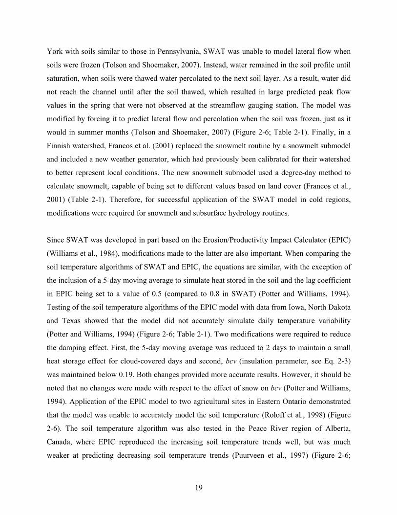
19

York with soils similar to those in Pennsylvania, SWAT was unable to model lateral flow when

soils were frozen (Tolson and Shoemaker, 2007). Instead, water remained in the soil profile until

saturation, when soils were thawed water percolated to the next soil layer. As a result, water did

not reach the channel until after the soil thawed, which resulted in large predicted peak flow

values in the spring that were not observed at the streamflow gauging station. The model was

modified by forcing it to predict lateral flow and percolation when the soil was frozen, just as it

would in summer months (Tolson and Shoemaker, 2007) (Figure 2-6; Table 2-1). Finally, in a

Finnish watershed, Francos et al. (2001) replaced the snowmelt routine by a snowmelt submodel

and included a new weather generator, which had previously been calibrated for their watershed

to better represent local conditions. The new snowmelt submodel used a degree-day method to

calculate snowmelt, capable of being set to different values based on land cover (Francos et al.,

2001) (Table 2-1). Therefore, for successful application of the SWAT model in cold regions,

modifications were required for snowmelt and subsurface hydrology routines.

Since SWAT was developed in part based on the Erosion/Productivity Impact Calculator (EPIC)

(Williams et al., 1984), modifications made to the latter are also important. When comparing the

soil temperature algorithms of SWAT and EPIC, the equations are similar, with the exception of

the inclusion of a 5-day moving average to simulate heat stored in the soil and the lag coefficient

in EPIC being set to a value of 0.5 (compared to 0.8 in SWAT) (Potter and Williams, 1994).

Testing of the soil temperature algorithms of the EPIC model with data from Iowa, North Dakota

and Texas showed that the model did not accurately simulate daily temperature variability

(Potter and Williams, 1994) (Figure 2-6; Table 2-1). Two modifications were required to reduce

the damping effect. First, the 5-day moving average was reduced to 2 days to maintain a small

heat storage effect for cloud-covered days and second, bcv (insulation parameter, see Eq. 2-3)

was maintained below 0.19. Both changes provided more accurate results. However, it should be

noted that no changes were made with respect to the effect of snow on bcv (Potter and Williams,

1994). Application of the EPIC model to two agricultural sites in Eastern Ontario demonstrated

that the model was unable to accurately model the soil temperature (Roloff et al., 1998) (Figure

2-6). The soil temperature algorithm was also tested in the Peace River region of Alberta,

Canada, where EPIC reproduced the increasing soil temperature trends well, but was much

weaker at predicting decreasing soil temperature trends (Puurveen et al., 1997) (Figure 2-6;

20

Table 2-1). A major limitation with SWAT (and EPIC) for cold regions is that it does not model

snow processes accurately. This, in turn, affects the soil temperature predictions. To accurately

model the FT cycles of cold regions with fine-grained soils, it is expected that further

modifications need to be incorporated into the SWAT model.

Figure 2-6: Location of study area near Whitecourt, Alberta (green), study area where SWAT model was

developed near Temple, Texas (red), and other North American sites where SWAT or EPIC have been

applied (blue).

21

Table 2-1: Summary of modifications made to SWAT as reported in the literature. Location Area

(km2) Annual Precipitation (mm)

Annual Air Temperature (oC)

Soils / Geology* Vegetation / Land-use

Modifications Reference

Ontonagon River, Michigan

3460 1000 to 800 -2.5 to 0 Rock, sandstone, limestone and dolomite.

Forest Wetland/Lake

Snowmelt parameters. Wu and Johnston, 2007

Upper Wind River Basin, Wyoming

4999 1250 to180 n/a Varies between bedrock, glacial till, and sand.

Alpine tundra Forest Range (with decreasing altitude)

Snowfall and snowmelt routines.

Fontaine et al., 2002

Ariel Creek, Pennsylvania

39.4 966 7.7 Glacial till, glaciofluvial material and lacustrine deposits. 75% of soils contain fragipans.

Residential Forest Cropland Wetland/Lake

Subsurface hydrology and snowmelt routines recommended.

Peterson and Hamlett, 1998

S. Laguna Madre, Lower Angelina, Upper Sabine, Leon, White, Hondo, Texas

7505 5046 3375 7812 4376 2807

663 1235 1041 767 515 732

n/a SCL, FSL FSL, LFS FSL LFS Clay loam GRV-L CBV-C

Range, agriculture Forests, pasture Forests, pasture Pasture, ag. Range Agriculture, range Range, agriculture

Water balance components.

Muttiah and Wurbs, 2002

Cannonsville Reservoir, New York

1178 1100 n/a n/a Forest (59%) Agriculture (26%) Farmland (10%)

Lateral flow and percolation routines for frozen soils.

Tolson and Shoemaker, 2007

Kerava River, Finland

400 n/a n/a Mainly moraine, sand, clay, peat.

Farmland Residential

Replaced snowmelt routine.

Francos et al., 2001

La Glace, Alberta n/a 475 1.9 Sand, silt, Chernozems Agriculture Evaluated EPIC snowmelt routine.

Puurveen et al., 1997

Mandan, N. Dakota Boone, Iowa Bushland, Texas

n/a 550 1016 532

5.3 10.1 13.4

Loam Loam Clay loam

Agriculture Evaluated EPIC soil temperature routines.

Potter and Williams, 1994

n/a = not applicable * SCL = sandy clay loam, FSL = fine sandy loam, LFS = loamy fine sand, GRV-L = gravelly loam, CBV-C = very cobbly clay

22

2.7 CONCLUSION

Many differences were identified between the study sites in the Swan Hills and agricultural lands

in southeast Texas where SWAT was developed:

• Soils on the Boreal Plain are mainly fine-grained Luvisols, compared to highly fertile

dark Vertisols on the Blackland Prairies in Texas.

• Vegetation in boreal forests is highly complex with overlapping canopy layers and a high

degree of spatial variability among sites due to anthropogenic and natural disturbance

regimes. In contrast, monocultures of agricultural sites generally have simple vertical

structure and similar amounts of vegetation biomass from one location to the next.

• The Swan Hills area is also 16oC colder (mean annual air temperature), dryer (578 vs 910

mm mean annual total precipitation) and snow depth was over 8 times greater than the

southern United States.

From these differences, one can conclude that modifications to the SWAT soil temperature

submodel will be necessary if it is to be used in the northern climate of the Boreal Plain. Based

on the literature, representation of the snowpack and its influence upon soil temperature seems to

be a very significant problem when attempting to use the SWAT model in cold regions.

2.8 REFERENCES

Acton, D., and Gregorich, L. 1995. Health of our soils - Understanding soil health [online].

Available from http://www.arg.gc.ca/nlwis-snite/print_e.cfm?s1=pub&s2=hs_ss&page=7

[accessed 3 April 2008].

Aluko, O.B., and Koolen, A.J. 2001. Dynamics and characteristics of pore space changes during

the crumbling on drying of structured agricultural soils. Soil Till. Res. 58: 45-54.

Andersland, O.B., and Ladanyi, B. 1994. Frozen Ground In An introduction to frozen ground

engineering. Chapman & Hall, New York, NY, USA. pp. 1-8.

Arnold, J.G., and Fohrer, N. 2005. SWAT2000: current capabilities and research opportunities in

applied watershed modelling. Hydrol. Process. 19: 563-572.

Arnold, J.G., Srinivasan, R., Muttiah R.S., and Williams J.R. 1998. Large area hydrologic

modeling and assessment. Part I: Model development. J. Am. Water Resour. Assoc. 34: 73-

89.

23

Barr, A.G., Black, T.A., Hogg, E.H., Kljun, N., Morgenstern, K., and Nesic, Z. 2004. Inter-

annual variability in the leaf area index of a boreal aspen-hazelnut forest in relation to net

ecosystem production. Agric. For. Meteorol. 126: 237-255.

Barry, R., Prévost, M., Stein, J., and Plamondon, A.P. 1990. Application of a snow cover energy

and mass balance model in a balsam fir forest. Water Resour. Res. 26: 1079-1092.

Bond-Lamberty, B., Wang, C., and Gower, S. 2005. Spatiotemporal measurement and modeling

of stand-level boreal forest soil temperatures. Agric. For. Meteorol. 131: 27-40.

Bosch, J.M., and Hewlett, J.D. 1982. A review of catchment experiments to determine the effect

of vegetation changes on water yield and evapotranspiration. J. Hydrol. 55: 3-23.

Comis, D. 2002. Texas SWAT team helps clean the world's water. Agric. Res. 50: 17.

Das, B.M. 2004. Geotechnical Properties of Soil In Principles of Foundation Engineering. 5th ed.

Brooks/Cole - Thomson Learning, Pacific Grove, CA, USA. pp. 1-63.

Efimov, S., Kozhevnikov, N., Kurilko, A.S., Nikitna, M., and Stepanov, A.V. 1980. Influence of

cyclic freezing-thawing on heat and mass transfer characteristics of clay soil. In Ground

Freezing 1980, Second International Symposium on Ground Freezing, Trondheim,

Norway, 24-25 June 1980. Edited by P.E. Frivik, N. Janbu, R. Saetersdal and L. Finborud.

Elsevier Scientific Publishing Company, Amsterdam, the Netherlands. pp. 147-152.

Environment Canada. 2008. Digital archive of the Canadian climatological data (surface)

[online]. Atmospheric Environment Service. Canadian Climate Centre, Data Management

Division, Downsview, Ont. Available from http://www.climate.weatheroffice.ec.gc.ca/

climateData/canada_e.html [accessed 14 April 2008].

Flerchinger, G.N., and Hardegree, S.P. 2004. Modelling near-surface soil temperature and

moisture for germination response predictions of post-wildfire seedbeds. J. Arid Environ.

59: 369-385.

Flerchinger, G.N., Baker, J.M., and Spaans, E.J.A. 1996. A test of the radiative energy balance of

the SHAW model for snowcover. Hydrol. Process. 10: 1359-1367.

Fontaine, T.A., Cruickshank, T.S., Arnold, J.G., and Hotchkiss, R.H. 2002. Development of a

snowfall-snowmelt routine for mountainous terrain for the soil water assessment tool

(SWAT). J. Hydrol. 262: 209-223.

Fowler, W.B., and Helvey, J.D. 1981. Soil and air temperature and biomass after residue

treatment. USDA For. Serv. Res. Note PNW-383.

24

Francos, A., Bidoglio, G., Galbiati, L., Bouraoui, F., Elorza, F.J., Rekolainen, S., Manni, K., and

Granlund, K. 2001. Hydrological and water quality modelling in a medium-sized coastal

basin. Phys. Chem. Earth 26: 47-52.

Gassman, P.W., Reyes, M.R., Green, C.H., and Arnold, J.G. 2007. The Soil and Water

Assessment Tool: Historical development, applications, and future research directions.

Trans. ASABE 50: 1211-1250.

Government of Alberta. 2007. A Changing Climate for Agriculture – How Can We Prepare?

[online]. Available from http://www1.agric.gov.ab.ca/$department/deptdocs.nsf/all/cl9706

[accessed 11 June 2009].

Government of Alberta. 2008a. 10 Years Statistical Summary: 10 years average [online].

Available from http://www.srd.gov.ab.ca/wildfires/pdf/10_year_average.pdf [accessed 11

June 2009].

Government of Alberta. 2008b. Forest Management Agreement holders [online]. Available from

http://www.srd.gov.ab.ca/forests/managing/fmasawarded.aspx [accessed 11 June 2009].

Government of Alberta. 2009. Overwinter mortality surveys underway [online]. Available from

http://www.industrymailout.com/Industry/LandingPage.aspx?id=393107&p=1 [accessed

16 June 2009].

Government of Canada. 1994. Soils of Canada – Maps [online]. Available from

http://www.agr.gc.ca/nlwis-snite/pub/hs_hs/1a_e.cfm [accessed 3 April 2008].

Gray, D., and Landine, P. 1987. Albedo model for shallow prairie snow covers. Can. J. Earth Sci.

24: 1760-1768.

Han, G., Zhou, G., Xu, Z., Yang, Y., Liu, J., and Shi, K. 2007. Soil temperature and biotic

factors drive the seasonal variation of soil respiration in a maize (Zea mays L.) agricultural

ecosystem. Plant Soil 291: 15-26.

Hardy, J.P., Groffman, P.M., Fitzhugh, R.D., Henry, K.S., Welman, A.T., Demers, J.D., Fahey,

T.J., Driscoll, C.T., Tierney, G.L., and Nolan, S. 2001. Snow depth manipulation and its

influence on soil frost and water dynamics in a northern hardwood forest. Biogeochemistry

56: 151-174.

Hayashi, M., Goeller, N., Quinton, W.L., and Wright, N. 2007. A simple heat-conduction

method for simulating the frost table depth in hydrological models. Hydrol. Process. 21:

2610-2622.

25

Henry, H.A.L. 2008. Climate change and soil freezing dynamics: historical trends and projected

changes. Clim. Change 87: 421-434.

Jumikis, A.R. 1982. Thermal modeling of freeze-thaw depths in soils. In Third International

Symposium on Ground Freezing, Hanover, NH, USA, 22-24 June 1982. US Army Corps

Cold Regions Research and Engineering Laboratory. pp. 213-216.

Kilmer, V.J. (ed.) 1982. Handbook of Soils and Climate in Agriculture. CRC Series in

Agriculture. CRC Press, Inc., Boca Raton, FL, USA.

Kudryavtsev, S. 2004. Construction on permafrost: Numerical modeling of the freezing, frost

heaving and thawing of soils. Soil Mech. Found. Eng. 41: 177-184.

Li, C., Flannigan, M.D., and Corns, I.G.W. 2000. Influence of potential climate change on forest

landscape dynamics of west-central Alberta. Can. J. For. Res. 30: 1905-1912.

MacDonald, J.D., Kiniry, J., Luke, S., Putz, G., and Prepas, E.E. 2007. Evaluating the role of

shrub, grass and forb growth after harvest in forested catchment water balance using

SWAT coupled with the ALMANAC model. Proc. 4th International SWAT Conf., 436-447.

UNESCO-IHE, Delft, the Netherlands.

McNabb, D.H., Startsev, A.D., and Nguyen, H. 2001. Soil wetness and traffic level effects on

bulk density and air-filled porosity of compacted boreal forest soils. Soil Sci. Soc. Am. J.

65: 1238-1247.

Mellander, P.-E., Stähli, M., Gustafsson, D., and Bishop, K. 2006. Modelling the effect of low

soil temperatures on transpiration by Scots pine. Hydrol. Process. 20: 1929-1944.

Mellander, P.-E., Lofvenius, M.O., and Laudon, H. 2007. Climate change impact on snow and

soil temperature in boreal Scots pine stands. Clim. Change 85: 179-193.

Melloh, R.A., Hardy, J.P., Davis, R.E., and Robinson, P.B. 2001. Spectral albedo/reflectance of

littered forest snow during the melt season. Hydrol. Process. 15: 3409-3422.

Melloh, R.A., Hardy, J.P., Bailey, R.N., and Hall, T.J. 2002. An efficient snow albedo model for

the open and sub-canopy. Hydrol. Process. 16: 3571-3584.

Michalowski, R.L., and Zhu, M. 2006. Freezing and ice growth in frost-susceptible soils. In Soil

Stress-Strain Behaviour: Measurement, Modeling and Analysis Geotechnical Symposium,

Roma, 16-17 March 2006. Edited by H.I. Ling, L. Callisto, D. Leshchinski, and J. Koseki.

pp. 429-441.

26

Millar Western Forest Products Ltd. 2007. Growth and yield plan: 2007-2016 Detailed Forest

Management Plan. pp. 1-44.

Muttiah, R.S., and Wurbs, R.A., 2002. Scale-dependent soil and climate variability effects on

watershed water balance of the SWAT model. J. Hydrol. 256: 264-285.

National Weather Service Forecast Office. 2007. Texas weather climate summary [online].

Available from http://www.srh.noaa.gov/fwd/CLIMO/ntxtrems.html [accessed 14 April

2008].

Neitsch S.L., Arnold, J.G., Kiniry, J.R., and Williams, J.R. 2005. Soil and Water Assessment

Tool Theoretical Documentation. Version 2005. Agricultural Research Service and Texas

Agricultural Experiment Station. Temple, TX.

Parviainen, J., and Pomeroy, J.W. 2000. Multiple-scale modelling of forest snow sublimation:

initial findings. Hydrol. Process. 14: 2669-2681.

Peterson, J., and Hamlett, J. 1998. Hydrologic calibration of the SWAT model in a watershed

containing fragipan soils. J. Am. Water Res. Assoc. 34: 531-544.

Pidwirny, M. 2006. Soil Classification In Fundamentals of Physical Geography. 2nd ed. [online].

Available from http://www.physicalgeography.net/fundamentals/10v.html [accessed 8 June

2009].

Pohl, S., and Marsh, P. 2006. Modelling the spatial-temporal variability of spring snowmelt in an

arctic catchment. Hydrol. Process. 20: 1773-1792.

Pomeroy, J.W., Gray, D.M., Hedstrom, N.R., and Janowicz, J.R. 2002. Prediction of seasonal

snow accumulation in cold climate forests. Hydrol. Process. 16: 3543-3558.

Potter, K.N., and Williams, J.R. 1994. Predicting daily mean soil temperatures in the EPIC

simulation model. Agron. J. 86: 1006-1011.

Putz, G., Burke, J.M., Smith, D.W., Chanasyk, D.S., Prepas, E.E., and Mapfumo, R. 2003.

Modelling the effects of boreal forest landscape management upon streamflow and water

quality: Basic concepts and considerations. J. Environ. Eng. Sci. 2 (Suppl. 1): 87-101.

Puurveen, H., Izaurralde, R.C., Chanasyk, D.S., Williams, J.R., and Grant, R.F. 1997. Evaluation

of EPIC’s snowmelt and water erosion submodels using data from the Peace River region

of Alberta. Can. J. Soil Sci. 77: 41-50.

Qi, J., Vermeer, P.A., and Cheng, G. 2006. A review of the influence of freeze-thaw cycles on

soil geotechnical properties. Permafrost Periglac. Process. 17: 245-252.

27

Roloff, G., de Jong, R., and Nolin, M.C. 1998. Crop yield, soil temperature and sensitivity of

EPIC under central-eastern Canadian conditions. Can. J. Soil Sci. 78: 431-439.

Sadler, J.E., Sudduth, K.A., and Jones, J.W. 2007. Separating spatial and temporal sources of

variation for model testing in precision agriculture. Precision Agric. 8: 297-310.

Safranyik, L., and Linton, D.A. 1998. Mortality of mountain pine beetle larvae, Dendroctonus

ponderosae (Coleoptera: Scolytidae) in logs of lodgepole pine (Pinus contorta var.

latifolia) at constant low temperatures. J. Entomol. Soc. British Columbia 95: 81-87.

Schlenker, W., Hanemann, M.W., and Fisher, A.C. 2007. Water availability, degree days, and

the potential impact of climate change on irrigated agriculture in California. Clim. Change

81: 19-38.

Smith, D. 1996. Thermal considerations. In Cold regions utilities monograph. 3rd ed. Edited by

N. Low. American Society of Civil Engineers, New York, NY, USA. pp. 4.1-4.54.

Southern Regional Climate Center. 2008. 1971-2000 National Climatic Data Center Normals

[online]. Available from http://www.srcc.lsu.edu/southernClimate/atlas/ [accessed 18 July

2008].

Texas Parks and Wildlife Department. 2007. Plant Guidance by Ecoregions Ecoregion 4 – The

Blackland Prairies [online]. Available from http://www.tpwd.state.tx.us/huntwild/wild/

wildscapes/guidance/plants/ecoregions/ecoregion_4.phtml [accessed 1 July 2009].

Thomas, H., and Tart, R. 1984. Two-dimensional simulation of freezing and thawing in soils. In

Third International Specialty Conference Cold Regions Engineering Northern Resource

Development, Edmonton, AB, 4-6 April 1984. Edited by D.W. Smith. Canadian Society for

Civil Engineering. pp. 265-274.

Tolson, B.A., and Shoemaker, C.A. 2007. Cannonsville reservoir watershed SWAT2000 model

development, calibration and validation. J. Hydrol. 337: 68-86.

Troendle, C.A., and Reuss, J.O. 1997. Effect of clear cutting on snow accumulation and water

outflow at Fraser, Colorado. Hydrol. Earth Sys. Sci. 1: 325-332.

Valentini, R., Matteucci, G., Dolman, A.J., Schulze, E.-D., Rebmann, C., Moors, E.J., Granier,

A., Gross, P., Jensen, N.O., Pilegaard, K., Lindroth, A., Grelle, A., Bernhofer, C.,

Grünwald, T., Aubinet, M., Ceulemans, R., Kowalski, A.S., Vesala, T., Rannik, Ü.,

Berbigier, P., Loustau, D., Guðmundsson, G., Thorgeirsson, H., Ibrom, A., Morgenstern,

K., Clement, R., Moncrieff, J., Montagnani, L., Minerbi, S., and Jarvis, P.G. 2000.

28

Respiration as the main determinant of carbon balance in European forests. Nature 404:

861-865.

Vattenteknik, M. 2008. Coup Model [online]. Available from

http://www.lwr.kth.se/vara%20datorprogram/CoupModel/index.htm [accessed 23 October

2008].

Wall, A., and Heiskanen, J. 2003. Water-retention characteristics and related physical properties

of soil on afforested agricultural land in Finland. Forest Ecol. Manage. 186: 21-32.

Warkentin, B.P. 1984. Physical Properties of Forest-Nursery Soils: Relation to Seedling Growth.

In Forest Nursery Manual: Production of Bareroot Seedlings. Edited by M.L. Duryea and

T.D. Landis. The Hague/Boston/Lancaster, for Forest Research Laboratory, Oregon State

University, OR, USA. pp. 53-61.

Westerling, A.L., Hidalgo, H.G., Cayan, D.R., and Swetnam, T.W. 2006. Warming and earlier

spring increase western U.S. forest wildfire activity. Science 313: 940-943.

Whitson, I.R., Chanasyk, D.S., and Prepas, E.E. 2004. Patterns of water movement on a logged

Gray Luvisolic hillslope during the snowmelt period. Can. J. Soil Sci. 84: 71-82.

Whitson, I.R., Chanasyk, D.S., and Prepas, E.E. 2005. Effect of forest harvest on soil

temperature and water storage and movement patterns on Boreal Plain hillslopes. J.

Environ. Eng. Sci. 4: 429-439.

Williams, J.R., Jones, C.A., and Dyke, P.T. 1984. A modeling approach to determining the

relationship between erosion and soil productivity. Trans. ASAE 27: 129-144.

World Wildlife Fund. 2001. Texas blackland prairies [online]. Available from

http://www.worldwildlife.org/wildworld/profiles/terrestrial/na/na0814_full.html [accessed

1 July 2009].

Wratt, D., Tait, A., Griffiths, G., Espie, P., Jessen, M., Keys, J., Ladd, M., Lew, D., Lowther, W.,

Mitchell, N., Morton, J., Reid, J., Reid, S., Richardson, A., Sansom, J., and Shankar, U.

2006. Climate for crops: integrating climate data with information about soils and crop

requirements to reduce risks in agricultural decision-making. Meteorol. Applic. 13: 305-

315.

Wu, K., and Johnston, C.A. 2007. Hydrologic comparison between a forested and a wetland/lake

dominated watershed using SWAT. Hydrol. Process. 337: 187-199.

29

Zhang, T., Osterkamp, T.E., and Stamnes, K. 1997. Effects of climate on the active layer and

permafrost on the north slope of Alaska, USA. Permafrost Periglac. Process. 8: 45-67.

Zhang, X., Vincent, L.A., Hogg, W.D., and Niitsoo, A. 2000. Temperature and precipitation

trends in Canada during the 20th century. Atmosphere-Ocean 38: 395-429.

Zhao, L., and Gray, D.M. 1997. A parametric expression for estimating infiltration into frozen

soils. Hydrol. Process. 11: 1761-1775.

30

CHAPTER 3: QUANTIFYING THE EFFECTS OF AIR TEMPERATURE, SOIL

MOISTURE AND SNOW DEPTH ON SOIL TEMPERATURES

DURING THE RAPID COOLING PERIOD, ON THE BOREAL PLAIN

3.1 INTRODUCTION

To understand streamflow and water quality dynamics within the boreal forest, and to predict

how landscape disturbance alters these dynamics, factors that influence water movement through

watershed soils are crucial. In boreal forests, the timing and rate of soil freezing in autumn affect

the relative volume of water moving over the soil surface and through shallow and deep

subsurface flowpaths. When soils are frozen, porosity is reduced and ice lenses form, which

prevents infiltration of water to deeper layers, and surface or saturated overland flow can then

occur (Carey and Woo, 2001). Thus, the moisture content of the soil at the time of freezing plays

a part in determining the degree to which infiltration is reduced in frozen soils relative to

unfrozen soils (Kane and Stein, 1983). In association with these processes, soil freezing patterns

also affect solute concentrations in water moving over and through soils, because they influence

the type of soils the water will encounter and the contact time between water and soil. In general,

litter and shallow soil horizons in the boreal forest are richer in organic compounds and labile

phosphorus and nitrogen than deeper mineral soil strata (Schoenau et al., 1989; D’Arcy and

Carignan, 1997; Anderson and Lepistö, 1998). It follows that lengthening the contact period for

water moving through shallow soils would increase concentrations of these solutes. Thus, the

annual soil freeze and thaw cycle in the boreal forest exerts a strong influence on water

movement patterns, nutrient concentrations in soil water, and water leaving the watershed in the

stream channel.

Many parameters interact to influence the cooling of soil temperatures in autumn. Air

temperature and soil moisture regulate soil temperature (Smith, 1996; Martinez et al., 2008), as

well as interacting with each other. As air temperatures in autumn decrease, dry soils cool

proportionally and heat stored within the soils is lost to the atmosphere; this relationship depends

on the soil’s thermal conductivity. Thermal conductivity is higher for soil than water (Arenson

31

and Sego, 2004); as air temperatures cool in the fall, soils with higher soil moisture cool more

slowly relative to dryer soils that have more voids filled with air. In addition, the presence of a

snowpack decreases the amount of solar radiation reaching the soil surface, since snow

(particularly fresh snow) has high albedo. In opposition to the albedo effect, which limits direct

radiant heating of soil, a snowpack also insulates soils, preventing heat loss from the soils to the

atmosphere (Hardy et al., 2001). The insulating effect keeps soils warm during winter but the

albedo effect delays thawing in the spring. Vegetation cover is a fourth factor that can influence

soil temperatures in autumn. Similarly to a snowpack, vegetation directly decreases the amount

of solar radiation that reaches the soil surface. For example, forest harvesting in a boreal forest

jack pine stand in northern Ontario increased soil temperatures by as much as 6oC in summer

months (Bhatti et al., 2000). Further, the forest canopy interacts with the snowpack by altering

snow accumulation patterns on the forest floor (Metcalfe and Buttle, 1998). Snow interception

rates are high for conifer trees and snow depth increases with horizontal distance outward from

tree trunks to approximately 3 m, depending on the size of the tree (Faria et al., 2000). As winter

progresses, wind can alter the snow distribution patterns on the ground and may clear snow from

open areas. During spring, the canopy cover shields the snow from the sun and snowmelt is

delayed compared to open sites. Forest harvest experiments in aspen stands in northern

Minnesota demonstrated that snowmelt was more rapid and occurred earlier after tree removal

(Verry et al., 1983). Although the effects of air temperature, soil moisture, snow depth and

vegetation on soil temperatures have been studied individually, there is need for a study that

integrates all four factors to determine how they interact.

In the boreal forest, snowmelt can be an important annual hydrologic event. Snowmelt runoff

accounted for up to 72% of annual streamflow in the central Canadian Boreal Shield (Beall et al.,

2001). Although snowmelt comprises a smaller proportion of annual streamflow on the western

Canadian Boreal Plain, where annual snowfall accounts for less than 30% of annual

precipitation, snowmelt runoff is important for nutrient movement in watersheds. For example,

the snowmelt period was estimated to account for 50% of the nitrate export from Boreal Plain

watersheds (Pelster et al., 2008). Therefore efforts to quantify disturbance (forest harvest or

wildfire for example) impacts on hydrologic regimes and the quality of receiving waters have

tended to consider the timing and rate of snowpack depletion (Hardy et al., 1998; Parviainen and

32

Pomeroy, 2000; Jones and Pomeroy, 2001). However, a key factor for predicting snowmelt in

spring is quantifying the formation of ice in soil layers during the cooling period in autumn

(Metcalfe and Buttle, 2001). Further, analysis of soil temperatures during the cooling period is

also important for forest products industries operating in the boreal forest, where winter

harvesting on frozen soils is commonly employed to limit soil compaction. Ground-based

logging equipment increases soil bulk density and strength and decreases air-filled porosity,

infiltration rate and hydraulic conductivity, which in turn can negatively affect tree regeneration

and growth (Elliot et al., 1998; McNabb et al., 2001).

This study is part of the Forest Watershed and Riparian Disturbance project (FORWARD), a

collaborative effort by researchers, forest-related industries, First Nations communities and

Federal and Provincial governments focused on two boreal forest study areas in Canada: the

western Boreal Plain and the central Boreal Shield. This study is based in the Boreal Plain study

area, situated in the Swan Hills of Alberta (Figure 3-1). The main objectives of FORWARD are

to collect meteorological and watershed data (vegetation, soils, surface water quality and

quantity and bioindicators) to adapt hydrological and water quality models to predict the effects

of watershed disturbance, and to apply this knowledge to develop decision support tools to aid in

forest management planning (Smith et al., 2003; Prepas et al., 2008a). One focus of the

modelling efforts within FORWARD has been adapting SWAT, a deterministic hydrological

model, for northern climates and forest conditions. To adequately modify the model, parameters

that influence soil temperature must be identified. The objectives of this study were to: (1)

quantify the effects of air temperature on soil temperature in autumn, (2) quantify the combined

effect of air temperature, soil moisture and snow depth on soil temperature, and (3) explain

differences in soil temperature among burned, harvested, conifer and deciduous stands, and

between upland sites and wetland sites.

33

Figure 3-1: Location of study sites within the Boreal Plain (see Table 3-2 for site descriptions).

3.2 SITE DESCRIPTION

The Swan Hills study area is approximately 225 km northwest of Edmonton, Alberta, Canada

(Figure 3-1). The five first- to third-order study watersheds constitute a subset of the

FORWARD research watersheds and cover an area of 182 km2 (Figure 3-1). The climate of the

Boreal Plain is sub-humid (Zoltai et al. 1998); long-term climate normals (1971 to 2000) for

precipitation and mean annual air temperature are 578 mm and 2.6oC, respectively, with 24% of

total precipitation falling as snow (Environment Canada, 2008). Generally, this area is snow-

covered for six to seven months of the year, beginning in October or November (Environment

34

Canada, 2008). Among the three study years and during the four-month study periods

(September to December), 2008 was relatively dry (precipitation was approximately 70% of the

climate normal), whereas precipitation in 2007 was similar to the climate normal and 2006 had

nearly double the normal precipitation (Table 3-1). Snowfall was lower than normal in 2007 and

almost twice as much as normal in 2006. In terms of the mean air temperature, 2006 and 2008

were cooler than the climate normal, and 2007 was 4.6oC warmer than normal (Table 3-1).

Table 3-1: Climate data for each study year and long-term means (1971-2000) from 1 September to 31

December, followed by annual means (1 January to 31 December) in brackets. Data from Environment

Canada Whitecourt A station (Environment Canada, 2008).

Year Total Precipitation (mm)

Total Snowfall (mm)

Mean Air Temperature (oC)

2006 231 (516) 125 (163) -1.5 (3.6) 2007 125 (533) 12 (94.3) 5.9 (3.8) 2008 92 (438) data missing -0.4 (2.7)

Long-term mean 128 (578) 57 (139) 1.3 (2.6)

Upland soils across the study area are mostly fine-grained Orthic Gray Luvisols overlaying deep

glacial tills (Whitson et al., 2003) and wetlands consist mainly of peat (Ecological Stratification

Working Group 1996). Peat depth varies, but is generally > 0.4 m (Couling et al., 2007). Tree

cover is mainly mixed-wood, consisting primarily of black spruce (Picea mariana (Mill.) BSP),

trembling aspen (Populus tremuloides Michx.), lodgepole pine (Pinus cortorta Dougl. ex

Loud.var. latifolia Engelm) and tamarack larch (Larix laricina (Du Roi) K. Koch) (Ecological

Stratification Working Group 1996). Other species present in the area include jack pine (Pinus

banksiana Lamb.), balsam poplar (Populus balsamifera L.) and white spruce (Picea glauca

(Moench) Voss) (Smith et al., 2003). Conifer and deciduous stands across the study area are

dominated by lodgepole pine and trembling aspen, respectively (Table 3-2). Most wetlands are

treed fens (Couling et al., 2007), dominated by black spruce and/or lodgepole pine (Table 3-2).

35

Table 3-2: Sample site descriptions

Site ID Watershed Cover type Canopy

Cover (%) Stand Characteristics

Species (Cover %) Elevation

(m) First date of

sampling B1 Goose Upland Burned 0 n/a 987 9 Aug 2006 B2 Goose Upland Burned 0 n/a 985 9 Aug 2006 B3 Goose Upland Burned 0 n/a 991 13 Jul 2006 H1 Kashka Upland Harvested 0 n/a 1043 1 Aug 2006 H2 Millions Upland Harvested 0 n/a 991 6 Aug 2006 H3 Millions Upland Harvested 0 n/a 1016 10 Aug 2006C1 Thistle Upland Conifer 92 PL(90) AW(10) 1028 20 Oct 2005 C2 Willow Upland Conifer 97 PL(90) AW(10) 1005 28 Oct 2005 C3 Willow Upland Conifer 89 PL(90) AW(10) 1054 3 Nov 2005 D1 Thistle Upland Deciduous 84 AW(70) SB(20) PL(10) 1053 27 Oct 2005 D2 Thistle Upland Deciduous 96 AW(60) SB(20) PL(20) 1026 3 Nov 2005 D3 Willow Upland Deciduous 95 AW(90) PL(10) 1013 28 Oct 2005 W1 Willow Wetland 69 SB(80) LT(10) PL(10) 1026 28 Jun 2006 W2 Millions Wetland 71 SB(100) 1028 10 Aug 2006

* PL: lodgepole pine, AW: trembling aspen, SB: black spruce, LT: tamarack larch.

3.3 DATA COLLECTION

Eight reference sites (three upland conifer, three upland deciduous and two wetland) and six

disturbed or open sites (three upland burned and three upland harvested) were selected within the

FORWARD watersheds (Figure 3-1; Table 3-2). Both wetlands were identified as peatlands,

with peat depths ranging from 1.6 to 2.8 m. There were slight differences in elevation and slope

(range from 0.01 to 0.04%) among sites (Table 3-2). The burned sites were a result of a severe

wildfire in the Virginia Hills in June 1998 (Prepas et al., 2003), where nearly 727,000 hectares of

forest burned (Government of Alberta, 2008). Regrowth since the wildfire mainly consists of

lodgepole pine with some trembling aspen; tree height ranges from 0.5 to 2 m. The harvested

sites were the result of logging activity that occurred between January and March of 2004. All

harvested sites received the same treatment after harvest, namely mechanical site preparation

(shear blading and Donaren mounding) between March and August 2004, and aerial application

of the herbicide glyphosate (2.1 kg/ha) in August 2004 (Prepas et al., 2008b). Regrowth since

harvesting is sparse and consists of lodgepole pine and white spruce; tree height ranges from 0.5

to 1 m.

Sample sites were set-up in the autumn of 2005 and summer of 2006 and data collection

36

occurred during the autumn to winter transition period (September to December) of 2006, 2007

and 2008. Soil temperature was measured and recorded either by water/soil temperature sensors

and HOBO® dataloggers (Onset Computer Corporation, Bourne, MA, USA) or YSI thermistors

(YSI Incorporated, Yellow Springs, OH, USA) and Data Dolphin dataloggers (Optimum

Instruments Inc., Edmonton, AB, Canada). Measurements were taken hourly at 0.1 and 0.5 m

depths for soils and at 2 m above ground level for air temperature (Figure 3-2). Soil moisture

content was measured with theta probes (Delta-T Devices Ltd., Burwell, Cambridge, UK) and

recorded by either a DL6 soil moisture datalogger (Delta-T Devices Ltd.) or a Data Dolphin

datalogger at 0.1 and 0.5 m depths (Figure 3-2). Theta probes were calibrated for mineral or

organic soils and measure volumetric moisture content. Snow depth was measured a total of 44

times in 2006 and 2007 during regular site visits. Data from burned and harvested sites were

pooled, since site access limited the amount of snow depth data that could be collected. The

canopy cover was measured using a spherical densiometer (Forest Densiometers, Bartlesville,

OK, USA) in August 2008. Measurements were taken at each site facing the four cardinal

directions, and averages of the measurements were taken as the percent cover of each site (Table

3-2).

Soil Surface

0.1 m 0.5 m

2 m

Air Temperature

0.1 m 0.5 m

Soil Moisture

Soil Temperature

Figure 3-2: Vertical profile of soil temperature, air temperature and soil moisture probes.

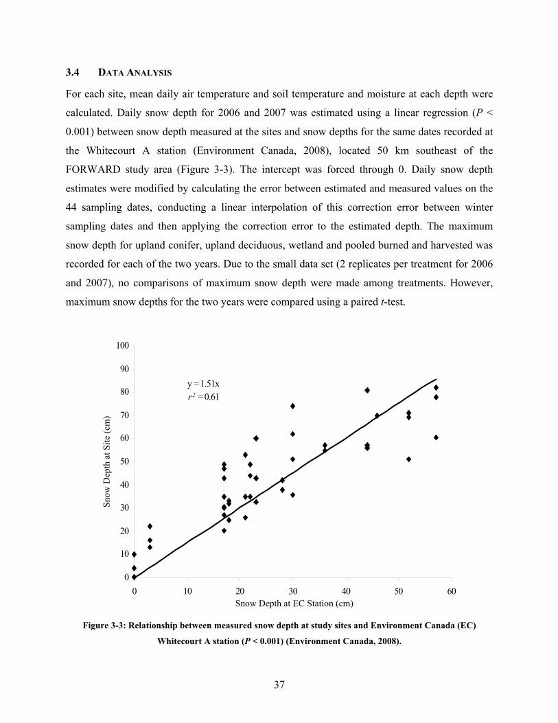
37

3.4 DATA ANALYSIS

For each site, mean daily air temperature and soil temperature and moisture at each depth were

calculated. Daily snow depth for 2006 and 2007 was estimated using a linear regression (P <

0.001) between snow depth measured at the sites and snow depths for the same dates recorded at

the Whitecourt A station (Environment Canada, 2008), located 50 km southeast of the

FORWARD study area (Figure 3-3). The intercept was forced through 0. Daily snow depth

estimates were modified by calculating the error between estimated and measured values on the

44 sampling dates, conducting a linear interpolation of this correction error between winter

sampling dates and then applying the correction error to the estimated depth. The maximum

snow depth for upland conifer, upland deciduous, wetland and pooled burned and harvested was

recorded for each of the two years. Due to the small data set (2 replicates per treatment for 2006

and 2007), no comparisons of maximum snow depth were made among treatments. However,

maximum snow depths for the two years were compared using a paired t-test.

y = 1.51xr2 = 0.61

0

10

20

30

40

50

60

70

80

90

100

0 10 20 30 40 50 60

Snow

Dep

th a

t Site

(cm

)

Snow Depth at EC Station (cm) Figure 3-3: Relationship between measured snow depth at study sites and Environment Canada (EC)

Whitecourt A station (P < 0.001) (Environment Canada, 2008).

38

Mean 1 September to 31 December air temperature and soil temperature and moisture at 0.1 and

0.5 m depths were calculated for each site for each of the three years. Treatment means were

calculated by pooling the three years, therefore the wetland treatment had six replicates (two

sites for three years) and each of the four upland treatments had nine replicates (three sites for

three years). In some cases, several days of data were missing and a four-month average could

not be calculated adequately; therefore the entire site for that year was taken out of the analysis.

A one-way Analysis of Variance was used to compare these means among the five treatments,

followed by the Tukey test for unequal sample sizes (Daniel, 1995) if P < 0.05. Variation around

the mean was expressed in terms of Standard Error (SE). A paired t-test (alpha 0.05) was

conducted grouping all treatments to compare soil temperature and soil moisture at 0.1 versus 0.5

m depths.

Simple linear regressions were conducted to determine relationships between daily air

temperature (independent variable) and daily soil temperature (dependent variable) at 0.1 and 0.5

m soil depths. Slopes of regression lines describing these relationships were compared between

upland conifer and deciduous treatments, and between burned and harvested treatments with

two-tailed t-tests and if slopes were similar, intercept tests were conducted (Zar, 1996). In

wetlands, the presence of porous peat at 0.1 m depth meant that soil moisture was not

representative of a wetland, and in most cases was dryer than the upland sites at the same depth.

Therefore, to include wetlands in this analysis, it was also conducted at 0.5 m depth for all

treatments. Multiple linear regressions were carried out for each year to determine the

interactions between air temperature, soil moisture and snow depth (independent variables) and

soil temperature (dependent variable) (2006-2008 in the absence of snow, 2006-2007 in the

presence of snow). Only two representative treatments (upland conifer and wetland) were

analyzed this way, to avoid repeatedly using snow depth data in the pooled datasets. Means of

percent contribution to variation in soil temperature for all years were calculated and these

results presented in terms of general trends. An alpha value of 0.01 was chosen for regression

analysis and regression t-tests, given the large size of the dataset.

39

3.5 RESULTS

Mean air temperatures during the period of rapid cooling from September to December differed

among cover types. Mean air temperatures in harvested sites were 1.0, 1.1, 1.1 and 1.8oC cooler

than burned, conifer, deciduous and wetland sites, respectively (P < 0.001) (Figure 3-4). Mean

air temperatures at wetlands were 0.8, 0.7 and 0.7oC warmer than burned, conifer and deciduous

sites, respectively (P < 0.001) (Figure 3-4). Mean air temperature was not detectably different

between burned, conifer and deciduous sites. Maximum snow depth in 2006 (59.2 ± 1.8 cm) was

deeper than in 2007 (41.0 ± 1.8 cm) (P < 0.001).

Mea

n A

ir Te

mpe

ratu

re(o C

) -3

-2

-1

0Burned Harvested Conifer Deciduous WetlandBurned Harvested Conifer Deciduous Wetland

Treatment Figure 3-4: Mean (± Standard Error) air temperature from 1 September to 31 December 2006-2008 under

five vegetation cover types. Note y-axis is inverted and negative.

3.5.1 SOIL TEMPERATURE AT 0.1 M DEPTH

Mean soil temperatures during the rapid cooling period in autumn followed different patterns in

the absence (September and October) and presence (November and December) of snow. In the

absence of snow, mean soil temperatures at harvested sites were 0.6, 1.0, 1.0 and 1.1oC warmer

than at burned, conifer, deciduous and wetland sites respectively, and burned sites were 0.6oC

warmer than wetland sites (P < 0.001) (Figure 3-5a). The mean soil temperature did not differ

between conifer and deciduous sites (Figure 3-5a). In the presence of snow, mean soil

temperatures did not differ among treatments (P = 0.43) (Figure 3-5b). Therefore in the absence

40

of snow, soil temperatures depended upon treatment, whereas in the presence of snow, treatment

did not affect soil temperature at 0.1 m depth.

0

2

4

6

8

10

Burned Harvested Conifer Deciduous Wetland

0.1 m 0.5 m

0

1

2

3


a

b

Mea

n So

il Te

mpe

ratu

re (o C

)


Treatment Figure 3-5: Mean (± Standard Error) soil temperature from (a) 1 September to 31 October 2006-2008 and (b)

1 November to 31 December 2006-2008, under five vegetation cover types at 0.1 and 0.5 m soil depths.

Over the four month period, a positive relationship existed between soil temperature at 0.1 m

depth and air temperature for burned and harvested sites (i.e. in the absence of tree cover). It was

evident that as air temperature cooled in the autumn, the soil temperature declined until an air

temperature of approximately -5oC, at which point the soil temperatures reached a plateau

(Figure 3-6; note x axis is inverted to show the cooling trend). This coincided with the presence

of snow; therefore the data were separated into snow-free and snow-covered periods (delineation

indicated by vertical line in Figure 3-6).

41

-10123456789

1011121314

-40-30-20-100102030

Burned 2006

Burned 2007Burned 2008

Harvested 2006Harvested 2007

Harvested 2008

Air Temperature (oC)

Soil

Tem

pera

ture

(o C) no snow with snow

Figure 3-6: Mean daily soil temperature at 0.1 m depth versus mean daily air temperature at 2 m above

ground surface for burned and harvested sites in 2006, 2007 and 2008. Vertical line shows an approximate

demarcation of absence and presence of snow. Note x-axis is inverted to show the cooling trend.

When the relationships between soil and air temperature are compared for all five treatments,

three distinct groups emerged: upland disturbed, upland treed and wetlands. As determined by

two-tailed t-tests, slopes and intercepts of the lines describing relationships between soil

temperature and air temperature did not differ between burned and harvested sites in the absence

(P = 0.29 and 0.80, respectively) or presence of snow (P = 0.67 and 0.83, respectively), therefore

these data were pooled into two datasets (upland disturbed without snow, upland disturbed with

snow). In the absence of snow, a much larger percentage of the variation in soil temperature

could be explained by air temperature than in the presence of snow (Figure 3-7). Similarly, the

slopes and intercepts of the regression lines for soil temperature versus air temperature were

similar for conifer and deciduous sites in the absence (P = 0.14 and 0.95, respectively) and

presence of snow (P = 0.92 and 0.87, respectively), therefore these data were also pooled into

two datasets (upland treed without snow, upland treed with snow).

42

-1

0

1

2

3

-35 -30 -25 -20 -15 -10 -5 0 5

-202468

10121416

-10 -5 0 5 10 15 20 25

Disturbed

Treed

Wetland


Soil

Tem

pera

ture

(o C)

a

b

Treedy = 0.5x + 3.69

r2 = 0.70

Disturbedy = 0.5x + 3.60

r2 = 0.70

Wetlandy = 0.6x + 3.09

r2 = 0.75

Treedy = 0.03x + 0.75

r2 = 0.10


r2 = 0.09

Wetlandy = 0.03x + 0.78

r2 = 0.11


ground surface for disturbed, treed, and wetland sites in (a) the absence and (b) the presence of snow from 1

September to 31 December 2006-2008. For all regressions P < 0.001. Note change in scale for both axes.

Relative to the untreed disturbed sites, the presence of trees in upland sites affected the

relationship between air and soil temperature. In the absence of snow, the slope of the regression

line was steeper for disturbed and wetland sites than for treed sites (P = 0.007 and < 0.001,

respectively) (Figure 3-7a). There were no detectable differences in slopes and intercepts

between disturbed and wetland sites (P = 0.014 and 0.57, respectively). In the presence of snow,

regression slopes did not differ among disturbed, wetland, and treed sites (P > 0.35), but the

intercept for disturbed sites was 0.3oC warmer than treed and wetland sites (P < 0.001) (Figure 3-

7b). Intercepts of treed and wetland sites were similar (P = 0.14). Thus, in the absence of snow,

upland tree cover affected the rate of change in soil temperature with each decrement in air

temperature, whereas the disturbed and wetland sites behaved similarly to each other. In the

presence of snow, soil temperature at disturbed sites were warmest for a given air temperature,

43

whereas soil temperatures at upland treed and wetland sites were similar for a given air

temperature.

At the 0.1 m depth, mean soil moisture from September to December for the three years was 79,

58 and 67% higher in burned, conifer and deciduous sites, respectively, compared to wetlands (P

= 0.002) (Figure 3-8). To determine how air temperature interacted with soil moisture and snow

depth to influence soil temperature, multiple regressions were conducted in both the absence and

presence of snow for upland (represented by upland conifer) and wetland sites. In the absence of

snow, air temperature and soil moisture accounted for 69.8 ± 5.1% and 3.2 ± 2.0%, respectively,

of the variation in soil temperature in upland sites among the three years (P < 0.001) (Figure 3-

9a). In 2006, there was no relationship between soil temperature and soil moisture at these

upland sites (P = 0.42). In wetlands in the absence of snow, air temperature and soil moisture

explained 74.8 ± 5.4% and 7.7 ± 2.8% of the variation in soil temperature, respectively, among

the three years (P < 0.001) (Figure 3-9a). Snow cover altered these patterns. For upland sites in

the presence of snow, air temperature, soil moisture and snow depth explained 2.0 ± 1.0%, 91.2

± 3.3%, and 0.6 ± 0.6% of the variation in soil temperature, respectively (P < 0.001) (Figure 3-

9a). In 2006, there was no relationship between soil temperature and snow depth at upland sites

(P = 0.08). For wetlands in the presence of snow, air temperature, soil moisture and snow depth

explained 37.1 ± 19.9%, 38.5 ± 22.3%, and 1.3 ± 1.3% of the variation in soil temperature,

respectively (P < 0.001) (Figure 3-9a). In 2007, there was no relationship between soil

temperature and snow depth at wetland sites (P = 0.49). For upland and wetland sites, air

temperature and soil moisture were the most important factors in the absence and presence of

snow, respectively.

44

0

200

400

600

800

1000

1200


0.1 m 0.5 mM

ean

Soil

Moi

stur

e (m

m3 H

20/m

m3 s

oil)


Treatment Figure 3-8: Mean (± Standard Error) soil moisture from 1 September to 31 December 2006-2008 under five

vegetation types.

45

0

20

40

60

80

100

Upland Wetland Upland Wetland

Unknown Snow Depth Soil Moisture Air Temperature

0

20

40

60

80

100

Upland Wetland Upland WetlandUpland Wetland Upland Wetland

Absence of Snow Presence of Snow

% V

aria

tion

in S

oil T

empe

ratu

re

a

b

Figure 3-9: Percentage of contribution to soil temperature based on multiple linear regression analyses for

upland conifer and wetland sites at (a) 0.1 m and (b) 0.5 m depths.

3.5.2 SOIL TEMPERATURE AT 0.5 M DEPTH

Mean soil temperatures for all treatments grouped were warmer at the 0.5 m than 0.1 m depth for

September to October (P = 0.03) (Figure 3-5a) and November to December (P = 0.001) (Figure

3-5b), with a more dramatic difference between the two depths later in the autumn. As with the

0.1 m depth, mean soil temperatures at the 0.5 m depth followed separate patterns in the absence

and presence of snow during the rapid cooling period, coinciding with an air temperature of

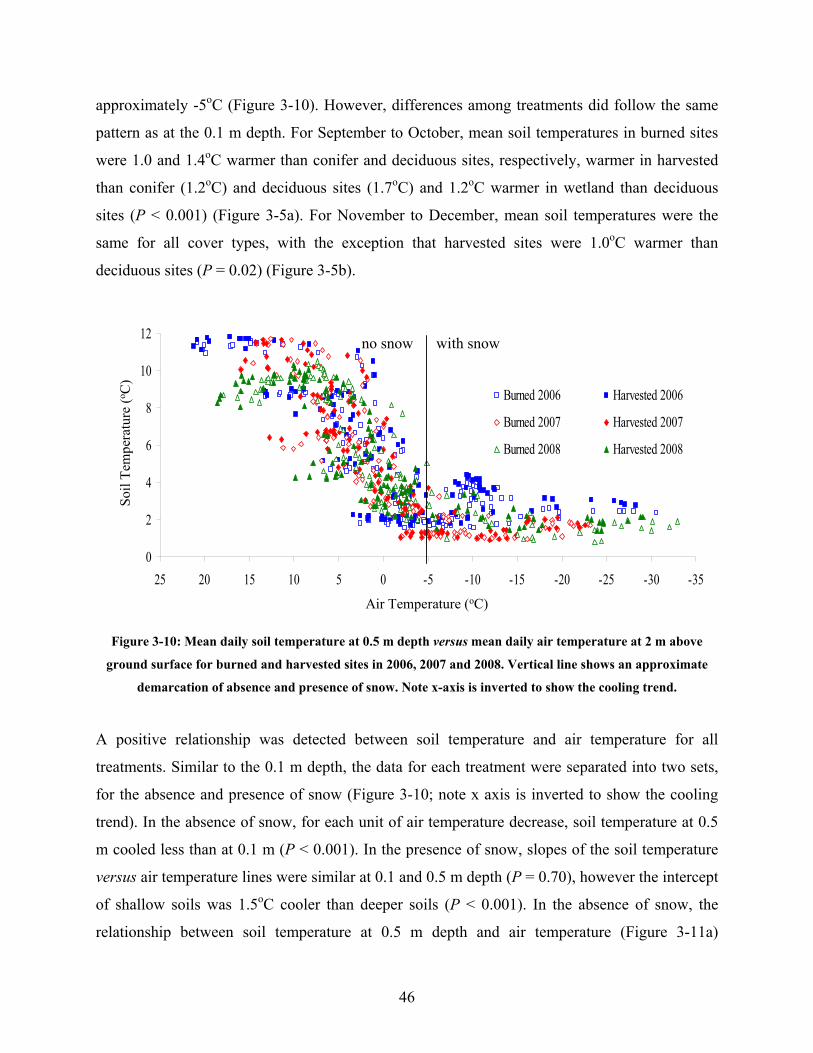
46

approximately -5oC (Figure 3-10). However, differences among treatments did follow the same

pattern as at the 0.1 m depth. For September to October, mean soil temperatures in burned sites

were 1.0 and 1.4oC warmer than conifer and deciduous sites, respectively, warmer in harvested

than conifer (1.2oC) and deciduous sites (1.7oC) and 1.2oC warmer in wetland than deciduous

sites (P < 0.001) (Figure 3-5a). For November to December, mean soil temperatures were the

same for all cover types, with the exception that harvested sites were 1.0oC warmer than

deciduous sites (P = 0.02) (Figure 3-5b).

0

2

4

6

8

10

12

-35-30-25-20-15-10-50510152025

Burned 2006 Harvested 2006




Soil

Tem

pera

ture

(o C)

no snow with snow


ground surface for burned and harvested sites in 2006, 2007 and 2008. Vertical line shows an approximate

demarcation of absence and presence of snow. Note x-axis is inverted to show the cooling trend.

A positive relationship was detected between soil temperature and air temperature for all

treatments. Similar to the 0.1 m depth, the data for each treatment were separated into two sets,

for the absence and presence of snow (Figure 3-10; note x axis is inverted to show the cooling

trend). In the absence of snow, for each unit of air temperature decrease, soil temperature at 0.5

m cooled less than at 0.1 m (P < 0.001). In the presence of snow, slopes of the soil temperature

versus air temperature lines were similar at 0.1 and 0.5 m depth (P = 0.70), however the intercept

of shallow soils was 1.5oC cooler than deeper soils (P < 0.001). In the absence of snow, the

relationship between soil temperature at 0.5 m depth and air temperature (Figure 3-11a)

47

explained 20% less variation when compared to the same regressions at the 0.1 m depth (Figure

3-7a). In the presence of snow, the relationship between soil and air temperature explained only

3% less variation at the 0.5 m depth (Figure 3-11b) than the 0.1 m depth (Figure 3-7b). The

slopes and intercepts of the lines describing relationships between soil temperature and air

temperature did not differ between burned and harvested sites in the absence (P = 0.40 and 0.49,

respectively) or presence of snow (P = 0.29 and 0.03, respectively), therefore these data were

pooled into two datasets (disturbed without snow, disturbed with snow). Slopes of soil

temperature versus air temperature lines did not differ between conifer and deciduous sites in the

absence (P = 0.77) or presence of snow (P = 0.83), however intercepts of conifer sites were 0.6

and 0.4oC warmer than deciduous sites, in the absence and presence of snow, respectively (P <

0.001). These data were therefore treated separately (conifer without snow, conifer with snow,

deciduous without snow, deciduous with snow). In the absence of snow, the treatments

(disturbed, conifer, deciduous and wetland) shared the same slope (P > 0.30) but for all cases

intercepts were different (P < 0.005) (Figure 3-11a). The intercept from disturbed sites was 0.7,

1.3 and 0.3oC warmer than conifer, deciduous, and wetland sites, respectively (P < 0.005)

(Figure 3-11a). In the presence of snow, there were no differences in the slopes and intercepts of

disturbed and wetland regressions (P = 0.17 and 0.86, respectively), while all other treatments

shared the same slope (P > 0.17) and had different intercepts (P < 0.001) (Figure 3-11b).

Therefore in the absence of snow and for a given air temperature, soil temperatures were

warmest for disturbed, wetland, conifer and deciduous sites, and in the presence of snow,

disturbed and wetland sites were warmest, followed by conifer and deciduous sites.

48

02468

101214

-10 -5 0 5 10 15 20

DisturbedConiferDeciduousWetland

0

1

2

3

4

5

-35 -30 -25 -20 -15 -10 -5 0 5


Soil

Tem

pera

ture

(o C)

a

b


r2 = 0.49

Wetlandy = 0.3x + 5.51

r2 = 0.52

Conifery = 0.03x + 2.05

r2 = 0.08


r2 = 0.08

Wetlandy = 0.02x + 2.48

r2 = 0.04

Deciduousy = 0.03x + 1.66

r2 = 0.08

Conifery = 0.3x + 5.17

r2 = 0.54

Deciduousy = 0.3x + 4.56

r2 = 0.50

Figure 3-11: Mean daily soil temperature at a 0.5 m depth versus mean daily air temperature at 2 m above

ground for disturbed, treed and wetland sites in (a) the absence and (b) the presence of snow from 1

September to 31 December 2006-2008. For all regressions P < 0.001. Note change in scale.

For all cover types, soil moisture for all treatments grouped was higher at the 0.5 m depth when

compared to 0.1 m (P < 0.008) (Figure 3-8). Mean soil moisture from September to December

was 3.0 ± 0.1 times higher in wetlands than all other treatments, and soil moisture in burned and

conifer sites was 16 and 17% higher, respectively, than deciduous sites (P < 0.001) (Figure 3-8).

In the absence of snow for upland sites, air temperature and soil moisture explained 20.9 ± 20%

and 62.5 ± 29% of the variation in soil temperature (P < 0.001) (Figure 3-9b). In wetlands, air

temperature and soil moisture accounted for 4.0 ± 1.8% and 89.2 ± 5.9% of the variation in soil

temperature in the absence of snow (Figure 3-9b). In the presence of snow, air temperature, soil

moisture and snow depth at upland sites explained 0.6 ± 0.6%, 91.2 ± 0.6%, and 4.0 ± 0.8%,

respectively, of the variation in soil temperature (P < 0.001) (Figure 3-9b). In 2006, there was no

relationship between air and soil temperature at 0.5 m (P = 0.09). For wetland sites, soil

49

temperature was only explained by air temperature (5.2 ± 1.2%) and soil moisture (83.9 ±

11.5%) (P < 0.001), because there was no relationship with the snow depth for either year (P >

0.08) (Figure 3-9b). Thus in either the absence or presence of snow, soil moisture was the most

important factor affecting soil temperatures at the 0.5 m depth.

3.6 DISCUSSION

The simplest scenario analyzed in this evaluation of factors that influence soil temperature was

disturbed (open) upland sites in the absence of snow. Positive linear relationships between air

and soil temperature at 0.1 m depth at these sites support similar observations for bare soils at an

agricultural site in Germany (Langholz, 1989). For each decrement in air temperature, disturbed

upland soils at 0.1 m cooled 1.7 times more than soils at 0.5 m. During the cooling of fine-

grained soils at shallow depths, heat flow increases due to large differences between air and soil

temperatures. At deeper soil depths, these differences in temperature are reduced and heat flow

decreases, therefore soil temperatures cool more slowly (Smith, 1996). The decreasing cooling

rate in deeper soils may also be related to the thermal gradient of soils (that decreases with soil

depth) and higher soil moisture (wetter soils have lower diffusivity, a lower rate of temperature

change) (Smith, 1996). Increased soil moisture at deeper soil depths also alters the thermal

conductivity of the bulk soil by filling voids with water rather than air. Consequently, with

increasing depth and soil moisture, the cooling rate of soils decreases.

Under snow cover, the decrease in soil temperature with each unit decrease in air temperature

was only 6 (0.1 m) to 10% (0.5 m) of the decrease observed when there was no snow cover. In

cold regions, snow cover has a critical role to play in soil temperature dynamics. It creates an

insulating layer over the soil due to its low thermal conductivity and reduces heat exchange

between the soil and atmosphere (Zhang et al., 1997; Mölders et al., 2003). This is particularly

important in disturbed sites, where there is no vegetation to intercept snow or shade snow from

solar radiation. Although snow depth was deeper in 2006 than 2007 in the present study, there

were no evident differences in soil temperature between the two years. In addition, snow depth

accounted for little or none of the variation in soil temperature at either 0.1 or 0.5 m in the

multiple regression analyses. Both of these observations support the concept that insulation from

50

a snowpack is nonlinear and that a threshold snow depth exists beyond which the insulation from

any additional snow does not provide an increased insulation effect (Henry, 2008). However, one

could argue that snow density would be a better measure of the insulation from a snowpack. For

this study snow density was not measured. Snow depth measured in snow water equivalents

could provide a better indication of insulation.

In the absence of snow, air temperature was the most important factor influencing soil

temperature in the upland and wetland sites at the 0.1 m depth, whereas at 0.5 m, soil moisture

became more important. The reduced importance of air temperature as a determinant of soil

temperature with increasing soil depth was also observed in an agricultural site in Germany

(Langholz, 1989). The stronger relationship between air and soil temperatures for wetlands

(when compared to upland sites) at the 0.1 m depth may explain why in the multiple linear

regressions, soil moisture was more important in upland sites than wetland sites. Snow depth was

relatively unimportant when compared to air temperature and soil moisture in the multiple linear

regressions at both soil depths. This shows that any relationships between soil temperature and

snow depth in simple linear regressions are linked to other parameters and that snow depth alone

cannot be used as an effective measure for predicting soil temperatures. However, the presence

of snow itself was important, since for all cases (upland and wetland soils at both depths), soil

moisture became the most important factor influencing soil temperatures when snow was

present. The snowpack insulates soils from cold air, reducing its effect on soil temperatures.

Deep snowpacks in the spring can delay soil thawing and increase overland flow, resulting in

lower concentrations of organic compounds being transported to streams. As soils freeze,

individual water particles move towards the freezing layer by cryogenic suction (Michalowski

and Zhu, 2006) and liquid water content decreases with decreasing temperature, which reduces

the overall mobility of soil water because infiltration and percolation of water within frozen soils

are inefficient (Mölders et al., 2003). In the presence of snow, the snowpack decreased the effect

of air temperature and increases the effect of soil moisture on regulating soil temperatures at both

soil depths.

The presence of trees was associated with cooler soil temperatures for a given air temperature

compared to disturbed sites. Unlike the 0.1 m depth, where there were no differences between

51

conifer and deciduous sites, intercepts of conifer sites were 0.4oC warmer than deciduous sites at

the 0.5 m depth. Warmer soils under conifer cover relative to deciduous cover could be

explained by stronger insulation from the thicker canopy during winter months, because

deciduous leaf senescence begins in late August to early September in the boreal forest. During

the freezing period in the presence of snow, soil temperatures of treed sites were again cooler

than disturbed sites (which coincides with the trend in air temperature). This might be

attributable to the open canopy in disturbed sites that allows soils to accumulate more heat

during the summer months before snowfall.

At the 0.1 m depth, shallow peat from wetlands was dryer than the upland disturbed and treed

soils. Wetlands store large amounts of water at deeper depths but near the surface, peat moisture

content fluctuates because evaporation from this shallow layer is high (Hökkä et al., 2008). Peat

has a lower thermal conductivity when compared to fine-grained soils and when dry, it releases

heat quickly during winter and insulates soils during summer (Smith, 1996). This could explain

the stronger relationship observed between soil and air temperatures in the absence of snow for

wetlands than for any other cover type at the 0.1 m depth. At the 0.5 m depth, deep peat was

significantly wetter and soil moisture exceeded 100% on a volume basis; this could be achieved

because voids are completely saturated with water and the organic matter itself contains

moisture. As moisture increases, diffusivity decreases and soils retain more heat, which explains

the strong relationship between soil temperature and moisture in the deeper soil layer of a

wetland (Figure 3-12).

52

absence of snowy = -0.32x + 333

r2 = 0.91

presence of snowy = -0.23x + 238

r2 = 0.85

0

2

4

6

8

10

12

1000 1005 1010 1015 1020 1025 1030 1035 1040

Absence of Snow

Presence of Snow

Soil Moisture (mm3H20/mm3

soil)

Soil

Tem

pera

ture

(o C)

Figure 3-12: Relationship between wetland soil temperature and soil moisture at 0.5 m depth. For all

regressions P < 0.001.

This analysis was a first attempt for the FORWARD study group to use an extensive data set to

determine factors that affect soil temperatures and explain an important element in hydrological

modelling: soil freezing. Movement of water in forests during unfrozen and frozen conditions is

highly dependent on the presence of frozen soils. Linking modelling to forest management

requires additional consideration of soil freezing as it relates to water movement. Forest removal

is known to increase soil moisture by removing an important sink for moisture:

evapotranspiration (Bosch and Hewlett, 1982). For the forest industry operating on the Boreal

Plain, compaction due to machinery on these fine-grained soils has been a concern for half a

century (McNabb et al., 2001). For this reason, winter harvesting on frozen soils is common;

therefore knowing the timing of freeze/thaw cycles is important. Daily and yearly variations in

air temperature, soil moisture and snow depth still pose a problem in this type of analysis. To

provide more confidence in the soil temperature predictions and to develop a tool to pinpoint

when soils freeze, long-term studies are still required. Although linear relationships were

identified in this study, it is possible that non-linear functions might better explain variations

observed in soil freezing patterns in these boreal forest soils. Within the FORWARD project, the

importance of snow’s effect on soil temperatures needs to be addressed in the deterministic

53

modelling. Although the current analysis would suggest that a simple snow presence/absence

approach is sufficient, a more detailed analysis of snow depth would determine if there is a

threshold depth beyond which the influence of snow depth plateaus. Further, snow density

measurements might clarify or strengthen relationships between snow and soil temperatures. By

combining these findings with the hydrological modelling that has already been conducted (Putz

et al., 2003; Watson et al., 2008), we will be better able to project streamflow year-round and

perform complete annual water and nutrient budgets for disturbed and forested watersheds.

3.7 REFERENCES

Anderson, L., and Lepistö, A. 1998. Links between runoff generation, climate and nitrate-N

leaching from forested catchments. Water Air Soil Pollut. 105:227-237.

Arenson, L.U., and Sego, D.C. 2004. Freezing processes for a coarse sand with varying

salinities. In Cold Regions Engineering & Construction Conference and Expo 2004,

Edmonton, AB, 16-19 May 2004.

Beall, F.D., Semkin, R.G., and Jeffries, D.S. 2001. Trends in the output of first-order basins at

Turkey Lakes watershed, 1982-96. Ecosystems 4: 514-526.

Bhatti, J.S., Fleming, R.L., Foster, N.W., Meng, F.-R., Bourque, C.P.A., and Arp, P.A. 2000.

Simulation of pre- and post-harvest soil temperature, soil moisture, and snowpack for jack

pine: comparison with field observations. For. Ecol. Manage. 138: 413-426.

Bosch, J.M., and Hewlett, J.D. 1982. A review of catchment experiments to determine the effect

of vegetation changes on water yield and evapotranspiration. J. Hydrol. 55:3-23.

Carey, S.K., and Woo, M-K. 2001. Slope runoff processes and flow generation in a subarctic,

subalpine catchment. J. Hydrol. 253:110-129.

Couling, K., Prepas, E.E., and Smith, D.W. 2007. Improved estimation of wetland cover in the

western Canadian boreal forest. Lake Reserv. Manage. 23: 245-254.

Daniel, W.W. 1995. Tukey’s test for unequal sample sizes. In Biostatistics: A foundation for

analysis in the health sciences. 6th ed. John Wiley & Sons. Inc., New York, NY, USA. pp.

296-298.

D’Arcy, P., and Carignan, R. 1997. Influence of catchment topography on water chemistry in

southeastern Québec Shield lakes. Can. J. Fish. Aquat. Sci. 54:2215-2227.

54

Ecological Stratification Working Group. 1996. A national ecological framework for Canada.

Centre for Land and Biological Resources Research, Research Branch, Agriculture and

Agri-Food Canada, Ottawa, Ont. 125 pp.

Elliot, J.A., Toth, B.M., Granger, R.J., and Pomeroy, J.W. 1998. Soil moisture storage in mature

and replanted sub-humid boreal forest stands. Can. J. Soil Sci. 78: 17-27.

Environment Canada. 2008. Digital archive of the Canadian climatological data (surface)

[online]. Atmospheric Environment Service. Canadian Climate Centre, Data Management

Division, Downsview, Ont. Available from http://www.climate.weatheroffice.ec.gc.ca/

climateData/canada_e.html [accessed 14 April 2008].

Faria, D.A., Pomeroy, J.W., and Essery, R.L.W. 2000. Effect of covariance between ablation and

snow water equivalent on depletion of snow-covered area in a forest. Hydrol. Process. 14:

2683-2695.

Government of Alberta. 2008. 10 Years Statistical Summary: 10 years average [online].

Available from http://www.srd.gov.ab.ca/wildfires/pdf/10_year_average.pdf [accessed 11

June 2009].

Hardy, J.P., Davis, R.E., Jordan, R., Ni, W., and Woodcock, C.E. 1998. Snow ablation modelling

in a mature aspen stand of the boreal forest. Hydrol. Process. 12: 1763-1778.

Hardy, J.P., Groffman, P.M., Fitzhugh, R.D., Henry, K.S., Welman, A.T., Demers, J.D., Fahey,

T.J., Driscoll, C.T., Tierney, G.L., and Nolan, S. 2001. Snow depth manipulation and its

influence on soil frost and water dynamics in a northern hardwood forest. Biogeochem. 56:

151-174.

Henry, H.A.L. 2008. Climate change and soil freezing dynamics: historical trends and projected

changes. Clim. Change 87: 421-434.

Hökkä, H., Repola, J., and Laine, J. 2008. Quantifying the interrelationship between tree stand

growth rate and water table level in drained peatland sites within Central Finland. Can. J.

For. Res. 38: 1775-1783.

Jones, H.G., and Pomeroy, J.W. 2001. Early spring snowmelt in a small boreal forest watershed:

Influence of concrete frost on the hydrology and chemical composition of streamwaters

during rain-on-snow events. In Proceedings of the 58th Eastern Snow Conference, Ottawa,

ON, 14-17 May 2001. Edited by J. Hardy and S. Frankenstein.

55

Kane, D.L., and Stein, J. 1983. Water movement into seasonally frozen soils. Water Resour. Res.

19: 1547-1557.

Langholz, H. 1989. A simple model for predicting daily mean soil temperatures. J. Agron. Crop

Sci. 163: 312-318.

Martinez, C., Hancock, G.R., Kalma, J.D., and Wells, T. 2008. Spatio-temporal distribution of

near-surface and root zone soil moisture at the catchment scale. Hydrol. Process. 22: 2699-

2714.

McNabb, D.H., Startsev, A.D., and Nguyen, H. 2001. Soil wetness and traffic level effects on

bulk density and air-filled porosity of compacted boreal forest soils. Soil Sci. Soc. Am. J.

65: 1238-1247.

Metcalfe, R.A., and Buttle, J.M. 1998. A statistical model of spatially distributed snowmelt rates

in a boreal forest basin. Hydrol. Process. 12: 1701-1722.

Metcalfe, R.A., and Buttle, J.M. 2001. Soil partitioning and surface store controls on spring

runoff from a boreal forest peatland basin in north-central Manitoba, Canada. Hydrol.

Process. 15: 2305-2324.

Michalowski, R.L., and Zhu, M. 2006. Freezing and ice growth in frost-susceptible soils. In Soil

Stress-Strain Behaviour: Measurement, Modeling and Analysis Geotechnical Symposium,

Roma, 16-17 March 2006. Edited by H.I. Ling, L. Callisto, D. Leshchinski, and J. Koseki.

pp. 429-441.

Mölders, N., Haferkorn, U., Döring, J., and Kramm, G. 2003. Long-term investigations on the

water budget quantities predicted by the hydro-thermodynamic soil vegetation scheme

(HTSVS) – Part I: Description of the model and impact of long-wave radiation, roots,

snow, and soil frost. Meteorol. Atmos. Phys. 84: 115-135.

Parviainen, J., and Pomeroy, J.W. 2000. Multiple-scale modelling of forest snow sublimation:

initial findings. Hydrol. Process. 14: 2669-2681.

Pelster, D.E., Burke, J.M., and Prepas, E.E. 2008. Runoff and inorganic nitrogen export from

Boreal Plain watersheds six years after wildfire and one year after harvest. J. Environ. Eng.

Sci. 7 (Suppl. 1): 51-61.

Prepas, E.E., Burke, J.M., Chanasyk, D.S., Smith, D.W., Putz, G., Gabos, S., Chen, W., Millions,

D., and Serediak, M. 2003. Impact of wildfire on discharge and phosphorus export from the

56

Sakwatamau watershed in the Swan Hills, Alberta during the first two years. J. Environ.

Eng. Sci. 2 (Suppl. 1): 63-72.

Prepas, E.E., Putz, G., Smith, D.W., Burke, J.M., and MacDonald, J.D. 2008a. The FORWARD



Prepas, E.E., Burke, J.M., Putz, G., and Smith, D.W. 2008b. Dissolved and particulate

phosphorus concentration and export patterns in headwater streams draining Boreal Plain

watersheds one year after experimental forest harvest and post-harvest silvicultural

activities. J. Environ. Eng. Sci. 7 (Suppl. 1): 63-77.

Putz, G., Burke, J.M., Smith, D.W., Chanasyk, D.S., Prepas, E.E., and Mapfumo, R. 2003.

Modelling the effects of boreal forest landscape management upon streamflow and water

quality: Basic concepts and considerations. J. Environ. Eng. Sci. 2 (Suppl. 1): 87-101.

Schoenau, J.J., Stewart, J.W.B., and Bettany, J.R. 1989. Forms and cycling of phosphorus in

prairie and boreal forest soils. Biogeochemistry 8:223-237.

Smith, D. 1996. Thermal considerations. In Cold regions utilities monograph. 3rd ed. Edited by

N. Low. American Society of Civil Engineers, New York, NY, USA. pp. 4.1-4.54.

Smith, D.W., Russell, J.S., Burke, J.M., and Prepas, E.E. 2003. Expanding the forest

management framework in the province of Alberta to include landscape-based research. J.


Verry, E.S., Lewis, J.R., and Brooks, K.N. 1983. Aspen clearcutting increases snowmelt and

storm flow peaks in north central Minnesota. Water Resour. Bull. 19: 59-67.

Watson, B.M., McKeown, R.A., Putz, G., and MacDonald, J.D. 2008. Modification of SWAT

for modelling streamflow from forested watersheds on the Canadian Boreal Plain. J.


Whitson, I.R., Chanasyk, D.S., and Prepas, E.E. 2003. Hydraulic properties of Orthic Gray

Luvisolic soils and impact of winter logging. J. Environ. Eng. Sci. 2 (Suppl. 1): 41-49.

Zar, J.H. 1996. Biostatistical analysis. 2nd ed. Prentice Hall, Englewood Cliffs, NJ, USA.

Zhang, T., Osterkamp, T.E., and Stamnes, K. 1997. Effects of climate on the active layer and

permafrost on the north slope of Alaska, USA. Permafrost Perigla. Process. 8: 45-67.

Zoltai, S.C., Morrissey, L.A., Livingston, G.P., and de Groot, W.J. 1998. Effects of fires on

carbon cycling in North American boreal peatlands. Environ. Rev. 6: 13-24.

57

CHAPTER 4: ANNUAL FREEZE/THAW TEMPERATURE CYCLE IN SOILS ON

THE CANADIAN BOREAL PLAIN: COMPARISON OF SWAT

PREDICTIONS TO MEASURED DATA1

4.1 INTRODUCTION

A critical element in modelling the quantity and quality of water in streams draining undisturbed

and disturbed forested watersheds is to understand how the annual freeze/thaw cycle affects soil

temperatures. Frozen soils are important factors in forest hydrology, because they prevent

infiltration of water to deeper layers and may cause surface or saturated overland flow (Carey

and Woo, 2001). Soil freezing patterns also affect solute concentrations in water moving over

and through soils, because they influence the type of soils the water will encounter and the

contact time between water and soils. In boreal forests, the timing and rate of soil freezing affect

the relative volume of water moving over the soil surface and through shallow and deep

subsurface flowpaths in the autumn and following spring.

The SWAT model has been applied across the United States and around the globe to predict

water movement in watersheds. However, SWAT was developed for agricultural lands in the

southern United States (on the Blackland Prairies of southeast Texas), where soils are

considerably different from those in boreal forests. Therefore it is expected that the soil

temperature submodel within SWAT will require some modifications if it is to be applied to

boreal forest conditions, as has been demonstrated in other studies in cold regions, where

changes were made to the snowmelt and subsurface hydrology routines when frozen soils were

present (Fontaine et al., 2002; Tolson and Shoemaker, 2007). The soil temperature algorithms in

SWAT are similar to and based upon those in the Erosion/Productivity Impact Calculator (EPIC)

(Williams et al., 1984). However, EPIC includes a 5-day moving average to simulate heat stored

in the soil, which is absent in SWAT. In addition, the lag coefficient (that controls the influence

of the previous day’s temperature on the current day) in EPIC is set to a value of 0.5, compared

1 A version of this chapter was submitted to the 5th International SWAT Conference, 3-7 August 2009, Boulder, CO. Authors for this paper were: J.A. Bélanger, G. Putz, B. Watson and E.E. Prepas.

58

to 0.8 in SWAT (Potter and Williams, 1994). It is critical that the SWAT algorithms be tested

stringently for cold regions because of differences in the hydrologic cycle in these areas

compared to warmer climates.

This study is part of the Forest Watershed and Riparian Disturbance project (FORWARD), a

collaborative effort by researchers, forest-related industries, First Nations communities, and

Federal and Provincial governments in Canada. The main objectives of FORWARD are to

collect watershed data (vegetation, soils, weather, surface water quality and quantity, and

bioindicators) to adapt hydrological and water quality models to predict the effects of watershed

disturbance, and to apply this knowledge to decision support tools to aid in forest management

planning in Canada (Smith et al., 2003; Prepas et al., 2008a). One focus of the modelling efforts

within FORWARD has been adapting the SWAT hydrological model for northern climates and

forest conditions. The objective of this study was to verify the suitability of the soil temperature

algorithms within SWAT to model soil temperatures in cold regions, specifically, the Canadian

Boreal Plain, for one representative example of each of the following five forest land

classification types: upland burned, harvested, conifer and deciduous forest and wetland forest.

4.2 MODEL DESCRIPTION

SWAT is a semi-distributed, physically based hydrological model that operates on a continuous

daily time-step (Neitsch et al. 2005). SWAT was developed in the early nineties for agricultural

land by the USDA. It is foremost a watershed hydrology model and the water balance is the

driving force for all functions, which include hydrology, sediment quantity and transport, and

pesticide and nutrient (nitrogen, phosphorus) concentrations. The model calculates forest canopy

water storage, infiltration, lateral subsurface flow, ground water flow, surface runoff (using

either SCS curve number procedure (USDA Soil Conservation Service, 1972) or Green & Ampt

infiltration method (Green & Ampt, 1911)) and potential and actual evapotranspiration (where

potential evapotranspiration is calculated by the Penman-Monteith (Monteith, 1965), Priestley-

Taylor (Priestley and Taylor, 1972) or Hargreaves method (Hargreaves et al., 1985)).

Redistribution is also calculated and both the variable storage coefficient (Williams, 1969) and

Muskingum (Overton, 1966) methods are used as routing equations.

59

To facilitate the modelling process, SWAT allows users to divide watersheds into multiple

subbasins. The model then partitions the subbasins into different hydrologic response units based

on their vegetation type, soil characteristics and land use. This allows the model to group similar

sites together. SWAT also separates the soil profiles into up to ten different layers to accurately

simulate belowground processes (Neitsch et al. 2005).

4.3 SWAT SOIL TEMPERATURE SUBMODEL

The soil temperature submodel in SWAT utilizes multiple input parameters that can be roughly

separated into three categories: soil characteristics, vegetation cover and climate (Table 4-1;

Figure 4-1). To calculate the soil temperature (T in oC) at a specific depth in the soil (z) on the

current day (Tsoil(z, dn)), SWAT utilizes a weighted soil temperature based on the soil

temperature on the previous day (Tsoil(z, dn-1)) and the soil surface temperature on the current day

(Tssurf):

Eq. 4-1 ( ) ( ) ( ) ( ){ }ssurfssurfAAirnsoilnsoil TTTdfdzTdzT +−⋅⋅−+⋅= − λλ 1,, 1

where λ is a lag coefficient that controls the influence of the previous day’s temperature on the

current day (set at 0.8 in SWAT), df is a depth factor, which accounts for the influence of the

depth of soil below the surface, and TAAir is the average annual air temperature based on long-

term data (Neitsch et al., 2005).

The depth factor (df) accounts for the influence of the depth of soil below the surface:

Eq. 4-2 ( )zdzdzddf

⋅−−+=

078.2867.0exp

where zd is a depth ratio, calculated with the following equation:

Eq. 4-3 ddzzd =

60

where z is the depth at the center of the soil layer in mm and dd is the damping depth in mm.

The damping depth is obtained from:

Eq. 4-4 ⎥⎥⎦

⎤

⎢⎢⎣

⎡⎟⎟⎠

⎞⎜⎜⎝

⎛+−

⋅⎟⎟⎠

⎞⎜⎜⎝

⎛⋅=

2

maxmax 1

1500lnexpϕϕ

dddddd

where ddmax is the maximum damping depth in mm and φ is a scaling factor. The maximum

damping depth is a function of the soil bulk density, ρb in Mg⋅m-3:

Eq. 4-5 ( )bb

bddρρ

ρ63.5exp686

25001000max −⋅++=

The scaling factor (φ) is calculated from the following equation:

Eq. 4-6 ( ) totb zSW

⋅−=

ρϕ

144.0356.0

where ztot is the depth from the soil surface to the bottom of the soil profile in mm and SW is the

soil moisture in mm.

The soil surface temperature is calculated from:

Eq. 4-7 ( ) ( ) barensoilssurf TbcvdTbcvT ⋅−+⋅= − 1,1 1

where bcv is above ground insulation and Tbare is the temperature of bare soil in oC. The above

ground insulation is calculated by a weighting factor that ranges from 0 (for bare soil) and 1

(100% cover):

61

Eq. 4-8 ( ) ( )⎭⎬⎫

⎩⎨⎧

⋅−+⋅⋅−+= − SNOSNO

SNOCVCV

CVbcv3002.0055.6exp

,10297.1563.7exp

max 4

where CV is above ground vegetation biomass and residue in kg⋅ha-1 and SNO is snow-water

equivalents in mm.

The temperature of bare soil is calculated from:

Eq. 4-9 ( )

2mnmx

sravbareTTTT +

+= ε

where Tav, Tmx and Tmn are average, maximum and minimum air temperatures in oC and εsr is a

radiation term, calculated empirically from:

Eq. 4-10 ( )20

141 −−⋅=

αε day

sr

H

where Hday is solar radiation in MJ⋅m-2d-1 and α is surface albedo, which varies according to the

cover present at the surface. The albedo for a snow-covered surface is set as 0.8 in the SWAT

model. When vegetation is present and snow-water equivalents are below 0.5 mm, the value of

albedo depends on cover and is calculated using the following equation:

Eq. 4-11 ( ) solsoilsolplant cvcv ⋅+−⋅= ααα 1

where αplant is the plant albedo, αsoil, is the soil albedo, and cvsol is a biomass factor. In the SWAT

soil temperature submodel, the plant and soil albedo values were set to 0.23 (Neitsch et al., 2005)

and 0.13 (URS Corporation, 2002) respectively. The biomass factor is calculated based on

aboveground vegetation biomass and residue (CV from Eq. 8) (Neitsch et al., 2005):

Eq. 4-12 ( ))100.5exp 5 CVcvsol ⋅×−= −

62

Table 4-1: SWAT soil temperature model input parameters.

Parameter Unit Symbol Aboveground vegetation biomass and residue kg⋅ha-1 CV Albedo unitless ratio α Daily mean temperature oC Tav Daily maximum temperature oC Tmx Daily minimum temperature oC Tmn Depth at the center of the soil layer mm z Depth of soil profile mm ztot Soil bulk density Mg⋅m-3 ρb Soil moisture mm SW Solar radiation MJ⋅m-2d-1 Hday Snow cover mm SNO

Figure 4-1 Schematic of SWAT soil temperature submodel.

4.4 MODEL TESTING

The SWAT soil temperature algorithms were set up in a Microsoft Excel spreadsheet and all

input parameters were integrated into the model. A sensitivity analysis was conducted by varying

the following parameters by ± 20%: aboveground vegetation biomass and residue, depth of the

soil profile, bulk density, snow equation coefficients and lag coefficient. The model was

modified by changing the most sensitive parameters and other default values. Original (default

63

parameter values) and modified (varied parameter values) SWAT soil temperature submodels

were run for each site at various depths and treatments. Daily differences between predicted and

observed data were calculated and maximum differences for summer and winter seasons were

determined. Model outputs were compared by calculating the correlation coefficient (r2), mean

absolute error (MAE), and root mean square error (RMSE).

4.5 SITE DESCRIPTION

The study area is located in the Swan Hills which is approximately 225 km northwest of

Edmonton, Alberta, Canada (Figure 4-2). The four first- to third-order watersheds used in this

study constitute a subset of the watersheds monitored by FORWARD and cover an area of 178

km2 (Figure 4-2; Table 4-2). The climate of the Boreal Plain is sub-humid (Zoltai et al. 1998);

long-term climate normals (1971 to 2000) for precipitation and mean annual air temperature are

578 mm and 2.6oC, respectively, with 24% of total annual precipitation falling as snow

(Environment Canada, 2008). Generally, this area is snow-covered for six to seven months of the

year, beginning in October or November (Environment Canada, 2008). All three study years

were dryer than normal; precipitation in 2006, 2007, and 2008 was 11, 8, and 24% lower than

normal, respectively. Snowfall was 17% higher than normal in 2006 and 32% lower in 2007 and

snowfall in 2008 was normal. In terms of the mean annual air temperature, 2006, 2007 and 2008

were 1.0, 1.2 and 0.1oC warmer than the climate normal (Environment Canada, 2008).

Table 4-2: Sample site descriptions (see also Figure 4-2).

Site ID Watershed Cover type Stand Species Cover (Approx. %)*

Canopy Cover (%) Elevation (m) First date of

sampling B Goose Upland Burned n/a 0 991 13 Jul 2006 H Millions Upland Harvested n/a 0 1016 10 Aug 2006 C Thistle Upland Conifer PL(90) AW(10) 92 1028 20 Oct 2005 D Thistle Upland Deciduous AW(70) SB(20) PL(10) 84 1053 27 Oct 2005 W Willow Wetland SB(80) LT(10) PL(10) 69 1026 28 Jun 2006

* PL: lodgepole pine, AW: trembling aspen, SB: black spruce, LT: tamarack larch.

64

Figure 4-2: Location of burned (B), harvested (H), conifer (C), deciduous (D) and wetland (W) soil sites

within the FORWARD study area.

Upland soils across the study area are mostly fine-grained Orthic Gray Luvisols overlaying deep

glacial tills (Whitson et al., 2003), and wetlands mainly consist of peat (Ecological Stratification

Working Group 1996). Peat depth varies, but is generally > 0.4 m (Couling et al., 2007). Conifer

and deciduous stands across the study area are dominated by lodgepole pine (Pinus cortorta

Dougl. ex Loud.var. latifolia Engelm) and trembling aspen (Populus tremuloides Michx.),

respectively (Ecological Stratification Working Group, 1996) (Table 4-2). Wetlands are treed

fens (Couling et al., 2007), dominated by black spruce (Picea mariana (Mill.) BSP) and include

some lodgepole pine and tamarack larch (Larix laricina (Du Roi) K. Koch) (Ecological

Stratification Working Group, 1996) (Table 4-2).

65

4.6 DATA COLLECTION

Five sites (one each of: upland burned, upland harvested, upland conifer, upland deciduous and

wetland) were selected within the FORWARD watersheds (Figure 4-2). The wetland is a

peatland, with peat depth of 2.8 m. There are slight differences in elevation and slope (range 0.01

to 0.04%) among sites (Table 4-2). The burned site is a result of a severe wildfire in the Virginia

Hills in June 1998 (Prepas et al., 2003). Regrowth since the wildfire mainly consists of lodgepole

pine with some trembling aspen; tree height ranges from 1.5 to 2 m. The harvested site is the

result of logging activity that occurred in January 2004. This site received post-harvest

mechanical site preparation (shear blading and Donaren mounding) between March and July

2004, and aerial application of the herbicide glyphosate (2.1 kg/ha) in August 2004 (Prepas et al.,

2008b). Regrowth since harvesting is sparse and consists of lodgepole pine and white spruce

(Picea glauca (Moench) Voss); tree height ranges from 0.5 to 1 m.

Sampling sites were set-up in the autumn of 2005 and summer of 2006. Soil temperature was

measured hourly and recorded either by water/soil temperature sensors and HOBO® dataloggers

(Onset Computer Corporation, Bourne, MA, USA) (conifer and deciduous sites) or YSI

thermistors (YSI Incorporated, Yellow Springs, OH, USA) and Data Dolphin loggers (Optimum

Instruments Inc., Edmonton, AB, Canada) (burned, harvested, and wetland sites). Measurements

were taken at 0.1, 0.5 and 1 m depths for soil temperature and at the ground surface and 2 m

above ground level for air temperature (Figure 4-3). Soil moisture content was measured hourly

with theta probes (Delta-T Devices Ltd., Burwell, Cambridge, UK) and recorded by either a DL6

soil moisture datalogger (Delta-T Devices Ltd.) or a Data Dolphin datalogger at 0.1, 0.5 and 1 m

depths (Figure 4-3). Snow depth was measured a total of 44 times in 2006 and 2007 during

regular site visits. Air temperature (at 2 m above ground level), precipitation and solar radiation

data were collected hourly at two FORWARD weather stations located in the study area (Figure

4-2). For each sampling site, precipitation and solar radiation data from the nearest weather

station were used in the modelling. Also, in the case of missing air temperature data, values from

the nearest soil temperature site or weather station were used. Measurements of aboveground

vegetation biomass and residue from the study area were obtained from an earlier study

(MacDonald et al., 2007). Canopy cover was measured using a spherical densiometer (Forest

Densiometers, Bartlesville, OK, USA) in August 2008. Measurements were taken at each site

66

facing the four cardinal directions, and averages of the measurements were taken as the percent

cover of each site (Table 4-2). Mean soil bulk density was measured as 1.5 Mg⋅m-3 with the

exception of wetlands at the 0.1 m depth, where bulk density was 0.3 Mg⋅m-3 (I. Whitson, Univ.

Alberta, pers. comm.).

0.1 m 0.5 m 1 m

Soil Temperature

Soil Surface

0.1 m 0.5 m 1 m

2 m 0 m

Air Temperature

Soil Moisture

Figure 4-3: Vertical profile of soil temperature, air temperature and soil moisture probes.

4.7 DATA ANALYSIS

For each site, mean, maximum and minimum daily air temperature, and mean daily soil

temperature and moisture at each depth were calculated. Daily snow depth (in cm) was estimated

using a linear regression (r2 = 0.61; P < 0.001) between snow depth measured at the sites and

snow depths for the same dates recorded at the Whitecourt A station (Environment Canada,

2008), located 50 km southeast of the FORWARD study area (Eq. 4-13).

67

Eq. 4-13 estimated snow depth at study sites = 1.51 * snow depth at Whitecourt

The intercept was forced through 0 in the equation above. Daily snow depth estimates were

modified by calculating the error between estimated and measured values on the 44 sampling

dates, conducting a linear interpolation of this correction error between winter sampling dates

and then applying the correction error to the estimated depth.

4.8 RESULTS AND DISCUSSION

Given the broad range in daily air temperature conditions on an annual basis on the Boreal Plain

(i.e. from a mean daily minimum of -17oC in January to a mean daily maximum of 22oC in July

(Environment Canada, 2008)), differences between predicted and observed soil temperatures

were identified separately for the summer (Jun-Aug) and winter (Nov-Mar) months. For all sites

and depths, the original SWAT model predicted soil temperatures that were 5.2 (conifer) to

17.3oC (burned) warmer than observed in summer and 4.1 (conifer) to 7.8oC (burned) cooler than

observed in winter (Table 4-3; Figure 4-4; Appendix). The latter outcome was unexpected, since

air temperatures in the study area fall below freezing 201 days each year (Environment Canada,

2008), compared to 31 days in southeast Texas (National Weather Service Forecast Office,

2007). A time-shift was also identified in transition periods. Predicted soil temperatures

decreased sooner in the autumn and increased sooner in the spring than was observed. For the

original SWAT model, over the three year period for each site and depth, the MAE ranged from

1.8 (wetland) to 4.3 (burned)) (Table 4-3). The time-shift increased with soil depth and was

larger for treed sites than open sites (Figure 4-4; Appendix). Cooler than predicted air

temperatures in the spring transition period and summer could be attributed to the vertically

complex, overlapping forest canopy in these boreal forest sites, which likely provided more

shade than the vegetation in croplands, for which the model was developed. In higher latitudes

compared to southeast Texas, the low angle of the sun over the horizon also reduces the amount

of solar radiation reaching the ground. Conversely, warmer than predicted air temperatures in the

autumn transition period and winter could be due to the insulation effect of aboveground

vegetation biomass, particularly at conifer sites. During winter months, differences are likely the

result of insulation by snow, which reaches a depth of 22 cm on average in January in the study

68

area (Environment Canada, 2008), compared to 2.5 cm for southeast Texas (City-Data, 2008).

Most snow-related equations in the original SWAT model were probably not subjected to the

same testing rigour for a wide range of conditions as the other components of the model because

at southern latitudes, below freezing days are few and deep snowpack is absent. Modifications

were often required when the model was applied in other cold regions, such as Pennsylvania

(Peterson and Hamlett, 1998), Michigan (Wu and Johnston, 2007), Wyoming (Fontaine et al.,

2002) and Finland (Francos et al., 2001).

69

Table 4-3: Maximum differences in summer and winter soil temperatures, and error measurements between

predicted and observed model outputs for original and modified SWAT model outputs at 0.1, 0.5 and 1.0 m

depths for each site.

Treatment SWAT model Lag coefficient Maximum

difference in summer (oC)

Maximum difference in winter (oC)

r2 MAE RMSE

0.1 m Original 0.80 11.6 -7.8 0.90 4.3 4.9 Burned Modified 0.95 6.7 -6.7 0.93 3.4 4.1 Original 0.80 7.9 -5.0 0.89 2.3 2.8 Harvested Modified 0.95 6.8 -5.0 0.90 1.8 2.3 Original 0.80 13.1 -4.8 0.83 3.0 3.8 Conifer Modified 0.96 7.3 -4.8 0.90 2.3 2.7 Original 0.80 17.3 -4.6 0.81 2.9 3.8 Deciduous Modified 0.96 14.9 -4.8 0.91 2.2 2.7 Original 0.80 9.9 -4.3 0.91 1.8 2.2 Wetland Modified 0.94 6.8 -3.8 0.94 1.4 1.7



70

-10

-5

0

5

10

15

20

25

30

1-Jan-06 1-Jun-06 1-Nov-06 1-Apr-07 1-Sep-07 1-Feb-08 1-Jul-08 1-Dec-08

Observed Soil Temp

Original SWAT

Modified SWAT

Date

Soil

Tem

pera

ture

(o C)

a

b

c

-5

0

5

10

15

20


0

5

10

15


Figure 4-4: Observed data and original and modified SWAT model outputs for the (a) burned site at 0.1 m,

(b) conifer site at 0.5 m and (c) wetland site at 1.0 m. Results for each site and depth are located in Appendix.

Note the differences in the y-axis scale.

71

Many factors were considered to address the problems in the original SWAT soil temperature

submodel, including: albedo, soil bulk density, depth of the soil profile, vegetation biomass and

the lag coefficient. The default albedo in the original SWAT model of 0.8 for a snow-covered

surface is not representative of northern disturbed or undisturbed forested sites, because it does

not account for vegetation in treed sites and smaller shrubs emerging from the snowpack in open

sites. Reported albedo values for this region of the boreal forest are 0.43 for treed sites (conifer,

deciduous and wetland) and to 0.66 for open sites (harvested and burned) (URS Corporation,

2002), which are much lower than the value provided by the SWAT model. As a result, the first

modification to the SWAT model was to alter the albedo value for a snow-covered surface based

on cover type.

The sensitivity analysis found that soil bulk density, depth of soil profile and vegetation biomass

cover did not significantly affect SWAT model results, as long as the parameters were varied

within a representative range of values for this region. However, the lag coefficient (recall fixed

at 0.8 in original SWAT model; see equation 4-1) was identified as a sensitive parameter. The

second modification to the SWAT model was to increase the lag coefficient for all treatments

and depths (Table 4-3; Figure 4-4; Appendix). The lag coefficient that provided the best overall

fit for each scenario was selected (Figure 4-5). In all cases, the lag coefficient increased from the

0.1 m depth to the 0.5 and 1.0 m depths, which demonstrates that the previous day’s soil

temperature was more important at deeper soil depths (Table 4-3). This finding, along with an

increasing time-shift with increasing soil depth, shows that the overlying soil layer also acts as an

insulator at deeper depths. By increasing lag coefficients, maximum differences between

predicted and observed soil temperatures were reduced by half in the summer (4.9 ± 0.9oC, mean

± SE) and by 30% in the winter (3.7 ± 0.4oC) (Table 4-3). The time-shift present in the spring

and autumn transition periods was also reduced (Figure 4-4; Appendix). By making both changes

to the model (decreasing the albedo and increasing the lag coefficient), the overall efficiency of

the modified SWAT model increased; MAE decreased and ranged from 0.7 (wetlands) to 3.4

(burned) (Table 4-3). Still, the modified soil temperature model predicted soil temperatures that

were cooler than observed during the winter months when snow was present.

72

-5

0

5

10

15

20

1-Nov-05 1-May-06 1-Nov-06 1-May-07 1-Nov-07 1-May-08 1-Nov-08

Observedλ = 0.70λ = 0.80λ = 0.96λ = 0.97λ = 0.98

Figure 4-5: Example of sensitivity analysis for the lag coefficient (λ) for a conifer sites at 0.5 m depth.

Following modifications to the model, predicted soil temperatures from January to March of

2006 at the conifer site (Figure 4-4b) were only slightly colder than observed in comparison to

the same periods in 2007 and 2008. This is because there was very little snow on the ground in

the winter of 2005/2006 and the modified SWAT model was more capable of accurately

modelling soil temperatures. This emphasizes the importance of considering the insulation effect

of deep snowpacks (> 20 cm). Although modifications to the snow albedo and lag coefficient

increased the efficiency of the model throughout the spring, summer and autumn, observed soil

temperatures during winter months were still generally warmer than predicted.

4.9 CONCLUSION

The comprehensive soil temperature dataset from the FORWARD study sites provided an

opportunity to contribute to the reworking of SWAT for cold climates. On the Boreal Plain, the

presence of snow drastically decreased the cooling effect of air temperature on soil temperatures

in autumn and winter, and from the literature one can surmise that snow also decreases the

warming effect of air temperature on soil temperature in early spring. The insulation from heat

transfer provided by a relatively deep snowpack is not reflected in the original SWAT model. To

adequately model forested sites in northern climates with SWAT, modelling efforts need to

73

incorporate the insulating effect of snow. By changing the lag coefficient, the modified SWAT

model was able to effectively model soil temperatures in the spring, summer and autumn seasons

in selected sites on the Boreal Plain where snow was absent. However, to effectively simulate

soil temperatures under a snowpack during winter months, further modifications to the model

must be incorporated. Recommended modifications consist of testing the equation presently in

SWAT that considers the insulating effect of snow and, if this proves insufficient, to include

another parameter to account for deep and persistent snowpacks in northern climates.

4.10 REFERENCES

Carey, S.K., and M-k Woo. 2001. Slope runoff processes and flow generation in a subarctic,

subalpine catchment. J. Hydrol. 253: 110-129.

City-Data. 2008. Average Climate in Temple, Texas. Available at: http://www.city-

data.com/city/Temple-Texas.html. Accessed 4 June 2009.

Couling, K., E.E. Prepas, and D.W. Smith. 2007. Improved estimation of wetland cover in the

western Canadian boreal forest. Lake Reserv. Manage. 23: 245-254.

Ecological Stratification Working Group. 1996. A national ecological framework for Canada.

Centre for Land and Biological Resources Research, Research Branch, Agriculture and

Agri-Food Canada, Ottawa, ON.

Environment Canada. 2008. Digital archive of the Canadian climatological data (surface).

Atmospheric Environment Service. Canadian Climate Centre, Data Management Division,

Downsview, Ont. Available at: http://www.climate.weatheroffice.ec.gc.ca/climateData/

canada_e.html. Accessed 14 April 2008.

Fontaine, T.A., T.S. Cruickshank, J.G. Arnold, and R.H. Hotchkiss. 2002. Development of a

snowfall-snowmelt routine for mountainous terrain for the soil water assessment tool

(SWAT). J. Hydrol. 262: 209-223.

Francos, A., G. Bidoglio, L. Galbiati, F. Bouraoui, F.J. Elorza, S. Rekolainen, K. Manni, and K.

Granlund. 2001. Hydrological and water quality modelling in a medium-sized coastal

basin. Phys. Chem. Earth 26: 47-52.

Green, W.H., and G.A. Ampt. 1911. Studies on soil physics, 1. The flow of air and water through

soils. J. Agr. Sci. 4: 11-24.

74

Hargreaves, G.L., G.H. Hargreaves, and J.P. Riley. 1985. Agricultural benefits for Senegal River

Basin. J. Irrig. Drain. Engr. 111: 113-124.

MacDonald, J.D., J. Kiniry, S. Luke, G. Putz, and E.E. Prepas. 2007. Evaluating the role of

shrub, grass and forb growth after harvest in forested catchment water balance using

SWAT coupled with the ALMANAC model. Proc. 4th International SWAT Conf., 436-447.

UNESCO-IHE, Delft, the Netherlands.

Monteith, J.L. 1965. Evaporation and the environment. In The state and movement of water in

living organisms. 19th Symposia of the Society for Experimental Biology, 205-234.

London, UK: Cambridge Univ. Press.

National Weather Service Forecast Office. 2007. Texas weather climate summary. Available at:

http://www.srh.noaa.gov/fwd/CLIMO/ntxtrems.html. Accessed 14 April 2008.

Neitsch, S.L., J.G. Arnold, J.R. Kiniry, and J.R. Williams. 2005. Soil and Water Assessment Tool

Theoretical Documentation, Version 2005. Temple, TX: Agricultural Research Service and

Texas Agricultural Experiment Station.

Overton, D.E. 1966. Muskingum flood routing of upland streamflow. J. Hydrol. 4: 185-200.

Peterson, J., and Hamlett, J. 1998. Hydrologic calibration of the SWAT model in a watershed

containing fragipan soils. J. Am. Water Res. Assoc. 34: 531-544.

Potter, K.N., and J.R. Williams. 1994. Predicting daily mean soil temperatures in the EPIC

simulation model. Agron. J. 86: 1006-1011.

Prepas, E.E., J.M. Burke, D.S. Chanasyk, D.W. Smith, G. Putz, S. Gabos, W. Chen, D. Millions,

and M. Serediak. 2003. Impact of wildfire on discharge and phosphorus export from the

Sakwatamau watershed in the Swan Hills, Alberta during the first two years. J. Environ.

Eng. Sci. 2 (Suppl. 1): 63-72.

Prepas, E.E., G. Putz, D.W. Smith, J.M. Burke, and J.D. MacDonald. 2008a. The FORWARD



Prepas, E.E., J.M. Burke, G. Putz, and D.W. Smith. 2008b. Dissolved and particulate phosphorus

concentration and export patterns in headwater streams draining Boreal Plain watersheds

one year after experimental forest harvest and post-harvest silvicultural activities. J.


75

Priestley, C.H.B., and R.J. Taylor. 1972. On the assessment of surface heat flux and evaporation

using large-scale parameters. Mon. Weather Rev. 100: 81-92.

Smith, D.W., E.E. Prepas, G. Putz, J.M. Burke, W.L. Meyer, and I. Whitson. 2003. The Forest

Watershed and Riparian Disturbance study: a multi-discipline initiative to evaluate and

manage watershed disturbance on the Boreal Plain of Canada. J. Environ. Eng. Sci. 2

(Suppl. 1): 1-13.

Tolson, B.A., and C.A. Shoemaker. 2007. Cannonsville reservoir watershed SWAT2000 model

development, calibration and validation. J. Hydrol. 337: 68-86.

URS Corporation. 2002. Preparation of Alberta environment regional AERMOD screening

meteorology data sets, Alberta Environment Science and Standards: 1-12.

USDA Soil Conservation Service. 1972. National Engineering Handbook Section 4 Hydrology,

Chapter 4-10.

Williams, J.R. 1969. Flood routing with variable travel time or variable storage coefficients.

Trans. ASAE 12: 100-103

Williams, J.R., C.A. Jones, and P.T. Dyke. 1984. A modelling approach to determining the

relationship between erosion and soil productivity. Trans ASAE 27: 129-144.

Whitson, I.R., Chanasyk, D.S., and Prepas, E.E. 2003. Hydraulic properties of Orthic Gray

Luvisolic soils and impact of winter logging. J. Environ. Eng. Sci. 2 (Suppl. 1): 41-49.

Wu, K., and Johnston, C.A. 2007. Hydrologic comparison between a forested and a wetland/lake

dominated watershed using SWAT. Hydrol. Process. 337: 187-199. doi:10.1002/hyp.6695.

Zoltai, S.C., L.A. Morrissey, G.P. Livingston, and W.J. de Groot. 1998. Effects of fires on

carbon cycling in North American boreal peatlands. Environ. Rev. 6: 13-24.

76

CHAPTER 5: CONCLUSIONS AND RECOMMENDATIONS

This study was a first attempt to identify factors influencing soil temperatures in the FORWARD

study area on the Boreal Plain. Further, to the best of my knowledge, this was the first study that

dealt with testing the soil temperature submodel within SWAT in the cold region of the Boreal

Plain. Previous studies south of the study area focussed on hydrological aspects of SWAT and

identified changes that were required in the snowmelt and subsurface hydrology routines, but

none of these explicitly looked at the soil temperature modelling subroutine.

A comprehensive review of the literature identified differences in soil characteristics, vegetation

biomass and climate between the study site and the Blackland Prairies of southeast Texas, where

SWAT was developed. The upland study sites had fine-grained soils and had complex

overlapping vegetation in treed sites (conifer, deciduous and wetland) and were relatively open

in disturbed sites (burned and harvested) compared to the monocultures of agricultural sites that

have less variation in the amount of biomass from one location to another. The area was also

dryer (578 versus 910 mm mean annual precipitation) and had a much cooler climate (2.6 versus

18.8oC mean annual air temperature) when compared to southeast Texas. Perhaps the most

important difference was the presence of a deep and persistent snowpack at the study sites, which

was absent in southeast Texas (22 vs. 2.5 cm mean January snow depth).

The complete dataset (three upland burned, three upland harvested, three upland conifer, three

upland deciduous sites and two wetland sites) was used to quantify the effects of air temperature,

soil moisture and snow depth on soil temperatures. In the absence of snow for shallow soil

depths (0.1 m), air temperature was identified as the most important parameter explaining

approximately 70% of the variation in soil temperature for upland and wetland sites. When snow

was present, soil moisture was more important at the 0.1 m depth. At a deeper soil depth (0.5 m),

the overlying soil layer and in the presence of snow, a deep snowpack, provided increased

insulation from the cold air and soil moisture was identified as the most important parameter

explaining from 63 to 91% of the variation in soil temperatures for upland and wetland. Further,

it should be noted that no distinction was observed between burned and harvested sites and they

77

were pooled into a set of “disturbed” sites. Conifer and deciduous sites also behaved similarly at

the 0.1 m depth (they were pooled as “treed” sites), but their effects on soil temperature at the 0.5

m depth were different. The presence of snow was significant when identifying and quantifying

factors that affect soil temperatures; although snow depth was relatively unimportant using the

multiple linear regression approach.

Snow was also important when testing the SWAT soil temperature submodel. To test the

submodel, one representative site of each treatment type (upland burned, harvested, conifer and

deciduous forest, and wetland) was used. Two modifications were made to the model, the albedo

for a snow-covered surface was decreased to provide a more representative value for the study

area and the lag coefficient (that controls the influence of the previous day’s soil temperature on

the current day) was increased. With these modifications, SWAT effectively predicted soil

temperatures during the spring, summer and autumn seasons. However, the presence of snow in

the study area (as identified in the literature review and shown to be an important factor

influencing soil temperatures in Chapter 3) was reflected in the model output. In the presence of

a shallow snowpack (< 20 cm) during winter months, as was observed from 1 January to

approximately 31 March 2006, SWAT adequately modelled soil temperatures. However, the

following winters, which had deep and persistent snowpacks (> 20 cm), SWAT persistently

underestimated soil temperatures relative to observed data. To address this problem when

modelling soil temperatures in cold climates, further work is needed to determine the effect of a

deep and persistent snowpack. It is recommended that the equation used by SWAT to calculate

the insulation effect of snow on soils be analysed. Previous studies have changed snow-related

and subsurface hydrology equations, consequently modifying the snow insulation equation may

not be sufficient to address the problem. In the event that the original model equation cannot be

modified, another function should be incorporated within SWAT that considers the non-linearity

of snow as an insulator of Boreal Plain soils.

Further recommendations include: analysing the soil temperature data to identify trends on the

Boreal Plain in the late-winter and spring seasons, measuring snow depth and snow density more

frequently throughout the winter season and collecting long-term data at these sites, spanning 10-

30 years. These would enable proper calibration and validation of the SWAT soil temperature

78

submodel and could also allow for the development of tools for the forestry industry that could

identify when frozen soils were present.

79

APPENDIX

80

-10

-5

0

5

10

15

20

25

30

13-Jul-06 13-Nov-06 13-Mar-07 13-Jul-07 13-Nov-07 13-Mar-08 13-Jul-08 13-Nov-08

Observed Soil Temp

Original SWAT

Modified SWAT

-5

0

5

10

15

20


-5

0

5

10

15


Date

Soil

Tem

pera

ture

(o C)

a

b

c

Figure A-1: Observed data and original and modified SWAT model outputs for the burned site at (a) 0.1 m,

(b) 0.5 m and (c) 1.0 m. Note the difference in the y-axis scale.

81

Date

Soil

Tem

pera

ture

(o C)

a

b

c

-5

0

5

10

15

20

25

10-Aug-06 10-Jan-07 10-Jun-07 10-Nov-07 10-Apr-08 10-Sep-08

Observed Soil Temp

Original SWAT

Modified SWAT

-5

0

5

10

15

20


-5

0

5

10

15


Figure A-2: Observed data and original and modified SWAT model outputs for the harvested site at (a) 0.1

m, (b) 0.5 m and (c) 1.0 m. Note the difference in the y-axis scale.

82

Date

Soil

Tem

pera

ture

(o C)

a

b

c

-10

-5

0

5

10

15

20

25

30

28-Oct-05 28-Apr-06 28-Oct-06 28-Apr-07 28-Oct-07 28-Apr-08 28-Oct-08

Observed Soil Temp

Original SWAT

Modified SWAT

-5

0

5

10

15

20


-5

0

5

10

15


Figure A-3: Observed data and original and modified SWAT model outputs for the conifer site at (a) 0.1 m,


83

Date

Soil

Tem

pera

ture

(o C)

a

b

c

-10

-5

0

5

10

15

20

25


Observed Soil Temp

Original SWAT

Modified SWAT

-5

0

5

10

15

20


-5

0

5

10

15


Figure A-4: Observed data and original and modified SWAT model outputs for the deciduous site at (a) 0.1

m, (b) 0.5 m and (c) 1.0 m. Note the difference in the y-axis scale.

84

-5

0

5

10

15

20

28-Jun-06 28-Nov-06 28-Apr-07 28-Sep-07 28-Feb-08 28-Jul-08 28-Dec-08

Observed Soil Temp

Original SWAT

Modified SWAT

Date

Soil

Tem

pera

ture

(o C)

a

b

c

-5

0

5

10

15

20


0

5

10

15


Figure A-5: Observed data and original and modified SWAT model outputs for the wetland site at (a) 0.1 m,


Faculty of Engineering, Lakehead University In Partial ... - CORE

Documents

Transcript of Faculty of Engineering, Lakehead University In Partial ... - CORE