TESI DI LAUREA IN INGEGNERIA DEI PROCESSI INDUSTRIALI E DEI MATERIALI PANNELLI FOTOVOLTAICI
Upload
khangminh22Category
view
1download
0
POLITECNICO DI TORINO
Corso di Laurea Magistrale in Ingegneria Civile
Tesi di Laurea Magistrale
STOCHASTIC ANALYSIS OF SEISMIC GROUND RESPONSE FOR VERIFICATION OF
STANDARD SIMPLIFIED APPROACHES
Relatori Candidato Prof. Sebastiano Foti Mauro Aimar Dott. Andrea Ciancimino
A.A. 2017/2018

II

I
Abstract The Final Draft of revision of the “Eurocode 8: Design of structures for earthquake
resistance - Part 1: General rules, seismic actions and rules for buildings” introduces new
criteria for the simplified deterministic approach of evaluation of the stratigraphic amplification of the seismic action. The Draft firstly proposes a new standard site categorisation, based on the bedrock depth and the average superficial shear wave velocity. It also introduces an instrumental approach to site categorisation, which employs the results of the H/V technique. The Draft proposes also a new shape for the horizontal elastic pseudo-absolute acceleration response spectrum, where the description of the stratigraphic amplification takes into account the period-dependence of the phenomenon, through a short period factor and a long period factor. The thesis aims to analyse different aspects introduced by the Draft. The first part evaluates the new site categorisation system, with particular focus on the instrumental approach, whose reliability is analysed with reference to a number of real sites. The main corpus attempts to assess the effectiveness of the proposed factors for the stratigraphic amplification. The verification consists of a comparison between the results of specific local response analyses, applying the equivalent linear elastic approach over a wide set of 1-D ground models, generated from a database of real soil profiles through a Monte-Carlo procedure, and the ones derived from the application of the draft’s
specifications. The reference input motion consists of 4 spectrum-compatible sets of accelerograms, covering as better as possible the range of seismic hazard in Italy. The interpretation of the results has been carried out with reference to a number of ground motion parameters, in order to assess the inter-class dispersion and evaluate the reliability of the proposed amplification factors. The analysis of the results shows that the new categorisation system allows a reduction of the variability with respect to the current version of Eurocode 8. As for the assessment of amplification factors, the comparison highlights that the proposed values provide a good prediction of the seismic action, when referring to a wide range of vibration periods of engineering interest. On the other side, the adoption of the site amplification factors give an underestimation with respect to the results of the analyses at short vibration periods, whereas the estimate is on the safe side at long vibration periods.
II
Sommario La Bozza Finale di revisione dell’“Eurocodice 8: Progettazione di strutture per la resistenza sismica - Parte 1: Regole generali, azioni sismiche e regole per gli edifici”
introduce nuovi criteri per l’approccio deterministico semplificato di valutazione dell'amplificazione stratigrafica dell’azione sismica. In primo luogo, la bozza propone una nuova classificazione standard dei siti, basata sulla profondità del substrato roccioso e sulla velocità media delle onde di taglio. Insieme a questo, introduce un approccio strumentale alla classificazione, che utilizza i risultati della tecnica H/V. La bozza propone anche una nuova formulazione dello spettro elastico di risposta delle pseudo-accelerazioni assolute orizzontali, in cui la descrizione dell’amplificazione stratigrafica tiene conto della periodo-dipendenza del fenomeno, attraverso un fattore a brevi periodi e un fattore a lunghi periodi di vibrazione. La tesi si propone di analizzare i diversi aspetti introdotti dal progetto. La prima parte valuta il nuovo sistema di classificazione dei suoli, con particolare attenzione all'approccio strumentale, la cui affidabilità viene analizzata con riferimento ad un numero di siti reali. Il corpo principale valuta invece l’efficacia dei fattori proposti per l'amplificazione stratigrafica. La verifica consiste in un confronto tra i risultati di specifiche analisi di risposta locale, applicando l’approccio elastico lineare equivalente su un’ampia serie di modelli monodimensionali, generati da un database di profili reali del suolo attraverso il processo Monte-Carlo, e quelli derivati dall’applicazione delle specifiche del progetto. L’input sismico di riferimento consiste in 4 serie di accelerogrammi spettro- compatibili, che coprono al meglio la gamma di pericolosità sismica in Italia. L’interpretazione dei risultati è stata effettuata con riferimento ad un numero di parametri di scuotimento, al fine di analizzare la dispersione inter-categoria e valutare l’attendibilità
dei fattori di amplificazione proposti. L’analisi dei risultati mostra che il nuovo sistema di classificazione consente una riduzione della variabilità rispetto alla versione corrente dell’Eurocodice 8. Per quanto riguarda la valutazione dei fattori di amplificazione, il
confronto evidenzia che i valori proposti forniscono una buona previsione dell’azione
sismica, quando si prende a riferimento un campo esteso di periodi di vibrazione di interesse ingegneristico. D’altra parte, l’impiego dei fattori di amplificazione dà luogo a
una sottostima rispetto ai risultati delle analisi a brevi periodi di vibrazione, mentre la stima è a favore di sicurezza a lunghi periodi di vibrazione.

III
Ringraziamenti Il mio primo ringraziamento è rivolto al prof. Sebastiano Foti, che mi ha offerto la possibilità di sviluppare questa tesi e mi ha dato grandissima disponibilità, sia in termini di materiale sia in termini di consigli. Ringrazio anche il dott. Andrea Ciancimino, che mi ha saputo indirizzare negli aspetti più pratici durante lo sviluppo della tesi e mi ha dato tante indicazioni, soprattutto nelle fasi finali. Un grazie va anche all’ing. Federico Passeri,
che mi ha dato un grosso aiuto nella fase di costruzione dei modelli, senza il quale probabilmente non sarei andato avanti.
Ringrazio i miei genitori, per il sostegno che non hanno mai esitato a darmi e per lo stimolo che mi hanno dato per studiare. Ringrazio mio padre che, nel vederlo lavorare duramente e con continuità nei campi, mi ha spinto a impegnarmi al massimo e a lavorare, anche senza sosta, nel mio settore. Ringrazio mia madre, soprattutto per la sua infinita pazienza nell’aspettarmi a casa, con la cena pronta, quando tornavo tardi dal Politecnico
con l’ultimo treno della sera. Ovviamente, non posso dimenticarmi di mia sorella Lucia,
che mi ha sempre sopportato e indirizzato verso scelte giuste, con le buone o con le cattive maniere.
Un grosso grazie va ad Amedeo, un grande amico che mi ha saputo supportare nei momenti di crisi, con cui mi sono divertito tantissimo e fatto chiacchierate di ore. Ringrazio anche i miei compagni di università, a partire dai compagni della Triennale, ossia Francesco, Vito, Rodrigo, Luca e Matteo, che in parte vedo ancora tutti i giorni giù al Politecnico (quando metto il naso fuori dal laboratorio) e in parte vedo più raramente, ma sempre con grande piacere. Ringrazio anche i compagni della magistrale, in particolare Giuseppe, Marco e Giacomo, con cui ho condiviso gli ultimi logoranti anni al Politecnico. In ultimo, voglio ringraziare anche i tecnici del laboratorio, Oronzo e Giampiero, come anche gli altri tesisti, Matteo e Viviana, per la compagnia che mi hanno fatto in questi ultimi mesi.

IV
Table of contents Chapter 1 : Introduction .................................................................................................... 1
Chapter 2 : Description of the EC8-1 Draft ...................................................................... 4
2.1 : Introduction .......................................................................................................... 4
2.2 : Site categorisation system .................................................................................... 5
2.3 : Seismic action: definition of the local seismic hazard ......................................... 8
2.4 : Seismic action: site amplification factors ........................................................... 10
2.5 : Seismic action: definition of the elastic response spectrum ............................... 13
Chapter 3 : Verification of the instrumental approach to site categorization ................. 15
3.1 : Introduction ........................................................................................................ 15
3.2 : Methodology ...................................................................................................... 16
3.2.1 : Data selection .............................................................................................. 16
3.2.2 : Standard site categorisation ......................................................................... 17
3.2.3 : Instrumental approach to site categorisation according to Draft n.2 ........... 19
3.2.4 : Instrumental approach to site categorisation according to the EC8-1 Draft 22
3.3 : Results ................................................................................................................ 26
Chapter 4 : Methodology of analysis .............................................................................. 27
4.1 : Description of the method of analysis ................................................................ 27
4.2 : SHAKE91 code .................................................................................................. 32
4.2.1 : Option 1 – Dynamic Soil Properties ............................................................ 34
4.2.2 : Option 2 – Soil profile ................................................................................. 40
4.2.3 : Option 3 – Input Motion .............................................................................. 41
4.2.4 : Option 4 – Assignment of Input Motion to a Specific Sublayer ................. 41
4.2.5 : Option 5 – Number of Iterations and Ratio of Equivalent Uniform Strain to Maximum Strain ..................................................................................................... 42
4.2.6 : Options 6 to 11 – Output data ...................................................................... 43
Chapter 5 : Generation of the 1-D ground models ......................................................... 44
5.1 : Introduction ........................................................................................................ 44

V
5.2 : Collection of data concerning real soil deposits ................................................. 45
5.2.1 : Reference databases..................................................................................... 45
5.2.2 : Data interpretation ....................................................................................... 47
5.3 : Velocity profiles randomisation .......................................................................... 50
5.3.1 : Layering randomisation ............................................................................... 50
5.3.2 : Velocity randomisation ................................................................................ 54
5.3.3 : Profiles selection and resampling ................................................................ 56
5.4 : Properties assignment ......................................................................................... 59
5.4.1 : Plasticity index ............................................................................................ 60
5.4.2 : Over-consolidation ratio .............................................................................. 61
5.4.3 : Lateral pressure coefficient at rest ............................................................... 62
5.4.4 : Porosity and unit weight .............................................................................. 63
5.4.5 : Groundwater level ....................................................................................... 64
5.4.6 : Darendeli random variables ......................................................................... 64
5.5 : Statistical analysis of the ground models ........................................................... 65
Chapter 6 : Seismic inputs .............................................................................................. 69
6.1 : Introduction ........................................................................................................ 69
6.2 : Selection of the reference sites ........................................................................... 70
6.2.1 : Definition of the distribution of hazard parameters .................................... 71
6.2.2 : Selection of the sites .................................................................................... 73
6.3 : Definition of the seismic hazard in the reference sites ....................................... 79
6.3.1 : Peak ground acceleration ............................................................................. 80
6.3.2 : Uniform hazard spectrum ............................................................................ 81
6.3.3 : Magnitude and epicentral distance .............................................................. 83
6.4 : Selection of the input motions ............................................................................ 85
6.4.1 : Criteria of selection ..................................................................................... 85
6.4.2 : Collection of the input motions ................................................................... 87
Chapter 7 : Analysis of the results .................................................................................. 94

VI
7.1 : Introduction ........................................................................................................ 94
7.2 : Filtering of the results ......................................................................................... 95
7.3 : Definition of the reference parameters ............................................................. 100
7.4 : Evaluation of the variability of the results ....................................................... 103
7.4.1 : Variability of the results in EC8-1 Draft approach .................................... 103
7.4.2 : Variability of the results in EC8-1 approach ............................................. 104
7.4.3 : Comparison of dispersion parameters ....................................................... 105
7.5 : Comparison of the amplification parameters .................................................... 110
7.5.1 : Comparison at short vibration periods ....................................................... 112
7.5.2 : Comparison at intermediate vibration periods ........................................... 116
7.5.3 : Global spectral amplification factor .......................................................... 121
Chapter 8 : Conclusions ................................................................................................ 123
: Amplification factors according to EC8-1 Draft .................................... 125
A.1 : Short period amplification factor ..................................................................... 125
A.1.1 : Site categories B, C and D ........................................................................ 125
A.1.2 : Site category E (low and very low seismicity) ......................................... 125
A.1.3 : Site category E (moderate seismicity) ...................................................... 126
A.1.4 : Site category E (high seismicity) .............................................................. 126
A.1.5 : Site category F .......................................................................................... 127
A.2 : Intermediate period amplification factor ......................................................... 128
A.2.1 : Site categories B, C and D ........................................................................ 128
A.2.2 : Site category E (low and very low seismicity) ......................................... 128
A.2.3 : Site category E (moderate seismicity) ...................................................... 129
A.2.4 : Site category E (high seismicity) .............................................................. 129
A.2.5 : Site category F .......................................................................................... 130
: Real soil deposits database ..................................................................... 131
B.1 : Symbols and abbreviations .............................................................................. 131
B.1.1 : Network code ............................................................................................ 131

VII
B.1.2 : Testing procedure ...................................................................................... 131
B.1.3 : Reference .................................................................................................. 131
B.1.4 : Notes ......................................................................................................... 132
B.2 : Soil deposits database ...................................................................................... 133
: Application of the instrumental approach to clusters of sites of the same ground category ............................................................................................................ 148
C.1 : Instrumental approach according to the Draft n.2 ........................................... 148
C.1.1 : Table with compatibility results ................................................................ 148
C.1.2 : Application of the instrumental approach to the elements of site category A .............................................................................................................................. 150
C.1.3 : Application of the instrumental approach to the elements of site category B .............................................................................................................................. 150
C.1.4 : Application of the instrumental approach to the elements of site category C .............................................................................................................................. 151
C.1.5 : Application of the instrumental approach to the elements of site category D .............................................................................................................................. 151
C.1.6 : Application of the instrumental approach to the elements of site category E .............................................................................................................................. 152
C.1.7 : Application of the instrumental approach to the elements of site category F .............................................................................................................................. 152
C.2 : Instrumental approach according to the EC8-1 Draft ...................................... 153
C.2.1 : Table with compatibility results ................................................................ 153
C.2.2 : Application of the instrumental approach to the elements of site category A .............................................................................................................................. 155
C.2.3 : Application of the instrumental approach to the elements of site category B .............................................................................................................................. 155
C.2.4 : Application of the instrumental approach to the elements of site category C .............................................................................................................................. 156
C.2.5 : Application of the instrumental approach to the elements of site category D .............................................................................................................................. 156
C.2.6 : Application of the instrumental approach to the elements of site category E

VIII
.............................................................................................................................. 157
C.2.7 : Application of the instrumental approach to the elements of site category F .............................................................................................................................. 157
: Results of spectrum-compatibility assessment ...................................... 158
D.1 : Termeno sulla Strada del Vino ......................................................................... 158
D.2 : Godrano ........................................................................................................... 158
D.3 : Urbino .............................................................................................................. 159
D.4 : Atina ................................................................................................................ 159
: Zero-period soil amplification factor ..................................................... 160
E.1 : Termeno sulla Strada del Vino ......................................................................... 160
E.1.1 : Site categories B, C and D ........................................................................ 160
E.1.2 : Site category E .......................................................................................... 160
E.1.3 : Site category F .......................................................................................... 161
E.2 : Godrano ............................................................................................................ 162
E.2.1 : Site categories B, C and D ........................................................................ 162
E.2.2 : Site category E .......................................................................................... 162
E.2.3 : Site category F .......................................................................................... 163
E.3 : Urbino .............................................................................................................. 164
E.3.1 : Site categories B, C and D ........................................................................ 164
E.3.2 : Site category E .......................................................................................... 164
E.3.3 : Site category F .......................................................................................... 165
E.4 : Atina ................................................................................................................. 166
E.4.1 : Site categories B, C and D ........................................................................ 166
E.4.2 : Site category E .......................................................................................... 166
E.4.3 : Site category F .......................................................................................... 167
: Short period spectral amplification factor .............................................. 168
F.1 : Termeno sulla Strada del Vino .......................................................................... 168
F.1.1 : Site categories B, C and D ......................................................................... 168
F.1.2 : Site category E ........................................................................................... 168
IX
F.1.3 : Site category F ........................................................................................... 169
F.2 : Godrano ............................................................................................................ 170
F.2.1 : Site categories B, C and D ......................................................................... 170
F.2.2 : Site category E ........................................................................................... 170
F.2.3 : Site category F ........................................................................................... 171
F.3 : Urbino ............................................................................................................... 172
F.3.1 : Site categories B, C and D ......................................................................... 172
F.3.2 : Site category E ........................................................................................... 172
F.3.3 : Site category F ........................................................................................... 173
F.4 : Atina ................................................................................................................. 174
F.4.1 : Site categories B, C and D ......................................................................... 174
F.4.2 : Site category E ........................................................................................... 174
F.4.3 : Site category F ........................................................................................... 175
: Intermediate period amplification factor ............................................... 176
G.1 : Termeno sulla Strada del Vino ......................................................................... 176
G.1.1 : Site categories B, C and D ........................................................................ 176
G.1.2 : Site category E .......................................................................................... 176
G.1.3 : Site category F .......................................................................................... 177
G.2 : Godrano ........................................................................................................... 178
G.2.1 : Site categories B, C and D ........................................................................ 178
G.2.2 : Site category E .......................................................................................... 178
G.2.3 : Site category F .......................................................................................... 179
G.3 : Urbino .............................................................................................................. 180
G.3.1 : Site categories B, C and D ........................................................................ 180
G.3.2 : Site category E .......................................................................................... 180
G.3.3 : Site category F .......................................................................................... 181
G.4 : Atina ................................................................................................................ 182
G.4.1 : Site categories B, C and D ........................................................................ 182

X
G.4.2 : Site category E .......................................................................................... 182
G.4.3 : Site category F .......................................................................................... 183
: Long period spectral amplification factor .............................................. 184
H.1 : Termeno sulla Strada del Vino ......................................................................... 184
H.1.1 : Site categories B, C and D ........................................................................ 184
H.1.2 : Site category E .......................................................................................... 184
H.1.3 : Site category F .......................................................................................... 185
H.2 : Godrano ........................................................................................................... 186
H.2.1 : Site categories B, C and D ........................................................................ 186
H.2.2 : Site category E .......................................................................................... 186
H.2.3 : Site category F .......................................................................................... 187
H.3 : Urbino .............................................................................................................. 188
H.3.1 : Site categories B, C and D ........................................................................ 188
H.3.2 : Site category E .......................................................................................... 188
H.3.3 : Site category F .......................................................................................... 189
H.4 : Atina ................................................................................................................ 190
H.4.1 : Site categories B, C and D ........................................................................ 190
H.4.2 : Site category E .......................................................................................... 190
H.4.3 : Site category F .......................................................................................... 191
: Intermediate period spectral amplification factor ................................... 192
I.1 : Termeno sulla Strada del Vino .......................................................................... 192
I.1.1 : Site category B, C and D ............................................................................ 192
I.1.2 : Site category E ........................................................................................... 192
I.1.3 : Site category F ........................................................................................... 193
I.2 : Godrano ............................................................................................................. 194
I.2.1 : Site categories B, C and D ......................................................................... 194
I.2.2 : Site category E ........................................................................................... 194
I.2.3 : Site category F ........................................................................................... 195

XI
I.3 : Urbino ............................................................................................................... 196
I.3.1 : Site categories B, C and D ......................................................................... 196
I.3.2 : Site category E ........................................................................................... 196
I.3.3 : Site category F ........................................................................................... 197
I.4 : Atina .................................................................................................................. 198
I.4.1 : Site categories B, C and D ......................................................................... 198
I.4.2 : Site category E ........................................................................................... 198
I.4.3 : Site category F ........................................................................................... 199
: Global spectral amplification factor ........................................................ 200
J.1 : Termeno sulla Strada del Vino .......................................................................... 200
J.1.1 : Site categories B, C and D ......................................................................... 200
J.1.2 : Site category E ........................................................................................... 200
J.1.3 : Site category F ........................................................................................... 201
J.2 : Godrano ............................................................................................................ 201
J.2.1 : Site categories B, C and D ......................................................................... 201
J.2.2 : Site category E ........................................................................................... 202
J.2.3 : Site category F ........................................................................................... 202
J.3 : Urbino ............................................................................................................... 203
J.3.1 : Site categories B, C and D ......................................................................... 203
J.3.2 : Site category E ........................................................................................... 203
J.3.3 : Site category F ........................................................................................... 204
J.4 : Atina .................................................................................................................. 205
J.4.1 : Site categories B, C and D ......................................................................... 205
J.4.2 : Site category E ........................................................................................... 205
J.4.3 : Site category F ........................................................................................... 206
Bibliography ................................................................................................................. 207

XII
List of Figures Figure 2-1. Representation of standard site categorisation in the 𝑣𝑆, 𝐻-𝐻800 domain. .. 5
Figure 2-2. Short period amplification factor for standard site categories B, C and D. . 12
Figure 2-3. Short period amplification factor for standard site category E (moderate seismicity level). ............................................................................................................. 12
Figure 2-4. Examples of response spectra according to the formulation provided by the EC8-1 Draft (taken from the EC8-1 Draft [5]). .............................................................. 14
Figure 3-1. Reference plot for the instrumental approach to site categorisation, according to the Draft n.2 (taken from [21]). .................................................................................. 19
Figure 3-2. Site categorisation according to the instrumental approach proposed by the Draft n.2. ......................................................................................................................... 20
Figure 3-3. Analysis of the compatibility results. ........................................................... 20
Figure 3-4. Application of the instrumental approach to site categorisation, according to Draft n.2, to locations of site category B ........................................................................ 21
Figure 3-5. Reference plot for the instrumental approach to site categorisation, according to the EC8-1 Draft. ......................................................................................................... 22
Figure 3-6. Instrumental approach to site categorisation, using HVSR data. ................ 23
Figure 3-7. Analysis of the compatibility results. ........................................................... 24
Figure 3-8. Application of the instrumental approach to site categorisation, according to EC8-1 Draft, to sites of ground category C. ................................................................... 24
Figure 4-1. Schematisation according to the one-dimensional model (taken from Kottke and Rathje [23]). ............................................................................................................. 27
Figure 4-2. Verticalisation of seismic rays (taken from Kramer [22]). .......................... 28
Figure 4-3. Description of equivalent linear parameters, with the variation curves (taken from Matasovic and Hashash [26]). Here, parameter 𝛽 is the damping ratio. ............... 29
Figure 4-4. Scheme of the iterative procedure involved in the equivalent linear analysis, with the use of nonlinear curves (nonlinear curves taken by Lai et al. [27]). ................ 30
Figure 4-5. Scheme of the reference model of wave propagation employed in SHAKE91 [24]. ................................................................................................................................ 33
Figure 4-6. Example of nonlinear curves obtained according to Darendeli model. ....... 36
Figure 4-7. Nonlinear curves according to Rollins model.............................................. 38
Figure 4-8. Nonlinear curves according to Idriss model. ............................................... 39
Figure 4-9. Example of layer discretization, applied to a mono-layer model (taken from Kramer [22]). .................................................................................................................. 40
Figure 4-10. Comparison between the transient time history and a harmonic time history with the same peak (taken from Kramer [22]). In case of identical peak, the harmonic time history is much more severe than the transient one. ............................................... 42

XIII
Figure 5-1. Distribution of the considered sites of the database. ................................... 47
Figure 5-2. Example of interpretation of Cross-Hole results, referred to Sturno site (data taken from [36]). ............................................................................................................. 48
Figure 5-3. Comparison between Toro layering curve (“Theoretical Curve”) and site-dependent curve (“Fitted Curve”). Case A represents homogeneous layering, cases B and
C represent a stratigraphy with increasing thickness with depth and case D represents a layering with inversion in thickness. .............................................................................. 52
Figure 5-4. Scheme of the blocks arrangement. ............................................................. 56
Figure 5-5. Blocks arrangement with colour mapping for indicating the maximum number of models inside each block............................................................................................ 57
Figure 5-6. Relationship between shear-wave velocity and porosity, taken from Hunter [53]. ................................................................................................................................ 63
Figure 5-7. Scheme of the procedure of construction of 1-D ground models. ............... 65
Figure 5-8. Distribution of the equivalent plasticity index. ............................................ 66
Figure 5-9. Number of models involving layers with shear wave velocities larger than 800 m/s. ................................................................................................................................. 67
Figure 5-10. Number of models involving layers with shear wave velocities smaller than 50 m/s. ............................................................................................................................ 68
Figure 5-11. Number of models with the reduction of maximum frequency to 15 Hz. . 68
Figure 6-1. Hazard data distribution for the Italian territory. ......................................... 72
Figure 6-2. Variability of horizontal acceleration spectra, normalized with respect to peak ground acceleration (taken from Rota et al. [61]). ......................................................... 73
Figure 6-3. Subdivision of the hazard parameters distribution according to seismicity levels introduced by the Draft [5]. .................................................................................. 74
Figure 6-4. Position of the selected points inside the Italian hazard parameters distribution. ..................................................................................................................... 75
Figure 6-5. Geographical position of the reference sites (map realised with the MyMaps service of Google Maps™). ............................................................................................ 76
Figure 6-6. Overlapping between the geographical distribution of mesozones and the borders of seismogenic zones, taken from Rota et al.[61].............................................. 76
Figure 6-7. Population of each mesozone, taken from Rota et al. [61] .......................... 77
Figure 6-8. Nonlinear fitting curve ("Design spectrum") compared with the uniform hazard spectrum and the Italian Code spectrum ("NTC spectrum") [6]. The reference site is Termeno sulla Strada del Vino (ID: 8516). ................................................................. 82
Figure 6-9. Pseudo-colour plot for the results of the disaggregation study, referred to the Termeno sulla Strada del Vino site (taken from [56]). ................................................... 83
Figure 6-10. Spectrum compatibility assessment for Termeno sulla Strada del Vino site.

XIV
........................................................................................................................................ 89
Figure 7-1. Histograms representing the percentage of removed results per standard site category. .......................................................................................................................... 97
Figure 7-2. Pseudo-colour plots representing the number of removed results per block. ........................................................................................................................................ 97
Figure 7-3. Pseudo-colour plots representing the number of effectively considered results per block. ........................................................................................................................ 99
Figure 7-4. Representation of standard site categorisation in the 𝑣𝑆, 30-𝐻800 domain, according to the EC8-1 prescriptions. .......................................................................... 105
Figure 7-5. Coefficients of variation with reference to the global spectral amplification, obtained according to the EC8-1 and EC8-1 Draft approaches. .................................. 106
Figure 7-6. EC8-1 Draft site categorisation system versus EC8-1 site categorisation system. .......................................................................................................................... 107
Figure 7-7. Evolution of global spectral amplification factor with equivalent shear-wave velocity in site categories B, C and D (reference site: Termeno sulla Strada del Vino). ...................................................................................................................................... 108
Figure 7-8. Frequency of situations where the prediction according to EC8-1 Draft provides a larger value of zero-period amplification factor with respect to the results.113
Figure 7-9. Comparison among the values of zero-period amplification factor derived from the results of the analysis and the default values of the EC8-1 Draft for the reference sites. ............................................................................................................................... 113
Figure 7-10. Frequency of situations where the prediction according to EC8-1 Draft provides a larger value of short period spectral amplification factor with respect to the results. ............................................................................................................................ 114
Figure 7-11. Comparison among the values of short period spectral amplification factor derived from the results of the analysis and the default values of the EC8-1 Draft for the reference sites. ............................................................................................................... 114
Figure 7-12. Distribution of zero-period amplification factor and short period spectral amplification factor (reference site: Termeno sulla Strada del Vino; site categories B, C and D). ........................................................................................................................... 115
Figure 7-13. Distribution of intermediate period amplification factor (reference site: Godrano; site categories B, C and D). ........................................................................... 116
Figure 7-14. Frequency of situations where the prediction according to EC8-1 Draft provides a larger value of intermediate period amplification factor with respect to the results. ............................................................................................................................ 117
Figure 7-15. Comparison among the values of intermediate period soil amplification factor derived from the results of the analysis and the default values of the EC8-1 Draft

XV
for the reference sites. .................................................................................................... 117
Figure 7-16. Frequency of situations where the prediction according to EC8-1 Draft provides a larger value of long period spectral amplification factor with respect to the results. ............................................................................................................................ 118
Figure 7-17. Comparison among the values of long period spectral amplification factor derived from the results of the analysis and the default values of the EC8-1 Draft for the reference sites. ............................................................................................................... 119
Figure 7-18. Frequency of situations where the prediction according to EC8-1 Draft provides a larger value of intermediate period spectral amplification factor with respect to the results. ................................................................................................................. 120
Figure 7-19. Comparison among the values of intermediate period spectral amplification factor derived from the results of the analysis and the default values of the EC8-1 Draft for the reference sites. ................................................................................................... 120
Figure 7-20. Distribution of global spectral amplification factor (reference site: Termeno sulla Strada del Vino; site categories B, C and D). ....................................................... 121
Figure 7-21. Frequency of situations where the prediction according to EC8-1 Draft provides a larger value of global spectral amplification factor with respect to the results. ...................................................................................................................................... 122
Figure 7-22. Comparison among the values of global spectral amplification factor derived from the results of the analysis and the default values proposed by the EC8-1 Draft for the reference sites. ........................................................................................................ 122

XVI
List of tables Table 2-1. Standard categorisation system (taken from the EC8-1 Draft [1]). ................. 5
Table 2-2. Site categorisation based on equivalent shear-wave velocity and resonance frequency (taken from the EC8-1 Draft [5]). .................................................................... 7
Table 2-3. Ranges of 𝑆𝛼, 475 values for the definition of seismicity levels (taken from EC8-1 Draft [5]). .............................................................................................................. 8
Table 2-4. Values of multiplying factor 𝑓ℎ (taken from EC8-1 Draft [5]). ...................... 9
Table 2-5. Indications for the computation of site amplification factors (taken from the EC8-1 Draft [5]). ............................................................................................................ 10
Table 2-6. Reference hazard parameters for the representation of the amplification factors pertaining to site category E. ........................................................................................... 11
Table 2-7. Description of the parameters involved in the response spectrum. ............... 14
Table 3-1. Standard site categorisation. .......................................................................... 18
Table 3-2. Site categorisation based on equivalent shear-wave velocity and resonance frequency (taken from the EC8-1 Draft [5]). .................................................................. 22
Table 4-1. Definition of the reference materials. ............................................................ 39
Table 5-1. Values of factor F per soil type, from Ohta and Goto [46]. ........................... 59
Table 5-2. Rules for plasticity index assignment. ........................................................... 60
Table 5-3. Rules for over-consolidation assignment. ..................................................... 61
Table 5-4. Rules for computation of lateral pressure coefficient at-rest. ........................ 62
Table 5-5. Rules for computation of total unit weight. ................................................... 63
Table 6-1. Ranges of 𝑆𝛼, 475 values for the definition of seismicity levels (taken from EC8-1 Draft [5]). ............................................................................................................ 74
Table 6-2. List of the reference sites. .............................................................................. 75
Table 6-3. List of the selected sites with spectral groups. .............................................. 77
Table 6-4. Values of peak ground acceleration for different values of annual exceedance frequency and percentile, referred to the Termeno sulla Strada del Vino site (taken from [56]). ............................................................................................................................... 80
Table 6-5. Values of peak ground acceleration for the reference sites. .......................... 80
Table 6-6. Uniform hazard spectra for the Termeno sulla Strada del Vino site (taken from [56]). ............................................................................................................................... 81
Table 6-7. Seismic hazard parameters for the reference sites. ........................................ 82
Table 6-8. Hazard parameters for each reference site. ................................................... 84
Table 6-9. Input parameters for the selection of ground motions. .................................. 88
.Table 6-10. Settings of the correction procedure. .......................................................... 88
Table 6-11. Characteristics of the selected records for Termeno sulla Strada del Vino site. ........................................................................................................................................ 90

XVII
Table 6-12. Characteristics of the selected records for Godrano site. ............................ 91
Table 6-13. Characteristics of the selected records for Urbino site. ............................... 92
Table 6-14. Characteristics of the selected records for Atina site. ................................. 93
Table 7-1. Maximum number of considered models per reference block. ..................... 98
Table 7-2. Number of considered models. ...................................................................... 98
Table 7-3. Coefficients of variation with reference to the global spectral amplification, obtained with the EC8-1 classification scheme. ........................................................... 106
Table 7-4. Coefficients of variation with reference to the global spectral amplification, obtained with the EC8-1 Draft classification scheme. ................................................. 106

XVIII

1
Chapter 1: Introduction
The evaluation of site effects in seismic conditions is a fundamental aspect in civil engineering, since the specific geological and morphological layout may induce significant alterations in the ground motion. On the other side, this kind of assessment requires detailed information about geotechnical properties in order to build a proper soil model and needs specific codes able to carry out advanced analyses. For this reason, within the field of ordinary design applications, several national and international building codes allow the use of a simplified deterministic approach. The principle of this approach is the schematisation of the ground response through amplification factors, which are numerical parameters scaling the seismic action – evaluated in a standard condition, corresponding to rock formation – as function of the geotechnical properties of the site. Site conditions are schematised through the definition of ground types, typically with reference to the average shear-wave velocity of the surficial layers.
The simplified approach introduces a rough simplification in the evaluation of seismic action, since it reduces a complex problem, involving a large number of parameters and uncertainties, into a simple procedure dependent on few variables. Therefore, the method has been object of several assessments, aiming at testing its reliability and improve it. The evaluation was based on the comparison of its predictions with the results of numerical analyses (e.g. [1], [2]), analyses of observed data (e.g. [3]) or both of them (e.g. [4]).
This study aims to perform an assessment of the Final Draft for update of the European “Eurocode 8: Design of structures for earthquake resistance - Part 1: General rules, seismic actions and rules for buildings” [5], henceforth called “EC8-1 Draft”, focusing on Chapter 5, which provides indications for the evaluation of site conditions and seismic action.
The EC8-1 Draft follows the path already traced by other seismic codes (e.g. [6], [7]), describing the seismic action according to a design horizontal response spectrum of pseudo-accelerations, as function of seismicity and site geology. The response spectrum is described according to a standard shape, referred to a specific site condition, i.e. horizontal outcropping formation of rock-like material. Then, the introduction of the effective site conditions determines a modification of the spectrum, according to amplification factors expressing, in a synthetic way, the specific site response to the design earthquake. The amplification factors depend on geological and geotechnical characteristics of the soil below the site, together with the morphological aspect. On one side, generally, the smaller stiffness of soil deposits induces the amplification of seismic waves, which the consequent increase of the ground motion. The result is an uplift of the spectrum. Furthermore, due to the damped behaviour, the soil deposit works as a “low-pass” filter removing high frequency content from earthquake signal and inducing the translation of the response spectrum towards

2
higher periods. The schematisation of soil behaviour refers to shear-wave velocity profile in the surficial layers. Indeed, shear-wave velocity represents soil stiffness, which is the parameter governing the response of the soil deposit. A large number of seismic codes (e.g. [6], [8]) refer to 𝑣𝑆,30 – the equivalent shear-wave velocity of the layers down to 30 m depth – as a proxy for the description of soil condition. On the other side, several studies questioned the reliability of the classification system based only on this parameter, highlighting the possibility of incorrect prediction of seismic response of soil deposits (e.g. [1], [9], [10]). The EC8-1 Draft [5] introduces a new, two-variable classification system, based on average shear-wave velocity and bedrock depth. The parameters assume the same weight in the soil categorisation, whereas amplification factors follow a continuous formulation depending on shear-wave velocity, for most classes. Amplification factors depend also on the entity of the seismic action in the site. This dependence represents the effect of nonlinearity in soil behaviour, since the shear modulus decreases and damping ratio increases when seismic input is larger, according to the equivalent linear schematisation. If the current codes adopt simplified approaches to take into account nonlinearity, e.g. discrete laws with reference to magnitude [8] or site peak ground acceleration [6], the EC8-1 Draft refers to a continuous law to model the decrease of amplification factors with the seismic hazard [5]. These new approaches for site-dependence make the new proposal more complex with respect to the current codes and potentially able to solve some of the limitations discussed in the last years.
The aim of this work is the evaluation of the indications proposed by the EC8-1 Draft for the simplified ground response analysis, assessing the reliability of the amplification factors and the contribution of the new classification system in reducing the uncertainties in ground response prediction. The adopted approach consists of a semi-stochastic ground response analysis, with performance of analyses according to the equivalent linear method over a large number of one-dimensional ground models, generated from a base case of real soil deposits and subjected to a collection of input motions representative of a range of possible seismic actions in Italy. The results are then object of a procedure of interpretation, consisting of a filtering of unacceptable values and then of the computation of synthetic parameters representing the response of the ground models. With reference to the obtained parameters, the results are aggregated according to the new standard categorisation system [5] and the analysis of the statistical dispersion inside each category provides indications about the effectiveness of the new classification system. Then, the resulting amplification factors are compared with the ones introduced by the EC8-1 Draft [5], in order to assess the reliability of the proposed amplification factors. In parallel, the present study performs a verification of an instrumental approach to site

3
categorisation, aiming at classifying soil deposits as function of shear-wave velocity and resonance frequency [5], in order to evaluate its accuracy.
In summary, the main objective of this study is the verification of the new indications proposed by the EC8-1 Draft, but its aim is also to provide a contribution to the discussion about the optimal schemes and procedures for the simplified ground response analysis.

4
Chapter 2: Description of the EC8-1 Draft
2.1: Introduction The Final Draft of revision of the “Eurocode 8: Design of structures for earthquake resistance
- Part 1: General rules, seismic actions and rules for buildings” [5], commonly referred simply as Eurocode 8 (or EC8), introduces new criteria for the simplified deterministic approach to estimate the seismic action and take into account the influence of local ground conditions on it. The document will be henceforth mentioned as “EC8-1 Draft” in this study.
From the conceptual point of view, the EC8-1 Draft is aligned with the main features of the current codes (e.g. [6]): the standard way of definition of the seismic action refers to the horizontal elastic response spectrum of absolute pseudo-accelerations, henceforth called “elastic response spectrum” or “response spectrum”. This function represents the response of a simple structural system, i.e. the linear elastic single-degree-of-freedom oscillator. The response spectrum is function of two aspects, which are the ones affecting seismic action. On one side, the response spectrum is time-dependent, since the seismic action depends of the return period 𝑇𝑟𝑒𝑓, related to the exceedance probability. The return period is a proxy for the entity of the phenomenon, since rare events are medially more intense. The EC8-1 Draft refers a large number of parameters to the standard period of return equal to 475 years, which corresponds to the design earthquake for ordinary structures [5]. On the other side, the response spectrum is site-dependent. The seismicity of a site, indeed, is the effect of the spatial distribution of the faults and the geological and morphological conditions. The current approach to the site-dependence consists of separating the seismologic component from the geo-morphological one. In particular, the seismological component is computed through a procedure of hazard analysis with reference to a standard site condition – typically, horizontal outcropping rigid formations. Then, the passage to the real condition requires the application of corrective factors, accounting site geology and topography, which modify the shape of the response spectrum. Focusing on local conditions, the EC8-1 Draft splits the site-specific contribution into geological aspects and topographic aspects, with stratigraphic coefficients and topographic coefficients [5]. Furthermore, it introduces an upgrade of the formulations for the computation of the stratigraphic amplification coefficients, since it proposes a new site categorisation system and new equations for amplification factors.
5
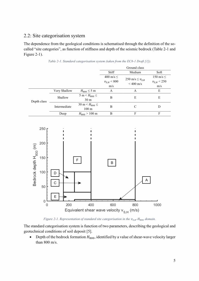
2.2: Site categorisation system The dependence from the geological conditions is schematised through the definition of the so-called “site categories”, as function of stiffness and depth of the seismic bedrock (Table 2-1 and Figure 2-1).
Table 2-1. Standard categorisation system (taken from the EC8-1 Draft [1]).
Ground class Stiff Medium Soft
400 m/s ≤ 𝑣𝑆,𝐻 < 800
m/s
250 m/s ≤ 𝑣𝑆,𝐻 < 400 m/s
150 m/s ≤ 𝑣𝑆,𝐻 < 250
m/s
Depth class
Very Shallow 𝐻800 ≤ 5 m A A E
Shallow 5 m < 𝐻800 ≤
30 m B E E
Intermediate 30 m < 𝐻800 ≤
100 m B C D
Deep 𝐻800 > 100 m B F F
Figure 2-1. Representation of standard site categorisation in the 𝑣𝑆,𝐻-𝐻800 domain.
The standard categorisation system is function of two parameters, describing the geological and geotechnical conditions of soil deposit [5].
Depth of the bedrock formation 𝐻800, identified by a value of shear-wave velocity larger than 800 m/s.
6
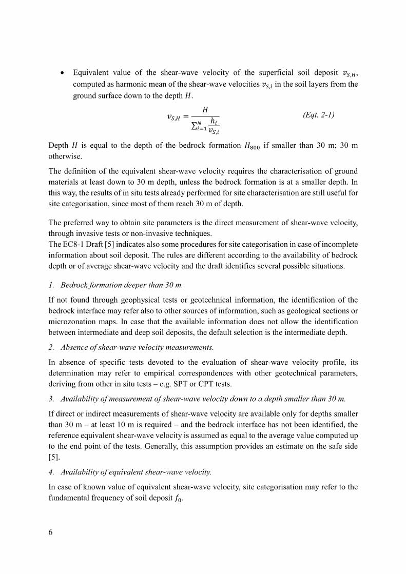
Equivalent value of the shear-wave velocity of the superficial soil deposit 𝑣𝑆,𝐻, computed as harmonic mean of the shear-wave velocities 𝑣𝑆,𝑖 in the soil layers from the ground surface down to the depth 𝐻.
𝑣𝑆,𝐻 =
𝐻
∑ℎ𝑖𝑣𝑆,𝑖
𝑁𝑖=1
(Eqt. 2-1)
Depth 𝐻 is equal to the depth of the bedrock formation 𝐻800 if smaller than 30 m; 30 m otherwise.
The definition of the equivalent shear-wave velocity requires the characterisation of ground materials at least down to 30 m depth, unless the bedrock formation is at a smaller depth. In this way, the results of in situ tests already performed for site characterisation are still useful for site categorisation, since most of them reach 30 m of depth.
The preferred way to obtain site parameters is the direct measurement of shear-wave velocity, through invasive tests or non-invasive techniques. The EC8-1 Draft [5] indicates also some procedures for site categorisation in case of incomplete information about soil deposit. The rules are different according to the availability of bedrock depth or of average shear-wave velocity and the draft identifies several possible situations.
1. Bedrock formation deeper than 30 m.
If not found through geophysical tests or geotechnical information, the identification of the bedrock interface may refer also to other sources of information, such as geological sections or microzonation maps. In case that the available information does not allow the identification between intermediate and deep soil deposits, the default selection is the intermediate depth.
2. Absence of shear-wave velocity measurements.
In absence of specific tests devoted to the evaluation of shear-wave velocity profile, its determination may refer to empirical correspondences with other geotechnical parameters, deriving from other in situ tests – e.g. SPT or CPT tests.
3. Availability of measurement of shear-wave velocity down to a depth smaller than 30 m.
If direct or indirect measurements of shear-wave velocity are available only for depths smaller than 30 m – at least 10 m is required – and the bedrock interface has not been identified, the reference equivalent shear-wave velocity is assumed as equal to the average value computed up to the end point of the tests. Generally, this assumption provides an estimate on the safe side [5].
4. Availability of equivalent shear-wave velocity.
In case of known value of equivalent shear-wave velocity, site categorisation may refer to the fundamental frequency of soil deposit 𝑓0.

7
The solution is an instrumental approach to site categorisation, based on H/V tests, which works as shown in Table 2-2.
5. Complete absence of geotechnical information.
In case of absence of specific information about shear-wave profile or bedrock depth, site categorisation refers to simplified geological criteria.
In this way, the EC8-1 Draft introduces quite rigorous criteria for site categorisation and tries to cover all the possible scenarios characterised by different degree of knowledge about geotechnical characteristic of soil deposit. Some procedures, e.g. the reference to other in situ tests or the geological classification, are already present in the current versions of several seismic codes (e.g. [6]), whereas the instrumental approach employing the results of H/V tests is a new methodology.
Table 2-2. Site categorisation based on equivalent shear-wave velocity and resonance frequency (taken from the EC8-1 Draft [5]).
𝑓0 range 𝑣𝑆,𝐻 range Site category 𝑓0 > 12 Hz - A 𝑓0 < 12 Hz 400 m/s ≤ 𝑣𝑆,𝐻 < 800 m/s B
𝑣𝑆,𝐻/250 < 𝑓0 < 𝑣𝑆,𝐻/120 250 m/s ≤ 𝑣𝑆,𝐻 < 400 m/s C 𝑣𝑆,𝐻/250 < 𝑓0 < 𝑣𝑆,𝐻/120 150 m/s < 𝑣𝑆,𝐻 < 250 m/s D 𝑣𝑆,𝐻/120 < 𝑓0 < 𝑣𝑆,𝐻/12 150 m/s < 𝑣𝑆,𝐻 < 400 m/s E
𝑓0 < 𝑣𝑆,𝐻/250 150 m/s < 𝑣𝑆,𝐻 < 400 m/s F

8
2.3: Seismic action: definition of the local seismic hazard As mentioned previously, the definition of the seismic action refers to a seismological component and to a geo-morphological one. The seismological component, referred as “local seismic hazard” [5], is the result of a seismic hazard assessment, typically according to a probabilistic scheme, which provides the expected values of ground motion parameters across the territory. In order to simplify the assessment, the analysis evaluates the ground motion under specific geological and morphological conditions, i.e. horizontal outcropping formation, assuming equivalent shear-wave velocity larger than 800 m/s. This condition corresponds to a formation described as site category A.
The EC8-1 Draft [5] assumes two standard parameters for the description of seismic hazard, evaluated according to the above-mentioned conditions.
Reference maximum spectral acceleration 𝑆𝛼,𝑟𝑒𝑓, corresponding to the constant acceleration branch of the horizontal 5% damped elastic response spectrum, for the reference return period 𝑇𝑟𝑒𝑓.
Reference spectral acceleration 𝑆𝛽,𝑟𝑒𝑓, evaluated at vibration period equal to 1 s, of the horizontal 5% damped elastic response spectrum, for the reference return period 𝑇𝑟𝑒𝑓.
As mentioned in the introduction, for ordinary constructions the reference return period 𝑇𝑟𝑒𝑓 is equal to 475 years. Actually, some components involved in the computation of the reference spectrum require the spectral parameters 𝑆𝛼,𝑅𝑃 and 𝑆𝛽,𝑅𝑃, referred to the specific return period adopted in the design. The EC8-1 Draft [5] allows the conversion from standard values 𝑆𝛼,𝑟𝑒𝑓 and 𝑆𝛽,𝑟𝑒𝑓 through performance factors 𝛾𝐿𝑆,𝐶𝐶. 𝑆𝛼,𝑅𝑃 = 𝛾𝐿𝑆,𝐶𝐶𝑆𝛼,𝑟𝑒𝑓 (Eqt. 2-2)
𝑆𝛽,𝑅𝑃 = 𝛾𝐿𝑆,𝐶𝐶𝑆𝛽,𝑟𝑒𝑓 (Eqt. 2-3)
If the return period is 475 years, the performance factor will be equal to 1.
In particular, the maximum spectral ordinate with reference to 475 years defines the seismicity level of a territory [5], as shown in Table 2-3.
Table 2-3. Ranges of 𝑆𝛼,475 values for the definition of seismicity levels (taken from EC8-1 Draft [5]).
Seismicity level Parameter 𝑆𝛼,475 (m/s2) Very low < 1.0
Low 1.0 ÷ 2.5 Moderate 2.5 ÷ 5.0
High > 5.0

9
The parameters are available in seismic maps provided in the National Annexes and they are computed through nonlinear, piecewise fitting of the standard spectral shape to the uniform hazard response spectrum resulting from seismic hazard assessments.
Actually, the EC8-1 Draft does not oblige a concurrent mapping of both parameters, but the parameter 𝑆𝛼,𝑟𝑒𝑓 is enough, since the other one may be derived through the application of a multiplying factor 𝑓ℎ, depending of site seismicity (Table 2-4). 𝑆𝛽,𝑟𝑒𝑓 = 𝑓ℎ𝑆𝛼,𝑟𝑒𝑓 (Eqt. 2-4)
Table 2-4. Values of multiplying factor 𝑓ℎ (taken from EC8-1 Draft [5]).
Seismicity level Factor 𝑓ℎ (-) Very low 0.2
Low 0.2 Moderate 0.3
High 0.4

10
2.4: Seismic action: site amplification factors The geo-morphological component, according to the EC8-1 Draft [5], is synthesised through two categories of amplification factors. On one side, the effect of significant morphologic irregularities as slopes, ridges, etc. corresponds to a period independent topography amplification factor, whose effect is a linear scaling of the response spectrum. On the other side, the representation of ground response refers to a couple of site amplification factors.
Short period amplification factor 𝐹𝛼.
Intermediate period amplification factor 𝐹𝛽, referred to vibration period 𝑇𝛽, namely 1 s.
The computation of the amplification factors in each standard site category, as shown in Table 2-5, follows formulations depending on site parameters 𝐻800 and 𝑣𝑆,𝐻, if available; the EC8-1 Draft indicates some default values, in absence of this information [5].
Table 2-5. Indications for the computation of site amplification factors (taken from the EC8-1 Draft [5]).
The site amplification factors depend on geotechnical characteristics of soil deposit, i.e. 𝐻800 and 𝑣𝑆,𝐻, and on seismic hazard parameters 𝑆𝛼,𝑅𝑃 and 𝑆𝛽,𝑅𝑃. The dependence from site seismicity is a consequence of the nonlinearity in the ground behaviour in dynamic conditions: due to nonlinearity, the ground response varies in a sensible way as function of the intensity of the applied seismic input, with reduction in stiffness and larger energy dissipation.
A significant difference between the EC8-1 Draft and other seismic codes is the formulation of

11
these dependences, since there is a passage from a discontinuous expression (e.g. [6], [8]) to a continuous law [5], either in terms of geotechnical parameters or in terms of seismic hazard. The new formulation aims to provide more specific estimate of site response, reducing the related uncertainties.
Thanks to the continuous formulation, a graphical description of the site amplification factors is possible. Since the equation depends of two parameters, the representation will occur in the 3-D domain 𝑣𝑆,𝐻-𝑆𝛼,𝑅𝑃-𝐹𝛼 (or 𝑣𝑆,𝐻-𝑆𝛽,𝑅𝑃-𝐹𝛽). Figure 2-2 shows an example of representation of the amplification factor, in this case referred to ground categories B, C and D, characterised by the same function. The 3-D representation is coupled with a contour plot, in order to facilitate the interpretation.
The situation is different – and more complex – for ground category E, since the amplification factor is given by a three-parameter equation, whose graphical representation is not possible. In order to obtain a graphical form, a solution may be the representation of a series of surfaces corresponding to “sections” of the actual shape for constant values of one independent
parameter. In particular, the representation occurs in the 3-D domain 𝑣𝑆,𝐻-𝐻800-𝐹𝛼 (or 𝑣𝑆,𝐻-𝐻800-𝐹𝛽) for assigned values of the hazard parameter 𝑆𝛼,𝑅𝑃 (or 𝑆𝛽,𝑅𝑃), representative of the different levels of seismicity defined by the EC8-1 Draft [5]. As regards 𝑆𝛼,𝑅𝑃, this is equal to the mean value of the range defining the seismicity level of interest, in compatibility with the seismic hazard in the Italian territory (more details in Figure 6-3). Parameter 𝑆𝛽,𝑅𝑃 is instead computed from 𝑆𝛼,𝑅𝑃, according to (Eqt. 2-4). Table 2-6 shows the reference values adopted for the representation and Figure 2-3 shows the short period amplification factor for moderate seismicity level, as example.
Table 2-6. Reference hazard parameters for the representation of the amplification factors pertaining to site category E.
Seismicity level 𝑆𝛼,𝑅𝑃 (m/s2) 𝑆𝛽,𝑅𝑃 (m/s2) Very low and low 1.25 0.25 Moderate 3.75 1.125 High 6 2.4
The graphical representation of the amplification factor for the other ground categories is available in Appendix A.

12
Figure 2-2. Short period amplification factor for standard site categories B, C and D.
Figure 2-3. Short period amplification factor for standard site category E (moderate seismicity level).

13
2.5: Seismic action: definition of the elastic response spectrum The seismic action is typically expressed by means of an elastic response spectrum of horizontal pseudo-absolute acceleration. The elastic response spectrum 𝑆𝑒(𝑇) is described according to a standardised, piecewise formulation with respect to vibration period 𝑇, in order to suit well the effective spectrum with a simple shape, from the mathematical and computational point of view. The formulation depends mainly on the hazard parameters 𝑆𝛼,𝑟𝑒𝑓 and 𝑆𝛽,𝑟𝑒𝑓, the site amplification factors 𝐹𝛼 and 𝐹𝛽 and the topography amplification factor 𝐹𝑇 [5], as shown in (Eqt. 2-5).
𝑆𝑒(𝑇) =
{
𝑆𝛼𝐹𝐴 0 ≤ 𝑇 ≤ 𝑇𝐴
𝑆𝛼𝑇𝐵 − 𝑇𝐴
[𝜂(𝑇 − 𝑇𝐴) +𝑇𝐵 − 𝑇
𝐹𝐴] 𝑇𝐴 ≤ 𝑇 ≤ 𝑇𝐵
𝜂𝑆𝛼 𝑇𝐵 ≤ 𝑇 ≤ 𝑇𝐶
𝜂𝑆𝛽𝑇𝛽
𝑇 𝑇𝐶 ≤ 𝑇 ≤ 𝑇𝐷
𝜂𝑇𝐷𝑆𝛽𝑇𝛽
𝑇2 𝑇 ≥ 𝑇𝐷
(Eqt. 2-5)
The reference spectral accelerations 𝑆𝛼 and 𝑆𝛽 are computed according to the equations (Eqt. 2-6) and (Eqt. 2-7), involving the topography and the site amplification factors.
𝑆𝛼 = 𝐹𝑇𝐹𝛼𝑆𝛼,𝑅𝑃 (Eqt. 2-6)
𝑆𝛽 = 𝐹𝑇𝐹𝛽𝑆𝛽,𝑅𝑃 (Eqt. 2-7)
Table 2-7 shows the meaning of the remaining parameters involved in the formulation.
As shown by Figure 2-4, the elastic response spectrum is composed by two constant acceleration branches, at small and intermediate vibration periods, connected by means of a linear portion. At larger periods, characterised by constant velocity and displacement ranges, the spectrum follows a hyperbolic law of the first order – in the constant velocity response range – and of the second order – in the constant displacement response range.

14
Table 2-7. Description of the parameters involved in the response spectrum.
Symbol Meaning Method of computation
𝑇𝛽 Reference vibration period, equal to 1 s
𝑇𝛽 = 1 𝑠
𝐹𝐴 Ratio of 𝑆𝛼 with respect to the
zero-period spectral acceleration 𝐹𝐴 = 2.5
(in absence of further information)
𝑇𝐴 - 𝑇𝐴 = 0.02 𝑠 (in absence of further information)
𝑇𝐶 Upper corner period of the constant acceleration range 𝑇𝐶 =
𝑆𝛽𝑇𝛽
𝑆𝛼
𝑇𝐵 Lower corner period of the constant acceleration range
𝑇𝐵 =
{
0.05 𝑠, 𝑖𝑓
𝑇𝐶𝜒< 0.05 𝑠
𝑇𝐶𝜒, 𝑖𝑓 0.05 𝑠 ≤
𝑇𝐶𝜒≤ 0.10 𝑠
0.10 𝑠, 𝑖𝑓 𝑇𝐶𝜒> 0.10 𝑠
𝜒 - 𝜒 = 4 (in absence of further information)
𝑇𝐷 Lower corner period of the
constant displacement range 𝑇𝐷 = {
2, 𝑖𝑓 𝑆𝛽,𝑅𝑃 ≤ 1 𝑚/𝑠2
1 + 𝑆𝛽,𝑅𝑃 , 𝑖𝑓 𝑆𝛽,𝑅𝑃 ≤ 1 𝑚/𝑠2
(in absence of further information)
𝜂 Structural damping correction
factor 𝜂 = 1 (for 5% viscous damping)
Figure 2-4. Examples of response spectra according to the formulation provided by the EC8-1 Draft (taken from
the EC8-1 Draft [5]).

15
Chapter 3: Verification of the instrumental approach to site
categorization
3.1: Introduction The EC8-1 Draft introduces an instrumental approach to site categorisation, alternative to the one based on geotechnical parameters [5]. The method uses the spectral horizontal-to-vertical ratio (also called H/V ratio or HVSR) obtained from microtremor data recorded at the ground surface and estimates the ground type by pointing out the first peak of the H/V-ratio into the spectral ranges corresponding to the standard site categories.
In this section, the study aims to assess the validity of the instrumental approach, by applying it over a number of sites with known geotechnical properties and characterised with HVSR technique. The verification compares the site category for each considered site, obtained according to the two systems and assuming the standard method as reference. Indeed, this approach is the more reliable because it employs direct measurements of geotechnical parameters, whereas the instrumental approach uses the results of non-invasive tests, without a specific seismic ground characterisation. This aspect is highlighted by the EC8-1 Draft itself, which suggests the use of the instrumental approach only in case of absence of specific documentation about quantitative geotechnical parameters [5]. The approach will be considered valid if it provides results compatible with the standard one.
The assessment is carried out with reference to two versions of the Draft of revision of the Eurocode 8.
The Draft n.2, which is an elder and superseded version, proposing an instrumental approach based on the frequency and the amplification factor of the first peak of the H/V ratio.
The current version, i.e. the EC8-1 Draft, which refers on the resonance frequency and the equivalent shear-wave velocity of the soil deposit.

16
3.2: Methodology The study compares the new standard site categorisation and the instrumental approaches to site categorisation proposed by the two drafts, with reference to a collection of sites. Sites are part of a larger set, realised for the stochastic analysis of ground response (the complete list is available in Appendix B) and correspond to the locations of a number of accelerometric stations of the Italian and Swiss strong motion networks, together with a number of sites taken from regional geological services. The locations in exam have a collection of data derived from site characterisation, including direct measurements of shear waves velocity and interpretation of recorded microtremors according to HVSR technique. In this way, each site presents all the information required for the application of the two systems of site categorisation.
3.2.1: Data selection
This part focuses only on indicating the sources of the data employed in this study, together with some specifications directly concerned with this topic. More details about the selection of the data and their interpretation are available in 5.2.1 and 5.2.2.
The primary source of data is the Italian Strong Motion Network (or RAN) of the Dipartimento di Protezione Civile [11]. Data have been queried by means of the Italian Accelerometric Archive (ITACA) [12], where metadata provide information concerning location and seismic site characterisation for each recording station . The data set is enriched with a number of sites belonging to the Swiss Strong Motion Network of the Swiss National Network (SED). The reference archives are the Engineering Strong-Motion Database (ESD) [13] and the Site Characterization Database for Seismic Stations in Switzerland [14]. A number of reference sites derives from regional services, as the Programma Valutazione degli Effetti Locali (VEL) of Toscana Region ([15], [16]), the Servizio Geologico Sismico e dei Suoli (SGSS) of Emilia-Romagna Region [17] and the geological service of Umbria Region [18].
The application of the instrumental approach requires the presence of a clear first peak in the H/V spectral ratio. The peak should be given an interpretation in light of site stratigraphy, if possible. In the ITACA database and in the regional services, the description of the peaks follows SESAME guidelines [19] and the peak should be able to fulfil at least 5 of the 6 SESAME criteria. In Swiss stations, metadata provide no information concerning clearness criteria but the first peak is indicated in the monography, coupled with a stratigraphic interpretation. Furthermore, site selection considers stations inserted in a regular topographic background, possibly with a flat ground surface. The condition is necessary since the interpretation of H/V technique and the application of the instrumental approach apply only in flat deposits with horizontally layered soil profile. As consequence, topography represents a restraint in the

17
selection and only sites of T1 topographic category [6] are considered in the analysis.
The collection of the sites involved in the study is available in Appendix C and the sites are part of a larger set (available in Appendix B), realised for the stochastic analysis of ground response. The elements fulfilling the above-mentioned restraints are 60.
3.2.2: Standard site categorisation
The categorisation system proposed by the EC8-1 Draft and the Draft n.2 distinguishes six site types (A, B, C, D, E and F), depending on ground class and depth class, which are function of bedrock depth 𝐻800 and equivalent shear-wave velocity 𝑣𝑆,𝐻 [5]. The approach introduced by the Draft n.2 was slightly qualitative, as it did not specify quantitative limits for the ranges of depth, whereas the criteria defined by the EC8-1 Draft are more precise. Despite this difference, the two methodologies provide the same result in terms of classification.
The ITACA database provides all the required information for site categorisation for the selected sites. When bedrock depth is not known because investigations have not reached the bedrock formation, it is assumed as coincident to the deepest detected point, in agreement with the indications of EC8-1 Draft [5]. On the other side, Swiss sites present a direct indication of bedrock depth and 𝑣𝑆,30, which is the reference parameter in case of deep soil deposits. In presence of a shallow formation, the equivalent velocity up to bedrock interface is estimated from the average velocity profile available in each station monography.
Table 3-1 shows the site categories obtained for each location through the standard site categorisation procedure. It can be noticed that a large number of stations are B or F class, whereas sites of A or D category are rare. Furthermore, according to the above-exposed criteria, sites BTT2 and CLF do not belong to any ground type, as the reference value of shear wave velocity – equal to 90 m/s and 136 m/s, respectively – is smaller than the lower bond of the “Soft” ground class. On the opposite side, site SNN assumes an equivalent shear-wave velocity equal to 835 m/s, larger than the upper bond of “Stiff” ground class and included in the collection of data due to the presence of an
inversion in shear-wave velocity profile at depths larger than 30 m. These cases represent a particular situation, for which the code does not provide any provision for the estimate of seismic action, evaluable only by means of devoted analysis – in a similar way of S1 and S2 ground categories defined by the current seismic codes [20]. Due to their particular nature, the verification of the instrumental approach to site categorisation will disregard them.

18
Table 3-1. Standard site categorisation.
Site number Site Site category Site number Site Site category
1 AVT A 31 Sant’Agostino – Zona Industriale
F
2 BRC A 32 SARK E 3 BRZ A 33 SEPFL D 4 SRT B 34 SINS F 5 BGN B 35 SIOM F 6 CPS B 36 SLOP F 7 CST B 37 SLUW F 8 GSN B 38 SOLB F 9 MAI C 39 SRHH E 10 NAS F 40 SVIT E 11 SPS E 41 SYVP C
12 BTT2 Unclassified 42 Foligno – Centro
Commerciale E
13 CLF Unclassified 43 Corciano – San
Mariano E
14 RTI F 44 Torgiano –
Miralduolo Zona Industriale
C
15 FVZ E 45 PNT F 16 BGI B 46 SNN Unclassified 17 MLC B 47 AQV B 18 MTL B 48 BRN B 19 PZS B 49 PNR F 20 RCC C 50 PVS B 21 TLM1 B 51 CTL D 22 TRL C 52 GRM F 23 VBM B 53 NVL F 24 VBV B 54 PNN C 25 AVZ F 55 BNV B 26 PGL C 56 SSV C 27 AQA B 57 BOJ C 28 NCR E 58 BVG F 29 ARN E 59 BVN C 30 MRN F 60 GBP D

19
3.2.3: Instrumental approach to site categorisation according to Draft n.2
The instrumental approach to site categorisation uses the spectral horizontal-to-vertical ratio obtained from microtremor data recorded at the ground surface, assuming that it approaches the transfer function of the soil profile in horizontally layered soil profiles. The estimate of the ground type is based on the first significant peak of the H/V ratio. The first peak frequency is the fundamental frequency 𝑓0, which is typically indicated in station monographies. The corresponding amplification factor 𝐴0 is read on the HVSR plot available in station documentation. The passage from the instrumental result to the ground category is performed through the reference plot provided by the Draft n.2 (Figure 3-1 - [21]). The peak values define a point inside the graph and the region into which it is falling indicates the standard ground type.
Figure 3-1. Reference plot for the instrumental approach to site categorisation, according to the Draft n.2 (taken
from [21]).
Figure 3-2 shows the application of the instrumental approach for the classification of the reference sites, represented with different icons related to the actual site category, derived from the standard approach. It can be noticed that a significant number of points lies outside the reference ranges and correspondent sites can not be classified according to this approach. For reason of compactness, the study represents only the global result, whereas Appendix C presents the plots representing the instrumental approach applied to sites clustered according to the actual site category. Appendix C contains also a table indicating the site category for each location in exam, obtained with the standard site categorisation and the instrumental approach. The table indicates the result of the check for compatibility between the two methods, which is positive when categories are the same in a single site, negative otherwise. In the assessment, sites BTT2, CLF and SNN are not considered because they do not belong to any site category, as exposed previously.

20
Figure 3-2. Site categorisation according to the instrumental approach proposed by the Draft n.2.
In particular, as highlighted by Figure 3-3, sites of category A, C and D are in limited number and the instrumental method indicates different classes (mainly B and E), without any matching of the results. On the opposite, in site classes B, D and F, compatibility between results rises up to 40%, which is a larger value but not so significant to give reliability to the method.
Figure 3-3. Analysis of the compatibility results.
The lack of compatibility is highlighted by analysing in detail the distribution of points in the reference plot, either in the global representation (Figure 3-2) or in the representations of the application of the instrumental method, limited at locations belonging to a specific site category (in Appendix C). From the analysis of each site category, it can be noticed that the proposed curves are not able

21
to create a boundary and identify a region corresponding to the ground class. Points clouds of each site type seem also to cross themselves for significant portions, complicating the geometrical delimitation of specific regions. Furthermore, it is interesting to notice that points tend to be located on the upper part of the graph, in an amplification factor range variable between 2 and 10 ÷ 15, independently from ground type, whereas the maximum ordinate of the curves is about 5. For this reason, a relevant number of sites is declared as “Unclassified”
because categorisation would be affected by too many uncertainties. This aspect is evident in Figure 3-4, showing the distribution of sites pertaining to ground category B, but the situation is similar for the other subsoil classes.
Figure 3-4. Application of the instrumental approach to site categorisation, according to Draft n.2, to locations
of site category B
These aspects justify the lack of compatibility of the results of the instrumental approach with respect to the standard site categorisation.

22
3.2.4: Instrumental approach to site categorisation according to the EC8-1 Draft
The instrumental approach to site categorisation introduced by the current version of the draft estimates the site category without referring only to the first significant peak of the H/V ratio, since the classification criterion depends on the fundamental frequency 𝑓0 and the equivalent shear-wave velocity 𝑣𝑆,𝐻, as shown in Table 3-2 and in Figure 3-5.
Table 3-2. Site categorisation based on equivalent shear-wave velocity and resonance frequency (taken from the EC8-1 Draft [5]).
𝑓0 range 𝑣𝑆,𝐻 range Site category 𝑓0 > 12 Hz - A 𝑓0 < 12 Hz 400 m/s ≤ 𝑣𝑆,𝐻 < 800 m/s B
𝑣𝑆,𝐻/250 < 𝑓0 < 𝑣𝑆,𝐻/120 250 m/s ≤ 𝑣𝑆,𝐻 < 400 m/s C 𝑣𝑆,𝐻/250 < 𝑓0 < 𝑣𝑆,𝐻/120 150 m/s < 𝑣𝑆,𝐻 < 250 m/s D 𝑣𝑆,𝐻/120 < 𝑓0 < 𝑣𝑆,𝐻/12 150 m/s < 𝑣𝑆,𝐻 < 400 m/s E
𝑓0 < 𝑣𝑆,𝐻/250 150 m/s < 𝑣𝑆,𝐻 < 400 m/s F
Figure 3-5. Reference plot for the instrumental approach to site categorisation, according to the EC8-1 Draft.
Figure 3-6 shows that the new approach provides better results, since each distribution of points pertaining to each class suits quite well the boundaries of the regions representative of site categories. The only exceptions are the points falling in ground categories C, F and D, which overlap with each other disregarding the boundaries.

23
Figure 3-6. Instrumental approach to site categorisation, using HVSR data.
In particular, as highlighted by Figure 3-7, the degree of compatibility is perfect for sites pertaining to site category B, whereas more deformable categories does not present a good level of compatibility. Furthermore, a number of locations of site category A show anomalous values of fundamental frequency with respect to the equivalent shear-wave velocity, maybe due to errors in the values provided by the reference databases. Notwithstanding these observations, the result is better than the one obtained with the approach proposed in the Draft n.2. Indeed, the number of unclassified sites is much more limited than before, with only three cases, coincident with the ones unclassified according to the standard approach. Moreover, the level of compatibility is close to 50% for site classes A and D. Actually, sites of category A and D are in limited number and the statistics may not be representative. On the opposite, in site classes C and F, compatibility between results rises up to 70%.

24
Figure 3-7. Analysis of the compatibility results.
With reference to the representations of the application of the instrumental method, limited at locations belonging to a specific site category (more details in Appendix C), the points clouds of each site type overlap themselves and cross the proposed boundaries, especially in the case of deformable soils. This aspect is evident in Figure 3-8, showing the distribution of sites pertaining to ground category C, but the situation is similar for classes F and D.
Figure 3-8. Application of the instrumental approach to site categorisation, according to EC8-1 Draft, to sites of
ground category C.
Moreover, even if the result is quite good, the instrumental approach proposed by the EC8-1 Draft has an intrinsic limitation. Focusing on the conditions for the attribution of site category

25
A, the resonance frequency should be higher than 12 Hz, without any restraint on the equivalent shear-wave velocity. This aspect is in contrast with the standard approach for site categorisation, which requires the average velocity to be larger than 250 m/s. For instance, a soil deposit composed by a 2 m thick layer characterised by shear wave velocity equal to 200 m/s presents the following fundamental frequency.
𝑓0 =𝑣𝑠4𝐻
=200
4 × 2= 25 𝐻𝑧
According to the instrumental approach, the soil deposit belongs to ground category A, whereas the standard approach classifies it as class E. Therefore, the new approach does not provide reliable results in case of shallow deposits made with deformable materials.

26
3.3: Results A comparative analysis of two categorisation systems has been carried out, associating a subsoil category to sites selected from the Italian Strong Motion Network and the Swiss Strong Motion Network, by employing the standard approach and the instrumental approach. The aim was the verification of the validity of the instrumental method. The calibration test, even if performed on a limited number of sites, showed that the instrumental approach proposed by Draft n. 2 provides results not compatible with the ones obtained through the standard way, generally underestimating the ground quality. On the other side, results are better with the approach introduced by the EC8-1 Draft, since the degree of compatibility between the standard method and the instrumental procedure is doubled, though some discrepancies especially in site categories A and D. Actually, the new approach conflicts with the standard method in presence of shallow soil deposits made with deformable materials. In order to solve this issue, the approach should take into account the restraint due to equivalent shear-wave velocity for the attribution of the ground class A, instead of considering only the fundamental frequency. Since the collection of data was limited and not fully representative of the different subsoil classes (especially for categories A and D), this result should be interpreted as a first stage assessment of the validity of the instrumental approach and a first reference for further improvements of this approach.
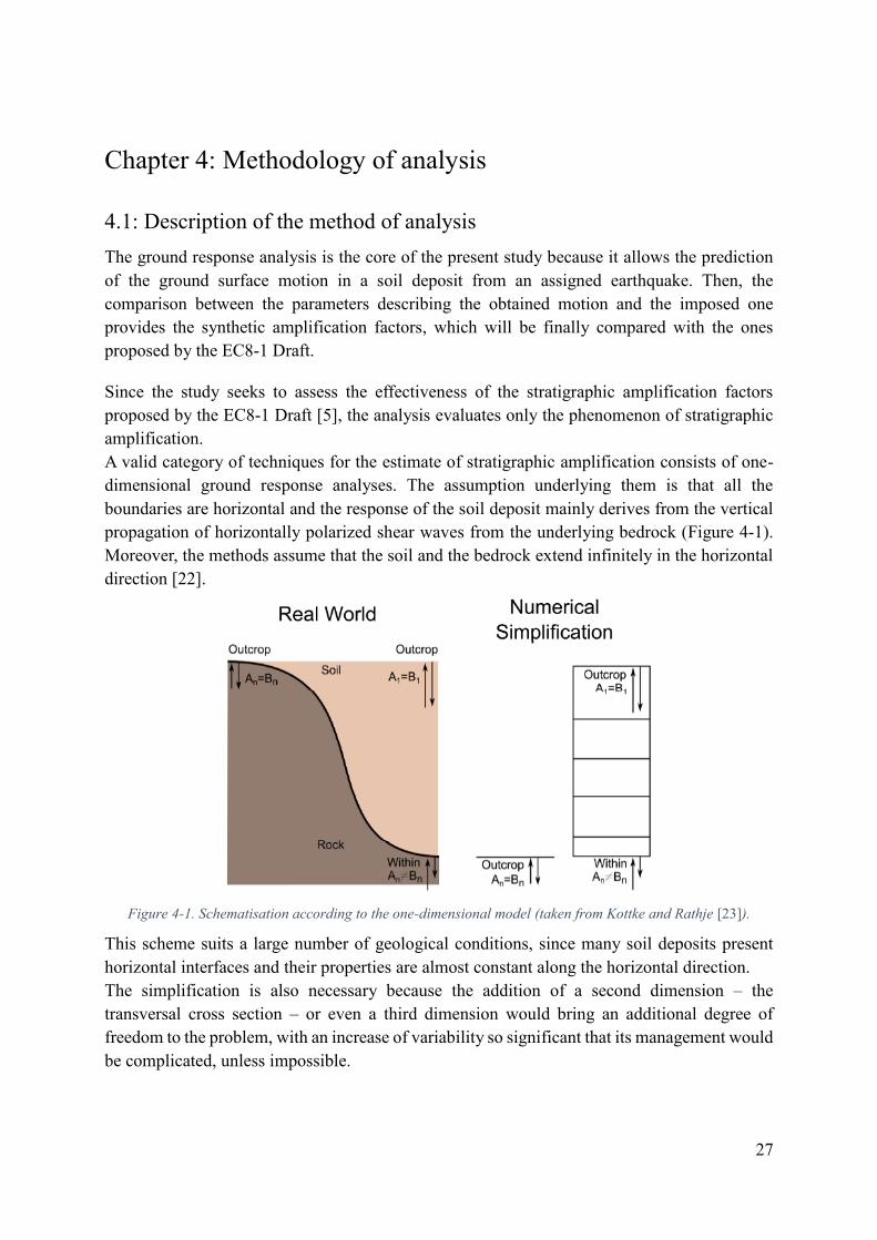
27
Chapter 4: Methodology of analysis
4.1: Description of the method of analysis The ground response analysis is the core of the present study because it allows the prediction of the ground surface motion in a soil deposit from an assigned earthquake. Then, the comparison between the parameters describing the obtained motion and the imposed one provides the synthetic amplification factors, which will be finally compared with the ones proposed by the EC8-1 Draft.
Since the study seeks to assess the effectiveness of the stratigraphic amplification factors proposed by the EC8-1 Draft [5], the analysis evaluates only the phenomenon of stratigraphic amplification. A valid category of techniques for the estimate of stratigraphic amplification consists of one-dimensional ground response analyses. The assumption underlying them is that all the boundaries are horizontal and the response of the soil deposit mainly derives from the vertical propagation of horizontally polarized shear waves from the underlying bedrock (Figure 4-1). Moreover, the methods assume that the soil and the bedrock extend infinitely in the horizontal direction [22].
Figure 4-1. Schematisation according to the one-dimensional model (taken from Kottke and Rathje [23]).
This scheme suits a large number of geological conditions, since many soil deposits present horizontal interfaces and their properties are almost constant along the horizontal direction. The simplification is also necessary because the addition of a second dimension – the transversal cross section – or even a third dimension would bring an additional degree of freedom to the problem, with an increase of variability so significant that its management would be complicated, unless impossible.

28
Furthermore, the results of the studies based on this model provide reliable results in many cases, i.e. the obtained values are in reasonably good agreement with measured response, as highlighted by several authors ([22], [24]). For this reason, the EC8-1 Draft [5] suggests the 1-D modelling for site-specific ground response analyses, unless complex geological or morphological conditions. On the other side, the approach simplifies the mechanism of propagation of seismic waves, assuming vertical propagation instead of three-dimensional propagation. Actually, the hypothesis is realistic when morphologic variations in soil deposits are not significant and the epicentral distance is large enough, since the refraction from deeper and stiffer materials to shallower and more deformable ones bends inclined rays to a pseudo-vertical direction, according to Snell’s law (Figure 4-2).
Figure 4-2. Verticalisation of seismic rays (taken from Kramer [22]).
The chosen method is the equivalent linear viscous-elastic analysis, introduced by Idriss and Seed [25], which schematises the nonlinear, hysteretic behaviour of soils in dynamic conditions into equivalent linear viscous-elastic behaviour, described with operative synthetic parameters.
The approach derives from the linear methods, whose aim is the estimate of the transfer function, representing the response of the soil deposit – in terms of displacement, acceleration, etc. – to an input motion. In particular, the method attempts to put the nonlinear behaviour of ground material together with the advantages offered by the linear approach: since the concept of transfer function relies on the principle of superposition – not valid in nonlinear field –, the equivalent linear analysis approximates the nonlinear behaviour with equivalent linear soil properties, derived through an iterative procedure. In particular, several laboratory tests showed that, under dynamic loading conditions, ground materials assume a nonlinear hysteretic stress-strain behaviour. This behaviour is described by a loop composed by curved portions closing a region of finite area. An approximation and simplification in the description of this phenomenon is possible through the introduction of two equivalent linear parameters.
Equivalent linear shear modulus 𝐺, equal to the secant shear modulus evaluated at the edge of the loop.
Equivalent linear damping ratio 𝐷, which produces the same energy loss in a single

29
cycle as the actual hysteresis loop and function of the area of the region closed within a single cycle.
The description is consistent with the Kelvin-Voigt solid, where the dynamic response is described through a purely elastic spring and a purely viscous dashpot [22]. The equivalent parameters are strain-dependent, in the same way with which the actual behaviour depends on the strain level. When increasing the strain level, the hysteresis loop rotates and moves towards the strain axis, with a smaller slope. This implies a reduction in soil stiffness, corresponding to a smaller value of secant modulus and so of the equivalent shear modulus. At the same time, the area of the region rises up, implying larger dissipation and a larger value of damping ratio (Figure 4-3).
Figure 4-3. Description of equivalent linear parameters, with the variation curves (taken from Matasovic and
Hashash [26]). Here, parameter 𝛽 is the damping ratio.
The construction – through laboratory testing or literature – of the curves allows a simplified description of the nonlinear behaviour, providing the relationships between shear modulus or damping ratio and strain level.
The equivalent linear method employs these curves for the choice of the operative values of the equivalent shear modulus 𝐺 – or the reduced modulus 𝐺/𝐺0, i.e. the ratio between the shear modulus and the small-strain value – and the damping ratio 𝐷, that should provide a compatible response with respect to the real case. The computation of these values requires an iterative procedure (Figure 4-4), which operates as follows.
1. Initial estimate of the values of reduced modulus and damping, typically starting from the low-strain values.
2. Computation of the ground response of the soil model.
3. Derivation of new values of the equivalent parameters from the strain level, through the nonlinear curves.
4. Check of convergence, by evaluating the difference between the computed values in the

30
two successive iterations. If the difference is smaller than a predetermined target value in all layers, convergence is achieved; otherwise, the procedure is repeated, updating the equivalent linear parameters according to the obtained strain level.
In the present study, the analyses are performed with the support of SHAKE91 code [24].
Figure 4-4. Scheme of the iterative procedure involved in the equivalent linear analysis, with the use of nonlinear curves (nonlinear curves taken by Lai et al. [27]).
This approach of analysis, as highlighted by Kramer [22], represents a good approximation of the nonlinear soil behaviour but it has some significant limitations. Being a linear method, the soil properties are constant throughout the duration of the earthquake, disregarding the actual changes of soil stiffness may occur during the event. Furthermore, the method is not reliable in deep deposits, since the one-dimensional model may suffer so large tangential stresses that they could bring to failure, whereas the actual situation does not. Finally, the method refers to a total stress approach and disregards the hydro-mechanical coupling, thus not accounting phenomena which may occur in case of strong seismic action (e.g. liquefaction).

31
As a consequence, the method is reliable up to small levels of shear strain, inferior to 1%. Above that threshold, the material shows significant nonlinearity – excess pore pressure, plasticisation, etc. – and the equivalent linear method does not have the capability of modelling these phenomena. In this case, nonlinear analysis is preferred. Despite this limitation, for moderate levels of shear strain, the equivalent linear viscous-elastic method is valid and convenient with respect to fully nonlinear analyses. On one side, the simplicity in the definition of input parameters and the moderate computational cost suit well the necessity of performing the thousands of ground response analyses required by the stochastic approach [2]. Then, the solutions provided by the method are more stable and reproducible than the ones obtained through the nonlinear analysis, since the latter is affected by large epistemic uncertainty, derived from the code-to-code sensitivity of the results due to different management of input parameters [28].

32
4.2: SHAKE91 code The SHAKE91 code, by Idriss and Sun [24], is a computer program for performing one-dimensional equivalent linear viscous-elastic analyses. It represents the upgrade of the elder version SHAKE, by Schnabel et al. [29], in order to improve its usability with personal computers – the original code was written for a main frame computer – and to enlarge the field of analysed soil deposits. The code is a DOS-based program, without graphic interface, and the auxiliary software used for the passage of input data and output interpretation is MATLAB®.
The algorithm couples the two approaches above described, i.e. it adopts an equivalent linear method over a one-dimensional ground model. In particular, the analysis follows a number of assumptions [29], listed below.
The soil system extends infinitely in the horizontal direction.
The generic 𝑖-th sublayer is completely defined by its value of shear modulus 𝐺𝑖, damping 𝐷𝑖, total unit weight 𝛾𝑖 and thickness ℎ𝑖. These parameters are independent of frequency (Figure 4-5).
The response in the system is caused by the upward propagation of horizontal shear waves from the underlying rock half-space.
The shear waves are specified as acceleration ordinates at equally spaced time intervals.
The strain dependence of the shear modulus and damping in each sublayer is accounted through an equivalent linear procedure.
The use of the code requires the previous compilation of a number of options, which define the fields of input arguments necessary for the analysis and the desired output elements. The organisation of the options follows the logical flow of a local seismic response analysis. The options are listed and described below, focusing on the assumptions introduced for the present study.

33
Figure 4-5. Scheme of the reference model of wave propagation employed in SHAKE91 [24].

34
4.2.1: Option 1 – Dynamic Soil Properties
This option allows the definition of the dynamic properties of the soil deposit, through the introduction of the materials involved in the analysis. The code limits the number of materials types to a maximum of 13.
The definition of the material types consists of the introduction of the modulus reduction 𝐺(𝛾)/𝐺0 and damping 𝐷(𝛾) relationships, which represent a synthetic way to model the actual nonlinear behaviour of the soil. The code allows the introduction of user-defined curves, according to the following restraints: the curves should be introduced in a discrete form, i.e. couples of shear strain vs. modulus reduction or damping, with a maximum of 20 strain values. The possibility of introducing user-defined curves represents an advantage for the present study, since it allows the use of modern and advanced models for nonlinear curves and gives the possibility to apply a significant degree of variability in the analysis. On the other side, the data management and computational constraints forced the author to limit the adopted nonlinear relationships just to three families taken from the literature, aiming anyway to be representative of the behaviour of the largest part of materials. The families tend to follow the settings of the original code SHAKE, which distinguished rocks, sands and clays [29].
Sands and clays: Darendeli model The description of the dynamic behaviour of clayey and sandy soils refers to the formulation proposed by Darendeli [30]. Darendeli adopts a hyperbolic model for the backbone curve, following the trend of the most recent studies about the dynamic soil behaviour.
𝐺(𝛾)
𝐺0=
1
1 + (𝛾𝛾𝑟)𝛼 (Eqt. 4-1)
The pseudo-reference shear strain 𝛾𝑟, corresponding to the shear strain level for which the reduced modulus 𝐺(𝛾)/𝐺0 is equal to 0,5, depends of the pre-consolidation level (described through the over-consolidation ratio 𝑂𝐶𝑅), the plasticity index 𝑃𝐼 and the confinement degree, described by means of the mean effective stress 𝜎0′ .
𝛾𝑟(%) = (𝜙1 + 𝜙2 × 𝑃𝐼 × 𝑂𝐶𝑅𝜙3) × (
𝜎0′
𝑝𝑎)
𝜙4
(Eqt. 4-2)
The curvature coefficient 𝛼, describing the steepness of the curve about the reference strain level, assumes a constant value.
𝛼 = 𝜙5 (Eqt. 4-3)
The values of the model parameters 𝜙𝑖 can be found in Darendeli [30]. In a similar way, damping computation refers to a hyperbolic model, describing the parameter as sum of small strain damping 𝐷0 and a function of the reduced modulus 𝐺(𝛾)/𝐺0.
𝐷(𝛾) = 𝐷0 + 𝑓 (𝐺(𝛾)
𝐺0) (Eqt. 4-4)

35
The small strain damping 𝐷0 may be estimated from the over-consolidation ratio 𝑂𝐶𝑅, the plasticity index 𝑃𝐼, the mean effective stress 𝜎0′ and the loading frequency 𝑓𝑟𝑒𝑞.
𝐷0 = (𝜙6 + 𝜙7 × 𝑃𝐼 × 𝑂𝐶𝑅𝜙8) × 𝜎0
′𝜙9 × [1 + 𝜙10 𝑙𝑛(𝑓𝑟𝑒𝑞)] (Eqt. 4-5)
The second addendum depends on the number 𝑁 of cycles and the Masing damping 𝐷𝑀(𝛾).
𝑓 (𝐺(𝛾)
𝐺0) = 𝑏 × 𝐷𝑀(𝛾) × (
𝐺(𝛾)
𝐺0)
0,1
, 𝑏 = 𝜙11 + 𝜙12 𝑙𝑛 𝑁 (Eqt. 4-6)
Darendeli provides an approximate value of the Masing damping 𝐷𝑀(𝛾), as function of the curvature coefficient 𝛼 and the reference shear strain 𝛾𝑟 [30]. The loading frequency 𝑓𝑟𝑒𝑞 and the number of cycles 𝑁 assume the standard values of 1 Hz and 10, respectively. In this way, the loading conditions represent the characteristics of an earthquake. The values of the model parameters 𝜙𝑖 can be found in Darendeli [30].
Through the analysis of the dispersion characteristics of the reference datasets, Darendeli assumed a normal distribution for the soil nonlinear properties, where the variance is dependent from the mean value of nonlinear parameters.
𝜎𝑁𝐺 = 𝑒
𝜙13 +√0.25
𝑒𝜙14−
([𝐺(𝛾)𝐺0
]𝑚𝑒𝑎𝑛
− 0.5)2
𝑒𝜙14
(Eqt. 4-7)
𝜎𝐷 = 𝑒𝜙15 + 𝑒𝜙16√[𝐷(𝛾)]𝑚𝑒𝑎𝑛 (Eqt. 4-8)
The values of the model parameters 𝜙𝑖 can be found in Darendeli [30]. The computation of the actual curves from the mean ones refers to a Monte Carlo procedure, based of two uncorrelated random variables 𝜀1 and 𝜀2, with zero mean and unit standard deviation. 𝐺(𝛾)
𝐺0= [
𝐺(𝛾)
𝐺0]𝑚𝑒𝑎𝑛
+ 𝜀1𝜎𝑁𝐺 (Eqt. 4-9)
𝐷(𝛾) = [𝐷(𝛾)]𝑚𝑒𝑎𝑛 + 𝜌𝜎𝐷𝜀1 + 𝜎𝐷√1 − 𝜌2𝜀2 (Eqt. 4-10)
The term 𝜌 is the linear correlation coefficient, which expresses the degree of inter-dependence between the modulus reduction curve and the damping curve. The curves, indeed, are dependent to each other: if the modulus reduction is larger, i.e. the soil is more rigid, the area inside the hysteresis loop will be smaller, with consequent reduction of the damping. This effect of inverse correlation is captured through a negative linear correlation coefficient, assumed equal to the value proposed by Kottke and Rathje [23].
𝜌 = −0.5 (Eqt. 4-11)
Actually, the description of the statistical dispersion through a normal distribution, even if coherent with the nature of the phenomenon, i.e. a classical experimental dispersion, could lead

36
to unacceptable results. Indeed, since the normal distribution is continuous and unlimited, the parameters may assume negative values, especially if the mean value is small. This problem occurs at large strains for the shear modulus and small strains for the damping. Moreover, the randomisation might also give values of reduced modulus larger than the unit at small strains. These scenarios are not physically possible and force the introduction of restraints in the values, implying a truncation in the distribution. The setting of the limits is slightly arbitrary and this study refers to the ones proposed by Kottke and Rathje [23]. 𝐺(𝛾)
𝐺0≥ 0,05 (Eqt. 4-12)
𝐺(𝛾)
𝐺0≤ 1 (Eqt. 4-13)
𝐷(𝛾) ≥ 𝐷0 (Eqt. 4-14)
Figure 4-6 shows an example of nonlinear curves from Darendeli model used in the analysis.
Figure 4-6. Example of nonlinear curves obtained according to Darendeli model.
As regards the field of validity, the continuous formulation of Darendeli curves would allow their application to whichever shear strain level, but the model is reliable up to 1%.

37
Gravels: Rollins model The description of the dynamic nonlinear behaviour of gravels is based on the curves proposed by Rollins [31], who refers to hyperbolic curves both for the reduced modulus and damping. The following equations describe the mean relationship. 𝐺(𝛾)
𝐺0=
1
1 + 20𝛾(1 + 10−10𝛾) (Eqt. 4-15)
𝐷(𝛾) = 0,8 + 18(1 + 0.15𝛾−0.9)−0.75 (Eqt. 4-16)
Rollins evaluated also the dispersion of the experimental data, providing the standard deviation bounds of the curves in a graphical form. The study evaluates also the dependence of the curves from the confining pressure. Gravels, indeed, are granular materials whose behaviour is dominated by friction and confinement. As consequence, this parameter affects the nonlinear curves: as the confining pressure increases, the mean curve of the reduced modulus moves towards the high end of the data range, whereas the mean damping curve moves closer to the lower range of data. Actually, this dependence is moderate and, at the different values of confining pressure, the curves always fall within the standard deviation bounds. Therefore, the author suggests the use of the mean curve for confining pressures larger than 100 kPa, since the deviation is small and the use of this curve would not cause significant error. This study attempts to take into account the effect of confining pressure in an indirect way, by using the three reference curves, i.e. the mean curve and the standard deviation bounds (Figure 4-7).
For depths smaller than 20 m, where confining pressure is relatively small, the reference is the lower bound for reduced modulus and the upper bound for damping.
For depths between 20 m and 50 m, the reference is the best-fit curve for reduced modulus and damping.
For depths larger than 50 m, where confining pressure is high, the reference is the upper bound for reduced modulus and the lower bound for damping.
This way of using the standard deviation reduces the statistical dispersion of the dataset involved in the analysis, since the random extraction of the curves is no longer possible. On the other side, this choice allows taking into account in a consistent way the role of confining pressure, which otherwise would be disregarded.

38
Figure 4-7. Nonlinear curves according to Rollins model.
An alternative and more complete model would have been the one proposed by Menq [32]. The description of the nonlinear properties refers to a hyperbolic model with an analytical formulation for the statistical dispersion, where the curves are function of the confining pressure. The model, even if more accurate, requires the introduction of granulometric parameters, as the uniformity coefficient or the median grain size, whose indirect estimate is not reliable. This limitation forced the author to adopt the simpler model proposed by Rollins. As regards the field of validity, Rollins formulation is reliable for shear strains less than 1%.
Rocks: Idriss model The description of the dynamic behaviour for rocky materials – either intact rock, fractured rock or cemented soil with shear wave velocity larger than 500 m/s – refers to the curves proposed by Sun and Idriss in the sample problem introduced in the SHAKE91 User’s Manual
[24]. The analytical formulation is not available, but the authors provide the definition of the curves in punctual form, giving the modulus reduction and damping at specific strain values (Figure 4-8).

39
Figure 4-8. Nonlinear curves according to Idriss model.
The introduction of these three models for the nonlinear curves will affect the evaluation and the classification of materials in the real deposits, which will be defined according to a scheme consistent with the models above introduced, as function of geological and geotechnical aspects (Table 4-1).
Table 4-1. Definition of the reference materials.
Material Examples Reference model Clay Clays, silts and sands with fines Darendeli Sand Clean sands Darendeli
Gravel Gravels, gravels with sands and fractured rocks
with 𝑣𝑠 smaller than 500 m/s Rollins
Rock Rocks, fractured rocks with 𝑣𝑠 larger than 500 m/s
and cemented soils Idriss

40
4.2.2: Option 2 – Soil profile
This option allows the definition of the one-dimensional ground model, in terms of small-strain shear wave velocity and initial damping profile and materials. The option requires the introduction of the number of sublayers and the assignment of the mechanical properties to each one, with a maximum of 50 sublayers, including the half-space. The layer subdivision is a key passage to provide reliability to the analysis since the method assumes that each soil layer is homogeneous but a soil deposit can vary its properties not only due to variations in the soil itself, but also due to the differences in the strain level induced during shaking. In order to ensure the representation of the deposit as a sequence of layers, each one with constant value of shear modulus and damping, the thickness of each layer should be limited, so that the intra-layer variations are negligible and the value read in the middle is representative [29]. From the analytical point of view, the layer discretization implies the passage from the initial 1-D ground model into an equivalent one, having the same mechanical properties but different layering (Figure 4-9).
Figure 4-9. Example of layer discretization, applied to a mono-layer model (taken from Kramer [22]).
Schnabel [29] suggested some values of thickness, increasing with depth – typically, ground properties are better in depth than in surface – and proposed trial runs to ensure enough accuracy.
In this study, actually, this strategy is not convenient because the dataset involves a very large number of soil models, with different properties, and the use of trial run would be computationally inconvenient and time-consuming. The alternative strategy consists of deriving the maximum thickness for each layer as fraction of the minimum wavelength to be captured in the analysis, as occurs in the software for equivalent linear computations STRATA [23]. ℎ𝑚𝑎𝑥,𝑖 = 𝛼𝜆𝑚𝑖𝑛 = 𝛼
𝑣𝑠,𝑖𝑓𝑚𝑎𝑥
(Eqt. 4-17)
Given the 𝑖-th layer with shear wave velocity 𝑣𝑠,𝑖, the thickness of the sublayers should be at most equal to ℎ𝑚𝑎𝑥,𝑖. From the practical point of view, the layer is subdivided in a number of sub-units equal to the nearest integer greater than the ratio between the layer thickness and the

41
maximum value, each one having thickness equal to the ratio between the layer thickness and the integer itself. The wavelength fraction 𝛼 is equal to 0.25. The value represents a compromise between the suggested values – between 0.1 and 0.2 and not more than 0.3 [23] – and the necessity of limiting the overall number of sublayers, in order to respect the restraints of SHAKE91. The maximum thickness is function of the maximum frequency – or the minimum wavelength – which can interest the model. The maximum frequency 𝑓𝑚𝑎𝑥 of engineering interest is typically equal to 25 Hz. Actually, the rigid application of this rule would determine computational problems due to the exceedance in the number of sublayers, especially in case of deep and deformable deposits (as shown in Figure 5-11). Therefore, if the discretisation brought to an exceedance of this limitation, the maximum frequency would be reduced down to 15 Hz. This strategy avoids the elimination of a significant portion of the reference database, even respecting the recommended values of maximum frequency, which is around 15 ÷ 20 Hz [22].
For each sublayer is assigned the dynamic mechanical properties i.e. the maximum shear wave velocity, the initial estimate of damping and the total unit weight (necessary for the definition of the inertial component). The shear wave velocity and the total unit weight are already available in the profiles database, whereas the initial damping assumes the typical value of 0.1%.
4.2.3: Option 3 – Input Motion
The passage of the input motion requires the definition of the number of values to be read and the time-step, together with other elements useful for the correct interpretation of the input motion file, e.g. the number of header lines and the format of numeric values. The unit of accelerations is gravity.
4.2.4: Option 4 – Assignment of Input Motion to a Specific Sublayer
The location of the input motion is mainly dependent of the source providing this kind of data and affects the way of interpretation. In this case, the ground motion data derive from accelerometric stations located on the surface, on outcropping rock formations. As consequence, the motion is affected by total reflection, which doubles the amplitude of the acceleration. On the other side, in the model the motion is applied at the bedrock formation, i.e. in correspondence of the interface with the half-space. In order to respect the boundary condition, where there is not total reflection, the input motion should be scaled down according to a factor 2. The operation is automatic, by specifying that the input is an outcrop motion.

42
4.2.5: Option 5 – Number of Iterations and Ratio of Equivalent Uniform Strain to
Maximum Strain
The code SHAKE91 follows a rigid scheme for the iterative procedure, since the computation ends at reaching a fixed number of iterations, regardless the error in the results [24]. As suggested by Schnabel et al. [29] and Seed and Idriss [24], about 5 ÷ 7 iterations are enough to obtain strain-compatible properties. In this study, the power of the available hardware units and the necessity of ensuring a good quality result in the analyses for different typologies of soil models induced to rise up the number of iterations to 10. Furthermore, the analysis results will be object of a check in order to ensure the error to be relatively small.
During each iteration, the extraction of the new values for reduced shear modulus and damping requires the value of effective strain. The effective strain represents the amplitude of a regular cyclic action, which produces the same effects of the real one and it is smaller than the maximum strain. Indeed, the nonlinear curves are the result of laboratory tests, where the load is a harmonic time history of shear strain [22]. The earthquake causes a transient time history and a conversion is necessary to a harmonic one, with the same degree of severity, as shown in Figure 4-10.
Figure 4-10. Comparison between the transient time history and a harmonic time history with the same peak (taken from Kramer [22]). In case of identical peak, the harmonic time history is much more severe than the
transient one.
Empirical results showed that the passage from the maximum strain 𝛾𝑚𝑎𝑥 to the effective strain 𝛾𝑒𝑓𝑓 occurs through a ratio, assumed as equal to the standard value of about 0.65 for each sublayer ([22], [23]). 𝛾𝑒𝑓𝑓 = 𝑅𝛾𝑚𝑎𝑥 , 𝑅 = 0.65 (Eqt. 4-18)

43
4.2.6: Options 6 to 11 – Output data
The results of the ground response analyses should consist of a data set composed by the parameters necessary and sufficient for a complete description of the response of each single one-dimensional ground model to the earthquake. The amount of data is quite relevant, since it is the result of 5 analyses over 91’500 soil models, multiplied for 4 reference sites. Therefore,
the selection of the output parameters rises from the intent of compensating the request of completeness of the information with the stocking capacity of the available hardware units.
This restraint induced not to save time histories, even though they could provide all the parameters of interest, because they would require excessive quantity of memory. The obtained parameters are the following.
Amplification function for accelerations. These functions, indeed, are the best way to represent the soil response to the ground motion and they allow the computation of ground motion time histories, making useless their direct saving. The code computes the function as the ratio of the amplitude of motion at the top of the shallower sublayer – interpreted as outcropping, since it corresponds to the surface – divided by that at the top of the bedrock – interpreted as outcropping, since it corresponds to the input motion applied at the interface with the half-space.
Pseudo-acceleration response spectrum at the surface. The mode of output is outcropping, since it is evaluated at the surface, where total reflection occurs.
Peak ground acceleration at the surface. The mode of output is outcropping, for the same reason of before.
The saved data include finally the variation with depth of the maximum shear strain and the maximum error in terms of damping and reduced modulus, in order to assess the quality of the results of the analysis.

44
Chapter 5: Generation of the 1-D ground models
5.1: Introduction The ground response analysis is performed over a set of about 100’000 one-dimensional ground models – more precisely, 91’500 elements – generated from a suite of 252 real soil profiles through a Monte Carlo procedure, in which the statistical distribution of geotechnical parameters is derived from the Toro model [33]. This solution allows the creation of a wide set of ground models which are realistic and aim to represent as better as possible the typical subsoil conditions present in Italy.
The randomisation process has been calibrated in a way that it gives a large number of models, able to cover each ground category in the same way and in a homogeneous way, avoiding unpleasant concentrations in specific areas. This strategy is necessary to ensure a good level of representativeness of the analyses for the verification of the prescriptions provided by the EC8-1 Draft. The randomisation is coupled with an operation of data filtering, in order to remove models representing deep deposits with several layers due to their incompatibility with SHAKE91 restraints [24] and avoid computational problems in the ground response analyses. As a consequence, the procedure of generation of the ground models representative of real soil deposits is structured into three steps.
1. Data collection about real soil deposits from accredited databases.
2. Profiles generation through Monte-Carlo procedure.
3. Selection of the models compatible with SHAKE91 restraints and check for the correct distribution with respect to the ground categories proposed by the EC8-1 Draft.
There is also a final step, not less important, consisting of the attribution of geotechnical parameters (e.g. plasticity index) to each ground model, necessary for the analysis.

45
5.2: Collection of data concerning real soil deposits
5.2.1: Reference databases
The generation of the set of one-dimensional ground models for the local seismic response analysis required the collection of geotechnical and geological data about a large number of real soil deposits. The data collection was not arbitrary, since they should fulfil several restraints, consequence of the requests of reliability and representativeness for the ground response analysis.
As highlighted in several reports (e.g. [34]), the chosen deposits should possibly derive from invasive tests or non-invasive tests, as Down-Hole testing, Cross-Hole testing or surface wave methods. In order to have adequate feedback about the data, a technical report about results interpretation and material characterisation should be attached. Data may include only the profile of shear-wave velocity with depth, whereas information about material type is not strictly necessary. Materials, indeed, can be derived indirectly also from geological sections, instead of stratigraphy or geotechnical analyses.
The data should represent all the possible different soil deposit conditions which could be found in engineering field or, at least, the ones that could be object of a simplified seismic response analysis according to the EC8-1 Draft.
In order to fulfil all these requirements, the field of search involved several accredited regional, national and international databases.
Italian Strong Motion database, which contains recordings and data about recording stations belonging to different networks, as the National Accelerometric Network (RAN) of the Dipartimento di Protezione Civile, the Basilicata Region network, the ENEA (now Agenzia nazionale per le nuove tecnologie e lo sviluppo economico sostenibile) and temporary networks [35]. Station metadata are available in standard reports, which include quantitative information for seismic site characterisation deriving from geotechnical and geophysical characterisation, such as invasive investigations, surface wave techniques and micro-tremor measurements. Data have been queried by means of the Italian Accelerometric Archive (ITACA) [36], where metadata provide information concerning location and seismic site characterisation for each recording station.
Swiss Strong Motion Network of the Swiss National Network (SED), composed by more than 150 seismic monitoring stations [37]. The reference archives are the Engineering Strong-Motion Database (ESD) [13] and the Site Characterization Database for Seismic Stations in Switzerland [14].
Programma Valutazione degli Effetti Locali (VEL) of Toscana Region [15], which

46
provides a set of geological and geotechnical characterisations in different sites – involving Down-Hole and seismic refraction tests – for ground response assessments. The results are available through a Web-GIS portal [16].
Servizio Geologico Sismico e dei Suoli (SGSS) of Emilia-Romagna Region, which is a Web-GIS service giving the results of seismic tests, geological sections and stratigraphic layouts [17]. This database is rich of data thanks to the massive activity of soil characterisation after the 2012 earthquake.
The database of geophysical and geotechnical tests provided by the geological service of Umbria Region [18], where data access is possible through Google Earth™.
European Interreg III project or Seismic hazard and alpine valley response analysis (SISMOVALP), consisting of a campaign of systematic seismic characterisation of the Alpine regions carried out from 2003 to 2006 ([38], [39]).
The collection includes also data about a number of sites in Piedmont, Emilia-Romagna, Tuscany and Sicily, kindly offered by Foti [40] and Capilleri [41].
In conclusion, the collection consists of geotechnical and geological data about 272 sites, mainly located in Italy and Switzerland. The full information concerning the sites is available in Appendix B, where a table shows the location, the equivalent shear-wave velocity, the bedrock depth and the results of HVSR tests, if available.
Actually, the procedure of generation of 1-D ground models refers only to a subset of this database, composed by 252 sites. The removed elements correspond to very deep soil models, with depth larger than 300 m. The ground response analysis, indeed, considers soil models with bedrock depth limited to 200 m, in order to respect the computational restraints of SHAKE91 code. Given this limitation, deep deposits would not give significant contribution in the randomisation procedure. Figure 5-1 shows the distribution of the 252 reference sites in the 𝑣𝑆,𝐻-𝐻800 domain.

47
Figure 5-1. Distribution of the considered sites of the database.
The distribution is not homogeneous, since the database includes a large number of sites with bedrock interface at small depth, whereas the number of elements with bedrock depth larger than 100 m is small. The reason of the inhomogeneity may be the smaller diffusion of deep soil deposits with respect to the shallower ones. On the other side, another cause is that the investigations are conducted down to the first tens meters deep and there are very few cases observing at larger depths. Furthermore, the upper portion of the region pertaining to ground category B is empty. This portion would represent deep soil deposits, with stiff surficial layers – the correspondent average shear-wave velocity is larger than 400 m/s –, which are infrequent situations.
5.2.2: Data interpretation
The data provided by the different sources are partially the result of invasive tests, such as Down-Hole or Cross-Hole tests. Actually, the largest portion is the result of non-invasive tests, as MASW tests and seismic arrays. This aspect is not just a statistical consideration because the data source plays a key role, as it affects the procedure of data interpretation for the realisation of the database. The interpretation, indeed, follows the framework of the method adopted for ground response analysis, assuming the soil deposit as composed by horizontal layers of homogeneous material, each one characterised by a constant value of shear wave velocity. Hence, the construction of the 1-D ground model requires the definition of soil stiffness profile as a step function of the shear-wave

48
velocity with respect to the depth. On one side, data deriving from Down-Hole tests or non invasive tests are already in agreement with this scheme, due to the interpretation procedures adopted. On the other side, Cross-Hole tests usually provide punctual values of shear wave velocity at different depths. In this case, the construction of the ground model requires a processing of the test results. The interpretation consists of defining homogeneous layers as function of the variations inside the result and of the stratigraphy (if available), to whom the mean value of shear wave velocity is assigned. Figure 5-2 shows an example of application of this scheme, referred to Sturno site (site n.258 in the database).
Figure 5-2. Example of interpretation of Cross-Hole results, referred to Sturno site (data taken from [36]).
Another significant aspect about the data interpretation is concerned with the bedrock interface and shear-wave velocity. The aim of the thesis is the evaluation of the stratigraphic amplification of the seismic motion measured on a bedrock formation, characterised by a bedrock formation with a shear wave velocity larger than 800 m/s [5]. Therefore, the obtained velocity profiles are truncated to the first interface at which velocity is equal or larger than 800 m/s, ignoring whatever is placed below – unless velocity inversions. A significant number of sites involve shear-wave velocity profiles stopping before reaching the standard value equal to 800 m/s. The situation is frequent especially in Italy, where soil deposits
49
may have deep seismic bedrock and ground characterisation is limited to the shallow 30 m of depth, since the current code refers to this depth for subsoil categorisation. In this case, the interpretation follows the prescriptions of the EC8-1 Draft [5] (more details in 2.2).
If geology shows the presence of a rigid bedrock at close distance from the end point of the test and without significant stratigraphic changes in between, the deepest layer is virtually prolonged up to the interface, which will represent the seismic bedrock.
Otherwise, the seismic bedrock is assumed to be located in correspondence of the deepest measured point. This aspect is in agreement with the indications for site categorisation, which suggest referring to the “Intermediate” depth class when the identification between intermediate and deep soil deposits is not possible.
In both cases, in absence of specific information, the value of bedrock shear-wave velocity is equal to the standard value of 800 m/s.
As regards materials, their description refers to the conventional codification introduced for the ground response analysis (Table 4-1). In partial or complete absence of information about stratigraphy, the material type is assigned after the randomisation, according to a procedure explained in 5.4.

50
5.3: Velocity profiles randomisation The process of generation of one-dimensional ground models can be interpreted as composed by two steps: the generation of shear-wave velocity profiles – this is the key element for the seismic analysis, since it affect the resonance frequency – and the assignment of the remaining parameters. The process employs a semi-stochastic approach consisting of the creation of new velocity profiles through randomising the ones derived from the data of real deposits. The randomisation refers to a Monte Carlo simulation, where the statistical properties about soil layering and shear wave velocity derive from the Toro probabilistic model [33]. The procedure starts from each single real profile and generates a set of compatible samples, through a two-level randomisation: layering randomisation and velocity randomisation.
5.3.1: Layering randomisation
The layering randomisation is a process of random extraction of the layers’ thicknesses of the
soil profile, according to a non-homogeneous Poisson process.
This probabilistic model corresponds to a stochastic process with events occurring at certain rate 𝜆 [42]. In this case, the event is a layer interface and the rate 𝜆 represents the number of layer interfaces per meter, which depends from the depth 𝑧. This dependence models the trend of soil deposits to show thin layers near to the surface and thicker at depth. The thickness increase implies a gradual reduction of the parameter 𝜆 with depth. Toro, from the analyses over a set of 557 soil profiles, proposed a modified power-law model to describe the depth-dependent rate of layer interfaces [33], described by (Eqt. 5-1).
𝜆(𝑧) = 𝑐3(𝑧 + 𝑐1)−𝑐2 (Eqt. 5-1)
Toro provides an estimate of the coefficients 𝑐1, 𝑐2 and 𝑐3, obtained through the application of the method of maximum likelihood on same dataset of velocity profiles. In this study, the chosen strategy consists of evaluating site-specific coefficients, following a procedure similar to the one introduced by Teague and Cox [43]. Given a real soil profile, the procedure starts from the computation, for each layer interface, of the ratio between the number of above interfaces and the interface depth. This quantity, by definition, is the empirical rate value and its coupling with the interface depth provides the empirical law of depth-dependence for the rate. Then, the modelling of the depth-dependence of the rate may refer to two possible formulations.
In case of soil profiles with more than two layers, the reference model is the modified power-law equation, already introduced by Toro. The computation of the coefficients occurs through non-linear least squares algorithm.
Some cases are not adapt for a description with the modified power-law equation. Single-layer or double-layer models do not give the possibility for the correct evaluation
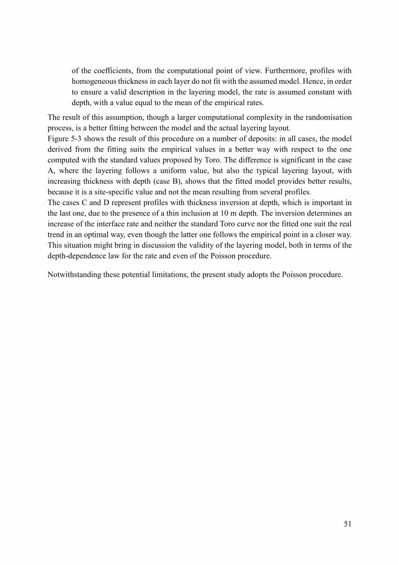
51
of the coefficients, from the computational point of view. Furthermore, profiles with homogeneous thickness in each layer do not fit with the assumed model. Hence, in order to ensure a valid description in the layering model, the rate is assumed constant with depth, with a value equal to the mean of the empirical rates.
The result of this assumption, though a larger computational complexity in the randomisation process, is a better fitting between the model and the actual layering layout. Figure 5-3 shows the result of this procedure on a number of deposits: in all cases, the model derived from the fitting suits the empirical values in a better way with respect to the one computed with the standard values proposed by Toro. The difference is significant in the case A, where the layering follows a uniform value, but also the typical layering layout, with increasing thickness with depth (case B), shows that the fitted model provides better results, because it is a site-specific value and not the mean resulting from several profiles. The cases C and D represent profiles with thickness inversion at depth, which is important in the last one, due to the presence of a thin inclusion at 10 m depth. The inversion determines an increase of the interface rate and neither the standard Toro curve nor the fitted one suit the real trend in an optimal way, even though the latter one follows the empirical point in a closer way. This situation might bring in discussion the validity of the layering model, both in terms of the depth-dependence law for the rate and even of the Poisson procedure.
Notwithstanding these potential limitations, the present study adopts the Poisson procedure.

52
Figure 5-3. Comparison between Toro layering curve (“Theoretical Curve”) and site-dependent curve (“Fitted
Curve”). Case A represents homogeneous layering, cases B and C represent a stratigraphy with increasing thickness with depth and case D represents a layering with inversion in thickness.
Having assumed two different models, depending on the stratigraphic layout, the layering randomisation extracts the thicknesses of each layer in different ways. In case of modelling of depth-dependence through uniform law, since the rate 𝜆 is constant, the sample generation becomes a classical homogeneous Poisson process and the random layer thickness ℎ is given according to (Eqt. 5-2) [42].
ℎ =𝑙𝑛(1 − ε)
−λ (Eqt. 5-2)
The term 𝜀 is a random number extracted from a uniform distribution ranging from 0 to 1. In the modelling with the modified power-law equation, Toro suggested a method to solve the non-homogenous Poisson process, by warping a unit homogeneous Poisson sample into it through the depth-dependence law. Let 𝑢 be the random depth provided by the unit homogeneous Poisson, obtained through the cumulative sum of the extracted values of layer thickness, Toro established a relationship for the conversion to the current depth of layer interfaces ([23], [33]), according to (Eqt. 5-3).

53
𝑧(𝑢) = (−
𝑐2𝑐3𝑢 +
1
𝑐3𝑢 + 𝑐1
−𝑐2+1)
1−𝑐2+1
− 𝑐1 (Eqt. 5-3)
The process of layering generation is not completely random, but it should respect two external restraints. The first restraint is the number of layers that the obtained model should present. In order to limit the degree of restraint exerted by this aspect and, at the same time, avoid unpleasant computational issues, the procedure assigns a maximum number of layers to each generated profile. The value derives from a random extraction from a normal distribution, with mean equal to the current number of layers and coefficient of variation equal to 0.25. This value is the result of a process of manual and visual calibration and provides a set of randomised profiles consistent with the base case. The second restraint of layering randomisation is bedrock depth, since it represents the lower boundary of the soil model. The computation of bedrock depth refers to a random extraction, according to a lognormal distribution. The mean value corresponds to the actual bedrock depth and the standard deviation is assumed equal to 0.3. The bedrock randomisation is independent of layering generation and the bedrock depth is primary with respect to interfaces depth. If the last interface or an entire layer falls below the bedrock interface, the soil model will be cut at that level; if the last interface falls above the bedrock interface, the last layer will be prolonged up to the bedrock depth.

54
5.3.2: Velocity randomisation
The procedure of velocity randomisation refers to an auto-correlated lognormal distribution, according to Toro model [33], in order to reproduce the inter-relationship among the velocities of layers close to each other, which are not completely independent. The Monte Carlo simulation, in this case, employs the following formulation for the realisation of shear wave velocity 𝑣𝑆(𝑖) in the 𝑖-th layer.
𝑣𝑆(𝑖) = 𝑒𝑙𝑛[𝑣𝑆,0(𝑖)]+𝑍𝑖𝜎𝑙𝑛𝑣𝑆 (Eqt. 5-4)
The term 𝑍𝑖 is a realization of a standard normal distribution for the 𝑖-th layer, accounting the inter-layer correlation.
{𝑍1 = 𝜀1
𝑍𝑖 = 𝜌𝑍𝑖−1 + 𝜀𝑖√1 − 𝜌2, 𝑖 > 1 (Eqt. 5-5)
The term 𝜀𝑖 is an independent standard normal variable, with zero mean and unit standard deviation. The correlation degree, expressed by the linear correlation coefficient 𝜌, is function of layers’
depth 𝑧 and of the distance 𝑡 between the layers midpoints.
𝜌(𝑧, 𝑡) = [1 − 𝜌𝑧(𝑧)]𝜌𝑡(𝑡) + 𝜌𝑧(𝑧) (Eqt. 5-6)
𝜌𝑧(𝑧) = {
𝜌200 (𝑧 + 𝑧0200 + 𝑧0
) , 𝑧 ≤ 200 𝑚
𝜌200, 𝑧 > 200 𝑚 (Eqt. 5-7)
𝜌𝑡(𝑡) = 𝜌0𝑒
−𝑡𝛥 (Eqt. 5-8)
The values of model parameters 𝜌200, 𝑧0, 𝜌0 and Δ are provided by Toro [33] as function of site geology or geotechnical characteristics, described with different systems of site classification. For the present study, since the shear wave velocity is available, the reference is the NEHRP site categorisation, depending of the time-weighted average shear wave velocity of the top 30 m, indicated as 𝑣𝑆,30.
As regards the statistical parameters of velocity distribution, i.e. the mean velocity 𝑣𝑆,0(𝑖) and the standard deviation 𝜎𝑙𝑛𝑣𝑆, Toro provides sets of parameters from generic and site-specific results [33]. The common approach consists of the direct application of these parameters in the randomisation process, performing an interpolation of the values when a virtual layer falls between two layers of the base case. This study uses a different approach [44], more aligned with the principle of the work proposed by Toro: assuming that the shear-wave velocity profile of the base-case follows the statistical distribution introduced by Toro, a first randomisation over the base-case layering has been performed. The result is a distribution of shear wave velocities pertaining the base case, from

55
which to obtain the correct site-specific profile of statistical parameters at each depth. The final randomisation, applied over the layering samples, employs the obtained parameters.
The Toro model provides also indications for the randomisation of bedrock velocity. In a similar way to soil layers, the reference distribution is the lognormal distribution, correlated with the previous layer.
𝑣𝑆,𝑏 = 𝑒𝑙𝑛[𝑣𝑆,0(𝑠𝑢𝑝)]+𝑍𝑠𝑢𝑝𝜎𝑙𝑛𝑣𝑆 (Eqt. 5-9)
Thus, the formulation followed in the calculation is the same employed in the previous step, adopting the current value of velocity as mean parameter and 0.3 as logarithmic standard deviation ([33], [45]). In order to avoid physical anomalies, the randomisation process has a lower bound, equal to the maximum between 1.1 times the shear wave velocity of the previous layer and 800 m/s. The first restraint avoids the velocity inversion in correspondence of the bedrock interface, whereas the second restraint ensures profile conditions fulfilling the EC8-1 Draft’s requests, i.e. the
presence of a bedrock with shear wave velocity larger than 800 m/s [5].

56
5.3.3: Profiles selection and resampling
The following step consists of a selection of the one-dimensional ground models resulting from the randomisation process, aiming at guaranteeing the same level of representativeness to each subsoil category, by considering the same number of models for each one. Then, this control is also necessary to ensure a uniform distribution inside every single category, in order to represent all the possible ground conditions with the same weight. The reference instrument used to fulfil these requirements is the representation of soil models in the 𝑣𝑆,𝐻-𝐻800 domain, which synthetises a single model as a point, with coordinates given by the average value of shear wave velocity of the superficial layers and the depth of bedrock formation, according to the definition provided by the EC8-1 Draft [5].
The followed procedure consists of dividing the regions, corresponding to the subsoil categories, into a system of blocks (Figure 5-4). The arrangement is made with 100 blocks, having the same size. Only exception is ground category E, represented by an irregularly shaped region, where the application of the standard scheme, regardless the actual shape, would give an effective number of blocks much smaller than in the others categories, with excessive penalisation either in terms of representativeness or in terms of distribution homogeneity. Hence, the discretisation rule is different and consists in coupling two blocks systems with 7 blocks per side, each one applied to a single rectangular semi-region, with a total of 98 blocks.
Figure 5-4. Scheme of the blocks arrangement.

57
Each block is associated with a maximum number of profiles. The basic assumption, deriving from computational restraints, is a maximum of 200 models per block. Actually, there is a reduction in the limit to 10% in the upper triangle of the region representative of ground category B. The sample set, indeed, includes a very small number of real profiles falling inside this portion and the filling of the portion would require several cycles of randomisation. This limitation is not a consequence of a lack inside the database because the portion represents deep soil deposits with stiff layers at the surface, characterised by large values of 𝑣𝑆,𝐻 and 𝐻800. From a geological point of view, this situation may correspond to deep deposits with a shallow rocky plate or deep stratifications of altered rock and these are extremely rare cases, compared with other situations falling in site category B. Thus, the necessity of ensuring a proper level of representativeness coherent with the level of occurrence of the different situations pushed forward the setting of this further limit. Finally, the limit is set to zero in the blocks falling in the region representative of ground category A. The study, indeed, ignores the corresponding soil models since the Draft does not assume stratigraphic amplification for this class [5].
The result is a collection of about 100’000 one-dimensional ground models – more precisely, 91’500 profiles –, which is a relatively large number and compatible with the computational capacity of the available hardware units. Figure 5-5 shows the distribution inside the blocks arrangement.
Figure 5-5. Blocks arrangement with colour mapping for indicating the maximum number of models inside each
block.

58
The selection does not only follow statistical criteria of representativeness, but it is also helpful in fulfilling the restraints of computational nature, mainly deriving from the limitations of SHAKE91. The code, indeed, presents two fundamental limitations in the implementation of soil models.
Soil models should have at most 13 different materials, including the half-space.
The layering discretisation should bring at most 50 sublayers.
The implemented procedure does not perform the immediate removal of the models not fulfilling these restraints, but applies a small relaxation to them, in an indirect way. As regards the number of materials, the procedure merges together neighbouring layers made with similar materials, i.e. layers described by the same type of nonlinear curves. In case of exceedance in the number of sublayers, the procedure changes the discretisation criterion, reducing the maximum frequency analysed from 25 Hz to 15 Hz. This reduction implies a more accurate selection in the seismic inputs for the analysis, as regards the frequency content. Thus, the pursued strategy does not consists in the simple removal of unadapt models. This solution, indeed, would cause a significant alteration of the statistics of the soil deposits, since it would not allow the inclusion of models representative of deep and highly deformable soil deposits or multi-stratified deposits, which should be described through a large number of nonlinear models or sublayers. Actually, these situations are quite rare cases and the analysis of their response should refer to an explicit nonlinear technique, instead of an equivalent linear approach or even the simplified method proposed by the Draft. On the other side, there is not the possibility of a priori judgement of the quality of the results and the request of ensuring a level of representativeness to these cases pushed forward to this strategy.
In conclusion, the resampling procedure consists of locating the adequate models in the competent block, as function of the value of 𝑣𝑆,𝐻 and 𝐻800, up to fill it reaching the established limit number. The result is a regular dispersion of points, representative of the soil models, selected in order to obtain the same level of population for each ground category.

59
5.4: Properties assignment The result of the previous passages was the generation of partial information about the one-dimensional ground models, i.e. the shear-wave velocity profiles. The next step estimates the remaining parameters required for the full definition of the ground model, adding the stratigraphic and geotechnical information to the stiffness description.
A preliminary stage is the assignment of the material type to the layers inside each profile, in order to set the subsequent definition of nonlinear curves and of the mechanical parameters. A number of real soil profiles include the stratigraphic information, interpreted according to the scheme defined previously (Table 4-1). In this case, the assignment criterion of the material to the virtual profiles is based on the depth: each layer of the generated model is assigned the material type pertaining the one having the closest midpoint depth. In absence of information, the material assignment follows the approach proposed by Ohta and Goto [46]. Even though conceived for the first-stage computation of shear wave velocity from the soil indexes, this study employs the inverse of the relationship as reference to obtain an indication about the material. Ohta and Goto found an empirical equation relating a factor 𝐹, which defines the soil type, to shear wave velocity 𝑣𝑆 and depth 𝑧.
𝐹 =𝑣𝑆
78.98𝑧0.312 (Eqt. 5-10)
As function of the factor 𝐹, Ohta and Goto provide an indication of the material type composing the layer, which is the interpreted according to the scheme adopted in this work (Table 5-1).
Table 5-1. Values of factor F per soil type, from Ohta and Goto [46].
Factor 𝐹 Soil type (Ohta and Goto) Soil type (this study) 1.000 Clay Clay/sand 1.260 Fine sand Clay/sand 1.282 Medium sand Sand 1.422 Coarse sand Sand 1.641 Sand and gravel Gravel 2.255 Gravel Gravel
The material assignment is performed during the procedure of profile resampling, since the material type is an information necessary for the evaluation of the number of nonlinear curves involved in the analysis, in order to assess the respect of the restraints of SHAKE91 code.
The complete definition of the 1-D ground models requires then the assignment of other geotechnical and physical properties to each layer, necessary for the construction of the nonlinear curves or the computation of other elements. These parameters are listed below.
Plasticity index 𝑃𝐼.
Over-Consolidation Ratio 𝑂𝐶𝑅.

60
At-rest lateral pressure coefficient 𝐾0.
Porosity 𝑛 and unit weight 𝛾.
Groundwater depth 𝑧𝑤.
Random variables for Darendeli curves 𝜀1 and 𝜀2.
The general criterion of computation of these parameters consists in limiting as much as possible the full random extraction from statistical parameters, since the assumed values may not be reliable. Therefore, the trend was to employ empirical relationships allowing the computation – deterministic or random, if information about data dispersion is available – starting from the known data, e.g. shear wave velocity. In this way, the resulting ground model will be consistent and robust from the conceptual point of view.
5.4.1: Plasticity index
The plasticity index 𝑃𝐼 is a fundamental parameter for the description of the dynamic behaviour of fine-grained material, since several studies demonstrated its effect on nonlinear curves, moving the linear and volumetric strain threshold (e.g. [47]). In particular, when increasing the plasticity index, the material shows linear behaviour over a wider strain range, the reduction in shear modulus is smaller and the damping ratio does not increase significantly.
The adopted approach for the estimate of plasticity index depends of the type of material composing the layer. In case of rocky or gravelly formation, plasticity index is null. In sandy layers, since this material category includes clean sands and sands with fine fraction, the plasticity index assumes a small value. For the sake of simplicity, the plasticity index is equal to 0 or 15 and the value is obtained through random extraction. In clays, the plasticity index is more significant and its evaluation consists of a random extraction among the values 30, 50, 75 and 100. This approach is similar to the one adopted by Pettiti and Foti [1]. Table 5-2 lists the adopted criteria in a synthetic way.
Table 5-2. Rules for plasticity index assignment.
Material type Plasticity index 𝑃𝐼 Rock 0
Gravel 0 Sand 0 or 15 Clay 30, 50, 75 or 100

61
5.4.2: Over-consolidation ratio
The over-consolidation ratio 𝑂𝐶𝑅 is a parameter describing the state of consolidation of the material and it is synthetises the geological history of the deposit in a parametric form.
Its definition and computation are immediate and simple in fine-grained materials, where the experimental determination through oedometric test is possible. The computed value depends on the shear wave velocity, according to the formulation proposed by Pettiti and Foti [1], and it can be equal to 1, 4 or 16.
𝑂𝐶𝑅𝑖 = {
1 𝑣𝑆,𝑖 < 250 𝑚/𝑠
4 250 𝑚/𝑠 ≤ 𝑣𝑆,𝑖 ≤ 600 𝑚/𝑠
16 𝑣𝑆,𝑖 > 600 𝑚/𝑠 (Eqt. 5-11)
This solution follows the trend of over-consolidated clays to be stiffer and characterised by larger values of shear wave velocity. In clean sands, the empirical evaluation of this parameter is more complex and the lack of useful relationships forces the adoption of a unitary value, regardless the shear wave velocity. In gravels and rocks, the computation of the over-consolidation ratio is not necessary since the confining stress does not play any role inside the chosen model for nonlinear properties. Table 5-3 lists the adopted criteria in a synthetic way.
Table 5-3. Rules for over-consolidation assignment.
Material type Over-consolidation ratio 𝑂𝐶𝑅 Rock -
Gravel - Sand 1 Clay (Eqt. 5-11)

62
5.4.3: Lateral pressure coefficient at rest
The lateral pressure coefficient at rest 𝐾0 is defined as the ratio between the effective horizontal stress and the effective vertical stress in geostatic conditions and participates in the computation of the confining pressure. Confinement is described by the mean effective stress 𝜎0′ , evaluated according to the following formulation from the vertical stress 𝜎𝑣′ .
𝜎0′ =
1 + 2𝐾03
𝜎𝑣′ (Eqt. 5-12)
The estimate of the coefficient is not simple because it requires specific and advanced in situ testing procedures. In absence of this kind of information, as suggested by Lancellotta [48], the reference is the formulation proposed by Schmidt [49] and Alpan [50], which identifies a normal-consolidation contribution and a pre-consolidation contribution. 𝐾0 = 𝐾0,𝑁𝐶𝑂𝐶𝑅
𝛼 (Eqt. 5-13)
The computation of the single components refers to different procedures, depending of the material type. In fine materials, where plasticity index is different from zero, the normal-consolidation contribution derives from the empirical equation proposed, whereas the pre-consolidation one involves the values suggested by Ladd et al. [51], as function of the plasticity index itself. 𝐾0,𝑁𝐶 = 0.43 + 0.0042 × 𝑃𝐼 (Eqt. 5-14)
𝛼 = {
0.42, 𝑠𝑚𝑎𝑙𝑙 𝑃𝐼 ⟶ 𝑃𝐼 ≤ 150.32, 𝑙𝑎𝑟𝑔𝑒 𝑃𝐼 ⟶ 𝑃𝐼 ≥ 30
(Eqt. 5-15)
In clean sands, the normal-consolidation contribution is computed according to Jàky [52] formulation, as function of the critical value of friction angle 𝜑′, which is adapt for coarse-grained materials. The friction angle assumes the typical value of 33°. K0,NC = 1 − sinφ′ (Eqt. 5-16)
The pre-consolidation contribution is not necessary, since the over-consolidation ratio is assumed as equal to 1. In presence of gravels and rocks, the computation of the coefficient is not necessary since the confining stress does not play any role inside the chosen models for nonlinear curves. Table 5-4 lists the adopted criteria in a synthetic way.
Table 5-4. Rules for computation of lateral pressure coefficient at-rest.
Material type Normal-consolidation contribution
𝐾0,𝑁𝐶 Pre-consolidation contribution 𝛼
Rock - - Gravel - - Sand 1 − sin𝜑′ -
Clay 0.43 + 0.0042 × 𝑃𝐼 0.42 for 𝑃𝐼 ≤ 15 0.32 for 𝑃𝐼 ≥ 30

63
5.4.4: Porosity and unit weight
Porosity is a parameter that reflects the granular nature of ground material and participates in the estimate of the unit weight 𝛾. Unit weight is necessary either for the definition of the confining stress – when required by the nonlinear curves – or for the computation of the inertial component of the seismic action inside the material, required for the solution of the waveform. The estimate of unit weight refers to the porosity medium theory.
𝛾 = 𝑛𝛾𝑠 + (1 − 𝑛)𝛾𝑤 (Eqt. 5-17)
The assumed soil grain density 𝜌𝑠 is equal to 2700 kg/m3, whereas water unit weight 𝛾𝑤 is equal to 10 kN/m3. As regards porosity 𝑛, the empirical correlation proposed by Hunter [53] gives an estimate as function of the shear wave velocity 𝑣𝑠 (Figure 5-6) and it is valid for sands, clays and gravels. Since Hunter provides both the mean law and the dispersion, the computation of porosity will involve a randomisation procedure.
𝑛 = 1.396 − 0.160 × ln 𝑣𝑆 (Eqt. 5-18)
𝜎 = ±0.13 (Eqt. 5-19)
Figure 5-6. Relationship between shear-wave velocity and porosity, taken from Hunter [53].
In rocky layers, where no relationship for the computation of porosity is available for the range of shear wave velocity of interest, the typical value of unit weight equal to 22 kN/m3 is assumed. Table 5-5 lists the adopted criteria in a synthetic way.
Table 5-5. Rules for computation of total unit weight.
Material type Total unit weight 𝛾 Porosity 𝑛 Rock 22 kN/m3 -
Gravel (Eqt. 5-17) (Eqt. 5-18), (Eqt. 5-19) Sand (Eqt. 5-17) (Eqt. 5-18), (Eqt. 5-19)
Clay (Eqt. 5-17) (Eqt. 5-18), (Eqt. 5-19)

64
5.4.5: Groundwater level
The groundwater level assumes a double role since, varying the profile of total unit weight with depth, it affects the inertial component of seismic action and the confining pressure. The estimate of water table depth consists of a uniform random extraction among the depths of interfaces between sublayers, according to the adopted rule for the layering discretisation (more details in 4.2.2).
5.4.6: Darendeli random variables
The parameters 𝜀1 and 𝜀2 are two uncorrelated random variables used in clayey and sandy layers for the selection of the Darendeli nonlinear curve with respect to the mean one, computed for the specific type of material under the assigned confining stress. This strategy allows the increase of the variability degree of the analysis and cover the limitations in the extraction of other parameters, such as plasticity index and over-consolidation ratio. Their evaluation consists of a random extraction from a standard normal distribution, having zero mean and unit standard deviation.

65
5.5: Statistical analysis of the ground models The previous stage allowed the construction of the one-dimensional ground models necessary for the analyses, according to a complex procedure of randomisation, selection and properties assignment, synthesised in the scheme in Figure 5-7.
Figure 5-7. Scheme of the procedure of construction of 1-D ground models.
The present part attempts to evaluate the statistical distribution of some significant mechanical or physical properties among the generated one-dimensional soil models, in order to obtain useful information for the interpretation of the results of the ground response analyses. Profiles characterised by similar properties, indeed, assume similar behaviour in seismic conditions and this aspect gives orientation in the interpretation.
The first parameter of interest is the plasticity index, since several studies underlined its role in the seismic response of ground materials (e.g. [47]). The statistical analysis requires the definition of a representative value of plasticity index for the single ground model, since this parameter is variable with depth. The equivalent plasticity index 𝑃𝐼𝐻 is defined as the harmonic mean of the values of plasticity index 𝑃𝐼𝑖 of each layer with respect to its travel-time 𝑡𝑖.
𝑃𝐼𝐻 =∑ 𝑃𝐼𝑖𝑡𝑖𝑁𝑖=1
∑ 𝑡𝑖𝑁𝑖=1
(Eqt. 5-20)
Figure 5-8 shows the distribution of the mean value of the equivalent plasticity index in the reference blocks. The plasticity index reflects the average shear-wave velocity: stiffer soil models assume lower values of plasticity index, since they are mainly composed by gravel or

66
rock, whereas the highest values are close to the left boundary, in correspondence of the most deformable soil models. The largest values of equivalent plasticity index can be found also in the lower portion of the region pertaining to ground category E, representing surficial soil deposits made with deformable materials – the average shear-wave velocity is smaller than 400 m/s – corresponding to sands or clays. Only exception are same spots in the region corresponding to site category B, characterised by very large values of plasticity index if compared to the neighbouring elements. Actually, these are particular cases because they lie in the upper triangle, where the maximum number of models is limited and the random extraction may have generated profiles with significant plasticity.
Figure 5-8. Distribution of the equivalent plasticity index.
An interesting element is the number of soil models involving layers with shear wave velocity larger than 800 m/s. These models are an undesired effect of the randomisation procedure, since the process was conceived for randomisation of real deposits and does not follow the restraints of the Draft in a rigorous way. The effect was the generation of a number of soil models with layers exceeding in the standard shear-wave velocity of 800 m/s, which should not be included in the analysis, in order to avoid alteration of the results. The amplification parameters, indeed, are computed with reference to the first layer with velocity equal or larger than 800 m/s and the addition of further layers would cause bigger amplifications of seismic action, due to the addition of another impedance contrast. As shown by Figure 5-9, a large number of models falling in ground category B exceed this limitation, especially in the blocks characterised by equivalent shear-wave velocity close to 800 m/s. These models, indeed, derive from models representative of stiff soil deposits, where shear-wave velocity is larger than 700 m/s and the randomisation generated very stiff layer, which are

67
compatible with the real case but not with the EC8-1 Draft’s specifications. The removal applies to a large number of profiles falling in ground category B, especially in the upper triangle, where the removal is substantially complete in some block. This would affect the statistical representativeness of the models for ground category B, even though the removal affects a region already composed by a small number of profiles, so the statistical sample is not affected so much.
Figure 5-9. Number of models involving layers with shear wave velocities larger than 800 m/s.
Oppositely, the statistical sample includes also a number of ground models with deformable layers, characterised by shear-wave velocity smaller than 50 m/s. As shown by Figure 5-10, the amount of these cases is not so significant in the statistical sample, with a maximum per block smaller than 10%, all concentrated adjacent to the left boundary, at bedrock depth close to 50 m. These models belong to same statistical family, since they derive from the randomisation starting from the real case identified as BTT2 (site n.34 in the database), which is a deep deposit of peat, with shear wave velocity ranging from 30 m/s to 80 m/s in the shallow layers. The analysis takes into account this aspect, since deformable soil deposits undergo significant nonlinear phenomena during the earthquake and the ground response analysis according to the equivalent linear scheme may be unresponsive.
The last aspect analysed in this section concerns a computational restraint by SHAKE91 code, i.e. the limitation of the number of sublayers in the soil model. In order to avoid excessive influence in the generation of the soil models due to this restraint, the procedure adopts a different rule for the ground response analysis, reducing the maximum considered frequency from 25 Hz to 15 Hz. The application of this solution is not systematic, but it pertains only the models potentially

68
exceeding the limit, i.e. the ones characterised by deformable layers and large bedrock depth. The number of sublayers, indeed, is proportional to bedrock depth and inversely proportional to shear-wave velocity. Therefore, as shown by Figure 5-11, profiles including layers with shear-wave velocity smaller than 200 m/s for moderate depths tend to violate the restraint and they require the reduction in the reference frequency.
Figure 5-10. Number of models involving layers with shear wave velocities smaller than 50 m/s.
Figure 5-11. Number of models with the reduction of maximum frequency to 15 Hz.

69
Chapter 6: Seismic inputs
6.1: Introduction The definition of the seismic action for the ground response analyses is a fundamental and delicate aspect. The analyses, indeed, involve phenomena characterised by significant nonlinearity and the use of simplified representations proposed by codes, as elastic response spectra, is not recommended. Therefore, the definition of the seismic action should refer to ground motion time histories. At the moment, no database provides an unique design time history involving all the aspects about the seismic conditions in the generic site. As consequence, the definition of seismic action will consist of a set of time histories having characteristics compatible with the seismic hazard of the site.
In this study, the site-dependence of the spectral shape proposed by the EC8-1 Draft [5] forces to refer to different sites for the evaluation of the seismic action, each one characterised by specific values of hazard parameters. In order to obtain a result which is general and representative of the national situation – but also not too much time-consuming –, the pursued strategy consists of a selection of a limited number of sites aiming to represent different levels of seismic hazard in the national territory. The next step defines the seismic action in terms of acceleration time histories, selecting a series of natural accelerograms compatible with the hazard conditions for each reference site, either in seismological terms or in spectral terms. The source of these data are accredited national and international databases, which allow an interactive search of waveforms with prescribed characteristics.

70
6.2: Selection of the reference sites The site-dependence of the spectral shape and of the stratigraphic amplification is not an aspect introduced only in the EC8-1 Draft. The current version of Eurocode 8 [20] proposes different values of the stratigraphic amplification factors in relationship with the expected earthquake magnitude, modelling in a simplified manner the site-dependence. The Italian code ([6], [7]) introduced a more refined and accurate relationship, which provides the amplification factors as function of maximum spectral acceleration measured on rock formation. These approaches derive from the awareness about the nonlinear behaviour of ground materials. In a linear system, the response – here represented by amplification factors – is the same, regardless the input entity. Soils are instead a complex nonlinear system whose behaviour strongly depends of the ground motion intensity. Under strong earthquakes, indeed, the strain level increases, inducing a reduction of stiffness and an increase of energy dissipation, with smaller amplification as result. The EC8-1 Draft inherits this concept and couples it with the intent of restraining the spectral shape at short periods and intermediate periods, through the introduction of the dependence of amplification factors 𝐹𝛼 and 𝐹𝛽 with respect the correspondent hazard parameters 𝑆𝛼,475 and 𝑆𝛽,475.
The introduction of these new parameters for the description of seismic hazard forces a change in the methodology of selection of seismic inputs. Several works assessing the amplification factors (e.g. [4], [54]) referred to a wide set of Italian records, aiming to represent the Italian seismicity. Other authors (e.g. [1]) focused more on the role of nonlinearity on amplification factors and selected a suite of ground motions able to cover the range of peak ground acceleration of engineering interest. Andreotti et al. [2] followed a similar approach, with particular focus on the site-dependence. They performed the ground response analyses over 4 sites in Italy characterised by different levels of expected peak ground acceleration, referring to suits of real accelerograms compatible with the hazard conditions of each site. In this way, their study does not simply evaluate the effect of peak ground acceleration in amplification factors, but performs a site-specific analysis in order to obtain a more accurate evaluation of the amplification.
In a similar way, this study uses ground motion time histories compatible with the conditions of a number of reference sites, whose selection refers to the seismic hazard parameters introduced by the EC8-1 Draft, i.e. 𝑆𝛼,475 and 𝑆𝛽,475. In particular, the selected sites are representative of the distribution of 𝑆𝛼,475 and 𝑆𝛽,475 in Italy.

71
6.2.1: Definition of the distribution of hazard parameters
In order to perform the selection of the reference sites, a preliminary step consists of the aggregation of the seismic hazard data of the Italian country and the definition of the distribution in terms of the reference parameters 𝑆𝛼,475 and 𝑆𝛽,475.since the available databases – following mainly the indications of current codes – provide this kind of data only in a partial way. The operation is not simple, since the seismic hazard databases do not provide these data yet. Due to this lack of information, the study introduces some assumptions for the evaluation of the parameters, in order to have the possibility to employ the available data.
On one side, the spectral parameter 𝑆𝛼,475 is assumed to be equal to the maximum spectral acceleration of the horizontal 5% damped elastic response spectrum on site category A introduced in the Italian building code [6], herein indicated as 𝑆𝐴,475. As consequence, the parameter 𝐹0 is equivalent or, at least, similar to the parameter 𝐹𝐴 introduced by the EC8-1 Draft [5] and this consideration validates the following assumption. 𝑆𝛼,475 ~ 𝑆𝐴,475 = 𝐹0𝑎𝑔 (Eqt. 6-1)
The values of peak ground acceleration 𝑎𝑔 and of the parameter 𝐹0 are available in the site of the Consiglio Superiore dei Lavori Pubblici (CSLP) [55]. The relationship (Eqt. 6-1) is not rigorous since the parameters derived from CSLP are the result of a nonlinear piecewise regression procedure over the uniform hazard acceleration spectra for Italian sites, according to the spectral shape adopted by the Italian building codes [6]. Since the EC8-1 Draft proposes a slightly different spectral shape [5], the maximum ordinate 𝑆𝛼,475 will assume a different value with respect to 𝑆𝐴,475. Despite this observation, the site selection refers to the parameter 𝑆𝐴,475 because the value is not so different from the real one (more details in 6.3.2). Furthermore, this assumption is adopted just for the identification of a pattern of sites representative of the distribution of hazard data, where the use of the correct parameter or a similar one brings substantially the same result.
In a similar way, the parameter 𝑆𝛽,475 is assumed as equal to the ordinate of the uniform hazard spectrum evaluated at 1 s, herein indicated as 𝑆𝐵,475. 𝑆𝛽,475 ~ 𝑆𝐵,475 = 𝑆𝑇=1 𝑠 (Eqt. 6-2)
The values of parameter 𝑆𝐵,475 are taken from the site of the Istituto Nazionale di Geofisica e Vulcanologia (INGV) [56], as result of the S1 Project of seismic hazard assessment ([57], [58]). Actually, the values are different since the parameter 𝑆𝛽,475 is the result of the regression procedure over the uniform hazard spectrum, whereas 𝑆𝐵,475 is an ordinate of the uniform hazard spectrum itself. The two curves, indeed, may not be coincident at 1 s. On the other side, the difference is not significant (more details in 6.3.2) and this error is acceptable in the construction of the distribution of hazard data.

72
Thus, the definition of the distribution of hazard data in the Italian territory employs the data of two separated databases, which are merged together. The merging procedure is not immediate, due to different coverage level of the two datasets. The INGV and CSLP databases provide the seismic hazard parameters on a large number of sites disseminated in the Italian territory but, even though the adopted identification code for sites is the same, the number and the geographical distribution are not the same.
The INGV study [59] is performed over 16’921 points, defined through a regular grid of knit equal to 0.05° in latitude and longitude.
The CSLP database provides the results of the nonlinear regression applied over the results of a large number of sites involved in the INGV study, excluding points falling in the sea and including points close to the national borders, for a total of 10’751 points [60].
The merging of the information provided by databases, aiming to couple together the information in common sites, results in a set of 10’159 points, described by the values of 𝑆𝐴,475 and 𝑆𝐵,475. Figure 6-1 shows the distribution of the obtained hazard data.
Figure 6-1. Hazard data distribution for the Italian territory.

73
6.2.2: Selection of the sites
The scatter plot representation of the distribution of 𝑆𝐴,475 and 𝑆𝐵,475 shows a certain degree of linear correlation between the two fields of data (Figure 6-1). The correlation is visible both from a graphical point of view, since the points are quite aligned along a straight line, and from a statistical point of view, as the linear correlation coefficient – equal to 0.78 – is quite close to the unit. Starting from this consideration, a way for supplying the representativeness of selected sites might consist of selecting a set of points lying along the linear trend line, maybe with equal spacing along the horizontal axis. This simplification may be acceptable thanks to the significant degree of linear correlation.
Actually, the linear correlation is not perfect, especially at the largest values of seismic hazard parameters, where there is a large deviation of real points from the ideal line This deviation is consequence of the different spectral shape in the Italian sites. As shown by Rota et al. [61], with reference to the normalised spectrum with respect to peak ground acceleration, there is a remarkable variability of spectral shapes in the Italian sites, which is an effect of the different seismological aspect from a site to another (Figure 6-2).
Figure 6-2. Variability of horizontal acceleration spectra, normalized with respect to peak ground acceleration
(taken from Rota et al. [61]).
The adopted strategy takes its inspiration from the work done by Andreotti et al. [2], who referred the choice of the sites to the level of the seismic hazard, based on the 2012 seismic classification of the Italian territory published by the Italian Department of Civil Protection (DPC). In particular, they considered four sites, each in one of the four different zones of seismic hazard level. In this case, according to the EC8-1 Draft [5], the seismicity level is function of the value of the hazard parameter 𝑆𝛼,475 (Table 6-1).

74
Table 6-1. Ranges of 𝑆𝛼,475 values for the definition of seismicity levels (taken from EC8-1 Draft [5]).
Seismicity level Parameter 𝑆𝛼,475 (m/s2) Very low < 1.0
Low 1.0 ÷ 2.5 Moderate 2.5 ÷ 5.0
High > 5.0 The application of the seismicity level to the distribution creates a subdivision of the domain into vertical bands, defining groups of sites with a different level of seismic hazard (Figure 6-3). As the number of sites with “Very low” seismicity level is small with respect to the other ones, this category will be unified with the “Low” level. The main reason of this assumption is the low representativeness of this group of sites, from a statistical point of view. Moreover, the EC8-1 Draft treats very low and low seismicity areas in the same way [5].
Figure 6-3. Subdivision of the hazard parameters distribution according to seismicity levels introduced by the
Draft [5].
Then, similarly to Andreotti et al. [2], each site correspond to a specific level of seismicity and it is represented by a point more or less in the central portion of the correspondent region in the 𝑆𝐴,475-𝑆𝐵,475 domain. Since the intermediate area – “Moderate” seismicity level – is the largest inside the Italian hazard data distribution, this is assigned two sites, corresponding to two points lying in the peripheral zones. In this way, the analysis refers to 4 sites, which is a number representing a good trade-off between the request of representativeness of the seismic hazard conditions in Italy and computational restraints, since it does not produce excessive amount of data for the available hardware units.

75
The above-mentioned operation is useful to establish the horizontal coordinate, i.e. the parameter 𝑆𝐴,475, for the reference sites. The evaluation of the second coordinate, i.e. 𝑆𝐵,475, refers to the linear fitting to the distribution, defined for each region. The linear fitting applied to each portion defined by the seismicity discretisation, indeed, suits in a better way the distribution than the same applied to the whole distribution, especially at high seismicity levels. As shown by Figure 6-4, each reference site corresponds to a point lying along the fit line in correspondence to the middle zone – for low and high seismicity level – or the peripheral zones – for moderate seismicity level. The selected points are considered as representative of the population of the seismic hazard parameters in Italy. The list of the reference sites resulting from the selection is available in Table 6-2 and their geographical position is shown in Figure 6-5.
Table 6-2. List of the reference sites.
Locality Region INGV/
CSLP ID Longitude Latitude 𝑆𝑠 (m/s2) 𝑆1 (m/s2)
Termeno sulla Strada
del Vino
Trentino Alto Adige
8516 11°.24 46°.36 1.384 0.446
Godrano Sicilia 46508 13°.42 37°.83 2.828 0.904 Urbino Marche 20522 12°.59 43°.68 4.171 1.284 Atina Lazio 29641 13°.75 41°.63 5.805 2.051
Figure 6-4. Position of the selected points inside the Italian hazard parameters distribution.
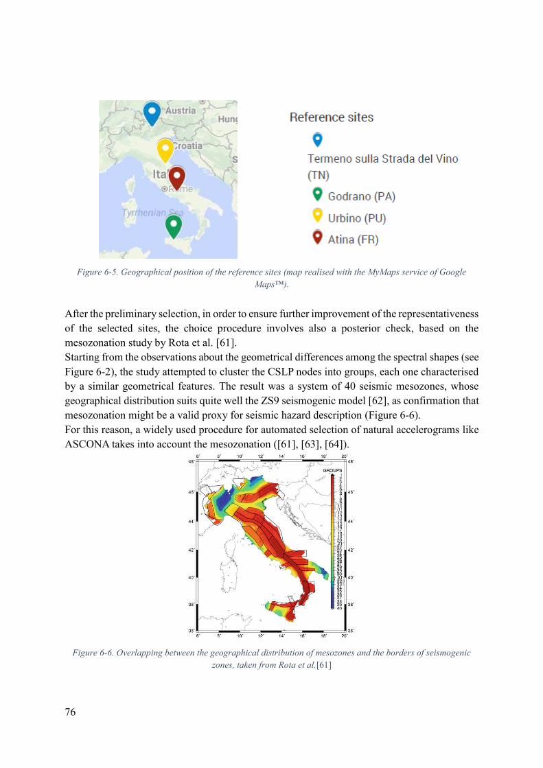
76
Figure 6-5. Geographical position of the reference sites (map realised with the MyMaps service of Google Maps™).
After the preliminary selection, in order to ensure further improvement of the representativeness of the selected sites, the choice procedure involves also a posterior check, based on the mesozonation study by Rota et al. [61]. Starting from the observations about the geometrical differences among the spectral shapes (see Figure 6-2), the study attempted to cluster the CSLP nodes into groups, each one characterised by a similar geometrical features. The result was a system of 40 seismic mesozones, whose geographical distribution suits quite well the ZS9 seismogenic model [62], as confirmation that mesozonation might be a valid proxy for seismic hazard description (Figure 6-6). For this reason, a widely used procedure for automated selection of natural accelerograms like ASCONA takes into account the mesozonation ([61], [63], [64]).
Figure 6-6. Overlapping between the geographical distribution of mesozones and the borders of seismogenic
zones, taken from Rota et al.[61]

77
Figure 6-7. Population of each mesozone, taken from Rota et al. [61]
Since their mesozonation criterion is purely geometric, each group does not have the same density of population and some include a limited number of sites, as shown by Figure 6-7. In order to ensure the optimal degree of representativeness, not only in terms of hazard parameters, but also in terms of the global shape of the response spectrum, the selection procedure involves a second step of check. This step verifies firstly whether the reference sites belong to different groups, in order to introduce an adequate level of variability of ground motion in the reference sites. Then, the selected sites should fall in one of the most populated zones or, at least, not in one of the poorest. In this way, the selection will not result in a system of sites with representative values of hazard parameters but with an anomalous and rare spectral shape. Table 6-3 shows the spectral group to whom each reference site belongs.
Table 6-3. List of the selected sites with spectral groups.
Locality INGV/ CSLP ID Group of spectra Termeno sulla Strada del Vino 8516 30
Godrano 46508 15 Urbino 20522 5 Atina 29641 1
All the reference sites fall in quite populated groups, especially the ones at highest seismicity levels, whereas the other sites belong to smaller groups. Actually, the second criterion is not a rigid restraint but it is secondary with respect to the distribution criterion, because the criteria are not in perfect accordance, e.g. some of the most populated groups often correspond to points lying in the peripheral regions of the distribution. A particular case is Godrano site, as it belongs to the spectra group n.15, which is the less populated than the group n.16. Despite this limitation, the choice did not fall over a site of the latter group, since this class corresponds to points falling in the peripheral side of the distribution in the 𝑆𝐴,475-𝑆𝐵,475 domain. On the other side, group n.15 is quite populated and its points fall in the central area of the distribution, thus fulfilling an adequate level of representativeness of the Italian seismic hazard, either in terms of hazard parameters or in terms of spectral shape.
In conclusion, the collection of sites consists of four locations, henceforth identified as Termeno

78
sulla Strada del Vino, Godrano, Urbino and Atina, and they seek to represent as better as possible the seismic hazard in Italy.

79
6.3: Definition of the seismic hazard in the reference sites The previous step allowed the creation of a collection of sites representative of the seismic hazard in Italy. The definition of the seismic action requires the evaluation of the seismic hazard, in terms of ground motion parameters, in order to set the criteria for the selection of ground motion time histories.
In this study, an explicit hazard assessment has not been carried out and the information derive from the results of probabilistic seismic hazard analysis performed into the Italian territory by the INGV ([56], [57]). The study provides an estimate of the ground shaking in terms of peak ground acceleration and spectral acceleration for different probabilities of exceedance in 50 years, in correspondence of the nodes of a regular grid of knit equal to 0.05° in latitude and longitude. The results assume a specific field of validity, due to the model hypotheses.
The computation of ground motion parameters refers to a specific geological and morphological condition, i.e. an outcropping plain formation characterised by surficial average shear-wave velocity larger than 800 m/s. According to EC8-1 Draft’s
indications, this corresponds to subsoil category [5].
The estimate refers to seismological data and attenuation laws deriving from the observations of past events to realise a predictive model for seismicity. Therefore, the result is affected by the information of the past and may not be completely representative of the effective site seismicity.
The information provided by INGV site include the expected values of peak ground acceleration, the uniform hazard response spectrum and the disaggregation of seismic hazard into magnitude and epicentral distance.

80
6.3.1: Peak ground acceleration
The Web-GIS service [56] provides, for each site, different values of peak ground acceleration as function of the annual exceedance frequency and the percentile [65]. An example of the resulting values, referred to Termeno sulla Strada del Vino site, is shown in Table 6-4.
Table 6-4. Values of peak ground acceleration for different values of annual exceedance frequency and percentile, referred to the Termeno sulla Strada del Vino site (taken from [56]).
The annual exceedance frequency is the inverse of the reference period of return, equal to 475 years according to the EC8-1 Draft [5].
𝑓 =1
𝑇𝑅= 0.0021 (6.3)
The percentile allows the selection of the specific value of the ground motion parameter from its statistical distribution and it is assumed as equal to 50%. Table 6-5 lists the values of peak ground acceleration for each reference site.
Table 6-5. Values of peak ground acceleration for the reference sites.
INGV/ CSLP ID 𝑃𝐺𝐴 (m/s2) 8516 0.530 46508 1.137 20522 1.706 29641 2.497

81
6.3.2: Uniform hazard spectrum
Then, this study analyses also uniform hazard spectrum, representing the response spectrum with constant exceedance probability. This parameter, indeed, allows the computation of the standard hazard parameters 𝑆𝛼,475 and 𝑆𝛽,475, through an operation of nonlinear piecewise fitting according to the new spectral shape introduced by the EC8-1 Draft [5]. In this way, there is the possibility of comparing the current hazard parameters versus the new ones and verify the reliability of the assumptions introduced for the definition of the hazard distribution.
The Web-GIS service provides the spectral ordinates for the 50th percentile, under different exceedance probabilities in 50 years ([56], [59]). Table 6-6 shows the values referred to Termeno sulla Strada del Vino site.
Table 6-6. Uniform hazard spectra for the Termeno sulla Strada del Vino site (taken from [56]).
The reference exceedance probability in 50 years depends of the period of return 𝑇𝑅 of the design seismic action: for 475 years, the probability is 10% in 50 years.
After the selection of the proper reference spectrum, an operation of nonlinear fitting has been carried out. The regression has two independent parameters, i.e. the standard ordinates 𝑆𝛼,475 and 𝑆𝛽,475, and followed three restrains.
Ordinate 𝑆𝛼,475 should be positive.
Ordinate 𝑆𝛽,475 should be positive.
Ordinate 𝑆𝛽,475 should be smaller than 𝑆𝛼,475.
The tool employed for this operation is the Solver tool of Microsoft® Excel 2013. In all the reference sites, the resulting curve fits adequately the uniform hazard spectrum and, furthermore, the new spectra suit quite well the ones proposed by the Italian code (Figure 6-8). Table 6-7 shows the obtained hazard parameters, compared with the assumed ones: the difference is very small for the peak spectral acceleration, whereas it is more significant for the

82
spectral ordinate at 1 s, but the deviation is less than 10%. As consequence, the assumptions adopted for the definition of the hazard data distribution were correct.
Figure 6-8. Nonlinear fitting curve ("Design spectrum") compared with the uniform hazard spectrum and the Italian Code spectrum ("NTC spectrum") [6]. The reference site is Termeno sulla Strada del Vino (ID: 8516).
Table 6-7. Seismic hazard parameters for the reference sites.
Locality 𝑆𝛼,475 (m/s2) 𝑆𝛽,475 (m/s2) 𝑆𝐴,475 (m/s2) 𝑆𝐵,475 (m/s2) Δ𝑆𝛼,475 (%) Δ𝑆𝛽,475 (%) Termeno
sulla Strada del Vino
1.351 0.474 1.384 0.446 2.3 6.3
Godrano 2.794 0.914 2.828 0.904 1.2 1.1 Urbino 4.116 1.377 4.171 1.284 1.3 7.2 Atina 5.764 1.988 5.805 2.051 0.7 3.1
0
0.2
0.4
0.6
0.8
1
1.2
1.4
1.6
0 0.5 1 1.5 2 2.5
Pse
ud
o-a
ccel
erat
ion
[m
/s2 ]
Period T [s]
Uniform Hazard Spectrum Design spectrum NTC spectrum

83
6.3.3: Magnitude and epicentral distance
The INGV study gives also some fundamental seismological parameters, which are necessary for the selection of the real accelerograms. In particular, the Web-GIS service provides the results of the study of disaggregation of seismic hazard in terms of maximum acceleration, consisting of a pseudo-colour plot indicating the amount of contribution to site hazard from the different couples of epicentral distance and magnitude [58]. This result defines the contribution of the different seismic sources to site hazard and its interpretation allows the estimate of reference ranges of magnitude and epicentral distance. For instance, in the Termeno sulla Strada del Vino site (Figure 6-9), the seismic hazard is only due to strong events occurring at large distances. As consequence, the reference epicentral distance may range between 50 and 120 km, whereas magnitude may range from to 4.0 to 6.5. Actually, an extension of the reference interval is possible, in order to consider every possible contribution and enlarge the field of potential input motions. Furthermore, as suggested by Lai et al. [27], the tolerance in the epicentral distance may be bigger, since its influence on frequency content and ground motion duration is smaller with respect to the magnitude. In this case, the epicentral distance may reach 200 km and magnitude could rise up to 7.0.
Figure 6-9. Pseudo-colour plot for the results of the disaggregation study, referred to the Termeno sulla Strada
del Vino site (taken from [56]).
Table 6-8 resumes the hazard and seismological parameters for each site, used then for the selection of input motions. As regards magnitude and epicentral distance, there are two reference ranges: the first is the most significant one, whereas the second is an extension including intervals giving smaller contributions, adopted if the search according to the first

84
range gave a limited number of acceleration records.
Table 6-8. Hazard parameters for each reference site.
Locality 𝑃𝐺𝐴 (m/s2) Magnitude range (-) Epicentral distance range
(km) Termeno sulla Strada del
Vino 0.530
4.0 ÷ 6.5 5.5 ÷ 7.0
50 ÷ 120 100 ÷ 200
Godrano 1.137 4 ÷ 6.5
6.5 ÷ 8.0 10 ÷ 50
120 ÷ 200
Urbino 1.706 4 ÷ 6.5 4 ÷ 6.5
0 ÷ 30 35 ÷ 120
Atina 2.497 4 ÷ 7.5 5 ÷ 7.5
0 ÷ 30 30 ÷ 80

85
6.4: Selection of the input motions
6.4.1: Criteria of selection
The hazard analysis provides, as result, the seismological aspects and ground motion parameters, defining the criteria for selection of the acceleration time histories aiming at representing the design shaking for each reference site. The hazard parameters do not assume the same weight inside the selection. As suggested by Stewart et al. [34], the selected ground motions should have magnitudes, fault distances, source mechanisms and site conditions similar to the ones responsible of the seismic action at the site. On the other side, response spectrum shape is the key aspect in nonlinear response and, consequently, it is the dominating criterion in selection of input ground motions for ground response analysis. This assumption allows small relaxation in the allowable range of the other parameters, thus increasing the number of available ground motion records for the analysis.
The EC8-1 Draft adopts a criterion of seismo-compatibility and spectrum-compatibility for the selection of real accelerograms [5]. Actually, the EC8-1 Draft does not provide specific indications for the fulfilment of seismo-compatibility criterion, simply requiring compatibility with regional tectonic regime, earthquake magnitude and epicentral distance. As regards spectrum-compatibility, the EC8-1 Draft introduces an evaluation with respect to the target spectrum within the period range between 𝑇𝐴 and the fundamental period of vibration of the soil deposit. In absence of specific information about the latter period, the range moves from 𝑇𝐴 to 2 s, in this case from 0.02 s to 2 s (more details about the definition of 𝑇𝐴 in 2.5). Within this range, three conditions have to be guaranteed.
The ratio between the average 5%-damped response spectrum of the collection and the target spectrum should fall within the band from 0.75 to 1.3.
The average value of the ratio should be larger than 0.95.
The 5%-damped response spectrum of each acceleration time history of the set should not fall below 50% of the target spectrum.
Compared to the current seismic codes ([6], [8]), the EC8-1 Draft introduces more specific and quantitative criteria for the assessment of spectral compatibility. As regards the single accelerograms, the collection should not contain two components of the same record and no more than two records of the same earthquake, in order to avoid excessive influence of a single contribution and represent correctly the variability of ground motions [63]. Then, acceleration time histories should not contain non-physical drifts, deriving from instrumental errors or motion components not related to the earthquake. Finally, linear scaling is allowed, limiting the scaling factor between 0.5 and 2 in the context of geotechnical applications, in order to avoid the application of unnatural motions inside the ground model.

86
The EC8-1 Draft does not give any indications about the minimum number of input motions required for the seismic response analysis. In absence of specific prescriptions, the present analysis refers to sets composed by 5 recorded accelerograms.

87
6.4.2: Collection of the input motions
As suggested by Stewart et al. [34], the management of the above-introduced seismological and spectral restraints is achieved by dividing the operation of the recorded motions selection into two steps.
The first step is a pre-selection of the ground motion records from qualified strong motion databases. The reference databases involved in the accelerograms search are the following.
Italian Strong Motion database, which contains recordings and data about accelerometric stations belonging to different networks operating in Italy [35]. Data have been queried by means of the Italian Accelerometric Archive (ITACA) [36].
Engineering Strong-Motion Database (ESM) [13], including earthquake waveforms for events recorded in Europe and Middle-East regions.
European Strong Motion Database (ESD) [66], which contains recordings of events in Iceland and Middle-East regions, not more available in the last releases of ESM.
The NGA-West2 ground motion database, by the Pacific Earthquake Engineering Research Center (PEER), including a large collection of ground motions recorded in worldwide earthquakes [67].
The databases simplify the selection procedure, since they allow specifying several restraints, in terms of peak ground acceleration, magnitude, epicentral distance, source mechanism and geological site conditions. In this way, the extraction of inputs compatible with the desired seismological conditions is immediate.
The reference ranges are the ones defined in the hazard analysis. As regards peak ground acceleration, where the input corresponds to two ranges: the first range varies from 0.7 to 1.4 times the design value; the second one ranges from 0.5 to 2 times the design value and allows the enlargement of the set of potential seismic inputs. As regards site conditions, a large number of ground motion databases requires a range of shear-wave velocities. The range, in agreement with the hypotheses of the seismic hazard analysis, should have 800 m/s as lower bond. On the other side, ITACA and ESM databases require the definition of the ground category according to the current European seismic code and this should correspond to A or A*. Site category A* is a fictitious class, corresponding to rocky formation object of simple geological characterisation, without specific geotechnical testing. This is not a proper classification, but the selection includes also this group of sites in order to facilitate the search of the input motions. A delicate aspect is the epicentral distance. The NGA-West2 database, indeed, does not consider this parameter and adopts the Joyner-Boore distance as distance metric. The Joyner-Boore distance is the closest horizontal distance to the rupture plane and, referring to the boundary of the fault instead of the epicentral point, it is smaller than the epicentral distance and the

88
difference increases with earthquake magnitude, since a larger magnitude implies a larger area of rupture [68]. As a consequence, in order to avoid epicentral distance of the records taken from the NGA-West2 database falling outside the adopted ranges, the selection procedure favours the motions recorded at small Joyner-Boore distance with respect to the reference range, in case of large magnitude events. Then, the procedure reads the correspondent epicentral distance in the metadata provided by the database [67], assessing the respect of the seismologic restraints. Table 6-9 lists the input parameters adopted for the search of earthquake waveforms inside the databases.
Table 6-9. Input parameters for the selection of ground motions.
Reference site 𝑃𝐺𝐴 ranges (m/s2) Magnitude 𝑀𝑤 ranges (-) Epicentral distance
ranges (km) Termeno sulla Strada del
Vino 0.371 ÷ 0.742 0.265 ÷ 1.059
4.0 ÷ 6.5 5.5 ÷ 7.0
50 ÷ 120 100 ÷ 200
Godrano 0.796 ÷ 1.592 0.569 ÷ 2.274
4 ÷ 6.5 6.5 ÷ 8.0
10 ÷ 50 120 ÷ 200
Urbino 1.194 ÷ 2.388 0.853 ÷ 3.412
4 ÷ 6.5 4 ÷ 6.5
0 ÷ 30 35 ÷ 120
Atina 1.748 ÷ 3.495 1.248 ÷ 4.993
4 ÷ 7.5 5 ÷ 7.5
0 ÷ 30 30 ÷ 80
Each single ground motion record is object of a preliminary check, aiming to assess the absence of incongruences, as non-physical drifts when integrated to velocity and displacement or unnatural frequency contents. In case that the time history shows an anomaly, there is a manual correction of the input motion, applied on raw data through the software SeismoSignal® [69]. The adopted correction procedures are the standard ones implemented inside the software, according to the default options, showed in Table 6-10.
.Table 6-10. Settings of the correction procedure.
Operation Values Baseline correction Polynomial curve: constant
Frequency filtering Filter type: Butterworth Filter configuration: bandpass (0.10 ÷ 25 Hz)
In order to verify the goodness of the correction and assess that the correction has not altered too much the ground motion record, a check on energy content is performed after this operation. In particular, the correction is valid when ground motion parameters as Arias intensity or Housner intensity do not change in a significant way.
The second step of selection of seismic inputs applies the criterion of spectral matching to the target spectrum. Among all the possible collections of time histories, this passage searches for the one best suiting the reference response spectrum, in agreement with the boundary conditions – i.e. the limitations in the scaling factor and in the ratio among mean spectrum and target

89
spectrum. The request of spectrum-compatibility is difficult to be satisfied, since it consists of a comparison between a deterministic element (the ground motion record) and the standard spectrum, which contains the contribution of different seismic sources. This aspect is relevant at large vibration periods, where the seismic inputs recorded on rigid formations show small spectral ordinates, often incompatible with the target spectrum [27]. For this reason, the search for the ground motion records often refers to enlarged ranges of the seismological parameters. This operation has been carried out with the software InSpector [70], which is a tool conceived for supporting the spectrum compatibility assessment. Figure 6-10 shows the application of the verification of spectrum compatibility with reference to Termeno sulla Strada del Vino site.
Figure 6-10. Spectrum compatibility assessment for Termeno sulla Strada del Vino site.
Table 6-11 to Table 6-14 list the resulting spectrum-compatible and seismo-compatible records, with the main motion characteristics, whereas graphical check of spectrum-compatibility is available in Chapter 8Appendix D. As can be noticed, Urbino and Atina sites include the largest number of records from the American database, since it contains several accelerograms of strong earthquakes.

90
Tabl
e 6-
11. C
hara
cter
istic
s of t
he se
lect
ed re
cord
s for
Ter
men
o su
lla S
trad
a de
l Vin
o si
te.
Even
t (C
ompo
nent
) D
ate
Dat
abas
e N
etw
ork-
Stat
ion
code
Site
con
ditio
ns
(EC
8 cl
ass)
M
agni
tude
𝑀𝑤
Epic
entra
l di
stan
ce
(km
)
Aria
s in
tens
ity
(m/s)
Spec
ific
dura
tion
(s)
Scal
ing
fact
or
Chi
C
hi
Taiw
an
05
(N/S
) 22
/09/
1999
PE
ER N
GA
- W
est2
C
WB
-TT
N04
2 A
6.
2 92
.27
84.6
8 0.
077
21
.18
1.35
Irpi
nia
(EW
) 23
/11/
1980
IT
AC
A
IT-A
LT
A
6.9
23.4
0.
062
38.8
9 0.
92
Lom
a Pr
ieta
(4
5°)
18/1
0/19
89
PEER
NG
A-
Wes
t2
CD
MG
-PJ
H
A
6.93
92
.21
72.9
0.
039
12.2
8 0.
9
Nor
th
Wes
tern
B
alka
n Pe
nins
ula
(NS)
15/0
4/19
79
ESM
C
R-D
UB
A
* 6.
9 10
4.4
0.08
1 27
.12
1.35
Mar
tiniq
ue
Reg
ion
Win
dwar
d Is
l. (E
W)
29/1
1/20
07
ESM
R
A-
SFG
A
A*
7.4
144.
8 0.
076
14.4
1 0.
82
Net
wor
ks
CW
B:
Cen
tral
Wea
ther
Bur
eau
(Tai
wan
); IT
: Ita
lian
Stro
ng M
otio
n N
etw
ork
(Ita
ly);
CD
MG
: C
alifo
rnia
Div
isio
n of
Min
es a
nd G
eolo
gy
(Cal
iforn
ia, U
SA);
CR
: Cro
atia
n Se
ism
ogra
ph N
etw
ork
(Cro
atia
); R
A: R
ésea
u A
ccél
érom
étriq
ue P
erm
anen
t (Fr
ance
)

91
Tabl
e 6-
12. C
hara
cter
istic
s of t
he se
lect
ed re
cord
s for
God
rano
site
.
Even
t (C
ompo
nent
) D
ate
Dat
abas
e N
etw
ork-
Stat
ion
code
Site
co
nditi
ons
(EC
8 cl
ass)
Mag
nitu
de
𝑀𝑤
Epic
entra
l di
stan
ce
(km
)
Aria
s in
tens
ity
(m/s)
Spec
ific
dura
tion
(s)
Scal
ing
fact
or
Sout
h Ic
elan
d (X
) 17
/06/
2000
ES
D
SM-
Min
ni-
Nup
ur
A
6.5
13
0.12
4.
58
0.85
Sout
h Ic
elan
d-af
ters
hock
(X
)
21/0
6/20
00
ESD
SM
-Se
lfoss
-C
ity H
all
A
6.4
15
0.19
4.
99
1.15
Cen
tral
Italy
(N
S)
26/1
0/20
16
ITA
CA
IT
-CLO
A
* 5.
9 10
.8
0.14
9.
74
0.7
Gre
ece
(3)
07/0
9/19
99
ESM
H
I-A
TH4
A
5.9
19.7
0.
11
5.02
1.
27
Cos
enza
(E
W)
25/1
0/20
12
ITA
CA
IT
-MR
M
A
5.2
2.4
0.14
2.
88
1.20
Net
wor
ks
SM: I
cela
ndic
Stro
ng M
otio
n N
etw
ork;
IT: I
talia
n St
rong
Mot
ion
Net
wor
k (I
taly
); H
I: IT
SAK
Stro
ng M
otio
n N
etw
ork
(Gre
ece)

92
Tabl
e 6-
13. C
hara
cter
istic
s of t
he se
lect
ed re
cord
s for
Urb
ino
site
.
Even
t (C
ompo
nent
) D
ate
Dat
abas
e N
etw
ork-
Stat
ion
code
Site
co
nditi
ons
(EC
8 cl
ass)
Mag
nitu
de
𝑀𝑤
Epic
entra
l di
stan
ce
(km
)
Aria
s in
tens
ity
(m/s)
Spec
ific
dura
tion
(s)
Scal
ing
fact
or
Sout
h Ic
elan
d (X
) 17
/06/
2000
ESD
SM
-Min
ni-
Nup
ur
A
6.5
13
0.27
4.
58
1.28
Cen
tral
Italy
(E
W)
26/1
0/20
16
ITA
CA
IT
-CLO
A
* 5.
9 10
.8
0.38
8.
29
1.23
Iwat
e,
Japa
n (N
S)
13/0
6/20
08
PEER
K
NET
-IW
T010
A
6.
9 23
.17
0.63
19
.9
0.7
Nor
th W
este
rn
Bal
kan
Peni
nsul
a (N
S)
15/0
4/19
79
ESM
EU
-ULA
A
* 6.
9 10
4.4
0.44
12
.2
0.85
Nor
thrid
ge-0
1 (0
°)
17/0
1/19
94
PEER
C
DM
G-
Vas
quez
R
ocks
Par
k A
6.
69
38.0
7 0.
41
8.26
1.
05
Net
wor
ks
SM: I
cela
ndic
Stro
ng M
otio
n N
etw
ork;
IT: I
talia
n St
rong
Mot
ion
Net
wor
k (I
taly
); C
DM
G: C
alifo
rnia
Div
isio
n of
Min
es a
nd G
eolo
gy (C
alifo
rnia
, U
SA);
KN
ET: K
yosh
in n
etw
ork
(Jap
an);
EU: G
ener
ic E
urop
ean
Stro
ng M
otio
n N
etw
ork
(Eur
ope)

93
Tabl
e 6-
14. C
hara
cter
istic
s of t
he se
lect
ed re
cord
s for
Atin
a si
te.
Even
t (C
ompo
nent
) D
ate
Dat
abas
e N
etw
ork-
Stat
ion
code
Site
co
nditi
ons
(EC
8 cl
ass)
Mag
nitu
de
𝑀𝑤
Epic
entra
l di
stan
ce
(km
)
Aria
s in
tens
ity
(m/s)
Spec
ific
dura
tion
(s)
Scal
ing
fact
or
Izm
it (E
W)
17/0
8/19
99
ESM
TK
-410
1 A
7.
6
3.4
1.33
23
.52
1.0
Iwat
e, J
apan
(N
S)
13/0
6/20
08
PEER
K
NET
-IW
T010
A
6.
9 23
.17
1.05
19
.9
0.9
Nor
th
Wes
tern
B
alka
n Pe
nins
ula
(EW
)
15/0
4/19
79
ESM
EU
-HR
Z A
* 6.
9 62
.9
0.61
11
.98
1.15
Nor
thrid
ge-
01 (2
65°)
17
/01/
1994
PE
ER
CD
MG
-Pa
coim
a D
am
(Dow
nstre
am)
A
6.69
20
.36
0.41
4.
08
0.75
Totto
ri,
Japa
n (E
W)
06/1
0/20
00
PEER
K
IKN
ET-
SMN
H10
A
6.
61
31.4
1 0.
82
9.97
1.
3
Net
wor
ks
TK: N
atio
nal S
trong
-Mot
ion
Net
wor
k of
Tur
key
(Tur
key)
; KN
ET: K
yosh
in n
etw
ork
(Jap
an);
EU: G
ener
ic E
urop
ean
Stro
ng M
otio
n N
etw
ork
(Eur
ope)
; CD
MG
: Cal
iforn
ia D
ivis
ion
of M
ines
and
Geo
logy
(Cal
iforn
ia, U
SA);
KIK
NET
: Kib
an K
yosh
in N
etw
ork
(Jap
an)

94
Chapter 7: Analysis of the results
7.1: Introduction The result of the ground response analyses consists of a data set composed by the parameters necessary and sufficient for a complete description of the response of each single one-dimensional ground model to the earthquake. The amount of data is quite relevant, since it is the result of 5 analyses over 91’500 soil models, multiplied for 4
reference sites.
As specified in 4.2.6, the number of output parameters is limited to the minimum necessary to guarantee adequate information about the response of soil models and includes the following quantities.
Transfer function of accelerations. Pseudo-acceleration response spectrum at the surface. Amplification factor in terms of peak ground acceleration.
The output data also include useful information for the assessment of the analysis reliability, either in computational terms – maximum error profile – or in geotechnical terms – maximum strain profile. These parameters are necessary for the quality control, in order to perform a conscious and critical interpretation of the response, respecting the limits of validity of the adopted method of analysis.
The interpretation of the results starts with a preliminary operation of mean among the values with respect to the collection of seismic inputs pertaining to each reference site. This data aggregation is performed through logarithmic mean, since values are lognormally distributed. Then, the study evaluates of the statistical dispersion of some significant parameters for the description of the ground response, aiming at estimating the degree of variability of the obtained values. In particular, the study compares the variability of the results when clustered according to the site categorisation system introduced by the EC8-1 Draft and the one of the current version of building codes. In this way, the study assesses the effectiveness and accuracy of the new categorisation approach. Finally, the present study evaluates the reliability of the values of site amplification factors proposed by the EC8-1 Draft, by comparing the distribution of the results with the theoretical values. The comparison refers to a number of parameters, capturing the behaviour at short vibration periods and long vibration periods and the global behaviour. The interpretation is preceded by a preliminary step of removal of results deriving from unreliable ground response analyses.

95
7.2: Filtering of the results Before the exposure and the interpretation of the results, each single outcome – the response of the single 1-D ground model to an assigned input motion – is object of a preliminary check, aiming at certifying its reliability.
The introduction of this stage of verification is the consequence of the simplifications applied by the equivalent linear method to soil behaviour, since it schematises the nonlinear, hysteretic response to dynamic loading according to an equivalent linear and undefined behaviour, where the material assumes constant response without failure. The method does not take care about the effect of plasticisation, excess pore pressures, etc. Consequently, the approach does not provide reliable results in some specific conditions.
From the geotechnical point of view, the field of validity of the equivalent linear method has an upper bound in terms of strain, as large levels of shear strain induce nonlinear phenomena so significant that the simplification according to the linear scheme would cause excessive loss of information. Indeed, each material is associated with a volumetric threshold, ranging from 10-4 % in sands and gravels to 10-2 % in clays. The threshold represents the passage to the plastic field, characterised by the shear-normal behaviour coupling, rise of plasticisation and excess pore pressures. In this field, the description according to the equivalent linear model would be fallacious. In light of these aspects, the maximum strain level could be equal to the volumetric threshold. Actually, the value is strongly sensible to the material type, with a variation of two orders of magnitude in the passage from cohesive soils to granular soils. Furthermore, several comparative studies between linear equivalent and nonlinear analyses showed a higher upper limit for the strain range into which the two approaches provide compatible results and the linear equivalent analysis is reliable. In this study, the reference for the maximum strain accepted is the one suggested by Matasovic and Hashash [26].
𝛾𝑙𝑖𝑚 = 1%
The method is also object of a convergence assessment, aiming to check whether the error is smaller than a fixed level of tolerance. This further check is not due to an intrinsic limitation of the equivalent linear method, but a restraint of SHAKE91 code. The software, indeed, adopts a rigid scheme in the iterative procedure for the computation of strain-compatible parameters, where the process ends at fixed number of cycles, regardless the error magnitude. From the mathematical point of view, the method achieves convergence when the error is smaller than 5%. This assumption defines a filtering criterion of the results, in order to remove the unreliable cases due to non-convergence.

96
In order to avoid excessive penalisation of the results due to a computational error, the restraint is softened by accepting one violation among the five inputs for each reference site.
The contextual application of the two restraints determines a reduction in the number of available data, varying as function of the selected site and thus of the intensity of the imposed seismic input. Figure 7-1 shows the percentage of removed soil models, resulting from the filtering process, for each site category. In order to get a more precise idea about the actual distribution of removed elements, Figure 7-2 shows the removed models in the reference representation introduced for the description of the database of ground models, i.e. the 𝑣𝑆,𝐻-𝐻800 domain divided in square portions (more details in 5.3.3). The number of removed elements is much more significant in the sites characterised by stronger seismic actions, i.e. Urbino and Atina sites. When seismic action is larger, indeed, the nonlinearity in the response is important and the equivalent linear approach does not provide reliable results, due to exceedance in the strain level and/or absence of convergence. As consequence, the average number of removed elements rises up from less than 10% in Termeno sulla Strada del Vino site up to 50% in Atina site. Actually, the aforementioned criteria lead to discard a specific group of soil models in each reference site, regardless the entity of the seismic action. These particular models lie in the left area of the domain, characterised by very small values of equivalent shear-wave velocity, with 𝑣𝑆,𝐻 smaller than 200 m/s. On one side, this group involves a number of deep soil deposits with deformable surficial layers, classified as site category F. Then, part of this group includes also intermediate-depth shallow soil models, with values of average shear-wave velocity ranging from 150 m/s to 200 m/s, thus belonging to site category D. A check on the soil models database showed that the last models include layers with extremely small values of shear-wave velocity (40 ÷ 50 m/s), since they are the statistical sample generated from a deposit containing layers of peat (site BTT2). This aspect is responsible of the inhomogeneity in the number of removed elements for each category, where site category D shows a reduction in the collection much higher than the other ones, reaching 75% in Atina site. On the other side, these particular situations fall within the limits of the standard categorisation system and, according to the EC8-1 Draft, they may be object of a simplified assessment of the seismic action. This aspect puts in evidence a potential weakness of the standard categorisation system. Indeed, the EC8-1 Draft proposes the application of simplified approaches to cases where neither a more sophisticated method like the equivalent linear analysis is able to provide reliable results. Therefore, the proposal of amplification factors for these cases may not be the most proper solution, especially when seismic action is quite strong. A possible alternative would be the reduction of the field of application of the simplified approach, by shifting the lower limit

97
to larger values of equivalent shear-wave velocity, e.g. at 200 m/s, at least in high seismicity sites.
Figure 7-1. Histograms representing the percentage of removed results per standard site category.
Figure 7-2. Pseudo-colour plots representing the number of removed results per block.
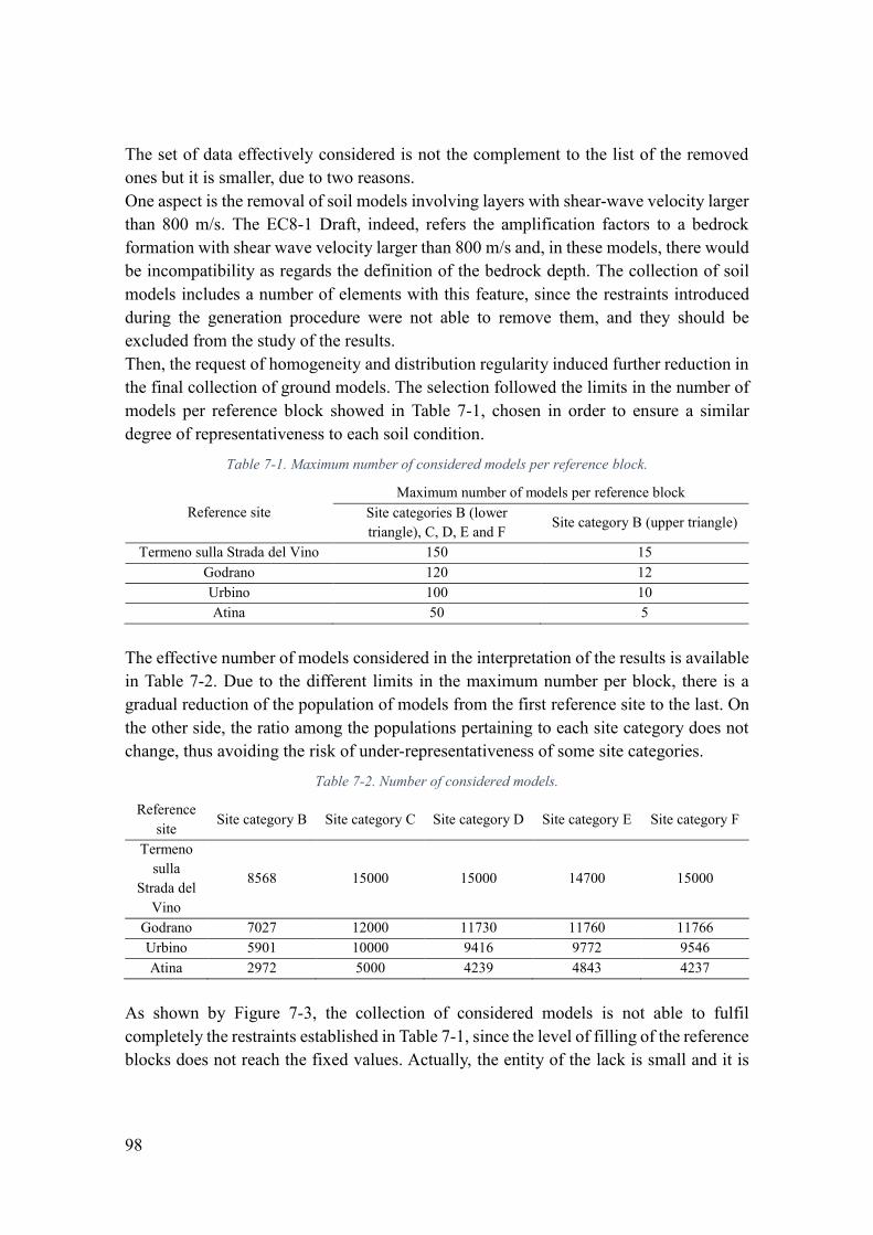
98
The set of data effectively considered is not the complement to the list of the removed ones but it is smaller, due to two reasons. One aspect is the removal of soil models involving layers with shear-wave velocity larger than 800 m/s. The EC8-1 Draft, indeed, refers the amplification factors to a bedrock formation with shear wave velocity larger than 800 m/s and, in these models, there would be incompatibility as regards the definition of the bedrock depth. The collection of soil models includes a number of elements with this feature, since the restraints introduced during the generation procedure were not able to remove them, and they should be excluded from the study of the results. Then, the request of homogeneity and distribution regularity induced further reduction in the final collection of ground models. The selection followed the limits in the number of models per reference block showed in Table 7-1, chosen in order to ensure a similar degree of representativeness to each soil condition.
Table 7-1. Maximum number of considered models per reference block.
Reference site Maximum number of models per reference block
Site categories B (lower triangle), C, D, E and F
Site category B (upper triangle)
Termeno sulla Strada del Vino 150 15 Godrano 120 12 Urbino 100 10 Atina 50 5
The effective number of models considered in the interpretation of the results is available in Table 7-2. Due to the different limits in the maximum number per block, there is a gradual reduction of the population of models from the first reference site to the last. On the other side, the ratio among the populations pertaining to each site category does not change, thus avoiding the risk of under-representativeness of some site categories.
Table 7-2. Number of considered models.
Reference site
Site category B Site category C Site category D Site category E Site category F
Termeno sulla
Strada del Vino
8568 15000 15000 14700 15000
Godrano 7027 12000 11730 11760 11766 Urbino 5901 10000 9416 9772 9546 Atina 2972 5000 4239 4843 4237
As shown by Figure 7-3, the collection of considered models is not able to fulfil completely the restraints established in Table 7-1, since the level of filling of the reference blocks does not reach the fixed values. Actually, the entity of the lack is small and it is

99
more concentrated in the regions where the analysis is less reliable, i.e. the ones corresponding to deposits with small values of shear-wave velocity or to deep and stiff soil deposits.
Figure 7-3. Pseudo-colour plots representing the number of effectively considered results per block.

100
7.3: Definition of the reference parameters The statistical analysis and the assessment of the amplification factors proposed by the EC8-1 Draft consider a number of parameters, which should be synthetic indicators for the description of the ground response. Since the assessment refers to the response of soil deposit to an assigned seismic motion, the analysis evaluates the ratio between each ground motion parameter evaluated at the surface and the corresponding one of the input motion, as proxy of the amplification factors.
The first parameter is the zero-period amplification factor 𝐹𝑇 = 0 𝑠, defined as the ratio between the values of peak ground acceleration at the free surface and of the input motion.
𝐹𝑇 = 0 𝑠 =𝑃𝐺𝐴𝑠𝑢𝑟𝑓𝑎𝑐𝑒
𝑃𝐺𝐴𝑟𝑜𝑐𝑘 (Eqt. 7-1)
The attribute “zero-period” recalls the fact that the peak ground acceleration corresponds to the spectral ordinate evaluated at vibration period equal to 0 s. The zero-period amplification factor has high variability and dispersion, since it derives from two peak singular values. Despite this limitation, this study includes an analysis over this parameter because it may be considered as indicator of the short period amplification factor 𝐹𝛼. Furthermore, the assessment is useful for the verification of the reliability of simplified approaches for the prediction of peak ground acceleration at the site, as this parameter is employed in several fields, e.g. preliminary assessments about liquefaction or slope stability.
In a similar way, the description of the behaviour at larger vibration periods refers to the intermediate period amplification factor 𝐹𝑇 = 1 𝑠, computed as ratio between the surface and the input spectral acceleration ordinates at vibration period equal to 1 s.
𝐹𝑇 = 1 𝑠 =𝑃𝑆𝐴𝑠𝑢𝑟𝑓𝑎𝑐𝑒(𝑇 = 1 𝑠)
𝑃𝑆𝐴𝑟𝑜𝑐𝑘(𝑇 = 1 𝑠) (Eqt. 7-2)
Due to this definition, the parameter may be representative of the intermediate period amplification factor 𝐹𝛽.
The introduced indicators, since depending of single spectral ordinates, do not have a robust definition and assume significant dispersion.
In order to manage the high degree of variability and enhance the level of control on amplification factors, the study refers also to some integral parameters for the definition of the amplification parameter. The reference integral parameter is the spectral intensity, firstly introduced by Housner [71] for spectral velocities and then adapted to spectral accelerations by Rey et al. [72], as shown by (Eqt. 7-3).

101
𝐼 = ∫ 𝑃𝑆𝐴(𝑇)𝑑𝑇
2.5
0.05
(Eqt. 7-3)
With reference to spectral intensity, the definition of the global spectral amplification factor 𝐹𝑆𝐴 is possible.
𝐹𝑆𝐴 =𝐼𝑠𝑢𝑟𝑓𝑎𝑐𝑒
𝐼𝑟𝑜𝑐𝑘 (Eqt. 7-4)
This parameter evaluates the average behaviour of the spectrum, as it derives from the integral of the response spectrum across short vibration periods and intermediate vibration periods. Therefore, it may be useful for the assessment in terms of global spectrum behaviour.
On the other side, the global spectral amplification factor is not able to separate the short period term from the long period one and it is not adequate for the specific assessment of the single amplification factors. In order to go beyond this limitation, the analysis evaluates other three integral parameters, one referred to short periods, one to intermediate periods and the last to long periods. Their definition is equivalent to the spectral intensity, except the integration boundaries.
Short period spectral intensity.
𝐼𝑇=0.1−0.5 𝑠 = ∫ 𝑃𝑆𝐴(𝑇)𝑑𝑇
0.5
0.1
(Eqt. 7-5)
Intermediate period spectral intensity.
𝐼𝑇=0.4−0.8 𝑠 = ∫ 𝑃𝑆𝐴(𝑇)𝑑𝑇
0.8
0.4
(Eqt. 7-6)
Long period spectral intensity.
𝐼𝑇=0.7−1.1 𝑠 = ∫ 𝑃𝑆𝐴(𝑇)𝑑𝑇
1.1
0.7
(Eqt. 7-7)
To these spectral intensities, new definitions of spectral amplification factor correspond. Short period spectral amplification factor.
𝐹𝑇=0.1−0.5 𝑠 =
𝐼𝑇=0.1−0.5 𝑠,𝑠𝑢𝑟𝑓𝑎𝑐𝑒
𝐼𝑇=0.1−0.5 𝑠,𝑟𝑜𝑐𝑘 (Eqt. 7-8)
Intermediate period spectral amplification factor.
𝐹𝑇=0.4−0.8 𝑠 =
𝐼𝑇=0.4−0.8 𝑠,𝑠𝑢𝑟𝑓𝑎𝑐𝑒
𝐼𝑇=0.4−0.8 𝑠,𝑟𝑜𝑐𝑘 (Eqt. 7-9)
Long period spectral amplification factor.
𝐹𝑇=0.7−1.1 𝑠 =
𝐼𝑇=0.7−1.1 𝑠,𝑠𝑢𝑟𝑓𝑎𝑐𝑒
𝐼𝑇=0.7−1.1 𝑠,𝑟𝑜𝑐𝑘 (Eqt. 7-10)
The intervals of vibration periods are not arbitrary, but they derive from microzonation

102
applications [73]. In particular, these factors cover a wide range of the response spectra and attempt to monitor the passage from the short-period behaviour to the long-period behaviour.

103
7.4: Evaluation of the variability of the results The analysis of the variability of soil amplification parameters evaluates the dispersion characteristics of the results of the ground response analyses, in terms of the aforementioned amplification parameters. The aim of this study is the assessment of the effectiveness of the prescriptions introduced by the EC8-1 Draft with respect to the current version of EC8-1, in terms of inter-class dispersion. The EC8-1 Draft, indeed, modifies the criteria for site categorization and introduces a more complex method for the estimate of site amplification factors, in order to reduce the uncertainties in the evaluation of the seismic action. For this purpose, the study computes a synthetic parameter representing the data variability, i.e. the coefficient of variation 𝐶𝑉, for each site category. The value is then compared with the one obtained according to the site categorisation defined by the current version of EC8-1. The new approach will be considered efficient if it produces a reduction in the data variability with respect to the other method. For the sake of simplicity, the assessment refers only to the global spectral amplification factor 𝐹𝑆𝐴, since it is a global parameter describing the overall response of ground models, involving the short period contribution and the long period contribution.
7.4.1: Variability of the results in EC8-1 Draft approach
The computation of the coefficient of variation of the spectral amplification factor in the EC8-1 Draft scheme is not a simple operation. Indeed, the analysis should evaluate the statistical characteristics of this parameter, taking into account that it depends on equivalent shear-wave velocity 𝑣𝑆,𝐻 (and bedrock depth 𝐻800, in site category E) in a continuous way. The double parametrisation would force to work in a two-dimensional or three-dimensional environment, implying several issues either in the statistical computation or in the visualisation of the results. In particular, the direct aggregation of the data pertaining to each site category is not possible, otherwise their continuous dependence from velocity and depth would be disregarded.
Therefore, the statistical analysis refers to the subdivision of the 𝑣𝑆,𝐻-𝐻800 domain into regular blocks, introduced during the definition of the database of ground models (more details in 5.3.3). In particular, the procedure clusters the results in each block, as function of the values of 𝑣𝑆,𝐻 and 𝐻800 of every soil model, according to the following methods.
In site categories B, C, D and F, where site amplification factors depend only on equivalent shear-wave velocity, data are clustered according to ranges of velocities, whose extent corresponds to the size of the reference blocks.
In site category E, where amplification factors depend on equivalent shear-wave velocity and bedrock depth, results are clustered in each reference block.

104
Then, having observed that the collection of parameters pertaining each block is lognormally distributed, the procedure computes the correspondent coefficient of variation, according to (Eqt. 7-11).
𝐶𝑉(%) = √𝑒𝜎ln𝐹𝑆𝐴 − 1 × 100 (Eqt. 7-11)
Finally, the procedure evaluates the value of coefficient of variation for each site category, through an operation of mean among the values of the discrete elements falling inside it.
This way of interpretation of data distribution is not rigorous, since the clustering into discrete blocks might cause the loss of some information about the actual distribution and its dependence with respect to 𝑣𝑆,𝐻 and 𝐻800. On the other side, the loss is not significant because the size of the blocks is quite small with respect to the domain and the variation of the parameters within each cluster is small. Moreover, this approximation is acceptable for the computation of first-order statistic moments such as mean and variance.
7.4.2: Variability of the results in EC8-1 approach
The second step evaluates the variability of the results of the analysis when clustered according to the site categorisation system defined by the current version of EC8-1 [20].
The rules for the definition of site categories are different from the ones proposed by the EC8-1 Draft, since classes B, C and D are defined for soil deposits deeper than 30 m, whereas class E corresponds to shallow deformable deposits. Therefore, the classification does not consider a group of shallow soil deposits, having bedrock depth ranging between 20 m and 30 m. In order to avoid the removal of an excessive number of models, the present study reduces the lower bound of bedrock depth for classes B, C and D to 20 m, as shown by Figure 7-4.
In this case, since the approach does not take into assume continuous dependence of amplification factors from equivalent shear-wave velocity and bedrock depth, the procedure computes the coefficient of variation from the collection of data pertaining to each site category in a direct way, without any discretisation of the reference domain. Regardless the different boundaries of site categories, the coefficients of variation should be larger or equal than the ones computed according to EC8-1 Draft, as computed assuming fixed mean and not from a mobile mean, which suits better the data.

105
Figure 7-4. Representation of standard site categorisation in the 𝑣𝑆,30-𝐻800 domain, according to the EC8-1 prescriptions.
7.4.3: Comparison of dispersion parameters
The comparison of dispersion parameters, with reference to the EC8-1 Draft and EC8-1 classification systems, provides different results as function of the site category, as shown in Figure 7-5, Table 7-3 and Table 7-4.
The comparison indicates a reduction of variability of the results in the scheme proposed by the EC8-1 Draft, from the general point of view. The variation is significant in site category C, with an average decrease of 5 units, but the reduction rises up to 20% of the value when seismicity is quite low. The reduction is large also in site category E, with a passage of average coefficient of variation from 15% to 10%. On the opposite, the reduction is smaller in site category B. As regards site category D, the new subsoil classification allows a reduction of the degree of variability, even though the final value is still high.

106
Figure 7-5. Coefficients of variation with reference to the global spectral amplification, obtained
according to the EC8-1 and EC8-1 Draft approaches.
Table 7-3. Coefficients of variation with reference to the global spectral amplification, obtained with the EC8-1 classification scheme.
Reference site Site category B C D E 𝐶𝑉̅̅ ̅̅ (%) per site
Termeno sulla Strada del Vino
CV (%) 17.4 16.7 22.3 13.7 18.0
Godrano CV (%) 16.1 18.3 26.4 13.7 18.4 Urbino CV (%) 15.6 20.1 29.5 16.2 19.6 Atina CV (%) 16.2 22.2 28.4 16.3 20.7 𝐶𝑉̅̅ ̅̅ (%) per category 16.4 19.0 25.5 14.5 Global value of coefficient of variation 𝑪𝑽𝑬𝑪𝟖−𝟏̅̅ ̅̅ ̅̅ ̅̅ ̅̅ ̅ (%) 18.8
Table 7-4. Coefficients of variation with reference to the global spectral amplification, obtained with the EC8-1 Draft classification scheme.
Reference site
Site category
B C D E F 𝐶𝑉̅̅ ̅̅ (%) per site
Termeno sulla Strada del Vino
CV (%) 15.9 12.2 18.3 9.5 18.8 14.9
Godrano CV (%) 15.3 13.1 22.1 9.8 19.5 16.0 Urbino CV (%) 14.9 14.8 25.3 11.2 20.7 17.5 Atina CV (%) 15.7 16.9 26.7 12.1 22.7 18.8 𝐶𝑉̅̅ ̅̅ (%) per category 15.4 13.6 21.9 10.3 19.9 Global value of coefficient of variation 𝑪𝑽𝑫𝒓𝒂𝒇𝒕̅̅ ̅̅ ̅̅ ̅̅ ̅̅ (%) 16.3

107
Figure 7-6. EC8-1 Draft site categorisation system versus EC8-1 site categorisation system.
Focusing on site category B, a possible reason of the reduction of variability might be the continuous parametrisation of the site amplification factors with respect to equivalent shear-wave velocity. Indeed, the response of the soil deposits falling in this site category is widely influenced by the impedance contrast and so by the shear wave velocity. This aspect may explain the reason for which the entity of the reduction does not depend on the intensity of the seismic action in a strong way. Larger seismicity, indeed, induces partial loss of the dependence of the results from equivalent shear-wave velocity, due to nonlinearity. Actually, this aspect does not produce significant reduction of the variability with respect to the EC8-1 approach, probably because the new scheme includes the contribution of stiff shallow soil deposits (Figure 7-6), which were disregarded in the old categorisation system.
As regards site categories C and D, the significant reduction in their variability may be due to the different geometry of the regions pertaining to them in the 𝑣𝑆,𝐻-𝐻800 domain (or 𝑣𝑆,30-𝐻800 domain), as shown in Figure 7-6. In particular, the new approach deals with deep soil models in a different way, clustering them in site category F. Indeed, the correspondent degree of variability is quite high, with an average value of the coefficient of variation equal to 20%. Furthermore, in site category C, another aspect contributing in the reduction of variability is the adoption of the continuous parametrisation of site amplification factors with respect to equivalent shear-wave velocity, since the results show a dependence from this parameter, as highlighted in Figure 7-7.

108
In site category D, the results are slightly independent of equivalent shear-wave velocity. Therefore, the continuous parametrisation of amplification factors with respect to shear wave velocity is not effective and the value of the coefficient of variation is higher than in the other subsoil classes, when evaluated according to the EC8-1 Draft scheme. The variability may be related to other parameters significant for the behaviour of deformable soil models. For instance, soil models falling in site category D show large variability in the equivalent plasticity index (Figure 5-8) and this might be responsible of the dispersion of the results in this field. Furthermore, the value of the coefficient of variation computed in the EC8-1 scheme is very large, since the correspondent field of equivalent velocities ranges from 100 m/s to 180 m/s (Figure 7-6) and includes ground models characterised by very high deformability, for which the analysis according to the equivalent linear approach is not recommended. As consequence, due to the procedure of filtering, this category involves a limited number of results, with respect to the other categories, and the dispersion tends to be larger.
Figure 7-7. Evolution of global spectral amplification factor with equivalent shear-wave velocity in site
categories B, C and D (reference site: Termeno sulla Strada del Vino).
A large reduction of variability occurs also in site category E, where the average coefficient of variation passes from 15% to 10%. A reason of this reduction is the redistribution of the results in the reference domain due to the different way of computation of the equivalent shear-wave velocity. Then, the parametrisation of site amplification factors with respect to shear-wave velocity and bedrock depth is effective for this site category in reducing uncertainties. This aspect explains the dependence of the reduction in the coefficient of variation with respect to seismicity, due to nonlinear effects.
As global result, the new approach proposed by the EC8-1 Draft reduces the overall

109
variability from 19% to 16%. In this sense, the approach seems to improve the management of the variability of the amplification factor, thanks to the new definition of the equivalent shear-wave velocity, the new standard site categories and the parametrisation of site amplification factors with respect to shear wave velocity and bedrock depth. Actually, the degree of accuracy for the computation of site amplification factors is not uniform. In particular, the approach is quite effective in presence of stiff soil deposits, where average shear-wave velocity plays a primary role, and for shallow deformable ones, whose behaviour mainly depends on shear wave velocity and bedrock depth. Then, the separation of between deep and intermediate deep deformable soil deposits entails a reduction of the variability in the latter case, whereas the parametrisation with respect to shear wave velocity is not useful for this purpose and it should refer to other properties.

110
7.5: Comparison of the amplification parameters The previous step analysed the variability of the results of ground response analyses within each site category, in order to assess the effectiveness of the parametrisation proposed for site amplification factors. The next passage focuses on the specific values of site amplification factors proposed by the EC8-1 Draft, performing a comparison between them and the ones derived from the results of ground response analyses. In this way, the present study evaluates the reliability of the site amplification factors introduced by the draft itself.
The assessment of site amplification factors is a delicate operation, as it requires the definition of synthetic and reliable parameters descriptors of the amplification. On one side, the analysis refers to the zero-period and the intermediate period amplification factors. The first parameter, indeed, is useful to assess the reliability of the short period amplification factor for the computation of the peak ground acceleration, whereas the second one is linked with the intermediate site amplification factor. On the other side, the analysis does not refer only to punctual parameters, as affected by large variability, but also to integral parameters. The integral parameters, indeed, are more stable and fit well the global definition of the response spectrum. The study attempts also to take into account the period-dependence of the amplification, by “splitting” the integral parameter into values referred to different intervals of vibration periods. As consequence, the reference parameters adopted for this study are the following ones.
Zero-period amplification factor.
Intermediate period amplification factor.
Global spectral amplification factor.
Short period spectral amplification factor.
Intermediate period spectral amplification factor.
Long period spectral amplification factor.
Due to the site-dependent and category-dependent definition of amplification factors, the check applies for each single site category inside each reference site. In particular, the analysis compares the data distribution inside each category with the trend defined according to the equations indicated by the EC8-1 Draft. The check takes place in a graphical form, inside the two-dimensional domain given by equivalent shear-wave velocity 𝑣𝑆,𝐻 and the amplification parameter for site categories B, C, D and F. In these categories, indeed, the only independent variable is shear-wave velocity. In order to facilitate the comparison, the representation involves the curves representing the mean value and the mean value plus or minus one standard deviation,

111
computed assuming lognormal distribution. Furthermore, since the amplification function is continuous in the passage from category B to C and C to D, these categories are aggregated into a unique plot. In site category E, the presence of two independent variables 𝑣𝑆,𝐻 and 𝐻800 forces to adopt a three-dimensional representation for the comparison, with the overlapping of the ideal surface proposed by the EC8-1 Draft and the surface corresponding to the mean value of the results. For the sake of simplicity, the plot does not include the extreme boundaries representing the data variability, in order to avoid difficulties in the visualisation. The results of this procedure are not reported in this study, but they are attached to it (from Appendix E to Appendix J).
Coupled with this rigorous procedure of assessment, the study reports the results in a more synthetic and compact manner. This method consists of evaluating the frequency with which the formulation proposed by the EC8-1 Draft provides an overestimation of the amplification with respect to the distribution of the results of the analysis, giving a value on the safe side. The results in the following sections indicate it as “frequency of exceedance” and the higher is the value,
the safer the estimate provided by the EC8-1 is. In particular, a frequency of 50% corresponds to a case where the theoretical curve derived from the proposed values is close to the mean of the distribution of the results. Larger frequencies, instead, correspond to cases where the theoretical curve lies in the upper portion of the distribution, giving an overestimation with respect to the mean value.
The study evaluates also the reliability of the default values of the site amplification factors proposed by the EC8-1 Draft (Table 2-5). Since the default values are constant within each site category, the procedure of assessment is simpler. The method compares the distribution of amplification factor, derived from the results of ground response analyses, with the default value for each site category. The distribution is represented by the mean value and the interval defined by one standard deviation, computed clustering the data in each site category, without taking into account the specific role of equivalent shear-wave velocity or bedrock depth.

112
7.5.1: Comparison at short vibration periods
The check starts from the comparison of the amplification factors conceived for the description of the response at short vibration periods, i.e. the zero-period amplification factor and the short period spectral amplification factor. In this way, the assessment of the reliability at short vibration periods of EC8-1 Draft’s indications is possible.
The comparison between the distribution of the results and the proposed values is available in Appendix E. The use of the factor proposed by the EC8-1 Draft provides an underestimation with respect to the distribution of the values obtained through the ground response analyses. The difference is significant, since the estimated points lie below the standard deviation intervals of the results for a large number of cases, especially in the stiffest site categories under small seismic actions. As shown by Figure 7-8, only deformable models present a significant frequency of exceedance, reaching the 50% in site category D.
A similar result is obtained with reference to the default value proposed by the EC8-1 Draft, where there is a significant underestimation in presence of small seismic action (Figure 7-9). When seismic action increases, the value predicted according to EC8-1 Draft is closer to the mean value of the distribution of the results. This aspect is relevant in site categories representing deformable soil deposits (D, E and F), where the gradual lowering of the distribution of results – due to nonlinearity – determines a better adaption with respect to the predicted values. Similar situation occurs for site categories B and C, but the variation in the first case is less significant and the degree of underestimate is still high.
As regards the short period spectral amplification factor, the situation is similar to what observed for the zero-period amplification factor, where the prediction provided by the EC8-1 Draft underestimates the distribution of the results. Actually, as shown in Figure 7-10, the comparison highlights a bigger number of cases where the estimate is larger than the mean value of the distribution of the results. In particular, even though site category B continues to present predominant underestimation, the other site categories assume higher frequencies of overestimation, especially when seismic action is larger. Indeed, the frequency ranges from 25% to 75% in high seismicity sites. More details about the comparison between the distribution of the results and the proposed values is available in Appendix F.
This aspect is more evident in the comparison of the result distribution with respect to the default value introduced by the EC8-1 Draft. In all cases, indeed, the proposed value for site amplification factor at short periods lies within the boundaries of the distribution, defined by one standard deviation (Figure 7-11).

113
Figure 7-8. Frequency of situations where the prediction according to EC8-1 Draft provides a larger
value of zero-period amplification factor with respect to the results.
Figure 7-9. Comparison among the values of zero-period amplification factor derived from the results of
the analysis and the default values of the EC8-1 Draft for the reference sites.

114
Figure 7-10. Frequency of situations where the prediction according to EC8-1 Draft provides a larger
value of short period spectral amplification factor with respect to the results.
Figure 7-11. Comparison among the values of short period spectral amplification factor derived from the
results of the analysis and the default values of the EC8-1 Draft for the reference sites.

115
Figure 7-12 shows the distribution of the factors for stratigraphic amplification at short periods, with reference to site categories B, C and D in Termeno sulla Strada del Vino site. The integral factor tends to assume smaller values, especially in stiff soil deposits. As a consequence, the estimate according to EC8-1 Draft is still smaller than the mean value, but it falls within the standard deviation boundaries. The difference in the results of the check is not only an effect of the different nature of the involved parameters, i.e. punctual value versus integral parameter. The estimate of peak ground acceleration, indeed, is not reliable with equivalent linear analyses, since this value is the result of ground motion components at very high frequencies, whereas the analysis considers a frequency up to 15 Hz or 25 Hz (see 4.2.2). Therefore, the spectral factor is more reliable not only thanks to its integral nature, but also because its field of integration, ranging from 0.1 to 0.5 s, includes a portion of the adopted field of frequencies. As result, if the short period spectral amplification factor is assumed as reference, the EC8-1 Draft formulation provides an underestimation of the stratigraphic amplification with respect to the results of the analyses, but it lies within the boundaries of the distribution.
Figure 7-12. Distribution of zero-period amplification factor and short period spectral amplification
factor (reference site: Termeno sulla Strada del Vino; site categories B, C and D).

116
7.5.2: Comparison at intermediate vibration periods
The evaluation of reliability of the EC8-1 Draft’s indications at intermediate vibration periods refers to the intermediate period amplification factor and to the long period spectral amplification factor.
The comparison between the distribution of the results and the proposed values is available in Appendix G. Comparing the intermediate period soil amplification factor and the correspondent site amplification coefficient (Figure 7-14), the formulation proposed by the EC8-1 Draft provides a slightly larger estimate with respect to the mean value observed in the ground response analyses. In particular, the frequency of exceedance is much higher with respect to what observed at short vibration periods, especially in deformable soil deposits (site categories D, E and F), where the frequency of overestimation is larger than 70%. In this sense, the situation is specular with respect to the zero-period soil amplification factor. In the other site categories, the frequency is about 50%, meaning that the proposed value falls close to the mean value of the distribution, as shown by Figure 7-13.
Figure 7-13. Distribution of intermediate period amplification factor (reference site: Godrano; site
categories B, C and D).
In a similar way, the comparison of the result distribution with respect to the default value introduced by the EC8-1 Draft shows that the latter provides an overestimation with respect to the results, regardless the site category and the seismic action (Figure 7-15). The gap is particularly large in site categories E and F, where the default value is twice the mean value of the analysis results.

117
Figure 7-14. Frequency of situations where the prediction according to EC8-1 Draft provides a larger
value of intermediate period amplification factor with respect to the results.
Figure 7-15. Comparison among the values of intermediate period soil amplification factor derived from
the results of the analysis and the default values of the EC8-1 Draft for the reference sites.

118
The long period spectral amplification factor assumes a similar behaviour to the intermediate period soil amplification factor, since the range of periods for the integration is almost centred at 1 s. In particular, the EC8-1 Draft tends to provide an estimate close to the mean of the distribution of the results in this field, as the frequency of exceedance is about 50% (Figure 7-16). In case of deformable site categories, the frequency of is higher and reaches 80%. More details are available in Appendix H. A similar result is visible in the comparison with the default value proposed by the EC8-1 Draft (Figure 7-17).
Figure 7-16. Frequency of situations where the prediction according to EC8-1 Draft provides a larger
value of long period spectral amplification factor with respect to the results.

119
Figure 7-17. Comparison among the values of long period spectral amplification factor derived from the
results of the analysis and the default values of the EC8-1 Draft for the reference sites.
Since the assessments conducted at short and long vibration periods led to such different results, the study also evaluates what happens in the transition field. For this purpose, the reference is the intermediate period spectral amplification factor, evaluated for vibration periods ranging from 0.4 s to 0.8 s. As expected, the prediction according to EC8-1 Draft estimates the value of amplification close to the mean of the results of the ground response analyses, since the frequency of exceedance is about 50% (Figure 7-18). Godrano site present smaller values of frequency of overestimation since the predicted value falls at the lower bound of the standard deviation interval. More details are available in Appendix I. The default values, instead, provide systematically a result on the safe side with respect to the distribution, as shown by Figure 7-19.

120
Figure 7-18. Frequency of situations where the prediction according to EC8-1 Draft provides a larger
value of intermediate period spectral amplification factor with respect to the results.
Figure 7-19. Comparison among the values of intermediate period spectral amplification factor derived
from the results of the analysis and the default values of the EC8-1 Draft for the reference sites.

121
7.5.3: Global spectral amplification factor
The analysis refers to the global spectral amplification factor, in order to obtain indications about the quality of the estimate according to the EC8-1 Draft’s provisions with respect of the experimental results, in average terms over a wide range of vibration periods.
The comparison between the distribution of the results and the proposed values is available in Appendix J. Since the indications of the EC8-1 Draft tends to underestimate the results at short vibration periods and overestimate them at long vibration periods, the theoretical trend of global spectral amplification factor, computed according to the EC8-1 Draft, is quite well aligned to the mean of the distribution of the results of the analysis, as shown in Figure 7-20.
Figure 7-20. Distribution of global spectral amplification factor (reference site: Termeno sulla Strada del
Vino; site categories B, C and D).
As consequence, the frequency of exceedance mainly varies from 15% to 50%, which means that the predicted value is ranging from the mean to the lower bound of the standard deviation interval. The frequency is higher in case of site categories representing deformable soils subjected to high levels of seismicity (Figure 7-21). Focusing on the default value proposed by the EC8-1 Draft, it provides an estimate on the safe side of the results of the analysis, especially in case of deformable soils (Figure 7-22).
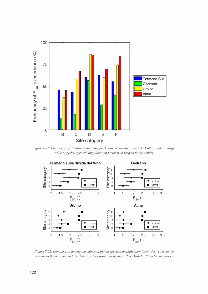
122
Figure 7-21. Frequency of situations where the prediction according to EC8-1 Draft provides a larger
value of global spectral amplification factor with respect to the results.
Figure 7-22. Comparison among the values of global spectral amplification factor derived from the
results of the analysis and the default values proposed by the EC8-1 Draft for the reference sites.

123
Chapter 8: Conclusions
The thesis is a study of the ground response in seismic conditions, aiming to assess the effectiveness and the reliability of the simplified approaches proposed by building codes, with particular reference to the Final Draft of revision of Eurocode 8.
The first section evaluates the instrumental approach to site characterisation, which is a new methodology for subsoil classification based on the results of HVSR tests, alternative to the standard procedure. A comparative analysis of the two categorisation systems has been carried out, with reference to a number of sites selected from the Italian Strong Motion Network and the Swiss Strong Motion Network. The test showed a good degree of compatibility between the standard method and the instrumental procedure, especially in presence of stiff soil deposits. On the other side, the instrumental approach is less accurate for sites characterised by larger deformability. Furthermore, the new method conflicts with the standard one in presence of shallow soil deposits made with deformable materials. In order to solve this issue, the approach should take into account the restraint due to equivalent shear-wave velocity for the attribution of the site category A, instead of considering only the fundamental frequency, through the limitation of the range of possible velocities only to values larger than 250 m/s. Since the collection of data was limited and not equally representative of all site categories – the dataset was poor of elements falling in site categories A or D –, this result should be interpreted as a first stage assessment of the validity of the instrumental approach and a first reference for further improvements of this approach.
The main corpus of this thesis consisted of an assessment of the simplified approach for the estimate of ground response in seismic conditions introduced by the Draft. For this purpose, the study performed ground response analyses adopting the equivalent linear method over a wide set of one-dimensional soil models, generated through a stochastic procedure from a sample of real deposits, taken from accredited databases or personal communications. The reference input motion consisted of a set of spectrum-compatible and seismo-compatible acceleration time histories referred to a number of sites, each one representative of a specific level of seismic hazard. The interpretation of the results started with a preliminary step of filtering in order to remove unreliable data. This passage highlighted the potential unreliability of the simplified approach for deep soil deposits with deformable surficial layers, characterised by values of average shear-wave velocity ranging from 150 m/s to 200 m/s, since the equivalent linear analysis is unable to provide reliable results. This aspect becomes significant when the input motion is strong. In order to mitigate this problem, a possible solution would be the reduction of the field of application of the simplified approach, by shifting the lower limit to larger values of equivalent shear-wave velocity, e.g. at 200 m/s,
124
at least in high seismicity sites. The study then compared the classification scheme proposed by the Draft and the one prescribed by the current version of Eurocode 8, aiming at assessing the effectiveness and the accuracy of the new approach in the estimate of site amplification factors. From the global point of view, the categorisation system proposed by the Draft reduces the overall variability from 19% to 15%. In this sense, the approach seems to improve the management of the variability of the amplification factor. One reason of this improvement is the different classification methodology, including a new definition of the equivalent shear-wave velocity – it does not simply refer to 30 m but takes into account bedrock depth – and the introduction of the new site category F, for deep and deformable soil deposits. Furthermore, the continuous parametrisation of site amplification factors with respect to shear wave velocity (and bedrock depth, for site category E) is useful in the reduction of uncertainties, since it takes into account the effect of impedance contrast in the ground response in seismic conditions. Actually, the approach is effective in presence of stiff soil deposits, where average shear-wave velocity plays a primary role, and for shallow deformable ones, whose behaviour mainly depends on shear wave velocity and bedrock depth. In case of deep deformable soil deposits, the proposed parametrisation is not useful in reducing uncertainties and it should refer to other properties, for instance the plasticity index. Finally, the study compared the distribution of the results of ground response analyses with the theoretical model proposed by the Draft, in order to assess the reliability of the predicted site amplification factors. The check evaluated either the continuous formulation of the factors with respect to equivalent shear-wave velocity (and bedrock depth, for site category E) or the default values, adopted in absence of specific information. The comparison showed that the proposed formulations for the amplification factors suit quite well the results with reference to a wide range of vibration periods. In this sense, the standard spectral shape introduced by the Draft is well aligned with the results of ground response analyses, from the global point of view. Actually, the predicted values of amplification factors tend to underestimate the results at short vibration periods, even though in high seismicity sites the proposed formulation fits better the distribution of the results. This aspect represents a limitation of the proposed amplification factors, since they underestimate the peak ground acceleration, thus providing an unsafe result for several applications geotechnical engineering. On the other side, the predicted values overestimate the long period contribution, especially when seismicity is low. Focusing on the default values, the comparison highlighted that they tend to provide an overestimation with respect to the effective distribution of the results. This aspect is a positive note for the new approach, since it provides an estimate on the safe side of seismic action, which is useful in absence of information and for preliminary assessments.

125
: Amplification factors according to EC8-1 Draft A.1: Short period amplification factor
A.1.1: Site categories B, C and D
A.1.2: Site category E (low and very low seismicity)

126
A.1.3: Site category E (moderate seismicity)
A.1.4: Site category E (high seismicity)

127
A.1.5: Site category F

128
A.2: Intermediate period amplification factor
A.2.1: Site categories B, C and D
A.2.2: Site category E (low and very low seismicity)

129
A.2.3: Site category E (moderate seismicity)
A.2.4: Site category E (high seismicity)

130
A.2.5: Site category F
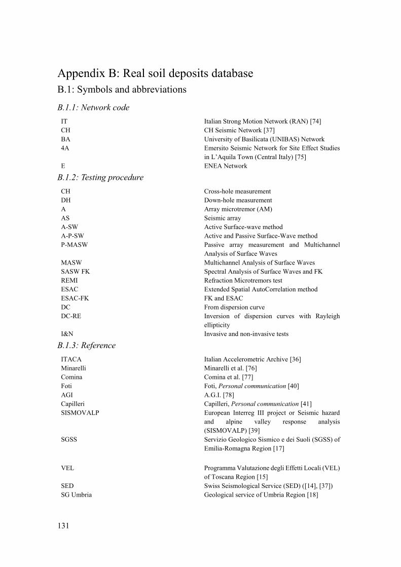
131
: Real soil deposits database B.1: Symbols and abbreviations
B.1.1: Network code IT Italian Strong Motion Network (RAN) [74] CH CH Seismic Network [37] BA University of Basilicata (UNIBAS) Network 4A Emersito Seismic Network for Site Effect Studies
in L’Aquila Town (Central Italy) [75] E ENEA Network
B.1.2: Testing procedure CH Cross-hole measurement DH Down-hole measurement A Array microtremor (AM) AS Seismic array A-SW Active Surface-wave method A-P-SW Active and Passive Surface-Wave method P-MASW Passive array measurement and Multichannel
Analysis of Surface Waves MASW Multichannel Analysis of Surface Waves SASW FK Spectral Analysis of Surface Waves and FK REMI Refraction Microtremors test ESAC Extended Spatial AutoCorrelation method ESAC-FK FK and ESAC DC From dispersion curve DC-RE Inversion of dispersion curves with Rayleigh
ellipticity I&N Invasive and non-invasive tests
B.1.3: Reference ITACA Italian Accelerometric Archive [36] Minarelli Minarelli et al. [76] Comina Comina et al. [77] Foti Foti, Personal communication [40] AGI A.G.I. [78] Capilleri Capilleri, Personal communication [41] SISMOVALP European Interreg III project or Seismic hazard
and alpine valley response analysis (SISMOVALP) [39]
SGSS Servizio Geologico Sismico e dei Suoli (SGSS) of Emilia-Romagna Region [17]
VEL Programma Valutazione degli Effetti Locali (VEL)
of Toscana Region [15] SED Swiss Seismological Service (SED) ([14], [37]) SG Umbria Geological service of Umbria Region [18]

132
B.1.4: Notes NB Bedrock depth is not reached by investigations BG Bedrock depth is not reached by investigations but
it is obtained from geological information NS Absence of evaluation of the quality of H/V peak
according to SESAME criteria X Site not included in the sample for the construction
of the 1-D ground models

133
B.2: Soil deposits database
Num
ber
Net
wor
k co
de
Stat
ion
code
Si
te
𝑣𝑆,𝐻
(m
/s)
𝐻800
(m)
𝑓 0
(Hz)
𝐴0
(-)
SESA
ME
Test
R
efer
ence
N
otes
1 IT
A
LT
Aul
etta
(Pet
ina)
55
8.0
6.0
- -
- P
ITA
CA
-
2 IT
A
QP
L’A
qu
ila
– V
. Ate
rno
– M
. Pet
tino
500.
0 7.
0 -
- -
ESA
C
ITA
CA
-
3 IT
A
SG
Asi
ago
(Roa
na)
750.
0 10
.0
- -
- P- M
ASW
IT
AC
A
-
4 IT
A
VT
Ave
trana
36
4.0
4.0
8.13
5.
8 6
P- MA
SW
ITA
CA
-
5 IT
B
RC
B
arci
s 55
0.0
5.0
12.0
9 4.
4 5
P- MA
SW
ITA
CA
-
6 IT
B
RZ
Ber
sezi
o 25
2.0
1.8
2.56
3.
6 5
MA
SW
ITA
CA
-
7 IT
C
RD
C
ort
ina
d’A
mp
ezzo
60
0.0
5.0
- -
- P- M
ASW
IT
AC
A
-
8 IT
C
RV
C
arov
igno
78
1.0
3.7
- -
- P- M
ASW
IT
AC
A
-
9 IT
G
NV
G
enov
a 36
9.9
3.1
- -
- M
ASW
IT
AC
A
-
10
IT
ISI
Ispi
ca
338.
0 0.
8 -
- -
MA
SW
ITA
CA
-
11
IT
LSS
Leon
essa
(Nuo
va)
700.
0 7.
0 -
- -
P- MA
SW
ITA
CA
-
12
IT
MC
N
Mor
cone
39
8.6
4.5
- -
- D
H
ITA
CA
-
13
IT
MN
N
Man
fredo
nia
414.
7 4.
0 -
- -
P IT
AC
A
-
14
IT
MTC
M
onte
cass
ino
(Cas
sino)
40
0.0
5.0
- -
- ES
AC
IT
AC
A
-
15
IT
RN
C
Rin
cine
(Lon
da)
568.
6 11
.0
- -
- P
ITA
CA
-
16
IT
SCN
Sc
anno
75
0.0
20.0
-
- -
ESA
C
ITA
CA
-

134
Num
ber
Net
wor
k co
de
Stat
ion
code
Si
te
𝑣𝑆,𝐻
(m
/s)
𝐻800
(m)
𝑓 0 (H
z)
𝐴0 (-
) SE
SAM
E Te
st
Ref
eren
ce
Not
es
17
IT
SGR
S.
Gio
rgio
la M
olar
a 68
9.1
13.5
1.
12
3 4
DC
IT
AC
A
-
18
IT
SRT
Sorti
no
628.
5 7.
0 5.
55
7.6
5 P-
MA
SW
ITA
CA
-
19
IT
BG
N
Bag
none
50
2.3
19.0
5.
88
4 6
DH
IT
AC
A
-
20
IT
BZZ
B
azza
no
640.
0 23
.0
- -
- ES
AC
-FK
IT
AC
A
-
21
IT
CLG
C
alta
giro
ne
373.
5 30
.3
- -
- M
ASW
IT
AC
A
-
22
IT
CPS
C
apes
trano
63
3.3
19.0
2.
39
4.6
5 ES
AC
IT
AC
A
-
23
IT
CST
C
aste
lfran
co 5
54
0.8
320.
0 0.
49
3.2
6 P
ITA
CA
-
24
IT
DM
N
Dem
onte
43
8.6
21.4
-
- -
MA
SW
ITA
CA
-
25
IT
GLD
G
ildon
e 42
6.3
24.0
2.
91
7.4
4 P
ITA
CA
-
26
IT
GSN
G
ioia
San
nitic
a 44
1.8
28.5
5.
18
5.2
6 P-
MA
SW
ITA
CA
-
27
IT
LNG
La
nghi
rano
(L
esig
nano
Bag
ni)
427.
7 64
.0
0.61
5.
2 4
P IT
AC
A
-
28
IT
CN
G
Con
eglia
no 5
28
2.8
165.
0 -
- -
P-M
ASW
IT
AC
A
-
29
IT
MA
I M
aian
o 25
5.4
67.0
2.
03
5.2
5 P-
MA
SW
ITA
CA
-
30
IT
NA
S N
aso
291.
1 17
2.7
0.83
5.
6 5
P-M
ASW
IT
AC
A
-
31
IT
NZZ
N
izza
Mon
ferr
ato
328.
2 82
.9
- -
- P-
MA
SW
ITA
CA
-
32
IT
SPS
Spez
zano
del
la S
ila
(Cam
igl.)
31
0.2
29.0
3.
55
6.8
5 ES
AC
IT
AC
A
-
33
IT
MN
S M
onse
lice
226.
8 70
.0
6.31
3.
9 4
P-M
ASW
IT
AC
A
-
34
IT
BTT
2 B
orgo
Otto
mila
- 2
(C
elan
o)
90.4
30
5.4
0.27
9.
9 5
MA
SW
ITA
CA
-
35
IT
CLF
C
olfio
rito
147.
1 54
.0
1.04
6.
2 5
DH
IT
AC
A
-
36
IT
RTI
R
ieti
(Cab
. EN
EL)
168.
3 19
9.0
0.77
10
.7
6 M
ASW
IT
AC
A
-

135
Num
ber
Net
wor
k co
de
Stat
ion
code
Si
te
𝑣𝑆,𝐻
(m
/s)
𝐻800
(m)
𝑓 0 (H
z)
𝐴0 (-
) SE
SAM
E Te
st
Ref
eren
ce
Not
es
37
IT
BR
S B
aris
cian
o 28
6.5
14.0
-
- -
DC
-RE
ITA
CA
-
38
IT
SSC
S.
Cas
cian
o de
i B
agni
30
0.7
14.0
-
- -
DH
IT
AC
A
-
39
IT
FVZ
Fivi
zzan
o 27
7.6
12.0
5.
62
4.1
5 D
H
ITA
CA
-
40
IT
VR
L V
ares
e Li
gure
45
4.4
6.4
- -
- M
ASW
IT
AC
A
- 41
IT
V
SD
Vie
ste
(Dan
te)
502.
9 11
.0
- -
- P
ITA
CA
-
42
IT
AQ
G
L'A
quila
-
V.
Ate
rno
- C
olle
G
rilli
654.
8 24
.0
- -
- D
H
ITA
CA
-
43
IT
BD
T B
adia
Ted
alda
59
2.9
30.0
5.
88
3.9
4 D
C-R
E IT
AC
A
- 44
IT
B
GI
Bag
noli
Irpi
no
498.
3 30
.0
0.71
2.
8 5
CH
IT
AC
A
- 45
IT
C
SC
Cas
cia
530.
0 10
.0
- -
- P
ITA
CA
-
46
IT
CSD
C
aste
l Vis
card
o 44
5.5
27.0
1.
34
3.7
4 P
ITA
CA
-
47
IT
FMG
Fi
amig
nano
59
4.8
13.0
-
- -
DC
IT
AC
A
-
48
IT
GSA
G
ran
Sass
o (L
ab.
INFN
Ass
ergi
) 49
2.3
39.1
-
- -
MA
SW
ITA
CA
-
49
IT
LRG
La
uria
Gal
do
543.
0 24
.0
- -
- D
H
ITA
CA
-
50
IT
MLC
M
alce
sine
42
9.7
35.0
6.
09
5.4
5 P-
MA
SW
ITA
CA
-
51
IT
MR
A
Mar
atea
39
9.2
14.2
-
- -
P IT
AC
A
- 52
IT
M
RV
M
arsi
co V
eter
e 59
0.0
17.0
-
- -
ESA
C
ITA
CA
-
53
IT
MTL
M
atel
ica
578.
7 50
.0
1.18
3.
9 5
P IT
AC
A
- 54
IT
M
ZR
Maz
ara
del V
allo
51
6.6
89.0
-
- -
P-M
ASW
IT
AC
A
- 55
IT
N
RC
N
orci
a 49
8.3
100.
0 -
- -
DC
-RE
ITA
CA
-

136
Num
ber
Net
wor
k co
de
Stat
ion
code
Si
te
𝑣𝑆,𝐻
(m
/s)
𝐻800
(m)
𝑓 0 (H
z) 𝐴0 (-
) SE
SAM
E Te
st
Ref
eren
ce
Not
es
56
IT
NSA
N
icos
ia
464.
8 85
.0
- -
- P-
MA
SW
ITA
CA
-
57
IT
NTE
N
oto
(Are
a EN
EL)
384.
9 7.
7 -
- -
MA
SW
ITA
CA
-
58
IT
OR
P O
rsar
a di
Pug
lia
608.
6 18
.0
- -
- P
ITA
CA
-
59
IT
PCH
Pa
chin
o 45
9.2
14.9
-
- -
MA
SW
ITA
CA
-
60
IT
PGA
Pi
gnol
a 41
8.1
68.5
5.
38
3.8
4 ES
AC
IT
AC
A
-
61
IT
PPL1
Po
rtopa
lo d
i C
apo
Pass
ero
1 67
3.5
11.0
-
- -
P-M
ASW
IT
AC
A
-
62
IT
PZS
Piaz
za a
l Ser
chio
54
5.0
22.5
7.
59
2.9
5 D
H
ITA
CA
-
63
IT
RC
C
Roc
cam
onfin
a 37
5.3
37.0
0.
33
3.3
5 P-
MA
SW
ITA
CA
-
64
IT
RN
S R
onco
Scr
ivia
31
0.5
3.1
- -
- M
ASW
IT
AC
A
-
65
IT
SGIU
A
S.
Giu
liano
di
Pu
glia
A
400.
0 6.
0 -
- -
DH
IT
AC
A
-
66
IT
STL
Satri
ano
di L
ucan
ia
395.
4 53
.5
- -
- ES
AC
IT
AC
A
-
67
IT
STS
S. S
ofia
44
7.9
29.0
-
- -
P-M
ASW
IT
AC
A
-
68
IT
SUS
Susa
39
6.9
8.8
- -
- M
ASW
IT
AC
A
-
69
IT
TDG
To
rre
del G
reco
43
4.7
63.9
-
- -
P IT
AC
A
-
70
IT
TLM
1 To
lmez
zo C
entra
le
- Dig
a A
mbi
esta
1
457.
8 31
.0
2.18
5.
6 5
P-M
ASW
IT
AC
A
-
71
IT
TOR
To
rtoric
i 36
8.1
17.4
5.
62
4 4
MA
SW
ITA
CA
-
72
IT
TRL
Term
inill
o 37
9.7
34.0
2.
65
6.8
5 D
C-R
E IT
AC
A
-
73
IT
VB
M
Vib
o M
arin
a 44
6.5
34.0
4.
95
9 6
ESA
C
ITA
CA
-
74
IT
VBV
V
ibo
Val
entia
45
3.4
24.0
6.
92
3.6
5 ES
AC
IT
AC
A
-
75
IT
AV
Z A
vezz
ano
198.
6 15
8.8
0.75
5.
7 6
MA
SW
ITA
CA
-

137
Num
ber
Net
wor
k co
de
Stat
ion
code
Si
te
𝑣𝑆,𝐻
(m
/s)
𝐻800 (m
) 𝑓 0
(Hz)
𝐴0 (-
) SE
SAM
E Te
st
Ref
eren
ce
Not
es
76
IT
CR
N
Cro
tone
(M
onte
diso
n)
286.
9 43
7.0
0 0
0 P- M
ASW
IT
AC
A
-
77
IT
PGL
Pegl
io
358.
4 35
.0
2.77
4.
4 5
P IT
AC
A
-
78
IT
PTT
Patti
- C
abin
a Pr
imar
ia
251.
4 63
.6
- -
- M
ASW
IT
AC
A
-
79
IT
SRP
Sorb
olo
(Pez
zani
) 21
7.9
280.
0 -
- -
P IT
AC
A
-
80
IT
AQ
A
L'A
quila
- V
. A
tern
o -
F.
Ate
rno
436.
7 18
.0
10.0
1 10
.5
5 D
H
ITA
CA
-
81
IT
NC
R
Noc
era
Um
bra
272.
1 9.
0 7.
41
8.6
6 D
H
ITA
CA
-
82
IT
PLZ
Pala
zzol
o A
crei
de
307.
4 6.
8 -
- -
MA
SW
ITA
CA
-
83
IT
SCR
S.
C
roce
C
amer
ina
298.
5 3.
7 -
- -
MA
SW
ITA
CA
-
84
IT
SCS
S.
Ces
area
Te
rme
323.
0 5.
7 -
- -
P- MA
SW
ITA
CA
-
85
IT
SDM
S.
D
emet
rio
nei V
estin
i 31
4.8
5.0
- -
- D
C
ITA
CA
-
86
IT
TRT
Torto
na
302.
6 12
.7
- -
- M
ASW
IT
AC
A
-
87
IT
TRR
Tr
icar
ico
522.
6 56
.0
- -
- C
H
ITA
CA
-
88
IT
AR
N
Arie
nzo
200.
0 8.
0 7.
94
6.2
6 R
EMI
ITA
CA
-
89
IT
BSC
B
isac
cia
350.
0 8.
0 -
- -
CH
IT
AC
A
-

138
Num
ber
Net
wor
k co
de
Stat
ion
code
Si
te
𝑣𝑆,𝐻
(m
/s)
𝐻800
(m)
𝑓 0
(Hz)
𝐴0
(-)
SESA
ME
Test
R
efer
ence
N
otes
90
Mira
bello
18
1.7
290.
0 -
- -
DH
M
inar
elli
-
91
Mira
ndol
a 21
8.7
113.
0 -
- -
DH
M
inar
elli
-
92
IT
MR
N
Mira
ndol
a (N
apol
i) 21
0.0
116.
0 0.
71
7.6
6 C
H
ITA
CA
-
93
Cat
ania
19
4.6
30.0
-
- -
A-P
-SW
C
omin
a N
B
94
Torr
e Pe
llice
28
5.7
30.0
-
- -
A-S
W
Com
ina
BG
95
Pisa
18
5.5
70.0
-
- -
A-P
-SW
C
omin
a N
B
96
Salu
ggia
38
6.0
46.0
-
- -
A-S
W
Com
ina
NB
97
Roj
o Pi
ano
332.
6 30
.0
- -
- A
-P-S
W
Com
ina
NB
98
Pian
ola
303.
2 30
.0
- -
- A
-P-S
W
Com
ina
NB
99
Ces
ana
Pario
l 1
348.
1 18
.0
- -
- SA
SW
Foti
NB
100
Ces
ana
Pario
l 2
337.
4 18
.0
- -
- SA
SW
Foti
NB
101
Ces
ana
Pario
l 3
318.
0 15
.0
- -
- SA
SW
Foti
NB
102
Ces
ana
Pario
l 4
353.
6 20
.0
- -
- SA
SW
Foti
NB
103
Ces
ana
Pario
l 5
430.
8 25
.0
- -
- SA
SW
Foti
NB
104
Mat
hi
460.
9 39
.0
- -
- A
-P-S
W
Foti
-
105
Ver
zuol
o 43
9.1
11.0
-
- -
SASW
FK
Fo
ti -
106
Pian
cast
agna
io C
ampo
Sp
ortiv
o 31
6.6
12.0
-
- -
SASW
Fo
ti -
107
Pian
cast
agna
io P
arco
27
0.3
8.0
- -
- SA
SW
Foti
-
108
Mas
sa M
aritt
ima
333.
1 13
.0
- -
- SA
SW
FK
Foti
-
109
Sarz
ana
483.
4 30
.0
- -
- SA
SW
FK
Foti
NB

139
Num
ber
Net
wor
k co
de
Stat
ion
code
Si
te
𝑣𝑆,𝐻
(m
/s)
𝐻800
(m)
𝑓 0
(Hz)
𝐴0
(-)
SESA
ME
Test
R
efer
ence
N
otes
110
Fuci
no
105.
6 40
.0
- -
- D
H
AG
I N
B
111
Pont
rem
oli B
occi
ofila
46
4.4
8.5
- -
- D
H
Foti
-
112
Pont
rem
oli 1
°Mag
gio
403.
3 7.
5 -
- -
DH
Fo
ti -
113
Pont
rem
oli A
SL
329.
9 6.
5 -
- -
DH
Fo
ti -
114
Pont
rem
oli
Parc
o G
ioch
i 40
0.9
9.0
- -
- D
H
Foti
-
115
Pian
a di
Cat
ania
19
2.2
55.0
-
- -
DH
C
apill
eri
BG
116
Cas
teln
uovo
di
G
arfa
gnan
a 1
476.
5 26
.5
- -
- D
H
Foti
-
117
Cas
teln
uovo
di
G
arfa
gnan
a 2
500.
1 32
.5
- -
- D
H
Foti
NB
118
Cas
teln
uovo
di
G
arfa
gnan
a 3
411.
7 9.
0 -
- -
DH
Fo
ti -
119
Cas
teln
uovo
di
G
arfa
gnan
a Pi
azza
1
330.
6 6.
5 -
- -
DH
Fo
ti -
120
Cas
teln
uovo
di
G
arfa
gnan
a Pi
azza
2
582.
4 35
.0
- -
- D
H
Foti
-
121
Cas
teln
uovo
di
G
arfa
gnan
a M
onac
he
306.
0 17
.0
- -
- SA
SW
FK
Foti
NB
122
Cas
teln
uovo
di
G
arfa
gnan
a Pi
eve
329.
6 17
.5
- -
- SA
SW
FK
Foti
NB
123
Torr
e Pe
llice
A1
314.
0 85
.0
- -
- I&
N
SISM
OV
ALP
-
124
Torr
e Pe
llice
A2
543.
0 60
.0
- -
- I&
N
SISM
OV
ALP
-
125
Torr
e Pe
llice
B1
348.
8 75
.0
- -
- I&
N
SISM
OV
ALP
-
126
Torr
e Pe
llice
B2
641.
3 43
.0
- -
- I&
N
SISM
OV
ALP
-

140
Num
ber
Net
wor
k co
de
Stat
ion
code
Si
te
𝑣𝑆,𝐻
(m
/s)
𝐻800
(m)
𝑓 0
(Hz)
𝐴0
(-)
SESA
ME
Test
R
efer
ence
N
otes
127
Brig
56
9.8
70.0
-
- -
I&N
SI
SMO
VA
LP
-
128
Brig
_2
378.
6 90
.0
- -
- I&
N
SISM
OV
ALP
-
129
Mon
they
29
6.1
640.
0 -
- -
DC
-FK
SI
SMO
VA
LP
X
130
Vèt
roz
247.
1 60
0.0
- -
- D
C-F
K
SISM
OV
ALP
X
131
Saill
on
340.
0 53
0.0
- -
- D
C-F
K
SISM
OV
ALP
X
132
Mar
tigny
20
8.5
430.
0 -
- -
DC
-FK
SI
SMO
VA
LP
X
133
Gre
nobl
e 24
0.0
525.
0 -
- -
I&N
SI
SMO
VA
LP
X
134
Tagl
iam
ento
1
321.
4 25
.0
- -
- I&
N
SISM
OV
ALP
-
135
Tagl
iam
ento
2
450.
0 10
.0
- -
- I&
N
SISM
OV
ALP
-
136
Bov
ec 1
40
0.0
100.
0 -
- -
I&N
SI
SMO
VA
LP
-
137
Bov
ec 2
36
1.9
270.
0 -
- -
I&N
SI
SMO
VA
LP
-
138
Bov
ec 3
33
0.0
145.
0 -
- -
I&N
SI
SMO
VA
LP
-
139
La S
alle
1
448.
6 85
.0
- -
- D
H
Foti
-
140
La S
alle
2
489.
5 30
.5
- -
- D
H
Foti
-
141
La S
alle
3
441.
9 30
.0
- -
- A
-P-
SW
Foti
-
142
La S
alle
4
463.
4 48
.0
- -
- A
-P-
SW
Foti
-
143
La S
alle
5
491.
2 38
.0
- -
- A
-P-
SW
Foti
-
144
Bon
deno
Cap
oluo
go
204.
0 63
3.0
- -
- A
S SG
SS
145
Bon
deno
_Sco
rtich
ino
199.
3 15
0.0
- -
- A
S SG
SS
-
146
Cam
posa
nto
191.
4 69
0.0
- -
- A
S SG
SS
X
147
Cen
to
187.
8 64
0.0
- -
- A
S SG
SS
X

141
Num
ber
Net
wor
k co
de
Stat
ion
code
Si
te
𝑣𝑆,𝐻
(m
/s)
𝐻800
(m)
𝑓 0 (H
z) 𝐴0 (-
) SE
SAM
E Te
st
Ref
eren
ce
Not
es
148
Con
a O
sped
ale
181.
3 15
00.0
-
- -
AS
SGSS
X
149
Con
cord
ia s
ulla
Se
cchi
a 18
9.0
275.
0 -
- -
AS
SGSS
-
150
Cre
valc
ore
189.
1 64
0.0
- -
- A
S SG
SS
X
151
Ferr
ara
24
Mag
gio
219.
6 84
0.0
- -
- A
S SG
SS
X
152
Ferr
ara
Bor
go
Pesc
ara
174.
2 10
0.0
- -
- A
S SG
SS
-
153
Fina
le E
mili
a 21
2.9
1100
.0
- -
- A
S SG
SS
X
154
Mar
rara
24
6.0
450.
0 -
- -
AS
SGSS
X
155
Mira
bello
-
Cav
our
173.
9 39
0.0
- -
- A
S SG
SS
X
156
Mira
ndol
a Sa
n Fa
ustin
o 18
5.0
900.
0 -
- -
AS
SGSS
X
157
Mira
ndol
a O
sped
ale
188.
0 10
50.0
-
- -
AS
SGSS
X
158
Nov
i di M
oden
a 18
6.1
290.
0 -
- -
AS
SGSS
-
159
Pogg
io R
enat
ico
180.
1 35
0.0
- -
- A
S SG
SS
-
160
Reg
giol
o 21
1.3
655.
0 -
- -
AS
SGSS
X
161
San
Poss
idon
io
195.
2 46
0.0
- -
- A
S SG
SS
X
162
San
t’A
go
stin
o –
Sa
n C
arlo
16
5.4
455.
0 -
- -
AS
SGSS
X
163
San
t’A
go
stin
o –
R
ossin
i 17
0.8
830.
0 -
- -
AS
SGSS
X

142
Num
ber
Net
wor
k co
de
Stat
ion
code
Si
te
𝑣𝑆,𝐻
(m
/s)
𝐻800
(m)
𝑓 0
(Hz)
𝐴0
(-)
SESA
ME
Test
R
efer
ence
N
otes
164
San
t’A
go
stin
o
–
Zona
Indu
stria
le
158.
6 11
50.0
1.
06
3.32
6
AS
SGSS
X
165
Vig
aran
o M
aina
rda
185.
7 28
5.0
- -
- A
S SG
SS
-
166
Bag
none
53
5.0
2.0
- -
- D
H
VEL
-
167
Bar
berin
o ne
l M
ugel
lo G
allia
no
228.
8 61
.0
- -
- D
H
VEL
-
168
Bar
berin
o ne
l M
ugel
lo S
cuol
e 25
8.3
3.0
- -
- D
H
VEL
-
169
Cec
ina
213.
4 25
.5
- -
- D
H
VEL
-
170
Licc
iana
Nar
di 1
37
8.3
13.0
-
- -
DH
V
EL
-
171
Licc
iana
Nar
di 2
31
9.8
18.0
-
- -
DH
V
EL
-
172
Tres
ana
465.
0 13
.5
- -
- D
H
VEL
-
173
San
Piet
ro a
Sie
ve
209.
0 2.
0 -
- -
DH
V
EL
-
174
Vill
afra
nca
in
Luni
gian
a 49
4.2
34.0
-
- -
DH
V
EL
-
175
CH
SA
RK
Sa
rnen
38
1.6
15.0
2.
28
2.25
-
A
SED
-
176
CH
SB
ERN
B
ern
366.
6 58
.0
- -
- A
SE
D
-
177
CH
SB
UB
B
uchs
erbe
rg
Mal
bun
450.
0 3.
0 -
- -
A-S
W
SED
-
178
CH
SC
HS
Scha
ffaus
en S
pita
l 71
4.6
15.0
-
- -
A
SED
-
179
CH
SE
PFL
Laus
anne
EPF
L 23
3.1
36.0
1.
9 6
- A
-SW
SE
D
NS
180
CH
SI
NS
Inte
rlake
n 26
3.2
287.
0 0.
51
8 -
A
SED
N
S

143
Num
ber
Net
wor
k co
de
Stat
ion
code
Si
te
𝑣𝑆,𝐻
(m
/s)
𝐻800
(m)
𝑓 0
(Hz)
𝐴0
(-)
SESA
ME
Test
R
efer
ence
N
otes
181
CH
SI
OM
Si
on M
ayen
nets
38
0.9
150.
0 0.
46
2.7
- A
-P-S
W
SED
N
S
182
CH
SL
OP
Loca
rno
305.
4 18
3.0
- -
- A
SE
D
NS
183
CH
SL
UB
Lu
zern
B
ram
berg
70
7.5
11.0
-
- -
A-P
-SW
SE
D
-
184
CH
SL
UW
Lu
zern
W
erkh
ofst
rass
e 22
8.2
186.
0 1.
15
7.5
- A
-SW
SE
D
NS
185
CH
SO
LB
Olo
thur
n Sc
hulh
aus
Bru
ehl
268.
6 19
3.0
0.6
4 -
A
SED
N
S
186
CH
SR
HH
R
iehe
n,
Zur
Hof
fnun
g, B
S 29
7.7
14.0
3.
2 2
- A
SE
D
NS
187
CH
SV
IT
Vis
p 25
8.5
8.0
9.2
2.2
- A
SE
D
NS
188
CH
SY
VP
Yve
rdon
25
4.0
92.0
1
10
6 M
ASW
SE
D
NS
189
Cam
pello
su
l C
litun
no
657.
9 25
.0
- -
- M
ASW
SG
Um
bria
-
190
Citt
à di
Cas
tello
C
elle
70
0.0
3.0
- -
- M
ASW
SG
Um
bria
-
191
Folig
no
Cen
tro
Com
mer
cial
e 35
6.3
19.0
6
6.8
6 M
ASW
SG
Um
bria
N
S
192
Folig
no
379.
3 28
.0
- -
- M
ASW
SG
Um
bria
-
193
San
Giu
stin
o U
mbr
o La
ma
495.
9 31
.0
- -
- M
ASW
SG
Um
bria
-
194
Mon
tone
30
5.4
20.0
-
- -
MA
SW
SG U
mbr
ia
-

144
Num
ber
Net
wor
k co
de
Stat
ion
code
Si
te
𝑣𝑆,𝐻
(m
/s)
𝐻800
(m)
𝑓 0
(Hz)
𝐴0 (-
) SE
SAM
E Te
st
Ref
eren
ce
Not
es
195
Pani
cale
1
200.
0 5.
0 -
- -
MA
SW
SG U
mbr
ia
-
196
Pani
cale
2
531.
4 6.
5 -
- -
MA
SW
SG U
mbr
ia
-
197
Cor
cian
o Sa
n M
aria
no
360.
0 6.
5 12
.5
2.7
5 M
ASW
SG
Um
bria
-
198
Torg
iano
M
irald
uolo
Zo
na
Indu
stria
le
333.
3 95
.0
0.7
4 6
AS
SG U
mbr
ia
NS
199
Torg
iano
Pes
cara
33
8.9
90.0
-
- -
AS
SG U
mbr
ia
NB
200
Trev
i 56
0.0
15.0
-
- -
MA
SW
SG U
mbr
ia
-
201
Der
uta
407.
6 45
.0
- -
- M
ASW
SG
Um
bria
N
B
202
IT
PNT
Pont
ecor
vo
325.
2 10
0.0
0.75
7
6 D
C-R
E IT
AC
A
NB
203
IT
SNN
Sa
nnic
andr
o G
arga
nico
83
6.0
38.0
1.
39
3.2
6 C
H
ITA
CA
-
204
E A
NR
A
ncon
a - R
occa
45
0.2
21.0
-
- -
CH
IT
AC
A
-
205
IT
AQ
K
L'A
quila
- V
. Ate
rno
- Aqu
il Pa
rk In
g.
693.
9 50
.0
- -
- D
H
ITA
CA
N
B
206
IT
AQ
V
L'A
quila
- V
. Ate
rno
- Cen
tro V
alle
47
0.7
48.0
3.
05
5.9
5 C
H
ITA
CA
-
207
IT
AR
I A
riano
Irpi
no
383.
6 30
.0
- -
- P
ITA
CA
N
B
208
IT
BR
M
Bra
sim
one
- C
ab.
ENEL
32
2.4
25.0
-
- -
P- MA
SW
ITA
CA
N
B
209
IT
BR
N
Brie
nza
402.
5 36
.0
6.6
3.8
6 C
H
ITA
CA
N
G
210
IT
CR
L C
orle
one
372.
7 87
.0
0.28
3.
3 4
P- MA
SW
ITA
CA
N
G

145
Num
ber
Net
wor
k co
de
Stat
ion
code
Si
te
𝑣𝑆,𝐻
(m
/s)
𝐻800
(m)
𝑓 0 (H
z)
𝐴0 (-
) SE
SAM
E Te
st
Ref
eren
ce
Not
es
211
IT
CSS
C
assin
o 57
9.1
20.0
-
- -
MA
SW
ITA
CA
N
G
212
IV
GM
N
Gem
ona
445.
1 35
.0
- -
- M
ASW
IT
AC
A
NB
213
IT
LGN
La
gone
gro
430.
7 60
.0
- -
- FK
-ESA
C
ITA
CA
N
B
214
BA
LT
S La
troni
co
Scuo
la
376.
3 30
.0
- -
- D
H
ITA
CA
N
B
215
4A
MI0
3 O
nna
377.
0 80
.0
- -
- ES
AC
-FK
IT
AC
A
NB
216
IT
MLF
M
elfi
414.
6 30
.0
- -
- D
H
ITA
CA
N
B
217
BA
M
RSN
M
arsi
co
Nuo
vo
397.
3 50
.0
- -
- D
H
ITA
CA
N
B
218
IT
NC
S N
icos
ia
352.
9 30
.0
- -
- P-
MA
SW
ITA
CA
N
B
219
IT
PNR
Pine
rolo
38
3.0
100.
0 0.
92
4.7
6 M
ASW
IT
AC
A
NB
220
BA
PO
LM
Polic
oro
Mun
icip
io
391.
3 10
0.0
- -
- D
H
ITA
CA
N
B
221
IT
PVS
Piev
e Sa
nto
Stef
ano
545.
5 22
.5
7.59
2.
8 5
DH
IT
AC
A
-
222
BA
SC
ZM
Scan
zano
M
unic
ipio
42
2.4
100.
0 -
- -
DH
IT
AC
A
NB
223
IT
SEL
Sest
ri Le
vant
e 45
4.0
16.0
-
- -
MA
SW
ITA
CA
N
B
224
IT
SGIU
B
S. G
iulia
no d
i Pu
glia
B
337.
1 20
.0
- -
- D
H
ITA
CA
N
B
225
IT
SNA
Sa
nt'A
rcan
gelo
41
9.8
79.8
0.
34
3.3
4 ES
AC
-FK
IT
AC
A
NB
226
IT
STG
S.
Aga
pito
37
6.1
30.0
0.
75
1.2
4 D
C
ITA
CA
N
B
227
IT
TRC
Ta
rcen
to
383.
2 4.
0 -
- -
CH
IT
AC
A
NB
228
IT
TRO
Tr
icar
ico
780.
0 5.
0 -
- -
ESA
C
ITA
CA
N
B
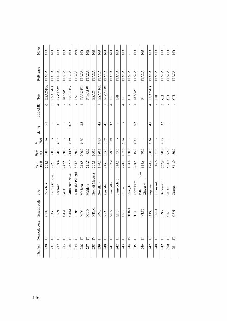
146
Num
ber
Net
wor
k co
de
Stat
ion
code
Si
te
𝑣𝑆,𝐻
(m
/s)
𝐻800
(m)
𝑓 0
(Hz)
𝐴0 (-
) SE
SAM
E Te
st
Ref
eren
ce
Not
es
230
IT
CTL
C
atto
lica
208.
1 90
.0
1.16
5.
8 6
ESA
C-F
K
ITA
CA
N
B
231
IT
FAZ
Faen
za (N
uova
) 29
2.3
300.
0 -
- -
ESA
C-F
K
ITA
CA
N
B
232
IT
FRN
Fo
rnov
o 30
9.4
70.0
4.
67
3.1
4 P-
MA
SW
ITA
CA
N
B
233
IT
GEA
G
ela
247.
5 30
.0
- -
- M
ASW
IT
AC
A
NB
234
IT
GR
M
Gru
men
to N
ova
282.
9 21
4.8
0.59
10
.5
6 ES
AC
-FK
IT
AC
A
NB
235
IT
LDP
Lam
a dei
Pel
igni
32
4.3
50.0
-
- -
DC
IT
AC
A
NB
236
IT
MD
N
Mod
ena
212.
5 20
0.0
0.65
3.
8 4
ESA
C-F
K
ITA
CA
N
B
237
IT
MLD
M
eldo
la
213.
7 83
.0
- -
- P-
MA
SW
ITA
CA
N
B
238
IV
ND
IM
Nov
i di M
oden
a 20
8.1
100.
0 -
- -
ESA
C
ITA
CA
N
B
239
IT
NV
L N
ovel
lara
19
0.2
180.
1 0.
65
4.9
5 ES
AC
-FK
IT
AC
A
NB
240
IT
PNN
Pe
nnab
illi
335.
2 55
.0
3.02
4.
1 5
P-M
ASW
IT
AC
A
NB
241
IT
SNG
Se
niga
llia
257.
9 89
.0
1.28
3.
5 4
P IT
AC
A
NB
242
IT
SNS
Sans
epol
cro
310.
5 55
.0
- -
- D
H
ITA
CA
N
B
243
IT
SRL
Siro
lo
270.
3 15
7.0
5.14
4
4 P
ITA
CA
N
B
244
IV
T082
1 C
asag
lia
184.
4 13
0.0
- -
- C
H
ITA
CA
-
245
IT
TRF
Torr
e Fa
ro
200.
5 15
.0
0.34
5.
5 4
MA
SW
ITA
CA
N
B
246
IT
VLS
2 V
illa
San
Gio
vann
i - 1
31
4.8
70.0
-
- -
P IT
AC
A
NB
247
IT
AR
G
Arg
enta
17
0.2
300.
0 0.
34
4.8
4 ES
AC
-FK
IT
AC
A
NB
248
IT
FRE1
Fi
renz
uola
1 31
6.6
31.0
-
- -
DH
IT
AC
A
NB
249
IT
BN
V
Ben
even
to
757.
9 98
.0
4.73
3.
5 5
CH
IT
AC
A
NB
250
IT
CLT
C
alitr
i 56
8.0
92.0
-
- -
CH
IT
AC
A
NB
251
IT
CSN
C
esen
a 54
1.9
50.0
-
- -
CH
IT
AC
A
NB

147
Num
ber
Net
wor
k co
de
Stat
ion
code
Si
te
𝑣𝑆,𝐻
(m
/s)
𝐻800
(m)
𝑓 0 (H
z)
𝐴0 (-
) SE
SAM
E Te
st
Ref
eren
ce
Not
es
252
E FR
C
Forg
aria
Cor
nino
42
0.2
63.0
-
- -
CH
IT
AC
A
NB
253
IT
MR
T M
erca
to
San
Seve
rino
433.
9 73
.0
1.42
8
4 C
H
ITA
CA
-
254
IT
RN
R
Rio
nero
in V
ultu
re
542.
3 98
.0
- -
- C
H
ITA
CA
N
B
255
IT
SELE
Se
llano
Est
419.
3 18
.0
1.65
4.
4 4
DH
IT
AC
A
-
256
IT
SELW
Se
llano
Ove
st
392.
8 15
.0
- -
- D
H
ITA
CA
N
B
257
IT
SSV
S.
Sev
ero
398.
5 99
.0
0.41
5.
5 6
CH
IT
AC
A
NB
258
IT
STR
St
urno
38
7.7
29.0
0.
34
3.3
4 C
H
ITA
CA
-
259
IT
VSS
V
iest
e 43
4.2
32.0
-
- -
CH
IT
AC
A
-
260
E A
NP
Anc
ona
- Pal
ombi
na
263.
7 59
.0
- -
- C
H
ITA
CA
-
261
IT
BO
J B
ojan
o (N
uova
) 31
1.8
30.0
0.
31
5 6
DH
IT
AC
A
NB
262
E B
UI
Bui
a 24
9.8
47.0
-
- -
CH
IT
AC
A
-
263
IT
BV
G
Bev
agna
21
1.1
150.
0 0.
35
3.8
5 ES
AC
-FK
IT
AC
A
NB
264
IT
BV
N
Bov
ino
353.
7 91
.0
2.62
5
5 C
H
ITA
CA
-
265
IT
CTC
C
ittà
di C
aste
llo
285.
1 26
.0
- -
- D
H
ITA
CA
N
B
266
IV
FER
S C
asag
lia (S
urfa
ce)
184.
4 13
0.0
- -
- C
H
ITA
CA
-
267
IT
FOR
Fo
rlì (N
uova
) 29
3.1
45.0
-
- -
CH
IT
AC
A
-
268
IT
GB
P G
ubbi
o Pi
ana
232.
7 57
.0
0.29
6.
7 6
DH
IT
AC
A
NB
269
IT
GR
G1
Gar
iglia
no
- Fr
ee
Fiel
d 1
196.
2 95
.0
- -
- C
H
ITA
CA
N
B
270
BA
G
VT
Cos
ta d
ella
Gav
eta
272.
1 50
.0
- -
- D
H
ITA
CA
N
B
271
IT
MA
A
Maj
ano
- Asc
enso
re
360.
3 52
.0
- -
- C
H
ITA
CA
N
B
272
BA
TT
S Ti
to S
calo
17
5.9
41.0
-
- -
CH
IT
AC
A
NB

148
: Application of the instrumental approach to clusters of sites of the same ground category C.1: Instrumental approach according to the Draft n.2
C.1.1: Table with compatibility results
Site number in the analysis
Site number in the database
Site (Station code or site
name)
Ground category
Compatibility Standard approach
(𝐻800, 𝑣𝑆,𝐻)
Instrumental approach (𝑓0 ,
𝐴0) 1 4 AVT A E Negative 2 5 BRC A E Negative 3 6 BRZ A E Negative 4 18 SRT B E Negative 5 19 BGN B E Negative 6 22 CPS B E Negative 7 23 CST B F Negative 8 26 GSN B F Negative 9 29 MAI C E Negative 10 30 NAS F F Positive 11 32 SPS E E Positive 12 34 BTT2 Unclassified Unclassified - 13 35 CLF Unclassified Unclassified - 14 36 RTI F Unclassified Negative 15 39 FVZ E E Positive 16 44 BGI B B Positive 17 50 MLC B E Negative 18 53 MTL B F Negative 19 62 PZS B B Positive 20 63 RCC C F Negative 21 70 TLM1 B E Negative 22 72 TRL C E Negative 23 73 VBM B Unclassified Negative 24 74 VBV B E Negative 25 75 AVZ F F Positive 26 77 PGL C E Negative 27 80 AQA B Unclassified Negative

149
Site number in the analysis
Site number in the database
Site (Station code or site
name)
Ground category
Compatibility Standard approach
(𝐻800, 𝑣𝑆,𝐻)
Instrumental approach (𝑓0 ,
𝐴0) 28 81 NCR E Unclassified Negative 29 88 ARN E E Positive 30 92 MRN F Unclassified Negative
31 164 Sant’Agostino
– Zona Industriale
F F Positive
32 175 SARK E B Negative 33 179 SEPFL D E Negative 34 180 SINS F Unclassified Negative 35 181 SIOM F F Positive 36 182 SLOP F F Positive 37 184 SLUW F Unclassified Negative 38 185 SOLB F F Positive 39 186 SRHH E B Negative 40 187 SVIT E B Negative 41 188 SYVP C Unclassified Negative
42 191 Foligno –
Centro Commerciale
E B Negative
43 197 Corciano –
San Mariano E A Negative
44 198
Torgiano – Miralduolo
Zona Industriale
C F Negative
45 202 PNT F Unclassified Negative 46 203 SNN Unclassified B Positive 47 206 AQV B E Negative 48 209 BRN B E Negative 49 219 PNR F F Positive 50 221 PVS B B Positive 51 230 CTL D D Positive 52 234 GRM F Unclassified Negative 53 239 NVL F F Positive 54 240 PNN C E Negative 55 249 BNV B B Positive
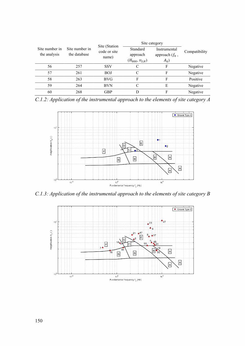
150
Site number in the analysis
Site number in the database
Site (Station code or site
name)
Site category
Compatibility Standard approach
(𝐻800, 𝑣𝑆,𝐻)
Instrumental approach (𝑓0 ,
𝐴0) 56 257 SSV C F Negative 57 261 BOJ C F Negative 58 263 BVG F F Positive 59 264 BVN C E Negative 60 268 GBP D F Negative
C.1.2: Application of the instrumental approach to the elements of site category A
C.1.3: Application of the instrumental approach to the elements of site category B

151
C.1.4: Application of the instrumental approach to the elements of site category C
C.1.5: Application of the instrumental approach to the elements of site category D

152
C.1.6: Application of the instrumental approach to the elements of site category E
C.1.7: Application of the instrumental approach to the elements of site category F

153
C.2: Instrumental approach according to the EC8-1 Draft
C.2.1: Table with compatibility results
Site number in the analysis
Site number in the database
Site (Station code or site
name)
Ground category
Compatibility Standard approach
(𝐻800, 𝑣𝑆,𝐻)
Instrumental approach (𝑓0 ,
𝑣𝑆,𝐻) 1 4 AVT A E Negative 2 5 BRC A A Positive 3 6 BRZ A E Negative 4 18 SRT B B Positive 5 19 BGN B B Positive 6 22 CPS B B Positive 7 23 CST B B Positive 8 26 GSN B B Positive 9 29 MAI C C Positive 10 30 NAS F F Positive 11 32 SPS E E Positive 12 34 BTT2 Unclassified Unclassified - 13 35 CLF Unclassified Unclassified - 14 36 RTI F D Negative 15 39 FVZ E E Positive 16 44 BGI B B Positive 17 50 MLC B B Positive 18 53 MTL B B Positive 19 62 PZS B B Positive 20 63 RCC C F Negative 21 70 TLM1 B B Positive 22 72 TRL C C Positive 23 73 VBM B B Positive 24 74 VBV B B Positive 25 75 AVZ F F Positive 26 77 PGL C C Positive 27 80 AQA B B Positive 28 81 NCR E E Positive 29 88 ARN E E Positive 30 92 MRN F F Positive

154
Site number in the analysis
Site number in the database
Site (Station code or site
name)
Ground category
Compatibility Standard approach
(𝐻800, 𝑣𝑆,𝐻)
Instrumental approach (𝑓0 ,
𝑣𝑆,𝐻)
31 164 Sant’Agostino
– Zona Industriale
F D Negative
32 175 SARK E C Negative 33 179 SEPFL D D Positive 34 180 SINS F F Positive 35 181 SIOM F F Positive 36 182 SLOP F F Positive 37 184 SLUW F D Negative 38 185 SOLB F F Positive 39 186 SRHH E E Positive 40 187 SVIT E E Positive 41 188 SYVP C F Negative
42 191 Foligno –
Centro Commerciale
E E Positive
43 197 Corciano –
San Mariano E A Negative
44 198
Torgiano – Miralduolo
Zona Industriale
C F Negative
45 202 PNT F F Positive 46 203 SNN Unclassified Unclassified - 47 206 AQV B B Positive 48 209 BRN B B Positive 49 219 PNR F F Positive 50 221 PVS B B Positive 51 230 CTL D D Positive 52 234 GRM F F Positive 53 239 NVL F F Positive 54 240 PNN C E Negative 55 249 BNV B B Positive 56 257 SSV C F Negative 57 261 BOJ C F Negative 58 263 BVG F F Positive

155
Site number in the analysis
Site number in the database
Site (Station code or site
name)
Ground category
Compatibility Standard approach
(𝐻800, 𝑣𝑆,𝐻)
Instrumental approach (𝑓0 ,
𝑣𝑆,𝐻) 59 264 BVN C C Positive 60 268 GBP D F Negative
C.2.2: Application of the instrumental approach to the elements of site category A
C.2.3: Application of the instrumental approach to the elements of site category B

156
C.2.4: Application of the instrumental approach to the elements of site category C
C.2.5: Application of the instrumental approach to the elements of site category D

157
C.2.6: Application of the instrumental approach to the elements of site category E
C.2.7: Application of the instrumental approach to the elements of site category F

158
: Results of spectrum-compatibility assessment D.1: Termeno sulla Strada del Vino
D.2: Godrano

159
D.3: Urbino
D.4: Atina

160
: Zero-period soil amplification factor E.1: Termeno sulla Strada del Vino
E.1.1: Site categories B, C and D
E.1.2: Site category E

161
E.1.3: Site category F

162
E.2: Godrano
E.2.1: Site categories B, C and D
E.2.2: Site category E

163
E.2.3: Site category F

164
E.3: Urbino
E.3.1: Site categories B, C and D
E.3.2: Site category E

165
E.3.3: Site category F

166
E.4: Atina
E.4.1: Site categories B, C and D
E.4.2: Site category E
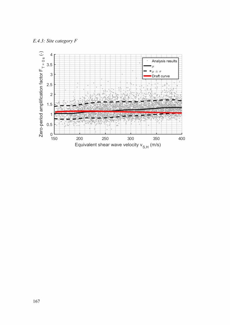
167
E.4.3: Site category F

168
: Short period spectral amplification factor F.1: Termeno sulla Strada del Vino
F.1.1: Site categories B, C and D
F.1.2: Site category E

169
F.1.3: Site category F

170
F.2: Godrano
F.2.1: Site categories B, C and D
F.2.2: Site category E

171
F.2.3: Site category F

172
F.3: Urbino
F.3.1: Site categories B, C and D
F.3.2: Site category E

173
F.3.3: Site category F

174
F.4: Atina
F.4.1: Site categories B, C and D
F.4.2: Site category E
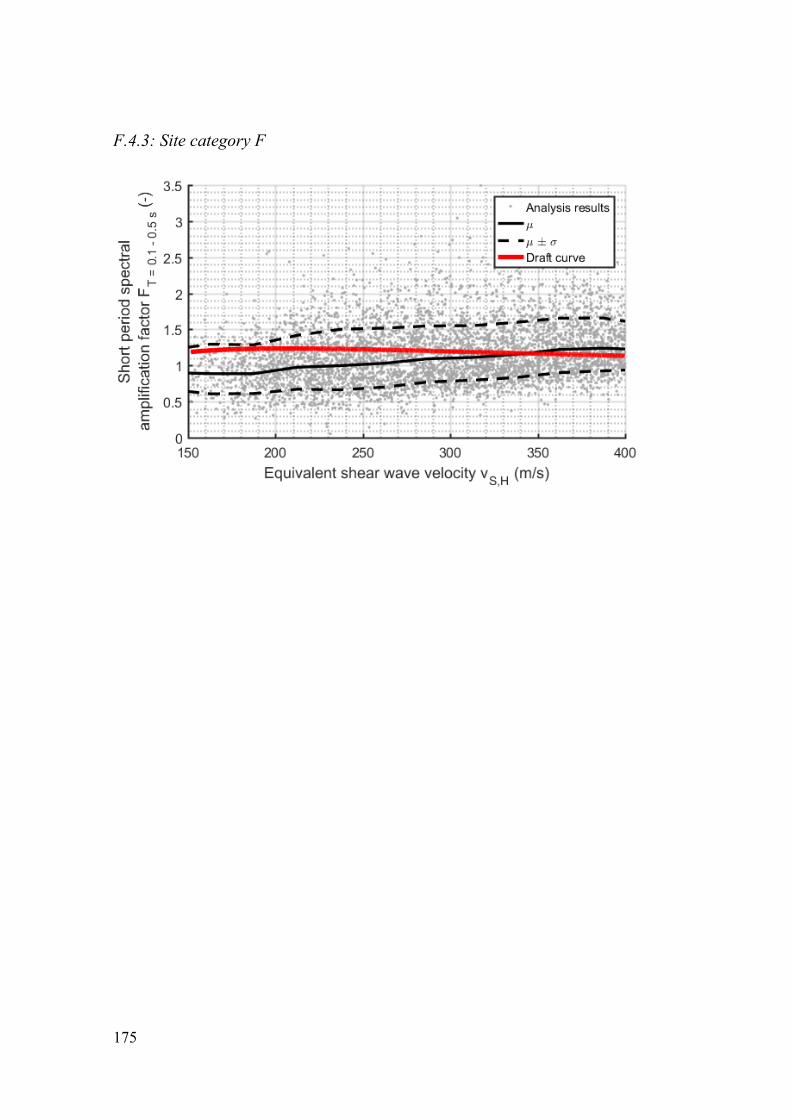
175
F.4.3: Site category F

176
: Intermediate period amplification factor G.1: Termeno sulla Strada del Vino
G.1.1: Site categories B, C and D
G.1.2: Site category E

177
G.1.3: Site category F

178
G.2: Godrano
G.2.1: Site categories B, C and D
G.2.2: Site category E

179
G.2.3: Site category F

180
G.3: Urbino
G.3.1: Site categories B, C and D
G.3.2: Site category E

181
G.3.3: Site category F

182
G.4: Atina
G.4.1: Site categories B, C and D
G.4.2: Site category E

183
G.4.3: Site category F

184
: Long period spectral amplification factor H.1: Termeno sulla Strada del Vino
H.1.1: Site categories B, C and D
H.1.2: Site category E

185
H.1.3: Site category F

186
H.2: Godrano
H.2.1: Site categories B, C and D
H.2.2: Site category E

187
H.2.3: Site category F

188
H.3: Urbino
H.3.1: Site categories B, C and D
H.3.2: Site category E

189
H.3.3: Site category F

190
H.4: Atina
H.4.1: Site categories B, C and D
H.4.2: Site category E

191
H.4.3: Site category F

192
: Intermediate period spectral amplification factor I.1: Termeno sulla Strada del Vino
I.1.1: Site category B, C and D
I.1.2: Site category E

193
I.1.3: Site category F

194
I.2: Godrano
I.2.1: Site categories B, C and D
I.2.2: Site category E

195
I.2.3: Site category F
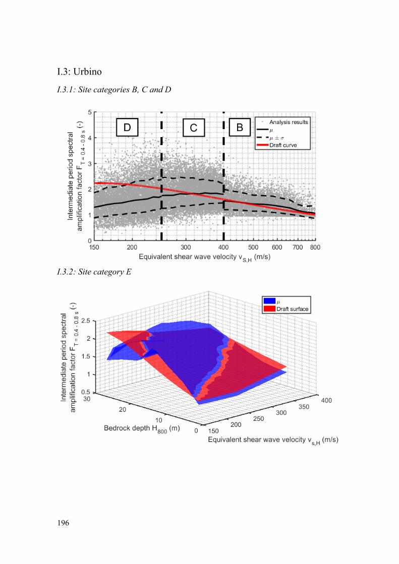
196
I.3: Urbino
I.3.1: Site categories B, C and D
I.3.2: Site category E

197
I.3.3: Site category F

198
I.4: Atina
I.4.1: Site categories B, C and D
I.4.2: Site category E

199
I.4.3: Site category F

200
: Global spectral amplification factor J.1: Termeno sulla Strada del Vino
J.1.1: Site categories B, C and D
J.1.2: Site category E

201
J.1.3: Site category F
J.2: Godrano
J.2.1: Site categories B, C and D
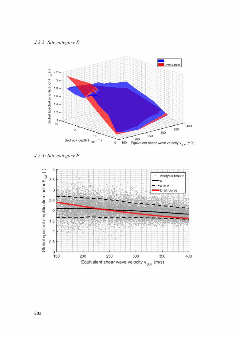
202
J.2.2: Site category E
J.2.3: Site category F

203
J.3: Urbino
J.3.1: Site categories B, C and D
J.3.2: Site category E

204
J.3.3: Site category F
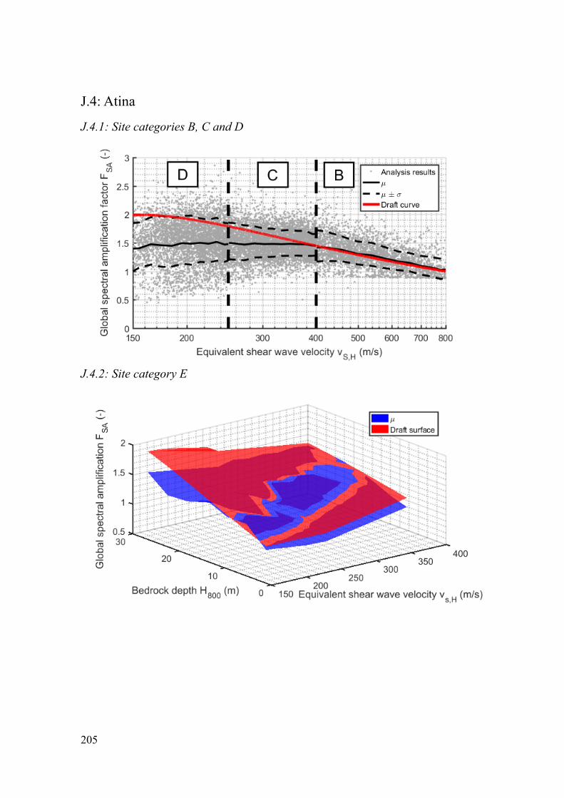
205
J.4: Atina
J.4.1: Site categories B, C and D
J.4.2: Site category E

206
J.4.3: Site category F

207
Bibliography [1] A. Pettiti and S. Foti, “Analisi stocastica della risposta sismica locale e
classificazione del sottosuolo,” in ANIDIS 2013 - L’ingegneria sismica in Italia, 2013.
[2] G. Andreotti, C. G. Lai, F. Bozzoni, and L. Scandella, “New soil factors for the
Italian Building Code (NTC08) derived from 1D fully stochastic ground response analyses,” 2008.
[3] K. Pitilakis, E. Riga, and A. Anastasiadis, “New code site classification ,
amplification factors and normalized response spectra based on a worldwide ground-motion database,” pp. 925–966, 2013.
[4] G. Tropeano, F. M. Soccodato, and F. Silvestri, “Re-evaluation of code-specified stratigraphic amplification factors based on Italian experimental records and numerical seismic response analyses,” Soil Dyn. Earthq. Eng., 2018.
[5] VV.AA., “Eurocode 8: Design of structures for earthquake resistance, Part 1:
general rules, seismic actions and rules for buildings. Final Draft Rev 24-00.”
2017. [6] Ministero delle Infrastrutture e dei Trasporti, “D.M. 14/01/2008 ‘Norme Tecniche
per le Costruzioni’ (NTC).” 2008. [7] Ministero delle Infrastrutture e dei Trasporti, “Circolare 02/02/2009, n.617
"Istruzioni per l’applicazione delle <Nuove norme tecniche per le costruzioni> di
cui al decreto ministeriale 14 gennaio 2008 (Suppl. Ordinario n.27).” 2009. [8] Comité Européen de Normalisation (CEN), “EN 1998-1. Eurocode 8: Design of
structures for earthquake resistance; Part 1: General rules, seismic actions and rules for buildings.” 2004.
[9] S. Barani, S. Barani, R. De Ferrari, G. Ferretti, and C. Eva, “Assessing the
Effectiveness of Soil Parameters for Ground Response Characterization and Soil Classification,” Earthq. Spectra, vol. 24, no. August 2008, pp. 565–597, 2008.
[10] M. R. Gallipoli and M. Mucciarelli, “Vs30 è un valido stimatore dell’amplificazione di sito?,” in ANIDIS 2009, 2009.
[11] Presidency of Counsil of Ministers - Civil Protection Department, “Italian Strong
Motion Network.” 1972. [12] L. Luzi, F. Pacor, and R. Puglia, “Italian Accelerometric Archive v 2.2. Istituto
Nazionale di Geofisica e Vulcanologia, Dipartimento della Protezione Civile Nazionale.,” 2017. .
[13] L. Luzi, R. Puglia, E. Russo, and O. WG5, “Engineering Strong Motion Database,
version 1.0. Istituto Nazionale di Geofisica e Vulcanologia, Observatories & Research Facilities for European Seismology.,” 2016. [Online]. Available: esm.mi.ingv.it/. [Accessed: 16-Oct-2017].
[14] Swiss Seismological Service (SED) at ETH Zurich, “The Site Characterization
Database for Seismic Stations in Switzerland.,” Zurich: Federal Institute of Technology., 2015. .
[15] Regione Toscana, “Valutazione effetti locali,” 2015. [Online]. Available: www.regione.toscana.it/-/programma-vel. [Accessed: 25-Nov-2017].
[16] Regione Toscana, “Banche Dati: Indagini sul terreno (VEL),” 2015. [Online]. Available: 150.217.73.23/BancaDatiCartografiaVEL/. [Accessed: 25-Nov-2017].

208
[17] Regione Emilia Romagna, “Sezioni geologiche e prove geognostiche della pianura
emiliano romagnola,” Geologia, sismica e suoli, 2015. [Online]. Available: http://www.regione.emilia-romagna.it. [Accessed: 25-Nov-2017].
[18] Regione Umbria, “Banca dati delle indagini geognostiche e geofisiche per Google
Earth,” 2015. [Online]. Available:
storicizzati.territorio.regione.umbria.it/Static/IndaginiGeologicheKmz/Index_kmz.htm. [Accessed: 25-Nov-2017].
[19] P.-Y. et al. Bard, “Guidelines for the implementation of the H/V spectral ratio
technique on ambient vibrations measurements, processing and interpretation,”
2004. . [20] Comité Européen de Normalisation (CEN), “Eurocode 8: Design of structures for
earthquake resistance, Part 1: general rules, seismic actions and rules for buildings. EN1998-1:2004.” Brussels, Belgium, 2004.
[21] VV.AA., “Eurocode 8: Design of structures for earthquake resistance, Part 1:
General rules, seismic actions and rules for buildings - Draft n.2.” 2017. [22] S. L. Kramer, Geotechnical Earthquake Engineering, Civil engi. 1996. [23] A. R. Kottke and E. M. Rathje, “Technical Manual for Strata,” Austin, 2009. [24] J. I. Sun and I. M. Idriss, “User’s manual for SHAKE91: A computer program for
conducting equivalent linear seismic response analyses of horizontally layered soil deposits.” Center for Geotechnical Modelling, Dept. of Civil and Environmental
Engineering, University of California at Davis, Davis, California, 1992. [25] I. M. Idriss and H. B. Seed, “Seismic response of horizontal soil layers,” J. Soil
Mech. Found. Div., vol. 94, pp. 1003–1031, 1968. [26] N. Matasovic and Y. Hashash, “Practices and Procedures for Site-Specific
Evaluations of Earthquake Ground Motions: A Synthesis of Highway Practice,”
Washington, 2012. [27] C. G. Lai, S. Foti, and M. Rota, Input sismico e stabilità geotecnica dei siti di
costruzione, Collana di. Pavia: IUSS Press, 2009. [28] J. Régnier, L. F. Bonilla, P. Y. Bard, H. Kawase, E. Bertrand, F. Hollender, and M.
Marot, “International Benchmark on Numerical Simulations for 1D, Nonlinear Site
Response (PRENOLIN): Verification Phase Based on Canonical Cases,” Bull. Seismol. Soc. Am., vol. 5, no. November, pp. 2122–2135, 2016.
[29] P. B. Schnabel, J. Lysmer, and H. Bolton Seed, “SHAKE - A computer program for earthquake response analysis of horizontally layered sites,” Earthquake
Engineering Research Center, 1972. [30] M. B. Darendeli, “Development of a new family of normalized modulus reduction
and material damping curves,” University of Texas, Austin, 2001. [31] K. M. Rollins, M. D. Evans, N. B. Diehl, and W. D. Daily III, “SHEAR
MODULUS AND DAMPING RELATIONSIDPS FOR GRAVELS,” J. Geotech. Geoenvironmental Eng., vol. 124, no. 5, pp. 396–405, 1998.
[32] F.-Y. Menq, “Dynamic Properties of Sandy and Gravelly Soils,” Univeristy of
Texas at Austin, 2003. [33] G. R. Toro, “Probabilistic models of site velocity profiles for generic and site-
specific ground-motion amplification studies.” Risk Engineering Inc., Boulder, CO
80303, 1995. [34] J. P. Stewart, K. Afshari, and Y. M. A. Hashash, “Guidelines for performing

209
hazard-consistent one-dimensional ground response analysis for ground motion prediction,” 2014.
[35] F. Pacor, R. Paolucci, L. Luzi, F. Sabetta, A. Spinelli, A. Gorini, M. Nicoletti, S. Marcucci, L. Filippi, and M. Dolce, “Overview of the Italian strong motion
database 1.0,” Bull. Earthq. Eng., 2011. [36] L. Luzi, F. Pacor, and R. Puglia, “Italian Accelerometric Archive v 2.3.” Istituto
Nazionale di Geofisica e Vulcanologia, Dipartimento della Protezione Civile Nazionale, 2017.
[37] “Swiss Seismological Service (SED) At ETH Zurich: National Seismic Networks
of Switzerland,” ETH Zurich. Other/Seismic Network, 1983. [Online]. Available: www.seismo.etzh.ch/en/home/. [Accessed: 25-Nov-2017].
[38] A. Piemonte, “SISMOVALP - Seismic hazard and alpine valley response analysis,”
2006. [39] C. Lacave and F. Lemeille, “Seismic hazard and alpine valley response analysis:
generic valley configurations,” in First European Conference on Earthquake Engineering and Seismology, 2006, no. 1.
[40] S. Foti, “Personal communication.” 2017. [41] P. Capilleri, “Caratterizzazione geotecnica e amplificazione sismica nella zona
industriale di Catania (Personal communication),” in ANIDIS 2009, 2017. [42] A. H.-S. Ang and W. H. Tang, Probability concepts in engineering planning and
design: Volume I - Basic Principles. New York, New York, 1975. [43] D. P. Teague and B. R. Cox, “Site response implications associated with using non-
unique Vs profiles from surface wave inversion in comparison with other commonly used methods of accounting for Vs uncertainty,” Soil Dyn. Earthq. Eng., pp. 1–17, 2016.
[44] F. Passeri, “Personal communication.” . [45] W. Silva, “Personal communication.” 1995. [46] Y. Ohta and N. Goto, “Empirical shear wave velocity equations in terms of
characteristic soil indexes,” Earthq. Eng. Struct. Dyn., vol. 6, pp. 167–187, 1978. [47] M. Vucetic and R. Dobry, “Effect of soil plasticity on cyclic response,” J. Geotech.
Eng., vol. 117, no. 1, pp. 89–107, 1991. [48] R. Lancellotta, Geotecnica. Bologna, 2012. [49] B. Schmidt, “Discussion on earth pressure at rest related to stress history,” Can.
Geotech. J., vol. 3, pp. 239–242, 1966. [50] I. Alpan, “The empirical evaluation of the coefficients K0 and K0r,” Soils Found.,
vol. 7, pp. 31–40, 1967. [51] C. C. Ladd, R. Foott, K. Ishihara, F. Schlosser, and H. G. Poulos, “Stress-
deformation and strength characteristics,” in IX ICSMFE, 1977, pp. 421–494. [52] J. Jàky, “The coefficient of earth pressure at rest,” J. Soc. Hungarian Archit. Eng.,
pp. 355–358, 1944. [53] J. A. Hunter, “Some observations of Vp, Vs, depth and porosity from borholes in
water-saturated unconsolidated sediments,” in Symposium on the applications of geophysics to Engineering and Environmental Problems, 2003, pp. 650–661.
[54] G. Lanzo, G. Scasserra, and Y. Ding, “Evaluation of EC8 site-dependent acceleration response spectra using strong-motion Italian records,” in Eurocode 8 Perspectives from the Italian Standpoint Workshop, 2009, pp. 13–22.

210
[55] Ministero delle Infrastrutture e dei Trasporti, “Consiglio Superiore dei Lavori
Pubblici,” 2008. [Online]. Available: www.cslp.it. [56] C. Meletti and F. Martinelli, “I dati online della pericolosità sismica in Italia,”
2008. [Online]. Available: esse1.mi.ingv.it. [57] C. Meletti, G. M. Calvi, and M. Stucchi, “Progetto S1: Proseguimento della
assistenza al DPC per il completamento e la gestione della mappa di pericolosità sismica prevista dall’Ordinanza PCM 3274/2003 e progettazione di ulteriori
sviluppi. Rapporto finale,” 2007. [58] D. Spallarossa and S. Barani, “Disaggregazione della pericolosità sismica in
termini di M-R-ε. Progetto DPC-INGV S1, Deliverable D14.,” Genova, 2007. [59] V. Montaldo and C. Meletti, “Valutazione del valore della ordinata spettrale a 1sec
e ad altri periodi di interesse ingegneristico. Progetto DPC-INGV S1, Deliverable 3,” Milano, 2007.
[60] “Norme Tecniche per le Costruzioni. Decreto 14/01/2008 del Ministero delle
Infrastrutture (G.U. n. 29 del 04/02/2008),” 2008. [Online]. Available: esse1.mi.ingv.it/ntc.html.
[61] M. Rota, E. Zuccolo, and C. G. Lai, “Mesozonation of the Italian territory for the
definition of real spectrum-compatible accelerograms,” Bull. Earthq. Eng., no. May, 2012.
[62] C. Meletti and G. Valensise, “Zonazione sismogenetica ZS9 – App.2 al Rapporto Conclusivo,” 2004.
[63] M. Corigliano, C. G. Lai, and M. Rota, “ASCONA : Automated Selection of
COmpatible Natural Accelerograms,” vol. 28, no. 3, pp. 965–987, 2012. [64] “Il codice di calcolo SEISM-HOME (SElection of Input Strong-Motion for
HOmogeneous MEsozones),” 2012. [65] C. Meletti and V. Montaldo, “Stime di pericolosità sismica per diverse probabilità
di superamento in 50 anni: valori di ag. Progetto DPC-INGV S1, Deliverable D2,”
Milano, 2007. [66] N. Ambraseys, P. Smit, R. Sigbjornsson, P. Suhadolc, and B. Margaris, “Internet-
Site for European Strong-Motion Data,” European Commission, Research-Directorate General, Environment and Climate Progress, 2002. [Online]. Available: www.isesd.hi.is/ESD_Local/frameset.htm. [Accessed: 20-Jan-2018].
[67] T. D. Ancheta, R. B. Darragh, J. P. Stewart, E. Seyhan, W. J. Silva, B. S. J. Chiou, K. E. Wooddell, R. W. Graves, A. R. Kottke, D. M. Boore, T. Kishida, and J. L. Donahue, “PEER NGA-West2 Database,” 2013.
[68] J. J. Bommer and S. Akkar, “Consistent source-to-site distance metrics in Ground-Motion Prediction Equations and seismic source models for PSHA,” Earthq. Spectra, vol. 28, no. 1, pp. 1–15, 2012.
[69] Seismosoft, “SeismoSignal - A computer program for signal processing of time-histories.” 2016.
[70] G. Acunzo, A. Pagliaroli, and G. Scasserra, “In-Spector: un software di supporto alla selezione di accelerogrammi naturali spettrocompatibili per analisi geotecniche e strutturali,” in 33° Convegno Nazionale GNGTS, 2014, pp. 107–114.
[71] G. W. Housner, “Spectrum Intensities of Strong-Motion Earthquakes,” in
Proceedings of the Symposium on Earthquake and Blast Effects on Structures: Los Angeles, California, June 1952, 1952, pp. 20–36.

211
[72] B. J. Rey, E. Faccioli, and J. J. Bommer, “Derivation of design soil coefficients ( S ) and response spectral shapes for Eurocode 8 using the European Strong-Motion Database Derivation of design soil coefficients ( S ) and response spectral shapes for Eurocode 8 using the European Strong- Motion Database,” 2002.
[73] Commissario Straordinario del Governo per la Ricostruzione Sisma 2016, Sismica), and Istituto di Geologia Ambientale e Geoingegneria del Consiglio Nazionale delle Ricerche (per il Centro per la Microzonazione Sismica e le sue Applicazioni), “Protocollo di acquisizione dati ed elaborazione relativi alle attività di Microzonazione di Livello III nei 140 Comuni di cui all’Ordinanza n. 24 del 12
maggio 2017 della Presidenza del Consiglio dei Ministri.” 2017. [74] “Sito del Dipartimento della Protezione Civile - Presidenza del Consiglio dei
Ministri.” [Online]. Available: www.protezionecivile.gov.it. [75] Istituto Nazionale di Geofisica e Vulcanologia (INGV), “Emersito Seismic
Network for Site Effect Studies in L’Aquila town (Central Italy),” International Federation of Digital Seismograph Networks. Other/Seismic Networks, 2009. .
[76] L. Minarelli, S. Amoroso, G. Tarabusi, M. Stefani, and G. Pulelli, “Down-hole geophysical characterization of middle-upper Quaternary sequences in the Apennine Foredeep , Mirabello , Italy,” Ann. Geophys., vol. 59, no. 5, 2016.
[77] C. Comina, S. Foti, D. Boiero, and L. V Socco, “Reliability of VS,30 Evaluation
from Surface-Wave Tests,” J. Geotech. Geoenvironmental Eng., no. June, pp. 579–
586, 2011. [78] A.G.I., “Caratteristiche geotecniche dell’argilla del Fucino.” pp. 145–159.
Copyright © 2022 FDOKUMEN