POLITECNICO DI TORINO DIMEAS – DEPARTMENT OF MECHANICAL AND AEROSPACE ENGINEERING

MASTER OF SCIENCE DEGREE

IN

AUTOMOTIVE ENGINEERING

Master’s degree thesis

Machine Learning application for Tool Wear Prediction in Milling

Supervisors: Laureandi

Prof. Franco Lombardi Vinay Nagabhushana Rao

Prof. Guilia Bruno 251256

Dott. Emiliano Traini

Academic Year – 2019-2020

i

Abstract

Milling is one of the most versatile processes used in the manufacture of various components. With this, the milling tool usage has gained momentum, so as the research on its wear phenomenon. Flank wear has been considered as, one of the most commonly observed and an unavoidable phenomenon in metal cutting process, which is also a major source of economic loss resulting due to material loss and machine downtime.

With the aim of implementing a predictive maintenance for the milling process, so as to avoid unnecessary cost and wastage of time due to sudden failure of cutting tool, and also to maintain the best product output quality, one of the applications of Machine Learning has been presented in this thesis by giving due importance to Tool Condition Monitoring.

By highlighting the usage of model based maintenance method, the study presents the implementation of the framework of predictive maintenance which has been proposed extensively by many research papers. This thesis presents a method to apply Machine Learning in the prediction of the tool wear, thereby assessing the remaining useful life of the tool for best performance with respect to cost, quality and time. The work here presents the methods of Data cleansing, manipulation of data to extract and select features, utilization of the features in training various machine learning models and testing them to conclude in finding the possible tool wear severeness and to assess the Remaining Useful Life based on wear results.

The study also presents the possible tools that can be used to carry out the regression analysis in order to train and test machine learning models like Linear Regression, Bayesian Ridge Regression, Kernel Ridge Regression, Neural Network and so on. Cross validation has been carried out in order to narrow down on the machine learning model, which has been further improved using Hyperparameter tuning. This has enabled to arrive at the best possible results for wear prediction and Remaining useful life of the tool.

ii

Acknowledgements

I would like to extend my sincere gratitude towards my thesis supervisor, Prof. Guilia Bruno and Prof. Franco Lombardi for providing this opportunity and for valuable feedback and constructive suggestions during the conduct of this master thesis.

I would like to offer my special thanks to Dott. Emiliano Traini for introducing me to the world of Artificial Intelligence, patiently listening to all of my queries and laying the pathway for me to learn quickly and efficiently, the concepts that required me to perform this study.

Last, but not least, I would like to express my profound gratitude to my family and friends for providing me with unfailing support and continuous encouragement throughout my years of study.

iii

iv

Contents

Abstract ....................................................................................................................................... i

Acknowledgements .................................................................................................................... ii

List of Code snippets ............................................................................................................... vii

List of Figures .......................................................................................................................... vii

List of Tables ......................................................................................................................... viii List of Equations ....................................................................................................................... ix

Chapter 1 - Introduction ............................................................................................................. 1

Synopsis ..................................................................................................................................... 1

1.1 Artificial Intelligence and its applications ........................................................................... 1

1.2 Tool wear ............................................................................................................................. 3

1.3 Thesis Objective and Structure ............................................................................................ 4

Chapter 2 – Predictive Maintenance .......................................................................................... 5

Synopsis ..................................................................................................................................... 5

2.1 Maintenance ......................................................................................................................... 5

2.1.1 Types of Maintenance ................................................................................................... 5

2.2 Predictive Maintenance ........................................................................................................ 6

2.2.1 Benefits of Predictive Maintenance .............................................................................. 7

Chapter 3 – Literature Review ................................................................................................... 8

Synopsis ..................................................................................................................................... 8

3.1 Literature Review................................................................................................................. 8

Chapter 4 – Milling Process ..................................................................................................... 21

Synopsis ................................................................................................................................... 21

4.1 Metal Cutting Process ........................................................................................................ 21

4.2 Milling cutting tool ............................................................................................................ 22

4.2.1 Single Point Cutting Tool ........................................................................................... 22

4.2.2 Mechanisms of Metal Cutting ..................................................................................... 23

4.3 Tool wear ........................................................................................................................... 24

4.3.1 Types of Tool wear ..................................................................................................... 25

4.3.1.1 Flank wear ............................................................................................................ 26

4.3.1.2 Crater Wear .......................................................................................................... 27

4.4 Milling data set – Case study ............................................................................................. 29

4.4.1 Experimental setup...................................................................................................... 29

Chapter 5 – Tools utilized ........................................................................................................ 31

v

Synopsis ................................................................................................................................... 31

5.1 Programming Language ..................................................................................................... 31

5.2 Integrated Development Environment ............................................................................... 35

5.3 Libraries used ..................................................................................................................... 36

5.3.1 Matplotlib .................................................................................................................... 36

5.3.2 Numpy......................................................................................................................... 36

5.3.3 Scipy ........................................................................................................................... 37

5.3.4 Pandas ......................................................................................................................... 37

5.3.5 Scikit Learn ................................................................................................................. 38

Chapter 6 – Data Analysis ....................................................................................................... 39

Synopsis ................................................................................................................................... 39

6.1 Data Cleansing ................................................................................................................... 39

6.2 Outlier Analysis ................................................................................................................. 40

6.3 Feature Extraction .............................................................................................................. 41

6.4 Normalization .................................................................................................................... 42

6.5 Feature Selection ................................................................................................................ 43

Chapter 7 - Model Training and Testing .................................................................................. 46

Synopsis ................................................................................................................................... 46

7.1 Train and Test data Preparation ......................................................................................... 46

7.2 Regression Analysis ........................................................................................................... 47

7.3 Linear Regression .............................................................................................................. 49

7.4 Decision Tree Regression .................................................................................................. 52

7.5 Random Forest Regression ................................................................................................ 55

7.6 Bayesian Ridge Regression................................................................................................ 58

7.7 Neural Network Regression ............................................................................................... 60

7.8 k-nearest neighbor Regression ........................................................................................... 62

7.9 Kernel Ridge Regression ................................................................................................... 64

Chapter 8 – Model Improvement ............................................................................................. 67

Synopsis ................................................................................................................................... 67

8.1 Cross Validation................................................................................................................. 67

8.1.1 Configuration of ‘k’ .................................................................................................... 68

8.1.2 Execution of Cross Validation .................................................................................... 69

8.2 Hyperparameter Tuning ..................................................................................................... 75

8.2.1 Linear Regression ....................................................................................................... 75

8.2.2 Bayesian Ridge Regression......................................................................................... 76

vi

8.2.3 Kernel Ridge Regression ............................................................................................ 77

8.2.4 Neural Network ........................................................................................................... 78

Chapter 9 – Remaining Useful Life ......................................................................................... 83

Synopsis ................................................................................................................................... 83

9.1 Remaining useful Life ........................................................................................................ 83

Chapter 10 – Conclusions and Future Work ............................................................................ 90

Synopsis ................................................................................................................................... 90

10.1 Conclusion ....................................................................................................................... 90

10.2 Scope for Future Work..................................................................................................... 91

Bibliography ............................................................................................................................ 92

vii

List of Code snippets

Code Snippet 1: Data Cleansing .............................................................................................. 40

Code Snippet 2: Detection of Outliers using Z-Score method ................................................ 41

Code Snippet 3: Removal of Outliers ...................................................................................... 41

Code Snippet 4: Example for Features Extraction in Time Domain ....................................... 44

Code Snippet 5: Train -Test dataset split ................................................................................. 46

Code Snippet 6: Example to find MSE .................................................................................... 48

Code Snippet 7: Example to find MAE ................................................................................... 48

Code Snippet 8: Example to find R2 ........................................................................................ 48

Code Snippet 9: Example to find Explained Variance ............................................................ 49

Code Snippet 10: Linear Regression ........................................................................................ 51

Code Snippet 11: Decision Tree .............................................................................................. 54

Code Snippet 12: Random Forest ............................................................................................ 57

Code Snippet 13: Bayesian Ridge Regression ......................................................................... 59

Code Snippet 14: Neural Network regression ......................................................................... 61

Code Snippet 15: knn regression ............................................................................................. 63

Code Snippet 16: Kernel Ridge Regression............................................................................. 65

Code Snippet 17: 10-Fold Cross Validation Linear Regression .............................................. 70

Code Snippet 18: 10-Fold Cross Validation Bayesian Ridge Regression ............................... 72

Code Snippet 19: sklearn function for Linear Regression ....................................................... 75

Code Snippet 20: sklearn function for Bayesian Ridge Regression ........................................ 76

Code Snippet 21: sklearn function for Kernel Ridge Regression ............................................ 77

Code Snippet 22: sklearn function for Neural Network MLP Regressor ................................ 78

Code Snippet 23: Neural Network Grid search error R2 metric .............................................. 82

Code Snippet 24: Neural Network Grid search explained Variance error metric ................... 82

Code Snippet 25: RUL Model Training................................................................................... 85

Code Snippet 26: Remaining Useful life ................................................................................. 87

List of Figures Figure 1: Integrated system employing three techniques for predictive maintenance ............... 9

Figure 2: Parameters related to equipment Condition ............................................................. 10

Figure 3: Comparison of different predictive modelling techniques regarding defect prognosis.................................................................................................................................................. 14

Figure 4: Framework of the integrated diagnosis and prognosis technique for wind turbines 14

Figure 5: Tool wear measuring Techniques............................................................................. 15

Figure 6: The framework of a Tool condition monitoring (TCM) system .............................. 16

Figure 7: The architecture of Neuro-Fuzzy Network (NFN) ................................................... 17

Figure 8: Features extracted in time domain............................................................................ 17

Figure 9: Features extracted in frequency domain ................................................................... 18

Figure 10: Metal Cutting Operation ......................................................................................... 21

Figure 11: Orthogonal cutting .................................................................................................. 22

Figure 12: Oblique Cutting ...................................................................................................... 22

Figure 13: Solid type single point cutting tool......................................................................... 23

viii

Figure 14: Tipped type single point cutting tool ...................................................................... 23

Figure 15: Index-able insert type single point cutting tool ...................................................... 23

Figure 16: Geometry of single point cutting tool..................................................................... 23

Figure 17: Metal Cutting Operation ......................................................................................... 24

Figure 18: Tool wear phenomena ............................................................................................ 25

Figure 19: Flank and Crater wear ............................................................................................ 26

Figure 20: The Flank wear ....................................................................................................... 26

Figure 21: The Crater Wear ..................................................................................................... 28

Figure 22: Effects of Cutting speed V and Cutting time T, on Crater wear depth KT ............ 28

Figure 23: Experimental setup ................................................................................................. 30

Figure 24: A view of a portion of dataset in MATLAB .......................................................... 30

Figure 25: US, Google searches for coding languages (100 = highest annual traffic for any language) .................................................................................................................................. 35

Figure 26:Data cleansing methods ........................................................................................... 39

Figure 27: Feature Selection Heat map .................................................................................... 45

Figure 28: Linear Regression ................................................................................................... 52

Figure 29: Decision Tree ......................................................................................................... 53

Figure 30: Decision Tree Regression ....................................................................................... 53

Figure 31: Random Forest ....................................................................................................... 56

Figure 32: Random Forest Regression ..................................................................................... 57

Figure 33: Bayesian Ridge Regression .................................................................................... 59

Figure 34: A simple feed neural network ................................................................................ 60

Figure 35: Regression in neural networks ............................................................................... 61

Figure 36: Neural Network ...................................................................................................... 62

Figure 37: Knn Regression ...................................................................................................... 64

Figure 38: Kernel Ridge Regression ........................................................................................ 66

Figure 39: 5-Fold Cross Validation example ........................................................................... 68

Figure 40: Improved Neural Network Performance ................................................................ 84

Figure 41: Flowchart to obtain RUL ........................................................................................ 86

Figure 42: RUL prediction performance – Neural Network .................................................... 88

Figure 43: RUL prediction Performance – Linear Regression ................................................ 88

Figure 44: RUL prediction performance – Bayesian Ridge Regression .................................. 89

Figure 45: RUL prediction performance – Kernel Ridge Regression ..................................... 89

List of Tables Table 1: Struct field names and description ............................................................................. 29

Table 2: Summary of Error metrics for Regression models .................................................... 66

Table 3: 10_fold CV - Linear Regression ................................................................................ 69

Table 4: 10-Fold Cross Validation Bayesian Ridge Regression .............................................. 71

Table 5: 10-Fold Cross Validation Kernel Ridge Regression ................................................. 71

Table 6: 10-Fold Cross Validation Neural Network Regression ............................................. 73

Table 7: 10-Fold Cross Validation Decision Tree Regression ................................................ 73

Table 8: 10-Fold Cross Validation Random Forest Regression .............................................. 74

Table 9: 10-Fold Cross Validation knn Regression ................................................................. 74

Table 10: Hyperparameter tuning results: Neural Network ..................................................... 81

ix

Table 11: Machining Parameters ............................................................................................. 83

List of Equations Equation 1: Tool Life Expectancy ........................................................................................... 26

Equation 2: Generalized tool life expectancy equation ........................................................... 27

Equation 3: Z-Score ................................................................................................................. 41

Equation 4: Explained Variance .............................................................................................. 49

1

Chapter 1 - Introduction

Synopsis

The introductory chapter gives an insight into the reasoning of the thesis topic and introduces many terms associated with the same. Upon basic introduction into many aspects of AI, Tool wear and maintenance, the chapter also gives objective of taking up this thesis work and the structure adopted here to present the same.

1.1 Artificial Intelligence and its applications

John McCarthy is known as the Father of Artificial Intelligence. According to him, AI is “The science and engineering of making intelligent machines, especially intelligent computer programs”. In the similar manner how a human Intelligence work, AI is the way of making the computer, computer controlled robots or a software to think intelligently. The basis for developing intelligent software and systems is the study of how a human brain works. Various studies have been performed to study how a human learns, decides and works while trying to solve a problem and these outcomes have paved the way for developing AI [1].

In a broader sense, following can be considered as goals of AI,

1. To create Expert systems: Expert systems are those which exhibit intelligent behavior, learn, demonstrate, explain and advise its users.

2. To implement human intelligence in Machines: Creating systems that understand, think, learn and behave like humans.

Artificial Intelligence is a big domain which is gaining momentum in the current market. It involves a variety of technologies and tools. The below mentioned are some of the recent technologies,

1. Natural Language Generation: It is a tool that produces text from computer data. This technology is currently used in customer service, report generation and summarizing business intelligence insights.

2. Speech Recognition: This is a technology which transcribes and transforms human speech into useful format for computer applications. This is presently used in interactive voice response systems and mobile applications.

3. Virtual Agent: A Virtual Agent is a computer generated, animated, artificial intelligence virtual character (usually with anthropomorphic appearance) that serves as an online customer service representative. It leads an intelligent conversation with users, responds to their questions and performs adequate non-verbal behavior. An example of a typical Virtual Agent is Louise, the Virtual Agent of eBay which was created by a French/American developer VirtuOz.

4. Machine Learning: Provides algorithms, APIs (Application Program interface) development and training toolkits, data, as well as computing power to design, train, and deploy models into

2

applications, processes, and other machines. Currently used in a wide range of enterprise applications, mostly involving prediction or classification.

5. Deep Learning Platforms: A special type of machine learning consisting of artificial neural networks with multiple abstraction layers. Currently used in pattern recognition and classification applications supported by very large data sets.

6. Biometrics: Biometrics uses methods for unique recognition of humans based upon one or more intrinsic physical or behavioral traits. In computer science, particularly, biometrics is used as a form of identity access management and access control. It is also used to identify individuals in groups that are under surveillance. Currently used in market research.

7. Robotic Process Automation: using scripts and other methods to automate human action to support efficient business processes. Currently used where it is inefficient for humans to execute a task.

8. Text Analytics and NLP: Natural language processing (NLP) uses and supports text analytics by facilitating the understanding of sentence structure and meaning, sentiment, and intent through statistical and machine learning methods. Currently used in fraud detection and security, a wide range of automated assistants, and applications for mining unstructured data.

AI has been adopted in various fields and there are certain fields, where it is dominating [1] [2]. Some of those fields are,

1. Gaming: AI plays crucial role in strategic games such as chess, poker, tic-tac-toe, etc., where machine can think of large number of possible positions based on heuristic knowledge.

2. Natural Language Processing: It is possible to interact with the computer that understands natural language spoken by humans.

3. Expert Systems: There are some applications which integrate machine, software, and special information to impart reasoning and advising. They provide explanation and advice to the users.

4. Vision Systems: These systems understand, interpret, and comprehend visual input on the computer. For example,

a. A spying aeroplane takes photographs, which are used to figure out spatial information or map of the areas. b. Doctors use clinical expert system to diagnose the patient. c. Police use computer software that can recognize the face of criminal with the stored portrait made by forensic artist.

5. Speech Recognition: Some intelligent systems are capable of hearing and comprehending the language in terms of sentences and their meanings while a human talks to it. It can handle different accents, slang words, noise in the background, change in human’s noise due to cold,

and so on.

6. Handwriting Recognition: The handwriting recognition software reads the text written on paper by a pen or on screen by a stylus. It can recognize the shapes of the letters and convert it into editable text.

3

7. Intelligent Robots: These are the robots that are able to perform the tasks given by a human. They have sensors to detect physical data from the real world such as light, heat, temperature, movement, sound, bump, and pressure. They have efficient processors, multiple sensors and huge memory, to exhibit intelligence. In addition, they are capable of learning from their mistakes and they can adapt to the new environment.

One of the applications of AI i.e. Machine Learning has been highlighted in this thesis work. Machine learning has been used to teach the system to predict the wear of the tool. Before going into the details of how it is being predicted, Tool wear and prediction is taken separately and presented for better understanding.

1.2 Tool wear

Metal cutting or traditional machining processes are also known as conventional machining processes. These processes are commonly carried out in machine shops or tool room for machining a cylindrical or flat job to a desired shape, size and finish on a rough block of job material with the help of a wedge shaped tool. The cutting tool is constrained to move relative to the job in such a way that a layer of metal is removed in the form of a chip. These machining processes are performed on metal cutting machines, more commonly termed as machine tools using various types of cutting tools (single or multi-point) [2]. From this we can conclude that as the cutting tool is progressively used, it is bound to lose some of its material as well. And this is termed as Tool wear.

Tool wear is the gradual failure of cutting tools due to regular operation. Tools affected include tipped tools, tool bits, and drill bits that are used with machine tools [3]. Tool wear brings about following undesirable effects,

1. Increased cutting forces

2. Increased cutting temperatures

3. Poor surface finish

4. Decreased accuracy of finished part

5. May lead to tool breakage

6. Causes change in tool geometry

Reduction in tool wear can be accomplished by using lubricants and coolants while machining. These reduces friction and temperature, thus reducing the tool wear. However, since only reduction is possible and not the total abstention of the tool wear, there will come a time where we need to replace the tool as it directly affects the way the machining is taking place and thus the quality of the final product.

With regard to changing the tool, what if we could predict the time as to when we have to replace the tool to get the maximum benefit out of it in terms of time, cost and quality. This is termed as Predictive maintenance which is one of the types of Maintenance which is further discussed in Chapter 2.

4

1.3 Thesis Objective and Structure

This thesis will present the implementation of a milling cutting tool wear monitoring and Predictive maintenance solution, built using Python with the help of various of its libraries. The thesis will present the machine learning models to achieve this task of prediction by providing the way to choose the best among them by implementing various error calculation metrics and validation methods.

The thesis report is structured to first give an insight into the Why of Predictive Maintenance, and later explores the framework of machine learning method for predictive maintenance by using one of the case studies of milling cutting tool wear prediction. Then ventures into the tools used to get the data, manipulate it for our advantage, and how this data is used to train and test the machine learning models. This is then followed up with the validation methods to choose the best model, and further improving its performance. The thesis ends with using this improved model to predict the remaining useful life of the tool.

5

Chapter 2 – Predictive Maintenance

Synopsis

In continuation with the Introductory chapter, the second chapter gives a brief overview of maintenance in an Industry and explains in detail one of the types of maintenance, i.e. Predictive maintenance with its Benefits.

2.1 Maintenance

Machinery maintenance is the means by which mechanical assets in a facility are kept in working order. Machinery maintenance involves regular servicing of equipment, routine checks, repair work, and replacement of worn or nonfunctional parts [4]. Maintenance costs are a major part of the total operating costs of all manufacturing or production plants. Depending on the specific industry, maintenance costs can represent between 15 and 60 percent of the cost of goods produced [5].

The dominant reason for this ineffective management is the lack of factual data to quantify the actual need for repair or maintenance of plant machinery, equipment, and systems. Maintenance scheduling has been, and in many instances still is, predicated on statistical trend data or on the actual failure of plant equipment [5].

Until recently, middle- and corporate-level management have ignored the impact of the maintenance operation on product quality, production costs, and more important, on bottom-line profit. The general opinion has been “Maintenance is a necessary evil” or “Nothing can be

done to improve maintenance costs.” Perhaps these statements were true 10 or 20 years ago, but the development of microprocessor- or computer based instrumentation that can be used to monitor the operating condition of plant equipment, machinery, and systems has provided the means to manage the maintenance operation. This instrumentation has provided the means to reduce or eliminate unnecessary repairs, prevent catastrophic machine failures, and reduce the negative impact of the maintenance operation on the profitability of manufacturing and production plants [5].

2.1.1 Types of Maintenance

Traditionally, 5 types of maintenance [6] have been distinguished, which are differentiated by the nature of the tasks that they include:

1. Corrective maintenance: The set of tasks is destined to correct the defects to be found in the different equipment and that are communicated to the maintenance department by users of the same equipment.

2. Preventive Maintenance: Its mission is to maintain a level of certain service on equipment, programming the interventions of their vulnerabilities in the most opportune time. It is used to be a systematic character, that is, the equipment is inspected even if it has not given any symptoms of having a problem.

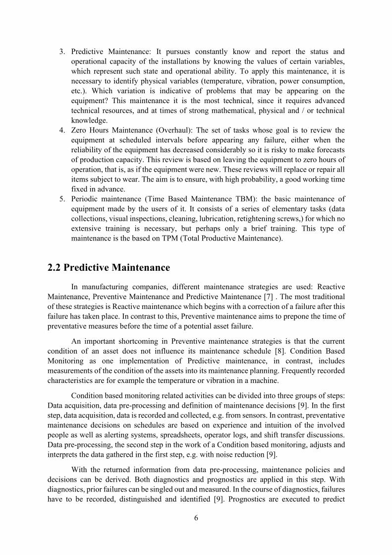
6

3. Predictive Maintenance: It pursues constantly know and report the status and operational capacity of the installations by knowing the values of certain variables, which represent such state and operational ability. To apply this maintenance, it is necessary to identify physical variables (temperature, vibration, power consumption, etc.). Which variation is indicative of problems that may be appearing on the equipment? This maintenance it is the most technical, since it requires advanced technical resources, and at times of strong mathematical, physical and / or technical knowledge.

4. Zero Hours Maintenance (Overhaul): The set of tasks whose goal is to review the equipment at scheduled intervals before appearing any failure, either when the reliability of the equipment has decreased considerably so it is risky to make forecasts of production capacity. This review is based on leaving the equipment to zero hours of operation, that is, as if the equipment were new. These reviews will replace or repair all items subject to wear. The aim is to ensure, with high probability, a good working time fixed in advance.

5. Periodic maintenance (Time Based Maintenance TBM): the basic maintenance of equipment made by the users of it. It consists of a series of elementary tasks (data collections, visual inspections, cleaning, lubrication, retightening screws,) for which no extensive training is necessary, but perhaps only a brief training. This type of maintenance is the based on TPM (Total Productive Maintenance).

2.2 Predictive Maintenance

In manufacturing companies, different maintenance strategies are used: Reactive Maintenance, Preventive Maintenance and Predictive Maintenance [7] . The most traditional of these strategies is Reactive maintenance which begins with a correction of a failure after this failure has taken place. In contrast to this, Preventive maintenance aims to prepone the time of preventative measures before the time of a potential asset failure.

An important shortcoming in Preventive maintenance strategies is that the current condition of an asset does not influence its maintenance schedule [8]. Condition Based Monitoring as one implementation of Predictive maintenance, in contrast, includes measurements of the condition of the assets into its maintenance planning. Frequently recorded characteristics are for example the temperature or vibration in a machine.

Condition based monitoring related activities can be divided into three groups of steps: Data acquisition, data pre-processing and definition of maintenance decisions [9]. In the first step, data acquisition, data is recorded and collected, e.g. from sensors. In contrast, preventative maintenance decisions on schedules are based on experience and intuition of the involved people as well as alerting systems, spreadsheets, operator logs, and shift transfer discussions. Data pre-processing, the second step in the work of a Condition based monitoring, adjusts and interprets the data gathered in the first step, e.g. with noise reduction [9].

With the returned information from data pre-processing, maintenance policies and decisions can be derived. Both diagnostics and prognostics are applied in this step. With diagnostics, prior failures can be singled out and measured. In the course of diagnostics, failures have to be recorded, distinguished and identified [9]. Prognostics are executed to predict

7

failures, which may be foreseen in the future. With prognostics, the Residual Useful Life, i.e. the remaining time before an asset runs into a failure [10], and the confidence interval can be estimated. The introduced asset condition is also referred to as the degradation signal of an asset and is the essential indicator and calculation element for predicting the Residual Useful life [11]. The invention of sensors and other means of information recording in a production environment led to more attention to Prognostic Health Management, a term comprising prognostic methods to measure and use the asset health statuses such as Predictive maintenance methods.

2.2.1 Benefits of Predictive Maintenance

One important Key Performance Indicator for many producing companies is the Overall Equipment Effectiveness (OEE) [12]. The OEE indicates the level of availability and performance of production assets and their output quality. By including downtime into the OEE measurement, unplanned outages of assets result in a negative impact on its value. In its aim to reduce unplanned outages, Predictive maintenance may have a positive effect on the OEE.

Other metrics affected by the application of Predictive maintenance include the reduction of scrap and enhanced output quality [7].

Product quality does not only depend on the degradation status of production machines but among others also on the components of a production machine [13] [10]. The planning of the necessity on the amount of repair parts at a certain time is difficult for companies and a higher inventory with many spare parts leads to higher inventory costs. Therefore, it may be reasonable to employ Predictive methods for planning repair parts inventory levels and keep at least as much inventory as is predicted necessary. In practice, Predictive maintenance often lack a joint optimization of inventory, however, models have been created, how stock management may be included in Predictive maintenance optimization, e.g. by Soltani [10].

Another benefit of Predictive maintenance may be achieved in the field of remote

sensing. CBM as a part of Predictive maintenance may be of extended benefit under conditions,

under which it is installed with remote sensing technologies allowing for Remote Condition Monitoring (RCM) and therewith enabling the review of conditions in an asset, where regular maintenance procedures would not be possible or safe [14], e.g. measurements of oil temperatures in a running engine.

Another possibility, partly enabled by Predictive maintenance, is the servitization of manufacturing as a new business model [15]. In this business model, an Original Equipment Manufacturer (OEM) retains an enduring relationship with the users of their products performing maintenance as a service to them. With an application of Predictive maintenance methods, an OEM can continuously collect data about the use, failures, and degradation of their products to consider these aspects for product improvement [16].

8

Chapter 3 – Literature Review

Synopsis

This chapter deals with the literature reviews of some of the well-known papers in the field pertaining to topics such as Tool condition monitoring, Predictive maintenance, Outlier analysis, Feature extraction, Feature selection and Machine learning models with remaining useful life determinations. These papers have been utilized as framework in developing this thesis.

3.1 Literature Review

Dr. H.M Hashemian [17] presented views on the condition-based maintenance techniques for industrial equipment and presented processes describing with examples of their use and benefits. The paper was presented by introducing about the importance of the predictive maintenance sometimes called “on-line monitoring,” “condition-based maintenance,” or “risk-based maintenance”.

The paper began by presenting the importance of the conventional visual inspection by highlighting also the other conventional means such as using sharp ears and nose, and how the sensors have replaced these conventional means in order to optimize and make the process of inspection more accurate. The paper also conveys that despite advances in predictive maintenance technologies, time-based and hands-on equipment maintenance is still the norm in many industrial processes. Today, nearly 30% of industrial equipment does not benefit from predictive maintenance technologies.

The paper gave the limitations of the time-based maintenance techniques as such. The case was evaluated by considering an exercise conducted by SKF group over the testing of 30 identical bearing elements. The failure of the bearings over the period were analysed and various plots were done. The time-based maintenance plots such as Bathtub, Wear-out and Fatigue accounted only for 11% of the total failures [18]. However, the Condition based maintenance plots such as Initial Break-In Period, Random and Infant mortality accounted for 89% of all the failures with 68% of them from only Infant mortality failures.

The paper also presented an introductory view of one of the forms of predictive maintenance i.e. Online calibration monitoring. Online calibration monitoring involves observing for drift and identifying the transmitters that have drifted beyond acceptable limits. When the plant shuts down, technicians calibrate only those transmitters that have drifted. This approach reduces by 80 to 90% the effort currently expended on calibrating pressure transmitters. This is according to data published by the author in a report he wrote for the U.S. Nuclear Regulatory Commission [19].

Based on the data sources available, the author proposed that the Predictive or online maintenance can be divided into 3 basic techniques

9

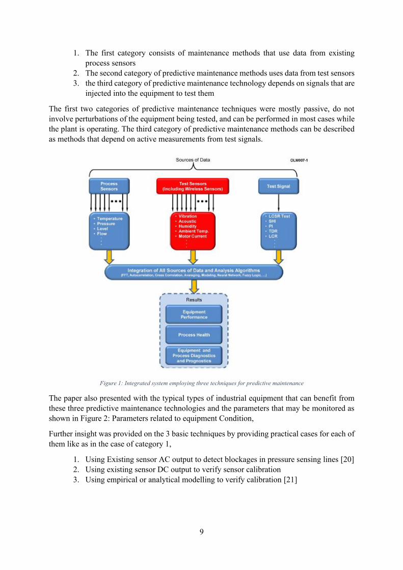
1. The first category consists of maintenance methods that use data from existing process sensors

2. The second category of predictive maintenance methods uses data from test sensors 3. the third category of predictive maintenance technology depends on signals that are

injected into the equipment to test them

The first two categories of predictive maintenance techniques were mostly passive, do not involve perturbations of the equipment being tested, and can be performed in most cases while the plant is operating. The third category of predictive maintenance methods can be described as methods that depend on active measurements from test signals.

Figure 1: Integrated system employing three techniques for predictive maintenance

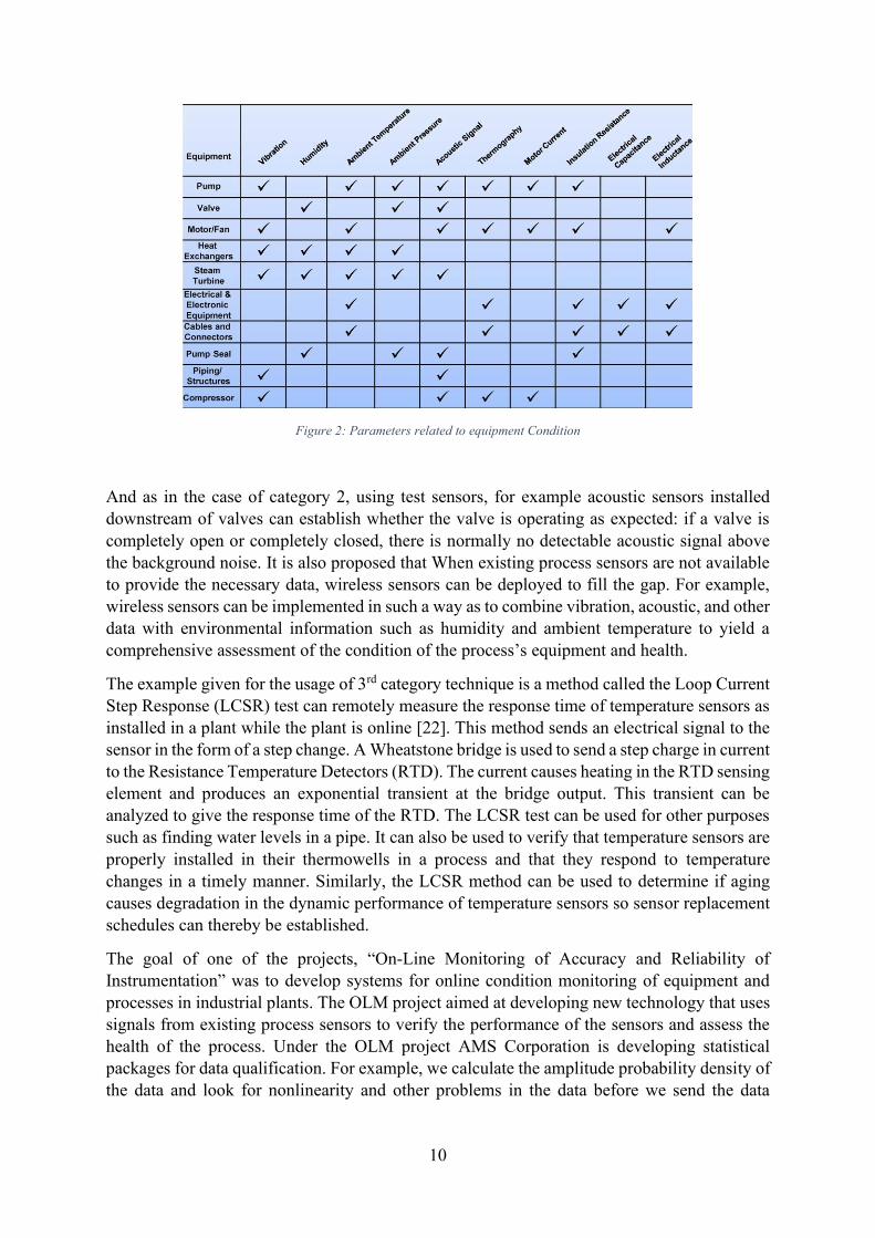
The paper also presented with the typical types of industrial equipment that can benefit from these three predictive maintenance technologies and the parameters that may be monitored as shown in Figure 2: Parameters related to equipment Condition,

Further insight was provided on the 3 basic techniques by providing practical cases for each of them like as in the case of category 1,

1. Using Existing sensor AC output to detect blockages in pressure sensing lines [20] 2. Using existing sensor DC output to verify sensor calibration 3. Using empirical or analytical modelling to verify calibration [21]

10

Figure 2: Parameters related to equipment Condition

And as in the case of category 2, using test sensors, for example acoustic sensors installed downstream of valves can establish whether the valve is operating as expected: if a valve is completely open or completely closed, there is normally no detectable acoustic signal above the background noise. It is also proposed that When existing process sensors are not available to provide the necessary data, wireless sensors can be deployed to fill the gap. For example, wireless sensors can be implemented in such a way as to combine vibration, acoustic, and other data with environmental information such as humidity and ambient temperature to yield a comprehensive assessment of the condition of the process’s equipment and health.

The example given for the usage of 3rd category technique is a method called the Loop Current Step Response (LCSR) test can remotely measure the response time of temperature sensors as installed in a plant while the plant is online [22]. This method sends an electrical signal to the sensor in the form of a step change. A Wheatstone bridge is used to send a step charge in current to the Resistance Temperature Detectors (RTD). The current causes heating in the RTD sensing element and produces an exponential transient at the bridge output. This transient can be analyzed to give the response time of the RTD. The LCSR test can be used for other purposes such as finding water levels in a pipe. It can also be used to verify that temperature sensors are properly installed in their thermowells in a process and that they respond to temperature changes in a timely manner. Similarly, the LCSR method can be used to determine if aging causes degradation in the dynamic performance of temperature sensors so sensor replacement schedules can thereby be established.

The goal of one of the projects, “On-Line Monitoring of Accuracy and Reliability of Instrumentation” was to develop systems for online condition monitoring of equipment and

processes in industrial plants. The OLM project aimed at developing new technology that uses signals from existing process sensors to verify the performance of the sensors and assess the health of the process. Under the OLM project AMS Corporation is developing statistical packages for data qualification. For example, we calculate the amplitude probability density of the data and look for nonlinearity and other problems in the data before we send the data

11

through for analysis. We also calculate signal skewness, kurtosis, and other measurements and trend them to identify problems in data.

The conclusion was that the Industrial plants should no longer assume that equipment failures will only occur after some fixed amount of time in service; they should deploy predictive and online strategies that assume that any failure can occur at any time (randomly). the three major types of predictive or online maintenance technologies discussed in this paper promises to deliver technologies that may be applied remotely, passively, and online in industrial processes to improve equipment reliability; predict failures before they occur; and contribute to process safety and efficiency. Integrating the predictive maintenance techniques described in this paper with the latest sensor technologies will enable plants to avoid unnecessary equipment replacement, save costs, and improve process safety, availability, and efficiency.

Nagdev Amruthnath and Tarun Gupta provided a study on unsupervised machine learning algorithms for early fault detection in predictive maintenance [23]. The paper presented that one of the prominent methods is watchdog agent, a design enclosed with various machine learning algorithms [24] [25]. Some of the other architectures are an OSA-CBM architecture [26], SIMAP Architecture [27], and predictive maintenance framework [28].

The paper presented introduction on machine learning and its classification.

1. Supervised learning where the predictors and response variables are known for building the model

2. Unsupervised learning, where only response variables are known 3. Reinforced learning, where the agent learns actions and consequences by

interacting with the environment

The paper mainly focused on the unsupervised learning and presented that one of the most commonly used approaches is Clustering, where, response variables are grouped into clusters either user-defined or model based on the distance, model, density, class, or characteristic of that variable. For this research, vibration data has been used.

A brief literature review was presented by the author, which focused on the Business analytics. According to the paper, the business analytics can be viewed in 3 different prospective [29],

1. Descriptive analytics 2. Predictive analytics 3. Prescriptive analytics

Coming back to the algorithms, the author presented that Principle component analysis (PCA) is one of the oldest and most prominent algorithms that are widely used today for fault detection. Since then, they have been many hybrid approaches to PCA for fault detection such as using Kernel PCA [30], adaptive threshold using Exponential weight moving average for T2 and Q statistic [31], multiscale neighborhood normalization-based multiple dynamic principal component analysis (MNNMDPCA) method [32], Independent Component Analysis. Another common method used for fault detection is clustering method. Similar to PCA, there are various algorithms such as neural net clustering algorithm neural networks and subtractive clustering [33], K-means [34], Gaussian mixture model [35], C-Means, Hierarchical Clustering [36], and Modified Rank Order clustering (MROC) [37].

12

The paper later presented case on Fault detection and about its importance. Here different algorithms such as Principle Component Analysis (PCA) T2 statistic, Hierarchical clustering, K- Means clustering, C-Means, and Model-based clustering for fault detection and benchmark its results for vibration monitoring data were discussed.

The paper later justified the reason for selecting vibration as the measuring parameter by stating that Vibration data is one of the most commonly used technique to detect any abnormalities in a submachine. Feature selection was done using PCA. Different features that were extracted were Peak acceleration, Peak velocity, turning speed, RMS Velocity and Damage accumulation. Principal component analysis (PCA) is a mathematical algorithm that reduces the dimensionality of the data while retaining most of the variation (information) in the data set [38]. In a simple context, it is an algorithm to identify patterns in data and expressing such a way to showcase those similarities and differences [39]. An algorithm was presented and the summary of the PCA indicated that the first two principal components show 95.65% of variance compared to the rest of the components. Hence from the summary data and screen plot, it was concluded that the first two principal components present maximum variation compared to rest of the principal components.

T2 Statistic analysis was also presented. This statistic can be used to measure the values against the threshold and any values above the threshold; can be concluded as out of control data. In this case, it is going to be faulty data. The results showed that the faults can be detected as early as 41 observations. Hence, this early detection would help the maintenance teams to monitor these process changes and take corrective actions accordingly.

The author later presented the evaluation of vibrations using cluster analysis. The procedure started with identifying the optimal number of clusters. To identify the number of clusters, there are many procedures available such as elbow method, Bayesian Inference Criterion method and nbClust package in R [40]. From both elbow method and nbClust package it was concluded that 3 clusters are the optimal number of clusters for fault detection. And it was theorized that each cluster represents a normal condition, warning condition and faulty condition.

The procedure was repeated with Hierarchical clustering, K-means and Fuzzy C-Means clustering. Upon careful consideration it was found that the results provided by K-means and Fuzzy C-means clustering were very similar to results obtained from Hierarchical clustering.

The final results were presented as follows, where the authors hypothesized that there are 2 states in data. One the healthy data set and the other was unhealthy data set. Using PCA and T2

statistic, they were able to fit the hypothesis states and were able to detect the faults 31 observations ahead. Whereas without a tool and just based on data plots, they could observe the trends only 11 observations ahead.

Hence the conclusion was drawn that, one of the benefits of using T2 statistic method as even when this is deployed to the manufacturing environment, with minimum or no domain knowledge, one can identify fault or critical condition when compared to clustering analysis. And that Clustering methodology is undoubtedly a better tool in detecting different levels of faults where T2 statistic would be challenging after certain levels. i.e. when the cost machine maintenance is expensive, clustering would be a flexible option where machine health can be

13

monitored continuously until a critical level is reached. But if fault detection needs to be performed under different levels then, clustering algorithms would be a better choice.

Jinjiang Wang, Yuanyuan Liang, Yinghao Zheng, Robert X. Gao, and Fengli Zhang have presented a paper on ‘Integrated fault diagnosis and prognosis approach for predictive

maintenance of wind turbine bearing with limited samples’ [41]. The paper presented a new model based approach of integrated fault diagnosis and prognosis for wind turbine remaining useful life estimation.

The paper started with providing introduction on the importance of harnessing wind energy and the usage of wind turbines and the need for it to operate in a highly reliable manner to improve the economic viability of wind energy. The paper states that according to the latest statistics from the NREL gearbox reliability database [42], the majority (about 76.2%) of wind turbine gearbox failures are caused by bearings.

In this paper to diagnose incipient defect and predict the remaining useful life of a wind turbine bearing, effective signal processing techniques and prognosis models have been investigated on monitoring sensing measurements [43] [44] [45]. In Ref. [46], an integrative approach of ensemble empirical mode decomposition and independent component analysis was investigated to separate bearing defect related signals from gear meshing signals for vibration analysis of bearing fault diagnosis. A linear regression analysis approach was presented in Ref. [47] to extract load-independent features for wind turbine bearing diagnosis. A dynamic time-warping algorithm was also presented to eliminate the speed fluctuation in vibration fault diagnosis of a wind turbine [48].

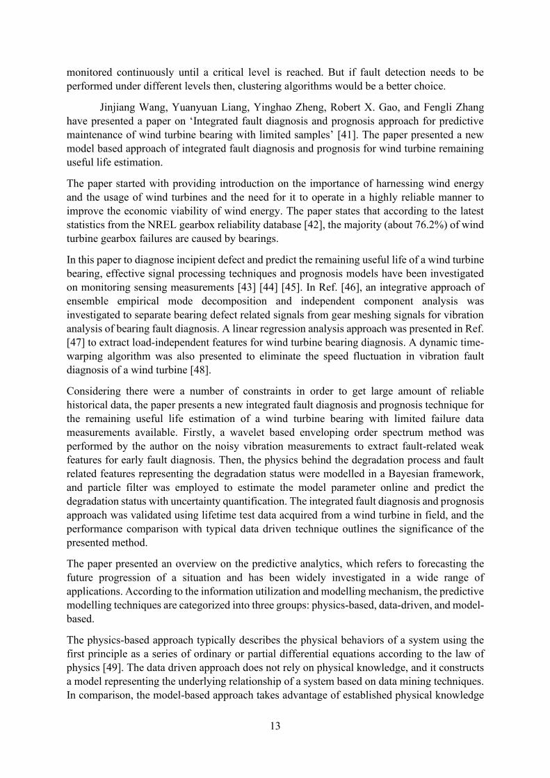
Considering there were a number of constraints in order to get large amount of reliable historical data, the paper presents a new integrated fault diagnosis and prognosis technique for the remaining useful life estimation of a wind turbine bearing with limited failure data measurements available. Firstly, a wavelet based enveloping order spectrum method was performed by the author on the noisy vibration measurements to extract fault-related weak features for early fault diagnosis. Then, the physics behind the degradation process and fault related features representing the degradation status were modelled in a Bayesian framework, and particle filter was employed to estimate the model parameter online and predict the degradation status with uncertainty quantification. The integrated fault diagnosis and prognosis approach was validated using lifetime test data acquired from a wind turbine in field, and the performance comparison with typical data driven technique outlines the significance of the presented method.

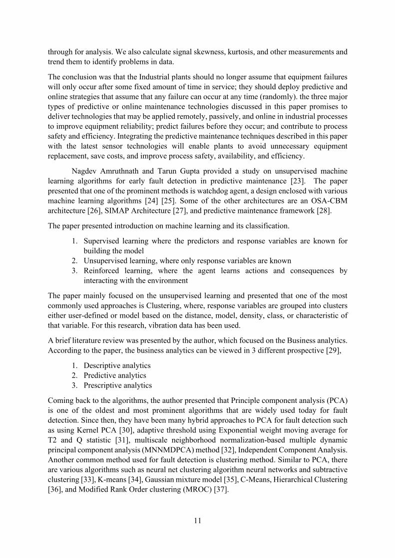
The paper presented an overview on the predictive analytics, which refers to forecasting the future progression of a situation and has been widely investigated in a wide range of applications. According to the information utilization and modelling mechanism, the predictive modelling techniques are categorized into three groups: physics-based, data-driven, and model-based.

The physics-based approach typically describes the physical behaviors of a system using the first principle as a series of ordinary or partial differential equations according to the law of physics [49]. The data driven approach does not rely on physical knowledge, and it constructs a model representing the underlying relationship of a system based on data mining techniques. In comparison, the model-based approach takes advantage of established physical knowledge

14

and collected data to enhance the prediction performance. Comparing with the data driven approach, the model-based approach requires less historical data to construct the models. The comparison of these predictive modelling techniques was provided as below,

Figure 3: Comparison of different predictive modelling techniques regarding defect prognosis

Figure 4: Framework of the integrated diagnosis and prognosis technique for wind turbines

From the results obtained, the authors arrived at the following conclusions,

1. The presented method takes advantage of physical knowledge and statistical models in one approach, and the accurate prediction is achieved by Bayesian inference with uncertainty quantification.

2. The extracted features based on wavelet transform manifest the incipient defects, and the fused feature shows a good representation of bearing defect conditions.

3. The presented method can adaptively learn from the noisy data measurements, and it is robust to different steps-ahead predictions with limited set of degradation samples.

Cunji Zhang, Xifan Yao, Jianming Zhang and Hong Jin have published a paper titled ‘Tool Condition Monitoring and Remaining Useful Life Prognostic Based on a Wireless Sensor in Dry Milling Operations’. This paper plays a vital role in the development of this thesis,

because of the impeccable, clear pathway that has been provided in this paper.

The paper introduces the Tool condition monitoring, by providing brief overview on the traditional machining operations like turning, milling, grinding and drilling. The importance of the Tool condition monitoring has been conveyed by iterating how a powerful TCM system can improve productivity and guarantee product quality, which has a considerable influence on machine efficiency [50].

The paper suggested that there are basically two methods of measuring Tool wear.

15

Figure 5: Tool wear measuring Techniques

In direct measuring methods, such as tool-workpiece junction resistance, radioactivity, vision inspection, and optical and laser beams, the shape parameters of the cutter are measured by microscope, surface profiler etc [51]. The advantages of the direct measuring methods were highlighted as the ‘Acquisition of accurate dimension changes due to tool wear’. However, this also meant that there were some disadvantages in using the direct method, as stated below,

1. Vulnerable to field conditions, cutting fluid and various disturbances 2. Since it is performed offline, this would interrupt the normal machining operations

because of the contact between the tool and the measuring device

This paved the way for the development of Indirect measuring methods. In indirect measuring methods, the tool wear is achieved by the corresponding sensor signals [52]. The measuring accuracy is lower than that of the direct measuring methods. However, they have the advantages of easy installation and easy to implement online in real time. This study focuses on indirect methods.

In the indirect methods, tool wear is measured based on various sensor signals containing cutting force, torque, vibration, Acoustic Emission (AE), sound, surface roughness, temperature, displacement, spindle power and current. Among these sensors, cutting force, vibration and AE measurements are robust and have been used more frequently than any other sensor measurement methods, and are more fit for the industrial field environment [53] [5]. The features of the signals correlating to the tool wear are captured to monitor tool condition. To do this, a mass of signal processing methods was used, such as time series modelling, Fast Fourier Transform (FFT) and time–frequency analysis, the amount of calculation involved in corresponding parameters with tool wear is enormous. Wavelet Transform (WT) is a well-developed signal processing method and has been successfully used in various science and engineering fields. In the process of TCM, the sensor signals contain information and noise typically. Therefore, it is needed to de-noise and extract the features that contain the characteristics of the tool wear from various noise disturbances [54].

Tool wear measurement

Techniques

Direct (Intermittent -

Offline)

Indirect (Continuos -

Online)

16

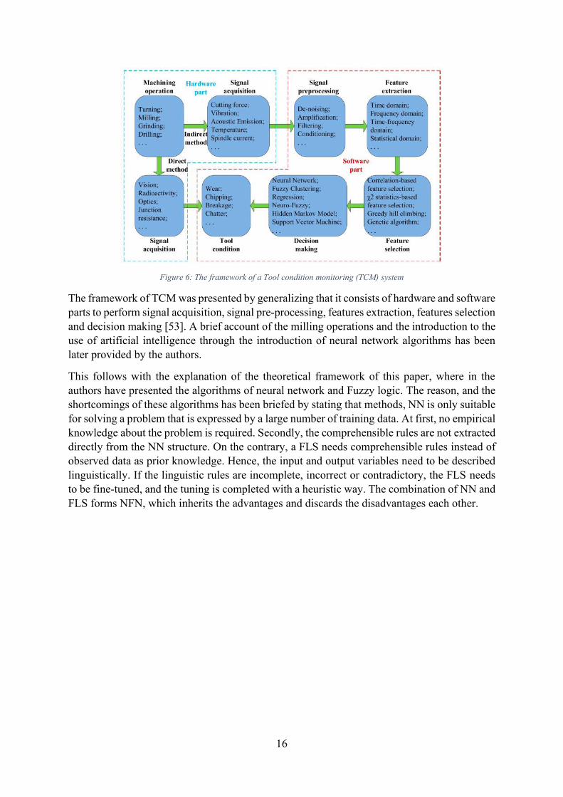
Figure 6: The framework of a Tool condition monitoring (TCM) system

The framework of TCM was presented by generalizing that it consists of hardware and software parts to perform signal acquisition, signal pre-processing, features extraction, features selection and decision making [53]. A brief account of the milling operations and the introduction to the use of artificial intelligence through the introduction of neural network algorithms has been later provided by the authors.

This follows with the explanation of the theoretical framework of this paper, where in the authors have presented the algorithms of neural network and Fuzzy logic. The reason, and the shortcomings of these algorithms has been briefed by stating that methods, NN is only suitable for solving a problem that is expressed by a large number of training data. At first, no empirical knowledge about the problem is required. Secondly, the comprehensible rules are not extracted directly from the NN structure. On the contrary, a FLS needs comprehensible rules instead of observed data as prior knowledge. Hence, the input and output variables need to be described linguistically. If the linguistic rules are incomplete, incorrect or contradictory, the FLS needs to be fine-tuned, and the tuning is completed with a heuristic way. The combination of NN and FLS forms NFN, which inherits the advantages and discards the disadvantages each other.

17

Figure 7: The architecture of Neuro-Fuzzy Network (NFN)

The paper later dealt with the description of the experiment apparatus, signal processing methods, and the methods of making sense of the sensor data acquired. This led the way to the explanation on Feature Extraction and Feature Selection.

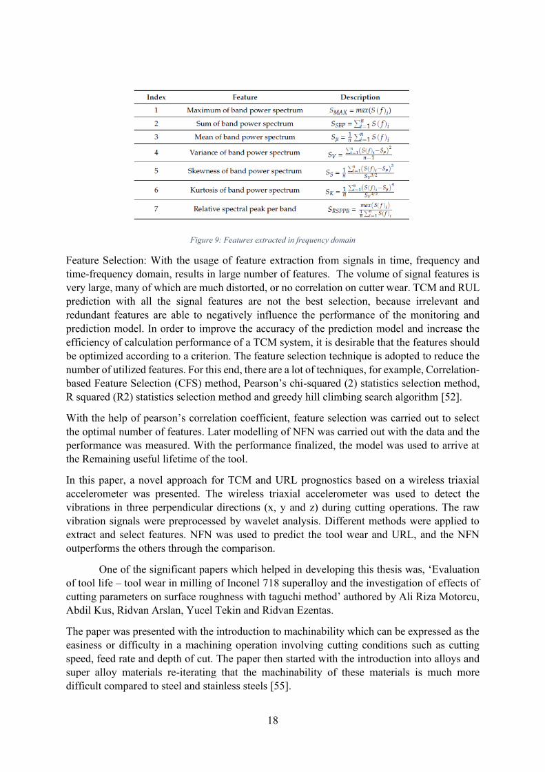
Feature Extraction: The preprocessed signal is very large in volume, which is needed to further extract features. The goal of features extraction is to reduce the dimension of the original signal, meanwhile, the extracted features associate well with the cutter wear, and are not affected by process conditions. Generally, features are extracted in time, frequency, time-frequency and statistical domains [53]. The different extraction approaches have different abilities in extracting the meaningful information about the tool wear.

With the help of below formulae, the ways of extracting the features in different domains were provided.

Figure 8: Features extracted in time domain

18

Figure 9: Features extracted in frequency domain

Feature Selection: With the usage of feature extraction from signals in time, frequency and time-frequency domain, results in large number of features. The volume of signal features is very large, many of which are much distorted, or no correlation on cutter wear. TCM and RUL prediction with all the signal features are not the best selection, because irrelevant and redundant features are able to negatively influence the performance of the monitoring and prediction model. In order to improve the accuracy of the prediction model and increase the efficiency of calculation performance of a TCM system, it is desirable that the features should be optimized according to a criterion. The feature selection technique is adopted to reduce the number of utilized features. For this end, there are a lot of techniques, for example, Correlation-based Feature Selection (CFS) method, Pearson’s chi-squared (2) statistics selection method, R squared (R2) statistics selection method and greedy hill climbing search algorithm [52].

With the help of pearson’s correlation coefficient, feature selection was carried out to select the optimal number of features. Later modelling of NFN was carried out with the data and the performance was measured. With the performance finalized, the model was used to arrive at the Remaining useful lifetime of the tool.

In this paper, a novel approach for TCM and URL prognostics based on a wireless triaxial accelerometer was presented. The wireless triaxial accelerometer was used to detect the vibrations in three perpendicular directions (x, y and z) during cutting operations. The raw vibration signals were preprocessed by wavelet analysis. Different methods were applied to extract and select features. NFN was used to predict the tool wear and URL, and the NFN outperforms the others through the comparison.

One of the significant papers which helped in developing this thesis was, ‘Evaluation

of tool life – tool wear in milling of Inconel 718 superalloy and the investigation of effects of cutting parameters on surface roughness with taguchi method’ authored by Ali Riza Motorcu,

Abdil Kus, Ridvan Arslan, Yucel Tekin and Ridvan Ezentas.

The paper was presented with the introduction to machinability which can be expressed as the easiness or difficulty in a machining operation involving cutting conditions such as cutting speed, feed rate and depth of cut. The paper then started with the introduction into alloys and super alloy materials re-iterating that the machinability of these materials is much more difficult compared to steel and stainless steels [55].

19

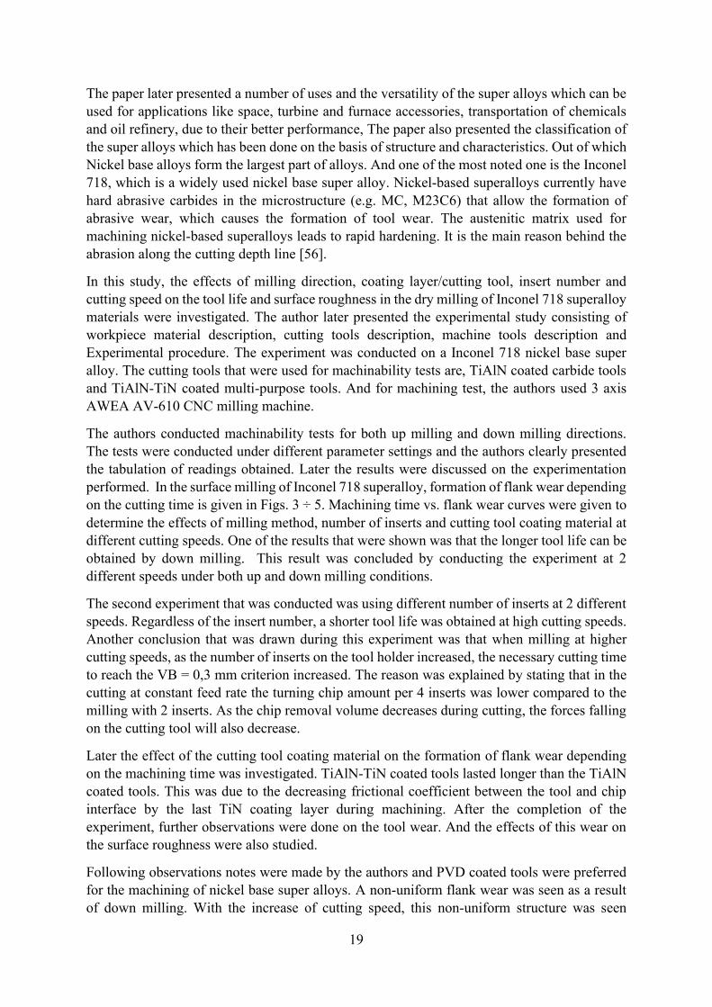
The paper later presented a number of uses and the versatility of the super alloys which can be used for applications like space, turbine and furnace accessories, transportation of chemicals and oil refinery, due to their better performance, The paper also presented the classification of the super alloys which has been done on the basis of structure and characteristics. Out of which Nickel base alloys form the largest part of alloys. And one of the most noted one is the Inconel 718, which is a widely used nickel base super alloy. Nickel-based superalloys currently have hard abrasive carbides in the microstructure (e.g. MC, M23C6) that allow the formation of abrasive wear, which causes the formation of tool wear. The austenitic matrix used for machining nickel-based superalloys leads to rapid hardening. It is the main reason behind the abrasion along the cutting depth line [56].

In this study, the effects of milling direction, coating layer/cutting tool, insert number and cutting speed on the tool life and surface roughness in the dry milling of Inconel 718 superalloy materials were investigated. The author later presented the experimental study consisting of workpiece material description, cutting tools description, machine tools description and Experimental procedure. The experiment was conducted on a Inconel 718 nickel base super alloy. The cutting tools that were used for machinability tests are, TiAlN coated carbide tools and TiAlN-TiN coated multi-purpose tools. And for machining test, the authors used 3 axis AWEA AV-610 CNC milling machine.

The authors conducted machinability tests for both up milling and down milling directions. The tests were conducted under different parameter settings and the authors clearly presented the tabulation of readings obtained. Later the results were discussed on the experimentation performed. In the surface milling of Inconel 718 superalloy, formation of flank wear depending on the cutting time is given in Figs. 3 ÷ 5. Machining time vs. flank wear curves were given to determine the effects of milling method, number of inserts and cutting tool coating material at different cutting speeds. One of the results that were shown was that the longer tool life can be obtained by down milling. This result was concluded by conducting the experiment at 2 different speeds under both up and down milling conditions.

The second experiment that was conducted was using different number of inserts at 2 different speeds. Regardless of the insert number, a shorter tool life was obtained at high cutting speeds. Another conclusion that was drawn during this experiment was that when milling at higher cutting speeds, as the number of inserts on the tool holder increased, the necessary cutting time to reach the VB = 0,3 mm criterion increased. The reason was explained by stating that in the cutting at constant feed rate the turning chip amount per 4 inserts was lower compared to the milling with 2 inserts. As the chip removal volume decreases during cutting, the forces falling on the cutting tool will also decrease.

Later the effect of the cutting tool coating material on the formation of flank wear depending on the machining time was investigated. TiAlN-TiN coated tools lasted longer than the TiAlN coated tools. This was due to the decreasing frictional coefficient between the tool and chip interface by the last TiN coating layer during machining. After the completion of the experiment, further observations were done on the tool wear. And the effects of this wear on the surface roughness were also studied.

Following observations notes were made by the authors and PVD coated tools were preferred for the machining of nickel base super alloys. A non-uniform flank wear was seen as a result of down milling. With the increase of cutting speed, this non-uniform structure was seen

20

increasing. Due to high temperature at high cutting speed the molten workpiece material diffused to the area where the chip depth terminated. In the up milling, cutting edge deteriorated in the flank wear zone, coating layers got worn and reached the main material of the cutting tool and the progressing of tool wear was more rapid. In the TiN/AlTiN coated tools, among the different wear types, the first noticeable wear was nose wear and chippings on the cutting edge. The notching at the cutting depth caused by high temperature, high workpiece resistance and abrasive chips also created machining problems. In this milling study, the effective wear for both milling methods was free surface wear and nose wear. In both milling wear increased linearly depending on the cutting time [57]. Because of the irregular and increasing tool wear created in the up milling operations, contributions of TiN layer on the cutting tool performance came out to be insufficient.

With the study on the effects of control factors on surface roughness, following observations were done. It was observed that surface roughness got worse depending on the increasing of cutting speed but the milling direction did not affect the increasing of surface roughness. It is also seen that cutting speed has no significant effect on the increase in surface roughness. In the down and up milling, a higher surface roughness value may be obtained because the number of tracks caused by the inserts on the surface during machining may be more in the milling with 4 inserts. At all the cutting speeds, the TiAlN-TiN coated tools exhibited better performances than the TiAlN coated tools.

With all the observations, following conclusions were drawn from this paper, which were also utilized in assessing the results of this study.

1. The effect of the cutting speed on tool life was higher than the effect of milling method and number of inserts.

2. Tool life decreased depending on the increase in cutting speed.

3. At both low and high cutting speeds, longer tool life was obtained with down milling method compared to up milling.

4. The effective wear for both of the milling methods was free surface wear and nose wear. Wear increased linearly in both of the milling methods depending on the cutting time.

5. A non-uniform flank wear was formed after down milling and this non-uniform structure increased with the increasing of cutting speed.

6. Due to the high temperature generated during the high-speed cutting, molten workpiece diffused into the area where the cutting depth terminated.

7. The contributions of TiN layer to the performance of the cutting tool for up milling operations were insufficient in the formation of increasing and irregular tool wear.

8. The most effective control factors on the surface roughness parameter were cutting tool coating material, number of cutting tool inserts, the milling direction and the cutting speed accordingly.

21

Chapter 4 – Milling Process

Synopsis

This chapter deals with the metal cutting processes, gives an introduction into milling processes, the milling cutting tool and its wear phenomena with continuous usage. This chapter also gives an overview of the experimental setup that was used in order to obtain the data from the sensors for processing.

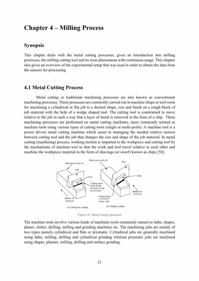
4.1 Metal Cutting Process

Metal cutting or traditional machining processes are also known as conventional machining processes. These processes are commonly carried out in machine shops or tool room for machining a cylindrical or flat job to a desired shape, size and finish on a rough block of job material with the help of a wedge shaped tool. The cutting tool is constrained to move relative to the job in such a way that a layer of metal is removed in the form of a chip. These machining processes are performed on metal cutting machines, more commonly termed as machine tools using various types of cutting tools (single or multi-point). A machine tool is a power driven metal cutting machine which assist in managing the needed relative motion between cutting tool and the job that changes the size and shape of the job material. In metal cutting (machining) process, working motion is imparted to the workpiece and cutting tool by the mechanisms of machine tool so that the work and tool travel relative to each other and machine the workpiece material in the form of shavings (or swarf) known as chips [58].

Figure 10: Metal Cutting Operation

The machine tools involve various kinds of machines tools commonly named as lathe, shaper, planer, slotter, drilling, milling and grinding machines etc. The machining jobs are mainly of two types namely cylindrical and flats or prismatic. Cylindrical jobs are generally machined using lathe, milling, drilling and cylindrical grinding whereas prismatic jobs are machined using shaper, planner, milling, drilling and surface grinding.

22

In metal cutting operation, the position of cutting edge of the cutting tool is important based on which the cutting operation is classified as orthogonal cutting and oblique cutting. Orthogonal cutting is also known as two dimensional metal cutting in which the cutting edge is normal to the work piece. In orthogonal cutting no force exists in direction perpendicular to relative motion between tool and work piece. Oblique cutting is the common type of three dimensional cutting used in various metal cutting operations in which the cutting action is inclined with the job by a certain angle called the inclination angle.

Figure 11: Orthogonal cutting

Figure 12: Oblique Cutting

4.2 Milling cutting tool

Cutting tools performs the main machining operation. They comprise of single point cutting tool or multipoint cutting tools. It is a body having teeth or cutting edges on it. A single point cutting tool (such as a lathe, shaper and planner and boring tool) has only one cutting edge, whereas a multi-point cutting tool (such as milling cutter, milling cutter, drill, reamer and broach) has a number of teeth or cutting edges on its periphery.

4.2.1 Single Point Cutting Tool

There are mainly two types of single point tools namely the solid type and the tipped tool. The solid type single point tool may be made from high speed steel, from a cast alloy. Brazed tools are generally known as tool bits and are used in tool holders. The tipped type of tool is made from a good shank steel on which is mounted a tip of cutting tool material. Tip may be made of high speed steel or cemented carbide. In addition to this, there are long index-able insert tools and throwaway. The Insert type tool throwaway refers to the cutting tool insert which is mechanically held in the tool holder. The inserts are purchased which are ready for use. When all cutting edges are used, the insert is discarded and not re-sharpened. These tools can be further classified depending upon the operations for which they are used and the type of the shank (straight or bent shank type). Tools may be of the types planning tools, turning tools, facing tool, boring tools, parting and slotting tools etc.

Different types of carbide tips are generally used on tipped tool. In general the straight shank type tools are cheaper to manufacture as compared to bent shank type. But bent shank type can

23

be used for turning either longitudinal or cross feed without resetting and for turning, facing and chamfering operations. Boring tools usually quite long and the cross-section is small.

Figure 13: Solid type single point cutting tool

Figure 14: Tipped type single point cutting tool

Figure 15: Index-able insert type single point cutting tool

A single point cutting tool can be understood by its geometry. Geometry comprises mainly of nose, rake face of the tool, flank, heel and shank etc. The nose is shaped as conical with different angles. The angles are specified in a perfect sequence as American Society of Tool Manufacturer for recognizing them as under.

Figure 16: Geometry of single point cutting tool

4.2.2 Mechanisms of Metal Cutting

The work piece is securely clamped in a machine tool vice or clamps or chuck or collet. A wedge shape tool is set to a certain depth of cut and is forced to move in direction as shown in figure. All traditional machining processes require a cutting tool having a basic wedge shape at the cutting edge. The tool will cut or shear off the metal, provided

1. the tool is harder than the metal

24

2. the tool is properly shaped so that its edge can be effective in cutting the metal 3. the tool is strong enough to resist cutting pressures but keen enough to sever the metal,

and 4. provided there is movement of tool relative to the material or vice versa, so as to make

cutting action possible.

Most metal cutting is done by high speed steel tools or carbide tools. In metal cutting, the tool does not slide through metal as a jack knife does through wood, not does the tool split the metal as an axe does a log. The metal is forced off the workpiece by being compressed, shearing off, and sliding along the face of the cutting tool. The way a cutting tool cuts the metal can be explained as follows. All metals in the solid state have a characteristic crystalline structure, frequently referred to as grain structure. The grain or crystals vary in size from very fine to very coarse, depending upon the type of metal and its heat-treatment. The cutting tool advances again in the work piece. Heavy forces are exerted on the crystals in front of the tool face. These crystals, in turn exert similar pressures on crystals ahead of them, in the direction of the cut or force applied by the cutter. As the tool continues to advance, the material at sheared point is sheared by the cutting edge of the tool or it may be torn loose by the action of the bending chip which is being formed. As the tool advances, maximum stress is exerted along sheared line, which is called the shear plane. This plane is approximately perpendicular to the cutting face of the tool. There exists a shear zone on both sides of the shear plane, when the force of the tool exceeds the strength of the material at the shear plane, rupture or slippage of the crystalline grain structure occurs, thus forming the metal chip. The chip gets separated from the workpiece material and moves up along the tool face. In addition, when the metal is sheared, the crystals are elongated, the direction of elongation being different from that of shear. The circles which represent the crystals in the uncut metal get elongated into ellipses after leaving the shearing plane.

Figure 17: Metal Cutting Operation

4.3 Tool wear

Cutting tools are subjected to an extremely severe rubbing process. They are in metal-to-metal contact between the chip and work piece, under high stress and temperature. The situation becomes severe due to the existence of extreme stress and temperature gradients near the surface of the tool [59].

Tool wear is generally a gradual process due to regular operation. Tool wear can be compared with the wear of the tip of an ordinary pencil. According to Australian standard, the tool wear

25

can be defined as “The change of shape of the tool from its original shape, during cutting, resulting from the gradual loss of tool material”.

Tool wear depends upon following parameters:

1. Tool and work piece material. 2. Tool shape. 3. Cutting Speed. 4. Feed. 5. Depth of cut. 6. Cutting fluid used. 7. Machine Tool characteristics etc.

Tool wear affects following items:

1. Increased cutting forces. 2. Increased cutting temperature. 3. Decreased accuracy of produced parts. 4. Decreased tool life. 5. Poor surface finish. 6. Economics of cutting operations.

4.3.1 Types of Tool wear

The high contact stresses are developed in machining process due to rubbing action of:

1. Tool rake face and chips. 2. Tool flank face and machined surface.

These results in a variety of wear patterns observed at the rake face and the flank face. We call this gradual wear of the tool. The gradual wear is unavoidable but controllable. It is the wear which cannot be prevented. It has to occur after certain machining time. The gradual wear can be controlled by remedial action. The gradual wear can be divided into two basic types of wear, corresponding to two regions in the cutting tool.

1. Flank wear 2. Crater wear

Figure 18: Tool wear phenomena

26

Figure 19: Flank and Crater wear

4.3.1.1 Flank wear

Wear on the flank face (relief or clearance face) of the tool is called flank wear.

Figure 20: The Flank wear

The characteristics of flank wear are following:

1. It is the most important wear that appears on the flank surface parallel to the cutting edge. It most commonly results from abrasive/adhesive wear of the cutting edge against the machined surface.

2. It generally results from high temperatures, which affect tool and work material properties.

3. It results in the formation of wear land. Wear land formation is not always uniform along the major and minor cutting edge of the tool.

4. It can be measured by using the average wear land size (V3) and maximum wear land size (VBmax).

5. It can be described using the Tool Life Expectancy Equation.

𝑉𝐶𝑇𝑛 = 𝐶

Equation 1: Tool Life Expectancy

A more general form of the equation (considering depth of cut and feed rate) is

27

𝑉𝐶𝑇𝑛𝐷𝑥𝐹𝑦 = 𝐶

Equation 2: Generalized tool life expectancy equation

Where,

VC = Cutting speed

T = Tool life

D = Depth of cut (mm)

F = Feed rate (mm/rev or inch/rev)

x and y = Exponents that are determined experimentally for each cutting condition

C = Machining constant, found by experimentation or published data book. Depends on properties of tool materials, work piece and feed rate

n = exponential

Values of n = 0.1 to 0.15 (For HSS tools)

n = 0.2 to 0.4 (For carbide tools)

n = 0.4 to 0.6 (For ceramic tools)

Reasons for the Flank wear can be summarized as below,

1. Increased cutting speed causes flank to wear grow rapidly. 2. Increase in feed and depth of cut can also result in larger flank wear. 3. Abrasion by hard panicles in the work piece. 4. Shearing of micro welds between tool and work-material. 5. Abrasion by fragments of built-up edge, which strike against the clearance face (Flank

face) of the tool.

Following are the harmful effects of severe Flank wear,

1. Increase in the total cutting force. 2. Increase in component surface roughness. 3. Also affect the component dimensional accuracy. 4. When form tools are used, flank wear will also change the shape of the components

produced,

Following remedies can be suggested in order to minimize the Flank wear

1. Reduce cutting speed. 2. Reduce feed and depth of cut. 3. Use hard grade of carbide if possible. 4. Prevent formation of built-up edge, using chip breakers.

4.3.1.2 Crater Wear

Wear on the rake face of the tool is called crater wear. As the name suggests, the shape of wear is that of a crater or a bowl.

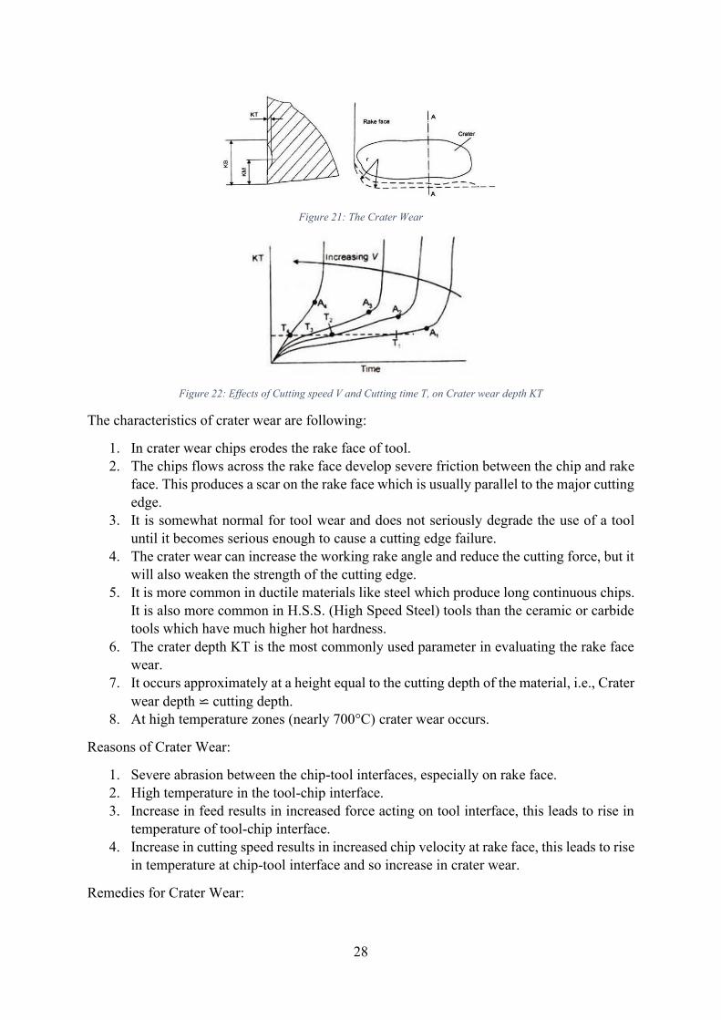
28

Figure 21: The Crater Wear

Figure 22: Effects of Cutting speed V and Cutting time T, on Crater wear depth KT

The characteristics of crater wear are following:

1. In crater wear chips erodes the rake face of tool. 2. The chips flows across the rake face develop severe friction between the chip and rake

face. This produces a scar on the rake face which is usually parallel to the major cutting edge.

3. It is somewhat normal for tool wear and does not seriously degrade the use of a tool until it becomes serious enough to cause a cutting edge failure.

4. The crater wear can increase the working rake angle and reduce the cutting force, but it will also weaken the strength of the cutting edge.

5. It is more common in ductile materials like steel which produce long continuous chips. It is also more common in H.S.S. (High Speed Steel) tools than the ceramic or carbide tools which have much higher hot hardness.

6. The crater depth KT is the most commonly used parameter in evaluating the rake face wear.

7. It occurs approximately at a height equal to the cutting depth of the material, i.e., Crater wear depth ⋍ cutting depth.

8. At high temperature zones (nearly 700°C) crater wear occurs.

Reasons of Crater Wear:

1. Severe abrasion between the chip-tool interfaces, especially on rake face. 2. High temperature in the tool-chip interface. 3. Increase in feed results in increased force acting on tool interface, this leads to rise in

temperature of tool-chip interface. 4. Increase in cutting speed results in increased chip velocity at rake face, this leads to rise

in temperature at chip-tool interface and so increase in crater wear.

Remedies for Crater Wear:

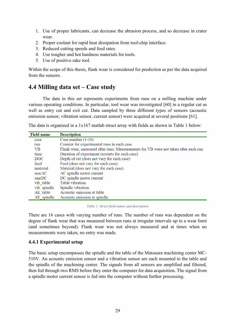
29

1. Use of proper lubricants, can decrease the abrasion process, and so decrease in crater wear.

2. Proper coolant for rapid heat dissipation from tool-chip interface. 3. Reduced cutting speeds and feed rates. 4. Use tougher and hot hardness materials for tools. 5. Use of positive rake tool.

Within the scope of this thesis, flank wear is considered for prediction as per the data acquired from the sensors.

4.4 Milling data set – Case study

The data in this set represents experiments from runs on a milling machine under various operating conditions. In particular, tool wear was investigated [60] in a regular cut as well as entry cut and exit cut. Data sampled by three different types of sensors (acoustic emission sensor, vibration sensor, current sensor) were acquired at several positions [61].

The data is organized in a 1x167 matlab struct array with fields as shown in Table 1 below:

Table 1: Struct field names and description

There are 16 cases with varying number of runs. The number of runs was dependent on the degree of flank wear that was measured between runs at irregular intervals up to a wear limit (and sometimes beyond). Flank wear was not always measured and at times when no measurements were taken, no entry was made.

4.4.1 Experimental setup

The basic setup encompasses the spindle and the table of the Matsuura machining center MC-510V. An acoustic emission sensor and a vibration sensor are each mounted to the table and the spindle of the machining center. The signals from all sensors are amplified and filtered, then fed through two RMS before they enter the computer for data acquisition. The signal from a spindle motor current sensor is fed into the computer without further processing.

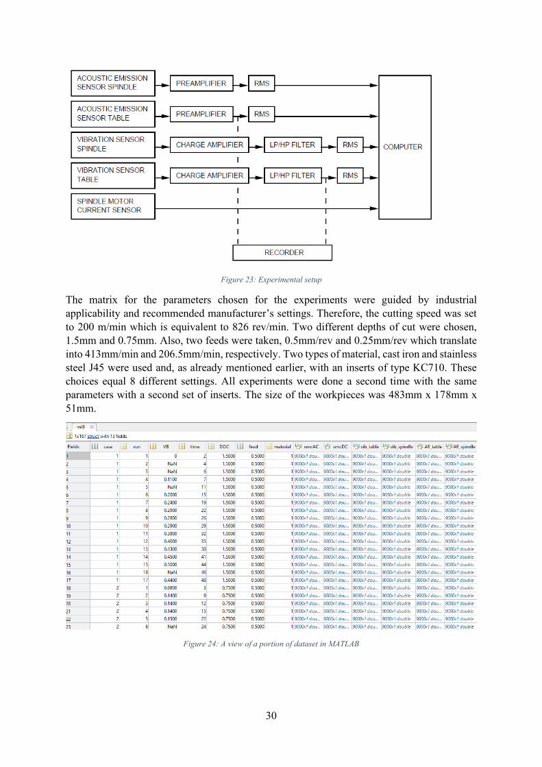
30

Figure 23: Experimental setup

The matrix for the parameters chosen for the experiments were guided by industrial applicability and recommended manufacturer’s settings. Therefore, the cutting speed was set

to 200 m/min which is equivalent to 826 rev/min. Two different depths of cut were chosen, 1.5mm and 0.75mm. Also, two feeds were taken, 0.5mm/rev and 0.25mm/rev which translate into 413mm/min and 206.5mm/min, respectively. Two types of material, cast iron and stainless steel J45 were used and, as already mentioned earlier, with an inserts of type KC710. These choices equal 8 different settings. All experiments were done a second time with the same parameters with a second set of inserts. The size of the workpieces was 483mm x 178mm x 51mm.

Figure 24: A view of a portion of dataset in MATLAB

31

Chapter 5 – Tools utilized

Synopsis

In order to perform the analysis on the data, as well as to use the data to come up with the final result intended, tools are an essential part. This chapter gives an introduction on to the tools used for the same.

5.1 Programming Language

For the execution of the thesis, Python has been used as the primary programming language. Python is an interpreted, object-oriented, high-level programming language with dynamic semantics. Its high-level built in data structures, combined with dynamic typing and dynamic binding, make it very attractive for Rapid Application Development, as well as for use as a scripting or glue language to connect existing components together. Python's simple, easy to learn syntax emphasizes readability and therefore reduces the cost of program maintenance. Python supports modules and packages, which encourages program modularity and code reuse. The Python interpreter and the extensive standard library are available in source or binary form without charge for all major platforms and can be freely distributed [62].

According to the latest TIOBE Programming Community Index, Python is one of the top 10 popular programming languages of 2017. Python is a general purpose and high level programming language. We can use Python for developing desktop GUI applications, websites and web applications. Also, Python, as a high level programming language, allows us to focus on core functionality of the application by taking care of common programming tasks. The simple syntax rules of the programming language further make it easier for us to keep the code base readable and application maintainable. There are also a few reasons why Python is preferred to other programming languages [63].

1. Readable and Maintainable Code While writing a software application, we must focus on the quality of its source code to simplify maintenance and updates. The syntax rules of Python allow us to express concepts without writing additional code. At the same time, Python, unlike other programming languages, emphasizes on code readability, and allows us to use English keywords instead of punctuations. Hence, we can use Python to build custom applications without writing additional code. The readable and clean code base helps us to maintain and update the software without putting extra time and effort.

2. Multiple Programming Paradigms Like other modern programming languages, Python also supports several programming paradigms. It supports object oriented and structured programming fully. Also, its language features support various concepts in functional and aspect-oriented programming. At the same time, Python also features a dynamic type system and

32

automatic memory management. The programming paradigms and language features helps us to use Python for developing large and complex software applications.

3. Compatible with Major Platforms and Systems At present, Python is supported many operating systems. We can even use Python interpreters to run the code on specific platforms and tools. Also, Python is an interpreted programming language. It allows us to run the same code on multiple platforms without recompilation. Hence, we are not required to recompile the code after making any alteration. We can run the modified application code without recompiling and check the impact of changes made to the code immediately. The feature makes it easier for us to make changes to the code without increasing development time.

4. Robust Standard Library Its large and robust standard library makes Python score over other programming languages. The standard library allows us to choose from a wide range of modules according to our precise needs. Each module further enables us to add functionality to the Python application without writing additional code. For instance, while writing a web application in Python, we can use specific modules to implement web services, perform string operations, manage operating system interface or work with internet protocols. We can even gather information about various modules by browsing through the Python Standard Library documentation.

5. Many Open Source Frameworks and Tools As an open source programming language, Python helps us to curtail software development cost significantly. We can even use several open source Python frameworks, libraries and development tools to curtail development time without increasing development cost. We even have option to choose from a wide range of open source Python frameworks and development tools according to our precise needs. For instance, we can simplify and speedup web application development by using robust Python web frameworks like Django, Flask, Pyramid, Bottle and Cherrypy. Likewise, we can accelerate desktop GUI application development using Python GUI frameworks and toolkits like PyQT, PyJs, PyGUI, Kivy, PyGTK and WxPython.

6. Simplify Complex Software Development Python is a general purpose programming language. Hence, we can use the programming language for developing both desktop and web applications. Also, we can use Python for developing complex scientific and numeric applications. Python is designed with features to facilitate data analysis and visualization. We can take advantage of the data analysis features of Python to create custom big data solutions without putting extra time and effort. At the same time, the data visualization libraries and APIs provided by Python helps us to visualize and present data in a more appealing and effective way. Many Python developers even use Python to accomplish artificial

33

intelligence (AI) and natural language processing tasks. This feature has been utilized in the realization of this thesis work.

7. Adopt Test Driven Development We can use Python to create prototype of the software application rapidly. Also, we can build the software application directly from the prototype simply by refactoring the Python code. Python even makes it easier for us to perform coding and testing simultaneously by adopting test driven development (TDD) approach. We can easily write the required tests before writing code and use the tests to assess the application code continuously. The tests can also be used for checking if the application meets predefined requirements based on its source code.

Python can be extensively used for machine learning purposes. Machine learning and artificial intelligence-based projects are obviously what the future holds. We want better personalization, smarter recommendations, and improved search functionality. Our apps can see, hear, and respond – that’s what artificial intelligence (AI) has brought, enhancing the user experience and creating value across many industries [64].

AI projects differ from traditional software projects. The differences lie in the technology stack, the skills required for an AI-based project, and the necessity of deep research. To implement our AI aspirations, we should use a programming language that is stable, flexible, and has tools available. Python offers all of this, which is why we see lots of Python AI projects today.

From development to deployment and maintenance, Python helps developers be productive and confident about the software they’re building. Benefits that make Python the best fit for machine learning and AI-based projects include simplicity and consistency, access to great libraries and frameworks for AI and machine learning (ML), flexibility, platform independence, and a wide community. These add to the overall popularity of the language.

1. Simple and consistent Python offers concise and readable code. While complex algorithms and versatile workflows stand behind machine learning and AI, Python’s simplicity allows

developers to write reliable systems. Developers get to put all their effort into solving an ML problem instead of focusing on the technical nuances of the language. Additionally, Python is appealing to many developers as it’s easy to learn. Python code

is understandable by humans, which makes it easier to build models for machine learning. Many programmers say that Python is more intuitive than other programming languages. Others point out the many frameworks, libraries, and extensions that simplify the implementation of different functionalities. It’s generally accepted that

Python is suitable for collaborative implementation when multiple developers are involved. Since Python is a general-purpose language, it can do a set of complex machine learning tasks and enable you to build prototypes quickly that allow you to test your product for machine learning purposes.

34

2. Extensive selection of libraries and frameworks

Implementing AI and ML algorithms can be tricky and requires a lot of time. It’s vital

to have a well-structured and well-tested environment to enable developers to come up with the best coding solutions.

To reduce development time, programmers turn to a number of Python frameworks and libraries. A software library is pre-written code that developers use to solve common programming tasks. Python, with its rich technology stack, has an extensive set of libraries for artificial intelligence and machine learning. Here are some of them:

• Keras, TensorFlow, and Scikit-learn for machine learning • NumPy for high-performance scientific computing and data analysis • SciPy for advanced computing • Pandas for general-purpose data analysis • Seaborn for data visualization

Scikit-learn features various classification, regression, and clustering algorithms, including support vector machines, random forests, gradient boosting, k-means, and DBSCAN, and is designed to work with the Python numerical and scientific libraries NumPy and SciPy.

3. Platform independence

Platform independence refers to a programming language or framework allowing developers to implement things on one machine and use them on another machine without any (or with only minimal) changes. One key to Python’s popularity is that it’s a platform independent language. Python is supported by many platforms including Linux, Windows, and macOS. Python code can be used to create standalone executable programs for most common operating systems, which means that Python software can be easily distributed and used on those operating systems without a Python interpreter.

What’s more, developers usually use services such as Google or Amazon for their

computing needs. However, we can often find companies and data scientists who use their own machines with powerful Graphics Processing Units (GPUs) to train their ML models. And the fact that Python is platform independent makes this training a lot cheaper and easier.

4. Great community and popularity

In the Developer Survey 2018 by Stack Overflow, Python was among the top 10 most popular programming languages, which ultimately means that 23 can find a development company with the necessary skill set to build your AI-based project.

If we look closely at the image below, we can see that Python is the language that people Google more than any other [65].

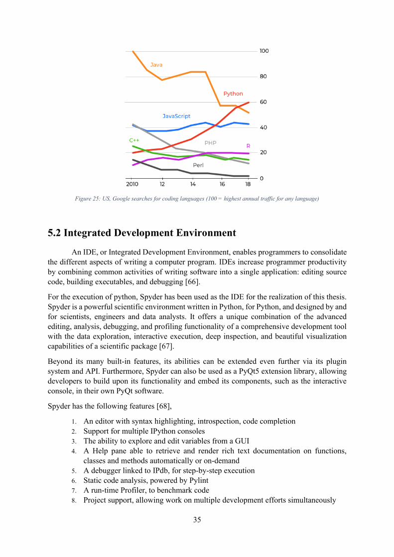
35

Figure 25: US, Google searches for coding languages (100 = highest annual traffic for any language)

5.2 Integrated Development Environment

An IDE, or Integrated Development Environment, enables programmers to consolidate the different aspects of writing a computer program. IDEs increase programmer productivity by combining common activities of writing software into a single application: editing source code, building executables, and debugging [66].

For the execution of python, Spyder has been used as the IDE for the realization of this thesis. Spyder is a powerful scientific environment written in Python, for Python, and designed by and for scientists, engineers and data analysts. It offers a unique combination of the advanced editing, analysis, debugging, and profiling functionality of a comprehensive development tool with the data exploration, interactive execution, deep inspection, and beautiful visualization capabilities of a scientific package [67].

Beyond its many built-in features, its abilities can be extended even further via its plugin system and API. Furthermore, Spyder can also be used as a PyQt5 extension library, allowing developers to build upon its functionality and embed its components, such as the interactive console, in their own PyQt software.

Spyder has the following features [68],

1. An editor with syntax highlighting, introspection, code completion 2. Support for multiple IPython consoles 3. The ability to explore and edit variables from a GUI 4. A Help pane able to retrieve and render rich text documentation on functions,

classes and methods automatically or on-demand 5. A debugger linked to IPdb, for step-by-step execution 6. Static code analysis, powered by Pylint 7. A run-time Profiler, to benchmark code 8. Project support, allowing work on multiple development efforts simultaneously

36

9. A built-in file explorer, for interacting with the filesystem and managing projects 10. A "Find in Files" feature, allowing full regular expression search over a specified

scope 11. An online help browser, allowing users to search and view Python and package

documentation inside the IDE 12. A history log, recording every user command entered in each console 13. An internal console, allowing for introspection and control over Spyder's own

operation

5.3 Libraries used

Python library is a collection of functions and methods that allows you to perform lots of actions without writing your own code. A brief description of the libraries used are provided below

5.3.1 Matplotlib

Matplotlib is a Python library that uses Python Script to write 2-dimensional graphs and plots. Often mathematical or scientific applications require more than single axes in a representation. This library helps us to build multiple plots at a time. We can, however, use Matplotlib to manipulate different characteristics of figures as well [69].

Features of Matplotlib,

1. Matplotlib can create such quality figures that are really good for publication. Figures we create with Matplotlib are available in hardcopy formats across different interactive platforms.

2. We can use MatPlotlib with different toolkits such as Python Scripts, IPython Shells, Jupyter Notebook, and many other four graphical user interfaces.

3. A number of third-party libraries can be integrated with Matplotlib applications. Such as seaborn, ggplot, and other projection and mapping toolkits such as basemap.

4. An active community of developers are dedicated to help with any of the inquiries with Matplotlib.

5. Another good thing is that we can track any bugs, new patches, and feature requests on the issue tracker page from Github. It is an official page for featuring different issues related to Matplotlib.

5.3.2 Numpy

Numpy is a popular array – processing package of Python. It provides good support for different dimensional array objects as well as for matrices. Numpy is not only confined to providing arrays only, but it also provides a variety of tools to manage these arrays. It is fast, efficient, and good for managing matrices and arrays [69].

Features of Numpy,

1. Arrays of Numpy offer modern mathematical implementations on huge amount of data. Numpy makes the execution of these projects much easier and hassle-free.

37

2. Numpy provides masked arrays along with general array objects. It also comes with functionalities such as manipulation of logical shapes, discrete Fourier transform, general linear algebra, and many more.

3. While we change the shape of any N-dimensional arrays, Numpy will create new arrays for that and delete the old ones.

4. This python package provides useful tools for integration. We can easily integrate Numpy with programming languages such as C, C++, and Fortran code.

5. Numpy provides such functionalities that are comparable to MATLAB. They both allow users to get faster with operations.

5.3.3 Scipy

Scipy is an open-source python library that is used for both scientific and technical computation. It is a free python library. And very suitable for machine learning. However, computation is not the only task that makes scipy special. It is also very popular for image manipulation, as well [69].

Features of Scipy,

1. Scipy contains different modules. These modules are suitable for optimization, integration, linear algebra, and statistics, as well.

2. It makes the best use of Numpy arrays for general data structures. In fact, Numpy is an integrated part of Scipy.

3. Scipy can handle 1-d polynomials in two ways. Whether we can use poly1d class from numpy or we can use co-efficient arrays to do the job.

4. High-level scipy contains not only numpy but also numpy.lib.scimath as well. But it is better to use them from their direct source.

5. A supporting community of Scipy is always there to answer our regular questions and solve any issues if aroused.

5.3.4 Pandas

Pandas is a python software package. It is a must to learn for data-science and dedicatedly written for Python language. It is a fast, demonstrative, and adjustable platform that offers intuitive data-structures. We can easily manipulate any type of data such as – structured or time-series data with this package [69].

Features of Pandas,

1. Pandas provide us with many Series and Data frames. It allows us to easily organize, explore, represent, and manipulate data.

2. Smart alignment and indexing featured in Pandas offers a perfect organization and data labeling.

3. Pandas has some special features that allows us to handle missing data or value with a proper measure.

4. This package offers such a clean code that even people with no or basic knowledge of programming can easily work with it.

5. It provides a collection of built-in tools that allows us to both read and write data in different web services, data-structure, and databases as well.

38

6. Pandas can support JSON, Excel, CSV, HDF5, and many other formats.

5.3.5 Scikit Learn

Scikit learn is a simple and useful python machine learning library. It is written in python, cython, C, and C++. However, most of it is written in the Python programming language. It is a free machine learning library. It is a flexible python package that can work in complete harmony with other python libraries and packages such as Numpy and Scipy [69].

Features of Scikit Learn,

1. Scikit Learn comes with a clean and neat API. It also provides very useful documentation for beginners.

2. It comes with different algorithms – classification, clustering, and regression. It also supports random forests, k-means, gradient boosting, DBSCAN and others

3. This package offers easy adaptability. 4. Scikit Learn offers easy methods for data representation. Whether we want to

present data as a table or matrix, it is all possible with Scikit Learn. 5. It allows us to explore through digits that are written in hands. We can not only load

but also visualize digits-data as well.

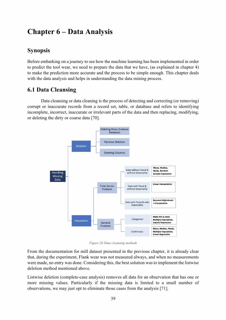
39

Chapter 6 – Data Analysis

Synopsis

Before embarking on a journey to see how the machine learning has been implemented in order to predict the tool wear, we need to prepare the data that we have, (as explained in chapter 4) to make the prediction more accurate and the process to be simple enough. This chapter deals with the data analysis and helps in understanding the data mining process.

6.1 Data Cleansing

Data cleansing or data cleaning is the process of detecting and correcting (or removing) corrupt or inaccurate records from a record set, table, or database and refers to identifying incomplete, incorrect, inaccurate or irrelevant parts of the data and then replacing, modifying, or deleting the dirty or coarse data [70].

Figure 26:Data cleansing methods

From the documentation for mill dataset presented in the previous chapter, it is already clear that, during the experiment, Flank wear was not measured always, and when no measurements were made, no entry was done. Considering this, the best solution was to implement the listwise deletion method mentioned above.

Listwise deletion (complete-case analysis) removes all data for an observation that has one or more missing values. Particularly if the missing data is limited to a small number of observations, we may just opt to eliminate those cases from the analysis [71].

40

With the implementation of the list wise deletion, the dataset which originally consisted of 167 rows and 13 columns, was reduced to 146 rows and 13 columns. The rows containing the missing values has been identified and removed using the following code,

cleaned_data = data.dropna()

filtered_data = data[data['VB'].isnull()] filtered_data_index = filtered_data.index cleaned_index = cleaned_data.index

Code Snippet 1: Data Cleansing

6.2 Outlier Analysis

An outlier is a data point that is significantly different from the remaining data. Hawkins defined [72] an outlier as follows: “An outlier is an observation which deviates so much from

the other observations as to arouse suspicions that it was generated by a different mechanism.”

Outliers are also referred to as abnormalities, discordant, deviants, or anomalies in the data mining and statistics literature. In most applications, the data is created by one or more generating processes, which could either reflect activity in the system or observations collected about entities. When the generating process behaves unusually, it results in the creation of outliers. Therefore, an outlier often contains useful information about abnormal characteristics of the systems and entities that impact the data generation process [73].

In the detection of an outlier, Data modelling plays a vital role. Virtually all outlier detection algorithms create a model of the normal patterns in the data, and then compute an outlier score of a given data point on the basis of the deviations from these patterns. For example, this data model may be a generative model such as a Gaussian-mixture model, a regression-based model, or a proximity-based model. All these models make different assumptions about the “normal”

behavior of the data. The outlier score of a data point is then computed by evaluating the quality of the fit between the data point and the model. In many cases, the model may be algorithmically defined. For example, nearest neighbor-based outlier detection algorithms model the outlier tendency of a data point in terms of the distribution of its k-nearest neighbor distance. Thus, in this case, the assumption is that outliers are located at large distances from most of the data.

Clearly, the choice of the data model is crucial. An incorrect choice of data model may lead to poor results. For example, a fully generative model such as the Gaussian mixture model may not work well, if the data does not fit the generative assumptions of the model, or if a sufficient number of data points are not available to learn the parameters of the model. Similarly, a linear regression-based model may work poorly, if the underlying data is clustered arbitrarily. In such cases, data points may be incorrectly reported as outliers because of poor fit to the erroneous assumptions of the model. Unfortunately, outlier detection is largely an unsupervised problem in which examples of outliers are not available to learn the best model (in an automated way) for a particular data set.

This aspect of outlier detection tends to make it more challenging than many other supervised data mining problems like classification in which labeled examples are available. Therefore, in practice, the choice of the model is often dictated by the analyst’s understanding of the kinds of deviations relevant to an application. For example, in a spatial application measuring a

41

behavioral attribute such as the location-specific temperature, it would be reasonable to assume that an unusual deviation of the temperature attribute in a spatial locality is an indicator of abnormality. On the other hand, for the case of high- dimensional data, even the definition of data locality may be ill-defined because of data sparsity. Thus, an effective model for a particular data domain may only be constructed after carefully evaluating the relevant modelling properties of that domain. In order to understand the impact of the model, it is instructive to examine the use of a simple model known as the Z-value test for outlier analysis. Consider a set of 1-dimensional quantitative data observations, denoted by X1 . . . XN, with mean μ and standard deviation σ. The Z-value for the data point Xi is denoted by Zi and is defined as follows:

Equation 3: Z-Score

The Z-value test computes the number of standard deviations by which a data point is distant from the mean. This provides a good proxy for the outlier score of that point. An implicit assumption is that the data is modeled from a normal distribution, and therefore the Z-value is a random variable drawn from a standard normal distribution with zero mean and unit variance. In cases where the mean and standard deviation of the distribution can be accurately estimated, a good “rule-of-thumb” is to use Zi ≥ 3 as a proxy for the anomaly [73].

Upon implementation of the Z-score method, an outlier row was detected and was removed using the code below,

for i in cleaned_index: meani[i]=np.mean(cleaned_data.smcAC[i]) stddev[i]=np.std(cleaned_data.smcAC[i]) z_score1[i]=np.sum(meani[i] - stddev[i]) z_score=np.divide(z_score1, stddev[i])

df_z_score = pd.DataFrame(z_score) df_z_score.columns = ['z_score']

Code Snippet 2: Detection of Outliers using Z-Score method

df = df_z_score[(df_z_score.z_score <= -3) | (df_z_score.z_score >= 3)]

df_outliers = df.loc[(df!=0).any(axis=1)]

a=df_outliers.index Code Snippet 3: Removal of Outliers

After the implementation of outlier analysis, the data now reduced to 145 rows and 13 columns.

6.3 Feature Extraction

From the data, as we look closer to the columns representing the features, we can notice that each cell contains a huge number of rows of data, which is usually called as structured

42

array. In order to make sense of this data, we need to employ a process called Feature Extraction or Feature Generation. Feature extraction is a process of dimensionality reduction by which an initial set of raw data is reduced to more manageable groups for processing. A characteristic of these large data sets is a large number of variables that require a lot of computing resources to process. Feature extraction is the name for methods that select and /or combine variables into features, effectively reducing the amount of data that must be processed, while still accurately and completely describing the original data set [74].

The process of feature extraction is useful when we need to reduce the number of resources needed for processing without losing important or relevant information. Feature extraction can also reduce the amount of redundant data for a given analysis. Also, the reduction of the data and the machine’s efforts in building variable combinations (features) facilitate the speed of

learning and generalization steps in the machine learning process [74].

During the feature extraction stage, the most appropriate features which correlate well with tool wear and not affected by process conditions are extracted from the prepared signals. Mostly features are derived from any of the time, frequency, time–frequency, or statistical domain [53]. For the purpose of this thesis, the features have been extracted from Time and Frequency domains.

For the time domain, Maximum value, Mean, RMS Value, Standard deviation, Skewness, Kurtosis and Peak to Peak value. An example of the same is Code Snippet 4: Example for Features Extraction in Time Domain.

Once the features were extracted, the data now consisted of 145 rows and 85 columns.

6.4 Normalization

One of the most important transformations we need to apply to our data is feature scaling. With few exceptions, Machine Learning algorithms don’t perform well when the input numerical attributes have very different scales. There are two common ways to get all attributes to have the same scale: min-max scaling and standardization [75].

Min-max scaling (normalization) is quite simple: values are shifted and rescaled so that they end up ranging from 0 to 1. We do this by subtracting the min value and dividing by the max minus the min. Standardization is quite different: first it subtracts the mean value (so standardized values always have a zero mean), and then it divides by the variance so that the resulting distribution has unit variance. Unlike min-max scaling, standardization does not bound values to a specific range, which may be a problem for some algorithms (e.g., neural networks often expect an input value ranging from 0 to 1). However, standardization is much less affected by outliers. For example, suppose a district had a median income equal to 100 (by mistake). Min-max scaling would then crush all the other values from 0–15 down to 0–0.15, whereas standardization would not be much affected [75].

The feature scaling was performed using Min-Max Scaling (Normalization) and the data values were converted to the range of 0-1.

43

6.5 Feature Selection

Though the feature extraction gave us an ample amount of data from which we can understand the dataset and the signals more precisely, this also posed a problem for arriving at the solution that we set out the project for.

With the usage of feature extraction from signals in time, frequency and time-frequency domain, results in large number of features. The volume of signal features is very large, many of which are much distorted, or no correlation on cutter wear. TCM and RUL prediction with all the signal features are not the best selection, because irrelevant and redundant features are able to negatively influence the performance of the monitoring and prediction model. In order to improve the accuracy of the prediction model and increase the efficiency of calculation performance of a TCM system, it is desirable that the features should be optimized according to a criterion. The feature selection technique is adopted to reduce the number of utilized features [50].

One of the common feature selection method used for a Supervised learning method is Pearson Correlation. Pearson's correlation coefficient is the covariance of the two variables divided by the product of their standard deviations. The form of the definition involves a "product moment", that is, the mean (the first moment about the origin) of the product of the mean-adjusted random variables; hence the modifier product-moment in the name [76].

With the Pearson correlation, the features which are more correlated with the Response Variable ‘VB’ are chosen as features of high importance to carry on with the next step. This can be visualized with the Heat map shown below,

The heat map is an indication of the effect of each feature on the response variable. Here the features which are correlated more than 50% towards the response variable are selected as reference features for the next step. 23 features were selected with this method and they are

'Maximum_smcAC', 'RMS_smcAC', 'Std_Dev_smcAC', 'p2p_smcAC',

'Maximum_smcDC', 'Mean_smcDC', 'RMS_smcDC', 'Std_Dev_smcDC', 'p2p_smcDC',

'Maximum_AE_table', 'RMS_AE_table', 'p2p_AE_table', 'Maximum_AE_spindle',

'p2p_AE_spindle', 'Maximum_power_smcAC', 'Total_Power_smcAC' ,

'Average_Power_smcAC', 'Standard_power_smcAC', 'Maximum_power_smcDC',

'Total_Power_smcDC', 'Average_Power_smcDC', 'Standard_power_smcDC'

44

maxi=np.zeros(167, dtype=float)

mini=np.zeros(167, dtype=float)

meani=np.zeros(167, dtype=float)

rms=np.zeros(167, dtype=float)

stddev=np.zeros(167, dtype=float)

skewi=np.zeros(167, dtype=float)

kurti=np.zeros(167, dtype=float)

p2p=np.zeros(167, dtype=float)

kurt=np.zeros(167, dtype=float)

kurto=np.zeros(167, dtype=float)

for i in clean_index:

maxi[i]=np.max(cleaned_outlier_data.smcAC[i])

mini[i]=np.min(cleaned_outlier_data.smcAC[i])

meani[i]=np.mean(cleaned_outlier_data.smcAC[i])

sizi=cleaned_outlier_data.smcAC[i].size

sumofsquares=np.sum(cleaned_outlier_data.smcAC[i]**2)

rms[i]=np.sqrt(sumofsquares/sizi)

stddev[i]=np.std(cleaned_outlier_data.smcAC[i])

skewi[i]=skew(cleaned_outlier_data.smcAC[i])

kurt[i]=np.sum((cleaned_outlier_data.smcAC[i]-meani[i])**4)

kurto[i]=np.divide(kurt[i], stddev[i]**4)

kurti[i]=np.divide(kurto[i], sizi)

p2p[i]=maxi[i]-mini[i]

dfmax=pd.DataFrame(maxi)

dfmean=pd.DataFrame(meani)

dfrms=pd.DataFrame(rms)

dfstd=pd.DataFrame(stddev)

dfskew=pd.DataFrame(skewi)

dfkurt=pd.DataFrame(kurti)

dfp2p=pd.DataFrame(p2p)

finalsmcAC = pd.concat([dfmax, dfmean, dfrms, dfstd, dfskew, dfkurt,

dfp2p], axis =1)

dffinalsmcAC=pd.DataFrame(finalsmcAC)

AC = finalsmcAC.columns = ['Maximum_smcAC', 'Mean_smcAC', 'RMS_smcAC',

'Std_Dev_smcAC', 'Skewness_smcAC', 'Kurtosis_smcAC', 'p2p_smcAC']

Final_smcAC = dffinalsmcAC.loc[(dffinalsmcAC!=0).any(axis=1)] Code Snippet 4: Example for Features Extraction in Time Domain

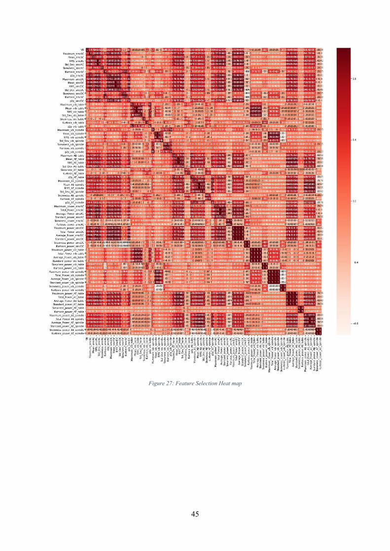
45

Figure 27: Feature Selection Heat map

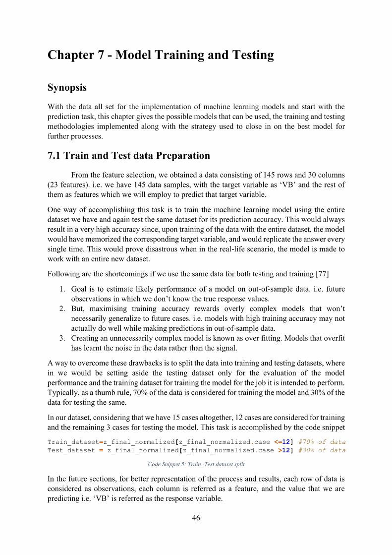
46

Chapter 7 - Model Training and Testing

Synopsis

With the data all set for the implementation of machine learning models and start with the prediction task, this chapter gives the possible models that can be used, the training and testing methodologies implemented along with the strategy used to close in on the best model for further processes.

7.1 Train and Test data Preparation

From the feature selection, we obtained a data consisting of 145 rows and 30 columns (23 features). i.e. we have 145 data samples, with the target variable as ‘VB’ and the rest of

them as features which we will employ to predict that target variable.

One way of accomplishing this task is to train the machine learning model using the entire dataset we have and again test the same dataset for its prediction accuracy. This would always result in a very high accuracy since, upon training of the data with the entire dataset, the model would have memorized the corresponding target variable, and would replicate the answer every single time. This would prove disastrous when in the real-life scenario, the model is made to work with an entire new dataset.

Following are the shortcomings if we use the same data for both testing and training [77]

1. Goal is to estimate likely performance of a model on out-of-sample data. i.e. future observations in which we don’t know the true response values.

2. But, maximising training accuracy rewards overly complex models that won’t

necessarily generalize to future cases. i.e. models with high training accuracy may not actually do well while making predictions in out-of-sample data.

3. Creating an unnecessarily complex model is known as over fitting. Models that overfit has learnt the noise in the data rather than the signal.

A way to overcome these drawbacks is to split the data into training and testing datasets, where in we would be setting aside the testing dataset only for the evaluation of the model performance and the training dataset for training the model for the job it is intended to perform. Typically, as a thumb rule, 70% of the data is considered for training the model and 30% of the data for testing the same.

In our dataset, considering that we have 15 cases altogether, 12 cases are considered for training and the remaining 3 cases for testing the model. This task is accomplished by the code snippet

Train_dataset=z_final_normalized[z_final_normalized.case <=12] #70% of data Test_dataset = z_final_normalized[z_final_normalized.case >12] #30% of data

Code Snippet 5: Train -Test dataset split

In the future sections, for better representation of the process and results, each row of data is considered as observations, each column is referred as a feature, and the value that we are predicting i.e. ‘VB’ is referred as the response variable.

47

The problem we are dealing with is Supervised learning, and as we know the supervised learning are further categorized into Regression problem and Classification problem. Classification is a supervised learning method in which the response is categorical. i.e. the values are in a finite un-ordered set. In contrast, a Regression problem is a supervised learning method, in which the response being predicted is ordered and continuous [77].

Within the scope of this thesis dissertation, only Regression analysis is considered.

7.2 Regression Analysis

With the conclusion made to use the regression analysis to move forward with the best model selection for prediction of the response variable, i.e. ‘VB’, with the help of one of the libraries of python i.e. Scikitlearn, following models are trained and tested.

1. Linear Regression 2. Decision Tree Regression 3. Random forest Regression 4. Bayesian Ridge Regression 5. Neural Network Regression 6. Knn Regression 7. Kernel Ridge Regression

Before the initialization of using the data to train the model, the features and the response variables are clearly distinguished. Once the training is completed, in order to assess the performance of the model, performance measuring metrics are used. Some of the commonly used and provided within the scikitlearn library are,

1. Mean Squared Error 2. Root mean squared error 3. Mean Absolute Error 4. Coefficient of Determination (R2) 5. Explained Variance

1. Mean Squared Error

In statistics, the mean squared error (MSE) or mean squared deviation (MSD) of an estimator (of a procedure for estimating an unobserved quantity) measures the average of the squares of the errors—that is, the average squared difference between the estimated values and the actual value. MSE is a risk function, corresponding to the expected value of the squared error loss. The fact that MSE is almost always strictly positive (and not zero) is because of randomness or because the estimator does not account for information that could produce a more accurate estimate [78].

The MSE is a measure of the quality of an estimator—it is always non-negative, and values closer to zero are better.

With the help of Scikit learn, Mean squared error can be found out as shown below [79],

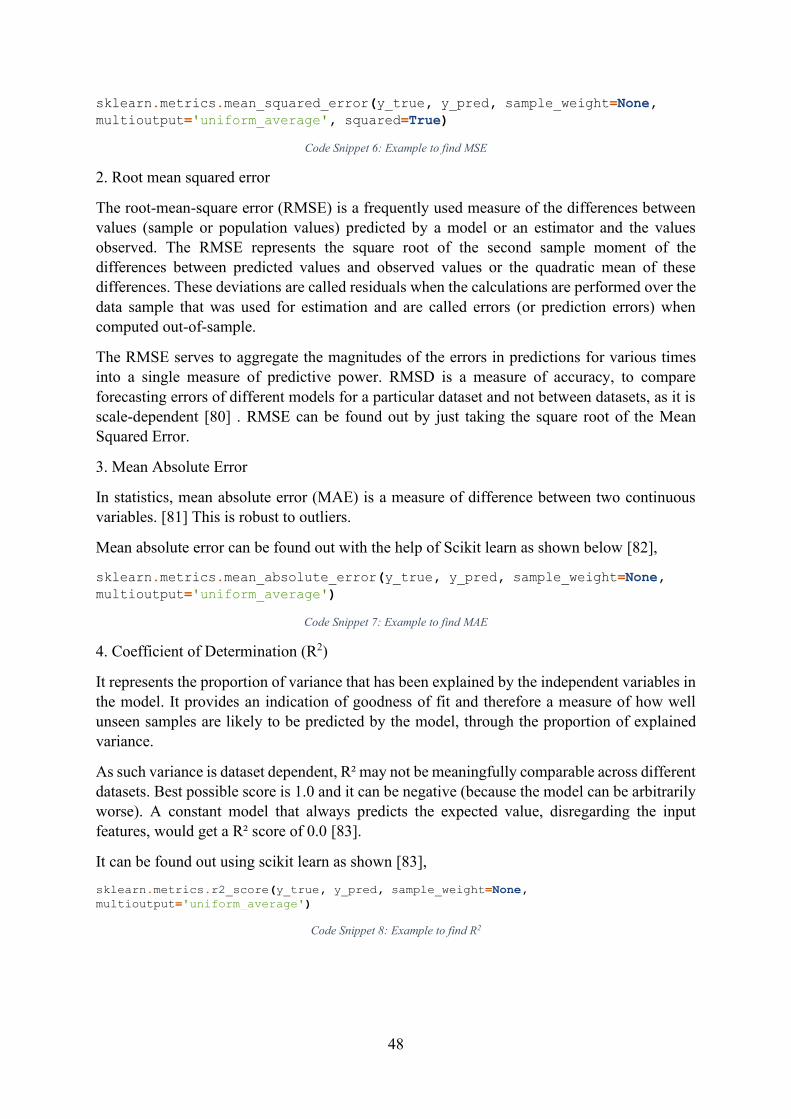
48

sklearn.metrics.mean_squared_error(y_true, y_pred, sample_weight=None,

multioutput='uniform_average', squared=True) Code Snippet 6: Example to find MSE

2. Root mean squared error

The root-mean-square error (RMSE) is a frequently used measure of the differences between values (sample or population values) predicted by a model or an estimator and the values observed. The RMSE represents the square root of the second sample moment of the differences between predicted values and observed values or the quadratic mean of these differences. These deviations are called residuals when the calculations are performed over the data sample that was used for estimation and are called errors (or prediction errors) when computed out-of-sample.

The RMSE serves to aggregate the magnitudes of the errors in predictions for various times into a single measure of predictive power. RMSD is a measure of accuracy, to compare forecasting errors of different models for a particular dataset and not between datasets, as it is scale-dependent [80] . RMSE can be found out by just taking the square root of the Mean Squared Error.

3. Mean Absolute Error

In statistics, mean absolute error (MAE) is a measure of difference between two continuous variables. [81] This is robust to outliers.

Mean absolute error can be found out with the help of Scikit learn as shown below [82],

sklearn.metrics.mean_absolute_error(y_true, y_pred, sample_weight=None,

multioutput='uniform_average') Code Snippet 7: Example to find MAE

4. Coefficient of Determination (R2)

It represents the proportion of variance that has been explained by the independent variables in the model. It provides an indication of goodness of fit and therefore a measure of how well unseen samples are likely to be predicted by the model, through the proportion of explained variance.

As such variance is dataset dependent, R² may not be meaningfully comparable across different datasets. Best possible score is 1.0 and it can be negative (because the model can be arbitrarily worse). A constant model that always predicts the expected value, disregarding the input features, would get a R² score of 0.0 [83].

It can be found out using scikit learn as shown [83],

sklearn.metrics.r2_score(y_true, y_pred, sample_weight=None,

multioutput='uniform_average') Code Snippet 8: Example to find R2

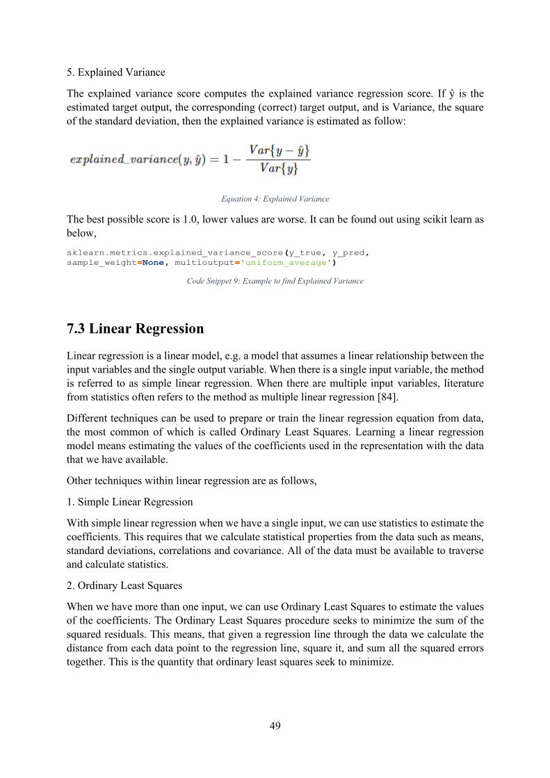
49

5. Explained Variance

The explained variance score computes the explained variance regression score. If ŷ is the estimated target output, the corresponding (correct) target output, and is Variance, the square of the standard deviation, then the explained variance is estimated as follow:

Equation 4: Explained Variance

The best possible score is 1.0, lower values are worse. It can be found out using scikit learn as below,

sklearn.metrics.explained_variance_score(y_true, y_pred,

sample_weight=None, multioutput='uniform_average') Code Snippet 9: Example to find Explained Variance

7.3 Linear Regression

Linear regression is a linear model, e.g. a model that assumes a linear relationship between the input variables and the single output variable. When there is a single input variable, the method is referred to as simple linear regression. When there are multiple input variables, literature from statistics often refers to the method as multiple linear regression [84].

Different techniques can be used to prepare or train the linear regression equation from data, the most common of which is called Ordinary Least Squares. Learning a linear regression model means estimating the values of the coefficients used in the representation with the data that we have available.

Other techniques within linear regression are as follows,

1. Simple Linear Regression

With simple linear regression when we have a single input, we can use statistics to estimate the coefficients. This requires that we calculate statistical properties from the data such as means, standard deviations, correlations and covariance. All of the data must be available to traverse and calculate statistics.

2. Ordinary Least Squares

When we have more than one input, we can use Ordinary Least Squares to estimate the values of the coefficients. The Ordinary Least Squares procedure seeks to minimize the sum of the squared residuals. This means, that given a regression line through the data we calculate the distance from each data point to the regression line, square it, and sum all the squared errors together. This is the quantity that ordinary least squares seek to minimize.

50

This approach treats the data as a matrix and uses linear algebra operations to estimate the optimal values for the coefficients. It means that all the data must be available, and we must have enough memory to fit the data and perform matrix operations.

3. Gradient Descent

When there are one or more inputs, we can use a process of optimizing the values of the coefficients by iteratively minimizing the error of the model on the training data.

This operation is called Gradient Descent and works by starting with random values for each coefficient. The sum of the squared errors is calculated for each pair of input and output values. A learning rate is used as a scale factor and the coefficients are updated in the direction towards minimizing the error. The process is repeated until a minimum sum squared error is achieved or no further improvement is possible.

When using this method, we must select a learning rate (alpha) parameter that determines the size of the improvement step to take on each iteration of the procedure.

Gradient descent is often taught using a linear regression model because it is relatively straightforward to understand. In practice, it is useful when we have a very large dataset either in the number of rows or the number of columns that may not fit into memory.

4. Regularization

There are extensions of the training of the linear model called regularization methods. These seek to both minimize the sum of the squared error of the model on the training data (using ordinary least squares) but also to reduce the complexity of the model (like the number or absolute size of the sum of all coefficients in the model).

Two popular examples of regularization procedures for linear regression are:

Lasso Regression: where Ordinary Least Squares is modified to also minimize the absolute sum of the coefficients (called L1 regularization).

Ridge Regression: where Ordinary Least Squares is modified to also minimize the squared absolute sum of the coefficients (called L2 regularization).

These methods are effective to use when there is collinearity in your input values and ordinary least squares would overfit the training data. Under Scikit learn, Ordinary least squares Linear regression is readily available. The code below is used to train and test the model

51

X_train = Train_dataset[['run','DOC', 'feed', 'material','Maximum_smcAC',

'RMS_smcAC', 'Std_Dev_smcAC', 'p2p_smcAC', 'Maximum_smcDC', 'Mean_smcDC',

'RMS_smcDC', 'Std_Dev_smcDC', 'p2p_smcDC', 'Maximum_AE_table',

'RMS_AE_table', 'p2p_AE_table', 'Maximum_AE_spindle', 'p2p_AE_spindle',

'Maximum_power_smcAC', 'Total_Power_smcAC' , 'Average_Power_smcAC',

'Standard_power_smcAC', 'Maximum_power_smcDC', 'Total_Power_smcDC',

'Average_Power_smcDC', 'Standard_power_smcDC']].copy() y_train = Train_dataset.VB X_test = Test_dataset[['run','DOC', 'feed', 'material','Maximum_smcAC',

'RMS_smcAC', 'Std_Dev_smcAC', 'p2p_smcAC', 'Maximum_smcDC', 'Mean_smcDC',

'RMS_smcDC', 'Std_Dev_smcDC', 'p2p_smcDC', 'Maximum_AE_table',

'RMS_AE_table', 'p2p_AE_table', 'Maximum_AE_spindle', 'p2p_AE_spindle',

'Maximum_power_smcAC', 'Total_Power_smcAC' , 'Average_Power_smcAC',

'Standard_power_smcAC', 'Maximum_power_smcDC', 'Total_Power_smcDC',

'Average_Power_smcDC', 'Standard_power_smcDC']].copy() y_test = Test_dataset.VB

linreg = LinearRegression() linreg.fit(X_train, y_train)

y_pred = linreg.predict(X_test) y_pred = pd.DataFrame(y_pred)

#Error calculation

from sklearn.metrics import mean_squared_error from sklearn.metrics import mean_absolute_error

lin_rmse = np.sqrt(metrics.mean_squared_error(y_test, y_pred))

lin_mse = mean_squared_error(y_test, y_pred)

lin_mae = mean_absolute_error(y_test, y_pred)

lin_r2 = metrics.r2_score(y_test, y_pred)

lin_variance = metrics.explained_variance_score(y_test, y_pred)

lin_error = pd.DataFrame([lin_rmse, lin_mse, lin_mae, lin_r2,

lin_variance]) lin_error.columns = ["Linear Regression"]

Code Snippet 10: Linear Regression

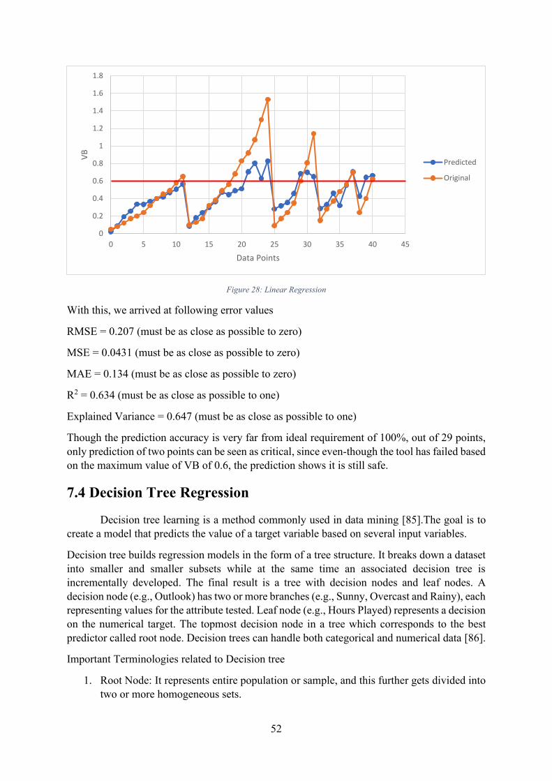
52

Figure 28: Linear Regression

With this, we arrived at following error values

RMSE = 0.207 (must be as close as possible to zero)

MSE = 0.0431 (must be as close as possible to zero)

MAE = 0.134 (must be as close as possible to zero)

R2 = 0.634 (must be as close as possible to one)

Explained Variance = 0.647 (must be as close as possible to one)

Though the prediction accuracy is very far from ideal requirement of 100%, out of 29 points, only prediction of two points can be seen as critical, since even-though the tool has failed based on the maximum value of VB of 0.6, the prediction shows it is still safe.

7.4 Decision Tree Regression

Decision tree learning is a method commonly used in data mining [85].The goal is to create a model that predicts the value of a target variable based on several input variables.

Decision tree builds regression models in the form of a tree structure. It breaks down a dataset into smaller and smaller subsets while at the same time an associated decision tree is incrementally developed. The final result is a tree with decision nodes and leaf nodes. A decision node (e.g., Outlook) has two or more branches (e.g., Sunny, Overcast and Rainy), each representing values for the attribute tested. Leaf node (e.g., Hours Played) represents a decision on the numerical target. The topmost decision node in a tree which corresponds to the best predictor called root node. Decision trees can handle both categorical and numerical data [86].

Important Terminologies related to Decision tree

1. Root Node: It represents entire population or sample, and this further gets divided into two or more homogeneous sets.

0

0.2

0.4

0.6

0.8

1

1.2

1.4

1.6

1.8

0 5 10 15 20 25 30 35 40 45

VB

Data Points

Predicted

Original

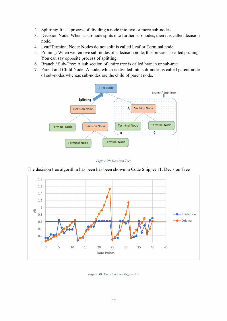
53

2. Splitting: It is a process of dividing a node into two or more sub-nodes. 3. Decision Node: When a sub-node splits into further sub-nodes, then it is called decision

node. 4. Leaf/Terminal Node: Nodes do not split is called Leaf or Terminal node. 5. Pruning: When we remove sub-nodes of a decision node, this process is called pruning.

You can say opposite process of splitting. 6. Branch / Sub-Tree: A sub section of entire tree is called branch or sub-tree. 7. Parent and Child Node: A node, which is divided into sub-nodes is called parent node

of sub-nodes whereas sub-nodes are the child of parent node.

Figure 29: Decision Tree

The decision tree algorithm has been has been shown in Code Snippet 11: Decision Tree

Figure 30: Decision Tree Regression

0

0.2

0.4

0.6

0.8

1

1.2

1.4

1.6

1.8

0 5 10 15 20 25 30 35 40 45

VB

Data Points

Prediction

Original

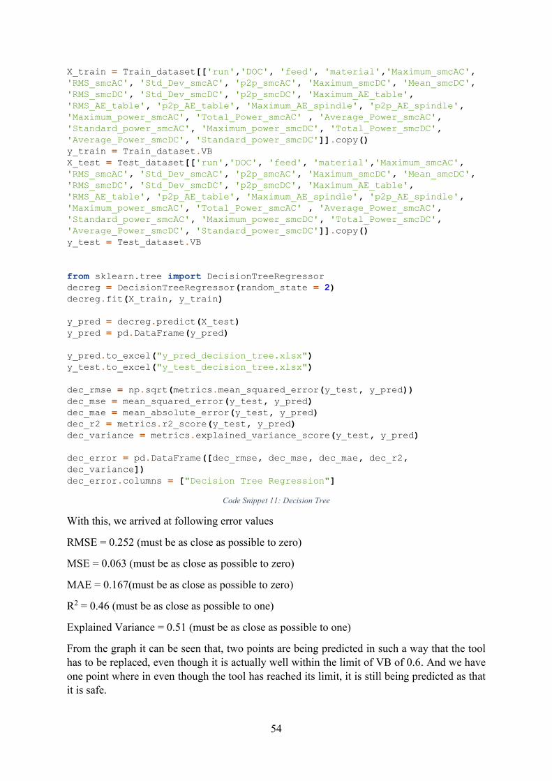
54

X_train = Train_dataset[['run','DOC', 'feed', 'material','Maximum_smcAC',

'RMS_smcAC', 'Std_Dev_smcAC', 'p2p_smcAC', 'Maximum_smcDC', 'Mean_smcDC',

'RMS_smcDC', 'Std_Dev_smcDC', 'p2p_smcDC', 'Maximum_AE_table',

'RMS_AE_table', 'p2p_AE_table', 'Maximum_AE_spindle', 'p2p_AE_spindle',

'Maximum_power_smcAC', 'Total_Power_smcAC' , 'Average_Power_smcAC',

'Standard_power_smcAC', 'Maximum_power_smcDC', 'Total_Power_smcDC',

'Average_Power_smcDC', 'Standard_power_smcDC']].copy() y_train = Train_dataset.VB X_test = Test_dataset[['run','DOC', 'feed', 'material','Maximum_smcAC',

'RMS_smcAC', 'Std_Dev_smcAC', 'p2p_smcAC', 'Maximum_smcDC', 'Mean_smcDC',

'RMS_smcDC', 'Std_Dev_smcDC', 'p2p_smcDC', 'Maximum_AE_table',

'RMS_AE_table', 'p2p_AE_table', 'Maximum_AE_spindle', 'p2p_AE_spindle',

'Maximum_power_smcAC', 'Total_Power_smcAC' , 'Average_Power_smcAC',

'Standard_power_smcAC', 'Maximum_power_smcDC', 'Total_Power_smcDC',

'Average_Power_smcDC', 'Standard_power_smcDC']].copy() y_test = Test_dataset.VB

from sklearn.tree import DecisionTreeRegressor decreg = DecisionTreeRegressor(random_state = 2) decreg.fit(X_train, y_train)

y_pred = decreg.predict(X_test) y_pred = pd.DataFrame(y_pred)

y_pred.to_excel("y_pred_decision_tree.xlsx") y_test.to_excel("y_test_decision_tree.xlsx")

dec_rmse = np.sqrt(metrics.mean_squared_error(y_test, y_pred)) dec_mse = mean_squared_error(y_test, y_pred) dec_mae = mean_absolute_error(y_test, y_pred) dec_r2 = metrics.r2_score(y_test, y_pred) dec_variance = metrics.explained_variance_score(y_test, y_pred)

dec_error = pd.DataFrame([dec_rmse, dec_mse, dec_mae, dec_r2,

dec_variance]) dec_error.columns = ["Decision Tree Regression"]

Code Snippet 11: Decision Tree

With this, we arrived at following error values

RMSE = 0.252 (must be as close as possible to zero)

MSE = 0.063 (must be as close as possible to zero)

MAE = 0.167(must be as close as possible to zero)

R2 = 0.46 (must be as close as possible to one)

Explained Variance = 0.51 (must be as close as possible to one)

From the graph it can be seen that, two points are being predicted in such a way that the tool has to be replaced, even though it is actually well within the limit of VB of 0.6. And we have one point where in even though the tool has reached its limit, it is still being predicted as that it is safe.

55

Also, the performance of this regression method is very bad compared to linear Regression for the data we have.

7.5 Random Forest Regression

Random forest is a Supervised Learning algorithm which uses ensemble learning method for classification and regression [87].

An Ensemble method is a technique that combines the predictions from multiple machine learning algorithms together to make more accurate predictions than any individual model. A model comprised of many models is called an Ensemble model.

Random forest is a bagging technique and not a boosting technique. The trees in random forests are run in parallel. There is no interaction between these trees while building the trees.

Bootstrap (Bagging) refers to random sampling with replacement. Bootstrap allows us to better understand the bias and the variance with the dataset. Bootstrap involves random sampling of small subset of data from the dataset.

It is a general procedure that can be used to reduce the variance for those algorithm that have high variance, typically decision trees. Bagging makes each model run independently and then aggregates the outputs at the end without preference to any model.

Random Forest operates by constructing a multitude of decision trees at training time and outputting the class that is the mode of the classes (classification) or mean prediction (regression) of the individual trees.

A random forest is a meta-estimator (i.e. it combines the result of multiple predictions) which aggregates many decision trees, with some helpful modifications [87]:

1. The number of features that can be split on at each node is limited to some percentage of the total (which is known as the hyperparameter). This ensures that the ensemble model does not rely too heavily on any individual feature and makes fair use of all potentially predictive features.

2. Each tree draws a random sample from the original data set when generating its splits, adding a further element of randomness that prevents overfitting.

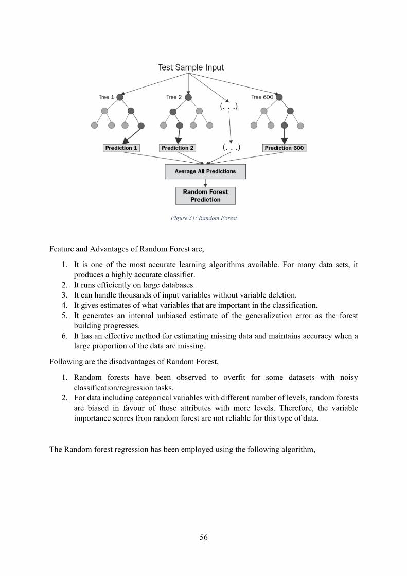
56

Figure 31: Random Forest

Feature and Advantages of Random Forest are,

1. It is one of the most accurate learning algorithms available. For many data sets, it produces a highly accurate classifier.

2. It runs efficiently on large databases. 3. It can handle thousands of input variables without variable deletion. 4. It gives estimates of what variables that are important in the classification. 5. It generates an internal unbiased estimate of the generalization error as the forest

building progresses. 6. It has an effective method for estimating missing data and maintains accuracy when a

large proportion of the data are missing.

Following are the disadvantages of Random Forest,

1. Random forests have been observed to overfit for some datasets with noisy classification/regression tasks.

2. For data including categorical variables with different number of levels, random forests are biased in favour of those attributes with more levels. Therefore, the variable importance scores from random forest are not reliable for this type of data.

The Random forest regression has been employed using the following algorithm,

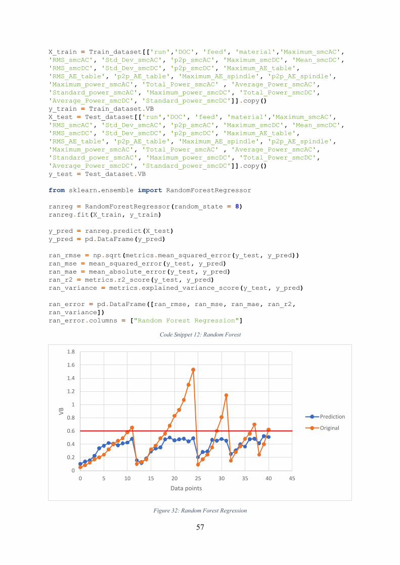
57

X_train = Train_dataset[['run','DOC', 'feed', 'material','Maximum_smcAC',

'RMS_smcAC', 'Std_Dev_smcAC', 'p2p_smcAC', 'Maximum_smcDC', 'Mean_smcDC',

'RMS_smcDC', 'Std_Dev_smcDC', 'p2p_smcDC', 'Maximum_AE_table',

'RMS_AE_table', 'p2p_AE_table', 'Maximum_AE_spindle', 'p2p_AE_spindle',

'Maximum_power_smcAC', 'Total_Power_smcAC' , 'Average_Power_smcAC',

'Standard_power_smcAC', 'Maximum_power_smcDC', 'Total_Power_smcDC',

'Average_Power_smcDC', 'Standard_power_smcDC']].copy() y_train = Train_dataset.VB X_test = Test_dataset[['run','DOC', 'feed', 'material','Maximum_smcAC',

'RMS_smcAC', 'Std_Dev_smcAC', 'p2p_smcAC', 'Maximum_smcDC', 'Mean_smcDC',

'RMS_smcDC', 'Std_Dev_smcDC', 'p2p_smcDC', 'Maximum_AE_table',

'RMS_AE_table', 'p2p_AE_table', 'Maximum_AE_spindle', 'p2p_AE_spindle',

'Maximum_power_smcAC', 'Total_Power_smcAC' , 'Average_Power_smcAC',

'Standard_power_smcAC', 'Maximum_power_smcDC', 'Total_Power_smcDC',

'Average_Power_smcDC', 'Standard_power_smcDC']].copy() y_test = Test_dataset.VB

from sklearn.ensemble import RandomForestRegressor

ranreg = RandomForestRegressor(random_state = 8) ranreg.fit(X_train, y_train)

y_pred = ranreg.predict(X_test) y_pred = pd.DataFrame(y_pred)

ran_rmse = np.sqrt(metrics.mean_squared_error(y_test, y_pred)) ran_mse = mean_squared_error(y_test, y_pred) ran_mae = mean_absolute_error(y_test, y_pred) ran_r2 = metrics.r2_score(y_test, y_pred) ran_variance = metrics.explained_variance_score(y_test, y_pred)

ran_error = pd.DataFrame([ran_rmse, ran_mse, ran_mae, ran_r2,

ran_variance]) ran_error.columns = ["Random Forest Regression"]

Code Snippet 12: Random Forest

Figure 32: Random Forest Regression

0

0.2

0.4

0.6

0.8

1

1.2

1.4

1.6

1.8

0 5 10 15 20 25 30 35 40 45

VB

Data points

Prediction

Original

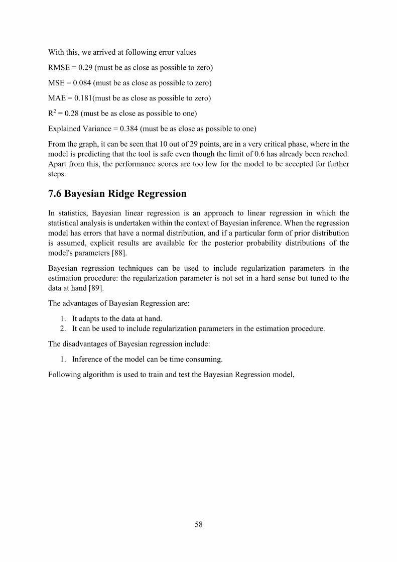
58

With this, we arrived at following error values

RMSE = 0.29 (must be as close as possible to zero)

MSE = 0.084 (must be as close as possible to zero)

MAE = 0.181(must be as close as possible to zero)

R2 = 0.28 (must be as close as possible to one)

Explained Variance = 0.384 (must be as close as possible to one)

From the graph, it can be seen that 10 out of 29 points, are in a very critical phase, where in the model is predicting that the tool is safe even though the limit of 0.6 has already been reached. Apart from this, the performance scores are too low for the model to be accepted for further steps.

7.6 Bayesian Ridge Regression

In statistics, Bayesian linear regression is an approach to linear regression in which the statistical analysis is undertaken within the context of Bayesian inference. When the regression model has errors that have a normal distribution, and if a particular form of prior distribution is assumed, explicit results are available for the posterior probability distributions of the model's parameters [88].

Bayesian regression techniques can be used to include regularization parameters in the estimation procedure: the regularization parameter is not set in a hard sense but tuned to the data at hand [89].

The advantages of Bayesian Regression are:

1. It adapts to the data at hand. 2. It can be used to include regularization parameters in the estimation procedure.

The disadvantages of Bayesian regression include:

1. Inference of the model can be time consuming.

Following algorithm is used to train and test the Bayesian Regression model,

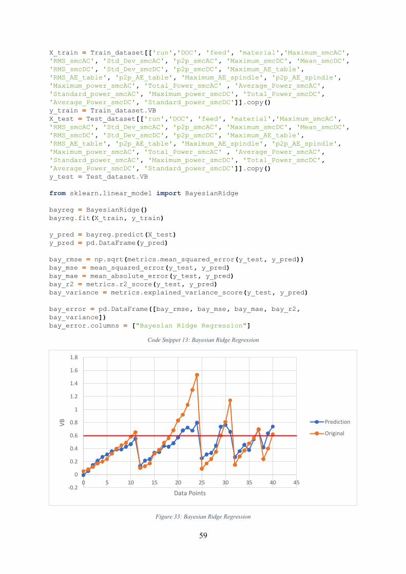
59

X_train = Train_dataset[['run','DOC', 'feed', 'material','Maximum_smcAC',

'RMS_smcAC', 'Std_Dev_smcAC', 'p2p_smcAC', 'Maximum_smcDC', 'Mean_smcDC',

'RMS_smcDC', 'Std_Dev_smcDC', 'p2p_smcDC', 'Maximum_AE_table',

'RMS_AE_table', 'p2p_AE_table', 'Maximum_AE_spindle', 'p2p_AE_spindle',

'Maximum_power_smcAC', 'Total_Power_smcAC' , 'Average_Power_smcAC',

'Standard_power_smcAC', 'Maximum_power_smcDC', 'Total_Power_smcDC',

'Average_Power_smcDC', 'Standard_power_smcDC']].copy() y_train = Train_dataset.VB X_test = Test_dataset[['run','DOC', 'feed', 'material','Maximum_smcAC',

'RMS_smcAC', 'Std_Dev_smcAC', 'p2p_smcAC', 'Maximum_smcDC', 'Mean_smcDC',

'RMS_smcDC', 'Std_Dev_smcDC', 'p2p_smcDC', 'Maximum_AE_table',

'RMS_AE_table', 'p2p_AE_table', 'Maximum_AE_spindle', 'p2p_AE_spindle',

'Maximum_power_smcAC', 'Total_Power_smcAC' , 'Average_Power_smcAC',

'Standard_power_smcAC', 'Maximum_power_smcDC', 'Total_Power_smcDC',

'Average_Power_smcDC', 'Standard_power_smcDC']].copy() y_test = Test_dataset.VB

from sklearn.linear_model import BayesianRidge

bayreg = BayesianRidge() bayreg.fit(X_train, y_train)

y_pred = bayreg.predict(X_test) y_pred = pd.DataFrame(y_pred)

bay_rmse = np.sqrt(metrics.mean_squared_error(y_test, y_pred)) bay_mse = mean_squared_error(y_test, y_pred) bay_mae = mean_absolute_error(y_test, y_pred) bay_r2 = metrics.r2_score(y_test, y_pred) bay_variance = metrics.explained_variance_score(y_test, y_pred)

bay_error = pd.DataFrame([bay_rmse, bay_mse, bay_mae, bay_r2,

bay_variance]) bay_error.columns = ["Bayesian Ridge Regression"]

Code Snippet 13: Bayesian Ridge Regression

Figure 33: Bayesian Ridge Regression

-0.2

0

0.2

0.4

0.6

0.8

1

1.2

1.4

1.6

1.8

0 5 10 15 20 25 30 35 40 45

VB

Data Points

Prediction

Original

60

With this, we arrived at following error values

RMSE = 0.206 (must be as close as possible to zero)

MSE = 0.042 (must be as close as possible to zero)

MAE = 0.136(must be as close as possible to zero)

R2 = 0.637 (must be as close as possible to one)

Explained Variance = 0.654 (must be as close as possible to one)

From the graph, it is evident that the performance of this model is definitely better than all those models which were previously discussed. In addition to that, we can see only one point being predicted as safe even though the condition of tool is unsafe. This does not deviate from the fact that the prediction is still not very great for other values.

7.7 Neural Network Regression

Neural network is machine learning technique or algorithm that try to mimic the working of neuron in human brain for learning. At first it is unstable and after certain iteration of data it adjust itself such that it’s accuracy increases [90].

Figure 34: A simple feed neural network

Neural networks are reducible to regression models—a neural network can “pretend” to be any

type of regression model. For example, this very simple neural network, with only one input neuron, one hidden neuron, and one output neuron, is equivalent to a logistic regression. It takes several dependent variables = input parameters, multiplies them by their coefficients = weights, and runs them through a sigmoid activation function and a unit step function, which closely resembles the logistic regression function with its error term [91].

When this neural network is trained, it will perform gradient to find coefficients that are better and fit the data, until it arrives at the optimal linear regression coefficients (or, in neural network terms, the optimal weights for the model) [91].

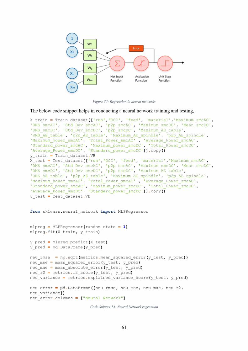
61

Figure 35: Regression in neural networks

The below code snippet helps in conducting a neural network training and testing,

X_train = Train_dataset[['run','DOC', 'feed', 'material','Maximum_smcAC',

'RMS_smcAC', 'Std_Dev_smcAC', 'p2p_smcAC', 'Maximum_smcDC', 'Mean_smcDC',

'RMS_smcDC', 'Std_Dev_smcDC', 'p2p_smcDC', 'Maximum_AE_table',

'RMS_AE_table', 'p2p_AE_table', 'Maximum_AE_spindle', 'p2p_AE_spindle',

'Maximum_power_smcAC', 'Total_Power_smcAC' , 'Average_Power_smcAC',

'Standard_power_smcAC', 'Maximum_power_smcDC', 'Total_Power_smcDC',

'Average_Power_smcDC', 'Standard_power_smcDC']].copy() y_train = Train_dataset.VB X_test = Test_dataset[['run','DOC', 'feed', 'material','Maximum_smcAC',

'RMS_smcAC', 'Std_Dev_smcAC', 'p2p_smcAC', 'Maximum_smcDC', 'Mean_smcDC',

'RMS_smcDC', 'Std_Dev_smcDC', 'p2p_smcDC', 'Maximum_AE_table',

'RMS_AE_table', 'p2p_AE_table', 'Maximum_AE_spindle', 'p2p_AE_spindle',

'Maximum_power_smcAC', 'Total_Power_smcAC' , 'Average_Power_smcAC',

'Standard_power_smcAC', 'Maximum_power_smcDC', 'Total_Power_smcDC',

'Average_Power_smcDC', 'Standard_power_smcDC']].copy() y_test = Test_dataset.VB

from sklearn.neural_network import MLPRegressor

mlpreg = MLPRegressor(random_state = 1) mlpreg.fit(X_train, y_train)

y_pred = mlpreg.predict(X_test) y_pred = pd.DataFrame(y_pred)

neu_rmse = np.sqrt(metrics.mean_squared_error(y_test, y_pred)) neu_mse = mean_squared_error(y_test, y_pred) neu_mae = mean_absolute_error(y_test, y_pred) neu_r2 = metrics.r2_score(y_test, y_pred) neu_variance = metrics.explained_variance_score(y_test, y_pred)

neu_error = pd.DataFrame([neu_rmse, neu_mse, neu_mae, neu_r2,

neu_variance]) neu_error.columns = ["Neural Network"]

Code Snippet 14: Neural Network regression

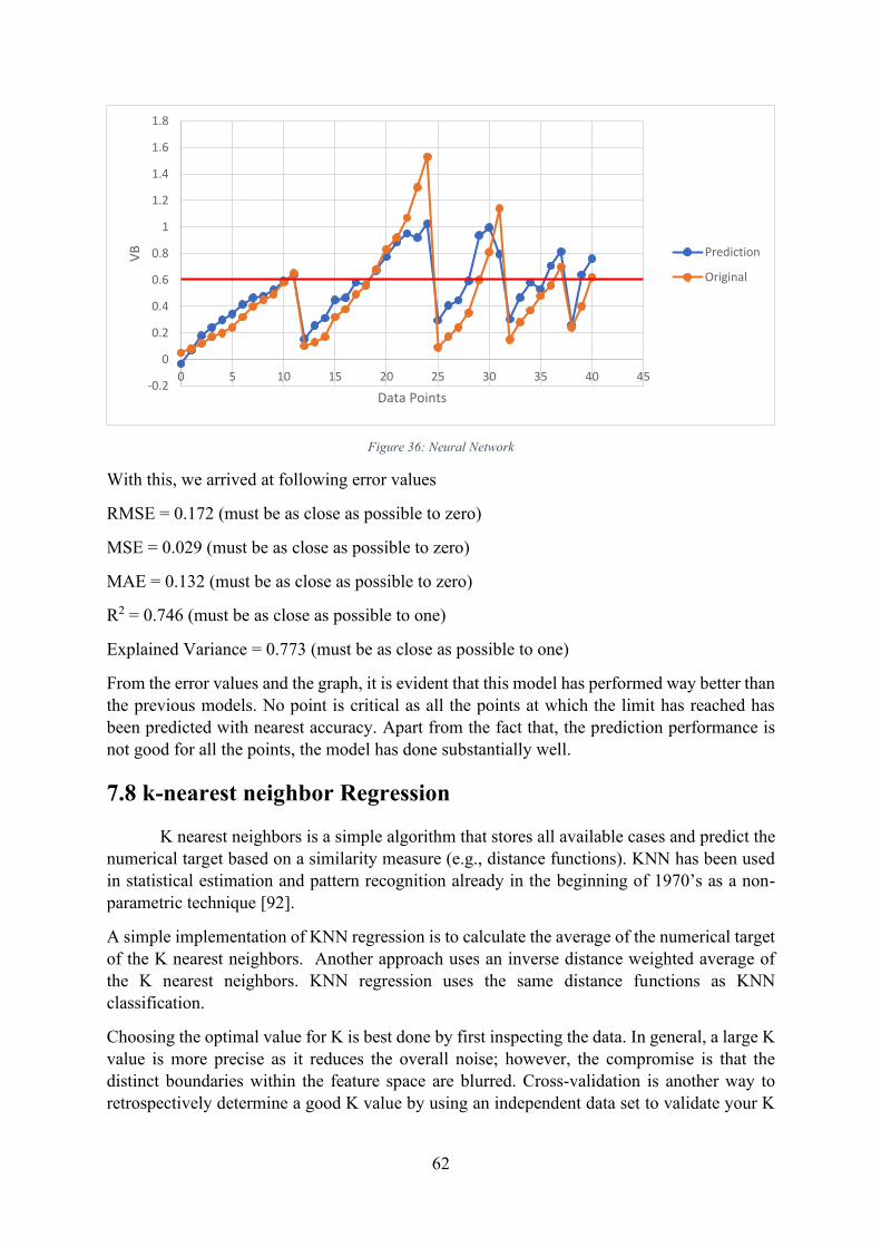
62

Figure 36: Neural Network

With this, we arrived at following error values

RMSE = 0.172 (must be as close as possible to zero)

MSE = 0.029 (must be as close as possible to zero)

MAE = 0.132 (must be as close as possible to zero)

R2 = 0.746 (must be as close as possible to one)

Explained Variance = 0.773 (must be as close as possible to one)

From the error values and the graph, it is evident that this model has performed way better than the previous models. No point is critical as all the points at which the limit has reached has been predicted with nearest accuracy. Apart from the fact that, the prediction performance is not good for all the points, the model has done substantially well.

7.8 k-nearest neighbor Regression

K nearest neighbors is a simple algorithm that stores all available cases and predict the numerical target based on a similarity measure (e.g., distance functions). KNN has been used in statistical estimation and pattern recognition already in the beginning of 1970’s as a non-parametric technique [92].

A simple implementation of KNN regression is to calculate the average of the numerical target of the K nearest neighbors. Another approach uses an inverse distance weighted average of the K nearest neighbors. KNN regression uses the same distance functions as KNN classification.

Choosing the optimal value for K is best done by first inspecting the data. In general, a large K value is more precise as it reduces the overall noise; however, the compromise is that the distinct boundaries within the feature space are blurred. Cross-validation is another way to retrospectively determine a good K value by using an independent data set to validate your K

-0.2

0

0.2

0.4

0.6

0.8

1

1.2

1.4

1.6

1.8

0 5 10 15 20 25 30 35 40 45

VB

Data Points

Prediction

Original

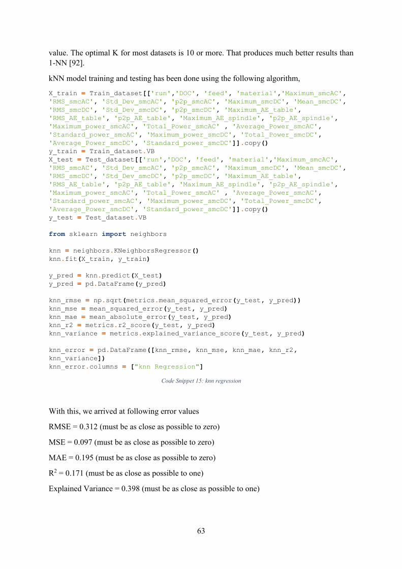
63

value. The optimal K for most datasets is 10 or more. That produces much better results than 1-NN [92].

kNN model training and testing has been done using the following algorithm,

X_train = Train_dataset[['run','DOC', 'feed', 'material','Maximum_smcAC',

'RMS_smcAC', 'Std_Dev_smcAC', 'p2p_smcAC', 'Maximum_smcDC', 'Mean_smcDC',

'RMS_smcDC', 'Std_Dev_smcDC', 'p2p_smcDC', 'Maximum_AE_table',

'RMS_AE_table', 'p2p_AE_table', 'Maximum_AE_spindle', 'p2p_AE_spindle',

'Maximum_power_smcAC', 'Total_Power_smcAC' , 'Average_Power_smcAC',

'Standard_power_smcAC', 'Maximum_power_smcDC', 'Total_Power_smcDC',

'Average_Power_smcDC', 'Standard_power_smcDC']].copy()

y_train = Train_dataset.VB

X_test = Test_dataset[['run','DOC', 'feed', 'material','Maximum_smcAC',

'RMS_smcAC', 'Std_Dev_smcAC', 'p2p_smcAC', 'Maximum_smcDC', 'Mean_smcDC',

'RMS_smcDC', 'Std_Dev_smcDC', 'p2p_smcDC', 'Maximum_AE_table',

'RMS_AE_table', 'p2p_AE_table', 'Maximum_AE_spindle', 'p2p_AE_spindle',

'Maximum_power_smcAC', 'Total_Power_smcAC' , 'Average_Power_smcAC',

'Standard_power_smcAC', 'Maximum_power_smcDC', 'Total_Power_smcDC',

'Average_Power_smcDC', 'Standard_power_smcDC']].copy()

y_test = Test_dataset.VB

from sklearn import neighbors

knn = neighbors.KNeighborsRegressor()

knn.fit(X_train, y_train)

y_pred = knn.predict(X_test)

y_pred = pd.DataFrame(y_pred)

knn_rmse = np.sqrt(metrics.mean_squared_error(y_test, y_pred))

knn_mse = mean_squared_error(y_test, y_pred)

knn_mae = mean_absolute_error(y_test, y_pred)

knn_r2 = metrics.r2_score(y_test, y_pred)

knn_variance = metrics.explained_variance_score(y_test, y_pred)

knn_error = pd.DataFrame([knn_rmse, knn_mse, knn_mae, knn_r2,

knn_variance])

knn_error.columns = ["knn Regression"] Code Snippet 15: knn regression

With this, we arrived at following error values

RMSE = 0.312 (must be as close as possible to zero)

MSE = 0.097 (must be as close as possible to zero)

MAE = 0.195 (must be as close as possible to zero)

R2 = 0.171 (must be as close as possible to one)

Explained Variance = 0.398 (must be as close as possible to one)

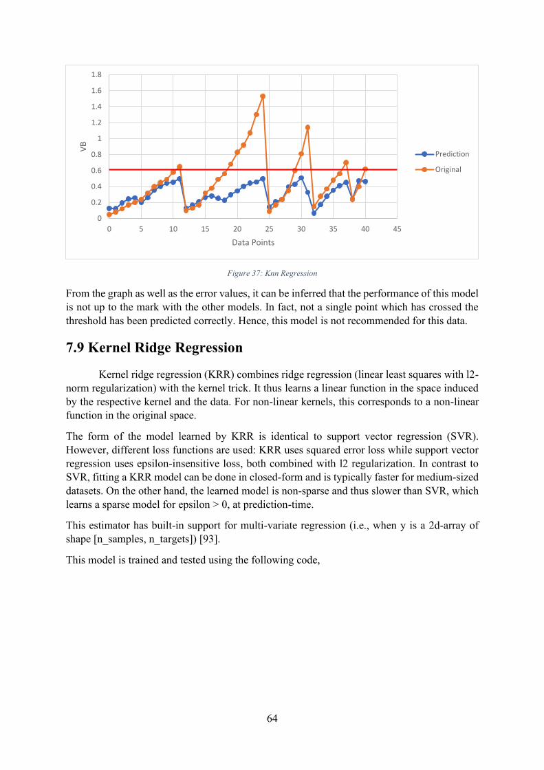
64

Figure 37: Knn Regression

From the graph as well as the error values, it can be inferred that the performance of this model is not up to the mark with the other models. In fact, not a single point which has crossed the threshold has been predicted correctly. Hence, this model is not recommended for this data.

7.9 Kernel Ridge Regression

Kernel ridge regression (KRR) combines ridge regression (linear least squares with l2-norm regularization) with the kernel trick. It thus learns a linear function in the space induced by the respective kernel and the data. For non-linear kernels, this corresponds to a non-linear function in the original space.

The form of the model learned by KRR is identical to support vector regression (SVR). However, different loss functions are used: KRR uses squared error loss while support vector regression uses epsilon-insensitive loss, both combined with l2 regularization. In contrast to SVR, fitting a KRR model can be done in closed-form and is typically faster for medium-sized datasets. On the other hand, the learned model is non-sparse and thus slower than SVR, which learns a sparse model for epsilon > 0, at prediction-time.

This estimator has built-in support for multi-variate regression (i.e., when y is a 2d-array of shape [n_samples, n_targets]) [93].

This model is trained and tested using the following code,

0

0.2

0.4

0.6

0.8

1

1.2

1.4

1.6

1.8

0 5 10 15 20 25 30 35 40 45

VB

Data Points

Prediction

Original

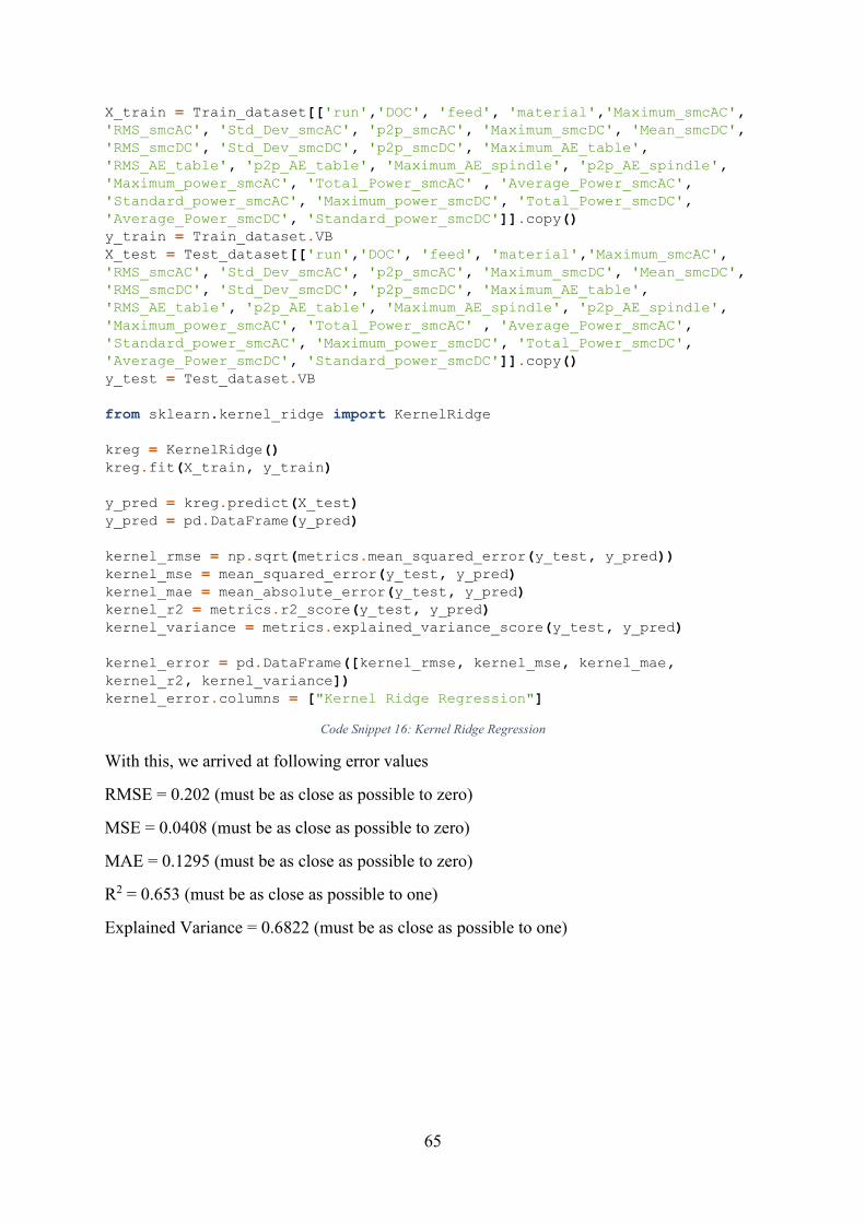
65

X_train = Train_dataset[['run','DOC', 'feed', 'material','Maximum_smcAC',

'RMS_smcAC', 'Std_Dev_smcAC', 'p2p_smcAC', 'Maximum_smcDC', 'Mean_smcDC',

'RMS_smcDC', 'Std_Dev_smcDC', 'p2p_smcDC', 'Maximum_AE_table',

'RMS_AE_table', 'p2p_AE_table', 'Maximum_AE_spindle', 'p2p_AE_spindle',

'Maximum_power_smcAC', 'Total_Power_smcAC' , 'Average_Power_smcAC',

'Standard_power_smcAC', 'Maximum_power_smcDC', 'Total_Power_smcDC',

'Average_Power_smcDC', 'Standard_power_smcDC']].copy()

y_train = Train_dataset.VB

X_test = Test_dataset[['run','DOC', 'feed', 'material','Maximum_smcAC',

'RMS_smcAC', 'Std_Dev_smcAC', 'p2p_smcAC', 'Maximum_smcDC', 'Mean_smcDC',

'RMS_smcDC', 'Std_Dev_smcDC', 'p2p_smcDC', 'Maximum_AE_table',

'RMS_AE_table', 'p2p_AE_table', 'Maximum_AE_spindle', 'p2p_AE_spindle',

'Maximum_power_smcAC', 'Total_Power_smcAC' , 'Average_Power_smcAC',

'Standard_power_smcAC', 'Maximum_power_smcDC', 'Total_Power_smcDC',

'Average_Power_smcDC', 'Standard_power_smcDC']].copy()

y_test = Test_dataset.VB

from sklearn.kernel_ridge import KernelRidge

kreg = KernelRidge()

kreg.fit(X_train, y_train)

y_pred = kreg.predict(X_test)

y_pred = pd.DataFrame(y_pred)

kernel_rmse = np.sqrt(metrics.mean_squared_error(y_test, y_pred))

kernel_mse = mean_squared_error(y_test, y_pred)

kernel_mae = mean_absolute_error(y_test, y_pred)

kernel_r2 = metrics.r2_score(y_test, y_pred)

kernel_variance = metrics.explained_variance_score(y_test, y_pred)

kernel_error = pd.DataFrame([kernel_rmse, kernel_mse, kernel_mae,

kernel_r2, kernel_variance])

kernel_error.columns = ["Kernel Ridge Regression"] Code Snippet 16: Kernel Ridge Regression

With this, we arrived at following error values

RMSE = 0.202 (must be as close as possible to zero)

MSE = 0.0408 (must be as close as possible to zero)

MAE = 0.1295 (must be as close as possible to zero)

R2 = 0.653 (must be as close as possible to one)

Explained Variance = 0.6822 (must be as close as possible to one)

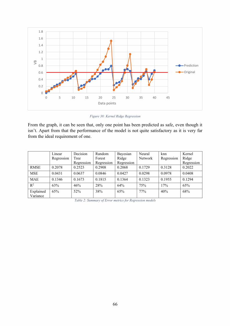
66

Figure 38: Kernel Ridge Regression

From the graph, it can be seen that, only one point has been predicted as safe, even though it isn’t. Apart from that the performance of the model is not quite satisfactory as it is very far from the ideal requirement of one.

Linear Regression

Decision Tree Regression

Random Forest Regression

Bayesian Ridge Regression

Neural Network

knn Regression

Kernel Ridge Regression

RMSE 0.2078 0.2523 0.2908 0.2068 0.1729 0.3128 0.2022 MSE 0.0431 0.0637 0.0846 0.0427 0.0298 0.0978 0.0408 MAE 0.1346 0.1673 0.1815 0.1364 0.1323 0.1955 0.1294 R2 63% 46% 28% 64% 75% 17% 65% Explained Variance

65% 52% 38% 65% 77% 40% 68%

Table 2: Summary of Error metrics for Regression models

0

0.2

0.4

0.6

0.8

1

1.2

1.4

1.6

1.8

0 5 10 15 20 25 30 35 40 45

VB

Data points

Prediction

Original

67

Chapter 8 – Model Improvement

Synopsis

In the previous chapter, various models were trained and were tested for its performance using separate training and testing data set. In the real case scenario, not all models can be used, and hence one of those models have to be selected. One way of accomplishing this task is by evaluating the error metrics and choosing the one with the best metric performance. Now this arises a question, whether the method of measuring the error metrics are efficient and consistent. This chapter deals with the Cross validation, a validation method to find and close in on the model to be used and Hyperparameter tuning, a method to improve the performance of the model chosen

8.1 Cross Validation

Cross-validation is a statistical method used to estimate the skill of machine learning models. It is commonly used in applied machine learning to compare and select a model for a given predictive modelling problem because it is easy to understand, easy to implement, and results in skill estimates that generally have a lower bias than other methods [94].

As there is never enough data to train your model, removing a part of it for validation poses a problem of underfitting. By reducing the training data, we risk losing important patterns/ trends in data set, which in turn increases error induced by bias. So, what we require is a method that provides ample data for training the model and also leaves ample data for validation. K Fold cross validation does exactly that [95].

Cross-validation is a resampling procedure used to evaluate machine learning models on a limited data sample. The procedure has a single parameter called k that refers to the number of groups that a given data sample is to be split into. As such, the procedure is often called k-fold cross-validation. When a specific value for k is chosen, it may be used in place of k in the reference to the model, such as k=10 becoming 10-fold cross-validation. Cross-validation is primarily used in applied machine learning to estimate the skill of a machine learning model on unseen data. That is, to use a limited sample in order to estimate how the model is expected to perform in general when used to make predictions on data not used during the training of the model.

The general procedure is as follows:

1. Shuffle the dataset randomly 2. Split the dataset into k groups 3. For each unique group:

a. Take the group as a hold out or test data set b. Take the remaining groups as a training data set c. Fit a model on the training set and evaluate it on the test set

68

d. Retain the evaluation score and discard the model 4. Summarize the skill of the model using the sample of model evaluation scores

Importantly, each observation in the data sample is assigned to an individual group and stays in that group for the duration of the procedure. This means that each sample is given the opportunity to be used in the hold out set 1 time and used to train the model k-1 times.

Figure 39: 5-Fold Cross Validation example

8.1.1 Configuration of ‘k’

The k value must be chosen carefully for the data sample. A poorly chosen value for k may result in a mis-representative idea of the skill of the model, such as a score with a high variance (that may change a lot based on the data used to fit the model), or a high bias, (such as an overestimate of the skill of the model).

Three common tactics for choosing a value for k are as follows:

1. Representative: The value for k is chosen such that each train/test group of data samples is large enough to be statistically representative of the broader dataset.

2. k=10: The value for k is fixed to 10, a value that has been found through experimentation to generally result in a model skill estimate with low bias a modest variance.

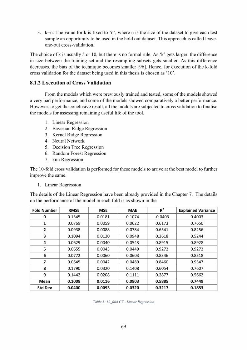
69

3. k=n: The value for k is fixed to ‘n’, where n is the size of the dataset to give each test sample an opportunity to be used in the hold out dataset. This approach is called leave-one-out cross-validation.

The choice of k is usually 5 or 10, but there is no formal rule. As ‘k’ gets larger, the difference in size between the training set and the resampling subsets gets smaller. As this difference decreases, the bias of the technique becomes smaller [96]. Hence, for execution of the k-fold cross validation for the dataset being used in this thesis is chosen as ‘10’.

8.1.2 Execution of Cross Validation

From the models which were previously trained and tested, some of the models showed a very bad performance, and some of the models showed comparatively a better performance. However, to get the conclusive result, all the models are subjected to cross validation to finalise the models for assessing remaining useful life of the tool.

1. Linear Regression 2. Bayesian Ridge Regression 3. Kernel Ridge Regression 4. Neural Network 5. Decision Tree Regression 6. Random Forest Regression 7. knn Regression

The 10-fold cross validation is performed for these models to arrive at the best model to further improve the same.

1. Linear Regression

The details of the Linear Regression have been already provided in the Chapter 7. The details on the performance of the model in each fold is as shown in the

Fold Number RMSE MSE MAE R2 Explained Variance

0 0.1345 0.0181 0.1074 -0.0403 0.4003

1 0.0769 0.0059 0.0622 0.6173 0.7650

2 0.0938 0.0088 0.0784 0.6541 0.8256

3 0.1094 0.0120 0.0948 0.2618 0.5244

4 0.0629 0.0040 0.0543 0.8915 0.8928

5 0.0655 0.0043 0.0449 0.9272 0.9272

6 0.0772 0.0060 0.0603 0.8346 0.8518

7 0.0645 0.0042 0.0489 0.8460 0.9347

8 0.1790 0.0320 0.1408 0.6054 0.7607

9 0.1442 0.0208 0.1111 0.2877 0.5662

Mean 0.1008 0.0116 0.0803 0.5885 0.7449

Std Dev 0.0400 0.0093 0.0320 0.3217 0.1853

Table 3: 10_fold CV - Linear Regression

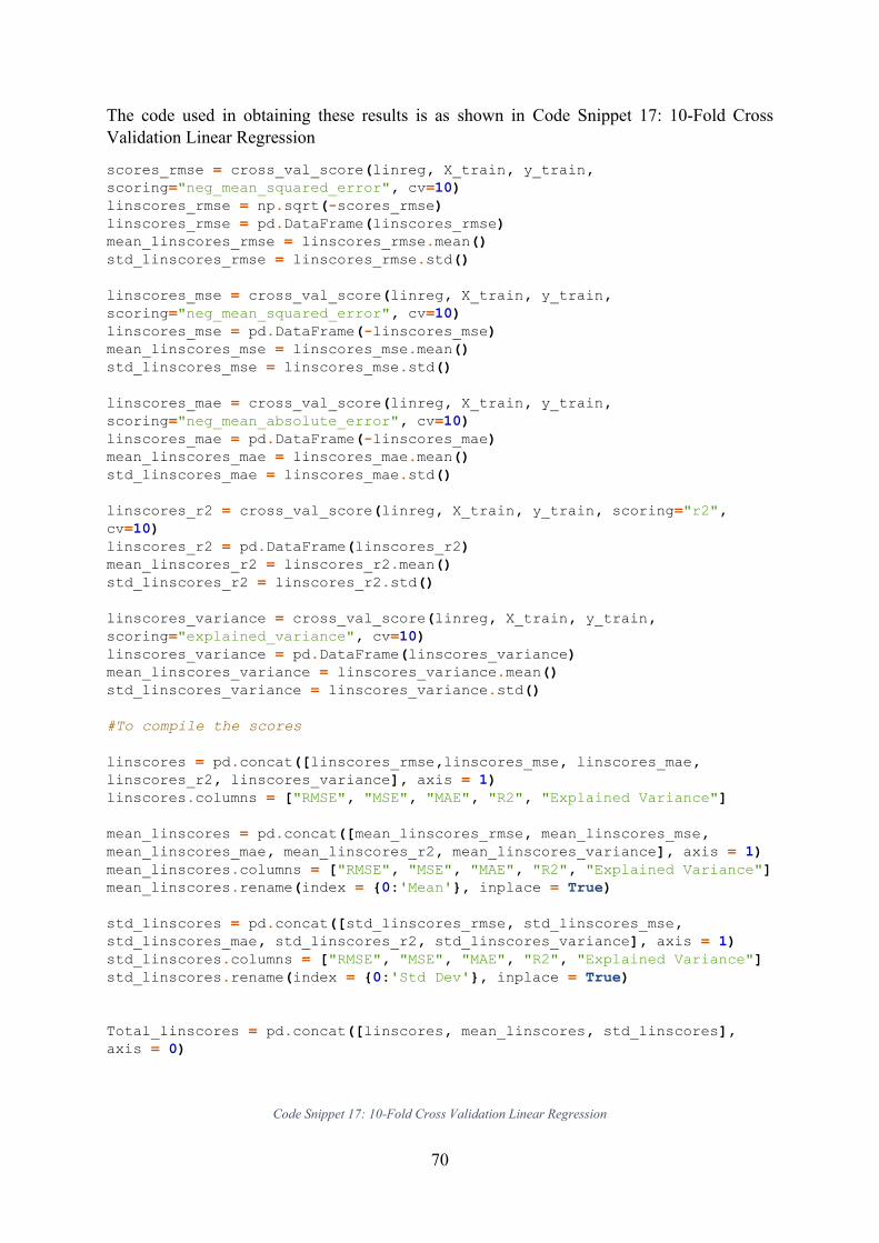
70

The code used in obtaining these results is as shown in Code Snippet 17: 10-Fold Cross Validation Linear Regression

scores_rmse = cross_val_score(linreg, X_train, y_train,

scoring="neg_mean_squared_error", cv=10)

linscores_rmse = np.sqrt(-scores_rmse)

linscores_rmse = pd.DataFrame(linscores_rmse)

mean_linscores_rmse = linscores_rmse.mean()

std_linscores_rmse = linscores_rmse.std()

linscores_mse = cross_val_score(linreg, X_train, y_train,

scoring="neg_mean_squared_error", cv=10)

linscores_mse = pd.DataFrame(-linscores_mse)

mean_linscores_mse = linscores_mse.mean()

std_linscores_mse = linscores_mse.std()

linscores_mae = cross_val_score(linreg, X_train, y_train,

scoring="neg_mean_absolute_error", cv=10)

linscores_mae = pd.DataFrame(-linscores_mae)

mean_linscores_mae = linscores_mae.mean()

std_linscores_mae = linscores_mae.std()

linscores_r2 = cross_val_score(linreg, X_train, y_train, scoring="r2",

cv=10)

linscores_r2 = pd.DataFrame(linscores_r2)

mean_linscores_r2 = linscores_r2.mean()

std_linscores_r2 = linscores_r2.std()

linscores_variance = cross_val_score(linreg, X_train, y_train,

scoring="explained_variance", cv=10)

linscores_variance = pd.DataFrame(linscores_variance)

mean_linscores_variance = linscores_variance.mean()

std_linscores_variance = linscores_variance.std()

#To compile the scores

linscores = pd.concat([linscores_rmse,linscores_mse, linscores_mae,

linscores_r2, linscores_variance], axis = 1)

linscores.columns = ["RMSE", "MSE", "MAE", "R2", "Explained Variance"]

mean_linscores = pd.concat([mean_linscores_rmse, mean_linscores_mse,

mean_linscores_mae, mean_linscores_r2, mean_linscores_variance], axis = 1)

mean_linscores.columns = ["RMSE", "MSE", "MAE", "R2", "Explained Variance"]

mean_linscores.rename(index = {0:'Mean'}, inplace = True)

std_linscores = pd.concat([std_linscores_rmse, std_linscores_mse,

std_linscores_mae, std_linscores_r2, std_linscores_variance], axis = 1)

std_linscores.columns = ["RMSE", "MSE", "MAE", "R2", "Explained Variance"]

std_linscores.rename(index = {0:'Std Dev'}, inplace = True)

Total_linscores = pd.concat([linscores, mean_linscores, std_linscores],

axis = 0)

Code Snippet 17: 10-Fold Cross Validation Linear Regression

71

If we observe the mean values, which is comparatively a good measure of the performance of the model, there is a significance difference with the values we obtained from the normal train/test split method.

2. Bayesian Ridge Regression

The below table shows the 10-fold cross validation results.

Fold Number RMSE MSE MAE R2 Explained Variance

0 0.08114 0.00658 0.07732 0.62145 0.96521

1 0.05840 0.00341 0.04792 0.77958 0.79932

2 0.04939 0.00244 0.03989 0.90414 0.91586

3 0.09092 0.00827 0.08137 0.49054 0.51685

4 0.06474 0.00419 0.04856 0.88516 0.91487

5 0.08053 0.00649 0.04544 0.88986 0.89817

6 0.05643 0.00318 0.04978 0.91161 0.94121

7 0.06597 0.00435 0.05125 0.83883 0.89783

8 0.13100 0.01716 0.11411 0.78852 0.86738

9 0.15452 0.02388 0.11827 0.18232 0.57829

Mean 0.08330 0.00800 0.06739 0.72920 0.82950

Std Dev 0.03425 0.00702 0.02907 0.23564 0.15572

Table 4: 10-Fold Cross Validation Bayesian Ridge Regression

From this, we get a clear picture of the performance of the model, since we calculate the mean of the 10 folds of the performance metrics. The Code Snippet 18: 10-Fold Cross Validation Bayesian Ridge Regression gives the method to find the scores.

3. Kernel Ridge Regression

Similar to Bayesian Regression, following table shows the scores obtained,

Fold Number RMSE MSE MAE R2 Explained Variance

0 0.09347 0.00874 0.08958 0.49756 0.95903

1 0.05878 0.00345 0.04679 0.77671 0.77723

2 0.04049 0.00164 0.03002 0.93556 0.93556

3 0.07949 0.00632 0.06994 0.61057 0.61134

4 0.07023 0.00493 0.05279 0.86485 0.90236

5 0.08892 0.00791 0.05061 0.86572 0.87108

6 0.07276 0.00529 0.06640 0.85307 0.89810

7 0.06546 0.00428 0.05054 0.84134 0.88203

8 0.11845 0.01403 0.10585 0.82711 0.87427

9 0.15046 0.02264 0.11271 0.22470 0.58577

Mean 0.08385 0.00792 0.06752 0.72972 0.82968

Std Dev 0.03149 0.00620 0.02715 0.22152 0.13092

Table 5: 10-Fold Cross Validation Kernel Ridge Regression

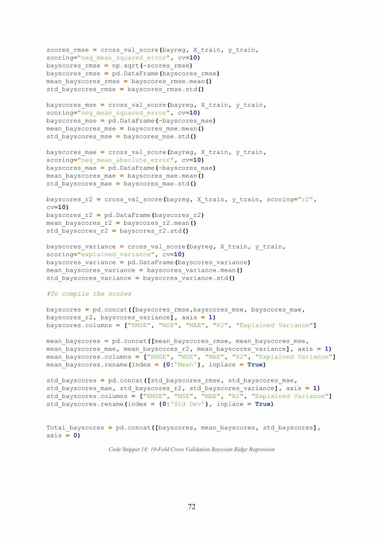
72

scores_rmse = cross_val_score(bayreg, X_train, y_train,

scoring="neg_mean_squared_error", cv=10)

bayscores_rmse = np.sqrt(-scores_rmse)

bayscores_rmse = pd.DataFrame(bayscores_rmse)

mean_bayscores_rmse = bayscores_rmse.mean()

std_bayscores_rmse = bayscores_rmse.std()

bayscores_mse = cross_val_score(bayreg, X_train, y_train,

scoring="neg_mean_squared_error", cv=10)

bayscores_mse = pd.DataFrame(-bayscores_mse)

mean_bayscores_mse = bayscores_mse.mean()

std_bayscores_mse = bayscores_mse.std()

bayscores_mae = cross_val_score(bayreg, X_train, y_train,

scoring="neg_mean_absolute_error", cv=10)

bayscores_mae = pd.DataFrame(-bayscores_mae)

mean_bayscores_mae = bayscores_mae.mean()

std_bayscores_mae = bayscores_mae.std()

bayscores_r2 = cross_val_score(bayreg, X_train, y_train, scoring="r2",

cv=10)

bayscores_r2 = pd.DataFrame(bayscores_r2)

mean_bayscores_r2 = bayscores_r2.mean()

std_bayscores_r2 = bayscores_r2.std()

bayscores_variance = cross_val_score(bayreg, X_train, y_train,

scoring="explained_variance", cv=10)

bayscores_variance = pd.DataFrame(bayscores_variance)

mean_bayscores_variance = bayscores_variance.mean()

std_bayscores_variance = bayscores_variance.std()

#To compile the scores

bayscores = pd.concat([bayscores_rmse,bayscores_mse, bayscores_mae,

bayscores_r2, bayscores_variance], axis = 1)

bayscores.columns = ["RMSE", "MSE", "MAE", "R2", "Explained Variance"]

mean_bayscores = pd.concat([mean_bayscores_rmse, mean_bayscores_mse,

mean_bayscores_mae, mean_bayscores_r2, mean_bayscores_variance], axis = 1)

mean_bayscores.columns = ["RMSE", "MSE", "MAE", "R2", "Explained Variance"]

mean_bayscores.rename(index = {0:'Mean'}, inplace = True)

std_bayscores = pd.concat([std_bayscores_rmse, std_bayscores_mse,

std_bayscores_mae, std_bayscores_r2, std_bayscores_variance], axis = 1)

std_bayscores.columns = ["RMSE", "MSE", "MAE", "R2", "Explained Variance"]

std_bayscores.rename(index = {0:'Std Dev'}, inplace = True)

Total_bayscores = pd.concat([bayscores, mean_bayscores, std_bayscores],

axis = 0) Code Snippet 18: 10-Fold Cross Validation Bayesian Ridge Regression

73

4. Neural Network

The below table shows the scores for the neural network,

Fold Number RMSE MSE MAE R2 Explained Variance

0 0.1058 0.0112 0.0995 0.3563 0.9256

1 0.0634 0.0040 0.0506 0.7405 0.7495

2 0.1321 0.0175 0.1208 0.3140 0.4117

3 0.0900 0.0081 0.0784 0.5007 0.6411

4 0.0972 0.0094 0.0726 0.7412 0.7996

5 0.1223 0.0149 0.0957 0.7461 0.7655

6 0.0844 0.0071 0.0725 0.8021 0.9479

7 0.0561 0.0031 0.0474 0.8836 0.9196

8 0.1247 0.0155 0.0954 0.8084 0.9205

9 0.1022 0.0104 0.0902 0.6422 0.7830

Mean 0.0978 0.0101 0.0823 0.6535 0.7864

Std Dev 0.0253 0.0048 0.0227 0.1972 0.1649

Table 6: 10-Fold Cross Validation Neural Network Regression

We can see that, Neural network which showed a good performance in the previous assessment, tend to have a low score during cross validation. This shows that the model was over fitting the data in the first instance.

5. Decision Tree Regression

The below table shows the performance of Decision Tree Regression,

Fold Number RMSE MSE MAE R2 Explained Variance

0 0.1713 0.0293 0.1636 -0.6875 0.8523

1 0.1382 0.0191 0.1236 -0.2338 0.4362

2 0.1099 0.0121 0.0827 0.5252 0.7941

3 0.0686 0.0047 0.0573 0.7103 0.7878

4 0.1413 0.0200 0.1000 0.4531 0.5453

5 0.1249 0.0156 0.0910 0.7352 0.7366

6 0.0868 0.0075 0.0600 0.7907 0.7917

7 0.0977 0.0095 0.0760 0.6467 0.8387

8 0.1319 0.0174 0.0950 0.7857 0.8085

9 0.2036 0.0415 0.1650 -0.4195 0.5129

Mean 0.1274 0.0177 0.1014 0.3306 0.7104

Std Dev 0.0400 0.0110 0.0383 0.5575 0.1520

Table 7: 10-Fold Cross Validation Decision Tree Regression

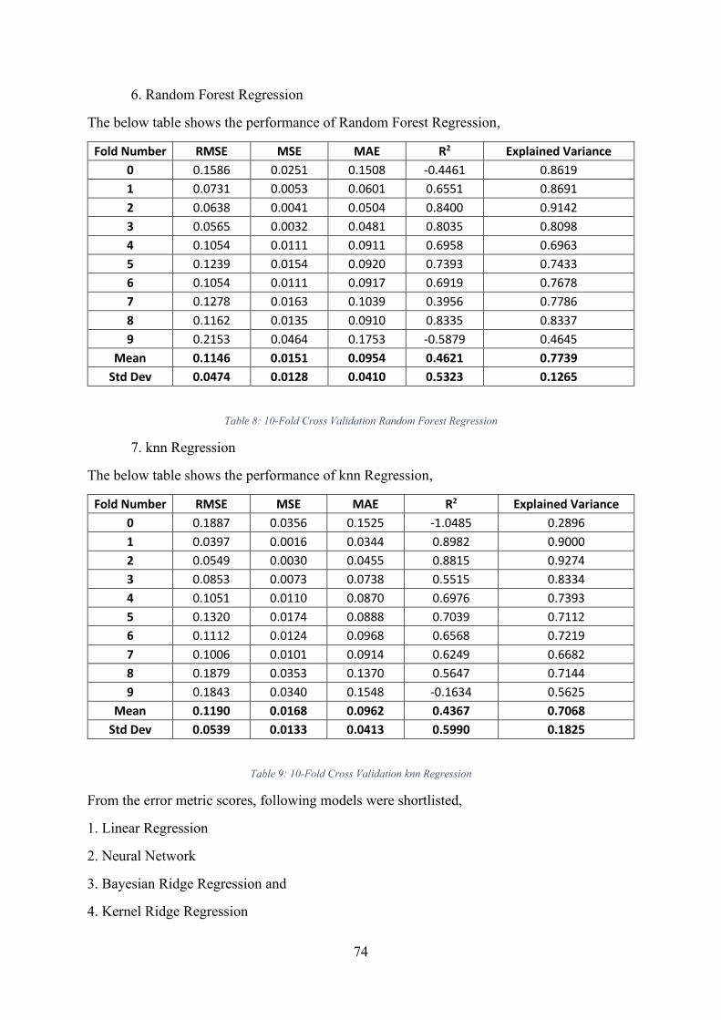
74

6. Random Forest Regression

The below table shows the performance of Random Forest Regression,

Fold Number RMSE MSE MAE R2 Explained Variance

0 0.1586 0.0251 0.1508 -0.4461 0.8619

1 0.0731 0.0053 0.0601 0.6551 0.8691

2 0.0638 0.0041 0.0504 0.8400 0.9142

3 0.0565 0.0032 0.0481 0.8035 0.8098

4 0.1054 0.0111 0.0911 0.6958 0.6963

5 0.1239 0.0154 0.0920 0.7393 0.7433

6 0.1054 0.0111 0.0917 0.6919 0.7678

7 0.1278 0.0163 0.1039 0.3956 0.7786

8 0.1162 0.0135 0.0910 0.8335 0.8337

9 0.2153 0.0464 0.1753 -0.5879 0.4645

Mean 0.1146 0.0151 0.0954 0.4621 0.7739

Std Dev 0.0474 0.0128 0.0410 0.5323 0.1265

Table 8: 10-Fold Cross Validation Random Forest Regression

7. knn Regression

The below table shows the performance of knn Regression,

Fold Number RMSE MSE MAE R2 Explained Variance

0 0.1887 0.0356 0.1525 -1.0485 0.2896

1 0.0397 0.0016 0.0344 0.8982 0.9000

2 0.0549 0.0030 0.0455 0.8815 0.9274

3 0.0853 0.0073 0.0738 0.5515 0.8334

4 0.1051 0.0110 0.0870 0.6976 0.7393

5 0.1320 0.0174 0.0888 0.7039 0.7112

6 0.1112 0.0124 0.0968 0.6568 0.7219

7 0.1006 0.0101 0.0914 0.6249 0.6682

8 0.1879 0.0353 0.1370 0.5647 0.7144

9 0.1843 0.0340 0.1548 -0.1634 0.5625

Mean 0.1190 0.0168 0.0962 0.4367 0.7068

Std Dev 0.0539 0.0133 0.0413 0.5990 0.1825

Table 9: 10-Fold Cross Validation knn Regression

From the error metric scores, following models were shortlisted,

1. Linear Regression

2. Neural Network

3. Bayesian Ridge Regression and

4. Kernel Ridge Regression

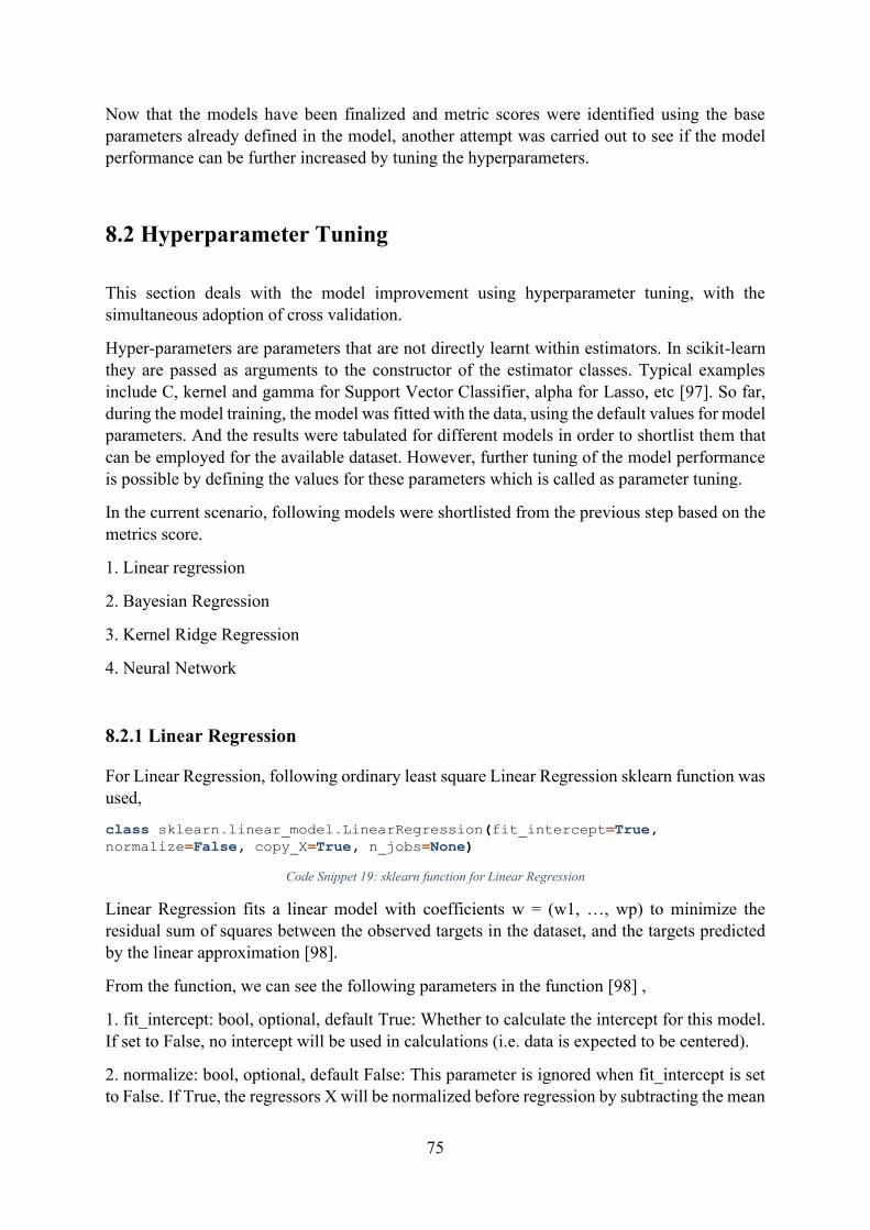
75

Now that the models have been finalized and metric scores were identified using the base parameters already defined in the model, another attempt was carried out to see if the model performance can be further increased by tuning the hyperparameters.

8.2 Hyperparameter Tuning

This section deals with the model improvement using hyperparameter tuning, with the simultaneous adoption of cross validation.

Hyper-parameters are parameters that are not directly learnt within estimators. In scikit-learn they are passed as arguments to the constructor of the estimator classes. Typical examples include C, kernel and gamma for Support Vector Classifier, alpha for Lasso, etc [97]. So far, during the model training, the model was fitted with the data, using the default values for model parameters. And the results were tabulated for different models in order to shortlist them that can be employed for the available dataset. However, further tuning of the model performance is possible by defining the values for these parameters which is called as parameter tuning.

In the current scenario, following models were shortlisted from the previous step based on the metrics score.

1. Linear regression

2. Bayesian Regression

3. Kernel Ridge Regression

4. Neural Network

8.2.1 Linear Regression

For Linear Regression, following ordinary least square Linear Regression sklearn function was used,

class sklearn.linear_model.LinearRegression(fit_intercept=True,

normalize=False, copy_X=True, n_jobs=None) Code Snippet 19: sklearn function for Linear Regression

Linear Regression fits a linear model with coefficients w = (w1, …, wp) to minimize the

residual sum of squares between the observed targets in the dataset, and the targets predicted by the linear approximation [98].

From the function, we can see the following parameters in the function [98] ,

1. fit_intercept: bool, optional, default True: Whether to calculate the intercept for this model. If set to False, no intercept will be used in calculations (i.e. data is expected to be centered).

2. normalize: bool, optional, default False: This parameter is ignored when fit_intercept is set to False. If True, the regressors X will be normalized before regression by subtracting the mean

76

and dividing by the l2-norm. If you wish to standardize, please use sklearn.preprocessing.StandardScaler before calling fit on an estimator with normalize=False.

3. copy_X: bool, optional, default True: If True, X will be copied; else, it may be overwritten.

4. n_jobs: int or None, optional (default=None): The number of jobs to use for the computation. This will only provide speedup for n_targets > 1 and sufficient large problems. None means 1 unless in a joblib.parallel_backend context. -1 means using all processors. See Glossary for more details.

From this linear Regression doesn’t particularly have any hyperparameters for optimization.

Hence no further improvement was done with respect to the Linear Regression.

8.2.2 Bayesian Ridge Regression

For Bayesian Ridge Regression, following modified linear sklearn function has been employed,

class sklearn.linear_model.BayesianRidge(n_iter=300, tol=0.001, alpha_1=1e-

06, alpha_2=1e-06, lambda_1=1e-06, lambda_2=1e-06, alpha_init=None,

lambda_init=None, compute_score=False, fit_intercept=True, normalize=False,

copy_X=True, verbose=False) Code Snippet 20: sklearn function for Bayesian Ridge Regression

From the function, following parameters are evident [99],

1. n_iter: int, default=300: Maximum number of iterations. Should be greater than or equal to 1.

2. tol: float, default=1e-3: Stop the algorithm if w has converged.

3. alpha_1: float, default=1e-6: Hyper-parameter : shape parameter for the Gamma distribution prior over the alpha parameter.

4. alpha_2: float, default=1e-6: Hyper-parameter : inverse scale parameter (rate parameter) for the Gamma distribution prior over the alpha parameter.

5. lambda_1: float, default=1e-6: Hyper-parameter : shape parameter for the Gamma distribution prior over the lambda parameter.

6. lambda_2: float, default=1e-6: Hyper-parameter : inverse scale parameter (rate parameter) for the Gamma distribution prior over the lambda parameter.

7. alpha_init: float, default=None: Initial value for alpha (precision of the noise). If not set, alpha_init is 1/Var(y).

8. lambda_init: float, default=None: Initial value for lambda (precision of the weights). If not set, lambda_init is 1.

9. compute_score: bool, default=False: If True, compute the log marginal likelihood at each iteration of the optimization.

77

10. fit_intercept: bool, default=True: Whether to calculate the intercept for this model. The intercept is not treated as a probabilistic parameter and thus has no associated variance. If set to False, no intercept will be used in calculations (i.e. data is expected to be centered).

11. normalize: bool, default=False: This parameter is ignored when fit_intercept is set to False. If True, the regressors X will be normalized before regression by subtracting the mean and dividing by the l2-norm. If you wish to standardize, please use sklearn.preprocessing.StandardScaler before calling fit on an estimator with normalize=False.

12. copy_X: bool, default=True: If True, X will be copied; else, it may be overwritten.

13. verbose: bool, default=False: Verbose mode when fitting the model.

From the parameters mentioned above, alpha_1, alpha_2, lambda_1 and lambda_2 can be identified as hyperparameters whose values can be further optimized to get better performance of the machine learning model.

8.2.3 Kernel Ridge Regression

For Kernel Ridge Regression, below mentioned sklearn function was utilized to model,

class sklearn.kernel_ridge.KernelRidge(alpha=1, kernel='linear',

gamma=None, degree=3, coef0=1, kernel_params=None) Code Snippet 21: sklearn function for Kernel Ridge Regression

From the function, following parameters can be extracted [100],

1. alpha: {float, array-like}, shape = [n_targets]: Small positive values of alpha improve the conditioning of the problem and reduce the variance of the estimates. Alpha corresponds to (2*C)^-1 in other linear models such as LogisticRegression or LinearSVC. If an array is passed, penalties are assumed to be specific to the targets. Hence they must correspond in number.

2. kernel: string or callable, default=”linear”: Kernel mapping used internally. A callable should accept two arguments and the keyword arguments passed to this object as kernel_params, and should return a floating point number. Set to “precomputed” in order to

pass a precomputed kernel matrix to the estimator methods instead of samples.

3. gamma: float, default=None: Gamma parameter for the RBF, laplacian, polynomial, exponential chi2 and sigmoid kernels. Interpretation of the default value is left to the kernel; see the documentation for sklearn.metrics.pairwise. Ignored by other kernels.

4. degree: float, default=3: Degree of the polynomial kernel. Ignored by other kernels.

5. coef0: float, default=1: Zero coefficient for polynomial and sigmoid kernels. Ignored by other kernels.

6. kernel_params: mapping of string to any, optional: Additional parameters (keyword arguments) for kernel function passed as callable object.

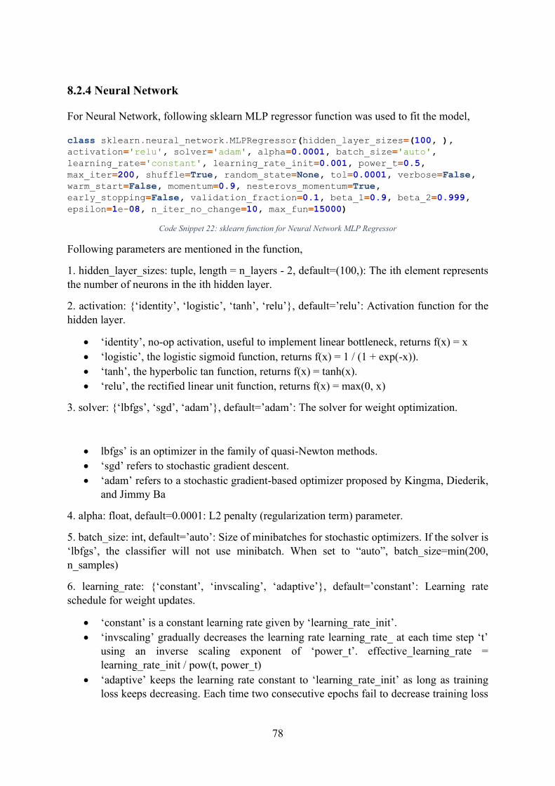
78

8.2.4 Neural Network

For Neural Network, following sklearn MLP regressor function was used to fit the model,

class sklearn.neural_network.MLPRegressor(hidden_layer_sizes=(100, ),

activation='relu', solver='adam', alpha=0.0001, batch_size='auto',

learning_rate='constant', learning_rate_init=0.001, power_t=0.5,

max_iter=200, shuffle=True, random_state=None, tol=0.0001, verbose=False,

warm_start=False, momentum=0.9, nesterovs_momentum=True,

early_stopping=False, validation_fraction=0.1, beta_1=0.9, beta_2=0.999,

epsilon=1e-08, n_iter_no_change=10, max_fun=15000) Code Snippet 22: sklearn function for Neural Network MLP Regressor

Following parameters are mentioned in the function,

1. hidden_layer_sizes: tuple, length = n_layers - 2, default=(100,): The ith element represents the number of neurons in the ith hidden layer.

2. activation: {‘identity’, ‘logistic’, ‘tanh’, ‘relu’}, default=’relu’: Activation function for the hidden layer.

• ‘identity’, no-op activation, useful to implement linear bottleneck, returns f(x) = x • ‘logistic’, the logistic sigmoid function, returns f(x) = 1 / (1 + exp(-x)). • ‘tanh’, the hyperbolic tan function, returns f(x) = tanh(x). • ‘relu’, the rectified linear unit function, returns f(x) = max(0, x)

3. solver: {‘lbfgs’, ‘sgd’, ‘adam’}, default=’adam’: The solver for weight optimization.

• lbfgs’ is an optimizer in the family of quasi-Newton methods. • ‘sgd’ refers to stochastic gradient descent. • ‘adam’ refers to a stochastic gradient-based optimizer proposed by Kingma, Diederik,

and Jimmy Ba

4. alpha: float, default=0.0001: L2 penalty (regularization term) parameter.

5. batch_size: int, default=’auto’: Size of minibatches for stochastic optimizers. If the solver is ‘lbfgs’, the classifier will not use minibatch. When set to “auto”, batch_size=min(200,

n_samples)

6. learning_rate: {‘constant’, ‘invscaling’, ‘adaptive’}, default=’constant’: Learning rate schedule for weight updates.

• ‘constant’ is a constant learning rate given by ‘learning_rate_init’. • ‘invscaling’ gradually decreases the learning rate learning_rate_ at each time step ‘t’

using an inverse scaling exponent of ‘power_t’. effective_learning_rate =

learning_rate_init / pow(t, power_t) • ‘adaptive’ keeps the learning rate constant to ‘learning_rate_init’ as long as training

loss keeps decreasing. Each time two consecutive epochs fail to decrease training loss

79

by at least tol, or fail to increase validation score by at least tol if ‘early_stopping’ is

on, the current learning rate is divided by 5.

7. learning_rate_init: double, default=0.001: The initial learning rate used. It controls the step-size in updating the weights. Only used when solver=’sgd’ or ‘adam’.

8. power_t: double, default=0.5: The exponent for inverse scaling learning rate. It is used in updating effective learning rate when the learning_rate is set to ‘invscaling’. Only used when

solver=’sgd’.

9. max_iter: int, default=200: Maximum number of iterations. The solver iterates until convergence (determined by ‘tol’) or this number of iterations. For stochastic solvers (‘sgd’,

‘adam’), note that this determines the number of epochs (how many times each data point will

be used), not the number of gradient steps.

10.shuffle: bool, default=True: Whether to shuffle samples in each iteration. Only used when solver=’sgd’ or ‘adam’.

11: random_state: int, RandomState instance or None, default=None: If int, random_state is the seed used by the random number generator; If RandomState instance, random_state is the random number generator; If None, the random number generator is the RandomState instance used by np.random.

12. tol: float, default=1e-4: Tolerance for the optimization. When the loss or score is not improving by at least tol for n_iter_no_change consecutive iterations, unless learning_rate is set to ‘adaptive’, convergence is considered to be reached and training stops.

13. verbose: bool, default=False: Whether to print progress messages to stdout.

14. warm_start: bool, default=False: When set to True, reuse the solution of the previous call to fit as initialization, otherwise, just erase the previous solution. See the Glossary.

15. momentum: float, default=0.9: Momentum for gradient descent update. Should be between 0 and 1. Only used when solver=’sgd’.

16. nesterovs_momentum: boolean, default=True: Whether to use Nesterov’s momentum.

Only used when solver=’sgd’ and momentum > 0.

17.early_stopping: bool, default=False: Whether to use early stopping to terminate training when validation score is not improving. If set to true, it will automatically set aside 10% of training data as validation and terminate training when validation score is not improving by at least tol for n_iter_no_change consecutive epochs. Only effective when solver=’sgd’ or ‘adam’

18. validation_fraction: float, default=0.1: The proportion of training data to set aside as validation set for early stopping. Must be between 0 and 1. Only used if early_stopping is True

19. beta_1: float, default=0.9: Exponential decay rate for estimates of first moment vector in adam, should be in [0, 1). Only used when solver=’adam’

20. beta_2: float, default=0.999: Exponential decay rate for estimates of second moment vector in adam, should be in [0, 1). Only used when solver=’adam’

80

21. epsilon: float, default=1e-8: Value for numerical stability in adam. Only used when solver=’adam’

22. n_iter_no_change: int, default=10: Maximum number of epochs to not meet tol improvement. Only effective when solver=’sgd’ or ‘adam’

23. max_fun: int, default=15000: Only used when solver=’lbfgs’. Maximum number of function calls. The solver iterates until convergence (determined by ‘tol’), number of iterations

reaches max_iter, or this number of function calls. Note that number of function calls will be greater than or equal to the number of iterations for the MLPRegressor.

From the extensive list of parameters mentioned above, following parameters can be considered as Hyperparameters, where an attempt has been carried out to optimize the values to improve the performance of the model,

1. hidden layers: Here by default, the model is considering one hidden layer with 100 neurons constituting the layer. Considering that there are 27 features to be used to do the prediction of tool wear, an empirical method is followed where in two instances are tried, first with one hidden layer with 27 neurons and the second with two hidden layers constituting 54 neurons (double the number of neurons compared to the first hidden layer).

2. activation function: Considering that there is possibility of employing any of the 4 mentioned activation functions, namely, ‘identity’, ‘logistic’, ‘tanh’ and ‘relu’ all of them have been tried

to see the performance variation of the model in combination with the checking of the hidden layers.

3. solver: Similar to the activation function, there are possibilities of utilizing the following solvers, namely ‘lbfgs’, ‘sgd’ and ‘adam’. All of them have been checked along with the

combinations with hidden layers and activation functions with various combinations.

4. batch size: Though there are a lot of possibilities of choosing the batch size to optimize the model, some of the instances showed that lower number of batch size increased the performance of the model. However, batch sizes of 1 and 2 were tested for analyzing the performance.

5. learning rate: Similar to activation function and solver, following learning rate methods have been tested to check for the performance, ‘constant’, ‘invscaling’ and ‘adaptive’.

With the hyperparameters values available, a method must be used where in a proper combination of these hyperparameters can be employed to optimize the models. There are several approaches to hyperparameter tuning,

1. Manual: select hyperparameters based on intuition/experience/guessing, train the model with the hyperparameters, and score on the validation data. Repeat process until you run out of patience or are satisfied with the results.

2. Grid Search: set up a grid of hyperparameter values and for each combination, train a model and score on the validation data. In this approach, every single combination of hyperparameters values is tried which can be very inefficient!

3. Random search: set up a grid of hyperparameter values and select random combinations to train the model and score. The number of search iterations is set based on time/resources.

81

4. Automated Hyperparameter Tuning: use methods such as gradient descent, Bayesian Optimization, or evolutionary algorithms to conduct a guided search for the best hyperparameters.

During the execution of this thesis, Grid search has been used to tune the hyperparameters. Grid search has been done to check the R2 and Explained variance error metrics of the model.

The Code Snippet 23: Neural Network Grid search error R2 metric gives the code used for carrying out grid search based on R2 error metric.

The Code Snippet 24: Neural Network Grid search explained Variance error metric gives the code used for carrying out grid search based on Explained Variance error metric.

Upon completion of the Grid search with Cross validation of 10 folds, the best results and corresponding best parameters are as shown below,

Hyperparameter Value R2 Score Explained Variance Score

Activation function logistic

0.79087 0.87591

Batch size 1

Hidden layer sizes 1 layer with 27 neurons

Learning rate method constant

Solver lbfgs

Table 10: Hyperparameter tuning results: Neural Network

The results that were obtained after hyperparameter tuning is significantly higher than the once obtained during the previous 10-fold cross validation as shown in Table 6: 10-Fold Cross Validation Neural Network Regression. Hence, the model is said to be tuned to optimize the performance.

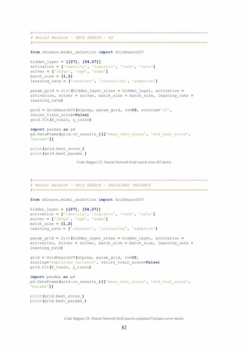
82

#==========================================================================

# Neural Network - GRID SEARCH - R2

#==========================================================================

from sklearn.model_selection import GridSearchCV

hidden_layer = [[27], [54,27]]

activation = ['identity', 'logistic', 'tanh', 'relu']

solver = ['lbfgs', 'sgd', 'adam']

batch_size = [1,2]

learning_rate = ['constant', 'invscaling', 'adaptive']

param_grid = dict(hidden_layer_sizes = hidden_layer, activation =

activation, solver = solver, batch_size = batch_size, learning_rate =

learning_rate)

grid = GridSearchCV(mlpreg, param_grid, cv=10, scoring='r2',

return_train_score=False)

grid.fit(X_train, y_train)

import pandas as pd

pd.DataFrame(grid.cv_results_)[['mean_test_score', 'std_test_score',

'params']]

print(grid.best_score_)

print(grid.best_params_) Code Snippet 23: Neural Network Grid search error R2 metric

#==========================================================================

# Neural Network - GRID SEARCH - EXPLAINED VARIANCE

#==========================================================================

from sklearn.model_selection import GridSearchCV

hidden_layer = [[27], [54,27]]

activation = ['identity', 'logistic', 'tanh', 'relu']

solver = ['lbfgs', 'sgd', 'adam']

batch_size = [1,2]

learning_rate = ['constant', 'invscaling', 'adaptive']

param_grid = dict(hidden_layer_sizes = hidden_layer, activation =

activation, solver = solver, batch_size = batch_size, learning_rate =

learning_rate)

grid = GridSearchCV(mlpreg, param_grid, cv=10,

scoring='explained_variance', return_train_score=False)

grid.fit(X_train, y_train)

import pandas as pd

pd.DataFrame(grid.cv_results_)[['mean_test_score', 'std_test_score',

'params']]

print(grid.best_score_)

print(grid.best_params_)

Code Snippet 24: Neural Network Grid search explained Variance error metric

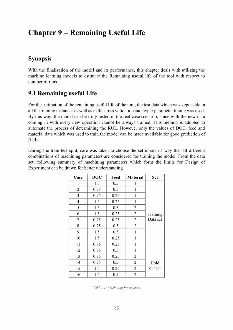
83

Chapter 9 – Remaining Useful Life

Synopsis

With the finalization of the model and its performance, this chapter deals with utilizing the machine learning models to estimate the Remaining useful life of the tool with respect to number of runs

9.1 Remaining useful Life

For the estimation of the remaining useful life of the tool, the test data which was kept aside in all the training instances as well as in the cross validation and hyper parameter tuning was used. By this way, the model can be truly tested in the real case scenario, since with the new data coming in with every new operation cannot be always trained. This method is adopted to automate the process of determining the RUL. However only the values of DOC, feed and material data which was used to train the model can be made available for good prediction of RUL.

During the train test split, care was taken to choose the set in such a way that all different combinations of machining parameters are considered for training the model. From the data set, following summary of machining parameters which form the limits for Design of Experiment can be drawn for better understanding.

Case DOC Feed Material Set 1 1.5 0.5 1

Training Data set

2 0.75 0.5 1 3 0.75 0.25 1 4 1.5 0.25 1 5 1.5 0.5 2 6 1.5 0.25 2 7 0.75 0.25 2 8 0.75 0.5 2 9 1.5 0.5 1 10 1.5 0.25 1 11 0.75 0.25 1 12 0.75 0.5 1 13 0.75 0.25 2

Hold out set

14 0.75 0.5 2 15 1.5 0.25 2 16 1.5 0.5 2

Table 11: Machining Parameters

84

Following steps were followed to estimate the remaining useful life of the tool wear,

1. The VB was predicted for the hold out set using the machine learning model, which was trained from the training data set

2. From this, the predicted VB which exceeded the safe VB limit of 0.6 was filtered and tabulated separately

3. corresponding machining parameters were filtered and tabulated along with the feasible number of runs corresponding to each parameter

4. the value under the column ‘runs’ corresponding to the maximum VB was identified

5. to get the possible feasible runs, one run less than the identified was taken and provided to the operator

6. This procedure is repeated for each request from operator based on the machining parameter

Here, in order to train the model, the values of the parameters obtained during Hyperparameter tuning is used to obtain best possible performance. The Code Snippet 25: RUL Model Training gives the code used train model and obtain the prediction of VB. The corresponding performance of the model is shown in Figure 40: Improved Neural Network Performance.

Figure 40: Improved Neural Network Performance

From the graph it is evident that, apart from one critical point, where even after the tool wear has crossed the VB of 0.6, the prediction is showing it is safe, the rest of the threshold points have been predicted well.

0

0.2

0.4

0.6

0.8

1

1.2

1.4

1.6

1.8

0 5 10 15 20 25 30 35 40 45

VB

Data Points

Prediction

Original

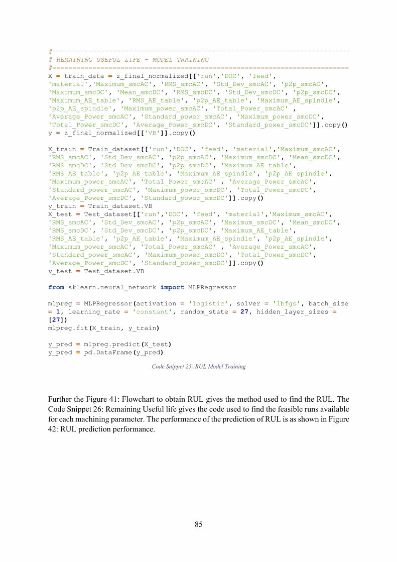
85

#========================================================================== # REMAINING USEFUL LIFE - MODEL TRAINING #========================================================================== X = train_data = z_final_normalized[['run','DOC', 'feed',

'material','Maximum_smcAC', 'RMS_smcAC', 'Std_Dev_smcAC', 'p2p_smcAC',

'Maximum_smcDC', 'Mean_smcDC', 'RMS_smcDC', 'Std_Dev_smcDC', 'p2p_smcDC',

'Maximum_AE_table', 'RMS_AE_table', 'p2p_AE_table', 'Maximum_AE_spindle',

'p2p_AE_spindle', 'Maximum_power_smcAC', 'Total_Power_smcAC' ,

'Average_Power_smcAC', 'Standard_power_smcAC', 'Maximum_power_smcDC',

'Total_Power_smcDC', 'Average_Power_smcDC', 'Standard_power_smcDC']].copy() y = z_final_normalized[['VB']].copy()

X_train = Train_dataset[['run','DOC', 'feed', 'material','Maximum_smcAC',

'RMS_smcAC', 'Std_Dev_smcAC', 'p2p_smcAC', 'Maximum_smcDC', 'Mean_smcDC',

'RMS_smcDC', 'Std_Dev_smcDC', 'p2p_smcDC', 'Maximum_AE_table',

'RMS_AE_table', 'p2p_AE_table', 'Maximum_AE_spindle', 'p2p_AE_spindle',

'Maximum_power_smcAC', 'Total_Power_smcAC' , 'Average_Power_smcAC',

'Standard_power_smcAC', 'Maximum_power_smcDC', 'Total_Power_smcDC',

'Average_Power_smcDC', 'Standard_power_smcDC']].copy() y_train = Train_dataset.VB X_test = Test_dataset[['run','DOC', 'feed', 'material','Maximum_smcAC',

'RMS_smcAC', 'Std_Dev_smcAC', 'p2p_smcAC', 'Maximum_smcDC', 'Mean_smcDC',

'RMS_smcDC', 'Std_Dev_smcDC', 'p2p_smcDC', 'Maximum_AE_table',

'RMS_AE_table', 'p2p_AE_table', 'Maximum_AE_spindle', 'p2p_AE_spindle',

'Maximum_power_smcAC', 'Total_Power_smcAC' , 'Average_Power_smcAC',

'Standard_power_smcAC', 'Maximum_power_smcDC', 'Total_Power_smcDC',

'Average_Power_smcDC', 'Standard_power_smcDC']].copy() y_test = Test_dataset.VB

from sklearn.neural_network import MLPRegressor

mlpreg = MLPRegressor(activation = 'logistic', solver = 'lbfgs', batch_size

= 1, learning_rate = 'constant', random_state = 27, hidden_layer_sizes =

[27]) mlpreg.fit(X_train, y_train)

y_pred = mlpreg.predict(X_test) y_pred = pd.DataFrame(y_pred)

Code Snippet 25: RUL Model Training

Further the Figure 41: Flowchart to obtain RUL gives the method used to find the RUL. The Code Snippet 26: Remaining Useful life gives the code used to find the feasible runs available for each machining parameter. The performance of the prediction of RUL is as shown in Figure 42: RUL prediction performance.

86

Figure 41: Flowchart to obtain RUL

Remaining Useful life based on

Number of Runs

Filter the data based on DOC, Feed, Material,

Runs and Predicted VB

Input from User on DOC, Feed and Material

Filter Predicted VB and Runs based on the input

Unsafe_data = Predicted VB>0.6

Take minimum of Predicted VB from Unsafe_data

Take the run corresponding to the Least Predicted VB in

unsafe data

Feasible Runs = run-1

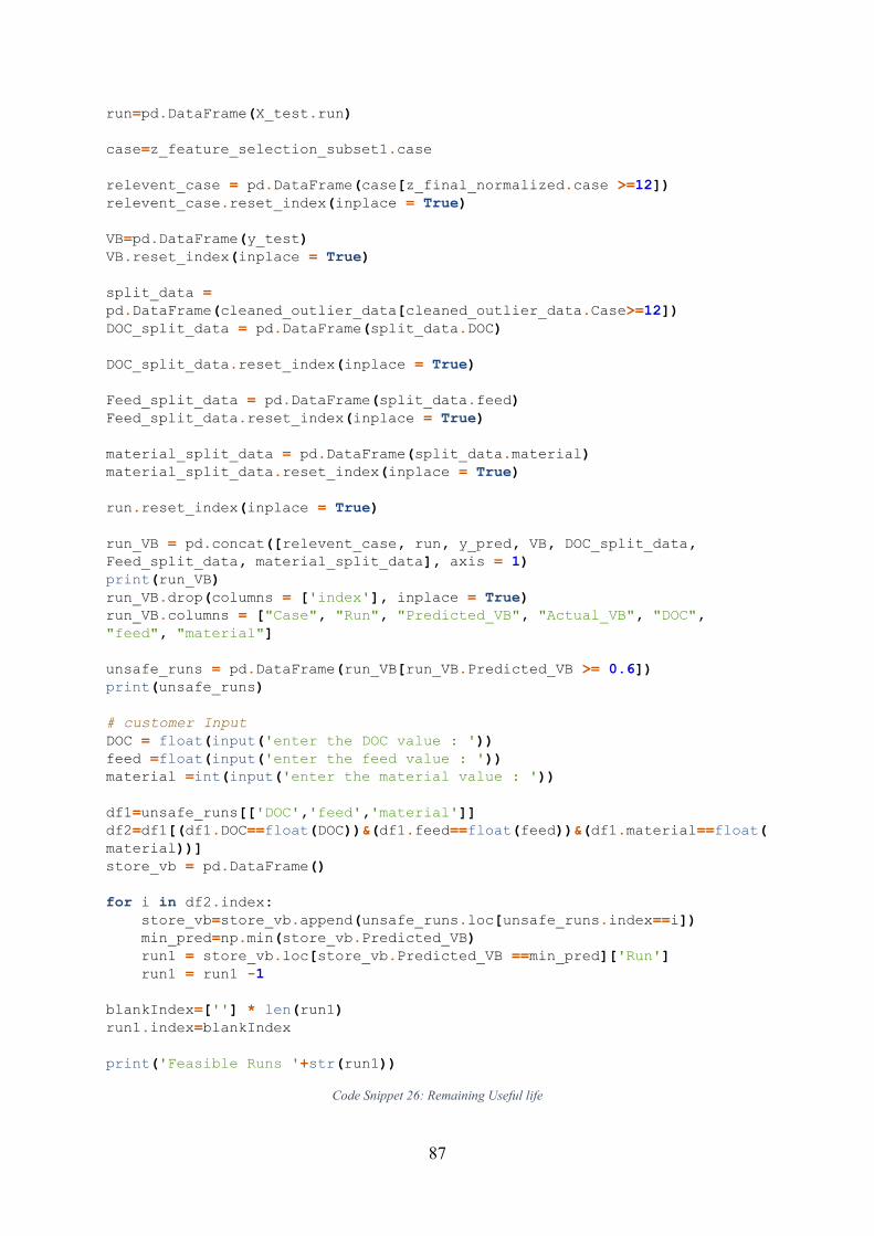
87

run=pd.DataFrame(X_test.run)

case=z_feature_selection_subset1.case

relevent_case = pd.DataFrame(case[z_final_normalized.case >=12]) relevent_case.reset_index(inplace = True)

VB=pd.DataFrame(y_test) VB.reset_index(inplace = True)

split_data =

pd.DataFrame(cleaned_outlier_data[cleaned_outlier_data.Case>=12]) DOC_split_data = pd.DataFrame(split_data.DOC)

DOC_split_data.reset_index(inplace = True)

Feed_split_data = pd.DataFrame(split_data.feed) Feed_split_data.reset_index(inplace = True)

material_split_data = pd.DataFrame(split_data.material) material_split_data.reset_index(inplace = True)

run.reset_index(inplace = True)

run_VB = pd.concat([relevent_case, run, y_pred, VB, DOC_split_data,

Feed_split_data, material_split_data], axis = 1) print(run_VB) run_VB.drop(columns = ['index'], inplace = True) run_VB.columns = ["Case", "Run", "Predicted_VB", "Actual_VB", "DOC",

"feed", "material"]

unsafe_runs = pd.DataFrame(run_VB[run_VB.Predicted_VB >= 0.6]) print(unsafe_runs)

# customer Input DOC = float(input('enter the DOC value : ')) feed =float(input('enter the feed value : ')) material =int(input('enter the material value : '))

df1=unsafe_runs[['DOC','feed','material']] df2=df1[(df1.DOC==float(DOC))&(df1.feed==float(feed))&(df1.material==float(

material))] store_vb = pd.DataFrame()

for i in df2.index: store_vb=store_vb.append(unsafe_runs.loc[unsafe_runs.index==i]) min_pred=np.min(store_vb.Predicted_VB) run1 = store_vb.loc[store_vb.Predicted_VB ==min_pred]['Run'] run1 = run1 -1

blankIndex=[''] * len(run1) run1.index=blankIndex

print('Feasible Runs '+str(run1)) Code Snippet 26: Remaining Useful life

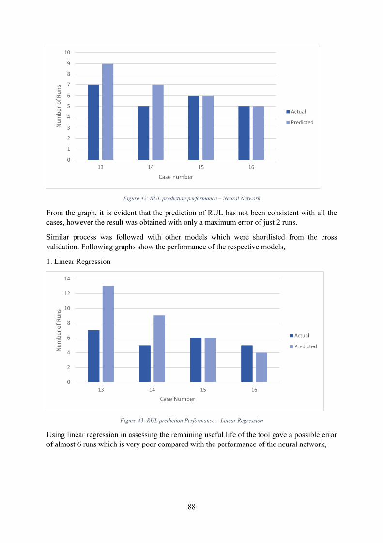
88

Figure 42: RUL prediction performance – Neural Network

From the graph, it is evident that the prediction of RUL has not been consistent with all the cases, however the result was obtained with only a maximum error of just 2 runs.

Similar process was followed with other models which were shortlisted from the cross validation. Following graphs show the performance of the respective models,

1. Linear Regression

Figure 43: RUL prediction Performance – Linear Regression

Using linear regression in assessing the remaining useful life of the tool gave a possible error of almost 6 runs which is very poor compared with the performance of the neural network,

0

1

2

3

4

5

6

7

8

9

10

13 14 15 16

Nu

mb

er o

f R

un

s

Case number

Actual

Predicted

0

2

4

6

8

10

12

14

13 14 15 16

Nu

mb

er o

f R

un

s

Case Number

Actual

Predicted

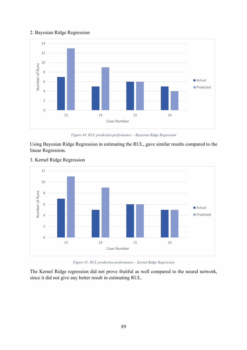
89

2. Bayesian Ridge Regression

Figure 44: RUL prediction performance – Bayesian Ridge Regression

Using Bayesian Ridge Regression in estimating the RUL, gave similar results compared to the linear Regression.

3. Kernel Ridge Regression

Figure 45: RUL prediction performance – Kernel Ridge Regression

The Kernel Ridge regression did not prove fruitful as well compared to the neural network, since it did not give any better result in estimating RUL.

0

2

4

6

8

10

12

14

13 14 15 16

Nu

mb

er o

f R

un

s

Case Number

Actual

Predicted

0

2

4

6

8

10

12

13 14 15 16

Nu

mb

er o

f R

un

s

Case Number

Actual

Predicted

90

Chapter 10 – Conclusions and Future Work

Synopsis

This concluding chapter gives the summary of the study carried out by highlighting the important steps. Here the future work that can be continued taking this study as the basis is also presented.

10.1 Conclusion

From the previous chapter, one clear conclusion that was arrived at, was that the neural network performed well compared with the rest of the models in estimating the RUL of tool.

In this study, along with the exploration of machine learning models to predict the severity of the tool wear, wide range of concepts were investigated.

1. The study explored into the different ways of adopting the cleaning of dataset, to optimize the learning process of the model during training period

2. The study investigated into the outlier analysis, to detect the anomaly in the data by exploring ways to streamline the process of detecting the same in any new dataset inserted. The z-score method used here to conduct the outlier analysis, proved enough for the dataset used, considering the data largely lies in the normal distribution curve

3. The study ventured into the adoption of machine learning framework for prediction by implementing Feature extraction and feature selection using optimum methods suitable for the dataset used. The Pearson’s co-relation method used for the feature selection paved way to implement the best features that can be used for the prediction process.

4. Various machine learning models were initially trained by splitting the data into train and test data sets, and by analyzing the error metrics, the models were shortlisted. Scikitlearn library was extensively used for the model training, testing as well as for the to find the error metrics.

5. The study also highlighted the uses of cross validation and hyperparameter training to improve the model performance, and finally the Remaining useful life was predicted using the improved model

Once the complete algorithm is made to run, there appears a direct prompt for the operator to insert the machining parameters like DOC, Feed and material for which the feasible runs is displayed. Since the ‘hold out’ data set is very small, only a portion of remaining useful life prediction is demonstrated in the work.

91

10.2 Scope for Future Work

Though the complete machine learning framework for the prediction of tool wear and also to determine the Remaining useful life of the tool was presented in this work, there lies a scope of improvement in many areas which can prove fruitful in further improving the prediction accuracy and thereby giving best suggestions for the operator with respect to the tool life.

Some of the key areas where the work can be further developed are as follows,

1. In the present work, only one method of outlier analysis was presented, where in few anomalies were removed. However, from the visual representation of the data, it is evident that there is a presence of machine noise. Additional methods can be explored in order to eliminate the background noise, thereby increasing the data set properties

2. Only machine learning methods were employed here to train and test the models. Though many methods were explored to improve the performance, final accuracy obtained was not satisfactory. Deep learning methods can be implemented to further improve the performance of the model thereby increasing the prediction accuracy of the tool wear

3. Considering that there was a limitation with the size of the data set, only a small amount of data was used to assess the algorithm performance in determining the Remaining useful life of the tool. If it is possible to obtain similar dataset with additional number of cases, significant amount of data points can be reserved for the final assessment thereby attesting the performance of the algorithm suggested in the study.

92

Bibliography

[1] "www.tutorialspoint.com," [Online]. Available: https://www.tutorialspoint.com/artificial_intelligence/artificial_intelligence_overview.htm.

[2] R. Singh, "Metal Cutting," in Introduction to Basic Manufacturing Processes and Worshop Technology, New Delhi, New Age International Private Limited, 2006, pp. 397-398.

[3] "Wikipedia," [Online]. Available: https://en.wikipedia.org/wiki/Tool_wear.

[4] "onupkeep.com," [Online]. Available: https://www.onupkeep.com/learning/maintenance-applications/machinery-maintenance.

[5] R. K. Mobley, "Impact of Maintenance," in An Introduction to Predictive Maintenance, Woburn, MA 01801-2041, Butterworth-Heinemann, 2002.

[6] S. G. Garrido, "https://www.mantenimientopetroquimica.com/," [Online]. Available: https://www.mantenimientopetroquimica.com/en/typesofmaintenance.html.

[7] B. A. W. D. S. a. J. L. Xiaoning Jin, "Present Status and Future Growth of Advanced Maintenance Technology and Strategy in US Manufacturing," 3 January 2017. [Online]. Available: https://www.ncbi.nlm.nih.gov/pmc/articles/PMC5207222/.

[8] K. A. K. a. N. Z. Gebraeel, "Predictive Maintenance Management Using Sensor-Based Degradation Models," in IEEE Transactions on Systems Man and Cybernetics - Part A Systems and Humans, August 2009.

[9] N. P. D. M. G. C. K. Efthymiou, "On a Predictive Maintenance Platform for Production Systems," in 45th CIRP Conference on Manufacturing Systems, 2012.

[10] M. Soltani, "Joint Optimization of Opportunistic Predictive Maintenance and Multi-location Spare Part Inventories for a Deteriorating System Considering Imperfect Actions," 16 October 2018. [Online]. Available: https://arxiv.org/abs/1810.06315. [Accessed 15 October 2018].

[11] M. A. L. L. &. K. R. NAGI Z. GEBRAEEL, "Residual-life distributions from component degradation signals: A Bayesian approach," 23 Feb 2007. [Online]. Available: https://www.tandfonline.com/doi/abs/10.1080/07408170590929018.

[12] V. J, "An Introduction to Total Productive Maintenance," [Online]. Available: http://www.plant-maintenance.com/articles/tpm_intro.shtml.

93

[13] S. M. I. Duenyas, "Integrated maintenance and production control of a deteriorating production system," 2002. [Online]. Available: https://link.springer.com/article/10.1023/A:1013596731865.

[14] D. G. a. K. Sharples, "A cross-sector analysis of human and organisational factors in the deployment of data-driven predictive maintenance," [Online]. Available: https://link.springer.com/article/10.1007/s10257-017-0343-1.

[15] JayLeeHung-AnKaoShanhuYang, "Service Innovation and Smart Analytics for Industry 4.0 and Big Data Environment," [Online]. Available: https://www.sciencedirect.com/science/article/pii/S2212827114000857?via%3Dihub#!.

[16] S.-J. S.-S. Y. &.-M. U. S.-H. Suh, "UbiDM: A new paradigm for product design and manufacturing via ubiquitous computing technology," [Online]. Available: https://www.tandfonline.com/doi/abs/10.1080/09511920802023012.

[17] M. Hashemian, "State of the Art Predictive Maintenance Techniques," IEEE, IEEE Transactions on Instrumentation and Measurement, vol. 60, Jan 2011.

[18] H. F.S.Nowlan, "Reliability centered maintenance," United Airlines for the US Department of Defence, Springfield, VA Rep. A066-J79, 1978.

[19] H.M.Hashemian, "On-line Testing of calibration of proces instrumentation channels in nuclear power plants," U.S. Nuclear Regulatory Commission, Vols. NUREG/CR-6343, Chicago, IL, Nov. 1995.

[20] H. Hashemian, "Accurately measure the dynamic response of pressure instruments," Power, vol. 151, no. 72-78, p. 11, 2007.

[21] J. a. R.Seibert, "Technical review of on-line monitoring techniques for performance assessment," in U.S. Nuclear Regulatory commission, Vol. 1: State of the Art, Chicago, IL, Jan 2006.

[22] H.M.Hashemian, "Sensor Performance and Reliability," Research Triangle Park, 2005.

[23] G. Amruthnath, "A research study on Unsupervised machine learning algorithms for early fault detection in predictive maintenance," in 5th International COnference on Industrial Engineering and Applications, 2018.

[24] H.-A. K. S. Y. Jay Lee, "Service Innovation and Smart Analytics for Industry 4.0 and Big data Environment," Procedia CIRP, vol. 16, pp. 3-8, 2014.

[25] L. J. N. J. Djurdjanovic D, "Watchdog agent, an infotronics-based prognostics approach for product performance degradation assessment and prediction," Advance Engineering Informatics, vol. 17, pp. 3-4, 109-125, 2003.

94

[26] T. M. Lebold M, "Open standards for condition based maintenance and Prognostic systems," in Proceedings of MARCON - 5th Annual maintenance and reliability conference, Gatlinburg, USA, 2001.

[27] G. H. L. J.-C. Z. N. Garcia E, "A new Industrial cooperative tele-maintenance platform," Comput Ind Eng, vol. 46(4), pp. 851-864, 2004.

[28] C. S. R. F. G. A. Groba C, "Architecture of the oredictive maintenance framework," in 6th International Conference on Computer Information Systems and Industrial Management Applications, IEEE, 2007.

[29] C. H. L. James R Evans, "Business Analytics: The Next Frontier for Decision Sciences," College of Business, University of Cincinnati, Decision Science Institute, Cincinnati, 2012.

[30] Y. C. Z. S. Jingli Yang, "A real-time fault detection and Isolation strategy for gas sensor arrays," in Instrumentation and Measurement Techology Conference, IEEE International , May 2017.

[31] A. K. A. B. Azzeddine Bakdi, "Fault detection and diagnosis in a cement rotary kiln using PCA with EWMA-based adaptive threshold monitoring scheme," Control Engineering Practice, vol. 66, pp. 64-75, September 2017.

[32] F. S. B. L. Yajun Wang, "Multiscale Neighborhood Normalization-Based Multiple Dynamic PCA Monitoring Method for Batch Processes with Frequent Operations," IEEE transactions on Automation Science and Engineering , vol. PP, no. 99.

[33] B. F. X. J. J. C. Zhimin Du, "Fault detection and diagnosis for buildings and HVAC systems using combined neural networks and subtractive clustering analysis," Building and Environment, vol. 73, pp. 1-11, March 2014.

[34] K. C. G. I. A. A. C T Yiakopoulos, "Rolling element bearing on a K-means clustering approach," Expert Systems with Application, vol. 38, no. 3, pp. 2888-2911, March 2011.

[35] S. R. Jacob Goldberger, "Hierarchical Clustering of a Mixture Model," in Neural Information Processing Systems.

[36] S. P. Borgatti, "How to Explain Hierarchical Clustering," Connections, vol. 17(2), pp. 78-80, 1994.

[37] T. G. Nagdev Amruthnath, "Modified Rank Order Clustering Algorithm Approach by Including Manufacturing Data," in 4th IFAC International Conference on Intelligent Control and Automation Sciences, Reims, France, June 2016.

[38] Jolliffe, "I.T Principal Component Analysis," Springer, 2002.

[39] L. I. Smith, "A tutorial on Principal Components Analysis," February 2002.

95

[40] N. G. V. B. A. N. Malika Charrad, "NbClust: An R Package for determining the relevant Number of Clusters in a Data set," Journal of Statistical Software, vol. 61, no. 6, pp. 1-36, 2014.

[41] Y. L. Y. Z. R. X. G. a. F. Z. Jinjiang Wang, "An Integrated fault diagnosis and prognosis approach for predictive maintenance of wind turbine bearing with Limited samples," 19 June 2019.

[42] "Gearbox reliability database," [Online]. Available: https://grd.nrel.gov/#/stats. [Accessed 22 July 2017].

[43] X. D. X. Z. e. a. W. Teng, "Multi-fault detection and failure analysis of wind turbine gearbox using complex wavelet transform," Renew. Energy 93, 2016.

[44] A. A. N. B. H.D.M.d. Azevedo, "A review of wind turbine bearing condition monitoring: State of the art and Challenges," Renew. Sustain Energy, vol. 56, p. 368 and 379, 2016.

[45] W.Y.Liu, "A review on wind turbine noise mechanism and de-noising techniques," Renew. Energy , p. 311 and 320, 2017.

[46] R. R. Y. J Wang, "Integration of EEMD and ICA for wind turbine gearbox diagnosis," Wind Energy , vol. 17, pp. 757-773, 2014.

[47] W. B. T. B. e. R. Zimroz, "Diagnostics of bearings in presence of strong operating conditions non-stationarity and a procedure of load dependent features processing with application to wind turbine bearings," Mechanical System Signal Processing, vol. 46, pp. 16 - 27, 2014.

[48] Y. Q. J. D. e. a. L. Hong, "A novel vibration based fault diagnostic algorithm for gearboxes under speed fluctuations without rotational speed measurement," Mechanical System Signal Processing, vol. 94, pp. 14 - 32, 2017.

[49] M. D. M. Z. Y. Peng, "Current status of machine prognostics in condition based maintenance: a review," Adv. Manuf. Technology, pp. 297-313, 2010.

[50] X. Y. J. Z. a. H. J. Cunji Zhang, "Tool Condition Monitoring and Remaining Useful Life Prognostic Based on aWireless Sensor in Dry Milling Operations," MDPI, 2016.

[51] B. C. A. Kurada S, "A review of machine vision sensors for tool condition monitoring," Comput, no. 34, pp. 55-72, 1997.

[52] S. B. S. A. Cho, "Design of multisensor fusion-based tool condition monitoring system in end milling," International Journal Adv Manuf. Technol, no. 46, pp. 681 - 694, 2010.

96

[53] P. R. Siddhpura A, "A review of flank wear prediction methods for tool condition monitoring in a turning process," Int. J. Adv. Manuf. Technol, no. 65, pp. 371-393, 2013.

[54] Y. D. R. Wu, "Feature extraction and assessment using wavelet packets for monitoring of machining processes," Mech. Syst. Signal. Proc, no. 10, pp. 29-53, 1996.

[55] A. &. K. A. &. A. R. &. T. Y. &. E. R. Motorcu, "Evaluation of tool life - tool wear in milling of inconel 718 superalloy and the investigation of effects of cutting parameters on surface roughness with taguchi method," Tehnicki Vjesnik, no. 20, pp. 765-774, 2013.

[56] E. &. B. J. &. Y. Y. Ezugwu, "An overview of the machinability of aeroengine alloys," Journal of Materials Processing Technology, no. J MATER PROCESS TECHNOL. 134. . 10.1016/S0924-0136(02)01042-7., pp. 233-253, 2003.

[57] H. &. Z. H. &. C. X. Li, "An experimental study of tool wear and cutting force variation in the end milling of Inconel 718 with coated carbide inserts," jmatprotec, 2006.

[58] R. Singh, Introduction to Basic Manufacturing Processes and Workshop Technology, New Delhi: New Age International, 2006.

[59] D. M, "yourarticlelibrary," [Online]. Available: http://www.yourarticlelibrary.com/metallurgy/tool-wear-meaning-types-and-causes-metal-cutting/96116.

[60] G. K, Management of Uncertainty in Sensor Validation, Sensor Fusion, and Diagnosis of Mechanical Systems Using Soft Computing Techniques, 1996.

[61] A. A. a. K. Goebel, ""Milling Data Set "," [Online]. Available: https://ti.arc.nasa.gov/tech/dash/groups/pcoe/prognostic-data-repository/#milling.

[62] "python.org/," [Online]. Available: https://www.python.org/doc/essays/blurb/.

[63] Mindfire Solutions, "Medium," 3 October 2017. [Online]. Available: https://medium.com/@mindfiresolutions.usa/python-7-important-reasons-why-you-should-use-python-5801a98a0d0bhttps://medium.com/@mindfiresolutions.usa/python-7-important-reasons-why-you-should-use-python-5801a98a0d0b.

[64] A. Beklemysheva, "Steel Kiwi," [Online]. Available: https://steelkiwi.com/blog/python-for-ai-and-machine-learning/.

[65] "The Economist," [Online]. Available: https://www.economist.com/graphic-detail/2018/07/26/python-is-becoming-the-worlds-most-popular-coding-language.

97

[66] "Code Academy," [Online]. Available: https://www.codecademy.com/articles/what-is-an-ide.

[67] "Spyder," [Online]. Available: https://www.spyder-ide.org/.

[68] "Spyder," [Online]. Available: https://docs.spyder-ide.org/overview.html.

[69] ROWNOK ARA, "ubuntupit," [Online]. Available: https://www.ubuntupit.com/best-python-libraries-and-packages-for-beginners/.

[70] S. Wu, "A review on coarse warranty data and analysis," Realiability Engineering System, no. 114, pp. 1-11, 2013.

[71] A. Swalin, "How to Handle Missing Data," 2018. [Online]. Available: https://towardsdatascience.com/how-to-handle-missing-data-8646b18db0d4.

[72] D. Hawkins, Identification of Outliers, Chapman and Hall, 1980.

[73] C. Agarwal, Outlier Analysis, Springer, 2017.

[74] "Deep AI," [Online]. Available: https://deepai.org/machine-learning-glossary-and-terms/feature-extraction.

[75] A. Géron, Hands-On Machine Learning with Scikit-Learn and TensorFlow, California: O’Reilly Media, Inc, 2017.

[76] "Wikipedia," [Online]. Available: https://en.wikipedia.org/wiki/Pearson_correlation_coefficient.

[77] K. Markham, "Github," 2019. [Online]. Available: https://github.com/justmarkham/scikit-learn-videos.

[78] G. Casella, Theory of Point Estimation, New York: Springer, 1998.

[79] "Scikit Learn," [Online]. Available: https://scikit-learn.org/stable/modules/generated/sklearn.metrics.mean_squared_error.html?highlight=mean%20squared%20error#sklearn.metrics.mean_squared_error.

[80] R. J. K. A. B. Hyndman, "Another look at measures of forecast accuracy," International Journel of Forecasting, vol. 22, pp. 679-688, 2006.

[81] "Wikipedia," [Online]. Available: https://en.wikipedia.org/wiki/Mean_absolute_error.

[82] S. Learn. [Online]. Available: https://scikit-learn.org/stable/modules/generated/sklearn.metrics.mean_absolute_error.html?highlight=mean%20absolute%20error#sklearn.metrics.mean_absolute_error.

[83] S. Learn. [Online]. Available: https://scikit-learn.org/stable/modules/generated/sklearn.metrics.r2_score.html.

98

[84] J. Brownlee, "Linear Regression for Machine Learning," 2016. [Online]. Available: https://machinelearningmastery.com/linear-regression-for-machine-learning/.

[85] L. M. O. Rokach, Data mining with decision trees: theory and applications, World Scientific Pub Co Inc, 2008.

[86] "saedsayad.com," [Online]. Available: https://www.saedsayad.com/decision_tree_reg.htm.

[87] A. Chakure, "Towards Datascience," [Online]. Available: https://towardsdatascience.com/random-forest-and-its-implementation-71824ced454f.

[88] Wikipedia. [Online]. Available: https://en.wikipedia.org/wiki/Bayesian_linear_regression.

[89] "Scikit Learn," [Online]. Available: https://scikit-learn.org/stable/modules/linear_model.html#bayesian-ridge-regression.

[90] R. Gupta, "Medium.com," 26 06 2017. [Online]. Available: https://medium.com/@rajatgupta310198/getting-started-with-neural-network-for-regression-and-tensorflow-58ad3bd75223.

[91] "missinglink.ai," [Online]. Available: https://missinglink.ai/guides/neural-network-concepts/neural-networks-regression-part-1-overkill-opportunity/.

[92] "www.saedsayad.com," [Online]. Available: https://www.saedsayad.com/k_nearest_neighbors_reg.htm.

[93] "scikit learn," [Online]. Available: https://scikit-learn.org/stable/modules/generated/sklearn.kernel_ridge.KernelRidge.html.

[94] J. Brownlee, "Machine Learning Mastery," 23 May 2018. [Online]. Available: https://machinelearningmastery.com/k-fold-cross-validation/.

[95] P. Gupta, "towards Data Science," 5 June 2017. [Online]. Available: https://towardsdatascience.com/cross-validation-in-machine-learning-72924a69872f.

[96] K. J. Max Kuhn, "Applied Predictive Modeling," 2013, p. 70.

[97] Scikit Learn, "Scikit Learn," [Online]. Available: https://scikit-learn.org/stable/modules/grid_search.html.

[98] sklearn, "Linear Regression," [Online]. Available: https://scikit-learn.org/stable/modules/generated/sklearn.linear_model.LinearRegression.html?highlight=linear%20regression#sklearn.linear_model.LinearRegression.

99

[99] sklearn, "Bayesian Ridge regression," [Online]. Available: https://scikit-learn.org/stable/modules/generated/sklearn.linear_model.BayesianRidge.html#sklearn.linear_model.BayesianRidge.

[100] sklearn, "Kernel Ridge Regression," [Online]. Available: https://scikit-learn.org/stable/modules/generated/sklearn.kernel_ridge.KernelRidge.html?highlight=kernel%20ridge%20regressor.

[101] "tutorialspoint.com," [Online]. Available: https://www.tutorialspoint.com/artificial_intelligence/artificial_intelligence_overview.htm.

[102] Y. P. L. e. a. F. Cheng, "Current based fault detection and identification for wind turbine drivetrain gearboxes," IEEE Trans., pp. 878 - 887, 2017.

[103] W. Y. L. B. P. T. e. a. Q. W. Gao, "A novel wind turbine fault diagnosis method based on integral extension load mean decomposition multiscale entropy and least squares support vector machine," Renew Energy, pp. 169-175, 2018.

[104] C. L. D. J. W. Yang, "An unsupervised spatiotemporal graphical modelling approach for wind turbine condition monitoring," Renew Energy, pp. 230 - 241, 2018.

[105] X. Z. Y. L. e. a. W. Teng, "Prognosis of the remaining useful life of bearings in a wind turbine gearbox," Energies, pp. 1 - 16, 2017.

[106] J. A. E. B. e. a. L. Saidi, "Wind turbine high-speed shaft bearings health prognosis through a spectra Kurtosis-derived indices and SVR," pp. 1 - 8, 2017.