
Graph Databases - Dipartimento di Ingegneria informatica ...
Upload
khangminh22Category
view
0download
0
POLITECNICO DI TORINODipartimento di Energia
(DENERG)
Corso di Laurea Magistrale in Ingegneria Energetica e Nucleare
Tesi di Laurea Magistrale
Development and optimization of aninnovative solar atmospheric water
generator
Relatore:
Prof. Marco Simonetti
Correlatore:
Vincenzo Maria Gentile
Candidato:
Marta Trinchieri
Anno Accademico 2018-2019
Abstract
Inadequate water supply is a crucial issue that involves millions of people living in the
poorest areas of the World. The technologies associated to water harvesting from the
atmosphere are receiving more and more attention due to the possibility of extracting
water from the air directly where it is needed, with no extra transportation nor sub-
stantial energy supply required.
This work aims to contribute to the realization of an Atmospheric Water Harvesting
Prototype based on adsorption material technologies and coupled with a low tempera-
ture heat source. The system is integrated with two flat plate solar thermal collectors,
installed directly on the prototype. The peculiarity of this system is its versatility,
being all contained in a square meter basis, and the possibility of realizing a complete
passive system. In order to optimize its performances, a preliminary study on a test-
prototype that works with the same thermodynamic principle was conducted. Both
the regeneration and the adsorption phases are analysed with the aim of quantifying
their performances during a complete daily cicle of adsorption/desorption. Further-
more, energy consumption aspects were studied, in particular specific consumption
and efficiency have been calculated.
Thanks to the results obtained, it was possible to realize a model having the newest
prototype’s characteristics. The model is realized on the software TRNSYS coupled
with an external Matlab routine that simulates the adsorption unit. The study was
oriented towards the investigation of different possible locations and climates, to con-
cretize where the effective utilization of the prototype could be feasible.
1

Contents
1 Introduction 8
1.1 The probem of access to water resources . . . . . . . . . . . . . . . . . 9
1.2 State of the art on water extraction techologies alternative to water
harvesting from the atmosphere . . . . . . . . . . . . . . . . . . . . . . 11
1.2.1 Groundwater resources . . . . . . . . . . . . . . . . . . . . . . . 11
1.2.2 Sea-water desalination . . . . . . . . . . . . . . . . . . . . . . . 13
1.3 Water extraction from the atmosphere . . . . . . . . . . . . . . . . . . 14
1.3.1 Refrigeration-based extraction . . . . . . . . . . . . . . . . . . . 15
1.3.2 Sorption material-based extraction . . . . . . . . . . . . . . . . 22
2 Test bench prototype: description and preliminary data analysis 26
2.1 Description of the prototype . . . . . . . . . . . . . . . . . . . . . . . . 26
2.2 Data analysis . . . . . . . . . . . . . . . . . . . . . . . . . . . . . . . . 31
2.2.1 Regeneration . . . . . . . . . . . . . . . . . . . . . . . . . . . . 31
2.2.2 Adsorption . . . . . . . . . . . . . . . . . . . . . . . . . . . . . 35
3 SAWG prototype 43
3.1 Components description . . . . . . . . . . . . . . . . . . . . . . . . . . 43
4 Model description 51
4.1 TRNSYS model . . . . . . . . . . . . . . . . . . . . . . . . . . . . . . . 51
4.2 Matlab routine . . . . . . . . . . . . . . . . . . . . . . . . . . . . . . . 57
4.2.1 Silica-gel isotherm adsorption curves . . . . . . . . . . . . . . . 58
4.2.2 Model equations . . . . . . . . . . . . . . . . . . . . . . . . . . 61
2

4.2.3 Model algorithm . . . . . . . . . . . . . . . . . . . . . . . . . . 62
4.2.4 Model validation . . . . . . . . . . . . . . . . . . . . . . . . . . 67
5 Results 76
5.1 Tunisi sample . . . . . . . . . . . . . . . . . . . . . . . . . . . . . . . . 76
5.2 Climate zones comparison . . . . . . . . . . . . . . . . . . . . . . . . . 79
6 Conclusions 88
3
List of Figures
1.1 Global water demand in 2000 and 2050 . . . . . . . . . . . . . . . . . . 10
1.2 Groundwater formations [6] . . . . . . . . . . . . . . . . . . . . . . . . 12
1.3 Desalination techologies [8]. . . . . . . . . . . . . . . . . . . . . . . . . 14
1.4 Protypes installed in the experimental site in the Ajaccio Gulf (Corsica
island,FR) [14] . . . . . . . . . . . . . . . . . . . . . . . . . . . . . . . 16
1.5 Schematic of testing facility [15] . . . . . . . . . . . . . . . . . . . . . . 17
1.6 [16] . . . . . . . . . . . . . . . . . . . . . . . . . . . . . . . . . . . . . 18
1.7 Scheme of the Integrated System [18] . . . . . . . . . . . . . . . . . . . 19
1.8 Scheme of the Integrated System [18] . . . . . . . . . . . . . . . . . . . 20
1.9 Iso-MHI lines plotted on a psychrometric chart for a condensation tem-
perature of [20] . . . . . . . . . . . . . . . . . . . . . . . . . . . . . . . 21
1.10 Fraction of the time out of the 10 years (2005–2014) meteorological data
in which the ambient conditions were estimated to be suitable for AMH
(e.g. MHI N 0.3), overlaid on the physical and economical global water
scarcity map [20] . . . . . . . . . . . . . . . . . . . . . . . . . . . . . . 22
1.11 MOFwater-harvesting system [24] . . . . . . . . . . . . . . . . . . . . . 24
1.12 MOFwater-harvesting system [24] . . . . . . . . . . . . . . . . . . . . . 24
1.13 Prototype scheme and structure of the adsorbent/desorbent matrix [22] 25
2.1 Thermodynamic cycle scheme . . . . . . . . . . . . . . . . . . . . . . . 27
2.2 Thermodynamic cycle . . . . . . . . . . . . . . . . . . . . . . . . . . . 28
2.3 Prototype scheme with sensors . . . . . . . . . . . . . . . . . . . . . . . 29
2.4 Prototype scheme . . . . . . . . . . . . . . . . . . . . . . . . . . . . . . 30
2.5 HX-ADS Finned heat exchanger filled with silica gel . . . . . . . . . . . 30
4

2.6 Air mass flowrate . . . . . . . . . . . . . . . . . . . . . . . . . . . . . . 31
2.7 RH, temperature and absolute humidity for 20°C group of tests . . . . 36
2.8 RH, temperature and absolute humidity for 30°C group of tests . . . . 37
2.9 Mass released during the regeneration process for tests at 20°C . . . . . 38
2.10 Mass released during the regeneration process for tests at 30°C . . . . 38
2.11 Specific consumption at different fan regulations . . . . . . . . . . . . . 39
2.12 T dew point vs T amb for tests at 20°C . . . . . . . . . . . . . . . . . . 40
2.13 T dew point vs T amb for tests at 30°C . . . . . . . . . . . . . . . . . . 40
2.14 TEST 20 . . . . . . . . . . . . . . . . . . . . . . . . . . . . . . . . . . . 41
2.15 TEST 22 . . . . . . . . . . . . . . . . . . . . . . . . . . . . . . . . . . . 41
2.16 TEST 24 . . . . . . . . . . . . . . . . . . . . . . . . . . . . . . . . . . . 41
2.17 TEST 26 . . . . . . . . . . . . . . . . . . . . . . . . . . . . . . . . . . . 42
2.18 TEST 28 . . . . . . . . . . . . . . . . . . . . . . . . . . . . . . . . . . . 42
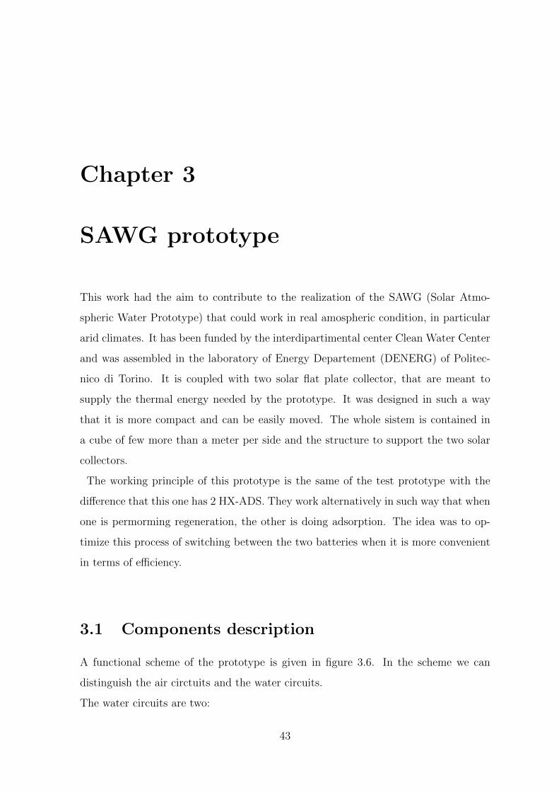
3.1 SAWG 3D . . . . . . . . . . . . . . . . . . . . . . . . . . . . . . . . . . 44
3.2 Adsorption battery . . . . . . . . . . . . . . . . . . . . . . . . . . . . . 45
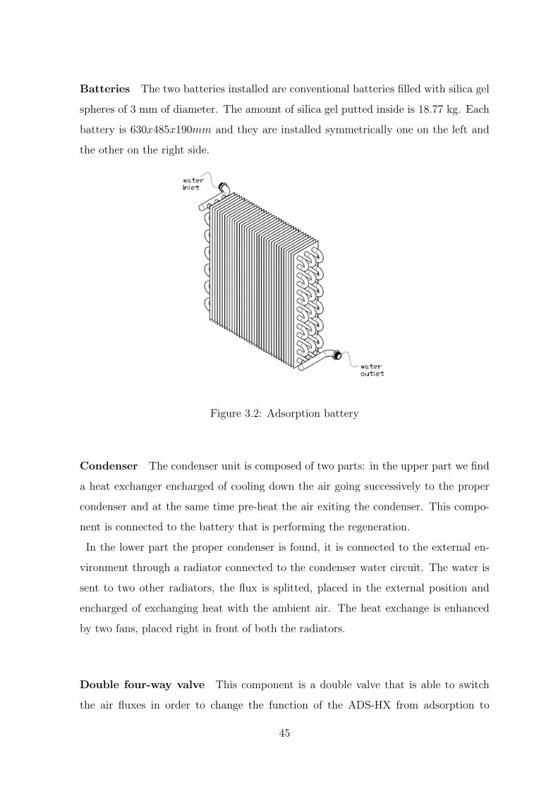
3.3 Condenser + regeneration air circuit . . . . . . . . . . . . . . . . . . . 46
3.4 Double four-way valve before being installed . . . . . . . . . . . . . . . 46
3.5 On the left RIG/ADS fans, on the right condenser circuit fans . . . . . 47
3.6 Functional scheme . . . . . . . . . . . . . . . . . . . . . . . . . . . . . 49
3.7 Assembled prototype . . . . . . . . . . . . . . . . . . . . . . . . . . . . 50
4.1 TRNSYS model scheme . . . . . . . . . . . . . . . . . . . . . . . . . . 56
4.2 Isotherms of adsorption . . . . . . . . . . . . . . . . . . . . . . . . . . . 59
4.3 Isotherms of adsorption in function of absolute humidity . . . . . . . . 60
4.4 Temperature dependence of coefficients used for polynomial approxima-
tion of adsorption isotherms . . . . . . . . . . . . . . . . . . . . . . . . 61
4.5 Volume fraction variation with respect to p/d ratio [35] . . . . . . . . . 66
4.6 TEST 20-Validation . . . . . . . . . . . . . . . . . . . . . . . . . . . . 70
4.7 TEST 22-Validation . . . . . . . . . . . . . . . . . . . . . . . . . . . . 70
4.8 TEST 26-Validation . . . . . . . . . . . . . . . . . . . . . . . . . . . . 71
4.9 TEST 28-Validation . . . . . . . . . . . . . . . . . . . . . . . . . . . . 71
5

4.10 TEST 32-Validation . . . . . . . . . . . . . . . . . . . . . . . . . . . . 72
4.11 TEST 38-Validation . . . . . . . . . . . . . . . . . . . . . . . . . . . . 72
4.12 TEST 23 (fan regulation 30%)-Validation . . . . . . . . . . . . . . . . . 74
4.13 TEST 25 (fan regulation 50%)-Validation . . . . . . . . . . . . . . . . . 74
4.14 TEST 33 (fan regulation 70%)-Validation . . . . . . . . . . . . . . . . . 75
4.15 TEST 17 (fan regulation 90%)-Validation . . . . . . . . . . . . . . . . . 75
5.1 Water content variation . . . . . . . . . . . . . . . . . . . . . . . . . . 77
5.2 HX-ADS air inlet and outlet . . . . . . . . . . . . . . . . . . . . . . . . 77
5.3 Collector variables . . . . . . . . . . . . . . . . . . . . . . . . . . . . . 77
5.4 World climate zones . . . . . . . . . . . . . . . . . . . . . . . . . . . . 79
5.5 Bangkok . . . . . . . . . . . . . . . . . . . . . . . . . . . . . . . . . . . 81
5.6 Bluefields . . . . . . . . . . . . . . . . . . . . . . . . . . . . . . . . . . 82
5.7 Tunisi . . . . . . . . . . . . . . . . . . . . . . . . . . . . . . . . . . . . 83
5.8 Bamako . . . . . . . . . . . . . . . . . . . . . . . . . . . . . . . . . . . 84
5.9 Perth . . . . . . . . . . . . . . . . . . . . . . . . . . . . . . . . . . . . . 85
5.10 Lisbona . . . . . . . . . . . . . . . . . . . . . . . . . . . . . . . . . . . 86
5.11 Torino . . . . . . . . . . . . . . . . . . . . . . . . . . . . . . . . . . . . 87
6
List of Tables
3.1 List of sensors . . . . . . . . . . . . . . . . . . . . . . . . . . . . . . . . 48
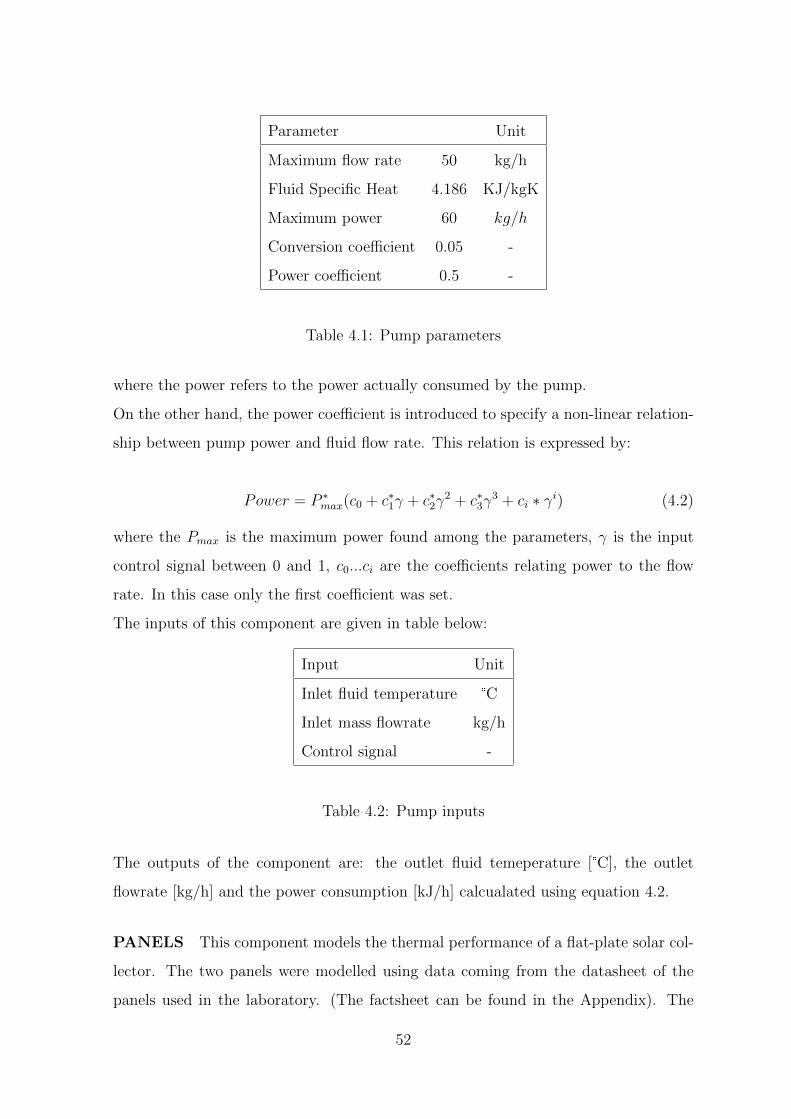
4.1 Pump parameters . . . . . . . . . . . . . . . . . . . . . . . . . . . . . . 52
4.2 Pump inputs . . . . . . . . . . . . . . . . . . . . . . . . . . . . . . . . 52
4.3 Collectors parameters . . . . . . . . . . . . . . . . . . . . . . . . . . . . 53
4.4 Collector inputs . . . . . . . . . . . . . . . . . . . . . . . . . . . . . . . 54
4.5 Regression parameter values . . . . . . . . . . . . . . . . . . . . . . . . 58
4.6 Constant ki values in function of temperature . . . . . . . . . . . . . . 60
4.7 Constant ki values in function of temperature . . . . . . . . . . . . . . 61
5.1 Representative cities for each climate zone . . . . . . . . . . . . . . . . 79
7

Chapter 1
Introduction
Among the Sustainable Developement Goals emitted by the United Nations, we find
”ensure access to water and sanitation for all”. Currently millions of people suffer
from diseases associated with inadequate water supply, sanitation and hygiene. Water
scaricty is generally associated with bad economics or poor infrastructure, this aspect
negatively influences food security, livelihood choices and educational opportunities
for poor families across the world.
To ensure safe access to drinking water and improve sanitation, there needs to be
increased investment and research on freshwater ecosystems and sanitation facilities
on a local level in many developing countries. [1] From the document ”Water for a
sustainable world”, it is possible to find a specific focus on this issue:
”A watersecure world is more than a goal unto itself. It is a critical
and necessary step towards a sustainable future. Progress in each of the
three dimensions of sustainable development (social, economic and envi-
ronmental) is bound by the limits imposed by finite and often vulnerable
water resources and the way these resources are managed to provide ser-
vices and benefits. It is therefore imperative that the role of water is taken
into account, when seeking to address all major sustainable development
objectives.” [2]
Lack of fresh water is mainly diffused in the regions of Northen Africa, Middle East,
and Central and Southern Asia. Providing drinking water to arid areas is generally
8
solved by the following methods [3]:
� transportation of water from other locations;
� desalination of sea water;
� extraction from the atmosphere.
It will be analyzed how extracting water from the atmosphere seems a good solution
to provide water to areas in which transportation of water is too expensive and desali-
nation is not possible due to the lack of saline water resources.
Although water is available in abundance on the earth, there is a severe shortage of
potable water in many countries. Furthermore, non-renewable energy from oil and nat-
ural gas is used to run desalination plants for multi-effect evaporators and a substantial
amount of electric power is needed to run reverse osmosis units. Both technologies
require large amount of energy and quite complex systems. Nevertheless, these meth-
ods are considered as the most diffused for Gulf countries, which suffer from shortage
of water but at the same time benefit from the availability of oil as cheap source of
energy.
Being nowadays CO2 emission an issue of environmental concern, it becomes no longer
possible to rely on technologies strictly based on fossil fuel energy consumption. Also
it is important to emphasise that there are many places where energy is both too
expensive and not accessible, sometimes fresh water is required at locations far from
the energy grid-lines and so requiring a local source of energy.
A brief overview of the cited technologies will be presented in this chapter.
1.1 The probem of access to water resources
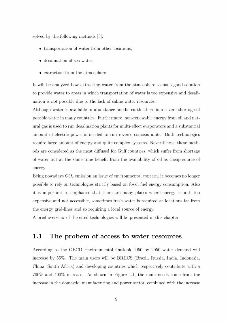
According to the OECD Environmental Outlook 2050 by 2050 water demand will
increase by 55%. The main users will be BRIICS (Brazil, Russia, India, Indonesia,
China, South Africa) and developing countries which respectively contribute with a
700% and 400% increase. As shown in Figure 1.1, the main needs come from the
increase in the domestic, manufacturing and power sector, combined with the increase
9
of population, expected to be up to 33% concentrated in developing countries [2].
Global water demand in 2000 and 2050
Figure 1.1: Global water demand in 2000 and 2050 1
Cities are the areas in which this phenomenon is the most relevant: according to
UNDESA report [4], in 2014 54% of the global popuation lived in cities and by 2050
it will raise up to 65%. Cities impact on the hydrological cycle in two ways:
� extending impenetrable surfaces which does not allow the natural recharge of
groundwater and aggravates flood risks;
� discharging polluting water bodies inside untreated wastewater.
Unfortunately, since much of the water consumed by cities generally comes from out-
side city limits and the pollution generated tends to flow outside too, the impact of
cities on water goes beyond their boundaries. Rapid urbanization, increased indus-
trialization, and improving living standards generally combine to increase the overall
demand for water in cities.
On the other hand, cities, as poles of innovation, provide opportunities for more sus-
tainable use of water, for example treatig used water and enabling it to be used again.
Furthermore, the concentration of people in small areas can reduce the cost of pro-
viding services such as water supply and sanitation. Cities can also connect with
their hinterlands and support the protection of water resources in their surrounding
areas by actively engaging in watershed management or providing PES (Payments for
Ecosystem Services).
Between 1990 and 2012, the number of people in urban areas without access to a
10
drinking water source increased from 111 million to 149 million [5]. Access to drinking
water is more critical where the most rapid urbanization is taking place, sub-Saharan
Africa is one of the most critical areas: in this region, the percentage of pleople who
had the access actually decreased from 42% to 34% [5]. This clearly indicates that ac-
cess to drinking water sources continues to be a major problem in cities in developing
world.
Similar to trends in drinking water, the number of people living in cities without access
to sanitation increased by 40%, from 541 to 754 million, between 1990 and 2012 [5].
Therefore, although sanitation coverage is generally higher in urban areas, because
of rapid urbanization, increasing numbers of urban residents, particularly the poor,
are unable to access improved sanitation. Also, due to higher population densities in
urban areas, the health consequences of poor sanitation can be pervasive. In urban
Cambodia, for example, 54% of the people in the poorest quintile still defecate in the
open, while among the richest 40% of the population, this has gone down to zero.
1.2 State of the art on water extraction techolo-
gies alternative to water harvesting from the
atmosphere
Up to now, the solutions available to satisfy the increasing water demand are: to dig
deeper to access available water resources, mainly groundwater resources, or exploit
innovative solutions such as sea-water desalination [2].
1.2.1 Groundwater resources
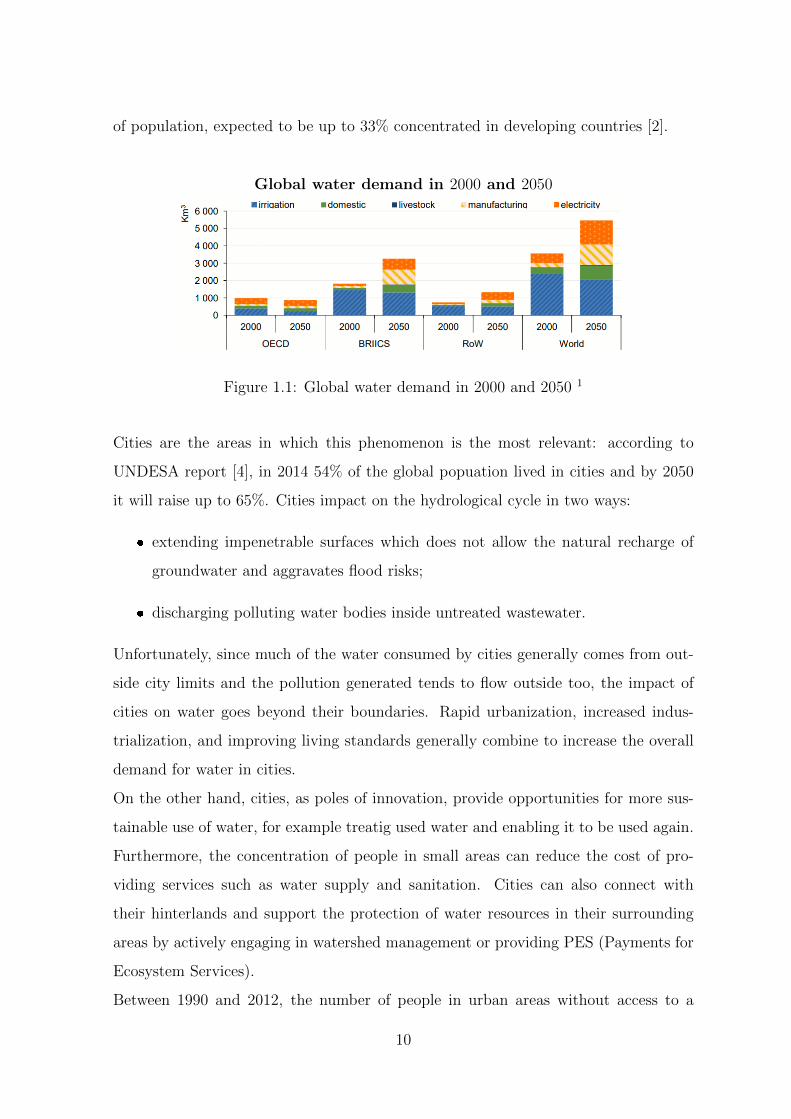
Groundwater is the water found underground in the cracks and spaces in soil, sand and
rock; it is stored in and moves slowly through geologic formations. Groundwater sup-
plies are recharge, by rain and snow melt that flows down into the cracks and crevices
underneath the land’s surface. Water in aquifers, is brought to the surface naturally
through a spring or can be discharged into lakes and streams [6]. Groundwater can
also be extracted through a well drilled into the aquifer, as shown in figure 1.2.
11
Figure 1.2: Groundwater formations [6]
In last decades goundwater has become one of the most important natural resources
for many countries. It happens that groundwater is available in places where there is
no surface water. The main advantages related to the use of groundwater are:
� better quality, being protected from possible pollution and possible infection;
� lower intermittency, since it is less subject to seasonal and perennial fluctuations;
� greater availablabily, being spread over large regions more uniformly than surface
water.
Groundwater is the only source of water supply for some countries in the world (Den-
mark, Malta, Saudi Arabia, etc.) [7]. It represents the substantial part of water re-
sources in the other countries. As an example, in Tunisia, groundwater is 95% of the
country total water resource, in Belgium it is 83%, in the Netherlands, Germany and
Morocco it is 75%, and in most of the European countries it is over 70% of the total
water consumption.
In countries with arid and semiarid climate groundwater is widely used for irrigation.
About one-third of the landmass is irrigated by groundwater. Out of the total irrigated
land in the United States of America, 45% is irrigated by groundwater, 58% in Iran,
67% in Algeria, and in Libya irrigated farming is wholly based on quality groundwater.
High quality groundwater is mainly used in domestic applications and drining water
supply. It results possible to use fresh groundwater for other purposes, such as indus-
try and irrigation, only having an acceptable availability of groundwater reserves. It
has to be sufficient for meeting the available and perspective demand in drinkin water
and by special permission of nature-protecting insitutions.
12

However, intensive groundwater exploitation, its considerable withdrawal under min-
eral deposits mining and different drainage measures, human activities impact on its
quality and resources put in the agenda the problem of groundwater rational use, the
main task being to work out scientific bases and technique of its resources management.
1.2.2 Sea-water desalination
Desalination is a process that involves the separation of saline water in two parts using
different forms of energy: one part is characterized by a low concentration of dissolved
salts (fresh water), the other has a much higher concentration of salts comparing it to
the original water (brine concentrate) [8].
The majority of water desalination processes are divided into two types: phase change
thermal processes and membrane processes. Thermal processes are based on the prin-
ciples of evaporation and condensation, water is brought to evaporation where the salt
is left behind and vapour is taken away and condensed in another heat exchanger to
produce fresh water. Membrane technologies use a relatively permeable membrane
to move either water or salt to induce two zones of different concentrations in order
to produce fresh water. The membrane is a thin film of porous material that allows
water molecules to pass through it and at the same time prevents the passage of larger
molecules (salt, bateria, metals etc.)
There are also some alternative technologies that includes freezing and ion exchange,
but they are less used. All the processes can be both driven by conventional or renew-
able energy sources.
In figure 1.3 we have an overview of the processes mentioned.
The main drowbacks related to this kind of technologies are related to the energy
needed to make them work. Large commercial desalination plants that use fossil fuels
are diffused in most of the countries suffering from water shortages. For instance, a
number of oil-rich countries use fossil fue to supplement the energy for water desali-
nation supply. In contrast people in many other areas of the world have neither the
financial nor oil resources to allow them to develop in a similar manner.
The typical solutions become economically feasible for large plants only. Moreover,
13
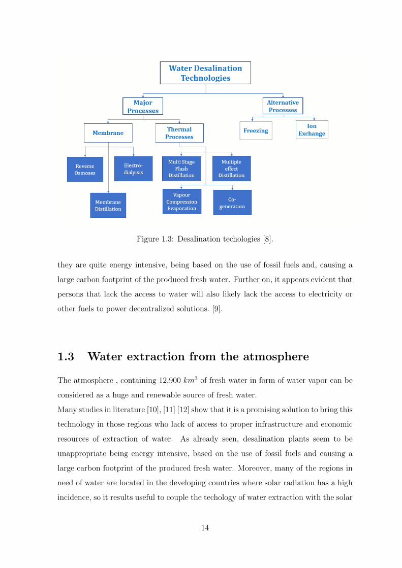
Figure 1.3: Desalination techologies [8].
they are quite energy intensive, being based on the use of fossil fuels and, causing a
large carbon footprint of the produced fresh water. Further on, it appears evident that
persons that lack the access to water will also likely lack the access to electricity or
other fuels to power decentralized solutions. [9].
1.3 Water extraction from the atmosphere
The atmosphere , containing 12,900 km3 of fresh water in form of water vapor can be
considered as a huge and renewable source of fresh water.
Many studies in literature [10], [11] [12] show that it is a promising solution to bring this
technology in those regions who lack of access to proper infrastructure and economic
resources of extraction of water. As already seen, desalination plants seem to be
unappropriate being energy intensive, based on the use of fossil fuels and causing a
large carbon footprint of the produced fresh water. Moreover, many of the regions in
need of water are located in the developing countries where solar radiation has a high
incidence, so it results useful to couple the techology of water extraction with the solar
14
resource.
In literature, we find different way to process air to extract water molecules from the
atmosphere. They are generally based on the phase change from vapor to liquid. The
studies normally investigate different humidification and dehumidification techniques
in which air is used as a medium to carry water in form of vapor.
Among these we find two main valid options [13]:
� the use of a refrigeration cycle based on vapor compression heat pumps or ab-
sorption chillers, to cool the air under dew point to cause condensation of the
vapor content of the air;
� use sorption materials to subtract water vapor contained in the atmosphere.
Afterwards the material is regenerated and the water is condensed at ambiend
temperature.
1.3.1 Refrigeration-based extraction
Concerning the refrigeration-based extraction one of the first technology proposed was
by radiative cooling [14]. It consist of extracting the atmospheric moisture by cooling
making an air stream go under its dew point following contact with a cold surface. In
terms of energy, this process involves a latent heat release close to 2500kJ/kg as well
as sensible heat interaction between the air and the surface. It becomes necessary to
keep the temperature of the surface below the dew point to ensure the condensation
process, and so a heat flux is necessary to compensate the heat exchange of the surface.
Radiative cooling towards the night sky drives natural amospheric moisture ectraction
via the formation of dew on surfaces.
An example of the prototypes used in the experiments is given in figure 1.4:
In general, the process limitations are given by the rate of radiative heat exchange,
the weather and the surface properties. In particular on weather conditions it depends
the ratio of latent and sensible heat exchange between the surface and the air. When
the dew point temperature is much lower than the air temperature most of the ra-
diative cooling is consumed by a sensible heat exchange. On the other hand, if the
difference between ambient air and dew point temperature it is more difficoult to get
15
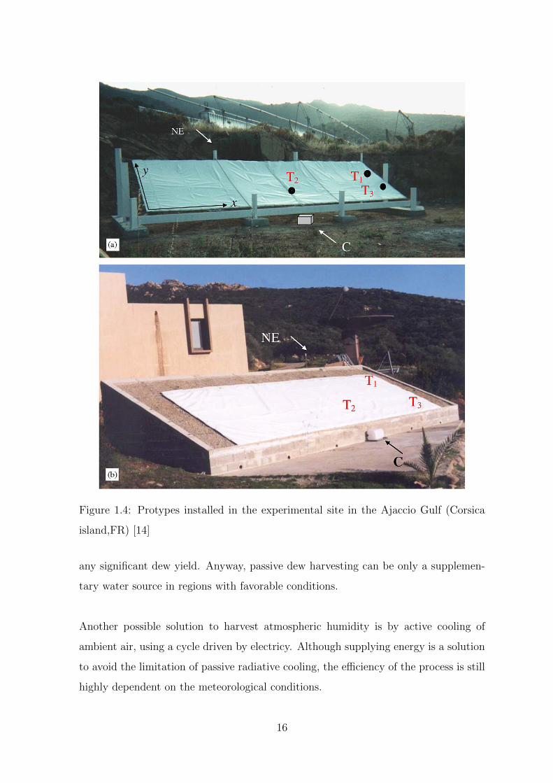
Figure 1.4: Protypes installed in the experimental site in the Ajaccio Gulf (Corsica
island,FR) [14]
any significant dew yield. Anyway, passive dew harvesting can be only a supplemen-
tary water source in regions with favorable conditions.
Another possible solution to harvest atmospheric humidity is by active cooling of
ambient air, using a cycle driven by electricy. Although supplying energy is a solution
to avoid the limitation of passive radiative cooling, the efficiency of the process is still
highly dependent on the meteorological conditions.
16
This type of systems are currently available in the market. Their main application is
for emergency and when relatively small amounts of fresh water are required.
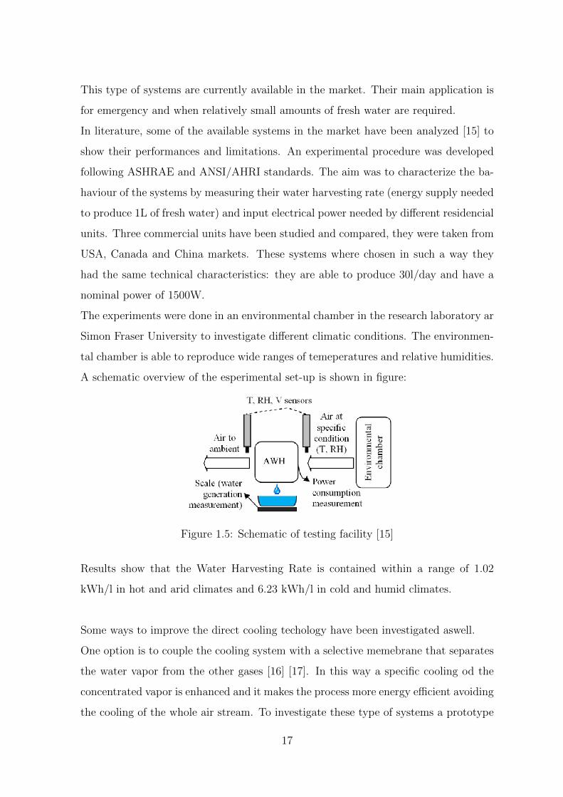
In literature, some of the available systems in the market have been analyzed [15] to
show their performances and limitations. An experimental procedure was developed
following ASHRAE and ANSI/AHRI standards. The aim was to characterize the ba-
haviour of the systems by measuring their water harvesting rate (energy supply needed
to produce 1L of fresh water) and input electrical power needed by different residencial
units. Three commercial units have been studied and compared, they were taken from
USA, Canada and China markets. These systems where chosen in such a way they
had the same technical characteristics: they are able to produce 30l/day and have a
nominal power of 1500W.
The experiments were done in an environmental chamber in the research laboratory ar
Simon Fraser University to investigate different climatic conditions. The environmen-
tal chamber is able to reproduce wide ranges of temeperatures and relative humidities.
A schematic overview of the esperimental set-up is shown in figure:
Figure 1.5: Schematic of testing facility [15]
Results show that the Water Harvesting Rate is contained within a range of 1.02
kWh/l in hot and arid climates and 6.23 kWh/l in cold and humid climates.
Some ways to improve the direct cooling techology have been investigated aswell.
One option is to couple the cooling system with a selective memebrane that separates
the water vapor from the other gases [16] [17]. In this way a specific cooling od the
concentrated vapor is enhanced and it makes the process more energy efficient avoiding
the cooling of the whole air stream. To investigate these type of systems a prototype
17
was realized. It is shown in figure:
Figure 1.6: [16]
The driving force of the process is a partial pressure differece, it is maintained thanks
to a condenser and a vacuum pump. The pump removes all the non-condensable
gases that leak into the system. It was also shown how, introducing a low-pressure,
recirculated sweep stream, the total permeate side pressure can be increased without
compromising the water vapor permeation. The advantages and disasvantages of using
vacuum and sweep stream are investigated and a combination of these two is intro-
duced, in order to obtain an optimal condition for water harvesting. In this way, even
in presence of leakages, it is possible to lower the power requirement of the vacuum
pump.
The technical specifications of the prototype are: a nominal power of 62 kW, a daily
production of water of 9.19m3/day that means 583MJ/m3.
Another option that has been investigated is to couple the direct cooling water har-
vesting with a conventional HVAC system. In this way, it is possible to contemporarly
use the cooled air for refrigeration [18] [19]. In this research, the humid air cooling
process below the dew point to cause the condensation is combined with the air con-
ditioning. A case study is taken into account and compared with a traditional HVAC
system to show the advantages achievable with the improved onee. The case study
takes into account the HVAC system of an existing hotel placed in sub-tropical, arid
18
climate. In this case, the production of water is meant to be used for the building
needs.
A scheme of the integrated plant is shown in figure.
Figure 1.7: Scheme of the Integrated System [18]
Calculation on daily water production and energy consumption of the traditional solu-
tion (TS) and the integrated solution (IS) have been studied. In table below is possible
to get an idea of the scale and the performances of the system:
An index has been introduced to try to estimate the energy performances of this tech-
nology [20]. The index is called MHI (Moisture Harvesting Index). It is calculated
as:
MHI =hfgq∗tot
where:
� hfg is the enthalpy of condensation [kJ/kgw]. It generally varies only slightly for
the range of condensation temperatures found in commercial application, so in
the article it is assumed a constant value equal to 2492 kJ/kgw;
19
Figure 1.8: Scheme of the Integrated System [18]
� q∗tot quantifies the total heat required to be removed from the air for the pro-
duction of 1 kg of liquid water and is calulated as:
q∗tot =ho − hiri − ri
[kJ/kgw]
being ho − hi[kJ/kga] the specific enthalpy difference considering an isobaric
process referred to 1kg of air. Since we are interested in calculating the heat
required for the transformation of water, the difference of enthalphies is divided
by r[kgw/kga] that is the air moisture content. In this way we obtain a quantity
relative to 1kg of water.
The MHI mainly depends on three parameters: the thermodynamic conditions of the
air at the inlet (Ti and ri, where Ti is the ambient air dry bulb temperature at the
inlet) and the condensation temperature To. Being the condensation temperature a
fixed parameter set during the design phase, the MHI only depends on the thermo-
dynamic conditions of the air at the inlet.
In this way, it is possible to draw up different behaviours of MHI: high MHI charac-
terizes warm and very humid ambient conditions, where the requirement for sensible
heat removal is small and the overall efficiency of the process is relatively high. On
the other hand, low MHI is typical of ambient conditions that bring to high demands
for sensible heat removal and low moisture condensation yield.
20
Figure 1.9: Iso-MHI lines plotted on a psychrometric chart for a condensation tem-
perature of [20]
From 1.9, it is possible to have an overview.
Being MHI daily and seasonally variable, it is found that continuous operation of e
device based on Atmosferic Moisture Harvesting by direct cooling is energetically and
economically possible only in specific regions. In particular, the favorable regions are
found to be the tropical ones since they esperience high relative humidity and stable
temperatures through-out the year. For other regions, in order to decrease the energy
requirements it would be preferable to avoid operation of the system when MHI is low,
and so shifting from continuous to non continuous operation. Clearly, there will be
some drowbacks of such intermittent operation mode: smaller water production and
mechanical provlems due to discontinuous operation cycle.
It was possible to observe that refrigeration based techologies have a limitation due
to climatic conditions. In arid regions, due to the low humidity, the dew point tem-
perature is lower than 15 C and even below 0 C in exrtemely dry desert climate. This
condition makes it infeasable in terms of practical implementation with a huge energy
consumption [21]. To supply this high request it would be needed to install a lot of PV
plate, in terms of making the system to be passive, which implies high cost and main-
tenance. Furthermore conventional refrigeration still uses chlorofluorocarbons (CFCs),
which contrivute to global high altitude ozone depletion [22].
21
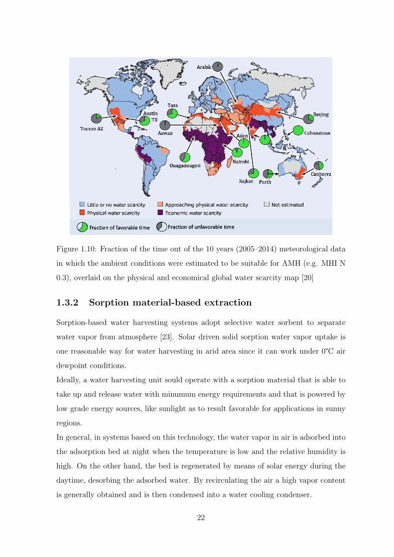
Figure 1.10: Fraction of the time out of the 10 years (2005–2014) meteorological data
in which the ambient conditions were estimated to be suitable for AMH (e.g. MHI N
0.3), overlaid on the physical and economical global water scarcity map [20]
1.3.2 Sorption material-based extraction
Sorption-based water harvesting systems adopt selective water sorbent to separate
water vapor from atmosphere [23]. Solar driven solid sorption water vapor uptake is
one reasonable way for water harvesting in arid area since it can work under 0°C air
dewpoint conditions.
Ideally, a water harvesting unit sould operate with a sorption material that is able to
take up and release water with minumum energy requirements and that is powered by
low grade energy sources, like sunlight as to result favorable for applications in sunny
regions.
In general, in systems based on this technology, the water vapor in air is adsorbed into
the adsorption bed at night when the temperature is low and the relative humidity is
high. On the other hand, the bed is regenerated by means of solar energy during the
daytime, desorbing the adsorbed water. By recirculating the air a high vapor content
is generally obtained and is then condensed into a water cooling condenser.
22
The selection of solid sorbents is a very crucial step for fresh water production based on
sorption. Different material have been investigated in literature to be used as sorption
material. In literature, it is possible to find different studies using: MOF and ACF +
salt combination.
MOFs MOFs(metal-organic framework), have been studied as possible sorbent ma-
terial to couple with this technology. In particular the attention was focused on MOF-
801(Zr6O4(OH)4(fumarate)6) [24]. They reported a device, that uses MOF, able to
harvest 2.8L of water per kg of MOF per day at 20% of RH. It is supplied by noncon-
centrated solar radiation, as to say less than 1000W/m2 requiring no additional power
input. The use of MOFs becomes interesting from the energy consumption poiint of
view since an isotherm with a strong increase in water uptake within a restricted range
of RH is obtained. In this way, we get maximum regeneration with minimal temepra-
ture increase. According to the study, MOF-801 shows suitability for regions such
North Africa, where RH is 20% and also India with RH = 40%, where regeneration
temepratures of 65C were possible. Once water vapor is absorbed into the MOF, solar
energy is used to release the adsorbate. Water is then collected using a condenser that
uses ambient temperature. For this type of application this sorbent material shows
several chemical advantages:
� well-studied water-adsorption behaviour at molecular scale;
� good performances due to aggregation of the water molecules into clusters within
the pores of the MOF;
� stability and possibility of recycling;
� available and low cost.
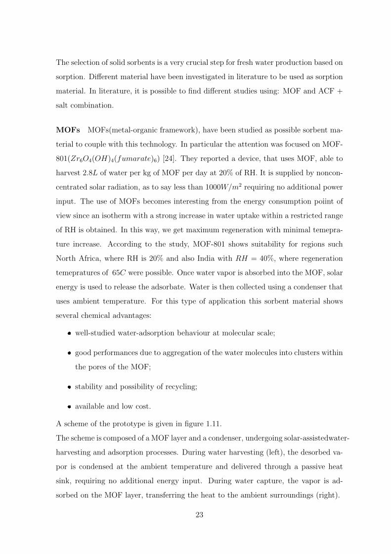
A scheme of the prototype is given in figure 1.11.
The scheme is composed of a MOF layer and a condenser, undergoing solar-assistedwater-
harvesting and adsorption processes. During water harvesting (left), the desorbed va-
por is condensed at the ambient temperature and delivered through a passive heat
sink, requiring no additional energy input. During water capture, the vapor is ad-
sorbed on the MOF layer, transferring the heat to the ambient surroundings (right).
23
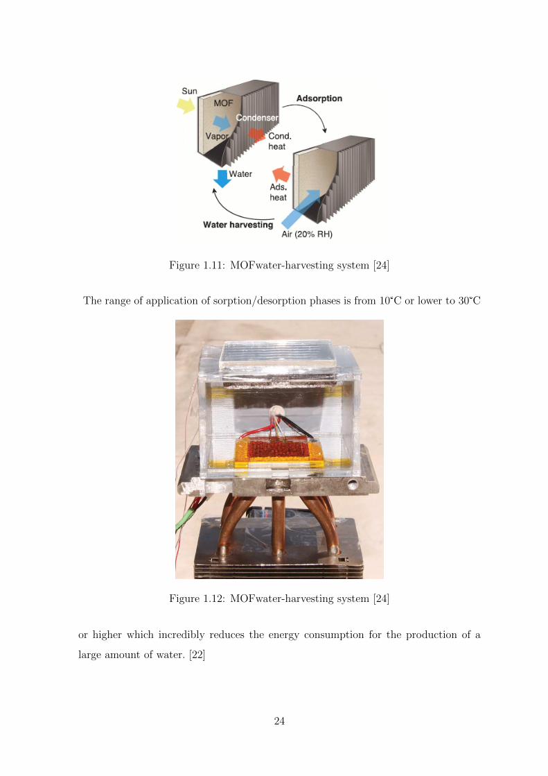
Figure 1.11: MOFwater-harvesting system [24]
The range of application of sorption/desorption phases is from 10°C or lower to 30°C
Figure 1.12: MOFwater-harvesting system [24]
or higher which incredibly reduces the energy consumption for the production of a
large amount of water. [22]
24
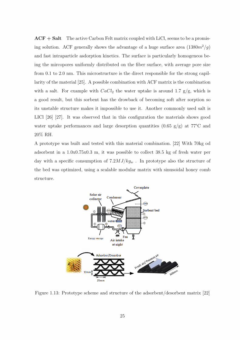
ACF + Salt The active Carbon Felt matrix coupled with LiCl, seems to be a promis-
ing solution. ACF generally shows the advantage of a huge surface area (1380m2/g)
and fast intraparticle asdorption kinetics. The surface is particularly homogeneos be-
ing the mircopores uniformly distributed on the fiber surface, with average pore size
from 0.1 to 2.0 nm. This microstructure is the direct responsible for the strong capil-
larity of the material [25]. A possible combination with ACF matrix is the combination
with a salt. For example with CaCl2 the water uptake is around 1.7 g/g, which is
a good result, but this sorbent has the drowback of becoming soft after sorption so
its unstable structure makes it impossible to use it. Another commonly used salt is
LICl [26] [27]. It was observed that in this configuration the materials shows good
water uptake performances and large desorption quantities (0.65 g/g) at 77°C and
20% RH.
A prototype was built and tested with this material combination. [22] With 70kg od
adsorbent in a 1.0x0.75x0.3 m, it was possible to collect 38.5 kg of fresh water per
day with a specific consumption of 7.2MJ/kgw . In prototype also the structure of
the bed was optimized, using a scalable modular matrix with sinusoidal honey comb
structure.
Figure 1.13: Prototype scheme and structure of the adsorbent/desorbent matrix [22]
25
Chapter 2
Test bench prototype: description
and preliminary data analysis
In the laboratory of Energy department at Politecnico di Torino, two prototypes based
on sorption materials have been assembled. One, the so-called test-prototype was
assembled in order to test its performances; the second one was built in a more compact
way in order to prove its feasability for real applications. This second type wioll be
analyzed in detail in the following chapters.
2.1 Description of the prototype
The test prototype assembled in the laboratory of Energy department of Politecnico
di Torino has the purpose of extracting water from atmospheric air.
The System can work alternating two different phases that are:
� Adsorption: humidity in ambient air is absorbed by t the adsorption material,
that for this prototype is Silica gel;
� Desoprption: adsorbent material is heated up using a low temperature energy
source. In this way, it releases the moisture collected during the adsorption
process.
The hot and humid flux leaving the heat exchanger is then condensed in a dry cooler
at the outdoor ambient temperature. It was connected to a UTA to keep the temper-
26
ature of the whole process constant and experiment different testing temperatures.
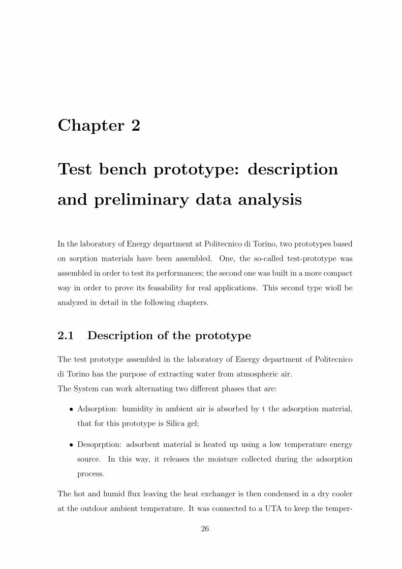
A schmatic of the process is given in figure below:
Figure 2.1: Thermodynamic cycle scheme
It was observed that to have significant production of water during condensation it
is necessary to reach a certain level of humidity and temperature for the air stream
going through the condenser in such a way that the dew point temperature of the
stream is always higher than the ambient air. Generally humid air going through ad-
sorption/desorption processes moves along isenthalpic transformations. This implies
that the variation of moisture content inside the air stream is always linked to a tem-
perature difference. In particular, during adsorption moisture content reduces and air
temperature increases and viceversa for regeneration processes. Being the goal of this
system the water production, it can be observed that through this kind of thermo-
dynamic transformations the amunt of moisture collected is quite poor considering to
have a condensing stream at ambient temperature, for istance at 35°C, like a possible
application temperature could be. In this case, the saturation point corresponds to
about 36.5 gv/kga (point 3 in figure 2.2). Moving on an isenthalpic transformation,
27

in order to reach the points on the saturation line an inlet desorption air at 50°C and
same moisture content of point 3 is needed (point 1). However, a very reduced amount
of moisture will be condensed.
The solution is to perform an isothermal transformation, in such a way that the
Figure 2.2: Thermodynamic cycle
humidity content difference on saturation line between point 2 and 3 is much higher.
In the exaple shown in figure, it would change from gv/kga of the isenthalpic transfor-
mation to more than 40 gv/kga of the isothermal one. To realize such transformation
a system exchanging heat and mass is needed, this is possible in a finned heat ex-
changer filled with adsorption material. The heat for the adsorption is supplied by
water circulation at temperatures of 50-80°C. A fan circulates the air flow through the
HX-ADS in a closed loop, to permit the continuos subtraction of water from sorption
28

material.
After this stage, the air is cooled down in a condenser that is subdivided into two parts.
The first one consists of a heat recovery the reheat the regeneration stream exiting the
component, the second part is the actual condenser that works with external ambient
air.
Going through the techical aspects of the prototype, it is possible to state that it is
able to collect around 2 liters from the treatment of an air volume of 100 m3. The
adsorption system contains about 20.5 kg of silica gel grain with average diameter of
3 mm. The heat is supplied by a circulation of water between 50-80°C produced by
an electric resistance of 1.25kW.
The air flow is moved by a centrifugal fan at variable velocity regulation with a maxi-
mum power consumption of 43W and air flow rate range 0-100 m3/h. All the compo-
nents are connected by a flexible duct.
Figure 2.3: Prototype scheme with sensors
29
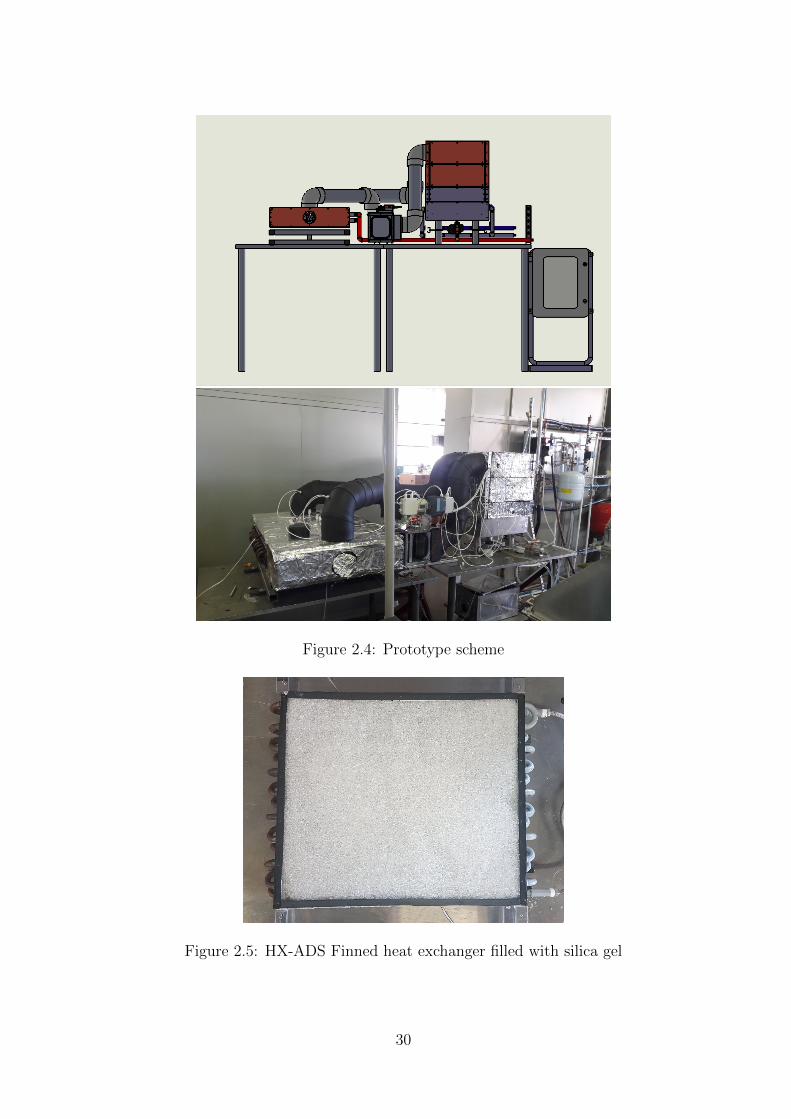
Figure 2.4: Prototype scheme
Figure 2.5: HX-ADS Finned heat exchanger filled with silica gel
30
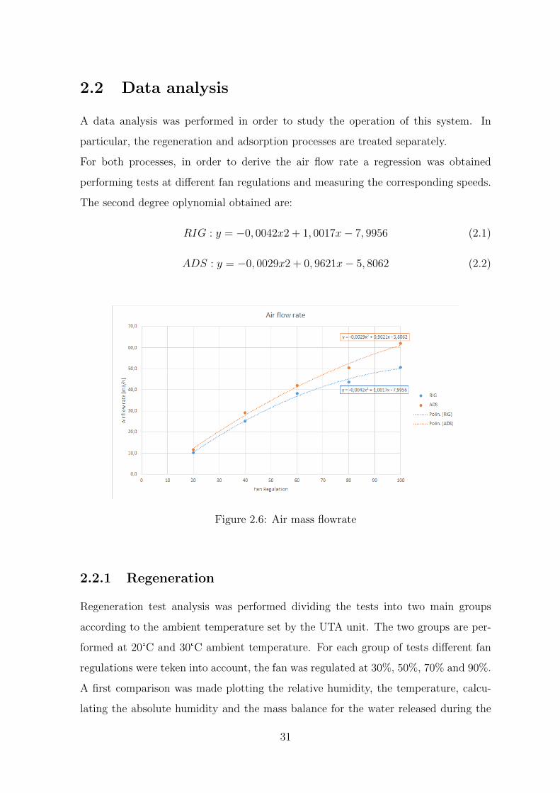
2.2 Data analysis
A data analysis was performed in order to study the operation of this system. In
particular, the regeneration and adsorption processes are treated separately.
For both processes, in order to derive the air flow rate a regression was obtained
performing tests at different fan regulations and measuring the corresponding speeds.
The second degree oplynomial obtained are:
RIG : y = −0, 0042x2 + 1, 0017x− 7, 9956 (2.1)
ADS : y = −0, 0029x2 + 0, 9621x− 5, 8062 (2.2)
Figure 2.6: Air mass flowrate
2.2.1 Regeneration
Regeneration test analysis was performed dividing the tests into two main groups
according to the ambient temperature set by the UTA unit. The two groups are per-
formed at 20°C and 30°C ambient temperature. For each group of tests different fan
regulations were teken into account, the fan was regulated at 30%, 50%, 70% and 90%.
A first comparison was made plotting the relative humidity, the temperature, calcu-
lating the absolute humidity and the mass balance for the water released during the
31
regeneration. Results are shown from figure 2.7 to 2.10.
Relative Humidity It is possible to observe how for both groups of tests, 20 and
30°C, increasing the speed of the fan a faster reduction of relative humidity enetering
in the HX is experienced. This implies that a much smaller difference between Rin
and Rout is found for higher flow rates. The curve of the entering, and consequently
the exiting flow, shows in general a behaviour similar to an exponential curve. As to
say that, in the first hours, the variation is bigger and infact it corresponds to the time
when the adsorption bed still have a high amount of moisture inside. Another remark
can be made considering that the relative humidity exiting the heat exchanger is lower
than the entering one, this is due to the fact that the temperature is increasing during
the transformation. We are moving along the transformation 3-1 of figure 2.2
Temperature The stream temperatures entering and exiting the HX-ADS are al-
most constant, showing a constant difference. It is possible to make a further remark
about a slight increase in temeperature once the curves of relative humidity tend to
stabilize, this correspond to a reduction in the condended water from the air stream.
It is worth to notice that for the tests done at Tamb = 30C, the sensor that measured
the Tin got broken as it dumps continuosly, so we cannot trust the results given by
temperature and conseguently the absolute humidity. This fail in the measure will
have an impact for all the rest of measurements, they are not reliable.
Absolute Humidity The absolute humidity calculated as:
x = 0.622RH · psat(T )
ptot −RH · psat(T )(2.3)
where ptot is the ambient pressure set at 101325 Pa and psat is calculated in function
of T as:
psat = exp( A · TB + T
+ C)
(2.4)
being A=17.438, B=239.78 and C=6.4147.
The curves starting from a large difference tend to come together as the number of
32
hours of the process gets sufficiently high.
Mass balance A further analysis can be made considering the mass balance in the
HX-ADS. On the graph the quantity of water released during the regeneration process
is diplayed. The regenerated mass was calculated in 3 different ways:
� the first one was obtained considering the variation in weight measured by the
load cell:
mri+1 = ml1 −mli+1 (2.5)
being mri the mass released at time i+1, ml1 the mass measured by the load
cell at the beginnig of the test and mli+1 the mass measured by the load cell at
time i+1.
� the second way was obtained calculating the water released at each time step as:
dm = ((ρout(i+ 1) · xout(i+ 1)− ρin(i+ 1) · xin(i+ 1)) ·Q · dt (2.6)
and so the total mass
mri+1 = mri + dm (2.7)
being Q the mass air flow calculated according to the regulation of the fan using
equation 2.1 and dt the time interval between the two measurements. The air
densities in and out are calculated using the ideal gas law at the respective
temperatures.
� the third way used is similar to the second one except that an average density
was used:
dm = (xout(i+ 1)− xin(i+ 1)) · ρave ·Q · dt (2.8)
ρave is calculated in function of an average temperature between the inlet flow
and the outlet flow.
33
Specific Consumption A useful comparison among the different fan regulations,
can be made calculating the specific consumption of the process at each time step.
This is generally used to get an idea about the water produced in relation to the en-
ergy consumed. As we had the chance to see from previous analysis a faster regulation
seems to lead to a better process. This aspect has to deal with the energy consump-
tion associated to each regulation and can be used to find a trade off between the
optimization of the specific conumption and the performances of the process.
The specific consumption is defined as:
e =Pth + Pel−prim
Q(ρoutxout − ρinxin)
[ kWh
kgH2O
](2.9)
at the denomitator all the quantities are referred to the air stream entering and exiting
the regeneration battery.
Pth is the thermal power absorbed by the prototipe from the boiler, it was calculated
as:
Pth = mwcpw(Tin − Tout)prim[kW ]; (2.10)
The electrical power consumed by the fan Pel−prim had to be converted into primary
source of energy before being used in the previous equation. It is firstly calculated
considering the nominal power of the fan Pn and the regulation percentage FR as:
Pel = Pn · FR; (2.11)
and then according to the Autority for electric energy and gas (Autorita per l’energia
elettrica e il gas) with ”Delibera EEN 3/08[2] del 20-03-2008 (GU n. 100 del 29.4.08
- SO n.107)”, the conversion factor from electricity to primary energy is fixed at
0.187∗10−3tep/kWh. Being 1 tep corresponding to 41.860 GJ, the final value is ob-
tained as:
Pel−prim = Pel · 0.187 · 10−6 · 41.860 · 109 (2.12)
Unfortunately, after this analysis it was not possible to compare the different regula-
tions since they showed significantly different behaviours for the two groups of tests.
The specific consumption tends to be very unstable after some hours of test, when xin
and xout converge. It raises very rapidly as we can see for fan70 at 20°C. However the
tendency is to have less consumption for tests at higher fan speeds, this depends on
34
the fact that the electrical energy consumed is very small compared to the thermal
one.
Dew Point Temperature The dew point temperature is a parameter that can be
useful to identify the status of the air stream that has to be consensed. It is defined as
the temperature to which air must be cooled to become saturated with water vapor.
Analitically, the dew point temperature of a generic point in the psychrometric chart
is obtained moving on a transformation with constant absolute humidity up to the
saturation curve.
There exists some relation to calculate it in function of the saturation pressure as:
Tdewpoint =B · (log(psat)− C)
A+ C − log(psat)(2.13)
where psat is calculated as:
psat(ϕ = 1) =xout · pamb
(0.622 + xout) · 1(2.14)
It can be useful to compare it with ambient temperature since it is the temperature at
which the condenser operates to produce the water and so the difference between the
dew point temperature and the ambient temperature will be the driving force of the
process. After the point where the two curves meet it is no more possible to perform
the condensation. It is possible to see how this point is variable from test to test,
generally test at lower temepratures tend to show this meeting point after more time
than tests at higher temperatures, this is why for this particular aspect it may be more
favorable to work in a cooler climate.
2.2.2 Adsorption
Regarding the asdorption process, a less accurate analysis was performed since the tests
where all conducted under similar conditions and the tests showed similar behaviours
between one test and the other. Five tests are reported in figure, plotting air and
water temperatures.
35

Figure 2.7: RH, temperature and absolute humidity for 20°C group of tests
36
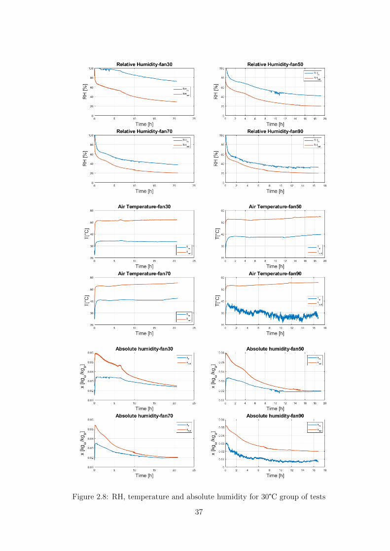
Figure 2.8: RH, temperature and absolute humidity for 30°C group of tests
37
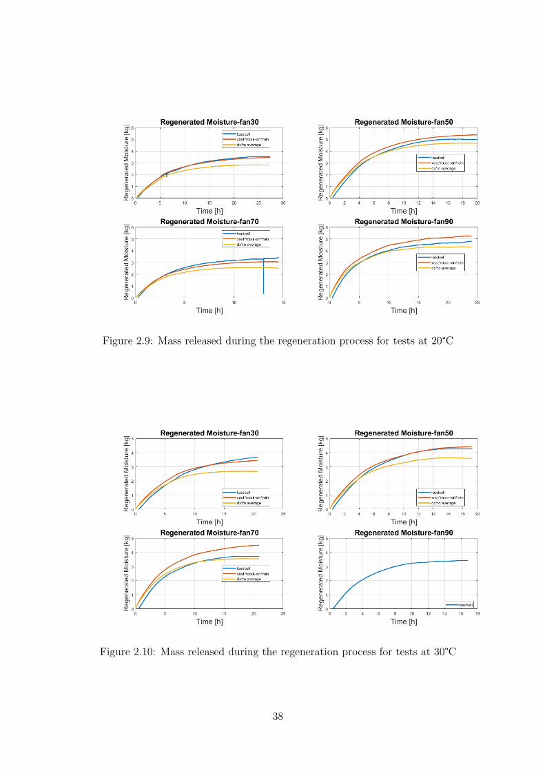
Figure 2.9: Mass released during the regeneration process for tests at 20°C
Figure 2.10: Mass released during the regeneration process for tests at 30°C
38

Figure 2.11: Specific consumption at different fan regulations
39
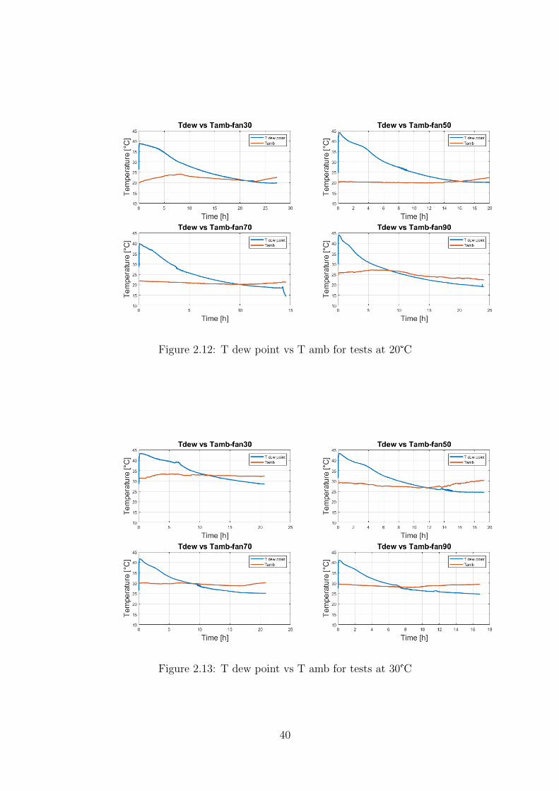
Figure 2.12: T dew point vs T amb for tests at 20°C
Figure 2.13: T dew point vs T amb for tests at 30°C
40

Figure 2.14: TEST 20-ADSORPTION
Figure 2.15: TEST 22-ADSORPTION
Figure 2.16: TEST 26-ADSORPTION
41
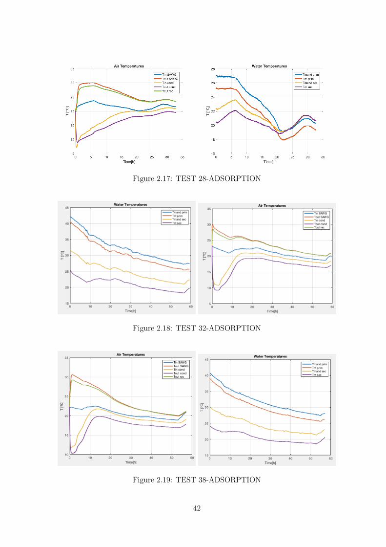
Figure 2.17: TEST 28-ADSORPTION
Figure 2.18: TEST 32-ADSORPTION
Figure 2.19: TEST 38-ADSORPTION
42
Chapter 3
SAWG prototype
This work had the aim to contribute to the realization of the SAWG (Solar Atmo-
spheric Water Prototype) that could work in real amospheric condition, in particular
arid climates. It has been funded by the interdipartimental center Clean Water Center
and was assembled in the laboratory of Energy Departement (DENERG) of Politec-
nico di Torino. It is coupled with two solar flat plate collector, that are meant to
supply the thermal energy needed by the prototype. It was designed in such a way
that it is more compact and can be easily moved. The whole sistem is contained in
a cube of few more than a meter per side and the structure to support the two solar
collectors.
The working principle of this prototype is the same of the test prototype with the
difference that this one has 2 HX-ADS. They work alternatively in such way that when
one is permorming regeneration, the other is doing adsorption. The idea was to op-
timize this process of switching between the two batteries when it is more convenient
in terms of efficiency.
3.1 Components description
A functional scheme of the prototype is given in figure 3.6. In the scheme we can
distinguish the air circtuits and the water circuits.
The water circuits are two:
43
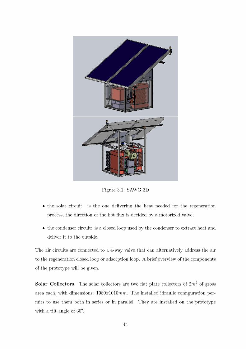
Figure 3.1: SAWG 3D
� the solar circuit: is the one delivering the heat needed for the regeneration
process, the direction of the hot flux is decided by a motorized valve;
� the condenser circuit: is a closed loop used by the condenser to extract heat and
deliver it to the outside.
The air circuits are connected to a 4-way valve that can alternatively address the air
to the regeneration closed loop or adsorption loop. A brief overview of the components
of the prototype will be given.
Solar Collectors The solar collectors are two flat plate collectors of 2m2 of gross
area each, with dimensions: 1980x1010mm. The installed idraulic configuration per-
mits to use them both in series or in parallel. They are installed on the prototype
with a tilt angle of 30°.
44
Batteries The two batteries installed are conventional batteries filled with silica gel
spheres of 3 mm of diameter. The amount of silica gel putted inside is 18.77 kg. Each
battery is 630x485x190mm and they are installed symmetrically one on the left and
the other on the right side.
Figure 3.2: Adsorption battery
Condenser The condenser unit is composed of two parts: in the upper part we find
a heat exchanger encharged of cooling down the air going successively to the proper
condenser and at the same time pre-heat the air exiting the condenser. This compo-
nent is connected to the battery that is performing the regeneration.
In the lower part the proper condenser is found, it is connected to the external en-
vironment through a radiator connected to the condenser water circuit. The water is
sent to two other radiators, the flux is splitted, placed in the external position and
encharged of exchanging heat with the ambient air. The heat exchange is enhanced
by two fans, placed right in front of both the radiators.
Double four-way valve This component is a double valve that is able to switch
the air fluxes in order to change the function of the ADS-HX from adsorption to
45
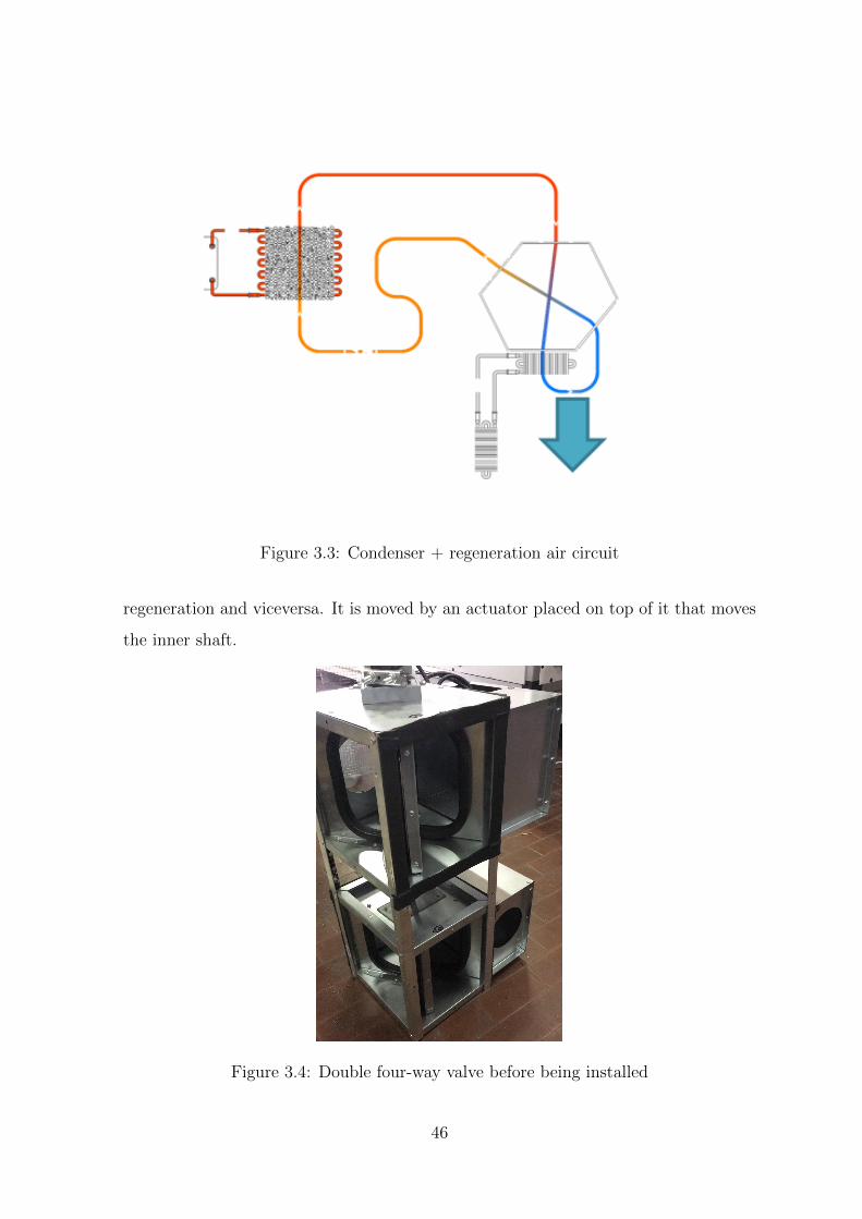
Figure 3.3: Condenser + regeneration air circuit
regeneration and viceversa. It is moved by an actuator placed on top of it that moves
the inner shaft.
Figure 3.4: Double four-way valve before being installed
46
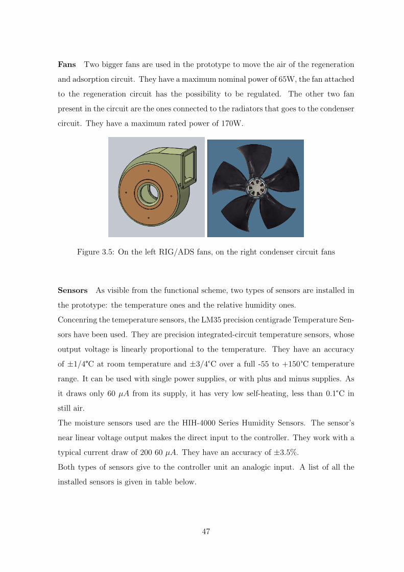
Fans Two bigger fans are used in the prototype to move the air of the regeneration
and adsorption circuit. They have a maximum nominal power of 65W, the fan attached
to the regeneration circuit has the possibility to be regulated. The other two fan
present in the circuit are the ones connected to the radiators that goes to the condenser
circuit. They have a maximum rated power of 170W.
Figure 3.5: On the left RIG/ADS fans, on the right condenser circuit fans
Sensors As visible from the functional scheme, two types of sensors are installed in
the prototype: the temperature ones and the relative humidity ones.
Concenring the temeperature sensors, the LM35 precision centigrade Temperature Sen-
sors have been used. They are precision integrated-circuit temperature sensors, whose
output voltage is linearly proportional to the temperature. They have an accuracy
of ±1/4°C at room temperature and ±3/4°C over a full -55 to +150°C temperature
range. It can be used with single power supplies, or with plus and minus supplies. As
it draws only 60 µA from its supply, it has very low self-heating, less than 0.1°C in
still air.
The moisture sensors used are the HIH-4000 Series Humidity Sensors. The sensor’s
near linear voltage output makes the direct input to the controller. They work with a
typical current draw of 200 60 µA. They have an accuracy of ±3.5%.
Both types of sensors give to the controller unit an analogic input. A list of all the
installed sensors is given in table below.
47

Name Fluid Type Location
TBD1 Air Temperature Inlet HX-ADS-DX
TBD2 Air Temperature Outlet HX-ADS-DX
TBS1 Air Temperature Inlet HX-ADS-SX
TBS2 Air Temperature Outlet HX-ADS-SX
TBD3 Water Temperature Inlet HX-ADS-DX
TBD4 Water Temperature Outlet HX-ADS-DX
TBS3 Water Temperature Inlet HX-ADS-SX
TBS4 Water Temperature Outlet HX-ADS-SX
TC1 Air Temperature Inlet Condenser
TC2 Air Temperature Outlet Condenser
TC3 Water Temperature Inlet Condenser
TC4 Water Temperature Outlet Condenser
TPD Water Temperature Outlet Solar Collector-DX
TPS Water Temperature Outlet Solar Collector-SX
FP Water Mass Flow Solar circuit
RHBD1 Air Relative Humidity Inlet HX-ADS-DX
RHBD2 Air Relative Humidity Outlet HX-ADS-DX
RHBS3 Air Relative Humidity Inlet HX-ADS-SX
RHBS4 Air Relative Humidity Outlet HX-ADS-SX
Table 3.1: List of sensors
Controllino This unit is the controller, it is able to read analogical input coming
from the circuit, elaborate them and send an analogic or digital output to the compo-
nents. A controller logic could be implemented in order to optimize the performances
of the prototype with the variation of external conditions.
Load cell Under one of the two batteries a load cell is placed, with the aim to detect
the weight variation of the HX and so the water edsorbed or released. It is used as a
double check with the RH and T sensors.
48
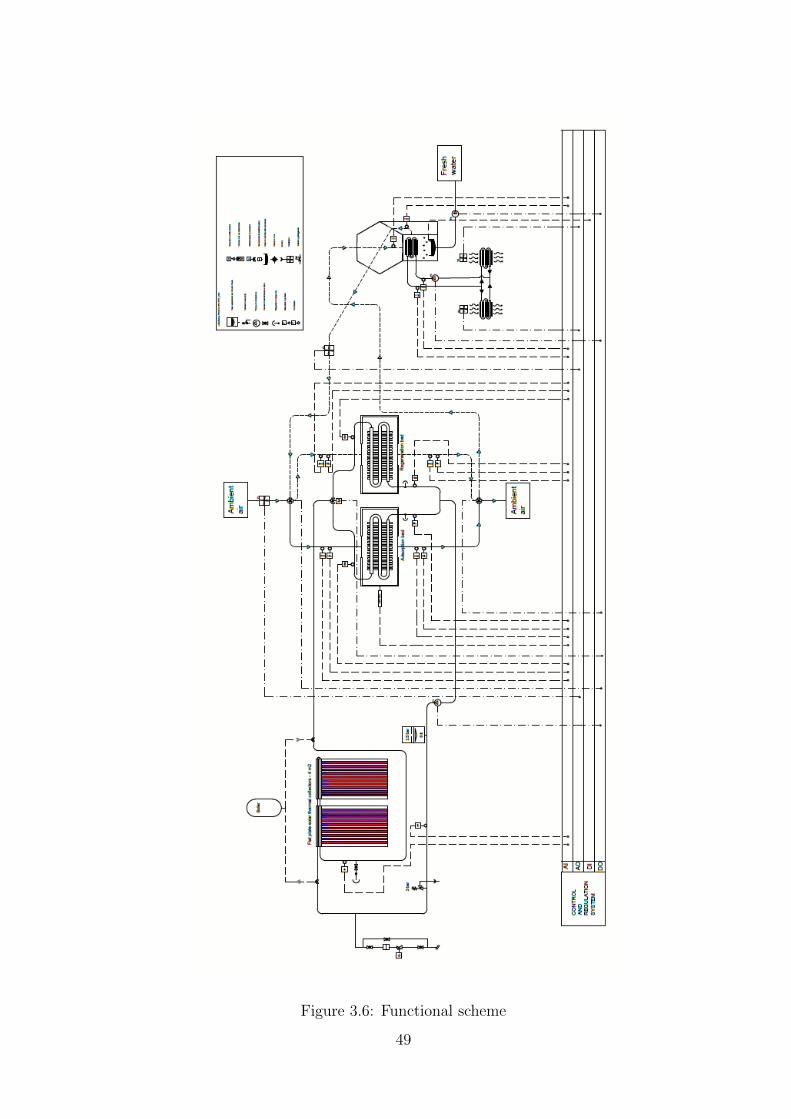
Figure 3.6: Functional scheme
49
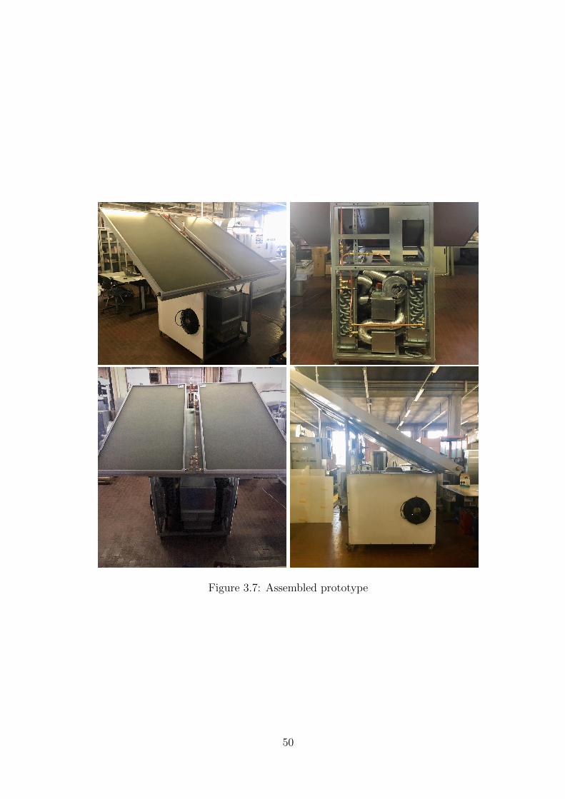
Figure 3.7: Assembled prototype
50
Chapter 4
Model description
4.1 TRNSYS model
In order to investigate the behaviour of the prototype in different climatic conditions,
a simulation model was developed on the software TRNSYS. In this model, many of
the components of the existing prototype are present but some of them are simplified.
For most of them, it already existed a correspondent component inside the software
libraries, but for the adsorption/desorption bed a Matlab model that is explained in
detail in the next paragraph, has been used.
Further on, each block of the model will be analyzed in detail.
PUMP It represents the pump of the solar circuit. This component sets the flow
rate for the rest of the components in the flow loop by multiplyinf the maximum
flowrate by the contol signal. It is connected to a hourly controller that according
to the user regulation is able to turn the pump on or off. As a first approach it was
supposed to have it on between 8am and 6pm assuming to use all the solar energy for
the regeneration processes.
The parameter needed by this component are given in table 4.1
The conversion coefficient mentioned in the table, is referred to the fraction of pump
power that is converted to fluid thermal energy. It can be defined as:
f =Power
mcp(Tout − Tin)(4.1)
51
Parameter Unit
Maximum flow rate 50 kg/h
Fluid Specific Heat 4.186 KJ/kgK
Maximum power 60 kg/h
Conversion coefficient 0.05 -
Power coefficient 0.5 -
Table 4.1: Pump parameters
where the power refers to the power actually consumed by the pump.
On the other hand, the power coefficient is introduced to specify a non-linear relation-
ship between pump power and fluid flow rate. This relation is expressed by:
Power = P ∗max(c0 + c∗1γ + c∗2γ
2 + c∗3γ3 + ci ∗ γi) (4.2)
where the Pmax is the maximum power found among the parameters, γ is the input
control signal between 0 and 1, c0...ci are the coefficients relating power to the flow
rate. In this case only the first coefficient was set.
The inputs of this component are given in table below:
Input Unit
Inlet fluid temperature °C
Inlet mass flowrate kg/h
Control signal -
Table 4.2: Pump inputs
The outputs of the component are: the outlet fluid temeperature [°C], the outlet
flowrate [kg/h] and the power consumption [kJ/h] calcualated using equation 4.2.
PANELS This component models the thermal performance of a flat-plate solar col-
lector. The two panels were modelled using data coming from the datasheet of the
panels used in the laboratory. (The factsheet can be found in the Appendix). The
52

parameters that were implemented for each panel are listed below:
Parameter Unit
Collector area 2 m2
Fluid Specific Heat 4.186 KJ/kgK
Tested flowrate 72 kg/(hrm2)
a0 0.788 -
a1 5.140 W/(m2K)
a2 0.017 W/(m2K2)
Table 4.3: Collectors parameters
The coefficients a0, a1 and a2 comes from the definition of the panel efficiency as:
η = a0 − a1(Tin− Tamb)
G− a2
(Tin− Tamb)2
G(4.3)
being G the incident radiation on the panel.
This component is also linked to the external weather condition file that provides all
the information about ambient condition. Depending on the latitude and the climatic
zone the performance of this component will visibly change. It was possible to load
different files from different locations and check this behaviour. In particular the input
parameter required by the panel TRNSYS model were:
Both the inlet temeperature and inlet flowrate are datas coming from the previous
component, the pump. The collector slope was set 30°, the other parameters changes
during the day and the year.
The output data coming from the panel are: the outlet temperature [°C], the outlet
flowrate [°C] and the useful energy gain [kJ/h]. This last parameter was is calculated
as:
Qu = mcp(Tout − Tin) (4.4)
Since in the prototype 2 panels were installed, this situation was represented connecting
in series these components in the model. This implies that the outlet temperature of
the first one is the inlet temperature of the second one; the same happens for the
flowrate that is the same flowing in the two panels.
53
Parameter Unit
Inlet temperature °C
Inlet flowrate kg/h
Ambient temperature °C
Incident radiation KJ/m2h
Total horizontal radiation KJ/m2h
Ground reflectance -
Incidence angle °
Collector slope °
Table 4.4: Collector inputs
HX-ADS This is the block that recalls the matlab routine that is explained in
detail in section 4.2. It simulates the behaviour of the adsorption/regeneration heat
exchanger filled with silicagel, for each step of the simulation it communicates with
TRNSYS which gives to it 8 inputs and receives 6 outputs.
The inputs are:
� Tw−in is the temperature of the water exiting the panels and entering the heat
exchanger;
� mw is the water flowrate exiting the panels and entering the heat exchanger;
� Tair−in is the temperature of the air entering the heat exchanger. Depending on
what process the system is performing it is equal to the ambient temperature in
case od adsorption, and equal to 40°C if the system is performing regeneration.
The value chosen for regeneration, was obtained from the data analysis on the
test bench prototype, it was seen that the temperature is almost constant in
regeneration phase and for each fan regulation is around the value of 40°C;
� xair−in is the absolute humidity of the air entering the heat exchanger. It is set
equal to the ambient absolute humidity if the system is performing the adsorp-
tion, on the other hand, if the system is doing regeneration it is set to a constant
54
value calculated in function of Tair−in and RH = 0.9. This value corresponds
to the condition of the air entering the heat exchanger after being condensated,
from the experimental data it was not properly constant, but in this case it is
set as constant as a simplification;
� win is the relative water content of the bed [kgw/kgs]. Through the TRNSYS
type 661, the values for each iteration are updated with the final value of the
previous iteration, after setting an initial value. Since the model divides the bed
in 18 layers and has as output 18 values of w for each layer, as a simplification
a mean value among them is used and reassigned in the next iteration;
� Ts−in is the bed temperature. As for the water content, the TRNSYS type 661 is
used so the values are updated with the output values of the previous iteration.
Again, since the model divides the bed in 18 layers and has as output 18 values
of w for each layer, as a simplification a mean value among them is used and
reassigned in the next iteration;
� E is the effectiveness of the heat exchanger, set to 0 for adsorption and 0.5 for
regeneration;
� ma is the air flow rate, set to 200m3/h for adsorption and 45m3/h for regenera-
tion.
Inside the script there are also the inputs neeed by the model to perform the calcula-
tion, but they are not reported nor saved on TRNSYS since they are constant in time
and not needed for the simulation purpose.
The output of the model are:
� Tw−out the temperature of the water exiting the heat exchanger and sent back to
the inlet of the collectors, passing through the pump;
� Tair−out the temperature of the air exiting the heat exchanger;
� xair−out the absolute humidity of the air exiting the heat exchanger;
� wout the relative water content of each layer of the bed;
55

� Ts−out the temperature of each layer of the bed;
� Tdewpoint calculated within the matlab routine in function of the vapor pressure.
This temperature is a fundamental parameter for the regeneration phase, since it
has to be higher than the ambient temperature in order to make the condensation
possible.
The HX-ADS is connected to a series of equation that regulate the switch among the
regeneration and the adsorption processes. The switch is performed considering the
temperature exiting the panels. If it is sufficiently high (Tw > 50C) calculator sets all
the parameters for regeneration. On the other hand, if it Tw < 50C the adsorption is
performed.
Figure 4.1: TRNSYS model scheme
56
4.2 Matlab routine
The model developed on Matlab has the aim of simulating the behaviour of the HX-
ADS, being a heat and mass exchanger.
In adsorption/desorption processes, it exists a strong correlation between mass and
heat transfer due heat of adsorption/desorption that is released or absorbed by packed
bed. This model is focused on the study of the packed bed filled with adsorbent
material, air can flow through the bed lapping sorbent material, and finally adsorption
or desorption phenomena will happen depending by inlet air and sorbent humidity
conditions.
We start with the hypotesis that the bed is composed by pseudospherical particles
of silica gel with an average diameter D=3mm, uniform initial temperature T0 and
humidity content W0. The air stream flows directly through the bed with temperature
and moisture conditions Tairin and xairin respectively. A water vapour mass transfer
happens between air and sorbent particles.
To evaluate the air humidity of the layer near particles, adsorption isotherms of the
material are needed.
The hypotesis of the model are listed below:
1. Physical adsorption and desorption are much faster than other phenomena like
water vapour diffusion through capillary of sorbent material. So in the neigh-
bouring area a local and instantaneous equilibrium condition exists;
2. All the problem can be simplified in one dimension, the only direction analyzed
is along air flow, that will be supposed stationary;
3. Adsorption heat due to “condensation” of water vapour is directly generated in
the pore volumes;
4. The heat is transferred by air forced convection. Heat conduction between sor-
bent material can be neglected in all the direction, in particular along flow di-
rection, hence temperature gradient it’s only function of convection phenomena;
5. Pressure drops are little if compared with total ambient pressure (atmospheric
57
pressure), so hypothesis of constant pressure it’s assumed, and it will be equal
to atmospheric pressure 101325 Pa.
4.2.1 Silica-gel isotherm adsorption curves
In order to model the behaviour of the silica gel, its characteristic isotherm curves
are needed. Itostherm curves permit to aveluate air bulk relative humidity (RH), as a
function of the moisture content of the adsorption material w[kgwater/kgsilica] and the
temperature of silica gel T [°C]. In a previous work, these curves relative to the silica
gel used in the bench prototype were obtained in the laboratory. A sample of adsorp-
tion material graines was weighted changing the variables RH and T. The experiment
were conducted in a climatic room, that permitted to maintain the temperature con-
stant during the experiment.
After collecting the experimental data, it was possible to obtain the following regres-
sion that correlates relative humidity with the water content and the temperature:
RH = S1·T+S2·T 2+S3·w+S4·w ·T+S5·w ·T 2+S6·w2+S7·T ·w2+S8·w3+S9·T 3
(4.5)
In table 4.5, the values of the coefficients of equation 4.5.
S1 -0.00249434
S2 0.0000529632
S3 5.65527
S4 0.0360887
S5 -0.0000713679
S6 -24.9044
S7 -0.112424
S8 54.8088
S9 -0.000000123558
Table 4.5: Regression parameter values
58

Solving the equation between 20°C and 70°C we map some possible functioning con-
dition of adsorption/desorption phenomena.
Figure 4.2: Isotherms of adsorption
We can observe how the temperature affects the behaviour of the bed at the equilib-
rium. For higher temeperatures we get lower water content in the bed, and viceversa
decreasing the temeprature the water content is lower.
In order to simplify the model calculation, it was useful to rewrite the relation of the
relative humidity in terms of absolute humidity. In this way we aim to obtain an
equation with only two variable, being x a quantity that contain both the information
of RH and T. This is possible through equation 4.6
x =0, 622pa
psat(T )·RH− 1
(4.6)
In this way we obtain a relation between absolute humidity and water content and a
new family of curves is obtained.
It becomes now possible to express the absolute humidity in therms of w. A third
order polynomial was needed to ensure the fitting of the curves. The new isotherms
curves and their fittings are shown in figure 4.3.
x∗ = k1 · w3 + k2 · w2 + k3 · w + k4 (4.7)
59
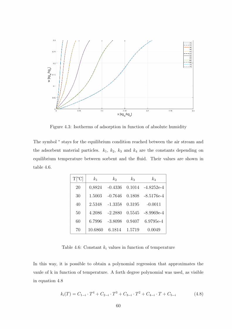
Figure 4.3: Isotherms of adsorption in function of absolute humidity
The symbol ∗ stays for the equilibrium condition reached between the air stream and
the adsorbent material particles. k1, k2, k3 and k4 are the constants depending on
equilibrium temperature between sorbent and the fluid. Their values are shown in
table 4.6.
T[°C] k1 k2 k3 k4
20 0,8824 -0.4336 0.1014 -4.8252e-4
30 1.5003 -0.7646 0.1808 -8.5176e-4
40 2.5348 -1.3358 0.3195 -0.0011
50 4.2086 -2.2880 0.5545 -8.9969e-4
60 6.7996 -3.8098 0.9407 6.9795e-4
70 10.6860 6.1814 1.5719 0.0049
Table 4.6: Constant ki values in function of temperature
In this way, it is possible to obtain a polynomial regression that approximates the
vaule of k in function of temperature. A forth degree polynomial was used, as visible
in equation 4.8
ki(T ) = C1−i · T 4 + C2−i · T 3 + C3−i · T 2 + C4−i · T + C5−i (4.8)
60
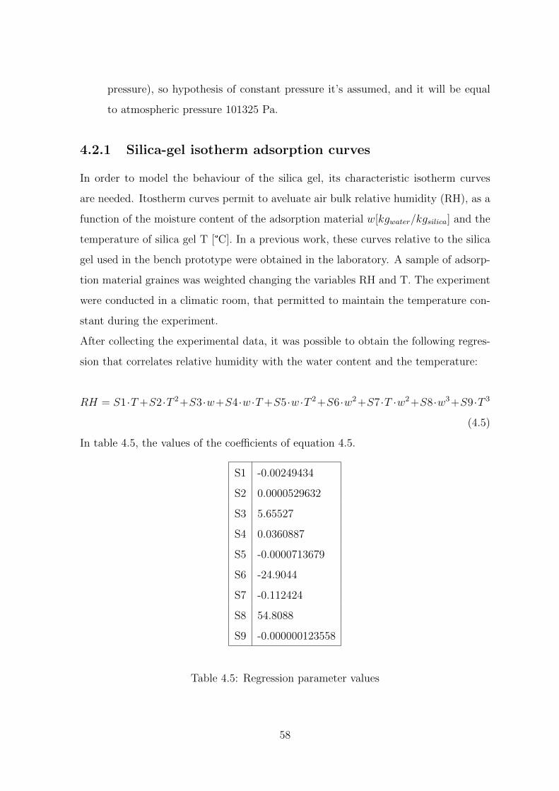
Figure 4.4: Temperature dependence of coefficients used for polynomial approximation
of adsorption isotherms
The coefficients for each k are:
k C1 C2 C3 C4 C5
k1 3.2432e-7 -9.9730e-6 0.0012 -0.0012 0.4491
k2 -2.9056e-7 1.8844e-5 -0.0013 0.0160 -0.3303
k3 1.1852e-7 -1.1206e-5 6.6180e-4 -0.0116 0.1396
k4 1.6940e-9 -1.6466e-7 5.9290e-6 -1.3063e-4 8.0470e-4
Table 4.7: Constant ki values in function of temperature
4.2.2 Model equations
The main equations used in the model can be subdivided in mass balance equations
and thermal balance equations.
The mass balance used in the model is based on the hypotesis that the variation with
respect to time of the water content in the bed is equal to the air stream flow multi-
plied by the difference of absolute huimidity between the input and the output.
Analitically we have:
61
d(msW )
dt= ma(xi − xe) (4.9)
where:
� ms is the mass of the dry silica gel in the bed [kg];
� W is the relative water content in the bed [kgw/kgs];
� ma is the air flow rate [kg/s];
� xi and xe respectively the inlet and outlet absolute humidity of the air [kgw/kga].
Regarding the thermal balance, according to the third hypotesis, heat is released or
absorbed directly in the particle, this phenomenon will obviously cause the increasing
or decreasing of bed temeprature.
For solid phase we have:
hadsMtA(xi − x∗e) = HtAS(Ts − Ta) + (1− ε)ρscsδTsδt
(4.10)
where Ht and Mt are respectively the heat and mass transfer coefficients, hads is the
specific thermal power generated or absorbed during mass transfer process. If mass
transfer goes from air to sorbent material, heat is generated; viceversa it will be
absorbed.
For the gaseous phase no heat is produced, but heat is exchanged through convection
along the flow direction.
CaρaνδTaδx
= hA(Ts − Ta) (4.11)
4.2.3 Model algorithm
The model algorithm is based on an iteration process that calculates the HX-ADS
quantities at each subsequent timestep, imposing a dt = 30s. The bed is subdivided
in 18 monodimentional layers from inlet to outlet and it is assumed that the outlet
condition of layer n is the inlet condition for layer n+ 1.
The algorithm with the calculation of Teq in each layer, that is the temeprature reached
62
by the air in the neightboourhoot of the silica gel particles, assuming the air flow to
reach the equilibrium condition in that area.
Teq = Ts + (Ta − Ts) · e−i (4.12)
where coefficient i is given by:
i =As ·Ht · lv · ρ · ca
(4.13)
Once the equilibrium temperature is obtained, it is possible to obtain the constants of
equation 4.8 so that:
ki = ki(Teq) (4.14)
At this point, the equilibrium water content is calculated in function of xin. Among
the roots of the polynomial, the only real solution is chosen.
k1w3eq + k2w
2eq + k3weq + k4 = xin (4.15)
It becomes now possible to solve the mass balance substituting xin and xout in function
of the water content:
dw
dt=ma
ms
[k1(w3eq − w3) + k2(w
2eq − w2) + k3(weq − w)] (4.16)
The equation cannot be solved analytically so a numerical method was implemented
approximating as:
dw
dt≈ wi+1 − wi
dt=ma
ms
[k1(w3eq − w3
i ) + k2(w2eq − w2
i ) + k3(weq − wi)] (4.17)
xout = xin − [k1(w3eq − w3
i ) + k2(w2eq − w2
i ) + k3(weq − wi)] (4.18)
If the model is simulating the regeneration, the heat exchanged with the water flux is
calculated using equation from the ε−NTU method:
Q =Ecw(Teq − Tw−in)
vl(1− gv)(4.19)
E is the effectiveness, at the denominator there is net volume occupied by the silica
gel, not the void grade. From this, the outlet temperature of water is calculated as:
Tw−out =Q · vl(1− gv)
cw+ Tw−in (4.20)
63
It is now possible to calculate the heat exchanged during the adsorption/regeneration:
Hads = hadsMtAs(xin − xout)−Q (4.21)
For the adsorption the term Q will be 0. From this Ts and Ta are evaluated combining
equations 4.10 and 4.11.
Auxiliary equations In many of the equations appearing in the model there are
intermediate coefficients obtained from experimental regression found in literature.
Heat and mass transfer coefficients are calculated using [28]:
Mt = 1.7GRe−0.42
Ht = 0.6GCaRe−0.42
where G is the specific flow rate expressed in kg/m2s, Re is the Reinolds number and
ca is the specific heat. All the quantities are referred to the bulk air stream.
Adsorption heat od the water vapor is calculated in function of the water content of
the bed [29]:
forw ≤ 0.05 → hads = 3500− 13400w
forw > 0.05 → hads = 2950− 1400w
Air thermophisical properties are calculated using the following equations [30]:
µ = (µaxa + µvxv)(1 +xv − x2v
2.75)
where:
µa = 7.801τ − 0.6266τ 2 + 0.02942τ + 0.00769ρa
µv =40.407
τ 2− 18.473
τ+ 3.853τ + ρv(0.4077− 1.988
τ)
xa =0.622072
0.22072 + w
xv =w
0.622072 + w
τ =T + 273.15
100
Air specific heat is evaluated using [31]
ca = 1.884m+ 1.005(1−m)
64

where:
m =w
1 + w
Silica gel specific heat is evaluated using [28]:
cs = 4.178q + 0.921
Proceeding with the model calculation, the pressure drop in the heat exchanger is
evaluated using the Ergun’s equation. Pressure drop is generally a parameter that
permits to quantify the energy consumption associated with the ventilation.
In a vertical fixed bed, with constant section, the velocity of the stream can be evalu-
ated with the mean velocity being the section smaller enough not to develop the typical
parabolic behaviour. Assuming that the particles have pseudospherical geometry with
average diameter D, pressure drops are function of the bed depth L, vacuum degree ε
and stream velocity.
The particles random distribution is called Random Close Packing, it generates a large
number of vacuum pores between silica gel particles. This volume is identified as vac-
uum degree, defined as the ratio between the volume of vacuum and the total bed
volume. According to Kepler’s conjecture, the minimum ε obtainable is:
εmin = 1− π√3/2≈ 25.95%
In some studies ( [32], [33]) it was demonstrated that for solid spheres pured randomly
like in our case ε cannot exceed 36.6%.
In thix model an equation derived from Darcy relations on pressure drops for packed
bed columns was used. It is valid in the case in which depth dimensions are greater
thatn column diameter [34].
∆P =( 150
Reeff + 1.75
)(L(1− ε)ρaDε3
)( Qρ2a3600S
)(4.22)
In a previous work, it was demonstrated that this model suits with the experimental
results. Another consideration has to be done about the presence of fins that affect
significantly the distribution on the spheres in the bed and consequently their void
degree.
65
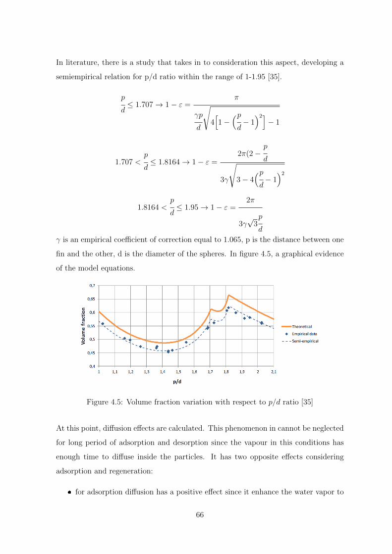
In literature, there is a study that takes in to consideration this aspect, developing a
semiempirical relation for p/d ratio within the range of 1-1.95 [35].
p
d≤ 1.707→ 1− ε =
π
γp
d
√4[1−
(pd− 1)2]− 1
1.707 <p
d≤ 1.8164→ 1− ε =
2π(2−p
d
3γ
√3− 4
(pd− 1)2
1.8164 <p
d≤ 1.95→ 1− ε =
2π
3γ√
3p
d
γ is an empirical coefficient of correction equal to 1.065, p is the distance between one
fin and the other, d is the diameter of the spheres. In figure 4.5, a graphical evidence
of the model equations.
Figure 4.5: Volume fraction variation with respect to p/d ratio [35]
At this point, diffusion effects are calculated. This phenomenon in cannot be neglected
for long period of adsorption and desorption since the vapour in this conditions has
enough time to diffuse inside the particles. It has two opposite effects considering
adsorption and regeneration:
� for adsorption diffusion has a positive effect since it enhance the water vapor to
66
get trapped inside the inner parts of silica gel spheres, decreasing its concentra-
tion on the external surface;
� for regeneration diffusion has a negative effect since it increases the energy nec-
essary for desorption, acting as a resistance on mass transfer phenomenon.
To solve this problem and calculate che water vapor concentration in time through sil-
ica gel particles, an approximation of the convolution integral of Fundamenta Solution
was used.
W (x, t) =
∫S(x− y, t,D) · f(y) · dy
S is the fundamental solution of transient diffusion problem without boundaries and
source equal to zero, its evaluation is given in equation 4.23
S(x, t,D) =e− x2√
4Dt
√4πD
(4.23)
D is the water vapor diffusivity in silica gel pores calculated in [m2/s], it is evaluated
in function of Ts and water vapor concentration, the relation used to evaluate it is
taken from literature [28].
D = D0 · e0.974·Hads·10
−3
Ts+273.15
where D0 is a constant value equal to 1.6 · 10−6m2/s
4.2.4 Model validation
In order to check the model reliability, a comparison with the experimental data was
done both for adsorption and regeneration. This analysis was carried out putting
in the model experimental data as input and check out the outputs obtained. Since
the experimental data available belonged to the test-bench prototype, the model was
adapted to it. Only the battery geometrical dimensions and the silica gel mass con-
tained were adapted being the thermodinamic principle among the two prototypes
exactly equal. The new dimensions used are 650x650x120mm and the mass of silica
gel, automatically calculated considering the new volume and the vacuum degree, is
28.45kg.
67

Adsorption Considering the adsorption process the experimental quantities used as
inputs are:
� the inlet temperature of the air Tin;
� the inlet absolute humidity of the air xin;
� the initial water content of the bed w0;
� the air mass flow pa, calculated considering equation 2.2 with fan regulation
equal to 100% .
The quantity controlled as output were:
� the outlet temperature of the air Tout
� the outlet absolute humidity of the air xout
The results,firstly obtained, showed good approximation for the temperatures but bad
approximations for the absolute humidities.
The reasons for this discrepancy are thought to be mainly related to a bad modelling
of the phenomenon of diffusion. In particular, the kinetics of diffusion seems to have
a strong influence on the overall system. According to Aristov et al , [36], the linear
diffusion models strongly underestimates the water uptake at short times and over-
estimates it for longer times. For the model purpose, that is mainly to quantify the
water collected by the prototype, it can be considered acceptable to only consider the
integral in time of the absolute humidity that according to the mass balance given in
equation 4.9 can be calculated as follows:
w(t) = w0 +ma
ms
(xin − xout)t
Multiplying this quantity for the silica gel mass ms we obtain the water content in kg
inside the bed at time t. It was observed comparing the results obtained by the model
with the experimental ones that in this case the model can be considered reliable,
containing the error within the 10%.
Anyway it was found that inserting in the model a correction factor equal to 3.23 to the
air flow, the results show a way better approximation also for the absolute humidities.
68

In this way the model seems to have a good approximation of the experimental data
and so can be considered reliable for the purpose of the study.
Figures from 4.6 to 4.11 show the comparison of the validation of the absolute humidity
and the temperature without (on the left) and with the correction factor (on the right).
It is possible to observe that the temperatures are not affected by the correction.
69
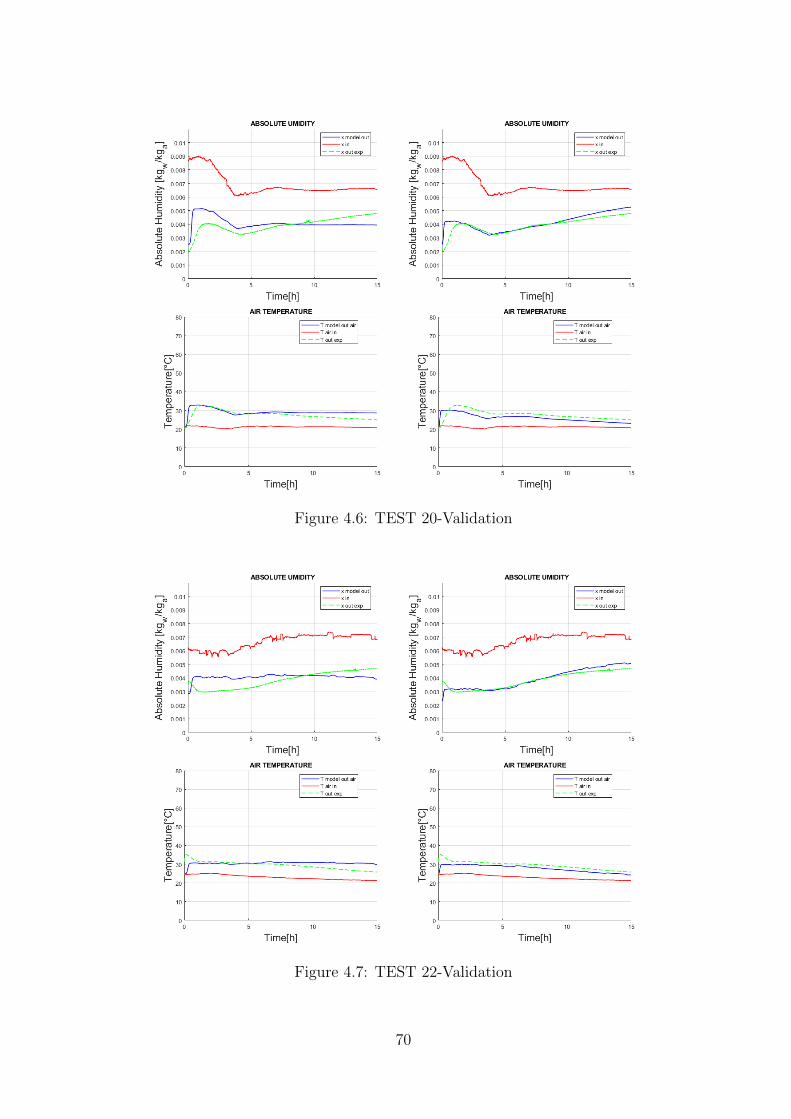
Figure 4.6: TEST 20-Validation
Figure 4.7: TEST 22-Validation
70

Figure 4.8: TEST 26-Validation
Figure 4.9: TEST 28-Validation
71
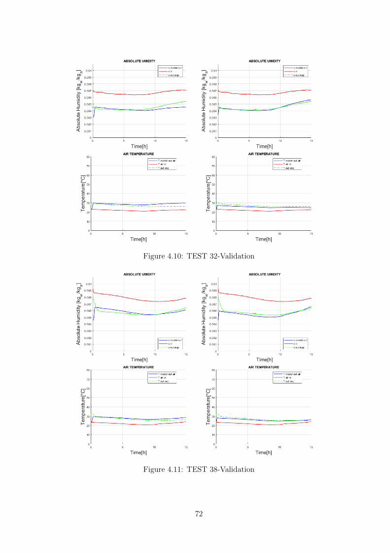
Figure 4.10: TEST 32-Validation
Figure 4.11: TEST 38-Validation
72
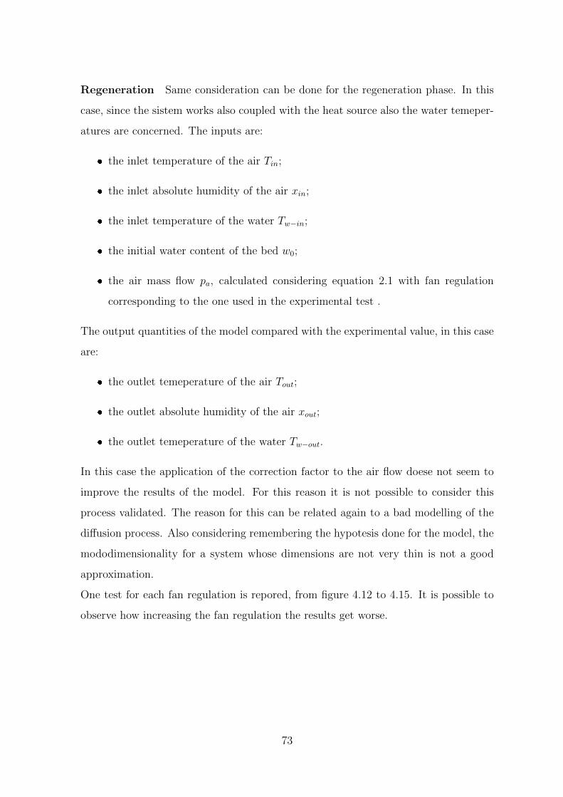
Regeneration Same consideration can be done for the regeneration phase. In this
case, since the sistem works also coupled with the heat source also the water temeper-
atures are concerned. The inputs are:
� the inlet temperature of the air Tin;
� the inlet absolute humidity of the air xin;
� the inlet temperature of the water Tw−in;
� the initial water content of the bed w0;
� the air mass flow pa, calculated considering equation 2.1 with fan regulation
corresponding to the one used in the experimental test .
The output quantities of the model compared with the experimental value, in this case
are:
� the outlet temeperature of the air Tout;
� the outlet absolute humidity of the air xout;
� the outlet temeperature of the water Tw−out.
In this case the application of the correction factor to the air flow doese not seem to
improve the results of the model. For this reason it is not possible to consider this
process validated. The reason for this can be related again to a bad modelling of the
diffusion process. Also considering remembering the hypotesis done for the model, the
mododimensionality for a system whose dimensions are not very thin is not a good
approximation.
One test for each fan regulation is repored, from figure 4.12 to 4.15. It is possible to
observe how increasing the fan regulation the results get worse.
73
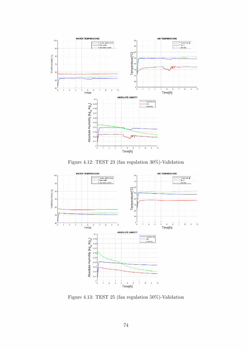
Figure 4.12: TEST 23 (fan regulation 30%)-Validation
Figure 4.13: TEST 25 (fan regulation 50%)-Validation
74
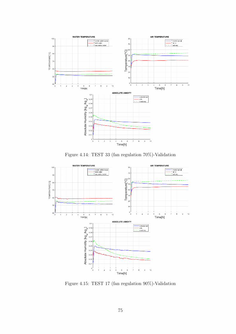
Figure 4.14: TEST 33 (fan regulation 70%)-Validation
Figure 4.15: TEST 17 (fan regulation 90%)-Validation
75
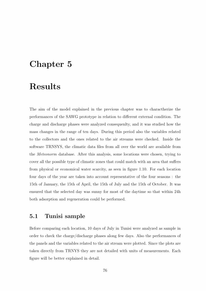
Chapter 5
Results
The aim of the model explained in the previous chapter was to charactherize the
performances of the SAWG prototype in relation to different external condition. The
charge and discharge phases were analyzed consequenlty, and it was studied how the
mass changes in the range of ten days. During this period also the variables related
to the collectors and the ones related to the air streams were checked. Inside the
software TRNSYS, the climatic data files from all over the world are available from
the Meteonorm database. After this analysis, some locations were chosen, trying to
cover all the possible type of climatic zones that could match with an area that suffers
from physical or economical water scarcity, as seen in figure 1.10. For each location
four days of the year are taken into account representative of the four seasons : the
15th of January, the 15th of April, the 15th of July and the 15th of October. It was
ensured that the selected day was sunny for most of the daytime so that within 24h
both adsorption and regeneration could be performed.
5.1 Tunisi sample
Before comparing each location, 10 days of July in Tunisi were analyzed as sample in
order to check the charge/discharge phases along few days. Also the performances of
the panels and the variables related to the air stream were plotted. Since the plots are
taken directly from TRNYS they are not detailed with units of measurements. Each
figure will be better explained in detail.
76
Figure 5.1: Water content variation
Figure 5.2: HX-ADS air inlet and outlet
Figure 5.3: Collector variables
77
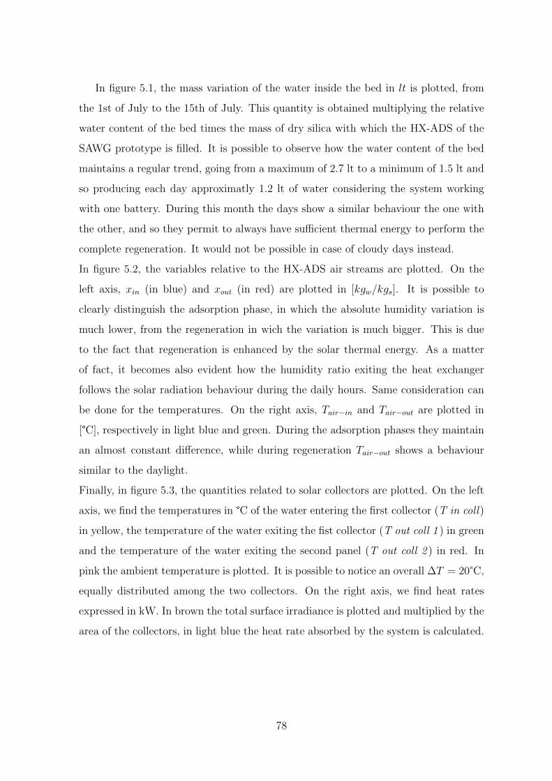
In figure 5.1, the mass variation of the water inside the bed in lt is plotted, from
the 1st of July to the 15th of July. This quantity is obtained multiplying the relative
water content of the bed times the mass of dry silica with which the HX-ADS of the
SAWG prototype is filled. It is possible to observe how the water content of the bed
maintains a regular trend, going from a maximum of 2.7 lt to a minimum of 1.5 lt and
so producing each day approximatly 1.2 lt of water considering the system working
with one battery. During this month the days show a similar behaviour the one with
the other, and so they permit to always have sufficient thermal energy to perform the
complete regeneration. It would not be possible in case of cloudy days instead.
In figure 5.2, the variables relative to the HX-ADS air streams are plotted. On the
left axis, xin (in blue) and xout (in red) are plotted in [kgw/kgs]. It is possible to
clearly distinguish the adsorption phase, in which the absolute humidity variation is
much lower, from the regeneration in wich the variation is much bigger. This is due
to the fact that regeneration is enhanced by the solar thermal energy. As a matter
of fact, it becomes also evident how the humidity ratio exiting the heat exchanger
follows the solar radiation behaviour during the daily hours. Same consideration can
be done for the temperatures. On the right axis, Tair−in and Tair−out are plotted in
[°C], respectively in light blue and green. During the adsorption phases they maintain
an almost constant difference, while during regeneration Tair−out shows a behaviour
similar to the daylight.
Finally, in figure 5.3, the quantities related to solar collectors are plotted. On the left
axis, we find the temperatures in °C of the water entering the first collector (T in coll)
in yellow, the temperature of the water exiting the fist collector (T out coll 1 ) in green
and the temperature of the water exiting the second panel (T out coll 2 ) in red. In
pink the ambient temperature is plotted. It is possible to notice an overall ∆T = 20°C,
equally distributed among the two collectors. On the right axis, we find heat rates
expressed in kW. In brown the total surface irradiance is plotted and multiplied by the
area of the collectors, in light blue the heat rate absorbed by the system is calculated.
78
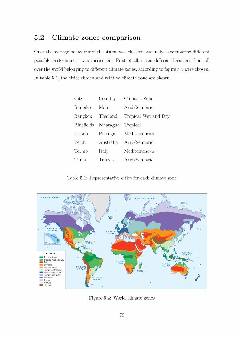
5.2 Climate zones comparison
Once the average behaviour of the sistem was checked, an analysis comparing different
possible performances was carried on. First of all, seven different locations from all
over the world belonging to different climate zones, according to figure 5.4 were chosen.
In table 5.1, the cities chosen and relative climate zone are shown.
City Country Climatic Zone
Bamako Mali Arid/Semiarid
Bangkok Thailand Tropical Wet and Dry
Bluefields Nicarague Tropical
Lisbon Portugal Mediterranean
Perth Australia Arid/Semiarid
Torino Italy Mediterranean
Tunisi Tunisia Arid/Semiarid
Table 5.1: Representative cities for each climate zone
Figure 5.4: World climate zones
79
For each city, a daily simulation was performed. In order to have a complete adsorption
phase the starting time of the calculation is around 6.00 pm when the sun sets, and a
low initial relative water content was set. In this way during the night the adsorption
goes on, it stops when the temperature of the water flowing inside the collectors start
to raise.
Having daily information available, the following quantities were analyzed:
� WP the daily water production [lt];
� CS the specific consumption that is the energy needed to collect 1 lt of water
[kWh/lt]. Only thermal power was considered, since as it was seen in data
analysis of the test bench prototype, electric power is negligible with respect to
the thermal one.
Furthermore the average relative humidity (RH), is plotted too since it helps to un-
derstand the quantity of moisture available in the air during the chosen day. Also the
percentage time of the day in which regeneration or adsorption are performetıd, have
been plotted. This quantity helps to quantify the time needed from each phase.
Grouping the cities in macro-climate zones, the following results are obtained.
Tropical Climate Tropical climates are typically characterized by a non-arid cli-
mate in which temperatures are generally constant and above 18.4°C. This areas are
characherized by only two seasons throughout the year: wet season and dry season.
Sunlight is predominantly intense. Both in Bangkok and Bluefields, the climate is very
humid during the whole year so there are not big variation on the performances of the
prototype during the year. These areas seem to be the most favorable zones for the
application of the prototype. The production of water is never below 1.6 lt/day and
the specific consumption associated to it is never above 6.3 kWh/lt.
80
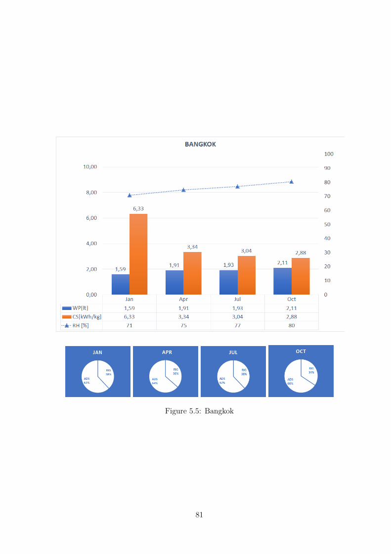
Figure 5.5: Bangkok
81
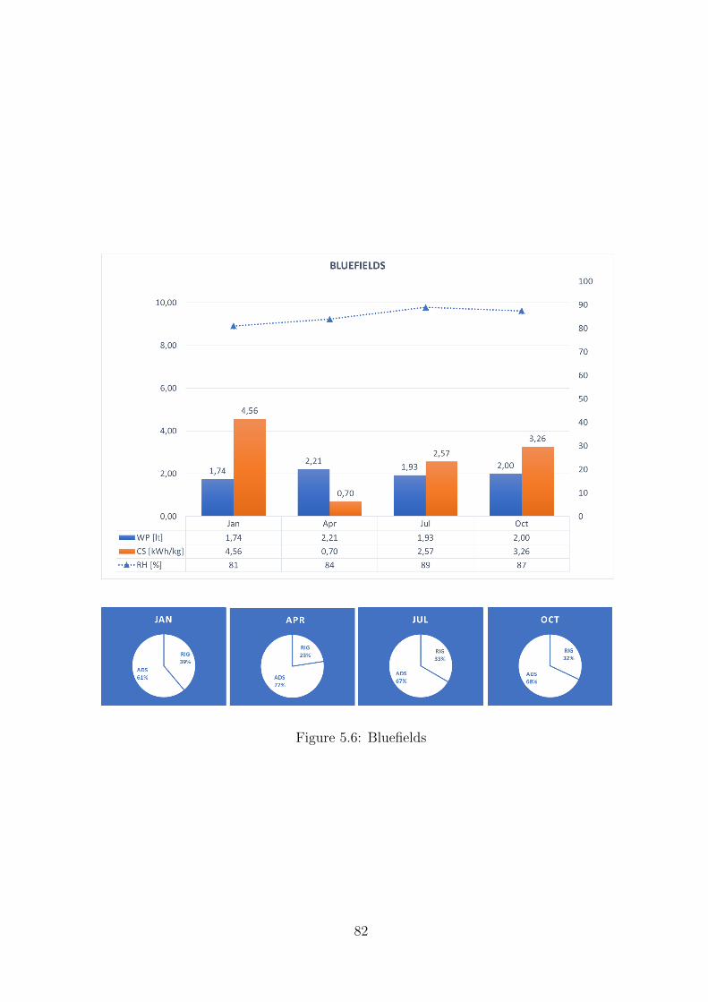
Figure 5.6: Bluefields
82

Arid or semiarid climate This type of climate is classified according to the level of
precipitation being below potential evapotranspiration. So it is characterized by very
dry climate and big variation in terms of air temperature. The sunlight is constantly
high. We can distinguish among two type of seasons: in January and April the relative
humidity is very low and so it the water production (up to 0.48 lt/day). This tipe
of climate is generally quite unfavorable for the application of an atmospheric water
generator. As a consequence of the low amount of water produced, very high specific
consumptions are shown. On the other hand in July and October the situation is
opposite.
Figure 5.7: Tunisi
83
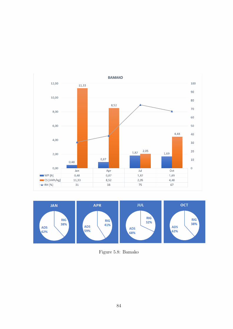
Figure 5.8: Bamako
84
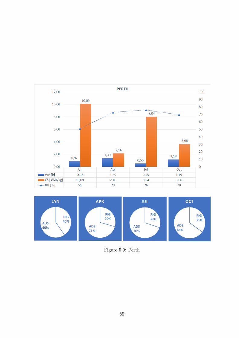
Figure 5.9: Perth
85
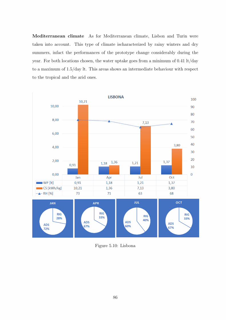
Mediterranean climate As for Mediterranean climate, Lisbon and Turin were
taken into account. This type of climate ischaracterized by rainy winters and dry
summers, infact the performances of the prototype change considerably during the
year. For both locations chosen, the water uptake goes from a minimum of 0.41 lt/day
to a maximum of 1.5/day lt. This areas shows an intermediate behaviour with respect
to the tropical and the arid ones.
Figure 5.10: Lisbona
86
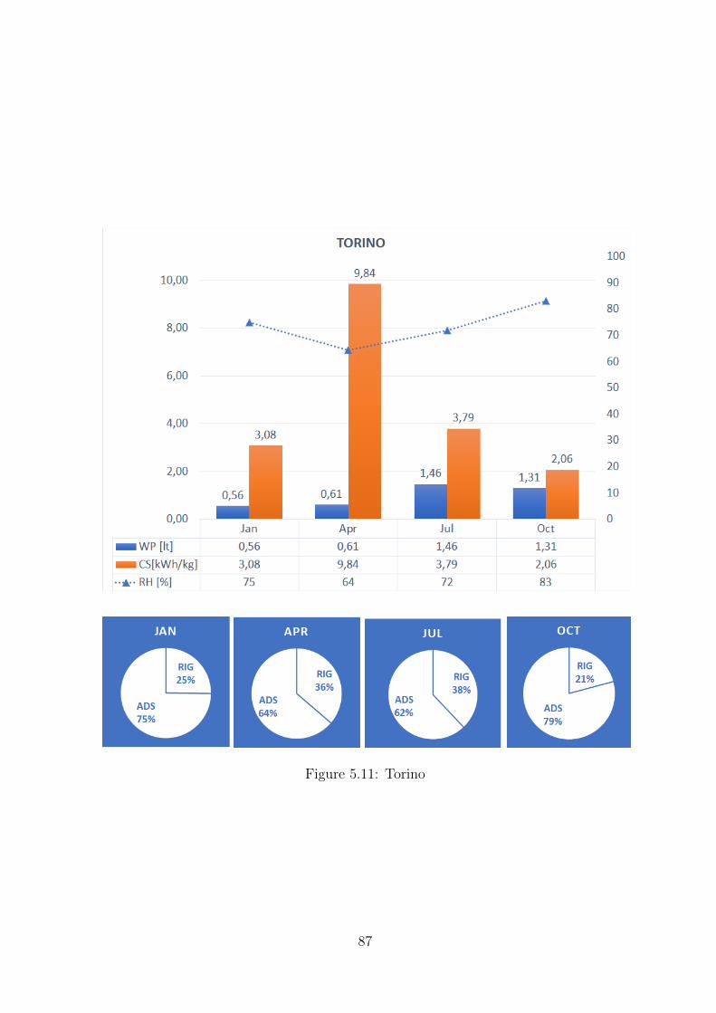
Figure 5.11: Torino
87
Chapter 6
Conclusions
The aim of the work was to optimize the performances of the water generator pro-
totype SAWG. This was possible through a previous data analysis of the test bench
prototype. The results of this first analysis showed tyipical trends of variables during
adsorption and regeneration. The variables on which the focus was concentrated were
mainly the ones that characterize the performances of the HX-ADS. These variables
are the inlet and outlet temperature, relative humidity and absolute humidity of the
air stream. Other variables investigated were the dew point temperature, whose com-
parison with ambient temperature permits to make consideration on the feasability of
condensation; the mass balance, and the specific consumption of the prototype. This
last quantity permits a comparison with the other prototypes already existing, whose
data were taken from literature.
An analysis on how different fan regulations during regeneration affect the specific
consumption was carried on. It was shown that it was not useful to quantify the
energetic performances of the prototype. The electricity consumption related to the
fans is very marginal with respect to the thermal consumption that is the same for
the different fan regulations.
With the data collected it was possible to build the model and adapt it to the proto-
type features.
The results of the model show, as expected, a variation in terms of performances of
the prototype for different climatic zones. It was seen how the water uptake change
from a maximum of 2.2 lt/day in tropical areas, to a minimum of 0.48 lt/day in arid
88

climates. Of course, water production is strictly related to the moisture content of the
external air.
As well as for the specigic consumption, it reaches a peak of 11 kWh/lt in Bamako
(Mali) that corresponds to the lower water production among the simulatios performed.
The minimum value for specific consumption is reached in the simulation carried in
Bluefields (Nicaragua) with a value of 0.7 kWh/lt.
These results were obtained considering only one of the two HX-ADS installed on the
prototype. For sure, increasing the available sorbent material, the water uptake should
increase considerably as well.
As future work, it could be interesting to investigate an optimization of the per-
formances with two batteries implementing a suitable controller logic that aims to
maximize the water production and minimize the consumption.
89
Bibliography
[1] https://www.un.org/sustainable development/water-and-sanitation/.
[2] United Nations. Water for a sustainable world. 2015.
[3] M M Faridb, J R Selmana, and Said Al-hallaj. Solar desalination with a
humidification-dehumidification technique - a comprehensive technical review.
160:167–186, 2004.
[4] UN. Back to our Common Future: Sustainable Development in the 21st Century
(SD21) project. Back to our Common Future: Sustainable Development in the
21st Century (SD21) project, page 39, 2012.
[5] Iv Com. INVESTING IN WATER AND SANITATION: INCREASING AC-
CESS, REDUCING INEQUALITIES Special Report for the Sanitation and Wa-
ter for All (SWA) High-Level Meeting (HLM) 2014 WHO Library Cataloguing-
in-Publication Data. 2014.
[6] https://www.groundwater.org/.
[7] Igor S. Zektser and Lorne G. Everett. 134433E. United Nations Educational,
Scientific and Cultural Organization, 2004.
[8] Mahmoud Shatat, Mark Worall, and Saffa Riffat. Opportunities for solar water
desalination worldwide: Review. Sustainable Cities and Society, 9:67–80, 2013.
[9] A M K El-ghonemy. Fresh water production from / by atmospheric air for arid
regions , using solar energy : Review. 16:6384–6422, 2012.
90
[10] M. Eslami, F. Tajeddini, and N. Etaati. Thermal analysis and optimization of a
system for water harvesting from humid air using thermoelectric coolers. Energy
Conversion and Management, 174(April):417–429, 2018.
[11] Onur Ozkan, Enakshi D Wikramanayake, and Vaibhav Bahadur. Modeling hu-
mid air condensation in waste natural gas-powered atmospheric water harvesting
systems. Applied Thermal Engineering, 118:224–232, 2017.
[12] Bathina Chaitanya, Vaibhav Bahadur, Ajay D. Thakur, and Rishi Raj. Biomass-
gasification-based atmospheric water harvesting in India. Energy, 165:610–621,
2018.
[13] Vincenzo Gentile, Marco Simonetti, Pietro Finocchiaro, and Gian Vincenzo Fra-
castoro. Water production from the atmosphere in arid climates using low grade
solar heat.
[14] M Muselli, D Beysens, and I Milimouk. A comparative study of two large radiative
dew water condensers. 64:54–76, 2006.
[15] Farshid Bagheri. Performance investigation of atmospheric water harvesting sys-
tems. Water Resources and Industry, 20(August):23–28, 2018.
[16] D. Bergmair, S. J. Metz, H. C. De Lange, and A. A. van Steenhoven. System anal-
ysis of membrane facilitated water generation from air humidity. Desalination,
2014.
[17] D Bergmair, S J Metz, H. C. De Lange, and A. A. Van Steenhoven. A low pres-
sure recirculated sweep stream for energy efficient membrane facilitated humidity
harvesting. Separation and Purification Technology, 150:112–118, 2015.
[18] A Magrini, L Cattani, M Cartesegna, and L Magnani. Production of water from
the air: The environmental sustainability of air-conditioning systems through a
more intelligent use of resources. The advantages of an integrated system. In
Energy Procedia, volume 78, pages 1153–1158. Elsevier B.V., 2015.
91
[19] Anna Magrini, Lucia Cattani, Marco Cartesegna, and Lorenza Magnani. Water
production from air conditioning systems: Some evaluations about a sustainable
use of resources. Sustainability (Switzerland), 9(8), 2017.
[20] Ben Gido, Eran Friedler, and David M Broday. Assessment of atmospheric mois-
ture harvesting by direct cooling. Atmospheric Research, 182:156–162, 2016.
[21] Nasrin Fathollahzadeh Attar, Keivan Khalili, Javad Behmanesh, and Neda Khan-
mohammadi. On the reliability of soft computing methods in the estimation of
dew point temperature : The case of arid regions of Iran. Computers and Elec-
tronics in Agriculture, 153(August):334–346, 2018.
[22] J. Y. Wang, R. Z. Wang, Y D Tu, and L W Wang. Universal scalable sorption-
based atmosphere water harvesting. Energy, 165:387–395, 2018.
[23] J. G. Ji, R. Z. Wang, and L. X. Li. New composite adsorbent for solar-driven fresh
water production from the atmosphere. Desalination, 212(1-3):176–182, 2007.
[24] Hyunho Kim, Sungwoo Yang, Sameer R Rao, Shankar Narayanan, Eugene A
Kapustin, Hiroyasu Furukawa, Ari S Umans, Omar M Yaghi, and Evelyn N Wang.
Water harvesting from air with metal-organic frameworks powered by natural
sunlight. 434(April):430–434, 2017.
[25] J. Y. Wang, J Y Liu, R. Z. Wang, and L W Wang. Experimental research
of composite solid sorbents for fresh water production driven by solar energy.
Applied Thermal Engineering, 121:941–950, 2017.
[26] N Yu, R Z Wang, Z S Lu, and L W Wang. Development and characterization of
silica gel – LiCl composite sorbents for thermal energy storage. 111:73–84, 2014.
[27] Duc Thuan, Aqdas Nida, Kim Choon, and Kian Jon. Water vapor permeation
and dehumidi fi cation performance of poly ( vinyl alcohol )/ lithium chloride
composite membranes. Journal of Membrane Science, 498:254–262, 2016.
[28] A A Pesaran, A F Mills Seri, and Solar Energy. Moisture Transport in Silica Gel
Packed Beds. 1986.
92
[29] X J Zhang, Y J Dai, and R Z Wang. A simulation study of heat and mass transfer
in a honeycombed rotary desiccant dehumidifier. 23:989–1003, 2003.
[30] J. Niu and L Zhang. Performance comparisons of desiccant wheels for air dehu-
midification and enthalpy recovery. Applied Thermal Engineering, 23:1347–1367,
2002.
[31] P. Ballany. Refrigeration and Air conditioning. 6th editio, 1983.
[32] Macro-encapsulated P C M F O R Dehumidification. HEAT AND MASS
TRANSFER IN A COMPOSITE BED OF SILICA GEL AND MACRO-
ENCAPSULATED PCM FOR 1 Introduction. (March 2016).
[33] P. Krishna, D. Pandey, and U.C. Cardiff. Close packed structure. International
Union of Crystallography, 2001.
[34] E. Sabri. Fluid flow through packed columns. Chemical Engineer Progress, 48,
1952.
[35] L. Pistocchini, S. Garrone, and M. Motta. Fluid dynamics optimization of a
novel isothermal adsorption dehumidification system for solar driven applications.
Energy Procedia, 2014.
[36] Yuri I Aristov, Mikhail M Tokarev, Angelo Freni, Ivan S Glaznev, and Giovanni
Restuccia. Kinetics of water adsorption on silica Fuji Davison RD. 1387:65–71,
2006.
93
Copyright © 2022 FDOKUMEN