POLITECNICO DI TORINO Master’s Degree in Civil Engineering

Master’s Degree Thesis

Study of a lightweight structure in the mountains with two different

materials through the Building Information Modelling

Tutor

Prof. Anna Osello

Co-Tutor

Prof Gabriele Bertagnoli

Candidate

Matthias Kather

1

2

Abstract

The building of high alpine environment facilities is certainly a current topic in a society that has seen

in recent years a rapid increase in mountain tourism; in modern times, many interesting different

types of new solutions are found and applied for these constructions whose priorities are, for the

conditions they are built in, lightness, high resistance, high thermal insulation and also aesthetical

fitting with the surrounding environment; for these purposes, the in most cases best satisfying material

is wood, which can have different applications and come in different forms; one of them is the

Structural Insulated Panel (SIP).

SIPs are, as the name suggests, panels that can have a structural function in a building and, if wood

based, their composition consists in two timber sheets and an insulating core. They arise as a

composite material potentially able to provide with excellent thermal performances and at the same

time additional stiffness to strengthen the whole structure and possibly decrease, or in some cases

also completely replace the presence of frame elements. In recent years, innovative types of SIPs with

various sorts of wood and different thicknesses of the layers have been developed in order to try to

further improve their performances, but on which, due to their young age, not much is known.

Especially in Italy, where timber framing and crosslam panels are the most common wood

construction systems, little information is present in literature about SIPs and their structural

behaviour.

The current thesis aims to do a research about two different Structural Insulated Panel types in order

to collect as much information possible about them and then create an accurate digital model of a

high mountain building, more precisely a bivouac, employing those panels.

To reach this goal, Building Information Modelling methodology and its software have been used,

which have proven to be a very useful tool for the collection of high amounts of intelligent data in

one or more programs and then creation of digital models reproducing real-life products.

The building modelled in this thesis in not an existing bivouac but a project, present currently only in

the form of drawings which were made and handed to me by the Leap Factory company.

3

Table of contents:

Introduction……………………………………………………………………………………...….6

Chapter 1: General introduction to bivouacs and BIM, territorial and structural framework of

the case study……………………………………………………………………………….………..8

1.1 Historical background of bivouacs……………………………………………………….….8

1.2 State of Art………………………………………………………………………...……….11

1.2.1 Transportation………………..…………………………………………...………...11

1.2.2 Foundation and structure………………………………………………...……….....12

1.2.3 Claddings and openings………………………………………………...…………..13

1.2.4 Spatial organization and technological aspect………………………………………13

1.3 Brief introduction to Building Information Modelling……………………………………..14

1.3.1 Background…………………………………………………………...…………….14

1.3.2 General information …………………………………………………...…………...15

1.3.3 Interoperability…………………………………………………………...…………18

1.3.4 BIM today……………………………………………………………...…………...18

1.4 The case study……………………………………………………………...………………20

1.4.1 Structural framework……………………………………………...………………..21

1.4.2 Setting of the structure………………………………………………………………23

Chapter 2 2D BIM: description of the structural panels and definition of the loads on the

structure……………………………………………………………………………………………24

2.1 What are SIPs?......................................................................................................................24

2.1.1 Benefits and drawbacks……………………………………………………………..25

2.2 The KINGSPAN system……………………………………………………………...26

2.2.1 Mechanical properties………………………………………………………………28

2.2.1 Thermal performance……………………………………………………………….30

2.2.3 Vapour diffusion and condensation risk…………………………………………….32

2.2.4 Connections………………………………………………………………………...35

2.2.5 Costs………………………………………………………………………………..38

2.3 The Panelo system……………………………………………………...…………………..38

2.3.1 Mechanical properties………………………………………………………………39

2.3.2 Thermal performance……………………………………………………………….42

2.3.3 Vapour diffusion and condensation risk…………………………………………….44

4

2.3.4 Connections…………………………………………………………...……………45

2.3.5 Costs………………………………………………………………...……………...47

2.4 Initial comparison………………………………………………………………..………...48

2.5 Definition of the loads on the structure……………………………………………………..49

2.5.1 Wind………………………………………………………………………………..49

2.5.2 Snow………………………………………………………………...……………...53

2.5.3 Temperature………………………………………………………………...………54

Chapter 3 Creation of the 3D models and software interoperability…………………………….58

3.1 The initial steps: Revit, Robot and SAP2000……………………………………………….58

3.2 The Dlubal structural model………………………………………………………………..60

3.2.1 The panel……………………………………………………………………………60

3.2.2 The geometry……………………………………………………………………….64

3.2.2.1 Structure with Kingspan TEK Panels………………………………………..64

3.2.2.2 Structure with Kingspan Panelo Panels…………………...…………………69

3.2.3 The panel connections………………………………………………………………71

3.2.3.1 Kingspan Panels…………………………………………………...………...72

3.2.3.2 Panelo Panels……………………………………………………...………...77

3.2.4 The frame connections………………………………………………………….......78

3.2.5 Application of the loads………………………………………………………….….84

3.2.5.1 Snow loads…………………………………………………………...……...84

3.2.5.2 Wind loads………………………………………………………...………...85

3.2.5.3 Temperature……………………………………………………...………….86

3.2.5.4 Limit States combinations……………………………………...…………....87

3.3 The Revit model……………………………………………………………………………90

3.3.1 The panel……………………………………………………………………………90

3.3.2 The spline connections……………………………………………………………...92

3.3.3 Final Geometry……………………………………………………………………..94

3.4 Interoperability……………………………………………………………………………..97

Chapter 4 Results: Structural analysis, thermal performance, interstitial condensation and

costs………………………………………………………………………………………………..100

4.1 Structural Analysis………………………………………………………………………..100

4.1.1 ULS………………………………………………………………………………..100

4.1.1.1 Kingspan structural model…………………………………………………100

4.1.1.2 Dlubal structural model…………………………………………………….104

5

4.1.1.3 The problem of the singularities……………………………………………108

4.1.2 SLS………………………………………………………………………………..108

4.1.2.1 Kingspan structural model…………………………………………………108

4.1.2.2 Panelo structural model…………………………………………………….112

4.2 Thermal performance……………………………………………………………………..114

4.3 Surface condensation……………………………………………………………………..115

4.4 Costs……………………………………………………………………………………...121

4.5 Final comparison……………………………………………….…………………………122

Conclusion and future works…………………………………………………………………….124

6

Introduction

Extreme environments have always been, throughout the history of humankind, a symbol of challenge

and exploration, which eventually led, in some cases, to new discoveries and improvements of the

society. In the case of building engineering it’s no different; the hostile climatic conditions that are to

be found when building in glacial or oceanic ambiances present difficulties that often require a deep

attention of the single case study, in order to allow the structure to “survive” those conditions.

In this context, in recent years, particular effort has been put in the research of h ow to optimize

structures situated on high altitudes in the mountains, as those territories have seen a more and more

increasing anthropization in the past decades and centuries. This is probably due to many factors,

such as the growth of interest for this environment for the practice of sports, as a place where to

escape to from the usual city life, but also at times to the improved accessibility these locations have

because of climate changes (e.g the retreat of glaciers, phenomenon often observable in the Alps).

One type of structure that has its “natural habitat” in these types of surroundings is the bivouac. It is

a usually small and lightweight construction, which purpose is originally not to be called “home” by

some inhabitants, but to offer shelter for those who need it. Therefore, generally these structures

provide only with the bare essential, i.e. walls, roof for protection and a bed. Given the utmost

challenging forces of nature to which they are subjected and the remote sites they are located in,

bivouacs potentially represent an ideal “…laboratory, of experimental nature, where to put to test, in

an environmental context close to the limits, central issues of modern architecture: prefabrication,

new materials, lightness related to stiffness, short times of building sites, but also the relation between

the object the and alpine environment,…” (Dini, Gibello, Girodo, Hoepli ed., 2018, translation by

M.K.).

The above-mentioned issues require, for their often-complex nature, new and more effective

approaches to study and solve them. One of them is offered, in the modern era, by the BIM (Building

Information Modelling) methodology. The Building Information Modelling was developed in recent

years, and it includes various tools (most of them consisting in computer files), which can be used

and modified by one or more people and then exchanged, extracted or networked in a process of

collaboration between professionals of different sectors of the construction industry. It has led to

drastic changed in the engineering world, regarding the designing phase but also the construction and

maintenance phase. Its basic concept consists in the realization of a digital model of the structure

containing information about the characteristics of the latter, which allow it to work as a digital

repository of the real building during its entire life cycle.

7

The aim of this thesis is to analyse a lightweight structure in the mountains, a bivouac, made with

two different wood based structural insulated panels, in order to make a structural, energetic and cost

based research and then comparison of the two construction systems. The study has been dealt with

using the BIM methodology, with the purpose of creating a digital model of the building working

with various software, to try to reach a high amount of information within the model and to put to test

the interoperability amongst them.

The work is divided in 4 chapters: in the first, there will be a brief illustration of the history and the

state of art of the bivouacs, an introduction to BIM, as well as a description of the territorial

organization of the case and of the architectonical and structural shape of the structure. The second

will display the used construction systems, meaning a detailed illustration of the two kinds of

composite materials and the main differences between them, and the definition of the loads acting on

the structure. The third chapter exposes the creation of the 3D BIM models of the specific case study,

including a suggested solution of a structural model for both panels and a more architectonical model,

and will examine the interoperability between the employed software. Finally, the fourth chapter

exposes the obtained results regarding the structural, energetic and costs analysis.

8

Chapter 1 General introduction to bivouacs and BIM,

territorial and structural framework of the case study

1.1 Historical background of bivouacs

When speaking about facilities providing shelter in high alpine environments, there are essentially

two kinds that can be the taken into account. The most famous and relevant one is probably the

mountain hut, which typically is a big structure able to, during summer season, host a relatively large

amount of people, who usually are paying clients and get offered a service in the form of beds, served

food, running water and a heating system by a staff living and working in the building. The second

kind consists in the bivouac, a much smaller and simpler construction that is normally free for

everyone and that doesn’t provide with any sort of comfort. Bivouacs are generally composed by one

or maximum two rooms that can contain tables, chairs, beds and possibly other kinds of supplies that

can vary from case to case depending on the function and use of the bivouac.

Those two different types of construction have in common the primary necessity of “hosting people

in a domesticated space, in the least habitable areas of Europe.” (Dini, Luca Gibello, Stefano Girodo,

Hoepli ed., 2018, translation by M.K.). They are the result of a relatively recent phenomenon,

widespread throughout Europe, that consisted in the “conquest” of the highest peaks of the Alps by

alpinists. It started in the late 18 th century, (in fact, the first mountain hut, called “Temple de la

Nature”, was built in 1795 in Montenvers, on the Mont Blanc massif), and reached its peak in the

second half of the 19 th century, during the so called “golden age” of alpinism between 1854 and 1865,

when the alps were considered to be “the playground of Europe” (“The playground of Europe”,

Stephen L., Longmans, Green, and Co., London, 1871).

Figure 1.1: Drawing by Charles Vallot, illustrating the “Temple de la Nature” in its original shape.

9

In these years, in the midst of the mountain enthusiasm caused by these big ascents, also the first

alpinism organisations and clubs were born in many countries throughout Europe; in England the

Alpine Club was founded London in 1857, followed by similar associations other countries, such as

Switzerland, Austria and Italy, where the Club Alpino Italiano (CAI) was founded in 1863. It is thanks

to the CAI that, in Italy, a more or less organized construction of a net of bivouacs in the Italian

territories of the Alps was conducted in the 1920s-1930s. The designing of most of them was entrusted

to the brothers Rivera from Turin, whose typical structure model was, as illustrated in Figure 1.2, of

semi-cylindrical form, with a height of 1.25m at the ridge, and 2.4 by 2 m base dimensions.

Figure 1.2: The “model Rivera”, source Historic Archive of the CAI, Biblioteca Nazionale del CAI di Torino

The materials involved in those constructions where all easily mountable and removable, and

lightweight, in order to be transportable by mules. As can be observed in figure Figure 1.2, the

structure was in wood and had a cladding consisting in sheet metal made of zinc, internally covered

with wooden boards covered by a layer of bituminous waterproofing. It could contain up to four

people.

Dimensions grew and the form slightly changed during and after the second world war; this period

saw, in Italy, two main very similar models designed one by the engineer Apollonio and the other one

by the engineer Baroni, with the help of the Berti foundation. As can be seen in Figure 1.3, the semi-

cylindrical shape was abandoned and replaced by bigger structures able to host more people (up to

nine). Above in the figure, drawings of the Apollonio model show the typical arch of variable radius

shaped roof, leaning on vertical walls that allowed the structure to reach heights of about 2.30 m. In

the Berti-Baroni model, shown below in the figure, the slight difference can be observed in the roof;

10

it is formed by six sides of equal length but different inclination. The base dimensions (2,82x2,28m)

as well as the materials on the other hand remained in both cases very similar to the model Rivera.

The model Apollonio and the model Berti-Baroni are until today the most replicated models in the

history of high altitude constructions.

Figure 1.3 The Apollonio model (above) and the Berti-Baroni model (below). Source Historical Archive of the CAI, Biblioteca Nazionale del CAI di Torino

With the economic boom between the late 60s and 90s, a new revolution in the design of these

structures took place. The newfound welfare allowed big steps forward in the progress of the

technologies related to materials and construction techniques, resulting in highly technological

buildings with futuristic shapes, perfectly reflecting the historical period they were built in, in which

humanity was parallelly beginning to explore space. Although, differently to the previous cases, those

configurations remained always experimental and were never replicated.

Figure 1.4 Above from the left: Bivacco Adolfo Hess (Rivera Model), built in 1925; bivacco Ivrea (Apollonio mo del), built in 1948. Below: two examples of futuristic shaped bivouacs from the 60s to 90s period. From the left: bivacco Bruno Ferrario, built in 1968 and bivouac du Dolent-La Maye built in 1973.

11

Nowadays there’s an estimated two thousand (or more) struc tures considering mountain huts and

bivouacs spread over the alpine territories of Italy, France, Monaco, Switzerland, Germany,

Liechtenstein, Austria, and Slovenia. This high number translates in a large variety of architectonical

and structural approaches regarding shapes and involved materials which, as seen in the paragraphs

above, has gone through a big evolution in time, leading to today’s situation.

Figure 1.5 Evolution of the shape of the bivouacs in time

1.2 State of Art

1.2.1 Transportation

The construction sites are normally located in faraway areas, isolated and very hard to reach. It is

therefore generally a good rule to maintain the construction times as short as possible; ice, snow and

freezing cold temperatures which in some cases affect the site for twelve months a year, surely appear

in large quantities or, when already present, increase during the winter season. In this context, a

massive progress was brought in recent years by the establishment of the helicopter as a transportation

tool, replacing the previously used mules or human shoulders. A revolution that allowed, apart from

drastically reducing the construction times, many more possibilities not only in the involved materials

but also in technical solutions, as the helicopter can work not only for the shipping of material but

also for the assembly of heavy pieces together. Nevertheless, despite the obvious advantages

implicated by its use, the aircraft transportation is a mean that still presents limits; the maximum

weight capacity of a single helicopter is depending from various factors, but usually has an average

of about 900 kg, corresponding more or less to that of a lorry. In some cases, in recent years, the

solution taken has been that of designing extremely lightweight and small structures whose total

weight was within those limits.

12

1.2.2 Foundation and structure

For what concerns the foundation, obviously the employment of materials such as concrete or steel

represent an enormous obstacle with a view of a possible transportation of those, as an operation of

that kind could become very expensive. With this in mind, it is often an adapted solution to choose a

position which characteristics allow it to at least partially avoid the implementation of this part of the

structure. This condition can occur in situations where the ground is already of extremely good

quality, and it’s enough to place wooden or metal spars on it, or when there are already pre-existing

base plates. In case a foundation has to be built, an efficient solution is to place punctual concrete

plinths, allowing to have a small digging surface so to minimize the damage to the ground. In addition,

it is always appropriate to elevate the structure from the ground in order to better isolate it thermally.

Figure 1.6 From left to right: Plinth foundation of the Jubiläumsgrat bivouac; Bivacco Gervasutti, built in 2 011

The structure itself has to face the massive challenge of being able to withstand the, in these

environments, very big wind and snow loads, and at the same time being as lightweight as possible

for the previously mentioned limitations imposed both by the transportation as well as by the lack of

real mechanical lifting arms. The material that best suits the combination of those conditions is

without a doubt wood, which is also usually the best solution from an aesthetic point of view, as it

reduces to the minimum the contrast between nature and building. It has a high versatility in terms of

processing, a good structural and thermal performance and is fairly durable and light; it is mostly

used in the form of frame and panels. Other solutions adapted in recent years resorted to the metallic

carpentry or in some cases to synthetic materials like plastic or fiberglass; an example of the latter

would be the Gervasutti bivouac (Figure 1.6, right) on the Mont Blanc massif.

13

1.2.3 Claddings and openings

The external cladding, which has as primary function that of protecting the structure from atmospheric

agents, is mostly used in its metallic forms; copper, sheet metal and aluminium are often adapted

solutions. Internally, the most common cover is wood or plastic based. Is it important for these

components to be light and easily installable, and for the internal claddings the vapour resistance can

be a factor of significance in order to avoid interstitial condensation.

Given the original function of a bivouac, that is not designed for a visitor to stay for more than a

certain amount of time, openings are usually a secondary element in the building. In general, it can

be noticed that while in the past it was not uncommon to see a use of windows reduced to its

minimum, today the tendency is to widen their surface in the construction (as can for example be seen

in the Gervasutti bivouac, Figure 1.6, right), so as to “bring” the surrounding environment inside the

bivouac. This is probably due to a phenomenon that started in recent years and is still ongoing today,

which consists in a radical change of the approach towards these structures, as they are in many cases

seen less and less as “only” a necessary shelter on the way of climbing before unreached peaks, and

more as a “destination” in themselves. Therefore, the attention to the aesthetical aspect and the effort

put in their design is much higher today than it was one century ago.

1.2.4 Spatial organization and technological aspect

As bivouacs are such small and essential buildings, the spatial organization plays a vital role in their

assessment. A functional solution is to have one space with beds developing vertically, in order to

optimize the space at the base; nevertheless, in the last years, more and more bivouacs are built with

more than one space, significantly increasing their dimensions with respect to less recent times.

The technological equipment of the structure represents in today’s time a new type of challenge and

is at the same time a largely discussed matter in the high mountains world. On one side, those who

have a more conservative view of alpinism and of the use of bivouacs favour a spartan type of

configuration, refusing any type of possible technological progress; on the other side, the convinced

innovators call for as much technological comfort as possible. Generally, it is today common to have

a “basic set”, provided with a small photovoltaic panel able to produce enough energy to feed a radio

transmitter for SOS. Furthermore, a few constructions nowadays are equipped with additional

supplies like a mechanical air circulation system, internet connection or a heating system. Those

gadgets, as much as they can increase the quality of the permanence inside bivouacs, have the problem

of requiring a lot of maintenance, which makes them often expensive and little practical.

14

1.3 Brief introduction to Building Information Modelling

Building Information Modelling, commonly referred to as “BIM”, is as of today probably one of the

hot topics in the construction world. A real milestone, considering the context in which it was born

and the changes it eventually contributed to in the approach towards many aspects of the industry.

Various definitions have been given to BIM; one is suggested by Eastman et al., 2008 in “BIM

Handbook”, where BIM is described as “a verb or adjective phrase to describe tools, processes, and

technologies that are facilitated by digital, machine readable documentation about a building and its

performance, design, construction and operation”. As the definition insinuates, BIM touches many

sectors of the whole building process, and is therefore perceived in different ways from people from

e.g. the design, construction and financial management field. In fact, BIM today refers to a product

(the building information model), a process (the creation of all the intelligent data that can be used

throughout the lifecycle of the construction, building information modelling) and to a system (the

management of the net of data and files useful to increase quality and efficiency, building information

management). One could say that, in a nutshell, the ultimate goal of BIM is to improve and maximize

the design efficiency and the management of a project; this is done through the employment of digital

modelling software that allow to have all the information needed in one single virtual building model

which can be linked to numerical data, texts, images and other type of information, accessible and

modifiable by all different professionals involved in the construction process.

1.3.1 Background

The construction sector employs 7 per cent of the world’s working population and is one of the largest

sectors in world economy, with about 10 trillion dollars spent on construction related goods every

year, equivalent to 13 percent of Gross Domestic Product (McKingsey&Company, 2017). However,

according to a study conducted by the McKingsey Global Institute in more than 20 countries and 30

companies, construction has suffered in the past decades from poor productivity relative to other

sectors; compared with a 2.8 percent growth average per year for the total world economy and a 3.6

percent for manufacturing, construction sector labor -productivity growth averaged 1 percent per year

over the past two decades. The labor-productivity performance of the construction sector is not equal

throughout the world and there are obviously regional differences, with better and worst performing

countries. For example, always refering to the analysis performed by McKingsey, in the United States

the labor-productivity of the branch is lower today than it was in 1968.

15

Figure 1.7 Productivity of construction industry in comparison with the manufacturing industry and the total economy

One of the main causes for these issues, is that many construction projects suffer from overruns in

cost and time. In fact, for any type of civil construction project there are tens to hundreds of

documents, blueprints and details that must be followed and interpreted, and this number can increase

even drastically in the case of a major infrastructure projects. This high number of data combined

with the oftentimes complicated communication taking place between the different parts involved in

the project result in many situations in delays in the construction times, unexpected high field costs

and also legal problems.

In this context, BIM can be an extremely useful tool in order to facilitate not only the creation of the

various information concerning a construction i.e. drawings, schedules and specification details

which are all contained in one digital model, but also the interaction between people from different

fields of the building industry having to collaborate for the project.

1.3.2 General information

Being BIM, as seen in the previous paragraphs, such a multitasking tool, the question often arises of

what exactly BIM is. In fact, a common mistake is to speak of BIM as of purely a set of software able

to create a model. Probably, a more appropriate way to refer to BIM is of a methodology integrating

all the professionals involved in the construction process (architects, engineers, contractors, etc) and

creating a flow of information between them thanks to a representation of “both the physical and

intrinsic properties of the building as an object-oriented model tied to a database” (Quirk, 2012).

Important features of BIM are listed below:

16

- All BIM software are able to update information automatically; this means that, as the model is

developed, all other drawings within the project are adjusted accordingly without the need of any

further intervention. This is particularly useful to reduce the times of the operations and avoid the

human error when they are performed.

- The different parts involved in the project all work on the same model. This allows for a more fluid

workflow and minimizes the loss of information during the process.

- The model is accessible and useful throughout every life-cycle phase of the structure or

infrastructure, from the initial conceptual planning and designing phase to the in -operation

maintenance, form the building phase to even the eventual deconstruction phase; this is an enormous

simplification with respect to any other previous existing method, where all o f those issues were in

many occasions newly approached, making it often very complicated to know th e necessary

information about the building, for example in the case of maintenance, in order to operate.

- Since the model is accessible to professionals of different construction fields, everyone can add

what for them is most essential for the project making it the closest thing to what can be a complete

representation of reality.

Every BIM model is developed in different so called “dimensions” that describe the levels of

information of the model, which will now be listed and explained:

- 1D, the idea:

The first phase usually consists in a first vision of the project to be done; a location is defined, as

well as the function of the to-build construction and possibly a qualitative first estimation of the order

of magnitude of the project (how many people are involved, costs etc).

- 2D, drawings:

The second dimension consists in the two-dimensional (x-y axis) drawings. Further information to be

added can be the materials involved, the definition of a structural scheme and the applied loads.

- 3D, model:

The z axis is added in the third dimension, and a three-dimensional model is created based on the

information collected in the first two dimensions. This is, perhaps, the most commonly known kind

of BIM, a concept that many are familiar with. The model however is not static, it evolves in time

with the adding of more and more details and information. The final model is the “As-built” one,

giving ideally a precise representation of the real product.

- 4D, the time element:

17

4D BIM adds an additional dimension to the project data in the form of time scheduling of the

different operations and construction phases. Information like the construction times or the order of

installation of the different components can be added here, resulting in improved control over conflict

detection or over the many changes occurring during a construction project.

- 5D, the costs:

The fifth dimension adds the component of the costs to the whole procedure. This variable is updated

regularly on the software and allows users to visualise regularly where they stand cost-wise in the

project and estimate the overall costing associated to the progress of the activities. Compared with

the traditional methodology, where the costs aren’t updated as regularly, cost managers will have to

start operating earlier and perform more iterations but this will result in better outcomes, as it will

make it easier to remain in the initially defined budgets.

- 6D, sustainability:

This dimension is used to assess the energetic performance of the construction during its operational

phase. Sensors should allow to collect the needed data in order to define a strategy aiming to optimize

the facility’s energy consumption.

- 7D, facility management:

7D is where the BIM data can definitely make a difference. In fact, the operation and maintenance of

a construction, that this dimension regards, can signify an important percentage of the total

accumulated costs of a building during its life cycle, and starting a facility management program

based on reliable data extracted from a well made as-built BIM model provides with the most effective

solutions for the management of a construction.

Figure 1.8 Level of Detail descriptions

18

Furthermore, all BIM models are characterised by a Level of Detail (LOD), that basically describes

the quality of the model, in terms of total amount of information contained. This value usually starts

at 100 at the very early stages of the procedure and increases over time with the progress of the

project, eventually reaching maximum quantity of 500, that represents the As-built model containing

all the possible information. An idea of the difference between the various LODs is given in Figure

1.8.

1.3.3 Interoperability

Interoperability is a very important aspect of BIM Software and of BIM in general. When creating a

BIM model, it may be necessary at times to transfer data from one software to another in order to

increase the amount of information of the model. In fact, some software may be specialized in some

types of operations but lacking at possibilities in others, which on the other hand can be better handled

by different products; interoperability should grant the opportunity to perform every operation with

the best fitting tool, so to have the most complete model possible. It is therefore important that during

this process the least amount of data goes lost. Additionally, one always has to take into account the

limitations imposed in this case by the costs, since these software usually have a relatively high price. However, interoperability is ultimately defined by the ASUL interoperability working group as “a

characteristic of a product or system, whose interfaces are completely understood, to work with other

products or systems, present or future, in either implementation or access, without any restrictions”.

As will be noticed, it is described as a characteristic of the tool, and not as a process.

Since poor interoperability can represent a big obstacle to the progress of the project and possibly be

the cause of financial losses, neutral, non-proprietary or open standards for sharing BIM data among

different software applications have been developed in order to achieve the best outcome. Examples

of BIM standards are the CIMSteel Integration Standard (CIS 2), which enables data exchange during

the design and construction of steel framed structures, Construction Operations Building information

exchange (COBie), useful particularly in the operation and main tenance phase, and finally the

probably most known Industry Foundation Classes (IFC), developed by buildingSMART and

recognised by the ISO. The latter has been an official standard, ISO 16739, since 2013.

1.3.4 BIM today

Nowadays, the implementation of BIM is spreading and increasing rapidly throughout the world. In

the United Kingdom, undisputed world leader in the branch, the British Standard Institute (BSI) has

19

strongly promoted the utilization of the methodology in recent years by producing various standard

(BS 1192) to support the construction industry in the adoption of BIM. The methodology has been

here classified in four “Levels of Maturity”, that go from 0 to 3; at level 0 there is a complete lack of

Building Information Modelling and no collaboration between the different parts is taking place; level

1 implies that 2D and 3D models have been made but collaboration between the parties is not achieved

yet; at level 2 the different professionals are collaborating on intelligent data in form of models and

possibly additional information, but there is still a lack of a single source of data, and finally at level

3 there is complete and total collaboration in the planning, construction and operational life cycle of

the facility and the information are all shared and stored in one single source of data. An idea of the

development of the levels is given better in Figure 1.9.

Figure 1.9 Levels of BIM Maturity

Since 2016, the British government has mandated the achievement of BIM level 2 Maturity for all

publicly funded construction work.

Other countries where the implementation of BIM is mandatory today for public projects are, amongst

others, Norway, Denmark, Finland, Sweden and Singapore. In many others, such the United Arab

Emirates or Australia BIM is mandatory for public projects that exceed certain dimensions or costs.

In the United States, BIM isn’t mandated across all the states yet but is expected to grow quickly. In

2010, the state of Wisconsin made it mandatory to implement BIM for public projects if equal or

above the total budget of $5 million. Finally, also in Italy in recent times the government has been

pushing with ordinances the increase of utilisation of the methodology for public works; since the

1/1/2019, the implementation of BIM is mandatory public works that exceed the budget of 100

million Euros, by 2020 the budget maximum budged was reduced to 50 million, from 2021 it will be

20

of 15M and this value will be further decreased (5.2M in 2022 and 1 million in 2023) until from 2025

it will be mandatory for all public projects.

Some of the leading firms in the BIM software industry are, as of today, Autodesk, producers of e.g.

Revit, Robot, Advanced Steel and Naviswork, and Trimble, whose main products are Tekla and

SketchUp. These, as well as other important tools, are illustrated in Figure 1.10. Apart from the more

innovative software such as those mentioned above, also more traditional programs like Microsoft

Excel and Microsoft Word can obviously be (and usually are) part of the BIM process.

Figure 1.10 List of useful BIM tools

1.4 The case study

The architectonical drawing of the building was handed to me by the company “Leap factory”, with

the task of doing a comparison between the performances of two structural materials applied on it, in

terms of structural and energetic behaviour. Leap factory is a company based in Turin who bui lt,

among others, the “Bivacco Gervasutti” in 2011, as well as other structures in extreme glacial

environments like the “frame” project in Greenland. The studied structure that will be presented in

the next paragraphs is not a typical bivouac; it is, in dimensions, more of a mixture between a bivouac

and a mountain hut (bigger than a usual bivouac but not big enough to be considered a mountain hut,

which is usually composed by more than one inside space). However, it is not thought to be managed

by a staff living inside of it and providing additional services to the visitors, and its planned function,

which is in the end what really matters, is therefore that of a bivouac.

21

1.4.1 Structural framework

As can be observed in Figure 1.11, the structure has a rectangular base of dimensions 6.12x4.8 m.

Three of the four walls are structural, made, depending on the case, of one of the two studied

composite materials, which both consist in wooden based panels; a fourth wall, on the short side of

the building, is a glass non bearing surface.

Figure 1.11 Floor plan of the building

There are two openings in the form of doors, one placed at the centre of one of the two long sides,

the other one on the glass wall, leading to a terrace of dimensions 1.01x4,56m. In addition to the panel

structure there can be added, if necessary, supporting frames every 1.2m, with a total of six possible

frames. The frame system is not associated to any initial pre-dimensioning, it is thought to be added

only in case the panels aren’t enough to withstand the whole load the bivouac is subjected to, and

therefore to be designed according to the “missing” resistance and stiffness, meaning that which the

panels cannot provide. From a more architectonical point of view, the drawing shows a p latform

developing from one long side to the other and from the short panel side towards the glass wall for

2.4 m containing five beds, as well as a table allocated more or less at the centre of the internal space

and some furniture placed against the long side opposite to the door.

Figure 1.12 illustrates a vertical section and the side view of the structure. The height from the

intrados of the floor to the extrados of the ridge of the roof panels is of 4.81 m; as will be explained

more specifically in chapter 4, for the creation of the model the thickness of the floor in the drawing

22

has been assumed to be of 12 cm (since not specified), which generates a total height of the frame

and of the entire structure of 5.05 m. It can be acknowledged, observing both drawings, first that the

two walls on the long sides are of different heights, and second that the door is placed on the smaller

wall.

Figure 1.12 From left to right: cross section and side view of the building

The two long walls are one of height 2,28 m (left on the left drawing) and the other of height 3,48 m

(right on the left drawing). The view of the cross section also allows to better recognise the supporting

frame, composed by four elements, two columns and two rafter beams. One can also notice three

levels at different heights which represent the platforms containing the beds, five on the first two and

four on the last one, making a total of fourteen beds.

Figure 1.13 Front view of the building

23

Figure 1.13 shows a view of the building as if one were to stand in front of the glass wall. One can

see the geometry of the frame supporting the glass surface, composed by elements of non-specified

dimensions.

1.4.2 Setting of the structure

The studied structure doesn’t have a specific location; it is placed in a generic point in the high

altitudes of the alpine areas in Italy. A consideration to be made, at this point, concerns the problem

of what can be considered “high” alpine environment. In fact, this denomination is not clearly defined,

as it could, purely theoretically speaking, vary depending on the latitude of the area, the climate and

other factors involved; nevertheless, for the sake of simplicity we will consider at high altitude those

environments above 2500 m amsl.

In the case of this building, the company probably originally sent the drawings to the CAI section of

Desio, as a keen eye will spot in Figure 1.11, which is a municipality situated in the Lombardy region,

so the first intention was perhaps to build it somewhere in the Lombard Alps. However, the

indications for this study from the company were to consider it to be at an altitude of 3000 m above

the sea level, but no more specific information were given since it was of no particular advantage and

therefore interest to give it an exact location. In any case, for the generation of e.g. temperature effects

on the model, the building has been given a certain exposition; the glass is facing west, the higher

longer wall faces south, and so on.

24

Chapter 2 2D BIM: description of the structural panels

and definition of the loads on the structure

The study of the structure was conducted with two different wooden based panels; one is produced

by the British company “KINGSPAN”, it is a traditional SIP (structural insulated panel), composed

of two OSB sheets separated by one layer of insulation material called PUR. The second on the other

hand is composed by an internal layer of LVL wood, a sheet of PUR insulation and one external layer

of OSB wood and is produced by a company from Estonia called “PANELO”. Apart from the

difference in the purely material composition of the panels, they are also characterized by two

different overall thicknesses, resulting in unalike values of stiffness, resistance and thermal

conductivity. The first part of this chapter will see a detailed description of those construction

systems, while the second one will see, in order to conclude the second BIM dimension described in

paragraph 1.3.2, the definition of the loads applied on the examined structure for the structural study.

2.1 What are SIPs?

Structural insulated panels are a form of sandwich panels, consisting of two structural faces and an

insulating foam core sandwiched in between them. They are a high-performance building system for

light construction developed during the first half of the last century in the United States, and while

they are not particularly common in western Europe, they are an often adapted solution in north

America and in Russia. The structural faces are usually made of OSB (oriented strand board) wood,

but can in some cases also be sheet metal, cement or other types of timber like plywood or LVL

(laminated veneer lumber), and the core is typically rigid Polyurethane (PUR), polyisocyanurate

(PIR), polystyrene foam (EPS) or extruded polystyrene (XPS) and is significantly thicker than the

structural layers. The structural properties of SIPs correspond to those of a I-beam or I-column, where

the insulating layer works as a web and the two faces as the flanges (Figure 2.1); the axial and bending

forces are therefore carried by the outer layers (the flanges) and the shear force by the core (the web).

To connect one panel to the other there are different options; one is to use timber posts, dimensioned

to fit in between the elements, which also work as a reinforcement for the structural purpose of the

panel; the problem related to this solution is that the timber creates a thermal bridge, since i ts

conductivity values are much higher than those of the isolation material. To prevent this connection

25

splines can be utilised, usually slightly thinner that the panel (thickness equal to that of the insulation),

but equally composed by two structural (OSB) sheets and an insulation core.

Figure 2.1 Typical sandwich plate; sign convention, stresses and internal stress resultants

2.1.1 Benefits and drawbacks

SIPs are very quick and quite easy to install, so much so that the placing of all the required panels for

one entire house can last just two or even one day. They are generally considered to be a lightweight

material, but are nevertheless heavy enough for it to be unlikely that one person alone is able to install

them unless he/she is equipped with some mechanical arm, therefore usually a crew of people is

necessary to build a house. Compared to a traditional timber stick framing construction system, SIPs

have much better thermal insulation properties, as the timber elements in the framing system represent

a thermal bridge, but they are also generally more expensive; although if one would be taking into

account savings related to construction speed and smaller heating and cooling costs, SIPs could very

well be just as or probably less expensive than stick framing in terms of total cycle costs. The main

difference which in this evaluation often makes people opt for the framing system, is that while in

framing construction one can buy one piece at a time and spread the costs more over time, in SIPs

one necessarily has to buy the whole piece at once, inevitably making it a higher immediate expense.

Moreover, an OSB skinned SIP structurally can outperform stick framed constructions in the case of

axial load strength. A significant throwback of SIP panels is related to moisture, in the form of

creation of interstitial condensation in between the layers during the heating season. This is due to

the fact that, during the winter, water vapor tends to migrate from the warmer inner environment

towards the colder outside. In case of SIPs however, especially the external OSB layer has a too low

26

permeability, causing the water vapor to be subjected to a “blocking” effect and condensate. Finally,

a downside of SIP panels that particularly affected this thesis is that there’s no real standardization of

them in Italy. Therefore, in the case the considered structure, their analysis was conducted with the

use of the CNR-DT-206-R1-2018, which is a general standard for the design of wood, and a PDF file

made by the Italian section of a wood promotion initiative of the Austrian company “pro:Holz” called

promo_legno. The name of the PDF is “Il calcolo dell`XLAM. Basi, normative, progettazione,

applicazione” and, as the title suggests, it actually concerns another type of wooden based panels,

namely the crosslams (in Italy often referred to as XLAM), which now won’t be illustrated in detail

but in many aspects can be considered similar to the SIPs, at least in the initial approach.

2.2 The KINGSPAN system

The Kingspan panel is called “Kingspan TEK”; as mentioned in the first paragraph of chapter 2, it

consists in two faces of OSB and an insulation core of PUR insulation. OSB stands for oriented strand

board, and is a type of wood obtained by adding adhesives and then compressing together wood

strands in a specific orientation, while PUR stands for rigid polyurethane; it is a polymer, which in

this case, as the name suggests, comes in a rigid form. For what concerns the OSB, there are 5 classes

of boards: OSB/0 doesn’t have any added formaldehyde, which is one of the components forming the

adhesive resins, OSB/1 and OSB/2 are to be used only in dry conditions (the difference relies in the

load bearing capacity) and OSB/3 and 4 can be used in humid conditions, where OSB/4 is a heavy

duty load-bearing board while OSB/3 is a regular load-bearing board; in the case of the Kingspan

panel, the employed class is OSB/3. Regarding the standard characteristics of the panel concerning

the thicknesses of the layers, dimensions etc, the datasheet made available by the company will be

quoted (BBA Certificate, pag. 5): “Each panel of the Kingspan TEK Building System is nominally

142 mm or 172 mm thick overall and has two outer skins of 15 mm thick OSB/3 (oriented strand

board type 3), separated by a core of 112 mm or 142 mm thick, zero rated ozone-depleting potential

(ODP) rigid urethane insulation (PUR). The panel mass is approximately 25 kg m^2 for the 142 mm

and 172 mm thick panels. The panels are available in widths ranging from 200 mm to 1220 mm, and

lengths up to 7500 mm. The panels are supplied in the appropriate shapes and sizes for each project,

together with any expanding urethane sealant, fixings and jointing pieces that may be required.

[…]

In addition to the panels, a number of other components are required to facilitate the assembly of the

system:

For the 142 mm thick panels:

27

• edge timbers — minimum 50 by 110 mm C16 graded or equivalent (+1/-1 tolerance on

dimensions)

• structural timber posts — minimum 100 by 110 mm C24 graded or equivalent

• insulated splines — 100 mm (w) by 110 mm (d), comprising two OSB/3, 15 by 100 mm skins

and rigid urethane insulation core (…).

For the 172 mm thick panels:

• edge timbers — minimum 38 by 140 mm C16 graded or equivalent (+1/-1 tolerance on

dimensions)

• structural timber posts — minimum 80 by 140 mm C24 graded or equivalent

• insulated splines — 80 mm (w) by 140 mm (d), comprising two OSB/3, 15 by 80 mm skins and

rigid urethane insulation core (…).”

Figure 2.2 View of the panels connected by an insulated spline

Of the two possible panel sizes in terms of thickness (142 and 172 mm) described by the datasheet,

the one chosen to perform the work was the TEK 142 mm system. This was done for the simple

reason that the Kingspan company provides significantly more information related to the connection

types to be used and to the standard details of the panel, all of which is of great help when dealing

with BIM software and in general with structural design; accordingly, the composition of the panel

is of 15 mm OSB, 112 mm PUR and 15 mm OSB.

The characteristics exposed in the next paragraphs regard the system’s strength and stability , the

thermal performance, the vapour permeability and the condensation risk of the system as well as the

construction details and were all taken from a different documents made public by the company: a

certificate awarded by the BBA (British Board of Agrément) and approved by the ETA (European

Technical Assessment) which are the UK and EU leading construction certification bodies, a brochure

of the panel, and a specification manual of the TEK system.

28

2.2.1 Mechanical properties

The exact density of the different components of the TEK 142 system is provided by the BBA

certificate (Table 2.1), same goes for the strength, resistance and stiffness values, that will be

illustrated in different Tables and commented throughout the paragraph.

Table 2.1 Density of panel components

The density values were used, in relation to the thickness of the layers, to calculate on excel the total

density and self-weight in 𝑘𝑁

𝑚3 of the panel.

Table 2.2 Density and selfweight of the panel

Table 2.3 shows contains the design values of strength that should be compared to the worst loa ding

case in the Ultimate Limit State (ULS).

Table 2.3 Structural properties - limit state design - TEK 142

t [mm] ρ [kg/m^3] m [kg/m^2] γtot, KS [kN/m^3]

OSB (ext) 15 650 9,75 /

PUR 112 35 3,92 /

OSB (int) 15 650 9,75 /

TOT,KINGSPAN 142 164,9295775 23,42 1,617959155

29

In addition to providing the typical bending, axial and shear strength and the stiffness, the given table

also contains values describing the panel’s racking resistance, which defines its in-plane lateral

strength. More specifically, racking occurs when a wall (or panel in this case) is forced out of plumb

and tilts due to high horizontal forces usually caused by wind or possibly also seismic actions; it is

strictly related to the type connections involved, hence the specifications regarding the nail

dimensions. In general, the layout of the data emphasizes the difference of strength values according

to the duration of the load or, in the case of axial force, to the height of the wall.

According to the EC5, the NTC2018 and the CNR (specific for wood) the definitions of permanent,

long, medium short term and instantaneous loads are the following:

-Permanent: more than 10 years

-Long-term: between 6 months and10 years

-Medium-term: between one week and six months

-Short-term: between one hour and one week

-Instantaneous: less than one hour

From a practical point of view, all the values which can be seen in Table 3 basically can be taken as

they are, without further calculations, and be used to verify the stability of the panel in the studied

case by comparing them with the calculated acting forces. To compute these forces, the arguably most

important feature that must be known is the stiffness of the system, which is also given in Table 2.3

but can be observed, along with the shear modulus and the values of k def, more in detail in another

table (Table 2.4) provided by Kingspan. The kdef term is a factor taking into account the increase of

deformability with time due to both creep and moisture content of the material. It is useful to

determine the reduced stiffness, to be used in order to find the final deformation in the serviceability

limit state, in the following way:

𝐸𝐼𝑑,𝑓𝑖𝑛 =𝐸𝐼𝑑

(1+𝑘𝑑𝑒𝑓) (2.1)

Where 𝐸𝐼𝑑 is the design value of the bending rigidity of the material and 𝐸𝐼𝑑,𝑓𝑖𝑛 is the reduced

stiffness.

Table 2.4 Bending and shear rigidity of the panel

30

2.2.2 Thermal performance

Regarding the thermal performance of the TEK 142 system, the datasheets come up with various

information. In order to calculate the thermal transmittance (U) of the panel, the BBA certificate gives

the thermal conductivity (λ) values that should be used, shown in Table 5, or alternatively, the total

panel’s thermal resistance (R), in this case given for the whole system. The thermal conductivities of

Table 2.5 have unit measure 𝑊

𝑚𝐾 and fundamentally describe a material’s tendency to conduct heat;

the greater they are, the less the material is isolating. The value related to solid timber refers to the

structural posts, which can potentially be used as a reinforcement for the panel.

Table 2.5 Thermal conductivities of the TEK Kingspan components

The thermal resistance R values can be observed in Table 2.6, as a function of the panel thickness.

They are computed using spline connections and not timber posts.

Table 2.6 R values of the system

Additionally to the above described layers, another document uploaded by the Kingspan company

called “TEK specification manual” states that “All Kingspan TEK® Building System panels should

be lined internally with plasterboard” (pag.13), adding a minimum thickness of 12.5 mm and a

conductivity λ equal to 0.25 𝑊

𝑚𝐾.

An example of thermal transmittance of a TEK system with an additional layer of Plasterboard of 15

mm, as well as other elements is provided by the BBA certificate and shown on Table 2.7.

Table 2.7 Example panel thermal transmittance

31

Hence, an approximated calculation of the panel’s thermal transmittance U both including and

excluding a 15 mm layer of plasterboard and without the employment of timber elements was

performed, to make a comparison with the value given by the BBA certificate. Th is was done through

the relation:

𝑈 =1

1

ℎ𝑖+∑

𝑠𝑖𝜆𝑖

𝑛𝑖=1 +∑ 𝑅𝑘+

1

ℎ𝑒

𝑚𝑗=1

(2.2)

where 𝑛 is the number of homogeneous layers of thickness 𝑠 and thermal conductivity 𝜆, 𝑚 the

number of non-homogenous layers for which a thermal resistance 𝑅 is defined, ℎ𝑖 is the internal heat

transfer coefficient and ℎ𝑒 the external heat transfer coefficient, both of the latter terms being given

by the summation of a convective and a radiation component.

The coefficients ℎ𝑖 and ℎ𝑒 were chosen, according to what literature gives as common values,

respectively to be 8 and 25 𝑊

𝑚2𝐾.

The values of s and λ for the respective layers were put in an excel table and the computation was

made as can be seen in Tables 2.8 and 2.9.

Table 2.8 Example of calculation of the thermal transmittance U with 15 mm plasterboard

Table 2.9 Example of calculation of the thermal transmittance U without 15 mm plasterboard

It can be noticed both how the values on Table 2.8 and 2.9 for the 142 panel don’t differ much from

those given as standard by the company, and also how the thermal transmittance doesn’t change

relevantly between with and without the 15 mm plasterboard; this is due to the fact that the most

important factor influencing the U value is the insulating core and not the other layers.

Further data provided by the Kingspan company consists in an exposure of other different U values

in function of the thickness of a hypothetical additional insulation layer that can be added to the panel

system as well as different types of claddings that could be used. Here it will be shown only the case

of a ventilated timber cladding, illustrated in Figure 2.3.

s [m] λ [W/mK] UKINGSPAN [W/(m^2*K)]

Plasterboard 0,015 0,25

OSB 0,015 0,13

PUR 0,112 0,024

OSB 0,015 0,13 0,195219622

s [m] λ [W/mK] UKINGSPAN [W/(m^2*K)]

OSB 0,015 0,13

PUR 0,112 0,024

OSB 0,015 0,13 0,197533365

32

Figure 2.3 TEK system with ventilated timber cladding

The thermal transmittances in function of an additional insulation layer are shown in Table 2.10. In

this specific case, the Table refers to an insulation board called Kingspan Thermawall® TW55.

Table 2.10 U values in function of thickness of TEK and thermawall

2.2.3 Vapour diffusion and condensation risk

To study the diffusion of water vapour inside the panel, originated by the difference in vapour

pressure between the internal and external environment, the BBA certificate provides, similarly to

the case of thermal conductivity, the values to be used when performing a calculation of the possible

condensation point. In this case, the given quantities are those of the vapour diffusion resistance factor

μ, which are dimensionless.

33

Table 2.11 Vapour diffusion factor of the TEK components

Fundamentally, those values show how much more resistance a material applies to the diffusion of

vapour inside of it with respect to air. In fact, to derive the material’s permeability given its diffusion

resistance factor, one puts in relation the latter to the air permeability, in the following way:

𝛿𝑖 =𝛿0

𝜇 (2.3)

where:

-𝛿𝑖 is the material’s vapour permeability in 𝑘𝑔

𝑚2∗𝑃𝑎∗𝑠,

-𝛿𝑜 is the vapour permeability of air equal to approximately 2 ∗ 10−10 𝑘𝑔

𝑚2∗𝑃𝑎∗𝑠,

-𝜇 is the vapour resistance of the material.

Knowing the permeabilities, one can easily compute the total vapor diffusion resistance of the wall

𝑅𝑣, defined in 𝑚2∗𝑃𝑎∗𝑠

𝑘𝑔, with the formula:

𝑅𝑣 =1

𝛽𝑖+ ∑ 𝑠𝑖

𝛿𝑖+

1

𝛽𝑒

𝑛𝑖=1 (2.4)

being n the number of layers of the wall, 𝑠𝑖 the thickness of the layer, 𝛿𝑖 the vapour permeability of

the layer and 𝛽𝑖 and 𝛽𝑒 the water vapour transfer coefficients, whose value is so high that the first and

last term of the equation can be assumed equal to zero. Therefore,

𝑅𝑣 = ∑ 𝑠𝑖

𝛿𝑖

𝑛𝑖=1 (2.5)

From the vapour resistance, one can compute the permeance of the wall, which is simply the inverse

of the resistance:

𝑀 =1

𝑅𝑣=

1

∑𝑠𝑖𝛿𝑖

𝑛𝑖=1

(2.6)

It conceptually describes the ease with which water vapour molecules diffuse through the wall.

However, as mentioned in paragraph 2.1.1, SIP panels generally are at high risk of interstitial

condensation, since they tend to “trap” the vapour which creates moisture. In fact, the “TEK

specification manual” states that “If a condensation risk is predicted, it can be controlled by ensuring

there is a layer of high vapour resistance on the warm side of the insulation layer. If required, the

vapour resistance of the wall lining can be increased by the use of a vapour check plasterboard*; the

use of Kingspan Thermapitch® TP10 or Thermawall® TW55, both of which contain an integral

vapour control layer*; the use of a layer of polythene sheeting*; or by the application of two coats

of Gyproc Drywall Sealer to the plasterboard lining” (pag.12).

34

In general, when trying to control interstitial condensation, it is always a good rule to place materials

with decreasing water vapour resistance from the inside out.

Following the indications of the manual, a calculation of the vapour resistance and of the permeance

of a wall composed by the Kingspan TEK system and a high vapour resistant plasterboard of thickness

15 mm, and one of a wall composed only by the TEK system were performed on Excel. The results

are shown Table 2.12 and 2.13; they have obviously only a pure indicative value, as the humidity

conditions the panel is exposed to play a significant role in the evaluation of those values.

Table 2.12 Water vapour resistance and permeance of the wall composed by the TEK system and a 15 mm plasterboard

Table 2.13 Water vapour resistance and permeance of the wall composed only by the TEK system

It can be observed how here, unlike the thermal transmittance case, the plasterboard added to the wall

makes a significant difference.

The vapour diffusion resistance factor of the plasterboard was taken from the webpage of a different

British company, that produces plasterboards, called “British gypsum”. It provides with the value of

the total vapour resistance of a plasterboard named “Gyproc WallBoard Duplex”, but since it

obviously follows British literature the value is given in 𝑀𝑁𝑠

𝑔 (Mega-Newton seconds per gram).

Quoting1: “The water vapour resistance of Gyproc WallBoard Duplex is 60MNs/g”. One must

multiply it times 109 to obtain the 𝑅𝑣 value in 𝑚2∗𝑃𝑎∗𝑠

𝑘𝑔 or, in order to convert it first into the vapour

diffusion resistance factor μ, one has to multiply the original value times 0.2 𝑀𝑁𝑠

𝑔 (which is the value

of vapour permeability of still air, equivalent to the 𝛿𝑜 term seen in (2.3)) and then divide it by the

thickness of the layer in meters.

1 https://www.british-gypsum.com/technical-advice/faqs/063-what-is-the-vapour-resistance-of-gyproc-wallboard-duplex-plasterboard

μ [-] s [m] λ [W/mK] δ [kg/Pa*m*s] Rv [m^2*Pa*s/kg] M [kg/m^2*Pa*s]

Plasterboard 800 0,015 0,25 2,5E-13 60000000000 1,66667E-11

OSB,int 50 0,015 0,13 4E-12 3750000000 2,66667E-10

PUR 60 0,112 0,024 3,33333E-12 33600000000 2,97619E-11

OSB,ext 30 0,015 0,13 6,66667E-12 2250000000 4,44444E-10

Tot / 0,157 / / 99600000000 1,00402E-11

μ [-] s [m] λ [W/mK] δ [kg/Pa*m*s] Rv [m^2*Pa*s/kg] M [kg/m^2*Pa*s]

OSB,int 50 0,015 0,13 4E-12 3750000000 2,66667E-10

PUR 60 0,112 0,024 3,33333E-12 33600000000 2,97619E-11

OSB,ext 30 0,015 0,13 6,66667E-12 2250000000 4,44444E-10

Tot / 0,142 / / 39600000000 2,52525E-11

35

2.2.4 Connections

To ensure continuity between one panel and the other there are two main elements that can be used;

one provides higher performance in terms of structural resistance and the other provides better

performance in terms of thermal insulation. The first one consists, as briefly described in paragraph

2.2, in a structural timber post, with a section of dimensions 100x112 mm. According to the BBA

certificate, the timber to be used must be of class C14 or higher.

The second one consists in an insulated connection spline called “cassette”, composed by the same

materials the panel is made of, so OSB and PUR. Just as the timber post, its composite cross section

is also 100 by 112 mm, where the 112 mm are 15 mm OSB, 82 mm PUR and then 15 mm OSB again.

The two elements can be observed in detail in Figure 2.4.

Figure 2.4 From left to right: connection through timber and cassette spline

To connect and fix the elements to each other different fastener types can be used, following the

indications given by the company on the brochure of the TEK 142. The connection splines are fixed

to the panel normally through the combination of nails and sealant, where according to the brochure

the nails should be 2.8 mm x 63 mm galvanized ring-shank nails with a spacing of 50 mm for the

timber posts and of 100 mm for the cassette splines, in both cases on both sides of the panel. The roof

to wall connection, as well as the wall corner joints, are done with screws, the brochure suggests using

6 mm x 210 mm sparrennagel or 4.8 mm x 203 mm FastenMaster Headlok, with a spacing of 300

mm along the contact side. The details of the connection are shown in Figure 2.5, taken from the

product brochure. For the roof to wall connection there are other options apart from that illustrated in

Figure 2.5 depending on the structure; for instance, the geometry changes if there is a supporting

beam. Nevertheless, the fastener suggested by the brochure is always the one described above and

shown in Figure 2.5.

36

Figure 2.5 From left to right: roof to wall and wall to wall corner connection

As described in paragraph 2.1, the panels usually require edge timber elements to be “complete”, in

order to facilitate the assembly of the system. Those elements can clearly be seen in Figure 2.5 (on

the left it is not specified, on the right it is the 50 mm 110 mm end timber element), in which also

their importance is underlined; in fact, those elements have the function of giving more grip to the

screw with respect to the normal panel elements, giving the whole connection more resistance. They

are sealed to the rest of the panel and nailed to it with 2.8 mm x 63 mm galvanized ring-shank nails,

to be placed on both sides of the panel every 50 mm. The roof ridge connection is done also with 6

mm x 210 mm sparrennagel or 4.8 mm x 203 mm FastenMaster Headlock screws; similarly to the

roof to wall connection, the exact geometry can vary from case to case.

Figure 2.6 Ridge connection without support

Finally, the connection panel-foundation is the least specified in the product’s brochure. A drawing

of one possible solution is exposed in Figure 2.7; as can be seen, the system’s bottom edge timber

plate (50 mm x 112 mm) is fixed with nails to the (timber) soleplate of dimension 40 mm x 142 mm,

which usually relies directly on the foundation. The suggested nail type to be used in this case

according to the brochure is a 3.1 mm x 90 mm galvanized ring-shank nail, placed in two staggered

37

rows along the plate with a spacing of 200 mm. Exact indications on the fixing of the bottom and

soleplate system to the foundation are not given by the brochure, it states that, quoting: “Specification

should be in accordance with project structural engineers’ recommendations based upon geography

and project foundation substructure” (pag 4). Although, Figure 2.7 suggests that some type of bolt

fastener should be used.

Figure 2.7 Panel-foundation connection

The exact indications given by the Kingspan company as they appear on the product’s brochure can

be seen in Table 2.14.

Table 2.14 Fastener indications given by the TEK 142 brochure

38

2.2.5 Cost

The exact cost of the panel, which in literature is usually given in price per square meter, is not given

by Kingspan. Some attempts were made, by sending emails to the company, to find out the

commercial price of the panel, but those were never answered. However, after some research, it

emerged that an average price of those kind of OSB type SIP panels is of usually around 50 Euro per

square meter2. In addition, prices for the in paragraph 2.2.4 mentioned nail types i.e. 3.1 mm x 90

mm and 2.8 mm x 63 mm galvanized ring nails are very low (about some cents per nail3), but come

in packs of usually around two thousand pieces which make it an expense of more or less 50 Euros

in total. Screws are a little bit more expensive, in the specific case of 6 mm x 210 mm sparrennagel,

the price can vary between 0,5 and 1 Euro4 per piece depending on the manufacturer, but they also

always come in bigger packs. Additional costs are related to the edge timber elements and to the

sealants, where for both the price cannot be generally defined, since it strongly depends on the type

of timber and sealing used.

2.3 The PANELO system

The second construction system that was studied on this thesis is quite innovative and produced by

an Estonian company named “Panelo". It is, quoting the company’s webpage5: “[…] similar to SIP

panels, but technically much more complex”. The composition is, much alike the Kingspan panel,

of three layers, although, in this case, the three layers consist also in three different materials.

Figure 2.8 From left to right: Laminated Veneer Lumber, detail of Panelo panel

2 http://www.acmepanel.com/sip-prices.asp 3 https://www.toolstop.co.uk/dewalt-dnpt3190g12z-galvanised-plain-shank-timber-nails-3-1mm-x-90mm-box-of-2200/ 4 https://webshop.schachermayer.com/cat/de-IT/product/sparrennagel-6-0x210-verzinkt/104445152 5 https://panelo.eu/panelo-wall-panels/

39

The insulation core is, like the TEK panel, in PUR material, while the outer sheets are in OSB

on the inside and in LVL on the outside.

LVL, which of those three is the only not introduced material so f ar, stands for “Laminated

Veneer Lumber”; it is a wood product consisting in multiple thin layers of “lumber” (North

American English word for timber) assembled together with adhesives to form beams or two-

dimensional boards. Differently from usual SIP panels, the two outer layers of the Panelo system

don’t have equal thickness; the LVL layer, already stiffer and stronger than the OSB layer, is also

thicker. The exact thicknesses of the different layers depend in this case if the considered system is a

roof or wall panel; the wall panel’s layers have thicknesses 39 mm for the LVL, 145 mm for the PUR

and 15 mm for the OSB, while the roof panels are composed with layers of thicknesses 27 mm LVL,

195 mm PUR and 15 mm OSB. As can be noticed, the wall panels have higher stiffness (more LVL),

while the roof panels provide with better insulation (more PUR). The products’ geometries are all

given on the company’s webpage Panelo.eu and shown here in Figure Table 2.15.

Table 2.15 From left to right: Wall and roof panel geometry and U-values

Apart from the above described types, there are other systems both for roof with different geometries,

which will not be analysed by this thesis.

2.3.1 Mechanical properties

Compared to the Kingspan company, Panelo provides with much less information about their product,

especially for what concerns its strength and mechanical characteristics. This is probably due to the

fact that their panel is more innovative, recent, and in general less studied by literature but in the first

place also by the company itself. The weight of the system is given on Panelo’s webpage in 𝑘𝑔

𝑚2 for

given thicknesses; however, the thickness values (Table 2.14) don’t coincide with the values exposed

in paragraph 2.3 and shown in Figure 2.13. This has been interpreted as a mistake done by the

company, as the first value observable in Table 2.16 probably refers to the wall panel (39 mm LVL,

40

145 mm PUR, 15 mm OSB) and the last one to the roof panel (27 mm LVL, 195 mm PUR, 15 mm

OSB).

Table 2.16 System's unit mass in kg/m^2

No information is given about the system’s strength and resistance, whether on the webpage nor on

any uploaded certificate or brochure. In any case, an email address to contact is made public on the

company’s webpage, for anybody who’s interested in the product and has que stions to ask. This

address was contacted for the first time around November of 2019, with the hope of obtaining some

data, but without any success; the answer was that the panel hadn’t been tested yet, therefore no

information about its structural behaviour was available. Anyhow, some months later, in June 2020,

the company was contacted again and the answer, as it was received, can be seen in Figure 2.9.

Figure 2.9 Email by the Panelo company

From the data given by this e-mail, the design axial design resistance of the wall panel NRd,d was

calculated. To do this, initially the value in kg was converted in kN per meter by dividing it by the

length of application of the load (1.2 meters), and multiplying it times the gravity acceleration 9,81 𝑚2

𝑠.

Table 2.17 Different unit measure conversions of the applied load

The value showed on the right in kN/m represents the characteristic strength NRd,k of the panel.

width [m] height [m] kg kg/m^2 kN/m^2 kN/m

1,2 2,5 32000 134003,3501 1314,572864 261,6

Panel dimentions Carried load

41

The next steps were done following the CNR-DT-206-R1-2018 (the Italian code specifically written

for wood design). In fact, according to it:

𝑋𝑑 =𝑘𝑚𝑜𝑑∗𝑋𝑘

𝛾𝑚 (2.7)

where 𝑋𝑑 is the design property of a material, 𝑋𝑘 the characteristic property, 𝑘𝑚𝑜𝑑 is a modification

factor taking into account the effect, on the resistance parameters, both of the duration of the load and

of the moisture content of the structure and 𝛾𝑚 is a partial factor for a material property.

For what concerns both the 𝛾𝑚 and the 𝑘𝑚𝑜𝑑 values, following other indications received per email

from the Panelo company, the ones appearing on the CNR code referring to LVL wood were taken.

Those are illustrated in the tables below.

Table 2.18 kmod factor for different materials

The service class depends on the moisture content of the material and was in this calculation

considered to be 3.

In the case of LVL wood, an interesting observation is that the values of 𝛾𝑚 given by the Italian NTC

2018 and those given by the CNR and the EC5 don’t coincide, as can be seen in Table 2.19; however,

the value indicated by the CNR were taken eventually.

Table 2.19 From left to right: partial safety factor according to the NTC 2018 and to the CNR

The resulting design values can be observed in Table 2.20.

Table 2.20 NRd design values

Permanent Long Medium Short Instantaneous109 119,9 141,7 152,6 196,2

NRd (kN/m)

42

Doing an inverse procedure to find out the long term load in tons (in order to do a comparison with

the 10 tons mentioned in the above showed email), it results being equal to 14.67 tons, which is

plausible considering the “lots of weight in reserve” comment in the email (figure 2.10). Therefore,

in order to have a safer approach, the same calculation was done again but taking this time as a

reference value 10000 kg for the long term load and deriving from that all the others. The final results

are presented in Table 2.21.

Table 2.21 NRd design values second iteration

Finally, the company also provides with no data about the stiffness of the panel. However, average

elasticity modulus values for the single components of the system can be found in literature; given

the background, normal values of Elasticity modulus along the main axis for OSB/3 boards is of the

order of magnitude of 3-5 GPa6, while a LVL board has usually higher stiffness. In the particular case

of the Panelo system, assuming the OSB is of type 3 (no detailed information is given in regard) and

of density 650 kg/m^3 and the PUR is of the same type as that of the Kingspan TEK panel (density

equal to 35 kg/m^3), considering the total system’s unit weight shown in Table 2.16 the LVL used is

most probably a heavy type, of density equal or greater than 700 kg/m^3. For this sort of LVL wood

boards, the normal E values on the board’s major axis are of the order of magnitude of 15 GPa7.

2.3.2 Thermal performance

The Panelo.eu website provides with the values of thermal transmittance U of the roof and wall panel

given in 𝑊

𝑚2𝐾, shown in Table 2.15 in paragraph 2.3. The exact thermal conductivities of each involved

material are not furnished, however datasheet documents provided by LVL researches8 suggest that

the thermal conductivity 𝜆 of relatively heavy LVL wood (around 700 kg/m^3) is of 0.17 𝑊

𝑚𝐾. The

LVL density approximation was derived from the values in Table 2.16, assuming the OSB and PUR

6 https://www.swisskrono.pl/en/mdb/OSB-boards/Technical-Data, https://baldolegnami.it/media/osb.pdf 7 docecity.com_smartlvl-18-design-guide-lvl-18.pdf, Allgemeine Bauartgenehmigung BauBuche Platte Z-9.1-838.pdf 8https://puutuoteteollisuus.fi/images/pdf/LVL_bulletin_eng.pdf, http://scholar.google.it/scholar_url?url=http://ojs.cnr.ncsu.edu/index.php/BioRes/article/download/BioRes_04_2_0756_Uysal_KO_Thermal_Cond_Laminated_Veneer/376&hl=it&sa=X&ei=9DB7X8StDtKsmwGBsoywCg&scisig=AAGBfm09ekDPg_9jyxAmsXdWb_VGIC7g_w&nossl=1&oi=scholarr

Permanent Long Medium Short Instantaneous74,3181818 81,75 96,61364 104,0454545 133,7727273

NRd (kN/m)

43

materials have the same densities as in the Kingspan TEK case. Knowing the LVL conductivity and

supposing the OSB and PUR have the same conductivities as defined in paragraph 2 .2.2, Table 2.5,

a calculation of an approximated thermal transmittance of the wall panel was performed for a

comparison with the data provided by the company, using formula (2.2). Since like Kingspan, also

Panelo suggests adding a plasterboard layer to the system (see Figure 2.11, paragraph 2.3.3), also in

this case the calculation was made both with the plasterboard and without.

Table 2.22 Example of calculation of the thermal transmittance U of the wall panel with 15 mm plasterboard

Table 2.23 Example of calculation of the thermal transmittance U of the wall panel without 15 mm plasterboard

As the Panelo product differs in dimensions and characteristics between wall and roof panel, a same

procedure was done for the roof case.

Table 2.24 Example of calculation of the thermal transmittance U of the roof panel with 15 mm plasterboard

Table 2.25 Example of calculation of the thermal transmittance U of the roof panel without 15 mm plasterboard

Also in this case, as it was for the TEK system, the resulting transmittance is not strongly dependent

on whether or not the plasterboard is added, and the resulting value are all approximately similar to

those seen in Table 2.15.

s [m] λ [W/mK] UPANELO (WALL) [W/(m^2*K)]

Plasterboard 0,015 0,25

LVL 0,039 0,17

PUR 0,145 0,024

OSB 0,015 0,13

WALL

0,151252452

s [m] λ [W/mK] UPANELO (WALL) [W/(m^2*K)]

LVL 0,039 0,17

PUR 0,145 0,024

OSB 0,015 0,13

WALL

0,152637662

s [m] λ [W/mK] UPANELO (ROOF) [W/(m^2*K)]

Plasterboard 0,015 0,25

LVL 0,027 0,17

PUR 0,195 0,024

OSB 0,015 0,13

ROOF

0,115952675

s [m] λ [W/mK] UPANELO (ROOF) [W/(m^2*K)]

LVL 0,027 0,17

PUR 0,195 0,024

OSB 0,015 0,13

ROOF

0,116765028

44

2.3.3 Vapour diffusion and condensation risk

There is not much to be said about the data provided by the company regarding the behaviour of the

product in relation to vapour diffusion and condensation. In fact, Panelo don’t provide with any sort

of information to that respect, whether on their webpage nor on any other uploaded file. Anyhow, an

approximated calculation of a hypothetical vapour diffusion resistance 𝑅𝑣 and permeance M was

performed, following the same steps described in paragraph 2.2.3.

Figure 2.10 Possible solution of panel and additional layers to improve the panel's performance

The value of the LVL vapour diffusion resistance factor μ was defined following the indications

given by an LVL wood producer named Metsawood9, who provide with different values depending

on the moisture content of the material and on the relative humidity conditions; however, it was

assumed μ=70, which is the value the material assumes when tested at 23°C - 50/93RH% and to be

applied when the mean relative humidity across the material is greater than or equal to 70 %. The

vapour diffusion resistance factors of the OSB and the PUR were assumed to be equal to those de fined

for the Kingspan TEK system. Before exposing the results, a detail already mentioned in paragraph

2.3.2 important to underline, is that the producers suggest the use of Plasterboard in addition to the

other components of the panel (Figure 2.10); therefore the calculation was done again both in the case

of a Plasterboard internally added and not added to the roof panel and wall panel system.

The results of the calculations for the wall and roof panel are shown in the tables below. For the

Plasterboard, the same characteristics used in paragraph 2.2.3 have been adopted.

9https://www.metsawood.com/global/Tools/MaterialArchive/MaterialArchive/Kerto-manual-lvl-moisture-behaviour.pdf

45

Table 2.26 Water vapour resistance and permeance of the wall composed by the Pa nelo wall system and a 15 mm plasterboard

Table 2.27 Water vapour resistance and permeance of the wall composed only by the Panelo wall system

Table 2.28 Water vapour resistance and permeance of the roof composed by the Panelo roof system and a 15 mm plasterboard

Table 2.29 Water vapour resistance and permeance of the roof composed only by the Panelo roof system

As for the Kingspan TEK 142 system, the use of a vapour resistant Plasterboard makes a significant

difference.

2.3.3 Connections

Details of the connection types to be used to assemble together the components of the panel as well

as the panels to each other are provided by three main documents; a drawing of the foundation to

panel and panel to roof connection, a drawing of the panel wall to wall and wall to wall corner

connection, and finally a step by step installation guide of the system. The panel requires an edge

timber element of unspecified thickness and of width equal to the insulation thickness (so 145 mm

for the wall panel and 195 mm for the roof panel). The wall-foundation connection is done by gluing

μ [-] s [m] λ [W/mK] δ [kg/Pa*m*s] Rv [m^2*Pa*s/kg] M [kg/m^2*Pa*s]

Plasterboard 800 0,015 0,25 2,5E-13 60000000000 1,66667E-11

LVL 70 0,039 0,17 2,85714E-12 13650000000 7,32601E-11

PUR 60 0,145 0,024 3,33333E-12 43500000000 2,29885E-11

OSB,ext 30 0,015 0,13 6,66667E-12 2250000000 4,44444E-10

Tot / 0,214 / / 1,194E+11 8,37521E-12

WALL

μ [-] s [m] λ [W/mK] δ [kg/Pa*m*s] Rv [m^2*Pa*s/kg] M [kg/m^2*Pa*s]

Plasterboard 800 0,015 0,25 2,5E-13 60000000000 1,66667E-11

LVL 70 0,027 0,17 2,85714E-12 9450000000 1,0582E-10

PUR 60 0,195 0,024 3,33333E-12 58500000000 1,7094E-11

OSB,ext 30 0,015 0,13 6,66667E-12 2250000000 4,44444E-10

Tot / 0,252 / / 1,302E+11 7,68049E-12

ROOF

μ [-] s [m] λ [W/mK] δ [kg/Pa*m*s] Rv [m^2*Pa*s/kg] M [kg/m^2*Pa*s]

LVL 70 0,027 0,17 2,85714E-12 9450000000 1,0582E-10

PUR 60 0,195 0,024 3,33333E-12 58500000000 1,7094E-11

OSB,ext 30 0,015 0,13 6,66667E-12 2250000000 4,44444E-10

Tot / 0,237 / / 70200000000 1,4245E-11

ROOF

46

the system to a soleplate either with wood sealing ribbon or with glue and PU foam or with rubber

sealing ribbon and PU gun foam. If done with wood sealing ribbon, the “PANELO installa tion guide”

specifies that “Product like ISOVER SK-C 20x200 mm or such” (pag 5) is to be used. Details of a

possible solution to adopt are shown in Figure 2.11.

Figure 2.11 Detail of the gluing between panel and edge and soleplate

Additionally, the panel is fixed to the foundation with screws of dimensions, as suggested by the

drawing, 8 mm x 150 mm and spacing 300 mm. The wall to roof connection is done in a very similar

way by placing gluing materials between the wall and the roof as described for the panel-soleplate

connection and adding fixing fasteners of dimensions 8 mm x 150 mm and spacing 300 mm. A

graphic representation of what explained is illustrated in Figure 2.12. The red lines that can be seen

at the connections represent the glue.

Figure 2.12 Foundation-wall and wall-roof connection

47

To connect the walls to each other, sealant glues and gun foam stripes are used as in the case of the

panel to foundation and panel to roof joint and fixing screws are employed. Although, in this respect,

the exact screw dimensions and spacings are not specified by the company but are to be defined

“according to load calculation” (see Figure 2.13).

Figure 2.13 Details of the wall to wall connection

For what concerns the wall corner joints, everything that was said in the previous case counts. The

only difference that can be spotted in Figure 2.14, is that in the side wall connection two fasteners are

involved that are crossing each other, while in the corner wall connection (for obvious geometrical

reasons) only one is.

Figure 2.14 Wall to wall corner joint

2.3.3 Cost

The cost of the panel is not given on the company’s webpage; however, similarly to other information

exposed in the previous paragraphs, also this was eventually obtained per email from a Panelo

representant, shown as it was received in Figure 2.15.

48

Figure 2.15 E-mail listing the prices for the Panelo panels

Furthermore, considering the cost of the connections, the price of 8/150 screws is of around 1.5 Euro

per piece10, while the price for a gluing material as ISOVER SK-C 20x200 is of more or less 2.50

Euro per meter11.

2.4 Initial comparison

Doing a comparison of the presented data and the results obtained in the previous paragraphs for the

respective panels, different considerations can be made. What first comes to the attention is the

difference in thickness of the two systems, with the Panelo panels being thicker both in the insulation

core and in the two outer sheets; moreover, LVL is, as exposed in paragraph 2.3.1, a generally stiffer

and stronger material with respect to OSB. It can be deduced that the combination of these two factors

(greater thickness and higher stiffness) will probably result, even if the exact bending and shear

rigidity of the Panelo system are not known, in the Panelo panel (both the roof and the wall one) being

in total stiffer and heavier than the Kingspan TEK 142 panel.

Additionally, greater thickness of the PUR core allows the Panelo system to also have better

performances than the TEK system in terms of thermal insulation, as can be noticed comparing the

tables of paragraphs 2.2.2 and 2.3.2, and the slightly higher vapour resistance of the LVL compared

to the OSB (paragraphs 2.2.3 and 2.3.3) allows it to have better performance in terms of preventing

interstitial condensation. All these advantages manifest themselves in the cost of the two panels,

which is higher for the Panelo one than for the Kingspan one. Finally, as will have been noticed,

much less information is known about the Panelo panels than about the Kingspan panels, due

obviously to the fact that they are a more recent product. This represented a problem for the intentions

of the work, and a lot of assumptions had to be made when creating and analysing the structural model

of the panel.

10https://www.westfieldfasteners.co.uk/Wood-Screws/Chipboard-Wood-Screw-Torx-Countersunk-8x150-A2-Stainless.html 11https://www.stark-suomi.fi/fi/eristyskaista-isover-sk-c-20x200-mm-14-m

49

2.5 Definition of the loads on the structure

The first and second dimension of the BIM methodology, that were first seen in paragraph 1.3.2, were

basically applied to the study case and exposed in chapter 1 and in the first paragraphs of this second

chapter of this thesis. In fact, in chapter 1 the first dimension is described, by introducing the function,

the order of magnitude and the setting of the facility, while the 2D BIM is seen mainly in this second

chapter with the description of the involved construction systems, but also partially in chapter 1 with

the two dimensional CAD drawings; however, to complete the second dimension for what is the

interest and purpose of this thesis, which is aiming to do a more structural study of the construction

than a purely graphical one, an important information is missing which is the definition of the loads

applied on the building, given the environment it is placed in.

Since the construction is placed in the mountains, the main expected loads are derived from the strong

wind, the big snow falls and the freezing cold temperatures the facility is subjected to. Therefore,

those were the loads taken in consideration, also under specific request of the Leap factory company.

Their calculation was performed following the NTC 2018 and their definition is illustrated in the

following paragraphs.

2.5.1 Wind

The Italian norm defines the basic wind velocity based on a certain altitude as:

𝑣𝑏 = 𝑣𝑏,0 ∗ 𝑐𝑎 (2.8)

where 𝑣𝑏,0 is the basic wind velocity at sea level, assigned based on the zone the structure is located

in (see Figure 2.16) and 𝑐𝑎 is the altitude factor. The basic wind velocity is the mean value for 10

minutes, at 10 m height from the ground on a flat and homogeneous terrain of exposure category II

(see Table 2.30) referred to a return period 𝑇𝑅 = 50 years. Furthermore, the reference wind velocity,

which depends on the design return period of the project, is calculated through the formula:

𝑣𝑟 = 𝑣𝑏 ∗ 𝑐𝑟 (2.9)

being 𝑐𝑟 the return coefficient, equal to 1 if 𝑇𝑅 = 50.

However, the altitude factor 𝑐𝑎 is on the norm only defined for altitudes equal or lower than 1500 m

amsl, while for higher altitudes “…the values of the reference velocity can be obtained through

appropriate documentation or statistical surveys...”. Therefore, following indications given by Leap

Factory, it was defined:

𝑣𝑟 = 55 𝑚𝑠⁄ .

50

Figure 2.16 Map of the Italian wind zones. The red zone is the one of interest for the study case

Knowing the reference velocity, one can determine the equivalent static action in the form of the

reference velocity pressure:

𝑞𝑟 =1

2𝜌𝑣𝑟

2 (2.10)

in which 𝜌 represents the air density, conventionally assumed to be constant equal to 1.25 𝑘𝑔

𝑚3. Finally,

the wind pressure is given by the relation:

𝑝 = 𝑞𝑟 ∗ 𝑐𝑒 ∗ 𝑐𝑝 ∗ 𝑐𝑑 (2.11)

where:

𝑐𝑒 is an exposure coefficient, to be calculated according to the category of exposure and the height of

the structure,

𝑐𝑝 is a pressure coefficient, which depends on the shape and inclination of the surface hit by the wind,

𝑐𝑑 is a dynamic coefficient, to be assumable in this case equal to 1 (according to paragraph 3.3.9. of

the code),

and the wind tangential pressure:

𝑝𝑓 = 𝑞𝑟 ∗ 𝑐𝑒 ∗ 𝑐𝑓 (2.12)

being 𝑐𝑓 a friction coefficient, in this case equal to 0,0112.

The category of exposure can be defined thanks to Table 2.30; in the case of the Leap bivouac, the

category of exposure is IV.

12 http://biblus.acca.it/calcolo-del-vento-sulle-costruzioni-parte-1/

51

Table 2.30 Classification of the categories of exposure

The pressure coefficient 𝑐𝑝 consists in both an internal component, 𝑐𝑝,𝑖 and an external one, 𝑐𝑝,𝑒 and

is to be determined for every surface composing the building singularly, based on the direction of the

wind and on the geometry of the surface. For the sake of this thesis, only the graphical representation

of the case of interest for the studied building will be shown (Figure 2.17).

Figure 2.17 Definition of the pressure coefficient

Ultimately, 𝑐𝑝 = 𝑐𝑝,𝑒 + 𝑐𝑝,𝑖 , with 𝑐𝑝,𝑖 being positive or negative based on what begets the heavier

combination.

The described procedure was applied and the wind pressure applied on each surface of the structure

was calculated, with the wind coming from direction x+,x-,y+ and y-. The result was the definition

four load cases, Wind 1, Wind 2, Wind 3 and Wind 4, which, as well as the tangential wind pressure

𝑝𝑓 , are illustrated in the tables below.

qr [N/m^2] ρ [kg/m^3] ce(z) kr z [m] z0 [m]

1890,625 1,25 1,62 0,22 5 0,3

52

Table 2.31 Calculation of the reference wind pressure and the tangential wind pressure

Table 2.32 Calculation of the wind pressures

Table 2.33 Inclination of the roof surfaces

Figure 2.18 shows the numbering of the various surfaces of the building and the direction of the x

and y axis.

Figure 2.18 Geometry of the structure

zmin [m] ce(zmin) ct cf cd cf pf [N/m^2]

8 1,62 1 0,01 1 0,01 30,628125

Superficie cp p [N/m^2] Superficie cp p [N/m^2]

1 1 3062,8125 1 -0,6 -1837,6875

2 0,52 1592,6625 2 0,52 1592,6625

3 -0,6 -1837,6875 3 0,22 673,81875

4 -0,6 -1837,6875 4 -0,6 -1837,6875

5 -0,6 -1837,6875 5 -0,6 -1837,6875

6 -0,6 -1837,6875 6 1 3062,8125

x+ [WIND1] y+ [WIND2]

Superficie cp p [N/m^2] Superficie cp p [N/m^2]

1 -0,6 -1837,6875 1 -0,6 -1837,6875

2 -0,6 -1837,6875 2 0,52 1592,6625

3 0,22 673,81875 3 0,22 673,81875

4 1 3062,8125 4 -0,6 -1837,6875

5 -0,6 -1837,6875 5 1 3062,8125

6 -0,6 -1837,6875 6 -0,6 -1837,6875

x- [WIND3] y- [WIND4]

inclinazione [°] superficie 2 superficie 3

α 44 34

53

2.5.2 Snow

The load caused by snow on the roof is determined, according to the NTC 2018, through the relation:

𝑞𝑠 = 𝑞𝑠𝑘 ∗ 𝜇𝑖 ∗ 𝐶𝐸 ∗ 𝐶𝑡 (2.13)

being:

𝑞𝑠𝑘 the reference value of snow load on the ground, that depends on the zone the structure is located

in,

𝜇𝑖 the shape coefficient of the roof,

𝐶𝐸 the coefficient of exposition, taking into account the specific characteristics of the area

surrounding the building. It is in this case assumed to be equal to 1.1 for heavier combination

(following indications given in paragraph 3.4.4. of the NTC 2018).

𝐶𝑡 the thermal coefficient, in this case equal to 1 (according to paragraph 3.4.5. of the NTC 2018).

Figure 2.19 Map of the Italian snow zones. The Leap bivouac is located in the green zone 1

Similarly to the case of the wind, also for this calculation the component of the reference value 𝑞𝑠𝑘

is defined in the norm only for altitudes until 1500 m amsl. Under indications from Leap Factory, it

was defined

𝑞𝑠 = 11,88 𝑘𝑁𝑚2⁄ ,

which is equivalent to about 6 𝑚3 of snow per square meter of the roof, assuming for the snow a

density of 200 𝑘𝑔

𝑚3.

54

The shape coefficient 𝜇𝑖 depends on the inclination of the roof surface, and has to be applied in (2.13)

according to the indications given in Figure 2.20, which refers to a double-pitched roof, as is the case

of the studied bivouac.

Equation (2.13) was employed with the 𝜇𝑖 values of the three different cases illustrated in Figure 2.20

to create three load cases, Snow 1, Snow 2 and Snow 3, whose values are exposed in Table 2.34. The

numbering of the surfaces is the same as that seen in Figure 2.18.

Figure 2.20 Load conditions for a double-pitched roof

Table 2.34 Calculation of snow load cases

2.5.3 Temperature

For the action on the construction caused by the effect of temperature, the Italian code provides

formulas to calculate the maximum and minimum outside air temperature, based on the zone the

studied structure is located in. For zone 1, which is that of interest for the studied structure, the

maximum temperature is defined as:

𝑇𝑚𝑎𝑥 = 42 − 6 ∗𝑎𝑠

1000 (2.14)

and the minimum:

𝑇𝑚𝑖𝑛 = −15 − 4 ∗𝑎𝑠

1000 (2.15)

where 𝑎𝑠 is the elevation of the building above mean sea level in meters.

Being the defined elevation of the facility 𝑎𝑠 = 3000 m amsl, the resulting values where:

𝑇𝑚𝑎𝑥 = 24 °𝐶,

and

𝑇𝑚𝑖𝑛 = −27 °𝐶.

CASE 1-SNOW1 CASE 2-SNOW2 CASE 3-SNOW3

qsk [kN/m^2] as [m] CE Ct Superficie μi qs [kN/m^2] qs [kN/m^2] qs [kN/m^2]

11,88088274 2000 1,1 1 2 0,426666667 5,576094301 2,788047151 5,576094301

3 0,693333333 9,061153239 9,061153239 4,53057662

55

Figure 2.21 Map of the Italian temperature zones. The zone of interest for the Leap bivouac is zone 1

These calculated temperatures can potentially cause stresses in the structure in two main ways; one

is through a uniform temperature variation, which comes to happen from one season to another, in

which the whole material composing the construction is subjected to a homogeneous cooling or

warming, based on the season, and a consequential shrinkage (if it’s cooling down) or expansion (if

it’s warming up), and will be referred to as ∆𝑇𝑢. The second one is generated through a temperature

difference between the inside and the outside environment of the s tructure, which is mostly

observable in a heated building in the winter; in this case, the deformations within the material itself

are different, creating a so called “butterfly” shape; the fibres subjected to warming will elongate

while those subjected to cooling will shorten. It will be here referred to as ∆𝑇𝑀.

The seasonal temperature variation is to be computed with the formula:

∆𝑇𝑢 = 𝑇 − 𝑇0, (2.16)

being T the mean actual temperature and 𝑇0 the initial temperature when the structural element is

constrained. Following documentation13, 𝑇0 was assumed to be equal to 10°C.

In the second case, the temperature is assumed to vary linearly within the structural element, as shown

in Figure 2.22, and the temperature difference is determined through the relation:

∆𝑇𝑚 = 𝑇𝑠𝑢𝑝,𝑖𝑛𝑡 − 𝑇𝑠𝑢𝑝,𝑒𝑠𝑡, (2.17)

in which 𝑇𝑠𝑢𝑝,𝑖𝑛𝑡 is the temperature of the internal surface and 𝑇𝑠𝑢𝑝,𝑒𝑠𝑡 of the outer one. They depend

on the inner and outer air temperature and on the thermal properties of the material, in the case of the

studied panels defined in paragraphs 2.2.2 and 2.3.2. The outer air temperature is that defined in

equations (2.14) and (2.15) and the inner air temperature can be assumed to be of 20°C.

13 https://eurocodes.jrc.ec.europa.eu/doc/WS2008/Holicky_Markova_2008.pdf

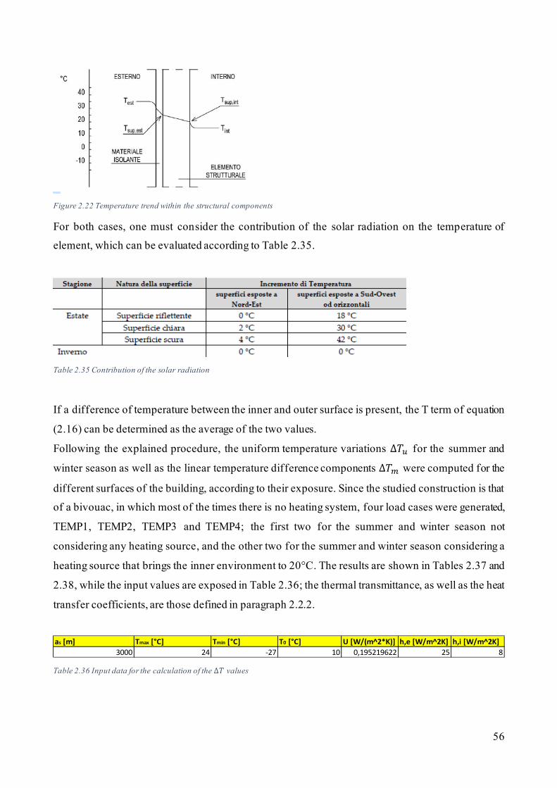
56

Figure 2.22 Temperature trend within the structural components

For both cases, one must consider the contribution of the solar radiation on the temperature of

element, which can be evaluated according to Table 2.35.

Table 2.35 Contribution of the solar radiation

If a difference of temperature between the inner and outer surface is present, the T term of equation

(2.16) can be determined as the average of the two values.

Following the explained procedure, the uniform temperature variations ∆𝑇𝑢 for the summer and

winter season as well as the linear temperature difference components ∆𝑇𝑚 were computed for the

different surfaces of the building, according to their exposure. Since the studied construction is that

of a bivouac, in which most of the times there is no heating system, four load cases were generated,

TEMP1, TEMP2, TEMP3 and TEMP4; the first two for the summer and winter season not

considering any heating source, and the other two for the summer and winter season considering a

heating source that brings the inner environment to 20°C. The results are shown in Tables 2.37 and

2.38, while the input values are exposed in Table 2.36; the thermal transmittance, as well as the heat

transfer coefficients, are those defined in paragraph 2.2.2.

Table 2.36 Input data for the calculation of the ∆𝑇 values

as [m] Tmax [°C] Tmin [°C] T0 [°C] U [W/(m^2*K)] h,e [W/m^2K] h,i [W/m^2K]

3000 24 -27 10 0,195219622 25 8

57

Table 2.37 Calculation of the temperature variations without a heating source

Table 2.38 Calculation of the temperature variations with a heating source

The mechanical stresses deriving from the defined ∆𝑇s are directly proportional to the deformation

ε, which, in turn, depends on the coefficient of thermal expansion α:

휀 = 𝛼∆𝑇 (2.18)

The standard α values for the different kinds of materials are shown in Table 2.39, taken from the

norm.

Table 2.39 Thermal expansion coefficients

Considering the linear elastic constitutive equations, one has:

𝜎 = 𝐸휀 = 𝐸𝛼∆𝑇 (2.19)

For the case of the two studied panels, it has been assumed 𝛼 = 5 ∗ 10−6, in the absence of any

further specifications.

T,e T,i Tp,e Tp,i Tmedia ΔT,uniform ΔT,butterfly

Nord 26 24 25,98438243 24,04880491 25,01659367 15,01659367 -1,935577525

Sud 54 24 53,76573645 24,73207358 39,24890502 29,24890502 -29,03366287

Est 26 24 25,98438243 24,04880491 25,01659367 15,01659367 -1,935577525

Ovest 54 24 53,76573645 24,73207358 39,24890502 29,24890502 -29,03366287

Estate

Locale non riscaldato-TEMP1

Esposizione superficie

T,e T,i Tp,e Tp,i Tmedia ΔT,uniform ΔT,butterfly

Nord -27 -27 -27 -27 -27 -37 0

Sud -27 -27 -27 -27 -27 -37 0

Est -27 -27 -27 -27 -27 -37 0

Ovest -27 -27 -27 -27 -27 -37 0

Esposizione superficie

Inverno

Locale riscaldato-TEMP2

T,e T,i Tp,e Tp,i Tmedia ΔT,uniform ΔT,butterfly

Nord 26 24 25,98438243 24,04880491 25,01659367 15,01659367 -1,935577525

Sud 54 24 53,76573645 24,73207358 39,24890502 29,24890502 -29,03366287

Est 26 24 25,98438243 24,04880491 25,01659367 15,01659367 -1,935577525

Ovest 54 24 53,76573645 24,73207358 39,24890502 29,24890502 -29,03366287

Estate

Locale riscaldato-TEMP3

Esposizione superficie

T,e T,i Tp,e Tp,i Tmedia ΔT,uniform ΔT,butterfly

Nord -27 20 -26,63298711 18,85308472 -3,889951195 -13,8899512 45,48607183

Sud -27 20 -26,63298711 18,85308472 -3,889951195 -13,8899512 45,48607183

Est -27 20 -26,63298711 18,85308472 -3,889951195 -13,8899512 45,48607183

Ovest -27 20 -26,63298711 18,85308472 -3,889951195 -13,8899512 45,48607183

Esposizione superficie

Inverno

Locale riscaldato-TEMP4

58

Chapter 3 Creation of the 3D models and software

interoperability

The 3D models exposed in this chapter are basically of two main types based on what was the purpose

of the work: the more structural ones, made with software specialized on performing structural

analysis, and the more graphical oriented architectonical ones, made with the purpose of reaching a

high LOD in terms of graphical information.

The initial intention was to work mainly with the Autodesk produced programs Revit (for the

architectonical model) and Robot as well as SAP2000 for the structural analysis, however, as will be

exposed in the following paragraphs, some obstacles were encountered during the progress of the

work that made the use of other software necessary, mainly that of the BIM tool Dlubal.

3.1 The initial steps: Revit, Robot and SAP2000

When creating a 3D model of a construction, it is always advisable to start with the structural model

in order to dimension the core of the building which is the structure, before passing on to a more

graphical detailed architectonical model in which also non-structural parts are considered. However,

a first, basic model was made on the software Revit, in which only the general geometry was defined

without giving any further information about materials, connections, exact thickness of the walls etc.

The intention was to, once created, export it and continue the work on the structural software Robot,

with the purpose of first testing how these two software work together. The reference-drawings that

were used to create these models, as well as all the other models created in the next paragraphs, were

the ones shown in paragraph 1.4.1.

Figure 3.1 First model created in Revit

59

As mentioned, this first work was then exported on the software Robot with, as can be seen in Figure

3.2, decent results.

Figure 3.2 Robot model, imported from Revit

The structure was then further studied on Robot; a structural framework was defined, as is shown in

Figure 3.3, and the Kingspan panels were modelled with the creation of a “Kingspan material”.

However, this software was then abandoned for the further steps of the work because of one main

reason: it is not specialized in wood structures. For this reason, it doesn’t for example allow the

modelling of connections for timber frames and has a rather limited choice in timber materials. This

was very important, because the intention was to consider basically the entire structure a s wood-

made. Parallelly, a trial of a model was started also on the software SAP2000 but was abandoned

even earlier for the same reason, since it has less possibilities than Robot for what concerns timber.

Figure 3.3 Robot model with elaborated structural framework

60

3.2 The Dlubal structural model

Eventually, the structural model was made on Dlubal, which is a BIM tool coming from Germany

working with the Finite Element Method. This software has tens if not hundreds of different timber

materials, from LVL to OSB types, from plywood to hardwood and softwood. Furthermore, it allows

through add-ons the modelling of specific timber to steel and timber to timber connections and of

complex section shapes for frame elements, which, as will be seen in the next paragraphs, was

required for the performed work. All in all, it was by far more suitable to the project than the previous

used software.

The next paragraphs expose an example of a possible solution of structural application of the panels

illustrated in paragraphs 2.2 and 2.3 on the case study seen in paragraph 1.4.

3.2.1 The panels

To model in the program the two studied panels, KINGSPAN TEK 142 and PANELO, that where

illustrated in paragraphs 2.2 and 2.3 of this thesis, various assumptions were made. Now, before

starting with the description of the applied procedure, it would be appropriate to clarify on the purpose

of the work presented in this paragraph: in fact, since the interest of this thesis was to do an

investigation of the appropriateness of the panels in the case study and not a more detailed research

on a single panel subjected to load case, the panels were considered as if to be composed of not

different materials distributed on three layers but of only one equivalent material, whose stiffness E

and shear modulus G result in the same EI and GA of the real composite panels. In other words, the

distribution of the stresses within the real panel case, that would follow the sandwich theory

(illustrated in image 2.1), was not taken into account and the panels were considered as if they were

homogeneous.

For the computation of the stiffness E and the shear modulus G of the equivalent Kingspan system,

the values of the design bending stiffness 𝐸𝐼𝑑 and shear rigidity 𝐺𝐴𝑑 given in Table 2.3 in paragraph

2.2.1 were used. According to the Table:

𝐸𝐼𝑑 = 4,6 ∗ 1011 𝑁𝑚𝑚2

and

𝐺𝐴𝑑 = 5,7 ∗ 105 𝑁.

61

Knowing the thickness t=142 mm, the value of the width to use to calculate the area A and the inertial

moment I was assumed to be of 1 m, in absence of further specification in any of the documents made

public by the Kingspan company.

Consequently, the resulting 𝐸𝑑 and 𝐺𝑑 values are:

𝐸𝑑 = 1928 𝑀𝑃𝑎,

𝐺𝑑 = 4 𝑀𝑃𝑎.

What first comes to the attention is the very low shear modulus value compared to the Young’s

modulus E. However, as the panel can be considered as a plate element where the given EI assumes

the role of the plate’s bending stiffness D, the G value doesn’t have much relevance for the problem

in the first place.

Anyhow, the program requires as an input the mean value of stiffness and not the design one. To

define it, the indications given by the Eurocode 5 where followed and not those given by the Italian

codes; this was done because the panel is produced by a British company, which is more likely to

provide the design values following the Eurocodes rather than the Italian ones. Consequently:

𝐸𝑑 =𝐸𝑚𝑒𝑎𝑛

𝛾𝑚 (3.1)

and

𝐺𝑑 =𝐺𝑚𝑒𝑎𝑛

𝛾𝑚 (3.2)

where 𝛾𝑚 is taken from the value of OSB given by the EC5 (same as that given by the CNR in Table

2.19, paragraph 2.3.1), being

𝛾𝑚 = 1,2.

Therefore:

𝐸𝑚𝑒𝑎𝑛,𝐾𝐼𝑁𝐺𝑆𝑃𝐴𝑁 = 2313,42 𝑀𝑃𝑎,

𝐺𝑚𝑒𝑎𝑛,𝐾𝐼𝑁𝐺𝑆𝑃𝐴𝑁 = 4,8 𝑀𝑃𝑎.

Table 3.1 Kingspan material properties input in the program

Furthermore, following indications given by online tutorials provided by Dlubal, the material was

modelled as an orthotropic elastic material, which is generally assumable for wood types, and the

panel was accordingly modelled as a plane element in the form of an orthotropic 2D surface. For

these kinds of surfaces, the different properties E, G and the Poisson’s ratio υ are, unlike in isotropic

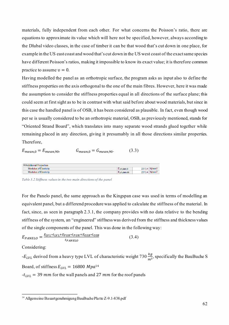
62

materials, fully independent from each other. For what concerns the Poisson’s ratio, there are

equations to approximate its value which will here not be specified, however, always according to

the Dlubal video classes, in the case of timber it can be that wood that’s cut down in one place, for

example in the US east coast and wood that’s cut down in the US west coast of the exact same species

have different Poisson’s ratios, making it impossible to know its exact value; it is therefore common

practice to assume υ = 0.

Having modelled the panel as an orthotropic surface, the program asks as input also to define the

stiffness properties on the axis orthogonal to the one of the main fibres. However, here it was made

the assumption to consider the stiffness properties equal in all directions of the surface plane; this

could seem at first sight as to be in contrast with what said before about wood materials, but since in

this case the handled panel is of OSB, it has been considered as plausible. In fact, even though wood

per se is usually considered to be an orthotropic material, OSB, as previously mentioned, stands for

“Oriented Strand Board”, which translates into many separate wood strands glued together while

remaining placed in any direction, giving it presumably in all those directions similar properties.

Therefore,

𝐸𝑚𝑒𝑎𝑛,0 = 𝐸𝑚𝑒𝑎𝑛,90, 𝐺𝑚𝑒𝑎𝑛,0 = 𝐺𝑚𝑒𝑎𝑛,90. (3.3)

Table 3.2 Stiffness values in the two main directions of the panel

For the Panelo panel, the same approach as the Kingspan case was used in terms of modelling an

equivalent panel, but a differend procedure was applied to calculate the stiffness of the material. In

fact, since, as seen in paragraph 2.3.1, the company provides with no data relative to the bending

stiffness of the system, an “engineered” stiffness was derived from the stiffness and thickness values

of the single components of the panel. This was done in the following way:

𝐸𝑃𝐴𝑁𝐸𝐿𝑂 =𝐸𝐿𝑉𝐿∗𝑡𝐿𝑉𝐿+𝐸𝑃𝑈𝑅∗𝑡𝑃𝑈𝑅+𝐸𝑂𝑆𝐵∗𝑡𝑂𝑆𝐵

𝑡𝑃𝐴𝑁𝐸𝐿𝑂 (3.4)

Considering:

-𝐸𝐿𝑉𝐿 derived from a heavy type LVL of characteristic weight 730 𝑘𝑔

𝑚3, specifically the BauBuche S

Board, of stiffness 𝐸𝐿𝑉𝐿 = 16800 𝑀𝑝𝑎14

-𝑡𝐿𝑉𝐿 = 39 𝑚𝑚 for the wall panels and 27 𝑚𝑚 for the roof panels

14 Allgemeine Bauartgenehmigung BauBuche Pla tte Z-9.1-838.pdf

63

-𝐸𝑂𝑆𝐵 = 4800 𝑀𝑝𝑎, taken from the datasheet of the Kronoswiss OSB type 3 panel15

-𝑡𝑂𝑆𝐵 = 15 𝑚𝑚

-𝐸𝑃𝑈𝑅 derived from an inverse procedure of the one described here applied to the Kingspan TEK

system. In fact, knowing the E value and the thickness of the equivalent Kingspan material (defined

in this paragraph) as well as the stiffness and the thickness of the OSB composing the Kingspan panel

(the same as that defined here of the Kronoswiss OSB), it was possible to compute the stiffness of

the Kingspan insulating core 𝐸𝑃𝑈𝑅 = 1647 𝑀𝑃𝑎. It was then assumed that the same type of PUR

composing the TEK panel is utilized for the insulating core of the PANELO system. This was done

because the stiffnesses of PUR boards found in literature through research had a huge range of

possible values (going more ore less from the order of magnitude of 5 MPa to 5GPa) depending from

the density of the PUR, which was therefore assumed to be equal as that of the Kingspan panel.

-𝑡𝑃𝑈𝑅 = 145 𝑚𝑚 for the wall panels and 195 𝑚𝑚 for the roof panels.

The LVL and OSB types were chosen according to the considerations made in paragraph 2.3.1.

Through (3.4), two values of mean stiffness, one for the wall panel and one for the roof panel were

computed. The shear modulus G was not computed because, as mentioned in the case of the Kingspan

panel, considered as of not great relevance for the problem.

The calculations of the stiffness values 𝐸𝑃𝐴𝑁𝐸𝐿𝑂,𝑊𝐴𝐿𝐿 and 𝐸𝑃𝐴𝑁𝐸𝐿𝑂,𝑅𝑂𝑂𝐹 as well as the derivation of

𝐸𝑃𝑈𝑅 from 𝐸𝐾𝐼𝑁𝐺𝑆𝑃𝐴𝑁 are schematized in Tables 3.3, 3.4 and 3.5.

Table 3.3 Stiffness values of OSB, KINGSPAN and PANELO

Table 3.4 Calculation of the PUR stiffness

Table 3.5 Calculation of the Panelo wall and roof panels stiffnesses

15 https://baldolegnami.it/media/osb.pdf

EOSB [N/mm^2] 4800

EKINGSPAN [N/mm^2] 2313,424287

ELVL [N/mm^2] 16800

FROM SWISS KRONO OSB/3 DATASHEET

FROM KINGSPAN

FROM BAUBUCHE S BOARD

t [mm] E [N/mm^2] t [mm] E [N/mm^2] t [mm] E [N/mm^2]

30 4800 112 1647,377221 142 2313,424287

KINGSPAN PANELOSB PUR

64

As can be noticed, being the stiffest component the LVL, the wall panel has obviously greater stiffness

than the roof panel. For what concerns all the other aspects regarding the modelling of the panels, the

same assumptions as for the Kingspan TEK system were made.

3.2.2 The geometry

3.2.2.1 Structure with Kingspan TEK Panels

The Kingspan panel has maximum dimensions 1.22 m x 7.5 m. Therefore, the panels used in the

model of the structure are all of width 1.2 m, while the height depends on the geometry of the walls

and roof, exposed in paragraph 1.4.1.

The disposition and numbering of the panels as well as the structural framework of the model of the

construction are shown in Figures 3.4 and 3.5. In this model, the x-axis is horizontal and its direction

is parallel to east and west wall, the y-axis is horizontal and its direction is parallel to south and north

wall and the z-axis is vertical. The origin of the system is in the corner between the foundation, the

east wall and the north wall.

Figure 3.4 From left to right: north side and east side of the building

Figure 3.5 From left to right: south side and west side of the building

65

Table 3.6 shows the exact dimensions and exposure of each panel. For the panels with inclined sides,

average height values have been considered. The base dimension of the modelled building is 4.8 m x

6 m.

Table 3.6 Dimensions and exposure of the panels

In the north wall, more precisely in panel 26, there’s an opening in form of a door of dimensions 0.76

m x 2.03 m. As can be observed in Figures 3.4 and 3.5, a series wooden frames were added as a

support to the panel structure based on the 2D drawings of paragraph 1.4, which can be seen in a

more detailed way in Figure 3.6. More specifically, 6 main frames composed of two columns and a

couple of rafter beams are placed with a spacing of 1.2 meters (corresponding to the width of the

panels) along the longer sides of the building, so the y axis in the model. The two columns as well as

the rafter beams composing those frames are made of C24 softwood timber and have section 220 mm

x 240 mm. On the east wall of the bivouac, an additional column of the same material has been placed

to contain the deformations of the panels as well as to take some of the vertical load coming to the

wall from the roof. This column has section 220 mm x 300 mm. Of the 6 main frames, 5 are on the

inner sides of the respective walls and roof they are connected to while another one, the one on the

east side of the building, is on the outer side of the wall, more precisely the east wall. For the west

wall, which, as was seen in the exposure of the 2D drawings in paragraph 1.4 , is made of non-

Panel Position Width [m] Height [m] Area [m^2]

1 Muro nord 1,2 2,42 2,904

25 Muro nord 1,2 2,42 2,904

26 Muro nord 1,2 2,42 1,355616

4 Muro nord 1,2 2,42 2,904

5 Muro nord 1,2 2,42 2,904

15 Tetto nord 1,2 3,62 4,344

16 Tetto nord 1,2 3,62 4,344

17 Tetto nord 1,2 3,62 4,344

18 Tetto nord 1,2 3,62 4,344

19 Tetto nord 1,2 3,62 4,344

6 Muro est 1,2 2,991666667 3,59

7 Muro est 1,2 4,125 4,95

27 Muro est 1,2 4,716666667 5,66

9 Muro est 1,2 3,958333333 4,75

10 Muro sud 1,2 3,55 4,26

11 Muro sud 1,2 3,55 4,26

12 Muro sud 1,2 3,55 4,26

13 Muro sud 1,2 3,55 4,26

14 Muro sud 1,2 3,55 4,26

20 Tetto sud 1,2 2,56 3,072

21 Tetto sud 1,2 2,56 3,072

22 Tetto sud 1,2 2,56 3,072

23 Tetto sud 1,2 2,56 3,072

24 Tetto sud 1,2 2,56 3,072

66

structural glass supported by a frame, only the wooden supporting structure of the glass was modelled.

The structural timber elements of this frame have all dimensions 120 mm x 300 mm and are of C24

softwood timber.

Figure 3.6 Details of the supporting frame

The frame connected to the east wall with the additional structural column as well as the timber glass

supporting frame can be observed in Figure 3.7.

Figure 3.7 From the left to the right: Detail of the east wall frame and the glass wall supporting frame

The initial intention was to not model the west wall at all and consider the whole glass + supporting

frame system as non-structural. However, after some launches of the structural analysis of the

building without these components, it was noticed that in complete absence of some elements

providing stiffness to the whole structural system in the direction of the x-axis (the red axis in Figure

67

3.7), the structure was experiencing a strong torsion around the vertical z-axis (the light blue axis in

Figure 3.7), mostly in the case of wind loads “hitting” the north or south wall, so with direction

parallel to the x-axis. This was due to the fact that the east wall, thanks to the panels, was providing

the whole structure system with much more stiffness than the non-existing west wall which was

obviously providing none. For this reason, the modelling of the glass frame was necessary.

Between one frame and the other, at the ridge of the roof and at the higher edge of the wall plates,

steel truss elements were modelled that mostly serve for the purpose of connecting the different

frames to each other and not to bear the weight of the roof. They are made of S 450 steel and were

modelled with the Dlubal add on module “SHAPE THIN”, specialized in the creation of sections for

thin 1D elements. Their shape follows the geometry of the walls and roof system, their thickness is

of 30 mm and their sides have length of 200 mm. Details of those elements are shown in Figures 3.8,

3.9 and 3.10.

Figure 3.8 From the left to the right: modelling of the section of the north wall edge truss element and detail of it within the structure

Figure 3.9 From the left to the right: modelling of the section of the roof ridge truss element and detail of it within the structure

68

Figure 3.10 From the left to the right: modelling of the section of the north wall edge truss element and detail of it within the structure

No additional bracing is required between the frames, because this function is already carried out by

the structural panels.

The foundation consists in a steel S450 grid composed of two longitudinal H beams and of six

transversal H beams, with the steel elements having section of properties shown in Figure 3.11.

Figure 3.11 Cross section of the steel foundation elements

It has been modelled as if it was lying on infinitely stiff elastic ground (spring constant of the member

elastic foundation in the vertical direction extremely high, see Figure 3.12)

69

Figure 3.12 Spring constants of the foundation members

Furthermore, it has been constrained in the x and y direction in one vertex of the grid (at one end of

one of the two longitudinal beams) and in the y direction in another vertex (at the other end of the

same beam). Details of the foundation and of the constraints are to be seen in Figure 3.13.

Figure 3.13 Details of the foundation and its constraints

All the structural elements were dimensioned based on an in-depth study of the structural behaviour

of the building with applied loads those defined in paragraph 2.5.

3.2.2.2 Structure with Panelo Panels

The geometry of the structure with the Panelo panels is basically very similar to that defined with the

Kingspan TEK panels, but there’s two things that change. The first one is concerning the supporting

frame system. In fact, since the Panelo panel is both thicker and stiffer, as seen in paragraph 3.2.1,

this allowed to reduce by a significant amount the section of those elements, which was of dimensions

220 x 240 mm for those supporting the Kingspan Panels, and is in this case of dimensions 130 x 240

mm, always of C24 Softwood timber. Furthermore, the high stiffness allowed to also completely

remove the additional column placed in paragraph 3.2.2.1 on the east wall of the building. The second

70

thing that was changed was the geometry of the east wall. This was done because the Panelo company

states on the brochure that the maximum dimensions of the panel are 12 m in width and 4 m in

height16, so it was impossible to model panels of height equal to that of the wall. The exact disposition

and numbering of the panels as well as the structural framework of the model of the construction are

shown in Figures 3.14 and 3.15.

Figure 3.14 From left to right: north side and east side of the building

Figure 3.15 From left to right: south side and west side of the building

16 https://panelo.eu/wp-content/uploads/2018/07/Brochure-ENG.pdf

71

Table 3.7 shows the dimensions and exposure of each panel. For the panels with inclined sides,

average height values have been considered.

Table 3.7 Dimensions and exposure of the panels

The information regarding all the other structural components, as the glass supporting frame, the steel

frame-connecting elements and the foundation are the same as those exposed in paragraph 3.2.2.1 for

the structure with the Kingspan panels.

3.2.3 The panel connections

The panels, both for the case of the Kingpan system and of the Panelo system, are all connected to

each other through insulated cassette splines and not through timber posts. This was done because

having already the supporting frame, additional timber posts weren’t needed. Having only the timber

posts and not the supporting frames, which would be a more practical solution, was impossible

because it was leading to failure in the system as the whole structure was not strong enough to bear

Panel Position Width Height Area

1 Muro nord 1,2 2,42 2,904

25 Muro nord 1,2 2,42 2,904

26 Muro nord 1,2 2,42 1,356

4 Muro nord 1,2 2,42 2,904

5 Muro nord 1,2 2,42 2,904

15 Tetto nord 1,2 3,62 4,344

16 Tetto nord 1,2 3,62 4,344

17 Tetto nord 1,2 3,62 4,344

18 Tetto nord 1,2 3,62 4,344

19 Tetto nord 1,2 3,62 4,344

27 Muro est 2,4 2 4,8

28 Muro est 2,4 1,566 3,759

29 Muro est 2,4 2 4,8

30 Muro est 2,4 2,333 5,599

10 Muro sud 1,2 3,55 4,26

11 Muro sud 1,2 3,55 4,26

12 Muro sud 1,2 3,55 4,26

13 Muro sud 1,2 3,55 4,26

14 Muro sud 1,2 3,55 4,26

20 Tetto sud 1,2 2,56 3,072

21 Tetto sud 1,2 2,56 3,072

22 Tetto sud 1,2 2,56 3,072

23 Tetto sud 1,2 2,56 3,072

24 Tetto sud 1,2 2,56 3,072

72

the weight of snow and wind. Additionally, avoiding the use of timber posts and placing only

insulated cassette splines also doesn’t allow the creation of thermal bridges within the walls and the

roof, which is a significant advantage. The next paragraphs explain how the fasteners mentioned

already in paragraphs 2.2.4 and 2.3.4 connecting the panels, the splines and the frame or the

foundation to each other were modelled, where with modelled what is meant is what constraints were

given to the connection and, if constraints were given, with what rigidity.

3.2.3.1 Kingspan Panels

The panel-panel-frame connection works with a combination of both fasteners and gluing material.

It is schematized with a section view in Figure 3.16. As can be observed, only one of the two panels

as well as the spline are directly connected to the frame element with a fastener, the other one is only

connected to the spline; the panel connected to the frame (the left one in Figure 3.16), is connected

to it thanks to screw elements, more specifically the Sparennagel 6 mm x 210 mm, also seen in

paragraph 2.2.4 which talks about the Kingspan connections. Always following the indications given

by the company, those screws are placed in line along the vertical z axis with a spacing of 300 mm.

The adjacent panel, in case of Figure 16 the right one, is jointed to the connection spline with nail

type fasteners, again following the indications exposed in paragraph 2.2.4, which suggests the use of

galvanized ring nails of dimesions 2.8 mm x 63 mm, placed with a spacing of 50 mm. In addition,

the spline on this side is glued to the panel with a sealer, where for the sake of calculations it was also

chosen a specific type, which is one called “SIP Seal”, produced in the United States.

Figure 3.16 Panel to panel to frame connection. The red line represents the gluing material.

The purpose of this whole system was to consider one panel (the right one in figure 3.16) basically

as if to form one single piece with the spline. In fact, those gluing materials are extremely strong and

73

have a very high shear modulus, of some orders of magnitude greater17 than what is usually the slip

modulus of the fasteners, which will be seen in the next pages, and can therefore provide, combined

with the nails, enough rigidity and resistance to completely fix the panel to the spline. Through this

assumption, it is possible to consider both panels connected to each other and to the frame with the

Sparrennagel 6 mm x 210 mm screw system, which makes it a little bit more intuitive to model and

understand the behaviour of the connection.

For what concerns the wall to wall to frame corner connection, details are shown in Figure 3.17. It

can be seen how in this case the one describe before was obviously not appliable; in this case, both

are connected through Sparennagel screws, one to the adjacent panel and the other to the frame, both

with a spacing of 300 mm; since the two rows cannot intersect, they will have to be staggered.

However, similarly to the previous case, also here one panel is connected to the other one which is

fastened to the frame, and it was also here considered as if both panels were connected both to each

other and to the frame with a row of Sparennagel of dimensions 6 mm x 210 mm and spacing 300

mm. In short, the two connections of Figures 3.16 and 3.17 were modelled in the same way.

Figure 3.17 Wall to wall to frame connection

The ridge connections of the roof panels and the wall to roof edge panels connections are those

suggested by the brochure of the TEK system and illustrated in paragraph 2.2.4 (Figure 2.5 and 2.6).

In these cases, the panels are only connected to each other and not to any frame element; however,

the geometry is here much simpler than in the previous two cases. It is therefore clear, that these

connections have to be modelled as exactly what they are, which is a row of Sparrennagel spaced 300

mm from each other. Being this the case, also these connections were defined with the same

characteristics as those of the first two that were described in this paragraph.

17 Mechanicalshearpropertiesofadhesives.pdf

74

The described connections were modelled on Dlubal with the command “Line hinges”, which allows

to input constraint degrees for surfaces. The contact line between two more surfaces is there assigned

an own reference system, that can be seen in Figure 3.18.

Figure 3.18 Line hinges in the Dlubal software

The first defined property was that the rotation around the main axes of the connection (x axis along

the contact line between the surfaces in Figure 3.18) is completely allowed, so 𝐶𝜑𝑥 = 0. Regarding

the constraints for the displacement in the two in plane axes 𝑢𝑥 and 𝑢𝑦, fasteners do have a limited

stiffness caused by their long and thin shape, which can deform in the way illustrated in Figure 3.19.

Figure 3.19 Deformed shape of the connection

75

This stiffness is defined, according to EC5, in the form of a slip modulus 𝐾𝑠𝑒𝑟 , whose value in 𝑘𝑁

𝑚 is

computed, for wood fasteners inserted without drilling (like nails) through the relation:

𝐾𝑠𝑒𝑟 = 𝜌𝑚1.5 𝑑0.8

30 (3.5)

and for fasteners needing drilling (like screws and bolts), this equation becomes:

𝐾𝑠𝑒𝑟 = 𝜌𝑚1.5 𝑑

23 (3.6)

being 𝜌𝑚 the mean density of the involved wood in 𝑘𝑔

𝑚3 and 𝑑 the diameter in mm. If the two connected

members are of two different wood materials, the density to consider is defined as 𝜌𝑚 = √𝜌𝑚,1𝜌𝑚,2.

In this case, the two considered densities were that of the Kingspan panel defined in paragraph 2.2.1

and of Softwood timber C24 of the frames. In order to have the value of (3.6) in 𝑘𝑁

𝑚2, which is the input

required by the program, an equivalent connection was modelled by applying

𝐾𝑠𝑒𝑟,𝑒𝑞 =𝐾𝑠𝑒𝑟

𝑠 (3.7)

where s is the spacing of the fasteners.

What 3.7 does, is it creates a fictitious connection distributed uniformly along the connection line in

the absolute absence of spacing (as can be observed in Figure 3.20), so basically in infinite number

of infinitesimal nails or screws one attached to the next one, which result in the same stiffness as the

real connection.

Figure 3.20 From the left to the right: real connection and fictitious connection

When performing a structural analysis at the Ultimate Limit State, the slip modulus should be taken

as:

𝐾𝑢 =2

3𝐾𝑠𝑒𝑟 (3.8)

The described procedure was applied and a value for the slip modulus was computed, assumed to be

equal in the x and y connection axes. The resulting values are shown in Table 3.8.

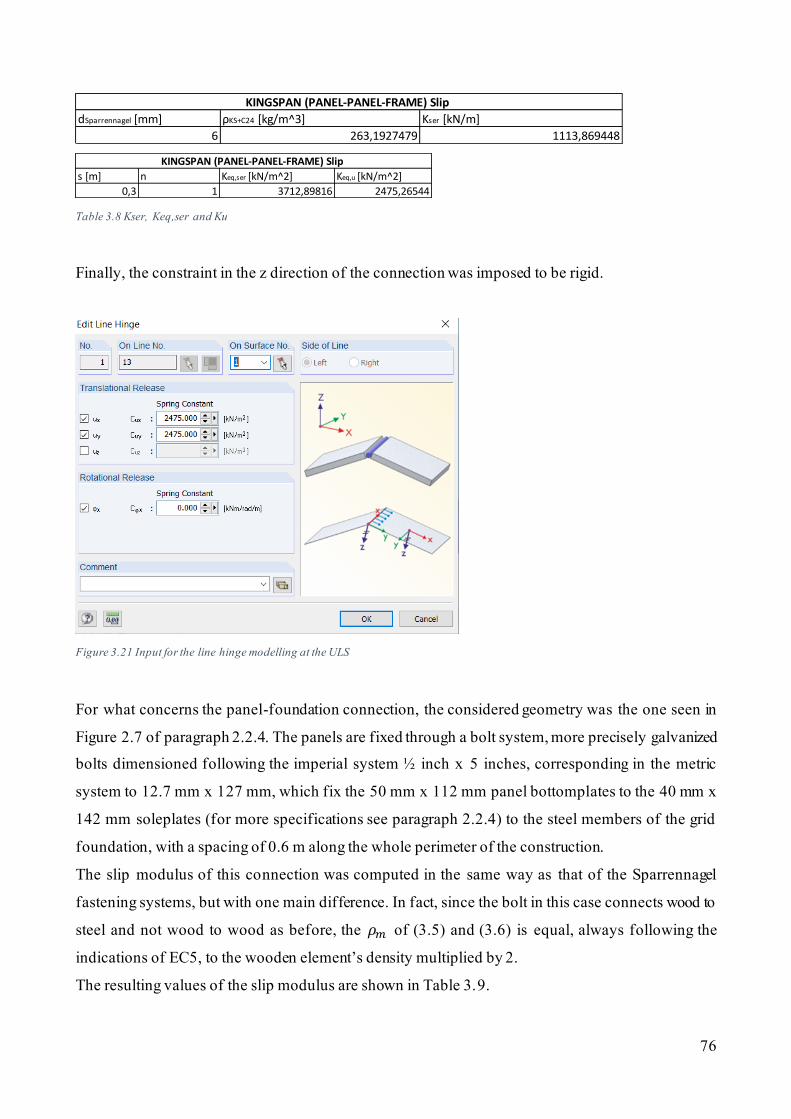
76

Table 3.8 Kser, Keq,ser and Ku

Finally, the constraint in the z direction of the connection was imposed to be rigid.

Figure 3.21 Input for the line hinge modelling at the ULS

For what concerns the panel-foundation connection, the considered geometry was the one seen in

Figure 2.7 of paragraph 2.2.4. The panels are fixed through a bolt system, more precisely galvanized

bolts dimensioned following the imperial system ½ inch x 5 inches, corresponding in the metric

system to 12.7 mm x 127 mm, which fix the 50 mm x 112 mm panel bottomplates to the 40 mm x

142 mm soleplates (for more specifications see paragraph 2.2.4) to the steel members of the grid

foundation, with a spacing of 0.6 m along the whole perimeter of the construction.

The slip modulus of this connection was computed in the same way as that of the Sparrennagel

fastening systems, but with one main difference. In fact, since the bolt in this case connects wood to

steel and not wood to wood as before, the 𝜌𝑚 of (3.5) and (3.6) is equal, always following the

indications of EC5, to the wooden element’s density multiplied by 2.

The resulting values of the slip modulus are shown in Table 3.9.

dSparrennagel [mm] ρKS+C24 [kg/m^3] Kser [kN/m]

6 263,1927479 1113,869448

KINGSPAN (PANEL-PANEL-FRAME) Slip

s [m] n Keq,ser [kN/m^2] Keq,u [kN/m^2]

0,3 1 3712,89816 2475,26544

KINGSPAN (PANEL-PANEL-FRAME) Slip

77

Table 3.9 Kser and Ku of the panel foundation bolt fasteners

In addition, consequently to some problems encountered in the initial modelling steps related to the

formation of singularities in the stress distribution within the panels (see paragraph 4.1.1.3), which

were then eventually solved in a different way, also an estimation of the vertical stiffness (meaning

in direction of the global z-axis of the model) of the panel to foundation connection was performed,

following different documents found on the web. However, the resulting spring constant value was

so high (around 200000 𝑘𝑁

𝑚2) that it didn’t make sense to insert it into the model, and the vertical

constraint was eventually considered as rigid. The joint was therefore given, apart from the partial in

plane restraints defined in Table 3.8, only freedom of rotation around the local x axis. The modelling

of the foundation to panel connection can be seen in Figure 3.22.

Figure 3.22 Modelling of the panel-foundation connection

3.2.3.2 Panelo Panels

The modelling of the Panelo connections was done in the exact same way as seen for the Kingspan TEK system in paragraph 3.2.3.1, only that instead of using Sparrennagel 6 mm x 210 mm screws, 8.0 mm x 300 mm Heco Topix screws were used to fasten the panels to the frame and coach screws 8.0 mm x 150 mm to each other. The panel foundation connection stayed the same also for what concerns the bolt type. The resulting stiffness values for the panel to panel to frame connections are

dGalvanized anchor bolts [mm] ρC24+S450 [kg/m^3] Kser [kN/m] s [m] n Keq,ser [kN/m^2]Keq,u [kN/m^2]

12,7 420 4752,803077 0,6 1 15842,67692 10561,78462

KINGSPAN (PANEL-FOUNDATION) Slip

78

given in Table 3.10. Since the Panelo systems have two different densities for the roo f and wall panels, the two resulting joint types also have different spring constants.

Table 3.10 Stiffness values of the panel to panel to frame connections

3.2.4 The frame connections

Differently to the modelling of the panel connections which were done by hands, the joints of the

supporting frame system were all modelled automatically by the Dlubal software thanks to the add-

on module “RF-Joints”. This add-on allows to create the geometry of steel to timber connections and

timber to timber connections between two or more beam members; once the geometry is set as an

input and the program is run, it generates a rigid joint member in the node of interest connected to the

beam elements (which on the other hand get completely released form the original node) with a certain

stiffness. However, this additional joint element works really well when studying the behaviour only

of the frame system, but it creates complications and “misunderstandings” in the model when

modelling additionally to the 1D frame elements also 2D surfaces (as the panels are) connected to

each other; for this reason, the geometry of the connections was defined on “RF-Joints” in a separate

model in which only one frame was considered.

Figure 3.23 The separate "frame" model

It was then proceeded to take the output constraint stiffness values that the software provides for the

modelled joint element and simply input this data in the traditional “member hinge” function, that the

dSparrennagel [mm] ρPANELO+C24 [kg/m^3] Kser [kN/m] s [m] n Keq,ser [kN/m^2] Keq,u [kN/m^2]

8 287,7824699 1698,082 0,3 1 5660,273282 3773,515521

PANELO WALL Slip

dSparrennagel [mm] ρPANELO+C24 [kg/m^3] Kser [kN/m] s [m] n Keq,ser [kN/m^2] Keq,u [kN/m^2]

8 250,5032909 1379,0573 0,3 1 4596,85759 3064,571727

PANELO ROOF Slip

79

Dlubal software offers, in both the Kingspan and the Panelo structural models. A representation of

what explained is shown in the Figures below, which are all referring to the Kingspan building

supporting frame, starting with the north wall column to north roof rafter beam connection.

Figure 3.24 Details and representation of the north side edge frame connection

As can be seen in Figure 3.24, the connection is made with two plates of thickness 12 mm each, and

a dowel group composed by 6 columns and 3 rows, with dowels of 8 mm diameter each and of length

220 mm (same as the width of the section). Further details are provided in Figures 3.25 and 3.26.

Figure 3.25 From the left to the right: side and front view of the east side edge frame connection

80

Figure 3.26 Close views of the east side edge frame connection

Figure 3.27 From the left to the right: Modelling of the connection by RF Joints, output stiffness values of the connection

Figure 3.27 shows on the left the automatic modelling done by the software of the connection through

a joint element (the dashed red line) and node releases (the light blue cubes), and on the right the

output connection constraints with relative stiffness given by the RF Joints module. The resulting

spring constant related to the rotation about the y-axis (𝐶𝜑Y in Figure 3.28) was approximated to 6000

kN/rad and used to define the rotational stiffness of the member hinge on the Kingspan structure

model of the same node The values of Figure 3.27 related to the stiffness in the x and z direction

where on the other hand not considered because so high to allow the assumption of a rigid constraint.

Figures 3.28 and 3.29 illustrate this step.

81

Figure 3.28 Modelling of the member line hinge on the Kingspan structural model

Figure 3.29 Rendering in the Kingspan structural model of the connection; the white dots represent the member hinges

For what concerns the joint of the rafter to rafter beams (ridge of the roof) and of the column to rafter

beam on the south side of the building, the connection maintains the same properties as those seen

now for the previous case being formed always by two plates and a dowel system of 3 columns by 6

rows of dowels of diameter 8 mm, but the general geometry, obviously following that of the structure,

changes. The resulting bending stiffness is the same as that defined previously for the column to rafter

connection, and it was modelled as seen in Figure 3.28 in the Kingspan structural model. Details of

those connections are shown in the Figures below.

82

Figure 3.30 Details of the ridge connection

Figure 3.31 Details of the south side frame connection

Regarding the column to foundation connections, it is also formed by two steel plates 12 mm thick

and dowels of diameter 8 mm, in this case placed in 5 columns and 4 rows. Details of the connection

as well as its stiffness values provided by the RF Joints add-on and its modelling in the Kingspan

structural model are shown in the figures below.

Figure 3.32 Details of the columns foundation connection

83

Figure 3.33 From the left to the right: Modelling of the connection by RF Joints, output stiffness values of the connection

The bending stiffness value of Figure 3.33 (8039.860 kNm/rad) was approximated to 8000 kNm/rad

and inserted in the Kingspan structural model at the same node.

Figure 3.34 From the left to the right: modelling of the member line hinge on the Kingspan structural model, rendering in the Kingspan structural model of the connection; the white dots represent the member hinges

For what concerns the supporting frame system of the structure made with the Panelo panels, whose

members have section, as mentioned in paragraph 3.2.2, of 13 cm x 24 cm, the exact geometry of the

connections were not modelled on RF Joints. However, the connections were assumed to have similar

characteristics to those defined above, and they were modelled in the Panelo structural model with

84

the function “member hinge” at the single members with the same stiffness values as those found for

the Kingspan structural model supporting frame.

3.2.5 The application of the loads

3.2.5.1 Snow loads

The snow loads are those defined in paragraph 2.5.2. They are applied vertically along the full span

of the roof and, since the building is located at altitudes greater than 1000 m amsl, they are medium

term loads. Their application in the models is shown in Figures 3.35, 3.36 and 3.37.

Figure 3.35 Definition and application of the load case Snow 1

Figure 3.36 Definition and application of the load case Snow 2

85

Figure 3.37 Definition and application of the load case Snow 3

3.2.5.2 Wind loads

The wind loads are those defined in paragraph 2.5.1. They are applied perpendicularly to each surface

of the structure and are instantaneous loads. Their application in the models is shown in Figures 3.38,

3.39, 3.40 and 3.41.

Figure 3.38 Definition and application of the load case Wind 1

Figure 3.39 Definition and application of the load case Wind 2

86

Figure 3.40 Definition and application of the load case Wind 3

Figure 3.41 Definition and application of the load case Wind 4

3.2.5.3 Temperature

Regarding the effect of the temperature variations described in paragraph 2.5.3, their application in

the Kingspan and Panelo models created a lot of problems in the initial stages of the modelling, mostly

concerning the stresses that it created inside the panels. This was due to the fact that, at first, the panel

joints were modelled as if only allowing rotation about the connection’s main direction axis, while

they were considered rigid for the in plane constraints, not allowing any translation at all along the x

and y axes of the connection (see Figure 3.21 for further details). This hindered the panel completely

to shrink or expand when subjected to temperature variations and created therefore huge normal

stresses in it close to the connection line. In fact, this phenomenon is why the stiffnesses of the

fastening connections were calculated and modelled in the first place. However, once this stiffness

and partial freedom of movement was input inside the program, the effects of the temperature both in

terms of stresses and strains became rather insignificant and negligible with respect to those generated

by wind and snow. In terms of deformations, just to give an idea, if one were to apply the equation

(2.18) (휀 = 𝛼∆𝑇) with the maximum ∆𝑇 possible for the studied case, which is of 37° C, and knowing

87

𝛼 = 5 ∗ 10−6, the total shrinkage in the longest span of the structure (6 m) is of 1.1 mm (with ∆𝐿 =

휀 ∗ 𝐿). Considering the types of connections used for the panels, it seems plausible that the system

doesn’t suffer too much from it, which in fact running the calculations with the software was the case.

Furthermore, the addition of the temperature load cases was slowing down the computation times of

the program for the analysis at the Ultimate and Serviceability Limit States (which had to be

performed every time some detail was changed), and where therefore eventually removed from the

model.

3.2.5.4 Limit States combinations

The Limit States load combinations applied were defined following the instructions of the NTC 2018.

The analysis was performed for two combinations:

- The Fundamental Ultimate Limit State combination (for persistent and transient design situations)

𝛾𝐺1 ∗ 𝐺1 + 𝛾𝐺2 ∗ 𝐺2 + 𝛾𝑃 ∗ 𝑃 + 𝛾𝑄1 ∗ 𝑄𝑘1 + 𝛾𝑄2 ∗ 𝜓02 ∗ 𝑄𝑘2 + 𝛾𝑄3 ∗ 𝜓03 ∗ 𝑄𝑘3 + ⋯ (3.25)

- The Characteristic (or rare) for irreversible Serviceability Limit State combination

𝐺1 + 𝐺2 + 𝑃 + 𝑄𝑘1 + 𝜓02 ∗ 𝑄𝑘2 + 𝜓03 ∗ 𝑄𝑘3 + ⋯ (3.26)

From these two equations, 96 combinations resulted, 64 ULS ones and 32 SLS.

The final load cases, load types and coefficients used for the combinations are shown in the Tables

below.

Table 3.11 Partial safety and contemporaneity coefficients

Table 3.12 List of load cases and load types

Contemp

Y0 Y1 Y2

G = G1 + G2 + G3 + … 0,9 1,1 1 1,3

Qs 0 1,5 0 1,5 0,7 0,5 0,2

Qw 0 1,5 0 1,5 0,6 0,2 0Wind

Coeff g for ULS verification

EQU A1

permanent actions

Snow (H > 1000 m a.s.l.)

Load case Load type Action

1 Self weight Permanent G

2 Snow 1 Snow Qs

3 Snow 2 Snow Qs

4 Snow 3 Snow Qs

5 Wind 1 Wind Qw

6 Wind 2 Wind Qw

7 Wind 3 Wind Qw

8 Wind 4 Wind Qw

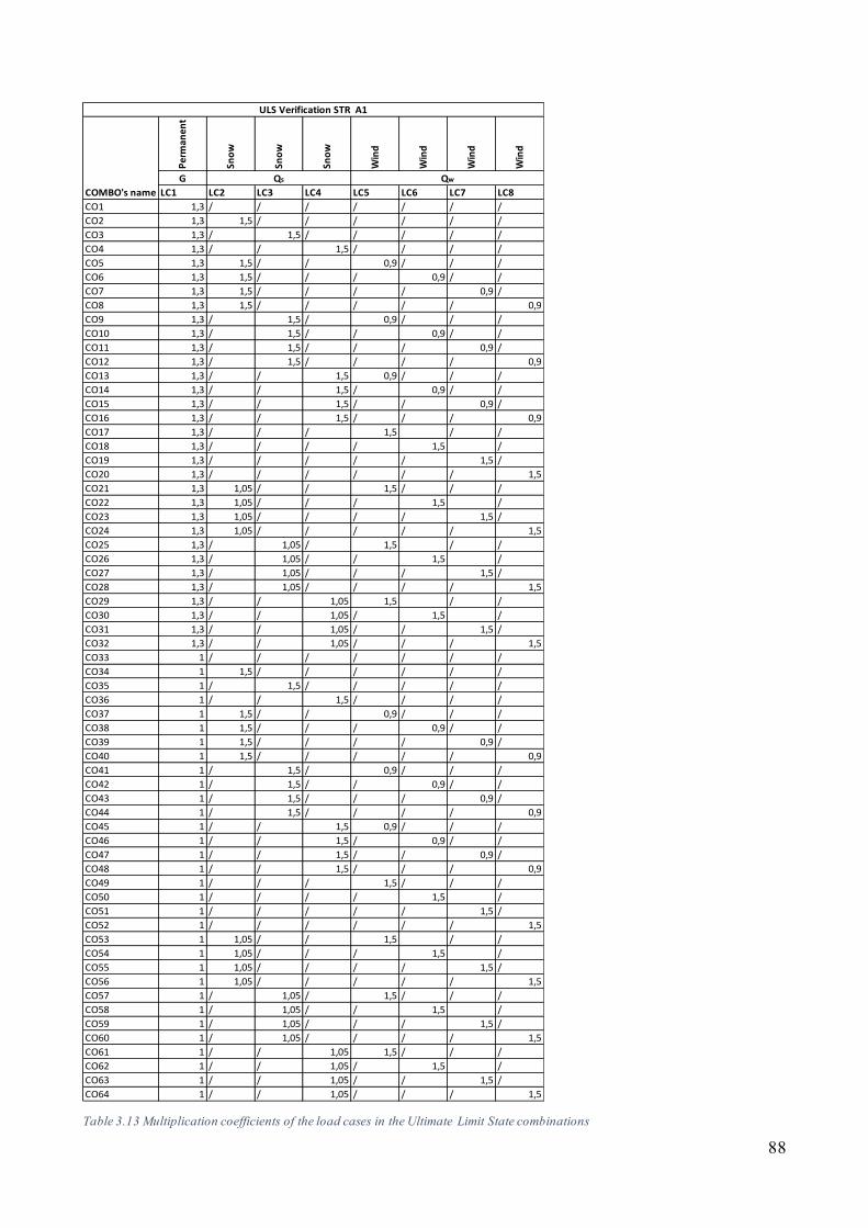
88

Table 3.13 Multiplication coefficients of the load cases in the Ultimate Limit State combinations

Per

man

ent

Sno

w

Sno

w

Sno

w

Win

d

Win

d

Win

d

Win

d

G

LC1 LC2 LC3 LC4 LC5 LC6 LC7 LC8

CO1 1,3 / / / / / / /

CO2 1,3 1,5 / / / / / /

CO3 1,3 / 1,5 / / / / /

CO4 1,3 / / 1,5 / / / /

CO5 1,3 1,5 / / 0,9 / / /

CO6 1,3 1,5 / / / 0,9 / /

CO7 1,3 1,5 / / / / 0,9 /

CO8 1,3 1,5 / / / / / 0,9

CO9 1,3 / 1,5 / 0,9 / / /

CO10 1,3 / 1,5 / / 0,9 / /

CO11 1,3 / 1,5 / / / 0,9 /

CO12 1,3 / 1,5 / / / / 0,9

CO13 1,3 / / 1,5 0,9 / / /

CO14 1,3 / / 1,5 / 0,9 / /

CO15 1,3 / / 1,5 / / 0,9 /

CO16 1,3 / / 1,5 / / / 0,9

CO17 1,3 / / / 1,5 / /

CO18 1,3 / / / / 1,5 /

CO19 1,3 / / / / / 1,5 /

CO20 1,3 / / / / / / 1,5

CO21 1,3 1,05 / / 1,5 / / /

CO22 1,3 1,05 / / / 1,5 /

CO23 1,3 1,05 / / / / 1,5 /

CO24 1,3 1,05 / / / / / 1,5

CO25 1,3 / 1,05 / 1,5 / /

CO26 1,3 / 1,05 / / 1,5 /

CO27 1,3 / 1,05 / / / 1,5 /

CO28 1,3 / 1,05 / / / / 1,5

CO29 1,3 / / 1,05 1,5 / /

CO30 1,3 / / 1,05 / 1,5 /

CO31 1,3 / / 1,05 / / 1,5 /

CO32 1,3 / / 1,05 / / / 1,5

CO33 1 / / / / / / /

CO34 1 1,5 / / / / / /

CO35 1 / 1,5 / / / / /

CO36 1 / / 1,5 / / / /

CO37 1 1,5 / / 0,9 / / /

CO38 1 1,5 / / / 0,9 / /

CO39 1 1,5 / / / / 0,9 /

CO40 1 1,5 / / / / / 0,9

CO41 1 / 1,5 / 0,9 / / /

CO42 1 / 1,5 / / 0,9 / /

CO43 1 / 1,5 / / / 0,9 /

CO44 1 / 1,5 / / / / 0,9

CO45 1 / / 1,5 0,9 / / /

CO46 1 / / 1,5 / 0,9 / /

CO47 1 / / 1,5 / / 0,9 /

CO48 1 / / 1,5 / / / 0,9

CO49 1 / / / 1,5 / / /

CO50 1 / / / / 1,5 /

CO51 1 / / / / / 1,5 /

CO52 1 / / / / / / 1,5

CO53 1 1,05 / / 1,5 / /

CO54 1 1,05 / / / 1,5 /

CO55 1 1,05 / / / / 1,5 /

CO56 1 1,05 / / / / / 1,5

CO57 1 / 1,05 / 1,5 / / /

CO58 1 / 1,05 / / 1,5 /

CO59 1 / 1,05 / / / 1,5 /

CO60 1 / 1,05 / / / / 1,5

CO61 1 / / 1,05 1,5 / / /

CO62 1 / / 1,05 / 1,5 /

CO63 1 / / 1,05 / / 1,5 /

CO64 1 / / 1,05 / / / 1,5

ULS Verification STR A1

COMBO's name

Qs Qw

89

Table 3.14 Multiplication coefficients of the load cases in the Serviceability Limit State combinations

Pe

rman

en

t

Sno

w

Sno

w

Sno

w

Win

d

Win

d

Win

d

Win

d

G

LC1 LC2 LC3 LC4 LC5 LC6 LC7 LC8

CO65 1 / / / / / / /

CO66 1 1 / / / / / /

CO67 1 / 1 / / / / /

CO68 1 / / 1 / / / /

CO69 1 1 / / 0,6 / / /

CO70 1 1 / / / 0,6 / /

CO71 1 1 / / / / 0,6 /

CO72 1 1 / / / / / 0,6

CO73 1 / 1 / 0,6 / / /

CO74 1 / 1 / / 0,6 / /

CO75 1 / 1 / / / 0,6 /

CO76 1 / 1 / / / / 0,6

CO77 1 / / 1 0,6 / / /

CO78 1 / / 1 / 0,6 / /

CO79 1 / / 1 / / 0,6 /

CO80 1 / / 1 / / / 0,6

CO81 1 / / / 1 / /

CO82 1 / / / / 1 /

CO83 1 / / / / / 1 /

CO84 1 / / / / / / 1

CO85 1 0,7 / / 1 / /

CO86 1 0,7 / / / 1 /

CO87 1 0,7 / / / / 1 /

CO88 1 0,7 / / / / / 1

CO89 1 / 0,7 / 1 / /

CO90 1 / 0,7 / / 1 /

CO91 1 / 0,7 / / / 1 /

CO92 1 / 0,7 / / / / 1

CO93 1 / / 0,7 1 / /

CO94 1 / / 0,7 / 1 /

CO95 1 / / 0,7 / / 1 /

CO96 1 / / 0,7 / / / 1

SLS Carachteristic COMBO

COMBO's name

Qs Qw

90

3.3 The Revit model

After completing the structural analysis, the Dlubal model was then exported to Revit in order to

create an architectonical more graphically detailed model; because of interoperability, and

consequentially time related issues, this was accomplished only partially, and only for the case of the

Kingspan panel; the Panelo structural system was not modelled on Revit.

In addition to what defined in Dlubal, the final Revit model includes architectonical details such as

the stratigraphy of the panels, the spline cassettes, the timber edge elements, the wooden door, the

glass wall and the glass door.

The work done will be illustrated in the following paragraphs.

3.3.1 The Panel

The Kingspan company makes available a digital model of their TEK 142 Panel system, which is

accessible on the bimobject platform, a website that allows the download of different BIM models or

“families” uploaded by software producers, manufacturers, etc. The file made available by Kingspan

is shown in Figure 3.42.

Figure 3.42 TEK digital object downloaded from bimobject

As can be seen, only a general geometry given, with one thickness; the different layers composing

the panel are not modelled. However, in addition to this three-dimensional element, the file also

contains information input about the panel’s insulating properties as well as other kinds of data like

91

the “GlobalWarmingPotential” and the Fire rating. Parts of these information are shown in Figure

3.44.

Table 3.15 TEK family provided information

In order to keep this given information, the family was imported on the main model exported from

Dlubal and was then used to perform the modelling of the single panel layers. Details of the modelled

composite panels are shown in the pictures below.

Figure 3.43 Composite panel modelling

92

Figure 3.45 shows the complete south wall, without the insulated splines.

Figure 3.44 South wall with the TEK panels

3.3.2 The Insulated splines and timber edge elements

The insulated spline was modelled according to the indications given by the BBA certificate uploaded

by the company and mentioned in paragraph 2.2; it has base dimensions 100 mm x 112 mm and is

composed in thickness by 15 mm of OSB, 82mm of PUR and 15 mm of OSB.

Details of the spline are shown in Figures 3.45.

Figure 3.45 From the left to the right: detail of the insulated spline, south wall with the spline connections added

93

Moving on, Figure 3.46 and 3.47 show the adding to the model of the timber edge elements and of

the soleplates to be placed between the panel and the foundation. The timber edge elements all have,

as seen in paragraph 2.2.4, dimensions 50 mm x 112 mm while the soleplate has dimensions 40 x

142, because the whole panel base is lying on it.

Figure 3.46 South wall with the added timber edge elements

Figure 3.47 Detail of the panel, the soleplate and the foundation

94

3.3.3 The final geometry

The Figures presented in this paragraph show the final model of the case study as it was made on the

Revit software, following the shape suggested by the structural model made on Dlubal, meaning

including the foundation, the supporting frame, the steel frame-connecting elements, etc.

Figure 3.48 Final Revit model

Following the suggestions given by the TEK specification manual and specified already in paragraphs

2.2.2 and 2.2.3, the TEK panels were lined internally with a 15 mm layer plasterboard, which was

mostly useful (as will be seen in the next chapter) for the prevention of interstitial condensation inside

the panel. The fastening connections of the panels as well of those of the frame members were not

added because of shortness of time.

95

Figure 3.48 Detail of the frame connecting member and of the internal side plasterboard lining

Figure 3.49 View of the east side frame of the building

96

Figure 3.50 The glass wall, the glass door (1m x 2.42 m) and the glass supporting frame

Figure 3.51 View of the building from above

97

3.4 Interoperability

The Dlubal-Revit interoperability was rather problematic. Before exposing the difficulties

encountered when moving from one software to the other though, a reminder must be done of the

definition of interoperability, already introduced in paragraph 1.3.3. In fact, as mentioned in that

paragraph, one of the huge advantages of the BIM methodology is that it allows to create one s ingle

model containing all the information needed about the structure, in the ideal case (which was here not

reached) an As-built digital building that faithfully recreates the real product; however, seeing how

in this thesis two different software are employed and for pages and pages the “Dlubal model” and

the “Revit model” are described, one could get confused about the meaning of “single” model. In

reality, the final BIM model is neither the Dlubal model nor the Revit model nor both, but much more

the IFC file (or a similar standardized type of file, see paragraph 1.3.3 for further specifications) that

is created through these programs and that can then be exported from one software to the other and

be further elaborated by these, in order to get improved in amount of information. In this sense, in

order to achieve real interoperability and test its effectiveness the programs must rely on a common

information exchange reference model, which is indeed the IFC. To do this, the model created on a

software must first be converted to an IFC file, and can then be opened on another software; there are

then tools that allow to convert the opened IFC data in local file format of the employed software (for

example .rvt for Revit). Many programs may have additional tools that allow direct data transfer with

other programs, but this is not interoperability, it’s compatibility.

Returning to the performed work, the two interoperability steps that were performed, or tried to

perform, were all regarding the Kingspan structural model; once from Dlubal to Revit after the

structural analysis to further model the building and once f rom Revit to Dlubal, just for the sake of

testing how well the interoperability in both ways between these two software works.

In the first case of Dlubal to Revit, the interoperability basically didn’t work at all; in fact, the Revit

program, when trying to open the IFC file, always gave error messages. After many trials in different

ways, the Dlubal model was eventually exported on Revit through a compatibility tool offered by

these two software. The result of the exportation are shown in Figures 3.52 and 3.53; as can be seen,

a lot of data regarding the geometry of the structure, like the eccentricity of the members and the

element’s materials was lost. By performing the compatibility different times, different ou tcomes

were obtained. For example, as can be seen, in Figure 3.52 some elements didn’t lose their material

information (the timber frame columns), while in Figure 3.53 all elements lost their information

regarding materials, but less data concerning the sections shapes was lost; in both cases however, a

lot of elaboration had to be performed in order to restore the right geometry.

98

Figure 3.52 Dlubal to Revit compatibility 1st trial

Figure 3.53 Dlubal to Revit compatibility 2nd trial

The Revit to Dlubal interoperability on the other hand worked, but also here with a lot of limitations.

In fact, no additional work only was performed only because the intention was not to further model

the building. However, the Revit model was exported on Dlubal once with an IFC file and once with

the compatibility tool, and the results can be compared in Figures 3.54 and 3.55.

99

Figure 3.54 Revit-Dlubal interoperability with the IFC file

Figure 3.55 Revit-Dlubal compatibility

As can be seen, in the interoperability process (Figure 3.55) the vertical surfaces are kept while all

the columns as well as the foundation members are deleted. On the contrary, with the compatibility

tool (Figure 3.56) all the surfaces are lost while columns and foundation are kept even if with a wrong

geometry. In both cases however, different elements are lost in the process.

100

Chapter 4 Results: Structural analysis, thermal

performance, interstitial condensation and costs

This chapter aims to expose and compare the obtained results in terms of structural and thermal

behaviour of the panels, risk of water vapour condensation and partial costs.

4.1 Structural analysis

The structural analysis was performed on the Dlubal model described in paragraph 3.2, by applying

the loads defined in paragraph 2.5. The verifications at the Fundamental Ultimate Limit State and

Characteristic Serviceability Limit State were applied following indications given by the CNR codes

and the PDF file “Il calcolo dell`XLAM. Basi, normative, progettazione, applicazione” (Bernasconi)

and were done only for the panels since it was the interest of this thesis. The frame elements and the

single connections were not verified.

4.1.1 ULS

4.1.1.1 Kingspan structural model

The following Figures are a graphical representation of the resulting forces obtained for the Ultimate

Limit State Design in the case of the Kingspan structural model.

Figure 4.1 Mx at ULS

101

Figure 4.2 My at ULS

Figure 4.3 Nx at ULS

Figure 4.4 Ny at ULS

102

Table 4.1 shows a sample of the forces per unit length and bending moments per unit length on panel

1 obtained from the structural analysis. The values have been taken dividing the panels in grids of 10

cm * 10 cm.

Table 4.1 Sample of forces in Panel 1 obtained from the structural analysis

Table 4.2 shows the maximum and minimum values for each force and bending moment per unit

length, for all panels.

Table 4.2

Table 4.3 contains the resistance values of the panels already seen in paragraph 2.2.1.

Table 4.3

Surface Grid

No. Point X Y Z mx my mxy vx vy nx ny nxy

1 1 4,800 4,800 0,000 0,04 0,13 0,51 0,16 0,17 13,21 19,21 1,99

-0,04 -0,11 -0,46 -0,19 -0,06 -12,38 -16,32 -2,34

2 4,800 4,900 0,000 0,07 0,11 0,30 0,13 0,93 10,47 10,46 1,83

-0,06 -0,09 -0,28 -0,14 -0,26 -9,95 -9,99 -2,19

3 4,800 5,000 0,000 0,10 0,09 0,08 0,09 1,70 7,72 1,72 1,67

-0,08 -0,08 -0,09 -0,10 -0,46 -7,52 -3,66 -2,03

4 4,800 5,100 0,000 0,15 0,05 0,04 0,07 1,67 5,51 3,56 1,21

-0,12 -0,05 -0,04 -0,07 -0,80 -5,52 -5,05 -1,42

5 4,800 5,200 0,000 0,21 0,01 0,00 0,05 1,64 3,29 5,41 0,74

-0,16 -0,01 0,00 -0,04 -1,14 -3,52 -6,43 -0,80

6 4,800 5,300 0,000 0,20 0,01 0,00 0,05 1,70 2,57 3,06 0,77

-0,14 -0,02 -0,01 -0,04 -1,19 -2,74 -4,23 -0,81

7 4,800 5,400 0,000 0,19 0,00 0,00 0,04 1,76 1,85 0,71 0,79

-0,13 -0,03 -0,01 -0,04 -1,24 -1,96 -2,02 -0,83

8 4,800 5,500 0,000 0,17 0,01 0,01 0,04 1,72 3,11 3,10 0,81

-0,12 -0,02 -0,02 -0,03 -1,16 -2,76 -5,30 -0,84

9 4,800 5,600 0,000 0,15 0,01 0,02 0,03 1,68 4,37 5,49 0,83

-0,11 -0,01 -0,02 -0,03 -1,08 -3,56 -8,58 -0,85

10 4,800 5,700 0,000 0,10 0,05 0,05 0,04 1,79 6,77 4,95 1,58

-0,09 -0,05 -0,05 -0,03 -0,87 -5,58 -6,52 -1,62

11 4,800 5,800 0,000 0,05 0,10 0,08 0,05 1,91 9,18 4,41 2,33

-0,07 -0,09 -0,07 -0,04 -0,66 -7,60 -4,46 -2,38

12 4,800 5,900 0,000 0,03 0,11 0,27 0,11 1,06 11,99 13,08 2,64

-0,05 -0,09 -0,29 -0,10 -0,44 -10,04 -10,28 -2,16

Grid Point Coordinates [m] Moments [kNm/m] Shear Forces [kN/m] Axial Forces [kN/m]

mx my mxy vx vy nx ny nxy

3,48 3,31 0,86 11,16 8,84 23,30 36,77 6,09

max

Moments [kNm/m] Shear Forces [kN/m] Axial Forces [kN/m]

mx my mxy vx vy nx ny nxy

-1,70 -2,10 -0,81 -11,59 -7,92 -20,61 -41,03 -6,16

Axial Forces [kN/m]

min

Moments [kNm/m] Shear Forces [kN/m]

NRd [kN/m] VRd [kN/m] MRd [kN*m/m]

50,4 15,2 10,4

RESISTANCE VALUES

103

Table 4.4 shows, always in samples, the verifications that were performed and the equations they

followed.

Table 4.4 From above to below: Acting-resistance normal stress ratio, shear and normal force verifications

No. Point X Y Z

1 1 4,800 4,800 0,000 0,262103175 0,381150794 0,003846154 0,0125

0,245634921 0,323809524 0,003846154 0,010576923

2 4,800 4,900 0,000 0,207738095 0,207539683 0,006730769 0,010576923

0,197420635 0,198214286 0,005769231 0,008653846

3 4,800 5,000 0,000 0,153174603 0,034126984 0,009615385 0,008653846

0,149206349 0,072619048 0,007692308 0,007692308

4 4,800 5,100 0,000 0,109325397 0,070634921 0,014423077 0,004807692

0,10952381 0,100198413 0,011538462 0,004807692

5 4,800 5,200 0,000 0,065277778 0,10734127 0,020192308 0,000961538

0,06984127 0,127579365 0,015384615 0,000961538

6 4,800 5,300 0,000 0,050992063 0,060714286 0,019230769 0,000961538

0,054365079 0,083928571 0,013461538 0,001923077

7 4,800 5,400 0,000 0,036706349 0,014087302 0,018269231 0

0,038888889 0,040079365 0,0125 0,002884615

8 4,800 5,500 0,000 0,061706349 0,061507937 0,016346154 0,000961538

0,054761905 0,10515873 0,011538462 0,001923077

9 4,800 5,600 0,000 0,086706349 0,108928571 0,014423077 0,000961538

NEd,x/NRd,x NEd,y/NRd,y MEd,x/MRd,x MEd,y/MRd,y

Surface Grid Grid Point Coordinates [m]

Grid VEd,x < VRd VEd,y < VRd NEd,x < NRd NEd,y < NRd

OK OK OK OK

NO CRITICAL AREA NO CRITICAL AREA NO CRITICAL AREA NO CRITICAL AREA

1 OK OK OK OK

OK OK OK OK

2 OK OK OK OK

OK OK OK OK

3 OK OK OK OK

OK OK OK OK

4 OK OK OK OK

OK OK OK OK

5 OK OK OK OK

OK OK OK OK

6 OK OK OK OK

OK OK OK OK

7 OK OK OK OK

OK OK OK OK

8 OK OK OK OK

OK OK OK OK

9 OK OK OK OK

OK OK OK OK

10 OK OK OK OK

OK OK OK OK

11 OK OK OK OK

Point

104

Table 4.5 Bending moment verification

4.1.1.1 Dlubal structural model

The following Figures are a graphical representation of the resulting forces obtained for the Ultimate

Limit State Design in the case of the Dlubal structural model.

Figure 4.5 Mx at ULS

Grid MEd,x < MRd MEd,y < MRd NEd,x/NRd,x + MEd,x/MRd,x <= 1 NEd,y/NRd,y + MEd,y/MRd,y <= 1

OK OK OK OK

NO CRITICAL AREA NO CRITICAL AREA NO CRITICAL AREA NO CRITICAL AREA

1 OK OK OK OK

OK OK OK OK

2 OK OK OK OK

OK OK OK OK

3 OK OK OK OK

OK OK OK OK

4 OK OK OK OK

OK OK OK OK

5 OK OK OK OK

OK OK OK OK

6 OK OK OK OK

OK OK OK OK

7 OK OK OK OK

OK OK OK OK

8 OK OK OK OK

OK OK OK OK

9 OK OK OK OK

OK OK OK OK

10 OK OK OK OK

OK OK OK OK

11 OK OK OK OK

Point

105

Figure 4.6 My at ULS

Figure 4.7 Nx at ULS

Figure 4.8 Ny at ULS

106

Table 4.6 shows a sample of the forces per unit length and bending moments per unit length on panel

1 obtained from the structural analysis. The values have been taken dividing the panels in grids of 10

cm * 10 cm.

Table 4.6 Sample of forces in Panel 1 obtained from the structural analysis

Table 4.7 shows the maximum and minimum values for each force and bending moment per unit

length for all panels.

Table 4.7

Table 4.8 contains the resistance values of the panel already seen in paragraph 2.3.1.

Table 4.8

Surface Grid

No. Point X Y Z mx my mxy vx vy nx ny nxy

1 1 4,800 4,800 0,000 0,05 0,35 0,09 2,45 2,72 2,88 0,36 4,64

-0,07 -0,33 -0,09 -1,69 -1,10 -2,78 -1,11 -5,53

2 4,800 4,900 0,000 0,22 0,35 0,09 2,04 2,72 2,18 0,36 4,64

-0,21 -0,33 -0,09 -1,41 -1,10 -2,19 -1,11 -5,53

3 4,800 5,000 0,000 0,38 0,35 0,09 1,63 2,72 1,47 0,36 4,64

-0,35 -0,33 -0,09 -1,13 -1,10 -1,60 -1,11 -5,53

4 4,800 5,100 0,000 0,51 0,35 0,09 1,24 2,72 0,97 0,36 4,64

-0,47 -0,33 -0,09 -0,85 -1,10 -1,18 -1,11 -5,53

5 4,800 5,200 0,000 0,63 0,35 0,09 0,84 2,72 0,46 0,36 4,64

-0,58 -0,33 -0,09 -0,58 -1,10 -0,75 -1,11 -5,53

6 4,800 5,300 0,000 0,67 0,35 0,09 0,45 2,72 0,47 0,36 4,64

-0,59 -0,33 -0,09 -0,30 -1,10 -0,63 -1,11 -5,53

7 4,800 5,400 0,000 0,72 0,35 0,09 0,06 2,72 0,48 0,36 4,64

-0,60 -0,33 -0,09 -0,03 -1,10 -0,51 -1,11 -5,53

8 4,800 5,500 0,000 0,68 0,40 0,09 0,30 3,11 0,78 1,83 4,53

-0,55 -0,37 -0,09 -0,40 -1,52 -0,66 -2,52 -5,76

9 4,800 5,600 0,000 0,65 0,45 0,09 0,54 3,49 1,08 3,29 4,42

-0,50 -0,41 -0,09 -0,77 -1,93 -0,82 -3,92 -5,99

10 4,800 5,700 0,000 0,51 0,45 0,09 0,86 3,49 1,80 3,29 4,42

-0,40 -0,41 -0,09 -1,24 -1,93 -1,23 -3,92 -5,99

11 4,800 5,800 0,000 0,36 0,45 0,08 1,17 3,49 2,51 3,29 4,42

-0,31 -0,41 -0,09 -1,71 -1,93 -1,64 -3,92 -5,99

12 4,800 5,900 0,000 0,24 0,45 0,09 1,50 3,49 3,49 3,29 4,42

-0,17 -0,41 -0,09 -2,21 -1,93 -2,20 -3,92 -5,99

Grid Point Coordinates [m] Moments [kNm/m] Shear Forces [kN/m] Axial Forces [kN/m]

mx my mxy vx vy nx ny nxy

6,29 11,28 5,38 10,20 12,35 34,18 20,58 8,39

Shear Forces [kN/m] Axial Forces [kN/m]Moments [kNm/m]

max

mx my mxy vx vy nx ny nxy

-6,86 -8,80 -5,40 -9,82 -11,39 -24,55 -59,41 -8,98

Moments [kNm/m] Shear Forces [kN/m] Axial Forces [kN/m]

min

NRd [kN/m]

104,0454545

RESISTANCE VALUES

107

Table 4.9 shows, always in samples, the verifications that were performed and the equations they

followed. Since for the Panelo case only the NRd is given, only the relative verification was performed.

Table 4.9 From above to below: Acting-resistance normal stress ratio, normal force verifications

No. Point X Y Z

1 1 4,800 4,800 0,000 0,026719091 0,010668414

0,020952381 0,003460026

2 4,800 4,900 0,000 0,021048493 0,010668414

0,01412844 0,003460026

3 4,800 5,000 0,000 0,015377894 0,010668414

0,009322848 0,003460026

4 4,800 5,100 0,000 0,011341197 0,010668414

0,004421145 0,003460026

5 4,800 5,200 0,000 0,007208388 0,010668414

0,004517256 0,003460026

6 4,800 5,300 0,000 0,006055046 0,010668414

0,004613368 0,003460026

7 4,800 5,400 0,000 0,004901704 0,010668414

0,007496723 0,017588467

8 4,800 5,500 0,000 0,006343381 0,024220183

0,010380079 0,031620795

9 4,800 5,600 0,000 0,007881171 0,037675841

NEd,x/NRd,x NEd,y/NRd,y

Surface Grid Grid Point Coordinates [m]

Grid NEd,x < NRd NEd,y < NRd

OK OK

Point NO CRITICAL AREA NO CRITICAL AREA

1 OK OK

OK OK

2 OK OK

OK OK

3 OK OK

OK OK

4 OK OK

OK OK

5 OK OK

OK OK

6 OK OK

OK OK

7 OK OK

OK OK

8 OK OK

OK OK

9 OK OK

108

4.1.1.3 The problem of the singularities

When performing a structural analysis on 2D surfaces, it is possible to encounter in the phenomenon

of singularities. Singularities occur in a limited area due to the concentration of the stress-dependent

result values, and are conditioned by the FEA methodology. In theory, the stiffness and/or the stress in

an infinite size concentrate on an infinitesimal small area. They often occur at the corners of the

modelled surfaces and, in reality, those singularities or the resulting stress concentrations do not

occur, at least not in the extent they appear in the model. This represented a huge problem for both

the Kingspan and the Dlubal model, since it was present in both cases and for a long period of time

no solution was found. It was eventually solved in two ways: by applying the function “Average

region” of Dlubal and, following the suggestion of the thesis supervisor, by “not caring too much

about it”, since it obviously doesn’t represent reality.

Figure 4.9 Example of singularity

4.1.2 SLS

4.1.2.1 Kingspan structural model

The following Figure shows the deformation of the Kingspan structural model obtained for the

Serviceability Limit State Characteristic combination.

109

Figure 4.10 Deformation at SLS

Table 4.10 shows a sample of the values of displacement for the single grid points composing Panel

1.

Table 4.10

Surface Grid

No. Point X Y Z ux uy uz jx jy jz

1 1 4,800 4,800 0,000 0,2 0,2 0,2 2,2 0,2 6,7

-0,2 0,0 -0,2 -2,5 -0,2 -6,8

2 4,800 4,900 0,000 0,2 0,2 0,2 3,0 0,2 3,4

-0,2 0,0 -0,2 -3,4 -0,2 -3,5

3 4,800 5,000 0,000 0,2 0,2 0,2 3,8 0,2 0,0

-0,2 0,0 -0,2 -4,3 -0,2 -0,1

4 4,800 5,100 0,000 0,2 0,1 0,1 3,8 0,2 0,0

-0,1 0,0 -0,2 -4,3 -0,2 -0,1

5 4,800 5,200 0,000 0,1 0,1 0,1 3,8 0,2 0,0

-0,1 0,0 -0,1 -4,3 -0,2 -0,1

6 4,800 5,300 0,000 0,1 0,1 0,1 3,9 0,2 0,0

-0,1 0,0 -0,1 -4,3 -0,2 -0,1

7 4,800 5,400 0,000 0,1 0,1 0,1 3,9 0,2 0,0

-0,1 0,0 -0,1 -4,4 -0,2 -0,1

8 4,800 5,500 0,000 0,1 0,1 0,1 3,9 0,1 0,0

-0,1 0,0 -0,1 -4,3 -0,2 -0,1

9 4,800 5,600 0,000 0,1 0,1 0,0 3,8 0,1 0,0

0,0 0,0 -0,1 -4,2 -0,1 -0,1

10 4,800 5,700 0,000 0,0 0,0 0,0 3,9 0,1 0,0

0,0 0,0 0,0 -4,2 -0,1 -0,1

11 4,800 5,800 0,000 0,0 0,0 0,0 3,9 0,1 0,0

0,0 0,0 0,0 -4,2 -0,1 -0,2

12 4,800 5,900 0,000 0,0 0,0 0,0 3,0 0,1 4,0

0,0 0,0 0,0 -3,2 -0,1 -3,9

Grid Point Coordinates [m] Displacements [mm] Rotations [mrad]

110

Figure 4.11 shows an example of deflection of a single panel.

Figure 4.11

Table 4.11 gives a sample of a verification of the deflection of the centre point of the panel 1

considering the average of the deflection at the two edges of the panel. It must be verified that 𝛿 <

𝐿

200.

Table 4.11

0,0

0,5

1,0

1,5

2,0

2,5

3,0

3,5

4,0

4,5

5,0

0 0,2 0,4 0,6 0,8 1 1,2 1,4

δ [m

m]

x [m]

SINGLE PANEL CASE

Panel No H [m] z1 [mm] z2 [mm] zc [mm] zm=(z1+z2)/2 [mm] δ=zm-zc [mm]

1 0 0,2 0,0 0,1 0,1 0,0

1 0 -0,2 0,0 -0,1 -0,1 0,0

1 0,1 0,5 0,2 0,6 0,4 0,3

1 0,1 -0,5 -0,2 -0,5 -0,4 -0,2

1 0,2 0,7 0,4 1,2 0,6 0,7

1 0,2 -0,7 -0,4 -1,0 -0,6 -0,5

1 0,3 1,0 0,7 1,7 0,9 0,9

1 0,3 -1,0 -0,7 -1,4 -0,9 -0,6

1 0,4 1,4 1,0 2,1 1,2 0,9

1 0,4 -1,3 -1,0 -1,8 -1,2 -0,7

1 0,5 1,7 1,3 2,6 1,5 1,1

1 0,5 -1,6 -1,3 -2,2 -1,5 -0,8

1 0,6 2,1 1,7 3,0 1,9 1,1

1 0,6 -2,0 -1,6 -2,5 -1,8 -0,7

1 0,7 2,5 2,0 3,4 2,3 1,2

1 0,7 -2,3 -2,0 -2,9 -2,2 -0,8

1 0,8 2,9 2,4 3,9 2,7 1,3

1 0,8 -2,7 -2,4 -3,3 -2,6 -0,8

1 0,9 3,4 2,8 4,3 3,1 1,2

1 0,9 -3,1 -2,8 -3,7 -3,0 -0,8

δmax,abs [mm] δmin,abs [mm] L [m] L/200 [mm] CHECK

4,3 2,3 1,2 6 OK

111

Figure 4.12 shows an example of deflection of the north wall.

Figure 4.12

Table 4.12 gives a sample of a verification of the deflection of the north wall edge.

Table 4.12 Edge displacement verification of the panels

0

0,5

1

1,5

2

2,5

0,0 10,0 20,0 30,0 40,0 50,0

H [

m]

δ [mm]

Wall case

Wall/Roof L [m] H [m] X [m] zedge//zridge [mm] δ=zedge-zridge [mm]

Edge north wall 2,4 2,4 0 9,6 9,6

Edge north wall 2,4 2,4 0 -8,8 -8,8

Edge north wall 2,4 2,4 0,1 9,6 9,6

Edge north wall 2,4 2,4 0,1 -8,8 -8,8

Edge north wall 2,4 2,4 0,2 9,6 9,6

Edge north wall 2,4 2,4 0,2 -8,9 -8,9

Edge north wall 2,4 2,4 0,3 9,6 9,6

Edge north wall 2,4 2,4 0,3 -9,0 -9,0

Edge north wall 2,4 2,4 0,4 9,6 9,6

Edge north wall 2,4 2,4 0,4 -9,0 -9,0

Edge north wall 2,4 2,4 0,5 9,6 9,6

Edge north wall 2,4 2,4 0,5 -9,0 -9,0

Edge north wall 2,4 2,4 0,6 9,6 9,6

Edge north wall 2,4 2,4 0,6 -9,1 -9,1

Edge north wall 2,4 2,4 0,7 9,6 9,6

Edge north wall 2,4 2,4 0,7 -9,1 -9,1

Edge north wall 2,4 2,4 0,8 9,6 9,6

Edge north wall 2,4 2,4 0,8 -9,1 -9,1

Edge north wall 2,4 2,4 0,9 9,7 9,7

Edge north wall 2,4 2,4 0,9 -9,1 -9,1

Edge north wall 2,4 2,4 1 9,7 9,7

Edge north wall 2,4 2,4 1 -9,1 -9,1

Edge north wall 2,4 2,4 1,1 9,7 9,7

Edge north wall 2,4 2,4 1,1 -9,1 -9,1

|δmax| [mm] |δmin| [mm] L/200 [mm] CHECK

9,7 9,6 12 OK

112

4.1.2.2 Panelo structural model

The following Figure shows the deformation of the Kingspan structural model obtained for the

Serviceability Limit State Characteristic combination.

Figure 4.13 Deformation at SLS

Table 4.13 shows a sample of the values of displacement for the single grid points composing Panel

1.

Table 4.13

Surface Grid

No. Point X Y Z ux uy uz jx jy jz

1 1 4,800 4,800 0,000 0,2 0,2 0,2 2,4 0,2 5,3

-0,2 0,0 -0,2 -2,7 -0,2 -6,6

2 4,800 4,900 0,000 0,2 0,2 0,2 3,3 0,2 2,6

-0,2 0,0 -0,2 -3,6 -0,2 -3,3

3 4,800 5,000 0,000 0,2 0,2 0,2 4,2 0,2 0,0

-0,2 0,0 -0,2 -4,5 -0,2 -0,1

4 4,800 5,100 0,000 0,2 0,1 0,1 4,1 0,2 0,0

-0,1 0,0 -0,2 -4,4 -0,2 -0,1

5 4,800 5,200 0,000 0,1 0,1 0,1 4,1 0,2 0,0

-0,1 0,0 -0,1 -4,3 -0,2 -0,1

6 4,800 5,300 0,000 0,1 0,1 0,1 4,1 0,2 0,0

-0,1 0,0 -0,1 -4,3 -0,2 -0,1

7 4,800 5,400 0,000 0,1 0,1 0,1 4,2 0,2 0,0

-0,1 0,0 -0,1 -4,4 -0,2 -0,1

8 4,800 5,500 0,000 0,1 0,1 0,1 4,2 0,1 0,0

-0,1 0,0 -0,1 -4,3 -0,2 -0,1

9 4,800 5,600 0,000 0,0 0,1 0,0 4,2 0,1 0,0

0,0 0,0 0,0 -4,3 -0,1 -0,1

10 4,800 5,700 0,000 0,0 0,1 0,0 4,3 0,1 0,0

0,0 0,0 0,0 -4,4 -0,1 -0,1

Grid Point Coordinates [m] Displacements [mm] Rotations [mrad]

113

Table 4.14 gives a sample of a verification of the deflection of the centre point of the panel 1

considering the average of the deflection at the two edges of the panel. It must be verified that 𝛿 <

𝐿

200.

Table 4.14

Table 4.15 gives a sample of a verification of the deflection of each wall’s or roof’s edge.

Panel No H [m] z1 [mm] z2 [mm] zc [mm] zm=(z1+z2)/2 [mm] δ=zm-zc [mm]

1 0 0,2 0,0 0,1 0,1 0,0

1 0 -0,2 0,0 -0,1 -0,1 0,0

1 0,1 0,5 0,2 0,5 0,4 0,2

1 0,1 -0,5 -0,2 -0,5 -0,4 -0,2

1 0,2 0,8 0,5 0,9 0,7 0,3

1 0,2 -0,7 -0,5 -0,9 -0,6 -0,3

1 0,3 1,1 0,8 1,4 1,0 0,5

1 0,3 -1,1 -0,8 -1,3 -1,0 -0,4

1 0,4 1,5 1,1 1,8 1,3 0,5

1 0,4 -1,4 -1,1 -1,7 -1,3 -0,5

1 0,5 1,9 1,5 2,2 1,7 0,5

1 0,5 -1,8 -1,5 -2,1 -1,7 -0,5

1 0,6 2,4 1,9 2,6 2,2 0,5

1 0,6 -2,2 -1,9 -2,5 -2,1 -0,5

1 0,7 2,8 2,3 3,1 2,6 0,6

1 0,7 -2,6 -2,3 -2,9 -2,5 -0,5

1 0,8 3,3 2,7 3,5 3,0 0,5

1 0,8 -3,1 -2,8 -3,3 -3,0 -0,4

1 0,9 3,8 3,2 4,0 3,5 0,5

1 0,9 -3,5 -3,3 -3,7 -3,4 -0,3

δmax,abs [mm] δmin,abs [mm] L [m] L/200 [mm] CHECK

1,1 0,7 1,2 6 OK

Wall/Roof L [m] H [m] X [m] zedge//zridge [mm] δ=zedge-zridge [mm]

Edge north wall 2,4 2,4 0 10,4 10,4

Edge north wall 2,4 2,4 0 -9,6 -9,6

Edge north wall 2,4 2,4 0,1 10,4 10,4

Edge north wall 2,4 2,4 0,1 -9,8 -9,8

Edge north wall 2,4 2,4 0,2 10,4 10,4

Edge north wall 2,4 2,4 0,2 -9,9 -9,9

Edge north wall 2,4 2,4 0,3 10,4 10,4

Edge north wall 2,4 2,4 0,3 -10,0 -10,0

Edge north wall 2,4 2,4 0,4 10,5 10,5

Edge north wall 2,4 2,4 0,4 -10,1 -10,1

Edge north wall 2,4 2,4 0,5 10,5 10,5

Edge north wall 2,4 2,4 0,5 -10,2 -10,2

114

Table 4.15 Edge displacement verification of the panels

4.2 Thermal performance

Following the thermal transmittance values defined in the paragraphs 2.2.2 (Table 2.7) and 2.3.2

(Table 2.15) for the Kingspan system and Panelo system, a calculation of a hypothetical thermal

energy needed to keep the internal building environment at 20° C with outside temperatures of -27°

C (minimum temperature according to the NTC 2018) and at -10 °C (assumed average winter

temperature at 3000 m a.s.l.), assuming the door to be insulated with the same characteristics of the

Panels (same thermal transmittance) and the Glass to have thermal transmittance 𝑈 = 1,1 𝑊

𝑚2𝐾18 .

The results are shown in the Tables below.

Table 4.16

18 https://uk.saint-gobain-building-glass.com/en-gb/glass-and-thermal-insulation

Edge north wall 2,4 2,4 0,6 10,5 10,5

Edge north wall 2,4 2,4 0,6 -10,2 -10,2

Edge north wall 2,4 2,4 0,7 10,6 10,6

Edge north wall 2,4 2,4 0,7 -10,3 -10,3

Edge north wall 2,4 2,4 0,8 10,6 10,6

Edge north wall 2,4 2,4 0,8 -10,4 -10,4

Edge north wall 2,4 2,4 0,9 10,6 10,6

Edge north wall 2,4 2,4 0,9 -10,4 -10,4

|δmax| [mm] |δmin| [mm] L/200 [mm] CHECK

10,7 10,6 12 OK

KINGSPAN GLASS Tot

T,e [°C]

T,i [°C]

ΔT [°C]

A [m^2] 84,686 18,95 103,636

U [W/(m^2*K)] 0,2 1,1 0,364566367

Tp,e [°C] -26,624 -24,932 -26,31461523

Tp,i [°C] 18,825 13,5375 17,85817259

ϕ [W/m^2] 9,4 51,7 17,13461924

Q [W] 796,0484 979,715 1775,7634

Con riscaldamento a 20° e temperatura minima

-27

20

47

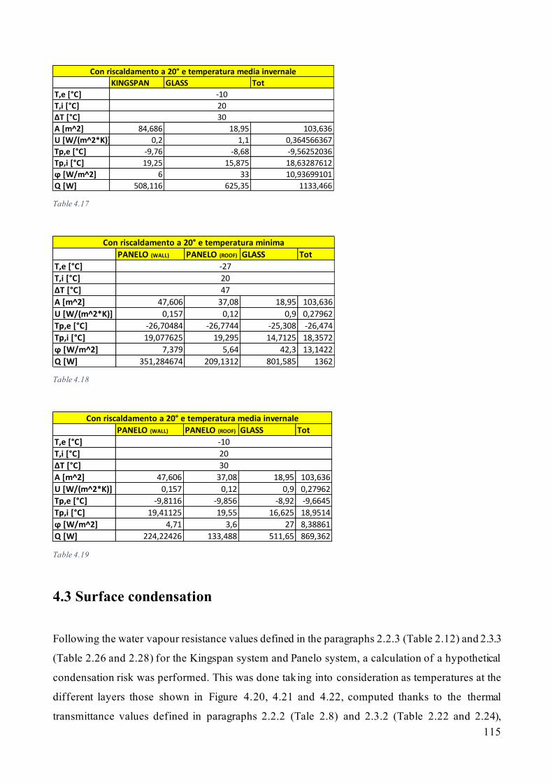
115

Table 4.17

Table 4.18

Table 4.19

4.3 Surface condensation

Following the water vapour resistance values defined in the paragraphs 2.2.3 (Table 2.12) and 2.3.3

(Table 2.26 and 2.28) for the Kingspan system and Panelo system, a calculation of a hypothetical

condensation risk was performed. This was done taking into consideration as temperatures at the

different layers those shown in Figure 4.20, 4.21 and 4.22, computed thanks to the thermal

transmittance values defined in paragraphs 2.2.2 (Tale 2.8) and 2.3.2 (Table 2.22 and 2.24),

KINGSPAN GLASS Tot

T,e [°C]

T,i [°C]

ΔT [°C]

A [m^2] 84,686 18,95 103,636

U [W/(m^2*K)] 0,2 1,1 0,364566367

Tp,e [°C] -9,76 -8,68 -9,56252036

Tp,i [°C] 19,25 15,875 18,63287612

ϕ [W/m^2] 6 33 10,93699101

Q [W] 508,116 625,35 1133,466

Con riscaldamento a 20° e temperatura media invernale

-10

20

30

PANELO (WALL) PANELO (ROOF) GLASS Tot

T,e [°C]

T,i [°C]

ΔT [°C]

A [m^2] 47,606 37,08 18,95 103,636

U [W/(m^2*K)] 0,157 0,12 0,9 0,27962

Tp,e [°C] -26,70484 -26,7744 -25,308 -26,474

Tp,i [°C] 19,077625 19,295 14,7125 18,3572

ϕ [W/m^2] 7,379 5,64 42,3 13,1422

Q [W] 351,284674 209,1312 801,585 1362

-27

20

47

Con riscaldamento a 20° e temperatura minima

PANELO (WALL) PANELO (ROOF) GLASS Tot

T,e [°C]

T,i [°C]

ΔT [°C]

A [m^2] 47,606 37,08 18,95 103,636

U [W/(m^2*K)] 0,157 0,12 0,9 0,27962

Tp,e [°C] -9,8116 -9,856 -8,92 -9,6645

Tp,i [°C] 19,41125 19,55 16,625 18,9514

ϕ [W/m^2] 4,71 3,6 27 8,38861

Q [W] 224,22426 133,488 511,65 869,362

20

30

-10

Con riscaldamento a 20° e temperatura media invernale

116

considering as outside temperature -27 °C and inside temperature 20 °C The different layers

composing the panels are (from the inside to the outside): Plasterboard-15 mm, OSB-15 mm, PUR

112 mm, OSB-15mm for the Kingspan panel, Plasterboard-15 mm, LVL-39 mm, PUR 145 mm, OSB-

15mm for the Panelo wall panel and Plasterboard-15 mm, LVL-27 mm, PUR 195 mm, OSB-15mm

for the Panelo roof panel.

Table 4.20 T-profile Kingspan

Table 4.21 T-profile Panelo wall

-30

-20

-10

0

10

20

30

0 0,05 0,1 0,15 0,2T [°

C] s [m]

T profile Kingspan

stot [mm]

Tpi 18,85308472 0

T2 18,30256539 0,015

T3 17,24387436 0,03

T4 -25,57429608 0,142

Tpe -26,63298711 0,157

T profile

-30

-20

-10

0

10

20

30

0 0,05 0,1 0,15 0,2 0,25T [°

C]

s [m]

T Profile on Wall Panelo

stot [mm]

Tpi 19,11139184 0

T2 18,68485993 0,015

T3 17,0540026 0,054

T4 -25,89539171 0,199

Tpe -26,71564539 0,214

T profile (WALL)

117

Table 4.22 T- profile Panelo roof

All the panels have been lined internally with a plasterboard of thickness 15 mm. Furthermore, the

computation was performed assuming a relative humidity in the inside environment of 70% and for

two cases of relative humidity in the outside environment: on 60% and once 65%.

The Glaser diagram as well as the Tables with the vapour pressure values for both panels and for both

relative humidity cases are shown below.

60% outside relative humidity case:

Table 4.23 Vapour pressure values within the Kingspan panel and saturation pressure values compared

-30

-20

-10

0

10

20

30

0 0,05 0,1 0,15 0,2 0,25 0,3T [°

C]

s [m]

T Profile on Roof Panelo

stot [mm]

Tpi 19,31877804 0

T2 18,9917915 0,015

T3 18,12623888 0,042

T4 -26,1531887 0,237

Tpe -26,78200897 0,252

T profile (ROOF)

Layer Pv [Pa] P,sat [Pa] Condensation

Int 1633,847159 2334,06737 NO

2 673,7566167 2100,118532 NO

3 613,7509578 1964,832979 NO

4 76,10025433 76,17743012 NO

Ext 40,096859 66,82809833 NO

118

Figure 4.14 Glaser diagram within the Kingspan panel

Table 4.24 Vapour pressure values within the Panelo wall panel and saturation pressure values compared

Figure 4.15 Glaser diagram within the Panelo wall panel

0

500

1000

1500

2000

2500

0 0,02 0,04 0,06 0,08 0,1 0,12 0,14 0,16 0,18

P [P

a]

s [m]

Glaser diagram Kingspan

Pv

Pv,s

Layer Pv [Pa] P,sat [Pa] Condensation

Int 1633,847159 2334,06737 NO

2 832,9676111 2150,93606 NO

3 650,767514 1941,394833 NO

4 70,12984204 73,97509545 NO

Ext 40,096859 66,82809833 NO

WALL

0

500

1000

1500

2000

2500

0 0,05 0,1 0,15 0,2 0,25

P [P

a]

s [m]

Glaser diagram on Wall

Pv

Pv,s

119

Table 4.25 Vapour pressure values within the Panelo roof panel and saturation pressure values compared

Figure 4.16 Glaser diagram within the Panelo roof panel

65% outside relative humidity case:

Table 4.26 Vapour pressure values within the Kingspan panel and saturation pressure values compared

Layer Pv [Pa] P,sat [Pa] Condensation

Int 1633,847159 2334,06737 NO

2 899,400016 2150,93606 NO

3 783,724591 1941,394833 NO

4 67,63862685 73,97509545 NO

Ext 40,096859 66,82809833 NO

ROOF

Layer Pv [Pa] P,sat [Pa] Condensation

Int 1633,847159 2334,06737 NO

2 675,7695112 2100,118532 NO

3 615,8896583 1964,832979 NO

4 79,3661757 76,17743012 YES

Ext 43,43826392 66,82809833 NO

120

Figure 4.17 Glaser diagram within the Kingspan panel

Table 4.27 Vapour pressure values within the Panelo wall panel and saturation pressure values compared

Figure 4.18 Glaser diagram within the Panelo wall panel

0

500

1000

1500

2000

2500

0 0,02 0,04 0,06 0,08 0,1 0,12 0,14 0,16 0,18

P [P

a]

s [m]

Glaser diagram

Pv

Pv,s

Layer Pv [Pa] P,sat [Pa] Condensation

Int 1633,847159 2334,06737 NO

2 834,6467091 2150,93606 NO

3 652,8286068 1941,394833 NO

4 73,40828078 73,97509545 NO

Ext 43,43826392 66,82809833 NO

WALL

0

500

1000

1500

2000

2500

0 0,05 0,1 0,15 0,2 0,25

P [P

a]

s [m]

Glaser diagram on Wall

Pv

Pv,s

121

Table 4.28 Vapour pressure values within the Panelo roof panel and saturation pressure values compared

Figure 4.19 Glaser diagram within the Panelo roof panel

4.4 Costs

Following what said in paragraphs 2.2.3 and 2.3.3 about the cost of the panels, a computation of the

total cost of only the panels composing the building studied has been computed. For this computation,

a price of 55 EURO/square meter has been considered for the Kingspan panels and of 60

EURO/square mater for the wall panels as well as 90 EURO/square meter for the roof panels of the

Panelo system. The total cost of the panels for the two cases is given in tables 4.29 and 4.30.

Table 4.29 Total cost of the Kingspan panels

Layer Pv [Pa] P,sat [Pa] Condensation

Int 1633,847159 2334,06737 NO

2 900,9398339 2150,93606 NO

3 785,5069303 1941,394833 NO

4 70,9222886 73,97509545 NO

Ext 43,43826392 66,82809833 NO

ROOF

0

500

1000

1500

2000

2500

0 0,05 0,1 0,15 0,2 0,25 0,3

P [P

a]

s [m]

Glaser diagram on Roof

Pv

Pv,s

Price [EUR/m^2 ] A [m^2] Tot Cost [EUR]

55 91,85 5051,75

Kingspan Panels

122

Table 4.30 Total cost of Panelo panels

In addition, an approximated calculation of a cost of only the supporting frame, without the

connections, has been performed, considering for the frames the cross sections defined in paragraphs

3.2.2. The cost of the wood elements is defined to be 500 EURO/meter cube19. The resulting costs

are given in Tables 4.31 and 4.32.

Table 4.31 Total cost of Kingspan supporting frame

Table 4.32 Total cost of Panelo supporting frame

4.5 Final comparison

From what seen in the results, the Panelo panel provides as expected with much more stiffness to the

structural system, resulting in having similar deformations to the Kingspan structural system with a

much less rigid supporting frame. Nevertheless, this higher stiffness also means, as seen in paragraph

4.1.1, greater stresses inside the panel when subjected to the loads; since, apart from the axial

resistance, all the other strength characteristics of this panel have yet to be defined, it has to be seen

if the panel has enough resistance to resist these loads. Furthermore, paragraph 4.2 shows that the

Panelo panel provides with significant energy savings related to the heating of the inside environment.

However, since the studied structure is a bivouac which most commonly doesn’t have any heating

19Avarage value, https://www.rifaidate.it/pareti-solai/travi/costo-travi-in-legno.asp#:~:text=Per%20quanto%20riguarda%20il%20costo,530%20euro%20per%20metro%20cubo.

Price [EUR/m^2 ] A [m^2] Tot Cost [EUR]

60 54,77 3286,2

Price [EUR/m^2 ] A [m^2] Tot Cost [EUR]

90 37,08 3337,2

6623,4 EURO

Panelo Wall Panels

TOT PANELS

Panelo Roof Panels

Vtot [m^3] Cost [EUR/m^3] Tot cost [EUR]

4,1778 500 2088,9

KINGSPAN

Vtot [m^3] Cost [EUR/m^3] Tot cost [EUR]

2,27448 500 1137,24

PANELO

123

system it is unsure whether these energy savings will also translate into financial savings or if they

“only” result in greater comfort for those arriving in need of shelter; although, from a more general

perspective this represents a clear advantage also economically for other types of building

constructions. In paragraph 4.2, the results clearly show that for the Kingspan panel the condensation

risk is higher, seeing that with slightly increased relative humidity there is interstitial condensation.

Anyhow, for both panels the condensation risk is present, also due to the huge temperature difference

between inside and outside. This is probably attributable to the outer OSB sheet, as can be seen in all

Glaser diagrams shown, which really creates a blocking barrier, and may be solved with the use either

of additional high water vapour resisting plasterboard, or with the use of breather membranes which

allow the blocked water to quickly leave the panels. Finally, paragraph 4.4 exposes a difference in

total price of the employed panels of more than 1500 Euros, which is reasonable considering all the

advantages the Panelo panel provides with, and this difference is already partially balanced by the

smaller total price of the supporting frame. However, to have real comparison of the costs of the

building phase of the facility, one should take into account, apart from the strictly material related

expenses, also the construction phase. In this sense, no research has been done to further deepen the

issue, which leaves a lot of open possibilities for the outcome of total expenses. Considering that the

Panelo system is bigger and heavier than the Kingspan one, it could very well be that more people

are necessary for the assembly of the panels, or, if as seen in paragraph 1.2.1, if the assembly and the

transportation is done by helicopter (which is for these types of structures often the case), it could

significantly reduce the number of panels that the helicopter is able to lift and translate into higher

transportation related expenses.

124

Conclusions and future works

This thesis was initially conceived with the purpose of creating a digital model of a building in the

mountains with the Building Information Modelling. During the course of the work however, the

main aims and leitmotivs changed and evolved while the thesis was taking form, and thanks to the

collaboration with the Leap Factory company it became additionally addressed to a research about

new and innovative construction systems as are the Kingspan TEK and the Panelo system.

For what concerns the conclusions drawn from the performed work and the possible future works on

the topics covered by this thesis, there’s some considerations to be made:

- The Panelo insulated panel could generally speaking be a very convenient construction system

considering the performance and cost comparisons seen with a more “traditional” structural

insulated panel such as the Kingspan one. However, the high number of assumptions made in

this work to study its rendering is a clear evidence that the amount of information given by

the producers is not yet enough to confirm such a statement. It would be interesting to perform

sample laboratory tests on it to gain the missing data, and in that sense, it will just be about

waiting what progresses the next months will bring, since they are in progress right now at

the company. Anyhow, there are plenty of possible future applications regarding not only

extreme environments buildings like the one seen in this thesis but e.g. also normal single-

family houses, for which this system could represent a both in comfort and in finances

appealing solution, and it is to follow how in the next years the product will do on the market.

- The application of both panels on the study case brought decent results in every aspect

addressed by the work, and they are structurally wise surely an appropriate solution for the

building. A further comparison with e.g. the wood framing or the traditional x-lam panels

could also give an idea of their performance and costs compared to the most used wooden

based construction systems in Italy.

- BIM allowed to combine the use of two software to create an accurate model in terms of

quantity, size, shape and material. Still, the complicated interoperability process between the

two employed programs that led to big data losses significantly slowed down the working

progress and partially contributed to preventing the finalisation of adding of architectonical

details such as inside furniture, pavement etc. There is therefore, regarding this aspect, big

room for improvement.

- Modelling two dimensional surfaces in Finite Element Method based programs is certainly

not an easy task if one doesn’t have the appropriate knowledge to begin with; first of all, the

125

stress distribution resulting from load applications is less intuitive than in beam members, and

secondly it presents very tricky obstacles like the singularities which, if one isn’t prepared on

how to handle them, can lead to the loss of a lot of time in the quest of trying to find “fair”

solutions (where with fair what is meant is without the help of any tool given by the software

whose function is specifically that of deleting singularities).

Finally, from a personal point of view, this thesis surely gave me the chance to put to test my skills

learned in those years at the Politecnico di Torino university, and more importantly to learn so much

that I could use for future applications, that it would be hard to put it all into a list; from notions, to

the approach towards the problem, to the interaction with the different people that certainly helped

me during this work. For example, to mention some of the things I surely approached in the wrong

way initially, a very important aspect to follow when creating a digital model of a construction is to

always start with the structural model to dimension the core of the structure before passing on to

software like Revit that allow to increase the graphical information. Secondly, the employed software

definitely does make the difference, both in the structural and in the graphical modelling; decisive

were in this case the possibilities related to the shaping of geometry, the materials and the connection

types. Thirdly, the connection type and its characteristics are when studying wood-based panels

extremely important for the stiffness of the whole system and should be inserted in the structural

model. Lastly, an additional lesson that this thesis gave me is surely to not try to be too perfectionist.

126

Acknowledgments

The conclusion of this thesis means also the conclusion of a very difficult, challenging and beautiful

part of my life which is that of the university studies, which so wouldn’t have come to happen without

the help of many people that I would like to thank.

First of all, I would like to thank my parents for the love and dedication they give me every day, and

for trusting and believing in me also when I give them good reasons not to. Words cannot express the

gratitude I feel for everything you have done for me.

I want to thank my sister and brother, just for being the best siblings and friends I could ask for and

making my life much happier and more interesting than it otherwise would be.

I want to thank my extended family, for being so various and colourful and fill my days with life

when I’m around them, especially my grandparents Enrico e Rosanna and Otto und Magdalene for

allowing me to spend many summers in the mountains with them preparing my exams.

I also want to thank my dearest friends, for having been such supportive and cheerful companions

throughout this journey.

Finally, I am also grateful to my tutors of this thesis, without whose availability and help this work

wouldn’t have been possible.

Thank you all,

Matthias Kather

127

List of Figures:

1.1 Drawing by Charles Vallot, illustrating the “Temple de la Nature” in its original shape. Source:

https://www.researchgate.net/figure/Montenvers-and-the-Temple-de-la-Nature-France-Above-

from-the-left-a-view-of-Mer-de_fig1_336529560

1.2 The “model Rivera”. Source: https://issuu.com/matteoponsetti/docs/tesi_ponsetti_pub

1.3 The Apollonio model and the Berti-Baroni model. Source:

https://issuu.com/matteoponsetti/docs/tesi_ponsetti_pub

1.4 Bivacco Adolfo Hess (Rivera Model), built in 1925; bivacco Ivrea (Apollonio model), built in

1948. Two examples of futuristic shaped bivouacs from the 60s to 90s period: bivacco Bruno Ferrario,

built in 1968 and bivouac du Dolent-La Maye built in 1973. Source:

https://www.inalto.org/it/relazioni/escursionismo/bivacco_hess,

https://www.alpinafriulana.it/soc_alp_friul/rifugi-e-bivacchi-2/bivacco-feruglio/,

http://www.diska.it/rifferrario.asp, https://www.cas-gruyere.ch/fr/cabanes/bivouac-du-dolent/

1.5 Evolution of the shape of the bivouacs in time. Source:

https://issuu.com/matteoponsetti/docs/tesi_ponsetti_pub

1.6 Plinth foundation of the Jubiläumsgrat bivouac; Bivacco Gervasutti, built in 2011. Source:

https://issuu.com/matteoponsetti/docs/tesi_ponsetti_pub,

https://www.youtube.com/watch?v=2dqOpfMOT84

1.7 Productivity of construction industry in comparison with the manufacturing industry and the total

economy. Source:

https://www.mckinsey.com/~/media/mckinsey/industries/capital%20projects%20and%20infrastruct

ure/our%20insights/reinventing%20construction%20through%20a%20productivity%20revolution/

mgi-reinventing-construction-executive-summary.ashx

1.8 Level of Detail descriptions. Source: https://www.trace-software.com/blog/the-level-of-detail-

and-the-level-of-development-in-the-bim-environment/

1.9 Levels of BIM Maturity. Source: https://www.stroma.com/certification/bim/levels

1.10 List of useful BIM tools. Source: https://www.youtube.com/watch?v=wghGeTwH2I4

1.11 Floor plan of the building. Source: Leap Factory

1.12 Cross section and side view of the building. Source: Leap Factory

1.13 Front view of the building. Source: Leap Factory

2. 1 Typical sandwich plate; sign convention, stresses and internal stress resultants. Source:

researchgate.net “High_order_behavior_of_sandwich_plates_with_free_e.pdf”

128

2.2 View of the panels connected by an insulated spline. Source: www.kingspan.com

“116169_Certificate_TEK_BBA_V2.pdf”

2.3 TEK system with ventilated timber cladding. Source: www.kingspan.com “tek-specification-

manual-12th-issue-nov-2018.pdf”

2.4 Connection through timber and cassette spline. Source: www.kingspan.com “tek-specification-

manual-12th-issue-nov-2018.pdf”

2.5 Roof to wall and wall to wall corner connection. Source: www.kingspan.com

25959_ProductBrochure_TEK142StandardDetails_UK.pdf

2.6 Ridge connection without support. Source: www.kingspan.com

25959_ProductBrochure_TEK142StandardDetails_UK.pdf

2.7 Panel-foundation connection. Source: www.kingspan.com

25959_ProductBrochure_TEK142StandardDetails_UK.pdf

2.8 Laminated Veneer Lumber, detail of Panelo panel. Source:

https://www.indiamart.com/proddetail/lvl-plywood-runners-laminated-veneer-lumber-

8838020473.html, https://panelo.eu/wp-content/uploads/2018/07/Brochure-ENG.pdf

2.9 Email by the Panelo company. Source: Priit Vahe, Panelo

2.10 Possible solution of panel and additional layers to improve the panel's performance. Source:

https://panelo.eu/panelo-wall-panels/

2.11 Detail of the gluing between panel and edge and soleplate . Source: https://panelo.eu/wp-

content/uploads/2020/04/PANELO-installation-guide-2020.pdf

2.12 Foundation-wall and wall-roof connection. Source: https://panelo.eu/wp-

content/uploads/2019/09/Conection-of-Floor-Wall-and-Roof-Vol.-1.pdf

2.13 Details of the wall to wall connection. Source: https://panelo.eu/wp-

content/uploads/2019/09/Wall-conection..pdf, https://panelo.eu/wp-

content/uploads/2020/04/PANELO-installation-guide-2020.pdf

2.14 Wall to wall corner joint. Source: https://panelo.eu/wp-content/uploads/2019/09/Wall-

conection..pdf

2.15 E-mail listing the prices for the Panelo panels. Source: Priit Vahe, Panelo

2.16 Map of the Italian wind zones. Source: NTC 2018

2.17 Definition of the pressure coefficient. Source: NTC 2018

2.18 Geometry of the structure

2.19 Map of the Italian snow zones. Source: NTC 2018

2.20 Load conditions for a double-pitched roof. Source: NTC 2018

2.21 Map of the Italian temperature zones. Source: NTC 2018

129

2.22 Temperature trend within the structural components. Source: NTC 2018

3.1 First model created in Revit

3.2 Robot model, imported from Revit

3.3 Robot model with elaborated structural framework

3.4 North side and east side of the building

3.5 South side and west side of the building

3.6 Details of the supporting frame

3.7 Detail of the east wall frame and the glass wall supporting frame

3.8 Modelling of the section of the north wall edge truss element and detail of it within the structure

3.9 Modelling of the section of the roof ridge truss element and detail of it within the structure

3.10 Modelling of the section of the north wall edge truss element and detail of it within the structure

3.11 Cross section of the steel foundation elements

3.12 Spring constants of the foundation members

3.13 Details of the foundation and its constraints

3.14 North side and east side of the building

3.15 South side and west side of the building

3.16 Panel to panel to frame connection. The red line represents the gluing material.

3.17 Wall to wall to frame connection

3.18 Line hinges in the Dlubal software

3.19 Deformed shape of the connection

3.20 Real connection and fictitious connection. Source:

https://www.scielo.br/scielo.php?script=sci_arttext&pid=S1516-14392008000200007

3.21 Input for the line hinge modelling at the ULS

3.22 Modelling of the panel-foundation connection

3.23 The separate "frame" model

3.24 Details and representation of the north side edge frame connection

3.25 Side and front view of the east side edge frame connection

3.26 Close views of the east side edge frame connection

3.27 Modelling of the connection by RF Joints, output stiffness values of the connection

3.28 Modelling of the member line hinge on the Kingspan structural model

3.29 Rendering in the Kingspan structural model of the connection

3.30 Details of the ridge connection

3.31 Details of the south side frame connection

3.32 Details of the columns foundation connection

130

3.33 Modelling of the connection by RF Joints, output stiffness values of the connection

3.34 Modelling of the member line hinge on the Kingspan structural model, rendering in the Kingspan

structural model of the connection

3.35 Definition and application of the load case Snow 1

3.36 Definition and application of the load case Snow 2

3.37 Definition and application of the load case Snow 3

3.38 Definition and application of the load case Wind 1

3.39 Definition and application of the load case Wind 2

3.40 Definition and application of the load case Wind 3

3.41 Definition and application of the load case Wind 4

3.42 TEK digital object downloaded from bimobject

3.43 Composite panel modelling

3.44 South wall with the TEK panels

3.45 Detail of the insulated spline, south wall with the spline connections added

3.46 South wall with the added timber edge elements

3.47 Detail of the panel, the soleplate and the foundation

3.48 Detail of the frame connecting member and of the internal side plasterboard lining

3.49 View of the east side frame of the building

3.50 The glass wall, the glass door (1m x 2.42 m) and the glass supporting frame

3.51 View of the building from above

3.52 Dlubal to Revit compatibility 1st trial

3.53 Dlubal to Revit compatibility 2nd trial

3.54 Revit-Dlubal interoperability with the IFC file

3.55 Revit-Dlubal compatibility

4.1 Mx at ULS

4.2 My at ULS

4.3 Nx at ULS

4.4 Ny at ULS

4.5 Mx at ULS

4.6 My at ULS

4.7 Nx at ULS

4.8 Ny at ULS

4.9 Example of singularity

4.10 Deformation at SLS

131

4.11

4.12

4.13 Deformation at SLS

4.14 Glaser diagram within the Kingspan panel

4.15 Glaser diagram within the Panelo wall panel

4.16 Glaser diagram within the Panelo roof panel

4.17 Glaser diagram within the Kingspan panel

4.18 Glaser diagram within the Panelo wall panel

4.19 Glaser diagram within the Panelo roof panel

List of Tables:

2.1 Density of panel components. Source:

https://www.bbacerts.co.uk/uploads/files/CertificateFiles/ET/ETA-11_0466i2.pdf

2.2 Density and selfweight of the panel.

2.3 Structural properties - limit state design - TEK 142. Source: www.kingspan.com

“116169_Certificate_TEK_BBA_V2.pdf”

2.4 Bending and shear rigidity of the panel. Source:

https://www.bbacerts.co.uk/uploads/files/CertificateFiles/ET/ETA-11_0466i2.pdf

2.5 Thermal conductivities of the TEK Kingspan components. Source: www.kingspan.com

“116169_Certificate_TEK_BBA_V2.pdf”

2.6 R values of the system. Source: www.kingspan.com “116169_Certificate_TEK_BBA_V2.pdf”

2.7 Example panel thermal transmittance. Source: www.kingspan.com

“116169_Certificate_TEK_BBA_V2.pdf”

2.8 Example of calculation of the thermal transmittance U with 15 mm plasterboard

2.9 Example of calculation of the thermal transmittance U without 15 mm plasterboard

2.10 U values in function of thickness of TEK and thermawall. Source: www.kingspan.com “tek-

specification-manual-12th-issue-nov-2018.pdf”

2.11 Vapour diffusion factor of the TEK components. Source: www.kingspan.com

“116169_Certificate_TEK_BBA_V2.pdf”

2.12 Water vapour resistance and permeance of the wall composed by the TEK system and a 15 mm

plasterboard

2.13 Water vapour resistance and permeance of the wall composed only by the TEK system

132

2.14 Fastener indications given by the TEK 142 brochure. Source: www.kingspan.com

25959_ProductBrochure_TEK142StandardDetails_UK.pdf

2.15 Wall and roof panel geometry and U-values. Source: https://panelo.eu/panelo-wall-panels/,

https://panelo.eu/panelo-roof-ceiling-panels/

2.16 System's unit mass in kg/m^2. Source: https://panelo.eu/brochures/

2.17 Different unit measure conversions of the applied load

2.18 kmod factor for different materials. Source: CNR-DT-206-R1-2018

2.19 Partial safety factor according to the NTC 2018 and to the CNR. Source: NTC 2018, CNR-DT-

206-R1-2018

2.20 NRd design values

2.21 NRd design values second iteration

2.22 Example of calculation of the thermal transmittance U of the wall panel with 15 mm plasterboard

2.23 Example of calculation of the thermal transmittance U of the wall panel without 15 mm

plasterboard

2.24 Example of calculation of the thermal transmittance U of the roof panel with 15 mm plasterboard

2.25 Example of calculation of the thermal transmittance U of the roof panel without 15 mm

plasterboard

2.26 Water vapour resistance and permeance of the wall composed by the Panelo wall system and a

15 mm plasterboard

2.27 Water vapour resistance and permeance of the wall composed only by the Panelo wall system

2.28 Water vapour resistance and permeance of the roof composed by the Panelo roof system and a

15 mm plasterboard

2.29 Water vapour resistance and permeance of the roof composed only by the Panelo roof system

2.30 Classification of the categories of exposure. Source: NTC 2018

2.31 Calculation of the reference wind pressure and the tangential wind pressure

2.32 Calculation of the wind pressures

2.33 Inclination of the roof surfaces

2.34 Calculation of snow load cases

2.35 Contribution of the solar radiation. Source: NTC2018

2.36 Input data for the calculation of the ∆T values

2.37 Calculation of the temperature variations without a heating source

2.38 Calculation of the temperature variations with a heating source

2.39 Thermal expansion coefficients. Source: NTC2018

3.1 Kingspan material properties input in the program

133

3.2 Stiffness values in the two main directions of the panel

3.3 Stiffness values of OSB, KINGSPAN and PANELO

3.4 Calculation of the PUR stiffness

3.5 Calculation of the Panelo wall and roof panels stiffnesses

3.6 Dimensions and exposure of the panels

3.7 Dimensions and exposure of the panels

3.8 Kser, Keq,ser and Ku

3.9 Kser and Ku of the panel foundation bolt fasteners

3.10 Stiffness values of the panel to panel to frame connections

3.11 Partial safety and contemporaneity coefficients

3.12 List of load cases and load types

3.13 Multiplication coefficients of the load cases in the Ultimate Limit State combinations

3.14 Multiplication coefficients of the load cases in the Serviceability Limit State combinations

3.15 TEK family provided information

4.1 Sample of forces in panel 1 obtained from the structural analysis

4.2

4.3

4.4 Acting-resistance normal stress ratio, shear and normal force verifications

4.5 Bending moment verification

4.6 Sample of forces in panel 1 obtained from the structural analysis

4.7

4.8

4.9 Acting-resistance normal stress ratio, normal force verifications

4.10

4.11

4.12 Edge displacement verification of the panels

4.13

4.14

4.15 Edge displacement verification of the panels

4.16

4.17

4.18

4.19

4.20 T-profile Kingspan

134

4.21 T-profile Panelo wall

4.22 T-profile Panelo roof

4.23 Vapour pressure values within the Kingspan panel and saturation pressure values compared

4.24 Vapour pressure values within the Panelo wall panel and saturation pressure values compared

4.25 Vapour pressure values within the Panelo roof panel and saturation pressure values compared

4.26 Vapour pressure values within the Kingspan panel and saturation pressure values compared

4.27 Vapour pressure values within the Panelo wall panel and saturation pressure values compared

4.28 Vapour pressure values within the Panelo roof panel and saturation pressure values compared

4.29 Total cost of the Kingspan panels

4.30 Total cost of Panelo panels

4.31 Total cost of Kingspan supporting frame

4.32 Total cost of Panelo supporting frame

Bibliography:

“Rifugi e bivacchi. Gli imperdibili delle Alpi”, Dini Roberto, Gibello Luca, Girodo Stefano, Hoepli

ed. 2018.

“BIVACCHI ALPINI: storia, attualità, futuro di unità abitative minime delle Alpi”, Ponsetti Matteo,

thesis, 2013.

“REINVENTING CONSTRUCTION: A ROUTE TO HIGHER PRODUCTIVITY”, McKingsey &

Company, 2017.

“Structural Health Monitoring through the Building Information Modelling”, Hernandez Luis, thesis,

2019.

“Applicazioni di termofisica dell’edificio e climatizzazione”, Corrado Vincenzo, Enrico Fabrizio,

Clut ed. 2009.

“BIM for heritage science: a review”, Pocobelli Danae Phaedra, Boehm Jan, Bryan Paul, Still James

& Grau-Bové Josep, 2018.

“A Brief History of BIM”, Quirk Vanessa, 2012.

“THE VARIOUS DIMENSIONS OF BIM EXPLAINED”, https://www.constructionlifecycle.com/,

2018.

“Building Information Modeling (BIM): cos’è, stato di adozione in Italia e nel mondo”, Camerini

Danilo, 2019.

“STATE OF ART IN THINKING OF BIM COMPETENCE”, Yakami Manish, 2016.

135

“The True Cost of SIPs. A Comprehensive Tool for Comparing the Price of Residential Structural

Insulated Panel and Stick Frame Construction”, Meis Adam, thesis, 2015.

“Condensa interstiziale, Metodo Glaser”, Corso di Fisica Tecnica a.a. 2017/2018, Prof. Marina

Mistretta.

“NORME TECNICHE PER LE COSTRUZIONI”, MINISTERO DELLE INFRASTRUTTURE E

DEI TRASPORTI, 2018.

“Il calcolo dell`XLAM. Basi, normative, progettazione, applicazione”, Bernasconi Andrea.

“Eurocode 5: Design of timber structures - Part 1-1: General -Common rules and rules for buildings”,

EUROPEAN COMMITTEE FOR STANDARDIZATION, 2004.

“Istruzioni per la Progettazione, l’Esecuzione ed il Controllo delle Strutture di Legno.” Consiglio

Nazionale delle Ricerche DT 206–R1, 2018.

“Una procedura numerica per il progetto di edifici in X–Lam”, Scotta Roberto, Zecchetto

Massimilano, 2015.

“Design of Connections in Timber Structures: A state-of-the-art report by COST Action FP1402 /

WG3, Shaker Verlag Aachen, 2018.”, Sandhaas Carmen, Munch-Andersen Jørgen, Dietsch Philipp,

2018.

“Wood: MechanicalFasteners”, Rammer Robert, 2016.

“Standard details FOR 142 MM STRUCTURAL INSULATED PANELS”, Kingspan, 2015

“Azioni del vento sulle costruzioni, guida al calcolo”, Furucolo Nicola, 2016

“Mechanical shear properties of adhesives”, E.M.P. Huveners, F. van Herwijnen, F. Soetens and H.

Hofmeyer, 2007

Sitography:

https://www.trinitybuildingsystems.com/what-are-sips/

https://www.sips.org/about/what-are-sips

https://www.bbacerts.co.uk/uploads/files/CertificateFiles/ET/ETA-11_0466i2.pdf

http://www.builddesk.co.uk/wp-content/uploads/2013/01/vapourResistances.pdf

https://www.united-bim.com/leading-countries-with-bim-

adoption/#:~:text=Scandinavian%20Region,in%20BIM%20adoption%20and%20implementation

https://www.autodesk.com/solutions/bim/benefits-of-bim

http://www.axdstudio.com/bim-dimensions/

https://www.metsawood.com/global/Tools/MaterialArchive/MaterialArchive/Kerto-manual-lvl-

moisture-behaviour.pdf

136

https://www.pollmeier.com/de, Allgemeine Bauartgenehmigung BauBuche Platte Z-9.1-838.pdf

https://baldolegnami.it/media/osb.pdf

https://www.dataholz.eu/fileadmin/dataholz/media/baustoffe/Datenblaetter_de/osb_de_01.pdf

https://en.wikipedia.org/wiki/Laminated_veneer_lumber

https://www.british-gypsum.com/technical-advice/faqs/063-what-is-the-vapour-resistance-of-

gyproc-wallboard-duplex-plasterboard

https://www.contorion.de/befestigungstechnik/simpson-sparrennagel-

77357000?$ps=125&diameter1=6&nail_length=210&simple_sku=2312909

https://www.amazon.co.uk/Fixman-413678-Galvanised-Ring-Nails/dp/B07663W5WV

https://www.ffx.co.uk/tools/product/Dewalt-Dnpt31R90G12Z-5902013961369-Galvanised-Ring-

Nails-3.1-X-90Mm-Box-Of-2200

http://www.4dhardware.com.au/uploads/smartframe_lvl18_design_guide_colour[1].pdf

https://panelo.eu/wp-content/uploads/2018/07/Brochure-ENG.pdf

https://panelo.eu/wp-content/uploads/2020/04/PANELO-installation-guide-2020.pdf

https://www.kingspan.com/, tek-specification-manual-12th-issue-nov-2018.pdf

http://www.acmepanel.com/sip-prices.asp

https://www.toolstop.co.uk/dewalt-dnpt3190g12z-galvanised-plain-shank-timber-nails-3-1mm-x-

90mm-box-of-2200/

https://webshop.schachermayer.com/cat/de-IT/product/sparrennagel-6-0x210-verzinkt/104445152

https://panelo.eu/

https://www.swisskrono.pl/en/mdb/OSB-boards/Technical-Data

https://puutuoteteollisuus.fi/images/pdf/LVL_bulletin_eng.pdf

https://eurocodes.jrc.ec.europa.eu/doc/WS2008/Holicky_Markova_2008.pdf

https://www.rifaidate.it/pareti-solai/travi/costo-travi-in-

legno.asp#:~:text=Per%20quanto%20riguarda%20il%20costo,530%20euro%20per%20metro%20c

ubo

https://www.westfieldfasteners.co.uk/Wood-Screws/Chipboard-Wood-Screw-Torx-Countersunk-

8x150-A2-Stainless.html

https://www.stark-suomi.fi/fi/eristyskaista-isover-sk-c-20x200-mm-14-m