Wairau River-Wairau Aquifer Interaction - Envirolink

Wairau River-Wairau Aquifer Interaction

Report 1003-5-R1

Scott Wilson, Thomas Wöhling

Lincoln Agritech Ltd

10 February 2015

Registered company office:

Lincoln Agritech Limited

Engineering Drive, Lincoln University

Lincoln 7640

Christchurch

New Zealand

PO Box 69133

Ph: +64 3 325 3700

Fax: +64 3 325 3725

Document Acceptance:

Action Name Date

Prepared by

Scott Wilson

10 Feb 2015

Reviewed by

Roland Stenger 6 Feb 2015

Approved by

Hugh Canard 6 Feb 2015

Wairau River-Wairau Aquifer Interaction Investigation (2014) Page 2

EXECUTIVE SUMMARY

This report presents initial findings from an investigation into understanding the nature of transient recharge from

the Wairau River to the Wairau Aquifer. This investigation has been a year-long collaboration between

Marlborough District Council (MDC), the Water & Earth System Science Competence Cluster (WESS) at University

of Tübingen in Germany, and Lincoln Agritech.

The intention of this phase of the Wairau Aquifer recharge project is twofold:

To review our conceptual understanding of the river and aquifer, and identify knowledge gaps

To develop a numerical model to quantify the river-aquifer exchange based on that conceptual

understanding

Historical flow gauging data shows that approximately 7.5 m3/s is recharged from the river to the Wairau Aquifer

between Rock Ferry and Wratts Road at flows less than 20 m3/s. Temporary flow sites have been established at

Rock Ferry, SH6 and Wratts Road, and a good flow-rating curve has been established at Rock Ferry. The difference

between flows at Rock Ferry and SH1 indicates that aquifer recharge increases as the river flow increases. The

preliminary evidence suggests that 15 m3/s or more may be lost as recharge pulses during high flow events,

although further work is required to correct flow for time lags in the river which will improve these estimates.

One of the key findings of this report is that the river appears to be perched above the Wairau Aquifer across its

main recharge reach. This means that there is a vertical hydraulic gradient between the river and aquifer where

most of the recharge occurs, which theoretically simplifies the calculation for estimating transient recharge rates.

Another key finding is that the hydraulic nature of the aquifer is more complex than our previous simple

unconfined aquifer conceptual model. Groundwater monitoring records and aquifer test data indicate that the

aquifer is highly stratified. This stratification explains the observation that the aquifer may be perched. The reason

for this is that a strong vertical to horizontal anisotropy in permeability enables groundwater to potentially drain

faster than it can be recharged by the river. There is also the possibility of distinct upper and lower aquifer

horizons, although this needs to be explored further.

The implication of aquifer stratification for estimating river recharge is that the groundwater monitoring sites are

representative of quite localised conditions. Therefore, for the prediction of recharge rates, groundwater data can

be used to constrain hydraulic parameters within our numerical model, but it is preferable to calculate recharge

rates based on river observations rather than changes in groundwater levels at a particular site. Furthermore, if

the is indeed river perched over its main recharge reach, as the available evidence suggests, the prediction of

transient recharge rates will be largely determined by river geometry, and the relationship between stage and

wetted river bed perimeter.

A steady state numerical model has been built and calibrated to accord with our conceptual understanding. A

combination of groundwater level observations and surface water fluxes were used for calibration targets. The

best-fit "compromise" solution resulted in data fits that are well within the measurement uncertainty ranges. One

of the key findings of the model was that the river was required to be perched to enable calibration, which

supports field evidence outlined in this report.

Further work for 2015 will involve a more intensive field program to improve our understanding of the relationship

between river flows and groundwater levels immediately adjacent to and beneath the river. Transient calibration

of the numerical model will also begin, and we intend to use the final calibrated model to estimate transient

aquifer recharge rates.


TABLE OF CONTENTS

Executive summary 2

Table of contents 3

List of figures 5

List of tables 6

Introduction 7

Study objectives 7

Scope & nature of the services 7

Hydrological setting 8

Steady state aquifer mass balance 9

Transient river mass balance 10

Background Theory to surface water-groundwater exchange 12

Definitions 13

Hydrogeology 14

Aquifer structure and properties 14

Aquifer internal structure 14

Aquifer stratification 15

Conders monitoring bores 16

Aquifer properties 19

Discussion 21

River flow and structure 22

Flow profiles 22

Flow time lags 24

River structure 25

River and aquifer surfaces 25

Geological control on river losses 27

River geometry 28

Groundwater observations 30

Hydraulic reponse to flow events 30

Riparian boreholes 31


Conders recharge bore 31

Pauls Road 32

River-aquifer relationship 34

1-D assessment 34

Oxygen isotopes 36

Temperature records 38

Numerical groundwater flow model 40

Model setup 40

model structure and extent 40

Boundary conditions 41

Observations 42

Properties 42

Model calibration 42

Model insights 43

Future Work 45

References 46


LIST OF FIGURES

Figure 1 The Wairau River at a relatively stable reach at SH6 .......................................................................................9

Figure 2 Location of MDC flow and river stage recorder sites ....................................................................................10

Figure 3 Time series of surface water inflows and discharges ....................................................................................11

Figure 4 Flow difference between Rock Ferry and SH1 compared to flow .................................................................11

Figure 5 Different flow regimes between surface water and groundwater (figure based on Winter et al. 1998;

Brunner et al. 2009a)...................................................................................................................................................12

Figure 6 Theoretical flow exchange between surface water and groundwater (from Brunner et al. 2009a). ...........12

Figure 7 Photograph of the Rapaura Formation at Foxes Island Quarry (from Brown, 1981) ....................................14

Figure 8 Illustration of the compounding effect that anisotropy has on vertical flow with depth .............................15

Figure 9 Schematic diagram showing how the Wairau Aquifer is stratified ...............................................................16

Figure 10 Monitoring records for Conders bores P28w/0398 and P28w/3821 ..........................................................17

Figure 11 Composite long term groundwater level at P28w/0398 .............................................................................17

Figure 12 Mean annual Wairau River flow at SH1 .......................................................................................................18

Figure 13 Relationship between mean monthly river flow and groundwater level at Conders .................................19

Figure 14 Locations of aquifers tests in the unconfined Wairau Aquifer ....................................................................19

Figure 15 Aerial photograph of the Wairau River upstream of Conders Bend ...........................................................22

Figure 16 Historical flow gauging profiles down the Wairau River .............................................................................23

Figure 17 Summary of historic Wairau River concurrent flow gauging surveys ..........................................................24

Figure 18 Graphical example of the probability approach for predicting time lags ....................................................24

Figure 19 Example Lidar image of the Conders area ...................................................................................................25

Figure 20 Composite piezometric survey across the Wairau Aquifer including river elevations ................................26

Figure 21 Longitudinal hydrological profile along the Wairau River from Conders to Giffords Road .........................26

Figure 22 Simplified longitudinal profile for the whole Wairau Plain .........................................................................27

Figure 23 Relationships between stage (h), flow (Q), cross-sectional area (A), and wetted perimeter (wp) at the SH1

recorder site ................................................................................................................................................................29

Figure 24 Groundwater and river flow hydrographs for the summer-autumn 2014 period ......................................30

Figure 25 Response at groundwater monitoring sites to a flow event during stable conditions ...............................31

Figure 26 Schematic representation of hydraulically connected (above) and disconnected (below) scenarios at the

Conders recharge bore ................................................................................................................................................32

Figure 27 Stratigraphic log for bore P28w/3950 .........................................................................................................33

Figure 28 Relationship between wetted perimeter width and river-aquifer head difference at the recharge bore ..35

Figure 29 Map of median Oxygen-18 isotope values ..................................................................................................36


Figure 30 Schematic profiles across the SH6 area showing hydraulically connected and disconnected scenarios ....37

Figure 31 Groundwater and Wairau River temperature monitoring records .............................................................38

Figure 32 Map showing the main elements for setting up the Modflow model.........................................................40

Figure 33 Simulated river exchange fluxes along the Wairau River as estimated with the best-fit parameter set ....43

Figure 34 Proposed MDC test sites and Wairau River/groundwater elevation survey arrays ....................................45

LIST OF TABLES

Table 1 Estimated representative average annual and summer water balances .........................................................9

Table 2 Recent aquifer test results for the Rapaura area ...........................................................................................20

Table 3 Summary of historical concurrent flow gaugings on the Wairau River ..........................................................23

Table 4 Historical riparian monitoring bore records and adjacent river level from Lidar survey................................31

Table 5 Representative parameter values for assessing hydraulic connectivity .........................................................34

Table 6 Temperature monitoring sites and their characteristic responses .................................................................38


INTRODUCTION

STUDY OBJECTIVES

The main objective of this study is to understand the process of recharge from the Wairau River to the Wairau

Aquifer. This includes understanding the factors that the river-groundwater exchange is most sensitive to. An

additional objective is to develop a steady state numerical model of the river and aquifer to quantify the exchange

fluxes. The steady state model is a critical step for testing the conceptual model and developing a transient model.

SCOPE & NATURE OF THE SERVICES

The scope of the study is specified in the project brief of 7 March 2014 and is as follows:

A review of the model development process, the assumptions used and a description of the model

structure

Discussion of the lessons learnt through the modelling process in terms of the drivers of Wairau Aquifer

recharge from the Wairau River. Where to next in terms of research or other approaches to try if there

are no firm conclusions

Assess whether it is practical to measure the real time recharge rate for allocation purposes using

measurements of:

a) driving head in conjunction with aquifer permeability

b) driving head in conjunction with wetted area, recharge reach length and channel bed permeability

Evaluate whether the Wairau River is perched above the Wairau Aquifer or is hydraulically embedded

within it


HYDROLOGICAL SETTING

The Wairau River is classified as a braided river system. A braided river forms in an environment where there is an

abundant supply of sediment or in a situation where the slope of the land is high, such as an alluvial fan. One of

the main characteristics of a braided river is its ability to erode the surrounding sediments. A stream with cohesive

banks that are resistant to erosion will form narrow, deep, meandering channels, whereas a stream with highly

erodible banks will form wide, shallow channels, resulting in the formation of braids. The combination of bank

erosion with a large sediment load results in a highly dynamic river bed morphology. Sediments in the active

channel are continuously being mobilised by the river, particularly during high flow events.

While the Wairau River is considered to be a braided river, its character has been modified immensely by river

flood works since the early 1900s. The history of river control works on the Wairau Plain is documented in Rae

(1987). One of the major early developments was to stem the flow of flood water from the Wairau River onto the

plain via the Opawa River (originally a major braid channel of the Wairau) by the building of the Conders Groyne in

1914-1926. By the 1960s a stop-bank network had been built to form a defined floodway with a purpose to

constrain flow during flood events. This network flood control system has remained in more or less in the same

position to the present day.

The river engineering works have resulted in fairly radical changes to the way the river operates, and also how

groundwater recharge occurs. Prior to the river works, the river had the freedom to widely across the Wairau Plain

so that the location of the channel was highly mobile. This freedom also meant that the location and volume of

recharge from the river to the Wairau Aquifer shifted considerably in space and though time.

Prior to the onset of engineering works, the river bed would have been much wider than its current form. Its

greater width would have potentially allowed a higher rate of flow loss than the present day. It is not

inconceivable that the river was historically ephemeral, with all of its flow lost during dry periods to the

unconfined aquifer prior to reaching the springs and wetlands along the edge of the Dillons Point Formation

aquitard. By contrast, the recent creation of a restrictive floodway river has trained the river into a comparatively

narrow and channelised form. The result of this training of the river has been to decrease the effective width of

the river, which turn has likely to have reduced the volume of recharge to the Wairau Aquifer.

Despite the controlling effect of the flood-works, the river remains braided in character, and this poses a number

of problems for characterising its flow and recharge to the aquifer. The braided nature of the river, and the high

permeability of sediments associated with the active channel make it extremely difficult to measure the flow at

any point in the river. Indeed the record of historical concurrent flow gauging surveys on the Wairau Plain is

limited to low flow conditions, and at points in the river where there are fewer braids. For this reason, it has not

been possible to measure the rate of recharge to the aquifer at flows above 20 m3/s (the median flow at SH1 is 60

m3/s).

Flow recorders in New Zealand’s braided rivers were originally installed for flood prediction purposes, and were

placed in relatively stable positions at the upper and lower extremities of alluvial plains. One of the important

components of this study is the installation of river stage recorders at key points along the alluvial floodplain. To

do this requires the development of flow rating curves at each site. Recent advances in flow gauging techniques

have allowed higher flows to be measured more accurately and safely. For this study, three temporary recorders

were installed, at Wratts Road, SH6, and Rock Ferry. Visually, these sites appear to be stable (Figure 1), however

the mobility of the riverbed has posed a particular challenge for the installation of recorders since the morphology

of the river bed changes upon high flow events. This means that the flow rating curve is only valid for a brief

period of time while the bed morphology is stable. However, these flow records do provide the first monitoring

data available to enable us to study how flow losses change within a braided river system over time.


Figure 1 The Wairau River at a relatively stable reach at SH6

STEADY STATE AQUIFER MASS BALANCE

Table 1 shows the estimated mass balance for the Wairau Aquifer. The only components of the mass balance that

are directly measured are the Spring Creek and Urban Springs discharge, which are the main discharge

contributions. The values of the other components are calculated from indirect measurements or estimated based

on the best available information.

Table 1 Estimated representative average annual and summer water balances

Annual recharge (m3/s) Annual discharge (m

3/s) Summer recharge (m

3/s) Summer discharge (m

3/s)

Wairau River 7.5 Abstraction 0.75 Wairau River 7 Abstraction 2

Rainfall & irrigation 0.3 Deep outflow 0.5 Rainfall & irrigation 0.1 Deep outflow 0.4

Southern Valleys inflow 0.75 Spring creek flow 3.5 Southern Valleys inflow 0.1 Spring creek flow 3

Grovetown springs 0.5 Grovetown springs 0.2

Urban springs 3.0 Urban springs 1.5

Return river flow 0.3 Return river flow 0.1

Total recharge 8.55 Total discharge 8.55 Total recharge 7.2 Total discharge 7.2

One of the large uncertainties in the mass balance is the variability of recharge from the Wairau River, and how

the annual recharge rate differs from observed summer conditions. River losses are by far the main contribution to

aquifer recharge. The summer river recharge rate is quite well constrained by flow loss observations, so we can

use this value to estimate the total discharge volume through the springs and confined aquifer flow towards the

coast. The measured loss of flow in the river does match quite well with the observed total discharge in the

springs. Because river recharge and spring discharge are the main components of the mass balance, the match

between the two provides confidence in the mass balance components, as well as the total flux.

There is also uncertainty over what the flow losses and gains measured within the Wairau River represent for the

purposes of the mass balance. For example, it is unknown how much of the observed flow gain and loss is

accounted for by hyporheic flow within the active channel deposits. Furthermore, there are a number of North

Bank streams that flow into the Wairau River between the top of the unconfined Wairau Aquifer at Rock Ferry,


and its lower point near Tuamarina. These streams, the Onamalutu River, Are Are Creek, Storeys Creek, Gibsons

Creek and the Waikakaho River, are expected to add half a cumec (m3/s) during summer conditions, and

considerably more during winter. To understand the impact that the North bank has on river flows, we need to

look at the transient mass balance of the river as measured at the long term and temporary stage records.

TRANSIENT RIVER MASS BALANCE

Temporary flow recorders have been installed at Rocky Ferry, SH6, and Wratts Road. This new monitoring network

allows us to gain an understanding of how the river relates to the aquifer dynamically, and is a new initiative for a

braided river in New Zealand. Figure 2 shows the location of the temporary river sites as well as the long term

monitoring site at SH1 and the groundwater level monitoring network.

Figure 2 Location of MDC flow and river stage recorder sites

At the time of writing this report a reliable flow rating curve has only been developed for a short period of record

at Rock Ferry. The reliability of the rating curve is limited to the range of flows that have been measured at the

site, so the site is only valid for flows less than 100 m3/s. The availability of flow data for Rock Ferry allows some

analysis of the dynamic change in flow across the Wairau Plain. To complement the Wairau River sites we also

have flow data from recorders on the Onamalutu River and Are Are Creek, which constitute (half to two thirds of

the north bank inflow), as well as aquifer discharge at Spring Creek.

Figure 3 shows the daily flow difference between Rock Ferry and SH1 compared to North Bank and Spring Creek

flows. The flow difference between Rock Ferry and SH1 is quite erratic compared to Spring Creek and the North

bank. The flow in Spring Creek is quite stable because any fluctuations in groundwater recharge from the river are

attenuated by storage in the aquifer. This results in a slow seasonal variation with no significant response to

individual flow events.

The highly fluctuating nature of the flow difference between Rock Ferry and SH1 is due to the travel time of the

river, which averages about 4 hours but changes at different flows. During periods of unstable flow, the daily

recession rate is of a similar value to the flow difference between the sites. This means that a change in the lag

time can significantly affect the flow difference, particularly during periods of steep flow recession.

Figure 4 shows the recent time-series data for river flow and the flow difference between Rock Ferry and SH1. The

calculated river flow loss ranges from approximately 5 m3/s to 15 m

3/s. The average flow loss for September to

January is 9.8 m3/s, which is slightly higher than the average of 7 m

3/s previously measured during concurrent low

flow gauging runs. These values include inflow from the Northbank, which is expected to contribute 1 to 1.5 m3/s

for most of the period plotted.


Figure 3 Time series of surface water inflows and discharges

One of the features of the flow difference curve plotted in Figure 4 is a marked shift before and after November.

During September and October the flow is consistently above 20 m3/s, and the flow difference recorded at this

time is small relative to that recorded in December. Theoretically we would expect river losses to be greater during

high flows, however if we plot flow versus flow difference we see that the flow difference decreases at higher

flows. The reason for the discrepancy is that the travel time between the two sites is quicker at higher flows, and

the steep recession curve produces an error in our calculations. This means that the flow difference is most

accurately represented by low flow conditions.

Figure 4 Flow difference between Rock Ferry and SH1 compared to flow

The flow data collected during December, when flows were lower and more reliable, indicates that flow losses from

the river increase at higher flows. If North Bank inflow is accounted for during this period, we can make a preliminary

estimate of aquifer recharge to be 6 to 14 m3/s during low and high flows respectively (average of 9 m

3/s). More

accurate calculations of flow loss can be made by making an adjustment for the time lag between the sites.

The observed variability of recharge with flow during December suggests the possibility of up to 15 m3/s being

recharged to the aquifer as pulses during high flow events. These recharge pulses account for the higher rates of

discharge springs that are observed during winter conditions. These higher flows must be sourced from river recharge

since there are no other possible external recharge sources. These recharge pulses also explain the groundwater

response to high flow events, and are a verification that groundwater recharge pulses do occur at high flows.


BACKGROUND THEORY TO SURFACE WATER-GROUNDWATER EXCHANGE

The methods that can be used to estimate river recharge depend on the hydraulic relationship between the river

and the adjacent aquifer. A summary of the steady state hydrological relationship between rivers and

groundwater is given by Brunner et al. (2011). A river can be thought of as being hydraulically connected and

gaining, or losing flow to groundwater, or hydraulically disconnected (perched) and losing flow to groundwater.

Figure 5 shows theoretical diagrams of these three different regimes.

Figure 5 Different flow regimes between surface water and groundwater (figure based on Winter et al. 1998;

Brunner et al. 2009a).

Figure 6 shows the theoretical nature of the transition from hydraulically connected to disconnected under steady

state conditions. The curve shows how the infiltration rate reaches a maximum when the river is hydraulically

disconnected from the aquifer. This is because the hydraulic gradient reaches unity (becomes vertical) when the

river is disconnected.

Figure 6 Theoretical flow exchange between surface water and groundwater (from Brunner et al. 2009a).

One of the simplifying assumptions made in Figure 6 is that the river bed has a clogging layer which has a lower

hydraulic conductivity than the underlying aquifer, and this limits the rate of infiltration though the river bed. An

alternative possibility is that there is no clogging layer, and that the rate of loss is determined by the vertical and

horizontal hydraulic conductivities of the aquifer.

Aquifers tend to be anisotropic in that their hydraulic conductivity values vary in different directions, which are

usually expressed as Kx (longitudinal), Ky (lateral), and Kz (vertical) flow vectors. In most aquifer environments we

expect Kx > Ky >> Kz. This tendency to anisotropy is particularly true for braided rivers due to the layering of

sediments of differing permeability intrinsic in their formation. If the horizontal hydraulic conductivity of the


aquifer is significantly greater than the vertical, the aquifer has the potential to drain faster than it can be

replenished by the river. This could cause the river to become perched above the aquifer, and a river bed clogging

layer need not be present for this to occur.

In the case of a hydraulic disconnection, an inverted water table is thought to form beneath the riverbed, and

represents the base of the saturated layer associated with the river (Xie et al. 2014). The thickness and shape of

the inverted saturated zone depend on the river stage, channel geometry, and bed sediments (Wang et al. (2011).

Wide rivers require a small water depth for a hydraulic connection to be maintained with the aquifer (Xie et al.

2014). This is because for a wide infiltrating water body, the wetted area of the river is greater, so the lateral flow

rate in the river bed is small relative to the downward rate. However, anisotropy increases the likelihood of

disconnection because it enhances preferential lateral flow.

Historically, the Wairau River has been considered to be hydraulically connected with the aquifer as it crosses the

Wairau Plain. The river has been known to lose approximately 7.5 m3/s between Rock Ferry and Wratts Road, with

a small flow gain occurring between Wratts Road and the flow recorder at Tuamarina. This report presents

evidence that the river upstream of Giffords Road may be hydraulically disconnected from the Wairau Aquifer, or

at least in a transitional state. The disconnected river is a special case where an unsaturated zone exists between

the river bed and the groundwater table, creating an inverted water table beneath the river. For a transitional

state, the hydraulic gradient between the river and aquifer approaches a vertical value, and there is some

hydraulic connection via a capillary fringe.

It is difficult to prove conclusively that a river is hydraulically disconnected from the regional water table, since

direct evidence is not easily to obtain. The process is hidden beneath the surface, and drilling into the river bed is

unlikely to prove the presence of an unsaturated zone because of sediment disturbance, leakage into the casing,

and difficulties in measuring the saturated water content within the piezometer. For this reason we are reliant on

a number of indirect lines of evidence to determine the hydraulic status of the connection.

The management implication for a disconnected river is that changes in the water table do not affect adjacent

river flows. The use of saturated flow equations for characterising the linkage between river flows and the aquifer

is also not a suitable approach because the unsaturated zone needs to be considered. However, the rate of river

recharge to the aquifer can be calculated if the river bed conductance, reach geometry and stage-wetted

perimeter relationships are known. The transient estimation of aquifer recharge can then be based primarily on

knowledge of river characteristics rather than the groundwater response.

DEFINITIONS

It is important to identify the nature of the hydraulic connection between the river and groundwater. This is

because in a hydraulically disconnected situation, analytical solutions that relate groundwater response to a

change in river conditions are not appropriate because of the presence of an unsaturated zone.

The definition of a disconnected river has been suggested by Brunner et al. (2012) as where an unsaturated zone

exists between the river bed and the regional water table. The key implication of this definition is that changes in

the regional water table do not affect the rate of infiltrated recharge from the river. A drop in the water table does

not change the infiltration rate from the river because the hydraulic gradient is vertical. It follows from this

definition that a disconnected river can only be confirmed in the field by the presence of an unsaturated horizon,

or a lack of river response to groundwater level changes, both of which are very difficult to measure.

Most studies on groundwater-surface water exchanges assume the presence of a clogging layer beneath the river

bed. In a braided river system, the presence of a clogging layer is problematic because it is difficult to distinguish a

clogging layer from any low permeability horizon within the alluvial deposits underlying the river bed. We suggest

that it is a reasonable assumption for the bed conductance term to be representative of the vertical hydraulic

conductivity between the regional water table and the river bed. It is therefore appropriate to replace the concept

of river bed hydraulic conductivity with the saturated vertical hydraulic conductivity in the unsaturated zone and

shallow aquifer.


HYDROGEOLOGY

This section looks at how the geology of the aquifer influences the way it interacts with the river. The way that

sediments are deposited by the river has a strong control over aquifer properties. The internal structure imparts a

strong influence on water table fluctuations seen in monitoring bores, and also how the river relates to the

aquifer.

AQUIFER STRUCTURE AND PROPERTIES

AQUIFER INTERNAL STRUCTURE

The internal structure of the Wairau Aquifer influences how it interacts with the Wairau River. Traditionally the

Rapaura Gravels, which constitute the host sediments of the aquifer, have been thought to produce unconfined

conditions in the Conders-Rapaura area. Recent aquifer test analyses have indicated that unconfined conditions

prevail at shallow depths, although much of the Wairau Aquifer may be best considered as a leaky-confined

system. The reason for this is that the aquifer is layered at a fine scale (stratified), and this layering creates a

marked difference between horizontal and vertical permeability (anisotropy).

Differences between the horizontal and vertical hydraulic conductivity of an aquifer can be formed during

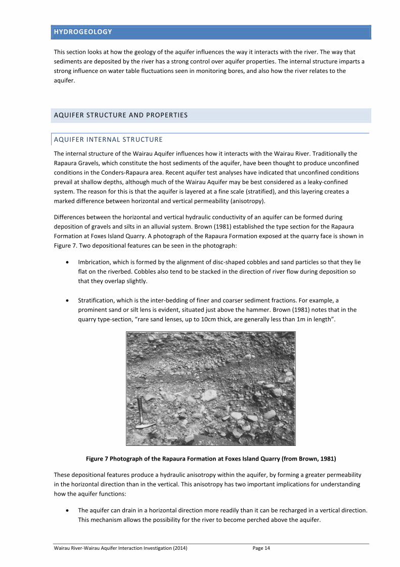
deposition of gravels and silts in an alluvial system. Brown (1981) established the type section for the Rapaura

Formation at Foxes Island Quarry. A photograph of the Rapaura Formation exposed at the quarry face is shown in

Figure 7. Two depositional features can be seen in the photograph:

Imbrication, which is formed by the alignment of disc-shaped cobbles and sand particles so that they lie

flat on the riverbed. Cobbles also tend to be stacked in the direction of river flow during deposition so

that they overlap slightly.

Stratification, which is the inter-bedding of finer and coarser sediment fractions. For example, a

prominent sand or silt lens is evident, situated just above the hammer. Brown (1981) notes that in the

quarry type-section, “rare sand lenses, up to 10cm thick, are generally less than 1m in length”.

Figure 7 Photograph of the Rapaura Formation at Foxes Island Quarry (from Brown, 1981)

These depositional features produce a hydraulic anisotropy within the aquifer, by forming a greater permeability

in the horizontal direction than in the vertical. This anisotropy has two important implications for understanding

how the aquifer functions:

The aquifer can drain in a horizontal direction more readily than it can be recharged in a vertical direction.

This mechanism allows the possibility for the river to become perched above the aquifer.


The vertical transmissivity and storage coefficient of the aquifer decrease rapidly with depth (Figure 8).

The reason for this is that permeable flow pathways become more tortuous as the depth is increased.

This resistance to vertical flow means that water is preferentially routed horizontally along shallow

pathways.

Figure 8 Illustration of the compounding effect that anisotropy has on vertical flow with depth

AQUIFER STRATIFICATION

The base of the Wairau Aquifer is usually identified as being at the base of the Rapaura Formation (or top of the

underlying Speargrass Formation). The surface of the Rapaura-Speargrass contact is not well defined, but it has

been broadly mapped from intercepts in exploration bores (see Brown, 1981). Based on observations from the

exploratory bores, the Wairau Aquifer can be considered to have a thickness of 20- 30m over much of the Wairau

Plain. The thickness does thin to the west where the Speargrass Formation outcrops at the surface around the

Waihopai River. The aquifer also thins to the east of Hammerichs Road where the confining sediments of the

Dillons Point Formation thicken as the coast is approached.

Drillers’ logs tend to report variations in sand and gravel with various clay contents which change with depth.

There is no clear or consistent pattern between individual bore logs, but perhaps what is notable is the fact that

variability has been observable by the drillers. The drilling logs also indicate a change in the water content of the

subsurface, and a log may include good and poor water-bearing horizons as well as clay-bound gravels with

negligible water.

Water levels in many bore logs tend to change with depth, although in some logs the water levels are recorded as

being stable with depth. However, there is a tendency for the upper 10-15m of saturated aquifer to show falling

water levels with depth. This suggests that unconfined conditions prevail within this upper part of the aquifer.

The rate of head loss with depth within the shallow saturated gravels is likely to be related to proximity to the

Wairau River. An example of a rapid fall in water table with depth is bore P28w/3950, which is situated adjacent to

the Wairau River at the end of Pauls Road. This bore has a 1.8m head difference between shallow and deeper

water-bearing horizons. The upper water-bearing gravels have a similar water level to the river, which is 70m

away, so it is most likely that this upper layer represents recent channel deposits. The deeper gravels (from 16.4m)

appear to represent the main Wairau Aquifer, and have a water level 2.3m below the top of the river (measured

from the DEM). The stratification seen in this bore is similar to that of the recharge bore (10485), and these two

bore logs suggest the possibility of an unsaturated zone between the river and regional water table.

Most of the aquifer tests on the Wairau Plain have been planned and analysed by Pattle Delamore Partners (PDP)

on behalf of private clients. For the purposes of analysing aquifer test results, PDP have in recent years considered

the aquifer as a two-layer system, an upper unconfined system, and a deeper leaky-confined system (PDP 2009,

PDP 2014).

The concept of a stratified system is shown schematically in Figure 9. One of the possible explanations for a two-

layer system is that there was a change in the climate or depositional environment between the shallow and


deeper layers. This shift may represent the transition between the early and late Holocene, with the earlier

sediments consisting of more silty outwash gravels that were formed prior to stabilisation of sea levels and the

deposition of the Dillons Point Formation. Under this scenario, the earlier deposits would have consisted of more

primitive outwash material from the last glacial period which has been deposited quite rapidly. The more recent

sediments would therefore be subjected to more alluvial reworking because of the stabilisation of the sea level. An

alternative explanation is that the deeper sediments represent Pleistocene gravels of the Speargrass Formation,

although these deposits are thought to be present at depths of about 30 meters. MDC intends to review the

geology of the Conders area in 2015 by using the 3D geological model developed by GNS (White and Tschritter,

2009) to focus on the upper part of the Wairau Plain.

Figure 9 Schematic diagram showing how the Wairau Aquifer is stratified

CONDERS MONITORING BORES

MDC monitors two bores in the Conders area, P28w/0398 or ‘Conders shallow’, and P28w/3821 ‘Conders deep’.

The Conders deep monitoring bore was drilled in late 2001 to replace water level monitoring in the existing

adjacent shallow bore, which has been used for long term water quality monitoring. The shallow bore was

deepened from 2m to 10m depth in mid-2012. This resulted in a small drop in water conductivity from 6.5 mS/m

to 5.7 mS/m, suggesting that the deeper gravels are subject to a smaller land surface recharge source.

The bore log for P28w/3821 records alternating lenses consisting of various mixtures of shingle, sand and clay. The

static water levels show a gradual falling of the water level with depth, followed by an abrupt increase at 20m

depth (a saturated depth of about 15m). This pattern suggests that a structural control is creating leaky-confined

conditions at that depth.


Intermittent periods of overlapping monitoring records are available for the shallow and deep bores, with the best

records available for January 2011 onwards. Figure 10 shows a comparison of the two records, and it is evident

that the water level is higher in the deeper bore by about 0.15m. Also, water levels in the two bores converge

during a recharge event, and diverge during a recession. This indicates that the upper gravels are more dynamic

and are recharged and drained more rapidly. Also, P28w/0398 shows no response to pumping from the nearby

Pernod Ricard abstraction, which is screened near the base of the Rapaura Formation gravels. So it seems likely

that the deeper gravels are recharged by leakage from overlying sediments in response to pumping, which buffers

the drawdown response in P28w/0398.

Figure 10 Monitoring records for Conders bores P28w/0398 and P28w/3821

The groundwater levels in P28w/3821 can be adjusted by 0.15m to create a continuous groundwater record at

P28w/0398 that extends back to 1982. Figure 11 shows the resulting composite hydrograph, and it is evident that

groundwater levels have been steadily falling over time. The current groundwater level is on average 0.6m lower

than it was in the early 1980s even though the river flow has not significantly declined during this period. An

obvious explanation for this decline would be to suggest that increased groundwater allocation has drawn

groundwater levels down. However, while this is feasible, it does seem an unlikely cause given the small

contribution that pumping makes to the mass balance.

Figure 11 Composite long term groundwater level at P28w/0398

0.00

0.05

0.10

0.15

0.20

0.25

0.30

0.35

0.40

0.45

0.50

34.0

34.5

35.0

35.5

36.0

36.5

Jan-2011 Jul-2011 Jan-2012 Jul-2012 Jan-2013 Jul-2013 Jan-2014 Jul-2014

Wat

er le

vel d

iffe

ren

ce (

m)

Gro

un

dw

ater

Lev

el (

m a

msl

)

P28w/0398

P28w/3821

Difference


The most likely explanation for declining groundwater levels is that there has been a reduction in the rate of

aquifer recharge from the river. There are several ways in which this could occur. One explanation is that there has

been a change in the frequency of high flow events. Analyses of the relationship between flow or stage and wetted

river bed perimeter show that they follow a power law. This means that a small increase in river stage can

potentially provide a large increase in groundwater recharge. So the number of high flow events is expected to be

a key factor in recharge to the aquifer. If high flow events become less frequent, there would be less potential for

recharge pulses in the aquifer to occur, so groundwater levels would decline.

Figure 12 shows the mean annual Wairau River flow at SH1, which gives a good indication of long-term climate

conditions since 1982. A comparison between Figure 12 and Figure 11 shows that mean annual flows do not align

very well with the trend in groundwater levels. The pattern suggests that long-term flow alone cannot explain the

drop in groundwater levels at Conders. However, this does not rule out the possibility that declining groundwater

levels are related to the frequency of high flow events, since these events will not necessarily lead to large mean

annual flow values.

Figure 12 Mean annual Wairau River flow at SH1

Since 1998 there have been less flow events exceeding 1,000 m3/s, and this does coincide with a drop in the water

table. There is also a moderate positive correlation between mean annual flow and groundwater levels at Conders,

which follows a power law relationship (Figure 13). This relationship does open the possibility that the decline in

groundwater levels at Conders could be related to fewer high flow events in the river. However, there is an

inflection in the curve at 50 m3/s, indicating that groundwater is more responsive to river recharge during lower

flow events. There is also a lessening of the groundwater response for mean monthly flows of 100-150 m3/s

onwards. Both of these factors suggest that there may be a structural rather than a climatic control on the

relationship, although further work is required to substantiate this.

Alternative explanations for the decline in Conders groundwater levels relate to the morphology of the river itself,

although groundwater levels may be sensitive to other contributing factors which we don’t yet know about. For a

scenario where the river is hydraulically connected to the aquifer, a decline in bed levels over time would reduce

the hydraulic gradient and therefore the rate of river loss to the aquifer. For a scenario where the river is

disconnected from the aquifer, the rate of groundwater recharge could be reduced by altering the wetted

perimeter of the river bed. This would happen in a situation where the river becomes more entrenched or

channelised over time, requiring higher flow events to generate a significant wetted river width. The evidence we

have available suggests that the river is perched above the regional water table in the Conders area, so

stabilisation of the river channel is a viable explanation for the observed long term decline in groundwater levels at

Conders.


Figure 13 Relationship between mean monthly river flow and groundwater level at Conders

AQUIFER PROPERTIES

Historically, a total of 15 aquifer tests have been carried out in the unconfined Rapaura Formation. Locations for

these tests are shown in Figure 14 (orange) along with the positions of MDC monitoring sites (blue). The results of

these tests are reported in Cunliffe (1988), or as evidence submitted for resource consent applications. These

historical test results indicate that aquifer transmissivity in the Rapaura-Conders area can be quite variable, from

320 to 15,000 m2/d (mean 4,800 m

2/d). These values are equivalent to a bulk hydraulic conductivity of 20 to 2,800

m/d (mean 590m/d).

Very few tests have been carried out using observation bores, so there is little empirical information about aquifer

storage coefficients. Historical tests that have been carried out using observation piezometers have returned

values of 0.1 to 0.15, for bores screened at depths less than 10m (see Cunliffe, 1988). Consultants have typically

assumed values of around 0.2 when assessing long-term drawdown predictions.

Figure 14 Locations of aquifers tests in the unconfined Wairau Aquifer

Tests carried out in recent years tend to provide more information about the aquifer because there have been

improvements in bore logging and data recording. With the advancement of test analysis procedures in recent

years, the use of observation bores has also become a more widely accepted practice. One of the outcomes from

these recent developments is the ability to partition drawdown into upper and lower layers with their respective

hydraulic conductivities and storage coefficients, including the ability to determine vertical leakage and hydraulic

conductivity. The results of the three most recent tests are summarised in the following section of this report, and

a summary of the analysed parameters is provided in Table 2.


Results from the three most recent aquifer tests suggest the Wairau Aquifer may be best considered as a stratified

system which becomes increasingly confined with depth. An aquifer test carried out on P28w/3758 at Conders

Bend returned a surprisingly low storage coefficient of 1 x 10-4

(PDP, 2001). This bore is thought to be screened

near the base of the Rapaura Formation, from 23.5 to 27.5m depth, and has been the first indication that the

Wairau Aquifer may not be a simple uniform unconfined aquifer system.

Table 2 Recent aquifer test results for the Rapaura area

Test Pumped bore Static water level (m bgl)

Top of screen (m bgl)

Pumped Horizon Overlying Sediments

Kx S Sy Kv

Montana P28w/3758 6 23.5 1,400 1 x 10-4

0.15 0.1

Oyster Bay P28w/4537 4.9 26 720 2 x 10-3

0.08 0.1

MDC Matua P28w/4867 4.4 16.5 320 8 x 10-5

0.03 0.5

Aquifer properties for the Conders Bend production bore P28w/3758 have been re-assessed by analysing its

pumping record together with the drawdown observed at Conders monitoring bore P28w/3821. Bore P28w/3738

is located about 230m from the Wairau River, and is screened below 23.5m, with an overlying depth of saturation

of 17.5m. The Conders monitoring bore is located 1,400m away from the pumped bore, 1,155m from the river,

and screened below 20.2m, with a 14m depth of saturation. Interestingly, the adjacent Conders shallow

monitoring bore (P28w/0398) shows negligible drawdown in response to pumping at P28w/3738. This suggests

that drawdown between the deeper and more shallow gavels are being buffered by an additional source of

storage, either from the overlying gravels, or recharge from the river.

The monitoring record for the Conders bore shows a drawdown of 10mm in response to a 50 l/s abstraction at

P28w/3758. Analysis of the drawdown curve gives a storage coefficient of 0.0005, a hydraulic conductivity for the

whole profile of about 1,400 m/d, and a vertical hydraulic conductivity of 0.2, a ratio of 1:5,800.

It is interesting to note that the Recharge bore (10485), which is only 480m from the pumped bore and 45m from

the river shows a response of less than 1mm. This bore is screened below 10.6m, which is considerably shallower

depth than the other two bores. Thus, it is difficult to know whether the poor response at the recharge bore is due

to the recharge effect of the river, or due to its shallower screen depth.

The Oyster Bay test showed hydraulic conductivity values of 700-750 m/d and a storage coefficient of 0.004 to

0.0007 for a water bearing horizon screened at 16.5-20m depth. When the leakage rates from the test are

converted to vertical K values for the aquifer saturated thickness, values of 0.05 to 0.15 are returned.

A more recent aquifer test carried out on bore P28w/4867 with two nearby piezometers (PDP, 2014) is the most

intensive test to be carried out in the Rapaura area. The pumped bore was screened below 16.5m depth, which

gives approximately 12m of saturated gravels above the screen. The shallow gravels above the screen appeared to

bear less water than those within the screened horizon, so conditions in the aquifer were interpreted to be best

represented by a two-layer system.

Analysis of the drawdown curves from the aquifer test at P28w/4867 indicates storage coefficients for the shallow

and deep layers to be 0.025 and 8 x 10-5

respectively. When the modelled transmissivity results are corrected to

layer thicknesses, the hydraulic conductivities of the upper and lower layers are 810 and 324 m/d respectively. The

leakage coefficient for the top layer was interpreted to be 0.025 d-1

, which corresponds to a vertical hydraulic

conductivity of 0.5 m/d. This gives a high anisotropy ratio of vertical to horizontal hydraulic conductivity at 1:1,600.

A characteristic of the recent aquifer tests is that if aquifer anisotropy is assumed, the drawdown curves can be

fitted by various methods (stream depletion, two-layer, multilayer). For drawdown in the pumped bore to be

simulated, it simply requires the influence of an overlying reservoir of some kind, such as a stream or shallow

layer. The source of this reservoir is open to interpretation, but is guided by the conceptual model of the

hydrological system. However the type of reservoir or conceptual model that is selected does determine the

drawdown model used, and this ultimately influences the result of the drawdown analysis.


It is also possible that an apparent stream depletion signature could be created by the recharge effect of the river

in a scenario where the river is perched above the regional water table. The resulting drawdown curve could be

interpreted to represent stream depletion even though no stream depletion is actually occurring. This highlights

the importance of verifying the conceptual setting of the aquifer test prior to analysis of the drawdown curves.

DISCUSSION

The internal aquifer structure of the aquifer is an important consideration for interpreting the response of

groundwater levels to river flow events. If the aquifer was unconfined and homogeneous, we could safely assume

that the response seen at each monitoring bore is a reflection of the timing and magnitude of river recharge that it

receives. However, if each monitoring bore is representative of different aquifer conditions, then it is very difficult

to compare the response at each monitoring bore. The key factor that influences the groundwater response is the

storage coefficient, since this is the characteristic which controls the timing and magnitude of a peak event.

The term ‘storage coefficient’ was defined by Theis (1935) as the amount of water released from storage from a

cylinder of aquifer, caused by a unit decline in head. Theis also proposed that storage is influenced by aquifer

drainage in unconfined aquifers (known as specific yield), or aquifer compression in confined aquifers (known as

storativity). The two processes differ in their characteristics in that the specific yield is independent of aquifer

thickness, whereas the storage coefficient of a confined aquifer is proportional to aquifer thickness.

A key assumption that is made for drawdown analysis is that aquifer storage at the well screen is released

instantaneously upon a reduction in pressure. However, in a case where the vertical hydraulic conductivity is

considerably smaller than the horizontal, the reduction in permeability produces a time delay for the release of

storage. The assumption of an instantaneous release of storage therefore results in an underestimation of the real

storage characteristics of the aquifer.


RIVER FLOW AND STRUCTURE

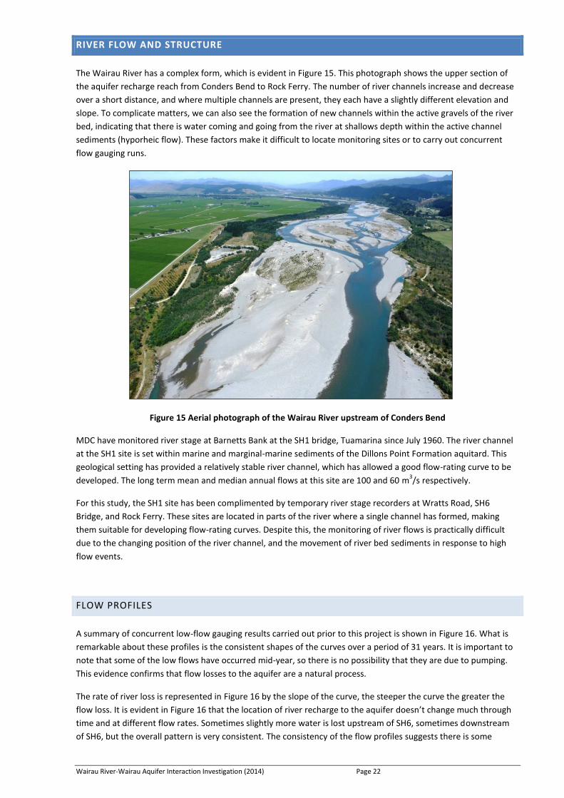
The Wairau River has a complex form, which is evident in Figure 15. This photograph shows the upper section of

the aquifer recharge reach from Conders Bend to Rock Ferry. The number of river channels increase and decrease

over a short distance, and where multiple channels are present, they each have a slightly different elevation and

slope. To complicate matters, we can also see the formation of new channels within the active gravels of the river

bed, indicating that there is water coming and going from the river at shallows depth within the active channel

sediments (hyporheic flow). These factors make it difficult to locate monitoring sites or to carry out concurrent

flow gauging runs.

Figure 15 Aerial photograph of the Wairau River upstream of Conders Bend

MDC have monitored river stage at Barnetts Bank at the SH1 bridge, Tuamarina since July 1960. The river channel

at the SH1 site is set within marine and marginal-marine sediments of the Dillons Point Formation aquitard. This

geological setting has provided a relatively stable river channel, which has allowed a good flow-rating curve to be

developed. The long term mean and median annual flows at this site are 100 and 60 m3/s respectively.

For this study, the SH1 site has been complimented by temporary river stage recorders at Wratts Road, SH6

Bridge, and Rock Ferry. These sites are located in parts of the river where a single channel has formed, making

them suitable for developing flow-rating curves. Despite this, the monitoring of river flows is practically difficult

due to the changing position of the river channel, and the movement of river bed sediments in response to high

flow events.

FLOW PROFILES

A summary of concurrent low-flow gauging results carried out prior to this project is shown in Figure 16. What is

remarkable about these profiles is the consistent shapes of the curves over a period of 31 years. It is important to

note that some of the low flows have occurred mid-year, so there is no possibility that they are due to pumping.

This evidence confirms that flow losses to the aquifer are a natural process.

The rate of river loss is represented in Figure 16 by the slope of the curve, the steeper the curve the greater the

flow loss. It is evident in Figure 16 that the location of river recharge to the aquifer doesn’t change much through

time and at different flow rates. Sometimes slightly more water is lost upstream of SH6, sometimes downstream

of SH6, but the overall pattern is very consistent. The consistency of the flow profiles suggests there is some


structural control over the rate of losses within each of the reaches, and that this structural control has remained

quite stable through time.

Figure 16 Historical flow gauging profiles down the Wairau River

The rate of loss between Rock Ferry and Giffords Road represents the total rate of river recharge to the Wairau

Aquifer. In general, the rate of loss is slightly greater upstream of SH6, and appears to peak between Conders Bend

and SH6. The change in magnitude of the loss between surveys is difficult to see in Figure 16, but it varies

upstream of SH6 from 0.5 m3/s/km in Feb 2009 to 1.5 m

3/s/km in July 1991. The river reaches an equilibrium with

the aquifer between Giffords Road and Wratts Road, and a small gain occurs downstream of Wratts Road.

A summary of the gauging runs is tabulated in Table 3, and the flow balances are plotted against SH1 flow in Figure

17. Unfortunately we can’t be very precise about river water budgets because of the braided nature of the river.

The magnitude of the flow losses and gains is also to some extent influenced by the number and position of the

gauging sites between Giffords Road and Wratts Road. Furthermore, there are uncertainties about the amount of

North bank flow entering the river, and any hyporheic flow that needs to be accounted for. Almost all of this water

can be accounted for once the river crosses the Dillons Point Aquitard, downstream of Selmes Road.

Despite the uncertainties, the majority of river flow does occur as inflow within the main channel, so the summary

does give a good indication of the values that we can expect. Flow losses vary from 6.65 to 9.54 m3/s, and Figure

17 shows that the river typically loses more water at larger flows (about 70 l/s per m3/s increase in flow).

Table 3 Summary of historical concurrent flow gaugings on the Wairau River

Date SH1 Flow (m3/s) Gaugings Total loss (m

3/s) Total gain (m

3/s) Flow balance (m

3/s)

2-Feb-78 14.10 4 -8.25 0.55 -7.70

14-Mar-78 4.91 5 -8.35 0.40 -7.95

9-Feb-82 18.81 4 -9.54 2.39 -7.15

2-May-88 16.44 6 -9.05 1.13 -7.92

18-Jul-91 14.94 9 -6.76 2.03 -4.74

14-May-92 11.66 9 -6.65 1.55 -5.10

16-Feb-01 9.54 4 -8.46 0.36 -8.09

19-Feb-09 18.26 5 -8.71 4.78 -3.93

Min 4.91 4 -9.54 0.36 -8.09

Max 18.81 9 -6.65 4.78 -3.93

Mean 13.58 6 -8.22 1.65 -6.57

0

5

10

15

20

25

0 2 4 6 8 10 12 14 16 18 20 22

Flo

w (

cum

ec)

Distance (km)

2-Feb-78 14-Mar-78

2-May-88 18-Jul-91

14-May-92 16-Feb-01

19-Feb-09

Ro

ck F

erry

Wa

iho

pa

ico

nfl

uen

ce

SH6

SH1

Wra

tts

Rd

Gif

ford

sR

d


The flow balance is largely influenced by the flow gain component at higher flows, which appears to have an

exponential increase with total river flow. This relationship suggests that the flow gain values may be related to

inflows from north bank tributaries such as the Waikakaho. The observed increase in river flow loss at higher flows

is not apparent if the total flow balance alone is studied because of the increased influence that total flow gains

have during high flow conditions. The influence of the North Bank tributaries increases as flow increases,

indicating that input flows from the North Bank will needed to be accounted for in transient model simulations.

Figure 17 Summary of historic Wairau River concurrent flow gauging surveys

FLOW TIME LAGS

It takes a few hours for water in the Wairau River to travel across the length of the Wairau Plain. However, the

time lag between sites varies with different flows, and whether the river is on a rising or receding phase. A

statistical analysis tool was written in Matlab to determine the dynamic time lags between river stages recorded at

four sites along the river. The cross-correlation technique used compares the offset between two sites in the daily

cycle generated by storage and release of water from the Branch River reservoir operated by Trustpower. Flow

peaks generated by the operation of this scheme are used to calculate time lags and corresponding probabilities.

The time lag with the highest probability is the selected for a specific site and flow condition (Figure 18). The

results of this analysis suggested a 2 ½ hour time lag from between Rock Ferry and Wratts Road, and a 4 hour lag

between Rock Ferry and SH1 at flows of about 20 m3/s. These times lessen as the river flow rate increases.

Figure 18 Graphical example of the probability approach for predicting time lags

8500 8600 8700 8800 8900 90005.99

5.995

6

6.005

6.01

6.015

6.02x 10

4

Ro

ck F

err

y &

Tu

am

ari

na

2600

2650

2700

2750

2800

2850

2900

Rock Ferry

-40 -20 0 20 400

0.1

0.2

0.3

0.4

0.5

0.6

0.7

0.8

0.9

1

Lag (16)

Rock Ferry & Tuamarina [15 minutes]


RIVER STRUCTURE

This section describes our current understanding of the nature of the hydraulic connection between the river and

underlying Wairau Aquifer.

One of the important datasets to become available in recent years is Lidar imaging. Lidar is a remote sensing

technique that measures distance by analysing the light reflected by a laser, and it provides a high resolution

survey image of the land surface. Because the method is based on surface reflectance, the image also provides

elevations for the surface of water bodies. The resulting image therefore gives us the first available detailed map

of the Wairau River surface and it’s adjacent topography. A Lidar image was captured for the Wairau Plain on 23 to

28 February 2014. An example of the resulting image is shown in Figure 19 with the active river channel drawn in

blue for the purposes of clarity.

Figure 19 Example Lidar image of the Conders area

RIVER AND AQUIFER SURFACES

One of the powerful aspects of the Lidar image is that it gives us the ability to compare the river surface with

groundwater level surveys. Figure 20 shows a piezometric survey across the Wairau Aquifer using data from

various sources in order to appreciate a complete picture of the hydrology. The assumption made in generating

this map is that vertical fluctuations over time are small compared to spatial changes in elevation. River elevations

were taken from the 24 February 2014 Lidar survey (light blue points) and stage recorders for the same date

(orange), when the flow at Tuamarina was approximately 10 m3/s.

The groundwater survey data was taken from a comprehensive piezometric survey of the Wairau Plain carried out

on 23-24 February 1987 (points shown in blue). The river flow at the time of the survey was approximately 20 m3/s

at Tuamarina. These data were supplemented by static water levels for boreholes on the north bank of the river

which have had their bore collars surveyed (green points).

What is evident in Figure 20 is the distortion of the water table around the river. The river level is consistently

higher than the adjacent water table between Onamalutu Road and Wratts Road. While the contours are largely

informed by the position of the measurement sites, it is still apparent that the hydraulic gradient is very steep

adjacent to the river in this area. In fact the offset is so marked in locations where groundwater sites are located

close to the river, such as upstream and downstream of SH6, that the river appears to be perched above the

regional water table. Further upstream at Rock Ferry, and also below Wratts Road the river level is very similar to

the regional groundwater table. This suggests that the two water bodies are hydraulically connected and in close

equilibrium in these areas.


Figure 20 Composite piezometric survey across the Wairau Aquifer including river elevations

Another method of studying the relationship between the river and aquifer is to project the groundwater

piezometric surface beneath the river and study the vertical difference between the two. Figure 21 shows the

result of this exercise as a longitudinal profile. Three groundwater interpolations have been made beneath the

river, the detailed piezometric surveys carried out in February 1987 and May 1988, and a surface generated from

all static water levels in the MDC database (to give a better spatial resolution). The longitudinal profile is

supplemented with historical observations made in riparian bores P28w/1692, 1696, 1697, and 1699 for a range of

hydrological conditions to indicate the variation in the water table.

Figure 21 Longitudinal hydrological profile along the Wairau River from Conders to Giffords Road

The longitudinal profile shows that the river is consistently 2-3 m above the regional water table for most of this

reach. The river and regional water table do converge downstream of Jeffries Road, just up-gradient of the Neal

bore P28w/1685. It is difficult to know whether this is an area of higher permeability, or if the convergence is an

expression of the anastomosing of the river in this area.

A simplified summary of the entire Wairau Plain longitudinal profile is shown in Figure 22. This plot includes the

low flow profile down the river from a fairly comprehensive concurrent flow gauging run that was carried out in

May 1992. The length of river that shows the most losses, from Rock Ferry to Wratts Road, coincides with the

length of river that is significantly higher than the regional groundwater table. The river losses and separation

distance are both fairly consistent from Rock Ferry to Jeffries Roads. Between Jeffries and Giffords Roads the river


level and regional water table start to converge (the hydraulic gradient flattens) and there is a corresponding

reduction in the flow loss. Downstream of Wratts Road the river approaches the Dillons Point Formation aquitard,

and a small flow gain is observed as groundwater from the unconfined aquifer become squeezed back into the

river.

Figure 22 Simplified longitudinal profile for the whole Wairau Plain

Comparison of river and groundwater levels along the river indicates that the hydraulic gradient between the two

is very steep and possibly vertical over the main recharge reach. In the case of a vertical hydraulic gradient, the

hydraulic relationship between the two is either disconnected or transitional. Furthermore, the vertical separation

is much greater than the fluctuations seen in the aquifer, which suggests that the hydraulic relationship across the

main recharge reach does not alter during the year. This is a significant insight, because it suggests that the

recharge rate does not vary significantly with changes in the hydraulic gradient. The recharge rate can be

estimated if the subsurface vertical and horizontal hydraulic conductivities can be constrained, and the source

area of recharge (e.g. wetted river perimeter) is known.

The hydraulic relationship at the up-gradient and down-gradient ends of the main recharge reach is expected to

change from hydraulically connected when groundwater levels are high to a transitional state when groundwater

levels are low. It is not known how much this transition zone migrates up and down the river in response to high

and low groundwater levels.

GEOLOGICAL CONTROL ON RIVER LOSSES

The Lidar image shown in Figure 19 clearly shows the presence of older river channels that were formed prior to

the river being constrained to its present position by flood protection works. Apart from a small entrenchment of

the modern river channel compared to the surrounding plain, no clear distinction can be made between the active

river channel gravels, and the adjacent, older alluvial deposits. Form a hydrological perspective, the gravels can be

considered to be a single entity of varying internal structure and permeability (anisotropy and heterogeneity).

Traditional approaches to calculating stream-aquifer exchanges include a bed conductance term to allow clogging

to occur in the stream bed. Such a term is undoubtedly appropriate for a meandering river or a spring where a

distinct clogging layer may be observable. However, in a braided river depositional environment, there is a

constancy of sediment re-deposition or re-working through time. We also see a spatial repetition of the

surrounding and underlying deposits, so that no obvious distinction can be made between the sediments in the

active river channel and those that adjacent or underneath. This calls to question the relevance of a stream bed

conductance term for a braided river environment.

It is perhaps more appropriate to consider that the sediments associated with the active river channel are more

permeable that the surrounding sediments. This is because the more recent deposits are likely to have been


subject to more reworking by the river, particularly since the training of the river position by flood works. We

suggest that a bed conductance term is not required for a braided river environment, although existing analytical

techniques such as Modflow do require a bed conductance to be formulated. Instead, it is more appropriate to

consider river flow to be determined by the horizontal and vertical hydraulic conductivity values within the shallow

aquifer.

It is also valuable to consider the effect of enhanced permeability within the active river channel gravels. How we

define the active river channel boundaries will inform our predictions for the wetted area of the river. It is

apparent from aerial photos of the river that river braids can appear and disappear at some distance from the

active river. We do not know if these braids are caused by localised high permeability channels (underflow) or

whether they are a representation of the regional water table or even the shallow table associated with the river.

Indeed, at this stage there is little known about the hydrology beneath braided rivers, and this should be

considered as a topic for further study by drilling investigation bores in the river bed, perhaps using geophysical

survey methods.

RIVER GEOMETRY

The bed of the Wairau River has been surveyed every few years at transects perpendicular to the river. The latest

survey results from 2012-2013 consist of 22 survey sections spaced at intervals of approximately 800m along the

river. Unfortunately, the river stage level for each river transect was not measured during the survey, but we do

have a snapshot of river stage from the Lidar survey. We also have transient stage records for SH1 and the three

temporary recorder sites at Wratts Road, SH6 and Rock Ferry.

Relationships have been established between stage, flow and wetted river bed perimeter for the purposes of

providing input data for the 22 cross sections employed in the numerical model. In theory, if the horizontal and

vertical hydraulic conductivity of the near-surface sediments can be constrained, the rate of recharge for a

hydraulically disconnected river is simply a function of wetted perimeter. Simple power-law functions were

derived to relate river stage, h, and width, w, to river flow, Q:

h(Q) = aQb and w(Q) = cQ

d,

Where a, b, c, d denote empirical fitting parameters.

To generate these formulas, several steps were undertaken. Firstly, the 22 surveyed cross sections along the river

were analysed. Relationships of river stage and width to the cross-sectional wetted area, A, were derived from the

river geometry data and fitting of parametric functions to these data.

For the river-gauging station at SH1, simultaneous measurements for both river water level and river flow were

available (bottom middle panel in Figure 23). Therefore, the equations for h(Q) at SH1 have been measured

directly and a function was fitted to the data. The equation for w(Q) was calculated from the cross-sectional area,

A as follows (Figure 23):

Q in h(Q) h; h in h(A) A; A in W(A) W; → W(Q)

Unfortunately, little river flow information was available for the other cross sections. The h(Q) relations for these

cross-sections were derived using the known h(Q) and Q(A) relationships at SH1, and the assumption of (on

average) normal flow along the various river sections. This leads to the assumption of constant velocity (but

variable in time since it is a function of flow), and allows us to establish h(Q) and w(Q) relationships at all other

cross-sections while preserving conservation of mass.


Figure 23 Relationships between stage (h), flow (Q), cross-sectional area (A), and wetted perimeter (wp) at the

SH1 recorder site

0 100 200 3000

2

4

6

8

xsection @ SH1

xsection length, x [m]

no

rma

lize

d s

tag

e, h

[m

]

0 500 1000 15000

1

2

3

4

5

6

7

no

rma

lize

d s

tag

e, h

[m

]

wetted area, A [m2]

h(A)

observed

0.14 A** 0.53

0 500 1000 15000

50

100

150

200

250

300

wetted area, A [m2]

we

tte

d p

eri

me

ter,

wp

[m

]

wp(A)

observed

30.3 A** 0.34

0 500 10000

0.5

1

1.5

2

2.5

3

3.5

flow, Q [m3/s]

no

rma

lize

d s

tag

e, h

[m

]

h(Q)

rating curve

observed

0.869 Q** 0.2088

0 500 10000

50

100

150

200

250

flow, Q [m3/s]

we

tte

d p

eri

me

ter,

wp

[m

]

wp(Q)

derived

91.3 Q** 0.1481

0 100 200 3000

2

4

6

8

xsection @ SH1

xsection length, x [m]

no

rma

lize

d s

tag

e, h

[m

]

0 500 1000 15000

1

2

3

4

5

6

7

no

rma

lize

d s

tag

e, h

[m

]

wetted area, A [m2]

h(A)

observed

0.14 A** 0.53

0 500 1000 15000

50

100

150

200

250

300

wetted area, A [m2]

we

tte

d p

eri

me

ter,

wp

[m

]

wp(A)

observed

30.3 A** 0.34

0 500 10000

0.5

1

1.5

2

2.5

3

3.5

flow, Q [m3/s]

no

rma

lize

d s

tag

e, h

[m

]h(Q)

rating curve

observed

0.869 Q** 0.2088

0 500 10000

50

100

150

200

250

flow, Q [m3/s]

we

tte

d p

eri

me

ter,

wp

[m

]

wp(Q)

derived

91.3 Q** 0.1481


GROUNDWATER OBSERVATIONS

HYDRAULIC REPONSE TO FLOW EVENTS

The responsive of groundwater to flow events in the river depends on the proximity of the monitoring bore to the

river. Figure 24 shows the groundwater and flow hydrographs for the summer to autumn 2014 period, a period of

quite stable hydrological conditions. The water levels at each site have been adjusted to allow the individual

responses to be compared with each other. It can be seen that the recharge bore mimics river flow quite closely,

and is very responsive. Small flow events (e.g. 20 m3/s flow increases) are recoded in the recharge bore, but are

not registered by Conders bore in particular. The reason for dissipation of the small flow events is probably that

much of the increase in flow is incorporated into storage within the vicinity of the river.

Figure 24 Groundwater and river flow hydrographs for the summer-autumn 2014 period

One of the useful aspects of the monitoring record shown in Figure 24 is the presence of a >400 m3/s fresh in the

river with clean recessions before and after the event. Figure 25 focuses on the aquifer response at each of the

MDC monitoring sites to this flow event. The groundwater response to the flow event can be considered as

composed of three characteristics, the magnitude of the response, the delay to the onset of the event, and the

peak delay. The way that each site responds to these characteristics depends on the proximity of the river, the

hydrogeological setting of the site (degree of confinement), and the local aquifer hydraulic properties.

The site with the fastest event response is the recharge bore because of its close proximity to the river. This is

closely followed by a response in the Conders monitoring bore. The Selmes Road bore is very responsive, and

shows a very rapid peak, and also exhibits fluctuations from the Trustpower scheme. The reason is that this bore is

situated in a confined environment which results in a low storativity value.

Perhaps the most interesting response is seen at the Conders bore, which shows the largest groundwater rise, but

has a much delayed peak. To some extent the sluggish response will be caused by its confined-leaky geological

setting. The rise in groundwater levels is imparted by the overlying unconfined gravels, which gives the long delay.

However, the main reasons for the delayed response and large magnitude of the rise will be caused by the bores

central position within the Conders recharge area. Because the river runs at an acute angle to the main direction

of groundwater flow, the Conders bore is subject to a large number of flow paths from the river. What we


effectively see in the hydrograph is the interference effect caused by multiple flow paths reaching the Conders

bore at different times.

One of the conclusions to be drawn from analysing the aquifer structure and the hydrological responses is that the

monitoring bores represent quite localised groundwater conditions. Because the aquifer is traditionally considered

to be unconfined, there is a tendency to think that a bore is representative of a particular area. However, we now

know that due to aquifer stratification, the groundwater response is very much a function of anisotropy and

screen depth, and can be even more complex when heterogeneity is considered.

Figure 25 Response at groundwater monitoring sites to a flow event during stable conditions

RIPARIAN BOREHOLES

There are few boreholes that have been drilled in close proximity to the Wairau River. MDC drilled a network of

Wairau Aquifer bores along the river stop-bank in early 1987. Several surveys were undertaken although the

results were not written up. The surveys were undertaken during different seasons from 1987 to 1992, and the

results are shown in (Table 4). The surveys show a groundwater fluctuation of 0.5 to 0.9m, with the greatest

fluctuation seen at Conders Forest. Assuming that the river bed level has remained stable over time, the river is

projected to be over 2m above the groundwater level at each site. The exception is at P28w/1699, which has a

lowest observed head difference of 1.5m.

Table 4 Historical riparian monitoring bore records and adjacent river level from Lidar survey

Well Location E N 24-Feb-87 7-Oct-87 2-May-88 16-Jul-91 15-May-92 Lidar river level

1692 Conders Bend 1665591 5406251 45.22 45.33 45.07 44.83 44.85 47.6

1696 Conders Forest 1667409 5407346 38.37 38.75 38.44 37.86 38.00 40.9

1697 SH6-Boyces Rd 1668491 5407700 33.10 33.53 33.33 32.84 33.04 35.9

1699 Ds Jeffries Rd 1671094 5408632 24.10 24.62 24.31 23.97 24.00 26.1

CONDERS RECHARGE BORE

The first discussions about the nature of the relationship between the Wairau river and aquifer resulted from the

drilling of the “recharge bore” 10485. This bore was drilled 43m from the river at Conders Bend and was drilled

specifically to monitor the effect of river flows on the Wairau Aquifer. The bore log shows that water-bearing


gravels, which are here interpreted to be productive gravels, are not encountered until 10.1m depth. Clean gravels

are also encountered at a shallow depth (at a similar elevation to the active channel deposits), but these are not

shown as being productive in the bore log.

The monitoring record for the recharge bore indicates that the level of the river is always at least 3.3m higher than

the groundwater level. The surveyed cross section at this location indicates that the groundwater level remains at

least 1.8m below the lowest point in the river bed throughout the year.

The large difference between the river level and adjacent groundwater level produces an uncharacteristically

steep hydraulic gradient adjacent to the river. Two possible conceptual interpretations may be considered for this

steep gradient, either that the aquifer is hydraulically connected to the river, and its effect on groundwater levels

is restricted to the immediate vicinity of the river, or that the river is hydraulically perched above the river. These

two scenarios are shown schematically for the Conders recharge bore in Figure 26.

Figure 26 Schematic representation of hydraulically connected (above) and disconnected (below) scenarios at

the Conders recharge bore

PAULS ROAD

There are very few existing boreholes that have been drilled close to the river. One noteworthy bore is P28w/3950

at the end of Pauls Road. This bore is located 70m from the river at the end of river survey cross section 54. Figure

27 shows the stratigraphic log for this bore, which shows the presence of two productive horizons separated by

7.9m of lower permeability sediments. What is most interesting about this bore log is the large difference in static

water levels recorded by the two productive horizons.


Figure 27 Stratigraphic log for bore P28w/3950

The upper water-bearing gravels have a similar water level to the river level as measured from the Lidar image. It

seems likely that this upper layer represents the active alluvial deposits associated with the river, and that the

water level represents hyporheic flow associated directly with the river. The deeper gravels have a water level

2.3m below the top of the river, and this horizon most likely represents the unconfined Wairau Aquifer and its

associated regional water table.

The significance of this bore log is that it provides the first direct evidence that there may be an unsaturated zone

between the river and regional water table. The setting and lithological of the Pauls Road bore is very similar to

that observed at the Conders recharge bore (10485), although the recharge bore does not record a near-surface

saturated horizon.

The drilling of a nested piezometer in the Pauls Road area is planned for 2015. The piezometer will test whether

the shallow two-layer system observed P28/3750 is laterally extensive adjacent to the river. The bore will be

screened with the shallow and deeper horizons to study the dynamics of the two by aquifer testing and water level

monitoring.


RIVER-AQUIFER RELATIONSHIP

1-D ASSESSMENT

Brunner et al. (2009) proposed that the status of the hydraulic connection could be assessed with a simple 1D

model where disconnection occurs if:

𝐾𝑐𝐾𝑎

≤ℎ𝑐

𝑑 + ℎ𝑐

Where Kc and hc are the hydraulic conductivity and thickness of the river clogging layer (or sediments between the

regional water table and river bed).The parameter Ka is the horizontal hydraulic conductivity of the aquifer, and d

is the depth of the river. It is therefore appropriate to consider the 1D equation as a balance between river water

depth and aquifer anisotropy. We can apply the 1D equation to the Conders recharge bore by inputting parameter

values based on observations made in the aquifer (Table 5).

Table 5 Representative parameter values for assessing hydraulic connectivity

Parameter Minimum Maximum Mean

River depth 1.5 4.4 2.3

Clogging thickness 1.7 2.4 2.2

Kc (Kv) 0.1 1 0.5

Ka (Kx) 20 2,800 600

The value of hc to river depth is fairly consistent, and ranges from 0.3 to 0.6. The results of aquifer tests indicate

that Kc/Ka aquifer anisotropy is the most likely control on the hydraulic connection because of the large observed

variability in hydraulic conductivity, and because of the large difference between observed horizontal and vertical

hydraulic conductivity values. For the aquifer hydraulic conductivities that have been returned from aquifer tests,

the vertical hydraulic conductivity would need to be between 6 and 840 m/d, or a kx/kv ratio of 3:1 or less for a

hydraulic connection to occur. The largest values of vertical hydraulic conductivity obtained from aquifer tests

have been 0.5 m/d.

The vertical hydraulic conductivity of the river bed between Rock Ferry and Jeffries Road has been estimated by

PDP (2001) as being 1 to 400 m/d, assuming a 100m channel width. This is certainly within the range of values

required for a hydraulic connection to occur, although the hydraulic conductivity of the river bed was estimated to

decrease downstream.

It is possible to apply a qualitative test to see whether the hydraulic gradient between the river and aquifer is

vertical (or at least steep). To do this we can study the relationship between the wetted river of the perimeter and

the head difference between the two, which has been plotted for the Conders recharge bore in Figure 28. We

know from observations along the river that there is a power function relationship between river stage and wetted

river perimeter. If there is a significant change in the hydraulic gradient we would expect to see considerable

scatter around the trend line. The relationship between the head difference in Figure 28 is very good (r2 0.92),

which suggests that the hydraulic gradient is being maintained at a constant value, and is therefore most likely to

be vertical.


Figure 28 Relationship between wetted perimeter width and river-aquifer head difference at the recharge bore

y = 12.255e0.649x

R² = 0.9223

100

150

200

250

300

350

400

450

3.0 3.5 4.0 4.5 5.0 5.5 6.0

Wet

ted

riv

er w

idth

(m

)

Head difference (m)


OXYGEN ISOTOPES

Oxygen Isotope data can provide valuable insight into the source of recharge to groundwater. Figure 29 shows a

composite of median 18

O values taken from Stewart (2008) and Taylor (2004). The 18

O data in Figure 29 has been

colour coded according to the thresholds suggested by Stewart (2008). Sites coloured blue (values of -8.6 to -9.2)

are representative of high altitude recharge that is typical of the Wairau River. The dark green coloured sites

(values of -6.8 to -7.4) are representative of recharge from local rainfall. Sites coloured orange and light green

indicate that the groundwater is a mixture of Wairau River and local rainfall recharge.

Figure 29 Map of median Oxygen-18 isotope values

The distribution of 18

O values on the Wairau Plain shows an interesting and unexpected pattern. Sites on the south

bank of the river show a significant influence from local land surface recharge, even though they are close to the

Wairau River. The river is known to contribute 95% or more of the recharge in the aquifer mass balance, so we

would expect these bores to have 18

O values very similar to the river. For example, the Neal bore P28w/1685

shows an 18

O signature that suggests a particularly high local recharge component and yet it is very close to the

river, and situated within the known river recharge reach.

A possible explanation for the presence of significant local recharge on the south bank is that the river is not acting

as a groundwater flow divide because it is perched above the regional water table. This hypothesis is a departure

from previous thinking, since the Wairau River has traditionally been considered to be hydraulically connected to

the aquifer. While the 18

O data does suggest the possibility of north bank water flowing under the river, the

evidence is not conclusive and requires further testing.

If there was a hydraulic connection between the aquifer and river, the river would tend to act as a hydrological

boundary, and any drainage from the north bank would most likely be intercepted by the river. If the river is

perched above the regional water table, it opens the possibility for groundwater from the north bank to pass

beneath the river and mix with groundwater on the south bank. Under this scenario, the Wairau River would

contribute recharge onto the water table by vertical drainage, but it would not act as a flow divide. Figure 30

schematically illustrates these hydraulically connected (left) and disconnected (right) scenarios.


Figure 30 Schematic profiles across the SH6 area showing hydraulically connected and disconnected scenarios

Down-gradient of Wratts Road, the river recharge signature becomes more dominant at bores P28w/0208 and

P28w/0222, and also in Spring Creek. In contrast to bores situated in the main river recharge area of the aquifer,

these bores are located a long way from the river. If the river was hydraulically connected to the aquifer, we would

expect these sites to have a greater local recharge component than those situated in the Conders area. It is most

likely that the river is hydraulically connected to the aquifer along the flow paths that contribute to this part of the

aquifer, and therefore acts as a flow divide and captures North Bank groundwater.

In summary, the spatial distribution of 18

O values suggests that the river is hydraulically disconnected from the

regional water table upstream of Giffords Road, and hydraulically connected somewhere between Giffords and

Wratts roads. This supports the indirect evidence provided in other sections of this report that the Wairau River is

perched above the aquifer in the main recharge reach from Rock Ferry to Giffords Road. There is a possibility that

North Bank water may flow beneath the river into the Wairau Aquifer, although to confirm this requires further

investigation.


TEMPERATURE RECORDS

Temperature loggers were installed at eleven groundwater sites in the Wairau Aquifer in August 2014. The

preliminary results of this monitoring are shown graphically in Figure 31. Long term temperature monitoring of the

river shows a cyclic pattern with temperatures ranging from around 6C in June-July to about 21C in January,

which closely follows the air and shallow earth temperature. Accordingly, high flow events result in a temporary

drop in water temperature.

Figure 31 Groundwater and Wairau River temperature monitoring records

Figure 31 shows that the temperature response varies quite markedly within the aquifer. In general, four

characteristic responses can be seen which range from rapid (~2 months), to seasonal (~4 months), to sluggish (>5

months), to weak or unresponsive sites. The more responsive sites show temperature rise events during more

prolonged flow recession events in the river. The details for each site and their response are listed in Table 6.

Table 6 Temperature monitoring sites and their characteristic responses

Well Depth (mbgl) SWL (mbgl) Screen top (mbgl) Saturated depth (m) Distance to river (m) Temp range (C) Response

1685 10 5.9 10 14.2 1,000 3.3 Rapid

0903 7 3.35 7 3.7 650 1.4 Rapid

10485 17 7.3 10.6 3.3 40 1.2 Rapid

10426 14 5.6 14 12.2 2,500 3.7 Seasonal

0398 10 6.2 10 3.8 1,500 3.2 Seasonal

3821 21 6.7 20.2 13.5 1,500 1.0 Sluggish

4722 15 4.95 21.4 16.5 2,600 0.67 Sluggish

4724 20 6.5 21.1 14.6 2,600 0.24 Weak

4577 14 1.65 14 12.4 4,500 0.19 Weak

3009 6 2.0 5 3.0 3,800 0.16 Weak

4723 30 5.7 28 22.3 2,600 0.07 Weak

The response at each site depends on both the distance from the river, and the screen depth (or depth of

saturation). The range in temperature observed at each site is a function of the seepage velocity compared to the

volume of media that the incoming groundwater is flowing through. Sites that show a large range in temperatures

are therefore expected to have a greater seepage velocity, particularly if they are located at some distance from

the river. The groundwater site that shows the largest range in temperatures is the Neal bore (P28w/1685), which

suggests that the aquifer transmissivity may be greater in this area (assuming a uniform effective porosity in the

aquifer).


The time lags shown at each site are a function of the seepage velocity of the aquifer. Sites that show a rapid

response to river temperature are located within a kilometre of the river and their temperatures follow the annual

river temperature cycle with a short time lag of approximately two months. Two of the sites, P28w/1685 and

10485, also show a response to individual rapid warming events with a time lag of approximately one month.

Sites that show a seasonal response show a large but delayed seasonal fluctuation in water temperature, and do

not show a response to individual warming events. These two sites, P28w/0398 and 10426, are screened in the

shallow productive gravels and are located within 2,500 m of the river.

Sites with a sluggish and attenuated seasonal response are greater than 1,500 m from the river and are screened

into the deeper, leaky-confined part of the aquifer. Sites that are located more than 2,500 m from the river tend to

show a weak response to seasonal changes in temperature regardless of the depth of the bore screen. This is a

significant observation because it suggests that the temperature fluctuations observed at sites closer to the river

are primarily caused by recharge temperatures rather than changes in shallow earth temperature.

The temperature response observed in the aquifer appears to be a function of both depth and distance from the

river. Close to the river, the depth does not appear to influence the temperature greatly. The responsiveness seen

at P28w/1685, which is a relatively deep bore, suggests that deep recharge is occurring adjacent to the river.

Further away from the river, we see a greater response in more shallow bores than deeper ones. For example, the

paired Conders monitoring bores P28w/0398 and P28w/3821 show quite different responses, reflecting their

respective unconfined and leaky-confined settings. The implication is that the transmissivity of the aquifer is

considerably greater at shallow depths than in the deeper sediments. This supports the hypothesis that the aquifer

permeability is highly anisotropic, and suggests that most of the flow is occurring close to the water table.


NUMERICAL GROUNDWATER FLOW MODEL

A steady state Modflow model focusing on the recharge area of the Wairau Aquifer was developed at the

University of Tübingen in Germany. The model was developed using the ModelMuse graphical user interface and

calibrated using a Matlab© -based multi-objective global parameter optimisation method. The period represented

by the steady state model was summer to autumn conditions in 2014, since this is the period for which sufficient

data was available to fully quantify the boundary conditions.

The objectives of the model were to:

Better understand the hydraulic relationship between the river and aquifer

Calibrate the hydraulic parameter field of the aquifer in the recharge zone

Prepare for modelling transient conditions

This section gives a brief summary of the model setup and outlines the insights gained during the steady state

model calibration.

MODEL SETUP

MODEL STRUCTURE AND EXTENT

The main elements and extent of the model domain are shown on Figure 32. The model was constructed to

account for the whole recharge reach of the river, and extends from Rock Ferry in the West to the MDC monitoring

wells within the confined aquifer at Selmes Road (P28w/4577), and Mills and Ford Road (P28w/4404). The model

grid is aligned West-East. To accommodate the southern extent of the model, a no-flow boundary was assumed

along Gibsons Creek, which is located just north of the contact between the Rapaura gravels and Speargrass

Formation over the western part of the Wairau Plain. A no-flow boundary is also assumed to the west of Rock

Ferry, and also along the North bank hills. At the eastern boundary, groundwater is allowed to discharge through

the confined Wairau Aquifer.

Figure 32 Map showing the main elements for setting up the Modflow model

Data for the land surface elevation was taken from the Lidar survey, which was interpolated onto the regular grid

used in the model. The base of the aquifer was taken from the contours of the top of the Speargrass Formation as

generated by Brown (1981), and represents a lower no-flow boundary.

Flow within the Wairau Aquifer is simulated in the Modflow model by a 170 x 70 cell rectangular finite difference

grid with a 100 m2 cell size. The aquifer was separated into twenty computational layers which were generated by

non-uniform horizontal interpolation between the upper and lower bounding elevations, allowing for finer grid


resolution at the land surface. This setup was chosen to get a higher grid resolution in areas of likely water-level

fluctuations in the top layers, while the bottom layers are always saturated, allowing for a lower resolution

towards the base of the aquifer.

BOUNDARY CONDITIONS

The model is constrained by five flow boundary conditions: land surface recharge, pumping demand, river

exchange fluxes, drains (springs), and down-gradient discharge through the confined aquifer in the Spring Creek-

Grovetown area.

Land surface recharge and pumping demand

Land surface recharge and irrigation demand were calculated using a modified version of the Rushton model

(Rushton et al. 2006). A daily soil moisture balance was calculated for different combinations of soil hydraulic

properties on the Wairau Plain. The results of this daily model were averaged over the Summer-Autumn period for

input to the steady state numerical model.

There was very little land surface recharge during the Summer-Autumn 2014 period covered by the steady state

numerical model. Irrigation demand during this period was calculated by applying 2.2mm of water when the soil

moisture store for each recharge zone reached a nominal value of 70% of the TAW. The demand record was also

averaged over the Summer-Autumn 2014 period to provide input values for the steady state numerical model.

River Exchange Fluxes

From the selection of Modflow packages for river simulation, the Stream-Flow Routing package (SFR2 package)

was chosen to represent the Wairau River in the model. The SFR package routs the water flow through a series of

continuous cells, while interaction with the groundwater (loss or gain of water) affects the flow for each cell. The

SFR package also allows for unsaturated flow to occur beneath the river bed.

Power functions are used in the SFR package to relate both river head and width to flow at the 22 surveyed river

cross sections that lie within the model domain. These were input to the model as 22 river segments, each with a

bed thickness, bed elevation (at segment start and end), bed hydraulic conductivity and w(Q) and h(Q) power

functions that were fitted to the data as explained above. The first segment at Rock Ferry also needed information

about the inflow into the river, which was an average flow of 32.2 m3/s during the steady state modelling period.

Since river loss estimates were available from consecutive flow gaugings at the four gauging sites during the low-

flow period used for the steady-state model, these were implemented into the model calibration as flux targets

which also helped to constrain river bed conductance values at the various stream segments.

Springs

Spring flow was modelled using the Drain package. Since the model grid with its 100 x 100m resolution was too

coarse to reproduce the indentation of the springs in the real topology into the model topology, the model surface

along the drain cells was deemed too high to lay the drains on top of it. Since altering the model geometry was not

easy and this inaccuracy had no further negative effect on the model, it was instead chosen to simulate the spring

elevation by assigning the drain cells to the deeper fourth layer which represented better the true elevation of the

spring channels.

Drain bed conductance values for five spring channels considered in the model were set as parameters to be

optimised during the calibration process. For Spring Creek, flows were measured and an average discharge of 3.2

m3/s was used as a flux target in the calibration.

Confined aquifer discharge

The down-gradient discharge boundary of the aquifer was set as a constant flux boundary in the model. An

appropriate flux rate of 500 l/s was set by estimating the rate of leakage through the aquitard east of the model

domain. The estimates were derived by multiplying the head difference between the confined aquifer and shallow


water table by a representative vertical hydraulic conductivity for the aquitard. A value of 0.005 m/d was used, as

based on the results of aquifer test analyses from bores in confined aquifer located east of SH1.

For any point in the coastal area the rate of vertical leakage rate is estimated to be about 20-25 m3/d (0.23-0.29

l/s). This leakage rate can be used to estimate the total aquifer discharge across the eastern margin of the model

domain. The area down-gradient of the model domain to the coastline is approximately 16 km2, which gives a total

discharge flux of approximately 54,000 m3/d, or 625 l/s. This value compares well with the 500 l/s estimate of

discharge derived from total spring flow discharges in the Lower Wairau.

OBSERVATIONS

Head observations were used in the model to constrain the shape of the water table and to calibrate the uncertain

model parameters. Head targets were set for groundwater levels at the MDC monitoring bores located within the

model domain. The sites used were Conders recharge (10485), Conders (P28w/3821), Wratts Road (P28w/3009),

Selmes Road (P28w/4577), and Mills and Ford Road (P28w/4404). Other observations used for model calibration

were the flow at spring creek and the river-groundwater exchange fluxes derived from the differential flow

gaugings described above.

PROPERTIES

Wairau River bed conductance

Conductance values for the river bed have been estimated from aquifer tests as being in the range between 150

m2/d and 1,500 m

2/d. This is equivalent to bed hydraulic conductivities of > 50 m/d. Since these values are highly

uncertain and strongly dependent on the assumptions made in aquifer test analysis, bed conductance values were

given wide bounds during model calibration.

Hydraulic conductivity

Little is known of the 3D hydraulic conductivity structure of the aquifer. A 2D-horizontal conductivity field was

assumed and hydraulic conductivity values at spatial regularisation locations ("pilot points") were estimated by

calibration. Data from aquifer tests was used to derive suitable starting values, and to constrain pilot point values

at locations where test data exist.

The hydraulic conductivity of the aquitard in the springs belt was assumed to be isotropic. Optimal values of 5-10

m/d were determined by the model calibration process.

MODEL CALIBRATION

The hydraulic conductivity field of the Rapaura formation, the ratio of horizontal to vertical conductivity, the river

bed conductance, and drain conductance values were uncertain parameters to be calibrated. Objective functions

used for model calibration were based on fits to groundwater head data, spring creek flow, two river exchange flux

values for the river sections between Rock Ferry, SH6, and Wratts Road, and two regularisation functions to ensure

smoothness of the hydraulic conductivity field and the river bed conductivity sequence.

The parameter calibration was carried out using the Matlab©

-based multiobjective global parameter optimisation

method AMALGAM. The calibration was carried out in two phases, an initial run using a linear field of aquifer

hydraulic conductivity values, and a second run using hydraulic conductivity fields constrained by pilot points. For

both approaches, vertical hydraulic conductivity values in the aquifer were represented by a single optimised

Kxy/Kz ratio. The ratio was assumed to be unity within the aquitard.

As the name suggests, the linear method generates a hydraulic conductivity field of linearly increasing values from

west to east. Field observations and preliminary modelling results suggested that this hydraulic conductivity

distribution might be plausible.


The second method of parameterisation for the steady-state model calibration assumes a medium-scale

heterogeneous conductivity field. To generate a hydraulic conductivity field according to this assumption, spatial

variability in the hydraulic conductivity has to be resolved in the parameters. A common approach to this problem

is to use pilot points, whereby a number of points are spread over the model area, each representing a single

parameter. The hydraulic conductivity field is generated from these points by interpolation.

Model tests runs using different setups suggested that a total number of forty pilot points were sufficient to

introduce heterogeneity into the conductivity field without a strong drawback of over-parameterisation. The pilot

points were distributed evenly across the model domain, and were supplemented by points at aquifer test

locations and several auxiliary points along the edges.

MODEL INSIGHTS

The steady-state model with pilot point parameterisation could be well calibrated to fit the available groundwater

level and stream flux targets. The trade-off between the fits to the different calibration objectives was rather

small. The best-fit "compromise" solution resulted in data fits that are well within the measurement uncertainty

ranges. The model allowed the analysis of the river-groundwater exchange fluxes and their spatial distribution

along the length of the Wairau River. The model realisation of simulated river exchange fluxes along the Wairau

River providing the best-fit "compromise solution" parameter set is shown in Figure 33.

Figure 33 Simulated river exchange fluxes along the Wairau River as estimated with the best-fit parameter set

Model calibration is a way to integrate available data in a best-fitting way that is constrained by fundamental

(flow) laws. The simulations with the calibrated model suggest perched conditions of the Wairau in the upper

recharge domain of the aquifer which is in agreement with observations from field data. The direction of flow from

the river to the aquifer is reversed in the lower, eastern part of the river, where groundwater is connected with

the river and is flowing back into it (Figure 33). The return flow consistently occurs close to the boundary to the

confining sediments where, further to the South, springs emerge at the Plains. The hydraulic conductivity field is

variable and exhibits large conductivity values exceeding 1,000 m/d, particularly in the eastern margins of the

unconfined aquifer, which is in agreement with earlier qualitative assessment of higher transmissivity values in this

area.

The stochastic calibration exercise allows also for a rough estimation of parameter uncertainty which was

generally small. Given the calibration setup, there was little variability in the conductivity fields which suggests

that the model does not suffer a lot from non-uniqueness which is often an issue in over-parameterised models.

Elevated variability of conductivity values was only observed at the western part of the model domain and the

eastern corners. This has to be expected, since the model was constrained by fewer observations in these regions.

0 2 4 6 8 10 12 14 16

-1

0

1

2

3

4

5

6

7

Distance [km]

Exc

ha

ng

e fl

ux

[x 1

0 -1 m

3/s

], D

ista

nce

[km

]

0.1 m3/s

0 2 4 6 8 10 12 14 160

5

Cu

m fl

ux

[m3/s

]


Using the linear conductivity field for aquifer property parameterisation performs quite well in terms of fitness to

the calibration data. However, this approach does lead to an implausible spatial distribution of the river exchange

fluxes. This justifies the need for explicit spatial parameterisation of the hydraulic conductivity field.

A sensitivity analysis for the best-fit parameter set showed that parameter sensitivities were generally lower for

heads than for surface water exchange fluxes. Also, the aquifer hydraulic conductivity field and river geometry

coefficients were the most sensitive parameters with respect to the river losses and spring creek flows. This finding

accords with our hypothesis that recharge rates can be calculated from river geometry if the shallow aquifer

hydraulic conductivity vectors can be constrained.


FUTURE WORK

The collaboration between MDC, WESS/University and Lincoln Agritech will continue into 2015 with transient

calibration of the transient Modflow model. The next phase of the model is intended to improve optimisation of

near-surface horizontal and vertical hydraulic conductivity values so that transient recharge rates can be

predicted. One of the key areas of study will be to develop flow rating curves for all of the Wairau River sites, and

to derive empirical relationships between them to account for the change in time lags with flow. This will enable

us to get a more accurate assessment of how losses from the river change with flow.

In addition, MDC have outlined a field program, which will focus on gathering more information about the aquifer

structure, including the possibility that north bank groundwater may flow to the south bank, and also the nature of

saturation and recharge in close proximity to the river. Figure 34 shows the intended surface water-groundwater

exploratory network, consisting of existing bores (green), permanent monitoring sites (pink), temporary

piezometers (red), and surface water survey sites (blue).

Figure 34 Proposed MDC test sites and Wairau River/groundwater elevation survey arrays

The intention of the expanded network is to more intensively study the key recharge reach of the river in order to

improve our understanding of the recharge process. The temporary and surface water monitoring sites have been

chosen to coincide with survey cross sections where we have records of river be morphology.

A key component of the field program is the drilling of a new nested piezometer at the end of Pauls Road (shown

in pink on Figure 34). The testing and monitoring of this bore will improve our knowledge of the structure and

recharge dynamics of the aquifer immediately adjacent to the river. This bore, together with temporary bores

installed in the river bed will hopefully resolve the issue of whether an unsaturated zone exists between the river

and the underlying regional water table.

Other potential studies that are likely to be carried out to complement our program are:

Detailed analysis of geological model in the recharge area to improve understanding of structure (GNS)

Analysis of groundwater and river temperature records to calculate aquifer seepage rates (ESR/GNS)

Geophysical surveys in river bed to map out the shallow water table (Victoria University)


REFERENCES

Bouwer, H., 1978. Groundwater Hydrology. McGraw-Hill, 480p.

Brown, L.J., 1981. Late Quaternary Geology of the Wairau Plain, Marlborough, New Zealand. New Zealand Journal

of Geology and Geophysics 24, 477-490.

Brunner, P., Simmons, C.T., Cook, P.G., 2009a. Spatial and temporal aspects of the transition from connection to

disconnection between rivers, lakes and groundwater. Journal of Hydrology 376, 159-169.

Brunner, P., Cook, P.G., Simmons, C.T., 2009b. Hydrogeologic controls on disconnection between surface water

and groundwater. Water Resources Research 45(1), W01422.

Brunner, P., Cook, P.G., Simmons, C.T., 2011. Disconnected surface water and groundwater: From theory to

practice. Ground Water 49(4), 460-467.

Cunliffe, J.J, (ed.) 1988. Water and soil resources of the Wairau volume two: Groundwater. Marlborough

Catchment and Regional Water Board, 107p.

Doherty, J.E., and Randall, R.J., 2010. Approaches to highly parameterised inversion: a guide to using PEST for

groundwater-model calibration. US Geological Survey Investigations Report 2010-5169, 59p.

Domenico, P.A., and Schwartz, F.W., 1998. Physical and Chemical Hydrogeology. Wiley, New York, 506p.

Freeze, R.A. and Cherry, J.A. 1979: Groundwater. Prentice Hall, Englewood Cliffs, NJ, 604p.

Harbaugh, A., 2005. MODFLOW-2005, the U.S. Geological Survey Modular Ground-Water Model - the Ground-

Water Flow Process. U. S. Geological Survey Techniques and Methods 6-A16, variously paginated.

Niswonger, R.G., Prudic, D.E., Regan, R.S., 2006. Documentation of the Unsaturated-Zone Flow (UZF1) Package for

modelling unsaturated flow between the land surface and the water table with MODFLOW-2005. U. S. Geological

Survey Techniques and Methods 6-A19, 62 p.

Pattle Delamore Partners Ltd, 2001. Assessment of effects of proposed abstractions at Upper Conders Bend. Client

report prepared for Montana Wines Ltd, 10p.

Pattle Delamore Partners Ltd, 2014. Assessment of Potential Drawdown Interference Effects due to Pumping from

the Matua Block bore 28w/4867. Client report C03048500R001 prepared for Marlborough District Council, 23p.

Rae, S.N., (ed.) 1987. Water and soil resources of the Wairau volume one: Water resources. Marlborough

Catchment and Regional Water Board, 301p.

Rushton, K.R.; Eilers, V.H.M.; Carter, R.C. 2006: Improved soil moisture balance methodology for recharge

estimation. Journal of Hydrology 318, 379-399.

Shanafield, Cook, P.G., M., Brunner, P., McCallum, J., Simmons, C.T., 2012. Aquifer response to surface water

transience in disconnected streams. Water Resources Research 48(11), W11510.

Stewart, M.K., 2008. Age and source of Wairau Plains groundwater. GNS Science Report 2008/18, 18p.

Taylor, C.B., 2004. Groundwater in the Kaituna area. Report prepared for Marlborough District Council, 9p.

Theis, C.V., 1935. "The relation between the lowering of the piezometric surface and the rate and duration of

discharge of a well using ground-water storage". Transactions, American Geophysical Union 16: 519–524.

Wang, W., Li, J., Feng, X., Chen, X., Yao, K., 2011. Evolution of stream-aquifer hydrologic connectedness during

pumping - Experiment. Journal of Hydrology 402 (3-4), 401-414.


White, P.A., and Tschritter, C., 2009. Geological model of Wairau Plain, Marlborough. GNS Science Consultancy

Report 2009/215. 216p.

Winter, T.C., Harvey, J.W., Franke, O.L., Alley, W.M., 1998. Ground Water and Surface Water A Single Resource,

Circular 1139. Denver: Colorado: USGS.

Xie, Y., Cook, P.G., M., Brunner, P., Irvine, D.J., Simmons, C.T., 2014. When can inverted water tables occur beneath

streams? Ground Water 52(5), 769-774.


Appendix 1: Historical Flow gauging data

Gauging Site Easting Northing Date Distance (km) Flow (m3/s) Flow change (m

3/s/km)

Rock Ferry 2572360 5968030 2-Feb-78 2.3 21.802

Giffords Rd 2581900 5971300 2-Feb-78 12.2 13.852 -807

Selmes Rd 2586530 5973300 2-Feb-78 17.2 13.552 -59

SH1 2590540 5973740 2-Feb-78 21.1 14.100 141

Rock Ferry 2572360 5968030 14-Mar-78 2.3 12.858

SH6 2577820 5969400 14-Mar-78 7.7 8.966 -727

Giffords Rd 2581900 5971300 14-Mar-78 12.2 5.320 -810

Selmes Rd 2586530 5973300 14-Mar-78 17.2 4.509 -161

SH1 2590635 5973631 14-Mar-78 21.1 4.910 102

Narrows 2567922 5965399 9-Feb-82 3.0 25.963

Giffords Rd 2582559 5971742 9-Feb-82 12.9 17.806 -822

Selmes Rd 2586575 5973342 9-Feb-82 17.3 20.194 553

SH1 2590635 5973631 9-Feb-82 21.1 18.813 -357

Rock Ferry 2573775 5968649 2-May-88 3.8 24.360

Conders Forest 2577046 5969064 2-May-88 6.8 20.435 -1,289

SH6 2577702 5969738 2-May-88 7.7 18.220 -2,518

Jeffries Rd 2580243 5970333 2-May-88 10.3 18.144 -30

Giffords Rd 2582559 5971742 2-May-88 12.9 15.310 -1,054

SH1 2590635 5973631 2-May-88 21.1 16.443 138

Waihopai Confluence 2570802 5966327 18-Jul-91 0.0 19.682

Rock Ferry 2573775 5968649 18-Jul-91 3.8 19.818 36

Conders Forest 2577046 5969064 18-Jul-91 6.8 18.707 -365

SH6 2577702 5969738 18-Jul-91 7.7 17.475 -1,401

Jeffries Rd 2580243 5970333 18-Jul-91 10.3 16.800 -264

Giffords Rd 2582559 5971742 18-Jul-91 12.9 14.922 -699

Wratts Rd 2583461 5972095 18-Jul-91 13.9 13.826 -1,133

Selmes Rd 2586575 5973342 18-Jul-91 17.3 13.055 -230

SH1 2590635 5973631 18-Jul-91 21.1 14.944 488

Waihopai Confluence 2570802 5966327 14-May-92 0.0 16.756

Rock Ferry 2573775 5968649 14-May-92 3.8 17.382 166

Conders Forest 2577046 5969064 14-May-92 6.8 14.542 -933

Boyces Rd 2579032 5969873 14-May-92 9.0 13.109 -668

Jeffries Rd 2580243 5970333 14-May-92 10.3 12.036 -829

Giffords Rd 2582559 5971742 14-May-92 12.9 10.846 -443

Wratts Rd 2583461 5972095 14-May-92 13.9 10.731 -119

Cravens Rd 2588244 5973651 14-May-92 18.9 11.197 93

SH1 2590635 5973631 14-May-92 21.1 11.657 207

Rock Ferry 2573775 5968549 16-Feb-01 3.7 17.637

SH6 2577702 5969738 16-Feb-01 7.7 13.066 -1,147

Wratts Road 2583461 5972095 16-Feb-01 13.9 9.182 -625

SH1 2590635 5973631 16-Feb-01 21.1 9.544 50

Waihopai Confluence 2570802 5966327 19-Feb-09 0.0 22.186

SH6 2577702 5969738 19-Feb-09 7.7 18.027 -540

Wratts Road 2583461 5972095 19-Feb-09 13.9 13.683 -699

Selmes Rd 2586575 5973342 19-Feb-09 17.3 13.479 -61

SH1 2590635 5973631 19-Feb-09 21.1 18.258 1,234

Wairau River-Wairau Aquifer Interaction - Envirolink

Documents

Transcript of Wairau River-Wairau Aquifer Interaction - Envirolink