Visualizing Model Data Using a Fast Approximation of a Radiative Transfer Model

VALLIAPPA LAKSHMANAN

Cooperative Institute of Mesoscale Meteorological Studies, University of Oklahoma, and National Oceanic and Atmospheric

Administration/National Severe Storms Laboratory, Norman, Oklahoma

ROBERT RABIN

National Oceanic and Atmospheric Administration/National Severe Storms Laboratory, Norman, Oklahoma

JASON OTKIN

Space Science and Engineering Center, University of Wisconsin—Madison, Madison, Wisconsin

JOHN S. KAIN

National Oceanic and Atmospheric Administration/National Severe Storms Laboratory, Norman, Oklahoma

SCOTT DEMBEK

Cooperative Institute of Mesoscale Meteorological Studies, University of Oklahoma, and National Oceanic and Atmospheric

Administration/National Severe Storms Laboratory, Norman, Oklahoma

(Manuscript received 3 January 2011, in final form 21 December 2011)

ABSTRACT

Visualizing model forecasts using simulated satellite imagery has proven very useful because the depiction of

forecasts using cloud imagery can provide inferences about meteorological scenarios and physical processes that

are not characterized well by depictions of those forecasts using radar reflectivity. A forward radiative transfer

model is capable of providing such a visible-channel depiction of numerical weather prediction model output,

but present-day forward models are too slow to run routinely on operational model forecasts.

It is demonstrated that it is possible to approximate the radiative transfer model using a universal

approximator whose parameters can be determined by fitting the output of the forward model to inputs

derived from the raw output from the prediction model. The resulting approximation is very close to the result

derived from the complex radiative transfer model and has the advantage that it can be computed in a small

fraction of the time required by the forward model. This approximation is carried out on model forecasts to

demonstrate its utility as a visualization and forecasting tool.

1. Introduction

Precipitation forecasts from numerical weather pre-

diction (NWP) models have traditionally been presented

to forecasters as accumulated depth over specified time

intervals (e.g., 6 h). Guidance regarding clouds has gen-

erally been lacking, aside from postprocessed statistics

about general cloud properties such as cloud cover (e.g.,

Jakob 1999; Teixeira and Hogan 2002). Part of the reason

for this rather ambiguous presentation of clouds and

precipitation is that many aspects of these features have

been parameterized in forecast models, rather than ex-

plicitly represented on the model grid (e.g., Sundqvist

et al. 1989; Janjic 1990). However, in recent years, in-

creases in computer power have allowed operational

NWP centers to increase spatial resolution and explicitly

resolve more key processes, such as deep precipitating

convection, which were previously parameterized (e.g.,

Weiss et al. 2008; Dixon et al. 2009). This transition has

allowed for the development of new ways to visualize

explicit forecasts for clouds and precipitation.

Most of this visualization work has focused on pre-

cipitation. Explicit precipitation output predicted by

NWP models with grid spacing on the order of several

Corresponding author address: V. Lakshmanan, 120 David

L. Boren Blvd., Norman, OK 73072.

E-mail: lakshman@ou.edu

MAY 2012 L A K S H M A N A N E T A L . 745

DOI: 10.1175/JTECH-D-11-00007.1

� 2012 American Meteorological Society

kilometers is now commonly viewed as a simulated re-

flectivity product (e.g., Kain et al. 2008). This product is

particularly revealing not so much because it depicts the

instantaneous precipitation rate, but because the pat-

terns formed by simulated reflectivity fields can be used

to infer a multitude of circulations, processes, and con-

figurations associated with precipitating weather sys-

tems (Koch et al. 2005). Simulated reflectivity provides

useful guidance for forecasters (e.g., Weisman et al. 2008)

and has been used for model validation in numerous

arenas, such as the National Oceanic and Atmospheric

Administration (NOAA) Hazardous Weather Test bed

(HWT; e.g., Kain et al. 2010b).

Visualization of clouds, in the form of simulated sat-

ellite imagery, can also provide unique information about

NWP model output (e.g., Otkin and Greenwald 2008;

Otkin et al. 2009). Although synthetic satellite imagery

has received less attention in the weather forecasting

community, it may ultimately prove to be more valuable

than simulated reflectivity because most clouds are non-

precipitating. Thus, cloud imagery can provide inferences

about physical processes not associated with precipitation

(e.g., Feltz et al. 2009) and/or processes that could allow

forecasters to anticipate better the development of pre-

cipitation. Synthetic satellite imagery has also proven to

be useful in the NOAA HWT in recent years (Clark

et al. 2012).

One way to calculate the reflectance for the Geosta-

tionary Operational Environmental Satellite (GOES)

0.65-mm visible channel is to use a complex forward

modeling system such as the Successive Order of Inter-

action (SOI) model developed by Heidinger et al. (2006)

wherein gas optical depths are computed for each model

layer and absorption and scattering properties are ap-

plied to each hydrometeor species predicted by the model

microphysics parameterization scheme.

Even with the recent development of fast forward

radiative transfer models, computing simulated satellite

observations, particularly those for visible channels, re-

mains a very time-consuming task. For instance, approx-

imately 13 h are required to compute GOES 0.65-mm

reflectances for a single output time for the high-resolution,

large-domain model configuration used for this study (1200

3 800 horizontal grid points and 35 vertical levels) using

the SOI model. Though the wall-clock time could be sub-

stantially reduced by using multiple processors, the overall

high computational cost remains and renders the real-time

generation of such observations difficult using present

computational resources. Because of this, it is useful to

explore other means to generate simulated visible satellite

imagery in real time. In this paper, we suggest the approach

of creating an approximation of the forward model using

a parametric approximation.

Neural networks (NNs) are a nonlinear statistical

modeling tool that were motivated by analogies to bi-

ological neural networks. Neural networks have enjoyed

widespread use in meteorological applications, ranging

from prediction of rainfall amounts (Venkatesan et al.

1997), and diagnosing tornado probability (Marzban

and Stumpf 1996) to quality control (Lakshmanan et al.

2007). However, all these uses of neural networks are

data driven, aiming to predict a desired value based on

inputs whose individual impacts are unknown. Our use

of neural networks is as an approximating mechanism,

to approximate a known function that is too complex to

compute. In other words, we know the exact impact of

each input variable, but the transfer functions are too

time consuming to compute. The use of a neural network

as a functional approximation is rarer in meteorological

applications, but has been explored before, notably by

Krasnopolsky et al. (2008).

We employed a neural network of the form:

y 5 �M

j51

wjh �d

i50

wjixi

!, (1)

where y is the output of the NN and the xi are the inputs

(there are d ‘‘true’’ inputs with x0 fixed to be a constant

value of 1). The w’s are referred to as the weights and

the ‘‘transfer function’’ h(x) is given by

h(x) 51

1 1 e2x. (2)

Each layer of transfer functions in the neural network

adds a ‘‘hidden layer’’ (i.e., a set of transformations

whose inputs and outputs are not the inputs and output

of the equation as a whole). In this case, the input of the

hidden layer is a weighted combination of the input

values xi. The output y of the NN is a weighted combi-

nation of the results of the transfer function at each of

the M hidden nodes. Neural networks of this form are

capable of approximating any continuous functional

mapping to arbitrary accuracy and are therefore suitable

for use as universal approximators (Bishop 1995).

A natural question that arises is why we need to ap-

proximate the forward model using the NN, rather than

have the NN approximate the observed visible field di-

rectly. There are several problems with training a NN to

estimate visible channel reflectance from model fields,

but the key problem is that model forecasts (and even

analysis fields) suffer from displacement and distortion

errors. In addition, some clouds visible on satellite im-

agery may not be depicted in the model and vice versa.

Finally, the satellite visible imagery is influenced by

surface reflectance, darkening due to sun angle, parallax

746 J O U R N A L O F A T M O S P H E R I C A N D O C E A N I C T E C H N O L O G Y VOLUME 29

errors, shadows, etc., all of which would have to be

accounted for when training a NN to predict the ob-

served value. Using a forward model where some of

these effects can be switched off provides more control

when training a NN.

2. Approximating the forward model

To approximate the forward model, a small, but di-

verse, set of numerical model data was selected as rep-

resentative input. The objective is to train the neural

network to approximate the behavior of the forward

model on this dataset. At each 2D pixel of the model

grid, data values from various model fields (mixing ra-

tios, temperature, pressure, etc.) were used as inputs to

a neural network. The goal of training was for the

resulting neural network to yield the best possible ap-

proximation of what the forward model does on the

dataset. If the training dataset is indeed representative,

then the neural network approximation can be used in

lieu of the computationally more expensive forward

model on real-time data to generate forecasts of visible

imagery.

It should be noted that because the neural network is

an approximation of the forward model, it suffers from

all the limitations of the forward model. For example,

because present-day forward models are not capable of

depicting cloud shadows, the NN approximation is also

not capable of depicting cloud shadows.

a. Training dataset

The optimization (or ‘‘training’’) process for the NN

consists of finding the best set of wij [in Eq. (1)] that will

allow the output of the neural network to approximate

the behavior of the radiative transfer forward model on

the dataset. In other words, the target value yt is ob-

tained from the radiative transfer model and the input xi

are obtained from the NWP model forecast. The NN

training process consists of determining the weights wij

at which the square error computed over all the pixels of

the training dataset [i.e., �(yt2 y)

2] is minimum.

The input dataset consisted of outputs from a Weather

Research and Forecasting (WRF; Skamarock et al.

2005) model that is run routinely at the National Severe

Storms Laboratory (NSSL), hereafter the NSSL-WRF

(Kain et al. 2010a). The NSSL-WRF has 4-km hori-

zontal grid spacing (grid size of 1200 3 800), 35 vertical

levels, and a time step of 24 s. It uses the WRF Single-

Moment 6-Class Microphysics scheme (WSM6) of Hong

and Lim (2006). Initial and lateral boundary conditions

are obtained from the North American model (Rogers

et al. 2009).

The input dataset consisted of NSSL-WRF model

forecasts for 1800–2300 UTC in 1-h increments on 3

April 1974, 1 July 2009, and 12–16 August 2009 (ex-

cluding 15 August 2009). At that time, the NSSL-WRF

domain was somewhat smaller, covering the eastern

two-thirds of the continental United States with 980 3

750 grid points. These model forecasts were provided to

the forward model and the resulting visible channel re-

flectance values stored for each grid point at each time

period. Because these datasets cover a wide area, this

dataset captures a wide variety of weather situations.

One problem is that even with just six days of data, the

representative training sets are incredibly large. We

used data from 36 output times in order to train the

model. Thus, the size of the input is about 26.5 million

patterns (there is one pattern corresponding to every

NSSL-WRF surface grid point). The model fields are

numerous as well. Fourteen 3D fields such as tempera-

ture and perturbation geopotential are produced at ev-

ery time step and for each of these fields, one would have

to consider 35 vertical slices. In addition, there are 67 2D

fields such as precipitation and soil moisture. Using all

of the possible inputs would result in a training set that

is about 15 billion points, a rather unrealistic option.

Hence, we reduced the number of inputs by vertically

integrating some of the 3D fields and choosing the input

parameters based on the variables considered by the

radiative transfer model and how these variables were

employed within it.

In the forward model of Heidinger et al. (2006), gas

optical depths are computed for each NSSL-WRF model

layer using a lookup table containing layer atmospheric

transmittances computed using line-by-line calculations.

Ice cloud absorption and scattering properties, such as

extinction efficiency, single scatter albedo, and full scat-

tering phase function obtained from the work of Baum

et al. (2005) are subsequently applied to each frozen (i.e.,

cloud ice, snow, and graupel) hydrometeor species pre-

dicted by the WRF model microphysics parameterization

scheme. A lookup table based on Lorenz–Mie calcula-

tions (for the scattering of electromagnetic radiation) is

used to assign the properties for the liquid (cloud water

and rainwater) species. Visible cloud optical depths are

calculated separately for the liquid and frozen hydro-

meteor species following the work of Han et al. (1995)

and Heymsfield et al. (2003), respectively. Surface albedo

and emissivity are obtained for land grid points using the

Filled Land Surface Albedo Product dataset developed

by the Moderate Resolution Imaging Spectroradiometer

(MODIS) atmospheric science team (http://modis-atmos.

gsfc.nasa.gov/ALBEDO/index.html). Over water sur-

faces, changes in reflectance due to waves and sun glint

are considered using the model developed by Sayer et al.

MAY 2012 L A K S H M A N A N E T A L . 747

(2010). Finally, the simulated skin temperature and at-

mospheric temperature profiles along with the layer gas

optical depths and cloud scattering properties are input

into the SOI forward radiative transfer model (Heidinger

et al. 2006), which is used to compute the simulated vis-

ible reflectances. Readers interested in the details of the

radiative transfer model are referred to Heidinger et al.

(2006)—for the purposes of this paper, it is enough to

understand that the radiative transfer model is compu-

tationally too intensive to carry out in real time.

The neural network is expected to approximate all

these computations by the universal approximator shown

in Eq. (1), except for the following modifications. Usu-

ally, the forward model takes the sun angle into account

in order to darken the visible image appropriately. Since

our goal is to create a synthetic visible field for the pur-

pose of visualizing the model microphysics, darkening

the image is inappropriate—there is no reason why one

should not be able to visualize the model at night.

Therefore, the forward model was modified to produce

images with a fixed sun angle corresponding to local

noon at all model output times. Another change that was

made to the output of the forward model was to subtract

out the surface albedo because a forecaster is interested

in visualizing the cloud albedo and there is no need, in

a synthetic field, to contaminate it with reflectance from

the earth’s surface.

Finally, all clear grid points (i.e., pixels where the

mixing ratios of cloud water, cloud ice, and snow were all

zero) were removed from the training set as, according

to the numerical model, there would be no cloud cover

whatsoever at that point. In the output of the neural net-

work when run on operational NSSL-WRF model fore-

casts, such points were assigned a visible reflectance value

of zero.

From the NSSL-WRF model layers, the following

variables were used to train the approximation to the

forward model:

1) qvapor, qcloud, qrain, qice, qsnow, and qgraup, which

are the mixing ratios (kg kg21) of water vapor, cloud

water, rain, cloud ice, snow, and graupel, respectively.

These quantities that are available at every model

layer were vertically integrated by weighting each

layer’s value with the thickness of that model layer in

meters.

2) qvapor, qcloud, qrain, qice, qsnow, and qgraup (as

above, but using only the top 17 model layers for the

vertical integration).

3) qvapor, qcloud, qrain, qice, qsnow, and qgraup

(vertically integrated by weighting each layer’s value

by pressure/temperature instead of by the thickness of

the layer).

4) Minimum temperature, height of minimum tem-

perature.

5) Skin surface temperature (TSK).

6) Wind speed.

It may appear surprising that full vertical profiles of

mixing ratios are provided to the neural network and not

merely the characteristics of the uppermost cloud layer.

It is necessary to use vertical profiles of temperature,

humidity (i.e., water vapor mixing ratio), and cloud hy-

drometeor characteristics such as mixing ratio and ef-

fective particle diameter, in a forward radiative transfer

model since all of these fields affect the top of atmo-

sphere radiance, even for visible wavelengths. The com-

mon belief that a visible imager cannot see below the

cloud top is inaccurate since this is dependent on the op-

tical depth of the cloud. For example, a visible imager will

also see the surface in the presence of semitransparent

clouds such as cirrus.

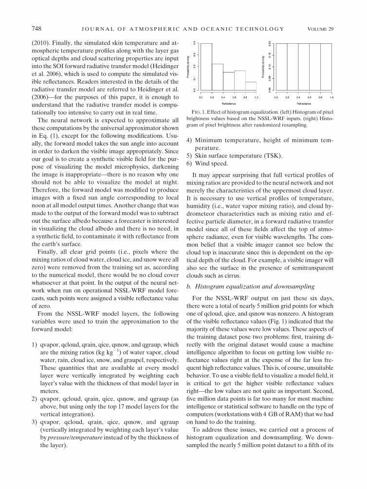
b. Histogram equalization and downsampling

For the NSSL-WRF output on just these six days,

there were a total of nearly 5 million grid points for which

one of qcloud, qice, and qsnow was nonzero. A histogram

of the visible reflectance values (Fig. 1) indicated that the

majority of these values were low values. These aspects of

the training dataset pose two problems: first, training di-

rectly with the original dataset would cause a machine

intelligence algorithm to focus on getting low visible re-

flectance values right at the expense of the far less fre-

quent high reflectance values. This is, of course, unsuitable

behavior. To use a visible field to visualize a model field, it

is critical to get the higher visible reflectance values

right—the low values are not quite as important. Second,

five million data points is far too many for most machine

intelligence or statistical software to handle on the type of

computers (workstations with 4 GB of RAM) that we had

on hand to do the training.

To address these issues, we carried out a process of

histogram equalization and downsampling. We down-

sampled the nearly 5 million point dataset to a fifth of its

FIG. 1. Effect of histogram equalization. (left) Histogram of pixel

brightness values based on the NSSL-WRF inputs. (right) Histo-

gram of pixel brightness after randomized resampling.

748 J O U R N A L O F A T M O S P H E R I C A N D O C E A N I C T E C H N O L O G Y VOLUME 29

size. These million grid points were obtained by ran-

domly selecting grid points from the original dataset

where the probability that a grid point was selected

depended on its brightness value. Thus, grid points with

a low brightness value had a lower probability of being

selected, while grid points with a high brightness value

were more likely to be selected. The likelihood of a grid

point with brightness value b being selected depends on

r, the repeat ratio, given by

r 5 nS/P(b), (3)

where n is the number of nonzero bins in the histogram,

S is the subsampling ratio (0.2 to reduce the dataset from

5 million to 1 million points), and P(b) is the probability

density of that brightness value (read out from the his-

togram in Fig. 1). If the r is, say 0.3, the grid point is

selected with a probability of 0.3. This is achieved by

generating a random number uniformly distributed in

the range [0–1] and selecting the point if the random

number is below 0.3. If the r is 2.3, the grid point is se-

lected twice and a third time with a probability of 0.3. To

avoid overfitting extremely rare values, the repeat ratio

was capped at 5. The subsampling ratio of 0.2 was chosen

because 1 million points was the hardware and software

limit of our system. The repeat ratio was capped at 5

arbitrarily; any number of the same order of magnitude

would have worked.

After histogram equalization and subsampling, the

resulting dataset of approximately 1 million grid points

had the frequency distribution shown in histogram on

the right in Fig. 1.

c. Neural network training

A neural network with 31 input variables and 3 hidden

nodes [i.e., in Eq. (1), d 5 31 and M 5 3] was trained on

1.01 million points selected through histogram equal-

ization and randomized subsampling from a dataset

consisting of 36 time steps from 6 days of NSSL-WRF

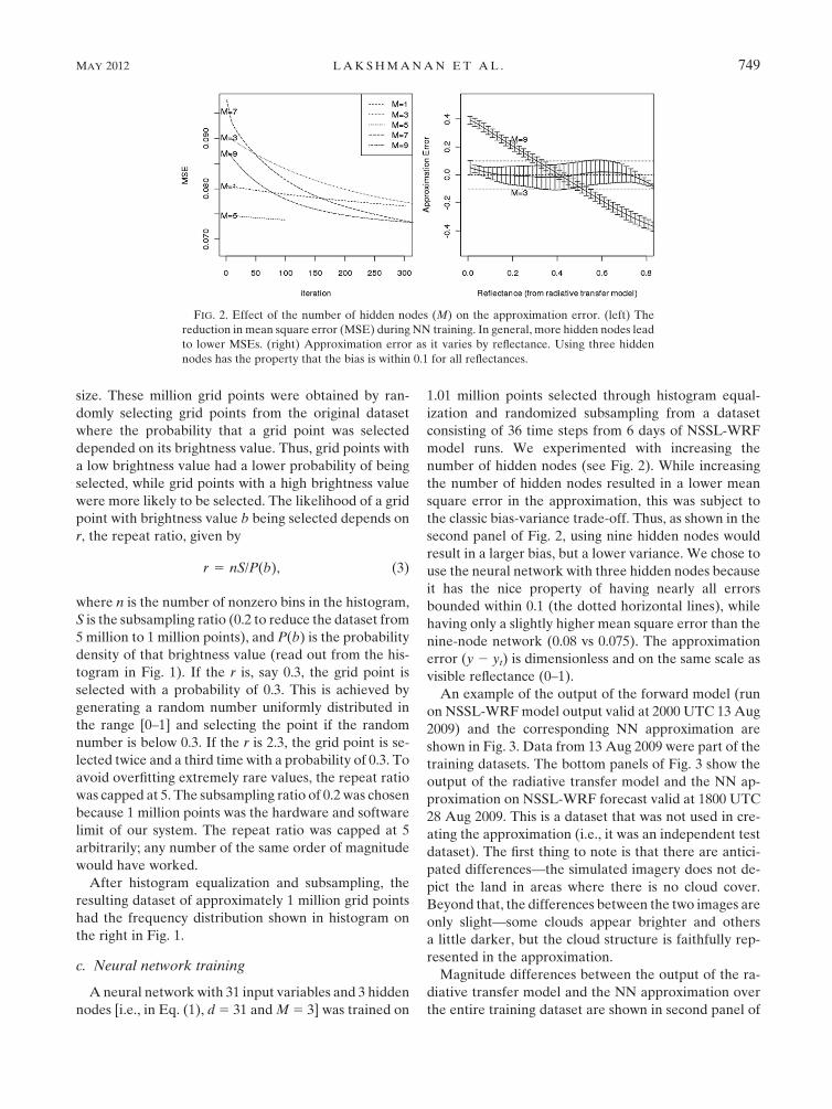
model runs. We experimented with increasing the

number of hidden nodes (see Fig. 2). While increasing

the number of hidden nodes resulted in a lower mean

square error in the approximation, this was subject to

the classic bias-variance trade-off. Thus, as shown in the

second panel of Fig. 2, using nine hidden nodes would

result in a larger bias, but a lower variance. We chose to

use the neural network with three hidden nodes because

it has the nice property of having nearly all errors

bounded within 0.1 (the dotted horizontal lines), while

having only a slightly higher mean square error than the

nine-node network (0.08 vs 0.075). The approximation

error (y 2 yt) is dimensionless and on the same scale as

visible reflectance (0–1).

An example of the output of the forward model (run

on NSSL-WRF model output valid at 2000 UTC 13 Aug

2009) and the corresponding NN approximation are

shown in Fig. 3. Data from 13 Aug 2009 were part of the

training datasets. The bottom panels of Fig. 3 show the

output of the radiative transfer model and the NN ap-

proximation on NSSL-WRF forecast valid at 1800 UTC

28 Aug 2009. This is a dataset that was not used in cre-

ating the approximation (i.e., it was an independent test

dataset). The first thing to note is that there are antici-

pated differences—the simulated imagery does not de-

pict the land in areas where there is no cloud cover.

Beyond that, the differences between the two images are

only slight—some clouds appear brighter and others

a little darker, but the cloud structure is faithfully rep-

resented in the approximation.

Magnitude differences between the output of the ra-

diative transfer model and the NN approximation over

the entire training dataset are shown in second panel of

FIG. 2. Effect of the number of hidden nodes (M) on the approximation error. (left) The

reduction in mean square error (MSE) during NN training. In general, more hidden nodes lead

to lower MSEs. (right) Approximation error as it varies by reflectance. Using three hidden

nodes has the property that the bias is within 0.1 for all reflectances.

MAY 2012 L A K S H M A N A N E T A L . 749

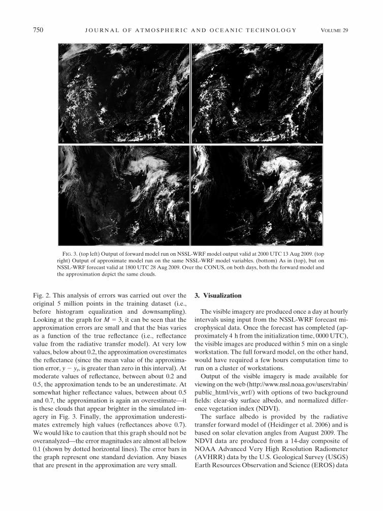
Fig. 2. This analysis of errors was carried out over the

original 5 million points in the training dataset (i.e.,

before histogram equalization and downsampling).

Looking at the graph for M 5 3, it can be seen that the

approximation errors are small and that the bias varies

as a function of the true reflectance (i.e., reflectance

value from the radiative transfer model). At very low

values, below about 0.2, the approximation overestimates

the reflectance (since the mean value of the approxima-

tion error, y 2 yt, is greater than zero in this interval). At

moderate values of reflectance, between about 0.2 and

0.5, the approximation tends to be an underestimate. At

somewhat higher reflectance values, between about 0.5

and 0.7, the approximation is again an overestimate—it

is these clouds that appear brighter in the simulated im-

agery in Fig. 3. Finally, the approximation underesti-

mates extremely high values (reflectances above 0.7).

We would like to caution that this graph should not be

overanalyzed—the error magnitudes are almost all below

0.1 (shown by dotted horizontal lines). The error bars in

the graph represent one standard deviation. Any biases

that are present in the approximation are very small.

3. Visualization

The visible imagery are produced once a day at hourly

intervals using input from the NSSL-WRF forecast mi-

crophysical data. Once the forecast has completed (ap-

proximately 4 h from the initialization time, 0000 UTC),

the visible images are produced within 5 min on a single

workstation. The full forward model, on the other hand,

would have required a few hours computation time to

run on a cluster of workstations.

Output of the visible imagery is made available for

viewing on the web (http://www.nssl.noaa.gov/users/rabin/

public_html/vis_wrf/) with options of two background

fields: clear-sky surface albedo, and normalized differ-

ence vegetation index (NDVI).

The surface albedo is provided by the radiative

transfer forward model of (Heidinger et al. 2006) and is

based on solar elevation angles from August 2009. The

NDVI data are produced from a 14-day composite of

NOAA Advanced Very High Resolution Radiometer

(AVHRR) data by the U.S. Geological Survey (USGS)

Earth Resources Observation and Science (EROS) data

FIG. 3. (top left) Output of forward model run on NSSL-WRF model output valid at 2000 UTC 13 Aug 2009. (top

right) Output of approximate model run on the same NSSL-WRF model variables. (bottom) As in (top), but on

NSSL-WRF forecast valid at 1800 UTC 28 Aug 2009. Over the CONUS, on both days, both the forward model and

the approximation depict the same clouds.

750 J O U R N A L O F A T M O S P H E R I C A N D O C E A N I C T E C H N O L O G Y VOLUME 29

center. The data currently used as the background for

the visible imagery are typical of summer. The NDVI

image is color enhanced to represent the relative

‘‘greenness’’ of the surface.

There is also an option to display microphysical quan-

tities from the forecast model as overlays on the visible

imagery; vertically integrated cloud liquid water, rainwa-

ter, ice, snow, and forecast precipitation accumulated in

FIG. 4. The 18-h forecast valid at 1800 UTC 28 Aug 2009. Relative values of superimposed quantities (kg m23)

increase from blue to green to red. (a) Visible image for 1800 UTC 28 Aug 2009 simulated using the NN approxi-

mation. (b) As in (a), but with vertically integrated cloud snow content superimposed. (c) As in (a), but with 1-h

accumulated precipitation superimposed. (d) As in (a), but with the vertically integrated cloud ice content super-

imposed. (e) As in (a), but with the vertically integrated cloud water content superimposed. (f) As in (a), but with

the vertically integrated cloud rainwater content superimposed. (g) Observed GOES-12 visible satellite image at

1815 UTC 28 Aug 2009.

MAY 2012 L A K S H M A N A N E T A L . 751

the previous hour. This option is useful to visualize the

microphysical composition of cloud fields being viewed,

and in relating the model forecast parameters with each

other. An example of the available visualizations on a test

dataset is shown in Fig. 4. The output of the forward

radiative transfer model on this NSSL-WRF forecast is

shown in Fig. 3.

The visible imagery created from the radiative trans-

fer forward model were produced at two different

forecast times (1800 and 2200) for comparison with the

FIG. 5. The 18-h forecast valid at 1800 UTC 13 Dec 2010. Relative values of superimposed quantities (kg m23) increase

from blue to green to red. (a) Visible image for 1800 UTC 13 Dec 2010 simulated using the NN approximation. (b) As in

(a), but with the vertically integrated cloud snow content superimposed. (c) As in (a), but with 1-h accumulated pre-

cipitation superimposed. (d) As in (a), but with the vertically integrated cloud ice content superimposed. (e) As in (a), but

with the vertically integrated cloud water content superimposed. (f) As in (a), but with vertically integrated cloud

rainwater content superimposed. (g) Observed GOES-13 visible satellite image at 1815 UTC 13 Dec 2010.

752 J O U R N A L O F A T M O S P H E R I C A N D O C E A N I C T E C H N O L O G Y VOLUME 29

neural network version during the NOAA HWT (Clark

et al. (2012)) and GOES-R Proving Ground Project in

2010. While the visible imagery from the forward model

took hours to compute and were generally available well

after the valid time of the forecast, the visible imagery

from the neural network approximation were available

minutes after the WRF forecasts were produced. It took,

on average, 3 min of wall-clock time to generate the

simulated visible image from a WRF forecast, with nearly

80% of time used in reading the WRF model output. If

the approximation is incorporated into the WRF post-

processing itself, where the inputs to the neural network

are already in main memory, the computation of visible

imagery can be reduced to a few seconds per forecast

period.

Example images from an 18-h forecast valid at

1800 UTC 13 December 2010 are shown in Fig. 5. It

should be noted that the simulated visible reflectance is

reasonable even though wintertime cases were not part

of the training dataset. Arctic airflow over the Great

Lakes and southeastern coastal waters was occurring at

this time. North to south cloud-oriented bands to the

south of Lakes Michigan, Huron, and Erie were asso-

ciated with heavy lake-effect snow squalls. Cloud snow

content and surface accumulation are significant in these

areas where several centimeters of snow were observed.

Parallel cloud bands and cellular clouds offshore of the

southeast U.S. and Gulf coasts are evident in the imag-

ery. Given the shallow nature of most of these clouds,

they are composed mainly of cloud water without much

rainwater. Large areas of thin cloud cover composed

mainly of ice surround the snow squalls, and are wide-

spead through an upper-level trough and surface low in

the northeast United States, with an upper jet stream

from northern California to Montana.

Figure 5g shows an observed visible image from the

GOES-13 (east) geostationary satellite corresponding

to the 18-h forecast from the NSSL-WRF shown in Figs.

5a–f. Much of the difference in cloud locations and vi-

sual properties between the observed (Fig. 5g) and NN-

simulated image (Fig. 5a) can be attributed to forecast

error. In general the qualitative structure of the cloud

areas are similar, especially the deeper (brighter) clouds

with precipitation or high water, ice, snow content, and

the shallow convective clouds where cold air is moving

over the warmer waters off the Atlantic and Gulf of

Mexico coasts. Some of the clear-sky regions in the ob-

served image (U.S. Midwest) appear bright (high al-

bedo) because of snow cover. The snow-covered surface

cannot be easily distiguished from cloud cover from the

visible image alone, but the distinction is clear in the

simulated image since the assumed clear-sky albedo is

representative of the summer months.

4. Summary

Although a forward radiative transfer model is capa-

ble of providing a depiction of nonprecipitating clouds in

a numerical weather prediction model forecast, present-

day forward models are too slow to provide timely output

for routine weather forecasts. Therefore, an approxima-

tion to the behavior of a radiative transfer model on some

representative NWP forecasts was created using a neural

network. The resulting approximation is very close to the

complex radiative transfer model, but has the advantage

of being calculable in a small fraction of the time required

for the full forward model. This approximation is now

carried out routinely in the NOAA HWT and used as

routine forecast guidance at the NOAA Storm Prediction

Center. Furthermore, the synthetic visible product has

been employed extensively as a diagnostic tool in recent

HWT research activities, particularly those focusing on

convective initiation.

Acknowledgments. The authors are grateful for sup-

port from the NOAA High Performance Computing

and Communication (HPCC) program, which made this

project possible. Funding for the lead author was pro-

vided under NOAA–OU Cooperative Agreement

NA17RJ1227. We thank Tom Greenwald for his sug-

gestions throughout the project. We also thank Justin

Sieglaff for his suggestion to include an analysis of the

NN approximation error by reflectance value (Fig. 2).

REFERENCES

Baum, B., P. Yang, A. J. Heymsfield, S. Platnick, M. D. King, Y.-X.

Hu, and S. T. Bedka, 2005: Bulk scattering properties for the

remote sensing of ice clouds. Part II: Narrowband models.

J. Appl. Meteor., 44, 1896–1911.

Bishop, C., 1995: Neural Networks for Pattern Recognition. Oxford

University Press, 504 pp.

Clark, A. J., and Coauthors, 2012: An overview of the 2010 Haz-

ardous Weather Testbed Experimental Forecast Program

Spring Experiment. Bull. Amer. Meteor. Soc., 93, 55–74.

Dixon, M., Z. Li, H. Lean, N. Roberts, and S. Ballard, 2009: Impact

of data assimilation on forecasting convection over the United

Kingdom using a high-resolution version of the Met Office

unified model. Mon. Wea. Rev., 137, 1562–1584.

Feltz, W. F., K. M. Bedka, J. A. Otkin, T. Greenwald, and S. A.

Ackerman, 2009: Understanding satellite-observed mountain-

wave signatures using high-resolution numerical model data.

Wea. Forecasting, 24, 76–86.

Han, Q., Q. Rossow, R. Welch, A. White, and J. Chou, 1995:

Validation of satellite retrievals of cloud microphysics and

liquid water path using observations from FIRE. J. Atmos.

Sci., 52, 4183–4195.

Heidinger, A., C. O’Dell, R. Bennartz, and T. Greewald, 2006: The

successive order-of-interaction radiative transfer model. Part

I: Model development. J. Appl. Meteor. Climatol., 45, 1388–

1402.

MAY 2012 L A K S H M A N A N E T A L . 753

Heymsfield, A., S. Matrosov, and B. Baum, 2003: Ice water path-

optical depth relationships for cirrus and deep stratiform ice

cloud layers. J. Appl. Meteor. Climatol., 42, 1369–1390.

Hong, S., and J.-O. J. Lim, 2006: The WRF single-moment 6-class

microphysics scheme. J. Korean Meteor. Soc., 42, 129–151.

Jakob, C., 1999: Cloud cover in the ECMWF reanalysis. J. Climate,

12, 947–959.

Janjic, Z. I., 1990: The step-mountain coordinate: Physical package.

Mon. Wea. Rev., 118, 1429–1443.

Kain, J. S., and Coauthors, 2008: Some practical considerations re-

garding horizontal resolution in the first generation of opera-

tional convection-allowing NWP. Wea. Forecasting, 23, 931–952.

——, S. Dembek, S. J. Weiss, J. L. Case, J. J. Levit, and R. A.

Sobash, 2010a: Monitoring selected fields and phenomena

every time step. Wea. Forecasting, 25, 1536–1542.

——, and Coauthors, 2010b: Assessing advances in the assimila-

tion of radar data and other mesoscale observations within a

collaborative forecasting–research environment. Wea. Fore-

casting, 25, 1510–1521.

Koch, S. E., B. Ferrier, M. Stolinga, E. Szoke, S. J. Weiss, and J. S.

Kain, 2005: The use of simulated radar reflectivity fields in the

diagnosis of mesoscale phenomena from high-resolution WRF

model forecasts. Preprints, 11th Conf. on Mesoscale Processes,

Albuquerque, NM, Amer. Meteor. Soc., J4J.7. [Available on-

line at http://ams.confex.com/ams/32Rad11Meso/techprogram/

paper_97032.htm.]

Krasnopolsky, V. M., M. Fox-Rabinovitz, H. Tolman, and A. A.

Belochitski, 2008: Neural network approach for robust and

fast calculation of physical processes in numerical environ-

mental models: Compound parameterization with a quality

control of larger errors. Neural Networks, 21, 535–543.

Lakshmanan, V., A. Fritz, T. Smith, K. Hondl, and G. J. Stumpf,

2007: An automated technique to quality control radar re-

flectivity data. J. Appl. Meteor., 46, 288–305.

Marzban, C., and G. Stumpf, 1996: A neural network for tornado

prediction based on Doppler radar-derived attributes. J. Appl.

Meteor., 35, 617–626.

Otkin, J., and T. Greenwald, 2008: Comparison of WRF model-

simulated and MODIS-derived cloud data. Mon. Wea. Rev.,

136, 1957–1970.

——, ——, J. Sieglaff, and H.-L. Huang, 2009: Validation of

a large-scale simulated brightness temperature dataset using

SEVIRI satellite observations. J. Appl. Meteor. Climatol., 48,

1613–1626.

Rogers, E., and Coauthors, 2009: The NCEP North American

mesoscale modeling system: Recent changes and future plans.

Preprints, 23rd Conf. on Weather Analysis and Forecasting/

19th Conf. on Numerical Weather Predicition, Omaha, NE,

Amer. Meteor. Soc., 2A.4. [Available online at http://ams

.confex.com/ams/pdfpapers/154114.pdf.]

Sayer, A., G. Thomas, and R. Grainger, 2010: A sea surface re-

flectance model for AATSR and application to aerosol re-

trievals. Atmos. Meas. Technol., 44, 1896–1911.

Skamarock, W., J. Klemp, J. Dudhia, D. Gill, D. Barker, W. Wang,

and J. Powers, 2005: A description of the Advanced Re-

search WRF version 2. National Center for Atmospheric

Research Tech. Rep. NCAR/TN-468-STR, 88 pp. [Available

from UCAR Communications, P.O. Box 3000, Boulder, CO

80307.]

Sundqvist, H., E. Berge, and J. E. Kristjnsson, 1989: Condensation

and cloud parameterization studies with a mesoscale numer-

ical weather prediction model. Mon. Wea. Rev., 117, 1641–

1657.

Teixeira, J., and T. Hogan, 2002: Boundary layer clouds in a global

atmospheric model: Simple cloud cover parameterizations.

J. Climate, 15, 1261–1271.

Venkatesan, C., S. Raskar, S. Tambe, B. Kulkarni, and

R. Keshavamurty, 1997: Prediction of all India summer

monsoon rainfall using error-back-propagation neural net-

works. Meteor. Atmos. Phys., 62, 225–240.

Weisman, M., C. Davis, W. Wang, K. Manning, and J. Klemp, 2008:

Experiences with 0–36-h explicit convective forecasts with the

WRF-ARW model. Wea. Forecasting, 23, 407–437.

Weiss, S. J., M. E. Pyle, Z. Janjic, D. R. Bright, J. S. Kain, and G. J.

DiMego, 2008: The operational high-resolution window WRF

model runs at NCEP: Advantages of multiple model runs for

severe convective weather forecasting. Preprints, 24th Conf.

on Severe Local Storms, Savannah, GA, Amer. Meteor. Soc.,

P10.8. [Available online at http://ams.confex.com/ams/24SLS/

techprogram/paper_142192.htm.]

754 J O U R N A L O F A T M O S P H E R I C A N D O C E A N I C T E C H N O L O G Y VOLUME 29