UNCORRECTEDPROOF

1

23 RESEARCH ARTICLE

4

5 Study of the Anisotropic Reflectance Behaviour of Wheat Canopy6 to Evaluate the Performance of Radiative Transfer Model7 PROSAIL5B

9 Debasish Chakraborty & Vinay Kumar Sehgal &10 Rabi Narayan Sahoo & Sanatan Pradhan &

11 Vinod Kumar Gupta

12

13

14 Received: 15 March 2014 /Accepted: 26 August 201415 # Indian Society of Remote Sensing 2014

16 Abstract A field experiment was conducted on wheat to17 analyze its bi-directional reflectance in relation to sun-target-18 sensor geometry. To achieve a large variation in crop param-19 eters, two extreme nitrogen treatments were applied. The20 study reconfirms the strong and consistent anisotropic patterns21 of wheat bi-directional reflectance in visible (VIS) and near22 infra-red (NIR) and its magnitude was highest in the principal23 plane. This anisotropic pattern extended equally in shortwave24 infra-red (SWIR). The hotspot broadened with crop growth25 due to increase in leaf area index (LAI), leaf size and26 planophilic orientation. The shape and magnitude of27 PROSAIL5B simulated spectra was in close agreement with28 the observed spectra in the optical region for most of the view29 zenith and azimuth angle combinations. In the NIR and30 SWIR, the magnitude of the model simulations showed good31 match in the principal plane, whereas underestimation was32 found in the backward scattering direction at higher view33 zenith angles in the VIS. The typical bowl shape of observed34 reflectance in principal plane was very well simulated in NIR

35by the model but failed in other wavebands. The model36performed best in the NIR region followed by SWIR and37maximum relative error was in VIS. Over the whole optical38region and view zenith angles, the model simulations showed39an average error of 26%. The model simulations were poor at40low LAI indicating the need to improve soil reflectance algo-41rithm in the model. Results of the study have implications for42understanding the shortcomings in the model and its inversion43to derive crop biophysical parameters from multispectral44sensors.

45Keywords Q1

46Introduction

47Estimation of vegetation biochemical and biophysical vari-48ables with reasonable accuracy has usefulness for a range of49agricultural, ecological, and meteorological applications50(Houborg et al. 2007; Darvishzadeh et al. 2008). Leaf area51indexes (LAI), leaf chlorophyll content (LCC) and leaf water52content (Cw) are the most important vegetation parameters53among all (Houborg et al. 2007). The two common ap-54proaches for estimating vegetation parameters from remotely55sensed data are: (a) Empirical/statistical and (b) Physical. But56the statistical relationships being sensor-specific and depen-57dent on site and sampling conditions, are supposed to change58in space and time (Meroni et al. 2004). The physical approach59involving radiative transfer models (RTM) can accurately60describes the spectral variation of canopy reflectance as a61function of canopy, leaf and soil background characteristics62(Goel 1989; Meroni et al. 2004) by explaining the transfer and63interaction of radiation inside the canopy based on physical64laws (Houborg et al. 2007).

D. Chakraborty :V. K. Sehgal (*) :R. N. Sahoo : S. Pradhan :V. K. GuptaDivision of Agricultural Physics, Indian Agricultural ResearchInstitute (IARI), New Delhi 110012, Indiae-mail: vksehgal@gmail.com

V. K. Sehgale-mail: sehgal@iari.res.in

D. Chakrabortye-mail: debasishagri@gmail.com

R. N. Sahooe-mail: rnsahoo.iari@gmail.com

S. Pradhane-mail: sanatan28@gmail.com

V. K. Guptae-mail: vk_001@gmail.com

J Indian Soc Remote SensDOI 10.1007/s12524-014-0411-7

JrnlID 12524_ArtID 411_Proof# 1 - 30/08/2014

UNCORRECTEDPROOF

65 The earth and plant surface features reflect radiation aniso-66 tropically. So the observed reflectance of a remotely sensed67 scene (with respect to a Lambertian reference) alters with the68 source and view geometry and is quantified as “bi-directional69 reflectance factor” (BRF). The BRF is not only a function of70 relative geometry of illumination and observation, but also71 depends on the biochemical composition of vegetation surface72 (leaf pigments, intercellular space, moisture content) and the73 spatial and geometrical arrangement of surface elements74 (shape, size and orientation of leaves, mutual shading). So,75 the inversion of bi-directional canopy reflectance models76 emerged as a promising alternative for retrieval of vegetation77 biophysical parameters (Goel 1989). The new generation of78 space borne instruments likes POLDER (Polarization and79 Directionality of the Earth′s reflectance) and MISR (Multi-80 angle Imaging Spectroradiometer) on board ADEOS81 (Advance Earth Observing Satellite) and Terra, respectively,82 are designed to study both the spectral and directional reflec-83 tance of the earth surface.84 Research on use of radiative transfer models (RTMs)85 for crop biophysical parameter retrieval has emerged as an86 area of scientific pursuit globally in last one decade87 (Meroni et al. 2004; Houborg et al. 2007; Yao et al.88 2008; Vohland and Jarmer 2008). The RTM inversion89 requires thorough validation of the model for target crops90 at various growth stages under different growing condi-91 tions, followed by analysis of model′s shortcomings.92 Though many studies have analyzed the bi-directional93 reflectance behaviour of vegetation canopies using94 spectroradiometers mounted on a variety of goniometers95 (Roman et al. 2011), only a few have pursued detailed96 evalution of the model simulations of bi-directional re-97 flectance at various growth stages under different growing98 conditions (Andrieu et al. 1997; Sridhar et al. 2009;99 Barman et al. 2010). Most of the studies have not been100 exhaustive to measure BRF in the whole optical domain101 from 400–2,500 nm, at different growth stages of crop102 and for crop experiencing extreme treatments resulting in103 varied crop growth. There is a merit in undertaking de-104 tailed field evaluation of canopy reflectance models under105 such varying crop growth conditions to evaluate their106 strengths and shortcomings for the purpose of their in-107 formed applications.108 Keeping this background in view, the bi-directional reflec-109 tance of wheat was studied at different source-target-view110 geometries, at two growth stages and under contrasting grow-111 ing conditions in the optical region (400–2,500 nm). Further,112 the bi-directional reflectance measurements were used to eval-113 uate the performance of model PROSAIL5B. This study114 specifically validated model at two growth stages of wheat115 which were grown under two contrasting treatments of nitro-116 gen application, thus resulting in a large variation in crop117 biophysical parameters.

118Methodology

119Study Area

120The field experiment was conducted in the experimental farm121of the Indian Agricultural Research Institute, New Delhi122which is located at 28°38’23” N latitude and 77°09’27” E123longitude with an altitude of 228.6 m above mean sea level.124The soil here is sandy loam in texture, deep and with moderate125fertility. The site is having semi-arid climate with two distinct126crop seasons, viz., kharif (Jun-Oct) and rabi (Nov-Mar).

127Experimental Detail

128Spring wheat (Triticum aestivum L.) variety PBW-502 was129grown during the rabi season of 2010–2011 with two nitrogen130treatments, each with three replications in a plot size of 6 m×1316 m. The treatments were applied with the objective to create132variability in crop growth vis-à-vis vegetation biophysical and133biochemical parameters. Crop was sown on November 25,1342010 by seed drill at a recommended row spacing of 22.5 cm.135Three nitrogen treatments, namely, 0 (N0) and 120 (N120) kg136ha−1 were applied. The full nitrogen dose was applied in three137splits - half as basal and one fourth each as topdressing at138crown-root-initiation (CRI) stage and flowering stage. The139recommended dose of phosphorous and potassium was ap-140plied as basal. Lowest chlorophyll and poor growth was141realized in N0 treatment resulting in sparse canopy. Highest142chlorophyll with better growth was realized in N120 treatment143resulting in a well developed dense canopy.

144Measurements of Plant Parameters

145Various plant parameters, to be used as input for PROSAIL146model, were measured on same day synchronizing with the147spectral observations taken at different growth stages. Five148plants were randomly selected in each plot and their height149was measured with a metric scale. Leaf length of second150mature leaf from the top of these five plants in each plot was151also measured by a metric scale and averaged. Leaf Area152Index (LAI) was measured using Plant Canopy Analyser153(LI-2000) following the procedure given by Welles and154Norman (1991). Multiple LAI observations (at least five) on155each date within each plot were taken and their average was156calculated to represent LAI of that plot on that date. Leaf angle157in degrees was measured using a protractor. All leaves on one158plant and five such plants in each plot were sampled for leaf159angle measurement and their average leaf angle (Angl) with160respect to horizontal was calculated. For leaf chlorophyll161content (Cab) measurements, 50mg of fresh leaf samples from162different treatments were weighed accurately on an analytical163balance and chlorophyll was extracted by a non macerated164method, equilibrating it with 10 ml DiMethyl SulfOxide

J Indian Soc Remote Sens

JrnlID 12524_ArtID 411_Proof# 1 - 30/08/2014

UNCORRECTEDPROOF

165 (DMSO) in a capped vial and keeping in an oven at 65 °C for166 about 3 h (Hiscox and Israelstam 1979). The decanted solution167 was used to estimate the absorbance at 645 and 663 nm168 wavelengths using Spectrophotometer. Plant samples were169 cut just above the soil surface and their leaves were separated.170 The area of fresh leaves was determined by passing them171 through leaf-area meter (LI-3100). These leaves were dried172 in an oven at 70 °C to achieve a constant weight and then their173 dry weight was recorded. The specific leaf weight (Cm) was174 calculated as the ratio of dry weight of leaves to leaf area of the175 same sample. Equivalent leaf moisture thickness (Cw), an176 index of leaf water content which represents volume of leaf177 water per unit leaf area, was calculated as the ratio of differ-178 ence in fresh and dry leaf weight to leaf area.

179 Bi-directional Reflectance Measurements

180 The BRF measurements were recorded between 11:00 and181 13:00 h under clear sky conditions using hand-held182 Spectroradiometer (ASD FieldSpec-3) installed on a portable183 field goniometer (same setupwas used as described in Barman184 et al. 2010). The spectroradiometer is having a default 25°185 Field of View (FOV) which was decreased to 10° using fore-186 optics provided with the instrument. The reflectance were187 measured at 1 nm interval in the spectral range of 350–188 2,500 nm at eight relative azimuthal angles (i.e. relative to189 the azimuth angle of sun) of 0°, 45°, 90°, 135°, 180°, 225°/-190 135°, 270°/-90° and 315°/-45°, and at six zenith angles of 20°,191 30°, 40°, 50° and 60° plus nadir. In principal plane (which is192 aligned to sun azimuth), 0° relative azimuth refers to the193 backward scattering direction of light while 180° relative194 azimuth refers to the forward scattering direction of light.195 Corresponding to each view azimuth and zenith position,196 reflectance was also recorded from a reference panel coated197 with barium sulphate, reflecting about 99 % radiation. Time198 taken for making these measurements was about 20–25 min199 during which we assumed a fixed position of sun at that200 location.

201 Bi-directional Reflectance Analysis

202 In order to analyze the BRF pattern of crop, BRF surface plots203 were prepared at four wavelengths corresponding to the central204 wavelengths of IRS-P6 LISS-3 (Indian Remote Sensing205 Satellite-P6, Linear Imaging Self Scanning-3) bands, viz.,206 568, 660, 790 and 1,634 nm. The 41 spectral reflectance values207 corresponding to all the view zenith and relative azimuth angles208 were interpolated using “smoothing spline” function to gener-209 ate a surface of bi-directional reflectance. The surface plots210 were prepared in rectangular coordinate system where view-211 zenith angle was plotted on x-axis (varying diagonally),212 relative-azimuth angle on y-axis (varying horizontally) and213 spectral reflectance on z-axis. Before plotting, the spherical

214coordinates of view zenith and relative azimuth angles were215transformed into rectangular coordinates. The bi-directional216surface plots at four wavelengths were prepared for N0 and217N120 treatments and compared.

218The Radiative Transfer Model PROSAIL

219This study used a variant of one of the widely applied canopy220radiative transfer model PROSAIL (Jacquemoud et al. 2009)221which is a combination of two models, i.e., the PROSPECT222model (Jacquemoud and Baret 1990 that describes leaf optical223properties and the SAIL model (Verhoef 1984) that computes224canopy reflectance at different wavelengths. The PROSAIL225model considers the detailed information on leaf optical prop-226erties and also accounts for hotspot effect. The PROSAIL5B227version of model (downloaded from http://teledetection.ipgp.228jussieu.fr/prosail/) was used in this study which incorporates229PROSPECT-5 and 4SAIL models. The input parameters of230PROSAIL5B with their units are given in Table 1.

231Validation of PROSAIL

232In order to validate the model for a given treatment on a233particular day, required input parameters of leaf, canopy, soil,234view and solar zenith and relative azimuth angles were pro-235vided. The model then simulated canopy bi-directional reflec-236tance between 400 and 2,500 nm at 1 nm interval. The237performance of the model was evaluated by comparing model238simulated values with observed values in two ways: (a) for the239whole spectra and (b) at specific wavelengths. In case of240whole spectra validation, the observed spectra in the range241of 400–2,500 nm at different view zenith angles in the princi-242pal plane were compared with the corresponding model

t1:1Table 1 Input parameters of PROSAIL-5B model

t1:2Parameters Description

t1:3Ihot Hot spot flag (1=use hot spot)

t1:4Angl Average leaf angle (°)

t1:5LAI Leaf Area Index (m2 m−2)

t1:6N Structural Coefficient (unit less)

t1:7Cab Chlorophyll a + b content (μg cm−2)

t1:8Car Carotenoid content (μg cm−2)

t1:9Cbrown Brown pigment content (arbitrary units)

t1:10Cw Leaf Equivalent Water Thickness (cm)

t1:11Cm Leaf Dry matter Content (g cm−2)

t1:12Hspot Hot-spot parameter (Leaf length/Crop height)

t1:13Skyl Percent Diffuse to Direct radiation

t1:14Psoil Soil Coefficient

t1:15Theta_S Solar Zenith Angle (°)

t1:16Theta_O Observer zenith angle (°)

t1:17Psi Relative Azimuth Angle (°)

J Indian Soc Remote Sens

JrnlID 12524_ArtID 411_Proof# 1 - 30/08/2014

UNCORRECTEDPROOF

243 simulated spectra. It helped in evaluating the performance of244 the model to simulate the variation in the reflectance due to the245 variation in the view zenith angles. The portions of spectra246 between 1,350–1,400 nm, 1,800–2,000 nm and 2,400–247 2,500 nmwere not considered for comparison due to presence248 of significant atmospheric noise in the observed spectra.249 Again for the validation of the model at specific wavelengths,250 simulated values were validated by comparing them with251 observed values at specific wavelengths (568, 660, 790 and252 1,634 nm) which corresponded to the central wavelength of253 IRS-P6 LISS-3 spectral bands. In this case also the validation254 was done in the principal plane at different view zenith angles255 (−60°, −50°, −40°, −30°, −20°, 00, 20°, 30°, 40°, 50°, 60°).256 The negative view zenith referred to backward scattering257 direction (i.e. sun behind sensor) and positive referred to258 forward scattering direction (i.e. sensor opposite to sun).

259 Model Performance Evaluation

260 The performance of the model was evaluated by calculating261 RootMean Square Error (RMSE) between observed and mod-262 el simulated reflectance values, either at particular wavelength263 or for a wavelength band using formula given below:

RMSE ¼ffiffiffiffiffiffiffiffiffiffiffiffiffiffiffiffiffiffiffiffiffiffiffiffiffiffiffiffiffiffiffiffiffiffiffiffiffiffiffiffi

Xn

i¼1Robs � Rsimð Þ2n

s

ð1Þ264265

266 where, Robs is observed reflectance, Rsim is simulated re-267 flectance, and n is number of observations.268 In order to compare RMSE across wavelength regions and269 at various growth stages of the crop, it was normalized by the270 average of observed reflectance values and thus normalized271 RMSE (nRMSE) was calculated as given below:

nRMSE ¼ RMSE

μð2Þ

272273

274 where, μ is mean of observed reflectance values.

275For whole spectra comparison, the RMSE and nRMSE276were calculated for wavelength regions 400–700 nm (VIS),277800–1,300 nm (NIR) and 1,500–2,400 nm (SWIR) and are278referred to as RMSE1, RMSE2, RMSE3 and nRMSE1,279nRMSE2 and nRMSE3, respectively.280

281Results

282Measured Parameters

283The measured values of PROSAIL parameters for wheat with284their standard deviation for two nitrogen treatments (N0 and285N120) on 46 and 106 days after sowing (DAS) are given in286Table 2. The LAI was 0.48 and 0.60 on 46 DAS which287increased to 1.7 and 3.2 on 106 DAS in N0 and N120 treat-288ments, respectively. The effect of nitrogen treatment on LAI289was little during initial growth stages (46 DAS) which became290more pronounced at later growth stages (106 DAS). In case of291Cab, the effect of nitrogen treatment was evident at all the292growth stages of wheat as chlorophyll content is very sensitive293to nitrogen availability. The variations in the Cw were limited294as crop was not exposed to any water treatment during its295growth season. Similarly, the range of variations in Cm was296less across treatments and DAS. The leaves were more erect297on 46 DAS as shown by Angl value of 70° but became less298erect on 106 DAS with Angl value ranging between 35 and29945°. On 46 DAS, the Hspot value was 0.78–0.79 under both300the treatments and the value decreased to 0.22 in N0 and 0.32301in N120 at 106 DAS. These varied observations constituted a302good dataset for analyzing the anisotropic behaviour of wheat303canopy reflectance and validation of PROSAIL5B over a304range of crop biophysical conditions.

305Bi-directional Reflectance Patterns

306Figure 1 and 2 shows the bi-directional reflectance patterns at30746 DAS and 106 DAS for N0 and N120 treatments,

t2:1 Table 2 Field measured values of wheat parameters with their standard deviation (SD) for N0 and N120 nitrogen treatments at 46 and 106 DAS

t2:2 Parameters Description N0 N120

t2:3 46 DAS 106 DAS 46 DAS 106 DAS

t2:4 Mean SD Mean SD Mean SD Mean SD

t2:5 LAI Leaf Area Index (m2 m−2) 0.48 0.02 1.70 0.07 0.60 0.18 3.20 0.22

t2:6 Cab Chlorophyll a+b content (μg cm−2) 28 1.92 29 4.14 52 6.62 65 8.82

t2:7 Cw Leaf Equivalent Water Thickness (cm) 0.033 0.003 0.027 0.0016 0.024 0.0012 0.030 0.0022

t2:8 Cm Leaf Dry matter Content (g cm−2) 0.0071 0.0004 0.0031 0.0006 0.0046 0.0002 0.0047 0.0003

t2:9 Angl Average leaf angle (°) 70 2.41 35 2.56 70 2.06 45 1.60

t2:10 Hspot Hot-spot parameter (Leaf length/Crop height) 0.79 0.055 0.22 0.014 0.78 0.034 0.32 0.013

J Indian Soc Remote Sens

JrnlID 12524_ArtID 411_Proof# 1 - 30/08/2014

UNCORRECTEDPROOF

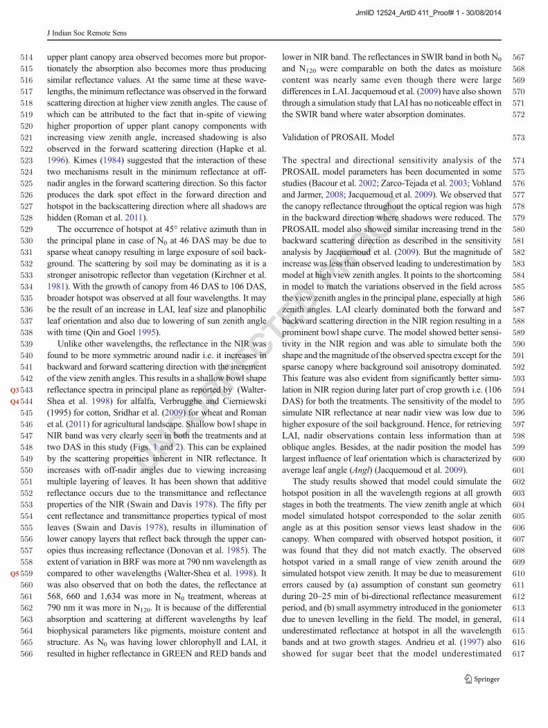
308 respectively. The symbol of star in these figures depicts the309 position of sun at the time of observations. The bi-directional310 reflectance was analyzed at four wavelengths corresponding311 to central wavelengths of IRS-P6 LISS-3 bands. These select-312 ed wavelengths also represent different mechanisms of inter-313 action of radiation with plant canopy.314 Figure 1 show the bi-directional reflectance pattern of315 wheat on 46 DAS when solar zenith angle was 51°. It shows316 wide variations in reflectance at a given wavelength with317 change in sun-target-sensor geometry. Overall, in both the318 treatments and at all the wavelengths, higher reflectance was319 observed in backward scattering direction than in forward.320 Highest reflectance was invariably observed in the principal321 plane between 50° and 60° view zenith angles and 0° relative322 azimuth which corresponded to the hot-spot position. An323 exception was at 790 nm for N0 where hot-spot occurred at

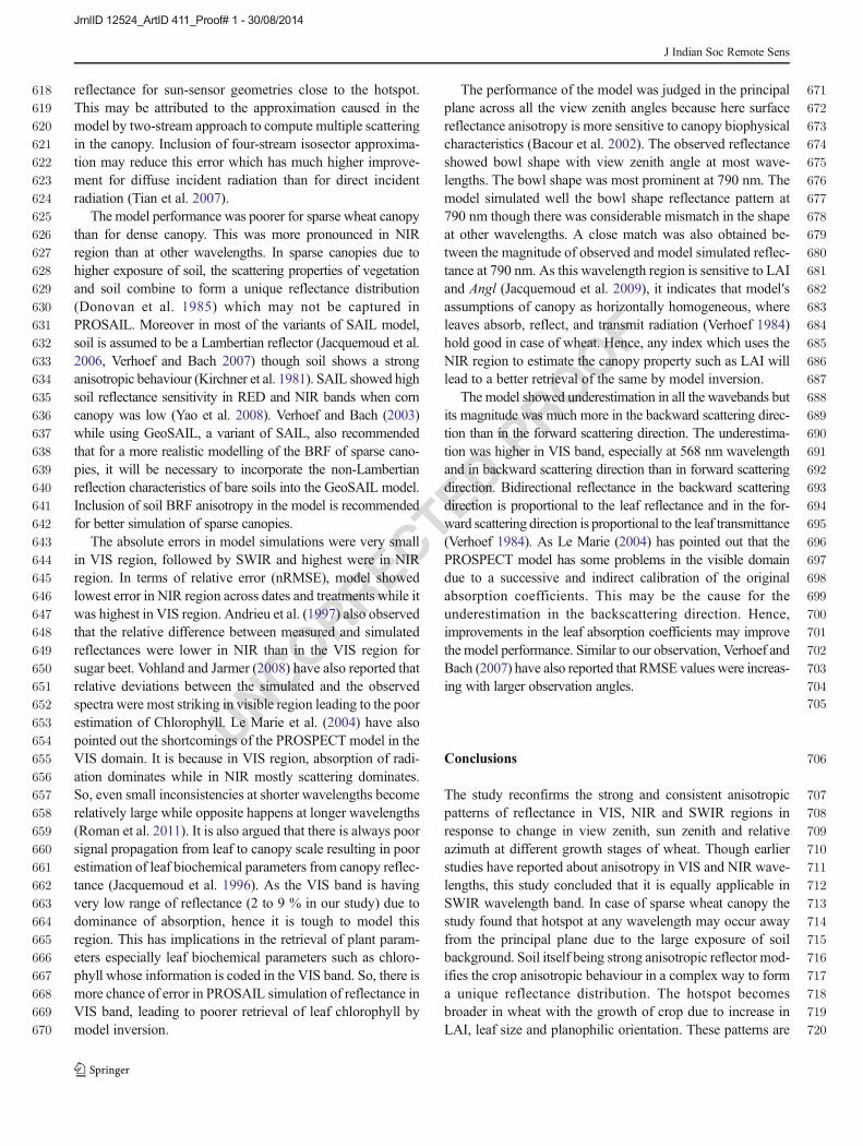
32445° relative azimuth instead of 0°. The hot-spot was very well325marked in N120 treatment than in N0. In both the treatments,326the reflectance at 790 nm (NIR) was higher at view zenith327angle of 50°–60° for all relative azimuth angles but such328pattern was not observed at other wavelengths. The N0 treat-329ment showed a little higher reflectance than N120 at 568, 660330and 1,634 nm but the trend was reversed at 790 nm. It may be331noted that the minimum reflectance at 568, 660 and 1,634 nm332was found at 600 view zenith angle in forward scattering333direction (relative azimuth 180°, 225° and 270°) but for334790 nm it was found at about 20° view zenith angle in forward335scattering direction in both the treatments.336Figure 2 shows the bi-directional reflectance pattern337of wheat on 106 DAS when solar zenith angle was 33°.338The bi-directional reflectance pattern showed higher re-339flectance in backward scattering direction and lower

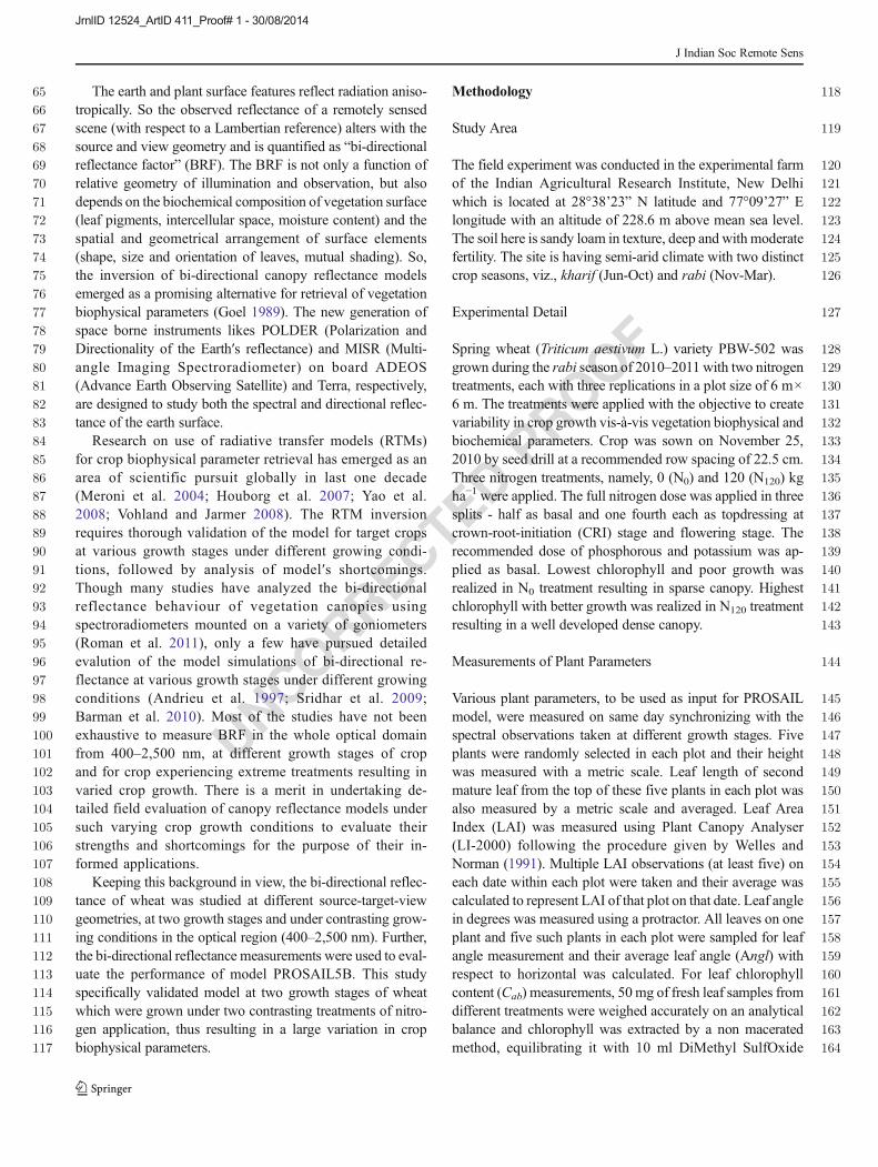
Fig. 1 Polar plots showing bi-directional reflectance factor(BRF) of wheat for N0 at (a)568 nm, (b) 660 nm, (c) 790 nmand (d) 1,634 nm and for N120 at(e) 568 nm, (f) 660 nm, (g)790 nm and (h) 1,634 nm, 46DAS

J Indian Soc Remote Sens

JrnlID 12524_ArtID 411_Proof# 1 - 30/08/2014

UNCORRECTEDPROOF

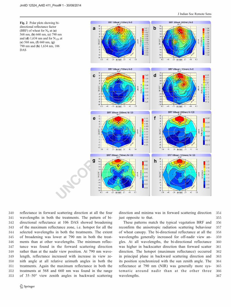
340 reflectance in forward scattering direction at all the four341 wavelengths in both the treatments. The pattern of bi-342 directional reflectance at 106 DAS showed broadening343 of the maximum reflectance zone, i.e. hotspot for all the344 selected wavelengths in both the treatments. The extent345 of broadening was lower at 790 nm in both the treat-346 ments than at other wavelengths. The minimum reflec-347 tance was found in the forward scattering direction348 rather than at the nadir view position. At 790 nm wave-349 length, reflectance increased with increase in view ze-350 nith angle at all relative azimuth angles in both the351 treatments. Again the maximum reflectance in both the352 treatments at 568 and 660 nm was found in the range353 of 35–50° view zenith angles in backward scattering

354direction and minima was in forward scattering direction355just opposite to that.356These patterns match the typical vegetation BRF and357reconfirm the anisotropic radiation scattering behaviour358of wheat canopy. The bi-directional reflectance at all the359wavelengths generally increased for off-nadir view an-360gles. At all wavelengths, the bi-directional reflectance361was higher in backscatter direction than forward scatter362direction. The hotspot (maximum reflectance) occurred363in principal plane in backward scattering direction and364its position synchronized with the sun zenith angle. The365reflectance at 790 nm (NIR) was generally more sys-366temat ic around nadir than a t the other three367wavelengths.

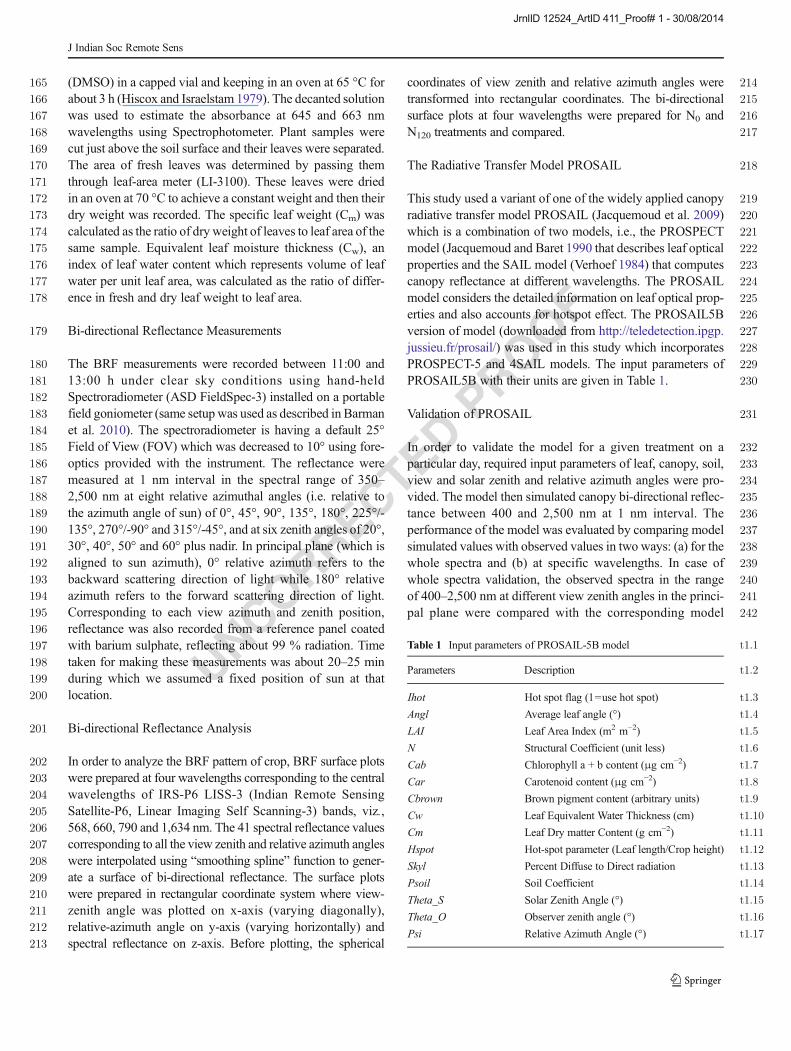
Fig. 2 Polar plots showing bi-directional reflectance factor(BRF) of wheat for N0 at (a)568 nm, (b) 660 nm, (c) 790 nmand (d) 1,634 nm and for N120 at(e) 568 nm, (f) 660 nm, (g)790 nm and (h) 1,634 nm, 106DAS

J Indian Soc Remote Sens

JrnlID 12524_ArtID 411_Proof# 1 - 30/08/2014

UNCORRECTEDPROOF

368 Validation of PROSAIL Model

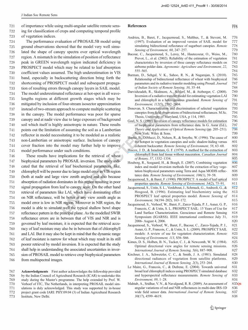
369 The model PROSAIL-5B was validated for wheat crop at370 specific wavelengths in the principal plane. Results are pre-371 sented for N0 and N120 treatments at 46 and 106 DAS which372 represented wide variation in leaf biochemical and canopy373 biophysical parameters. The default values of parameters374 Car=1 μg.cm−2 and Cbrown=0.05 were used. The leaf struc-375 tural parameter N, whose value ranges between 1.0 to 1.5 for376 monocotyledonous plants (Q2 Jaquemound 1993), was specified377 a value of N=1.0. The value N=1.0 was found to best fit the378 model simulated spectra with the observed spectra in most of379 the cases. The value of percent diffuse to direct sunlight (skyl)380 was assumed to be of 10 because all the spectroradiometeric381 observations were taken under clear sky conditions. The pa-382 rameter psoil=0.1 was found to best fit the observed spectra of383 shaded soil in field with that of model generated soil spectra.384 The Figs. 3 and 4 show that the model performance varied385 across different view zenith angles in backward and forward386 scattering directions, respectively. The performance of the387 model (in terms of RMSE and nRMSE) in principal plane at

388different wavebands across treatments at two dates are sum-389marized in Table 3.390The model simulated well the canopy spectra maintaining a391close resemblance in terms of shape with that of the observed392spectra at different view zenith angles in the principal plane on393106 DAS (Figs. 3 and 4). The observed spectra showed394increase in reflectance with increase in zenith angle and model395also showed similar result indicating model′s sensitivity to396variation view zenith angle. The RMSE1, RMSE2 and397RMSE3 in backward scattering ranged between 0.01–0.02,3980.02–0.05 and 0.01–0.04, respectively. The RMSE1, RMSE2399and RMSE3 in forward scattering direction were nearly same400with a value of 0.01. The model performed better in the401forward scattering direction than in the backward scattering402direction across the optical region. In backward scattering403direction, the model errors were highest at higher zenith404angles of 50–60°.405In absolute terms, the N0 treatment showed better match in406VIS and SWIR bands than in NIR band at all view zenith407angles throughout the principal plane as indicated by lower408magnitude of RMSE1 (0.02–0.03) and RMSE3 (0.01–0.09)

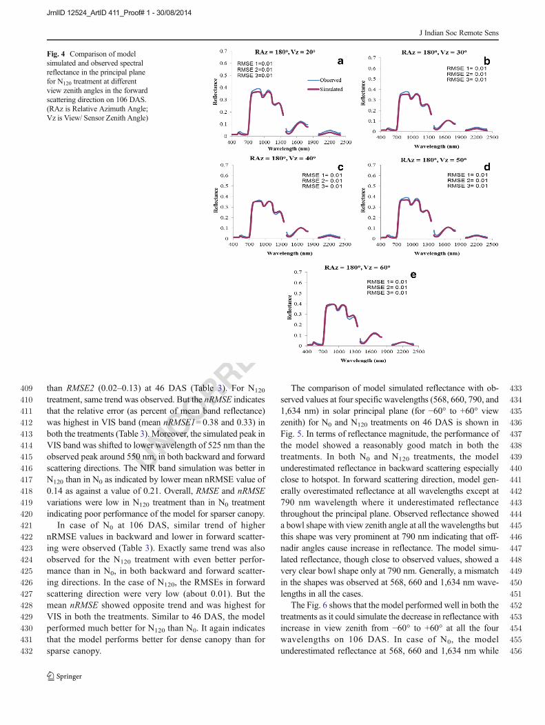
Fig. 3 Comparison of modelsimulated and observed spectralreflectance in principal plane forN120 treatment at different viewzenith angles in the backwardscattering direction on 106 DAS.(RAz is Relative Azimuth Angle;Vz is View/ Sensor Zenith Angle)

J Indian Soc Remote Sens

JrnlID 12524_ArtID 411_Proof# 1 - 30/08/2014

UNCORRECTEDPROOF

409 than RMSE2 (0.02–0.13) at 46 DAS (Table 3). For N120

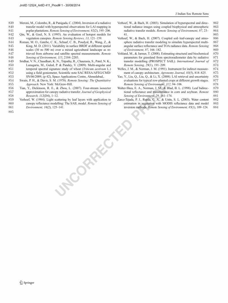
410 treatment, same trend was observed. But the nRMSE indicates411 that the relative error (as percent of mean band reflectance)412 was highest in VIS band (mean nRMSE1=0.38 and 0.33) in413 both the treatments (Table 3). Moreover, the simulated peak in414 VIS band was shifted to lower wavelength of 525 nm than the415 observed peak around 550 nm, in both backward and forward416 scattering directions. The NIR band simulation was better in417 N120 than in N0 as indicated by lower mean nRMSE value of418 0.14 as against a value of 0.21. Overall, RMSE and nRMSE419 variations were low in N120 treatment than in N0 treatment420 indicating poor performance of the model for sparser canopy.421 In case of N0 at 106 DAS, similar trend of higher422 nRMSE values in backward and lower in forward scatter-423 ing were observed (Table 3). Exactly same trend was also424 observed for the N120 treatment with even better perfor-425 mance than in N0, in both backward and forward scatter-426 ing directions. In the case of N120, the RMSEs in forward427 scattering direction were very low (about 0.01). But the428 mean nRMSE showed opposite trend and was highest for429 VIS in both the treatments. Similar to 46 DAS, the model430 performed much better for N120 than N0. It again indicates431 that the model performs better for dense canopy than for432 sparse canopy.

433The comparison of model simulated reflectance with ob-434served values at four specific wavelengths (568, 660, 790, and4351,634 nm) in solar principal plane (for −60° to +60° view436zenith) for N0 and N120 treatments on 46 DAS is shown in437Fig. 5. In terms of reflectance magnitude, the performance of438the model showed a reasonably good match in both the439treatments. In both N0 and N120 treatments, the model440underestimated reflectance in backward scattering especially441close to hotspot. In forward scattering direction, model gen-442erally overestimated reflectance at all wavelengths except at443790 nm wavelength where it underestimated reflectance444throughout the principal plane. Observed reflectance showed445a bowl shape with view zenith angle at all the wavelengths but446this shape was very prominent at 790 nm indicating that off-447nadir angles cause increase in reflectance. The model simu-448lated reflectance, though close to observed values, showed a449very clear bowl shape only at 790 nm. Generally, a mismatch450in the shapes was observed at 568, 660 and 1,634 nm wave-451lengths in all the cases.452The Fig. 6 shows that the model performed well in both the453treatments as it could simulate the decrease in reflectance with454increase in view zenith from −60° to +60° at all the four455wavelengths on 106 DAS. In case of N0, the model456underestimated reflectance at 568, 660 and 1,634 nm while

Fig. 4 Comparison of modelsimulated and observed spectralreflectance in the principal planefor N120 treatment at differentview zenith angles in the forwardscattering direction on 106 DAS.(RAz is Relative Azimuth Angle;Vz is View/ Sensor Zenith Angle)

J Indian Soc Remote Sens

JrnlID 12524_ArtID 411_Proof# 1 - 30/08/2014

UNCORRECTEDPROOF

457it remained close at 790 nm. The RMSE values were 0.03,4580.04, 0.03 and 0.04 for 568, 660, 790 and 1,634 nm, respec-459tively. The magnitude of underestimation was more in the460backward scattering direction, particularly at 568 and461660 nm bands. A close match was observed at 790 and4621,634 nm in comparison to 568 and 660 nm. Model simula-463tions were much better in N120 than in N0 at all the four464wavelengths as indicated by lower RMSE values of 0.024,4650.009, 0.042 and 0.025, respectively. The model performance466significantly improved at 568 and 660 nm in N120 over N0.467Little but consistent underestimation was observed at 568 and468660 nm, especially in the backward scattering direction. Here469also observed reflectance showed prominent bowl shape at470790. The model could also simulate bowl shape of reflectance471at this wavelength. These results also indicate that the model472performance is much better for dense canopy than for sparse.473

474Discussion

475Bi-directional Reflectance Patterns

476In this study, the bi-directional reflectance observed at477different wavelengths and at different growth stages of478wheat confirmed the typical highly anisotropic scattering479behaviour of wheat canopy throughout optical wavelength480region as has been reported by Sridhar et al. (2009) and481Barman et al. (2010). Anisotropic scattering of vegetation482canopies generally results in increasing reflectance with483off-nadir view angles for all solar zenith angles (Donovan484et al. 1985) and our results also showed similar pattern.485As reported in literature (Kimes et al. 1984, Donovan486et al. 1985 and Roman et al. 2011), our results also487showed that the bi-directional reflectance was significant-488ly higher in backward scattering direction than in forward489scattering direction in the optical region. The Figs. 1 and4902 clearly showed that peak reflectance was observed in491principal plane in backward scattering direction in the492direction of the sun referred to as “hotspot”. This pattern493occurred for all the four wavelength bands centred at 568494(GREEN), 660 (RED), 790 (NIR) and 1,634 nm (SWIR)495with the magnitude of reflectance being higher in the496NIR, followed by SWIR and lowest in RED. Similar497patterns have been reported by Kimes (1984) and498Sridhar et al. (2009) in RED and NIR bands. Increasing499reflectance with off-nadir viewing is a function of viewing500different proportions of the canopy layers as the view501zenith angle changes. As the view zenith angle increases,502a higher percentage of upper canopy layers are viewed.503The proportion of shadowed canopy to sunlit canopy504layers increases with canopy depth. Thus, viewing a505higher percentage of upper canopy layers than at nadir

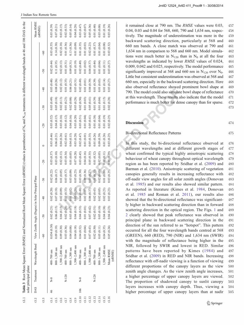
t3:1

Tab

le3

RootM

eanSq

uareError

(RMSE

)andNormalized

RootM

eanSquareError

(nRMSE)(valuesinparentheses)of

N0andN120treatm

entsindifferentw

avelengthbandsat46

and106DASinthe

solarprincipalp

lane

t3:2

DAS

Treatment

WavelengthBand

ViewZenith

Angle(D

egree)

inSo

larPrincipalP

lane

MeanRMSE

(nRMSE)

t3:3

−60

−50

−40

−30

−20

0+20

+30

+40

+50

+60

t3:4

46N-0

400–700nm

0.034(0.30)

0.02

(0.21)

0.02

(0.20)

0.02

(0.22)

0.03

(0.37)

0.03

(0.46)

0.03

(0.52)

0.03

(0.49)

0.03

(0.48)

0.02

(0.44)

0.03

(0.55)

0.03

(0.39)

t3:5

800–1,300nm

0.09

(0.19)

0.06

(0.15)

0.07

(0.19)

0.06

(0.17)

0.03

(0.10)

0.06

(0.21)

0.04

(0.15)

0.05

(0.18)

0.08

(0.26)

0.11

(0.35)

0.14

(0.38)

0.07

(0.21)

t3:6

1,500–2,400nm

0.09

(0.30)

0.04

(0.15)

0.02

(0.09)

0.01

(0.05)

0.02

(0.13)

0.04

(0.26)

0.03

(0.16)

0.02

(0.13)

0.02

(0.12)

0.02

(0.13)

0.02

(0.18)

0.03

(0.15)

t3:7

N-120

400–700nm

0.03

(0.36)

0.02

(0.24)

0.03

(0.33)

0.03

(0.37)

0.03

(0.34)

0.02

(0.61)

0.01

(0.12)

0.01

(0.23)

0.01

(0.35)

0.01

(0.31)

0.01

(0.36)

0.02

(0.33)

t3:8

800–1,300nm

0.04

(0.08)

0.03

(0.07)

0.01

(0.02)

0.03

(0.09)

0.01

(0.05)

0.04

(0.15)

0.04

(0.16)

0.02

(0.08)

0.06

(0.21)

0.09

(0.31)

0.13

(0.36)

0.05

(0.14)

t3:9

1,500–2,400nm

0.04

(0.18)

0.04

(0.18)

0.05

(0.21)

0.05

(0.23)

0.07

(0.28)

0.03

(0.28)

0.03

(0.20)

0.03

(0.28)

0.03

(0.31)

0.01

(0.19)

0.01

(0.09)

0.04

(0.28)

t3:10

106

N-0

400–700nm

0.04

(0.52)

0.04

(0.53)

0.04

(0.49)

0.03

(0.39)

0.03

(0.45)

0.02

(0.47)

0.03

(0.51)

0.02

(0.50)

0.02

(0.49)

0.02

(0.49)

0.01

(0.35)

0.03

(0.47)

t3:11

800–1,300nm

0.01

(0.04)

0.01

(0.01)

0.02

(0.07)

0.09

(0.36)

0.04

(0.16)

0.01

(0.01)

0.01

(0.04)

0.01

(0.03)

0.01

(0.01)

0.01

(0.02)

0.01

(0.03)

0.02

(0.07)

t3:12

1,500–2,400nm

0.07

(0.43)

0.07

(0.42)

0.06

(0.37)

0.03

(0.27)

0.05

(0.35)

0.05

(0.35)

0.05

(0.41)

0.05

(0.41)

0.04

(0.39)

0.04

(0.37)

0.02

(0.23)

0.05

(0.36)

t3:13

N-120

400–700nm

0.02

(0.50)

0.02

(0.51)

0.02

(0.43)

0.01

(0.33)

0.01

(0.32)

0.01

(0.26)

0.01

(0.38)

0.01

(0.39)

0.01

(0.39)

0.01

(0.44)

0.01

(0.37)

0.01

(0.40)

t3:14

800–1,300nm

0.05

(0.11)

0.05

(0.10)

0.02

(0.05)

0.02

(0.05)

0.02

(0.05)

0.09

(0.39)

0.01

(0.04)

0.01

(0.04)

0.01

(0.03)

0.01

(0.04)

0.01

(0.04)

0.03

(0.08)

t3:15

1,500–2,400nm

0.04

(0.35)

0.04

(0.38)

0.02

(0.23)

0.01

(0.09)

0.01

(0.11)

0.01

(0.26)

0.01

(0.19)

0.01

(0.15)

0.01

(0.14)

0.01

(0.11)

0.01

(0.08)

0.01

(0.19)

t3:16

MeanRMSE

(nRMSE

)0.05

(0.24)

0.04

(0.23)

0.03

(0.23)

0.03

(0.25)

0.03

(0.29)

0.03

(0.25)

0.02

(0.25)

0.02

(0.28)

0.03

(0.27)

0.03

(0.27)

0.03

(0.32)

0.03

(0.26)

J Indian Soc Remote Sens

JrnlID 12524_ArtID 411_Proof# 1 - 30/08/2014

UNCORRECTEDPROOF

506 viewing results in higher reflectance. The highest reflec-507 tance at hotspot occurred because each leaf hide its own508 shadow when viewed from the direction of incident light509 (Hapke et al. 1996).

510The hotspot reflectances at 568, 660 and 1,634 nm were511significantly lower than at 790 nm. This may be due to512significant absorption of radiation by leaf pigments or mois-513ture. So, with the increase in the view zenith angle though the

0.00

0.02

0.04

0.06

0.08

0.10

0.12

0.14

0.16

0.18

-60 -40 -20 0 20 40 60R

efle

ctan

ceView Zenith Angle (Degree)

Reflectance at 568 nm

RMSE_N0 = 0.018RMSE_N120 = 0.031

a

0.00

0.02

0.04

0.06

0.08

0.10

0.12

0.14

0.16

0.18

-60 -40 -20 0 20 40 60

Ref

lect

ance

View Zenith Angle (Degree)

Reflectance at 660 nm

RMSE_N0 = 0.027RMSE_N120 = 0.025

b

0.00

0.10

0.20

0.30

0.40

0.50

-60 -40 -20 0 20 40 60

Refl

ecta

nce

View Zenith Angle (Degree)

Reflectance at 790 nm

RMSE_N0 = 0.102RMSE_N120 = 0.086

0.00

0.10

0.20

0.30

0.40

-60 -40 -20 0 20 40 60

Refl

ecta

nce

View Zenith Angle (Degree)

Reflectance at 1634 nm

RMSE_N0 = 0.037RMSE_N120 = 0.033

c d

Fig. 5 Comparison of theobserved (square & line) andmodel simulated (triangle &dashed line) reflectance in theprincipal plane on 46 DAS for N0(blue) and N120 (red) at (a)568 nm, (b) 660 nm, (c) 790 nmand (d) 1,634 nm

0.00

0.02

0.04

0.06

0.08

0.10

0.12

-60 -40 -20 0 20 40 60

Ref

lect

ance

View Zenith Angle (Degree)

Reflectance at 568 nm

RMSE_N0 = 0.034RMSE_N120 = 0.024

0.00

0.02

0.04

0.06

0.08

0.10

-60 -40 -20 0 20 40 60

Ref

lect

ance

View Zenith Angle (Degree)

Reflectance at 660 nm

RMSE_N0 = 0.041RMSE_N120 = 0.009

0.00

0.10

0.20

0.30

0.40

0.50

0.60

-60 -40 -20 0 20 40 60

Ref

lect

ance

View Zenith Angle (Degree)

Reflectance at 790 nm

RMSE_N0 = 0.029RMSE_N120 = 0.042

0.00

0.05

0.10

0.15

0.20

0.25

-60 -40 -20 0 20 40 60

Ref

lect

ance

View Zenith Angle (Degree)

Reflectance at 1634 nm

RMSE_N0 = 0.036RMSE_N120 = 0.025

a

c

b

d

Fig. 6 Comparison of theobserved (square & line) andmodel simulated (triangle &dashed line) reflectance in theprincipal plane on 106 DAS forN0 (blue) and N120 (red) at (a)568 nm, (b) 660 nm, (c) 790 nmand (d) 1,634 nm

J Indian Soc Remote Sens

JrnlID 12524_ArtID 411_Proof# 1 - 30/08/2014

UNCORRECTEDPROOF

514 upper plant canopy area observed becomes more but propor-515 tionately the absorption also becomes more thus producing516 similar reflectance values. At the same time at these wave-517 lengths, the minimum reflectance was observed in the forward518 scattering direction at higher view zenith angles. The cause of519 which can be attributed to the fact that in-spite of viewing520 higher proportion of upper plant canopy components with521 increasing view zenith angle, increased shadowing is also522 observed in the forward scattering direction (Hapke et al.523 1996). Kimes (1984) suggested that the interaction of these524 two mechanisms result in the minimum reflectance at off-525 nadir angles in the forward scattering direction. So this factor526 produces the dark spot effect in the forward direction and527 hotspot in the backscattering direction where all shadows are528 hidden (Roman et al. 2011).529 The occurrence of hotspot at 45° relative azimuth than in530 the principal plane in case of N0 at 46 DAS may be due to531 sparse wheat canopy resulting in large exposure of soil back-532 ground. The scattering by soil may be dominating as it is a533 stronger anisotropic reflector than vegetation (Kirchner et al.534 1981). With the growth of canopy from 46 DAS to 106 DAS,535 broader hotspot was observed at all four wavelengths. It may536 be the result of an increase in LAI, leaf size and planophilic537 leaf orientation and also due to lowering of sun zenith angle538 with time (Qin and Goel 1995).539 Unlike other wavelengths, the reflectance in the NIR was540 found to be more symmetric around nadir i.e. it increases in541 backward and forward scattering direction with the increment542 of the view zenith angles. This results in a shallow bowl shape543 reflectance spectra in principal plane as reported by (Q3 Walter-544 Shea et al. 1998) for alfalfa,Q4 Verbrugghe and Cierniewski545 (1995) for cotton, Sridhar et al. (2009) for wheat and Roman546 et al. (2011) for agricultural landscape. Shallow bowl shape in547 NIR band was very clearly seen in both the treatments and at548 two DAS in this study (Figs. 1 and 2). This can be explained549 by the scattering properties inherent in NIR reflectance. It550 increases with off-nadir angles due to viewing increasing551 multiple layering of leaves. It has been shown that additive552 reflectance occurs due to the transmittance and reflectance553 properties of the NIR (Swain and Davis 1978). The fifty per554 cent reflectance and transmittance properties typical of most555 leaves (Swain and Davis 1978), results in illumination of556 lower canopy layers that reflect back through the upper can-557 opies thus increasing reflectance (Donovan et al. 1985). The558 extent of variation in BRF was more at 790 nm wavelength as559 compared to other wavelengths (Q5 Walter-Shea et al. 1998). It560 was also observed that on both the dates, the reflectance at561 568, 660 and 1,634 was more in N0 treatment, whereas at562 790 nm it was more in N120. It is because of the differential563 absorption and scattering at different wavelengths by leaf564 biophysical parameters like pigments, moisture content and565 structure. As N0 was having lower chlorophyll and LAI, it566 resulted in higher reflectance in GREEN and RED bands and

567lower in NIR band. The reflectances in SWIR band in both N0

568and N120 were comparable on both the dates as moisture569content was nearly same even though there were large570differences in LAI. Jacquemoud et al. (2009) have also shown571through a simulation study that LAI has no noticeable effect in572the SWIR band where water absorption dominates.

573Validation of PROSAIL Model

574The spectral and directional sensitivity analysis of the575PROSAIL model parameters has been documented in some576studies (Bacour et al. 2002; Zarco-Tejada et al. 2003; Vohland577and Jarmer, 2008; Jacquemoud et al. 2009). We observed that578the canopy reflectance throughout the optical region was high579in the backward direction where shadows were reduced. The580PROSAIL model also showed similar increasing trend in the581backward scattering direction as described in the sensitivity582analysis by Jacquemoud et al. (2009). But the magnitude of583increase was less than observed leading to underestimation by584model at high view zenith angles. It points to the shortcoming585in model to match the variations observed in the field across586the view zenith angles in the principal plane, especially at high587zenith angles. LAI clearly dominated both the forward and588backward scattering direction in the NIR region resulting in a589prominent bowl shape curve. The model showed better sensi-590tivity in the NIR region and was able to simulate both the591shape and the magnitude of the observed spectra except for the592sparse canopy where background soil anisotropy dominated.593This feature was also evident from significantly better simu-594lation in NIR region during later part of crop growth i.e. (106595DAS) for both the treatments. The sensitivity of the model to596simulate NIR reflectance at near nadir view was low due to597higher exposure of the soil background. Hence, for retrieving598LAI, nadir observations contain less information than at599oblique angles. Besides, at the nadir position the model has600largest influence of leaf orientation which is characterized by601average leaf angle (Angl) (Jacquemoud et al. 2009).602The study results showed that model could simulate the603hotspot position in all the wavelength regions at all growth604stages in both the treatments. The view zenith angle at which605model simulated hotspot corresponded to the solar zenith606angle as at this position sensor views least shadow in the607canopy. When compared with observed hotspot position, it608was found that they did not match exactly. The observed609hotspot varied in a small range of view zenith around the610simulated hotspot view zenith. It may be due to measurement611errors caused by (a) assumption of constant sun geometry612during 20–25 min of bi-directional reflectance measurement613period, and (b) small asymmetry introduced in the goniometer614due to uneven levelling in the field. The model, in general,615underestimated reflectance at hotspot in all the wavelength616bands and at two growth stages. Andrieu et al. (1997) also617showed for sugar beet that the model underestimated

J Indian Soc Remote Sens

JrnlID 12524_ArtID 411_Proof# 1 - 30/08/2014

UNCORRECTEDPROOF

618 reflectance for sun-sensor geometries close to the hotspot.619 This may be attributed to the approximation caused in the620 model by two-stream approach to compute multiple scattering621 in the canopy. Inclusion of four-stream isosector approxima-622 tion may reduce this error which has much higher improve-623 ment for diffuse incident radiation than for direct incident624 radiation (Tian et al. 2007).625 The model performance was poorer for sparse wheat canopy626 than for dense canopy. This was more pronounced in NIR627 region than at other wavelengths. In sparse canopies due to628 higher exposure of soil, the scattering properties of vegetation629 and soil combine to form a unique reflectance distribution630 (Donovan et al. 1985) which may not be captured in631 PROSAIL. Moreover in most of the variants of SAIL model,632 soil is assumed to be a Lambertian reflector (Jacquemoud et al.633 2006, Verhoef and Bach 2007) though soil shows a strong634 anisotropic behaviour (Kirchner et al. 1981). SAIL showed high635 soil reflectance sensitivity in RED and NIR bands when corn636 canopy was low (Yao et al. 2008). Verhoef and Bach (2003)637 while using GeoSAIL, a variant of SAIL, also recommended638 that for a more realistic modelling of the BRF of sparse cano-639 pies, it will be necessary to incorporate the non-Lambertian640 reflection characteristics of bare soils into the GeoSAIL model.641 Inclusion of soil BRF anisotropy in the model is recommended642 for better simulation of sparse canopies.643 The absolute errors in model simulations were very small644 in VIS region, followed by SWIR and highest were in NIR645 region. In terms of relative error (nRMSE), model showed646 lowest error in NIR region across dates and treatments while it647 was highest in VIS region. Andrieu et al. (1997) also observed648 that the relative difference between measured and simulated649 reflectances were lower in NIR than in the VIS region for650 sugar beet. Vohland and Jarmer (2008) have also reported that651 relative deviations between the simulated and the observed652 spectra were most striking in visible region leading to the poor653 estimation of Chlorophyll. Le Marie et al. (2004) have also654 pointed out the shortcomings of the PROSPECT model in the655 VIS domain. It is because in VIS region, absorption of radi-656 ation dominates while in NIR mostly scattering dominates.657 So, even small inconsistencies at shorter wavelengths become658 relatively large while opposite happens at longer wavelengths659 (Roman et al. 2011). It is also argued that there is always poor660 signal propagation from leaf to canopy scale resulting in poor661 estimation of leaf biochemical parameters from canopy reflec-662 tance (Jacquemoud et al. 1996). As the VIS band is having663 very low range of reflectance (2 to 9 % in our study) due to664 dominance of absorption, hence it is tough to model this665 region. This has implications in the retrieval of plant param-666 eters especially leaf biochemical parameters such as chloro-667 phyll whose information is coded in the VIS band. So, there is668 more chance of error in PROSAIL simulation of reflectance in669 VIS band, leading to poorer retrieval of leaf chlorophyll by670 model inversion.

671The performance of the model was judged in the principal672plane across all the view zenith angles because here surface673reflectance anisotropy is more sensitive to canopy biophysical674characteristics (Bacour et al. 2002). The observed reflectance675showed bowl shape with view zenith angle at most wave-676lengths. The bowl shape was most prominent at 790 nm. The677model simulated well the bowl shape reflectance pattern at678790 nm though there was considerable mismatch in the shape679at other wavelengths. A close match was also obtained be-680tween the magnitude of observed and model simulated reflec-681tance at 790 nm. As this wavelength region is sensitive to LAI682and Angl (Jacquemoud et al. 2009), it indicates that model′s683assumptions of canopy as horizontally homogeneous, where684leaves absorb, reflect, and transmit radiation (Verhoef 1984)685hold good in case of wheat. Hence, any index which uses the686NIR region to estimate the canopy property such as LAI will687lead to a better retrieval of the same by model inversion.688The model showed underestimation in all the wavebands but689its magnitude was much more in the backward scattering direc-690tion than in the forward scattering direction. The underestima-691tion was higher in VIS band, especially at 568 nm wavelength692and in backward scattering direction than in forward scattering693direction. Bidirectional reflectance in the backward scattering694direction is proportional to the leaf reflectance and in the for-695ward scattering direction is proportional to the leaf transmittance696(Verhoef 1984). As Le Marie (2004) has pointed out that the697PROSPECT model has some problems in the visible domain698due to a successive and indirect calibration of the original699absorption coefficients. This may be the cause for the700underestimation in the backscattering direction. Hence,701improvements in the leaf absorption coefficients may improve702the model performance. Similar to our observation, Verhoef and703Bach (2007) have also reported that RMSE values were increas-704ing with larger observation angles.705

706Conclusions

707The study reconfirms the strong and consistent anisotropic708patterns of reflectance in VIS, NIR and SWIR regions in709response to change in view zenith, sun zenith and relative710azimuth at different growth stages of wheat. Though earlier711studies have reported about anisotropy in VIS and NIR wave-712lengths, this study concluded that it is equally applicable in713SWIR wavelength band. In case of sparse wheat canopy the714study found that hotspot at any wavelength may occur away715from the principal plane due to the large exposure of soil716background. Soil itself being strong anisotropic reflector mod-717ifies the crop anisotropic behaviour in a complex way to form718a unique reflectance distribution. The hotspot becomes719broader in wheat with the growth of crop due to increase in720LAI, leaf size and planophilic orientation. These patterns are

J Indian Soc Remote Sens

JrnlID 12524_ArtID 411_Proof# 1 - 30/08/2014

UNCORRECTEDPROOF

721 of importance while using multi-angular satellite remote sens-722 ing for classification of crops and computing temporal profile723 of vegetation indices.724 The performance evaluation of PROSAIL5B model using725 ground observations showed that the model very well simu-726 lated the shape of canopy spectra over optical wavelength727 region. Amismatch in the simulation of position of reflectance728 peak in GREEN wavelength region indicated deficiency in729 PROSPECT model which may be related to leaf absorption730 coefficient values assumed. The high underestimation in VIS731 band, especially in backscattering direction bring forth the732 shortcoming of PROSPECT model and subsequent propaga-733 tion of resulting errors through canopy layers in SAIL model.734 The model underestimated reflectance at hot-spot in all wave-735 lengths regions at different growth stages which may be736 mitigated by inclusion of four-stream isosector approximation737 instead of two-stream approach to compute multiple scattering738 in the canopy. The model performance was poor for sparse739 canopy and at nadir view due to large exposure of background740 soil which itself is highly anisotropic in nature. These results741 points out the limitation of assuming the soil as a Lambertian742 reflector in model necessitating it to be modeled as a realistic743 non-Lambertian or anisotropic surface. Inclusion of canopy744 cover fraction into the model may further help to improve745 model performance under such conditions.746 These results have implications for the retrieval of wheat747 biophysical parameters by PROSAIL inversion. The study indi-748 cated that the retrieval of leaf biochemical parameters, like,749 chlorophyll will be poorer due to largemodel error in VIS region750 (both at nadir and large view zenith angles) and also because751 absorption of radiation dominates in this region resulting in poor752 signal propagation from leaf to canopy scale. On the other hand753 retrieval of parameters like LAI, which have dominating effect754 on NIR reflectance, will be better at any view zenith angle as755 model error is low in NIR region. Moreover in NIR region, the756 model is able to simulate well the typical shallow bowl shape757 reflectance pattern in the principal plane. As the modelled SWIR758 reflectance errors are in between that of VIS and NIR and is759 governed by leaf moisture, it is expected that the retrieval accu-760 racy of leaf moisture may also be in between that of chlorophyll761 and LAI. But it may also be kept in mind that the dynamic range762 of leaf moisture is narrow for wheat which may result in its still763 poorer retrieval by model inversion. It is expected that the study764 shall help in understanding the associated uncertainties in inver-765 sion of PROSAIL model to retrieve crop biophysical parameters766 from multispectral images.

767 Acknowledgments First author acknowledges the fellowship provided768 by the Indian Council of Agricultural Research (ICAR) to undertake this769 study during the Master′s programme. The help extended by Prof. W.770 Verhoef of ITC, The Netherlands, in interpreting PROSAIL model sim-771 ulations is duly acknowledged. This study was supported by in-house772 project grant code IARI: PHY:09:04 (3) of Indian Agricultural Research773 Institute, New Delhi.

774References 775

776Andrieu, B., Baret, F., Jacquemoud, S., Malthus, T., & Stevent, M.777(1997). Evaluation of an improved version of SAIL model for778simulating bidirectional reflectance of sugarbeet canopies. Remote779Sensing of Environment, 60, 247–257.780Bacour, C., Jacquemoud, S., Leroy, M., Hautecoeur, O., Weiss, M.,781Prevot, L., et al. (2002). Reliability of the estimation of vegetation782characteristics by inversion of three canopy reflectance models on783airborne polder data. Agronomie: Agriculture and Environment, 22,784555–565.785Barman, D., Sehgal, V. K., Sahoo, R. N., & Nagarajan, S. (2010).786Relationship of bidirectional reflectance of wheat with biophysical787parameters and its radiative transfer modeling using Prosail. Journal788of Indian Society of Remote Sensing, 38, 35–44.789Darvishzadeh, R., Skidmore, A., Schlerf, M., & Atzberger, C. (2008).790Inversion of a radiative transfer model for estimating vegetation LAI791and chlorophyll in a heterogeneous grassland. Remote Sensing of792Environment, 112(5), 2592–2604.793Donovan, S. Characterization and discrimination of selected vegetation794canopies from field observations of bidirectional reflectances. M.Sc.795Thesis, University of Maryland, USA, p 114, 1985.796Goel, N. S. (1989). Inversion of canopy reflectance models for estimation797of biophysical parameters from reflectance data. In G. Asrar (Ed.),798Theory and Applications of Optical Remote Sensing (pp. 205–251).799New York: Wiley & Sons.800Hapke, B., DiMucci, D., Nelson, R., & Smythe, W. (1996). The cause of801the hotspot in vegetation canopies and soils: shadow-hiding versus802coherent backscatter. Remote Sensing of Environment, 58, 63–68.803Hiscox, J. D., & Israelstam, G. F. (1979). A method for the extraction of804chlorophyll from leaf tissue without maceration. Canadian Journal805of Botany, 57, 1332–1334.806Houborg, R., Soegaard, H., & Boegh, E. (2007). Combining vegetation807index and model inversion methods for the extraction of key vege-808tation biophysical parameters using Terra and Aqua MODIS reflec-809tance data. Remote Sensing of Environment, 106(1), 39–58.810Jacquemoud, S., & Baret, F. (1990). PROSPECT: A model of leaf optical811properties spectra. Remote Sensing of Environment, 34(2), 75–91.812Jacquemoud, S., Ustin, S. L., Verdebout, J., Schmuck, G., Andreoli, G., &813Hosgood, B. (1996). Estimating leaf biochemistry using the814PROSPECT leaf optical properties model. Remote Sensing of815Environment, 56(194–202), 163–172.816Jacquemoud, S., Verhoef, W., Baret, F., Zarco-Tejada, P. J., Asner, G. P.,817Francois, C. & Ustin, S. L. PROSPECT SAIL: 15 Years of Use for818Land Surface Characterization. Geoscience and Remote Sensing819Symposium (IGARSS). IEEE international conference July 31,8202006- August 4, 2006.821Jacquemoud, S., Verhoef, W., Baret, F., Bacour, C., Zarco-Tejada, P. J.,822Asner, G. P., Francois, C., & Ustin, S. L. (2009). PROSPECT SAIL823models: A review of use for vegetation characterization. Remote824Sensing of Environment, 113, S56–S66.825Kimes, D. S., Holben, B. N., Tucker, C. J., & Newcomb, W. W. (1984).826Optimal directional view angles for remote sensing missions.827International Journal of Remote Sensing, 5(6), 887–908.828Kirchner, J. A., Schwetzler, C. C., & Smith, J. A. (1981). Simulated829directional radiances of vegetation from satellite platforms.830International Journal of Remote Sensing, 2(3), 253–264.831Le Maire, G., Francois, C., & Dufrene, E. (2004). Towards universal832broad leaf chlorophyll indices using PROSPECTsimulated database833and hyperspectral reflectance measurements. Remote Sensing of834Environment, 89, 1–28.835Q6Mahtab, A., Sridhar, V. N., & Navalgund, R. R. (2009). An assessment of836angular variations of red and NIR reflectances in multi-date IRS-1D837wide field sensor data. International Journal of Remote Sensing,83830(17), 4599–4619.

J Indian Soc Remote Sens

JrnlID 12524_ArtID 411_Proof# 1 - 30/08/2014

UNCORRECTEDPROOF

839 Meroni, M., Colombo, R., & Panigada, C. (2004). Inversion of a radiative840 transfer model with hyperspectral observations for LAI mapping in841 poplar plantations.Remote Sensing of Environment, 92(2), 195–206.842 Qin, W., & Goel, N. S. (1995). An evaluation of hotspot models for843 vegetation canopies. Remote Sensing Reviews, 13, 121–159.844 Roman, M. O., Gatebe, C. K., Schaaf, C. B., Poudyal, R., Wang, Z., &845 King, M. D. (2011). Variability in surface BRDF at different spatial846 scales (30 m–500 m) over a mixed agricultural landscape as re-847 trieved from airborne and satellite spectral measurements. Remote848 Sensing of Environment, 115, 2184–2203.849 Sridhar, V. N., Chaudhari, K. N., Tripathy, R., Chaurasia, S., Patel, N. K.,850 Lunagaria, M., Guled, P. & Pandey, V. (2009). Multi-angular and851 temporal spectral signature study of wheat (Triticum aestivum L.)852 using a field goniometer, Scientific note SAC/RESA/AFEG/CMD/853 SN/06/2009, (p 42), Space Applications Centre, Ahmedabad,.854 Swain, P. H., & Davis, S. M. (1978). Remote Sensing: The Quantitative855 Approach. New York: McGraw-Hill.856 Tian, Y., Dickinson, R. E., & Zhou, L. (2007). Four-stream isosector857 approximation for canopy radiative transfer. Journal of Geophysical858 Research, 112(D4), 1–12.859 Verhoef, W. (1984). Light scattering by leaf layers with application to860 canopy reflectance modelling: The SAIL model. Remote Sensing of861 Environment, 16(2), 125–141.

862Verhoef, W., & Bach, H. (2003). Simulation of hyperspectral and direc-863tional radiance images using coupled biophysical and atmospheric864radiative transfer models. Remote Sensing of Environment, 87, 23–86541.866Verhoef, W., & Bach, H. (2007). Coupled soil–leaf-canopy and atmo-867sphere radiative transfer modeling to simulate hyperspectral multi-868angular surface reflectance and TOA radiance data. Remote Sensing869of Environment, 87, 166–182.870Vohland, M., & Jarmer, T. (2008). Estimating structural and biochemical871parameters for grassland from spectroradiometer data by radiative872transfer modelling (PROSPECT SAIL). International Journal of873Remote Sensing, 29(1), 191–209.874Welles, J. M., & Norman, J. M. (1991). Instrument for indirect measure-875ment of canopy architecture. Agronomy Journal, 83(5), 818–825.876Yao, Y., Liu, Q., Liu, Q., & Li, X. (2008). LAI retrieval and uncertainty877evaluations for typical row-planted crops at different growth stages.878Remote Sensing of Environment, 112, 94–106.879Walter-Shea, E. A., Norman, J. M., & Blad, B. L. (1998). Leaf bidirec-880tional reflectance and transmittance in corn and soybean. Remote881Sensing of Environment, 29, 161–174.882Zarco-Tejada, P. J., Rueda, C. A., & Ustin, S. L. (2003). Water content883estimation in vegetation with MODIS reflectance data and model884inversion methods. Remote Sensing of Environment, 85(1), 109–124.

885

J Indian Soc Remote Sens

JrnlID 12524_ArtID 411_Proof# 1 - 30/08/2014