1

403 - Exploitation of radiative transfer model for assessing solar radiation: the relative importance of atmospheric constituents

Armel Oumbe1*, Lucien Wald1, Philippe Blanc1, Marion Schroedter-Homscheidt2 1Ecole des Mines de Paris, BP 207, 06904 Sophia Antipolis, France

2German Aerospace Center - German Remote Sensing Data Center, Postfach 1116, D-82234 Wessling, Germany * Corresponding Author, armel.oumbe@ensmp.fr

Abstract

Solar radiation is modified in its way downwards by the content of the atmosphere. Quantifying the influences of the parameters describing the optical state of the atmosphere is necessary for development of a method for the assessment of the solar surface irradiance (SSI). This paper performs an inventory of the variables (e.g., cloud) and their attributes (e.g., optical depth) available in an operational mode and then assesses to which degree the uncertainty on an attribute of a variable –including the absence of value –leads to a departure from the perfect result, i.e., when assuming that all attributes are known with a perfect accuracy. Clouds are the most important variable for the SSI. Aerosol loading and type, water vapour amount and atmospheric profile have a great influence. Ground albedo has an important influence on diffuse part and spectral distribution of SSI. The influences of vertical position and geometrical thickness of clouds in the atmosphere are negligible. Thus, the solution of the RTM for a cloudy atmosphere is equivalent to the product of the irradiance obtained under a clear sky and the extinction coefficient due to the cloud. The results are combined with the data availability for design of the new method Heliosat-4 for assessing the SSI. Keywords: solar radiation, atmospheric optics, satellite images, Heliosat method

1. Introduction

A wealth of methods has been developed in the past years to assess solar surface irradiance (SSI) from images taken by satellites (Cano et al. 1986; Pinker et al. 1995; Hammer 2000; Rigollier et al. 2004). Current methods are inverse, i.e., the inputs are satellite images whose digital counts result from the ensemble of interactions of radiation with the atmosphere and the ground and the method deduces the radiation from the inputs. On the opposite, solar radiation may be assessed by a direct method, i.e., the various processes occurring during the path of the light from the outer space towards the ground can be modelled by the means of a radiative transfer model (RTM) in 2D or 3D. RTMs take into account a large number of inputs: optical properties including spectral aspects of gases, aerosols, clouds and ground reflectance, types of interactions, mathematical solving methods (Kato et al. 1999; Liou 1976, 1980; Mayer, Kylling 2005; Perrin de Brichambaut, Vauge 1982; Vermote et al. 1997). The quality of the results depend strongly on the quality of the inputs.

Nowadays, the exploitation of recent sensors and satellite data such as MSG, Envisat and MetOp combined with recent data assimilation techniques into atmospheric modelling offers a favourable context for the design and exploitation of a method based on direct modelling. Despite noticeable

2

advances in the operational assessment of optical properties of the atmosphere at any location, we do not have enough information for 3D RTM. The available atmospheric information is typically 2D. Even so, many of the inputs are unknown. Some are known every ¼ h (clouds), others every day (ozone, water vapour) and others only from times to times (aerosols). The ground albedo and its spectral distribution is known only if the sky is clear. Furthermore, if available, these quantities are known at different spatial resolutions. Hence, the set of inputs to the RTM is heterogeneous with respect to spatial coverage, spatial sampling step, spatial support of information, temporal sampling frequency, temporal support of information, and accuracy.

The goal of the work presented here is to perform an inventory of the variables (e.g., cloud) and their attributes (e.g., optical depth) available in an operational mode and then to assess to which degree the uncertainty on an attribute of a variable –including the absence of value –leads to a departure from the perfect result, i.e., when assuming that all attributes are known with a perfect accuracy.

The spectral region of interest is [0.3 µm, 4 µm]. Energy-related applications require spectrally-integrated or spectrally-resolved SSI. For this sensitivity study, we use: the code libRadtran (Mayer, Kylling 2005) because it is accurate, versatile and well exploited in atmospheric optics (Bernhard et al. 2002 ; Mueller et al. 2004 ; Ineichen, 2006); the correlated-k approach of Kato et al. (1999) for spectral resolution; the radiative transfer solver DISORT (Stamnes et al. 1988).

2. Parameters influencing SSI

Clouds regularly cover about 50 % of the earth and represent the most important modulators of radiation in the earth-atmosphere system (Liou 1976). A cloud in libRadtran is characterized by its optical thickness (τc), type (cloud water or ice cloud), height of cloud top (ztop) and bottom (zbot) and the effective radius (reff) particles.

Many radiative transfer codes contain the same six atmospheric profiles corresponding to geographical and seasonal averages (Mayer , Kylling 2005; Vermote et al. 1997): Midlatitude Summer (afglms), Midlatitude Winter (afglmw), Subarctic Summer (afglss), Subarctic Winter (afglsw), Tropical (afglt) and U.S. Standard (afglus). “afgl” means Air Force Geophysics Laboratory.

The gas whose variation have a major influence on the SSI are water vapour (H2O), ozone (O3), carbon dioxide (CO2), oxygen (O2), methane (CH4), and nitrous oxide (N2O) (Vermote et al. 1997).

The attenuation of radiation by aerosols varies with its nature, density and size distribution. Following Shettle (1989), required parameters in libRadtran are: aerosol type from 0 km to 2 km altitude (haze), aerosol type above 2 km altitude (vulcan), season, and visibility (vis). The visibility is closely linked to the aerosol optical thickness (τaer) (Vermote et al. 1997). τaer represents the total extinction induced by aerosols of the medium for a given wavelength. It is sensitive to micro-physical properties of aerosols. Because these properties are difficult to assess accurately, the spectral variation of the aerosol optical thickness is usually calculated using a simplified method:

τaer λ = β (λ / λM)-α (1)

where λM = 1000 nm, β is the aerosol optical thickness at the wavelength 1000 nm and α is the Ångström coefficient (Perrin de Brichambaut and Vauge, 1982).

3

When radiation reaches the earth's surface, it can be absorbed or reflected. The intensity of the reflected radiation varies with the value of the incident radiation and the reflectance of the receiving surface. The ground reflectance is the function of the illuminating and emitting angles; the albedo is its hemispherical average. Both change with soil type and wavelength. A portion of this reflected radiation is then backscattered by the atmosphere and increases the value of the diffuse component of the SSI.

3. Methods for analysis and results

3.1. Atmospheric gases Firstly, one calculates Ig0 which is the SSI for a clear atmosphere containing none of the six gases nor aerosol. Attenuation in this case is due to the rest of molecules in the atmosphere, which is called background Mbg. Secondly, one computes the clearness index KT0 which is the ratio of Ig0 to the extraterrestrial irradiance I0. Then, one varies the amount of a molecule M in the atmosphere and maintains to zero the other quantities. M will be successively H2O, O3, CO2, O2, CH4, and N2O, thus leading to SSI IgM. The ratio of IgM to I0 gives the clearness index KTM+ for the molecule M plus Mbg. Since the transmittance of several gases is obtained by multiplying the transmittances of each gas, the clearness index due to the single molecule M is given by:

KTM = KTM+ / KT0 (2)

We observe an important variation of the transmittance with molecule and wavelength. Changes in quantities of O2, CO2, CH4, and N2O create a variation of transmittance of the atmospheric column less than 1 / 10000 for all wavelengths. We can thus conclude that changes in these quantities have a negligible effect on radiation. The transmittance of O3 is almost zero for wavelengths less than 0.3 µm. Its change is large in the region [0.31 μm, 0.33 μm] (more than 0.2) and is about 0.02 in the region [0.52 μm, 0.68 μm]. Regarding water vapour, the variation of transmittance which change in content is important in the region [0.57 μm, 4 μm] (Fig. 1 left). In addition, the influence of the atmosphere profile on the range of variation is significant ; the errors committed on the SSI if one does not take the right atmospheric profile are shown in Fig. 1 right.

0

0,2

0,4

0,6

0,8

1

0 1 2 3 4

transm

ittance

wavelength (µm)

solar zenith angle = 30°

10  kg m‐2

30  kg m‐2

60  kg m‐2

80  kg m‐2

‐40

‐30

‐20

‐10

0

10

20

30

40

50

0 1 2 3 4

relative

  deviation

 (%)

wavelength (µm)

solar zenith angle = 30°

afglms

afglmw

afglss

afglsw

afglt

Figure 1. Spectral transmittance of H2O (on left) for different water content (in kg m-2) and relative error due to atmosphere profile (on right); the reference model is afglus. Calculations for Kato bands.

0.2 

0.4 

0.6 

0.8 

4

3.2. Aerosols For assessing the deviation on the SSI induced by deviation of the properties of aerosols, one computes the SSI of reference Iaref with the aerosol optical thickness at 550 nm τaer 550 set to 0.1, α to 1.5 and the aerosol types to haze 1 and vulcan 1 and season 1. Then these parameters are changed and one computes the absolute deviation of the SSI to the reference case.

Fig. 2 (left) shows the influence of aerosol optical thickness on the SSI. The deviation due to α is large (up to 20% of deviation on the SSI for α = 2) and decreases as the wavelength increases. As α increases, the SSI decreases. The influence of aerosol optical thickness at 550 nm is similar. Then, aerosol type is changed from haze 1 to haze 4, haze 5 and haze 6, vulcan 1 to vulcan 2, vulcan 3 and vulcan 4 and season 1 to season 2. The influences of the models vulcan and season are very low: the absolute deviations on the SSI are below 0.5%. Fig. 2 (right) shows the influence of the aerosol types on the SSI. The deviation due to model haze (on right) is less important than that due to the aerosol optical thickness and reaches 3 %.

‐100

‐80

‐60

‐40

‐20

0

20

40

60

80

100

‐10

‐8

‐6

‐4

‐2

0

2

4

6

8

10

0 1 2 3 4 glob

al irradiance (W m

‐2)

absolute  deviation

 (W m

‐2)

wavelength (µm)

α = 1

α = 2

τaer 550 = 0.25

τaer 550 = 0.5

Iaref

‐100

‐80

‐60

‐40

‐20

0

20

40

60

80

100

‐10

‐8

‐6

‐4

‐2

0

2

4

6

8

10

0 1 2 3 4

glob

al  irradiance (W

 m‐ ²)

absolute  deviation

 (W m

‐2)

wavelength (µm)

haze 4

haze 5

haze 6

Iaref

Figure 2. Absolute deviation on spectral irradiance in comparison to the reference case. Solar zenith angle (30°), water content (15 kg m-2), ozone amount (300 DU) and ground albedo (0). haze 1, 4, 5 and 6 respectively

means rural, marine, urban and tropospheric aerosol type from 0 km to 2 km altitude.

3.3. Cloud We compute the spectral transmittance of clouds in the same way than the gas transmittances (Fig. 3). An increase in τc leads to a large decrease in cloud transmittance and consequently in the SSI. This decrease is wavelength-dependent. For τc greater than 15, cloud transmittance is very small or null for wavelengths greater than 2 μm. For the same τc, attenuation of radiation is stronger for water cloud than for ice cloud. The decrease in direct SSI is more marked than that in diffuse SSI; the direct SSI normal to sun rays reaches zero for τc around 7.

5

0,0

0,2

0,4

0,6

0,8

1,0

0 1 2 3 4

clou

d transm

ittance

wavelength (µm)

τc = 0.5

τc = 2

τc = 7

τc = 15

τc = 30

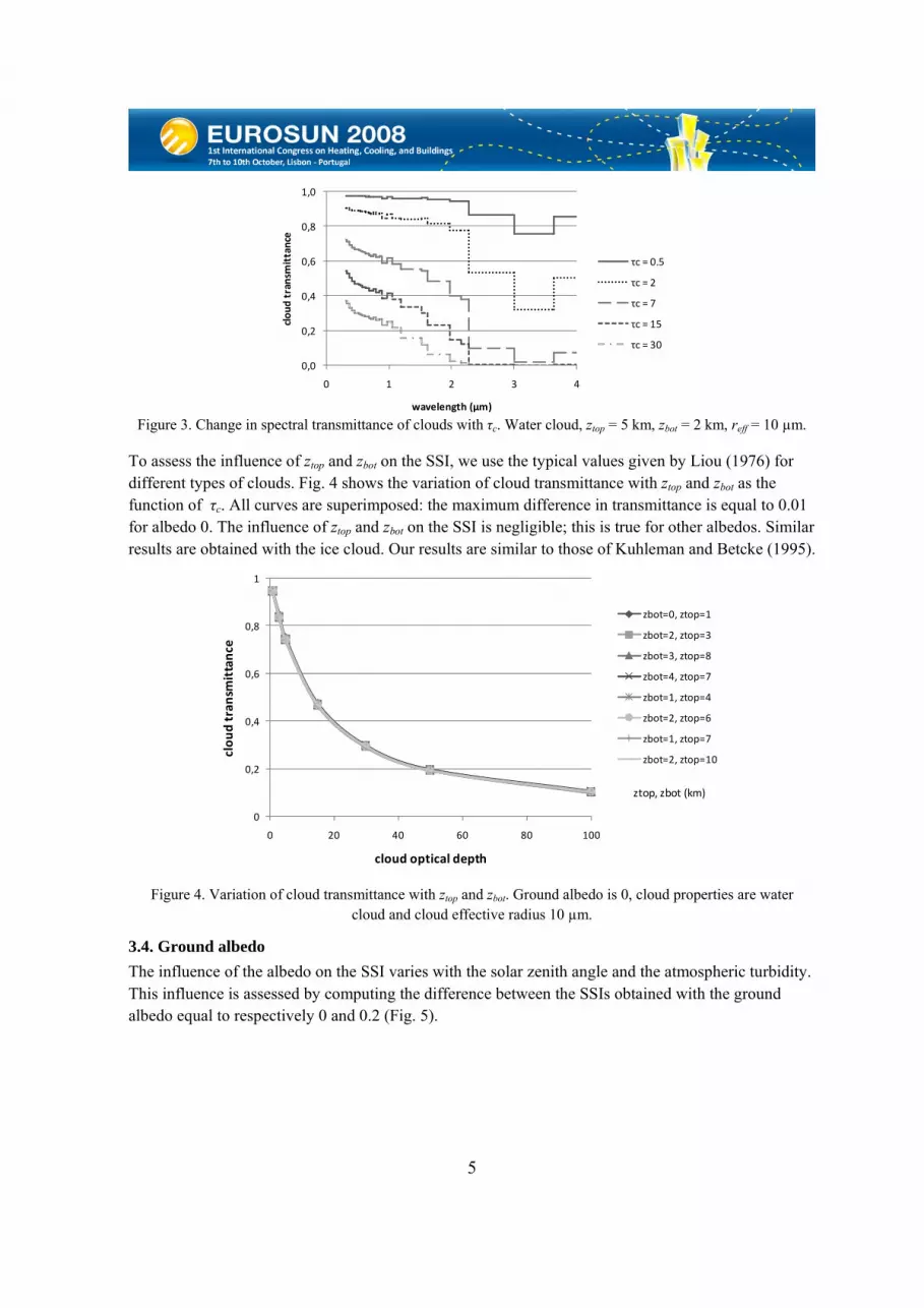
Figure 3. Change in spectral transmittance of clouds with τc. Water cloud, ztop = 5 km, zbot = 2 km, reff = 10 µm.

To assess the influence of ztop and zbot on the SSI, we use the typical values given by Liou (1976) for different types of clouds. Fig. 4 shows the variation of cloud transmittance with ztop and zbot as the function of τc. All curves are superimposed: the maximum difference in transmittance is equal to 0.01 for albedo 0. The influence of ztop and zbot on the SSI is negligible; this is true for other albedos. Similar results are obtained with the ice cloud. Our results are similar to those of Kuhleman and Betcke (1995).

0

0,2

0,4

0,6

0,8

1

0 20 40 60 80 100

clou

d tran

smittance

cloud optical depth

ztop, zbot (km)

zbot=0, ztop=1

zbot=2, ztop=3

zbot=3, ztop=8

zbot=4, ztop=7

zbot=1, ztop=4

zbot=2, ztop=6

zbot=1, ztop=7

zbot=2, ztop=10

Figure 4. Variation of cloud transmittance with ztop and zbot. Ground albedo is 0, cloud properties are water cloud and cloud effective radius 10 µm.

3.4. Ground albedo The influence of the albedo on the SSI varies with the solar zenith angle and the atmospheric turbidity. This influence is assessed by computing the difference between the SSIs obtained with the ground albedo equal to respectively 0 and 0.2 (Fig. 5).

6

1E‐04

1E‐03

1E‐02

1E‐01

1E+00

1E+01

0 1 2 3 4

absolute  deviation

 (W m

‐²)

wavelength (µm)

sza = 32°, vis = 12 km

sza = 32°, vis = 50 km

sza = 60°, vis = 12 km

sza = 60°, vis = 50 km

0

2

4

6

8

10

12

14

0 1 2 3 4

relative

  deviation

 (%)

wavelength (µm)

sza = 32°, vis = 12 km

sza = 32°, vis = 50 km

sza = 60°, vis = 12 km

sza = 60°, vis = 50 km

Figure 5. Absolute and relative deviation on SSI when the ground albedo is set to 0 while it is equal to 0.2.

The influence of the albedo on the SSI decreases as the wavelength increase because the intensity of diffusion decreases. It increases with increasing atmospheric turbidity and so, decreases also with increasing visibility. This influence decreases when the solar zenith angle is growing because of the decreasing of the SSI; this is also true for the relative deviation. Presence of clouds increases the relative influence of the albedo: the larger τc, the larger the relative deviation.

3.5. Bidirectional reflectance and shadow into a pixel

The soil bidirectional reflectance can be expressed as (Rahman et al., 1993):

rs = r0 M FHG H (3)

where r0 is an arbitrary parameter characterizing the intensity of the surface cover. The function H is characterised by a large reflection in the illuminating direction. M and FHG are the symmetric and asymmetric angular functions. The variation of this reflectance around the albedo can be greater than 0.1. In the specific case of oceans, the reflectance varies from zero to values greater than cloud reflectance, it also depends on wind speed (Lefèvre et al. 2007). Thus, by considering the albedo instead of the bidirectional reflectance, one commits a significant error on irradiance reflected by the ground then backscattered by the atmosphere, thus contributing to the diffuse fraction of the SSI. This omission is very often made for operational reasons because of the lack of data describing the ground.

Very often, for operational reasons, the irradiance calculations are done under the assumption of a flat terrain inside the pixel. However, the cosine of the local incident angle θ is:

cosθ(β,α) = (cosωcosδcosφ + sinδsinφ)cosβ + cosωcosδsinφcosαsinβ + sinωcosδsinαsinβ - sinδcosφcosαsinβ (4)

where ω is the hour angle, δ is the solar declination, φ is the latitude of the site, α and β correspond to the direction of the local slope, respectively in azimuth and tilt. Thus, the SSI of the pixel should be modified by the ratio:

R = ∫∫pixelcosθ(α(p),β(p))dp / cosθ(0,0) (5)

7

4. Conclusion

We have quantified the influence of the different atmospheric properties on the SSI. Clouds (cloud optical thickness and type) are the most important variable for the SSI. They also exhibit high temporal (~ 30 m) and spatial (~ 10 min) variation (Rossow and Schiffer 1999). Aerosol loading and type, water vapour amount and atmospheric profile have a great influence on SSI, particularly in clear skies. Wald and Baleynaud (1999) demonstrate noticeable variation in atmospheric transmittance due to local pollution in cities at scale of 100 m. Ground albedo and its spectral variation have an important influence on diffuse part and spectral distribution of SSI. They exhibit very high spatial variation on a pixel basis and seasonal temporal variations. The influence of ozone amount is large in the ultraviolet range, but remains low on the integrated wavelength SSI.

Data availability of water vapour and aerosol loading is fairly low. We are expecting one value per day for a 50 km pixel. The error induced on the SSI depends on the variation of these parameters within the pixel. The clearer the sky, the greater the error. Comparisons of ground measurements of hourly means of SSI made at sites in Europe less than 50 km apart for clear skies show that the spatial variation in SSI, expressed as the relative root mean square difference, can be greater than 10 %.This result is in agreement with Perez et al. (1997) who stressed the large spatial variability of the SSI.

The influences of vertical position and geometrical thickness of clouds in the atmosphere are negligible. Thus, the solution of the RTM for a cloudy atmosphere is equivalent to the product of the irradiance obtained under a clear sky and the extinction coefficient due to the cloud. In particular, it means that the method Heliosat-4 may be composed of two distinct parts: the clear-sky part and the cloudy-sky part. In addition, given the fact that the cloud parameters may be known every ¼ h and 3 km and the clear-sky parameters every day and 50 km, the adoption of the concept of "a model for the clear sky, another for other types of skies" saves time: the first model, which takes into account all other atmospheric parameters, focuses the bulk of computation resources.

The results of this work form the basis for the establishment of the method, called Heliosat-4, based on the exploitation of a RTM for the operational processing of satellite data to produce assessments of solar surface irradiance every 3 km and ¼ h on Europe and Africa. The necessary inputs to Heliosat-4 have been identified; a gross assessment of the relative importance of their uncertainties on the final assessment has been obtained.

References

[1] Bernhard, G., Booth, C. R., Ehramjian, J. C., 2002. Comparison of measured and modeled spectral ultraviolet irradiance at Antarctic stations used to determine biases in total ozone data from various sources. In Ultraviolet Ground-and Space-based Measurements, Models, and Effects, edited by J.R. Slusser, J.R. Herman, and W. Gao, Proceedings of SPIE, Vol. 4482, 115-126.

[2] Cano D., Monget J.M., Albuisson M., Guillard H., Regas N., and Wald L., 1986, A method for the determination of the global solar radiation from meteorological satellite data. Solar Energy, 37, 31-39.

[3] Hammer, A., 2000. Anwendunsgspezifische Solarstrahlungsinformationen aus Meteosat-Daten. Dissertation, Carl von Ossietzky Universität Oldenburg, Fachbereich Physik, Oldenburg, Germany.

[4] Ineichen, P., 2006. Comparison of eight clear sky broadband models against 16 independent data banks. Solar Energy, 80 (4), 468-478.

8

[5] Kato S., Ackerman T.P., Mather J.H., Clothiaux E.E., 1999. The k-distribution method and correlated-k approximation for shortwave radiative transfer model. Journal of Quantitative Spectroscopy & Radiative Transfer 62 (1999) 109-121.

[6]Kuhleman, R., Betcke, J., 1995. CloudS: A new parameterization of radiative transfer through clouds (summary of development and first validations). Heliosat-3 Reports, 21 p., http://www.heliosat3.de/documents/.

[7] Liou K.N., 1976. On the absorption, reflection and transmission of solar radiation in cloudy atmospheres. Journal of the Atmospheric Sciences vol.33 798-805.

[8] Liou K.N., 1980. An Introduction to Atmospheric Radiation. International Geophysics Series, volume 26, Academic Press, 392 p.

[9] Mayer B., Kylling A., 2005. Technical note: The libRadtran software package for radiative transfer calculations – description and examples of use. Atmospheric Chemistry and Physics, 5, 1855-1877.

[10] Mueller, R., Dagestad, K.F., Ineichen, P., Schroedter, M., Cros, S., Dumortier, D., Kuhlemann, R., Olseth, J.A., Piernavieja, G., Reise, C., Wald, L., Heinnemann, D., 2004. Rethinking satellite based solar irradiance modelling - The SOLIS clear sky module. Remote Sensing of Environment, 91 (2), 160-174.

[11] Perez R., Seals R., Zelenka A., 1997. Comparing satellite remote sensing and ground network measurements for the production of site/time specific irradiance data, Solar Energy, 60, 89-96.

[12] Perrin de Brichambaut C. et Vauge C., 1982. Le Gisement Solaire : Evaluation de la Ressource Energétique. Technique et Documentation, Librairie Lavoisier, Paris, France, 222 pages.

[13] Pinker R. T., Frouin R., Z. Li, 1995. A review of satellite methods to derive surface shortwave irradiance. Remote Sensing of Environment, 51 (1), 108-124.

[14] Rigollier, C., Lefèvre, M., Wald, L., 2004. The method Heliosat-2 for deriving shortwave solar radiation from satellite images. Solar Energy, 77 (2), 159-169.

[15] Rossow W.B., Schiffer R.A., 1999. Advances in understanding clouds from ISCCP, B. Bulletin of the American Meteorological Society, 80, 2261-2287.

[16] Shettle E. P., 1989. Models of aerosols, clouds and precipitation for atmospheric propagation studies. In AGARD Conference Proceedings No. 454, Atmospheric propagation in the UV, visible, IR and mm-region and related system aspects.

[17] Stamnes, K., S.-C. Tsay, W. Wiscombe and K. Jayaweera, 1988. Numerically stable algorithm for discrete-ordinate-method radiative transfer in multiple scattering and emitting layered media. Applied Optics, 27, 2502.

[18] Vermote, E., Tanré, D., Deuzé, J. L., Herman, M., Morcrette, J. J., 1997. Second simulation of the satellite signal in the solar spectrum (6S), 6S: An overview. IEEE Transactions on Geoscience and Remote Sensing, 35, 675-686.

[19] Wald L., Baleynaud J.-M., 1999. Observing air quality over the city of Nantes by means of Landsat thermal infrared data. International. Journal of Remote Sensing, 20, 5, 947-959.