Computers & Fluids 97 (2014) 143–155

Contents lists available at ScienceDirect

Computers & Fluids

journal homepage: www.elsevier .com/ locate /compfluid

Visualization of three-dimensional incompressible flowsby quasi-two-dimensional divergence-free projections

http://dx.doi.org/10.1016/j.compfluid.2014.04.0090045-7930/� 2014 Elsevier Ltd. All rights reserved.

⇑ Tel.: +972 36407207; fax: +972 36407334.E-mail address: gelfgat@tau.ac.il

Alexander Yu. Gelfgat ⇑School of Mechanical Engineering, Faculty of Engineering, Tel-Aviv University, Ramat Aviv, Tel-Aviv 69978, Israel

a r t i c l e i n f o

Article history:Received 8 April 2013Received in revised form 2 April 2014Accepted 4 April 2014Available online 16 April 2014

Keywords:Incompressible flowFlow visualizationGalerkin methodNatural convection benchmarkLid-driven cavity benchmark

a b s t r a c t

Context: A visualization of three-dimensional incompressible flows by divergence-free quasi-two-dimensional projections of velocity field on three coordinate planes is proposed.

Objective: To visualize 3D incompressible flow by 3 two-dimensional plots.Method: It is argued that such divergence-free projections satisfying all the velocity boundary condi-

tions are unique for a given velocity field. It is shown that the projected fields and their vector potentialscan be calculated using divergence-free Galerkin bases.

Results: Using natural convection flow in a laterally heated cube as an example, it is shown that the pro-jections proposed allow for a better understanding of similarities and differences of three-dimensionalflows and their two-dimensional likenesses. An arbitrary choice of projection planes is further illustratedby a lid-driven flow in a cube, where the lid moves parallel either to a sidewall or a diagonal plane.

Conclusion: A new method for visualization of 3D incompressible flows is developed and described.� 2014 Elsevier Ltd. All rights reserved.

1. Introduction choice of visualization coordinate system is arbitrary, so that the

With the growth of available computer power, development ofnumerical methods and experimental techniques dealing withfully developed three-dimensional flows the importance of flowvisualization becomes obvious. While two-dimensional flows canbe easily described by streamline or vector plots, there is no com-monly accepted methodology for representation of three-dimen-sional flows on a 2D plot. Streamlines can be defined also for ageneral 3D flow, however cannot be represented by a single streamfunction. Other textbook techniques, such as streak lines, trajecto-ries and arrow fields, are widely used but become unhelpful withincrease of flow complexity. Same can be said about plotting of iso-surfaces and isolines of velocity or vorticity components, whichproduce beautiful pictures, however, do not allow one to find outvelocity direction at a certain point. Basic and more advancedrecent state-of-the-art visualization techniques are discussed inreview papers [1–3] where reader is referred for the details. Herewe develop another visualization technique, applicable only toincompressible flows, and related to the surface-based techniquesdiscussed in [2]. Our technique considers projections of 3D velocityfield onto coordinate planes and allows one to compute a set ofsurfaces to which the projected flow is tangent. Thus, the flow isvisualized in all three sets of coordinate planes (surfaces). The

axes can be directed along ‘‘most interesting’’ directions, e.g. direc-tions parallel and orthogonal to dominating velocity or vorticity.

The goal of this study is to visualize a three-dimensional incom-pressible flow computed numerically at some grid nodes. The visu-alization described below is independent on the method used forflow calculation. It is based on divergence-free projections of acomputed 3D velocity field on two-dimensional coordinate planes.Initially, this study was motivated by a need to visualize three-dimensional benchmark flows, which are direct extensions ofwell-known two-dimensional benchmarks, e.g., lid-driven cavityand convection in laterally heated rectangular cavities. Thus, weseek for a visualization that is capable to show clearly both similar-ities and differences of flows considered in 2D and 3D formula-tions. It seems, however, that the technique proposed can havesignificantly wider area of applications and can be applied for visu-alization of different divergence free vector functions, e.g., vorticityand magnetic field. The last example below illustrates that thetechnique allows one to visualize along or perpendicular to anarbitrarily chosen direction that can differ from coordinate axes.

Consider a given velocity field, which can be a result of compu-tation or experimental measurement. Note, that modern means offlow measurement, like PIV and PTV, allow one to measure threevelocity components on quite representative grids, which leadsto the same problem of visualization of results. Here we observethat a three-dimensional divergence-free velocity field can be rep-resented as a superposition of two vector fields that describe the

144 A.Yu. Gelfgat / Computers & Fluids 97 (2014) 143–155

motion in two sets of coordinate planes, say (x–z) and (y–z), with-out a need to consider the (x–y) planes. These fields allow for def-inition of vector potential of velocity, whose two independentcomponents have properties of two-dimensional stream function.The two parts of velocity field are tangent to isosurfaces of the vec-tor potential components, which allows one to visualize the flow intwo sets of orthogonal coordinate planes. This approach, however,does not allow one to preserve the velocity boundary conditions ineach of the fields separately, so that some of the boundary condi-tions are satisfied only after both fields are superimposed. The lat-ter is not good for visualization purposes. We argue further, that itis possible to define divergence-free projections of the flow on thethree sets of coordinate planes, so that (i) the projections areunique, (ii) each projection is described by a single component ofits vector potential, and (iii) the projection vectors are tangent toisosurfaces of the corresponding non-zero vector potential compo-nent. This allows us to visualize the flow in three orthogonal sets ofcoordinate planes. In particular, it helps to understand how thethree-dimensional model flows differ from their two-dimensionallikenesses. To calculate the projections we propose to use diver-gence-free Galerkin bases, on which the initial flow can be orthog-onally projected. Clearly, these projections can be calculated byother numerical approaches.

For a representative example, we choose convection in a later-ally heated square cavity with perfectly thermally insulated hori-zontal boundaries, and the corresponding three-dimensionalextension, i.e., convection in a laterally heated cube with perfectlyinsulated horizontal and spanwise boundaries. The most represen-tative solutions for steady states in these model flows can be foundin [4] for the 2D benchmark, and in [5,6] for the 3D one. In thesebenchmarks the pressure p, velocity v = (u,v,w) and temperatureT are obtained as a solution of Boussinesq equations

Fig. 1. Streamlines of two-dimensional buoyancy convection flow in a laterally heatedcirculation is clockwise.

@T@tþ ðv � rÞT ¼ DT ð1Þ

@v@tþ ðv � rÞv ¼ �rpþ PrDv þ RaPrTez ð2Þ

div ½v� ¼ 0 ð3Þ

defined in a square 0 6 x, z 6 1 or in a cube 0 6 x,y,z 6 1, with theno-slip boundary conditions on all the boundaries. The boundariesx = 0, 1 are isothermal and all the other boundaries are thermallyinsulated, which in the dimensionless formulation reads

Tðx ¼ 0Þ ¼ 1; Tðx ¼ 1Þ ¼ 0;@T@y

� �y¼0;1

¼ 0;@T@z

� �z¼0;1

¼ 0:

ð4Þ

Ra and Pr are the Rayleigh and Prandtl numbers. The reader isreferred to the above cited papers for more details. Here we focusonly on visualization of solutions of 3D problem and comparisonwith the corresponding 2D flows. All the flows reported beloware calculated on 1002 and 1003 stretched finite volume grids,which is accurate enough for present visualization purposes (forconvergence studies see also [7]).

Apparently, the 2D flow v = (u,0,w) is best visualized by thestreamlines, which are the isolines of the stream function wdefined as u ¼ @w

@z ;w ¼ �@w@x . In each point the velocity vector is

tangent to a streamline passing through the same point, so thatplot of streamlines and schematic indication of the flow directionis sufficient to visualize a two-dimensional flow. This is illustratedin Fig. 1, where streamlines of flows calculated for Pr = 0.71, and Ravaried from 103 to 108 are shown. Note how the streamline pat-terns get more complex with the increase of Rayleigh number.Our further purpose is to visualize three-dimensional flows at

square cavity at Pr = 0.71 and different Rayleigh numbers. The direction of main

A.Yu. Gelfgat / Computers & Fluids 97 (2014) 143–155 145

the same Rayleigh numbers, so that it will be possible to seesimilarities and differences between 2D and 3D flows.

2. Preliminary considerations

We consider an incompressible flow in a rectangular box0 6 x 6 X, 0 6 y 6 Y, 0 6 z 6 Z, satisfying the no-slip conditions onall boundaries. The continuity equation @u/@x + @v/@y + @w/@z = 0makes one velocity component dependent on two others, so thatto describe the velocity field we need two scalar three-dimensionalfunctions, while the third one can be found via continuity. Thisobservation allows us to decompose the velocity field in the fol-lowing way

v ¼u

vw

264

375¼

u

0w1

264

375þ

0v

w2

264

375; w1 ¼�

Z z

0

@u@x

dz; w2 ¼�Z z

0

@v@y

dz

ð5Þ

This decomposition shows that the divergence-free velocityfield can be represented as superposition of two fields having com-ponents only in the (x,z) or (y,z) planes. Moreover, we can easilydefine the vector potential of velocity field as

W ¼Wx

Wy

0

264

375 ¼

R z0 vdz

�R z

0 udz

0

264

375; v ¼ rot½W� ð6Þ

Fig. 2. Calculation for Ra = 103. Vector potentials Wy and Wx defined in Eq. (6) superpisosurface for Wy = 0.16; (b) max jWxj = 0.053, isosurfaces for Wx = ±0.008. Frames (c) and

Thus, W is the vector potential of velocity field v, and its twonon-zero components have properties of the stream function:

u ¼ � @Wy

@z; w1 ¼

@Wy

@x; v ¼ @Wx

@z; w2 ¼ �

@Wx

@y: ð7Þ

This means, in particular, that vectors of the two components ofdecomposition (5), i.e., (u,0,w1) and (0,v,w2), are tangent to isosur-faces of Wy and Wx, and the vectors are located in the planes (x–z)and (y–z), respectively. Thus, it seems that the isosurfaces of Wy andWx, which can be easily calculated from numerical or experimental(e.g., PIV) data, can be a good means for visualization of the velocityfield. Unfortunately, there is a drawback, which can make such visu-alization meaningless. Namely, only the sum of vectors w1 and w2,calculated via the integrals in (5), vanish at z = Z, while each vectorseparately does not. Thus, visualization of flow via the decomposi-tion (5) in a straight-forward way will result in two fields that vio-late no-penetration boundary conditions at one of the boundaries,which would make the whole result quite meaningless. The latteris illustrated in Fig. 2, where isosurfaces of the two componentsof vector potentials are superimposed with the (u, 0,w1) and(0,v,w2) vectors. It is clearly seen that the vector arrows are tangentto the isosurfaces, however the velocities w1 and w2 do not vanishat the upper boundary. The latter is illustrated additionally by iso-lines of w1 and w2 plotted at the upper boundary (Fig. 2c and d).One can see also that the sum of functions plotted in Fig. 2c and dyields zero. Furthermore, the choice of integration boundaries in(5) is arbitrary, so that the whole decomposition (5) is not unique.

osed with the vector fields (u,0,w1) and (0,v,w2). (a) max Wy = 1.066, min Wy = 0,(d) show isolines of the vectors w1 and w2 defined in Eq. (5) on the boundary z = 1.

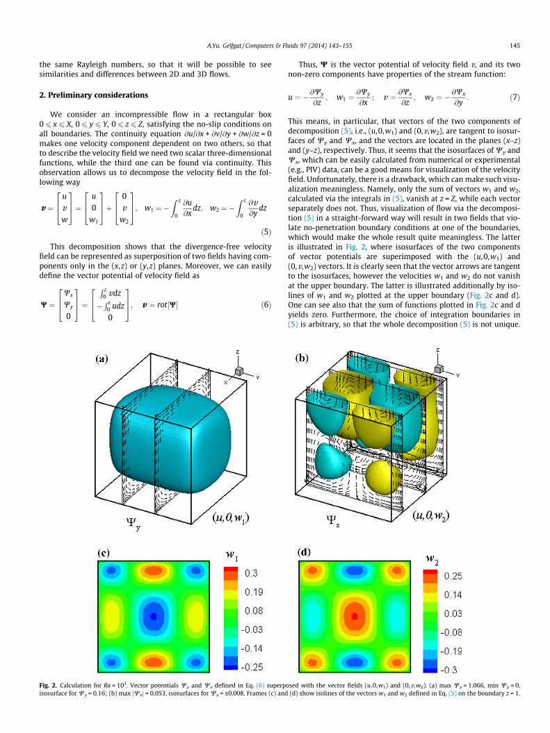
Fig. 3. Visualization of a three-dimensional flow at Ra = 103. (a) Two flow trajectories starting at the points (0.1,0.1,0.1) and (0.9,0.9,0.9). The trajectories are colored due tothe temperature values at the points they pass. The temperature color map is shown aside. (b), (c), (d) Isosurfaces of WðyÞy , WðxÞx and WðzÞz superimposed with the vector plots ofthe fields uðyÞ; uðxÞ and uðzÞ , respectively. The isosurfaces are plotted for WðyÞy ¼ 0:28;WðxÞx ¼ �0:063, and WðzÞz ¼ �0:080. (For interpretation of the references to color in thisfigure legend, the reader is referred to the web version of this article.)

Table 1Maximal values of the calculated vector potentials of the three velocity projectionsand their locations.

Ra 103 104 105 106 107 108

WðxÞx0.144 0.602 1.408 2.925 5.988 15.200

xmax 0.812 0.867 0.926 0.956 0.0272 0.176ymax 0.159 0.118 0.0702 0.0419 0.0969 0.0921zmax 0.465 0.414 0.364 0.315 0.745 0.877

WðyÞy1.127 4.993 9.954 17.863 32.854 61.465

xmax 0.509 0.509 0.693 0.841 0.0844 0.0521ymax 0.500 0.653 0.812 0.912 0.0444 0.0236zmax 0.500 0.483 0.414 0.431 0.535 0.535

WðzÞz0.148 0.768 1.915 3.983 14.793 33.272

xmax 0.517 0.586 0.535 0.154 0.133 0.960ymax 0.154 0.154 0.143 0.176 0.176 0.980zmax 0.805 0.805 0.841 0.936 0.963 0.254

146 A.Yu. Gelfgat / Computers & Fluids 97 (2014) 143–155

Clearly, one would prefer to visualize unique properties of the flowrather than non-unique ones.

To define unique flow properties similar to those shown in Fig. 2we observe that decomposition (5) can be interpreted as represen-tation of a three-dimensional divergence-free vector into twodivergence free vector fields located in orthogonal coordinateplanes, i.e., having only two non-zero components. Consider a vec-tor built from only two components of the initial field, sayu = (u,v,0). It is located in the (x,y,z = const) planes, satisfies allthe boundary conditions for u and v, however, is not divergence-free. We can apply the Helmholtz–Leray decomposition [8] thatdecomposes this vector into solenoidal and potential part,

u ¼ ruþ u; r � u ¼ 0 ð8Þ

As is shown in [8], together with the boundary conditions

u � n ¼ 0; and@u@n¼ u � n ð9Þ

where n is a normal to the boundary, the decomposition (8) isunique. For the following, we consider (8) in the (x,y,z = const) planesand seek for a decomposition of u = (u,v,0) in a (x,y,z = const) plane

u ¼ rðx;yÞuþ u; rðx;yÞ � u ¼ 0; rðx;yÞ ¼ ex@

@xþ ey

@

@y: ð10Þ

We represent the divergence-free two-dimensional vectoru ¼ ðu; v ;0Þ as

u ¼ rot½W�; W ¼ ð0;0;WzÞ ) u ¼ @Wz

@y; v ¼ � @Wz

@xð11Þ

Fig. 4. Visualization of a three-dimensional flow at Ra = 105. (a) Two flow trajectories starting at the points (0.1,0.1, 0.1) (0.9,0.9,0.9) and (0.4,0.5,0.5). The trajectories arecolored due to the temperature values at the points they pass. The temperature color map is shown aside. (b), (c), (d) Isosurfaces of WðyÞy , WðxÞx and WðzÞz superimposed with thevector plots of the fields uðyÞ; uðxÞ and uðzÞ , respectively. The isosurfaces are plotted for WðyÞy ¼ 4:0;WðxÞx ¼ �0:46, and WðzÞz ¼ �0:8. (For interpretation of the references to color inthis figure legend, the reader is referred to the web version of this article.)

A.Yu. Gelfgat / Computers & Fluids 97 (2014) 143–155 147

which yields for the z-component of rot[u]:

ez � rot½u� ¼ ez � rot½u� ¼ ez � rot½rot½W�� ¼ �ez � DW ¼ �DWz ð12Þ

This shows that Wz is an analog of the two-dimensional streamfunction, so that in each plane (x,y,z = const) vector u is tangentto an isoline of Wz. To satisfy the no-slip boundary conditions foru and v , Wz and its normal derivative must vanish on the boundary,which makes the definition of both Wz and u unique. Note, that con-trary to the boundary conditions (9), to make vector u in the decom-position (10) unique and satisfying all the boundary conditions of u,we do not need to define any boundary conditions for the scalarpotential u.

To conclude, the resulting solenoidal part u of vector u = (u,v,0)(i) is unique, (ii) is defined by a single non-zero z-component Wz ofits vector potential, and (iii) in each (x,y,z = const) plane vectors ofu are tangent to the isosurfaces of Wz. Defining same solenoidalfields for two other sets of coordinate planes we arrive to threequasi-two-dimensional divergence-free projections of the initialvelocity field. Each projection is described by a single scalarthree-dimensional function, which, in fact, is a single non-zerocomponent of the corresponding vector potential.

In the following we use the three above quasi-two-dimensionaldivergence-free projections for visualization of convective flow in alaterally heated cube, and offer a way to calculate them. Inparticular, to compare a three-dimensional result with the corre-sponding two-dimensional one, we need to compare one of theprojections. Thus, if the 2D convective flow was considered inthe plane (x,z), we compare it with the corresponding projectionsof the 3D flow on the (x,y = const,z) planes, which are tangent toisosurfaces of the non-zero y-component of the correspondingvector potential.

3. Numerical realization

A direct numerical implementation of the Helmholtz–Leraydecomposition to an arbitrary velocity field is known in CFD asChorin projection. This procedure is well-known, uses the bound-ary conditions (9), but does not preserve all the velocity boundaryconditions. Therefore, it is not applicable for our purposes. Alterna-tively, we propose orthogonal projections of the initial velocityfield on divergence-free Galerkin bases used previously for compu-tations of different two-dimensional flows.

Fig. 5. Visualization of a three-dimensional flow at Ra = 107. (a) Two flow trajectories starting at the points (0.1,0.1,0.1), (0.9,0.9,0.9) and (0.1,0.5,0.5). The trajectories arecolored due to the temperature values at the points they pass. The temperature color map is shown aside. (b), (c), (d) Isosurfaces of WðyÞy ;WðxÞx and WðzÞz superimposed with thevector plots of the fields u(y),u(x) and u(z), respectively. The isosurfaces are plotted for WðyÞy ¼ 20:2, WðxÞx ¼ �1:94, and WðzÞz ¼ �2:2. (For interpretation of the references to color inthis figure legend, the reader is referred to the web version of this article.)

148 A.Yu. Gelfgat / Computers & Fluids 97 (2014) 143–155

Divergence-free basis functions that satisfy all the linearhomogeneous boundary conditions were introduced in [9] fortwo-dimensional flows and were then extended in [10,11] tothree-dimensional cases. To make the numerical process clear webriefly describe these bases below. The bases are built from shiftedChebyshev polynomials of the 1st and 2nd kind, Tn(x) and Un(x),that are defined as

TnðxÞ ¼ cos½n � arccosð2x� 1Þ�; UnðxÞ ¼sin½ðnþ 1Þarccosð2x� 1Þ�

sin½arccosð2x� 1Þ�ð13Þ

and are connected via derivative of Tn(x) as T 0nðxÞ ¼ 2nUn�1ðxÞ. Eachsystem of polynomials forms basis in the space of continuous func-tions defined on the interval 0 6 x 6 1. It is easy to see that vectors

q2Dij ¼

X2i Ti

xX

� �Uj�1

yY

� �� Y

2j Ui�1xX

� �Tj

yY

� �" #

ð14Þ

form a divergence-free basis in the space of divergence-free func-tions defined on a rectangle 0 6 x 6 X, 0 6 y 6 Y. Assume that atwo-dimensional problem is defined with two linear and homoge-neous boundary conditions for velocity at each boundary, e.g., theno-slip conditions. This yields four boundary conditions in either

x- or y-direction for the two velocity components. To satisfy theboundary conditions we extend components of the vectors (14) intolinear superpositions as

q2Dij ¼

X2

P4l¼0

ailðiþlÞ Tiþl

xX

� �P4m¼0bjmUjþm�1

yY

� �� Y

2

P4l¼0ailUiþl�1

xX

� �P4m¼0

bjm

ðjþmÞ TjþmyY

� �24

35 ð15Þ

For each i a substitution of (15) into the boundary conditions yieldsfour linear homogeneous equations for five coefficients ail, l = 0, 1, 2,3, 4. Fixing ai0 = 1, allows one to define all the other coefficients,whose dependence on i and l can be derived analytically. The coef-ficients bjm are evaluated in the same way. Expressions for thesecoefficients for the no-slip boundary conditions can be found in[9,11]. Since the basis functions q2D

ij are divergence-free in the plane

ðx; yÞ; @ q2Dij

� �x=@xþ @ q2D

ij

� �y=@y ¼ 0, and satisfy the non-penetration

conditions through all the boundaries x = 0, X and y = 0, Y, they areorthogonal to every two-dimensional potential vector field, i.e.,Z Y

0

Z X

0r2Dp �q2D

ij dxdy¼Z Y

0

Z X

0

@p@x

exþ@p@y

ey

� ��q2D

ij dxdy¼0; ð16Þ

which is an important point for further evaluations.

Fig. 6. Visualization of a three-dimensional flow at Ra = 108. (a) Two flow trajectories starting at the points (0.1,0.1, 0.1) (0.9,0.9,0.9) and (0.1,0.5,0.5). The trajectories arecolored due to the temperature values at the points they pass. The temperature color map is shown aside. (b), (c), (d) Isosurfaces of WðyÞy ;WðxÞx and WðzÞz superimposed with thevector plots of the fields u(y),u(x) and u(z), respectively. The isosurfaces are plotted for WðyÞy ¼ 39:3;WðxÞx ¼ �4:3, and WðzÞz ¼ �6:8. (For interpretation of the references to color inthis figure legend, the reader is referred to the web version of this article.)

A.Yu. Gelfgat / Computers & Fluids 97 (2014) 143–155 149

For extension of the two-dimensional basis to the three dimen-sional case we recall that for a divergence-free vector field we haveto define independent three-dimensional bases for two compo-nents only. Representing the flow in the form (5) and using thesame idea as in the two-dimensional basis (15) we arrive to a setof three-dimensional basis functions formed from two followingsubsets

qðyÞijk ðx;y;zÞ¼

X2

P4l¼0

ailðiþlÞTiþl

xX

� �P4m¼0bjmTjþm

yY

� �P4n¼0cknUkþn�1

zZ

� �0

� Z2

P4l¼0ailUiþl�1

xX

� �P4m¼0bjmTjþm

yY

� �P4n¼0

cknðkþnÞTkþn

zZ

� �2664

3775

ð17Þ

qðxÞijk ðx;y;zÞ¼

0Y2

P4l¼0~ailTiþl

xX

� �P4m¼0

~bjm

ðjþmÞTjþmyY

� �P4n¼0~cknUkþn�1

zZ

� �� Z

2

P4l¼0~ailTiþl

xX

� �P4m¼0

~bjmUjþm�1yY

� �P4n¼0

~cknðkþnÞTkþn

zZ

� �2664

3775

ð18Þ

where coefficients ail, bjm, ckn, ~ail, ~bjm, ~ckn are defined from theboundary conditions. Their derivation for no-slip boundary condi-tions is explained in Appendix A. Expressions for these coefficients

in the case of a slip-free condition on the upper boundary can befound in [11]. The velocity field is projected on truncated series

uðxÞ ¼XNx

i¼0

XNy

j¼0

XNz

k¼0

AijkqðxÞijk ; uðyÞ ¼XNx

i¼0

XNy

j¼0

XNz

k¼0

BijkqðyÞijk ð19Þ

Here one must be cautious with the boundary conditions in z-direc-tion since, as it was explained above, the two parts of representa-tion (6) satisfy the boundary condition for w at z = Z only as asum. Therefore we must exclude this condition from definition ofbasis functions (17) and (18) and set ck4 ¼ ~ck4 ¼ 0. The correspond-ing boundary condition should be included in the resulting systemof equations for Aijk and Bijk as an additional algebraic constraint.Note that this fact was overlooked in [10] that could lead to missingof some important three-dimensional Rayleigh–Bénard modes. Onthe other hand, comparison of 3D basis functions (17) and (18) withthe 2D ones (15) shows that with all the boundary conditionsincluded, the functions qðyÞijk ðx; y; zÞ and qðxÞijk ðx; y; zÞ form the completetwo-dimensional bases in the (x,y = const,z) and (x = const,y,z)planes, respectively. The coefficients bjm and ~ail are used to satisfythe boundary conditions in the third direction. For the basis in the(x,y,z = const) planes we add

Fig. 7. Isosurfaces of WðyÞy at different Rayleigh numbers. The isosurfaces are plotted at levels (a) 0.53, 4.0, 8.8; (b) 2.5, 10.9, 16.0; (c) 5.4, 17.3, 26.6; (d) 12.6, 33.7, 50.6.

150 A.Yu. Gelfgat / Computers & Fluids 97 (2014) 143–155

qðzÞijk ðx; y; zÞ ¼

X2

P4l¼0

�ailðiþlÞ Tiþl

xX

� �P4m¼0

�bjmUjþm�1yY

� �P4n¼0�cknTjþn

zZ

� ��Y2

P4l¼0�ailUiþl�1

xX

� �P4m¼0

�bjm

ðjþmÞ TjþmyY

� �P4n¼0�cknTkþn

zZ

� �0

2664

3775

ð20Þ

Together with the third projection of the velocity

uðzÞ ¼XNx

i¼0

XNy

j¼0

XNz

k¼0

CijkqðzÞijk ð21Þ

Now, we define an inner product as

hu;vi ¼Z

Vu � vdV ð22Þ

and compute projections of the velocity vector V, to be visualized,on each of the three basis systems separately. To do that, we needto calculate Gram matrices Gx,Gy, and Gz for each of the three basessystems q(x), q(y), and q(z), respectively. This does not require muchCPU time since inner products in each spatial direction can be cal-culated separately. The coefficients Aijk, Bijk, and Cijk in the decompo-sitions (19) and (21) are calculated as a product of inversed Gram

matrices with vectors composed of the inner products of the veloc-ity field V with basis functions q(x), q(y), and q(z). The latter can beexpressed as

fAijkg ¼ G�1x V ;qðxÞijk

D En o; fBijkg ¼ G�1

y V ;qðyÞijk

D En o;

fCijkg ¼ G�1z V ;qðzÞijk

D En oð23Þ

where brackets {} denote assembling of a 3D array into a vector,which is done by assignment of a single index I = Nz[Ny

(i � 1) + j � 1] + k to each three-dimensional array, e.g., Aijk or

V ;qðxÞijk

D E, described by the indices i, j, k that vary from 1 to Nx,Ny,

and Nz, respectively. Adding the definition J = Nz[Ny

(l � 1) + m � 1] + n, the (I, J) element of the Gram matrices is defined

as GðI;JÞx ¼ qðxÞI ;qðxÞJ

D E¼ qðxÞijk ;q

ðxÞlmn

D E;GðI;JÞy ¼ qðyÞI ;qðyÞJ

D E¼ qðyÞijk ; q

ðyÞlmn

D E,

and GðI;JÞz ¼ qðzÞI ; qðzÞJ

D E¼ qðzÞijk ;q

ðzÞlmn

D E. Above integrals must be evalu-

ated numerically using an appropriate quadrature formula. Forexample, for the finite volume solution defined on staggered gridswe used summation of the function values in finite volumes centersmultiplied by the corresponding volumes. More details are given inAppendix B. The Gram matrices are symmetric by definition. Their

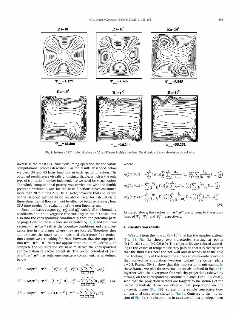
Fig. 8. Isolines of WðyÞy in the midplane y = 0.5 at different Rayleigh numbers. The direction of main circulation is clockwise.

A.Yu. Gelfgat / Computers & Fluids 97 (2014) 143–155 151

inverse is the most CPU time consuming operation for the wholecomputational process described. For the results described belowwe used 30 and 40 basis functions in each spatial direction. Theobtained results were visually undistinguishable, which is the onlytype of truncation number independence we need for visualization.The whole computational process was carried out with the doubleprecision arithmetic, and for 303 basis functions never consumedmore than 20 min for a 2.9 GHz PC. Note, however, that applicationof the Galerkin method based on above bases for calculation ofthree-dimensional flows will not be effective because of a very longCPU time needed for evaluation of the non-linear terms.

Since the basis vectors qðxÞijk ;qðyÞijk and qðzÞijk satisfy all the boundary

conditions and are divergence-free not only in the 3D space, butalso into the corresponding coordinate planes, the potential partsof projections on these planes are excluded by (16), and resultingvectors uðxÞ; uðyÞ; uðzÞ satisfy the boundary conditions and are diver-gence free in the planes where they are located. Therefore, theyapproximate the quasi-two-dimensional divergence-free projec-tion vectors we are looking for. Note, however, that the superposi-tion uðxÞ þ uðyÞ þ uðzÞ does not approximate the initial vector v. Tocomplete the visualization we have to derive the correspondingapproximation of vector potentials. The vector potential of eachof uðxÞ; uðyÞ; uðzÞ has only one non-zero component, as is definedbelow

uðxÞ ¼ rot½WðxÞ�; WðxÞ ¼ WðxÞx ;0; 0� �

; WðxÞx �XNx

i¼0

XNy

j¼0

XNz

k¼0

AijkuðxÞijk ;

uðyÞ ¼ rot½WðyÞ�; WðyÞ ¼ 0;WðyÞy ; 0� �

; WðyÞy �XNx

i¼0

XNy

j¼0

XNz

k¼0

BijkuðyÞijk ;

uðzÞ ¼ rot½WðzÞ�; WðzÞ ¼ 0;0;WðzÞz

� �; WðzÞz �

XNx

i¼0

XNy

j¼0

XNz

k¼0

CijkuðzÞijk

ð24Þ

where

uðxÞijk ðx; y; zÞ ¼ �X4

l¼0

~ailTiþlxX

� �X4

m¼0

~bjm

ðjþmÞ TjþmyY

� �X4

n¼0

~ckn

ðkþ nÞ TkþmzZ

� �

uðyÞijk ðx; y; zÞ ¼X4

l¼0

ail

ðiþ lÞ TiþlxX

� �X4

m¼0

bjmTjþmyY

� �X4

n¼0

ckn

ðkþ nÞ TkþmzZ

� �

uðzÞijk ðx; y; zÞ ¼X4

l¼0

�ail

ðiþ lÞ TiþlxX

� �X4

m¼0

�bjm

ðjþmÞ TjþmyY

� �X4

n¼0

�cknTkþmzZ

� �ð25Þ

As stated above, the vectors uðxÞ; uðyÞ; uðzÞ are tangent to the isosur-faces of WðxÞx ;WðyÞy and WðzÞz , respectively.

4. Visualization results

We start from the flow at Ra = 103, that has the simplest pattern(Fig. 3). Fig. 3a shows two trajectories starting at points(0.1,0.1,0.1) and (0.9,0.9,0.9). The trajectories are colored accord-ing to the values of temperature they pass, so that it is clearly seenthat the fluid rises near the hot wall and descends near the coldone. Looking only at the trajectories, one can mistakenly concludethat convective circulation weakens toward the center planey = 0.5. Frames 3b–3d show that this impression is misleading. Inthese frames we plot three vector potentials defined in Eqs. (23),together with the divergence-free velocity projections (shown byarrows) on the corresponding coordinate planes. First, it is clearlyseen that the projection vectors are tangent to the isolines of thevector potentials. Then we observe that projections on they = const. planes (Fig. 3b) represent the simple convective two-dimensional circulation shown in Fig. 1a. Contrary to the impres-sion of Fig. 3a, the circulations in (x,z) are almost y-independent

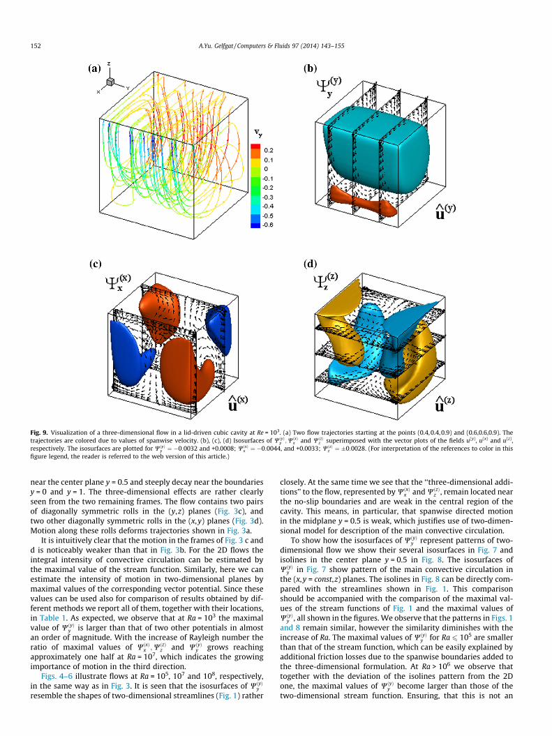
Fig. 9. Visualization of a three-dimensional flow in a lid-driven cubic cavity at Re = 103. (a) Two flow trajectories starting at the points (0.4,0.4,0.9) and (0.6,0.6,0.9). Thetrajectories are colored due to values of spanwise velocity. (b), (c), (d) Isosurfaces of WðyÞy ;WðxÞx and WðzÞz superimposed with the vector plots of the fields u(y), u(x) and u(z),respectively. The isosurfaces are plotted for WðyÞy ¼ �0:0032 and +0.0008; WðxÞx ¼ �0:0044, and +0.0033; WðzÞz ¼ �0:0028. (For interpretation of the references to color in thisfigure legend, the reader is referred to the web version of this article.)

152 A.Yu. Gelfgat / Computers & Fluids 97 (2014) 143–155

near the center plane y = 0.5 and steeply decay near the boundariesy = 0 and y = 1. The three-dimensional effects are rather clearlyseen from the two remaining frames. The flow contains two pairsof diagonally symmetric rolls in the (y,z) planes (Fig. 3c), andtwo other diagonally symmetric rolls in the (x,y) planes (Fig. 3d).Motion along these rolls deforms trajectories shown in Fig. 3a.

It is intuitively clear that the motion in the frames of Fig. 3 c andd is noticeably weaker than that in Fig. 3b. For the 2D flows theintegral intensity of convective circulation can be estimated bythe maximal value of the stream function. Similarly, here we canestimate the intensity of motion in two-dimensional planes bymaximal values of the corresponding vector potential. Since thesevalues can be used also for comparison of results obtained by dif-ferent methods we report all of them, together with their locations,in Table 1. As expected, we observe that at Ra = 103 the maximalvalue of WðyÞy is larger than that of two other potentials in almostan order of magnitude. With the increase of Rayleigh number theratio of maximal values of WðxÞx ;WðzÞz and WðyÞy grows reachingapproximately one half at Ra = 107, which indicates the growingimportance of motion in the third direction.

Figs. 4–6 illustrate flows at Ra = 105, 107 and 108, respectively,in the same way as in Fig. 3. It is seen that the isosurfaces of WðyÞy

resemble the shapes of two-dimensional streamlines (Fig. 1) rather

closely. At the same time we see that the ‘‘three-dimensional addi-tions’’ to the flow, represented by WðxÞx and WðzÞz , remain located nearthe no-slip boundaries and are weak in the central region of thecavity. This means, in particular, that spanwise directed motionin the midplane y = 0.5 is weak, which justifies use of two-dimen-sional model for description of the main convective circulation.

To show how the isosurfaces of WðyÞy represent patterns of two-dimensional flow we show their several isosurfaces in Fig. 7 andisolines in the center plane y = 0.5 in Fig. 8. The isosurfaces ofWðyÞy in Fig. 7 show pattern of the main convective circulation inthe (x,y = const,z) planes. The isolines in Fig. 8 can be directly com-pared with the streamlines shown in Fig. 1. This comparisonshould be accompanied with the comparison of the maximal val-ues of the stream functions of Fig. 1 and the maximal values ofWðyÞy , all shown in the figures. We observe that the patterns in Figs. 1and 8 remain similar, however the similarity diminishes with theincrease of Ra. The maximal values of WðyÞy for Ra 6 105 are smallerthan that of the stream function, which can be easily explained byadditional friction losses due to the spanwise boundaries added tothe three-dimensional formulation. At Ra > 106 we observe thattogether with the deviation of the isolines pattern from the 2Done, the maximal values of WðyÞy become larger than those of thetwo-dimensional stream function. Ensuring, that this is not an

Fig. 10. Visualization of a three-dimensional flow in a lid-driven cubic cavity with a lid moving along a diagonal, at Re = 10 3. (a) Two flow trajectories starting at the points(0.1,0.1,0.9) and (0.9,0.9, 0.9). The trajectories are colored due to values of vertical velocity. (b), (c), (d) Isosurfaces of WðyÞy , WðxÞx and WðzÞz superimposed with the vector plots ofthe fields u(y), u(x) and u(z), respectively. The isosurfaces are plotted for WðyÞy ¼ �0:015 and +0.0015; WðxÞx ¼ �0:015, and +0.0015; WðzÞz ¼ �0:0024. (For interpretation of thereferences to color in this figure legend, the reader is referred to the web version of this article.)

A.Yu. Gelfgat / Computers & Fluids 97 (2014) 143–155 153

effect of truncation in the sums (23), we explain this by strongthree-dimensional effects, in which motion along the y-axis startto affect the motion in the (x,y = const,z) planes.

As an example of arbitrary choice of projection planes we con-sider another well-known benchmark problem of flow in a lid-driven cubic cavity. We consider it in two different formulations:a classical configuration where the lid moves parallel to a side wall,and a modified configuration with the lid moving along the diago-nal of the upper boundary [12,13]. Obviously, three-dimensionaleffects are significantly stronger in the second case. Both flowsare depicted in Figs. 9 and 10 in the same way as convective flowswere represented above. Comparing the flow pattern shown inFig. 9, one can see clear similarities with the well-known two-dimensional flow in a lid-driven cavity. The main vortex andreverse recirculation in the lower corner are clearly seen inFig. 9b. Fig. 9c and d show additional three-dimensional recircula-tions in the (x,y,z = const) and (x = const,y,z) planes. The same rep-resentation of the second configuration in Fig. 10 exhibits similarpatterns of WðxÞx and WðyÞy together with the similar patterns of corre-sponding projection vectors. This is an obvious consequence of theproblem configuration, where main motion is located in the diago-nal plane and the planes parallel to it. To illustrate motion in these

planes we project the flow on planes orthogonal to the diagonalplane (or parallel to the second diagonal plane). The result is shownin Fig. 11. The isosurfaces belong to the corresponding vectorpotential, so that the divergence-free projection of velocity on thediagonal and parallel planes is tangent to these and other isosurfac-es. Arrows in the diagonal plane depict this projection and illustratethe main vortex, as well as small recirculation vortices in lower cor-ners. It is seen that the arrows are tangent to both isosurfaces.

5. Conclusions

We proposed to visualize three-dimensional incompressibleflows by divergence-free projections of velocity field on three coor-dinate planes. We presented the arguments showing that such arepresentation allows, in particular, for a better understanding ofsimilarities and differences between three-dimensional bench-mark flow models and their two-dimensional counter parts. Weargued also that the choice of projection planes is arbitrary, so thatthey can be fitted to the flow pattern.

To approximate the divergence-free projections numerically wecalculated orthogonal projections on divergence-free Galerkinvelocity bases. Obviously, there are other ways of doing that,

Fig. 11. Visualization of a three-dimensional flow in a lid-driven cubic cavity with alid moving along a diagonal, at Re = 103. Isosurfaces of vector potential of velocityprojection on the diagonal planes, and the vector plot of the correspondingprojected velocity field. The isosurfaces are plotted for the levels �0.017 and +0.004,while the minimal and maximal values of the calculated vector potential are �0.083and +0.012.

154 A.Yu. Gelfgat / Computers & Fluids 97 (2014) 143–155

among which we can mention inverse of the Stokes operator dis-cussed in [14]. We believe also that the proposed method of visu-alization is suitable for a significantly wider class of incompressibleflows, and can be applied not only to numerical, but also to exper-imental data.

Acknowledgement

This work was supported by the LinkSCEEM-2 project, fundedby the European Commission under the 7th Framework Programthrough Capacities Research Infrastructure, INFRA-2010-1.2.3 Vir-tual Research Communities, Combination of Collaborative Projectand Coordination and Support Actions (CP-CSA) under Grant agree-ment No. RI-261600.

Appendix A. Derivation of coefficients ail; bjm,ckn; ~ail;

~bjm; ~ckn; �ail;�bjm; �ckn of the basis functions (17) and (18) for

no-slip boundary conditions

As mentioned above, the coefficients ail, bjm; ckn; ~ail,~bjm; ~ckn; �ail;

�bjm; �ckn are obtained after substitution of the basisfunctions in the boundary conditions. The values of the shiftedChebyshev polynomials at the boundary points are

Tnð0Þ ¼ ð�1Þn; Tnð1Þ ¼ 1; Unð0Þ ¼ ð�1Þnðnþ 1Þ;Unð1Þ ¼ nþ 1 ð25Þ

Thus, for the coefficients ail we obtain the following system of fourlinear equations

ð�1Þi

iai;0þ

ð�1Þiþ1

iþ1ai;1þ

ð�1Þiþ2

iþ2ai;2þ

ð�1Þiþ3

iþ3ai;3þ

ð�1Þiþ4

iþ4ai;4¼ 0 ð26:1Þ

1i

ai;0þ1

iþ1ai;1þ

1iþ2

ai;2þ1

iþ3ai;3þ

1iþ4

ai;4¼ 0 ð26:2Þ

ð�1Þiðiþ1Þai;0þð�1Þiþ1ðiþ2Þai;1þð�1Þiþ2ðiþ2Þai;2

þð�1Þiþ3ðiþ4Þai;3þð�1Þiþ4ðiþ5Þai;4 ¼0 ð26:3Þðiþ1Þai;0þðiþ2Þai;1þðiþ2Þai;2þðiþ4Þai;3þðiþ5Þai;4 ¼0 ð26:4Þ

for five unknown coefficients. To make the system definite, weassign ai;0 ¼ 1, and assuming i – 0 obtain

ai;1 ¼ ai;3 ¼ 0; ai;2 ¼ �i

iþ 2� ðiþ 1Þðiþ 4Þ2

iðiþ 2Þðiþ 3Þ ;

ai;4 ¼ðiþ 1Þðiþ 4Þ

iðiþ 3Þ ð27Þ

For the first basis function corresponding to i = 0 we define addi-tionally U�1(x) = 0 and for the zero Chebyshev polynomial replacethe coefficient ai;0=i by a0;0. This yields

a0;1 ¼ a0;3 ¼ 0; a0;2 ¼ �163; a0;4 ¼

83

ð28Þ

Now we notice that the coefficients �ail, ~bjm;�bjm; ckn and ~ckn are

obtained from same systems of equations where index i should bereplaced by either j or k. Therefore,

�ail ¼ ~bil ¼ �bil ¼ cil ¼ ~cil ¼ ail; i ¼ 0;1;2;3; . . . ;

l ¼ 0;1;2;3;4 ð29Þ

The remaining coefficients bjm; ~ail, and �ckn must be defined so thatthe basis functions vanish on all the boundaries. It is easy to see that

bj;0 ¼ ~ai;0 ¼ �ck;0 ¼ 1; bj;2 ¼ ~ai;2 ¼ �ck;2 ¼ �1 ð30Þbj;1 ¼ ~ai;1 ¼ �ck;1 ¼ bj;3 ¼ ~ai;3 ¼ �ck;3 ¼ bj;4 ¼ ~ai;4 ¼ �ck;4 ¼ 0 ð31Þ

Appendix B. Numerical evaluation of divergence freeorthogonal projections on a staggered grid

Here we present more details on numerical evaluation of Eqs.(14)–(25) assuming that the flow is calculated on a staggered griddefined in the following way. First, for the grid size (Mx + 1)(My + 1)(Mz + 1) we define uniformly distributed grid nodes xi, yj,and zk as

xi ¼XNx

i; yj ¼YNy

j; zk ¼Z

Nzk ð32Þ

where i, j, k are integers varying from 0 to Mx, My, Mz, respectively.The uniformly distributed nodes can be stretched near the bound-aries, or redistributed in any other way that does not alter theirnumbering in the sense x0 < x1 < � � � < xMx , etc. To cluster the gridnodes near the boundaries we use the same mapping as in [11]

xi Xxi

X� a sin 2p xi

X

� �h i; yj Z

yj

Y� b sin 2p

yj

Y

� �� ;

zk Zzk

Z� c sin 2p zk

Z

� �h ið33Þ

where a, b, and c can vary from 0 to 0.12. The steepest stretching isobtained for a = b = c = 0.12, the values used in the current study.After the stretching is completed we define the shifted nodes

xiþ1=2 ¼12ðxi þ xiþ1Þ; yjþ1=2 ¼

12ðyj þ yjþ1Þ;

zkþ1=2 ¼12ðzk þ zkþ1Þ ð34Þ

and the corresponding grid steps

hðxÞiþ1=2¼ xiþ1�xi; hðyÞjþ1=2¼ yjþ1�yj; hðzÞkþ1=2¼ zkþ1�zk ð35Þ

hðxÞi ¼ xiþ1=2�xi�1=2; hðyÞj ¼ yjþ1=2�yj�1=2; hðzÞk ¼ zkþ1=2�zk�1=2 ð36Þ

The numerical solution is obtained on the staggered grids. The sca-lar variables, i.e., temperature, pressure and velocity divergence, aredefined in the nodes (xi,yj,zk). The x-, y-, and z-velocity componentsare defined in the nodes (xi+1/2,yj,zk), (xi,yj+1/2,zk), and (xi,yj,zk+1/2),respectively. For the following we define the node values of

Table 2CPU times consumed using 2.9 GHz PC for computation of the Gram matrices,solution of the linear algebraic equations problem with a Gram matrix by theCholesky decomposition and computation of the final sums.

Numberof basisfunctions

Computing asingle Grammatrix (s)

Solution of a linearproblem with aGram matrix (s)

Calculationsof sums (24)(s)

Absolute error insolution of thelinear system

203 0.895 10.6 0.099 1.4 � 10�16

303 9.0 380 0.17 4.6 � 10�16

403 61.8 5700 0.286 5.0 � 10�16

A.Yu. Gelfgat / Computers & Fluids 97 (2014) 143–155 155

numerically calculated functions as pijk, Tijk, ui+1/2,j,k, vi,j+1/2,k, wi,j,k+1/2.The velocity divergence is approximated in the nodes (xi,yj,zk) as

½divðvÞ�ijk ¼uiþ1=2;j;k � ui�1=2;j;k

hðxÞi

þ v i;jþ1=2;k � v i;j�1=2;k

hðyÞj

þwi;j;kþ1=2 �wi;j;k�1=2

hðzÞk

ð37Þ

The finite volume method combined with the fractional step timeintegration yields zero values of the numerical divergence (37) inthe corresponding nodes. To calculate the divergence free projec-tions described above, we prefer to keep these values equal to zero,rather than the exact differential operator div. To do that we definenode values of the Chebyshev polynomials of the first kind T

Tn;iðxiÞ ¼ cos½n � arccosð2xi � 1Þ�;Tn;iþ1=2ðxiþ1=2Þ ¼ cos½n � arccosð2xiþ1=2 � 1Þ� ð38Þ

The node values of second kind polynomial U are defined in the waythat makes the numerical approximation of the relationT 0nðxÞ ¼ 2nUn�1ðxÞ valid. Therefore, in all the inner points we define

Un�1;iðxiÞ ¼1

2nhðxÞi

½Tn;iþ1=2ðxiþ1=2Þ � Tn;i�1=2ðxi�1=2Þ� ð39:1Þ

Un�1;iþ1=2ðxiþ1=2Þ ¼1

2nhðxÞiþ1=2

½Tn;iþ1ðxiþ1Þ � Tn;iðxiÞ� ð39:2Þ

and add the analytical values of Un in all the boundary points. Thepolynomials grid values in the y- and z-direction are defined inthe same way. After the polynomials in Eqs. (14)–(20) are replacedby their grid values, the approximate divergence (37) of the basisfunctions remains an analytic zero. Since boundary values of thegrid-defined polynomials are the same as those of the analyticalones, the coefficients found as described in Appendix A remainunchanged. Clearly, redefinition of the polynomials U (39) is notnecessary for the visualization purposes, however it yields bettercomparison with the two-dimensional results that were calculatedkeeping the 2D version of the divergence approximation (37) equalto zero.

Now, the inner product of two vectors u = (u(x),u(y),u(z)) and w =(w(x),w(y),w(z)) defined by Eq. (22) is replaced by the followingquadrature formula

hu;wi ¼XMx�2

i¼1

XMy�1

j¼1

XMz�1

k¼1

uðxÞiþ1=2;j;kwðxÞiþ1=2;j;khðxÞi hðyÞjþ1=2hðzÞkþ1=2

h i

þXMx�1

i¼1

XMy�2

j¼1

XMz�1

k¼1

uðyÞi;jþ1=2;kwðyÞi;jþ1=2;khðxÞiþ1=2hðyÞj hðzÞkþ1=2

h i

þXMx�1

i¼1

XMy�1

j¼1

XMz�2

k¼1

uðzÞi;j;kþ1=2wðzÞi;j;kþ1=2hðxÞiþ1=2hðyÞjþ1=2hðzÞk

h ið40Þ

The Gram matrices and the inner products of Eqs. (23) arecomputed using the quadrature (40). Since the Gram matrices aresymmetric and positive defined, they can be effectively invertedby the Cholesky decomposition.

The characteristic CPU times needed for computing of the Grammatrices, their inverse and further summation of the series (24) areshown in Table 2. The last row of Table 2 displays the maximal

absolute residual over all rows of the linear equations systems,which shows that no numerical difficulties connected to a possibleill-conditioning of the linear systems are observed. Clearly, themost computationally demanding is the Gram matrix inverse. Itshould be stressed, however, that these matrices depend only onthe geometry and boundary conditions, so that they can be calcu-lated once for a series of visualizations, say, at different Reynolds orGrashof numbers. For visualization purposes we usually do notneed too demanding convergence. Thus, in the present study theresults obtained with 303 and 403 basis functions, were visuallyindistinguishable.

References

[1] McLaughlin T, Laramee RS, Peikert R, Post FH, Chen M. Over two decades ofintegration-based, geometric flow visualization. Comp Graph Forum2010;29:1807–29.

[2] Edmunds M, Laramee RS, Chen G, Max N, Zhang E, Ware C. Surface-based flowvisualization. Comp Graph 2012;36:974–90.

[3] Etien T, Nguyen H, Kirby RM, Siva CT. ‘‘Flow visualization’’ juxtaposed with‘‘visualization of flow’’: synergistic opportunities between two communities.In: Proceedings of the 51st AIAA aerospace science meeting. New Horiz. ForumAerosp. Exp.; 2013. p. 1–13.

[4] Le Quéré P. Accurate solutions to the square thermally driven cavity at highRayleigh number. Comp Fluids 1991;20:29–41.

[5] Tric E, Labrosse G, Betrouni M. A first incursion into the 3D structure of naturalconvection of air in a differentially heated cavity, from accurate numericalsolutions. Int J Heat Mass Transf 1999;43:4043–56.

[6] Wakashima S, Saitoh TS. Benchmark solutions for natural convection in a cubiccavity using the high-order time–space method. Int J Heat Mass Transf2004;47:853–64.

[7] Gelfgat AYu. Stability of convective flows in cavities: solution of benchmarkproblems by a low-order finite volume method. Int J Numer Meths Fluids2007;53:485–506.

[8] Foias C, Manley O, Rosa R, Temam R. Navier–Stokes equations andturbulence. Cambridge Univ. Press; 2001.

[9] Gelfgat AYu, Tanasawa I. Numerical analysis of oscillatory instability ofbuoyancy convection with the Galerkin spectral method. Numer Heat Transf.Pt A 1994;25(6):627–48.

[10] Gelfgat AYu. Different modes of Rayleigh–Bénard instability in two- and three-dimensional rectangular enclosures. J Comput Phys 1999;156:300–24.

[11] Gelfgat AYu. Two- and three-dimensional instabilities of confined flows:numerical study by a global Galerkin method. Comput Fluid Dynam J2001;9:437–48.

[12] Povitsky A. Three-dimensional flow in cavity at Yaw. J Nonlin Anal2005;63:e1573–84.

[13] Feldman Yu, Gelfgat AYu. From multi- to single-grid CFD on massively parallelcomputers: numerical experiments on lid-driven flow in a cube usingpressure-velocity coupled formulation. Comp Fluids 2011;46:218–23.

[14] Vitoshkin H, Gelfgat AYu. On direct inverse of Stokes, Helmholtz and Laplacianoperators in view of time-stepper-based Newton and Arnoldi solvers inincompressible CFD. Commun Comput Phys 2013;14:1103–19.