Fish Supply Projections by Production Environments and ...

Agricultural Economics Research Review

Vol. 19 July-December 2006 pp 327-351

Fish Supply Projections by Production

Environments and Species Types in India1

Praduman Kumar2 , Madan M. Dey3 and Ferdinand J. Paraguas4

Abstract

The supply studies on the fisheries sector in India have been addressed at

the disaggregated level by production environment and by species groups.

These would be more imperative and useful for assessing the fish supply

at the national level. The fish supply projections by species groups under

different production environments have been obtained to a medium-term

horizon, by the year 2015 under various technological scenarios. The

study has concluded that the supply response to fish price changes has

been stronger under aquaculture than marine environment in India. Price

and technology have been reported as the important instruments to induce

higher supply. The change in the relative prices of fish species would

change the species-mix in the total supply. The fish production has been

projected as 4.6-5.5 million tonnes of inland fish and 3.2-3.6 million tonnes

of marine fish by the year 2015. More than 60 per cent of the additional fish

production will be contributed by aquaculture and mainly by the Indian

major carps.

Introduction

Fisheries, a sunrise sector in India, has recorded a faster growth than

that of the crop and livestock sectors. The sector contributes to the livelihood

of a large section of economically-underprivileged population of the country.

1 The paper is drawn from the India study under the multi-country project on

‘Strategies and Options for Increasing and Sustaining Fisheries and Aquaculture

Production to Benefit Poor Households in Asia’. RETA 5945. Asian Development

Bank and WorldFish Center. February 2005.2 Consultant, Agricultural Economics, Policy Economics and Social Science Disci-

pline, WorldFish Center, Penang, Malaysia. E-mail: [email protected] Portfolio (Regional) Director, The WorldFish Center, Penang, Malaysia. E-mail:

[email protected] Senior Research Analyst, The WorldFish Center, Penang, Malaysia. E-mail:

[email protected]

328 Agricultural Economics Research Review Vol. 19 July-December 2006

It is undergoing a transformation and the policy support, production strategies,

public investment in infrastructure, and research and extension for fisheries

have significantly contributed to the increased fish production. The share of

fisheries in agricultural gross domestic product (Ag-GDP) has increased

from 1.7 per cent in the year 1980 to 4.2 per cent in 2000. The fish production

increased at the rate of 5.1 per cent per year during 1980-2003 and reached

5.9 million tonnes in 2003 from a level of 1.76 million tonnes in 1970-71 and

2.44 million tonnes in 1980-81 FAO (2005).

The depleting water resources for inland capture fisheries, and high

cost of fishing with crafts and gears have led to an increased realization of

the potential and versatility of inland aquaculture, making it a sustainable

and cost-effective alternative to inland capture fisheries. The emerging

production technologies (improved fish breeding, scientific aquaculture

practices), higher economic growth and policy reforms with higher emphasis

on aquacultural development are driving a rapid growth in the fisheries sector

in India. The contribution of inland fisheries to the total fish production has

increased significantly, from less than one-third of the total production in

1950-51 to more than its half in 2000-01.

The supply studies on the fisheries sector have not only been limited but

have not adequately addressed it also at the disaggregated level by fish

types and production environment. The supply studies would be more

imperative and useful for pragmatic planning, if addressed at the disaggregated

level. The present paper has attempted to: (i) estimate the fish supply and

factor demand model under aquaculture and marine production environments,

(ii) derive the fish supply and factor demand elasticities by fish species

under various production environments, and (iii) provide mid-term projections

of fish supply by fish species and production environment.

Data and Methodology

The time-series data on fish production (species-wise) and their prices

at the state level were compiled from various sources. The Handbook on

Fisheries Statistics, published by the Ministry of Agriculture, Government

of India, and the specific publications of different states on fisheries statistics

were the important sources of data for this study. Some unpublished data

were extracted from the state government records personally. The data on

input prices (wages, fertilizer, feed, fuel) were obtained from the Agricultural

Prices in India, reports of the Commission for Agricultural Costs and Prices

and Economic Survey, published by the Government of India, and from the

Fertilizer Statistics, published by the Fertilizer Association of India. The

export data on quantity and unit value of various species of fish were compiled

Kumar et al.: Fish Supply Projections by Production Environments 329

from Marine Products Export Development Authority, Kochi. The data on

fishery water resources were collected from Central Water Commission.

The Indian Livestock Census provided the data on fisherman population

and fishery resources. The data used in the study were classified as follows:

• Marine fish production by species for states/ union territories, their

quantity and prices.

• Inland fish production by species for states/union territories, their quantity

and prices.

• Prawn production by states/union territories, their quantity and prices.

• Exports of marine products by species, their quantity and value.

• Inland fishery resources by states/union territories: Length of rivers

and canals, area under reservoirs, ponds and tanks, water bodies,

brackish water.

• Coastal length by states/union territories.

• Fisherman population by states/union territories: It included the total

number of members, number of family members engaged in fishing

operations (full time and part time), family members engaged in fishing-

related activities (marketing of fish, repairing of fishing nets, and

processing of fish).

• Data on fishing crafts (traditional, motorised traditional, mechanised

boats – gill-netters, trawlers, liners) and fishing gears (dragnets, gill

nets, trawl nets, cast nets) by states/union territories.

The data on inland fish production, inputs and their prices were compiled

for the period 1991-92 to 1998-99, covering 27 states/union territories of

India. The data on inputs, viz. land, labour, feed (rice bran, oil cake and

other feeds), fertilizer (cow dung, poultry manure, and chemical fertilizers),

seed, and specific costs (diesel, medicine and others) were compiled5 . The

data on marine fish production and its value by species were compiled for

the period 1986-87 to 1998-99, covering 12 maritime Indian states. The data

on labour and fuel were also compiled from various published sources. The

quantity of diesel used was worked out by taking into account various types

of crafts, number of fishing days, hours of work per day, with the norms that

200 litres of diesel would be used per HP. The total HP utilisation was

worked out in consultation with experts.

5 The time-series cross-section data on specific inputs were not available at the

state level. The input-output coefficients for aquaculture fish were reviewed from

various studies. The time-series and cross-sectional information on the use of

various inputs were generated and used in the analysis. The data for the missing

years were obtained by interpolation. For the missing states, the information from

the neighbouring states were used.


The fish species were aggregated into 8 groups (Appendix Table 1) to

keep the model simple. These groups were formed on the basis of production

environment, commercial value, consumers’ taste and preferences and

experts’ opinion.

The Supply Model

Given a profit function, output supply and input demand equations can

be derived using Hotelling’s Lemma (Hotelling, 1932) by differentiating with

respect to prices. The profit function derivative with respect to the price of

a product is equal to the supply function of that product; and its derivative

with respect to the price of an input is equal to the negative of the demand

function of that input. To implement this process empirically, it was necessary

to first specify functional form for the profit function. In the present analysis,

we have used normalized quadratic form of the profit function.

Let q be a (n×1) ‘netput’ vector composed of k positive values of

outputs and l negative values of variable inputs. Let p be the corresponding

(k×l) vector of output and input prices. Both fixed inputs and other exogenous

factors are included in the vector Z. Let the profit (π) and prices (π) be

normalized by the price of the nth commodity (pn) such that π* = π / πn and

pi* = pi / pn. The normalized profit function can be written as Equation (1):

…(1)

Applying Hotteling’s Lemma, the derived system for output supply and factor

demand are given by Equation (2) and Equation (3), respectively:

Output supply

…(2)

Factor demand

…(3)

Equations (1), (2) and (3) can be estimated using system of equations

approach. The supply equation for the nth commodity, whose price served

as a numeraire can be worked-out as per Equation (4):

…(4)


Following the theory of production function (see, Wall and Fisher, 1988),

it is expected that the estimated profit function will follow the properties of

homogeneity, symmetry, monotonicity and convexity. Homogeneity in prices

is maintained in Equations (1), (2) and (3) due to normalization and hence

cannot be tested. Symmetry was implemented by imposing bij = bji during

estimation.

The monotonicity and convexity properties do not necessarily hold. The

consistency of the estimated model with the properties of convexity and

monotonicity were evaluated after estimation. For the normalized quadratic

form to satisfy the monotonicity condition, the estimated values of output

supply and input demand must be positive. To satisfy the convexity condition,

the Hessian of price derivatives must be positive semi-definite.

The elasticities can be computed at any particular value of prices and

quantities as per Equation (5) :

, where, i, j = 1, 2, …,(n-1) …(5)

Equation (5) measures the own-price elasticity when i = j, and cross-

price elasticity when i ≠ j. The corresponding numeraire netput can be

derived indirectly using the property of “homogeneity in prices” of the

normalized profit function using Equations (6) and (7):

…(6)

where, i = 1, 2, …, (n-1)

and

…(7)

Model Specification

An outline discussion on environment-specific multi-output multi-input

models is provided below. A description of the variables used in the both

models has been provided in Appendix A.

Inland Zone (Aquaculture)

The inland aquaculture model was consisted of three outputs, three

variable inputs and one shifter-pond area. The outputs were Indian major


carps (IMC), other freshwater fish (OFW), and freshwater shrimp (FS). In

the inputs, feed was measured as crude protein, fertilizer as nitrogen, and

labour as person-day6 . For simplicity, the corresponding unit prices of these

variables used in the model were coded as PIMC , POFW , PFS , Pfeed , Pfert,

Wage1, Zarea (see Appendix A for more information).

Marine Zone

The marine capture model was consisted of six outputs and two variable

inputs over the time span of the study. The state-level length of coastline

(coast) served as the shifter variable. The outputs were: pelagic high-value

(PHV), pelagic low-value (PLV), demersal high-value (DHV), demersal

low-value (DLV), shrimps, and molluscs. The factor demand was composed

of the main inputs, namely fuel and labour.

Results and Discussion

Fish Production

Total fish production, including both inland and marine sources, had

increased from 4.3 million tonnes to 5.5 million tonnes during the period

1993-1998 with an annual growth rate of 4.8 per cent (Table 1). This inland

fish production had increased with annual growth of 6.6 per cent during this

period and attained a level of 2.8 million tonnes in the year 1998. The IMC

had contributed half to the total inland fish production. Other species of fish,

except prawn, had contributed about 37 per cent. The prawn production

which was 310 thousand tonnes in the year 1991, had increased to 380

thousand tonnes with an annual growth rate of 4.4 per cent. The marine fish

production during 1993-1998 had increased from 2.3 million tonnes to 2.6

million tonnes, with the annual growth rate of 3 per cent. Pelagic fish was

found to be the major group of species and contributed nearly half to the

6 Feed is a critical input in fish production and is used for the purpose of a better

and faster growth of fish. Oil cake and rice bran are the most common supplemen-

tary feeds in aquaculture. These feeds were converted into crude protein equiva-

lent and used in the estimation of the supply model. The manure and fertilizers are

applied in the ponds to facilitate the growth of macro and micro vegetative plants

for ultimate consumption by fish. The most common chemical fertilizers used in

aquaculture are urea, single super phosphate (SSP), and di-ammonium phosphate

(DAP). These fertilizers were converted in nutrient equivalent and included in the

producer core system. Stocking refers to application of external fish seeds into

the ponds for the purpose of raising them up to marketable size. Data on stocking

(i.e. fingerling supply) were not available, it was not included in the model.


total marine fish production, followed by demersal (22.2%), molluscs (18.5%)

and shrimp (9.7%).

Input Use

Aquaculture: The inputs were categorized into two groups, viz. fixed and

variable inputs. Only variable inputs, viz. human labour, manures, fertilizers,

and feed were taken into account in the supply analysis in the fish model.

The most crucial inputs were labour and management. The share of inputs

in the total variable cost varied across states at around 33 to 52 per cent for

labour, 9 to 33 per cent for feed, 12 to 19 per cent for stocking, 9 to 15 per

Table 1. Production and price of fish by species group, India

Species Production (million kg) Price (Rs/kg)

TE1993 TE1998 Annual TE1993 TE1998 Annual

growth growth

(per cent) (per cent)

Inland fish

Indian major carps 958562 1418262 8.1 27.1 30.9 2.6

(46.3) (49.8)

Other freshwater fish 803573 1047258 5.4 15.8 24.6 9.3

(38.8) (36.7)

Freshwater shrimp/prawn 309005 383930 4.4 43.1 63.6 8.1

(14.9) (13.5)

Total 2071140 2849450 6.6 25.1 33.0 5.6

(47.7) (52.0)

Marine fish

Pelagic (high-value) 353273 374128 1.2 13.4 27.7 15.7

(15.6) (14.2)

Pelagic (low-value) 896014 931422 0.8 7.4 14.2 13.9

(39.5) (35.4)

Demersal (high-value) 270841 367666 6.3 9.2 18.6 15.1

(11.9) (14.0)

Demersal (low-value) 205830 216237 1.0 7.9 14.0 12.0

(9.1) (8.2)

Marine shrimp 244377 255774 0.9 33.1 52.0 9.5

(10.8) (9.7)

Molluscs 299349 486886 10.2 10.8 15.0 6.7

(13.2) (18.5)

Total 2269683 2632114 3.0 11.8 19.4 10.4

(52.3) (48.0)

Grand total 4340822 5481563 4.8 18.2 26.5 7.8

Note: Figures within the parentheses are the shares of fish species in total production.


cent for fertilizer and 15 to 22 per cent for specific inputs (Table 2). The

total labour employment in aquaculture which was 432 million person-days

during 1991, declined to 331 million person-days in the year 1998, at the rate

of (-)3.7 per cent per annum. The negative employment trend was

confirmative to the survey conducted by NSSO on employment recently

(1999). The wage which was Rs 20.8 per person-day in 1991 had gone up

to Rs 56 per person-day in the year 1998, with an annual growth rate of

14.3 per cent. The crude protein used for aquaculture had increased from

497.5 million kg in 1991 to 573.4 million kg in 1998, with an annual growth

rate of 2 per cent. The prices of crude protein per kg also increased from

Rs 12.30 to Rs 18.20, with an annual growth rate of 4.2 per cent. The

fertilizer-use had increased from 16.9 million kg in 1991 to 29.2 million kg in

1998, with an annual growth rate of 4.5 per cent in quantity and 8.6 per cent

in terms of value. The utilization of diesel had increased with 4 per cent

growth and attained a level of 46 million litres in year 1998.

Marine: Labour and fuel being the major inputs in the marine fisheries

sector, were taken into account in the estimation of the supply functions for

this sector. The marine sector in fish catching activity had used 432.5 million

person-days of labour in 1991, which had increased to 505.2 million person-

days in 1998, with an annual growth rate of 2.2 per cent. The use of diesel

had increased from 34.9 million litres to 45.9 million litres, with annual growth

rate 4 per cent during the period 1991-98. The wages had increased from

Rs 28.30 per person-day to Rs 59.20 per person-day during the period 1991-

1998, with an annual growth rate of 11.6 per cent. It was followed by the

Table 2. Annual use of inputs in aquaculture and marine fishery: 1991-1998

Item Unit 1991 1995 1998 Annual

growth

(per cent)

Aquaculture

Labour Million person-days 432.0 375.9 331.0 -3.7

Feed Million kg crude protein 497.5 525 573.4 2.0

Fertilizer Million kg nutrients 89.5 113.4 121.7 4.5

Wages Rs/day 20.8 40.4 56.1 14.3

Feed price Rs/kg of crude protein 12.3 11.3 18.2 4.2

Fertilizer price Rs/kg nutrient 16.9 27.2 29.3 8.6

Marine

Labour Million person-days 432.5 476.6 505.2 2.2

Diesel Million litres 34.9 40.9 45.9 4.0

Wages Rs/day 28.3 44.8 59.2 11.6

Diesel price Rs/litre 5.3 7.5 10.9 8.8


diesel prices from Rs 5.30 per litre to Rs.10.90 per litre, with annual growth

rate of 8.8 per cent. The increase in fuel-use was due to the modernization

and the replacement of a large number of traditional boats by the mechanised

boats.

Total Factor Productivity

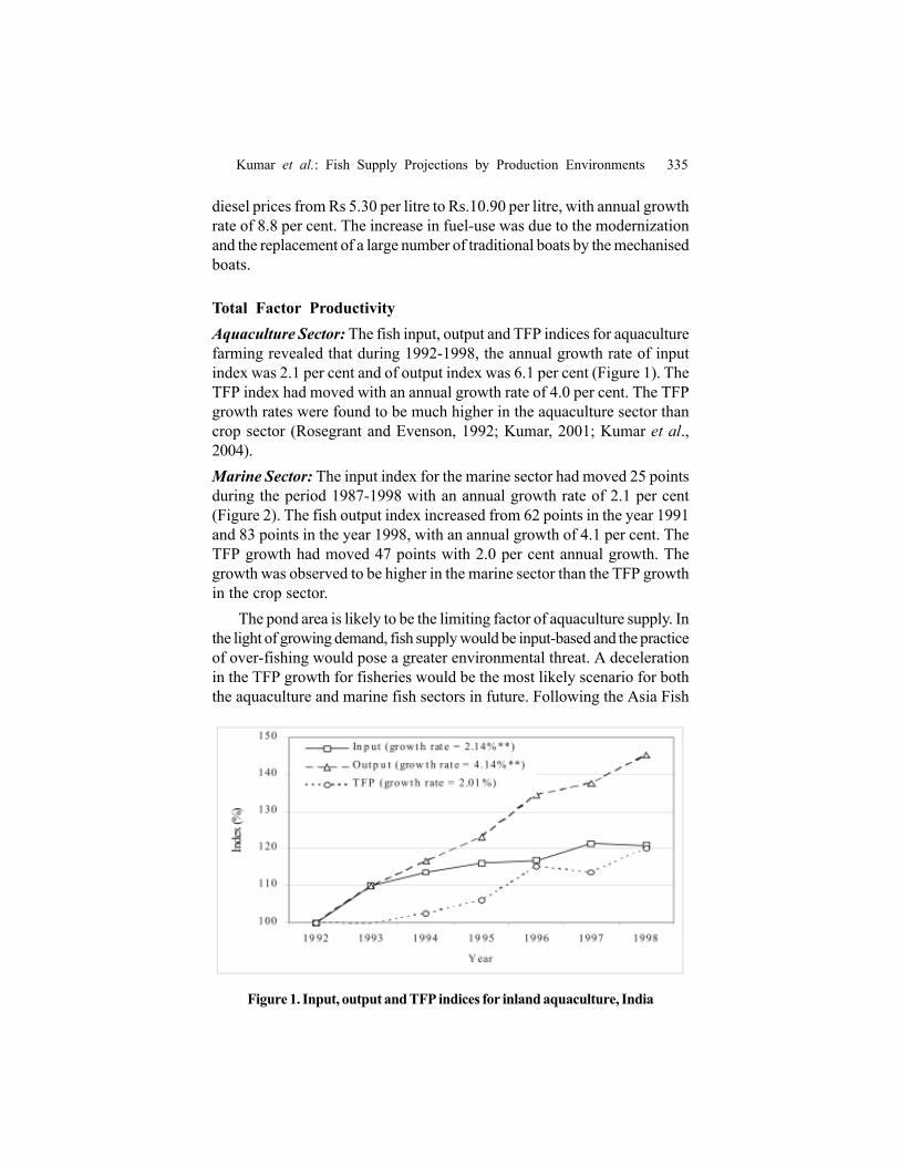
Aquaculture Sector: The fish input, output and TFP indices for aquaculture

farming revealed that during 1992-1998, the annual growth rate of input

index was 2.1 per cent and of output index was 6.1 per cent (Figure 1). The

TFP index had moved with an annual growth rate of 4.0 per cent. The TFP

growth rates were found to be much higher in the aquaculture sector than

crop sector (Rosegrant and Evenson, 1992; Kumar, 2001; Kumar et al.,

2004).

Marine Sector: The input index for the marine sector had moved 25 points

during the period 1987-1998 with an annual growth rate of 2.1 per cent

(Figure 2). The fish output index increased from 62 points in the year 1991

and 83 points in the year 1998, with an annual growth of 4.1 per cent. The

TFP growth had moved 47 points with 2.0 per cent annual growth. The

growth was observed to be higher in the marine sector than the TFP growth

in the crop sector.

The pond area is likely to be the limiting factor of aquaculture supply. In

the light of growing demand, fish supply would be input-based and the practice

of over-fishing would pose a greater environmental threat. A deceleration

in the TFP growth for fisheries would be the most likely scenario for both

the aquaculture and marine fish sectors in future. Following the Asia Fish

Figure 1. Input, output and TFP indices for inland aquaculture, India


Model (Dey et al., 2005), supply by fish types has been projected under

different scenarios7 of a decelerated TFP growth.

Estimation of Supply Model

In both the production environments, the model with the normalized

quadratic profit function included in the specification was not satisfactory.

It was because the number of parameters in the profit equation was large

and the Hessian matrix became ill-conditioned. As a consequence, the

normalized quadratic profit function was dropped from the specification,

leaving only the systems of output supply and factor demand for the

estimation. Though this might have resulted in some loss of efficiency, the

inherent multicollinearity problems were reduced.

The supply system was estimated using the cross-section time-series

data described earlier. Estimates of the model were obtained using the

Zellner’s generalized least squares with correction for serial correlation and

heteroscedasticity in the disturbance terms. Following the application of the

Figure 2. Input, output and TFP indices for marine capture, India

7 Scenario I: Baseline assumptions with the existing growth in TFP for marine

capture (2%) and aquaculture (4%) to continue till 2015

Scenario II: Baseline assumptions with 25% deceleration in TFP growth by

2015

Scenario III: Baseline assumptions with 50% deceleration in TFP growth by

2015

Scenario IV: Baseline assumptions with 75% deceleration in TFP growth by

2015

Scenario V: Base line assumptions without TFP growth during the projected

period, by 2015


Prais-Winsten estimator, the GLS SUR estimator was applied to the

transformed variables from the last iteration of the Prais-Western estimator

to generate the final parameter estimates for the system of equations in the

supply system.

Aquaculture Fish Supply and Input Demand

During the analysis all possible input/output prices were used as the

numeraire. OFW turned out to be best numeraire. The estimated parameters

of price variables in the supply and input demand equations agreed with a

sign of a-priori expectations (Table 3). The own-price parameters for fish

supply were statistically significant and positive. The cross-price parameters

were negative and in general, significant also. Both the own- and cross-

price parameters in the output supply were important in fish supply decisions.

Price of inputs had a negative influence on the fish supply, but it was not

significant for IMC and prawn/shrimp. The significance could not be tested

for OFW, being the numeraire in equation. The own-input price parameters

in the factor demand equation were significantly negative. The rise in wages

and other input prices will adversely affect the employment and use of input

levels in aquaculture. The shifter pond area under aquaculture, as expected,

would induce fish supply and inputs. The supply of IMC would increase

significantly with time. The results revealed that the input demand and fish

supply were sensitive to their own-prices. This suggests that Indian fish

producers respond to price changes in an effective manner. Price instruments

along with technological policy were likely to be quite effective in the fish

supply. The changes in relative price of fish species would influence the

supply-mix consisting of various fish species. Significant cross-price effects

for fish supply and insignificant crop-price effects for input demand were

observed. Since fish supply was interrelated through prices, policymakers

should ensure that the effects of one policy do not conflict with the policy

decisions for other fish types. It is suggested that a comprehensive approach

to fish price policy be taken rather than the product-by-product approach.

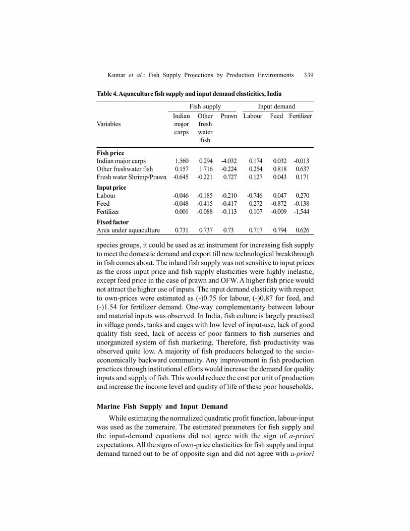
The elasticities calculated at mean data values have been given in Table

4. The own-price elasticity estimates had the expected signs; they were

greater than unity for IMC and OFW, and less than unity for prawn/shrimp

(FS). The prawn-cultivation was more capital-intensive as compared to

other species. The short-run price effect on supply was sharp and quick for

IMC and OFW than FS. The price of IMC would affect the FS supply

negatively. The cross-price elasticity of IMC and FS was negative and

highly elastic (-4.03). The input price had the mild effect on IMC supply,

whereas the supply of prawn and OFW was affected sharply. Since the

acreage effect on fish supply was quite high (0. 7) for all the aquaculture


Tab

le 3

. Aq

uacu

ltu

re fis

h s

up

ply

an

d in

pu

t d

eman

d m

od

els,

In

dia

India

n m

ajor

carp

sF

resh

wat

erL

abour

Fee

dF

ertilize

rO

ther

Shri

mp/P

raw

nfr

eshw

ater

fish

Coef

fici

ent

t-val

ue

Coef

fici

ent

t-val

ue

Coef

fici

ent

t-val

ue

Coef

fici

ent

t-val

ue

Coef

fici

ent

t-val

ue

Coef

fici

ent

Inte

rcep

t-1

2991

.90

2.55

1843

.47

1.23

-125

.63

0.10

615.

080.

2567

.07

0.12

–

Pri

ce (

Rs/

kg

)

India

n m

ajor

carp

s40

.14

2.05

-16.

583.

561.

190.

301.

250.

15-0

.03

-0.0

35.

98

Pra

wn

-16.

583.

562.

991.

640.

870.

821.

710.

720.

461.

19-2

.48

Lab

our

-1.1

90.

30-0

.87

0.82

-5.1

02.

021.

860.

530.

730.

45-3

.12

Fee

d-1

.25

0.15

-1.7

10.

721.

860.

53-3

4.45

4.12

-0.3

70.

25-2

0.11

Fer

tilize

r0.

030.

03-0

.46

1.19

0.73

0.45

-0.3

70.

25-4

.19

2.19

-2.1

4

Oth

er f

resh

wat

er f

ish

5.98

-2.4

83.

1220

.11

2.14

51.7

5

Sh

ifte

rs

Are

a (h

a)0.

008.

550.

006.

880.

0012

.19

0.00

12.1

60.

008.

140.

01

Yea

r6.

522.

55-0

.91

1.21

0.07

0.11

-0.3

00.

24-0

.03

0.11

IMR

-35.

512.

17-1

0.35

3.77

––

––

––

–

Syst

em w

eighte

d R

2 =

0.2

441


species groups, it could be used as an instrument for increasing fish supply

to meet the domestic demand and export till new technological breakthrough

in fish comes about. The inland fish supply was not sensitive to input prices

as the cross input price and fish supply elasticities were highly inelastic,

except feed price in the case of prawn and OFW. A higher fish price would

not attract the higher use of inputs. The input demand elasticity with respect

to own-prices were estimated as (-)0.75 for labour, (-)0.87 for feed, and

(-)1.54 for fertilizer demand. One-way complementarity between labour

and material inputs was observed. In India, fish culture is largely practised

in village ponds, tanks and cages with low level of input-use, lack of good

quality fish seed, lack of access of poor farmers to fish nurseries and

unorganized system of fish marketing. Therefore, fish productivity was

observed quite low. A majority of fish producers belonged to the socio-

economically backward community. Any improvement in fish production

practices through institutional efforts would increase the demand for quality

inputs and supply of fish. This would reduce the cost per unit of production

and increase the income level and quality of life of these poor households.

Marine Fish Supply and Input Demand

While estimating the normalized quadratic profit function, labour-input

was used as the numeraire. The estimated parameters for fish supply and

the input-demand equations did not agree with the sign of a-priori

expectations. All the signs of own-price elasticities for fish supply and input

demand turned out to be of opposite sign and did not agree with a-priori

Table 4. Aquaculture fish supply and input demand elasticities, India

Fish supply Input demand

Indian Other Prawn Labour Feed Fertilizer

Variables major fresh

carps water

fish

Fish price

Indian major carps 1.560 0.294 -4.032 0.174 0.032 -0.013

Other freshwater fish 0.157 1.716 -0.224 0.254 0.818 0.637

Fresh water Shrimp/Prawn -0.645 -0.221 0.727 0.127 0.043 0.171

Input price

Labour -0.046 -0.185 -0.210 -0.746 0.047 0.270

Feed -0.048 -0.415 -0.417 0.272 -0.872 -0.138

Fertilizer 0.001 -0.088 -0.113 0.107 -0.009 -1.544

Fixed factor

Area under aquaculture 0.731 0.737 0.73 0.717 0.794 0.626


expectations. By changing the numeraire and introducing the state dummies,

the expected sign of the parameters could not be obtained. Since, a majority

of cross-price parameters were insignificant, the supply function was

estimated by dropping the cross-price variables. The estimated equations

then turned-out with expected sign for own prices.

The final results of marine fish supply and input-demand model have

been presented in Table 5. The most of the estimated parameters were

statistically significant at the 1 per cent level. Only two fuel price parameters

in PHV and DHV supply equations and one fish price parameter in fuel

input-demand equation were not statistically significant. This was reasonable

for the supply system models of this size. The R2 statistics were used as a

measure of goodness of fit. Its value was about 0.97 for all the equations,

indicating high degree of explanatory power. In the estimation, labour was

used as the numeraire variable, the parameter of wages in supply equations,

fuel-demand equation and the parameters of labour demand were derived

from the estimated model. The coastal length and time trend had positive

and significant influence on fish supply and input demand. The own-price

was a statistically significant determinant of fish supply. It was true for all

the fish species groups. Diesel price and wages influenced the fish supply

and factor demand negatively.

The elasticities, calculated at mean data values, have been given in

Table 6. The own-price elasticity of fish supply was highest for shrimp

(0.49), followed by DHV (0.45), PLV (0.32), molluscs (0.28), PHV (0.28)

and was minimum for DLV (0.20). The effect of diesel price on shrimp

supply was more negatively pronounced than that on the supply of other

species groups. The effect of wages on fish supply was highly inelastic. It

was because the labour-input was almost fixed for the marine fishing for a

given technology. The diesel price elasticity of fuel demand was highly elastic

(-4.6). The fuel price inflation would hinder the process of modernization

from the traditional non-mechanized boats to modernized boats. There is a

need to extend the diesel subsidy to help the fishermen to adopt modern

technologies. The operating costs accounted for the maximum proportion

(92%) of the total cost in the traditional fishing units, followed by ring seine

(89%), gill net (84%), trawler (78%) and purse seine unit (74%). The high

operating cost of the fishing unit was due to high cost on fuel. Keeping the

price of fuel lower would improve the working conditions and socio-economic

status of the crewmen by adopting mechanization. Until the fishers get an

opportunity to work with improved technologies, they would continue to be

under the trap of poverty.


Tab

le 5

. Mari

ne

fish

su

pp

ly a

nd

fact

or

dem

an

d, I

nd

ia

Var

iable

Ou

tpu

t su

pp

ly

Input

Dem

and

Pel

agic

Pel

agic

Dem

ersa

lD

emer

sal

Shri

mp

Mo

llu

scs

Fuel

Lab

or

(hig

h-v

alue)

(low

-val

ue)

(hig

h-v

alue)

(low

-val

ue)

Coef

fi-

t-val

ue

Coef

fi-

t-val

ue

Coef

fi-

t-val

ue

Coef

fi-

t-val

ue

Coef

fi-

t-val

ue

Coef

fi-

t-val

ue

Coef

fi-

t-val

ue

Coef

fi-

cien

tsci

ents

cien

tsci

ents

cien

tsci

ents

cien

tsci

ents

Inte

rcep

t0

.06

10

.66

00

.01

70

.17

0-0

.00

60

.05

00

.23

60

.92

00

.00

20

.02

0-0

.00

40

.07

0 1

.25900**

4.0

7–

Pri

ce o

f fi

sh

Pel

agic

(hig

h-v

alue)

3.7

35

9.8

30

0.0

26

Pel

agic

(lo

w-

val

ue)

21.4

28

9.1

70

0.0

26

Dem

ersa

l (hig

h-v

alue)

8.9

67

7.1

80

0.0

26

Dem

ersa

l (l

ow

-val

ue)

3.1

40

2.8

60

0.0

25

Shri

mp

2.3

25

12.1

30

0.0

25

Mo

llu

scs

9.0

31

14.0

80

0.0

26

Aver

age

pri

ce0

.20

90

.82

0

Inp

ut

pri

ce

Fuel

-2.0

15

1.0

60

-20.7

51

4.2

20

-4.7

88

1.7

60

-7.3

18

6.7

80

-22.6

55

10.0

40

-12.2

57

3.3

10

-4.6

31

10.3

00

-0.0

26

Lab

our

-0.0

65

-0.1

21

-0.2

59

0.0

56

0.0

48

-0.0

03

-0.0

90

-0.1

34

Fix

ed f

act

ors

Co

ast

len

gth

0.0

21

14.0

30

0.0

36

6.8

30

0.0

17

6.2

30

0.0

14

12.6

40

0.0

12

5.6

30

0.0

43

14.7

80

0.0

06

13.4

20

0.0

06

Yea

r0

.05

95

.41

00

.28

09

.58

00

.00

60

.33

00

.06

27

.65

00

.14

111.7

30

0.0

69

3.4

10

0.0

38

15.4

30

0.0

38

R2

0.9

87

0.9

90

0.9

87

0.9

82

0.9

88

0.9

74

0.9

77


Tab

le 6

. Mari

ne

fish

su

pp

ly a

nd

fact

or

dem

an

d e

last

icit

ies,

In

dia

Var

iable

sP

elag

icP

elag

icD

emer

sal

Dem

ersa

lS

hri

mp

Mo

llu

scs

Fuel

Lab

our

(hig

h-v

alue)

(low

-val

ue)

(hig

h-v

alue)

(low

-val

ue)

Fis

h p

rice

Pel

agic

(hig

h-v

alue)

0.27

60.

001

Pel

agic

(lo

w-

val

ue)

0.32

60.

001

Dem

ersa

l (hig

h-v

alue)

0.45

40.

001

Dem

ersa

l (lo

w-v

alue)

0.20

30.

001

Shri

mp

0.49

40.

003

Mo

llu

scs

0.27

80.

001

Av

erag

e fi

sh p

rice

0.09

5

Inp

ut p

rice

Fuel

-0.0

59-0

.242

-0.1

42-0

.368

-0.9

64-0

.274

-1.0

99-0

.001

Wag

es

-0.0

04-0

.004

-0.0

100.

002

0.00

50.

000

-0.0

02-0

.016

Fix

ed fact

ors

Co

ast

len

gth

0.44

50.

309

0.37

50.

527

0.36

70.

714

1.08

0

Yea

r0.

318

0.60

20.

033

0.57

61.

101

0.28

41.

639


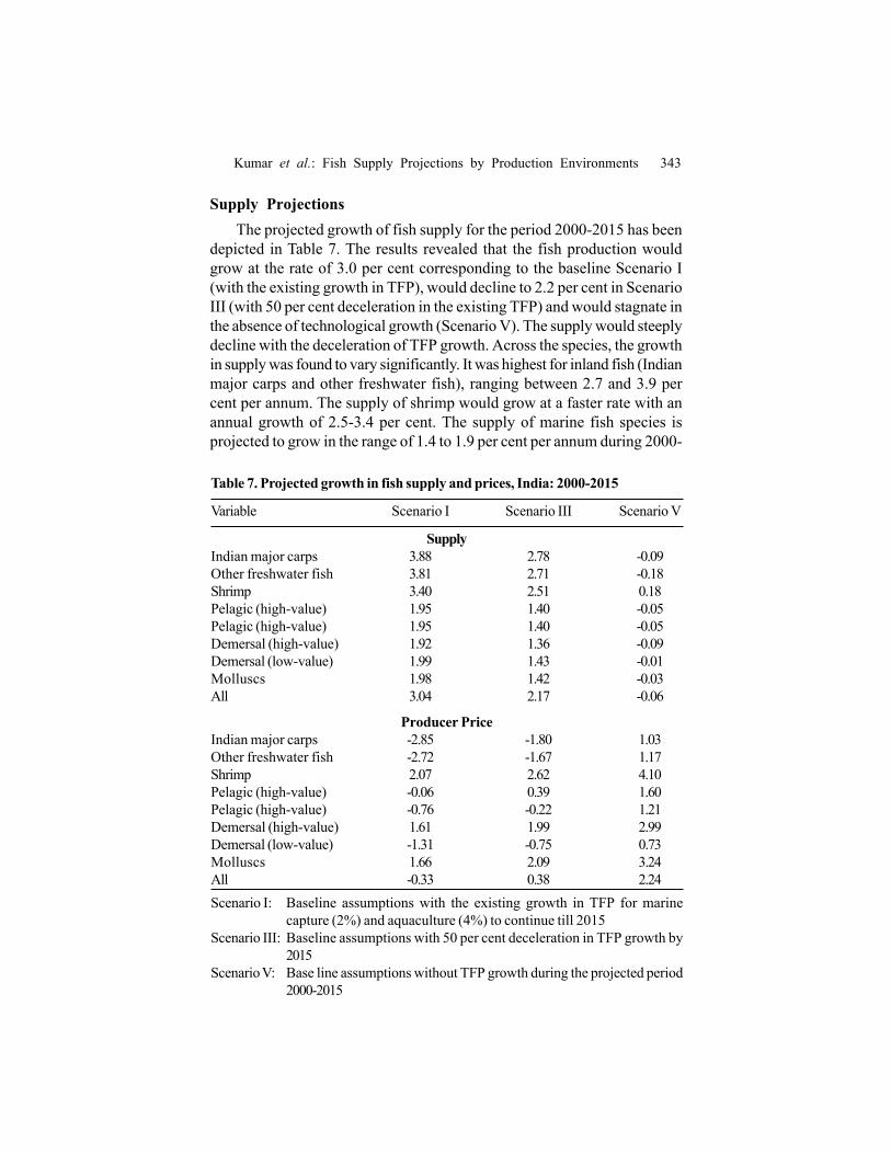
Supply Projections

The projected growth of fish supply for the period 2000-2015 has been

depicted in Table 7. The results revealed that the fish production would

grow at the rate of 3.0 per cent corresponding to the baseline Scenario I

(with the existing growth in TFP), would decline to 2.2 per cent in Scenario

III (with 50 per cent deceleration in the existing TFP) and would stagnate in

the absence of technological growth (Scenario V). The supply would steeply

decline with the deceleration of TFP growth. Across the species, the growth

in supply was found to vary significantly. It was highest for inland fish (Indian

major carps and other freshwater fish), ranging between 2.7 and 3.9 per

cent per annum. The supply of shrimp would grow at a faster rate with an

annual growth of 2.5-3.4 per cent. The supply of marine fish species is

projected to grow in the range of 1.4 to 1.9 per cent per annum during 2000-

Table 7. Projected growth in fish supply and prices, India: 2000-2015

Variable Scenario I Scenario III Scenario V

Supply

Indian major carps 3.88 2.78 -0.09

Other freshwater fish 3.81 2.71 -0.18

Shrimp 3.40 2.51 0.18

Pelagic (high-value) 1.95 1.40 -0.05

Pelagic (high-value) 1.95 1.40 -0.05

Demersal (high-value) 1.92 1.36 -0.09

Demersal (low-value) 1.99 1.43 -0.01

Molluscs 1.98 1.42 -0.03

All 3.04 2.17 -0.06

Producer Price

Indian major carps -2.85 -1.80 1.03

Other freshwater fish -2.72 -1.67 1.17

Shrimp 2.07 2.62 4.10

Pelagic (high-value) -0.06 0.39 1.60

Pelagic (high-value) -0.76 -0.22 1.21

Demersal (high-value) 1.61 1.99 2.99

Demersal (low-value) -1.31 -0.75 0.73

Molluscs 1.66 2.09 3.24

All -0.33 0.38 2.24

Scenario I: Baseline assumptions with the existing growth in TFP for marine


Scenario III: Baseline assumptions with 50 per cent deceleration in TFP growth by

2015

Scenario V: Base line assumptions without TFP growth during the projected period

2000-2015


2015, except for the shrimp. The Scenario V revealed that the fish production

would stagnate if the technological growth does not take place in future. To

maintain the supply at the desired level, concerted efforts need to be put for

improving the efficiency of fish production and catches, and enhancement

of the growth in TFP through appropriate policies for research, extension,

and development.

The rise in fish supply would not affect a decline in the price of shrimp.

It is true for the export-oriented species. The prices of IMC and OFW are

expected to decline in the projected period at the rate of 1.7 to 2.8 per cent

per annum. Among the low-value marine species of fish, price would decline

less than 0.76 per cent per annum for PLV and 0.75-1.31 per cent for DLV.

The price of export-oriented fish species would continue to rise in spite of

the increasing supply of fish. The higher growth in fish supply for the species

used in the domestic market would benefit the common man, as this fish

species would be available at cheaper prices in future. In the fish species

which are export-oriented, the rise in supply would not cut down the price in

the domestic market substantially, and the price would keep rising and would

benefit the producer. The price of shrimp, the most potential export fish,

would rise from 2.1 per cent to 2.6 per cent annually. Other exportable fish

species would be: PHV, DHV and molluscs; for these also, the price would

rise from 1.6 per cent to 2 per cent.

Under the baseline scenario, with the increase of fish supply (as projected

in various scenarios), producers’ prices in the domestic market would decline

at an annual rate of 2.9 per cent for IMC, 2.7 per cent for OFW, 1.3 per

cent for DLV, and 0.8 per cent for PLV. These species are meant mostly

for the domestic market. Shrimp, PHV, DHV and molluscs (high-value) are

the potential exportable species. A part of their output would be retained for

domestic consumption also. Their prices in the domestic market are unlikely

to decline even after the increase in their supply; rather their prices are

likely to increase by 2.1 per cent for shrimp, 1.6 per cent for DHV and 1.7

per cent for molluscs. The prices of PHV group are likely to remain

unchanged. Exports would help the producers to stabilize fish prices in the

domestic market (at the aggregate level). Taking all the species together,

the price of fish would move within a very narrow band with the annual

growth ranging from –0.3 per cent to 0.4 per cent at constant price.

Based on the projected growth rate, the supply of fish has been estimated

under various scenarios using TE 1998 as the base year (Table 8). Scenarios

I, II, and III are the most likely scenarios that would prevail in future; these

have assumed that the maximum decline in the TFP growth of fish production


would be 50 per cent by the year 2015. Under the most optimistic Scenario

I, the production of fish8 would be 9.04 million tonnes by the year 2015.

Considering the other scenarios, the fish production has been projected to

be 8.4 million tonnes in Scenario II; 7.8 million tonnes in Scenario III; and

7.1 million tonnes under Scenario IV. For the scenario without TFP growth,

the production would be stagnant almost at the current level.

A perusal of Figures 3a and 3b revealed the annual production of inland

fish in the year 2005 to be in the range of 3.6 - 3.7 million tonnes, which

would reach 4.6-5.5 million tonnes by 2015, with an annual growth rate of

2.9 - 4.0 per cent under different scenarios. The share of inland fish in the

total fish production, which was about 50 per cent in the year 2000, would

increase to 61 per cent by 2015. The production of marine fish, which has

been 2.9 - 3.0 million tonnes in 2005, will grow to 3.2 - 3.6 million tonnes by

Table 8. Projected supply, import and production of fish in India:2005-2015

(million kg)

Year Scenario I Scenario II Scenario III Scenario IV Scenario V

Supply

1998(base) 5481.6 5481.6 5481.6 5481.6 5481.6

2005 6741.8 6669.0 6576.3 6441.2 5460.1

2010 7833.7 7575.0 7275.5 6893.9 5445.0

2015 9119.4 8519.5 7894.1 7199.4 5430.1

Import

1998(base) 70.7 70.7 70.7 70.7 70.7

2005 75.6 75.4 75.1 74.7 71.6

2010 79.3 78.7 77.9 76.8 72.3

2015 83.3 81.9 80.3 78.5 73.0

Production

1998(base) 5410.9 5410.9 5410.9 5410.9 5410.9

2005 6666.3 6593.6 6501.2 6366.5 5388.5

2010 7754.4 7496.3 7197.6 6817.1 5372.7

2015 9036.1 8437.6 7813.8 7121.0 5357.1



Scenario II: Baseline assumptions with 25 % deceleration in TFP growth by 2015

Scenario III: Baseline assumptions with 50 % deceleration in TFP growth by 2015

Scenario IV: Baseline assumptions with 75 % deceleration in TFP growth by 2015

Scenario V: Base line assumptions without TFP growth during the projected period,

2000-2015

8 The production projection has been arrived at after subtracting the projected

import from the supply projection.


2015. The fish production is likely to grow at the annual rate of 2.9 - 4.0 per

cent for inland fish and 1.2 - 1.8 per cent for marine fishes. The share of

marine fish in the total fish production would decline from 50 per cent in the

year 2000 to about 40 per cent by 2015.

The supply of IMC, which contributed 25 per cent to the total supply,

has been projected to be 1.79 -1.85 million tonnes by 2005, 2.04 - 2.24

million tonnes by 2010 and 2.26-2.71 million tonnes by 2015 (Table 9). The

supply of other fish categories by 2015 has been projected as 1.6 - 1.8

million tonnes for pelagic fish, 0.7 - 0.8 million tonnes for demersal fish, and

0.6 - 0.7 million tonnes for molluscs, etc. The changes in the share of different

species in total production during the period 2000 - 2015 have revealed that

the share of IMC in the total fish production would increase to 30 per cent

by 2015 from 25 per cent in 2000 and of OFW to 22 per cent from 19 per

cent. The share of shrimp, however, is likely to remain almost unchanged.

The shares of pelagic, demersal, and molluscs have been projected to decline

during this period.

By the year 2015, the incremental production has been projected to be

3.3 million tonnes. In this additional production, IMC would contribute

maximum (36%), followed by OFW (26%), pelagic (14%), shrimp (13%),

demersal (6%), and molluscs (5%).

A comparison of Scenarios I and V provides the effect of TFP growth

on fish supply (Table 9). The production of fish would decline substantially

with deceleration in the fish technological growth. The contribution of TFP

to total fish production has been projected as 2.4 million tonnes by 2010 and

3.7 million tonnes by 2015 (41%). The contribution of TFP has been projected

to be the highest (48%) in the inland fish sector by 2015. The technological

change (measured in terms of TFP) would contribute about 29 per cent to

the total marine fish production, except shrimp, by 2015. In the case of

shrimp, it would be about 20 per cent by 2005 and 42 per cent by 2015.

Conclusions

The study has concluded that the TFP growth for the fish sector has

been higher (2-4 %) even to that in the crop and livestock sectors (< 2%,

see Rosegrant and Evenson, 1992; Dholakia and Dholakia, 1993; Kumar et

al., 1998; Kumar et al., 2005). Price response to fish supply has been stronger

for aquaculture than marine fisheries. Price instruments along with

technological policy would be the dominating factors to increase the fish

supply, especially for aquaculture. The changes in relative prices of fish

species would change the supply-mix consisting of various species. Fish

supply would be 4.6-5.5 million tonnes under the inland sector and 3.2-3.6


Table 9. Projected production of fish by species and TFP contribution, India: 2005-

2015

Year Production (million kg) TFP contribution

Scenario I Scenario III Scenario V Quantity Per cent

(million kg)

Indian major carp

2005 1851.7 1793.6 1409.2 442.5 23.9

2010 2240.2 2039.7 1402.7 837.5 37.4

2015 2710.3 2260.9 1396.2 1314.0 48.5

Other freshwater fish

2005 1360.6 1317.8 1034.3 326.3 24.0

2010 1640.3 1493.0 1025.1 615.2 37.5

2015 1977.5 1648.4 1016.0 961.5 48.6

Shrimp (marine and freshwater)

2005 808.2 787.6 647.8 160.4 19.8

2010 955.2 885.1 653.7 301.4 31.6

2015 1128.8 974.3 659.7 469.1 41.6

Pelagic (high-value)

2005 428.4 421.5 372.9 55.5 13.0

2010 471.9 449.8 372.0 99.9 21.2

2015 519.9 473.8 371.1 148.7 28.6

Pelagic (low-value)

2005 1066.5 1049.3 928.4 138.0 12.9

2010 1174.8 1119.8 926.3 248.5 21.1

2015 1294.0 1179.7 924.2 369.9 28.6

Demersal (high-value)

2005 419.9 413.1 365.4 54.5 13.0

2010 461.7 440.1 363.8 97.9 21.2

2015 507.7 462.7 362.3 145.4 28.6

Demersal (low-value)

2005 248.2 244.2 216.0 32.1 12.9

2010 273.8 261.0 215.9 57.9 21.2

2015 302.1 275.4 215.8 86.4 28.6

Molluscs and others

2005 558.4 549.4 486.0 72.4 13.0

2010 615.8 587.0 485.4 130.4 21.2

2015 679.1 619.0 484.8 194.3 28.6

All fish categories

2005 6666.3 6501.2 5388.5 1277.8 19.2

2010 7754.4 7197.6 5372.7 2381.7 30.7

2015 9036.1 7813.8 5357.1 3679 40.7



Scenario III: Baseline assumptions with 50 % deceleration in TFP growth by 2015

Scenario V: Base line assumptions without TFP growth during the projected period,

2000-2015


million tonnes under the marine sector by the year 2015. Indian major carps

would be the major player in aquaculture supply. The contribution of

technology in fish supply has been estimated to be 48 per cent and 29 per

cent, respectively for the inland and marine sectors by 2015. Social welfare

has been anticipated for both producers and consumers. The technological

development in fisheries would make the fish available at cheaper prices

and would improve household nutritional-security.

The study has suggested that aquaculture should be given priority in the

national fisheries strategies. Fish production is technology-driven and largely

dependent on national strategies towards prioritization of fish technologies

to benefit the poor households. Constraints to its growth lay beginning from

input supply, down to post-harvest services, processing, and marketing, in

addition to dissemination of technology. On input side, the major constrains

outlined are unavailability of quality fish seed, and lack of access to credit.

Both need to be addressed by hatchery and quality brood stock policy as

well as credit institutions. On the post-harvest and processing side, need

has been projected to invest in landing and development of post-harvest

facilities, training of fishers and processors towards better quality and global

food safety standards and market access. Strengthening of community-

based institutions for managing common areas, as well as investments in

appropriate stock enhancement and enrichment systems, are the promising

means for increasing supply under marine environment and providing benefits

to the poor fishermen.

References

Chavas, J.P. and T.L. Cox, (1988) A nonparametric analysis of agricultural technology.

American Journal of Agricultural Economics, 70: 303-310.

Christensen, L.R., (1975) Concepts and measurement of agricultural productivity.

American Journal of Agricultural Economics, 57:910-15.

Cox, T.L. and J.P. Chavas, (1990) A nonparametric analysis of agricultural technology:

The case of U.S. agriculture, European Review of Agricultural Economics, 17:

449-464.

Dey, M. M., R. Briones and M. Ahmed, (2005) Disaggregated analysis for fish

supply, demand and trade in Asia: Baseline model and estimation strategy.

Aquaculture Economics & Management, 9(1&2): 113-139.

Dholakia, R.H. and B.H. Dholakia, (1993) Growth of total factor productivity in

Indian agriculture. Indian Economic Review, 28(1): 25-40.

Diewert, W.E., (1976) Exact and superlative index numbers. Journal of Econometrics,

4: 115-145.


Diewert, W.E., (1978) Superlative index numbers and consistency in aggregation.

Econometrica, 46: 883-900.

FAO (2005) FishStat+ v.2.3. [Online]: http://www.fao.org/fi/statist/Fisoft/FishPlus

[August].

Griliches, Z., (1964) Research expenditures, education and the aggregate agricultural

production function. American Economic Review, 54: 961-974.

Hotelling, H., (1932) Edgeworth’s taxation paradox and the nature of demand and

supply functions. Journal of Political Economy, 40: 577-616.

Kumar, A., D. Jha and U.K. Pandey, (2005) Total factor productivity of the livestock

sector in India. In: Impact of Agricultural Research: Post-Green Revolution

Evidence from India, Eds: P.K. Joshi, S., Pal, P.S. Birthal and M.C.S. Bantilan,

pp. 205-216. New Delhi, India: Naional Centre for Agricultural Economics and

Policy Research and Patancheru, Andhra Pradesh, India: International Crops

Research Institute for the Semi-Arid Tropics.

Kumar, P., P. K. Joshi, C. Johansen and M. Asokan (1998) Sustainability of rice-

wheat based cropping system in India. Economic and Political Weekly,33: A-

152 to A-158.

Kumar, P., (2001) Agricultural performance and productivity. In: Indian Agricultural

Policy at the Crossroads, Eds: S.S. Acharya and D.P. Chaudhri, New Delhi,

India: Rawat Publications.

Kumar, P., A. Kumar and S. Mittal, (2004) Total factor productivity of crop sector in

the Indo-Gangetic Plain of India: Sustainability issues revisited. Indian

Economic Review, 39(1): 169-201.

Rosegrant, M.W. and R.E. Evenson, (1992) Agricultural productivity and sources

of growth in South Asia. American Journal of Agricultural Economics, 74:757-

61.

Schultz, T.W., (1953) Economic Organization of Agriculture, New York, USA:

McGraw-Hill Co.

Solow, R.M., (1957) Technical change and aggregate production function. Review

of Economics and Statistics, 39(3): 312-320.

Wall, C.A. and B.S. Fisher, (1988) Modeling a Multiple Output Production System:

Supply Response in the Australian Sheep Industry. Research Report No. 11,

Department of Agricultural Economics, University of Sydney, Australia.


Appendix A

Definition of variables

PIMC : Price of Indian major carp (Rs/kg)

POFW : Price of other fresh water fish (Rs/kg)

PPrawn : Price of prawn (Rs/kg)

Wage1 : Wages for labour working in aquaculture (Rs/day)

pfeed : Price of feed (Rs/kg of crude protein )

pfert : Price of fertilizer (Rs /kg of nutrients)

Zarea : Area under aquaculture in ha

PPHV : Price of pelagic (high-value) (Rs/kg )

PPLV : Price of pelagic (low-value) (Rs/kg)

PDHV : Price of demersal (high-value) (Rs/kg )

PDLV : Price of demersal (low-value) (Rs/kg)

PShrimp : Price of shrimp (Rs/kg)

PMolluscs : Price of molluscs (Rs/kg)

pFuel : Price of diesel (Rs/litre)

Wage 2 : Wages for labour working in marine (Rs/day)

ZCoast : Coastal length in kilometres by state

qIMC : Production of IMC (million kg)

qOFW : Production of OFW (million kg)

qPrawn : Production of prawn (million kg)

qPHV : Production of PHV (million kg)

qPLV : Production of PLV (million kg)

qDHV : Production of DHV (million kg)

qDLV : Production of DLV (million kg)

qShrimp : Production of shrimp ( million kg )

qMolluscs : Production of molluscs (million kg)

Fish inputs are defined as

qLabour1 : Labour input in million person-days used in aquaculture farming

qfeed : Feed input in terms of crude protein in million kg

qfert : Fertilizer input in terms of nitrogen in million kg

qLabour2 : Labour input in million person-days used in aquaculture farming

qFuel : Diesel used in marine catch in million litres

Zcoast : Coastal length in kilometres


Appendix Table 1

Fish species groups and fish species composition in India

Species group Short/ Major species

Variable

name

Freshwater fish (aquaculture)

(1) Indian major carps IMC Rohu, catla, mirgal, calbasu

(2) Other freshwater fish OFW Silver carp, grass carp, common carp,

murrels, hilsa (inland) and other

unspecified inland fish

(3) Prawn/Shrimp FS Penaeid shrimp

Marine fish (capture)

(4) Pelagic (high-value) PHV Seerfish, oceanic tunas (yellowfin tuna,

skipjack tuna), large carangids (Caranx

sp.), pomfrets, pelagic sharks, mullets

(5) Pelagic (low-value) PLV Sardines, mackerel, anchovies,

bombayduck, coastal tunas, scads, horse

mackerel, barracudas

(6) Demersal (high-value) DHV Rock cods, snappers, lethrinids, big-jawed

jumper (Lactarius), threadfins

(polynemids)

(7) Demersal (low-value) DLV Rays, silverbellies, lizard fish, catfish, goat

fish, nemipterids, soles

(8) Crustaceans MS Shrimps, lobsters

(9) Molluscs and others Molluscs Cephalopods (squids, cuttlefishes and

octopus), mussels, oysters, non-penaeid

prawns

Fish Supply Projections by Production Environments and ...

Documents

Transcript of Fish Supply Projections by Production Environments and ...