THE DIMENSION OF PROJECTIONS OF SELF-AFFINE SETS ...

Annales Academiæ Scientiarum FennicæMathematicaVolumen 42, 2017, 473–486

THE DIMENSION OF PROJECTIONS OFSELF-AFFINE SETS AND MEASURES

Kenneth Falconer and Tom Kempton

University of St Andrews, Mathematical InstituteNorth Haugh, St Andrews, Fife, KY16 9SS, Scotland; [email protected]

University of St Andrews, Mathematical InstituteNorth Haugh, St Andrews, Fife, KY16 9SS, Scotland; [email protected]

Abstract. Let E be a plane self-affine set defined by affine transformations with linear partsgiven by matrices with positive entries. We show that if µ is a Bernoulli measure on E withdimH µ = dimL µ, where dimH and dimL denote Hausdorff and Lyapunov dimensions, then theprojection of µ in all but at most one direction has Hausdorff dimensionmin{dimH µ, 1}. We transferthis result to sets and show that many self-affine sets have projections of dimension min{dimH E, 1}in all but at most one direction.

1. Introduction

Marstrand’s projection theorem states that, given a set E ⊂ Rn, for almost everym-dimensional linear subspace K of Rm

(1.1) dimH πKE = min{dimH E,m},where πK denotes orthogonal projection onto K and dimH denotes Hausdorff dimen-sion, see [6, 17, 18]. The analogous projection theorem for measures, generally provedusing potential theoretic methods, see [16], is that for a finite Borel measure µ onRn,(1.2) dimH πKµ = min{dimH µ,m},for almost all subspaces K, where the (lower) Hausdorff dimension of a probabilitymeasure is given in terms of dimensions of sets by

dimH ν = inf{dimH U : ν(U) = 1}.However, these projection theorems are no help in identifying the subspaces K, ifany, for which (1.1) or (1.2) fail. Recently there has been a great deal of interest infinding the ‘exceptional directions’ for projections of fractals and fractal measures ofvarious types, especially those with a recursive structure or which are dynamicallygenerated, see the survey [7] and references therein. In particular, various classes ofmeasures and sets have been shown to have every projection satisfying (1.1). Forexample, for self-similar sets satisfying the open set condition, (1.1) holds for allsubspaces K provided that the group generated by the orthonormal components ofthe defining similarities is dense in the orthogonal group O(n), with similar resultsfor measures, see [8, 19, 13]. On the other hand, if the group is not dense then thereare always some exceptional directions, see [10].

It is natural to ask under what circumstances (1.1) holds for self-affine sets and(1.2) for self-affine measures (by which we mean Bernoulli measures on self-affine

https://doi.org/10.5186/aasfm.2017.42322010 Mathematics Subject Classification: Primary 28A30.Key words: Dimension, projection, self-affine set, Furstenberg measure, r-scale entropy.This research was supported by EPSRC grant EP/K029061/1.

474 Kenneth Falconer and Tom Kempton

sets) in all or virtually all directions. Dimensional analysis in the self-affine case ismore awkward than in the self-similar case, not least because the dimensions of thesets or measures themselves are not continuous in the defining affine transformations.Nevertheless, the dimensions of many specific self-affine sets and also of generic self-affine sets in certain families are now known. In particular, the Hausdorff dimensiondimH E of a self-affine set E ‘often’ equals its affinity dimension dimAE, defined in(2.2)–(2.3) below, see [5].

Much of the work to date on projections of self-affine sets concerns projectionsof plane self-affine carpets, that is where the defining affine maps preserve bothhorizontal and vertical axes; see [1, 11] for various examples. Perhaps not surprisingly,for many carpets (1.1) fails only for projections in the horizontal and/or verticaldirections.

In this paper we consider projections of plane self-affine sets and measures wherethe linear parts of the self-affine maps may be represented by matrices with all entriespositive, in other words where the linear parts map the positive quadrant strictly intoitself. We show that in many cases projections onto lines in all directions (in somecases all but one direction) satisfy (1.1) or (1.2). Many self-affine sets and measuresfit into this context, both in the ‘generic setting’ (provided that the affine mapsare sufficiently contracting), see [4, 22], and for many specific cases including thosepresented in [2, 9, 12].

To study projections of a set one normally examines the projections of a suitablemeasure on the set. Thus, we first study projections of a Bernoulli measure µ sup-ported by a self-affine set E. Then µ induces a measure µF , known as a Furstenbergmeasure, on the space of line directions. Recent results on the dynamical structureof self-affine sets [2, 9] imply that the projections of µ are exact dimensional in µF -almost all directions. Together with lower bounds for the dimension of projectionsfrom [13] involving r-scale entropies we conclude that the dimensions of projectionsof measures are well-behaved in all but perhaps one direction. The results on pro-jections of self-affine sets follow by supporting suitable Bernoulli measures on E.

2. Preliminaries

In this section we introduce the self-affine sets that we consider along with per-tinent notation. Let A1, · · · , Ak be a collection of 2× 2 matrices of Euclidean normless than 1 with strictly positive entries, and let d1, · · · , dk ∈ R2. Then the mapsTi : R

2 → R2 (i = 1, · · · , k) given by

(2.1) Ti(x) = Ai(x) + di (x ∈ R2)

are affine contractions which form an iterated function system (IFS). By standardIFS theory, see [6, 14] there exists a unique non-empty compact set E satisfying

E =k⋃i=1

Ti(E),

termed a self-affine set.There is a natural coding on E and its usual iterated construction. Let Λ :=

{1, · · · , k}, let Σ∗ =⋃∞n=0 Λn be the space of finite words formed by elements of Λ,

and let Σ = ΛN be the corresponding space of infinite words. Associated with eacha1 · · · an ∈ Σ∗ is the cylinder

[a1 · · · an] = {a1 · · · anbn+1bn+2, · · · : bi ∈ Λ} ⊂ Σ;

The dimension of projections of self-affine sets and measures 475

the cylinders form a basis of open and closed sets for the natural topology on Σ.We abbreviate compositions of the Ti by Ta1···an := Ta1◦· · ·◦Tan for a1 · · · an ∈ Σ∗.

Let D ⊂ R2 be the unit disk so that

Da1···an := Ta1···an(D)

are the ellipses obtained as images of D under compositions of the Ti. By scalingwe may assume that Ti(D) ⊂ D for all i, in which case the self-affine set E may bewritten as

E =∞⋂n=0

⋃a1···an

Ta1···an(D).

Let PR1 = (R2 \ 0)/ ∼ be 1-dimensional real projective space where ∼ identifiespoints on each line through the origin. We may parameterise PR1 by the anglebetween lines and the horizontal axis, and these angles define a metric d on PR1

in the obvious way. Each matrix A−1i induces a projective linear transformation

φi : PR1 → PR1 given by φi := A−1i / ∼, that is, A−1

i maps straight lines at angleθ to straight lines at angle φi(θ). Since the matrices Ai are strictly positive, eachφi restricted to the negative quadrant Q2 is a contraction so that the system ofcontractions (φi)

ki=1 is an iterated function system on Q2. Let F be the attractor of

this IFS, that is the non-empty compact subset of Q2 such that F =⋃ki=1 Ti(F ).

Now let µ be a Bernoulli probability measure on Σ; for notational conveniencewe also write µ for the corresponding measure on E, that is its image under themap (a1a2 · · · ) 7→

⋂∞n=0 Ta1···an(D). The Furstenberg measure µF is defined to be the

stationary probability measure supported by K ⊂ RP1 associated to the maps φichosen according to the measure µ, see for example, [3]. Specifically,

µF (U) =k∑i=1

µ[i]µF (φ−1i (U)),

for all Borel sets U . The Furstenberg measure is central to the proofs of our results.Ideally we would like to be able to express the Hausdorff dimension of a self-

affine set E in terms of its defining IFS maps (2.1), as can be done for self-similarsets subject to a separation condition. (For the definition and basic properties ofHausdorff dimension, which we denote by dimH , see for example [6, 18].) A naturalcandidate for dimH E is the affinity dimension defined in [4] in terms of the linearparts of the IFS maps. Let α1(A) ≥ α2(A) ≥ 0 be the singular values of a linearmapping or matrix A on R2, that is the lengths of the major and minor semiaxes ofthe ellipse A(D) or equivalently the positive square roots of the eigenvalues of AAT .For 0 ≤ s ≤ 2 we define the singular value function of A by

φs(A) =

αs1, 0 < s ≤ 1,

α1αs−12 , 1 ≤ s ≤ 2,

(detA)s/2, 2 ≤ s.

The submultiplicativity of the singular value functions enables us to define the affinitydimension of a set E ⊂ R2 defined by the IFS (2.1) by

(2.2) dimA(A1, · · · , Ak) ≡ dimAE =

s : limn→∞

( ∑a1···an∈Λn

φs(Aa1···an)

)1/n

= 1


or equivalently

(2.3) dimA(A1, · · · , Ak) ≡ dimAE = inf

{s :

∞∑n=1

∑a1···an∈Λn

φs(Aa1···an) <∞

}.

Note that the affinity dimension depends on the {Ai} that occur in the iteratedfunction system that defines E, rather than on E itself, but referring to dimAEgenerally causes little problem. For every self-affine set E it is the case that dimH E ≤dimAE, but equality holds in many cases, both generic and specific, see the survey[5] and recent examples in [2, 9].

We will also refer to Lyapunov dimension, which reflects the geometry of theself-affine set E relative to the measure µ. The Lyapunov exponents λ1(µ), λ2(µ) areconstants such that, for µ-almost every a1a2 · · · ∈ Σ,

(2.4) limn→∞

1

nlogαi(a1 · · · an) = λi (i = 1, 2).

The Lyapunov dimension of µ is given by

(2.5) dimL µ :=

hσ(µ)

−λ1(µ), hσ(µ) ≤ −λ1(µ),

1 +hσ(µ) + λ1(µ)

−λ2(µ), hσ(µ) ≥ −λ1(µ),

where hσ(µ) is the Kolmogorov–Sinai entropy of the system (Σ, σ, µ) with σ the leftshift on Σ. Note that dimL µ depends only on the matrices {A1, · · · , Ak} and themeasure µ. It is always the case that dimH µ ≤ dimL µ, see [15].

To obtain our dimension estimates, we will use r-scale entropies, given by

Hr(ν) := −ˆ

[−1,1]

log ν(Br(x)) dν(x),

where ν is a probability measure on [−1, 1] and r > 0. A measure ν is termed exactdimensional of dimension β if

(2.6) limr→0

log ν(Br(x))

log r= β

for ν-almost all x. In particular, if ν is exact dimensional, then

(2.7) dimH ν = β = limr→0

Hr(ν)

− log r.

3. Statement of results

We define B ⊂ PR1 by B = PR1 \ {θ0} if all matrices Ai have a commonmaximal eigenvector in some direction θ0, and by B = PR1 otherwise. The setPR1 \B consists of at most one angle and represents the set of possible exceptionaldirections for our projection theorems.

It was proved in [2, Proposition 3.3] that there exists a constant β(µ) such that forµF -almost every θ the projected measure πθ(µ) is exact dimensional with dimensionβ(µ). This allows us to state our main theorem.

Theorem 3.1. Let µ be a Bernoulli measure on a planar self-affine set definedby an IFS (2.1) with strictly positive matrices Ai. Then for all θ ∈ B

dimH πθ(µ) ≥ β(µ).

This yields the following corollaries.


Corollary 3.2. Let µ be a Bernoulli measure on a planar self-affine set associatedto strictly positive matrices Ai. Suppose dimH µ = dimL µ. Then for all θ ∈ B,

dimH πθ(µ) = min{dimH µ, 1}.Proof. If we can show that

(3.1) dimH µ = dimL µ =⇒ β(µ) = min{dimH µ, 1}.

the conclusion follows directly from Theorem 3.1. Under the additional assumptionthat the self-affine set satisfies the strong separation condition, (3.1) along with theconverse implication was established in [9]. However, the strong separation condi-tion is not required for the implication (3.1). This is because the left hand side ofinequality (4.2) of [9, Lemma 4.2] holds even without strong separation. �

Theorem 3.1 can be applied to the projection of self-affine sets. The next corollaryshows that if the set supports Bernoulli measures with dimensions approximating theaffinity dimension there is no dimension drop for projections of E except possibly inone direction.

Corollary 3.3. Let E be a planar self-affine set defined by an IFS (2.1) withstrictly positive matrices Ai. If there exists a sequence (µn) of Bernoulli measuressupported on E with dimH µn → dimAE then, for all θ ∈ B,

(3.2) dimH πθ(E) = min{dimH E, 1}.Proof. Let µn,F denote the Furstenberg measure associated to µn, and let βn

denote the value of dimH πθ(µn) that occurs for µn,F -almost every θ by [2, Proposi-tion 3.3]. Then Theorem 3.1 implies that for all θ ∈ B,

dimH πθ(E) ≥ limn→∞

βn = min{dimAE, 1},

this last equality holding because dimH µn → dimAE and using [2, Theorem 2.7].Since for all θ

min{dimAE, 1} ≥ min{dimH E, 1} ≥ dimH πθ(E),

(3.2) follows. �

It would be nice to replace the condition in Corollary 3.3 on the existence of thesequence of Bernoulli measures by the requirement that dimAE = dimH E. Howeverthe relationship between the statements ‘dimAE = dimH E’, ‘E supports an ergodicmeasure µ with dimH µ = dimAE’ and ‘there exists a sequence (µn) of Bernoullimeasures supported on E with dimµn → dimAE’ is not clear. All three statementshold for almost all sets of translation vectors (d1 · · · dk) whenever each Ai has ||Ai|| <12, but the relationship between the statements is difficult to understand.

Note that our results require the matrices Ai to have positive entries, so thatthe matrices all map the first quadrant into its interior. This assumption is used invarious ways and shortens some of the proofs, but it is crucial in Bárány’s proof [2,Proposition 3.3] that projections of self-affine measures are exact dimensional, whichin turn is used in the proof of Theorem 4.6 on averages of r-scale entropies.

3.1. Examples. There are many families of measures on self-affine sets forwhich dimH µ = dimL µ and hence for which our main theorem holds. In particular,this includes classes of examples presented in Hueter and Lalley [12], Bárány [2] andFalconer and Kempton [9]. The corollary below shows that this situation also arisesfor almost all sets of translations in the affine maps in the IFS that defines E.


Corollary 3.4. Let {Ti}ki=1 be an affine IFS (2.1) where the matrices Ai arestrictly positive with ‖Ai‖ < 1

2for all i. For each translation vector d = (d1, · · · , dk) ∈

R2k let Ed be the self-affine attractor thus defined. Then for almost all d ∈ R2k (inthe sense of 2k-dimensional Lebesgue measure)

dimH πθ(Ed) = min{dimH Ed, 1} = min{dimAEd, 1}

for all θ ∈ B simultaneously (where as before B is either PR1 or is PR1 with oneangle omitted).

Proof. The right-hand equality follows since dimH Ed = min{dimAEd, 2} foralmost all d, see [4, 22]. For the left-hand equality we will show that for all ε > 0we can find a Bernoulli measure µ on Σ that induces measures µd on the Ed withdimH µd > dimH Ed − ε for almost all d, so that the conclusion will follow fromCorollary 3.3.

As the Ai have strictly positive entries, there is a cone K strictly inside theupper-right quadrant that is mapped into itself by all finite compositions of the Ai.This implies, see [21, Lemma 3.1], that there is a number c ≥ 1 that depends onlyon K such that for all finite words a = a1 · · · aj, b = b1 · · · bj′ ∈ Σ∗,

‖AaAb‖ ≤ ‖Aa‖‖Ab‖ ≤ c ‖AaAb‖.

Since φs(A) = ‖A‖s (0 ≤ s ≤ 1) and φs(A) = ‖A‖2−s(detA)s−1 (1 ≤ s ≤ 2), itfollows that

(3.3) φs(AaAb) ≤ φs(Aa)φs(Ab) ≤ c φs(AaAb).

for all s ≥ 0.Write dA := dimA(A1, · · · , Ak) ≡ dimAEd for the affinity dimension. We may

assume that 0 < dA ≤ 2 (if dA > 2 then Ed has positive plane Lebesgue measurefor almost all d and the result is clear). Let 0 < t < dA (t not an integer). Using asimple estimate of the rate of decrease of φs(Aa) with s, see [4], we may choose anN ∈ N sufficiently large to ensure that for some 0 < λ < 1

(3.4) cφdA(Aa)

φt(Aa)< λ for all a = a1 · · · aN ∈ ΛN .

From the definition of dA (2.2) and submultiplicative properties,

infn∈N

∑|a|=n

φdA(Aa)

1/n

= 1,

so we may choose s ≥ dA such that

(3.5)∑a∈ΛN

φs(Aa) =

∑a∈ΛN

φs(Aa)

1/N

= 1

using the continuity of these sums in s.Let Σ∗N =

⋃∞j=0 ΛjN . We define a Bernoulli measure µ on Σ by specifying µ on

cylinders defined by words in Σ∗N :

µ([a1 · · · an]) = φs(Aa1)φs(Aa2) · · ·φ

s(Aan) (n ∈ N, ai ∈ ΛN).


By (3.5) µ defines a Borel probability measure on Σ = (ΛN)N. Using (3.3) and (3.4)

(3.6)µ([a1· · · an])

φt(Aa1···an)≤

φs(Aa1) · · ·φs(Aan)

c1−nφt(Aa1) · · ·φt(Aan)≤cn−1φdA(Aa1) · · ·φ

dA(Aan)

φt(Aa1) · · ·φt(Aan)≤ c−1λn.

We now proceed as in the proof of [4, Theorem 5.3]. We represent points of Ed

in the usual way by xd(a) =⋂∞i=0 Ta|i(D) for a ∈ Σ. We write µd for the push-down

of µ onto Ed, given by µd(F ) = µ{a : xd(a) ∈ F}. We write a ∧ b for the commoninitial word of a, b ∈ Σ. As in [4, Theorem 5.3] we may bound the energy integral ofµd integrated over some disc B ⊂ R2k byˆ

d∈B

ˆx∈Ed

ˆy∈Ed

dµd(x) dµd(y) dd

|x− y|t=

ˆd∈B

â∈Σ

ˆb∈Σ

dµ(a) dµ(b) dd

|xd(a)− xd(b)|t

≤ c1

â∈Σ

ˆb∈Σ

φt(Aa∧b)−1 dµ(a) dµ(b) ≤ c1

∑p∈Σ∗

φt(Ap)−1µ([p])2

≤ c1c2c3

∑q∈Σ∗N

φt(Aq)−1µ([q])2.

For the last inequality we have regarded each word p ∈ Σ∗ as p = qq1 · · · qj withq ∈ Σ∗N and 0 ≤ j ≤ N − 1, and used that φt(Ap)−1µ([p])2 ≤ c2φ

t(Aq)−1µ([q])2

for some c2 independent of p, since the summands increase by a bounded factor onadding each single letter to a word q. The constant c3 =

∑N−1i=0 ki is the number

of words p ∈ Σ∗ for which the summands are estimated by the summand of eachq ∈ Σ∗N . Writing c4 = c1c2c3 and using (3.6),

ˆd∈B

ˆx∈Ed

ˆy∈Ed

dµd(x) dµd(y) dd

|x− y|t≤ c4

∞∑j=0

∑q∈ΛjN

φt(Aq)−1µ([q])µ([q])

≤ c4c−1

∞∑j=0

λj∑q∈ΛjN

µ([q]) = c4c−1

∞∑j=0

λj < ∞.

We conclude that for almost all d,´x∈Ed

ý∈Ed|x− y|−t dµd(x) dµd(y) <∞ implying

that for µd-almost all x ∈ Ed there is a constant c0 such that µd(B(x, r)) ≤ c0rt for

all r > 0, so dimµd ≥ t. This is the case for all t < dA, as required. �

4. Proof of the main theorem

In this section we prove Theorem 3.1. There are two intermediate results whichhave relatively technical proofs whose main ideas are already well-understood in otherwork. Since these proofs are quite long and somewhat tangential to the thrust of ourargument, we defer them to the appendix.

We first recall a proposition from [9] on the dynamics of projections of self-affinesets. Let πθ : D → [−1, 1] denote orthogonal projection in direction θ onto thediameter of D at angle perpendicular to θ, where we identify this diameter (of length2) with the line [−1, 1].

Proposition 4.1. For each i ∈ {1, · · · , k}, θ ∈ PR1 there is a well defined linearcontraction fi,θ : [−1, 1]→ [−1, 1] given by

fi,θ = πθ ◦ Ti ◦ π−1φi(θ)

such that πθ(Ti(A)) = fi,θ(πφi(θ)(A)) for all Borel sets A ⊂ D.


This identity represents πθ(E) as a union of scaled-down copies of projections ofE in other directions.

We let Σ∗ denote the space of all finite words made by concatenating the letters{1, · · · , k}. We think of Σ∗ as a tree, letting words a1 · · · an+1 be children of theparent node a1 · · · an. Given a direction θ in which we want to project E, we definea length function | · |θ on the tree Σ∗ by declaring the length of the path from theroot to the node a1 · · · an to be

|a1 · · · an|θ = − log2

(|πθ(Da1···an)|

2

).

Since |πθ(D)| = 2, the division by 2 inside the log is necessary to ensure that thelength of the empty word is zero.

Lemma 4.2. The length function | · |θ satisfies|a1 · · · an+1|θ − |a1 · · · an|θ = |an+1|φan···a1 (θ).

Proof. Identically,

log2

(|πθ(Da1···an+1)|

2

)= log2

(|πθ(Da1···an)|

2

)+ log2

(|πθ(Da1···an+1)||πθ(Da1···an)|

).

Applying the linear map T−1a1···an to Da1···an and using Proposition 4.1,

log2

(|πθ(Da1···an+1)||πθ(Da1···an)|

)= log2

( |πφan···a1 (θ)(Dan+1)|/2|πφan···a1 (θ)(D)|/2

)= log2

( |πφan···a1 (θ)(Dan+1)|2

)since |πθ(D)|, the length of the projection of the unit disk, is equal to 2 for all θ. �

Let N ∈ N be fixed. For each a ∈ Σ, θ ∈ PR1 and j ∈ N we define nj =nj(a,N, θ) to be the natural number satisfying

(4.1) |a1 · · · anj−1|θ < Nj ≤ |a1 · · · anj |θ.We define the infinite tree ΣN = ΣN(θ) ⊂ (Σ∗)N to be the tree with nodes at levelj labeled by words a1 · · · anj , and edges between level j − 1 nodes and level j nodeslabelled by anj−1+1 · · · anj .

A word a ∈ Σ can also be regarded as an element of ΣN in which the first symbolis a1 · · · an1 , the second is an1+1 · · · an2 etc. When the distinction between Σ andΣN is important we specify which space a is in. The measure µ on Σ may also beregarded as a measure on ΣN , which we also denote by µ.

We consider the metric dN on the tree ΣN given by

dN(a, b) = 2−max{j:a1···anj=b1···bnj }.

This metric depends on θ through the definition of the sequences anj , bnj . For allsequences a, b ∈ Σ, and the corresponding sequences in ΣN ,

|πθ(a)− πθ(b)| ≤ |πθ(Da∧b)| ≤ dN(a, b)

for all N . In particular the map πθ : (ΣN , dN) 7→ [−1, 1] is Lipschitz.Let µ[a1···an] := µ|[a1···an]/µ[a1 · · · an]. We state a variant of results of Hochman

and Shmerkin [13] that we will apply to the projections.

Theorem 4.3. If

(4.2) limN→∞

lim infn→∞

1

N log 2

1

n

n∑i=1

H2−(i+1)N

(πθ(µ[a1···ani ])

)≥ C

for µ-almost every a ∈ ΣN , then dimH πθ(µ) ≥ C.


This statement is essentially contained in Theorems 4.4 and 5.4 of [13]. However,a little work is required to translate those theorems to our setting and the proof isgiven in the appendix.

The rest of the proof of Theorem 3.1 depends on studying the limits in (4.2). Let

λmax := max{|ai|θ : i ∈ {1, · · · , k}, θ ∈ PR1}.Lemma 4.4. For all a ∈ Σ, all i, N ∈ N and all θ ∈ PR1,

(4.3) H2−(i+1)N (πθ(µ[a1···ani ])) ≥ H2λmax2−N (πφani ···a1 (θ)(µ)).

Proof. Note thatπθ(µ[a1···ani ]) = S(πφani ···a1 (θ)(µ)),

where S is the map on measures on [−1, 1] induced by a linear map on [−1, 1] whichcontracts by a factor 2−|a1···an|θ . An entropy Hλ(τ) is unchanged by rescaling themeasure τ provided that we rescale the parameter λ by the same amount. From thedefinitions of λmax and nk,

|a1 · · · ani |θ ∈ [iN, iN + λmax].

Then

H2−(i+1)N (πθ(µ[a1···ani ])) = H 2−(i+1)N

2−|a1···ani |θ

(πφani ···a1 (θ)(µ)) = Hρ.2−N (πφani ···a1 (θ)(µ))

where the ‘error’ ρ is given by

ρ =2iN

2−|a1···ani |θ∈ [1, 2λmax ].

Since the entropy Hλ(µ) is monotone decreasing in λ, we obtain (4.3). �

We need to pass from equidistribution results with respect to the sequence(φan···a1(θ))

∞n=1 to corresponding results for the subsequence (φani ···a1(θ))

∞i=1.

Proposition 4.5. There exists a measure νF on PR1 which is equivalent toµF and such that for all θ ∈ B, N ∈ N and µ-almost all a ∈ Σ, the sequence(φani ···a1(θ))

∞i=1 equidistributes with respect to νF , i.e., for all intervals A ⊂ PR1 we

havelimI→∞

1

I

∣∣∣{i ∈ {1, · · · , I} : φani ···a1(θ) ∈ A}∣∣∣ = νF (A).

The proof of this proposition is relatively long but involves only standard ergodictheory so is postponed to the appendix.

We now study the sums in (4.2).

Theorem 4.6. For all θ ∈ B and µ-almost every a ∈ Σ,

(4.4) limN→∞

lim infn→∞

1

N log 2

1

n

n∑i=1

H2−(i+1)N (πθ(µ[a1···ani ])) ≥ β(µ).

Proof. By Lemma 4.4, for θ ∈ B and µ almost every a ∈ Σ,

lim infn→∞

1

N log 2

1

n

n∑i=1

H2−(i+1)N (πθ(µ[a1···ani ]))

≥ lim infn→∞

1

N log 2

1

n

n∑i=1

H2−(N−λmax)(πφani ···a1 (θ)(µ))

≥ 1

N log 2

ˆPR1

H2−(N−λmax)(πα(µ)) dνF (α).

(4.5)


where the second inequality holds because the function

α 7→ H2−N (πα(µ))

is lower semi-continuous in α and the sequence (φani ···a1(θ))∞i=1 equidistributes with

respect to νF by Proposition 4.5.For µF almost every α the measure πα(µ) is exact dimensional with dimension

β(µ), and since µF and νF are equivalent the same is true for νF almost all α. By(2.7)

(4.6) limN→∞

1

(N − λmax) log 2H2−(N−λmax)(πα(µ)) = β(µ)

for νF almost every α.Noting that limN→∞

NN−λmax = 1, we may integrate (4.6) over α to get

ˆPR1

limN→∞

1

N log 2H2−(N−λmax)(πα(µ))dνF (α) = β(µ).

Since this integrand is bounded, we may interchange the limit and integral by thedominated convergence theorem. Combining this with inequality (4.5) gives (4.4).

�

Putting together Theorems 4.3 and 4.6 we conclude that, for all θ ∈ B,

dimH πθ(µ) ≥ limN→∞

limn→∞

1

N log 2

1

n

n∑i=1

H2−(i+1)N (πθ(µ[a1···ani ])) ≥ β(µ)

which completes the proof of Theorem 3.1.

5. Appendix: Technical proofs

5.1. Proof of Theorem 4.3. We use the terms ‘tree morphism’ and ‘faithfulmap’ as defined in [13]: essentially a tree morphism is a map from one sequencespace to another which preserves the metric and the structure of cylinder sets, and afaithful map is a map (in our case from a sequence space to [−1, 1]) which does notdistort dimension too much. The interested reader can find technical definitions ofthese terms, along with many lemmas of Hochman and Shmerkin which we use butdo not write out in full, in [13].

Proof. First we define a space YN and split the projection πθ : ΣN → [−1, 1] intoa tree-morphism gN : ΣN → YN which is easier to deal with than πθ itself, and afaithful map hN : YN → [−1, 1].

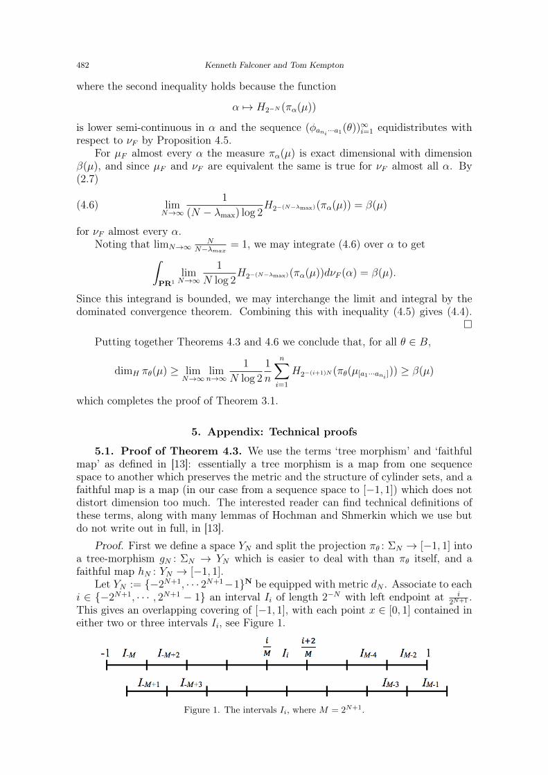
Let YN := {−2N+1, · · · 2N+1−1}N be equipped with metric dN . Associate to eachi ∈ {−2N+1, · · · , 2N+1 − 1} an interval Ii of length 2−N with left endpoint at i

2N+1 .This gives an overlapping covering of [−1, 1], with each point x ∈ [0, 1] contained ineither two or three intervals Ii, see Figure 1.

Figure 1. The intervals Ii, where M = 2N+1.


Let Si : [−1, 1] → [−1, 1] be the linear contraction mapping [−1, 1] onto Ii, andlet hN : YN → [−1, 1] be given by

hN(a) = limn→∞

Sa1 ◦ · · · ◦ San(0) (a ∈ Σ).

The map hN is 3-faithful in the sense of [13] since for each point x in each intervalhN [a1 · · · an] there are at most three values of an+1 ∈ {0, · · · , 2N+1 − 1} for whichx ∈ hN [a1 · · · an+1]. By [13, Proposition 5.2] there exists a constant C2, independentof N , such that for every measure ν on YN

(5.1) dimH ν −C2

N log 2≤ dimH hN(ν).

With the standard binary coding of [−1, 1] it is not the case that for any intervalA ⊂ [−1, 1] with |A| < 2−(j+1) one has that A is contained in some binary intervalof depth j. However, with the overlapping coding given by the intervals Ii and themap hN , it holds that for any A with |A| < 2−N(j+1) there is a choice of a1 · · · aj suchthat A ⊂ hN [a1 · · · aj]. Furthermore, these codings can be iterated in the sense thatif B ⊂ A has |B| < 2−N(j+2) then B is contained in the interval hN [a1 · · · ajbj+1] forsome choice of bj+1.

We now define a map gN : ΣN → YN which maps depth-n cylinders in ΣN todepth-n cylinders in YN . The map gN is defined iteratively. Given a depth-2 cylinder[a1 · · · an2 ] ⊂ ΣN , there exists at least one depth-1 cylinder [b1] ⊂ YN such thatπθ(Da1···an2 ) ⊂ hN([b1]), since |πθ(Da1···an2 )| < 2−N . We choose such a cylinder [b1].

Now assume we have already chosen a depth-(j − 1) cylinder [b1 · · · bj−1] corre-sponding to word a1 · · · anj . Then we may choose for each depth-(j + 1) cylinder[a1 · · · anj+1

] ⊂ [a1 · · · anj ] a letter bj such that

πθ(Da1···anj+1) ⊂ hN([b1 · · · bj]).

This process defines a tree morphism gN : ΣN → YN such that πθ : ΣN → [−1, 1] canbe written πθ = hN ◦ gN . Since hN is faithful and πθ = hN ◦ gN ,∣∣H2−(i+1)N

(πθ(µ[a1···ani ])

)−H2−(i+1)N

(gN(µ[a1···ani ])

)∣∣is bounded above by some constant which is independent of N . In particular, in-equality (4.2) holds if and only if

limN→∞

lim infn→∞

1

N log 2

1

n

n∑i=1

H2−(i+1)N (gN(µ[a1···ani ])) ≥ C.

But since gN is a tree morphism, [13, Theorem 4.4] gives

limN→∞

dimH gN(µ) ≥ C,

so setting ν = gN(µ) in (5.1),

dimH πθ(µ) ≥ C. �

5.2. Proof of Proposition 4.5. Proposition 4.5 involves transferring anequidistribution result for sequences (φan···a1(θ))

∞n=1 to a different equidistribution

result for the subsequences (φani ···a1(θ))∞i=1. To do this we first need to encode the

subsequences dynamically, which can be done by building a suspension flow basedaround the maps φi. In order to pick out the correct terms ni we introduce a notionof time for our flow based on the numbers |a1|θ. This is a standard approach inergodic theory when one is interested in looking at a system with a different notionof time than is given by just counting iterations of a map.


Secondly, we need to ask whether the time-N map associated to this suspensionflow is ergodic. There are classical results in ergodic theory which deal with thisquestion, see for example [20]. We verify that our time-N map is indeed ergodic,allowing us to conclude our equidistribution result. The fact that we need Proposi-tion 4.5 to hold for all θ ∈ Q2, and not just almost all θ, also requires us to provesome extra continuity results on the roof function of our flow.

We begin by defining a map T : Σ×PR1 → Σ×PR1 by

T (a, θ) = (σ(a), φa1(θ)).

We can map the two-sided full shift Σ± onto Σ×PR1 by mapping two-sided sequencea± to (a1a2a3 · · · , limn→∞ φa0···a−n(0)). Then T is a factor of the right shift σ−1 underthis factor map, and the two-sided extension µ of µ is mapped to µ×µF . Since factorsof mixing dynamical systems are mixing, the system (Σ×PR1, µ×µF , T ) is mixing,see [23] for a proof of this and other basic statements in ergodic theory.

The map T helps us understand the sequence (φani ···a1(θ))∞i=1, but we need to

know about the sequence ni = ni(a, θ,N). For this we build a suspension flow overT by introducing a notion of time. Consider the space

W := {(a, θ, t) ∈ Σ×PR1 ×R : 0 ≤ t ≤ |a1|θ}where the points (a, θ, |a1|θ) and (σ(a), φa1(θ), 0) are identified. Define a suspensionsemiflow ψ on W by letting

ψs(a, θ, t) = (a, θ, t+ s)

for 0 ≤ t+s ≤ |a1|θ, and extending this to a well-defined semiflow for all s > 0, usingthe identification (a, θ, |a1|θ) = (σ(a), φa1(θ), 0). This flow preserves the measure(µ × µF × L)|W , where L is Lebesgue measure. Since suspension semiflows overergodic maps are ergodic, ψs is ergodic.

We now prove some uniform continuity lemmas involving θ, θ′ ∈ Q2, which alsogive non-uniform continuity for θ, θ′ ∈ B, since all θ ∈ B are eventually mapped intoQ2 by compositions of the φi. We first show that small variations of θ have littleeffect on the time taken to flow through the base a given number of times.

Lemma 5.1. There exists a constant C such that for all θ, θ′ ∈ Q2, n ∈ N anda ∈ Σ, ∣∣|a1 · · · an|θ − |a1 · · · an|θ′

∣∣ < C|θ − θ′|.Proof. For each i ∈ {1, · · · , k}, the map θ 7→ |ai|θ is differentiable with derivative

bounded above by 2, since sin and cos have derivatives bounded by 1. Furthermore,there exists a constant 0 < ρ < 1 such that the maps φi restricted to Q2 are strictcontractions with derivative bounded above by ρ. Then∣∣|a1 · · · an|θ − |a1 · · · an|θ′

∣∣ ≤ n∑i=1

∣∣|ai|φan−1···a1 (θ) − |ai|φan−1···a1 (θ′)

∣∣≤(2 max

i,θ′′|ai|θ′′

) n∑i=1

∣∣φan−1···a1(θ)− φan−1···a1(θ′)∣∣

≤(2 max

i,θ′′|ai|θ′′

)|θ − θ′|

(n∑i=1

ρi−1

)< C|θ − θ′|

for all θ, θ′ ∈ Q2. �


Lemma 5.2. Suppose that the orbit under ψ of point (a, θ, t) equidistributeswith respect to the measure (µ × µF × L)|W . Then the same is true of (a, θ′, t′) forall θ′ ∈ Q2 and t′ ∈ [0, |a1|θ′ ].

Proof. The distance |T n(a, θ) − T n(a, θ′)| → 0 as n → ∞ since the maps φi arestrict contractions on Q2. All we need to check is that there is not too much timedistortion when we replace the transformation T with the flow ψ. But this has beendealt with by the previous lemma. �

Given a flow ψs on W , the time-N map is the map ψN on W regarded as adiscrete time dynamical system.

Lemma 5.3. The time-N map ψN : W → W preserves the measure (µ × µF ×L)|W and (W,ψN , (µ× µF × L)|W ) is ergodic.

Proof. First we deal with the case when there exists an irrational number c > 0such that every periodic orbit of the suspension flow has period equal to an integermultiple of c. Then it was argued in [20, Proposition 5], using the Livschitz Theorem,that the roof function of our flow is cohomologous to a function which always takesvalues equal to an integer multiple of c. We add this coboundary, which has noeffect on the dynamics of the flow or the time N map, and assume now that our rooffunction always takes value equal to an integer multiple of c. Now using the fact thatthe base map T of our suspension flow is mixing, coupled with the fact that the mapx 7→ x+N (mod c) is ergodic, it follows that the map ψN is ergodic.

In the case that there is a rational number c > 0 such that every periodic orbithas period equal to an integer multiple of c, we replace log2 with log3 in the definitionof our distance function |.|θ which makes the roof function. Then the correspond-ing constant for our new suspension flow is irrational, and we apply the previousargument in this setting.

Finally we deal with the case that there exists no c > 0 such that every periodicorbit of the suspension flow has period equal to an integer multiple of c. In [20,Proposition 5] it is shown that this ensures that the flow is weak mixing. But if thesuspension flow ψ is weak mixing then the corresponding time-N map ψN is ergodicas required. �

Finally we complete the proof of Proposition 4.5. Let π2 : W → PR1 be given byπ2(a, θ, t) = θ, and let the measure νF on PR1 be νF =

((µ×µF ×L)|W

)◦π−1

2 . Thismeasure is equivalent to µF . If ψN(a, θ, 0) equidistributes with respect to (µ×µF×L)then the sequence

(φani ···a1(θ)

)∞i=1

equidistributes with respect to νF . This is because,from the definition of the sequence ani ,

φani−1···a1(θ) = π2

(ψiN(a, θ, 0)

).

Then it is enough to prove that for all θ ∈ B, for µ-almost all a, the sequence(ψiN(a, θ, 0)

)∞i=0

equidistributes with respect to νF . We have already argued thatthis holds for (µ×µF )-almost all pairs (a, θ), so the extension to all θ follows readilyfrom Lemma 5.2 and the fact that for all θ ∈ B, for µ-almost every a, the orbit(φan···a1(θ)

)gets arbitrarily close to some µF -typical point of PR1.


References

[1] Almarza, J. I.: CP-chains and dimension preservation for projections of (×m,×n)-invariantGibbs measures. - Adv. Math. 304, 2017, 227–265.

[2] Bárány, B.: On the Ledrappier–Young formula for self-affine measures. - Math. Proc. Cam-bridge Philos. Soc. 159:3, 2015, 405–432.

[3] Bárány, B., M. Pollicott, and K. Simon: Stationary measures for projective transforma-tions: the Blackwell and Furstenberg measures. - J. Stat. Phys. 148:3, 2012, 393–421.

[4] Falconer, K. J.: The Hausdorff dimension of self-affine fractals. - Math. Proc. CambridgePhilos. Soc. 103:2, 1988, 339–350.

[5] Falconer, K.: Dimensions of self-affine sets: A survey. - In: Further developments in fractalsand related fields, Trends Math., Birkhäuser/Springer, New York, 2013, 115–134.

[6] Falconer, K.: Fractal geometry: Mathematical foundations and applications. - John Wiley& Sons, Ltd., Chichester, third edition, 2014.

[7] Falconer, K., J. Fraser, and X. Jin: Sixty years of fractal projections. - In: Fractalgeometry and stochastics V, Progr. Probab., Birkhäuser/Springer, New York, 2015, 115–134.

[8] Falconer, K. J., and X. Jin: Exact dimensionality and projections of random self-similarmeasures and sets. - J. Lond. Math. Soc. (2) 90:2, 2014, 388–412.

[9] Falconer, K., and T. Kempton: Planar self-affine sets with equal Hausdorff, box and affinitydimensions. - Ergodic Theory Dynam. Systems, 2016 (to appear).

[10] Farkas, Á.: Projections of self-similar sets with no separation condition. - Israel J. Math. (toappear).

[11] Ferguson, A., J.M. Fraser, and T. Sahlsten: Scaling scenery of (×m,×n) invariantmeasures. - Adv. Math. 268, 2015, 564–602.

[12] Hueter, I., and S. P. Lalley: Falconer’s formula for the Hausdorff dimension of a self-affineset in R2. - Ergodic Theory Dynam. Systems 15:1, 1995, 77–97.

[13] Hochman, M., and P. Shmerkin: Local entropy averages and projections of fractal measures.- Ann. of Math. (2) 175:3, 2012, 1001–1059.

[14] Hutchinson, J. E.: Fractals and self-similarity. - Indiana Univ. Math. J. 30:5, 1981, 713–747.

[15] Jordan, T., M. Pollicott, and K. Simon: Hausdorff dimension for randomly perturbedself affine attractors. - Comm. Math. Phys. 270:2, 2007, 519–544.

[16] Kaufman, R.: On Hausdorff dimension of projections. - Mathematika 15, 1968, 153–155.

[17] Marstrand, J.M.: Some fundamental geometrical properties of plane sets of fractional di-mensions. - Proc. London Math. Soc. (3) 4, 1954, 257–302.

[18] Mattila, P.: Geometry of sets and measures in Euclidean spaces: Fractals and rectifiability.- Cambridge Stud. Adv. Math. 44, Cambridge Univ. Press, Cambridge, 1995.

[19] Peres, Y., and P. Shmerkin: Resonance between Cantor sets. - Ergodic Theory Dynam.Systems 29:1, 2009, 201–221.

[20] Quas, A., and T. Soo: Weak mixing suspension flows over shifts of finite type are universal.- J. Mod. Dyn. 6:4, 2012, 427–449.

[21] Shmerkin, P.: Self-affine sets and the continuity of subadditive pressure. - In: Geometry andanalysis of fractals, Springer Proc. Math. Stat. 88, Springer, Heidelberg, 2014, 325–342.

[22] Solomyak, B.: Measure and dimension for some fractal families. - Math. Proc. CambridgePhilos. Soc. 124:3, 1998, 531–546.

[23] Walters, P.: An introduction to ergodic theory. - Grad. Texts in Math. 79, Springer-Verlag,New York-Berlin, 1982.

Received 13 November 2015 • Accepted 11 October 2016

THE DIMENSION OF PROJECTIONS OF SELF-AFFINE SETS ...

Documents

Transcript of THE DIMENSION OF PROJECTIONS OF SELF-AFFINE SETS ...