Viscoelastic Flow through an Axisymmetric Contraction Using ...

Hindawi Publishing CorporationJournal of Applied MathematicsVolume 2012, Article ID 420189, 15 pagesdoi:10.1155/2012/420189

Research ArticleViscoelastic Flow through an AxisymmetricContraction Using the Grid-by-Grid InversionMethod

H. M. Park

Department of Chemical and Biomolecular Engineering, Sogang University,Seoul 121-742, Republic of Korea

Correspondence should be addressed to H. M. Park, [email protected]

Received 1 December 2011; Revised 5 January 2012; Accepted 15 January 2012

Academic Editor: M. F. El-Amin

Copyright q 2012 H. M. Park. This is an open access article distributed under the CreativeCommons Attribution License, which permits unrestricted use, distribution, and reproduction inany medium, provided the original work is properly cited.

The newly developed algorithm called the grid-by-grid inversion method is a very convenientmethod for converting an existing computer code for Newtonian flow simulations to that forviscoelastic flow simulations. In this method, the hyperbolic constitutive equation is split suchthat the term for the convective transport of stress tensor is treated as a source which is updatediteratively. This allows the stress tensors at each grid point to be expressed in terms of velocitygradient tensor at the same location, and the set of stress tensor components is found after invertinga small matrix at each grid point. To corroborate the robustness and accuracy of the grid-by-gridinversion method, we apply it to the 4 : 1 axisymmetric contraction problem. This algorithm isfound to be robust and yields accurate results as compared with other finite volume methods. Anycommercial CFD packages for Newtonian flow simulations can be easily converted to those forviscoelastic fluids exploiting the grid-by-grid inversion method.

1. Introduction

Contrary to the techniques of computational fluid dynamics for Newtonian fluids, thenumerical algorithms for viscoelastic flows are not so matured. The hyperbolic nature of theconstitutive equation incurs peculiar flow phenomena such as rod-climbing and extrudateswell as well as causes difficulties in numerical simulation [1–3]. Since the momentumbalance equation is elliptic in steady state and parabolic in unsteady state, the completeset for viscoelastic flows is a mixed type, hyperbolic-elliptic, or hyperbolic-parabolic. Thissituation is difficult to treat numerically since it is difficult to devise a numerical algorithmthat works for mixed systems. Another difficulty associated with the hyperbolic constitutiveequation is the choice of appropriate boundary conditions for the stress field at the boundary

2 Journal of Applied Mathematics

of computational domain. One can impose nonslip boundary condition on the walls forthe velocity field but there exist no apparent or natural boundary conditions for the stresscomponents at the wall. Various numerical techniques for solving viscoelastic flows, such asfinite volume methods, finite element methods, and spectral methods, are well documentedin the references cited [4–9].

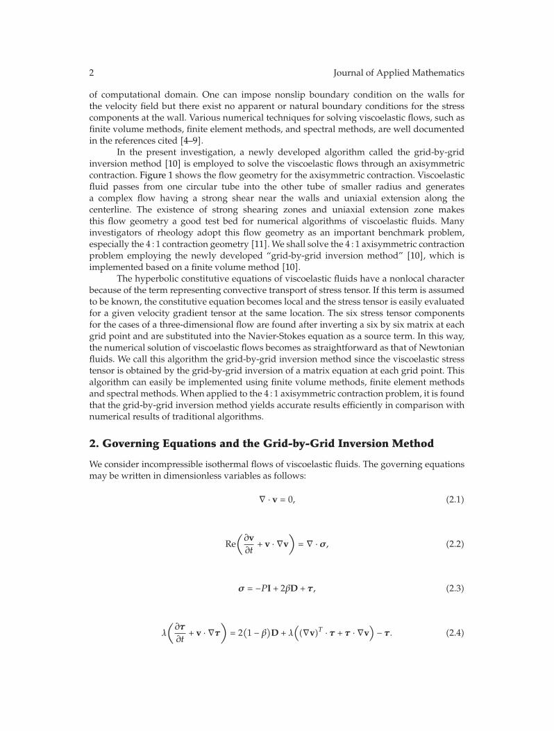
In the present investigation, a newly developed algorithm called the grid-by-gridinversion method [10] is employed to solve the viscoelastic flows through an axisymmetriccontraction. Figure 1 shows the flow geometry for the axisymmetric contraction. Viscoelasticfluid passes from one circular tube into the other tube of smaller radius and generatesa complex flow having a strong shear near the walls and uniaxial extension along thecenterline. The existence of strong shearing zones and uniaxial extension zone makesthis flow geometry a good test bed for numerical algorithms of viscoelastic fluids. Manyinvestigators of rheology adopt this flow geometry as an important benchmark problem,especially the 4 : 1 contraction geometry [11]. We shall solve the 4 : 1 axisymmetric contractionproblem employing the newly developed “grid-by-grid inversion method” [10], which isimplemented based on a finite volume method [10].

The hyperbolic constitutive equations of viscoelastic fluids have a nonlocal characterbecause of the term representing convective transport of stress tensor. If this term is assumedto be known, the constitutive equation becomes local and the stress tensor is easily evaluatedfor a given velocity gradient tensor at the same location. The six stress tensor componentsfor the cases of a three-dimensional flow are found after inverting a six by six matrix at eachgrid point and are substituted into the Navier-Stokes equation as a source term. In this way,the numerical solution of viscoelastic flows becomes as straightforward as that of Newtonianfluids. We call this algorithm the grid-by-grid inversion method since the viscoelastic stresstensor is obtained by the grid-by-grid inversion of a matrix equation at each grid point. Thisalgorithm can easily be implemented using finite volume methods, finite element methodsand spectral methods. When applied to the 4 : 1 axisymmetric contraction problem, it is foundthat the grid-by-grid inversion method yields accurate results efficiently in comparison withnumerical results of traditional algorithms.

2. Governing Equations and the Grid-by-Grid Inversion Method

We consider incompressible isothermal flows of viscoelastic fluids. The governing equationsmay be written in dimensionless variables as follows:

∇ · v = 0, (2.1)

Re(∂v∂t

+ v · ∇v)

= ∇ · σ, (2.2)

σ = −PI + 2βD + τ , (2.3)

λ

(∂τ

∂t+ v · ∇τ

)= 2(1 − β

)D + λ

((∇v)T · τ + τ · ∇v

)− τ . (2.4)

Journal of Applied Mathematics 3

4 r

z

272

492

D

D

D

D

Figure 1: The 4 : 1 axisymmetric contraction.

In the above equations, P is pressure,D is the rate of deformation tensor, τ is the viscoelasticpart of the stress tensor. The parameter β is the ratio of the retardation and relaxation timesof the fluid. Equation (2.4) is the constitutive equation of the Oldroyd-B model [9], λ is thedimensionless relaxation time or the Deborah number, and Re is the Reynolds number. Thesuperscript T in (2.4) is the transpose. The Reynolds number and the dimensionless Deborahnumber are defined by

Re =ρUL

η, λ =

λ1U

L, (2.5)

where ρ is the density, λ1 the dimensional relaxation time, U the characteristic speed, and L

is the characteristic length. The characteristic velocity U and the characteristic length L aretaken as the average velocity in the downstream tube and the radius of the downstream tube,respectively. To compare with the results of other investigators [9, 11], we take the value of βto be 1/9.

Next, we consider the grid-by-grid inversion method as applied to the set of equations(2.1)–(2.4). Contrary to the Newtonian fluids where the stress field τ depends on the velocitygradient tensor ∇v locally, the stress depends on the velocity gradient tensor nonlocally dueto the fact that constitutive equation is hyperbolic partial differential equation. The convectivetransport of the stress tensor, represented by v ·∇τ in (2.4), takes care of the memory effect ofτ in its dependence on∇v and causes the functional dependence of τ on∇v to be nonlocal. Inthe grid-by-grid inversion method, v · ∇τ is assumed to be a known source term which shallbe updated iteratively in the process. Then the constitutive equation (2.4) can be convertedsuch that τ is represented as a local function of ∇v as in the case of Newtonian fluids. Thisarrangement renders the numerical solution of viscoelastic fluids as straightforward as thatof Newtonian fluids. The steps for obtaining the velocity and the stress at time step n+1, vn+1

and τn+1, using known velocity and stress at time step n,vn and τn, proceed in an iterativemanner as follows. First, define

C ≡ vn+1(it) · ∇τn+1(it), (2.6)


where the superscript n + 1(it) indicates variable at time step n + 1 in the itth iteration.Discretizing (2.4) in time implicitly and representing D in terms of the velocity gradient ∇v,we find the following local matrix equations defined at each grid point.

(λ

Δt+ 1.0

)τn+1(it+1) − λ(∇v)T

n+1(it) · τn+1(it+1) − λτn+1(it+1) · (∇v)n+1(it)

=λ

Δtτn − λC +

(1 − β

)[(∇v)n+1(it) + (∇v)T

n+1(it)].

(2.7)

Once C is evaluated using variables at n + 1(it), (2.7) can be solved for τn+1(it+1) by invertinga six-by-six matrix at each grid point for the six independent stress components for the caseof three-dimensional flows. Equation (2.7) is also solved at the boundary grid points to findthe boundary stress field. This suggests a natural method of imposing boundary conditionsfor the hyperbolic constitutive equations at all boundaries of the computational domain.This method had been employed to impose outflow boundary conditions by Papanastasiouet al. [12] and is called the open boundary condition. Using τn+1(it+1) obtained from (2.7),the velocity at the n + 1 th time step in the it + 1 th iteration, vn+1(it+1), is found by solving(2.1)–(2.3) as follows:

∇ · vn+1(it+1) = 0, (2.8)

Re

(vn+1(it+1) − vn

Δt+ vn+1(it+1) · ∇vn+1(it+1)

)= −∇Pn+1(it+1) + 2β∇2vn+1(it+1) +∇ · τn+1(it+1).

(2.9)

Although (2.8)-(2.9) can be solved using any numerical methods for incompressible Navier-Stokes equations, we employ a finite volumemethod based on the SIMPLE algorithm [13, 14].To stabilize the numerical scheme for large values of λ, (2.6) is evaluated using one of thevarious upwind schemes. In the present work, we adopt a higher-order upwind scheme,MinMod [14], to evaluate C.

The case of β = 0 requires a special deliberation before employing standard algorithmsfor incompressible Navier-Stokes equations in the grid-by-grid inversion technique. Whenβ = 0, we decompose the total stress σ into pure viscous and elastic parts −PI + 2D and Σ,respectively, such that

σ = −PI + 2D + Σ, (2.10)

where

Σ ≡ τ − 2D. (2.11)


Then the momentum and constitutive equations for the case of β = 0 may be written as

∇ · v = 0, (2.12)

Re(∂v∂t

+ v · ∇v)

= −∇P +∇2v +∇ · Σ, (2.13)

λ

(∂Σ∂t

+ v · ∇Σ − (∇v)T · Σ − Σ · (∇v))+ Σ = −2λ

(∂D∂t

+ v · ∇D − (∇v)T ·D −D · ∇v).

(2.14)

This decomposition is called the EVSS formulation and was proposed by Perera and Walters[15]. The implementation of grid-by-grid inversion method to the set of (2.12)–(2.14) isstraightforward. First, we evaluate

E ≡ vn+1(it) · ∇Σn+1(it). (2.15)

Next, convert (2.14) to the following local matrix equations for Σ decoupled at each gridpoint:

(λ

Δt+ 1.0

)Σn+1(it+1) − λ(∇v)T

n+1(it) · Σn+1(it+1) − λΣn+1(it+1) · (∇v)n+1(it)

=λ

ΔtΣn − λE − 2λ

(1Δt

Dn+1(it) − 1Δt

Dn + v · ∇D − (∇v)T ·D −D · ∇v)n+1(it)

.

(2.16)

Then, (2.12) and (2.13) are discretized as follows:

∇ · vn+1(it+1) (2.17)

Re

(vn+1(it+1) − vn

Δt+ vn+1(it+1) · ∇vn+1(it+1)

)=−Pn+1(it+1)+∇2vn+1(it+1)+∇ · Σn+1(it+1). (2.18)

The structure of (2.16) is the same as that of (2.7) and can be solved for Σn+1(it+1) byinverting a six-by-six matrix at each grid point for a three-dimensional flow once (∇v)n+1(it) isgiven. After obtaining Σn+1(it+1), vn+1(it+1) is found by solving (2.17)-(2.18) using the SIMPLEalgorithm [13]. The second-order derivative terms appearing in v ·∇D of (2.14) are evaluatedusing a one-sided finite difference formula at the boundaries.

The overall solution procedure for the grid-by-grid inversion method may besummarized as follows.

(1) vn and τn have obtained in the previous time step n.

The procedure for the time step n + 1 begins as follows.

(2) Assume vn+1(it) and τn+1(it). For the first iteration (it = 1), vn+1(it)=vn and τn+1(it)=τn.


(3) Evaluate C of (2.6) (β /= 0) or E of (2.15) (β = 0) using an upwind scheme.

(4) Using vn+1(it), solve (2.7) (β /= 0) or (2.16) (β = 0) for τn+1(it+1) by inverting a six-by-six matrix at each grid point including the boundary grids.

(5) Using τn+1(it+1),

(β /= 0) solve the momentum equation, (2.9), and continuity equation to find vn+1(it+1).(β = 0) solve themomentum equation, (2.18), and continuity equation to find vn+1(it+1).

(6) Convergence check for τn+1 and vn+1. If not converged, go to step (2). Otherwise,update the time step and go to step (1).

Usually convergence is attained in two or three iterations. The novelty of the grid-by-grid inversion method is its easiness of numerical implementation. As noted in theabove procedure, one can easily convert any existing computer code for Newtonian flowsimulations to that for viscoelastic flow simulation by adding a subroutine that solves theviscoelastic constitutive equation using the grid-by-grid inversion method, summarizedas steps (3)∼(4), to evaluate the viscoelastic source terms in the Navier-Stokes equation,∇ · τ . Adding a source term to the Navier-Stokes equation is an easy procedure whetherwe employ a finite volume method or a finite element method. In the subroutine for theviscoelastic constitutive equation, one inverts a small matrix at each grid point, which canbe performed cheaply. Therefore, one can easily convert any commercial CFD package forNewtonian fluid flows to that for viscoelastic fluids employing the grid-by-grid inversionmethod. Its robustness and accuracy are corroborated in the next section, where the grid-by-grid inversion method is employed to solve the 4 : 1 viscoelastic axisymmetric contractionproblem. Although Phillips and Williams [16] solve the viscoelastic constitutive equationby converting small matrix equations in their semi-Lagrange method, it is very difficult toconvert an existing Newtonian code to a viscoelastic code using the semi-Lagrange methodsince it treats the momentum and the constitutive equation simultaneously.

3. Viscoelastic Flow through an Axisymmetric Contraction

In this section, we solve the flow of an Oldroyd-B fluid through a 4 : 1 axisymmetriccontraction geometry using the grid-by-grid inversion method. The schematic representationof the flow geometry is depicted in Figure 1. The viscoelastic flow through the circularcontraction geometry has served as a standard benchmark problem for numerical algorithmsfor viscoelastic fluids. The presence of a singularity in the entry-flow geometry as well asregions of high shear and extension in the flow have been a significant challenge for a longtime, and many investigators have struggled to develop accurate and robust algorithmsfor viscoelastic flows through contraction geometries [17, 18]. The contraction ratio 4 : 1 isthe standard one in this benchmark problem. A good review of old works may be Trebotichet al. [18]. Recently, Phillips and Williams [11, 16] used a finite volume method to solve theflow of an Oldroyd-B fluid through planar and axisymmetric contractions. Among these twogeometries, the axisymmetric contraction yields more dramatic viscoelastic effects. In thepresent investigation, we will solve the flow of Oldroyd-B fluid through the axisymmetricgeometry using the grid-by-grid inversion method based on the SIMPLE algorithm tocorroborate the accuracy and robustness of the grid-by-grid inversion method. When solving(2.8)-(2.9) or (2.17)-(2.18) using the SIMPLE algorithm, we adopt a collocated mesh and


the pressure oscillation induced by the collocated mesh is eliminated using the Rhie-Chowmethod [19], and a higher-order upwind scheme, MinMod [14], is used to treat the inertiaforce term in the momentum equation and the convective transport of stress tensor in theconstitutive equation. For the 4 : 1 axisymmetric contraction geometry depicted in Figure 1,the number of relevant components of stress tensor is four because the ∇ · τ term in (2.9)contains a circular stress component τθθ as follows:

(∇ · τ)r =1r

∂

∂r(rτrr) +

∂

∂zτrz − τθθ

r,

(∇ · τ)z =1r

∂

∂r(rτrz) +

∂

∂zτzz.

(3.1)

Although the relevant velocity components for axisymmetric flows are (vr, vz), it is necessaryto find the four stress components, τrr , τrz, τzz, and τθθ which appear in (3.1). The constitutiveequation (2.4)may be written for an axisymmetric geometry as follows:

λ

(∂τrr

∂t+ vr ∂τ

rr

∂r+ vz ∂τ

rr

∂z

)= 2(1 − β

)∂vr

∂r+ λ

(2∂vr

∂rτrr + 2

∂vr

∂zτrz)− τrr , (3.2)

λ

(∂τrz

∂t+ vr ∂τ

rz

∂r+ vz ∂τ

rz

∂z

)

=(1 − β

)(∂vz

∂r+∂vr

∂z

)+ λ

(∂vr

∂rτrz +

∂vr

∂zτzz + τrr

∂vz

∂r+ τrz

∂vz

∂z

)− τrz,

(3.3)

λ

(∂τzz

∂t+ vr ∂τ

zz

∂r+ vz ∂τ

zz

∂z

)= 2(1 − β

)∂vz

∂z+ λ

(2∂vz

∂rτrz + 2

∂vz

∂zτzz)− τzz, (3.4)

λ

(∂τθθ

∂t+ vr ∂τ

θθ

∂r+ vz ∂τ

θθ

∂z

)= 2(1 − β

)vr

r+ λ

(2vr

rτθθ)− τθθ. (3.5)

It is to be noted that equations for (τrr , τrz, τzz) are coupled with each other, while that forτθθ is decoupled. The relevant components of C of (2.6) are

CIJ = vr ∂τIJ

∂r+ vz ∂τ

IJ

∂z, (3.6)


where IJ = rr, rz, zz, θθ. Assuming known values of CIJ , (3.2)–(3.4) may be representedas a set of matrix equations at each grid point including the boundary grids as follows:

⎡⎢⎢⎢⎢⎢⎢⎢⎣

λ

Δt+ 1 − 2λ

∂vr

∂r−2λ∂v

r

∂z0

−λ∂vz

∂r

λ

Δt+ 1 − λ

(∂vr

∂r+∂vz

∂z

)−λ∂v

r

∂z

0 −2λ∂vz

∂r

λ

Δt+ 1 − 2λ

∂vz

∂z

⎤⎥⎥⎥⎥⎥⎥⎥⎦

n+1(it)

ik

⎡⎣τ

rr

τrz

τzz

⎤⎦

n+1(it+1)

ik

=

⎡⎢⎢⎢⎢⎢⎢⎣

λτrr(n)

Δt− λCrr + 2

(1 − β

)∂vr

∂rλτrz(n)

Δt− λCrz +

(1 − β

)(∂vz

∂r+∂vr

∂z

)

λ

Δtτzz(n) − λCzz + 2

(1 − β

)∂vz

∂z

⎤⎥⎥⎥⎥⎥⎥⎦

n+1(it)

ik

.

(3.7)

On the other hand, from (3.5), τθθik

can be found at each grid point within the computationaldomain and on the boundary as follows:

(τθθ)n+1(it+1)ik

=

(λ

Δt

(τθθ)n − λCθθ + 2

(1 − β

)vr

r

)n+1(it)

ik(λ

Δt+ 1 − 2λ

vr

r

)n+1(it)

ik

. (3.8)

Once (τrrik, τrz

ik, τzz

ik, τθθ

ik)n+1(it+1) are obtained from (3.7)-(3.8), they are used to solve (2.8)-(2.9)

to find (vr, vz)n+1(it+1)ik

in the 4 : 1 axisymmetric contraction geometry.

4. Results

In this section, we compare the results from the grid-by-grid inversion method with thoseof Phillips and Williams [11] to corroborate the accuracy and robustness of the grid-by-gridinversion method. To make the comparison meaningful, we adopt the same flow geometryand inlet conditions as those employed by Phillips andWilliams [11]. Namely, the contraction


0 2 40

500

1000

1500

τzz

λ = 1r = 1

Grid A (14, 580)Grid B (32, 535)

Grid C (57, 960)Reference [16]

−4 −2

z

Re = 0

(a)

0 5 10 150

50

100

150

200

250

300

τzz

−15 −10 −5

z

Grid A (14, 580)Grid B (32, 535)

Grid C (57, 960)Reference [16]

λ = 1r = 0.064Re = 0

(b)

Figure 2: Confirmation of grid convergence of the grid-by-grid inversion method when Re = 0.0 andλ = 1.0 (a) along r = 1.0 (b) along r = 0.064.

ratio is 4 : 1, the length of the larger channel is 27R, and that of smaller channel is 49R whenR is the radius of the smaller channel (cf. Figure 1). At the inlet, the parabolic Poiseuille flowis adopted as Phillips and Williams [11] have done.

(-) inlet velocity

vz(r) =164

(16 − r2

), vr = 0, 0 ≤ r ≤ 4, (4.1)


0 2 40

500

1000

1500

2000

τzz

−4 −2

z

r = 1

λ = 0.5λ = 1λ = 1.5

λ = 0.5 (reference [16])λ = 1 (reference [16])λ = 1.5 (reference [16])

Re = 0

(a)

0 5 10 150

100

200

300

400

500

600

λ = 0.5λ = 1λ = 1.5

λ = 0.5 (reference [16])λ = 1 (reference [16])λ = 1.5 (reference [16])

−15 −10 −5

r = 0.064

τzz

z

Re = 0

(b)

Figure 3: Stress overshoot at various λwhen Re = 0.0 (a) along r = 1.0 (b) along r = 0.064.

where r ≡ r ′/R and r ′ is the dimensional radial distance. Contrary to Phillips and Williams[11], we do not impose inlet boundary conditions for the stress field, since the grid-by-gridinversion method does not require them and simply solve (3.7)-(3.8) at the inlet grid pointsto find the stress field at the inlet location. This is also an important merit of the grid-by-gridinversion method over other algorithms for the viscoelastic flows. Although Papanastasiouet al. [12] employed this method of imposing open outflow boundary conditions previouslyand named it open boundary condition method or free boundary condition method, itappears very naturally in the grid-by-grid inversion method.


λ = 0

Phillips and Williams [11] Grid-by-grid inversion method

λ = 0.5

λ = 1

λ = 1.5

Re = 0

Figure 4: Comparison of streamlines for λ = 0.0, λ = 0.5, λ = 1.0, and λ = 1.5 when Re = 0.0.

We have employed three sets of grid system to ensure grid convergence of numericalresults. For the three sets of grids, that is, 14,580 (Grid A), 32,535 (Grid B), and 57,960 (GridC), the extrastress component τzz is plotted when λ = 1.0 for Re = 0.0 along r = 1 inFigure 2(a), and along r = 0.064 in Figure 2(b). For there three mesh systems, the numbers ofcells along r in the small tube are 30, 45, and 60, respectively. For Grid A, the minimum Δr is0.005 at the wall and it grows gradually until it becomes 5.1 × 10−2 at the center. For Grid B,(Δr)min is 0.003 and (Δr)max is 3.4 × 10−2 at the center, and for Grid C, (Δr)min = 0.002 at thewall and (Δr)max = 2.3 × 10−2 at the center. The results of the present work are also comparedwith those of Phillips and Williams [11]. Though the grid number increases from 32,535 to57,960, there is not appreciable change in τzz. Therefore, we adopt Grid B in the subsequentcomputations. Figure 3 shows the extrastress component τzz at Re = 0.0 for λ = 0.5, 1.0,and 1.5 along r = 1.0 (Figure 2(a)) and along r = 0.064 (Figure 2(b)). The grid-convergeddata for τzz obtained from the grid-by-grid inversion method are somewhat smaller thanthe benchmark data of Phillips and Williams [11]. At the corner of the contractor, τzz hasa sharp overshoot, which increases with respect to λ, and it settles down to a downstream


Phillips and Williams [11]

λ = 0

Grid-by-grid inversion method

λ = 0.5

λ = 1

λ = 1.5

Re = 0

Figure 5: Comparison of streamlines for λ = 0.0, λ = 0.5, λ = 1.0, and λ = 1.5 when Re = 1.0.

value rapidly. Near the center of the contracted channel (r = 0.064), a smaller overshoot ofτzz appears, which increases as λ increases, and it settles down to a downstream value muchslowly as compared to that at the wall (r = 1.0).

Figure 4 shows comparison of streamlines for λ = 0.0, 0.5, 1.0, and 1.5 obtained fromthe grid-by-grid inversion method with those from the Phillips and Williams [11] whenRe = 0.0. The grid-by-grid inversion method yields accurate results as compared with thebenchmark data for the range of λ values considered. The size of the corner vortex increases asλ increases. Figure 5 depicts comparison of streamlines at various values of λ when Re = 1.0.The predictions of the grid-by-grid inversion method are also in good agreement with thoseof the benchmark data [11]. Comparing with the streamlines of Re = 0.0, it is found thatthe vortex sizes are diminished due to the inertia effect [11]. The size of the corner vortexcan be measured using a parameter L1, as suggested by Phillips and Williams [11] andOliveira et al.[8], which is the distance of the upstream separation point from the salientcorner. Figure 6 shows the variation of L1 with respect to λ for Re = 0.0 and Re = 1.0.


0.5 1 1.5

1

1.5

2

2.5

3

L1

λ

(grid-by-grid inversion)1 (grid-by-grid inversion)

Re =Re =Re = 0

Re =Re =

1 [11]0 [11]0 [8]

Figure 6: Variation of the size of corner vortex L1 with respect to λwhen Re = 0.0 and Re = 1.0.

For Re = 1.0, the grid-by-grid inversion method is found to yield results similar to thoseof the benchmark data of Phillips and Williams [11]. For Re = 0.0, the results of the grid-by-grid inversion method are compared with those of Oliveira et al. [8] as well as thoseof Phillips and Williams [11]. It is shown that both the grid-by-grid inversion and Phillipsand Williams [11] yield L1 somewhat larger than those of Oliveira et al. [8]. Since Oliveiraet al. [8] do not consider the case Re = 1.0, we cannot compare the grid-by-grid inversionmethod with Oliveira et al. when Re = 1.0. To corroborate the accuracy of the grid-by-gridinversionmethod further, we compare the results for the vortex intensityΨR, which is definedas the flow rate in recirculation divided by inlet flow rate, in Figure 7 when Re = 0.0. As inprevious comparison, the grid-by-grid inversion method yields results similar to those ofPhillips and Williams [11], while Oliveira et al. [8] predicts results somewhat smaller thanthe grid-by-grid inversion method. The grid-by-grid inversion method yields results for λlarger than 1.5 and Re larger than 1.0, which demonstrates the robustness of the grid-by-gridinversion method as compared to other finite volume methods or finite element methods[9, 11, 16, 18].

5. Conclusion

The grid-by-grid inversion method [10] has been applied to the 4 : 1 circular contractionproblem in the present investigation. Viscoelastic flows through the contraction generatecomplex flows exhibiting strong shear and uniaxial extension, which is a good test bed forthe robustness and accuracy of a new numerical algorithms. In the grid-by-grid inversion


0.5 1 1.5

102

101

100

λ

ψR×1

03

(grid-by-grid inversion)

Re =Re =Re = 0

0 [11]0 [8]

Figure 7: Variation of the dimensionless vortex intensity ΨR with respect to λ when Re = 0.0.

method [10], the hyperbolic constitutive equation is split such that the term for the convectivetransport of stress tensor is treated as a source, which is updated iteratively. This allows thestress tensor at each grid point to be expressed in terms of velocity gradient tensor at the samelocation, and the set of stress tensor components is found after inverting a small matrix at eachgrid point. The grid-by-grid inversion method can be implemented easily in any commercialCFD packages for Newtonian fluid flows to convert them to be used for viscoelastic fluidflows. The grid-by-grid inversion method is found to yield accurate results as compared withthe benchmark data of Phillips andWilliams [11]. It predicts accurately the variation of cornervortex size and the τzz overshoot with respect to λ at Re = 0.0 and Re = 1.0.

Acknowledgment

This paper was supported by the Human Resources Development of the Korea Instituteof Energy Technology Evaluation and Planning (KETEP) Grant funded by the KoreaGovernment Ministry of Knowledge and Economy (no. 20114010203090).

References

[1] R. B. Bird, R. C. Amstrong, and O. Hassager, Dynamics of Polymeric Liquids, vol. 1, Wiley, New York,NY, USA, 1987.

[2] R. R. Huilgol and N. Phan-Thien, Fluid Mechanics of Viscoelasticity, Elsevier, Amsterdam, TheNetherlands, 1997.


[3] D. D. Joseph, Fluid Dynamics of Viscoelastic Liquids, vol. 84 of Applied Mathematical Sciences, Springer,1990.

[4] M. A. Alves, F. T. Pinho, and P. J. Oliveira, “The flow of viscoelastic fluids past a cylinder: finite-volume high-resolutions method,” Journal of Non-Newtonian Fluid Mechanics, vol. 97, no. 2-3, pp. 207–232, 2001.

[5] M. J. Crochet, A. R. Davis, and K. Walters, Numerical Simulation of Non-Newtonian Flow, Elsevier,Amsterdam, The Netherlands, 1984.

[6] F. Yurun andM. J. Crochet, “High-order finite element methods for steady viscoelastic flows,” Journalof Non-Newtonian Fluid Mechanics, vol. 57, no. 2-3, pp. 283–311, 1995.

[7] B. Khomami, K. K. Talwar, and H. K. Ganpule, “A comparative study of higher- and lower-orderfinite element techniques for computation of viscoelastic flows,” Journal of Rheology, vol. 38, no. 2, pp.255–289, 1994.

[8] M. S. N. Oliveira, P. J. Oliveira, F. T. Pinho, and M. A. Alves, “Effect of contraction ratio uponviscoelastic flow in contractions: the axisymmetric case,” Journal of Non-Newtonian Fluid Mechanics,vol. 147, no. 1-2, pp. 92–108, 2007.

[9] R. G. Owens and T. N. Phillips, Computational Rheology, Imperial College Press, London, UK, 2002.[10] H. M. Park and J. Y. Lim, “A new numerical algorithm for viscoelastic fluid flows: the grid-by-grid

inversion method,” Journal of Non-Newtonian Fluid Mechanics, vol. 165, no. 5-6, pp. 238–246, 2010.[11] T. N. Phillips and A. J. Williams, “Comparison of creeping and inertial flow of an Oldroyd B fluid

through planar and axisymmetric contractions,” Journal of Non-Newtonian Fluid Mechanics, vol. 108,no. 1–3, pp. 25–47, 2002.

[12] T. C. Papanastasiou, N. Malamataris, and K. Ellwood, “A new outflow boundary condition,”International Journal for Numerical Methods in Fluids, vol. 14, no. 5, pp. 587–608, 1992.

[13] S. V. Patankar, Numerical Heat Transfer and Fluid Flow, Hemisphere, New York, NY, USA, 1980.[14] H. K. Versteeg and W. Malalasekera, An Introduction to Computational Fluid Dynamics, Pearson

Education Limited, Essex, UK, 2007.[15] M. G. N. Perera and K. Walters, “Long-range memory effects in flows involving abrupt changes in

geometry: part1. Flows associatedwith L-shaped and T-shaped geometries,” Journal of Non-NewtonianFluid Mechanics, vol. 2, no. 2, pp. 191–204, 1977.

[16] T. N. Phillips and A. J. Williams, “Viscoelastic flow through a planar contraction using a semi-Lagrangian finite volume method,” Journal of Non-Newtonian Fluid Mechanics, vol. 87, no. 2-3, pp.215–246, 1999.

[17] R. Keunings and M. J. Crochet, “Numerical simulation of the flow of a viscoelastic fluid through anabrupt contraction,” Journal of Non-Newtonian Fluid Mechanics, vol. 14, pp. 279–299, 1984.

[18] D. Trebotich, P. Colella, and G. H. Miller, “A stable and convergent scheme for viscoelastic flow incontraction channels,” Journal of Computational Physics, vol. 205, no. 1, pp. 315–342, 2005.

[19] C. M. Rhie and W. L. Chow, “Numerical study of the turbulent flow past an airfoil with trailing edgeseparation,” AIAA Journal, vol. 21, no. 11, pp. 1525–1532, 1983.

Viscoelastic Flow through an Axisymmetric Contraction Using ...

Documents

Transcript of Viscoelastic Flow through an Axisymmetric Contraction Using ...