IOP PUBLISHING and INTERNATIONAL ATOMIC ENERGY AGENCY NUCLEAR FUSION

Nucl. Fusion 52 (2012) 013015 (11pp) doi:10.1088/0029-5515/52/1/013015

Integrated modelling of ICRH in aquasi-axisymmetric stellaratorM. Jucker1, W.A. Cooper and J.P. Graves

Ecole Polytechnique Federale de Lausanne (EPFL), Centre de Recherches en Physique desPlasmas, Association EURATOM-Confederation Suisse, CH-1015 Lausanne, Switzerland

E-mail: mjucker@princeton.edu

Received 13 July 2011, accepted for publication 23 November 2011Published 23 December 2011Online at stacks.iop.org/NF/52/013015

AbstractWe apply the code package SCENIC to a two field-period quasi-axisymmetric stellarator. Ion cyclotron resonanceheating (ICRH) is applied both on the high- and low-field side to a 1% 3He minority in a deuterium plasma. Itis shown that due to toroidal variations, the results are considerably different from similar tokamak studies. Inparticular, toroidal variations in power deposition and pressure are created and accentuated during radio frequencyheating, such that modifications to the magnetic equilibrium depend on toroidal angle. We demonstrate that dueto enhanced particle loss, low-field side heating is significantly less efficient than high-field side heating, and thattoroidally trapped particles impose upper power limits for efficient radio frequency injection.

(Some figures may appear in colour only in the online journal)

1. Introduction

Quasi-axisymmetric stellarators (QASs) represent feasiblecombinations of tokamaks and stellarators, combining the bestfeatures of each configuration. On the one hand, the three-dimensional geometry allows for a plasma without toroidalcurrent, thus improving considerably MHD stability andallowing for disruption free steady state. On the other hand,and in contrast to conventional stellarators, the magnetic fieldstrength depends only on two variables, a radial and an angularvariable, such that the particle orbits stay confined tokamak-like around constant pressure surfaces [1]. Furthermore,controlling a desired asymmetry in toroidal direction of astellarator can be more efficient than trying to suppressmagnetic field ripple and other inhomogeneities in a tokamak,and it adds one more dimension for plasma stability control [2].

Until now, self-consistent solutions of the wave fields inthe ion cyclotron resonance heating (ICRH) spectrum andfast particle distribution solvers have been limited mostlyto two-dimensional tokamak plasmas which fail to includethe modifications to the equilibrium state [3–6]. In three-dimensional magnetically confined plasmas, the TASK/WMfield solver has been coupled with the GNET drift kineticequation solver, but the equilibrium modifications have beenexcluded from the iterative loop [7].

We apply the unique code package SCENIC [8] to atwo-field period QAS, in order to study ICRH in a three-dimensional equilibrium. SCENIC generates self-consistent

1 Present address: Princeton University, AOS Program, Princeton, NJ 08544,USA.

three-dimensional solutions, which include varying MHDequilibrium, radio frequency (RF) wave field and resonantparticle distribution functions, through the guise of an iterativescheme. To our knowledge, this is the first time suchcomprehensive ICRH simulations are performed in a three-dimensional geometry. In the next section, we will introducethe numerical setup, before reporting our simulation results insection 3, and finish with concluding remarks.

2. Numerical model and geometry

2.1. SCENIC

The fully three-dimensional code package SCENIC has beendescribed extensively in [8], and we will only give a generaloverview for the clarity of this work. SCENIC is an iterativescheme and comprises three codes plus additional modulesrequired for the iterations. The MHD equilibrium code VMEC[9, 10] computes a new anisotropic fixed boundary equilibriumafter each iteration. Then, the full-wave code LEMan [11, 12]reads the newly created equilibrium and updates the RF wavefield. Finally, VENUS [13, 14] advances the distributionfunction based on the updated equilibrium and wave field,and re-creates new inputs for the next iteration of VMECand LEMan. Wave–particle interactions are modelled in aMonte Carlo approach, and the iterative scheme can be rununtil convergence is achieved, and total input RF power equalstotal power going to the background plasma plus power lossdue to energetic particles crossing the plasma boundary.

0029-5515/12/013015+11$33.00 1 © 2012 IAEA, Vienna Printed in the UK & the USA

Nucl. Fusion 52 (2012) 013015 M. Jucker et al

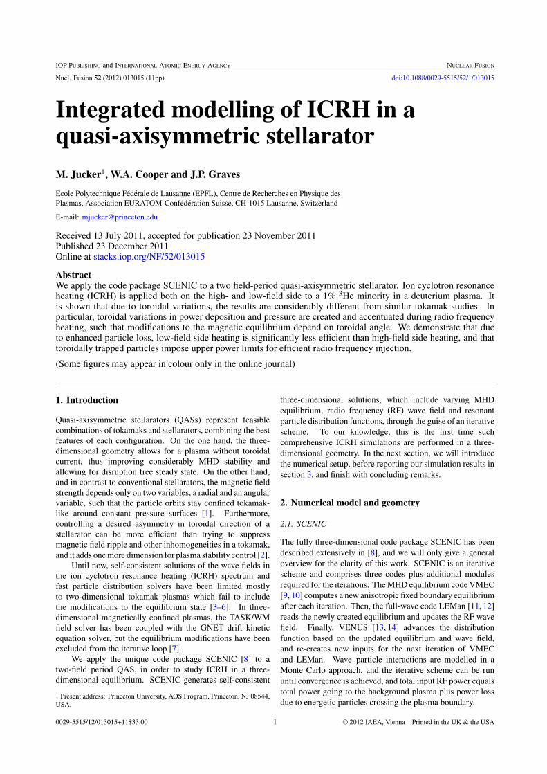
Figure 1. Initial magnetic equilibrium for the two-period QAS. Themagnetic field varies from Bmin = 2.0 T (blue) to Bmax = 3.2 T(red), with the on axis magnitude of B0 = 2.57 T. The poloidal cutsare at ! = {0, pi}.

2.2. Quasi-axisymmetric stellarator

We investigate a two-field period QAS of size comparable tothe Joint European Torus (JET). This is a rescaled version ofCHS-qa, a design proposed in Japan [15], and its magneticequilibrium studied numerically in [16]. This particular choiceof geometry is motivated by recent work [8, 17], which appliesthe SCENIC package to a JET-like two-dimensional torus.It is interesting to consider a three-dimensional geometrywith as many similar parameters as possible, as it allows fora more direct comparison between tokamak and stellaratorsimulations. Figure 1 illustrates the magnetic field strength,which varies in the range 2.0 T ! B ! 3.2 T. The toroidalangle is defined to have its origin to the left of the figure, andthe plasma volume is semi-transparent between ! = 0 and" = 2"/L, with L = 2 the number of field periods. We choseto match major (R0 = 2.91 m) and minor (a = 0.89 m) radiirather than plasma volume (37.3 m3), as well as magnetic fieldstrength on axis (B0 = 2.57 T). The safety factor varies onlyvery little around q ! 3, and the volume averaged thermalbeta is "## = 0.5%. Whereas we could have pushed for higherthermal beta, there are two good reasons for our choice: first,as mentioned above, our approach is to take previous resultsone step further by adding a third dimension to the studiesperformed in [8]. Second, we are mainly interested in fast(resonant) particle effects, and therefore do not necessarilyneed high thermal pressure. As for the geometry, note that theplasma volume is about half of JET’s plasma volume even withcomparable major and minor radii, which is due to the toroidalplasma shaping of the QAS. The electron density profile waschosen n = n0(1 $ s4) with n0 = 3 % 1019 m$3, and thetemperature profile T = T0(1 $ s) with T0 = 3 keV. Here, s

is the Boozer radial coordinate and is proportional to toroidalflux. The plasma is composed of 1% helium-3 in a deuteriumbackground. The choice of helium-3 is motivated by the factthat it prevents the appearance of a deuterium second harmonicresonance in the plasma, and for the sake of comparison withtokamak simulations in [17]. In the latter studies, helium-3minority was chosen as it is relevant for reactor-like scenarios(such as ITER).

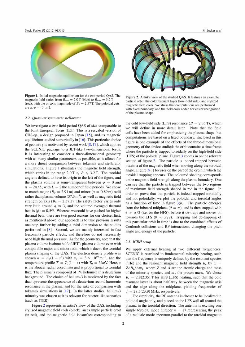
Figure 2 represents an artist’s view of the QAS, includingstylized magnetic field coils (black), an example particle orbit(in red), and the magnetic field isosurface corresponding to

Figure 2. Artist’s view of the studied QAS. It features an exampleparticle orbit, the cold resonant layer (low-field side), and stylizedmagnetic field coils. We stress that computations are performedwith fixed boundary, and the field coils added for easier recognitionof the plasma shape.

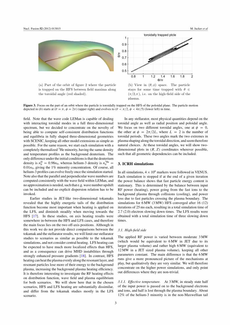
the cold low-field side (LFS) resonance (B = 2.35 T), whichwe will define in more detail later. Note that the fieldcoils have been added for emphasizing the plasma shape, butcomputations are based on a fixed boundary. Enclosed in thisfigure is one example of the effects of the three-dimensionalgeometry of the device studied: the orbit contains a time framewhere the particle is trapped toroidally on the high-field side(HFS) of the poloidal plane. Figure 3 zooms in on the relevantsection of figure 2. The particle is indeed trapped betweenmaxima of the magnetic field when moving along the toroidalangle. Figure 3(a) focuses on the part of the orbit in which thetoroidal trapping appears. The coloured shading correspondsto the magnetic field strength along the plasma boundary. Onecan see that the particle is trapped between the two regionsof maximum field strength shaded in red in the figure. Inorder to prove that the particle is indeed trapped toroidallyand not poloidally, we plot the poloidal and toroidal anglesas a function of time in figure 3(b). The particle emergesfrom the inboard midplane ($ = " ), and is then trapped with$ > "/2 (i.e. on the HFS), before it de-traps and moves ontowards the LFS ($ < "/2). Trapping and de-trapping ofthis particular orbit in time is due to the combined effects ofCoulomb collisions and RF interactions, changing the pitchangle and energy of the particle.

2.3. ICRH setup

We apply external heating at two different frequencies.SCENIC is restricted to fundamental minority heating, suchthat the frequency is uniquely defined by the resonant species(3He) and the resonant magnetic field strength Bc by % =ZeBc/Amp, where Z and A are the atomic charge and massof the minority species, and mp the proton mass. We choseBc = 2.8(2.35) T for HFS (LFS) heating, such that the coldresonant layer is about half way between the magnetic axisand the edge along the midplane, yielding frequencies off = 28.5(23.9) MHz, respectively.

For simplicity, the RF antenna is chosen to be localized inpoloidal angle only, and placed on the LFS wall all around theplasma in the toroidal direction. The antenna is exciting onesimple toroidal mode number n = 17 representing the peakof a realistic mode spectrum parallel to the toroidal magnetic

2

Nucl. Fusion 52 (2012) 013015 M. Jucker et al

Figure 3. Focus on the part of an orbit where the particle is toroidally trapped on the HFS of the poloidal plane. The particle motiondepicted in (b) starts at ($ = " , ! = 2" ) (upper right) and evolves to ($ < "/2, ! < 4"/5) (lower left) in time.

field. Note that the wave code LEMan is capable of dealingwith interacting toroidal modes in a full three-dimensionalspectrum, but we decided to concentrate on the novelty ofbeing able to compute self-consistent distribution functionsand equilibria in fully shaped three-dimensional geometrieswith SCENIC, keeping all other model extensions as simple aspossible. For the same reason, we start each simulation with acompletely thermalized 3He minority, having the same densityand temperature profiles as the background deuterium. Theonly difference under the initial conditions is that the deuteriumdensity is nD

0 = 0.98n0, whereas helium-3 density is n3He0 =

0.01n0, giving the 1% minority concentration. Of course, allhelium-3 profiles can evolve freely once the simulation started.Note also that the parallel and perpendicular wave numbers arecomputed consistently with the wave field within LEMan, andno approximation is needed, such that e.g. wave number upshiftcan be included and no explicit dispersion relation has to beinvoked.

Earlier studies in JET-like two-dimensional tokamaksrevealed that the highly energetic tails of the distributionfunction become most important when heating is applied onthe LFS, and diminish steadily when moving towards theHFS [17]. In these studies, on axis heating results weresomewhere in-between the HFS and LFS cases, and thereforethe main focus lies on the two off-axis positions. Although inthis work we do not provide direct comparisons between thetokamak and the stellarator results, we will limit our stellaratorstudies to scenarios as similar as possible to the tokamaksimulations, and not consider central heating. LFS heating canbe expected to have much more localized effects than HFS,and as a consequence can drive MHD instabilities throughstrongly enhanced pressure gradients [18]. In contrast, HFSheating can heat the plasma evenly along the resonant layer, andresonant particles lose more of their energy to the backgroundplasma, increasing the background plasma heating efficiency.It is therefore interesting to investigate the RF heating effectson distribution function, wave field and plasma equilibriumfor both scenarios. We will show here that in the chosenscenarios, HFS and LFS heating are substantially dissimilar,and differ from the tokamak studies mostly in the LFSscenario.

In any stellarator, most physical quantities depend on thetoroidal angle as well as radial position and poloidal angle.We focus on two different toroidal angles, one at ! = 0,the other at ! = 2"/2L, where L = 2 is the number oftoroidal periods. These two angles mark the two extremes inplasma shaping along the toroidal direction, and seem thereforenatural choices. At these toroidal angles, we will show two-dimensional plots in (R, Z) coordinates wherever possible,such that all geometric dependencies can be included.

3. ICRH simulations

In all simulations, 4 % 106 markers were followed in VENUS.Each simulation is stopped if at the end of a given iterationthe power balance shows that fast particle energy content isstationary. This is determined by the balance between inputRF power (heating), power going from the fast ions to thebackground plasma through collisions (cooling), and powerloss due to fast particles crossing the plasma boundary. Thesimulations for 6 MW (3 MW) HFS converged after 16 (12)iterations of 25 ms each, resulting in a total simulation time of2.7 (2.0) electron slowing down times. The LFS results wereobtained with a total simulation time of three slowing downtimes.

3.1. High-field side

The applied RF power is varied between moderate 3 MW(which would be equivalent to 6 MW in JET due to itslarger plasma volume) and rather high 6 MW (equivalent to12 MW in a JET sized plasma volume), keeping all otherparameters constant. The main difference is that the 6 MWruns give a more pronounced picture of the mechanisms atplay, but qualitatively they are very similar. We will thereforeconcentrate on the higher power simulations, and only pointout differences where they are non-trivial.

3.1.1. Effective temperature. At 3 MW, in steady state halfof the input power is passed on to the background electronsand ions, and half is lost through the plasma boundary. About12% of the helium-3 minority is in the non-Maxwellian tail

3

Nucl. Fusion 52 (2012) 013015 M. Jucker et al

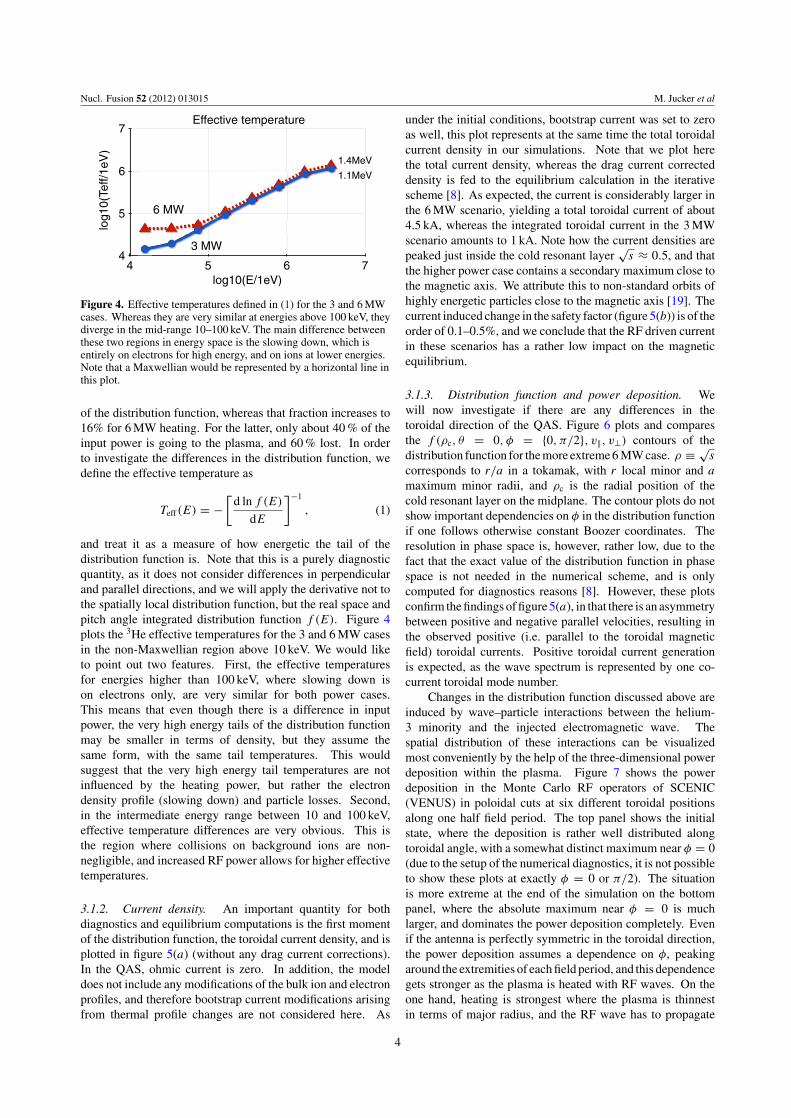
Figure 4. Effective temperatures defined in (1) for the 3 and 6 MWcases. Whereas they are very similar at energies above 100 keV, theydiverge in the mid-range 10–100 keV. The main difference betweenthese two regions in energy space is the slowing down, which isentirely on electrons for high energy, and on ions at lower energies.Note that a Maxwellian would be represented by a horizontal line inthis plot.

of the distribution function, whereas that fraction increases to16% for 6 MW heating. For the latter, only about 40 % of theinput power is going to the plasma, and 60 % lost. In orderto investigate the differences in the distribution function, wedefine the effective temperature as

Teff(E) = $!

d ln f (E)

dE

"$1

, (1)

and treat it as a measure of how energetic the tail of thedistribution function is. Note that this is a purely diagnosticquantity, as it does not consider differences in perpendicularand parallel directions, and we will apply the derivative not tothe spatially local distribution function, but the real space andpitch angle integrated distribution function f (E). Figure 4plots the 3He effective temperatures for the 3 and 6 MW casesin the non-Maxwellian region above 10 keV. We would liketo point out two features. First, the effective temperaturesfor energies higher than 100 keV, where slowing down ison electrons only, are very similar for both power cases.This means that even though there is a difference in inputpower, the very high energy tails of the distribution functionmay be smaller in terms of density, but they assume thesame form, with the same tail temperatures. This wouldsuggest that the very high energy tail temperatures are notinfluenced by the heating power, but rather the electrondensity profile (slowing down) and particle losses. Second,in the intermediate energy range between 10 and 100 keV,effective temperature differences are very obvious. This isthe region where collisions on background ions are non-negligible, and increased RF power allows for higher effectivetemperatures.

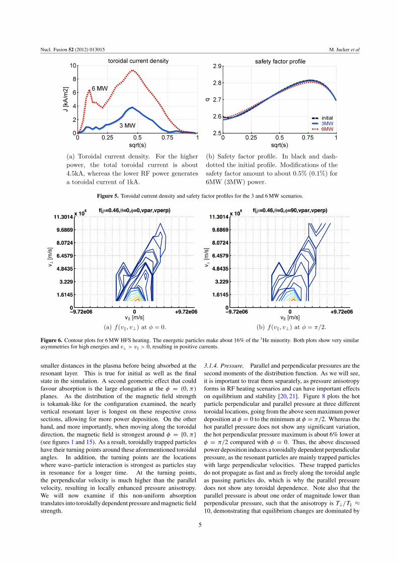
3.1.2. Current density. An important quantity for bothdiagnostics and equilibrium computations is the first momentof the distribution function, the toroidal current density, and isplotted in figure 5(a) (without any drag current corrections).In the QAS, ohmic current is zero. In addition, the modeldoes not include any modifications of the bulk ion and electronprofiles, and therefore bootstrap current modifications arisingfrom thermal profile changes are not considered here. As

under the initial conditions, bootstrap current was set to zeroas well, this plot represents at the same time the total toroidalcurrent density in our simulations. Note that we plot herethe total current density, whereas the drag current correcteddensity is fed to the equilibrium calculation in the iterativescheme [8]. As expected, the current is considerably larger inthe 6 MW scenario, yielding a total toroidal current of about4.5 kA, whereas the integrated toroidal current in the 3 MWscenario amounts to 1 kA. Note how the current densities arepeaked just inside the cold resonant layer

&s ! 0.5, and that

the higher power case contains a secondary maximum close tothe magnetic axis. We attribute this to non-standard orbits ofhighly energetic particles close to the magnetic axis [19]. Thecurrent induced change in the safety factor (figure 5(b)) is of theorder of 0.1–0.5%, and we conclude that the RF driven currentin these scenarios has a rather low impact on the magneticequilibrium.

3.1.3. Distribution function and power deposition. Wewill now investigate if there are any differences in thetoroidal direction of the QAS. Figure 6 plots and comparesthe f (&c, $ = 0,! = {0,"/2}, v', v() contours of thedistribution function for the more extreme 6 MW case. & )

&s

corresponds to r/a in a tokamak, with r local minor and a

maximum minor radii, and &c is the radial position of thecold resonant layer on the midplane. The contour plots do notshow important dependencies on ! in the distribution functionif one follows otherwise constant Boozer coordinates. Theresolution in phase space is, however, rather low, due to thefact that the exact value of the distribution function in phasespace is not needed in the numerical scheme, and is onlycomputed for diagnostics reasons [8]. However, these plotsconfirm the findings of figure 5(a), in that there is an asymmetrybetween positive and negative parallel velocities, resulting inthe observed positive (i.e. parallel to the toroidal magneticfield) toroidal currents. Positive toroidal current generationis expected, as the wave spectrum is represented by one co-current toroidal mode number.

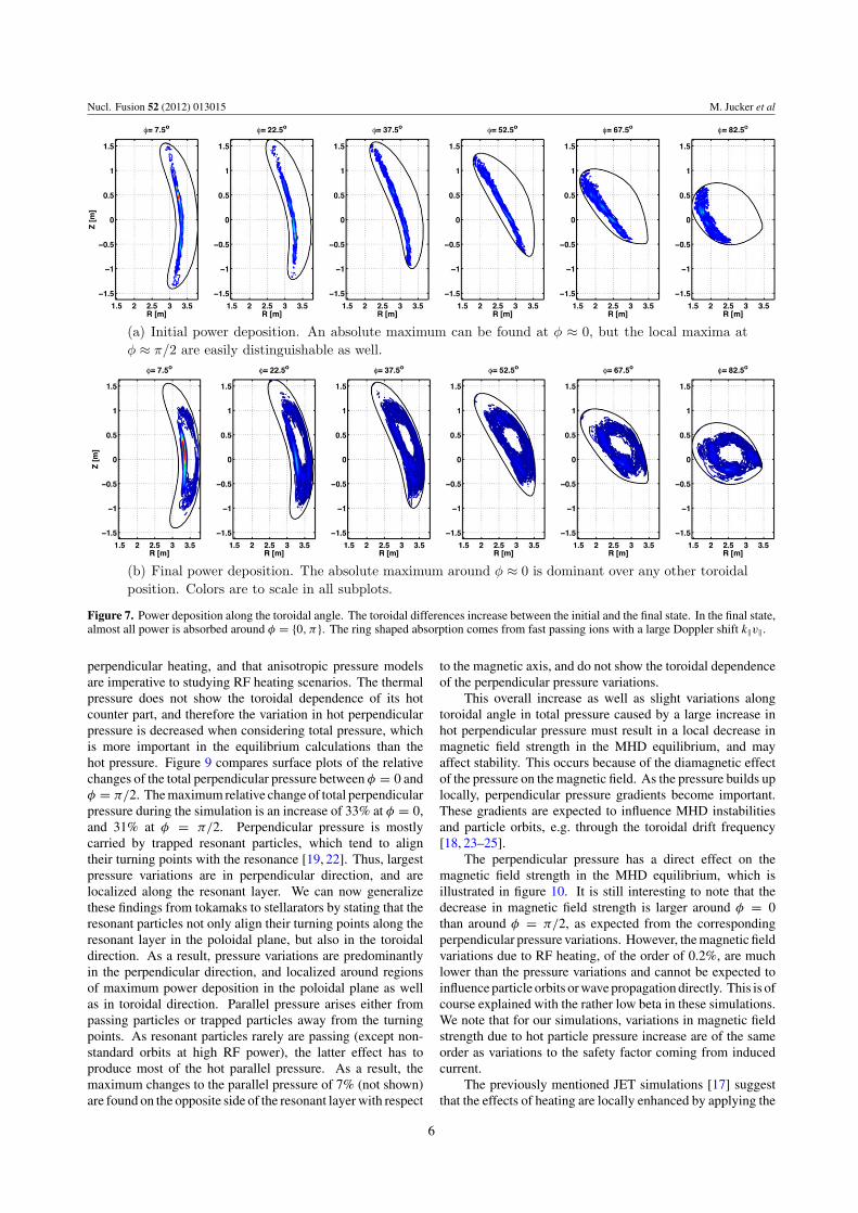
Changes in the distribution function discussed above areinduced by wave–particle interactions between the helium-3 minority and the injected electromagnetic wave. Thespatial distribution of these interactions can be visualizedmost conveniently by the help of the three-dimensional powerdeposition within the plasma. Figure 7 shows the powerdeposition in the Monte Carlo RF operators of SCENIC(VENUS) in poloidal cuts at six different toroidal positionsalong one half field period. The top panel shows the initialstate, where the deposition is rather well distributed alongtoroidal angle, with a somewhat distinct maximum near ! = 0(due to the setup of the numerical diagnostics, it is not possibleto show these plots at exactly ! = 0 or "/2). The situationis more extreme at the end of the simulation on the bottompanel, where the absolute maximum near ! = 0 is muchlarger, and dominates the power deposition completely. Evenif the antenna is perfectly symmetric in the toroidal direction,the power deposition assumes a dependence on !, peakingaround the extremities of each field period, and this dependencegets stronger as the plasma is heated with RF waves. On theone hand, heating is strongest where the plasma is thinnestin terms of major radius, and the RF wave has to propagate

4

Nucl. Fusion 52 (2012) 013015 M. Jucker et al

Figure 5. Toroidal current density and safety factor profiles for the 3 and 6 MW scenarios.

Figure 6. Contour plots for 6 MW HFS heating. The energetic particles make about 16% of the 3He minority. Both plots show very similarasymmetries for high energies and v( > v' > 0, resulting in positive currents.

smaller distances in the plasma before being absorbed at theresonant layer. This is true for initial as well as the finalstate in the simulation. A second geometric effect that couldfavour absorption is the large elongation at the ! = (0,")

planes. As the distribution of the magnetic field strengthis tokamak-like for the configuration examined, the nearlyvertical resonant layer is longest on these respective crosssections, allowing for more power deposition. On the otherhand, and more importantly, when moving along the toroidaldirection, the magnetic field is strongest around ! = {0,"}(see figures 1 and 15). As a result, toroidally trapped particleshave their turning points around these aforementioned toroidalangles. In addition, the turning points are the locationswhere wave–particle interaction is strongest as particles stayin resonance for a longer time. At the turning points,the perpendicular velocity is much higher than the parallelvelocity, resulting in locally enhanced pressure anisotropy.We will now examine if this non-uniform absorptiontranslates into toroidally dependent pressure and magnetic fieldstrength.

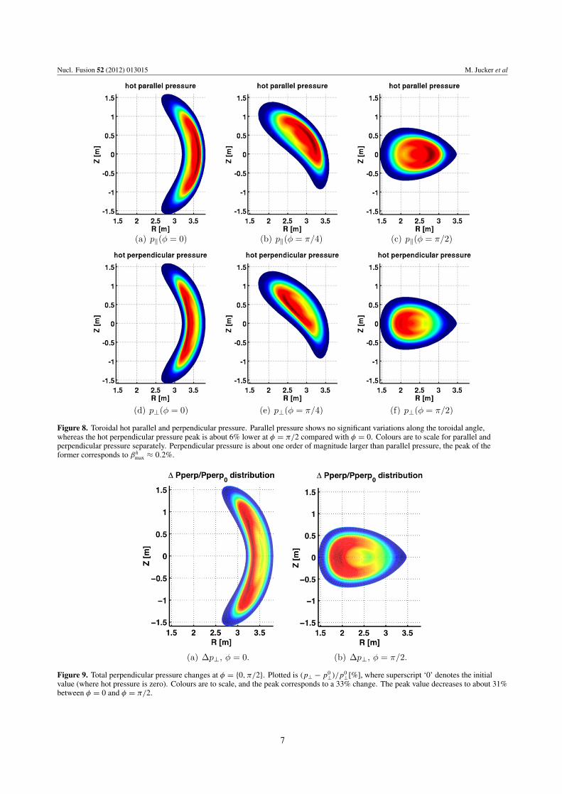
3.1.4. Pressure. Parallel and perpendicular pressures are thesecond moments of the distribution function. As we will see,it is important to treat them separately, as pressure anisotropyforms in RF heating scenarios and can have important effectson equilibrium and stability [20, 21]. Figure 8 plots the hotparticle perpendicular and parallel pressure at three differenttoroidal locations, going from the above seen maximum powerdeposition at ! = 0 to the minimum at ! = "/2. Whereas thehot parallel pressure does not show any significant variation,the hot perpendicular pressure maximum is about 6% lower at! = "/2 compared with ! = 0. Thus, the above discussedpower deposition induces a toroidally dependent perpendicularpressure, as the resonant particles are mainly trapped particleswith large perpendicular velocities. These trapped particlesdo not propagate as fast and as freely along the toroidal angleas passing particles do, which is why the parallel pressuredoes not show any toroidal dependence. Note also that theparallel pressure is about one order of magnitude lower thanperpendicular pressure, such that the anisotropy is T(/T' !10, demonstrating that equilibrium changes are dominated by

5

Nucl. Fusion 52 (2012) 013015 M. Jucker et al

Figure 7. Power deposition along the toroidal angle. The toroidal differences increase between the initial and the final state. In the final state,almost all power is absorbed around ! = {0,"}. The ring shaped absorption comes from fast passing ions with a large Doppler shift k'v'.

perpendicular heating, and that anisotropic pressure modelsare imperative to studying RF heating scenarios. The thermalpressure does not show the toroidal dependence of its hotcounter part, and therefore the variation in hot perpendicularpressure is decreased when considering total pressure, whichis more important in the equilibrium calculations than thehot pressure. Figure 9 compares surface plots of the relativechanges of the total perpendicular pressure between ! = 0 and! = "/2. The maximum relative change of total perpendicularpressure during the simulation is an increase of 33% at ! = 0,and 31% at ! = "/2. Perpendicular pressure is mostlycarried by trapped resonant particles, which tend to aligntheir turning points with the resonance [19, 22]. Thus, largestpressure variations are in perpendicular direction, and arelocalized along the resonant layer. We can now generalizethese findings from tokamaks to stellarators by stating that theresonant particles not only align their turning points along theresonant layer in the poloidal plane, but also in the toroidaldirection. As a result, pressure variations are predominantlyin the perpendicular direction, and localized around regionsof maximum power deposition in the poloidal plane as wellas in toroidal direction. Parallel pressure arises either frompassing particles or trapped particles away from the turningpoints. As resonant particles rarely are passing (except non-standard orbits at high RF power), the latter effect has toproduce most of the hot parallel pressure. As a result, themaximum changes to the parallel pressure of 7% (not shown)are found on the opposite side of the resonant layer with respect

to the magnetic axis, and do not show the toroidal dependenceof the perpendicular pressure variations.

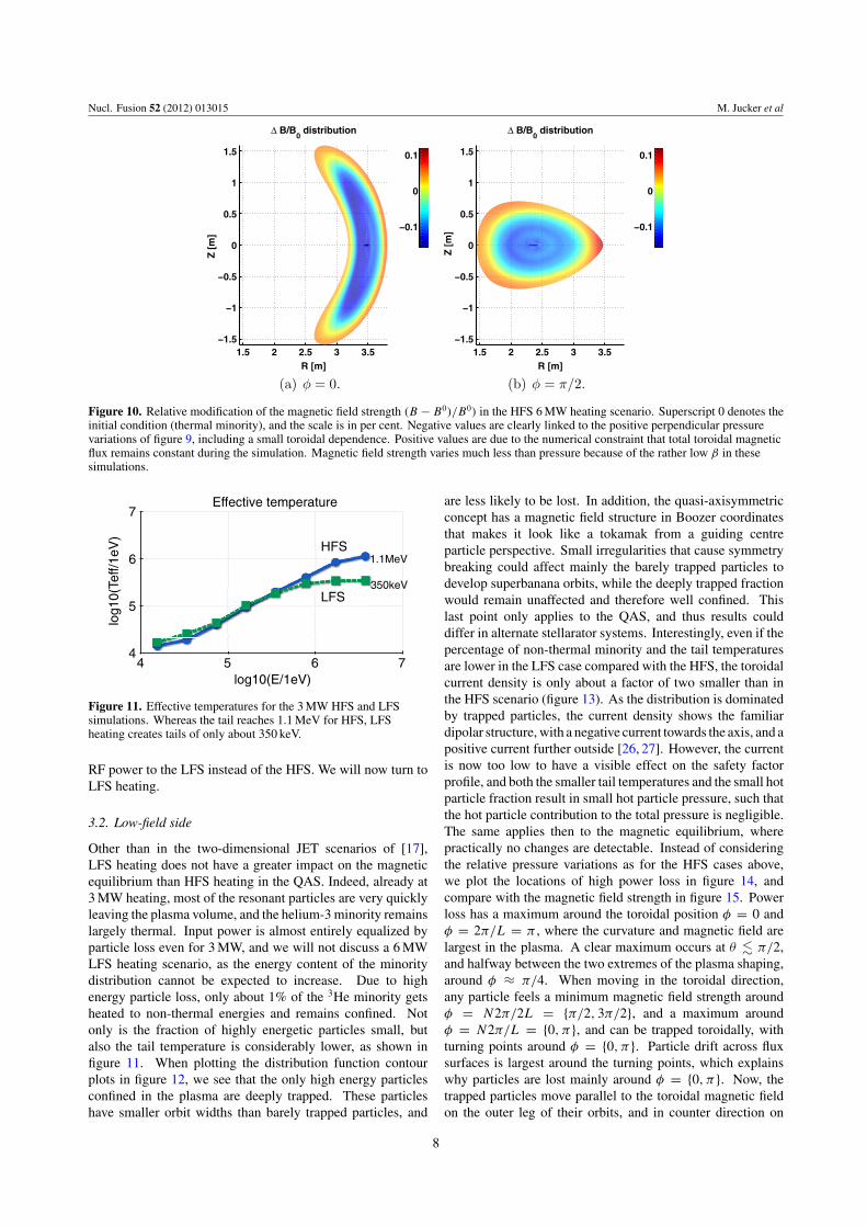
This overall increase as well as slight variations alongtoroidal angle in total pressure caused by a large increase inhot perpendicular pressure must result in a local decrease inmagnetic field strength in the MHD equilibrium, and mayaffect stability. This occurs because of the diamagnetic effectof the pressure on the magnetic field. As the pressure builds uplocally, perpendicular pressure gradients become important.These gradients are expected to influence MHD instabilitiesand particle orbits, e.g. through the toroidal drift frequency[18, 23–25].

The perpendicular pressure has a direct effect on themagnetic field strength in the MHD equilibrium, which isillustrated in figure 10. It is still interesting to note that thedecrease in magnetic field strength is larger around ! = 0than around ! = "/2, as expected from the correspondingperpendicular pressure variations. However, the magnetic fieldvariations due to RF heating, of the order of 0.2%, are muchlower than the pressure variations and cannot be expected toinfluence particle orbits or wave propagation directly. This is ofcourse explained with the rather low beta in these simulations.We note that for our simulations, variations in magnetic fieldstrength due to hot particle pressure increase are of the sameorder as variations to the safety factor coming from inducedcurrent.

The previously mentioned JET simulations [17] suggestthat the effects of heating are locally enhanced by applying the

6

Nucl. Fusion 52 (2012) 013015 M. Jucker et al

Figure 8. Toroidal hot parallel and perpendicular pressure. Parallel pressure shows no significant variations along the toroidal angle,whereas the hot perpendicular pressure peak is about 6% lower at ! = "/2 compared with ! = 0. Colours are to scale for parallel andperpendicular pressure separately. Perpendicular pressure is about one order of magnitude larger than parallel pressure, the peak of theformer corresponds to #h

max ! 0.2%.

Figure 9. Total perpendicular pressure changes at ! = {0,"/2}. Plotted is (p( $ p0()/p0

([%], where superscript ‘0’ denotes the initialvalue (where hot pressure is zero). Colours are to scale, and the peak corresponds to a 33% change. The peak value decreases to about 31%between ! = 0 and ! = "/2.

7

Nucl. Fusion 52 (2012) 013015 M. Jucker et al

Figure 10. Relative modification of the magnetic field strength (B $ B0)/B0) in the HFS 6 MW heating scenario. Superscript 0 denotes theinitial condition (thermal minority), and the scale is in per cent. Negative values are clearly linked to the positive perpendicular pressurevariations of figure 9, including a small toroidal dependence. Positive values are due to the numerical constraint that total toroidal magneticflux remains constant during the simulation. Magnetic field strength varies much less than pressure because of the rather low # in thesesimulations.

Figure 11. Effective temperatures for the 3 MW HFS and LFSsimulations. Whereas the tail reaches 1.1 MeV for HFS, LFSheating creates tails of only about 350 keV.

RF power to the LFS instead of the HFS. We will now turn toLFS heating.

3.2. Low-field side

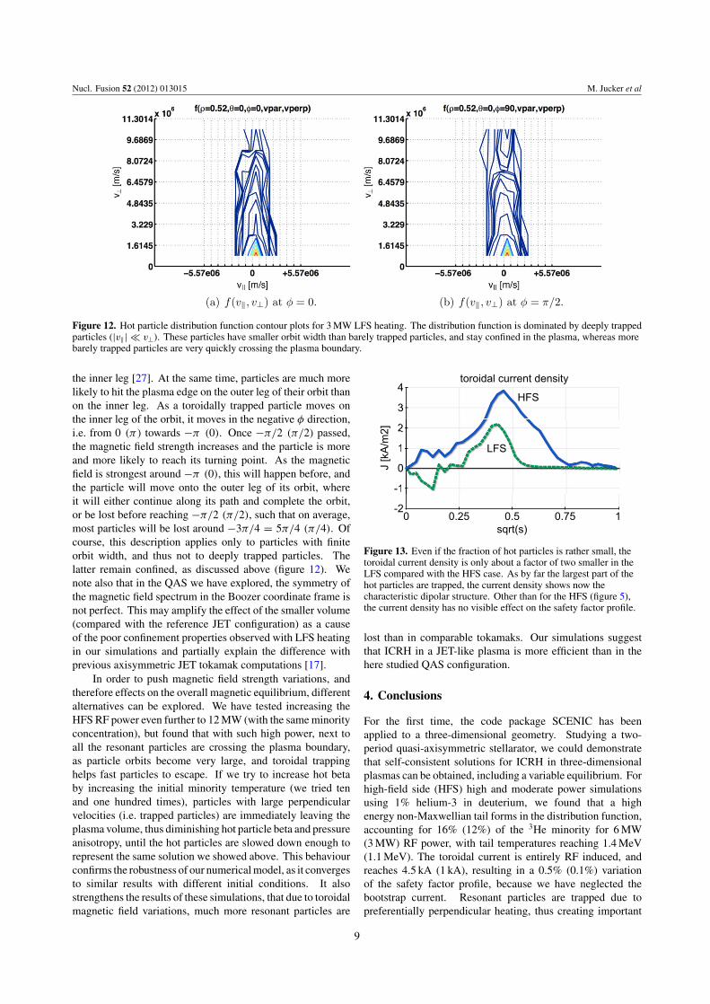
Other than in the two-dimensional JET scenarios of [17],LFS heating does not have a greater impact on the magneticequilibrium than HFS heating in the QAS. Indeed, already at3 MW heating, most of the resonant particles are very quicklyleaving the plasma volume, and the helium-3 minority remainslargely thermal. Input power is almost entirely equalized byparticle loss even for 3 MW, and we will not discuss a 6 MWLFS heating scenario, as the energy content of the minoritydistribution cannot be expected to increase. Due to highenergy particle loss, only about 1% of the 3He minority getsheated to non-thermal energies and remains confined. Notonly is the fraction of highly energetic particles small, butalso the tail temperature is considerably lower, as shown infigure 11. When plotting the distribution function contourplots in figure 12, we see that the only high energy particlesconfined in the plasma are deeply trapped. These particleshave smaller orbit widths than barely trapped particles, and

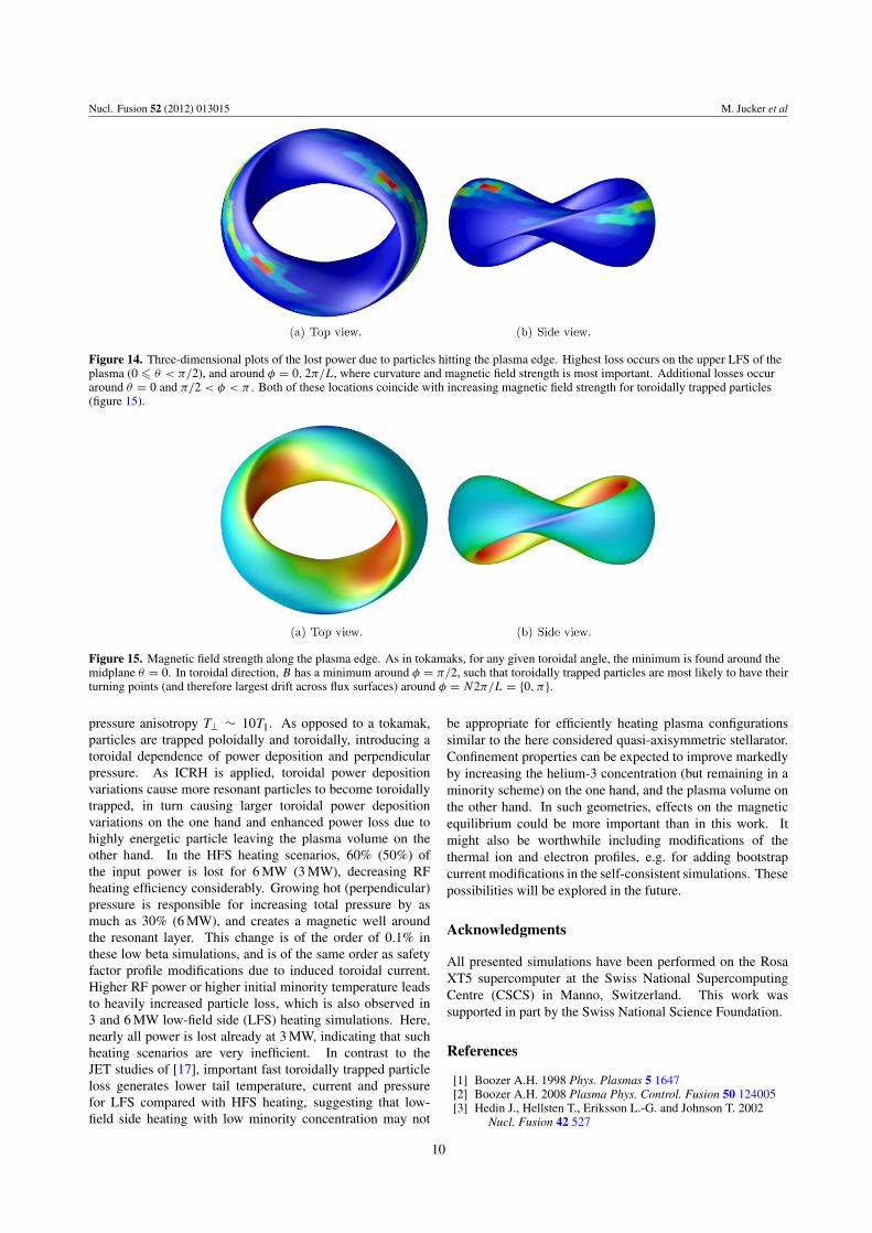
are less likely to be lost. In addition, the quasi-axisymmetricconcept has a magnetic field structure in Boozer coordinatesthat makes it look like a tokamak from a guiding centreparticle perspective. Small irregularities that cause symmetrybreaking could affect mainly the barely trapped particles todevelop superbanana orbits, while the deeply trapped fractionwould remain unaffected and therefore well confined. Thislast point only applies to the QAS, and thus results coulddiffer in alternate stellarator systems. Interestingly, even if thepercentage of non-thermal minority and the tail temperaturesare lower in the LFS case compared with the HFS, the toroidalcurrent density is only about a factor of two smaller than inthe HFS scenario (figure 13). As the distribution is dominatedby trapped particles, the current density shows the familiardipolar structure, with a negative current towards the axis, and apositive current further outside [26, 27]. However, the currentis now too low to have a visible effect on the safety factorprofile, and both the smaller tail temperatures and the small hotparticle fraction result in small hot particle pressure, such thatthe hot particle contribution to the total pressure is negligible.The same applies then to the magnetic equilibrium, wherepractically no changes are detectable. Instead of consideringthe relative pressure variations as for the HFS cases above,we plot the locations of high power loss in figure 14, andcompare with the magnetic field strength in figure 15. Powerloss has a maximum around the toroidal position ! = 0 and! = 2"/L = " , where the curvature and magnetic field arelargest in the plasma. A clear maximum occurs at $ " "/2,and halfway between the two extremes of the plasma shaping,around ! ! "/4. When moving in the toroidal direction,any particle feels a minimum magnetic field strength around! = N2"/2L = {"/2, 3"/2}, and a maximum around! = N2"/L = {0,"}, and can be trapped toroidally, withturning points around ! = {0,"}. Particle drift across fluxsurfaces is largest around the turning points, which explainswhy particles are lost mainly around ! = {0,"}. Now, thetrapped particles move parallel to the toroidal magnetic fieldon the outer leg of their orbits, and in counter direction on

8

Nucl. Fusion 52 (2012) 013015 M. Jucker et al

Figure 12. Hot particle distribution function contour plots for 3 MW LFS heating. The distribution function is dominated by deeply trappedparticles (|v'| * v(). These particles have smaller orbit width than barely trapped particles, and stay confined in the plasma, whereas morebarely trapped particles are very quickly crossing the plasma boundary.

the inner leg [27]. At the same time, particles are much morelikely to hit the plasma edge on the outer leg of their orbit thanon the inner leg. As a toroidally trapped particle moves onthe inner leg of the orbit, it moves in the negative ! direction,i.e. from 0 (") towards $" (0). Once $"/2 ("/2) passed,the magnetic field strength increases and the particle is moreand more likely to reach its turning point. As the magneticfield is strongest around $" (0), this will happen before, andthe particle will move onto the outer leg of its orbit, whereit will either continue along its path and complete the orbit,or be lost before reaching $"/2 ("/2), such that on average,most particles will be lost around $3"/4 = 5"/4 ("/4). Ofcourse, this description applies only to particles with finiteorbit width, and thus not to deeply trapped particles. Thelatter remain confined, as discussed above (figure 12). Wenote also that in the QAS we have explored, the symmetry ofthe magnetic field spectrum in the Boozer coordinate frame isnot perfect. This may amplify the effect of the smaller volume(compared with the reference JET configuration) as a causeof the poor confinement properties observed with LFS heatingin our simulations and partially explain the difference withprevious axisymmetric JET tokamak computations [17].

In order to push magnetic field strength variations, andtherefore effects on the overall magnetic equilibrium, differentalternatives can be explored. We have tested increasing theHFS RF power even further to 12 MW (with the same minorityconcentration), but found that with such high power, next toall the resonant particles are crossing the plasma boundary,as particle orbits become very large, and toroidal trappinghelps fast particles to escape. If we try to increase hot betaby increasing the initial minority temperature (we tried tenand one hundred times), particles with large perpendicularvelocities (i.e. trapped particles) are immediately leaving theplasma volume, thus diminishing hot particle beta and pressureanisotropy, until the hot particles are slowed down enough torepresent the same solution we showed above. This behaviourconfirms the robustness of our numerical model, as it convergesto similar results with different initial conditions. It alsostrengthens the results of these simulations, that due to toroidalmagnetic field variations, much more resonant particles are

Figure 13. Even if the fraction of hot particles is rather small, thetoroidal current density is only about a factor of two smaller in theLFS compared with the HFS case. As by far the largest part of thehot particles are trapped, the current density shows now thecharacteristic dipolar structure. Other than for the HFS (figure 5),the current density has no visible effect on the safety factor profile.

lost than in comparable tokamaks. Our simulations suggestthat ICRH in a JET-like plasma is more efficient than in thehere studied QAS configuration.

4. Conclusions

For the first time, the code package SCENIC has beenapplied to a three-dimensional geometry. Studying a two-period quasi-axisymmetric stellarator, we could demonstratethat self-consistent solutions for ICRH in three-dimensionalplasmas can be obtained, including a variable equilibrium. Forhigh-field side (HFS) high and moderate power simulationsusing 1% helium-3 in deuterium, we found that a highenergy non-Maxwellian tail forms in the distribution function,accounting for 16% (12%) of the 3He minority for 6 MW(3 MW) RF power, with tail temperatures reaching 1.4 MeV(1.1 MeV). The toroidal current is entirely RF induced, andreaches 4.5 kA (1 kA), resulting in a 0.5% (0.1%) variationof the safety factor profile, because we have neglected thebootstrap current. Resonant particles are trapped due topreferentially perpendicular heating, thus creating important

9

Nucl. Fusion 52 (2012) 013015 M. Jucker et al

Figure 14. Three-dimensional plots of the lost power due to particles hitting the plasma edge. Highest loss occurs on the upper LFS of theplasma (0 ! $ < "/2), and around ! = 0, 2"/L, where curvature and magnetic field strength is most important. Additional losses occuraround $ = 0 and "/2 < ! < " . Both of these locations coincide with increasing magnetic field strength for toroidally trapped particles(figure 15).

Figure 15. Magnetic field strength along the plasma edge. As in tokamaks, for any given toroidal angle, the minimum is found around themidplane $ = 0. In toroidal direction, B has a minimum around ! = "/2, such that toroidally trapped particles are most likely to have theirturning points (and therefore largest drift across flux surfaces) around ! = N2"/L = {0,"}.

pressure anisotropy T( + 10T'. As opposed to a tokamak,particles are trapped poloidally and toroidally, introducing atoroidal dependence of power deposition and perpendicularpressure. As ICRH is applied, toroidal power depositionvariations cause more resonant particles to become toroidallytrapped, in turn causing larger toroidal power depositionvariations on the one hand and enhanced power loss due tohighly energetic particle leaving the plasma volume on theother hand. In the HFS heating scenarios, 60% (50%) ofthe input power is lost for 6 MW (3 MW), decreasing RFheating efficiency considerably. Growing hot (perpendicular)pressure is responsible for increasing total pressure by asmuch as 30% (6 MW), and creates a magnetic well aroundthe resonant layer. This change is of the order of 0.1% inthese low beta simulations, and is of the same order as safetyfactor profile modifications due to induced toroidal current.Higher RF power or higher initial minority temperature leadsto heavily increased particle loss, which is also observed in3 and 6 MW low-field side (LFS) heating simulations. Here,nearly all power is lost already at 3 MW, indicating that suchheating scenarios are very inefficient. In contrast to theJET studies of [17], important fast toroidally trapped particleloss generates lower tail temperature, current and pressurefor LFS compared with HFS heating, suggesting that low-field side heating with low minority concentration may not

be appropriate for efficiently heating plasma configurationssimilar to the here considered quasi-axisymmetric stellarator.Confinement properties can be expected to improve markedlyby increasing the helium-3 concentration (but remaining in aminority scheme) on the one hand, and the plasma volume onthe other hand. In such geometries, effects on the magneticequilibrium could be more important than in this work. Itmight also be worthwhile including modifications of thethermal ion and electron profiles, e.g. for adding bootstrapcurrent modifications in the self-consistent simulations. Thesepossibilities will be explored in the future.

Acknowledgments

All presented simulations have been performed on the RosaXT5 supercomputer at the Swiss National SupercomputingCentre (CSCS) in Manno, Switzerland. This work wassupported in part by the Swiss National Science Foundation.

References

[1] Boozer A.H. 1998 Phys. Plasmas 5 1647[2] Boozer A.H. 2008 Plasma Phys. Control. Fusion 50 124005[3] Hedin J., Hellsten T., Eriksson L.-G. and Johnson T. 2002

Nucl. Fusion 42 527

10

Nucl. Fusion 52 (2012) 013015 M. Jucker et al

[4] Brambilla M. and Bilbato R. 2009 Nucl. Fusion49 85004

[5] Jaeger E.F. et al 2006 Nucl. Fusion 46 S397[6] Choi M. et al 2010 Phys. Plasmas 17 56102[7] Murakami S. et al 2006 Nucl. Fusion 46 S425[8] Jucker M. et al 2011 Comput. Phys. Commun. 182 912[9] Hirshman S.P. and Betancourt O. 1991 J. Comput. Phys.

96 99[10] Cooper W.A. et al 2009 Comput. Phys. Commun. 180 1524[11] Popovich P., Cooper W.A. and Villard L. 2006 Comput. Phys.

Commun. 175 250[12] Mellet N. et al 2011 Comput. Phys. Commun. 182 570[13] Fischer O., Cooper W.A., Isaev M.Y. and Villard L. 2002 Nucl.

Fusion 42 817[14] Cooper G.A. et al 2007 Phys. Plasmas 14 102506[15] Okamura S. et al 1998 J. Plasma Fusion Res. 1 164[16] Cooper W.A. et al 2006 Nucl. Fusion 46 683

[17] Jucker M., Graves J.P., Cooper W.A. and Johnson T. 2011Plasma Phys. Control. Fusion 53 054010

[18] Jucker M., Graves J.P., Cooper G.A. and Cooper W.A. 2008Plasma Phys. Control. Fusion 50 65009

[19] Hellsten T. et al 2004 Nucl. Fusion 44 892[20] Madden N.A. and Hastie R.J. 1994 Nucl. Fusion 34 519[21] Cooper W.A. et al 2007 Plasma Phys. Control. Fusion 49 1177[22] Eriksson L.-G. et al 1998 Phys. Rev. Lett. 81 1231[23] Connor J.W., Hastie R.J. and Taylor J.B. 1978 Phys. Rev. Lett.

40 396[24] McClements K.G., Dendy R.O., Hastie R.J. and Martin T.J.

1996 Phys. Plasmas 3 2994[25] Bourdelle C. et al 2005 Nucl. Fusion 45 110[26] Hellsten T., Carlsson J. and Eriksson L.-G. 1995 Phys. Rev.

Lett. 74 3612[27] Carlsson J., Hellsten T. and Hedin J. 1998 Phys. Plasmas

5 2885

11