The University of MaineDigitalCommons@UMaine

Electronic Theses and Dissertations Fogler Library

5-2003

Viscoelastic Roll Coating FlowsMitchell A. Johnson

Follow this and additional works at: http://digitalcommons.library.umaine.edu/etd

Part of the Complex Fluids Commons

This Open-Access Dissertation is brought to you for free and open access by DigitalCommons@UMaine. It has been accepted for inclusion inElectronic Theses and Dissertations by an authorized administrator of DigitalCommons@UMaine.

Recommended CitationJohnson, Mitchell A., "Viscoelastic Roll Coating Flows" (2003). Electronic Theses and Dissertations. 235.http://digitalcommons.library.umaine.edu/etd/235

VISCOELASTIC ROLL COATING FLOWS

BY

Mitchell A. Johnson

B.Ch.E. University of Minnesota, 1995

M.S. Institute of Paper Science and Technology, 1997

A THESIS

Submitted in Partial Fulfillment of the

Requirements for the Degree of

Doctor of Philosophy

(in Chemical Enpeering)

The Graduate School

The University of Maine

May, 2003

Advisory Committee:

Douglas W. Bousfield, Professor of Chemical Engineering, Advisor

Adriaan R. P. van Heiningen, J. Larcom Ober Professor of Chemical Engineering

Albert Co, Associate Professor of Chemical Engineering

Vincent Caccese, Associate Professor of Mechanical Enpeering

Stephen A. Austin, Ph. D., Gerber Technologies

COPYRIGHT NOTICE

O 2003 Mitchell A. Johnson

All Rrghts Reserved

VISCOELASTIC ROLL COATING FLOWS

By mtchell A. Johnson

Thesis Advisor: Dr. Douglas W. Bousfield

An Abstract of the Thesis Presented in Partial Fulfillment of the Requirements for the

Degree of Doctor of Philosophy (in Chemical Enpeering)

May, 2003

The physics of a fluid flow between two rotating cylinders is important in processes

such as bearing lubrication, roll coating, and printing. A small amount of dissolved polymer

in the fluid can have a large impact on the behavior of the process. Viscoelasticity affects

the stabihty of application and metering processes, and reduces the maximum speed at which

a uniform film can be coated onto a substrate.

The goal of this work is to characterize the effect of viscoelasticity on the forward

roll coating operation. A bench-top apparatus simulated the process. Measurements of the

gap between the roll surfaces, pressure profile, and film thickness were made for a known

roll speed and external load. Newtonian, Boger, and shear-thinning viscoelastic fluids were

characterized and tested. Two-dimensional hnite element analysis of forward roll coating

between two rigid rolls was completed for Newtonian, Oldroyd-B, and Giesekus fluids.

The results for the Newtonian liquid were consistent with published experimental

and theoretical data after the elasticity of the deformable cover was included in the analysis.

A dimensionless empirical expression described the results. A lubrication analysis with non-

Hertzian cover deformation and visco-capillary boundary conditions at the film-merge and

film-split corresponded with experimental measurements over a limited load range.

The viscoelastic fluids showed a trade-off between shear thinning and elasticity.

Thtee fluids were Boger-like in that they exhibited nearly constant viscosity in simple shear

but had significant elasticity. Two liquids obeyed the Carreau model but showed significant

elasticity. AJl five liquids exhibited varying degrees of the Weissenberg effect. The Boger

fluids produced larger gaps and showed increased sensitivity to roll speed compared to the

Newtonian liquid. The two shear-thinning elastic fluids produced larger gaps and increased

sensitivity to the external load. Dimensionless, empirical expressions described the results.

The hnite element analysis revealed the presence of a stress boundary layer at the

free surface downstream of the hlm-split for the Oldroyd-B fluid; the Giesekus fluid, under

the same conditions, did not produce the stress boundary layer. Competing effects of shear

thinning and elasticity were revealed as a reduction of roll separating force produced by the

Giesekus fluid.

ACKNOWLEDGEMENTS

I would like to express my gratitude to my advisor Dr. Douglas W. Bousfield for

providing me with the opportunity and means to undertake a fundamental study of the

behavior of viscoelastic liquids in a coating environment. Dr. Albert Co, Dr. Adriaan van

Heiningen, Dr. Steve Austin, and Dr. Vince Caccese have provided perspective and valuable

expertise, which helped me to develop and undertake this project. I would like to thank Dan

Jolicoeur and Amos Cline for their efforts in the design and construction of the experimental

apparatus. The continuous support and enthusiasm from my parents, Sharon and David, is

very much appreciated. David's vast expertise in all things mechanical, and genuine interest

in my endeavors, were invaluable resources.

I would especially like to thank Kerry. Her support and encouragement was

instrumental to our success in the trials of the past years of which this project was just small

part. Thank you Kerry.

TABLE OF CONTENTS

... ACKNOWLEDGEMENTS ............................................................................................................ m

............................................................................................................................. LIST OF TABLES vi

... LIST OF FIGURES ......................................................................................................................... vm

Chapter

...................................................................................................................... 1 INTRODUCTION 1

1.1 Coating Processes ......................................................................................................... 1

1.1.1 Roll Coating ............................................................................................................. 1

................................................................................................................. 1 .1.2 Equipment 2

1 . 1 . 3 Process Stability .................................................................................................. 5

........................................................................................ 1.1.4 Non-Newtonian Effects 10

...................................................................................................................... 1.2 Motivation 11

................................................................................................................. 1.3 Thesis Layout 12

2 NEWTONLAN COATING FLOWS ..................................................................................... 13

................................................................................................................... 2.1 Introduction 13

2.1.1 Theoretical Analyses .............................................................................................. 13

........................................................................................... 2.1.2 Experimental Analyses 16

.......................................................................................... 2.2 Experimental Investuption 18

................................................................................................................. 2.2.1 Apparatus 18

...................................................................................... 2.2.2 Measurement Techniques 20

2.2.3 Roll Cover ................................................................................................................ 22

....................................................................................... 2.2.4 Experimental Procedure 2 3

. . 2.3 Theoretical Investlgatlon ........................................................................................... 25

2.4 Results and Discussion ................................................................................................. 29

2.5 Summary .................................................................................................................... 40

3 VISCOELASTIC COATING FLOWS .................................................................................. 41

3.1 Introduction ................................................................................................................... 41

3.1 . 1 Theoretical Analyses ........................................................................................... 42

........................................................................................... 3.1.2 Experimental Analyses 43

. . .......................................................................................... 3.2 Experimental Invesagaaon 45

3.2.1 Viscoelastic Fluids ............................................................................................. 4 5

3.2.2 Apparatus ................................................................................................................ 51

3.2.3 Procedure ................................................................................................................. 52

. . 3.3 Theoretical Invesagaaon ......................................................................................... 52

................................................................................................. 3.4 Results and Discussion 57

3.5 Summary ......................................................................................................................... 89

4 SUMMARY ................................................................................................................................ 91

4.1 Summary of Chapter 2 .................................................................................................. 91

4.2 Summary of Chapter 3 .............................................................................................. 92

4.3 Recommendations for Futute Work ......................................................................... 93

REFERENCES ................................................................................................................................ 95

APPENDIX ........................................................................................................................... 1 0 2

BIOGRAPHY OF THE AUTHOR ............................................................................................ 119

LIST OF TABLES

................................................................ Table 2.1 Physical properties of Newtonian test fluid 21

.............................................. Table 2.2 Conditions for the model and compared experiments 32

Table 2.3 Experimental operating conditions ............................................................................. 34

Table 2.4 Empirical relations for the gap width ....................................................................... 39

Table 3.1 Physical properties of the test liquids .......................................................................... 46

Table 3.2 Carreau model parameters ............................................................................................. 50

Table 3.3 Arhenius temperature function parameters ............................................................ 51

Table 3.4 Fitted model parameters for the viscoelastic test fluids ............................................ 55

Table 3.5 Experimental operating conditions .............................................................................. 58

Table 3.6 Summary of empirical correlations ............................................................................ 72

Table 3.7 Model parameters used in the flow simulations ....................................................... 77

Table A . 1 Silicone oil, W = 1020 N/m .................................................................................. 102

Table A . 2 Silicone oil, W = 21 00 N/m .................................................................................... 102

Table A . 3 Silicone oil, W = 3200 N/m ...................................................................................... 103

Table A . 4 Silicone oil, W = 4400 N/m .................................................................................... 103

. .................................................................................. Table A 5 Sihcone oil, W = 6400 N/m 104

Table A . 6 Silicone oil, W = 8500 N/m .................................................................................... 104

Table A . 7 0.12% PIB, W = 2100 N/m ...................................................................................... 105

..................................................................................... Table A . 8 0.12% PIB, W = 3200 N/m 1 0 5

. .................................................................................. Table A 9 0.12% PIB, W = 4400 N/m 106

. ................................................................................... Table A 10 0.12% PIB, W = 5050 N/m 106

Table A . 11 0.12% PIB, W = 6400 N/m ............................................................................... 107

vii

Table A . 12 0.24% PIB. W = 21 00 N/m ................................................................................ 107

Table A . 13 0.24% PIB. W = 3200 N/m ................................................................................... 108

Table A . 14 0.24% PIB. W = 6400 N/m ................................................................................... 108

Table A . 15 0.24% PIB. W = 8500 N/m ................................................................................ 109

Table A . 16 0.36% PIB. W = 2100 N/m ................................................................................... 110

Table A . 17 0.36% PIB. W = 3200 N/m .................................................................................... 110

Table A . 18 0.36% PIB. W = 4400 N/m ................................................................................ 111

Table A . 19 0.36% PIB. W = 6400 N/m ................................................................................ 1 11

Table A . 20 0.36% PIB. W = 8500 N/m .................................................................................... 112

Table A . 21 0.45% PIB. W = 1020 N/m .................................................................................... 112

Table A . 22 0.45% PIB. W = 21 00 N/m ........................................................................... 1 13

Table A . 23 0.45% PIB. W = 3200 N/m .............................................................................. 113

Table A . 24 0.45% PIB. W = 4400 N/m .................................................................................. 114

Table A . 25 0.45% PIB. W = 6400 N/m .................................................................................... 114

Table A . 26 0.45% PIB. W = 8500 N/m .................................................................................... 115

Table A . 27 0.62% PIB. W = 1020 N/m .................................................................................... 115

Table A . 28 0.62% PIB. W = 2100 N/m ................................................................................. 116

Table A . 29 0.62% PIB. W = 3200 N/m ................................................................................. 116

Table A . 30 0.62% PIB. W = 4400 N/m .................................................................................... 117

Table A . 31 0.62% PIB. W = 6400 N/m .................................................................................... 117

Table A . 32 0.62% PIB. W = 8500 N/m ................................................................................... 118

LIST OF FIGURES

.............................................................................................. Figure 1 . 1 Rigid roll coating systems 3

Figure 1.2 Elasto-hydrodynamic roll coating systems ................................................................... 4

.......................................................................... Figure 1.3 Elasto-hydrodynamic coating systems 5

Figure 1.4 Gap flow in a forward roll coater .............................................................................. 6

Figure 1.5 Rotational coating flows ................................................................................................ 7

.............................................................................................................. Figure 1.6 Film split defects 9

................................................................................................................. Flgure 1.7 Coating liquid 11

............................................................................... Figure 2.1 Elasto-hydrodynamic gap profiles 17

........................................................................... Flgure 2.2 Experimental roll coating apparatus 19

................................................................. Flgure 2.3 Stress vs . strain for the roll cover material 23

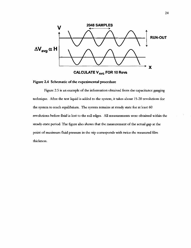
Flgure 2.4 Schematic of the experimental procedure .................................................................. 24

Flgure 2.5 Measured gap width and film thickness ..................................................................... 25

Figure 2.6 Flow domain for the lubrication model ..................................................................... 26

Figure 2.7 Pressure profiles a constant speed .......................................................................... 30

................................................................................ Figure 2.8 Pressure profiles at constant load 31

Figure 2.9 Integrated pressure profiles compared to measured load ........................................ 31

............................. Figure 2.1 0 Comparison of the calculated and measured pressure profiles 33

Flgure 2.11 Measured gap width as a function of Ne ................................................................ 35

Flgure 2.12 Measured gap width as a function of Nw .............................................................. 35

Flgure 2.1 3 Best-fit of experimental data ..................................................................................... 37

Flgure 2.14 Comparison with published data ............................................................................... 38

Figure 3.1 Apparent viscosity of the Boger test fluids ................................................................ 47

Figure 3.2 Steady shear viscosity for the shear-thinning liquids ............................................... 48

Figure 3.3 Elastic modulus G' vs . frequency of PIB solutions .................................................. 49

Figure 3.4 Flow domain ................................................................................................................ 56

Figure 3.5 Typical tinite element mesh .......................................................................................... 56

Figure 3.6 Dimensionless gap vs . elasticity parameter for 0.12% PIB ..................................... 59

Figure 3.7 Dimensionless gap vs . the load parameter for 0.12% PIB ................ : ..................... 59

Figure 3.8 Dimensionless gap vs . elasticity parameter for 0.24% PIB ..................................... 60

Figure 3.9 Dimensionless gap vs . the load parameter for 0.24% PIB ...................................... 61

Figure 3.10 Dimensionless gap vs . the elasticity parameter for 0.36% PIB ............................. 62

Figure 3.1 1 Dimensionless gap vs . the load parameter for 0.36% PIB .................................... 62

Figure 3.12 Comparison of empirical relations with measured gap .......................................... 63

Figure 3.1 3 Comparison between elastic fluids at low load ....................................................... 64

Figure 3.14 Comparison of elastic fluids at intermediate load ................................................... 65

Figure 3.15 Comparison of elastic fluids at high load ............................................................. 66

Figure 3.1 6 Pressure profiles for the 0.1 2% PIB fluid ............................................................ 67

Figure 3.17 Pressure profdes of the constant viscosity elastic fluids ........................................ 67

Figure 3.18 Dimensionless gap vs . the elasticity parameter for 0.45% PIB ............................. 69

Figure 3.19 Measured gap vs . the load parameter for 0.45% PIB solution ............................. 69

Figure 3.20 Measured gap as a function of elasticity number for 0.62% PIB ......................... 70

Figure 3.21 Measured gap as a function of load parameter for the 0.62% PIB solution ....... 70

Figure 3.22 Best fit of the empirical correlations with the measured data ............................... 72

Figure 3.23 Gap as a function of Ne at low load ......................................................................... 73

Figure 3.24 Gap as a function of Ne at intermediate load ......................................................... 73

Figure 3.25 Gap as a function of Ne at high load ...................................................................... 75

Figure 3.26 Pressure profiles of the shear-thinning elastic liquids ........................................ 75

Figure 3.27 Pressure profiles for shear-thinning and elastic liquids .......................................... 76

Figure 3.28 Streamlines for Newtonian and Oldtoyd-B models ............................................... 78

Figure 3.29 Contours of the first normal stress ........................................................................... 79

Figure 3.30 Contours of the shear stress ....................................................................................... 80

Figure 3.31 Contours of the second normal stress ...................................................................... 80

Figure 3.32 Streamlines for low Ca flow ....................................................................................... 81

Figure 3.33 Contours of the first normal stress at low and high Ca ......................................... 82

Figure 3.34 Contours of the second normal stress for low and high Ca ................................ 82

Figure 3.35 Streamlines for the Giesekus model ......................................................................... 83

Figure 3.36 Contours of the first normal stess for Oldroyd-B (a) and Giesekus (b) .............. 84

Figure 3.37 Contours of the second normal stress for Oldroyd-B (a) and Giesekus (b) ....... 85

Figure 3.38 Pressure profiles .......................................................................................................... 86

Figure 3.39 Integrated pressure profiles ........................................................................................ 87

Figure 3.40 Film split position .................................................................................................... 87

Figure 3.41 Dimensionless flow rate for the viscoelastic flows ................................................. 89

1 INTRODUCTION

1.1 Coating Processes

Coatings are applied to paper and paperboard, metal, plastic films, woven, and non-

woven materials as liquids and then solidified in order to increase the functionality or

improve the appearance of the substrate. Plastic films or disks are improved by coating

with magnetic media, photographic, x-ray, or photo-resist materials. Pressure sensitive

adhesives are coated to create fasteners. Anticorrosion coatings improve the life of steel

mineral pigments applied to a paper substrates increase brightness and printability. Ultra-

thin layers of silicone are applied to paper and polymer film as release agents. Hydrophobic

materials applied to papers protect foods and increase the water repellency of fabrics.

Embossed polymer coatings applied to road signs and LCD computer displays increase their

brightness and visibility.

The goal of most coating operations is to apply a uniform liquid film to a substtate

which is usually a continuous web. Uniform film thickness is not the only important factor;

the internal microstructure of the film often affects the mechanical, chemical, optical, and

electrical properties of the f i s h e d product. There are many devices used by the industry to

apply liquid films to substrates (Booth 1970). Industrial coaters can be classified by the

methods they employ to feed, distribute, meter, and apply the liquid to the substtate.

1.1.1 Roll Coating

There are many unit operations contained in the coating process, however, the main

function of the coater is the deposition of the liquid onto the substrate. Of the many ways

to apply a coating to a substrate, one of the more versatile, inexpensive, and mechanically

simple processes is roll coating. The roll coating process forms a thin liquid film on a

continuous web by the use of two or more rotating rolls (H~ggms 1965, Zink 1979, Satas

1984). A roll coater can apply a wide range of film thickness for a variety of liquid properties.

However, in general, the hlms applied by roll coaters are not as uniform as those applied by

a pre-metered coating device except when an expensive precision roll coater is used.

1.1.2 Equipment

The two major types of roll coaters are designated by the direction that the roll

surfaces move in the nip. In forward mode roll coaters, the roll surfaces move in the same

direction. The surfaces of the rolls move in opposite directions in reverse mode coaters.

Schematics of these systems are shown in Figure 1 .I where it should be noted that the gaps

between the roll surfaces have been greatly exaggerated.

Forward roll coaters, or meniscus roll coaters, are used to apply optical quality hlms

10-200 pm thick of low viscosity, 20-1000 mPas, liquids at relatively low speeds 0.05-2 m/s

(Zink 1979, Satas 1984). The forward roll coating process is sensitive to speed, viscosity,

and the gap between the rollers. Reverse roll coaters are more versatile than forward

machines, however, they are very complex and expensive. A wider range of hlm thicknesses

from 5 - 400 pm can be applied at speeds up to 400 m/min for liquids with viscosities

rangmg from 100 - 50,000 mPas.

Roll coating systems can be further characterized by whether or not the application

and metering elements deform, in terms of theit shape or position, as a result of the balance

of forces in the application or metering zones. In the rigid systems shown in Figure 1 .I, a

narrow gap is set between two q d rollers. The film thickness and uniformity is determined

by the gap width and roll speeds. A detailed review of the q d roll coating literature can be

found in (Coyle 1997).

Forward Reverse

Figure 1.1 Rigid roll coating systems

In the schematics shown in Figure 1.2, application and metering of the liquid are

controlled by the interaction between the elastic forces of the deformable applicator or

metering element and the hydrodynamic viscous forces. In these elasto-hydrodynamic roll

coating systems, one of the boundaries deforms to an equilibrium shape or position

determined by the balance between the elastic restoring forces of the deformable element,

external loading, and the hydrodynamic forces generated by dragging the liquid into the nip.

Elasto-hydrodynamic coating systems are more versatile than rigid systems because they can

apply greatly reduced film thicknesses with less sensitivity to mechanical tolerances, process

disturbances, and operating parameters. The direct gravure coater, Figure 1.2a, operates

differently from the other operations. In this configuration, the elasto-hydrodynamic

interaction is used to ensure transfer of the liquid from the gravure cells to the substrate by

allowing the substrate, which is wrapped around the deformable backing roll, to conform to

the engraved surface of the gravure roll. Figure 1.2b is a two-sided squeeze roll coater, a

Figure 1.2 Elasto-hydrodynamic roll coating systems

Schematics of other elasto-hydrodynamic coating arrangements, which may or may

not contain a roll, are shown in Figure 1.3. In Figure 1.3a, the tensioned web kiss coater

uses the flexible substrate to control the film thickness but the pump that supplies liquid to

the die in the tensioned web slot coater, Figure 1.3b, determines the film thickness rather

than the balance of forces. In Figure 1.3c, a flexible doctor blade is used to control the

coated film thickness. Prankh and Coyle (1997) provide a recent review and analysis of

elasto-hydrodynamic coating systems.

Figure 1.3 Elasto-hydrodynamic coating systems

Elasto-hydrodynamic coating systems are much more versatile than their rigid

counterparts because they can apply greatly reduced film thickness and are less sensitive to

mechanical tolerances. Roll speed, viscosity, and external loads have a smaller effect on

these systems with the added bonus of being less sensitive to process perturbations; however,

this is not always achieved because the stability of the process is determined by the

interactions of many parameters.

1.1.3 Process Stability

Roll coating flows have been studied for many decades both experimentally and

mathematically, with the goal of predicting the film thickness, interface locations, roll

velocities, pressure profiles, separation forces, recitculation locations, and flow stability.

Even though the flow in the narrow gap region of a roll coater can be considered as a one-

dimensional lubrication flow, it is complicated by the influences of air-liquid interfaces,

deformable boundaries, static and dynamic contact lines, adjacent hLgh and low shear areas,

and extensional flows at the inlet and film split regions. Figure 1.4 is a schematic of the gap

flow.

Dynamic Defonna ble

Film Split

Figure 1.4 Gap flow in a forward roll coater

The roll coating process can become unstable to process disturbances at both the

inlet and film split regions and defects in the coated film are the result. The occurrence of

defects usually requires production speeds to be decreased, refinements in the mechanical

tolerances of the equipment, or the relaxing of quality control restrictions. Typical sources

of disturbances are variations in the gap between the rolls either through mechanical

tolerances or substrate hckness. Roll eccentricity can also cause disturbances. Fluctuating

roll speeds and mechanical vibrations are other triggers of instabilities.

The inlet region of the roll coater contains a rolling bank of liquid that has multiple

vortices rotating on an axis perpendicular to the machine direction depending on process

conditions. Rotating flows are susceptible to inertial instabilities through an imbalance of

rotational momentum. Coating flows that exhibit inertial instabilities are found in short-

dwell and puddle coater ponds Figure 1.5.

Figure 1.5 Rotational coating flows

It is possible that the vortices in the rolling bank at the inlet region of a forward roll

coater could be even more susceptible to the inertial instability mechanism because of the

free surface boundary. The inertial instability mechanism has also been shown to cause

ribbing in film flows of liquids on rotating rolls (Yih, 1960). However, it would requite an

extreme set of operating conditions, such as very low viscosities and wide gaps, for ribs to

form near the inlet region during a forward roll coating operation.

Roll coating operations are prone to air entrainment at the dynamic wetting line.

Entrained air bubbles tend to agglomerate and cause coating thickness variations across the

web. Air entrainment may also occur where the rolling bank meets the free surface of a

second incoming hlm.

Excessive feed to nip may disturb the flow. The liquid not drawn into the nip or the

rolling bank may run back down the £ilm and cause instabilities, which could perturb the

flow; this flow situation may lead to air enttainment as well.

Starving the nip of coating liquid can also lead to £ilm thickness variations. When

the nip is starved, the coating thickness remains nearly constant in the center of the web but

decreases toward the edges. This failure mode is common in meniscus coating where both

viscosity and roll speeds are low. However, in printing applications, all of the unit nips are

starved from the metering roll to the blanket.

The £ilm split region of the roll coater is also susceptible to instability. The balance

between surface tension and viscous forces at the £ilm split meniscus shows that the

diverging flow field is always unstable to three-dimensional disturbances. If the coating

speed and viscosity are high, then the stabilizing effect of surface tension can be overcome

and a three-dimensional flow will result. This flow forms a pattern known as ribbing. The

uniformity of the coated layer is then determined by the ability of the £ilm to level the

defects. Figure 1.6 shows examples of the defects in the £ilm split region.

Other defects occur at the £ilm split region as the roll speeds increase. Booth (1970)

called the h membranes of coating liquid that form in the diverging nip "webs". Dontula

et al. (1996) labeled them septae. When the process is disturbed, the webs rupture and

filamentation occurs.

Figure 1.6 Film split defects

Cavitation of the liquid phase has also been proposed as a mechanism leading to

filamentation. The filament ruptures as it is stretched and, depending on the number of

places it breaks, it can leave behind a stalagmite of liquid on the web or it can eject a droplet

of liquid into the air. Adachi et al (1988) reported that liquid droplets were ejected from the

nip from the edges of the roll due to the presence of the thicker edge beads.

Ejected droplets, called mist, leaves behind defects after the coating is solidified and

can become an environmental hazard. The metered-size-press process and printing

operations can suffer from misting (Roper et al (1997), Gron et al (1998), and Roper e t aL

(1999), Voet (1956), Miller and Myers (1958), Myers and Hoffmann (1961), Christiansen

(1995), MacPhee (1 997), and Blayo e t al (1 998)). Alonso and Tanguy (2001) reported that

the rheological behavior of the coating liquid affects the misting behavior in a metered size

press coater.

Physical destruction of the substrate, especially in printing operations, can occur

depending on the fluid properties and operating parameters. The tensile stress generated at

the nip exit can be so great that the liquid, rather than rupturing the filament, will pick fibers

from the web to relieve the stress. Picking occurs readily at hlgh production speeds (Fetsko

et al. (1 963) and Jorgenson and Lavi (1 973)).

1.1.4 Non-Newtonian Effects

Nearly all industrially significant coating liquids have some form of non-Newtonian

behavior: shear thinning, dilatancy, or viscoelasticity. Coating liquids are commonly

suspensions of mineral pigments, solutions of dissolved polymers, or combinations of both,

as shown in Figure 1.7. A wide range of non-Newtonian behavior in roll coating flows is

caused by the behavior of the complex liquid in the flow domain. In fixed gap, rigd roll

coaters, shear-thinning fluids increase the flow rate through the nip. Shear-thinning liquids

tend to be split nearly evenly between the rolls even when the roll speeds are unequal (Coyle

e t al. 1987, Benkreira e t al. 1981). The faster roll will carry away more of a Newtonian liquid.

The onset of the ribbing instability is usually delayed to higher roll speeds for shear-thinning

liquids.

Pigment

Figure 1.7 Coating liquid

Adding small amounts of long chain polymers to the coating liquid, however, can

trigger the onset of ribbing at much lower machine speeds through the effects of elasticity

and elongational viscosity. Studies with polymer solutions have shown that instabilities

caused by elasticity may lead to air entrainment Cohu and Benkreira (1998). Ink

formulations that have high extensional viscosities have shown increased tack and propensity

for filamentation and picking. Viscoelastic coating liquids have also been shown to decrease

the flow through a blade coater nip and increase the separating force agamst the blade.

1.2 Motivation

It is important to understand how viscoelastic liquids affect the roll coating process

to meet the demand for high quality coated products. The goal of this work was to establish

a technique to measure the effects of viscoelasticity on forward roll coating flow. Both

experimental and computer-aided techniques were used. The unique aspect of the

experimental work is the simultaneous measurement of applied load, hlm thickness, pressure

prohle, and the gap between the roll surfaces. In general, little information is available on

how viscoelasticity affects the flow of the liquid through the nip of a roll coater. For

instance, are the pressure profile, or the positions of the inlet and film split menisci, altered

by the presence of elasticity? Does the shear in the nip region generate normal stresses that

could change the flow rate by deforming further the elastic boundary in an elasto-

hydrodynamic system? What happens when shear-thinning and elasticity compete? Does

elasticity mgger its own instability mechanism unique to roll coating flows? These questions

should be answered if a more complete understanding of the viscoelastic roll coating flow is

desired.

1.3 Thesis Layout

The bulk of the work performed in this research was to establish techniques to

measure the effects of viscoelasticity on roll coating flows. An experimental roll coating

apparatus was constructed and measurements of the film thickness and pressure profile were

made for both Newtonian and non-Newtonian test fluids. The effects of viscoelasticity

could then be determined based on the differences in film thickness and pressure between

the Newtonian fluids and non-Newtonian fluids. Computer aided techniques were used to

study the parameters of various viscoelastic fluid models to determine their effect of the

fixed rigid roll coating flow. A discussion of the results obtained for Newtonian fluids is

presented in Chapter 2 and the results for the viscoelastic fluids are presented in Chapter 3.

A summary of the thesis and recommendations for future work are presented in Chapter 4.

2 NEWTONIAN COATING FLOWS

2.1 Introduction

Many studies have been presented for two rigid rolls with a hxed gap; detailed

reviews of the literature on rigid roll coating flow studies are presented in Coyle (1992),

Benjamin (1 994), and Coyle (1 997). However, many roll coating systems employ a roll with

a deformable elastomer cover on backing roll to produce the coated film. The elastic layer

on the backing roll creates an elasto-hydrodynamic system, one where the flow geometry,

thickness and uniformity of the coated film, depend on the balance between the

hydrodynamic forces generated by the liquid, external loads, and the elastic restoring force of

the cover. Elasto-hydrodynamic coating systems are quite prevalent throughout the industry.

There is also a vast amount of information in the literature concerning a similar flow system,

the lubrication flow in bearings and gear teeth. A recent review of elasto-hydrodynamic

coating systems can be found in Prankh and Coyle (1997). Information on bearing

lubrication is contained in Dowson and Higginson (1966).

2.1.1 Theoretical Analyses

The forward mode squeeze-roll coater has an elastomeric cover on one or both rolls.

In this system, the fluid is dragged into the nip by the moving roll surfaces through the

action of viscosity. Hgh pressure is generated at the inlet of the nip. The fluid pressure

causes the deformable roll surface, and possibly the substrate, to deflect. The coated £ilm

thickness becomes a function of two dimensionless groups. The elasticity number Ne, is the

ratio of the viscous stresses to the elastic restoring forces,

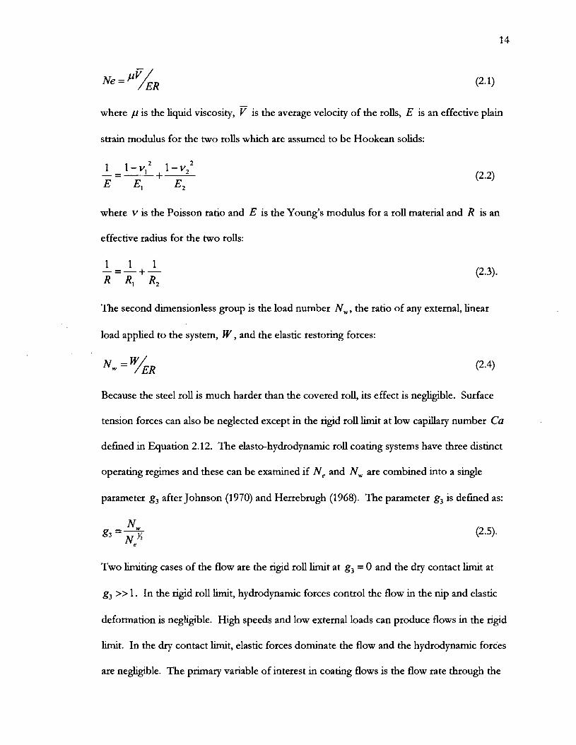
where ,u is the liquid viscosity, V is the average velocity of the rolls, E is an effective plain

strain modulus for the two rolls which are assumed to be Hookean solids:

where v is the Poisson ratio and E is the Young's modulus for a roll material and R is an

effective radius for the two rolls:

The second dimensionless group is the load number N,, the ratio of any external, linear

load applied to the system, W , and the elastic restoring forces:

Because the steel roll is much harder than the covered roll, its effect is negkble. Surface

tension forces can also be neglected except in the rigd roll limit at low capillary number Ca

defined in Equation 2.12. The elasto-hydrodynamic roll coating systems have three distinct

operating r e p e s and these can be examined if N, and N, are combined into a single

parameter g3 after Johnson (1970) and Herrebrugh (1968). The parameter g3 is defined as:

Two limiting cases of the flow are the rigid roll limit at g, = 0 and the dry contact limit at

g3 >> 1. In the rigid roll h i t , hydrodynamic forces control the flow in the nip and elastic

deformation is negligible. High speeds and low external loads can produce flows in the rigid

limit. In the dry contact limit, elastic forces dominate the flow and the hydrodynamic forces

are negligible. The primary variable of interest in coating flows is the flow rate through the

H roll nip, which can be expressed, in dimensionless form as - where H is the local gap

R

between the roll surfaces at the point in the nip where the maximum fluid pressure occurs.

Hooke (1986) has shown that the thickness of the roll cover material can influence the flow

if the ratio of the cover thickness b to the Hettzian contact half width a is less than 1 where

a is:

Herrebrugh (1968) solved the elasto-hydrodynamic lubrication flow between a rigid roll and

a roll with a semi-infinite thickness deformable cover, for large values of g, and a constant

viscosity liquid. Hall and Savage (1988) used improved numerical methods and obtained

similar results. Coyle (1988b) used a one-dimensional model for a finite thickness cover but

his model only produced qualitative predictions of the flow rate. Hooke (1986) produced

solutions for a wide range of loads and layer thicknesses. Coyle (1990) incorporated the

effects of nonlinear finite deformation of the elastic solid layer and also invesagated the

influence of a viscoelastic cover layer. The calculations by Bapat and Batra (1984) for dry

rolling contact of viscoelastic solids have shown that viscoelasticity is important. Carvalho

and Scriven (1994) used several one-dimensional spring models and a two-dimensional

model coupled with the lubrication approximation to study the deformable roll coating flow.

Carvalho and Scriven (1997a) employed finite element methods to study the two-

dimensional flow and roll cover deformation. Carvalho and Scriven (1997b) also performed

a perturbation analysis of the two-dimensional deformable roll coating flow.

2.1.2 Experimental Analyses

There is a vast body of experimental data concerning the flow in a narrow, fixed gap

between two rigid rollers Pitts and Greiller (1961), Savage (1982), Benjamin e t al. (1995).

However, many coating systems employ a deformable layer on one of the rollers. Crook

(1958) first measured the deformed gap profiles for a lubricated elasto-hydrodynamic

contact with a fixed extemal load. At high loads, a nearly parallel gap region forms between

the two roll surfaces over which the pressure profile is nearly Hertzian. Examples of the

surface profile are shown in Figure 2.1. In this figure, there was an initial 10 pm gap

between the roll surfaces and the flow rate was specified. As the load increases, the

hydrodynamic forces generated by dragging the liquid into the nip increase and overcome

the elastic restoring force of the deformable cover. The cover deflection increases and a

nearly parallel channel forms between the rolls.

Many investigators have performed experiments with constant extemal load

operation of the nip for Newtonian liquids. Smith and Maloney (1966) provide the most

extensive set of data that correlates the flow rate with the operating parameters. Swales e t al.

(1972), Vamam and Hooke (1977), and Coyle (1988a) have also presented empirical

correlations for the flow rate through the nip.

asing !ma1

\ \ 0

Elongated

Original surface

/ profile

-0.09 -0.06 -0.03 0 0.03 0.06 0.09

fie

Figute 2.1 Elasto-hydrodynamic gap profiles

Adachi et al. (1988) and Kang, Lee, and Liu (1991) presented coating thickness data

for squeeze roll nips. In this configuration, the rolls are engaged to create a particular

amount of deflection of the deformable cover and then held in place. These systems can

either have an initial gap between the roll surfaces, or be operated with a negative gap, or nip.

Benjamin (1994) examined both positive and negative fixed gaps for a deformable roll

operation where the d e t was flooded with a Newtonian liquid. He varied the roll speed

ratio and found that the film split ratio of the outgoing films had a much more significant

dependence on the roll speed ratio compared to similar conditions with two rigid rollers.

Cohu and Mangin (1997) measured the flow rate of Newtonian liquids for fixed

external loads. Their results agreed quantitatively with the finite element analysis by Coyle

(1988a) for a thick deformable cover. In their analysis, Cohu and M a n p (1997) also

accounted for the viscoelastic behavior of the cover material by using an elastic modulus that

depended on roll speed. Their results showed that when thin covers were used, the flow rate

was significantly reduced. m s may have been caused by reduced deflection of the cover.

2.2 Experimental Investigation

The purpose of the Newtonian liquid study was to establish an investigative

technique by comparing the results of flow rate and film thickness measurements to

published data. The ultimate goal was to examine the effectiveness of a new technique that

made it possible to measure the actual gap between the roll surfaces at the point within the

nip where the maximum fluid pressure occurred. No one has reported any attempts to

repeat or improve upon the measurements of the gap profile first made by Crook (1 958).

Since that time, investigators have relied mainly on scraping the coated film from the roll

surfaces and measuring its mass after a length of time, inferring flow rate from thls

measurement. These investigators have reported that incomplete scraping was a sigmficant

cause of error in their measurements. The gap measurement technique applied in this

investigation eliminated this error and was verified by measurements of the coated wet hlm

thickness. The gap measurement was supplemented with pressure profile and applied load

measurements.

2.2.1 Apparatus

Forward roll elasto-hydrodynamic coating flows were studied with a bench-top

apparatus. A schematic of the coating rig is shown in Figure 2.2. The device consists of two

rolls, both 12.7 cm in diameter and 20.3 cm wide, with 3.6 cm diameter shafts. One roll is a

steel tube that has a 2.5 cm thick shell and removable endplates. The other roll is solid steel

and has an elastomeric cover that is 6 rnm thick.

' Transducers

Figure 2.2 Experimental roll coating apparatus

The rolls are supported by pillow block b e a ~ g housings model PU-324 (Rexnord

Corp., Milwaukee, WI). Both of the rolls are fixed to a steel base plate, however, the

deformable roll is mounted on crossed roller slide tables, model NBT-6160 (Del-Tron

Precision Inc., Bethel, 0, allowing the roll to change its position with little friction. Two

pneumatic, rolling-diaphragm actuators, model S-4 (Marsh Bellofram Corp., Newell, WV),

one on each end, are used to load the deformable roll against the rigid roll. A hgh

performance regulator, model 960 (Marsh Bellofram Corp., Newell, WV), controls the

pressure in each cylinder. A force transducer, model ELA-B2E-250L Fntran, Fairfield, NJ

sandwiched between the tie-rod and the bearing housing post, monitors the load applied by

each actuator. A pair of 5.3 hp servomotors, model MGM-4120, with EN-214 drives

Fmerson, S t Louis, MO), rotate the rolls.

A personal computer-based data acquisition system was used to send roll speed

information to the drives and acquire data from the sensors. The signal from the pressure

transducer was removed from the roll via a slip ring assembly. The system uses a 16 channel,

12 bit, data acquisition board, model PCI-DAS-1002 (Measurement Computing, Middleboro,

MA), that can sample up to a total rate of 200 kHz with a 3 microsecond delay between

channels and has an analog to digital conversion resolution of 2.44 mV DC. The Visual

BASIC based graphical interface of SoftWIRE version 3.0 (SoftWIRE Technology,

Middleboro, MA), controls the data acquisition. Sampling is performed based on the

position of the roll from the feedback of the encoder in each motor with a resolution of up

to 2048 points per revolution.

2.2.2 Measurement Techniques

A non-contact, capacitance technique was used throughout the experiments to

determine the coated hlm thickness applied to the roll surface and the gap between the rolls.

The capacitance probe system used in the experiments was the Accumeasurem 5000

amplifier and the ASP-10-CTA and ASP-10-ILA capacitance transducers (MTI Instruments,

Latham, NY). The amplifier has a frequency response of 20 kHz and output noise level of

1.7 mV rms DC and has a linear response of &O.lO/o over 10 to 100% of the full scale range

of 0 to 10 V DC for either gap or dielectric me&- thickness changes. The 3rnm diameter

capacitance transducers have a range of 500 microns with a sensitivity of 50 microns/V and

an accuracy of 0.1% of the range.

Capacitance gauging is a reliable and convenient technique that has been used to

measure hlm thickness in other roll coating applications (Spiers et al. 1974, and

Tharmalingam and W i h s o n 1978 a and b). Crook (1958) used a capacitance technique to

measure the gap profile in an elasto-hydrodynamic system. Bohan et al. (2001) recently

applied a capacitance measurement coupled with an inductance sensor to immediately

remove the effect of roll eccentricity. Capacitance, and the resulting voltage, changes

'air proportionally to the thickness and dielectric constant, k = - , of the measured medtum. 5k"id

For this measuring system, the dielectric constant of the test liquid must be predetermined.

This was done according to parallel plate capacitor theory, by measuring the change in

voltage for a change in gap when the entire gap was filed with the test liquid. The

Newtonian test fluid used throughout the investigation was a mixture of two Dow-200

silicone oils. The physical properties, and the components by weight percent, of the test

liquid are shown in Table 2.1. Fluid density was measured by pycnometer and the surface

tension was measured with a DuNouy Ring. The fluid viscosity was measured with a Bohlin

CVO-50 cone and plate rheometer.

Table 2.1 Physical properties of Newtonian test fluid

P 0 k 'lo

Test Fluid &g/m3) ('h) (Pas)

Silicone Oil 1000 cst 10,000 cst

0.86 0.1 4 977 0.021 2.79 1.35

Because of construction limitations, the rolls and shafts have a certain amount of

run-out, or eccentricity, that caused the distance from the target to the probe surface to

change. The run-out of the deformable roll shaft is on the order of 40 pm and the run-out

of the rigid roll is on the order of 20 pm.

A piezoelectric pressure transducer monitored the pressure profile within the nip; the

rapid response of the piezoelectric material and integrated circuit make are ideal for this

application. The transducer was mounted in the shell of the rigid roll so that the sensor

surface was flush with the roll surface. The sensor, a model 105-C12 (PCB Piezottonics,

Depew, NY) is a miniature transducer with a diameter of 2.5 mrn. It has a resonant

frequency of 250 kHz and a range of +I000 psi with a sensitivity of 5.385 mV/psi and

linearity equal to 0.56% of full scale. The sensor requires a minimum 20 V DC to drive the

internal citcuitry of the sensor housing. Both the excitation voltage and the signal from the

sensor are passed between the roll and the signal conditioner via a slip ring assembly, model

IECU 12 (IEC Corp., Austin, TX) that has two silver-graphite brushes per ring.

2.2.3 Roll Cover

The roll cover material is polyurethane; model A-9 (Ait Products and Chemicals Inc.,

Allentown, PA), with a hardness of 70 Shore-A. Dynamic oscillatory measurements of stress

and strain in compression mode revealed that this material is quite viscoelastic. A sample of

the material was compressed at three different rates and the resulting stress and strain of the

material was tracked; the results are shown in Figure 2.3.

The change in the amount of deformation of the roll cover can also be measured on

the roll coating apparatus. The results shown in the following figure are plotted with values

of deformation predicted by Hertz contact theory using a Young's modulus of the cover as

El = 30 MPa. The range of contact times encountered during the experiments was between

0.005 and 0.01 1 seconds. Therefore, using El = 30 MPa as the modulus in the following

calculations is a reasonable approximation. Measurements of the Poisson ratio for materials

are difficult to obtain and the value used throughout the experiments and analysis was based

on fits to experimental measurements of the pressure profle in dry contact with a non-

Hertzian deformation approximation (Johnson, 1985). The estimated value was v = 0.49.

Strain

Figure 2.3 Stress vs. strain for the roll cover material

2.2.4 Experimental Procedure

The run-out of the roll surfaces caused each experiment to consist of a preliminary

run and test run. Air was the test medum in the preliminary run which was used to establish

the distance between the probe face and the target at various points around the

circumferences of the rolls. The test liquid was then added to the system in the test run and

the output voltage from the probes was obtained at the same points around the

circumference of the roll or shaft. The minimum gap and the wet film thickness of the test

liquid are proportional to the voltage difference between the baseline run and the run with

the test liquid. The procedure is presented schematically in Figure 2.4. After the

measurements were obtained, the roll speed was increased and more fluid was added to the

system.

v 2048 SAMPLES - RUN-OUT

CALCULATE V,, FOR 10 Revs

Figure 2.4 Schematic of the experimental procedure

Figure 2.5 is an example of the information obtained from the capacitance gauging

technique. After the test liquid is added to the system, it takes about 15-20 revolutions for

the system to reach equihbrium. The system remains at steady state for at least 60

revolutions before fluid is lost to the roll edges. All measurements were obtained within the

steady-state period. The figure also shows that the measurement of the actual gap at the

point of maximum fluid pressure in the nip corresponds with twice the measured 6lm

thickness.

--+ Film Measurement

0 40 80 120 160

Revolution Number

Figure 2.5 Measured gap width and film thiclcness

2.3 Theoretical Investigation

The forward mode, Newtonian, elasto-hydrodynamic roll coating flow was analyzed

with a lubrication approximation based mathematical model. This analysis has been carried

out many times before with various methods for treating the deformation of the roll cover

including both Hertzian contact and various spring models as well as with a viscoelastic

model for the roll cover material. The model in this analysis used non-Hertzian contact

theory for a finite thickness cover, a method &st suggested by Johnson (1985). This analysis

is unique in that the position of the deformable roll is allowed to change with the operating

conditions and a visco-capdlary boundary condition is employed at the film split. Previous

models fixed the positions of the rolls such that a small initial gap or nip was maintained

between the rolls and the resulting elasto-hydrodynamic equilibrium state was allowed to

develop. Figure 2.6 is a schematic of the flow domain.

Figure 2.6 Flow domain for the lubrication model

The liquid is taken to be Newtonian and incompressible. The roll radri are much

larger than the distance between the roll surfaces, therefore the flow in the gap region is

nearly rectilinear and the governing Navier-Stokes system of differential equations can be

simplified to the lubrication approximation Cameron (1976). The pressure profile through

the gap is given by:

where V is the average roll speed, Ho is an initial gap or engagement, and H(x) is roll

surface profile which is well approximated as a parabola in the nip region:

In equation 2.8, D(x) is the local deformation of the roll cover, which is dependent on the

fluid pressure and the Poisson ratio after Johnson (1985):

where b is the thickness of the roll cover. This model for deformation does not account for

shear stresses in the cover or the effects of neighboring deformations. It is also difficult to

use this expression for incompressible materials, such as roll covers, when the Poisson ratio

approaches v = 0.5. Carvalho and Scriven (1997a), suggest that this relation cannot be used

when computing elasto-hydrodynamic roll coating flows because of the large deformations

encountered. They have proposed a one-dimensional spring model as well as a plane strain

model to describe cover deformation and solved the full two-dimensional flow and

deformation problem via the hnite element method. Equation 2.7 is integrated with an

implicit Euler method.

A relatively simple but important aspect of the model is the inclusion of a film-split

at the nip exit. The split-point is made to depend on the viscous and capillary forces via a

visco-caprllary boundary condition for the pressure. At the split-point the capillary pressure

in the liquid is given by:

where a is the surface tension of the liquid and r is the radius of curvature of the film-split

meniscus. The radius of curvature is given by:

where Qis the total flow rate through the nip and Ca is the capillary number defined as:

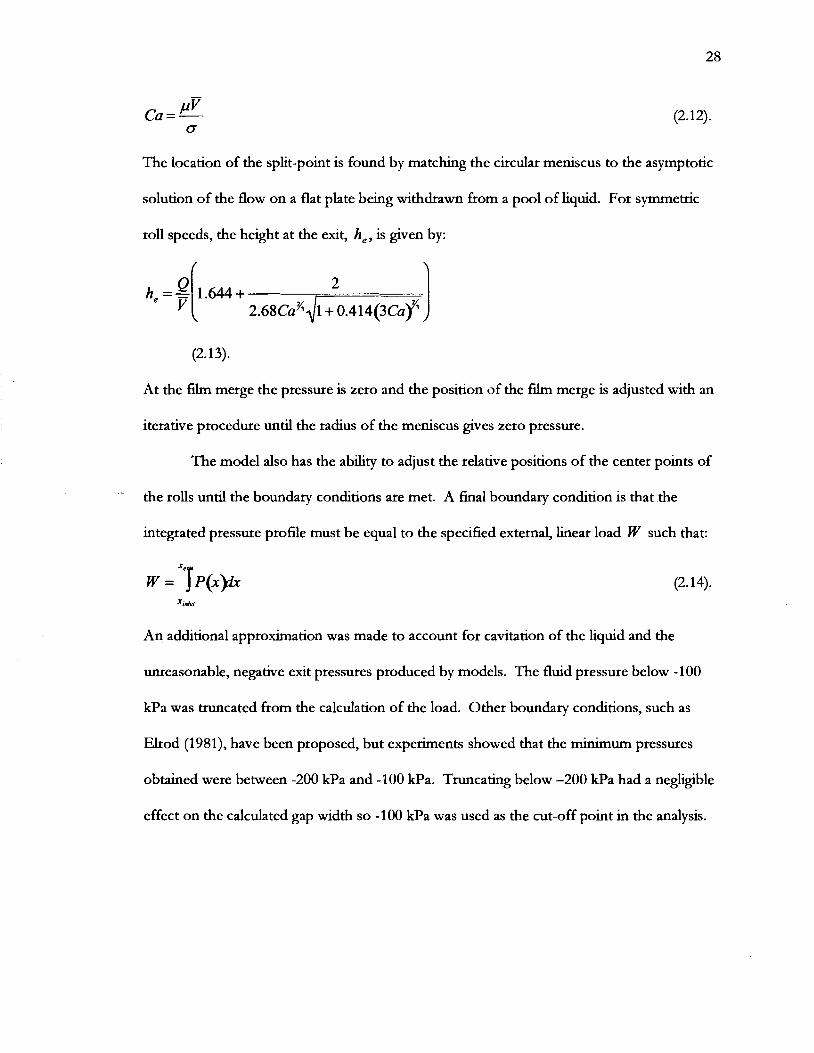
The location of the split-point is found by matching the circular meniscus to the asymptotic

solution of the flow on a flat plate being withdrawn from a pool of liquid. For symmetric

roll speeds, the height at the exit, he, is given by:

(2.1 3).

At the frlm merge the pressure is zero and the position of the hlm merge is adjusted with an

iterative procedure until the radius of the meniscus gives zero pressure.

The model also has the ability to adjust the relative positions of the center points of

' ' the rolls until the boundary conditions are met. A final boundary condition is that the

integrated pressure proiile must be equal to the specified external, linear load W such that:

An additional approximation was made to account for cavitation of the liquid and the

unteasonable, negative exit pressures produced by models. The fluid pressure below -100

kPa was truncated from the calculation of the load. Other boundary conditions, such as

Elrod (1981), have been proposed, but experiments showed that the minimum pressures

obtained were between -200 kPa and -100 kPa. Truncating below -200 kPa had a negbble

effect on the calculated gap width so -100 kPa was used as the cut-off point in the analysis.

2.4 Results and Discussion

The pressure is presented in dimensionless form and scaled with the elastic

deformation of the roll cover as:

The thickness of the roll cover was used in the scaling to include the effects of a finite

thrckness cover. Figure 2.7 shows examples of the pressure profiles obtained from the

piezoelectric ttansducer for three extemal loads given as the load number Nw at one roll

speed and fluid viscosity Ne. Each point is the average of ten measurements and the curves

X have been shifted so that the pressure peak occurs at - = 0. As the dry contact h t is

R

approached, at hgh Nw, the gap between the rolls decreases and the magnitude of the

pressure peak increases. When conditions near the rigid roll limit, the pressure profile

becomes more symmetric; the gap increases and nip length decreases, as the roll surfaces are

forced apart.

In Figure 2.8, the applied load is held constant and pressure profiles for four

combinations of viscosity and roll speed are plotted. As Ne increases, the maximum

pressure in the nip increases and the nip length decreases because the system is operating

near the rigid h t and viscous forces dominate. If the rolls were fixed in position, there

would be a large amount of cover deformation, however, because the extemal load is fixed,

the large viscous force results in an increase in the gap and a small cover deflection.

Nearly dry contact

Ne =4.3 x 10 -'

Nearly rigid/ roll behavior

Pmin decreases as Nw Increases

Figure 2.7 Pressure profiles at constant speed

Conversely, as the roll speed decreases, viscous forces diminish, the gap width decreases, and

the deformation of the cover increases because the external load dominates the restoring

force of the cover material.

Figure 2.9, is a comparison of the integrated pressure prohles measured by the

piezoelectric transducer with the force per unit length measured by the force transducers on

either end of the deformable roll shaft. The integrated areas, for the entire range of roll

speeds, are within 10% of the ltne loads for the range of conditions in the tests and the

effect of the convolution of the pressure signal with nip length is minimal.

P, increases with Ne Ne = 0.43 x 10 -6

N e s 0 . 8 6 ~ 10 -6

Ne = 0.22 x 10 -6

Nw = 6 . 8 ~ 10

Figure 2.8 Pressure profiles at constant load

1000

Load Cells (Nlm)

100

Figure 2.9 Integrated pressure profiles compared to measured load

I ! I I , ,

Figure 2.10 compares the measured pressure profiles with the prediction of the

lubrication model for two sets of conditions. The conditions for the comparisons are listed

in Table 2.2. For the two condtions compared, the predicted profiles are in excellent

agreement with the measured profiles. This is rather remarkable for such a simple model

because of the limitations introduced by the non-Hertzian contact deformation model.

Even though the model captured the cover deformation well, it limited results to low applied

loads.

Table 2.2 Conditions for the model and compared experiments

Parameter High Load Model Experiment

Dimensionless

Low Load Model Experiment

Dimensional

The results indtcate that the non-Hertzian contact model and the requitement that

0.021

the roll positions be changed to accommodate the visco-capillary boundary condition can

0.02

accurately represent an elasto-hydrodynamic coating system for low applied loads where the

deflection of the cover is small. It is important to note that the results of the calculations

have the portion of the negative pressure peak below -100 kPa subtracted from the load

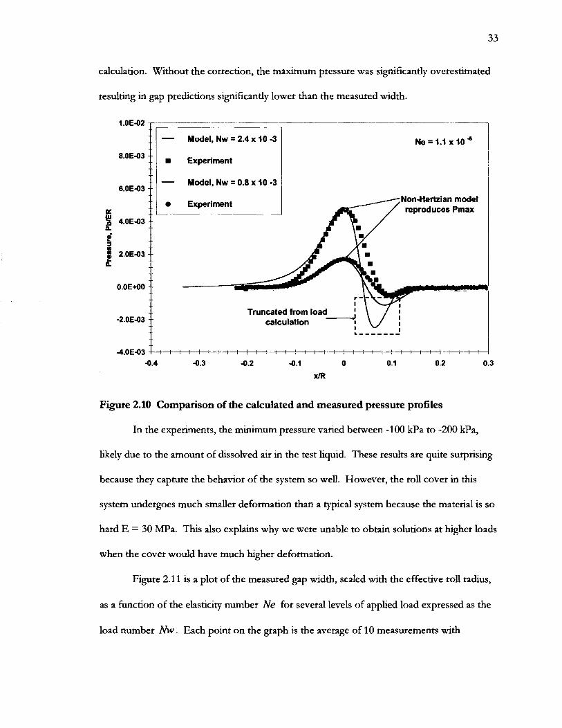
calculation. Without the correction, the maximum pressure was significantly overestimated

resulting in gap predictions signtficantly lower than the measured width.

-

- Model, Nw = 2.4 x 10 -3

Experiment

- Model, Nw = 0.8 x 10 -3 / Experiment Non-Hertzian model

reproduces Pmax Experiment NonHertzian model

reproduces Pmax

Figure 2.10 Comparison of the calculated and measured pressure profiles

In the experiments, the minimum pressure varied between -100 kPa to -200 kPa,

likely due to the amount of dissolved air in the test liquid. These results are quite surprising

because they capture the behavior of the system so well. However, the roll cover in this

system undergoes much smaller deformation than a typical system because the material is so

hard E = 30 MPa. This also explains why we were unable to obtain solutions at higher loads

when the cover would have much higher deformation.

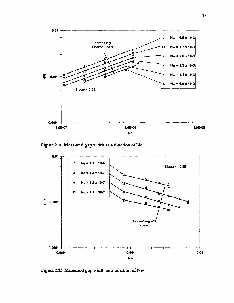
Figure 2.1 1 is a plot of the measured gap width, scaled with the effective roll radius,

as a function of the elasticity number Ne for several levels of applied load expressed as the

load number Nw . Each point on the graph is the average of 10 measurements with

deviations from the mean of less than 1 pm. The operating conditions are presented in

Table 2.3.

Table 2.3 Experimental operating conditions

Parameter Dimensional Dimensionless

Increasing the roll speed strengthened the effect of the viscous forces and caused the rolls to

separate and sustain higher flow rates through the nip. Increasing the applied load overcame

the viscous forces and reduced the gap width. The sensitivity of the gap width to the

elasticity number is represented in terms of the slope of the best-fit h e . The slope is less

than 1 so a large change in roll speed is requited to make a sipficant change in the gap

width.

The effect of the applied load on the gap width is plotted in Figure 2.12 as a function

of the load number at several levels of Ne . As the load is increased, the viscous forces are

overcome and the gap decreases. The conditions that were tested indicate that the gap width

is even less sensitive to applied load than to the roll speed. Both of these trends make the

roll coater with a deformable cover robust and relatively easy to install and operate because

of the insensitivity to process perturbations.

0.01 --

external load Nw=1.7xlO-3

+ NW = 2.6 x 10-3

x Nw=3 .5~10 -3

$ 0.001 NW = 5.1 x 10-3

Ne

Figure 2.11 Measured gap width as a function of Ne

Increasing roll speed

o Ne= l . l x lO-6

A Ne=4.4x10-7

* Ne = 2.2 x 10-7

Ne= l . l x lO-7

Figure 2.12 Measured gap width as a function of Nw

\ Slope - - 0.39

The best-fit lines in the preceding two figures were obtained by fitting all of the data

to an empitical relation. The dimensionless gap width, or flow rate, H/R, can be fit with the

equation:

Equation 2.16 can be rearranged to show the dependence of the gap on the operating

variables, input in MKS units, as:

H = 0 . 4 2 b ~ ) ~ ~ ~ d 3 9 ~ - 0 . l 6 ~ 0 . 8 1 (2.17).

It should be noted that only one value of roll radius and a single value of elastic modulus

were used throughout the experiments and in the fitting procedure. Therefore, it can't be

conhrmed that the inhcated dependencies on these two quantities are true. However, 95%

of the data agree within f 5% of the empirical correlation. The empitical correlation is

compared with the experimental data in Figure 2.13.

0.001

Experimental Data. HIR

Figure 2.13 Best-fit of experimental data

In the next figure, 2.14, the experimental data are plotted in terms of a modified

H elasticity number, - ~ e - ' . ~ so that they can be compared with published data. Throughout

R

the analysis, a single value of the elastic modulus of the roll cover was used. Even though

dynamic oscillatory tests on the cover show that it behaves viscoelastically, the

measurements indicate that the gap width is relatively insensitive to the viscoelastic behavior

of the cover in the speed ranges tested. Cohu and Mangin (1997) made a similar conclusion.

The data are in very good agreement, in terms of the magnitude of the gap, with the

analysis of Herrebrugh (1968). The difference between the two sets of data appears in the

sensitivity to the load parameter. The experimental data are more sensitive to the applied

load. A possible cause of the difference between the two sets is the thin rubber cover that

was used. Cohu and Mangin (1997) have shown increased sensitivity to load when the ratio

of the cover thickness to half the nip length approaches 1.

The gap width measurements are in very good agreement with the experimental data

of Smith and Maloney (1966). They used a thick, deformable cover in their experiments. At

high loads, the experimental data begm to diverge from the correlation of Smith and

Maloney (1966) which is more evidence supporting the influence of the cover thickness.

Figure 2.14 Comparison with published data

10 :: 7

m z x C I

1 --

0.1

The data show similar sensitivity to the applied load when compared with the

Herrebrugh 1968

Coyle 1988a FEM Cohu and Mangin 1997

Smith and Maloney 1966

1

experimental measurements and h t e element calculations of Coyle (1988a). However,

0.0001 0.001 0.01

1 0.1

Nw

agreement in terms of magnitude is poor. Coyle (1988a) attributed the discrepancies

between his data and other published data, to the influence of the viscoelasticity of the

deformable cover. The measurements of flow rate by Cohu and Mangm (1997) agree with

the finite element calculations of Coyle (1988a). The data of Adachi et al. (1988) are not

plotted because of an unreliable measurement of the elastic modulus of the cover material

used in the analysis of their experimental measurements. The data in Figure 2.14 are

summarized, in Table 2.4.

Table 2.4 Empirical relations for the gap width

Experiment 1 0.42 0.55 0.55 -0.39 -0.16 0.84

Smith and Maloney, 1966 1 0.64 0.58 -0.34 -0.35 0.58

Herrebrugh, 1968 1 3.12 0.6 0.6 -0.2 -0.4 0.6

Coyle, 1988a FEM I 0.4 0.6 0.6 -0.3 -0.3 Cohu and Mangin, 1997

0.7

Coyle, 1988a Exp. 1 4.1 0.49 0.49 -0.43 -0.41 0.42

Further comparison of the gap width measurements are made with the mo-dimensional

h t e element analysis of Carvalho and Scriven (1997a). The sensitivity of the measured gap .

width to the load parameter is in very good agreement with the calculations where the

exponent is equal to -0.39.

Throughout the experiments, the speed ratio between the rolls was maintained at

v 2 = 1. In the lubrication equation, the average roll speed is used to predict the gap v,

between the rolls so in effect it d scale it to a set of roll speeds with a ratio of 1. However,

the experiments of Benjamin et al. (1994), showed that the film split ratio was much more

sensitive to the roll speed ratio, for a deformable roll system, compared to two rigid rolls

operating with a small gap between the roll surfaces. Contrary to thls conclusion, Kang, Lee,

and Liu (1991) found the film-split ratio for a fixed engagement, deformable roll system to

be relatively insensitive to the roll speed ratio. Future experiments should consider the roll

speed ratio as an independent variable.

2.5 Summary

The experiments and calculations from the lubrication model, with symmetric roll

speeds for Newtonian liquids in an applied load, deformable, forward roll coating system are

summarized as follows:

A bench-top apparatus was constructed to study elasto-hydtodynamic forward roll

coating flows.

A technique was developed and applied to measure the gap between the roll surfaces.

Measurements of the gap corresponded with the expected value at the point of

maximum fluid pressure within the nip and the measured wet hlm thickness.

The measured gap and its sensitivity to the external load and roll speed were

consistent with published experimental data and theoretical analyses.

There was some evidence of increasing sensitivity to the applied load caused by the

influence of the thin, deformable roll cover used in the experiments.

A model of the deformable roll coating system was developed based on the

lubrication approximation with non-Hertzian deformation of the roll cover and a

visco-capillary boundary condition at the &-split.

The lubrication model reproduced the maptude and shape of the measured

pressure, for low external loads, after values of the negative pressure below -100 kPa

were removed from the calculations.

3 VISCOELASTIC COATING FLOWS

3.1 Introduction

Previous investigations of roll coating flows have focused on two roll systems with a

fixed rigid gap between the roll surfaces. These systems were operated in either forward or

reverse mode and used a Newtonian test liquid. These works described the dependence of

the coated wet film thickness on the fluid properties and operating variables. Much

attention was given to the stability of the system and documenting the appearance of the

three-dimensional ribbing instability as a function of the fluid properties and operating

conditions.

Many industrially important coating liquids are non-Newtonian, however. In many

0 .

cases, polymers are added to the coating liquid to modify its viscosity or to act as a bindmg

aid for some other component of the liquid. Often, a molten polymer is applied to a

substrate. These liquids exhibit viscoelastic behavior in the roll coating environment. The

viscosity of the liquids is often shear-rate dependent. The behavior of the liquid in a

particular coating system is often dependent on past deformation events. In some instances,

adding only a small amount of polymer to the coating liquid caused a dramatic reduction of

the stable operating window. Consequently, much of the current research has focused on

the appearance of defects, with the presence of polymer additives, in flows between rig~d roll

systems. Triantafilopoulos (1996) and Glass and Prud'homme (1 997) present recent

discussions of the effects of coating liquid rheology in various coating systems.

A system that is used widely throughout the coating and printing industries involves

the use one or more deformable rolls to apply and meter a thin film onto a substrate. The

deforrnable roll coating system is simple to operate and relatively insensitive to process

perturbations and mechanical tolerances. Surprisingly, little has been published, either

experimental or theoretical, that documents how the viscoelastic behavior of the coating

liquid affects the deformable roll coating system.

3.1.1 Theoretical Analyses

Most past theoretical analyses attempted to simulate non-Newtonian behavior by

including shear rate dependence of the viscosity in the calculations of flows in rigid roll

systems. There have been few attempts to include elastic effects in flow models because of

the complexity added to the calculations and the lack of an appropriate fluid model that can

adequately describe observed behavior. The available models often describe one behavior

well but cannot describe all of the behaviors exhibited by a liquid in a typical roll coating

geometry. The wide variety of choices makes it difficult to compare one set of results to . .

another. However, some attempts at viscoelastic calculations in rigid roll coating systems

have been made. Tanner (1960) and Greener and Middleman (1975) examined small

viscoelastic effects by including first order terms in a Weissenberg number expansion of the

lubrication approximation for the flow between two rigid rollers. Tanner used a co-

rotational derivative in the Maxwell model and Greener and Middleman used an empitical

constitutive relation to describe viscoelastic effects. They observed decreased pressures and

reduced separating forces at small Weissenberg numbers.

Davies and Walters (1973) analyzed journal-bearing flow. This system, the flow

between two eccentric cylinders with the inner rotating, is similar to the roll coating system

and can be described by the lubrication approximation. Davies and Walters used several

non-linear models and an Oldroyd model with a Jaumann derivative to describe viscoelastic

effects. They observed that when the normal stresses are much larger than the shear stress,

the journal bearing was able to support increased loads, compared to the Newtonian case, at

small eccentricity. Beris et al. (1984) used finite element methods, with a variety of fluid

models, to simulate the viscoelastic joumal-bearing flow. They explored a range of Deborah

numbers at low eccentricity to determine the family of stable solutions. The load bearing

capacity was not reported. They extended their work to higher levels of eccentricity in Beris

et al. (1 9 86).

3.1.2 Experimental Analyses

Fukushima (1976) observed markedly different ribbing patterns in flows of butter

and printing inks. Glass (1978a-d) performed extensive studies of industrial paint

formulations, developing a connection between a rheological property, called "dynamic

uniaxial extensional viscosity" and the appearance of ribbing defects. Matsuda and Brendly

(1979) found that coatings with hlgh degrees of shear-thinning behavior increased rib

amplitude. Doremus and Piau (1 981,1983) measured reduced flow rates and larger

separating forces for flows of viscoelastic liquids with high extensional viscosity; however,

the gap to diameter ratio used in these experiments is approximately 3 orders of maptude

larger than industrial coating systems and the results may not be applicable. Bauman et al.

(19823 found that addtng a small amount of polymer to the forward roll coating system

dramatically reduced the maximum speed at which the ribbing defect occurred. Soules et al.

(1988) showed that a polymer additive with a rigid backbone and low extensional viscosity,

only slightly exaggerated ribbing behavior. Fernando and Glass (1988) studied a variety of

polymer additives that had similar steady shear viscosities but a wide range of extensional

behavior. The appearance of ribbing at lower roll speeds correlated with increasing

extensional viscosity. Kang, Lee, and Liu (1991) observed that viscoelasticity increased both

the coating thickness and its sensitivity to roll speed in a fixed engagement, deformable roll

system. Large ribbing defects were also observed. Dontula ei al. (1996) observed reduced

critical capillary numbers for the onset of ribbing with dilute solutions of polymers having

different molecular conformations. Both solutions had constant shear viscosities, no

measurable elastic properties, and large extensional viscosities. The flow at the film-split was

observed to be different from Newtonian flow. Lopez ei a[. (2002) examined the effects of

polymer additives on the ribbing instability in an eccentric, rotating cylinder system. For low

polymer concentrations, a small reduction in the critical capillary number was observed. At

large concentrations, the critical capillary number remained constant for inelastic fluids,

while elastic fluids caused it to decrease. A strong effect of elastic properties was observed

on ribbing amplitude.

A two roll interface with one roll having a deformable cover commonly occurs in

printing press ink trains. Misting has been correlated with the pressure at the nip exit. The

pressure at the nip exit is also related to a property of the ink known as "tack" (Reed (1937),

Zang ei al. (1 99l), Aspler and Taylor (1 99l), Aspler ei a[. (1 994), and Pate1 and Dealy (1 987)).

Measurements with inks containing dissolved polymers produced the highest tack values.

Adding polymer molecules to ink solutions increased the sensitivity of tack to the film

thickness in the nip. Bohan ei al. (2001) made dynamic measurements of ink film thickness,

pressure, and temperature in rolling nip contacts. They observed that the magnitude of the

sub-ambient pressure at the nip exit with flows of shear-thinning inks, was larger than the

Newtonian fluids tested.

The metered size press coater is commonly used in paper coating and it has the

potential to encounter misting defects, (Roper et a/. (1 997), Gron et a[. (1 998), and Roper ei al.

(19991, Voet (1956), Miller and Myers (1958), Myers and Hoffmann (1961), Christiansen

(1 995) MacPhee (1 997), and Blayo ei al. (1 998)). Poranen ei a/. (2000) observed that when

highly elastic starch molecules were added to the coating liquids with suspended pigment

particles, higher metering rod loadmg was needed to produce a particular wet hlm thickness.

Alsonso and Tanguy (2001) reported that the rheological behavior of the coating liquid

affected misting in a metered size press coater.

Williamson et al. (1997) conducted experiments with polymer-modified oils in a

journal bearing geometry. They observed that the load bearing capacity, the extra load

requited to produce a hlm thickness, increased with the relaxation time of the polymer

modified oils.

The results of past work indicate that non-Newtonian rheology does influence the

process in qualitative ways, but experiments where loads, gap, and pressure profile are

measured for well-characterized rheology are non-existent. The work summarized in this

chapter is intended to add this information to the literature.

3.2 Experimental Investigation

3.2.1 Viscoelastic Fluids

The objective of this study was to study the elasticity of the test liquid independent

of shear-thinning behavior. The tool most commonly applied for this purpose is a fluid that

has constant, steady shear viscosity but also has elasticity, Boger (1977). The Boger fluid

exhibits nearly constant viscosity in steady shear because of the small amount of dissolved

polymer it contains. However, because the dissolved polymer is very hlgh molecular weight,

it exhibits increasing normal stresses with shear rate in steady shear flow. Adding more

polymer to the solution can gradually introduce shear-thinning behavior.

The viscoelastic liquids used in this study were solutions of polyisobutylene (PIB) in

a mixed solvent of kerosene (KJ and polybutene. The PIB was obtained from Aldrich

Chemical Company. It had a quoted molecular weight of 4,800,000 g/mol and a density of

918 kg/m3. Small pieces of the PIB were dissolved in kerosene with mild stirring for 3 days.

The stock solution had a concentration of 3.4% by weight. The stock solution was diluted

with a mixture of low molecular weight polybutenes , MW - 750 g/mol (PB 750) and MW

- 320 g/mol (PB 320), also from Aldrich Chemical Company. The solution was stirred

mildly for three additional days to ensure thorough mixing. The preparation and mixing

procedure used in this study followed the methods presented by Nguyen and Sridhar (1990).

Preparation methods for alternative, water-based, model elastic liquids with polyacrylamide,

Prilutski ei al. (1983) or polyethylene oxide, Dontula et al. (1998) are also available. Water

based solutions were not used because of the strong dependence of capacitance, the primary

indicator of £ilm thickness, on concentration.. The physical properties and components by

weight percent of the model fluids are given in Table 3.1.

Table 3.1 Physical properties of the test liquids

Silicone Oil 1000 cst 10,000 cst

0.86 0.14 977 0.021 2.79

Boger Fluids PIB PB 320 PB 750 K

0.0012 0.3720 0.558 0.0697 857 0.028 2.24 0.0024 0.3710 0.557 0.0696 858 0.028 2.24 0.0036 0.3709 0.556 0.0695 858 0.029 2.23

Elastic, Shear-thinning Fluids PIB PB 320 PB 750 K

The steady shear and oscillatory flow behavior of the test liquids were characterized

with a cone and plate, Bohlin CVO-50 controlled stress rheometer (Bohlin Instruments Inc.,

East Brunswick, Nn. The CVO-50 permitted measurements of the apparent viscosity rl@)

with shear rate )'and, for small amplitude oscillations, the dynamic viscosity $(@)and the

dynamic ng~dity ~ ' ( o ) with applied frequency o . The simple shear flow information was

obtained for both the non-Newtonian solutions and their Newtonian solvent components.

The apparent viscosity of the test fluids is shown in Figure 3.1 and Flgure 3.2.

I A 0.12% PIB I

1 .OE02 1 .OE-O1 1 .OE+M) l.OE+Ol 1 .OE+02 1 .OE+03

Shear Rate (11s)

Figure 3.1 Apparent viscosity of the Boger test fluids

Adding more polymer molecules to the Newtonian solvent was intended to create

different levels of elasticity and shear thinning. The elastic modulus of the test liquids is

presented in Flgure 3.3. Adding polymer caused the zero-shear viscosity to increase as well.

During the steady shear measutements, instability in the flow in the cone and plate

rheometer limited the maximum shear rate at which data could be obtained. The instability

manifested itself as a tendency of the test fluid to climb out of the gap from between the

cone and plate, then onto the cone. Steiert and Wolff (1990) observed similar behavior.

The cause was attributed to the buildup and breakdown of fluid structure through transient

network formation Sridhar (1990). Measurements of apparent viscosity at higher shear rates

were not available.

1 0.45% PIB 0.62% PIB I I x Solvent (0.45%) x Solvent (0.62%)

l.OE-02 : I I 1 3 1 1 1 1 1 I 7 1 1 1 1 1 1 1 6

1 .OE-02 1 BE-01 1 .OE+OO l.OE+Ol 1 .OE+02 1 .OE+03

Shear Rate (11s)

Figute 3.2 Steady shear viscosity for the shear-thinning liquids

Increasing the polymer content above 0.36% PIB required the solutions to be altered.

For the 0.45% PIB solution, the amount of PB 750 was decreased and PB 320 was increased,

to create a solution with an apparent viscosity in a useable range. It was not possible to mix

the solution when the polymer content was increased to 0.62% without increasing the

amount of K in the solution. This solution showed the intended increased shear-thinning

behavior but at the cost of altered elastic properties; changing the ratio of K to PB caused

the elasticity of the solution to be less than intended, as shown in Figure 3.3.

1 .OE-04 1 .OEQ3 1 .OE-02 1 .OE-Ol 1 .OE+OO 1 .OE+Ol l.OE+O2

Frequency (11s)

Figure 3.3 Elastic modulus G' vs. frequency of PIB solutions

Measurements of the normal stress and extensional viscosity of the test liquids were

not available. However, each of the liquids exhibited the Weissenberg effect, or rod

climbing, during mixing; the tendency to climb the stitring rod increased with polymer

content indicating increased elasticity. The CVO-50 was not able to reach a frequency small

enough to achleve a terminal slope of 2 for the elastic modulus. A wide spectrum of

relaxation times may be caused by the polydispersity of the PIB.

The commercial software package POLYMAT, (Fluent Inc. Lebanon, NH), was

used to determine the Carreau model parameters in steady shear. The Carreau model is

defined as:

In the model, n is the power-law index, ~,l(3) is the apparent viscosity, ?,lo is the zero-shear

viscosity, 77, is the infinite shear rate viscosity, y is the shear rate, and z is the inverse of

the shear rate at which the power-law behavior begms. The Carreau model parameters and

components by weight percent of the test liquids at 23' C are presented in Table 3.2.

Table 3.2 Caneau model parameters

Silicone Oil 1000 cst 10,000 cst

0.86 0.14 1.35

Boger Fluids PIB PB 320 PB 750 K

Elastic, Shear-thinning Fluids PIB PB 320 PB 750 K

0.0045 0.556 0.370 0.0695 0.84 0.1 5 0.88 1.12 0.0062 0.5191 0.3461 0.1286 0.92 0.09 0.81 - -- 1.35

Because the temperature of the lab varied throughout the day the temperature of the

test liquid, and its viscosity, varied too. In order to remove the temperature dependence

from the analysis, the viscosity of the test liquid at the test conditions was used in the

analysis. To determine the viscosity at a particular set of test conditions, the simple shear

flow properties of the fluids were measured at 20°, 23O, and 25O C. The steady shear

viscosity of the fluids was found to obey an Arenhius relationship with temperature. The

viscosity of the test liquid at a particular conhtion could be calculated by multiplying a

reference viscosity with the maptude of a shifting function H(T) defined as:

where H(T) followed an Arhenius expression:

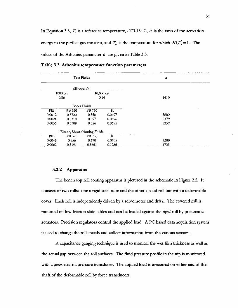
In Equation 3.3, T, is a reference temperature, -273.1S0 C, a is the ratio of the activation

energy to the perfect gas constant, and T, is the temperature for which H ( T ) = 1 . The

values of the Arhenius parameter a are given in Table 3.3.

Table 3.3 Arhenius temperature function parameters

Test Fluids a

Silicone Oil 1000 cst 10,000 cst

0.86 0.14

Boger Fluids PIB PB 320 PB 750 K

Elastic, Shear-thinning Fluids PIB PB320 PB 750 K

0.0045 0.556 0.370 0.0695 4280 0.0062 0.5191 0.3461 0.1 286 4733

3.2.2 Apparatus

The bench top roll coating apparatus is pictured in the schematic in Figure 2.2. It

consists of two rolls: one a rigid steel tube and the other a solid roll but with a deformable

cover. Each roll is independently driven by a servomotor and drive. The covered roll is

mounted on low friction slide tables and can be loaded against the rigid roll by pneumatic

actuators. Precision regulators control the applied load. A PC based data acquisition system

is used to change the roll speeds and collect information from the various sensors.

A capacitance gauging technique is used to monitor the wet film thickness as well as

the actual gap between the roll surfaces. The fluid pressure profile in the nip is monitored

with a piezoelectric pressure transducer. The applied load is measured on either end of the

shaft of the deformable roll by force transducers.

3.2.3 Procedure

The run-out of the roll surfaces caused each experiment to consist of a

preliminary run and a test run. Air was the test medum in the preliminary run which was

used to establish the distance between the probe face and the target at various points around

the circumferences of the rolls. The test liquid was then added to the system in the test run

and the output voltage from the probes was obtained at the same points around the

circumference of the roll or shaft. The minimum gap, and the wet film thickness of the test

liquid, is proportional to the voltage difference between the baseline run and the run with

the test liquid. The procedure is presented schematically in Figure 2.5. After the

measurements were obtained, the roll speed was increased and more fluid was added to the

system.

3.3 Theoretical Investigation

A commercially available finite element software package, POLYFLOW (Fluent Inc.,

Lebanon, NH) was used to study the flow of viscoelastic fluids in a rigid roll coating

geometry. An initial attempt at incorporating an Oldroyd-B fluid model in the Newtonian

lubrication model was made, but with limited success. Due to the limitations of the

boundary conditions available in the commercial software, the flow domain had to be

modeled as a fixed position, rigd roll system. Two non-Newtonian fluid models were used

in the study. The Oldroyd-B model was used to study purely elastic behavior and a Giesekus

model was used to study the combined effects of viscoelasticity and shear thinning. The

governing momentum equation, excluding gravitational effect but includmg inertial terms is:

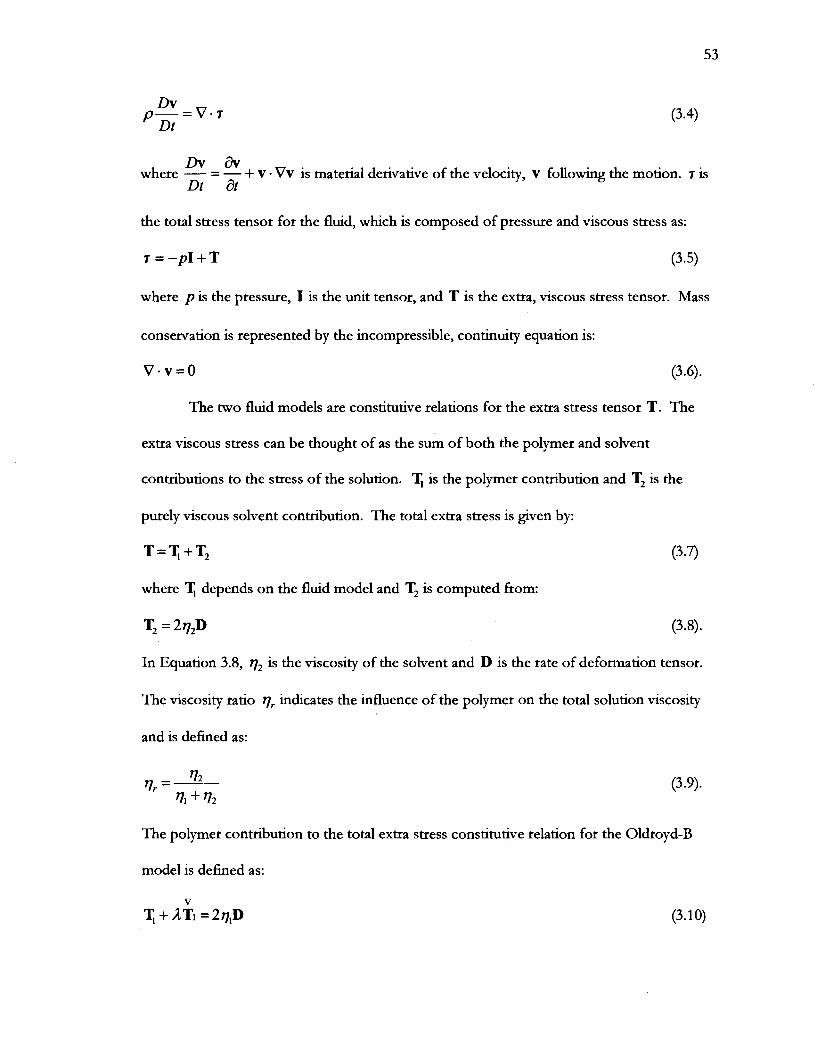
Dv av where - = - + v . VV is material derivative of the velocity, v following the motion. T is

Dt at

the total stress tensor for the fluid, which is composed of pressure and viscous stress as:

T = - p I + T (3-5)

where p is the pressure, I is the unit tensor, and T is the extra, viscous stress tensor. Mass

conservation is represented by the incompressible, continuity equation is:

V - v = O (3.6).

The two fluid models are constitutive relations for the extra stress tensor T. The

extra viscous stress can be thought of as the sum of both the polymer and solvent

contributions to the stress of the solution. T, is the polymer contribution and T2 is the

purely viscous solvent contribution. The total extra stress is given by:

T=T,+T2

where 'I; depends on the fluid model and T2 is computed from:

T2 = 2q2D (3.8).

In Equation 3.8, 77, is the viscosity of the solvent and D is the rate of deformation tensor.

The viscosity ratio 77, indicates the influence of the polymer on the total solution viscosity

and is defined as:

The polymer contribution to the total extra stress constitutive relation for the Oldroyd-B

model is defined as:

where A is a relaxation time constant of the material and the upper convected time

derivative of the viscoelastic extra stress and it is defined as:

The constitutive relation for the viscoelastic extra stress in the Giesekus model is given by:

where a is a material constant related to the interaction between polymer molecules.

The values for the material parameters and the components of the test fluids by

weight percent, at T = 23' C, are presented in Table 3.4. The total solution viscosity and the

solvent viscosity were measured on the Bohlin CVO-50 constant stress rheometer. The

values for a and A were determined by fitting the fluid models to the steady shear and

dynamic oscillatory measurements. The fitung algorithm, which minimizes the difference

between the measured value and fitted value, is described in the POLYMAT user guide. The

information for the zero-shear viscosity and the solvent viscosity were fixed as parameters.

An initial guess for the relaxation time, equal to the inverse of the frequency where the

elastic and viscous moduli were equal, was used to begin the iterations. It should be noted

that the relaxation times listed in Table 3.4 are fitted values and not measured directly.

Table 3.4 Fitted model parameters for the viscoelastic test fluids

' l r 'l ' l2 k a Test Fluids as as) (4

Boger Fluids PIB PB 320 PB 750 K

0.0012 0.3720 0.558 0.0697 0.5 0.69 0.35 0.01 0.0024 0.3710 0.557 0.0696 0.4 0.86 0.35 0.04 0.0036 0.3709 0.556 0.0695 0.26 1.38 0.35 0.96

Elastic, Shear-thinning Fluids PIB PB 320 PB 750 K

0.0045 0.556 0.370 0.0695 0.1 8 0.84 0.15 0.94 0.0003 0.0062 0.5191 0.3461 0.1 286 0.095 0.92 0.09 1.63 0.0003

The Galerkin finite element method was used to solve the governing system of

equations for the two-dimensional, free surface flow problem. The flow domain is shown in

Figure 3.4 along with the boundary conditions. Because the roll speeds were equal, a

symmetry boundary condition could be imposed on the mid-plane between the two rolls and

saving computation time. The POLYFLOM code had difficulty obtaining a stable solution

when an incoming hlm to the nip was used. Therefore, the inlet was assumed to be flooded

and a zero pressure condition was imposed far upstream. Zero pressure was also imposed at

the outlet of the flow domain, which was far down-stream of the nip and hlm-split. A free

surface condition was also used. The domain appears distorted in Figure 3.4 because the

length scale in the Y direction is exaggerated by 5 times the length scale in the X direction.

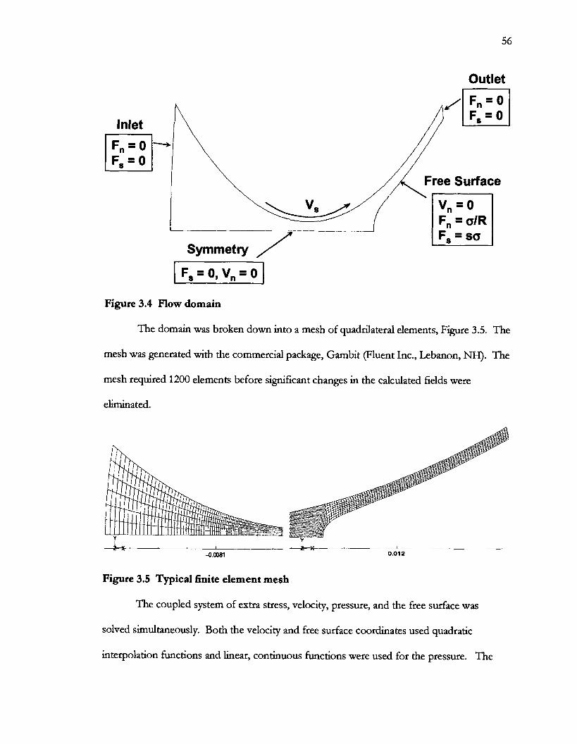
Outlet

Free Surface

Figure 3.4 Flow domain

The domain was broken down into a mesh of quadrilateral elements, Figure 3.5. The

mesh was generated with the commercial package, Gambit (Fluent Inc., Lebanon, NH). The

mesh required 1200 elements before significant changes in the calculated fields were

eliminated.

Figure 3.5 Typical finite element mesh

The coupled system of extra stress, velocity, pressure, and the free surface was

solved simultaneously. Both the velocity and free surface coordinates used quadratic

interpolation functions and linear, continuous functions were used for the pressure. The

extra stress tensor used a 4x4 bllinear interpolation with streamline up-winding to improve

the stabhty (Debbaut e t al. (1 988), Marchal e t al. (1 987)). Please refer to the POLYFLOW

User Guide for more information regarding the interpolation functions. The Thompson

transformation remeshing method was used in the calculations; further information

regarding POLYFLOWs implementation of this technique can be found in the

POLYFLOW User Guide. The solution to a series of elliptic partial differential equations is

required to translate the mesh nodes. This remeshing scheme is robust for large mesh

deformations. Convergence was determined by the relative error between the modifications

at each node between two successive iterations to the maximum value of the field at the

current iteration. When this value reached 0.0001, the solution was considered converged.

Because free surface and viscoelastic flows are highly nonlinear problems, it is very

difficult to obtain converged solutions. In order to facilitate this, the problem was solved for

the Newtonian base case first and this solution was used as the initial guess for the

viscoelastic problem. Viscoelastic effects were then gradually introduced through an

evolution scheme via the relaxation time.

3.4 Results and Discussion

The next set of six figutes present the measured gap width, scaled with the effective

roll radius, as a function of the elasticity number Ne and the load parameter Nw for the

three constant viscosity elastic test fluids. Each point on the graph is the average of ten

measurements with deviations from the mean of less than 1 pm. Even though the Boger

fluids showed a small dependence on the shear rate, n < 1, the viscosity used in the analysis

was considered as a constant under the operating conditions. The experimental operating

conditions are presented in Table 3.5. Measurements for the 0.12% PIB test fluid are

presented in Figures 3.6 and 3.7.

Table 3.5 Experimental operating conditions

Parameter Dimensional Dimensionless

Figure 3.6 shows behavior similar to the Newtonian base case in that as the roll

speed increased, so d ~ d the measured gap width. However, a slight difference in the

sensitivity to the elasticity parameter was observed; the slope increased from 0.55 to 0.59.

Figure 3.7 plots the dimensionless gap as a function of the load parameter. The most

notable feature is that the measured gap is much more sensitive to the applied load

compared to the Newtonian base case; the slope changed from -0.39 to -48. The measured

gap width data for the 0.12% solution can be fit to the empirical relation:

H - = 0 . 6 0 ~ ~ ~ . ~ ~ ~ ~ ~ . ~ ~ R

Slope - 0.59

Figure 3.6 Dimensionless gap vs. elasticity parameter for 0.12O/0 PIB

Slope - - 0.48

Figure 3.7 Dimensionless gap vs. the load parameter for 0.12% PIB

60

The measured gap as a function of the elasticity and load numbers for the 0.24'/0 PIB

solution are presented next. In Figure 3.8, doubling the concenttation of polymer caused the

sensitivity to roll speed to increase further; the slope increased from 0.59 to 0.63. Sensitivity

to the applied load also increased as shown in Figure 3.9; the slope decreased fiom a value of

-0.48 to a slope of -0.58. The measured gap width data for the 0.24% solution can be fit to

the empirical relation:

H - = o . 4 2 ~ ~ ~ ~ ~ ~ ~ ~ - ~ ~ ~ ~ (3.14). R

-

Slope - 0.63

Figure 3.8 Dimensionless gap vs. elasticity parameter for 0.24Y0 PIB

-. -- -

Slope - - 0.58

Ne = 2.6 x 10-7

Ne= 1 . 3 ~ 10-7

Ne = 0.7 x 10-7

Figure 3.9 Dimensionless gap vs. the load parameter for 0.24% PIB

Figures 3.10 and 3.11 show the results for the 0.36% PIB solution. Adding more

polymer to the solution did not produce a detectible change in the sensitivity to the roll

speed, compared to the 0.24% PIB solution. However, the sensitivity to the applied load

continued to increase from -0.58 to -1.05. This result indicated that higher levels of fluid

elasticity are changing the relationship between the load and gap. The measured gap width

for the 0.36% solution can be fit to the empirical relation:

Ne

Figure 3.10 Dimensionless gap vs. the elasticity parameter for 0.36% PIB

Slope - - 1.05

Figure 3.11 Dimensionless gap vs. the load parameter for 0.36% PIB

It should be noted that only one value of roll radius and elastic modulus were used

throughout the experiments and in the fitting procedure. Therefore, it cannot be c o n b e d

that the indicated dependencies on these two quantities are absolute. However, dimensional

analysis indicates that these three dimensionless groups, H/R, Ne, and Nw should fully

describe the system unless some other important parameter, that is not included, is

influencing the system. The empirical correlation is compared with the experimental data in

Figure 3.12.

0.01 -

C I r' 0 P Q - f 5 0.001 --

0 - 3 - L - f" W

0.001

Experimental Data, HIR

Figure 3.12 Comparison of empirical relations with measured gap

The effects of elasticity on the flow can be resolved by comparing the empirical

relations to the Newtonian base case. In the next set of figures, a modlfied load number,

64

H 0.39 . N,,, , is plotted as a function of the elasticity number. Figure 3.13 shows the behavior

at relatively low loads, Nw = 0.001.

... . 0.36 % PIB

...).. 0.24 % PI6 ...

.-*.'- VE more sensitive to speed Slopes - 0.62 - 0.65 ..

VE produces

Figure 3.13 Comparison between elastic fluids at low load

The viscoelastic fluids are more sensitive to roll speed. At low applied load, the

shear stresses are small but the normal stress generated is large enough to separate the roll

surfaces beyond what is expected for an equivalent Newtonian fluid. This behavior is similar

to the increased load bearing capacity observed by Williamson et al. (1997) in their journal

bearing studies. Kang, Lee, and Liu (1991) observed increased flow rate in their experiments

with viscoelastic liquids in a fixed engagement deformable roll coating flow study. Flgure

3.14 shows the behavior at intermediate loading.

I --+ 0.24 % PIB I . . .... 1 0.12 % PIB I - Newtonian

1 .OE-08 1 .OE-07 l.OE-06 l.OE-05

Ne

Figure 3.14 Comparison of elastic fluids at intermediate load

At intermediate loads shear stress increased. The htgher concentration fluid still

produced larger H/R compared to the Newtonian case but the overall map tude decreased.

For the lower concentration liquids at low speeds, the shear stress overcomes the normal

stress and the measured gap is equivalent to the Newtonian case; at higher speeds wider gaps

are observed. The behavior at high loads is plotted in Figure 3.15.

At hlgh loads the shear stress is quite large. It is likely that shear-thinning effects

have overcome the roll separating forces. However, the fluid with the weakest dependence

on shear rate produced enough extra roll separating force at hgh speeds to create larger

H/R than the Newtonian case.

- - 0.36 % PIB

..*.. 0.24 % PIB

- - r 0.12 % PIB

- Newtonlan

-- . -- --

Nw = 0.01 High shear rates

Still larger HIR

\

Shear-thinning overcomes elastic effects, produces

sma

1 .OE-08 1 .OE-07 1 .OE-06 1 .OE-05

Ne

Figure 3.15 Cornpanson of elastic fluids at high load

Examples of the measured pressure profiles are shown in Figure 3.16. The measured

pressure has been scaled with the roll cover thickness, b, effective roll radius R, and the

effective elastic modulus, E, of the cover. The pressure was scaled with the thickness of the

cover because of the observations of previous workers that indicate the cover thickness

influences the film thickness. The measured profiles have been shlfted so that the maximum

pressure occurs at x/R = 0. The profiles of the 0.12% PIB solution are very similar to the

Newtonian base case except for the behavior at the film-split. At the nip exit, it was

observed that the minimum pressure was larger than the Newtonian base case over the range

of applied loads tested. Also, the magnttude of the minimum pressure was much less

sensitive to changes in the applied load compared to the Newtonian case. This behavior was

exhibited by all three of the constant viscosity elastic liquids over the range of roll speeds

shown in Figure 3.17.

- N w = S . l x l ~ ~

I ~ w = l . 7 x l 0 ~ P,,, for VE fluid is

Figure 3.16 Pressure profiles for the 0.12% PIB fluid

i * 0.24 % PIB

3.0E-03 * 0.12 Y. PIB

Figure 3.17 Pressure profiles of the constant viscosity elastic fluids

The measured gap width for the viscoelastic, shear-thinning liquids are plotted next.

The shear-thinning fluids were analyzed with a viscosity that corresponded to an estimated

shear rate in the nip and the fit to the Carreau viscosity model. The shear rate in the nip was

calculated from the roll speed and measured gap width:

Figure 3.18 shows the measured gap as a function of the elasticity parameter at

several applied loads for the 0.45% PIB solution. Even though this solution has a

sipficantly different power-law index, n = 0.88, compared to the previous liquids, the

sensitivity to the elasticity parameter is nearly equivalent. The sensitivity to the elasticity

number remained relatively constant when compared to the 0.24% and 0.36OIo PIB solutions.

The measured gap as a function of applied load is plotted in Figure 3.19. The sensitivity to

the applied load did not change relative to the 0.36% PIB solution, however, the gap width is

still much more sensitive to the applied load than the Newtonian base case.

The measured gap as a function of the elasticity parameter for the 0.62% PIB

solution is shown in Figure 3.20. The relationship for the load number is in Figure 3.21.

Further increase in polymer concentration did not produce a detectable change in the

sensitivity to the roll speed or load. In some way, the shear-thinning behavior balances the

increase in normal force. There must be some aspect of this polymer-solvent system when

the influence of the polymer comes to some steady behavior.

Slope -

Figure 3.18 Dimensionless gap vs. the elasticity parameter for 0.45% PIB

Slope - - 1.07

I

Figure 3.19 Measured gap vs. the load parameter for 0.45% PIB solution

Slope - 0.63 6

Ne

Figure 3.20 Measured gap as a function of elasticity number for 0.62% PIB

0.01 -q--- . .- -- - - - - - - .- - -

Figure 3.21 Measured gap as a function of load parameter for the 0.62% PIB solution

The measured gap width data was correlated with the elasticity and load parameters

for the range of operating condtions tested. This set of data produced more scatter than the

previous data sets. However, the correlation produced a fit to within +/- 5% for 95% of the

measured data points, Figure 3.22. The measured gap width is correlated with the elasticity

and load parameters in the following empitical relations. The 0.45% PIB solution follows:

and the 0.62% PIB solution follows:

The data are more scattered compared to the previous data sets as shown in Figure 3.19.

The empirical correlations are summarized in Table 3.6 in terms of the operating variables

with inputs in MKS units.

The measured gap widths for the test conditions are summarized in Figures 3.23-

3.25. The behavior of the shear-thinning fluids can be compared to the Newtonian base

H 0.39 case by plotting the modified load number - N , versus the elasticity parameter Ne.

R

The data for the 0.36% fluid has been included as an additional comparator. Figure 3.23

compares the behavior at low applied load. At low loads and the resulting low shear rate,

the shear-thinning elastic fluids produced an increase in the measured gap between the roll

surfaces, compared to the constant viscosity elastic fluids. The sensitivity to the roll speed

increased from the Newtonian case but remained relatively consistent with the 0.24% and

0.36% PIB solutions. The measuring system could barely detect a difference in the

measured gap, between the two shear-thinning fluids.

0.001

Experimental Data, HIR

Figure 3.22 Best fit of the empirical correlations with the measured data

Table 3.6 Summaty of empirical correlations

H

Newtonian

0.1 2% PIB

0.24% PIB

0.36% PIB

0.45% PIB

0.62% PIB

k a b c d e

0.42 0.55 0.55 -0.39 -0.16 0.84

0.60 0.59 0.59 -0.48 -0.11 0.89

0.42 0.63 0.63 -0.58 -0.05 0.95

0.036 0.62 0.62 -1.05 -0.43 1.43

0.065 0.65 0.65 -1.07 -0.42 1.42

0.048 0.63 0.63 -1.08 -0.45 1.45

Nw = 0.0001

Low shear rates

VE more sensitive to speed Slopes - 0.62 - 0.65

Figure 3.23 Gap as a function of Ne at low load

Figure 3.24 Gap as a function of Ne at intermediate load

As the applied load is increased, as reported in Figure 3.24, the measured gap width

of the shear-thinning fluids decreased signtficantly. A further increase in the applied load, by

another order of magnttude, produced further decreases in the measured gap. At high loads,

shown in Figure 3.25, the measured gap of the shear-thinning fluids was much less than the

Newtonian base case and less than the constant viscosity elastic test liquids. This indicates

that the shear-thinning behavior can overcome the normal stress produced by the dissolved

polymer. This result was expected because the Newtonian component no longer dominates

the solution at such high concentrations. Also, at low speeds, even though the gap between

the rolls is small, the shear rate is also small. Published measurements of the &st normal

stress indicate that normal stress effects grow with shear rate for PIB solutions. Thls result

was observed by Davies and Walters (1973) who showed for elastic, shear-thinning liquids,

the ratio of the &st normal stress difference to the shear stress, had to be large in order for

extra load bearing capacity to occur.

The dimensionless, measured pressure profiles of the shear-&mug liquids are

shown in Figure 3.26 for an intermediate load. The pressure profiles for the viscoelastic

liquids are very similar to the Newtonian case. Increasing the polymer content of the

solution caused the minimum pressure at the nip exit to increase relative to the Newtonian

case. Even at h h e r loads, the minimum pressure of the Newtonian fluid, at the nip exit, is

consistently less than the viscoelastic fluids Figure 3.27. This result seems to contradict the

results of measurements of ink "tack" measured in printing press nips. However, "tack" has

been shown to be quite dependent on the thickness of the ink layer in the nip. The gap in

the tack tests is no known. Here, the gap increases with increasing polymer concentration.

1 .OE-02

Newtonian 1 .OE-03

m a

C I Shear-thinning overcomes

elastic effects, produces 1 .OE-04 smaller H/R

Nw = 0.01 High shear rates

Ne

Figure 3.25 Gap as a function of Ne at high load

* 0.45 % PIB

-+ Newtonian

Figure 3.26 Pressure profiles of the shear-thinning elastic liquids

-+ Newtonian

P,,, increases wlth concentration

Figure 3.27 Pressure profiles for shear-thinning and elastic liquids

Even though comparing the results from the finite element calculations ditectly to

the experimental measurements is not possible because the flow systems are fundamentally

different, the calculations reveal interesting features of the viscoelastic flow that have not

been shown in the literature. The finite element calculations were used to study the

competing effects of elasticity and shear thinning in a symmetric, rigid roll, forward coating

system.

The simulations were run to as hlgh Weissenberg number, We, as possible where We

indicates the effect of elasticity and is defined as:

where V is the average roll speed, H is the measured gap between the rolls, and A is a

characteristic relaxation time of the test fluid. The capillary number, Ca, was used as another

dimensionless group to characterize the viscous and surface tension forces in the system and

is given by:

where 7, is the zero-shear viscosity and a is the surface tension of the liquid. Above We =

5.0, the mesh became distorted at the domain exit. Even though the simulation converged,

these results were not plotted because of the unnatural shape of the free surface at the

domain exit. Typical streamlines for the Newtonian and Oldroyd-B fluids are compared in

Figure 3.28. The model parameters for the results presented in the following contour plots

are presented in Table 3.7.

Table 3.7 Model parameters used in the flow simulations --

Parameter Oldroyd-B Giesekus -

H ( 4 0.0005 0.0005 R ( 4 0.05 0.05

V (m/s) 0.004,0.5 0.004,0.5 * W m ) 0.02 0.02

P @ d m 3 1000 1000

The streamlines of the viscoelastic flow are similar to the Newtonian flow, however,

the film-split point in the viscoelastic model is shifted down-stream slightly at moderate We,

compared to the Newtonian model.

Figure 3.28 Streamlines for Newtonian and Oldroyd-B models

The contours of the first normal stress component of the total extra stress, TI,, are

shown in Figure 3.29. There is a large normal stress build-up at the point of high extension

in the Newtonian base case. This stress concentration transforms into a sort of stress

boundary layer that is attached to the free surface downstream from the split point in the

viscoelastic flow. There are two explanations for the appearance of the stress layer. The

first is that it may be an artifact of the Oldroyd-B model. The extension rate in the area

where the boundary layer appears is quite large and may be in the range of where the

extensional viscosity of the Oldroyd-B fluid becomes unbounded. Unbounded extensional

viscosity would produce errors near the surface. However, the error would decrease as the

extension rate in the flow decreased and this is indicated by the decreasing gradient of the

stress contours toward the roll surface.

The other explanation is that the boundary layer is a genuine effect of a viscoelastic

fluid in the roll coating geometry. If this is the case, the stress boundary layer may influence

the behavior of the polymer molecules in the area and may indicate the presence of a purely

elastic instability mechanism. It is difficult to obtain any information regarding stability from

the results available from the POLYFLOW package. However, finite element calculations

and experimental observations of the recirculation flows of constant viscosity elastic fluids

have linked the stretching of polymer molecules, in areas of high extension, to purely elastic

instabilities (Shaqfeh el al. (1 996)).

Figure 3.29 Contours of the first normal stress

The contours of the shear stress component, T,, , of the total extra stress are plotted

in Figure 3.30. Shear stress increased in the viscoelastic flow model, however, the gradient

of the shear stress throughout the domain decreased. The contours of the second normal

stress component, T,,, of the total extra stress are plotted in Figure 3.31. The second

normal stress also increased throughout the domain and a stress boundary layer formed at

the surface of the meniscus.

When the Capillary number was decreased, a recirculation appeared on the

downstream side of the nip, as shown in the streamlines plotted in Figure 3.32. Again, at

low Ca, the film-split position was shifted slightly downstream at moderate We.

Figure 3.30 Contours of the shear stress

Figure 3.31 Contours of the second normal stress

Figure 3.32 Streamlines for low Ca flow

Contours of the first normal stress at high and low Ca are compared in Figure 3.33.

The stress boundary layer at the free surface does not appear in the low Ca flow at similar

levels of elasticity. At low Ca, the extension rate along the free surface is reduced compared

to the high Ca flow. This suggests that the observed stress boundary layer may be an artifact

of the unbounded extensional viscosity of the Oldroyd-B model used in the calculations.

Contours of the second normal stress are shown in Figure 3.34. At low Ca, there

appears to be a high stress concentration near the roll surface, downstream of the split point

At, large Ca, the stress concentration shifts to the free surface at the film-split. It should be

noted that the magnitudes of the second normal stresses observed at low and high Ca differ

by three orders of magnitude.

Figure 3.33 Contours of the first normal stress at low and high Ca

Figure 3.34 Contours of the second normal stress for low and high Ca

The next set of figures reveals the effects of shear-thinning viscosity on the

viscoelastic flow through the Giesekus fluid model. Streamlines are plotted in Figure 3.35.

The Giesekus model, for similar operating parameters, has shifted the split-point much

fuaher downstream. This observation may be explained by the large amount of shear

thinning produced by the model with the parameters used in the calculations; the power law

index is approximately 0.46. Coyle eta1 (1987) observed a downstream shift of the film-split

meniscus in finite element simulations of purely viscous shear-thinning fluids in a forward

roll coating geometry.

Figure 3.35 Streamlines for the Giesekus model

Contours of the first normal stress, for both the Oldroyd-B and Giesekus models,

are compared in Figure 3.36. The stress boundary layer has disappeared in the Giesekus

model flow. The Giesekus fluid model has a bounded extensional viscosity and the results

from the simulations further point to the unbounded extensional viscosity of the Oldroyd-B

model as the cause of the appearance of the stress boundary layer at the free surface. It

should be noted, however, that the Ca used in the comparisons, is based on the zero shear

viscosity of the fluid. Because of the presence of shear-thinning, a modified Ca that

accounts for decreasing viscosity, may need to be used before quantitative comparisons can

be made between the two models.

Figure 3.36 Contours of the first normal stess for Oldroyd-B (a) and Giesekus (b)

The magnitudes of the second normal stress are dramatically reduced by the

presence of shear thinning as shown in Figure 3.37b. It is possible to make a cautious

estimate of some effects of viscoelasticity on the stability of the flow from Figure 3.36 and

3.37. If the stability of the flow is influenced by the appearance of the stress boundary layer,

then adding shear thinning had a stabilizing effect on the flow. Gutoff and Kendrick (1982)

observed a stabilizing effect on the slide-coating bead when they added small amounts of

polymer to their test fluid.

Figure 3.37 Contours of the second normal stress for Oldroyd-B (a) and Giesekus (b)

Examples of the pressure profiles are plotted in Figure 3.38. Increasing the level of

elasticity, We, had a much larger influence on both the maximum and minimum pressure for

the Giesekus fluid. At high We, the pressure gradient at the film-split was much less than at

low We, indicating that it may have a significant effect on the ribbing instability mechanism.

It appears that the pressure gradient for the purely elastic fluid increased as elastic effects

increased.

-0.02 -0.015 -0.01 -0.005 0 0.005 0.01 0.01 5 0.02

x (m)

Figure 3.38 Pressure profiles

The pressure prohles can be integrated to study the roll separating force and are

plotted in Figure 3.39. Decreasing the viscosity ratio increased the roll separating force in

the Oldroyd-B flow up to a We = 1.6 and maintained increased separating force as We

increased further. Increasing the viscosity ratio in the Giesekus model reduced the roll

separating force and continued the reduction as We increased.

Oldroyd-B

increased - 20

a = 0.5

Figure 3.39 Integrated pressure

Elasticity shifts film- split downstream

~hear- th inkn~ can Increase shift down

stream or compete with elasticity

Figure 3.40 Film split position

Figure 3.40 reveals that elasticity shifts the &-split downstream. Also, increasing

the polymer effect, by decreasing the viscosity ratio, had a large impact on the film-split

position with the Giesekus fluid. This behavior is commonly observed in calculations with

purely viscous shear-thinning fluids (Coyle e t al. 1987). Coyle e t al (1987) and Benkteita e t al.

(1981) showed that the film-split recedes into the nip as the Ca of the flow increases. At

equal roll speeds and gaps, a shear-thmning liquid has a lower viscosity and thus a lower Cay

which translates into a downstream shift of the split point. Figure 3.40 also shows that for

an equivalent level of polymer contribution to the solution, the purely elastic fluid has a split

point located further downstream than the shear-thmning fluid. Elasticity is definitely

changing the relationship between the film split location and the Ca of the flow. The

dimensionless flow rate for both models is plotted in Figure 3.41. Increasing elasticity

increased the flow rate of the Oldroyd-B fluid much more than the Giesekus fluid. In both

cases, increasing the polymer contribution produced a significant increase in dimensionless

flow rate. Keep in mind that the gap is held constant. Elasticity seems to be able to pull

more fluid through the nip, possibly because of the large extensional stresses in the flow.

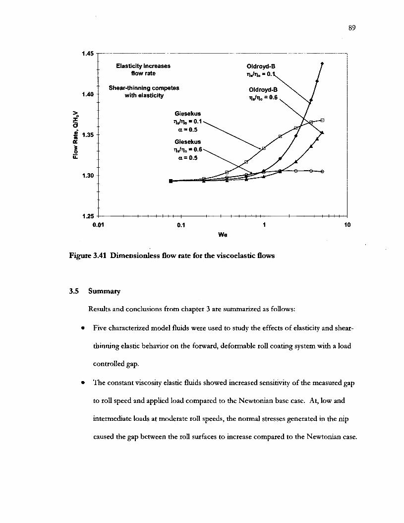
Elasticity increases Oldroyd-B flow rate

Shear-thinning competes with elasticity

Giesekus

Giesekw

Figure 3.41 Dimensionless flow rate for the viscoelastic flows

3.5 Summary

Results and conclusions ftom chapter 3 are summarized as follows:

Five characterized model fluids were used to study the effects of elasticity and shear-

thinning elastic behavior on the forward, deformable roll coating system with a load

controlled gap.

* The constant viscosity elastic fluids showed increased sensitivity of the measured gap

to roll speed and applied load compared to the Newtonian base case. At, low and

intermediate loads at moderate roll speeds, the normal stresses generated in the nip

caused the gap between the roll surfaces to increase compared to the Newtonian case.

Elastic shear-thinning fluids showed increased sensitivity of the measured gap to

both roll speed and applied load compared to the Newtonian base case. At low and

intermediate loads at high speeds, the normal stress generated in the nip increased

the gap between the roll surfaces further from the Newtonian case.

Increased gap is consistent with experimental observations of increased flow rate in a

fixed engagement deformable roll system and it is consistent with observed increase

in load bearing capacity in a journal bearing flow system.

The Galerkin finite element method was used to study the two-dimensional, free

surface, viscoelastic flow between to fixed, rigid rolls with symmetric roll speeds. A

purely elastic fluid model revealed the presence of a first normal stress boundary

layer downstream of the £ilm split at high Ca and moderate We.

An elastic, shear-thinning fluid model showed that the presence of shear thinning

delayed the appearance of the first normal stress boundary layer.

The pressure gradient in the flow of a purely elastic liquid increased with We

indicating that the flow became unstable. Adding shear thinning decreased the

pressure gradient indicating that the flow became more stable.

4 SUMMARY

4.1 Summary of Chapter 2

A bench-top apparatus was constructed to study elasto-hydrodynamic forward roll

coating flows.

A technique was developed and applied to measure the gap between the roll surfaces.

Measurements of the gap corresponded with the expected value at the point of

maximum fluid pressure within the nip and the measured wet film thickness.

The measured gap and its sensitivity to the external load and roll speed were

consistent with published experimental data and theoretical analyses.

There was some evidence of increasing sensitivity to the applied load caused by the

influence of the thin, deformable roll cover used in the experiments.

A model of the deformable roll coating system was developed based on the

lubrication approximation with non-Hertzian deformation of the roll cover and a

visco-capillary boundary condition at the film-split.

The lubrication model reproduced the magnitude and shape of the measured

pressure, for low external loads, after values of the negative pressure below -100 kPa

were removed from the calculations.

4.2 Summary of Chapter 3

Results and conclusions from chapter 3 are summarized as follows:

Five characterized model fluids were used to study the effects of elasticity and shear-

thinning elastic behavior on the forward, deformable roll coating system with a load

controlled gap.

The constant viscosity elastic fluids showed increased sensitivity of the measured gap

to roll speed and applied load compared to the Newtonian base case. At, low and

intermediate loads at moderate roll speeds, the normal stresses generated in the nip

caused the gap between the roll surfaces to increase compared to the Newtonian case.

Elastic shear-thinning fluids showed increased sensitivity of the measured gap to

both roll speed and applied load compared to the Newtonian base case. At low and

intermediate loads at high speeds, the normal stress generated in the nip increased

the gap between the roll surfaces further from the Newtonian case.

Increased gap is consistent with experimental observations of increased flow rate in a

tixed engagement deformable roll system and it is consistent with observed increase

in load bearing capacity in a journal bearing flow system.

The Galerkin h t e element method was used to study the two-dimensional, free

surface, viscoelastic flow between to fixed, rigid rolls with symmetric roll speeds. A

purely elastic fluid model revealed the presence of a first normal stress boundary

layer downstream of the £ilm split at hgh Ca and moderate We.

An elastic, shear-thinning fluid model showed that the presence of shear thinning

delayed the appearance of the first normal stress boundary layer.

The pressure gradient in the flow of a purely elastic liquid increased with We

indicating that the flow became unstable. Adding shear thinning decreased the

pressure gradient indicating that the flow became more stable.

4.3 Recommendations for Future Work

A significant factor conmbuting to the uncertainty in the measurements was the

extent of the eccentricity of the rolls and bearings. The first step in future

experiments should include a rebuild of the rolls and bearing so that the total runout

for each roll is less than 10 pm. Including split pillow blocks or bearing mounts

would enable quick change over to study different roll diameters or roll covers.

The lack of safety measures on the device should be addressed. At the minimum,

and emergency stop switch should be installed in the form of a cable encircling the

entire apparatus so that the rolls can be stopped. An improvement would be to

include a means of opening the nip when the E-stop was triggered.

Permanently fixing the drive for the deformable roll to the base plate would decrease

the error in the applied load significantly by removing the extra inertia. Using a

Schmitt coupling to connect the drive shaft to the roll would accomplish this task.

A means of fixing the gap, and setting a precise gap, should also be installed. This

would allow more types of roll coating flows to be studied.

There was also some problem with the convolution of the pressure data with the nip

length. Increasing the diameter of the rolls to 20 cm would increase the nip length

and reduce the convolution. A larger diameter roll would also reduce the error in the

capacitance probe measurements. If a larger diameter roll is installed, it would be

important to include gear reducers between the drive shaft and the rolls so that the

drives could continue to operate within their limits at low speed conditions. Gear

reducers would also increase the resolution from the pressure and capacitance

transducers.

Increasing the thickness of the roll cover would facilitate comparison to other

published data and decreases its influence on the flow through the nip.

Some information regarding the test fluids was unavailable, including: extensional

viscosity, normal sttess, and relaxation time measurements.

Previous work has shown contradictory observations of the sensitivity to roll speed

differential. Future experiments should study the speed differential to examine the

effects of increased shear on flow of viscoelastic liquids.

The reverse roll coating flow of viscoelastic fluids also should be investigated.

Finite element models of the two-dimensional, viscoelastic roll coating flow should

continue to be explored over a wider range of capillary number. Much information

could be gained without includulg the effects of a deformable roll cover.

REFERENCES

Adachi, K.; Tamura, T., and Nakamura, R. Coating flows in a nip region and various critical phenomena. AIChE Journal. 1988; 34(3):456-464.

Alonso, S. and Tanguy, P. A. Hydrodynamic instabilities in the metering nip of a lilm coater. TAPPI Journal. 2001; 84(5):1-20.

Aspler, J. S. and Taylor, S. Tack development in water-based inks. Nordic Pulp and Paper Research Journal. 1991; 6(1):4-7.

Bapat, C. N. and Batra, R. C. Finite plane strain deformations of nonlinear viscoelastic rubber-covered rolls. International Journal for Numerical Methods in Engineering. 1984; 20(1):1911-1927.

Bauman, T.; Sullivan, T., and Middleman, S. Ribbing instability in coating flows: effect of polymer additives. Chemical Engineering Communications. 1 982; 1 4:35-46.

Benjamin, D. F. Roll Coating Flows and Multiple Roll Systems. Mmneapolis, MN: University of Minnesota; 1994.

Benjamin, D. F.; Anderson, T. J., and Scriven, L. E. Multiple roll systems: steady-state operation. AIChE Journal. 1995; 41 (5):lO45-1060.

Benjamin, D. F.; Carvalho, M. S.; Anderson, T. J., and Scriven, L. E. Forward roll lilm- splitting: theory and experiment. TAPPI Coating Conference Proceedings; 1994: 109-123.

Benkreira, H.; Edwards, M. F., and Wilkinson, W. L. Roll coating of purely viscous liquids. Chemical Engineering Science. 1981; 36:429-434.

Beris, A. N.; Armstrong, R. C., and Brown, R. A. Perturbation theory for viscoelastic fluids between eccentric rotating cylinders. Journal of Non-Newtonian Fluid Mechanics. 1983; 13(1):109-148.

---. Finite element calculation of viscoelastic flow in a journal bearing: 11. Moderate viscosity. Journal of Non-Newtonian Fluid Mechanics. 1986; 19:323-347.

Blayo, A.; Fang, S. W.; Gandini, A., and Le Nest, J. F. Study of ink misting phenomena. American Ink Maker. 1998; 76(5):54-61.

Bohan, M. F. J.; Claypole, T. C., and Gethin, D. T. Dynamic measurement of ink lilm thickness, pressure and temperature in rolling contacts. Technical Association of Graphic Arts Proceedings. Bookcrafters, Inc. Chelsea, MI; 2001 : pgs 11 1-124.

Bohan, M. F. J.; Claypole, T. C., and Grethin, D. T. The application of roughness model to a soft EHL contact. International Journal of Numerical Methods for Heat & Fluid Flow. 2002; 12(4):356-374.

Bohan, M. F. J.; Lim, C. H.; Korochkina, T. V.; Claypole, T. C.; Gethin, D. T., and Roylance, B. J. An invesugation of the hydrodyanmic and mechanical behavior of a soft nip rolling contact. Proc Instn. Mech. Engrs. 1997; 21 1037-49.

Booth, G. L. Coating Equipment and Pmcesses. New York, NY: Lockwood Publishing Company; 1970.

Cameron, A. Basic Lubn'cation Tbeoty. New York, NY: John Wiley & Sons; 1976.

Carvalho, M. S. and Scriven, L. E. Effect of deformable roll cover on roll coating. TAPPI Journal. 1994; 77(5):2Ol-208.

---. Deformable roll coating flows: steady state and linear perturbation analysis. Journal of Fluid Mechanics. 1997a; 339:143-172.

---. Flows in forward deformable roll coating gaps: comparison between spring and plane- strain models of roll cover. Journal of Computational Physics. 1997b; 138:449-479.

Christiansen, S. Resins are gaining weight. American Ink Maker. 1995; 73(lO):l4-60.

Cohu, 0. and Benkreira, H. Air entrainment in angled dip coating. Chemical Engineering Science. 1998; 53(1):533.

Cohu, 0. and Magnin, A. Forward roll coating of Newtonian fluids with deformable rolls: an experimental investigation. Chemical Engineering Science. 1997; 52(8): 1339-1 347.

Coyle, D. J. Experimental Studies of Flow Between Deformable Rolls. AIChE Spring National Meeting; New Orleans, LA. 1988a.

---. Forward roll coating with deformable rolls: a simple one-dimensional elastohydrodynamic model. Chemical Engineering Science. 1988b; 43(10):2673-2684.

---. Nonlinear Theory of squeeze-roll coating. AIChE Spring National Meeting; Orlando, FL. 1990.

---. Roll Coating. In: Mohm Coating and Dying Technology. Cohen, E. D.; Gutoff, E. B. (eds). New York, NY: VCH Publishers; 1992; pp. 63-1 16.

---. Knife and Roll Coating. In: Liquid Film Coating. Kistler, S. F.; Schweizer, P. M. (eds). London: Chapman & Hall, 1997; pp. 539-571.

Coyle, D. J.; Macosko, C. W., and Scriven, L. E. Film-splitting flows of shear-thinning liquids in forward roll coating. AIChE Journal. 1987; 33(5):741-746.

Crook, A. W. The lubrication of rollers. Philosophical Transactions of the Royal Society of London, Series A, Mathematical and Physical Sciences. 1958; 250(A):387-409.

Davies, M. J. and Walters, K. The Behavior of Non-Newtonian Lubricants in Journal Bearings- A Theoretical Study. In: Rbeology 4Lubricant.r. Davenport, T. C., (ed.)New York, NY: John Wiley & Sons; 1973; pp. 65-80.

Dobbels, F. and Mewis, J. Analysis of nip flow operations involving a viscoelastic roller. Chemical Engineering Science. 1978; 33:493-500.

Dontula, P.; Macosko, C. W., and Scriven, L. E. Model elastic liquids with water-soluble polymers. AIChE Journal. 1998; 44(6):1247-1255.

Dontula, P.; Pasquali, M.; Macosko, C. W., and Scriven, L. E. Viscoelastic effects in forward- roll coating flows, Ait-Kadi, A.; Dealy, J. M.; James, D. F., and Williams, M. C., (eds). Proc. XIIth Int. Congr. on Rheology; Quebec City, Quebec, Canada. Canadian Rheology Group; 1996: 709-710.

Doremus, P. and Piau, J. Viscoelastic elongational lubrication. Journal of Non-Newtonian Fluid Mechanics. 1981; 9:389-400.

Doremus, P. and Piau. J. Experimental study of viscoelastic effects in a cylinder-plane lubricated contact. Journal of Non-Newtonian Fluid Mechanics. 1983; 13:79-91.

Dowson, D. and -son, H. G. Elbsto-Hydru&namic Lubrication. New York, NY: Pergamon Press; 1966.

Elrod, H. G. A cavitation algorithm. Journal of Lubrication Technology. 1981; 1 O3(1):35O- 354.

Fernando, R. H. and Glass, J. E. Dynamic uniaxial extensional viscosity (DUEV) effects in roll application 11. Polymer blend studies. Journal of Rheology. 1988; 32(2):199-213.

Fetsko, J. M.; Schaeffer, W. D., and Zettlemoyer, A. C. Sources of differences in picking results among presses. TAPPI Journal. 1963; 46(3):157-162.

Gaskell, P. H.; Innes, G. E., and Savage, M. D. An experimental investigation of meniscus roll coating. Journal of Fluid Mechanics. 1998; 355:17-44.

Gaskell, P. H.; Savage, M. D.; Summers, J. L., and Thompson, H. M. Modeling and analysis of meniscus roll coating. Journal of Fluid Mechanics. 1995; 298(1):113-137.

Glass, J. E. Dynamics of roll spatter and ttacking Part 1: commercial latex trade paints. Journal of Coatings Technology. 1978a; 50(640):53-60.

---. Dynamics of roll spatter and ttackmg Part 2: Formulation effects in experimental paints. Journal of Coatings Technology. 1978b; 50(640):61-68.

---. Dynamics of roll spatter and tracking Part 3: Importance of extensional viscosities. Journal of Coatings Technology. 1978c; 50(641):56-71.

---. Dynamics of roll spatter and tracking Part 4: Importance of G* recovery and N1 tracking. Joumal of Coatings Technology. 1978d; 50(641):72-78.

Glass, J. E. and Prud'hornme, R. K. Coating Rheology: component influence on the rheological response and performance of water-borne coatings in roll applications. Schweizer, P. M. and Kistler, S. F., (eds.). liquid Film Coating. Cambridge UK: Chapman & Hall; 1997; pp. 137-1 82.

Greener, J. and Middleman S. A theory of roll coating of viscous and viscoelastic fluids. Polymer Engineering and Science. 1975; 15(1):1-10.

Greener, J.; Sullivan, T.; Turner, B., and Middleman, S. Ribbing instability of a two-roll coater: Newtonian fluids. Chemical Engineering Communications. 1980; 5(1):73-83.

Gron, J.; Sunde, H., and Nikula, E. Runnability aspects in bh-speed film transfer coating. TAPPI Joumal. 1998; 81 (2):157-165.

Gutoff, E. B. and Kendrick, C. E. Low flow limits of coatability on a slide coater. AIChE Journal. 1987; 33(1):141-145.

Hall, R. W. and Savage, M. D. Two-dimensional elastohydrodynamic lubrication Part 1: the associated dry contact problem. Proc Insm. Mech. Engrs. 1988; 202(C5):347-353.

Herrebrugh, K. Solving the incompressible and isothermal problem in elastohydrodynamic lubrication through an integral equation. Journal of Lubrication Technology. 1968; 90(1):262-270.

Higglns, B. G. Coating Methods. In: Enyckpedia $Polymer Science and Technology. 1" ed. New York, NY: John Wiley; 1965; pp. 765-807.

Hooke, C. J. The elastohydrodynamic lubrication of a cylinder on an elastomeric layer. Wear. 1986; 11 1:83-99.

Johnson, K. L. Regimes of Elastohydrodynamic lubrication. Journal of Mechanical Engineering Science. 1970; l2(1):9- 16.

---. Contact Mechanics. Cambridge, UK: Cambridge University Press; 1985.

Jorgensen, G. W. and Lavi, A. lithographic Pnsmzan'~ Handbook. GATF; 1973.

Kang, Y.; Lee, K., and Liu, T. The effect of polymer additive on the performance of a two- roll coater. Journal of Applied Polymer Science. 1991; 43:1187-1195.

Lopez, F.V., Pauchard, L., Rosen, M., and Rabaud, M. Non-Newtonian effects on ribbing instability threshold. Joumal of Non-Newtonian Fluid Mechanics. 2002; 103:123- 139

MacPhee, J. A unified view of the 6lm splitting process. American Ink Maker. 1997; 75(1):42-50.

Mewis, J. and Dobbles, F. Nip flow and tack of printing inks. Industrial and Enpeering Chemistry Product Research and Development. 1981; 20:515-519.

Md, C. C. and South, G. R. Formation of ribs on rotating rollers. Journal of Fluid Mechanics. 1967; 28:523-529.

Miller, J. C. and Myers, R. R. A Photographic Study of Liquid Flow in a Roll Nip. Transactions of the Society of Rheology. 1958; 2:77-93.

Myers, R. R. and Hoffman, R. D. The Dismbution of Pressure in the Roll Application of Newtonian Fluids. Transactions of the Society of Rheology. 1961; 5:317-328.

Myers, R. R.; Miller, J. C., and Zettlemoyer, A. C. The splitting of thin liquid 6lms. Kinematics. Journal of Colloid Science. 1959; 14:287-299.

Nguyen, D.A. and Sridhar, T. Preparation and some properties of MI and its constituents. Journal of Non-Newtonian Fluid Mechanics. 1990; 35:pp 93-104.

Patel, N. and Dealy, J. M. Measurement of tensile stress at the exit of a printing nip. Journal of Non-Newtonian Fluid Mechanics. 1987; 22:245-252.

Pitts, E. and Greiller, J. The flow of thin liquid 6lms between rollers. Journal of Fluid Mechanics. 1961; 11:33-50.

POLYFLOW User Guide. Fluent Inc., Lebanon, NH, 2002.

Poranen, J.; Kataja, M.; Niernisto, A., and Gron, J. A method for measuring and controlling the pressure in the metering nip of a metering size press coating process. Nordic Pulp and Paper Research Journal. 2000; 15(5):486-493.

Pranckh, F. R. and Coyle, D. J. Elastohydrodynamic Coating Systems. In: Liquid Film Coating. Kistler, S. F.; Schweizer, P. M. (eds). London: Chapman & Hall, 1997; pp. 599-635.

Prilutski, G., Gupta, K., Sridhar, T., and Ryan, M.E. Model viscoelastic liquids. Journal of Non-Newtonian Fluid Mechanics. 1983; 12:pp 233-241.

Reglat, 0 . and Tanguy, P. A. Experimental study of the flow in the metering nip of a metering-size press. AIChE Journal. 1997; 43(11):2911-2920.

Roper, J. A.; Bousfield, D. W.; Urscheler, R., and Salminen, P. Observations and proposed mechanisms of misting on high-speed metered size press coaters. TAPPI Coating Conference Proceedings; 1997: 1-1 4.

Roper, J. A.; Salrninen, P.; Urscheler, R., and Bousfield, D. W. Studies of orange peel formation in high-speed 6lm coating. TAPPI Journal. 1999; 82(l):23 1-238.

Satas, D. Web Pmcessing and Converting Tecbnoh~ and Equipment. New York, NY. Van Nostrand Reinhold; 1984.

Savage, M. D. Mathematical models for coating processes. Journal of Fluid Mechanics. 1982; 1 1743-455.

Shaqfeh, E. S. G. Purely elastic instabilities in viscometric flows. Annual Review of Fluid Mechanics. 1996; 28:129-185.

Smith, J. W. and Maloney, J. D. Flow of fluids between rotating rollers. TAPPI Journal. 1966; 49(11):63A-66A.

Soules, D. A.; Fernando, R. H., and Glass, J. E. Dynamic uniaxial extensional viscosity (DUEV) effects in roll application I. Rib and web growth in commercial coatings. Journal of Rheology. 1988; 32(2):18l-l98.

Spiers, R. P.; Subbaraman, C. V., and Wilkinson, W. L. Chemical Engineering Science. 1974; 29(1):389.

Sridhar, T. An overview of the MI project. Journal of Non-Newtonian Fluid Mechanics. 1990; 35:pp 85-92.

Swales, P. D.; Dowson, D., and Latham, J. L. Theoretical and experimental observations of the behavior of soft elastic materials under elastohydrodynamic conditions. Proceedings of the Institution of Mechanical Engineers 1972 Symposium on Elastohydrodynamic Lubrication ; 1972: 22-28.

Taylor, J. H. and Zettlemoyer, A. C. Hypothesis on the mechanism of ink splitting during printing. TAPPI Journal. 1958; 41 (12):749-757.

Tharrnalingam, S. and Wilkinson, W. L. The coating of Newtonian liquids onto a roll rotating at low speeds. Polymer Engineering and Science. 1978; l8(l5):1155-ll59.

---. The coating of Newtonian liquids onto a rotating roll. Chemical Engineering Science. 1978; 33:1481-1487.

Triantafillopoulos N. G. Paper Coating Vzscoelastin'~ and its Signzjicance zn Blbde Coating. Atlanta, GA: TAPPI Press; 1996.

Varnam, C. J. and Hooke. C. J. Non-Hertzian elastohydrodynamic contacts: an experimental invesagation. Journal of Mechanical Engineering Science. 1977; 19(5):189-192.

Voet, A. Ink misting and its prevention. American Ink Maker. 1956; 34(2):32.

Yih, C. S. Instability of a rotating liquid film with a free surface. Philosophical Transactions of the Royal Society of London, Series A, Mathematical and Physical Sciences. 1960; 258(1):63-89.

Zang, Y. H.; Aspler, J. S.; Boluk, M. Y., and De Grace, J. H. Direct measurement of tensile stress ("tack") in thm ink films. Journal of Rheology. 1991; 35(3):345-361.

Zink, S. C. Coating Processes. In: Enylopedia ofchemical Technology. 3rd ed. New York, NY: Wiley; 1979; pp. 386-426.

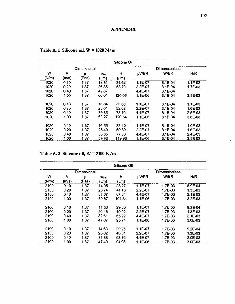
APPENDIX

Table A. 1 Silicone oil, W = 1020 N/m

Silicone Oil

Table A. 2 Silicone oil, W = 2190 N/m

Dimensional W V CI h~ilrn H

(Nlm) (mls) (Pas) (m) (v) 1020 0.10 1.37 17.31 34.62 1020 0.20 1.37 26.85 53.70 1020 0.40 1.37 42.87 1020 1 .OO 1.37 60.04 120.08

Dimensionless pVlER WER HIR

1.1E-07 8.1 E-04 1.1 E-03 2.2E-07 8.1 E-04 1.7E-03 4.4E-07 8.1 E-04 1.1E-06 8.lE-04 3.8E-03

(Nlm) (rnls) (&s) (v) (w) I 2100 0.10 1.37 14.95 28.27 1 1.1E-07 1.7E-03 8.9E-04

Silicone Oil

Dimensional I Dimensionless W V u h~i~rn H uVIE R WER HIR

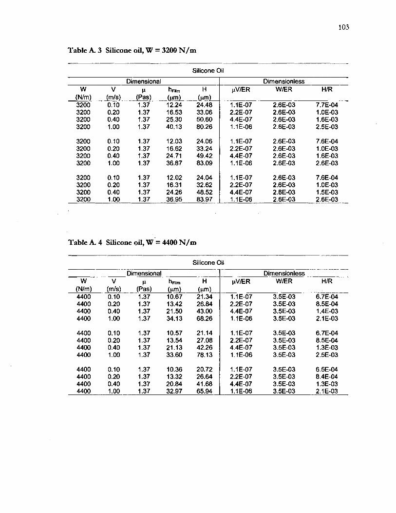
Table A. 3 Silicone oil, W = 3200 N/m

Table A. 4 Silicone oil, w = 4400 N/m

Silicone Oil

Silicone Oil

Dimensional W V CI h~ilrn H

(Nlm) (mls) (Pas) (w) (w) 3200 0.10 1.37 12.24 24.48

Dimensionless W E R WER HIR

1.1 E-07 2.6E-03 7.7E-04

(Nlm) (mls) (pas) (Wn) (w) I 4400 0.10 1.37 10.67 21.34 1 1.1E-07 3.5E-03 6.7E-04

Dimensional Dimensionless W V P h~ilrn H I pVE R WER HIR

Table A. 5 Silicone oil, W = 6400 N/m

Silicone Oil

Table A. 6 Silicone oil, W = 8500 N/m

Dimensional W V P h ~ i l m H

(Nlm) (mls) (Pas) (w) (W ) 6400 0.20 1.37 11.97 23.94 6400 0.40 1.37 18.55 37.10 6400 0.80 1.37 26.50 53.00 6400 1.20 1.37 34.61

Silicone Oil

Dimensionless pV1ER WER HIR

2.2E-07 5.1 E-03 7.5E-04 4.4E-07 5.1 E-03 1.2E-03 8.8E-07 5.1 E-03 1.7E-03

5.1 E-03

Dimensional Dimensionless W V u h~i~rn H uVIER WER HIR

Table A. 7 0.12% PIB, W = 2100 N/m

0.12% PIB

Table k 8 0.12% PIB, W = 3200 N/m

Dimensional w v P h~ilrn H

(Nlm) (mls) (Pas) (run) (w) 2100 0.10 0.79 11.01 20.38

0.12% PIB

Dimensionless pV1E R WlER HIR

6.3E-08 1.7E-03 6.4E-04

~imensional W V P h~ilrn H

(Nlm) (mls) (Pas) (w) (w) 3200 0.10 0.79 10.48 3200 0.20 0.79 11.66 23.32 3200 0.30 0.79 17.17 31.02 3200 0.40 0.79 20.06 35.44 3200 0.60 0.79 23.78 47.36

Dimensionless pV1ER WER HIR

6.3E-08 2.6E-03 1.3E-07 2.6E-03 7.3E-04 1.9E-07 2.6E-03 9.8E-04 2.5E-07 2.6E-03 1.1 E-03 3.8E-07 2.6E-03 1.5E-03

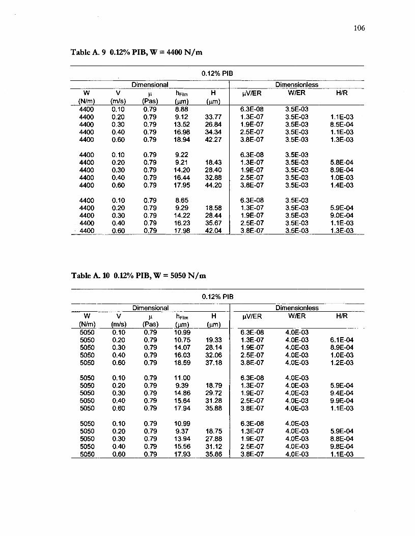
Table A. 9 0.12% PIB, W = 4400 N/m

0.12% PIB

(Nlm) (mls) (Pas) (w) (m) 1 4400 0.10 0.79 8.88 1 6.3E-08 3.5E-03

Dimensional W V I' h~ilrn H

Table k 10 O.UOh PIB, W = 5050 N/m

Dimensionless pVlE R WIER H/R

0.12% PIB

(Nlm) (mls) (Pas) (w) (w) I 5050 0.10 0.79 10.99 1 6.3E-08 4.OE-03

Dimensional Dimensionless W V CI h~i~rn H pV/ER WIER H/R

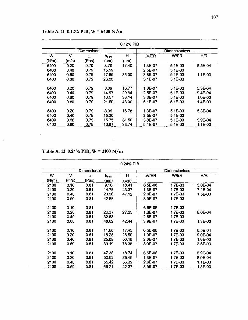
Table k 11 0.12% PIB, W = 6400 N/m

0.12% PIB

Table k 12 0.24% PIB, W = 2100 N/m

Dimensional W V P h ~ i l m H

(Nlm) (mls) (Pas) ( pm) (w) 6400 0.20 0.79 8.70 17.40 6400 0.40 0.79 1 5.59 6400 0.60 0.79 17.65 35.30 6400 0.80 0.79 26.00

0.24% PIB

Dimensionless pV/E R WER HIR

1.3E-07 5.1 E-03 5.5E-04 2.5E-07 5.1 E-03 3.8E-07 5.1 E-03 1.1 E-03 5.1 E-07 5.1 E-03

Dimensional W V h ~ i ~ r n H

(Nlm) (mls) (Pas) (w) ( pm) 2100 0.10 0.81 9.10 18.41 2100 0.20 0.81 14.78 23.37 2100 0.40 0.81 23.56 47.12 21 00 0.60 0.81 42.58

Dimensionless pVlE R WIER H/R

Table A. 13 0.24% PIB, W = 3200 N/m

0.24% PIB

(Nlm) (mls) (Pas) (w) (pm) 3200 0.10 1.04 149.30 15.73 1 8.3E-08 2.6E-03 5.OE-04

Dimensional

Table A. 14 0.24% PIB, W = 6400 N/m

Dimensionless

0.24% PIB

Dimensional W V U h~i~rn H

W V P h~ilrn H

(Nlm) (mls) ( P k ) (pm) (pm) 6400 0.10 0.86 13.45 8.32

W E R WER HIR

Dimensionless pV1ER W E R HIR

Table A. 15 0.24% PIB, W = 8500 N/m

0.24% PIB

Dimensional Dimensionless

(Nlm) (mls) (pas) 1 (w) 8500 1 .OO 1.04 34.29 30.28 8.3E-07 6.8E-03 9.5E-04

W V P h~ilrn H pV1E R WIER HIR

Table A. 16 0.36% PIB, W = 2100 N/m

W v (Nlrn) (mls) 2100 0.10 2100 0.20 2100 0.40 2100 0.60 2100 1 .oo

Dimensional CI h~ilm H

(Pas) (run) (run) 1.38 15.21 52.41 1.38 18.25 73.93 1.38 41.68 121.30 1.38 90.54 139.60 1.38 117.50 200.60

Table k 17 0.36% PIB, W = 3200 N/m

Dimensionless pV1E R WER HIR

Dimensional W V CI h~i~rn H

(Nlm) (mls) (Pas) ( m ) (w) 3200 0.10 1.38 10.06 35.37 3200 0.20 1.38 11.31 48.43 3200 0.40 1.38 21.63 68.74 3200 0.60 1.38 35.90 102.20

Dimensionless pV1E R WER HIR

Table A. 18 0.36% PIB, W = 4400 N / m

0.36% PIB

Table A. 19 0.36% PIB, W = 6400 N / m

Dimensional W V CI h~i~rn H

(Nlm) (mls) (Pas) (w) (w) 4400 0.10 1.38 9.69 19.39 4400 0.20 1.38 10.02 40.44 4400 0.40 1.38 17.68 58.39 4400 0.60 1.38 20.50 70.01 4400 1 .OO 1.38 35.42 104.50

0.36% PIB

Dimensionless pV1E R WIER HIR

1.1E-07 3.5E-03 6.1 E-04 2.2E-07 3.5E-03 1.3E-03 4.4E-07 3.5E-03 1.8E-03 6.6E-07 3.5E-03 2.2E-03 1.1 E-06 3.5E-03 3.3E-03

(Nlm) (mls) (I%) (w) ( m ) I 6400 0.20 1.38 8.51 22.53 1 2.2E-07 5.1 E-03 7.1 E-04

Dimensional Dimensionless W V CI h~ilm H pVlER WIER HIR

Table A. 20 0.36% PIB, W = 8500 N/m

0.36% PIB

Table A. 21 0.45% PIB, W = 1020 N/m

Dimensional Dimensionless

- -- -

0.45 % PIB

W V U h~i~rn H

Dimensional W V CI h~ilrn H

(Nlm) (mls) (Pas) ( pm) (pm) 1020 0.10 0.47 18.98 1020 0.20 0.45 53.21 120.50 1020 0.40 0.44 88.46 196.80 1020 0.60 0.44 123.30 246.60

uV1ER WIER HIR

Dimensionless W E R WIER HIR

3.7E-08 8.1 E-04 7.1 E-08 8.1 E-04 3.8E-03 1.4E-07 8.1E-04 6.2E-03 2.1E-07 8.1E-04 7.8E-03

113

Table A. 22 0.45% PIB, W = 2100 N/m

0.45 % PIB

Dimensional w v h ~ i l m H

(Nlm) (mls) (Pas) (pm) ( pm) 2100 0.20 0.42 8.24 56.40

Table A. 23 0.45% PIB, W = 3200 N/m

Dimensionless pVIER WIER HIR

Dimensional W V I-' h ~ i ~ m H

(Nlm) (mls) (Pas) (w) (pm) 3200 0.20 0.41 5.60 3200 0.40 0.40 10.59 47.91 3200 0.60 0.39 11.05 57.45 3200 1 .OO 0.39 19.04 91.20

Dimensionless pVER WIER HIR

Table A. 24 0.45% PIB, W = 4400 N/m

0.45 % PIB

(Nlm) (mls) (&s) ( pm) ( pm) 4400 0.20 0.40 5.42 10.83 1 6.4E-08 3.5E-03 3.4E-04

-

Dimensional

Table k 25 0.45% PIB, W = 6400 N/m

Dimensionless

0.45 % PIB

W V P h ~ i l m H

(~ / rn ) (m/s) (Pas) ( pm ) (pm) 6400 0.20 0.39 4.94 1 6.2E-08 5.1 E-03

PVIER WIER HIR

Dimensional I Dimensionless W V P h ~ i l m H pVlER WIER HIR

115

Table k 26 0.45% PIB, W = 8500 N/m

0.45 % PIB

Dimensional W V CL h~i~rn H

(Nlm) (mls) (Pas) ( pm ) (pm) 8500 0.20 0.38 5.12 10.23 8500 0.40 0.37 9.00 16.37 8500 0.60 0.36 9.37 20.37 8500 1 .OO 0.36 11.69 29.30

Dimensionless @/ER W/ER H/R

Table G 27 0.62% PIB, W = 1020 N/m

0.62 % PIB

Dimensional W V U h~i~rn H

(Nlm) (mls) (Pas) ( pm) (pm) 1020 0.10 0.32 22.66

Dimensionless W E R W/ER H/R

Table A. 28 0.62% PIB, W = 2100 N/m

0.62 % PIB

(Nlm) (mls) (Pas) (pm) (pm) 2100 0.10 0.27 6.63 1 2.1E-08 1.7E-03

Dimensional

Table A. 29 0.62% PIB, W = 3200 N/m

Dimensionless

0.62 % PIB

W V CI h ~ i l m H

- (Nlm) (mls) (Pas) (pm) (pm) 3200 0.10 I

pVlE R WER HIR

Dimensional W V CI h ~ i l m H

Dimensionless W E R WIER HIR

Table A. 30 0.62% PIB, W = 4400 N/m

Table A. 31 0.62% PIB, W = 6400 N/m

0.62 % PIB

Dimensional W V CI h~ilrn H

(Nlm) (mls) (Pas) (pm) (pm) 4400 0.20 0.25 5.72

Dimensionless pVER WIER HIR

4.OE-08 3.5E-03

0.62 % PIB

Dimensional W V CI h~ilrn H

(Nlm) (mls) (Pas) ( pm) (pm) 6400 0.20 0.24 3.14 6400 0.40 0.22 7.16 15.75 6400 0.60 0.21 6.29 19.89 6400 1 .OO 0.21 9.41 25.66

Dimensionless pVER WIER HIR

3.8E-08 5.1 E-03 7.OE-08 5.1 E-03 5.OE-04 1 .OE-07 5.1 E-03 6.3E-04 1.7E-07 5.1 E-03 8.1 E-04

Table A. 32 0.62% PIB, W = 8500 N/m

0.62 % PIB

(Nlm) (mls) (Pas) ( pm) (pm) 8500 0.20 0.23 3.07 6.14 1 3.7E-08 6.8E-03 1.9E-04

Dimensional W V h ~ i l m H

Dimensionless pV1E R WIER HIR

BIOGRAPHY OF THE AUTHOR

Mitchell A. Johnson was born in St. Paul, Minnesota on September 2,1972. He

attended the University of Minnesota in Minneapolis, Minnesota while working as a

Technical Aide at 3M Company in St. Paul, Minnesota to fund his education. Mitchell

graduated from the University of Minnesota in 1995 with the Bachelor of Chemical

Engineering degree. In 1997 he earned the Master of Science degree in Chemical

Engineering from the Institute of Paper Science and Technology at the Georgn Institute of

Technology, Atlanta, Georgn. After several professional internships, Mttchell enrolled at

the University of Maine in 1998 to pursue his interest in the science and art of coating. A

member of the Technical Association of the Pulp and Paper Industry since 1995, Mitchell

has presented several papers at technical conferences, and was awarded the Louis Georgevits

Memorial Award for the Best Student Paper by the Coating and Graphic Arts Division of

TAPPI at the 2000 Coating Conference. He is an active member of the Society of Rheology

and the American Institute of Chemical Engineers. Mitchell is currently employed by 3M

Company, St. Paul, Minnesota as a Senior Research Engineer and is a candidate for the

Doctor of Philosophy degree in Chemical Engineering from The University of Maine in May,

2003.