Open Loop Transient Forcing of an Axisymmetric Bluff Body Wake

American Institute of Aeronautics and Astronautics

1

Open Loop Transient Forcing of an Axisymmetric Bluff Body Wake

Stefan Siegel*, Jürgen Seidel†, Kelly Cohen‡, Selin Aradag§ and Thomas McLaughlin** Department of Aeronautics, U.S. Air Force Academy, Colorado Springs, CO 80840, USA

Unforced and open loop forced experiments of the axisymmetric wake at ReD=1,500 are analyzed to explore the effect of forcing. Particle Image Velocimetry (PIV) is used to acquire flow data in slices of the wake with the goal of establishing observability of the flow structures. In the unforced wake, because of the axial symmetry, structures do not maintain a constant azimuthal phase over time. Forcing with a fixed phase is therefore introduced to study the wake structures in detail. The results of a parameter study of forcing frequency and amplitude are used to establish a “lock-in” region where the flow responds to forcing, similar to prior investigations of the wake behind a circular cylinder. We are able to experimentally verify the extent of frequencies and forcing amplitudes for which the flow locks into the forcing input. The data obtained from these experiments provide the baseline dynamic model in order to develop controllers for feedback controlled simulations and experiments of the axisymmetric bluff body wake.

Nomenclature A = amplitude of oscillation A0 = maximum forcing amplitude D = cylinder diameter Fx = X component of the resultant force acting on the body Fy = Y component of the resultant force acting on the body Fz = Z component of the resultant force acting on the body f = frequency f0 = natural shedding frequency k = azimuthal wave number St = fU/D, Strouhal number t = time U0 = free stream velocity Θ = azimuthal coordinate Θ0 = azimuthal phase Ω = total vorticity ωx = X component of vorticity

I. Introduction WO-DIMENSIONAL bluff body wakes as well as their control have been investigated for quite some time.1-5 The main goal of these efforts is to reduce the unsteady pressure fluctuations induced by the von Kármán

Vortex Street above a Reynolds number of approximately 47. These pressure variations results in undesirable lift fluctuations as well as increased drag.2 Passive as well as active flow control techniques have been applied to the cylinder wake to reduce the fluctuating amplitude.4,6-8

* Assistant Research Associate, Department of Aeronautics, Senior Member † Visiting Researcher, Department of Aeronautics, Senior Member ‡ Associate Professor, Department of Aerospace Engineering , Univ. of Cincinnati, Associate Fellow § Visiting Researcher, Department of Aeronautics, Member AIAA ** Director, Aeronautics Research Center, Department of Aeronautics, Associate Fellow

T

46th AIAA Aerospace Sciences Meeting and Exhibit7 - 10 January 2008, Reno, Nevada

AIAA 2008-595

This material is declared a work of the U.S. Government and is not subject to copyright protection in the United States.

Dow

nloa

ded

by U

NIV

ER

SIT

Y O

F C

INC

INN

AT

I on

Dec

embe

r 3,

201

4 | h

ttp://

arc.

aiaa

.org

| D

OI:

10.

2514

/6.2

008-

595


2

In contrast to the numerous studies of two-dimensional wakes, there are relatively few publications of investigations of three-dimensional wakes behind axisymmetric bodies. The published studies usually investigate the wake behind spheres or disks. Aschenbach9 identified two different types of vortex shedding in the wake behind a sphere, a shear layer mode for moderate Reynolds numbers where the Strouhal number increases with Reynolds number, and a second mode comprised of two counter-rotating helical modes with a Strouhal number almost constant over a large Reynolds number range. Sakamoto and Haniu10 corroborate the finding of two modes of instability in the wake of a sphere. They showed that the formation of symmetric large scale vortex loops starts at a Reynolds number (based on the diameter of the sphere) of 300. For slightly higher Reynolds numbers (>420), the symmetry plane starts to meander randomly. Starting at Re=800, small scale structures related to the shear layer instability start to appear. Finally, for Re=30,000, the wake structure changes drastically with the transition of the boundary layer on the sphere. A stability analysis of wake profiles performed by Monkewitz11 showed that a range of absolutely unstable Strouhal numbers, St=fD/U, between 0.17 and 0.21 exists above a Reynolds number of about 700. There are even less studies of the flow topology of the wake behind more complex bodies of revolution. One of the few is an investigation by Cannon12, who experimentally found two counter rotating helical modes in the wake of bullet shaped bodies. Schwarz13 and later Tourbier14, whose investigations covered a Reynolds number range from 500 to 2000, used simulations to confirm the dominance of these helical modes above a Reynolds number of 700, in excellent agreement with the predictions of Monkewitz. For Reynolds numbers larger than 2000, small scale turbulent motion started to appear in addition to the helical modes. In the context of feedback flow control, the authors have developed a methodology for closed loop flow control and applied it successfully for the case of a cylinder wake at Re=100 15,16. In this approach, the investigations start with establishing a lock-in region for the flow under consideration, which will be defined in more detail in the Results secion. This is critically important because the structures in the wake only synchronize to the frequency if forcing is applied with frequency/amplitude pairs inside this region. Outside the lock-in region, the wake does not respond in a manner synchronous to the forcing and active control is therefore not possible. Once the lock-in region is established, open loop and transient forcing is introduced to study the dynamics of the flow field. The resulting data is then used as the basis of a Low Dimensional Model (LOM) based on Double Proper Orthogonal Decomposition (DPOD). With this LOM, flow sensor configurations can be studied to best determine the instantaneous state of the flow. Finally, these studies will lead to the development and analysis of a control law and its implementation and validation.17 The current investigation is aimed at experimentally studying the wake behind an axisymmetric bluff body for the purpose of developing low dimensional order model based feedback flow control methods, especially the first two stages of the methodology outlined above. First, the unforced wake will be analyzed to examine the structures shed from the axisymmetric body. Second, transient open loop forcing will be applied and the resulting wake will be analyzed using Double Proper Orthogonal Decomposition (DPOD)18, see section II c. The DPOD modes will be compared to the results obtained from numerical open loop forced simulations. The mode amplitudes will be used to develop a dynamic model of the flow behavior, using an ANN-ARX system identification method19. This model can be used to develop feedback flow controllers.

II. Experimental and Data Acquisition Setup

A. Experiment and Model The Eidetics International Water Tunnel at the United States Air Force Academy Aeronautics Laboratory was used for this research. The tunnel has a test section length of 1.524m and the flow cross section is 381mm wide and 400 mm deep. The flow velocity in the test section can range from 0.02 to 0.4 m/s. An Omega DP251 temperature probe is used to monitor the water temperature in the tunnel. For a Reynolds number ReD=1,500, based on the body diameter, D, and the free stream velocity, U0, the non-dimensional natural shedding frequency is approx. St=fD/U0=0.17,10 which translates into a physical shedding frequency of f0=0.35Hz. The model set-up resembles the work of Siegel et al.20 The sting model is placed directly in the center of the cross section of the test area with the nose of the model placed just behind the turbulence management system, upstream of the test section. Figure 1 shows the set-up in the tunnel section including the sting model. The sting is an axisymmetric bluff body machined from stainless steel with a length of 2m and diameter of 30mm. For model support, an airfoil strut is machined from a composite which is placed far upstream on the model where the flow velocity is low to eliminate the wake effects of such an airfoil shape when flow reaches the section of interest in the wake of the bluff body. In addition to providing the main model support, the electrical wires for the servo actuators and the boundary layer suction tube are routed through the

Dow

nloa

ded

by U

NIV

ER

SIT

Y O

F C

INC

INN

AT

I on

Dec

embe

r 3,

201

4 | h

ttp://

arc.

aiaa

.org

| D

OI:

10.

2514

/6.2

008-

595


3

support out of the tunnel. A wire is used as a secondary support upstream of the suction area to eliminate bowing caused by the weight over the length of the model since the airfoil strut is at the front of the model. Along the surface of the model a thick boundary layer forms as the flow travels along the entire length. The suction area reduces the boundary layer thickness by using a siphon to remove water from the boundary layer to a location outside of the tunnel through the body and airfoil strut. Gravity alone is used to induce the suction simply by placing the end of the tube outside the tunnel below the water level of the tunnel. The resulting thickness of the boundary layer creates a flow field equivalent to a much shorter model, while still allowing a significant length for mounting purposes and mechanical devices inside of the model. Due to the complexity in the nature of forcing the flow in the wake of an axisymmetric bluff body, an elaborate mechanical set-up is required to create the forcing of different helical modes with varying frequencies and amplitudes. The wake is controlled by eight blowing and suction slots located near the base of the body (Figure 2). For this investigation, these slots are driven by an external controller to introduce azimuthal modes k=±1 at a specified frequency, f. For forcing in this open loop fashion, the amplitudes are computed as

)0 0( , ) exp( ( 2 ) . .A t A k ft c ck πΘ = Θ −Θ − + , where Θ represents the azimuthal angle. The eight actuation slots are

uniformly distributed. Θ is measured against the positive z-axis. The pistons of the forcing mechanisms are driven by miniature model aircraft servos which are controlled through a National Instruments timer board that provides the necessary pulse width modulated signals to control servo position. This timer board is installed in a PC running a real time operating system to provide deterministic updates of the servo position at a rate of 50 Hz under software control. The software is able to generate transient open loop wave forms for the actuator motion, as well as trigger pulses for the PIV system (see next section).

Figure 1: Model in Water Tunnel Test Section

��yyyy

��

yyyyyyyyyyyyyyyyyyyyyyyyyyyyyyyyyyyyyyyyyyyyyyyyyyyyyyyyyyyyyyyyyyyyyyyyyyyyyyyyyyyyyyyyyyyyyyyyyyyyyyyyyyyyyyyyyyyyyyyyyyyyyyyyyyyyyyyyyyyyyyyyyyyyyyyyyyyyyyyyyyyyyyyyyyyyyyyyyyyyyyyyyyyyyyyyyyyyyyyyyyyyyyyyyyyyyyyyyyyyyyyyyyyyyyyyyyyyyyyy

Dye SlotSuspension Wires

Suction Area

Test Section

Airfoil StrutElliptic Nose

Endpiece

TurbulenceManagementSystem

Contraction

to Suction

to Actuators

��yyyy

��

yyyyyyyyyyyyyyyyyyyyyyyyyyyyyyyyyyyyyyyyyyyyyyyyyyyyyyyyyyyyyyyyyyyyyyyyyyyyyyyyyyyyyyyyyyyyyyyyyyyyyyyyyyyyyyyyyyyyyyyyyyyyyyyyyyyyyyyyyyyyyyyyyyyyyyyyyyyyyyyyyyyyyyyyyyyyyyyyyyyyyyyyyyyyyyyyyyyyyyyyyyyyyyyyyyyyyyyyyyyyyyyyyyyyyyyyyyyyyyyy

Dye Slot

Suspension Wires

Suction Area

Test Section

Airfoil Strut

Elliptic Nose

Endpiece

TurbulenceManagementSystem

Contraction

Dow

nloa

ded

by U

NIV

ER

SIT

Y O

F C

INC

INN

AT

I on

Dec

embe

r 3,

201

4 | h

ttp://

arc.

aiaa

.org

| D

OI:

10.

2514

/6.2

008-

595


4

Figure 2: Left, base of axisymmetric body with eight blowing/suction slots. Right, piston actuators driven by model aircraft servos, arranged in four sets of two servos and connected to the pistons by pushrods.

B. Particle Image Velocimetry Particle Image Velocimetry is used to acquire data in a slice of the flow field, which can be either oriented in the

stream wise direction to study the evolution of the vortices in that direction, or perpendicular to the flow parallel to the base at a given downstream distance. The latter measurements reveal the stream wise component of vorticity, and thus the flow dynamics in terms of azimuthal modes. While used in an off-line mode in this investigation, the system can be used for closed-loop. The PIV system consists of an X-stream VISION XS-3 digital camera capable of acquiring 1.4 Mpixel images equipped with various focal length Nikon Lenses, a New Wave Research Gemini 150 mJ pulse laser and Dantec 8080x0631 and 9080x0611 lenses to form a laser light sheet. The resulting images are processed using a direct correlation algorithm with Gaussian sub pixel interpolation. National Instruments frame grabber and timing board hardware, along with image acquisition and timing software written in LabVIEW is used to acquire and process images. The system can be triggered from the actuation system in order to allow for phase locked measurements.

Since the maximum firing frequency of the laser is 15 Hz, a temporal resolution of approx. 45 measurements per shedding cycle results. This yields sufficient time resolution to both identify vortex dynamics as well as input to feedback control.

C. Proper Orthogonal Decomposition POD is an efficient means to reduce spatially highly complex flow fields by representing them by a small number of spatial modes and their mode amplitudes21. Equation 1 shows this decomposition,

1

( , , ) ( ) ( , ),K

k kk

u x y t a t x yφ=

=∑ (1)

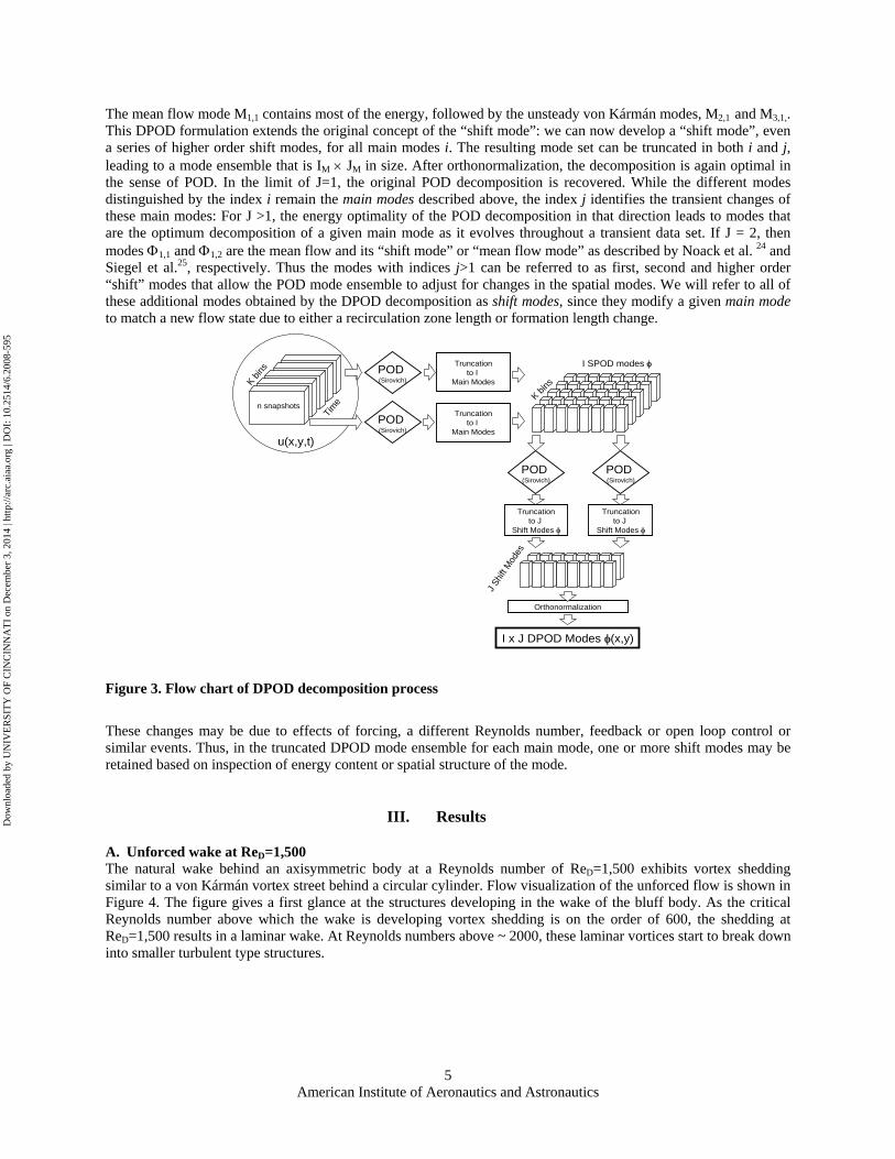
where a flow quantity u is represented by the spatial modes φk(x,y) and mode amplitudes ak(t). While this decomposition is well suited to time periodic flow fields, it faces problems for transient flows (see Siegel et al.22). Different additions to the basic POD procedure have been proposed, most notably the addition of a shift mode as introduced independently by Noack, Afanasiev, Morzynski and Thiele24 as well as Siegel, Cohen and McLaughlin.25 This shift mode originally only addressed changes to the mean flow, but the concept has been extended recently by Siegel, Cohen, Seidel and McLaughlin18 to adjust the fluctuating modes of transient flows as well. This modified POD procedure, referred to as Double POD (DPOD), provides shift modes for all main modes of a transient flow field. A pictorial representation of the DPOD procedure is given in figure 3. Starting in the top left corner, the data is split into K bins and each bin is used as an input data set for its individual POD procedure. The resulting SPOD (Short Time POD) modes are then collected across the bins and POD is applied again to obtain the shift modes. The procedure is expressed mathematically in Equation (2), where the index i refers to the main (SPOD) modes of the first POD procedure, while the index j identifies the shift mode order,

, ,1 1

( , , ) ( ) ( , ).I J

i j i ji j

u x y t t x yα= =

= Φ∑∑ (2)

Dow

nloa

ded

by U

NIV

ER

SIT

Y O

F C

INC

INN

AT

I on

Dec

embe

r 3,

201

4 | h

ttp://

arc.

aiaa

.org

| D

OI:

10.

2514

/6.2

008-

595


5

The mean flow mode M1,1 contains most of the energy, followed by the unsteady von Kármán modes, M2,1 and M3,1,. This DPOD formulation extends the original concept of the “shift mode”: we can now develop a “shift mode”, even a series of higher order shift modes, for all main modes i. The resulting mode set can be truncated in both i and j, leading to a mode ensemble that is IM × JM in size. After orthonormalization, the decomposition is again optimal in the sense of POD. In the limit of J=1, the original POD decomposition is recovered. While the different modes distinguished by the index i remain the main modes described above, the index j identifies the transient changes of these main modes: For J >1, the energy optimality of the POD decomposition in that direction leads to modes that are the optimum decomposition of a given main mode as it evolves throughout a transient data set. If J = 2, then modes Φ1,1 and Φ1,2 are the mean flow and its “shift mode” or “mean flow mode” as described by Noack et al. 24 and Siegel et al.25, respectively. Thus the modes with indices j>1 can be referred to as first, second and higher order “shift” modes that allow the POD mode ensemble to adjust for changes in the spatial modes. We will refer to all of these additional modes obtained by the DPOD decomposition as shift modes, since they modify a given main mode to match a new flow state due to either a recirculation zone length or formation length change.

I x J DPOD Modes (x,y)

Truncationto I

Main Modes

�

Orthonormalization

POD(Sirovich)

Truncationto J

Shift Modes

n snapshots

Kbin

s

u(x,y,t)

POD(Sirovich)

POD(Sirovich)

Truncationto I

Main Modes

K bins

I SPOD modes

POD(Sirovich)

Truncationto J

Shift Modes

�

Time

J Shif

t Mod

es

Figure 3. Flow chart of DPOD decomposition process

These changes may be due to effects of forcing, a different Reynolds number, feedback or open loop control or similar events. Thus, in the truncated DPOD mode ensemble for each main mode, one or more shift modes may be retained based on inspection of energy content or spatial structure of the mode.

III. Results

A. Unforced wake at ReD=1,500 The natural wake behind an axisymmetric body at a Reynolds number of ReD=1,500 exhibits vortex shedding similar to a von Kármán vortex street behind a circular cylinder. Flow visualization of the unforced flow is shown in Figure 4. The figure gives a first glance at the structures developing in the wake of the bluff body. As the critical Reynolds number above which the wake is developing vortex shedding is on the order of 600, the shedding at ReD=1,500 results in a laminar wake. At Reynolds numbers above ~ 2000, these laminar vortices start to break down into smaller turbulent type structures.

Dow

nloa

ded

by U

NIV

ER

SIT

Y O

F C

INC

INN

AT

I on

Dec

embe

r 3,

201

4 | h

ttp://

arc.

aiaa

.org

| D

OI:

10.

2514

/6.2

008-

595


6

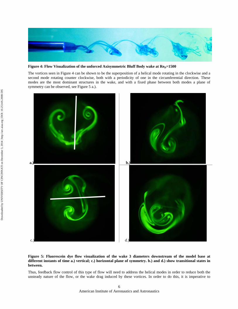
Figure 4: Flow Visualization of the unforced Axisymmetric Bluff Body wake at ReD=1500

The vortices seen in Figure 4 can be shown to be the superposition of a helical mode rotating in the clockwise and a second mode rotating counter clockwise, both with a periodicity of one in the circumferential direction. These modes are the most dominant structures in the wake, and with a fixed phase between both modes a plane of symmetry can be observed, see Figure 5 a.).

a.) b.)

c.) d.)

Figure 5: Fluorescein dye flow visualization of the wake 3 diameters downstream of the model base at different instants of time a.) vertical; c.) horizontal plane of symmetry. b.) and d.) show transitional states in between.

Thus, feedback flow control of this type of flow will need to address the helical modes in order to reduce both the unsteady nature of the flow, or the wake drag induced by these vortices. In order to do this, it is imperative to

B C

Dow

nloa

ded

by U

NIV

ER

SIT

Y O

F C

INC

INN

AT

I on

Dec

embe

r 3,

201

4 | h

ttp://

arc.

aiaa

.org

| D

OI:

10.

2514

/6.2

008-

595


7

develop an estimation method for the magnitude, frequency and phase of these vortices. In addition, it needs to be established that the actuation system is able to excite and control these vortices, in other words, controllability of these vortices needs to be demonstrated. In order to establish the amplitude and frequency range where controllability exists, the flow was forced with the 8 actuator setup exciting modes +-1. The flow was inspected and the plane of symmetry was identified as shown in Figure 5a. Then the phase between modes +1 and -1 was changed by 90 degrees followed by a second inspection, see Figure 5c for a typical result. If the plane of symmetry followed the forcing, the amplitude/frequency combination was determined to result in lock-in, a necessary but not sufficient condition for the wake was to be controllable. Otherwise, the flow was determined to be non-responsive to the forcing. Figure 6 shows both computational results obtained by Seidel et al.26 as well as the experimental results of this investigation. It can be seen that the lock-in region in the experiment is slightly smaller than the computational lock-in region. This can be attributed to a number of slight differences between experiment and simulation. While the simulation prescribed a blowing and suction boundary condition with a uniform velocity at the surface throughout the entire boundary patch, the experiment features a channel flow due to the setup of the actuation system, where the velocity distribution is not uniform over the blowing and suction opening. Thus, less actuation energy is delivered to the flow in the experiment compared to the simulation. Overall, there is a good agreement between experiment and simulation.

Figure 6: Lock-in plot compiled based on fluorescein dye flow visulazation observations; overlaid on computational result by Seidel et al.26

With these qualitative inspections of the flow in place, the next step in the open loop forcing evaluation is to determine the transient behavior of the flow quantitatively and in more detail. For this investigation, the flow was forced with a transient actuation input while PIV data was acquired throughout the transition. A typical wave form for the 8 actuators is shown in Figure 7. The flow is forced with a given frequency and amplitude as well as phase difference of modes +1 and -1. Then the phase between both modes is changed instantaneously from one forcing cycle to the next, in the example wave form of Figure 7 after two full shedding cycles. This leads to a change in the plane of symmetry as shown in the instantaneous blowing and suction distributions in Figure 8. Figure 8a shows the velocities at the peak of the forcing cycle before the phase change, while Figure 8b shows the velocities after the change in plane of symmetry.

Dow

nloa

ded

by U

NIV

ER

SIT

Y O

F C

INC

INN

AT

I on

Dec

embe

r 3,

201

4 | h

ttp://

arc.

aiaa

.org

| D

OI:

10.

2514

/6.2

008-

595


8

Ampl

itude

1

-1

-800m

-600m

-400m

-200m

0

200m

400m

600m

800m

t/T [-]3.980

Piston 0

Piston 1

Piston 2

Piston 3

Piston 4

Piston 5

Piston 6

Piston 7

Figure 7: Sample actuator amplitudes for transient forcing with a 90 degree change in plane of symmetry of forcing after two cycles, forcing helical modes +-1, amplitude 1.

y

0.75

-0.75

-0.6

-0.5

-0.4

-0.3

-0.2

-0.1

0

0.1

0.2

0.3

0.4

0.5

0.6

x0.75-0.75 -0.5 -0.25 0 0.25 0.5

Cylinder

Actuator 0

Actuator 1

Actuator 2

Actuator 3

Actuator 4

Actuator 5

Actuator 6

Actuator 7

Tip Trace

XY Graph

y

0.75

-0.75

-0.6

-0.5

-0.4

-0.3

-0.2

-0.1

0

0.1

0.2

0.3

0.4

0.5

0.6

x0.75-0.75 -0.5 -0.25 0 0.25 0.5

Cylinder

Actuator 0

Actuator 1

Actuator 2

Actuator 3

Actuator 4

Actuator 5

Actuator 6

Actuator 7

Tip Trace

XY Graph

Figure 8: Instantaneous blowing and suction distribution, a.) t/T = 0.25; b.) t/T = 2.25. Refer to Figure 7 for actuator time signals and time reference.

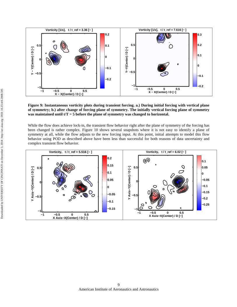
PIV results for transient forcing of the flow at the natural frequency with 35% of the free stream velocity forcing amplitude are shown in Figure 9. Figure 9a represents the vorticity present in the flow three diameters downstream of the base, at a time of 3.36 shedding cycles after the forcing. It can be seen that the flow is symmetric along the vertical axis, which is consistent with the forcing applied. Figure 9b shows the vorticity after the plane of symmetry has been changed to horizontal (which occurred after 5 shedding cycles total). Again, the orientation of the vortices is consistent with the forcing, but now with the new horizontal plane of symmetry.

Dow

nloa

ded

by U

NIV

ER

SIT

Y O

F C

INC

INN

AT

I on

Dec

embe

r 3,

201

4 | h

ttp://

arc.

aiaa

.org

| D

OI:

10.

2514

/6.2

008-

595


9

X − X(Center) / D [−]

Y −

Y(C

ente

r) /

D [

−]Vorticity [1/s], t / t_ref = 3.36 [− ]

−1 −0.5 0 0.5−1

−0.5

0

0.5

−0.2

−0.1

0

0.1

0.2

X − X(Center) / D [−]

Y−Y

(Cen

ter)

/ D

[−]

Vorticity [1/s], t / t_ref = 7.616 [− ]

−1 −0.5 0 0.5−1

−0.5

0

0.5

−0.2

−0.1

0

0.1

0.2

0.3

Figure 9: Instantaneous vorticity plots during transient forcing. a.) During initial forcing with vertical plane of symmetry; b.) after change of forcing plane of symmetry. The initially vertical forcing plane of symmetry was maintained until t/T = 5 before the plane of symmetry was changed to horizontal.

While the flow does achieve lock-in, the transient flow behavior right after the plane of symmetry of the forcing has been changed is rather complex. Figure 10 shows several snapshots where it is not easy to identify a plane of symmetry at all, while the flow adjusts to the new forcing input. At this point, initial attempts to model this flow behavior using POD as described above have been less than successful for both reasons of data uncertainty and complex transient flow behavior.

X Axis−X(Center) / D [−]

Y A

xis−

Y(C

ente

r) /

D [

−]

Vorticity, t / t_ref = 5.516 [− ]

−1 −0.5 0 0.5−1

−0.5

0

0.5

−0.15

−0.1

−0.05

0

0.05

0.1

0.15

0.2


Y A

xis−

Y(C

ente

r) /

D [

−]

Vorticity, t / t_ref = 6.02 [− ]

−1 −0.5 0 0.5−1

−0.5

0

0.5

−0.25

−0.2

−0.15

−0.1

−0.05

0

0.05

0.1

Dow

nloa

ded

by U

NIV

ER

SIT

Y O

F C

INC

INN

AT

I on

Dec

embe

r 3,

201

4 | h

ttp://

arc.

aiaa

.org

| D

OI:

10.

2514

/6.2

008-

595


10


Y A

xis−

Y(C

ente

r) /

D [

−]Vorticity, t / t_ref = 6.496 [− ]

−1 −0.5 0 0.5−1

−0.5

0

0.5

−0.15

−0.1

−0.05

0

0.05

0.1

0.15

0.2


Y A

xis−

Y(C

ente

r) /

D [

−]

Vorticity, t / t_ref = 7 [− ]

−1 −0.5 0 0.5−1

−0.5

0

0.5

−0.2

−0.15

−0.1

−0.05

0

0.05

0.1

0.15

Figure 10: Instantaneous vorticity plots during transient forcing. a.) through d.) are snapshots in half shedding cycle increments of about 0.5, 1.0, 1.5, and 2.0 after change of forcing plane of symmetry. The initially vertical forcing plane of symmetry was maintained until t/T = 5 before the plane of symmetry was changed to horizontal.

IV. Conclusion Initial measurements of the unforced wake of an axisymmetric bluff body at a Reynolds number base on diameter of Re=1,500 corroborate the numerical findings of large scale, vortical structures in the wake. As found in the simulations and earlier experiments, the unforced wake shows a superposition of multiple unstable modes. We confirm experimentally the lock-in region of the flow that was identified by Seidel et al. based on CFD simulations, where the experimentally determined lock-in region is slightly smaller than what was found in the simulations. Initial transient forced PIV measurements show very complex transient flow behavior as a result of a change in the plane of symmetry of the forcing input, for which efforts to develop a numerical model are still ongoing. One main next step will be to acquire phase locked open loop forced data, in order to perform phase averaging to eliminate non-periodic flow events. This should improve the ability to develop spatial POD/DPOD modes greatly.

Acknowledgments The authors would like to acknowledge funding by the Air Force Office of Scientific Research, LtCol Rhett Jeffries. The contributions of Cadets Andrés A. Ascázubi, Derek W. Haun, Sompop Thongfuang, and Daniel C. Wynn to the experimental results presented here are acknowledged.

References 1. Koopmann, G., “The Vortex Wakes of Vibrating Cylinders at Low Reynolds Numbers”, Journal of Fluid Mechanics,

Vol. 28 Part 3, 1967, pp. 501-512. 2. Williamson, C.H.K., “Vortex Dynamics in the Cylinder Wake”, Ann. Rev. Fluid Mech., 1996, 28:477-539 3. Monkewitz, P. A., “Modeling of self-excited wake oscillations by amplitude equations”, Experimental Thermal and Fluid

Science, Vol. 12, 1996, pp. 175-183. 4. Noack, B. R., Eckelmann, H. “A global stability analysis of the steady and periodic cylinder wake”, Journal of Fluid

Mechanics, Vol. 270, pp. 331-347. 5. Blevins, R., “Flow Induced Vibration”, 2nd Edition, Van Nostrand Reinhold, 1990, pp. 54-58. 6. Siegel, S., Cohen, K. & McLaughlin T., 2003, “Feed-back control of a circular cylinder wake in experiment and

simulation (invited)”, AIAA 2003-3569. 7. Cohen K., Siegel S., McLaughlin T. & Gillies E., “Feedback Control of a Cylinder Wake Low-Dimensional Model”,

AIAA Journal 41, No. 7, 1389-1391. 8. Cohen, K., Siegel,S., McLaughlin, T., “Sensor Placement Based on Proper Orthogonal Decomposition Modeling of a

Cylinder Wake”, 33rd AIAA Fluid Dynamics Conference, Orlando, AIAA 2003-4259, 2003 9. Aschenbach, E. 1974, “Vortex shedding from spheres”, Journal of Fluid Mechanics, Vol 62, 209.

Dow

nloa

ded

by U

NIV

ER

SIT

Y O

F C

INC

INN

AT

I on

Dec

embe

r 3,

201

4 | h

ttp://

arc.

aiaa

.org

| D

OI:

10.

2514

/6.2

008-

595


11

10. Sakamoto, Haniu, 1990, “A study on vortex shedding from spheres in a uniform flow”, J. Fluids Eng., 112, pp. 386-393. 11. Monkewitz, P.A. 1988, “A note on vertex shedding from axisymmetric bluff bodies”, Journal of Fluid Mechanics, Vol

192, pp 561-575. 12. Cannon, S.C., 1991, “Large-Scale Structures and the Spatial Evolution of Wakes behind Axisymmetric Bluff Bodies”,

Dissertation, University of Arizona. 13. Schwarz, V., Bestek, H., Fasel, H. 1994, “Numerical simulation of nonlinear waves in the wake of an axisymmetric bluff

body”, AIAA 94-2285. 14. Tourbier, D., 1996, “Numerical investigation of transitional and turbulent axisymmetric wakes at supersonic speeds”.

Dissertation, University of Arizona. 15. S. Siegel, K. Cohen and T. McLaughlin., "Numerical simulations of a feedback controlled circular cylinder wake", AIAA

Journal, vol. 44, no. 6, pp.1266-1276, June 2006. 16. Siegel, S., Cohen, K. & McLaughlin, T., 2004, “Experimental Variable Gain Feedback Control of a Circular Cylinder

Wake”, AIAA 2004-2611. 17. Cohen, K., Siegel,S., Seidel, J., McLaughlin, T., “Reduced Order Modeling for Closed-Loop Control of Three

Dimensional Wakes”, AIAA Paper 2006-3356. 18. Stefan Siegel, Kelly Cohen, Jürgen Seidel, Thomas McLaughlin, 'State estimation of transient flow fields using Double

Proper Orthogonal Decomposition (DPOD)', Active Flow Control, NNFM 95, R. King (Editor), Springer, pp. 105-118, 2007

19. Stefan Siegel, Jürgen Seidel, Kelly Cohen, Selin Aradag, Thomas McLaughlin, 'Dynamic Flow Modeling Using Double POD and ANN-ARX System Identification', 60th Annual Meeting of the American Physical Society, Division of Fluid Dynamics, Salt Lake City, UT, November 2007

20. Siegel, S., Fasel, H., “Effect of Forcing on the Wake Drag of an Axisymmetric Bluff Body”, AIAA 2001-0736 21. R. Noack, G. Tadmor, and M. Morzynski, "Low-dimensional models for feedback flow control. Part I: Empirical

Galerkin models", presented at the 2nd AIAA Flow Control Conference, Portland, Oregon, 28 Jun - 1 Jul 2004, AIAA Paper 2004-2408

22. Siegel, S., Cohen, K., Seidel, J., McLaughlin, T., 'Short Time Proper Orthogonal Decomposition for State Estimation of Transient Flow Fields', 43rd AIAA Aerospace Sciences Meeting, Reno, AIAA2005-0296, 2005

23. Siegel, S., Cohen, K., Seidel, J., McLaughlin, T., 'Short Time Proper Orthogonal Decomposition for State Estimation of Transient Flow Fields', 43rd AIAA Aerospace Sciences Meeting, Reno, AIAA2005-0296, 2005

24. B. R. Noack, K. Afanasiev, M. Morzynski and F. Thiele “A hierarchy of low dimensional models for the transient and post-transient cylinder wake”, J. Fluid Mechanics, vol. 497, pp. 335–363, 2003.

25. S. Siegel., K. Cohen., J. Seidel and T. McLaughlin, “State estimation of transient flow fields using double proper orthogonal decomposition (DPOD)”, presented at the International Conference on Active Flow Control, Berlin, Germany, September 27-29, 2006.

26. J. Seidel, S. Siegel, K. Cohen,and T. McLaughlin, 'Simulations of Flow Control of the Wake Behind an Axisymmetric Bluff Body', 3rd AIAA Flow Control Conference San Francisco, 5-8th June 2006, AIAA 2006-3490, , 2006

Dow

nloa

ded

by U

NIV

ER

SIT

Y O

F C

INC

INN

AT

I on

Dec

embe

r 3,

201

4 | h

ttp://

arc.

aiaa

.org

| D

OI:

10.

2514

/6.2

008-

595

Open Loop Transient Forcing of an Axisymmetric Bluff Body Wake

Documents

Transcript of Open Loop Transient Forcing of an Axisymmetric Bluff Body Wake