DOI 10.1140/epje/i2011-11067-x

Regular Article

Eur. Phys. J. E (2011) 34: 67 THE EUROPEANPHYSICAL JOURNAL E

Analytical expressions for the shape of axisymmetric membraneswith multiple domains

T. Idema1,a and C. Storm2

1 Department of Physics and Astronomy, University of Pennsylvania, 209 S 33rd street, Philadelphia, Pennsylvania 19104, USA2 Department of Applied Physics and Institute for Complex Molecular Systems, Eindhoven University of Technology, P.O. Box

513, 5600 MB Eindhoven, The Netherlands

Received 5 April 2011 and Received in final form 9 June 2011Published online: 14 July 2011c© The Author(s) 2011. This article is published with open access at Springerlink.com

Abstract. Based on the Canham-Helfrich free energy, we derive analytical expressions for the shapes ofaxisymmetric membranes consisting of multiple domains. We give explicit equations for both closed vesiclesand almost cylindrical tubes. Using these expressions, we also find the shape of a tube attached to aspherical vesicle. The resulting shapes compare well to numerical data, and our expressions can be usedto easily determine membrane parameters from experimentally obtained shapes.

1 Introduction

Membranes compartmentalize the interior of eukaryoticcells, and separate the inside world from the outside. Theyare also essential for many cellular processes like signal-ing, trafficking and nutrient uptake, and provide a plat-form for physical and chemical interactions between pro-teins [1]. A key component of many such processes is theshape of the membrane, which is either determined intrin-sically by its composition, or by the external influence ofproteins and molecular motors. A typical example is endo-cytosis, where several membrane-associated proteins worktogether to split off a small vesicle with a specific com-position from a large membrane [2–5]. Another exampleis the extraction of long membrane tubes from organelleslike the endoplasmic reticulum by motors walking on thecell cytoskeleton [6]. Both intrinsic membrane shapes andthe effect of the application of forces on them have beenstudied extensively. One line of study focuses on artifi-cial membrane systems consisting of a mixture of choles-terol and two other lipids, resulting in a rich phase be-havior, including the separation into liquid-ordered (Lo)and liquid-disordered (Ld) domains [7–11]. Such domainshave been visualized and studied by many groups in recentyears [12–18]. Based on the Canham-Helfrich free energyfor lipid bilayer membranes [19,20], and the associatedshape equations [21–23], several analytical and numericalresults on the relation between the shape and composi-tion of membranes have been obtained on the stabilityand budding of vesicles with domains [24–26], and recentlyalso for their shapes [14,17].

a e-mail: tidema@sas.upenn.edu

Another line of study focuses on the applicationof a point force on a membrane vesicle, resulting innarrow membrane tethers or tubes pulled from thevesicles. In such experiments the surface tension ofthe membrane in the vesicle is usually controlled usingpipette aspiration [27–29]. Tubes are often pulled usingmicropipettes [30] or optical tweezers [31], but also bymolecular motors [32–35]. Several attempts have beenmade to study the effect of a point force on a large mem-brane vesicle theoretically [36–39], resulting in analyticalexpressions for small deformations [37,38] as well asfor almost-cylindrical long tubes pulled from these vesi-cles [39]. Recent experimental results also show sorting ofmulti-component bilayer membranes due to the curvatureimposed by tube pulling [40–43], as well as protein sortingdue to their spontaneous curvature [43], and domainnucleation at the neck connecting the tube to its mothervesicle [44]. The shape equations for tubular membraneswith multiple domains have been solved numerically [44,45] and approximate expressions based on linearizations ofthe associated shape equations have also been found [46].

In this paper we study membranes consisting of twodifferent domains in two specific settings: 1) a closed mem-brane vesicle and 2) an almost cylindrical tube. As out-lined above, both have been studied numerically in thepast; here we complement those results by deriving ana-lytical expressions for the shape of the membrane. To doso, we first write the shape equation in terms of a singleunknown variable: the tangent angle ψ for vesicles, andthe radius r for tubes. In both systems, earlier results arebased on linearizations of both ψ and r [14,39]. By firsteliminating one of those and only linearizing afterwards,

Page 2 of 10 The European Physical Journal E

we eliminate one linearization step, but still obtain shapeequations that may be solved in closed form for realis-tic boundary conditions. These solutions permit analyti-cal analysis of nontrivial shapes, some of which were pre-viously only accessible with numerical methods. For vesi-cles, this approach leads to a refinement of our earlier re-sults [14]. For tubes, we retrieve the decaying oscillationsfound before [37–39,46]. Moreover, we use the analyticalexpression for the shape of a tubular membrane to obtainan approximation of the shape of a tube connected to aspherical vesicle, complementing the known analytical andnumerical results.

2 Shape equation

The energy associated with the curvature of a membrane isgiven by the Canham-Helfrich free energy, which includesall contributions of membrane curvature up to second or-der [19,20]. We assume the membrane to be inextensibleand hence the total surface area of the membrane to beconserved, which we ensure by adding a Lagrange multi-plier (commonly interpreted as the surface tension σ) tothe free energy. We can also add a Lagrange multiplier forthe total volume enclosed by the membrane (interpretedas the pressure difference across the membrane p) and anexternal force f . For a single-component membrane withbending modulus κ and Gaussian modulus κ, the free en-ergy is then given by

F =∫ (κ

2(2H − C0)2 + κK + σ

)dA + pV − fL, (1)

where H is the mean curvature and K the Gaussian cur-vature, A and V are the membrane’s area and enclosedvolume, C0 its spontaneous curvature, and L is the ex-tension in the direction in which the force is applied. Fora single-component closed membrane, the Gauss-Bonnettheorem tells us that the integral over K is a constant. Inmulti-component membranes, it integrates to a constantplus a boundary term [47].

It is well known that the infinite tube under externaltension is a surface which minimizes the Canham-Helfrichfree energy [37,38,48]. We will show this below from theshape equation associated with the free energy (1). Moredirectly, we can also use the argument of Derenyi et al. [37]to relate the radius and applied force for a stable tube tothe membrane’s material parameters. For a tube of lengthL and radius R we find from (1)

Ftube = 2πRL

[κ

2

(1R

− C0

)2

+ σ

]+ πpR2L − fL. (2)

In equilibrium, the bending modulus (which favors a largeradius) and the surface tension (which favors a small area,and hence a small radius) have to balance. We find theequilibrium radius R0 and force f0 by taking derivativesof Ftube with respect to R and L and equating them to

zero, resulting in

0 = σ − 12R2

0

+12C2

0 + pR0, (3)

f0

2πκ=

p

2R2

0 +R0

2

(1

R0− C0

)2

+ σR0, (4)

where σ = σ/κ and p = p/κ. We note that eq. (3) isthe derivative of eq. (4) with respect to R0. For the casef = 0 these equations were first given by Ou-Yang andHelfrich [21]. For the special case that p = C0 = 0, eqs. (3)and (4) simplify to [37]

R0 =√

κ

2σ, (5)

f0 = 2π√

2κσ . (6)

This simple argument gives the correct values of R0 andf0, but also has a major shortcoming: the free energy asgiven in eq. (2) is marginally unstable to the unphysicalmode of uniform (de)swelling of the entire cylindrical tube.As was shown by Powers et al. [38], a more careful analysisshows that membrane tubes are in fact stable to arbitrarysmall perturbations, a result we also find as part of ouranalysis in sect. 4.

Another minimizer of the Canham-Helfrich free energyat vanishing force is a sphere. Following the same proce-dure as above, we write for the free energy

Fsphere = 2πκR2

(2R

− C0

)2

+ 4πR2σ +43πpR3, (7)

from which we find the equilibrium condition

pR2 + 2σR − κC0(2 − C0R) = 0. (8)

Equation (8) was also first given by Ou-Yang and Hel-frich [21], who also showed that for low pressures thesphere is a stable solution of the shape equation, althoughfor higher pressures it is not. We will only consider thelow-pressure case here. For the case of vanishing sponta-neous curvature, eq. (8) simplifies to the condition that thepressure difference across the membrane must be given bythe Laplace pressure, p = −2σ/R.

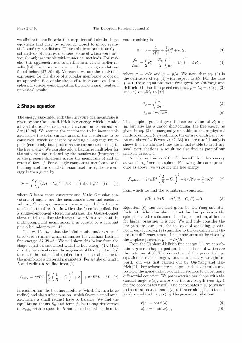
From the Canham-Helfrich free energy (1), we can ob-tain a general shape equation, the solutions of which arethe extrema of F . The derivation of this general shapeequation is rather lengthy but conceptually straightfor-ward, and was first carried out by Ou-Yang and Hel-frich [21]. For axisymmetric shapes, such as our tubes andvesicles, the general shape equation reduces to an ordinarydifferential equation. We parameterize our shape with thecontact angle ψ(s), where s is the arc length (see fig. 1for the coordinates used). The coordinates r(s) (distanceto the rotation axis) and z(s) (distance along the rotationaxis) are related to ψ(s) by the geometric relations

r(s) = cos ψ(s), (9)z(s) = − sin ψ(s), (10)

T. Idema and C. Storm: Analytical expressions for the shape of multi-component membranes Page 3 of 10

-100 -50 50 100

-4

-2

2

4r

z

r

ψ(s)

a

20 40

-60

-40

-20

20

40

r

z s=0

s=s*

s=πR/2R

b

ψ(s)

R s=0

1

2

Fig. 1. Coordinate systems used. (a) Coordinates on a closedvesicle. (b) Coordinates on a tubular membrane.

where the dot denotes a derivative with respect to thearc length s. We can also express the mean and Gaussiancurvatures in terms of ψ (dropping explicit dependencieson s)

2H = ψ +sin ψ

r, (11)

K =sinψ

rψ. (12)

Substituting (11) and (12) into the shape equation de-rived by Ou-Yang and Helfrich [21] gives us the axisym-metric shape equation

...ψ = −2 cos ψ

rψ − 1

2ψ3 +

sin ψ

rψ2 +

12

sin ψ

r(ψ − C0)2

+12

(sin ψ

r− C0

)2

ψ +1 − 2 sin2 ψ

r2ψ +

σ

κψ

−cos2 ψ + 12r3

sin ψ +σ

κ

sinψ

r+

p

κ. (13)

As was shown by Zheng and Liu [49], eq. (13) can bewritten as a total derivative, which can be integrated togive an equivalent second-order differential equation forψ(s)

ψ cos ψ = −12ψ2 sinψ − cos2 ψ

rψ +

sin ψ

2

(sinψ

r− C0

)2

+cos2 ψ

r2sin ψ +

σ

κsinψ +

p

2κr − 1

2πκ

f

r. (14)

Substituting a tubular shape (r = R0 and ψ = π/2) intoeq. (14) we again obtain eq. (4), and substituting theminto eq. (13) gives eq. (3), in accordance with the observa-tion we made above that eq. (3) is simply the derivativeof eq. (4) with respect to the tube radius R0. We also findfrom both eqs. (13) and (14) that in the absence of a forcea sphere of any radius R is a solution, provided eq. (8) issatisfied.

In an alternative approach, we can derive the axisym-metric shape equation (14) by writing the energy func-tional (1) as an integral over a Lagrangian, and performing

variational analysis, as detailed by Julicher et al. [22,23].The advantage of the latter approach is that it can be eas-ily extended to membranes containing multiple domains,and also gives the boundary conditions at their commonedge [23]. Equation (14) holds within the bulk of any con-tinuous piece of membrane, i.e., in any piece where thematerial constants are the same throughout. At bound-aries between coexisting phases 1 and 2, the Lagrangianderivation of (14) gives four boundary conditions: conti-nuity of r and ψ, and two more complicated conditions forψ and ψ (expressions below are for a boundary at s = 0):

limε↓0

(κ2ψ(ε) − κ1ψ(−ε)

)= −(Δκ + Δκ)

sin ψ0

r0

+κ2C0,2 − κ1C0,1, (15)

limε↓0

(κ2ψ(ε) − κ1ψ(−ε)

)= (2Δκ + Δκ)

cos ψ0 sinψ0

r20

−(κ2C0,2 − κ1C0,1)cos ψ0

r0

+sin ψ0

r0τ. (16)

Here ψ0 and r0 are the values of ψ and r at the boundary,Δκ = κ2 − κ1, Δκ = κ2 − κ1, and τ is the line tension atthe boundary.

3 Closed vesicles

We first study closed-vesicle solutions of the axisymmetricshape equation (14). For a single-component membrane,the shape is determined by the ratio of the membrane’ssurface area and enclosed volume. The optimal solution,i.e., the solution with the minimum total bending energyfor a given total membrane area, is a sphere, which alsoencloses the maximum volume given the total area. Forsmaller, but fixed, enclosed volumes, solutions include el-lipsoids and the biconcave shapes found in red blood cells.Because lipid bilayer vesicles are permeable to water onlong time scales, any single-component membrane vesicleleft to relax long enough will eventually end up with aspherical shape.

The equilibrium shape of two-component vesicles is notspherical if there is a line tension present at the bound-ary between the two domains. In that case, the equilib-rium shape is determined by a balance between the bend-ing modulus (which drives the system towards a spher-ical shape) and the line tension (which favors a shortboundary line). For approximately equal-sized domainsand appropriate values of the material parameters, the re-sulting shape is a snowman-like vesicle with two almostspherical domains connected by a narrower “waist” or“neck” [9,12,14]. We will derive an approximate analyt-ical expression for the shape of these vesicles from theshape equation (14). Since there is no external force in thiscase, we set f = 0. Moreover, as in the case of a single-component membrane, for the spherical parts to be stable,eq. (8) must be satisfied in each of the two domains, whichmeans that the pressure, surface tension and spontaneous

Page 4 of 10 The European Physical Journal E

curvature terms in eq. (14) cancel. The resulting differen-tial equation for the contact angle ψ does not depend onany material parameters, which thus only influence theshape because of the boundary conditions. Within thebulk of each of the domains, far away from the bound-ary, the shape of the vesicle should approximately be asphere of radius R, so ψ(s) ∼ s/R and r(s) ∼ R sin(s/R).To meet the boundary conditions, we will perturb thesespherical “bulk solutions” and write ψ(s) = s/R + δψ(s).It is not obvious how this perturbation carries over to r(s).Earlier approaches therefore also linearized r(s); insteadwe eliminate r(s) by isolating it from eq. (14), differen-tiating the resulting expression and using the geometricrelation r = cos ψ (eq. (9)). First rewriting (14), we have

r2(2ψ cos ψ + ψ2 sin ψ)

+r(2 cos2 ψψ) − (cos2 ψ + 1) sin ψ = 0, (17)

from which we get two solutions for r(s)

r(s) =− cos ψψ

2ψ + ψ2 tan ψ

±

√ψ2 sec2 ψ + 2ψ tan ψ(1 + cos2 ψ)

2ψ + ψ2 tan ψ. (18)

Because the sphere is only a solution of eq. (18) when weuse the plus sign in front of the square root, we drop theequation with the minus sign. Differentiating the remain-ing equation with respect to s and using eq. (9), we get athird-order nonlinear differential equation for ψ

0 =(2 cos ψψ

...ψ − 6 cos ψψ2 − sin ψψ2ψ + sec ψψ

)

·√

ψ2 sec2 ψ + 2ψ tan ψ(1 + cos2 ψ)

−2 tan ψ(1 + cos2 ψ)ψ...ψ + 2(3 − 4 sin2 ψ)ψψ2

+(sin2 ψ + tan2 ψ − 2 sec2 ψ)ψ2...ψ

−(1 + 2 sin2 ψ) tan ψψ3ψ − sec2 ψψ5. (19)

We now use the expansion ψ(s) = s/R + εδψ(s) andexpand up to linear order in ε. In doing so, we assumethat the derivatives of δψ are of the same order as δψ it-self. Carrying out the expansion, we find a much simplerthird-order linear differential equation for δ

...ψ

0 = 3 cos(s/R)δψ + R sin(s/R)δ...ψ, (20)

where δψ(s) = dδψ(s)/ds and δψ(s) and δ...ψ(s) similarly

defined. Equation (20) can be integrated directly, resultingin an expression for δψ

δψ(s) = A csc3( s

R

), (21)

with A an integration constant which has dimension 1/R2,and in which we absorb the expansion coefficient ε. Inte-grating again, we get

δψ(s) =AR

2log

[tan

( s

2R

)]− AR

2cos(s/R)sin2(s/R)

+ b, (22)

where b is another integration constant. Because the in-tegral of b gives a term that scales with s, it gives a con-

stant contribution to the term s/R in ψ(s); we thereforeset b = 0. A final integration gives us δψ(s)

δψ(s) =AR2

2

{1

sin(s/R)+ i log

(tan

( s

R

))

·[log

(1 − i tan

( s

2R

))− log

(1 + i tan

( s

2R

))]

+ i[Li2

(i tan

( s

2R

))− Li2

(−i tan

( s

2R

))]}

+d, (23)

with d a third integration constant and Lin(z) the poly-logarithm (also known as Jonquiere’s function), defined as

Lin(z) =∞∑

k=1

zk

kn, (24)

for z ∈ C. The combination of the two logarithms in (23),as well as that of the two polylogarithms, is real for ourregion of interest (0 < s < πR, see fig. 1a). The functionδψ(s) goes to infinity at both ends of this interval and hasa minimum at the center s = πR/2. We therefore assumethe vesicle to be a perfect sphere for 0 ≤ s ≤ πR/2, andgiven by ψ(s) = s/R + δψ(s) for πR/2 ≤ s ≤ s∗, wherethe boundary with the other domain is at s = s∗ < πR.This choice fixes the value of the integration constant dbecause now δψ(πR/2) should vanish, which gives

d = −AR2

2(1 − 2G), (25)

where G is Catalan’s constant, with numerical value ∼0.91596559.

Having found expressions for δψ(s) and δψ(s), we canalso find an expression for r(s). To do so, we first expandthe geometric relation (9) and then integrate it. As thestarting point of the integration we take the same referencepoint s0 = πR/2 as we did for δψ(s), at which point r(s) =R. We then find

r(s) = R +∫ s

s0

cos(

s′

R+ δψ(s′)

)ds′

= R sin( s

R

)+ R

[δψ(s′) cos

(s′

R

)]s′=s

s′=s0

−R

∫ s

s0

δψ(s′) cos(

s′

R

)ds′

= R sin( s

R

)+ R cos

( s

R

)δψ(s) − AR3

2cot

( s

R

)

−AR3

2sin

( s

R

)log

(tan

( s

2R

)), (26)

where we first expanded the cosine and then used partialintegration. In exactly the same fashion we also find anexpression for z(s)

z(s) = z0 + R cos( s

R

)− R sin

( s

R

)δψ(s)

−AR3

2cos

( s

R

)log

(tan

( s

2R

)), (27)

where z0 = z(s0).

T. Idema and C. Storm: Analytical expressions for the shape of multi-component membranes Page 5 of 10

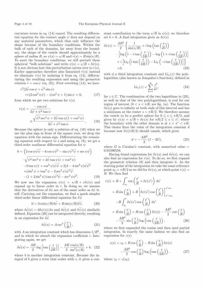
Fig. 2. Shape of a closed vesicle with two domains. Panel (a) shows ψ(s), with dashed lines indicating ψ(s) of a sphere with thesame radius. Panels (b) (cross-section) and (c) (revolution plot) show the actual shape of the axisymmetric vesicle, (r(s), z(s)).Note that the bottom part (with the lower bending modulus) curves towards the top part near the boundary, and that the twoparts of the ψ(s) plot are not symmetric.

Using the expressions for r(s), δψ(s) and its deriva-tives given above, we can find the shape of a vesicle withtwo domains with different material parameters from theboundary conditions (15) and (16), as well as continu-ity of r(s) and ψ(s) at the boundary. Writing down thefour boundary conditions for the general solution givenby eqs. (23) and (26), we find that we have six unknowns:the values of the total arc length s∗i , the domain radius Ri

and the dimensionless small parameter AiR2i for each do-

main (i = 1, 2). To get a closed system, we can there-fore choose any two of the six unknowns, and solve forthe other four, although there may not be solutions forevery possible choice. Example plots of resulting shapesare given in fig. 2, for which we chose values for theradii R1 and R2 and solved for the values of s∗i andAiR

2i .

The fact that our shapes are not completely fixed bythe set of equations is to be expected, because we did notspecify parameters such as the total area or enclosed vol-ume. These are of course fixed in experiment, which allowsone to determine (in principle) any two of the six unknownparameters of our system by directly measuring e.g. thedomain areas (because of the relation between the pres-sure, spontaneous curvatures and surface tensions givenby eq. (8), the enclosed volume is then fixed). One possi-ble approach is to measure the two values of s∗ directly bymeasuring the total arc length of the domains. However,a much simpler and more reliable approach is to measurethe values of the two radii R1 and R2. This can simply bedone by fitting a sphere to the upper and lower parts ofa snowman-shaped vesicle with two domains. Given thesevalues we are then left with four equations and four un-knowns, for any set of the material parameters. There areonly two material parameters that play a role in the de-termination of the shape of the vesicle: the line tension τand the difference in Gaussian moduli Δκ. We can there-fore use this method to fit the shape of the vesicle, andextract value for the line tension and difference in Gaus-

sian modulus, as we have done before using a simplermodel [14]. Experiments are commonly carried out usingGiant Unilamellar Vesicles, or GUVs, which have typicalradii of 10–100μm. For such large vesicles the assump-tions that go into our approach are easily justified. Thevesicles are indeed almost indistinguishable from spheresfar away from the domain boundary (see e.g. experimen-tal data in [12,14]). Moreover, they are smooth near theboundary, and deviate from the spherical shape very lit-tle even there, which means that δψ is indeed small. Ourapproach would break down for much smaller vesicles, fortwo possible reasons. One is that the deviations may be-come large compared to the size of the vesicle itself, mak-ing a linearized approach invalid. The second reason ismore fundamental and has to do with the basic energybalance that results in the snowman shape of bidomainvesicles. In these vesicles, the line tension on the bound-ary tends to contract the “neck” between the two domain,thus shortening the boundary length. On the other handthe bending energy of both domains tends to expand theneck, making the overall shape vesicle more like that of asphere and thus lowering the total mean curvature. Thetradeoff between these two is characterized by a lenth scaleknown as the invagination length ξ = κ/τ , first introducedby Lipowsky [24]. For domains with a radius much smallerthan the invagination length, the bending term in the en-ergy is dominant. The shape of small multi-domain vesi-cles will therefore not be like our snowman vesicle, butsimply a sphere.

4 Tubes

Suppose we have a tubular membrane with Lo and Ld

domains on it. Within the bulk of those domains, the re-spective pieces of the tube will approximately be the idealtube with radii and forces determined by their bendingmoduli and surface tensions, and given by eqs. (3) and (4)

Page 6 of 10 The European Physical Journal E

for R0 and f0. For a patterned tube to be stable, the forcesin both domains have to be equal. For the special case thatp = C0,1 = C0,2 = 0 this gives two simple observations;first that the simple relation

κoσo = κdσd (28)

holds, and second that, if κo �= κd, then the radii of thedifferent tube domains are different. Close to the bound-ary between the two domains the shape will therefore de-viate from the cylindrical tube. Shapes for the tube insuch boundary regions were first calculated numericallyby Allain et al. [45], and more recently also by Heinrichet al. [44]. An approximate analytical expression for thedeviation of a tube from a perfect cylinder, for instancebecause of the presence of a domain boundary, was firstgiven by Bozic et al. [39]. For completeness we briefly re-produce their argument here, where for simplicity we againset p = C0 = 0. We first re-parametrize from the arclength s to the z-coordinate using eq. (10), and next ex-pand r(z) around R0, writing r(z) = R0+u(z). If we more-over assume that the deviations from ψ = π/2 are verysmall, we can also write sin ψ = 1 and cos ψ = dr(s)

ds =− sin ψ(z)dr(z)

dz = −du(z)dz . Denoting derivatives to z by

primes, we similarly find ψ′(z) = u′′(z), ψ′′(z) = u′′′(z),and ψ′′′(z) = u′′′′(z). Substituting back into the third-order shape equation (13), and taking only terms linear inu(z) and its derivatives, we get the simple equation

R40u

′′′′(z) + u(z) = 0. (29)

The solution of eq. (29) is a sum of two exponentiallydecaying oscillations. As shown by Derenyi et al. [37],these two oscillations can be interpreted as being asso-ciated with the two ends of a finite tube pulled from avesicle: one end attached to the vesicle, the other closed.Campelo et al. [46] used these solutions in combinationwith the boundary conditions (15) and (16) to predict theshape of two-component tubes. One possible complicationof this approach is that it involves two linearizations, onefor r(z) and another one for ψ(z). As we will show be-low, a different approach allows us to eliminate one of thelinearizations, resulting in a different differential equationfor the deviation from the tube, but with similar exponen-tially decaying oscillations as solutions.

The basis of our approach is that we no longer pa-rameterize the tube with the contact angle ψ, but simplyby its radius as a function of arc length, r(s), and elimi-nate ψ from the shape equations, similarly to the way weeliminated r in the previous section. Using the geometricrelation (9), we can translate ψ and its derivatives into ex-pressions in r and its derivatives. First taking derivativesof (9), we find

r = cos ψ, (30)

r = − sin ψψ, (31)...r = − sin ψψ − cos ψψ2. (32)

We can invert these to express functions and derivativesof ψ in terms of r and its derivatives

cos ψ = r, (33)

sin ψ =√

1 − r2, (34)

ψ = − r√1 − r2

, (35)

ψ = − 1√1 − r2

(...r +

rr2

1 − r2

). (36)

We substitute (33)–(36) back into the shape equation (14).We then find a nonlinear third-order differential equationin r

0 = r...r +

r2r2

1 − r2− 1

2r2 +

r2r

r+

r2

r2(1 − r2)

+1 − r2

2

(√1 − r2

r− C0

)2

+ σ(1 − r2)

+(

pr

2− f

2πκr

) √1 − r2, (37)

where as before σ = σ/κ and p = p/κ. The boundaryconditions translate to continuity of r and r, and

limε↓0

(κ2r2(ε) − κ1r1(−ε)

)= (Δκ + Δκ)

1 − r20

r0

−(κ2C0,2 − κ1C0,1)√

1 − r20 , (38)

and

limε↓0

(κ2

...r 2(ε) − κ1

...r 1(−ε)

)

+r0

1 − r20

limε↓0

(κ2r2(ε)2 − κ1r1(−ε)2)

= −(2Δκ − Δκ)r0(1 − r2

0)r20

− 1 − r20

r0τ

+(κ2C0,2 − κ1C0,1)r0

√1 − r2

0

r0, (39)

for the second and third derivatives. Here r0 and r0 arethe values of r and r at the domain boundary, and thesubscripts 1 and 2 indicate the two domains.

In general the parts of the tube which correspondto the different domains will have unequal stable radii,and thus the tube gets deformed near the domain bound-ary. Moreover, even with identical radii, but a nonzeroline tension τ or difference in Gaussian modulus Δκ, theboundary conditions will distort the shape near the do-main boundary as well. To find the perturbed shapes, wemake an expansion of r(s) around the stable radius R0

(with the appropriate R0 for each domain)

r(s) = R0 + εδr(s). (40)

Substituting (40) into (37), the O(1) term reproduceseq. (4) and thus vanishes by construction. Moreover, by

T. Idema and C. Storm: Analytical expressions for the shape of multi-component membranes Page 7 of 10

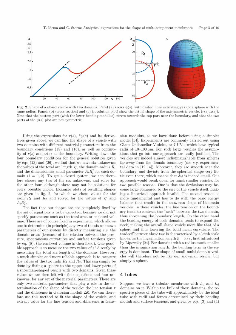
Fig. 3. Example tubes with two domains. (a) Two domains with different material parameters (κo = 1.25κd), but no differencein Gaussian moduli (Δκ = 0) and no line tension at the domain boundary (τ = 0). Note the remarkable shape at the boundarywith a horizontal tangent line, and the slight deviation of the tube radius just before and after the boundary. These features arealso found in numerical solutions of the shape equation (14) [45]. (b) Two domains with different material parameters (againκo = 1.25κd), with a nonzero difference in Gaussian moduli and also a nonzero line tension at the domain boundary. Thenonzero boundary contributions allow the high-curvature part associated with the boundary to move into the domain with thelower bending modulus, reducing the total energy. Consequently the tube shows a slight bulge near the boundary. (c) Revolutionplot of the actual (r, z) shape of the tube shown in (b). In these plots p = C0,1 = C0,2 = 0.

eqs. (3) and (4), the O(ε) term vanishes as well, so ther = R0 solution is indeed stable, as we claimed in sect. 2.To second order in ε we find the equation which will giveus the linear perturbation δr(s)(

1R4

0

+p

R0

)δr2 +

(2C0

R0+ pR0

)δr2 − δr2 + 2δrδ

...r = 0,

(41)where δr represents the derivative of δr(s) with respect tos, and so on. To simplify eq. (41), we first introduce twodimensionless parameters

α ≡ 1 + pR30, (42)

β ≡ −pR30 − 2C0R0, (43)

so we can express (41) as

α

R40

δr2 − β

R0δr2 − δr2 + 2δrδ

...r = 0. (44)

Equation (44) can be solved by using the ansatz δr(s) =eλs, which results in a simple fourth-order equation for λ

λ4 − β

R0λ2 +

α

R40

= 0. (45)

From eq. (45) we find for λ2

λ2 =1

R20

(β

2± 1

2

√β2 − 4α

)≡ 1

R20

ρ±, (46)

which means that we have four solutions: λ = ±√ρ±/R0.

The perturbation δr(s) is therefore again a sum of twoexponentially decaying oscillations. For infinite tubes, thesolutions with positive real part represent exponentiallygrowing perturbations, which we discard. The two solu-tions with negative real part can be combined into a singlesolution, which is an exponentially damped oscillation.

In the special case that p = C0 = 0, we get ρ± = ±i,so λ = 1

R0√

2(±1± i), and the resulting expression for r(s)

is given by

r(s) =√

κ

2σ+ e−μs

(a sin(μs) + b cos(μs)

), (47)

where μ =√

σ/κ = 1/(R0

√2), and a and b (which should

both be O(ε)) are set by the boundary conditions. Anexample plot of a tubular membrane with two domains isshown in fig. 3.

In the more general case that only p = 0 (which is oftentrue in experimental setups, because tubes are connectedto large vesicles), we can also find simple expressions forR0, f0 and λ. To do so, we write C0 = γ/R0, and findfrom eqs. (3) and (4)

R0 =

√(1 − γ2)κ

2σ=

(2σ

κ+ C2

0

)−1/2

, (48)

f0 = 2πκ1 − γ

R0= 2πκ

(√2σ

κ+ C2

0 − C0

). (49)

For λ we find from eq. (46) after some algebra

λ =1

R0

√2

(±

√1 − γ ± i

√1 + γ

), (50)

with R0 now given by eq. (48). For r(s) we find in thiscase

r(s) =

√(1 − γ2)κ

2σ+ e−μ−s

(a sin(μ+s) + b cos(μ+s)

),

(51)where μ± = 1

R0√

2

√1 ± γ, and a and b as before set by the

boundary conditions.

Page 8 of 10 The European Physical Journal E

As shown by eqs. (48) and (49), the effect of a spon-taneous curvature is to lower both the equilibrium radiusand the equilibrium force of a membrane tube. Moreover,as shown by eq. (51), the presence of a spontaneous cur-vature does not change the qualitative shape of a tubenear a domain boundary, but does increase both the de-cay length (μ−) and the frequency (1/μ+) of the associ-ated oscillations.

Unlike the closed vesicles, the tubes have no free pa-rameters to adjust, because the equilibrium radii of thetwo tubes are determined by the material parameters. Wethus have four equations (the four boundary conditions)for four unknowns (the amplitudes ai and bi of the sine andcosine part in eqs. (47) and (51), i = 1, 2). Because the ra-dius of a tube is already small (tens of nanometers), andthe deviations of the tubular shape close to the domainboundary are small compared to their radius, they will behard to detect directly in experiment. Tubes are thereforenot a useful experimental tool to determine parametersthat only come in as boundary conditions: the line ten-sion τ and the difference in Gaussian moduli Δκ. How-ever, because forces can be measured with high precision,and because many proteins have spontaneous curvaturescomparable to the inverse radius of a tube, measurementson tube extension forces are useful potential probes forthe effects of spontaneous curvature. Recent experimen-tal results show that proteins can indeed spontaneouslysort in an environment with different curvatures, and aremoreover facilitating lipid sorting as well [42,43].

We note that our calculations predict that when thespontaneous curvature becomes comparable to the inverseof the tube radius, the oscillations near the domain bound-ary become large compared to the radius as well. Our re-sults are therefore no longer strictly valid for values of γclose to 1. However, we do observe that as γ gets larger, thetube shrinks while the relative importance of the oscilla-tions grows. The oscillations may therefore play an impor-tant role in the eventual instability and breakup of multi-domain tubes, which would thus occur sooner for tubeswith spontaneous curvature (or containing proteins withan appropriate spontaneous curvature) than for tubes forwhich the spontaneous curvature vanishes.

As an application of the results derived above, we con-sider the experimentally more realistic case of a finite tubepulled from a large vesicle. Because the radius of the tube(of the order of tens of nanometers) is much smaller thanthat of the vesicle (typically several tens of micrometers),the tube will hardly perturb the vesicle shape a distanceseveral times the tube radius away from the neck thatconnects the two. We simply assume the vesicle has a per-fectly spherical shape beyond that point and smoothlyconnect it to the tube. Our approach breaks down forshort tubes, and can therefore not be used to describetube formation, but can be used to obtain the shape of al-ready formed tubes. Moreover, we consider the case thatthe force applied at the tip of the tube is distributed over adisk-shaped area (as is the case in actual experiments, e.g.,when pulling on an attached bead with optical tweezers),rather than a point force. At the tip we therefore imposethe boundary condition that the tangent line to the mem-

brane in the (z, r) plane must be vertical. At the vesicleend we simply impose that the tube connects smoothly tothe vesicle. Because we now impose boundary conditionsat both ends of the tube, we need to use all four solutionsof eq. (45), where now one exponentially damped oscilla-tion will start at the tube tip (where the force is applied),and the other at the junction with the vesicle, as shownearlier by Derenyi et al. [37]. Again specializing to the casethat p = C0 = 0, we then obtain

r(s) =√

κ

2σ+ e−μs

(a1 sin(μs) + b1 cos(μs)

)

+e−μ(s0−s)(a2 sin(μ(s0 − s)) + b2 cos(μ(s0 − s))

),

(52)

where s0 is the total arc length of the tube. Because inour approach we write r(s) as a function of arc length, wecan easily connect to any axisymmetric vesicle shape.

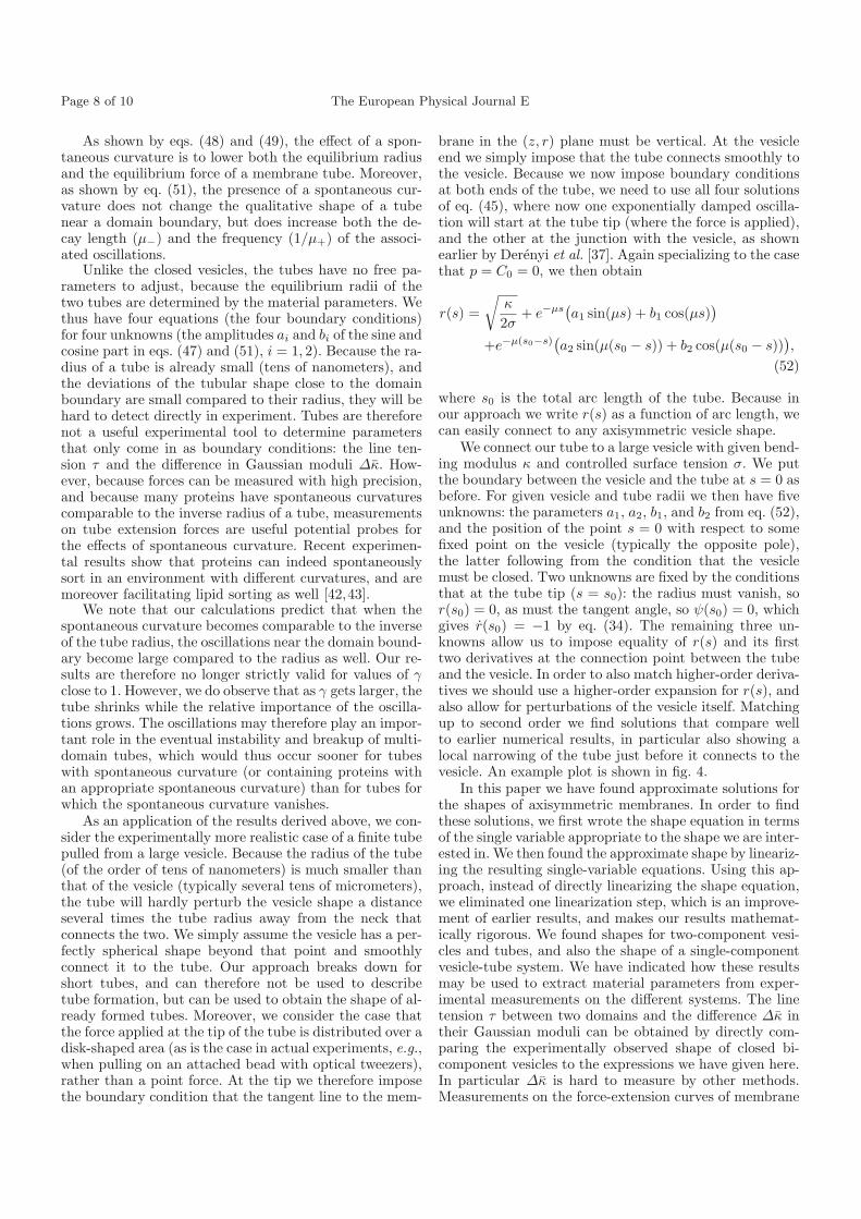
We connect our tube to a large vesicle with given bend-ing modulus κ and controlled surface tension σ. We putthe boundary between the vesicle and the tube at s = 0 asbefore. For given vesicle and tube radii we then have fiveunknowns: the parameters a1, a2, b1, and b2 from eq. (52),and the position of the point s = 0 with respect to somefixed point on the vesicle (typically the opposite pole),the latter following from the condition that the vesiclemust be closed. Two unknowns are fixed by the conditionsthat at the tube tip (s = s0): the radius must vanish, sor(s0) = 0, as must the tangent angle, so ψ(s0) = 0, whichgives r(s0) = −1 by eq. (34). The remaining three un-knowns allow us to impose equality of r(s) and its firsttwo derivatives at the connection point between the tubeand the vesicle. In order to also match higher-order deriva-tives we should use a higher-order expansion for r(s), andalso allow for perturbations of the vesicle itself. Matchingup to second order we find solutions that compare wellto earlier numerical results, in particular also showing alocal narrowing of the tube just before it connects to thevesicle. An example plot is shown in fig. 4.

In this paper we have found approximate solutions forthe shapes of axisymmetric membranes. In order to findthese solutions, we first wrote the shape equation in termsof the single variable appropriate to the shape we are inter-ested in. We then found the approximate shape by lineariz-ing the resulting single-variable equations. Using this ap-proach, instead of directly linearizing the shape equation,we eliminated one linearization step, which is an improve-ment of earlier results, and makes our results mathemat-ically rigorous. We found shapes for two-component vesi-cles and tubes, and also the shape of a single-componentvesicle-tube system. We have indicated how these resultsmay be used to extract material parameters from exper-imental measurements on the different systems. The linetension τ between two domains and the difference Δκ intheir Gaussian moduli can be obtained by directly com-paring the experimentally observed shape of closed bi-component vesicles to the expressions we have given here.In particular Δκ is hard to measure by other methods.Measurements on the force-extension curves of membrane

T. Idema and C. Storm: Analytical expressions for the shape of multi-component membranes Page 9 of 10

Fig. 4. Example of a tube connected to a spherical vesicle. Here the vesicle radius is 100R0 and the tube length is 50R0, withR0 the radius of the tube; also p = C0,1 = C0,2 = 0. (a) r(s) from the neck connecting the tube to the vesicle to the tube tip,showing the characteristic narrowing of the tube at the neck, and widening next to the tip. (b) Large-scale shape of a tubeconnected to a spherical vesicle in (z, r) coordinates. (c) Revolution plot of panel (b).

tethers can be used as a probe for spontaneous curva-ture in the membrane, in particular when the membranecontains proteins. We have shown that the presence of adomain boundary in a membrane tube causes decayingoscillations in the tube radius close to the boundary, andhow the presence of a spontaneous curvature changes thisobservation. In particular, we observe that if the sponta-neous curvature becomes comparable to the inverse of theradius of the tether, then these oscillations may play arole in the stability of the tether, causing it to break upsooner than one would expect without the presence of theoscillations.

We thank Dr. S. Semrau, Prof. Dr. T. Schmidt and Dr. G.P.Alexander for helpful discussions. This work was supportedby funds from the Netherlands Organization for Scientific Re-search (NWO and NWO-FOM) within the program on Ma-terial Properties of Biological Assemblies (FOM-L2601M) andthe Rubicon program.

Open Access This article is distributed under the terms of theCreative Commons Attribution Noncommercial License whichpermits any noncommercial use, distribution, and reproductionin any medium, provided the original author(s) and source arecredited.

References

1. B. Alberts, A. Johnson, J. Lewis, M. Raff, K. Roberts, P.Walter, Molecular Biology of the Cell, 5th edition (GarlandScience, New York, NY, USA, 2008).

2. R. Schekman, L. Orci, Science 271, 1526 (1996).3. J.E. Rothman, F.T. Wieland, Science 272, 227 (1996).4. J. Bigay, P. Gounon, S. Robineau, B. Antonny, Nature

426, 563 (2003).5. M. Ehrlich, W. Boll, A. van Oijen, R. Hariharan, K. Chan-

dran, M.L. Nibert, T. Kirchhausen, Cell 118, 591 (2004).6. C.M. Waterman-Storer, E.D. Salmon, Curr. Biol. 8, 798

(1998).

7. C. Dietrich, L.A. Bagatolli, Z.N. Volovyk, N.L. Thompson,M. Levi, K. Jacobson, E. Gratton, Biophys. J. 80, 1417(2001).

8. S.L. Veatch, S.L. Keller, Phys. Rev. Lett. 89, 268101(2002).

9. T. Baumgart, S.T. Hess, W.W. Webb, Nature 425, 821(2003).

10. S. Munro, Cell 115, 377 (2003).11. S.L. Veatch, S.L. Keller, Biochim. Biophys. Acta, Biom-

embr. 1746, 172 (2005).12. T. Baumgart, S. Das, W.W. Webb, J.T. Jenkins, Biophys.

J. 89, 1067 (2005).13. A.J. Garcia-Saez, S. Chiantia, P. Schwille, J. Biol. Chem.

282, 33537 (2007).14. S. Semrau, T. Idema, L. Holtzer, T. Schmidt, C. Storm,

Phys. Rev. Lett. 100, 088101 (2008).15. A.R. Honerkamp-Smith, P. Cicuta, M.D. Collins, S.L.

Veatch, M. den Nijs, M. Schick, S.L. Keller, Biophys. J.95, 236 (2008).

16. S. Semrau, T. Idema, T. Schmidt, C. Storm, Biophys. J.96, 4906 (2009).

17. T.S. Ursell, W.S. Klug, R. Phillips, Proc. Natl. Acad. Sci.U.S.A. 106, 13301 (2009).

18. T. Idema, S. Semrau, C. Storm, T. Schmidt, Phys. Rev.Lett. 104, 198102 (2010).

19. P.B. Canham, J. Theor. Biol. 26, 61 (1970).20. W. Helfrich, Z. Naturforsch. C 28, 693 (1973).21. Z.-C. Ou-Yang, W. Helfrich, Phys. Rev. A 39, 5280 (1989).22. F. Julicher, U. Seifert, Phys. Rev. E 49, 4728 (1994).23. F. Julicher, R. Lipowsky, Phys. Rev. E 53, 2670 (1996).24. R. Lipowsky, J. Phys. II 2, 1825 (1992).25. U. Seifert, S. Langer, Europhys. Lett. 23, 71 (1993).26. U. Seifert, Adv. Phys. 46, 13 (1997).27. R.M. Hochmuth, E.A. Evans, J.T. McCown, Biophys. J.

39, 71 (1982).28. R.M. Hochmuth, H.C. Wiles, E.A. Evans, J.T. McCown,

Biophys. J. 39, 83 (1982).29. E. Evans, W. Rawicz, Phys. Rev. Lett. 64, 2094 (1990).30. E. Evans, H. Bowman, A. Leung, D. Needham, D. Tirrel,

Science 273, 933 (1996).31. G. Koster, A. Cacciuto, I. Derenyi, D. Frenkel, M.

Dogterom, Phys. Rev. Lett. 94, 068101 (2005).

Page 10 of 10 The European Physical Journal E

32. G. Koster, M. van Duijn, B. Hofs, M. Dogterom, Proc.Natl. Acad. Sci. U.S.A. 100, 15583 (2003).

33. C. Leduc, O. Campas, K.B. Zeldovich, A. Roux, P. Joli-maitre, L. Bourel-Bonnet, B. Goud, J.-F. Joanny, P.Bassereau, J. Prost, Proc. Natl. Acad. Sci. U.S.A. 101,17096 (2004).

34. P.M. Shaklee, T. Idema, G. Koster, C. Storm, T. Schmidt,M. Dogterom, Proc. Natl. Acad. Sci. U.S.A. 105, 7993(2008).

35. C. Leduc, O. Campas, J.-F. Joanny, J. Prost, P. Bassereau,Biochim. Biophys. Acta, Biomembr. 1798, 1418 (2010).

36. D.J. Bukman, J.H. Yao, M. Wortis, Phys. Rev. E 54, 5463(1996).

37. I. Derenyi, F. Julicher, J. Prost, Phys. Rev. Lett. 88,238101 (2002).

38. T.R. Powers, G. Huber, R.E. Goldstein, Phys. Rev. E 65,041901 (2002).

39. B. Bozic, V. Heinrich, S. Svetina, B. Zeks, Eur. Phys. J. E6, 91 (2001).

40. A. Roux, D. Cuvelier, P. Nassoy, J. Prost, P. Bassereau,B. Goud, EMBO J. 24, 1537 (2005).

41. H. Jiang, T.R. Powers, Phys. Rev. Lett. 101, 018103(2008).

42. B. Sorre, A. Callan-Jones, J.-B. Manneville, P. Nassoy, J.-F. Joanny, J. Prost, B. Goud, P. Bassereau, Proc. Natl.Acad. Sci. U.S.A. 106, 5622 (2009).

43. A. Tian, T. Baumgart, Biophys. J. 96, 2676 (2009).44. M. Heinrich, A. Tian, C. Esposito, T. Baumgart, Proc.

Natl. Acad. Sci. U.S.A. 107, 7208 (2010).45. J.-M. Allain, C. Storm, A. Roux, M. Ben Amar, J.-F.

Joanny, Phys. Rev. Lett. 93, 158104 (2004).46. F. Campelo, J.-M. Allain, M. Ben Amar, EPL 77, 38006

(2007).47. M. do Carmo, Differential Geometry of Curves and Sur-

faces (Prentice-Hall, Englewood Cliffs, NJ, USA, 1976).48. E. Evans, A. Yeung, Chem. Phys. Lipids 73, 39 (1994).49. W.-M. Zheng, J. Liu, Phys. Rev. E 48, 2856 (1993).