Ocean Modelling 31 (2010) 88–104

Contents lists available at ScienceDirect

Ocean Modelling

journal homepage: www.elsevier .com/locate /ocemod

An ERA40-based atmospheric forcing for global ocean circulation models

Laurent Brodeau a,*, Bernard Barnier a, Anne-Marie Treguier b, Thierry Penduff a,d, Sergei Gulev c

a LEGI, UMR 5519 CNRS-UJF-INPG, BP 53, 38041 Grenoble, Franceb LPO, UMR 6523 CNRS-IFREMER-IRD-UBO, IFREMER, BP 70, 29280 Plouzané, Francec P.P. SIO – RAS, 36 Nakhimovsky Ave., 117218 Moscow, Russian Federationd Department of Oceanography, The Florida State University, Tallahassee, Florida

a r t i c l e i n f o

Article history:Received 10 June 2008Received in revised form 7 October 2009Accepted 23 October 2009Available online 1 November 2009

Keywords:OceanHindcastAtmospheric forcingAir-sea fluxesWeather reanalyzesSatellite

1463-5003/$ - see front matter � 2009 Elsevier Ltd. Adoi:10.1016/j.ocemod.2009.10.005

* Corresponding author. Address: Laboratoire de Ph5519 CNRS-UJF-INPG, BP 53, 38041 Grenoble, France.

E-mail addresses: laurent@misu.su.se, brodeau@gm

a b s t r a c t

We develop, calibrate and test a dataset intended to drive global ocean hindcasts simulations of the lastfive decades. This dataset provides surface meteorological variables needed to estimate air-sea fluxes andis built from 6-hourly surface atmospheric state variables of ERA40. We first compare the raw fields ofERA40 to the CORE.v1 dataset of Large and Yeager (2004), used here as a reference, and discuss our choiceto use daily radiative fluxes and monthly precipitation products extracted from satellite data rather thantheir ERA40 counterparts. Both datasets lead to excessively high global imbalances of heat and freshwaterfluxes when tested with a prescribed climatological sea surface temperature. After identifying unrealistictime discontinuities (induced by changes in the nature of assimilated observations) and obvious globaland regional biases in ERA40 fields (by comparison to high quality observations), we propose a set of cor-rections. Tropical surface air humidity is decreased from 1979 onward, representation of Arctic surface airtemperature is improved using recent observations and the wind is globally increased. These correctionslead to a significant decrease of the excessive positive global imbalance of heat. Radiation and precipita-tion fields are then submitted to a small adjustment (in zonal mean) that yields a near-zero global imbal-ance of heat and freshwater. A set of 47-year-long simulations is carried out with the coarse-resolution(2� � 2�) version of the NEMO OGCM to assess the sensitivity of the model to the proposed corrections.Model results show that each of the proposed correction contributes to improve the representation ofcentral features of the global ocean circulation.

� 2009 Elsevier Ltd. All rights reserved.

1. Introduction ally weak components of reanalyzes, such as radiation and precip-

Simulating the evolution of the global ocean over the last fewdecades using Ocean General Circulation models (OGCMs) hasbeen made possible since globally gridded interannual weatherreanalysis products have become available. Atmospheric fieldsfrom these reanalyzes are used to derive fluxes to be applied assurface boundary conditions for OGCMs.

Large and Yeager (2004), hereafter referred to as LY04, intro-duced a dataset for the ‘‘Coordinated Ocean Reference Experi-ments” carried out in the framework of the Working Group onOcean Model Development (WGOMD) of WCRP (COREs, Griffieset al., 2009). This dataset provides the ocean modeling communitywith a complete long-term ocean and sea-ice forcing, intended todrive interannual OGCM inter-comparisons and ocean hindcastexperiments of the last 5 decades (1958 to present). This dataset,from now on referred to as LYDS (Large and Yeager dataset), isbased on the NCEP reanalysis (Kalnay et al., 1996) and implementsrecent reconstructed flux products as a replacement for tradition-

ll rights reserved.

ysique des Oceans, LEGI, UMRTel.: +33 626600561.ail.com (L. Brodeau).

itation (Table 1). The authors applied corrections to these originalfields and they verified that corrections are consistent with a near-zero global imbalance of heat and freshwater fluxes estimatedfrom a prescribed sea surface temperature (SST) and sea-ice con-centration. LYDS will serve as our reference dataset when buildingour ERA40-based datasets.

Röske (2006) developed another dataset designed to forceocean models based on ERA15, the first reanalysis carried out atECMWF (Gibson et al., 1997). He applied corrections to close heatand freshwater budgets by means of an inverse procedure. How-ever, only a climatological year was estimated due to the shorttime coverage of ERA15 (1979–1993).

Ocean forcing datasets such as those discussed here must becontinuously reevaluated and updated to account for new observa-tions (especially from satellites), new atmospheric reanalyzes, andfeedbacks from the modeling community. This has been done re-cently for LYDS, in coordination with WGOMD, and a new releasehas been recently made available (Large and Yeager, 2008) whichis sometimes referred to as CORE.v2.

Being more recent than NCEP or ERA15, the ERA40 reanalysis ofECMWF (Uppala et al., 2005) takes advantage of more advancednumerical features (such as resolution, atmospheric models and

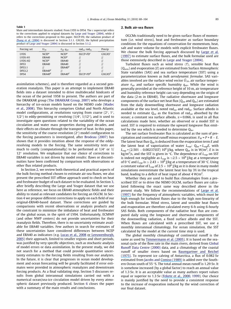
Table 1Main and intermediate datasets studied. From LYDS to DFS4. The c superscript refersto the corrections applied to original datasets by Large and Yeager (2004), while drefers to the corrections proposed in this paper. ISCCP-FD, the radiation product ofZhang et al. (2004) is discussed in Section 3.1.1. GXGXS, the hybrid precipitationproduct of Large and Yeager (2004) is discussed in Section 3.1.2.

Forcing set U10 hair qair radsw radlw Precip

LYDS NCEPc NCEPc ISCCP-FDc GXGXSc

LYDS-H1 ERA40 NCEPc // //LYDS-H2 NCEPc ERA40 // //DFS3 ERA40 ERA40 // //DFS3.1 // ERA40d // //DFS3.2 ERA40d // // //DFS4 ERA40d ERA40d ISCCP-FDd GXGXSd

L. Brodeau et al. / Ocean Modelling 31 (2010) 88–104 89

assimilation schemes), and is therefore regarded as a second gen-eration reanalysis. This paper is an attempt to implement ERA40fields into a dataset intended to drive multidecadal hindcasts ofthe ocean of the period 1958 to present. The authors are part ofthe DRAKKAR group (The DRAKKAR Group, 2007) who develops ahierarchy of ice-ocean models based on the NEMO code (Madecet al., 2008). This hierarchy comprises Global and North Atlanticmodel configurations, at resolutions varying from coarse (2�, 1�,1/2�) to eddy-permitting or resolving (1/4�, 1/12�), and is used toinvestigate open questions related to the variability of the oceancirculation and water mass properties during past decades, andtheir effects on climate through the transport of heat. In this paper,the sensitivity of the coarse-resolution (2�) model configuration tothe forcing parameters is investigated, after Brodeau (2007) hasshown that it provides intuition about the response of the eddy-resolving models to the forcing. The same sensitivity tests aremuch to costly (computationally) to be performed at 1/4� or 1/12� resolution. We emphasize that our choice of corrections toERA40 variables is not driven by model results: flaws or disconti-nuities have been confirmed by comparison with observations orother flux related products.

In Section 2, we review both theoretical and practical aspects ofthe bulk forcing method chosen to estimate air-sea fluxes, we alsopresent the prescribed SST offline approach used to check on heatand freshwater budget of each dataset to be evaluated. In Section 3,after briefly describing the Large and Yeager dataset that we usehere as reference, we focus on ERA40 atmospheric fields and theirability to stand as relevant candidates for forcing an OGCM. In Sec-tion 4 we propose different corrections to apply on each field of ouroriginal-ERA40-based dataset. These corrections are guided bycomparisons with recent observations or analysis products andthe constraint to minimize the imbalance of heat and freshwaterof the global ocean, in the spirit of LY04. Unfortunately, ECMWF(and other NWP centers) do not provide uncertainties for theirreanalysis fields. Therefore, there is no uncertainty estimate avail-able for ERA40 variables. Few authors in search for estimates ofthese uncertainties have considered differences between NCEPand ERA40 as indicators (e.g. Lucas et al., 2008 or Leeuwenburgh,2005) their approach, limited to smaller regions and short periods,was justified by very specific objectives, such as stochastic analysisof model errors or data assimilation. In the present study, we didnot search for a method that could provide quantitative uncer-tainty estimates to the forcing fields resulting from our analyzes.In the future, it is clear that progresses in ocean model develop-ment and ocean forecasting will be greatly facilitated if error esti-mates were provided in atmospheric reanalyzes and downstreamforcing products. As a final validating step, Section 5 discusses re-sults from global interannual simulations carried out with anumerical ocean/sea-ice circulation model driven by every atmo-spheric dataset previously produced. Section 6 closes the paperwith a summary of the main results and conclusions.

2. Bulk air-sea fluxes

OGCMs traditionally need to be given surface fluxes of momen-tum (i.e. wind stress), heat and freshwater as surface boundaryconditions for the equations of conservation for momentum, heat,salt and water volume for models with explicit freshwater fluxes.We choose the bulk forcing approach discussed by Large et al.(1997) to estimate surface fluxes, and the bulk formulae used arethose extensively described in Large and Yeager (2004).

Turbulent fluxes such as wind stress ð~sÞ, sensible heat flux(Qsens) and evaporation (E) are estimated from Surface AtmosphericState variables (SAS) and sea surface temperature (SST) using aparameterization known as bulk aerodynamic formulae. SAS vari-ables involved are the surface wind vector ~U10, air surface temper-ature hair and surface specific humidity qair. While the wind isgenerally provided at the reference height of 10 m, air temperatureand humidity reference height can vary depending on the origin ofthe data (2 m in ERA40). The radiative shortwave and longwavecomponents of the surface net heat flux (Qsw and Qlw) are estimatedfrom the daily downwelling shortwave and longwave radiationavailable at the sea level, noted radsw and radlw. Surface albedo isneeded to estimate Qsw as the fraction of radsw absorbed by theocean; a constant sea surface albedo, a = 0.066, is used in all fluxcalculations made here, whether an observed or a model SST isused. SST is required to estimate the upward longwave flux emit-ted by the sea which is needed to determine Qlw.

The net surface freshwater flux is calculated as the sum of pre-cipitation and continental runoff minus evaporation: FW = P + R � E.The latent heat flux Qlat is deduced from the evaporation term E andthe latent heat of vaporization of water Lvap: Qlat = LvapE, withLvap = (2.501 � 0.00237SST) 106 J/kg, where Qlat is in W/m2, E is inkg/m2/s, and the SST is given in �C. The dependence of Lvap on SSTis indeed not negligible as Lvap is ’2.5 � 106 J/kg at a temperatureof 0 �C and Lvap is ’ 2.43 � 106 J/kg at a temperature of 30 �C. Usinga constant value of Lvap of 2.5 � 106 J/kg as it is done in many modelsimulations overestimate the latent heat loss by 3% in the tropicalband, leading to a deficit of heat input of about 4 W/m2.

Whether they are used to build flux climatologies from a pre-scribed SST or to drive the NEMO OGCM, surface fluxes are calcu-lated following the exact same way described above in thepresent study. We follow the recommendations of Large et al.(1997) for the frequency of atmospheric variables, which must behigh enough for turbulent fluxes due to the high non-linearity ofthe bulk formulae. Wind stress, latent and sensible heat fluxesand evaporation are therefore calculated every 6-h using 6-hourlySAS fields. Both components of the radiative heat flux are com-puted daily using the longwave and shortwave components ofthe downwelling radiation, a fixed surface albedo and the SST.When fluxes are calculated with a prescribed SST, we use amonthly interannual climatology. For ocean simulation, the SSTcalculated by the model at the current time step is used.

The global monthly climatology of continental runoff is thesame as used by Timmermann et al. (2005). It is based on the sea-sonal cycle of the flow rate in the main rivers, derived from GlobalRunoff Data Centre (2000) data, and a climatology of the coastalrunoff of smaller rivers based on Baumgartner and Reichel(1975). To represent ice calving of Antarctica, a flux of 0.082 Svestimated from Jacobs and Comiso (1989) is added over the South-ern Ocean south of 55 �S. The total annual mean runoff is 1.29 Sv. Itis somehow increased (by a global factor) to reach an annual valueof 1.3 Sv. It is an acceptable value as many authors report valuesequal or superior to 1.3 Sv (Fekete et al., 2000, 1999). Our choiceis mainly justified by the need to provide a consistent responseto the increase of evaporation induced by the wind correction ofour final dataset.

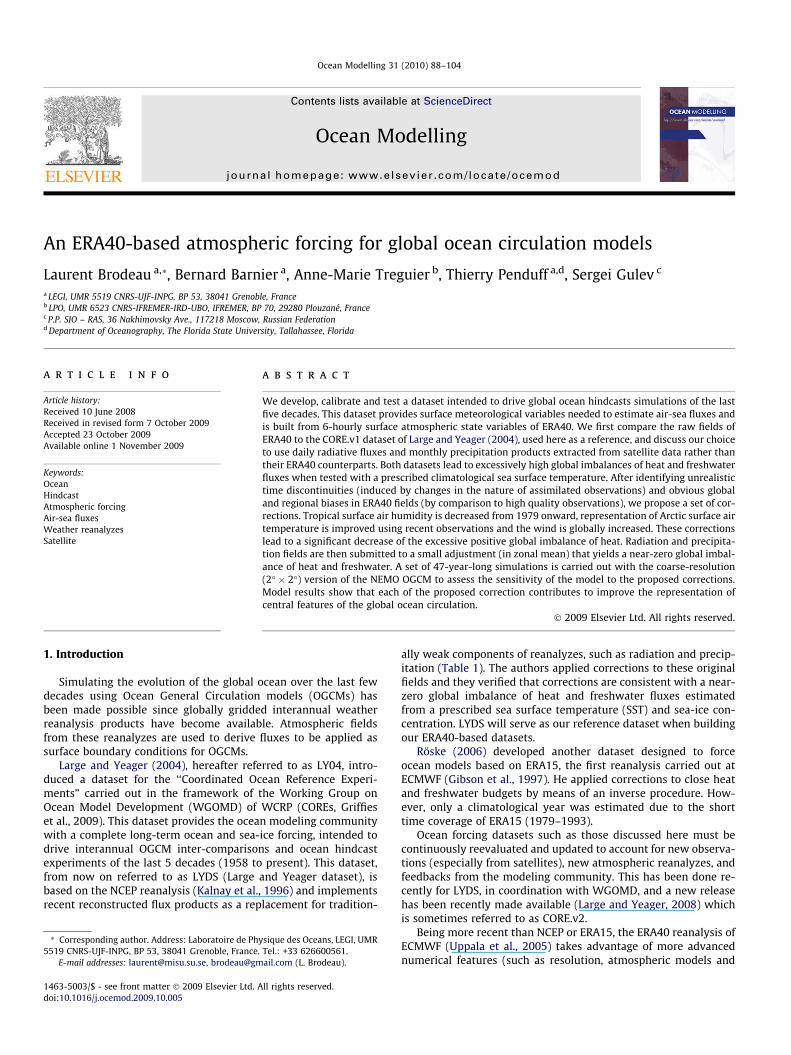
Fig. 1. (a) Zonally averaged downwelling shortwave radiation over sea (1984-2001); DFS4 radiation product is discussed in Section 4. (b) zonally averaged total precipitationover sea (1979–2001), including corrected ERA40 precipitation (Troccoli and Kållberg, 2004).

1 http://www.ecmwf.int/research/era/DataServices/section3.html.

90 L. Brodeau et al. / Ocean Modelling 31 (2010) 88–104

In the following, observed monthly interannual SST and sea-iceconcentration climatologies of Hurrell et al. (2008) are used to esti-mate air-sea fluxes from a given set of atmospheric variables andbulk parameterization. This approach is widely used by the climatecommunity for building flux climatologies and to adjust atmo-spheric fields or bulk formulae. Flux calculations are carried outfrom 1958 to 2004 on the global ORCA2 grid that is also used forthe ocean model simulations presented in Section 5. Our calcula-tion ends in 2004 as dictated by the availability of the LYDS fieldsat the beginning of our study. SST and sea-ice concentration arelinearly interpolated from monthly to daily values. Following themethod described by LY04, turbulent fluxes are computed every6 h. Daily-averaged turbulent heat fluxes and daily radiation inputprovide the daily net heat flux estimate while monthly averagedevaporation plus monthly precipitation and runoff provide themonthly net freshwater flux estimate.

3. DFS3: a forcing dataset based on ERA40

In this section, we review the atmospheric fields used by LY04to build their dataset (LYDS). We assess the ability of the corre-sponding ERA40 fields to stand as relevant candidates to driveocean-ice models by comparing them to LYDS and third party data.The global balance of heat and freshwater induced by LYDS and ourfirst ERA40-based dataset, named DFS3 for DRAKKAR Forcing Set#3, is studied for the 1958–2004 period.

3.1. Reanalysis fluxes versus satellite products

3.1.1. RadiationLY04 did not use NCEP radiation and precipitation in their data-

set. Both precipitation and downwelling radiation estimates heav-ily depend on the representation of the cloud cover, which is one ofthe weakest feature of weather forecasting models (Taylor, 2000).Instead, they favored the use of the ISCCP-FD radiation productdeveloped by Zhang et al. (2004). These fields are outputs of theradiative transfer model of the NASA Goddard Institute for SpaceStudies (GISS) and are based on various satellite data and climatol-ogies gathered by the ISCCP. However, these fields are not in a formthat makes them directly usable to drive an ocean model. A signif-icant amount of processing was made by LY04 to produce regulargridded daily fields for the period 1984 to 2004. LY04 also reducedthe downwelling shortwave radiation of the original product by 5%between 50�S and 40�N to better agree with other independentproducts. The effect of this correction can be seen in Fig. 1a whichdisplays the zonal average downward shortwave radiations for dif-ferent datasets (compare ISCCP-FD to LYDS). Despite the correc-

tion, LYDS shortwave radiation remains high, greater than theNOC climatology for example. They also limited arctic shortwaveinput by applying a negative offset of 5 W/m2 north to 70�N. InLYDS, a climatological daily mean of radiation fields, built as theaverage of years 1984 to 2004, is used to cover the missing years(1958 to 1983).

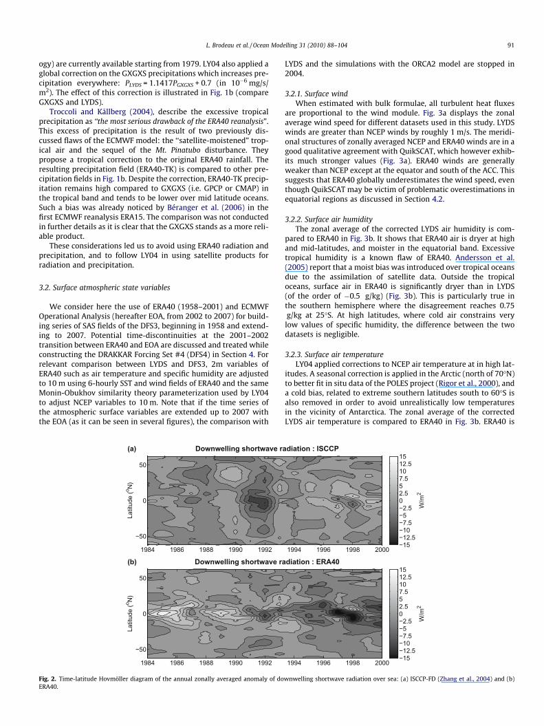
ECMWF documentation is clear on that matter, the quality ofERA40 radiative products is not satisfactory. Quoting their web-site1: ‘‘Radiation budget fields suffer from deficiencies in the radiativeproperties of the clouds, and are not recommended for use in studieswhere accurate fluxes are required”. This is confirmed when compar-ing ISCCP and ERA40 interannual variability of the zonally averageddownwelling shortwave radiation between 1984 and 2000 (Fig. 2).ERA40 exhibits an unrealistic variability pattern when compared tothe ISCCP-FD dataset, the time variability of the latter being consid-ered more reliable as it is based on satellite observations. A substan-tial underestimation of the tropical insolation is introduced in ERA40from 1991 onwards. This problem is likely to be linked to the well-documented issue of an overestimation of tropical precipitation inERA40: the eruption of Mt. Pinatubo in 1991 is reported to haveintroduced a misinterpretation of the HIRS infrared radiance databy the assimilation scheme, due to the effects of volcanic aerosolsUppala et al., 2004. The result is a significant increase of ERA40 rain-fall over the tropical oceans during the last years (see next para-graph). The resulting tropical underestimation of shortwaveradiation in ERA40 is striking when looking at zonally averaged radi-ation from different origins displayed in Fig. 1a.

Another important discrepancy between data from ISCCP andERA40 is found along the west coasts of continents betweenroughly 20� and 30� latitude in both hemispheres (no figureshown). In these regions, ERA40 can locally overestimate the an-nual mean insolation by more than 60 W/m2. This flaw, linked tothe ECMWF prognostic cloud model, is a recurrent flaw in ECMWFproducts, already discussed by Gibson et al. (1997). It is due to apoor representation of low-level stratus and stratocumulus in theregions of subsidence of the Walker cell.

3.1.2. PrecipitationLY04 reviewed and compared precipitation data from different

sources and then developed a global precipitation dataset, namedGXGXS, based on a zonal blending of several products, includingtwo of the most widely used datasets: GPCP (Huffmanet al.,1997) and CMAP( Xie and Arkin, 1997). A third party data source,the Serreze and Hurst (2000) dataset was used to cover the Arcticregion. All these datasets (excepted for Serreze, which is a climatol-

L. Brodeau et al. / Ocean Modelling 31 (2010) 88–104 91

ogy) are currently available starting from 1979. LY04 also applied aglobal correction on the GXGXS precipitations which increases pre-cipitation everywhere: PLYDS = 1.1417PGXGXS + 0.7 (in 10�6 mg/s/m2). The effect of this correction is illustrated in Fig. 1b (compareGXGXS and LYDS).

Troccoli and Kållberg (2004), describe the excessive tropicalprecipitation as ‘‘the most serious drawback of the ERA40 reanalysis”.This excess of precipitation is the result of two previously dis-cussed flaws of the ECMWF model: the ‘‘satellite-moistened” trop-ical air and the sequel of the Mt. Pinatubo disturbance. Theypropose a tropical correction to the original ERA40 rainfall. Theresulting precipitation field (ERA40-TK) is compared to other pre-cipitation fields in Fig. 1b. Despite the correction, ERA40-TK precip-itation remains high compared to GXGXS (i.e. GPCP or CMAP) inthe tropical band and tends to be lower over mid latitude oceans.Such a bias was already noticed by Béranger et al. (2006) in thefirst ECMWF reanalysis ERA15. The comparison was not conductedin further details as it is clear that the GXGXS stands as a more reli-able product.

These considerations led us to avoid using ERA40 radiation andprecipitation, and to follow LY04 in using satellite products forradiation and precipitation.

3.2. Surface atmospheric state variables

We consider here the use of ERA40 (1958–2001) and ECMWFOperational Analysis (hereafter EOA, from 2002 to 2007) for build-ing series of SAS fields of the DFS3, beginning in 1958 and extend-ing to 2007. Potential time-discontinuities at the 2001–2002transition between ERA40 and EOA are discussed and treated whileconstructing the DRAKKAR Forcing Set #4 (DFS4) in Section 4. Forrelevant comparison between LYDS and DFS3, 2m variables ofERA40 such as air temperature and specific humidity are adjustedto 10 m using 6-hourly SST and wind fields of ERA40 and the sameMonin-Obukhov similarity theory parameterization used by LY04to adjust NCEP variables to 10 m. Note that if the time series ofthe atmospheric surface variables are extended up to 2007 withthe EOA (as it can be seen in several figures), the comparison with

Latit

ude

(o N)

(a) Downwelling shortwave ra

1984 1986 1988 1990 1992

−50

0

50

Latit

ude

(o N)

(b) Downwelling shortwave ra

1984 1986 1988 1990 1992

−50

0

50

Fig. 2. Time-latitude Hovmöller diagram of the annual zonally averaged anomaly of doERA40.

LYDS and the simulations with the ORCA2 model are stopped in2004.

3.2.1. Surface windWhen estimated with bulk formulae, all turbulent heat fluxes

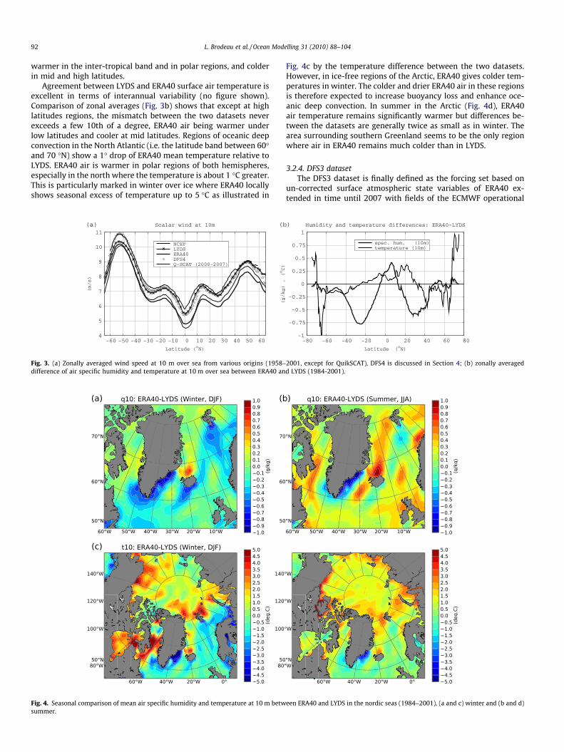
are proportional to the wind module. Fig. 3a displays the zonalaverage wind speed for different datasets used in this study. LYDSwinds are greater than NCEP winds by roughly 1 m/s. The meridi-onal structures of zonally averaged NCEP and ERA40 winds are in agood qualitative agreement with QuikSCAT, which however exhib-its much stronger values (Fig. 3a). ERA40 winds are generallyweaker than NCEP except at the equator and south of the ACC. Thissuggests that ERA40 globally underestimates the wind speed, eventhough QuikSCAT may be victim of problematic overestimations inequatorial regions as discussed in Section 4.2.

3.2.2. Surface air humidityThe zonal average of the corrected LYDS air humidity is com-

pared to ERA40 in Fig. 3b. It shows that ERA40 air is dryer at highand mid-latitudes, and moister in the equatorial band. Excessivetropical humidity is a known flaw of ERA40. Andersson et al.(2005) report that a moist bias was introduced over tropical oceansdue to the assimilation of satellite data. Outside the tropicaloceans, surface air in ERA40 is significantly dryer than in LYDS(of the order of �0.5 g/kg) (Fig. 3b). This is particularly true inthe southern hemisphere where the disagreement reaches 0.75g/kg at 25�S. At high latitudes, where cold air constrains verylow values of specific humidity, the difference between the twodatasets is negligible.

3.2.3. Surface air temperatureLY04 applied corrections to NCEP air temperature at in high lat-

itudes. A seasonal correction is applied in the Arctic (north of 70�N)to better fit in situ data of the POLES project (Rigor et al., 2000), anda cold bias, related to extreme southern latitudes south to 60�S isalso removed in order to avoid unrealistically low temperaturesin the vicinity of Antarctica. The zonal average of the correctedLYDS air temperature is compared to ERA40 in Fig. 3b. ERA40 is

diation : ISCCP

1994 1996 1998 2000

W/m

2

−15−12.5−10−7.5−5−2.502.557.51012.515

diation : ERA40

1994 1996 1998 2000

W/m

2

−15−12.5−10−7.5−5−2.502.557.51012.515

wnwelling shortwave radiation over sea: (a) ISCCP-FD (Zhang et al., 2004) and (b)

92 L. Brodeau et al. / Ocean Modelling 31 (2010) 88–104

warmer in the inter-tropical band and in polar regions, and colderin mid and high latitudes.

Agreement between LYDS and ERA40 surface air temperature isexcellent in terms of interannual variability (no figure shown).Comparison of zonal averages (Fig. 3b) shows that except at highlatitudes regions, the mismatch between the two datasets neverexceeds a few 10th of a degree, ERA40 air being warmer underlow latitudes and cooler at mid latitudes. Regions of oceanic deepconvection in the North Atlantic (i.e. the latitude band between 60�and 70 �N) show a 1� drop of ERA40 mean temperature relative toLYDS. ERA40 air is warmer in polar regions of both hemispheres,especially in the north where the temperature is about 1 �C greater.This is particularly marked in winter over ice where ERA40 locallyshows seasonal excess of temperature up to 5 �C as illustrated in

Fig. 3. (a) Zonally averaged wind speed at 10 m over sea from various origins (1958–difference of air specific humidity and temperature at 10 m over sea between ERA40 an

Fig. 4. Seasonal comparison of mean air specific humidity and temperature at 10 m betwsummer.

Fig. 4c by the temperature difference between the two datasets.However, in ice-free regions of the Arctic, ERA40 gives colder tem-peratures in winter. The colder and drier ERA40 air in these regionsis therefore expected to increase buoyancy loss and enhance oce-anic deep convection. In summer in the Arctic (Fig. 4d), ERA40air temperature remains significantly warmer but differences be-tween the datasets are generally twice as small as in winter. Thearea surrounding southern Greenland seems to be the only regionwhere air in ERA40 remains much colder than in LYDS.

3.2.4. DFS3 datasetThe DFS3 dataset is finally defined as the forcing set based on

un-corrected surface atmospheric state variables of ERA40 ex-tended in time until 2007 with fields of the ECMWF operational

2001, except for QuikSCAT), DFS4 is discussed in Section 4; (b) zonally averagedd LYDS (1984-2001).

een ERA40 and LYDS in the nordic seas (1984–2001), (a and c) winter and (b and d)

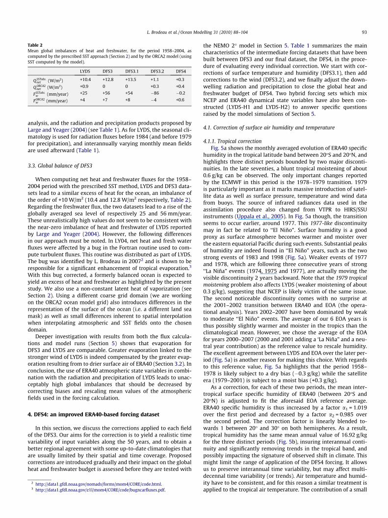
Table 2Mean global imbalances of heat and freshwater, for the period 1958–2004, ascomputed by the prescribed SST approach (Section 2) and by the ORCA2 model (usingSST computed by the model).

LYDS DFS3 DFS3.1 DFS3.2 DFS4

QSSTobs:net (W/m2) +10.4 +12.8 +13.5 +1.1 +0.3

QORCA2net (W/m2) +0.9 0 0 +0.3 +0.4

FSSTobs:w (mm/year) +25 +56 +54 �86 �0.2

FORCA2w (mm/year) +4 +7 +8 �4 +0.6

L. Brodeau et al. / Ocean Modelling 31 (2010) 88–104 93

analysis, and the radiation and precipitation products proposed byLarge and Yeager (2004) (see Table 1). As for LYDS, the seasonal cli-matology is used for radiation fluxes before 1984 (and before 1979for precipitation), and interannually varying monthly mean fieldsare used afterward (Table 1).

3.3. Global balance of DFS3

When computing net heat and freshwater fluxes for the 1958–2004 period with the prescribed SST method, LYDS and DFS3 data-sets lead to a similar excess of heat for the ocean, an imbalance ofthe order of +10 W/m2 (10.4 and 12.8 W/m2 respectively, Table 2).Regarding the freshwater flux, the two datasets lead to a rise of theglobally averaged sea level of respectively 25 and 56 mm/year.These unrealistically high values do not seem to be consistent withthe near-zero imbalance of heat and freshwater of LYDS reportedby Large and Yeager (2004). However, the following differencesin our approach must be noted. In LY04, net heat and fresh waterfluxes were affected by a bug in the Fortran routine used to com-pute turbulent fluxes. This routine was distributed as part of LYDS.The bug was identified by L. Brodeau in 20072 and is shown to beresponsible for a significant enhancement of tropical evaporation.3

With this bug corrected, a formerly balanced ocean is expected toyield an excess of heat and freshwater as highlighted by the presentstudy. We also use a non-constant latent heat of vaporization (seeSection 2). Using a different coarse grid domain (we are workingon the ORCA2 ocean model grid) also introduces differences in therepresentation of the surface of the ocean (i.e. a different land seamask) as well as small differences inherent to spatial interpolationwhen interpolating atmospheric and SST fields onto the chosendomain.

Deeper investigation with results from both the flux calcula-tions and model runs (Section 5) shows that evaporation forDFS3 and LYDS are comparable. Greater evaporation linked to thestronger wind of LYDS is indeed compensated by the greater evap-oration resulting from to drier surface air of ERA40 (Section 3.2). Inconclusion, the use of ERA40 atmospheric state variables in combi-nation with the radiation and precipitation of LYDS leads to unac-ceptably high global imbalances that should be decreased bycorrecting biases and rescaling mean values of the atmosphericfields used in the forcing calculation.

4. DFS4: an improved ERA40-based forcing dataset

In this section, we discuss the corrections applied to each fieldof the DFS3. Our aims for the correction is to yield a realistic timevariability of input variables along the 50 years, and to obtain abetter regional agreement with some up-to-date climatologies thatare usually limited by their spatial and time coverage. Proposedcorrections are introduced gradually and their impact on the globalheat and freshwater budget is assessed before they are tested with

2 http://data1.gfdl.noaa.gov/nomads/forms/mom4/CORE/code.html.3 http://data1.gfdl.noaa.gov/z1l/mom4/CORE/code/bugncarfluxes.pdf.

the NEMO 2� model in Section 5. Table 1 summarizes the maincharacteristics of the intermediate forcing datasets that have beenbuilt between DFS3 and our final dataset, the DFS4, in the proce-dure of evaluating every individual correction. We start with cor-rections of surface temperature and humidity (DFS3.1), then addcorrections to the wind (DFS3.2), and we finally adjust the down-welling radiation and precipitation to close the global heat andfreshwater budget of DFS4. Two hybrid forcing sets which mixNCEP and ERA40 dynamical state variables have also been con-structed (LYDS-H1 and LYDS-H2) to answer specific questionsraised by the model simulations of Section 5.

4.1. Correction of surface air humidity and temperature

4.1.1. Tropical correctionFig. 5a shows the monthly averaged evolution of ERA40 specific

humidity in the tropical latitude band between 20�S and 20�N, andhighlights three distinct periods bounded by two major disconti-nuities. In the late seventies, a blunt tropical moistening of about0.6 g/kg can be observed. The only important changes reportedby the ECMWF in this period is the 1978–1979 transition. 1979is particularly important as it marks massive introduction of satel-lite data as well as surface pressure, temperature and wind datafrom buoys. The source of infrared radiances data used in theassimilation procedure also changed from VTPR to HIRS/SSUinstruments (Uppala et al., 2005). In Fig. 5a though, the transitionseems to occur earlier, around 1977. This 1977-like discontinuitymay in fact be related to ‘‘El Niño”. Surface humidity is a goodproxy as surface atmosphere becomes warmer and moister overthe eastern equatorial Pacific during such events. Substantial peaksof humidity are indeed found in ‘‘El Niño” years, such as the twostrong events of 1983 and 1998 (Fig. 5a). Weaker events of 1977and 1978, which are following three consecutive years of strong‘‘La Niña” events (1974, 1975 and 1977), are actually moving thevisible discontinuity 2 years backward. Note that the 1979 tropicalmoistening problem also affects LYDS (weaker moistening of about0.3 g/kg), suggesting that NCEP is likely victim of the same issue.The second noticeable discontinuity comes with no surprise atthe 2001–2002 transition between ERA40 and EOA (the opera-tional analysis). Years 2002–2007 have been dominated by weakto moderate ‘‘El Niño” events. The average of our 6 EOA years isthus possibly slightly warmer and moister in the tropics than theclimatological mean. However, we chose the average of the EOAfor years 2000–2007 (2000 and 2001 adding a ‘La Niña” and a neu-tral year contribution) as the reference value to rescale humidity.The excellent agreement between LYDS and EOA over the later per-iod (Fig. 5a) is another reason for making this choice. With regardsto this reference value, Fig. 5a highlights that the period 1958–1978 is likely subject to a dry bias (�0.3 g/kg) while the satelliteera (1979–2001) is subject to a moist bias (+0.3 g/kg).

As a correction, for each of these two periods, the mean inter-tropical surface specific humidity of ERA40 (between 20�S and20�N) is adjusted to fit the aforesaid EOA reference average.ERA40 specific humidity is thus increased by a factor a1 = 1.019over the first period and decreased by a factor a2 = 0.985 overthe second period. The correction factor is linearly blended to-wards 1 between 20� and 30� on both hemispheres. As a result,tropical humidity has the same mean annual value of 16.92 g/kgfor the three distinct periods (Fig. 5b), insuring interannual conti-nuity and significantly removing trends in the tropical band, andpossibly impacting the signature of observed shift in climate. Thismight limit the range of application of the DFS4 forcing. It allowsus to preserve interannual time variability, but may affect multi-decennal time variability (or trends). Air temperature and humid-ity have to be consistent, and for this reason a similar treatment isapplied to the tropical air temperature. The contribution of a small

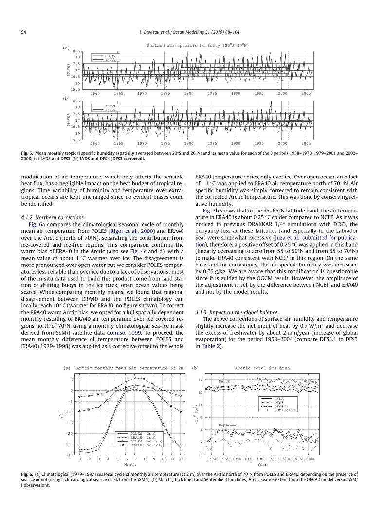
Fig. 5. Mean monthly tropical specific humidity (spatially averaged between 20�S and 20�N) and its mean value for each of the 3 periods 1958–1978, 1979–2001 and 2002–2006; (a) LYDS and DFS3, (b) LYDS and DFS4 (DFS3 corrected).

94 L. Brodeau et al. / Ocean Modelling 31 (2010) 88–104

modification of air temperature, which only affects the sensibleheat flux, has a negligible impact on the heat budget of tropical re-gions. Time variability of humidity and temperature over extra-tropical oceans are kept unchanged since no evident biases couldbe identified.

4.1.2. Northern correctionsFig. 6a compares the climatological seasonal cycle of monthly

mean air temperature from POLES (Rigor et al., 2000) and ERA40over the Arctic (north of 70�N), separating the contribution fromice-covered and ice-free regions. This comparison confirms thewarm bias of ERA40 in the Arctic (also see Fig. 4c and d), with amean value of about 1 �C warmer over ice. The disagreement ismore pronounced over open water but we consider POLES temper-atures less reliable than over ice due to a lack of observations; mostof the in situ data used to build this product come from land sta-tion or drifting buoys in the ice pack, open ocean values beingscarce. While comparing monthly means, we found that regionaldisagreement between ERA40 and the POLES climatology canlocally reach 10 �C (warmer for ERA40, no figure shown). To correctthe ERA40 warm Arctic bias, we opted for a full spatially dependentmonthly rescaling of ERA40 air temperature over ice covered re-gions north of 70�N, using a monthly climatological sea-ice maskderived from SSM/I satellite data Comiso, 1999. To proceed, themean monthly difference of temperature between POLES andERA40 (1979–1998) was applied as a corrective offset to the whole

Fig. 6. (a) Climatological (1979–1997) seasonal cycle of monthly air temperature (at 2 msea-ice or not (using a climatological sea-ice mask from the SSM/I). (b) March (thick lines)I observations.

ERA40 temperature series, only over ice. Over open ocean, an offsetof �1 �C was applied to ERA40 air temperature north of 70 �N. Airspecific humidity was simply corrected to remain consistent withthe corrected Arctic temperature. This was done by conserving rel-ative humidity.

Fig. 3b shows that in the 55–65�N latitude band, the air temper-ature in ERA40 is about 0.25 �C colder compared to NCEP. As it wasnoticed in previous DRAKKAR 1/4� simulations with DFS3, thebuoyancy loss at these latitudes (and especially in the LabradorSea) were somewhat excessive (Juza et al., submitted for publica-tion), therefore, a positive offset of 0.25 �C was applied in this band(linearly decreasing to zero from 55 to 50�N and from 65 to 70�N)to make ERA40 consistent with NCEP in this region. On the samebasis and for consistency, the air specific humidity was increasedby 0.05 g/kg. We are aware that this modification is questionablesince it is guided by the OGCM result. However, the amplitude ofthe adjustment is set by the difference between NCEP and ERA40and not by the model results.

4.1.3. Impact on the global balanceThe above corrections of surface air humidity and temperature

slightly increase the net input of heat by 0.7 W/m2 and decreasethe excess of freshwater by about 2 mm/year (increase of globalevaporation) for the period 1958–2004 (compare DFS3.1 to DFS3in Table 2).

) over the Arctic north of 70�N from POLES and ERA40, depending on the presence ofand September (thin lines) Arctic sea-ice extent from the ORCA2 model versus SSM/

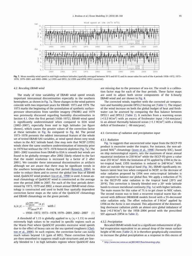
Fig. 7. Mean monthly wind speed in mid-high southern latitudes (spatially averaged between 50�S and 65�S) and its mean value for each of the 4 periods 1958–1972, 1973–1978, 1979–2001 and 2002–2006; (a) LYDS and DFS3, (b) LYDS and DFS4 (DFS3 corrected).

4 http://www.noc.soton.ac.uk/JRD/MET/fluxclimatology.php.

L. Brodeau et al. / Ocean Modelling 31 (2010) 88–104 95

4.2. Rescaling ERA40 wind

The study of time variability of ERA40 wind speed revealsimportant interannual discontinuities especially in the southernhemisphere, as shown in Fig. 7a. These changes in the wind patterncoincide with two important years for ERA40: 1973 and 1979. The1973 marks the beginning of the assimilation of synthetic surface-pressure observations from satellite imagery (PAOBS) and 1979was previously discussed regarding humidity discontinuities inSection 4.1. Over the first period (1958–1972), ERA40 wind speedis significantly underestimated when compared to EOA wind(2002–2007), especially from mid to high latitudes (no figureshown), which causes the greater values of the correction factorat these latitudes in Fig. 8a compared to Fig. 8d. The period1973–1978 presents the oddest interannual feature of the wholeset of tested ERA40 SAS variables, as wind speed shows very weakvalues in the ACC latitude band. One may note that NCEP (LYDS)winds show the same southern underestimation of intensity priorto 1979 but without the 1973–1978 Antarctic depletion (Fig. 7a). The2001–2002 transition from ERA40 to EOA is smooth but winds arefound to be globally stronger after 2002 (likely related to the factthat the model resolution is increased by a factor of 2 after2001). We consider these interannual discontinuities as artifactsalthough we are aware that there may be significant trends inthe southern hemisphere during that period (Renwick, 2004). Inorder to reduce them and to correct the global low bias of ERA40wind, QuikSCAT wind product (Liu et al., 1998) is used. A mean an-nual climatology of QuikSCAT wind is constructed as the averageover the period 2000 to 2007. For each of the four periods deter-mined by 1973, 1979 and 2002, a mean annual ERA40 wind clima-tology is constructed and used to build four spatially dependentcorrection factor maps as the ratio of the QuikSCAT climatologyand ERA40 climatology on the given periods:

aiðx; yÞ ¼j~Uj2000—2007

QSCAT ðx; yÞj~UjiERA40ðx; yÞ

with i

¼ 1958—1972;1973—1978;1979—2001;2002—2007 ð1Þ

A threshold of 1.15 is globally applied to ai (ai < 1.15) to avoidextremely high values to be reached in specific regions such asthe Warm Pool where QuikSCAT provides excessive wind speedsdue to the effect of heavy rain on the sea spotted roughness (Chel-ton et al., 2006). In such regions, the correction factor can easilyreach values beyond 1.6 (gain of 60%). These correction factorsare then smoothed to suppress small scale structures and are line-arly blended to 1 in high latitudes regions where QuikSCAT data

are missing due to the presence of sea-ice. The result is a calibra-tion factor map for each of the four periods. These factor mapsare used to adjust both vector components of the 6-hourlyERA40 wind and are shown in Fig. 8.

The corrected winds, together with the corrected air tempera-ture and humidity provide DFS3.2 forcing set (Table 1). The impactof the wind increase on both the global budget of heat and fresh-water can be assessed by comparing the flux balance betweenDFS3.1 and DFS3.2 (Table 2). It switches from a warming ocean(+13.5 W/m2) with an excess of freshwater input (+54 mm/year)to an almost thermally balanced ocean (+1.1 W/m2) with a strongdeficit of freshwater (�86 mm/year).

4.3. Correction of radiation and precipitation input

4.3.1. RadiationFig. 1a suggests that uncorrected solar input from the ISCCP-FD

product is excessive under the tropics. For instance, the non-ad-justed NOC4 climatology (Josey et al., 1998) (formerly SOC), basedon ship meteorological reports, sets the maximum of mean annualequatorial insolation to 230 W/m2 while the ISCCP-FD gives a valuenear 255 W/m2. With the limitation of 5% applied by LY04 in the in-ter-tropical band, LYDS insolation is reduced to 240 W/m2. Withdrier air outside the tropical band (Fig. 3b), ERA40 significantly en-hances latent heat loss when compared to NCEP, so the decrease ofsolar radiation proposed by LY04 over extra-tropical latitudes isnot required to balance our global flux. We apply a reduction of 7%to the ISCCP-FD solar radiation in the tropical band (20�S and20�N). This correction is linearly blended over a 20� wide latitudebands to ensure meridional continuity (Fig. 1a) with higher latitudes.The main reason for this value of 7% is to get closer to NOC values.The second reason was to limit a recurrent tropical warm bias ob-served with different DRAKKAR models forced with a 5%-decreasedsolar radiation only. The offset reduction of 5 W/m2 applied byLY04 on the Arctic is not retained. This adjustment of the downwel-ling shortwave radiation yields an almost-zero global imbalance ofheat (+0.3 W/m2) for the 1958–2004 period with the prescribedSST approach (DFS4 in Table 2).

4.3.2. PrecipitationRescaled ERA40 winds lead to a significant enhancement of glo-

bal evaporation equivalent to an annual drop of the mean surfaceheight of 86 mm (Table 2). It is therefore geophysically consistentto increase the global precipitation as a response to this excess of

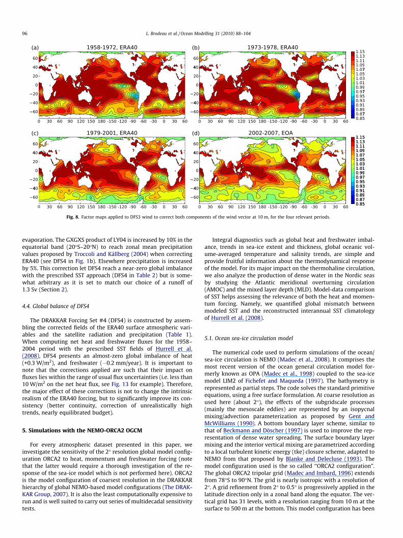
Fig. 8. Factor maps applied to DFS3 wind to correct both components of the wind vector at 10 m, for the four relevant periods.

96 L. Brodeau et al. / Ocean Modelling 31 (2010) 88–104

evaporation. The GXGXS product of LY04 is increased by 10% in theequatorial band (20�S–20�N) to reach zonal mean precipitationvalues proposed by Troccoli and Kållberg (2004) when correctingERA40 (see DFS4 in Fig. 1b). Elsewhere precipitation is increasedby 5%. This correction let DFS4 reach a near-zero global imbalancewith the prescribed SST approach (DFS4 in Table 2) but is some-what arbitrary as it is set to match our choice of a runoff of1.3 Sv (Section 2).

4.4. Global balance of DFS4

The DRAKKAR Forcing Set #4 (DFS4) is constructed by assem-bling the corrected fields of the ERA40 surface atmospheric vari-ables and the satellite radiation and precipitation (Table 1).When computing net heat and freshwater fluxes for the 1958–2004 period with the prescribed SST fields of Hurrell et al.(2008), DFS4 presents an almost-zero global imbalance of heat(+0.3 W/m2), and freshwater (�0.2 mm/year). It is important tonote that the corrections applied are such that their impact onfluxes lies within the range of usual flux uncertainties (i.e. less than10 W/m2 on the net heat flux, see Fig. 13 for example). Therefore,the major effect of these corrections is not to change the intrinsicrealism of the ERA40 forcing, but to significantly improve its con-sistency (better continuity, correction of unrealistically hightrends, nearly equilibrated budget).

5. Simulations with the NEMO-ORCA2 OGCM

For every atmospheric dataset presented in this paper, weinvestigate the sensitivity of the 2� resolution global model config-uration ORCA2 to heat, momentum and freshwater forcing (notethat the latter would require a thorough investigation of the re-sponse of the sea-ice model which is not performed here). ORCA2is the model configuration of coarsest resolution in the DRAKKARhierarchy of global NEMO-based model configurations (The DRAK-KAR Group, 2007). It is also the least computationally expensive torun and is well suited to carry out series of multidecadal sensitivitytests.

Integral diagnostics such as global heat and freshwater imbal-ance, trends in sea-ice extent and thickness, global oceanic vol-ume-averaged temperature and salinity trends, are simple andprovide fruitful information about the thermodynamical responseof the model. For its major impact on the thermohaline circulation,we also analyze the production of dense water in the Nordic seasby studying the Atlantic meridional overturning circulation(AMOC) and the mixed layer depth (MLD). Model-data comparisonof SST helps assessing the relevance of both the heat and momen-tum forcing. Namely, we quantified global mismatch betweenmodeled SST and the reconstructed interannual SST climatologyof Hurrell et al. (2008).

5.1. Ocean sea-ice circulation model

The numerical code used to perform simulations of the ocean/sea-ice circulation is NEMO (Madec et al., 2008). It comprises themost recent version of the ocean general circulation model for-merly known as OPA (Madec et al., 1998) coupled to the sea-icemodel LIM2 of Fichefet and Maqueda (1997). The bathymetry isrepresented as partial steps. The code solves the standard primitiveequations, using a free surface formulation. At coarse resolution asused here (about 2�), the effects of the subgridscale processes(mainly the mesoscale eddies) are represented by an isopycnalmixing/advection parameterization as proposed by Gent andMcWilliams (1990). A bottom boundary layer scheme, similar tothat of Beckmann and Döscher (1997) is used to improve the rep-resentation of dense water spreading. The surface boundary layermixing and the interior vertical mixing are parametrized accordingto a local turbulent kinetic energy (tke) closure scheme, adapted toNEMO from that proposed by Blanke and Delecluse (1993). Themodel configuration used is the so called ‘‘ORCA2 configuration”.The global ORCA2 tripolar grid (Madec and Imbard, 1996) extendsfrom 78�S to 90�N. The grid is nearly isotropic with a resolution of2�. A grid refinement from 2� to 0.5� is progressively applied in thelatitude direction only in a zonal band along the equator. The ver-tical grid has 31 levels, with a resolution ranging from 10 m at thesurface to 500 m at the bottom. This model configuration has been

L. Brodeau et al. / Ocean Modelling 31 (2010) 88–104 97

used extensively over the last 10 years with the older versions ofthe OPA and LIM codes (e.g. Timmermann et al., 2005).

In a model forced by an observed atmospheric state (with bulkformulae) rather than coupled to an interactive atmosphere, thereis no feedback between the ocean and precipitations. The resultingmodel drift is made worse by the large uncertainties of the precip-itation fields. For this reason we choose to apply a restoring of sur-face salinity to the climatology of Levitus et al. (1998). Acomparison of 7 different models forced by the ‘‘normal year” forc-ing of LY04 showed that most models (including ORCA2) produceunrealistic solution with a weak salinity relaxation (Griffies et al.,2009), one of the consequences being the weakening of the ther-mohaline circulation. In the present study, we use a rather strongsalinity restoring, corresponding to a relaxation time scale of 33days for the first model level (10 m), in the open ocean as well asunder sea ice. Note that this will significantly constrain the fresh-water balance in our experiments.

ORCA2 is initialized in 1958 with the temperature and salinityclimatology of Levitus et al. (1998) and is run for 47 years untilthe end of 2004. Surface fluxes used to drive the simulations arecomputed using strictly the same method (i.e. same flux calcula-tion algorithm and input data) as used in the offline calculationof Sections 2 and 3, except that the prognostic SST and sea-ice con-centration of the model are used rather than prescribed observa-tions. Note that NEMO handles solar penetration, therefore, Qsw,the radiative shortwave component of the net heat flux, must beexplicitly specified. The run being fully interannual from 1984 on-ward (constrained by radiation data) we only consider this laterperiod for time-averaged diagnostics.

5.2. DFS3 driven runs

5.2.1. AMOC and mixed layer depthAs we used the LYDS forcing dataset as reference in the previous

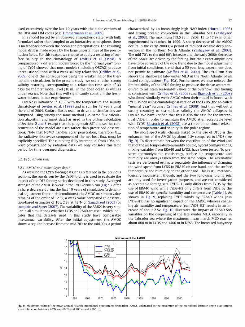
sections, the run driven by the LYDS forcing is used to evaluate theimpact of the DFS forcing series developed in this study. Averagedstrength of the AMOC is weak in the LYDS-driven run (Fig. 9). Aftera sharp decrease during the first 10 years of simulation (a dynam-ical adjustment from initial conditions), the AMOC maximum valueremains of the order of 12 Sv, a weak value compared to observa-tion-based estimates of 16 ± 2 Sv at 48�N of Ganachaud (2003) orLumpkin and Speer (2007). The variability of the AMOC is very sim-ilar in all simulations whether LYDS or ERA40 are used, which indi-cates that the datasets used in this study have comparableinterannual variability. After the initial adjustment, the AMOCshows a regular increase from the mid 70’s to the mid 90’s, a period

10

11

12

13

14

15

16

17

18

1960 1965 1970 1975 198

(Sv)

Maximum

LYDS LYDS-H1 LYDS-H2 DFS3 DFS4

Fig. 9. Maximum value of the mean annual Atlantic meridional overturning circulationstream function between 20�N and 60�N, and 200 m and 2500 m).

characterized by an increasingly high NAO index (Hurrell, 1995)and strong oceanic convection in the Labrador Sea (Yashayaevet al., 2003). The maximum (13.5 Sv in LYDS, 15 to 17 Sv in otherexperiments) is reached in 1999. A sharp decrease of the AMOCoccurs in the early 2000’s, a period of reduced oceanic deep con-vection in the northern North Atlantic (Yashayaev et al., 2003).The mid 70’s to the mid 90’s increase and the early 2000s decreaseof the AMOC are driven by the forcing, but their exact amplitudeshave to be corrected of the slow trend due to the model adjustmentfrom initial conditions, trend that a 50 year long experiment doesnot permit to estimate (Griffies et al., 2009). The LYDS run alsoshows the shallowest late-winter MLD in the North Atlantic of alltested configurations (Fig. 10a). Furthermore, we also noticed thelimited ability of the LYDS forcing to produce the dense waters re-quired to maintain reasonable values of the overflow. This findingis consistent with Griffies et al. (2009) and Biastoch et al. (2008)who found similarly weak AMOC when their model is forced withLYDS. When using climatological version of the LYDS (the so-called‘‘normal year” forcing), Griffies et al. (2009) find that without astrong restoring to sea surface salinity the AMOC collapses inORCA2. We have verified that this is also the case for the interan-nual LYDS. In order to maintain the AMOC at an acceptable levelwith LYDS, Biastoch et al. (2008) use a three dimensional relaxa-tion of temperature and salinity in the polar regions.

The most spectacular change linked to the use of DFS3 is theenhancement of the AMOC by about 2 Sv compared to LYDS (seeFig. 9). To discriminate between the contribution of the wind andthat of the air temperature-humidity couple, hybrid configurations,mixing variables from ERA40 and LYDS, have been tested. To pre-serve thermodynamic consistency, surface air temperature andhumidity are always taken from the same origin. The alternativetests we performed estimate separately the influence of changingthe wind speed from LYDS to ERA40 on one hand, and the surfacetemperature and humidity on the other hand. This is still meteoro-logically inconsistent though, and the two following forcing setsare only used for investigation purposes, and are not consideredas acceptable forcing sets. LYDS-H1 only differs from LYDS by theuse of ERA40 wind while LYDS-H2 only differs from LYDS by theuse of ERA40 air specific humidity and temperature (Table 1). Asshown in Fig. 9, replacing LYDS winds by ERA40 winds (runLYDS-H1) has no significant impact on the AMOC, whereas chang-ing air humidity and temperature (run LYDS-H2) results in an in-crease of about 2 Sv. Fig. 10 illustrates the impact of ERA40 SASvariables on the deepening of the late winter MLD, especially inthe Labrador sea where the maximum mean march MLD reachesabout 800 m in LYDS and 1400 m in DFS3. The increased buoyancy

0 1985 1990 1995 2000

of the AMOC

(AMOC, calculated as the maximum of the meridional latitude-depth overturning

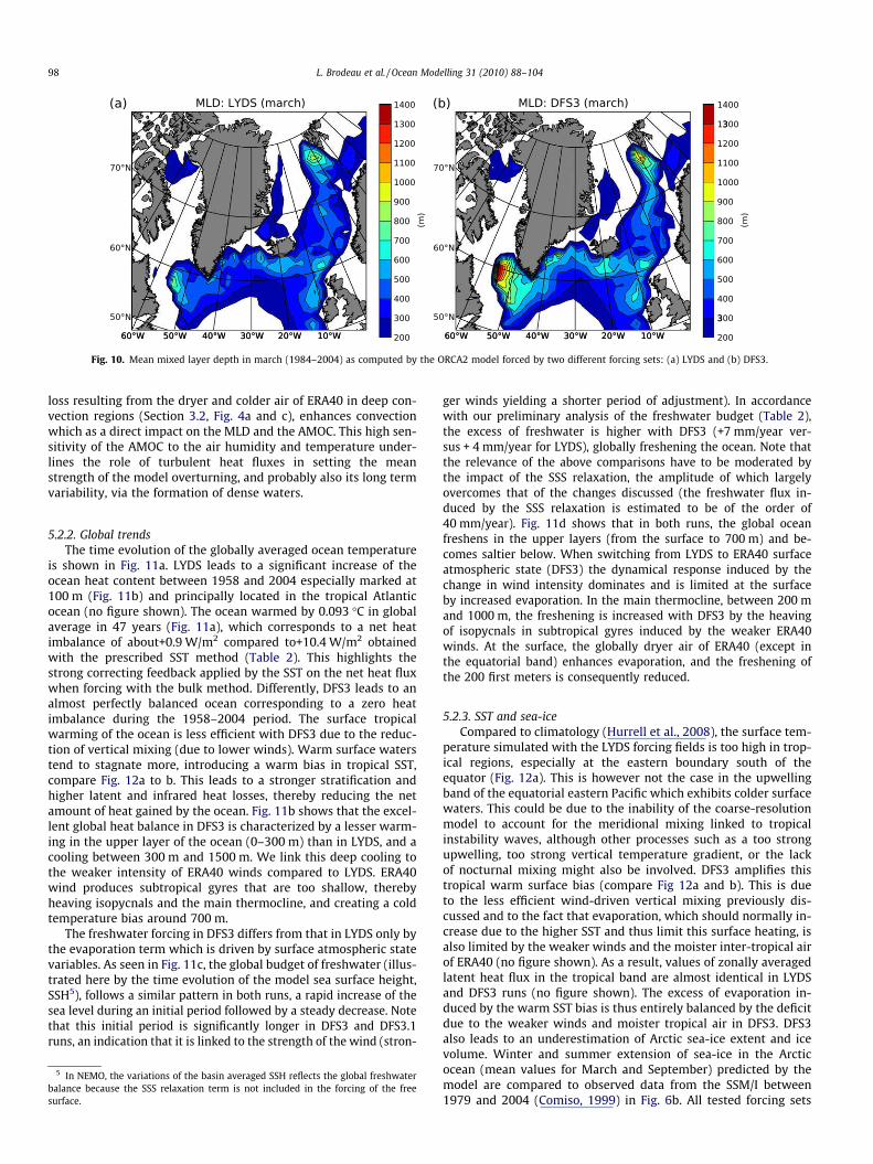
Fig. 10. Mean mixed layer depth in march (1984–2004) as computed by the ORCA2 model forced by two different forcing sets: (a) LYDS and (b) DFS3.

98 L. Brodeau et al. / Ocean Modelling 31 (2010) 88–104

loss resulting from the dryer and colder air of ERA40 in deep con-vection regions (Section 3.2, Fig. 4a and c), enhances convectionwhich as a direct impact on the MLD and the AMOC. This high sen-sitivity of the AMOC to the air humidity and temperature under-lines the role of turbulent heat fluxes in setting the meanstrength of the model overturning, and probably also its long termvariability, via the formation of dense waters.

5.2.2. Global trendsThe time evolution of the globally averaged ocean temperature

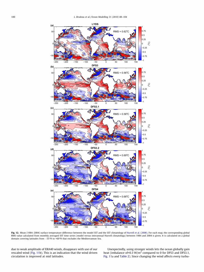
is shown in Fig. 11a. LYDS leads to a significant increase of theocean heat content between 1958 and 2004 especially marked at100 m (Fig. 11b) and principally located in the tropical Atlanticocean (no figure shown). The ocean warmed by 0.093 �C in globalaverage in 47 years (Fig. 11a), which corresponds to a net heatimbalance of about+0.9 W/m2 compared to+10.4 W/m2 obtainedwith the prescribed SST method (Table 2). This highlights thestrong correcting feedback applied by the SST on the net heat fluxwhen forcing with the bulk method. Differently, DFS3 leads to analmost perfectly balanced ocean corresponding to a zero heatimbalance during the 1958–2004 period. The surface tropicalwarming of the ocean is less efficient with DFS3 due to the reduc-tion of vertical mixing (due to lower winds). Warm surface waterstend to stagnate more, introducing a warm bias in tropical SST,compare Fig. 12a to b. This leads to a stronger stratification andhigher latent and infrared heat losses, thereby reducing the netamount of heat gained by the ocean. Fig. 11b shows that the excel-lent global heat balance in DFS3 is characterized by a lesser warm-ing in the upper layer of the ocean (0–300 m) than in LYDS, and acooling between 300 m and 1500 m. We link this deep cooling tothe weaker intensity of ERA40 winds compared to LYDS. ERA40wind produces subtropical gyres that are too shallow, therebyheaving isopycnals and the main thermocline, and creating a coldtemperature bias around 700 m.

The freshwater forcing in DFS3 differs from that in LYDS only bythe evaporation term which is driven by surface atmospheric statevariables. As seen in Fig. 11c, the global budget of freshwater (illus-trated here by the time evolution of the model sea surface height,SSH5), follows a similar pattern in both runs, a rapid increase of thesea level during an initial period followed by a steady decrease. Notethat this initial period is significantly longer in DFS3 and DFS3.1runs, an indication that it is linked to the strength of the wind (stron-

5 In NEMO, the variations of the basin averaged SSH reflects the global freshwaterbalance because the SSS relaxation term is not included in the forcing of the freesurface.

ger winds yielding a shorter period of adjustment). In accordancewith our preliminary analysis of the freshwater budget (Table 2),the excess of freshwater is higher with DFS3 (+7 mm/year ver-sus + 4 mm/year for LYDS), globally freshening the ocean. Note thatthe relevance of the above comparisons have to be moderated bythe impact of the SSS relaxation, the amplitude of which largelyovercomes that of the changes discussed (the freshwater flux in-duced by the SSS relaxation is estimated to be of the order of40 mm/year). Fig. 11d shows that in both runs, the global oceanfreshens in the upper layers (from the surface to 700 m) and be-comes saltier below. When switching from LYDS to ERA40 surfaceatmospheric state (DFS3) the dynamical response induced by thechange in wind intensity dominates and is limited at the surfaceby increased evaporation. In the main thermocline, between 200 mand 1000 m, the freshening is increased with DFS3 by the heavingof isopycnals in subtropical gyres induced by the weaker ERA40winds. At the surface, the globally dryer air of ERA40 (except inthe equatorial band) enhances evaporation, and the freshening ofthe 200 first meters is consequently reduced.

5.2.3. SST and sea-iceCompared to climatology (Hurrell et al., 2008), the surface tem-

perature simulated with the LYDS forcing fields is too high in trop-ical regions, especially at the eastern boundary south of theequator (Fig. 12a). This is however not the case in the upwellingband of the equatorial eastern Pacific which exhibits colder surfacewaters. This could be due to the inability of the coarse-resolutionmodel to account for the meridional mixing linked to tropicalinstability waves, although other processes such as a too strongupwelling, too strong vertical temperature gradient, or the lackof nocturnal mixing might also be involved. DFS3 amplifies thistropical warm surface bias (compare Fig 12a and b). This is dueto the less efficient wind-driven vertical mixing previously dis-cussed and to the fact that evaporation, which should normally in-crease due to the higher SST and thus limit this surface heating, isalso limited by the weaker winds and the moister inter-tropical airof ERA40 (no figure shown). As a result, values of zonally averagedlatent heat flux in the tropical band are almost identical in LYDSand DFS3 runs (no figure shown). The excess of evaporation in-duced by the warm SST bias is thus entirely balanced by the deficitdue to the weaker winds and moister tropical air in DFS3. DFS3also leads to an underestimation of Arctic sea-ice extent and icevolume. Winter and summer extension of sea-ice in the Arcticocean (mean values for March and September) predicted by themodel are compared to observed data from the SSM/I between1979 and 2004 (Comiso, 1999) in Fig. 6b. All tested forcing sets

Fig. 11. Global oceanic volume-averaged evolution of (a) temperature and (c) SSH computed by the ORCA2 model. Global oceanic level-averaged drift of (b) temperature and(d) salinity as a function of depth after 47 years of simulation, equivalent to comparing the last year to the initial condition (Levitus et al., 1998). The vertical patterns of thedrift in (b) and (d) appear early in the run and are rapidly steady, so the plots are representative. In (b) and (d), the curves for DFS3 and DFS3.1 are almost identical.

L. Brodeau et al. / Ocean Modelling 31 (2010) 88–104 99

underestimate the total area covered by sea-ice in winter by morethan 106 km2. LYDS leads to the lowest estimation while DFS3 (de-spite warmer temperatures over ice) slightly increases the winterice extension. However, colder winter temperatures of LYDS areresponsible for enhancing ice production more than ERA40 whichexplains why its summer ice extent is more important, and closerto observations. The summer representation of ice extent is verysatisfying for the LYDS-driven run, while it is evident that SAS vari-ables of ERA40 used in DFS3 lead to an underestimation of almost2 � 106 km2. This is likely linked to excessively warm tempera-tures (Fig. 4d). Note that similar flaws are also identified in simu-lations carried out under LYDS forcing with the same model at aresolution of 1/4� (Lique et al., 2009, 2007).

5.3. Model sensitivity to corrections in DFS4

5.3.1. Humidity and temperature correctionThe DFS3.1 simulation is similar to DFS3, but uses the air

humidity and temperature corrections described in Section 4.1.The drying of the surface air applied in DFS3.1 in the tropics duringthe last two decades enhances the evaporation term which is ex-pected to affect both heat and freshwater forcing. A comparisonbetween the SST fields of DFS3 and DFS3.1 runs (Fig. 12b and c)shows that the correction slightly decreases the warm bias in thetropics, but this remains insufficient since the difference with cli-matology remains of the order of+0.5 �C. Fig. 13a shows that ourcorrection increases the latent heat loss by about 2 W/m2 (up to3.5 W/m2 at the equator, see the curve for DFS3.1) and is partly bal-

anced by the decrease of sensible and infrared heat losses due tothe sea surface cooling (Fig. 13b and c). This explains why thenet heat flux is weakly modified by the introduction of the tropicalhumidity correction (Fig. 13d). The resulting extra equatorial heatloss is balanced by the decrease in heat loss linked to our northerncorrection (Section 4.1.2). Therefore, like DFS3, DFS3.1 leads to azero imbalance of heat (Fig. 11a and Table 2). Due to the surfacesalinity restoring, the effect on surface salinity is hardly discern-ible. Globally the ocean is freshening slightly more than withDFS3 (freshwater imbalance of +8 mm/year, Fig. 11c and Table 2).The correction of the Arctic temperature also improves the repre-sentation of the sea-ice extent, which becomes more realistic,especially in summertime (Fig. 6b). The northern correction ap-plied to ERA40 actually yields shallower winter MLDs in the NordicSeas compared to DFS3 (no figure shown). This is accompanied byreduction in the mean annual maximum of the AMOC by roughly0.3Sv.

5.3.2. Rescaled windSimulation DFS3.2 uses rescaled wind defined in Section 4.2 in

addition to the air temperature and humidity corrections alreadyincluded in DFS3.1. As expected, evaporation is significantlyenhanced (Fig. 13a), leading to a significant deficit of freshwater in-put (compare DFS3.2 to DFS3.1 in Fig. 11c). This also cools the SSTalmost everywhere (Fig. 12c and d). The warm surface inter-trop-ical bias is thus reduced, but mid-latitude surface temperature coldbiases are increased. The cold bias at 700 m discussed in Section5.2.2 and linked to the heaving of isopycnal in subtropical gyres

(a)

(b)

(c)

(d)

(e)

LYDS

−250 −200 −150 −100 −50 0 50 100 150

−50

0

50

(o C)

−1

−0.75

−0.5

−0.25

0

0.25

0.5

0.75

1

DFS3

−250 −200 −150 −100 −50 0 50 100 150

−50

0

50

(o C)

−1

−0.75

−0.5

−0.25

0

0.25

0.5

0.75

1

DFS3.1

−250 −200 −150 −100 −50 0 50 100 150

−50

0

50

(o C)

−1

−0.75

−0.5

−0.25

0

0.25

0.5

0.75

1

DFS3.2

−250 −200 −150 −100 −50 0 50 100 150

−50

0

50

(o C)

−1

−0.75

−0.5

−0.25

0

0.25

0.5

0.75

1

DFS4

−250 −200 −150 −100 −50 0 50 100 150

−50

0

50

(o C)

−1

−0.75

−0.5

−0.25

0

0.25

0.5

0.75

1

RMS = 0.62 C

RMS = 0.56 C

RMS = 0.58 C

RMS = 0.69 C

RMS = 0.68 C

o

o

o

o

o

Fig. 12. Mean (1984–2004) surface temperature difference between the model SST and the SST climatology of Hurrell et al. (2008). For each map, the corresponding globalRMS value calculated from monthly averaged SST time series (model versus interannual Hurrell climatology) between 1984 and 2004 is given. It is calculated on a globaldomain covering latitudes from �55�N to +60�N that excludes the Mediterranean Sea.

100 L. Brodeau et al. / Ocean Modelling 31 (2010) 88–104

due to weak amplitude of ERA40 winds, disappears with use of ourrescaled wind (Fig. 11b). This is an indication that the wind drivencirculation is improved at mid latitudes.

Unexpectedly, using stronger winds lets the ocean globally gainheat (imbalance of+0.3 W/m2 compared to 0 for DFS3 and DFS3.1,Fig. 11a and Table 2). Since changing the wind affects every turbu-

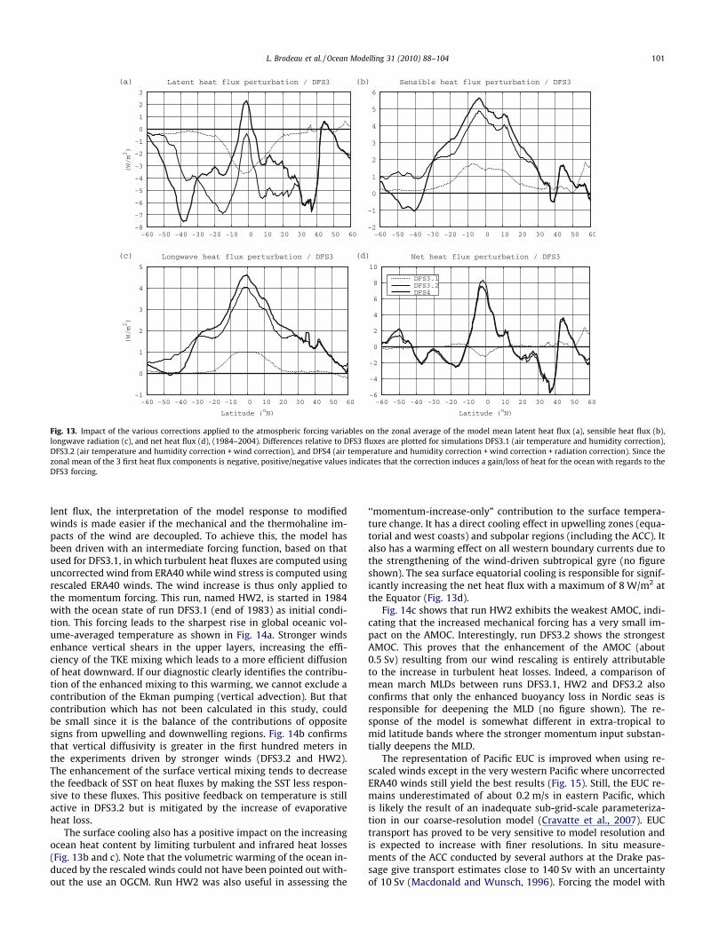
Fig. 13. Impact of the various corrections applied to the atmospheric forcing variables on the zonal average of the model mean latent heat flux (a), sensible heat flux (b),longwave radiation (c), and net heat flux (d), (1984–2004). Differences relative to DFS3 fluxes are plotted for simulations DFS3.1 (air temperature and humidity correction),DFS3.2 (air temperature and humidity correction + wind correction), and DFS4 (air temperature and humidity correction + wind correction + radiation correction). Since thezonal mean of the 3 first heat flux components is negative, positive/negative values indicates that the correction induces a gain/loss of heat for the ocean with regards to theDFS3 forcing.

L. Brodeau et al. / Ocean Modelling 31 (2010) 88–104 101

lent flux, the interpretation of the model response to modifiedwinds is made easier if the mechanical and the thermohaline im-pacts of the wind are decoupled. To achieve this, the model hasbeen driven with an intermediate forcing function, based on thatused for DFS3.1, in which turbulent heat fluxes are computed usinguncorrected wind from ERA40 while wind stress is computed usingrescaled ERA40 winds. The wind increase is thus only applied tothe momentum forcing. This run, named HW2, is started in 1984with the ocean state of run DFS3.1 (end of 1983) as initial condi-tion. This forcing leads to the sharpest rise in global oceanic vol-ume-averaged temperature as shown in Fig. 14a. Stronger windsenhance vertical shears in the upper layers, increasing the effi-ciency of the TKE mixing which leads to a more efficient diffusionof heat downward. If our diagnostic clearly identifies the contribu-tion of the enhanced mixing to this warming, we cannot exclude acontribution of the Ekman pumping (vertical advection). But thatcontribution which has not been calculated in this study, couldbe small since it is the balance of the contributions of oppositesigns from upwelling and downwelling regions. Fig. 14b confirmsthat vertical diffusivity is greater in the first hundred meters inthe experiments driven by stronger winds (DFS3.2 and HW2).The enhancement of the surface vertical mixing tends to decreasethe feedback of SST on heat fluxes by making the SST less respon-sive to these fluxes. This positive feedback on temperature is stillactive in DFS3.2 but is mitigated by the increase of evaporativeheat loss.

The surface cooling also has a positive impact on the increasingocean heat content by limiting turbulent and infrared heat losses(Fig. 13b and c). Note that the volumetric warming of the ocean in-duced by the rescaled winds could not have been pointed out with-out the use an OGCM. Run HW2 was also useful in assessing the

‘‘momentum-increase-only” contribution to the surface tempera-ture change. It has a direct cooling effect in upwelling zones (equa-torial and west coasts) and subpolar regions (including the ACC). Italso has a warming effect on all western boundary currents due tothe strengthening of the wind-driven subtropical gyre (no figureshown). The sea surface equatorial cooling is responsible for signif-icantly increasing the net heat flux with a maximum of 8 W/m2 atthe Equator (Fig. 13d).

Fig. 14c shows that run HW2 exhibits the weakest AMOC, indi-cating that the increased mechanical forcing has a very small im-pact on the AMOC. Interestingly, run DFS3.2 shows the strongestAMOC. This proves that the enhancement of the AMOC (about0.5 Sv) resulting from our wind rescaling is entirely attributableto the increase in turbulent heat losses. Indeed, a comparison ofmean march MLDs between runs DFS3.1, HW2 and DFS3.2 alsoconfirms that only the enhanced buoyancy loss in Nordic seas isresponsible for deepening the MLD (no figure shown). The re-sponse of the model is somewhat different in extra-tropical tomid latitude bands where the stronger momentum input substan-tially deepens the MLD.

The representation of Pacific EUC is improved when using re-scaled winds except in the very western Pacific where uncorrectedERA40 winds still yield the best results (Fig. 15). Still, the EUC re-mains underestimated of about 0.2 m/s in eastern Pacific, whichis likely the result of an inadequate sub-grid-scale parameteriza-tion in our coarse-resolution model (Cravatte et al., 2007). EUCtransport has proved to be very sensitive to model resolution andis expected to increase with finer resolutions. In situ measure-ments of the ACC conducted by several authors at the Drake pas-sage give transport estimates close to 140 Sv with an uncertaintyof 10 Sv (Macdonald and Wunsch, 1996). Forcing the model with

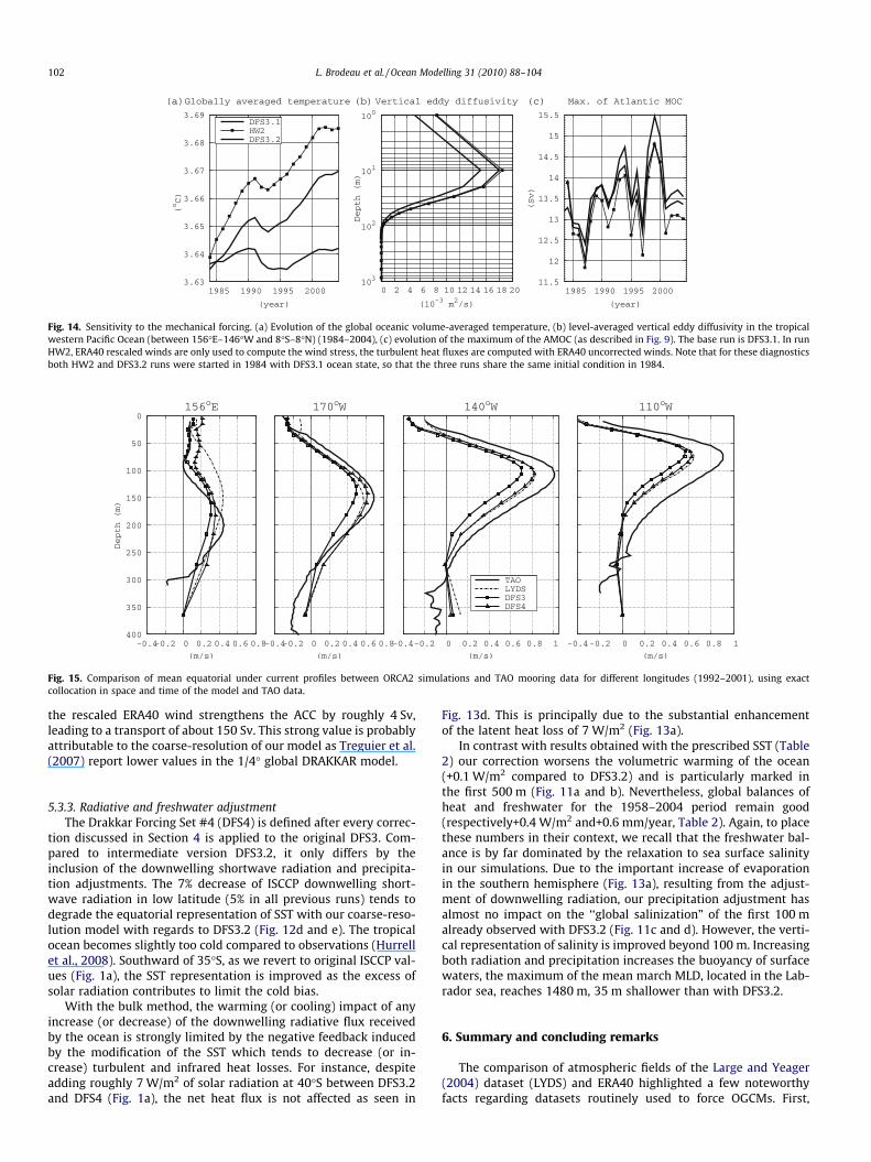
Fig. 14. Sensitivity to the mechanical forcing. (a) Evolution of the global oceanic volume-averaged temperature, (b) level-averaged vertical eddy diffusivity in the tropicalwestern Pacific Ocean (between 156�E–146�W and 8�S–8�N) (1984–2004), (c) evolution of the maximum of the AMOC (as described in Fig. 9). The base run is DFS3.1. In runHW2, ERA40 rescaled winds are only used to compute the wind stress, the turbulent heat fluxes are computed with ERA40 uncorrected winds. Note that for these diagnosticsboth HW2 and DFS3.2 runs were started in 1984 with DFS3.1 ocean state, so that the three runs share the same initial condition in 1984.

Fig. 15. Comparison of mean equatorial under current profiles between ORCA2 simulations and TAO mooring data for different longitudes (1992–2001), using exactcollocation in space and time of the model and TAO data.

102 L. Brodeau et al. / Ocean Modelling 31 (2010) 88–104

the rescaled ERA40 wind strengthens the ACC by roughly 4 Sv,leading to a transport of about 150 Sv. This strong value is probablyattributable to the coarse-resolution of our model as Treguier et al.(2007) report lower values in the 1/4� global DRAKKAR model.

5.3.3. Radiative and freshwater adjustmentThe Drakkar Forcing Set #4 (DFS4) is defined after every correc-

tion discussed in Section 4 is applied to the original DFS3. Com-pared to intermediate version DFS3.2, it only differs by theinclusion of the downwelling shortwave radiation and precipita-tion adjustments. The 7% decrease of ISCCP downwelling short-wave radiation in low latitude (5% in all previous runs) tends todegrade the equatorial representation of SST with our coarse-reso-lution model with regards to DFS3.2 (Fig. 12d and e). The tropicalocean becomes slightly too cold compared to observations (Hurrellet al., 2008). Southward of 35�S, as we revert to original ISCCP val-ues (Fig. 1a), the SST representation is improved as the excess ofsolar radiation contributes to limit the cold bias.

With the bulk method, the warming (or cooling) impact of anyincrease (or decrease) of the downwelling radiative flux receivedby the ocean is strongly limited by the negative feedback inducedby the modification of the SST which tends to decrease (or in-crease) turbulent and infrared heat losses. For instance, despiteadding roughly 7 W/m2 of solar radiation at 40�S between DFS3.2and DFS4 (Fig. 1a), the net heat flux is not affected as seen in

Fig. 13d. This is principally due to the substantial enhancementof the latent heat loss of 7 W/m2 (Fig. 13a).

In contrast with results obtained with the prescribed SST (Table2) our correction worsens the volumetric warming of the ocean(+0.1 W/m2 compared to DFS3.2) and is particularly marked inthe first 500 m (Fig. 11a and b). Nevertheless, global balances ofheat and freshwater for the 1958–2004 period remain good(respectively+0.4 W/m2 and+0.6 mm/year, Table 2). Again, to placethese numbers in their context, we recall that the freshwater bal-ance is by far dominated by the relaxation to sea surface salinityin our simulations. Due to the important increase of evaporationin the southern hemisphere (Fig. 13a), resulting from the adjust-ment of downwelling radiation, our precipitation adjustment hasalmost no impact on the ‘‘global salinization” of the first 100 malready observed with DFS3.2 (Fig. 11c and d). However, the verti-cal representation of salinity is improved beyond 100 m. Increasingboth radiation and precipitation increases the buoyancy of surfacewaters, the maximum of the mean march MLD, located in the Lab-rador sea, reaches 1480 m, 35 m shallower than with DFS3.2.

6. Summary and concluding remarks

The comparison of atmospheric fields of the Large and Yeager(2004) dataset (LYDS) and ERA40 highlighted a few noteworthyfacts regarding datasets routinely used to force OGCMs. First,

L. Brodeau et al. / Ocean Modelling 31 (2010) 88–104 103

winds from the two major reanalyzes (NCEP and ERA40) tend to beunderestimated when compared to more trustworthy data such asscatterometer wind products (QuikSCAT). Second, surface atmo-spheric state variables of ERA40, and to a lesser extent those ofNCEP, suffer from time discontinuities related to the evolution ofthe origin of data used in their respective assimilation process. Fi-nally, downwelling radiation components and precipitation data ofreanalyzes are not reliable and satellite products stand as betteralternatives. A first forcing data set, DFS3, is thus constructed byassembling the ERA40 surface atmospheric state variables withradiation and precipitation from LYDS, but the global heat andfreshwater budget computed with DFS3 and observed SST is foundto be unbalanced. A set of corrections was applied to both atmo-spheric and radiation fields of the DFS3, our initial ERA40-baseddataset. They include a time-dependent recalibration of surfaceatmospheric fields of ERA40 in the tropical band, re-adjustmentsof Arctic air temperature and humidity based on the POLES clima-tology, a global increase of the wind speed based on QuikSCAT val-ues, and zonal adjustments of the downwelling radiation andprecipitation products proposed by Large and Yeager (2004). Oneof the constraint was to reach a near-zero global imbalance of heatand freshwater when computing fluxes with a prescribed climato-logical surface state of the ocean. Note that the amplitude of thecorrections are small and such that their impact on fluxes lieswithin the range of usual flux uncertainties (i.e. less than 10 W/m2).

Global simulations performed with ORCA2, a coarse-resolutionocean/sea-ice circulation model forced with surface atmosphericstate variables of ERA40 showed several differences with respectto LYDS-driven simulations. These include an increase of the AMOCfrom 12 to 14 Sv. Further efforts to force the model with hybridforcing functions permitted to link this modification of the AMOCintensity to the enhancement of surface buoyancy loss in the Nor-dic seas and the Northern North Atlantic. DFS4, our final ERA40-based dataset, is shown to preserve positive features of DFS3 whilesignificantly correcting its major flaws, such as tropical warm bias,weak wind driven circulation in subtropical gyres and the ACC, andunrealistic arctic ice cover. Representation of the vertical structureof temperature is also improved when compared to the solution ofthe LYDS-driven run (Fig. 11b). However, the ocean surface re-mains globally cooler than observations (Fig. 12e) and significantdifferences persist in the vicinity of the largest currents (GulfStream, Kuroshio, Agulhas, Brazil-Malvinas confluence, ACC). Theyare caused by known model dynamical biases due to numerics andcoarse-resolution (position of Gulf Stream, overshoot of westernboundary currents, etc.). We expect these to be significantlyreduced at the eddy-resolving resolution. Still, possible sources oferror are likely to arise from missing elements like the diurnal cy-cle of shortwave heating, or the spatially varying chlorophyll-dependent solar penetration into the water column. As it has beenshown in several model studies, both aspects can have major im-pacts on the climatological SST, mixed-layer depth, and interan-nual variability, especially in weakly stratified regions like thetropical warm pools (see Bernie et al., 2007; Bernie et al., 2008for the diurnal cycle, and (Lengaigne et al., 2007; Anderson et al.,2009) for the chlorophyll dependency of solar penetration).

As highlighted by Table 2, and especially for our intermediateforcing configurations, prescribed SST studies are weak in predict-ing the actual response of a bulk-driven OGCM to a given forcingset. This is mainly due to the important role played by the SSTwhen estimating both heat and freshwater fluxes. Interestingly,with DFS4, a good agreement is found between the two ap-proaches. When tested with the observed SST, DFS4 leads to an al-most closed budget of heat and freshwater for the 1958–2004period (respectively +0.3 W/m2 and �0.2 mm/year), the samefluxes computed interactively with ORCA2’s SST lead (for the same

period) to an annual imbalance of heat and freshwater of respec-tively +0.4 W/m2 and +0.6 mm. Prescribed SST diagnostics cannotaccount for the modification of evaporation induced by a radiationadjustment, which proved to have a significant impact on bothheat and freshwater budgets of the ocean when using our model.The corrective feedback applied by the SST on the net heat fluxhas also been verified as global imbalances of heat computed bythe model were always much closer to zero than those computedwith the prescribed SST approach.

The response of our coarse-resolution model to the differentatmospheric datasets, has shown some counter-intuitive sensitivi-ties. The strengthened winds, as expected, enhance heat lossthrough evaporation, but also globally warm the ocean by increas-ing the vertical mixing. Enhanced vertical diffusion helps maintaina cooler SST, which tends to limit the amount of heat lost by theocean (through turbulent and infrared heat losses), thereby allow-ing the ocean to store more heat. Surface atmospheric state vari-ables, through their direct influence on turbulent heat fluxes, areshown to play a significant role on important features of the oceancirculation such as the AMOC, tropical SST representation, etc. Sur-face atmospheric state variables from NCEP and ERA40 lead to dis-tinct solutions for trends and mean state. However, interannualand decadal variability of the simulated circulation features aresimilar, indicating that atmospherically driven variability is similarin both reanalysis products. Modification of the downwelling radi-ation input is partially balanced by the response of the SST-depen-dent heat fluxes which tend to limit the impact of suchmodifications.

In conclusion, we propose a new set of forcing variables forOGCMs based on ERA40 which provide an alternative to LYDS,and that can be used to perform ocean hindcasts of the last 5 dec-ades. The DFS4 dataset is currently extended to year 2007, and willbe made available on request by the Drakkar group. Generally, itshould permit further sensitivity studies to atmospheric forcingduring this period. Surface atmospheric variables from reanalysisproducts should still be improved further to provide better forcingfields for ocean models, and we are now investigating the latestreanalysis of ECMWF, ERA-interim (1989 to present).

Acknowledgments

The authors acknowledge support from Centre National de laRecherche Scientifique (CNRS), Université Joseph Fourier (UJF) deGrenoble and IFREMER in Brest. This study, carried out as part ofthe DRAKKAR project, was supported by grants from SHOM, CNES,GMMC and MERCATOR-Ocean, INSU/CNRS (PICS 2475), and by theEuropean Integrated project MERSEA. Computer resources wereprovided by Institut du Développement et des Resources en Infor-matique Scientique (IDRIS) in Orsay and the MIRAGE platform inGrenoble.

References

Anderson, W., Gnanadesikan, A., Wittenberg, A., 2009. Regional impacts of oceancolor on tropical Pacific variability. Ocean Sci. 5, 313–327.

Andersson, E., Bauer, P., Blazon, A., Chevallier, F., Ólm, E., Janisková, M., Kållberg, P.,Kelly, G., Lopez, P., McNally, A., Moreau, E., Simmons, A., Thépaut, J.N.,Tompkins, A., Andrae, U., Sokka, N., Onogi, K., 2005. Assimilation andmodeling of the atmospheric hydrological cycle in the ECMWF forecastingsystem. Bull. Am. Meteorol. Soc. 86, 387–402.

Baumgartner, A., Reichel, E., 1975. The World Water Balance, Mean Annual Global,Continental and Maritime Precipitation, Evaporation and Runoff. Elsevier (p.179).

Beckmann, A., Döscher, R., 1997. A method for improved representation of densewater spreading over topography in geopotential-coordinate models. J. Phys.Oceanogr. 27, 581–591.

Béranger, K., Barnier, B., Gulev, S., Crépon, M., 2006. Comparing 20 years ofprecipitation estimates from different sources over the world ocean. OceanDynam. 56, 104–138.

104 L. Brodeau et al. / Ocean Modelling 31 (2010) 88–104

Bernie, D.J., Guilyardi, E., Madec, G., Slingo, J.M., Woolnough, S.J., 2007. Impact ofresolving the diurnal cycle in an ocean-atmosphere GCM. Part 1: A diurnallyforced OGCM. Clim. Dyn. 29, 575–590.

Bernie, D.J., Guilyardi, E., Madec, G., Slingo, J.M., Woolnough, S.J., 2008. Impact ofresolving the diurnal cycle in an ocean-atmosphere GCM. Part 2: A diurnallycoupled CGCM. Clim. Dyn. 31, 909–925.

Biastoch, A., Böning, C., Getzlaff, J., Molines, J.-M., Madec, G., 2008. Mechanisms ofinterannual – decadal variability in the meridional overturning circulation ofthe mid-latitude north atlantic ocean. J. Clim. 21, 6599–6615.

Blanke, B., Delecluse, P., 1993. Variability of the tropical atlantic ocean simulated bya general circulation model with two different mixed-layer physics. J. Phys.Oceanogr. 23, 1363–1388.

Brodeau, L., 2007. Contribution à l’amélioration de la fonction de forçage desmodèles de circulation générale océanique. Ph.D. Thesis, Université JosephFourier, Grenoble, France.

Chelton, D.B., Freilich, M.H., Sienkiewicz, J.M., Von Ahn, J.M., 2006. On the use ofQuikSCAT scatterometer measurements of surface winds for marine weatherprediction. Mon. Wea. Rev. 134, 2055–2071.

Comiso, J., 1999, updated 2008. Bootstrap sea ice concentrations from NIMBUS-7SMMR and DMSP SSM/I Boulder, Colorado USA: National Snow and Ice DataCenter. Digital Media.

Cravatte, S., Madec, G., Izumo, T., Menkes, C., Bozec, A., 2007. Progress in the 3Dcirculation of the eastern equatorial pacific in a climate ocean model. OceanModel. 17, 28–48.

Fekete, B.M., Vörösmarty, C.J., Grabs, W., 2000. Global composite runoff fields basedon observed river discharge and simulated water balances. Tech. Rep., GlobalRunoff Data Centre Rep. 22, Koblenz, Germany, p. 39.

Fichefet, T., Maqueda, M.M., 1997. Sensitivity of a global sea ice model to thetreatment of ice thermodynamics and dynamics. J. Geophys. Res. 102 (12), 609–646.

Ganachaud, A., 2003. Large scale mass transports, water mass formation anddiffusivities estimated from the woce hydrographic data. J. Geophys. Res., 108.

Gent, P.R., McWilliams, J.C., 1990. Isopycnal mixing in ocean circulation models. J.Phys. Oceanogr. 20, 150–155.

Gibson, J.K., Kållberg, P., Uppala, S., Hernandez, A., Nomura, A., Serrano, E., 1997. ERAdescription. ECMWF Reanalysis Project Rep. vol. 1, p. 72.

Global Runoff Data Centre, 2000. Observed historical discharge data from majorrivers for climate model validation. Tech. Rep., Max Planck Institute.

Griffies, S., Biastoch, A., Boning, C., Bryan, F., Danabasoglu, G., Chassignet, E.,England, M., Gerdes, R., Haak, H., Hallberg, R., Hazeleger, W., Jungclaus, J., Larg,W., Madex, G., Samuels, B., Scheinert, M., Severijns, C., Simmons, H., Treguier, A.,Winton, M., Yeager, S., Yin, J., 2009. Coordinated Ocean-ice ReferenceExperiments (COREs). Ocean Model. 11, 59–74.

Huffman, G.J., Adler, R.F., Arkin, P., Chang, A., Ferraro, R., Gruber, A., Janowiak, J.,Joyce, R.J., McNab, A., Rudolf, B., Schneider, U., Xie, P., 1997. The globalprecipitation climatology project (gpcp) combined precipitation data set. Bull.Am. Meteor. Soc. 78, 5–20.

Hurrell, J.W., 1995. Decadal trends in the north atlantic oscillation: regionaltemperatures and precipitation. Science 269 (5224), 676–679.

Hurrell, J.W., Hack, J.J., Shea, D., Caron, J.M., Rosinski, J., 2008. A new sea surfacetemperature and sea ice boundary dataset for the community atmospheremodel. J. Clim. 21 (19), 5145–5153.

Jacobs, S., Comiso, J., 1989. Sea ice and oceanic processes on the Ross Sea continentalshelf. J. Geophys. Res. 94, 18195–18211.

Josey, S.A., Kent, E.C., Taylor, P.K., 1998. The Southampton Oceanography Centre(SOC) Ocean - Atmosphere Heat, Momentum and Freshwater Flux. Atlas. Tech.rep., Southampton Oceanography Centre, pp. 30.

Juza, M., Penduff, T., Barnier, B., Brankart, J.-M., 2009. Analysis of monthly ARGOsampling errors in the global ocean mixed layer: a DRAKKAR model study, J.Geophys. Res. submitted for publication.

Kalnay, E., Kanamitsu, M., Kistler, R., Collins, W., Deaven, D., Gandin, L., Iredell, M.,Saha, S., White, G., Woollen, J., Zhu, Y., Chelliah, M., Ebisuzaki, W., Higgins, W.,Janowiak, J., Mo, K., Ropelewski, C., Wang, J., Leetmaa, A., Reynolds, E., Jenne, R.,Joseph, D., 1996. The NCEP/NCAR 40-year reanalysis project. Bull. Am. Meteor.Soc. 77, 437–471.

Large, W.G., Danabasoglu, G., Doney, S.C., McWilliams, J.C., 1997. Sensitivity tosurface forcing and boundary layer mixing in a global ocean model. J. Phys.Oceanogr. 27, 2418–2447.

Large, W.G., Yeager, S.G., 2004. Diurnal to decadal global forcing for ocean and sea-ice models. NCAR Technical Note, p. 22.

Large, W.G., Yeager, S.G., 2008. The global climatology of an interannually varyingair-sea flux data set. Clim. Dyn.. doi:10.1007/s00382–008–0441–3.

Leeuwenburgh, O., 2005. Assimilation of along-track altimeter data in the tropicalPacific region of a global OGCM ensemble. Quart. J. Roy. Meteor. Soc. 131, 2455–2472.

Lengaigne, M., Menkes, C., Aumont, O., Gorgues, T., Bopp, L., André, J.-M., Madec, G.,2007. Influence of the oceanic biology on the tropical Pacific climate in acoupled general circulation model. Clim. Dyn. 28, 503–516.

Levitus, S., Boyer, T.P., Conkright, M.E., O’Brien, T., Antonov, J., Stephens, C.,Stathoplos, L., Johnson, D., Gelfeld, R., 1998. NOAA Atlas NESDIS 18 and WorldOcean Database 1998, vol. 1. U.S. Gov. Printing Office, Washington, DC.

Lique, C., Treguier, A.-M., Scheinert, M., Penduff, T., 2009. A model-based study of iceand freshwater transport variabilities along both sides of Greenland. Clim. Dyn..doi:10.1007/s00382–008–0510–7.

Liu, W.T., Tang, W., Polito, P.S., 1998. Nasa scatterometer provides global ocean-surface wind fields with more structures than numerical weather prediction.Geophys. Res. Lett. 24, 761–764.

Lucas, M., Ayoub, N., Barnier, B., Penduff, T., de Mey, P., 2008. Stochastic study of thetemperature response of the upper ocean to uncertainties in the atmosphericforcing in an Atlantic OGCM. Ocean Model. 20, 90–113.

Lumpkin, R., Speer, K., 2007. Global ocean meridional overturning. J. Phys. Oceanogr.37, 2550–2562.

Macdonald, A.M., Wunsch, C., 1996. An estimate of global ocean circulation and heatfluxes. Nature 382, 436–439.

Madec, G., 2008. NEMO, the Ocean Engine. Tech. Rep., Notes de l’IPSL (27), ISSN1288-1619, Université P. et M. Curie, B102 T15-E5, 4 Place Jussieu, Paris Cedex5, p. 193.

Madec, G., Delecluse, P., Imbard, M., Levy, C., 1998. OPA 8.1 general circulationmodel reference manual. Tech. Rep., Notes de l’IPSL, Université P. et M. Curie,B102 T15-E5, 4 Place Jussieu, Paris Cedex 5, France, p. 91.

Madec, G., Imbard, M., 1996. A global ocean mesh to overcome the North Polesingularity. Clim. Dyn. 12, 381–388.

Oki, T., 1999. The global water cycle. In: Browning, K.A., Gurney, R.J. (Eds.), GlobalEnergy and Water Cycles. Cambridge University Press, pp. 10–29.

Renwick, J.A., 2004. Trends in the Southern Hemisphere polar vortex in NCEP andECMWF reanalyses. Geophys. Res. Lett. 31 (7), L07209.

Rigor, I., Colony, R., Martin, S., 2000. Variations in surface air temperatureobservations in the arctic. J. Clim. 13, 896–914.

Röske, F., 2006. A global heat and freshwater forcing dataset for ocean models.Ocean Model. 11, 235–297.

Serreze, M., Hurst, C., 2000. Representation of mean arctic precipitation from NCEP-NCAR and ERA reanalyses. J. Clim. 13, 182–201.

Taylor, P.K. (Ed.), 2000. Intercomparison and Validation of Ocean-AtmosphereEnergy Flux Fields – Final Report of the Joint WCRP/SCOR Working Group onAir-Sea Fluxes. WCRP-112, WMO/TD-1036, p. 306.

The DRAKKAR Group, 2007. Eddy-permitting ocean circulation hindcasts of pastdecades. CLIVAR Exchanges 12, 3.

Timmermann, R., Goosse, H., Madec, G., Fichefet, T., Ethe, C., Dulière, V., 2005. On therepresentation of high latitude processes in the ORCA-LIM global coupled seaice. Ocean Model. 8, 175–201.

Treguier, A.-M., England, M.H., Rintoul, S.R., Madec, G., Sommer, J.L., Molines, J.-M.,2007. Southern Ocean overturning across streamlines in an eddying simulationof the Antarctic Circumpolar Current. Ocean Sci. 3, 491–507.

Troccoli, A., Kållberg, P., 2004. Precipitation correction in the ERA-40 reanalysis.ERA-40 Project Report Series 13.

Uppala, S., Kållberg, P., Hernandez, A., Saarinen, S., Fiorino, M., Li, X., Onogi, K.,Sokka, N., Andrae, U., Bechtold, V.D.C., 2004. ERA-40: ECMWF’s 45-yearreanalysis of the global atmosphere and surface conditions 1957–2002.ECMWF Newslett. 101, 2–21.

Uppala, S.M., Kållberg, P.W., Simmons, A.J., Andrae, U., da Costa Bechtold, V., Fiorino,M., Gibson, J.K., Haseler, J., Hernandez, A., Kelly, G.A., Li, X., Onogi, K., Saarinen,S., Sokka, N., Allan, R.P., Andersson, E., Arpe, K., Balmaseda, M.A., Beljaars, A.C.M.,van de Berg, L., Bidlot, J., Bormann, N., Caires, S., Chevallier, F., Dethof, A.,Dragosavac, M., Fisher, M., Fuentes, M., Hagemann, S., Holm, E., Hoskins, B.J.,Isaksen, L., Janssen, P.A.E.M., Jenne, R., McNally, A.P., Mahfouf, J.-F., Morcrette, J.-J., Rayner, N.A., Saunders, R.W., Simon, P., Sterl, A., Trenberth, K.E., Untch, A.,Vasiljevic, D., Viterbo, P., Woollen, J., 2005. The ERA-40 re-analysis. Quart. J. Roy.Meteor. Soc. 131, 2961–3012.

Xie, P., Arkin, P.A., 1997. Global precipitation: a 17-year monthly analysis based ongauge observations, satellite estimate, and numerical model outputs. Bull Am.Meteor. Soc. 78, 2539–2558.

Yashayaev, I.M., Lazier, J.R.N., Clarke, R.A., 2003. Temperature and salinity in thecentral Labrador Sea during the 1990s and in the context of the longer-termchange. International Council for the Exploration of the Sea (ICES). Marine Sci.Sympos. 219, 32.

Zhang, Y.C., Rossow, W.B., Lacis, A.A., Oinas, V., Mishchenko, M.I., 2004. Calculationof radiative fluxes from the surface to top of atmosphere based on ISCCP andother global data sets: refinements of the radiative transfer model and the inputdata. J. Geophys. Res. 109, 27.