1

Comparison of ERA40 and NCEP/DOE near-surface datasets with

other ISLSCP-II datasets

Alan K. Betts

Pittsford, VT 05763, USA

akbetts@aol.com

Mei Zhao (mzhao@cola.iges.org )

and

P. A. Dirmeyer (dirmeyer@cola.iges.org)

Center for Ocean-Land-Atmosphere Studies, Calverton, Maryland 20705, USA

and

A.C.M. Beljaars

ECMWF, Reading RG2 9AX, UK

Anton.Beljaars@ecmwf.int

JGR (Accepted)

May 17, 2006 2006JD007174

2

Abstract

The fields of 2-m temperature, relative humidity, precipitation, downward, short-wave and long-

wave radiation, net radiation, sensible and latent heat flux from the ERA40 and NCEP/DOE

reanalyses are compared with each other and with other independent ISLSCP-II data sets, where

available. There are differences in the climatologies of the different data sets, but generally they

show consistent patterns of the major seasonal anomaly fields. The anomaly patterns are coherent,

showing warm, dry seasonal biases associated with reduced precipitation and cloudiness, and the

converse. This confirms that major changes in the atmospheric circulation patterns, with the

associated differences in surface temperature, humidity, precipitation, cloud fields and incoming

surface SW and LW radiation fluxes are captured by both reanalyses and the comparison ISLSCP-

II datasets.

3

1. Introduction

Near-surface meteorology data sets were extracted for the years 1986-95 for the second

International Land-Surface Climatology Project (ISLSCP-II) from the European Centre for

Medium-range Weather Forecasts (ECMWF) re-analysis [ERA40, Simmons and Gibson 2000;

Kållberg et al. 2004; Uppala et al. 2005; http://www.ecmwf.int/research/era/ ), and by the Center

for Ocean-Land Atmosphere Studies (COLA) from the National Centers for Environmental

Predictions (NCEP)/Department of Energy (DOE) Atmospheric Model Intercomparison Project

(AMIP)-II Reanalysis. [http://wesley.wwb.noaa.gov/reanalysis2/, Kanamitsu et al. 2002]. For

brevity we will refer to the two reanalyses as ERA40 and NCEP2. In this paper we compare five

basic climate parameters; near-surface temperature, relative humidity, precipitation, incoming short-

wave and long-wave radiation fluxes from the two reanalyses with other ISLSCP-II data sets [Hall

et al. 2006]. We also intercompare the surface sensible and latent heat fluxes from the two

reanalyses, for which there is no corresponding global observational time-series over land (although

we have an ocean climatology). The purpose of this analysis, which is purely qualitative, is to give

users of the ISLSCP-II datasets a broad visual overview of the differences and similarities between

some key datasets.

1.1 The concept of reanalysis and data assimilation

Routine analyses are produced by operational meteorological centers in real time several

times each day using the current version of the centers’ global forecast and analysis system. These

models are constantly being updated and improved, so that over time fundamental climatological

properties of the model are also changed, sometimes drastically. This makes a long time series of

operational analyses useless for examining long-term trends or variations in climate. A reanalysis

4

is a way to produce a dynamically consistent global analysis of the state of the atmosphere over an

extended period of time (many years or decades) with no gaps in space or time. This is done by

using a “frozen” version of the analysis model, and performing a retrospective analysis using the

historic archive of observations. This allows for the use of more observational data, as many high-

quality observations are not available to the operational centers in real-time.

Observational networks do not cover the entire globe uniformly, but have gaps in space

and vary in their coverage over time. However, observational measurements provide the best

estimate of the state of the atmosphere where they are taken. On the other hand, a geophysical

fluid-dynamical model of the atmosphere containing parameterizations of important physical

processes like radiative transfer, convection, turbulent transfer and diffusion of heat, moisture and

momentum, can provide a complete global simulation of the atmosphere and is also used for

forecasting purposes as it can be integrated forward in time. However, the models are imperfect

representations of the atmosphere (as many small-scale processes are parameterized), and are

prone to systematic errors, drift, and limitations owing to their finite spatial and temporal

resolutions. A reanalysis is a combination of model and measurement, using observations to

constrain the dynamical model to optimize between the properties of complete coverage and

accuracy. The insertion of observational information into the model integration is called data

assimilation. Operational meteorological centers developed data assimilation as a means to

generate initial conditions for dynamical numerical models that are consistent both with the model

and the observed state of the atmosphere, thereby improving forecasts. However, the data

assimilation practiced by operational centers is an adjustment of state variables – essentially an

additional term in the predictive equations called an analysis increment. Because of the addition

of these increments, reanalyses frequently do not locally conserve mass, energy, water or

5

momentum. This can make operational reanalyses challenging to use in certain science

applications.

Although the reanalysis model is frozen, there are significant changes with time in the

observational datasets, especially during the last few decades in satellite data. The ISLSCP-II

decade of 1986-1995 does include significant changes in the satellite observations; and especially

the introduction of microwave sensor data in 1987. Note that the changes with time in the

observational systems means that these reanalyses still cannot determine trends on decadal

timescales, although, as we shall show, the seasonal anomalies are coherent and useful.

1.2 Description of the two reanalyses

1.2.1 ERA40 reanalysis system

The European Centre for Medium-range Weather Forecasts (ECMWF) re-analysis [ERA40,

Kållberg et al. 2004; Uppala et al. 2005] covers the period from September 1957 to August 2002.

Links can be found at http://www.ecmwf.int/research/era/ for many aspects of ERA40, including

documentation of the cycle 23r4 Integrated Forecast System that was used for this reanalysis; and a

summary and discussion of the observations available at different times during the 40-year

reanalysis. The ERA40 model has 60 atmospheric levels in the vertical, from the top of the model at

0.1 hPa to the lowest model level at about 10 m above the surface. The spectral resolution is TL-159

(triangular truncation at wave number 159) with a corresponding resolution of about 125 km in grid

point space. A so-called reduced Gaussian grid (N80, described in

http://www.ecmwf.int/products/data/technical/gaussian/) is used for many physical processes and

the land surface parameters. The ISLSCP products have been interpolated from this grid to the

uniform 1x1 deg ISLSCP Earth grid, as much as possible consistent with the land-sea mask

6

definitions. The ERA40 land sea mask (LSM) and the ISLSCP LSM are used to ensure that when

possible only land points are transformed into land points, and only sea points are used for sea

points. The ERA40 analysis uses the so-called 3-dimensional variational method, where a cost

function in relation to observations and background model field is minimized. The weighting of the

different parts of the cost function is controlled by estimates of observation errors and model

background errors. The spreading of observations in the horizontal and the vertical is controlled by

horizontal and vertical correlation of the background errors. Most satellite observations (e.g. from

infrared sensors) are used by computing radiances from the model fields (using a forward model)

and by comparing them with the satellite radiances. The analysis system uses a wide range of other

observations, from conventional radiosonde and synoptic (SYNOP) observations, to ocean winds

from satellite scatterometry. The ISLSCP period of 1986-1995 spans changes in the satellite

observations used in the analysis. The satellite microwave data from the Special Sensor

Microwave/Imager (SSM/I) was introduced in 1987 and the European Remote-Sensing Satellite

(ERS) data in 1991.

The analysis of T and q at the 2-m level and the snow depth analysis are part of a separate

surface analysis, which uses a successive correction method. Because large areas over land do not

have snow depth observations, a weak relaxation is applied to a snow depth climatology that is

specified. ERA40 uses an optimal interpolation of soil water [Douville et al. 2000], which adds

soil water increments based on analysis increments in 2-m T and q. The land-surface scheme for

ERA40 and its parameters are discussed in Van den Hurk et al. [2000] and its performance over

the boreal forest in Betts et al. [2001]. ERA40 has a four layer soil model with a representation of

frozen and unfrozen soil. In each grid box, there are tiles for bare soil and two classes of

vegetation, short and tall, each with a specified vegetation type with a fixed set of parameters:

fractional area, rooting distribution, leaf area index, roughness and canopy resistance. None of the

7

vegetation parameters vary with time. Snow is represented by a single layer, which lies on top of

bare ground and short vegetation, so that it is directly coupled to the atmosphere; but under the

canopy for tall vegetation, with a separate energy balance that is less strongly coupled to the

atmosphere. A report series evaluating ERA40 is available at

http://www.ecmwf.int/research/era/Products/

This paper extends the work of Betts and Beljaars [2003], which compared intercompared

ERA40 with other ISLSCP-II data sets. Evaluations of ERA40 have been made using river basin

budgets for the Mississippi, Mackenzie, and Amazon basins [Betts et al. 2003a, b, 2005; Betts and

Viterbo 2005]. A useful time-series analysis of the trends and variability in the CRU, ERA40 and

the earlier NCEP/NCAR analyses of surface air temperature is given in Simmons et al. [2004]. A

global evaluation of the hydrological cycle in ERA40 is given in Hagemann et al. [2005]. The

ERA40 system has a spin-up of the precipitation field at high latitudes for the first 24-36 hours,

associated with a problem in the moisture analysis [Betts et al. 2003b]. The ERA40 reanalysis has

a high bias in precipitation over the tropical oceans, stemming from a problem in the use of

satellite radiances in the analysis of humidity [Troccoli and Kållberg, 2004]. ERA40 has a known

error in the diurnal cycle of precipitation over land (a bias towards precipitation too early in the

day) which is larger in the tropics [Betts and Jakob 2002] than the mid-latitudes. Betts [2006]

analyzes the coupling of the diurnal cycle of temperature in ERA40 to the net long-wave radiation

field. Here we average over the diurnal cycle. There is also a cold bias over ice-covered oceans in

both the Arctic and the Antarctic [Betts and Beljaars 2003], relating to the assimilation of infrared

data satellite data, which affects part of the ISLSCP-II period, 1989-1996 (it was identified and

largely corrected as the reanalysis progressed). The eruption of Pinatubo in 1991, which put

volcanic aerosol into the stratosphere, impacts the infrared radiances, which in turn impact the

analysed tropical circulation and rainfall, mainly over the tropical oceans.

8

The output from ERA40 is an analysis every 6h at the standard synoptic times: 00, 06, 12

and 18 UTC. From each analysis 6-h forecasts are run; and twice a day from the 00 and 12UTC

analyses, these forecasts are extended to 36h, with fields archived every three hours. The ISLSCP-

II data includes both analyses every six hours, and model forecast data every three hours. In this

paper, the ERA40 data comes primarily from monthly averages of the four daily 0-6h short-range

forecasts, except for precipitation, where we shall show the monthly averages from 24-36h

forecasts. All flux variables are averages accumulated during a model forecast, while some

variables, such as temperature, humidity and wind are instantaneous fields. The ERA40 ISLSCP-II

dataset comprises some fixed fields, soil and snow variables (monthly time-step), surface fluxes

(monthly and 3-hrly), near surface variables (monthly, 3-hrly) at the lowest model level (roughly

10m above the surface); and a level about 100m above the surface (intended for driving off-line

land-surface models in a loosely coupled mode). There are also the conventional 2-m temperature

and dewpoint, and the 10-m wind that are computed using the boundary layer model from the

predicted variables at the surface and the lowest model level. In addition, there is a separate 2-m

analysis of temperature and dewpoint (6-hrly).

1.2.2 NCEP2 reanalysis system

The Center for Ocean-Land Atmosphere Studies (COLA) near-surface meteorology data

set for ISLSCP-II has been derived from the NCEP/DOE AMIP-II reanalysis (NCEP2)

[Kanamitsu et al. 2002] that covers the years from 1979-2003. The purpose of this NCEP/DOE

Reanalysis is to provide an improved version of the original NCEP/National Center for

Atmospheric Research (NCAR) reanalysis [Kalnay et al. 1996; Kistler et al. 2001] for use by the

AMIP-II project [Gleckler, 1996; http://www-pcmdi.llnl.gov/projects/amip/NEWS/amipnl8.pdf]

for general circulation model validation. The NCEP2 reanalysis uses a very similar analysis

9

system to the NCEP/NCAR reanalysis and an upgraded version of the same general circulation

model, with known errors fixed and assimilation of a more complete stream of observational data

after 1993. To co-register the NCEP2 reanalysis to the ISLSCP 1° Earth grid, the reanalysis data

set was re-gridded using bi-linear interpolation from its native T62 Gaussian grid resolution (192 x

94 grid boxes globally) to the 1° spatial resolution required by ISLSCP-II. When possible, NCEP2

land grid points are mapped to ISLSCP land grid points, and NCEP2 water grid points are mapped

to ISLSCP water grid points. On occasions where there is no overlap of like surfaces between the

two grids, a straight interpolation is performed. The NCEP2 reanalysis scheme is also a three-

dimensional variational scheme called spectral statistical interpolation [Parrish and Derber 1992].

The NCEP reanalysis system is thoroughly reviewed in Kalnay et al. [1996]: here we summarize

the error fixes, model changes, new components and boundary conditions implemented for

NCEP2 [Kanamitsu et al. 2002]. Errors found and corrected include misregistration of PAOBS

(subjective sea-level pressure analyses) over the Southern Hemisphere for 1979-1992,

mishandling of observed snow-cover data between 1974-1994, a problem in humidity diffusion

that led to extremely noisy snow analysis maps, spatial discontinuities in the relationships between

relative humidity and cloudiness, and problems in the representation of ocean albedo and

snowmelt. Major changes to the model physics for NCEP2 were the implementation of a new

planetary boundary layer scheme [Hong and Pan 1996] and shortwave radiation parameterization

[Chou and Lee 1996]. Minor changes include an increase in the frequency of full radiation

calculations from 8 to 24 times daily, retuning of the stratus cloud and convective

parameterizations, improved cloud-top cooling and calculation of radiation on the full Gaussian

grid. Two new system components may have a particularly strong impact on the surface fields in

ISLSCP-II. An assimilation of precipitation was incorporated to improve the simulation of soil

wetness. The difference of pentad-averaged reanalysis rainfall from the Xie and Arkin [1997]

10

precipitation estimate is subtracted from infiltration into the top soil layer in an effort to improve

the land surface hydrology. Similarly, adjustments to observed snow cover analyses based on

model predicted snow cover replaced a simple empirical estimate for more realistic winter

hydrology. Finally, several fixed fields were changed, including new data for desert albedos,

ozone, Northern Hemisphere snow cover; and the sea surface temperatures and sea-ice data used

are consistent with AMIP-II. The land surface scheme used in NCEP2 is the same as for the

original NCEP/NCAR reanalysis. It is a relatively simple two-layer soil with simple

parameterizations of surface flux exchanges, including restrictions on evapotranspiration caused

by plant vascular systems [Pan and Mahrt 1987]. This scheme includes no interannual or

seasonal variations in vegetation cover, and minimal spatial variability of surface properties.

Some data comparisons of the COLA NCEP2 dataset are contained in a report by Zhao

and Dirmeyer [2003], who discuss the production of a hybrid data set for the second Global Soil

Wetness Project [Dirmeyer et al. 2006]. There are several studies of the hydrologic cycle of the

NCEP2 reanalysis. Roads et al. [2002] evaluated the NCEP2 water and energy budgets on a global

scale. Roads et al. [2003] is a comprehensive analysis of the water and energy budgets for the

Mississippi river basin comparing the two NCEP reanalyses with operational model products and

an off-line hydrologic model [Maurer at al., 2001]. Roads [2003] evaluates the tropical

precipitation of both NCEP reanalyses against TRMM data. Lu et al. [2005] compared the

simulations of soil wetness to observations and the earlier NCEP/NCAR reanalysis and found

some improvements, although Dirmeyer et al. [2004] describe shortcomings in the ability of

NCEP2 to simulate interannual variations of soil wetness where long-term observations are

available.

The analysis increment for the NCEP2 reanalysis is six hours, and output data are routinely

reported every hour or six hours. In order to satisfy the ISLSCP-II requirement for 3-hourly data,

11

twice daily 36 hour forecasts were made and hourly output were obtained from the 24-36 hour

forecasts. The 24-36 hour forecasts were chosen instead of the 0-12 hour forecasts to minimize

initial "spin-up/spin-down" problems. The one-hour data were later combined to produce 3-hourly

data. Time averaging was performed on the native reanalysis grid before regridding. The fields

from the NCEP2 reanalysis that are provided for ISLSCP-II are near surface meteorological fields,

fluxes of heat, moisture and momentum at the surface, and land surface state variables, all with a

spatial resolution of 1° in both latitude and longitude. There are five temporal categories of data;

time invariant and monthly mean annual cycle fields (together referred to as “fixed” fields);

monthly mean fields; monthly-3-hourly (mean diurnal cycle) fields, and 3-hourly fields. Two

types of variables exist in this data; instantaneous fields (primarily state variables), and average

fields (primarily flux fields expressed as a rate).

1.3 Differences between NCEP2 and ERA40 Reanalyses

Note that there are fundamental differences between the NCEP2 and ERA40 reanalysis

products (Table 1), which are not evident to the user of the ISLSCP-II versions of the products,

since they have been co-registered on the same 1° grid, and presented with the same time

structure. These differences may contribute beyond what might be expected simply from the

disparities in model physics and assimilated data streams. For example, the differences in the

forecast intervals used are a response to very different spin-up behaviours in the two products,

particularly for precipitation and surface fluxes.

1.4 Comparison with ISLSCP-II data

12

In this paper, we show comparisons of the two reanalyses with three other ISLSCP-II

datasets [Hall et al. 2006]. For temperature and relative humidity, we compare with the ISLSCP-II

surface meteorology data set re-gridded from the Climatic Research Unit, University of East

Anglia data set [New et al. 1999, 2000]. This we shall refer to as the CRU dataset. Temperature is

a primary variable with extensive coverage, which is directly analyzed. Where observations are

sparse and over mountainous terrain, this gridded temperature analysis may not be representative.

However New et al. [2000] treat vapor pressure (from which we compute relative humidity, RH)

as a secondary variable, and the gridded analysis uses not only station observations where

available (converting monthly mean RH to vapor pressure for some stations) but also synthetic

data (found by estimating monthly dewpoint from monthly mean minimum temperature), which is

added to the analysis in regions of sparse data.

For precipitation we compare with the Global Precipitation Climatology Project (GPCP)

Version 2 Satellite-Gauge (SG) combination global gridded monthly precipitation dataset [Adler et

al. 2003], which is considered the best all-round monthly precipitation in the ISLSCP-II set, that is

derived from observations as opposed to reanalysis [Hall et al., 2006]. Over land, the GPCP SG

consists of a standard gauge analysis with climatological bias correction, in combination with a

community-based satellite-only product to improve estimates where gauges are sparse.

Furthermore, the GPCP SG provides a seamless transition to that satellite-only product alone over

the oceans and other un-gauged regions. Thus, the GPCP SG is globally complete, albeit with

reduced confidence over the oceans and at high latitudes. For brevity, this will be referred to in

this paper as the GPCP precipitation. Further discussion of this GPCP dataset, and the other

precipitation data sets in the ISLSCP-II collection is given in Hall et al. [2006].

For the surface radiation, we compare the downwelling shortwave (SWdown) and

longwave (SWdown) radiation fluxes with the corresponding radiation fluxes from the surface

13

radiation budget dataset (for which we use the acronym SRB) developed by Stackhouse et al.

[2004] and Cox et al. [2004] from the ISCCP cloud data [Rossow and Schiffer 1999]. The

algorithms used for the SW fluxes are documented in Pinker and Laszlo [1992] and Gupta et al.

[1992] for the LW radiation fluxes. Meteorological profile information is developed at the

processing grid resolution from the NASA Data Assimilation Office Goddard Earth Observing

System version 1 (GEOS-1) reanalysis [Schubert et al. 1995]. Note that this is a different and

earlier reanalysis, which has a different set of temperature and humidity biases from NCEP2 and

ERA40.

For the surface sensible and latent heat fluxes, we have no comparison data set over land,

but we will compare the reanalyses over the oceans with a monthly climatology, derived from

marine observations [DaSilva et al. 1994]. This climatology does end however in 1993, so we use

the 1986-1993 climatology for comparison.

2. Comparison of reanalyses with selected ISLSCP-II products

The advantage of surface fields from model reanalyses is that they have complete coverage

at 3-hourly time resolution (in this ISLSCP-II data). In contrast, surface observations are not

uniformly distributed globally, and are sparse over many regions in the tropics, where only

monthly mean data may be available, or even just climatology. Surface observations can be

interpolated to a common grid, as is the case for our CRU dataset, but where observations are

sparse; the gridded analysis may not be representative. Models not only assimilate data, but in

regions of missing data, the global model will compute a complete set of fields from continuity

and the dynamic and thermodynamic equations. This means that model products have biases,

related to the specific set of model equations and the parameterizations for unresolved physical

14

processes. The NCEP and ECMWF analysis-forecast systems differ in their model structure,

physical parameterizations and horizontal and vertical resolution, and in their methods of

processing the input observations. Consequently there are differences between the model surface

fields. In this short paper, we cannot analyze in detail all the differences between the reanalyses.

Our intent is to help the users of the ISLSCP-II data assess which products might be useful for

different purposes. In many cases the differences between reanalyses and other datasets will give

an estimate in our uncertainty in a given variable. We will give a broad overview on seasonal

timescales of differences at the surface by comparing the reanalysis fields with independent data

from the ISLSCP-II data collection. The ISLSCP data set contains several other near-surface

products, some derived directly from surface observations, and some from satellite observations.

We will present the 10-year mean climatology for DJF (December, January, February) and JJA

(June, July, August) for the two reanalyses and a corresponding dataset; and the difference fields

of the reanalyses from this dataset, as well as the difference of the two reanalyses. We will also

compare anomaly fields for two seasons (DJF, 1991-1992 and JJA, 1988), where the anomalies

are computed from the separate climatologies for each reanalysis or other data set. The first, DJF,

1991-1992, has a warm anomaly in the eastern Pacific, the onset of an El Nino event; and the

second, JJA 1988 has a cold anomaly in the eastern Pacific, and also corresponded to a drought

over the continental United States. A full set of these anomaly fields for all four seasons is

available for ERA40 at

http://www.ecmwf.int/research/demeter/d/inspect/catalog/research/era/diagnostics/ISLSCP-II/

2.1 Surface temperature and relative humidity fields

2.1.1 The 2-m temperature

15

Figures 1 and 2 show the 2-m temperature distribution from ERA40, NCEP2 and the CRU

data (over land) for the 10-year (1986-1995) DJF and JJA climatologies and selected difference

fields. The three climatologies on the left (panels (a), (b) and (c)) show that the two reanalyses are

similar to each other and to the CRU analysis over land. The very low JJA temperatures (below –

55 oC) over the Antarctic icecap do not appear with the contouring shown. Three difference fields

are shown on the right in panels (d), (e) and (f); for ERA40-CRU, NCEP2-CRU, and NCEP2-

ERA40 respectively. ERA40 tends to be a little cooler in the tropics than the CRU analysis, and a

little warmer in mid- and high latitudes, especially over the boreal forest in the northern winter.

These ERA40 temperature biases are consistent with those shown in Betts et al. [2003b] for the

Mackenzie River basin and Betts et al. [2005] for the Amazon basin. The pattern of the NCEP2

temperature bias differs from ERA40. The cool bias over the Amazon and Sahara is a little larger

for NCEP2 than ERA40, but over the Sahel in JJA, the two reanalyses have opposite biases. The

Eurasian warm bias during DJF is larger in NCEP2 further to the east than in ERA40. Although

sea surface temperature is specified, NCEP2 has a slightly warmer 2-m temperature over much of

the oceans. The comparisons over regions of sparse data and over high terrain should be viewed

with some caution. There are differences in the orography used in the two analyses, and in

mountainous regions data coverage is generally and stations are often limited to the valleys. In

polar regions where we have no CRU data, NCEP2 is warmer than ERA40 in the winter

hemisphere and cooler in the summer hemisphere. ERA40 has a known cold bias over ice-covered

oceans in both the Arctic and the Antarctic, relating to the assimilation of infrared satellite data

(which was identified as the reanalysis progressed, so that only the years, 1989-1996, are

affected). The difference pattern in Figures 1(f) and 2(f) resemble 1(e) and 2(e) more closely than

they do 1(d) and 2(d); which means that, away from polar regions, ERA40 has generally smaller

biases over land than NCEP2.

16

Figure 3 shows the anomaly fields (each from their own climatologies) for two seasons,

DJF, 1991-1992 (left) and JJA, 1988 (right) for the two reanalyses and the CRU analysis over

land. Despite the differences in the climatologies, the anomaly patterns are quite similar, showing

that both reanalyses capture the broad character of differences in seasonal weather regimes.

2.1.2 The 2-m relative humidity

Figures 4 and 5 show the relative humidity (RH) distribution (with respect to water

saturation) from ERA40, NCEP2 and the CRU data (over land) for the 10-year DJF and JJA

climatologies. The differences between the reanalyses are small over the oceans. Over land,

NCEP2 generally has a higher RH than ERA40. With respect to the CRU analysis, ERA40 is drier

at most high northern latitudes in DJF, while elsewhere the ERA40 bias is small. The NCEP2 RH

bias is generally positive over land. As a result, RH in NCEP2 is generally higher than in ERA40,

which would correspond to a lower mean lifting condensation level. Figure 6 shows the anomaly

fields for DJF 1991-1992, and JJA, 1988 (the same seasons as Figure 3). There is some

correspondence in the anomaly patterns of RH: generally the ERA40 anomaly extremes are larger

than those of the CRU dataset, and for NCEP2 they are larger still. Comparing Figures 3 and 6, we

see the correspondence in the summer hemisphere of warm-dry and cool-wet anomalies, as

expected: for example, the warm, dry conditions associated with the summer drought over the

United States in JJA 1988.

However New et al. [2000] treat vapor pressure (from which we compute relative

humidity, RH) as a secondary variable, and the gridded analysis uses not only station observations

where available (converting monthly mean RH to vapour pressure for some stations) but also

synthetic data (found by estimating monthly dewpoint from monthly mean minimum temperature)

17

in regions of limited observations. As a result there is considerably more uncertainty in their

humidity analysis that in their temperature analysis, especially over regions of sparse data.

2.2 Precipitation fields

Precipitation in the reanalyses is most affected by the spin-up of the dynamic fields in mid-

latitudes [Betts et al. 2003b]. For ERA-40, the ISLSCP-II dataset includes monthly precipitation

computed from the 0-6, 0-12, 12-24 and 24-36h forecasts so user can assess this spinup. Betts and

Beljaars [2003] includes some examples. For NCEP2, the ISLSCP-II dataset is derived from the

24-36h forecasts as discussed in section 1.2.2. In this section we compare the 24-36h forecast

precipitation for both ERA40 and NCEP2 with the observationally-based GPCP data set, which

combines a standard gauge analysis over land (with climatological bias correction) with a

community-based satellite-only product to improve estimates where gauges are sparse. Thus, this

GPCP analysis is globally complete, albeit with reduced confidence over regions such as open

oceans and at high latitudes, where it is a satellite-only product. Figures 7 and 8 show the

precipitation distribution from ERA40, NCEP2 and the GPCP data for the 10-year DJF and JJA

climatologies. They have the same structure as earlier figures with the three climatologies on the

left and the difference fields on the right. Although the climatologies are generally similar, the

reanalyses have significant biases. Over the tropical oceans both reanalyses have more rainfall

than GPCP, with ERA40 greater than NCEP2. Roads [2003] discusses the high bias of the NCEP2

reanalysis with respect to the Tropical Rainfall Measuring Mission (TRMM) satellite

precipitation. The high bias of tropical precipitation in the ERA40 reanalysis, stems from a

problem in the use of satellite radiances in the analysis of humidity [Troccoli and Kållberg 2004].

ERA40 also has a negative DJF bias over the Amazon. For NCEP2, the biases over the tropics are

18

smaller than in ERA40. In mid-latitudes, the NCEP2 biases are generally positive over the oceans

in the winter hemisphere, negative over the oceans in the summer hemisphere, and positive over

the summer continents. The corresponding mid-latitude biases of ERA40 from GPCP are

generally smaller. The difference fields between NCEP2 and ERA40 show that NCEP2 has

generally more precipitation over the summer continents, and less over the tropical oceans; where

there are also differences in the location and width of the convergence zones in the two reanalyses.

Over Africa in JJA, the ITCZ precipitation in both reanalyses does not extend as far north as in the

GPCP analysis. The biases for ERA40 are a little smaller with the 24-36h forecast precipitation

than for the 0-6h forecast precipitation (not shown, although the ISLSCP-II dataset includes both

for ERA40), so for most users 24-36h precipitation is the preferred choice for the reanalyses.

ERA40 has a known error in the diurnal cycle of precipitation over land (a bias towards

precipitation too early in the day) which is larger in the tropics [Betts and Jakob, 2002] than the

mid-latitudes. Similar biases in the diurnal cycle exist for NCEP2. However, the seasonal means

that we show average over the diurnal cycle in the reanalyses.

Figure 9 compares the ERA40, NCEP2 and GPCP precipitation anomalies for DJF, 1991-

1992 and JJA, 1988. Despite the differences in their means, the anomaly patterns are remarkably

similar, especially considering that the three analyses differ in their native horizontal resolution.

Generally the anomalies for the higher resolution ERA40 are a little closer to the GPCP analysis

than for NCEP2, which has generally slightly larger anomalies. Precipitation in the reanalyses is

entirely a computed field, while the GPCP analysis is derived from a blend of satellite data for the

cloud field and rain-gage data, primarily over land. Again if Figures 3, 6 and 9 are compared, we

see coherent anomaly patterns in the summer hemispheres with high precipitation associated with

cool-wet anomalies and the converse. This suggests that reanalyses have a good representation of

the major circulation differences for the two seasons shown.

19

2.3 Surface radiation budget

The SRB dataset [Stackhouse et al. 2004; Cox et al. 2004] computes the SW and LW

radiation fluxes from the ISCCP cloud data set [Rossow and Schiffer 1999], using the algorithms

of Pinker and Laszlo [1992] and Gupta et al. [1992], and meteorological profile information from

the GEOS-1 reanalysis [Schubert et al., 1995]. This is an earlier reanalysis than NCEP2 and

ERA40, with a different set of biases in temperature and humidity. The ERA40 and NCEP2

reanalyses use their own radiation codes, meteorological profiles and model cloud fields to

compute their radiation fluxes. The satellite-based datasets for shortwave are generally similar to

each other, because they typically use cloud information from the International Satellite Cloud

Climatology Project (ISCCP). One problem with the SRB SW dataset is that it under-estimates the

downward shortwave flux over the central part of the Tibetan Plateau [Masuda, 2004], and the

bias extends to a wide area of elevated terrain in western China, according to comparison between

the SRB SW and an empirical estimation based on sunshine duration (calibrated with ground-

based observations) by Xu et al [2005]. It is likely that the SRB retrieval model assumed too low

values of clear-air transmittance for this region. It is not known whether this low bias extends to

other regions of elevated terrain.

The downward surface SW flux, SWdown, can be written as the difference between the

clear-sky flux and the surface SW cloud forcing (SSWCF):

SWdown = SWdown(clear) + SSWCF

For both reanalyses and SRB dataset, SWdown(clear) is a model calculation from the top-of-the-

atmosphere (TOA) incoming flux, modified by the atmospheric absorption. Since all three

calculations use different radiation models, together with slightly different atmospheric structure

20

and composition, some small differences (not shown) can be expected in the their estimates of

SWdown(clear). However, the primary differences between the three estimates of SWdown come

from the computation of the impact of the cloud field, SSWCF. Whereas, the SRB estimate is

based on the TOA flux measurements of the observed cloud field, ERA40 and NCEP2 calculate

their cloud fields using their model parameterizations. We presume therefore that the SRB

SWdown estimate is closer to the truth (since it is based on an observed cloud field); so that the

model differences from SRB represent primarily model bias, associated with errors in the model

cloud fields.

2.3.1 Incoming short-wave radiation flux, SWdown

Figure 10 shows (left) the 10-year climatology of surface SWdown for southern summer

DJF from ERA40, NCEP2 and SRB and (right) the difference of ERA40 and NCEP2 from SRB

climatology (top and middle right), and (bottom right) the difference, NCEP2-ERA40. The three

difference patterns have some similarities. For DJF, SWdown for ERA40 is systematically low in

the tropics (-10 to -50 Wm-2), suggesting too much reflective cloud cover. SWdown is too large

(suggesting too little cloud), for the southern ocean, for the stratocumulus areas off the western

edge of continents, and for some continental regions. For NCEP2, the bias pattern is similar and

the biases are generally larger (e.g. -20 to -90 Wm-2 in the tropics), except over Antarctica (where

the uncertainty of the SRB estimate becomes large because of the difficulty of distinguishing

clouds over background ice). Figure 11 is the corresponding plot of SWdown for northern

summer, JJA. Again we see that the reanalyses have low biases over the tropical oceans, and high

biases over the stratocumulus regimes and parts of the northern continents. Again the NCEP2

biases are larger, especially over the northern continents, where clearly NCEP2 has too little cloud

cover. The ERA40 biases over the northern continents are mixed and generally smaller. The low

21

bias of the SRB SWdown data over the Tibetan plateau [Masuda 2004 is consistent with the

positive difference we see for ERA40-SRB. In the tropics, differences in the location and width of

the ITCZ is responsible for the banded structure near the equator in the difference NCEP2-ERA40.

Comparing Figures 10 and 11 with the corresponding Figures 7 and 8 for the precipitation bias

shows that some (but not all) of the model errors in cloud cover over the tropical oceans are not

surprisingly associated with errors in the model precipitation field. Figure 12 compares anomaly

fields for ERA40, NCEP2 and SRB (from their own climatologies) for DJF, 1991-1992 (left) and

(right) JJA 1988. Encouragingly, despite the biases in their climatologies, the major anomaly

signals are similar in the two reanalyses and the SRB dataset except at very high latitudes.

Comparing Figures 3, 6, 9 and 12, the coherence of the anomaly patterns can be again seen in the

summer hemispheres, with the association of high SWdown with higher temperature but lower

precipitation and RH. For this pair of seasons, the SRB anomalies are generally closer to the

ERA40 anomalies over the tropical oceans.

Differences in SWup are not shown here: they reflect differences in background albedo, as

well as the albedo with snow cover. The two reanalyses have different specified background

albedos, and the SRB dataset albedo differs substantially from ERA40 [Betts and Beljaars 2003].

The ISLSCP-II data collection contains six other albedo products [Hall et al. 2006]; and this

important surface parameter is still not known to sufficient accuracy for climate studies.

2.3.2 Incoming long-wave radiation flux, LWdown

LWdown depends on the atmospheric structure and composition, as well as on the cloud-

base temperature, and retrievals from satellite data often differ significantly. Uncertainty in cloud

base temperature is a source of uncertainty in the SRB dataset, and it uses atmospheric

temperature and humidity profiles from GEOS-1, a different reanalysis. For the ERA40 and

22

NCEP2 reanalyses, differences in the LW flux are primarily related to differences in model cloud

cover and atmospheric temperature and moisture structure. Generally LWdown will have a low

bias if low- and medium-level cloud cover is underestimated, because these clouds are nearly

black in the infrared.

Figure 13 shows the DJF climatology and difference fields, and Figure 14 is the

corresponding JJA comparison. For ERA40 the differences from SRB are generally small over the

oceans. The stratocumulus regions, which have too little low cloud, have correspondingly reduced

LWdown in ERA40 and NCEP2. There are some regions in the sub-tropics where LWdown is

higher in ERA40 and NCEP2, which correspond to regions with a high cloud bias. At higher

latitudes, especially in the summer hemisphere, NCEP2 has a lower LWdown over the oceans than

ERA40 and SRB (by -10 to -20 Wm-2). For DJF over the northern continents, ERA40 has a higher

LWdown than SRB, especially over western Eurasia; for NCEP2, this region of higher LWdown

is further east. When we compare the difference field (NCEP2-ERA40 in Figure 13(f) with Figure

1(f) and Figure 10(f), we see the influence of the temperature difference in eastern Russia and the

added impact of reduced cloud cover over Europe in NCEP2. For JJA over the northern

continents, ERA40 and SRB agree quite closely, but NCEP2 has a lower LWdown (-10 Wm-2)

over land as well as over the ocean. The high values of SWdown in Figure 11(e) suggest that the

bias of LWdown in Figure 14(e) is also caused by too little cloud cover. There are surprisingly

large differences between the reanalyses over the Artic in JJA: with NCEP2 values a little less

than SRB and ERA40 much greater. At high latitudes in the winter hemisphere, the SRB estimates

of the cloud field have larger uncertainties. In addition, large cold biases in winter in the skin

temperatures in the GEOS-1 reanalysis adversely affect the SRB LWdown; so we cannot say with

any confidence that the SRB LWdown is more accurate over the continents. Differences in the

upward long wave fluxes reflect primarily differences in radiometric skin temperature, and we do

23

not show this comparison. The GEOS-1 reanalysis has cold biases in wintertime skin temperature,

which give a large negative bias in upward LW flux [see Betts and Beljaars 2003]. In addition,

there is still considerable uncertainty in model skin temperatures, because these depend strongly

on poorly known (as well as conceptually questionable) roughness lengths for heat [e.g. Betts and

Beljaars 1993].

Figure 15 shows that the anomaly fields for the two reanalyses and SRB are rather similar

and rather small (< ±20W m-2), suggesting again that both reanalyses represent the major changes

in the atmospheric circulation. Comparing Figure 3 and 15 for DJF, shows the association of the

LWdown anomalies with temperature anomalies in winter.

2.3.3 Net radiation flux, Rnet

Figure 16 compares the JJA climatology and difference fields for JJA for Rnet. Comparing

with the patterns in Figure 11 for SWdown and Figure 14 for LWdown, we see that Rnet

differences are dominated by SWdown differences in the tropics, while LW flux differences are

dominant at high latitudes. There are of course differences in the surface albedo and the upward

LW fluxes, which we have not shown. Note the large differences in Rnet over the Sahara, with

NCEP2 having the lowest values, which we shall see in the next section lead to low values of

sensible heat flux.

3. Surface sensible and latent heat fluxes (SH and LH)

The partition of the surface Rnet into sensible and latent heat fluxes is of fundamental

importance over land in driving the diurnal cycle of the atmospheric boundary layer. However the

two reanalyses differ substantially in this energy partition, and we have no comparison ISLSCP-II

24

data product for evaluation. We therefore compared the sensible and latent heat fluxes from

ERA40 and NCEP2 with each other, and over the oceans with the DaSilva climatology [DaSilva

et al. 1994]. This covers the years 1945-1993, and has both the long-term mean and the monthly

anomaly fields. For our comparison we use the 8-yr DaSilva climatology for 1986-1993. Six

additional Figures for the climatologies, difference and anomaly fields for SH and LH are

available in a supplementary file via Web browser or via Anonymous FTP from

ftp://ftp.agu.org/apend/jd/2006JD007174" (Username = "anonymous", Password = "guest").

3.1 Sensible heat flux

ERA40 has a higher SH over most of the ocean in both seasons than the DaSilva

climatology, except for a band in the southern ocean and over parts of the Gulf Stream and

Kuroshio currents. In DJF in the Arctic Circle, ERA40 has a negative heat flux over the ice,

whereas the DaSilva climatology has an unrealistically large upward heat flux. The NCEP2 SH

fluxes are less than the DaSilva climatology over much of the oceans especially at mid-latitudes in

winter; so that over most of the oceans NCEP2 has a smaller SH flux than ERA40. Over land as

well the NCEP2 SH flux is generally less than ERA40, except for a few regions in summer. Over

the Sahara NCEP2 has rather low values of SH heat flux in JJA because of the low values of Rnet

(see Figure 16). The reanalyses have a similar structure in their anomalies however, although the

NCEP2 anomalies are generally larger, consistent with Figure 3. The DaSilva anomaly fields have

considerable uncertainty as observations are sparse in many regions, and we have averaged only

three months. (See Figures S1, S2 and S3 in Supplementary file.)

3.2 Latent heat flux

25

Over the oceans, evaporation is generally higher in NCEP2 than ERA40 except in the

summer hemisphere, where ERA40 is higher. There is a tendency for evaporation in ERA40 over

the oceans to be higher in southern hemisphere mid-latitudes and lower in some regions of the

tropics than the DaSilva climatology (which is again unrealistic over the Artic in winter). Over

land, NCEP2 has generally a higher latent heat flux than ERA40, which is consistent with its

lower SH flux. The anomaly fields show some similarities between the reanalyses, but again the

NCEP2 anomalies are larger than those of ERA40. There are considerable differences over the

tropical oceans between the reanalyses for JJA 1988. Again, the DaSilva anomalies may be less

reliable on a seasonal basis. The summer drought over the USA in 1988 is picked up in both

reanalyses; with a stronger signal in the NCEP2 reanalysis (consistent with Figure 6). (See Figures

S4, S5 and S6 in Supplementary file.)

4. Discussion

We have given a broad overview on seasonal timescales of differences at the surface by

comparing the reanalysis fields with independent data from the ISLSCP-II data collection. Our

purpose is to help the users of these data to assess which products might be useful for different

purposes. In many cases the differences between reanalyses and other datasets give an estimate in

our uncertainty in a given variable. Models not only assimilate data, but in regions of missing data

a global model analysis will compute a complete set of fields using short-term forecasts of the

model. Consequently, the ERA40 and NCEP2 reanalyses have biases that relate to their specific

analysis-forecast systems and their choice of physical parameterizations. The comparison

ISLSCP-II datasets each have their own issues of bias and representivity. In-situ surface

26

observations can be interpolated to a common grid, as is the case for our CRU dataset, but where

observations are sparse; the gridded analysis may not be representative. The GPCP precipitation

analysis is a blend of in-situ precipitation measurements and satellite data, and biases over the

open oceans and the arctic regions are unknown. The SRB dataset is derived from satellite visible

and infrared observations using parameterized radiation codes and atmospheric profiles coming

from another earlier reanalysis with its own biases.

It is clear from the figures that there are systematic differences in the climatologies of the

two reanalyses and the other ISLSCP-II data sets that we have shown for comparison. For

temperature and RH, we compared the reanalyses with the CRU data set [New et al. 1999].

ERA40 has generally smaller biases of temperature over land than NCEP2. The CRU humidity

analysis has more uncertainty in some regions because synthetic observations are added where

there are few observations [New et al. 2000]. ERA40 has small biases in RH, often slightly

negative, and NCEP2 has in many regions a small positive RH bias. The NCEP2 RH anomalies

are larger than those for ERA40, which in turn are larger than those in the CRU analysis.

For precipitation we compared with the GPCP Satellite-Gauge combination monthly

precipitation dataset [Adler et al. 2003]. Over the tropical oceans, both reanalyses have more

rainfall than GPCP, with ERA40 greater than NCEP2. This is a known error in the ERA40

reanalysis [Troccoli and Kållberg 2004]. ERA40 also has a negative bias over the Amazon in DJF.

In mid-latitudes, the NCEP2 biases (from GPCP) are generally positive over the oceans in the

winter hemisphere, negative over the oceans in the summer hemisphere, and positive over the

summer continents. The corresponding mid-latitude biases from GPCP are generally smaller for

ERA40.

The incoming radiation fluxes at the surface are a critical component of the surface

radiation budget, which are heavily modified by clouds. So we compared the downward SW and

27

LW fluxes from the reanalyses with those in the SRB dataset [Stackhouse et al. 2004], which

computes them from the ISCCP cloud data set [Rossow and Schiffer 1999] using atmospheric

profiles from the GEOS-1 reanalysis [Schubert et al. 1995]. The SRB downward SW flux, which

is derived from the observed cloud field, probably has smaller biases than the reanalysis fluxes,

which calculate their cloud fields using their model parameterizations. The biases in the

climatology of the reanalyses are significant: they suggest too much reflective cloud over the

tropical oceans (more for NCEP2 than ERA40), except for the stratocumulus regimes, where

reanalysis cloud cover is too low. Over the northern continents in summer, NCEP2 has too little

cloud cover, so that downward SW is too large. The corresponding ERA40 biases are mixed and

generally smaller.

The downward LW depends on the atmospheric structure and composition, as well as

cloud-base temperature. Uncertainty in cloud base temperature is a source of uncertainty in the

SRB dataset, as are atmospheric boundary layer temperatures, which come from the GEOS-1

reanalysis. For the reanalyses, differences in the LW flux are primarily related to differences in

model cloud cover and atmospheric temperature and moisture structure. Generally, over the

tropical oceans, the differences in downward LW for the reanalyses come from differences in

cloud cover; so that there is a positive bias where model cloud cover is too high (trade-wind

regimes) and a negative bias where model cloud cover is too low (stratocumulus regimes, and

northern summer mid-latitudes for NCEP2). Over the winter continents, the SRB LW has

significant biases coming from a cold bias in the near-surface temperatures in the GEOS-1

reanalysis. We showed a single comparison of the surface net radiation flux for the northern

summer. In the tropics, differences in cloud cover lead to differences in SWdown and Rnet, while

at high latitudes the substantial LW flux differences dominate. Rnet of course drives the important

surface energy budget over land.

28

The two reanalyses differ considerably in their SH and LH fluxes over land, which are of

importance to ISLSCP; yet we have no comparison data set over land for evaluation. For many

regions over land NCEP2 has more evaporation and reduced SH in comparison to ERA40, but

larger seasonal anomalies. The larger seasonal anomalies for the NCEP2 reanalysis are consistent

with Dirmeyer et al. [2004], who noted that the annual range of soil wetness was smaller for

ERA40 than NCEP2. Ferranti and Viterbo [2006] concluded from a study of the European

summer of 2003 that variability in the European Centre model climate is dampened by the soil

moisture increments. It is likely that the different methods used in the reanalyses’ land surface

models for controlling drifts of soil wetness (see sections 1.2.1 and 1.2.2) are responsible, so

uncertainty remains in the energy flux partition over land.

These biases in the climatologies of the reanalyses, as well as the uncertainties in the

datasets which we have compared them with, must be considered by users of the datasets in the

ISLSCP-II collection. In contrast, a striking and encouraging feature of all our comparisons is that

the anomaly fields derived from each climatology show similar features in both datasets and

reanalyses. The anomalies are also coherent in the sense that we see warm, dry seasonal biases

associated with reduced precipitation and cloudiness, and the converse. This confirms that major

changes in the atmospheric circulation patterns, with the associated differences in surface

temperature, humidity, precipitation, cloud fields and incoming surface SW and LW radiation

fluxes are captured by both reanalyses and our other comparison ISLSCP-II datasets. Thus, the

anomaly fields are useful in identifying seasonal changes in the climatological patterns. For

precipitation and SWdown, the large-scale anomalies for the higher resolution ERA40 appear to

be a little closer to the comparison ISLSCP-II data set than are the NCEP2 anomalies, but there are

regions over land where this is not so. Our advice to the user of these ISLSCP-II data can only be

very general, since these data will be used for such a wide variety of analyses.

29

Acknowledgments

Alan Betts acknowledges support from NSF under Grant ATM-0529797, and from the NASA

under NEWS Grant NNG05GQ88A and Grant NAS5-11578 (which also supported the production

of the ISLSCP-II dataset at ECMWF). The COLA portion of this work was supported by NASA

grant NAG5-11579 as well as by omnibus support at the Center for Ocean-Land-Atmosphere

Studies, from NSF grant ATM 9814265, NOAA grant NA96GP0056 and NASA grant NAG5-

8202. The authors would like to thank both reanalysis teams, and all the ISLSCP-II data providers,

especially George Huffman for providing the GPCP dataset, and Paul Stackhouse and Shashi

Gupta for the SRB dataset.

References

Adler, R.F., G.J. Huffman, A. Chang, R. Ferraro, P. Xie, J. Janowiak, B. Rudolf, U. Schneider,

S.Curtis, D. Bolvin, A. Gruber, J. Susskind, P. Arkin and E. Nelkin (2003), The version-2 Global

Precipitation Climatology Project (GPCP) monthly precipitation analysis (1979-Present). J.

Hydrometeorology., 4, 1147-1167.

Betts, A. K. (2006), Radiative scaling of the nocturnal boundary layer and the diurnal temperature

range, J. Geophys. Res., 111, D07105, doi:10.1029/2005JD006560.

Betts, A.K. and A. Beljaars (1993), Estimation of effective roughness length for heat and

momentum from FIFE data. Atmos. Res. 30, 251-261.

30

Betts, A. K. and C. Jakob (2002), Evaluation of the diurnal cycle of precipitation, surface

thermodynamics and surface fluxes in the ECMWF model using LBA data. J. Geophys. Res., 107,

8045, doi:10.1029/2001JD000427.

Betts , A. K.,, P. Viterbo, A.C.M. Beljaars and B.J.J.M. van den Hurk (2001). Impact of

BOREAS on the ECMWF Forecast Model. J. Geophys. Res., 106, 33593-33604.

Betts, A.K., and A.C.M. Beljaars, 2003: ECMWF ISLSCP-II near-surface dataset from ERA-40.

ERA-40 Project report series No. 8 from ECMWF, Reading RG2 9AX, UK.

http://www.ecmwf.int/publications/library/ecpublications/_pdf/era40/ERA40_PRS_8.pdf

Betts, A. K and P. Viterbo (2005), Land-surface, boundary layer and cloud-field coupling over the

south-we stern Amazon in ERA-40. J. Geophys. Res., 110, D14108, doi:10.1029/2004JD005702.

Betts, A. K., J. H. Ball, M, Bosilovich, P. Viterbo, Y.-C. Zhang, and W. B. Rossow (2003a),

Intercomparison of Water and Energy Budgets for five Mississippi Sub-basins between ECMWF

Reanalysis (ERA-40) and NASA-DAO fvGCM for 1990-1999. J. Geophys. Res., 108 (D16),

8618, doi:10.1029/2002JD003127.

Betts, A. K., J. H. Ball and P. Viterbo (2003b), Evaluation of the ERA-40 surface water budget

and surface temperature for the Mackenzie River basin. J. Hydrometeorology, 4, 1194-1211.

Betts, A. K, J.H., Ball, P. Viterbo, A. Dai and J. A. Marengo (2005), Hydrometeorology of the

Amazon in ERA-40. J. Hydrometeorology, 6, 764-774.

Chou, M.-D., and K.-T. Lee (1996), Parameterizations for the absorption of solar radiation by

water vapor and ozone. J. Atmos. Sci., 53, 1203-1208.

Cox, S.J., P.W. Stackhouse, Jr., S.K. Gupta, J.C. Mikovitz, M. Chiacchio and T. Zhang (2004),

The NASA/GEWEX Surface Radiation Budget Project: Results and Analysis. International

Radiation Symposium, Busan, Korea, 23-27 August.

31

Da Silva, A., C.C. Young and S. Levitus (1994), Atlas of surface marine data. Vol. 1: Algorithms

and procedures. NOAA Atlas NESDIS 6. US Department of Commerce, Washington DC, 83pp.

Dirmeyer, P. A., Z. Guo and X. Gao (2004), Comparison, validation and transferability of eight

multi-year global soil wetness products. J. Hydrometeorology., 5, 1011-1033.

Dirmeyer, P. A., X. Gao, M. Zhao, Z. Guo, T. Oki and N. Hanasaki (2006), The Second Global

Soil Wetness Project (GSWP-2): Multi-model analysis and implications for our perception of the

land surface. Bull Amer. Meteor. Soc. (accepted).

Douville, H., P. Viterbo, J.-F. Mahfouf and A.C.M. Beljaars (2000), Evaluation of optimal

interpolation and nudging techniques for soil moisture analysis using FIFE data. Mon. Wea. Rev.,

128, 1733-1756.

Ferranti L. and P. Viterbo (2006), The European summer of 2003: sensitivity to soil water

initial conditions. J. Climate, 19, in press.

Gleckler, P. (ed.) (1996), AMIP II guidelines. AMIP Newsletter, 8, 20 pp.

http://www-pcmdi.llnl.gov/projects/amip/NEWS/amipnl8.pdf

Gupta, S. K., W. L. Darnell, and A. C. Wilber (1992), A parameterization of longwave surface

radiation from satellite data: Recent improvements. J. Appl. Meteorol., 31, 1361-1367.

Hagemann, S., K. Arpe and L. Bengtsson (2005), Validation of the hydrological

cycle of ERA-40, ERA-40 Project Report, No. 24, 31pp., ECMWF, Shinfield Park, Reading RG2

9AX, UK.

http://www.ecmwf.int/publications/library/ecpublications/_pdf/era40/ERA40_PRS24.pdf

Hall, F. G., E. Brown de Colstoun, G. J. Collatz, D. Landis, P. Dirmeyer, A.Betts, G. Huffman, L.

Bounoua and B. Meeson (2006), The ISLSCP Initiative II Global Datasets: Surface Boundary

Conditions and Atmospheric Forcings for Land-Atmosphere Studies, J. Geophys. Res., submitted,

this issue.

32

Hong, S.-Y., and H.-L. Pan (1996), Nonlocal boundary layer vertical diffusion in a medium-range

forecast model. Mon. Wea. Rev., 124, 2322-2339.

Kållberg, P., A. Simmons, S. Uppala and M. Fuentes (2004), The ERA-40 archive. ERA-40

Project Report, No. 17, 31pp., ECMWF, Shinfield Park, Reading RG2 9AX, UK.

http://www.ecmwf.int/publications/library/ecpublications/_pdf/era40/ERA40_PRS17.pdf

Kalnay, E., M. Kanamitsu, R. Kistler, W. Collins, D. Deaven, L. Gandin, M. Iredell, S. Saha,

G.White, J. Woollen, Y. Zhu, M. Chelliah, W. Ebisuzaki, W. Higgins, J. Janowiak, K. C. Mo,

C. Ropelewski, J. Wang, A. Leetmaa, R. Reynolds, R. Jenne, and D. Joseph (1996), The

NCEP/NCAR 40-year reanalysis project. Bull. Amer. Meteor. Soc., 77, 437-471.

Kanamitsu, M., W. Ebisuzaki, J. Woollen, S.-K. Yang, J. J.Hnilo, M. Fiorino and G.L. Potter

(2002), NCEP/DOE AMIP-II Reanalysis (R-2). Bull. Amer. Meteorol. Soc., 83, 1631-1643.

Kistler, R., E. Kalnay, W. Collins, S. Saha, G. White, J. Woollen, M. Chelliah, W. Ebisuzaki, M.

Kanamitsu, V, Kousky, H. van den Dool, R. Jenne, and M. Fiorino (2001), The NCEP-NCAR 50

year reanalysis monthly means CD-ROM and documentation. Bull. Amer. Meteorol. Soc., 82, 247-

267.

Lu, C.-H., M. Kanamitsu, J. O. Roads, W. Ebisuzaki, and K. E. Mitchell (2005), Evaluation of soil

moisture in the NCEP-NCAR and NCEP-DOE global reanalyses. J. Hydrometeor., 6, 391-408.

Masuda, K. (2004), Surface radiation budget: comparison between global satellite-derived

products and land-based observations in Asia and Oceania. International Radiation Symposium

2004, Busan, Korea, August 2004. http://www.jamstec.go.jp/frcgc/research/p2/masuda/radcmp/.

Maurer, E.P., G.M. O'Donnell. D.P. Lettenmaier, J.O. Roads (2001), Evaluation of the Land

Surface Water Budget in NCEP/NCAR and NCEP/DOE Reanalyses using an Off-line Hydrologic

Model. J. Geophys. Res., 106, (D16), 17841-17862.

33

New, M., M. Hulme and P. Jones (1999), Representing twentieth-century space-time

climatevariability. Part I: Development of a 1961-90 mean monthly terrestrial climatology. J.

Climate 12, 829-856.

New, M., M. Hulme and P. Jones (2000), Representing twentieth-century space-time

climatevariability. Part II: Development of 1901-1996 monthly grids of terrestrial surface climate.

J. Climate, 13, 2217-2238.

Pan, H.-L., and L. Mahrt, (1987), Interaction between soil hydrology and boundary-layer

development. Bound.-Layer Meteor., 38, 185-202.

Parrish, D. F., and J. C. Derber, (1992) The National Meteorological Center's spectral statistical-

interpolation analysis system. Mon. Wea. Rev.,120, 1747-1763.

Pinker, R. T., and I. Laszlo (1992), Modeling surface solar irradiance for satellite applications on a

global scale. J. Appl. Meteor., 31, 194-211.

Roads, J., M. Kanamitsu, and R. Stewart (2002), CSE Water and Energy Budgets in the NCEP-

DOE Reanalysis II. J. Hydrometeorology, 3 (3), 227-248.

Roads, J., R. Lawford, E. Bainto, E. Berbery, S. Chen, B. Fekete, K. Gallo, A. Grundstein, W.

Higgins, M. Kanamitsu, W. Krajewski1, V. Lakshmi, D. Leathers, D. Lettenmaier, L. Luo, E.

Maurer, T. Meyers, D. Miller, K. Mitchell, T. Mote, R. Pinker, T. Reichler, D. Robinson, A.

Robock, J. Smith, G. Srinivasan, K. Verdin, K. Vinnikov, T. Vonder Haar, C. Vorosmarty, S.

Williams, E. Yarosh (2003), GCIP Water and Energy Budget Synthesis (WEBS). J. Geophys.

Res., 108, (D18), 10.1029/2002JD002583, GCP 4, 1-39.

Roads, J. (2003), The NCEP/NCAR, NCEP/DOE and TRMM Tropical Atmosphere Hydrologic

Cycles. J. Hydrometeorology, 4, 826-840.

Rossow, W.B., and R.A. Schiffer (1999), Advances in understanding clouds from ISCCP, Bull.

Amer. Meteorol. Soc., 80, 2261-2287.

34

Schubert, S., C.-K. Park, C.-Y. Wu, W. Higgins, Y. Kondratyeva, A. Molod, L. Takacs, M.

Seablom, R. Rood, 1995: A multiyear assimilation with the GEOS-1 system: Overview and

results. NASA Tech. Memo. No. 104606, volume 6, Goddard Space Flight Center, Greenbelt, MD

20771. Available at http://dao.gsfc.nasa.gov/subpages/tech-reports.html.

Simmons A.J. and J.K. Gibson (2000), The ERA-40 Project Plan, ERA-40 Project Report Series

No. 1, ECMWF, Reading RG2 9AX, UK., 63pp.

A.J. Simmons, P.D. Jones, V. da Costa Bechtold, A.C.M. Beljaars, P.W. Kållberg, S. Saarinen,

S.M. Uppala, P. Viterbo and N. Wedi (2004), Comparison of trends and variability in CRU, ERA-

40 and NCEP/NCAR analyses of monthly-mean surface air temperature, ERA-40 Project report

series No. 18 from ECMWF, Reading RG2 9AX, UK.

http://www.ecmwf.int/publications/library/ecpublications/_pdf/era40/ERA40_PRS18.pdf

Stackhouse, P.W., Jr., S. K. Gupta, S.J. Cox, J. C. Mikovitz, T. Zhang, and

M. Chiacchio (2004), 12-Year Surface Radiation Budget Data Set. GEWEX News, V

14, No. 4, November.

Troccoli A. and P. KDllberg (2004), Precipitation correction in the ERA-40 reanalyses. ERA-40

Project Report 13, 6pp., ECMWF, Shinfield Park, Reading RG2 9AX, UK.

http://www.ecmwf.int/publications/library/ecpublications/_pdf/era40/ERA40_PRS13.pdf

Uppala, S.M. and 45 co-authors (2005), The ERA-40 Reanalysis. Quart. J. Roy. Meteorol. Soc,

131, 2961-3012.

Van den Hurk, B.J.J.M., P. Viterbo, A.C.M. Beljaars and A. K. Betts (2000), Offline validation of

the ERA-40 surface scheme. ECMWF Tech Memo, 295, 43 pp., Eur. Cent. For Medium-Range

Weather Forecasts, Shinfield Park, Reading RG2 9AX, England, UK.

http://www.ecmwf.int/publications/library/ecpublications/_pdf/tm/001-300/tm295.pdf

35

Xie, P., and P. A. Arkin (1997), Global precipitation: A 17-year monthly analysis based on gauge

observations, satellite estimates, and numerical model outputs. Bull. Amer. Meteor. Soc., 78, 2539-

2558.

Xu, J., Hayasaka, T., Kawamoto, K. and Haginoya, S., (2005), Estimates of downward surface

radiation over China. (Submitted)

Zhao, M. and P.A. Dirmeyer (2003), Production and Analysis of GSWP-2 Near-Surface

Meteorology Data Sets. Publication No 159, Center for Ocean-Land-Atmosphere Studies, 4041

Powder Mill Rd., Suite 302, Calverton, MD 20705. ftp://grads.iges.org/pub/ctr/ctr_159.pdf

36

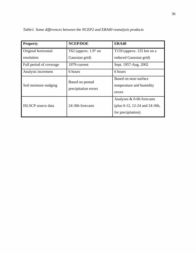
Table1. Some differences between the NCEP2 and ERA40 reanalysis products

Property NCEP/DOE ERA40

Original horizontal T62 (approx. 1.9° on T159 (approx. 125 km on a

resolution Gaussian grid) reduced Gaussian grid)

Full period of coverage 1979-current Sept. 1957-Aug. 2002

Analysis increment 6 hours 6 hours

Soil moisture nudging Based on pentad

precipitation errors

Based on near-surface

temperature and humidity

errors

ISLSCP source data 24-36h forecasts

Analyses & 0-6h forecasts

(plus 0-12, 12-24 and 24-36h,

for precipitation)

37

List of Figures.

Figure 1(a), (b) and (c) 2-m temperature distribution from ERA40, NCEP2 and the CRU data

(over land) for the 10-year (1986-1995) DJF climatologies and (d), (e) and (f) difference fields for

ERA40-CRU, NCEP2-CRU, and NCEP2-ERA40.

Figure 2 As Figure 1 for JJA climatologies and difference fields.

Figure 3. 2-m temperature anomaly fields from ERA40, NCEP2 and the CRU data (over land) for

(a), (b) and (c) DJF 1991-1992 and (d), (e) and (f) for JJA 1988.

Figure 4. As Figure 1 for 2-m RH

Figure 5. As Figure 2 for 2-m RH

Figure 6. As Figure 3 for 2-m RH

Figure 7. As Figure 1 for 24-36h forecast precipitation and GPCP precipitation.

Figure 8. As Figure 7 for JJA climatology.

Figure 9. As Figure 3 for precipitation anomalies.

Figure 10. As Figure 1 for surface SWdown from reanalyses and SRB data.

Figure 11. As Figure 2 for surface SWdown from reanalyses and SRB data.

Figure 12. As Figure 3 for surface SWdown anomalies

Figure 13. As Figure 10 for surface LWdown.

Figure 14. As Figure 11 for surface LWdown.

Figure 15. As Figure 12 for surface LWdown anomalies.

Figure 16. As Figure 11 for surface Rnet.

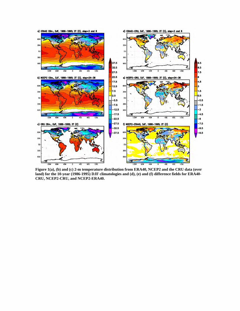
Figure 1(a), (b) and (c) 2-m temperature distribution from ERA40, NCEP2 and the CRU data (over land) for the 10-year (1986-1995) DJF climatologies and (d), (e) and (f) difference fields for ERA40-CRU, NCEP2-CRU, and NCEP2-ERA40.

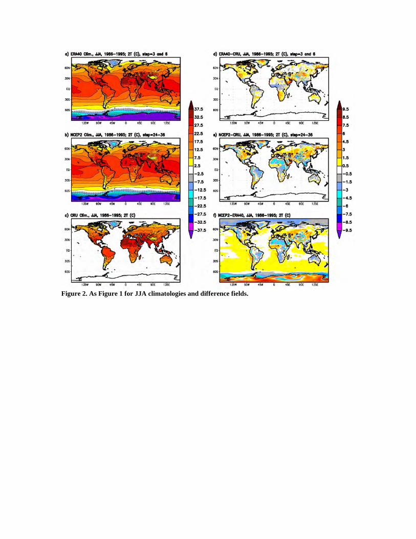
Figure 2. As Figure 1 for JJA climatologies and difference fields.

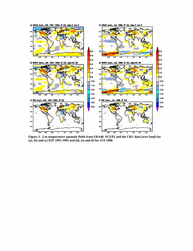
Figure 3. 2-m temperature anomaly fields from ERA40, NCEP2 and the CRU data (over land) for (a), (b) and (c) DJF 1991-1992 and (d), (e) and (f) for JJA 1988.

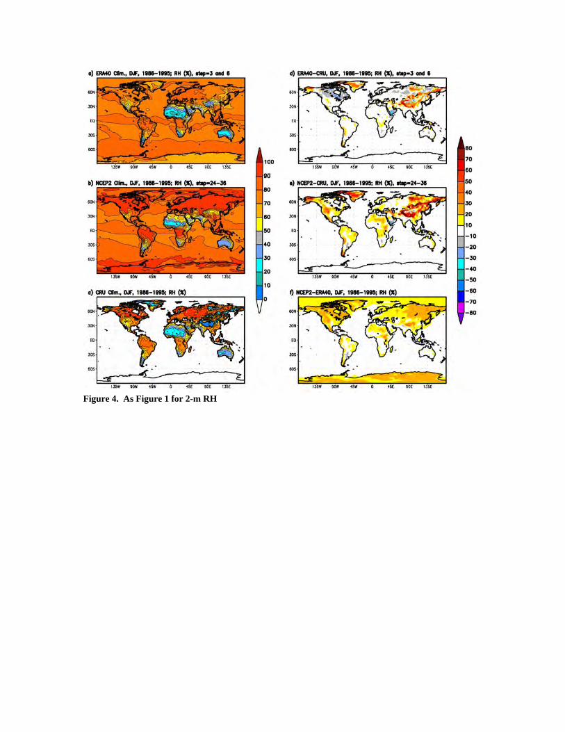
Figure 4. As Figure 1 for 2-m RH

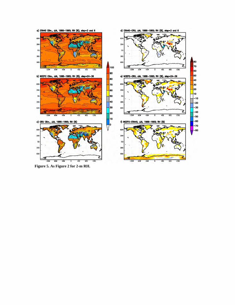
Figure 5. As Figure 2 for 2-m RH.

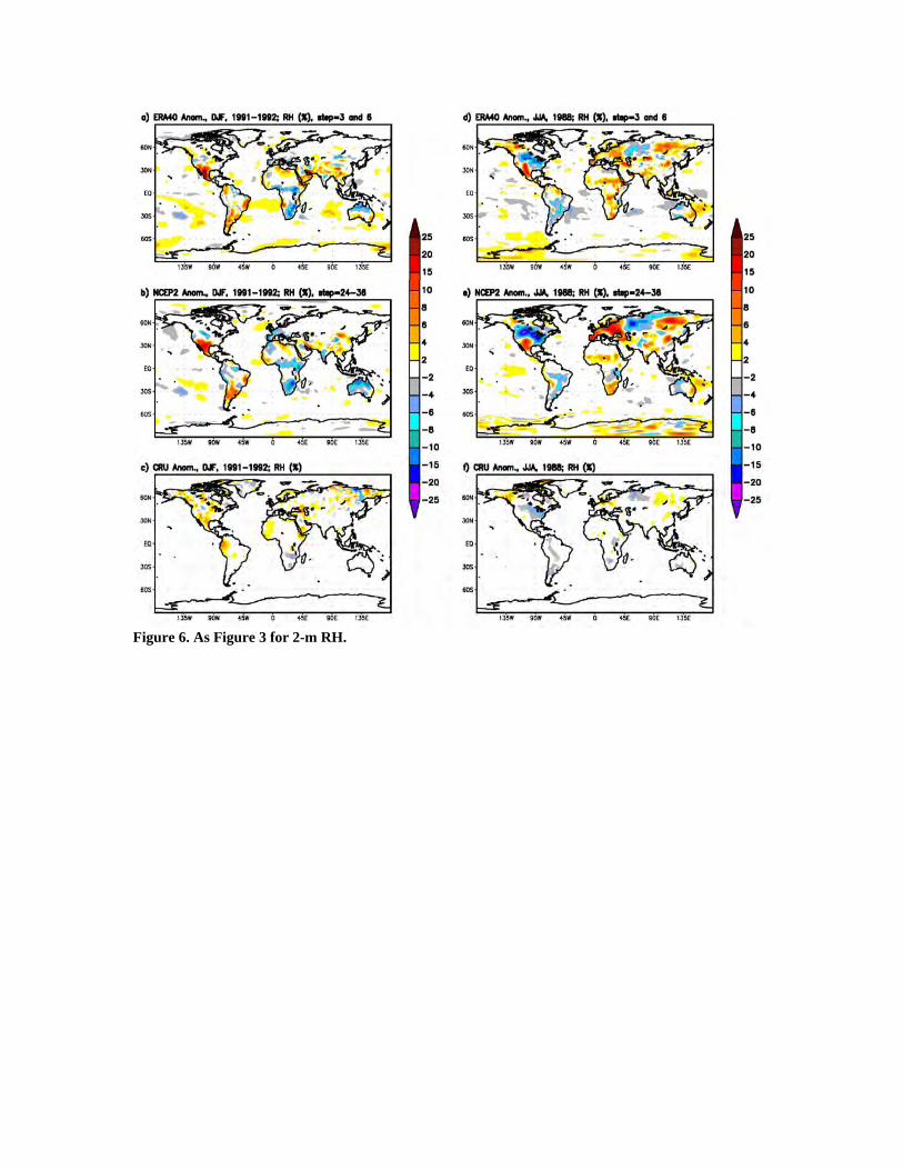
Figure 6. As Figure 3 for 2-m RH.

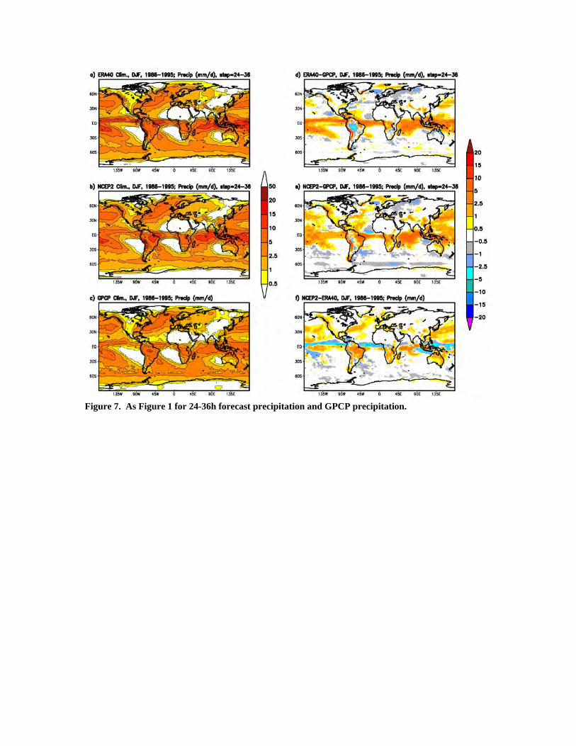
Figure 7. As Figure 1 for 24-36h forecast precipitation and GPCP precipitation.

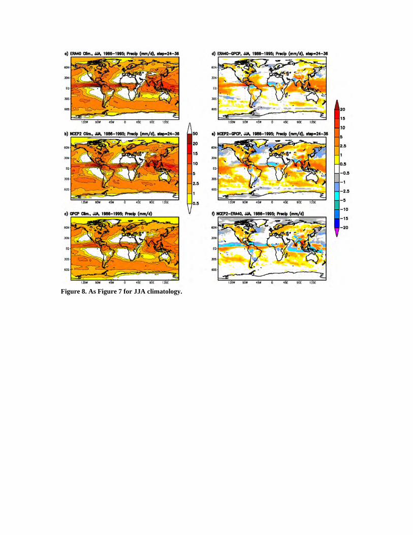
Figure 8. As Figure 7 for JJA climatology.

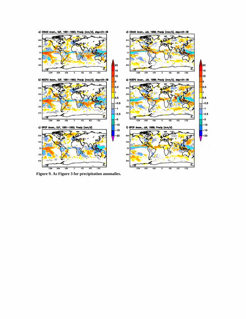
Figure 9. As Figure 3 for precipitation anomalies.

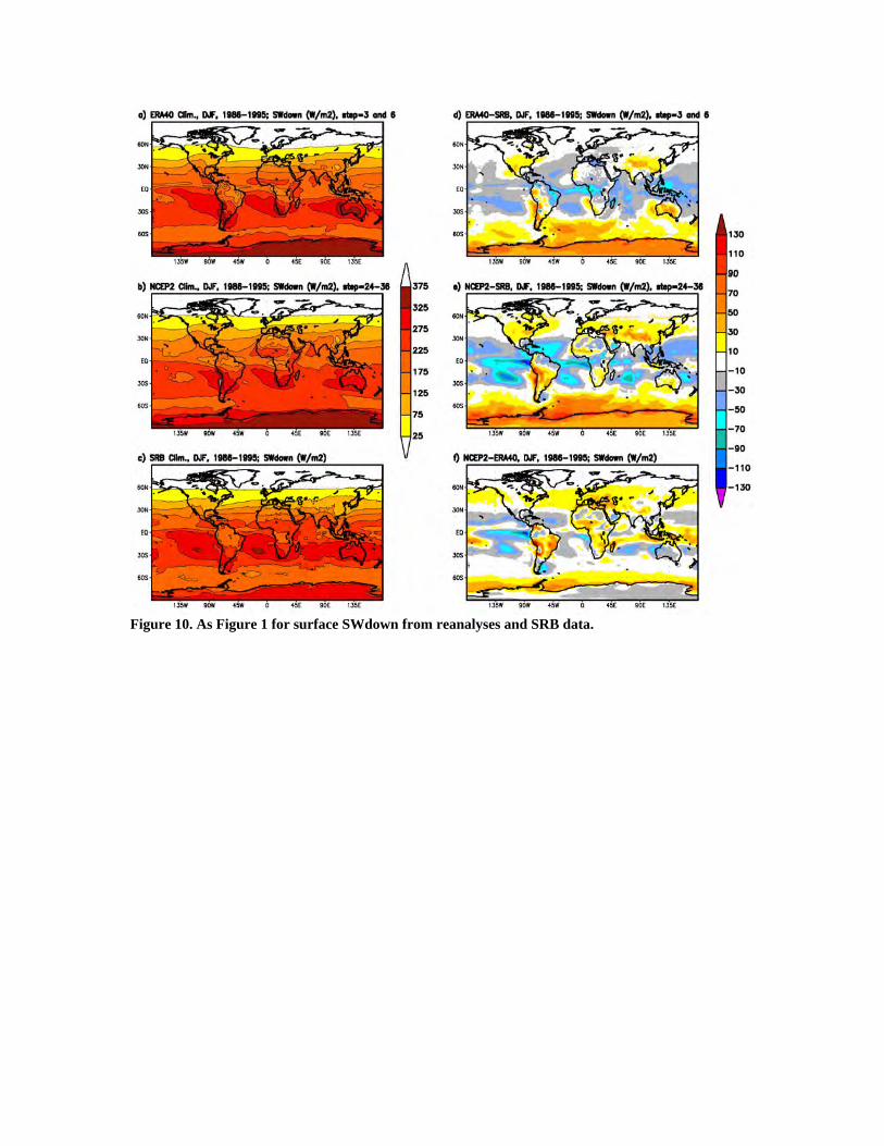
Figure 10. As Figure 1 for surface SWdown from reanalyses and SRB data.

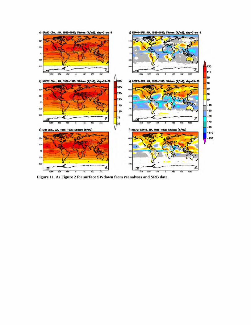
Figure 11. As Figure 2 for surface SWdown from reanalyses and SRB data.

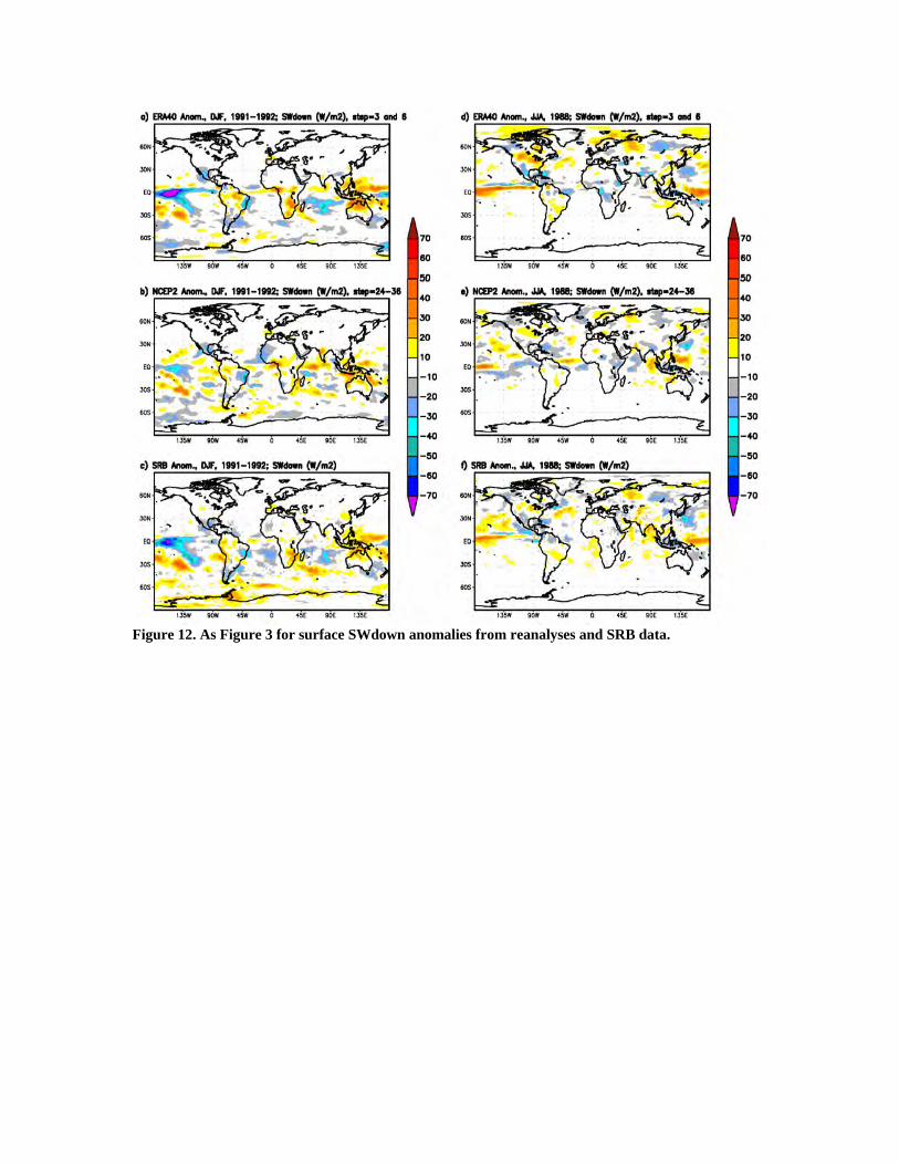
Figure 12. As Figure 3 for surface SWdown anomalies from reanalyses and SRB data.

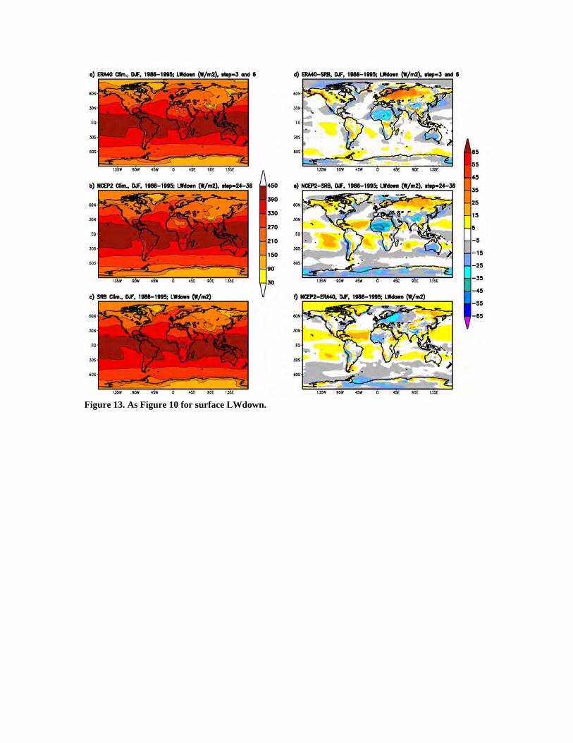
Figure 13. As Figure 10 for surface LWdown.

Figure 14. As Figure 11for surface LWdown.

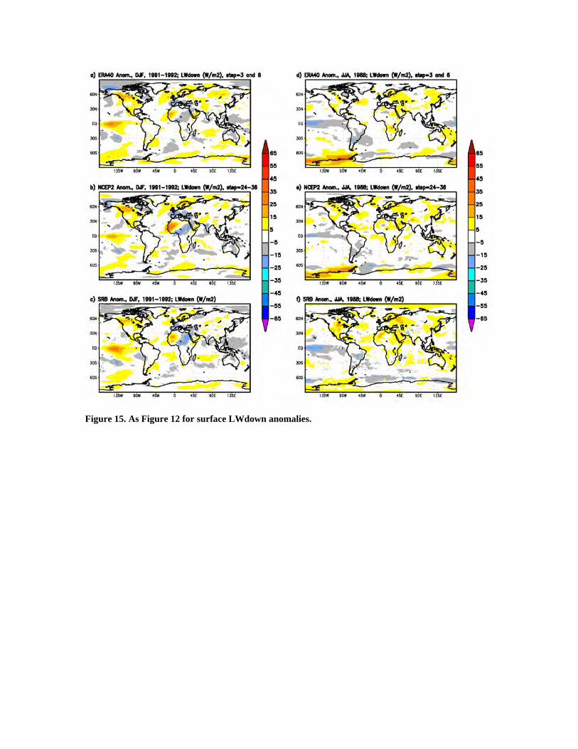
Figure 15. As Figure 12 for surface LWdown anomalies.

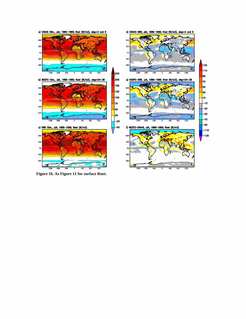
Figure 16. As Figure 11 for surface Rnet.

Six additional Figures are included in this file 2006JD007174supplement.pdf . These go with the discussion in section 3. Figure S1(a), (b) and (c). Sensible Heat (SH) from ERA40, NCEP2 and the DaSilva

climatology over oceans for the 10-year (1986-1995) DJF climatologies and (d), (e) and (f)

difference fields for ERA40-DaSilva, NCEP2-DaSilva, and NCEP2-ERA40.

Figure S2. As Figure S1 for JJA climatologies and difference fields.

Figure S3. SH anomaly fields from ERA40, NCEP2 and DaSilva over oceans for (a), (b)

and (c) DJF 1991-1992 and (d), (e) and (f) for JJA 1988.

Figure S4. As Figure S1 for LH

Figure S5. As Figure S2 for LH

Figure S6. As Figure S3 for LH anomalies.

Figure S1(a), (b) and (c). Sensible Heat (SH) from ERA40, NCEP2 and the DaSilva

climatology over oceans for the 10-year (1986-1995) DJF climatologies and (d), (e) and (f)

difference fields for ERA40-DaSilva, NCEP2-DaSilva, and NCEP2-ERA40.

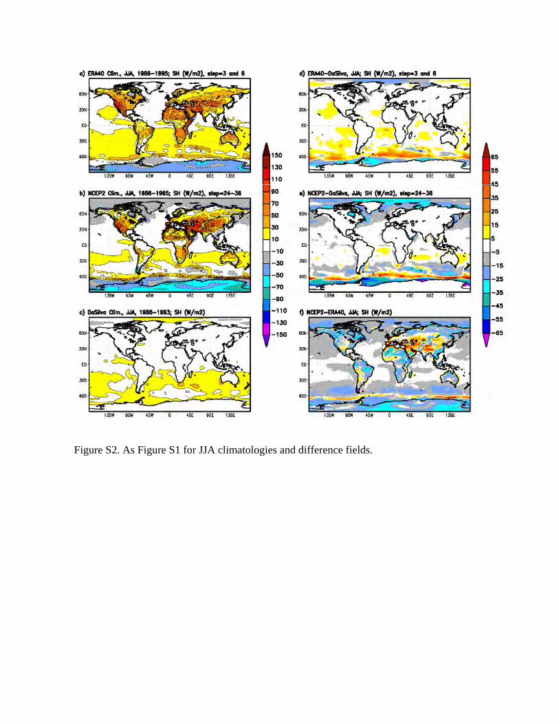
Figure S2. As Figure S1 for JJA climatologies and difference fields.

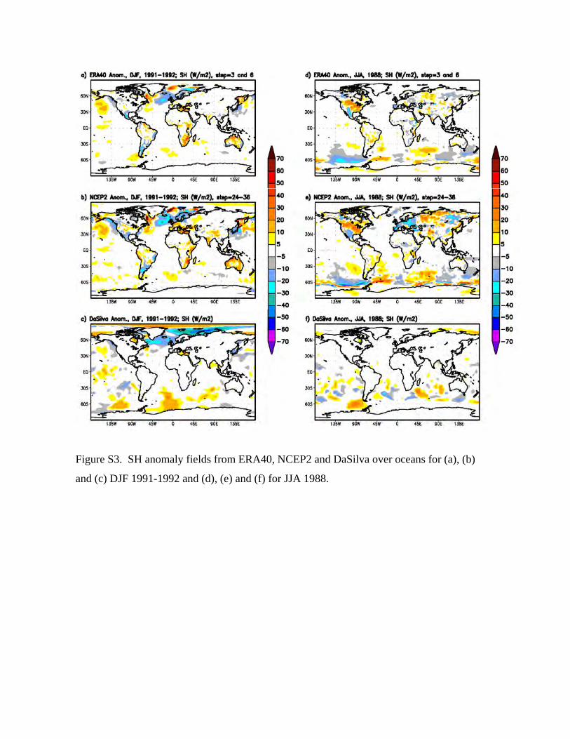
Figure S3. SH anomaly fields from ERA40, NCEP2 and DaSilva over oceans for (a), (b)

and (c) DJF 1991-1992 and (d), (e) and (f) for JJA 1988.

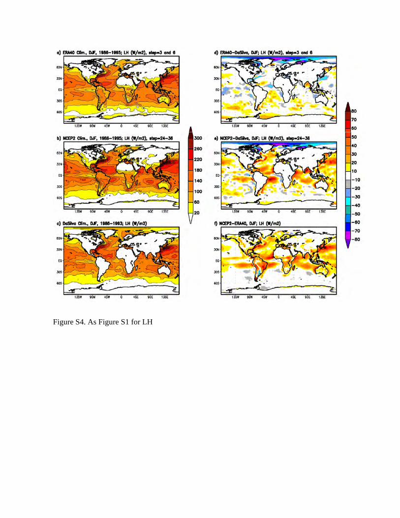
Figure S4. As Figure S1 for LH

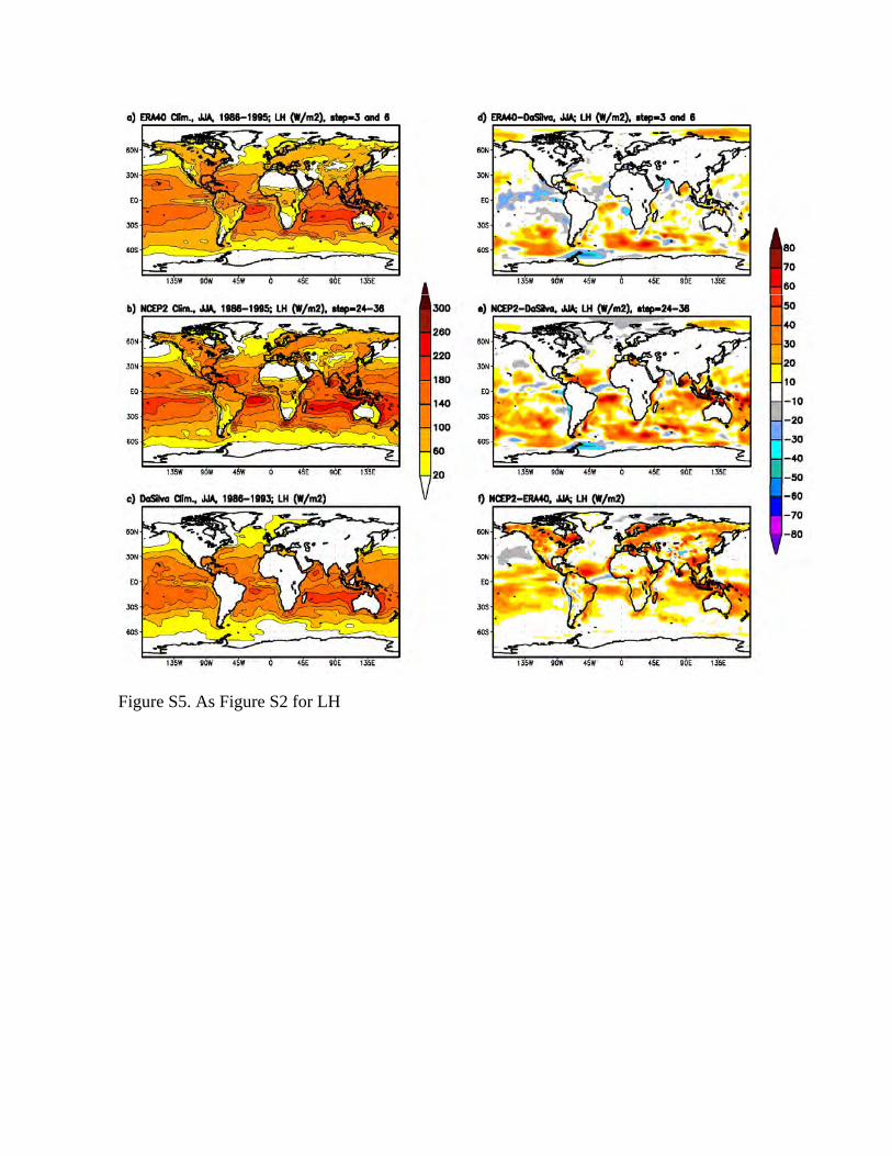
Figure S5. As Figure S2 for LH

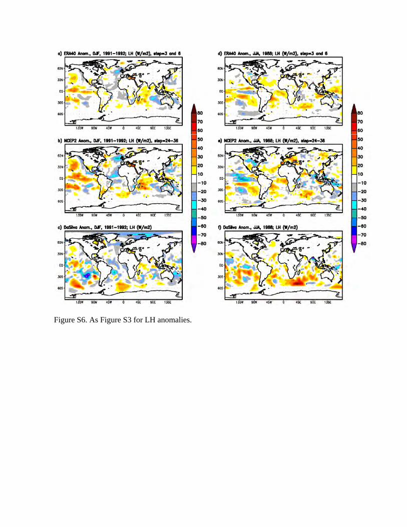
Figure S6. As Figure S3 for LH anomalies.