J. Fluid Mech. (2008), vol. 608, pp. 161–196. c© 2008 Cambridge University Press

doi:10.1017/S0022112008002073 Printed in the United Kingdom

161

Feedback shear layer control for bluff bodydrag reduction

MARK PASTOOR1†, LARS HENNING1,BERND R. NOACK2, RUDIBERT KING1

AND GILEAD TADMOR3

1Berlin Institute of Technology ER2–1, Department of Process Engineering, Chair of Measurement andControl, Hardenbergstraße 36a, D-10623 Berlin, Germany

2Berlin Institute of Technology MB1, Department of Fluid Dynamics and Technical Acoustics, Straßedes 17. Juni 135, D-10623 Berlin, Germany

3Northeastern University, Department of Electrical and Computer Engineering, 440 Dana ResearchBuilding, Boston, MA 02115, USA

(Received 3 May 2007 and in revised form 27 March 2008)

Drag reduction strategies for the turbulent flow around a D-shaped body are examinedexperimentally and theoretically. A reduced-order vortex model describes the inter-action between the shear layer and wake dynamics and guides a path to an efficientfeedback control design. The derived feedback controller desynchronizes shear-layerand wake dynamics, thus postponing vortex formation. This actuation is tested in awind tunnel. The Reynolds number based on the height of the body ranges from 23 000to 70 000. We achieve a 40% increase in base pressure associated with a 15% dragreduction employing zero-net-mass-flux actuation. Our controller outperforms otherapproaches based on open-loop forcing and extremum-seeking feedback strategies interms of drag reduction, adaptivity, and the required actuation energy.

1. IntroductionWe experimentally study the effect of open- and closed-loop flow control on the

coherent structures in the wake of an elongated D-shaped body. A key enabler forrobustness and efficient control design is an understanding of the mechanism of activeflow control by analysis of a reduced-order vortex model. This knowledge is utilizedto design an efficient control strategy for the reduction of pressure-induced drag. Ourfocus is on feedback control for wake stabilization leading to drag reduction.

The flow around ground and airborne transport vehicles is determined byaerodynamic design, manifesting a trade-off between fluid-dynamical and practicalrequirements, such as usability, safety, reliability and cost (Hucho 2002). The disciplineof aerodynamic design has become mature, owing particularly to potential theory.Small control devices can subsequently be added to improve performance and widenthe dynamical envelope by the manipulation of boundary and shear-layer physics(Leder 1992). Control devices range from passive, active open-loop to active closed-loop actuation. This paper is focused on the latter. These flow control approacheshave been explored in the community for decades.

† Author to whom correspondence should be addressed: Mark.Pastoor@TU-Berlin.de

162 M. Pastoor, L. Henning, B. R. Noack, R. King and G. Tadmor

Various passive means for bluff body flow control are well-investigated and havebeen applied in numerous experiments. For example, Bearman (1965) described thestabilizing effect of a splitter plate on the wake flow. Tanner (1972) examined thedrag reduction for various kinds of a spanwise modulation of the trailing edge, suchas segmented, curved, and M-shaped trailing edges. A significant drag reduction ona blunt-based model was achieved by modifying vortex shedding using wavy trailingedges or vortex disruptors (Tombazis & Bearman 1997; Park et al. 2006).

Passive devices, such as vortex generators, may have an adverse effect, away fromthe specific operating conditions for which they were designed. Active flow control canreproduce effects of passive devices. In addition, it can widen the operating envelopewith beneficial impact by adapting to changing flow conditions. Literature surveys onopen-loop flow control are provided by Fiedler & Fernholz (1990) or Gad-el-Hak,Pollard, & Bonnet (1998). For instance, a beneficial effect of active base bleed for dragreduction was observed by Bearman (1967) and Grosche & Meier (2001). An activecontrol application with spanwise distributed forcing at the trailing edges of a two-dimensional bluff body was described by Kim et al. (2004). Here, a significant dragreduction and a suppression of vortex shedding in the wake was achieved by open-loopforcing, both in experiment and LES. Another approach is active surface actuation.This strategy was applied to airfoils (Wu, Xie & Wu 2003) in order to increase theaerodynamic performance and for drag reduction of a circular cylinder (Wu, Wang& Wu 2007). The first active open-loop flow control demonstration for a full-scaleaeroplane was achieved by Wygnanski (2004) with an XV-15 tilt-rotor aircraft.

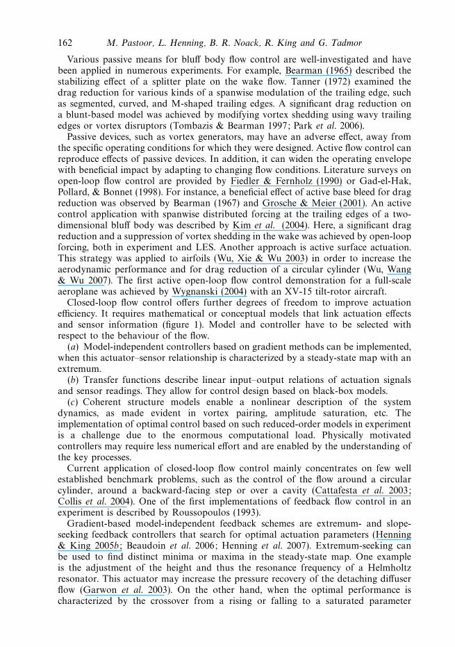
Closed-loop flow control offers further degrees of freedom to improve actuationefficiency. It requires mathematical or conceptual models that link actuation effectsand sensor information (figure 1). Model and controller have to be selected withrespect to the behaviour of the flow.

(a) Model-independent controllers based on gradient methods can be implemented,when this actuator–sensor relationship is characterized by a steady-state map with anextremum.

(b) Transfer functions describe linear input–output relations of actuation signalsand sensor readings. They allow for control design based on black-box models.

(c) Coherent structure models enable a nonlinear description of the systemdynamics, as made evident in vortex pairing, amplitude saturation, etc. Theimplementation of optimal control based on such reduced-order models in experimentis a challenge due to the enormous computational load. Physically motivatedcontrollers may require less numerical effort and are enabled by the understanding ofthe key processes.

Current application of closed-loop flow control mainly concentrates on few wellestablished benchmark problems, such as the control of the flow around a circularcylinder, around a backward-facing step or over a cavity (Cattafesta et al. 2003;Collis et al. 2004). One of the first implementations of feedback flow control in anexperiment is described by Roussopoulos (1993).

Gradient-based model-independent feedback schemes are extremum- and slope-seeking feedback controllers that search for optimal actuation parameters (Henning& King 2005b; Beaudoin et al. 2006; Henning et al. 2007). Extremum-seeking canbe used to find distinct minima or maxima in the steady-state map. One exampleis the adjustment of the height and thus the resonance frequency of a Helmholtzresonator. This actuator may increase the pressure recovery of the detaching diffuserflow (Garwon et al. 2003). On the other hand, when the optimal performance ischaracterized by the crossover from a rising or falling to a saturated parameter

Feedback shear layer control 163

Actuation

Control goal

Sensors

Coherent structures Control law

Modelling Application

Control designSteady-statebehaviour

Gradient-based controller(e.g extremum-and slope-seeking)

Black box based controller(e.g �∞ and QFT)

Physically motivated controller(e.g. phase and opposition control)

Model-independent

Transferfunction

Coherentstructure model

Linearbehaviour

Nonlinearbehaviour

Figure 1. The coherent structure dynamics determines the choice of the controller. Thestructures communicate actuation effects to the sensors, e.g. pressure readings. The control lawcomputes actuation signals from the current state resolved by sensor readings. The actuatorsmanipulate excitable coherent structure dynamics in order to enforce the control goal, here thereduction of drag. A range of feedback flow control schemes allows us to select the best-suitedcontrol law, depending on the behaviour of the flow, as elaborated in the text.

regime, slope-seeking feedback is preferred. A case in point is the saturated effectof an actuation amplitude on the separation region and flow reattachment overan aircraft wing (Becker et al. 2007). Once the flow is completely attached, furtherincreases in amplitude will not lead to significant changes in the lift.

Control design based on experimentally identified black-box models was conductedby Becker et al. (2005), King et al. (2004) and Henning & King (2005a). Here,the turbulent reattachment process behind a backward-facing step was controlledat Reynolds numbers up to 25 000 based on the step height. Robust closed-loopcontrol based on these models was able to prescribe the reattachment length and tocompensate disturbances. Adaptive schemes were developed by Garwon et al. (2003)to adjust the actuation amplitude. Henning et al. (2007) proposed a black-box modelto control the pressure drag of a D-shaped body at Reynolds numbers based on bodyheight up to 70 000. Rowley et al. (2002) suppressed Rossiter modes of a cavity flowby black-box model-based control.

Black-box models, however, do not resolve coherent structures of the flow: theymerely link input and output signals. Reduced-order vortex and POD models explicitlydescribe the coherent structures as communicators between input and output. PODmodels were employed for flow control of different configurations, e.g. the cylinderwake (Bergmann, Cordier, & Brancher 2005; Gerhard et al. 2003; King et al. 2005;Noack et al. 2003; Noack, Tadmor & Morzynski, 2004; Noack, Papas & Monkewitz,2005; Tadmor et al. 2004; Siegel, Cohen, & McLaughlin 2003; Siegel et al. 2007, 2008)or the cavity flow (Little et al. 2007). Introductions to POD models are provided byLumley & Blossey (1998)or Cordier & Bergmann (2003).

POD models are convenient for standard control design, due to their mathematicalstructure. In contrast, vortex models inhibit most control design methods by their

164 M. Pastoor, L. Henning, B. R. Noack, R. King and G. Tadmor

hybrid nature (changing phase space of vortex positions). However, vortex modelsexhibit a larger dynamical bandwidth, which is crucial for the current flow controltask. The theoretical foundation of vortex models dates back to Helmholtz (1858) andThomson (1869). In the early twentieth century the N-vortex problem was discussed.Von Karman (1911) used vortex models for a stability analysis of the vortex streetconfiguration. A numerical simulation of a mixing layer using point vortices wasconducted by Rosenhead (1931), encouraging investigations of many configurationsuntil the 1960s. Birkhoff (1962) found an inherent ill-posed convergence behaviourin vortex models. This finding gave rise to doubts about the predictive power of thismodelling approach. Nonetheless, vortex models were pursued by several authors, suchas Clements (1973), who described vortex shedding in the wake of a bluff body. Later,convergence of vortex models with finite-core radii to solutions of the Navier–Stokesequation could be shown (Beale & Majda 1982; Krasny 1986). In the 1980s and 1990shigh-dimensional vortex models were investigated by several researchers (Ghoniem& Gagnon 1987; Cottet & Koumoutsakos 2000; Soteriou 2003) as an alternativeapproach to DNS, and extended for three-dimensional flows (Leonard 1985; Meiburg1995). In recent years reduced-order models were proposed as coherent structuremodels (Cortelezzi 1996; Coller et al. 2000) and plants for control design (Tang &Aubry 2000; Protas 2004, 2006). In this study, reduced-order vortex models are usedto explain the physical effects of actuation and to improve control. Efficient means tosynchronize two-dimensional coherent flow structures for achieving the control goal,a significant drag reduction, are proposed.

This paper is organized as follow. In § 2, we describe the experimental setup andthe vortex model. Our study and analysis of the natural and open-loop forced flowis detailed in § 3. The observed processes are explained in § 4. Experiments withfeedback controllers are outlined in § 5. Finally, we summarize the main findings andtheir implications for other configurations in § 6. The vortex model and the extendedKalman filter used in § 5 are detailed in Appendices A and B, respectively.

2. Experimental testbed and vortex modelThis section provides a description of the experimental setup and outlines the vortex

model.

2.1. Wind tunnel

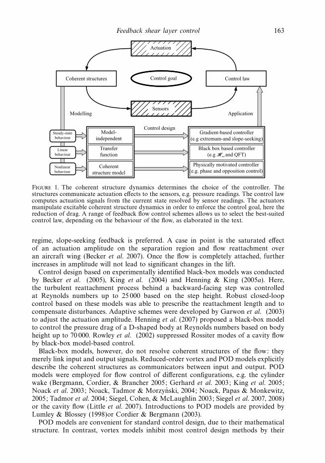
Experiments are conducted in an Eiffel-type wind tunnel. The maximum free-stream velocity is approximately 20 m s−1 with a turbulence level of less than 0.5%.The dimensions of the closed test section are Lts = 2500 mm, Hts = 555 mm andWts = 550 mm in the streamwise, transverse and spanwise directions, respectively. Theflow is described in a Cartesian coordinate system x, y, z; the origin is located at thevertical and horizontal centre of the body’s stern (see figure 2).

The D-shaped body has the following dimensions: chord length L = 262 mm, bodyheight H = 72 mm and spanwise width W = 550 mm. The geometric blockage of themodel in the wind tunnel is approximately 13%. Therefore, the free-stream velocity U∞is adjusted to U∞,c = U∞

√Bc, according to the blockage correction method proposed

by Mercker (1980). Trip tapes are placed 30 mm downstream of the nose in orderto trigger boundary layer transition. The model is mounted on two aluminium rodsand is vertically centred in the wind tunnel. The rods have a diameter of 15 mmand are attached to the model’s lower surface at (x, y) = (−131 mm, −175 mm) and(x, y) = (−131 mm, 175 mm), respectively. Reynolds and Strouhal numbers are given

Feedback shear layer control 165

Wts

U∞

Hts

Referencepressure

Trip tapes

Pressure gauges

PIV

Actuatorslots

W

H

L

Lts

Figure 2. Sketch of the experimental setup with the D-shaped body. For details, see text.

with respect to body height and corrected free-stream velocity:

ReH =U∞,c H

νand St =

f H

U∞,c

.

Here, ν represents the kinematic viscosity of the fluid and f is the frequency to beexpressed as a Strouhal number. All experiments are conducted at Reynolds numbersin the range from 23 000 to 70 000.

A sinusoidal zero-net-mass-flux actuation is effected by loudspeakers (VisatonW200S, 4 Ω) through spanwise slots (slot width S =1 mm, spanwise length250 mm) located at the upper and lower trailing edges. Harmonic actuationg(t) = A sin(2π fA t), with the actuation amplitude A and frequency fA, is appliedto each slot, thus generating periodical sucking and blowing. The cost of actuation ischaracterized by the non-dimensional excitation momentum coefficient

cμ = 2S

H

q2A

U 2∞,c

,

where qA is the r.m.s. value of the velocity generated by the actuator. The factor 2accounts for the number of actuators. The actuation signal g is equal to the velocityat the centre of the actuation slot. The frequency response of the actuator iscompensated.

The base pressure is monitored by 3 × 3 difference pressure gauges (PascaLinePCLA02X5D1 ) mounted in three parallel rows on the stern at y = {−32, 0, 32} mmand z = {−82.5, 0, 82.5} mm. Pressure gauges are calibrated and temperaturecompensated. Their operating pressure range is ±2.5 mbar with an accuracy of±0.25%. The free-stream dynamic pressure is monitored by a Prandtl probe. Theprobe was mounted at (x, y, z)= (−1181 mm, 127.5 mm, −175 mm) and is connectedto a differential pressure transducer (MKS Baratron 220D) with a measurementaccuracy of 0.15%. Four strain gauges (HBM 6/350LY13, metering precision ±0.35%)are applied to the aluminium rods for drag force measurements. The strain gaugesare glued on a milled out section of the aluminium rods 5 mm underneath the bluffbody. Thereby, the drag on the aluminum rods does not contribute to the measuredbody force. A power amplifier HBM ML55b is used for calibration and voltage

166 M. Pastoor, L. Henning, B. R. Noack, R. King and G. Tadmor

amplification. Base pressure and drag are described by non-dimensional coefficients

cP (y, z, t) =�p(y, z, t)

ρ U 2∞,c/2

, and cD(t) =Fx(t)

ρ U 2∞,c H W/2

,

respectively. Here, �p is the instantaneous pressure difference between a stern-mounted pressure gauge and the reference pressure, ρ denotes the density, and Fx

is the drag force. Time-averaged base pressure and drag are denoted by cP (y, z)and cD , respectively. The surface-averaged base pressure over the stern is markedby 〈cP (t)〉. Boundary layer conditions and velocity fluctuations in the wake floware acquired by hot-wire measurements, using 5 μm-hot-wires and the constanttemperature anemometer A.A. Lab Systems Ltd. AN-1003.

PIV measurements are conducted in the vertical symmetry plane (x ∈ [0, 144] mm,y ∈ [−58, 58] mm and z = 0 mm) at ReH =23 000 with a spatial resolution ofdx = dy = 2.3 mm. Temporal resolution is limited to 4 Hz. The PIV system consistsof a frequency-doubled Nd:YAG laser, a CCD-Cross-Correlation-Camera (PCOSensiCam Double Shutter) and a synchronization unit. The VidPiv software ofILA corp. is used for the computation of velocity fields. Data acquisition andthe implementation of the controllers is realized by rapid prototyping hardware(dSPACE -PPC1005 controller). The sampling time is �t = 1/1000 s.

2.2. Vortex model

Hereafter, all quantities are non-dimensionalized by H , U∞,c and ρ. Experimentaland numerical investigations show that the initial separation and roll-up of the shearlayers in the bluff body wake is dominated by two-dimensional coherent structures(see § 3.3). On a kinematic level, two-dimensional vortex models approximate thevorticity distribution ω of the flow by adding vortices to an irrotational flow withthe potential Φ (e.g. Milne-Thomson 1968; Lugt 1996). The induced velocity from N

vortices at a sample point x is calculated by

u(x, t) = ∇Φ(x, t) +

N∑i=1

Γi uω(x, xi), (2.1)

where Γi is the circulation and xi the position of the ith vortex. The circulation isconstant by Helmholtz’s law. The kernel uω is derived from potential theory usingBiot–Savart’s law for the induced velocity. The vortices move with the flow:

dxi

dt= u(xi , t), i = 1, . . . , N. (2.2)

In this paper, a reduced-order vortex model for the flow around the D-shapedbody in a wind tunnel is proposed. Approximately 650 vortices are required to resolvethe dynamics of the coherent structures. Similar models have been investigated forthe flow around a D-shaped body (Clements 1973), the flow over an edge (Evans &Bloor 1977), the wake flow past a plate (Cortelezzi 1996), the diffuser flow (Colleret al. 2000), and the flow around a backward-facing step (Pastoor et al. 2003). Theno-penetration boundary condition at the walls for the potential flow is enforced byusing a conformal mapping from the upper half-plane onto the D-shaped body (see§ A.1). Boundary conditions are enforced in the computational domain. The potentialflow is represented by a pair of sources in the computational domain (see § A.2). Theeffect of zero-net-mass-flux actuation is modelled by two oscillating sources at thetrailing edges of the body (see § A.3). Vortices and their mirror images transform intoa vortex solution in the physical domain that respects the no-penetration condition

Feedback shear layer control 167

at the walls (see § A.4). Vortex production at the trailing edges follows a generalizedKutta condition a fair approximation of the production rate, while smoothing thestochastic vorticity production in the boundary layers. In order to maintain the low-dimensionality of the model, vortices are gradually merged (see § A.6), where a highresolution is not required (x > 2) or faded out, when they leave the region of interest(x > 30). The numerical integration of (2.2) is computed by a third-order, explicitAdams–Bashforth scheme.

3. Investigation of the natural and periodically forced flowKey features of the natural and the periodically forced (open-loop) flow around

the D-shaped body are described in § 3.1 and § 3.2, respectively.

3.1. Natural flow

The flow around the D-shaped body is governed by an absolute wake instability(Huerre & Monkewitz 1990). This mechanism generates a von Karman vortexstreet with an alternating sequence of vortices at characteristic frequencies. Thetwo-dimensional vortex shedding in a wake of a bluff body is only weakly perturbedby three-dimensional fluctuation (Zhang et al. 1995).

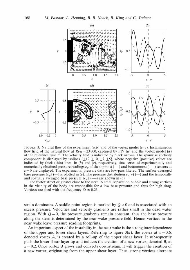
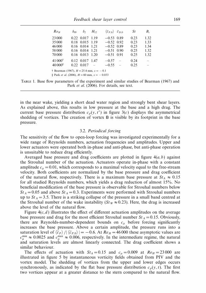
An instantaneous vorticity field of the natural flow at ReH = 23 000 captured by PIVindicating bent shear layers at the upper and lower edges is shown in figure 3(a). Twolarge vortical structures appear almost at the centreline, whereas the lower vortex iscloser to the stern. Pressure readings indicate a pressure minimum at the bottommostpressure gauges. The time-averaged and spatially averaged base pressure coefficientis 〈cP,0〉 = −0.53. This corresponds to an average drag coefficient of cD,0 = 0.98.Dominant Strouhal numbers of bluff body wakes are usually within a range of 0.2for circular cylinders and 0.26 for short D-shaped bodies (Leder 1992).

In agreement with these common observations, the frequency spectra of hot-wire measurements at (x, y, z)= (1, 0.7, 0) indicate a maximum fluctuation level atSt ≈ 0.23 in the current study. Upper and lower boundary layer conditions, as theboundary layer thickness δ99, the momentum deficit thickness δ2 and the form factorH12, are acquired by hot-wire measurements in the vicinity of the trailing edges(x, y, z) = (−0.01, ±0.5, 0) and averaged. The results are in good agreement withmeasurements given by Bearman (1967) and Park et al. (2006). The large boundarylayer thickness observed at ReH = 23 000 results from a small separation bubble in thefront section of the body. This phenomenon was reported by Cooper (1985) for bluffbodies with rounded front edges. The results for the investigated range of Reynoldsnumbers and the two reference cases are summarized in table 1.

Figure 3(d ) displays the vorticity field obtained from a snapshot of the vortexmodel. The corresponding pressure field can be calculated by solving the Poissonequation:

�p = − ∇u · · ∇uT = W · · W − S · · S = Q , (3.1)

where ∇u is the Jacobian of the velocity, the superscript T denotes the transposeof the tensor and ·· is the double contraction. The Jacobian ∇u is decomposed ina symmetrical tensor S and a antimetrical tensor W . Here, S represents the strainand W the rotation of a fluid element. In (3.1), the source term Q can be expressedas the local difference of the double contraction of the rotation and strain tensors,respectively. Inside a vortex, rotation dominates (Q > 0), which indicates a lowerpressure in the core, according to (3.1). In a plain shear layer, rotation and strainare balanced (Q =0). On the convex side of a bent shear layer and between vortices,

168 M. Pastoor, L. Henning, B. R. Noack, R. King and G. Tadmor

0 0.5 1.0 1.5 2.0

–0.5

0

0.5

x

y

(a)

–5 0 5

–1.0

–0.5

0

t – t∗

–5 0 5

t – t∗

cp

(b)

–1.0 –0.5 0

–0.5

0

0.5

cp|t∗

y

(c)

0 0.5 1.0 1.5 2.0

–0.5

0

0.5

x

y

(d)

A

B

–1.0

–0.5

0

c p,�

c p�

(e)

Figure 3. Natural flow of the experiment (a, b) and of the vortex model (c–e). Instantaneousflow field of the natural flow at ReH = 23 000, captured by PIV (a) and the vortex model (d )at the reference time t∗. The velocity field is indicated by black arrows. The spanwise vorticitycomponent is displayed by isolines {±12, ±10, ±7, ±5}, where negative (positive) values areindicated by thick (thin) lines. In (b) and (e), respectively, time series of experimentally andnumerically obtained pressure readings cp of the topmost (—–) and bottommost (−−) sensors atz = 0 are displayed. The experimental pressure data are low-pass filtered. The surface-averagedbase pressure 〈cp〉 (—) is plotted in (e). The pressure distribution cp(y) (—) and the temporallyand spatially averaged base pressure 〈cp〉 (—–) are shown in (c).

The vortex street originates close to the stern. A small separation bubble and strong vorticesin the vicinity of the body are responsible for a low base pressure and thus for high drag.Vortices are shed with the frequency St ≈ 0.23.

strain dominates. A saddle point region is marked by Q< 0 and is associated with anexcess pressure. Velocities and velocity gradients are rather small in the dead waterregion. With Q = 0, the pressure gradients remain constant, thus the base pressurealong the stern is determined by the near-wake pressure field. Hence, vortices in thenear wake leave pressure reading footprints.

An important aspect of the instability in the near wake is the strong interdependenceof the upper and lower shear layers. Referring to figure 3(d ), the vortex at x = 0.6,denoted vortex A, is created by a roll-up of the upper shear layer. It subsequentlypulls the lower shear layer up and induces the creation of a new vortex, denoted B, atx = 0.2. Once vortex B grows and convects downstream, it will trigger the creation ofa new vortex, originating from the upper shear layer. Thus, strong vortices alternate

Feedback shear layer control 169

ReH δ99 δ2 H12 〈cP,0〉 cD,0 St Bc

23 000 0.22 0.017 1.19 −0.53 0.89 0.23 1.3235 000 0.18 0.015 1.19 −0.52 0.92 0.23 1.3346 000 0.16 0.014 1.21 −0.52 0.89 0.23 1.3458 000 0.16 0.014 1.21 −0.51 0.90 0.25 1.3270 000 0.16 0.013 1.20 −0.51 0.91 0.25 1.32

41 000† 0.12 0.017 1.47 −0.57 – 0.24 –40 000‡ 0.22 0.017 – −0.55 – 0.25 –

† Bearman (1967), H =25.4 mm, x = − 0.1

‡ Park et al. (2006), H =60 mm, x = − 0.033

Table 1. Base flow parameters of the experiment and similar studies of Bearman (1967) andPark et al. (2006). For details, see text.

in the near wake, yielding a short dead water region and strongly bent shear layers.As explained above, this results in low pressure at the base and a high drag. Thecurrent base pressure distribution cp(y, t∗) in figure 3(c) displays the asymmetricalshedding of vortices. The creation of vortex B is visible by its footprint in the basepressure.

3.2. Periodical forcing

The sensitivity of the flow to open-loop forcing was investigated experimentally for awide range of Reynolds numbers, actuation frequencies and amplitudes. Upper andlower actuators were operated both in-phase and anti-phase, but anti-phase operationis unsuitable to reduce drag efficiently.

Averaged base pressure and drag coefficients are plotted in figure 4(a, b) againstthe Strouhal number of the actuation. Actuators operate in-phase with a constantamplitude cμ = 0.01, which corresponds to a maximal velocity equal to the free-streamvelocity. Both coefficients are normalized by the base pressure and drag coefficientof the natural flow, respectively. There is a maximum base pressure at StA ≈ 0.15for all studied Reynolds numbers, which yields a drag reduction of almost 15%. Nobeneficial modification of the base pressure is observable for Strouhal numbers belowStA = 0.05 and above StA =0.3. Experiments were performed with Strouhal numbersup to StA = 3.5. There is a striking collapse of the pressure in a small band centred atthe Strouhal number of the wake instability (StW ≈ 0.23). Here, the drag is increasedabove the level of the natural flow.

Figure 4(c, d ) illustrates the effect of different actuation amplitudes on the averagebase pressure and drag for the most efficient Strouhal number StA =0.15. Obviously,there are Reynolds-number-dependent bounds on cμ before forcing significantlyincreases the base pressure. Above a certain amplitude, the pressure runs into asaturation level of 〈cP 〉 /| 〈cP,0〉 | = −0.6. At ReH = 46 000 these asymptotic values arecminμ ≈ 0.0025 and cmax

μ ≈ 0.006, respectively. In the intermediate regime, the naturaland saturation levels are almost linearly connected. The drag coefficient shows asimilar behaviour.

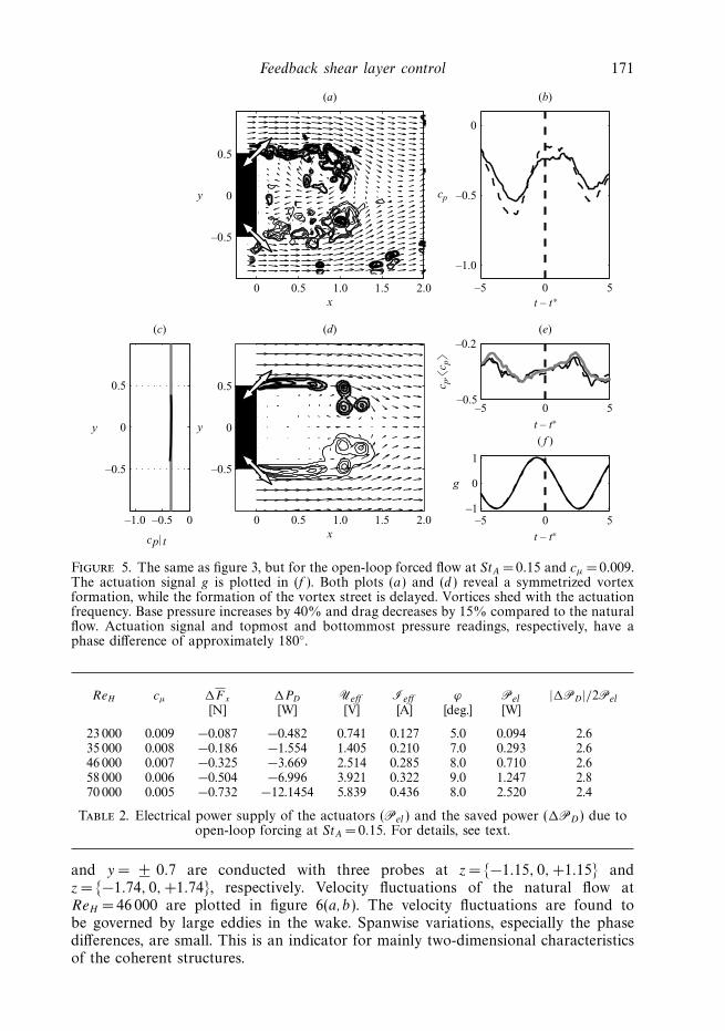
The effects of actuation with StA = 0.15 and cμ = 0.009 at ReH = 23 000 areillustrated in figure 5 by instantaneous vorticity fields obtained from PIV and thevortex model. The shedding of vortices from the upper and lower edges occurssynchronously, as indicated by the flat base pressure distribution cp(y, t). The firsttwo vortices appear at a greater distance to the stern compared to the natural flow.

170 M. Pastoor, L. Henning, B. R. Noack, R. King and G. Tadmor

0 0.1 0.2 0.3–1.2

–1.0

–0.8

–0.6

–0.4

StA

(a)

0 0.1 0.2 0.30.8

0.9

1.0

1.1

StA

(b)

ReH

(d)

0 0.005 0.010

ReH

cμ

0 0.005 0.010cμ

(c)

�c P

�/|�

c P,0�

|

c D/c

D,0

c D/c

D,0

0.8

0.9

1.0

1.1

–1.2

–1.0

–0.8

–0.6

–0.4

�c P

�/|�

c P,0�

|

Figure 4. Normalized and averaged base pressure (a,c) and drag coefficient (b, d ). Theseparameters are plotted as functions of the actuation frequency StA at cμ = 0.01 (a, b), and asfunctions of the momentum coefficients (c, d ) at StA = 0.15 and Reynolds numbers 23 000 (•),35 000 (◦), 46 000 (×), 58 000 (+), 70 000 (∗).

As a result, the formation of the alternating vortex street is delayed and the deadwater region is elongated. The mean base pressure increases by 40% while the dragdecreases by 15%.

The net power saving due to the actuation effect is determined in what follows. Thetowing power reduction �PD is computed by

�PD = U∞,c �F x. (3.2)

Here, �F x denotes the time-averaged reduction of the drag force. The electrical powerPel of each actuator is

Pel = Ueff Ieff cosϕ, (3.3)

where Ueff and Ieff are, respectively, the effective voltage and current applied to theactuator, and ϕ is the phase between both. A gain |�PD|/2 Pel > 1 implies a netsaving. The electrical power requirement for in-phase forcing with the most efficientfrequency StA = 0.15 and the achieved drag reduction are summarized in table 2 forthe investigated range of Reynolds numbers. We find a gain of 2.4 to 2.8 for periodicalforcing.

3.3. Two-dimensional flow characteristics

In this section the two-dimensionality of the flow under nominally two-dimensionalboundary conditions is investigated. Simultaneous hot-wire measurements at x = 1

Feedback shear layer control 171

0 0.5 1.0 1.5 2.0

–0.5

0

0.5

x

y

0 0.5 1.0 1.5 2.0

–0.5

0

0.5

x

y

(a)

–1.0

–0.5

0

cp

(b)

–1.0 –0.5 0

–0.5

0

0.5

cp| t

y

(c) (d)

–5 0 5–0.5

–0.2(e)

–1

0

1

g

( f )

–5 0 5t – t∗

t – t∗

–5 0 5

t – t∗

c p,�

c p�

Figure 5. The same as figure 3, but for the open-loop forced flow at StA = 0.15 and cμ = 0.009.The actuation signal g is plotted in (f ). Both plots (a) and (d ) reveal a symmetrized vortexformation, while the formation of the vortex street is delayed. Vortices shed with the actuationfrequency. Base pressure increases by 40% and drag decreases by 15% compared to the naturalflow. Actuation signal and topmost and bottommost pressure readings, respectively, have aphase difference of approximately 180◦.

ReH cμ �F x �PD Ueff Ieff ϕ Pel |�PD |/2Pel[N] [W] [V] [A] [deg.] [W]

23 000 0.009 −0.087 −0.482 0.741 0.127 5.0 0.094 2.635 000 0.008 −0.186 −1.554 1.405 0.210 7.0 0.293 2.646 000 0.007 −0.325 −3.669 2.514 0.285 8.0 0.710 2.658 000 0.006 −0.504 −6.996 3.921 0.322 9.0 1.247 2.870 000 0.005 −0.732 −12.1454 5.839 0.436 8.0 2.520 2.4

Table 2. Electrical power supply of the actuators (Pel ) and the saved power (�PD) due toopen-loop forcing at StA = 0.15. For details, see text.

and y = ± 0.7 are conducted with three probes at z = {−1.15, 0, +1.15} andz = {−1.74, 0, +1.74}, respectively. Velocity fluctuations of the natural flow atReH =46 000 are plotted in figure 6(a, b). The velocity fluctuations are found tobe governed by large eddies in the wake. Spanwise variations, especially the phasedifferences, are small. This is an indicator for mainly two-dimensional characteristicsof the coherent structures.

172 M. Pastoor, L. Henning, B. R. Noack, R. King and G. Tadmor

0 10 20 30

–0.4

–0.2

0

0.2

0.4

t

u′

(a)

0 10 20 30

–0.4

–0.2

0

0.2

0.4

t

(b)

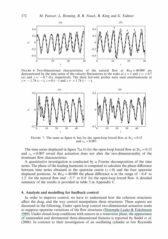
Figure 6. Two-dimensional characteristics of the natural flow at ReH = 46 000 aredemonstrated by the time series of the velocity fluctuations in the wake at x =1 and y = +0.7(a) and y = − 0.7 (b), respectively. The three hot-wire probes were used simultaneously atz = − 1.74 (−−), z = 0 (—) and z = + 1.74 (− · −).

0 10 20 30 40–0.2

0

0.2

t

u′

(a)

0 10 20 30 40–0.2

0

0.2

t

(b)

Figure 7. The same as figure 6, but for the open-loop forced flow at StA = 0.15and cμ =0.007.

The time series displayed in figure 7(a, b) for the open-loop forced flow at StA = 0.15and cμ = 0.007 reveal that actuation does not alter the two-dimensionality of thedominant flow characteristics.

A quantitative investigation is conducted by a Fourier decomposition of the timeseries. The phase of the leading harmonic is computed to calculate the phase differencebetween time series obtained at the spanwise centre (z = 0) and the four spanwisedisplaced positions. At ReH = 46 000 the phase difference is in the range of −0.4◦ to1.2◦ for the natural flow and −5.7◦ to 0.4◦ for the open-loop forced flow. A detailedsummary of the results is provided in table 3 in Appendix C.

4. Analysis and modelling for feedback controlIn order to improve control, we have to understand how the coherent structures

affect the drag, and the way control manipulates these structures. These aspects arediscussed in the following. Under open-loop control two-dimensional actuation tendsto suppress spanwise variations of the flow structures (Detemple-Laake & Eckelmann1989). Under closed-loop conditions with sensors in a transverse plane, the appearanceof unintended and detrimental three-dimensional features is reported by Seidel et al.(2006). In contrast to their investigation of an oscillating cylinder at low Reynolds

Feedback shear layer control 173

–1.0 –0.5 0

–0.5

0

0

0.5

y

(a)

(d)

0 0.5 1.0 1.5 2.0 2.5 3.0

–0.5

0

0.5

y

y

y

y

(b )

–5 0 5

–1.0

–0.5

0

–1.0

–0.5

0

(c)

(e)

5 10 15

(f )

20 25 30

(i)

95 100 105t

(l)

–1.0 –0.5 0

–0.5

0.5

y

0 0.5 1.0 1.5 2.0 2.5 3.0

–0.5

0

0.5

0

(g) (h)

–1.0 –0.5 0

–0.5

0.5

y

0 0.5 1.0 1.5 2.0 2.5 3.0

–0.5

0

0.5

0

(j) (k)

–1.0 –0.5

cp(y)

0

–0.5

0.5

y

0 0.5 1.0 1.5x

2.0 2.5 3.0

–0.5

0

0.5

c p,�

c p�

c p,�

c p�

–1.0

–0.5

0

c p,�

c p�

–1.0

–0.5

0

c p,�

c p�

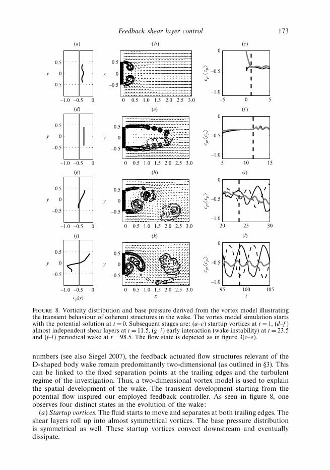
Figure 8. Vorticity distribution and base pressure derived from the vortex model illustratingthe transient behaviour of coherent structures in the wake. The vortex model simulation startswith the potential solution at t = 0. Subsequent stages are: (a–c) startup vortices at t = 1, (d–f )almost independent shear layers at t =11.5, (g–i ) early interaction (wake instability) at t = 23.5and (j–l ) periodical wake at t = 98.5. The flow state is depicted as in figure 3(c–e).

numbers (see also Siegel 2007), the feedback actuated flow structures relevant of theD-shaped body wake remain predominantly two-dimensional (as outlined in §3). Thiscan be linked to the fixed separation points at the trailing edges and the turbulentregime of the investigation. Thus, a two-dimensional vortex model is used to explainthe spatial development of the wake. The transient development starting from thepotential flow inspired our employed feedback controller. As seen in figure 8, oneobserves four distinct states in the evolution of the wake:

(a) Startup vortices. The fluid starts to move and separates at both trailing edges. Theshear layers roll up into almost symmetrical vortices. The base pressure distributionis symmetrical as well. These startup vortices convect downstream and eventuallydissipate.

174 M. Pastoor, L. Henning, B. R. Noack, R. King and G. Tadmor

(a) (b)

uBuB

uA

uA

C

C

D B

A

Shear layerevolution

Asymmetricwake

Shear layerevolution

Symmetricwake

Asymmetricwake

B

A

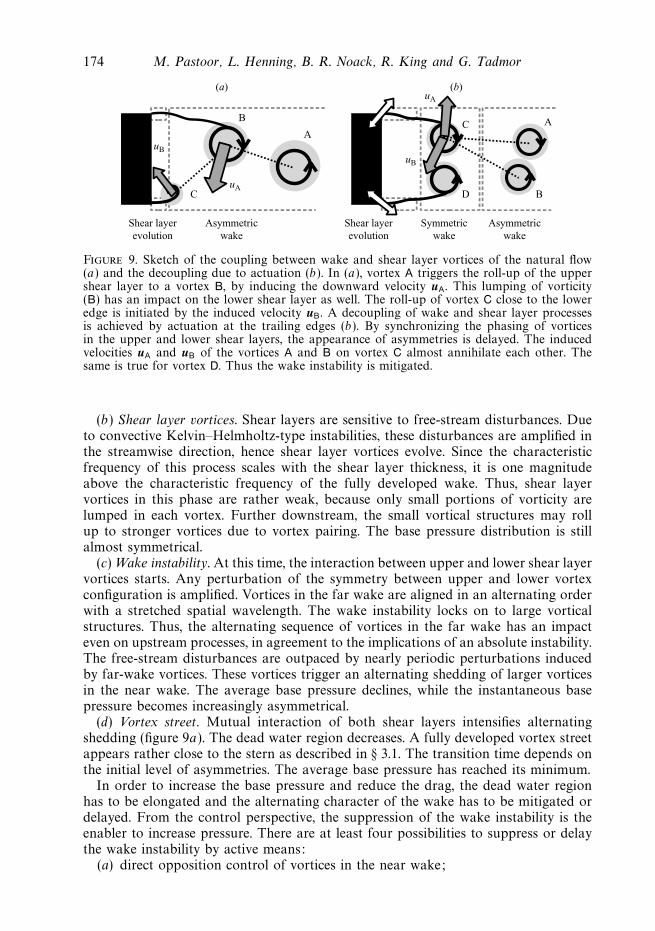
Figure 9. Sketch of the coupling between wake and shear layer vortices of the natural flow(a) and the decoupling due to actuation (b). In (a), vortex A triggers the roll-up of the uppershear layer to a vortex B, by inducing the downward velocity uA. This lumping of vorticity(B) has an impact on the lower shear layer as well. The roll-up of vortex C close to the loweredge is initiated by the induced velocity uB. A decoupling of wake and shear layer processesis achieved by actuation at the trailing edges (b). By synchronizing the phasing of vorticesin the upper and lower shear layers, the appearance of asymmetries is delayed. The inducedvelocities uA and uB of the vortices A and B on vortex C almost annihilate each other. Thesame is true for vortex D. Thus the wake instability is mitigated.

(b) Shear layer vortices. Shear layers are sensitive to free-stream disturbances. Dueto convective Kelvin–Helmholtz-type instabilities, these disturbances are amplified inthe streamwise direction, hence shear layer vortices evolve. Since the characteristicfrequency of this process scales with the shear layer thickness, it is one magnitudeabove the characteristic frequency of the fully developed wake. Thus, shear layervortices in this phase are rather weak, because only small portions of vorticity arelumped in each vortex. Further downstream, the small vortical structures may rollup to stronger vortices due to vortex pairing. The base pressure distribution is stillalmost symmetrical.

(c) Wake instability. At this time, the interaction between upper and lower shear layervortices starts. Any perturbation of the symmetry between upper and lower vortexconfiguration is amplified. Vortices in the far wake are aligned in an alternating orderwith a stretched spatial wavelength. The wake instability locks on to large vorticalstructures. Thus, the alternating sequence of vortices in the far wake has an impacteven on upstream processes, in agreement to the implications of an absolute instability.The free-stream disturbances are outpaced by nearly periodic perturbations inducedby far-wake vortices. These vortices trigger an alternating shedding of larger vorticesin the near wake. The average base pressure declines, while the instantaneous basepressure becomes increasingly asymmetrical.

(d) Vortex street. Mutual interaction of both shear layers intensifies alternatingshedding (figure 9a). The dead water region decreases. A fully developed vortex streetappears rather close to the stern as described in § 3.1. The transition time depends onthe initial level of asymmetries. The average base pressure has reached its minimum.

In order to increase the base pressure and reduce the drag, the dead water regionhas to be elongated and the alternating character of the wake has to be mitigated ordelayed. From the control perspective, the suppression of the wake instability is theenabler to increase pressure. There are at least four possibilities to suppress or delaythe wake instability by active means:

(a) direct opposition control of vortices in the near wake;

Feedback shear layer control 175

(b) mitigating the evolution of large-scale vortex formations by high-frequencyforcing;

(c) breaking large-scale vortex formations by forcing three-dimensional structures;(d) enhancing the initial symmetry by forcing synchronous vortex shedding.

In search of a tunable and low-cost active control device for existing bluff bodies,we select the last method in the course of this paper. Zero-net-mass-flux actuationincreases the magnitude of perturbations in the initial shear layer. The convectiveinstability, which yields shear layer vortices due to roll-up, starts with a largerinitial amplitude. From analysis of vortex models of various configurations (mixinglayer, backward-facing step, D-shaped body), we know that actuators also commandthe phasing of vortex roll-up. Transferring this behaviour to our control goal,synchronization of the upper and lower shear layers should be achieved by enforcingin-phase vortex generation. Perturbations of the symmetry would be reduced andtherefore the evolution of the wake instability could be delayed. However, in the farwake the alternating character imposed by the wake instability is still a pronouncedfeature (figure 9b).

The effect of actuation on the phase difference between the vortices in the two shearlayers is analysed by the phase angles between the actuation signal g(t) and pressurefluctuations cp(y, z, t) close to the upper and lower edges. The vortex model predictsa phase angle of 180◦ for optimal open-loop forcing (StA = 0.15). Notwithstandingstochastic short-term effects, pressure fluctuations are also strongly dominated byoscillations at the actuation frequency. A detailed examination of these predictions inexperimental results is given in the following.

Phase angles �φu/l = � {g(t)u/l, cP (±0.44, z, t)}, calculated either with pressurereadings at the upper or lower edge, are displayed in figure 10(a, b) as functions ofthe Strouhal number of actuation (open-loop). Additionally, these pressure readingsare processed by harmonic analysis. We are interested in the amplitudes

P (St) =2

Ns

∣∣∣∣∣Ns∑k=1

cp(y = ±0.44, z = 0, tk) ei 2π St tk

∣∣∣∣∣ (4.1)

of harmonic oscillations with the actuation frequency St = StA as well as thewake instability frequency St = StW =0.23. Here, Ns is the number of samples.The imaginary unit is denoted by i . The amplitudes P (St) are normalized by ther.m.s. value of the pressure readings and plotted versus the actuation frequency infigure 10(c, d ).

Four ranges of actuation frequencies are examined in detail: see the frequencyranges (i)–(iv) in figure 4(a). In all cases, the Reynolds number is 46 000 and bothactuators operate in-phase at a constant actuation amplitude cμ =0.01.

Forcing frequencies in the range 0.1 � StA � 0.2 (ii) yield a high base pressure(figure 4a). Vortex creation in the upper and lower shear layer occur simultaneously,as indicated by almost identical phase angles between the actuation signal and pressurereadings in figure 10(a, b). Both phase angles φu/l are approximately 170◦, which is inaccordance with 180◦ predicted by the vortex model. This figure implies that vorticesappear when the actuators switch from blowing to sucking.

Most of the pressure fluctuations are imposed by vortices shed at the actuationfrequency, as can be seen by P (StA) in figure 10(c). The influence of the wake instabilityon the pressure fluctuations is low, as indicated by P (StW ) in figure 10(d ). Actuationin this frequency range is beneficial, since it triggers strong and synchronized coherentstructures in both shear layers. This allows for the evolution of an elongated dead

176 M. Pastoor, L. Henning, B. R. Noack, R. King and G. Tadmor

0 0.1 0.2 0.3

90

180

Δφ

u (d

eg.)

Δφ

l (de

g.)

270

360(i) (ii) (iii) (iv)

(a)

0 0.1 0.2 0.3

90

180

270

360(b)

0 0.1 0.2 0.3

0.2

0.4

0.6

0.8

1.0

StA

(c) (d)

P(S

t A)/

√2c P

,r.m

.s

0 0.1 0.2 0.3

0.2

0.4

0.6

0.8

1.0

StA

P(S

t W)/

√2c P

,r.m

.s

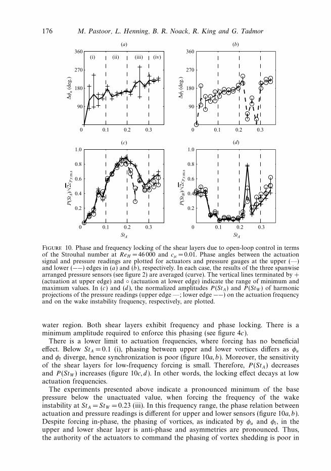
Figure 10. Phase and frequency locking of the shear layers due to open-loop control in termsof the Strouhal number at ReH = 46 000 and cμ = 0.01. Phase angles between the actuationsignal and pressure readings are plotted for actuators and pressure gauges at the upper (—)and lower (−−) edges in (a) and (b), respectively. In each case, the results of the three spanwisearranged pressure sensors (see figure 2) are averaged (curve). The vertical lines terminated by +(actuation at upper edge) and ◦ (actuation at lower edge) indicate the range of minimum andmaximum values. In (c) and (d ), the normalized amplitudes P (StA) and P (StW ) of harmonicprojections of the pressure readings (upper edge —; lower edge −−) on the actuation frequencyand on the wake instability frequency, respectively, are plotted.

water region. Both shear layers exhibit frequency and phase locking. There is aminimum amplitude required to enforce this phasing (see figure 4c).

There is a lower limit to actuation frequencies, where forcing has no beneficialeffect. Below StA =0.1 (i), phasing between upper and lower vortices differs as φu

and φl diverge, hence synchronization is poor (figure 10a, b). Moreover, the sensitivityof the shear layers for low-frequency forcing is small. Therefore, P (StA) decreasesand P (StW ) increases (figure 10c, d ). In other words, the locking effect decays at lowactuation frequencies.

The experiments presented above indicate a pronounced minimum of the basepressure below the unactuated value, when forcing the frequency of the wakeinstability at StA = StW = 0.23 (iii). In this frequency range, the phase relation betweenactuation and pressure readings is different for upper and lower sensors (figure 10a, b).Despite forcing in-phase, the phasing of vortices, as indicated by φu and φl , in theupper and lower shear layer is anti-phase and asymmetries are pronounced. Thus,the authority of the actuators to command the phasing of vortex shedding is poor in

Feedback shear layer control 177

this regime. Apparently, the perturbations imposed by the wake instability outpacethe attempt to synchronize the shear layer evolution. In fact, the actuators increasethe perturbation level of the shear layer in a frequency range that is perfectly suitedto amplifying the wake instability. As a result, the base pressure is decreased by 10%whilst drag is increased by some 5% (figure 4a, b).

Frequencies in the range StA > 0.3 (iv) are beneficial with respect to base pressureand drag but this effect declines at higher frequencies (figure 4a, b). At highfrequencies, there is still some authority to command phasing, as vortices are releasedsynchronously (compare φu and φl), but fluctuations imposed by these vortices andthe wake instability are almost of equal size, as can be seen by comparing P (StA) andP (StW ) (figure 10c, d ). High-frequency forcing creates small vortices. Due to roll-upand vortex pairing triggered by the wake instability in the far wake, large alternatingcoherent structures still appear relatively close to the stern, which reduce the basepressure.

5. Feedback controlAs derived in the previous section, our feedback control should decouple shear

layer development and wake processes. Increasing the initial symmetry of the flowmitigates the wake instability. This is achieved by forcing a symmetrical vortexformation in the near wake due to a synchronized development of both shear layers.In § 5.1, an adaptive controller is proposed that respects these requirements and findsoptimal actuation parameters. A physically motivated controller that explicitly forcesa symmetrical evolution of the shear layers is outlined in § 5.2. In both cases, controlis applied to the steady-state base flow.

5.1. Adaptive controller

Slope-seeking feedback is an adaptive method for the control of nonlinear plants. Itis an extension to well-known extremum-seeking schemes and is described in detail byKrstic & Wang (2000) and Ariyur & Krstic (2003). In § 5.1.1, a slope-seeking feedbackscheme for maintaining the optimal actuation amplitude is outlined. Experimentalresults are presented in § 5.1.2.

5.1.1. Slope-seeking feedback scheme

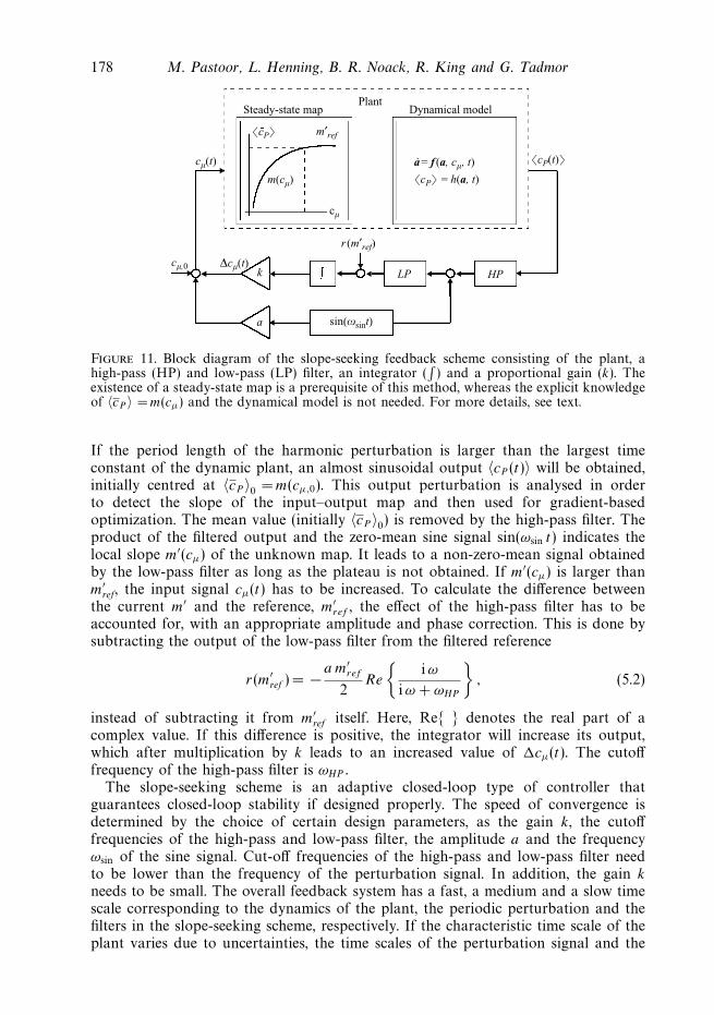
A block diagram of the slope-seeking feedback scheme is displayed in figure 11.The plant is considered as a block with the input variable cμ(t), being the actuationamplitude, and the output variable 〈cP (t)〉, represented by the controlled base pressure.We assume that the plant can be described by two characteristic features:

(1) a plateau-type steady-state input-output map 〈cP 〉 = m(cμ);(2) a state-space model representing the dynamics of the controlled process.

The control idea is to achieve a state of the plant which is marked by a certainreference slope m′

ref = ∂ 〈cP 〉 /∂cμ in the steady-state map. Side constraints for thiskind of feedback are fast process dynamics in comparison to variations of the input.Neither the dynamical model nor the steady-state map need to be known.

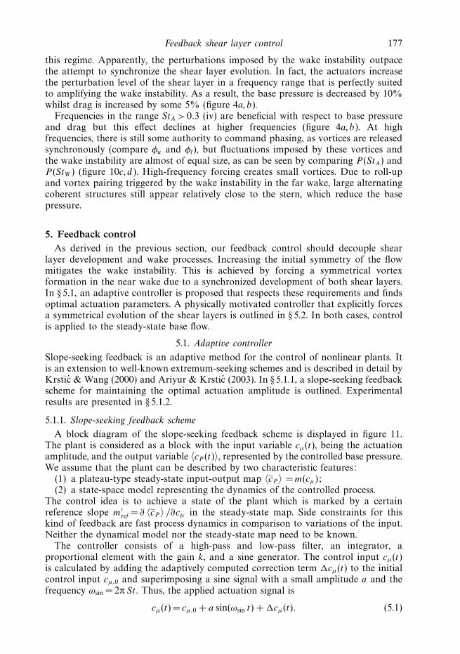
The controller consists of a high-pass and low-pass filter, an integrator, aproportional element with the gain k, and a sine generator. The control input cμ(t)is calculated by adding the adaptively computed correction term �cμ(t) to the initialcontrol input cμ,0 and superimposing a sine signal with a small amplitude a and thefrequency ωsin = 2π St . Thus, the applied actuation signal is

cμ(t) = cμ,0 + a sin(ωsin t) + �cμ(t). (5.1)

178 M. Pastoor, L. Henning, B. R. Noack, R. King and G. Tadmor

sin(ωsint)a

cμ,0

cμ(t)

Plant

m′ref

cμ

�cP�

�cP(t)�

m(cμ)

Steady-state map

a = f (a, cμ, t)

�cP� = h(a, t)

Dynamical model

HPLP

r (m′ref)

kΔcμ(t)

Figure 11. Block diagram of the slope-seeking feedback scheme consisting of the plant, ahigh-pass (HP) and low-pass (LP) filter, an integrator (

∫) and a proportional gain (k). The

existence of a steady-state map is a prerequisite of this method, whereas the explicit knowledgeof 〈cP 〉 =m(cμ) and the dynamical model is not needed. For more details, see text.

If the period length of the harmonic perturbation is larger than the largest timeconstant of the dynamic plant, an almost sinusoidal output 〈cP (t)〉 will be obtained,initially centred at 〈cP 〉0 = m(cμ,0). This output perturbation is analysed in orderto detect the slope of the input–output map and then used for gradient-basedoptimization. The mean value (initially 〈cP 〉0) is removed by the high-pass filter. Theproduct of the filtered output and the zero-mean sine signal sin(ωsin t) indicates thelocal slope m′(cμ) of the unknown map. It leads to a non-zero-mean signal obtainedby the low-pass filter as long as the plateau is not obtained. If m′(cμ) is larger thanm′

ref, the input signal cμ(t) has to be increased. To calculate the difference betweenthe current m′ and the reference, m′

ref , the effect of the high-pass filter has to beaccounted for, with an appropriate amplitude and phase correction. This is done bysubtracting the output of the low-pass filter from the filtered reference

r(m′ref ) = −

a m′ref

2Re

{i ω

iω + ωHP

}, (5.2)

instead of subtracting it from m′ref itself. Here, Re{ } denotes the real part of a

complex value. If this difference is positive, the integrator will increase its output,which after multiplication by k leads to an increased value of �cμ(t). The cutofffrequency of the high-pass filter is ωHP .

The slope-seeking scheme is an adaptive closed-loop type of controller thatguarantees closed-loop stability if designed properly. The speed of convergence isdetermined by the choice of certain design parameters, as the gain k, the cutofffrequencies of the high-pass and low-pass filter, the amplitude a and the frequencyωsin of the sine signal. Cut-off frequencies of the high-pass and low-pass filter needto be lower than the frequency of the perturbation signal. In addition, the gain k

needs to be small. The overall feedback system has a fast, a medium and a slow timescale corresponding to the dynamics of the plant, the periodic perturbation and thefilters in the slope-seeking scheme, respectively. If the characteristic time scale of theplant varies due to uncertainties, the time scales of the perturbation signal and the

Feedback shear layer control 179

0 1000 2000 3000

3

6

9

c μ ×

103

(b)

0 1000 2000 3000–0.6

–0.4

–0.2(c)

0 1000 2000 30003

5

7R

e H ×

10–4

(d)

t

0 0.003 0.006 0.009 0.0120.6

0.5

0.4

0.3

0.2

cμ

�c P

�

(a)

�c P

�

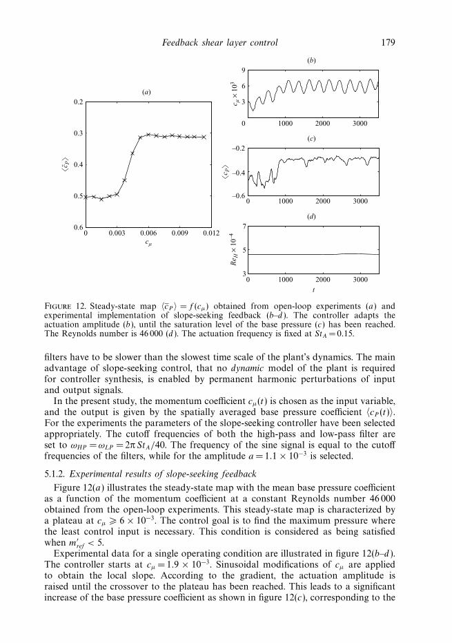
Figure 12. Steady-state map 〈cP 〉 = f (cμ) obtained from open-loop experiments (a) andexperimental implementation of slope-seeking feedback (b–d ). The controller adapts theactuation amplitude (b), until the saturation level of the base pressure (c) has been reached.The Reynolds number is 46 000 (d ). The actuation frequency is fixed at StA = 0.15.

filters have to be slower than the slowest time scale of the plant’s dynamics. The mainadvantage of slope-seeking control, that no dynamic model of the plant is requiredfor controller synthesis, is enabled by permanent harmonic perturbations of inputand output signals.

In the present study, the momentum coefficient cμ(t) is chosen as the input variable,and the output is given by the spatially averaged base pressure coefficient 〈cP (t)〉.For the experiments the parameters of the slope-seeking controller have been selectedappropriately. The cutoff frequencies of both the high-pass and low-pass filter areset to ωHP =ωLP = 2π StA/40. The frequency of the sine signal is equal to the cutofffrequencies of the filters, while for the amplitude a = 1.1 × 10−3 is selected.

5.1.2. Experimental results of slope-seeking feedback

Figure 12(a) illustrates the steady-state map with the mean base pressure coefficientas a function of the momentum coefficient at a constant Reynolds number 46 000obtained from the open-loop experiments. This steady-state map is characterized bya plateau at cμ � 6 × 10−3. The control goal is to find the maximum pressure wherethe least control input is necessary. This condition is considered as being satisfiedwhen m′

ref < 5.Experimental data for a single operating condition are illustrated in figure 12(b–d ).

The controller starts at cμ = 1.9 × 10−3. Sinusoidal modifications of cμ are appliedto obtain the local slope. According to the gradient, the actuation amplitude israised until the crossover to the plateau has been reached. This leads to a significantincrease of the base pressure coefficient as shown in figure 12(c), corresponding to the

180 M. Pastoor, L. Henning, B. R. Noack, R. King and G. Tadmor

0 2000 4000 6000

(b)

0 2000 4000 6000

(c)

0 2000 4000 6000t

(d)

0 0.003 0.006 0.009 0.0120.6

0.5

0.4

0.3

0.2

cμ

(a)

ReH

3

6

12

9

c μ ×

103

–0.6

–0.4

–0.2

3

5

7

Re H

× 1

0–4�

c P�

�c P

�

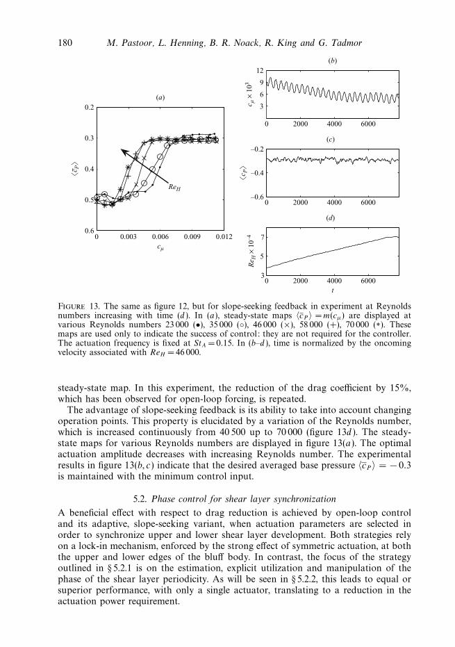
Figure 13. The same as figure 12, but for slope-seeking feedback in experiment at Reynoldsnumbers increasing with time (d ). In (a), steady-state maps 〈cP 〉 = m(cμ) are displayed atvarious Reynolds numbers 23 000 (•), 35 000 (◦), 46 000 (×), 58 000 (+), 70 000 (∗). Thesemaps are used only to indicate the success of control: they are not required for the controller.The actuation frequency is fixed at StA = 0.15. In (b–d ), time is normalized by the oncomingvelocity associated with ReH = 46 000.

steady-state map. In this experiment, the reduction of the drag coefficient by 15%,which has been observed for open-loop forcing, is repeated.

The advantage of slope-seeking feedback is its ability to take into account changingoperation points. This property is elucidated by a variation of the Reynolds number,which is increased continuously from 40 500 up to 70 000 (figure 13d ). The steady-state maps for various Reynolds numbers are displayed in figure 13(a). The optimalactuation amplitude decreases with increasing Reynolds number. The experimentalresults in figure 13(b, c) indicate that the desired averaged base pressure 〈cP 〉 = − 0.3is maintained with the minimum control input.

5.2. Phase control for shear layer synchronization

A beneficial effect with respect to drag reduction is achieved by open-loop controland its adaptive, slope-seeking variant, when actuation parameters are selected inorder to synchronize upper and lower shear layer development. Both strategies relyon a lock-in mechanism, enforced by the strong effect of symmetric actuation, at boththe upper and lower edges of the bluff body. In contrast, the focus of the strategyoutlined in § 5.2.1 is on the estimation, explicit utilization and manipulation of thephase of the shear layer periodicity. As will be seen in § 5.2.2, this leads to equal orsuperior performance, with only a single actuator, translating to a reduction in theactuation power requirement.

Feedback shear layer control 181

A

ExtendedKalman filter

Actuation:g = A sin (θ + Δφ)

Phase:θ(t)

Figure 14. Sketch of a single actuator configuration implementing the proposed phasecontroller. The estimated phase of the pressure oscillations at the lower edge is utilizedto calculate the actuation signal, which is applied to the upper actuator.

5.2.1. Implementation of phase control

The guiding principle of the phase feedback is illustrated in figure 14. The pressurefluctuations induced by vortex shedding at the lower edge of the body are monitoredat x = 0, y = − 0.4, z = 0. These pressure fluctuations are approximated by a simplesine function cP (t) = c0 + c1 sin θ , with the phase θ (t) = θ0 + ωt and the frequencyω =2π St . The hat marks estimated quantities.

The parameters c0 and c1 are assumed to be slowly varying (nominally, constant)and θ is assumed to grow linearly; their instantaneous values are estimated in realtime by a dynamic observer, realized by an extended Kalman filter (EKF), which isdescribed in Appendix B. Based on the estimated phase θ , a harmonic actuation signalg(t) = A sin(θ + �φ) is calculated and applied to the upper actuator slot only. Theterm �φ = 180◦ represents the desired angle between actuation and pressure readingsas discussed in § 4. The amplitude A corresponds to a momentum coefficient ofcμ = 7.5 × 10−3. Since we only use a single actuator, the effective impulse contributionis only half that amount (ceff

μ = 3.8 × 10−3).

5.2.2. Experimental results of phase control

Our proposed phase controller is tested in our experimental rig at Reynolds number46 000. Control is applied at t = 0 and decreases the drag at the same rate as open-loopforcing or slope-seeking feedback with optimal actuation parameters (figure 15). Timeseries of the sensed and estimated pressure oscillations at the lower edge are in goodagreement, indicating a proper estimation of the amplitude c and phase θ (figure 15a).The estimated frequency of the leading harmonic displayed in figure 15(b) is close tothe natural instability frequency of St ≈ 0.23, when actuation is off, and decreases toSt ≈ 0.15 when control is applied. Based on the phase estimation an almost harmonicactuation signal for the upper actuator is calculated (figure 15c). The normalized dragcoefficient plotted in figure 15(d ) decreases by at least 15% after ten vortex sheddingperiods. Comparing the effective impulse coefficient ceff

μ =3.8 × 10−3 used here, with

the results of slope-seeking feedback at ReH = 46 000 (cμ ≈ 6.7 × 10−3, see figure 12b),we only need 56% of the actuation energy.

Hot-wire measurements in the controlled flow, as described in § 3.3 for thenatural and open-loop forced flow to corroborate the predominantly two-dimensionalcharacter of the coherent structures, are presented in figure 16(a, b). The coherentstructures remain two-dimensional under feedback control as well.

182 M. Pastoor, L. Henning, B. R. Noack, R. King and G. Tadmor

0 50 100 150–0.5

0

0.5c′ P

, c′ P

(a)

0 50 100 1500.10

0.15

0.20

0.25

St

(b)

0 50 100 150

–1

0

1

g

t

(c)

0 50 100 150

0.8

0.9

1.0

1.1

t

(d)

c D/c

D,0

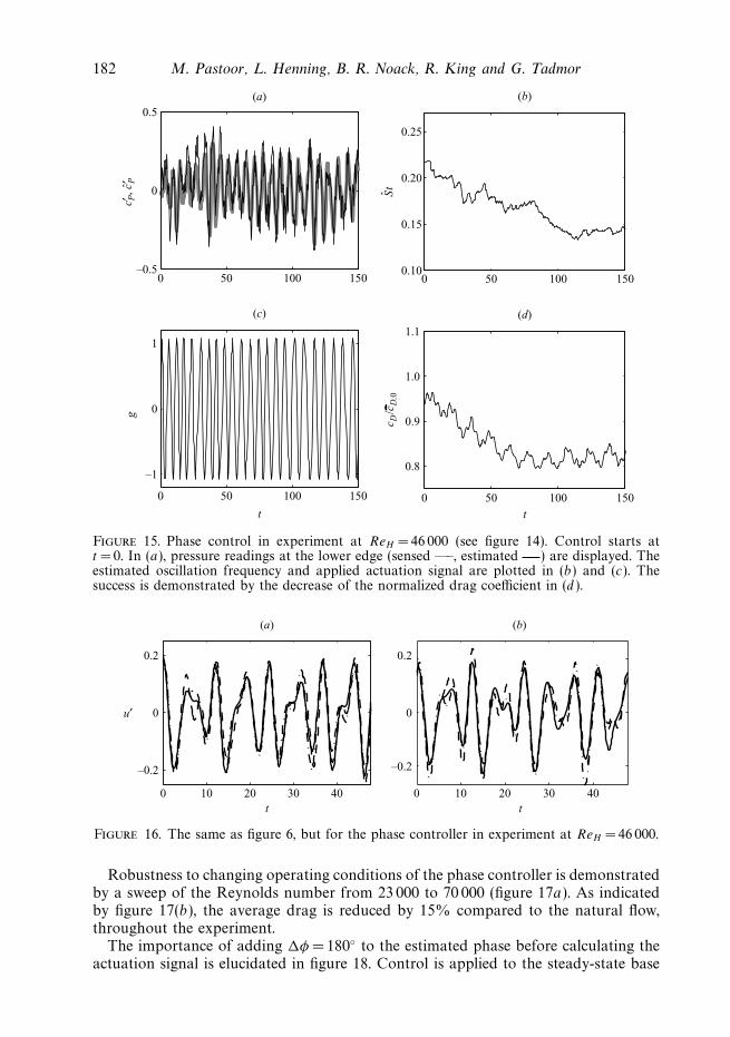
Figure 15. Phase control in experiment at ReH = 46 000 (see figure 14). Control starts att = 0. In (a), pressure readings at the lower edge (sensed —–, estimated ) are displayed. Theestimated oscillation frequency and applied actuation signal are plotted in (b) and (c). Thesuccess is demonstrated by the decrease of the normalized drag coefficient in (d ).

0 10 20 30 40

–0.2

0

0.2

t0 10 20 30 40

–0.2

0

0.2

t

u′

(a) (b)

Figure 16. The same as figure 6, but for the phase controller in experiment at ReH =46 000.

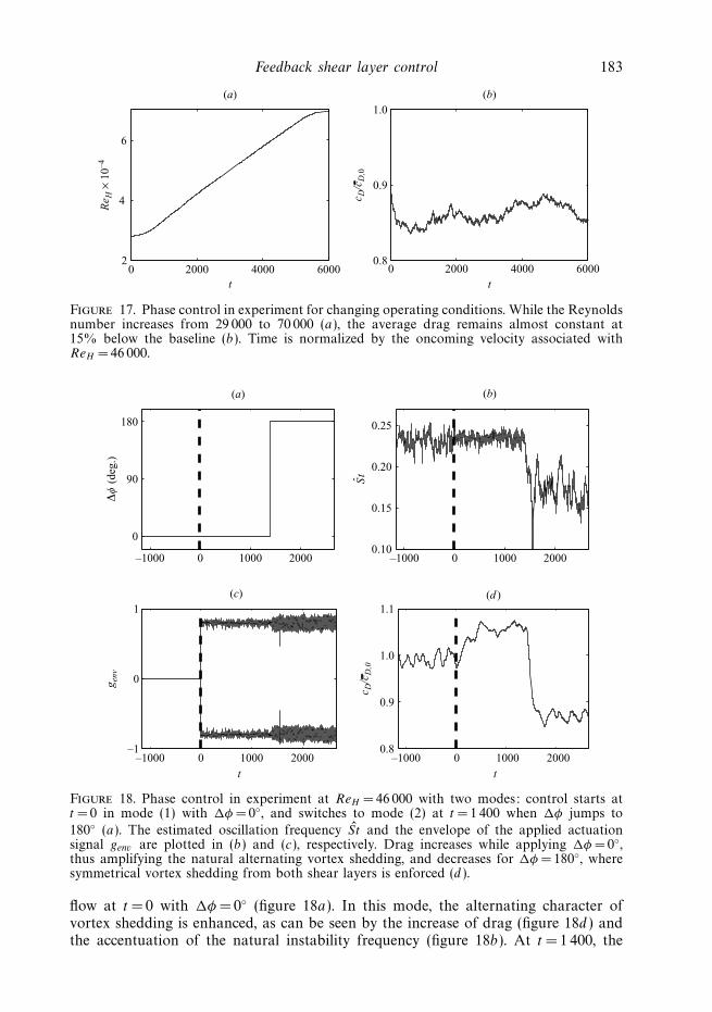
Robustness to changing operating conditions of the phase controller is demonstratedby a sweep of the Reynolds number from 23 000 to 70 000 (figure 17a). As indicatedby figure 17(b), the average drag is reduced by 15% compared to the natural flow,throughout the experiment.

The importance of adding �φ =180◦ to the estimated phase before calculating theactuation signal is elucidated in figure 18. Control is applied to the steady-state base

Feedback shear layer control 183

0 2000 4000 60002

4

6

Re H

× 1

0–4

t

(a)

0 2000 4000 60000.8

0.9

1.0

t

(b)

c D/c

D,0

Figure 17. Phase control in experiment for changing operating conditions. While the Reynoldsnumber increases from 29 000 to 70 000 (a), the average drag remains almost constant at15% below the baseline (b). Time is normalized by the oncoming velocity associated withReH = 46 000.

–1000 0 1000 2000 –1000 0 1000 2000

0

90

180

Δφ (

deg.

)

(a)

0.10

0.15

0.20

0.25

St

(b)

–1000 0 1000 2000–1

0

1

g env

t

–1000 0 1000 2000t

(c)

0.8

0.9

1.0

1.1(d )

c D/c

D,0

Figure 18. Phase control in experiment at ReH =46 000 with two modes: control starts att =0 in mode (1) with �φ = 0◦, and switches to mode (2) at t = 1 400 when �φ jumps to

180◦ (a). The estimated oscillation frequency St and the envelope of the applied actuationsignal genv are plotted in (b) and (c), respectively. Drag increases while applying �φ =0◦,thus amplifying the natural alternating vortex shedding, and decreases for �φ = 180◦, wheresymmetrical vortex shedding from both shear layers is enforced (d ).

flow at t = 0 with �φ = 0◦ (figure 18a). In this mode, the alternating character ofvortex shedding is enhanced, as can be seen by the increase of drag (figure 18d ) andthe accentuation of the natural instability frequency (figure 18b). At t = 1 400, the

184 M. Pastoor, L. Henning, B. R. Noack, R. King and G. Tadmor

0 0.5 1.0 1.5 2.0

–0.5

0

0.5

x

y

(a)

–5 0 5

–1.0

–0.5

0

t

cp

(b)

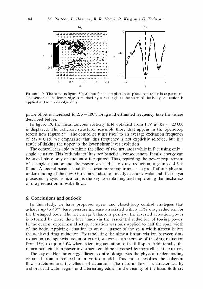
Figure 19. The same as figure 3(a, b), but for the implemented phase controller in experiment.The sensor at the lower edge is marked by a rectangle at the stern of the body. Actuation isapplied at the upper edge only.

phase offset is increased to �φ = 180◦. Drag and estimated frequency take the valuesdescribed before.

In figure 19, the instantaneous vorticity field obtained from PIV at ReH =23 000is displayed. The coherent structures resemble those that appear in the open-loopforced flow (figure 5a). The controller tunes itself to an average excitation frequencyof StA ≈ 0.15. We emphasize, that this frequency is not explicitly selected, but is aresult of linking the upper to the lower shear layer evolution.

The controller is able to mimic the effect of two actuators while in fact using only asingle actuator. This ‘redundancy’ has two beneficial consequences. Firstly, energy canbe saved, since only one actuator is required. Thus, regarding the power requirementof a single actuator and the power saved due to drag reduction, a gain of 4.5 isfound. A second benefit – and this is even more important – is a proof of our physicalunderstanding of the flow. Our control idea, to directly decouple wake and shear layerprocesses by synchronization, is the key to explaining and improveing the mechanicsof drag reduction in wake flows.

6. Conclusions and outlookIn this study, we have proposed open- and closed-loop control strategies that

achieve up to 40% base pressure increase associated with a 15% drag reduction forthe D-shaped body. The net energy balance is positive: the invested actuation poweris returned by more than four times via the associated reduction of towing power.In the current experimental setup, actuation was only applied to half the span widthof the body. Applying actuation to only a quarter of the span width almost halvesthe achieved drag reduction. Extrapolating the almost linear relation between dragreduction and spanwise actuator extent, we expect an increase of the drag reductionfrom 15% to up to 30% when extending actuation to the full span. Additionally, thereturn per actuation power investment could be increased by more efficient actuators.

The key enabler for energy-efficient control design was the physical understandingobtained from a reduced-order vortex model. This model resolves the coherentflow structures and the effects of actuation. The natural flow is characterized bya short dead water region and alternating eddies in the vicinity of the base. Both are

Feedback shear layer control 185

Physically motivatedcontroller

Black-box-based

controller

Periodsfor adaption

1

10

100 Extremum-/ slope-seeking feedback

Adaptiveblack-box-

basedcontroller

Increasingdesigneffort

Robustness

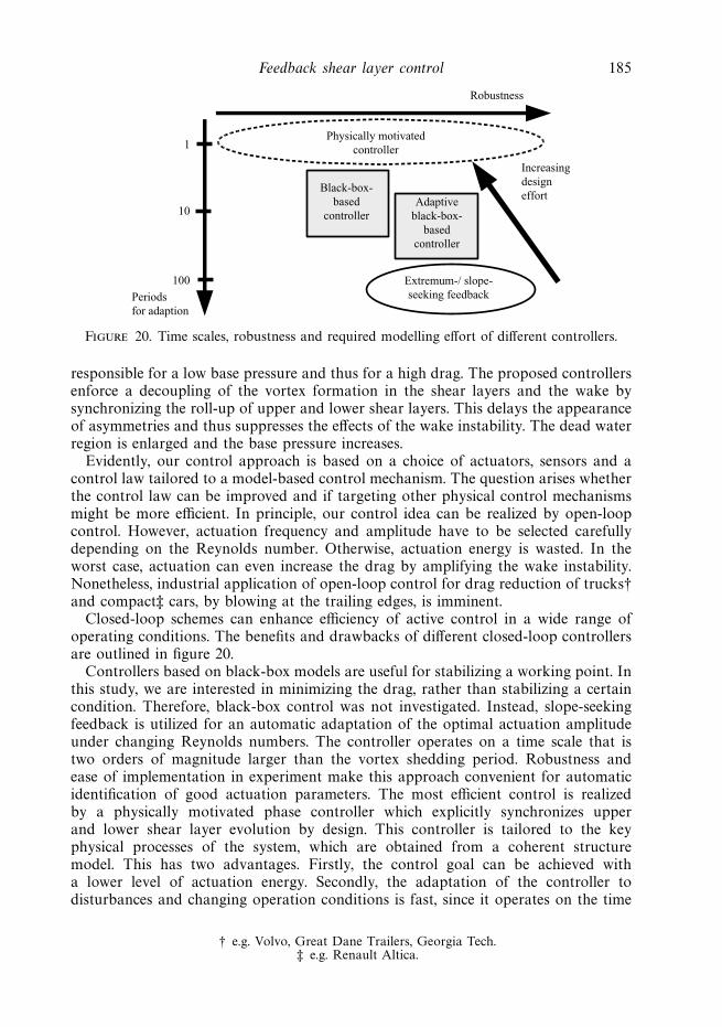
Figure 20. Time scales, robustness and required modelling effort of different controllers.

responsible for a low base pressure and thus for a high drag. The proposed controllersenforce a decoupling of the vortex formation in the shear layers and the wake bysynchronizing the roll-up of upper and lower shear layers. This delays the appearanceof asymmetries and thus suppresses the effects of the wake instability. The dead waterregion is enlarged and the base pressure increases.

Evidently, our control approach is based on a choice of actuators, sensors and acontrol law tailored to a model-based control mechanism. The question arises whetherthe control law can be improved and if targeting other physical control mechanismsmight be more efficient. In principle, our control idea can be realized by open-loopcontrol. However, actuation frequency and amplitude have to be selected carefullydepending on the Reynolds number. Otherwise, actuation energy is wasted. In theworst case, actuation can even increase the drag by amplifying the wake instability.Nonetheless, industrial application of open-loop control for drag reduction of trucks†and compact‡ cars, by blowing at the trailing edges, is imminent.

Closed-loop schemes can enhance efficiency of active control in a wide range ofoperating conditions. The benefits and drawbacks of different closed-loop controllersare outlined in figure 20.

Controllers based on black-box models are useful for stabilizing a working point. Inthis study, we are interested in minimizing the drag, rather than stabilizing a certaincondition. Therefore, black-box control was not investigated. Instead, slope-seekingfeedback is utilized for an automatic adaptation of the optimal actuation amplitudeunder changing Reynolds numbers. The controller operates on a time scale that istwo orders of magnitude larger than the vortex shedding period. Robustness andease of implementation in experiment make this approach convenient for automaticidentification of good actuation parameters. The most efficient control is realizedby a physically motivated phase controller which explicitly synchronizes upperand lower shear layer evolution by design. This controller is tailored to the keyphysical processes of the system, which are obtained from a coherent structuremodel. This has two advantages. Firstly, the control goal can be achieved witha lower level of actuation energy. Secondly, the adaptation of the controller todisturbances and changing operation conditions is fast, since it operates on the time

† e.g. Volvo, Great Dane Trailers, Georgia Tech.‡ e.g. Renault Altica.

186 M. Pastoor, L. Henning, B. R. Noack, R. King and G. Tadmor

Natural wake

(a) Direct wake control (opposition control)

(b) Energizing both shear layers

(c) Synchronizing both shear layers

(d) Wake reorganization (fish)

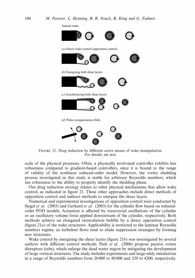
Figure 21. Drag reduction by different active means of wake manipulation.For details, see text.

scale of the physical processes. Often, a physically motivated controller exhibits lessrobustness compared to gradient-based controllers, since it is bound to the rangeof validity of the nonlinear reduced-order model. However, the vortex sheddingprocess investigated in this study is stable for arbitrary Reynolds numbers, whichties robustness to the ability to properly identify the shedding phase.

Our drag reduction strategy relates to other physical mechanisms that allow wakecontrol, as indicated in figure 21. These other approaches include direct methods ofopposition control and indirect methods to energize the shear layers.

Numerical and experimental investigations of opposition control were conducted bySiegel et al. (2003) and Gerhard et al. (2003) for the cylinder flow based on reduced-order POD models. Actuation is affected by transversal oscillations of the cylinderor an oscillatory volume force applied downstream of the cylinder, respectively. Bothmethods achieve an elongated recirculation bubble by a direct opposition control(figure 21a) of the wake structures. Applicability is restricted to the laminar Reynoldsnumbers regime, as turbulent flows tend to elude suppression strategies by formingnew structures.

Wake control by energizing the shear layers (figure 21b) was investigated by severalauthors with different control methods. Park et al. (2006) propose passive vortexdisruptors (tabs), which enlarge the dead water region by mitigating the developmentof large vortical structures. The study includes experiments and large-eddy simulationsin a range of Reynolds numbers from 20 000 to 80 000 and 320 to 4200, respectively.

Feedback shear layer control 187

The base pressure increases by 30% for an optimized tab configuration. A similarbut active controller was proposed by Kim et al. (2004). Protas & Wesfreid (2002)numerically studied the effect of open-loop control on the formation of the wake flowbehind a cylinder at a Reynolds number based on the diameter of 150. They obtainedresults similar to those presented in our study. A significant drag reduction is relatedto an elongation of the recirculation bubble by supporting an unstable symmetricstate. Control is applied by cylinder rotations at various frequencies, which turned outto be energetically inefficient at low Reynolds numbers. Wu et al. (2007) completelysuppressed the von Karman vortex street of a circular cylinder. In their numericalinvestigation at Reynolds numbers up to 5 000 a drag reduction of 85% was achievedby generating travelling waves on the flexible surface of the body. The invested powerfor actuating the surface is found to be 94% of the power saving. Extremum-seekingfeedback control was applied by Beaudoin et al. (2006) to a bluff body configurationthat is similar to a backward-facing step. Actuation is implemented by a rotatingcylinder at the trailing edge. The rotation frequency is adaptively controlled in orderto minimize the drag (up to 5%) with a given power requirement.

The phase controller proposed in this study marks a change of paradigm. Thetwo-dimensional phase control strategies investigated by Siegel et al. (2003) andGerhard et al. (2003) aim at a suppression of the wake structures, by generatinganti-cyclic control forces. As mentioned before, these methods are restricted to alaminar regime. The proposed strategy promotes symmetrical shear layer structureswithout significantly energizing their fluctuation level. Thus, the formation of thevortex street is delayed at low-actuation amplitudes (figure 21c). Furthermore, ourstrategy seems to be applicable in a turbulent regime.

The very mechanism of intervening in the coupling between the shear layers andthe vortex formation can be envisioned to be applicable to three-dimensional flowconfigurations, e.g. for flows behind spheres. A rigorous comparison is still needed toverify this understanding. It should be noted that nature provides its own solution toreducing wake-induced drag (figure 21d ): the strokes of a fishtail create a propulsivejet flow, by inverting the vortical structure in the wake (Ahlborn 2004).

The authors emphasize the superiority of feedback control in contrast to open-loop control. In steady low-turbulent wind tunnel experiments open-loop actuationmay be optimized to a level which is comparable to closed-loop control. In realworld applications flow control has to cope with varying oncoming velocities, highturbulence levels and other perturbations. Hence, by utilizing feedback design, thebenefits of active flow control can be fully exploited. In future work, the authors willpursue the direct usage of reduced-order vortex and Galerkin models as plants forcontrol and observer design, targeting the industrial application of closed-loop flowcontrol.

The work was funded by the Deutsche Forschungsgemeinschaft (DFG) undergrants NO 258/1-1 and NO 258/2-3, by a CNRS invited researcher grant, by the USNational Science Foundation (NSF) under grants 0524070 and 0410246, and by theUS Air Force Office of Scientific Research (AFOSR) under grants FA95500510399 andFA95500610373. The authors acknowledge funding and excellent working conditionsof the Collaborative Research Centre (Sfb 557) ‘Control of Complex Turbulent ShearFlows’, supported by the DFG and hosted at the Berlin Institute of Technology.Stimulating discussions with Katarina Aleksic, Laurent Cordier, Hans-Christian Hege,Oliver Lehmann, Mark Luchtenburg, Eckart Meiburg, Marek Morzynski, MichaelSchlegel, Jon Scouten, Avi Seifert, Stefan Siegel, Tino Weinkauf, and Jose-Eduardo

188 M. Pastoor, L. Henning, B. R. Noack, R. King and G. Tadmor

Wesfreid are acknowledged. We are grateful for outstanding hardware and softwaresupport by Joachim Kraatz, Frank Kunze, Ingolf Richter, Lars Oergel and MartinFranke and excellent administration of our Sfb 557 by Steffi Stehr.

Appendix A. Vortex modelIn this section, the building blocks of the vortex model are outlined. We recapitulate

the kinematics of the model from (2.1) for convenience, and decompose the stationarypotential Φs from the unsteady actuation potential Φa:

u(x, t) = ∇Φs(x) + ∇Φa(x, t) +

N∑i=1

Γi uω(x, xi). (A 1)

A.1. Conformal mapping

Following Clements (1973), Evans & Bloor (1977), Cortelezzi (1996) and Coller et al.(2000), the no-penetration condition is enforced by employing a conformal mapping.This procedure is computationally cheaper and more accurate for low-order vortexmodels compared with a computational panel approach (see e.g. Fletcher 1988).The conformal map bijectively transforms the computational domain – the upperhalf-plane ζ = ξ + i η with ξ ∈ � and η ∈ �+ – into the physical domain. In thecomputational domain, the no-penetration condition with discrete vortices is satisfiedby introducing image vortices with the abscissae as the axis of reflection.

The conformal mapping from the computational domain, ζ = ξ + i η, into thephysical domain, z = x + i y, is obtained by integration of the following Schwarz–Christoffel transformation:

dz

dζ= C1

√ζ 2 − 1

ζ 2 − a2, where C1, a ∈ �. (A 2)

The map z(ζ ) is expressed by

z(ζ ) = C2 + C1

1

2a

(2a log(ζ +

√ζ 2 − 1)

−√

a2 − 1 log

(1 − a ζ −

√a2 − 1

√ζ 2 − 1

−ζ + a

)

+√

a2 − 1 log

(−1 − a ζ +

√a2 − 1

√ζ 2 − 1

ζ + a

) ), C2 ∈ �. (A 3)

The constants a/√

a2 − 1 = h/(h−H ), C1 = h/π and C2 = −7i are obtained from theequation of continuity and from geometrical considerations. The imaginary unit isdenoted by i . The inverse mapping ζ (z) is calculated numerically with the Newton–Raphson method. No analytical solution has been found.

A.2. Potential flow

Vortex models yield potential flow solutions of the Navier–Stokes equation withsingularities at the vortex loci. The conformal mapping is used to satisfy the no-penetration condition at the walls in an efficient manner. The potential flow solutionis generated by a pair of point sources at ζi = ± a, which is mapped to x → −∞.The complex source potential is transformed to the physical domain by applying the

Feedback shear layer control 189

chain rule of differentiation:

dWζs

dζ=

2∑n=1

Qn

2π

1

ζ − ζn

,

dWzs

dz=

dWζs

dζ

dζ

dz=: wz

s (z),

∇Φs(x) =

(Re{wz

s (z)}−Im{wz

s (z)}

). (A 4)

The source strength Qn = 2h/(h − H ) corresponds to the flow rate in each cross-section of the physical domain. The velocity field generated by both sources in thephysical domain describes a potential flow around the aft section of the D-shapedbody without separation. The abscissa of the ζ -plane represents wall streamlines inthe physical domain.

A.3. Actuation

The actuation is modelled by two harmonic oscillating sources near the trailing edgesof the body, – following the authors’ work for the backward-facing step configurationin Pastoor et al. (2003). Thus, for the actuated flow, a time-dependent potential isadded to the potential flow. The corresponding velocity field reads

∇Φa(x, t) =

(Re{wz

a(z, t)}−Im{wz

a(z, t)}

), (A 5)

where

dWza (t)

dz=

dWζa

dζ

dζ

dz=: wz

a(z, t),

dWζa (t)

dζ=

2∑n=1

Qn(t)

2π

1

ζ − ζn

.

This field fulfils the boundary conditions, as long as the sources are placed on thecontour of the body. The position ζn of the actuators is adjusted to blow with anangle of attack of 45◦at the point of insertion of vortices (see below). The strengthQn(t) depends on the selected actuation. The instantaneous mass flux into the upperhalf-plane is chosen to be similar to the corresponding quantity of the actuators inexperiment.

A.4. Vortex elements

The no-penetration condition for a potential flow superimposed onto a vortex flowis fulfilled with a virtual vortex with mirrored coordinates and opposite circulation.Similarly, an ensemble of vortices is supplemented by their image vortices. The N

vortices at the time t in the physical domain induce the velocity

uω(x, t) =

(Re{wz

v(z, t)}−Im{wz

v(z, t)}

), (A 6)

190 M. Pastoor, L. Henning, B. R. Noack, R. King and G. Tadmor

where

dWzv (t)

dz=

dWζv

dζ

dζ

dz=: wz

v(z, t),

dWζv (t)

dζ= −i

N∑n=1

Γn

2π

1

ζ − ζn(t)+ i

N∑n=1

Γn

2π

1

ζ − ζ n(t).

The coordinate ζn denotes the current position of the nth vortex and Γn its circulation.The overbar indicates the complex conjugate of a complex number. The circulation Γn

of each vortex is preserved according to Kelvin’s law. When the velocity is prescribedat the centre of the vortex element, the velocity calculation is modified according toRouth’s theorem (Milne-Thomson 1968). In this case, the induced complex velocityat zn reads

wzv(zn, t) =

⎛⎜⎝−i

N∑j=1j �=n

Γj

2π

1

ζn − ζj (t)+ i

N∑j=1

Γj

2π

1

ζn − ζ j (t)

⎞⎟⎠ dζ

dz

∣∣∣∣zn

− iΓn

2π

d2ζ/dz2

2 dζ/dz

∣∣∣∣zn

.

Up to now, a point vortex discretization has been assumed in agreement withpotential flow theory. The discontinuity in the vortex field is regularized in a morerefined model by Hamel and Oseen. Their solution for the azimuthal velocity uϕ asa function of the distance r between vortex and sample point smoothly connects aRankine vortex core at r → 0 with the potential vortex at r → ∞,

uϕ(r) =Γ0

2π r

(1 − e−r2/R2)

, (A 7)

where R denotes the core radius of the vortex. The initial core radius at the trailingedges is chosen to be similar to the boundary layer thickness. A linear temporalgrowth of the core diameter is implemented to account for turbulent diffusion ofvorticity.

A.5. Vorticity production

Experiments and simulations indicate straight shear layers emerging from the upperand lower edges of the body in the direction of the oncoming flow. Giesing (1969)proposes a generalized Kutta condition for the idealized infinitely thin shear layer ininviscid flow. According to this condition, the shear layer is aligned with the oncomingflow. The circulation contribution dΓ of a small shear layer segment of the length dx

is

dΓ =(Ulower − Uupper

)dx, (A 8)

where Uupper and Ulower are the velocities above and below the shear layer, respectively.This criterion is in good agreement with experimental and numerical investigationsof the flow around a D-shaped body.

In our vortex model, Giesing’s solution is discretized by inserting vortices each timestep �t with a circulation |Γ | =U 2

1 �t/2 at x = U1�t/4 and y = ±0.5 (Clements 1973).The circulation of vortices is negative at the upper edge and positive at the loweredge. The velocity U1 is computed at y = ± 0.7. To avoid numerical problems withthe singularities of the Schwarz–Christoffel transformation at both edges, vortices arelead a short distance away from the singularity (x < 0.05).

Feedback shear layer control 191

A.6. Vortex merging

A discretization parameter of our model is the number of vortices consistent withthe desired low-dimensionality. The perpetual creation of new vortices increases theorder of our model. This order can be reduced by merging two vortices when theirdistance is below a critical value. The result of a merging process is one vortex withthe combined circulation located at the barycentre of both predecessors. A reasonablecompromise between accuracy and dimensionality is obtained by a merging distancewhich increases linearly from R = 0.05 at x = 0 to R = 0.5 at x � 10.

Appendix B. Extended Kalman FilterAn extended Kalman filter (EKF) is an established and efficient method to estimate

the state of a dynamical system from a series of incomplete or noisy measurements. Agood source is Gelb (1986) and a description of the method used here can be foundin Tadmor (2004). For completeness, this section begins with a brief review of theEKF framework, followed by the specifics of the implementation used in this article.

A dynamical system can be described by

a = f (a, g, t) + w (B 1)

where a is the true state of the system, g represents control variables and w is a zero-mean white noise process with spectral density Q (obtained from a Wiener processw). A measurement of the true state at discrete times is made according to

sk = h(ak, gk, tk) + vk, (B 2)

where vk is observation noise with covariance Rk .The state of the Kalman filter is represented by two variables, namely the estimated

state a and the error covariance matrix P , which is a measure of the estimatedaccuracy of the state estimate. The Kalman filter has the following two distinct phases.

Prediction (time update). In this phase no measurement is available. The estimatedstate from the previous time tk−1 is used to produce an estimation of the current stateat time tk , here by a simple Euler step:

ak = ak−1 + f (ak−1, gk−1, tk−1) �t. (B 3)

The covariance of the estimation error changes according to

Pk = Pk−1 +(Fk−1 Pk−1 + Pk−1 F T

k−1 + Q)�t. (B 4)

Here, F is the Jacobian of the dynamical system evaluated with the current stateestimate

Fk =∂ f∂a

∣∣∣∣ak ,gk

. (B 5)

Update (measurement update). In this phase, current measurement information isused to refine the prediction. In the following, all states are marked by superscript(−) before and by (+) after the measurement update. The estimated state is correctedbased on the innovation or measurement residual

�sk = sk − h(a−k , gk, tk) (B 6)

and the optimal Kalman gain

Kk = P −k HT

k

(Hk P −

k HTk + Rk

)−1, (B 7)

192 M. Pastoor, L. Henning, B. R. Noack, R. King and G. Tadmor

where Hk is the Jacobian of the output equation evaluated with the predicted state

Hk =∂h∂a

∣∣∣∣a−

k ,gk

. (B 8)

The updated state estimate is

a+k = a−

k + Kk �sk, (B 9)

while the updated estimate of the covariance matrix is

P +k = (I − Kk Hk) P −

k . (B 10)

Q and Rk have an intuitively clear meaning for a one-dimensional system. When Rk islarge, the filter does not trust in the measurement. The computed Kalman gain (B 7) issmall and thus the filter prefers the state estimate already in the model (B 9). VanishingRk indicates an ideal sensor and the Kalman gain is 1/Hk . After the measurementupdate the covariance of the estimation error is exactly zero (B 10). When Q is large,the filter expects a lot of process noise. The covariance of the estimation error growsrapidly with each time update (B 4). In the measurement update, the filter prefersinformation from the measurement over the predicted state.

In our application, pressure fluctuations at the base of the D-shaped body areapproximated by a sine function cp(t) = s = c0 + c1 sin θ . We assume a dynamicalmodel with the four states frequency ω, amplitude c1, phase θ and offset c0, whichare combined in a state-space vector

a =

⎛⎜⎝

ω

θ

c1

c0

⎞⎟⎠ .

Pressure fluctuations are then described by the output equation

sk = h(ak) = a2,k sin a3,k + a4,k.

A simple stochastic state-space model for the temporal evolution is provided by

ak =

⎡⎢⎣

1 0 0 0�t 0 1 00 1 0 00 0 0 1

⎤⎥⎦

︸ ︷︷ ︸F

ak−1 + wk−1.

This means that frequency, amplitude and offset are considered nominally constant,while the phase grows with time according to the current frequency. A fairapproximation of Q is obtained when the estimated variances of the states dividedby T are placed along the diagonal. Here, T is the expected time scale on which thevariances of the states appear. The same procedure is applied to the matrix Rk withthe variance of the measurement noise over T . Thus, covariance matrices of processand measurement noise are supposed to be

Q =

⎡⎢⎣

200 0 0 00 0 0.01 00 1 0 00 0 0 1

⎤⎥⎦ × 10−2 and Rk = 5 × 10−2.

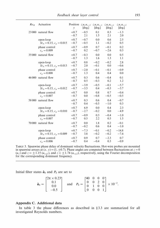
Feedback shear layer control 193

ReH Actuation Position �ucuc−2 �ucuc−1 �ucuc+1 �ucuc+2

y [deg.] [deg.] [deg.] [deg.]

23 000 natural flow +0.7 −0.5 0.1 0.3 −1.3−0.7 2.1 1.5 2.1 2.0

open-loop +0.7 −0.7 0.0 0.6 2.5StA =0.15, cμ =0.015 −0.7 −0.5 1.1 −0.2 0.5

phase control +0.7 −0.9 0.7 −0.1 0.2cμ =0.009 −0.7 0.2 −0.7 −2.6 0.3

35 000 natural flow +0.7 −0.3 0.0 0.0 0.5−0.7 1.3 1.6 1.3 1.1

open-loop +0.7 0.8 −0.2 −0.2 2.8StA =0.15, cμ =0.013 −0.7 2.0 −0.1 0.0 −0.6

phase control +0.7 −2.0 −0.1 −0.1 −0.9cμ =0.008 −0.7 1.3 0.4 0.4 0.0

46 000 natural flow +0.7 0.3 0.6 −0.4 0.1−0.7 0.5 −0.3 0.2 1.2

open-loop +0.7 −3.9 −0.5 −0.1 −5.7StA =0.15, cμ =0.012 −0.7 −3.5 0.4 −0.3 −5.7

phase control +0.7 0.0 0.8 0.7 −0.4cμ =0.007 −0.7 0.0 −0.8 −0.5 −0.5

58 000 natural flow +0.7 0.3 0.6 0.4 −0.7−0.7 0.4 −0.5 −1.0 0.3

open-loop +0.7 6.9 0.0 0.4 2.3StA =0.15, cμ =0.010 −0.7 −2.7 −0.2 0.0 −4.9

phase control +0.7 −0.9 0.3 −0.4 −1.0cμ =0.007 −0.7 0.5 2.2 0.5 1.5

70 000 natural flow +0.7 0.0 1.8 0.2 −0.1−0.7 −0.2 0.6 0.4 −1.0

open-loop +0.7 −7.3 −0.1 −0.2 −14.8StA =0.15, cμ =0.009 −0.7 3.8 −0.2 −0.2 −7.4

phase control +0.7 0.9 0.7 −2.3 0.7cμ =0.006 −0.7 0.4 −0.4 0.3 −0.9

Table 3. Spanwise phase delay of dominant velocity fluctuations. Hot-wire probes are mountedin spanwise arrays at (x, y) = (1, ±0.7). Phase angles are computed between fluctuations at z = 0(uc) and z = ±1.15 (uc±1), and z = ±1.74 (uc±2), respectively, using the Fourier decompositionfor the corresponding dominant frequency.

Initial filter states a0 and P0 are set to

a0 =

⎡⎢⎣2π × 0.23

0.10.0

−0.5

⎤⎥⎦ and P0 =

⎡⎢⎣40 0 0 00 0 2 00 1 0 00 0 0 1

⎤⎥⎦ × 10−2.

Appendix C. Additional dataIn table 3 the phase differences as described in § 3.3 are summarized for all

investigated Reynolds numbers.

194 M. Pastoor, L. Henning, B. R. Noack, R. King and G. Tadmor

REFERENCES

Ahlborn, B. K. 2004 Zoological Physics. Springer.

Ariyur, K. & Krstic, M. 2003 Real-Time Optimization by Extremum-Seeking Control. John Wiley &Sons.

Beale, J. T. & Majda, A. 1982 Vortex methods I: Convergence in three dimensions. Math. Comput.39, 1–27.

Bearman, P. W. 1965 Investigation of the flow behind a two-dimensional model with a blunt trailingedge and fitted with splitter plates. J. Fluid Mech. 21, 241–255.

Bearman, P. W. 1967 The effect of base bleed on the flow behind a two-dimensional model with ablunt trailing edge. Aeronaut. Q. 18, 207–224.

Beaudoin, J. F., Cadot, O., Aider, J.-L., & Wesfreid, J.-E. 2006 Drag reduction of a bluff bodyusing adaptive control methods. Phys. Fluids 18, 08510.

Becker, R., Garwon, M., Gutknecht, C., Barwolff, G. & King, R. 2005 Robust control ofseparated shear flows in simulation and experiment. J. Process Control 15, 691–700.

Becker, R., King, R., Petz, R. & Nitsche, W. 2007 Adaptive closed-loop separation control on ahigh-lift configuration using extremum seeking. AIAA J. 45, 1382–1392.

Bergmann, M., Cordier, L. & Brancher, J.-P. 2005 Optimal rotary control of the cylinder wakeusing proper orthogonal decomposition reduced order model. Phys. Fluids 17, 1–21.

Birkhoff, G. 1962 Helmholtz and Taylor instability. In Proc. Symp. Appl. Maths XII, pp. 55–76.AMS.

Cattafesta, L., Williams, D. R., Rowley, C. W. & Alvi, F. 2003 Review of active control offlow-induced cavity resonance. AIAA Paper 2003-3567.

Clements, R. R. 1973 An inviscid model of two-dimensional vortex shedding. J. Fluid Mech. 57,321–336.

Coller, B. D., Noack, B. R., Narayanan, S., Banaszuk, A. & Khibnik, A. I. 2000 Reduced-basismodel for active separation control in a planar diffuser flow. AIAA Paper 2000-2563.

Collis, S. S., Joslin, R. D., Seifert, A. & Theofilis, V. 2004 Issues in active flow control: theory,control, simulation, and experiment. Prog. Aerospace Sci. 40, 237–289.

Cooper, K. R. 1985 The effect of front-edge rounding and rear edge shaping on the aerodynamicdrag of bluff vehicles in proximity. SAE Paper 850288.

Cordier, L. & Bergmann, M. 2003 Proper Orthogonal Decomposition: An Overview. VKI LectureSeries 2003–04. Von Karman Institut for Fluid Dynamics.

Cortelezzi, L. 1996 Nonlinear feedback control of the wake past a plate with a suction point onthe downstream wall. J. Fluid Mech. 327, 303–324.

Cottet, G. H. & Koumoutsakos, P. 2000 Vortex Methods – Theory and Practice. CambridgeUniversity Press.

Detemple-Laake, E. & Eckelmann, H. 1989 Phenomenology of Karman vortex streets in oscillatoryflow. Exps. Fluids 7, 217–227.

Evans, R. A. & Bloor, M. I. G. 1977 The starting mechanism of wave-induced flow through asharp-edged orifice. J. Fluid Mech. 82, 115–128.

Fiedler, H.-E. & Fernholz, H. H. 1990 On management and control of turbulent shear flows.Prog. Aeronaut. Sci. 27, 305–387.

Fletcher, C. A. J. 1988 Computational Techniques for Fluid Dynamics; Volume II: Specific Techniquesfor Different Flow Categories. Springer.

Gad-el-Hak, M., Pollard, A. & Bonnet, J.-P. 1998 Flow Control - Fundamentals and Practices.Springer.

Garwon, M., Darmadi, L. H., Urzynicok, F., Barwolff, G. & King, R. 2003 Adaptive control ofseparated flow. In Proc. European Control Conf. ECC’03, ECC Paper 543.

Gelb, A. 1986 Applied Optimal Estimation. The MIT Press.

Gerhard, J., Pastoor, M., King, R., Noack, B. R., Dillmann, A., Morzynski, M. & Tadmor, G.

2003 Model-based control of vortex shedding using low-dimensional Galerkin models. AIAAPaper 2003-4262.

Ghoniem, A. F. & Gagnon, Y. 1987 Vortex simulation of laminar recirculating flow. J. Comput.Phys. 68, 346–377.

Giesing, J. P. 1969 Vorticity and Kutta condition for unsteady multi-energy flows. Trans. ASME:J. Appl. Mech. 36, 608–613.

Feedback shear layer control 195

Grosche, F. R. & Meier, G. E. A. 2001 Research at the DLR Gottingen on bluff body aerodynamics,drag reduction by wake ventilation and active flow control. J. Wind. Engng Ind. Aerodyn. 89,1201–1218.

Helmholtz, H. 1858 Uber Integrale der hydrodynamischen Gleichungen, welche den Wirbel-bewegungen entsprechen. Crelles J. 55, 25–55.

Henning, L. & King, R. 2005a Multivariable closed-loop control of the reattachement lengthdownstream of a backward-facing step. In Proc. 16th IFAC World Congress. IFAC Paper02575.

Henning, L. & King, R. 2005b Drag reduction by closed-loop control of a separated flow over abluff body with a blunt trailing edge. In Proc. 44th IEEE Conf. on Decision and Control andEuropean Control Conference CDC-ECC’05, pp. 494–499.

Henning, L. & King, R. 2007 Robust multivariable closed-loop control of a turbulent backward-facing step flow. J. Aircraft 40, 201–208.

Henning, L., Pastoor, M., King, R., Noack, B. R. & Tadmor, G. 2007 Feedback control applied tobluff body wake. In Active Flow Control (ed. R. King). Notes on Numerical Fluid Mechanicsand Multidisciplinary Design, vol. 95. Springer.

Hucho, W.-H. 2002 Aerodynamik der stumpfen Korper. Physikalische Grundlagen und Anwendungenin der Praxis. Vieweg.

Huerre, P. & Monkewitz, P. A. 1990 Local and global instabilities in spatially developing flows.Annu. Rev. Fluid Mech. 22, 473–537.

von Karman, T. 1911 Uber den Mechanismus des Widerstandes, den ein bewegter Korper in einerFlussigkeit erfahrt. Nachrichten der Kaiserlichen Gesellschaft der Wissenschaften zu Gottingen,pp. 324–338.

Kim, J., Hahn, S., Lee, D., Choi, J., Jeon, W.-P. & Choi, H. 2004 Active control of turbulent flowover a model vehicle for drag reduction. J. Turb. 5, 1–25.

King, R., Becker, R., Garwon, M. & Henning, L. 2004 Robust and adaptive closed-loop controlof separated shear flows. AIAA Paper 2004-2519.

King, R., Seibold, M., Lehmann, O., Noack, B. R., Morzynksi, M. & Tadmor, G. 2005 Nonlinearflow control based on a low dimensional model of fluid flow. In Control and Observer Designfor Nonlinear Finite and Infinite Dimensional Systems (ed. T. Meurer et al. ). Lecture Notes inControl and Information Sciences, vol. 322, pp. 369–386. Springer.

Krasny, R. 1986 Desingularization of periodic vortex sheet roll-up. J. Comput. Phys. 65, 292–313.

Krstic, M. & Wang, H.-H. 2000 Stability of extremum seeking feedback for general nonlineardynamic systems. Automatica 36, 595-601.

Leder, A. 1992 Abgeloste Stromungen – Physikalische Grundlagen. Vieweg.

Leonard, A. 1985 Computing three-dimensional incompressible flows with vortex elements. Annu.Rev. Fluid Mech. 17, 523–559.

Little, J., Debiasi, M., Caraballo, E., & Samimy, M. 2007 Effects of open-loop and closed-loopcontrol on subsonic cavity flows. Phys. Fluids 19, 065104.

Lugt, H. J. 1996 Introduction to Vortex Theory. Vortex Flow Press.

Lumley, J. L. & Blossey, P. N. 1998 Control of turbulence. Annu. Rev. Fluid Mech. 30, 311–327.

Meiburg, E. 1995 Three-dimensional vortex dynamics simulation. In Fluid Vortices (ed. S. Green),pp. 651–685. Kluwer.

Mercker, E. 1980 Eine Blockierungskorrektur fur aerodynamische Messungen in offenen undgeschlossenen Unterschallwindkanalen. PhD Thesis, Technische Universitat Berlin.

Milne-Thomson, L. M. 1968 Theoretical Hydrodynamics. Macmillan.

Noack, B. R,, Afanasiev, K., Morzynski, M., Tadmor, G. & Thiele, F. 2003 A hierarchy oflow-dimensional models for the transient and post-transient cylinder wake. J. Fluid Mech.497, 335–363.

Noack, B. R., Papas, P. & Monkewitz, P. A. 2005 The need for a pressure-term representation inempirical Galerkin models of incompressible shear flows. J. Fluid Mech. 523, 339–365.

Noack, B. R., Tadmor, G. & Morzynski, M. 2004 Low-dimensional models for feedback flowcontrol. Part I: Empirical Galerkin models (Invited). AIAA Paper 2004-2408.

Park, H., Lee, D., Jeon, W.-P., Hahn, S., Kim, J., Kim, J., Choi, J. & Choi, H. 2006 Drag reductionin flow over a two-dimensional bluff body with a blunt trailing edge using a new passivedevice. J. Fluid Mech. 563, 389–414.

196 M. Pastoor, L. Henning, B. R. Noack, R. King and G. Tadmor

Pastoor, M., King, R., Noack, B. R., Dillmann, A. & Tadmor, G. 2003 Model-based coherent-structure control of turbulent shear flows using low-dimensional vortex models. AIAA Paper2003-4261.

Protas, B. 2004 Linear feedback stabilization of laminar vortex shedding based on a point vortexmodel. Phys. Fluids 16, 4473–4488.

Protas, B. 2006 Higher-order Foppl models of steady wake flows. Phys. Fluids 18, 117109.

Protas, B. & Wesfreid, J.-E. 2002 Drag force in the open-loop control of the cylinder wake in thelaminar regime. Phys. Fluids 14, 810–826.

Rosenhead, L. 1931 The formation of vortices from a surface of discontinuity. Proc. R. Soc. Lond.134, 170–192.

Roussopoulos, K. 1993 Feedback control of vortex shedding at low Reynolds numbers. J. FluidMech. 248, 267–296.

Rowley, C. W., Williams, D. R., Colonius, T., Murray, R. M., MacMartin, D. G. & Fabris, D.

2002 Model-based control of cavity oscillations. Part II: System identification and analysis.AIAA Paper 2002-0972.

Seidel, J., Siegel, S., Cohen, K., Becker, V. & McLaughlin, T. 2007 Simulations of threedimensional feedback control of a circular cylinder wake. AIAA Paper 2006-1404.

Siegel, S., Aradag, S., Seidel, J., Cohen, K. & McLaughlin, T. 2007 Low diimensional PODbased estimation of a 3D turbulent separated flow. AIAA Paper 2007-0112.

Siegel, S., Cohen, K. & McLaughlin, T. 2003 Feedback control of a circular cylinder wake inexperiment and simulation. AIAA Paper 2003-3571.

Siegel, S., Cohen, K., Seidel, J., Luchtenburg, M. & McLaughlin, T. 2008 Low dimensionalmodelling of a transient cylinder wake using double proper-orthogonal decomposition.J. Fluid Mech. (in press).

Soteriou, M. 2003 Vortex element method – expansion about incompressible flow computation ofnoise generation by subsonic shear flows – the impact of external forcing. J. Turb. 4, 1–9.

Tadmor, G. 2004 Observers and feedback control for a rotating vortex pair. IEEE Trans. ControlSystems Technol. 12, 36–51.

Tadmor, G., Noack, B. R., Morzynski, M. & Siegel, S. 2004 Low-dimensional models for feedbackflow control. Part II: Observer and controller design (Invited). AIAA Paper 2004-2409.

Tang, S. & Aubry, N. 2000 Suppression of vortex shedding inspired by a low-dimensional model,J. Fluids Struct. 14, 443–468.

Tanner, M. 1972 A method of reducing the base drag of wings with blunt trailing edges. Aeronaut.Q. 23, 15–23.

Thomson, W. 1869 On vortex motion. Trans. R. Soc. Edin. 25, 217–260.

Tombazis, N. & Bearman, P. W. 1997 A study of three-dimensional aspects of vortex shedding froma bluff body with a mild geometric disturbance. J. Fluid Mech. 330, 85–112.

Wu, C.-J., Wang, L. & Wu, J.-Z. 2007 Suppression of the von Karman vortex street behind a circularcylinder by a travelling wave generated by a flexible surface. J. Fluid Mech. 574, 365–391.

Wu, C.-J., Xie, Y. & Wu, J.-Z. 2003 Fluid roller bearing effect and flow control. Acta MechanicaSinica 19 (5), 476–484.

Wygnanski, I. 2004 The variables affecting the control of separation by periodic excitation. AIAAPaper 2004-2505.

Zhang, H.-Q., Fey, U., Noack, B. R., Konig, M. & Eckelmann, H. 1995 On the transition of thecylinder wake. Phys. Fluids 7, 779–794.