Analysis of an Axisymmetric Bluff Body Wake Using Fourier Transform and POD

American Institute of Aeronautics and Astronautics1

Analysis of an Axisymmetric Bluff Body Wake using FourierTransform and POD

Jürgen Seidel*, Stefan Siegel†, Tiger Jeans‡, Selin Aradag§, Kelly Cohen**, and Thomas McLaughlin††

Department of Aeronautics, U.S. Air Force Academy, Colorado Springs, CO 80840, USA

The data from unforced and open loop forced simulations of the wake behind anaxisymmetric bluff body at ReD=1,500 is analyzed to explore the effect of forcing. In theunforced wake, because of the axial symmetry of the body, structures do not maintain aconstant azimuthal phase over time, which leads to inaccurate predictions of the flow fieldwhen applying POD. Forcing inside the “lock-in” region in amplitude-frequency space witha fixed azimuthal phase is therefore introduced to study the wake in detail. The resultingflow field is analyzed using three methods, namely an azimuthal Fourier transform, amoment of inertia calculation, and a velocity vector histogram, to determine the azimuthalphase of the wake structures. The overall goal is to minimize the necessary data volume toanalyze the flow for eventual implementation in real time feedback flow control experiments.It is shown that the methods used to determine the azimuthal phase all yield a measure of thephase angle of the symmetry plane in the wake.

0BNomenclatureA = amplitude of oscillationA0 = maximum forcing amplitudeD = cylinder diameterf = frequencyf0 = natural shedding frequencyk = azimuthal wave number

,ℜ ℑ = real/imaginary part

Re = Re=U0D/ν, Reynolds numberSt = fU/D, Strouhal numbert = timeT = Shedding/forcing periodU0 = free stream velocityν = viscosityΩ = total vorticityωx = X component of vorticityΘ = azimuthal coordinateΘ0 = azimuthal phase

I. 1BIntroductionHE WAKES of bluff bodies as well as their control have been studied for some time.1-5 The main goal of mostefforts is to reduce the pressure fluctuations induced by the Vortex Street that develops above a critical

Reynolds number. These pressure variations results in undesirable force fluctuations as well as a general increase in

* Visiting Researcher, Department of Aeronautics, Senior Member† Assistant Research Associate, Department of Aeronautics, Senior Member‡ Visiting Researcher, Department of Aeronautics, Member§ Visiting Researcher, Department of Aeronautics, Member** Associate Professor, Department of Aerospace Engineering, University of Cincinnati, Associate Fellow†† Director, Aeronautics Research Center, Department of Aeronautics, Associate Fellow

T

46th AIAA Aerospace Sciences Meeting and Exhibit7 - 10 January 2008, Reno, Nevada

AIAA 2008-552

This material is declared a work of the U.S. Government and is not subject to copyright protection in the United States.

Dow

nloa

ded

by U

NIV

ER

SIT

Y O

F C

INC

INN

AT

I on

Dec

embe

r 4,

201

4 | h

ttp://

arc.

aiaa

.org

| D

OI:

10.

2514

/6.2

008-

552


drag.2 To control the wake of a circular cylinder, passive as well as active flow control techniques have been appliedto reduce the amplitude of the fluctuations.4,6-8 Compared to the numerous studies of two-dimensional wakes, there are very few publications that address three-dimensional wakes behind axisymmetric bodies (usually spheres or disks). Aschenbach9 identified two differenttypes of vortex shedding in the wake behind a sphere. The first, a shear layer mode, at moderate Reynolds numbers,identified by a increase in the Strouhal number with increasing Reynolds number; and a second mode, comprised oftwo counter-rotating helical modes with a Strouhal number that is approximately constant over a large Reynoldsnumber range. Sakamoto and Haniu10 corroborate the existence of two modes of instability in the wake of a sphere.They showed that large scale vortex loops form at Reynolds number (based on the diameter of the sphere) above300. For slightly higher Reynolds numbers (Re>420), they found that the symmetry plane starts to meanderrandomly. For Re>800, small scale structures, related to the shear layer instability, start to appear. Finally, for muchhigher Reynolds numbers (Re>30,000), the wake structure changes drastically because of boundary layer transitionon the sphere. A stability analysis of wake profiles performed by Monkewitz11 showed that a range of absolutelyunstable Strouhal numbers, St, between 0.17 and 0.21 exists above a Reynolds number of about Re=700.There are even less studies of the flow topology of the wake behind more complex bodies of revolution. One is theinvestigation by Cannon12, who experimentally found two counter rotating helical modes k=±1 in the wake of bulletshaped bodies, corroborating the results obtained by Aschenbach. Schwarz13 and later Tourbier14, whose numericalinvestigations covered a Reynolds number range from Re=500 to Re=2,000, confirmed the dominance of thesehelical modes above a Reynolds number of Re=700, in excellent agreement with the predictions of Monkewitz. ForReynolds numbers larger than Re=2000, small scale turbulent motion started to appear in addition to the helicalmodes.In the context of feedback flow control, the authors have developed a methodology for closed loop flow control andapplied it successfully for the case of a two-dimensional cylinder wake at Re=100.6 In this approach, theinvestigations start with establishing a “lock-in” region for the flow under consideration. This is critically importantbecause the wake only reacts deterministically to forcing if it is applied with a frequency/amplitude combinationinside this region. Outside the “lock-in” region, the wake does not respond to the forcing and active control istherefore not possible. Once the “lock-in” region is established using open loop forcing, transient forcing can beintroduced to study the dynamics of the flow field in detail. The resulting data is then used as the basis of a LowDimensional Model (LOM), developed using Proper Orthogonal Decomposition (POD).The development of a LOM is critically dependent on a set of data that on the one hand fully describes the dynamicsof the flow field, including the case when control inputs are applied, and on the other hand is as low order aspossible, i.e. has the fewest POD modes, as possible. For the axisymmetric bluff body wake, the authors presentedone possible approach, based on rotating the POD modes about the axis of symmetry, earlier.15 While that approachsuccessfully described the dynamics of the flow, it was deemed too cumbersome and time consuming to beimplemented in real time flow control.This paper discusses in detail the analysis of the axisymmetric bluff body wake using three different techniques,namely an azimuthal Fourier transform, a moment of inertia computation based on flow quantities, and a velocityvector histogram, to identify the phase angle of the symmetry plane in the wake. The phase angle is a critical pieceof information necessary to reduce the complexity of the analysis of the wake flow. With this information, POD canthen be applied with the correct orientation and the computational overhead can be minimized. The resulting PODmode amplitudes can then be used in conjunction with the phase information as a global flow field estimator andenable the development of a low dimensional model of the flow, which ultimately will lead to an effective low ordermodel (LOM) that can be used feedback flow control.

II. 2BComputational Setup

A. 7BSimulationsThe computations are performed using Cobalt from Cobalt Solutions LLC. In the code, the full compressibleNavier-Stokes equations are solved based on a finite volume formulation. The method is formally second orderaccurate in both space and time.An unstructured grid with approximately 1.5M cells is used for the current investigation. In XFigure 1 X, the grid in thex-y plane is shown, where x is the streamwise direction and y and z are the directions normal to the cylinder axis.The origin of the coordinate system is located at the nose of the body, which consists of a 1:4 semi-ellipsoid nosecone and a cylindrical aft section. The overall length of the body is x/D=7. The grid extends from -40D to 40D in thex direction and from -20D to 20D in the y and z directions. Grid point clustering is used near the body and in thewake region to accurately capture the initial vortex development (see XFigure 1 X). Note that because the current

Dow

nloa

ded

by U

NIV

ER

SIT

Y O

F C

INC

INN

AT

I on

Dec

embe

r 4,

201

4 | h

ttp://

arc.

aiaa

.org

| D

OI:

10.

2514

/6.2

008-

552


investigation in concerned with the azimuthal orientation of the flow field, it is advantages to perform thecomputations on an unstructured grid so that the possibility of inadvertently favoring a certain phase angle isminimized.Uniform flow boundary conditions at the far field are imposed using Riemann invariants. The wake is controlled byeight blowing and suction slots located near the base of the body ( XFigure 2 X). The slots extend from x/D=6.88 tox/D=6.96 and cover an azimuthal angle of 44o with a 1o gap between slots. For this investigation, these slots aredriven by an external controller to introduce azimuthal modes k=±1 at a specified frequency, f, and azimuthal phaseΘ0. For forcing in this open loop fashion, the amplitudes are computed as

..)2)0

(exp(0

),( cciftikAtk

A +−Θ−Θ=Θ π , where Θ represents the azimuthal location of the center of a

given forcing slot. Θ is measured against the positive z-axis.To ensure computational efficiency, the Mach number is set to M=0.1 and the time step is ∆t=0.001s. For aReynolds number ReD=1,500, based on the body diameter, D, and the free stream velocity, U0, the non-dimensionalnatural shedding frequency is approx. St=fD/U0=0.17,10 which translates into a physical shedding frequency off0=5.75Hz, resulting in a temporal resolution of approx. 175 time steps per shedding cycle.

Figure 1: Grid in the center plane. Left: full domain, right: section in the body wake.

Figure 2: Base of axisymmetric body with eightblowing/suction slots.

Figure 3: Tap grid in the near wake.

For data analysis, the tap output option in Cobalt was used. The taps for pressure and the three velocity componentswere located in the wake on a cylindrical grid with a streamwise spacing of ∆x/D=0.5, radial spacing ∆r/D=0.05,and an azimuthal spacing of ∆Θ=2π/64, resulting in a manageable 25,000 points ( XFigure 3 X).The investigation consists of three simulations. In the first simulation, no forcing was introduced, which provides abaseline case and the initial condition of the natural vortex shedding. In the second, forcing was applied at thenatural shedding frequency f0 and a phase angle of Θ0=0; in the third, which was conducted as a continuation of thesecond case, the flow was forced with f0 and Θ0=π/2. The continuation enabled us to observe the transient betweenthe two forcing scenarios.

Dow

nloa

ded

by U

NIV

ER

SIT

Y O

F C

INC

INN

AT

I on

Dec

embe

r 4,

201

4 | h

ttp://

arc.

aiaa

.org

| D

OI:

10.

2514

/6.2

008-

552


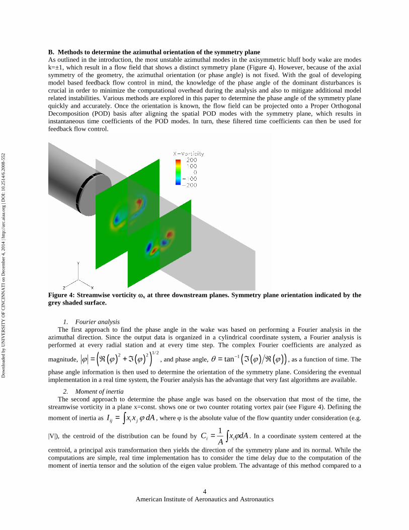
B. 8BMethods to determine the azimuthal orientation of the symmetry planeAs outlined in the introduction, the most unstable azimuthal modes in the axisymmetric bluff body wake are modesk=±1, which result in a flow field that shows a distinct symmetry plane ( XFigure 4 X). However, because of the axialsymmetry of the geometry, the azimuthal orientation (or phase angle) is not fixed. With the goal of developingmodel based feedback flow control in mind, the knowledge of the phase angle of the dominant disturbances iscrucial in order to minimize the computational overhead during the analysis and also to mitigate additional modelrelated instabilities. Various methods are explored in this paper to determine the phase angle of the symmetry planequickly and accurately. Once the orientation is known, the flow field can be projected onto a Proper OrthogonalDecomposition (POD) basis after aligning the spatial POD modes with the symmetry plane, which results ininstantaneous time coefficients of the POD modes. In turn, these filtered time coefficients can then be used forfeedback flow control.

Figure 4: Streamwise vorticity ωx at three downstream planes. Symmetry plane orientation indicated by thegrey shaded surface.

1. 1 2BFourier analysisThe first approach to find the phase angle in the wake was based on performing a Fourier analysis in the

azimuthal direction. Since the output data is organized in a cylindrical coordinate system, a Fourier analysis isperformed at every radial station and at every time step. The complex Fourier coefficients are analyzed as

magnitude, ( ) ( )( )1/ 22 2ϕ ϕ ϕ= ℜ +ℑ , and phase angle, ( ) ( )( )1tanθ ϕ ϕ−= ℑ ℜ , as a function of time. The

phase angle information is then used to determine the orientation of the symmetry plane. Considering the eventualimplementation in a real time system, the Fourier analysis has the advantage that very fast algorithms are available.

2. 1 3BMoment of inertiaThe second approach to determine the phase angle was based on the observation that most of the time, the

streamwise vorticity in a plane x=const. shows one or two counter rotating vortex pair (see XFigure 4 X). Defining the

moment of inertia as ij i jI x x dAϕ= ∫ , where ϕ is the absolute value of the flow quantity under consideration (e.g.

|V|), the centroid of the distribution can be found by ∫= dAxA

C ii ϕ1. In a coordinate system centered at the

centroid, a principal axis transformation then yields the direction of the symmetry plane and its normal. While thecomputations are simple, real time implementation has to consider the time delay due to the computation of themoment of inertia tensor and the solution of the eigen value problem. The advantage of this method compared to a

Dow

nloa

ded

by U

NIV

ER

SIT

Y O

F C

INC

INN

AT

I on

Dec

embe

r 4,

201

4 | h

ttp://

arc.

aiaa

.org

| D

OI:

10.

2514

/6.2

008-

552


Fourier analysis is that the integration over the flow field provides some smoothing so that small fluctuations do nothave a significant influence on the result. This is particularly important in an experimental implementation.

3. 1 4BVelocity vector histogramAnother method was developed after observing the time varying velocity vector field in a plane x/D=const. As

shown above, in such a plane the flow field is dominated by a counter rotating vortex pair that results from cuttingthrough the streamwise vortex loops (see also XFigure 6 X and XFigure 7 X). The majority of the velocity vectors, mainlydue to the induced velocity of the vortex pair, is aligned with the symmetry plane. Obtaining the direction of eachvelocity vector and using a histogram to quantify the result, the dominant vector orientation should therefore be inthe direction of the symmetry plane.

For real time implementation, this method is well suited because it analyzes quantities that can be measuredusing PIV. PIV is a sensor tool for laboratory based feedback flow control that has been shown to be effective by theauthors.6

III. 3BResults

A. 9BUnforced WakeThe natural wake behind an axisymmetric body at a Reynolds number of ReD=1,500 exhibits vortex sheddingsimilar to a von Kármán vortex street behind a circular cylinder. Initial computational results and an approach toanalyzing this data have been presented by the authors.15 To give a impression of the flow features in the near wake,instantaneous contours of total vorticity Ω are shown in XFigure 5 X. In XFigure 6 X, the instantaneous wake structures arevisualized using a total vorticity isosurface. In XFigure 7 X, the same time instant is visualized using an isosurface of theQ vortex identification criterion.18 While the overall flow structures are clearly captured by both visualizationmethods, the Q criterion eliminates the influence of the mean shear in the boundary layer and early shear layer,showing more detail of the vortical structures near the base of the axisymmetric body.

Figure 5: Instantaneous total vorticity Ω contours.

Figure 6: Isosurface of total vorticity Ω=40 s-1. Left: view from the positive z-direction. Right: view from thenegative y-direction.

Dow

nloa

ded

by U

NIV

ER

SIT

Y O

F C

INC

INN

AT

I on

Dec

embe

r 4,

201

4 | h

ttp://

arc.

aiaa

.org

| D

OI:

10.

2514

/6.2

008-

552


Figure 7: Q=10 s-2. Left: view from the positive z-direction. Right: view from the negative y-direction.

The unforced wake computation is used to initialize the forced runs. In addition, the results obtained using thenewly developed tools will be presented at the end of this section.

In the following sections, unless stated otherwise, the flow field is analyzed at a location x/D=2 downstream ofthe base of the axisymmetric bluff body.

B. 10BForcing Θ0=0When forcing of modes k=±1 is applied within the lock-in region using the eight blowing and suction slots, the flowreacts to the forcing by adjusting the shedding frequency to the forcing frequency and the also by aligning thesymmetry plane with the forcing.

1. 1 5BFourier decompositionAfter analyzing a number of streamwise and radial locations, x/D=2 and r/D=0.55 was selected for performing

the Fourier analysis of the flow field. For forcing at Θ=0, the result are plotted in XFigure 8 X over the time span of tenforcing cycles. Each plot shows the phase angles of the first four Fourier modes. XFigure 8 Xa shows the phase anglesof the modes of the streamwise velocity component. The mean flow doesn’t have an azimuthal variation. The firstmode (second graph) is shown to oscillate between zero and ±π, indicating the movement of the vortex pair shownin XFigure 4 X along the y axis. The higher modes are shown for completeness. In XFigure 8 Xb, the phase angles of theFourier modes of the v-velocity component are shown. The mean flow (mode 0) oscillates between 0 and π,indicating the motion of the vortex pair along the y axis. Although the first and second modes show many phasejumps, they also indicate a motion between phase angles 0 and π. For the W-velocity, the mean flow showssomewhat random oscillations compared to the v-velocity. This is due to the predominant motion along the y-axis;the magnitude of the W-velocity is negligible, as can be seen from the Fourier mode amplitude (not shown) andtherefore the determination of the phase angle is difficult. The final panel, XFigure 8 Xd, shows the phase angles of theFourier modes of ωx. Focusing on the first mode, the phase angle shows a distinct oscillation between Θ=±π/2.

With these results, it seems reasonable to use the Fourier mode phase orientation as a tool to determine theorientation of the symmetry plane in the flow field. While the zeroth mode of the V-velocity seems to show the bestsignal, it cannot be relied upon for forcing at different phase angles, as indicated by the zeroth mode of the W-velocity and its vanishing magnitude. Also, the additional computations necessary to obtain the streamwise vorticityis viewed as an obstacle to eventual real time implementation. However, testing the criterion using different forcingphase angles will clarify which quantity (U-, V-, W-velocity or ωx) and which mode to focus on (see below).

Dow

nloa

ded

by U

NIV

ER

SIT

Y O

F C

INC

INN

AT

I on

Dec

embe

r 4,

201

4 | h

ttp://

arc.

aiaa

.org

| D

OI:

10.

2514

/6.2

008-

552


a) b)

c) d)

Figure 8: Fourier phase angles for a) U-velocity, b) V-velocity, c) W-velocity, d) streamwise vorticity ωx

2. 1 6B Moment of inertiaAs outlined above, the computation of the moment of inertia is a straight forward integration of the absolute

value of a given flow quantity. In this case, the streamwise velocity component, U, does not yield very good resultsbecause the fluctuations are masked by the free stream. While subtracting the mean flow is certainly possible, itnecessitates extra computations and was deemed too time consuming when considering real time implementation ofthis procedure.

The phase angles of the V- and W-velocity components are plotted in XFigure 9 X. As shown in XFigure 9 Xa, the firstprincipal axis of the V-velocity is oriented at Θ=±π, i.e., along the y-axis. The second principal axis (the ordering isdetermined based on the magnitude of the eigen value) is orthogonal, i.e., Θ=-π/2, or along the z-axis. For the W-velocity, the roles of the principal axes are reversed, but the information obtained from the data is the same: Thesymmetry plane is oriented in either the y-direction or the z-direction. However, without some additionalinformation, it is currently unclear how to determine which of the two principal axes is aligned with the symmetryplane. Nonetheless, with the goal of locating the symmetry plane, the problem has been reduced considerably, sinceonly two orientations remain to be checked.

Dow

nloa

ded

by U

NIV

ER

SIT

Y O

F C

INC

INN

AT

I on

Dec

embe

r 4,

201

4 | h

ttp://

arc.

aiaa

.org

| D

OI:

10.

2514

/6.2

008-

552


a) b)

Figure 9: Principal directions of the moment of inertia of a) V-velocity, b) W-velocity.

For completeness, the direction of the principal axes as obtained from the streamwise vorticity, ωx, is shown inXFigure 10 X.

Figure 10: Principal directions of the moment of inertia obtained by analyzing ωx.

3. 1 7B Velocity vector histogramThe idea of analyzing the velocity vector field directly was developed after observing the vector field obtained

from experimental investigations. An example of such a vector field is shown in XFigure 11 Xa. Aside from the flowaround the vortex pair, the velocity field is essentially aligned with the symmetry plane. To obtain an estimate of theorientation of the symmetry plane, the direction of each velocity vector is determined and a histogram with a verydistinct maximum is computed (XFigure 11 Xb). From the histogram data, in this instance the flow is predominantly inthe Θ=-π direction, i.e., to the left, in agreement with the observation of the velocity field.D

ownl

oade

d by

UN

IVE

RSI

TY

OF

CIN

CIN

NA

TI

on D

ecem

ber

4, 2

014

| http

://ar

c.ai

aa.o

rg |

DO

I: 1

0.25

14/6

.200

8-55

2


a) b)

Figure 11: Left: Instantaneous velocity vector plot, right: Histogram.

This analysis was performed for all ten forcing cycles and the dominant phase angle, i.e. the maximum angle inthe histogram, is plotted as a function of time in XFigure 12 Xa. An additional variable that has to be considered in thistype of analysis is the number of bins to be considered in the histogram. XFigure 12X shows the result for 64, 32, 16,and 8 bins. XFigure 12 Xa shows that it takes approximately three forcing periods for the flow to achieve a phase ofΘ=0/π. The figure also shows that the “lock-in” that can be achieved, when measured by the phase angle, is not asobvious as in the case of the von Kármán vortex shedding behind a circular cylinder. A possible explanation is thatslight (numerical) variations in the forcing amplitudes because of grid variation at the forcing slots (the grid is notforced to mirror the symmetry of the geometry).

As with the other methods introduced above, the velocity histogram analysis shows that the symmetry plane isoriented in the y-direction. While this is the most important result of this analysis, the figures also show that the flowfield, even at the forcing level of A/U∞=0.3, takes approximately four shedding cycles before it fully ‘locks-in’ tothe forcing input. While this phenomenon can also be observed in the other analysis methods, it is most clearly seenin the velocity histograms. This will have important implications when considering transient forcing.

Dow

nloa

ded

by U

NIV

ER

SIT

Y O

F C

INC

INN

AT

I on

Dec

embe

r 4,

201

4 | h

ttp://

arc.

aiaa

.org

| D

OI:

10.

2514

/6.2

008-

552


a) b)

c) d)

Figure 12: Flow angle obtained from velocity vector histogram. a) 64 bins, b) 32 bins, c) 16 bins, d) 8 bins.

C. 11BTransient Forcing Θ0=0π/2This case was computed as a continuation of the previous simulation with the goal of studying the transient

behavior of the wake. In the figures shown in this section, the complete time history of forcing ten cycles with aphase orientation of Θ0=0 and ten cycles with Θ0=π/2 is shown.

1. 18BFourier decompositionXFigure 13 X shows the result of applying the Fourier decomposition and plotting the phase angle of the modes over

time. The red line indicates the time when the forcing is turned to the new orientation. For the U-velocity ( XFigure13Xa), the first mode shows that the phase angle shifts within less than two forcing cycles. The V-velocity ( XFigure13Xb), as expected from the analysis above, does not give meaningful data after the rotation of the forcing since thevelocity magnitude is now minimal. However, in the zeroth mode it can be observed that it takes approximately oneand a half forcing cycles for the wake to rotate and follow the forcing. In contrast, the W-velocity ( XFigure 13 Xc), thephase information of the zeroth mode becomes periodic within one forcing cycle, indicating that the flow has turnedat the observed downstream location x/D=2. For the streamwise vorticity, the first mode shows a shift from adominant orientation of Θ=±π/2 to Θ=0 and Θ=π. In summary, independent of the flow quantity observed, theFourier transform does show a clear signature of the turning of the symmetry plane in the wake.

Dow

nloa

ded

by U

NIV

ER

SIT

Y O

F C

INC

INN

AT

I on

Dec

embe

r 4,

201

4 | h

ttp://

arc.

aiaa

.org

| D

OI:

10.

2514

/6.2

008-

552


a) b)

c) d)

Figure 13: Fourier phase angles for a) U-velocity, b) V-velocity, c) W-velocity, d) streamwise vorticity ωx.

2. 1 9B Moment of inertiaThe results obtained using the moment of inertia of the U-velocity and the V-velocity are plotted in XFigure 14X.

As the figures indicate, this method of analysis does not provide an indicator of the change in the orientation of thesymmetry planes. However, the streamwise vorticity ( XFigure 15X) indicates the rotation of the first principal axisrotates from Θ=-π to Θ=-π/2. It is interesting to note that it takes approximately five forcing cycles before thesymmetry plane stabilizes in its new azimuthal orientation.

a) b)

Figure 14: Principal directions of the moment of inertia of a) V-velocity, b) W-velocity.

Dow

nloa

ded

by U

NIV

ER

SIT

Y O

F C

INC

INN

AT

I on

Dec

embe

r 4,

201

4 | h

ttp://

arc.

aiaa

.org

| D

OI:

10.

2514

/6.2

008-

552


Figure 15: Principal directions of the moment of inertia obtained by analyzing ωx.

3. 20B Velocity vector histogramAs in the previous sections, the velocity histograms are computed and analyzed. The results are shown in XFigure

16X for four different bin sizes, 64, 32, 16, and 8 bins. After the change in the forcing orientation at t/T=10, the phaseangle turns to Θ=±π/2 within one to two forcing cycles, however, it takes about seven cycles before the maximum inthe velocity vector histogram stabilizes in this orientation. When fewer bins are used, the measurement seems tobecome more focused, however, the azimuthal phase change and the observed “lock-in” does not changesignificantly.

a) b)

c) d)

Figure 16: Flow angle obtained from velocity vector histogram. a) 64 bins, b) 32 bins, c) 16 bins, d) 8bins.

Dow

nloa

ded

by U

NIV

ER

SIT

Y O

F C

INC

INN

AT

I on

Dec

embe

r 4,

201

4 | h

ttp://

arc.

aiaa

.org

| D

OI:

10.

2514

/6.2

008-

552


IV. 4BConclusionComputations of the unforced and forced wake of an axisymmetric bluff body at a Reynolds number of Re=1,500based on diameter were performed. Due to the natural flow instability, the dominant structures in the wake are twocounter rotating helical modes with azimuthal wave numbers k=±1. The resulting flow field exhibits a plane ofsymmetry that can rotate over time in a random fashion in the natural (unforced) wake flow. When forcing inside the“lock-in” envelope is applied, the symmetry plane can be forced to remain at a fixed orientation.Three methods, namely azimuthal Fourier decomposition, analysis based on a moment of inertia computation, and avelocity vector histogram, have been investigated to determine the azimuthal phase of the symmetry plane. The firsttwo methods can be applied to any flow quantity. While all methods show the rotation of the symmetry plane whenthe forcing is rotated, all methods show transients that, when only one instant in time is available as an observation,could be misinterpreted as a rapid rotation of the symmetry plane. These transients, while inherent in the flow field,are not the goal of eventual feedback flow control, and an observer that takes some time history into considerationmight become necessary. In the end, the real time implementation, where the goal is a minimal computationaloverhead in addition to an accurate determination of the phase angle, will have to show which method is mostsuitable.

5BAcknowledgmentsThe authors would like to acknowledge funding by the Air Force Office of Scientific Research, LtCol Wells.Computational support provided by the Modeling and Simulation Research Center, directed by Dr. Keith Bergeron,as well as the support by Dr. Jim Forsythe, Cobalt Solutions, LLC, is gratefully acknowledged.

6BReferences1. Koopmann, G., “The Vortex Wakes of Vibrating Cylinders at Low Reynolds Numbers”, Journal of Fluid Mechanics, Vol.

28 Part 3, 1967, pp. 501-512.2. Williamson, C.H.K., “Vortex Dynamics in the Cylinder Wake”, Ann. Rev. Fluid Mech., 1996, 28:477-5393. Monkewitz, P. A., “Modeling of self-excited wake oscillations by amplitude equations”, Experimental Thermal and Fluid

Science, Vol. 12, 1996, pp. 175-183.4. Noack, B. R., Eckelmann, H. “A global stability analysis of the steady and periodic cylinder wake”,J. Fluid Mechanics,

Vol. 270, pp. 331-347.5. Blevins, R., “Flow Induced Vibration”, 2nd Edition, Van Nostrand Reinhold, 1990, pp. 54-58.6. Siegel, S., Cohen, K. & McLaughlin T., 2003, “Feed-back control of a circular cylinder wake in experiment and simulation

(invited)”, AIAA 2003-3569.7. Cohen K., Siegel S., McLaughlin T. & Gillies E., “Feedback Control of a Cylinder Wake Low-Dimensional Model”,

AIAA Journal 41, No. 7, 1389-1391.8. Cohen, K., Siegel,S., McLaughlin, T., “Sensor Placement Based on Proper Orthogonal Decomposition Modeling of a

Cylinder Wake”, 33rd AIAA Fluid Dynamics Conference, Orlando, AIAA 2003-4259, 20039. Aschenbach, E. 1974, “Vortex shedding from spheres”, Journal of Fluid Mechanics, Vol 62, 209.10. Sakamoto, Haniu, 1990, “A study on vortex shedding from spheres in a uniform flow”, J. Fluids Eng., 112, pp. 386-393.11. Monkewitz, P.A. 1988, “A note on vertex shedding from axisymmetric bluff bodies”, Journal of Fluid Mechanics, Vol

192, pp 561-575.12. Cannon, S.C., 1991, “Large-Scale Structures and the Spatial Evolution of Wakes behind Axisymmetric Bluff Bodies”,

Dissertation, University of Arizona.13. Schwarz, V., Bestek, H., Fasel, H. 1994, “Numerical simulation of nonlinear waves in the wake of an axisymmetric bluff

body”, AIAA 94-2285.14. Tourbier, D., 1996, “Numerical investigation of transitional and turbulent axisymmetric wakes at supersonic speeds”.

Dissertation, University of Arizona.15. J. Seidel, S. Siegel., K. Cohen., and T. McLaughlin, “Simulations Of Flow Control Of The Wake Behind An

Axisymmetric Bluff Body”, AIAA Paper 2006-3490, 2006.16. Cohen, K., Siegel,S., Seidel, J., McLaughlin, T., “Reduced Order Modeling for Closed-Loop Control of Three

Dimensional Wakes”, AIAA Paper 2006-3356.17. Siegel, S., Fasel, H., “Effect of Forcing on the Wake Drag of an Axisymmetric Bluff Body”, AIAA 2001-0736.18. Y. Dubief and F. Delcayre. 2000, “On coherent-vortex identification in turbulence” J. Turbulence 1, 1-22.

Dow

nloa

ded

by U

NIV

ER

SIT

Y O

F C

INC

INN

AT

I on

Dec

embe

r 4,

201

4 | h

ttp://

arc.

aiaa

.org

| D

OI:

10.

2514

/6.2

008-

552

Analysis of an Axisymmetric Bluff Body Wake Using Fourier Transform and POD

Documents

Transcript of Analysis of an Axisymmetric Bluff Body Wake Using Fourier Transform and POD