Linear Induction Motor (LIM) for Hyperloop Pod Prototypes

Research Collection

Master Thesis

Linear Induction Motor (LIM) for Hyperloop Pod Prototypes

Author(s): Timperio, Christopher

Publication Date: 2018-07

Permanent Link: https://doi.org/10.3929/ethz-b-000379531

Rights / License: In Copyright - Non-Commercial Use Permitted

This page was generated automatically upon download from the ETH Zurich Research Collection. For moreinformation please consult the Terms of use.

ETH Library

https://doi.org/10.3929/ethz-b-000379531

http://rightsstatements.org/page/InC-NC/1.0/

https://www.research-collection.ethz.ch

https://www.research-collection.ethz.ch/terms-of-use

Institute of Electromagnetic Fields (IEF)

Linear Induction Motor (LIM) for

Hyperloop Pod Prototypes

MASTER THESIS

Presented by: Christopher Louis Timperio

Supervised by: Prof. Dr. Jasmin Smajic

Prof. Dr. Juerg Leuthold

July 2018

In collaboration with:


This page is intentionally left blank.


LINEAR INDUCTION MOTOR (LIM) FOR HYPERLOOP POD PROTOTYPES

A thesis submitted to attain the degree of

MASTER OF SCIENCE of ETH ZÜRICH

(MSc ETH Zürich)

presented by

CHRISTOPHER LOUIS TIMPERIO

BSc ECE, Georgia Institute of Technology

born on 17.12.1990

United States of America

accepted on the recommendation of

Prof. Dr. Jasmin Smajic, examiner

Prof. Dr. Juerg Leuthold, co-examiner

July 2018

For papers written by groups the names of all authors are

required. Their signatures collectively guarantee the entire

content of the written paper.

Declaration of originality

The signed declaration of originality is a component of every semester paper, Bachelor’s thesis,

Master’s thesis and any other degree paper undertaken during the course of studies, including the

respective electronic versions.

Lecturers may also require a declaration of originality for other written papers compiled for their

courses.

I hereby confirm that I am the sole author of the written work here enclosed and that I have compiled it

in my own words. Parts excepted are corrections of form and content by the supervisor.

Title of work (in block letters):

Authored by (in block letters):

For papers written by groups the names of all authors are required.

Name(s):

First name(s):

With my signature I confirm that

− I have committed none of the forms of plagiarism described in the ‘Citation etiquette’ information

sheet.

− I have documented all methods, data and processes truthfully.

− I have not manipulated any data.

− I have mentioned all persons who were significant facilitators of the work.

I am aware that the work may be screened electronically for plagiarism.

Place, date

Signature(s):

https://www.ethz.ch/content/dam/ethz/main/education/rechtliches-abschluesse/leistungskontrollen/plagiarism-citationetiquette.pdf



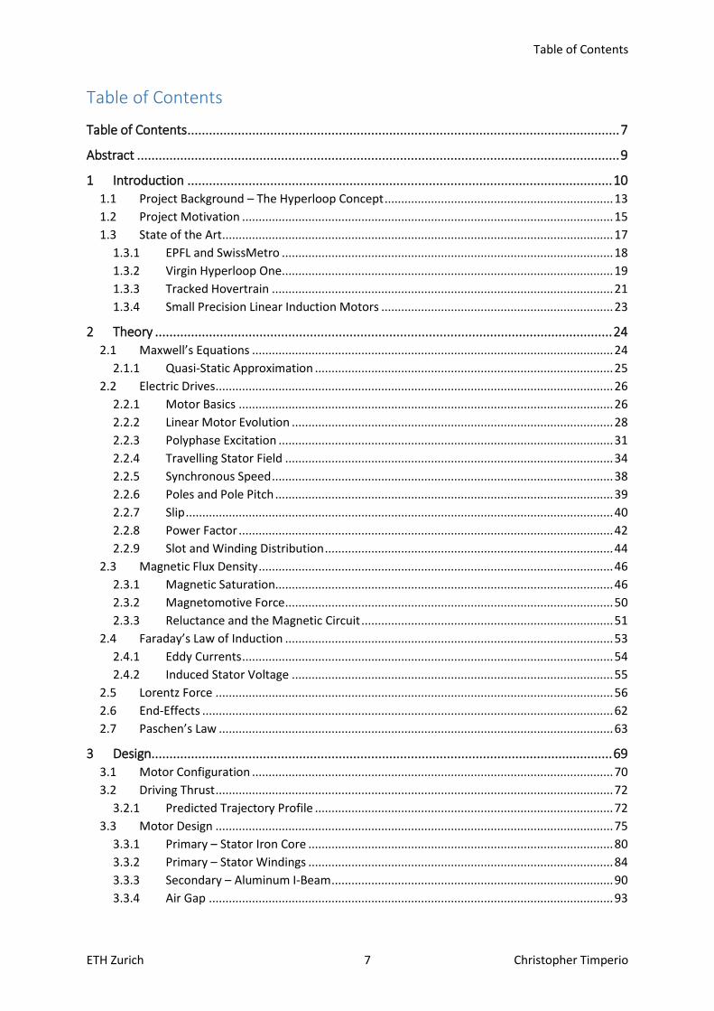
Table of Contents

ETH Zurich 7 Christopher Timperio

Table of Contents

Table of Contents ........................................................................................................................ 7

Abstract ...................................................................................................................................... 9

1 Introduction ...................................................................................................................... 10

1.1 Project Background – The Hyperloop Concept ..................................................................... 13

1.2 Project Motivation ................................................................................................................ 15

1.3 State of the Art ...................................................................................................................... 17

1.3.1 EPFL and SwissMetro .................................................................................................... 18

1.3.2 Virgin Hyperloop One .................................................................................................... 19

1.3.3 Tracked Hovertrain ....................................................................................................... 21

1.3.4 Small Precision Linear Induction Motors ...................................................................... 23

2 Theory ............................................................................................................................... 24

2.1 Maxwell’s Equations ............................................................................................................. 24

2.1.1 Quasi-Static Approximation .......................................................................................... 25

2.2 Electric Drives ........................................................................................................................ 26

2.2.1 Motor Basics ................................................................................................................. 26

2.2.2 Linear Motor Evolution ................................................................................................. 28

2.2.3 Polyphase Excitation ..................................................................................................... 31

2.2.4 Travelling Stator Field ................................................................................................... 34

2.2.5 Synchronous Speed ....................................................................................................... 38

2.2.6 Poles and Pole Pitch ...................................................................................................... 39

2.2.7 Slip ................................................................................................................................. 40

2.2.8 Power Factor ................................................................................................................. 42

2.2.9 Slot and Winding Distribution ....................................................................................... 44

2.3 Magnetic Flux Density ........................................................................................................... 46

2.3.1 Magnetic Saturation...................................................................................................... 46

2.3.2 Magnetomotive Force ................................................................................................... 50

2.3.3 Reluctance and the Magnetic Circuit ............................................................................ 51

2.4 Faraday’s Law of Induction ................................................................................................... 53

2.4.1 Eddy Currents ................................................................................................................ 54

2.4.2 Induced Stator Voltage ................................................................................................. 55

2.5 Lorentz Force ........................................................................................................................ 56

2.6 End-Effects ............................................................................................................................ 62

2.7 Paschen’s Law ....................................................................................................................... 63

3 Design ................................................................................................................................ 69

3.1 Motor Configuration ............................................................................................................. 70

3.2 Driving Thrust ........................................................................................................................ 72

3.2.1 Predicted Trajectory Profile .......................................................................................... 72

3.3 Motor Design ........................................................................................................................ 75

3.3.1 Primary – Stator Iron Core ............................................................................................ 80

3.3.2 Primary – Stator Windings ............................................................................................ 84

3.3.3 Secondary – Aluminum I-Beam ..................................................................................... 90

3.3.4 Air Gap .......................................................................................................................... 93

Table of Contents


3.4 Final Model ........................................................................................................................... 95

3.5 Electrical Design .................................................................................................................... 98

3.5.1 Power ............................................................................................................................ 98

3.5.2 Batteries ...................................................................................................................... 103

3.5.3 Inverters ...................................................................................................................... 108

3.6 Motor Fabrication ............................................................................................................... 113

3.7 Temperature Considerations .............................................................................................. 116

4 Results ............................................................................................................................. 118

4.1 Double-Sided 24 Slot 2-Pole LIM......................................................................................... 118

5 Summary ......................................................................................................................... 125

5.1 Project Challenges ............................................................................................................... 125

5.2 Outlook ............................................................................................................................... 127

5.2.1 Design Improvements ................................................................................................. 128

6 References ....................................................................................................................... 129

Acknowledgements ................................................................................................................. 131

Appendix A: Why Linear Motors? ...................................................................................... 133

Appendix B: SpaceX Hyperloop Subtrack Technical Drawing ............................................. 135

Appendix C: Swissloop Test Track – Dübendorf Testing Facilities ...................................... 137

Appendix D: Escher Pod with Double-Sided 24 Slot LIM .................................................... 139

Appendix E: M400-50A Iron Core Material Data Sheet ..................................................... 141

Appendix F: LIM Technical Drawing: 24 Slot 2-Pole........................................................... 143

Appendix G: Comsol Multi-turn Coil Geometry Arrangement ............................................ 145

Abstract


Abstract

Mobility is one of the main dilemmas facing a sustainable, clean-energy future. How can people and

cargo be transported over long distances, without expending large amounts of fossil fuel energies or

producing a large carbon footprint? How can this be done quickly and efficiently? Finding a mode of

transportation which is energy-efficient, inexpensive, and even offers passenger transport is the task

which the Swissloop team is striving towards each day. We as a team are currently focused on building

the first ever Swiss solution for the Hyperloop. We are proud to say that our Swissloop product aims

to be the fastest form of ground transportation ever conceived.

Swissloop’s long term vision is to find ways to propel its pod capsules at speeds in excess of 1,000

km/h or 600 mi/h, while at the same time, having the smallest impact possible on our environment.

These incredibly fast, yet energy-efficient ground speeds are to be realized by means of a magnetic

linear accelerator. Therefore, we at Swissloop are researching and developing a linear induction motor

prototype to be the foundation for future high-speed linear propulsion drives for Hyperloop-like

systems.

Developing an efficient yet powerful Linear Induction Motor (LIM) is key to Swissloop’s future as a

sustainable Hyperloop transportation company. Passenger and cargo capsules need to be accelerated

via some form of a high-speed linear accelerator – and a LIM is believed to be one of the best options

for such a system. Before such a feat can be accomplished, scalable prototype motors should be

developed in the short to medium term to help understand and formulate future, more complex linear

accelerator systems. Therefore, the aim of the thesis is to develop a prototype LIM – providing

Swissloop with a first iteration of a sustainable and efficient, yet powerful linear drive system.

“I could spend years trying to discover the origin of these mystic forces of electromagnetism, but as

an engineer I haven't got time to do this.” October 1972

Professor Eric Roberts Laithwaite – "Father of Maglev"

(1921 – 1997)

Introduction


1 Introduction

The need to revolutionize current transportation systems towards a faster, more energy-efficient and

environmentally sustainable solution will be one of the defining goals of this generation. When

thinking of transport, a loss of time, crowded trains with delays, cancelled flights, missed connections,

traffic jams on packed freeways, pollution and an overall unpleasant obstacle come to mind. The most

common mode of transport today is the automobile or car. It’s reliable, convenient, gets us to where

we need to be in a relatively short time span, and is generally affordable for the average middle-class

family. However, the most obvious and well-known downside of the car, is soul-crushing traffic.

In addition to the car, the other two most popular modes of transport include trains and planes.

Railways are efficient and simple to arrange travel with, but tend to arrive slow to the destination,

when compared with planes or cars. Air travel is known for its negative impact on the environment

and airport security is probably one of the most dreadful encounters to experience. Each have their

obvious downsides, however, they have become the norm in our current way of thinking about

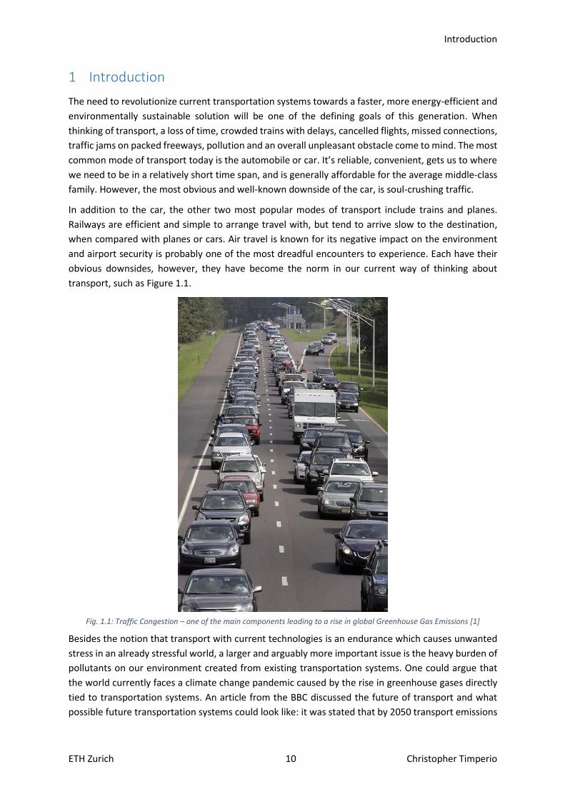
transport, such as Figure 1.1.

Fig. 1.1: Traffic Congestion – one of the main components leading to a rise in global Greenhouse Gas Emissions [1]

Besides the notion that transport with current technologies is an endurance which causes unwanted

stress in an already stressful world, a larger and arguably more important issue is the heavy burden of

pollutants on our environment created from existing transportation systems. One could argue that

the world currently faces a climate change pandemic caused by the rise in greenhouse gases directly

tied to transportation systems. An article from the BBC discussed the future of transport and what

possible future transportation systems could look like: it was stated that by 2050 transport emissions

Introduction


are projected to double due to a strong increase in demand for cars in developing countries. There

could be as many as 2.5 billion cars on the road at that time, with most of them concentrated in large

cities [2]. More cars would mean huge increases in the amount of global carbon emissions.

The Organization for Economic Co-operation and Development (OECD) conducted a study in 2010,

which found that global carbon levels have reached 30.6 gigatonnes, and that by 2050, current

greenhouse gas emissions will increase by another 50% [3]. The OECD also projects that atmospheric

concentration of greenhouse gas emissions will reach almost 685 parts per million (ppm) CO2-

equivalents by 2050. This amount is well over the concentration level of 450 ppm, which is the upper

bound for having a 50% chance of stabilizing the climate at a 2°C global average temperature increase

[3]. Transportation systems are one of the leading causes of this ever-increasing concentration of

greenhouse gas emissions.

The U.S. Global Change Research Program, which includes federal government organizations such as

NASA, NOAA, DoD, Dept. of Transportation, Dept. of Commerce, Dept. of Energy, and other U.S.

federal organizations, – have launched a National Climate Assessment with the sole purpose of

assessing and summarizing the impacts of climate change on the United States, now and into the

future. The assessment stated that current transportation systems contribute to changes in the

climate through emissions [1]. In 2010, the U.S. transportation sector accounted for 27% of total U.S.

greenhouse gas emissions, with passenger cars and trucks accounting for 65% of that total.

Furthermore, petroleum accounts for 93% of the nation’s transportation energy use [1]. These

findings indicate that policies and behavioral changes – aimed at reducing greenhouse gas emissions

– will have significant implications for the various components of future transportation sectors.

As one studies the topic of current transportation systems, it becomes very clear, that if the goal is a

sustainable future – one in which greenhouse gas emissions are decreasing instead of increasing – a

new mode of transportation is required. For example, a transportation system which at its core,

operates on a clean propulsion technology. Such a solution would need to be both economically viable

into the long term and environmentally sustainable – producing low or no carbon emissions.

MunichRe; one of the world’s largest insurance companies has recently performed a comprehensive

risk analysis study on Hyperloop Transportation Technologies (HTT) – one of the leading Hyperloop

companies focusing on passenger and cargo transport – to see if the overarching Hyperloop

technology is feasible. They not only evaluated the company itself, but also the many risks and

challenges in developing a full-scale Hyperloop system. After evaluating the company and its core

competencies, they came to the conclusion that the Hyperloop technology is in indeed feasible, and

also insurable in the medium term [4]. Also stated in [4]; “The analysis constitutes a milestone for the

future success of HTT’s Hyperloop technology and of the company itself.” Having a world-renowned

insurance company classify the Hyperloop technology as feasible and state that a future based on the

technology’s success is possible, is extremely optimistic and promising. Some renderings of what a

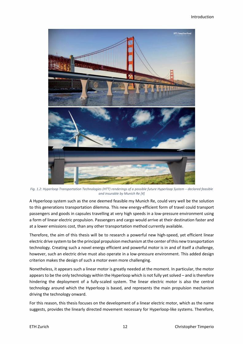
possible Hyperloop future might look like – as imagined by HTT – can be seen below in Figure 1.2.

Introduction


Fig. 1.2: Hyperloop Transportation Technologies (HTT) renderings of a possible future Hyperloop System – declared feasible

and insurable by Munich Re [4]

A Hyperloop system such as the one deemed feasible my Munich Re, could very well be the solution

to this generations transportation dilemma. This new energy-efficient form of travel could transport

passengers and goods in capsules travelling at very high speeds in a low-pressure environment using

a form of linear electric propulsion. Passengers and cargo would arrive at their destination faster and

at a lower emissions cost, than any other transportation method currently available.

Therefore, the aim of this thesis will be to research a powerful new high-speed, yet efficient linear

electric drive system to be the principal propulsion mechanism at the center of this new transportation

technology. Creating such a novel energy efficient and powerful motor is in and of itself a challenge,

however, such an electric drive must also operate in a low-pressure environment. This added design

criterion makes the design of such a motor even more challenging.

Nonetheless, it appears such a linear motor is greatly needed at the moment. In particular, the motor

appears to be the only technology within the Hyperloop which is not fully yet solved – and is therefore

hindering the deployment of a fully-scaled system. The linear electric motor is also the central

technology around which the Hyperloop is based, and represents the main propulsion mechanism

driving the technology onward.

For this reason, this thesis focuses on the development of a linear electric motor, which as the name

suggests, provides the linearly directed movement necessary for Hyperloop-like systems. Therefore,

Introduction


this thesis offers a prototype design of a linear induction motor (LIM) with the potential to be the

foundation for future linear motor development for the Hyperloop. A LIM could be scaled up and

deployed into future full-scale Hyperloop systems. Further explanation into why a linear induction

motor has been chosen, is discussed further in Appendix A. Several iterations of the design have been

studied and simulated, and an optimized version has been selected. The final LIM that has been built,

has also been optimized for speed and performance, on a specified track.

The linear motor presented here has been designed and manufactured in Switzerland. It has been

designed to operate at approximately half the speed of a full-scale Hyperloop: 500 km/h. It weighs a

total of 80kg and generates a peak thrust of 4.69kN. This yields a thrust-to-weight ratio of 3 – similar

to that of the Space Shuttle.

The motor is planned to be mounted onto a prototype testing Pod weighing roughly 250kg. This testing

Pod comes complete with avionics, telemetry, stability and braking systems. This means that the

required telemetry data from sensors can be collected without added engineering. The mechanical

design is also complete, and the Pod runs well on the selected track. After testing on an open-air test

track facility in Dübendorf Switzerland, top speeds will be measured and recorded.

Additionally, the motor’s operation will be tested in a low-pressure environment of pressurized

conditions around 8mbar. Together with a design top speed of 500 km/h, a thrust-to-weight ratio of

3 and low-pressure operation, this linear induction motor prototype is the fastest, most powerful,

robust, and efficient LIM prototype to date – for the application of the Hyperloop.

1.1 Project Background – The Hyperloop Concept

The Hyperloop concept as it is known today, was introduced back in 2013 by Elon Musk [5]. Musk

talked about a cheaper, faster and more environmentally friendly alternative to the roughly $70 billion

USD California high-speed rail project, and introduced the Hyperloop; as a fifth mode of transportation

[5]. To which – if developed properly – could revolutionize cargo and passenger transportation and

travel as we know it today. A sketch of the original Hyperloop idea from Musk can be seen below in

Figure 1.3.

Fig. 1.3: Early Hyperloop Sketch [5]

Introduction


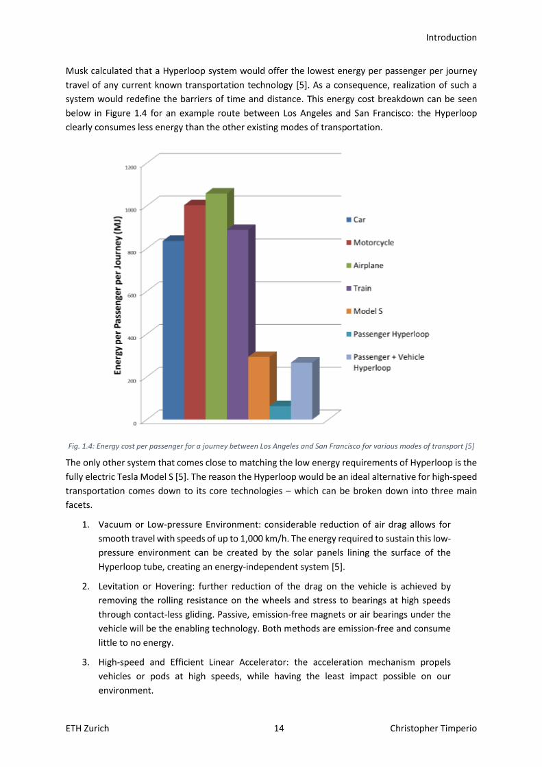
Musk calculated that a Hyperloop system would offer the lowest energy per passenger per journey

travel of any current known transportation technology [5]. As a consequence, realization of such a

system would redefine the barriers of time and distance. This energy cost breakdown can be seen

below in Figure 1.4 for an example route between Los Angeles and San Francisco: the Hyperloop

clearly consumes less energy than the other existing modes of transportation.

Fig. 1.4: Energy cost per passenger for a journey between Los Angeles and San Francisco for various modes of transport [5]

The only other system that comes close to matching the low energy requirements of Hyperloop is the

fully electric Tesla Model S [5]. The reason the Hyperloop would be an ideal alternative for high-speed

transportation comes down to its core technologies – which can be broken down into three main

facets.

1. Vacuum or Low-pressure Environment: considerable reduction of air drag allows for

smooth travel with speeds of up to 1,000 km/h. The energy required to sustain this low-

pressure environment can be created by the solar panels lining the surface of the

Hyperloop tube, creating an energy-independent system [5].

2. Levitation or Hovering: further reduction of the drag on the vehicle is achieved by

removing the rolling resistance on the wheels and stress to bearings at high speeds

through contact-less gliding. Passive, emission-free magnets or air bearings under the

vehicle will be the enabling technology. Both methods are emission-free and consume

little to no energy.

3. High-speed and Efficient Linear Accelerator: the acceleration mechanism propels

vehicles or pods at high speeds, while having the least impact possible on our

environment.

Introduction


These three fundamental technologies make the Hyperloop an attractive choice for a future

transportation solution. Although it seems appealing to replace all modes of transport with

Hyperloop-like systems, the Hyperloop is only an ideal choice for certain cases. Situations that would

benefit most would be transport between cities having very high frequency travel and on routes below

1500 km or 900 miles in separation [5]. In these instances, use of a Hyperloop-like system would

greatly optimize travel and decrease the frequency of dramatic delays due to overpopulated areas,

traffic jams, and the unnecessary added pollutants to our carbon footprint. However, for longer

distances, it appears as though air travel is still most advantageous.

Although Elon Musk has recently pioneered this technology, and popularized the idea to the

mainstream public, the idea of traveling at high speeds inside evacuated tunnels dates back to even

the 19th century. Inventors such as Alfred Beach – most notably known for Beach Pneumatic Transit,

which was New York City’s first attempt at a subway – pictured a future where commuting could be

both fast and reliable [6]. More specifically, Beach thought to combine the efficiency of modern-day

railway systems with the speed of air travel, while at the same time, keeping environmental impact to

a minimum. However, Musk re-energized the idea, and initiated a movement with the public which in

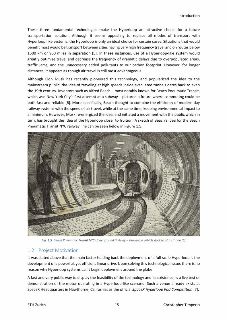
turn, has brought this idea of the Hyperloop closer to fruition. A sketch of Beach’s idea for the Beach

Pneumatic Transit NYC railway line can be seen below in Figure 1.5.

Fig. 1.5: Beach Pneumatic Transit NYC Underground Railway – showing a vehicle docked at a station [6]

1.2 Project Motivation

It was stated above that the main factor holding back the deployment of a full-scale Hyperloop is the

development of a powerful, yet efficient linear drive. Upon solving this technological issue, there is no

reason why Hyperloop systems can’t begin deployment around the globe.

A fast and very public way to display the feasibility of the technology and its existence, is a live test or

demonstration of the motor operating in a Hyperloop-like scenario. Such a venue already exists at

SpaceX Headquarters in Hawthorne, California; as the official SpaceX Hyperloop Pod Competition [7].

Introduction


This competition is open to university students all over the world, giving them the opportunity to

develop and test Hyperloop Pod prototypes, and Hyperloop technology in general, under the guidance

of experienced SpaceX engineers. It’s an engineering competition which encourages students to get

involved with and help grow the principal components behind the Hyperloop technology (such as its

key propulsion or levitation systems). Growing the different technologies, helps drive the overall goal

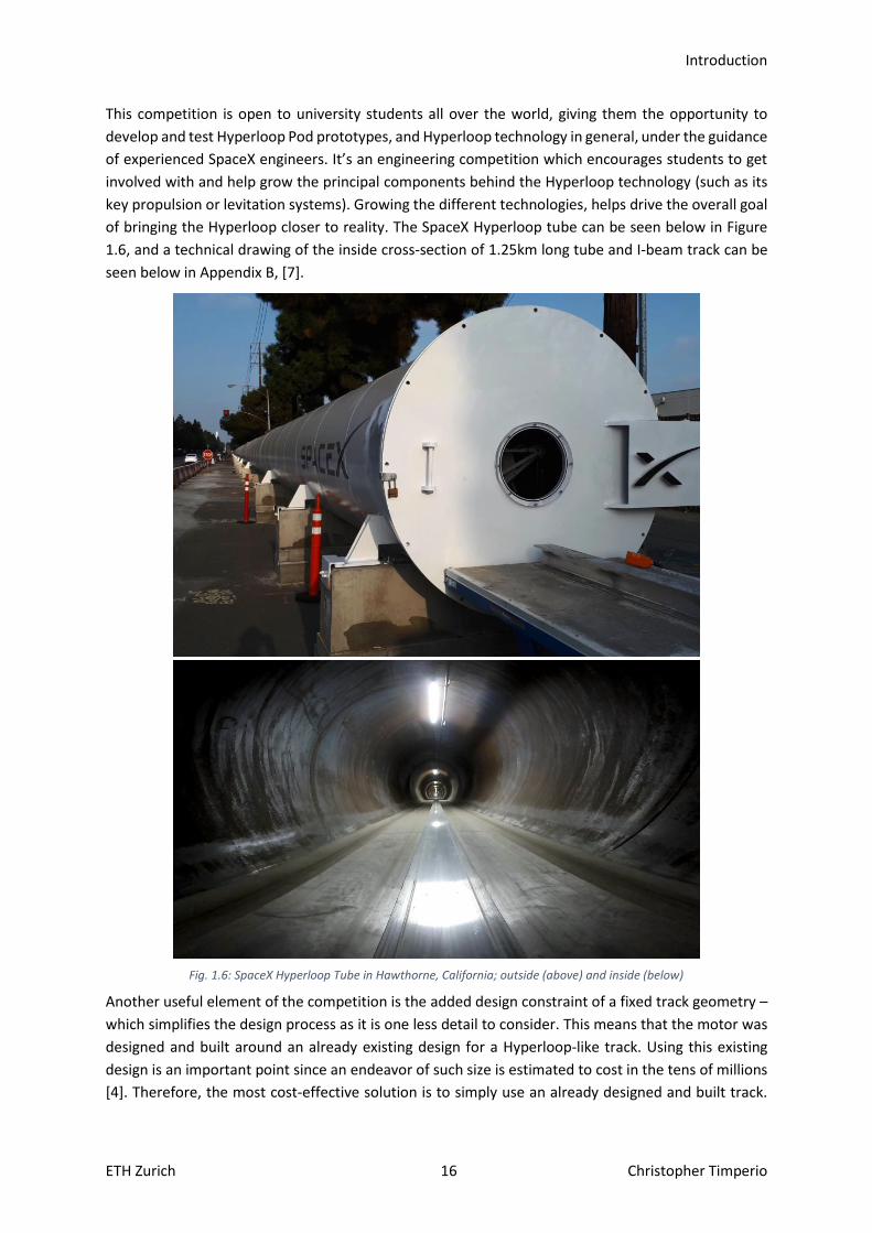
of bringing the Hyperloop closer to reality. The SpaceX Hyperloop tube can be seen below in Figure

1.6, and a technical drawing of the inside cross-section of 1.25km long tube and I-beam track can be

seen below in Appendix B, [7].

Fig. 1.6: SpaceX Hyperloop Tube in Hawthorne, California; outside (above) and inside (below)

Another useful element of the competition is the added design constraint of a fixed track geometry –

which simplifies the design process as it is one less detail to consider. This means that the motor was

designed and built around an already existing design for a Hyperloop-like track. Using this existing

design is an important point since an endeavor of such size is estimated to cost in the tens of millions

[4]. Therefore, the most cost-effective solution is to simply use an already designed and built track.

Introduction


This also means, the motor can be brought to any one of the numerous testing facilities that uses this

common track geometry, and the motor system can be tested with ease.

Therefore, the competition is the perfect test bench to test and measure such a prototype motor as

the one developed in this thesis. This standardization ensures the availability of a known track to test

the motor upon its completion. In addition to the SpaceX tube, which can be fully evacuated down to

low-pressures, there is also open-air test track at the Swissloop testing facilities in Dübendorf

Switzerland. The test track at the Dübendorf testing facility can be seen below in Figure 1.7, and the

technical drawing of this track layout can be seen in Appendix C.

Fig. 1.7: Test Track at Dübendorf Testing Facility

This test track can be used to test the linear motor in ambient pressure before testing inside a more

realistic Hyperloop tube – such as the SpaceX tube – which can operate under a low-pressure

environment.

Using such test tracks will help validate the motor design, and optimize performance and efficiency

through such testing – therefore reaching the speed goal of 500 km/h. If this speed goal is reached

here – in a university thesis – there is no telling what could be accomplished within a few years of

additional development.

In addition to the incentive of using the Hyperloop tube at SpaceX as a test bench for the prototype

linear motor, the competition also provides an open and transparent viewing of the most current

Hyperloop technology to the public. A competition with such a large audience will help grow the

overall Hyperloop technology faster and make the Hyperloop more realistic and deployable.

Therefore, another goal of this thesis to inform the public about linear induction motors. Since the

linear motor is the key technology behind making a sustainable and efficient new mode of

transportation possible, it seems unfair to keep this technology hidden from those who might be able

to even further advance it.

1.3 State of the Art

The state of the art can be broken into two different categories; 1) Complete Linear Induction Motors

designed specifically for Hyperloop-like systems – and 2) Linear Induction Motors designed for

Introduction


applications other than that of the Hyperloop, but can still be used as starting designs of linear motors

for Hyperloop-like systems.

Since this thesis focuses on developing a complete linear induction motor specifically for Hyperloop-

like systems, this is the technology that will be focused on first in this State of the Art Section.

1.3.1 EPFL and SwissMetro As this thesis is taking place in Switzerland, it seems only fitting that the first state of the art linear

motor technology to be discussed, is the technology developed in 1970 for the SwissMetro project at

the Swiss Federal Institute of Technology Lausanne (EPFL) [8], [9].

The technology developed at EPFL from the late 1970’s to the early 2000’s made great strides in linear

motor technology. The project went into the early stages of development and feasibility studies for

the Swiss Federal Department of the Environment, Transport, Energy and Communications (DETEC)

were even completed to request funding to build a pilot system with this linear motor technology in

Switzerland – connecting Geneva - Lausanne [8]. This very well could have been the very first

Hyperloop-like system ever built.

The SwissMetro system was very similar to the Hyperloop idea that Musk envisioned back in 2013.

The project was designed to be a system in a low-pressure environment, using a form of linear motor

with magnetic levitation. Sadly, due to funding reasons, the SwissMetro project was not given priority

to build this system. However, design, manufacturing, and testing of linear induction motors to be

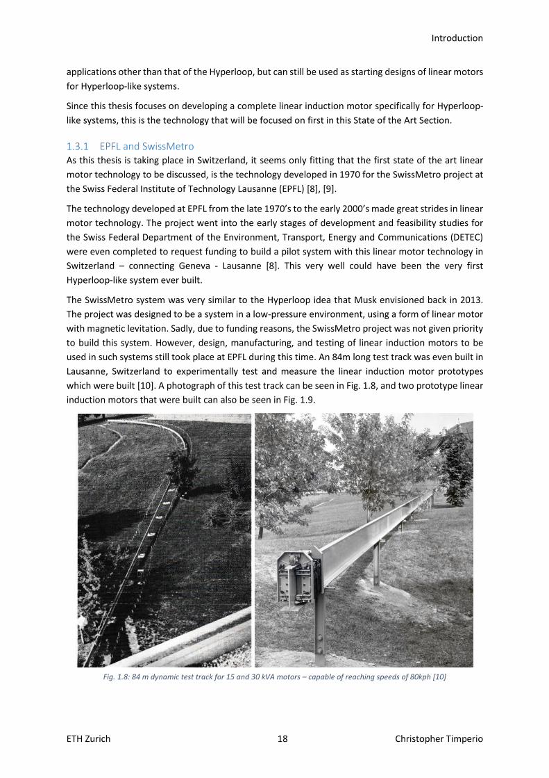
used in such systems still took place at EPFL during this time. An 84m long test track was even built in

Lausanne, Switzerland to experimentally test and measure the linear induction motor prototypes

which were built [10]. A photograph of this test track can be seen in Fig. 1.8, and two prototype linear

induction motors that were built can also be seen in Fig. 1.9.

Fig. 1.8: 84 m dynamic test track for 15 and 30 kVA motors – capable of reaching speeds of 80kph [10]

Introduction


Fig. 1.9: Prototype Linear Induction Motors – EPFL 1970’s [10]

The linear induction motors produced by EPFL were capable of generating speeds of approximately

80 km/h [10]. Although these motors were very advanced for their time – being developed in the

1960’s and 1970’s – they would not be fitting for a Hyperloop-like system to be developed today. The

main reason being that the speeds reached and the masses capable of being moved are just too low

for that of a prototype Hyperloop pod.

Additionally, since it was extremely difficult to achieve a variable frequency drive back in the 1970’s,

these motors were not frequency variable. This greatly decreases the motors performance without

having the possibility to vary the frequency throughout acceleration. Nevertheless, these motors were

a great achievement in the field of linear motors and are a great state of the art to build from today.

1.3.2 Virgin Hyperloop One More recently, Virgin Hyperloop One has been getting a lot of media attention as the main Hyperloop

company pursuing Hyperloop technology. They seem to be the farthest along compared to any other

Hyperloop company today. However, not much is known from their linear motor technology – as they

keep most of the information and technical specifications proprietary and confidential. This returns to

one of the main points of this thesis – to make the technology of a linear induction motor which could

be used in a Hyperloop system – open and more accessible to those who wish to know.

Introduction


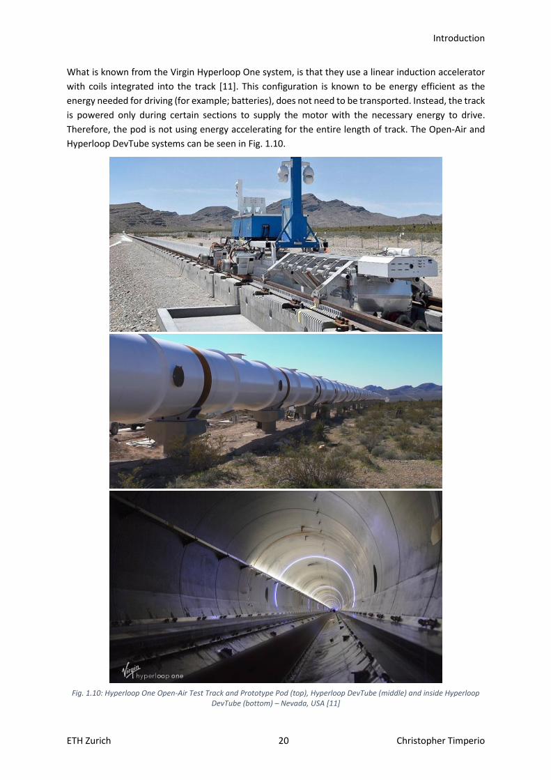
What is known from the Virgin Hyperloop One system, is that they use a linear induction accelerator

with coils integrated into the track [11]. This configuration is known to be energy efficient as the

energy needed for driving (for example; batteries), does not need to be transported. Instead, the track

is powered only during certain sections to supply the motor with the necessary energy to drive.

Therefore, the pod is not using energy accelerating for the entire length of track. The Open-Air and

Hyperloop DevTube systems can be seen in Fig. 1.10.

Fig. 1.10: Hyperloop One Open-Air Test Track and Prototype Pod (top), Hyperloop DevTube (middle) and inside Hyperloop

DevTube (bottom) – Nevada, USA [11]

Introduction


It is known that Virgin Hyperloop One has been able to achieve speeds up to 385 km/h with their

system on their approximately 500m test track [11]. Any further technical specifications of the motor

are not exactly known at this time.

1.3.3 Tracked Hovertrain Probably the most influential linear induction motor up until this point would be the one developed

for vehicle propulsion in September 1969 [12]. It was Professor Eric Laithwaite at Imperial College

London who published the first patent for linear induction motors to be used in vehicle systems as the

core propulsion mechanism. Professor Laithwaite made great strides in linear induction motor

development, and has even been named the Father of Maglev after patenting several surrounding

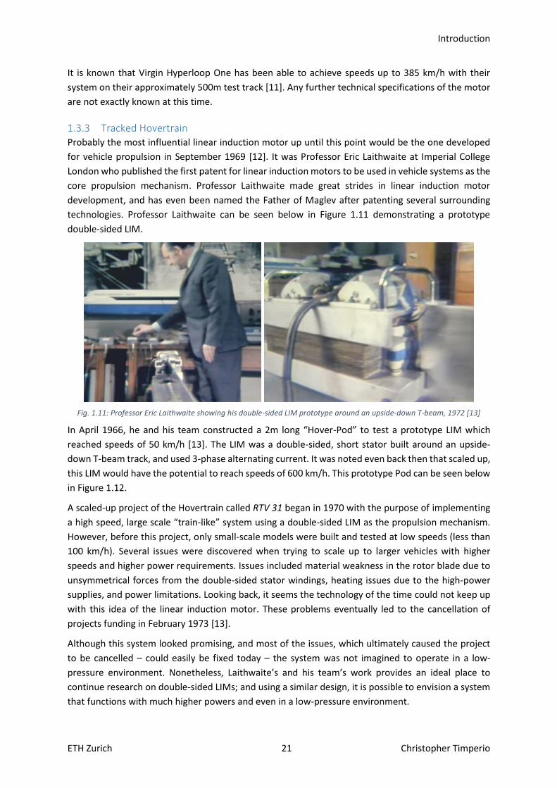
technologies. Professor Laithwaite can be seen below in Figure 1.11 demonstrating a prototype

double-sided LIM.

Fig. 1.11: Professor Eric Laithwaite showing his double-sided LIM prototype around an upside-down T-beam, 1972 [13]

In April 1966, he and his team constructed a 2m long “Hover-Pod” to test a prototype LIM which

reached speeds of 50 km/h [13]. The LIM was a double-sided, short stator built around an upside-

down T-beam track, and used 3-phase alternating current. It was noted even back then that scaled up,

this LIM would have the potential to reach speeds of 600 km/h. This prototype Pod can be seen below

in Figure 1.12.

A scaled-up project of the Hovertrain called RTV 31 began in 1970 with the purpose of implementing

a high speed, large scale “train-like” system using a double-sided LIM as the propulsion mechanism.

However, before this project, only small-scale models were built and tested at low speeds (less than

100 km/h). Several issues were discovered when trying to scale up to larger vehicles with higher

speeds and higher power requirements. Issues included material weakness in the rotor blade due to

unsymmetrical forces from the double-sided stator windings, heating issues due to the high-power

supplies, and power limitations. Looking back, it seems the technology of the time could not keep up

with this idea of the linear induction motor. These problems eventually led to the cancellation of

projects funding in February 1973 [13].

Although this system looked promising, and most of the issues, which ultimately caused the project

to be cancelled – could easily be fixed today – the system was not imagined to operate in a low-

pressure environment. Nonetheless, Laithwaite’s and his team’s work provides an ideal place to

continue research on double-sided LIMs; and using a similar design, it is possible to envision a system

that functions with much higher powers and even in a low-pressure environment.

Introduction


Fig. 1.12: Double-Sided Linear Induction Motor powering “Hovertrain” Prototype reaching speeds of about 50 km/h, April

1966 [13]

Introduction


1.3.4 Small Precision Linear Induction Motors As stated above, some companies just focus on small linear motor drives purely capable of small

precise movements such as for conveyer belt or manufacturing applications. An example of this can

be seen in Fig. 1.13.

Fig. 1.13: Example of Small Linear Induction Motor Drives, ETEL [14]

This technology – although it is still a type of linear induction motor – is not the technology needed in

Hyperloop-like systems. The performance specifications such as the masses these motors can drive,

the range, power limitations, and the achievable speeds – all make such motors non-ideal for a

Hyperloop system. This is not to say that these drives perform worse, they are simply designed for a

different application. As a matter of fact, they tend to be much more precise in their movements –

down to the micrometer range in some cases. In general, such a precise movement would be highly

desirable, however, precision is a parameter that is not needed in a Hyperloop-like system.

Therefore, this thesis aims to fill the gaps in the linear induction motor technologies described here.

Speed is a main goal of this thesis, where a maximum speed of 500 km/h is the goal. Also, the motor

should be able to reach this speed while transporting prototype Hyperloop Pods with masses weighing

approximately 250kg. And again lastly, the knowledge or information learned here in this thesis should

be open and publicly available.

The motor designed in this thesis needs to not only meet the current state of the art specifications,

but also surpass them. SwissMetro / EPFL built a prototype motor with a top speed of 80 km/h (not in

a low-pressure environment), and Hyperloop One’s top speed is 385 km/h. The motor developed in

this thesis will advance further and even set a new top speed record for Hyperloop Pods.

Theory


2 Theory

To help better understand the linear motor to be presented, a brief theoretical background on linear

induction motors and their underlying fundamental principles is provided here.

2.1 Maxwell’s Equations

Maxwell’s Equations are the governing equations for any electromagnetics problem, and thus are the

fundamental equations behind the linear induction motor and its operating principles. Maxwell’s

Equations are shown below in Eqn. 2.1 – Eqn. 2.4 in differential form [15].

∇ × �⃑� = −∂�⃑�

∂t (2.1)

∇ × �⃑⃑� = 𝐽 +∂�⃑⃑�

∂t (2.2)

∇ ∙ �⃑⃑� = 𝜌𝑣 (2.3)

∇ ∙ �⃑� = 0 (2.4)

Where �⃑� ̅ is the electric field strength, �⃑⃑� ̅ is the magnetic field strength, �⃑⃑� ̅ is the electric flux density, �⃑� ̅

is the magnetic flux density, 𝐽 ̅is the electric current density, and 𝜌𝑣 is the local charge density [15].

Eqn. 2.4 – which can be derived from Gauss’s Law for Magnetism [15] – states that all magnetic fields

must begin and end on themselves. Therefore, for any closed surface, the sum of the total number of

magnetic field lines entering and exiting that surface i.e., the net flux through that surface, will be

zero. In other words, all field lines that exit this surface, must re-enter it. This leads to the inference

that no magnetic monopoles or charges exist.

However, electric charges do exist and produce electric field lines that do not close on themselves.

Therefore, summing the total number of electric field lines over some surface, gives the total charge

density over that surface (or volume). In this case, the net charge dictates the total flux out of any

given volume or surface. This yields Eqn. 2.3, which again is derived from Gauss’s Law [15].

Eqn. 2.1 can be derived from Faraday’s Law and states that a changing (time-varying) magnetic field

produces and sustains an electric field. Eqn. 2.2 can be described by Ampere’s Law, and states that a

changing (time-varying) electric field produces and sustains a magnetic field. Additionally, Ampere’s

Law states that currents can also produce and sustain magnetic fields. The currents inferred here can

either be a conduction current density or convection current density. Therefore, 𝐽 in Eqn. 2.2 is

comprised of both 𝐽 𝑐𝑑 = 𝜎�⃑� (conduction) and 𝐽 𝑐𝑣 = 𝜌𝑣𝑣 (convection) [15].

Eqn. 2.1 and Eqn. 2.2 are the most important physical laws for the LIM, as they act to induce the

currents which is the underlying fundamental force that generates movement – or Thrust – in the

induction motor. A detailed derivation for this force follows in the Lorentz Force Section below.

These are Maxwell’s Equations in differential form and assume the presence of time-varying fields,

with current and charge distributions (𝐽 and 𝜌𝑣) in the system. If this were not the case, these terms

would tend towards zero, as the system would be source-free, which is the case in a perfect vacuum

(free-space).

Additionally, the following material (constitutive) relations hold in Eqn. 2.5 – Eqn. 2.7 [15];

Theory


�⃑⃑� = 휀�⃑� (2.5)

�⃑� = 𝜇�⃑⃑� (2.6)

𝐽 = 𝜎�⃑� (2.7)

with 휀 and 𝜇 being the absolute permittivity and permeability properties. These values are in turn

comprised of the relative or material permittivity and permeability quantities (휀𝑟 and 𝜇𝑟), and the free

space or vacuum permittivity and permeability quantities (휀0 and 𝜇0).

2.1.1 Quasi-Static Approximation Low-frequency electric or magnetic fields do not propagate in the same manner as electromagnetic

waves of higher frequencies do. These low frequency fields oscillate slowly and therefore have not yet

evolved into time dependent fields or propagating waves. This is because an insufficient amount of

time has elapsed over too short a distance [16]. In other words, the fields are oscillating so slowly due

to their low frequency that the time-dependent portion of the fields is negligible. These slowly

oscillating fields can even be thought of as DC magnetic or electric fields, which once generated,

remain stationary.

The magnetic fields generated in the motor (more specifically the stator) operate at such low

frequencies that a “Quasi-static Approximation” can be employed [16], [15]. The quasi-static

approximation gives simplifications for a low frequency field and states that the time dependent

electric or magnetic field terms drop out of their respective equations.

To clarify, any field terms “dropped” from an equation are still technically there: they just do not add

a noticeable contribution to the total field and are thus negligible. However, this condition only holds

true above a certain threshold. This threshold is the quasi-static approximation, which can be seen in

Eqn. 2.8 below [16].

𝐿

𝑐≪ 𝜏 or 𝜔𝐿 ≪ 𝑐 (2.8)

Eqn. 2.8 states that the ratio of a field’s propagation length 𝐿 to its velocity 𝑐, must be much less than

𝜏: the characteristic time constant for the sinusoidal steady state response of an oscillating signal [16].

Stated differently, the field with angular frequency 𝜔 traveling over some length 𝐿, must be slower

than the speed of light. Unless this condition is met, low frequency field terms cannot be removed, as

they are too large to be neglected [16].

The quasi-static approximation can be employed for the time derivative of the electric flux density

term in Ampere’s Law, given in Eqn. 2.2. This term, ∂�⃑⃑� ∂t⁄ , can be re-written as 𝐽 𝑑, and denoted as

the displacement current density. The displacement current density can be thought of as the currents

moving back and forth in some volume. When considering motors and the low frequency stator

magnetic field, this term is so small compared to the other currents in Eqn. 2.2, that under the quasi-

static approximation, it can be neglected.

∇ × �⃑⃑� = 𝐽 + 𝐽 𝑑 (2.9)

Thus, with this displacement current density term neglected, Ampere’s Law takes on the

magnetoquasistatic (MQS) form of Eqn. 2.10 [16], [15].

∇ × �⃑⃑� = 𝐽 (2.10)

0

Theory


Eqn. 2.10 is the form of Ampere’s Law used when working with the magnetic stator fields of this LIM.

Let it be noted that the remaining Maxwell Equations are still used in their time-varying forms.

2.2 Electric Drives

In general, an electrical drive or motor is designed to convert electrical energy – say from a battery or

electrical source – to a form of mechanical motion. In a conventional rotary motor, this motion is

transferred rotationally, and commonly turns an axle in a car – which rotates the wheels, turns water

pumps, fans, or anything requiring rotational motion. However, in the linear drive case, this motion is

now generated and transferred linearly, which is exactly the type of motion desired in a Hyperloop-

like system.

To understand how motion is transferred in a linear direction and how a forward thrust is generated,

a simple breakdown of rotational motors is necessary. Next, a discussion of how the transformation

to the linear motor is accomplished follows, and then finally the equations and theory needed to

design a linear motor are presented.

2.2.1 Motor Basics A conventional rotary motor is comprised of two main parts; the stator and the rotor. The stator

(generally, and in most cases) remains stationary, while the rotor rotates inside of the stator, as its

function is to transfer the input energy (from the stator) to a rotational mechanical output; hence its

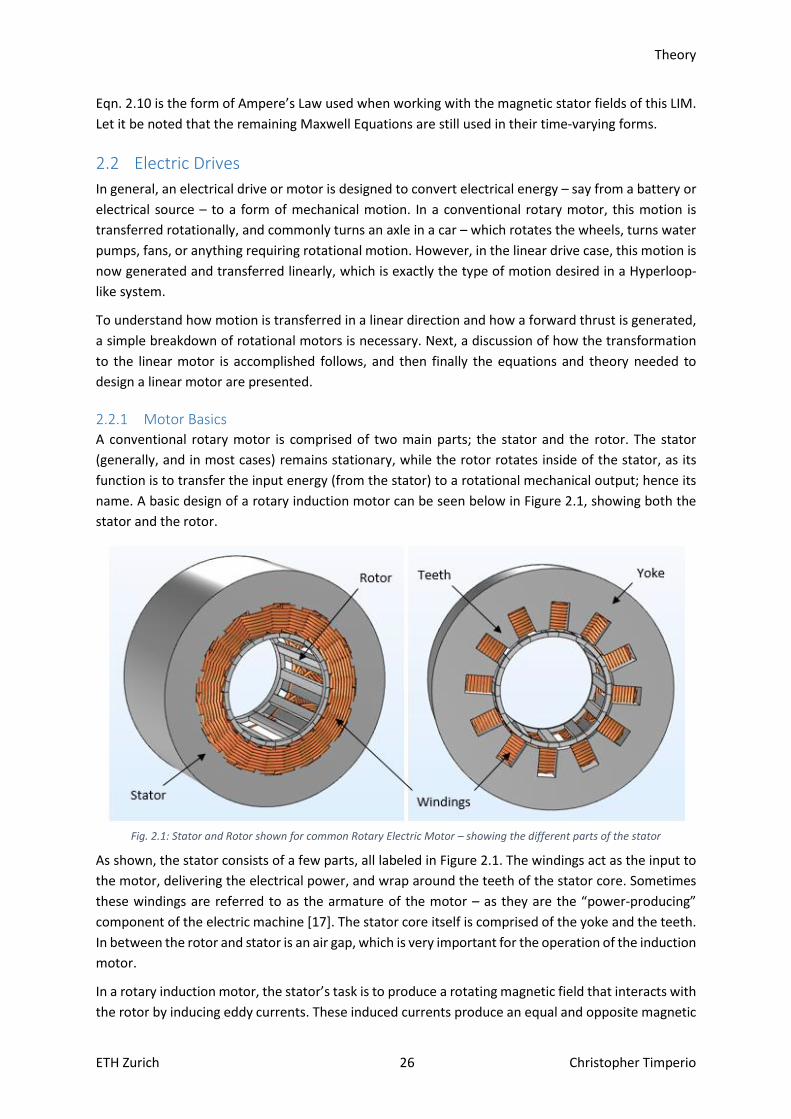
name. A basic design of a rotary induction motor can be seen below in Figure 2.1, showing both the

stator and the rotor.

Fig. 2.1: Stator and Rotor shown for common Rotary Electric Motor – showing the different parts of the stator

As shown, the stator consists of a few parts, all labeled in Figure 2.1. The windings act as the input to

the motor, delivering the electrical power, and wrap around the teeth of the stator core. Sometimes

these windings are referred to as the armature of the motor – as they are the “power-producing”

component of the electric machine [17]. The stator core itself is comprised of the yoke and the teeth.

In between the rotor and stator is an air gap, which is very important for the operation of the induction

motor.

In a rotary induction motor, the stator’s task is to produce a rotating magnetic field that interacts with

the rotor by inducing eddy currents. These induced currents produce an equal and opposite magnetic

Theory


field that is attracted to the source magnetic field produced by the stator. Thus, an attractive force, or

torque in the rotary case, between the magnetic fields is generated and causes the rotor to rotate

[17].

The stator material is most commonly iron. The need for induction (i.e., currents induced in the rotor),

however, does not dictate that the stator be made of iron. On the other hand, performance increases

dramatically with an iron core. The stator core has historically been made of iron because it – or any

other magnetically permeable material – helps constrain the field to the shape of the stator. By

constraining the field so that it flows through the stator core and the stator teeth, the strength of the

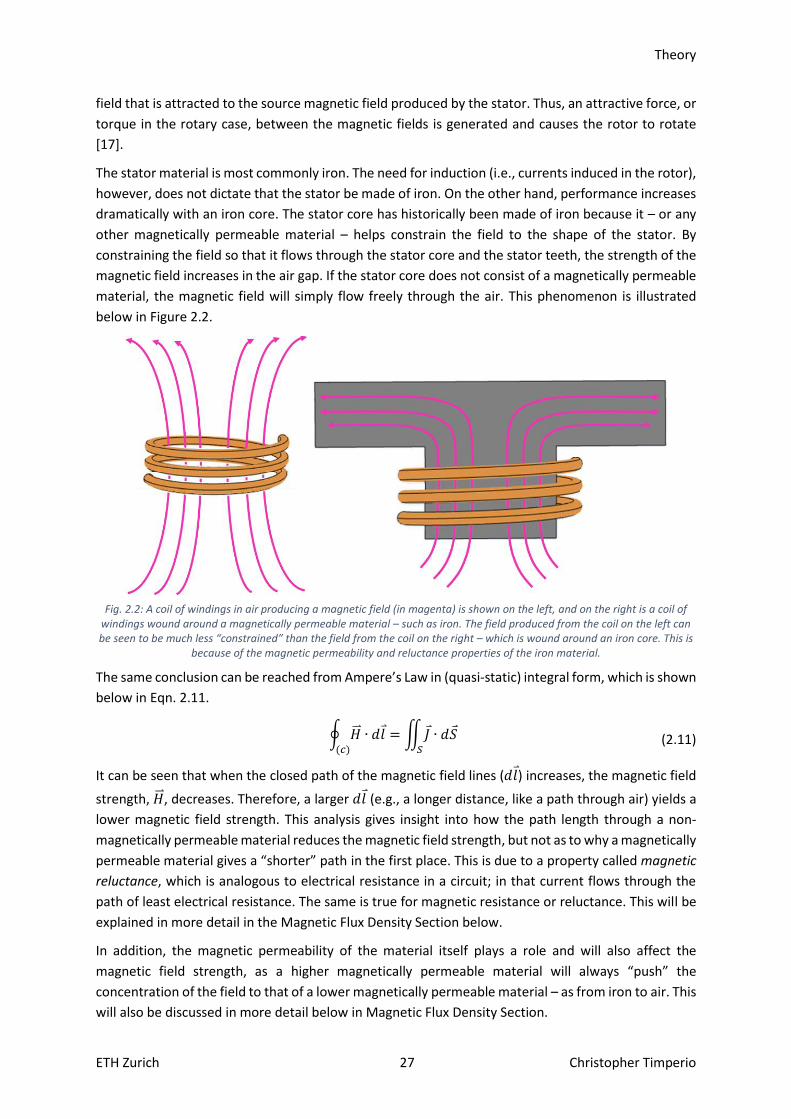
magnetic field increases in the air gap. If the stator core does not consist of a magnetically permeable

material, the magnetic field will simply flow freely through the air. This phenomenon is illustrated

below in Figure 2.2.

Fig. 2.2: A coil of windings in air producing a magnetic field (in magenta) is shown on the left, and on the right is a coil of

windings wound around a magnetically permeable material – such as iron. The field produced from the coil on the left can be seen to be much less “constrained” than the field from the coil on the right – which is wound around an iron core. This is

because of the magnetic permeability and reluctance properties of the iron material.

The same conclusion can be reached from Ampere’s Law in (quasi-static) integral form, which is shown

below in Eqn. 2.11.

∮ �⃑⃑� ∙ 𝑑𝑙

(𝑐)

= ∬𝐽 ∙ 𝑑𝑆

𝑆

(2.11)

It can be seen that when the closed path of the magnetic field lines (𝑑𝑙 ) increases, the magnetic field

strength, �⃑⃑� , decreases. Therefore, a larger 𝑑𝑙 (e.g., a longer distance, like a path through air) yields a

lower magnetic field strength. This analysis gives insight into how the path length through a non-

magnetically permeable material reduces the magnetic field strength, but not as to why a magnetically

permeable material gives a “shorter” path in the first place. This is due to a property called magnetic

reluctance, which is analogous to electrical resistance in a circuit; in that current flows through the

path of least electrical resistance. The same is true for magnetic resistance or reluctance. This will be

explained in more detail in the Magnetic Flux Density Section below.

In addition, the magnetic permeability of the material itself plays a role and will also affect the

magnetic field strength, as a higher magnetically permeable material will always “push” the

concentration of the field to that of a lower magnetically permeable material – as from iron to air. This

will also be discussed in more detail below in Magnetic Flux Density Section.

Theory


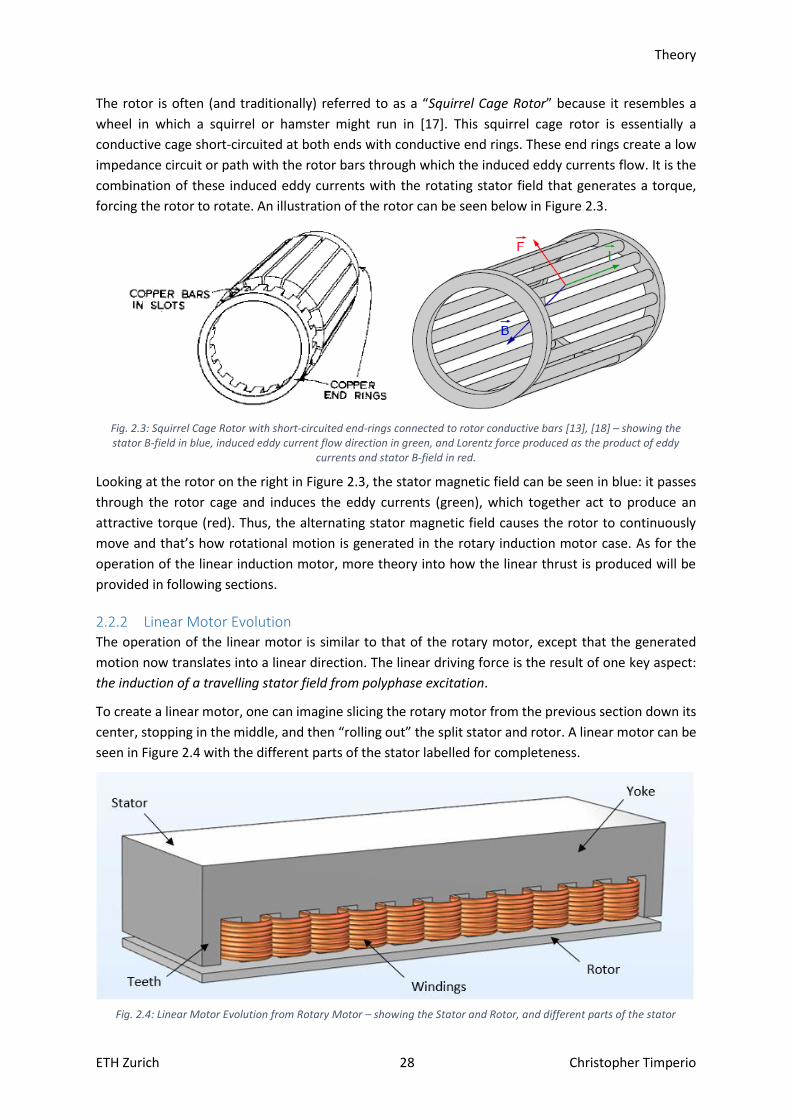
The rotor is often (and traditionally) referred to as a “Squirrel Cage Rotor” because it resembles a

wheel in which a squirrel or hamster might run in [17]. This squirrel cage rotor is essentially a

conductive cage short-circuited at both ends with conductive end rings. These end rings create a low

impedance circuit or path with the rotor bars through which the induced eddy currents flow. It is the

combination of these induced eddy currents with the rotating stator field that generates a torque,

forcing the rotor to rotate. An illustration of the rotor can be seen below in Figure 2.3.

Fig. 2.3: Squirrel Cage Rotor with short-circuited end-rings connected to rotor conductive bars [13], [18] – showing the stator B-field in blue, induced eddy current flow direction in green, and Lorentz force produced as the product of eddy

currents and stator B-field in red.

Looking at the rotor on the right in Figure 2.3, the stator magnetic field can be seen in blue: it passes

through the rotor cage and induces the eddy currents (green), which together act to produce an

attractive torque (red). Thus, the alternating stator magnetic field causes the rotor to continuously

move and that’s how rotational motion is generated in the rotary induction motor case. As for the

operation of the linear induction motor, more theory into how the linear thrust is produced will be

provided in following sections.

2.2.2 Linear Motor Evolution The operation of the linear motor is similar to that of the rotary motor, except that the generated

motion now translates into a linear direction. The linear driving force is the result of one key aspect:

the induction of a travelling stator field from polyphase excitation.

To create a linear motor, one can imagine slicing the rotary motor from the previous section down its

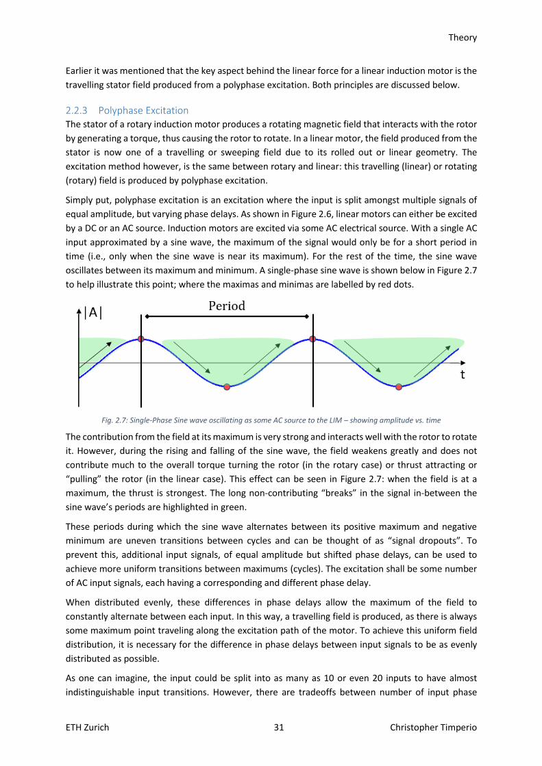
center, stopping in the middle, and then “rolling out” the split stator and rotor. A linear motor can be

seen in Figure 2.4 with the different parts of the stator labelled for completeness.

Fig. 2.4: Linear Motor Evolution from Rotary Motor – showing the Stator and Rotor, and different parts of the stator

Theory


As indicated, all parts of the rotary motor are still there, the only difference being that the shape of

the stator and rotor are now exactly as the name implies, linear.

The biggest difference in the linear motor when compared to the rotary motor is at the ends of the

linear motor. The motor is no longer a continuous object, but instead has open-ended air gaps at each

end, which do not exist in the rotary motor. These air gaps at the end lead to “end-effects” at both

ends of the LIM that cause unwanted losses and decrease performance [19]. The study of end-effects

is a very specialized and deep topic in and of itself and will therefore not be covered in-depth in this

thesis. However, some of the key issues associated with end-effects will be investigated and discussed

in the End-Effects Section below.

Another difference in the linear motor is that the long conductive bars or end rings of the rotor, in the

rotary case, which allowed eddy currents to flow around in a low-impedance circuit, are not present

in the linear case. In the linear case, a simplified conductive “plate” or “blade” is used as the rotor.

The solid conductive plate of the linear case distributes the travelling stator field continuously,

according to Maxwell’s Equations, the field cannot be influenced. In the rotary case, this can be

designed for, and chosen how or where the eddy currents are induced.

The main motivation for adding bars in the rotary case is to give an “entrance” for the field to induce

currents. If the rotor were just a solid plate as in the linear case, the field would flow around the rotor

and not interact as well with it. Instead rotor bars are designed so that when the field passes through

these bars, currents are induced in them and flow through in a low impedance path. This effect is not

that large in the linear case, as the field does not avoid the rotor. An efficiency comparison between

the “Squirrel Cage Rotor” and the “Blade Rotor” can be seen below in Figure 2.5 [13].

Fig. 2.5: Efficiency comparison between the conventional rotary squirrel cage rotor, and linear blade rotor – also denoted as

a “Sheet Rotor” [13]

As can be seen, at higher speeds, the sheet rotor is not significantly less efficient than the squirrel cage

rotor, perhaps only by 5-10% [13]. Nevertheless, one might try to recover this efficiency by slicing

optimized holes in the linear rotor blade1, so that a path is created for induced eddy currents to flow.

1 This would also reduce the mass of the rotor blade, thus helping with weight saving or weight constraints that might exist in high performance Hyperloop-like systems. Such optimized holes are shown in Musk’s Hyperloop Alpha Whitepaper [5].

Theory


However, this significantly increases design complexity and manufacturing and does not noticeably

improve performance. The induced eddy currents still flow in the plate, but unfortunately not as well

as in the rotary case. Therefore, this “sheet” geometry is simply a design tradeoff between

manufacturing and design simplicity.

Additionally, in the rotary motor, the stator is conventionally fixed in place, while the rotor rotates in

place2. One difference for the linear motor is that depending on the application, it might be

advantageous to switch which part of the motor is moving and which is fixed in place. As an example,

a Pod or Hyperloop vehicle can have the stator fixed onboard the moving Pod, while the rotor blade

is fixed to the track. In this case, the rotor is the part that is fixed, while the stator is technically moving.

This grants extra design options when deciding which motor configuration to choose.

Several different configurations or types of linear motors exist. The classification can be split into two

main types, Synchronous and Asynchronous [17], [20]. Asynchronous motors can also be referred to

as induction motors: the two terms are used interchangeably and refer to the same type of motor.

Therefore, the type of motor presented in this thesis can also be referred to as a linear asynchronous

motor; however, by convention it is referred to as a linear induction motor.

An Asynchronous motor was chosen for this thesis because the design is much less complex than that

of a synchronous motor, which involves the use of permanent magnets to create an attractive Lorentz

force that is otherwise generated with induction. Thus, from a design perspective alone, the LIM offers

a good starting point for a prototype, because it is much simpler than it synchronous counterpart. The

different topologies or linear motor classifications can be seen below in Figure 2.6.

Since, the linear motor developed in this thesis is a linear induction motor, the theory discussed in the

following sections focuses on the topics necessary for understanding induction or asynchronous motor

theory. Nevertheless, it is informative to show the other linear motor types to indicate that many

other choices or options for linear motor configurations exist.

Fig. 2.6: Classification of Linear Motor Types – showing Asynchronous or Induction and how it is categorized [20]

2 This is not always the case, there can be a moving outer stator with a fixed inner rotor – often used in race car applications where the motor is fixed directly inside of the car’s wheels. However conventionally, the stator is stationary, and the rotor rotates.

Theory


Earlier it was mentioned that the key aspect behind the linear force for a linear induction motor is the

travelling stator field produced from a polyphase excitation. Both principles are discussed below.

2.2.3 Polyphase Excitation The stator of a rotary induction motor produces a rotating magnetic field that interacts with the rotor

by generating a torque, thus causing the rotor to rotate. In a linear motor, the field produced from the

stator is now one of a travelling or sweeping field due to its rolled out or linear geometry. The

excitation method however, is the same between rotary and linear: this travelling (linear) or rotating

(rotary) field is produced by polyphase excitation.

Simply put, polyphase excitation is an excitation where the input is split amongst multiple signals of

equal amplitude, but varying phase delays. As shown in Figure 2.6, linear motors can either be excited

by a DC or an AC source. Induction motors are excited via some AC electrical source. With a single AC

input approximated by a sine wave, the maximum of the signal would only be for a short period in

time (i.e., only when the sine wave is near its maximum). For the rest of the time, the sine wave

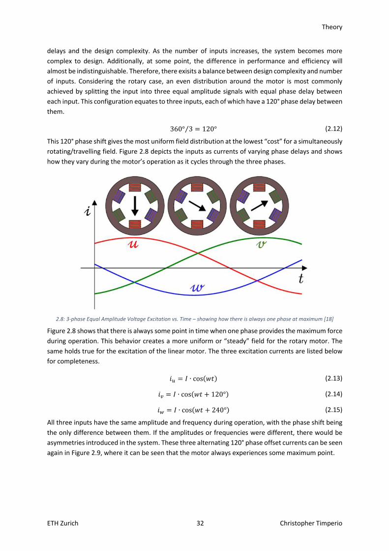
oscillates between its maximum and minimum. A single-phase sine wave is shown below in Figure 2.7

to help illustrate this point; where the maximas and minimas are labelled by red dots.

Fig. 2.7: Single-Phase Sine wave oscillating as some AC source to the LIM – showing amplitude vs. time

The contribution from the field at its maximum is very strong and interacts well with the rotor to rotate

it. However, during the rising and falling of the sine wave, the field weakens greatly and does not

contribute much to the overall torque turning the rotor (in the rotary case) or thrust attracting or

“pulling” the rotor (in the linear case). This effect can be seen in Figure 2.7: when the field is at a

maximum, the thrust is strongest. The long non-contributing “breaks” in the signal in-between the

sine wave’s periods are highlighted in green.

These periods during which the sine wave alternates between its positive maximum and negative

minimum are uneven transitions between cycles and can be thought of as “signal dropouts”. To

prevent this, additional input signals, of equal amplitude but shifted phase delays, can be used to

achieve more uniform transitions between maximums (cycles). The excitation shall be some number

of AC input signals, each having a corresponding and different phase delay.

When distributed evenly, these differences in phase delays allow the maximum of the field to

constantly alternate between each input. In this way, a travelling field is produced, as there is always

some maximum point traveling along the excitation path of the motor. To achieve this uniform field

distribution, it is necessary for the difference in phase delays between input signals to be as evenly

distributed as possible.

As one can imagine, the input could be split into as many as 10 or even 20 inputs to have almost

indistinguishable input transitions. However, there are tradeoffs between number of input phase

Theory


delays and the design complexity. As the number of inputs increases, the system becomes more

complex to design. Additionally, at some point, the difference in performance and efficiency will

almost be indistinguishable. Therefore, there exisits a balance between design complexity and number

of inputs. Considering the rotary case, an even distribution around the motor is most commonly

achieved by splitting the input into three equal amplitude signals with equal phase delay between

each input. This configuration equates to three inputs, each of which have a 120° phase delay between

them.

360° 3⁄ = 120° (2.12)

This 120° phase shift gives the most uniform field distribution at the lowest “cost” for a simultaneously

rotating/travelling field. Figure 2.8 depicts the inputs as currents of varying phase delays and shows

how they vary during the motor’s operation as it cycles through the three phases.

2.8: 3-phase Equal Amplitude Voltage Excitation vs. Time – showing how there is always one phase at maximum [18]

Figure 2.8 shows that there is always some point in time when one phase provides the maximum force

during operation. This behavior creates a more uniform or “steady” field for the rotary motor. The

same holds true for the excitation of the linear motor. The three excitation currents are listed below

for completeness.

𝑖𝑢 = 𝐼 ∙ cos(𝑤𝑡) (2.13)

𝑖𝑣 = 𝐼 ∙ cos(𝑤𝑡 + 120°) (2.14)

𝑖𝑤 = 𝐼 ∙ cos(𝑤𝑡 + 240°) (2.15)

All three inputs have the same amplitude and frequency during operation, with the phase shift being

the only difference between them. If the amplitudes or frequencies were different, there would be

asymmetries introduced in the system. These three alternating 120° phase offset currents can be seen

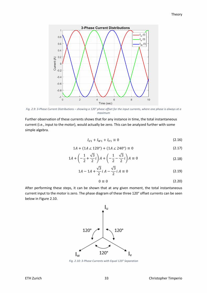
again in Figure 2.9, where it can be seen that the motor always experiences some maximum point.

Theory


Fig. 2.9: 3-Phase Current Distributions – showing a 120° phase offset for the input currents, where one phase is always at a

maximum

Further observation of these currents shows that for any instance in time, the total instantaneous

current (i.e., input to the motor), would actually be zero. This can be analyzed further with some

simple algebra.

𝐼𝑈1 + 𝐼𝑊1 + 𝐼𝑉1 ≡ 0 (2.16)

1𝐴 + (1𝐴 ∠ 120°) + (1𝐴 ∠ 240°) ≡ 0 (2.17)

1𝐴 + (−1

2+

√3

2𝑖)𝐴 + (−

1

2−

√3

2𝑖)𝐴 ≡ 0 (2.18)

1𝐴 − 1𝐴 +√3

2𝑖 𝐴 −

√3

2𝑖 𝐴 ≡ 0 (2.19)

0 ≡ 0 (2.20)

After performing these steps, it can be shown that at any given moment, the total instantaneous

current input to the motor is zero. The phase diagram of these three 120° offset currents can be seen

below in Figure 2.10.

Fig. 2.10: 3-Phase Currents with Equal 120° Separation

Theory


This diagram shows the 120° separation between the 3-phase currents. It is this 3-phase excitation

that leads to the creation of a travelling stator field. [21]

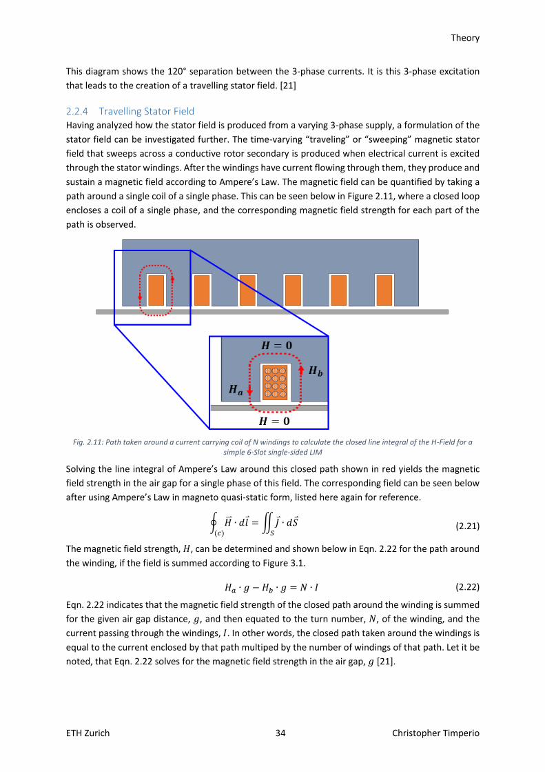
2.2.4 Travelling Stator Field Having analyzed how the stator field is produced from a varying 3-phase supply, a formulation of the

stator field can be investigated further. The time-varying “traveling” or “sweeping” magnetic stator

field that sweeps across a conductive rotor secondary is produced when electrical current is excited

through the stator windings. After the windings have current flowing through them, they produce and

sustain a magnetic field according to Ampere’s Law. The magnetic field can be quantified by taking a

path around a single coil of a single phase. This can be seen below in Figure 2.11, where a closed loop

encloses a coil of a single phase, and the corresponding magnetic field strength for each part of the

path is observed.

Fig. 2.11: Path taken around a current carrying coil of N windings to calculate the closed line integral of the H-Field for a

simple 6-Slot single-sided LIM

Solving the line integral of Ampere’s Law around this closed path shown in red yields the magnetic

field strength in the air gap for a single phase of this field. The corresponding field can be seen below

after using Ampere’s Law in magneto quasi-static form, listed here again for reference.

∮ �⃑⃑� ∙ 𝑑𝑙

(𝑐)

= ∬𝐽 ∙ 𝑑𝑆

𝑆

(2.21)

The magnetic field strength, 𝐻, can be determined and shown below in Eqn. 2.22 for the path around

the winding, if the field is summed according to Figure 3.1.

𝐻𝑎 ∙ 𝑔 − 𝐻𝑏 ∙ 𝑔 = 𝑁 ∙ 𝐼 (2.22)

Eqn. 2.22 indicates that the magnetic field strength of the closed path around the winding is summed

for the given air gap distance, 𝑔, and then equated to the turn number, 𝑁, of the winding, and the

current passing through the windings, 𝐼. In other words, the closed path taken around the windings is

equal to the current enclosed by that path multiped by the number of windings of that path. Let it be

noted, that Eqn. 2.22 solves for the magnetic field strength in the air gap, 𝑔 [21].

Theory


Summing the magnetic field strengths of the path shows that the tangential field components are

zero, but that the normal field components are opposite in sign to one another. Using this principle, a

substitution can be made for the field components to simplify the equation.

𝐻𝑎 = −𝐻𝑏 (2.23)

From here, some simple algebra can be performed to equate the magnetic field strength to the

enclosed current of 𝑁 windings.

𝐻𝑎 ∙ 𝑔 + 𝐻𝑎 ∙ 𝑔 = 2𝐻𝑎 ∙ 𝑔 = 𝑁 ∙ 𝐼 (2.24)

𝐻1 = �̂� =𝑁𝐼

2𝑔 (2.25)

Rearranging the equation and setting the total magnetic field strength to �̂�, the magnetic field

strength in the air gap is determined. Since 𝑔 is the distance of the air gap, the magnetic field strength

found from Eqn. 2.25 passes twice through this air gap. Observation of Figure 3.1 shows that the field

has two contributions from the air gap because the path of the line integral enclosing the winding

must close on itself. The total length of the path plays an important role in determining the magnetic

field strength and will be discussed later in the Magnetic Flux Density and Motor Design Sections.

To produce a time-varying magnetic stator field, Eqn. 2.26 and Eqn. 2.27 are introduced to add time

and space varying components to the equation.

sin(𝜔𝑡) (2.26)

sin (𝜋𝑦

𝜏𝑝) (2.27)

Eqn. 2.25 can be multiplied by Eqn. 2.26 and Eqn. 2.27 to produce a time- and space-varying magnetic

field strength similar to the actual field [21]. 𝑦 is the horizontal or linear direction in which the linear

motor translates when thrust is generated and 𝜏𝑝 is the pole pitch of the motor, which is described in

more detail in its own section below. However, for now 𝜏𝑝 is referred to as the half period of the stator

sine wave [21], illustrated below in Figure 2.12.

Fig. 2.12: Pole Pitch Identified as the half period of the stator sine wave [21]

Combining the time and space varying components above with Eqn. 2.25 yields the following time-

varying magnetic field strength for a single phase, 𝑢, of the motor.

𝐻𝑢(𝑦, 𝑡) =4

𝜋∙ �̂� ∙ sin(

𝜋𝑦

𝜏𝑝) ∙ sin(𝜔𝑡) (2.28)

𝐻𝑢(𝑦, 𝑡) =4

𝜋∙𝑁𝐼

2𝑔∙ sin(

𝜋𝑦

𝜏𝑝) ∙ sin(𝜔𝑡) (2.29)

Theory


Assuming a 3-phase input comprised of three equal amplitude 120° (corresponding to 2𝜋3⁄ radians)

phase shifted magnetic fields, the remaining two phases of the input are listed below.

𝐻𝑢(𝑦, 𝑡) =4

𝜋∙𝑁𝐼

2𝑔∙ sin(

𝜋𝑦

𝜏𝑝) ∙ sin(𝜔𝑡) (2.30)

𝐻𝑣(𝑦, 𝑡) =4

𝜋∙𝑁𝐼

2𝑔∙ sin (

𝜋𝑦

𝜏𝑝+

2𝜋

3) ∙ sin (𝜔𝑡 +

2𝜋

3) (2.31)

𝐻𝑤(𝑦, 𝑡) =4

𝜋∙𝑁𝐼

2𝑔∙ sin(

𝜋𝑦

𝜏𝑝−

2𝜋

3) ∙ sin (𝜔𝑡 −

2𝜋

3) (2.32)

t can be seen that there are now three 120° offset stator fields that vary in time and space (position).

To create the total stator field that sweeps the distance of the stator and induces eddy currents in the

rotor for thrust production, these 3-phase fields can be summed together. However, first it is desirable

to decompose the sines into cosines to make the math less complex. This decomposition process can

be completed to produce the final 3-phase cosine fields seen below.

𝐻𝑢(𝑦, 𝑡) =4

𝜋∙𝑁𝐼

2𝑔∙ (cos (

𝜋𝑦

𝜏𝑝− 𝜔𝑡) − cos (

𝜋𝑦

𝜏𝑝+ 𝜔𝑡)) (2.33)

𝐻𝑣(𝑦, 𝑡) =4

𝜋∙𝑁𝐼

2𝑔∙ (cos(

𝜋𝑦

𝜏𝑝− 𝜔𝑡) − cos (

𝜋𝑦

𝜏𝑝+ 𝜔𝑡 +

4𝜋

3)) (2.34)

𝐻𝑤(𝑦, 𝑡) =4

𝜋∙𝑁𝐼

2𝑔∙ (cos (

𝜋𝑦

𝜏𝑝− 𝜔𝑡) − cos(

𝜋𝑦

𝜏𝑝+ 𝜔𝑡 −

4𝜋

3)) (2.35)

Finally, the superposition of all three phases yields the total sweeping or travelling magnetic stator

field.

𝐻𝑡𝑜𝑡(𝑦, 𝑡) =6

𝜋∙𝑁𝐼

2𝑔∙ cos(

𝜋𝑦

𝜏𝑝− 𝜔𝑡) (2.36)

This field is the total magnetic stator field seen in the air gap of the motor that travels or sweeps across

the stator to induce eddy currents in the rotor.

The total magnetic stator field sweeps across the rotor and resembles a cosine or sine-like distribution.

It will be seen in the subsequent Winding Configuration Section how this sine-like distribution is

achieved or approximated. However, if these separate 3-phase and total fields are plotted as a

function of position, it can be seen how the total resulting stator field is created and sweeps in

position. Figure 3.3 shows these equations plotted in Matlab for a generic air gap spacing and pole

pitch value.

Theory


Fig. 2.13: 3-Phase Stator Fields and Total Stator Field – showing one instance in time how the three-phase fields (red, green,

and blue) add up to produce the total stator field (pink)

As can be seen from Figure 2.13, the three-phase fields (red, green, and blue) add up to produce the

total stator field (pink). A time evolution of the stator fields is plotted below in Figure 2.14 for different

time instances to help visualize the travelling field.

Fig. 2.14: 3-Phase Stator Fields and Total Stator Field – showing a progression of the system from t=1 sec to t=9 sec

Theory


As can be seen in Figure 2.14, the 3-phase fields are all plotted and the superposition shows the total

field as a function of position and time. It can be seen that the 3-phase fields do not move in position,

as they simply oscillate vertically in time. The total field only moves horizontally in position as it

progresses towards the right side of the plots where no vertical oscillation is observed.

Now that the magnetic field strength of the travelling stator field has been quantified, it will be shown

below how it interacts with the rotor to create thrust, as it is solely responsible for inducing the eddy

currents which help generate a Lorentz thrust force. Interactions of this stator field with the rotor to

induce currents used for thrust production, will be shown in the subsequent sections.

2.2.5 Synchronous Speed The travelling stator field sweeps across the secondary with speed 𝑣𝑠. This is defined as the

synchronous speed of the motor and is a key parameter for the motor. The motor’s synchronous

speed, or sync speed for short, is defined as the final speed reached by the motor for a given applied

source frequency [21], [17], [22]. In the case of this thesis, the speed goal was specified as 500 km/h,

so that is the sync speed to be used later in this thesis. The sync speed is often defined in its SI units,

so 500 km/h is converted to 138.89 m/sec.

At the sync speed, there is no longer a contribution from the stator field and hence no counter-

travelling field is produced by the rotor: its speed at this point, in principle, is the stator synchronous

speed [17].

To derive an expression for this sync speed, the argument of the cosine in the total stator field

expression can be set to one. This is the part of the equation which varies and therefore describes the

speed of the field.

cos (𝜋𝑦

𝜏𝑝− 𝜔𝑡) = 1 (2.37)

If Eqn. 2.37 is solved for and rearranged, the following expression for the sync speed can be found.

cos−1(1) =𝜋𝑦

𝜏𝑝− 𝜔𝑡 (2.38)

0 + 𝜔𝑡 =𝜋𝑦

𝜏𝑝 (2.39)

𝜏𝑝 ∙ 𝜔𝑡 = 𝜋𝑦 (2.40)

𝜏𝑝

𝜋∙ 𝜔 =

𝑦

𝑡= 𝑣𝑠 (2.41)

Performing the algebra and describing the expression in terms of its position and frequency yields a

translation of space over time. This quantity is the synchronous speed velocity, 𝑣𝑠 , of the motor and

is shown below in simplified expressions, where the frequency of the stator field, 𝑓𝑠, is substituted for

the angular frequency 𝜔 because the frequency of the stator field is often described in Hz rather than

in rad/sec.

𝜏𝑝

𝜋∙ 2𝜋 ∙ 𝑓𝑠 = 𝑣𝑠 (2.42)

𝑣𝑠 = 2 𝜏𝑝 𝑓𝑠 (2.43)

This expression describes the speed of the travelling stator field of the motor.

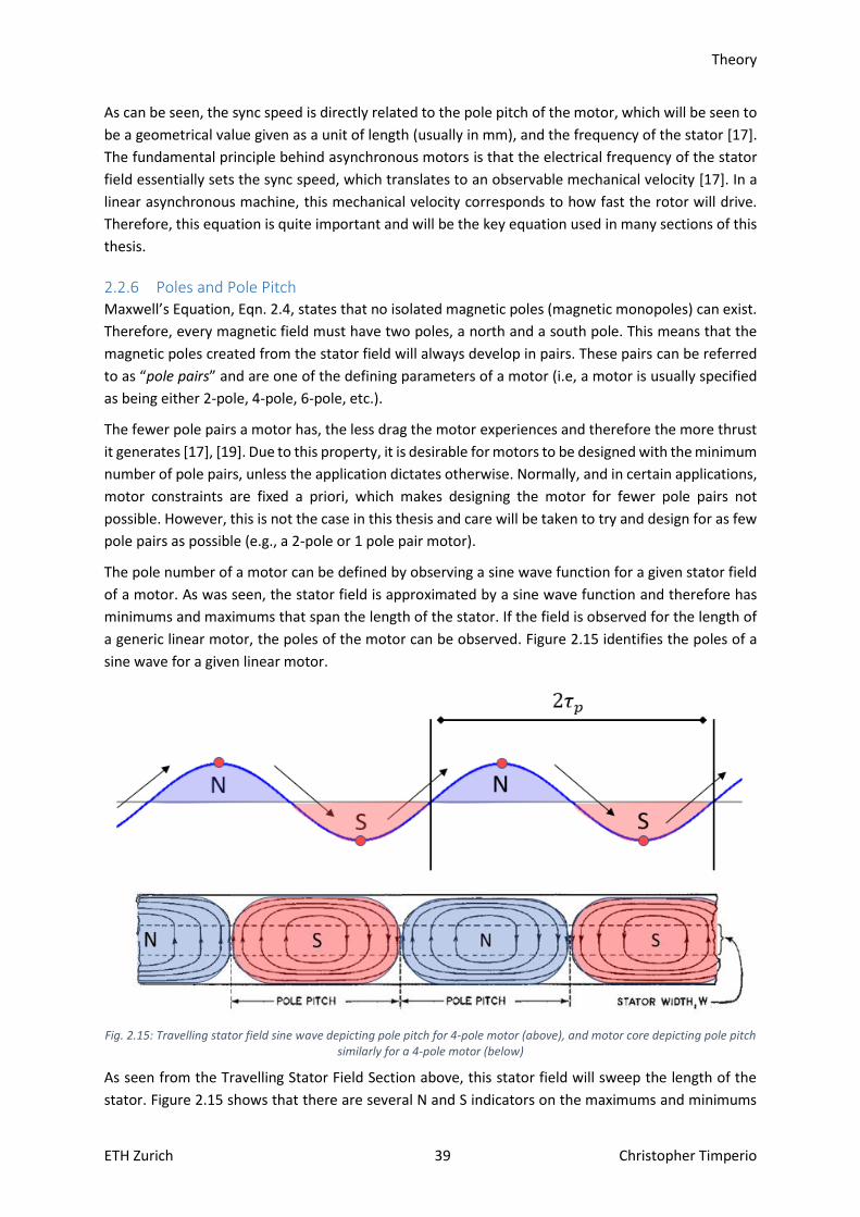
Theory


As can be seen, the sync speed is directly related to the pole pitch of the motor, which will be seen to

be a geometrical value given as a unit of length (usually in mm), and the frequency of the stator [17].

The fundamental principle behind asynchronous motors is that the electrical frequency of the stator

field essentially sets the sync speed, which translates to an observable mechanical velocity [17]. In a

linear asynchronous machine, this mechanical velocity corresponds to how fast the rotor will drive.

Therefore, this equation is quite important and will be the key equation used in many sections of this

thesis.

2.2.6 Poles and Pole Pitch Maxwell’s Equation, Eqn. 2.4, states that no isolated magnetic poles (magnetic monopoles) can exist.

Therefore, every magnetic field must have two poles, a north and a south pole. This means that the

magnetic poles created from the stator field will always develop in pairs. These pairs can be referred

to as “pole pairs” and are one of the defining parameters of a motor (i.e, a motor is usually specified

as being either 2-pole, 4-pole, 6-pole, etc.).

The fewer pole pairs a motor has, the less drag the motor experiences and therefore the more thrust

it generates [17], [19]. Due to this property, it is desirable for motors to be designed with the minimum

number of pole pairs, unless the application dictates otherwise. Normally, and in certain applications,

motor constraints are fixed a priori, which makes designing the motor for fewer pole pairs not

possible. However, this is not the case in this thesis and care will be taken to try and design for as few

pole pairs as possible (e.g., a 2-pole or 1 pole pair motor).

The pole number of a motor can be defined by observing a sine wave function for a given stator field

of a motor. As was seen, the stator field is approximated by a sine wave function and therefore has

minimums and maximums that span the length of the stator. If the field is observed for the length of

a generic linear motor, the poles of the motor can be observed. Figure 2.15 identifies the poles of a

sine wave for a given linear motor.

Fig. 2.15: Travelling stator field sine wave depicting pole pitch for 4-pole motor (above), and motor core depicting pole pitch

similarly for a 4-pole motor (below)

As seen from the Travelling Stator Field Section above, this stator field will sweep the length of the

stator. Figure 2.15 shows that there are several N and S indicators on the maximums and minimums

Theory


of the stator sine wave, respectively. These indicators represent the north and south poles of the

magnetic stator field. Therefore, from the stator field shown in Figure 2.15, it can be seen that this

motor has 4 magnetic poles, or 2 pole pairs, and would be classified as a 4-pole motor.

The pole pitch, 𝜏𝑝, also shows up in Figure 2.15. The pole pitch is defined as the geometrical length for

a single pole in a motor: it is the pole’s “pitch” or length. Figure 2.15 shows that this stator field spans

the length of the linear motor’s stator producing the travelling field shown in blue, and that the pole

pitch is roughly a quarter of the total length of the motor (i.e., the pitch or length of one pole). The

length of the motor is directly related to the pole pitch, or vise-versa and therefore represents another

key design parameter. If the length of the motor is known, the pole pitch can be determined if the

pole number is also known. A simple formula for relating the pole pitch to the length of the motor can

be seen below in Eqn. 2.44.

𝜏𝑝 =𝐿

2 ∙ 𝑝 (2.44)

Where L is the length of the stator, and 𝑝 is the pole number. Therefore, for a 2-pole motor, the pole

pitch is half of the length of the stator; for a 4-pole motor, the pole pitch is a fourth of the stator’s

length and for a 6-pole motor, the pole pitch is a sixth of the stator length.

2.2.7 Slip The travelling stator field created from the 3-phase excitation has a velocity called the sync speed, 𝑣𝑠.

This velocity, as was seen in Eqn. 2.43, is directly related to the frequency of the stator field, 𝑓𝑠. This

field sweeps across the rotor, which produces its own magnetic field that is equal and opposite to that

of the stator field. This equal and opposite rotor field creates a repulsive force between the rotor and

the stator that produces the main linear movement in the linear asynchronous motor. This

fundamental thrust generation will be discussed in more detail in the Lorentz Force Section.

However, from this introduction, it can now be seen that the rotor has its own travelling field,

complete with its own some speed and frequency defined as 𝑣𝑟 and 𝑓𝑟 , respectively. The speed and

frequency of this newly created rotor field will, however, be different from that of the stator field. The

rotor field will be slightly slower compared to the stator field due to a “delay” between the two fields.

This delay in the fields can also be referred to as the slip of an asynchronous motor.

Therefore, it is from the differences in the two fields that the slip is defined. Put more accurately, the

slip is defined as the difference between the synchronous speed of the travelling field produced by

the stator and the actual mechanical speed of the rotor [17], [13], as shown below in Eqn. 2.45.

𝑠 =𝑣𝑠 − 𝑣𝑟

𝑣𝑠 (2.45)

Thus, the slip is the difference in speed between the two fields and takes on a value between 0 and 1.

A slip equal to 1 is defined as full slip and a slip equal to 0 means there is no slip. The slip is plotted

below in Figure 2.16 against the moving rotor velocity to help better visualize its characteristics during

operation.

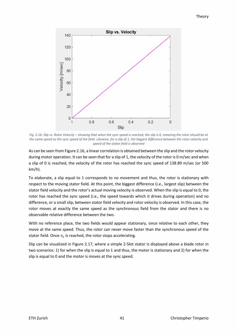
Theory


Fig. 2.16: Slip vs. Rotor Velocity – showing that when the sync speed is reached, the slip is 0, meaning the rotor should be at the same speed as the sync speed of the field. Likewise, for a slip of 1, the biggest difference between the rotor velocity and

speed of the stator field is observed

As can be seen from Figure 2.16, a linear correlation is obtained between the slip and the rotor velocity

during motor operation. It can be seen that for a slip of 1, the velocity of the rotor is 0 m/sec and when

a slip of 0 is reached, the velocity of the rotor has reached the sync speed of 138.89 m/sec (or 500

km/h).

To elaborate, a slip equal to 1 corresponds to no movement and thus, the rotor is stationary with

respect to the moving stator field. At this point, the biggest difference (i.e., largest slip) between the

stator field velocity and the rotor’s actual moving velocity is observed. When the slip is equal to 0, the

rotor has reached the sync speed (i.e., the speed towards which it drives during operation) and no

difference, or a small slip, between stator field velocity and rotor velocity is observed. In this case, the

rotor moves at exactly the same speed as the synchronous field from the stator and there is no

observable relative difference between the two.

With no reference place, the two fields would appear stationary, since relative to each other, they

move at the same speed. Thus, the rotor can never move faster than the synchronous speed of the

stator field. Once 𝑣𝑠 is reached, the rotor stops accelerating.

Slip can be visualized in Figure 2.17, where a simple 2-Slot stator is displayed above a blade rotor in

two scenarios: 1) for when the slip is equal to 1 and thus, the motor is stationary and 2) for when the

slip is equal to 0 and the motor is moves at the sync speed.

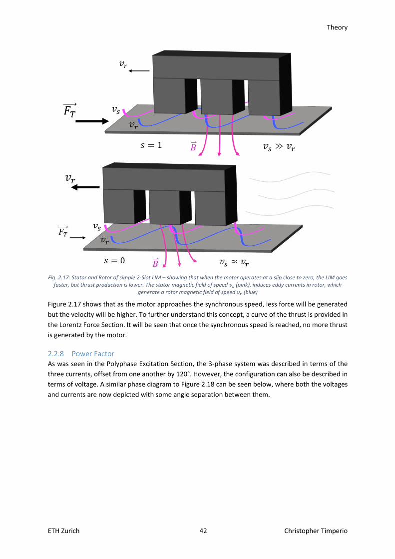
Theory


Fig. 2.17: Stator and Rotor of simple 2-Slot LIM – showing that when the motor operates at a slip close to zero, the LIM goes

faster, but thrust production is lower. The stator magnetic field of speed 𝑣𝑠 (pink), induces eddy currents in rotor, which generate a rotor magnetic field of speed 𝑣𝑟 (blue)

Figure 2.17 shows that as the motor approaches the synchronous speed, less force will be generated

but the velocity will be higher. To further understand this concept, a curve of the thrust is provided in

the Lorentz Force Section. It will be seen that once the synchronous speed is reached, no more thrust

is generated by the motor.

2.2.8 Power Factor As was seen in the Polyphase Excitation Section, the 3-phase system was described in terms of the

three currents, offset from one another by 120°. However, the configuration can also be described in

terms of voltage. A similar phase diagram to Figure 2.18 can be seen below, where both the voltages

and currents are now depicted with some angle separation between them.

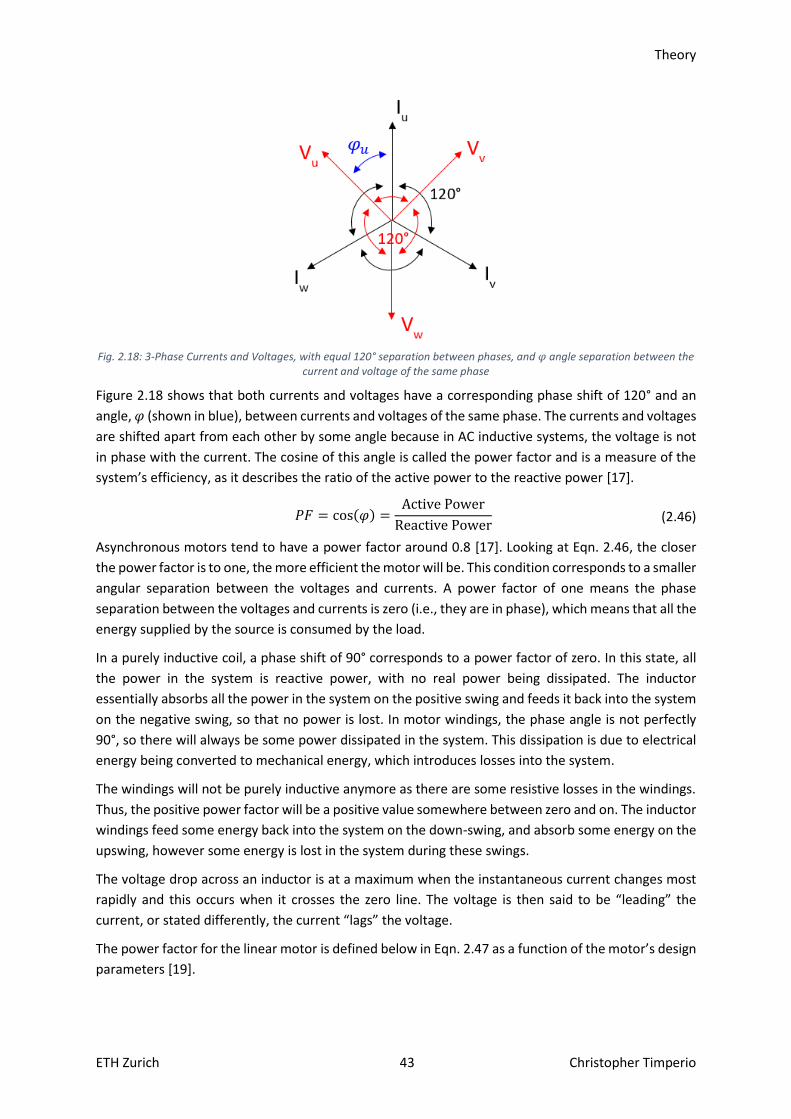
Theory


Fig. 2.18: 3-Phase Currents and Voltages, with equal 120° separation between phases, and 𝜑 angle separation between the

current and voltage of the same phase

Figure 2.18 shows that both currents and voltages have a corresponding phase shift of 120° and an

angle, 𝜑 (shown in blue), between currents and voltages of the same phase. The currents and voltages

are shifted apart from each other by some angle because in AC inductive systems, the voltage is not

in phase with the current. The cosine of this angle is called the power factor and is a measure of the

system’s efficiency, as it describes the ratio of the active power to the reactive power [17].

𝑃𝐹 = cos(𝜑) =Active Power

Reactive Power (2.46)

Asynchronous motors tend to have a power factor around 0.8 [17]. Looking at Eqn. 2.46, the closer

the power factor is to one, the more efficient the motor will be. This condition corresponds to a smaller

angular separation between the voltages and currents. A power factor of one means the phase

separation between the voltages and currents is zero (i.e., they are in phase), which means that all the

energy supplied by the source is consumed by the load.

In a purely inductive coil, a phase shift of 90° corresponds to a power factor of zero. In this state, all

the power in the system is reactive power, with no real power being dissipated. The inductor

essentially absorbs all the power in the system on the positive swing and feeds it back into the system

on the negative swing, so that no power is lost. In motor windings, the phase angle is not perfectly

90°, so there will always be some power dissipated in the system. This dissipation is due to electrical

energy being converted to mechanical energy, which introduces losses into the system.

The windings will not be purely inductive anymore as there are some resistive losses in the windings.

Thus, the positive power factor will be a positive value somewhere between zero and on. The inductor

windings feed some energy back into the system on the down-swing, and absorb some energy on the

upswing, however some energy is lost in the system during these swings.

The voltage drop across an inductor is at a maximum when the instantaneous current changes most

rapidly and this occurs when it crosses the zero line. The voltage is then said to be “leading” the

current, or stated differently, the current “lags” the voltage.

The power factor for the linear motor is defined below in Eqn. 2.47 as a function of the motor’s design

parameters [19].

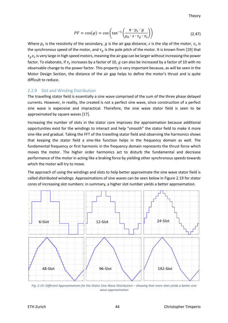
Theory


𝑃𝐹 = cos(𝜑) = cos (tan−1 (𝜋 ∙ 𝑝𝑠 ∙ 𝑔

𝜇0 ∙ 𝑠 ∙ 𝜏𝑝 ∙ 𝑣𝑠)) (2.47)

Where 𝑝𝑠 is the resistivity of the secondary, 𝑔 is the air gap distance, 𝑠 is the slip of the motor, 𝑣𝑠 is

the synchronous speed of the motor, and 𝜏𝑝 is the pole pitch of the motor. It is known from [19] that

𝜏𝑝𝑣𝑠 is very large in high speed motors, meaning the air gap can be larger without increasing the power

factor. To elaborate, if 𝑣𝑠 increases by a factor of 10, 𝑔 can also be increased by a factor of 10 with no

observable change to the power factor. This property is very important because, as will be seen in the

Motor Design Section, the distance of the air gap helps to define the motor’s thrust and is quite

difficult to reduce.

2.2.9 Slot and Winding Distribution The travelling stator field is essentially a sine wave comprised of the sum of the three phase delayed

currents. However, in reality, the created is not a perfect sine wave, since construction of a perfect

sine wave is expensive and impractical. Therefore, the sine wave stator field is seen to be

approximated by square waves [17].

Increasing the number of slots in the stator core improves the approximation because additional

opportunities exist for the windings to interact and help “smooth” the stator field to make it more

sine-like and gradual. Taking the FFT of the travelling stator field and observing the harmonics shows

that keeping the stator field a sine-like function helps in the frequency domain as well. The

fundamental frequency or first harmonic in the frequency domain represents the thrust force which

moves the motor. The higher order harmonics act to disturb the fundamental and decrease

performance of the motor in acting like a braking force by yielding other synchronous speeds towards

which the motor will try to move.

The approach of using the windings and slots to help better approximate the sine wave stator field is

called distributed windings. Approximations of sine waves can be seen below in Figure 2.19 for stator

cores of increasing slot numbers: in summary, a higher slot number yields a better approximation.

Fig. 2.19: Different Approximations for the Stator Sine Wave Distribution – showing that more slots yields a better sine

wave approximation

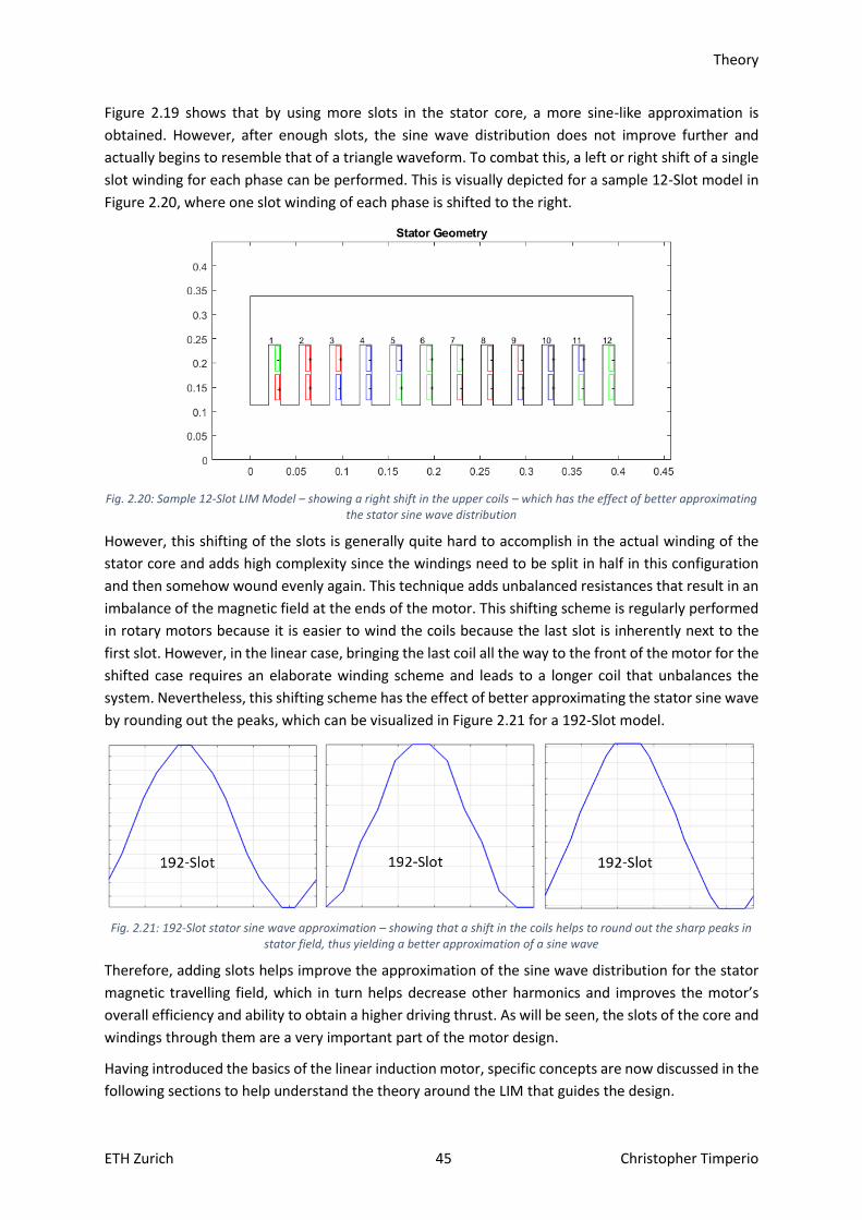
Theory


Figure 2.19 shows that by using more slots in the stator core, a more sine-like approximation is

obtained. However, after enough slots, the sine wave distribution does not improve further and

actually begins to resemble that of a triangle waveform. To combat this, a left or right shift of a single

slot winding for each phase can be performed. This is visually depicted for a sample 12-Slot model in

Figure 2.20, where one slot winding of each phase is shifted to the right.

Fig. 2.20: Sample 12-Slot LIM Model – showing a right shift in the upper coils – which has the effect of better approximating

the stator sine wave distribution

However, this shifting of the slots is generally quite hard to accomplish in the actual winding of the

stator core and adds high complexity since the windings need to be split in half in this configuration

and then somehow wound evenly again. This technique adds unbalanced resistances that result in an

imbalance of the magnetic field at the ends of the motor. This shifting scheme is regularly performed

in rotary motors because it is easier to wind the coils because the last slot is inherently next to the

first slot. However, in the linear case, bringing the last coil all the way to the front of the motor for the

shifted case requires an elaborate winding scheme and leads to a longer coil that unbalances the

system. Nevertheless, this shifting scheme has the effect of better approximating the stator sine wave

by rounding out the peaks, which can be visualized in Figure 2.21 for a 192-Slot model.

Fig. 2.21: 192-Slot stator sine wave approximation – showing that a shift in the coils helps to round out the sharp peaks in

stator field, thus yielding a better approximation of a sine wave

Therefore, adding slots helps improve the approximation of the sine wave distribution for the stator

magnetic travelling field, which in turn helps decrease other harmonics and improves the motor’s

overall efficiency and ability to obtain a higher driving thrust. As will be seen, the slots of the core and

windings through them are a very important part of the motor design.

Having introduced the basics of the linear induction motor, specific concepts are now discussed in the

following sections to help understand the theory around the LIM that guides the design.

Theory


2.3 Magnetic Flux Density

Eqn. 2.4 Gausses Law for Magnetism shows that no magnetic monopoles can exist.

∇ ∙ �⃑� = 0 (2.48)

with �⃑� as the magnetic flux density in free space – defined as the product of the absolute permeability

and the magnetic field strength;

�⃑� = 𝜇�⃑⃑� (2.49)

with 𝜇 being the absolute permeability comprised of the relative or material permeability 𝜇𝑟, and the

free space or vacuum permeability 𝜇0 = 4𝜋 ∙ 10−7 H/m [15].

The flux is then defined as the number of magnetic field lines passing through some surface. Since the

magnetic field lines begin and end on themselves, they are closed and do not terminate on a “magnetic

charge” [15]. Therefore, the flux passing through some defined open surface area is defined as;

Φ = ∫�⃑� ∙ 𝑑𝑆

𝑆

= 𝐵 ∙ 𝑆𝐴 (2.50)

The number of magnetic field lines passing through some surface area is defined as the net magnetic

flux. The magnetic flux is measured in units of Webers. As the stator field is produced, this flux passes

through and exists in-between the stator and rotor, or in the air gap of the LIM. This is the initial step

of how the LIM’s thrust is produced.

2.3.1 Magnetic Saturation The magnetic flux is a product between the magnetic flux density, 𝐵, and the total surface area, 𝑆𝐴,

through which the flux passes. Therefore, if the flux should be increased, the only way to do so, is by

either increasing the magnetic flux density, or by increasing the total surface area through which the

flux passes. What is not evident by simply looking at Eqn. 2.50 is that the B-field can only be increased

to a certain level: beyond this point, it is no longer possible it is no longer possible to achieve

noticeable3 changes in the flux by simply increasing the magnetic flux density, 𝐵.

This point is known as the magnetic saturation flux density, 𝐵𝑠𝑎𝑡, and is dependent on the type of

magnetic material used. The known physical limit for the magnetic saturation point of any magnetic

material is usually around 1.8T [15], [17], [23]. Under special conditions, or for some rare materials,

magnetic saturation values of 2.6T have been observed [23]. However, in general, this property is

observed as a fundamental physical and theoretical limit on a material that cannot be surpassed.

As a result, to further increase the flux, one must increase the overall surface area through which the

flux is allowed to pass. This means increasing the size of the stator so 𝐵𝑠𝑎𝑡 is not reached for a given

input source. 𝐵𝑠𝑎𝑡 is therefore sought to be as large as possible for a given material as this has the

effect of shrinking the size of the electric machine [23]. Otherwise, passing too much flux through a

designated surface area can cause 𝐵 to saturate to 𝐵𝑠𝑎𝑡. This phenomenon can be seen in Figure 2.22,

where magnetic saturation is observed for a simple soft iron stator core.

3 The core will appear to not accept any more flux, however, increasing 𝐵 after the saturation point will still slightly increase the flux, however diminishing returns will be observed, as asynchronous machines cannot be overloaded.

Theory


Fig. 2.22: Simplified LIM showing the magnetic saturation limit reached for a Soft Iron Stator Core. The stator core above is

magnetically saturated, while the stator core below is not operating under magnetic saturation conditions.

The plot on top shows how the core saturates with a magnetic flux density point of 1.8T for a given

input source. The below plot shows when the core is not saturated; this operating condition has been

achieved by drastically lowering the input source. When operating below magnetic saturation

conditions, the thrust produced will not be as large as it could be for higher input levels. When the

core approaches saturation, the corners begin to saturate first due to their high field potentials. This

behavior can be seen in the bottom plot where the corners of the stator core begin to saturate past

1.8T.

Conditions drawn from Figure 2.22 indicate that this linear motor stator core needs to be made much

larger in order to support higher inputs and fluxes that would otherwise cause this current core to

saturate. Otherwise, this core would simply produce less thrust for its current size. Less thrust

correlates to a much lower motor efficiency because the machine does not produce an equivalent

force relative to the applied input level. Thus, the core operates in a region implied by its name,

saturation.

Saturation is not necessarily bad; it is a physical condition of the material describing what happens

when too much flux is “pushed” through the stator core. The stator core will first try to react to this

changing flux by accepting or supporting it. However, if the core is not large enough, it does not matter

how much input is applied, it will saturate at 𝐵𝑠𝑎𝑡 for the given material.

As stated earlier, iron is usually deployed as the material of the stator core. Iron is a soft magnetic

material, meaning the magnetic flux density, 𝐵, can be easily changed by applying small values of the

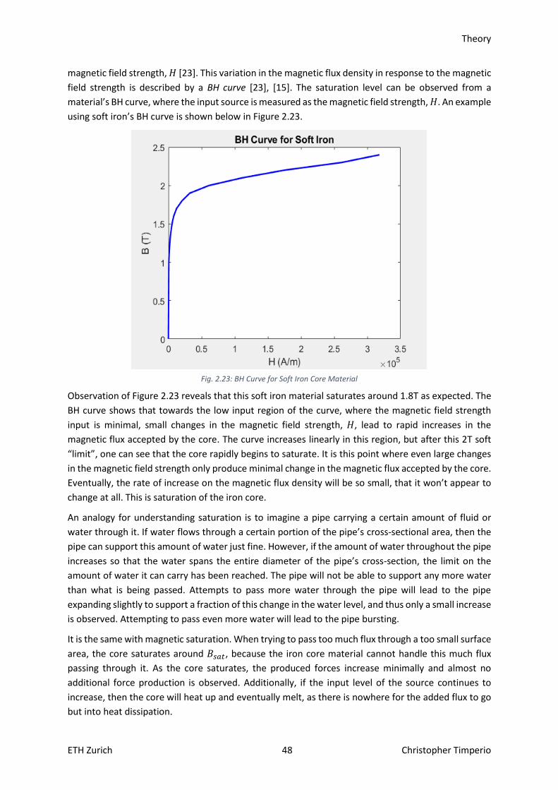
Theory


magnetic field strength, 𝐻 [23]. This variation in the magnetic flux density in response to the magnetic

field strength is described by a BH curve [23], [15]. The saturation level can be observed from a

material’s BH curve, where the input source is measured as the magnetic field strength, 𝐻. An example

using soft iron’s BH curve is shown below in Figure 2.23.

Fig. 2.23: BH Curve for Soft Iron Core Material

Observation of Figure 2.23 reveals that this soft iron material saturates around 1.8T as expected. The

BH curve shows that towards the low input region of the curve, where the magnetic field strength

input is minimal, small changes in the magnetic field strength, 𝐻, lead to rapid increases in the

magnetic flux accepted by the core. The curve increases linearly in this region, but after this 2T soft

“limit”, one can see that the core rapidly begins to saturate. It is this point where even large changes

in the magnetic field strength only produce minimal change in the magnetic flux accepted by the core.

Eventually, the rate of increase on the magnetic flux density will be so small, that it won’t appear to

change at all. This is saturation of the iron core.

An analogy for understanding saturation is to imagine a pipe carrying a certain amount of fluid or

water through it. If water flows through a certain portion of the pipe’s cross-sectional area, then the

pipe can support this amount of water just fine. However, if the amount of water throughout the pipe

increases so that the water spans the entire diameter of the pipe’s cross-section, the limit on the

amount of water it can carry has been reached. The pipe will not be able to support any more water

than what is being passed. Attempts to pass more water through the pipe will lead to the pipe

expanding slightly to support a fraction of this change in the water level, and thus only a small increase

is observed. Attempting to pass even more water will lead to the pipe bursting.

It is the same with magnetic saturation. When trying to pass too much flux through a too small surface

area, the core saturates around 𝐵𝑠𝑎𝑡, because the iron core material cannot handle this much flux

passing through it. As the core saturates, the produced forces increase minimally and almost no

additional force production is observed. Additionally, if the input level of the source continues to

increase, then the core will heat up and eventually melt, as there is nowhere for the added flux to go

but into heat dissipation.

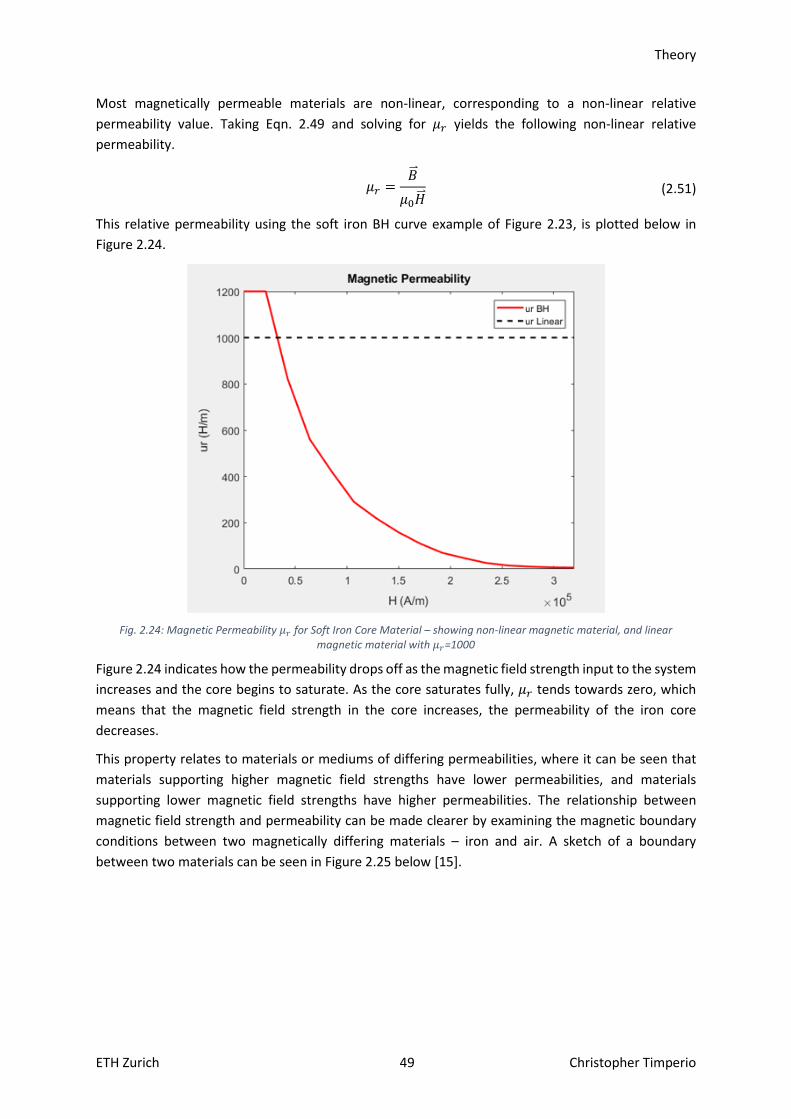
Theory


Most magnetically permeable materials are non-linear, corresponding to a non-linear relative

permeability value. Taking Eqn. 2.49 and solving for 𝜇𝑟 yields the following non-linear relative

permeability.

𝜇𝑟 =�⃑�

𝜇0�⃑⃑� (2.51)

This relative permeability using the soft iron BH curve example of Figure 2.23, is plotted below in

Figure 2.24.

Fig. 2.24: Magnetic Permeability 𝜇𝑟 for Soft Iron Core Material – showing non-linear magnetic material, and linear

magnetic material with 𝜇𝑟=1000

Figure 2.24 indicates how the permeability drops off as the magnetic field strength input to the system

increases and the core begins to saturate. As the core saturates fully, 𝜇𝑟 tends towards zero, which

means that the magnetic field strength in the core increases, the permeability of the iron core

decreases.

This property relates to materials or mediums of differing permeabilities, where it can be seen that

materials supporting higher magnetic field strengths have lower permeabilities, and materials

supporting lower magnetic field strengths have higher permeabilities. The relationship between

magnetic field strength and permeability can be made clearer by examining the magnetic boundary

conditions between two magnetically differing materials – iron and air. A sketch of a boundary

between two materials can be seen in Figure 2.25 below [15].

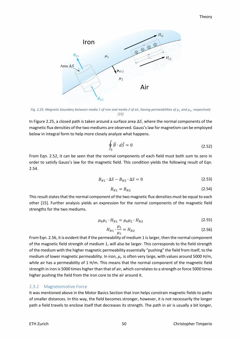
Theory


Fig. 2.25: Magnetic boundary between media 1 of iron and media 2 of air, having permeabilities of 𝜇1 and 𝜇2, respectively

[15]

In Figure 2.25, a closed path is taken around a surface area ∆𝑆, where the normal components of the

magnetic flux densities of the two mediums are observed. Gauss’s law for magnetism can be employed

below in integral form to help more closely analyze what happens.

∮�⃑� ∙ 𝑑𝑆

𝑆

= 0 (2.52)

From Eqn. 2.52, it can be seen that the normal components of each field must both sum to zero in

order to satisfy Gauss’s law for the magnetic field. This condition yields the following result of Eqn.

2.54.

𝐵𝑁1 ∙ ∆𝑆 − 𝐵𝑁2 ∙ ∆𝑆 = 0 (2.53)

𝐵𝑁1 = 𝐵𝑁2 (2.54)

This result states that the normal component of the two magnetic flux densities must be equal to each

other [15]. Further analysis yields an expression for the normal components of the magnetic field

strengths for the two mediums.

𝜇0𝜇1 ∙ 𝐻𝑁1 = 𝜇0𝜇2 ∙ 𝐻𝑁2 (2.55)

𝐻𝑁1 ∙𝜇1

𝜇2= 𝐻𝑁2 (2.56)

From Eqn. 2.56, it is evident that if the permeability of medium 1 is larger, then the normal component

of the magnetic field strength of medium 1, will also be larger. This corresponds to the field strength

of the medium with the higher magnetic permeability essentially “pushing” the field from itself, to the

medium of lower magnetic permeability. In iron, 𝜇𝑟 is often very large, with values around 5000 H/m,

while air has a permeability of 1 H/m. This means that the normal component of the magnetic field

strength in iron is 5000 times higher than that of air, which correlates to a strength or force 5000 times

higher pushing the field from the iron core to the air around it.

2.3.2 Magnetomotive Force It was mentioned above in the Motor Basics Section that iron helps constrain magnetic fields to paths

of smaller distances. In this way, the field becomes stronger, however, it is not necessarily the longer

path a field travels to enclose itself that decreases its strength. The path in air is usually a bit longer,

Iron

Air

Theory


but only about three to five times as long as the path in iron. The main reason the field strength is

much higher is the fact that fields in highly magnetically permeable materials are pushed or driven to

less magnetically permeable materials and thus concentrate the field strength in these regions [13].

This force can be described as the Magnetomotive Force or MMF, and is best described by Ampere’s

Law, as the product of the magnetic field strength �⃑⃑� and its closed path 𝑑𝑙 .

Θ = ∮ �⃑⃑� ∙ 𝑑𝑙

(𝑐)

= ∬𝐽 ∙ 𝑑𝑆

𝑆

= 𝐻 ∙ 𝐿 = Φ ∙ ℛ = 𝑁 ∙ 𝐼 (2.57)

Where Θ is the MMF [13], [21]. The MMF is a phenomenon that gives rise to magnetic fields. Electrons

within the material itself oppose the magnetic field and create a force that can be observed as the

MMF [13]. This opposing force “pushes” the field from materials with higher magnetic permeabilities

to materials with lower magnetic permeabilities. In this manner, the iron core provides the MMF force

necessary to drive the flux throughout its closed path. Note, flux does not flow as electric current flows

through a circuit, it is rather a state of molecules in a material [13].

The MMF can also be described in other ways, as seen in Eqn. 2.57 above. The most appropriate form

for this linear motor application is the turn number times the current, measured in ampere-turns (At).

Thus, it is clear why it is desirable to increase the flux passing through the stator core: flux is the main

component of the MMF and by increasing the flux, thee MMF increases. It will be shown in the

subsequent sections that the MMF is directly related to how the Lorentz Force is produced, which is

the main parameter of interest in generating the thrust for this linear motor.

2.3.3 Reluctance and the Magnetic Circuit It was stated above that the MMF is the force pushing or guiding the flux towards materials of lower

magnetic permeabilities. However, the path that the flux takes, is defined differently; as a material’s

reluctance. Magnetic reluctance can be most easily thought of as a kind of magnetic resistance

property, which essentially defines the path for the magnetic flux lines to follow inside of a magnetic

material. Just as in an electric circuit, where the current takes the path of least electric resistance, in

a magnetic circuit or path, the flux exists through the path of least magnetic resistance, or reluctance

[15].

Rearranging Eqn. 2.57 allows the reluctance to be defined as the ratio of the MMF to the magnetic

flux.

ℛ =Θ

Φ (2.58)

The reluctance defines the path in which the flux exists, which is why flux paths are shorter through

the magnetic material. If the 𝜇𝑟 of a material is higher, the reluctance will be lower and thus the path

taken is shorter. This property can be seen if Eqn. 2.58 is manipulated to show the following;

ℛ =Θ

Φ=

𝐻 ∙ 𝐿

𝐵 ∙ 𝑆=

𝐻 ∙ 𝐿

𝜇𝐻 ∙ 𝑆=> ℛ =

𝐿

𝜇0𝜇𝑟 ∙ 𝑆 (2.59)

From Eqn. 2.59, it can be observed that as 𝜇𝑟 of a magnetic material increases, the length of the path

which the flux takes, 𝐿, decreases. Therefore, if the stator core is made of iron, the magnetic

permeability will be higher in this material, meaning it can support higher magnetic field strengths. A

higher magnetic field strength means that the MMF driving the field lines or flux will be much larger

than in any surrounding materials and will force the field towards these materials of lower magnetic

Theory


permeabilities. The route is dictated by the iron’s magnetic reluctance, which will favor paths of

shorter lengths.

Not only can magnetic reluctance be explained from a field perspective, but the reluctance can also

be explained by a circuit analogue. In this analogy, the entire linear motor is described by a

corresponding magnetic circuit. The magnetic circuit can be constructed to detail the resistances and

reactance’s in the system and help determine the voltage levels supplied to the motor.

A simplified magnetic circuit for the primary stator core and stator windings with a passive aluminum

“blade”-type secondary, can be seen below in Figure 2.26.

Fig. 2.26: Magnetic Circuit of the LIM showing Stator Winding Resistance, Rotor Reactance and Resistivity of Rotor for a

single phase of the linear motor

Where 𝑅𝑠 is the stator winding resistance, 𝑗𝑋𝑠 is the inductive stator winding reactance, 𝑅𝑎𝑙 is the

resistivity of the secondary aluminum rotor blade, 𝑗𝑋𝑎𝑙 is the inductive reactance of the aluminum

rotor blade, and 𝑗𝑋𝑔𝑎𝑝 is the reactance of the air gap (which can also be capacitive) [21], [13].

In 3-phase systems, it is best practice to calculate everything in terms of ‘per phase’. Therefore, the

source is represented as one phase of the system, 𝑈. The other phases, 𝑉 and 𝑊, would be the same.

The rotary motor’s equivalent circuit includes the rotor’s mechanical rotating losses. The magnetic

circuit for the linear motor on the other hand is much simpler, as these losses do not exist. However,

the dominant losses in the linear motor are from the stray flux4 losses of the motor, which often

constitute a large percentage of the flux produced [13]. These stray flux losses do not contribute to

overall thrust production of the motor and must therefore be minimized, while the useful or

contributing flux should be maximized. A depiction of the stray flux compared to the useful flux can

be seen below in Figure 2.27.

4 Stray flux is defined as the flux which links one or two windings together, and acts just as the name suggests; stray. It can exist in air and usually encircles the coils. This stray flux leaks through all parts of the machine, and is unused in thrust production. The reason it is unused is that it does not generally pass near enough to the rotor to induce sufficient eddy currents into the rotor blade. Stray flux is sometimes referred to as leakage flux.

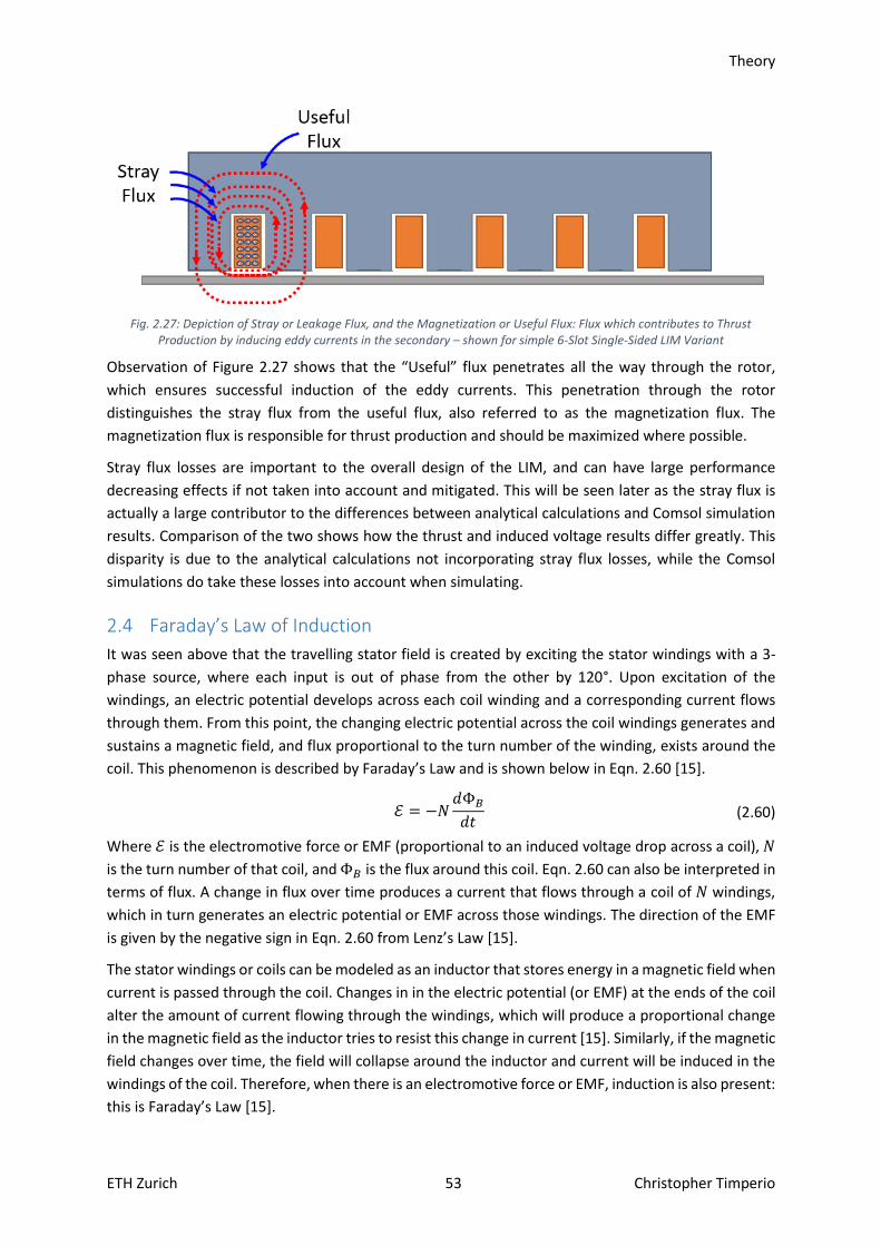
Theory


Fig. 2.27: Depiction of Stray or Leakage Flux, and the Magnetization or Useful Flux: Flux which contributes to Thrust

Production by inducing eddy currents in the secondary – shown for simple 6-Slot Single-Sided LIM Variant

Observation of Figure 2.27 shows that the “Useful” flux penetrates all the way through the rotor,

which ensures successful induction of the eddy currents. This penetration through the rotor

distinguishes the stray flux from the useful flux, also referred to as the magnetization flux. The

magnetization flux is responsible for thrust production and should be maximized where possible.

Stray flux losses are important to the overall design of the LIM, and can have large performance

decreasing effects if not taken into account and mitigated. This will be seen later as the stray flux is

actually a large contributor to the differences between analytical calculations and Comsol simulation

results. Comparison of the two shows how the thrust and induced voltage results differ greatly. This

disparity is due to the analytical calculations not incorporating stray flux losses, while the Comsol

simulations do take these losses into account when simulating.

2.4 Faraday’s Law of Induction

It was seen above that the travelling stator field is created by exciting the stator windings with a 3-

phase source, where each input is out of phase from the other by 120°. Upon excitation of the

windings, an electric potential develops across each coil winding and a corresponding current flows

through them. From this point, the changing electric potential across the coil windings generates and

sustains a magnetic field, and flux proportional to the turn number of the winding, exists around the

coil. This phenomenon is described by Faraday’s Law and is shown below in Eqn. 2.60 [15].

ℰ = −𝑁𝑑Φ𝐵

𝑑𝑡 (2.60)

Where ℰ is the electromotive force or EMF (proportional to an induced voltage drop across a coil), 𝑁

is the turn number of that coil, and Φ𝐵 is the flux around this coil. Eqn. 2.60 can also be interpreted in

terms of flux. A change in flux over time produces a current that flows through a coil of 𝑁 windings,

which in turn generates an electric potential or EMF across those windings. The direction of the EMF

is given by the negative sign in Eqn. 2.60 from Lenz’s Law [15].

The stator windings or coils can be modeled as an inductor that stores energy in a magnetic field when

current is passed through the coil. Changes in in the electric potential (or EMF) at the ends of the coil

alter the amount of current flowing through the windings, which will produce a proportional change

in the magnetic field as the inductor tries to resist this change in current [15]. Similarly, if the magnetic

field changes over time, the field will collapse around the inductor and current will be induced in the

windings of the coil. Therefore, when there is an electromotive force or EMF, induction is also present:

this is Faraday’s Law [15].

Theory


To elaborate, induction is a phenomenon concerning electric and magnetic fields whereby magnetic

field changes produce electric fields, at the same moment and in the same place [17], [13].

Induction is therefore taking place in the motor due to the electric potential which is dropped across

the stator windings. The EMF across the windings causes a proportional current to flow that produces

the stator magnetic field according to Faraday’s Law. This stator magnetic field varies in position, and

sweeps across the length of the stator because the excitation is by a simultaneous 3-phase source.

As the travelling stator magnetic field sweeps across the stator, flux passes through and interacts with

the rotor to induce eddy currents according to the Maxwell-Faraday Law of Eqn. 2.61.

∇ × �⃑� = −∂�⃑�

∂t (2.61)

Where the travelling stator field is defined as a time-varying magnetic field to the rotor, denoted here

as ∂�⃑� ∂t⁄ , and creates a corresponding electric field strength, �⃑� , from Faraday’s law [13], [15]. Since

the electric field strength is proportional to the product of the medium's current density and its

conductivity (i.e., by Eqn. 2.7), it is analogous to an electric current. Therefore, the stator's time-

varying magnetic field induces currents in the conductive rotor secondary, herein referred to as eddy

currents. These induced eddy currents lead to thrust generation in the LIM and help to realize the

basic working principle behind an asynchronous motor: Induction, as is stated in the name of the

motor; linear induction motor.

2.4.1 Eddy Currents These eddy currents are induced from the EMF existing across a given stator winding. Once induced

in the rotor by the travelling stator field, the eddy currents will in turn produce an equal and opposite

magnetic field of their own. The generation of this field follows the same laws by which the eddy

currents themselves were produced. However, the order is now reversed: while the induced currents

were initially created by a time-varying magnetic field, now, the time-varying eddy currents produce

a magnetic field. The resulting magnetic field is equal and opposite to the initial stator field from the

source.

Thus, Eqn. 2.1 and Eqn. 2.2 sustain one another as is the case in a propagating electromagnetic wave.

Additionally, just as the stator field is produced from 3-phase alternating currents, this newly created

field from the eddy currents will also be 3-phase and alternating. These properties allow the rotor field

to sweep the length of the motor like the travelling stator field does. This interaction of the traveling

stator field to induce eddy currents in the rotor blade and the subsequent production of a

corresponding magnetic field by the eddy currents can be seen in Figure 2.28 below.

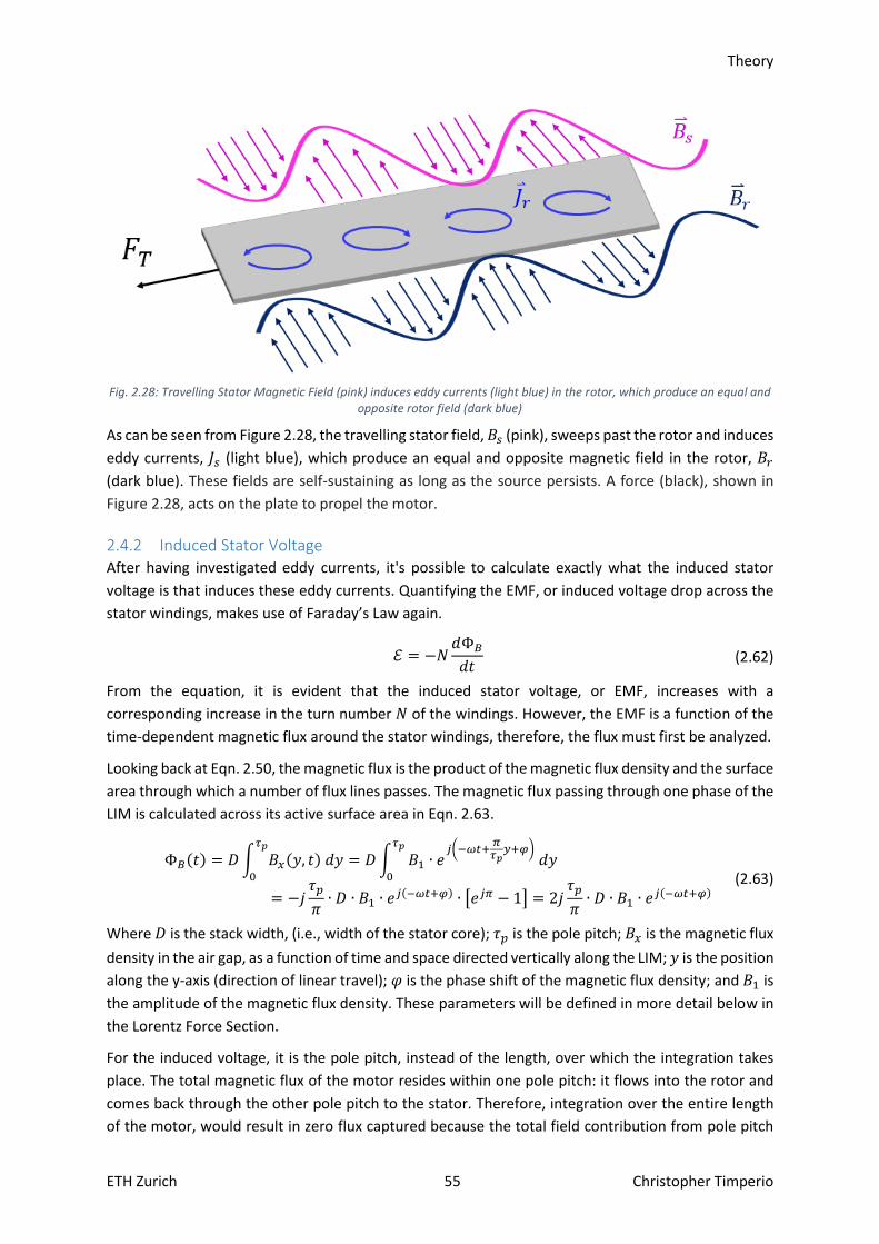
Theory


Fig. 2.28: Travelling Stator Magnetic Field (pink) induces eddy currents (light blue) in the rotor, which produce an equal and

opposite rotor field (dark blue)

As can be seen from Figure 2.28, the travelling stator field, 𝐵𝑠 (pink), sweeps past the rotor and induces

eddy currents, 𝐽𝑠 (light blue), which produce an equal and opposite magnetic field in the rotor, 𝐵𝑟

(dark blue). These fields are self-sustaining as long as the source persists. A force (black), shown in

Figure 2.28, acts on the plate to propel the motor.

2.4.2 Induced Stator Voltage After having investigated eddy currents, it's possible to calculate exactly what the induced stator

voltage is that induces these eddy currents. Quantifying the EMF, or induced voltage drop across the

stator windings, makes use of Faraday’s Law again.


𝑑𝑡 (2.62)

From the equation, it is evident that the induced stator voltage, or EMF, increases with a

corresponding increase in the turn number 𝑁 of the windings. However, the EMF is a function of the

time-dependent magnetic flux around the stator windings, therefore, the flux must first be analyzed.

Looking back at Eqn. 2.50, the magnetic flux is the product of the magnetic flux density and the surface

area through which a number of flux lines passes. The magnetic flux passing through one phase of the

LIM is calculated across its active surface area in Eqn. 2.63.

Φ𝐵(𝑡) = 𝐷 ∫ 𝐵𝑥(𝑦, 𝑡) 𝑑𝑦

𝜏𝑝

0

= 𝐷 ∫ 𝐵1 ∙ 𝑒𝑗(−𝜔𝑡+

𝜋𝜏𝑝

𝑦+𝜑) 𝑑𝑦

𝜏𝑝

0

= −𝑗𝜏𝑝

𝜋∙ 𝐷 ∙ 𝐵1 ∙ 𝑒𝑗(−𝜔𝑡+𝜑) ∙ [𝑒𝑗𝜋 − 1] = 2𝑗

𝜏𝑝

𝜋∙ 𝐷 ∙ 𝐵1 ∙ 𝑒𝑗(−𝜔𝑡+𝜑)

(2.63)

Where 𝐷 is the stack width, (i.e., width of the stator core); 𝜏𝑝 is the pole pitch; 𝐵𝑥 is the magnetic flux

density in the air gap, as a function of time and space directed vertically along the LIM; 𝑦 is the position

along the y-axis (direction of linear travel); 𝜑 is the phase shift of the magnetic flux density; and 𝐵1 is

the amplitude of the magnetic flux density. These parameters will be defined in more detail below in

the Lorentz Force Section.

For the induced voltage, it is the pole pitch, instead of the length, over which the integration takes

place. The total magnetic flux of the motor resides within one pole pitch: it flows into the rotor and

comes back through the other pole pitch to the stator. Therefore, integration over the entire length

of the motor, would result in zero flux captured because the total field contribution from pole pitch

Theory


pairs would cancel each other out, as they are the opposite of each other: Eqn. 2.4. To correctly

determine the magnetic flux, integration must be performed over only one pole pitch and not the

entirety of the motor length [22].

From Eqn. 2.63, the time derivative of the flux is then multiplied by the turn number, 𝑁, to get the

total EMF or induced voltage of the stator windings, as seen in Eqn. 2.64.

ℰ = 𝐸𝑠(𝑡) = −𝑁𝑑Φ𝐵

𝑑𝑡= −𝑁

𝑑 (2𝑗𝜏𝑝

𝜋 ∙ 𝐷 ∙ 𝐵1 ∙ 𝑒𝑗(−𝜔𝑡+𝜑))

𝑑𝑡 (2.64)

Substitution of a sinusoidal frequency domain dependency, 𝑗𝜔𝑠, for the time dependent derivative,

𝑑𝑑𝑡⁄ , is performed in Eqn. 2.65 to help simplify the equation.

𝐸𝑠(𝑡) = −𝑁𝑑Φ𝐵

𝑑𝑡= −𝑁 ∙ (𝑗𝜔𝑠) ∙ 2𝑗

𝜏𝑝

𝜋∙ 𝐷 ∙ 𝐵1 ∙ 𝑒𝑗(−𝜔𝑡+𝜑) (2.65)

The stator induced voltage is a function of time and can be treated as a first order, differential equation

with a particular solution equal to an exponential multiplied by some amplitude. This scaled

exponential is then set equal to the stator induced voltage function to determine the amplitude of the

induced stator winding voltage.

𝐸𝑠(𝑡) = 𝑁 ∙ 𝜔𝑠 ∙ 2𝜏𝑝

𝜋∙ 𝐷 ∙ 𝐵1 ∙ 𝑒𝑗(−𝜔𝑡+𝜑) (2.66)

𝐸𝑠(𝑡) => 𝐸1 ∙ 𝑒𝑗(−𝜔𝑡+𝜑) = 𝑁 ∙ 𝜔𝑠 ∙ 2𝜏𝑝

𝜋∙ 𝐷 ∙ 𝐵1 ∙ 𝑒𝑗(−𝜔𝑡+𝜑) (2.67)

Cancelling out the exponential function on both sides of the equation yields the amplitude of the

induced stator winding voltage. After some additional algebra, a more elegant expression can be

obtained.

𝐸1 = 2 ∙ 𝜔𝑠 ∙𝜏𝑝

𝜋∙ 𝐷 ∙ 𝑁 ∙ 𝐵1 = 2 ∙ 𝑣𝑠 ∙ 𝐷 ∙ 𝑁 ∙ 𝐵1 (2.68)

The sync speed for the motor is substituted into Eqn. 2.68, and the induced stator voltage is quantified

as a function of the sync speed, the stack or core width, the turn number, and the amplitude of the

magnetic flux density. This induced voltage, or EMF, is observed across the stator windings, and as a

consequence, the travelling stator field is produced. It is because the stator field induces eddy currents

in the rotor that this motor is classified as a linear induction motor. The following section will show

how the stator field interacts with this equal and opposite rotor field to create a time-average Lorentz

Force between the stator and the rotor to generate thrust.

2.5 Lorentz Force

It was seen in the previous sections that the induction of eddy currents in the rotor leads to the

generation of an equal and opposite magnetic field that is attracted to the stator magnetic field. The

field produced from the induced eddy currents will be slightly slower than the stator field: the

difference in speed is the slip. This slip delay is linear and always moving along the stator with the

progression of the travelling field. The constant difference between the stator field and induced field

of the rotor creates the opportunity for a magnetic force. Since the rotor moves at a speed slightly

slower than the stator, it will always try to “catch up” and match the speed of the stator field (i.e., the

sync speed) and will exhibit a sort of “chasing” behavior. As discussed in the Slip Section, once the

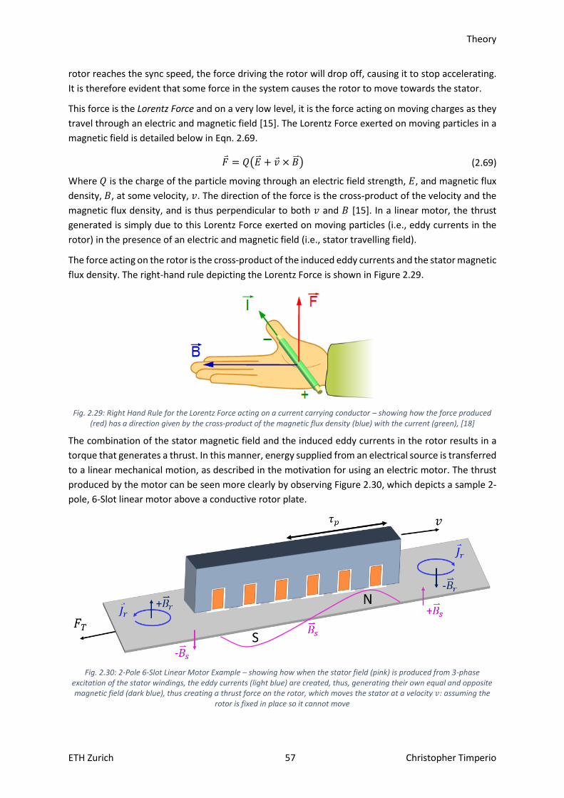
Theory


rotor reaches the sync speed, the force driving the rotor will drop off, causing it to stop accelerating.

It is therefore evident that some force in the system causes the rotor to move towards the stator.

This force is the Lorentz Force and on a very low level, it is the force acting on moving charges as they

travel through an electric and magnetic field [15]. The Lorentz Force exerted on moving particles in a

magnetic field is detailed below in Eqn. 2.69.

𝐹 = 𝑄(�⃑� + 𝑣 × �⃑� ) (2.69)

Where 𝑄 is the charge of the particle moving through an electric field strength, 𝐸, and magnetic flux

density, 𝐵, at some velocity, 𝑣. The direction of the force is the cross-product of the velocity and the

magnetic flux density, and is thus perpendicular to both 𝑣 and 𝐵 [15]. In a linear motor, the thrust

generated is simply due to this Lorentz Force exerted on moving particles (i.e., eddy currents in the

rotor) in the presence of an electric and magnetic field (i.e., stator travelling field).

The force acting on the rotor is the cross-product of the induced eddy currents and the stator magnetic

flux density. The right-hand rule depicting the Lorentz Force is shown in Figure 2.29.

Fig. 2.29: Right Hand Rule for the Lorentz Force acting on a current carrying conductor – showing how the force produced

(red) has a direction given by the cross-product of the magnetic flux density (blue) with the current (green), [18]

The combination of the stator magnetic field and the induced eddy currents in the rotor results in a

torque that generates a thrust. In this manner, energy supplied from an electrical source is transferred

to a linear mechanical motion, as described in the motivation for using an electric motor. The thrust

produced by the motor can be seen more clearly by observing Figure 2.30, which depicts a sample 2-

pole, 6-Slot linear motor above a conductive rotor plate.

Fig. 2.30: 2-Pole 6-Slot Linear Motor Example – showing how when the stator field (pink) is produced from 3-phase

excitation of the stator windings, the eddy currents (light blue) are created, thus, generating their own equal and opposite magnetic field (dark blue), thus creating a thrust force on the rotor, which moves the stator at a velocity 𝑣: assuming the

rotor is fixed in place so it cannot move

Theory


As can be seen in Figure 2.30, as the stator field induces eddy currents, 𝐽, in the rotor, corresponding

magnetic fields opposite in direction to the stator field are created from Ampere’s Law. These

magnetic fields then create the Lorentz force that moves the stator5 at velocity 𝑣.

Another way to examine the Lorentz force is to look at a simpler picture of a magnet moving over a

conductive plate in Figure 2.31. The magnet produces a DC magnetic field, so the field will remain

constant. However, if the magnet is moved over some distance at a certain velocity, then the change

in flux experienced by the conductive plate also changes. The fact that the magnet moves means that

eddy currents will be induced in this plate by the flux lines of the magnet sweeping past the conductive

plate. As seen, these eddy currents produce their own corresponding magnetic field relative to the

changing flux from the moving magnet.

Fig. 2.31: Simple magnet showing induced eddy currents when thrust force exerted on magnet – or it is moving.

approximated with a simple DC field. but then when you have a 3-phase AC “travelling” or moving field, the rotor will want to follow the stator, or in this case, the magnet.

Figure 2.31 shows that from the perspective of the conductive plate, as the magnet moves across the

plate, there will always appear to be an increasing flux in the front of the magnet, and a decreasing

flux behind the magnet. These fluxes this will act to “push” the plate from behind and “pull” the plate

from the front, as the fields from the eddy currents try to align themselves with the slightly faster and

continuously moving fields from the magnet. This scenario is similar to what happens to the rotor in

the linear motor: the field from the eddy currents will always try to “catch up” to the faster time-

varying travelling stator field.

This interaction of the eddy currents induced in the plate together with the source magnetic field is

observed as the magnet sweeps across the aluminum plate at some velocity, 𝑣.

Understating how the Lorentz Force is developed in a linear motor, requires further investigation of

the interaction between the induced eddy currents and travelling stator magnetic field. The

combination of the stator magnetic field and the induced eddy currents gives rise to the Lorentz Force.

Therefore, in order to quantify the thrust force produced by the LIM, Maxwell-Faraday’s and Maxwell-

Ampere’s Laws must be deployed. These equations are the governing equations behind thrust

production in the LIM.

5 Note: in the entirety of this analysis, the rotor is the part of the motor assumed to be moving as the Lorentz Force acts on it to attract it to the stator. However, the part of the motor that moves can be reversed as it only depends on which part is fixed and which is left free. Therefore, either the rotor or the stator can be considered to be the moving part of the motor.

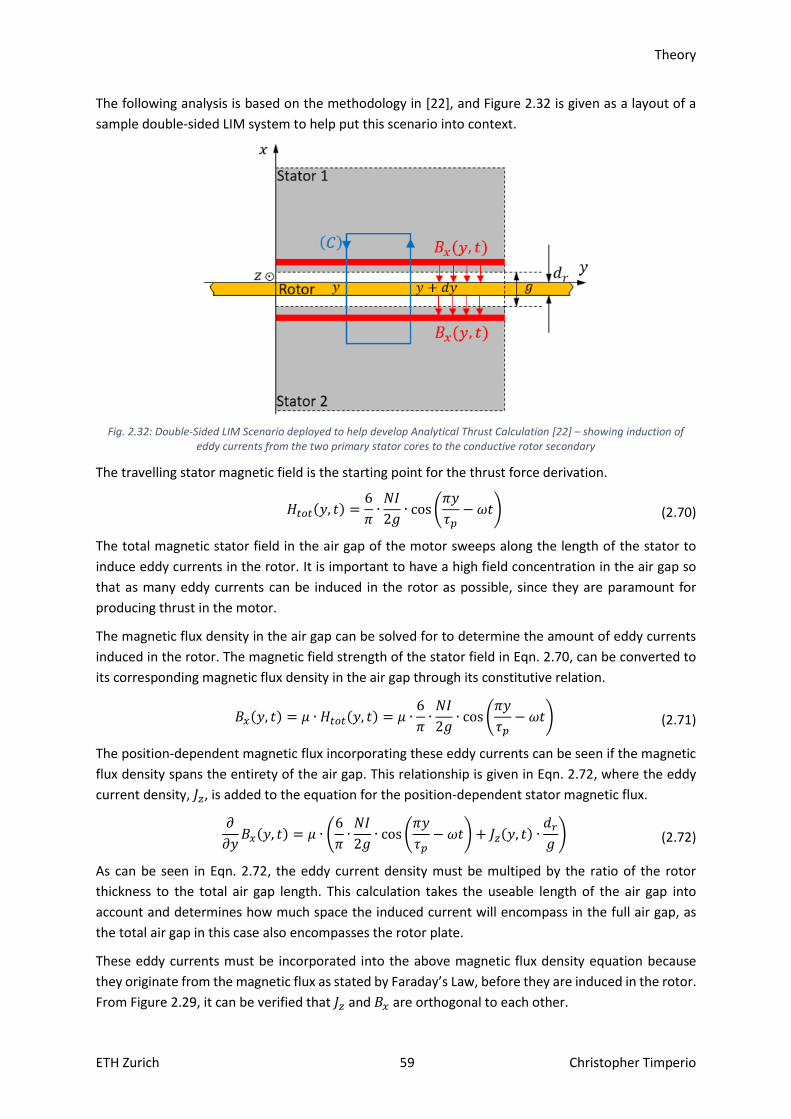
Theory


The following analysis is based on the methodology in [22], and Figure 2.32 is given as a layout of a

sample double-sided LIM system to help put this scenario into context.

Fig. 2.32: Double-Sided LIM Scenario deployed to help develop Analytical Thrust Calculation [22] – showing induction of

eddy currents from the two primary stator cores to the conductive rotor secondary

The travelling stator magnetic field is the starting point for the thrust force derivation.

𝐻𝑡𝑜𝑡(𝑦, 𝑡) =6

𝜋∙𝑁𝐼

2𝑔∙ cos(

𝜋𝑦

𝜏𝑝− 𝜔𝑡) (2.70)

The total magnetic stator field in the air gap of the motor sweeps along the length of the stator to

induce eddy currents in the rotor. It is important to have a high field concentration in the air gap so

that as many eddy currents can be induced in the rotor as possible, since they are paramount for

producing thrust in the motor.

The magnetic flux density in the air gap can be solved for to determine the amount of eddy currents

induced in the rotor. The magnetic field strength of the stator field in Eqn. 2.70, can be converted to

its corresponding magnetic flux density in the air gap through its constitutive relation.

𝐵𝑥(𝑦, 𝑡) = 𝜇 ∙ 𝐻𝑡𝑜𝑡(𝑦, 𝑡) = 𝜇 ∙6

𝜋∙𝑁𝐼

2𝑔∙ cos (

𝜋𝑦

𝜏𝑝− 𝜔𝑡) (2.71)

The position-dependent magnetic flux incorporating these eddy currents can be seen if the magnetic

flux density spans the entirety of the air gap. This relationship is given in Eqn. 2.72, where the eddy

current density, 𝐽𝑧, is added to the equation for the position-dependent stator magnetic flux.

𝜕

𝜕𝑦𝐵𝑥(𝑦, 𝑡) = 𝜇 ∙ (

6

𝜋∙𝑁𝐼

2𝑔∙ cos (

𝜋𝑦

𝜏𝑝− 𝜔𝑡) + 𝐽𝑧(𝑦, 𝑡) ∙

𝑑𝑟

𝑔) (2.72)

As can be seen in Eqn. 2.72, the eddy current density must be multiped by the ratio of the rotor

thickness to the total air gap length. This calculation takes the useable length of the air gap into

account and determines how much space the induced current will encompass in the full air gap, as

the total air gap in this case also encompasses the rotor plate.

These eddy currents must be incorporated into the above magnetic flux density equation because

they originate from the magnetic flux as stated by Faraday’s Law, before they are induced in the rotor.

From Figure 2.29, it can be verified that 𝐽𝑧 and 𝐵𝑥 are orthogonal to each other.

Theory


The next step in the analysis is to quantify these eddy currents and solve for the magnetic flux density

in the air gap. To do so, Eqn. 2.73 can be deployed to relate the induced eddy currents to the electric

field strength.

𝐽𝑧(𝑦, 𝑡) = 𝜎𝐸𝑧(𝑦, 𝑡) (2.73)

These induced eddy currents, 𝐽𝑧 , are a function of time and space and are connected to the electric

field strength, 𝐸𝑧 , through the conductivity of the rotor plate, 𝜎. Now the electric field strength must

be determined in order to solve for these currents and consequently, the magnetic flux density.

Faraday’s Law can be deployed again in Eqn. 2.74, to relate this electric field strength to the change in

the passing flux.

ℰ = ∮ �⃑� ∙ 𝑑𝑙

(𝐶1)

= −𝑑Φ𝐵

𝑑𝑡 (2.74)

Where 𝐶1 is the closed curve over which the total electric components are summed and is

perpendicular to the closed curve over which the magnetic field strength, 𝐶, is summed. Summing

over this closed path 𝐶, yields the following equation relating the electric field strength to the

magnetic flux density, as in [22].

𝜕

𝜕𝑦𝐸𝑧(𝑦, 𝑡) =

𝜕

𝜕𝑡𝐵𝑥(𝑦, 𝑡) + 𝑣

𝜕

𝜕𝑦𝐵𝑥(𝑦, 𝑡) (2.75)

Where it can now be seen that the magnetic flux density varies with position (i.e., along the length of

the stator in the horizontal y-axis) and time.

With the expressions for the magnetic flux density in the air gap and the induced eddy currents, the

system has been fully defined. Eqn. 2.72, Eqn. 2.73, and Eqn. 2.75, can be combined to find the

magnetic flux density in the airgap. Combining the expressions yields Eqn. 2.76, which describes the

behavior for the magnetic flux density in the air gap.

𝜕2

𝜕𝑦2𝐵𝑥(𝑦, 𝑡) − 𝜇𝜎 ∙

𝑑𝑟

𝑔[𝜕

𝜕𝑡𝐵𝑥(𝑦, 𝑡) + 𝑣

𝜕

𝜕𝑦𝐵𝑥(𝑦, 𝑡)] = 𝜇 ∙

6

𝜋∙𝑁𝐼

2𝑔∙ cos (

𝜋𝑦

𝜏𝑝− 𝜔𝑡) (2.76)

As seen from Eqn. 2.76, the combination of these equations leads to the creation of a second order

non-homogenous differential equation. However, this is not a problem, because it is the particular

solution of Eqn. 2.76, which has the form of a scaled exponential, that is of interest. The particular

solution is given in Eqn. 2.77.

𝐵 𝑥(𝑦, 𝑡) = 𝐵1 ∙ 𝑒𝑗(

𝜋𝑦𝜏𝑝

−𝜔𝑡+𝜑) (2.77)

The particular solution for the magnetic flux density can then be substituted back into Eqn. 2.76 in

order to obtain the amplitude of the magnetic flux density, 𝐵1, and the phase shift, 𝜑. After this

substitution and reducing and simplifying the equations, the amplitude of the magnetic flux density

can be expressed as in Eqn. 2.78.

𝐵1 =

3√2 ∙ Θ

√(𝜋𝑔𝜇 )

2+ (𝑣𝑠 − 𝑣𝑟)

2 ∙ (𝜎 ∙ 𝑑𝑟 ∙ 𝜏𝑝)2

(2.78)

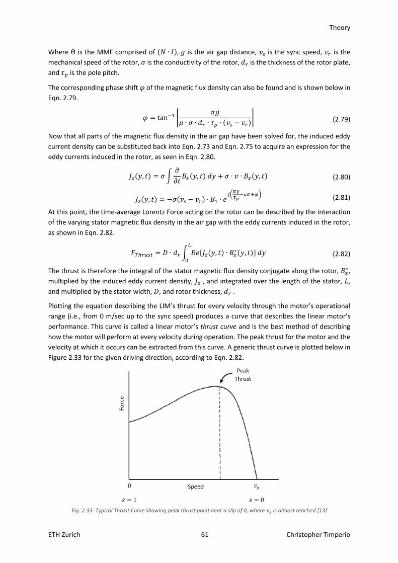
Theory


Where Θ is the MMF comprised of (𝑁 ∙ 𝐼), 𝑔 is the air gap distance, 𝑣𝑠 is the sync speed, 𝑣𝑟 is the

mechanical speed of the rotor, 𝜎 is the conductivity of the rotor, 𝑑𝑟 is the thickness of the rotor plate,

and 𝜏𝑝 is the pole pitch.

The corresponding phase shift 𝜑 of the magnetic flux density can also be found and is shown below in

Eqn. 2.79.

𝜑 = tan−1 [𝜋𝑔

𝜇 ∙ 𝜎 ∙ 𝑑𝑟 ∙ 𝜏𝑝 ∙ (𝑣𝑠 − 𝑣𝑟)] (2.79)

Now that all parts of the magnetic flux density in the air gap have been solved for, the induced eddy

current density can be substituted back into Eqn. 2.73 and Eqn. 2.75 to acquire an expression for the

eddy currents induced in the rotor, as seen in Eqn. 2.80.

𝐽𝑧(𝑦, 𝑡) = 𝜎 ∫𝜕

𝜕𝑡𝐵𝑥(𝑦, 𝑡) 𝑑𝑦 + 𝜎 ∙ 𝑣 ∙ 𝐵𝑥(𝑦, 𝑡) (2.80)

𝐽𝑧(𝑦, 𝑡) = −𝜎(𝑣𝑠 − 𝑣𝑟) ∙ 𝐵1 ∙ 𝑒𝑗(

𝜋𝑦𝜏𝑝

−𝜔𝑡+𝜑) (2.81)

At this point, the time-average Lorentz Force acting on the rotor can be described by the interaction

of the varying stator magnetic flux density in the air gap with the eddy currents induced in the rotor,

as shown in Eqn. 2.82.

𝐹𝑇ℎ𝑟𝑢𝑠𝑡 = 𝐷 ∙ 𝑑𝑟 ∫ 𝑅𝑒{𝐽𝑧(𝑦, 𝑡) ∙ 𝐵𝑥∗(𝑦, 𝑡)}

𝐿

0

𝑑𝑦 (2.82)

The thrust is therefore the integral of the stator magnetic flux density conjugate along the rotor, 𝐵𝑥∗,

multiplied by the induced eddy current density, 𝐽𝑧 , and integrated over the length of the stator, 𝐿,

and multiplied by the stator width, 𝐷, and rotor thickness, 𝑑𝑟 .

Plotting the equation describing the LIM’s thrust for every velocity through the motor’s operational

range (i.e., from 0 m/sec up to the sync speed) produces a curve that describes the linear motor’s

performance. This curve is called a linear motor’s thrust curve and is the best method of describing

how the motor will perform at every velocity during operation. The peak thrust for the motor and the

velocity at which it occurs can be extracted from this curve. A generic thrust curve is plotted below in

Figure 2.33 for the given driving direction, according to Eqn. 2.82.

Fig. 2.33: Typical Thrust Curve showing peak thrust point near a slip of 0, where 𝑣𝑠 is almost reached [13]

Theory


It can be seen from this curve that the peak thrust occurs when the rotor is almost at the sync speed.

After this peak thrust point, the thrust falls off rapidly and at the sync speed, the thrust force is zero.

The thrust goes to zero because when the rotor finally reaches the same velocity of the stator field,

there is no longer any slip, or difference in the velocities of these two fields. If velocity increases

beyond the sync speed, the motor will enter a regeneration region and it will act as a generator, which

is undesirable in this application.

Thus, the process by which a linear motor produced thrust has been clarified. The Motor Design

Section will show the linear motor in this thesis is designed to achieve the thrust required to propel a

Hyperloop Pod to the desired sync speed.

2.6 End-Effects

End-effects are described as decreases or losses in the linear motor’s performance due to the open-

ended air gaps at the ends of the linear motor [19]. These air gaps constitute the biggest difference

between rotary and linear motors and heavily influence the motor’s thrust, power factor, and

efficiency, all of which are reduced as a consequence of end-effects. End-effects do not exist in a rotary

machine because there is never an “end”, as the motor is circular and continuous. Therefore, the

rotating stator field will always be continuously rotating without interruption.

However, in a linear motor, there is a “beginning” and an “end”, which has the effect of “cutting off”

the field at the motor ends. This interruption of the field means it is not a continuously travelling field

anymore. Therefore, the field of the linear motor abruptly stops and starts at the beginning and ends

of the motor instead of continuously flowing. End-effects lead to discontinuities in the stator field, and

if not mitigated properly, can degrade design performance [19].

At low speeds, the end-effects are not significant and do not come much into play. However, at the

higher speeds, they start to have a greater impact and become problematic [19]. At high speeds, the

magnetic field distribution in the air gap, which was seen to be important for the overall thrust

produced, is different at the ends of the motor, where the air gap is “open”, more than in the middle.

The difference is due to the “entering” and “exiting” travelling stator fields having a different wave

velocity when compared to the fields in the middle of the motor. The decay rate or attenuation of

these “entering” and “exiting” fields is low, which allows them to interface with the thrust producing

fields in the middle of the motor [19]. For instance, the entry-end-effect field decays rather slowly and

is present along the entire longitudinal length of the air gap. This field significantly degrades

performance by interfering with the phase distribution of the magnetic field in the air gap produced

by the motor’s main stator field.

One solution to this issue is to vary the frequency of the motor during operation. End-effects play a

large role in the high-slip region of the thrust curve. Therefore, by always operating in a low-slip region,

near the synchronous speed, these end-effects can be mitigated. Using a variable speed or frequency

drive allows for this kind of operation. Additionally, the thrust is relatively small in this high-slip region,

so operation is kept to the region of the thrust curve near the synchronous speed. Therefore, if the

motor is operating near synchronous speed, end-effects should be minimized.

Another way to help further reduce the contribution of the end-effects is to adjust parameters such

as the air gap distance, pole number, supply frequency, secondary resistivity, etc. However, it can be

Theory


that by tweaking these variables to reduce the influence of the end-effects, motor performance

decreases. Therefore, a trade-off must be made when selecting and adjusting parameters.

End-effects can also be mitigated by altering the winding configuration. The main mechanism behind

these end-effects is the non-uniform magnetic field distributions in the air gap, which lead to

performance degradations because of the discontinuity between the beginning and end of the motor.

A more gradual travelling stator field would help guide the transition from the end of the motor to the

beginning. Therefore, for 3-phase excitation, proper winding techniques should be implemented to

ensure symmetric and gradual phase distribution throughout the linear motor. Such techniques

include increasing the number of slots or windings per phase of the stator: doing so yields a better

approximation of the sine-like distribution of the travelling stator field. In this way, the disruption in

the field seen from the end-effects is less and the field distribution in the air gap will appear less

discontinuous to the secondary.

One final end-effect mitigation technique is to make the last teeth (i.e., the end teeth) on the beginning

and end of the motor larger. Making the end teeth larger helps alleviate some of the end-effects by

capturing more of the field. Capturing more of the field helps increase the overall thrust produced by

adding more active surface area to the end teeth, which have been seen to saturate slightly faster

than the other teeth in simulations.

2.7 Paschen’s Law

Another important consideration for the motor, which introduces an additional challenge to

overcome, is that it must also operate in the low-pressure environment of the tube. Operating in a

low-pressure environment means there is an increased probability for voltage breakdowns within the

motor. Voltage breakdowns can occur when operating at the high voltages needed to drive the motor

in reduced pressure environments. The low-pressure environment or “near-vacuum” levels inside the

tube help reduce air friction on the vehicles or Pods. Therefore, even if the motor works well in

ambient pressure, this is no guarantee that it will also work well in the low-pressure environment of

the Hyperloop tube.

To explain the problem further, a voltage breakdown is a discharge event that can occur between two

conductive objects separated by a specific distance in a given medium, at certain pressures. A voltage

breakdown can be defined as a conductive channel that is created by discharges between the two

conductive objects. This discharge occurs when the electric field potential between the two

conductive objects is high enough for a given separation distance or pressure in the medium. The

product of the two, pressure and distance, is stated as 𝑝𝑑, and represents a key quantity in the

analysis. Once this product equals a specific value, a breakdown can occur.

Therefore, the pressure in the medium and distance act as a sort of insulation between conductive

objects. They do not allow a connection, or channel, between the objects unless the conditions of the

environment changed to support potential breakdowns. Such changes can include decreasing the

pressure, decreasing the distance between the objects, or increasing the electric field potential

between the objects. An example illustration of a few potential scenarios can be seen in Figure 2.34.

Theory


Fig. 2.34: Different scenarios for Paschen’s Law in Air (light blue) – showing that if either the pressure or the distance is changed, voltage breakdowns can occur, as the effect of creating conductive channels between two conductive objects,

depends both on the pressure of the medium and the distance between the objects

It can be difficult to quantify these effects analytically and most attempts only yield approximate

results. Most analysis is performed experimentally and solving the derived analytical equations to

explain these effects shows the differences in the two results. Nevertheless, estimates of the voltage

breakdown point can be made to provide a general idea of where a possible breakdown can occur.

Pachen’s Law can be deployed in this endeavor to help analyze the voltage breakdown between two

conductive objects of a certain separation distance, and to describe and quantify this level in given

gaseous mediums. Eqn. 2.83 models this phenomenon and describes the voltage breakdown 𝑉𝐵, [24],

[25].

𝑉𝐵 =

𝐵 ∙ 𝑝𝑑

ln [𝐴 ∙ 𝑝𝑑

ln(1 + 1𝛾𝑠𝑒⁄ )

]

(2.83)

Where 𝑝 is the pressure of the medium, 𝑑 is the distance between the two conductive objects in

question, and 𝐴, 𝐵, and 𝛾𝑠𝑒 are all constants describing the ionization characteristics of the medium.

𝐴 is the saturation ionization in the gas at a certain electric field strength, 𝐵 is related to the excitation

and ionization energy, and 𝛾𝑠𝑒 is the secondary ionization coefficient [25]. These values describe the

medium’s electron mobility and how ions are produced during the fundamental mechanism behind

the discharge channel’s creation, avalanching. This effect of avalanching is illustrated in Figure 2.35.

Theory


Fig. 2.35: Avalanching Effects depicted [24], where the Primary electron is the original or initial ionization event, from which

the ionization events occur and avalanching follows if there is enough energy to do so.

Avalanching is best described as a process in which a number of free electrons in a transmission

medium, subject to strong acceleration by an electric field, collide with other atoms and ionize them

upon impact: a phenomenon otherwise referred to as ionization [24]. Ionization is a process by which

an atom or a molecule acquires a negative or positive charge by gaining or losing electrons [24]. The

acquisition or loss of electrons in this case is due to collisions with other atoms, molecules, or ions.

After the initial ionization event takes place, the released electrons can collide with other molecules

in the medium, which subsequently release additional electrons that accelerate and collide with other

atoms. This cascading release of electrons is the avalanching effect.

These ionization values are key in explaining when a voltage breakdown occurs. However, obtaining

these values is not straightforward and is generally accomplished experientially, which leads to wide

variations depending on the source used. However, these variations make sense as the parameters

greatly depend on the pressure, temperature, and chemical composition of the medium. Since air is

most commonly taken as the medium of interest, and is the medium to be used in a Hyperloop-like

system, it is instructive to study how these values differ over varying environments. Table 2.1 shows

the values for the ionization parameters used in this thesis from [25], which seem to match up closely

to those of [24].

Parameters used in Evaluating Voltage Breakdown (for Air)

𝒑 ∙ 𝒅 [kPa-cm] 0.0133 – 0.2 0.2 – 100 100 – 1400

k 2.0583 ∙ (𝑝𝑑)−0.1724 3.5134 ∙ (𝑝𝑑)0.1599 4.6295

A [ionization/kPa-cm] 112.5

B [V/kPa-cm] 2737.5

Table 2.1: Ionization parameters used in Evaluating Voltage Breakdown (for Air) – for the given pd pressures distance range

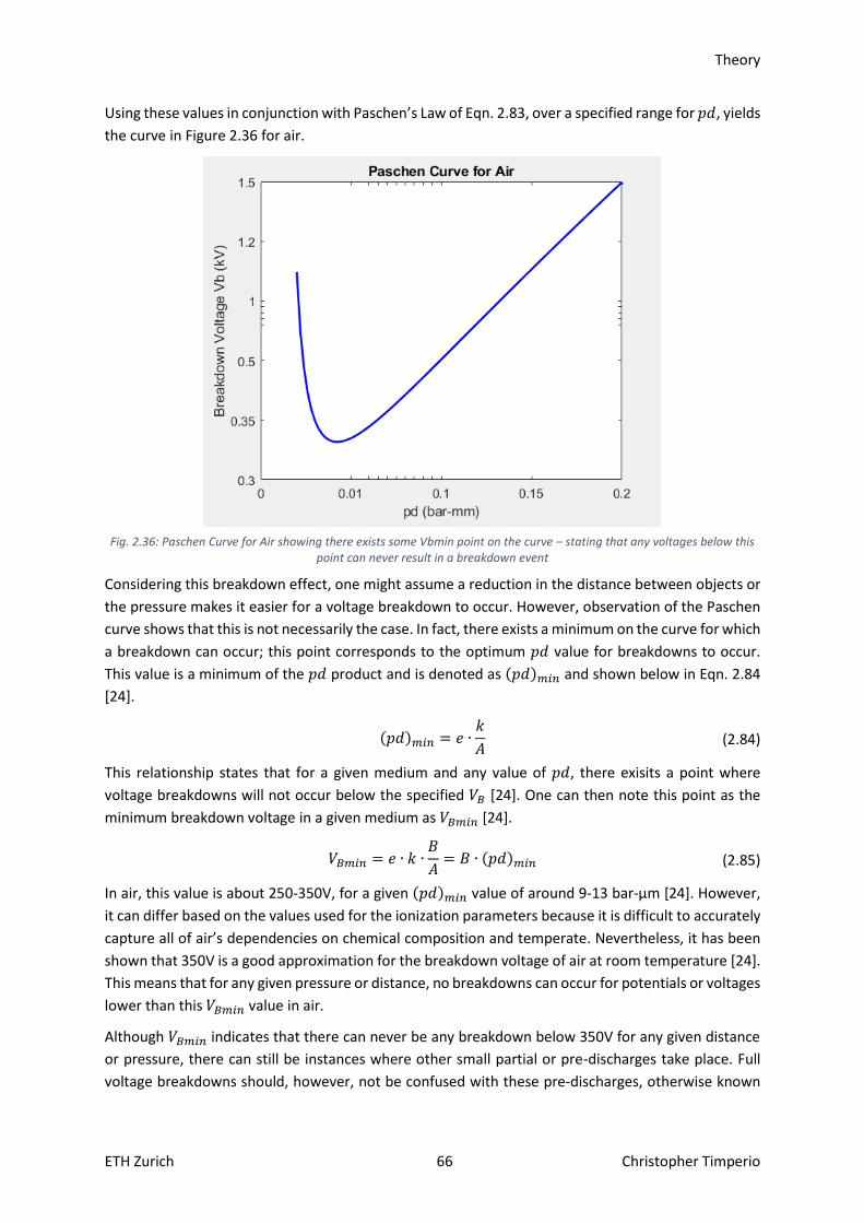
Theory


Using these values in conjunction with Paschen’s Law of Eqn. 2.83, over a specified range for 𝑝𝑑, yields

the curve in Figure 2.36 for air.

Fig. 2.36: Paschen Curve for Air showing there exists some Vbmin point on the curve – stating that any voltages below this

point can never result in a breakdown event

Considering this breakdown effect, one might assume a reduction in the distance between objects or

the pressure makes it easier for a voltage breakdown to occur. However, observation of the Paschen

curve shows that this is not necessarily the case. In fact, there exists a minimum on the curve for which

a breakdown can occur; this point corresponds to the optimum 𝑝𝑑 value for breakdowns to occur.

This value is a minimum of the 𝑝𝑑 product and is denoted as (𝑝𝑑)𝑚𝑖𝑛 and shown below in Eqn. 2.84

[24].

(𝑝𝑑)𝑚𝑖𝑛 = 𝑒 ∙𝑘

𝐴 (2.84)

This relationship states that for a given medium and any value of 𝑝𝑑, there exisits a point where

voltage breakdowns will not occur below the specified 𝑉𝐵 [24]. One can then note this point as the

minimum breakdown voltage in a given medium as 𝑉𝐵𝑚𝑖𝑛 [24].

𝑉𝐵𝑚𝑖𝑛 = 𝑒 ∙ 𝑘 ∙𝐵

𝐴= 𝐵 ∙ (𝑝𝑑)𝑚𝑖𝑛 (2.85)

In air, this value is about 250-350V, for a given (𝑝𝑑)𝑚𝑖𝑛 value of around 9-13 bar-μm [24]. However,

it can differ based on the values used for the ionization parameters because it is difficult to accurately

capture all of air’s dependencies on chemical composition and temperate. Nevertheless, it has been

shown that 350V is a good approximation for the breakdown voltage of air at room temperature [24].

This means that for any given pressure or distance, no breakdowns can occur for potentials or voltages

lower than this 𝑉𝐵𝑚𝑖𝑛 value in air.

Although 𝑉𝐵𝑚𝑖𝑛 indicates that there can never be any breakdown below 350V for any given distance

or pressure, there can still be instances where other small partial or pre-discharges take place. Full

voltage breakdowns should, however, not be confused with these pre-discharges, otherwise known

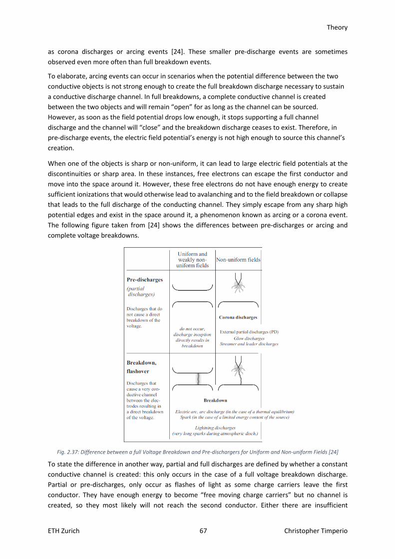
Theory


as corona discharges or arcing events [24]. These smaller pre-discharge events are sometimes

observed even more often than full breakdown events.

To elaborate, arcing events can occur in scenarios when the potential difference between the two

conductive objects is not strong enough to create the full breakdown discharge necessary to sustain

a conductive discharge channel. In full breakdowns, a complete conductive channel is created

between the two objects and will remain “open” for as long as the channel can be sourced.

However, as soon as the field potential drops low enough, it stops supporting a full channel

discharge and the channel will “close” and the breakdown discharge ceases to exist. Therefore, in

pre-discharge events, the electric field potential’s energy is not high enough to source this channel’s

creation.

When one of the objects is sharp or non-uniform, it can lead to large electric field potentials at the

discontinuities or sharp area. In these instances, free electrons can escape the first conductor and

move into the space around it. However, these free electrons do not have enough energy to create

sufficient ionizations that would otherwise lead to avalanching and to the field breakdown or collapse

that leads to the full discharge of the conducting channel. They simply escape from any sharp high

potential edges and exist in the space around it, a phenomenon known as arcing or a corona event.

The following figure taken from [24] shows the differences between pre-discharges or arcing and

complete voltage breakdowns.

Fig. 2.37: Difference between a full Voltage Breakdown and Pre-dischargers for Uniform and Non-uniform Fields [24]

To state the difference in another way, partial and full discharges are defined by whether a constant

conductive channel is created: this only occurs in the case of a full voltage breakdown discharge.

Partial or pre-discharges, only occur as flashes of light as some charge carriers leave the first

conductor. They have enough energy to become “free moving charge carriers” but no channel is

created, so they most likely will not reach the second conductor. Either there are insufficient

Theory


molecules to form a full avalanche and create the channel, or the distance is too large between the

two objects. Thus, a constant conductive channel is not created, as the energy from the electric field

between the two objects is not strong enough.

For the LIM presented in this thesis, full voltage breakdowns can be mitigated and prevented,

however, this does not mean that small arcing events or corona discharges won’t take place during

operation. To be realistic, some small arcing might occur, but it does not pose a huge threat for the

motor itself. This arcing should not cause any damage to the core or windings, but may still introduce

noise to any surrounding electronics on the Pod that have not been shielded properly against

electromagnetic interference (EMI) created from the corona discharge. Therefore, these effects have

to be measured and quantified in vacuum test chambers once the final motor has been fabricated.

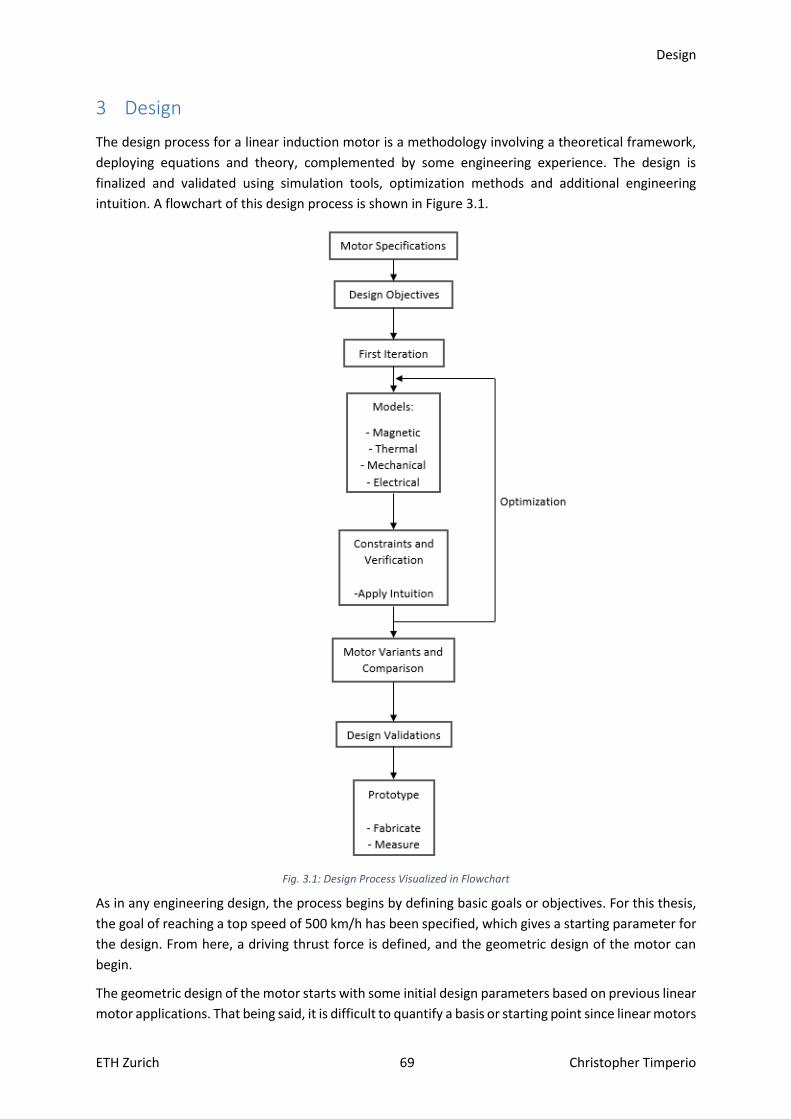
Design


3 Design

The design process for a linear induction motor is a methodology involving a theoretical framework,

deploying equations and theory, complemented by some engineering experience. The design is

finalized and validated using simulation tools, optimization methods and additional engineering

intuition. A flowchart of this design process is shown in Figure 3.1.

Fig. 3.1: Design Process Visualized in Flowchart

As in any engineering design, the process begins by defining basic goals or objectives. For this thesis,

the goal of reaching a top speed of 500 km/h has been specified, which gives a starting parameter for

the design. From here, a driving thrust force is defined, and the geometric design of the motor can

begin.

The geometric design of the motor starts with some initial design parameters based on previous linear

motor applications. That being said, it is difficult to quantify a basis or starting point since linear motors

Design


of this application (high-speed and in a low-pressure environment) have never really been designed

before. Nevertheless, a basic linear motor structure can be used to provide some initial intuitions

about the fundamental operation or functionality of a linear induction motor. After this step, the

design is improved to meet design specifications. This initial step provides an opportunity to become

familiar with the simulation software of choice. The design of this motor relies on Comsol Multiphysics

simulation software and uses the Electric & Magnetic Fields and Eddy Current solvers.

An example of a design criterion that makes this motor unique is the fact that the motor must operate

at very high powers in a low-pressure environment. These conditions are ideal for creating high

voltage breakdowns and arcing issues as discussed in the Paschen’s Law Section above. However,

these issues were addressed through proper coil insulation and reduction of the battery voltage to a

low enough level to where arcing or breakdown is not possible. In addition to the high-power

requirements, reaching the desired high speeds is also a non-trivial achievement.

There are also other design constraints, such as size, weight and manufacturing complexity, all of

which have to be taken into account when designing the motor. Size is important in that the motor

should consume as little volume as possible on the Pod. The Pod also needs to be able to mechanically

support the stresses of the motor during operation, so the total weight is important. Lastly, the motor

should be capable of being fabricated in a reasonable amount of time. This last concern relates to the

winding configuration, as the winding scheme should not be too overly complex to construct.

3.1 Motor Configuration

The LIM to be designed is one a “double-sided short primary, single long stationary secondary”

configuration. As the name suggests, in this configuration, the primary is the accelerating part of the

LIM and the secondary is fixed in place (i.e., stationary). Therefore, the secondary can be incorporated

into the Hyperloop tube track and thought of as the track itself. The primary can then be mounted

onto the vehicle or Pod, which will then straddle the secondary as it accelerates along it. The primary

is “double-excited”, meaning it will be dual powered. Therefore, the primary will have two separate

sources, each independently powering one corresponding side of the LIM separately. Examples of this

LIM configuration can be seen in Figure 3.2, and additional images of the full configuration, also

incorporating the electrical supply, can be seen below in the Electrical Design Section in Figure 3.40

and Figure 3.41.

It should be noted that the stator and rotor will be referred to interchangeably as the primary and the

secondary, respectively, in this configuration.

Design


Fig. 3.2: Examples of Double-sided Short Primary, Single Long Secondary Configuration [21], [19]

As was stated in the Project Motivation, one goal of this thesis is to display the prototype motor at the

SpaceX Hyperloop Pod Competition in Los Angeles, CA. In order for this to be possible, the motor will

have to be designed around the same track that is inside of the Hyperloop tube at SpaceX. This I-beam

track is shown in Appendix B.

Therefore, the SpaceX I-beam track geometry of Appendix B can also be considered as the secondary

of this motor. The given I-beam track geometry thus becomes a fixed design constraint for the

secondary and the design of the primary needs to fit accordingly within the inside dimensions of the

I-beam. The complete specifications are shown below in Figure 3.3, with the critical dimensions

highlighted in red as 4.17 in or 106 mm. With the I-beam as the secondary, it becomes clear why the

primary was chosen to have the “double-sided short” configuration: it is the most optimal

configuration for a “single long stationary” secondary.

Fig. 3.3: SpaceX I-beam Track Geometry chosen as LIM Secondary [7]

It is however, important that the secondary also be conductive, as this is the working principle behind

the induction motor. The secondary needs to allow induced eddy currents to flow through it. The

secondary is made of Aluminum 60-61 T6, which is a very common aluminum material with a

conductivity of roughly 2.5x107 S/m.

Unfortunately, the secondary inside of the SpaceX tube is not the optimal geometry for a secondary

due to its minimized inside surface area. Electromagnetic principles show that larger surface areas

lead to higher magnetic flux, which in turn gives rise to a stronger driving force! This property was

discussed in the Magnetic Flux Density Section (Eqn. 2.50), where the flux produced is a direct product

of the stator H-field and the active surface area of the stator.

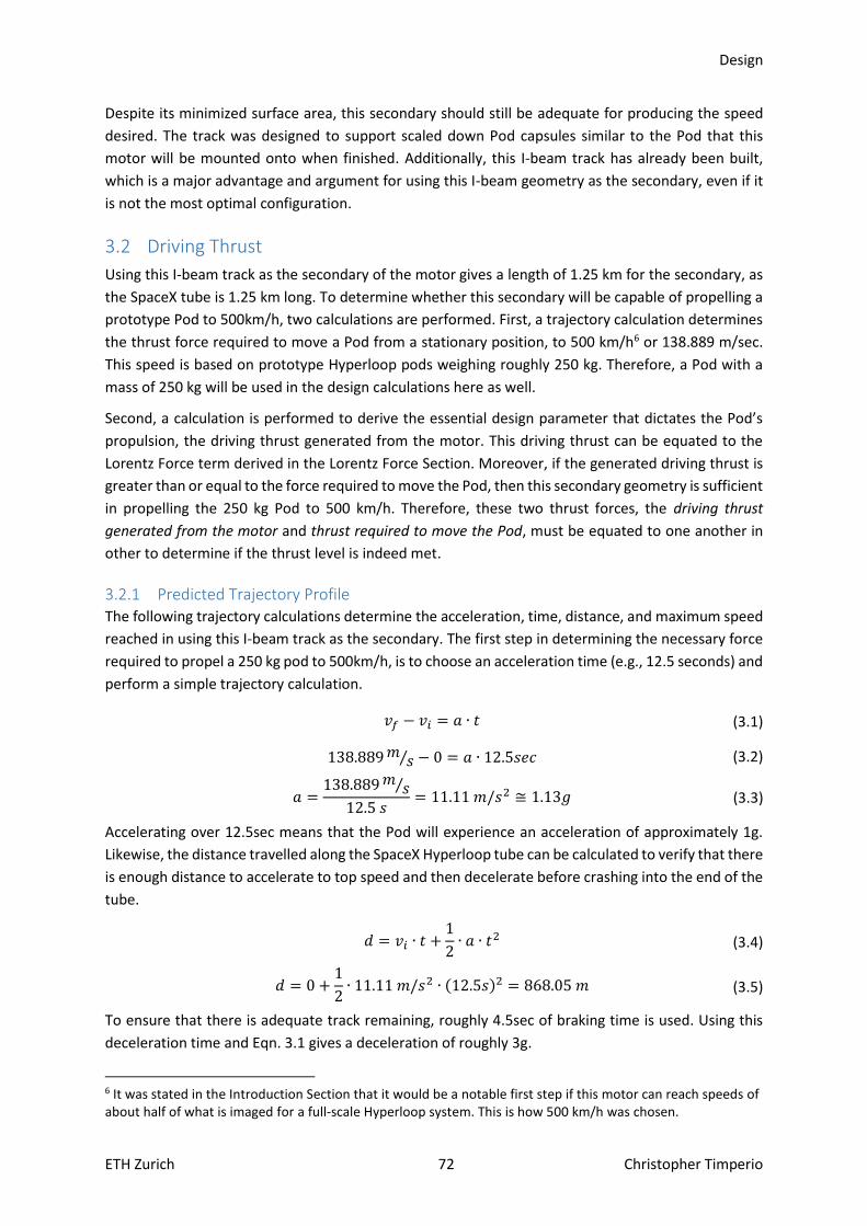
Design


Despite its minimized surface area, this secondary should still be adequate for producing the speed

desired. The track was designed to support scaled down Pod capsules similar to the Pod that this

motor will be mounted onto when finished. Additionally, this I-beam track has already been built,

which is a major advantage and argument for using this I-beam geometry as the secondary, even if it

is not the most optimal configuration.

3.2 Driving Thrust

Using this I-beam track as the secondary of the motor gives a length of 1.25 km for the secondary, as

the SpaceX tube is 1.25 km long. To determine whether this secondary will be capable of propelling a

prototype Pod to 500km/h, two calculations are performed. First, a trajectory calculation determines

the thrust force required to move a Pod from a stationary position, to 500 km/h6 or 138.889 m/sec.

This speed is based on prototype Hyperloop pods weighing roughly 250 kg. Therefore, a Pod with a

mass of 250 kg will be used in the design calculations here as well.

Second, a calculation is performed to derive the essential design parameter that dictates the Pod’s

propulsion, the driving thrust generated from the motor. This driving thrust can be equated to the

Lorentz Force term derived in the Lorentz Force Section. Moreover, if the generated driving thrust is

greater than or equal to the force required to move the Pod, then this secondary geometry is sufficient

in propelling the 250 kg Pod to 500 km/h. Therefore, these two thrust forces, the driving thrust

generated from the motor and thrust required to move the Pod, must be equated to one another in

other to determine if the thrust level is indeed met.

3.2.1 Predicted Trajectory Profile The following trajectory calculations determine the acceleration, time, distance, and maximum speed

reached in using this I-beam track as the secondary. The first step in determining the necessary force

required to propel a 250 kg pod to 500km/h, is to choose an acceleration time (e.g., 12.5 seconds) and

perform a simple trajectory calculation.

𝑣𝑓 − 𝑣𝑖 = 𝑎 ∙ 𝑡 (3.1)

138.889𝑚𝑠⁄ − 0 = 𝑎 ∙ 12.5𝑠𝑒𝑐 (3.2)

𝑎 =138.889𝑚

𝑠⁄

12.5 𝑠= 11.11 𝑚/𝑠2 ≅ 1.13𝑔 (3.3)

Accelerating over 12.5sec means that the Pod will experience an acceleration of approximately 1g.

Likewise, the distance travelled along the SpaceX Hyperloop tube can be calculated to verify that there

is enough distance to accelerate to top speed and then decelerate before crashing into the end of the

tube.

𝑑 = 𝑣𝑖 ∙ 𝑡 +1

2∙ 𝑎 ∙ 𝑡2 (3.4)

𝑑 = 0 +1

2∙ 11.11 𝑚/𝑠2 ∙ (12.5𝑠)2 = 868.05 𝑚 (3.5)

To ensure that there is adequate track remaining, roughly 4.5sec of braking time is used. Using this

deceleration time and Eqn. 3.1 gives a deceleration of roughly 3g.

6 It was stated in the Introduction Section that it would be a notable first step if this motor can reach speeds of about half of what is imaged for a full-scale Hyperloop system. This is how 500 km/h was chosen.

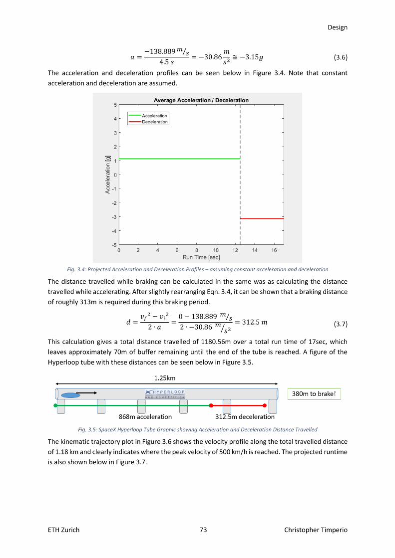
Design


𝑎 =−138.889𝑚

𝑠⁄

4.5 𝑠= −30.86

𝑚

𝑠2≅ −3.15𝑔 (3.6)

The acceleration and deceleration profiles can be seen below in Figure 3.4. Note that constant

acceleration and deceleration are assumed.

Fig. 3.4: Projected Acceleration and Deceleration Profiles – assuming constant acceleration and deceleration

The distance travelled while braking can be calculated in the same was as calculating the distance

travelled while accelerating. After slightly rearranging Eqn. 3.4, it can be shown that a braking distance

of roughly 313m is required during this braking period.

𝑑 =𝑣𝑓

2 − 𝑣𝑖2

2 ∙ 𝑎=

0 − 138.889 𝑚𝑠⁄

2 ∙ −30.86 𝑚𝑠2⁄

= 312.5 𝑚 (3.7)

This calculation gives a total distance travelled of 1180.56m over a total run time of 17sec, which

leaves approximately 70m of buffer remaining until the end of the tube is reached. A figure of the

Hyperloop tube with these distances can be seen below in Figure 3.5.

Fig. 3.5: SpaceX Hyperloop Tube Graphic showing Acceleration and Deceleration Distance Travelled

The kinematic trajectory plot in Figure 3.6 shows the velocity profile along the total travelled distance

of 1.18 km and clearly indicates where the peak velocity of 500 km/h is reached. The projected runtime

is also shown below in Figure 3.7.

Design


Fig. 3.6: Projected Pod Trajectory Profile showing Distance Travelled down the Hyperloop Tube

Fig. 3.7: Projected Pod Run Time Profile for Accelerating the Pod to 500 km/h over 12.5sec

Finally, the required mechanical force to accelerate the 250kg Pod to the final velocity of 500 km/h

can be calculated using Newton’s second law, 𝐹 = 𝑚𝑎, which states that the net force required to

accelerate an object, is equal to the product of the object’s mass and its acceleration.

𝐹 = 250 𝑘𝑔 ∙ 11.11 𝑚/𝑠2 ≅ 2.778𝑘𝑁 (3.8)

Therefore, accelerating a 250kg prototype Pod at 1g over a 12.5sec time interval requires the LIM to

produce a constant driving force of 2.778kN. This required force gives the necessary design value for

Eqn. 3.9.

Design


𝐿𝑜𝑟𝑒𝑛𝑡𝑧 𝐹𝑜𝑟𝑐𝑒 ∶= 2.778𝑘𝑁 (3.9)

To reiterate, if the LIM’s secondary can generate a constant Lorentz Force of 2.778kN for 12.5sec, then

the Pod will reach 500 km/h. Applying this force for longer than 12.5sec or generating an even greater

force means that higher speeds can be achieved. The kinematic data from the above calculations is

listed below in Table 3.1.

Kinematic Data

Pod Acceleration to 500 km/h 11.11 [m/s²]

Braking Deceleration of Pod 30.86 [m/s²]

Total Acceleration Distance for 500 km/h 868.05 [m]

Total Braking Distance (500-0 km/h) 312.50 [m]

Total Run Distance 1180.55 [m]

Total Acceleration Time (0-500 km/h) 12.5 [sec]

Maximum Braking Time 4.5 [sec]

Total Run Time 17 [sec]

Table 3.1: Detailed Kinematic Data

3.3 Motor Design

Initial designs have the linear motor mounted on Swissloop’s Pod from the previous year; “Escher”

[26]. The primary reason for mounting the LIM on the existing chassis is that this Pod is already built

and fully functioning. This Pod is complete with avionics, braking, and stability systems to help guide

the Pod safely along the pre-selected I-beam secondary. A CAD rendering of the LIM mounted onto

the Escher Pod is shown below in Appendix D.

However, if the chassis is to support this LIM, some additional design constraints must be defined.

These constraints for the size and weight of the LIM are given by the Escher Pod. Table 3.2 lists these

known design constraints.

The motor type shall also be a 2-pole motor because the lower the number of magnetic poles a motor

has, the higher the thrust generation. Since no magnetic monopoles can exist (from Eqn. 2.4), the

lowest number of poles a motor can have is limited to 2. This means the highest thrust-drag ratio is

for a 2-pole motor. The LIM will therefore be constrained to a 2-pole motor configuration, which will

be the driving factor influencing the design of the windings.

Design


Initial LIM Design Constraints

Speed Goal 500 [km/h]

Force Required 2.778 [kN]

Pole Number 2-Pole

Size Limits 1 (length), 0.2 (height), 0.08 (width) [m]

Weight Limit 80 [kg]

Power Limit 450 [kW]

Table 3.2: Initial Motor Design Constraints

The main constraints for mounting the LIM on the Escher Pod are the weight and size of the LIM. The

weight constraints are important because the overall weight of the Pod should be around 250 kg, the

value assumed for the trajectory calculations. In this manner, the weight is more of a limit on the

maximum achievable speed, because the speed is dictated by the weight. The current Escher Pod

consisting of the chassis and avionics, braking, and stability systems is about 100 kg. This setup leaves

about 150 kg spare for the entire LIM system, which consists of the stator, battery source, and any

other required DC/AC power electronics equipment.

The size constraints that the motor must satisfy are important so that the LIM physically fits onto the

Escher Pod in the dedicated space for the motor. Given these dimensions, a space roughly 1m in length

and 0.2m is height is available on the Pod. The LIM’s width is also important because the LIM needs

to fit within the I-beam’s inner-most dimension, which was seen to be roughly 80 mm from Figure 3.3

above: given the “keep-out-zone” areas are taken into account. The implications of this width

constraint will also be discussed in more detail in the Stator Core Design Section below, because the

stator core width greatly influences the thrust generation of the motor.

The power limitations have been chosen to be around 450 kW. This value was selected as a trade-off

between the battery design (both complexity and cost) and the power needed to produce thrust for

speeds of 500 km/h.

Now that these constraints have been listed, the motor and its design constraints have become

clearer. These constraints are for the most part fixed, however, there is some leeway for adjustment

if the design values needed deviate slightly from these limits during the final design consideration

(e.g., weight or power limits). Nevertheless, size constraints must be strictly adhered to, as there is

finite space available on the Pod. In this manner, some of these “constraints” can be interpreted as

“target specifications”.

Before starting the design process, a simple linear motor concept was studied to gain intuition of how

linear induction motor modelling is performed in Comsol. This simple model consisted of a basic

magnetic iron core as the double-sided stator, with a simple 2-pole 3-phase winding configuration

arranged to produce the travelling magnetic stator field. The stator fits in-between the I-beam

secondary inner dimension, which acts as motor’s rotor. Figure 3.8 shows this initial design concept

and its dimensions. The inner dimension is approximated by a simple aluminum plate for simulation

simplicity.

Design


Fig. 3.8: Initial design concept acting as a starting point in the design process. Once enough intuition was gained by

studying this simple model, the design process moved forward to further, more complex iterations.

As was seen in the Slot and Winding Distribution Section, the more slots the stator core has, the more

sine-like the approximation for the travelling stator field. In examining Figure 3.8, one can see that this

stator is quite basic with only 3 teeth and 2 slots – in a simple “E” configuration. Therefore, the stator

field produced from such a design would clearly not be as efficient as a design with a greater number

of slots. Additionally, the windings are approximated by coils, which are in turn specified in Comsol as

a collection of many smaller windings. Appendix G shows how this is approximated in Comsol.

Such a simple model is insufficient for a motor to be used in this high-speed Hyperloop application,

where speeds of 500 km/h are desired. Nonetheless, this model was important because it served as

an initial step to see the operation and functionality of linear motors in Comsol. It also helped to

demonstrate how varying certain parameters impact the final values, such as thrust production, core

saturation, or induced voltage. Table 3.3 lists the intuitions gained during the study of this 2-slot

concept.

Design


Intuitions Gained from the Simple 2-Slot Model

Parameter Varied Effect on the Thrust

Air Gap As one might imagine, the smaller the air gap distance, the greater the thrust

force produced.

Active Surface Area As the active width increases, the thrust produced increases. This property

makes sense as the width or length (active surface area) is directly related to

flux passing through some surface. Also, as seen in the Lorentz Force Section,

the Stack Width is directly multiplied by the thrust produced.

Saturation In order to avoid saturation of the iron core, one must increase the active

surface area to a size large enough to handle the existing flux. The more the core

saturates, the more it heats up and no additional thrust is produced.

Pole Pitch The pole pitch is determined by the number of poles produced from the motor

as well as by the winding scheme and slot number. However, in this simple

design, one can manipulate the pole pitch by varying the length of the core, or

more appropriately, the distance between the teeth. By adjusting the pole pitch,

a maximum in produced thrust is achieved.

Turn Number More turns in each winding produces more thrust. This is an intuitive result as

the MMF is directly related to the turn number. However, there is also a higher

voltage induced in the coil, which must be supported by the source. If this is not

the case, the voltage level will drop to whatever can be supported by the source,

and the thrust will then drop accordingly.

Slot Size For the same wire cross-section, larger overall slot size allows for a greater

number of turns in the slot, which increases the thrust production. More slots

also mean that the stator field will more closely approximate a sine wave.

Yoke Height The yoke height is not directly related to the thrust, however, it is important for

saturation and heating considerations. Taller yokes will help dissipate more

heat, however, they are larger because of the added material and will therefore

be heavier. For saturation, if the yoke height is too small, the yoke will become

saturated during operation, as there will be too much flux trying to pass through

a small and limited space. On the other hand, if the yokes are too large, there is

“unused” space which only adds more weight. There is a rule of thumb stating

that the yoke height should be roughly proportional to the tooth width for an

even distribution of flux field lines.

Input Current and

Coil Cross-Section

As more current passes through the windings, a higher the thrust level is

produced. This property is intuitive as the MMF is directly related to the input

current. However, more current also means that the core and the coils will heat

up at a faster rate. Additionally, as the current is increased to a high enough

level, the resistance will increase drastically, and thrust production will actually

decrease as the current level is unsupported by the winding cross-section. The

smaller the cross-section of the coil winding, the higher the current density of

the coil.

Table 3.3: Intuitions Gained from the Simple 2-Slot Model

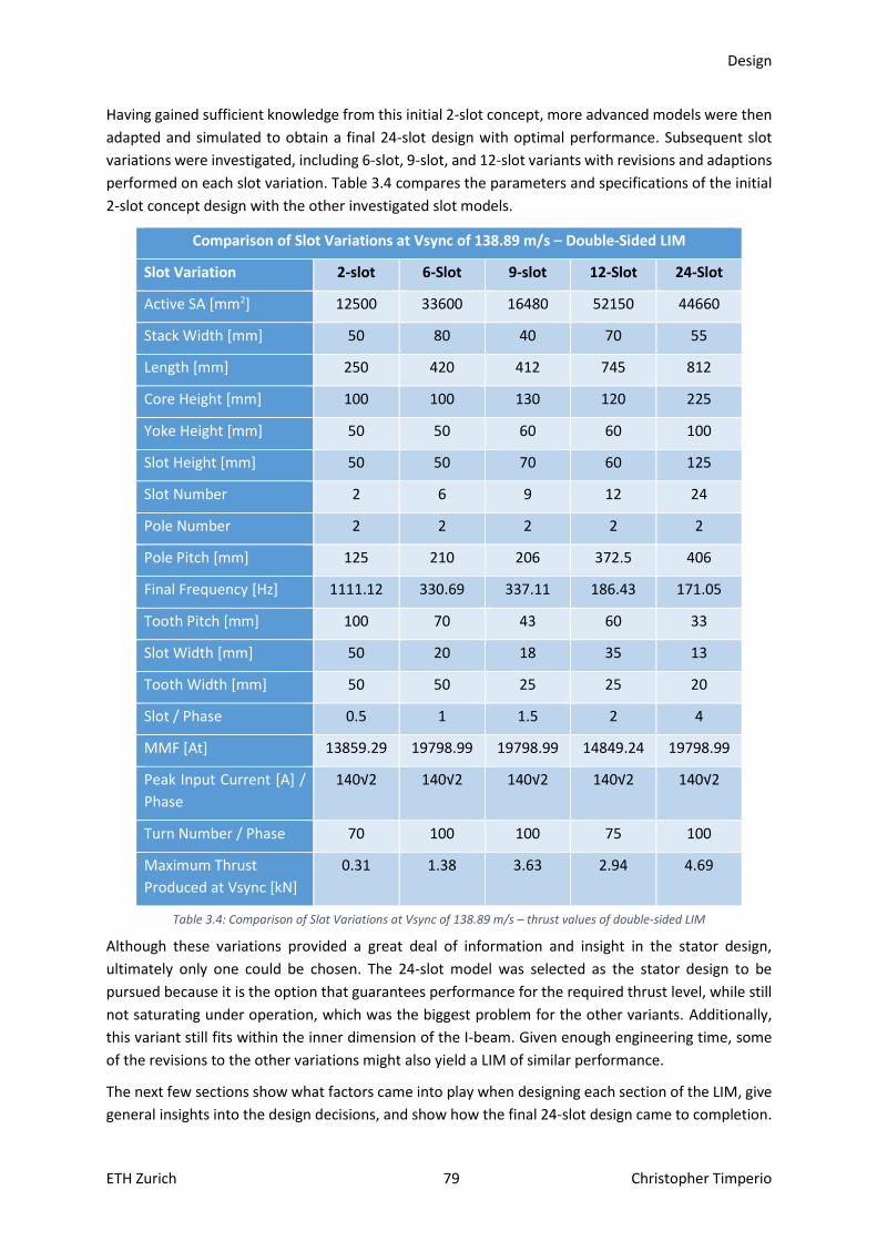
Design


Having gained sufficient knowledge from this initial 2-slot concept, more advanced models were then

adapted and simulated to obtain a final 24-slot design with optimal performance. Subsequent slot

variations were investigated, including 6-slot, 9-slot, and 12-slot variants with revisions and adaptions

performed on each slot variation. Table 3.4 compares the parameters and specifications of the initial

2-slot concept design with the other investigated slot models.

Comparison of Slot Variations at Vsync of 138.89 m/s – Double-Sided LIM

Slot Variation 2-slot 6-Slot 9-slot 12-Slot 24-Slot

Active SA [mm2] 12500 33600 16480 52150 44660

Stack Width [mm] 50 80 40 70 55

Length [mm] 250 420 412 745 812

Core Height [mm] 100 100 130 120 225

Yoke Height [mm] 50 50 60 60 100

Slot Height [mm] 50 50 70 60 125

Slot Number 2 6 9 12 24

Pole Number 2 2 2 2 2

Pole Pitch [mm] 125 210 206 372.5 406

Final Frequency [Hz] 1111.12 330.69 337.11 186.43 171.05

Tooth Pitch [mm] 100 70 43 60 33

Slot Width [mm] 50 20 18 35 13

Tooth Width [mm] 50 50 25 25 20

Slot / Phase 0.5 1 1.5 2 4

MMF [At] 13859.29 19798.99 19798.99 14849.24 19798.99

Peak Input Current [A] /

Phase

140√2 140√2 140√2 140√2 140√2

Turn Number / Phase 70 100 100 75 100

Maximum Thrust

Produced at Vsync [kN]

0.31 1.38 3.63 2.94 4.69

Table 3.4: Comparison of Slot Variations at Vsync of 138.89 m/s – thrust values of double-sided LIM

Although these variations provided a great deal of information and insight in the stator design,

ultimately only one could be chosen. The 24-slot model was selected as the stator design to be

pursued because it is the option that guarantees performance for the required thrust level, while still

not saturating under operation, which was the biggest problem for the other variants. Additionally,

this variant still fits within the inner dimension of the I-beam. Given enough engineering time, some

of the revisions to the other variations might also yield a LIM of similar performance.

The next few sections show what factors came into play when designing each section of the LIM, give

general insights into the design decisions, and show how the final 24-slot design came to completion.

Design


3.3.1 Primary – Stator Iron Core The design of the stator comes down to two main aspects, the stator core, and the windings. The

core’s design was adapted from the intuitive 2-Slot model, while the winding design was much more

complicated. It took several iterations to achieve the target performance from the windings, while still

having them fit in-between the I-beam. The design of the stator core will be discussed first.

By following the intuition developed from the 2-Slot model, one can start with a basic yoke and tooth

design and increase sizes until performance / target specifications are met. As stated previously, the

24-Slot model was chosen as the core design for this thesis. The core material was chosen to be iron

stacks of M400-50A, which is a common iron core used in motor applications. The data sheet given in

Appendix E details further information about the iron stacks.

Several parts of the stator make up the iron core. Deploying some engineering rules of thumb can help

guide the basic geometrical design of these stator parts.

Teeth:

As seen earlier, the teeth can easily saturate from the flux passing through them. Therefore,

for a given input, one should use as much surface area for the teeth as possible while still keeping the

flux density of the teeth at a reasonable level, before saturation is reached. The teeth should be fully

"loaded" with flux before increasing their size further. The larger the teeth, the more they should be

loaded with flux. For example, if the teeth are large and only have a 0.2T magnetic flux density, then

one should think about shrinking the overall size of the teeth until the average flux density through

them is approaching a moderate saturation limit of roughly 1.8T. However, one should not over

saturate the teeth past a limit of 2T, otherwise they will begin to overheat and the motor’s efficiency

will decrease. If this occurs, and additional input is needed to achieve a certain desired thrust force,

then one must increase the teeth size so they can handle the higher flux density.

Yoke:

Similar to the condition for teeth saturation, the yoke height just needs to be large enough to

handle the flux density passing through it. If the yoke is extremely saturated, it should be made larger.

A general rule of thumb is that the yoke height should be roughly the same size as the tooth width.

These two parameters do not have to be exactly equal; however, the ratio of the two should be as

close as possible to one. This relationship helps create more gradually routed flux paths throughout

the stator core. If the yoke is too large for instance, extra space in which the field lines "circle around”

more, or aren’t as evenly distributed because the reluctance begins to dictate the paths less

accurately, might exist. If the yoke is too small relative to the tooth width, then the field lines might

be more “compressed” and won't distribute as evenly. There is a tradeoff here, because the yoke

should also not get so large that it weighs drastically more than the rest of the stator, including the

windings.

Slot:

The slot needs to be wide enough to fit the needed turn number (which is needed for the

MMF) inside of it for the given wire gauge. The given wire gauge is in turn based on the current density

being driven through the windings. The slot should also not be so wide that there is more space than

required. In general, the slot width should also be somewhat proportional to the tooth width. If there

is inadequate space for the designed winding turn number, then the wire gauge will have to be

reduced so that the desired turn number can fit inside the slot. In doing so, however, increases the

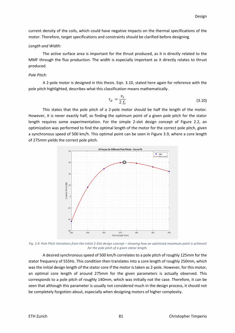
Design


current density of the coils, which could have negative impacts on the thermal specifications of the

motor. Therefore, target specifications and constraints should be clarified before designing.

Length and Width:

The active surface area is important for the thrust produced, as it is directly related to the

MMF through the flux production. The width is especially important as it directly relates to thrust

produced.

Pole Pitch:

A 2-pole motor is designed in this thesis. Eqn. 3.10, stated here again for reference with the

pole pitch highlighted, describes what this classification means mathematically.

𝜏𝑝 =𝑣𝑠

2 𝑓𝑠 (3.10)

This states that the pole pitch of a 2-pole motor should be half the length of the motor.

However, it is never exactly half, so finding the optimum point of a given pole pitch for the stator

length requires some experimentation. For the simple 2-slot design concept of Figure 2.2, an

optimization was performed to find the optimal length of the motor for the correct pole pitch, given

a synchronous speed of 500 km/h. This optimal point can be seen in Figure 3.9, where a core length

of 275mm yields the correct pole pitch.

Fig. 3.9: Pole Pitch Variations from the initial 2-Slot design concept – showing how an optimized maximum point is achieved

for the pole pitch of a given stator length.

A desired synchronous speed of 500 km/h correlates to a pole pitch of roughly 125mm for the

stator frequency of 555Hz. This condition then translates into a core length of roughly 250mm, which

was the initial design length of the stator core if the motor is taken as 2-pole. However, for this motor,

an optimal core length of around 275mm for the given parameters is actually observed. This

corresponds to a pole pitch of roughly 140mm, which was initially not the case. Therefore, it can be

seen that although this parameter is usually not considered much in the design process, it should not

be completely forgotten about, especially when designing motors of higher complexity.

Design


The Motor Configuration Section indicated that the configuration of this LIM is one of a double-sided

stator core. This arrangement has each core producing half of the necessary thrust to move the Pod,

which corresponds to each side of the LIM producing roughly 1.4kN of thrust.

In addition to using more of the secondary’s surface area to generate a higher thrust force, using a

double-sided configuration, as opposed to a single-sided configuration, increases flux in the air gap by

adding a second core. As seen in the Lorentz Force Section, a high flux concentration in the air gap

induces more eddy currents in the secondary, which leads to greater thrust production.

The reason the magnetic flux density increases in the air gap when a second core is added is because

the 𝜇𝑟 of the iron core, together with the MMF, act to push the fields from materials with higher 𝜇𝑟

to materials of a lower 𝜇𝑟 (i.e., air in this case). Therefore, the MMF guides the high field concentration

from the iron core to the air. However, without a second core, the MMF drives the flux out of the iron

core to the air along a longer path and below the secondary, where it is unusable. It is desirable to

have a high field concentration only in the air near the rotor blade where it can contribute to thrust

production. This location corresponds to the air gap where the flux can continuously produce eddy

currents during operation. Field concentration pushed to air elsewhere around the motor is wasted

below the rotor blade and does not contribute to the force production.

Properly guiding the flux is achieved by adding a second core below the rotor blade. Doing so adds a

second side to the LIM that constrains the field to the air gap, since the MMF of the iron cores from

both LIMs will now act to push the flux from the iron cores to the air. However now, the only place

where the flux exists is in the air in-between the two cores. In this arrangement, the two iron cores

act together to constrain the fields and produce a high magnetic flux density in the air gap.

Additionally, adding two cores helps further reduce the path length taken by the flux, since the

magnetic field lines must “travel” back to close on themselves – Eqn. 2.4. A reduced path length will

also slightly increase the flux density in the air gap, as less is “wasted” in the air beneath the rotor

blade like in the single-sided case.

The reduction in path length can be seen again from Amperes’ Law in its quasi-static integral form:

the magnetic field strength is directly related to the path of the field.

∮ �⃑⃑� ∙ 𝑑𝑙

(𝑐)

= ∬𝐽 ∙ 𝑑𝑆

𝑆

= 𝑁 ∙ 𝐼 (3.11)

If no second core is added, the path taken by the magnetic field, 𝑑𝑙 , will be longer than the path taken

if a second iron stator core is added. Shortening the paths that the fields take to enclose back on

themselves (i.e., the route the flux exists through around the windings and the core teeth), increases

the magnetic field strength, �⃑⃑� from the current density flowing through 𝑁 windings, ∬ 𝐽 ∙ 𝑑𝑆

𝑆. An

illustration of this explanation can be seen below in Figure 3.10.

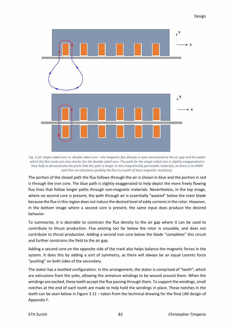
Design


Fig. 3.10: Single-sided core vs. double sided core – the magnetic flux density is now constrained to the air gap and the paths which the flux exists are also shorter for the double-sided core. The path for the single-sided core is slightly exaggerated in blue help to demonstrate the point that the path is longer in non-magnetically permeable materials, as there is no MMF

and thus no reluctance guiding the flux to a path of least magnetic resistance.

The portion of the closed path the flux follows through the air is shown in blue and the portion in red

is through the iron core. The blue path is slightly exaggerated to help depict the more freely flowing

flux lines that follow longer paths through non-magnetic materials. Nevertheless, in the top image,

where no second core is present, the path through air is essentially “wasted” below the rotor blade

because the flux in this region does not induce the desired level of eddy currents in the rotor. However,

in the bottom image where a second core is present, the same input does produce the desired

behavior.

To summarize, it is desirable to constrain the flux density to the air gap where it can be used to

contribute to thrust production. Flux existing too far below the rotor is unusable, and does not

contribute to thrust production. Adding a second iron core below the blade “completes” this circuit

and further constrains the field to the air gap.

Adding a second core on the opposite side of the track also helps balance the magnetic forces in the

system. It does this by adding a sort of symmetry, as there will always be an equal Lorentz force

“pushing” on both sides of the secondary.

The stator has a toothed configuration. In this arrangement, the stator is comprised of “teeth”, which

are extrusions from the yoke, allowing the armature windings to be wound around them. When the

windings are excited, these teeth accept the flux passing through them. To support the windings, small

notches at the end of each tooth are made to help hold the windings in place. These notches in the

teeth can be seen below in Figure 3.11 – taken from the technical drawing for the final LIM design of

Appendix F.

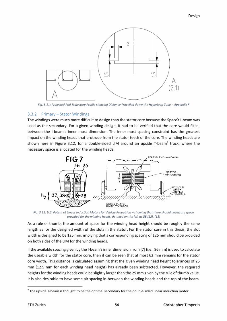
Design


Fig. 3.11: Projected Pod Trajectory Profile showing Distance Travelled down the Hyperloop Tube – Appendix F

3.3.2 Primary – Stator Windings The windings were much more difficult to design than the stator core because the SpaceX I-beam was

used as the secondary. For a given winding design, it had to be verified that the core would fit in-

between the I-beam’s inner most dimension. The inner-most spacing constraint has the greatest

impact on the winding heads that protrude from the stator teeth of the core. The winding heads are

shown here in Figure 3.12, for a double-sided LIM around an upside T-beam7 track, where the

necessary space is allocated for the winding heads.

Fig. 3.12: U.S. Patent of Linear Induction Motors for Vehicle Propulsion – showing that there should necessary space

provided for the winding heads; detailed on the left as 38 [12], [13]

As a rule of thumb, the amount of space for the winding head height should be roughly the same

length as for the designed width of the slots in the stator. For the stator core in this thesis, the slot

width is designed to be 125 mm, implying that a corresponding spacing of 125 mm should be provided

on both sides of the LIM for the winding heads.

If the available spacing given by the I-beam’s inner dimension from [7] (i.e., 86 mm) is used to calculate

the useable width for the stator core, then it can be seen that at most 62 mm remains for the stator

core width. This distance is calculated assuming that the given winding head height tolerances of 25

mm (12.5 mm for each winding head height) has already been subtracted. However, the required

heights for the winding heads could be slightly larger than the 25 mm given by the rule of thumb value.

It is also desirable to have some air spacing in-between the winding heads and the top of the beam.

7 The upside T-beam is thought to be the optimal secondary for the double-sided linear induction motor.

Design


This extra space provides some tolerance for error and ensures that the winding heads will not contact

the top of the beam during operation. Therefore, to be safe, the width of the stator core is set to 55

mm, leaving about an extra 3.4 mm on each side of the stator core for the winding heads.

It was seen previously that the width of the stator core directly influences the amount of thrust

produced by the motor. By using the I-beam as a secondary, one of the major parameters dictating

the LIM’s driving thrust is limited by the inner spacing of this I-beam. The magnetic flux density has a

limit of around 2T; therefore, if flux, the key driving parameter in thrust production, should increase

by a noticeable amount, the active surface area of the stator core must also increase. However, as

seen here, the core is limited in width by the constraint of the I-beam inner spacing. The only other

way to increase the flux noticeably is to increase the length of the stator core, which unfortunately

cannot be made incredibly long. As a good approximation, given the material and weight of the stator

core, the limit on the length can be set to 1 m. It is not evident that there exists some theoretical limit

on the flux produced, a conclusion that can be seen below in Eqn. 3.13.

Φ = ∫�⃑� ∙ 𝑑𝑆

𝑆

= 𝐵 ∙ 𝑆𝐴 = 𝐵 ∙ 𝑊 ∙ 𝐿 = 2 T ∙ 0.055 m ∙ 1 m (3.12)

Φ𝐿𝐼𝑀𝐼𝑇 = 2 T ∙ 0.055 m ∙ 1 m = 0.11 Wb (3.13)

This limit on the flux is a key reason why using the I-beam provided by SpaceX as the secondary rotor

for this LIM is not an optimal decision. However, for reaching speeds of 500 km/h, this already

constructed secondary will be sufficient for this first prototype LIM.

Continuing the design process with this flux constraint in mind, a winding scheme that fits inside the

I-beam was found after several design iterations. Since the stator core has a toothed configuration,

the windings will wrap around each of the teeth to produce the flux. This configuration of how the

stator teeth are wound, is known as the winding diagram. The final winding diagram for the 24-Slot

LIM can be seen in Figure 3.13.

Fig. 3.13: 24-Slot Stator Winding Diagram for a Parallel Star (Wye) Configuration

This winding diagram assumes 4 slots per phase for the chosen 24-Slot design, which guarantees a 2-

pole motor. The 24-Slot LIM with the 3-phase windings highlighted, can be seen below in Figure 3.14.

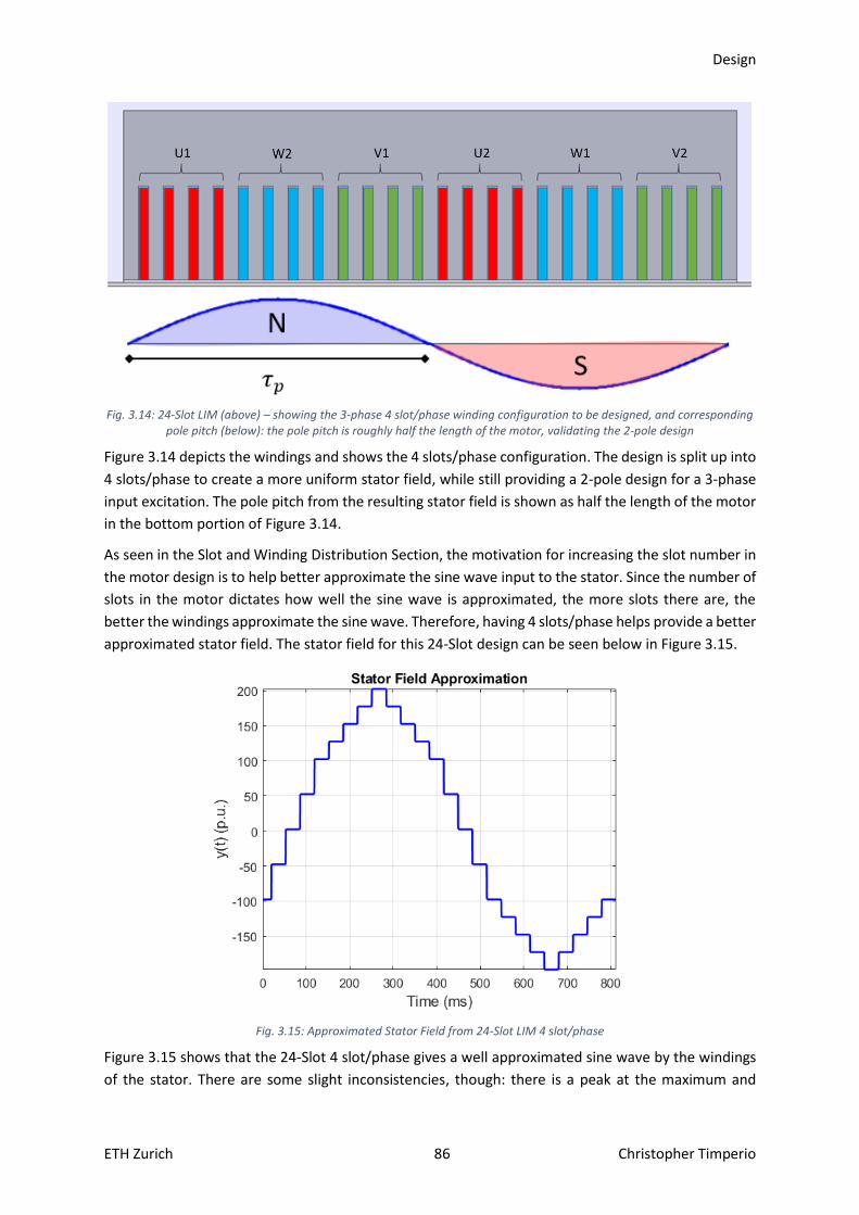
Design


Fig. 3.14: 24-Slot LIM (above) – showing the 3-phase 4 slot/phase winding configuration to be designed, and corresponding

pole pitch (below): the pole pitch is roughly half the length of the motor, validating the 2-pole design

Figure 3.14 depicts the windings and shows the 4 slots/phase configuration. The design is split up into

4 slots/phase to create a more uniform stator field, while still providing a 2-pole design for a 3-phase

input excitation. The pole pitch from the resulting stator field is shown as half the length of the motor

in the bottom portion of Figure 3.14.

As seen in the Slot and Winding Distribution Section, the motivation for increasing the slot number in

the motor design is to help better approximate the sine wave input to the stator. Since the number of

slots in the motor dictates how well the sine wave is approximated, the more slots there are, the

better the windings approximate the sine wave. Therefore, having 4 slots/phase helps provide a better

approximated stator field. The stator field for this 24-Slot design can be seen below in Figure 3.15.

Fig. 3.15: Approximated Stator Field from 24-Slot LIM 4 slot/phase

Figure 3.15 shows that the 24-Slot 4 slot/phase gives a well approximated sine wave by the windings

of the stator. There are some slight inconsistencies, though: there is a peak at the maximum and

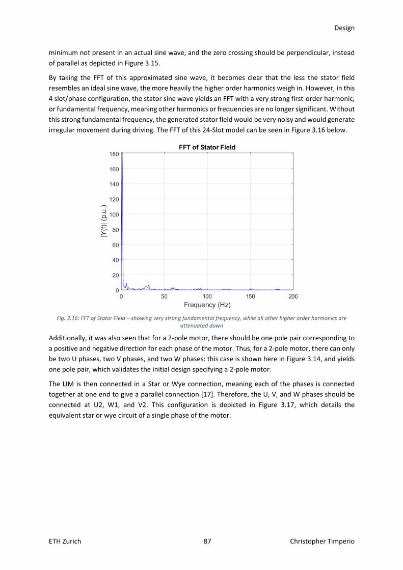
Design


minimum not present in an actual sine wave, and the zero crossing should be perpendicular, instead

of parallel as depicted in Figure 3.15.

By taking the FFT of this approximated sine wave, it becomes clear that the less the stator field

resembles an ideal sine wave, the more heavily the higher order harmonics weigh in. However, in this

4 slot/phase configuration, the stator sine wave yields an FFT with a very strong first-order harmonic,

or fundamental frequency, meaning other harmonics or frequencies are no longer significant. Without

this strong fundamental frequency, the generated stator field would be very noisy and would generate

irregular movement during driving. The FFT of this 24-Slot model can be seen in Figure 3.16 below.

Fig. 3.16: FFT of Stator Field – showing very strong fundamental frequency, while all other higher order harmonics are

attenuated down

Additionally, it was also seen that for a 2-pole motor, there should be one pole pair corresponding to

a positive and negative direction for each phase of the motor. Thus, for a 2-pole motor, there can only

be two U phases, two V phases, and two W phases: this case is shown here in Figure 3.14, and yields

one pole pair, which validates the initial design specifying a 2-pole motor.

The LIM is then connected in a Star or Wye connection, meaning each of the phases is connected

together at one end to give a parallel connection [17]. Therefore, the U, V, and W phases should be

connected at U2, W1, and V2. This configuration is depicted in Figure 3.17, which details the

equivalent star or wye circuit of a single phase of the motor.

Design


Fig. 3.17: Star / Wye Connection for a Single Phase of the 3-Phase 24-Slot LIM System

Finally, the coils of each phase are made from copper of a certain cross-sectional diameter. The

diameter of the windings directly dictates how much current can pass through them. Once the turn

number and current is chosen based on the MMF needed to provide the required thrust, a coil cross-

section large enough to ensure that the current does not burn the windings can be selected. To

determine the appropriate winding size, one must first determine the current density passing through

each of the coils. To find the current density, the overall winding system must be analyzed. Figure 3.18

shows the final winding system for a single phase of the LIM, given the 4 slots/phase configuration.

Fig. 3.18: 24-Slot LIM Winding Scheme for 4 slot/phase configuration for a Single Phase – showing roughly MMF of roughly

20000 At is achieved

From this illustration, it can be seen that the MMF of roughly 20000 At is indeed achieved for this 4

slot/phase LIM configuration;

Θ𝐿𝐼𝑀 = 𝑁 ∙ 𝐼𝑝 = (25 turns ∙ 4 slots

phase) ∙ 140√2 𝐴 = 19798.99 𝐴𝑡 (3.6)

This 4 slot/phase configuration states that each slot of the LIM will support 25 windings for each phase;

however, the full coil will appear to have 100 windings, as each coil is connected in series, which

effectively sums the turn numbers.

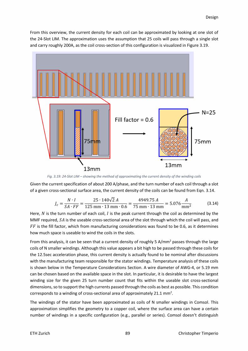
Design


From this overview, the current density for each coil can be approximated by looking at one slot of

the 24-Slot LIM. The approximation uses the assumption that 25 coils will pass through a single slot

and carry roughly 200A, as the coil cross-section of this configuration is visualized in Figure 3.19.

Fig. 3.19: 24-Slot LIM – showing the method of approximating the current density of the winding coils

Given the current specification of about 200 A/phase, and the turn number of each coil through a slot

of a given cross-sectional surface area, the current density of the coils can be found from Eqn. 3.14.

𝐽𝑐 =𝑁 ∙ 𝐼

𝑆𝐴 ∙ 𝐹𝐹=

25 ∙ 140√2 𝐴

125 mm ∙ 13 mm ∙ 0.6=

4949.75 𝐴

75 mm ∙ 13 mm= 5.076

𝐴

mm2 (3.14)

Here, 𝑁 is the turn number of each coil, 𝐼 is the peak current through the coil as determined by the

MMF required, 𝑆𝐴 is the useable cross-sectional area of the slot through which the coil will pass, and

𝐹𝐹 is the fill factor, which from manufacturing considerations was found to be 0.6, as it determines

how much space is useable to wind the coils in the slots.

From this analysis, it can be seen that a current density of roughly 5 A/mm2 passes through the large

coils of N smaller windings. Although this value appears a bit high to be passed through these coils for

the 12.5sec acceleration phase, this current density is actually found to be nominal after discussions

with the manufacturing team responsible for the stator windings. Temperature analysis of these coils

is shown below in the Temperature Considerations Section. A wire diameter of AWG-4, or 5.19 mm

can be chosen based on the available space in the slot. In particular, it is desirable to have the largest

winding size for the given 25 turn number count that fits within the useable slot cross-sectional

dimensions, so to support the high currents passed through the coils as best as possible. This condition

corresponds to a winding of cross-sectional area of approximately 21.1 mm2.

The windings of the stator have been approximated as coils of N smaller windings in Comsol. This

approximation simplifies the geometry to a copper coil, where the surface area can have a certain

number of windings in a specific configuration (e.g., parallel or series). Comsol doesn’t distinguish

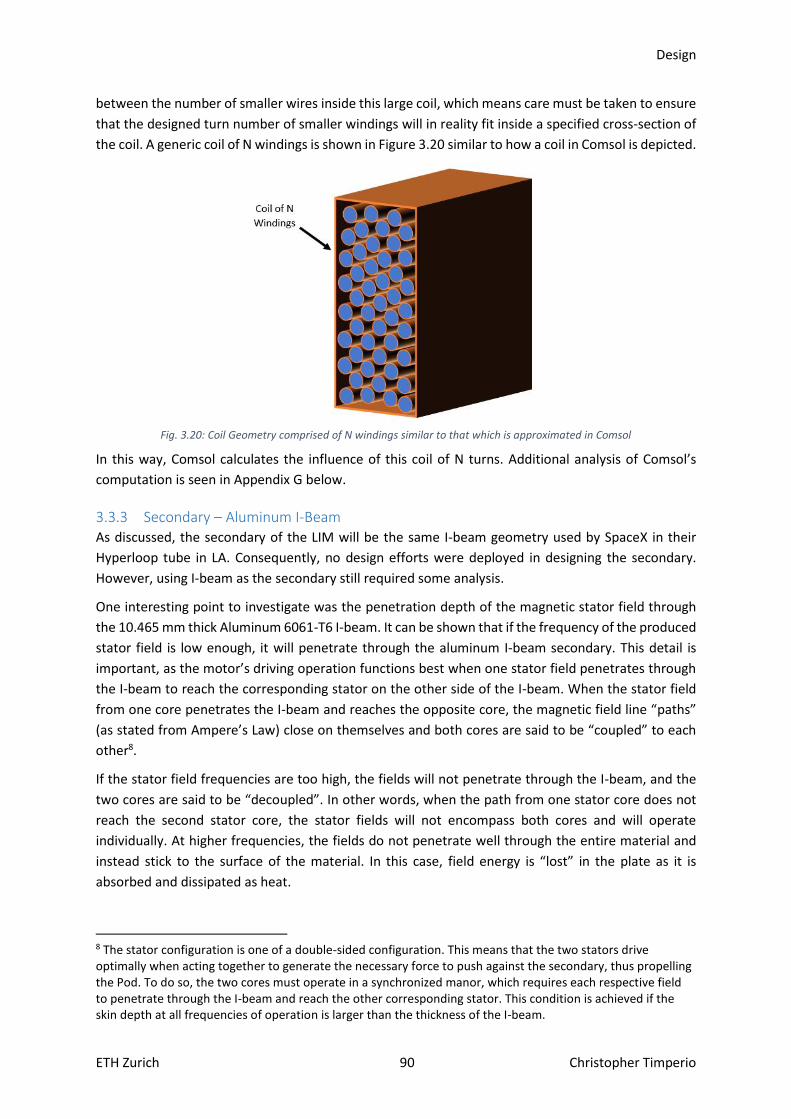
Design


between the number of smaller wires inside this large coil, which means care must be taken to ensure

that the designed turn number of smaller windings will in reality fit inside a specified cross-section of

the coil. A generic coil of N windings is shown in Figure 3.20 similar to how a coil in Comsol is depicted.

Fig. 3.20: Coil Geometry comprised of N windings similar to that which is approximated in Comsol

In this way, Comsol calculates the influence of this coil of N turns. Additional analysis of Comsol’s

computation is seen in Appendix G below.

3.3.3 Secondary – Aluminum I-Beam As discussed, the secondary of the LIM will be the same I-beam geometry used by SpaceX in their

Hyperloop tube in LA. Consequently, no design efforts were deployed in designing the secondary.

However, using I-beam as the secondary still required some analysis.

One interesting point to investigate was the penetration depth of the magnetic stator field through

the 10.465 mm thick Aluminum 6061-T6 I-beam. It can be shown that if the frequency of the produced

stator field is low enough, it will penetrate through the aluminum I-beam secondary. This detail is

important, as the motor’s driving operation functions best when one stator field penetrates through

the I-beam to reach the corresponding stator on the other side of the I-beam. When the stator field

from one core penetrates the I-beam and reaches the opposite core, the magnetic field line “paths”

(as stated from Ampere’s Law) close on themselves and both cores are said to be “coupled” to each

other8.

If the stator field frequencies are too high, the fields will not penetrate through the I-beam, and the

two cores are said to be “decoupled”. In other words, when the path from one stator core does not

reach the second stator core, the stator fields will not encompass both cores and will operate

individually. At higher frequencies, the fields do not penetrate well through the entire material and

instead stick to the surface of the material. In this case, field energy is “lost” in the plate as it is

absorbed and dissipated as heat.

8 The stator configuration is one of a double-sided configuration. This means that the two stators drive optimally when acting together to generate the necessary force to push against the secondary, thus propelling the Pod. To do so, the two cores must operate in a synchronized manor, which requires each respective field to penetrate through the I-beam and reach the other corresponding stator. This condition is achieved if the skin depth at all frequencies of operation is larger than the thickness of the I-beam.

Design


This phenomenon can be further analyzed by looking at the skin depth for all frequencies of driving

operation, which corresponds to a frequency range from 50Hz to approximately 171Hz9. The

performed validation observed variation in skin depth distances across this frequency range.

The skin depth for a given material can be seen below in Eqn. 3.15, assuming low frequencies10 [15].

𝛿 = √2𝜌

𝜔𝜇 (3.15)

Where ρ is the resistivity of the material, 𝜔 is the frequency of operation, and 𝜇 is the magnetic

permeability. A plot of a frequency sweep of the skin depth from 0Hz to 171Hz can be seen below in

Figure 3.21.

Fig. 3.21: Skin Depth Penetration Distance of Aluminum 6061-T6 I-beam Secondary

As shown, below frequencies of roughly 20Hz, the curve asymptotically approaches infinity.

A more interesting curve for operational frequencies of 50Hz through 171Hz, which are the

frequencies through which the motor will sweep during its acceleration period, is shown in Figure

3.22. Table 3.5 lists some key values within this range.

9 171.047 Hz corresponds to the synchronous speed of the motor: 138.89 m/s for a pole pitch of 0.406m. 10 The approximation holds if the frequency of operation is lower than 1 𝜌휀⁄ for a given material.

Design


Fig. 3.22: Skin Depth Penetration Distance of Aluminum 6061-T6 I-beam Secondary for Frequencies 50Hz through 171Hz

showing coupled and decoupled regions

Skin Depth – Penetration Distances

Frequency [Hz] Skin Depth [mm]

50 14.217

92 10.481

93 10.425

171 7.688

Table 3.5: Key Values for Skin Depth Penetration Distance of Aluminum 6061-T6 I-beam Secondary

From 50Hz to 171Hz, the penetration depth ranges from 14.22mm (at 50Hz) to 7.69mm (at 171Hz). At

about 93Hz, the penetration depth is less than the thickness of the aluminum I-beam, so any further

increase in frequency causes the two cores to decouple from one another.

The decoupling boundary is depicted in Figure 3.22 as a black dotted line. At low frequencies above

this line, the two sides of the LIM will be magnetically coupled to each other and below this line at the

higher frequencies, the penetration distance is too short to penetrate all the way through the

aluminum, so the two sides will be magnetically decoupled.

Thus, with regard to skin depth, for about half of the frequency range of operation, the cores will be

decoupled from one another. Since coupling guarantees that the cores’ produced fields complement

each other, extra care that the fields still accompany one another and do not fight against each other

must be taken beyond this decoupling point of 93Hz. The main way to ensure complementary

behavior is by verifying that the produced fields point in the same direction as one another during all

points of operation. This configuration ensures that the moving fields support each other and will also

be synchronized to each other during the decoupling region of operation. Coupling of the fields

ensures a greater synchronization between the fields, as illustrated below in Figure 3.23.

Coupled

Decoupled

Design


Fig. 3.23: Showing coupling I-beam, fields should be same orientation so motor thrusts are working together not against

each other – reinforcing the thrust or complementing.

The I-beam was modelled in Comsol to simulate the effects of the secondary as close to reality as

possible. The modelled I-beam in Comsol can be seen below in Figure 3.24.

Fig. 3.24: I-beam with “Keep-out-Zones” Modelled in Comsol – CAD of each motor prototype can be inserted into this design

to see exactly how it fits in the I-beam dimensions

After modelling the complete I-beam, the 3D simulation was very computationally heavy, as Comsol

places very fine mesh elements in the edges/corners of the I-beam during discretization, even when

taking symmetries. Instead, and for the entirety of the simulations, the I-beam was modelled as a

single aluminum plate with the same length as the inner dimension (106mm) of the I-beam. Doing so

greatly reduced the run time and complexity during simulations in Comsol.

3.3.4 Air Gap Analysis and theory indicate that a smaller air gap yields a stronger thrust force [17], [21], [13].

Therefore, the closer the double-sided stator cores are to the rotor I-beam, the smaller the air gap will

be, and thus the greater the thrust produced. Nevertheless, determining the right air gap for the motor

design was aided by performing a parametric sweep of varying air gap distances shown in Figure 3.25,

which further validated this smaller air gap ansatz.

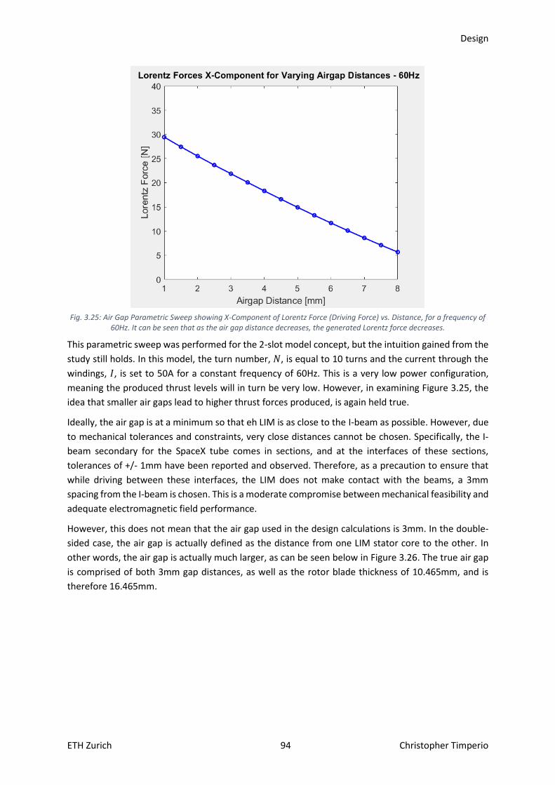
Design


Fig. 3.25: Air Gap Parametric Sweep showing X-Component of Lorentz Force (Driving Force) vs. Distance, for a frequency of

60Hz. It can be seen that as the air gap distance decreases, the generated Lorentz force decreases.

This parametric sweep was performed for the 2-slot model concept, but the intuition gained from the

study still holds. In this model, the turn number, 𝑁, is equal to 10 turns and the current through the

windings, 𝐼, is set to 50A for a constant frequency of 60Hz. This is a very low power configuration,

meaning the produced thrust levels will in turn be very low. However, in examining Figure 3.25, the

idea that smaller air gaps lead to higher thrust forces produced, is again held true.

Ideally, the air gap is at a minimum so that eh LIM is as close to the I-beam as possible. However, due

to mechanical tolerances and constraints, very close distances cannot be chosen. Specifically, the I-

beam secondary for the SpaceX tube comes in sections, and at the interfaces of these sections,

tolerances of +/- 1mm have been reported and observed. Therefore, as a precaution to ensure that

while driving between these interfaces, the LIM does not make contact with the beams, a 3mm

spacing from the I-beam is chosen. This is a moderate compromise between mechanical feasibility and

adequate electromagnetic field performance.

However, this does not mean that the air gap used in the design calculations is 3mm. In the double-

sided case, the air gap is actually defined as the distance from one LIM stator core to the other. In

other words, the air gap is actually much larger, as can be seen below in Figure 3.26. The true air gap

is comprised of both 3mm gap distances, as well as the rotor blade thickness of 10.465mm, and is

therefore 16.465mm.

Design


Fig. 3.26: Double-Sided 24-Slot LIM showing the full air gap distance of 16.465mm, with windings omitted

Thus, it can be deduced that linear motors require large air gaps, which is a conclusion also stated in

[19], [13], [21].

Rotary motors do not require air gaps as large, a property that constitutes one of the main negative

aspects of a linear motor. For this reason, it is sometimes advantageous to use permanent magnet

(PM) or synchronous linear motors. PM linear motors generate higher field strengths in the air gap

when compared to induction or asynchronous machines, thereby enabling operation in larger air gaps

through an increased overall field strength in the air gap.

In the Comsol simulations, the air gap was modelled as a separate geometric object, defined by a finer

mesh, which was needed because the air gap is always much smaller than the rest of the motor. In

this way, the simulations yield more accurate results. A screenshot of the mesh produced for a single

side of the 24-Slot variant can be seen below in Figure 3.27 – which shows the finer mesh in the air

gap compared to the rest of the model.

Fig. 3.27: Mesh of Symmetric 24-Slot Comsol model showing very fine mesh created in the air gap

Finally, considering all the points listed in the preceding sections, an optimized 24-Slot revision was

reached, and a final design specified. The final optimized 24-Slot design is detailed in the following

section.

3.4 Final Model

The final design presented in this thesis is a 24-Slot Double-Sided 2-pole LIM. The model was designed

according to the processes laid out in the previous sub-sections and is the results of several design

iterations and revisions. Simulations were performed in 2D in Comsol to reduce the computational

time and complexity relative to 3D simulations. The final 2D Comsol CAD model can be seen below in

Figure 3.28 with the according dimensions given in the technical drawing Appendix F.

Design


Fig. 3.28: Final Double-Sided 24-Slot LIM model modelled in Comsol

Additionally, by using a symmetry point in the middle of the single aluminum plate (modeled as the I-

beam), the need to model and simulate the full double-sided LIM in Comsol was eliminated. Instead,

simulating half of the LIM is sufficient, as the thrust produced from a single-side of the LIM can simply

be doubled to find the correct complete double-sided result. A single-side of the 2D LIM model in

Comsol can be seen below in Figure 3.29.

Fig. 3.29: 24-Slot LIM shown as 2D simulation in Comsol with a symmetry taken on the x=o plane (I-beam middle) – the

bottom blue boundary is a PMC boundary, while all other boundaries in the simulation are magnetic insulation boundaries

This figure shows a blue boundary line on the bottom of this model running beneath the I-beam plate.

This is a perfect magnetic conductor (PMC) boundary, which sets the tangential component of the

magnetic field strength, 𝐻, and the current density, 𝐽, to zero. This PMC boundary accurately models

the second half of the LIM. By creating this boundary, the magnetic flux lines are continuous across it,

as this correctly models reality in the case of a double-sided LIM.

The rest of the boundaries in the simulation are all set to magnetic insulation boundaries. These

boundary conditions set the tangential components of the magnetic potential, 𝐴, to zero.

As can also be seen in the simulation, the rotor is taken as some “shorter” than reality rotor. This is

because Comsol cannot simulate the entire 1.25 km long I-beam blade. However, it is also not

necessary to simulate a full-scale rotor blade in these simulations. It will be seen in the subsequent

sections that velocity or distance travelled, can be modeled differently in Comsol.

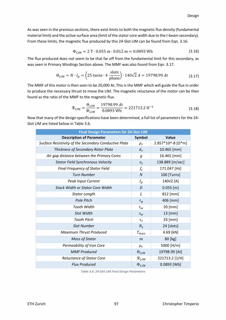
Design


As was seen in the previous sections, there exist limits to both the magnetic flux density (fundamental

material limit) and the active surface area (limit of the stator core width due to the I-beam secondary).

From these limits, the magnetic flux produced by this 24-Slot LIM can be found from Eqn. 3.16.

Φ𝐿𝐼𝑀 = 2 T ∙ 0.055 m ∙ 0.812 m = 0.0893 Wb (3.16)

The flux produced does not seem to be that far off from the fundamental limit for this secondary, as

was seen in Primary Windings Section above. The MMF was also found from Eqn. 3.17.


phase) ∙ 140√2 𝐴 = 19798.99 𝐴𝑡 (3.17)

The MMF of this motor is then seen to be 20,000 At. This is the MMF which will guide the flux in order

to produce the necessary thrust to move the LIM. The magnetic reluctance of the motor can be then

found as the ratio of the MMF to the magnetic flux.

ℛ𝐿𝐼𝑀 =Θ𝐿𝐼𝑀

Φ𝐿𝐼𝑀=

19798.99 𝐴𝑡

0.0893 Wb= 221713.2 H−1 (3.18)

Now that many of the design specifications have been determined, a full list of parameters for the 24-

Slot LIM are listed below in Table 3.6.

Final Design Parameters for 24-Slot LIM

Description of Parameter Symbol Value

Surface Resistivity of the Secondary Conductive Plate 𝜌𝑟 2.857*10^-8 [Ω*m]

Thickness of Secondary Rotor Plate 𝑑𝑟 10.465 [mm]

Air gap distance between the Primary Cores 𝑔 16.465 [mm]

Stator Field Synchronous Velocity 𝑣𝑠 138.889 [m/sec]

Final Frequency of Stator Field 𝑓𝑠 171.047 [Hz]

Turn Number 𝑁 100 [Turns]

Peak Input Current 𝐼𝑝 140√2 [A]

Stack Width or Stator Core Width 𝐷 0.055 [m]

Stator Length 𝐿 812 [mm]

Pole Pitch 𝜏𝑝 406 [mm]

Tooth Width 𝑡𝑤 20 [mm]

Slot Width 𝑠𝑤 13 [mm]

Tooth Pitch 𝜏𝑡 33 [mm]

Slot Number 𝑁𝑠 24 [slots]

Maximum Thrust Produced 𝑇𝑚𝑎𝑥 4.69 [kN]

Mass of Stator 𝑚 80 [kg]

Permeability of Iron Core 𝜇𝑟 5000 [H/m]

MMF Produced Θ𝐿𝐼𝑀 19798.99 [At]

Reluctance of Stator Core ℛ𝐿𝐼𝑀 221713.2 [1/H]

Flux Produced Φ𝐿𝐼𝑀 0.0893 [Wb]

Table 3.6: 24-Slot LIM Final Design Parameters

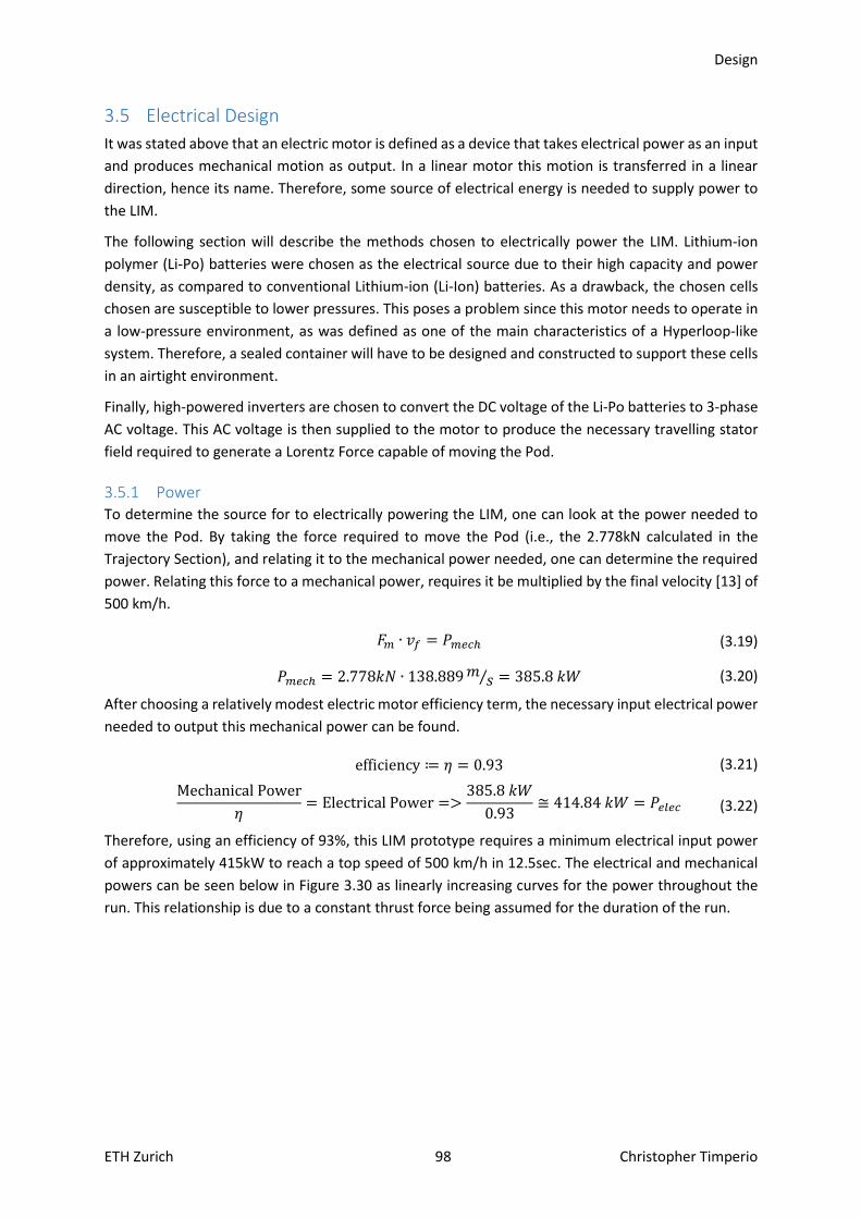
Design


3.5 Electrical Design

It was stated above that an electric motor is defined as a device that takes electrical power as an input

and produces mechanical motion as output. In a linear motor this motion is transferred in a linear

direction, hence its name. Therefore, some source of electrical energy is needed to supply power to

the LIM.

The following section will describe the methods chosen to electrically power the LIM. Lithium-ion

polymer (Li-Po) batteries were chosen as the electrical source due to their high capacity and power

density, as compared to conventional Lithium-ion (Li-Ion) batteries. As a drawback, the chosen cells

chosen are susceptible to lower pressures. This poses a problem since this motor needs to operate in

a low-pressure environment, as was defined as one of the main characteristics of a Hyperloop-like

system. Therefore, a sealed container will have to be designed and constructed to support these cells

in an airtight environment.

Finally, high-powered inverters are chosen to convert the DC voltage of the Li-Po batteries to 3-phase

AC voltage. This AC voltage is then supplied to the motor to produce the necessary travelling stator

field required to generate a Lorentz Force capable of moving the Pod.

3.5.1 Power To determine the source for to electrically powering the LIM, one can look at the power needed to

move the Pod. By taking the force required to move the Pod (i.e., the 2.778kN calculated in the

Trajectory Section), and relating it to the mechanical power needed, one can determine the required

power. Relating this force to a mechanical power, requires it be multiplied by the final velocity [13] of

500 km/h.

𝐹𝑚 ∙ 𝑣𝑓 = 𝑃𝑚𝑒𝑐ℎ (3.19)

𝑃𝑚𝑒𝑐ℎ = 2.778𝑘𝑁 ∙ 138.889𝑚𝑠⁄ = 385.8 𝑘𝑊 (3.20)

After choosing a relatively modest electric motor efficiency term, the necessary input electrical power

needed to output this mechanical power can be found.

efficiency ≔ 𝜂 = 0.93 (3.21)

Mechanical Power

𝜂= Electrical Power =>

385.8 𝑘𝑊

0.93≅ 414.84 𝑘𝑊 = 𝑃𝑒𝑙𝑒𝑐 (3.22)

Therefore, using an efficiency of 93%, this LIM prototype requires a minimum electrical input power

of approximately 415kW to reach a top speed of 500 km/h in 12.5sec. The electrical and mechanical

powers can be seen below in Figure 3.30 as linearly increasing curves for the power throughout the

run. This relationship is due to a constant thrust force being assumed for the duration of the run.

Design


Fig. 3.30: Mechanical and electrical powers during the acceleration phase of the run – showing an electrical power of about

415kW is consumed by the end of the run, in order to reach 500 km/h

The total energy needed for the run can also be calculated as the effective electrical power multiplied

by the total acceleration time.

𝐸 = 𝑃𝑒𝑙𝑒𝑐 ∙ 𝑡 ∙ (1 ℎ

3600 𝑠𝑒𝑐) = 414.84 𝑘𝑊 ∙ 12.5 𝑠𝑒𝑐 ∙ (

1 ℎ

3600 𝑠𝑒𝑐) = 1.44 𝑘𝑊ℎ (3.23)

It is also recommended to have at least 10 times the required capacity for safety concerns and

operating flexibility. This condition would require the electrical source to be capable of providing

around 14.40 kWh.

Using this electrical power, the remaining electrical design parameters needed for the LIM, such as

the required driven voltage and current draw of the LIM, are determined. For this analysis, Figure 3.31

is created to depict the corresponding powers for each stage in the LIM’s electrical design.

Fig. 3.31: Different Power Levels seen in the LIM system

As can be seen from Figure 3.31, each stage in the LIM electrical design is depicted by a different

power parameter, where each of these powers are defined below.

𝑃𝑏𝑎𝑡𝑡 = 𝑉𝐷𝐶 ∙ 𝐼𝐷𝐶 (3.24)

𝑃𝑒𝑙𝑒𝑐 = √3 ∙ 𝑉𝑈𝑊 ∙ 𝐼𝑈 cos𝜑 (3.25)

Design


𝑃𝑚𝑒𝑐ℎ = 𝐹𝑚 ∙ 𝑣𝑓 (3.26)

𝑃𝑚𝑒𝑐ℎ and 𝑃𝑒𝑙𝑒𝑐 were both already found above as 385.8 kW and 414.8 kW, respectively. However,

the source power, 𝑃𝑏𝑎𝑡𝑡 must still be determined and is an important parameter because the source

must be capable of driving the LIM to the 𝑃𝑚𝑒𝑐ℎ level found in Eqn. 3.26. The LIM will try to draw the

requisite power from the supply, however, if the amount needed is unavailable, the estimated

trajectory of 500 km/h over 12.5sec will not be reached, and the LIM will operate on a lower level.

To find the 𝑃𝑏𝑎𝑡𝑡 required by the LIM, the inverter efficiency is required. A value of roughly 99% for

maximum power output is found from [27]. 𝑃𝑏𝑎𝑡𝑡 is then calculated as roughly 417 kW.

𝑃𝑏𝑎𝑡𝑡 =𝑃𝑒𝑙𝑒𝑐

0.995= 416.926 𝑘𝑊 (3.27)

With the required battery source power, the corresponding voltage level for the battery can be

determined. The MMF discussed in the Motor Design Section requires roughly 200A/phase of current

supply to generate the 2.778 kN of necessary thrust force for the LIM to reach 500 km/h. This MMF

constraint then fixes the input current from the battery. Therefore, the DC input current sourced from

the battery should be at least 200A. The corresponding voltage drop11 required to sustain the power

level of the battery source can now be determined. To find this voltage, one can use the electrical

power formula.

𝑉𝐷𝐶 =𝑃𝑏𝑎𝑡𝑡

𝐼𝐷𝐶=

416.93 𝑘𝑊

140√2 𝐴𝐷𝐶= 2.105 𝑘𝑉𝐷𝐶 (3.28)

Eqn. 3.28 shows that an induced voltage of approximately 2kV is required to drive the LIM for 12.5sec

to 500 km/h. However, this is not ideal as finding a portable high-density power source to supply this

much voltage would be impractical. Decreasing the induced voltage needed to supply the LIM requires

further analysis and inspection of the winding configuration of the LIM.

As seen from Faraday’s Lawn, the number of turns, 𝑁, is directly related to the induced voltage across

a set of coils. The relationship is rewritten here for clarity.


𝑑𝑡 (3.29)

Here, ℰ is the electromotive force or EMF and it is proportional to an induced voltage. By increasing

the number of turns in a coil, more voltage will be induced across its windings. Therefore, if it is desired

to reduce the coils’ required voltage drop, the number of turns in a coil should be reduced. However,

it was seen that the turn number is also directly related to the MMF; therefore, by decreasing the turn

number to reduce the induced voltage drop across the coils, the MMF also correspondingly decreases.

A smaller MMF decreases the amount of thrust produced and is undesired and actually

counterproductive to the central point of this thesis.

Thus, if the number of turns in a coil is increased for the purpose of increasing thrust, then the voltage

supplied by the electrical source must also increase to support this level. This relationship is well

known as most high-powered motor applications, such as trains or wind turbines, all supply high

voltages in the kV range.

11 This voltage drop is also the induced voltage required by the LIM’s coils to drive the desired MMF. If this level is not reached, the MMF will drop to a voltage level that can be sustained.

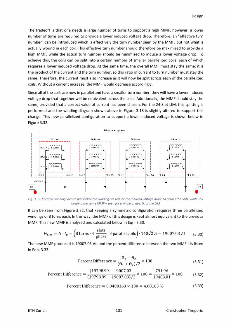
Design


The tradeoff is that one needs a large number of turns to support a high MMF, however, a lower

number of turns are required to provide a lower induced voltage drop. Therefore, an “effective turn

number” can be introduced which is effectively the turn number seen by the MMF, but not what is

actually wound in each coil. This effective turn number should therefore be maximized to provide a

high MMF, while the actual turn number should be minimized to induce a lower voltage drop. To

achieve this, the coils can be split into a certain number of smaller parallelized coils, each of which

requires a lower induced voltage drop. At the same time, the overall MMF must stay the same: it is

the product of the current and the turn number, so this ratio of current to turn number must stay the

same. Therefore, the current must also increase as it will now be split across each of the parallelized

coils. Without a current increase, the MMF would decrease accordingly.

Since all of the coils are now in parallel and have a smaller turn number, they will have a lower induced

voltage drop that together will be equivalent across the coils. Additionally, the MMF should stay the

same, provided that a correct value of current has been chosen. For the 24-Slot LIM, this splitting is

performed and the winding diagram shown above in Figure 3.18 is slightly altered to support this

change. This new parallelized configuration to support a lower induced voltage is shown below in

Figure 3.32.

Fig. 3.32: Creative winding Idea to parallelize the windings to reduce the induced voltage dropped across the coils, while still

keeping the same MMF – seen for a single phase, U, of the LIM

It can be seen from Figure 3.32, that keeping a symmetric configuration requires three parallelized

windings of 8 turns each. In this way, the MMF of this design is kept almost equivalent to the previous

MMF. This new MMF is analyzed and calculated below in Eqn. 3.30.


phase∙ 3 parallel coils) ∙ 140√2 𝐴 = 19007.03 𝐴𝑡 (3.30)

The new MMF produced is 19007.03 At, and the percent difference between the two MMF’s is listed

in Eqn. 3.33.

Percent Difference =|Θ1 − Θ2|

(Θ1 + Θ2) 2⁄× 100 (3.31)

Percent Difference =|19798.99 − 19007.03|

(19798.99 + 19007.03) 2⁄× 100 =

791.96

19403.01× 100 (3.32)

Percent Difference = 0.0408163 × 100 = 4.08163 % (3.33)

Design


It can be seen that by implementing this new winding scheme, the percent difference between the

two MMF values is about 4%.

It can be seen that the MMF is slightly lower now because the equivalent turn number is also slightly

lower: the effective turn number has decreased from 100 turns to 96 turns. However, 100 turns cannot

be achieved by parallelizing the coils into three groups. Therefore, this slight 4% decrease is a non-

avoidable design trade-off.

Reducing the turn number from 25 turns to three parallel windings of 8 turns, produces a 702 VDC

voltage drop across the coils instead of 2kV. However, it can also be seen that the current had to be

increased correspondingly by three-fold to compensate for this lower induced voltage change. These

changes are seen in Eqn. 3.34 and Eqn. 3.35.

𝑉𝐷𝐶 = 2.105 𝑘𝑉𝐷𝐶 3⁄ = 701.9 𝑉𝐷𝐶 (3.34)

𝐼𝐷𝐶 = 140√2 𝐴 ∙ 3 = 420√2 𝐴 (3.35)

If the induced voltage must be decreased, the windings can be parallelized to support a lower induced

voltage.

Therefore, this 𝑉𝐷𝐶 should be the voltage that the electrical source can supply, which also gives a

corresponding new 𝐼𝐷𝐶. The new peak current to be supplied by the electrical source is shown below

in Eqn. 3.36.

𝐼𝐷𝐶 =𝑃𝑏𝑎𝑡𝑡

𝑉𝐷𝐶=

416.93 𝑘𝑊

702 𝑉𝐷𝐶= 593.969 𝐴 𝐷𝐶 (3.36)

This states that the required current will now be about 600A, which is a design trade-off to make for

a lower induced voltage. This larger current matches up with the required MMF needed for

200A/phase. Therefore, the electrical source will have to be large enough to support both this current

level as well as the new induced voltage level dropped across the parallelized coils. The source must

provide this voltage level at a minimum, but should ideally be a bit higher. If the source cannot provide

the necessary voltage drop across the coils needed for the constant driving thrust, then lower

velocities or accelerations will be achieved because there will be insufficient power to reach these

higher levels.

An estimate of the drawn current during the run, based on these solved powers, is seen below in

Figure 3.33, where the final current level of approximately 600A is sourced by the end of the run.

Design


Fig. 3.33. The current to be supplied from the electrical source during motor acceleration

The simulation ends on the final value of 593.969 A, which means it will almost reach the designed

600A level. Providing an electrical source to support these specifications will be shown in the next

section.

It was also discovered above that 𝑉𝐵𝑚𝑖𝑛 for air is roughly around 330V to 350V [24]. This means that

for any voltage below this breakdown minimum, there can never be any pressure or distance product

which causes a breakdown. Therefore, if the DC source or battery voltage level is set to 350 VDC, the

issue of breakdown and discharges is eliminated.

To further reduce the induced voltage drop and to meet this minimum voltage breakdown level, this

702 VDC source can be split into two separate sources, each capable of supplying 351 VDC at the

needed 600A current. Splitting up the source like this is acceptable since there are two sides of the

LIM and each side will supply half of the required thrust. Together they will produce the full 2.778kN

of thrust needed to reach 500 km/h.

Finally, the power factor of the LIM can be found as roughly 0.6, by using Eqn. 3.25 above.

𝑃𝐹 = cos𝜑 =𝑃𝑒𝑙𝑒𝑐

√3 ∙ 𝑉𝑈𝑊 ∙ 𝐼𝑈=

414.84 𝑘𝑊

√3 ∙ 698.42 𝑉𝐷𝐶 ∙ 420√2 𝐴𝐷𝐶= 0.577 (3.37)

This then corresponds to a phase angle 𝜑 between the voltage and current of 54.736°.

𝜑 = cos−1(0.577) = 54.736° (3.38)

Now that the electrical power specifications have been determined, an electrical power source

capable of providing the high currents and voltages required by the motor can be chosen. The source

should be able to provide the high powers while supporting a relatively high voltage level.

3.5.2 Batteries Two custom built 351.5 VDC Li-Po batteries provide these high-power levels, by supplying the high

current draw and high voltage needed to drive the LIM. Each battery configuration is a 95S-4P design

Design


(95 cells in series with 4 submodules in parallel) of SLPB7646143 cells from Malesta. Together the full

190S-4P battery configuration has a total voltage of 703 VDC and is capable of supplying currents

above 600A. This meets both of the electrical design constraints listed above for the voltage and

current required to drive the LIM. A table of the specifications of the individual cells from Malesta is

shown in Table 3.7 below.

Malesta SLPB7646143 Cell Specifications

Nominal Voltage 3.7 [VDC]

Cell Dimensions Thickness: 7 [mm]

Width: 46 [mm]

Length: 144 [mm]

Cell Mass 106.5 [g]

Cell Capacity 5 [Ah]

C Rating 30C

Max Continuous

Discharge Current

150 [A]

Power Produced 555 [W]

Energy Stored 18.5 [Wh]

Internal Resistance 1.2 [mΩ]

Table 3.7: Malesta Li-Po Cell Specifications

Each battery will be separated into five submodules of a 19S-4P configuration. Three parallel cells will

be connected in series via a CUPAL connection element onto which the cell’s connection tabs will be

laser welded. CUPAL is a metal composite material consisting of aluminum and copper often used in

wiring applications to save costs and weight over traditional pure copper, while still having the

conductive advantages of pure copper. To connect the submodules, an end-element, also made out

of CUPAL, will be used and an aluminum connection will be fixed onto it. CAD models of the Malesta

cells, submodules and complete battery packs are shown below in Figure 3.34 and Figure 3.35.

Fig. 3.34 Single Malesta Cell [left], and 19S-4P submodule [right] – both modelled in CAD

Design


Fig. 3.35: One of the custom built 95S-4P batteries modelled in CAD

The complete battery specifications are listed below in Table 3.8.

Assembled Battery Specifications

Total Cells 380

Cells in Series 95

Cells in Parallel 4

Battery Mass 40.47 [kg]

Battery Voltage 351.5 [VDC]

Number of Battery Packs 2

Total Number of Cells 760

Total Mass 80.94 [kg]

Total Voltage 703 [VDC]

Continuous Current Supply 30C or 600 [A]

Peak Current Supply 35C or 700 [A] ≤ 1sec

Total Capacity 20 [Ah]

Total Power Produced 421.8 [kW]

Total Energy Stored 14.06 [kWh]

Table 3.8: Malesta Li-Po Full Battery Specifications

The weight of a single 95S-4P battery configuration is 40.47kg, as it is comprised of 380 Malesta Li-Po

cells. Therefore, the total weight of the190S-4P battery is then 80.94kg. This is computed by

multiplying the mass of an individual cell (106.5g) by the number of series and parallel cells, as seen

in Eqn. 3.39.

𝑚𝑡𝑜𝑡 = 𝑚𝑖 ∙ 𝑆 ∙ 𝑃 = 106.5 g ∙ 190 ∙ 4 = 80940 g (3.39)

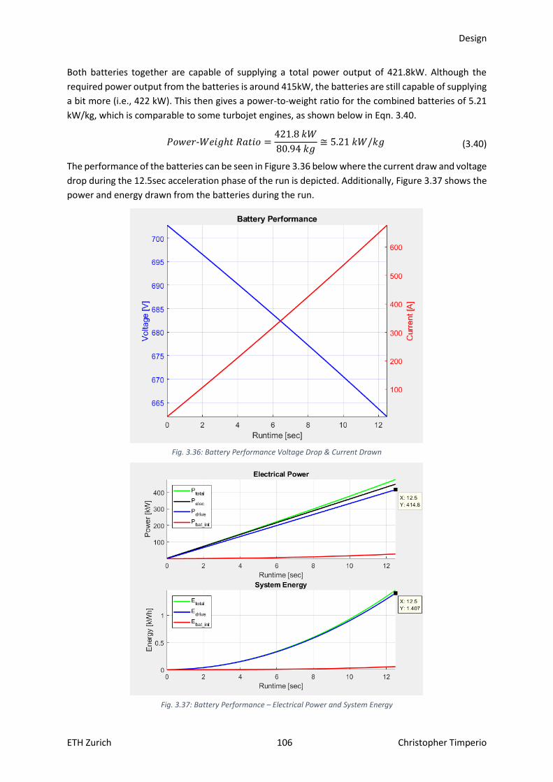
Design


Both batteries together are capable of supplying a total power output of 421.8kW. Although the

required power output from the batteries is around 415kW, the batteries are still capable of supplying

a bit more (i.e., 422 kW). This then gives a power-to-weight ratio for the combined batteries of 5.21

kW/kg, which is comparable to some turbojet engines, as shown below in Eqn. 3.40.

𝑃𝑜𝑤𝑒𝑟-𝑊𝑒𝑖𝑔ℎ𝑡 𝑅𝑎𝑡𝑖𝑜 =421.8 𝑘𝑊

80.94 𝑘𝑔≅ 5.21 𝑘𝑊/𝑘𝑔 (3.40)

The performance of the batteries can be seen in Figure 3.36 below where the current draw and voltage

drop during the 12.5sec acceleration phase of the run is depicted. Additionally, Figure 3.37 shows the

power and energy drawn from the batteries during the run.

Fig. 3.36: Battery Performance Voltage Drop & Current Drawn

Fig. 3.37: Battery Performance – Electrical Power and System Energy

Design


These results were calculated using the Malesta cell specification data, meaning these estimates are

more precise than the previous trajectory calculations as they encompass the actual effects in the

cells. These effects include internal resistance, heating losses, and discharge rates, and should

therefore more accurately depict the cells function during the run.

It can be seen that the energy drawn from the batteries during the entirety of the run is 1.4Wh, which

is almost exactly what was calculated for the energy consumption of the run. This is a good sign that

validates the design and confirms the results of the above kinematic calculations. This results also

shows that these batteries should provide a significant source of energy for the Pod during the run.

Additionally, the voltage drop during this time is minimal, as the final voltage level after the 12.5sec

interval is 662 VDC: only about 41V dropped during acceleration time.

Since it is known that the LIM will be mounted onto the Escher 2017 Swissloop Pod and this current

LIM prototype does not levitate the Pod, the wheel speed can be calculated in revolutions per minute

(RPM) as seen below in Figure 3.38.

Fig. 3.38 Rotational Speed in RPM of the Escher Pod’s Wheels experienced if double-sided LIM is mounted on and a top

speed of 500 km/h is reached

To calculate this wheel speed in RPM from the produced velocity of the motor, Eqn. 3.41 is deployed.

Ω [RPM] =𝑣𝑟

𝑟𝑤∙60

2𝜋 (3.41)

Where 𝑣𝑟 is the speed that the rotor experiences (from 0 to 500 km/h), and 𝑟𝑤 is the radius of the

Escher wheels at 0.19m. Therefore, one can see the wheel rotational speed denoted by Ω in RPM.

Levitation would be ideal in further reducing the friction on the wheels, especially since it was laid out

as one of the key principles behind the overall Hyperloop technology. However, for the speeds of the

scaled down prototypes, and for design simplicity, the LIM of this thesis will not levitate. Therefore,

wheels are indeed needed on the Escher pod. It can be seen that the wheels experience about 7000

RPM during this 12.5sec acceleration period. It is interesting to note, that this is well within the limits

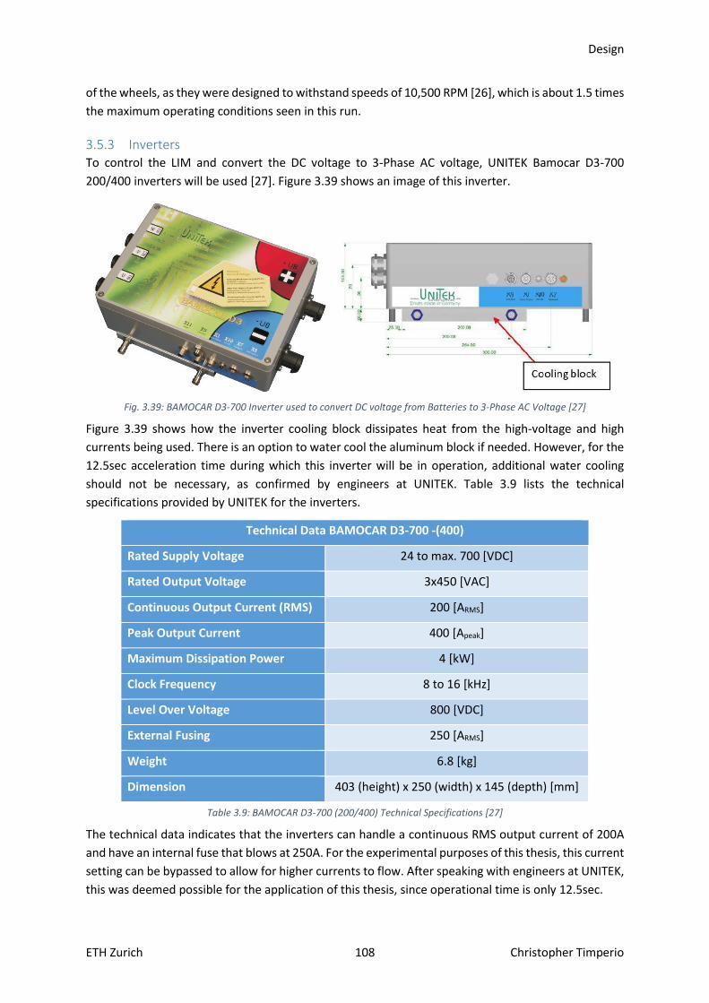
Design


of the wheels, as they were designed to withstand speeds of 10,500 RPM [26], which is about 1.5 times

the maximum operating conditions seen in this run.

3.5.3 Inverters To control the LIM and convert the DC voltage to 3-Phase AC voltage, UNITEK Bamocar D3-700

200/400 inverters will be used [27]. Figure 3.39 shows an image of this inverter.

Fig. 3.39: BAMOCAR D3-700 Inverter used to convert DC voltage from Batteries to 3-Phase AC Voltage [27]

Figure 3.39 shows how the inverter cooling block dissipates heat from the high-voltage and high

currents being used. There is an option to water cool the aluminum block if needed. However, for the

12.5sec acceleration time during which this inverter will be in operation, additional water cooling

should not be necessary, as confirmed by engineers at UNITEK. Table 3.9 lists the technical

specifications provided by UNITEK for the inverters.

Technical Data BAMOCAR D3-700 -(400)

Rated Supply Voltage 24 to max. 700 [VDC]

Rated Output Voltage 3x450 [VAC]

Continuous Output Current (RMS) 200 [ARMS]

Peak Output Current 400 [Apeak]

Maximum Dissipation Power 4 [kW]

Clock Frequency 8 to 16 [kHz]

Level Over Voltage 800 [VDC]

External Fusing 250 [ARMS]

Weight 6.8 [kg]

Dimension 403 (height) x 250 (width) x 145 (depth) [mm]

Table 3.9: BAMOCAR D3-700 (200/400) Technical Specifications [27]

The technical data indicates that the inverters can handle a continuous RMS output current of 200A

and have an internal fuse that blows at 250A. For the experimental purposes of this thesis, this current

setting can be bypassed to allow for higher currents to flow. After speaking with engineers at UNITEK,

this was deemed possible for the application of this thesis, since operational time is only 12.5sec.

Design


To control the AC power supplied to the stators, an 8kHz pulse width modulation (PWM) signal is used

as a clock rate to control the insulated-gate bipolar transistors (IGBTs), which act as very high speed

electronic switches in the inverters. Construction of the stator field is accomplished by discretizing and

approximating a sine wave. This discretization is performed by switching these high-power transistors

(IGBTs) on and off very fast and in a controlled way. Using a PWM signal, sampling at 8kHz to construct

the sine wave, should be sufficient to construct a reasonably clear sine wave input. This sampling

frequency is also the maximum clock rate that can be used while still allowing the maximum current

possible to pass through the inverters. Higher clock rates will have aliasing effects on the output of

the IGBTs that will act to decrease the current being supplied to the motors.

Using two inverters and two batteries power to each side of the LIM is supplied independently. The

inverters use control feedback to verify that each side of the LIM is being powered symmetrically. This

feedback ensures that each side of the LIM is the same as the other and that synchronization between

the fields takes place so that power is not supplied in an unbalanced fashion.

To power the double-sided 24-Slot LIM, two batteries will be connected to two inverters, each of

which supplies approximately 350VDC to the inverters. This DC voltage is then converted to 3-phase

AC voltage, which is then supplied to each corresponding side of the LIM. This configuration can be

seen in Figure 3.40 and Figure 3.41 below.

Fig. 3.40: Single Side of LIM Electrical Configuration

Fig. 3.41: Complete LIM Electrical Configuration

Design


Additionally, by varying the width of the pulses, or the ‘on’ time of the IGBTs, one can also dictate the

frequency of the input sine wave, and therefore the speed of the motor because the frequency of the

stator field is directly related to its velocity – Eqn. 2.43. This property leads to the use of a variable

frequency drive (VFD), which allows one to sweep through a range of frequencies. Every frequency

provides a different synchronous speed and thus a new optimized peak thrust value.

Using a VFD and programming the motor inverters allows for continuous operation at a maximum

thrust value by sweeping through a range of frequencies. This optimum on the thrust curve is denoted

in the generic thrust curve of Figure 3.42 where a stable optimal point on the curve is specified. The

inverters will be programmed to try and always “land” as close to this point as possible.

Fig. 3.42: Generic Thrust Curve – showing stable and unstable thrust points to choose in frequency inverter programming

The point on the right of the curve is in a more stable working region than the corresponding thrust

point on the left side of the curve. In fact, the point on the left is in an unstable working region when

the speed adjusts itself during the frequency sweep because the shape of the curve to the right of the

peak will not change significantly whereas the curve on the left side will. Therefore, once this thrust

point on the right has been found, the inverters can be programmed to maintain this point so as to

not drastically alter performance. Programming these inverters for the frequency sweep requires

noting the discrete frequency points desired in the sweep. It is important to choose the frequency that

yields the correct synchronous speed value for each thrust curve.

For each thrust curve, the inverters should be programmed at the same thrust level for each varying

frequency curve. Doing so yields a constant thrust during acceleration. Once this frequency sweep is

performed by the inverters, the LIM experiences a constant thrust. Thrust curves at various

frequencies are shown in Figure 3.43 where the frequency sweep takes place and the constant thrust

level of 2.778kN for the 12.5sec acceleration period from 0 km/h to 500 km/h is sustained.

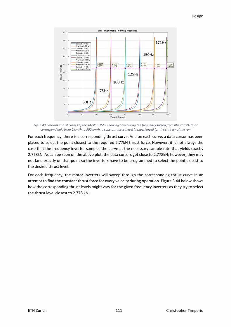
Design


Fig. 3.43: Various Thrust curves of the 24-Slot LIM – showing how during the frequency sweep from 0Hz to 171Hz, or

correspondingly from 0 km/h to 500 km/h, a constant thrust level is experienced for the entirety of the run

For each frequency, there is a corresponding thrust curve. And on each curve, a data cursor has been

placed to select the point closest to the required 2.77kN thrust force. However, it is not always the

case that the frequency inverter samples the curve at the necessary sample rate that yields exactly

2.778kN. As can be seen on the above plot, the data cursors get close to 2.778kN; however, they may

not land exactly on that point so the inverters have to be programmed to select the point closest to

the desired thrust level.

For each frequency, the motor inverters will sweep through the corresponding thrust curve in an

attempt to find the constant thrust force for every velocity during operation. Figure 3.44 below shows

how the corresponding thrust levels might vary for the given frequency inverters as they try to select

the thrust level closest to 2.778 kN.

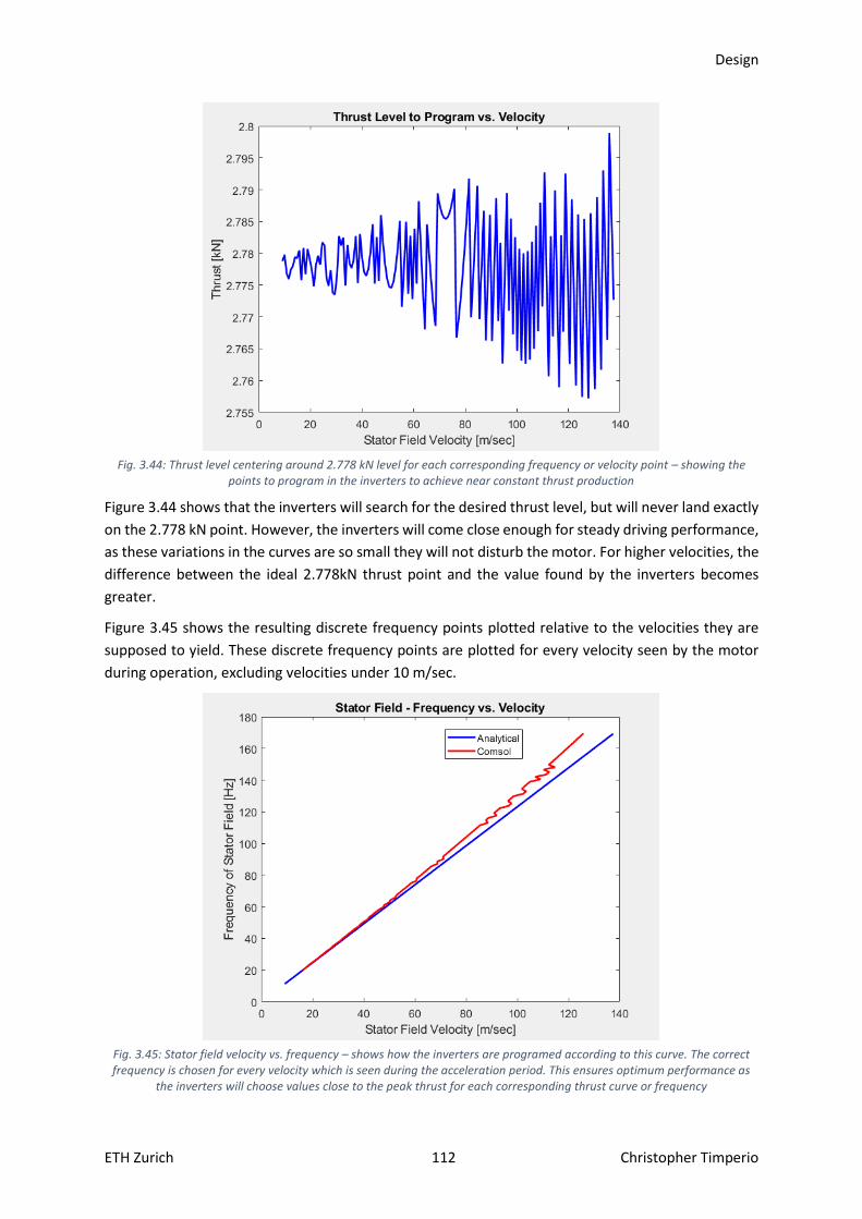
Design


Fig. 3.44: Thrust level centering around 2.778 kN level for each corresponding frequency or velocity point – showing the

points to program in the inverters to achieve near constant thrust production

Figure 3.44 shows that the inverters will search for the desired thrust level, but will never land exactly

on the 2.778 kN point. However, the inverters will come close enough for steady driving performance,

as these variations in the curves are so small they will not disturb the motor. For higher velocities, the

difference between the ideal 2.778kN thrust point and the value found by the inverters becomes

greater.

Figure 3.45 shows the resulting discrete frequency points plotted relative to the velocities they are

supposed to yield. These discrete frequency points are plotted for every velocity seen by the motor

during operation, excluding velocities under 10 m/sec.

Fig. 3.45: Stator field velocity vs. frequency – shows how the inverters are programed according to this curve. The correct frequency is chosen for every velocity which is seen during the acceleration period. This ensures optimum performance as

the inverters will choose values close to the peak thrust for each corresponding thrust curve or frequency

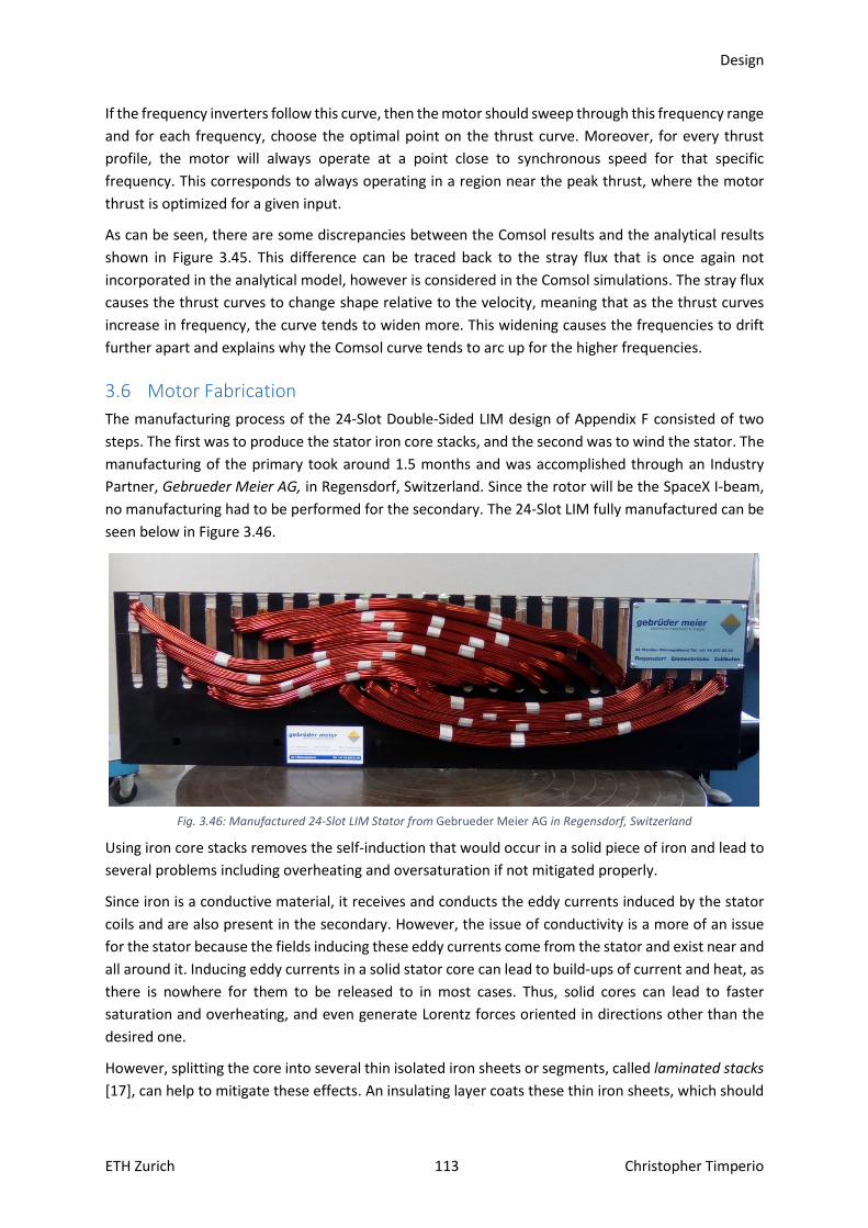
Design


If the frequency inverters follow this curve, then the motor should sweep through this frequency range

and for each frequency, choose the optimal point on the thrust curve. Moreover, for every thrust

profile, the motor will always operate at a point close to synchronous speed for that specific

frequency. This corresponds to always operating in a region near the peak thrust, where the motor

thrust is optimized for a given input.

As can be seen, there are some discrepancies between the Comsol results and the analytical results

shown in Figure 3.45. This difference can be traced back to the stray flux that is once again not

incorporated in the analytical model, however is considered in the Comsol simulations. The stray flux

causes the thrust curves to change shape relative to the velocity, meaning that as the thrust curves

increase in frequency, the curve tends to widen more. This widening causes the frequencies to drift

further apart and explains why the Comsol curve tends to arc up for the higher frequencies.

3.6 Motor Fabrication

The manufacturing process of the 24-Slot Double-Sided LIM design of Appendix F consisted of two

steps. The first was to produce the stator iron core stacks, and the second was to wind the stator. The

manufacturing of the primary took around 1.5 months and was accomplished through an Industry

Partner, Gebrueder Meier AG, in Regensdorf, Switzerland. Since the rotor will be the SpaceX I-beam,

no manufacturing had to be performed for the secondary. The 24-Slot LIM fully manufactured can be

seen below in Figure 3.46.

Fig. 3.46: Manufactured 24-Slot LIM Stator from Gebrueder Meier AG in Regensdorf, Switzerland

Using iron core stacks removes the self-induction that would occur in a solid piece of iron and lead to

several problems including overheating and oversaturation if not mitigated properly.

Since iron is a conductive material, it receives and conducts the eddy currents induced by the stator

coils and are also present in the secondary. However, the issue of conductivity is a more of an issue

for the stator because the fields inducing these eddy currents come from the stator and exist near and

all around it. Inducing eddy currents in a solid stator core can lead to build-ups of current and heat, as

there is nowhere for them to be released to in most cases. Thus, solid cores can lead to faster

saturation and overheating, and even generate Lorentz forces oriented in directions other than the

desired one.

However, splitting the core into several thin isolated iron sheets or segments, called laminated stacks

[17], can help to mitigate these effects. An insulating layer coats these thin iron sheets, which should

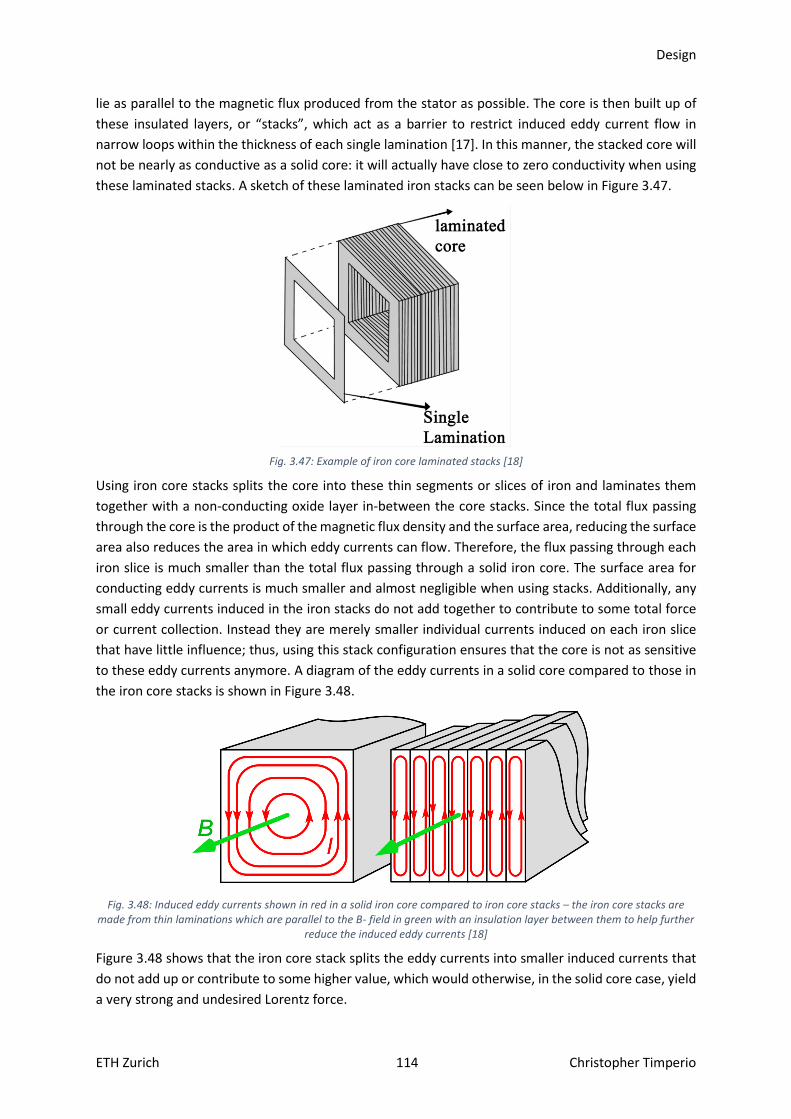
Design


lie as parallel to the magnetic flux produced from the stator as possible. The core is then built up of

these insulated layers, or “stacks”, which act as a barrier to restrict induced eddy current flow in

narrow loops within the thickness of each single lamination [17]. In this manner, the stacked core will

not be nearly as conductive as a solid core: it will actually have close to zero conductivity when using

these laminated stacks. A sketch of these laminated iron stacks can be seen below in Figure 3.47.

Fig. 3.47: Example of iron core laminated stacks [18]

Using iron core stacks splits the core into these thin segments or slices of iron and laminates them

together with a non-conducting oxide layer in-between the core stacks. Since the total flux passing

through the core is the product of the magnetic flux density and the surface area, reducing the surface

area also reduces the area in which eddy currents can flow. Therefore, the flux passing through each

iron slice is much smaller than the total flux passing through a solid iron core. The surface area for

conducting eddy currents is much smaller and almost negligible when using stacks. Additionally, any

small eddy currents induced in the iron stacks do not add together to contribute to some total force

or current collection. Instead they are merely smaller individual currents induced on each iron slice

that have little influence; thus, using this stack configuration ensures that the core is not as sensitive

to these eddy currents anymore. A diagram of the eddy currents in a solid core compared to those in

the iron core stacks is shown in Figure 3.48.

Fig. 3.48: Induced eddy currents shown in red in a solid iron core compared to iron core stacks – the iron core stacks are

made from thin laminations which are parallel to the B- field in green with an insulation layer between them to help further reduce the induced eddy currents [18]

Figure 3.48 shows that the iron core stack splits the eddy currents into smaller induced currents that

do not add up or contribute to some higher value, which would otherwise, in the solid core case, yield

a very strong and undesired Lorentz force.

Design


Splitting up the currents also acts to reduce the overall heat produced. If iron core stacks are not used,

the iron core could even melt if it were one solid piece of iron, due to the high level of current induced

from the nearby coils. Generally, more flux passes through the core than through the secondary, so if

a solid core is used, all the input current is essentially self-induced in the core. Additionally, since the

power dissipated in a system is proportional to the square of the current, breaking up a solid core into

narrow laminations, significantly reduces the power losses in the core. Thus, this design employs

laminated core stacks.

Securing these iron stacks together requires creative ideas. Some ideas involve the use of clamps or

fixtures to hold the stacks together. In this thesis’s design, they are precisely glued together, which

should be sufficiently as long as they are not exposed to very high temperatures. While it is more

difficult to manufacture the stator from iron core stacks than from a solid core, it is a necessary step

because the motor would not function otherwise with a solid core. The process of manufacturing

these stacks is more of a chemical than mechanical process. The individual stacks need to be well

laminated with an oxide layer, so that the core stacks don’t create conductive channels between them

in which larger eddy currents can then be induced.

It is important that the oxide layers between each stack cannot be “breached” because if this occurs,

the core, or any connecting stacks, will be conductive again. Therefore, extra precaution must be taken

to prohibit the flux from penetrating the laminations by ensuring that the stacks are not electrically

connected while securing them together, which could happen if portions of the oxide lamination layer

are scratched off [17].

Mounting holes have been designed in the yoke of the stator core to mount the LIM on the Escher

Pod. The LIM will be supported mechanically to the Pod chassis throughout operation by mounting

bolts fitted through these mounting holes. Therefore, the bolts fixing the LIM to the Pod must be

capable of attaching the LIM efficiently to the chassis. The mounting fixture drafted up for this purpose

is shown below in Figure 3.49: the LIM is shown in light blue, mounted onto the Escher Pod.

Fig. 3.49: LIM mounted onto the Escher Pod, held in place by a mounting fixture

Design


3.7 Temperature Considerations

With the high powers the motor uses to accelerate to high speeds, it is an interesting exercise to

perform a short temperature analysis to quantify the thermodynamic effects and temperature

changes experienced by the motor during its operation.

Estimating the temperatures in the motor, is important because the motor will operate with little to

no thermal convection or air cooling in the low-pressure environment once the air is pumped out of

the Hyperloop tube. The heat generated in a motor is usually transferred via convection to the

medium surrounding the machine (i.e., air); however, in the low-pressure environment of the

Hyperloop tube, there is less air to facilitate this heat transfer. Thus, heat transfer in the motor will

occur solely by conduction or radiation.

Quantifying the temperature change that the motor experiences during the 12.5sec accelerating

period uses heat transfer or energy equilibrium equations. The calculations focus on the temperature

change experienced by the coils, as these high currents flow through them during operation, and

experienced by the core around which these coils are wrapped.

Eqn. 3.42 is deployed to analyze the change in temperature seen in the coils.

𝑄 = 𝑚 ∙ ∆𝑇 ∙ 𝑐𝑡 = 𝐼2 ∙ 𝑅 ∙ ∆𝑡 (3.42)

𝑅 = 𝜌𝑙

𝑆𝐴 (3.43)

Where 𝑄 is the heat content or energy transfer in Joules, 𝐼 is the supply current to the LIM, 𝑅 is the

resistance of the coils, 𝑚 is the mass of the coils, 𝑐𝑡 is the specific heat value for copper, ∆𝑡 is the

duration of operation time, and ∆𝑇 is the absolute change in temperature experienced. The

resistance, 𝑅, is comprised of the copper coil’s resistivity 𝜌, multiplied by the length of coil, 𝑙, divided

by its cross-sectional area, 𝑆𝐴.

Given a copper coil resistivity of 1.68 ∙ 10−8 Ω ∙ m, a specific heat value of 390 J/𝑘𝑔 ∙ 𝐾, a coil mass

of 1.067 kg, a total RMS input current of 420A passing through a cross-sectional area of 2.11 ∙

10−5 m2, and a length of coil of 16 m, the heat transfer is calculated as follows.

𝑅 = (1.68 ∙ 10−8 Ω ∙ m) ∙16 m

2.11 ∙ 10−5 m2= 12.74 𝑚Ω (3.44)

∆𝑇 =

𝐼2 ∙ 𝑅 ∙ ∆𝑡

𝑐𝑡 ∙ 𝑚=

420𝐴 2 ∙ 12.74 𝑚Ω ∙ 12.5 𝑠𝑒𝑐

(390 𝐽 𝑘𝑔 ∙ 𝐾⁄ ) ∙ 1.067 𝑘𝑔= 67.51 𝐾

(3.45)

The temperature change experienced by the coils is large due to the high currents being passed. Heat

transfer effects for the stator core are analyzed similarly and performed below using Eqn. 3.46.

𝑄 = 𝑚 ∙ ∆𝑇 ∙ 𝑐𝑡 = 𝑙 ∙ ∆𝑡 (3.46)

Where 𝑄 is the heat content or energy transfer in Joules, 𝑐𝑡 is the specific heat of the core, 𝑙𝑠 are the

losses in the iron stator core, 𝑚 is the mass of the core, ∆𝑡 is the duration of operation in seconds,

and ∆𝑇 is the absolute change in temperature. ∆𝑇 is then calculated using Eqn. 3.47.

∆𝑇 =𝑙𝑠 ∙ ∆𝑡

𝑐𝑡=

400 𝑊 𝑘𝑔⁄ ∙ 12.5𝑠𝑒𝑐

457 𝐽 𝑘𝑔 ∙ 𝐾⁄= 10.94 𝐾 (3.47)

Design


The values for the specific heat, 𝑐𝑡 , and the losses, 𝑙𝑠 , in the stator core are obtained for the M400

iron core used in this LIM from Appendix E. As shown, the core does not experience as large of a

temperature increase as the coils do. The main reason why the core does not heat up much from this

heat transfer is that the iron core is essentially acting as a large heatsink for the coils, dissipating the

heat from them and dispersing it evenly throughout the iron core. Significantly heating up this iron

core would require a much longer operational time. Therefore, the temperature change observed is

manageable and will not negatively influence the motor’s functionality or performance during the

12.5sec operation time.

Assuming the motor is initially at room temperature (i.e., 293 K), the final temperature for the coils

and the core can be calculated.

Coils: ∆𝑇 = 67.51 𝐾 = 𝑇𝑓 − 𝑇𝑖 => 67.51 𝐾 = 𝑇𝑓 − 273 𝐾 (3.48)

𝑇𝑓 = 293 𝐾 + 61.51 𝐾 = 360.51 𝐾 (3.49)

Core: ∆𝑇 = 10.94 𝐾 = 𝑇𝑓 − 𝑇𝑖 => 10.94𝐾 = 𝑇𝑓 − 273 𝐾 (3.50)

𝑇𝑓 = 293 𝐾 + 10.94 𝐾 = 303.94 𝐾 (3.51)

The final temperatures for the core and coils, converted to Celsius, are shown below.

Coils: 360.51 𝐾 − 273.15 𝐾 = 87.36 ℃ (3.52)

Core: 303.94 𝐾 − 273.15 𝐾 = 30.79 ℃ (3.53)

The final temperatures of the coils and the core after 12.5sec of operation are seen to be 87.36 ℃

and 30.79 ℃ , respectively. If the temperature changes were larger, for example, due to longer

continuous motor operation or an increase in input current, then other cooling methods or mitigation

techniques would have to be applied so that the motor would not overheat or melt during operation.

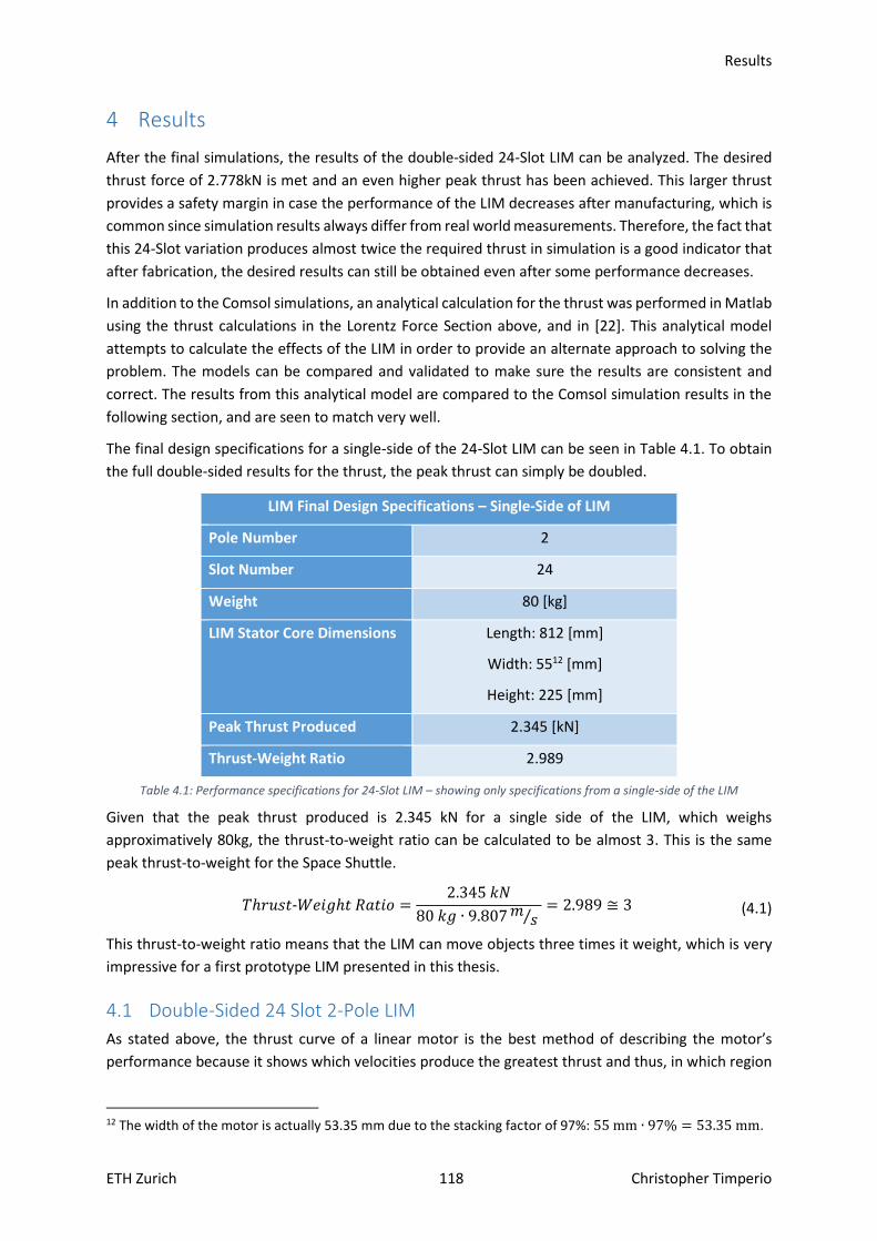
Results


4 Results

After the final simulations, the results of the double-sided 24-Slot LIM can be analyzed. The desired

thrust force of 2.778kN is met and an even higher peak thrust has been achieved. This larger thrust

provides a safety margin in case the performance of the LIM decreases after manufacturing, which is

common since simulation results always differ from real world measurements. Therefore, the fact that

this 24-Slot variation produces almost twice the required thrust in simulation is a good indicator that

after fabrication, the desired results can still be obtained even after some performance decreases.

In addition to the Comsol simulations, an analytical calculation for the thrust was performed in Matlab

using the thrust calculations in the Lorentz Force Section above, and in [22]. This analytical model

attempts to calculate the effects of the LIM in order to provide an alternate approach to solving the

problem. The models can be compared and validated to make sure the results are consistent and

correct. The results from this analytical model are compared to the Comsol simulation results in the

following section, and are seen to match very well.

The final design specifications for a single-side of the 24-Slot LIM can be seen in Table 4.1. To obtain

the full double-sided results for the thrust, the peak thrust can simply be doubled.

LIM Final Design Specifications – Single-Side of LIM

Pole Number 2

Slot Number 24

Weight 80 [kg]

LIM Stator Core Dimensions Length: 812 [mm]

Width: 5512 [mm]

Height: 225 [mm]

Peak Thrust Produced 2.345 [kN]

Thrust-Weight Ratio 2.989

Table 4.1: Performance specifications for 24-Slot LIM – showing only specifications from a single-side of the LIM

Given that the peak thrust produced is 2.345 kN for a single side of the LIM, which weighs

approximatively 80kg, the thrust-to-weight ratio can be calculated to be almost 3. This is the same

peak thrust-to-weight for the Space Shuttle.

𝑇ℎ𝑟𝑢𝑠𝑡-𝑊𝑒𝑖𝑔ℎ𝑡 𝑅𝑎𝑡𝑖𝑜 =2.345 𝑘𝑁

80 𝑘𝑔 ∙ 9.807𝑚𝑠⁄

= 2.989 ≅ 3 (4.1)

This thrust-to-weight ratio means that the LIM can move objects three times it weight, which is very

impressive for a first prototype LIM presented in this thesis.

4.1 Double-Sided 24 Slot 2-Pole LIM

As stated above, the thrust curve of a linear motor is the best method of describing the motor’s

performance because it shows which velocities produce the greatest thrust and thus, in which region

12 The width of the motor is actually 53.35 mm due to the stacking factor of 97%: 55 mm ∙ 97% = 53.35 mm.

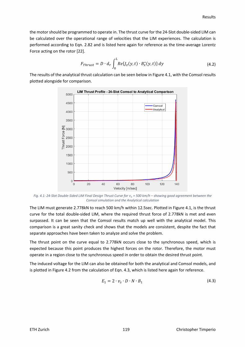
Results


the motor should be programmed to operate in. The thrust curve for the 24-Slot double-sided LIM can

be calculated over the operational range of velocities that the LIM experiences. The calculation is

performed according to Eqn. 2.82 and is listed here again for reference as the time-average Lorentz

Force acting on the rotor [22].

𝐹𝑇ℎ𝑟𝑢𝑠𝑡 = 𝐷 ∙ 𝑑𝑟 ∫ 𝑅𝑒{𝐽𝑧(𝑦, 𝑡) ∙ 𝐵𝑥∗(𝑦, 𝑡)}

𝐿

0

𝑑𝑦 (4.2)

The results of the analytical thrust calculation can be seen below in Figure 4.1, with the Comsol results

plotted alongside for comparison.

Fig. 4.1: 24-Slot Double-Sided LIM Final Design Thrust Curve for 𝑣𝑠 = 500 km/h – showing good agreement between the

Comsol simulation and the Analytical calculation

The LIM must generate 2.778kN to reach 500 km/h within 12.5sec. Plotted in Figure 4.1, is the thrust

curve for the total double-sided LIM, where the required thrust force of 2.778kN is met and even

surpassed. It can be seen that the Comsol results match up well with the analytical model. This

comparison is a great sanity check and shows that the models are consistent, despite the fact that

separate approaches have been taken to analyze and solve the problem.

The thrust point on the curve equal to 2.778kN occurs close to the synchronous speed, which is

expected because this point produces the highest forces on the rotor. Therefore, the motor must

operate in a region close to the synchronous speed in order to obtain the desired thrust point.

The induced voltage for the LIM can also be obtained for both the analytical and Comsol models, and

is plotted in Figure 4.2 from the calculation of Eqn. 4.3, which is listed here again for reference.

𝐸1 = 2 ∙ 𝑣𝑠 ∙ 𝐷 ∙ 𝑁 ∙ 𝐵1 (4.3)

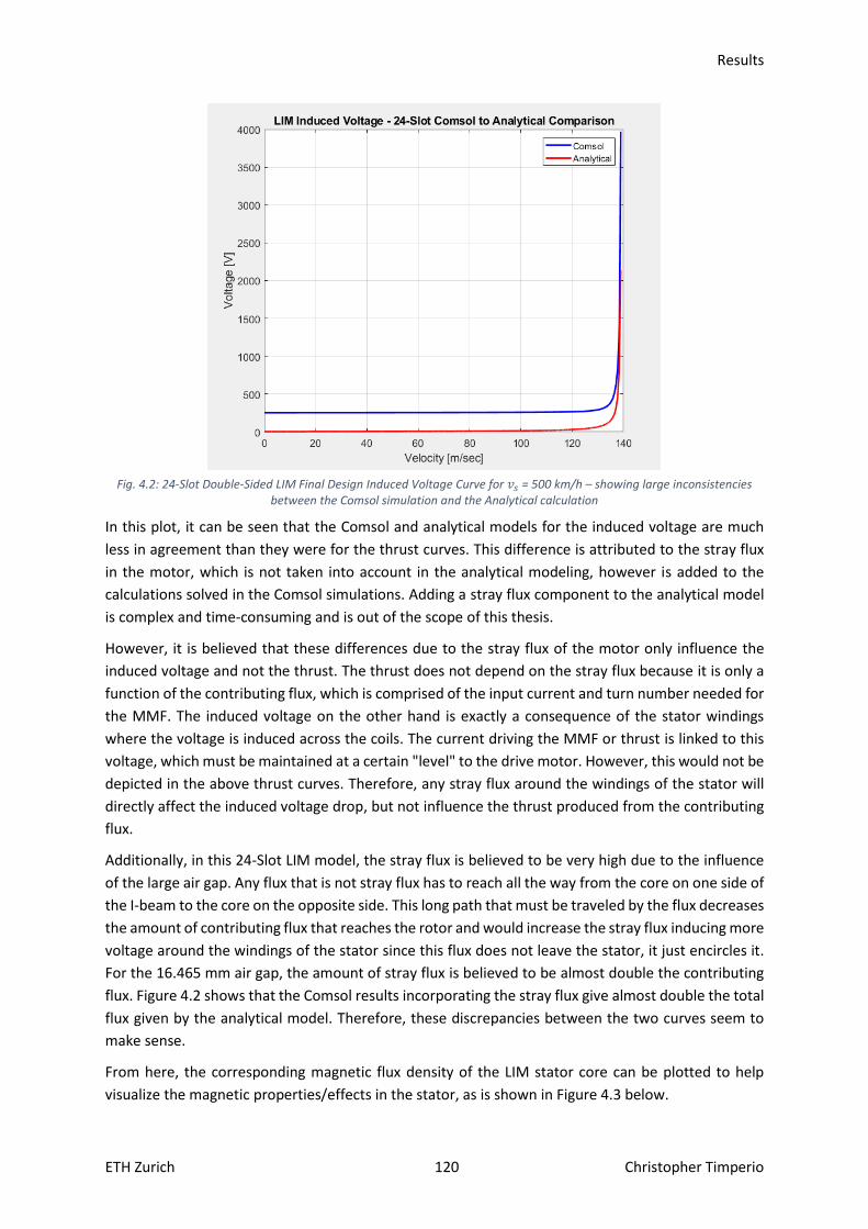
Results


Fig. 4.2: 24-Slot Double-Sided LIM Final Design Induced Voltage Curve for 𝑣𝑠 = 500 km/h – showing large inconsistencies

between the Comsol simulation and the Analytical calculation

In this plot, it can be seen that the Comsol and analytical models for the induced voltage are much

less in agreement than they were for the thrust curves. This difference is attributed to the stray flux

in the motor, which is not taken into account in the analytical modeling, however is added to the

calculations solved in the Comsol simulations. Adding a stray flux component to the analytical model

is complex and time-consuming and is out of the scope of this thesis.

However, it is believed that these differences due to the stray flux of the motor only influence the

induced voltage and not the thrust. The thrust does not depend on the stray flux because it is only a

function of the contributing flux, which is comprised of the input current and turn number needed for

the MMF. The induced voltage on the other hand is exactly a consequence of the stator windings

where the voltage is induced across the coils. The current driving the MMF or thrust is linked to this

voltage, which must be maintained at a certain "level" to the drive motor. However, this would not be

depicted in the above thrust curves. Therefore, any stray flux around the windings of the stator will

directly affect the induced voltage drop, but not influence the thrust produced from the contributing

flux.

Additionally, in this 24-Slot LIM model, the stray flux is believed to be very high due to the influence

of the large air gap. Any flux that is not stray flux has to reach all the way from the core on one side of

the I-beam to the core on the opposite side. This long path that must be traveled by the flux decreases

the amount of contributing flux that reaches the rotor and would increase the stray flux inducing more

voltage around the windings of the stator since this flux does not leave the stator, it just encircles it.

For the 16.465 mm air gap, the amount of stray flux is believed to be almost double the contributing

flux. Figure 4.2 shows that the Comsol results incorporating the stray flux give almost double the total

flux given by the analytical model. Therefore, these discrepancies between the two curves seem to

make sense.

From here, the corresponding magnetic flux density of the LIM stator core can be plotted to help

visualize the magnetic properties/effects in the stator, as is shown in Figure 4.3 below.

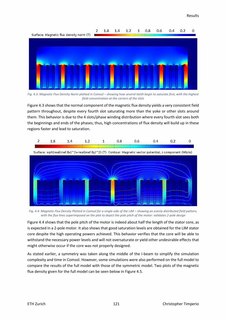
Results


Fig. 4.3: Magnetic Flux Density Norm plotted in Comsol – showing how several teeth begin to saturate first, with the highest

field concentration at the corners of the slots

Figure 4.3 shows that the normal component of the magnetic flux density yields a very consistent field

pattern throughout, despite every fourth slot saturating more than the yoke or other slots around

them. This behavior is due to the 4 slots/phase winding distribution where every fourth slot sees both

the beginnings and ends of the phases; thus, high concentrations of flux density will build up in these

regions faster and lead to saturation.

Fig. 4.4: Magnetic Flux Density Plotted in Comsol for a single-side of the LIM – showing an evenly distributed field pattern,

with the flux lines superimposed on the plot to depict the pole pitch of the motor: validates 2-pole design

Figure 4.4 shows that the pole pitch of the motor is indeed about half the length of the stator core, as

is expected in a 2-pole motor. It also shows that good saturation levels are obtained for the LIM stator

core despite the high operating powers achieved. This behavior verifies that the core will be able to

withstand the necessary power levels and will not oversaturate or yield other undesirable effects that

might otherwise occur if the core was not properly designed.

As stated earlier, a symmetry was taken along the middle of the I-beam to simplify the simulation

complexity and time in Comsol. However, some simulations were also performed on the full model to

compare the results of the full model with those of the symmetric model. Two plots of the magnetic

flux density given for the full model can be seen below in Figure 4.5.

Results


Fig. 4.5: Magnetic flux density plot for the full double-sided 24-Slot LIM – showing coupling (below) vs decoupling (above)

scenarios; the above plot is most likely where operation will occur.

The image on top shows the motor operating close to the synchronous speed. The operating

frequency will be higher at the synchronous speed and corresponds to the motor operating in a

decoupling region. The image below depicts an operating point further away from the synchronous

speed in the coupling region, and thus for a lower frequency. Here, the fields penetrate all the way

through the aluminum I-beam secondary as a result of the lower frequency.

When comparing the two Comsol models (symmetric and full), it is evident that the two models match

each other quite perfectly when the thrust curve results are doubled for the symmetric model. This

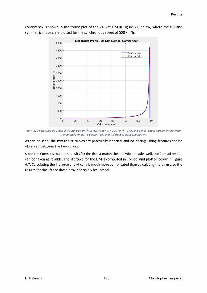
Results


consistency is shown in the thrust plot of the 24-Slot LIM in Figure 4.6 below, where the full and

symmetric models are plotted for the synchronous speed of 500 km/h.

Fig. 4.6: 24-Slot Double-Sided LIM Final Design Thrust Curve for 𝑣𝑠 = 500 km/h – showing almost exact agreement between

the Comsol symmetric single-sided and full double-sided simulations

As can be seen, the two thrust curves are practically identical and no distinguishing features can be

observed between the two curves.

Since the Comsol simulation results for the thrust match the analytical results well, the Comsol results

can be taken as reliable. The lift force for the LIM is computed in Comsol and plotted below in Figure

4.7. Calculating the lift force analytically is much more complicated than calculating the thrust, so the

results for the lift are those provided solely by Comsol.

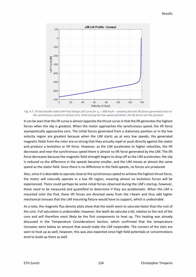
Results


Fig. 4.7: 24-Slot Double-Sided LIM Final Design Lift Curve for 𝑣𝑠 = 500 km/h – showing that the lift forces generated close to

the synchronous speed are almost zero, while during the low-speed operation, the lift forces are the greatest

It can be seen that the lift curve is almost opposite the thrust curve in that the lift generates the highest

forces when the slip is greatest. When the motor approaches the synchronous speed, the lift force

asymptotically approaches zero. The initial forces generated from a stationary position or in the low

velocity region are greatest because when the LIM starts up at very low speeds, the generated

magnetic fields from the rotor are so strong that they actually repel or push directly against the stator

and produce a levitation or lift force. However, as the LIM accelerates to higher velocities, the lift

decreases and near the synchronous speed there is almost no lift force generated by the LIM. The lift

force decreases because the magnetic field strength begins to drop off as the LIM accelerates: the slip

is reduced so the difference in the speeds become smaller, and the LIM moves at almost the same

speed as the stator field. Since there is no difference in the field speeds, no forces are produced.

Also, since it is desirable to operate close to the synchronous speed to achieve the highest thrust force,

the motor will naturally operate in a low lift region, meaning almost no levitation forces will be

experienced. There could perhaps be some initial forces observed during the LIM’s startup, however,

these need to be measured and quantified to determine if they are problematic. When the LIM is

mounted onto the Pod, these lift forces are directed away from the I-beam and thus add higher

mechanical stresses that the LIM mounting fixture would have to support, which is undesirable.

As a note, the magnetic flux density plots show that the teeth seem to saturate faster than the rest of

the core. Full saturation is undesirable; however, the teeth do saturate a bit, relative to the rest of the

core and will therefore most likely be the first components to heat up. This heating was already

discussed in the Temperature Considerations Section, which confirmed that the temperature

increases were below an amount that would make the LIM inoperable. The corners of the slots are

seen to heat up as well, however, this was also expected since high field potentials or concentrations

tend to build up there as well.

Summary


5 Summary

This thesis focuses on the design and manufacturing of a 24-Slot Linear Induction Motor. The motor

meets the design specifications laid out in the beginning of the thesis and achieves the main goal of

reaching 500 km/h while fitting around the SpaceX I-beam secondary. The motor was also designed

to operate in a low-pressure environment, making it suitable for a prototype LIM to be used as the

main propulsion mechanism for Hyperloop-like systems. The motor has not been measured/tested

yet due to time constraints, however, testing, characterization, and validation of the motor will

continue after the thesis, and appropriate findings will be documented in a supplementary paper.

5.1 Project Challenges

One of the first challenges encountered during this thesis was the large lift forces observed relative to

the thrust forces. In the concept 2-Slot design, the observed lift forces were repeatedly orders of

magnitude greater than the produced thrust forces. In this manner, the motor acted more like a

magnet repelling its own magnetic field, than a linear motor driving itself. However, this behavior was

only observed in the 2-Slot stator, and was the main motivation to shift to a stator with more slots.

After subsequent design iterations and simulations, this effect disappeared and the subsequent linear

motors functioned as expected.

When taking into account the end-effects of the linear motor, the end teeth were extended to try and

mitigate the observed performance losses. Designing the outer teeth of the core to be slightly larger

and not placing any coils around them helped the core capture more of the field that would otherwise

be “lost” in the air. This behavior is illustrated in Figure 5.1 by a plot of the magnetic flux density for

the concept 2-Slot motor, where a 2D simulation shows how the end-effects of the motor can be

drastic: most of the field is lost in the air.

Fig. 5.1: Magnetic Flux Density of the 2-Slot Concept – showing how the field escapes the LIM due to the end-effects of the motor: to mitigate these effects, coils should not be placed on the outside of the motor, and the end teeth should be made

larger to capture more of the external fields

The winding design, and how to effectivity fit the winding heads inside the tight inner dimension of

the I-beam, were also difficult challenges in this thesis. As seen in the winding design portion of this

thesis, what can be practically manufactured and wound is much different from what theoretically

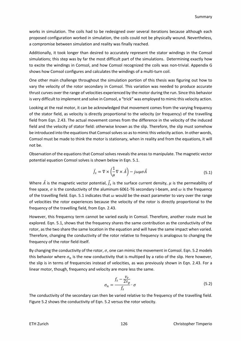
Summary


works in simulation. The coils had to be redesigned over several iterations because although each

proposed configuration worked in simulation, the coils could not be physically wound. Nevertheless,

a compromise between simulation and reality was finally reached.

Additionally, it took longer than desired to accurately represent the stator windings in the Comsol

simulations; this step was by far the most difficult part of the simulations. Determining exactly how

to excite the windings in Comsol, and how Comsol recognized the coils was non-trivial. Appendix G

shows how Comsol configures and calculates the windings of a multi-turn coil.

One other main challenge throughout the simulation portion of this thesis was figuring out how to

vary the velocity of the rotor secondary in Comsol. This variation was needed to produce accurate

thrust curves over the range of velocities experienced by the motor during the run. Since this behavior

is very difficult to implement and solve in Comsol, a “trick” was employed to mimic this velocity action.

Looking at the real motor, it can be acknowledged that movement comes from the varying frequency

of the stator field, as velocity is directly proportional to the velocity (or frequency) of the travelling

field from Eqn. 2.43. The actual movement comes from the difference in the velocity of the induced

field and the velocity of stator field: otherwise known as the slip. Therefore, the slip must somehow

be introduced into the equations that Comsol solves so as to mimic this velocity action. In other words,

Comsol must be made to think the motor is stationary, when in reality and from the equations, it will

not be.

Observation of the equations that Comsol solves reveals the areas to manipulate. The magnetic vector

potential equation Comsol solves is shown below in Eqn. 5.1.

𝐽 𝑠 = ∇ × (1

𝜇∇ × 𝐴 ) − 𝑗𝜔𝜇𝜎𝐴 (5.1)

Where 𝐴 is the magnetic vector potential, 𝐽 𝑠 is the surface current density, 𝜇 is the permeability of

free space, 𝜎 is the conductivity of the aluminum 6061-T6 secondary I-beam, and 𝜔 is the frequency

of the travelling field. Eqn. 5.1 indicates that 𝜔 would be the exact parameter to vary over the range

of velocities the rotor experiences because the velocity of the rotor is directly proportional to the

frequency of the travelling field, from Eqn. 2.43.

However, this frequency term cannot be varied easily in Comsol. Therefore, another route must be

explored. Eqn. 5.1, shows that the frequency shares the same contribution as the conductivity of the

rotor, as the two share the same location in the equation and will have the same impact when varied.

Therefore, changing the conductivity of the rotor relative to frequency is analogous to changing the

frequency of the rotor field itself.

By changing the conductivity of the rotor, 𝜎, one can mimic the movement in Comsol. Eqn. 5.2 models

this behavior where 𝜎𝑛 is the new conductivity that is multiped by a ratio of the slip. Here however,

the slip is in terms of frequencies instead of velocities, as was previously shown in Eqn. 2.43. For a

linear motor, though, frequency and velocity are more less the same.

𝜎𝑛 =

𝑓𝑠 −𝑣𝑟2𝜏𝑝

𝑓𝑠∙ 𝜎 (5.2)

The conductivity of the secondary can then be varied relative to the frequency of the travelling field.

Figure 5.2 shows the conductivity of Eqn. 5.2 versus the rotor velocity.

Summary


Fig. 5.2: Sigma Variation to Mimic Frequency Sweep in Comsol Simulations

5.2 Outlook

As mentioned, the linear motor of this thesis still needs to be tested to see how well the measured

values match the simulated results. Several other tasks must be completed before this motor can be

fully operational and integrated onto a Hyperloop Pod. To elaborate, the motor control algorithms to

control the inverters must be programmed to sweep though the range of frequencies in order to

provide an optimal, constant thrust progression. Efficient and dedicated programming will yield very

powerful drivetrain performance.

Additionally, the structure and chassis of the Escher Pod must be strong enough to support the LIM.

Additional mounting fixations or even a new chassis may need to be developed to support this LIM.

However, once an appropriate chassis is found, the LIM can be mounted and tested in high-speed test

runs in the Hyperloop tube at SpaceX. Prior to testing at SpaceX, low-speed runs to validate and tune

the motor can take place at the Dübendorf testing facilities here in Switzerland.

It will also be beneficial to test the motor’s operation in a vacuum chamber before testing in the

SpaceX tube. These tests will show how much, if any, arcing occurs in a low-pressure environment.

Finally, a second prototype will most likely be developed after characterizing this initial prototype and

seeing the areas where the performance can be improved.

Additional next steps include conducting a feasibility study for the overall Hyperloop system to

determine the optimal track geometry. Such a track would be deployed in full-scale Hyperloop

systems. It was shown that the SpaceX I-beam is a non-optimal geometry for the secondary due to the

confined inner dimensions. Scaling up these systems for fully-fledged Hyperloop systems around the

world is the end goal and perhaps descendants of this prototype LIM design will even one day be used

to support passenger and cargo transportation around the world.

Summary


5.2.1 Design Improvements The biggest design constraint of the motor is the width of the stator due to the limited space in-

between the I-beam. Therefore, the main design improvement to be made is the removal of one of

the tops of the I-beam track, thereby creating a longer “T-beam” track. This change would allow for

increased active surface areas of the stator and allow more thrust to be generated from the motor.

Additionally, perhaps it is later determined that linear induction motors of a short primary and long

secondary track configuration are not ideal for a Hyperloop-like system.

For instance, it may be the case that the primary and secondary are swapped or reversed. In this case,

the rotor blade would be mounted to the vehicle or Pod, and the primary would be married to the

track. It is known that having the primary aboard the Pod is not optimal for larger scaled up systems.

Factors making this primary configuration suboptimal include 1) bringing the energy to power the

motor aboard the pod capsules, thus adding mass and requiring more energy 2) added pod capsule

costs: placing the primary in each pod significantly drives up the overall value and maintenance cost

of each pod. However, it could also be the case that designing a complex track infrastructure to

support the required high-powers over long distances would also be expensive. Therefore, a feasibility

study is needed to discover an optimal and efficient configuration for such a system.

Nevertheless, the working principles and motor theory for linear motors is more or less universal and

thus the fundamentals learned in this thesis can be directly applied to optimized linear motor

configurations later. For example, the configuration proposed by Elon Musk in the Hyperloop Alpha

Whitepaper suggests having the linear accelerator or primary coil windings fixed at various

“accelerating” stations in the low-pressure tube with secondary rotors contained in each Pod capsule.

This configuration can be seen below in Figure 5.3 and is similar to the one used in Hyperloop One’s

system.

Fig. 5.3: Rotor and Stator Concept Proposed by Elon Musk [5]

Having the rotor blade on the Pod and the stator mounted to the track may perhaps be the more

feasible and power efficient way to build the motor because additional power to account for the motor

does not need to be brought aboard. However, the reversed configuration shown in this thesis was a

useful first step because it fostered the development of a strong intuition into the working principles

of a LIM. With some engineering work, the LIM design of this thesis could simply be reversed to match

this configuration. The prototype LIM designed in this thesis has been an impressive first step towards

a sustainable linear motor eventually capable of reaching speeds of 1,000 km/h.

References


6 References

[1] H. G. Schwartz, M. Meyer, C. J. Burbank and M. Kuby, "Ch. 5: Transportation. Climate Change

Impacts in the United States: The Third National Climate Assessment," 2014. [Online].

Available: https://nca2014.globalchange.gov/report/sectors/transportation.

[2] R. Chin, "Solving transport headaches in the cities of 2050," BBC, 2013. [Online]. Available:

http://www.bbc.com/future/story/20130617-moving-around-in-the-megacity. [Accessed

2018].

[3] "THE OECD ENVIRONMENTAL OUTLOOK TO 2050. Key Findings on Climate Change,"

Organization for Economic Co-operation and Development (OECD), 2012.

[4] C. Höft, P. Armstrong and M. Berger, "Abstract: Hyperloop Transportation Technologies Risk

Report," Münchener Rückversicherungs-Gesellschaft, München, 2017.

[5] E. Musk, "Hyperloop Alpha," Hawthorne, 2013.

[6] "Beach Pneumatic Transit," nycsubway.org, 2012. [Online]. Available:

https://www.nycsubway.org/wiki/Beach_Pneumatic_Transit. [Accessed 2018].

[7] SpaceX, "SpaceX Hyperloop Track Specification, Revision. 13.0," Space Exploration

Technologies, Hawthorne, 2017.

[8] M. Jufer, "Swissmetro - Introduction," 1999.

[9] M. Jufer and A. Cassat, "Collaboration with the Korean Railroad," 2010.

[10] M. Jufer and N. Wavre, "Le Moteur Linéaire: Développement Théorique et Applications,"

Lausanne.

[11] "Facts & Frequently Asked Questions," Hyperloop One, [Online]. Available: https://hyperloop-

one.com/facts-frequently-asked-questions. [Accessed 2018].

[12] E. R. Laithwaite, "Linear Induction Motor for Vehicle Propulsion". England Patent US3585939A,

22 June 1971.

[13] E. R. Laithwaite, Propulsion without Wheels, English Universities Press, 1970.

[14] "LINEAR MOTORS OVERVIEW," ETEL, [Online]. Available: http://www.etel.ch/linear-

motors/overview/. [Accessed 2018].

[15] W. Hayt and J. Buck, Engineering Electromagnetics, New York: McGraw-Hill, 2012.

[16] C. Timperio, "Inertial Navigation System using Magnetoquasistatic Field Data to Improve Non-

Line-of-Sight (NLoS) Communication," ETH Zürich, Zürich, 2016.

[17] J. Pyrhönen, T. Jokinen and V. Hrabovcová, Design of Rotating Electrical Machines, John Wiley

& Sons, 2008.

References


[18] M. Larsson, "Electric Motors for Vehicle Propulsion," Linköpings Universitet, Linköping, 2014.

[19] S. Yamamura, Theory of Linear Induction Motors, 1st ed., Wiley, 1972.

[20] S. Chevailler, "Comparative Study and Selection Criteria of Linear Motors," École Polytechnique

Fédérale de Lausanne, Lausanne, 2006.

[21] M. Jufer, "Chapitre 12: Champ Tournant et Bobinage," in Électromécanique, Lausanne, Presses

Polytechniques et Universitaires Romandes, 2004, pp. 283-287.

[22] J. Smajic, "Theory of Linear Induction Motor (LIM)," Zürich, 2018.

[23] W. Soong, "Chapter 3: Magnetic Materials," University of Adelaide, Australia, 2016.

[24] A. Küchler, High Voltage Engineering, Berlin: Springer Vieweg, 2018.

[25] E. Husain and R. S. Nema, "Analysis of Paschen Curves for Air, N2 and SF6 Using the Townsend

Breakdown Equation," IEEE Transactions on Electrical Insulation, Vols. EI-17, no. 4, 1982.

[26] C. Timperio and I. Besler, "Swissloop Pod: "Escher"," Zürich, 2017.

[27] UniTek, "Manual, Digital Battery-Motor-Controller, BAMOCAR-D3 for AC Induction Motors,"

Leutenbach.

Acknowledgements


Acknowledgements

I would like to thank Prof. Dr. Jasmin Smajic, Prof. Dr. Juerg Leuthold, Prof. Hon. Dr. Marcel Jufer, and

Dr. Marco Zahner for their valuable discussions, suggestions, and help in providing both theoretical

insight and practical background which was needed in the research and development of this project.

I would also like to thank D-ITET and Gebrüder Meier AG for financially sponsoring this thesis.

Lastly, I would like to thank my friends and family for their continued support throughout this thesis,

as well as all of the members of the Swissloop team for their help in various aspects of this project, it

has been a pleasure to work with you all.

Appendix A


Appendix A: Why Linear Motors?

With all of the current hype around linear motors and the Hyperloop, one of the most common

questions asked is, “Why linear motors?” People want to know why this concept has not been pursued

earlier if linear motors are indeed as great as described. They wonder why rotary motors are still used

if linear motors are better, and what in particular makes the linear configuration better.

The main reason linear motors are considered to be better than conventional rotary motors is due to

their higher efficiency: a linear motor does not experience the frictional losses that a rotary motor

experiences. To elaborate further, in a rotary motor, the rotor is excited from the rotating stator field

and spins according to the direction of the moving field. The rotor then turns an axial, which is

connected to wheels that spin and move a vehicle. In an optimized linear motor, on the other hand,

there is no need for wheels. If designed properly, a linear motor can levitate, and the losses due to

rolling friction from wheels are completely removed from the equation. By eliminating the moving

parts, the major source of losses in the system at higher speeds is removed.

The moving parts of a rotary motor also require regularly scheduled maintenance, which is another

point in favor of linear motors. However, why then, if they are so much better than rotary motors,

have linear motors not already been implemented? The answer to this question is that linear motors

require a dedicated track. Rotary motors used in conventional train systems already all use a

standardized track. Currently, there has been no industry standard adopted for linear motors for use

in Hyperloop-like systems. Establishing one would require a complete redesign of existing train tracks,

which would be a huge infrastructural undertaking.

Additionally, friction losses only become significant at speeds above 500 km/h, which conventional

train systems do not experience, as they stay under 400 km/h. Therefore, until now there has not been

a need to further reduce this rolling friction. In some areas like Japan, Korea, and Europe, where

innovation is a driving motivator, construction of specialized tracks has begun. However, it will take a

long time until the entire train system is replaced with linear motors.

Although it may seem advantageous to use linear motors because the reduced rolling friction at higher

speeds increases efficiency, their use would require a complete redesign/rebuild of current

transportation infrastructure. Even building a completely new system dedicated to linear motors, such

as the Hyperloop, would be an expensive endeavor. Therefore, if a new system is to be developed, an

industry standard for linear motors must be established and the right driving force i.e., a need from

the public, must be cultivated. If this is accomplished, then perhaps one day a Hyperloop-like system

will be a reality.

Appendix B


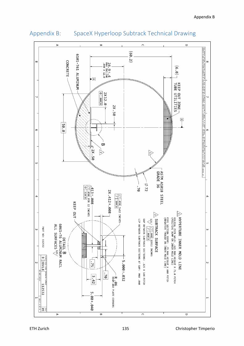
Appendix B: SpaceX Hyperloop Subtrack Technical Drawing

Appendix C


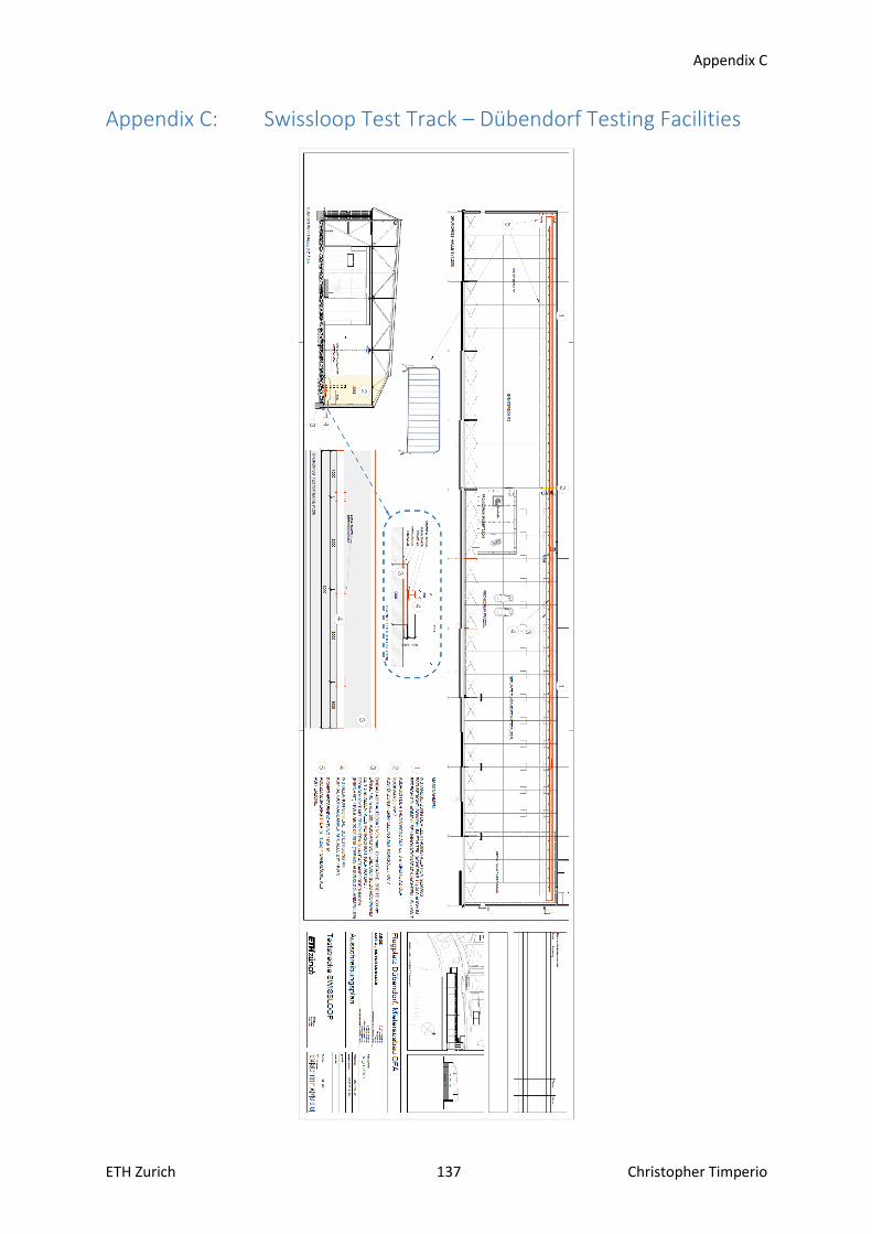
Appendix C: Swissloop Test Track – Dübendorf Testing Facilities

Appendix D


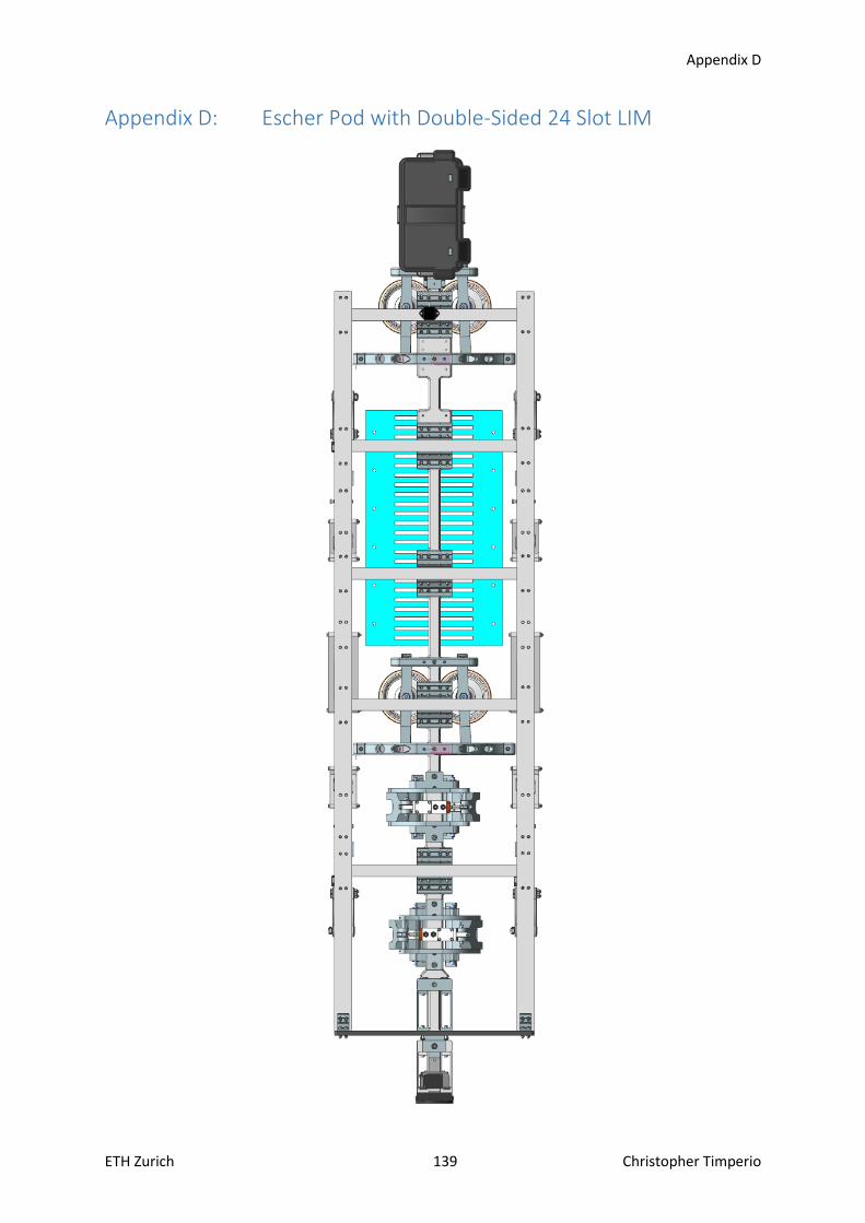
Appendix D: Escher Pod with Double-Sided 24 Slot LIM

Appendix E


Appendix E: M400-50A Iron Core Material Data Sheet

Appendix F


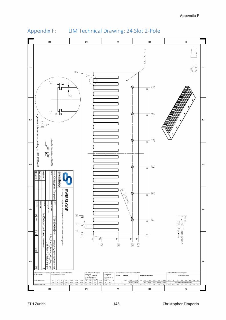
Appendix F: LIM Technical Drawing: 24 Slot 2-Pole

Appendix G


Appendix G: Comsol Multi-turn Coil Geometry Arrangement

Linear Induction Motor (LIM) for Hyperloop Pod Prototypes

Documents

Transcript of Linear Induction Motor (LIM) for Hyperloop Pod Prototypes