�����������������

Citation: Salvoldi, M.; Tubul, Y.;

Karnieli, A.; Herrmann, I.

VENµS-Derived NDVI and REIP at

Different View Azimuth Angles.

Remote Sens. 2022, 14, 184. https://

doi.org/10.3390/rs14010184

Academic Editor: Yasushi

Yamaguchi

Received: 30 November 2021

Accepted: 28 December 2021

Published: 1 January 2022

Publisher’s Note: MDPI stays neutral

with regard to jurisdictional claims in

published maps and institutional affil-

iations.

Copyright: © 2022 by the authors.

Licensee MDPI, Basel, Switzerland.

This article is an open access article

distributed under the terms and

conditions of the Creative Commons

Attribution (CC BY) license (https://

creativecommons.org/licenses/by/

4.0/).

remote sensing

Technical Note

VENµS-Derived NDVI and REIP at Different ViewAzimuth AnglesManuel Salvoldi 1 , Yaniv Tubul 2, Arnon Karnieli 1 and Ittai Herrmann 2,*

1 The Remote Sensing Laboratory, French Associates Institute for Agriculture and Biotechnology of Drylands,Jacob Blaustein Institutes for Desert Research, Ben-Gurion University of the Negev, Sede Boqer Campus,Beersheba 8455902, Israel; salvoldi@post.bgu.ac.il (M.S.); karnieli@bgu.ac.il (A.K.)

2 The Robert H. Smith Institute of Plant Sciences and Genetics in Agriculture, The Hebrew University ofJerusalem, Rehovot 7610001, Israel; yanivtu@savion.huji.ac.il

* Correspondence: Ittai.Herrmann@mail.huji.ac.il

Abstract: The bidirectional reflectance distribution function (BRDF) is crucial in determining thequantity of reflected light on the earth’s surface as a function of solar and view angles (i.e., azimuthand zenith angles). The Vegetation and ENvironment monitoring Micro-Satellite (VENµS) provides aunique opportunity to acquire data from the same site, with the same sensor, with almost constantsolar and view zenith angles from two (or more) view azimuth angles. The present study was aimedat exploring the view angles’ effect on the stability of the values of albedo and of two vegetationindices (VIs): the normalized difference vegetation index (NDVI) and the red-edge inflection point(REIP). These products were calculated over three polygons representing urban and cultivated areasin April, June, and September 2018, under a minimal time difference of less than two minutes.Arithmetic differences of VIs and a change vector analysis (CVA) were performed. The results showthat in urban areas, there was no difference between the VIs, whereas in the well-developed field cropcanopy, the REIP was less affected by the view azimuth angle than the NDVI. Results suggest thatREIP is a more appropriate index than NDVI for field crop studies and monitoring. This conclusioncan be applied in a constellation of satellites that monitor ground features simultaneously but fromdifferent view azimuth angles.

Keywords: vegetation indices; change vector analysis; precision agriculture; BRDF; albedo

1. Introduction

The Vegetation and ENvironment monitoring Micro-Satellite (VENµS) is an earthobservation space mission jointly developed, manufactured, and operated by the NationalCentre for Space Studies (CNES) and the Israel Space Agency (ISA) [1]. The satellite,launched in August 2017, crosses the equator at around 10:30 a.m. Coordinated UniversalTime (UTC) through a sun-synchronous orbit at a 720-km height with a 98◦ inclination. Thescientific objective of VENµS is to frequently acquire images on 160 preselected sites with atwo-day revisit time, a high spatial resolution of 5 m, and 12 narrow bands, ranging from424 to 909 nm, including four red-edge bands (Table 1). This band setting was designed tocharacterize vegetation status, monitor water quality in coastal areas and inland waters,and estimate the aerosol optical depth and the water vapor content of the atmosphere.Duplication of the red band enables the creation of digital terrain models (DTMs) of theearth’s surface and clouds. To observe specific sites within its 27-km swath, the satellite canbe tilted up to 30 degrees along and across track. Uniquely, the preselected sites are alwaysobserved with constant view azimuth and zenith angles.

Figure 1a depicts the footprint of the three VENµS strips over Israel and their corre-sponding view azimuth angles. The west strip, composed of 12 tiles named W01–W12,was the first area covered by the satellite during its descending orbit at around 8:30 UTC(Table 2). The duration of the image capturing was 36 s in a forward view mode. After a few

Remote Sens. 2022, 14, 184. https://doi.org/10.3390/rs14010184 https://www.mdpi.com/journal/remotesensing

Remote Sens. 2022, 14, 184 2 of 10

seconds of maneuvering, while the camera was in standby mode, the satellite measuredthe five tiles of the east strip (i.e., E01–E05) in a backward view mode for 20 s. Finally,the 10 tiles of the south strip (i.e., S01–S10) were covered in 30 s in the backward viewmode. The time needed to acquire all 27 tile images over the Israeli scientific sites was161 s. According to the spatial coverage of these strips, there are some overlapping zonesbetween the west and the south strips. The overlapping images can be used to explorethe effect of the view azimuth angle on the spectral reflectance acquired from space as onecomponent of the bidirectional reflectance distribution function (BRDF) [2]. The differencesbetween the other three components, i.e., view zenith angle, solar azimuth angle, and solarzenith angle, are assumed to be minimal and, therefore, neglected.

Table 1. VENµS satellite band information.

Bands Central Wavelength (nm) Bandwidth (nm) Main Application

B1 423.9 40 Atmospheric Correction, WaterB2 446.9 40 Aerosols, CloudsB3 491.9 40 Atmospheric Correction, WaterB4 555.0 40 LandB5 619.7 40 Vegetation IndicesB6 619.7 40 DEM, Image QualityB7 666.2 30 Red EdgeB8 702.0 24 Red EdgeB9 741.1 16 Red EdgeB10 782.2 16 Red EdgeB11 861.1 40 Vegetation IndicesB12 908.7 20 Water Vapor

B stands for band; DEM stands for digital elevation model.

Table 2. BRDF components and acquisition time for tiles W08 (west strip) and S01 (south strip) on18 April, 27 June, and 11 September 2018.

W08 S01Apr. 18 Jun. 27 Sep. 11 Apr. 18 Jun. 27 Sep. 11

View zenith angle (deg) 35.29 35.54 35.29 30.10 30.31 30.13View azimuth angle (deg) 25.88 27.16 25.77 179.15 177.41 179.26Solar zenith angle (deg) 26.21 18.17 31.14 25.85 17.63 30.86

Solar azimuth angle (deg) 138.39 112.50 146.93 139.78 113.76 148.21Acquisition time (UTC) 08:31:27 08:31:43 8:32:58 08:33:23 08:33:40 08:34:54

The view angle and sun elevation, along with their combination, are well known andhave been explored from various spaceborne platforms and observation heights [3–5]. Tothe best of our knowledge, the VENµS satellite is the only publicly available platform thatallows data collection from the same site, with the same sensor, from two (or more) viewazimuth angles within minutes. The current study was aimed at exploring the view angle’seffect on the stability of the values of vegetation indices (VIs) and albedo due to changesin the view angle under the minimum time gap. It was hypothesized that the view anglewould affect VI values and that this effect would vary between ground features. The twoselected VIs were the normalized difference vegetation index (NDVI) [6], which is easilyavailable and frequently applied, and the red-edge inflection point (REIP), which is uniqueto sensors with four red-edge bands (e.g., VENµS and Sentinel-2 [7]). The REIP showedbetter sensitivity to several vegetation properties, such as leaf area index (LAI) [8] andchlorophyll and nitrogen contents [9]. The albedo characterizes the brightness of groundfeatures affected by the BRDF, which was used as a reference for each VI.

Remote Sens. 2022, 14, 184 3 of 10Remote Sens. 2022, 13, x FOR PEER REVIEW 3 of 11

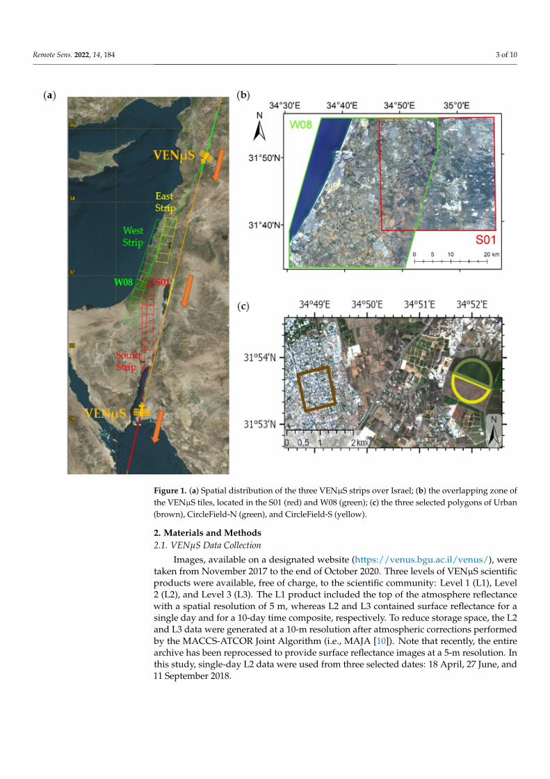
Figure 1. (a) Spatial distribution of the three VENµS strips over Israel; (b) the overlapping zone of the VENµS tiles, located in the S01 (red) and W08 (green); (c) the three selected polygons of Urban (brown), CircleField-N (green), and CircleField-S (yellow).

The view angle and sun elevation, along with their combination, are well known and have been explored from various spaceborne platforms and observation heights [3–5]. To the best of our knowledge, the VENµS satellite is the only publicly available platform that allows data collection from the same site, with the same sensor, from two (or more) view azimuth angles within minutes. The current study was aimed at exploring the view an-gle’s effect on the stability of the values of vegetation indices (VIs) and albedo due to changes in the view angle under the minimum time gap. It was hypothesized that the view angle would affect VI values and that this effect would vary between ground fea-tures. The two selected VIs were the normalized difference vegetation index (NDVI) [6], which is easily available and frequently applied, and the red-edge inflection point (REIP), which is unique to sensors with four red-edge bands (e.g., VENµS and Sentinel-2 [7]). The REIP showed better sensitivity to several vegetation properties, such as leaf area index (LAI) [8] and chlorophyll and nitrogen contents [9]. The albedo characterizes the bright-ness of ground features affected by the BRDF, which was used as a reference for each VI.

2. Materials and Methods

Figure 1. (a) Spatial distribution of the three VENµS strips over Israel; (b) the overlapping zone ofthe VENµS tiles, located in the S01 (red) and W08 (green); (c) the three selected polygons of Urban(brown), CircleField-N (green), and CircleField-S (yellow).

2. Materials and Methods2.1. VENµS Data Collection

Images, available on a designated website (https://venus.bgu.ac.il/venus/), weretaken from November 2017 to the end of October 2020. Three levels of VENµS scientificproducts were available, free of charge, to the scientific community: Level 1 (L1), Level2 (L2), and Level 3 (L3). The L1 product included the top of the atmosphere reflectancewith a spatial resolution of 5 m, whereas L2 and L3 contained surface reflectance for asingle day and for a 10-day time composite, respectively. To reduce storage space, the L2and L3 data were generated at a 10-m resolution after atmospheric corrections performedby the MACCS-ATCOR Joint Algorithm (i.e., MAJA [10]). Note that recently, the entirearchive has been reprocessed to provide surface reflectance images at a 5-m resolution. Inthis study, single-day L2 data were used from three selected dates: 18 April, 27 June, and11 September 2018.

Remote Sens. 2022, 14, 184 4 of 10

2.2. Study Area

The study area was located in the overlapping zone of the west strip’s tile W08 and thesouth strip’s tile S01 (Figure 1b). This 188.31 km2 area contained different types of land-useand land-cover categories: urban, vegetation, soil, vineyards, orchards, and water, amongstothers. Table 2 shows the acquisition times in UTC and the BRDF components of the W08and S01 tiles on 18 April 2018. It can be seen that tile S01 was acquired 1 min and 56 s aftertile W08, and the difference in the view azimuth is notable, i.e., more than 150 degrees.Furthermore, image W08 was acquired in a forward direction, while S01 was in a backwarddirection. The current study focused on a representative section in the northern part of theoverlap zone, including three polygons (Figure 1c). Two polygons in the center compriseirrigated fields in a cultivated area, representing agricultural soil and vegetation surfaces(hereafter named CircleField-N and CircleField-S). A third polygon included an urbanarea (hereafter named Urban) and is an example of a heterogeneous surface. To fulfill thestudy goal, three clear-sky days were used in different seasons of the year (i.e., 18 April,27 June, and 11 September 2018). The CircleField-N area had bare soil on the first date,developed corn plants on the second date, and bare soil on the third. The CircleField-S areahad developed chickpea plants on the first date, ready-to-harvest dry chickpea plants onthe second date, and bare soil on the third.

2.3. Vegetation Indices and Albedo

To explore the effect of the view zenith angle across the study sites, two VIs wereselected, the normalized difference vegetation index (NDVI) [6] and the red-edge inflectionpoint (REIP) [7–9]:

NDVI =(ρ782 − ρ667)

(ρ782 + ρ667)(1)

REIP = 702 + 40{[(ρ667 + ρ782)/2]− ρ702

ρ742 − ρ702

}(2)

where ρ is the relative reflectance of the subscript wavelength expressed in nm. TheNDVI is a well-known and frequently used VI that can be calculated from many satellitesensors, while the REIP is less known and rarely used because the four needed bands arenot available in many spaceborne sensors. These bands are available in the VENµS andSentinel-2 satellites. The NDVI and the REIP were simulated and discussed for VENµSresampled bands to estimate leaf area index by [8] and, in the current study, were calculatedfrom space to allow a comparison of their values under different view angles. In the currentstudy, the NDVI was calculated with bands B7 and B10, and the REIP was calculated withbands B7, B8, B9, and B10 (Table 1).

Additionally, the albedo α was calculated as follows [11]:

α =∑12

i=1;i 6=5 Bibi

∑12i=1;i 6=5 bi

(3)

where Bi and bi are the surface reflectance and the bandwidth, in nm, for band i, respectively.All VENµS bands were involved in this process.

2.4. Pixel Subtraction

The VIs’ value change was calculated as measured by the VENµS satellite from twodifferent view azimuth angles. First, the indices were calculated for all pixels in the overlapzone for each of the two tiles, and later, the former tile value (W08) was subtracted fromthe later one (S01):

∆VI = VIS01 −VIW08 (4)

where VI is the vegetation index (Equations (1) and (2)), and subscript S01 and W08 indicatethe relevant tile.

Remote Sens. 2022, 14, 184 5 of 10

2.5. Change Vector Analysis

The change vector analysis (CVA) is a robust methodology for detecting multivariantchanges from two or more spectral bands, spectral features, or biophysical indicators (e.g.,spectral indices) associated with the pixel of an image [12]. In the current study, CVAwas computed to measure the magnitude and direction of the change in NDVI and REIP(Equations (1) and (2)) versus the albedo α (Equation (3)), between the two tiles (i.e., S01with respect to W08), and across all pixels in the overlap zone. The VIs represent vegetatedpixels since the high index value indicates more biomass, while the albedo represents barelight-colored soil since higher values indicate a more exposed non-vegetated surface. First,these variables were computed in the overlap zone, and then, the VIs were normalized tovalues between 0 and 1 to eliminate the bias of the CVA magnitude due to the dynamicrange of each index. Finally, the CVA was performed pixel-by-pixel between the referencedataset W08 and the target dataset S01. The output of the CVA consists of the changevector (CV) magnitude (Equation (5)) and the change direction (θ, Equation (6)). The CVmagnitude, |CV|, is the Euclidean distance of the vector between the reference and thetarget datasets:

|CV| =√(nVIS01 − nVIW08)

2 + (αS01 − αW08)2 (5)

where nVI is the normalized vegetation index, and α is the albedo. A threshold was definedin order to distinguish between changed and unchanged pixels (i.e., noise). One standarddeviation (1-STD) was selected as a threshold [13–15]. The direction of the change vector isrepresented by the angle θ, as depicted in Figure 2:

tan θ =nVIS01 − nVIW08

αS01 − αW08(6)

where nVI is the normalized vegetation index, α is the albedo, and subscript S01 and W08indicate the relevant tile.

Remote Sens. 2022, 13, x FOR PEER REVIEW 6 of 11

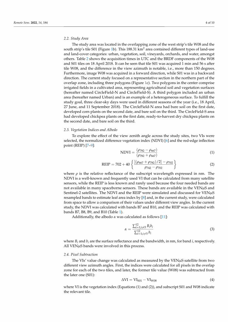
Figure 2. A graphical scheme illustrates how the change vector analysis (CVA) equations were ap-plied to calculate the change magnitude and change direction (angle θ) for the VENµS-derived NDVI, REIP, and albedo and between the reference tile W08 and the target tile S01. The change mag-nitude is represented by the distance of S01 from W08, and the change direction is represented by the degree angle in the range between 0° and 360°. The direction value range is divided into four main classes of 90° (i.e., quadrant).

3. Results and Discussion To explore the view azimuth angle’s effect on the spectral reflectance, the change in

the VIs (Equation (4)) was examined in three selected polygons (Figure 3a). The NDVI pixel subtraction (∆NDVI) of the two tiles (S01–W08) showed the distinct difference as a function of the land use (Figure 3b,c). For example, on April 18, the southern half-circle of the chickpea crop field (i.e., CircleField-S, yellow-colored polygon in Figure 3a) was char-acterized by negative values of ∆NDVI, while the post-sowing bare soil of the northern half-circle of the corn crop field (i.e., CircleField-N, green-colored polygon in Figure 3a) was characterized by positive ∆NDVI values. Similarly, most northern corn fields showed negative values, while the southern dry chickpea field showed values distributed around zero on June 27. On September 11, bare soil was found in both cultivated fields with ∆NDVI values distributed similarly at around zero difference. On all the selected dates, the relatively homogeneous half-circle fields were characterized by narrow distributions (yellow and green-colored bars in Figure 3c). In contrast, the inhomogeneous urban area (i.e., Urban) was characterized by a wider distribution of ∆NDVI (brown-colored bars in Figure 3c). In accordance with its relatively low seasonal variability, the urban area was characterized by similar distributions for all selected dates with no negative–positive dominance. Examination of the ∆REIP values (Figure 3d,e) for the exact dates and poly-gons also showed distinct differences. Areas with dominant vegetation, such as the chick-pea field’s southern half-circle (yellow-colored polygon on April 18) or the corn field’s northern half-circle (green-colored polygon on June 27), showed nearly zero differences

Figure 2. A graphical scheme illustrates how the change vector analysis (CVA) equations wereapplied to calculate the change magnitude and change direction (angle θ) for the VENµS-derivedNDVI, REIP, and albedo and between the reference tile W08 and the target tile S01. The changemagnitude is represented by the distance of S01 from W08, and the change direction is representedby the degree angle in the range between 0◦ and 360◦. The direction value range is divided into fourmain classes of 90◦ (i.e., quadrant).

Remote Sens. 2022, 14, 184 6 of 10

3. Results and Discussion

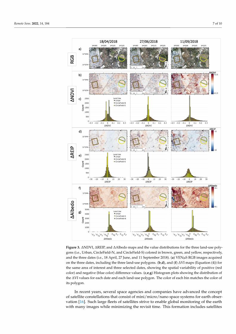
To explore the view azimuth angle’s effect on the spectral reflectance, the change inthe VIs (Equation (4)) was examined in three selected polygons (Figure 3a). The NDVIpixel subtraction (∆NDVI) of the two tiles (S01–W08) showed the distinct difference as afunction of the land use (Figure 3b,c). For example, on April 18, the southern half-circleof the chickpea crop field (i.e., CircleField-S, yellow-colored polygon in Figure 3a) wascharacterized by negative values of ∆NDVI, while the post-sowing bare soil of the northernhalf-circle of the corn crop field (i.e., CircleField-N, green-colored polygon in Figure 3a)was characterized by positive ∆NDVI values. Similarly, most northern corn fields showednegative values, while the southern dry chickpea field showed values distributed aroundzero on June 27. On September 11, bare soil was found in both cultivated fields with∆NDVI values distributed similarly at around zero difference. On all the selected dates,the relatively homogeneous half-circle fields were characterized by narrow distributions(yellow and green-colored bars in Figure 3c). In contrast, the inhomogeneous urban area(i.e., Urban) was characterized by a wider distribution of ∆NDVI (brown-colored barsin Figure 3c). In accordance with its relatively low seasonal variability, the urban areawas characterized by similar distributions for all selected dates with no negative–positivedominance. Examination of the ∆REIP values (Figure 3d,e) for the exact dates and polygonsalso showed distinct differences. Areas with dominant vegetation, such as the chickpeafield’s southern half-circle (yellow-colored polygon on April 18) or the corn field’s northernhalf-circle (green-colored polygon on June 27), showed nearly zero differences (Figure 3e).On the other hand, bare soil and urban areas consistently showed wider distributions andlarger differences. The ∆Albedo values (Figure 3f,g) showed a mainly positive change asexpected based on the solar and view angles (Table 2).

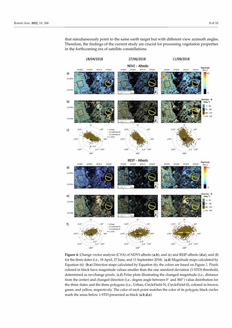
The CVA magnitude for the NDVI-albedo combination showed that pixels with a CVmagnitude (Figure 4a) lower than the threshold (1-STD) were considered as no-changepixels and colored black. The same threshold was also used for the REIP-albedo combi-nation (Figure 4d). The urban area and the bare soil in the circle fields showed relativelylarge magnitude changes, while areas such as field crops or dry matter showed no change.Therefore, the NDVI values, as obtained by VENµS, of vegetative areas were less affectedby the view azimuth angle than those of soil areas. Nevertheless, dry standing vegetativebiomass (i.e., CircleField-S on June 27) areas or bare soil fields a relatively long time afterharvest (i.e., CircleField-S on September 11) had a magnitude below the threshold (i.e.,showed no change). Figure 4a shows the CV magnitudes as a function of land use, similarto the direction in Figure 4b. In addition, the polar plots in Figure 4c illustrate both themagnitude and the direction changes for each polygon of interest on the selected dates.Following the positive changes in albedo for the two half-circle crop fields (Figure 3f,g),their direction continued to be on the upper part (i.e., positive ∆Albedo). In contrast,the urban area was characterized by negative and positive changes in albedo, with somepatterns connecting these changes of ∆Albedo with changes in ∆NDVI (Figure 4c).

The similarities between NDVI-albedo and REIP-albedo (Figure 4) included the domi-nant positive ∆Albedo in the crop field areas vs. positive or negative ∆Albedo in the urbanarea and the distinct narrow distribution of ∆REIP in the vegetative crop field areas vs. thewider distribution of ∆REIP in the bare soil, dry matter, and urban areas. It was found thatthose areas of nearly zero ∆REIP (i.e., the half-circle crop fields with vegetation) also hadmagnitude values smaller than the 1-STD threshold. Therefore, the change in the viewazimuth angle did not affect the REIP in these areas as obtained by VENµS.

The results obtained in the present work, based on the VENµS mission, suggest thatthe REIP index was less affected by the view azimuth angle than the NDVI, thus making it abetter tool for analyzing and comparing the spectral response in vegetative areas measuredat different azimuth angles. In addition to the VENµS mission, described in Section 1, theMultiSpectral Imager (MSI) onboard the Sentinel-2 mission captures the reflected lightsignal at the four red-edge bands [8,9] with no charge for users.

Remote Sens. 2022, 14, 184 7 of 10

Remote Sens. 2022, 13, x FOR PEER REVIEW 7 of 11

(Figure 3e). On the other hand, bare soil and urban areas consistently showed wider dis-tributions and larger differences. The ∆Albedo values (Figure 3f,g) showed a mainly pos-itive change as expected based on the solar and view angles (Table 2).

Figure 3. ∆NDVI, ∆REIP, and ∆Albedo maps and the value distributions for the three land-use pol-ygons (i.e., Urban, CircleField-N, and CircleField-S) colored in brown, green, and yellow, respec-tively, and the three dates (i.e., April 18, June 27, and September 11, 2018). (a) VENµS RGB images acquired on the three dates, including the three land-use polygons. (b,d), and (f) ∆VI maps (Equa-tion (4)) for the same area of interest and three selected dates, showing the spatial variability of positive (red color) and negative (blue color) difference values. (c,e,g) Histogram plots showing the distribution of the ∆VI values for each date and each land-use polygon. The color of each bin matches the color of its polygon.

Figure 3. ∆NDVI, ∆REIP, and ∆Albedo maps and the value distributions for the three land-use poly-gons (i.e., Urban, CircleField-N, and CircleField-S) colored in brown, green, and yellow, respectively,and the three dates (i.e., 18 April, 27 June, and 11 September 2018). (a) VENµS RGB images acquiredon the three dates, including the three land-use polygons. (b,d), and (f) ∆VI maps (Equation (4)) forthe same area of interest and three selected dates, showing the spatial variability of positive (redcolor) and negative (blue color) difference values. (c,e,g) Histogram plots showing the distribution ofthe ∆VI values for each date and each land-use polygon. The color of each bin matches the color ofits polygon.

In recent years, several space agencies and companies have advanced the conceptof satellite constellations that consist of mini/micro/nano space systems for earth obser-vation [16]. Such large fleets of satellites strive to enable global monitoring of the earthwith many images while minimizing the revisit time. This formation includes satellites

Remote Sens. 2022, 14, 184 8 of 10

that simultaneously point to the same earth target but with different view azimuth angles.Therefore, the findings of the current study are crucial for processing vegetation propertiesin the forthcoming era of satellite constellations.

Remote Sens. 2022, 13, x FOR PEER REVIEW 9 of 11

Figure 4. Change vector analysis (CVA) of NDVI-albedo (a,b), and (c) and REIP-albedo (d,e), and (f) for the three dates (i.e., April 18, June 27, and September 11, 2018). (a,d) Magnitude maps calcu-lated by Equation (6). (b,e) Direction maps calculated by Equation (6); the colors are based on Figure 2. Pixels colored in black have magnitude values smaller than the one standard deviation (1-STD) threshold, determined as no-change pixels. (c,f) Polar plots illustrating the changed magnitude (i.e., distance from the center) and changed direction (i.e., degree angle between 0° and 360°) value dis-tribution for the three dates and the three polygons (i.e., Urban, CircleField-N, CircleField-S), col-ored in brown, green, and yellow, respectively. The color of each point matches the color of its pol-ygon; black circles mark the areas below 1-STD-presented as black (a,b,d,e).

4. Conclusions The current study aimed to explore the effect of the view azimuth angle on two

VENµS-derived VI values (i.e., NDVI and REIP) used in image processing for agricultural applications. The effect of the view azimuth angle on the NDVI value for field crops was more significant than its effect on REIP, while in the urban area, there was no difference

Figure 4. Change vector analysis (CVA) of NDVI-albedo (a,b), and (c) and REIP-albedo (d,e), and (f)for the three dates (i.e., 18 April, 27 June, and 11 September 2018). (a,d) Magnitude maps calculated byEquation (6). (b,e) Direction maps calculated by Equation (6); the colors are based on Figure 2. Pixelscolored in black have magnitude values smaller than the one standard deviation (1-STD) threshold,determined as no-change pixels. (c,f) Polar plots illustrating the changed magnitude (i.e., distancefrom the center) and changed direction (i.e., degree angle between 0◦ and 360◦) value distribution forthe three dates and the three polygons (i.e., Urban, CircleField-N, CircleField-S), colored in brown,green, and yellow, respectively. The color of each point matches the color of its polygon; black circlesmark the areas below 1-STD-presented as black (a,b,d,e).

Remote Sens. 2022, 14, 184 9 of 10

4. Conclusions

The current study aimed to explore the effect of the view azimuth angle on twoVENµS-derived VI values (i.e., NDVI and REIP) used in image processing for agriculturalapplications. The effect of the view azimuth angle on the NDVI value for field crops wasmore significant than its effect on REIP, while in the urban area, there was no differencebetween the VIs. The main finding is that in a fully developed field crop canopy, the REIPwas less affected by the view azimuth angle than the NDVI. This finding provides additionalevidence for preferring the REIP to the NDVI, which is more affected by high above-groundbiomass. Currently, as the four red-edge bands are freely available by VENµS as well asSentinel-2, the REIP has demonstrated its advantage in the view azimuth angle for fieldcrops, in addition to its higher sensitivity to increasing vegetation biomass. Therefore, theREIP, when applicable, is recommended for field crop studies and monitoring. Specifically,the findings of the current study are crucial for processing vegetation properties in theforthcoming era of satellite constellations.

Author Contributions: M.S.: methodology, software, data curation, writing, and visualization; Y.T.:methodology, software, data curation, writing, and visualization; A.K.: methodology, writing, andfunding acquisition; I.H.: conceptualization, methodology, data curation, writing, and fundingacquisition. All authors have read and agreed to the published version of the manuscript.

Funding: This study was partially supported by the Hebrew University of Jerusalem’s IntramuralResearch Fund in Career Development.

Institutional Review Board Statement: Not applicable.

Informed Consent Statement: Not applicable.

Data Availability Statement: The satellite imagery used are available on VENµS site https://venus.bgu.ac.il/venus/ (accessed on 15 December 2021).

Conflicts of Interest: The authors declare no conflict of interest.

References1. Dedieu, G.; Karnieli, A.; Hagolle, O.; Jeanjean, H.; Cabot, F.; Ferrier, P.; Yaniv, Y. A Joint Israeli–French Earth Observation Scientific

Mission with High Spatial and Temporal Resolution Capabilities. In Proceedings of the 4th ESA CHRIS/Proba Work, ESRIN,Frascati, Italy, 19–21 September 2006; pp. 19–21.

2. Schaepman-Strub, G.; Schaepman, M.E.; Painter, T.H.; Dangel, S.; Martonchik, J.V. Reflectance quantities in optical remotesensing—definitions and case studies. Remote Sens. Environ. 2006, 103, 27–42. [CrossRef]

3. Roy, D.P.; Zhang, H.K.; Ju, J.; Gomez-Dans, J.L.; Lewis, P.E.; Schaaf, C.B.; Sun, Q.; Li, J.; Huang, H.; Kovalskyy, V. A generalmethod to normalize Landsat reflectance data to nadir BRDF adjusted reflectance. Remote Sens. Environ. 2016, 176, 255–271.[CrossRef]

4. Mueller, N.; Lewis, A.; Roberts, D.; Ring, S.; Melrose, R.; Sixsmith, J.; Lymburner, L.; McIntyre, A.; Tan, P.; Curnow, S.; et al. Waterobservations from space: Mapping surface water from 25 years of Landsat imagery across Australia. Remote Sens. Environ. 2016,174, 341–352. [CrossRef]

5. Liu, Y.; Hill, M.; Zhang, X.; Wang, Z.; Richardson, A.D.; Hufkens, K.; Filippa, G.; Baldocchi, D.D.; Ma, S.; Verfaillie, J.; et al.Using data from Landsat, MODIS, VIIRS and PhenoCams to monitor the phenology of California oak/grass savanna and opengrassland across spatial scales. Agric. For. Meteorol. 2017, 237–238, 311–325. [CrossRef]

6. Tucker, C.J. Red and photographic infrared linear combinations for monitoring vegetation. Remote Sens. Environ. 1979, 8, 127–150.[CrossRef]

7. Martimort, P.; Fernandez, V.; Kirschner, V.; Isola, C.; Meygret, A. Sentinel-2 MultiSpectral imager (MSI) and calibra-tion/validation.Int. Geosci. Remote Sens. Symp. 2012, 6999–7002.

8. Herrmann, I.; Pimstein, A.; Karnieli, A.; Cohen, Y.; Alchanatis, V.; Bonfil, D.J. LAI assessment of wheat and potato crops byVENµS and Sentinel-2 bands. Remote Sens. Environ. 2011, 115, 2141–2151. [CrossRef]

9. Clevers, J.G.P.W.; Gitelson, A.A. Remote estimation of crop and grass chlorophyll and nitrogen content using red-edge bands onSentinel-2 and -3. Int. J. Appl. Earth Obs. Geoinf. 2013, 23, 344–351. [CrossRef]

10. Hagolle, O.; Huc, M.; Desjardins, C.; Auer, S.; Richter, R. MAJA Algorithm Theoretical Basis Document. Development 2017, 1–39.Available online: http://tully.ups-tlse.fr/olivier/maja_atbd/raw/master/atbd_maja.pdf (accessed on 15 December 2021).

11. Robinove, C.J.; Chavez, P.S.; Gehring, D.; Holmgren, R. Arid land monitoring using Landsat albedo difference images. Remote.Sens. Environ. 1981, 11, 133–156. [CrossRef]

Remote Sens. 2022, 14, 184 10 of 10

12. Johnson, R.D.; Kasischke, E.S. Change vector analysis: A technique for the multispectral monitoring of land cover and condition.Int. J. Remote Sens. 1998, 19, 411–426. [CrossRef]

13. Karnieli, A.; Qin, Z.; Wu, B.; Panov, N.; Yan, F. Spatio-Temporal Dynamics of Land-Use and Land-Cover in the Mu Us SandyLand, China, Using the Change Vector Analysis Technique. Remote Sens. 2014, 6, 9316–9339. [CrossRef]

14. Zanchetta, A.; Bitelli, G.; Karnieli, A. Monitoring desertification by remote sensing using the Tasselled Cap transform for long-termchange detection. Nat. Hazards 2016, 83, 223–237. [CrossRef]

15. Bayarjargal, Y.; Karnieli, A.; Bayasgalan, M.; Khudulmur, S.; Gandush, C.; Tucker, C.J. A comparative study of NO-AA-AVHRRderived drought indices using change vector analysis. Remote Sens. Environ. 2006, 105, 9–22. [CrossRef]

16. Curzi, G.; Modenini, D.; Tortora, P. Large Constellations of Small Satellites: A Survey of Near Future Challenges and Missions.Aerospace 2020, 7, 133. [CrossRef]