JAWRA Page 1 2/4/2004

Priestley-Taylor Alpha Coefficient: Variability and Relationship to NDVI in Arctic

Tundra Landscapes

Submitted To:

Journal of the American Water Resources Association (JAWRA)

Ryan N. Engstrom1, Allen S. Hope1, Douglas A. Stow1, George L. Vourlitis2, and Walter

C. Oechel3

1Department of Geography, San Diego State University, San Diego, CA 92182 USA

2Biology Program, California State University, San Marcos, CA 92096 USA

3Global Change Research Group, Department of Biology, San Diego State University,

San Diego, CA 92182 USA

JAWRA Page 2 2/4/2004

Abstract

Average daily values of the Priestley-Taylor coefficient, α, were calculated for

two eddy covariance (flux) tower sites with contrasting vegetation, soil moisture, and

temperature characteristics on the North Slope of Alaska over the 1994 and 1995 growing

seasons. Because variations in α have been shown to be associated with changes in

vegetation, soil moisture, and meteorological conditions in Arctic ecosystems, we

hypothesized that α values would be significantly different between sites. Since

variations in the normalized difference vegetation index (NDVI) follow patterns of

vegetation community composition and state that are largely controlled by moisture and

temperature gradients on the North Slope of Alaska, we hypothesized that temporal

variations in α respond to these same conditions and thus, co-vary with NDVI.

Significant differences in α values were found between the two sites in 1994 under

average precipitation conditions. However, in 1995, when precipitation conditions were

above average, no significant difference was found. Overall, the variations in α over the

two growing seasons showed little relationship to the seasonal progression of the regional

NDVI. The only significant relationship was found at the drier, upland study site.

Key Terms: Evapotranspiration, Remote Sensing, Priestley-Taylor, Tundra ecosystems,

Climate Change, Statistical Analysis

JAWRA Page 3 2/4/2004

Introduction

Increased air temperatures and the associated rise in surface temperatures due to

global warming are predicted to vary over the globe, with changes in Arctic ecosystems

expected to occur sooner and to be more dramatic than in other ecosystems (Gates et al.,

1992; Manabe and Stouffer 1993; Meehl et al. 1993). These changes may significantly

impact permafrost dynamics, thus altering hydrologic processes and the surface energy

balance in Arctic ecosystems (Hinzman and Kane, 1992). The National Science

Foundation (NSF) Arctic System Sciences (ARCSS) Land Atmosphere Ice Interactions

(LAII) research program was initiated with the goal of improving scientific

understanding of the drivers and processes influencing change in Arctic tundra

landscapes. The primary research objectives of the current LAII project, Arctic

Transitions in the Land-Atmosphere System (ATLAS), are 1) to determine the

geographical patterns of, and controls over, the atmosphere-land surface exchanges of

mass and energy in order to 2) quantify current patterns and processes and to develop

reasonable scenarios of future change in the Arctic system. Additionally, this research

project seeks to expand our understanding of local-scale mass and energy exchange and

to extrapolate this knowledge to the regional and circumpolar scales.

Following snowmelt, evapotranspiration (ET) is the hydrologic process that

dominates the Arctic summer water balance, usually exceeding summer precipitation

(Rovanesk et al., 1996). Therefore, latent heat flux is a primary mechanism of summer

surface energy dissipation (Kane et al., 1990). Higher Arctic air and surface

temperatures, and evaporation rates, and the resulting increase in atmospheric water

vapor may exert a positive feedback on regional or global warming (Maxwell, 1992).

JAWRA Page 4 2/4/2004

Arctic tundra contains a range of vegetation, physiographic, and climatic

conditions that may give rise to significant spatial and temporal variations in ET. Few

studies have investigated this spatial and temporal variability due to the limited number

of meteorological sites, logistic difficulty, and the significant costs associated with

reaching many areas of the Arctic (Kane et al., 1990). Due to this data poor environment,

a number of hydrologic studies have utilized simple ET models including, the Priestley-

Taylor (1972) model (PT) (e.g. Kane et al., 1990). The PT model has been shown to

provide acceptable accuracy for predicting daily evaporation in Arctic ecosystems if the

value of the α coefficient is known (Rouse et al., 1977). However, α values in Arctic

ecosystems have been shown to vary over time and space with variations related to

changes in vegetation type and state, soil moisture, and meteorological conditions (Kane

et al., 1990; Rovanesk et al., 1996; Mendez et al., 1998; Stewart and Rouse, 1976).

Changes in vegetation type and state are controlled by differences in soil moisture

regime and by soil and air temperatures on the North Slope of Alaska (Ostendorf and

Reynolds, 1998). Hope et al. (1993) and Stow et al. (1993) demonstrated that variations

in the remotely sensed normalized difference vegetation index (NDVI) are related to

changes in vegetation type and state in Arctic tundra ecosystems. Therefore, we

hypothesized that changes in the NDVI would be indicative of variability in vegetation

and soil moisture conditions, variables shown to co-vary with α in Arctic landscapes. In

this study, α values were calculated at two eddy flux tower sites located in regions with

contrasting vegetation, surface moisture, and meteorological characteristics to determine

if 1) α values were significantly different between sites, and 2) seasonal variations in α

were correlated with the regional patterns of vegetation phenology as characterized by the

JAWRA Page 5 2/4/2004

NDVI. This research represents a preliminary step towards determining if satellite

remotely sensed data (i.e. NDVI) can be used as a tool to predict seasonal changes in α.

Modeling Evapotranspiration in the Arctic: the Priestley-Taylor Model

The PT model is based on the concept of equilibrium evaporation postulated by

Slatyer and McIlroy (1961). Equilibrium evaporation occurs when air moving large

distances in the lower atmospheric boundary over a homogeneous, well-watered surface

becomes saturated. Since the air is saturated and additions and losses of water vapor to

the lower atmospheric boundary layer are in equilibrium, the atmospheric/mass transfer

term from the Penman-Monteith equation (Monteith, 1965) can be eliminated. Thus, the

evaporation rate becomes simply a function of the available energy (Rn-G) and air

temperature.

Equilibrium evaporation conditions rarely exist in natural environments, with

deviations arising from large-scale or regional advection effects involving horizontal

variations of surface and/or atmospheric conditions (e.g. Eichinger, 1996). In order to

compensate for these deviations, Priestley and Taylor (1972) adjusted the equilibrium

evaporation model via an empirical coefficient, α. The PT model for estimating latent

heat flux (LE) is:

LE = α(Rn - G)[S/(S + U)] (1)

where α (alpha) is an empirical coefficient relating actual evaporation to equilibrium

evaporation, S is the slope of the saturation vapor pressure and air temperature curve

(kPa°C-1), U is the psychometric constant (kPa°C-1), Rn is net radiation (Wm-2), and G is

ground heat flux (Wm-2). Based upon a number of experiments in different climates over

both land and water surfaces, Priestley and Taylor (1972) established a 'best estimate' of

JAWRA Page 6 2/4/2004

α= 1.26 (for mid-latitude environments). The value of 1.26 for α has been supported by

a number of other studies (e.g. McNaughten and Black, 1973; Mukammal and Neumann,

1977; Parlange and Katul, 1992).

Values of the α coefficient have been shown to be generally constant (e.g., 1.26)

in landscapes where vegetation cover is almost complete and of short stature if moisture

availability for evaporation is unrestricted. However, authors such as McNaugton and

Black (1973), Barton (1979) and Shuttleworth and Calder (1979) have reported large

deviations in α under drier or varied vegetation conditions. Stannard (1993) suggests that

as soil moisture decreases and the canopy becomes water stressed, α values decrease due

to the surface restrictions on ET rates. A number of field studies over different types of

vegetation have related decreases in soil moisture to decreases in α values (Davies and

Allen, 1973; Barton 1979; Flint and Childs 1991). Vegetation height and type has also

been shown to cause α to deviate from 1.26 with values of 1.03 in a rainforest

(Viswanadham et al., 1991), 1.05 in a Douglas fir forest (McNaughton and Black, 1973)

and 1.12 over grass (De Bruin and Holtslag, 1982). These results indicate that variations

in soil moisture and vegetation characteristics need to be addressed when attempting to

model values for α over time and space.

Variability of the Alpha Coefficient in the Arctic

The PT α coefficient has been shown to vary over time and space in Arctic

ecosystems (Kane et al., 1990; Rovanesk et al., 1996; Mendez et al., 1998). Results from

previous studies indicate that the value for α in dry upland regions characterized by sedge

tussocks, mosses, lichens and shrubs, is at or near 1.00 (α = 0.95 Rouse and Stewart,

1972 and Rouse et al. 1977; α = 1.00 Stewart and Rouse 1976). Stewart and Rouse

JAWRA Page 7 2/4/2004

(1976) noted that the non-transpiring lichens restricted evaporation rates so α values

tended to be lower than the 1.26 reported by Priestley and Taylor (1972). Furthermore, in

a similar dry, upland study site, Kane et al. (1990) found that the PT model with α set at

0.95 produced daily evapotranspiration rates that were similar to those calculated by

other models, including the water balance and surface energy balance approaches.

In wet, lowland areas characterized by wet sedge tundra and small ponds, a

number of studies have indicated that appropriate α values should be at or above 1.26 (α

= 1.26 Stewart and Rouse 1976; α = 1.3 Roulet and Woo 1986; α = 1.35 Bello and Smith

1990; α = 1.3 Rovanesk et al. 1996). In these areas, water from the early season

snowmelt is present at the surface for much of the growing season therefore surface

restrictions on ET rates are not significant.

Seasonal changes in α have been reported due to changes in surface wetness and

the corresponding transpiration properties of the vegetation. Rovanesk et al. (1996) and

Mendez et al. (1998) found that different α values (decreasing throughout the growing

season) were required to accurately calculate ET rates through an entire growing season

in a coastal wetland near Prudhoe Bay, Alaska. Their calculations of cumulative daily

evapotranspiration for five growing seasons (1992-1996) compared well with the

Penman-Monteith, energy balance and other model estimates. Rovanesk et al. (1996)

adjusted α every 15 days to model ET over a two year period (1992 and 1993) with

values ranging from 1.6 to 1.3 prior to Julian Date (JD) 212 and reduced to 1.1 after JD

213. Mendez et al. (1998) used two values for α (1.15 before JD 200 and 1.1 after JD

200) for the three years of their study (1994-1996). α values are highest early in the

growing season due to open surface water after snowmelt coinciding with the most rapid

JAWRA Page 8 2/4/2004

plant growth during growing season (Hobbie, 1980). As time progresses through the

season, the freestanding water above the surface (due to poor drainage) slowly evaporates

and the active layer depth increases causing the water table to drop exposing the

background surface. Additionally, the vegetation moves toward maturity and finally,

senescence. Together these factors reduce ET rates and α values due to increasing surface

resistance as the growing season progresses (Rovanesk et al., 1996).

Research Hypothesis: Alpha Variability and Relationship with NDVI in Arctic

Tundra Landscapes

Soil moisture differences are a major determinant of productivity patterns in

Arctic tundra vegetation (e.g. Peterson and Billings, 1980; Jasieniuk and Johnson, 1982;

Matthes-Sears et al., 1988; Gold and Bliss, 1995; Ostendorf and Reynolds, 1998).

Variations in the NDVI have been related to changes in the abundance and type of tundra

vegetation (Hope et al., 1993; Stow et al., 1993). It follows that variations in NDVI are

likely to reflect the average, long-term patterns in soil moisture conditions, climate and

soil characteristics that control vegetation distribution and productivity over time and

space (Ostendorf and Reynolds, 1998). These same environmental drivers have also been

shown to affect α (Kane et al., 1990; Rovanesk et al., 1996; Mendez et al., 1998), leading

to the following general hypotheses tested in this study 1) regions with contrasting

surface moisture, vegetation, and meteorological characteristics will have significantly

different α values and 2) seasonal variations in α are related to changes in vegetation

phenology as characterized by the NDVI. We test these hypotheses by a) determining if

there is a significant difference between daily α values at two tower sites located in

regions with contrasting surface moisture regimes, vegetation characteristics, and

JAWRA Page 9 2/4/2004

meteorological conditions and b) determining if seasonal variations in α are correlated

with the regional patterns of vegetation phenology as characterized by the NDVI. The α-

NDVI relationship was examined using (1) the pooled data (both towers and both years)

(2) the data pooled by year (each year with the data pooled for both tower locations) and

(3) the data pooled by tower location (each tower location with the data pooled for both

years).

Study Site

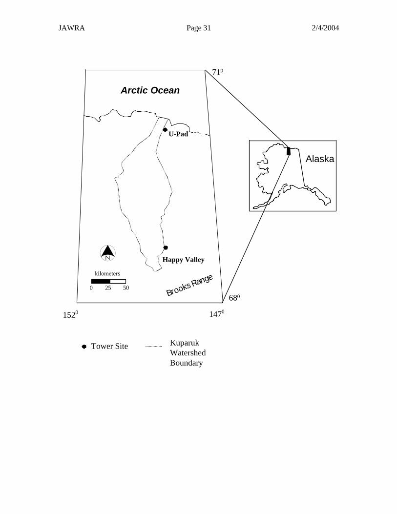
The study was conducted within a rectangular region encompassing 9200 km2

Kuparuk river watershed on the North Slope of Alaska (figure 1). The study area can be

divided into two distinct physiographic regions, the Arctic coastal plain and the foothills

of the Brooks Mountain Range. The coastal plain is dominated by wet sedge and moist

non-acidic tundra vegetation and is characterized by low relief, poor sub-surface

drainage, and a large number of shallow thaw lakes. The foothills consist mostly of moist

acidic tussock and dwarf shrub tundra vegetation and are typified by low rolling hills,

water track drainages and shallow active layer depths. Mean monthly temperatures range

between –12.8 and 10.3° C at the coast and from –11.1 to 6.7° C in the foothills (Oechel,

1989). Total summer (June-August) precipitation in the foothills region is between 90-

170 mm and is approximately 80 mm in the coastal plain (30 year average 1961-1990;

Alaska Cooperative Snow Survey Data 1994).

Eddy correlation tower measurements were collected at two tower sites, U-PAD

in the coastal plain and Happy Valley in the foothills (figure 1) (Vourlitis and Oechel,

1999). The U-PAD tower site (70°16.88' N, 148°53.23' W) is located near Prudhoe Bay,

approximately 10 km south of the Arctic Ocean (figure 1). Vegetation at this site is wet

JAWRA Page 10 2/4/2004

sedge tundra, dominated by Carex aquatilis and Eriophorum angustifolium interspersed

with a number of shallow thaw lakes. The Happy Valley tower site (69°08.54' N,

148°35.47' W) is located 135 km south of the Arctic Ocean and 1.5 km west of the Trans-

Alaska Pipeline Haul Road on the North Slope of Alaska (figure 1). Vegetation at this

site is moist acidic tussock tundra, dominated by Eriophorum vaginatum. These two sites

are representative of the extremes within the Kuparuk River study area in terms of

temperature, latitudinal variation in NDVI values, topography, vegetation type, and

surface moisture values (Eugster et al., 1997).

INSERT FIGURE 1 ABOUT HERE

Tower Measurements

Data from the two flux towers were collected throughout the 1994 and 1995

summer growing seasons (early June to mid-September) and detailed descriptions of the

instrumentation and data collection procedures are given in Vourlitis and Oechel (1997)

and Vourlitis and Oechel (1999). The net fluxes of H2O (LE) and sensible heat (H) were

measured using the eddy covariance (flux) technique. Sensors were mounted at 2.5 m

above the ground and fluxes were computed using a 200-second running mean and stored

on data loggers as 30-minute averages (CR 21X, Campbell Scientific Inc., Ogden Utah).

Net radiation (Rn) was measured at a height of 1 m using a net radiometer (Q-6, REBS,

Seattle, Washington). Ground heat flux (G) was measured using two soil heat flux plates

(HFT-1, REBS, Seattle) buried 2 cm below the moss surface (Vourlitis and Oechel, 1997;

Vourlitis and Oechel, 1999). The measured G values were adjusted prior to our analysis

in order to correct for energy lost to the moss layer because of its high heat capacity

(Miller et al., 1984; Waelbroeck, 1993). Measurements of wet and dry bulb temperatures

JAWRA Page 11 2/4/2004

were made at 25, 100, and 200 cm above ground level using ventilated psychrometers

affixed with cross-calibrated type-t thermocouples. All meteorological and flux

measurements were made every 60 seconds and stored as 30-minute averages (Vourlitis

and Oechel, 1997; Vourlitis and Oechel, 1999).

Derivation of Alpha

Rearranging the Priestley-Taylor evaporation equation (equation 1) to solve for α

yields:

α = [LE (S + U)] / [(Rn – G) S] (2)

Observed 30-minute average LE, Rn and G (G was taken as the average value of the two

measurements made at each site) values were used in this equation along with calculated

values of U and S based on the measured air temperature. α values were calculated for

each 30-minute interval and averaged to daily values using only the 30-minute intervals

in which LE and available energy (Rn-G) were positive. This screening limited α values

to periods when evaporation was or could be occurring (the period of interest in this

study) and so eliminated negative α values. The psychometric constant U, was obtained

from:

U = 100.3/(0.677*T) (3)

where U is in Kpa°C-1 and T is air temperature in °C measured at 2 m above ground level.

S, the slope of the saturation vapor pressure and temperature curve, was calculated as a

function of the 2 m air temperature using the following equation:

S = {25083/(T + 237.3)2 exp(17.3T/(T + 237.3))}*0.1 (4)

where S is in Kpa°C-1 (Dingman, 1994).

JAWRA Page 12 2/4/2004

NDVI

The ultimate goal of this research is to use remote sensing as a tool to predict α

values over the circumpolar region. In order to estimate α at these spatial scales while

accounting for seasonal changes described in previous studies (i.e. 15-days Rovanesk et

al. 1996) the only suitable satellite data available is from the National Oceanic and

Atmospheric Administration (NOAA) Advanced Very High Resolution Radiometer

(AVHRR) suite of satellites. Therefore, NDVI values were extracted from the NOAA

AVHRR maximum value composite (MVC) images that have been used as a data input in

a number of other ET studies (e.g., Szilagyi and Parlange, 1999). The MVC NDVI

images are twice monthly or bi-weekly (depending on the year) composites of the highest

NDVI values, derived on a pixel-by-pixel basis and extracted from a geo-referenced,

multi-temporal data set (Holben 1986). MVC is a widely used method to reduce

atmospheric affects and cloud contamination that frequently inhibits optical remote

sensing in Arctic environments (Hope et al., 1999a). NDVI is calculated using

reflectance values for channel 1, red (0.58-0.68 µm) and channel 2, NIR (0.72-1.1 µm)

based on the following equation:

(NIR – Red) / (NIR + Red) (5)

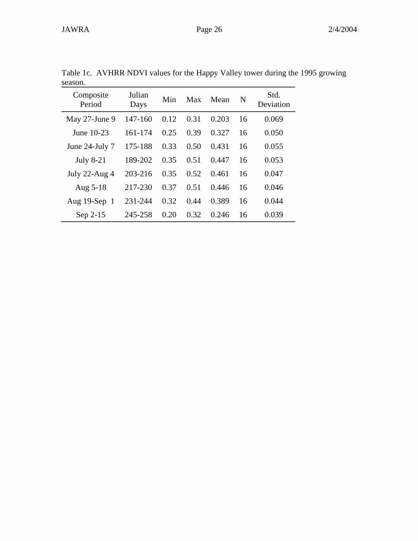
We characterized regional phenology (seasonal growth) by using a 16 km2 (4

pixel by 4 pixel) subset area from each MVC NDVI image for the operational periods of

the two towers during the 1994 (tables 1a and 1b) and 1995 (tables 1c and 1d) growing

seasons. This subset size was used to provide an estimate of the regional change in the

vegetation and the associated energy and moisture regimes, which co-vary with

vegetation type and state and to account for any mis-registration between the images and

JAWRA Page 13 2/4/2004

the actual tower location on the ground. The 4 by 4 pixel NDVI values were averaged,

providing a single NDVI value of ‘relative greenness’ for each composite period around

the tower.

INSERT TABLES 1a, b, c AND d ABOUT HERE

Analytical Approach/Statistical Procedures

The significance of the two components of this study, comparing α values

between tower sites and the α-NDVI relationship, was determined using a matched pairs

t-test and ordinary least squares (OLS) regression respectively. Both statistical tests are

parametric and assume mutually independent random samples and the time series data

used in this study may exhibit trends (temporal autocorrelation) that violate this

assumption. Temporal autocorrelation can influence the variance, thus affecting the

confidence intervals used to determine the significance of the relationship. Therefore, the

possible influences of temporal autocorrelation were addressed to ensure correct

interpretation of the statistical results.

Comparison Between Towers-Spatial Differences

A matched pairs t-test was used to determine if daily average α values were

significantly different between the tower sites. The daily average α values may not be

mutually independent random samples due to longer-term (i.e. longer than one day)

variations in surface and weather conditions which can affect the daily average α values

(Bello and Smith, 1990; Viswandham, 1991). Therefore, the autocorrelation function

(ACF) was used to determine the length of the skip/lag that would be used to subset the

data prior to analysis.

JAWRA Page 14 2/4/2004

The ACF is an important metric of the serial dependence within a stationary

random function (Diggle, 1990). The ACF describes the amount of correlation and the

corresponding significance between pairs of data in a time series. This function can be

used to determine when pairs of data (values that follow each other in the time series) are

not dependent on a previous value or values and are, therefore, not temporally auto-

correlated.

Alpha-NDVI Relationship

Ordinary least squares (OLS) regression was used to examine the relationship

between α and NDVI. Because α and NDVI values are sequential in nature, the Durbin-

Watson test was used to determine if the regression results were influenced by temporal

autocorrelation.

Results and Discussions

Daily Average Alpha Values

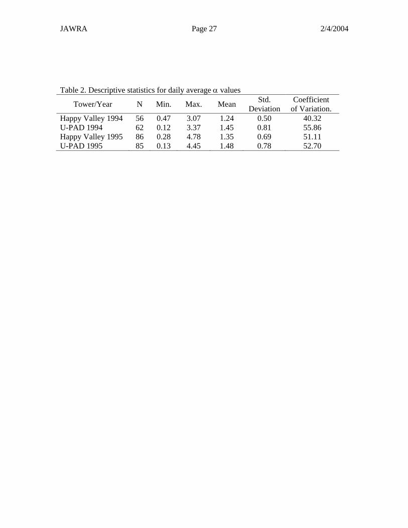
Figures 2 and 3 display the daily average α values over time for both towers and

both years. α was highly variable with coefficients of variation (CV) between 40 and

50% (Table 2). From the results given in table 2, it is evident that day-to-day variability

in α is greater than the differences in the mean α value between the two sites. This

indicates that meteorological variability at the sites causes greater variability in α then the

differences in surface conditions at the two sites. Overall, average daily α values at the

upland, Happy Valley site were smaller, less variable and closer to the value of 1.26

compared to the U-PAD site. Both the average and maximum values of α for both towers

were larger in 1995 compared 1994. The increase in average and maximum values may

be due to the greater summer precipitation totals in 1995. In 1994 Happy Valley and U-

JAWRA Page 15 2/4/2004

PAD received 137.5 mm and 77.5 mm of precipitation, respectively, compared to 449.6

and 195.8 mm in 1995. This increase in precipitation at both sites during 1995 led to a

shallower depth to water table and increased surface moisture at both sites (Vourlitis and

Oechel 1997; Vourlitis and Oechel 1999). Moisture availability at the surface affects the

partitioning of available energy into sensible (H) and latent heat (LE) fluxes. The

relationship of α to the partitioning of energy at the Earth’s surface into these

components can be examined using the Bowen Ration (β) (H/LE). α is related to β as

follows:

α = (1 +U/S) / (1 + β) (6)

Therefore, as surface moisture increases and a greater proportion of the available energy

at the surface is partitioned into LE, the β decreases causing an increase in α values.

INSERT FIGURES 2 AND 3 AND TABLE 2 ABOUT HERE

Comparison Between Towers

ACF results from the 1994 growing season at both the Happy Valley and U-PAD

tower sites indicate that correlation between pairs of data fell within the 95% confidence

limit after a one-day lag (figure 4a,b). Therefore, the matched pairs t-test utilized daily

average α values sub-sampled every other day from both tower sites during the 1994

growing season. ACF results from U-PAD tower in 1995 indicated that the correlation

between pairs of values fell within the 95% confidence interval after a one-day lag (figure

4d). However, at the Happy Valley tower in 1995 the correlation between pairs of α

values fell within the 95% confidence interval after a two-day lag (figure 4c). Thus, the

matched pairs t-test utilized every 3rd daily average α value in 1995.

INSERT FIGURE 4 ABOUT HERE

JAWRA Page 16 2/4/2004

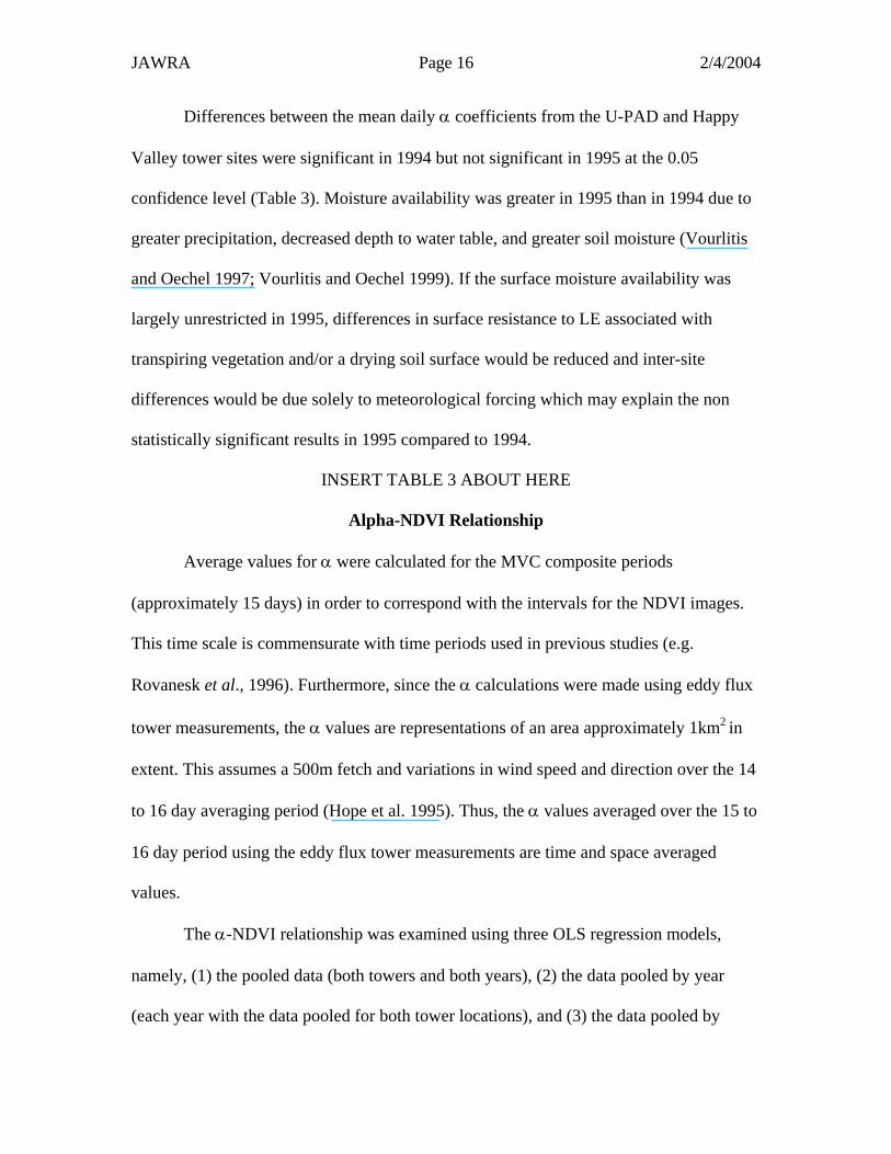
Differences between the mean daily α coefficients from the U-PAD and Happy

Valley tower sites were significant in 1994 but not significant in 1995 at the 0.05

confidence level (Table 3). Moisture availability was greater in 1995 than in 1994 due to

greater precipitation, decreased depth to water table, and greater soil moisture (Vourlitis

and Oechel 1997; Vourlitis and Oechel 1999). If the surface moisture availability was

largely unrestricted in 1995, differences in surface resistance to LE associated with

transpiring vegetation and/or a drying soil surface would be reduced and inter-site

differences would be due solely to meteorological forcing which may explain the non

statistically significant results in 1995 compared to 1994.

INSERT TABLE 3 ABOUT HERE

Alpha-NDVI Relationship

Average values for α were calculated for the MVC composite periods

(approximately 15 days) in order to correspond with the intervals for the NDVI images.

This time scale is commensurate with time periods used in previous studies (e.g.

Rovanesk et al., 1996). Furthermore, since the α calculations were made using eddy flux

tower measurements, the α values are representations of an area approximately 1km2 in

extent. This assumes a 500m fetch and variations in wind speed and direction over the 14

to 16 day averaging period (Hope et al. 1995). Thus, the α values averaged over the 15 to

16 day period using the eddy flux tower measurements are time and space averaged

values.

The α-NDVI relationship was examined using three OLS regression models,

namely, (1) the pooled data (both towers and both years), (2) the data pooled by year

(each year with the data pooled for both tower locations), and (3) the data pooled by

JAWRA Page 17 2/4/2004

tower location (each tower location with the data pooled for both years). Only the pooled

data from both towers and years had an adequate sample size, (N=25) to test for temporal

auto-correlation with the Durbin-Watson test. The Durbin-Watson test from the pooled

regression produced a value of 1.81 that was above the upper threshold (Du) value, 1.20,

at the 0.05 significance level. Therefore, the residuals were not temporally auto-

correlated. The other regression models (i.e. individual towers and years) were comprised

of small sample sizes (i.e. <15 samples), therefore the residuals were visually examined

for patterns and/or trends that may have been due to temporal auto-correlation. Visual

examination of the scatterplots indicated no temporal autocorrelation.

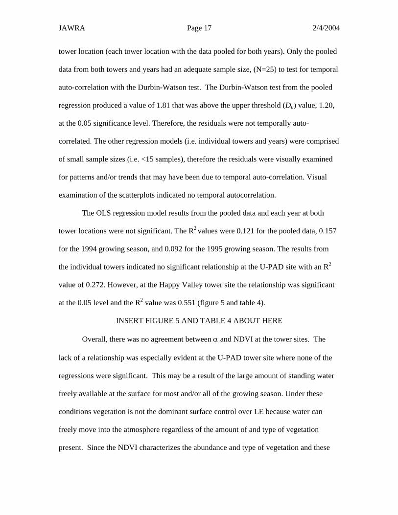
The OLS regression model results from the pooled data and each year at both

tower locations were not significant. The R2 values were 0.121 for the pooled data, 0.157

for the 1994 growing season, and 0.092 for the 1995 growing season. The results from

the individual towers indicated no significant relationship at the U-PAD site with an R2

value of 0.272. However, at the Happy Valley tower site the relationship was significant

at the 0.05 level and the R2 value was 0.551 (figure 5 and table 4).

INSERT FIGURE 5 AND TABLE 4 ABOUT HERE

Overall, there was no agreement between α and NDVI at the tower sites. The

lack of a relationship was especially evident at the U-PAD tower site where none of the

regressions were significant. This may be a result of the large amount of standing water

freely available at the surface for most and/or all of the growing season. Under these

conditions vegetation is not the dominant surface control over LE because water can

freely move into the atmosphere regardless of the amount of and type of vegetation

present. Since the NDVI characterizes the abundance and type of vegetation and these

JAWRA Page 18 2/4/2004

factors did not restrict water availability to the atmosphere, α values were not related to

changes in NDVI at this site.

Conversely, the Happy Valley tower site is located in a drier upland landscape

where the amount of water freely available at the surface was significantly less than at the

U-PAD tower site. Therefore, the amount and abundance of vegetation characterized by

the NDVI is a stronger influence on the surface resistance to LE through the transpiration

properties of the vegetation at the Happy Valley tower site (Vourlitis and Oechel, 1999).

This leads to the significant α-NDVI relationship over time at the Happy Valley tower

site.

Summary and Conclusions

The objective of this research was to determine 1) the variability of the Priestley-

Taylor α coefficient between two regions with contrasting vegetation, surface moisture,

and meteorological characteristics and 2) if seasonal variations in α were correlated to the

satellite-derived regional NDVI in Arctic tundra ecosystems. This research was

performed by comparing site-to-site differences between α values calculated at two eddy

flux towers located in contrasting regions and by determining the significance of the

correlation between α and the regional NDVI over time.

Differences in daily average α values between the two tower sites were

significant in only one of the two years, 1994. In 1995 the lack of a significant difference

between the tower sites appears to be due to the significantly higher precipitation totals

leading to greater moisture availability, thus diminishing differences in the surface

restrictions on α values between sites. Under these conditions, atmospheric restrictions

JAWRA Page 19 2/4/2004

such as vapor pressure deficit (VPD) may have become the dominant factor influencing

ET rates and α values.

Overall, the results indicate that the regional NDVI is a poor predictor of changes

in α at the time/space scales of this study in Arctic ecosystems. Originally it was

hypothesized that changes in vegetation amount and state, as reflected by the regional

NDVI, would be indicative of average soil moisture conditions and the highly related

meteorological conditions in Arctic ecosystems, and that these conditions were the major

factors controlling the temporal variability in α. From this research it is apparent that

NDVI is not significantly related to α at the time/space scales investigated. Other factors

may have affected the α values (e.g. significant inter-annual differences in precipitation),

and/or the regional scale NDVI values did not provide an adequate representation of

vegetation amount and state, average soil moisture conditions, and the related

meteorological conditions at the tower sites during the study period that were affecting α

values.

This study used regional estimates of NDVI derived from the NOAA AVHRR

suite of satellites because temporal fidelity of the data set. The regional scale NDVI

provides an acceptable estimate of changes in vegetation greenness over time in Arctic

ecosystems however, fine-scale variations in surface characteristics due to topography

and/or soil characteristics, such as open water conditions after snowmelt, are not well

captured by the regional NDVI and may have affected the results in this study.

Furthermore, one of the major limiting characteristics of NDVI is its inability to

distinguish between different background components such as soil, non-

photosynthetically active vegetation (NPV), and/or water (Peddle et al., 1999). Because

JAWRA Page 20 2/4/2004

fine-scale variations in surface conditions such as open water and NPV may influence α

values, and because NDVI cannot distinguish between them, other remote sensing

techniques may improve predictions of α. One remote sensing technique that might be

used is Spectral Mixture Analysis (SMA), which provides estimates of the fractions of

green vegetation, NPV, soil and water within individual pixels. Changes in these

fractions over time and space may be better predictors of α than a single NDVI value,

particularly in areas where vegetation is not the dominant control over LE (e.g. the U-

PAD site). Hope et al. (1999b) have shown that water cover, in the form of lakes, in the

Arctic can be identified using SMA with AVHRR data. In addition to different analytical

methods, new sensors such as the Moderate Resolution Imaging Spectrometer (MODIS)

aboard the NASA Earth Observing System (EOS) Terra satellite may allow for improved

models of α over time and space. With its similar temporal resolution and increased

spectral and spatial resolutions compared to the NOAA AVHRR sensor, the MODIS

sensor may provide improved model inputs for the prediction of α through SMA, as well

as for the estimation of surface temperature, and other variables that may be strongly

related to the α coefficient over time and space in Arctic ecosystems.

Acknowledgements

This research was funded by the National Science Foundation’s Office of Polar Programs

as part of the Arctic Systems Science (ARCSS) Land Atmosphere Ice Interactions (LAII)

FLUX study, Grant No OPP-9318527 and OPP-9216109. The authors would like to

thank Dr. Arthur Getis for his help with the statistical analysis and Steve Hastings,

Rommel Zulueta, and Joe Verfaille Jr. for their field and technical assistance.

JAWRA Page 21 2/4/2004

Literature Cited

Barton, I. J., 1979. A Parameterization of the Evaporation from Nonsaturated Surfaces. Journal of Applied Meteorology 18:43-47. Bello, R. and J. D. Smith, 1990. The effect of Weather Variability on the Energy Balance of a Lake in the Hudson Bay Lowlands, Canada. Arctic and Alpine Research 22(1):98-107. Davies, J. A. and C. D. Allen, 1973. Equilibrium, Potential, and Actual Evaporation from Cropped Surfaces in Southern Ontario. Journal of Applied Meteorology 12:649-657. De Bruin, H. A. R. and A. A. M. Holtstag, 1982. A Simple Parameterization of the Surface Fluxes of Sensible and Latent Heat during Daytime Compared with Penman-Monteith Concept. Journal of Applied Meteorology 21:1610-1621. Diggle, P. J., 1990. Time Series: A Biostatistical Introduction. Oxford University Press, New York, New York. Dingman, S. L., 1994. Physical Hydrology. Prentice-Hall, Inc., Upper Saddle River, New Jersey. Eichinger, W. E., M. B. Parlange, and H. Stricker, 1996. On the Concept of Equilibrium Evaporation and the Value of the Priestley-Taylor Coefficient. Water Resources Research 32:161-164. Eugster, W., J. P. McFadden, and F. S. Chapin III, 1997. A Comparative Approach to Regional Variation in Surface Fluxes using Mobile Eddy Correlation Towers. Boundary-Layer Meteorology 85:293-307. Flint, A. L. and S. W. Childs, 1991. Use of the Priestley-Taylor Evaporation Equation for Soil Water Limited Conditions in a Small Forest Clearcut. Agricultural and Forest Meteorology 56:247-260. Gates, W. L., J. F. B. Mitchell, G. J. Boer, U. Cubasch, and V. P. Meleshko, 1992. Climate Modeling, Climate Prediction and Model Validation. In: Climate Change 1992: The Supplemental Report to the IPCC Scientific Assessment, J. T. Houghton, B. A. Callander and S. K. Varney (Editors). Cambridge University Press, Cambridge, UK, pp. 97-135. Gold, W. G. and L. C. Bliss, 1995. Water Limitations and Plant Community Development in a Polar Desert. Ecology 76(5):1558-1568. Hinzman, L. D. and D. L. Kane, 1992. Potential Response of an Arctic Watershed during a Period of Global Warming. Journal of Geophysical Research 97(D3):2811-2820.

JAWRA Page 22 2/4/2004

Hobbie, J. E. 1980. Introduction and Site Description. In: Liminology of Tundra Ponds, J. E. Hobbie (Editor). Dowden, Hutchinson, and Ross, Stroudsburg, Pennsylvania pp. 19-50. Holben, B. N., 1986. Characteristics of Maximum-Value Composite Images from Temporal AVHRR Data. International Journal of Remote Sensing 7(11):1417-1434. Hope, A. S., J. S. Kimball, and D. A. Stow, 1993. The Relationship Between Tussock Tundra Spectral Reflectance Properties and Biomass and Vegetation Composition. International Journal of Remote Sensing 14(10):1861-1874. Hope, A. S., J. B. Fleming, G. Vourlitis, D. A. Stow, W. C. Oechel and T. Hack, 1995. Relating CO2 fluxes to spectral vegetation indices in tundra landscapes: importance of footprint definition. Polar Record 31:245-250. Hope, A. S., L. L. Coulter, and D. A. Stow, 1999b. Estimating Lake Area in the Arctic Landscape Using Linear Mixture Modeling with AVHRR Data. International Journal of Remote Sensing 20(4):829-835. Hope, A. S., K. R. Pence, D. A. Stow, 1999a. Response of the Normalized Difference Vegetation Index to Varying Cloud Conditions in Arctic Tundra Environments. International Journal of Remote Sensing 20(1):207-212. Jasieniuk, M. A. and E. A. Johnson, 1982. Peatland Vegetation Organization and Dynamics in the Western Subarctic, Northwest Territories, Canada. Canadian Journal of Botany 60:2581-2593. Kane, D. L., R. E. Gieck, and L. D. Hinzman, 1990. Evapotranspiration from a Small Alaskan Arctic Watershed. Nordic Hydrology 21:253-272. Manabe, S. and R. J. Stouffer, 1993. Century-Scale Effects of Increased Atmospheric CO2 on the Ocean-Atmosphere System. Nature 364:215-218. Matthes-Sears, U., W. C. Matthes-Sears, S. J. Hastings and W. C. Oechel, 1988. The Effects of Topography and Nutrient Status on the Biomass, Vegetative Characteristics, and Gas Exchange of Two Deciduous Shrubs on an Arctic Tundra Slope. Arctic and Alpine Research 20:342-351. Maxwell, B., 1992. Arctic Climate: Potential for Change under Global Warming. In: Arctic Ecosystems in a Changing Climate: An Ecophysiological Perspective, F. S. Chapin III, J. L. Jeffries, J. F. Reynolds, G. R. Shaver and J. Svoboda (Editors). Academic Press, Inc., San Diego, California, pp. 11-34. McNaughton, K. G. and T. A. Black, 1973. A Study of Evapotranspiration from a Douglas Fir Forest Using the Energy Balance Approach. Water Resources Research 9:1579-1590.

JAWRA Page 23 2/4/2004

Meehl, G. A., W. M. Washington, and T. R. Karl, 1993. Low-frequency Variability and CO2 Transient Climate Change: Part 1. Time Averaged Differences. Climate Dynamics 8:117-133. Mendez, J., L. D. Hinzman, and D. L. Kane, 1998. Evapotranspiration from a Wetland Complex on the Arctic Coastal Plain of Alaska. Nordic Hydrology 29(4/5):303-330. Miller, P. C., P. M. Miller, et al., 1984. Plant-Soil Processes in Eriophorum Vaginatum Tussock Tundra in Alaska: A Systems Modeling Approach. Ecological Monographs 54(4):361-405. Monteith, J. L., 1965. Evaporation and environment. In: Proceedings of the 19th Symposium of the Society for Experimental Biology. Cambridge University Press, New York, New York, pp. 205-233. Mukammal, E. I. and H. H. Neumann, 1977. Application of the Priestley-Taylor Evaporation Model to Assess the Influence of Soil Moisture on the Evaporation from A Large Weighing Lysimeter and Class A Pan. Boundary-Layer Meteorology 14:243-256. Oechel, W. C., 1989. Nutrient and Water Flux in a Small Arctic Watershed: An Overview. Holarctic Ecology 12:187-201. Ostendorf, B. and J. F. Reynolds, 1998. A Model of Arctic Tundra Vegetation Derived from Topographic Gradients. Landscape Ecology 13:187-201. Parlange, M. B. and G. G. Katul, 1992. Estimation of the Diurnal Variation of Potential Evaporation from a Wet Bare-Soil Surface. Journal of Hydrology 132:71-89. Peddle, D. R., F. G. Hall, and E. F. LeDrew, 1999. Spectral Mixture Analysis and Geometrical Optical Reflectance Modeling of Boreal Forest Biophysical Structure. Remote Sensing of Environment 67:288-297. Peterson, K. M. and W. D. Billings, 1980. Tundra Vegetational Patterns and Succession in Relation to Microtopography near Atkasook, Alaska. Arctic and Alpine Research 12:473-482. Priestley, C. H. B. and R. J. Taylor, 1972. On the Assessment of Surface Heat Flux and Evaporation Using Large-Scale Parameters. Monthly Weather Review 100(2):81-92. Roulet, N. T. and M. Woo, 1986. Hydrology of a Wetland in the Continuous Permafrost Region. Journal of Hydrology 89:73-91. Rouse, W. R., P. F. Mills, and R. B. Stewart, 1977. Evaporation in High Latitudes. Water Resources Research 13:909-914.

JAWRA Page 24 2/4/2004

Rouse, W. R. and R. B. Stewart, 1972. A Simple Model for Determining the Evaporation from High Latitude Upland Sites. Journal of Applied Meteorology 11:1063-1070. Rovansek, R. J., L. D. Hinzman, and D. L. Kane, 1996. Hydrology of a Tundra Wetland Complex on the Alaskan Arctic Coastal Plain, U.S.A. Arctic and Alpine Research 28(3):311-317. Shuttleworth, W. J. and I. R. Calder, 1979. Has the Priestley-Taylor Equation Any Relevance to Forest Evaporation? Journal of Applied Meteorology 18:639-646. Slatyer, R. O. and I. C. McIlroy, 1967. Practical Microclimatology. CISRO, Melbourne, Australia. Stannard, D. I., 1993. Comparison of Penman-Monteith, Shuttleworth-Wallace, and Modified Priestley-Taylor Evapotranspiration Models for Wildland Vegetation in Semiarid Rangeland. Water Resources Research 29(5):1379-1392. Stewart, R. B. and W. R. Rouse, 1976. Simple Models for Calculating Evaporation from Dry and Wet Tundra Surfaces. Arctic and Alpine Research 8(3):263-274. Stow, D. A., B. H. Burns, A. S. Hope, 1993. Spectral, Spatial and Temporal Characteristics of Arctic Tundra Reflectance. International Journal of Remote Sensing 14(13):2445-2465. Szilagyi, J. and M. G. Parlange, 1999. Defining watershed-scale evaporation using a normalized difference vegetation index. Journal of the American Water Resources Association 35:1245-1255. Viswanadham, Y., V. P. Silva Filho, and R. G. B. Andre, 1991. The Priestley-Taylor Parameter Alpha for the Amazon Forest. Forest Ecology and Management 38:211-225. Vourlitis, G. L. and W. C. Oechel, 1997. Landscape-scale CO2, H2O Vapor, and Energy Flux of Moist-Wet Coastal Tundra Ecosystems Over Two Growing-Seasons. Journal of Ecology 85:575-590. Vourlitis, G. L. and W. C. Oechel, 1999. Eddy Covariance Measurements of Net CO2 Flux and Energy Balance of an Alaskan Moist-Tussock Tundra Ecosystem. Ecology 80(2):686-701. Waelbrock, C., 1993. Climate-Soil Processes in the Presence of Permafrost: A Systems Modeling Approach. Ecological Modeling 69:185-225.

JAWRA Page 25 2/4/2004

Table 1a. AVHRR NDVI values for the U-PAD tower during the 1994 growing season. Composite

Period Julian Days Min Max Mean N Std.

Deviation

June 1-15 152-166 -0.10 0.03 0.017 16 0.015

June 16-30 167-181 0.07 0.15 0.112 16 0.019

July 1-15 182-196 0.09 0.26 0.176 16 0.040

July 16-31 197-212 0.22 0.33 0.276 16 0.036

Aug 1-15 213-227 0.17 0.27 0.216 16 0.034

Aug 16-31 228-243 0.09 0.17 0.124 16 0.025

Sep 1-15 244-258 0.11 0.23 0.164 16 0.036 Table 1b. AVHRR NDVI values for the Happy Valley tower during the 1994 growing season.

Composite Period

Julian Days Min Max Mean N Std.

Deviation

June 1-15 152-166 0.19 0.35 0.302 16 0.048

June 16-30 167-181 0.25 0.42 0.349 16 0.058

July 1-15 182-196 0.33 0.51 0.436 16 0.057

July 16-31 197-212 0.38 0.52 0.469 16 0.044

Aug 1-15 213-227 0.25 0.48 0.379 16 0.064

Aug 16-31 228-243 0.23 0.39 0.323 16 0.058

Sep 1-15 244-258 0.17 0.35 0.283 16 0.058

Table 1c. AVHRR NDVI values for the U-PAD tower during the 1995 growing season. Composite

Period Julian Days min max mean N Std.

DeviationMay 27-June 9 147-160 0.00 0.02 0.004 16 0.006

June 10-23 161-174 0.02 0.14 0.093 16 0.037

June 24-July 7 175-188 0.13 0.28 0.201 16 0.038

July 8-21 189-202 0.20 0.29 0.245 16 0.028

July 22-Aug 4 203-216 0.21 0.33 0.283 16 0.036

Aug 5-18 217-230 0.21 0.32 0.270 16 0.032

Aug 19-Sep 1 231-244 0.18 0.30 0.246 16 0.032

Sep 2-15 245-258 0.03 0.03 0.042 16 0.008

JAWRA Page 26 2/4/2004

Table 1c. AVHRR NDVI values for the Happy Valley tower during the 1995 growing season.

Composite Period

Julian Days Min Max Mean N Std.

Deviation

May 27-June 9 147-160 0.12 0.31 0.203 16 0.069

June 10-23 161-174 0.25 0.39 0.327 16 0.050

June 24-July 7 175-188 0.33 0.50 0.431 16 0.055

July 8-21 189-202 0.35 0.51 0.447 16 0.053

July 22-Aug 4 203-216 0.35 0.52 0.461 16 0.047

Aug 5-18 217-230 0.37 0.51 0.446 16 0.046

Aug 19-Sep 1 231-244 0.32 0.44 0.389 16 0.044

Sep 2-15 245-258 0.20 0.32 0.246 16 0.039

JAWRA Page 27 2/4/2004

Table 2. Descriptive statistics for daily average α values

Tower/Year N Min. Max. Mean Std. Deviation

Coefficient of Variation.

Happy Valley 1994 56 0.47 3.07 1.24 0.50 40.32 U-PAD 1994 62 0.12 3.37 1.45 0.81 55.86 Happy Valley 1995 86 0.28 4.78 1.35 0.69 51.11 U-PAD 1995 85 0.13 4.45 1.48 0.78 52.70

JAWRA Page 28 2/4/2004

Table 3. Paired samples t-test results

Year N t-value t-critical* Null Hypothesis Rejected

1994 19 -2.310 0.033 Yes 1995 26 0.534 0.598 No

* 0.05 Confidence Level

JAWRA Page 29 2/4/2004

Table 4. Regression statistics for the 1994 and 1995 data from the Happy Valley tower

site.

N R R2 Adj. R2 F-Value Sig. F* Durbin-Watson

12 0.742 0.551 0.506 12.275 0.006 2.341

Variable Coefficient Std. Error t-Value Sig. t

Constant -0.002 0.384 -0.042 0.967 NDVI 3.400 0.970 3.504 0.006

*0.05 Confidence level

JAWRA Page 30 2/4/2004

List of figures:

Figure 1: Kuparuk river watershed within the North Slope of Alaska and the location of

the study tower sites.

Figure 2: Daily average α values from the 1994 growing season at both tower sites.

Figure 3: Daily average α values from the 1995 growing season at both tower sites.

Figure 4. Auto-correlation functions for a) Happy Valley 1994 b) U-PAD 1994 c) Happy

Valley 1995 and d) U-PAD 1995 with 95% confidence intervals.

Figure 5. Scatterplot of α versus NDVI during the 1994 and 1995 growing

seasons at the Happy Valley tower site.

JAWRA Page 31 2/4/2004

1470

710

680

1520

25 0 50

Kuparuk WatershedBoundary

Brooks Range kilometers

Arctic Ocean

U-Pad

Happy Valley

Tower Site

Alaska

JAWRA Page 32 2/4/2004

0

1

2

3

4

5

151

157

163

169

175

181

187

193

199

205

211

217

223

229

235

241

247

Julian Day

Alp

ha

Happy Valley

UPAD

JAWRA Page 33 2/4/2004

0

1

2

3

4

5

151

157

163

169

175

181

187

193

199

205

211

217

223

229

235

241

247

Julian Day

Alp

haHappy ValleyUPAD

JAWRA Page 34 2/4/2004

Lag Number

1615

1413

1211

109

87

65

43

21

ACF

1.0

.5

0.0

-.5

-1.0

Confidence Limits

Coefficient

a

Lag Number

1615

1413

1211

109

87

65

43

21

AC

F

1.0

.5

0.0

-.5

-1.0

Confidence Limits

Coefficient

b

Lag Number

1615

1413

1211

109

87

65

43

21

AC

F

1.0

.5

0.0

-.5

-1.0

Confidence Limits

Coefficient

d

Lag Number

1615

1413

1211

109

87

65

43

21

AC

F

1.0

.5

0.0

-.5

-1.0

Confidence Limits

Coefficient

c

JAWRA Page 35 2/4/2004

.

NDVI

.5.4.3.2.1

ALP

HA

2.0

1.8

1.6

1.4

1.2

1.0

.8

.6

JAWRA Page 36 2/4/2004

Equations: Equation 1:

Equation 2:

Equation 3:

Equation 4:

Equation 5: