Hydrol. Earth Syst. Sci., 16, 2233–2251, 2012www.hydrol-earth-syst-sci.net/16/2233/2012/doi:10.5194/hess-16-2233-2012© Author(s) 2012. CC Attribution 3.0 License.

Hydrology andEarth System

Sciences

Variational assimilation of streamflow into operational distributedhydrologic models: effect of spatiotemporal scale of adjustment

H. Lee1,2, D.-J. Seo1,2,*, Y. Liu 1,3,** , V. Koren1, P. McKee4, and R. Corby4

1NOAA, National Weather Service, Office of Hydrologic Development, Silver Spring, Maryland, USA2University Corporation for Atmospheric Research, Boulder, Colorado, USA3Riverside Technology, Inc., Fort Collins, Colorado, USA4NOAA, National Weather Service, West Gulf River Forecast Center, Fort Worth, Texas, USA* present address: Department of Civil Engineering, The University of Texas at Arlington, Arlington, TX 76019-0308, USA** present address: Goddard Space Flight Center, National Aeronautics and Space Administration, Greenbelt, MD 20771, USA

Correspondence to:H. Lee (haksu.lee@noaa.gov)

Received: 13 December 2011 – Published in Hydrol. Earth Syst. Sci. Discuss.: 5 January 2012Revised: 30 May 2012 – Accepted: 14 June 2012 – Published: 23 July 2012

Abstract. State updating of distributed rainfall-runoff mod-els via streamflow assimilation is subject to overfittingbecause large dimensionality of the state space of themodel may render the assimilation problem seriously under-determined. To examine the issue in the context of op-erational hydrologic forecasting, we carried out a set ofreal-world experiments in which streamflow data is assim-ilated into the gridded Sacramento Soil Moisture Account-ing (SAC-SMA) and kinematic-wave routing models of theUS National Weather Service (NWS) Research DistributedHydrologic Model (RDHM) via variational data assimilation(DA). The nine study basins include four in Oklahoma andfive in Texas. To assess the sensitivity of the performanceof DA to the dimensionality of the control vector, we usednine different spatiotemporal adjustment scales, with whichthe state variables are adjusted in a lumped, semi-distributed,or distributed fashion and biases in precipitation and PE areadjusted at hourly or 6-hourly scale, or at the scale of thefast response of the basin. For each adjustment scale, threedifferent assimilation scenarios were carried out in whichstreamflow observations are assumed to be available at basininterior points only, at the basin outlet only, or at all loca-tions. The results for the nine basins show that the optimumspatiotemporal adjustment scale varies from basin to basinand between streamflow analysis and prediction for all threestreamflow assimilation scenarios. The most preferred ad-justment scale for seven out of the nine basins is found to bedistributed and hourly. It was found that basins with highly

correlated flows between interior and outlet locations tendto be less sensitive to the adjustment scale and could ben-efit more from streamflow assimilation. In comparison withoutlet flow assimilation, interior flow assimilation producedstreamflow predictions whose spatial correlation structure ismore consistent with that of observed flow for all adjustmentscales. We also describe diagnosing the complexity of theassimilation problem using spatial correlation of streamflowand discuss the effect of timing errors in hydrograph simula-tion on the performance of the DA procedure.

1 Introduction

Improving flood forecasting has long been an importantresearch topic for natural hazard mitigation (Droegemeieret al., 2000; NHWC, 2002; NRC, 2010; USACE, 2000).Changes in spatiotemporal patterns of precipitation and oc-currences of record-breaking events at unprecedented scalesaround the globe during the past decades (Knutson et al.,2010; Milly et al., 2008; Min et al., 2011; Trapp et al., 2007;Trenberth et al., 2003) are pressing further the needs for rapidadvances in real-time flood forecasting (NRC, 2010). In theUS River Forecast Centres (RFCs), the flood forecasting pro-cess has often involved manual modifications of the modelstates by human forecasters (MOD; Seo et al., 2003; Smith etal., 2003) to reconcile any significant differences between themodel results and the observations. With distributed models,

Published by Copernicus Publications on behalf of the European Geosciences Union.

2234 H. Lee et al.: Variational assimilation of streamflow into operational distributed hydrologic models

such MOD’s are a very difficult proposition due to the gener-ally very large dimensionality of the state variables involved.As such, automatic data assimilation (DA) procedures are anecessity.

DA techniques merge information in the real-time hy-drologic and hydrometeorological observations into the hy-drologic model dynamics by considering uncertainties fromdifferent error sources (Liu and Gupta, 2007; McLaughlin,2002; Moradkhani, 2008; Seo et al., 2003, 2009; Troch etal., 2003). Compared to applying DA to lumped rainfall-runoff models (e.g., Bulygina and Gupta, 2009; Moradkhaniet al., 2005a,b; Seo et al., 2003, 2009; Vrugt et al., 2005,2006; Weerts and El Serafy, 2006), state updating of dis-tributed rainfall-runoff models is subject to overfitting to amuch greater extent due to the typically much larger dimen-sionality of the state space of the model.

In operational streamflow forecasting, other than the atmo-spheric forcing data, streamflow observation is usually theonly source of data available for assimilation, which is ofteninsufficient to reduce the large degrees of freedom (DOF)associated with distributed models. As such, most, if notall, distributed rainfall-runoff models are under-determined,i.e., the information available in the data is not enough touniquely determine the state variables and/or parameters ofthe model. Note that, while a vast amount of remote-sensingdata, in particular satellite-based, are widely available, theyare generally of limited utility for operational river and flashflood forecasting due to large temporal sampling intervalsand relatively low information content at the catchment scale.In an under-determined system, streamflow analysis at inde-pendent validation locations as well as streamflow predictionat any locations in a basin could be worse than the base modelstreamflow simulation due to overfitting. This poses an obvi-ous obstacle to advances in DA for distributed models whichrequires developing appropriate assimilation strategy to con-strain large degrees of freedom causing a state and/or param-eter identifiability problem.

In the following, we summarize previous studies that ad-dress state and/or parameter identifiability when applyingDA techniques to distributed hydrologic modelling. Clarket al. (2008) tested the impact of assimilating streamflowat one location on streamflow prediction at other locationsin the Wairau River basin in New Zealand by using theensemble square root Kalman filter (EnSRF) and the dis-tributed model TopNet. They obtained degraded streamflowresults from assimilation at independent validation locationsin the basin, highlighting the importance of accurately mod-elling spatial variability, or correlation structure of hydrolog-ical processes in order to improve streamflow prediction atungauged locations by assimilating streamflow observationsfrom elsewhere in the basin. With the limited data availablein field operations, the assimilation technique may neces-sarily adjust state variables at some lumped fashion (e.g.,at the sub-basin scale) that reflects or preserves the spatialcorrelation length or structure of hydrological processes. Lee

et al. (2011) found in a synthetic experiment using the El-don basin (ELDO2) in Oklahoma that assimilating outletflow into the gridded SAC via variational assimilation de-graded streamflow prediction at interior locations. This indi-cates difficulty of solving the inverse problem in distributedmodelling based on the limited information available in theoutlet flow data alone, and points out the need for differ-ent assimilation strategies to reduce the degrees of freedomassociated with the problem. Van Loon and Troch (2002)noted degraded prediction of ground water depth at somelocations in a 44-ha catchment in Costa Rica from assimi-lating soil moisture measured by a Trime time domain re-flectometry (TDR) system at multiple sites. The above re-sult was obtained even though discharge predictions werebenefited considerably from soil moisture assimilation. Chenet al. (2011) carried out assimilation of 20 different sets ofsynthetically generated soil moisture observations into theSWAT model with the ensemble Kalman filter (EnKF). Theyfound that, for some cases, analyses of groundwater flowand percolation rate were degraded. Brocca et al. (2010) as-similated the rescaled Soil Wetness Index (SWI) into thesemi-distributed model Modello Idrologico SemiDistribuitoin continuo (MISDc) in a synthetic experiment. They foundthat the assimilation results for flood prediction were de-graded for some experimental settings. Performance degra-dation following assimilation from above studies may bedue to a combination of factors, including inadequate modelphysics as mentioned in Van Loon and Troch (2002) andChen et al. (2011) or inappropriate assimilation strategy. Al-though it is difficult to trace the causes in real-world appli-cations due to the presence of a number of different errorsources and their unknown characteristics, the degraded as-similation results in the above studies warrant exploring dif-ferent assimilation strategies.

To address the aforementioned issues with DA into dis-tributed models in an operational setting and to develop aneffective assimilation strategy in order to limit the degrees offreedom in DA with distributed models, in this study we in-vestigate the effect of the spatiotemporal scale of adjustmenton analysis and prediction of streamflow. The analysis andprediction are generated by assimilating streamflow data intothe distributed SAC-SMA and kinematic-wave routing mod-els of HL-RDHM with the variational DA procedure (Seoet al., 2010; Lee et al., 2011). We tested nine spatiotempo-ral adjustment scales based on combinations of three spatialscales of adjustment (lumped, semi-distributed, distributed)to state variables and three temporal scales (hourly, 6-hourly,fast-response time of the basin) of adjustment to mean fieldbias in the precipitation and PE data. The strategy of adjust-ing short-term biases in the forcing data in the assimilationprocedure is motivated by the use of long-term bias adjust-ment factors in the SAC-SMA model calibration. Adoptinga coarser spatiotemporal adjustment scale would reduce thedimensionality of the control vector, which may help pre-vent overfitting when solving the inverse problem. For basins

Hydrol. Earth Syst. Sci., 16, 2233–2251, 2012 www.hydrol-earth-syst-sci.net/16/2233/2012/

H. Lee et al.: Variational assimilation of streamflow into operational distributed hydrologic models 2235

46

800

Fig 1. Schematic of the gridded SAC and kinematic-wave routing models of HL-RDHM (from Lee 801

et al., 2011) 802

803

804

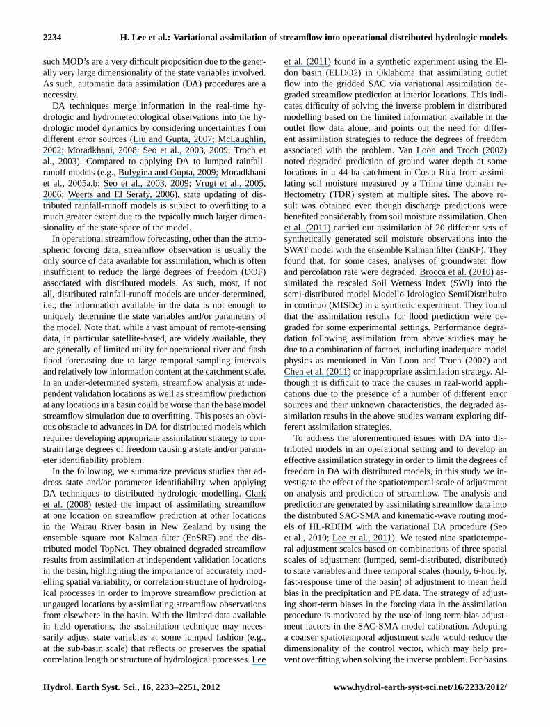
Fig. 1.Schematic of the gridded SAC and kinematic-wave routing models of HL-RDHM (from Lee et al., 2011).

with highly heterogeneous soil and physiographic propertiesand precipitation patterns, however, a finer adjustment scalemay be preferable. In this work, three streamflow assimila-tion scenarios are considered, i.e., assimilating interior flowobservations only, outlet flow observations only, or all flowobservations. Given a spatiotemporal adjustment scale, eachstreamflow assimilation scenario is carried out for four basinsin Oklahoma and five basins in Texas, US.

The paper is organised as follows: Sect. 2 describes themethodology including the hydrologic model, the assimi-lation technique, and the evaluation metrics; Sect. 3 de-scribes the study basins; Sect. 4 describes the multi-basinexperiment and presents the results and discussions; and fi-nally, Sect. 5 summarises conclusions and future researchrecommendations.

2 Methodology

2.1 The gridded SAC and kinematic-wave routingmodels of HL-RDHM

The models used are the gridded Sacramento Soil Mois-ture Accounting (SAC-SMA) and kinematic-wave routingmodels of the National Weather Service (NWS) HydrologyLaboratory’s Research Distributed Hydrologic Model (HL-RDHM, Koren et al., 2004). The SAC-SMA is a conceptualrainfall runoff model (Burnash et al. 1973) which calculatesfast and slow runoffs from two subsurface zones, i.e., Upper

Zone (UZ) and Lower Zone (LZ). The UZ is thinner than theLZ and consists of tension and free water storages. The LZ iscomposed of tension and primary and supplemental free wa-ter storages. Soil moisture states at each subsurface storagecompartment are named as Upper Zone Tension Water Con-tent (UZTWC), Upper Zone Free Water Content (UZFWC),Lower Zone Tension Water Content (LZTWC), Lower ZonePrimary Free Water Content (LZFPC), and Lower Zone Sup-plemental Free Water Content (LZFSC) (Koren et al., 2004).The sum of the surface and subsurface runoff is then routedthrough the kinematic-wave routing model to calculate flowat each HRAP grid. The models operate at an hourly timestep on the Hydrologic Rainfall Analysis Project (HRAP)grid (∼ 16 km2) (Greene and Hudlow, 1982; Reed and Maid-ment, 1999). The NEXRAD-based multi-sensor precipita-tion data (Fulton et al., 1998; Seo, 1998; Seo et al., 1999;Young et al., 2000) are available on the HRAP grid, a pri-mary reason for its use by HL-RDHM. If higher-resolutiondata and model parameters are available, it is possible torun HL-RDHM on a finer grid. For PE, monthly climatol-ogy is used (Smith et al., 2004). Figure 1 shows a schematicof the gridded SAC and kinematic-wave routing models ofthe HL-RDHM (Lee et al., 2011). The a priori estimates ofthe SAC parameters (Koren et al., 2000) are derived from thesoil data, STATSGO2 (NRCS, 2006) and SSURGO (NRCS,2004). Optimisation of the a priori parameters is carried outvia manual or automatic calibration (Koren et al., 2004). Forthe four Oklahoma basins, we used the manually-optimised

www.hydrol-earth-syst-sci.net/16/2233/2012/ Hydrol. Earth Syst. Sci., 16, 2233–2251, 2012

2236 H. Lee et al.: Variational assimilation of streamflow into operational distributed hydrologic models

parameters used in the Distributed Model IntercomparisonProject (DMIP, Smith et al., 2004). For the five Texas basins,we used the manual calibration results from WGRFC. Therouting parameters are estimated from the DEM, channelhydraulic data and observed flow data (Koren et al., 2004).The flow direction from upstream to downstream HRAP gridcells is determined by the Cell Outlet Tracing with an AreaThreshold (COTAT) algorithm (Reed, 2003) using the Digi-tal Elevation Model (DEM) data. We note here that, in thisstudy, streamflow predictions were generated assuming per-fectly known forcing, i.e., using the historical observed forc-ing data rather than forecast forcing because our primary in-terest here is in reducing hydrologic uncertainty (Krzyszto-fowicz, 1999; Seo et al. ,2006).

2.2 DA procedure

The automated DA procedure used in this study is basedon the variational DA (VAR) technique. There are a num-ber of reasons for this choice among different DA tech-niques. While simpler to implement, EnKF is optimum onlyif the observation equation is linear, which is easily violatedwhen assimilating streamflow for soil moisture updating. Onthe other hand, the VAR technique is optimum in the leastsquares sense, even if observation equations are stronglynonlinear (Zhang et al., 2001). Also, since the VAR proce-dure is smoother than a filter and, hence, equivalent to ensem-ble Kalman smoother, but with an ability to handle nonlin-ear observation equations, it can easily account for the timelag due to flow routing (Seo et al., 2003; Clark et al., 2008;Pauwels and De Lannoy, 2006; Weerts and El Serafy, 2006).In theory, one may use the particle filter to overcome thelinearity or distributional assumptions (Doucet et al., 2001;Pham, 2001). In reality, however, particle filtering is compu-tationally prohibitively expensive for high-dimensional prob-lems such as the one dealt with in this work.

In the following, we formulate the DA problem for thegridded SAC and kinematic-wave routing models of HL-RDHM, which may be stated as follows:Given the a pri-ori SAC states at the beginning of the assimilation windowand observations/estimates of precipitation, potential evapo-transpiration (PE) and streamflow at the outlet and/or inte-rior locations, update the state variables of the gridded SACand kinematic-wave routing models by adjusting the initialSAC states and multiplicative biases for precipitation and PEover the assimilation window at the predefined spatiotempo-ral scales of adjustment.

The VAR technique formulates the above as a least-squares minimisation problem that minimises the objectivefunction J constrained by the model physics (Lewis et al.,2006; Liu and Gupta, 2007):

Minimize

JK

(XS,K−L, XP,k, XE,k, XW,k

)=

1

2

K∑k=K−L+1[

ZQ,k − HQ,k

(XS,K−L, XP,K−L+1:k, XE,K−L+1:k, XW,K−L+1:k

)]T R−1Q,k[

ZQ,k − HQ,k

(XS,K−L, XP,K−L+1:k, XE,K−L+1:k, XW,K−L+1:k

)]+

1

2

K∑k=K−L+1

[ZP,k − HP,kXP,k

]T R−1P,k

[ZP,k − HP,k XP,k

]+

1

2

K∑k=K−L+1

[ZE,k − HE,kXE,k

]T R−1E,k

[ZE,k − HE,k XE,k

]+

1

2

[ZB,K−L − HB XS,K−L

]T R−1B,K−L

[ZB,K−L − HB XS,K−L

]+

1

2

K∑k=K−L+1

XTW,k R−1

W,k XW,k (1)

subject to

XS,k = M

(XS,k−1,XP,k,XE,k,XW,k

),

k = K − L + 1, ...,K

XminS,j,i≤XS,j,i,k≤Xmax

S,j,i

k = K − L,...,K;j = 1, ...,nS; i = 1, ...,nC

(2)

The objective function presented above is based on the fol-lowing observation equations:

ZB,K−L = HB XS,K−L + V B,K−L (3)

ZP,k = HP,k XP,k + V P,k (4)

ZE,k = HE,k XE,k + V E,k (5)

ZQ,k = HQ,k

(XS,K−L, XP,K−L+1:k, XE,K−L+1:k,

XW,K−L+1:k

)+ V Q,k (6)

In Eqs. (1) to (6),XS,k−1, XS,k, and XS,K−L denotethe five SAC states (UZTWC, UZFWC, LZTWC, LZFSC,LZFPC) at hourk − 1, k, and K − L, respectively;XP,k

andXE,k denote the multiplicative adjustment factors for bi-ases in precipitation and PE at hourk, respectively;ZB,K−L,ZP,k, ZE,k, and ZQ,k denote the observations of SACstates at the beginning of the assimilation window, precip-itation, PE, and streamflow, respectively;HP,k and HE,k

are the same asZP,k and ZE,k (this follows from thefact thatXP,k andXE,k are multiplicative adjustment fac-tors), respectively;HQ,k represents the gridded SAC andkinematic-wave routing models;HB is the identity matrix;XW,k denotes the model error;V B,K−L, V P,k, V E,k andV Q,k denote the measurement error vectors associated withZB,K−L, ZP,k, ZE,k, andZQ,k, respectively;XP,K−L+1:k

denotesXP,K−L+1, XP,K−L+2, ..., XP,k; XE,K−L+1:k de-notesXE,K−L+1, XE,K−L+2, ..., XE,k; XW,K−L+1:k de-notesXW,K−L+1, XW,K−L+2, ..., XW,k; RP,k, RE,k, RQ,k,RB,K−L, and RW,k represent the observation error covari-ance matrices associated withZP,k, ZE,k, ZQ,k, ZB,K−L,and a priori estimates of the model error, respectively.

In simplifying the above minimisation problem, we dropthe model error,XW,k because, in reality, little is knownabout its statistical properties. Seemingly an oversimplifica-tion, such strong-constraint formulation (Zupanski, 1997) isstill very reasonable for our problem becauseV P,k andV E,k

in Eqs. (4) and (5) act like model errors to a certain extent

Hydrol. Earth Syst. Sci., 16, 2233–2251, 2012 www.hydrol-earth-syst-sci.net/16/2233/2012/

H. Lee et al.: Variational assimilation of streamflow into operational distributed hydrologic models 2237

(Seo et al., 2003). We then assume that the observation errorsare independent and time-invariant (Seo et al., 2003) so thatRP,k, RE,k, RQ,k andRB,K−L become diagonal and static.This assumption significantly reduces statistical modellingand computational requirements. Eq. (7) shows the resultingobjective function used in this work:

Minimize

JK

(λj,i, XP,k, XE,k

)=

1

2

K∑k=K−L+1

nQ∑l=1[

ZQ,l,k − HQ,l,k

(XS,K−L, XP,K−L+1:k, XE,K−L+1:k

)]2σ−2

Q,l

+1

2

K∑k=K−L+1

Z2P,k

[1 − XP,k

]2σ−2

P

+1

2

K∑k=K−L+1

Z2E,k

[1 − XE,k

]2σ−2

E

+1

2

nS∑j=1

nC∑i=1

[ZB,j,i,K−L − λj,i ZB,j,i,K−L

]2σ−2

B,j,i (7)

subject to

XS,k = M

(XS,k−1, XP,k, XE,k

),

k = K − L + 1, ..., K

XminS,j,i ≤ XS,j,i,k ≤ Xmax

S,j,i,

k = K − L, ..., K; j = 1, ..., nS; i = 1, ..., nC

(8)

Equations (7) and (8) pose a nonlinear constrained least-squares minimisation problem with the model dynamics as astrong constraint. In Eqs. (7) and (8),nQ denotes the numberof stream gauge stations,ZQ,l,k denotes the streamflow ob-servation at thel-th gauge station at hourk, andZB,j,i,K−L

denotes the background (i.e., the a priori or before-DA)model soil moisture state associated with thej -th state vari-able andi-th cell at the beginning of the assimilation win-dow, HQ,l,k() denotes the observation operator that mapsXS,K−L to streamflow at thel-th gauge station and hourk,XS,K−L denotes the SAC states at hourK − L, σQ,l denotesthe standard deviation of the streamflow observation errorat thel-th stream gauge location,σP andσE denote the er-ror standard deviations of observed precipitation and PE, re-spectively,σB,j,i denotes the standard deviation of the errorassociated with thej -th background model state at thei-thgrid, andλj,i denotes the multiplicative adjustment factor toZB,j,i,K−L. The vectorXS,K−L consists ofλj,i ZB,j,i,K−L.

At the beginning of the minimisation, the control vari-ables,XP,k, XE,k, and λj,i , are set to unity for alli, j ,and k. During the minimisation, we allowXP,k and XE,k

to vary hourly or 6-hourly or keep them constant over theentire assimilation window andλj,i to be adjusted at eachcell, uniformly over each sub-catchment or over the entirebasin. The computation time for the model simulation wasnot very sensitive to the spatiotemporal scale of adjustment.Equations (7) and (8) are solved using the Fletcher-Reeves-Polak-Ribiere minimisation (FRPRMN) algorithm (Press etal., 1992), a conjugate gradient method. Gradients of theobjective function with respect to the control vector were

calculated using the adjoint code generated from Tapenade(http://tapenade.inria.fr:8080/tapenade/index.jsp).

2.3 Evaluation metrics

The performance of DA procedure is evaluated using correla-tion coefficient (r), skill score (SS), root-mean-square-error(RMSE), and timing error (TE). We developed two types ofcorrelation-based matrices (r1, andr2) as defined in Eqs. (9)to (10) below. Ther1-matrix defines spatial (i.e., intersta-tion) correlation of streamflow, either observed or simulated,at paired gauge locations. Ther2-matrix compares differ-ences in spatial correlation between observed and simulatedstreamflow in off-diagonal entries, and defines correlationbetween the two at the same locations in diagonal entities.

r1(Q) = R(Qi, Qj

)for all i andj (9)

r2(Q−

s , Qo

)=

R(Q−

s,i, Q−

s,j

)− R

(Qo,i, Qo,j

)if i 6= j

R(Q−

s,i, Qo,j

)if i = j

(10)

whereR denotes the operator for the Pearson’s correlationcoefficient between the two streamflow time series;Q−

s,i

and Q−

s,j denote the simulated flow (without assimilation)at gaugesi andj , respectively;Qo,i andQo,j denote the ob-served flow at gaugesi andj , respectively;Q in Eq. (9) canbe eitherQ−

s or Qo; subscriptsi andj denote the indices forthe stream gauges at interior or outlet locations.

The Skill Score (SS; Murphy, 1996) is calculated based onthe summed squared errors of simulated streamflow beforeand after assimilation:

SS= 1 −

k2∑k=k1

(Q+

s,k − Qo,k

)2

k2∑k=k1

(Q−

s,k − Qo,k

)2(11)

In the above,k denotes the time index,Q−

s,k andQ+

s,k denotethe simulated streamflow valid at timek before and after as-similation, respectively;Qo,k denotes the streamflow obser-vation valid at timek. A positive SS means improvement af-ter assimilation and the opposite for a negative SS. The SSvalue is 1 if DA is perfect and 0 if DA adds nothing.

Root-Mean-Square-Error (RMSE) of streamflow is calcu-lated by Eq. (12) whereQs,k denotes eitherQ−

s,k or Q+

s,k.

RMSE =

√√√√ 1

k2 − k1 + 1

k2∑k=k1

(Qs,k − Qo,k

)2 (12)

Timing Error (TE) in streamflow simulation is representedby the phase difference between observed and simulated hy-drographs as computed by a wavelet-based technique (Liu etal., 2011).

TE =T

2πtan−1

(=(⟨s−1WXY

n (s)⟩)

<(⟨s−1WXY

n (s)⟩)) (13)

www.hydrol-earth-syst-sci.net/16/2233/2012/ Hydrol. Earth Syst. Sci., 16, 2233–2251, 2012

2238 H. Lee et al.: Variational assimilation of streamflow into operational distributed hydrologic models

47

805

Fig 2. Map showing the locations of study basins, channel network, and stream gauges 806

807

808

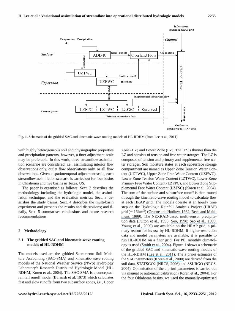
Fig. 2.Map showing the locations of study basins, channel network and stream gauges.

whereT denotes the equivalent Fourier period of the wavelet;s and n denote the scale and location parameter of thewavelet, respectively;WXY

n (s) denotes the cross waveletspectrum of the two time seriesX andY ; =() and<() denotethe imaginary and real parts of the variable bracketed, respec-tively; 〈 〉 denotes the smoothing operation in both time andfrequency domains (Torrence and Compo, 1998). The TE hasa unit of time, e.g., h. A smaller TE means better model per-formance. In our study, a positive/negative TE means thatthe simulated hydrograph leads/trails the observed hydro-graph. Compared to small basins, large basins may producelarge TE because of longer travel time. Further details on thewavelet-based timing error estimation technique are found inLiu et al. (2011).

3 Study basins

Figure 2 shows the nine basins used in this study, and Ta-ble 1 provides additional details on the data used for eachbasin. In Fig. 2, ELDO2 and SLOA4 are nested in the IllinoisRiver basin located near the border of Oklahoma (OK) andArkansas (AR); TIFM7 is a part of the Elk River basin nearthe border of Missouri (MO) and Arkansas (AR); BLUO2 isa headwater basin to the Blue River in southern Oklahoma(OK). These four basins are located in the service area ofthe Arkansas-Red Basin River Forecast Centre (ABRFC).The other five basins, GBHT2, HBMT2, ATIT2, KNLT2,HNTT2, are located in Texas (TX) in the service area ofthe West Gulf River Forecast Centre (WGRFC). Topogra-phy of the ABRFC basins ranges from gently rolling to hillywith the maximum elevation difference between the basin

outlet and the interior exceeding 200 m (Smith et al., 2004).In contrast, topography of the WGRFC basins is generallycharacterised as flat to very flat (Vieux, 2001). Very largerunoff coefficients for HBMT2 and GBHT2 are due mainlyto the large urbanised areas around Houston, TX (Liscum,2001). In particular, HBMT2 has an extremely large runoffcoefficient due to the combined effect of 85 % of the wa-tershed area being highly developed, clayey soils with lowinfiltration rates, and the lower 42 km of the channel be-ing lined with concrete (Vieux, 2001). The basins, BLUO2,KNLT2, HNTT2 and ATIT2 are relatively dry with annualprecipitation of less than 850 mm and runoff coefficientsof less than 0.14 (Table 1). As with HBMT2, these fourbasins are also largely covered by clayey soils. Morphologi-cally, BLUO2 is very elongated. SLOA4 and TIFM7 have aradial channel network with tributaries with similarly-sizeddrainage areas. Figure 3 shows the maps of delineated sub-basins, the soil type and mean event precipitation on theHRAP grid for each basin; selected flood events summarisedin the Table 2 are used to calculate mean event precipitation.In Fig. 3, sub-basins were delineated based on the channelconnectivity information derived from the COTAT algorithm(Reed, 2003) and an area threshold for channel cell identifi-cation, which delineates the channel network the most sim-ilar to the actual channel network. Inter-grid variability ofmean event precipitation ranges from 12 (HBMT2) to 90 mm(HNTT2). The basins BLUO2 and HNTT2 show a clearerpattern of spatial variability of precipitation than the otherbasins. Mean event precipitation in the upper half of theBLUO2 basin is approximately 25 mm smaller than that inthe lower half. Each basin has one or more interior stream

Hydrol. Earth Syst. Sci., 16, 2233–2251, 2012 www.hydrol-earth-syst-sci.net/16/2233/2012/

H. Lee et al.: Variational assimilation of streamflow into operational distributed hydrologic models 2239

48

809

Fig 3. Map of delineated sub-basins, soil type, and mean accumulated rainfall per event. 810

811

812

Fig. 3.Map of delineated sub-basins, soil type and mean accumulated rainfall per event.

gauges (nine for ATIT2). The drainage area ranges from 137(GBHT2) to 2258 (TIFM7) km2.

4 Streamflow DA experiments

4.1 Experimental design and procedure

Simulation experiments were carried out in which stream-flow data were assimilated into the distributed SAC-SMA atthe pre-specified spatiotemporal scale of adjustment. Threestreamflow assimilation scenarios are considered: outlet flowassimilation, interior flow assimilation, and outlet and inte-rior flow assimilation. The experiment is designed to inves-tigate: (1) the effect of spatiotemporal adjustment scale onstreamflow analysis and prediction, (2) the sensitivity of theoptimum spatiotemporal adjustment scale to the streamflowassimilation scenario, and (3) the performance of the DA pro-cedure at the optimum spatiotemporal adjustment scale. Theexperiment is composed of the following four steps:

– Step 1: carry out the base model simulation (i.e., withoutassimilation) and evaluate its performance on stream-flow simulation.

– Step 2: estimate the observational error variances.

– Step 3: given a spatiotemporal adjustment scale, assim-ilate streamflow observations into the model for each of

the three assimilation scenarios, i.e., assimilation of out-let flow, of interior flow, and of both outlet and interiorflows.

– Step 4: repeat Step 3 for each of the nine spatiotemporaladjustment scales.

In Step 2, the sensitivity of the performance of DA onstreamflow observational error variance (σ 2

Q) is examined to

obtain an optmumσ 2Q. In these sensitivity runs, seven dif-

ferent values forσ 2Q (0.01, 0.1, 1, 10, 100, 1000, 10000

(m3 s−1)2) were used for each of three streamflow assim-ilation scenarios. The results show thatσ 2

Q = 10 (m3 s−1)2

yields the best results for streamflow analysis and predictionin terms of RMSE for all basins except TIFM7, for whichσ 2

Q = 100 (m3 s−1)2 was better. For each basin, the optimum

σ 2Q showed largely insensitive to the assimilation scenario

possibly because similar properties associated with flow pro-cesses and channel geometry at upstream and downstreamlocations in the same basin result in the similar amount of er-ror in the estimation of the rating curve and the rating curve-to-flow conversion at those locations. Observational errorvariances for precipitation and PE are taken directly fromSeo et al. (2003). Sample variances calculated from the basemodel simulation for the entire period of record were usedas error variances for background model states (Lee et al.,2011). We assumed that the streamflow observation errors

www.hydrol-earth-syst-sci.net/16/2233/2012/ Hydrol. Earth Syst. Sci., 16, 2233–2251, 2012

2240 H. Lee et al.: Variational assimilation of streamflow into operational distributed hydrologic models

Table 1.Study basins whereA denotes drainage area,NG the number of interior stream gauges in a basin,P mean annual precipitation,Q

mean annual runoff,C runoff coefficient.

Location of Basin and A USGS ID NG Period of P Q C

stream sub-basin (km2) record (mm yr−1) (mm yr−1)gauge at the namebasin outlet

Baron Fork ELDO2 795 7197000 2 Jan 1996– 1163 371 0.32at Eldon, DUTCH 105 7196900OK CHRISTI 65 7196973 Jan 2004

Illinois SLOA4 1489 7195430 3 Apr 2000– 1324 383 0.29River South SAVOY 433 7194800 Jan 2002of Siloam ELMSP 337 7195000Springs, AR CAVESP 90 7194880

Elk river TIFM7 2258 7189000 2 May 2000– 1117 246 0.22near Tiff LANAG 619 7188885 Sep 2006City, MO POWELL 365 7188653

Blue river BLUO2 1232 7332500 1 Oct 2003– 846 117 0.14near Blue, BLUP2 419 7332390 Sep 2006OK

Brays Bayou HBMT2 246 08075000 1 Jan 1997– 1202 1124 0.94at Houston, GSST2 136 08074810 Jul 2009TX

Greens GBHT2 137 08076000 1 Jan 2000– 1467 944 0.64Bayou near HGBT2 95 08075900 Jul 2009Houston, TX

Sandy Creek KNLT2 904 08152000 2 Oct 1997– 767 68 0.09near SNBT2 401 ∗ Sep 2008Kingsland, OXDT2 381 ∗

TX

Guadalupe HNTT2 769 08165500 1 Jan 1998– 697 82 0.12River at HNFT2 438 08165300 Jun 2009Hunt, TX

Onion Creek ATIT2 844 08159000 9 Jan 1997– 752 96 0.13at US Hwy ONIT2 469 08158827 Jun 2009183, Austin, BDUT2 437 ∗

TX DRWT2 321 08158700BRBT2 62 08158819SLHT2 60 08158860AAIT2 49 08158930BCDT2 32 08158810SCAT2 21 08158840WKLT2 16 08158920

∗ denotes stream gauges operated by Lower Colorado River Authority.

are homoscedastic and that the observation errors for pre-cipitation and PE are homogeneous in space. These assump-tions may be lifted in the future in order to more effectivelyconstrain the assimilation problem, relying on advances inuncertainty techniques that properly parameterise and quan-tify uncertainty associated with stage measurement, stage todischarge conversion, and spatial correlation of forcing error(Clark et al., 2008; Mandapaka et al., 2009).

4.2 Results and discussion

In this subsection, the experiment results are comparativelyevaluated. We focus on analysis vs. prediction and depen-dent vs. independent validation to address the questions as-sociated with overfitting due to large degrees of freedom indistributed modelling.

Hydrol. Earth Syst. Sci., 16, 2233–2251, 2012 www.hydrol-earth-syst-sci.net/16/2233/2012/

H. Lee et al.: Variational assimilation of streamflow into operational distributed hydrologic models 2241

Table 2. The length of assimilation window, the number of sub-basins delineated from the channel connectivity map, the number of floodevents denoted asNF and the threshold of streamflow (QT) used to identify flood events.

Basin name ELDO2 SLOA4 TIFM7 BLUO2 HBMT2 GBHT2 KNLT2 HNTT2 ATIT2

Assimilation 36 48 60 60 42 48 36 30 36windowlength (h)

No. of sub- 3 3 5 5 3 3 5 3 3basinsQT (m3 s−1) 200 200 200 100 400 150 200 200 100

NF 17 7 15 7 20 16 15 9 23

49

813

Fig 4. Spatial correlation structure of the streamflow processes. 814

815

Fig. 4.Spatial correlation structure of the streamflow processes.

4.2.1 Analysis of the assimilation problem

Prior to assimilation, we assess for each basin the level ofcomplexity of the assimilation problem by examining thespatial correlation structure of observed and base-simulatedstreamflow, and the basin characteristics such as spatial het-erogeneity of soil and precipitation. Figure 4 presents thecorrelation-based matrices of streamflow. In Fig. 4, the cor-relation coefficients were calculated using streamflow dataat any paired gauges (i.e., interior and outlet as well as in-terior and interior). The data were paired at concurrent timesteps due to the difficulty of correctly estimating travel timefor all paired gauges. Correlations of time-lagged simulatedinterior and outlet flow as a function of a lag time closely fol-lowed those based on streamflow observations. This supportsthe idea of using correlation matrices in Fig. 4 for analysingspatial correlation structure of streamflow. The 1st row ofFig. 4 presents ther1-matrices (see Eq. 9) showing the spa-tial correlation of observed streamflow. In all correlation ma-trices, the stream gauges are sorted in the increasing or-der of the drainage area starting from the bottom-left cor-ner. Note in Fig. 4 that, for most basins, observed stream-flow at the outlet is highly correlated with that at interiorlocations. For BLUO2, the low correlation between the in-terior and outlet flows may be due to the distance betweenthe two and large variability in precipitation. For ELDO2,

the weak spatial correlation in flow between the outlet andDUTCH may be contributed by the different soil types. ForATIT2, the upstream flows at some interior gauges, particu-larly SCAT2 and BCDT2, are weakly correlated with down-stream flows at BDUT2 and at the outlet. This may be due tothe small drainage areas involved and the locations of SCAT2and BCDT2 being on minor tributaries. The 2nd row in Fig. 4shows ther1-matrices of streamflow from base model simu-lation, and the 3rd row in Fig. 4 presentsr2-matrices (Eq. 10)of observed and simulated flows prior to assimilation, respec-tively. Both r1- andr2-matrices in the 2nd and 3rd rows inFig. 4 indicate that the model simulation generally well re-produces the spatial correlation of streamflow at two loca-tions in a basin, particularly for GBHT2, HBMT2, HNTT2and KNLT2 for which the differences in correlation betweenobserved and simulated streamflow (off-diagonal terms inr2) are less than 0.1. In addition to the absolute value ofr2 off-diagonal terms, the unity of their signature is treatedas another information associated with the degree of com-plexity of the assimilation problem; that is, overall overes-timation or underestimation of spatial correlation structureof the streamflow is considered less ill-posed than combina-tion of over- and under-estimation. In the latter case, inde-pendent validation results posterior to the assimilation maybenefit less at any adjustment scales than the former due to

www.hydrol-earth-syst-sci.net/16/2233/2012/ Hydrol. Earth Syst. Sci., 16, 2233–2251, 2012

2242 H. Lee et al.: Variational assimilation of streamflow into operational distributed hydrologic models

50

816

Fig 5. Mean skill score of streamflow analysis where mean skill score is obtained by averaging 817

mean squared error-based skill score calculated for individual event (D: distributed, S: semi-818

distributed, L: lumped, 1: 1-hr, 6: 6-hr, W: the length of time equal to that of the assimilation 819

window). 820

821

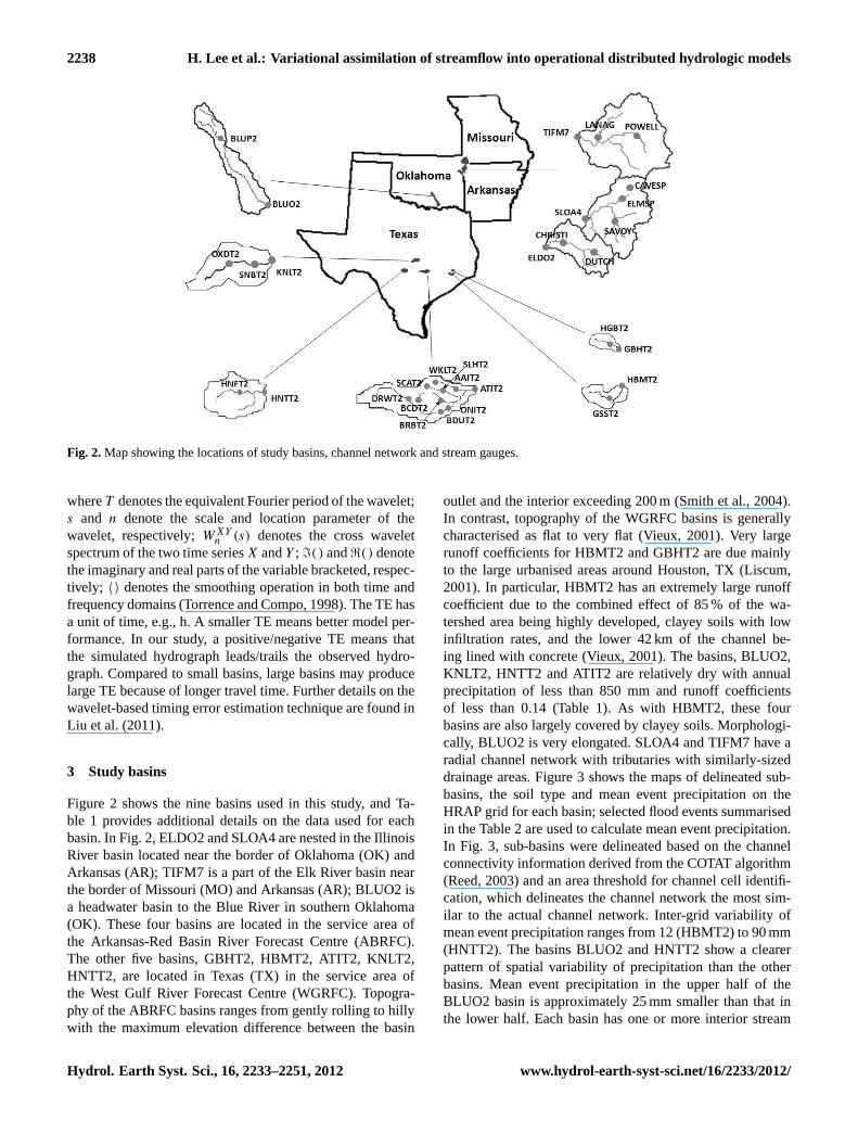
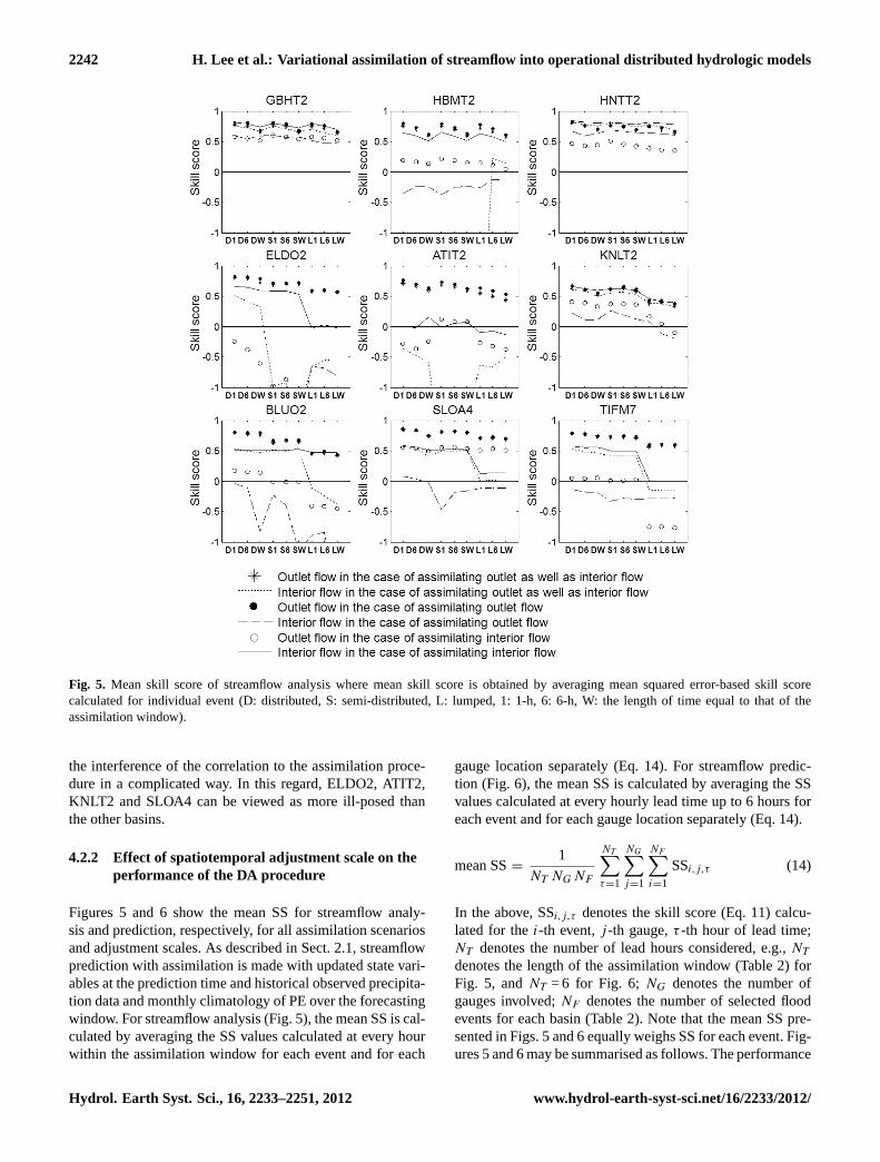
Fig. 5. Mean skill score of streamflow analysis where mean skill score is obtained by averaging mean squared error-based skill scorecalculated for individual event (D: distributed, S: semi-distributed, L: lumped, 1: 1-h, 6: 6-h, W: the length of time equal to that of theassimilation window).

the interference of the correlation to the assimilation proce-dure in a complicated way. In this regard, ELDO2, ATIT2,KNLT2 and SLOA4 can be viewed as more ill-posed thanthe other basins.

4.2.2 Effect of spatiotemporal adjustment scale on theperformance of the DA procedure

Figures 5 and 6 show the mean SS for streamflow analy-sis and prediction, respectively, for all assimilation scenariosand adjustment scales. As described in Sect. 2.1, streamflowprediction with assimilation is made with updated state vari-ables at the prediction time and historical observed precipita-tion data and monthly climatology of PE over the forecastingwindow. For streamflow analysis (Fig. 5), the mean SS is cal-culated by averaging the SS values calculated at every hourwithin the assimilation window for each event and for each

gauge location separately (Eq. 14). For streamflow predic-tion (Fig. 6), the mean SS is calculated by averaging the SSvalues calculated at every hourly lead time up to 6 hours foreach event and for each gauge location separately (Eq. 14).

mean SS=1

NT NG NF

NT∑τ=1

NG∑j=1

NF∑i=1

SSi,j,τ (14)

In the above, SSi,j,τ denotes the skill score (Eq. 11) calcu-lated for thei-th event,j -th gauge,τ -th hour of lead time;NT denotes the number of lead hours considered, e.g.,NT

denotes the length of the assimilation window (Table 2) forFig. 5, andNT = 6 for Fig. 6; NG denotes the number ofgauges involved;NF denotes the number of selected floodevents for each basin (Table 2). Note that the mean SS pre-sented in Figs. 5 and 6 equally weighs SS for each event. Fig-ures 5 and 6 may be summarised as follows. The performance

Hydrol. Earth Syst. Sci., 16, 2233–2251, 2012 www.hydrol-earth-syst-sci.net/16/2233/2012/

H. Lee et al.: Variational assimilation of streamflow into operational distributed hydrologic models 2243

51

822

Fig 6. Same as Fig 5 but for streamflow prediction for 1- to 6-hr lead time. 823

824

825

Fig. 6.Same as Fig. 5, but for streamflow prediction for 1- to 6-h lead time.

of DA is less sensitive to the temporal adjustment scale thanthe spatial adjustment scale. The basins with high spatial cor-relation between interior and outlet flows (GBHT2, HBMT2,HNTT2), show less sensitive in DA performance to the spa-tial adjustment scale than those with lower correlation. ForBLUO2, lumped adjustment yields less improvement thanother assimilation cases due possibly to the low spatial cor-relation of interior and outlet flows. In a number of indepen-dent validation cases (i.e., validating assimilation results withstreamflow data not used in the assimilation), the mean SS forstreamflow analysis is less than zero, suggesting overfitting.For GBHT2, HNTT2 and KNLT2, assimilating interior flowsproduced positive mean SS for streamflow prediction for thefirst 6 h of lead time at both interior and outlet locations.However, assimilating outlet flow generally degrades interiorflow prediction for most basins, compared to the base modelsimulation. This implies assimilating interior flow makes theDA problem less subject to overfitting. Note that some events

are affected by timing errors in the model simulation whichare partially responsible for small to negative mean SS forsome cases. We further discuss timing errors at the end ofthis section.

To further examine the sensitivity of DA performanceto the adjustment scale, Figs. 7 and 8 show the box-and-whiskers plot of the mean SS shown in Figs. 5 and 6, respec-tively. In Figs. 7 and 8, each box-and-whiskers plot is con-structed with 27 samples resulted from the combinations ofnine basins and three (space or time) scales. Figures 7 and 8can be summarised as follows. The performance of DA isgenerally higher at finer adjustment scales and is more sen-sitive to the spatial adjustment scale than the temporal ad-justment scale in terms of both the median SS and the in-terquartile range of the SS. The DA performance greatly de-pends on the streamflow assimilation scenario, i.e., assim-ilating outlet and/or interior flow data. Assimilating outletflow does not improve interior flow simulation in most cases,

www.hydrol-earth-syst-sci.net/16/2233/2012/ Hydrol. Earth Syst. Sci., 16, 2233–2251, 2012

2244 H. Lee et al.: Variational assimilation of streamflow into operational distributed hydrologic models

52

826

Fig 7. Mean skill score vs. spatial adjustment scale where the mean skill score is obtained by 827

averaging mean squared error-based skill score calculated for individual event. Mean skill score for 828

the prediction period is calculated using streamflow predicted for 1- to 6-hr lead time. In the above, 829

D, S, and L denote distributed, semi-distributed, and lumped ways of adjusting the SAC-states, 830

respectively; Qo&Qi DA, Qo DA, and Qi DA denote both outlet and interior flow assimilation, 831

outlet flow assimilation, and interior flow assimilation, respectively. 832

833

Fig. 7.Mean skill score vs. spatial adjustment scale where the meanskill score is obtained by averaging mean squared error-based skillscore calculated for individual event. Mean skill score for the pre-diction period is calculated using streamflow predicted for 1- to6-h lead time. In the above, D, S, and L denote distributed, semi-distributed and lumped ways of adjusting the SAC-states, respec-tively; Qo & Qi DA, Qo DA and Qi DA denote both outlet and in-terior flow assimilation, outlet flow assimilation and interior flowassimilation, respectively.

whereas, not surprisingly, assimilating interior flows typi-cally improves outlet flow simulation to some degree. Thisindicates the difficulty of propagating the information con-tained in outlet flow data backward (i.e., upstream) throughthe stream network and the hydrologic processes involved toimprove prediction of interior flow.

For the three different assimilation scenarios, “optimum”spatiotemporal scales are selected for interior and outlet flowpredictions (Fig. 9). The selection is based on the meanSS for streamflow analysis or prediction shown in Figs. 5and 6. Not surprisingly, a number of cases in streamflowanalysis showed the largest improvement with the finestspatiotemporal scale of adjustment. For streamflow predic-tion, on the other hand, the optimum scale of adjustmentis spread over a broader range. This indicates the possiblelarge over-adjustment of state variables in the cases of dis-tributed, hourly adjustment. Despite the issue associated withthe over-fitting problem, the cases of distributed, hourly ad-justment generally produce the best assimilation results incomparison to other adjustment scales.

53

834

Fig. 8. Same as Fig. 7 but for the temporal adjustment scale. Here 1, 6, and W denote adjusting 835

mean field bias in the precipitation and potential evaporation data on an 1-hr or 6-hr basis, or 836

uniformly over the entire assimilation window, respectively. 837

838

Fig. 8. Same as Fig. 7, but for the temporal adjustment scale. Here1, 6 and W denote adjusting mean field bias in the precipitation andpotential evaporation data on an 1-h or 6-h basis, or uniformly overthe entire assimilation window, respectively.

4.2.3 Performance of the DA procedure at the optimumspatiotemporal adjustment scale

For more detailed quantitative analysis of the assimilationresults, we chose a single optimum adjustment scale foreach basin which produces reasonable assimilation results,based on mean SS in Figs. 5 and 6, for analysis and pre-diction of interior and outlet flows. The selected adjustmentscales are semi-distributed and hourly for GBHT2, lumpedand hourly for HBMT2 and distributed and hourly for allthe other basins. Figure 10 shows the RMSE of streamflowanalysis and prediction evaluated at every hour of lead timefor each basin and for each assimilation scenario. Figure 11shows the amount of reduction in the RMSE of streamflowanalysis and prediction for all basins collectively. Figure 12shows the timing error estimates from streamflow analysisand prediction for each assimilation scenario.

To diagnose streamflow analysis similarly to Fig. 4, we ex-amined the spatial correlation structure of streamflow anal-ysis at the optimum spatiotemporal adjustment scale (notshown). The spatial correlation between observed and simu-lated flows at both interior and outlet locations are generallyimproved for all basins by assimilating streamflow data, butat the expense of slightly adjusting spatial correlation struc-ture of streamflow. Especially, for ELDO2, the spatial corre-lation between CHRISTIE and the outlet is improved notice-ably after streamflow assimilation whereas, for ATIT2 and

Hydrol. Earth Syst. Sci., 16, 2233–2251, 2012 www.hydrol-earth-syst-sci.net/16/2233/2012/

H. Lee et al.: Variational assimilation of streamflow into operational distributed hydrologic models 2245

54

839

Fig. 9. Optimum spatiotemporal scales of adjustment for streamflow analysis and prediction for 840

each basin and assimilation scenario. Underscored italic letters represent interior flow results and 841

the others represent outlet flow results (A: ATIT2, B: BLUO2, E: ELDO2, G: GBHT2, Hb: 842

HBMT2, Hn: HNTT2, K: KNLT2, S: SLOA4, T: TIFM7). 843

844

845

Fig. 9.Optimum spatiotemporal scales of adjustment for streamflow analysis and prediction for each basin and assimilation scenario. Under-scored italic letters represent interior flow results and the others represent outlet flow results (A: ATIT2, B: BLUO2, E: ELDO2, G: GBHT2,Hb: HBMT2, Hn: HNTT2, K: KNLT2, S: SLOA4, T: TIFM7).

KNLT2, the spatial correlation at some paired gauges was re-duced after streamflow assimilation compared to that of basemodel simulation. This indicates that the performance gainsfrom the DA do not always lead to improving the spatial cor-relation structure of the streamflow, a possible symptom ofover-adjustment. In addition, examining the spatial correla-tion structure of streamflow at all adjustment scales indicatedthat, compared to outlet flow assimilation, interior flow as-similation produces correlation structure that is more consis-tent with that of observed streamflow. This may be explainedby the local information available in interior flow observa-tions which is diluted at the outlet location due to the varioushydrologic and hydraulic processes involved.

Figure 10 shows the RMSE of streamflow as a functionof lead time. The lead time is negative over the assimila-tion window and positive over the prediction horizon. ForGBHT2, HBMT2 and HNTT2, all three assimilation scenar-ios improved both streamflow analysis and prediction. Thesebasins show high spatial correlation between interior and out-let flows and the base model simulation reproduces the spa-tial correlation structure very well (see Fig. 4). For ill-posedbasins ELDO2, ATIT2, KNLT2 and SLOA4, there is an indi-cation of over-adjustment for streamflow analysis and predic-tion. For ELDO2, over-adjustment is not conspicuous pos-sibly due to the smaller basin size and the relatively betterbase model simulation than the other ill-posed basins. ForBLUO2, weak spatial correlation between interior and outletflow may explain little improvement in streamflow at gaugelocations where the data were not assimilated. The basinTIFM7 also shows similar results as BLUO2. It is noted that

for TIFM7 we use an observational error variance ten timeslarger than that for the other basins. This may have consid-erably reduced the amount of adjustment to state variablesat most cells. Overall, assimilating streamflow data generallyproduces, expectedly, improved streamflow analysis and pre-diction at that gauge location. The margin of improvementat other locations varies, depending on the level of under-determinedness and basin characteristics.

Figure 11 shows the margin of reduction in the RMSEof streamflow analysis and prediction due to the assimila-tion versus the peak flow of selected events. To evaluate theoverall performance of the VAR procedure, each plot is con-structed with simulations from all nine basins. Assimilatinginterior flow yielded similar improvement (14 % reduction inRMSE with assimilation) to outlet flow assimilation in outletflow prediction for the first 6 h of lead time. In contrast, in thecase of outlet flow assimilation, gains in interior flow analy-sis (19 % reduction in RMSE after the assimilation) did notlead to improvement in multi-basin averaged skill in interiorflow prediction over the first 6 lead hours, even though break-down into each basin showed RMSE reduction by assimila-tion ranging from−31 % (ATIT2) to 14 % (GBHT2). Thisindicates that the outlet flow assimilation case is more vul-nerable to overfitting than the interior flow assimilation case.Assimilating both outlet and interior flows outperforms theoutlet flow assimilation case in terms of outlet flow predic-tion (22 % vs. 14 % reduction in RMSE with assimilation),although outlet flow analysis is less improved (55 % vs. 59 %reduction in RMSE with assimilation). This shows the value

www.hydrol-earth-syst-sci.net/16/2233/2012/ Hydrol. Earth Syst. Sci., 16, 2233–2251, 2012

2246 H. Lee et al.: Variational assimilation of streamflow into operational distributed hydrologic models

55

846

Fig. 10. RMSE of streamflow vs. lead hour where the lead hour is negative within the assimilation 847

window. 848

849

850

Fig. 10.RMSE of streamflow vs. lead hour where the lead hour is negative within the assimilation window.

of additionally assimilating interior flow for streamflow pre-diction at the basin outlet.

Phase (or timing) and flow magnitude are the two distinc-tive attributes in hydrograph evaluation (Liu et al., 2011). Toexamine the performance of DA, we also examine the tim-ing error of a hydrograph within the assimilation and pre-diction windows separately as estimated via wavelet anal-ysis (Liu et al., 2011) (see Eq. 13). Note that our timingerror analysis is somewhat exploratory because of the ob-jective equation, Eq. (7), used in this study, which includesno explicit timing error modelling component. Figure 12shows the box-and-whiskers plots of the timing error esti-mates of simulated hydrographs that characterise inter-basinand inter-event variability. In Fig. 12, the reference is theevent-scale timing error in the base simulation. On the whole,timing errors in the simulated hydrographs following assim-ilation at both outlet and interior stream gauge locations for

the assimilation period are generally smaller than the refer-ence. While flow timing errors for the prediction period areless improved via streamflow assimilation, their medians aremostly free of timing error especially in the case of outletflow. For events with significant timing errors in the risinglimb, the assimilation procedure slightly improved the tim-ing of streamflow analysis, but yielded significant magnitudeerrors in predicted flows. Examples of this are illustrated inFig. 13. Note in the figure that the base model simulation forEvent A shows significant timing errors in the rising limb,peak flow and the overall shape of the hydrograph, whereasEvent B has smaller timing errors than Event A. The abovesituation arises due to lack of timing error modelling in theDA formulation used in this study (see Eq. 7). As a result,the VAR procedure over-adjusts control variables to com-pensate for timing errors in streamflow analysis which re-sult in magnitude errors in predicted flows. Further analysis

Hydrol. Earth Syst. Sci., 16, 2233–2251, 2012 www.hydrol-earth-syst-sci.net/16/2233/2012/

H. Lee et al.: Variational assimilation of streamflow into operational distributed hydrologic models 2247

56

851

Fig. 11. Reduction in the RMSE of streamflow analysis due to the assimilation vs. peak flows of 852

selected events summarized in Table 2 (top panel); the bottom panel shows the same but for 853

Fig. 11.Reduction in the RMSE of streamflow analysis due to the assimilation vs. peak flows of selected events summarised in Table 2 (toppanel); the bottom panel shows the same but for streamflow prediction for 1- to 6-h lead time. The RMSE is calculated for each event andindividual lead hour separately. The figure in the parenthesis denotes the percentage reduction in RMSE after the assimilation.

based onr2-matrices indicates that the assimilation problemfor events with timing errors of 3 h or bigger in the risinglimb or peak flow simulation is more ill-posed than the otherevents, and that the spatial correlation structure of streamflowfrom the entire simulation appear to be very similar to that of

events with timing errors. To address the above issues, tim-ing errors must be dealt with explicitly, a topic left for futureendeavours.

www.hydrol-earth-syst-sci.net/16/2233/2012/ Hydrol. Earth Syst. Sci., 16, 2233–2251, 2012

2248 H. Lee et al.: Variational assimilation of streamflow into operational distributed hydrologic models

57

streamflow prediction for 1- to 6-hr lead time. The RMSE is calculated for each event and 854

individual lead hour separately. The figure in the parenthesis denotes the percentage reduction in 855

RMSE after the assimilation. 856

857

858

859

860

861

Fig. 12. Timing error estimates in the simulation of outlet and interior flows. The box-plot 862

characterizes both inter-basin and event-to-event variability. 863

864

Fig. 12.Timing error estimates in the simulation of outlet and interior flows. The box-plot characterises both inter-basin and event-to-eventvariability.

5 Conclusion and future work

The importance of hydrologic DA has been emphasised bymany researchers as a unifying approach to accounting fordifferent error sources in hydrologic model simulations in acohesive manner and improving skill in streamflow predic-tion (Aubert et al., 2003; Liu and Gupta, 2007; Seo et al.,2003, 2009; Clark et al., 2008; Vrugt et al., 2006). Com-pared to lumped models, distributed rainfall-runoff modelsare subject to overfitting to a much greater extent due to largedimensionality of the inverse problem involved. In this work,we investigated the effects of the spatiotemporal scale of ad-justment in assimilating streamflow data at outlet and/or in-terior locations into the NWS’s Hydrology Laboratory Re-search Distributed Hydrologic Model (HL-RDHM, Koren etal., 2004). The assimilation technique used is variational as-similation similar to those used in Seo et al. (2009) withlumped models and Lee et al. (2011) with distributed models.For large sample evaluation, we used 4 basins in Oklahomaand 5 basins in Texas in the US.

The main conclusions from this study are as follows:

– The optimum spatiotemporal scale of adjustment variesfrom basin to basin and between streamflow analysisand prediction. The latter indicates over-adjustment ofstate variables. The performance of the assimilation pro-cedure is more sensitive to the spatial scale of adjust-ment than the temporal scale. The preferred strategyidentified in this study is to adjust the state variables ina spatially distributed manner and precipitation and PEon an hourly basis, despite the fact that validation with

streamflow at interior and outlet gauge locations at thisadjustment scale may indicate overfitting in some cases.

– The quality of streamflow analysis and prediction ishighly dependent on the availability of streamflow dataat interior locations. At the optimum spatiotemporal ad-justment scale, assimilating interior flow and assimilat-ing outlet flow yielded comparable improvement (14 %reduction in RMSE after the assimilation) in outlet flowprediction for the first 6 h of lead time. However, out-let flow assimilation produced degraded interior flowprediction for the first 6-h lead time (10 % increase inRMSE after assimilation), but 15 % reduction in RMSEin the case of assimilating interior flow observations.This indicates that, as one might expect, outlet flow as-similation is more susceptible to overfitting than inte-rior flow assimilation. Assimilating both outlet and inte-rior flows outperforms assimilating outlet flow only forstreamflow prediction at the outlet (22 % vs. 14 % re-duction in RMSE with assimilation), indicating the im-portance of additionally assimilating interior flow.

– Basins with highly correlated interior and outlet flowstend to benefit more from streamflow assimilation andbe less sensitive to the adjustment scale. Streamflow as-similation at most adjustment scales generally improvesthe match in the interstation correlation pattern betweenthe observed and the simulated flows. Compared to out-let flow assimilation, interior flow assimilation repro-duces better the spatial correlation structure of observedflow. This may be explained by the local informationavailable in interior flow observations, whereas at the

Hydrol. Earth Syst. Sci., 16, 2233–2251, 2012 www.hydrol-earth-syst-sci.net/16/2233/2012/

H. Lee et al.: Variational assimilation of streamflow into operational distributed hydrologic models 2249

58

865

Fig. 13. Streamflow evaluated at the outlet and interior gauge locations for two events in HNTT2. 866

The adjustment scale used is distributed and hourly. The data assimilated is outlet flow. Each curve 867

represents analysis (at the prediction time) and prediction of hourly streamflow generated at 868

different prediction time. 869

870

871

Fig. 13.Streamflow evaluated at the outlet and interior gauge locations for two events in HNTT2. The adjustment scale used is distributedand hourly. The data assimilated is outlet flow. Each curve represents analysis (at the prediction time) and prediction of hourly streamflowgenerated at different prediction time.

outlet location the information is diluted, or fuzzed up,due to the various intervening hydrologic and hydraulicprocesses.

– Timing errors in streamflow analysis and prediction arefound to be largely related to the ill-posedness of the as-similation problem, which was diagnosed using the in-formation associated with the spatial correlation struc-ture of streamflow. In the cases of events with signifi-cant timing errors in rising limb, the assimilation proce-dure yielded large magnitude errors in streamflow pre-diction followed by slight improvement in the timing ofstreamflow analysis. This indicates error compensationwith over-adjusting state variables due partly to a lackof timing error modelling component in the objectivefunction used in this study.

The future work should include improving the DAmethodology to account for timing errors explicitly, account-ing for the model structural error (Van Loon and Troch, 2002;Chen et al., 2011) by applying the model as a weak constraint(Zupanski, 1997), and generalising the procedure in an en-semble framework via, e.g., maximum likelihood ensemblefilter (Zupanski, 2005).

Acknowledgements.This work is supported by the AdvancedHydrologic Prediction Service (AHPS) programme of the NationalWeather Service (NWS). This support is gratefully acknowledged.The first author is grateful to Pedro Restrepo and Minxue Hefor helpful comments on the manuscript. We are also gratefulto Guillaume Thirel and the anonymous reviewer for many veryhelpful comments.

Edited by: F. Pappenberger

References

Aubert, D., Loumagne, C., and Oudin, L.: Sequential assimilationof soil moisture and streamflow data in a conceptual rainfall-runoff model, J. Hydrol., 280, 145–161, 2003.

Brocca, L., Melone, F., Moramarco, T., Wagner, W., Naeimi, V.,Bartalis, Z., and Hasenauer, S.: Improving runoff predictionthrough the assimilation of the ASCAT soil moisture product,Hydrol. Earth Syst. Sci., 14, 1881–1893,doi:10.5194/hess-14-1881-2010, 2010.

Bulygina, N. and Gupta, H.: Estimating the uncertain math-ematical structure of a water balance model via Bayesiandata assimilation, Water Resour. Res., 45, W00B13,doi:10.1029/2007WR006749, 2009.

www.hydrol-earth-syst-sci.net/16/2233/2012/ Hydrol. Earth Syst. Sci., 16, 2233–2251, 2012

2250 H. Lee et al.: Variational assimilation of streamflow into operational distributed hydrologic models

Burnash, R. J., Ferral, R. L., and McGuire, R. A.: A generalizedstreamflow simulation system: conceptual modelling for digitalcomputers, US Department of Commerce National Weather Ser-vice and State of California, Department of Water Resources,1973.

Chen, F., Crow, W. T., Starks, P. J., and Moriasi, D. N.: Improv-ing hydrologic predictions of a catchment model via assimila-tion of surface soil moisture, Adv. Water Resour., 34, 526–536,doi:10.1016/j.advwatres.2011.01.011, 2011.

Clark, M. P., Rupp, D. E., Woods, R. A., Zhend, X., Ibbitt, R. P.,Slater, A. G., Schmidt, J., and Uddstrom, M. J.: Hydrologicaldata assimilation with the ensemble Kalman filter: Use of stream-flow observations to update states in a distributed hydrologicalmodel, Adv. Water Resour., 31, 1309–1324, 2008.

Doucet, A., De Freitas, N., and Gordon, N.: Sequential Monte CarloMethods in Practice, Springer, New York, USA, 2001.

Droegemeier, K. K., Smith, J. D., Businger, S., Dosell III, C., Doyle,J., Duffy, C., Foufoula-Georgiou, E., Graziano, T., James, L. D.,Krajewski, V., LeMone, M., Lettenmaier, D., Mass, C., PielkeSr., R., Ray, P., Rutledge, S., Schaake, J., and Zipser, E.: Hydro-logical aspects of weather prediction and flood warnings: Reportof the 9th Prospectus Development Team of the U.S. Weather Re-search Program, B. Am. Meteorol. Soc., 81, 2665–2680, 2000.

Fulton, R. A., Breidenbach, J. P., Seo, D.-J., and Miller, D. A.:WSR-88D rainfall algorithm, Weather Forecast., 13, 377–395,1998.

Greene, D. R. and Hudlow, M. D.: Hydrometeorologic grid map-ping procedures, AWRA International Symposium on Hydrome-teor, Denver, CO, 1982.

Knutson, T. R., McBride, J. L., Chan, J., Emanuel, K., Holland, G.,Landsea, C., Held, I., Kossin, J. P., Srivastava, A. K., and Sugi,M.: Tropical cyclones and climate change, Nat. Geosci., 3, 157–163, 2010.

Koren, V., Smith, M., Wang, D., and Zhang, Z.: Use of soil propertydata in the derivation of conceptual rainfall-runoff model param-eters, Proceedings of the 15th Conference on Hydrology, AMS,Long Beach, CA, 103–106, 2000.

Koren, V., Reed, S., Smith, M., Zhang, Z., and Seo, D. J.: Hydrol-ogy Laboratory Research Modelling System (HL-RMS) of theU.S. National Weather Service, J. Hydrol., 291, 297–318, 2004.

Krzysztofowicz, R.: Bayesian theory of probabilistic forecasting viadeterministic hydrologic model, Water Resour. Res., 35, 2739–2750, 1999.

Lee, H., Seo, D.-J., and Koren, V.: Assimilation of streamflow andin-situ soil moisture data into operational distributed hydrologicmodels: Effects of uncertainties in the data and initial model soilmoisture states, Adv. Water Resour., 34, 1597–1615, 2011.

Lewis, J. M., Lakshmivarahan, S., and Dhall, S. K.: Dynamic DataAssimilation: A Least Squares Approach, Cambridge UniversityPress, 2006.

Liscum, F.: Effects of urban development on stormwater runoffcharacteristics for the Houston, Texas, metropolitan area,USGS Water-Resources Investigations Report 01-4071, U.S.Dept. of the Interior, US Geological Survey, Austin, Texas, 2001.

Liu, Y. and Gupta, H. V.: Uncertainty in hydrologic modelling: To-ward an integrated data assimilation framework, Water Resour.Res., 43, W07401,doi:10.1029/2006WR005756, 2007.

Liu, Y., Brown, J., Demargne, J., and Seo, D.-J.: A wavelet-basedapproach to assessing timing errors in hydrologic predictions, J.Hydrol., 397, 210–224, 2011.

Mandapaka, P. V., Krajewski, W. F., Ciach, G. J., Villarini, G., andSmith, J. A.: Estimation of radar-rainfall error spatial correlation,Adv. Water Resour., 32, 1020–1030, 2009.

McLaughlin, D.: An integrated approach to hydrologic data assim-ilation: interpolation, smoothing, and filtering, Adv. Water Re-sour., 25, 1275–1286, 2002.

Milly, P. C. D., Betancourt, J., Falkenmark, M., Hirsch, R. M.,Kundzewicz, Z. W., Lettenmaier, D. P., and Stouffer, R. J.: Sta-tionarity is dead: Whither water management?, Science, 319,573–574, 2008.

Min, S.-K., Zhang, X., Zwiers, F. W., and Hegerl, G. C.: Humancontribution to more-intense precipitation extremes, Nature, 470,378–381, 2011.

Moradkhani, H.: Hydrologic remote sensing and land surface dataassimilation, Sensors, 8, 2986–3004, 2008.

Moradkhani, H., Sorooshian, S., Gupta, H. V., and Hauser, P.R.: Dual state-parameter estimation of hydrological models us-ing ensemble Kalman filter, Adv. Water Resour., 28, 135–147,2005a.

Moradkhani, H., Hsu, K., Gupta, H. V., and Sorooshian, S.: Un-certainty assessment of hydrologic model states and parameters:Sequential data assimilation using particle filter, Water Resour.Res., 41, W05012,doi:10.1029/2004WR003604, 2005b.

Murphy, A. H.: General decompositions of MSE-based skill scores:Measures of some basic aspects of forecast quality, Mon.Weather Rev., 124, 2353–2369, 1996.

NHWC – National Hydrologic Warning Council, 2002: Use andbenefits of the National Weather Service River and Flood Fore-casts, available on line athttp://www.nws.noaa.gov/oh/aAHPS/AHPS%20Benefits.pdf(last access: 3 January 2012), 2002.

NRC – National Research Council: When weather matters: Sci-ence and service to meet critical societal needs, the NationalAcademies Press, Washington, D.C., 2010.

NRCS – Natural Resources Conservation Service, United StatesDepartment of Agriculture: Soil Survey Geographic (SSURGO)Database, available on line athttp://soildatamart.nrcs.usda.gov(last access: 19 July 2012), 2004.

NRCS – Natural Resources Conservation Service, United StatesDepartment of Agricultur: US General Soil Map (STATSGO2),available on line athttp://soildatamart.nrcs.usda.gov(last access:19 July 2012), 2006.

Pauwels, V. R. N. and De Lannoy, G. J. M.: Improvement of mod-eled soil wetness conditions and turbulent fluxes through the as-similation of observed discharge, J. Hydrometeorol., 7, 458–477,2006.

Pham, D. T.: Stochastic methods for sequential data assimilationin strongly nonlinear systems, Mon. Weather Rev., 129, 1194–1207, 2001.

Press, W. H., Teukolsky, S. A., Vetterling, W. T., and Flannery, B.P.: Numerical recipes in fortran, 2nd Edn., Cambridge UniversityPress, New York, USA, 1992.

Reed, S. M.: Deriving flow directions for coarse-resolution (1–4 km) gridded hydrologic modelling, Water Resour. Res., 39,1238,doi:10.1029/2003WR001989, 2003.

Hydrol. Earth Syst. Sci., 16, 2233–2251, 2012 www.hydrol-earth-syst-sci.net/16/2233/2012/

H. Lee et al.: Variational assimilation of streamflow into operational distributed hydrologic models 2251

Reed, S. M. and Maidment, D. R.: Coordinate transformations forusing NEXRAD data in GIS-based hydrologic modelling, J. Hy-drol. Eng., 4, 174–183, 1999.

Seo, D.-J.: Real-time estimation of rainfall fields using radar rainfalland rain gauge data, J. Hydrol., 208, 37–52, 1998.

Seo, D.-J., Breidenbach, J. P., and Johnson, E. R.: Real-time esti-mation of mean field bias in radar rainfall data, J. Hydrol., 223,131–147, 1999.

Seo, D.-J., Koren, V., and Cajina, N.: Real-time variational assimila-tion of hydrologic and hydrometeorological data into operationalhydrologic forecasting, J. Hydrometeorol., 4, 627–641, 2003.

Seo, D.-J., Herr, H. D., and Schaake, J. C.: A statistical post-processor for accounting of hydrologic uncertainty in short-rangeensemble streamflow prediction, Hydrol. Earth Syst. Sci. Dis-cuss., 3, 1987–2035,doi:10.5194/hessd-3-1987-2006, 2006.

Seo, D.-J., Cajina, L., Corby, R., and Howieson, T.: Automatic stateupdating for operational streamflow forecasting via variationaldata assimilation, J. Hydrol., 367, 255–275, 2009.

Seo, D.-J., Demargne, J., Wu, L., Liu, Y., Brown, J. D., Regonda,S., and Lee, H.: Hydrologic ensemble prediction for risk-basedwater resources management and hazard mitigation, Joint Fed-eral Interagency Conference on Sedimentation and HydrologicModelling (JFIC2010), 27 June–1 July 2010, Las Vegas, Nevada,USA, 2010.

Smith, M. B., Laurine, D. P., Koren, V. I., Reed, S. M., and Zhang,Z.: Hydrologic Model Calibration in the National Weather Ser-vice, in: Calibration of Watershed Models, Water Science andApplication 6, edited by: Duan, Q., Gupta, H., Sorooshian, S.,Rousseau, A., and Turcotte, R., AGU Press, Washington, D.C.,133–152, 2003.

Smith, M. B., Seo, D.-J., Koren, V. I., Reed, S. M., Zhang, Z., Duan,Q., Moreda, F., and Cong, S.: The distributed model intercompar-ison project (DMIP): motivation and experiment design, J. Hy-drol., 298, 4–26, 2004.

Torrence, C. and Compo, G. P.: A practical guide to wavelet analy-sis, B. Am. Meteorol. Soc., 79, 61–78, 1998.

Trapp, R. J., Diffenbaugh, N. S., Brooks, H. E., Baldwin, M. E.,Robinson, E. D., and Pal, J. S.: Changes in severe thunderstormenvironment frequency during the 21st century caused by anthro-pogenically enhanced global radiative forcing, P. Natl. Acad. Sci.USA, 104, 19719–19723, 2007.

Trenberth, K. E., Dai, A., Rasmussen, R. M., and Parsons, D. B.:The changing character of precipitation, B. Am. Meteorol. Soc.,84, 1205–1217, 2003.

Troch, P. A., Paniconi, C., and McLaughlin, D.: Catchment-scalehydrological modelling and data assimilation, Adv. Water Re-sour., 26, 131–135, 2003.

USACE – US Army Corps of Engineers: Annual Flood DamageReport to Congress for Fiscal Year 2000, USACE, Washington,D.C., 2000.

van Loon, E. E. and Troch, P. A.: Tikhonov regularization as atoll for assimilating soil moisture data in distributed hydrolog-ical models, Hydrol. Process., 16, 531–556, 2002.

Vieux, B. E.: Distributed hydrologic modelling using GIS, KluwerAcademic Publishers, 2001.

Vrugt, J. A., Diks, C. G. H., Gupta, H. V., Bouten, W., andVerstaten, J. M.: Improved treatment of uncertainty in hydro-logic modelling: Combining the strengths of global optimiza-tion and data assimilation, Water Resour. Res., 41, W01017,doi:10.1029/2004WR003059, 2005.

Vrugt, J. A., Gupta, H. V., Nuallain, B., and Bouten, W.: Real-TimeData Assimilation for Operational Ensemble Streamflow Fore-casting, J. Hydrometeorol., 7, 548–565, 2006.

Weerts, A. H. and El Serafy, G. Y. H.: Particle filtering and ensem-ble Kalman filtering for state updating with hydrological con-ceptual rainfall-runoff models, Water Resour. Res., 42, W09403,doi:10.1029/2005WR004093, 2006.

Young, C. B., Bradley, A. A., Krajewski, W. F., and Kruger, A.:Evaluating NEXRAD multisensor precipitation estimates for op-erational hydrologic forecasting, J. Hydrometeorol., 1, 241–254,2000.

Zhang, S., Zou, X., and Ahlquist, J. E.: Examination of numericalresults from tangent linear and adjoint of discontinuous nonlinearmodels, Mon. Weather Rev., 129, 2791–2804, 2001.

Zupanski, D.: A general weak constraint applicable to operational4DVAR data assimilation systems, Mon. Weather Rev., 125,2274–2292, 1997.

Zupanski, M.: Maximum Likelihood Ensemble Filter: Theoreticalaspects, Mon. Weather Rev., 133, 1710–1726, 2005.

www.hydrol-earth-syst-sci.net/16/2233/2012/ Hydrol. Earth Syst. Sci., 16, 2233–2251, 2012