Variance models for project financial risk analysis withapplications to greenfield BOT highway projects

NICOLA CHIARA1* and MICHAEL J. GARVIN2

1 Department of Civil Engineering and Engineering Mechanics, Columbia University, New York, USA2 Myers-Lawson School of Construction, Virginia Tech, Blacksburg, USA

Received 27 July 2007; accepted 6 June 2008

Assessment of BOT project financial risk is generally performed by combining Monte Carlo simulation with

discounted cash flow analysis. The outcomes of this risk assessment depend, to a significant extent, upon the

total project uncertainty, which aggregates aleatory and epistemic uncertainties of key risk variables. Unlike

aleatory uncertainty, modelling epistemic uncertainty is a rather difficult endeavour. In fact, BOT epistemic

uncertainty may vary according to the significant information disclosed during the concession period. Two

properties generally characterize the stochastic behaviour of the uncertainty of BOT epistemic variables: (1) the

learning property and (2) the increasing uncertainty property. A new family of Markovian processes, the

Martingale variance model and the general variance model, are proposed as an alternative modelling tool for

BOT risk variables. Unlike current stochastic models, the proposed models can be adapted to incorporate a risk

analyst’s view of properties (1) and (2). A case study, a hypothetical BOT transportation project, illustrates that

failing to properly model a project’s epistemic uncertainty may lead to a biased estimate of the project’s

financial risk. The variance models may support, guide and extend the thinking process of risk analysts who face

the challenging task of representing subjective assessments of key risk factors.

Keywords: Build-operate-transfer, Monte Carlo simulation, risk analysis, stochastic models.

Introduction

Over roughly the last three decades, the private sector’s

involvement in public infrastructure projects has multi-

plied dramatically. Indeed, the public–private partner-

ship (P3) approach is increasingly viewed as a potential

strategy to expand or improve infrastructure systems

and services. P3 arrangements can take a variety of

forms from availability arrangements to greenfield

concessions. A popular approach within the surface

transportation domain for expanding a highway net-

work is the build-operate-transfer (BOT) project

delivery method (Levy, 1996; Asian Development

Bank, 2000). This method is frequently employed to

develop toll roads. In this scheme a public entity, the

government, and a private entity, the sponsor, enter

into an agreement where the sponsor is bound to

design, build, finance and operate the toll road on

behalf of the government for a predetermined period of

time, the concession period. At the end of the

concession period, the sponsor transfers its operating

and cash flow rights back to the government. The

critical success factor for a BOT project is the efficient

and effective allocation of project risks and returns

among the government, the sponsor and lenders. In

such arrangements, proper implementation of risk

management instruments such as risk analysis and risk

mitigation is crucial for their success (Dailami et al.,

1999). Greenfield (or new development) BOT toll road

projects are particularly challenging for risk modelling

and quantification because project analysts can only

collect a limited amount of direct information on

critical sources of project uncertainty.

Project uncertainty aggregates uncertainties from key

project risk variables. These uncertainties can fall into

two groups: aleatory or epistemic. The first type of

uncertainty, the aleatory uncertainty, is related to the

intrinsic and natural variation of a risk variable.

Aleatory uncertainty cannot be reduced because it is

inherently variational in nature (Hoffman and*Author for correspondence. E-mail: chiara@civil.columbia.edu

Construction Management and Economics (September 2008) 26, 925–939

Construction Management and EconomicsISSN 0144-6193 print/ISSN 1466-433X online # 2008 Taylor & Francis

http://www.tandf.co.uk/journalsDOI: 10.1080/01446190802259027

Hammonds, 1994; Hora, 1996). The second uncer-

tainty, the epistemic uncertainty, is due to the lack of

knowledge about the behaviour of a risk variable.

Epistemic uncertainty can be reduced or eliminated if

further pieces of relevant information are collected

(Hoffman and Hammonds, 1994; Hora, 1996).

A review of the literature shows that while much

attention has been given to representing the general

behaviour of BOT risk variables (Seneviratne and

Ranasinghe, 1997; Lam and Tam, 1998; Malini,

1999; Wibowo and Kochendorfer, 2005; Aziz and

Russell, 2006) no specific studies have focused upon

how the variance (uncertainty) of risk variables changes

over time. Certainly, this issue needs some attention as

the combined total project variance, which represents

the project uncertainty, can dramatically affect both the

results of BOT risk analysis assessments (Ye and

Tiong, 2000; Shen and Wu, 2005; Aziz and Russell,

2006) and the economic value of BOT risk mitigation

tools, such as government-sponsored revenue guaran-

tees (Dailami et al., 1999; Irwin, 2003; Cheah and Liu,

2006; Chiara and Garvin, 2007). Since these assess-

ments and mitigation tools are prone to asymmetry,

that is, they tend to focus upon the downside ‘spread’

of risk, their outcomes are sensitive to the magnitude of

the resulting total variance. For instance, Figure 1

depicts a constant expected net present value (NPV)

of a project with differing values of the total variance;

clearly, the alternative measures of variance can

influence a decision maker’s choice about rejecting or

accepting the project.

In a cash flow risk analysis of a BOT toll road, the

traffic volume is one of the key risk variables an analyst

must consider. Often, a risk analyst will consult an

expert or a group of experts to elicit the parameters for

building the stochastic process of the traffic volume.

Traffic experts use different methods to model the toll

road’s market share of the network traffic demand

(Hensher and Button, 2000; Ortuzar and Willumsen,

2001). Forecasting methods for highway traffic

volumes can be divided into two broad groups:

micro-simulation methods, which are based on indivi-

duals and households, and macro-simulation methods,

which are based on zonal averages (Meyer and Miller,

2001; NCHRP, 2007). Typical traffic demand models,

however, are based upon ex ante assumptions of, for

instance, traveller preferences, trip generation/distribu-

tion, and growth of demographic/macroeconomic

factors. Eventually, these assumptions are the primary

source of the epistemic uncertainty of the predicted

traffic volume. Figure 2 illustrates the common traffic

demand forecasting methods and their underlying

critical assumptions.

In BOT cash flow analysis under uncertainty, the

evolution of a risk variable is represented through a

stochastic model (Dailami et al., 1999). This stochastic

model is usually identified once the following para-

meters, which are illustrated in Figure 3, are deter-

mined: the evolution of the expected value (or the

predicted value), the evolution of the variance (or

the uncertainty around the expected value) and the

probability distribution function that shapes either the

Figure 1 Variance of NPV distribution affects the probability of project financial unfeasibility

926 Chiara and Garvin

frequency (in case of aleatory variables) or the degree

of beliefs (in case of epistemic variables) of a range of

potential outcomes (Hoffman and Hammonds, 1994;

Pate-Cornell, 1996; Condamin et al., 2007).

A new family of Markovian processes, the Martingale

variance model (MVM) and the general variance model

(GVM), is presented for modelling BOT risk variables.

These variance models give a project risk analyst an

extremely flexible and transparent tool to represent the

evolution of the expected value, the evolution of the

uncertainty (variance), and the shape of the probability

distribution function of the project risk variables. The

variance models are particularly useful when modelling

the traffic volume since they permit the modeller to

incorporate two properties that limit the spread of the

traffic volume uncertainty over the operational period:

(1) Learning property. At the time the risk analysis is

performed, the BOT analyst knows that s/he can

learn significant information about the traffic

flow once the road opens for operation. Through

the learning process, s/he will be able to identify

the steady traffic demand that follows the end of

the traffic ramp-up period. At this stage, stable

annual growth figures typically emerge and are

usually in line with traffic patterns observed on

Figure 2 Traffic demand forecasting methods and their critical assumptions

Figure 3 BOT cash flow model under uncertainty

Variance models 927

other comparable parts of the highway network

(Bain, 2002a).

(2) Increasing uncertainty property. At the time the

risk analysis is performed, the advising experts

have usually provided the BOT analyst with a

vector of predicted annual traffic volume values:

�WW~ �WW0, �WW1, �WW2, . . . . . . , �WWT½ �

and indicated how uncertain they are about the

annual predictions. As with any forecasting

activity, the shorter the time horizon is the more

reliable the prediction (Bain, 2002b). Thus, the

analyst’s uncertainty about the traffic volume

prediction will increase with time starting from

the most ‘reliable’ prediction, i.e. year 1, to the

next year’s prediction and so forth.

The details of these properties are discussed subsequently.

This paper has four sections. The background

section presents the stochastic approach used to frame

the learning and increasing uncertainty properties of the

traffic volume uncertainty. Furthermore, significant

discrepancies related to the variance evolution

embedded in two frequently used stochastic models

are highlighted. The variance models section presents

the Martingale variance model (MVM) and the general

variance model (GVM), a set of Markovian stochastic

processes that are well suited for modelling the BOT

traffic volume. The case study section presents a

hypothetical case that illustrates how to implement

the variance models in a greenfield BOT toll road

project. This case demonstrates that failure to properly

model the variance evolution of the project traffic

volume may lead to overestimating the downside

project risk which, in turn, may prompt the decision

to abandon a BOT project that otherwise might be

viable. The conclusions section closes the paper.

Background

One way to express the stochastic evolution of

the annual traffic volume {Y0,Y1,Y2,…,Yt,…YT} is

Yt~Y0zPt

k~1

DYk where Y050 is the traffic volume at

time t50; DYk5Yk2Yk21 is the annual increment in

traffic volume.

Assuming that the annual increments of traffic

volume are independent, the variance function at time

t is given by:

Var Yt½ �~Var Y0zXt

k~1

DYk

" #~Xt

k~1

Var DYk½ � ð1Þ

The learning property refers to the capacity to learn

significant information once the toll road opens to

traffic. In fact, initial prediction about traffic volume is

based on the available information, I0. Once the project

starts operating, new information is collected

{I1,I2…,It\ I1,I2…,It}. If the information ‘learned’

over time can improve future predictions, then the

uncertainty of predictions relative to the variation of the

traffic volume in consecutive periods of time, Var[DYt]

with DYt5(Yt2Yt21), may decrease. For instance, if

the operational phase of a BOT toll road has a lifespan

of 40 years, then the prediction of traffic volume made

in year 39 for year 40 is likely less uncertain than the

prediction made in year 3 for year 4. In probabilistic

terms this yields

Var DY1½ �§Var DY2½ � . . . . . . §Var DYt½ � ð2Þ

which states that the variance of the annual increments

of the traffic volume may decrease with time because of

the information learned over time. The amount of

uncertainty reduction due to the ‘learning’ process

depends on the specific BOT project, and it can range

‘theoretically’ from 0 to 100%. Normally, considering

no uncertainty reduction is the result of either a

conservative choice or the belief that information

collected over time cannot be more significant than

current information, I0. On the other hand, a 100%

uncertainty reduction occurs at times t>t* when the

uncertainty about the traffic volume is completely

revealed at time t5t*. Generally, the quality of

information collected during the project’s lifespan will

be more significant than that which is received at time

t50 but not revealing enough to warrant a 100%

uncertainty reduction. The learning property of the

traffic volume, aside from its intuitive appeal, is based

on observations of how actual traffic volume progresses

over operational periods. In fact, studies show that

there is a transitory period after the toll road is open to

traffic in which the traffic demand builds, the ramp-up

phase (Blanquier, 1997; Bain and Polakovic, 2005).

This ramp-up stage, which usually lasts from two to

eight years with an average of five years (Wibowo,

2005), precedes the development of a steady traffic

demand. The establishment of an observable and

quantifiable stable traffic trend suggests that a reduc-

tion in prediction uncertainty is quite reasonable. Once

the traffic volume reaches the steady phase it should

become easier for an analyst to predict the next annual

traffic volume increment.

The uncertainty increasing property refers to the fact

that the uncertainty associated with the traffic volume

predictions increases monotonically with time. This is

consistent with the well-known notion that what is

known two units of time from now is more uncertain

928 Chiara and Garvin

than what is known one unit of time from now. In

probabilistic terms this yields

Var Y1½ �vVar Y2½ � . . . vVar Yt½ � ð3Þ

or the variance of the process increases with time.

Thus, incorporating the learning property

(Equation 2) and the increasing variance property

(Equation 3) in Equation 1 results in Equation 1 being

a non-convex function (i.e. either a linear function or a

concave function) that must lie within the boundaries

UpB, Var[Yt](Var[Yt]UpB5Var[Y1]6t, and DownB,

Var[Yt].Var[Yt]DownB5Var[Y1], as illustrated inFigure 4.

BOT analysts routinely employ two approaches to

stochastically represent the traffic volume evolution:

the first approach considers a single probability

distribution and the second one uses a combination

of two probability distributions.

When a single probability distribution is employed to

represent the evolution of the traffic volume (Shen and

Wu, 2005), the resulting stochastic process is an

independent and identically distributed (IID) random

process {Y15Y25Y35…5Yt} that is stationary (i.e.

both expected value and variance are constant over the

years). Accordingly:

Var Y1½ �~Var Y2½ � . . . ~Var Yt½ � ð4Þ

However, assuming a constant variance (Equation 4)

over the operational period contradicts the increasing

uncertainty property (Equation 3).

When a combination of two probability distributions

is employed for modelling the traffic volume (Aziz and

Russell, 2006; Cheah and Liu, 2006) then the resulting

stochastic process is

Yt~X 1zZ:t1

� �~XzXZ:t

1

where:

X is the random initial traffic volume with

probability distribution f1(x);

Z is the random annual traffic growth rate with

probability distribution f2(z);

t*5(t21) is the adjusted time.

Thus, the evolution of the process uncertainty is

Var Yt½ �~Var XzXZ:t1

h i~Az2Bt

1zC:t

12 ð5Þ

where A5Var[X], B5Cov[X,XZ], and C5Var[XZ].

The variance function (Equation 5) is a convex

parabolic curve. The convexity of Equation 5 implies

that the variance of the annual traffic increments

increases through time

Var DY1½ �vVar DY2½ � . . . . . . vVar DYt½ � ð6Þ

However, Equation 6 contradicts the learning property

concept in Equation 2. Moreover, Equation 6 para-

doxically suggests that the BOT analyst becomes more

and more uncertain (or ignorant) about the next annual

traffic volume increment as he/she collects new

information over time.

The variance models

The novel family of Markovian stochastic models

presented, the Martingale variance model (MVM)

and the general variance model (GVM), allow BOT

analysts to adjust the variance of a BOT risk variable

over time. The adjustment is based upon the

analyst’s perceptions of how uncertainty evolves in

the future and whether or not project learning is

possible.

Martingale variance model (MVM)

At the outset of a BOT highway project, or when t50,

the information known is:

� the duration of the BOT operating life-

time, 0,T½ �� the expected value vector of the forecasted

traf f ic volume

�WW~ �WW0, �WW1, �WW2, . . . . . . , �WWT½ �� and, the initial value of the process, Y0~ �WW0~0

8>>>>>>>><>>>>>>>>:

ð7Þ

The traffic volume is represented by the discrete-time

stochastic process

Yt~Y0zXt

k~1

DYk ð8Þ

where DYk is the yearly traffic volume increment, i.e.

DYk5(Yk2Yk21).

Figure 4 Variance evolution Var[Yt] consistent with learn-

ing and increasing uncertainty properties

Variance models 929

Further, the yearly traffic volume increments

{DYt}t51,2,…T can be represented as the stochastic

process:

DYt~D �WWtzXt ð9Þ

where D �WWt is the non-random component and Xt is the

random component.

The random component of Equation 9, {Xt}t51,2,…T,

can be modelled as a Martingale process:

Xt~g tð Þet ð10Þ

where {e1,e2,…,et} is an independently distributed

random sequence with a mean of zero and a unit

variance, and g(t) is the time function:

g tð Þ~s

ffiffiffiffiffiffiffiffiffiffiffiffiffiffiffiffi1Pt

i~1

ci{1

vuuut ð11Þ

with cg[0,1], the coefficient of variance reduction, and

s25Var[Y1]5Var[DY1].

The Martingale process (Equation 10) has an

expected value and variance (see Appendix A for

details) of:

E Xt½ �~0

Var Xt½ �~s2 1{c

1{ct

� � ð12Þ

Accordingly, the expected value and variance of the

stochastic process (Equation 9) are, respectively (see

Appendix B):

E DYt½ �~D �WWt

Var DYt½ �~s2 1{c1{ct

� �(ð13Þ

One can observe from Equation 13 that the variance of

the process {DYt}t51,2,…T is decreasing with time, and it

will approach the ‘long-term’ yearly variance Var[DYt*]

Var DYt1

� �~ lim

t?t1Var DYt½ �~

limt?t

1:ct?0s2 1{c

1{ct

� �~s2 1{cð Þ ð14Þ

with c, the reduction coefficient, indicating the percen-

tage variance reduction from the initial yearly variance,

Var[DY1]5s2.

Thus, the discrete-time traffic volume process

represented by the MVM (Equation 8) retains the

following properties:

N Equations 8 and 9 illustrate that this is a Markov

process.

N The variance of the process, Var[Yt], is mono-

tonically increasing with time:

Var Yt½ �~Xt

k~1

Var DYk½ �:

N If the coefficient of reduction is equal to zero,

c50, then:

Var DY1½ �~Var DY2½ � . . . Var DYT½ �~s2

and

Var Yt½ �~Xt

k~1

Var DYk½ �~s2t ð15Þ

that is, the diffusion process characterized by

Var[Yt]5s2t is a process that shows no ‘learning’

over time, as depicted in Figure 5. If the

coefficient of reduction is 0,c(1, then

Var[DYt] shows ‘learning’ over time by decreas-

ing toward the ‘long-term’ yearly variance

s2(12c), as depicted in Figure 5.

General variance model (GVM)

The approach used to develop the MVM can be

generalized to create a general variance model (GVM);

this model also retains the three properties that

characterize MVM: traffic volume treated as a

Markov process, increasing uncertainty with time, and

the learning property. In this case, the same informa-

tion is known at the outset of the project, or at time

Figure 5 Adjusting the Martingale variance model’s ‘learning’

930 Chiara and Garvin

t50, as summarized in Equation 7. Similarly, the

stochastic process for the traffic volume is represented

by:

Yt~Y0zXt

k~1

DYk ð16Þ

with

DYk~D �WWkzXk ð17Þ

and

Xt~g tð Þet ð18Þ

where {et} is an independently distributed random

sequence with a mean of zero and a unit variance, and g(t)

is a time function. Since Var[DYt]5Var[Xt] it yields that

Var Yt½ �~Xt

k~1

Var DYk½ �~Xt

k~1

Var Xk½ �~H tð Þ ð19Þ

where H(t), the variance function of the process, is

H tð Þ~Xt

k~1

g kð Þ2 ð20Þ

The chosen variance function, H(t), should fit the expect-

ed evolution of the process variance over time. Once H(t)

is known, g(t) can be computed from Equation 20:

g 1ð Þ~ffiffiffiffiffiffiffiffiffiffiffiH 1ð Þ

pg 2ð Þ~

ffiffiffiffiffiffiffiffiffiffiffiffiffiffiffiffiffiffiffiffiffiffiffiffiffiffiffiH 2ð Þ{g 1ð Þ2

q~

ffiffiffiffiffiffiffiffiffiffiffiffiffiffiffiffiffiffiffiffiffiffiffiffiffiffiffiH 2ð Þ{H 1ð Þ

p. . . . . . . . . . . . . . . . . . . . . . . . . . . . . . . . . . . . . . . . . .

g tð Þ~ffiffiffiffiffiffiffiffiffiffiffiffiffiffiffiffiffiffiffiffiffiffiffiffiffiffiffiffiffiffiffiffiffiffiffiffiffiffiffiffiffiffiffiffiffiffiffiffiffiffiffiffiffiffiH tð Þ{g 1ð Þ2. . . {g t{1ð Þ2

q~ffiffiffiffiffiffiffiffiffiffiffiffiffiffiffiffiffiffiffiffiffiffiffiffiffiffiffiffiffiffiffiffi

H tð Þ{H t{1ð Þp

8>>>>>>>><>>>>>>>>:

ð21Þ

to completely define Equation 18 and consequently the

stochastic process (Equation 16).

As indicated in Equation 16 and Equation 17, the

GVM is a Markov process. Furthermore, a mono-

tonically increasing H(t) function, confined within the

boundaries DownB and UpB of Figure 4, will be

consistent with the learning and increasing uncertainty

properties. Accordingly, the ‘learning’ property of the

process is governed by the shape of H(t) where the

variance of the yearly traffic volume increment is

given by

Var DYk½ �~H kð Þ{H k{1ð Þ ð22Þ

Therefore, in a non-learning process, i.e.

{Var[DYt]5constant}t51,2,…T, H(t) must be a straight

line, and in a learning process, i.e.

Var[DY1]>Var[DY2]>…Var[DYt], H(t) is an increas-

ing concave function with its first derivative decreasing

through time.

Hence, Equation 16 and Equation 17 become a

general form of the variance model where alternative

variance functions, H(t), may be utilized. Two variance

functions are considered in this paper: the variance

function derived from the MVM process:

H1 tð Þ~s2Xt

k~1

1{c

1{ck

� �ð23Þ

and the linear piece-wise variance function:

H2 tð Þ~Xn

i~1

Ii, ai ,bi½ �:p tð Þi, ai ,bi½ � ð24Þ

where Ii,½ai ,bi �, the indicator function, equals 1 if

tg[ai,bi] otherwise it is zero, and p tð Þi, ai ,bi½ � is a linear

function defined in the domain [ai,bi]. For instance, a

simple linear piece-wise variance function H2(t)5

I1[1,t9]?p1(t)+I2[t9,t0]?p2(t) is shown in Figure 6, where:

I1 1,t’½ �~1 for t[ 1,t’½ � otherwise I1 1,t’½ �~0

I2 t’,t00½ �~1 for t[ t’,t00½ � otherwise I2 t’,t00½ �~0:

(

The variance function (Equation 24) is extremely

useful and effective due to its flexibility. In fact, it is

possible to approximate any other variance function

with it, including Equation 23.

Though the annual traffic volume increments

(Equation 17) are independent, the annual traffic

volume process (Equation 16) modelled through the

variance models turns out to be autocorrelated. It

should not be unexpected that a stochastic process

obtained by summing independent non-overlapping

increments may be autocorrelated. For instance,

the well-known Brownian motion process,

XB1 ,XB

2 , . . . . . . ,XBt

� , a Gaussian Markovian process

with independent non-overlapping increments, is an

autocorrelated process with autocorrelation coefficient:

Csvt s,tð Þ~Cov XB

s ,XBt

�ffiffiffiffiffiffiffiffiffiffiffiffiffiffiffiffiffiffiffiffiffiffiffiffiffiffiffiffiffiffiffiffiffiffiffiffiffiffiffiffiffiffiffiVar XB

s

�|Var XB

t

�q ~

ffiffiffiffis

t

r

Figure 6 A simple linear piece-wise variance function H2(t)

Variance models 931

Unlike Brownian motion, the variance models do not

have a closed-form solution for the autocorrelation

coefficient. Consequently, the variance model auto-

correlation coefficients must be obtained through

statistical computational analysis. More details about

the autocorrelation properties of the variance models

are addressed in the illustrative case study.

Illustrative case study

The illustrative case study examines a hypothetical

greenfield BOT toll road project with a two-year

construction phase and a 30-year operational phase.

The illustrative case study is divided into two sections.

In the first section, a deterministic project analysis, or

base case analysis, is presented. The base case analysis

is usually performed to assess the toll road’s financial

feasibility when uncertainty is not considered. The

second section, the stochastic financial project analysis,

explains how to perform a project financial risk analysis

under uncertainty using the variance models, MVM

and GVM.

Base case analysis

A main objective in the base case analysis is for the

BOT analyst to assess whether or not the toll road can

generate the expected sponsor’s rate of return. No

uncertainty is considered at this stage, i.e. all the values

used in the analysis are considered projected or

expected (Yescombe, 2003). A simplified cash flow

model (Equation 25) to determine the project’s annual

net revenue available to the sponsors during the period i

is given by Esty (1999):

ECFi~Gross Revenuei{Total Costi{

Tax i{Debt Servicei ð25Þ

where

Figure 7 Project’s financial projections

932 Chiara and Garvin

ECFi is the equity cash flow accumulated in the

time period i;

Gross Revenuei is the toll revenue, i.e. average

traffic volume in time interval i multiplied by toll price;

Total Costi represents all project costs in the time

interval i;

Taxi represents the project tax in time interval i;

and

Debt Servicei represents debt principal and inter-

est paid during the time interval i.

The simplified model (Equation 25) is presented for

illustrative purposes. A more sophisticated cash flow

model could also be used such as the one found in

Dailami et al. (1999).

The hypothetical project’s capital structure, capital

expenses, tax structure and other cash flow assump-

tions are shown at the bottom of Figure 7. For the sake

of simplicity, it is also assumed that this toll road

project has only one vehicle class. A pool of traffic

analysts usually computes the projected annual traffic

volume using one of the forecasting methods previously

shown in Figure 2. Regardless of the forecasting

method employed, traffic analysts are asked to deter-

mine an expected future scenario for a project by taking

into account the critical assumptions listed in Figure 2

(NCHRP, 2007). Once traffic analysts have completed

the traffic forecast demand model, they provide the

BOT analyst with both the vector of predicted/expected

traffic volumes (column [1] on Figure 7), which may

Figure 8 Procedure to model the variance function H(t)

Variance models 933

take the form of a time function such as Equation 26

(Aziz and Russell, 2006):

Annual Vehicles0 Demand~

6:34E6z6:95E5:tð Þ,Vt§1 ð26Þ

and the expected toll price time structure (column [2] on

Figure 7). It is worth noting that recent research has

pointed out that traffic forecast demand for greenfield

highway projects may be affected by the so-called

‘optimism bias’ which may lead, on average, to an

overestimation of the forecasted traffic demand (Bain

and Polakovic, 2005; NCHRP, 2007). This ‘optimism

bias’ can be corrected provided that explicit, empirically

based adjustments to the predicted traffic demand are

made (NCHRP, 2007).

Once the BOT analyst has collected all the project

information about the financial projections, which is

shown in the upper portion of Figure 7, s/he performs a

net present value analysis on the sponsor’s ECF

(Yescombe, 2003). The computed project NPV on

the sponsor’s ECF yields a positive NPV of roughly

$39.9 million.

Sensitivity analysis

At this stage, it is common for the BOT analyst to perform

a simplistic risk assessment by running a sensitivity

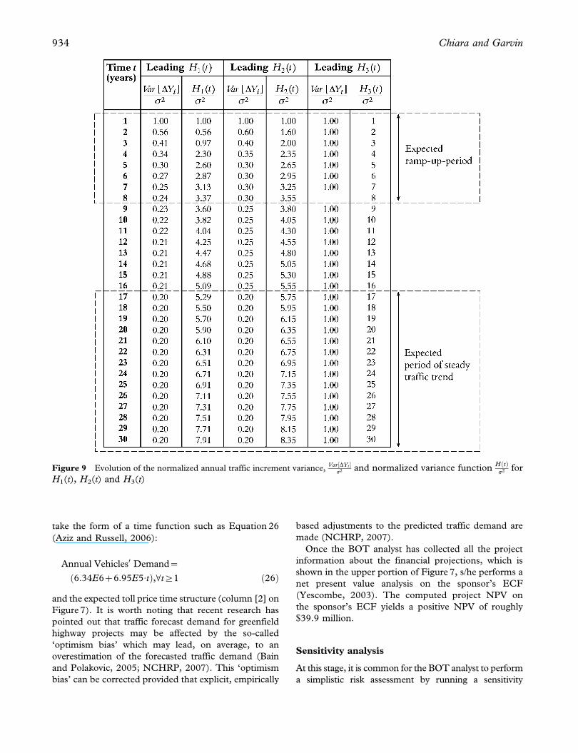
Figure 9 Evolution of the normalized annual traffic increment variance,Var DYt½ �

s2 and normalized variance functionH tð Þs2 for

H1(t), H2(t) and H3(t)

934 Chiara and Garvin

analysis on the cash flow model (Equation 25) (NCHRP,

2007). In this respect, traffic analysts will provide the

BOT analyst with alternative traffic demand forecast

scenarios based on different values of the critical

assumptions shown in Figure 2. Though the sensitivity

analysis may provide useful insights about critical risk

variables, practitioners and academics have recognized

that a sensitivity analysis is not generally sufficient to

evaluate project risk (NCHRP, 2007). A more effective

way to proceed is to carry out a complete risk analysis that

can evaluate many different scenarios by considering a

wide range of potential outcomes with their related

probabilities (Dailami et al., 1999).

Financial risk analysis under uncertainty

In order to single out the effects of the variance

models on the project’s NPV, only one risk variable

is considered, the annual traffic volume, Y, while the

Figure 10 Normalized variance reduction of annual traffic increments over time,s2{Var DYt½ �

s2

Figure 11 Representation of the MVM variance function

H1(t) and H3(t) as well as of the linear piece-wise variance

function H2(t)

Figure 12 Probability of project financial unfeasibility as

the estimated uncertainty at year 1 changes

Variance models 935

other parameters in Equation 25 are kept determi-

nistic. The vector of the predicted values of the

annual traffic volume, �WW~ �WW0, �WW1, �WW2, . . . . . . , �WWT½ �, is

taken from the financial projections of the base case

analysis (column [1] on Figure 7). A three-step

procedure, illustrated in detail in Figure 8, is used

to build the two variance models with learning

features, the Martingale variance model H1(t) and

the linear piece-wise variance model H2(t). These

models incorporate the BOT analyst’s predictions

about the duration of the traffic ramp-up phase,

which is assumed to occur in the first eight years,

and the establishment of a defined steady traffic

trend, which is assumed to occur after 16 years. The

assumptions about the length of the ramp-up period

and when the steady traffic trend is established come

from a data-driven analysis on comparable transpor-

tation facilities. Furthermore, another variance

model, H3(t) with no learning feature, is introduced

for comparison. Details on how to build H3(t) are

also presented in Figure 8. All the three models are

built to have the same initial variance, H1(1)5

H2(1)5H3(1)5s2.

Now, Monte Carlo risk analyses are performed

using 10 000 simulations for each model. In the first

analysis where the Martingale variance function H1(t)

is used, the probability of a negative NPV is 15.2%.

In the second analysis where the piece-wise variance

function H2(t) is used, the probability of a negative

NPV is 15.6%. When the no-learning function H3(t)

is used, the probability of a negative NPV is 25.0%.

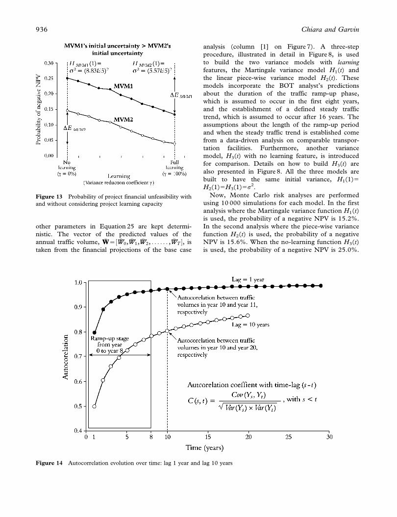
Figure 13 Probability of project financial unfeasibility with

and without considering project learning capacity

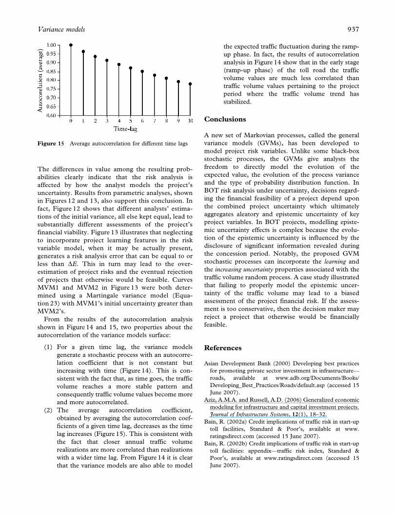
Figure 14 Autocorrelation evolution over time: lag 1 year and lag 10 years

936 Chiara and Garvin

The differences in value among the resulting prob-

abilities clearly indicate that the risk analysis is

affected by how the analyst models the project’s

uncertainty. Results from parametric analyses, shown

in Figures 12 and 13, also support this conclusion. In

fact, Figure 12 shows that different analysts’ estima-

tions of the initial variance, all else kept equal, lead to

substantially different assessments of the project’s

financial viability. Figure 13 illustrates that neglecting

to incorporate project learning features in the risk

variable model, when it may be actually present,

generates a risk analysis error that can be equal to or

less than DE. This in turn may lead to the over-

estimation of project risks and the eventual rejection

of projects that otherwise would be feasible. Curves

MVM1 and MVM2 in Figure 13 were both deter-

mined using a Martingale variance model (Equa-

tion 23) with MVM1’s initial uncertainty greater than

MVM2’s.

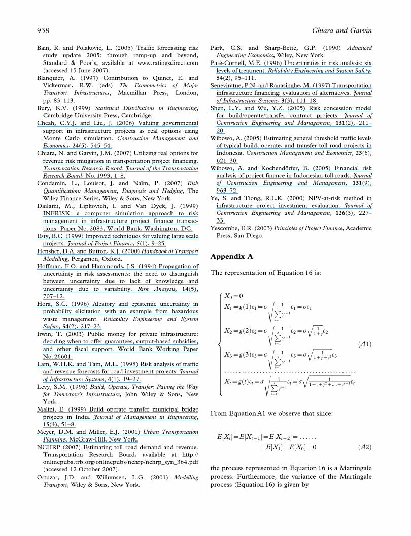
From the results of the autocorrelation analysis

shown in Figure 14 and 15, two properties about the

autocorrelation of the variance models surface:

(1) For a given time lag, the variance models

generate a stochastic process with an autocorre-

lation coefficient that is not constant but

increasing with time (Figure 14). This is con-

sistent with the fact that, as time goes, the traffic

volume reaches a more stable pattern and

consequently traffic volume values become more

and more autocorrelated.

(2) The average autocorrelation coefficient,

obtained by averaging the autocorrelation coef-

ficients of a given time lag, decreases as the time

lag increases (Figure 15). This is consistent with

the fact that closer annual traffic volume

realizations are more correlated than realizations

with a wider time lag. From Figure 14 it is clear

that the variance models are also able to model

the expected traffic fluctuation during the ramp-

up phase. In fact, the results of autocorrelation

analysis in Figure 14 show that in the early stage

(ramp-up phase) of the toll road the traffic

volume values are much less correlated than

traffic volume values pertaining to the project

period where the traffic volume trend has

stabilized.

Conclusions

A new set of Markovian processes, called the general

variance models (GVMs), has been developed to

model project risk variables. Unlike some black-box

stochastic processes, the GVMs give analysts the

freedom to directly model the evolution of the

expected value, the evolution of the process variance

and the type of probability distribution function. In

BOT risk analysis under uncertainty, decisions regard-

ing the financial feasibility of a project depend upon

the combined project uncertainty which ultimately

aggregates aleatory and epistemic uncertainty of key

project variables. In BOT projects, modelling episte-

mic uncertainty effects is complex because the evolu-

tion of the epistemic uncertainty is influenced by the

disclosure of significant information revealed during

the concession period. Notably, the proposed GVM

stochastic processes can incorporate the learning and

the increasing uncertainty properties associated with the

traffic volume random process. A case study illustrated

that failing to properly model the epistemic uncer-

tainty of the traffic volume may lead to a biased

assessment of the project financial risk. If the assess-

ment is too conservative, then the decision maker may

reject a project that otherwise would be financially

feasible.

References

Asian Development Bank (2000) Developing best practices

for promoting private sector investment in infrastructure—

roads, available at www.adb.org/Documents/Books/

Developing_Best_Practices/Roads/default.asp (accessed 15

June 2007).

Aziz, A.M.A. and Russell, A.D. (2006) Generalized economic

modeling for infrastructure and capital investment projects.

Journal of Infrastructure Systems, 12(1), 18–32.

Bain, R. (2002a) Credit implications of traffic risk in start-up

toll facilities, Standard & Poor’s, available at www.

ratingsdirect.com (accessed 15 June 2007).

Bain, R. (2002b) Credit implications of traffic risk in start-up

toll facilities: appendix—traffic risk index, Standard &

Poor’s, available at www.ratingsdirect.com (accessed 15

June 2007).

Figure 15 Average autocorrelation for different time lags

Variance models 937

Bain, R. and Polakovic, L. (2005) Traffic forecasting risk

study update 2005: through ramp-up and beyond,

Standard & Poor’s, available at www.ratingsdirect.com

(accessed 15 June 2007).

Blanquier, A. (1997) Contribution to Quinet, E. and

Vickerman, R.W. (eds) The Econometrics of Major

Transport Infrastructures, Macmillan Press, London,

pp. 83–113.

Bury, K.V. (1999) Statistical Distributions in Engineering,

Cambridge University Press, Cambridge.

Cheah, C.Y.J. and Liu, J. (2006) Valuing governmental

support in infrastructure projects as real options using

Monte Carlo simulation. Construction Management and

Economics, 24(5), 545–54.

Chiara, N. and Garvin, J.M. (2007) Utilizing real options for

revenue risk mitigation in transportation project financing.

Transportation Research Record: Journal of the Transportation

Research Board, No. 1993, 1–8.

Condamin, L., Louisot, J. and Naım, P. (2007) Risk

Quantification: Management, Diagnosis and Hedging, The

Wiley Finance Series, Wiley & Sons, New York.

Dailami, M., Lipkovich, I. and Van Dyck, J. (1999)

INFRISK: a computer simulation approach to risk

management in infrastructure project finance transac-

tions. Paper No. 2083, World Bank, Washington, DC.

Esty, B.C. (1999) Improved techniques for valuing large scale

projects. Journal of Project Finance, 5(1), 9–25.

Hensher, D.A. and Button, K.J. (2000) Handbook of Transport

Modelling, Pergamon, Oxford.

Hoffman, F.O. and Hammonds, J.S. (1994) Propagation of

uncertainty in risk assessments: the need to distinguish

between uncertainty due to lack of knowledge and

uncertainty due to variability. Risk Analysis, 14(5),

707–12.

Hora, S.C. (1996) Aleatory and epistemic uncertainty in

probability elicitation with an example from hazardous

waste management. Reliability Engineering and System

Safety, 54(2), 217–23.

Irwin, T. (2003) Public money for private infrastructure:

deciding when to offer guarantees, output-based subsidies,

and other fiscal support. World Bank Working Paper

No. 26601.

Lam, W.H.K. and Tam, M.L. (1998) Risk analysis of traffic

and revenue forecasts for road investment projects. Journal

of Infrastructure Systems, 4(1), 19–27.

Levy, S.M. (1996) Build, Operate, Transfer: Paving the Way

for Tomorrow’s Infrastructure, John Wiley & Sons, New

York.

Malini, E. (1999) Build operate transfer municipal bridge

projects in India. Journal of Management in Engineering,

15(4), 51–8.

Meyer, D.M. and Miller, E.J. (2001) Urban Transportation

Planning, McGraw-Hill, New York.

NCHRP (2007) Estimating toll road demand and revenue.

Transportation Research Board, available at http://

onlinepubs.trb.org/onlinepubs/nchrp/nchrp_syn_364.pdf

(accessed 12 October 2007).

Ortuzar, J.D. and Willumsen, L.G. (2001) Modelling

Transport, Wiley & Sons, New York.

Park, C.S. and Sharp-Bette, G.P. (1990) Advanced

Engineering Economics, Wiley, New York.

Pate-Cornell, M.E. (1996) Uncertainties in risk analysis: six

levels of treatment. Reliability Engineering and System Safety,

54(2), 95–111.

Seneviratne, P.N. and Ranasinghe, M. (1997) Transportation

infrastructure financing: evaluation of alternatives. Journal

of Infrastructure Systems, 3(3), 111–18.

Shen, L.Y. and Wu, Y.Z. (2005) Risk concession model

for build/operate/transfer contract projects. Journal of

Construction Engineering and Management, 131(2), 211–

20.

Wibowo, A. (2005) Estimating general threshold traffic levels

of typical build, operate, and transfer toll road projects in

Indonesia. Construction Management and Economics, 23(6),

621–30.

Wibowo, A. and Kochendorfer, B. (2005) Financial risk

analysis of project finance in Indonesian toll roads. Journal

of Construction Engineering and Management, 131(9),

963–72.

Ye, S. and Tiong, R.L.K. (2000) NPV-at-risk method in

infrastructure project investment evaluation. Journal of

Construction Engineering and Management, 126(3), 227–

33.

Yescombe, E.R. (2003) Principles of Project Finance, Academic

Press, San Diego.

Appendix A

The representation of Equation 16 is:

X0~0

X1~g 1ð Þe1~sffiffiffiffiffiffiffiffiffiffiffiffi

1P1

i~1

ci{1

se1~se1

X2~g 2ð Þe2~sffiffiffiffiffiffiffiffiffiffiffiffi

1P2

i~1

ci{1

se2~s

ffiffiffiffiffiffiffi1

1zc

qe2

X3~g 3ð Þe3~sffiffiffiffiffiffiffiffiffiffiffiffi

1P3

i~1

ci{1

se3~s

ffiffiffiffiffiffiffiffiffiffiffiffiffiffi1

1zczc2

qe3

. . . . . . . . . . . . . . . . . . . . . . . . . . . . . . . . . . . . . . . . . . . . .

Xt~g tð Þet~sffiffiffiffiffiffiffiffiffiffiffiffi

1Pt

i~1

ci{1

set~s

ffiffiffiffiffiffiffiffiffiffiffiffiffiffiffiffiffiffiffiffiffiffiffiffiffiffiffiffiffiffi1

1zczc2z::::zct{1

qet

8>>>>>>>>>>>>>>>>>>>><>>>>>>>>>>>>>>>>>>>>:

ðA1Þ

From Equation A1 we observe that since:

E Xt½ �~E Xt{1½ �~E Xt{2½ �~ . . . . . .

~E X1½ �~E X0½ �~0 ðA2Þ

the process represented in Equation 16 is a Martingale

process. Furthermore, the variance of the Martingale

process (Equation 16) is given by

938 Chiara and Garvin

Var X0½ �~0

Var X1½ �~s2

Var X2½ �~s2 11zc

Var X3½ �~s2 11zczc2

. . . . . . . . . . . . . . . . . . . . . . . . . . . . . . . . . . . . . . . . . .

Var Xt½ �~s2 11zczc2z...zct{1

8>>>>>>>>><>>>>>>>>>:

ðA3Þ

Then, the equivalent representation of Var[Xt] for

0(c,1 is given by

Var Xt½ �~s2 1Pti~1

ci{1

~s2 1

1{ct

1{c

� �~s2 1{c

1{ct

� �ðA4Þ

Appendix B

E DYt½ �~E D �WWtzXt½ �~E D �WWt½ �zE Xt½ �~D �WW ðB1Þ

Var DYt½ �~Var D �WWzXt½ �~Var Xt½ �~s2 1{c

1{ct

� �ðB2Þ

Variance models 939