Validation of Goddard Earth Observing System‐version 5 ...
15
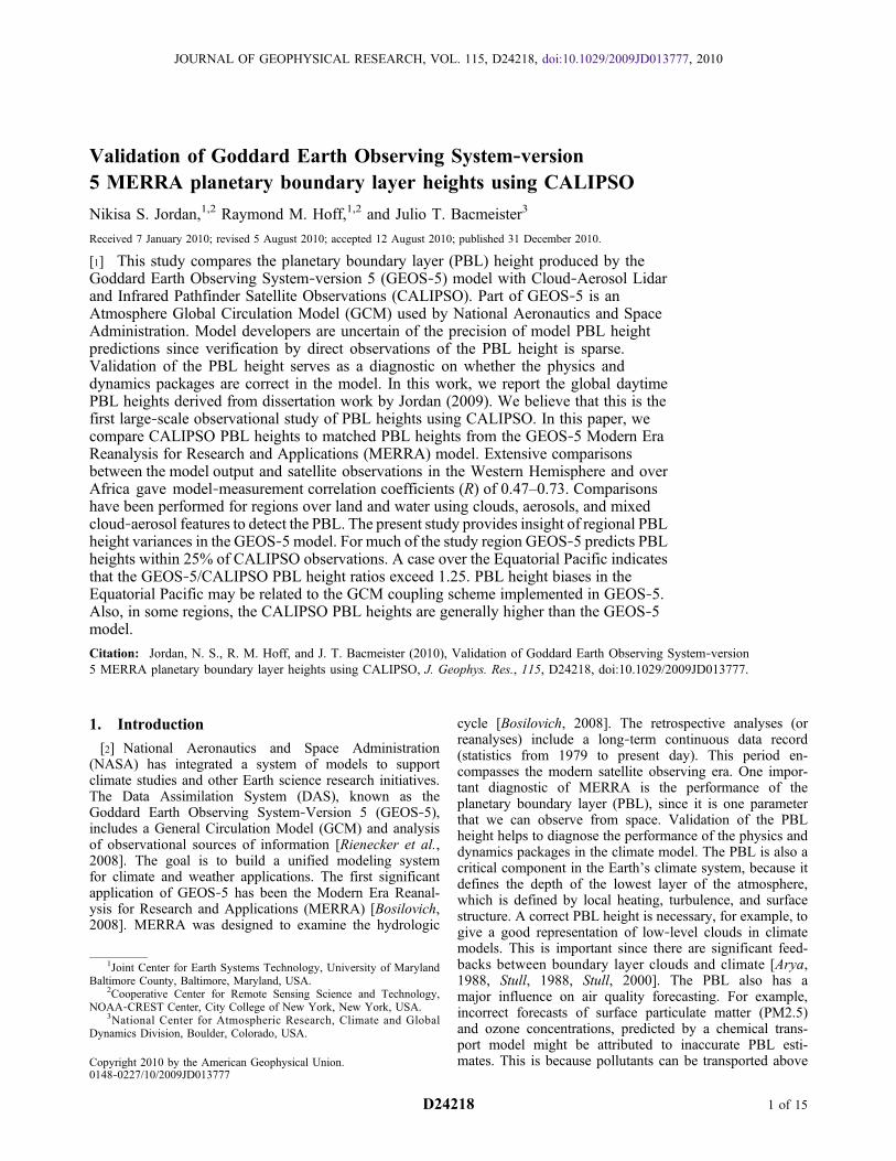
Validation of Goddard Earth Observing System‐version 5 MERRA planetary boundary layer heights using CALIPSO Nikisa S. Jordan, 1,2 Raymond M. Hoff, 1,2 and Julio T. Bacmeister 3 Received 7 January 2010; revised 5 August 2010; accepted 12 August 2010; published 31 December 2010. [1] This study compares the planetary boundary layer (PBL) height produced by the Goddard Earth Observing System‐version 5 (GEOS‐5) model with Cloud‐Aerosol Lidar and Infrared Pathfinder Satellite Observations (CALIPSO). Part of GEOS‐5 is an Atmosphere Global Circulation Model (GCM) used by National Aeronautics and Space Administration. Model developers are uncertain of the precision of model PBL height predictions since verification by direct observations of the PBL height is sparse. Validation of the PBL height serves as a diagnostic on whether the physics and dynamics packages are correct in the model. In this work, we report the global daytime PBL heights derived from dissertation work by Jordan (2009). We believe that this is the first large‐scale observational study of PBL heights using CALIPSO. In this paper, we compare CALIPSO PBL heights to matched PBL heights from the GEOS‐5 Modern Era Reanalysis for Research and Applications (MERRA) model. Extensive comparisons between the model output and satellite observations in the Western Hemisphere and over Africa gave model‐measurement correlation coefficients (R) of 0.47–0.73. Comparisons have been performed for regions over land and water using clouds, aerosols, and mixed cloud‐aerosol features to detect the PBL. The present study provides insight of regional PBL height variances in the GEOS‐5 model. For much of the study region GEOS‐5 predicts PBL heights within 25% of CALIPSO observations. A case over the Equatorial Pacific indicates that the GEOS‐5/CALIPSO PBL height ratios exceed 1.25. PBL height biases in the Equatorial Pacific may be related to the GCM coupling scheme implemented in GEOS‐5. Also, in some regions, the CALIPSO PBL heights are generally higher than the GEOS‐5 model. Citation: Jordan, N. S., R. M. Hoff, and J. T. Bacmeister (2010), Validation of Goddard Earth Observing System‐version 5 MERRA planetary boundary layer heights using CALIPSO, J. Geophys. Res., 115, D24218, doi:10.1029/2009JD013777. 1. Introduction [2] National Aeronautics and Space Administration (NASA) has integrated a system of models to support climate studies and other Earth science research initiatives. The Data Assimilation System (DAS), known as the Goddard Earth Observing System‐Version 5 (GEOS‐5), includes a General Circulation Model (GCM) and analysis of observational sources of information [Rienecker et al., 2008]. The goal is to build a unified modeling system for climate and weather applications. The first significant application of GEOS‐5 has been the Modern Era Reanal- ysis for Research and Applications (MERRA) [Bosilovich, 2008]. MERRA was designed to examine the hydrologic cycle [Bosilovich, 2008]. The retrospective analyses (or reanalyses) include a long‐term continuous data record (statistics from 1979 to present day). This period en- compasses the modern satellite observing era. One impor- tant diagnostic of MERRA is the performance of the planetary boundary layer (PBL), since it is one parameter that we can observe from space. Validation of the PBL height helps to diagnose the performance of the physics and dynamics packages in the climate model. The PBL is also a critical component in the Earth’s climate system, because it defines the depth of the lowest layer of the atmosphere, which is defined by local heating, turbulence, and surface structure. A correct PBL height is necessary, for example, to give a good representation of low‐level clouds in climate models. This is important since there are significant feed- backs between boundary layer clouds and climate [Arya, 1988, Stull, 1988, Stull, 2000]. The PBL also has a major influence on air quality forecasting. For example, incorrect forecasts of surface particulate matter (PM2.5) and ozone concentrations, predicted by a chemical trans- port model might be attributed to inaccurate PBL esti- mates. This is because pollutants can be transported above 1 Joint Center for Earth Systems Technology, University of Maryland Baltimore County, Baltimore, Maryland, USA. 2 Cooperative Center for Remote Sensing Science and Technology, NOAA‐CREST Center, City College of New York, New York, USA. 3 National Center for Atmospheric Research, Climate and Global Dynamics Division, Boulder, Colorado, USA. Copyright 2010 by the American Geophysical Union. 0148‐0227/10/2009JD013777 JOURNAL OF GEOPHYSICAL RESEARCH, VOL. 115, D24218, doi:10.1029/2009JD013777, 2010 D24218 1 of 15
-
Upload
khangminh22 -
Category
Documents
-
view
4 -
download
0
Transcript of Validation of Goddard Earth Observing System‐version 5 ...
Validation of Goddard Earth Observing System‐version5 MERRA planetary boundary layer heights using CALIPSO
Nikisa S. Jordan,1,2 Raymond M. Hoff,1,2 and Julio T. Bacmeister3
Received 7 January 2010; revised 5 August 2010; accepted 12 August 2010; published 31 December 2010.
[1] This study compares the planetary boundary layer (PBL) height produced by theGoddard Earth Observing System‐version 5 (GEOS‐5) model with Cloud‐Aerosol Lidarand Infrared Pathfinder Satellite Observations (CALIPSO). Part of GEOS‐5 is anAtmosphere Global Circulation Model (GCM) used by National Aeronautics and SpaceAdministration. Model developers are uncertain of the precision of model PBL heightpredictions since verification by direct observations of the PBL height is sparse.Validation of the PBL height serves as a diagnostic on whether the physics anddynamics packages are correct in the model. In this work, we report the global daytimePBL heights derived from dissertation work by Jordan (2009). We believe that this is thefirst large‐scale observational study of PBL heights using CALIPSO. In this paper, wecompare CALIPSO PBL heights to matched PBL heights from the GEOS‐5 Modern EraReanalysis for Research and Applications (MERRA) model. Extensive comparisonsbetween the model output and satellite observations in the Western Hemisphere and overAfrica gave model‐measurement correlation coefficients (R) of 0.47–0.73. Comparisonshave been performed for regions over land and water using clouds, aerosols, and mixedcloud‐aerosol features to detect the PBL. The present study provides insight of regional PBLheight variances in the GEOS‐5 model. For much of the study region GEOS‐5 predicts PBLheights within 25% of CALIPSO observations. A case over the Equatorial Pacific indicatesthat the GEOS‐5/CALIPSO PBL height ratios exceed 1.25. PBL height biases in theEquatorial Pacific may be related to the GCM coupling scheme implemented in GEOS‐5.Also, in some regions, the CALIPSO PBL heights are generally higher than the GEOS‐5model.
Citation: Jordan, N. S., R. M. Hoff, and J. T. Bacmeister (2010), Validation of Goddard Earth Observing System‐version5 MERRA planetary boundary layer heights using CALIPSO, J. Geophys. Res., 115, D24218, doi:10.1029/2009JD013777.
1. Introduction
[2] National Aeronautics and Space Administration(NASA) has integrated a system of models to supportclimate studies and other Earth science research initiatives.The Data Assimilation System (DAS), known as theGoddard Earth Observing System‐Version 5 (GEOS‐5),includes a General Circulation Model (GCM) and analysisof observational sources of information [Rienecker et al.,2008]. The goal is to build a unified modeling systemfor climate and weather applications. The first significantapplication of GEOS‐5 has been the Modern Era Reanal-ysis for Research and Applications (MERRA) [Bosilovich,2008]. MERRA was designed to examine the hydrologic
cycle [Bosilovich, 2008]. The retrospective analyses (orreanalyses) include a long‐term continuous data record(statistics from 1979 to present day). This period en-compasses the modern satellite observing era. One impor-tant diagnostic of MERRA is the performance of theplanetary boundary layer (PBL), since it is one parameterthat we can observe from space. Validation of the PBLheight helps to diagnose the performance of the physics anddynamics packages in the climate model. The PBL is also acritical component in the Earth’s climate system, because itdefines the depth of the lowest layer of the atmosphere,which is defined by local heating, turbulence, and surfacestructure. A correct PBL height is necessary, for example, togive a good representation of low‐level clouds in climatemodels. This is important since there are significant feed-backs between boundary layer clouds and climate [Arya,1988, Stull, 1988, Stull, 2000]. The PBL also has amajor influence on air quality forecasting. For example,incorrect forecasts of surface particulate matter (PM2.5)and ozone concentrations, predicted by a chemical trans-port model might be attributed to inaccurate PBL esti-mates. This is because pollutants can be transported above
1Joint Center for Earth Systems Technology, University of MarylandBaltimore County, Baltimore, Maryland, USA.
2Cooperative Center for Remote Sensing Science and Technology,NOAA‐CREST Center, City College of New York, New York, USA.
3National Center for Atmospheric Research, Climate and GlobalDynamics Division, Boulder, Colorado, USA.
Copyright 2010 by the American Geophysical Union.0148‐0227/10/2009JD013777
JOURNAL OF GEOPHYSICAL RESEARCH, VOL. 115, D24218, doi:10.1029/2009JD013777, 2010
D24218 1 of 15

the PBL and pollution concentrations increase at thesurface when layers aloft mix down into the PBL. Instable air masses, pollutants can be trapped within thePBL which subsequently raises pollutant concentrations.Therefore, verification of PBL outputs from models isessential. However, it is difficult for modelers to assessthe accuracy of the predicted PBL height due to sparse (insitu) global observations. Validation is especially impor-tant now since MERRA is now complete and available tothe community along with other GEOS‐5 analysis andforecast results [e.g., Moncrieff et al., 2010; available online http://www.ucar.edu/yotc/documents/ip_090707.pdf].[3] With recent advancement in remote sensing capabili-
ties, PBL height determination is possible using data fromactive spaceborne lidar, which possesses the ability to viewvast and remote areas on a regular basis. The aim of thispresent study is to use the attenuated backscatter coefficientfrom Cloud‐Aerosol Lidar and Infrared Pathfinder SatelliteObservations (CALIPSO) [Winker et al., 2007], part of theA‐Train satellite constellation, to obtain PBL heights andthen compare those observations to the NASA GEOS‐5model outputs. The study was performed for August andDecember 2006. All CALIPSO PBL observations wereaveraged spatially and matched in space and time to com-pare with estimates from the GEOS‐5 MERRA model.[4] Satellite lidar data have been used to validate PBL
estimates by models. Analysis of boundary layer heightfrom Lidar In‐space Technology (LITE) has been comparedwith PBL parameters in a climate model [Randall et al.,1998]. The study by Randall et al. [1998] specificallycompared PBL heights derived from LITE to a GCM andNational Center for Atmospheric Research (NCAR) climatemodel. Results indicated that GCM PBL predictions werevery close to the LITE‐derived PBL retrievals, while thePBL heights from the NCAR climate model were generally300–400 m lower than the satellite‐derived estimate. GLAS(Geoscience Laser Altimeter System) data was used in thefirst global validation of the European Center for Medium‐Range Weather Forecasts (ECMWF) forecast model [Palmet al., 2005]. Palm found that the GLAS derived PBLheight was 200–400 m higher over oceans than the model.However, there was an apparent correlation between thedata sets on a global scale. CALIPSO, a satellite based lidar,has not been used to validate PBL depths estimated bymodels. This is the first hemispheric observational study ofPBL heights using CALIPSO with comparisons to theGEOS‐5 MERRA model. In order to avoid detection ofnighttime residual layers that are not related to local heatingat the time of the overpass, PBL height comparisons pre-sented in this study were only derived from daytime data.
2. Data and Methods
[5] We compare PBL heights from the GEOS‐5 modelwith PBL heights determined from CALIPSO global satel-lite measurements during 2 months, August 2006 andDecember 2006. These 2 months were chosen becauseCALIPSO data were only available after June 2006, theGEOS‐5 output was available only for the 6 month periodJune to December 2006. However, the 2 months period
should capture the maximum change in the seasonal varia-tions expected in boundary layer behavior.
2.1. GEOS‐5 PBL Heights
[6] This study will examine PBL heights in the GEOS‐5data assimilation system (DAS). The GEOS‐5 DAS is astate of the art system coupling a global atmospheric generalcirculation model (GEOS‐5 AGCM) to NCEP’s Grid‐pointStatistical Interpolation (GSI) analysis [Rienecker et al.,2008]. The GEOS‐5 DAS assimilates a variety of in situand remotely sensed data. Ground‐based observations fromaircraft, radiosondes, and dropsondes are included. Satelliteradiance data streams that are assimilated include TIROSOperational Vertical Sounders (TOVS), Earth ObservingSystem (EOS) Aqua sounders, GOES Sounders, and SpecialSensor Microwave Imagers (SSMI) [Rienecker et al., 2008].Data corrections in the system are introduced via an Incre-mental Analysis Update (IAU) procedure [Bloom et al.,1996] in which the corrections appear as forcing terms inthe prognostic equations for the AGCM state variables. Thisprocedure is known to minimize shocks to model physics asnewly analyzed data is introduced every 6 h. In addition,forcing for the AGCM during the DAS cycle includes pre-scribed aerosols and radiatively active trace gases, sea sur-face temperature (SST), and sea ice. The Modern EraReanalysis for Research and Applications (MERRA)[Rienecker et al., 2008] is the first major application of theGEOS‐5 DAS [Bosilovich, 2008].[7] The PBL scheme employed in GEOS‐5 uses the Lock
et al. [2000] scheme for unstable layers and the Louis et al.[1982] scheme in stable shear driven regimes. Turbulentfluxes at a specific altitude depend on local gradients of thetransported quantity, but the diffusion coefficient (Kzz) maydepend on atmospheric properties at different levels. Non-local fluxes are not parameterized in GEOS‐5. The finaldiffusion coefficient Kzz represents vertical mixing by allturbulent processes, including surface and cloud‐top buoy-ancy production, and shear production.[8] The quantity referred to as planetary boundary layer
height (PBLH) in this study is found by examining verticalprofiles of the Kzz. PBLH is diagnosed as the lowest modellevel for which Kzz falls below 1 m2/s when values abovethis threshold exist in the lowest two levels of the column.This threshold is somewhat arbitrary. It represents turbulentintensity roughly two orders of magnitude below typicalpeak values (∼100 m2/s) in a strongly convective modelPBL. We use PBLH derived from Kzz profiles because itdirectly measures the extent of strong vertical mixing pro-duced by the model’s PBL parameterization, and is thereforethe most useful height‐like quantity to validate using theCALIPSO data. The GEOS‐5 PBLH data used for this studyis averaged over two 1800 s model physics time steps, i.e.,hourly averages, on the AGCM’s native two‐dimensional2/3° × 1/2° longitude‐latitude horizontal grid with 72 pres-sure levels extending to 0.01 hPa.[9] It is worth emphasizing that only AGCM state vari-
ables (winds, temperature, humidity, and ozone) are directlyassimilated, every 6 h. For 6 h intervals centered at analysistimes, the GEOS‐5 AGCM is run with incremental anal-ysis update (IAU) corrections [Bloom et al., 1996] to thesestate variables. During these intervals, PBL diffusivities
JORDAN ET AL.: VALIDATION OF GEOS‐5 USING CALIPSO D24218D24218
2 of 15

(and therefore heights) in the GEOS‐5 DAS are producedby the AGCM physics routines at each 1800 s modelphysics time step exactly as they would be in a free run-ning simulation.
2.2. PBL Heights From CALIPSO
[10] The CALIPSO payload includes (1) Cloud‐AerosolLidar with Orthogonal Polarization (CALIOP), (2) anImaging Infrared Radiometer (IIR), and (3) a moderatespatial resolution Wide Field Camera (WFC). All instru-ments operate separately and continuously. Together theyprovide information on the horizontal and vertical structureand properties of aerosols and clouds. CALIPSO is part ofthe afternoon (crosses the equator in the early afternoon∼1:30pm local time) A‐Train constellation, which is a for-mation of several satellites flying in close proximity. This isof value since other satellites in the constellation canobserve the same scene [Winker et al., 2007]. Key char-acteristics of CALIOP are given by Winker et al. [2007,2010].[11] CALIOP is a three‐channel (532 nm parallel, 532 nm
perpendicular, 1064 nm) elastic lidar receiving light at thesame wavelength as the emitted laser frequency. CALIOPsends short and intense pulses (1064 and 532 nm) of lin-early polarized laser light downward towards Earth. Thebackscattered light is collected by the telescope receiverand is subsequently converted to an electronic signal. Theatmospheric backscatter profile is retrieved at 30 m vertical
resolution from 0–8 km with a horizontal resolution of333m.[12] CALIPSO data are available from 13 June 2006 to
present. The version 2 Level 1B (CAL_LID_L1‐Prov‐V2‐01) data product was used in this study. A routine CALIPSOPBL product is currently not available. Methods used toderive the PBL height from CALIPSO are described byJordan [2009]. Briefly, three separate methods have beenevaluated: (1) a gradient technique [Melfi et al., 1985; Boersand Eloranta, 1986; Palm et al., 1998, 2005], (2) the Haarwavelet technique [Davis et al., 2000; Brooks, 2003], and(3) a maximum variance technique, chosen here. Daytimelidar observations were used from CALIPSO to insure thatresidual layers were not picked out in nighttime data.Residual layers at night are most closely related to daytimemaximum PBL heights and the matchup of the position of thePBL in daytime with a nighttime retrieval would needlesslycomplicate this analysis by having to compute transport overa 12 h period from a prior day PBL maximum. DaytimeCALIPSO profiles have lower signal‐to‐noise ratio (SNR)than nighttime profiles due to the solar background reflectedfrom clouds and the surface. This noise makes detection of agradient in aerosol backscatter difficult because gradienttechniques generally use some form of derivative calculation,which behaves poorly with noisy data. The second methodemploys a Haar wavelet [Cohn and Angevine, 2000], whichassumes a structural form of the backscatter profile at the topof the PBL where the scattering has a strong increase justunder the PBL (perhaps due to humidification of the aerosol),
Figure 1. 9 July 2006 ELF ground‐based lidar profile, with the PBL height via the maximum variancemethod (black dashed line) and Haar wavelet technique (red dashed line). The vertical fuchsia line isthe coincidence between the radiosonde (26 km south of UMBC) potential temperature inversion at1.64 km (shown on the right) and the ELF ground system PBLH,1.60 km, derived from the maximumvariance method at 17:51 UTC. The black vertical line corresponds to the closest point of approach(CPA ∼ 60 km) of CALIPSO to ELF at 18:19 UTC. At that time the ELF PBLH determined bythe variance method was ∼1.70 km and CALIPSO was 1.60 km.
JORDAN ET AL.: VALIDATION OF GEOS‐5 USING CALIPSO D24218D24218
3 of 15

Figure 2
JORDAN ET AL.: VALIDATION OF GEOS‐5 USING CALIPSO D24218D24218
4 of 15
a strong negative gradient of backscatter with height, and thena return to a constant or slowly decreasing backscatter coef-ficient above the PBL. This technique works reasonably wellfor a class of PBL structures which have high backscatteringin the PBL peaking at the base of the inversion in the PBLfollowed by a detectable gradient in scattering and a lowerbackscattering above. The choice of the dilation (verticalscale) and magnitude (peak scattering) of the wavelet is moreof an art than a science and it was found that the waveletrequired more quality assurance than the third techniquewhich is used here. The maximum variance technique isbased on an idea byMelfi et al. [1985] which assumes that atthe PBL there is a maximum in the variance of the backscattersignal both in the vertical dimension and in the horizontaldimension. Melfi used the technique with horizontal struc-tures (rolls) in the cloud and aerosol field in over long hori-zontal flight paths with a downward looking lidar. Wetested a similar technique from the ground where theassumption is that at the PBL, there is a maximum in thebackscatter variance because within the entrainment regionat the top of the PBL, downward clean eddies are mixingwith upwelling hazier and higher backscatter parcels. If theentrainment zone is smaller or comparable to the region
over which we evaluate the variance in the signal, the peakvariance in the vertical should identify the base of theentrainment zone since the absolute difference between thePBL value and the entrainment zone should be highestthere, whether a peak in the signal due to aerosol swellingnear the PBL top due to increased humidity or cloud baseis seen or not. The use of variance (independent of the signof the backscatter change) is more robust in clear air andpartly cumulus convective cases. It was found for the noisydaytime CALIPSO data used here that the maximum var-iance technique with a sliding window best detected thePBL height (as evaluated visually by looking at the spatiallatitude‐height images from CALIPSO and in comparisonwith radiosoundings in the Baltimore‐Washington area).Figure 1 shows such a comparison between a radio-sounding with a very weak inversion in the potentialtemperature, the height of the PBL determined from bothmethods (2) and (3) from ground‐based lidar at Universityof Maryland Baltimore County (UMBC; with a muchhigher SNR than CALIPSO) and a nearby CALIPSOretrieval using method (3). From this evaluation (includingothers with similar results but not shown here) [seeJordan, 2009], we chose to process the CALIPSO data set
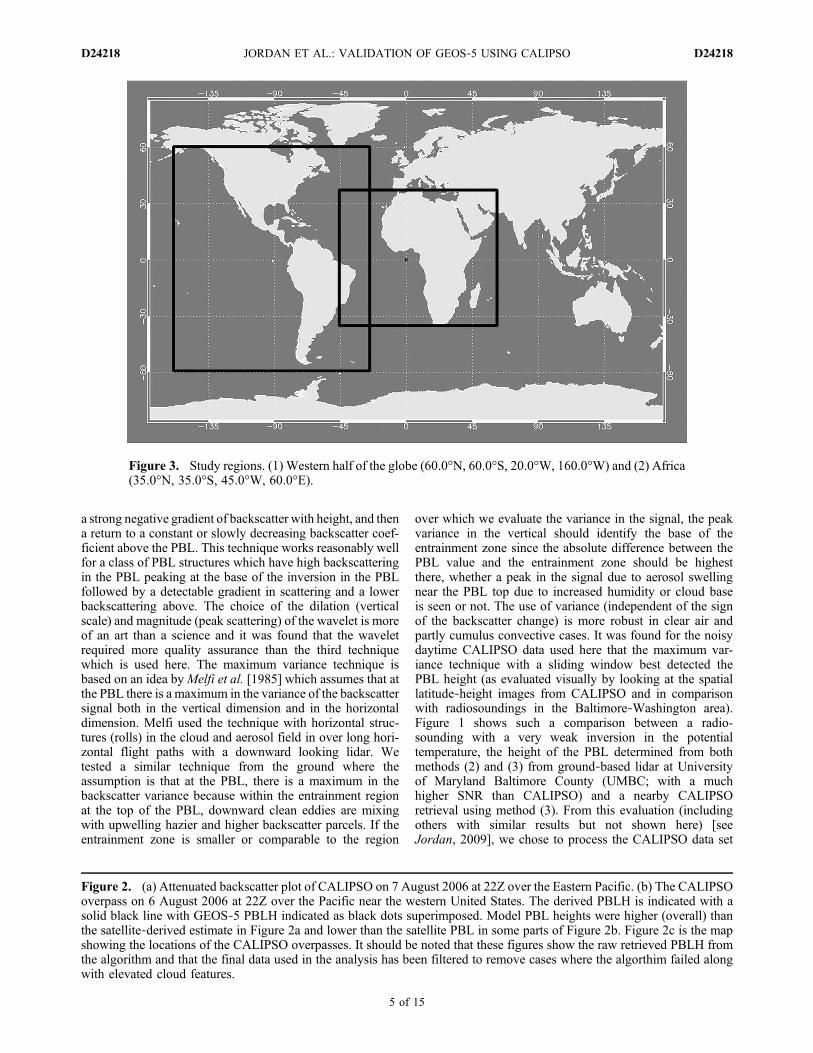
Figure 3. Study regions. (1) Western half of the globe (60.0°N, 60.0°S, 20.0°W, 160.0°W) and (2) Africa(35.0°N, 35.0°S, 45.0°W, 60.0°E).
Figure 2. (a) Attenuated backscatter plot of CALIPSO on 7 August 2006 at 22Z over the Eastern Pacific. (b) The CALIPSOoverpass on 6 August 2006 at 22Z over the Pacific near the western United States. The derived PBLH is indicated with asolid black line with GEOS‐5 PBLH indicated as black dots superimposed. Model PBL heights were higher (overall) thanthe satellite‐derived estimate in Figure 2a and lower than the satellite PBL in some parts of Figure 2b. Figure 2c is the mapshowing the locations of the CALIPSO overpasses. It should be noted that these figures show the raw retrieved PBLH fromthe algorithm and that the final data used in the analysis has been filtered to remove cases where the algorthim failed alongwith elevated cloud features.
JORDAN ET AL.: VALIDATION OF GEOS‐5 USING CALIPSO D24218D24218
5 of 15
using the maximum variance technique for PBL detection.Figures 2a and 2b are plots showing subsets of the derivedCALIPSO PBL heights (variance technique (solid blackline) before quality control) superimposed on the corre-sponding backscatter image with the GEOS‐5 model PBLheights (shown as black circles). Figure 2a corresponds toa subset over the equatorial Pacific and Figure 2b is over thePacific near the western United States. Further discussionregarding the variation between the satellite and model PBLheights is given in section 4. In that section ratio plots of themodel estimate over the satellite observation are shown andprovide a more comprehensive assessment of the differencesin the data sets.[13] The CALIPSO PBL data was flagged according to
the feature type (i.e., aerosol, cloud, or both) used to deriveit. The satellite and model data have different resolutions.Therefore, it is important to note that the satellite data wasaveraged to matchup to the model. As explained earlier,the model output is on a 2/3° by 1/2° longitude‐latitudehorizontal grid. Therefore, the CALIPSO PBL data wasaveraged (the mean was taken) every 1/2° in latitude.Satellite and model data were then compared at the sametime (within 30 min, where 30 min is the average timeseparation between model time step and the CALIPSOobservation) and latitude and longitude. Model/satellitePBL height ratio maps were produced for all regions.Creating ratio plots was a great visual value since it madeit easier to determine where the estimates were signifi-cantly different. Correlation plots of the model and satellitePBLs were created using the statistical software SAS
(Statistical Analysis System, 2009). Histogram charts werecreated as well to get a better understanding of the modeland satellite PBL distributions.
3. Study Areas
[14] Possible matchups between CALIPSO and GEOS‐5were largely found in regions with few overlying cloudsystems and clearly delineated PBL heights in the CALIPSOdata. The predominance of such data occurs over the ocean.Therefore, a large portion of the Western Hemisphere wasselected for comparisons. The area is bounded by the co-ordinates 60.0°N, 60.0°S, 20.0°W, and 160.0°W (Figure 3).Quality assurance via visual inspection was performed oneach of the retrieved CALIPSO PBL heights. This was donefor all of the data used in this study. Several subregions werechosen within the Western Hemisphere. Subregions wereselected based on season and meteorological regimes; datawere analyzed for August and December 2006. The GEOS‐5model data set available was limited when this research wasconducted. August and December were selected to maximizethe seasonal difference.[15] PBL heights in Africa were also analyzed and
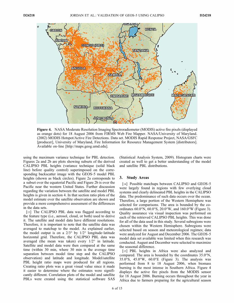
compared. The area is bounded by the coordinates 35.0°N,35.0°S, 45.0°W, 60.0°E (Figure 3). The analysis wasperformed from 8 to 18 August 2006, when biomassburning is the most intense in Southern Africa. Figure 4displays the active fire pixels from the MODIS sensorfor 18 August 2006. Burning occurs throughout the year inAfrica due to farmers preparing for the agricultural season
Figure 4. NASAModerate Resolution Imaging Spectroradiometer (MODIS) active fire pixels (displayedas orange dots) for 18 August 2006 from FIRMS Web Fire Mapper. NASA/University of Maryland.(2002) MODIS Hotspot/Active Fire Detections. Data set. MODIS Rapid Response Project, NASA/GSFC[producer], University of Maryland, Fire Information for Resource Management System [distributors].Available on‐line [http://maps.geog.umd.edu].
JORDAN ET AL.: VALIDATION OF GEOS‐5 USING CALIPSO D24218D24218
6 of 15
and grazing areas. Burning also occurs at the end of theagricultural harvest. Thus, burning events are conductedbased on the meteorological regimes of the continent
[Justice et al., 1996]. Many papers have been publishedthat look at the release of smoke particles in this area[Justice et al., 1996; Ichoku et al., 2003; Ichoku and
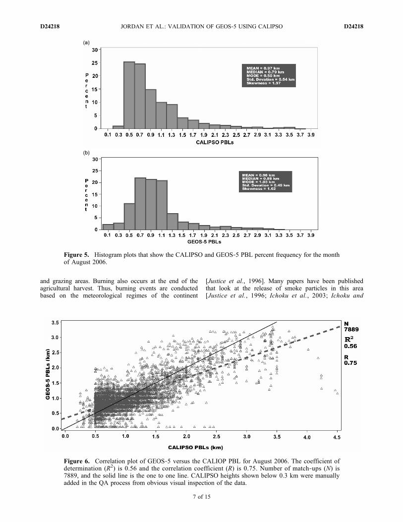
Figure 5. Histogram plots that show the CALIPSO and GEOS‐5 PBL percent frequency for the monthof August 2006.
Figure 6. Correlation plot of GEOS‐5 versus the CALIOP PBL for August 2006. The coefficient ofdetermination (R2) is 0.56 and the correlation coefficient (R) is 0.75. Number of match‐ups (N) is7889, and the solid line is the one to one line. CALIPSO heights shown below 0.3 km were manuallyadded in the QA process from obvious visual inspection of the data.
JORDAN ET AL.: VALIDATION OF GEOS‐5 USING CALIPSO D24218D24218
7 of 15
Kaufman, 2005; Matichuk et al., 2007]. All current smokeemission estimates have significant uncertainty errors[Andreae and Merlet, 2001; French et al., 2004; Jordanet al., 2008]. One contributing factor in the error of
smoke emission estimates can be attributed to the factthat scientists are not always sure of the relevant PBLheight, which greatly impacts pollutant concentrationsnear the surface. The height of the PBL is important to
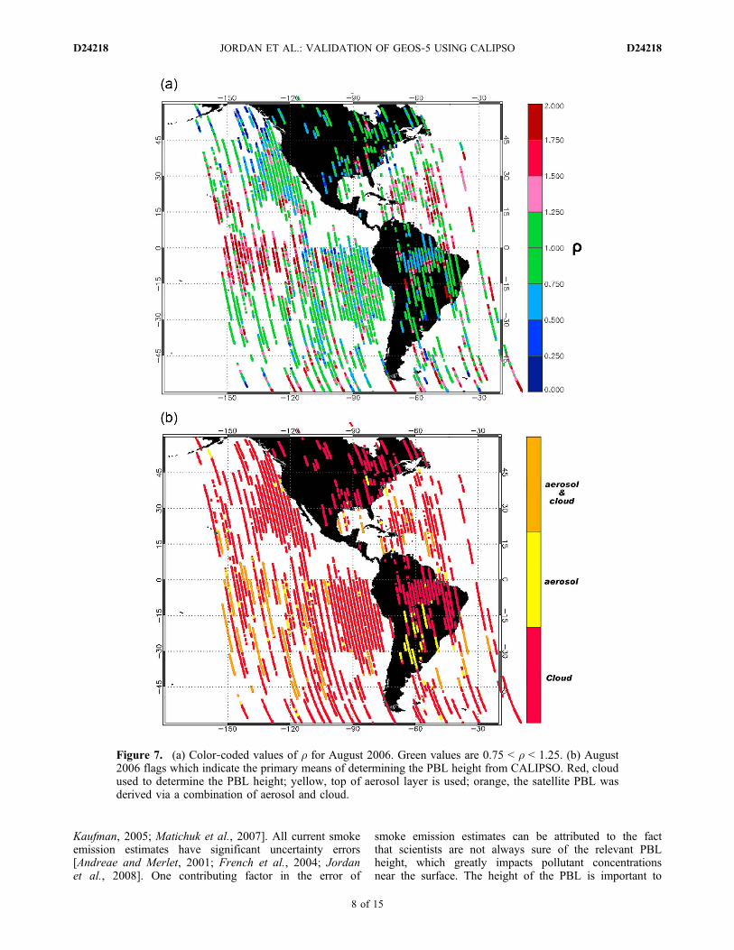
Figure 7. (a) Color‐coded values of r for August 2006. Green values are 0.75 < r < 1.25. (b) August2006 flags which indicate the primary means of determining the PBL height from CALIPSO. Red, cloudused to determine the PBL height; yellow, top of aerosol layer is used; orange, the satellite PBL wasderived via a combination of aerosol and cloud.
JORDAN ET AL.: VALIDATION OF GEOS‐5 USING CALIPSO D24218D24218
8 of 15

help researchers better understand smoke injection heightas it relates to fire intensity.
4. Results
[16] Results are organized as follows: (1) the PBL heightsderived from CALIPSO and GEOS‐5 are presented in his-togram charts which show the probability density functionof PBL heights, (2) a correlation plot between the satelliteand model PBL heights is given, (3) a ratio plot of the modelestimate over the satellite observation is shown, and (4) amap of the flags which indicate the primary means to derivethe PBL height from CALIPSO (via aerosol, cloud, oraerosol and cloud combined) is given.
4.1. Western Hemisphere; August 2006
[17] Figure 5a shows the distribution of the CALIPSOPBL height data. It is positively (right) skewed, which in-dicates that it has few large PBL values. Furthermore, themean (0.97 km) is greater than the median (0.79 km) andmode (0.50 km). The most frequently occurring PBL heightestimates range from 0.45 to 1.00 km. The GEOS‐5 data(Figure 5b) is also positively skewed to the right but is notas extreme as the CALIPSO data set. The mean GEOS‐5
PBL height is 0.98 km. The median and mode are 0.88 and1.03 km, respectively.[18] A correlation plot of the satellite versus the model
PBL is shown in Figure 6. There were 7889 PBL match‐upsbetween GEOS‐5 and CALIPSO. The correlation coeffi-cient is 0.75. Extreme outliers were mostly noted in caseswhere the model PBL height was significantly smaller thanthe satellite estimate. In most of these extreme daytime casesthe model predicted a PBL height of 0.06 km (near thesurface; lowest native vertical resolution level (i.e., 1) inGEOS‐5), while most of the matched satellite PBLs variedfrom 0.50 to 2.50 km. There were few CALIPSO PBL in-stances less than 0.50 km because the algorithm started at0.30 km to avoid land surface features around the globe. Inmost cases the SNR (signal‐noise ratio) limitations of theCALIPSO daytime data make it very difficult to discernPBL heights below 500 m using the variance method.Strong attenuation of the daytime signal in the PBL has beenrecognized as a problem in the retrieval of extinction (M.Kacenelenbogen et al., An accuracy assessment of theCALIOP/CALIPSO version 2 aerosol extinction productbased on a detailed multi‐sensor, multi‐platform case study,submitted to Atmospheric, Physical and Chemical Discuss,2010) leading to a number of artifacts in the CALIPSO near
Figure 8. (a) Histogram plot that shows the CALIPSO PBL percentage frequency for the entire month ofDecember 2006. (b) For the GEOS‐5 model data set.
JORDAN ET AL.: VALIDATION OF GEOS‐5 USING CALIPSO D24218D24218
9 of 15

surface data. We believe that this has may have led to asimilar artificial decrease in the number of PBL heightsbelow 500 m in this study, which is a potential source of bias.[19] A correlation plot of all the model and satellite match‐
ups is useful to identify variability in the data set. However, itis difficult to get a good understanding of where the outlyingpoints lay on the globe. Each point on Figure 7a indicates themodel/satellite PBL height ratio (r) relative to the same spaceand time. Moreover, green points are match‐ups within 25%of unity (a perfect match between the model and satellite).Reddish points indicate cases where the model PBL wassignificantly greater (>25%) than that of the satellite estimate.Bluish points display cases where the model PBL was sig-nificantly lower than that of the CALIPSO estimate.[20] The preponderance of green on the map (Figure 7a)
indicates general approximate agreement between GEOS‐5and CALIPSO. The results displayed on the map reflect thecorrelation analysis (Figure 6). Underestimates (red points,r < 0.75) are mainly localized over water in the centralequatorial Pacific. The PBL in this zone plays a key role inthe coupled ocean‐atmosphere dynamics that governENSO so that errors here are a concern. The fraction oflow cloud and cloud radiative forcing in this zone are alsooverestimated in MERRA.[21] Figure 7b shows the flag used based on the type of
scattering to determine the PBL height from CALIPSO. Reddots in this figure indicate that clouds were used to decipherthe PBL height from CALIPSO. Yellow dots indicate caseswhere the PBL height was derived from the top of a well‐defined aerosol layer. Orange dots indicate cases where thesatellite estimate was determined via well‐defined mixedaerosol and cloud layer. For the Pacific near the equator,most of the CALIPSO PBL estimates determined fromCALIPSO were determined by analyzing cloud layers
(indicated as red dots in Figure 7a over the Pacific region).Skin surface temperatures used in the GEOS‐5 model wereanalyzed to determine if there might have been an overes-timation in the model that could have led to the excessivelarger than expected PBLH over the equatorial Pacific.Surface skin temperature measured by the AtmosphericInfrared Sounder (AIRS) [Tobin et al., 2006] satellite wascompared to surface temperatures from the GEOS‐5MERRA model to further investigate this.[22] AIRS (Aqua) is part of the A‐Train constellation and
views the same region on Earth 75 s before CALIPSO. AIRSskin surface temperatures (daily AIRS Level‐3 surface tem-perature product) from the ascending node were compared tothe GEOS‐5 skin surface. The mean skin surface temperaturedifference between AIRS and MERRA was found to be only0.45°K with median of 0.51°K, not enough to change theheight in the PBL over sea by a factor of 2.[23] There are other disagreements between the model
and satellite PBL estimates. A subregion worth highlightingin Figure 7a includes Central Brazil along the Amazon,where a swath of r less than 0.75 occurs. This case isanalyzed in more detail by Jordan [2009]. Maps of pre-cipitation correlate with the mismatch in PBL heights;however, we still do not have concrete evidence to explainthe disagreements.
4.2. Western Hemisphere: December 2006
[24] The distribution of the PBLs derived via CALIPSOfor December 2006 (Figure 8a) is also positively skewedsimilarly to the August 2006 data set. The mean PBLheight derived from CALIPSO was 0.83 km. The medianwas 0.73 km, and mode was 0.50 km. However, theDecember data set is smaller (a difference ofN = 2632 points)than August. This is because CALIPSO was not operating for
Figure 9. Correlation plot of GEOS‐5 versus CALIOP PBL. The correlation coefficient (R) is 0.47, andthe black line is the one to one line.
JORDAN ET AL.: VALIDATION OF GEOS‐5 USING CALIPSO D24218D24218
10 of 15
10 days in December. Nevertheless, there are still a signifi-cant number of available points to conduct a statistical study.The GEOS‐5 data (Figure 8b) is closer to a normal distribu-tion. The summary statistics include a mean PBL height of0.94 km and a 0.89 kmmedian value. The mode is 0.89 km aswell. Few instances exist where the model PBL was greaterthan 1.70 km.
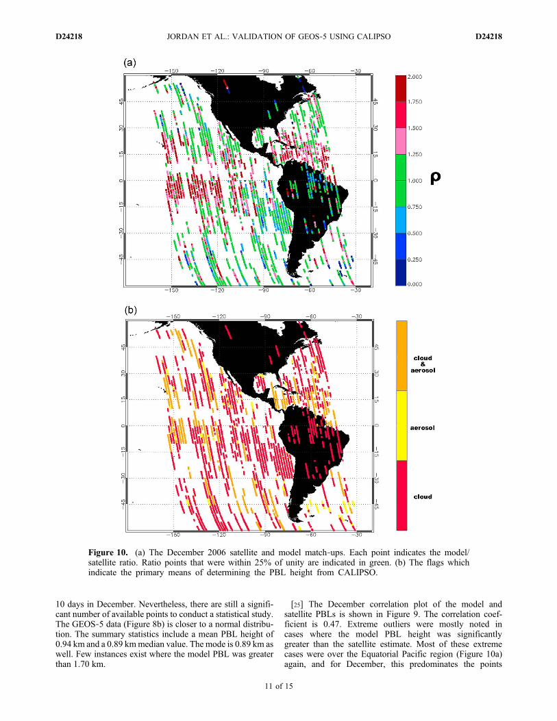
[25] The December correlation plot of the model andsatellite PBLs is shown in Figure 9. The correlation coef-ficient is 0.47. Extreme outliers were mostly noted incases where the model PBL height was significantlygreater than the satellite estimate. Most of these extremecases were over the Equatorial Pacific region (Figure 10a)again, and for December, this predominates the points
Figure 10. (a) The December 2006 satellite and model match‐ups. Each point indicates the model/satellite ratio. Ratio points that were within 25% of unity are indicated in green. (b) The flags whichindicate the primary means of determining the PBL height from CALIPSO.
JORDAN ET AL.: VALIDATION OF GEOS‐5 USING CALIPSO D24218D24218
11 of 15
responsible for the poorer correlation. Other noted out-liers include cases where the model estimated a PBLheight (∼0.064 km) that was significantly lower than thesatellite estimate. Furthermore, all of those cases wereover water.[26] There are more instances of r > 1.25 in the December
2006 (Figure 10a) data set than in August 2006 (Figure 7a).As in the August case, many of these instances occur overthe equatorial Pacific. In the December data, there appears tobe an increase in the number point with r > 1.25 in theCaribbean. Figure 10b displays the flag used to determinethe PBL height from CALIPSO. Clouds were again theprimary flag used in the December 2006 data set, but alarger proportion of cloud/aerosol flags are also evidentcompared with the August 2006 case (Figure 7b).[27] An El Nino event was developing in December
2006 (NOAA NCEP CPC, http://www.cpc.noaa.gov/). It isexpected that warmer equatorial Pacific SSTs associatedwith the El Nino event would drive greater than normalPBL heights over the equatorial Pacific. Seasonal cyclealso has to be considered. August SSTs along the equa-torial Pacific (150°W–90°W) represent the coldest phase of
the normal annual cycle. For both reasons, we wouldexpect higher PBLs in December 2006 than in August2006. This was evident in the GEOS‐5 model, PBLheights in GEOS‐5 increased from ∼0.6 to ∼0.9 km in thiszone; whereas in the CALIPSO data the increase was onlyfrom ∼0.5 to ∼0.6 km. The model’s mean overprediction ofPBL height in this region, as well as the apparent over-sensitivity to SST may indicate a problem in its imple-mentation of the Lock et al. [2000] scheme, or mayindicate a bias in large scale descent over this region.
4.3. Africa Study Region
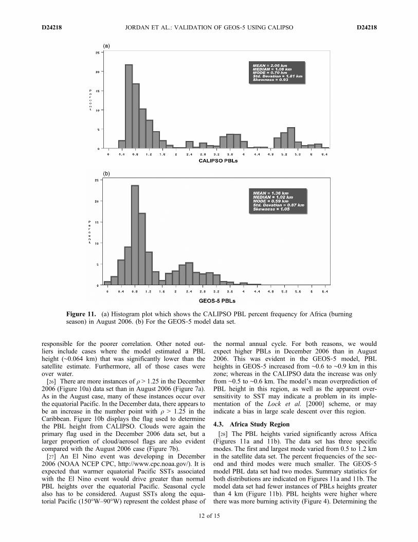
[28] The PBL heights varied significantly across Africa(Figures 11a and 11b). The data set has three specificmodes. The first and largest mode varied from 0.5 to 1.2 kmin the satellite data set. The percent frequencies of the sec-ond and third modes were much smaller. The GEOS‐5model PBL data set had two modes. Summary statistics forboth distributions are indicated on Figures 11a and 11b. Themodel data set had fewer instances of PBLs heights greaterthan 4 km (Figure 11b). PBL heights were higher wherethere was more burning activity (Figure 4). Determining the
Figure 11. (a) Histogram plot which shows the CALIPSO PBL percent frequency for Africa (burningseason) in August 2006. (b) For the GEOS‐5 model data set.
JORDAN ET AL.: VALIDATION OF GEOS‐5 USING CALIPSO D24218D24218
12 of 15
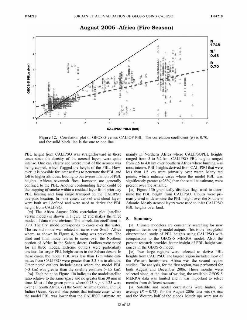
PBL height from CALIPSO was straightforward in thesecases since the density of the aerosol layers were quiteintense. One can clearly see where most of the aerosol wasbeing capped, which flagged the height of the PBL. How-ever, it is possible for intense fires to penetrate the PBL andloft to higher altitudes, leading to our overestimation of PBLheights. African savannah fires, however, are generallyconfined to the PBL. Another confounding factor could bethe trapping of smoke within a residual layer from prior dayPBL heating and long range transport to the CALIPSOoverpass location. In most cases, aerosol and cloud layerswere both well defined and were used to derive the PBLheight from CALIPSO.[29] The Africa August 2006 correlation plot (satellite
versus model) is shown in Figure 12 and makes the threemodes of data more obvious. The correlation coefficient is0.70. The first mode corresponds to cases over the water.The second mode was related to cases over South Africawhere, as shown in Figure 4, burning was prevalent. Thethird and final mode relates to cases over the Northernportion of Africa in the Sahara desert. Outliers were notedfor all three modes. Extreme outliers were particularlyobvious for larger PBL height cases in the Sahara desert. Inthese cases, the model PBL was less than 1km while esti-mates from CALIPSO were greater than 3.3 km in altitude.Other noted outliers include cases where the model PBL(∼3 km) was greater than the satellite estimate (∼1.5 km).[30] Each point on Figure 13a indicates the model/satellite
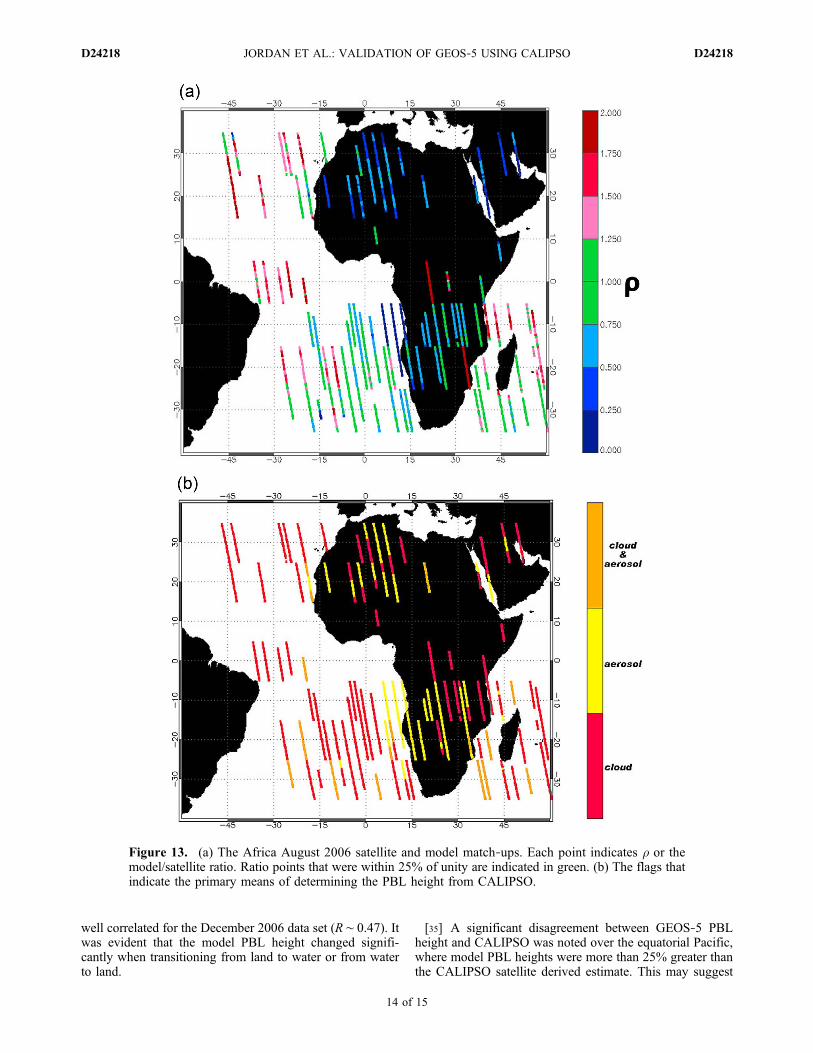
ratio relative to the same space and no greater than 30 min intime. Most of the green points where 0.75 < r < 1.25 wereover (1) South Africa, (2) the South Atlantic Ocean, and (3)Indian Ocean. Several blue points that indicate cases wherethe model PBL was lower than the CALIPSO estimate are
mainly in Northern Africa where CALIPSOPBL heightsranged from 5 to 6.2 km. CALIPSO PBL heights rangedfrom 2.5 to 4.0 km over Southern Africa where burning wasmost intense. PBL heights derived from CALIPSO that wereless than 1.5 km were primarily over water. Many redpoints, which indicate cases where the model PBL wassignificantly greater (>25%) than the satellite estimate, werepresent over the Atlantic.[31] Figure 13b graphically displays flags used to deter-
mine the PBL height from CALIPSO. Clouds were pri-marily used to determine the PBL height over the SouthernAtlantic. Mostly aerosol layers were used to infer CALIPSOPBL heights over land.
5. Summary
[32] Climate modelers are constantly searching for newopportunities to verify model outputs. This is the first globalobservational study of PBL heights using CALIPSO withcomparisons to the GEOS‐5 MERRA model. Also, thepresent research provides better insight of PBL height var-iances in the GEOS‐5 model.[33] Two large regions were selected to derive PBL
heights from CALIPSO. The largest region included most ofthe Western hemisphere. Africa was the second regionstudied. The analysis, for the first region, was performed forboth August and December 2006. These months wereselected since, at the time of writing, the available GEOS‐5MERRA data was limited and it was important to selectmonths from different seasons.[34] Satellite and model correlations were higher, on
average (R ∼ 0.73), for the August 2006 data sets (Africaand the Western half of the globe). Match‐ups were not as
Figure 12. Correlation plot of GEOS‐5 versus CALIOP PBL. The correlation coefficient (R) is 0.70,and the solid black line is the one to one line.
JORDAN ET AL.: VALIDATION OF GEOS‐5 USING CALIPSO D24218D24218
13 of 15
well correlated for the December 2006 data set (R ∼ 0.47). Itwas evident that the model PBL height changed signifi-cantly when transitioning from land to water or from waterto land.
[35] A significant disagreement between GEOS‐5 PBLheight and CALIPSO was noted over the equatorial Pacific,where model PBL heights were more than 25% greater thanthe CALIPSO satellite derived estimate. This may suggest
Figure 13. (a) The Africa August 2006 satellite and model match‐ups. Each point indicates r or themodel/satellite ratio. Ratio points that were within 25% of unity are indicated in green. (b) The flags thatindicate the primary means of determining the PBL height from CALIPSO.
JORDAN ET AL.: VALIDATION OF GEOS‐5 USING CALIPSO D24218D24218
14 of 15
excessive forcing of turbulence by cloud top cooling in theGEOS‐5 implementation of the Lock et al. PBL scheme.[36] Our results also suggest significant disagreements in
some land regions where wet surface conditions may exist(e.g., central Brazil) or where high surface temperaturesexist (e.g., Saharan desert). There are indications that whenan area has undergone recent precipitation the model PBLheight deviates from what CALIPSO observes. There werecases over Northern Africa where the model PBL heightswere much lower than the satellite‐derived estimates. CA-LIPSO clearly observed well‐defined aerosol and cloudlayers up to 6 km in this area, but the model PBL wasgenerally less than half of this value. It was also obvious thatthere were many instances where the CALIPSO derivedPBL heights are generally higher, except for limited areasover the ocean, than the GEOS‐5 model. It is important tonote that most of the CALIPSO PBL heights were derivedfrom cloudy data.
[37] Acknowledgments. This work was funded by CooperativeCenter for Remote Sensing Science and Technology (CREST) CUNYgrant 49100‐00‐02‐B and NASA NAS1‐99107.
ReferencesAndreae, M. O., and P. Merlet (2001), Emission of trace gases and aerosolsfrom biomass burning, Global Biogeochem. Cycles, 15, 955–966,doi:2000GB001382.
Arya, S. P. (1988), Introduction to Micrometerology, Academic, San Diego,Calif.
Bloom, S. C, L. L. Takacs, D. A. Silva, A. M., and D. Ledvina (1996),Data assimilation using incremental analysis updates, Mon. WeatherRev., 124, 1256–1271.
Boers, R., and E. W. Eloranta (1986), Lidar measurements of the atmo-spheric entrainment zone and the potential temperature jump across thetop of the mixed layer, Boundary Layer Meteorol., 34, 357–375.
Bosilovich, M. G. (2008), NASA’s modern era retrospective‐analysis forresearch and applications: Integrating earth observations, Earthzine.(Available at http://www.earthzine.org/2008/09/26/nasas‐modern‐era‐retrospective‐analysis)
Brooks, I. M. (2003), Finding boundary layer top: Application of a waveletcovariance transform to lidar backscatter profiles, J. Atmos. OceanicTechnol., 20, 1092–1105.
Cohn, S. A., and W. M. Angevine (2000), Boundary‐layer height andentrainment zone thickness measured by lidars and wind profiling radars,J. Appl. Meteorol., 39, 1233–1247.
Davis, K. J., N. Gamage, C. R. Hagelberg, C. Kiemle, D. H. Lenschow, andP. P. Sullivan (2000), An objective method for deriving atmosphericstructure from airborne lidar observations, J. Atmos. Oceanic Technol.,17, 1455–1468.
French, N., P. Goovaerts, and E. S. Kasischke (2004), Uncertainty in esti-mating carbon emissions from boreal forest fires, J. Geophys. Res., 109,D14S08, doi:10.1029/2003JD003625.
Ichoku, C., L. A. Remer, Y. J. Kaufman, R. Levy, D. A. Chu, D. Tanré,and B. N. Holben (2003), MODIS observation of aerosols and estima-tion of aerosol radiative forcing over southern Africa during SAFARI2000, J. Geophys. Res., 108(D13), 8499, doi:10.1029/2002JD002366.
Ichoku, C., and Y. J. Kaufman (2005), A method to derive smoke emissionrates from MODIS fire radiative energy measurements, IEEE Trans.Geosci. Remote Sens., 43(11), 2636–2649.
Jordan, N. S., C. Ichoku, and R. M. Hoff (2008), Estimating smoke emis-sions over the US Southern Great Plains using MODIS fire radiative
power and aerosol observations, Atmos. Environ., 42, 2007–2022,doi:10.1016/j.atmosenv.2007.12.023.
Jordan, N. S. (2009), Validation of the Version 5 Goddard Earth ObservingSystem (GEOS‐5) using Cloud‐Aerosol Lidar and Infrared PathfinderSatellite Observations (CALIPSO), Ph.D. dissertation, Univ. of Mary-land, Baltimore County. (Available at http://alg.umbc.edu/3d‐aqs/doc/Jordan_2009.pdf)
Justice, C. O., J. D. Kendall, P. R. Dowty, and R. J. Scholes (1996),Satellite remote sensing of fires during the SAFARI campaign usingNOAA advanced very high resolution radiometer data, J. Geophys. Res.,101(D19), 23,851–23,863, doi:10.1029/95JD00623.
Justice, C. O., L. Giglio, S. Korontzi, J. Owens, J. T. Morisette, D. Roy,J. Descloitres, S. Alleaume, F. Petitcolin, and Y. Kaufman (2002), TheMODIS fire products, Remote Sens. Environ., 83, 244–262.
Lock, A. P., A. R. Brown, M. R. Bush, G. M. Martin, and R. N. B. Smith(2000), A new boundary layer mixing scheme: Part I. Scheme descriptionand single column model tests, Mon. Weather Rev., 128, 3187–3199.
Louis, J. F., M. Tiedtke, and J. F. Geleyn (1982), A short history of theoperational PBL parameterization at ECMWF, in Proceedings ofECMWF Workshop on PBL Parameterization, ECMWF, Reading, UK.
Matichuk, R. I., P. R. Colarco, J. A. Smith, and O. B. Toon (2007),Modeling the transport and optical properties of smoke aerosols fromAfrican savanna fires during the Southern African Regional ScienceInitiative campaign (SAFARI 2000), J. Geophys. Res., 112, D08203,doi:10.1029/2006JD007528.
Melfi, S. H., J. Spinhirne, S.‐H. Chou, and S. Palm (1985), Lidar observa-tions of vertically organized convection in the planetary boundary layerover the ocean, J. Clim. Appl. Meteorol., 24, 806–824.
Palm, S. P., D. Hagan, G. Schwemmer, and S. H. Melfi (1998), Inference ofmarine atmospheric boundary layer moisture and temperature structureusing airborne lidar and infrared radiometer data, J. Appl. Meteorol.,37, 308–324.
Palm, S. P., A. Benedetti, and J. Spinhirne (2005), Validation of ECMWFglobal forecast model parameters using GLAS atmospheric channelmeasurements, Geophys. Res. Lett., 32, L22S09, doi:10.1029/2005GL023535.
Randall, D. A., Q. Shao, and M. Branson (1998), Representation of clearand cloudy boundary layers in climate models, in Clear and CloudyBoundary Layers, edited by A. A. M. Holtslag and P. G. Duynkerke,pp. 305–322, Roy. Neth. Acad. Arts and Sci., Amsterdam.
Rienecker, M. M., et al. (2008), The GEOS‐5 Data Assimilation System—Documentation of Versions 5.0.1 and 5.1.0. NASA GSFC TechnicalReport Series on Global Modeling and Data Assimilation, vol. 27,pp. 92, NASA/TM‐2007‐104606.
Stull, R. B. (1988), An Introduction to Boundary Layer Meteorology,666 pp. Kluwer Acad., Norwell, Mass.
Stull, R. B. (2000),Meteorology for Scientists and Engineers, Brooks/Cole,Pacific Grove, Calif.
Tobin, D. C., H. E. Revercomb, R. O. Knuteson, B. M. Lesht, L. L. Strow,S. E. Hannon, W. F. Feltz, L. A. Moy, E. J. Fetzer, and T. S. Cress(2006), Atmospheric Radiation Measurement site atmospheric state bestestimates for Atmospheric Infrared Sounder temperature and water vaporretrieval validation, J. Geophys. Res., 111, D09S14, doi:10.1029/2005JD006103.
Winker, D. M., W. H. Hunt, and M. J. McGill (2007), Initial performanceassessment of CALIOP, Geophys. Res. Lett., 34, L19803, doi:10.1029/2007GL030135.
Winker, D. M., et al. (2010), The CALIPSO Mission: A global 3D view ofaerosols and clouds, Bull. Am. Meteorol. Soc. , doi:10.1175/2010BAMS3009.1.
J. T. Bacmeister, National Center for Atmospheric Research, Climate andGlobal Dynamics Division, Boulder, CO, USA.R. M. Hoff and N. S. Jordan, Joint Center for Earth Systems Technology,
University of Maryland Baltimore County, Ste. 320, 5523 Research ParkDr., Baltimore, MD 21228, USA. ([email protected])
JORDAN ET AL.: VALIDATION OF GEOS‐5 USING CALIPSO D24218D24218
15 of 15