iSHELL OBSERVING MANUAL

of 41

iSHELL OBSERVING MANUAL

John Rayner ([email protected]) and Adwin Boogert ([email protected])

August 27, 2021

NASA Infrared Telescope Facility Institute for Astronomy University of Hawaii

of 41

Contents 1 Purpose ................................................................................................................................... 42 Introduction ........................................................................................................................... 43 Instrument Description .......................................................................................................... 44 Spectrograph Array ............................................................................................................. 164.1 Testing for correct exposure level....................................................................................... 174.2 ‘Flush Go’ .......................................................................................................................... 184.3 Observing efficiency ........................................................................................................... 184.4 Measurement Spectrograph S/N ........................................................................................ 19

4.4.1 S/N widget in DV ....................................................................................................... 194.4.2 S/N measured in ‘Quicklook’ spectral extraction ..................................................... 21

4.5 Spectrograph calibration .................................................................................................... 234.5.1 Macros....................................................................................................................... 234.5.2 Wavelength calibration .............................................................................................. 234.5.3 Flat fielding and fringing ........................................................................................... 244.5.4 Darks ......................................................................................................................... 24

5 Infrared Guider Array ......................................................................................................... 265.1 Testing for correct exposure level....................................................................................... 265.2 Observing efficiency ........................................................................................................... 266 Data size, transfer and storage ............................................................................................ 277 Example Observing Sequence ............................................................................................. 287.1 Set up spectrograph ............................................................................................................ 287.2 Set up slit viewer for target ................................................................................................. 287.3 Take spectra of target ......................................................................................................... 297.4 Set up slit viewer for A0V standard star ............................................................................. 297.5 Take spectra of A0V standard star ..................................................................................... 297.6 Take darks for JHK spectra................................................................................................ 297.7 Sensitivity ........................................................................................................................... 32

7.7.1 Spectroscopy .............................................................................................................. 357.7.2 Imaging and guiding .................................................................................................. 37

8 Data Reduction ..................................................................................................................... 38• Prepare wavelength calibration and flat fielding data .................................................. 38

8.1 xspextool ............................................................................................................................. 388.2 xcombspec .......................................................................................................................... 38

• Scale corresponding spectral orders for each extracted exposure ................................. 38• Combine (scale and median typically) multiple exposures and write out....................... 38

8.3 xtellcor ................................................................................................................................ 38• Fit H lines in spectra of A0V telluric standard star using the instrument profile ........... 38• Scale individual H lines if required .............................................................................. 38• Construct telluric correction spectrum ......................................................................... 38

of 41

• Determine any spectral shift between object and A0V standard star and correct .......... 38• Divide object spectrum by telluric correction spectrum derived from A0V standard star 38

................................................................................................................................................. 388.4 xmergeorders ...................................................................................................................... 38

• Merge spectral orders in the combined and corrected exposures .................................. 38• Write out final spectrum ............................................................................................... 38

8.5 xcleanspec .......................................................................................................................... 38• Clean spectra ............................................................................................................... 38• Smooth spectra if desired ............................................................................................. 38

9 Resolving Power ................................................................................................................... 399.1 Optical design ..................................................................................................................... 399.2 Effects of diffraction .......................................................................................................... 399.3 Spectral line spread functions and resolving power measurements ................................... 40

of 41

1 Purpose The purpose of this document is to provide iSHELL observers with a guide to the new instrument. Commissioning on the telescope started in September 2016. Shared risk observing started October 2016 and iSHELL is now in regular use. The data reduction package (Spextool) is available by download from the IRTF website. Spextool now reduces both iSHELL and SpeX data. 2 Introduction iSHELL is a 1.06-5.3 µm cross-dispersed high-resolution echelle spectrograph. A resolving power of about R=80,000 is matched to a slit width of 0.375². Wider slits are also available. Different wavelength ranges are selected by choosing from the six cross-dispersing (XD) gratings and selecting an allowed XD tilt position. Object acquisition and guiding is done with an infrared slit-viewing camera. The position angle of the slit on the sky can be changed with an internal instrument rotator. Changing most instrument configurations takes no longer than about one minute; changing a XD grating takes about two minutes. A calibration system for wavelength calibration and flat fielding is provided. Accurate wavelength calibration at 3-5 µm requires the use of telluric features in the data frames. iSHELL is operated with two GUIs in a manner identical to the IRTF’s medium resolution spectrograph, SpeX. One GUI runs the spectrograph and the other the IR slit viewer. The GUIs can be run remotely by VNC. 3 Instrument Description The cryostat is comprised of three sections: foreoptics, slit viewer and spectrograph (see Figure 1). A calibration unit containing integrating sphere, lamps and illumination optics is located on the top of the cryostat vacuum jacket. Like other IRTF instruments iSHELL is stowed on the back of the telescope and can be moved into position within about 30 minutes. In the foreoptics the f/38.3 telescope focal plane (TFP) is re-imaged at a magnification of one-to-one onto the slit. To minimize background and stray light an image of the telescope secondary is formed on a 10.0-mm diameter cold stop located just in front of a K-mirror image rotator. In the slit viewer collimator-camera optics image a circular 42 arcsec FOV onto a 512´512 Aladdin array at an image scale of 0.10 arcsec/pixel. The FOV slightly under fills the array (see Figure 13a). To limit aberrations in the spectrograph the beam speed into the slit is f/38.3 and so the FOV is limited by the practical size limit of the slit mirrors (38.1-mm diameter) at this slow beam speed. The filters in the slit-viewer filter wheel are listed in Table 1. The spectrograph is a white pupil design. The slits in the slit wheel are listed in Table 2 together with the corresponding measured resolving powers. The resolving powers are slightly higher than expected probably due to conservative assumptions made about optical aberrations in the design. Note that if a point source under fills the slit width a higher resolving power will result compared to a filled slit. Slit length is set by a Dekker slide, which is located immediately behind the slit wheel (see Table 3). An order-sorting filter wheel follows the Dekker (see Table 4). From the slit the beam is collimated by an off-axis parabolic (OAP) mirror and the beam is dispersed at a silicon immersion grating. Following

of 41

recollimation at a second OAP the beam is cross dispersed at gratings housed in a turret wheel. Different XD gratings cover different wavelength ranges. A separate mechanism tilts the wheel to move orders up and down the array. The beam from the XD gratings is focused onto a 2048´2048 H2RG by a camera lens.

Figure 1. Schematic layout of iSHELL (approximately to scale). The cryostat optics consists of three major components: foreoptics, slit viewer, and white-pupil spectrograph. A spectral calibration unit is built into the box that mounts the cryostat to the telescope multiple instrument mount (MIM). There are eight cold mechanisms: k-mirror image rotator, slit-viewer filter wheel, slit-mirror wheel, Dekker slide, order-sorter filter wheel, cross-disperser grating turret (rotate and tilt), and spectrograph focus stage. The foreoptics and slit viewer are mounted on the opposite of side of a cold optical bench to the spectrograph. In this view the layout is shown unfolded for clarity.

Figures 2-8 show images of the XD spectral formats plotted across the free spectral range. The XD grating turret can be rotated to select one of the six available wavelength ranges (gratings J, H, K, L, L’ and M) and the selected grating tilted to put the desired spectral orders on the array. Details of the XD gratings and the corresponding wavelength ranges and useable slit lengths are given in Table 5. The M band orders overfill the array and so two different XD gratings and two exposures are required for contiguous coverage (see Figure 8). (These M band XD gratings are identical but tilted differently.)

of 41

Table 1. Filters in the slit-viewer filter wheel (filters each 19.05-mm diameter).

Position # Filter Notes 0 KMK 2.027-2.363 µm (guide) 1 JOS 1.05-1.45 µm (guide) 2 Pupil Viewer lens

+3.464 µm (5%) Pupil diameter 325 pixels, spatial resolution 3.6 pixels (33 mm on primary)

3 1.58 µm (1%) leaks (check with support astronomer) 4 nbM 5.1 µm 2% (Orton Jupiter imaging) 5 3.464 µm 5% (H3

+ acquisition) 6 L¢MK 3.424-4.124 µm (daytime comet acquisition) 7 continuum K 2.26 µm 1.5% (guide)

Table 2. Slit wheel (slit mirrors each 38.10-mm diameter). See section 9 for resolving power details and measurements.

Position # Slit width R Comment 0 4.0² ~9,000 Scaled from 0.75² slit measurements. For a star in

the wide slit R depends on the FWHM 1 Mirror n/a 2 0.375² ~81,000 Average of JHK arc line measurements (filled slit) 2 0.75² ~49,000 Average of JHK arc line measurements (filled slit) 3 1.50² ~24,500 Scaled from 0.75² slit measurements

Table 3. Slit Dekker slide

Position # Slit length Notes 0 5.0² 2.79 mm long 1 15.0² 8.36 mm long 2 25.0² 13.93 mm long

Table 4. Order sorter filter wheel (filters each 19.05-mm diameter).

Position # Name Filter 0 K wedge Do not use 1 L wedge Do not use 2 M wedge Do not use 3 JOS 1.05-1.45 µm 4 HOS 1.40-1.90 µm 5 KOS 1.80-2.60 µm 6 LOS 2.70-4.20 µm 7 MOS 4.50-5.50 µm

of 41

Mode Wavelength coverage

(µm)

Order Sorter XD tilt

(degrees)

Slit length

(arcsec)

XD (line/mm)

Blaze wavel. (µm)

Blaze angle (deg.)

Orders Covered (approx.)

J0 1.065-1.165 JOS 51.3 5.0 1200 1.10 41.3 505-455 J1 1.11-1.22 JOS 53.8 5.0 1200 1.10 41.3 481-436 J2 1.20-1.30 JOS 58.3 5.0 1200 1.10 41.3 442-405 J3 1.27-1.36 JOS 61.8 5.0 1200 1.10 41.3 416-386 H1 1.48-1.67 HOS 44.0 5.0 720 1.90 43.1 354-314 H2 1.55-1.74 HOS 45.7 5.0 720 1.90 43.1 338-300 H3 1.64-1.82 HOS 48.1 5.0 720 1.90 43.1 319-287 K1 1.94-2.23 KOS 40.5 5.0 497 2.25 34.0 268-232 K2 2.09-2.38 KOS 43.0 5.0 497 2.25 34.0 249-219 K3 2.26-2.55 KOS 45.9 5.0 497 2.25 34.0 230-205

Kgas 2.18-2.47 KOS 44.5 5.0 497 2.25 34.0 240-212 L1 2.74-3.02 LOS 50.0 15.0 450 3.10 45.0 189-172 L2 2.96-3.24 LOS 53.9 15.0 450 3.10 45.0 175-160 L3 3.20-3.48 LOS 58.5 15.0 450 3.10 45.0 161-149 Lp1 3.28-3.66 LOS 48.0 15.0 360 3.70 42.0 158-142 Lp2 3.57-3.95 LOS 52.3 15.0 360 3.70 42.0 144-132 Lp3 3.83-4.18 LOS 52.3 15.0 360 3.70 42.0 135-125 Lp4 3.83-4.14 LOS 55.7 25.0 360 3.70 42.0 133-125 M1 4.52-5.25 s MOS 40.4 15.0 210 5.0 31.7 113-98 M2 4.52-5.25 l MOS 40.4 15.0 210 5.0 31.7 113-98

Table 5. List of cross dispersers and spectral formats available in iSHELL. On changing settings wavelength ranges are reproducible to within about one order. See also Figures 2 to 8. These modes are all reducible with the Spextool data reduction package. The wavelength limits may be changed using the custom wavelength widget (see Figure 12b) but Spextool is not currently designed to extract custom wavelength ranges.

iSHELL was designed assuming a short wavelength cut-off in the Silicon immersion grating of about 1.15 µm due to absorption in the Silicon substrate. However, at the operating temperature of 80 K Silicon was found to be transparent to about 1.05µm. We have therefore added the J0 mode (see Table 5 and Figure 2b) making the He I line at 1.083 µm accessible. However, since the Silicon anti-reflection coating was not optimized for these short wavelengths the throughput is relatively low at J (< 4%) and 1.08 µm (< 2%) compared to longer wavelengths (see Tables 6 and 11).

of 41

Figure 2a. The J1 (blue), J2 (green) and J3 (red) exposures (see Table 5), slit length 5², 1200 line per mm grating. ThAr lamp (left) and QTH lamp flat fields (right). A new J0 mode (only partially shown) has since been added. See Figure 2b for complete coverage of J0. The free spectral range (FSR) is shown (yellow). Line identifications are in microns (the decimal point indicates the exact location).

of 41

Figure 2b. The J0 exposure (see Table 5), slit length 5², 1200 line per mm grating. ThAr lamp (left) and QTH lamp flat fields (right). The free spectral range (FSR) is shown (yellow). Line identifications are in microns (the decimal point indicates the exact location). The approximate location of the 1.0830 µm He I line is also indicated (blue – measured in LBV MWC 930 radial velocity +23.2 km/s).

1.167

1.149

1.140 1.136

1.123

1.106

1.096 1.088

1.073?? 1.068

1.083

J0

of 41

Figure 3. The H1 (blue), H2 (green) and H3 (red) exposures (see Table 5), slit length 5², 720 line per mm grating. ThAr lamp (left) and QTH lamp flat fields (right). The free spectral range (FSR) is shown (yellow). Line identifications are in microns (the decimal point indicates the exact location).

of 41

Figure 4. The K1 (blue), K2 (green), K3 (red) and Kgas (purple) exposures (see Table 5), slit length 5², 497 line per mm grating. ThAr lamp (left) and QTH lamp flat fields (right). The Kgas mode can be used without the gas cell in the beam. The free spectral range (FSR) is shown (yellow). Line identifications are in microns (the decimal point indicates the exact location).

of 41

Figure 5. The Kgas exposure (2.18-2.47 µm, mid-way between K2 and K3), slit length 5², 497 line per mm grating. In this exposure the 13CH4 gas cell is placed over the cryostat window and backlit by the QTH lamp. The free spectral range (FSR) is shown (yellow).

of 41

Figure 6. The L1 (blue), L2 (green) and L3 (red) exposures (see Table 5), slit length 15², 450 line per mm grating. ThAr lamp (left) and black body lamp (1100K) flat fields (right). The free spectral range (FSR) is shown (yellow). Line identifications are in microns (the decimal point indicates the exact location).

of 41

Figure 7. The Lp1 (blue), Lp2 (green) and Lp3 (red) exposures (see Table 5), slit length 15², 360 line per mm grating. ThAr lamp (left) and black body lamp (1100K) flat fields (right). The free spectral range (FSR) is shown (yellow). Line identifications are in microns (the decimal point indicates the exact location).

of 41

Figure 8. The M1 and M2 settings, slit length 15², 210 line per mm grating. ThAr lamp (left) and black body lamp (1100K) flat fields (right). The free spectral range (FSR) is shown (blue). Line identifications are in microns (the decimal point indicates the exact location).

of 41

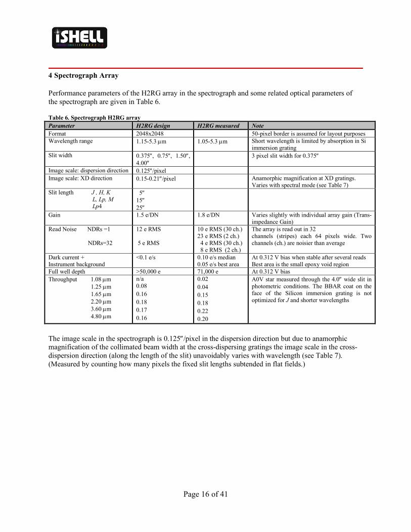
4 Spectrograph Array Performance parameters of the H2RG array in the spectrograph and some related optical parameters of the spectrograph are given in Table 6. Table 6. Spectrograph H2RG array Parameter H2RG design H2RG measured Note Format 2048x2048 50-pixel border is assumed for layout purposes Wavelength range 1.15-5.3 µm 1.05-5.3 µm Short wavelength is limited by absorption in Si

immersion grating Slit width 0.375², 0.75², 1.50²,

4.00² 3 pixel slit width for 0.375²

Image scale: dispersion direction 0.125²/pixel Image scale: XD direction 0.15-0.21²/pixel Anamorphic magnification at XD gratings.

Varies with spectral mode (see Table 7) Slit length J , H, K L, Lp, M Lp4

5² 15² 25²

Gain 1.5 e/DN 1.8 e/DN Varies slightly with individual array gain (Trans-impedance Gain)

Read Noise NDRs =1 NDRs=32

12 e RMS 5 e RMS

10 e RMS (30 ch.) 23 e RMS (2 ch.) 4 e RMS (30 ch.) 8 e RMS (2 ch.)

The array is read out in 32 channels (stripes) each 64 pixels wide. Two channels (ch.) are noisier than average

Dark current + Instrument background

<0.1 e/s 0.10 e/s median 0.05 e/s best area

At 0.312 V bias when stable after several reads Best area is the small epoxy void region

Full well depth >50,000 e 71,000 e At 0.312 V bias Throughput 1.08 µm 1.25 µm 1.65 µm 2.20 µm 3.60 µm 4.80 µm

n/a 0.08 0.16 0.18 0.17 0.16

0.02 0.04 0.15 0.18 0.22 0.20

A0V star measured through the 4.0² wide slit in photometric conditions. The BBAR coat on the face of the Silicon immersion grating is not optimized for J and shorter wavelengths

The image scale in the spectrograph is 0.125²/pixel in the dispersion direction but due to anamorphic magnification of the collimated beam width at the cross-dispersing gratings the image scale in the cross-dispersion direction (along the length of the slit) unavoidably varies with wavelength (see Table 7). (Measured by counting how many pixels the fixed slit lengths subtended in flat fields.)

of 41

Table 7. Image scale in the cross-dispersion direction. Measurements are accurate to about ± 0.005 arcsec

Spectral Mode

Image scale in XD direction At short l limit/arcsec At long l limit/arcsec

J0 0.172 0.156 J1 0.172 0.167 J2 0.192 0.167 J3 0.208 0.178 H1 0.172 0.152 H2 0.167 0.152 H3 0.172 0.152 K1 0.161 0.147 K2 0.161 0.151 K3 0.172 0.156 L1 0.174 0.161 L2 0.190 0.167 L3 0.200 0.176 Lp1 0.174 0.160 Lp2 0.183 0.165 Lp3 0.195 0.172 Lp4 0.192 0.172 M1 0.171 0.160 M2 0.171 0.160

4.1 Testing for correct exposure level An important feature of array operation is the need to keep exposure levels below the intensity level that can be reasonably corrected (to 1% or better) for non-linear response of the detector. This level is about 30,000 DN (three-quarters full well, gain 1.8 e/DN). When multiple non-destructive reads are done to reduce read noise, as is the default, DV displays the average of the NDRs and so half the NDRs will be above the average intensity level by an amount depending upon photon rate from the object. We therefore recommend that observers measure the maximum signal rate with a short integration (£10 s) with NDR=1 and then use the following formula to set the maximum ‘itime’ (on-chip integration time in seconds):

𝑖𝑡𝑖𝑚𝑒 =30,0002 × 𝑟𝑎𝑡𝑒

− 0.5

Where itime is in seconds and rate is in DN/s. To measure the rate set the itime manually and then click the ‘Test Go’ button. This will turn save off, put the telescope beam in position A, set NDRs to one, take an image and then restore the original set up. Finally, measure the rate using the maximum level reported in DV (avoiding hot pixels and scaling to one second), and adjust the itime. In practice, in DV, this optimal itime will correspond to a maximum count number of 8,000 DN for NDR values of >8, and more for less NDRs. Observers can always use shorter itimes appropriate to their S/N requirements. For faint objects we do not recommend itimes longer than about 600 seconds even if the rate measurement allows it. Due to the array clocking scheme itimes round down to the nearest multiple of 0.463 s (the minimum full array read out time).

of 41

The full array read out time of 0.463 s is the time required for one NDR. By default, the array does as many NDRs as possible up to a maximum of 32. For example, for an itime of 9.26 s, ten NDRs will be done (9.26/0.463 = 10), reducing the read noise by about 101/2. Since there is little improvement in read noise above 32 NDRs, itimes longer than 14.82 s default to 32 NDRs. The penalty paid for doing multiple NDRs is an increase in the clock time required by 0.461 s ´ the number of NDRs. To increase observing efficiency observers can choose to reduce NDRs manually. Using shorter exposures and coadding (e.g. for M-band observations) can significantly increase read out overheads and decrease observing efficiency. 4.2 ‘Flush Go’ Historically infrared arrays are known to exhibit residual image artifacts when exposed to bright sources. These can manifest themselves as an increased signal offset (residual) or enhanced dark current (persistence). Experience with the Aladdin arrays originally used in SpeX and that are still used in the SpeX and iSHELL slit viewers has shown that these artifacts can be minimized by taking a short exposure before taking a series of science exposures. The H2RG spectrograph arrays in SpeX and iSHELL do not experience significant residual image and persistent artifacts but the ‘Flush Go’ macro can still be used as a precaution if a very bright or saturated exposure precedes a science exposure sequence. The ‘Flush Go’ command takes a 15 s un-stored integration before proceeding with the entered exposure sequence (itime, coadds, cycles). The Flush Go’ macro also removes a ‘picture frame’ effect in H2RG arrays that can sometimes be seen in the first exposure of a very low background exposure sequence (see the SpeX User Manual). 4.3 Observing efficiency Tables 12-15 estimate the integration time required to reach a desired S/N but do not estimate the clock time, which includes a number of observing overheads. By default, iSHELL does the maximum number of NDRs that it can fit into a given on-chip integration time (itime) up to a maximum of 32, to minimize read noise. Each NDR takes an additional 0.464 s. (The total number of reads per itime is NDRs ´ coadds. NDRs ´ coadds is defined as the DIVISOR keyword in the header.) For example, 21 NDRs can be done in an on-chip integration time of 9.7 s and so with the default number of NDRs selected a 9.7 s on-chip integration time actually takes about 9.744 s + 21x0.464 s or 19.488 s of clock time. If the user chooses to do only one NDR then the same integration times takes 9.744 s but with higher read noise. Coadding images is also less efficient than one long integration time but is often required when short on-chip integration times are required to avoid saturation or to reduce the number of nods. Additional overhead is also needed to display and store data. Table 8 is a guide to the efficiency of observing with different combinations of integration times, NDRs and coadds.

of 41

Table 8. Measured clock time for typical combinations of itime, NDRs and coadds.

itime (s) coadds NDRs Total itime (s) Clock time (s)

Default number of NDRs 1 30 2 30 71 3 10 3 30 63

10 3 21 30 62 15 2 32 30 62 30 1 32 30 47 60 1 32 60 77

120 1 32 120 137 NDRs manually set to 1

1 30 1 30 58 3 10 1 30 39

10 3 1 30 34 15 2 1 30 33 30 1 1 30 33 60 1 1 60 63

120 1 1 120 123 Clearly, executing the default number of NDRs can sometimes double the effective integration time. Other overheads included in Table 6 are the times taken to display and store data. One overhead not included is the beam switch dead time (Beam DTime in the XUI). This is the wait time between nodding the telescope and restarting spectrograph integrations when performing cycles. This wait time allows time for the telescope to nod and for the guider to then lock onto the guide star before resuming spectrograph integrations. The default is five seconds but can be set by an observer. A particular example is observing at M1 or M2 with iSHELL and a 0.375² slit. In good sky conditions the itime needs to limited to a maximum of about 15 s to keep signal (which is typically dominated by sky background) within the linear correctable range. For good sky subtraction the telescope needs to be nodded no longer than about every 30 s. A typical observing sequence might be itime=15.0 s, coadds=2, AB cycles=15. Other overheads include the time required to nod the telescope and settle (beam switch dead-time DTime=5.0 s) and the time required to display the data and write to disk (about 5 s). Using the default number of NDRs (32 for 15 s) the clock time required for this observation sequence is about 34 minutes. However, observations in the M-band are strongly background limited and so NDRs can be manually set to one without any read noise penalty. In this case the clock time required is about 19 minutes, saving 15 minutes of clock time. 4.4 Measurement Spectrograph S/N 4.4.1 S/N widget in DV The S/N widget estimates the S/N per resolution element (i.e slit width). The S/N per pixel column is roughly S/N / (slit width in pixels)1/2 when sky background or signal limited, or S/N / (slit width in pixels) when read noise limited.

of 41

4.4.1.1 L, Lp and M modes In these modes the star is nodded along the 15²-long slit and the A-B beam is displayed in DV buffer C. The cursor Pointer is selected in display panel 3 (set to buffer C) and the cursor moved over the desired location of the spectrum in display panel 2 (set to buffer C). The S/N is then displayed in display panel 3 along with the location of the pseudo box placement (see Figure 9). Signal is measured in an object box 14 pixels long (1.75²) and the same width as the slit. The signal in a skybox is measured at the same location in the B beam. To allow for variations in the sky background level affecting the A-B subtraction the summed signal in two boxes each 7 pixels long and the same width as the slit on either side of the object box are subtracted from the summed object box signal. The signal-to-noise is given by:

𝑆𝑁=

𝐺(𝑜𝑏𝑗𝑒𝑐𝑡𝑏𝑜𝑥 − 𝑠𝑖𝑑𝑒𝑏𝑜𝑥)(𝐺 × (𝑜𝑏𝑗𝑒𝑐𝑡𝑏𝑜𝑥 − 𝑠𝑖𝑑𝑒𝑏𝑜𝑥) + 𝐺 × 𝑠𝑘𝑦𝑏𝑜𝑥 + 14 × 𝑠𝑙𝑖𝑡𝑤𝑖𝑑𝑡ℎ × 𝑅𝑁)F/H

Where the gain G=1.8 e/DN and read noise RN=7 e RMS (conservative estimate). 4.4.1.2 J, H and K modes In these modes the slit length of 5² is too short for nodding. However, nodding is not required since at iSHELL resolving powers the sky background is almost negligible. The cursor Pointer is selected in display panel 3 (set to buffer C) and the cursor moved over the desired location of the spectrum in display panel 2 (set to buffer C). The S/N is then displayed in display panel 3 along with the location of the pseudo box placement (see Figure 9). Signal is measured in an object box 14 pixels long (1.75²) and the same width as the slit. To allow for small variations in the sky background level affecting the A frame (e.g. unsubtracted sky lines) the summed signal in two boxes each 7 pixels long and the same width as the slit on either side of the object box are subtracted from the summed object box signal. The signal-to-noise is given by:

𝑆𝑁=

𝐺(𝑜𝑏𝑗𝑒𝑐𝑡𝑏𝑜𝑥 − 𝑠𝑖𝑑𝑒𝑏𝑜𝑥)(𝐺 × (𝑜𝑏𝑗𝑒𝑐𝑡𝑏𝑜𝑥 − 𝑠𝑖𝑑𝑒𝑏𝑜𝑥) + 14 × 𝑠𝑙𝑖𝑡𝑤𝑖𝑑𝑡ℎ × 𝑅𝑁)F/H

Where the gain G=1.8 e/DN and read noise RN=7 e RMS (conservative estimate).

of 41

4.4.2 S/N measured in ‘Quicklook’ spectral extraction During observing sessions, spectra are automatically extracted and displayed in DV (see Figure 10). This “Quicklook” data reduction enables observers to assess the quality of their data in (near-) real-time. All iSHELL observing modes are supported, except non-nodded L- and M-band observations. The software determines from the FITS headers if sufficient data are available to run a scripted version of Spextool. It then automatically extracts spectra, using a fixed aperture (i.e., the optimal extraction method

Figure 9. Signal-to-noise widget in DV. The pointer is selected in display 3 (buffer C) and moved over the spectrum in in display 2 (buffer C). The widget only works for point sources. Select for iSHELL in the lower right of DV. A zoomed section of the M1 spectral mode in display 3 is shown in this view

of 41

is not used). For off-slit nodding in the L and M-bands, it is assumed the target is extended and the inner 30% of the slit length is extracted. Currently, the spectra are not divided by a standard star, and hence they display atmospheric absorption lines, as well as the typical curved response shape for echelle gratings. The reduced spectra and signal-to-noise values as a function of wavelength are automatically displayed in DV. The result of the latest cycle is sent to DV buffer F, and the average for a given target and observing mode is sent to buffer G. To view these, one needs to select Display Type “QuickLook”. At present, only one of the nods is sent to DV (the nod pair is not averaged), and the signal-to-noise values are per spectral pixel. The signal-to-noise values will be square root 2 higher if the A and B nod spectra are averaged. The signal-to-noise values can be converted from per pixel to per resolution element by multiplication with the square root of the slit width in pixels. Flat field and wavelength calibration files are also automatically reduced after the calibration macro is executed. The best matching calibration files (closest in sky position and time) will be used for the data reduction. If no calibrations were taken yet during the observing session, they will be selected (closest in time) from a calibration database. If such calibrations are not available, the data reduction will only start once the calibration macro has been executed. Also, using flat fields from the calibration database will result in relatively large fringe amplitudes. To check the status of the Quicklook data reduction, see the messages in the dedicated x-terminal in the observing session. For further information, visit <http://irtfweb.ifa.hawaii.edu/~quicklook/>.

Figure 10. Quicklook data reduction widget in DV

of 41

4.5 Spectrograph calibration 4.5.1 Macros Wavelength and flat fielding is done using standard macros (scripts). The macros move mechanisms and turn lamps on and off in the calibration box, which is located immediately above the instrument entrance window. The calibration macros do not move anything inside iSHELL. The macros are run from the Macro window (see Figure 10) by selecting the desired macro file name and clicking Execute (not Go). The path is /home/cartman/macro. The file names are in the format ‘cal_ordersorter_slitwidth’; select the appropriate name of the spectrograph mode that needs to be calibrated. The macros take flat fields (S/N about 300) and ThAr lamp exposures and take between four minutes (MOS) and seven minutes (JOS) to run. The macros return the instrument to the configuration in which the macro is started; no observer intervention is required. Due to flexure and mechanism reproducibility the calibration macros must be executed before changing modes. Observers requiring higher S/N in their flats can write and run custom macros. Observer macros should be stored in /home/cartman/macro/UserMacros but some are also /home/cartman/macro.

Figure 11. Calibration macro GUI in Cartman

4.5.2 Wavelength calibration In the JHK modes Th and Ar lines from the ThAr lamp are used for wavelength calibration. In the LL’M modes telluric features should be used since due to the higher background fewer lamp lines are detectable (see Figures 2-8). The data reduction tool (the iSHELL part of the new Spextool code) uses files created by the calibration macros. At LL’M Spextool uses telluric features in on-sky data files (although the L1

of 41

mode uses a combination of lamp lines and telluric features). However, the macros still take lamp line data at LL’M since the fewer measurable lines may still be useful for observers choosing not to use Spextool. 4.5.3 Flat fielding and fringing Flat fielding is done using a QTH lamp at JHK and an IR (blackbody) lamp at LL’M. Flux from the lamps is integrated to about half full well and five exposures taken to give a S/N of about 300. Unfortunately, slight fringing is visible in the flats with a spatial frequency increasing from about 20 pixels at J to about 70 pixels are M and with a fringe contrast of about 5% (e.g. see Figure 7 right). Due to slight flexure in the instrument fringes do not divide out perfectly as the telescope tracks. With the telescope tracking and with flats taken one hour apart the fringing can be divided out to the level of about 1% (S/N=100). For programs requiring higher S/N flats should be taken more frequently. Typically, fringing is produced by interference in parallel sided optical substrates. Potential culprits in iSHELL are the detector substrate, and the order-sorting filter, slit and window substrates. We have been able to eliminate all these possibilities. The H2RG detector is substrate removed. Wedging the filters has had no effect and the slit substrates are tilted such that interfered beams are absorbed by the backside metal absorption coating. A ZnSe substrate placed in optical contact with the warm cryostat entrance window also had no effect on the fringe frequency and contrast as would be expected if the window was the source. Consequently, the source of the fringing remains unknown.

4.5.4 Darks In the JHK modes the 5²-long slit is too short for nodding point sources along the slit to subtract off the sky background and the dark/bias. However, since there is virtually no sky background at these wavelengths at the high resolving power of iSHELL (aside from sparse sky emission lines) dark exposures taken before or after the data are taken can be used to remove the dark/bias. The darks are stable for time periods of a day. Intermittently noisy pixels still remain but these can be removed during spectral extraction (by optimal extraction or cleaning). Dark current frames are taken at daytime by the support astronomers, for the itimes that were used in the preceding night. For each itime the frames are automatically averaged (using the Spextool combine option Robust Weighted Mean at the default threshold of 8). The observer can download the averaged darks using scp and their observer account (2020AXXX): - find out which darks are available: + ssh [email protected] + cd /home/quicklook/Data_ishell/Cal_library_ishell/ + find the dark with the desired itime and date closest to the observing date (hint: use “ls -ltr dark*” for a time-sorted list). For example, dark-29pt65:200205_191039ut.fits is for data obtained on 5 February 2020 (UT) and an itime of 29.65 seconds (note that this is the actual itime used when entering 30 seconds in the XUI).

of 41

- copy the dark to your own machine: ‘scp [email protected]:/home/quicklook/Data_ishell/Cal_library_ishell/dark29pt65:200205_191039ut.fits .’ If the observer prefers to download the raw (un-averaged) dark frames, this can be done using the above instructions, replacing the directory with /scrs1/cartman/2020A901/200205/ (for 5 Feb 2020 in this example).

of 41

5 Infrared Guider Array Performance parameters of the Aladdin 2 InSb array in the guider are given in Table 9. Table 9. Parameter SpeX iSHELL Note Format 512x512 512x512 SpeX uses one quadrant of a 1024x1024

four quadrant Aladdin 3 array Wavelength range 0.9-5.5 µm 0.9-5.5 µm FOV 60x60² 42² diameter iSHELL FOV underfills array Sub-array read out no yes See Figure 13b. Image scale 0.1185²/pixel 0.1040±0.007²/pixel Measured Gain 17 e/DN 17 e/DN Read Noise NDRs=1 NDRs=16

94 e RMS 34e RMS

110 e RMS 45 e RMS

At 7µs/pixel (0.241 s min. itime)

Dark current + instrument background

6 e/s 10 e/s At 0.400 V bias when stable

Well depth 90,000 e ~120,000 e

90,000 e ~120,000 e

At 0.400 V bias (the default) At 0.700 V bias (useful for nbM imaging)

Throughput J K

0.18 0.25

0.17 0.33

UKIRT FS 151 K=11.87 J-H=0.274 H-K=0.061

5.1 Testing for correct exposure level The full well depth on the 512x512 InSb Aladdin 2 array in the guider is 6000 DN (gain 15 e/DN). To keep in the linear range counts should be kept below about 3000 DN. Since fewer NDRs are done with the imaging array (the maximum is 8 NDRs) than the spectrograph array the signal level can be measured directly from the image in DV without the need for a test exposure. Guiding also works reasonably well on saturated images. The full array read out time of 0.241 s is the time required for one NDR. itimes round down to the nearest multiple of 0.241 s (the minimum full array read out time). By default, the array does as many NDRs as possible up to a maximum of 8. For example, for an itime of 1.205 s five NDRs will be done (1.205/0.241 = 5), reducing the read noise by about 101/2. Since there is little improvement in read noise above 8 NDRs itimes longer than 1.928 s default to 8 NDRs. The narrow-band 5.1µm saturates on the sky in the shortest itime (0.241 sec) available in the standard readout mode. Using single reads (shortest itime 0.120 sec) and/or increasing the bias to 700mV can fix this (both are set in the engineering menu – check with your support astronomer). 5.2 Observing efficiency The penalty paid for doing multiple NDRs is an increase in the time required by 0.241 s ´ the number of NDRs. To increase observing efficiency observers can choose to reduce NDRs manually. For example, an itime of 1.928 s with default NDRs (8) is only 50% efficient.

of 41

6 Data size, transfer and storage For the 2048x2048 H2RG array in the spectrograph the individual file size is 16.8MB. However, we store three files per image: pedestal minus signal, pedestal, and signal, for a of total image size of 50MB. The reason for the extra files, which are stored as extensions to each image, is to more accurately compute corrections for non-linearity using the absolute pedestal and signal levels rather than the relative pedestal minus signal level. For the active 512x512 quadrant of the InSb Aladdin 3 array in the infrared guider the individual file size is 1 MB. Only the pedestal minus read is stored. The best way get your data is to download it to your home machine from the IRTF data disk by sftp (rsync is also available). Ask your support astronomer for details. Long-time observers should also note that spectrograph images require ten times more disk space to store and take about ten times longer to ftp than with the old SpeX 1024x1024 array images. iSHELL data is also archived. The total number of reads per itime is NDRs ´ coadds. NDRs ´ coadds is defined as the DIVISOR keyword in the header. In DV the displayed flux is scaled to the itime by dividing the summed flux by the DIVISOR. This is not done automatically when displaying stored fits data in IDL or IRAF, for example. To reproduce the DV display the data must first be divided by the DIVISOR.

of 41

7 Example Observing Sequence The setup procedure for iSHELL is very similar to that for SpeX. A significant difference is that the slit length in iSHELL is only 5.0² in the JHK modes compared to 15.0² in SpeX and so point sources are not nodded along the slit. Instead a dark exposure of the same integration time is subtracted from the target exposure made in the center of the slit. The small sky background along the slit in these modes is fitted and subtracted in data reduction. At LL¢M where the sky background is higher a 15.0² slit allows point source to be nodded along the slit. Extended sources are nodded out of the slit if a sky exposure needs to be subtracted. A 25² slit can be used at 3.8-4.2 µm (Lp4, see Table 5). An A0V standard star is required for telluric removal. Observers may also choose to forgo the A0V standard and use an atmospheric model to remove telluric features but IRTF does not provide feature in the data reduction tool for iSHELL. A tool to locate A0V stars can be found on the SpeX webpage. A Thorium-Argon lamp is used for wavelength calibration at JHK and a combination of the lamp and telluric features at longer wavelengths. 7.1 Set up spectrograph The spectrograph GUI is shown in Figure 12a.

1. Set wavelength range by selecting XD mode (see Table 5) in the XD Tilt icon. This automatically sets the following mechanisms:

a. Dekker (slit length) b. Order Sorter Filter Wheel (order sorting filter) c. XD Rotate (XD grating) d. XD Tilt (tilt of XD grating) e. Afocus (spectrograph focus)

2. Select the Slit width (this sets the spectrograph resolving power) Observers also have the option of using custom wavelength settings. These are set using the GUI shown in Figure 12.b. The widget allows the lower wavelength or upper wavelength limits of the 19 default settings (see Table 5) to be changed. The 19 standard modes can be fully reduced with the iSHELL data reduction tool. If the default wavelength ranges are changed the iSHELL data reduction tool cannot be used and observers will need to reduce their own iSHELL data. 7.2 Set up slit viewer for target This procedure is very similar to acquisition and guiding with SpeX (see SpeX manual on the IRTF website). The FOV and image scale of iSHELL are 42² (circular) and 0.10² per pixel. The FOV slightly under fills the array. The slit-viewer GUI is shown in Figure 12a and 12b (sub-arrays).

1. Slew telescope to target 2. Select guide filter in slit-viewer filter wheel Gflt (see Table 1) 3. Move Rotator to set desired position angle of slit on the sky. For point sources setting the

position angle to the parallactic angle is optimum. 4. Take acquisition image and focus if required

of 41

5. If guiding on a point source target select Autoguidebox setup 6. Move target into Guidebox A drawn in DV. Otherwise set up to guide on object in the FOV or

with the telescope’s off-axis guider (see SpeX manual). (Point sources can only be nodded along the slit in the LLpM modes (15.0²slit). In the JHK modes the target is positioned in the center of the slit (5.0² slit)

7. Set integration time of guider and start guiding. Guiding is done by offsetting the telescope and so guide corrections more frequent than once per second are not possible; so don’t set the integration time (itime x coadds) shorter than one second.

7.3 Take spectra of target 1. Set integration time of spectrograph (see section 4.1) and start integrating 2. At end of integration stop guiding 3. Run calibration macro (arcs and flats). This should be done at the target position. The flat

macros are exposed long enough to achieve a S/N of about 300. Observers requiring higher S/N will need to get more flat exposures (see Section 4.5.1 Macros)

7.4 Set up slit viewer for A0V standard star

1. Slew telescope to standard star 2. Select guide filter in slit-viewer filter wheel Gflt 3. Move Rotator to the parallactic angle 4. Take acquisition image and focus if required 5. If guiding on a point source target select Autoguidebox setup 6. Move target into Guidebox A drawn in DV. Otherwise set up to guide on object in the FOV or

with the telescope’s off-axis guider (see SpeX manual). (Point sources can only be nodded along the slit in the LL¢M modes (15.0²slit). In the JHK modes the target is positioned in the center of the slit (5.0² slit)

8. Set integration time of guider and start guiding. Guiding is done by offsetting the telescope and so guide corrections more frequent than once per second are not possible; so don’t set the integration time short.

7.5 Take spectra of A0V standard star

1. Set integration time of spectrograph (see Section 4.1) and start integrating 2. At end of integration stop guiding 3. For optimum calibration the calibration macro can be run at the standard star too

7.6 Take darks for JHK spectra At a suitable time during the observing shift (ask your support astronomer) take dark/bias frames needed to subtract from JHK spectra.

1. Set slit to Mirror (this action blanks off spectrograph) 2. Set integration time 3. Run dark macro 4. Repeat for different integration times

of 41

Figure 12a. iSHELL spectrograph GUI.

Figure 12b. Custom wavelength GUI

of 41

Figure 13a. iSHELL infrared guider/slit viewer GUI. Real data is displayed (the moon in Kcont and Saturn in K). The ‘t3remote’ panel to the right displays telescope information. Within t3remote the ‘offset’ panel can be used to offset the telescope and guide on objects too extended for auto-guiding.

Figure 13b. Example of 208x224 sub-array in Kyle. The first two numbers are the top-left x,y co-ords of the sub-array location and the second two numbers the array size Dx, Dy.

of 41

7.7 Sensitivity The instrument parameters used to estimate spectral sensitivity are given in Table 10. In practice array performance and instrument throughput are slightly better than used in the sensitivity model (discussed below). The efficiency of the slit is not included in throughput estimates since it is dependent on image size (seeing etc.).

Table 10. Instrument sensitivity parameters: spectrograph

A realistic FWHM at 2.2 µm is used in the sensitivity model and the FWHM is scaled with wavelength according to Kolmogorov turbulence (l-0.2 dependence, confirmed with SpeX measurements). The seeing profile is then convolved with a diffraction-limited profile and the light transmitted by the rectangular slit (slit efficiency) calculated. At IRTF the nighttime median K-band FWHM (seeing plus diffraction) is about 0.7² (see Figure 14).

Figure 14. Point source image size

Parameter iSHELL Resolving power (R) 70,000 Spectral sampling 3 pixels per slit width Wavelength coverage 1.1-5.3 µm Spatial sampling 0.125² per pixel Slit width 0.375² Detector 2040x2040 H2RG Read noise (multiple reads) 5 e RMS Dark current 0.1 e/s Throughput 0.10 (see Table 7)

of 41

The slit efficiency is plotted for a point source image size of 0.7² (seeing convolved with diffraction) with 0.375² (R=70,000) and 0.75² (R=35,000) wide slits (see Figure 15). Imperfect guiding and focus will further reduce slit efficiency.

Figure 15. Slit efficiency

The atmospheric transmission code ATRAN was used to compute a telluric transmission spectrum (R=70,000) for an air mass of 1.15 (60° elevation) and 2 mm of precipitable water (average for Mauna Kea). Thermal emission from the sky was calculated by assuming a sky emissivity (1 – sky transmission) and a sky temperature of 263 K. Estimates of the non-thermal continuum are from Maihara et al. (1993). Sky emission lines (nearly all OH) are included even though they only cover at most 0.5% of pixels in any particular waveband (maximum in the H-band) at a resolving power of R=70,000. Thermal background from the telescope and cryostat window was calculated assuming a temperature of 273 K and an emissivity of 0.1 (typical measurements are about 0.06 for IRTF). Due to the high dispersion (R=70,000) and small pixel-field-of-view (0.125 ²/pix), the sensitivity of iSHELL is limited by detector performance at wavelengths shorter than 2.5 µm. The Hawaii-2RG detector in iSHELL sees an instrument background (including dark current) of about 0.1 e/s and achieves a read noise of about 5 e RMS with multiple non-destructive reads (NDRs). The quantum efficiency of the array averages about 85%. See Table 6 for details of H2RG array performance.

of 41

Table 11. iSHELL throughput estimates.

Element Efficiency Notes 1.25µm 1.65µm 2.20µm 3.60µm 4.80µm

Telescope Primary 0.98 0.98 0.98 0.98 0.98 Total measured emissivity 4% Secondary 0.98 0.98 0.98 0.98 0.98 See above Foreoptics CaF2 window 0.94 0.95 0.95 0.95 0.95 BBAR witness sample Fold mirror 1 0.96 0.96 0.96 0.96 0.98 Protected-silver, fold Collimating mirror 0.98 0.98 0.98 0.98 0.98 Protected-silver Fold mirror 2 0.96 0.96 0.96 0.96 0.98 Protected-silver, fold Cold stop 0.95 0.95 0.95 0.95 0.95 Undersized to mask telescope Rotator mirror 1 0.96 0.96 0.96 0.96 0.98 Protected-silver, fold Rotator mirror 1 0.96 0.96 0.96 0.96 0.98 Protected-silver, fold Rotator mirror 1 0.96 0.96 0.96 0.96 0.98 Protected-silver, fold Fold mirror 3 0.96 0.96 0.96 0.96 0.98 Protected-silver, fold Lens 1 (BaF2) 0.93 0.95 0.96 0.96 0.95 BBAR witness sample Lens 2 (LiF) 0.94 0.95 0.95 0.95 0.95 BBAR witness sample Fold mirror 4 0.96 0.96 0.96 0.96 0.96 Protected-silver, fold Total Foreoptics 0.55 0.58 0.58 0.58 0.58 Slit viewer Slit mirror 0.97 0.97 0.97 0.97 0.97 Gold-coated CaF2, fold Fold mirror 5 0.96 0.96 0.96 0.96 0.96 Protected-silver, fold Lens 3 (BaF2) 0.93 0.95 0.96 0.96 0.95 BBAR coat est. Lens 4 (LiF) 0.94 0.95 0.95 0.95 0.95 BBAR coat est. Cold stop 1.00 1.00 1.00 1.00 1.00 Oversized Filter 0.85 0.90 0.85 0.95 0.91 Measured average across range Lens 5 (LiF) 0.94 0.95 0.95 0.95 0.95 BBAR witness sample Lens 6 (BaF2) 0.93 0.95 0.96 0.96 0.95 BBAR coat est. Aladdin 2 array 0.85 0.85 0.85 0.85 0.85 Eng. array from SpeX est. Total Slit Viewer 0.48 0.52 0.53 0.53 0.53 Total FO + SV 0.26 0.30 0.31 0.31 0.31 Spectrograph Slit substrate (CaF2) 0.94 0.95 0.95 0.95 0.95 BBAR coat est. Order sorting filter 0.85 0.90 0.90 0.95 0.91 Measured average across range Fold mirror 0.96 0.96 0.96 0.96 0.96 Protected-silver, fold OAP 1 0.98 0.98 0.98 0.98 0.98 Gold-coated aluminum SIG - grating 0.75 0.75 0.75 0.75 0.75 Est. peak (measured at H and K) SIG - substrate 0.75 0.95 0.96 0.95 0.98 BBAR coating (two surface transmission) OAP 1 0.98 0.98 0.98 0.98 0.98 Gold-coated aluminum Spectrum mirror 0.98 0.98 0.98 0.98 0.98 Protected-silver OAP 2 0.98 0.98 0.98 0.98 0.98 Gold-coated aluminum XD grating 0.60 0.65 0.70 0.65 0.65 Off-the-shelf replica gratings Lens 1 (BaF2) 0.93 0.95 0.96 0.96 0.95 BBAR witness sample Lens 2 (ZnS) 0.96 0.98 0.98 0.99 0.99 BBAR witness sample Lens 3 (LiF) 0.94 0.95 0.95 0.95 0.95 BBAR witness sample H2RG QE 0.70 0.90 0.90 0.90 0.85 Teledyne measurements for iSHELL array Total Spectrograph 0.14 0.28 0.31 0.30 0.28 At blaze peak/average across blaze Total FO + Spectr. 0.08 0.16 0.18 0.17 0.16 Predicted at blaze peak Total FO + Spectr. 0.04 0.15 0.18 0.22 Measured on-sky at blaze peak

of 41

7.7.1 Spectroscopy Observers should use the ETC on the iSHELL page of the website: http://irtfweb.ifa.hawaii.edu/~ishell/iSHELL_Exposure_Time_Calculator/sn.php (Updated July 2020.) Typical output is shown in Figure 16. The S/N is given per spectral resolution element not per pixel. To get the S/N per pixel divide S/N by (slit width in pixels)1/2. For the purposes of the ETC there is no difference between coadds and cycles. Both just mean the number of different exposures taken to build up S/N. In the spectrograph GUI there is the option for doing A beams only (‘A’) or A and B beams (‘AB’ – nod along slit). If AB is selected and cycles is set to six then 12 exposures will be taken. That distinction is not made in the ETC; cycles or coadds just means the total number of exposures taken.

Figure 16. Online Exposure Time Calculator (ETC)

of 41

The results of the sensitivity model for the spectrograph discussed above are tabulated in Table 12 (point source) and Table 13 (extended source). Note that the measured resolving powers are now slightly higher. The sensitivity is per spectral resolution element (i.e. not per pixel). Table 12. iSHELL one-hour (600 sec x 6 coadds) point-source sensitivity (read noise 5 e RMS, dark 0.1 e/s, seeing 0.7², throughput 0.1 except 0.05 at J), sum rows 1.5 x seeing FWHM (arcsec) along slit.

R S/N Magnitude (Vega) Line flux (erg s-1 cm-2)

J0 J2 H K L M J0 H K L M 75,000 100 8.5 9.1 9.9 9.5 7.4 5.0 2.9x10-14 2.5x10-15 1.8x10-15 2.6x10-15 1.2x10-14 75,000 10 11.3 11.9 12.7 12.3 10.0 7.5 2.2x10-15 1.9x10-16 1.4x10-16 2.4x10-16 1.2x10-15 37,500 100 9.6 10.2 10.9 10.5 8.3 5.9 2.2x10-14 1.9x10-15 1.4x10-15 2.2x10-15 1.0x10-14 37,500 10 12.3 12.9 13.7 13.2 10.9 8.4 1.8x10-15 1.6x10-16 1.1x10-16 2.0x10-16 1.0x10-15

Table 13. iSHELL one-hour (600 sec x 6 coadds) extended source sensitivity (read noise 5 e RMS, dark 0.1 e/s, seeing 0.7², throughput 0.1 except 0.05 at J), sum rows 1.0²along slit.

R S/N Magnitude arcsec-2 (Vega) Line flux (erg s-1 cm-2 arcsec-2)

J0 J2 H K L M J0 H K L M 75,000 100 8.6 9.2 9.8 9.4 7.2 4.9 2.7x10-14 2.7x10-15 2.0x10-15 3.0x10-15 1.4x10-14

75,000 10 11.4 12.0 12.6 12.2 9.8 7.4 2.0x10-15 2.1x10-16 1.5x10-16 2.7x10-16 1.3x10-15 37,500 100 9.8 10.4 11.0 10.6 8.4 6.0 1.7x10-14 1.8x10-15 1.3x10-15 2.1x10-15 9.7x10-15 37,500 10 12.5 13.1 13.7 13.3 10.9 8.5 1.4x10-15 1.5x10-16 1.1x10-16 2.0x10-16 9.6x10-16

Table 14 gives point-source sensitivity over a range of exposure times for R=70,000 (0.375² slit) in mediocre seeing (1.0² at K). Recent measurements indicate R=81,000 in the 0.375² slit (see Table 2). Table 14. Estimated point-source sensitivity for R=75,000 (0.375² slit) at 100s in mediocre seeing (1.0² at K). To remove hot or noisy pixels requires about six or more median-combined spectral images. The ETC assumes a conservative throughput of 0.1 except 0.05 at J

Total exp. (sec)

itime (sec)

number of coadds

Magnitude (Vega) J H K L M

0.5 0.5 1 -0.16 0.7 0.4 -0.8 -1.5 10.0 10.0 1 3.1 4.0 3.6 2.4 1.1 60.0 10.0 6 4.6 5.5 5.1 3.9 2.2 60.0 60.0 1 5.0 5.9 5.5 4.1 2.3

300.0 60.0 5 6.4 7.3 6.9 5.3 3.2 300.0 300.0 1 6.7 7.5 7.1 5.4 3.2 600.0 120.0 5 7.1 8.0 7.6 5.8 3.6 600.0 600.0 1 7.3 8.2 7.8 5.8 3.6

1800.0 300.0 6 8.1 9.0 8.6 6.6 4.2 1800.0 1800.0 1 8.2 9.1 8.7 6.6 4.2 3600.0 600.0 6 8.7 9.5 9.2 7.0 4.6 3600.0 3600.0 1 8.8 9.7 9.3 7.0 4.6 7200.0 600.0 12 9.1 10.0 9.6 7.4 5.0 7200.0 7200.0 1 9.2 10.1 9.7 7.4 5.0

Table 15 gives point-source sensitivity over a range of exposure times for R=35,000 in (0.75² slit) mediocre seeing (1.0² at K). Recent measurements indicate R=49,000 in the 0.75² slit (see Table 2).

of 41

Table 15. Estimated point-source sensitivity for R=35,000 (0.75² slit) at 100s in mediocre seeing (1.0² at K). To remove hot or noisy pixels requires about six or more median-combined spectral images. The ETC assumes a conservative average throughput of 0.1 except 0.05 at J

Total exp. (sec)

itime (sec)

number of coadds

Magnitude (Vega) J H K L M

0.5 0.5 1 1.1 2.0 1.6 0.5 -0.2 10.0 10.0 1 4.4 5.3 4.9 3.6 2.2 60.0 10.0 6 5.8 6.7 6.3 5.0 3.3 60.0 60.0 1 6.3 7.2 6.8 5.3 3.3

300.0 60.0 5 7.6 7.3 6.9 5.3 3.2 300.0 300.0 1 7.9 7.5 7.1 5.4 3.2 600.0 120.0 5 8.2 9.1 8.7 6.9 4.6 600.0 600.0 1 8.5 9.4 9.0 7.0 4.6

1800.0 300.0 6 9.2 10.1 9.7 7.6 5.2 1800.0 1800.0 1 9.4 10.3 9.9 7.6 5.2 3600.0 600.0 6 9.8 10.6 10.2 8.0 5.6 3600.0 3600.0 1 9.9 10.8 10.4 8.0 5.6 7200.0 600.0 12 10.2 11.1 10.7 8.4 6.0 7200.0 7200.0 1 10.3 11.2 10.8 8.4 6.0

Commissioning data indicates that sensitivity is roughly as predicted, except at J, where the absorptivity of the silicon substrate of the immersion grating increases and where the efficiency of the BBAR coat on the immersion grating could not be optimized. 7.7.2 Imaging and guiding The slit viewer in iSHELL has about the same sensitivity as the slit viewer in SpeX at J, H, and K. iSHELL uses the Aladdin 2 512x512 InSb array that was used in SpeX prior to its upgrade in 2014. The magnitude limit for guiding on spill over from a target in the slit is JHK~15 in ~10 s in median seeing. The imaging sensitivity is given in Table 16. Table 16. Slit viewer sensitivity 60s 10s

Magnitude (Vega) JOS K L¢ 18.0 16.6 11.7

of 41

8 Data Reduction The data reduction package for iSHELL runs as part of Spextool (Spectral extraction tool), the IDL-based code originally developed for SpeX. Spextool components have now been modified to reduce both SpeX and iSHELL data. SpeX users will be familiar with the different components of Spextool: 8.1 xspextool

8.2 xcombspec

8.3 xtellcor

8.4 xmergeorders

8.5 xcleanspec

The iSHELL code is designed to reduce all the spectral modes listed in Table 5. The wavelength limits of these modes can be changed using the custom wavelength GUI (see Figure 11b). However, if the default wavelength limits are changed Spextool is not currently designed to reduce these and observers will need to use other data reduction methods. Spextool for iSHELL is now available: http://irtfweb.ifa.hawaii.edu/research/dr_resources/ For details please ask your support astronomer.

• Prepare wavelength calibration and flat fielding data • Spectral order finding and tracing • Spectral extraction and linearity correction of raw data and calibration data • Output linearity corrected, flat fielded and wavelength calibrated individual spectral orders for

each exposure

• Scale corresponding spectral orders for each extracted exposure • Combine (scale and median typically) multiple exposures and write out

• Fit H lines in spectra of A0V telluric standard star using the instrument profile • Scale individual H lines if required • Construct telluric correction spectrum • Determine any spectral shift between object and A0V standard star and correct • Divide object spectrum by telluric correction spectrum derived from A0V standard star

• Merge spectral orders in the combined and corrected exposures • Write out final spectrum

• Clean spectra • Smooth spectra if desired

of 41

9 Resolving Power 9.1 Optical design

The science requirement is for a spectrograph resolving power Rºl/dl³70,000, where spectral resolution dl, the smallest resolvable wavelength, is taken as the Full Width at Half Maximum (FWHM). In iSHELL the aberration-free diffraction-limited resolving power of R=80,000 at 2.2 µm is matched to three pixels. R is also slightly dependent upon wavelength due to the 3% decrease in the refractive index of silicon from 1.1 µm to 5.3 µm. Using a Monte Carlo analysis and industry standard tolerances, 90% of the trials gave worst-case geometric 50% encircled energy dispersion widths better than 1.1 pixels. When added in quadrature with the diffraction-limited width of three pixels the FWHM is 3.2 pixels, equivalent to R=75,000.

In fact, the measured resolving power matched to the narrowest slit (0.375²) is about R=80,000 at 1-3

µm and about R=88,100 at 5 µm (see Table 17). The reason for the slightly higher resolving powers is probably due a combination of better than expected optical performance, some uncertainty in the as-built geometrical optical parameters, and the effects of diffraction.

The dispersion, and therefore the resolving power, also changes across spectral orders as a function of

the angle of diffraction for a fixed angle of incidence at the grating (e.g. Schroeder Astronomical Optics 2000). The effect becomes larger with increasing blaze angle and is therefore more significant in large format echelle grating spectrographs like iSHELL (tand =3). At J, K and M, the variations across the free spectral range are about R±2%, R±4% and R±8%, with respect to R at the center of the array respectively, with R increasing with wavelength across the order. 9.2 Effects of diffraction

Diffraction at the narrowest slit broadens the image of the entrance pupil imaged through the slit. This image is projected onto the silicon immersion grating (SIG). The effect is most significant at 5 µm (see Figure 16). The increased number of grating lines illuminated compared to the projected geometrical pupil is consistent with the higher resolving power measured at 5 µm.

By design, iSHELL’s resolving is limited by the projected slit width (‘spectral purity’) onto the detector. The intrinsic resolving power due to the grating is much higher (R=spectral order ´ total number of lines from Schroeder Astronomical Optics 2000) and is not the limitation. The spectral line spread function (i.e. the instrument profile, see Figure 17) is effectively the convolution of the slit width with the monochromatic line profile from the grating. For a slit spectrograph the measured

Figure 16. The effect of diffraction at the 0.375² (209 µm) slit on the pupil image projected onto the SIG. The pupil image at 5.00 µm is significantly broadened compared to that at 1.25 µm, resulting in higher resolving power due to the increased number grooves illuminated. Diffraction is much reduced in the direction along the slit (5² at 1.25 µm and 15² at 5.0 µm). Flux outside the SIG aperture does not reach the grating. Modelling of diffraction was done with the Physical Optics Propagation package in ZEMAX.

of 41

FWHM of the spectral line spread function is used to characterize the spectral resolution (dl, Robertson PASA 30, 48R, 2013). 9.3 Spectral line spread functions and resolving power measurements

The measured spectral line spread functions and resolving powers in the J2, H2, K2 and L1 modes (see

Table 5) and the narrow slit (0.375²) are shown in Figure 17. The best fit profiles are Voight profiles. Measurements are made by stacking up about 30 individual Th-Ar lines in each of the modes to improve S/N. The measured resolving powers at the center of the free spectral range (FSR) are listed in Table 17. The higher resolving power in the M1 and M2 modes is most likely due to the effects of diffraction. The higher resolving power at M is also consistent with that measured on unresolved CO absorption lines observed towards Herbig Ae/Be stars (about R=92,000, Banzatti et al. ApJ, 2022).

Similarly, the measured resolving powers at the center of the free spectral range (FSR) for the 0.75² slit are also listed in Table 17. In the latter case the errors are smaller since the Th-Ar lines are better sampled. Note that all the Th-Ar line measurements are made with the slits evenly illuminated. Higher resolving powers can result if a point source, for example, underfills the slit, in particular for slit widths 0.75² and wider.

Figure 17. Spectral line spread functions and the resolving power of iSHELL measured from Th-Ar lines and the 0.375² slit in the J2 (1.25 µm), H2 (1.65 µm), K3 ((2.20 µm), and L1 (2.90 µm) modes (see Table 5). About 30-40 individual lines are stacked to improve the S/N. The best fit is a Voight profile. The errors shown are the standard deviations of the profile fits. In these measurements the arc line illumination evenly fills the slit.

of 41

Table 17. Measured resolving power (R) at center of FSR

Mode Slit width R

J2 0.375² 85,100 ± 900

H2 0.375² 80,000 ± 1,300

K2 0.375² 78,100 ± 1,100

L1 0.375² 83,300 ± 500

M1/M2 0.375² 88,100 ± 2,000

J2 0.75² 48,200 ± 300

H2 0.75² 50,800 ± 400

K2 0.75² 47,600 ± 400

L1 0.75² 49,800 ± 400

M1/M2 0.75² 53,300 ± 300

iSHELL OBSERVING MANUAL

Documents

Transcript of iSHELL OBSERVING MANUAL