Observing and Intervening: Rational and Heuristic Models of Causal Decision Making
17
The Open Psychology Journal, 2010, 3, 119-135 119 1874-3501/10 2010 Bentham Open Open Access Observing and Intervening: Rational and Heuristic Models of Causal Decision Making Björn Meder 1, * , Tobias Gerstenberg 1,3 , York Hagmayer 2 and Michael R. Waldmann 2 1 Max Planck Institute for Human Development, Berlin, Germany 2 University of Göttingen, Göttingen, Germany 3 University College London, London, United Kingdom Abstract: Recently, a number of rational theories have been put forward which provide a coherent formal framework for modeling different types of causal inferences, such as prediction, diagnosis, and action planning. A hallmark of these theories is their capacity to simultaneously express probability distributions under observational and interventional scenar- ios, thereby rendering it possible to derive precise predictions about interventions (“doing”) from passive observations (“seeing”). In Part 1 of the paper we discuss different modeling approaches for formally representing interventions and review the empirical evidence on how humans draw causal inferences based on observations or interventions. We contrast deterministic interventions with imperfect actions yielding unreliable or unknown outcomes. In Part 2, we discuss alterna- tive strategies for making interventional decisions when the causal structure is unknown to the agent. A Bayesian approach of rational causal inference, which aims to infer the structure and its parameters from the available data, provides the benchmark model. This account is contrasted with a heuristic approach which knows categories of causes and effects but neglects further structural information. The results of computer simulations show that despite its computational parsimony the heuristic approach achieves very good performance compared to the Bayesian model. Keywords: Causal reasoning, causal decision making, Bayesian networks, rational inference, bounded rationality, heuristics, computer simulation. INTRODUCTION Causal knowledge underlies various tasks, including prediction, diagnosis, and action planning. In the past decade a number of theories have addressed the question of how causal knowledge can be related to the different types of inferences required for these tasks (see [1] for a recent over- view). One important distinction concerns the difference between predictions based on merely observed events (“see- ing”) and predictions based on the very same states of events generated by means of external interventions (“doing”) [2, 3]. Empirically, it has been demonstrated that people are very sensitive to this important distinction and have the capacity to derive correct predictions for novel interventions from observational learning data [4-7]. This research shows that people can flexibly access their causal knowledge to make different kinds of inferences that go beyond mere covariation estimates. The remainder of this paper is organized as follows. In the first part of this article we discuss different frameworks that can be used to formally represent interventions and to model observational and interventional inferences [2, 3, 8]. We also discuss different types of interventions, such as “perfect” interventions that deterministically fix the state of *Address correspondence to this author at the Center for Adaptive Behavior and Cognition, Max Planck Institute for Human Development, Lentzeallee 94, 14195 Berlin, Germany; Tel: +49 (0) 30-82406239; Fax: +49 (0) 30-8249939; E-mail: [email protected] the target variable and “imperfect” interventions that only exert a probabilistic influence on the target variable. Finally, we outline the empirical evidence regarding seeing and do- ing in the context of structure induction and probabilistic causal reasoning. In the second part of the paper we examine different strategies an agent may use to make decisions about inter- ventions. A Bayesian model, which aims to infer causal structures and parameter estimates from the available data, and takes into account the difference between observations and interventions, provides the benchmark model [9, 10]. This Bayesian model is contrasted with a heuristic approach that is sensitive to the fundamental asymmetry between causes and effects, but is agnostic to the precise structure and parameters of the underlying causal network. Instead, the heuristic operates on a “skeletal causal model” and uses the observed conditional probability P(Effect | Cause) as a proxy for deciding which variable in the network should be tar- geted by an intervention. To compare the models we ran a number of computer simulations differing in terms of avail- able data (i.e., sample size), model complexity (i.e., number of involved variables), and quality of the data sample (i.e., noise levels). CAUSAL MODEL THEORY AND CAUSAL BAYESIAN NETWORKS Causal Bayesian networks [2, 3] provide a general modeling framework for representing complex causal
-
Upload
xn--uni-gttingen-8ib -
Category
Documents
-
view
2 -
download
0
Transcript of Observing and Intervening: Rational and Heuristic Models of Causal Decision Making

The Open Psychology Journal, 2010, 3, 119-135 119
1874-3501/10 2010 Bentham Open
Open Access
Observing and Intervening: Rational and Heuristic Models of Causal Decision Making
Björn Meder1,*, Tobias Gerstenberg
1,3, York Hagmayer
2 and Michael R. Waldmann
2
1Max Planck Institute for Human Development, Berlin, Germany
2University of Göttingen, Göttingen, Germany
3University College London, London, United Kingdom
Abstract: Recently, a number of rational theories have been put forward which provide a coherent formal framework for
modeling different types of causal inferences, such as prediction, diagnosis, and action planning. A hallmark of these
theories is their capacity to simultaneously express probability distributions under observational and interventional scenar-
ios, thereby rendering it possible to derive precise predictions about interventions (“doing”) from passive observations
(“seeing”). In Part 1 of the paper we discuss different modeling approaches for formally representing interventions and
review the empirical evidence on how humans draw causal inferences based on observations or interventions. We contrast
deterministic interventions with imperfect actions yielding unreliable or unknown outcomes. In Part 2, we discuss alterna-
tive strategies for making interventional decisions when the causal structure is unknown to the agent. A Bayesian
approach of rational causal inference, which aims to infer the structure and its parameters from the available data,
provides the benchmark model. This account is contrasted with a heuristic approach which knows categories of
causes and effects but neglects further structural information. The results of computer simulations show that despite its
computational parsimony the heuristic approach achieves very good performance compared to the Bayesian model.
Keywords: Causal reasoning, causal decision making, Bayesian networks, rational inference, bounded rationality, heuristics, computer simulation.
INTRODUCTION
Causal knowledge underlies various tasks, including prediction, diagnosis, and action planning. In the past decade a number of theories have addressed the question of how causal knowledge can be related to the different types of inferences required for these tasks (see [1] for a recent over-view). One important distinction concerns the difference between predictions based on merely observed events (“see-ing”) and predictions based on the very same states of events generated by means of external interventions (“doing”) [2, 3]. Empirically, it has been demonstrated that people are very sensitive to this important distinction and have the capacity to derive correct predictions for novel interventions from observational learning data [4-7]. This research shows that people can flexibly access their causal knowledge to make different kinds of inferences that go beyond mere covariation estimates.
The remainder of this paper is organized as follows. In the first part of this article we discuss different frameworks that can be used to formally represent interventions and to model observational and interventional inferences [2, 3, 8]. We also discuss different types of interventions, such as “perfect” interventions that deterministically fix the state of
*Address correspondence to this author at the Center for Adaptive Behavior
and Cognition, Max Planck Institute for Human Development, Lentzeallee
94, 14195 Berlin, Germany; Tel: +49 (0) 30-82406239;
Fax: +49 (0) 30-8249939; E-mail: [email protected]
the target variable and “imperfect” interventions that only exert a probabilistic influence on the target variable. Finally, we outline the empirical evidence regarding seeing and do-ing in the context of structure induction and probabilistic causal reasoning.
In the second part of the paper we examine different strategies an agent may use to make decisions about inter-
ventions. A Bayesian model, which aims to infer causal
structures and parameter estimates from the available data, and takes into account the difference between observations
and interventions, provides the benchmark model [9, 10].
This Bayesian model is contrasted with a heuristic approach that is sensitive to the fundamental asymmetry between
causes and effects, but is agnostic to the precise structure and
parameters of the underlying causal network. Instead, the heuristic operates on a “skeletal causal model” and uses the
observed conditional probability P(Effect | Cause) as a proxy
for deciding which variable in the network should be tar-geted by an intervention. To compare the models we ran a
number of computer simulations differing in terms of avail-
able data (i.e., sample size), model complexity (i.e., number of involved variables), and quality of the data sample (i.e.,
noise levels).
CAUSAL MODEL THEORY AND CAUSAL BAYESIAN NETWORKS
Causal Bayesian networks [2, 3] provide a general modeling framework for representing complex causal

120 The Open Psychology Journal, 2010, Volume 3 Meder et al.
networks and can be used to model different causal queries, including inferences about observations and interventions. Formally, these models are based on directed acyclic graphs (DAGs), which represent the structure of a causal system (Fig. 1). On a causal interpretation of these graphs (as opposed to a purely statistical semantics) the model can be used for reasoning about interventions on the causal system.
Graphical causal models make two central assumptions to connect causal structures with probability distributions over the domain variables: the causal Markov assumption and the Faithfulness assumption (for details see [2, 3] for a critical view see [11]). The causal Markov assumption states that the value of any variable Xi in a graph G is independent of all other variables in the network (except for its causal descendants) conditional on the set of its direct causes. Ac-cordingly, the probability distribution over the variables in the causal graph factors such that:
=XX
iii
i
XpaXPXP ))(|()( (1)
where pa(Xi) denotes the Markovian parents of variable Xi, that is, the variable’s direct causes in the graph. If there are no parents, the marginal distribution P(Xi) is used. Thus, for each variable in the graph the Markov condition defines a local causal process according to which the state of the vari-able is a function of its Markovian parents. The second im-portant assumption is the Faithfulness assumption, which states that the probabilistic dependency and independency relations in the data are a consequence of the Markov condi-tion applied to the graph, and do not result from specific parameterizations of the causal structure (e.g., that there are no two causal paths that exactly cancel each other out).
Within the causal Bayes nets framework, a variety of learning algorithms have been developed to infer causal
structures and parameter values [12]. Briefly, one can distin-
guish two classes of learning algorithms: constraint-based and Bayesian methods. Constraint-based methods [2, 3] ana-
lyze which probabilistic dependency and independency rela-
tions hold in the data. This information is used to add or re-
move edges between the nodes of the network. The alterna-
tive approach, Bayesian methods [9, 13], starts from a set of
hypotheses about causal structures and updates these hypotheses in the light of the data. The models’ posterior
probabilities serve as scoring function to determine the graph
that most likely underlies the data. Alternatively, one can use other scoring functions, such as the Bayesian information
criterion (BIC) or Minimum Description Length (MDL),
which penalize complex models with many parameters [14].
A variety of approaches address the problem of parame-
ter learning. The simplest approach is to compute maximum likelihood (ML) estimates of the causal model’s parameters,
which can be directly derived from the observed frequency
estimates. An alternative approach is to compute a full poste-rior distribution over the parameter values, whereby the prior
distributions are updated in accordance with the available
data [10, 15, 16]. Given a posterior distribution over the parameters, one can either obtain a point estimate (e.g., the
maximum a posteriori (MAP) estimate) or preserve the full
distributions.
PART 1: OBSERVATIONS AND INTERVENTIONS
There is an important difference between inferences based on merely observed states of variables (“seeing”) and the very same states generated by means of external inter-ventions (“doing”) [2, 3, 17, 18]. For example, observing the state of a clinical thermometer allows us to make predictions about the temperature of the person (observational infer-ence), whereas the same state generated by an external ma-nipulation obviously does not license such an inference (in-terventional inference).
Most of the debate on the difference between observa-tional and interventional inferences has focused on the im-plications of interventions that deterministically fix the target variable to a specific value. Such “perfect” interventions have been variously referred to as “atomic” [2], “strong” [18], “structural” [19], or “independent” [20] interventions. This type of intervention also provides the basis for Pearl’s
Fig. (1). Basic causal models. The lower row illustrates the principle of graph surgery and the manipulated graphs resulting from an
intervention in B (shaded node). See text for details.
Common Cause Model
CB
A
CB
A
Causal Chain Model
CB
A
CB
A
D
CB
A
Confounder Model
D
CB
A
Common Effect Model
CB
A
CB
A
Obs
erva
tion
Inte
rven
tion

Observing and Intervening The Open Psychology Journal, 2010, Volume 3 121
“do-calculus” [2]. To distinguish between merely observed states of variables and the same state generated by interven-tions, Pearl introduced the do-operator, do (•). Whereas the probability P(A | B) refers to the probability of A given that B was passively observed to be present, the expression P(A | do B) denotes the probability of A conditional on an external intervention that fixes the state of B to being present.
The characteristic feature of such perfect interventions is that they render the target variable independent of its actual causes (its Markovian parents). For example, if we arbitrarily change the reading of a thermometer, our action renders its state independent of its usual cause, temperature. Graphi-cally, this implication can be represented by removing all arrows pointing towards the variable intervened upon, a pro-cedure Pearl [2] called graph surgery; the resulting subgraph is a called a “manipulated graph” [3]. Fig. (1) (lower row) shows the implications of an intervention that fixes the state of variable B to a certain value (i.e., “do B”). As a conse-quence, all arrows pointing towards B are removed.
Given the original and the manipulated graph, we can formally express the difference between observations and interventions and model the different causal inferences ac-cordingly. For example, consider the common cause model shown in Fig. (1) (left hand side). In this model, the prob-ability of C given an observation of B, P(C | B), is computed by P(A | B) · P(C | A), where P(A | B) is computed according to Bayes’s theorem, P(A | B) = P(B | A) · P(A) / P(B). By taking into account the difference between observations and interventions, we can also compute the probability of C con-ditional on an intervention that generates B, that is, the inter-ventional probability P(C | do B). The crucial difference be-tween the two inferences is that we must take into account that under an interventional scenario the state of B provides no diagnostic evidence for its actual cause, event A, which therefore remains at its base rate (i.e., P(A | do B) = P(A | do ¬B) = P(A)). Consequently, the probability of C conditional on an intervention in B is given by P(A) · P(C | A). Crucially, we can use parameter values estimated from observational, non-experimental data to make inferences regarding the outcomes of novel interventions whose outcomes have not been observed yet.
THE PSYCHOLOGY OF REASONING ABOUT
CAUSAL INTERVENTIONS: DOING AFTER SEEING
In psychology, the difference between inferences based on observations or interventions has been used to challenge accounts that try to reduce human causal reasoning to a form of logical reasoning [21] or associative learning [22]. Sloman and Lagnado [7] used verbal descriptions of causal scenarios to contrast logical with causal reasoning. Their findings showed that people are capable of differentiating between observational and interventional inferences and arrived at different conclusions in the two scenarios.
Waldmann and Hagmayer [6] went one step further by providing their participants with observational learning data that could be used to infer the parameters of causal models. In their studies, participants were first presented with graphi-cal representations of the structure of different causal mod-els. Subsequently, learners received a data sample consisting of a list of cases that they could use to estimate the models’ parameters (i.e., causal strengths and base rates of causes).
To test participants’ competency to differentiate between observational and interventional inferences they were then asked to imagine an event to be present versus to imagine that the same event was generated by means of an external intervention. Based on these suppositions participants were asked to make inferences regarding the state of other vari-ables in the network. The results of the experiments revealed that peoples’ inferences were not only very sensitive to the implications of the underlying causal structure, but also that participants could provide fairly accurate estimates of the interventional probabilities, which differed from their esti-mates of the observational probabilities.
1
Meder and colleagues [4] extended this paradigm by us-ing a trial-by-trial learning procedure. In this study, partici-pants were initially presented with a causal structure contain-ing two alternative causal pathways leading from the initial event to the final effect (the confounder model shown in Fig. (1), right hand side). Subsequently, they passively observed different states of the causal network. After observing the autonomous operation of the causal system, participants were requested to assess the implications of observations of and interventions in one of the intermediate variables (event B in Fig. (1), right hand side). The results showed that par-ticipants made different predictions for the two scenarios and, in particular, took into account the confounding alterna-tive pathway by which the initial event A could generate the final effect D.
Overall, these studies demonstrated that people are capa-ble of deriving interventional predictions from passive ob-servations of causal systems, which refutes the assumption that predictions of the consequences of interventional actions require a prior phase of instrumental learning. Since in these studies the learning data were not directly manipulated, Meder et al. [5] conducted two further studies to directly assess participants’ sensitivity to the parameter values of a given causal model. Using again a trial-by-trial learning paradigm, the results showed that people’s inferences about the consequences of interventions were highly sensitive to the models’ parameters, both with respect to causal strength estimates and base rate information.
LEARNING CAUSAL STRUCTURE FROM INTER-
VENTIONS
The difference between observations and interventions has also motivated research on structure induction. From a normative point of view, interventions are important because they enable us to differentiate models which are otherwise Markov equivalent, that is, causal structures that entail the same set of conditional dependency and independency rela-tions [23]. For instance, both a causal chain A B C and a common-cause model A B C entail that all three events are correlated, and they also belong to the same Markov class since A and C are independent conditional on B. How-ever, by means of intervention we can dissociate the two structures (e.g., generating B has different implications in the
1 Note that the intervention calculus does not distinguish between inferences based on
actual observations or interventions and inferences based on hypothetical observations
or interventions. From a formal perspective, the crucial point is what we know (or
what we assume to know) about the states of the variables in the network. Whether
people actually reason identically about actual and hypothetical scenarios might be an
interesting question for future research.

122 The Open Psychology Journal, 2010, Volume 3 Meder et al.
two causal models). It has been proven that for a graph com-prising N variables, N-1 interventions suffice to uniquely identify the underlying causal structure [24].
Recent work in psychology has examined empirically whether learners are capable of using the outcomes of inter-ventions to infer causal structure and to differentiate between competing causal models [23, 25-27]. For example, Lagnado and Sloman [27] compared the efficiency of learning simple causal structures based on observations versus interventions. Their results showed that learners were more successful in identifying the causal model when they could actively intervene on the system than when they could only observe different states of the causal network. However, their findings also indicated that the capacity to infer causal structure is not only determined by differences regarding the informativeness of observational and interventional data, but that the advantage of learning through interventions also results from the temporal cues that accompany interventions. According to their temporal cue heuristic [27, 28] people exploit the temporal precedence of their actions and the resulting outcomes.
Similarly, Steyvers et al. [23] demonstrated that learners perform better when given the opportunity to actively inter-vene on a causal system than when only passively observing the autonomous operation of the system. Their experiments also show that participants’ intervention choices were sensi-tive to the informativeness of possible interventions, that is, how well the potential outcomes could discriminate between alternative structure hypotheses. However, these studies also revealed limitations in structure learning from interventions. Many participants had problems to infer the correct model, even when given the opportunity to actively intervene on the causal system.
Taken together, these studies indicate that learning from interventions substantially improves structure induction, al-though the Steyvers et al. studies show that there seem to be boundary conditions. Consistent with this idea, the studies of Lagnado and Sloman [27, 28] indicate that interventional learning might be particularly effective when it is accompa-nied by information about the temporal order of events. In this case, the observed temporal ordering of events can be attributed to the variable generated by means of intervention, thereby dissolving potential confounds. These findings sup-port the view that humans may exploit a number of different “cues to causality” [29-31], such as temporal information or prior knowledge, which aid the discovery of causal structure by establishing categories of causes and effects and by constraining the set of candidate models.
MODELING IMPERFECT INTERVENTIONS
So far we have focused on the simplest types of interven-tions, namely actions that deterministically fix the state of a single variable in the causal system. Although some real-world interventions (e.g., gene knockouts) correspond to such “perfect” interventions, such actions are not the only possible or informative kind of intervention. Rather, inter-ventions can be “imperfect” in a number of ways. First, an intervention may be imperfect in the sense that it does not fix the value of a variable, but only exerts a probabilistic influ-ence on the target. For instance, medical treatments usually do not screen off the target variable from its usual causes
(e.g., when taking an antihypertensive drug, the patient’s blood pressure is still influenced by other factors, such as her diet or genetic make-up). Such probabilistic interventions have been called “weak” [18], “parametric” [19], or “de-pendent” [20] interventions. Second, interventions may have the causal power to influence the state of the target variable, but do not always succeed in doing so (e.g., when an at-tempted gene knockout fails or a drug does not influence a patient’s condition). Such interventions have been termed unreliable interventions [32]. Finally, we do not always know a priori the targets and effects of an intervention. For example, the process of drug development comprises the identification and characterization of candidate compounds as well as the assessment of their causal (i.e., pharmacologi-cal) effects. Such actions have been called uncertain inter-ventions [32]. Note that these three dimensions (strong vs. weak, reliable vs. unreliable, and certain vs. uncertain) are orthogonal to each other.
Because many interventions appear to be imperfect, it is useful to choose a more general modeling framework in which interventions are explicitly represented as exogenous cause variables [3, 8, 20, 32]. An intervention on a domain variable Xi is then modeled by adding an exogenous cause variable Ii with two states (on/off) and a single arrow con-necting it with the variable targeted by the intervention. Fig. (2) shows some causal models augmented with intervention nodes.
The state of such a (binary) intervention variable indi-
cates whether an intervention has been attempted or not.
When the intervention node Ii is off (i.e., no intervention is attempted), the passive observational distribution over the
graph’s variables obtains. Thus,
P(Xi | I i = off ) = P(Xi | pa (Xi ),I i = off , I i = off ) (2)
where pa(Xi) are the Markovian parents of domain variable
Xi in the considered graph; Ii is the intervention node that
affects Xi, and offIi=
are the “normal” parameters (e.g., ob-
served conditional probabilities) that obtain from the
autonomous operation of the causal system. By contrast,
when the intervention node is active (i.e., Ii = on) the state of
the target variable is causally influenced by the intervention
node. Thus, in the factored joint probability distribution the
influence of the intervention on domain variable Xi is in-
cluded:
P(Xi | I i = on) = P(Xi | pa (Xi ),I i = on, I i = on ) (3)
where pa(Xi) are the Markovian parents of Xi, Ii is the inter-
vention node that affects domain variable Xi, and onI
i=
is
the set of parameters specifying the influence of intervention
Ii on its target Xi.
This general notation can be used to formalize different
types of interventions. The key to modeling different kinds
of interventions is to precisely specify what happens when
the intervention node is active, that is, we need to specify
onIi= . Table 1 outlines how a perfect intervention on E
in the single link model shown in Fig. (2) (left-hand side)
can be modeled: when the intervention node is off, the

Observing and Intervening The Open Psychology Journal, 2010, Volume 3 123
normal (observational) parameter set I E = off obtains (left
column), whereas switching on the intervention node results
in the (interventional) parameter set I E = on , which entails
that E is present regardless of the state of its actual cause C
(middle column of Table 1). Note that modeling perfect in-
terventions this way has the same implications as graph sur-
gery, that is, P(C | E, IE) = P(C) [33].
By using exogenous cause variables we can also model
weak interventions, which causally affect the target variable,
but do not screen off the variable from its usual causes.
In this case, onI
i=
encodes the joint causal influence of the
intervention and the target’s Markovian parents. The right-
most column of Table 1 shows an example of an intervention
that only changes the conditional probability distribution of
the variable intervened on, variable E, but does not render it
independent of its actual cause C (i.e., P(E | C, IE) >
P(E | ¬C, IE)).
The major challenge for making quantitative predictions
regarding the outcomes of such weak interventions is that we
must precisely specify how the distribution of the variable
acted upon changes conditional upon the intervention and
the variable’s other causes. If the value of the intervened
variable is simply a linear, additive function of its parents,
then the impact of the intervention could be an additional
linear factor (e.g., drinking vodka does not render being
drunk independent of drinking beer and wine, but seems to
add to the disaster). In case of binary variables it is necessary
to specify how multiple causes interact to generate a com-
mon effect. If we assume that the causes act independently
on the effect, we can use a noisy-OR parameterization [2, 10,
34] to derive the probability distribution of the target vari-
able conditional on the intervention and its additional causes.
Further options include referring to expert opinion to esti-
mate the causal influences of the intervention or to use em-pirical data to derive parameter estimates.
Using intervention variables also enables us to model
unreliable interventions, that is, interventions that succeed
with probability r and fail with probability 1-r. This prob-
ability can be interpreted as referring to the strength of the
causal arrow connecting intervention node Ii with domain
variable Xi. Note that this issue is orthogonal to the question
of whether an intervention has the power to deterministically
fix the state of the target variable. For example, we can
model unreliable strong interventions, such as gene knock-
outs that succeed or fail on a case by case basis. The same
logic applies to unreliable weak interventions. For instance,
in a clinical study it may happen that not all patients comply
with the assigned treatment, that is, only some of them take
the assigned drug (with probability r). However, even when
a patient does take the drug, the target variable (e.g., blood
pressure) is not rendered independent of its other causes. If
we know the value of r we can derive the distribution of Xi
for scenarios comprising unreliable interventions. In this
case, the resulting target distribution of Xi can be represented
by a mixture model in which the two distributions are
weighted by ri, the probability that intervention Ii succeeds
(see [32] for a detailed analysis):
Table 1. Example of a Conditional Probability Table (CPD) for an Effect Node E Targeted by no Intervention, a “Strong” Inter-
vention, and a “Weak” Intervention (cf. Fig. 2a). See Text for Details
No Intervention
( I E = off ) “Strong” Intervention
( I E = on )
“Weak” Intervention
( I E = on )
C present C absent C present C absent C present C absent
E present P = 0.5 P = 0.0 P = 1.0 P = 1.0 P = 0.75 P = 0.5
E absent P = 0.5 P = 1.0 P = 0.0 P = 0.0 P = 0.25 P = 0.5
Fig. (2). Causal models augmented with intervention variables. A, B, C, and E represent domain variables; IA, IB, IC, and IE denote inter-
vention variables.
(a) (b) (c)
IC
IA
IBIC
IA
IBIC
IA
IB
E
C
IE
IC
(d)
CB
A
CB
A
CB
A

124 The Open Psychology Journal, 2010, Volume 3 Meder et al.
),),(|(
)1(),|(),,),(|(
offiIoniIiXpaiXP
ironiIoniIiXPiririoniIiXpaiXP
==
+====
Finally, we can model uncertain interventions, that is,
interventions for which it is unclear which variables of the
causal network are actually affected by a chosen action. Ea-
ton and Murphy [32] give the example of drug target discov-
ery in which the goal is to identify which genes change their
mRNA expression level as a result of adding a drug. A major
challenge in such a situation is that several genes may
change subsequent to such an intervention, either because the
drug affects multiple genes at the same time, or because the
observed changes result from indirect causal consequences
of the intervention (e.g., the drug affects gene A which, in
turn, affects gene B).
To model such a situation Eaton and Murphy [32] used causal graphs augmented with intervention nodes, where the causal effects of the interventions were a priori unknown. Their algorithms then tried to simultaneously identify the targets of the performed intervention (i.e., to learn the con-nections between the intervention nodes and the domain variables) and to recover the causal dependencies that hold between the domain variables. Both synthetic and real-world data (a biochemical signaling network and leukemia data) were examined. The results showed that the algorithms were remarkably successful in learning the causal network that generated the data, even when the targets of the interventions were not specified in advance.
THE PSYCHOLOGY OF REASONING WITH
IMPERFECT INTERVENTIONS
Whereas a number of studies have examined how people reason about perfect interventions, not much is known about peoples’ capacity to learn about and reason with imperfect interventions. However, a recent set of studies has examined causal reasoning in situations with uncertain and unreliable interventions [35; see also 36, 37]. In these studies partici-pants were confronted with causal scenarios in which the causal effects of the available interventions and the structure of the causal system acted upon were unknown prior to learning. In addition, the interventions were not perfectly reliable, that is, the available courses of actions had the power to fix the state of the variable intervened upon, but they only succeeded with a certain probability. The results of these studies showed that people were capable of learning which domain variables were affected by different interven-tions and they could also make inferences about the structure of the causal system acted upon. For example, they suc-ceeded in learning whether an intervention targeted only a single domain variable, which in turn generated another do-main variable, or whether the intervention directly affected the two variables.
SUMMARY PART 1
There are important differences between inferences based on merely observed states of variables and the same states generated by means of external interventions. Formal frameworks based on causal model theory capture this distinction and provide an intervention calculus that enables us to derive interventional predictions from observational
data. In particular, augmenting causal models with nodes that explicitly represent interventions offers a modeling approach that can account for different types of interventions.
Regarding human causal cognition, it has been demon-strated that people differentiate between events whose states have been observed (seeing) and events whose states have been generated by means of external interventions (doing). While learners diagnostically infer the presence of an event’s causes from observations, they understand that generating the very same event by means of an intervention renders it independent of its normal causes, so that the event temporar-ily loses its diagnostic value. Moreover, people are capable of inferring the consequences of interventions they have never taken before from mere observations of the causal sys-tem (“doing after seeing”). Finally, learners can acquire knowledge about the structure and parameters of a causal system from a combination of observations and interven-tions, and they can also learn about causal systems from the outcomes of unreliable interventions. Causal Bayes nets al-low for modeling these capacities, which go beyond the scope of models of instrumental learning [22] and logical reasoning [21].
PART 2: HEURISTIC AND COMPLEX MODELS FOR
MAKING INTERVENTIONAL DECISIONS
In the previous section we have examined different nor-mative approaches for deriving interventional predictions from observational learning data. We now extend this dis-cussion and focus on different decision strategies an agent could use to choose among alternative points of interventions when the generative causal network underlying the observed data is unknown. Consider a local politician who wants to reduce the crime rate in her community. There are several variables that are potentially causally relevant: Unemploy-ment, social work projects, police presence, and many more. Given the limited financial resources of her community, the politician intends to spend the money on the most effective intervention. Since it is not possible to run controlled ex-periments, she has to rely on observational data.
A simplified and abstract version of such a decision mak-ing scenario is depicted in Fig. (3a). In this scenario, there are two potential points of intervention, C1 and C2, and a goal event E which the agent cannot influence directly, but whose probability of occurrence she wants to maximize by means of intervention. In addition, there is another variable H, which is observed but not under the potential control of the agent (i.e., cannot be intervened upon). Furthermore we assume that we have a sample of observational data D indicating that all four variables are positively correlated with each other (dashed lines in Fig. 3a).
The general problem faced by the agent is that, in princi-ple, several causal structures are compatible with the observed data. However, the alternative causal structures have different implications for the consequences of potential interventions. Figs (3b-3d) show some possible causal networks that may underlie the observed data. According to Fig (3b), both C1 and C2 exert a causal influence on E, with the observed correlation between C1 and C2 resulting from their common cause, H. Under this scenario, generating either C1 or C2 by means of intervention will raise the prob-ability of effect E, with the effectiveness of the intervention

Observing and Intervening The Open Psychology Journal, 2010, Volume 3 125
determined by the causal model’s parameters. Fig (3c) de-picts a different causal scenario. Again the two cause events covary due to their common cause H, but only C1 is causally related to the effect event E. As a consequence, only inter-vening in C1 will raise the probability of E. In this situation the observed statistical association between C2 and E is a non-causal, merely covariational relation arising from the fact that C1 tends to co-occur with C2 (due to their common cause, H). Finally, Fig (3d) depicts a causal model in which only an intervention in C2 may generate E. In this causal scenario, event C1 is an effect, not a cause of E. This struc-ture, too, implies that C1 covaries with the other three vari-ables. However, due to the asymmetry of causal relations intervening in C1 will not influence E.
Given some observational data D and the goal of generat-ing E by intervening on either C1 or C2, how would a causal Bayes net approach tackle this inference problem? Briefly, such an approach would proceed as follows (we will later provide a detailed analysis). The first step would be to infer the generative causal structure that underlies the data. In a second step, the data can be used to estimate the graph’s parameters (e.g., conditional and marginal probabilities). Finally, given the causal model and its parameters one can use an intervention calculus to derive the consequences of the available courses of actions. By comparing the resulting interventional distributions, an agent can choose the optimal point of intervention, that is, perform the action do (Ci) that maximizes the probability of the desired effect E.
Such a Bayesian approach provides the benchmark for rational causal inference. It operates by using all available data to infer the underlying causal structure and the optimal intervention. However, as a psychological model such an approach might place unrealistic demands on human infor-mation processing capacities, because it assumes that people have the capacity to consider multiple potential causal mod-
els that may underlie the data. We therefore contrast the Bayesian approach with a heuristic model, which differs substantially in terms of informational demands and compu-tational complexity.
THE INTERVENTION-FINDER HEURISTIC
Our heuristic approach addresses the same decision prob-lem, that is, it aims to identify an intervention which maxi-mizes the probability that a particular effect event will occur. We therefore call this model the Intervention-Finder heuris-tic. In contrast to the Bayesian approach, this heuristic uses only a small amount of causal and statistical information to determine the best intervention point. This heuristic might help a boundedly rational agent when information is scarce, time pressure is high, or computational resources are limited [38-40].
While the heuristic, too, does operate on causal model representations, it requires only little computational effort regarding parameter estimation. Briefly, the proposed inter-ventional heuristic consists of the following steps. First, given a set of observed variables a “skeletal” causal model is formed, which seeks to identify potential causes of the de-sired effect, but makes no specific assumptions about the precise causal structure and its parameters. The variables are classified relative to the desired effect variable E (i.e., whether they are potential causes or further effects of E), but no distinction is made regarding whether an event is a direct or indirect cause of the effect. Based on this elemental event classification, the heuristic uses the conditional probability P(Effect | Cause) as a proxy for deciding where to intervene. More specifically, the decision rule is that given n causes C1, …, Cn and the associated conditional probabilities P(E | Ci), the cause Ci for which P(E | Ci) = max is selected as the point of intervention. Thus, instead of trying to reveal the exact causal model that generated the data and using an
Fig. (3). Example of a causal decision problem. Dashed lines indicate observed correlations, arrows causal relations. a) Observed correla-
tions, b) - d) Alternative causal structures that may underlie the observed correlations.
(b)
?
(d)
?
(c)
?
(a)
H
E
C2C1
H
E
C2C1
H
E
C2C1
H
E
C2C1
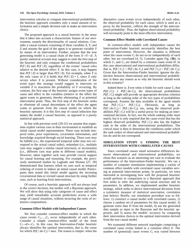
126 The Open Psychology Journal, 2010, Volume 3 Meder et al.
intervention calculus to compute interventional probabilities, the heuristic approach considers only a small amount of in-formation and a simple decision rule to make an intervention choice.
The proposed approach is a causal heuristic in the sense
that it takes into account a characteristic feature of our envi-
ronment, namely the directionality of causal relations. Con-sider a causal scenario consisting of three variables X, Y, and
Z and assume the goal of the agent is to generate variable Y
by means of an intervention. Further, assume that the true generating model is a causal chain of the form X Y Z. A
purely statistical account may suggest to omit the first step of
the heuristic and only compute the conditional probabilities P(Y | X) and P(Y | Z), regardless of the events’ causal roles
relative to the desired effect Y. In this case, it may happen
that P(Y | Z) is larger than P(Y | X). For example, when Y is the only cause of Z it holds that P(Y | Z) = 1, since Z only
occurs when X is present. Without consideration of the
event types this strategy would suggest to intervene on variable Z to maximize the probability of Y occurring. By
contrast, the first step of the heuristic assigns event types of
cause and effect to the variables (relative to the effect the agent wants to generate), thereby eliminating Z as potential
intervention point. Thus, the first step of the heuristic seeks
to eliminate all causal descendants of the effect the agent wants to generate from the causal model on which the
heuristic operates. It is this first step of causal induction that
makes the model a causal heuristic, as opposed to a purely statistical approach.
In line with previous work [29-31] we assume that organ-
isms exploit various cues in their environment to establish an initial causal model representation. These cues include tem-
poral order, prior experiences, covariation information, and
knowledge acquired through social learning. These cues may be fallible (i.e., the experienced temporal order may not cor-
respond to the actual causal order), redundant (i.e., multiple
cues may suggest a similar causal structure), or inconsistent (i.e., different cues may point to different causal models).
However, taken together such cues provide crucial support
for causal learning and reasoning. For example, the previ-ously mentioned studies by Lagnado and Sloman [27, 28]
demonstrated that learners relied on cues such as temporal
ordering of events to induce an initial causal model. Partici-pants then tested this initial model against the incoming
covariational data or revised causal structure by using further
cues, such as learning from interventions.
Of course, such a heuristic approach will not always lead
to the correct decision, but neither will a Bayesian approach. We will show that using only categories of cause and effect
may yield remarkably accurate predictions across a wide
range of causal situations, without incurring the costs of ex-tensive computations.
Common-Effect Models with Independent Causes
We first consider common-effect models in which the cause events C1,…,Cn occur independently of each other. Consider a simple common-effect model of the form C1 E C2. In this case, the Intervention-Finder heuristic always identifies the optimal intervention, that is, the cause for which P(E | do Ci) = max. The reason is simple: when the
alternative cause events occur independently of each other, the observed probability for each cause, which is used as a proxy by the heuristic, reflects the strength of the interven-tional probability. Thus, the highest observational probability will necessarily point to the most effective intervention.
Common-Effect Models with Correlated Causes
In common-effect models with independent causes the Intervention-Finder heuristic necessarily identifies the best point of intervention. However, the situation is different when the cause events Ci do not occur independently of each other, but are correlated [4, 5]. Consider again Fig. (3b), in which C1 and C2 are linked by a common cause event H. In this case observational and interventional probabilities differ, that is, P(E | C1) > P(E | do C1) and P(E | C2) > P(E | do C2). Given that the Intervention-Finder heuristic ignores the dis-tinction between observational and interventional probabili-ties: is there any reason as to why the heuristic should work in this scenario?
Indeed there is. Even when it holds for each cause Ci that P(E | Ci) P(E | do Ci), the observational probabilities P(E | Ci) might still provide an appropriate decision criterion as long as the ranking order of the two types of probabilities correspond. Assume the data available to the agent entails that P(E | C1) > P(E | C2) . Obviously, as long as P(E | do C1) > P(E | do C2), too, using the observed prob-abilities P(E | Ci) will be a useful proxy for making an inter-ventional decision. In fact, not the whole ranking order must match, but it is only required that the cause event that has the highest observed probability P(E | Ci) also has the highest rank in the order of the interventional probabilities. The critical issue is then to determine the conditions under which the rank orders of observational and interventional probabili-ties do and do not correspond.
SIMULATION STUDY 1: FINDING THE BEST
INTERVENTION WITH CORRELATED CAUSES
Since correlated causes entail normative differences be-tween observational and interventional probabilities, we chose this scenario as an interesting test case to evaluate the performance of the Intervention-Finder heuristic. We ran a number of computer simulations implementing a variety of common effect models with correlated cause variables serv-ing as potential interventions points. In particular, we were interested in investigating how well the proposed heuristic would perform in comparison to a Bayesian approach that first seeks to infer the underlying causal structure and its parameters. In addition, we implemented another heuristic strategy, which seeks to derive interventional decisions from a symmetric measure of statistical association, correlation (see below). Briefly, our simulation procedure was as fol-lows: 1) construct a causal model with correlated causes, 2) choose a random set of parameters for this causal model, 3) generate some data D from the model, 4) use the generated data sample as input to the Bayesian and the heuristic ap-proach, and 5) assess the models’ accuracy by comparing their intervention choices to the optimal intervention derived from the true causal model.
We examined different network topologies comprising n correlated cause events linked to a common effect E. The number of (potential) cause events Ci was varied between

Observing and Intervening The Open Psychology Journal, 2010, Volume 3 127
two and six. The correlation between these cause variables resulted from a common cause node H that generated these events (cf. Fig. 4), thereby ensuring a normative difference between observational and interventional probabilities. For each scenario containing n cause variables Ci we constructed a model space by permutating the causal links between the cause nodes Ci and the effect node E. To illustrate, consider a network topology with three potential causes C1, C2, and C3. Excluding a scenario in which none of the potential causes generates E, the model space consists of seven graphs (Fig. 4). Note that all seven causal models imply that the cause events (C1, C2, and C3) are correlated with the effect. However, the structures entail different sets of effective points of interventions. For example, whereas the leftmost model entails that intervening on any of the cause variables will raise the probability of the effect (with the effectiveness of the interventions determined by the model’s parameters) the rightmost model implies that only an intervention in C3 provides an effective action.
The same procedure was used to construct the model
spaces for network topologies containing more than three cause variables. The rationale behind this procedure was that
categories of cause and effect are assumed to be known to
the agent. To allow for a fair comparison of the different approaches, this restricted set of models was also used as the
search space for the Bayesian model. In fact, without con-
straining the search space the Bayesian approach soon be-comes intractable, since the number of possible graphs is
super-exponential in the number of nodes. For example,
without any constraints there are 7.8 1011
possible graphs that can be constructed from eight nodes (i.e., a model com-
prising six intervention points Ci, their common cause H, and
the effect node E), whereas the restricted model space con-tains only 63 models.
For the simulations, first one of the causal structures from the model space was randomly selected. Next, a ran-
dom set of parameters (i.e., conditional and marginal prob-
abilities) was generated. These parameters included the base rate of the common cause H, the links between H and the
cause variables Ci, and the causal dependencies between the
cause variables and the effect E. Each parameter could take any value in the range (0, 1). The joint influence of the cause
variables Ci on effect E was computed in accordance with a
noisy-OR parameterization [34]; the probability of the effect in the absence of all cause variables Ci was fixed to zero. By
forward sampling, the causal model was then used to gener-
ate some data D (i.e., m cases with each instance consisting of a complete configuration of the variables’ states). These
data served as input to the different decision strategies.
To evaluate model performance, the true generative causal model served as a benchmark. Thus, we applied the do-
calculus to the true causal model in order to derive the distri-
bution of the interventional probabilities for all cause events
Ci, and later examined whether the choices suggested by the different strategies corresponded to the optimal intervention
derived from the true causal model.
We also systematically varied the size of the generated
data sample. The goal was to assess the interplay between
model complexity (i.e., number of nodes in the network) and sample size regarding model performance. For example, the
first step of the Bayes nets approach is to identify the pres-
ence and strengths of the links between the potential inter-vention points Ci and the effect node E. Identifying the cor-
rect structure increases the chances to identify the optimal
point of intervention, but the success of this step often de-pends on how much data are available [41]. We systemati-
cally varied the size of the data sample between 10 and 100
in steps of 10, and between 100 and 1,000 in steps of 100. For each type of causal model and sample size we ran 5,000
simulation trials. Hence, in total we ran 5 (number of causes
Ci = two to six) 19 (different sample sizes) 5,000 (num-ber of simulations) = 475,000 simulation rounds.
Implementing the Decision Strategies
For the simulation study we used the Bayes Net Toolbox
(BNT) for Matlab [42]; in addition we used the BNT Struc-
ture Learning Package [12]. This software was used for gen-erating data from the true causal networks and to implement
the Bayesian approach. To derive interventional probabili-
ties, we implemented Pearl’s do-calculus [2]. (All Matlab code is available upon request). In the simulations we com-
pared the performance of the Bayesian inference model with
the Intervention-Finder heuristic. In addition, we included a model that uses the bivariate correlations between each of
the cause variables and the effect as a proxy for deciding
where to intervene. This model was included to test the im-portance of using appropriate statistical indices in causal
decision making: since the goal of the agent is to choose the
intervention that maximizes the interventional probability P(E | do Ci), we consider the observed conditional probabil-
ity P(E | C) as a natural decision proxy an agent may use.
Another option would be to use a symmetrical measure of covariation, such as correlation. Using such an index, how-
ever, may be problematic since it does not reflect the asym-
metry of cause-effect relations (see below for details). To evaluate the importance of using an appropriate statistical
index, we pitted these two decision proxies against each
other. Generally, to ensure that the computational goals of the models were comparable all approaches started with ini-
tial knowledge about categories of causes and effects. For all
models, the task was to decide on which of the cause vari-ables Ci one should intervene in order to maximize the prob-
Fig. (4). Common-effect models with three potential cause events C1, C2, and C3. Due to the common cause H all three cause events are sta-
tistically correlated with the effect E, although not all of them are causally related to E.
E
C2C1
H
C3
E
C2C1
H
C3
E
C2C1
H
C3
E
C2C1
H
C3
E
C2C1
H
C3
E
C2C1
H
C3
E
C2C1
H
C3

128 The Open Psychology Journal, 2010, Volume 3 Meder et al.
ability of effect E occurring. However, the inferential proc-
ess by which this decision was made differed between the
approaches.
The Bayesian approach was implemented as follows. First, we defined a search space consisting of the restricted model space from which the true causal model had been cho-sen. This procedure not only ensured that the Bayesian ap-proach remained tractable, but also guaranteed that both the Bayesian and the heuristic approach started from the same set of assumptions about the types of the involved events. For example, for the simulations concerning three possible causes C1, C2, and C3 the search space included the seven graphs shown in Fig. (4). We used a uniform prior over the graphs (i.e., all causal structures had an equal a priori prob-ability). The next step was to use Bayesian inference to compute which causal model was most likely to have gener-ated the observed data. To do so, we computed the graphs’ marginal likelihoods, which reflect the probability of the data given a particular causal structure, marginalized over all possible parameter values for this graph [9, 13]. Using a uniform model prior allowed us to use the marginal likeli-hood as a scoring function to select the most likely causal model. The selected model was then parameterized by deriv-ing maximum likelihood estimates (MLE) from the data. Finally, we applied the do-calculus to the induced causal model to determine for each potential cause Ci the corre-sponding interventional probability P(E | do Ci). The cause variable for which P(E | do Ci) = max was then chosen as intervention point.
The Intervention-Finder heuristic, too, started from an initial set of categories of cause and effect. Thus, E repre-
sented the desired effect variable and the remaining variables
Ci were considered as potential intervention points. How-ever, in contrast to the Bayesian approach the heuristic did
not seek to identify the existence and strengths of the causal
relations between these variables. Instead, the heuristic model simply derived all observational probabilities P(E | Ci)
from the data sample and used the rank order of the observa-
tional probabilities as criterion for deciding where to inter-vene in the causal network. For example, for the network
class with three cause events C1, C2, and C3, the correspond-
ing three probabilities P(E | C1), P(E | C2), and P(E | C3) were computed. Then the cause variable for which
P(E | Ci) = max was selected as point of intervention.
Finally, we implemented another variant of the heuristic model, which bases its decision on a symmetric measure of
statistical association, namely the bivariate correlations be-
tween the cause variables and the effect. For each cause Ci the -correlation was computed, given by
),,(),,(),,(),,(
,,,,
,E
iC
nE
iC
nE
iC
nE
iC
nE
iC
nE
iC
nE
iC
nE
iC
n
Ei
Cn
Ei
Cn
Ei
Cn
Ei
Cn
Ei
C
¬¬+¬¬+¬¬+¬¬+
¬¬¬¬=
(5)
where n denotes the number of cases for the specified com-bination of cause Ci and effect E in the data sample. As a decision rule, the correlational model selected the cause vari-able which had the highest correlation with the effect. Note that the computed proxy, correlation, takes into account all four cells of a 2 2 contingency table, whereas the condi-tional probability P(E|Ci) used by the Intervention-Finder heuristic is derived from only two cells (i.e., nC,E and nC, ¬E). Nevertheless, we expected the correlational approach to perform worse since this decision criterion ignores the asymmetry of causal relations. For example, consider the two data sets shown in Table 2. In both data sets the correlation between cause and effect is identical (i.e.,
C, E = 0.48). However, the conditional probability P(E | C) strongly differs across the two samples: whereas in the first data set (left-hand side) P(E | C) = 0.99, in the second data set (right-hand side) P(E | C) = 0.4. As a consequence, an agent making interventional decisions based on such a symmetric measure of covariation may arrive at a different conclusion than an agent using a proxy that reflects causal directionality.
Simulation Study 1: Results
We first analyzed the performance of the Bayesian approach regarding the induction of the causal model from which the data were generated. Fig. (5) shows that the model recovery rate was a function of sample size and network complexity [41, 43]. The Bayesian approach was better able to recover the generating causal graph with more data and simpler models.
Next we examined how accurate the different strategies performed in terms of deciding where to intervene in the network. We analyzed the proportion of correct decisions (relative to the true causal model) and the relative error, that is, the mean difference in the probability of the effect that would result from the best intervention derived from the true causal model and the probability of the effect given the cho-sen intervention. As can be seen from Fig. (6), the Bayesian approach performed best, with the percentage of correct in-tervention choices and size of error being a function of model complexity and sample size. The larger the data sam-ple, the more likely the intervention choice corresponded to the decision derived from the true causal model. Conversely, the number of erroneous decisions increased with model complexity, and more data were required to achieve similar levels of performance compared to simpler network topolo-gies. These findings also illustrate that inferring the exact causal structure is not a necessary prerequisite for making the correct intervention decision. Consider the most complex network class, which contains six potential intervention points (i.e., Ci = 6). As Fig. (5) shows, for a data sample con-taining 1,000 cases, the probability of inferring the true gen-erating model from the 63 possible graphs of the search space was about 50%. However, a comparison with Fig. (6)
Table 2. Two Data sets with Identical Correlations between a Cause C and an Effect E ( C, E =0 .48) but Different Conditional
Probabilities of Effect given Cause, P(E | C) (0.99 and 0.4, respectively)
E ¬E E ¬E
C 99 1 C 40 60
¬C 60 40 ¬C 1 99

Observing and Intervening The Open Psychology Journal, 2010, Volume 3 129
shows that the number of correct intervention decisions was clearly higher, namely about 80%. The reason for this diver-gence is that stronger causal links within the network are more likely to be recovered than weaker causal relations, particularly when only limited data are available. Thus, the inferred model is likely to contain the strongest causal links, which often suffices to choose the most effective point of intervention. Therefore, even a partially incorrect model may allow for a correct decision. Taken together, the findings indicate that the Bayesian approach was very successful in deriving interventional decisions from observational learning data.
The most interesting results concern the performance of the Intervention-Finder heuristic. Given the computational parsimony of the heuristic, the main question was how the model would compare to the more powerful Bayesian ap-proach. The results of the simulations indicate that the heu-ristic was remarkably accurate in deciding where to inter-vene in the causal network (cf. Fig. 6). Although the heuris-tic model does not require as extensive computations as the Bayesian approach, its performance came close to the much more powerful Bayesian account. Thus, operating on a skele-tal causal model assuming all variables to be potential causes and using a rather simple statistic as proxy for making an interventional decision provided a good trade-off between computational simplicity and accuracy. Finally, the analyses show that using a symmetric measure of statistical associa-tion, correlation, provided a poor decision criterion for causal decision making. This approach performed worst, both in terms of the number of correct decisions and size of error. Thus, using an appropriate decision proxy is important for making good decisions.
SIMULATION STUDY 2: WHY AND WHEN DOES
THE INTERVENTION-FINDER HEURISTIC WORK?
The previous simulations have shown that the Interven-tion-Finder heuristic achieved a good performance in scenar-
ios involving correlated cause variables. To understand when and why the heuristic works, we ran a systematic simulation involving the confounder model shown in Fig. (3b), which contains two correlated cause events, C1 and C2. Since this model contains only few causal relations it was possible to systematically vary the strength of all causal links in the network: the base rate of the common cause H, the probabil-ity with which H caused C1 and C2, respectively, as well as the two causal links connecting C1 and C2 with their com-mon effect E. As before, P(E | C1, C2) was derived from a noisy-OR gate and P(E | ¬C1, ¬C2) was set to zero. We var-ied the strength of the five causal connections between 0.1 and 1.0 in steps of 0.1, resulting in 10
5 = 100,000 simulation
rounds. For each parameter combination we generated a data sample of 1,000 cases, which served as input to the heu-ristic model.
Across all simulations, the heuristic identified the best
point of intervention in 87% of the cases. This result pro-
vides further evidence that the heuristic performs quite well
across a wide range of parameter combinations. Since the
difference between observational and interventional prob-
abilities depends on how strongly the cause variables corre-
late, we next analyzed the heuristic’s performance in relation
to the size of the correlation between C1 and C2. We com-
puted the correlation between the two cause variables in each
simulation and pooled them in intervals of 0.1. Fig. (7a)
shows that the performance of the heuristic crucially depends
on how strongly the two cause variables covary: while the
model makes very accurate predictions when the cause
variables are only weakly correlated, performance decreases
as a function of the size of the correlation. As can be seen
from Fig. (7b), the size of the error, too, depends on the
correlation between the cause variables. The higher the
correlation, the larger the discrepancy between the interven-
tion decision derived from the true causal model and the
intervention chosen by the heuristic.
Fig. (5). Model recovery rates of the Bayesian approach as a function of model complexity and sample size. Ci denotes the number of
potential intervention points in the network
0 100 200 300 400 500 600 700 800 900 1000 0
10
20
30
40
50
60
70
80
90
100
Sample Size
Cor
rect
Mod
el C
hoic
es (
%)
Ci=2
Ci=3
Ci=4
Ci=5
Ci=6

130 The Open Psychology Journal, 2010, Volume 3 Meder et al.
To understand the very good overall performance of the heuristic approach it is important to consider the distribution of correlations between the two cause variables across the parameter space. Fig. (7c) shows that the distribution is highly skewed: whereas many parameter combinations entail that C1 and C2 are rather weakly correlated, high correlations occur only rarely. In other words, the particular situations in which the heuristic is prone to errors did not occur very of-ten, whereas situations in which the causal heuristic per-formed well were frequent in our simulation domain. (Note, however, that this only holds for a uniform distribution over the parameter values; see the General Discussion). Taken together, these analyses indicate that the size of the correla-
tion between the cause variables provides an important boundary condition for the accuracy of the Intervention-Finder heuristic.
SIMULATION STUDY 3: FINDING THE BEST INTERVENTION WITH NOISY DATA
In a further set of simulations we examined the robust-ness of the different approaches when inferences have to be drawn from noisy data. These simulations mimic situations in which an agent must make inductive inferences from noisy data, which is often the case in real world domains. For instance, in the medical domain doctors often have to base their intervention decision regarding treatments on
Fig. (6). Simulation results for different network topologies. Dashed lines indicate causal links that were varied (present vs. absent) during
the simulations.

Observing and Intervening The Open Psychology Journal, 2010, Volume 3 131
noisy data resulting from the imperfect reliability of medical tests.
We adopted the same simulation method as in the first study, but this time we introduced different levels of noise to the data sample. Noise was introduced by flipping the state of each variable (present vs. absent) in each data case m with probability . For example, when a variable was present in an instance m, its state was changed to absent with probability
, whereas the variable remained in its actual state with pro- bability 1- . This was done independently for each variable in each instance of the sample data D. To simulate different levels of noise, we varied from 0.1 to 0.5 in steps of 0.1 (i.e., we examined five different levels of noise). The noisy data then served as input to the different decision models.
Fig. (8) shows the results of these simulations. Not sur-prisingly, model performance decreased as a function of noise and model complexity. In fact, with the highest level of noise (i.e., = 0.5) the accuracy of all three models dropped to chance level. However, particularly interesting is the find-ing that the performance of the heuristic matched the Baye-sian approach, particularly for small levels of noise (e.g., = 0.1). Given that the Bayesian model always outperformed the heuristic in the previous simulations this is clearly a very interesting result. In line with previous research on heuristic models [39, 40], these findings suggest that a heuristic model of causal decision making may have the capacity to be more robust than computationally more complex models. In the present study, the increased performance of the heuristic model is mostly due to an impaired model recovery rate of the Bayesian approach.
EXTENSIONS TO OTHER CAUSAL SCENARIOS
So far we only have analyzed the Intervention-Finder heuristic in a restricted set of causal scenarios. Thus, further analyses are needed to explore other scenarios. As a first step in this direction, we have examined common-effect models with conjunctive or disjunctive interactions between the cause variables, and causal models containing direct and indirect causes of the desired effect.
Conjunctive Interactions
Interestingly, the heuristic’s accuracy in common-effect models with independent causes does not seem to depend on the assumption that there is no conjunctive interaction be-
tween the candidate causes (see [44] for a general analysis of interactive causal power). Consider a common-effect model C1 E C2, with two independently occurring causes C1 and C2. Imagine C1 occurs with base rate P(C1) = 0.8, C2 occurs with P(C2) = 0.1, and the desired effect E occurs only when both causes are present (i.e., an AND conjunction). Which of the two variables should an agent intervene upon to maxi-mize the probability of the effect? Intuitively, it is better to generate the less frequent cause variable C2, since C1 has a high probability of occurring anyway, which is a necessary precondition for the occurrence of the effect.
In such a scenario the heuristic will infer the correct point of intervention (i.e., the less frequent cause variable) because the base rate of the different causes also affects the observed conditional probabilities P(E | Ci). Formally, the two condi-tional probabilities are given by
P(E | C1) = P(C2) · P(E | C1, C2) + P(¬C2) · P(E | C1, ¬C2) (5)
and
P(E | C2) = P(C1) · P(E | C1, C2) + P(¬C1) · P(E | ¬C1, C2) (6)
When both C1 and C2 are necessary to produce the effect, the second term of these equations reduces to zero (since P(E | C1, ¬C2) = P(E | ¬C1, C2) = 0), while the first term reduces to the base rate of the alternative cause (since P(E | C1, C2) = 1). As a consequence, the conditional prob-ability of a cause variable is equal to the base rate of the al-ternative cause, that is, P(E | C1) = P(C2) = 0.1 and P(E | C2) = P(C1) = 0.8. Thus, the heuristic will always select the optimal point of intervention, namely the cause variable that is less frequent (here: C2).
Disjunctive Interactions
Now consider a common-effect model in which the two causes have the same base rates as before (i.e., P(C1) = 0.8 and P(C2) = 0.1), but are connected by an exclusive-OR (XOR) interaction (i.e., E only occurs when either C1 or C2 are present, but not when both causes are present). In this case, it is best to generate the more frequent event, since the presence of the other case would inhibit the occurrence of the effect. Although the situation is exactly opposite to a conjunctive interaction, the heuristic will again select the correct point of intervention. Consider again Equations (5) and (6). In case of a XOR, the first term of both equations reduces to zero, since P(E | C1, C2) = 0. The second term
Fig. (7). Results of the systematic evaluation for a causal network containing two correlated points of intervention, C1 and C2, affecting a
single effect E.
0
0.02
0.04
0.06
0.08
0.10
0.12
0.14
0.16
Phi(C1,C
2)
-.2 -
-.1
-.1 -
00
- .1
.1 -
.2.2
- .3
.3 -
.4
.4 -
.5
.5 -
.6
.6 -
.7
.7 -
.8
.8 -
.9.9
- 1
Pro
ba
bili
ty
0
0.05
0.1
0.15
0.2
0.25
Phi(C1,C
2)
-.2 -
-.1
-.1 -
00
- .1
.1 -
.2.2
- .3
.3 -
.4
.4 -
.5
.5 -
.6
.6 -
.7
.7 -
.8
.8 -
.9.9
- 1
Re
lativ
e E
rro
r
0
20
40
60
80
100
Phi(C1,C
2)
-.2 -
-.1
-.1 -
00
- .1
.1 -
.2.2
- .3
.3 -
.4
.4 -
.5
.5 -
.6
.6 -
.7
.7 -
.8
.8 -
.9.9
- 1
Co
rre
ct In
terv
en
tion
Ch
oic
es
(%)
(a)
Proportion of correct choices as afunction of correlation between C1 and C2
(b)
Size of error as a function of thecorrelation between C1 and C2
(c)
Distribution of correlations

132 The Open Psychology Journal, 2010, Volume 3 Meder et al.
equals the probability that the alternative cause will not occur (i.e., 1-P(C2) in Equation (5) and 1-P(C1) in Equation 6), since P(E | C1, ¬C2) = P(E | ¬C1, C2) = 1. The resulting two conditional probabilities are P(E | C1) = 0.9 and P(E | C2) = 0.2, therefore the heuristic would correctly sug-gest to intervene in C1, which is the more frequent event. Thus, although conjunctive and disjunctive interactions re-quire diametrically opposed decisions, the heuristic will suc-ceed in both cases.
Direct vs. Indirect Causes
Another interesting scenario concerns a causal model con-taining direct and indirect causes. Assume the true generat-ing model is a causal chain of the form C1 C2 E. Intui-tively, intervening on a variable’s direct cause will tend to be more effective, since interventions on indirect causes are
more error prone, as they require the generation of interme-diate events to produce the desired effect. Interestingly, the heuristic will almost always select the direct cause (here: C2), as point of intervention. The reason is that in probabilis-tic causal chains the influence of any indirect cause on E is attenuated as a function of causal path length. Using P(E | Ci) as a proxy will select the effect’s direct cause to intervene upon, since usually the conditional probability P(E | Ci) is higher for a direct cause than for an indirect cause. The limiting case are deterministic causal chains, since then P(E | C1) = P(E | C2) = 1. Yet, although in this situation an agent using the heuristic must resort to randomly choosing between the two causes, this actually does not mat-ter since in both cases the effect will be generated with a probability of one.
Fig. (8). Model performance for different levels of noise, model complexity, and sample size.

Observing and Intervening The Open Psychology Journal, 2010, Volume 3 133
However, there are also situations in which it is better to
intervene in indirect causes. This is the case when the indi-
rect cause generates multiple direct causes, such as in the
confounder model shown in Fig. (3b), in which H generates
two direct causes, C1 and C2. However, since P(E | H) in-
cludes the joint influence of both C1 and C2 this conditional
probability will be larger than the conditional probabilities
P(E | C1) and P(E | C2). Hence, the Intervention-Finder heu-
ristic will correctly select the indirect cause H as the most
effective point of intervention.
GENERAL DISCUSSION
The goals of this paper were twofold. First, we reviewed
alternative approaches for formally representing interven-
tions in causal networks and modeling probabilistic reason-
ing about observations (seeing) and interventions (doing).
This issue has recently received considerable attention in
research on causal cognition given that not all theories
of causal reasoning are capable of differentiating between
these types of inferences. We reviewed a number of studies
showing that people are capable of making interventional
predictions based on observational data [4-7], and can learn
causal structures based on mixtures of observations and
interventions [23, 25-28]. In addition there is some recent
evidence that people engage in causal reasoning in decision
making and conceive of choices as interventions when they
decide on actions [45]. A limitation of previous research is
that it has neglected interventions which do not deterministi-
cally fix the state of a variable. Interventions may be unreli-
able, interact with other causes in the system, or it may be
unclear which variable(s) an intervention actually targets.
We discussed these cases in the context of alternative
methods of modeling interventions. However, so far little is
known about how people reason about different kinds of
interventions, and future research needs to examine these
issues in more detail (but see [35-37]).
The second part of the paper was concerned with how an
agent may make an interventional decision when the struc-
ture of the causal system acted upon is unknown and only a
sample of observational data is available. One solution to
this problem is offered by causal Bayes net approaches,
which seek to infer causal structures and parameter estimates
from data, and use an intervention calculus to determine the
most effective intervention. This approach was contrasted
with a heuristic model, which operates on skeletal causal
model representations that merely distinguish categories of
cause and effect. Instead of deriving all parameters of a
causal model the heuristic uses the conditional probability
P(Effect | Cause) as a proxy for deciding which of the cause
variables in the network should be targeted by an interven-
tion. We tested the accuracy of this heuristic in a number of
computer simulations. The results showed that the Bayesian
model achieved a better performance than the heuristic
model, but at considerably more computational costs. How-
ever, the picture was different when inferences had to be
drawn from noisy data. In this case, the performance of the
heuristic model matched the Bayesian approach. Thus,
particularly in a noisy environment computational simplicity
may pay off.
DIRECTIONS FOR FUTURE RESEARCH
The present results indicate that the Intervention-Finder
heuristic is a promising candidate for a strategy that a
boundedly rational agent may pursue when engaging in
causal decision making. We see two main issues that should
be addressed in future research. One important question
concerns the empirical validity of the heuristic, both in the
laboratory and in real-world situations. Previous research has
provided strong evidence that people take into account
causal knowledge when making probabilistic inferences
and when engaging in decision making [35-37, 45], but the
particular decision problem examined in the present paper
has not been examined empirically yet. One important line of
research will be to investigate how people exploit different
cues to causality in order to establish a skeletal causal model,
which provides the representational basis for the subsequent
steps of the Intervention-Finder heuristic. For example,
previous research in the context of structure induction has
shown that learners use temporal cues to establish initial
hypotheses about causal structure [27, 28]. Other studies
show that during causal learning people may start with a
skeletal model only containing information about potential
causes and potential effects and then use covariation infor-
mation to restrict the class of possible causal models
[46, 47].
These findings also point to another interesting question,
namely the interplay between different cues to causality. For
example, [27, 28] demonstrated that temporal cues can over-
ride covariational data in structure induction. Conversely,
when learners already had a specific causal model in mind
when being presented with covariation information, they
tended to ignore temporal information and map the learning
input onto the existing model [46, 47]. We plan to systemati-
cally examine these questions in future studies on interven-
tion choice. A natural first step will be to investigate causal
scenarios similar to the ones examined here, in which
knowledge of the basic event types (i.e., categories of cause
and effect) exists prior to presenting covariational data. Fur-
ther steps will be to examine how other cues, such as tempo-
ral order, are used to establish skeletal causal structures and
to pit different cues to causality against each other.
The second issue concerns the ecological validity of the
heuristic, that is, an analysis of the fit between the heuristic
and the informational structure of the task environment
[39, 40]. Our simulation studies have shown that the heuris-
tic is particularly successful when the cause variables are
independent or only weakly correlated. The analyses also
revealed a highly skewed distribution of the size of the
correlations (i.e., weak correlations occurred more frequently
than strong correlations), but these results were obtained
from a uniform distribution over the causal model’s parame-
ter values. Recent research has argued that it may be more
reasonable to assume that causal relations tend to be sparse
and strong [15]. Whether this assumption is only a learning
bias or a feature of reality needs to be explored.
CONCLUSIONS
In a nutshell, the two parts of this paper lead to two key messages. First, causal knowledge is essential for making

134 The Open Psychology Journal, 2010, Volume 3 Meder et al.
interventional decisions based on observational data; consid-ering merely statistical relations does not allow us to deter-mine the most effective intervention. Second, skeletal causal knowledge in combination with a statistical indicator is often sufficient to make good decisions. The analyses showed that it is crucial to separate out potential causes and effects of the variable the agent wants to generate. But, often no further in-depth analysis of causal structure and its parameters may be necessary for causal decision making. These two points sug-gest that in addition to rational modeling it is interesting to search for heuristics people may employ when dealing with the complex causal systems in their environment. In line with other authors [48] we consider rational and heuristic models as being complementary, rather than contradictory. The Intervention-Finder heuristic proposed here is a promis-ing candidate for complementing rational models of causal decision making.
AUTHOR NOTE
This research was supported by three research grants of
the Deutsche Forschungsgemeinschaft to M. R. W. and Y. H.
(DFG, Wa 621/20-1, 2) and Y. H. (DFG, HA 3406/3-1). TG
is the beneficiary of a doctoral grant from the AXA Research
Fund. We thank Christian Elsner and Johannes Mebert for
their technical assistance.
REFERENCES
[1] Perales JC, Shanks DR. Models of covariation-based causal
judgment: A review and synthesis. Psychon Bull Rev 2007; 14:
577-96.
[2] Pearl J. Causality. Cambridge, MA: Cambridge University Press
2000.
[3] Spirtes P, Glymour C, Scheines R. Causation, prediction, and
search. Cambridge, MA: MIT Press 2001.
[4] Meder B, Hagmayer Y, Waldmann MR. Inferring interventional
predictions from observational learning data. Psychon Bull Rev
2008; 15: 75-80.
[5] Meder B, Hagmayer Y, Waldmann MR. The role of learning data
in causal reasoning about observations and interventions. Mem
Cogn 2009; 37: 249-64.
[6] Waldmann MR, Hagmayer Y. Seeing versus doing: Two modes of
accessing causal knowledge. J Exp Psychol Learn Mem Cogn
2005; 31: 216-27.
[7] Sloman SA, Lagnado DA. Do we “do”? Cogn Sci 2005; 29: 5-39.
[8] Dawid AP. Influence diagrams for causal modeling and inference.
Int Stat Rev 2002; 70: 161-89.
[9] Heckerman D, Geiger D, Chickering DM. Learning Bayesian net-
works: the combination of knowledge and statistical data. Mach
Learn 1995; 20: 197-243.
[10] Griffiths TL, Tenenbaum JB. Structure and strength in causal in-
duction. Cogn Psychol 2005; 51: 334-84.
[11] Cartwright N. What is wrong with Bayes nets? Monist 2001; 84:
242-64.
[12] Leray P, François O. BNT structure learning package: Documenta-
tion and experiments. Technical report, Laboratoire PSI, Université
et INSA de Rouen 2004.
[13] Cooper G, Herskovitz E. A Bayesian method for the induction of
probabilistic networks from data. Mach Learn 1992; 9: 330-47.
[14] Shiffrin RM, Lee MD, Kim W, Wagenmakers EJ. A survey of
model evaluation approaches with a tutorial on hierarchical Baye-
sian methods. Cogn Sci 2008; 32: 1248-84.
[15] Lu H, Yuille AL, Liljeholm M, Cheng PW, Holyoak KJ. Bayesian
generic priors for causal learning. Psychol Rev 2008; 115: 955-84.
[16] Meder B, Mayrhofer R, Waldmann, MR. In: Taatgen NA, van Rijn
H, Eds. A rational model of elemental diagnostic inference. Pro-
ceedings of the 31th Annual Conference of the Cognitive Science
Society 2009; 2176-81.
[17] Meek C, Glymour C. Conditioning and intervening. Br J Philos Sci
1994; 45: 1001-21.
[18] Woodward J. Making things happen. A theory of causal explana-
tion. Oxford: Oxford University Press 2003.
[19] Eberhardt F, Scheines R. Interventions and causal inference. Philos
Sci 2007; 74: 981–95.
[20] Korb K, Hope L, Nicholson A, Axnick K. Varieties of causal inter-
vention. In: Zhang C, Guesgen HW, Yeap WK, Eds. PRICAI
2004, LNAI 3157. Berlin: Springer 2004; pp. 322–331.
[21] Goldvarg Y, Johnson-Laird PN. Naïve causality: a mental model
theory of causal meaning and reasoning. Cogn Sci 2001; 25: 565-
610.
[22] Dickinson A. Causal learning: An associative analysis. Q J Exp
Psychol 2001; 54: 3-25.
[23] Steyvers M, Tenenbaum JB, Wagenmakers EJ, Blum B. Inferring
causal networks from observations and interventions. Cogn Sci
2003; 27: 453-89.
[24] Eberhardt F, Glymour C, Scheines R. N-1 Experiments suffice to
determine the causal relations among N variables. In: Holmes D,
Jain L, Eds. Innovations in machine learning, theory and applica-
tions series: studies in fuzziness and soft computing. Heidelberg:
Springer 2006; pp. 97-112.
[25] Gopnik A, Glymour C, Sobel DM, Schulz LE, Kushnir T, Danks
D. A theory of causal learning in children: causal maps and Bayes
nets. Psychol Rev 2004; 111: 3-32.
[26] Hagmayer Y, Sloman SA, Lagnado DA, Waldmann MR. Causal
reasoning through intervention. In: Gopnik A, Schulz L, Eds.
Causal learning: psychology, philosophy, and computation.
Oxford: Oxford University Press 2007; pp. 86-100.
[27] Lagnado D, Sloman SA. The advantage of timely intervention. J
Exp Psychol Learn Mem Cogn 2004; 30: 856-76.
[28] Lagnado D, Sloman, SA. Time as a guide to cause. J Exp Psychol
Learn Mem Cogn 2006; 32: 451-60.
[29] Einhorn HJ, Hogarth RM. Judging probable cause. Psychol Bull
1986; 99: 3-19.
[30] Lagnado DA, Waldmann MR, Hagmayer Y, Sloman SA. Beyond
covariation: Cues to causal structure. In: Gopnik A, Schulz L,
Eds. Causal learning: psychology, philosophy, and computation.
Oxford: Oxford University Press 2007; pp. 154-72.
[31] Perales C, Catena A. Human causal induction: A glimpse at the
whole picture. Eur J Cogn Psychol 2006; 18: 277-320.
[32] Eaton D, Murphy K. Belief net structure learning from uncertain
interventions. J Mach Learn Res 2007; 1: 1-48.
[33] Waldmann MR, Cheng, PW, Hagmayer Y, Blaisdell AP. Causal
learning in rats and humans: a minimal rational model. In: Chater
N, Oaksford M, Eds. The probabilistic mind Prospects for Bayesian
cognitive science. Oxford: Oxford University Press 2008; pp. 453-
84.
[34] Cheng PW. From covariation to causation: a causal power theory.
Psychol Rev 1997; 104: 367-405.
[35] Meder B, Hagmayer Y. Causal induction enables adaptive
decision making. Taatgen NA, van Rijn H, Eds. Proceedings of the
31th Annual Conference of the Cognitive Science Society 2009;
pp. 1651-56.
[36] Hagmayer Y, Meder B. In: Love, C, McRae, K, Sloutsky, VM,
Eds. Causal learning through repeated decision making. Proceed-
ings of the 30th Annual Conference of the Cognitive Science
Society 2008; pp. 179-184.
[37] Hagmayer Y, Meder B, Osman M, Mangold S, Lagnado D. Spon-
taneous causal learning while controlling a dynamic system. Open
Psychology Journal, Special Issue "Causal learning beyond causal
judgment"
[38] Simon HA. Invariants of human behavior. Annu Rev Psychol 1990;
41: 1-19.
[39] Gigerenzer G, Todd P. The ABC group. Simple heuristics that
make us smart. New York: Oxford University Press 1999.
[40] Gigerenzer G, Brighton H. Homo heuristicus: why biased minds
make better inferences. Topics Cogn Sci 2009; 1:107-43.
[41] Chickering DM. Optimal structure identification with greedy
search. J Mach Learn Res 2002; 3: 507-54.
[42] Murphy K. The Bayes net toolbox for Matlab. Comput. Sci. Stat.
33. Braverman A, Hesterberg T, Minnotte M, Symanzik J, Said Y,
Eds. Proceedings of Interface; 2001; pp. 330-50.

Observing and Intervening The Open Psychology Journal, 2010, Volume 3 135
[43] Dai H, Korb KB, Wallace CS. The discovery of causal models with
small samples. Australian New Zealand Conference on Intelligent
Information Systems Proceedings, Narasimhan VL, Jain LC. Eds.
2003; 27-30.
[44] Novick LR, Cheng PW. Assessing interactive causal influence.
Psychol Rev 2004; 111: 455-85.
[45] Hagmayer Y, Sloman SA. Decision makers conceive of their
choice as intervention. J Exp Psychol Gen 2009; 138: 22-38.
[46] Waldmann MR. Competition among causes but not effects in
predictive and diagnostic learning. J Exp Psychol Learn Mem Cogn
2000; 26: 53-76.
[47] Waldmann MR. Predictive versus diagnostic causal learning:
Evidence from an overshadowing paradigm. Psychon Bull Rev
2001; 8: 600-8.
[48] Chater N, Oaksford M, Nakisa R, Redington M. Fast, frugal, and
rational: How rational norms explain behavior. Organ Behav Hum
Decis Process 2003; 90: 63-86.
Received: August 27, 2009 Revised: December 11, 2009 Accepted: January 07, 2010
© Meder et al.; Licensee Bentham Open.
This is an open access article licensed under the terms of the Creative Commons Attribution Non-Commercial License (http://creativecommons.org/licenses/by-nc/3.0/) which permits unrestricted, non-commercial use, distribution and reproduction in any medium, provided the
work is properly cited.