Complete Observing Systems V2.0 - Department of Geography

v

Remote Sensing LaboratoriesDepartment of Geography University of Zurich, 2011

REMOTE SENSING SERIES 60

ANDREAS HUENI

Contribution to CompleteObserving Systems Integrating Sparse In Situ and Spatially Continuous Airborne Remote Sensing Data

ISBN: 13 978-3-03703-026-4

AN

DR

EAS

HU

ENI

C

ontr

ibut

ion

to C

ompl

ete

Obs

ervi

ng S

yste

ms

60

Editorial Board of the Remote Sensing Series: Prof. Dr. Michael E. Schaepman, Dr. Erich Meier, Dr. Mathias Kneubühler, Dr. David Small, Dr. Felix Morsdorf Author: Andreas Hueni Remote Sensing Laboratories Department of Geography, University of Zurich Winterthurerstrasse 190, CH-‐8057 Zurich, Switzerland http://www.geo.uzh.ch/rsl Hueni, Andreas Contribution to Complete Observing Systems: Integrating Sparse In Situ and Spatially Continuous Airborne Remote Sensing Data Remote Sensing Series, Vol. 60, Remote Sensing Laboratories, Department of Geography, University of Zurich, Switzerland, 2011 ISBN: 13 978-‐3-‐03703-‐026-‐4 © Copyright 2011 by Andreas Hueni, University of Zurich, Switzerland. All rights reserved.

Front page: Illustration of the components and scales of observation of a complete observing system

This work was approved as a PhD thesis by the Faculty of Science of the University of Zurich in the spring semester of 2011.

Die vorliegende Arbeit wurde von der Mathematisch-‐naturwissenschaftlichen Fakultät der Universität Zürich im Frühlingssemester 2011 als Dissertation angenommen.

Doctorate Committee/Promotionskomitee: Prof. Dr. Michael E. Schaepman (Chair/Vorsitz), Prof. Dr. Klaus Itten, Dr. Mathias Kneubühler.

i

Summary Change is a perpetual, inherent part of the Earth System and has always influenced the many life forms existing on this planet. The rather recent notion of Global Change is connected with an increased rate of changes, some of which can be largely or partly attributed to anthropogenic activities. Mitigating the negative impacts of Global Change requires a holistic knowledge about the function of the Earth System.

Remote sensing technology has the potential of observing Earth System features on a global scale with sufficient spatial detail, allowing data stemming from remote sensing systems to be used for the parameterisation of Earth System models. The current limitation of these models in the accurate prediction of future Earth System states is largely caused by the uncertainties of both the initial parameterisation and of the models themselves. Consequently, data products of higher accuracy are required to reduce the uncertainties currently associated with many remotely sensed data. This necessitates a number of measures such as accurate pre-‐launch sensor calibration and calibration/validation of sensors and data products over all scales of observation during the whole lifetime of systems, essentially tying data to a common reference system and hence rendering data comparable.

The paradigm of the Complete Observing System supports the generation of holistic Earth System knowledge by seamlessly integrating in situ, airborne and space based sensor data. Key to the integrative function of Complete Observing Systems is the ability to locate and share data suitable for a given task within the system. This functionality requires the excessive documentation of the primary datasets with metadata, detailing both provenance and uncertainties.

This thesis provides a contribution to Complete Observing Systems by addressing three specific research questions: 1) What are the important metadata of field spectroradiometer data collections and how can these primary and associated secondary resources be efficiently entered into, stored in and retrieved from a spectral database to ensure long-‐term usage and enable data sharing? 2) How can spectroradiometer data collections be exchanged between distributed database systems while retaining the full metadata context? and 3) How can an operational, high accuracy, Airborne Prism Experiment (APEX) imaging spectrometer data calibration processor be implemented and subsequently integrated into a generic processing framework?

Research addressing the three research questions resulted in the development of specific components, namely: 1) the generation of the SPECCHIO spectral database system, offering easy and efficient storage of spectral data described by a rich metadata set and being available to the remote sensing community as online system or on-‐site installation, b) description of the steps required for the extraction of a spectral subset including its full metadata context and its subsequent, non-‐conflicting import into a target system plus the according implementation of the concept as a function of the SPECCHIO system and 3) the provision of an operational data processor for the APEX system, fully integrated into a generic processing framework at VITO and carrying out data segregation and radiometric, geometric and spectral calibration to produce highly accurate, uniformly calibrated data cubes.

This thesis concludes that further research is needed to 1) accomplish the integration of airborne imaging spectrometer data processing and archiving facilities in complete observing systems in order to allow the bridging of scales between ground and space-‐based data, 2) provide full uncertainty propagation throughout processing and archiving systems, 3) generate new Earth system science products that take advantage of top-‐end imaging spectrometers and 4) advance the integration of spectral databases in imaging spectrometer data processing systems to allow the automated calibration/validation of continuous remote sensing data with sparse in situ spectral data. To this end, the development of automated quality indicator generation, the provision of generic metadata storage capabilities and work on the standardisation of metadata are the main improvements envisaged for spectral database systems.

iii

Zusammenfassung

Die Erde unterliegt einem beständigen Wandel, welcher die vielfältigen Lebensformen dieses Planeten seit jeher beeinflusste. Der Begriff des Globalen Wandels (Global Change) ist mit einer erhöhten Rate von stattfindenden Veränderungen verbunden, von denen einige partiell, andere sogar grösstenteils von menschlichen Aktivitäten hervorgerufen werden. Die Entschärfung von negativen Einflüssen des globalen Wandels erfordert ein ganzheitliches Funktionsverständnis des Systems Erde.

Die Technologie der Fernerkundung bietet die Möglichkeit, die gesamte Erdoberfläche mit genügender räumlicher Auflösung zur Parameterisierung von globalen Modellen der Erde zu erfassen. Der momentan limitierende Faktor bezüglich der akkuraten Vorhersage von zukünftigen Zuständen der Erde ist die Unsicherheit der initialen Modellparameterisierung als auch der Modelle per se. Eine Verbesserung der Modellresultate erfordert deshalb eine erhöhte Genauigkeit der Fernerkundungsprodukte. Entsprechende Massnahmen beinhalten die präzise Kalibrierung von weltraumbasierten Sensorsystemen vor dem Start sowie Kalibrierung und Validation von Sensoren und abgeleiteten Produkten während der gesamten Lebensdauer der Systeme. Dies erlaubt die Anbindung der Daten an ein allgemeines Referenzsystem und ermöglicht somit eine Vergleichbarkeit von verschiedenen Datensätzen.

Die Generierung eines ganzheitlichen Verständnisses der Erde wird durch das Paradigma des Complete Observing System (Ganzheitliches Beobachtungssystems) unterstützt, in welchem in situ, luftgestützte and weltraumbasierte Sensordaten integriert werden. Die Integration dieser Daten ist eine Schlüsselfunktion eines Complete Observing Systems und basiert auf der Fähigkeit zur Lokalisierung und zum Austausch von Daten für eine spezifische Aufgabe innerhalb des Systems. Dies bedingt eine ausführliche Dokumentation der primären Datensätze durch die Speicherung von entsprechenden Metadaten, welche sowohl Entstehung als auch Unsicherheit der Daten beinhalten.

Diese Dissertation befasst sich mit drei Forschungsfragen, welche einen Beitrag zu Complete Observing Systems darstellen: 1) Welches sind die wichtigsten Metadaten von Feldspektrometerdatenkollektionen und welche Methoden erlauben die effiziente Eingabe, Speicherung und Abfrage von Spektral-‐ und Metadaten in einer spektralen Datenbank, um sowohl Datenaustausch als auch eine längerfristige Benutzung sicherzustellen? 2) Wie können Feldspektrometerdatenkollektionen inklusive des gesamten Metadatenkontexts zwischen verteilten Spektraldatenbanken ausgetauscht werden? 3) Wie kann ein operationeller Prozessor zur präzisen Kalibrierung von Daten des Airborne Prism Experiment (APEX) Bildspektrometers implementiert und anschliessend in ein generisches Prozessierungssystem integriert werden?

Die Beantwortung der Forschungsfragen resultierte in der Entwicklung von drei spezifischen Komponenten: 1) Das Spektraldatenbanksystem SPECCHIO wurde entwickelt und erlaubt die einfache und effiziente Speicherung von Spektraldaten und ausführlichen Metadaten. SPECCHIO steht der Fernerkundungsgemeinschaft sowohl als Onlinesystem als auch zur lokalen Installation zur Verfügung. 2) Alle notwendigen Schritte zur Extraktion eines Spektraldatensatzes inklusive der relevanten Metadaten und des anschliessenden konfliktlosen Imports in ein Zielsystem sowie der entsprechenden Implementierung des Konzepts als Funktion des Spektraldatenbanksystems SPECCHIO wurden beschrieben. 3) Ein operationeller Datenprozessor wurde für das APEX System bereitgestellt und in das generische Prozessierungssystem von VITO integriert. Dieses Prozessierungssystem erlaubt die Datensegregation und Erstellung von hochpräzisen, einheitlich radiometrisch, geometrisch and spektral kalibrierten Datensätzen.

Die Ergebnisse der vorliegenden Dissertation zeigen weiteren Forschungsbedarf in folgenden Bereichen auf: (1) Die Integration von Prozessierungssystemen für flugzeuggestützte Bildspektrometer in Complete Observing Systems muss verbessert werden, um die bestehende Lücke zwischen bodenbasierten und weltraumgestützten Systemen zu schliessen, (2) Die Implementierung einer kompletten Fehlerfortpflanzung in Prozessierungs-‐ und

iv

Archivierungssystemen erscheint essentiell, (3) Die Ableitung von Erdsystemwissenschaftsprodukten, welche die technischen Möglichkeiten erstklassiger Bildspektrometer ausnutzen, wird als bedeutsam angesehen, (4) Spektraldatenbanken müssen in Prozessierungssystemen von Bildspektrometern eingebettet werden, um automatische Kalibrierungs-‐ und Validierungsprozesse von kontinuierlichen Fernerkundungsdaten unter Einbezug von in situ Spektraldaten zu realisieren. Um die Entwicklung der benannten Optionen zu ermöglichen sind spezifisch folgende Entwicklungen im Bereich spektraler Datenbanken essentiell: Die Entwicklung von Methoden für die automatische Generierung von Qualitätsindikatoren, die Speicherung von Metadaten in generischer Form sowie die Standardisierung der Metadatenparameter zwischen unterschiedlichen Spektraldaten-‐banksystemen.

v

Table of Contents SUMMARY ........................................................................................................................................... I ZUSAMMENFASSUNG .................................................................................................................... III TABLE OF CONTENTS ..................................................................................................................... V LIST OF FIGURES ............................................................................................................................ IX LIST OF TABLES ............................................................................................................................... X LIST OF ABBREVIATIONS ............................................................................................................ XI 1 INTRODUCTION ........................................................................................................................ 1 1.1 THE CHANGING EARTH .......................................................................................................................... 1 1.2 EARTH SYSTEM SCIENCES ..................................................................................................................... 1 1.3 REMOTE SENSING IN SUPPORT OF EARTH SYSTEM SCIENCES ....................................................... 2 1.4 OBJECTIVES AND RESEARCH QUESTIONS ........................................................................................... 3 1.5 OUTLINE OF THIS THESIS ...................................................................................................................... 4

2 COMPLETE OBSERVING SYSTEMS: BACKGROUND, POLICY, THEORY AND STATE OF THE ART .................................................................................................................. 7

2.1 OVERVIEW ................................................................................................................................................ 7 2.2 COMPONENTS OF COMPLETE OBSERVING SYSTEMS ........................................................................ 8 2.2.1 Sensors and Platforms ................................................................................................................... 8 2.2.2 Archiving and Data Management ............................................................................................ 9 2.2.3 Processing ........................................................................................................................................... 9

2.3 STATE OF THE ART .............................................................................................................................. 12 2.3.1 GEOSS: The System of Systems ................................................................................................ 12 2.3.2 Complete Observing Systems at Continental and Regional Scale ............................ 13

3 THE SPECTRAL DATABASE SPECCHIO FOR IMPROVED LONG TERM USABILITY AND DATA SHARING ...................................................................................... 15

3.1 INTRODUCTION ..................................................................................................................................... 17 3.2 STATE OF THE ART OF SPECTRAL DATABASES ................................................................................ 18 3.3 CONCEPTS .............................................................................................................................................. 19 3.3.1 Metadata space ............................................................................................................................. 19 3.3.2 Data types of dimensions ........................................................................................................... 19 3.3.3 Metadata of spectral data collections ................................................................................. 20 3.3.4 Referencing based on timelines .............................................................................................. 21 3.3.5 Non-‐redundant and automated data input ...................................................................... 22 3.3.6 Metadata quality .......................................................................................................................... 23 3.3.7 Navigation in metadata spaces .............................................................................................. 23

3.4 IMPLEMENTATION ............................................................................................................................... 24 3.4.1 Architecture .................................................................................................................................... 24 3.4.2 Database ........................................................................................................................................... 25 3.4.3 Client application ......................................................................................................................... 25

3.5 DISCUSSION ........................................................................................................................................... 26 3.6 CONCLUSIONS ....................................................................................................................................... 27

4 DATA EXCHANGE BETWEEN DISTRIBUTED SPECTRAL DATABASES .................. 29 4.1 INTRODUCTION ..................................................................................................................................... 31 4.1.1 Complete Observing Systems in Support of Earth System Sciences ........................ 31 4.1.2 Spectral Databases and Data Exchange ............................................................................. 32 4.1.3 Definition of the Partial Database Import/Export Problem ...................................... 33

4.2 METHODS .............................................................................................................................................. 34

vi

4.2.1 Retrieval of the Relational Structure ................................................................................... 35 4.2.2 Table Categories ........................................................................................................................... 36 4.2.3 Ordered Table Export ................................................................................................................. 37 4.2.4 File Format ...................................................................................................................................... 38 4.2.5 Import ................................................................................................................................................ 39 4.2.5.1 Primary and Foreign Key Exchange ............................................................................................................. 39 4.2.5.2 System Tables ........................................................................................................................................................ 40

4.2.6 Software Design ............................................................................................................................ 40 4.2.7 Metadata Space Density ............................................................................................................ 41

4.3 RESULTS ................................................................................................................................................ 42 4.3.1 Export Speed ................................................................................................................................... 43 4.3.2 File Sizes ........................................................................................................................................... 45 4.3.3 Import Speed .................................................................................................................................. 45

4.4 DISCUSSION ........................................................................................................................................... 47 4.4.1 Database Structure Extraction and Order Table Export ............................................ 47 4.4.2 Data Volume and Import/Export Speeds ........................................................................... 47 4.4.3 XML as Data Exchange File Format ..................................................................................... 47 4.4.4 Metadata Space Density ............................................................................................................ 48 4.4.5 Exchange between heterogeneous Database Systems ................................................. 48

4.5 CONCLUSIONS ....................................................................................................................................... 49 5 APEX -‐ THE HYPERSPECTRAL ESA AIRBORNE PRISM EXPERIMENT ................... 51 5.1 INTRODUCTION ..................................................................................................................................... 53 5.2 SENSOR OVERVIEW .............................................................................................................................. 54 5.3 CALIBRATION ........................................................................................................................................ 56 5.3.1 The Calibration Test Master .................................................................................................... 57 5.3.2 In-‐Flight Calibration Facility ................................................................................................... 59 5.3.3 The Processing and Archiving Facility ................................................................................ 60 5.3.4 Vicarious calibration ................................................................................................................... 61

5.4 SCIENTIFIC PRODUCTS AND APPLICATION FIELDS ......................................................................... 61 5.4.1 Scientific data products ............................................................................................................. 62 5.4.2 Water quality monitoring ......................................................................................................... 63 5.4.3 Vegetation analysis and ecology ............................................................................................ 64 5.4.4 Aerosols retrieval .......................................................................................................................... 64 5.4.5 Materials classification .............................................................................................................. 65 5.4.6 Snow characterization ............................................................................................................... 66 5.4.7 BRDF ................................................................................................................................................... 66 5.4.8 Spectral Database: SPECCHIO ................................................................................................ 67

5.5 CONCLUSIONS ....................................................................................................................................... 68 6 STRUCTURE, COMPONENTS AND INTERFACES OF THE AIRBORNE PRISM

EXPERIMENT (APEX) PROCESSING AND ARCHIVING FACILITY ............................ 71 6.1 INTRODUCTION ..................................................................................................................................... 73 6.2 SYSTEM REQUIREMENTS .................................................................................................................... 74 6.2.1 Product Level Support ................................................................................................................ 74 6.2.2 Archiving .......................................................................................................................................... 74 6.2.3 Web Access and User Transparency ..................................................................................... 75 6.2.4 Auxiliary Data Support .............................................................................................................. 75 6.2.5 Parallel Processing Capability ................................................................................................ 75 6.2.6 Reprocessing Functionality ...................................................................................................... 75 6.2.7 Flexible Higher Level Processing ........................................................................................... 75

6.3 SYSTEM OVERVIEW ............................................................................................................................. 76 6.4 EXTERNAL ENTITIES & INTERFACES ................................................................................................ 77 6.4.1 APEX (Airborne Prism Experiment) ..................................................................................... 77 6.4.2 CHB (Calibration Home Base) ................................................................................................. 77

vii

6.4.3 Campaign Metadata .................................................................................................................... 78 6.4.4 Applanix POS/AV 410 ................................................................................................................. 78 6.4.5 GPS Base Station Data ................................................................................................................ 78 6.4.6 DEM Data ......................................................................................................................................... 78 6.4.7 Operator ........................................................................................................................................... 79 6.4.8 User ..................................................................................................................................................... 79 6.4.9 Spectroradiometer Data ............................................................................................................ 80 6.4.10 SPECCHIO System ...................................................................................................................... 81 6.4.11 Spectral Simulation Models ................................................................................................... 81

6.5 STORAGE COMPONENTS ..................................................................................................................... 82 6.5.1 Data Archive ................................................................................................................................... 82 6.5.2 Product and Processing Database ......................................................................................... 82 6.5.3 Spectral Reference Database ................................................................................................... 82 6.5.4 Working Pool .................................................................................................................................. 83 6.5.5 FTP Account .................................................................................................................................... 83

6.6 PROCESSING COMPONENTS ................................................................................................................ 83 6.6.1 Product Order Page Generation ............................................................................................. 83 6.6.2 Order Creation ............................................................................................................................... 84 6.6.3 Level 0-‐3 Processing .................................................................................................................... 84 6.6.3.1 Workflow Manager .............................................................................................................................................. 84 6.6.3.2 Level 0-‐1 ................................................................................................................................................................... 85 6.6.3.3 Level 2-‐3 ................................................................................................................................................................... 86

6.6.4 CTM Processor ................................................................................................................................ 86 6.6.5 Archiving Workflow ..................................................................................................................... 87 6.6.6 POSPac ............................................................................................................................................... 87 6.6.7 DEM Feed ......................................................................................................................................... 88 6.6.8 Spectral Reference Generator ................................................................................................. 88 6.6.9 Operation Control ......................................................................................................................... 88

6.7 CASE STUDY .......................................................................................................................................... 88 6.8 DISCUSSION ........................................................................................................................................... 90 6.9 CONCLUSION ......................................................................................................................................... 91

7 CONCLUSIONS ......................................................................................................................... 93 7.1 MAIN RESULTS ..................................................................................................................................... 93 7.2 REFLECTIONS ........................................................................................................................................ 96 7.3 GENERAL CONCLUSIONS AND OUTLOOK ......................................................................................... 99 7.3.1 Processing and Archiving Facilities ...................................................................................... 99 7.3.1.1 Sensor Models ....................................................................................................................................................... 99 7.3.1.2 Data Quality and Uncertainty ......................................................................................................................... 99 7.3.1.3 Calibration and Validation using in situ Data ....................................................................................... 100 7.3.1.4 Data Exchange .................................................................................................................................................... 100

7.3.2 Spectral Databases ................................................................................................................... 100 7.3.2.1 Roadmap to Data Sharing and Long-‐term Usage ................................................................................ 101 7.3.2.2 Quality Indicators for Spectroradiometer Data ................................................................................... 102 7.3.2.3 General Future Capabilities .......................................................................................................................... 102

8 REFERENCES ......................................................................................................................... 105 9 ACKNOWLEDGEMENTS ..................................................................................................... 127 10 CURRICULUM VITAE ........................................................................................................ 129 10.1 PERSONAL DATA ............................................................................................................................. 129 10.2 HIGHER EDUCATION ....................................................................................................................... 129

11 LIST OF PUBLICATIONS .................................................................................................. 131 11.1 PEER REVIEWED JOURNALS .......................................................................................................... 131 11.2 OTHER SCIENTIFIC PUBLICATIONS .............................................................................................. 131 11.3 SCIENTIFIC PRESENTATIONS ......................................................................................................... 134

viii

12 APPENDIX ........................................................................................................................... 137 12.1 DEFINITIONS .................................................................................................................................... 137 12.1.1 Uncertainty ................................................................................................................................ 137 12.1.2 Data Quality .............................................................................................................................. 137

12.2 ATTRIBUTES OF SELECTED SPECTRAL DATABASE SYSTEMS ................................................... 138 12.3 ROADMAP TO DATA SHARING AND LONG-‐TERM USAGE OF SPECTRAL GROUND DATA .... 139 12.4 QUALITY INDICATORS FOR SPECTRORADIOMETER DATA ....................................................... 140 12.5 PROCESSING LEVELS FOR SPECTRAL DATABASES .................................................................... 142

ix

List of Figures Figure 1: Components of a Complete Observing System _________________________________________________ 7 Figure 2 Common representation of the DIKW hierarchy (adapted from Rowley 2007) _____________ 10 Figure 3: The Knowledge Pyramid applied to Complete Observing Systems __________________________ 10 Figure 4: Referencing of white reference correction ratios by spectra and calibration of panels against standards ________________________________________________________________________________________ 22 Figure 5: An example of spectra grouped (clustered) by their spatial properties _____________________ 23 Figure 6: Visualisation of a subspace projection in a 3D metadata cube: constraints (light coloured) imposed on a cube (left) lead to a subspace (darkly coloured) (right) ________________________________ 24 Figure 7: SPECCHIO system architecture ________________________________________________________________ 24 Figure 8: SPECCHIO metadata editor ___________________________________________________________________ 25 Figure 9: Entity relationship diagram showing user and system tables and their associations ______ 35 Figure 10: Illustration of the building of SQL insert statements based on XML table data and key exchanges using LUTs ____________________________________________________________________________________ 40 Figure 11: UML Class Diagram of the main classes used for partial database import/export _______ 41 Figure 12: Export speeds for ASD SPARSE (left) and GER SPARSE (right) test cases _________________ 44 Figure 13: Export speed for ASD DENSE test case ______________________________________________________ 44 Figure 14: Export speed for the GONIO test case, showing rows per second (left) and dependencies on the sensor (right). _____________________________________________________________________________________ 45 Figure 15: Import speed in rows per second and total number of imported rows for the four test cases _______________________________________________________________________________________________________ 46 Figure 16: Overview APEX subsystems __________________________________________________________________ 54 Figure 17: Optical system of the APEX sensor. __________________________________________________________ 55 Figure 18: APEX installation on the integrating sphere at DLR for radiometric analysis. ____________ 57 Figure 19: CTM logical working flow. The CTM interfaces APEX, the CHB, and the PAF. _____________ 57 Figure 20: Visualization of a Calibration Cube _________________________________________________________ 58 Figure 21: The In-‐Flight Calibration (IFC) facility. _____________________________________________________ 59 Figure 22: Spectral features of the NIST rare earth filter SRM 2085 used in the IFC spectral calibration. Numbers 1 to 15 denote the spectral absorption features. _______________________________ 60 Figure 23: Example of APEX applications. ______________________________________________________________ 62 Figure 24: Level 2/3 APEX Processors. __________________________________________________________________ 63 Figure 25: Aerosol retrieval algorithm flowchart. A first iteration is carried out at reference target pixels with a known spectral surface reflectance. This helps to constrain the unknown variables and to find the appropriate aerosol model. The following iterations continue with this aerosol model and retrieve AOD at dark pixels, where the influence of the error in surface reflectance is relatively small. _____________________________________________________________________________________________________________ 65 Figure 26: Simulated spectrodirectional signatures (left) and corresponding ANIFnadir (right) for Triticale within the APEX FOV for an observation zenith (zn) angle of 5° and an observation azimuth (az) angle of 30° ________________________________________________________________________________ 67 Figure 27: APEX processing and archiving facility data flow diagram ________________________________ 76 Figure 28: Internet interface towards the PPDB showing the result of a query for level-‐1 imagery. 79 Figure 29: Specification of sensor specific atmospheric processing parameters in the web interface _____________________________________________________________________________________________________________ 80 Figure 30: Scheme of the Master/Worker pattern showing a cluster comprising one Master and two Worker nodes. ____________________________________________________________________________________________ 85 Figure 31: Level-‐2/3 processing scheme of APEX. ______________________________________________________ 86 Figure 32: Calibration cube ______________________________________________________________________________ 87 Figure 33: APEX band combinations – RGB, CIR and CHC of Oostende (left) and Baden (right) _____ 97 Figure 34: Number of SPECCHIO online users per country (Date: June 2010) ________________________ 98 Figure 35: Roadmap to data sharing and long-‐term usage of spectral ground data _______________ 139

x

List of Tables Table 1: Metadata variables contained in the SPECCHIO data model _________________________________ 20 Table 2: Tables of the example schema sorted into user and system table categories ________________ 36 Table 3: Intersection and recursive table definitions ___________________________________________________ 36 Table 4: General export steps for a table row and associated operations _____________________________ 37 Table 5: iref-‐rules for system tables _____________________________________________________________________ 38 Table 6: Test cases for speed and data size measurements ____________________________________________ 43 Table 7: Spectral table sizes in relation to number of bands for the SPARSE test cases ______________ 43 Table 8: File sizes of the exported test cases ____________________________________________________________ 45 Table 9: Achievable post-‐processed absolute accuracies (root mean square errors) _________________ 88 Table 10: Level-‐1 to level-‐2 standard product processing metrics for a typical hyperspectral data-‐cube (Hymap sensor) within a subcluster comprised of one master node and 3 worker nodes ______ 89 Table 11: Attributes of selected spectral database systems as by May 2010 ________________________ 138 Table 12: Proposed quality indicators for spectroradiometer data _________________________________ 140 Table 13: Proposed processing levels for spectral databases ________________________________________ 142

xi

List of Abbreviations

ADFD APEX PAF Dataflow Diagram

AOC APEX Operations Centre

AO-‐DAAC Australian Oceans Distributed Active Archive Centre

AOD Aerosol Optical Depth

AOT Aerosol Optical Thickness

APEX Airborne Prism Experiment

ASC APEX Science Centre

ASCII American Standard Code for Information Interchange

ASD Analytical Spectral Devices

ATBD Algorithm Theoretical Basis Document

AVHRR Advanced Very High Resolution Radiometer

BOA Bottom-‐of Atmosphere

Cal/Val Calibration and Validation

CCD Charged Coupled Device

CDOM Coloured Dissolved Organic Matter

CEOS Committee on Earth Observation Satellites

CHB Calibration Home Base

CMOS Complementary Metal Oxide Semiconductor

CPU Central Processing Unit

CSU Control and Storage Unit

CSV Comma Separated Values

CTM Calibration Test Master

BRDF Bidirectional Reflectance Distribution Function

DBMS Database Management System

DEM Digital Elevation Model

DIKW Data – Information – Knowledge – Wisdom

DN Digital Number

dGPS Differential GPS

DGVM Dynamic Global Vegetation Model

DOM Document Object Models

xii

DOS Declarative Objective and Semantic

DTD Document Type Definition

EBNF Extended Backus Naur Form

ECV Essential Climate Variable

ENVISAT Environmental Satellite

ESA European Space Agency

EUFAR EUropean Facility for Airborne Research

ETC Environmental Thermal Control

FAPAR Fraction of Absorbed Photosynthetically Active Radiation

FCDR Fundamental Climate Data Record

FEE Front-‐End Electronic

FGDC US Federal Geographic Data Committee

FLIGHT Forest Light Interaction Model

FIGOS Field Goniometer System

FOV Field of View

FTP File Transfer Protocol

GCMP Climate Monitoring Principles

GCI GEOSS Common Infrastructure

GCOS Global Climate Observing System

GEO Group on Earth Observation

GEOSS Global Earth Observing System of Systems

GIS Geographic Information System

GMES Global Monitoring for Environment and Security

GML Geography Markup Language

GPS Global Positioning System

GSSL Global Spectral Soils Library

GUI Graphical User Interface

HCRF Hemispherical-‐Conical Reflectance Factor

HDRF Hemispherical-‐Directional Reflectance Factor

HYQUAPRO Quality Layers for Hyperspectral Imaging Products joint research activity

IFC In-‐Flight Calibration facility

IMOS Integrated Marine Observing System

xiii

IMU Inertial Measurement Unit

INS Inertial Navigation System

INSPIRE Infrastructure for Spatial Information in Europe

IPCC Intergovernmental Panel on Climate Change of the United Nations

IFOV Instantaneous Field of View

JRC The European Commission Joint Research Centre

JSP Java Server Page

LAI Leaf Area Index

LiDAR Light Detection And Ranging

LUT Lookup Table

LVM Logical Volume Management

MERIS Medium Resolution Imaging Spectrometer

MIP Modular Inversion and Processing

MMI Man-‐Machine Interface

MODIS Moderate-‐Resolution Imaging Spectroradiometer

MPI Message Passing Interface

MSD Metadata Space Density

NASA National Aeronautics and Space Administration

NEON National Ecological Observatory Network

NIR Near Infrared

NIST National Institute of Standards and Technology

MODTRAN MODerate spectral resolution atmospheric TRANSsmittance algorithm

NN Neural Network

OMU Opto-‐Mechnical Unit

OSI Open System Interconnection

OSU Optical Sub-‐Unit

PAF Processing and Archiving Facility

PDOP Position Dilution of Precision

PPDB Product and Processing Database

PROMET-‐V PROcess oriented Modular Environment and Vegetation Model

QA4EO Quality Assurance Framework for Earth Observation

QF Quality Flag

xiv

QI Quality Indicator

QTH Quartz Tungsten Halogen

RAID Redundant Arrays of Inexpensive Disks

RAM Read Access Memory

RDBMS Relational Database Management System

RINEX Receiver Independent Exchange

RMS Root Mean Square

RPS Rows per Seconds

RSDI Revised Standard Definition of Information

RSL Remote Sensing Laboratories, University of Zurich, Switzerland

RT Radiative Transfer

RTM Radiative Transfer Model

SAIL Scattering by Arbitrarily Inclined Leaves

SAM Spectral Angle Mapper

SAN Storage Area Network

SBET Smoothed Best Estimated Trajectory

SDI Standard Definition of Information

SIOP Specific Inherent Optical Properties

SNR Signal to Noise Ratio

SOA Service Oriented Architecture

SQL Structured Query Language

SRF Spectral Response Function

SRTM Shuttle Radar Topography Mission

STP Stabilized Platform

SVM Support Vector Machine

SWIR Shortwave Infrared

TERN Terrestrial Ecosystem Research Network

TIR Thermal Infrared

UML Unified Modelling Language

UNFCCC United Nations Framework Convention on Climate Change

UPA Uncertainty propagation analysis

UTM Universal Transverse Mercator

xv

UV Ultraviolet

VIS Visible

VITO Flemish Institute for Technological Research

WWW World Wide Web

XML Extensible Markup Language

XSD XML Schema Definition

1

1 Introduction

“Nothing endures but change.”

Heraclitus

1.1 The Changing Earth Since the birth of our planet some 4.54 billion years ago (Dalrymple 2001), change has been a constant factor (ESA 2006). The main, natural forces driving these changes are the geometry of the Earth’s orbit, solar irradiation and tectonics including volcanic activities and continental drifts (Doney and Schimel 2007). Some of these forces, such as plate tectonics, influence the Earth’s climate over millions of years, (Haug and Tiedemann 1998), while others are cyclic, like the solar irradiance (Willson and Hudson 1991; Doney and Schimel 2007), or random events, for instance volcanic eruptions (Doney and Schimel 2007). These natural forces largely drive the climate system, which comprises the atmosphere, hydrosphere, cryosphere, geosphere and biosphere. All these components are interacting, resulting in a highly complex and dynamic system, which has enabled and driven the evolution of life. However, these natural sources of change have been gradually supplemented by the anthropogenic influence, which has become a new factor to be reckoned with on a global scale (Vitousek et al. 1997; Crutzen and Steffen 2003).

There is mounting evidence that human activities in the last 250 years, starting with the advent of industrialism, have become a further factor contributing to the changes of the Earth system with profound impacts happening since the middle of the 19th century (Crutzen and Steffen 2003; ESA 2006; Doney and Schimel 2007). Changes by mankind are manifold; including the transformation of landcover, destruction of ecosystems with according loss of biodiversity, pollution of air, water and soil and changes in land use by moving from extensive to intensive practices (Meyer and Turner II 1992; Vitousek et al. 1997; Keller et al. 2008). However, the most prominent of changes today is climate change (Bernholdt et al. 2005), which is generally attributed to significant increase in greenhouse gases caused by the prodigious burning of fossil fuel (Vitousek et al. 1997; Doney and Schimel 2007). The certainty of anthropogenic impact on the climate has increased over the years as science produced more accurate results. In 2001 the IPCC report stated that the humans were “likely” to influence the climate, with an associated certainty of 66% or greater (IPCC 2001). In 2007, this likelihood was already assessed as very likely (≧ 90%) (IPCC 2007).

By now, it is unequivocal that human activities are responsible for climate change (Ward 2008). It also cannot be denied that the imminent changes are of a mostly unpleasant sort, having chiefly negative effects on all aspects of life. The potential impacts on the economy and social system were presented in various reports, of which the Stern review (Stern 2007) is the most prominent (Ward 2008). What may however be debated is the actual nature of these changes. The reason for this is the uncertainty inherent in all climate predictions and its reduction is the key challenge in climate modelling today (Cox and Stephenson 2007; Ward 2008).

1.2 Earth System Sciences Earth System Science encompasses all studies concerned with developing a quantitative understanding on how the Earth system works and evolved to its current state as well as predicting its future. Central to the paradigm is the view of the Earth as a coupled set of dynamic systems (ESA 2006). The Earth System Sciences endeavour to describe these systems by appropriate models, which can be parameterised by current states and allow the simulation of future behaviour within a given range of conditions, e.g. forests represented by dynamic global vegetation models (DGVMs) being subjected to a certain climatology regime (Sitch et al. 2003; Morales et al. 2007; Thomas et al. 2008).

These models must be able to deal with both global and regional aspects, as global changes can feedback to local effects while global effects can arise from regional processes (ESA 2006). Model

2

output allows the estimation of the effects of global change in a spatial fashion, delivering important information to the decision makers for mitigation and adaption planning. Many current outputs display a relatively high uncertainty in terms of future Earth System conditions. Reducing this wide range of estimates is important to allow for optimised risk management. A study by Cox and Stephenson (2007) has indicated that the biggest source of uncertainty for climate modelling time frames of 30 years can be attributed to lacking information on the initial conditions while for longer time scales the dominant uncertainties are associated with climate system processes and feedbacks. Both initial conditions and processes/feedback mechanisms are defined or constrained based on contemporary and historical climate observations. It is therefore one of the technological and scientific challenges to provide both accurate observations about the current state of systems as well as time line data reaching back into the past (Ward 2008).

In an effort to coordinate the collection of Earth system observations, the Global Climate Observing System (GCOS) has defined essential climate variables (ECVs). These are parameters with a high impact on the requirements set by the IPCC and UNFCCC (WMO 2003; UNFCCC 2005; Richter 2009) while being feasible for a collection on a global scale. The acquisition of ECVs in the framework of GCOS utilises both in situ and remote sensing platforms, which are to be coordinated on an international level.

1.3 Remote Sensing in Support of Earth System Sciences Remote sensing technologies have the potential of acquiring data with a spatial coverage, temporal resolution and continuity that allow the parameterisation of Earth System Science models at regional and global scales. Remote sensing data are referred to as Fundamental Climate Data Records (FCDRs). These basic data are subsequently transformed into end-‐user products for ECVs by data assimilation (Ward 2008). Of the 44 ECVs identified in the GCOS Second Adequacy Report (GCOS 2003), a total of 25 are largely dependent on satellite observations, effectively rendering remote sensing instruments one of the most important means of data collection for Earth system sciences. Today Earth observation satellites are capable of providing measurements of geophysical parameters in the categories atmosphere, land, ocean, snow and ice, gravity and magnetic fields (Ward 2008).

Of the multitude of available sensor systems, the family of imaging spectrometers, also known as hyperspectral instruments, exhibits a high potential for the retrieval of ECVs from all spheres of the climate system (National Research Council 2007; Schaepman et al. 2009b). While some spaceborne imaging spectrometers do exist (Pearlman et al. 2003; Barnsley et al. 2004) or are planned (e.g.Kaufmann et al. 2006; National Research Council 2007; Labate et al. 2009; Stuffler et al. 2009), the majority of instruments (e.g. Lehmann et al. 1995; Cocks et al. 1998; Green et al. 1998) is currently deployed on airborne platforms (Schaepman et al. 2009b). One of the current top-‐end airborne instruments is the Airborne Prism Experiment (APEX), built to observe Earth features at a very high accuracy and serve as a simulation and calibration/validation instrument for spaceborne spectroscopy missions (Itten et al. 2008).

The most important challenges posed on remote sensing technology and associated mission programmes by the requirements of Earth System science may be summarised as follows: (a) measurements must be provided as physical measurements, making them inter-‐comparable between sensors and traceable to a set of standardised units (Teillet et al. 2001b), (b) the data accuracy must be increased to reduce the uncertainty in Earth system models and initial conditions parameterisation (Cox and Stephenson 2007), (c) data continuity must be guaranteed by allocation of adequate funding for long-‐term missions (GCOS 2003), (d) new technological approaches for the measurement of further ECVs must be developed and operationalised.

Current challenges in the domains of data storage, processing, modelling and dissemination include: (a) setup of repository systems for the long-‐term storage of data records, adequately described by metadata, making them searchable and retrievable in an automated fashion (Latham et al. 2009), (b) development of new methods to infer new products from existing data (Ward 2008) and (c) creation of assimilation methods for the integration of satellite and in situ data (Teillet et al. 2002; Ward 2008).

3

The importance of an integrated approach to data collection and information extraction by the combination of various sensors collecting data at different spatial, temporal and spectral scales has been realised by leading research bodies (GCOS 2003; GEO 2005; National Research Council 2007). The paradigm of the Complete Observing System, combining in situ, airborne and spaceborne data (cf. chapter 2), is the proposed technical solution to address the needs of global climate observation and modelling.

1.4 Objectives and Research Questions While the overall concepts of complete observing systems are fundamental and easily understood, the real challenges are posed by the detailed concepts and the actual implementation of components forming a complete observing system. At the same time it is important to realise that such systems are unlikely to ever assume a static state but remain under constant redevelopment, optimisation and adaptation. This seemingly endless cycle is brought about by the very nature of remote sensing technology, which is largely driven by both the technological advances and the ever-‐increasing requirements from the users regarding data accuracy, temporal/spatial/spectral and radiometric resolution and reduced order-‐to-‐product cycle times.

Considering the above, one cannot aspire to solve the challenges in building complete observing systems once and for all but rather to advance the state of the art, providing a sound basis for extending the system capabilities in future.

This thesis thus addresses three objectives, which form essential components of a complete observing system:

1. Development of an advanced spectral database for the support of long-‐term usage and data sharing.

2. Provision of concepts and mechanisms for the data exchange between distributed spectral databases.

3. Development of an operational processing and archiving system for the APEX sensor data, delivering high-‐accuracy imaging spectrometer data.

Based on the above objectives the following research questions will be investigated in this thesis:

1. What are the important metadata of field spectroradiometer data collections and how can these primary and associated secondary resources be efficiently entered into, stored in and retrieved from a spectral database to ensure long-‐term usage and enable data sharing (investigated in chapter 3)?

2. How can spectroradiometer data collections be exchanged between distributed database systems while retaining the full metadata context (investigated in chapter 4)?

3. How can an operational, high accuracy, APEX-‐specific data calibration processor be implemented and subsequently integrated into a generic processing framework (investigated in chapter 6)?

4

1.5 Outline of this Thesis The objectives of this thesis as introduced above are treated in three dedicated, peer-‐reviewed papers, presented in chapters 3, 4 and 6. The overall structure of the remainder of this thesis is given below.

Chapter 2 presents information regarding the background, policy, theory and state of the art of complete observing systems. It comprises a detailed description of the DIKW hierarchy and its application in the context of remote sensing data processing and product generation.

Chapter 3 details the metadata required to describe field spectroradiometer data collections, introduces the concept of metadata space and describes the data structures, processes and graphical user interfaces that form the SPECCHIO spectral database system (Hueni et al. 2009d).

Chapter 4 introduces the specific problem of the partial data exchange between distributed spectral databases and describes generic approaches that allow the export of spectral sampling campaigns into XML files and their subsequent import into a target database while retaining the full metadata context (Hueni et al. 2011).

Chapter 5 provides information on the APEX system and has been added for completeness and for better understanding of the paper on the APEX processing system presented in chapter 6 (Itten et al. 2008).

Chapter 6 describes the APEX RAW to Level1 and higher level processors, their integration into a generic processing and archiving framework and the overall structure of the framework including components and interfaces to the external world (Hueni et al. 2009b).

Chapter 7 presents main results, general conclusions and outlook of this thesis and aims at setting the stage for the next iterations improving the quality of information provided by complete observing systems.

7

2 Complete Observing Systems: Background, Policy, Theory and State of the Art

2.1 Overview The quest of solving the complexity of observing and predicting global change has led to the concept of the complete observing system (Torres-‐Martinez et al. 2003; GEO 2005; National Research Council 2007). Such a system would encompass space-‐based, airborne and in situ data, offering the possibility of seamless data integration at different scales of observation. This particular capability addresses the need to describe key processes on a local scale for increased understanding and better representation in global models (Anderson et al. 2003b; Lewis and Disney 2007; Schaepman et al. 2009a); combining in-‐situ, airborne and satellite data can enable the bridging from plot level to regional and global scales (Schaepman et al. 2007; National Research Council 2008; Kokaly et al. 2009).

The need for such a global observing system in support of global change issues was recognised during the 2002 World Summit on Sustainable Development as well as by the G8 countries, essentially realising the importance of international collaboration in the area of Earth observation (DESA 2003; G8 2006). Consequently, GEO (Group on Earth Observation) was tasked with the coordination of building the Global Earth Observing System of Systems (GEOSS) (Christian 2008). A 10-‐year implementation plan outlines the purpose and scope of the envisioned system (GEO 2005). The fundamental concept involves the linking of existing and future systems via interoperable interfaces. GEOSS is thus not proposing to implement a new, centralised architecture, but aims at achieving interoperability by standardising the access to Earth observations (Khalsa et al. 2009). This federalistic approach gives national and international organisations the freedom to implement their specific programs, given that the interface standards are adhered to. Examples are (a) the complete observing system outlined by the National Research Council, which will clearly be a US national program but part of GEOSS at the same time (National Research Council 2007) or (b) the Global Climate Observing System (GCOS), whose implementation plan represents the commonly agreed basis for the GEOSS climate component (UNFCCC 2005).

Figure 1: Components of a Complete Observing System

Image sources: !Google Earth!www.boeing.com!

Spacebased!

Airborne!

In situ!

Sensors and Platforms!Archiving and

Data Management!

The Complete Observing System!

Processing!

Processors!

8

The building of Complete Observing Systems is a logical step in the technical evolution of data systems, driven by the need to generate information and knowledge about the Earth System. Traditional data centres have gradually transformed from simple data storage and transaction processing systems for specific sensor systems or study projects to value-‐added information service centres in the past decade (Kempler et al. 2009). The notion of the Complete Observing System takes this step a level further by combining a wider range of sensors and consequently data and information (Teillet et al. 2002; Liang et al. 2005), leading to the ability to generate knowledge from more information sources in a transparent, traceable manner with full uncertainty propagation (Fox 2008; Reusen et al. 2009).

The main components of a complete observing system are: (a) sensors and platforms that gather data from in situ to global scales, (b) archiving and data management including data exchange and dissemination and (c) processing algorithms, generating information from data (see Figure 1) (Durbha et al. 2008). These components are discussed in greater detail in turn below.

2.2 Components of Complete Observing Systems

2.2.1 Sensors and Platforms Within the context of a complete observing system, sensors encompass all instruments acquiring measurements of the Earth system at all scales, while platforms refer to contrivances carrying sensors (Torres-‐Martinez et al. 2003; National Research Council 2007; Pearlman et al. 2008). This also includes sensors other than remote sensing, e.g. airborne in situ detectors for atmospheric composition measurements, ocean salinity sensors mounted on buoys or traditional precipitation gauges (National Research Council 2007). For practical purposes, proximal sensing, such as spectral ground data collection by field spectroradiometers, is considered to be encompassed by in situ sensing (Teillet et al. 2002).

Satellite based remote sensing systems offer many advantages over traditional measurement methods, such as wide area observation, spatial coverage of the whole planet and frequent revisiting periods. However, one of the major deficiencies of many current systems is the measurement accuracy, which is not meeting the requirements of climate observation (Ward 2008). Building highly accurate and stable instruments for the measurement of climate signals is a formidable technological challenge. For this reason, GCOS defined a list of Climate Monitoring Principles (GCMPs). The GCMPs are targeted at assisting space agencies in building specialised climate-‐observing systems (GCOS 2009).

The GCMPs contain a number of points directly related to the fidelity of satellite based measurements (i.e. FCDRs): (a) radiance calibration, calibration monitoring and satellite-‐to-‐satellite cross-‐calibration must be a part of operational satellite systems, (b) rigorous pre-‐launch calibration must be carried out against an international radiance scale and (c) in situ measurement have to be maintained, providing a baseline for satellite measurements (GCOS 2009). Calibration and validation (Cal/Val) are crucial points of satellite systems and pose considerable technical difficulties (Teillet et al. 2001a). The Cal/Val requirements of GEO and GEOSS are currently coordinated by the CEOS Working Group on Calibration and Validation (WGCV)1 and governed by principles established by the Quality Assurance Framework for Earth Observation (QA4EO). Cal/Val of spectrometers falls into the domain of the IVOS2 (Infrared and Visible Optical Sensors) subgroup of WGCV. It addresses all sensors (ground based, airborne and satellite) used in connection with Cal/Val activities of satellite sensors. This includes the utilisation of terrestrial Cal/Val sites3 such as desert playas or salt pans (Kneubühler et al. 2003; Gurol et al. 2008) or new promising concepts for the cross-‐calibration of space-‐based sensors by the planned introduction of highly accurate benchmark instruments, serving as references for

1 http://www.ceos.org/index.php 2 http://ceoswgcv-‐ivos.org/ 3 http://calvalportal.ceos.org/cvp/web/guest/ceos-‐landnet-‐sites

9

other environmental satellite systems, such as the proposed TRUTHS benchmark mission (Fox et al. 2003).

2.2.2 Archiving and Data Management Archiving and data management are concerned with long-‐term storage of data in a manner that makes data searchable and retrievable as well as with the dissemination of data (Bernholdt et al. 2005; Durbha et al. 2008; Kampe et al. 2010). The principles, as summarised below, for modern data systems were laid out in the mid-‐1980s by three pilot programs by NASA: the Pilot Climate Data System (PCDS), the Pilot Ocean Data System (PODS) and the Pilot Land Data System (PLDS) (Kempler et al. 2009):

1. Manage large collections of (climate-‐related) data 2. Store satellite, airborne and ground acquired data 3. Provide uniform data catalogues 4. Permit the researchers to extract and use data rapidly and conveniently 5. Display the data graphically 6. Allow remote access to data and information about data 7. Enable transmission of data to distant geographical locations

Data management systems thus form an essential part of a complete observing system by facilitating access, use and interpretation of raw data, metadata and products (GCOS 2009). The main challenges of data management and archiving are threefold: (a) storage of data at large spatial and temporal scales takes up huge volumes of storage space (National Research Council 1995; Pouchard et al. 2003; Bernholdt et al. 2005), requiring according specialised hardware and software setups, (b) storage of metadata, which are paramount to broad and long-‐term use and interpretation of scientific data and must thus be acquired and stored in a rigorous way (Curtiss and Goetz 1994; Michener et al. 1997; Michener 2000; Latham et al. 2009; Lawrence et al. 2009) and (c) retrieving useful information from the massive volume of distributed data (Bernholdt et al. 2005; Khalsa et al. 2009; Lawrence et al. 2009).

Metadata are the documentation or description of facts, circumstances and conditions associated with the actual data (National Research Council 1995). In this respect, they may be regarded as even more crucial than the primary resource, which will lose its value when not documented by metadata (Curtiss and Goetz 2001). Metadata are of prime importance in systems like GEOSS where data sharing is a key aspect. They are used in connection with components known as clearinghouses. Clearinghouses are middleware components that allow users and processes to carry out queries for data, information and services offered by the components of the complete observing system (Christian 2008). The mediating capability of the clearinghouses allows searching metadata catalogues for available resources in a uniform manner (Khalsa et al. 2009).

2.2.3 Processing

“Data are just facts and figures. Once they have been structured and processed, they become information. ” (Williams and Summers 2004)

Processing generally describes the act of transforming a thing from one form into another by a defined routine or set of routines. Processing plays a major role as science strives to gain a holistic knowledge of our planet from a massive and ever increasing flood of data (GEO 2005). The building of knowledge from information based on facts is a field of multi-‐disciplinary research, ranging from philosophy to systems analysis (Floridi 2002; Floridi 2008). Most of the relevant works make use of the DIKW (Data – Information – Knowledge – Wisdom) model (Ackoff 1989; Kempler et al. 2009), which exists in various flavours (Rowley 2007). The common model distinguishes four tiers, although some derivatives with more or less levels do exist. Most

10

graphical representations show the DIKW model as a pyramid, with data forming the foundation and wisdom sitting at the top (Figure 2). The DIKW model is frequently also referred to as the ‘Information Hierarchy’ or the ‘Knowledge Pyramid’ (Rowley 2007).

Figure 2 Common representation of the DIKW hierarchy (adapted from Rowley 2007)

It is commonly agreed upon that in order to reach a certain level, one must have fulfilled all previous levels, e.g. to gain information from data, the relations between the available data must be understood. There is however a dispute among scholars as to the exact differentiation of these tiers (Floridi 2005) and, consequently, it has been suggested that there is no sharp divide between the layers and that data, information and knowledge lie within a continuum with different levels of structure, meaning and actionability (Herold 2003; Rowley 2007). For the following placement of the components of a complete observing system within the DIKW hierarchy, such a continuum is assumed.

Figure 3 represents the location of components of a complete observing system as well as of specific processes and data levels related to remote sensing in particular and Earth System Sciences in general within the knowledge pyramid. One may readily identify the main components: (a) Sensors, (b) Archiving and Data Management, which support all stages of data on the path to wisdom and (c) Processing, comprising processes at various stages of the DIKW pyramid. The tiers, their related content and transforming processes will be explained and reasoned about in turn below.

Figure 3: The Knowledge Pyramid applied to Complete Observing Systems

!"#"$

%&'()*"+(&$

,-./(*$

0&(123/43$

!"#$%&'(

)%*%(+!,$'-.(!/,0"10(!/%0,2(

3$4-.5%6-$(

7%&8,9(:

,%$"$#(

;"#<(

=->(

;"#<(

=->(

?.@,.A!*.80*8.,(

BCD(E(=,F,&(G(H%&"I.%6-$(

)%*%(+3$*,.$%6-$%&(B%@"%$0,(!0%&,(!/%0,2(

=,F,&(J(H%&"I.%6-$(

D"'@-5(

K$->&,@#,(

L%.*<(!M'*,5((:-@,&'(

=,F,&(N(O.-@80*(P,$,.%6-$(

C.0<"F"$#(%$@(()%*%(:%$%#,5,$*(

!,$'-.'(

11

The lowest level is formed by the signals (Choo 1996); these represent the electromagnetic waves emitted from or scattered by objects towards a sensor. The sensor is the combination of hardware and software that selects and measures parts of the electromagnetic spectrum. Sensors thus effect the transformation from Signals into Data Space. This Data Space is sensor specific, meaning that the data exist in a certain data representation, e.g. file format, byte order and transmission verifications like checksums. Data at this stage, usually referred to as RAW data, obviously follows certain syntactical rules, usually only known to the designers of the system or to the developers of the following processing software. However, to the majority of users, data at this point is without meaning and value and is just data.

The next transformation involves the processing of RAW data to Level 1 data, meaning the calibration of data to an international radiance scale as required by the GCMPs (GCOS 2009). This step is insofar important as it moves data from a sensor specific space into a standardised space where measurements of different sensors may be compared. The Level 1 calibration brings about an increase in both meaning and value when transforming digital numbers (DN’s) into radiances [Wm-‐2sr-‐1nm-‐1]. It tells the amount of energy reaching the sensor from a certain solid angle and surface per wavelength. To some users this may already be meaningful enough to count as information. However, if the goal of remote sensing entails the extraction of object properties, i.e. information about the object, then radiance may not be regarded as pure information. Radiance obtained under natural conditions by a spectrometer contains information about the object illuminated by a given irradiance and sensed from a specific direction as well as atmospheric transmission and scattering information. The irradiance consists of both direct and diffuse components with the latter being non-‐homogenous (Schaepman-‐Strub et al. 2006; Schaepman-‐Strub et al. 2009). The radiation reflected from an object is dependent on the object’s BRDF (bidirectional reflectance distribution function), which is an object inherent property and the final signal captured by the sensor is attenuated or increased by absorption and scattering processes in the atmosphere. Under these circumstances, radiance does not yet fully qualify as information for many uses; e.g. most main FAPAR product providers require some type of surface reflectance as input (Gobron and Verstraete 2009). A notable exception is the FAPAR retrieval algorithm by JRC, which takes radiance as input but actually performs an internal atmospheric rectification before running a radiative transfer model (RTM) to estimate FAPAR (Gobron et al. 2006). Due to this uncertainty on discriminating data and information (Shannon 1993), no defined borders between DIKW layers are drawn from the radiance level onwards but rather a continuum is assumed, indicated by the grey level gradient in Figure 3. From this point onwards, transformations are presumed to add value, meaning or structure to either data or already existing information (Zimmerman 2008).

The process of Level 2 Calibration entails atmospheric processing. This is a vital step to reach a higher level of value and meaning, as the influence of both irradiance, atmosphere and, depending on the algorithm, also neighbourhood effects are removed from the data, theoretically producing at-‐ground-‐reflectance data, or more precisely hemispherical-‐conical reflectance factors (HCRFs). HCRF may be approximated by HDRF if the instantaneous field of view (IFOV) is sufficiently small, however, it is not the true object property as it is still dependent on both the non-‐homogeneous irradiance and the sensing direction. A better solution would be the provision of spectral albedo values, however, their generation is not trivial, ideally requiring angular characterisation of the irradiance (Schopfer et al. 2008) and information about the object specific BRDF (Schopfer et al. 2008; Feingersh et al. 2010). Still, HDRF is sufficiently useful, while not entirely true, to act as the basis for the generation of products.

Product generation, such as the computation of leaf are index (LAI) or chlorophyll maps (Haboudane et al. 2002; Haboudane et al. 2004; Hatfield et al. 2008; Malenovsky et al. 2009), generates new, higher-‐level information, but may also create knowledge depending on the product and usage. For example in precision agriculture, a simple yield prediction map may already be classified as knowledge if it is used to change the irrigation or fertilizer application patterns4.

4 Knowledge builds upon information, adding actionability (Rowley 2007)

12

Higher-‐level information is used to parameterise Earth System Science models, which may generate knowledge, i.e. information leading to informed decisions and actions in a defined context. Again, such knowledge, once encoded, adds to the pool of information and may be drawn upon for the generation of further knowledge and/or information (Herold 2003; Zimmerman 2008). As such, there also exists a feedback mechanism from knowledge, leading to improvements in the underlying layers: (a) design of new sensors to fill data and, consequently, information gaps, (b) refined accuracy requirements for sensor and data calibration, (c) implementation of new algorithms for the extraction of information from existing data sets and (d) refinement of existing or generation of new Earth System models.

The topmost level, wisdom, is an elusive concept at best (Jashapara 2005). Wisdom implies that existing knowledge may be applied to new situations while being linked to truth and even moral standards (Jashapara 2005; Rowley 2007). Processes transforming knowledge into wisdom would need to possess a querying nature, coupled with the ability to deal with the relevance of the semantic information they receive as answers to these queries, i.e. a form of artificial intelligence that has not yet been accomplished (Floridi 2008). Hence, the generation of wisdom remains in the domain of the human researcher for the time being.

As we follow the path from signals to wisdom, the notion of truth and accuracy or uncertainty respectively must be inspected with care. One might assume that, as wisdom is inherently connected with truth (Floridi 2007; Floridi 2008), it may also have the highest degree of relevance, i.e. the lowest uncertainty. However, the combination of various information or knowledge sources within processes and models rather tends to increase the uncertainty. Under the assumption that the combined information is not correlated, the total uncertainty

!

" tot would be given by (Eq. 1):

!

" tot = " i2# Eq. 1

For this reason, it is important that complete observing systems implement full uncertainty propagation in order to quantify the total uncertainty. This requires the quantification of uncertainty of all sources; not only of the sensors and their related calibration sources as advocated by CEOS (Ward 2008), but also of the processing algorithms (Reusen et al. 2009).

2.3 State of the Art

2.3.1 GEOSS: The System of Systems The Global Earth Observation System of Systems (GEOSS) has been conceived to monitor the Earth System at a global scale. GEOSS is bringing together thousands of previously isolated Earth observation systems, rather than building a new, monolithic system (Khalsa et al. 2009). Hence also the name ‘System of Systems’, as GEOSS links existing systems into an overall system, greatly enhancing the wealth of available information and increasing the possibilities to generate further knowledge. Interoperability between the contributing systems is the key to making GEOSS indeed more than the sum of its parts (Christian 2008). Therefore, GEOSS will be implemented as SOA (Service Oriented Architecture), in which the system components interact with each other over a network (Khalsa et al. 2009).

Similar to other Data Grid based systems, GEOSS uses a clearinghouse component to present users or processes with a homogenous interface to the heterogeneous components offering services (GEO 2009). The clearinghouse provides service discovery in the distributed system and implements mediation, which is needed to harmonise the different standards used by the system components and their services (Bernard et al. 2005; Khalsa et al. 2009).

GEOSS is currently being implemented according to the 2009-‐2011 Work Plan. The cornerstones of the current work plan are: (a) essential contributions towards the GEOSS Common Infrastructure (GCI), which includes the setup of clearinghouses and component/service

13

registries and (b) development and implementation of the GEO data sharing principles (GEO 2009).

2.3.2 Complete Observing Systems at Continental and Regional Scale The Integrated Marine Observing System (IMOS) is an Australian government initiative, targeted at gathering information on the vast expanse of ocean known as Australia’s Exclusive Economic Zone (EEZ). The strategic research goal is to provide data in support of research on the role of oceans in the climate system and on the impact of the major boundary currents on continental shelf environments, ecosystems and biodiversity (IMOS 2008). Sensors include satellites (MODIS and AVHRR) (Beggs et al. 2009) and in situ instruments using platforms such as moorings, ships and ocean gliders. Data sets are made accessible via the Australian Oceans Distributed Active Archive Centre (AO-‐DAAC) and its interactive, graphical IMOS web portal user interface5. IMOS is structured into several regional nodes, each forming its own observing system but contributing to the national IMOS.

The Terrestrial Ecosystem Research Network (TERN) is a further Australian government initiative similar to IMOS but targeted at land ecosystems (TERN 2010). It combines various data source ranging from traditional ecosystem test sites to flux towers and satellite data. Of particular interest is the inclusion of two Supersite Network demonstrators referred to as nodes. These supersites will link specific site based observations to regional and continental scales (TERN 2010), i.e. these nodes are complete observing systems within the TERN observing system.

The National Ecological Observatory Network (NEON) has been setup to monitor ecosystems in the United States of America and is sponsored by the National Science Foundation (NEON 2010). The goal of NEON is to collect information of the ecosystem structure and its response to changes in climate, land use and invasive species over a time frame of thirty years (Kampe et al. 2010). It utilises airborne sensor data to bridge the gap between in situ and satellite acquired data, thus allowing regional-‐to-‐continental connectivity assessments (Keller et al. 2008; Kampe et al. 2010). The airborne sensors include imaging spectrometers, continuous waveform LiDARs and high spatial resolution digital cameras (Kampe et al. 2010).

5 http://imos.aodn.org.au/webportal/

15

3 The spectral database SPECCHIO for improved long term usability and data sharing

Hueni, A., Nieke, J., Schopfer, J., Kneubühler, M. and Itten, K.

2009

Computers & Geosciences

35(3): 557-‐565

17

The spectral database SPECCHIO for improved long term usability and data sharing

Abstract

The organised storage of spectral data described by metadata is important for long-‐term use and data sharing with other scientists. Metadata describing the sampling environment, geometry and measurement process serves to evaluate the suitability of existing data sets for new applications. There is a need for spectral databases that serve as repositories for spectral field campaign and reference signatures, including appropriate metadata parameters. Such systems must be (a) highly automated in order to encourage users entering their spectral data collections and (b) provide flexible data retrieval mechanisms based on subspace projections in metadata spaces.

The recently redesigned SPECCHIO system stores spectral and metadata in a relational database based on a non-‐redundant data model and offers efficient data import, automated metadata generation, editing and retrieval via a Java application.

RSL is disseminating the database and software to the remote sensing community in order to foster the use and further development of spectral databases.

Keywords: Metadata, Hyperspectral Signatures, Software, MySQL, Calibration

3.1 Introduction Ground-‐based hyperspectral signatures are collected for the basic investigation of the relationship between physical or biochemical properties and the electromagnetic reflectance of objects and for the calibration, validation and simulation of remote sensing imagery and its data products.

Since the advent of field spectroscopy with the first specifically built portable field instrument appearing in the late 1980s, considerable research on the spectral properties in the VIS/NIR/SWIR (visible, near-‐infrared and shortwave infrared) electromagnetic spectrum of natural and manmade objects has been carried out. At the same time, much less effort has been spent on the issue of standardisation of the measurement process itself and the systematic collection and interpretation of ancillary data, the so-‐called metadata. Even less focus has been put on the issues of integrated spectral and metadata storage, efficient and automated methods for data input and formulation of data queries. There is a need for systems that support not only single reference spectra, but also handle the large amount of data resulting from hyperspectral field or laboratory measurement campaigns.

The comparison of spectral signatures between studies is complicated by the many different techniques used for the capturing of spectral field data (Milton 2004) and the influence of the sampling environment on the measurement. The accuracy of spectral measurements depends on a clear definition of what is being measured and on the conditions under which it is being measured (Milton et al. 2006).

Utilising data from other studies requires an assessment of the data quality and suitability of the data set for the given task. The key factor for data sharing is thus the existence of metadata, which support the broad and long-‐term use and interpretation of scientific data (Michener 2000). The lack of metadata can render previously collected data useless for new applications (Curtiss and Goetz 1994).

Given the scenario outlined above, an organised, shareable and non-‐redundant storage of spectral data and associated metadata is an important step towards better data quality, long-‐

18

term usability and the possibility of data sharing between researchers. It is paramount to the success of such a storage system that the data input is highly automated, thus not deterring users from entering their spectral collections.

To this end the Remote Sensing Laboratories (RSL) have implemented the SPECCHIO system. A recent redesign of the data model and user interface has been based on an analysis of the metadata space and minimises the needed user actions during data input, while offering added value to the researcher (Hüni et al. 2007a; Hüni et al. 2007b).

In this paper, we review the existing spectral database systems in the remote sensing context; describe the concept of metadata space, the metadata set implemented in SPECCHIO, the referencing via timelines, the issues of automated, non-‐redundant data input, the data quality and the navigation in the metadata space and the technical implementation of the system.

3.2 State of the art of spectral databases The organised storage of spectral data can be achieved via two principal methods: spectral libraries and spectral databases. The fundamental difference lies in the concept rather than the underlying technology.

Spectral libraries are data collections providing reference spectra for a number of procedures in remote sensing, such as spectral unmixing based on endmember spectra, landcover classification or atmospheric correction by the empirical line method (Richards and Jia 2006). A number of public or commercial spectral libraries exist; for example, the USGS spectral library (Clark et al. 2007) or the SPECMIN package (Spectral International Inc. 2005), containing high quality spectra of numerous targets, mainly minerals. Such libraries usually contain first order statistical information only, i.e. one representative spectrum per target. This poses a serious restriction on their use for e.g. classifications, as the variation described by second-‐order statistics is not available (Landgrebe 1997). There is a need to include such information in spectral libraries to increase the matching accuracy of field spectra against library spectra (Price 1994). Furthermore, such libraries rarely account for the spatiotemporal variability of objects, for example, plant phenology or intra species variability (Pfitzner et al. 2005). Spectral libraries are commonly available as static files. This has drawbacks such as low flexibility and low query performance (Bojinski et al. 2003), and thus spectral libraries are not suitable for the storage of spectral campaign data, which exhibit a more dynamic nature.

Spectral databases on the other hand utilise a Database Management System (DBMS) to store spectra and metadata in relational tables. The DBMS offers functions for data definition and manipulation, but neither enforces data integrity nor removes redundancies. The latter two issues must be accounted for during the design of the data model.

In the remote sensing context, only three spectral database systems appear in literature: SPECCHIO (Bojinski et al. 2002; Bojinski et al. 2003), SpectraProc (Hueni and Tuohy 2006) and the free online reference library for hyperspectral reflectance signatures by Ferwerda et al. (2006).

The first version of SPECCHIO (Bojinski et al. 2003) offered web access and the data model included metadata, describing the sampling environment and geometry, spatial position, target type, landuse, sensor and campaign. SPECCHIO is used at RSL to store spectra and metadata in a central repository, which is accessible to all members of the laboratory. It serves as a spectral data source for various calibration/validation and simulation tasks and provides parameters for level 2/3 processing of Airborne Prism Experiment (APEX) hyperspectral imagery (Schlaepfer and Nieke 2007). However, operational experience has shown that the success of such a spectral database system is highly dependant on its adoption by users. Many researchers were deterred from entering their data into the database due to suboptimal data capturing system interfaces, which necessitated redundant data entries. Furthermore, the redundancy was also inherent to the data model. A full redesign of the SPECCHIO system was undertaken to mend the existing deficiencies and include new requirements, such as the handling of instrument calibrations and reference panel performances.

19

The SpectraProc system (Hueni and Tuohy 2006) is a solution for the storage, processing and analysis of hyperspectral signatures collected by ASD spectroradiometers (Analytical Spectral Devices Inc. 2007). Data are stored in a relational database system and software written in C+ serves as an interface, allowing the application of waveband filters, sensor convolutions, smoothing filters, derivative calculations and feature space transformations to data. SpectraProc is focused on hyperspectral signature processing and the data model, therefore, contains only minimal metadata. Still, some data model structures used in SpectraProc were included in the new SPECCHIO design. The SpectraProc system package can be downloaded from the RSL webpage 6.

The free online reference library by Ferwerda et al. (2006) was constructed to facilitate data sharing. The data model includes spectra and metadata, the latter being organised flexibly enough to handle diverse metadata parameters. Web interfaces allow data browsing, geographic selections and data export. The system has been put online, but is still under development and currently lacks queries on metadata and import. Thus users cannot upload their own spectral collections at this point of time.

3.3 Concepts

3.3.1 Metadata space Metadata are essentially descriptive data about, a resource. In the case of spectral data, the resource is the spectral response of an object and the metadata contains further information about the object and the sampling environment at the time of data capture. Metadata spaces are n-‐dimensional spaces defined by descriptive dimensions and most efficiently described by orthogonal vectors (Wason and Wiley 2000).

Metadata spaces provide an analogy for thinking about, describing and creating effective metadata systems (Wason and Wiley 2000). The descriptive quality of a metadata space can be defined via the notions of precision, resolution and repeatability. Precision is the degree of accuracy with which a resource can be represented. Resolution is the ability to differentiate between two similar items. Repeatability is the ability to have the same resource described the same way on two or more occasions (Wason and Wiley 2000).

3.3.2 Data types of dimensions The metadata vector of a spectral resource contains four types of variables: quantitative, categorical (qualitative), alphanumeric string and pictorial.

Quantitative variables are gained from measurements of quantitative features of the sampled object or the surrounding environment, e.g. spatial position or ambient temperature.

Categorical variable values are assigned to objects on the basis of a priori knowledge. Examples for such qualitative data are landcover type or species.

Alphanumeric strings are used to hold textual descriptions. String dimensions are searchable via full text search or can be parsed and indexed previous to queries.

Pictorial variables can hold supplementary information about the sampled object or its environment in the form of images, for example, photos of the sky (hemispherical), sampling setup or target.

6http://www.geo.uzh.ch/en/units/rsl/research/spectroscopy-‐spectrolab/research-‐fields/data-‐

processing/spectroproc//

20

3.3.3 Metadata of spectral data collections The metadata variables implemented in the SPECCHIO system are based on Bojinski et al. (2003) and Pfitzner et al. (2005; 2006).

Table 1 lists the metadata variables and their data type as currently implemented in the SPECCHIO data model. Data types are abbreviated as follows: Categorical (C), Quantitative (Q), String (S) and Pictorial (P). The ‘A.’ column lists the possibility for automated retrieval or calculation with the data sources coded as: Spectral File (SF), Weather Station (WS), Calculation (CA) and File System (FS). Mandatory variables, according to the definition of metadata quality in SPECCHIO, are denoted with an asterisk.

Table 1: Metadata variables contained in the SPECCHIO data model

Group Variable Description Data Type

A.

General/

Campaign

Campaign name Name of the sampling campaign S

Campaign description Textual information about the campaign S

Investigator* Person responsible for the campaign C

File path File system path to the spectral campaign data S

Spatial and temporal information

Capturing date and time Date and time of the sampling in UTC. Q SF

Latitude* Spatial sampling position Q SF

Longitude*

Altitude*

Target information

Target homogeneity* Homogenous or heterogeneous C

Landcover type* Based on CORINE land cover (European Commission DG XI 1993)

C

Spectrum names Scientific and common names of the target C

Target type* RSL internal designation of target types, e.g. snow, pasture C

Pictures Images depicting the target. May also be used to document the sampling environment.

P

Sampling geometry

Sensor zenith angle* Sensor zenith angle measured from nadir, i.e. nadir = 0 Q CA

Sensor azimuth angle* Sensor azimuth angle relative to the illumination angle, i.e. 180° for the principal plane opposite of illumination source

Q CA

Sensor distance Distance of the sensor to the target Q

Illumination zenith angle* Illumination source zenith angle measured from nadir Q CA

Illumination azimuth angle* Absolute illumination source azimuth angle measured from geographic North

Q CA

Illumination distance Distance between the illumination source and target Q

Measurement details

No of averaged spectra Number of spectra averaged internally by the instrument Q SF

White reference White reference panel used C

Sensor* Sensor model C SF

Instrument* Specific instrument identified by a serial number C SF

Instrument calibration Number of the instrument calibration C SF

21

number

Foreoptic* Additional optic that changes the field of view (FOV) in degrees

C SF

Illumination source Type of illumination source, e.g. sun, Hg lamp C

Sampling environment* Field or laboratory C

Measurement type* Single, directional, temporal C

Measurement unit* Reflectance, digital numbers, radiance, absorbance C SF

Goniometer model Name of the goniometer used C

Environmental conditions

Cloud cover* Amount of clouds covering the sky defined in octas C WS

Ambient temperature Air temperature in degrees Q WS

Air pressure Air pressure in hPa Q WS

Relative humidity Relative humidity as percentage Q WS

Wind speed Qualitative description of the wind speed: calm, breezy, windy, stormy

C WS

Wind direction Direction classes in 45 degree steps, measured from geographic North

C WS

File information

Auto number Automatic, consecutive number assigned by the spectroradiometer capturing software

Q SF

User comment Comment added by the user S SF

Spectral file name Name of the spectral file S FS

File format File format of the spectral file C SF/

FS

Data structuring information Hierarchical structure as gleaned from folder structure C FS

3.3.4 Referencing based on timelines Spectral data can be tied to instrument calibrations (Hüni et al. 2007b) and reference panels via temporal information. The handling of the latter is elaborated hereafter.

White reference panels are required to obtain reflectance or absorbance values from radiance measurements. It is important to calibrate the reference panel over time (Pfitzner et al. 2005). This can be achieved by comparing the field panel to a non-‐contaminated laboratory panel. Based on such measurements, a wavelength-‐dependent ratio can be calculated which subsequently can be used to correct field spectra to the ‘true’ white reference standard. The laboratory reference itself should be calibrated against some national or international standard on a regular basis. This procedure will again yield correction ratios.

It is possible to link spectra to the correction ratios automatically by maintaining a history of field and laboratory references in the database. This linking function reduces the amount of input, as it requires only the selection of the reference panel used in the field campaign.

Figure 4 illustrates the concept using timelines. At time t1, a new laboratory reference panel is acquired and calibrated against a national reference standard. Just before starting field campaign 1 at time t2, the field reference panel is calibrated against the laboratory panel, yielding the FLPR(t2–t3). The spectra collected during campaign 1 (S1–S4), all refer the field reference panel and consequently the correction ratios. At the end of the campaign, the field panel is again

22

calibrated against the laboratory standard. The performance of the panel during the campaign can thus be assessed.

Figure 4: Referencing of white reference correction ratios by spectra and calibration of panels against standards

3.3.5 Non-‐redundant and automated data input Based on experience with the first version of SPECCHIO (Bojinski et al. 2003), it has become clear that in order to be successful, a spectral database system must minimise the manual data input as much as possible by removing data redundancies and offering automated metadata generation.

Redundancy is avoided in two ways: (a) the database model is in third normal form, which by definition contains no data redundancies (McFadden and Hoffer 1988) and (b) the interface software that is used to feed data into the system is flexible enough to support the relational model by offering group updates.

Groups are sets of spectra that are projected to a common subspace by fixing the values of some of their metadata properties. Such a grouping is shown in Figure 5, where the spatial positions of the spectral samples of two species are plotted. In this two-‐dimensional (2D) metadata subspace, the samples form clusters, which can be treated as groups. A definition of the plant name for all the samples contained in this subspace is then reduced to two group updates carried out on the spatially defined sample groups.

Table 1 lists the automation possibility and the data source for every metadata variable. The files produced by the spectroradiometer data capturing software usually include, by default, a wealth of information that can be easily extracted and inserted into the database.

!"#$%&'(%)*#+),#

!- !. !/ !0

%%- %. %/ %1%2

3'%)4,'+(&#5#&#,$#(6%',7'&7(%)*#+),#

8'94&'%4&:(&#5#&#,$#("',#+(%)*#+),#

83;<=%- > %1?

@8;<=%. > %/?@)#+7(&#5#&#,$#("',#+(%)*#+),#@8;<=%0 > %A?

%0 %A

!A !1

B'*"')C,(%)*#+),#B'*"')C,(- B'*"')C,(.

D,%)%:(%)*#+),#6

83;<=%1 E %,?

83;<=%, E %*?(F(8'94&'%4&:(%4(3'%)4,'+(;',#+(<'%)4(54&(%G#("#&)47(%, E %*

@8;<=%, E %*?(F(@)#+7(%4(8'94&'%4&:(;',#+(<'%)4(54&(%G#("#&)47(%, E %*

F(<#5#&#,$),C(),(%G#(7'%'9'6#

F(B'+)9&'%)4,(',7(&'%)4($'+$H+'%)4,

23

Figure 5: An example of spectra grouped (clustered) by their spatial properties

3.3.6 Metadata quality Assessment of the data quality is a prime issue, when it comes to using spectral collections from other scientists. Within SPECCHIO, we define metadata quality by the descriptive power of the metadata space. If the metadata are non-‐existent, the spectral data are not described and, thus rendered useless to persons, not having intimate knowledge of the data set. The more the metadata are recorded, the higher the chance that a sampled object can be discriminated in metadata space. Utilisation of all dimensions of the metadata space enables the user to assess the sampling circumstances in great detail, and thus decide if the data can be trusted. Other researchers are provided with a mandatory, minimal subset of metadata parameters (Table 1), allowing for an assessment of the data.

3.3.7 Navigation in metadata spaces The position of every spectrum in metadata space is given by its descriptive vector. The space can be projected to a subspace by fixing the value of one or more dimensions. Thus, the specification of query conditions puts restrictions on metadata space dimensions and the resulting subspace contains the queried data sets (Wason and Wiley 2000). Restriction in several dimensions is achieved by a logical AND of the constraints per dimension. Multiple restrictions on one dimension, i.e. several allowed classes for categorical variables, several value intervals for quantitative variables or several matching patterns for alphanumeric string variables are combined by a logical OR.

The concept of subspace projection is illustrated in Figure 6, where the values of target type and spatial sampling position, given as latitude and longitude, are fixed to a certain class (pasture) or value range, respectively (longitude ≥ 10° AND ≤ 15° and latitude ≥ 45° AND ≤ 47°). The subspace, shown as dark little cube (Figure 6, right) contains all spectra that represent pastures being sampled at a geographic location limited by the above coordinates.

The structure of subspace projections can be directly translated into Structured Query Language (SQL). The definition of the appropriate SQL syntax in Extended Backus-‐Naur Form (EBNF) (ISO/IEC 1996) is contained in Hüni et al. (2007b).

24

Figure 6: Visualisation of a subspace projection in a 3D metadata cube: constraints (light coloured) imposed on a cube (left) lead to a subspace (darkly coloured) (right)

3.4 Implementation

3.4.1 Architecture The core of the SPECCHIO system is a MySQL database (MySQL AB 2007) hosted on a database server (cf. Figure 7). The SPECCHIO application was implemented as a Java 2 (Sun Microsystems Inc. 2006) application which allows full flexibility on local file system operations. The Java technology keeps the software independent of the operating system, thus allowing its use in a heterogeneous computing environment. The application runs on any machine with a Java Virtual Machine (VM) installation and connects to the database via TCP/IP on a configurable port. Connection to the SPECCHIO database is, therefore, possible via the Internet, enabling the sharing of data between research groups worldwide. The application can also be run remotely from a terminal on a server by the use of the X11 protocol.

The spatial aspect of data sets offers the possibility for direct linkage with a GIS system. In the case of ArcGIS (ESRI 2006), a database connection is established via Open Database Connectivity (ODBC).

Figure 7: SPECCHIO system architecture

!"#$%&'()

!*&%&'()

+*,$)&-&./)

0#"1

2*3&',)

04,'5

6-789 :;-789 <<6;-7=9

:-7=96->=9

:;->=9 <<-6;->?9

:->?9

!"#$%&'()

!*&%&'()

+*,$)&-&./)

0#"1

2*3&',)

04,'5

6-789 :;-789 <<6;-7=9

:-7=96->=9

:;->=9 <<-6;->?9

:->?9

!"#"$"%&'(&)*&)!"#"$"%&'(&)*&)

+,)-%#"#.,/012+,)-%#"#.,/012

1,)#'3333

1,)#'3333

4"*"'56'4"*"'56'7489':;<=7489':;<=

!"#$$%&'!"#$$%&'

(1922>?@'!A(1922>?@'!A76B(CD=76B(CD=

(&)*&)(&)*&)

4"*"'56'4"*"'56'7489':;<=7489':;<=

!"#$$%&'!"#$$%&'

E&)F./"GE&)F./"G

!"#$$%&'!"#$$%&'()&()&

3::1),#,H,G

+,)-%#"#.,/012+,)-%#"#.,/012

9(8?'9(8?'I)HF"JI)HF"J

@!A2@!A2

25

3.4.2 Database The database was implemented on a MySQL Version 5 database server. The schema comprises 42 tables and views. Starting with version 5, MySQL provides views and access to the information schema containing table structure information. This allows for the dynamic and generic building of SQL statements in the client application for e.g. retrieving primary and foreign key column names of related tables.

Multiuser support is an important issue as the system is designed as a platform for spectral data exchange. Users can upload, modify and delete their own data and are allowed to browse and download all data in the database. This is achieved using individual database user accounts, views, triggers and the granting of rights. All tables of the SPECCHIO schema are available for select operations.

Delete, update and insert operations are only granted on the views, where the views include a restriction based on the current user id. Therefore, users can modify only their own data. The update of the underlying tables with the user id upon inserts is handled via triggers, thus keeping the data consistent, irrespective of the client application used to send insert statements.

Data modification rights for system tables like sensor, instrument or calibration are only granted to the administrator of the system.

3.4.3 Client application User interaction with the database is handled by the SPECCHIO client application based on graphical user interfaces (GUI). The main functions are: creating and loading of spectral campaigns, metadata editing, data querying, visualising and exporting. Figure 8 shows the SPECCHIO metadata editor GUI.

Figure 8: SPECCHIO metadata editor

26

The current version of SPECCHIO supports the following spectral signature files as data input formats: ASD binary (Analytical Spectral Devices Inc. 2007), GER signature (Spectra Vista Co. 2005), ENVI Spectral Library (Research Systems Inc. 2005), ASCII tab separated and MFR OUT (Yankee Environmental Systems Inc. 2000). Support for other spectroradiometer input file formats depends on user demands. According requests should be directed to the first author.

Further file formats are: sensor specifications in a proprietary format for the definition of sensors in the database and GER calibration files to maintain calibration histories of GER instruments in the database.

Two output formats are implemented: Comma Separated Value (CSV) files that can be read by statistical and spreadsheet applications and ENVI Spectral Library files that are primarily a data format used by ENVI (Research Systems Inc. 2005), but can be read by other remote sensing packages as well.

3.5 Discussion The implemented metadata space comprises 41 variables. The suggested metadata parameters by van der Meer and de Jong (2001) and Pfitzner et al. (2005; 2006) sum up to a total of 57 parameters. Most of the additional variables not accounted for in the SPECCHIO data model are connected with enhanced target information, such as ground cover, soil, phenology or plant height. These are in some cases very specific variables that may not be suited for a generic data model. The validation of the current metadata definition is an issue for future work. The data model may be extended to support further important metadata which include: (a) the documentation of the illumination source over time, by the use of sun photometer data, (b) storage of chemical or biophysical measurement values, which are connected to spectrally sampled objects and are subsequently used, for e.g. the generation of inversion models and (c) flags that help to assess the data quality of the spectrum.

The current implementation defines data quality via the descriptive power of the metadata space. It would, however, be desirable to evaluate the spectral data quality as well. This could be assessed by the estimation of the SNR, where a low SNR would indicate low quality and vice versa, detection of spectral misregistrations between VNIR and SWIR detectors and data screening procedures based on reference spectra, as defined by Zhang et al. (2004). These screenings are designed to identify and exclude outliers in spectral data sets. Zhang et al. (2004) list three tests to assess the so-‐called ‘spectral data quality’: (a) checking the existence and position of spectral characteristics of a measured spectrum against a reference spectrum, (b) testing the shape similarity by calculating correlation coefficients between the measured and the reference spectrum and (c) building upper and lower thresholds for the intensity, by defining a so-‐called spectrum zone around the mean using standard deviations of the reference data set.

The CORINE landcover scheme (CLC) (European Commission DG XI 1993) has been chosen for the current implementation of SPECCHIO. However, analysis of the precision, resolution and repeatability of the CORINE vocabulary suggests that other schemes should also be considered. One of the identified problems with the CORINE scheme is that some classes tend towards a description of landuse rather than of pure landcover (Kuntz 2006). Alternative landcover schemes include the Core Service Land Cover (CSL) (Kuntz 2006), which comprises 21 thematic classes compared to the 44 classes of CLC. This reduction in classes may decrease the precision and resolution, but should provide better repeatability.

An optimal metadata space should be orthogonal; however, the SPECCHIO metadata model contains the sensor, instrument and calibration dimensions, which are correlated. The implications of this are an increased complexity of the metadata editor user interface implementation, due to the needed dependency checks and the possible creation of queries yielding no data sets when contradicting restrictions are put on correlated dimensions.

Although the spectrum name is listed as a categorical variable, the current data model implements it as an alphanumeric string. This approach was chosen due to simplicity, however, having a well-‐defined vocabulary based on e.g. known plant taxonomies, would increase the repeatability and precision of this variable. The problem of combining different taxonomies into one hierarchical vocabulary is an issue for further research.

27

Metadata should comply with some widely and internationally accepted standards (Lanz et al. 2007). For data sharing purposes, other file formats or database access interfaces should be considered. However, such standards should be generic enough to accommodate all metadata that are contained in the current SPECCHIO data model. Formats and definitions to be considered include: (a) the geographic information/geomatics standards developed by ISO TC 211 such as ISO 19115 (ISO TC 211), (b) the FGDC Content Standard for Digital Geospatial Metadata defined by the US Federal Geographic Data Committee (FGDC) (Di 2003) and (c) the OpenGIS standards Sensor Observation Service (SOS) (Na and Priest 2006), Geography Markup Language (GML) (Portele 2007) and Observations and Measurements (O&M) (Cox 2007). The provision of a standardised data interface to SPECCHIO requires further investigation of the potential standards.

3.6 Conclusions Metadata support the interpretation of scientific data in general, help to ensure long-‐term usability and provide a basis for the assessment of data quality and possibility of data sharing between scientists. The recently updated SPECCHIO system is a repository for spectroradiometer data and associated metadata, thus providing a platform for spectral signature data exchange. The generation of metadata in the system has been optimised by automated gleaning of metadata from spectral input files and containing data structures, and by providing group updates on spectral sets. Spectral data sets are retrieved by the means of metadata space queries, which put restrictions on metadata dimensions and thus create a subspace containing the required data sets.

A Java application is used for the interaction with the database, enabling the use of the system in a heterogeneous computing environment with a server hosting the database.

RSL maintains an online version of the SPECCHIO database and interested parties can acquire a database account for testing and data sharing purposes. The SPECCHIO system installation package allows local installation and is intended for users requiring access control over their data. In-‐house databases may also offer higher performance than the online version. RSL distributes the SPECCHIO system package free of charge. Expressions of interest are welcome and should be directed to the first author. For further information, please refer to the SPECCHIO website7.

7 http://www.specchio.ch

29

4 Data Exchange between distributed Spectral Databases

Hueni, A., Malthus, T., Kneubuehler, M. and Schaepman, M.

2011

Computers & Geosciences

In Press

31

Data Exchange between Distributed Spectral Databases

Abstract

Spectral databases constitute one of the components of a complete observing system, storing in situ spectroscopic measurements plus associated metadata and providing data for the validation, calibration and simulation of imaging spectrometer products. Such databases may be employed by physically or organisationally separate entities. Consequently, methods for data exchange between distributed spectral databases are required, allowing the transfer of defined subsets of spectral data including their full metadata context from a source to a target system. The data exchange comprises generic approaches to the sequential steps of ordered table row export, relational storage in XML files and non-‐conflicting import into the target database. The SPECCHIO spectral database system was used as a testbed for the data exchange between databases of identical schemata and according import/export functionality has been added to the SPECCHIO application. Import and export speeds were assessed using test cases of different metadata space densities, a score for the density with which associated metadata are detailed and of potential utility as a quantitative rating for quality. Future spectral databases should allow the exchange between heterogeneous systems, ideally implementing a common subset of metadata parameters and thus supporting the long-‐term usability and data sharing between research partners.

Keywords: Complete Observing System, Spectral Database, Spectroradiometer, XML, Relational Database

4.1 Introduction

4.1.1 Complete Observing Systems in Support of Earth System Sciences Since the birth of our planet some 4.54 billion years ago (Dalrymple 2001), change has been a constant factor (ESA 2006). Natural parameters and forces such as the geometry of the Earth’s orbit, solar irradiation and plate tectonics have driven this change. However, these natural sources of change have been gradually supplemented by the anthropogenic influence, which has become a new factor to be reckoned with on a global scale. There is mounting evidence that human activities in the last 250 years have had a profound influence on the changes of the Earth System (ESA 2006; IPCC 2007). These changes not only threaten to change finely tuned ecosystems but also jeopardize the functioning of human societies (Stern 2007). Consequently, policy makers are obliged to react to these threats by implementing useful mitigations. Such actions must be based on informed decisions, which in turn have to be delivered by science. For these reasons, a thorough understanding of the Earth system and the changes induced by anthropogenic and natural causes is of high importance and represents one of the biggest current scientific challenges (National Research Council 2007). The issue of global change is to be tackled by addressing objectives defined during the first Earth Observation Summit in 2003 (GEO 2005). These objectives are put into action by the Group on Earth Observations (GEO) by continuously monitoring the state of the Earth, increasing the knowledge about the dynamic Earth processes and enhancing the prediction of the Earth system (GEO 2005).

The global, technical strategy to put the above objectives into action is to build a ‘Global Earth Observation System of Systems’ (GEOSS). GEOSS will be comprised of components and processes needed to generate information from signals collected by space-‐based, airborne and in situ sensors (GEO 2005). Systems like GEOSS, comprised of sensors at various scales, storage and processing systems, have also been termed “complete observing systems” (National Research Council 2007). Within a complete observing system, in situ spectral data play a crucial role by providing a baseline for satellite and airborne measurements (GCOS 2009). The remainder of this

32

section describes the structure of complete observing systems and the role spectral databases come to play within such systems.

As proposed in this paper a complete observing system may be defined as a system including all primary sensors, secondary sensors, storage and processing capacity and auxiliary data needed to describe complex Earth systems as entirely as possible. In this definition, primary sensors are dependant on the scale of the phenomena to be observed, e.g. satellite observations for global scales and airborne systems for regional scales, while secondary sensors deliver observations supporting the primary data. Thus, the structure of a complete observing system may vary from small, well-‐contained processing and archiving systems designed for specific primary sensor systems (Hueni et al. 2009b) to large networks with spatially and organisationally distributed entities including many sensors and data archives (Bernard et al. 2005; Bernholdt et al. 2005; Muchoney 2008; Latham et al. 2009; Lawrence et al. 2009). The latter have lately been based on grid architectures, employing metadata catalogues and vocabulary services to present users with a homogenous interface to data stored in a network of heterogeneous computing systems (Lawrence et al. 2009). Such system architectures support the dissemination, exchange and sharing of products, eventually allowing the generation of new information based on existing products (Christian 2008; Durbha et al. 2008; Pearlman et al. 2008). Independent of the size of the complete observing system, its main feature is the assimilation of observations at various scales including ground-‐based data, enabling the calibration and validation of data and products (Liang et al. 2005; Cao et al. 2008).

Spectroscopic point observations acquired by field spectroradiometers are one form of in situ data (Milton et al. 2009). In the remote sensing context, spectroradiometers are used for the collection of spectral data for calibration, validation and simulation of imaging spectrometers and derived products covering all domains of the Earth system (Schaepman et al. 2009b). As such, field spectroradiometer data constitute an important in situ part in a complete observing system and must be stored in a manner enabling efficient retrieval and independent, comprehensive assessment regarding their usefulness and quality. We propose that spectral databases are the tool of choice for the storage of spectroscopic point observations within complete observing systems.

4.1.2 Spectral Databases and Data Exchange Spectral databases are systems for the storage of spectral data acquired by spectroradiometers under both field and laboratory conditions, augmented with associated auxiliary data. From a technical point of view, spectral databases include systems based on relational or object oriented databases, but do not include collections of spectral data held in any semi-‐structured or static way, such as files and folders on servers or spectral library files. Metadata play a key role in spectral database systems, as they define the context of each spectrum and allow the retrieval of spectra via metadata subspace projections (Hüni et al. 2007b). In fact, one may argue that the metadata are more important than the primary record, as they are paramount to broad and long-‐term use and interpretation of scientific data (Michener 2000).

The common use cases of spectral databases include: (a) storage and retrieval of spectral data using a centralised server, which may be part of a complete observing system, with permanent network connection and intranet/internet accessibility, (b) incremental storage and documentation of ongoing field campaigns on computers not necessarily connected to a network, (c) maintenance of several databases with differing contents for project specific or educational purposes with varying data access rights and (d) building of specialised, centralised databases in research networks or complete observing systems by copying spectral data collections between database servers. Most of these use cases require the exchange of data between separate database entities at some point.

In general, information transfer between systems is carried out for various reasons: enhanced storage redundancy, disaster recovery or increased access speed by data replication (Chen et al. 2007), shared data access to collections of data resources (Pouchard et al. 2003; Bernholdt et al. 2005) and consolidation of data in central storage systems, e.g. for auditing purposes (Chen et al. 2007). For standard situations, data replication techniques between database systems are well

33

established and allow live replications using lock mechanisms to prevent data inconsistencies. However, full database access rights and simultaneous online connections to the involved schemata are required to carry out such data exchanges. In the case of spectral databases, possible ontologies range from standalone machines to computers being part of a network. This implies that standard database replication techniques based on, e.g. authentication services (Chervenak et al. 2005) may not be used. The following section describes the specific requirements for data exchange between distributed spectral databases of identical schemata, covering the described use cases. It must be noted that many, if not most, of the problems treated within this study are not necessarily specific to spectral databases but occur with relational databases in general. In this respect, spectral databases may be seen as a case example. However, within the field of remote sensing and geographic information in general, the notion of spectral databases is fairly new and only a few implementations exist. As a result, there are no standards for the data exchange between spectral databases and the existing protocols available for sensor information (Na and Priest 2006; Cox 2007) or geographic information (Di 2003) seem ill fitted to the particular nature of spectral point data collections.

4.1.3 Definition of the Partial Database Import/Export Problem As defined in the preceding section, the use cases of spectral databases necessitate methods for the data exchange. In particular, a defined spectral dataset including its full metadata context is required to be transferred between two relational spectral database systems. We refer to this requirement as the partial database import/export. The partial nature of the problem results from the requirement of exchanging specific spectral datasets only rather than the whole database content. The data are to be imported into the target database without causing any conflicts, producing an exact copy of the original dataset (Barcel 2009). This copy process is similar to the initial copy applied during the setup of database replications. However, in contrast to the common replication, which defines the set of tables to be replicated (Chen et al. 2007), the partial database import/export requires the replication of a data subset contained in several tables. For these subsets, both the required tables and their involved content are defined by the metadata context of the primary resource. It is due to this context dependency that no ‘off the shelf’ solutions seem to exist, despite the fact that data exchange is an old and common data management problem (Fagin et al. 2005). Consequently, the development of specialised code and interfaces is required. The remainder of this section describes the implications of the relational, normalised storage on the data exchange and the requirements for the data export and import operations and associated schema and access related constraints.

Generally, relational databases store data in a normalised form, meaning that data are represented naturally and completely in simplest, least redundant form (McFadden and Hoffer 1988; Yannakakis 1996). The normalised form avoids anomalies during insertions, updates and deletions and lowers the required storage size by minimising data redundancies (Codd 1990). The relational approach is vastly superior to flat records when it comes to query-‐speed, data integrity and storage size but incurs a higher complexity due to data being spread over a multitude of tables. It is therefore beneficial to retain the relational, normalised structure during data exchange for two main reasons. Firstly, an export to a flat file structure will introduce redundancy and hence considerably increase the data size during transfer. Secondly, restructuring the data to create relational table entries during import on the target database is not trivial and may not achieve exact reproductions of the original relations (Florescu and Kossman 1999; Shanmugasundaram et al. 2001).

The main functionality of the export operation is the extraction of a spectral data subset and its storage in a transferrable, relational form. As already alluded to above, the tables and tuples (table rows) involved in an export operation are defined by the metadata context of the primary resource. The export must therefore retrieve the metadata context of the spectral data subset in question. To do this, knowledge about the ontology of the schema is required. Information about the tables and their associations may be extracted from the schema, a process commonly referred to as entity relationship extraction (Premerlani and Blaha 1994). This extraction utilises the foreign key information contained by the schema. Foreign keys are referential constraints between tables, enforcing 1:N relationships, i.e. they provide the means by which one tuple can refer to another tuple (Buneman et al. 2001). Essentially, the export therefore needs to extract

34

the entity relationship information of the given schema. This information is also of importance regarding the import into the target system.

The insert of relational data into a schema requires a certain order of insert statements to avoid inconsistencies. These are caused by foreign key violations, which happen if a tuple tries to reference another tuple that has not yet been inserted. In other words, a table row can only be inserted when all referenced tuples are inserted beforehand. Thus, the correct order of the inserts is essential for consistent inserts. This order may already be provided by the export operation, as it possesses the ontology information about the schema.

The nature of relational databases gives rise to a number of constraints regarding the import of data into a target system. These further complicate the data exchange and are introduced in the following paragraphs.

Every table within relational schemata requires a primary key in order to uniquely identify each row within a table. Importing data from a different database leads to primary key conflicts if identical primary key values already exist in the target database. The data import must therefore avoid the creation of such conflicts by assigning unique key values to the imported table rows.

The tables of a database may be categorised into user tables and system tables. Normal database users can modify user tables while system tables can be read by all users but only changed by system administrators. This, for example, serves to protect the integrity of categorical variables that have a defined range of possible values. Inserting system table information into a database requires the corresponding rights, i.e. the role of system administrator. For the given use cases of distributed spectral databases, this causes a problem as different administrators are often involved. A live connection between two databases for system table information transfer is only possible if the exporting user has administrator rights on the target database. A live transaction is therefore generally not feasible for the given scenario. Consequently, the transfer of data must be arranged by the means of a file that can be sent to the administrator of the target system for offline import. The file format must allow for the storage of alphanumeric and binary data, the latter enabling the transfer of imagery or data vectors encoded in a binary format.

The aim of this paper is thus to present methods for the partial data exchange between distributed spectral databases where neither constant database availability nor common administrator access can be assumed.

4.2 Methods The solution of the partial database import/export problem requires a number of concepts described in this section, which cover the retrieval of the database structure and categorisation of tables, the definition of the sequence required for an ordered table export/import, the definition of a suitable data exchange file format, import strategies that avoid the occurrence of conflicts and a corresponding, object oriented software design. The concepts were finally implemented as a new functionality of the SPECCHIO database system (Hueni et al. 2009d). SPECCHIO serves as a repository for field and laboratory spectroscopy data and related metadata and is based on a client-‐server architecture with data stored in a relational MySQL database (MySQL AB 2007) with end-‐user access provided via a platform independent Java application (Sun Microsystems Inc. 2006). The SPECCHIO schema implements a comprehensive data model, allowing the non-‐redundant definition and storage of metadata. A subset of the SPECCHIO schema comprising system and user tables is used to illustrate the concepts presented in this paper. The according entity relationship diagram (ERD) is provided in Figure 9.

The final implementation was tested using a number of test cases, characterised by a new metric termed Metadata Space Density (MSD), which is introduced within this section.

35

Figure 9: Entity relationship diagram showing user and system tables and their associations

4.2.1 Retrieval of the Relational Structure Knowledge about the topology of relations is required for an automated information extraction by the export process. It allows for traversing of the network defined by relations and associations, enabling the retrieval of the full metadata context of a primary resource.

The relational structure of a schema can be retrieved from a database in a generic fashion, given that the associations were properly defined via foreign keys during implementation and that the relational database management system (RDBMS) offers access to this information. In the case of MySQL databases, the required information is contained in the information_schema (MySQL AB 2007).

First, all table names of the schema are extracted. The results are then used to retrieve information about all fields per table by a generic SQL query:

SELECT column_name, data_type, column_key FROM information_schema.columns WHERE table_name = '<table name>' AND table_schema = '<schema name>'

The above query allows assigning a defined data type and field category (primary key, foreign key or normal field) to all fields. Associations between relations are retrieved from the key_column_usage table. This compiled field information is required to resolve associations during data export and to carry out key exchanges during data import, as will be detailed further on.

spectrum ?

spectrum_id INT(11) PNA

goniometer_id INT(10) +/-

target_homogeneity_id INT(10) +/-

foreoptic_id INT(10) +/-

illumination_source_id INT(10) +/-

sampling_environment_id INT(10) +/-

measurement_type_id INT(10) +/-

measurement_unit_id INT(10) F+/-

sampling_geometry_id INT(10) +/-

environmental_condition_id INT(10) +/-

position_id INT(10) +/-

landcover_id INT(10) +/-

number INT(11)

measurement BLOB

file_comment VARCHAR(160)

date DATETIME

file_name VARCHAR(100)

internal_average_cnt INT(10) +/-

is_reference TINYINT(1)

hierarchy_level_id INT(11)

sensor_id INT(11) F

file_format_id INT(11)

campaign_id INT(11) F

instrument_id INT(11) F+/-

loading_date DATETIME N

required_quality_level_id INT(10) +/-

quality_level_id INT(10) +/-

user_id INT(10) FDN+/-

reference_id INT(11)

Index FK_spectrum_1(hierarchy_level_id)

Index FK_spectrum_2(sensor_id)

Index FK_spectrum_3(file_format_id)

Index FK_spectrum_4(campaign_id)

Index spectrum_ibfk_16(position_id)

Index FK_spectrum_17(empty)

Index FK_spectrum_18(empty)

Index FK_spectrum_20(quality_level_id)

Index FK_spectrum_21(required_quality_level_id)

Index FK_spectrum_user_id(user_id)

Index spec_ref_brand_fk(reference_id)

picture ?

picture_id INT(10) PNA+/-

caption VARCHAR(255)

image_data LONGBLOB


Index FK_picture_user_id(user_id)

spectrum_x_target_type ?

spectrum_id INT(11) FPN

target_type_id INT(10) FPN+/-

abundance FLOAT


Index FK_spectrum_x_target_type_user_id(user_id)

instrument ?

instrument_id INT(11) FPNA+/-

sensor_id INT(11) FNU

serial_number VARCHAR(45)

name VARCHAR(45)

institute_id INT(10) F+/-

Index instrument_ibfk_2(institute_id)

specchio_user ?

user_id INT(10) PNA+/-

user CHAR(16) N

first_name VARCHAR(45) N

last_name VARCHAR(45) N

title VARCHAR(10)

email VARCHAR(45) N

www VARCHAR(250)

institute_id INT(10) F+/-

admin TINYINT(1) DN

Index FK_specchio_user_1(institute_id)

sensor_element ?

sensor_element_id INT(11) PNA

avg_wavelength DECIMAL(10,4)

fwhm FLOAT

sensor_id INT(11) F

sensor_element_type_id INT(10) FN+/-

Index FK_sensor_element_1(sensor_id)

Index FK_sensor_element_2(sensor_element_type_id)

target_category ?

target_category_id INT(10) PNA+/-

name VARCHAR(45)

description VARCHAR(45)

target_type ?

target_type_id INT(10) PNA+/-

target_category_id INT(10) FN+/-

name VARCHAR(45)


sensor ?

sensor_id INT(11) PNA

name VARCHAR(45)


response_type VARCHAR(45)

sensor_type_no INT(11) N

no_of_channels INT(11)

manufacturer_id INT(11)

Index manufacturer_fk(manufacturer_id)

sensor_element_type ?

sensor_element_type_id INT(10) PNA+/-

name VARCHAR(20)

code INT(10) N+/-

institute ?

institute_id INT(10) PNA+/-

name VARCHAR(100) N

department VARCHAR(100)

street VARCHAR(100)

street_no VARCHAR(45)

po_code VARCHAR(45)

city VARCHAR(45)

country_id INT(10) F+/-

www VARCHAR(250)

Index FK_institute_1(country_id)

campaign ?

campaign_id INT(11) PNA

name VARCHAR(45) N


path VARCHAR(500) N

quality_comply TINYINT(1)


Index FK_campaign_user_id(user_id)

country ?

country_id INT(10) PNA+/-

name VARCHAR(100) N

measurement_unit ?

measurement_unit_id INT(10) PNA+/-

name VARCHAR(45)

ASD_coding INT(10) N+/-spectrum_x_picture ?

picture_id INT(10) FPN+/-

spectrum_id INT(11) FPN


Index FK_spectrum_x_picture_user_id(user_id)

!"#$%&'()#"%*+",#-%&'()#"%

36

4.2.2 Table Categories Tables need to be assigned to categories for the reason of being treated differently during import and export. From a user point of view, tables belong to two main categories: system and user tables. The latter can be modified by all database users while the former can only be edited by system administrators. As a rule, user tables can reference system tables but not vice-‐versa. System tables thus store data shared by multiple user table rows and require special treatment during import and export, as will be demonstrated in the sections below.

A generic identification of table categories is possible based on schema information. In the schema provided in Figure 9, all user tables reference the specchio_user table. This association is needed for the implementation of the multiuser concept and can thus be used systematically for system table determination. Consequently, the system tables are identical to the set of tables not being user tables:

sys_tables = all_tables ∩ user_tables

System tables may further be categorised into nodes and end-‐nodes. The importance of this differentiation will be detailed in the export concept. System table end-‐nodes encompass all system tables that are nodes at the edge of the entity relationship network; they have no foreign keys and are thus only referenced by other tables. Identification of the end-‐nodes can be achieved by projecting the system tables to a subspace using a ‘no foreign keys’ constraint. Applying this categorisation to the entities shown in Figure 9 results in the groups listed in Table 2.

Table 2: Tables of the example schema sorted into user and system table categories

User Tables System Tables Nodes System Table End-‐Nodes

campaign

picture

spectrum

spectrum_x_picture

spectrum_x_target_type

institute

instrument

sensor

sensor_element

specchio_user

target_type

country

measurement_unit

sensor_element_type

target_category

All tables may optionally belong to further, special table types: intersection (cross reference) and recursive tables (Table 3). Both types need special attention during the design of the export algorithm. They can be identified using the structure information of the schema.

Table 3: Intersection and recursive table definitions

Table type Description

Intersection Table

A table that is used to resolve N:M relationships between two tables by storing primary key values of both tables in foreign key fields. Intersection tables are introduced during the normalisation of the database schema.

Recursive Table Recursive tables are defined by introducing foreign keys that reference the same table (recursive associations). This allows for example, for the storage of hierarchical structures in a single table.

37

4.2.3 Ordered Table Export Tables are to be exported in a defined order, allowing insertion in the target system without causing foreign key constraints to fail. In the following, we assume that data are exported in a campaign context, i.e. all spectral data and associated metadata being part of a spectral measurement campaign will be exported (nonetheless, the export mechanism would work in a similar fashion on spectral datasets belonging to one or more campaigns). The export virtually navigates through the entity relationship network by resolving all associations and thus relies on the relational structure retrieved as described above.

The export of a row R of table T consists generally of three main steps for which corresponding operations are defined (Table 4).

Table 4: General export steps for a table row and associated operations

Step Explanation Operation

1 All foreign key references of R are resolved. Foreign key fields and corresponding referenced tables are known from the relational structure. All table rows referenced by R are exported; this prevents foreign key violations during data import.

ref(R)

2 The row R itself is exported. exp(R)

3 Indirect references are resolved. Table rows referencing R are found by identifying tables that have foreign keys referencing the table T. All table rows referencing R are exported.

iref(R)

The above steps hold true for the user tables. However, system tables require some more rules, as will be demonstrated by the following description of an export for the schema shown in Figure 9.

The export starts at the campaign table with a user-‐defined row that specifies the campaign to be exported. The first operation is therefore: ref(campaign). The campaign has one foreign key, referring to the specchio_user table, thus export is called on that table. By resolving the associations, a cascade of operations evolves as shown below.

ref(campaign)

ref(specchio_user)

ref(institute)

ref(country)

exp(country)

iref(country)

exp(institute)

iref(institute)

exp(specchio_user)

iref(specchio_user)

exp(campaign)

iref(campaign)

ref(spectrum)

…

38

In the above cascade of operations, skipped iref() operations are printed in italics and stroked through; these represent special cases:

1. The iref(country) operation would lead to undesirable consequences: all institutes of this country would be exported, thus violating the requirement that only the metadata context relevant for the chosen campaign shall be exported. Generally speaking, the iref operation must not be applied to system tables without foreign keys, i.e. these are tables that are only referenced by other tables. In fact, this is exactly the definition of the system table end-‐nodes.

2. The iref(institute) operation is undesirable as neither all instruments nor all users belonging to this institute shall be exported. In this respect, it is similar to the first special case above. However, the institute is not a system table end-‐node and therefore further rules are required. The choice whether a referencing table must be exported depends on answers to the following question: “What further tables are needed to define the current table?”. The sensor system table serves as an example for this case. The sensor_element table is needed for the full definition of the sensor as it holds the band characteristics. A corresponding rule, answering this question, cannot be created from the information schema; it requires knowhow about the business logic and must therefore be defined by the system developer.

3. The iref(specchio_user) operation must not be called, as this would trigger the export of all data this user has ever entered into the system. Therefore, the iref operation of system tables must not consider user tables.

The consolidated rules regarding the iref operation for system tables are summarized in Table 5. The special exceptions for the presented example (Figure 9) are (a) institute: no iref at all and (b) sensor: iref for sensor_element only.

Table 5: iref-‐rules for system tables

Rule

System table end-‐nodes do not call the iref operation.

Normal system tables resolve indirect references only for other system tables, but not for user tables.

Special exceptions for normal system tables must be defined based on business logic.

The export operations ref, exp and iref combined with the above iref-‐rules for system tables suffice to export a spectroradiometer campaign including the full metadata context. Multiple exports of the same table row are avoided by keeping a list of already exported rows per table.

4.2.4 File Format The nature of the distributed databases considered in this paper requires an electronic file for the exchange of data between systems. The file format should be able to store all data types occurring in the exported schema, i.e. alphanumeric and binary. Furthermore, it should be human readable for easy interpretation without the need for special software and contain information allowing consistency checks during import.

The Extensible Markup Language (XML) is a widespread file format that meets these requirements, although the transfer of binary data needs special attention. XML is based on SGML (Standard Generalized Markup Language) (ISO 1986; Needleman 1999). For these reasons, XML was chosen as file format for the data exchange in SPECCHIO.

39

The file format for the relational data exchange of spectral campaigns can be described using EBNF (Extended Backus Naur Form) (ISO/IEC 1996) as follows:

spectral_campaign_exchange_file = ‘<campaign>’, {table}, ‘</campaign>’;

table = ‘<table>’, field, (Hatfield et al.), ‘</table>’;

field = ‘<field name=”’, field_name, ‘”>’, field_value, ‘</field>;

Examples of the representation of table rows in XML can be found in Figure 10.

Including binary data in a text file requires suitable encoding. Hexadecimal representation of byte values allows such storage of binary vector or image data as hex strings in text files and was selected as a suitable solution.

4.2.5 Import Importing a spectral campaign into a new database system requires the insert of new rows into the required tables. Due to the ordered table export, the XML file already contains the tables in the correct order ready for insert. However, three issues remain and are discussed further: (a) the insertion of tables with new primary keys to avoid conflicts with already existing rows, (b) the exchange of foreign key field values with the new primary key values and (c) avoiding duplication of existing system table entries.

4.2.5.1 Primary and Foreign Key Exchange Primary keys act as unique identifiers for table rows and are quite commonly artificially generated keys, i.e. they have no relation with the rest of the content of the row. In any case, inserting rows originating from a different system leads to inconsistencies if the key values already exist in the target system. Primary keys of new table rows must therefore be newly created during the insert to ensure the uniqueness of keys. Creating new primary keys also implies that all foreign key values referencing the old primary key must be updated to refer to the new key value. For this study, we rely on the fact that all tables use system generated primary key values, automatically assigned to the primary key field upon insert.

The insert of tables is a sequential process: 1) the table fields are read from the XML input file, 2) an insert statement is created and 3) the insert is executed. The creation of insert statements requires the following steps:

• Removal of the primary key field from the field list of the table row to be inserted. • Exchange of the values of all foreign key fields with the new primary key values on the

target system. The foreign key exchange requires continuously updated lists of old/new primary key pairs for all tables during import. Every insert of a table row generates a new primary key, which is stored in a list along with the original key value. This mechanism is illustrated in Figure 10: the XML table data shown on the left are transformed to SQL insert statements. The old primary keys, shown in bold in the XML definitions, and the new primary keys are stored in table-‐specific lookup tables (LUT). Foreign key values are replaced by the new values, for example when building the insert statement for the campaign, the user_id value 37 of the campaign row is swapped with the new specchio_user primary key value of 58.

40

Figure 10: Illustration of the building of SQL insert statements based on XML table data and key exchanges using LUTs

4.2.5.2 System Tables System tables are designed to hold general information, which is referenced by entries in the user tables. Changes to the system tables can have grave consequences for all data stored in user tables and special care must be taken to ensure the integrity of system table information. The duplication of system table entries upon import of a spectral campaign must be avoided, as it would lead to inconsistencies in the database. For this reason, checks for already existing table rows must be carried out. Existing system table entries are identified by building a query containing all fields apart from the primary key. Foreign key values in such queries must be replaced with the values of the current system in a manner identical to the foreign key exchange during insert. The primary keys of already existing rows are entered along with the old primary keys into the key lookup table. This ensures that other tables can carry out foreign key value exchanges before insert or perform existence checks. Consequently, system table rows are only ever inserted if no existing, matching table entry is found.

4.2.6 Software Design One goal of this study was the actual implementation of data exchange functionality as a new feature of the SPECCHIO Java application to support the consolidation of spectral data collections stored in various SPECCHIO database instances. The implementation of the introduced import/export concepts therefore required an object oriented software design, as will be detailed in this section.

The generic and recursive nature of the partial database import/export allows a streamlined object oriented design approach, illustrated by the UML (Unified Modelling Language) diagram in Figure 11 (Booch et al. 2000). The design consists of classes which model the structure of the database in a generic way, i.e. table structures are not pre-‐programmed but created during runtime.

The DbTable class models the table entities. A DbTable instance is instantiated with a specific table name and contains methods to retrieve the table structure autonomously. The structure is stored in dynamic, dedicated lists, holding all fields of the respective table, primary/foreign keys,

!"#$%&'!"&('#)$**+!(,-#$%'.-#$%/'

0%#&,"12$/'31#&,"12$/'4&3$/'$21!3/'555/'

162!"/'!"#4&-&$,!67'813-$#'.9162!":/':,:/'

:,:/'"-33/':162!";#)$**+!(<*+:/'

:555<#)$**+!(<*+:/'=/'=7'

!"#$%&'!"&('*12)1!>"'."12$/'6$#*%!)4("/'

)1&+/'?-13!&@,*(2)3@/'-#$%,!67'813-$#'

.:31>(#,1%40*!13,&-%A:/'BC%40*!13'&-%A<:/'

"-33/'"-33/'!"7'

D&1E3$'"12$F:#)$**+!(,-#$%:G'

D0$36'"12$F:-#$%,!6:G#$DH0$36G'

D0$36'"12$F:-#$%:G162!"DH0$36G'

D0$36'"12$F:0%#&,"12$:G,DH0$36G'

D0$36'"12$F:31#&,"12$:G,DH0$36G'

D0$36'"12$F:4&3$:GDH0$36G'

D0$36'"12$F:$21!3:G162!";#)$**+!(<*+DH0$36G'

D0$36'"12$F:555:G555<#)$**+!(<*+DH0$36G'

D0$36'"12$F:!"#4&-&$,!6:G=DH0$36G'

D0$36'"12$F:162!":G&%-$DH0$36G'

DH&1E3$G'

D&1E3$'"12$F:*12)1!>":G'

D0$36'"12$F:*12)1!>",!6:G""DH0$36G'

D0$36'"12$F:"12$:G31>(#,1%40*!13,&-%ADH0$36G'

D0$36'"12$F:6$#*%!)4("9GC%40*!13'&-%ADH0$36G'

D0$36'"12$F:)1&+:GDH0$36G'

D0$36'"12$F:?-13!&@,*(2)3@:GDH0$36G'

D0$36'"12$F:-#$%,!6:G#$DH0$36G'

DH&1E3$G'

I-!36'1"6'$J$*-&$''

!"#$%&'#&1&$2$"&''

K'#&(%$''

(36H"$5'L$@#'#)$**+!(,-#$%'L$@'MNO'

%&'()*+( ,*-()*+(

PQ' RS'

I-!36'1"6'$J$*-&$''

!"#$%&'#&1&$2$"&''

K'#&(%$''

(36H"$5'L$@#' *12)1!>"'L$@'MNO'

%&'()*+( ,*-()*+(

SS' =RT'

UVM'O1E3$'W$0"!4("#'

41

exported row ids per primary key and key LUTs. The DbTable contains further methods to export a row of this table to XML, insert data as new row, effect key exchanges and check on the existence of identical rows to avoid duplication of system tables.

Database table fields are modelled as two classes: TableField for normal fields and FkTableField for foreign key fields, where the latter is a subclass of the former and contains additional information about the referenced table. The TableField class is again very generic with the actual value of a field stored in a subclass of the abstract class FieldValue. There are FieldValue subclasses for all types of fields used in the SPECCHIO schema, such as Integer, Boolean, DateTime, Varchar and Blob (binary large object). The FieldValue class holds methods to read the actual value from either SQL result sets or strings when parsing XML files and to write the value to a string for XML file export. The conversion to a string representation of a value depends on the data type, for example binary values are transformed into their hexadecimal form.

Upon creation of a TableField, the required instance of a FieldValue is instantiated by calling the FieldValueFactory. This class utilises both Singleton and Factory patterns (Gamma et al. 1997), i.e. it may only exist as one instance with a global access point and encapsulates the instantiation of the FieldValue subclasses. This design allows the easy integration of further data types by the definition of corresponding new FieldValue subclasses and modification of the FieldValueFactory, thus avoiding impacts on the generic DbTable and TableField classes.

Figure 11: UML Class Diagram of the main classes used for partial database import/export

4.2.7 Metadata Space Density The metadata space density (MSD) is a metric for the quantitative information content of the metadata space of a resource. In the context of this study the MSD serves to characterise the nature of the test cases used to assess the performance of the data exchange implementation. We define the MSD as the total count of values in all dimensions of the metadata space, where the metadata space comprises all user definable parameters. The metric is fairly simple but its retrieval from data scattered over the relational tables requires some special attention as detailed below.

In the context of relational databases, the MSD for a table T is defined as:

!

MSDT id( ) = not _ null coli,id( )i=1

n

" + MSDref _ table( i) val u_ fk _coli,id( )( )i=1

u

" +

not _ null sys_ fk _coli,id( )i=1

s

" + MSDiref _ table( i) rt _ idi( )i=1

r

"

Eq. 2

Class Diagram1

-all_cols : list

-PKs : list

-FKs : list

-exported_rows : list

-key_lookup : list

+read_table_structure()

+export(id : int, caller : DbTable)

+insert_as_new_row()

+get_new_key(keyname : String, old_key : int) : int

+exists()

DbTable -value : FieldValue

-name : String

-data_type : String

TableField

-referenced_table : String

-referencing_table : String

-referenced_column_name : String

FkTableField

+read_value(rs : ResultSet, id : int)

+toString() : String

+fromString(str : String)

+insertable_string() : String

FieldValue

IntFieldValue

DateTimeFieldValue

VarcharFieldValueBlobFieldValue

BooleanFieldValue

+get_value(type : String) : FieldValue

FieldValueFactory

dummy

use for field value generation

1

1

0..*

1

0..*

1

Visual Paradigm for UML Community Edition [not for commercial use]

42

where

id = primary key value identifying a row in table T

n = number of non-‐key fields of T

col = non-‐key column

u_fk_col = foreign key column of T referencing a user table

sys_fk_col = foreign key column referencing a system table

u = number of user tables referenced via foreign key fields of T

s = number of system tables referenced via foreign key fields of T

r = if T ∈ A: number of tables referencing T, else: 0

A = {t|t is a table that needs to resolve indirect referencing for MSD calculation}

rt_id = primary key of a table referencing the row identified by id in T

not_null(col, id) = function returning 1 if the supplied column is not empty

ref_table(i) = function returning the table name of the table referenced by fk_coli of T

iref_table(i) = function returning the table name of the table referencing T

val(col, id) = value of the column col in the row of table T identified by id

Note that the last term of the summation will only be called for selected tables to restrict the density calculation to metadata related to the current primary resource only. In the case of the SPECCHIO schema, only the spectrum table needs to resolve indirect references, thus: A = {t|spectrum}.

The recursive nature of the function definition ensures that the relational structure is traversed automatically. In the case of spectra referring to other spectra, e.g. a target spectrum referencing a reference panel spectrum, the MSD can reach higher values than expected, as the MSD of the referenced spectrum is also taken into account. While logically true, such a measurement may lead to false perceptions about the density. Therefore, the MSD is restricted to the metadata space of just one primary resource.

Multiple calls of MSD on the same row due to foreign key resolving must be avoided by keeping a list of ids already handled during the current MSD operation.

4.3 Results The results of the implemented concepts are presented in the form of speed and data size metrics hereafter. Tests were carried out on a machine equipped with a 2.2 GHz Intel Core 2 Duo processor and 2 GB RAM at a clock speed of 667MHz, with the database server and the Java application running on the same machine.

Speed test results are based on the logged system time per insert/export operation, resampled to rows per second in 0.1s steps. The sampling interval of 0.1s was chosen to document the short-‐term fluctuations in performance present in a multitasking system.

43

Four test cases were created to assess the impact of the number of spectral bands, metadata space density (MSD) and number of spectra on the import/export speed (Table 6). The MSD is given as mean (μ) and standard deviation (σ). The spectral data of the test cases were acquired with two makes of spectroradiometers: the ASD FSFR (Analytical Spectral Devices Inc. 2007) and the GER 3700 (Spectra Vista Co. 2005).

Table 6: Test cases for speed and data size measurements

Test Case

No of Spectra

MSD Description

ASD SPARSE

1920 μ: 13

σ: 0

ASD FSFR spectra with minimal metadata description

GER SPARSE

1920 μ: 14

σ: 1

GER 3700 spectra with minimal metadata description

ASD DENSE

1920 μ: 63

σ: 0

ASD FSFR spectra with a rich metadata description

GONIO 3300 μ: 33.8

σ: 1.5

A real dual-‐view FIGOS (Schopfer et al. 2008) goniometer campaign containing GER 3700 and ASD FSFR spectral data. Metadata include spatial position, illumination & sampling geometry, pictures, target type for all spectra and reference panel spectrum links for GER target spectra.

4.3.1 Export Speed The export speed was measured as the total of exported rows versus system time and as exported rows per second (RPS). The results for the ASD SPARSE and GER SPARSE test cases are shown in Figure 12. In a first phase, both exports start with a high number of RPS till about 2160 rows for ASD SPARSE and 700 rows for GER SPARSE, then the speed drops to mean values of 119 RPS (ASD) and 216 RPS (GER). The high RPS at the beginning of the exports are associated with the extraction of sensor band specifications. Therefore, the ASD test case features a longer period of high RPS due to the higher number of sensor bands compared to the GER (see also Table 7). The difference in RPS between ASD and GER during phase 1 is not readily explained. This effect is presumably caused by the caching mechanisms of the database server.

In a second phase, the lower export speeds following the sensor export are related to the amount of data per spectrum. This data volume per spectrum is mainly governed by the size of the spectral data vector, i.e. it is a function of the number of bands of the sampling instrument. The dependency of spectral table size on the number of bands of the sampling instrument is presented in Table 7.

Table 7: Spectral table sizes in relation to number of bands for the SPARSE test cases

Sensor Number of bands

Exported table size for the spectrum entity [bytes]

Ratio of table size to number of bands [bytes]

GER 647 6,405 9.9

ASD 2151 18,425 8.6

44

The observed mean export speeds during the spectrum export partly reflect the difference in data volume of a factor of about 1:3. However, as the spectral table contains mainly metadata and spectral data is contained in one field only, the drop in speed is not a direct function of the number of bands, i.e. the effective export speed for ASD spectra is about half the export speed of GER spectra. The undulating RPS curves are most likely caused by the varying data flow between database server and Java application; however, the real causes of these short stalls are difficult to assess and beyond the scope of this paper.

Figure 12: Export speeds for ASD SPARSE (left) and GER SPARSE (right) test cases

Figure 13 shows the export speed measurements for the ASD DENSE test case. The observable, inverse exponential drop in RPS is the result of combined effects caused by the characteristics of the ASD DENSE test case, which contains a lot of metadata held by table rows of relatively small data volumes when compared to the spectrum entity. The export of spectral vectors is interspersed with metadata and, therefore, no sharp drop of RPS after exporting the sensor band specifications can be observed. The gradual drop in RPS is a penalty caused by the increasing time needed to check the lookup tables for already exported rows.

Figure 13: Export speed for ASD DENSE test case

The GONIO test case is a real world example of a sampling campaign, comprising data of two different sensors (ASD FSFR and GER 3700) and a host of metadata, although not as excessive as the one used for the ASD DENSE test case. The export speed measurement reveals a combination of two effects: (a) dependency on the sensor, i.e. the number of spectral bands are having a direct impact on the memory footprint of the signatures and hence influence to export speed and (b) complexity of the metadata space resulting in increased time needed for row-‐id lookups (Figure 14).

In summary, the export speed is governed by (a) number of bands, (b) number of spectra and (c) complexity of the metadata space. For sparse metadata spaces, the export speed is a constant function dominated by the number of bands. For dense metadata spaces, the export speed is

0 2 4 6 8 10 12 14 16 18 200

500

1000

1500

2000

2500

3000

3500

4000

4500

Export Speed for ASD SPARSE

time [s]

To

tal n

um

be

r o

f e

xp

ort

ed

ro

ws

Number of exported rows

0 2 4 6 8 10 12 14 16 18 200

200

400

600

800

1000

1200

1400

Exp

ort

ed

ro

ws p

er

se

co

nd

Exported rows per second

0 2 4 6 8 10 12 14 160

500

1000

1500

2000

2500

3000

3500

4000

Export Speed for GER SPARSE

time [s]

Tota

l num

ber

of export

ed r

ow

s


0 2 4 6 8 10 12 14 160

200

400

600

800

1000

1200

Export

ed r

ow

s p

er

second


0 20 40 60 80 100 1200

0.5

1

1.5

2

2.5

3x 10

4 Export Speed for ASD DENSE

time [s]

To

tal n

um

be

r o

f e

xp

ort

ed

ro

ws


0 20 40 60 80 100 1200

500

1000

1500

Exp

ort

ed

ro

ws p

er

se

co

nd


45

similar to an inverse exponential function, largely controlled by the number of spectra and the complexity of the metadata space.

Figure 14: Export speed for the GONIO test case, showing rows per second (left) and dependencies on the sensor (right).

4.3.2 File Sizes The file size metric refers to the number of bytes required to store an exported campaign in an XML file. The sizes of the XML files for all test cases are listed in Table 8. For the sparse metadata space density tests (ASD SPARSE and GER SPARSE), file sizes are directly related to the size of the spectral data vector, i.e. the ASD SPARSE XML file is about 3 times bigger than the GER SPARSE file. An increase of metadata density of factor 4.8 (ASD SPARSE to ASD DENSE) results in only a marginal increase of file size (factor 1.14). This effect is due to storing data in their relational, i.e. least redundant, form. In fact, many of the metadata of the ASD DENSE test case are shared data, e.g. all spectra refer to the same photos documenting the sampling setup. These shared data are exported only once and linked to the respective spectra by relational information. Obviously, the relative metadata overhead per spectrum is dependent on the number spectra in the file. It is also worth noting that the optimisation of the file size by preserving the relational form causes an increase in time required for the export (cf. 4.3.1).

Table 8: File sizes of the exported test cases

Test Case No of Spectra MSD (mean) File size [MB]

ASD SPARSE 1920 13 34.4

GER SPARSE 1920 14 12.2

ASD DENSE 1920 63 39.4

GONIO 3300 33.8 34.1

The storage of data in XML format significantly increases the data volume compared to binary formats. For example the input data size of the ASD SPARSE case totals to 22.8MB while the XML file takes 34.4MB. Thus, the increase in storage size for ASD SPARSE is considerable at 33%.

4.3.3 Import Speed The import speed quantifies the time needed to import a campaign stored in an XML file into a target database. The test campaigns exported during the export speed tests were imported again into the same database for import speed tests. The results for the four test cases are shown in Figure 15. Generally, the following may be observed:

0 50 100 1500

0.5

1

1.5

2

2.5

3x 10

4

Num

ber

of export

ed r

ow

s

Export Speed for GONIO

No of exported rows

0 50 100 1500

500

1000

1500

time [s]

Export

ed r

ow

s p

er

second


0 20 40 60 80 100 120 140 160

time [s]

Se

nso

r

Export Speed for GONIO

ASD FSFR

GER 3700

0 20 40 60 80 100 120 140 1600

0.5

1

1.5

2

2.5

3x 10

4

Nu

mb

er

of

exp

ort

ed

ro

ws

No of exported rows

46

(a) The number of inserted rows is not equal to the number of exported rows. This is due to system table entries already existing in the target system.

(b) The insert always starts after some delay. This is due to the system table entries being checked regarding their existence and not being inserted. The delay is dependent on the sensor type and on the number of referenced system parameters.

(c) The import speed is sensor dependent, i.e. varies with the length of the spectral data vector. The overall speed is fairly linear and thus independent of the number of imported rows.

(d) Import speeds are always dropping at the beginning of the import and then stabilising. The number of rows per second is highly varying. The causes of both effects are presumably linked to the performance of the database server.

(e) The RPS increases for higher metadata densities. This may seem counter-‐intuitive but is caused by, on average, smaller row sizes of the tables holding metadata. Note that the total time needed for the import of higher MSDs is not decreasing. This can be observed from the ASD DENSE test case where the time for the import is more than double than the time needed for ASD SPARSE. The higher RPS effect is only apparent during import but not during export. The RPS difference between import/export of campaigns with high MSD is caused by the checks needed during these operations. Importing data is a much simpler process and the shorter processing times for metadata tables consequently prevail over the administration overhead. Exporting data is rather more complex and the overhead dominates the time needed for the processing of metadata tables.

Figure 15: Import speed in rows per second and total number of imported rows for the four test cases

0 5 10 15 20 25 30 350

200

400

600

800

1000

1200

1400

1600

1800

2000

Import Speed for ASD SPARSE

time [s]

To

tal n

um

be

r o

f im

po

rte

d r

ow

s

Number of imported rows

0 5 10 15 20 25 30 350

20

40

60

80

100

120

140

160

180

Imp

ort

ed

ro

ws p

er

se

co

nd

Imported rows per second

0 10 20 30 40 50 60 70 800

0.5

1

1.5

2

2.5x 10

4 Import Speed for ASD DENSE

time [s]

To

tal n

um

be

r o

f im

po

rte

d r

ow

s


0 10 20 30 40 50 60 70 800

100

200

300

400

500

600

700

800

Imp

ort

ed

ro

ws p

er

se

co

nd


0 2 4 6 8 10 12 14 16 180

500

1000

1500

2000

2500

3000

3500

Import Speed for GER SPARSE

time [s]

Tota

l num

ber

of im

port

ed r

ow

s


0 2 4 6 8 10 12 14 16 180

50

100

150

200

250

300

350

Import

ed r

ow

s p

er

second


0 10 20 30 40 50 60 70 800

0.5

1

1.5

2

2.5

3x 10

4 Import Speed for GONIO

time [s]

Tota

l num

ber

of im

port

ed r

ow

s


0 10 20 30 40 50 60 70 800

100

200

300

400

500

600

700

Import

ed r

ow

s p

er

second


47

4.4 Discussion This paper set out to present a solution to the partial data exchange between spectral databases of identical schemata. The following sections discuss the fundamental nature of database structure extraction, the rules governing ordered table export, speed, data volume and data storage issues, the usability of the MSD as quantitative quality score and the exchange between databases of dissimilar schemata.

4.4.1 Database Structure Extraction and Order Table Export The elaborated solution for the partial database import/export relies heavily on detailed knowledge about the database structure. Database structure extraction from existing schemata thus represents a central component of the database import/export algorithm. The extraction is simplified by the a priori knowledge about the schema and therefore the implementation is not complicated by functionality needed to accommodate generic schemata (Premerlani and Blaha 1994). The strict use of foreign keys during the database implementation greatly facilitates the extraction of associations. One might argue that extracting a structure already known to the designer of the system would be a needless overhead. However, it ensures that changes to the data model have no impact on the extraction function. Furthermore, the algorithm should be generic enough to be applicable to other databases as long as a number of database design rules were adhered to.

The ordered table export relies on a set of simple rules, of which most can be gleaned automatically from the schema. However, for a few system tables, these generic rules do not apply when resolving indirect references. Our analysis suggests that these rules are based on business knowledge and thus cannot be generalised. In fact, this rule definition process is the only non-‐generic part of the export.

4.4.2 Data Volume and Import/Export Speeds The results of the speed and data size tests carried out in this study suggest that neither presents a real bottleneck in terms of computing time or data volume. It would thus be feasible to carry out data exchanges regularly. However, the current implementation is targeted at one-‐time transfers. Extension to regular data exchanges would imply changes to both the import/export functionality and the data model. In an ideal case, only delta information would be transferred. Identifying the delta would require information about the changes carried out over time (Chawathe et al. 1998).

4.4.3 XML as Data Exchange File Format An XML type file format has been chosen for the transportation of data between systems. XML is now one of the main standards for information exchange (Fong et al. 2003) and is especially suited for the storage of metadata (Houlding 2001). The main advantages are the ability to represent tree structures and the self-‐descriptive data format. However, a major deficiency of XML is its space efficiency as it increases file sizes considerably (Lawrence 2004). Our current implementation uses hexadecimal coding for binary data, but this is not the most optimal form of encoding in terms of resulting file sizes. The most common approach in use today is the BASE64 algorithm, which is also used to encode email attachments, commonly known as the MIME format (Freed and Borenstein 1996; Brás et al. 2008). Therefore, future SPECCHIO software versions may implement the BASE64 algorithm instead.

Recently, XML has been identified as a possible solution for the general exchange of spectroradiometer data and metadata (Malthus and Hueni 2009). The conversion of data stored in RDBMS into XML documents and vice-versa has been the focus of intense research (Shanmugasundaram et al. 2000; Fong et al. 2003). These efforts have been caused by XML being an emergent standard for data exchange while having deficiencies regarding efficient searches when stored as a file (Florescu and Kossman 1999). The transformation from a relational model to a hierarchical XML structure involves a denormalisation (Fong et al. 2003), which usually leads to the introduction of redundancies and the increase of data sizes. The inverse transformation requires the building of a relational model based on hierarchical structures (Fong 1992; Shanmugasundaram et al. 2001; Min et al. 2008). Storing XML data in RDBMS has been applied for the sake of superior search

48

functionality offered by relational databases. In the case of our presented export approach, the step of denormalisation is avoided and the data are stored in their relational structure. While this proves to be an advantageous concept for the problem of data exchange between identical schemata, it is clear that the XML structure used does not accord to standard XML rules, where the information is stored in a, usually redundant, tree structure. Introducing the notion of keys in the XML DTD (Document Type Definition) would allow to properly represent relational structures in XML (Buneman et al. 2001; Arenas and Libkin 2004). A possibility to comply with XML standards would be to use the ID and IDREF attribute types. These allow the definition of links within XML documents and should permit the use of generic XML tools to create Document Object Models (DOM).

4.4.4 Metadata Space Density The implementation of the partial database import/export was tested using a number of test cases described by the newly introduced metadata space density metric. It has proven to be useful to quantitatively describe the amount of information contained in the metadata of spectra. While being a simple measure in the context of metadata spaces, its determination in a relational storage model is more complex but could be implemented using a generic approach. It is of interest to note that automated import of spectroradiometer files already creates an MSD of around 13. The effective number depends on the content of the input file and the data structuring applied before loading. Metrics such as MSD can act as a quality indicator and are of importance for the automated estimation of data quality. In the case of MSD, it is an indication of the amount of metadata being available to judge the sampling context of the spectrum and consequently deduct some notion of data quality. The use of a weighted MSD taking into account the importance of the different metadata parameters might provide more realistic estimations of metadata quality. Such weighting will need further research, along with the definition of a minimal, common parameter set for spectral metadata.

The import and export speed metrics have shown that the metadata space density has an impact on the total time and the number of rows per second. Exporting metadata spaces of high density increases both the amount of data and the time needed to retrieve the data in the relational schema, as the latter must include checks to avoid multiple exports. The drop in export speed versus the exported number of rows might be addressed by using lookup tables with indexing for faster checks.

4.4.5 Exchange between heterogeneous Database Systems The presented solution is targeted at data exchanges between identical schemata. The more general case of data exchange between heterogeneous systems would require a mapping of parameters between differing schemata (Gottlob 2005; Libkin and Sirangelo 2008). Such a mapping would be eased by the definition of a minimal metadata set common to all systems. The definition of a common dataset would need a consolidation of existing field and laboratory measurement protocols and techniques. Additionally, community specific parameter sets complementing the common dataset would have to be established to cater for the requirements of the various field spectrometry sub-‐communities (e.g. vegetation, soils, geology, etc).

The mapping between different schemata requires explicit knowledge about the schemata. Consequently, the XML file structure would have to be extended by field type and key information or, alternatively, the relational structure could be contained in an additional file. As with the identical schemata case, a denormalisation should be avoided to prevent redundancies. In general, the complications incurred by the exchange between heterogeneous systems have been a topic of increasing interest over the past years (Fagin et al. 2005) and remain an area of active research. It is recommended to base implementations of data exchange between heterogeneous spectral databases on the extensive knowledge about data exchange available in computer sciences.

49

4.5 Conclusions With the advent of spectral databases for the storage of spectroradiometer data and associated metadata, efficient methods for the exchange of data between storage systems are getting ever more important. This paper introduces the concepts required for the partial export of spectral data from a relational database while preserving the full relational metadata context and the mechanisms for the seamless import into a target system. The solution to the partial database import/export problem presented has been implemented in the SPECCHIO Java application from version 2.0 onwards and enables the easy transfer of spectral campaigns between SPECCHIO database instances of identical schema versions using XML type files.

The spectral data exchange between heterogeneous systems including the full metadata context is a problem yet to be solved and may utilise XML files for data exchange as well. We propose that data stored in relational databases should be exported in their relational form whenever possible to avoid redundancies and minimize the data volume. One of the main challenges connected with exchange between heterogeneous systems will be the mapping of metadata parameters between the schemata involved. The definition of a common, minimal metadata set describing spectroradiometer measurements and supported by all spectral database systems would be an important step towards the exchange, long-‐term use and quality assessment of spectral data collections.

51

5 APEX -‐ the Hyperspectral ESA Airborne Prism Experiment

Itten, K., Dell'Endice, F., Hueni, A., Kneubühler, M., Schläpfer, D., Odermatt, D., Seidel, F., Huber, S., Schopfer, J., Kellenberger, T., Bühler, Y., D'Odorico, P., Nieke,

J., Alberti, E. and Meuleman, K.

2008

Sensors

8

Special Issue: 6235-‐6259

The contribution of A. Hueni to this paper was: methods 15% and writing 20%.

53

APEX -‐ the Hyperspectral ESA Airborne Prism Experiment

Abstract

The airborne ESA-‐APEX (Airborne Prism Experiment) hyperspectral mission simulator is described with its distinct specifications to provide high quality remote sensing data. The concept of an automatic calibration, performed in the Calibration Home Base (CHB) by using the Control Test Master (CTM), the In-‐Flight Calibration facility (IFC), quality flagging (QF) and specific processing in a dedicated Processing and Archiving Facility (PAF), and vicarious calibration experiments are presented. A preview on major applications and the corresponding development efforts to provide scientific data products up to level 2/3 to the user is presented for limnology, vegetation, aerosols, general classification routines and rapid mapping tasks. BRDF (Bidirectional Reflectance Distribution Function) issues are discussed and the spectral database SPECCHIO (Spectral Input/Output) introduced. The optical performance as well as the dedicated software utilities make APEX a state-‐of-‐the-‐art hyperspectral sensor, capable of (a) satisfying the needs of several research communities and (b) helping the understanding of the Earth’s complex mechanisms.

Keywords: Hyperspectral, pushbroom, imaging spectrometer

5.1 Introduction Early hyperspectral airborne experiments in Europe in the late 80s, EISAC (European Imaging Spectrometry Airborne Campaign), and especially the deployment of AVIRIS (Airborne Visible/Infrared Imaging Spectrometer) (Chrien et al. 1990) in the MAC-‐Europe campaign (Multi Aircraft Campaign) in 1991, which consolidated a sound research community, showed that a European instrument and an according industrial development was required for securing continuation in hyperspectral research.

Hyperspectral imaging spectrometers integrate imaging and spectroscopy in a single system, providing a series of contiguous and narrow spectral channels for the study of Earth surface materials in the solar-‐reflected region of the electromagnetic spectrum, i.e. between 380 nm and 2500 nm.

Even though a few systems were acquired from overseas, namely CASI (Compact Airborne Spectrographic Imager) (Babey and Anger 1993), GERIS (Geophysical Environment Research Imaging Spectrometer) (Spatz and Aymard 1991) and DAIS (Digital Airborne Imaging Spectrometer) (Lehmann et al. 1995), which provided state of the art data, it became obvious that ESA (European Space Agency) was in need of a flexible hyperspectral space mission simulator and applications demonstrator covering the full VIS-‐NIR-‐SWIR (Visible-‐Near-‐Infrared-‐ Shortwave Infrared) wavelength range. The national development of ROSIS (Reflective Optics System Imaging Spectrometer) in Germany was meant to partially serve this purpose. Spectra Vista’s Hymap (Hyperspectral Scanner) (Cocks et al. 1998) instrument was leased in the late 90s and early 2000, and AHS (Airborne Hyperspectral System) (Sobrino et al. 2006) was used to cover the basic experimental needs of the hyperspectral research community.

The planning for APEX (Airborne Prism Experiment) started in 1993, a formal pre-‐phase A was granted by ESA in 1995. APEX was then designed and developed under ESA-‐PRODEX (Programme pour le dévelopement des éxperiments) and co-‐funded by Switzerland and Belgium. An industrial consortium, in phases C and D under the prime contractor RUAG (Rüstungsunternehmungen AG) Aerospace (Emmen, CH), responsible for the total system and the mechanical components, OIP (Oudenaarde, BE) contributing the spectrometer, and Netcetera (Zurich, CH), responsible for the electronics, built APEX. Remote Sensing Laboratories (RSL,

54

University of Zurich, CH) acts as scientific PI together with the Co-‐PI VITO (Flemish Institute for Technological Research, Mol, BE). The system is currently in the calibration and test phase (phase D), and will deliver first scientific data to users late in 2008. Fully-‐fledged flight campaigns are foreseen to start in 2009.

APEX is a flexible airborne hyperspectral mission simulator and calibrator for existing and upcoming or future space missions. It is operating between 380 and 2,500 nm in 313 freely configurable bands, up to 534 bands in full spectral mode. Besides general applications development and research, the system is foreseen, to carry out experiments for e.g. ESA Sentinels II and III (Nieke et al. 2008a), the evaluated Explorers FLEX (Fluorescent Explorer) (Sobrino et al. 2007) and TRAQ (Tropospheric Composition and Air Quality) (Levelt et al. 2006), the German national initiative ENMAP (Advanced Hyperspectral Mission) (Stuffler et al. 2007), and the South African MSMI (Multi Sensor Micro satellite Imager) (Mostert et al. 2003) among others.

5.2 Sensor overview The APEX instrument consists of several sub-‐units (Figure 1). The optical sub-‐unit (OSU) is the core element of the instrument including the sensitive optics, properly interfaced with customized front-‐end electronic (FEE) boards. The OSU is operated on a stabilized platform (STP) in order to dampen all the externally induced vibrations and ensure stable vertical measurements. The platform is controlled by the navigation system, which receives orientation information from an inertial measurement unit (IMU) implemented on the OSU and position signals from a GPS receiver. The orientation and position information are then synchronized with the image data by the control and storage unit (CSU). Each data frame is thus time and day tagged and stored on a hard disk array. This information is finally transferred to the processing and archiving facility (PAF), either over a Gigabit Ethernet or via storage tapes.

The instrument is temperature and pressure stabilized. The opto-‐mechnical unit (OMU) is enclosed by the environmental thermal control box (ETC). The thermal control unit (TCU) controls the temperature of the OMU cooling circuits and of the ETC box atmosphere. The SWIR (Short Wavelength) detector is directly linked with a dedicated cooling system that keeps its temperature at about -‐100 °C, thus drastically reducing the thermal noise. The main units are illustrated in Figure 16.

Figure 16: Overview APEX subsystems

A custom aircraft interface (A/C-‐I/F) allows the Dornier Do-‐228 airplane to carry and operate the instrument during the mission phases.

55

A detailed representation of the optical subunit (OSU) is given in Figure 17. This subsystem is composed of the following elements:

• An entrance window, located underneath the folding mirror. • One folding mirror, guiding the entering light towards the ground imager. • A removable polarization scrambler that reduces the polarization sensitivity of the

instrument. • A filter wheel, containing a series of neutral density filters in order to avoid saturation

and a series of bandpass filters used in connection with the in-‐flight calibration facility (IFC).

• A ground imager that images the ground section on the spectrometer rectangular slit, whose dimensions are 0.04 mm x 40 mm.

• A spectrometer section that decomposes the incoming light into its spectral components and re-‐images the slit image onto two array detectors.

Figure 17: Optical system of the APEX sensor.

Light enters the spectrometer part through a curved slit and a collimator redirects the light towards a beamsplitter, which separates the VNIR (Visible Near Infrared) wavelengths (380-‐1000 nm) from the SWIR (Short Wavelength Infrared) wavelengths (950-‐2,500 nm). The VNIR wavelengths are then dispersed from another face of the beamsplitter/prism and imaged by a CCD (Charged Coupled Device) detector after passing through a customized VNIR optic; the dynamic range of the VNIR is spread over 14 bits. The SWIR wavelengths enter a further prism and are dispersed from a second surface of this prism. A focusing SWIR optic then projects the spectral components onto a CMOS (Complementary Metal Oxide Semiconductor) detector, proving a dynamic range of 12 bits. The pitch size of the CCD detector is 22.5 μm whereas the one of the CMOS is 30 μm. The VNIR array detector can record up to 335 unbinned bands and SWIR 199 unbinned bands. Customized binning patterns can be applied in order to satisfy specific scientific applications.

One of the main features of APEX is providing spatial synchronization of the VNIR and SWIR images, otherwise offered separately from other sensors. This characteristic led to design the instrument with very stringent requirements in order to offer low data uncertainty. Therefore the scanner has been optimized for non-‐uniformities, mainly caused by the intrinsic nature of the acquisition mechanism and by the non-‐linear nature of the light. In order to allow users implementing hyperspectral-‐based applications with a satisfactory radiometric resolution, the APEX bands will provide a high Signal-‐To-‐Noise-‐Ratio (SNR), usually higher than 100. Thanks to its high spectral, spatial and radiometric performances, APEX is a promising instrument that will help researchers in improving significantly the understanding of the Earth.

56

5.3 Calibration The APEX calibration concept has been developed in order to offer high quality products in terms of accuracy and tolerance to the user. The calibration strategy is targeted to guarantee an absolute radiometric accuracy of 3%.

The calibration strategy makes use of several utilities:

• The Calibration Test Master (CTM): a hardware/software utility (Dell'Endice et al. 2007) that automatically performs the on-‐ground calibration procedures by interfacing APEX with the Calibration Home Base (CHB), a laboratory installation located at DLR (Deutsches Zentrum für Luft-‐ und Raumfahrt) Oberpfaffenhofen (Germany).

• The In-‐Flight Calibration facility (IFC): the APEX on-‐board calibration equipment (Nieke et al. 2004) whose objectives are (a) monitoring the absolute and relative stability of calibration parameters during the operation phases, i.e. the image acquisition, and (b) performing spectral and radiometric in-‐flight calibration by using a set of customized spectral filters.

• The Level 0-‐1 Processor: a software component that includes modules for the transformation of raw image data from digital numbers (DN) to physical units of radiance (Biesemans et al. 2007; Hueni et al. 2009b), i.e. generating radiometrically, spectrally and geometrically well calibrated, uniform data (Level 1C). The level 0-‐1 processor has been developed by RSL and is integrated into the APEX Processing and Archiving Facility (PAF).

• Quality Flags (QF): those are pixel-‐wise metadata, directly linked to the image data. They provide users with useful information on both sensor performance and product quality. Namely, QF inform users about (a) sensor quality, e.g. bad pixels, bad columns, noise level, saturation, (b) relative and absolute stability of radiometric and spectral calibration parameters and (c) classification information in order to let users employ only the pixels that are consistent with their application (e.g. vegetation, limnology, aerosols, snow, geology, soil).

• Vicarious Calibration: on-‐ground campaigns as well as inter-‐comparison with other sensors data (Strub et al. 2002) will improve the validation and traceability of the APEX products. RSL owns a number of advanced and state-‐of-‐the-‐art ground equipments, supporting the APEX vicarious calibration approach. The available instrumentation includes the dual-‐view goniometer system (FIGOS) for bi-‐directional reflectance distribution function (BRDF) measurements (Schopfer et al. 2007), several ASD (Analytical Spectral Devices) spectroradiometers, a certified integrating sphere for absolute radiometric calibration, and Spectralon panels that are tied to a laboratory panel with well known spectral characteristics. Furthermore, the well-‐established international scientific network gives APEX’s science team the chance for sensor data exchanges.

• Scene-‐based algorithms: those algorithms are directly applied to the acquired data during post-‐processing in order to identify smile (Gao et al. 2004), spatial misregistration (Dell’Endice et al. 2007) and to retrieve spectral response function (SRF) shapes (Brazile et al. 2006) and centre wavelengths. In some cases, these procedures can generate absolute coefficients that can eventually be used to improve the respective correction and/or refine the characterization of the detector.

57

Figure 18: APEX installation on the integrating sphere at DLR for radiometric analysis.

5.3.1 The Calibration Test Master The APEX calibration strategy focuses on the measurement of several calibration and characterization parameters at selected pixels within the detector area. For this purpose, a calibration test master (CTM) is used (Dell'Endice et al. 2007). The CTM is a hardware/software facility that optimizes the time needed for the calibration by automatic generation of optical stimuli. Thus no manual action is required, apart from some secondary settings, e.g. switching on/off the light sources. The CTM interfaces APEX with both a laboratory ground facility, i.e. the Calibration Home Base (CHB) in Oberpfaffenhofen (Germany), and an In-‐Flight Calibration facility (IFC). The instrumentation in both the CHB and the IFC can be controlled remotely via a computer interface, thus enabling automatic measurements.

The CTM consists of three main elements (Figure 19):

• The controller, which is the core unit of the CTM. • The storage unit, which is partly embedded in APEX and partly located on an external

desktop computer. • The processor, whose function is to process all the calibration data.

Figure 19: CTM logical working flow. The CTM interfaces APEX, the CHB, and the PAF.

58

The CTM controller is embedded in the APEX instrument and sets up all the necessary parameters, i.e. APEX settings (e.g. frame rate, integration time) and calibration facility settings (e.g. monochromator wavelength, integrating sphere lamp intensity) for a particular calibration procedure. Once the setting is completed, the calibration measurements take place and the acquired data are stored in the storage unit. The CTM processor is a complementary software utility, installed on dedicated external hardware, whose goal is to generate the calibration parameters necessary to calibrate the acquired raw data by processing all the data in the CTM storage unit. The Processing and Archiving Facility (PAF) (Hueni et al. 2009b) utilizes the calibration parameters provided by the CTM for the level-‐0 to level-‐1 processing.

For automated procedures a certain number of sequential sub-‐requests for both the CHB (e.g. folding mirror height, scan angle, lamp voltage, etc.) and APEX are generated. For each sub-‐request to be processed by the hardware, the controller generates a well-‐formatted file, which in turn will be transformed into an electric and/or mechanic signal. The measurements are carried out once the sub-‐ requests have been executed by the relevant hardware. The time needed to process every sub-‐request has been estimated to be about 5s but this can be reduced if no drastic changes on the setup are necessary. The overall calibration phase therefore requires about one week.

Several units of the laboratory facility can be controlled remotely, e.g. the folding mirror (i.e., linear position, and angular position), the monochromator (e.g., voltage, current, wavelength), the collimator and the integrating sphere (e.g. lamp combination), thus facilitating the automated approach chosen for the CTM.

The CTM activities generate a series of information that need to be processed and partly stored. The primary goal is the provision of calibration parameters compiled into the so-‐called calibration cubes that are used during level0-‐1 processing. The calibration cube (Figure 20) is a three-‐dimensional matrix where each of its layers represents a calibration parameter. A layer has the same dimensions as the detector dimensions when it is operated in the un-‐binned configuration. The third dimension of the cube is formed by the calibration parameters.

In order to distinguish between external calibration sources, e.g. the CHB, and internal calibration sources, e.g. the IFC, another calibration cube is generated containing the IFC measurements. Consequently, four calibration cubes are produced:

• The VNIR calibration cube. • The SWIR calibration cube. • The IFC-‐CHB calibration cubes (VNIR and SWIR respectively).

Figure 20: Visualization of a Calibration Cube

!"#$%&'()*+%

,-.*/%&'()*+%

!"#$%&"'()*!+%,*

!,)-&,*."/,#,)0-12*

3.45*

6-&"7#$01-*

8"&9*!+&&,)-*

:";$(<,-&$=*>"$)*

?@-1,&*A"&"<,-,&B*

59

5.3.2 In-‐Flight Calibration Facility If remote sensing instruments are to provide accurate data over the whole mission lifespan, their characterization and calibration must be an ongoing process that extends beyond the laboratory checks. An important part of instrument characterization is therefore resulting from the in-‐flight monitoring of instrument behaviour over time. Stresses due to the positioning of the instrument within its carrier and due to changes in external temperature and pressure during flight, coupled with ageing-‐driven degradation, inevitably affect sensor characteristics. For the APEX instrument a built-‐in In-‐Flight Calibration (IFC) facility allows taking measurements before and after each image acquisition flight strip making use of secondary calibration standards (Nieke et al. 2004). Comparing IFC measurements taken in-‐flight with IFC measurements taken in the laboratory will allow assessing the stability of the instrument. If changes are such that the best detector performance cannot be guaranteed, the operational phase has to be terminated and APEX has to return to the laboratory for a fresh characterization and calibration (Dell'Endice et al. 2007), or to the manufacturer for an eventual upgrade of the instrument.

During IFC measurements a mirror will be moved into the optical path to reflect the light of the internal stabilized QTH (Quartz Tungsten Halogen) lamp through filter wheel openings into the APEX spectrometer.

Figure 21: The In-‐Flight Calibration (IFC) facility.

Five different filters are mounted on the rotating filter wheel (see Figure 21): a filter doped with rare earth material, three bandpass filters with small spectral bandwidths (at 694, 1,000 and 2,218 nm, respectively) and a NG4 attenuation filter used to avoid detector saturation at maximum radiance level in the VNIR channel. The sixth position on the filter-‐wheel is left empty with no filter inserted. The rare earth material filter from NIST (National Institute of Standards and Technology) will be used to determine APEX spectral stability, i.e. to trace any shifts in centre-‐wavelength position of the bands. This filter has been specifically manufactured for the calibration of hyperspectral instruments, exhibiting high spectral stability and a spectrum with many narrow absorption features through the visible and near infrared part of the electromagnetic spectrum (see Figure 22). The bandpass filters will be used in a similar fashion in order to monitor APEX spectral and radiometric stability (Nieke et al. 2008b).

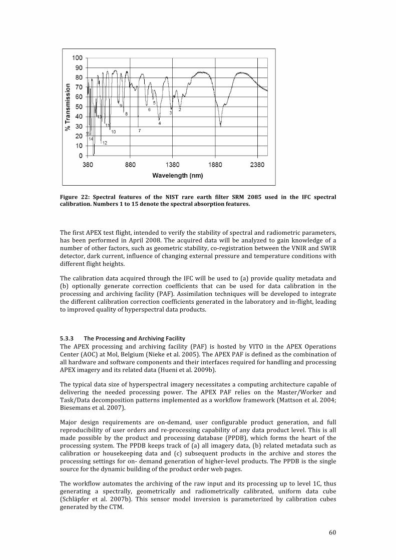
60

Figure 22: Spectral features of the NIST rare earth filter SRM 2085 used in the IFC spectral calibration. Numbers 1 to 15 denote the spectral absorption features.

The first APEX test flight, intended to verify the stability of spectral and radiometric parameters, has been performed in April 2008. The acquired data will be analyzed to gain knowledge of a number of other factors, such as geometric stability, co-‐registration between the VNIR and SWIR detector, dark current, influence of changing external pressure and temperature conditions with different flight heights.

The calibration data acquired through the IFC will be used to (a) provide quality metadata and (b) optionally generate correction coefficients that can be used for data calibration in the processing and archiving facility (PAF). Assimilation techniques will be developed to integrate the different calibration correction coefficients generated in the laboratory and in-‐flight, leading to improved quality of hyperspectral data products.

5.3.3 The Processing and Archiving Facility The APEX processing and archiving facility (PAF) is hosted by VITO in the APEX Operations Center (AOC) at Mol, Belgium (Nieke et al. 2005). The APEX PAF is defined as the combination of all hardware and software components and their interfaces required for handling and processing APEX imagery and its related data (Hueni et al. 2009b).

The typical data size of hyperspectral imagery necessitates a computing architecture capable of delivering the needed processing power. The APEX PAF relies on the Master/Worker and Task/Data decomposition patterns implemented as a workflow framework (Mattson et al. 2004; Biesemans et al. 2007).

Major design requirements are on-‐demand, user configurable product generation, and full reproducibility of user orders and re-‐processing capability of any data product level. This is all made possible by the product and processing database (PPDB), which forms the heart of the processing system. The PPDB keeps track of (a) all imagery data, (b) related metadata such as calibration or housekeeping data and (c) subsequent products in the archive and stores the processing settings for on-‐ demand generation of higher-‐level products. The PPDB is the single source for the dynamic building of the product order web pages.

The workflow automates the archiving of the raw input and its processing up to level 1C, thus generating a spectrally, geometrically and radiometrically calibrated, uniform data cube (Schläpfer et al. 2007b). This sensor model inversion is parameterized by calibration cubes generated by the CTM.

61

Level 1C and higher-‐level products are ordered by user input via dynamic web interfaces. These orders are entered into the PPDB and trigger the processing by the workflow. The final data products are downloadable via FTP accounts.

5.3.4 Vicarious calibration Vicarious calibration is an independent pathway for monitoring instrument radiometric performance, including error assessment with reflectance standards, field instruments and atmospheric radiation measurements. The experiment generally follows a reflectance-‐based approach with ground measurements of the atmospheric optical depth and surface reflectance over a bright natural target (Abdou et al. 2002). The accuracy of vicarious calibration experiments over land is highly dependent on the choice of an appropriate calibration target. Ideally, such a calibration site should be flat, bright, spatially uniform, and spectrally stable over time, near Lambertian for small angles off nadir, and of sufficiently large spatial extent. Desert playas (e.g., Railroad Valley Playa, NV, U.S.A.) are preferred for vicarious calibration due to their optical properties, predictably sunny conditions and low atmospheric aerosol loading (Bruegge et al. 2002). In-‐situ sunphotometer data are used to determine aerosol model and horizontal visibility, subsequently applied for radiative transfer (RT) calculation. RT codes, such as MODTRAN-‐4 (Moderate Resoloution Atmospheric Transmission) (Berk et al. 1989) are used and often constrained by field data to calculate at-‐sensor-‐radiances. Input parameters to these codes include ground measurements of the surface reflectance, sun-‐target-‐sensor geometries and atmospheric properties (aerosol model, horizontal visibility). Reflectance-‐based vicarious calibration methods generally have absolute uncertainties of 3-‐5% (Thome 2001). In the past, RSL has performed extensive vicarious calibration efforts for MERIS (Medium Resolution Imaging Spectrometer) on ENVISAT (Environmental Satellite), where absolute uncertainties in the method were found between 3.36-‐7.15%, depending on the accuracies of the available ground truth data (Kneubühler et al. 2003). In the case of APEX, planned vicarious calibration experiments will account for a range of pre-‐defined flight altitudes and target radiances (bright and dark targets) to assess the sensor’s radiometric performance.

5.4 Scientific products and application fields Given the unprecedented performance requirements and data quality of APEX (Nieke et al. 2005), the instrument will serve the needs of a broad range of both scientific and administrative user communities in Earth System remote sensing, e.g., in ecology, limnology, geology, atmospheric sciences, natural hazard and disaster management and materials detection. Applications based on APEX data will increasingly foster qualitative and especially quantitative remote sensing by allowing for improved Earth System variables retrieval (Figure 23) (Schaepman 2007). The optimized workflow for APEX Level 2/3 processing follows a product oriented way with major modules for the identified main hyperspectral applications (Schläpfer et al. 2007a). These modules act as processors to deliver the expected products (e.g., plant biochemical distribution maps, inland water constituents maps, hazard maps etc.) following minimum standard requirements for optimized interoperability and processing within the APEX PAF. Application specific simulation models, empirical or physically based RT models, will form the basis of each module. Within the APEX Science Centre (ASC) aiming at the scientific exploitation of APEX data, a number of application modules are presently being developed. Potential applications in the domains of water quality monitoring, vegetation analysis and ecology, aerosol retrieval, materials classification, snow characterization, as well as BRDF and spectral database issues are addressed. Future extensions to the modules and additional applications may easily be added to a streamlined level 2/3 workflow to support a growing number of researchers and data users (Figure 24).

62

Figure 23: Example of APEX applications.

5.4.1 Scientific data products After the Level 0-‐1 processing of APEX data, well-‐calibrated at-‐sensor radiance data, scaled to a 16-‐bit format are available. At this stage, three options are distinguished, based on their respective levels of uniformity (Schläpfer et al. 2007b; Nieke et al. 2008b):

• Non-‐uniform data (Level 1A): these data are containing the originally measured radiometrically calibrated data, without any corrections for smile and frown or co-‐ registration. As such, no interpolation has been performed on the data except for bad pixel replacement. The data are of interest for highest resolution applications such as atmospheric sensing in the VNIR spectral range.

• Partially-‐uniform data (Level 1B): the specified quality of the APEX system defines small deviations regarding optical aberrations within each detector (i.e. below 0.2 pixels). When correcting for these smile and frown effects only, a set of detector-‐wise uniform data may be produced. Such data sets are well suited for applications making use of the spectral range of one detector only, e.g., geological applications in the SWIR or limnological applications in the VNIR.

• Fully-‐uniform data (Level 1C): co-‐registration (i.e. synchronization) (Schläpfer et al. 2007b) between the detectors is expected to be better than one pixel offset. Therefore, the creation of a fully uniform data set is feasible by interpolation of the SWIR detector outputs onto the spatial response of the (uniformized) VNIR detector. A spectral cut-‐off limit is defined between the detectors, in order to produce a contiguous spectrum across both detectors after interpolation. This level is expected to be the normal, and most requested output of the APEX calibration chain.

The Level 1 products are accompanied by geometric information, i.e., an index, which defines the orthometric locations of each pixel, which is produced on the basis of a DEM (Digital Elevation Model). In Level 1A, the index will refer to the reference centers of the pixels, in Level 1B, two indices will be required for the two detectors, respectively. The combination of Level 1 products with the geometric information leads to three kinds of Level 2A radiance products.

The subsequent compensation for atmospheric effects will use Level 1C or possibly 1B products. The atmospheric correction uses a special implementation of the ATCOR (Atmospheric Correction) procedure (Richter and Schläpfer 2002) to derive bottom-‐of atmosphere (BOA) reflectance, which may also be referred to as an in-‐field hemispherical-‐directional reflectance factor (in-‐field HDRF, (Martonchik et al. 2000)). This product is the ('traditional') Level 2B

63

reflectance product, which is useful for methods relying on directional model inversion such as in vegetation canopy models.

The ultimate goal of radiometric compensation is to derive a directionally independent surface reflectance, i.e., a bi-‐hemispherical spectral albedo product, which we name Level 2C (Figure 9). Such a product allows an unbiased use of spectral processing techniques for classification and physical parameter inversion, as described below. A yet to be implemented BRDF correction method shall allow such processing in an automatic system.

Figure 24: Level 2/3 APEX Processors.

5.4.2 Water quality monitoring Natural inland waters contain a variety of optically active constituents, such as organic and inorganic suspended matter, phytoplankton and their pigments, and CDOM (Coloured Dissolved Organic Matter). The relationship between the constituent’s concentrations and the reflectance of water is non-‐linear, but can be described by their specific inherent optical properties (SIOP), i.e. scattering and absorption coefficients (Mobley 1994). Reflectance is generally lower and less variable than with land surfaces, and atmospherically scattered radiance often dominates water reflected radiance in the blue region. Therefore, the quantitative determination of water constituents requires very accurate sensor calibration and atmospheric correction. In spite of this complexity, statistical approaches are applicable where extensive, concurrent ground truth measurements are available (Brezonik et al. 2005). Physical algorithms based on radiative transfer modelling provide a more flexible alternative, such as the Neural Network-‐based MERIS case II water algorithm (Doerffer and Schiller 2007). However, the time-‐consuming training of individual NN (Neural Network) for regional variations in SIOP is not very efficient for use with non-‐ recurring acquisitions with an airborne sensor.

The APEX level 3 water constituent product is based on the physically based modular inversion and processing scheme MIP (Heege and Fischer 2004). MIP consists of an atmospheric correction module, which calculates subsurface irradiance reflectances from at-‐sensor radiances. Several retrieval modules exist for the calculation of aerosol optical thickness (AOT) based on multi-‐directional airborne measurements (Heege and Fischer 2004), on an atmospheric correction reference band in the water vapour window at 890 nm (Odermatt et al. 2007) or coupled water constituents and aerosol retrieval algorithms (Miksa et al. 2006). The inversion of subsurface irradiance reflectance into water constituent concentrations for regionalized SIOPs is then performed by a non-‐linear optimization procedure. A simplified process was automatised for

64

MERIS data of Lake Constance, proofing the general applicability of this method and the adjustment of adequate SIOP (Odermatt et al. 2007).

5.4.3 Vegetation analysis and ecology Vegetation is a key component of the terrestrial biosphere in terms of biomass production (food, fibre and fuel) and its role in land-‐atmosphere interactions. The properties of vegetation determine the exchange of energy and matter between terrestrial ecosystems and the atmosphere. Therefore, accurate characterization of vegetation properties and temporal dynamics serve as key components to many land-‐cover schemes that form part of Earth System models, ecosystem process models or water interception models, which in turn are used as prediction tools in climate and ecosystem research.

With the advent of imaging spectroscopy in the mid-‐1980s, a significant advancement was achieved in the modelling, monitoring and understanding of vegetation canopies due to the extended spectral dimension (Curran 1989; Ustin 2004). Recent imaging spectrometers have contributed significantly to the mapping of quantitative vegetation parameters (Goodenough et al. 2006; Koetz 2006; Huber et al. 2007), global change studies (Goetz et al. 2005; Kurz and Apps 2006), agroecosystem modeling (Dorigo et al. 2007) and precision farming (Moran et al. 1997; Brisco et al. 1998). Lately, interest has arisen in using hyperspectral sensing for biodiversity monitoring (Turner and Spector 2003; Schaepman et al. 2007), ecological fingerprinting (Kalacska and Sanchez-‐Azofeifa 2007) and invasive species mapping (Asner and Vitousek. 2005).

The advanced data quality of the APEX instrument will progress many of these applications; moreover, it will inspire innovative combinations of advanced remote sensing products and foster developments of novel analyses techniques and applications. Together with further developments in radiative transfer (RT) modeling, APEX will help to derive a more robust and comprehensive characterization of the complex and dynamic nature of vegetation canopies, which serve as input to sophisticated Earth System and ecological models as well as decision making processes. However, only an integrated approach of remote sensing complemented with in situ sensing, through assimilation or modelling approaches, will allow a more consistent understanding of the relevant processes of vegetated ecosystems and the full Earth System. The linking between in-‐situ observations and coarse resolution satellite products can be substantially supported with APEX data by providing accurate, spatially and temporally comprehensive quantitative measurements of vegetation and land surface properties to overcome the spatial scaling gap at intermediate level.

5.4.4 Aerosols retrieval Aerosols have a significant, yet largely unknown impact on the Earth’s climate system. They are measured by sophisticated in-‐situ techniques and by remote sensing instruments from space. A gap remains between the local and the global scale. APEX has the ability to provide two-‐dimensional spatial data on aerosol properties, such as aerosol optical depth (AOD), Angstrom exponent, asymmetry factor and estimated particle size distribution. The aerosol retrieval benefits from its high spatial and spectral resolution as well as high signal-‐to-‐noise ratio (SNR).

The main objective of the APEX aerosol retrieval is to support the correction for atmospheric influences during the processing of APEX data to level 2B and above. Therefore, AOD and appropriate aerosol model information are needed. This step is crucial to generate high accuracy level 3 data. The secondary objective of the algorithm is to provide a high spatial resolution aerosol parameter map, which is of special interest to climate research, air quality monitoring and modelling purposes as well as for the validation of AOD products from satellite sensors.

65

Figure 25: Aerosol retrieval algorithm flowchart. A first iteration is carried out at reference target pixels with a known spectral surface reflectance. This helps to constrain the unknown variables and to find the appropriate aerosol model. The following iterations continue with this aerosol model and retrieve AOD at dark pixels, where the influence of the error in surface reflectance is relatively small.

The aerosol retrieval strategy is explained in Figure 25 and (Seidel et al. 2005). The embedding of previous knowledge and reasonable assumptions on the atmospheric conditions are required to constrain the ill-‐ posed problem of retrieval and solve it by means of inversion with a radiation transfer model. The available near-‐UV/blue spectral bands below 400nm are a further asset of APEX, which helps to reduce the influence of uncertainties by surface reflection assumptions. A recent study analyzed the sensor performance requirements for the AOD retrieval in terms of SNR and proved its feasibility with APEX for various surface reflectances (Seidel et al. 2008).

5.4.5 Materials classification Within the workflow for APEX Level 2/3, information extraction and classification is not confined to the major modules for dedicated variables retrieval, the so-‐called processors. Basic multiple threshold classification of at-‐sensor measurements into broad landcover classes (e.g. water, cloud, snow) is a prerequisite for the subsequent atmospheric correction and BRDF processing. However, the proper information and parameter extraction and the classification of landcover and materials are mainly based on the spectral at surface reflectances. In a first classification module, the hyperspectral reflectances are decomposed into a limited number of object primitives like quantitative fractions of (chemical) material components, considering the spectral database SPECCHIO (Spectral Input/Output) and further ground based measurements. The spectral quantification techniques applied are the Spectral Angle Mapper SAM (Kruse et al. 1993), Linear Spectral Unmixing (Boardman 1989), Multiple Endmember Spectral Mixture analysis (MESMA) (Roberts et al. 1998), Spectral Feature Fitting (Clark et al. 1990), Matched Filtering (Chen and Reed 1987) and Mixture-‐Tuned Matched Filtering MTMF (Boardman 1998).

In a second step, quantitative fractions are incorporated in either the dedicated processors or are qualitatively classified in a labelling module. The high spatial resolution of APEX together with the fractional input restricts the labelling techniques for the latter module. Support Vector Machines SVM (Cortes and Vapnik 1995), artificial Neural Networks and SAM are supervised and pixel-‐based techniques, which can handle the fuzzy data space of fractional quantities and label the composition of materials in particular. The pixel wise techniques are applied to APEX land-‐data over Europe where variability within homogeneous landcover and land use classes is mapped, i.e. analysis of waste deposits, alpine geology, topsoil composition, vegetation states, etc.). Natural and anthropogenic landcover in rural and urban Europe are usually very heterogeneous and fractional. Pixel based labelling techniques will generally fail and are therefore replaced by object-‐oriented techniques, where object features include in addition to spectral and fractional quantities properties such as texture, shape, area, scale and neighbourhood (de Kok et al. 1999).

66

5.4.6 Snow characterization Snow parameters such as snow grain optical equivalent diameter, impurities, liquid water content, snow-‐pack stratigraphy or variations in surface roughness are important input data for operational and scientific applications. Today most of these parameters are sporadically measured in situ at isolated locations and do not represent the small-‐scale snow-‐pack variations of Alpine regions (McClung and Schaerer 2006). Continuous large-‐area mapping of such parameters would both improve existing and foster new applications in the domains of hazard mitigation and climate change.

In the visible part of the electromagnetic spectrum snow has a high reflectance and is mainly sensitive to impurities. In the infrared part of the spectrum, snow absorbs most of the incoming radiance and is sensitive to a number of other parameters such as optical equivalent diameter (grain size), grain shape or liquid water content (Warren 1982; Dozier and Painter 2004). Because of its high spatial, spectral and radiometric resolution, APEX is an ideal platform to a) deliver data for snow parameter retrieval, and b) identify the optimal sensor specifications for future remote sensing instruments designed to retrieve such parameters.

Rapid detection and mapping of recent avalanches is a promising application field. Information about avalanche occurrence is important for avalanche forecast, model evaluation and hazard map generation (McClung and Schaerer 2006). The turbulent transportation of snow in an avalanche mixes the layers of the snow pack and results in a reflectance different to the adjacent undisturbed snow. This feature could be mapped and measured by APEX. Information extraction from shadowed areas might still be feasible due to the instrument’s high radiometric dynamic range, 14 bits for the VNIR channel and 12 for the SWIR. Furthermore, the good spatial resolution also enables the detection and mapping of small-‐scale avalanches.

5.4.7 BRDF The BRDF (Bidirectional Reflectance Distribution Function) is an object inherent property and describes the dependency of an observed reflectance on the wavelength and the illumination and observation geometry (Nicodemus et al. 1977). BRDF effects can be readily identified in airborne and satellite imagery and do hinder the utilization of such data for subsequent analysis, as identical objects can appear to have differing spectral signatures. The severity of the BRDF effects in airborne imagery is dependent on the field of view (FOV) and on the orientation of the flight strip relative to the sun. Effects are most pronounced with large FOVs and flight directions perpendicular to the principal solar plane (Beisl 2001b) and reach a maximum in the hotspot configuration (coinciding observation and illumination direction) for e.g. vegetation or in the specular reflectance configuration for e.g. water surfaces. The occurrence of both hotspot and specular reflectance is dependent on the solar zenith angle, terrain and the FOV of the sensor. Thus, for a given latitude and flat terrain only a limited number of across-‐track pixels are able to observe these effects. For example the minimum solar zenith angle in Zurich, Switzerland is roughly 23.9° on the 21 June, consequently, hotspot and specular reflectance would not appear in APEX imagery over flat areas. However, their occurrence can be expected for data acquired at latitudes ≤ 37° N.

BRDF effects are not necessarily undesirable artifacts that need to be corrected, but may also be considered to contain additional information for quantitative retrieval of e.g. vegetation (Strub et al. 2002; Weiss et al. 2002), snow (Painter 2002) or soil parameters. In both cases, fundamental knowledge of the BRDF involved may be needed for either correction or information extraction. The acquisition of the BRDF can be based upon hyperspectral data measured by a goniometer such as the dual-‐view FIGOS (Schopfer et al. 2007). Such data sets can be used to analyse the anisotropic reflectance characteristics of objects and to retrieve the surface BRF (Bidirectional Reflectance Factor). Furthermore, expected BRDF effects for a specific sensor FOV, illumination direction and target type can be simulated based on goniometer data. The simulation consists of a spectral convolution and an observation angle selection according to the instrument’s FOV specification.

67

Figure 26: Simulated spectrodirectional signatures (left) and corresponding ANIFnadir (right) for Triticale within the APEX FOV for an observation zenith (zn) angle of 5° and an observation azimuth (az) angle of 30°

Figure 26 illustrates the spectrodirectional effects of a wheat target (Triticale) for a solar zenith angle (zn) of 29.4° simulated for APEX. The left plot shows the MODTRAN-‐4 simulated spectral signatures in the principal plane for nadir (0°), forward and backward scattering (±14°) and the directional variability (up to 60 %) as relative reflectance differences between the backward and forward scattering directions. The nadir normalized anisotropy factor ANIFnadir for a FOV of 28° and a wavelength of 670 nm is presented in the right plot on an angular grid (Figure 26); the observation zenith (zn) and azimuth (az) angles are 5° and 30°, respectively.

For vegetation surfaces, strong BRDF effects are observed in the visible range of the spectrum, most prominently in the solar principal plane as shown in Figure 26. This is due to the distribution of shadowed and illuminated target facets, which leads to high reflectance values for backward scattering directions and a minimum for forward scattering reflectances. Directional effects are also visible in the NIR part of the spectrum, although at a lower degree (20 – 30% variability) due to increased multiple scattering processes.

5.4.8 Spectral Database: SPECCHIO Hyperspectral applications as discussed in the previous sub-‐sections are often relying on spectral ground data and associated metadata. Such data are utilized to carry out feasibility experiments and parameterize processing modules for higher-‐level products in the APEX PAF. The organized storage of spectroradiometer signatures and describing metadata is a prerequisite for their efficient analysis and long-‐term utilization (Hüni et al. 2007a). To these means the Remote Sensing Laboratories have developed the spectral database SPECCHIO (Hueni et al. 2009d). SPECCHIO is used to (a) store spectral and metadata in a central repository which is accessible to all members of the laboratory, (b) serve as a spectral data source for various calibration/validation and simulation tasks and (c) provide parameters for APEX level 2/3 processing (Schläpfer et al. 2007a).

The system is comprised of a relational MySQL (Structured Query Language) database (MySQL AB 2007) and a graphical user interface implemented as a Java 2 application (Sun Microsystems Inc. 2006). The Java technology keeps the software independent of the operating system, thus allowing its use in a heterogeneous computing environment.

Special focus has been put on the automated loading mechanisms to minimize the required user input. The generation of metadata in the system has been optimized by automated gleaning of metadata from spectral input files and containing data structures and by providing group updates on spectral sets (Hueni et al. 2009d).

68

Spectral datasets are retrieved by the means of metadata space queries, which put restrictions on metadata dimensions and thus create a subspace containing the required datasets (Hüni et al. 2007b).

RSL maintains an online version of the SPECCHIO database and interested parties can acquire a database account for testing and data sharing purposes. The SPECCHIO system installation package allows local installation and is intended for users requiring access control over their data. RSL distributes the SPECCHIO system package free of charge. For further information please refer to the SPECCHIO website: http://www.specchio.ch.

5.5 Conclusions It took almost 15 years from the first ideas to the fully developed APEX system. Its design could be called conservative, but the specifications were such that, for instance new detectors had to be developed first, novel calibration concepts and a specific calibration laboratory had to be built up to ensure high data quality, and a fully fledged processing and archiving facility with its software and hardware had to be developed and installed.

The APEX Science Team has in parallel carried out research in some application fields with a variety of existing air and spaceborne sensors aiming at assessing the applicability of the new APEX system. Its great flexibility makes it an ideal universal platform for calibrating and validating existing sensors or simulating newly planned dedicated air and spaceborne systems. APEX is currently in its test phase. The near future will show for which of the anticipated roles the new instrument will be suited best.

Acknowledgements

The authors thank our science partners at VITO and DLR, the industrial team under RUAG leadership, ESA Earth Observation specialists and ESA PRODEX responsible for their highly valued support. ESA delegations, national space organizations in Switzerland and Belgium and national science foundations have supported the development of APEX and enabled the corresponding research.

71

6 Structure, Components and Interfaces of the Airborne Prism Experiment (APEX) Processing and Archiving Facility

Hueni, A., Biesemans, J., Meuleman, K., Dell'Endice, F., Schläpfer, D., Adriaensen, S., Kempenaers, S., Odermatt, D., Kneubuehler, M., Nieke, J. and Itten, K.

2009

IEEE Transactions on Geoscience and Remote Sensing

47(1): 29-‐43.

73

Structure, Components, and Interfaces of the Airborne Prism Experiment (APEX) Processing and Archiving Facility

Abstract

The product generation from hyperspectral sensor data has high requirements on the processing infrastructure, both hardware and software. The Airborne Prism Experiment (APEX) processing and archiving facility has been set up to provide for the automated generation of level-‐1 calibrated data and user-‐ configurable on-‐demand product generation for higher processing levels. The system offers full reproducibility of user orders and processing parameters by employing a relational database. The flexible workflow software allows for the quick integration of novel algorithms or the definition of new processing sequences. Reprocessing of data is supported by the archiving approach. Configuration management based on the database enables the control over different versions of processing modules to be applied. The system is described with a focus on the APEX instrument; however, its generic design allows adaptation to other sensor systems.

Keywords: Database systems, hyperspectral data calibration, on-‐demand processing, parallel processing, system architecture.

6.1 Introduction Airborne and spaceborne hyperspectral imagers provide raster data with a high number of contiguous spectral bands (Green 1998; Schaepman et al. 2006). Every spatial cell contains a vector representing the electromagnetic spectrum reflected from objects due to interaction with solar irradiance. Given a sufficient spectral resolution, identification of materials with diagnostic spectral features is possible (Goetz et al. 1985). The ability to accurately detect specific narrow spectral features relies on precise knowledge about the position and spectral response curve of the instrument channels (Mouroulis and McKerns 2000). The derivation of quantitative results from hyperspectral imagery requires the data to be spectrally, radiometrically and spatially calibrated (Green 1998).

The airborne imaging spectrometer APEX (Airborne Prism Experiment) is a dispersive pushbroom system engineered to contribute to the preparation, calibration, validation and simulation of future hyperspectral imaging space instruments and to the understanding of processes associated with air, water and land at local and regional scale in support of global applications (Nieke et al. 2005).

A detailed characterization of the APEX instrument must be carried out to achieve the required data quality (Schläpfer and Schaepman 2002). The needed system parameters can be gathered by specific measurements carried out in the calibration home base (CHB) (Dell'Endice et al. 2007). Data collected during the CHB phase are subjected to post processing and subsequently fed into the processing system for a sensor model inversion, converting digital numbers to at sensor radiances and applying corrections to achieve data uniformity (Schläpfer et al. 2007b).

System calibrations of the APEX instrument are slated to be carried out on a regular basis. The collected calibration data sets provide means for long-‐term system performance analysis. Short term changes of a limited set of instrument characteristics can also be observed by using the inflight characterization (IFC) facility (Nieke et al. 2005). Recording IFC data at the start and end of each flight strip may be used to assess the stability of the instrument over shorter periods of time.

APEX offers configurable on-‐chip binning, enabling users to optimize signal to noise ratios (SNR) for specific applications. The availability of binning and the changing instrument characteristics

74

imply that every flight dataset will be defined in a differing spectral space where the dimensions are given by the spectral bands.

A processing and archiving system must therefore be engineered to deal with the above mentioned instrument dynamics and the high volume of data typically produced by hyperspectral imagers. It furthermore acts as data source for the user, offering products at several processing levels via online order pages and on demand processing facilities.

The nature of hyperspectral data cubes is well suited for parallel processing with spatial domain partitioning being a logical approach (Plaza 2007). The system architecture must therefore include the aspect of concurrency issues for all resources that may be accessed by several processes in parallel.

In this paper we present the structure of the APEX processing and archiving facility, decomposed into storage and processing components and their internal and external interfaces. Decomposition has been recognized as a powerful technique to handle complex systems in many areas of engineering and science (Courtois 1985). It allows studying the resulting components and their interactions in detail. Interfaces are used to provide external abstractions of components and define the communication between components.

A case study based on a limnology application (estimation of water constituents) illustrates the processing flexibility and the interactions of the system components and external entities via well-‐defined interfaces.

6.2 System Requirements

The requirements for the APEX processing and archiving facility (PAF) listed hereafter are the result of studies (APEX Phase B (Schaepman and Itten 2000) and SPECTRA project (Dangel et al. 2005)) previously carried out by RSL (Remote Sensing Laboratories), Zurich.

6.2.1 Product Level Support Data pass through several, well-‐defined stages during the processing from raw instrument data to end user products. Data at these distinct stages are referred to as level-‐<N> data, where N is the number of the stage. The system must support these conceptual levels. Within the APEX project, levels are defined as follows (Schläpfer et al. 2007a):

Level name Description

level-‐0 Raw data as produced by the instrument (digital numbers)

level-‐1 Radiometrically, spectrally and geometrically calibrated, uniform data (radiances)

level-‐2 Surface reflectance data: corrected for atmospheric and topographic influences

level-‐3 Application oriented products

6.2.2 Archiving Flight scene and calibration data in their raw formats are the foundation of the data chain. Any higher-‐level product can be reprocessed based on the raw input and its archiving is thus compulsory. The archiving strategy for higher-‐level products is based on a trade-‐off between processing time and storage space required, influenced by the user demand of a certain level. Therefore, radiometrically corrected data (level-‐1) are archived as they represent a base for higher-‐level processing while an atmospherically corrected data cube will be processed on demand and may be deleted once downloaded by the user.

In this manner the archiving strategy is defined for all product levels.

75

6.2.3 Web Access and User Transparency On demand processing of higher-‐level data is supported by generalized, interactive web product order pages.

Such pages must be dynamically built to reflect the access and processing rights of the current user. Selection of available products must be possible in the domains of acquisition time, spatial position and processing levels. The provision of georeferenced quicklook images supports the user during the selection process.

The specification of processing parameters must reflect the technical specification of the sensor in question, thus different configurations such as binning modes or calibrations must be handled transparently for the user.

Information on the previous orders of the current user and their status must be available.

6.2.4 Auxiliary Data Support Auxiliary data include: 1) spectral vicarious calibration data, 2) meteorological information supporting atmospheric corrections, 3) digital surface models for orthorectification and 4) miscellaneous in situ observations used for model building and validation, e.g. for limnology applications where suspended matter concentrations are used to model the contribution from particulate backscattering to infrared radiances prior to atmospheric correction.

6.2.5 Parallel Processing Capability The typical data volume of hyperspectral image cubes puts high demands on the processing power. Parallel processing is a solution to deal with these needs and is expected to play a major role in future remote sensing applications (Plaza 2007). Parallelization relies on task and data decomposition patterns, producing parts that can be processed concurrently. Some processes for radiometric and geometric correction can be decomposed into highly independent subtasks (Brazile et al. 2004). In practice a flight campaign cube can be broken down into individual flight strips which themselves may be further decomposed into blocks of several frames or even single frames for low-‐level processing. The primary data will thus be independent, however, parallel processes will share additional processing parameters such as calibration parameters and the system must be engineered to handle such concurrent resource access.

6.2.6 Reprocessing Functionality On demand processing enables users to define module parameters online, thus customizing their output product. In case of problems appearing in the delivered products, a full record of the order parameters must exist to allow a reprocessing of the data. The system must therefore keep track of all incoming user product orders including all processing settings. This includes keeping track of module versions by configuration management of the system.

6.2.7 Flexible Higher Level Processing Flexibility is required at higher processing levels to support the APEX platform in its role as a testbed for new algorithms and to allow the definition of application specific processing step sequences (Schläpfer et al. 2007a).

This specifically requires a framework that assists the flexible concatenation of processing modules, thus allowing 1) the setup of special processing sequences such as for the retrieval of limnology parameters where standard atmospheric corrections may not be applicable (Vidot and Santer 2003) and 2) the quick and easy integration of new processing modules provided by collaborating researchers and developers.

76

6.3 System Overview

The APEX processing and archiving facility (PAF) is hosted by VITO (Flemish Institute for Technological Research) in the APEX Operations Center (AOC) at Mol, Belgium (Nieke et al. 2005).

The APEX PAF is defined as the combination of all hardware and software components and their interfaces required for handling and processing APEX imagery and its related data. This paper focuses mainly on the software part of the APEX PAF and the interaction of the system with the external entities in their function as data sources or sinks.

From a dataflow perspective, the three main functionalities of the APEX PAF are: 1) the storage of system calibration measurements obtained at the beginning of every flight season and their subsequent processing to obtain calibration coefficients, 2) the storage of incoming raw flight data streams and according level-‐1 imagery after radiometric, geometric and spectral calibration, and 3) the creation and distribution of higher level product data based on user orders.

Figure 27 shows the dataflow diagram of the APEX PAF (ADFD). Dashed lines denote system boundaries, external entities are shown as rectangles, processes as circles, data sinks as two parallel, horizontal lines and data flows as uni-‐ or bidirectional edges. The ADFD shows the structure of the PAF and the interaction of its components. As a general rule a processing component must exist in between two data sinks, where external entities are treated as data sinks as well. The process description defines the operations applied to the data during their transfer from one storage component to the next. Interaction between processing and storage components relies on defined interfaces.

Figure 27: APEX processing and archiving facility data flow diagram

The following three sections describe 1) the external entities to the APEX PAF and their interaction with the system based on well-‐defined interfaces, 2) the storage components and 3) the processing components.

Structure, components and interfaces of the APEX processing and

archiving system: Overview

CHB

APEX

User

GPS

Base

Station

Archiving

Workflow

Data Archive

CTM

Order

creation

Product order

page creation

Product & processing

databaseLevel 0-2/3

Processing

SPECCHIO spectral

database

SPECCHIO

Application

Field & Laboratory

spectroradiometer

measurements

Spectral reference

database

Spectral

reference

generator

Spectral

Simulation Models

FTP Account

Working PoolDEMDEM

Feed

Campaign

Metadata

OperatorOperation

Control

SPECCHIO System

APEX Processing &

Archiving Facility

Applanix

POS/AV

410

POSPac

77

In order to ease the understanding of the entities and components within the following sections, please keep referring to the ADFD, which shows all described objects and their respective links. The reader may also wish to refer to the case study presented later in this paper, as it illustrates the interaction of the components in a succinct manner.

6.4 External Entities & Interfaces

6.4.1 APEX (Airborne Prism Experiment) APEX (Airborne Prism Experiment) is a dispersive pushbroom system with 28° field of view. Two spectrometers cover the spectral range from 380-‐2500 nm, both having an across track resolution of 1000 pixels (Nieke et al. 2005). At a typical flying height of 3500 metres above ground with an aircraft speed of 270km/h, pixel sizes are 1.75m across track and 3.9m along track with an overlap of 33% between consecutive frames. The unbinned configuration offers 312 spectral bands in the visible and near infrared (VNIR) and 199 bands in the short wave infrared (SWIR).

Frame data plus housekeeping data are written as a binary stream to an on board storage unit at a data rate of 50 MB/s (Brazile et al. 2003). Expected data volumes per flight campaign range around several hundred gigabytes. The inertial navigation system (INS) data stream consisting of attitude and GPS (Global Positioning System) data is recorded in parallel as a separate file. All data are transferred from the onboard storage to the AOC using tapes.

6.4.2 CHB (Calibration Home Base) The CHB is located at DLR (German Aerospace Center) Oberpfaffenhofen, Germany. It comprises the hard-‐ and software to carry out highly accurate and automated radiometric, geometric and spectral characterizations of hyperspectral imaging sensors (Suhr et al. 2005).

For geometric and spectral characterizations the instrument is placed on columns above a granite workbench and adjusted to the axes of the bench. Collimated light beams originating from either monochromatic or panchromatic sources are reflected into the aperture of the instrument by a moveable, tiltable folding mirror. Very precise, computer controlled positioning of the mirror allows sub-‐pixel illumination of single detector elements, yielding data for the construction of the pixel point spread function (PSF). Similarly, the spectral response curve can be derived by subsequent measurements at changing monochromator frequencies.

Radiometric calibration involves two integrating spheres of which one is used for absolute calibration against the German national standard and the other for relative measurements to derive the linearity of the instrument with changing irradiance levels.

The characterization process is managed by the CTM (Calibration Test Master) software which optimizes the time needed for calibration by automatic generation of optical stimuli (Dell'Endice et al. 2007). The CTM interfaces APEX with both laboratory ground facility, i.e. the CHB, and an In-‐Flight characterization facility (IFC). The instrumentation in both the CHB and the IFC can be controlled remotely via a computer interface, thus enabling automatic measurements. This results in a consistent reduction of the time spent for calibration; therefore additional measurements can be performed in a way that the overall APEX calibration and characterization is substantially improved.

Data gained from measurements at the CHB consist of APEX raw data frames and CTM controller logs linking each frame to the settings of the CHB. APEX data thus flow into the CHB as indicated in the ADFD (see Figure 27).

Data are transferred to the AOC on tapes. The expected data volume ranges from 100 to 200 gigabytes.

78

6.4.3 Campaign Metadata Campaign metadata, also called auxiliary data, encompass all data collected during a flight campaign not stemming from the APEX sensor system. In general, metadata support the broad and long-‐term use and interpretation of scientific data (Michener 2000). The storage of the auxiliary data linked with the APEX instrument data in the APEX PAF is of prime importance to preserve the scientific campaign context. APEX metadata support the calibration, validation and analysis of images cubes. Examples are: meteorological data, sunphotometer readings, ground truth maps of landcover or landuse or physical and chemical in-‐situ measurements (e.g. leaf area index measurements of vegetated areas or specific inherent optical properties of water bodies). Auxiliary data are entered by the means of separate electronic files.

Hyperspectral in situ measurements taken by spectroradiometers are part of the imagery metadata as well, e.g. subsurface reflectance measurements acquired with water spectroradiometers. However, spectral ground data are preferably stored in the SPECCHIO database (Hüni and Kneubühler 2007) rather than just supplying spectral files as part of the campaign metadata.

6.4.4 Applanix POS/AV 410 The APEX instrument is equipped with an Applanix POS/AV 410 v4. GPS/INS system. Such a GPS/INS system enables for direct georeferencing of the acquired imagery and is now widely used in airborne remote sensing. Direct georeferencing allows to directly relate the collected data to the Earth by accurately measuring the geographic position and orientation of the sensor without the use of traditional ground-‐based measurements.

The GPS/INS system is comprised of four main components:

1) an IMU (Inertial Measurement Unit), 2) a GPS receiver, 3) a POS computer system and 4) a post-‐processing software (PosPACTM).

The IMU is rigidly mounted to the sensor’s mainframe, preventing variations in their relative position and orientation and measures the sensor’s position and orientation at a 200 Hz data rate. The GPS receiver is integrated in the computer system and has a 1 Hz logging rate. The GPS antenna is placed on top of the aircraft. During a mission the POS/AV computer system records the IMU and GPS data together with the recording time of each image line and stores it as part of the APEX raw data stream. Both are then synchronised to a common time scale, which typically is the GPS time.

6.4.5 GPS Base Station Data Differential GPS data are provided from one or several base stations located at precisely surveyed positions. The base stations, also called reference stations, calculate differential corrections for their own location and time. The correction data are usually available in the RINEX (Receiver Independent Exchange) format and are used for subsequent differential GPS correction of data recorded by the GPS receiver of the aircraft.

6.4.6 DEM Data For the production of orthorectified products, the following external data layers are available in the image processing workflows: 1) the EGM96 (Lemoine et al. 1998) geoid model, 2) user supplied LIDAR (Light Detection and Ranging) DEM’s in the WGS84 datum and in latitude/longitude or UTM (e.g: above Flanders, Belgium, a LIDAR DEM at a spatial resolution of 5 meters and a vertical accuracy of 7 cm for areas covered with short grass or pavement and 20 cm for areas with complex vegetation is typically being used in support of the hyperspectral campaigns), 3) the SRTM (Farr et al. 2007) (Shuttle Radar Topography Mission) DEM at a spatial

79

resolution of 90 m (to be used as fallback mechanism if no user-‐supplied LIDAR DEM is available), 4) the NOAA “GLOBE” (Hastings and Dunbar 1998) global DEM at a spatial resolution of 1 km (used as fallback mechanism to determine the mean elevation over the area covered by the image in case no user-‐supplied LIDAR DEM is available and the SRTM DEM contains invalid or no data).

6.4.7 Operator User friendly man-‐machine-‐interfaces (MMI) are necessary to ease the tasks of the operators and to quickly diagnose the software and hardware problems. Currently, the operator can monitor the activity of all workflows (level-‐0 to level-‐1 archiving workflow and level-‐1 to level-‐2/3 processing workflow) through 1) a platform independent Java application which allows on-‐site and off-‐site workflow tuning and hardware system monitoring and 2) a WWW interface towards the Product and Processing Database (PPDB) providing access to some essential database maintenance operations.

6.4.8 User The major user-‐segment of the APEX instrument will be scientific/academic users active in the domain of fundamental low-‐level image processing, e.g. atmospheric correction, BRDF (bidirectional reflectance distribution function) correction, sensor design or atmospheric modelling. For this type of users, the availability of level-‐1 data is essential for complete control over the level-‐1 to level-‐2 correction algorithms. To serve this user-‐segment, level-‐1 products will be the lowest level products available on-‐line.

Figure 28: Internet interface towards the PPDB showing the result of a query for level-‐1 imagery.

80

A minor user segment will be the academic, governmental and commercial users active in higher-‐level application development, e.g. land use/cover mapping or soil/water quality mapping. In support of this user segment the processing workflow is capable of generating user configurable level-‐2 products on-‐demand.

Users interact with the APEX PAF via web page interfaces. These allow the search and selection of level-‐1 data (see Figure 29), the specification of processing parameters for higher-‐level processing and the monitoring of product orders. Imagery from different sensors can be ordered at the same time. The web interface thus allows the user to select the processing options, e.g. bands for atmospheric correction algorithms, dependant on the sensor type (see Figure 29).

Figure 29: Specification of sensor specific atmospheric processing parameters in the web interface

6.4.9 Spectroradiometer Data Ground based hyperspectral signatures are collected for 1) basic investigation of the relationship between physical or biochemical properties and the electromagnetic reflectance of objects and 2) calibration, validation and simulation of remote sensing imagery and its data products.

A thorough collection of metadata describing the sampling process and the surrounding environment enables long-‐term usability and data sharing between research groups (Milton 2004; Hueni et al. 2009d). This is of high importance when acquiring spectral in situ data during a flight campaign as the imagery plus the auxiliary data will be disseminated to users lacking the intrinsic knowledge of the circumstances of data capture.

One example of metadata usage is the description of illumination and viewing geometry in support of spectrodirectional measurements. Such data, usually acquired by a goniometer, can be used to analyse the anisotropic reflectance characteristics of objects and to retrieve the BRDF, which is fundamental to the correction of remotely sensed data (Schopfer et al. 2007).

81

The usage of native spectroradiometer data files is recommended as they include a host of useful metadata that may be gleaned automatically for subsequent storage in a spectral database.

6.4.10 SPECCHIO System SPECCHIO is a system designed to hold reference spectra and spectral campaign data obtained by spectroradiometers (Hüni et al. 2007a; Hüni et al. 2007b). It comprises two components: 1) a relational database schema and 2) a Java application for data input, maintenance and output. The metadata model contains parameters relevant for long-‐term usage and data sharing.

SPECCHIO is available as a free online tool for users to test the system and exchange data. For more information refer to the SPECCHIO website: www.specchio.ch.

The SPECCHIO database stores ground-‐based spectral signatures and their associated metadata in a relational database schema on a MySQL5 (MySQL AB 2005) database server. The data model implements the 34 dimensional metadata space defined by the parameters as listed in Hüni et al (2007a).

The normalisation step carried out on the data model during engineering supports non-‐redundant data entries for group updates where one metadata dimension is set to a common value for several spectra (Hueni et al. 2009d).

The SPECCHIO application is implemented as a Java 2 (Sun Microsystems Inc. 2006) application which allows full flexibility on local file system operations. Being based on Java keeps the software operating system independent, which is of importance in a heterogeneous computing environment. The application thus runs on any platform with a Java Virtual Machine (VM) installation and connects to the database via TCP/IP on a configurable port.

The main task of the software is to provide user interfaces and processing functionality for the input, editing and output of spectral data. Data input is highly automated and includes the extraction of metadata from the data sources. This addresses the problem of users being deterred from entering their spectral collections due to overly complicated procedures (Hüni et al. 2007a). Metadata editing is optimised by the concept of group updates where several spectra can be updated to refer to one metadata parameter value. Data retrieval is implemented by the interactive definition of constraints on metadata space dimensions. The space is thus projected to a subspace containing the queried data set (Hueni et al. 2009d).

6.4.11 Spectral Simulation Models Measurements of a remote sensing instrument can be interpreted to describe the radiative properties of the observed media (e.g. soil, vegetation, atmosphere) (Pinty and Verstraete 1998; Hueni et al. 2009d). Any quantitative interpretation of remote sensing data relies on performing the inversion of a model. Models can be conceptual, empirical or based on the mathematical representation of the physics underpinning radiation transfer as implemented into radiative transfer (RT) models (Pinty et al. 2001). The last decades have seen significant advances in the development of RT models for the purpose of retrieving useful information from remote sensing data in a number of application areas (Goel 1988; Pinty and Verstraete 1998). RT models such as the leaf optical properties model PROSPECT (Jacquemoud and Baret 1990; Jacquemoud et al. 1996) and the SAIL (Scattering by Arbitrarily Inclined Leaves) canopy bidirectional reflectance model (Verhoef 1984) have been developed to describe coupled processes that occur at leaf and canopy level, respectively, when light is intercepted by plant canopies. They have been widely used to interpret the reflectance in terms of vegetation biophysical characteristics (Jacquemoud et al. 2006). SAIL nowadays exists in several versions, one of them being GeoSAIL, which is a combination of SAIL and a geometric model to simulate discontinuous canopies (Huemmerich 2001). Another well known RT model is FLIGHT (Forest Light Interaction Model) (North 1996), being a three-‐dimensional ray-‐tracing model using Monte-‐Carlo techniques for the radiative transfer within crown boundaries and deterministic ray tracing between the crowns and other canopy components. GeoSAIL and FLIGHT have recently been used to describe the canopy

82

reflectance at scene level for subsequent estimation of forest fire fuel properties (Koetz et al. 2004). As for applications in the domain of vegetation analysis, comparable models exist for water constituent retrieval (e.g., Modular Inversion and Processing Scheme (MIP), (Heege and Fischer 2004; Odermatt et al. 2007), atmosphere research (e.g., MODTRAN (MODerate spectral resolution atmospheric TRANSsmittance algorithm and computer model) (Berk et al. 1989)) or land surface processes description (e.g., PROMET-‐V (PROcess oriented Modular Environment and Vegetation model), (Bach and Mauser 2003)). Models have further been developed for correction of directional effects in remote sensing data (Leroy and Roujean 1994; Beisl 2001a) and a growing number of simulation models also account for BRDF effects (e.g., SAILH, (Kuusk 1991; Jacquemoud et al. 2006)). Application specific simulation models will be incorporated in the APEX processing and archiving facility for the generation of spectral reference data for level-‐2 (e.g., BRDF corrected reflectance data) and level-‐3 product generation (e.g., plant biochemical distribution maps, inland water constituent maps etc.).

6.5 Storage Components

6.5.1 Data Archive The archiving hardware system is a dedicated cluster of about 30 dual processor machines (3.2 GHz Intel XEON) and about 45 TB iSCSI SAN (Storage Area Network) storage. The hard disk arrays and the workstation nodes are interconnected via two 1 GBit/s iSCSI interfaces and the partitions of the archive and user-‐order database system are managed through the Linux LVM (Logical Volume Management) software, which allows for on-‐line reconfiguration of the storage capacity of the logical volume.

In contrast with satellite missions, where the data stream is usually continuous, airborne missions are carried out on a commercial basis, meaning that for every airborne imaging mission there is a client who is paying for the imaging mission. Therefore it is rather difficult to determine the effective storage needs. Given the impressive data rate of 50 MB/s during data acquisition, it was chosen to only archive the raw and level-‐1 data. Higher-‐level data will not be archived. However all parameter settings used to generate the higher-‐level product will be stored in the database system to ensure full product traceability.

6.5.2 Product and Processing Database The Product and Processing Database (PPDB) is implemented as a relational database on a MySQL5 database server. It is the heart of the processing workflows since it keeps track of all input and output settings needed by these workflows. It offers full traceability of users, image products and image product processing history. The database system uses a generic data model, which works with any airborne imaging sensor.

The PPDB is the single source for the dynamic building of the product order web pages. It maintains the links to the archived products and contains information about the sensors, the product orders and specific processing parameters. Furthermore, the software versions of processing modules can be tracked, offering the operator the choice to reprocess data with some different module version.

6.5.3 Spectral Reference Database The spectral reference database is currently a conceptual component only that will be implemented along with higher-‐level processing in the APEX PAF.

Certain higher-‐level processing algorithms may need spectral reference data, e.g. identifying materials by spectral matching, tuning of models for subsequent inversion, BRDF corrections or spectral albedo product generation. The database approach allows for the dynamic selection of data subsets based on metadata queries, e.g. relevant vegetation spectra of a given region describing a phenological state can be selected by applying a spatio-‐temporal constraint on the metadata space.

83

The data model of the spectral reference database is based on the SPECCHIO data model but is enhanced to support derived spectral information such as BRDF. However, the main reasons of separating the external SPECCHIO database from the internal reference database of the APEX PAF are 1) the provision of stable, controlled data, 2) version control of the reference sets in order to enable reprocessing of data at a later stage and 3) the preprocessing applied for increased performance of higher-‐level processes.

The SPECCHIO database is highly dynamic in its content due to constant user interaction resulting in added, changed or deleted data sets. These dynamics are attenuated by the separation into two components connected by the spectral reference generator process controlling the data transfer.

Spectra are stored in SPECCHIO as vectors in spectral spaces defined by the channels of the capturing spectroradiometers. Application of reference data in algorithms processing hyperspectral imagery may necessitate a previous convolution to the bands of the imaging instrument. Such preprocessing can be handled by the spectral reference generator resulting in reference sets optimized for direct application in algorithms while minimizing the storage space in the reference database.

6.5.4 Working Pool Given the volume of the expected data stream, introducing parallelism is inevitable. Since the processing of hyperspectral imagery or photogrammetric camera images is very data intensive, it was decided to combine the task/data decomposition pattern in combination with a master/worker program structure pattern to implement concurrency (Mattson et al. 2004).

Due to the large data volume the working pool was implemented on fileservers with fast internal disks configured in RAID-‐0 (Redundant Arrays of Inexpensive Disks).

The processing workflow ensures system scalability by the concurrent handling of multiple masters. The masters are mutually independent subsystems by 1) allocation of a dedicated fileserver and thus of a dedicated working storage and 2) assignment of dedicated workers, who pull jobs from a specific master only and access the common working directory of the master.

6.5.5 FTP Account Upon successful processing of a user order, the user is informed via the WWW interface about the status and FTP (File Transfer Protocol) download point. However, if huge data volumes have been ordered, the possibility exists to forward the data on external hard drive(s). New, password protected FTP accounts are created for every order and only the authorized user may download the products within a limited timeframe.

6.6 Processing Components

6.6.1 Product Order Page Generation The product order web pages are created dynamically by reading the relevant information from the PPDB. Page creation is based on JSP (Java Server Pages) technology and utilizes the Apache Struts framework (The Apache Software Foundation 2007).

The user can browse the level-‐1 image table of the PPDB using a WWW interface. Once a selection of images is made, the user can order the level-‐1 data or define custom level-‐2/3 processing actions on the selected images. The processing order details are submitted back to the web server and subsequently handled by the Order Creation process.

84

User access control for both data and processing actions is implemented based on the Role Based Access Control (RBAC) model (Ferraiolo and Kuhn 1992).

6.6.2 Order Creation Processing orders that have been defined via the WWW user interface are handled on the web server to generate new records in the relevant tables of the PPDB.

The master or masters of the processing workflow constantly check the database system for new incoming product orders and adjust their job queues accordingly to accommodate these new processing requests. Masters can be configured to only listen to orders submitted by certain users or user groups. The workers installed on the working nodes then pull jobs from the master queue and return the process return value to the master.

Orders are being served according to the ‘first-‐in first-‐out’ (FIFO) principle. However, operators have the possibility to change the priority of orders upon explicit user request via the Java Workflow Monitoring Application (see 6.4.7 and 6.6.3.1).

6.6.3 Level 0-‐3 Processing The level 0-‐3 processing is shown as one process in the ADFD, however, it comprises several different major processing sub components which are described hereafter.

6.6.3.1 Workflow Manager The Workflow Manager implements the job-‐pulling model with respect to job scheduling (simplicity, fault tolerance, load balancing) according the Master/Worker and Task/Data Decomposition patterns (Mattson et al. 2004). Multithreading or MPI (Message Passing Interface) is not being used in the algorithmic components; the workflow is optimized for processing a large quantity of images instead of processing single images as fast as possible. This also keeps the algorithmic code as “simple” as possible to enhance cooperation with other scientific/academic groups (Biesemans et al. 2007).

Java is used to implement the Master/Worker workflows via message passing through reliable TCP/IP sockets. C++ is the preferred language for algorithmic components, but Fortran 77, Java and IDL are supported as well.

The master node maintains a job queue (see Figure 30). Filling of the job queue can be triggered by new events in the file system, PPDB or by other software components. The Worker Threads that carry out the actual processing run on the worker nodes and are controlled by Worker Handler Threads running on the master (see Figure 30). Master and worker nodes can be monitored and configured by a Workflow Monitoring & Configuration Application. The communication is handled via sockets with specific port numbers assigned to masters and workers, indicated by the numbered rectangles within the application/workstation entities in Figure 30.

The worker nodes can be made to request jobs from a job-‐queue at the moment they have got the CPU (Central Processing Unit) power available to process another job. Job pulling has the following advantages over job pushing software systems: 1) load balancing, 2) fault tolerance and 3) simplicity (Biesemans et al. 2007).

Load balancing: The load on a workstation strongly depends on the characteristics of the images being analyzed. The computing load only becomes clear during the actual processing. Job pulling results in a load-‐balancing scheme that takes the CPU load of each workstation into account. In case of job pushing, this is significantly more complex: the component that sends the job has typically little information to determine the load of the workstation to which the job is pushed. Mechanisms that make the load information available to the supervisor are complex and will require third party middleware software. Job pulling inherently allows these differences in CPU

85

time to be taken into account. Furthermore, it automatically adapts to the computing power of the workstation.

Figure 30: Scheme of the Master/Worker pattern showing a cluster comprising one Master and two Worker nodes.

Fault tolerance: Workstations that have crashed, e.g. due to Ethernet interface failures are unable to request further jobs. Therefore, the load is automatically balanced over the remaining workstations that are operational. In case of job pushing, the supervisor needs a mechanism to determine whether workstations are operational or not.

Simplicity: In case of job pulling, no details of the CPU power of the different workstations, or the types of jobs they are executing need to be known to the supervisor. Nor does the supervisor need to know which workstations it is supervising, and whether they are operational or not.

6.6.3.2 Level 0-‐1 The level 0-‐1 processing takes level-‐0 data as input and generates a calibrated, uniform at sensor radiance cube, referred to as level-‐1. The correction scheme is derived from the inversion of the sensor model consisting of three distinct parts: 1) the optical model describing the optical aberrations, 2) the bad pixel model describing the resulting data loss, also dealing with saturation and 3) the radiometric model that accounts for the transformation of at sensor photon flux to recorded digital numbers (Schläpfer et al. 2003).

Characterisation data obtained in the CHB and post processed by the CTM, the so-‐called calibration cubes, are used for the parameterisation of the inverse model. The PPDB holds the information to provide the correct calibration cube based on a timeline selection, i.e. CHB characterisations result in time slots where one specific calibration cube is valid for all flight data sets acquired during the cube’s slot.

Level 0-‐1 processing utilizes the Working Pool as source for the input files and destination for the output files. The Working Pool is instantiated and filled with the required data by the Workflow Manager prior to level 0-‐1 processing calls.

Master Application

Workstation 1

Worker Application

Workstation 3

Worker Application

Workstation 2

Worker Thread 1

Worker Thread 2

Worker Thread 3

Worker Thread 1

Worker Thread 2

6669

6669

6668

6670

Workflow Monitoring & Configuration Application

Worker Handler Thread

1


2


3

Job Queue

File System

PPDB

Software

Worker Thread N

86

6.6.3.3 Level 2-‐3 The higher level processing workflow for hyperspectral data is normally a sequential procedure from raw imagery to rectified and calibrated imagery, further to surface reflectance data and finally to products. The respective processing level definitions for APEX are 'level-‐2' for surface reflectance or spectral albedo data, and 'level-‐3' for application oriented products. Within the APEX PAF, an optimized workflow is foreseen which tries to avoid redundancies by organizing level-‐2/3 in a product-‐oriented modular system (see (Schläpfer et al. 2007a)).

Figure 31 gives an overview of the processing flow after level-‐1 processing up to final data product maps. The geometric processing is split in two parts -‐ before starting with the level-‐2 processing all pixels are indexed with their geographic location and the DEM-‐related parameters are resampled to the raw image geometry. The rectification step is done only on the final data products (i.e. level-‐3b) to avoid resampling artefacts and processing overhead. Spectral reference data are a crucial input to this processing chain and are used for both level-‐2 and level-‐3 processing steps.

Figure 31: Level-‐2/3 processing scheme of APEX.

MODTRAN (Berk et al. 1989) derived atmospheric look-‐up tables and well-‐prepared digital elevation models are the required main data sources for the atmospheric and topographic correction of the imagery.

Further inputs provided by the processing database system (PPDB) are required for most of the product generator modules, e.g. the tuning of respective models parameters, which are inverted for the parameters of interest.

6.6.4 CTM Processor The CTM consists of three main elements: 1) the controller, being the core unit of the CTM, 2) the storage unit, partly embedded in APEX, and partly located on external storage units and 3) the processor, which processes all the calibration data.

The CTM controller is embedded in the APEX instrument and sets up all the necessary parameters, i.e. APEX settings (e.g. integration time) and calibration facility settings (e.g. monochromator wavelength, integrating sphere lamp intensity), for a particular calibration procedure (e.g. spectral calibration, radiometric calibration, geometric calibration) to be performed efficiently. Once the setting is completed, the calibration measurements take place and the acquired data are saved on the storage unit as frames along with the corresponding metadata. Each frame has a spatial and a spectral dimension, where the size of the latter depends on the spectral band configuration, i.e. binning. The CTM processor is run inside the APEX PAF

87

and processes the acquired frames by using dedicated algorithms. Depending on the calibration procedure, the CTM processor will generate one or more calibration layers, containing calibration parameters for each detector pixel with VNIR and SWIR channels handled separately. Examples of parameters are: center wavelength or FWHM (full width at half maximum). Stacking all the calibration layers per detector results in a calibration cube per channel (VNIR and SWIR) (see Figure 32).

Figure 32: Calibration cube

In order to distinguish between external calibration sources, i.e. the CHB, and internal calibration sources, i.e. the IFC, separate VNIR and SWIR calibration cubes are generated per source.

The calibration cubes are used to parameterize the inverse sensor model during the level 0-‐1 processing, calibrating the acquired scenes and correcting for artifacts and non-‐uniformities.

6.6.5 Archiving Workflow The archiving workflow stores the original data as a base for reprocessing, triggers the level 0-‐1 processing of the incoming sensor data stream augmented by positional data and subsequently produces self-‐descriptive level-‐1 image files. These HDF5 (Hierarchical Data Format) files contain all relevant metadata besides the lossless compressed image data, such as: sensor interior orientation, sensor exterior orientation as measured by the sensor integrated GPS and IMU, boresight angles (offset angles between IMU and sensor reference frames), raw and/or dGPS corrected IMU time series, sensor spectral response curves and orthorectified quick-‐looks. The production of self-‐descriptive level-‐1 files delivers a starting point for level-‐2/3 product generation.

The PPDB is updated by the archiving workflow in order to list the newly archived level-‐1 file in the product order web interface accordingly.

6.6.6 POSPac The POSPac (Applanix 2007) software is used for the post-‐processing of GPS/INS data. The procedure is semi-‐automatic and requires operator interaction, mainly for the acquisition and selection of the optimal GPS Base Station data, as data quality of base stations can differ due to the satellite geometry, an effect termed PDOP (Position Dilution of Precision). The processing typically commences with the differential correction of the aircraft recorded GPS data with Base Station GPS data. The differentially corrected GPS data are then integrated with the raw measurements of the IMU system. Together with the synchronised recording times of the APEX sensor this yields the exterior orientation parameters of every image line in the earth-‐centred earth-‐fixed reference frame of GPS. These data are stored in SBET (Smoothed Best Estimated Trajectory) files and are used for geo-‐indexing of the APEX imagery in the level-‐2 processing chain.

!"#$%&'()*+%

,-.*/%&'()*+%

!"#$%&"'()*!+%,*

!,)-&,*."/,#,)0-12*

3.45*

6-&"7#$01-*

8"&9*!+&&,)-*

:";$(<,-&$=*>"$)*

?@-1,&*A"&"<,-,&B*

88

With good mission planning and proper flight operations together with good multiple base station GPS data, the APEX POS/AV system should be able to provide the following absolute accuracies after post-‐processing (Applanix 2008) (see Table 9).

Thus, APEX data can be corrected up to (sub)pixel level accuracies for the common ground resolutions of 2-‐5 meters.

Table 9: Achievable post-‐processed absolute accuracies (root mean square errors)

Parameter Accuracy (RMS) POS/AV 410

Position (m) 0.05 – 0.30

Velocity (m/s) 0.005

Roll and Pitch (deg) 0.008

Heading (deg) 0.015

6.6.7 DEM Feed The DEM Feed process loads new DEMs to the archive. The reference to the physical storage location of DEMs and their spatial extent is stored in a dedicated table in the PPDB. This DEM information is subsequently used during the order page creation, giving the user the choice of selecting the most appropriate DEM for topographic corrections.

6.6.8 Spectral Reference Generator The spectral reference generator is currently a conceptual component only that will be implemented along with higher-‐level processing in the APEX PAF.

The spectral reference generator will handle data input into the spectral reference database. It will implement 1) control mechanisms that create stable reference data sets, 2) version control of data sets by tagging, thus enabling reprocessing and 3) transformations, such as sensor convolutions, to be applied to raw measurements or modelled data for direct usage in higher-‐level processing algorithms.

6.6.9 Operation Control The main operation monitoring and control is being served by a lightweight, platform independent Java “monitoring tool” which can communicate with all running workers and the master(s) on a subnet over a TCP/IP socket. This software module is intended to present the workflow operator with a quick overview of the workflow status and offer tuning of the worker load by increasing or decreasing the number of active threads and changing of the master order-‐queue priority. The Nagios host and service monitoring software (Nagios Enterprises 2007) is being used for hardware system monitoring.

6.7 Case Study The sequence of processing steps and the interaction of the external entities and system components is demonstrated hereafter on the example of a limnology study. To illustrate the possible performance of such processing, the case study is concluded by an example of processing metrics.

Specialized higher-‐level processing is used to estimate water constituents like chlorophyll a (chl-‐a), suspended matter (sm) and gelbstoff (y) (Heege and Fischer 2004).

Water bodies are some of the darkest natural targets. This implies that the sensor must deliver high SNR and be well calibrated; 1) both SNR and radiances tend to be low in the 400-‐500 nm wavelengths, which are important for separating chl-‐a and y contributions to the spectrum and 2) the near infrared channels (800-‐900 nm) exhibit low readings over water bodies, but are essential for the separation of atmospheric and aquatic backscattering, which is in turn needed

89

for an adequate atmospheric correction. Thus, successful retrieval of atmospheric influences on the spectra depends on accurate sensor calibrations.

APEX is therefore shipped to the CHB at the start of every flight season and characterized over a time period of several days. The CHB data are then transferred to the APEX Operations Center where the archiving workflow ensures the archiving of the raw data, the generation of the calibration cubes by the CTM process and the update of the PPDB. All data acquired after this instrument calibration on the CHB will make use of the respective calibration cubes during the level 0-‐1 processing.

The first flight campaign of the season is timed for the peak of the yearly spring algae bloom. APEX is programmed to a special binning pattern that optimizes the SNR in the blue wavelengths and data are acquired over a freshwater lake to support a study on the spatial dynamics of the algae bloom phenomenon. Data are delivered to the APEX Operations Center on tape, read to a hard disc in the processing system and augmented by base station corrected positional data using the POSPAC system and by the correct instrument calibration cubes, which are used by the subsequent level 0-‐1 processing. Placing the data in a special input directory automatically triggers the archiving workflow, which in turn archives the raw input data, registers the new raw imagery in the PPDB, starts the level 0-‐1 processing, archives the level-‐1 product and updates the PPDB with the newly created product information.

The customer now has the ability to order level-‐1 or higher-‐level products via the web order page. Depending on the desired level-‐3 product, standard level-‐2 processing may not apply. This is the case for the limnology example where a physically based algorithm for inland water constituent retrieval applies a specialized algorithm for atmospheric correction, requiring an initial value of sm concentration. The aerosol optical thickness (AOT) used for the correction can then be estimated as the non-‐atmospheric signal over water is attributed to backscattering from particulate matter.

The user is given the choice of different processing modules to be applied to the data and thus can directly select the water constituents retrieval algorithm. A further choice may be the geometric rectification, which is applied at the very end of the processing chain. After confirming the processing settings, a new product order with all the specified parameters is inserted into the PPDB. The workflow, continually polling the database for new orders, schedules the processing and the working nodes carry out the actual computation. Meanwhile the website reflects the current status of the processing and thus makes the progress visible to the user. The final result consists of maps for chl-‐a, sm, y and AOT. These are transferred to a new FTP account and an email is sent to the user, specifying the download point and access details.

Table 10: Level-‐1 to level-‐2 standard product processing metrics for a typical hyperspectral data-‐cube (Hymap sensor) within a subcluster comprised of one master node and 3 worker nodes

Job type Job Count Time [s] Time [%]

Extract Level1 Camera Time 126 3 0.01

Extract Level1 IMU/GPS Configuration 1 0 0.00

Extract Level1 IMU/GPS Data 1 0 0.00

Extract Level1 Sensor Configuration 1 0 0.00

Extract Level1 Sensor Data 126 3267 10.76

Extract Level1 Spectral Configuration 1 0 0.00

Extract Level1 GPS/IMU-Camera Sync 1 0 0.00

Sub-total: archive data extraction 257 3270 10.77

Customized Modtran4 simulations 126 9283 30.58

Visibility determination (AOD) 1 279 0.92

Water vapor determination 1 2629 8.66

90

Atmospheric correction 126 9466 31.18

Sub-total: atmospheric correction 254 21657 71.34

Append binary files 2 0 0.00

Append grid files 1 3 0.01

Sub-total: data reformatting 3 3 0.01

Viewing geometry determination 6 289 0.95

Preparation projection and resampling 1 75 0.25

Image projection and resampling 126 1472 4.85

False color bitmap generation 1 7 0.02

Sub-total: geometric correction 134 1843 6.07

File copy 5 170 0.56

Reformatting: multi-band grid creation 3 123 0.41

Creating ZIP: GIS type data reformatting 252 1303 4.29

Creating ZIP: Level2 Product Package 1 1590 5.24

Creating HDF5: Level2 Product Package 1 393 1.29

Sub-total packaging and distribution 262 3579 11.79

Total processing time [s] 30359

Actual subcluster processing time [s] 6094

Number of Intel XEON CPU’s (3.2 GHz) 6

As real APEX data were not yet available at the time of writing, a more generic example of the processing steps and execution times is presented hereafter. Table 10 gives an overview of the processing metrics for a typical hyperspectral image (Hymap sensor data with 126 spectral bands and 2595 scan lines). Processing was carried out on a subcluster (1 Master and 3 Worker nodes) within a workflow at full load, i.e. the processing of this image cube was part of a multi-‐image level-‐1 to level-‐2 product processing order. Processing time of the subcluster was around a fifth of total processing time of the three dual-‐processor machines.

6.8 Discussion The processing system described in this paper has been elaborated in the context of the APEX sensor; however, the underlying conceptual structure is very generic and VITO has demonstrated that other sensors can be accommodated with little effort. But APEX may be seen as the current biggest challenge to the system as firstly it introduces large image data volumes in comparison to most other hyperspectral sensors due to the increased number of bands and secondly the available instrument characterization data are of unprecedented detail and, consequently, need large storage spaces.

The APEX PAF introduces on demand higher-‐level processing with user configurable module options. This offers the chance to use the high-‐performance computing environment at VITO to carry out computing intensive tasks, thus benefiting the users in terms of product generation time. It must however be stated that standard processing of sensitive and complex algorithms, such as atmospheric corrections, may currently not match the results that could be achieved by time and man power consuming optimization of the module parameters. However, for non-‐academic users, such standard products may already be sufficient in terms of accuracy.

The full reprocessing capability supports the application of improved processing modules to previously acquired and processed data. For example a new version of the CTM may create calibration cubes of greater accuracy, thus necessitating a reprocessing of the original CHB data stream followed by level 0-‐1 reprocessing of the related image cubes. This feature may prove

91

useful as APEX is intended to be a scientific platform, thus new processing modules will become available over time with existing data being able to gain value by reprocessing.

The inclusion of algorithms into the processing chain depends on their degree of operationalization. Modules requiring heavy operator interaction are not suited for the on-‐demand product generation approach. An example is the utilisation of limnology process output for subsequent derivation of bathymetry maps. Such a method carries out a water body correction to generate bottom reflectance (Pinnel et al. 2004); however, manual interaction with an experienced operator is still needed at this point of time, rendering it unsuitable for inclusion in the workflow.

The rapid inclusion of new algorithms into the APEX PAF is an important requirement in order to support experimental processing. A standardised parameter interface is therefore essential. Algorithms are configured by XML (Extensible Markup Language) / XSD (XML Schema Definition) pairs within the workflow. The XSD defines the general scheme of all required and optional algorithm configuration parameters per algorithm. The default parameters for every algorithm and sensor type are stored in the PPDB. These defaults are used to present the operator/user an initialised GUI when defining level-‐1 to level-‐2/3/4 processing orders. The operator/user processing settings are stored in the PPDB and it is the responsibility of the workflow job queue configuration software to create valid XML configuration files for every elementary processing job (i.e. setting defaults, setting user specified parameters, definition of the actual file paths towards input maps, intermediate maps and output maps). Thus, any new algorithm can be easily incorporated into the APEX PAF as long as a configuration via XML file is possible. XML configuration can be achieved for virtually any algorithm by using a wrapper object that translates XML parameters to internal algorithm calling syntax.

The VITO experimental processing cluster for airborne remote sensing currently contains about 40 dual processor nodes (Intel XEON 3.2 GHz CPUs). To ensure scalability, the overall workflow system allows for multiple Master nodes and can thus be seen as a cluster of sub-‐clusters. Typically, to balance the disk I/O load, about 10 Worker CPU’s are assigned to a Master. The Master and Worker nodes share their own RAID-‐0 configured working pool. Masters can be configured to pull only orders from the database submitted by specific users or user groups or take only specific job types. Thus, a very flexible system can be set up, allowing for ad-‐hoc reconfiguration according the mission and user requirements.

6.9 Conclusion The APEX PAF is a highly flexible system that caters for the requirements of a dedicated hyperspectral processing system, namely: 1) the handling and application of detailed system calibration parameters needed for the production of spectrally, radiometrically and spatially well calibrated image products, 2) scalability and parallel processing capability through the master-‐worker pattern, 3) flexible definition of higher-‐level processing steps for the easy integration of specialized processing modules, 4) product and order traceability ensured by a data model implemented in a relational database, 5) product reprocessing with different version of algorithmic components and 6) on demand processing and user configurable module parameters via a web interface.

The main advancements in the field of remote sensing imagery processing chains are 1) the provision of a highly flexible, generic system that can be easily adapted to new sensors and that supports scientific experimentation within an operational setting and 2) a level 0-‐1 processor creating uniform data by accounting for sub-‐pixel (frown/smile) distortions based on high accuracy instrument characterization data.

The APEX Science Center at the Remote Sensing Laboratories in Zurich, Switzerland, is interested in collaborating with researchers who would like to test their hyperspectral algorithms on APEX data. Scientists are also invited to contribute working algorithms to be operationalized at the APEX Operation Center at VITO, Mol, Belgium.

93

7 Conclusions

7.1 Main Results This thesis focused on three research questions treated in chapters 3, 4 and 6 respectively. The corresponding conclusions are summarised in turn below.

1. What are the important metadata of field spectroradiometer data collections and how can these primary and associated secondary resources be efficiently entered into, stored in and retrieved from a spectral database to ensure long-‐term usage and enable data sharing?

Chapter 3 described the requirements and the corresponding implementation of a spectral database for the organised, long-‐term storage of spectroradiometer data. During the system design phase, a review of common metadata parameters was undertaken, analysing existing parameter lists from both general field spectroscopy and specific vegetation studies. This resulted in a compilation of 41 generic parameters, thus not limiting the use of the system to a specific application type while guaranteeing long-‐term usage. These metadata parameters were the baseline for the generation of the SPECCHIO relational data model, which was implemented in a MySQL (MySQL AB 2007) relational database schema. The schema stores spectral data and associated metadata in their relational form, thus minimising the actual volume of stored metadata. Avoiding redundancies by normalising the data model also lead to the possibility of efficient metadata entries in the graphical user interface. In fact, analysis of the previous version of SPECCHIO had shown that many users were deterred from entering data by the time-‐consuming definition of metadata. Consequently, during system design phase, special focus was put on easing the definition of metadata. The corresponding concept supports multiple updates, i.e. if a range of metadata parameters applies to several spectra, an according entry must be possible by one single operation only. This group-‐update concept resulted in the design of a software component named the ‘Metadata Editor’, allowing the entry of metadata in their normalised form.

The retrieval of data was based on the concept of metadata space (Wason and Wiley 2000). The metadata space holds the primary resources and the descriptive vector, i.e. a vector comprising the metadata parameters, defines the location of the primary data within the metadata space. Therefore, retrieving primary resources is achieved by applying restrictions on the metadata parameter space; an operation also known as a subspace projection. This metadata space restriction was implemented in the ‘Query Builder’ software component, allowing the placement of restricting conditions on metadata parameters. A further, intuitive way of retrieving data utilises metadata restrictions on the folder hierarchy, which is part of the metadata. Hierarchy information is automatically retrieved from the file system during data load and offers the possibility of easily browsing through spectral data collections.

Finally, data sharing was facilitated by (a) processing and user interfaces implemented in Java (Sun Microsystems Inc. 2006), making SPECCHIO deployable in heterogeneous computing environments , (b) multi-‐user capability of the database, controlling the data access and (c) online availability by the deployment of a SPECCHIO instance on a web server8.

8 www.specchio.ch

94

2. How can spectroradiometer data collections be exchanged between distributed database systems while retaining the full metadata context?

Chapter 4 detailed the problem of partial database imports/exports of spectral campaign data involving the full metadata context and introduced a conceptual approach addressing the data exchange between distributed spectral database systems of the same schemata. Addressing the data exchange between distributed spectral databases was a logical follow-‐on of the provision of the spectral database SPECCHIO. The system design of SPECCHIO had been focused on enabling data sharing and long-‐term usage. Consequently, exchanging data between distributed instances of SPECCHIO was a further step in enhancing the data sharing capabilities of the system. An analysis of database replications and predominant spectral database hosting structures led to the requirement of a specialised solution to the problem of data exchange between spectral databases. The identified solution comprised three main components: (a) retrieval of the full metadata context of spectral data collections within a relational schema, (b) export of spectral data and metadata in their normalised form to an electronic file for the transport between database sites and (c) non-‐conflicting import of exported spectral data collections into a target system.

Retrieving the full metadata context of spectral resource in a relational spectral database required the extraction of the data model from the schema, the tracing of relations between entities to identify all needed entries and the prevention of multiple exports to ensure the normal form of the exported data. Here, it could be demonstrated that part of the data export requires knowledge about the semantics of the involved entities; thus, a fully generic solution to the partial database export problem could not be attained.

XML files were identified as a viable option to store spectral data and metadata for the exchange of information between spectral database sites, mainly due to their common use and self-‐descriptive property. The storage of binary spectral and pictorial data in XML could be achieved by hexadecimal encoding. It could be concluded that the normal form should be maintained for data transfer whenever possible to avoid massive increases in data size due to denormalisation.

Importing spectral data collections into target databases required the implementation of special routines to avoid the insert of conflicting entries in the system tables. The creation of new entries in the system tables also entails the availability of system administrator rights on the target system. In fact, this is one of the limiting factors governing the data exchange between distributed systems, as they are commonly maintained by various entities that will usually not share administrative rights. Therefore, export and import functions were separated with XML files acting as transporting media, allowing the data exchange without simultaneous connections to source and target system.

Export and import routines were implemented within the SPECCHIO system and tested regarding their performance. It could be shown that also extensive spectral collections could be exchanged in an operational, timely fashion. Therefore, the tools needed for data exchange between SPECCHIO databases are in place, essentially allowing the augmentation of a central database by importing selected spectral collections from the various, distributed SPECCHIO installations.

It must however be noted that the presented concepts and methods are only applicable to identical schemata. Exchanging data between heterogeneous systems would require the use of software components with mediating functionalities. Consequently, the development of a common metadata parameter set would be beneficial to the setup of data exchange between heterogeneous spectral databases.

95

3. How can an operational, high accuracy, APEX-‐specific data calibration processor be implemented and subsequently integrated into a generic processing framework?

Chapter 6 described the structure, components and interfaces of the APEX PAF, specifically the processes related to calibration and higher-‐level data processing.

The APEX system was developed with a special focus on high radiometric, geometric and spectral accuracy. In order to achieve this goal, a dedicated calibration facility, called the calibration home base (CHB) was put into place at DLR in Oberpfaffenhofen. The CHB allows a detailed characterisation and calibration of the APEX system, eventually rendering radiometric, geometric and spectral calibration parameters for every spatial/spectral pixel in an APEX data frame. These coefficients are stored in calibration cubes and consequently used to carry out APEX data calibration within the APEX level1 processor. The APEX RAW-‐level1 processor comprises two main components: (a) a RAW to level0 processor, that splits the raw data stream into image data, IFC data and dark current data and (b) a level1 processor, that applies the CHB calibration parameters to the image data. The dedicated level1 processing is computationally demanding but allows the generation of uniform, high accuracy radiance products that are comparable across campaigns, as they all base on the same laboratory calibration information, essentially tying the calibrated data to international standards.

The specific APEX RAW-‐level1 processor was then integrated into a generic processing framework at VITO in Mol, Belgium. Integration proved fairly straightforward due to the flexible setup of the VITO PAF, at the heart of which lies a product and processing database (PPDB). The PPDB schema was enhanced during the APEX processor integration, allowing the concept of calibration cubes to be fully implemented. These efforts led to a current state of the VITO framework that can easily accommodate processors of other dedicated imaging spectrometers in the future. This general applicability is further enhanced by (a) scalability of the processing system by basing on master-‐worker patterns, (b) flexible implementation of higher level processing modules, (c) storage of metadata including provenance data in the relational product and processing database, allowing the reprocessing of data with specific processing module versions and (d) on-‐demand processing including user configurable processing modules via a web interface.

Furthermore, a SPECCHIO spectral database component was introduced to the framework of components, serving as a data source for Cal/Val processes. However, the component’s integration into the operational framework at VITO still remains conceptual at the time of writing.

Future work on the APEX PAF should concentrate on the generation of higher-‐level processors, generating information for the better understanding of Earth System processes at regional scale. For this reason, RSL and VITO are inviting the remote sensing community to contribute algorithms specialised on high accuracy imaging spectrometer data for the inclusion in the generic framework offered by VITO.

96

7.2 Reflections This thesis dealt with three components of a complete observing system: a) a spectral database for the organised storage of sparse in situ measurements, b) methods for the exchange of data between distributed spectral databases and c) a processing and archiving system for the generation of high accuracy products based on the APEX imaging spectrometer. This section provides a synthesised view on how these components evolved and interact.

The need for a repository of spectroradiometer data had been realised already a few years prior to this thesis leading to the creation of the first version of SPECCHIO (Bojinski et al. 2002; Bojinski et al. 2003). It provided a fairly rich set of metadata and was accessible via Intranet. However, usage of the system remained sparse, mainly due to the effort involved in feeding data as well as by restricting it to internal use only. Consequently, in late 2006 a new version of SPECCHIO was implemented (Hüni et al. 2007a), benefiting from the lessons learned and basing on the previous SPECCHIO metadata model while incorporating features of the SpectraProc system (Hueni 2006; Hueni and Tuohy 2006) and of metadata suggested by other studies (Pfitzner et al. 2005; Pfitzner et al. 2006). The enhanced metadata model of the new system allowed for the storage of further information such as instrument calibration, reference panel history and corresponding correction coefficients and a simple data quality indicator while efficient metadata definition for multiple spectra was supported by intelligent user interfaces and generic algorithms (Hüni et al. 2007b). Basing on the MySQL relational database (MySQL AB 2007) and implementing processing and user interfaces in Java (Sun Microsystems Inc. 2006) made SPECCHIO deployable in heterogeneous computing environments.

The new version of SPECCHIO thus represented an important step towards long-‐term usage and data sharing of spectral in situ data, as it was the first spectral database handling also metadata to be fully accessible online, allowing users to create their own accounts, upload new datasets and access data provided by other researchers.

SPECCHIO could now be easily deployed in various instances, ranging from personal workstations to web servers, which was a novelty for spectral database systems. Consequently, a practical session at the first HYPER-‐I-‐NET summer school allowed the participants to connect to the online system and upload example data sets (Hueni 2007), signifying the advent of true data sharing capabilities of spectroradiometer data (Hüni and Kneubühler 2007).

From the start, SPECCHIO had been set up to store spectro-‐directional data but the operational generation of BRF information was still elusive. In 2008, concepts for the processing of dual-‐view FIGOS data were developed, leading to a first notion of the Space Processing Chain; a concept for the implementation of processing workflows for the SPECCHIO system (Hueni et al. 2008). This Space Chain concept was then further developed, leading to the SPECCHIO processing extension (Hueni et al. 2009c). This development based on the processing chain introduced in the SpectraProc software (Hueni 2006; Hueni and Tuohy 2006) but took it a major step forward by allowing flexible configuration of the chain. It represented significant progress in the development of spectral database systems that at this point largely lacked the means of configurable, flexible data processing.

The provision of a specialised APEX data processor and its integration into the operational processing framework at VITO constitutes a further, major objective addressed in this thesis. Research and development on the APEX PAF had started while the instrument was still being designed and built by industry. Therefore, the first acquisition of real APEX imagery was eagerly anticipated, as it would provide the basis of proving the not only the concept of the PAF but also of verifying the high data quality expected of APEX, putting it at the forefront of imaging spectrometers. The first APEX flight operations took place in late 2008 and mid 2009. Consequently, the general concept of the APEX PAF could be validated in practice, resulting in uniform, radiometrically, spectrally and geometrically calibrated data cubes. Figure 33 presents APEX imagery acquired in June 2009 in Oostende (Belgium) and Baden (Switzerland) with three band combinations: true colour (RGB), infrared false colour (CIR) and bands related to cellulose, hydrocarbon and canopy structure (CHC). Quality assessment of the imagery utilised spectral ground data stored in RSL’s internal SPECCHIO database, thus linking in situ measurements with

97

continuous, airborne data. However, the process of at-‐sensor radiance simulation for APEX radiance data validation was still requiring manual interactions, highlighting the necessity of further research on the integration of in situ and airborne/space-‐based systems to form true complete observing systems.

Figure 33: APEX band combinations – RGB, CIR and CHC of Oostende (left) and Baden (right)

Thus, at the time of writing the APEX PAF is operational and ready to provide high accuracy, uniform, radiance calibrated data to the research community. However, there are some open points for improvements as detailed hereafter.

Gaining a full understanding of a complex sensor system such as APEX to provide the highest data quality possible necessitates several iterations of laboratory calibration and flight data acquisition cycles. Furthermore, time or technical instrument upgrades may change the properties of the system. As such, the PAF will have to remain under active development to assure data quality.

There is still a lack of higher-‐level processors that utilise APEX data to generate new and precise information about the imaged Earth systems. The full potential of APEX can only be unlocked if specific processors are written that take advantage of the system’s capabilities and hence, scientists are invited to contribute their proven algorithms for the operational generation of Earth system products.

One important research topic in imaging spectroscopy is the correction for BRDF effects (Martonchik et al. 2000; Schaepman-‐Strub et al. 2006; Schläpfer et al. 2009; Weyermann et al. 2010). Again, in situ data can help to characterise the non-‐lambertian properties of land surfaces and to carry out according corrections. The storage of spectro-‐directional data in SPECCHIO and the required pre-‐processing to derive the needed factors for the subsequent correction of directional effects have been theoretical treated (Hueni et al. 2009e) but not yet been implemented in airborne spectrometer PAFs such as the APEX PAF. This once more signifies the need for the inclusion of a spectral reference database into processing systems such as the APEX PAF (Hueni et al. 2009a; Hueni et al. 2009b).

The crucial issues of data quality and uncertainty of airborne imaging spectrometer data were addressed in the framework the EUFAR JRA2 activities (Beekhuizen et al. 2009a; Beekhuizen et al. 2009b; Bachmann et al. 2010). This signified an important step in the development of

98

processing and archiving facilities within Europe and the APEX PAF was upgraded to comply with the quality indicators agreed upon. However, further efforts are needed to fully quantify all sources of uncertainty within PAFs and provide uncertainty budgets along with calibrated imagery products.

Future work on the APEX PAF should thus concentrate on four issues: (a) further development of the data calibration process to even further advance the accuracy of the data and allow quantitative, pyhsical validation including cause-‐effect relationships, (b) generation of higher-‐level processors that generate products for the better understanding of Earth System processes at regional scale, (c) implementation of the spectral ground reference database as fully integrated part of the system and development of corresponding Cal/Val processes that can bridge the gap between ground and airborne sensors on a radiance unit level and (d) integration of a full uncertainty propagation throughout the processing chain.

Regarding the evolvement of spectral databases, an increased interest from the user community could be noted by mid 2009; more than 60 researchers had subscribed to the SPECCHIO online system (Hueni and Kneubuehler 2009). This success may be attributed to the freely available access and the user friendliness of the system. At the time of writing, a total of 117 users had acquired access to SPECCHIO Online (Figure 34).

Figure 34: Number of SPECCHIO online users per country (Date: June 2010)

At the same time, the number of SPECCHIO entities installed worldwide had reached a total of 16 instances. This clearly highlights the need for easy data exchange between these systems in order to build up a central reference database or to bilaterally share information between institutes. The SPECCHIO import/export functionality implements the ability of transferring spectral data including their full metadata context between SPECCHIO database instances, thus increasing the data sharing capabilities (Hueni et al. 2011).

Thus, tools and methods for the long-‐term usage and data sharing of spectroradiometer data are in place. However, the full integration of spectral databases into imaging spectroscopy processing systems as described in Hueni et al. (2009b) remains still absent. Consequently, vicarious calibration and validation processes utilising in situ data still remain by and large manual and sporadic tasks, binding valuable human resources. Therefore, this integration should constitute one of the major forthcoming research and development efforts.

99

7.3 General Conclusions and Outlook General conclusions and future directions for airborne imaging spectrometer processing and archiving facilities and spectral databases are presented below.

7.3.1 Processing and Archiving Facilities

7.3.1.1 Sensor Models

“Know thy sensor”

(Wallis et al. 2007)

Fully understanding our sensors is of utmost importance as they represent our link with the physical world we try to understand and model. In this context, it is worth noting that spectroradiometer measurements are still considered as one of the least reliable of all physical measurements (Kostkowski 1997; Milton et al. 2009). The technical specifications on one side and the intrinsic, instrument specific properties (Hemmer and Westphal 2000; Salvaggio et al. 2005; MacArthur et al. 2006) on the other side govern the transformation from signal into data space. Only thorough knowledge of the capabilities and limitations of the sensor in question allows an assessment on the trustworthiness of the collected data for scientific investigations. In order to gain such knowledge, sensor models that accurately describe the behaviour of the sensors should be developed for the reason given hereafter.

Sensor models could serve multiple purposes: (a) determination of ideal operation parameters for the acquisition of given targets and illumination conditions, (b) estimation of the combined uncertainty, comprising calibration source uncertainty, uncertainty of supporting sensors and sensor noise, (c) design, implementation and parameterisation of dedicated data calibration algorithms, (d) estimation of data quality (cf. 7.3.2.2 and 12.3) and (e) modelling of sensor responses for given scenarios (Pfeifer et al. 2007; Widlowski submitted), e.g. for sensitivity analyses or imaging sensor quality reports utilising in situ data modelled at sensor level.

Sensor models would therefore be important constructs to reach levels of data accuracy required to build and parameterise Earth System models that can predict changes with smaller uncertainties than current systems.

7.3.1.2 Data Quality and Uncertainty The issues of data quality and uncertainty9 are intrinsically linked with the goal of building Earth System models of high accuracy and by parameterising these systems with data or information supplied by archiving and data management systems. According to the guidelines of QA4EO, data and derived products are to have an associated quality indicator (QI), based on quantitative assessment of the metrological traceability to a community agreed reference standard (GEO and CEOS 2008). It must however be noted that a mere quality indicator based on uncertainty may not be sufficient to assess the suitability of a dataset for a particular application. For example, a dataset may have very high accuracies, i.e. low uncertainties and small measurement errors but may prove unsuitable to observe a natural phenomenon due to e.g. the sensor’s technical configuration (Nidamanuri and Zbell 2010) or experimental setup. Utilising metadata other than QIs may provide the additional information to assess the suitability of a dataset.

Future storage and processing systems should incorporate full uncertainty propagation capabilities, providing uncertainties for all stages within the signals-‐knowledge hierarchy and

9 For definitions of data quality and uncertainty see appendix 12.1

100

allowing traceability to the origins of these uncertainties, ideally tying them to international standards. According guidelines are provided by the various documents supplied by QA4EO10.

7.3.1.3 Calibration and Validation using in situ Data The importance of integrating Cal/Val procedures utilising in situ data into imaging spectrometer PAFs has already been mentioned in the preceding chapters. Adding such facilities would in fact be a first step to transform simple PAFs into complete observing systems, as the latter are designed to integrate observations from various scales to generate consolidated information on the observed object. In practice, sparse in situ data held by spectral databases would be used to validate or calibrate data acquired by airborne sensor systems. Again, full traceability of these Cal/Val processes would be required, utilising data quality and uncertainty information of the involved data or processes to derive uncertainties of the Cal/Val results. Cal/Val across scales involves up/down-‐scaling problems and not all in situ data may qualify for Cal/Val usage. Cal/Val processes would thus require concepts and algorithms that can deal with scaling issues in an automated fashion.

7.3.1.4 Data Exchange Data exchange is one of the key features of complete observing systems as information and knowledge building relies heavily on the ability to retrieve and share data and information within a network of data storage systems. In order to add the airborne component to complete observing systems, existing and future airborne spectrometer PAFs should be integrated into complete observing systems, making their stored data retrievable by the other components of the system. Retrieval operations must be able to identify suitable information, i.e. they must act upon data quality indicators and uncertainty estimates. Consequently, data or information must be described by metadata, which is published within the complete observing system, making data or information searchable (Latham et al. 2009). Solving these problems is a matter of information technology coupled with structural, homogenised approaches to data description. These are currently addressed by GEOSS and data providers are asked to register their data management systems with GEOSS11. It is therefore highly recommended that providers of airborne spectrometer PAFs do register to GEOSS to make their data available to the global research community.

A further hurdle to overcome regarding such component registration is imposed by the willingness of organisations to share data. Recommendations on how to change the philosophy of data sharing have already been addressed in the 1990’s (National Research Council 1995) and have been increasingly treated in the new millennium due to new initiatives like INSPIRE (Infrastructure for Spatial Information in Europe), GMES (Global Monitoring for Environment and Security) and GEOSS (Nativi and Bigagli 2009; Sluiter et al. 2009). However, current practice regarding data sharing and dissemination suggests revisiting these existing principles as well as adhering to QA4EO recommendations that advocate a quid pro quo data policy (Stensaas and Bojkov 2008b) when setting up new archiving and processing systems or planning scientific experiments and projects.

7.3.2 Spectral Databases Over the past few years a number of spectral database systems have started to appear in the remote sensing community. Still, despite the fact that field spectroscopy has been a widely used technology, the number of published spectral database solutions remain scarce. It may well be that more systems are in existence, however, one may assume that the lack of publications is either due to the proprietary or the makeshift nature of these systems.

10 http://qa4eo.org/index.html 11 http://www.earthobservations.org/gci_cr.shtml

101

An overview of the attributes and the current state of selected spectral database systems is given in the appendix (cf. 12.1). From this, one may infer that, firstly, the number of published spectral databases is still surprisingly low, pointing towards a general neglect of the spectral ground data when it comes to organised, long-‐term storage. Secondly, online accessibility and multi-‐user capability are available for most systems, implying that there are fair chances for data exchange and collaboration. Thirdly, local installation is supported by only two out of the five systems, most likely leading to a reduced usage of spectral databases, as most users remain reluctant in putting their data into online databases and therefore, data remain in proprietary and usually semi-‐organised storage structures. Fourth, the majority of the studied systems are currently no longer actively developed, a lamentable issue, most likely caused by a combination of lacking long-‐term commitment, technical complications and lacking user acceptance.

One may conclude that the potential of spectral databases has not yet been unlocked and that many users are not yet aware of the benefits such systems do provide. The following sections present suggestions for future spectral database systems, targeted at building systems that provide spectral information of known quality to support various processes within complete observing systems.

First of all, a roadmap towards long-‐term data usage and data sharing is introduced. A second section is dedicated to the crucial problem of data quality and the related generation of quality indicators. The last section outlines recommendations regarding the general capabilities of future systems.

7.3.2.1 Roadmap to Data Sharing and Long-‐term Usage Data sharing and long-‐term usage are key requirements for scientific data collections. In order to attaining such a stage with spectral databases, a number of consecutive developments must undertaken as outline in Figure 35 provided in the appendix (cf. 12.3).

First of all, the acquisition of high accuracy, well-‐documented data must be guaranteed. This requires accurate, traceable calibration of the instruments, detailed knowledge about the characteristics of the sensors as well as field campaign planning with scientific objectives, systematic sampling approaches allowing the acqusition of reproducible measurements and corresponding sampling protocols.

Secondly, spectral databases must be provided that support the organised storage of spectral data and metadata in dedicated data models and assist data loading, editing and retrieval tasks by means of specialised, intelligent graphical user interfaces. Design of the data model requires particular attention, as it must be generic enough to support the needs of various user communities while ensuring the repeatability, resolution and precision for categorical variables and the retrievability of spectral data by metadata subspace projections.

Thirdly, algorithms and data structures for the automated generation of quality indicators (QIs) must be developed. QIs are a fundamental baseline for data sharing, which ultimately relies on providing data of a known or estimated quality (cf. also 7.3.1.1.). Indications towards the implementation of QIs are given in a dedicated section below.

Fourth, metadata including the QIs need to be homogenised among the existing spectral database systems. This will improve the possibilities for data exchange and thus prepare the final goal of full integration within a complete observing system. The homogenisation would require efforts similar to those carried out for airborne imaging spectrometer data in the framework of EUFAR (Reusen et al. 2009).

Fifth, spectral databases are to be registered as components within a complete observing system such as GEOSS. The step involves the implementation of interfaces that permit the publication of information within the data grid by the clearing house component, which provides uniform access to all data contained by the grid (Christian 2008).

102

7.3.2.2 Quality Indicators for Spectroradiometer Data The importance of QIs was already alluded to in the preceding sections (cf. 7.3.1.1 and 7.3.2.1). Spectral data quality estimation and development of according QIs is still an area of ongoing research and remains only marginally supported in current systems. This section strives to provide some guidance regarding the future development of QIs in spectral database systems.

Generally, the generation of QIs should rely on rational, automated processes rather than on subjective ratings by users. Quantitative QIs are preferred over qualitative ones, as continuous information is better suited for algorithmic processing. QI generation processes operate on the accumulated and assimilated metadata and spectral data within the spectral database, i.e. the existence of rich metadata sets is a prerequisite.

A list of proposed quality indicators for spectroradiometer data is given in the appendix (cf. 12.3). Many of the proposed QIs depend on various models, e.g. sensor models, to provide estimates of uncertainty. Development and utilisation, especially of model-‐based QIs, will require standardisation efforts to render these QIs comparable. Such standardisation of models could be aided by the provision of QI model services in a data grid. Thus, centrally registered model services would exist and only accepted models would be used, making the data quality estimates comparable among different spectral databases.

Once QI generation will be implemented, methods will need defining by which these QIs are integrated into decision processes. Careful study of the various QIs using sensitivity analyses will be required to assess their relation with data quality. Such information will be required to rate the QIs and produce overall quality flags. Moreover, the foreseen usage of data will dictate the needed quality, i.e. data retrieval mechanisms should be parameterised with data quality requirements.

7.3.2.3 General Future Capabilities The vision of data sharing and long-‐term usability of spectral ground data is enticing, as it will provide a wealth of information at a low cost when compared to project specific data acquisitions (Pfitzner et al. 2009). However, this vision is dependant on a number of factors including rigorous documentation of the sampling process by standardised protocols, organised storage of spectral signatures and associated metadata and development of data quality indicators. All these factors are co-‐related and must be considered when designing spectral databases. Only when sampling and documenting procedures have been established, storage systems coping with the accumulated data have been implemented and the quality may be assessed, will data sharing move beyond the research realm and into operational use (Pfitzner et al. 2006). The situation of spectral ground data collections may be compared to the current stage of imaging spectrometry, where the necessity of setting up operational services has been recognised but commercialisation is still far from being realised (Ben-‐Dor 2009). It must thus be a goal of spectral database systems to support and enable the move of spectral data usage beyond project realm.

Provenance is an important, but often overlooked, aspect of any science data processing system (Tilmes et al. 2009). It comprises information on the source of data (e.g. links to the providing archives or identities of the entities responsible for the data stewardship) and processing applied to these data during their transformation to higher levels of the knowledge pyramid (e.g. origin and version of the applied algorithms. Algorithm theoretical basis documents (ATBDs) or description of the processing framework) (Tilmes et al. 2009). Such information is not stored in current spectral databases systems known to the author. Provenance extends the metadata space and allows retrieving data based on their processing history or source. Query language extensions to support provenance have already been proposed (Srivastava and Velegrakis 2007) and should be taken into consideration when adding provenance to spectral databases.

Processing level structures are closely linked to provenance, as these structures hold data at a certain stage of processing, traceable via provenance. The processing levels are linked to the progress of data within the knowledge pyramid. Processing levels are a common concept in satellite and airborne data processing systems, although not strictly standardised. Similar setups will be required for spectral databases, supporting the storage of spectral data or products at defined levels (see Table 13 in Appendix 12.5 for a list of proposed processing levels).

103

Product generation as alluded to above has not yet been introduced to spectral database systems. Generation of bio-‐geophysical properties from spectral data using corresponding models may be beneficial in three ways. Firstly, it will allow searching for spectra that exhibit a parameter within a certain range, e.g. retrieving all vegetation spectra with defined chlorophyll content. Such a feature could be useful for bio-‐geophysical model parameterisation and validation. Secondly, the automated product generation could serve as a further data quality control, as it can help to detect spectral outliers. Thirdly, it could provide bio-‐geophysical properties for spectra whose properties were not determined by independent measurements such as chemical laboratory analyses. In this way, data gaps could be closed with estimated properties; a method, which is currently applied to the spectra contained in the global spectral soils library (GSSL) (Viscarra-‐Rossel 2009; Viscarra-‐Rossel 2010).

Spectral databases as listed in Table 11 are essentially stand-‐alone systems that are interfaced to other systems by the means of exported files. This is a rather cumbersome, inefficient and non-‐interactive way of information extraction and ingestion into other systems. The integration of spectral database interfaces in remote sensing software packages would be of particular interest to the end user, providing dynamic access to spectral ground data. Furthermore, interfaces to simulation tools, such as sensitivity analyses (Damm et al. to be submitted) or optimised configuration determination for imaging spectrometers (Dell'Endice et al. 2009), would be beneficial due to the large stock of spectra usually provided by spectral databases.

Current spectral database systems support data retrieval based on metadata queries of varying, system interface dependant flexibility. Selection of data based on their spectral characteristics is not yet possible on database level but needs to be implemented by server or client based applications. Future spectral database designs should evaluate the technical possibility of offering spectral search functions via structured query languages.

Metadata are the key to long-‐term data usage and data sharing. The exact metadata parameters required to document spectral data of a given provenance are certainly ambiguous among researchers of the same field, even more so among all possible user communities. Spectral databases should be designed to cope with the metadata requirements of various user communities while remaining generic. The proposed solution to this is the design of highly granular data structures that allow the generation of community specific metadata profiles and extensions (Stensaas and Bojkov 2008a). In this way, spectral databases can be configured to displaying dynamic, community specific metadata parameter masks, thus serving the needs of e.g. soil spectroscopy and vegetation studies within the same system.

Finally, the user acceptance of spectral databases must be increased in order to reach a critical mass of spectral information of good quality being offered by spectral databases. One way is to provide intuitive and intelligent user interfaces, such as free text searches as offered by web search services (Lynnes et al. 2009) or browseable, interactive provenances. Another option is to exploit the community factor of spectral databases using information technology to provide dynamically updated information over the web. This includes ideas such as: ‘Best documented spectral collection’, ‘Sampling picture of the week’, automatically generated RSS feeds informing about new spectral data and new browsing interfaces similar to online shopping facilities, where recommendations regarding further data are given to the user, such as ‘Other users also downloaded spectra of the following campaigns: …’. All these measures should combine to turn spectral database systems into ‘Spectral One-‐Stop Shops’, establishing spectral databases as the default reference and ground spectral information source of the remote sensing community.

105

8 References

Abdou, W. A., Bruegge, C. J., Helmlinger, M. C., Conel, J. E., Pilorz, S. H., Ledeboer, W., Gaitley, B. J. and Thome, K. J. (2002). "Vicarious calibration experiment in support of the Multi-‐angle Imaging SpectroRadiometer." IEEE Transactions on Geoscience and Remote Sensing 40: 1500-‐1511. Ackoff, R. L. (1989). "From data to wisdom." Journal of Applied Systems Analysis 16: 3–9. Analytical Spectral Devices Inc. (2007). Technical Guide, Analytical Spectral Devices Inc.: 136. from http://www.asdi.com/tg_rev4_web.pdf. Anderson, K. and Milton, E. J. (2006). "On the temporal stability of ground calibration targets: implications for the reproducibility of remote sensing methodologies." International Journal of Remote Sensing 27(16): 3365–3374. Anderson, K., Milton, E. J. and Rollin, E. M. (2003a). Sources of uncertainty in vicarious calibration: understanding calibration target reflectance. IGARSS '03, Toulouse, France. Anderson, M. C., Kustas, W. P. and Norman, J. M. (2003b). "Upscaling and downscaling—a regional view of the soil-‐plant-‐atmosphere continuum." Agronomy Journal 95(1): 1408-‐1423. Applanix(2007). POSPac, Richmond Hill, Canada. www.applanix.com. Applanix (2008). "POSTrack Specifications." Retrieved 27.01., from http://www.applanix.com/media/downloads/products/specs/POSTrack%20Specs.pdf. Arenas, M. and Libkin, L. (2004). "A Normal Form for XML Documents." ACM Transactions on Database Systems 29(1): 195–232. Asner, G. P. and Vitousek., P. M. (2005). Remote analysis of biological invasion and biogeochemical change. Proceedings of the National Academy of Sciences. Babey, S. K. and Anger, C. D. (1993). "Compact airborne spectrographic imager (CASI): a progress review." Imaging Spectrometry of the Terrestrial Environment 1937: 152-‐163. Bach, H. and Mauser, W. (2003). "Methods and Examples for Remote Sensing Data Assimilation in Land Surface Process Modeling." IEEE Transactions on Geoscience and Remote Sensing 41(7): 1629-‐1637. Bachmann, M., Adar, S., Ben-‐Dor, E., Biesemans, J., Grant, M., Hanus, J., Heuvelink, G., Holzwarth, S., Hueni, A., Knaeps, E., Kneubuehler, M., Meuleman, K., de Miguel Llanes, E., Pimstein, A., Prado Ortega, E., Reusen, I., Ruhtz, T. and Schaale, M. (2010). Generic Quality Indicators and Quality Layers. DJ2.2.1, EUFAR FP7 JRA2 -‐ HYQUAPRO: 48. Barcel, P. (2009). "Logical foundations of relational data exchange." SIGMOD Rec. 38(1): 49-‐58. Barnsley, M. J., Settle, J. J., Cutter, M. A. and Teston, F. (2004). "The PROBA/CHRIS MISSION: A low-‐cost smallsat for hyperspectral multiangle observations of the earth surface and atmosphere." IEEE Transactions On Geoscience and Remote Sensing 42: 1512-‐1520. Becvar, M. (2008). "DLR Spectral Archive 2006 -‐ 2008." Retrieved 25.11, 2009, from http://cocoon.caf.dlr.de/intro_en.html. Beekhuizen, J., Bachmann, M., Ben-‐Dor, E., Biesemans, J., Grant, M., Heuvelink, G., Hueni, A., Kneubuehler, M., de Miguel Llanes, E., Pimstein, A., Prado Ortega, E., Reusen, I., Ruhtz, T. and

106

Schaale, M. (2009a). Report on Full error propagation concept. DJ2.1.2, EUFAR FP7 JRA2 -‐ HYQUAPRO: 118. Beekhuizen, J., Bachmann, M., Ben-‐Dor, E., Biesemans, J., Grant, M., Heuvelink, G., Hueni, A., Kneubuehler, M., Malthus, T., de Miguel Llanes, E., Pimstein, A., Prado Ortega, E., Reusen, I., Ruhtz, T. and Schaale, M. (2009b). Report on Calibration, geometric and atmospheric error model/concept. DJ2.1.1, EUFAR FP7 JRA2 -‐ HYQUAPRO: 173. Beggs, H., Majewski, L. and Paltoglou , G. (2009). NEW AUSTRALIAN HIGH RESOLUTION AVHRR SST PRODUCTS FROM THE INTEGRATED MARINE OBSERVING SYSTEM. GHRSST Data Users Symposium, Santa Rosa, USA. Beisl, U. (2001a). Correction of Bidirectional Effects in Imaging Spectrometer Data. Dept. of Geography, University of Zürich (CH), Remote Sensing Series Vol. 37, University of Zürich (CH): 188. Beisl, U. (2001b). Correction of Bidirectional Effects in Imaging Spectrometer Data. Zurich, Remote Sensing Laboratories. Ben-‐Dor, E. (2009). Summary of the EARSEL SIG IS Workshop. EARSEL SIG IS, Tel Aviv, Israel. Berk, A., Bernstein, L. S. and Robertson, D. C. (1989). MODTRAN: A Moderate Resolution Model for LOWTRAN7, Air Force Geophys. Lab., Bedford, MA, Report GL-‐TR-‐89-‐0122: 38. Bernard, L., Kanellopoulos, I., Annoni, A. and Smits, P. (2005). "The European geoportal-‐-‐one step towards the establishment of a European Spatial Data Infrastructure." Computers, Environment and Urban Systems 29(1): 15-‐31. Bernholdt, D., Bharathi, S., Brown, D., Chanchio, K., Chen, M., Chervenak, A., Cinquini, L., Drach, B., Foster, I., Fox, P., Garcia, J., Kesselman, C., Markel, R., Nefedova, V., Pouchard, L., Shoshani, A., Sim, A., Strand, G. and Williams, D. (2005). The Earth System Grid: Supporting the Next Generation of Climate Modeling Research. IEEE. Biesemans, J., Sterckx, S., Knaeps, E., Vreys, K., Adriaensen, S., Hooyberghs, J., Meuleman, K., Kempeneers, P., Deronde, B., Everaerts, J., Schlaepfer, D. and Nieke, J. (2007). IMAGE PROCESSING WORKFLOWS FOR AIRBORNE REMOTE SENSING. 5th EARSeL Workshop on Imaging Spectroscopy, Bruges, Belgium. BIPM, IEC, IFCC, ISO, IUPAC, IUPAP and OIML (1995). Guide to the Expression of Uncertainty in Measurement. Switzerland, ISO. Boardman, J. W. (1989). Inversion of imaging spectrometry data using singular value decomposition. IGARSS, 12th Canadian Symposium on Remote Sensing. Boardman, J. W. (1998). Leveraging the High Dimensionality of AVIRIS Data for Improved Sub -‐ Pixel Target Unmixing and Rejection of False Positives: Mixture Tuned Matched Filtering. Summaries of the Seventh Annual JPL Airborne Geoscience Workshop, Pasadena, CA. Bojinski, S., Schaepman, M., Schlaepfer, D. and Itten, K. (2002). "SPECCHIO: a Web-‐accessible database for the administration and storage of heterogeneous spectral data." Photogrammetry and Remote Sensing 57: 204-‐211. Bojinski, S., Schaepman, M., Schlaepfer, D. and Itten, K. (2003). "SPECCHIO: a spectrum database for remote sensing applications." Computers & Geosciences 29: 27-‐38. Booch, G., Jacobson, I. and Rumbaugh, J. (2000). OMG Unified Modeling Language Specification. Retrieved 31. 06. 2009, from http://www.omg.org/spec/UML/1.3/.

107

Brás, N. B., Ramos, P. M. and Cruz Serra, A. (2008). "Extensible mark-‐up language file definition for structured acquisition data storage and transfer." Measurements 41: 320–326. Brazile, J., Kohler, P. and Hefti, S. (2003). A Software Architecture for In-‐Fligth Acquisition and Offline Scientific Post-‐Processing of Large Volume Hyperspectral Data. Tcl'2003, Ann Arbor, Michigan, USA. Brazile, J., Neville, R. A., Staenz, K., Schläpfer, D., Sun, L. and Itten, K. I. (2006). "Scene-‐based spectral response function shape discernibility for the APEX imaging spectrometer." IEEE Geoscience and Remote Sensing Letters 3: 414–418. Brazile, J., Schaepman, M. E., Schläpfer, D., Kaiser, J. W., Nieke, J. and Itten, K. (2004). "Cluster versus grid for large-‐volume hyperspectral image preprocessing." SPIE Atmospheric and Environmental Remote Sensing Data Processing and Utilization: an End-‐to-‐End System Perspective 5548: 48-‐58. Brezonik, P. L., Menken, K. and Bauer, M. (2005). "Landsat-‐based remote sensing of lake water quality characteristics, including chlorophyll and colored dissolved organic matter (CDOM)." Lake and Reservoir Management 21: 373-‐382. Brisco, B., Brown, R. J., Hirose, T. and Staenz, K. (1998). "Precision Agriculture and the Role of Remote Sensing: A Review." Canadian Journal of Remote Sensing 24: 315-‐327. Bruegge, C. J., Chrien, N. L., Ando, R. R., Diner, D. J., Abdou, W. A., Helmlinger, M. C., Pilorz, S. H. and Thome, K. J. (2002). "Early validation of the multi-‐angle Imaging SpectroRadiometer (MISR) radiometric scale." IEEE Transactions on Geoscience and Remote Sensing 40: 1477-‐1492. Buneman, P., Davidson, S., Fan, W., Hara, C. and Tan, W. C. (2001). Keys for XML. 10th International World Wide Web Conference, Hong Kong. Cao, C., Ungar, S., Lecomte, P., Fox, N., Xiong, X., Henry, P., Buck, G., Stenssas, G., Zhan, X. and Campbell, P. (2008). TOWARD CONSISTENT SATELLITE CALIBRATION AND VALIDATION FOR GEOSS INTEROPERABILITY. IGARSS 2008, Boston, MA. Cazorla, A., Olmo, F. J. and Alados-‐Arboledasl, L. (2008). "Development of a sky imager for cloud cover assessment." Journal of the Optical Society of America A-‐Optics Image Science and Vision 25(1): 29-‐39. Chawathe, S. S., Abiteboul, S. and Widom, J. (1998). Representing and Querying Changes in Semistructured Data. Proceedings of the Fourteenth International Conference on Data Engineering, IEEE Computer Society. Chen, J. Y. and Reed, I. S. (1987). "A detection algorithm for optical targets in clutter." IEEE Transactions on Aerospace and Electronic Systems AES-‐23 / 1: 46-‐59. Chen, Y., Berry, D. and Dantressangle, P. (2007). Transaction-‐Based Grid Database Replication. AHM, Nottingham, UK. Chervenak, A., Schuler, R., Kesselman, C., Koranda, S. and Moe, B. (2005). Wide Area Data Replication for Scientific Collaborations. IEEE/ACM International Workshop on Grid Computing. Choo, C. W. (1996). "The knowing organization: how organizations use information to construct meaning, create knowledge and make decisions." International Journal of Information Management 16(5): 329–340. Chrien, T. G., Green, R. O. and Eastwood, M. L. (1990). "Accuracy of the Spectral and Radiometric Laboratory Calibration of the Airborne Visible/Infrared Imaging Spectrometer (AVIRIS)." Imaging Spectroscopy of the Terrestrial Environment 1298: 37-‐49.

108

Christian, E. J. (2008). "GEOSS Architecture Principles and the GEOSS Clearinghouse." IEEE Systems Journal 2(3): 333 -‐ 337. Clark, R. N., Gallagher, A. J. and Swayze, G. A. (1990). Material absorption band depth mapping of imaging spectrometer data using the complete band shape least-‐squares algorithm simultaneously fit to multiple spectral features from multiple materials. Proceedings of the Third Airborne Visible/Infrared Imaging Spectrometer (AVIRIS) Workshop. Clark, R. N., Swayze, G. A., Wise, R., Livo, E., Hoefen, T., Kokaly, R. and Sutley, S. J. (2007). USGS digital spectral library splib06a, The U. S. Geological Survey. 231. from http://speclab.cr.usgs.gov/spectral-‐lib.html. Cocks, T., Jenssen, R., Stewart, A., Wilson, I. and Shields, T. (1998). The HYMAP airborne hyperspectral sensor: the system, calibration and performance. 1st EARSEL Workshop on Imaging Spectroscopy, Zurich. Codd, E. F. (1990). The relational model for database management: version 2, Addison-‐Wesley Longman Publishing Co., Inc. Cortes, C. and Vapnik, V. (1995). "Support-‐Vector Networks." Machine Leaming 20: 273-‐297. Courtois, P. J. (1985). "On time and space decomposition of complex structures." Communications of the ACM 28(6): 590 -‐ 603. Cox, P. and Stephenson, D. (2007). "A Changing Climate for Prediction." Science 317: 207-‐208. Cox, S. (2007). Observations and Measurements -‐ Part 1 -‐ Observation schema. OGC 07-‐022r1, Open Geospatial Consortium, Inc.: 85. from http://portal.opengeospatial.org/files/?artifact_id=22466. Crutzen, P. J. and Steffen, W. (2003). "How long have we been in the Anthropocene Era?" Climatic Change 61: 251–257. Curran, P. J. (1989). "Remote Sensing of Foliar Chemistry." Remote Sensing of Environment, 30: 271-‐278. Curtiss, B. and Goetz, A. F. H. (1994). Field Spectrometry: techniques and instrumentation. International Symposium on Spectral Sensing Research. Curtiss, B. and Goetz, A. F. H. (2001). Field Spectrometry: techniques and instrumentation, Analytical Spectral Devices Inc.: 9. from http://www.asdi.com/Field%20Spectroscopy-‐screen.pdf. D'Odorico, P., Alberti, E. and Schaepman, M. (2010). "In-‐flight Spectral Performance Monitoring of APEX." Applied Optics 46(6): 3082-‐3091. Dalrymple, G. B. (2001). "The age of the Earth in the twentieth century: a problem (mostly) solved." Geological Society, London, Special Publications 190: 205-‐221. Damm, A., Erler, A., Meroni, M., Verhoef, W., Schaepman, M. E., Hillen, W. and Rascher, U. (to be submitted). "Quantifying the accuracy of sun-‐induced chlorophyll fluorescence retrieval using variable instrument characteristics and methods." Remote Sensing of Environment. Dangel, S., Kneubühler, M., Itten, K., Petitcolin, F., Brazile, J., Piesbergen, J., Miesch, C., Poutier, L., Briottet, X., Jia, L., Moreno, J., Alonso, L., Gloor, M., Carnicero, B. and Rast, M. (2005). SPECTRA End-‐to-‐End Simulator, Final Report ESA Contract No. 17600/03/NL/CB, RSL.

109

de Kok, R., Schneider, T. and Ammer, U. (1999). "Object-‐Based Classification and Applications in the Alpine Forest Environment." International Archives of Photogrammetry and Remote Sensing 32: 3-‐4. Dell'Endice, F., Nieke, J., Koetz, B., Schaepman, M. E. and Itten, K. (2009). "Improving radiometry of imaging spectrometers by using programmable spectral regions of interest." ISPRS Journal of Photogrammetry and Remote Sensing 64(6): 632-‐639. Dell'Endice, F., Nieke, J., Schlaepfer, D., Hueni, A. and Itten, K. (2007). Automatic Calibration and Correction Scheme for APEX (Airborne Prism Experiment spectrometer). Proceedings of 5th EARSeL Workshop on Imaging Spectroscopy, Bruges, Belgium. Dell’Endice, F., Nieke, J., Schläpfer, D. and Itten, K. I. (2007). "A scene based method for spatial misregistration detection in hyperspectral imagery." Applied Optics 46: 1-‐14. DESA (2003). Plan of Implementation of the World Summit on Sustainable Development, UN Department of Economy and Social Affairs. from http://www.un.org/esa/sustdev/documents/WSSD_POI_PD/English/WSSD_PlanImpl.pdf. Di, L. (2003). The Development of Remote-‐Sensing Related Standards at FGDC, OGC, and ISO TC 211. Geoscience and Remote Sensing Symposium, Toulouse, France, IEEE International. Doerffer, R. and Schiller, H. (2007). "The MERIS Case 2 water algorithm." International Journal of Remote Sensing 28: 517-‐535. Doney, S. C. and Schimel, D. S. (2007). "Carbon and climate system coupling on timescales from the Precambrian to the Anthropocene." Annual review of environment and resources 32: 31–66. Dorigo, W. A., Zurita-‐Milla, R., de Wit, A. J. W., Brazile, J., Singh, R. and Schaepman, M. E. (2007). "A review on reflective remote sensing and data assimilation techniques for enhanced agroecosystem modeling." International Journal of Applied Earth Observation and Geoinformation 9: 165-‐ 193. Dozier, J. and Painter, T. H. (2004). "Multispectral and hyperspectral remote sensing of alpine snow properties." Annual Review of Earth and Planetary Sciences 32: 465-‐494. Durbha, S. S., King, R. L. and Younan, N. H. (2008). "An Information Semantics Approach for Knowledge Management and Interoperability for the Global Earth Observation System of Systems." IEEE Systems Journal 2(3): 358 -‐ 365. ESA (2006). The Changing Earth. SP-‐1304: 84. ESRI(2006). ArcGIS.9.2, Redlands, CA, USA. European Commission DG XI (1993). CORINE land cover, European Commission Directorate-‐General Environment, Nuclear Safety and Civil Protection, Office for Official Publications of the European Communities, Luxembourg: 136. Fagin, R., Kolaitis, P. G. and Popa, L. (2005). "Data exchange: getting to the core." ACM Trans. Database Syst. 30(1): 174-‐210. Farr, T. G., Rosen, P. A., Caro, E., Crippen, R., Duren, R., Hensley, S., Kobrick, M., Paller, M., Rodriguez, E., Roth, L., Seal, D., Shimada, J., Umland, J., Werner, M., Oskin, M., Burbank, D. and Alsdorf, D. (2007). "The Shuttle Radar Topography Mission." REVIEWS OF GEOPHYSICS 45. Feingersh, T., Ben-‐Dor, E. and Filin, S. (2010). "Correction of reflectance anisotropy: a multi-‐sensor approach." International Journal of Remote Sensing 31(1): 49 -‐ 74.

110

Ferraiolo, D. F. and Kuhn, D. R. (1992). Role-‐Based Access Control. Proceedings of the 15th National Computer Security Conference. Baltimore, MD. Ferwerda, J. G., Jones, S. D. and Reston, M. (2006). "A free online reference library for hyperspectral reflectance signatures." SPIE Newsroom: 1-‐2. Florescu, D. and Kossman, D. (1999). "Storing and querying XML data using an RDMBS." IEEE Data Engineering Bulletin 22(3): 27–34. Floridi, L. (2002). "On defining library and information science as applied philosophy of information." SOCIAL EPISTEMOLOGY 16(1): 37-‐49. Floridi, L. (2005). "Is Information Meaningful Data?" Philosophy and Phenomenological Research 70(2): 351-‐370. Floridi, L. (2007). "In defence of the veridical nature of semantic information." European Journal of Analytic Philosophy 3(1): 31-‐41. Floridi, L. (2008). "Understanding Epistemic Relevance." Erkenntnis 69(1): 69-‐92. Fong, J. (1992). "Methodology for schema translation from hierarchical or network into relational." Information and Software Technology 34(3): 159-‐174. Fong, J., Wong, H. K. and Cheng, Z. (2003). "Converting relational database into XML documents with DOM." Information and Software Technology 45(6): 335-‐355. Fox, N. (2008). A guide to expression of uncertainty of measurements. QA4EO-‐CEOS-‐GEN-‐DQK-‐006, CEOS. from http://calvalportal.ceos.org/CalValPortal/showQA4EO.do?document=QA4EO-‐CEOS-‐GEN-‐DQK-‐006.pdf. Fox, N., Aiken, J., Barnett, J. J., Briottet, X., Carvell, R., Frohlich, C., Groom, S. B., Hagolle, O., Haigh, J. D., Kieffer, H. H., Lean, J., Pollock, D. B., Quinn, T., Sandford, M. C. W., Schaepman, M., Shine, K. P., Schmutz, W. K., Teillet, P. M., Thome, K. J., Verstraete, M. M. and Zalewski, E. (2003). "Traceable radiometry underpinning terrestrial-‐ and helio-‐studies (TRUTHS)." Advances in Space Research 32(11): 2253-‐2261. Freed, N. and Borenstein, N. (1996). RFC 2045, Multipurpose Internet Mail Extensions (MIME) Part One, Format of Internet Message Bodies. G8 (2006). Climate Change, Clean Energy and Sustainable Development, G8. from http://en.g8russia.ru/g8/history/gleneagles2005/7/. Gamma, E., Helm, R., Johnson, R. and Vlissides, J. (1997). Design Patterns, Elements of Reusable Object-‐Oriented Software. Reading, MA, Addison Wesley Longman Inc. Gao, B. C., Montes, M. J. and Davis, C. O. (2004). "Refinement of wavelength calibrations of hyperspectral imaging data using a spectrum-‐matching technique." Remote Sensing of Environment 90: 424-‐433. GCOS (2003). The Second Report on the Adequacy of the Global Observing Systems for Climate in Support of the UNFCCC. GCOS-‐82 (WMO/TD 1143), World Meteorological Organization (WMO). GCOS (2009). Guideline for the Generation of Satellite-‐based Datasets and Products meeting GCOS Requirements. GCOS-‐128 (WMO/TD No. 1488), World Meteorological Organization (WMO). GEO (2005). Global earth observation system of systems GEOSS: 10-‐Year implementation plan reference document. 2200 AG Noordwijk, The Netherlands ESA Publications Division

111

GEO (2009). GEO 2009-‐2011 WORK PLAN: 62. Retrieved 10.05.2010, from http://www.earthobservations.org/documents/work%20plan/geo_wp0911_rev2_091210.pdf. GEO and CEOS (2008). A Quality Assurance Framework for Earth Observation: Operational Guidelines, Group on Earth Observations / Committee on Earth Observation Satellites: 19. from http://calvalportal.ceos.org/CalValPortal/showQA4EO.do?document=Guidelines_Framework_v2.0.pdf. Gobron, N., Pinty, B., Taberner, M., Mélin, F., Verstraete, M. M. and Widlowski, J.-‐L. (2006). "Monitoring the Photosynthetic Activity Vegetation from Remote Sensing Data." Advances in Space Research 38: 2196-‐2202. Gobron, N. and Verstraete, M. M. (2009). FAPAR -‐ Fraction of Absorbed Photosynthetically Active Radiation (FAPAR), Global Terrestrial Observing System. from www.fao.org/gtos/doc/ECVs/T10/T10.pdf. Goel, N. (1988). "Models of Vegetation Canopy Reflectance and their Use in Estimation of Biophysical Parameters from Reflectance Data." Remote Sens. Rev. 4(1-‐212). Goetz, A. F. H., Vane, G., Solomon, J. E. and Barrett, N. R. (1985). "Imaging Spectrometry for Earth Remote Sensing." Science 228(4704): 1147-‐1153. Goetz, S. J., Bunn, A. G., Fiske, G. J. and Houghton, R. A. (2005). Satellite-‐observed photosynthetic trends across boreal North America associated with climate and fire disturbance. Proceedings of the National Academy of Sciences of the United States of America. Goodenough, D. G., Li, J. Y. and Dyk, A. (2006). Combining hyperspectral remote sensing and physical modeling for applications in land ecosystems. IGARSS, Denver, Colorado. Gottlob, G. (2005). Computing cores for data exchange: new algorithms and practical solutions. Proceedings of the twenty-‐fourth ACM SIGMOD-‐SIGACT-‐SIGART symposium on Principles of database systems, Baltimore, Maryland, ACM. Green, R. O. (1998). "Spectral calibration requirement for Earth-‐looking imaging spectrometers in the solar-‐reflected spectrum." Applied Optics 37(4): 683-‐690. Green, R. O., Eastwood, M. L., Sarture, C. M., Chrien, T. G., Aronsson, M., Chippendale, B. J. and al., e. (1998). "Imaging spectroscopy and the Airborne Visible/Infrared Imaging Spectrometer (AVIRIS)." Remote Sensing of Environment 65: 227–248. Gurol, S., Ozen, H., Leloglu, U. M. and Tunali, E. (2008). TUZ GÖLÜ: NEW ABSOLUTE RADIOMETRIC CALIBRATION TEST SITE. ISPRS, Beijing. Haboudane, D., Miller, J. R., Pattey, E., Zarco-‐Tejada, P. J. and Strachan, I. B. (2004). "Hyperspectral vegetation indices and novel algorithms for predicting green LAI of crop canopies: Modeling and validation in the context of precision agriculture." Remote Sensing of Environment 90: 337-‐352. Haboudane, D., Miller, J. R., Tremblay, N., Zarco-‐Tejada, P. J. and Dextraze, L. (2002). " Integration of Hyperspectral Vegetation Indices for Prediction of Crop Chlorophyll Content for Application to Precision Agriculture." Remote Sensing of Environment 81(2-‐3): 416-‐426. Hastings, D. A. and Dunbar, P. K. (1998). Development & Assessment of the Global Land One-‐km Base Elevation Digital Elevation Model (GLOBE). International Society of Photogrammetry and Remote Sensing (ISPRS), Commission IV, Symposium, ISPRS Archives. 32: 218-‐221. Hatfield, J. L., Gitelson, A. A., Schepers, J. S. and Walthall, C. L. (2008). "Application of Spectral Remote Sensing for Agronomic Decisions." Agron. J.(100): 117-‐131.

112

Haug, G. and Tiedemann, R. (1998). "Effect of the Isthmus of Panama on Atlantic Ocean thermohaline circulation." Nature 393: 673–676. Heege, T. and Fischer, J. (2004). "Mapping of Water Constituents in Lake Constance using Multispectral Airborne Scanner Data and a Physically Based Processing Scheme." Can. J. Remote Sensing 30(1): 77-‐86. Hemmer, T. H. and Westphal, T. L. (2000). Lessons learned in the post-‐processing of field spectroradiometric data covering the 0.4 to 2.5μm wavelength region. SPIE, Image Exploitation and Target Recognition, Algorithms for Multispectral, Hyperspectral, and Ultraspectral Imagery VI, Orlando, FL. Herold, K. (2003). "An information continuum conjecture." Minds and Machines 13: 553–66. Houlding, S. W. (2001). "XML -‐-‐ an opportunity for <meaningful> data standards in the geosciences." Computers & Geosciences 27(7): 839-‐849. Huber, S., Kneubuehler, M., Koetz, B. and Itten, K. I. (2007). The potential of spectrodirectional CHRIS/PROBA data for biochemistry estimation. Envisat Symposium, Montreux, Switzerland, ESA Communication Production Office, ESTEC: Noordwijk, The Netherlands. Huemmerich, K. F. (2001). "The GEOSail Model: a Simple Addition to the SAIL Model to Discribe Discontinuous Canopy Reflectance." Remote Sens. Environ. 75: 423-‐431. Hueni, A. (2006). Field Spectroradiometer Data: Acquisition, Organisation, Processing and Analysis on the Example of New Zealand Native Plants. Institute of Natural Resources. Palmerston North, Massey University. Hueni, A. (2007). Practice session on SPECCHIO, a spectral database. First HYPER-‐I-‐NET School on Hyperspectral Imaging. Caceres, Spain. Hueni, A., Biesemans, J., Dell'Endice, F., Alberti, E., Meuleman, K. and Schaepman, M. (2009a). THE STRUCTURE OF THE APEX (AIRBORNE PRISM EXPERIMENT) PROCESSING AND ARCHIVING FACILITY. WHISPERS, Grenoble, France. Hueni, A., Biesemans, J., Meuleman, K., Dell'Endice, F., Schläpfer, D., Adriaensen, S., Kempenaers, S., Odermatt, D., Kneubuehler, M., Nieke, J. and Itten, K. (2009b). "Structure, Components and Interfaces of the Airborne Prism Experiment (APEX) Processing and Archiving Facility." IEEE Transactions on Geoscience and Remote Sensing 47(1): 29-‐43. Hueni, A. and Kneubuehler, M. (2009). SPECCHIO: A Free Spectral Data Management and Processing System. SPIE Optics and Photonics, San Diego, CA. Hueni, A., Kneubuehler, M., Nieke, J. and Itten, K. (2009c). PROCESSING EXTENSION FOR THE SPECTRAL DATABASE SPECCHIO. EARSeL SIG IS, Tel Aviv, Israel. Hueni, A., Malthus, T., Kneubuehler, M. and Schaepman, M. (2011). "Data Exchange between distributed Spectral Databases." Computers & Geosciences In Press, Corrected Proof. Hueni, A., Nieke, J., Schopfer, J., Kneubühler, M. and Itten, K. (2009d). "The spectral database SPECCHIO for improved long term usability and data sharing." Computers & Geosciences 35(3): 557-‐565. Hueni, A., Rey, S., Schläpfer, D., Schopfer, J. and Kneubuehler, M. (2009e). VISUALISATION, PROCESSING AND STORAGE OF SPECTRODIRECTIONAL DATA BASED ON THE SPECTRAL DATABASE SPECCHIO. IGARSS 09, Cape Town, South Africa.

113

Hueni, A., Schopfer, J., Schläpfer, D., Kneubuehler, M. and Nieke, J. (2008). PRE-‐PROCESSING OF DUAL-‐VIEW FIGOS DATA: TOWARDS OPERATIONAL BRDF RETRIEVAL. Proc. XXI ISPRS Congress, Beijing. Hueni, A. and Tuohy, M. (2006). "Spectroradiometer Data Structuring, Pre-‐Processing and Analysis -‐ An IT Based Approach." Journal of Spatial Science 51(2): 93-‐102. Hüni, A. and Kneubühler, M. (2007). "SPECCHIO: a system for storing and sharing spectroradiometer data." SPIE Newsroom(December 2007). Hüni, A., Nieke, J., Schopfer, J., Kneubühler, M. and Itten, K. (2007a). 2nd Generation of RSL's Spectrum Database "SPECCHIO". 10th Intl. Symposium on Physical Measurements and Spectral Signatures in Remote Sensing, Davos (CH). Hüni, A., Nieke, J., Schopfer, J., Kneubühler, M. and Itten, K. (2007b). Metadata of Spectral Data Collections. 5th EARSeL Workshop on Imaging Spectroscopy, Bruges, Belgium. IMOS (2008). "The Australian Integrated Marine Observing System." Journal of Ocean Technology 3(3): 80-‐81. IPCC (2001). Climate Change 2001:The Scientific Basis. Contribution of Working Group I to the Third Assessment Report of the Intergovernmental Panel on Climate Change. IPCC (2007). Climate Change 2007; The Physical Science Basis. Contribution of Working Group I to the Fourth Assessment Report of the Intergovernmental Panel on Climate Change. ISO (1986). Information processing — Text and Office Systems — Standard Generalized Markup Language (SGML). Geneva, Switzerland, ISO (International Organization for Standardization). ISO TC 211. "ISO TC 211 homepage." Retrieved 11th April, 2007, from http://www.isotc211.org/. ISO/IEC (1996). Information technology -‐-‐ Syntactic metalanguage -‐-‐ Extended BNF (14977). Geneva, Switzerland, ISO/IEC Copyright Office. Itten, K., Dell'Endice, F., Hueni, A., Kneubühler, M., Schläpfer, D., Odermatt, D., Seidel, F., Huber, S., Schopfer, J., Kellenberger, T., Bühler, Y., D'Odorico, P., Nieke, J., Alberti, E. and Meuleman, K. (2008). "APEX -‐ the Hyperspectral ESA Airborne Prism Experiment." Sensors 8, Special Issue: 6235-‐6259. Jackson, R. D., Clarke, T. R. and Susan Moran, M. (1992). "Bidirectional calibration results for 11 spectralon and 16 BaSO4 reference reflectance panels." Remote Sensing of Environment 40(3): 231-‐239. Jacquemoud, S. and Baret, F. (1990). "PROSPECT: A Model of Leaf Optical Properties Spectra." Remote Sens. Environ. 34: 75-‐91. Jacquemoud, S., Ustin, S. L., Verdebout, J., Schmuck, G., Andreoli, G. and Hosgood, B. (1996). "Estimating Leaf Biochemistry using the PROSPECT Leaf Optical Properties Model." Remote Sens. Environ. 56(3): 194-‐202. Jacquemoud, S., Verhoef, W., Baret, F., Zarco-‐Tejada, P. J., Asner, G., Francois, C. and Ustin, S. L. (2006). PROSPECT+SAIL: 15 Years of Use for Land Surface Characterization. Proc. IEEE Geoscience and Remote Sensing Symposium 2006, Denver, CO, IEEE. Jashapara, A. (2005). Knowledge Management: an Integrated Approach. Harlow, England, FT Prentice Hall. JCGM (2008). International vocabulary of metrology -‐ Basic and general concepts and associated terms (VIM): 90.

114

Kalacska, M. and Sanchez-‐Azofeifa, G. A. (2007). "Ecological fingerprinting of ecosystem succession: Estimating secondary tropical dry forest structure and diversity using imaging spectroscopy." Remote Sensing of Environment 108: 82-‐96. Kampe, T. U., Johnson, B. R., Kuester, M. and Keller, M. (2010). "NEON: the first continental-‐scale ecological observatory with airborne remote sensing of vegetation canopy biochemistry and structure." Journal of Applied Remote Sensing 4: 043510-‐24. Kaufmann, H., Segl, K., Chabrillat, S., Hofer, S., Stuffler, T. and Mueller, A. (2006). EnMAP A hyperspectral sensor for environmental mapping and analysis. IGARSS, Denver, USA. Keller, M., Schimel, D. S., Hargrove, W. W. and Hoffman, F. M. (2008). "A continental strategy for the National Ecological Observatory Network." Front. Ecol. Environ. 65: 282-‐284. Kempler, S., Lynnes, C., Vollmer, B., Alcott, G. and Berrick, S. (2009). "Evolution of information management at the GSFC Earth Sciences (GES) Data and Information Services Center (DISC): 2006 -‐ 2007." IEEE Transactions on Geoscience and Remote Sensing 47: 21-‐28. Khalsa, S., Nativi, S. and Geller, G. N. (2009). "The GEOSS Interoperability Process Pilot Project (IP3)." IEEE Transactions on Geoscience and Remote Sensing 47(1): 80-‐91. Kimes, D. S. and Kirchner, J. A. (1982). "Irradiance measurement errors due to the assumption of a Lambertian reference panel." Remote Sensing of Environment 22: 145–158. Kneubühler, M., Schaepman, M., Thome, K. and Schäpfer, D. (2003). MERIS/ENVISAT Vicarious Calibration Over Land. SPIE 10th Int. Symposium, Barcelona. Koetz, B. (2006). Estimating Biophysical and Biochemical Properties over Heterogeneous Vegetation Canopies–Radiative Transfer Modeling in Forest Canopies Based on Imaging Spectrometry and Lidar. Remote Sensing Laboratories, Dept. of Geography. Zurich, University of Zurich. PhD. Koetz, B., Schaepman, M., Morsdorf, F., Bowyer, P., Itten, K. and Allgöwer, B. (2004). "Radiative Transfer Modeling within a Heterogeneous Canopy for Estimation of Forest Fire Fuel Properties." Remote Sens. Environ. 92: 332-‐344. Kokaly, R., Asner, G., Ollinger, S. V., Martin, M. E. and Wessman, C. A. (2009). "Characterizing canopy biochemistry from imaging spectroscopy and its application to ecosystem studies." Remote Sensing of Environment: 78-‐91. Kostkowski, H. (1997). Reliable spectroradiometry. La Plata, MA, Spectroradiometry Consulting. Kruse, F. A., Lefkoff, A. B., Boardman, J. B., Heidebrecht, K. B., Shapiro, A. T., Barloon, P. J. and Goetz, A. F. H. (1993). "The Spectral Image Processing System (SIPS) -‐ Interactive Visualization and Analysis of Imaging Spectrometer Data." Remote Sensing of Environment 44: 145-‐163. Kuntz, S. (2006). Geoland Core Service Land Cover Findings -‐ Rationale for the Geoland Core Service Land Cover. CSL-‐0350-‐TN-‐05, Geoland Consortium: 24. from http://www.gmes-‐geoland.info/upload/files/CSL-‐0350-‐TN-‐05_CoreServiceRationale-‐I1.0.PDF. Kurz, W. and Apps, M. (2006). Developing Canada's National Forest Carbon Monitoring, Accounting and Reporting System to Meet the Reporting Requirements of the Kyoto Protocol. Mitigation and Adaptation Strategies for Global Change. Kuusk, A. (1991). The Hot Spot Effect in Plant Canopy Reflectance. Photon-‐Vegetation Interaction. Applications in Optical Remote Sensing and Plant Ecology. R. B. Myneni and J. Ross, Springer Verlag, Berlin: 139-‐159.

115

Labate, D., Ceccherini, M., Cisbani, A., De Cosmo, V., Galeazzi, C., Giunti, L., Melozzi, M., Pieraccini, S. and Stagi, M. (2009). "The PRISMA payload optomechanical design, a high performance instrument for a new hyperspectral mission." Acta Astronautica 65(9-‐10): 1429-‐1436. Landgrebe, D. (1997). On Information Extraction Principles for Hyperspectral Data. West Lafayette, IN, Purdue University. Lanz, A., Brändli, M. and Baltensweiler, A. (2007). A Large-‐scale, Long-‐term view on Collecting and Sharing Landscape Data. A Changing World -‐ Challenges for Landscape Research. F. Kienast, O. Wildi and S. Gosh, Springer Netherlands: 93-‐111. Latham, S. E., Cramer, R., Grant, M., Kershaw, P., Lawrence, B. N., Lowry, R., Lowe, D., O'Neill, K., Miller, P., Pascoe, S., Pritchard, M., Snaith, H. and Woolf, A. (2009). "The NERC DataGrid services." Philosophical Transactions of the Royal Society A: Mathematical, Physical and Engineering Sciences 367(1890): 1015-‐1019. Lawrence, B. N., Lowry, R., Miller, P., Snaith, H. and Woolf, A. (2009). "Information in environmental data grids." Philosophical Transactions of the Royal Society A: Mathematical, Physical and Engineering Sciences 367(1890): 1003-‐1014. Lawrence, R. (2004). "The space efficiency of XML." Information and Software Technology 46(11): 753-‐759. Lehmann, F., Oertel, D., Richter, R., Strobl, P., Rothfuß, H., Mueller, A., Hausknecht, P., Tischler, S., Mueller, R., Beran, D., Fries, J., Boehl, R. and Obermeier, P. (1995). The Digital Airborne Imaging Spectrometer DAIS 7915. Hyperspectral Applications with a New Sensor, ISSSR Proceedings. Lemoine, F. G., Kenyon, S. C., Factor, J. K., Trimmer, R. G., Pavlis, N. K., Chinn, D. S., Cox, C. M., Klosko, S. M., Luthcke, S. B., Torrence, M. H., Wang, Y. M., Williamson, R. G., Pavlis, E. C., Rapp, R. H. and Olson, T. R. (1998). The Development of the Joint NASA GSFC and NIMA Geopotential Model EGM96, NASA Goddard Space Flight Center. from http://cddis.nasa.gov/926/egm96/egm96.html. Lenhard, K., Gege, P. and Damm, M. (2009). IMPLEMENTATION OF ALGORITHMIC CORRECTION OF STRAY LIGHT IN A PUSHBROOM HYPERSPECTRAL SENSOR. EARSeL SIG IS, Tel Aviv, Israel. Leroy, M. and Roujean, J.-‐L. (1994). "Sun and View Angle Corrections on Reflectances Derived from NOAA/AVHRR Data." IEEE Transactions on Geoscience and Remote Sensing 32(3): 684-‐697. Levelt, P. F., van den Oord, G. H. J., Dobber, M., Eskes, H., van Weele, M., Veefkind, P., van Oss, R., Aben, I., Jongma, R. T., Landgraf, J., de Vries, J. and Visser, H. (2006). TROPOMI and TROPI. Proceedings of SPIE, San Diego. Lewis, P. and Disney, M. (2007). "Spectral invariants and scattering across multiple scales from within-‐leaf to canopy." Remote Sensing of Environment 109: 196–206. Liang, S., Croitoru, A. and Tao, C. V. (2005). "A distributed geospatial infrastructure for Sensor Web." Computers & Geosciences 31: 221–231. Libkin, L. and Sirangelo, C. (2008). Data exchange and schema mappings in open and closed worlds. Proceedings of the twenty-‐seventh ACM SIGMOD-‐SIGACT-‐SIGART symposium on Principles of database systems, Vancouver, Canada, ACM. Luo, L., Hamilton, D. and Han, B. "Estimation of total cloud cover from solar radiation observations at Lake Rotorua, New Zealand." Solar Energy 84(3): 501-‐506.

116

Lynnes, C., Strub, R., Seiler, E., Joshi, T. and MacHarrie, P. (2009). "Mirador: A Simple Fast Search Interface for Global Remote Sensing Data Sets." IEEE Transactions on Geoscience and Remote Sensing 47(1): 92-‐96. MacArthur, A., MacLellan, C. and Malthus, T. J. (2006). What does a spectroradiometer see? Annual Conference of the Remote Sensing and Photogrammetry Society, Cambridge, UK, UK Remote Sensing and Photogrammetry Society. Malenovsky, Z., Mishra, K. B., Zemek, F., Rascher, U. and Nedbal, L. (2009). "Scientific and technical challenges in remote sensing of plant canopy reflectance and fluorescence." Journal of Experimental Botany 60(11): 2987–3004. Malthus, T. and Hueni, A. (2009). An XML-‐based format for the exchange of spectroradiometric data. EARSeL SIG IS, Tel Aviv, Israel. Martonchik, J. V., Bruegge, C. J. and Strahler, A. H. (2000). "A Review of Reflectance Nomenclature Used in Remote Sensing." Remote Sensing Reviews 19: 9-‐20. Mattson, T. G., Sanders, B. A. and Massingill, B. L. (2004). Patterns for Parallel Programming, Addison-‐Wesley. McClung, M. and Schaerer, P. (2006). The Avalanche Handbook. Seattle, Washington. McFadden, F. R. and Hoffer, J. A. (1988). Database Management. Redwood City, The Benjamin/Cummings Publishing Co. Meyer, W. B. and Turner II, B. L. (1992). "Human Population Growth and Global Land-‐Use/Cover Change." Annual Review of Ecology and Systematics 23: 39-‐61. Michener, W. K. (2000). Metadata. Ecological data: Design, management and processing. W. K. Michener and J. W. Brunt. Oxford, UK, Blackwell Science: 92-‐116. Michener, W. K., Brunt, J. W., Helly, J. J., Kirchner, T. B. and Stafford, S. G. (1997). "NONGEOSPATIAL METADATA FOR THE ECOLOGICAL SCIENCES." Ecological Applications 7(1): 330–342. Miksa, S., Haese, C. and Heege, T. (2006). Time series of water constituents and primary production in Lake Constance using satellite data and a physically based modular inversion and processing system. Ocean Optics Conf. XVIII, Montreal, Canada. Milton, E. J. (2004). Field Spectroscopy. Geoinformatics, Encyclopaedia of Life Support Systems (EOLSS). P. Atkinson. Oxford, UK, EOLSS Publishers. Milton, E. J., Fox, N. P. and Schaepman, M. (2006). Progress in Field Spectroscopy. Geoscience and Remote Sensing Symposium, Denver, CO, US, IEEE International. Milton, E. J. and Goetz, A. F. H. (1997). Atmospheric influences on field spectrometry: Observed relationships between spectral irradiance and the variance in spectral reflectance. Seventh International Symposium on Physical Measurements and Signatures in Remote Sensing (ISPRS), Courchevel, France. Milton, E. J., Schaepman, M. E., Anderson, K., Kneubühler, M. and Fox, N. (2009). "Progress in field spectroscopy." Remote Sensing of Environment 113: 92-‐109. Min, J.-‐K., Lee, C.-‐H. and Chung, C.-‐W. (2008). "XTRON: An XML data management system using relational databases." Information and Software Technology 50(5): 462-‐479. Mobley, C. D. (1994). Light and Water. San Diego, Academic Press Inc.

117

Morales, P., Hickler, T., Rowell, D. P., Smith, B. and Sykes, M. T. (2007). "Changes in European ecosystem productivity and carbon balance driven by regional climate model output." Global Change Biology 13(1): 108-‐122. Moran, M. S., Inoue, Y. and Barnes, E. (1997). "Opportunities and limitations for image-‐based remote sensing in precision crop management." Remote Sensing of Environment 61: 319-‐346. Mostert, S., Milne, G. W., Steyn, H. and Schoonwinkel, A. (2003). The ZASat Satellite Programm Innovation and Application. Proceedings of the International Conference on Recent Advances in Space Technologies, Istanbul, Turkey. Mouroulis, P. and McKerns, M. M. (2000). "Pushbroom imaging spectrometer with high spectroscopic data fidelity: experimental demonstration." Optical Engineering 39(3): 808-‐816. Muchoney, D. M. (2008). "Earth observations for terrestrial biodiversity and ecosystems." Remote Sensing of Environment 112: 1909 – 1911. MySQL AB(2005). MySQL. http://www.mysql.com. MySQL AB(2007). MySQL Reference Manual.5.0, Cupertino, CA, USA. http://dev.mysql.com/doc/refman/5.0/en/index.html. Na, A. and Priest, M. (2006). Sensor Observation Service. OGC 06-‐009r1, Open Geospatial Consortium Inc.: 91. from http://portal.opengeospatial.org/files/?artifact_id=13928. Nagios Enterprises(2007). Nagios. www.nagios.org. National Research Council (1995). Finding the Forest in the Trees: The Challenge of Combining Diverse Environmental Data, Committee for a Pilot Study on Database Interfaces. National Research Council (2007). Earth Science and Applications from Space: National Imperatives for the Next Decade and Beyond. Washington, DC, The National Academies Press. National Research Council (2008). Earth Observations from Space: The First 50 Years of Scientific Achievements. Washington, DC, The National Academies Press. Nativi, S. and Bigagli, L. (2009). "Discovery, Mediation, and Access Services for Earth Observation Data." Selected Topics in Applied Earth Observations and Remote Sensing, IEEE Journal of 2(4): 233-‐240. Needleman, M. H. (1999). "XML." Serials Review 25(1): 117-‐121. NEON (2010). "National Ecological Observatory Network." Retrieved 05. May, 2010, from www.neoninc.org. Nicodemus, F. E., Richmond, J. C., Hsia, J. J., Ginsberg, I. W. and Limperis, T. (1977). Geometrical Considerations and Nomenclature for Reflectance, Institute for Basic Standards, National Bureau of Standards: 67. Nidamanuri, R. R. and Zbell, B. (2010). "A method for selecting optimal spectral resolution and comparison metric for material mapping by spectral library search." Progress in Physical Geography 34(1): 47–58. Nieke, J., Frerick, J., Stroede, C., Mavrocordatos, C. and Berruti, B. (2008a). Status of the optical payload and processor development of ESA’s Sentinel 3 mission. IEEE International Geoscience & Remote Sensing Symposium, Boston, Massachusetts, USA. Nieke, J., Itten, K., Debryun, W. and the APEX Team (2005). The Airborne Imaging Spectrometer APEX: From Concept to Realisation. 4th EARSeL Workshop on Imaging Spectroscopy, Warsaw.

118

Nieke, J., Kaiser, J. W., Schläpfer, D., Brazile, J., Itten, K. I., Strobl, P., Schaepman, M. E. and Ulbrich, G. (2004). "Calibration Methodology for the Airborne Dispersive Pushbroom Imaging Spectrometer (APEX)." SPIE Atmospheric and Environmental Remote Sensing Data Processing and Utilization: an End-‐to-‐End System Perspective 5570. Nieke, J., Schläpfer, D., Dell’Endice, F., Brazile, J. and Itten, K. I. (2008b). "Uniformity of Imaging Spectrometry Data Products." IEEE Transactions on Geoscience and Remote Sensing 46(2): 326-‐3336. North, P. (1996). "Three-‐Dimensional Forest Light Interaction Model using a Monte-‐Carlo Method." IEEE Transactions on Geoscience and Remote Sensing 34(4): 946-‐956. Odermatt, D., Heege, T., Nieke, J., Kneubühler, M. and Itten, K. I. (2007). Evaluation of a physically based Inland Water Processor for MERIS Data. EARSeL Special Interest Group Workshop Remote Sensing of the Coastal Zone, Bolzano, Italy, EARSeL. Painter, T. (2002). The Hyperspectral Bidirectional Reflectance of Snow: Modeling, Measurement and Instrumentation. Santa Barbara, USA, University of Santa Barbara. PhD. Pearlman, J., Holt, S. and Waldmann, C. (2008). Creation and operation of a global earth observation system of systems. Oceans 2008, Quebec, CA. Pearlman, J. S., Barry, P. S., Segal, C. C., Shepanski, J., Beiso, D. and Carman, S. L. (2003). "Hyperion, a space-‐based imaging spectrometer." IEEE Transactions on Geoscience and Remote Sensing 41(6): 1160–1173. Pfeifer, M., Disney, M. and Lewis, P. (2007). SIMULATING CANOPY GAP FRACTION OF COMPLEX 3D FOREST SCENES OF PICEA SITCHENSIS (SITKA SPRUCE). 10th Intl. Symposium on Physical Measurements and Spectral Signatures in Remote Sensing, Davos (CH). Pfitzner, K., Bartolo, R. E., Ryan, B. and Bollhöfer, A. (2005). Issues to consider when designing a spectral library database. SSC 2005 Spatial Intelligence, Innovation and Praxis: The national biennial Conference of the Spatial Sciences Institute, Melbourne, Spatial Sciences Institute. Pfitzner, K., Bollhöfer, A. and Carr, G. (2006). "A standard design for collecting vegetation reference spectra: Implementation and implications for data sharing." Journal of Spatial Science 51(2): 79-‐92. Pfitzner, K., Bollhöfer, A. and Carr, G. (2009). Standards for reflectance spectral measurement, Australian Government, Department of the Environment, Water, Heritage and Arts, Supervising Scientist. Publication Registry File SG2007/0152: 120. Pfitzner, K., Esparon, A. and Bollhoefer, A. (2008). SSD's Spectral Library Database. 14th Australasian Remote Sensing and Photogrammetry Conference, Darwin, AU. Pinnel, N., Heege, T. and Zimmermann, S. (2004). Spectral Discrimination of Submerged Macrophytes in Lakes Using Hyperspectral Remote Sensing Data. SPIE Proc. Ocean Optics XVII, , Fremantle, The International Society for Optical Engineering. Pinty, B., Gobron, N., Widlowski, J.-‐L., Gerstl, S. A. W., Verstraete, M. M., Antunes, M., Bacour, C., Gascon, F., Gastellu, J. P., Goel, N., Jacquemoud, S., North, P., Qin, W. and Thompson, R. (2001). "Radiation Transfer Model Intercomparison (RAMI) Exercise." Journal of Geophysical Research 106(D11): 11937-‐11956. Pinty, B. and Verstraete, M. M. (1998). "Modeling the Scattering of Light by Homogeneous Vegetation in Optical Remote Sensing." Journal of the Atmospheric Sciences 55(2): 137-‐150.

119

Plaza, A. J. (2007). "Parallel techniques for information extraction from hyperspectral imagery using heterogeneous networks of workstations." J. Parallel Distrib. Comput. Portele, C. (2007). Geography Markup Language v3.2.1. OGC 07-‐036, Open Geospatial Consortium, Inc.: 437. from http://portal.opengeospatial.org/files/?artifact_id=20509. Pouchard, L., Cinquini, L., Drach, B., Middleton, D., Bernholdt, D., Kasidit, C., Foster, I., Nefedova, V., Brown, D., Fox, P., Garcia, J., Strand, G., Williams, D., Chervenak, A., Kesselman, C., Shoshani, A. and Sim, A. (2003). An Ontology for Scientific Information in a Grid Environment: the Earth System Grid. IEEE/ACM International Symposium on Cluster Computing and the Grid. Premerlani, W. J. and Blaha, M. R. (1994). "An Approach for Reverse Engineering of Relational Databases." Communications of the ACM 37(5): 42-‐49. Price, J. C. (1994). "How Unique Are Spectral Signatures?." Remote Sensing of Environment 49: 181-‐186. QA4EO. "The Quality Assurance Framework for Earth Observation." Retrieved 27.02., 2010, from http://qa4eo.org/index.html. Research Systems Inc.(2005). ENVI.4.2, Boulder, CO, USA. Reusen, I., Bachman, M., Beekhuizen, J., Ben-‐Dor, E., Biesemans, J., Brenguier, J.-‐L., Brown, P., Chabrillat, S., Eisele, A., Gomez-‐Sanchez, J. A., Grant, M., Groom, S., Hanus, J., Heuvelink, G. B. M., Holzwarth, S., Hueni, A., Kaufmann, H., Knaeps, E., Kneubühler, M., Malthus, T., Meuleman, K., de Miguel Llanes, E., Mueller, A., Pimstein, A., Prado Ortega, E., Purcell, P., Ruhtz, T., Schaale, M., Schaepman, M. and Wendisch, M. (2009). EUFAR goes hyperspectral in FP7. WHISPERS, Grenoble, France. Richards, J. A. and Jia, X. (2006). Interpretation of Hyperspectral Image Data. Remote Sensing Digital Image Analysis. Berlin; New York, Springer: 368. Richter, C. (2009). "Global Climate Observing System: Improving Climate Observations in Support of the UNFCCC." from http://unfccc.int/files/meetings/application/pdf/screen6_7&8dec_gcos_unfccc_climate_kiosk_animated.pdf. Richter, R. and Schläpfer, D. (2002). "Geo-‐atmospheric processing of airborne imaging spectrometry data. Part 2: Atmospheric/Topographic Correction." International Journal of Remote Sensing 23: 2631-‐2649. Roberts, D. A., Gardner, M. E., Church, R., Ustin, S., Scheer, G. and Green, R. O. (1998). "Mapping Chaparral in the Santa Monica Mountains Using Multiple Endmember Spectral Mixture Models." Remote Sensing of Environment 65: 267-‐279. Rollin, E. M., Milton, E. J. and Emery, D. R. (2000). "Reference panel anisotropy and diffuse radiation -‐ some implications for field spectroscopy." International Journal of Remote Sensing 21(15): 2799 -‐ 2810. Rowley, J. (2007). "The wisdom hierarchy: representations of the DIKW hierarchy." Journal of Information Science 33(2): 163–180. Salvaggio, C., Smith, L. E. and Antoine, E. J. (2005). Spectral signature databases and their application/misapplication to modelling and exploitation of multispectral/hyperspectral data. SPIE, Sensor Data Exploitation and Target Regognition, Algorithms and Technologies for Multispectral, Hyperspectral and Ultraspectral Imagery XI. Schaepman, M. (1998). Calibration of a Field Spectroradiometer. Remote Sensing Laboratories, Department of Geography. Zurich, University of Zurich.

120

Schaepman, M. (2007). "Spectrodirectional Remote Sensing: From Pixels to Processes." Int. J. of Applied Earth Eobservation and Geoinformation 9: 204-‐223. Schaepman, M. and Itten, K. (2000). APEX -‐ Airborne PRISM Experiment Institute Phase B Final Report, ESA/ESTEC 13115/98/NL/VJ(IC): 255. Schaepman, M., Malenovsky, Z., Mücher, C. A., Kooistra, L. and Thullier, W. (2007). Bridging scaling gaps for the assessment of biodiversity from space. The full picture. Geneva, Switzerland, GEO Secretariat: 258-‐261. Schaepman, M., Ustin, S., Plaza, A., Painter, T. H., Verrelst, J. and Liang, S. (2009a). "Earth system science related imaging spectroscopy—An assessment." Remote Sens. Environ.: 123-‐137. Schaepman, M. E., Green, R. O., Ungar, S., Boardman, J., Plaza, A. J., Gao, B. C., Ustin, S., Miller, J., Jacquemoud, S., Ben-‐Dor, E., Clark, R., Davis, C., Dozier, J., Goodenough, D., Roberts, D. and Goetz, A. F. H. (2006). The Future of Imaging Spectroscopy – Prospective Technologies and Applications. IEEE International Geoscience and Remote Sensing Symposium, Denver. Schaepman, M. E., Ustin, S. L., Plaza, A. J., Painter, T. H., Verrelst, J. and Liang, S. (2009b). "Earth system science related imaging spectroscopy-‐-‐An assessment." Remote Sensing of Environment 113(123-‐137). Schaepman-‐Strub, G., Schaepman, M., Painter, T. H., Dangel, S. and Martonchik, J. V. (2006). "Reflectance quantities in optical remote sensing -‐ definitions and case studies." Remote Sensing of Environment 103: 27-‐42. Schaepman-‐Strub, G., Schaepman, M. E., Martonchik, J. V., Dangel, S. and Painter, T. (2009). Terminology of Radiometry and Reflectance – From Concepts to Measured Quantities. The SAGE Handbook of Remote Sensing: SAGE. T. A. Warner, M. D. Nellis and G. Foody. London, UK: 215-‐228. Schlaepfer, D. and Nieke, J. (2007). Optimizing the Workflow for APEX Level2/3 Processing. 5th EARSeL Workshop on Imaging Spectroscopy, Bruges, Belgium. Schläpfer, D. (1998). Differential Absorption Methodology for Imaging Spectroscopy of Atmospheric Water Vapor. Remote Sensing Laboratories. Zurich, University of Zurich. PhD: 131. Schläpfer, D., Kaiser, J. W., Brazile, J., Schaepman, M. E. and Itten, K. (2003). Calibration concept for potential optical aberrations of the APEX pushbroom imaging spectrometer. International Symposium on Remote Sensing. Sensors, Systems, and Next Generation Satellites IX. SPIE, Barcelona. Schläpfer, D., Nieke, J., Dell'Endice, F., Hueni, A., Biesemans, J., Meuleman, K. and Itten, K. (2007a). Optimized Workflow for APEX level 2/3 Processing. 5th EARSeL Workshop on Imaging Spectroscopy, Bruges, Belgium. Schläpfer, D., Nieke, J. and Itten, K. (2007b). "Spatial PSF non-‐uniformity effects in airborne pushbroom imaging spectrometry data." IEEE Transactions on Geoscience and Remote Sensing 45(2): 458-‐468. Schläpfer, D., Richter, R. and Hueni, A. (2009). RECENT DEVELOPMENTS IN OPERATIONAL ATMOSPHERIC AND RADIOMETRIC CORRECTION OF HYPERSPECTRAL IMAGERY. EARSeL SIG IS, Tel Aviv, Israel. Schläpfer, D. and Schaepman, M. E. (2002). "Modelling the noise equivalent radiance requirements of imaging spectrometers based on scientific applications." Applied Optics 41(27): 5691-‐5701.

121

Schopfer, J., Dangel, S., Kneubühler, M. and Itten, K. (2007). Dual Field-‐of-‐View Goniometer System FIGOS. 10th Intl. Symposium on Physical Measurements and Spectral Signatures in Remote Sensing, Davos (CH). Schopfer, J., Dangel, S., Kneubühler, M. and Itten, K. I. (2008). "The Improved Dual-‐view Field Goniometer System FIGOS." Sensors 8(8): 5120-‐5140. Secker, J., Staenz, K., Gauthier, R. P. and Budkewitsch, P. (2001). "Vicarious calibration of airborne hyperspectral sensors in operational environments." Remote Sensing of Environment 76(1): 81-‐92. Seidel, F., Nieke, J., Schlaepfer, D., Hoeller, R., von Hoyningen-‐Huene, W. and Itten, K. I. (2005). Aerosol retrieval for APEX airborne imaging spectrometer: a preliminary analysis. SPIE. Seidel, F., Schlaepfer, D., Nieke, J. and Itten, K. I. (2008). "Sensor performance requirements for the retrieval of atmospheric aerosols by airborne optical remote sensing." Sensors 8: 1901-‐1914. Seidel, F. C., Kokhanovsky, A. A. and Schaepman, M. E. (2010). "Fast and simple model for atmospheric radiative transfer." Atmospheric Measurement Techniques 3: 1129-‐1141. Shanmugasundaram, J., Shekita, E., Barr, R., Carey, M., Lindsay, B. and Pirahesh, H. (2000). Efficiently Publishing Relational Data as XML Documents. 26th International Conference on Very Large Databases, Cairo, Egypt. Shanmugasundaram, J., Shekita, E., Kiernan, J., Krishnamurthy, R., Viglas, E., Naughton, J. and Tatarinov, I. (2001). "A General Technique for Querying XML Documents using a Relational Database System." SIGMOD Record 30(3): 20–26. Shannon, C. E. (1993). Collected Papers. Los Alamos, Ca, IEEE Computer Society Press. Sitch, S., Smith, B., Prentice, I. C., Arneth, A., Bondeau, A., Cramer, W., Kaplan, J. O., Levis, S., Lucht, W., Sykes, M. T., Thonicke, K. and Venevsky, S. (2003). "Evaluation of ecosystem dynamics, plant geography and terrestrial carbon cycling in the LPJ dynamic global vegetation model." Global Change Biology 9(2): 161-‐185. Sluiter, R., de Jeu, R. and Schaepman, M. E. (2009). "Introduction to the Issue on Heterogeneous Data Access and Use for Geospatial User Communities." Selected Topics in Applied Earth Observations and Remote Sensing, IEEE Journal of 2(4): 231-‐232. Sobrino, J. A., Jiménez-‐Muñoza, J. C., Zarco-‐Tejadab, P. J., G., S.-‐C. b. and de Miguel Llanes, E. (2006). "Land surface temperature derived from airborne hyperspectral scanner thermal infrared data." Remote Sensing of Environment 102: 99-‐115. Sobrino, J. A., Soria, G., Jimenez-‐Munoz, J. C., Franch, B., Hidalgo, V., Moreno, J., Sepulcre-‐ Canto, G., Zarco-‐Tejada, P. J. and Moya, I. (2007). Surface temperature in the context of FLuorescence EXplorer (FLEX) mission. IGARSS. Spatz, D. and Aymard, W. (1991). Airborne Scanner (GERIS) Imagery of the Delamar Gold Mining District. ACSM-‐ASPRS Fall Convention Technical Papers, Lincoln County, Nevada. Spectra Vista Co. (2005). GER 3700 User Manual, Spectra Vista Co.: 45. Spectral International Inc.(2005). SPECMIN: Reference Mineral Spectral Library And Mineral Spectral Identification System.3.1, Arvada, CO, USA. Srivastava, D. and Velegrakis, Y. (2007). Intensional associations between data and metadata. Proceedings of the 2007 ACM SIGMOD international conference on Management of data, Beijing, China, ACM.

122

Stensaas, G. and Bojkov, B. (2008a). A guide for providing cal/val data: content and metadata. QA4EO-‐CEOS-‐GEN-‐DPK-‐002, CEOS. Retrieved 10.05.2010, from http://calvalportal.ceos.org/CalValPortal/showQA4EO.do?document=QA4EO-‐CEOS-‐GEN-‐DPK-‐002.pdf. Stensaas, G. and Bojkov, B. (2008b). A guide on cal/val data sharing principles and data exchange. QA4EO-‐CEOS-‐GEN-‐DPK-‐001, CEOS. Retrieved 10.05.2010, from http://calvalportal.ceos.org/CalValPortal/showQA4EO.do?document=QA4EO-‐CEOS-‐GEN-‐DPK-‐001.pdf. Stern, N. (2007). The Economics of Climate Change. Cambridge, United Kingdom and New York, USA, Cambridge University Press. Strub, G., Beisl, U., Schaepman, M., Schlaepfer, D., Dickerhof, C. and Itten, K. (2002). "Evaluation of diurnal hyperspectral HDRF data acquired with the RSL field goniometer during the DAISEX'99 campaign." Journal of Photogrammetry and Remote Sensing 57: 184-‐193. Stuffler, T., Forster, K., Hofer, S., Leipold, M., Sang, B., Kaufmann, H., Penne, B., Mueller, A. and Chlebek, C. (2009). "Hyperspectral imaging-‐An advanced instrument concept for the EnMAP mission (Environmental Mapping and Analysis Programme)." Acta Astronautica 65(7-‐8): 1107-‐1112. Stuffler, T., Kaufmann, H., Hofer, S., Förster, K.-‐P., Schreier, G., Müller, A., Eckardt, A., Bach, H., Penne, B., Benz, U. and Haydn, R. (2007). "The EnMAP hyperspectral imager-‐ An advanced optical payload for future applications in Earth observation programmes." Acta Astronautica 61: 115-‐120. Suhr, B., Gege, P., Strobel, P., Kaiser, J. W., Nieke, J., Itten, K. and Ubrich, G. (2005). The Calibration Homebase for the Airborne Imaging Spectrometer APEX. 4th EARSeL Workshop on Imaging Spectroscopy, Warsaw. Sun Microsystems Inc.(2006). JavaTM 2 Platform Standard Edition.5.0, Santa Clara, CA. Teillet, P. M., Fedosejevs, G., Gauthier, R. P., O'Neill, N. T., Thome, K. J., Biggar, S. F., Ripley, H. and Meygret, A. (2001a). "A generalized approach to the vicarious calibration of multiple Earth observation sensors using hyperspectral data." Remote Sensing of Environment 77(3): 304-‐327. Teillet, P. M., Gauthier, R. P., Chichagov, A. and Fedosejevs, G. (2002). Towards integrated earth sensing: the role of in-‐situ sensing. First International Workshop on Future Intelligent Earth Observing Satellites (FIEOS), Denver, CO, USA. Teillet, P. M., Thome, K. J., Fox, N. and Morrisette, J. T. b. P. o., , 246␣254. (2001b). Earth Observation sensor calibration using a Global Instrumented and Automated Network of Test Sites (GIANTS). SPIE — The International Society for Optical Engineering. TERN (2010). "Terrestrial Ecosystem Research Network." Retrieved 5. May, 2010, from http://www.tern.org.au/. The Apache Software Foundation(2007). Struts. http://struts.apache.org/. Thomas, C. D., Ohlemüller, R., Anderson, B., Hickler, T., Miller, P. A., Sykes, M. T. and Williams, J. W. (2008). "Exporting the ecological effects of climate change. Developed and developing countries will suffer the consequences of climate change, but differ in both their responsibility and how badly it will affect their ecosystems " EMBO reports 9(S1): 28-‐33. Thome, K. J. (2001). "Absolute radiometric calibration of Landsat 7 ETM+ using the reflectance-‐based method." Remote Sensing of Environment 78: 27-‐38.

123

Tilmes, C., Linda, M. and Fleig, A. J. (2009). "Atmospheric Composition Processing System (ACPS)." IEEE Transactions on Geoscience and Remote Sensing 47(1): 51 -‐58. Torres-‐Martinez, E., Paules, G., Schoeberg, M. and Kalb, M. W. (2003). "A web of sensors: Enabling the earth science vision." Acta Astronautica 53(4-‐10): 423-‐428. Turner, W. and Spector, S. (2003). "Remote sensing for biodiversity science and conservation trends." Ecology & Evolution 18: 306-‐314. UNFCCC (2005). Implementation of the Implementation Plan for the Global Observing System for Climate in Support of the UNFCCC. FCCC/SBST A/2005/MISC.14. Retrieved 10.05.2010, from http://unfccc.int/resource/docs/2005/sbsta/eng/misc14.pdf. University of Waikato(2005). WEKA.3-‐4-‐5. Accessed 18.02.2006, http://www.cs.waikato.ac.nz/~ml/weka/. Ustin, S. (2004). Remote sensing for natural resource management and environmental monitoring. Hoboken, NJ, John Wiley & Sons. van der Meer, F. D. and de Jong, S. M. (2001). Imaging Spectrometry, Kluwer Academic Publishers, Netherlands. Verhoef, W. (1984). "Light Scattering by Leaf Layers with Application to Canopy Reflectance Modeling: the SAIL Model." Remote Sens. Environ. 17: 165-‐178. Vidot, J. and Santer, R. P. (2003). Atmospheric correction for inland waters: application to SeaWiFS and MERIS. Proceedings of the SPIE. R. J. Frouin, Y. Yuan and H. Kawamura, The International Society for Optical Engineering. 4892: 536-‐545. Viscarra-‐Rossel, R. (2009). The Soil Spectroscopy Group and the development of a global soil spectral library. EGU General Assembly, Vienna, Austria. Viscarra-‐Rossel, R. (2010). The development of a global soil spectral library -‐ useful for digital soil mapping. Workshop Quantitative applications of soil spectroscopy. GFZ -‐ German Research Centre for Geosciences, Potsdam, Germany. Vitousek, P. M., Mooney, H. A., Lubchenco, J. and Melillo, J. M. (1997). "Human Domination of Earth’s Ecosystems." Science 277(494–499). Wallis, J. C., Borgman, C. L., Mayernik, M. S., Pepe, A., Ramanathan, N. and Hansen, M. (2007). Know Thy Sensor: Trust, Data Quality, and Data Integrity in Scientific Digital Libraries. Lecture Notes in Computer Science. Berlin / Heidelberg, Springer. 4675: 380-‐391. Ward, S. (2008). The Earth Observation Handbook -‐ Climate Change Special Edition 2008. (ESA SP-‐1315), ESTEC. Warren, S. (1982). "Optical Properties of Snow." Reviews of Geophysics and Space Physics 20: 67-‐89. Wason, T. D. and Wiley, D. (2000). "Structured Metadata Spaces." Journal of Internet Cataloging 3(2/3): 263-‐277. Weiss, M., Baret, F., Myneni, R. B., Pragnere, A. and Knyazikhin, Y. (2002). "Investigation of a model inversion technique to estimate canopy biophysical variables from spectral and directional reflectance data." Agronomie 20: 3-‐22. Weyermann, J., Hueni, A., Kneubühler, M. and Schaepman, M. (2010). Capabilities and limitations of methods for BRDF characterization in Imaging Spectrometry data. ESA Hyperspectral Workshop, Frascati, Italy.

124

Widlowski, J.-‐L. (submitted). "On the bias of instantaneous FAPAR estimates in open forest canopies." Forest and Agricultural Meteorology. Williams, D. and Summers, R. (2004). "Database Design." Retrieved 02. Feb., 2006, from http://gisweb.massey.ac.nz/Topic/DatabaseDesign/lectures/introduction.html. Willson, R. C. and Hudson, H. S. (1991). "The Sun's luminosity over a complete solar cycle." Nature 351: 42-‐44. WMO (2003). Second Report on the Adequacy of the Global Observing Systems for Climate in Support of the UNFCCC, World Meteorological Organization. Yankee Environmental Systems Inc. (2000). MFR-‐7 Rotating Shadowband Radiometer, Yankee Environmental Systems Inc.: 42. Yannakakis, M. (1996). "Perspectives on database theory." SIGACT News 27(3): 25-‐49. Zhang, X., Liu, S., Wang, J., Mao, D., Yang, S. and Chen, W. (2004). Studies on Methods for Quality Assessment of Crop Spectral Data. Geosience and Remote Sensing Symposium IGARSS 04. Zimmerman, A. S. (2008). "New Knowledge from Old Data: The Role of Standards in the Sharing and Reuse of Ecological Data." Science, Technology & Human Values 33(5): 631-‐652.

127

9 Acknowledgements

Writing up acknowledgements is a good time for reflections on how this PhD came to pass. I must therefore slightly extend the time frame and begin with a profound experience that eventually set new directions in my life. Therefore, my thanks must first go to my long-‐time friend and outdoor companion Marcel Udech, who persuaded me to visit New Zealand for several months, where we experienced breathtaking sceneries and gripping adventures in the backcountry. It was this extended holiday that made me quit my job in the IT industry and take up postgraduate studies at Massey University, Palmerston North, New Zealand. Here, studying got a new aspect and for the first time I thoroughly enjoyed university, largely due to Derek Williams who taught GIS with true British understatement and Mike Tuohy, who was always buoyant with enthusiasm about remote sensing. Here, I must extend my thanks to my classmates Ian Wordsworth and Dhia Dawood, who kept telling me that I had just a knack for the subjects. My liking of remote sensing and the generally wonderful time of staying in New Zealand, largely due to the bunch of outdoor enthusiasts that all joined up in the famous Massey University Alpine Club, persuaded me to pursue a Masters degree. Here, my thanks go to Mike Tuohy, who always supported my ideas about building a spectral database and processing system and organized a trip to a hyperspectral workshop in Toowooba, Southern Queensland where I got excellent feedback from the audience; a fact that made me seriously consider to take up a PhD study.

At this point, my gratitude is extended to Klaus Itten and Mathias Kneubuehler who gave me the opportunity to present my MSc thesis at RSL and consequently employed me to upgrade the SPECCHIO database. This short-‐term contract proved to be the start of a longer involvement at RSL, which was rendered highly enjoyable by my colleagues. Special thanks go in no particular order to: Yves Buehler, with whom I enjoyed many field trips, also involving ski touring with the ASD; Joerg Weyermann who proved an excellent travelling partner at various conferences on this globe; Edoardo Alberti, who introduced me to Italian humour and was always a good bloke to discuss scientific problems over a couple of beers; Petra D’Odorico with whom I spent many happy hours at the blackboard discussing science; Yousef Rezai, our Iranian friend, who remained calm even when the destriping would produce some unexpected results; Zbynek Malenovsky, who was always keen to go tramping and camping besides some discussions about the (non)sense of science; Alexander Damm, who kindly reviewed this thesis and provided constructive, encouraging input; Mathias Kneubuehler, with whom I shared adventures in many places ranging from Cornwall over Namibia to the Rwenzori Mountains in Uganda and who was always supportive of my scientific ideas and plans; and Michael Schaepman, who pointed me towards complete observing systems, essentially shaping the framework of this thesis, and fully supported the work on spectral databases.

Furthermore, I wish to thank my various scientific colleagues whom I met at various conferences, meetings and campaigns, especially: Bart Bomans from VITO, who always kept his good humour during the APEX flight campaigns; the DLR flight crew, that was always cheered when I announced: “New mission: RTB”; Tim Malthus, who cordially invited me to Edinburgh for a visit at NERC and was always a good man to talk to; and Raphael Viscarra-‐Rossel, with whom I had excellent discussions about the GSSL at the hotel bar in Potsdam.

Last but not least, my gratitude is extended to my parents, who always supported my scientific endeavours and remained intrigued by the stories I related on my occasional visits.

129

10 Curriculum Vitae

10.1 Personal Data Surname: Hueni

Given name: Andreas

Birth date: 08.10.1973

Sex: M

Place of origin: Winterthur and Horgen

Nationality: Swiss

10.2 Higher Education

Time Study Institution Diploma

1994 -‐ 1997 BSc Computer Science HTL Brugg – Windisch Switzerland

Dipl. Inf. Ing. FH

2004 -‐ 2005 Postgraduate Diploma in Arts in Geographic Information Systems

Massey University Palmerston North New Zealand

PgDip Arts GIS with Distinction.

2005 -‐ 2006 Master of Philosophy in Earth Science (Remote Sensing)

Massey University Palmerston North New Zealand

MPhil(Sc) Earth Science with Distinction

2007 -‐ 2011 PhD in Remote Sensing University of Zurich, Switzerland

Dr. sc. nat.

131

11 List of Publications

11.1 Peer Reviewed Journals

Hueni, A. and Tuohy, M. (2006). "Spectroradiometer Data Structuring, Pre-‐Processing and Analysis -‐ An IT Based Approach." Journal of Spatial Science 51(2): 93-‐102.

Itten, K., Dell'Endice, F., Hueni, A., Kneubühler, M., Schläpfer, D., Odermatt, D., Seidel, F., Huber, S., Schopfer, J., Kellenberger, T., Bühler, Y., D'Odorico, P., Nieke, J., Alberti, E. and Meuleman, K. (2008). "APEX -‐ the Hyperspectral ESA Airborne Prism Experiment." Sensors 8, Special Issue.

Kusumo, B., Hedley, C. B., Hedley, M. J., Hueni, A., Tuohy, M. and Arnold, G. C. (2008). "The use of diffuse reflectance spectroscopy for in situ carbon and nitrogen analysis of pastoral soils." Australian Journal of Soil Research 46: 623-‐635.

Kusumo, B., Hedley, M. J., Hedley, C. B., Hueni, A., Arnold, G. C. and Tuohy, M. (2009). "The use of Vis-‐NIR spectral reflectance for determining root density: evaluation of ryegrass roots in a glasshouse trial." European Journal of Soil Science 60: 22-‐32.

Hueni, A., Nieke, J., Schopfer, J., Kneubühler, M. and Itten, K. (2009). "The spectral database SPECCHIO for improved long term usability and data sharing." Computers & Geosciences 35(3): 557-‐565.

Hueni, A., Biesemans, J., Meuleman, K., Dell'Endice, F., Schläpfer, D., Adriaensen, S., Kempenaers, S., Odermatt, D., Kneubuehler, M., Nieke, J. and Itten, K. (2009). "Structure, Components and Interfaces of the Airborne Prism Experiment (APEX) Processing and Archiving Facility." IEEE Transactions on Geoscience and Remote Sensing 47(1): 29-‐43.

Bühler, Y., Hueni, A., Christen, M., Meister, R. and Kellenberger, T. (2009). "Automated detection and mapping of avalanche deposits using airborne optical remote sensing data." Cold Regions Science and Technology 57(2-‐3): 99 -‐ 106.

Hueni, A., Malthus, T., Kneubuehler, M. and Schaepman, M., "Data Exchange between distributed Spectral Databases." Computers & Geosciences. In Press, Corrected Proof.

11.2 Other Scientific Publications Tuohy, M. and Hueni, A. (2005). A SPECTRAL LIBRARY OF THE NATIVE FORESTS OF NEW ZEALAND. Pecora 16 “Global Priorities in Land Remote Sensing”, Sioux Falls, South Dakota. Hueni, A. and Tuohy, M. (2006). Spectroradiometer Data Structuring, Pre-‐Processing and Analysis – an IT Based Approach. Workshop on Hyperspectral Remote Sensing and Field Spectroscopy of Agricultural Crops and Forest Vegetation, USQ, Toowoomba, Queensland, Australia. Hueni, A. (2006). Field Spectroradiometer Data: Acquisition, Organisation, Processing and Analysis on the Example of New Zealand Native Plants. Institute of Natural Resources. Palmerston North, Massey University. Hüni, A., Nieke, J., Schopfer, J., Kneubühler, M. and Itten, K. (2007). 2nd Generation of RSL's Spectrum Database "SPECCHIO". 10th Intl. Symposium on Physical Measurements and Spectral Signatures in Remote Sensing, Davos (CH).

132

Dell'Endice, F., Nieke, J., Schlaepfer, D., Hueni, A. and Itten, K. (2007). Automatic Calibration and Correction Scheme for APEX (Airborne Prism Experiment spectrometer). Proceedings of 5th EARSeL Workshop on Imaging Spectroscopy, Bruges, Belgium. Schläpfer, D., Nieke, J., Dell'Endice, F., Hueni, A., Biesemans, J., Meuleman, K. and Itten, K. (2007). Optimized Workflow for APEX level 2/3 Processing. 5th EARSeL Workshop on Imaging Spectroscopy, Bruges, Belgium. Hüni, A., Nieke, J., Schopfer, J., Kneubühler, M. and Itten, K. (2007). Metadata of Spectral Data Collections. 5th EARSeL Workshop on Imaging Spectroscopy, Bruges, Belgium. Nieke, J., Dell'Endice, F., Hüni, A., Kneubühler, M., Schläpfer, D., Kötz, B., Schopfer, J., Itten, K. and Plaza, A. (2007). Calibration and Validation Activities in the Scope of HYPER-‐I-‐NET: The RSL Approach. IEEE International Geoscience and Remote Sensing Symposium (IGARSS'07), Barcelona, Spain. Hüni, A. and Kneubühler, M. (2007). "SPECCHIO: a system for storing and sharing spectroradiometer data." SPIE Newsroom(December 2007). Hueni, A., Schopfer, J., Schläpfer, D., Kneubuehler, M. and Nieke, J. (2008). PRE-‐PROCESSING OF DUAL-‐VIEW FIGOS DATA: TOWARDS OPERATIONAL BRDF RETRIEVAL. Proc. XXI ISPRS Congress, Beijing. Nieke, J., Itten, K., Meuleman, K., Gege, P., Dell'Endice, F., Hueni, A., Alberti, E., Ulbrich, G., Meynart, R. and the APEX team (2008). Supporting Facilities of the Airborne Imaging Spectrometer APEX. IGARSS 08, Boston. Schläpfer, D., Biesemans, J., Hueni, A. and Meuleman, K. (2008). Evaluation of the atmospheric correction procedure for the APEX level 2/3 processor. SPIE Remote Sensing of Clouds and the Atmosphere XIII, Cardiff, UK. Buehler, Y., Hueni, A., Meister, R. and Kellenberger, T. (2008). Rapid Avalanche Detection using Optical Remote Sensing Data. 5th EARSeL Workshop on Remote Sensing of Snow and Glaciers. Berne, Switzerland. Buehler, Y., Hueni, A., Kellenberger, T. and Itten, K. (2009). TOWARDS AN AUTOMATED DETECTION OF AVALANCHES USING THEIR DIRECTIONAL REFLECTANCE PROPERTIES. EARSeL SIG IS, Tel Aviv, Israel. Dell'Endice, F., Hueni, A. and Itten, K. (2009). SENSING EARTH SURFACE WITH THE APEX AIRBORNE IMAGING SPECTROMETER. EARSeL SIG IS, Tel Aviv, Israel. Hueni, A., Kneubuehler, M., Nieke, J. and Itten, K. (2009). PROCESSING EXTENSION FOR THE SPECTRAL DATABASE SPECCHIO. EARSeL SIG IS, Tel Aviv, Israel. Itten, K., Meuleman, K., Schaepman, M., Alberti, E., Bomans, B., Dell'Endice, F., D'Odorico, P., Hueni, A., Nieke, J., Schläpfer, D. and Ulbrich, G. (2009). FIRST TEST RESULTS OF THE AIRBORNE DISPERSIVE PUSHBROOM IMAGING SPECTROMETER APEX. EARSeL SIG IS, Tel Aviv, Israel. Malthus, T. and Hueni, A. (2009). An XML-‐based format for the exchange of spectroradiometric data. EARSeL SIG IS, Tel Aviv, Israel. Schläpfer, D., Richter, R. and Hueni, A. (2009). RECENT DEVELOPMENTS IN OPERATIONAL ATMOSPHERIC AND RADIOMETRIC CORRECTION OF HYPERSPECTRAL IMAGERY. EARSeL SIG IS, Tel Aviv, Israel.

133

Treichler, D. S., Buehler, Y., Hueni, A., Kneubuehler, M. and Itten, K. (2009). SPECTRAL DISCRIMINATION OF AVALANCHE DEPOSITS. EARSeL SIG IS, Tel Aviv, Israel. Weyermann, J., Schläpfer, D., Hueni, A., Kneubühler, M. and Itten, K. (2009). LAND COVER CLASSIFICATION CONCEPT FOR ANISOTROPY CORRECTION IN HYPERSPECTRAL IMAGERY. EARSeL SIG IS, Tel Aviv, Israel. Reusen, I., Bachmann, M., Ben-‐Dor, E., Biesemans, J., Brenguier, J.-‐L., Brown, P., Chabrillat, S., Gomez-‐Sanchez, J. A., Groom, S., Hanus, J., Heuvelink, G., Holzwarth, S., Hueni, A., Itten, K., Kaufmann, H., Kneubühler, M., Malthus, T., Meuleman, K., de Miguel Llanes, E., Müller, A., Purcell, P., Roessner, S., Ruhtz, T., Schaale, M. and Wendisch, M. (2009). HYRESSA AND EUFAR JOIN FORCES ON AIRBORNE RESEARCH IN FP7. EARSeL SIG IS, Tel Aviv, Israel. Buehler, Y., Hueni, A., Christen, M., Meister, R. and Kellenberger, T. (2009). Automated detection and mapping of avalanche deposits and other types of rough snow surfaces using airborne optical remote sensing. International Snow Science Workshop, Davos, Switzerland. Hueni, A., Rey, S., Schläpfer, D., Schopfer, J. and Kneubuehler, M. (2009). VISUALISATION, PROCESSING AND STORAGE OF SPECTRODIRECTIONAL DATA BASED ON THE SPECTRAL DATABASE SPECCHIO. IGARSS 09, Cape Town, South Africa.

D'Odorico, P., Alberti, E., Dell'Endice, F., Hueni, A. and Schaepman, M. (2009). SPECTRAL STABILITY MONITORING OF AN IMAGING SPECTROMETER BY MEANS OF ONBOARD SOURCES. IGARSS 09, Cape Town, South Africa.

Hueni, A., Biesemans, J., Dell'Endice, F., Alberti, E., Meuleman, K. and Schaepman, M. (2009). THE STRUCTURE OF THE APEX (AIRBORNE PRISM EXPERIMENT) PROCESSING AND ARCHIVING FACILITY. WHISPERS, Grenoble, France.

Reusen, I., Bachman, M., Beekhuizen, J., Ben-‐Dor, E., Biesemans, J., Brenguier, J.-‐L., Brown, P., Chabrillat, S., Eisele, A., Gomez-‐Sanchez, J. A., Grant, M., Groom, S., Hanus, J., Heuvelink, G. B. M., Holzwarth, S., Hueni, A., Kaufmann, H., Knaeps, E., Kneubühler, M., Malthus, T., Meuleman, K., de Miguel Llanes, E., Mueller, A., Pimstein, A., Prado Ortega, E., Purcell, P., Ruhtz, T., Schaale, M., Schaepman, M. and Wendisch, M. (2009). EUFAR goes hyperspectral in FP7. WHISPERS, Grenoble, France.

Hueni, A. and Kneubuehler, M. (2009). SPECCHIO: A Free Spectral Data Management and Processing System. SPIE Optics and Photonics, San Diego, CA.

Weyermann, J., Schläpfer, D., Hueni, A., Kneubuehler, M. and Schaepman, M. (2009). Spectral Angle Mapper (SAM) for anisotropy class indexing in Imaging Spectrometry data. SPIE Imaging Spectrometry XIV, San Diego, CA, USA. Beekhuizen, J., Bachmann, M., Ben-‐Dor, E., Biesemans, J., Grant, M., Heuvelink, G., Hueni, A., Kneubuehler, M., Malthus, T., de Miguel Llanes, E., Pimstein, A., Prado Ortega, E., Reusen, I., Ruhtz, T. and Schaale, M. (2009). Report on Calibration, geometric and atmospheric error model/concept. DJ2.1.1, EUFAR FP7 JRA2 -‐ HYQUAPRO: 173.

Beekhuizen, J., Bachmann, M., Ben-‐Dor, E., Biesemans, J., Grant, M., Heuvelink, G., Hueni, A., Kneubuehler, M., de Miguel Llanes, E., Pimstein, A., Prado Ortega, E., Reusen, I., Ruhtz, T. and Schaale, M. (2009). Report on Full error propagation concept. DJ2.1.2, EUFAR FP7 JRA2 -‐ HYQUAPRO: 118.

Hueni, A. (2009). Spectral Databases -‐ Motivations, State of the Art, Visions. Seminar “Advances in Spectroradiometry”. Madrid, Spain.

Schaepman, M. E., Kneubühler, M., Bartholomeus, H., Malenovsky, Z., Damm, A., Schaepman-‐Strub, G. and Hueni, A. (2010). Scaling Spectroscopic Approaches – from Leaf Albedo to Ecosystems Mapping. ASARS Symposium, Boulder, CO.

134

Hueni, A., Kneubuehler, M. and Schaepman, M. (2010). The Spectral Database SPECCHIO -‐ A tool for long-‐term usability and data sharing. ASARS Symposium. Boulder, CO.

Hueni, A. and Kneubuehler, M. (2010). THE SPECTRAL DATABASE SPECCHIO IN SUPPORT OF CAL/VAL ACTIVITIES. ESA Hyperspectral Workshop, Frascati, Italy.

Alberti, E., Dell’Endice, F., D'Odorico, P., Hueni, A., Schaepman, M. E., Schläpfer, D., Meuleman, K., Bomans, B., Raymaeckers, D., Vreys, K., Kempenaers, S., Sterckx, S., Knaeps, E., Damm, A., Kneubuehler, M., Rezaei, Y., Malenovsky, Z., Weyermann, J. and Seidel, F. (2010). APEX Status Pt.1: Instrument Development and Performance. ESA Hyperspectral Workshop, Frascati, Italy.

Meuleman, K., Bomans, B., Vreys, K., Kempenaers, S., Deroose, T., Biesemans, J., Hueni, A., Alberti, E., Dell'Endice, F., D'Odorico, P., Schaepman, M. and Schläpfer, D. (2010). APEX Status part 2: Operations and Product Generation. ESA Hyperspectral Workshop, Frascati, Italy.

Weyermann, J., Hueni, A., Kneubühler, M. and Schaepman, M. (2010). Capabilities and limitations of methods for BRDF characterization in Imaging Spectrometry data. ESA Hyperspectral Workshop, Frascati, Italy.

Bachmann, M., Adar, S., Ben-‐Dor, E., Biesemans, J., Grant, M., Hanus, J., Heuvelink, G., Holzwarth, S., Hueni, A., Knaeps, E., Kneubuehler, M., Meuleman, K., de Miguel Llanes, E., Pimstein, A., Prado Ortega, E., Reusen, I., Ruhtz, T. and Schaale, M. (2010). Generic Quality Indicators and Quality Layers. DJ2.2.1, EUFAR FP7 JRA2 -‐ HYQUAPRO: 48.

Hueni, A., Kneubuehler, M. and Schaepman, M. (2010). DATA EXCHANGE BETWEEN SPECTRAL DATABASES. IGARSS, Hawaii, USA.

11.3 Scientific Presentations Listed if not yet included in 11.2.

Hueni, A. (2007). Practice session on SPECCHIO, a spectral database. First HYPER-‐I-‐NET School on Hyperspectral Imaging. Caceres, Spain.

Hueni, A. (2008). Operational Processing of Hyperspectral Imagery. CREASO IDL 7.0 und ENVI 4.5 Workshop. ETH Zurich, Switzerland.

Hueni, A. (2008). SPECCHIO: a system for storing and sharing spectroradiometer data. IPEG 2008. University of Zurich, Switzerland.

Hueni, A. (2009). APEX data processing chain. Third HYPER-‐I-‐NET School on Hyperspectral Imaging. Pavia, Italy.

Hueni, A. (2010). Military Applications of Remote Sensing -‐ Introduction for INTEL Officers -‐ TLG B Nof 2010. Swiss Armed Forces College. Kriens, Switzerland.

Hueni, A. (2010). The Spectral Database SPECCHIO and its Application in Soil Spectroscopy. EUFAR Workshop Quantitative Applications of Soil Spectroscopy, GFZ, Potsdam, Germany.

137

12 Appendix

12.1 Definitions

12.1.1 Uncertainty Uncertainty is related to the dispersion of a quantity value attributed to a measurand (BIPM et al. 1995; JCGM 2008).

12.1.2 Data Quality Data quality determines the overall suitability of a product for a given task (Fox 2008), i.e. it is the key to interoperability (GEO and CEOS 2008).

138

12.2 Attributes of selected Spectral Database Systems Table 11 gives an overview of the current status and properties of selected spectral database systems, namely: SPECCHIO (Bojinski et al. 2003; Hueni et al. 2009d), DLR Spectral Archive (Becvar 2008), SSI Hyperspectral.Info (Ferwerda et al. 2006), SSD’s Spectral Library Database (Pfitzner et al. 2008) and SpectraProc (Hueni and Tuohy 2006).

Table 11: Attributes of selected spectral database systems as by May 2010

System / Attributes

SPECCHIO DLR Spectral Archive

SSI Hyperspectral.Info

SSD's Spectral Library Database

SpectraProc

Institute RSL, University of Zurich, Switzerland

DLR, Oberpfaffen-‐hofen, Germany

SSI, Australia

SSD, Darwin, Australia

Massey University, Palmerston North, New Zealand / A. Hueni

Website www.specchio.ch

cocoon.caf.dlr.de www.hyperspectral.info/

environment.gov.au/ssd/research/protect/rehabilitation.html

www.geo.uzh.ch/en/units/rsl/research/spectroscopy-‐spectrolab/research-‐fields/data-‐processing/spectroproc/

Online accessible

✔

✔

✔

✘

✘

Publicly accessible

✔

~ ✔

✔

✘

✘

Multi-‐user capability

✔

✔

✔

- ✘

Underactive development

✔

✘

✘

✔

✘

# of spectra available online

5235 2008 A few dozen

NIL NIL

# of install. 15 1 1 1 > 2 Database MySQL MySQL MySQL SQL Server MySQL Interface Java and PHP Web PHP - Microsoft

Windows C++/MFC and TCL/TK

Local installation possible

✔

✘

✘

✘

✔

Import formats

ASD binary, GER, Apogee, ENVI SLB, ASCII, XML

ASD binary, ASCII

ASD binary ASD text GER, ASCII ENVI SLB

ASD binary

ASD binary

Export formats

CSV ENVI SLB XML

Metadata zip file Zip file containing ASD binary files

ASCII ENVI SLB JCAMP

- CSV ENVI SLB ARFF (University of Waikato 2005)

139

12.3 Roadmap to Data Sharing and Long-‐term Usage of Spectral Ground Data

Figure 35: Roadmap to data sharing and long-‐term usage of spectral ground data

140

12.4 Quality Indicators for Spectroradiometer Data Table 12 lists proposed quality indicators for spectroradiometer data, corresponding descriptions and methods, data required for the generation of the QI and its data type (Q=Quantitative, C=Categorical). Some of the required methods already exist or could be implemented easily, whereas others may have been alluded to in scientific publications but will necessitate further research, in particular the ones basing on various models.

Table 12: Proposed quality indicators for spectroradiometer data

QI Description/Method Required data Data Type

Metadata Space Density (MSD)

MSD is a score for the density with which associated metadata are detailed (Hueni et al. 2011).

All metadata Q

Weighted MSD Similar to the MSD but with weights attached to the metadata parameters based on their importance (Hueni et al. 2011).

All metadata Q

Instrument calibration degradation uncertainty

Calibration fidelity indicator based on a model that estimates the goodness of calibration over time, i.e. it estimates the uncertainty related to the degradation of the instrument calibration.

Instrument calibration dates and sensor model.

Q

Reference panel calibration uncertainty

Calibration fidelity indicator based on a model that estimates the goodness of calibration over time (Jackson et al. 1992). May additionally be parameterised by spectral data comparing the panel to a laboratory reference, i.e. stemming from the panel history.

Reference panel calibration dates or reference panel spectral history

Q

Dark current uncertainty

Model estimating the uncertainty imposed by the changing dark current, parameterised by the time since the last dark current acquisition. May also be dependant on temperature and instrument warm-‐up time (Pfitzner et al. 2006).

Time since last dark current acquisition, instrument warm-‐up time, ambient temperature and sensor model.

Q

Irradiance change uncertainty

Model estimating the uncertainty on irradiance imposed by the time gap between panel and target readings, parameterised by the time gap between panel and target acquisition times (Milton and Goetz 1997). May be further parameterised by atmospheric conditions.

Acquisition times of panel and target spectra.

Q

Reference panel BRDF related uncertainty

Model estimating the uncertainty introduced by non-‐Lambertian behaviour of reference panels (Kimes and Kirchner 1982; Jackson et al. 1992; Rollin et al. 2000; Secker et al. 2001), parameterised by the illumination and viewing angles. Ideally, these BRDF induced errors are corrected for by utilising angular calibration data of the reference panel or by the former model, in which case the uncertainty would be reduced.

Illumination and viewing angles. Optionally angular characteristics of reference panels.

Q

Cloudiness Estimation of cloud coverage based on hemispherical sky photos (Cazorla et al. 2008), either as percentage or in oktas, or estimation of cloudiness based on the relationship between ratio of observed solar radiation to clear-‐sky solar radiation (E0/Ec) and total cloud cover (TC) (Luo et al.).

Hemispherical photos of the sky or irradiance to total cloud cover models

Q/C

Atmospheric water vapour

Estimation of atmospheric water vapour from water vapour absorption bands in the spectral data (Schläpfer 1998).

Spectra of white reference panel

Q

141

Aerosol optical depth

Retrieval of aerosol optical depth using radiative transfer models (Seidel et al. 2010).


Q

Visibility Determination of visibility based on aerosol optical thickness (Schläpfer 1998).

Aerosol optical thickness

Q

Atmospheric stability

Detection of the presence of invisible patches of water vapour by rationing a white reference panel reading of a clear atmosphere to the ones acquired during the data collection whose quality is being assessed (Milton and Goetz 1997; Schläpfer 1998; Anderson et al. 2003a).


Q

Irradiance stability

Uncertainty of the irradiance during data takes, estimated based on white reference panel readings over time or associated irradiance measurements from sun photometers (Milton and Goetz 1997; Anderson et al. 2003a).

Spectra of white reference panel or sun photometer data

Q

Radiance calibration uncertainty due to radiance distribution

Estimation of the radiance calibration uncertainty due to the different radiance distribution of calibration lamp and real world target. This uncertainty can be related to either non-‐linearity of the sensor or straylight problems. The estimation requires sensor models describing the radiance distribution dependence (Lenhard et al. 2009).

Sensor model Q

NeDL in relation to internal averaging

Estimated using sensor model data and actual internal averaging number (Schaepman 1998).

Sensor model and number of internal averages

Q

Spectral accuracy

Estimation based on atmospheric feature tracking in radiance spectra of the white reference panel. Methods similar to spectral misregistration estimation algorithms for imaging spectrometers (Secker et al. 2001; D'Odorico et al. 2010).

Radiance of white reference panel

Q

Saturation flag Number of channels that are close to or at saturation (Bachmann et al. 2010). May either rely on flags generated by the sensors or based on sensor models when data are available in digital numbers (DN).

Sensor flag or sensor model and spectral data as DN

C

DC flag Flag indicating whether DC correction was carried out (Bachmann et al. 2010).

Sensor flag C

Instrument thermal equilibrium related uncertainty

Uncertainty estimation based on sensor models parameterised with the instrument warm-‐up time (Hemmer and Westphal 2000).

Sensor model and warm-‐up time

Q

Measurement uncertainty due to environmental parameters

Estimation of uncertainty using a sensor model describing the influence of environmental parameters such as temperature or humidity (Hemmer and Westphal 2000; Anderson and Milton 2006).

Sensor model and environmental parameters

Q

142

12.5 Processing Levels for Spectral Databases

Table 13: Proposed processing levels for spectral databases

Level Description RAW Raw, sensor generated files, stored as binary objects in the database system. This

forms the first tier of the DIKW hierarchy and allows regeneration of data/information at the following tiers.

Level 0 Spectral measurements as digital number (DN), described by auto-‐generated metadata augmented by user defined metadata parameters.

Level 1 Spectral measurements as radiances traceable to an international standard. Metadata as in level 0 but including information related to the data calibration process.

Level 2 Spectral measurements as factors (reflectance factors, transmittance, absorbance), corrected for reference panel deficiencies where needed (non-‐ideal reflective and Lambertian properties). Metadata as in level 1 but including information related to the data calibration process.

Higher level products

Products derived from the lower levels, similar to products generated in imaging spectrometer processing systems, such as estimated bio-‐geophysical properties.

Complete Observing Systems V2.0 - Department of Geography

Documents

Transcript of Complete Observing Systems V2.0 - Department of Geography