Characterizing interannual variations in global fire calendar using data from Earth observing...

Characterizing interannual variations in global firecalendar using data from Earth observing satellites

C E S A R C A R M O N A - M O R E N O *, A L A N B E L WA R D *, J E A N - PA U L M A L I N G R E A U w ,

A N D R E W H A R T L E Y *, M A R I A G A R C I A - A L E G R E *, M I K H A I L A N T O N O V S K I Y z ,

V I C T O R B U C H S H T A B E R § and V I C T O R P I V O VA R O V §

*European Commission, Joint Research Centre, Global Vegetation Monitoring Unit, Institute for Environment and Sustainability,

TP. 440, 21020 Ispra (VA), Italy, wEuropean Commission, Joint Research Centre, SDM85, Brussels, Belgium, zInstitute of Global

Climate and Ecology, 107258, Moscow, st. Glebovskaya 20-b, Russia, §National Russian Research Institute of Physical-Technical

and Radiotechnical Measurements, 141570 Moscow region, Solnechnogorsky raion, p.Mendeleevo, Russia

Abstract

Daily global observations from the Advanced Very High-Resolution Radiometers on the

series of meteorological satellites operated by the National Oceanic and Atmospheric

Administration between 1982 and 1999 were used to generate a new weekly global burnt

surface product at a resolution of 8 km. Comparison with independently available

information on fire locations and timing suggest that while the time-series cannot yet be

used to make accurate and quantitative estimates of global burnt area it does provide a

reliable estimate of changes in location and season of burning on the global scale. This

time-series was used to characterize fire activity in both northern and southern

hemispheres on the basis of average seasonal cycle and interannual variability. Fire

seasonality and fire distribution data sets have been combined to provide gridded maps

at 0.51 resolution documenting the probability of fire occurring in any given season for

any location. A multiannual variogram constructed from 17 years of observations shows

good agreement between the spatial–temporal behavior in fire activity and the ‘El Nino’

Southern Oscillation events, showing highly likely connections between both

phenomena.

Keywords: El Nino southern oscillation (ENSO), fire activity seasonal cycle, global burnt surfaces time

series, global fire dynamics

Received 10 July 2004; revised version received 12 January 2005 and accepted 2 March 2005

Introduction

Fires occur naturally and recurrently in a number of

ecosystems (e.g. boreal forests, shrublands, grassland

savannahs), although they can also be set by humans;

elsewhere, fire is very seldom natural and usually the

result of anthropogenic activity (e.g. the humid tropical

forests); in yet other ecosystems it is rare altogether (e.g.

peat swamp forests), and in others nonexistent (e.g. the

fuel-less arid deserts). But generally speaking if there is

fuel to burn and people, or natural events (such as

lightning strikes) to cause ignition, fires will occur and

fire remains one of the major agents of disturbance on a

global scale (Thonicke et al., 2001). Many societies use fire

as a land-management tool, with vegetation fires being

set by humans for reasons ranging from forest land

clearance to burning agricultural waste, from manage-

ment of grazing lands to hunting (Andreae, 1991;

Huggard & Gomez, 2001). The growing human popula-

tion and the associated exploitation of natural resources

means that fires of anthropogenic origin are unlikely to

decline (Tilman et al., 2000), and an increase in vegetation

fires is often cited as one consequence of global warming

(IPCC, 2000). Indeed, the climate anomalies associated

with the Southern Oscillation events have already been

linked to changes in fire patterns (Malingreau et al., 1985;

Swetnam et al., 1990). Furthermore, the fires themselves,

whether natural or anthropogenic, have pronounced

climate forcing effects. They load the atmosphere with

black and organic carbon, mineral ash and volatile

organic compounds, as well as greenhouse gases such

as nitrous oxide, carbon dioxide and methane (Crutzen

et al., 1979; Dignon & Penner, 1991; Galanter et al., 2000).Correspondence: Cesar Carmona-Moreno, fax 1 39 0332 789073,

e-mail: [email protected]

Global Change Biology (2005) 11, 1537–1555, doi: 10.1111/j.1365-2486.2005.001003.x

r 2005 Blackwell Publishing Ltd 1537

Carbon dioxide emissions from fires occurring in

some ecosystems (e.g. savannah grasslands) have little

impact on the long-term trend of atmospheric CO2

concentration because a similar amount of CO2 is

sequestered in the following year’s vegetation re-

growth, at least in the absence of major interannual

changes in biomass (Andreae, 1991; Crutzen & Carmi-

chael, 1993). However, other ecosystems, such as forests

and woodlands do not regrow so soon, and therefore

the CO2 emitted alters atmospheric concentrations for

decades, even centuries (Amiro et al., 2001a, b; Hicke

et al., 2003). In both savannah and forest fires, emitted

products, other than CO2, can remain in the atmosphere

for a long period (Crutzen et al., 1979; Galanter et al.,

2000), thus exacerbating the greenhouse effect.

Regular monitoring of global burnt surface (GBS)

areas has been identified as an essential climate variable

by the Global Climate Observing System (GCOS, 2003)

because vegetation fires are important drivers of

climate, indicators of possible climate change and have

a role to play in climate change adaptation and

mitigation strategies. The GCOS’s requirements include

the need to identify areas around the globe affected by

fire, monitoring the occurrence/seasonality of fire

activity and interannual variability as well as estimat-

ing the spatial distribution of burnt surfaces. Accurate

descriptions of changes in fire seasonality, frequency,

intensity, severity, size, rotation period and changes in

fire return interval are also needed for ecological

studies (Payette, 1992) because these factors have a

strong influence on plant species composition (Tho-

nicke et al., 2001).

Unfortunately, suitable long-term, globally consistent

records of global fire activity do not yet exist. Global

estimates of burnt areas have been generated from

national and international statistics (Seiler & Crutzen,

1980; Hao & Liu, 1994; FAO, 2001a, b), and others have

generated regional and global fire disturbance products

from Earth observing satellites (Dwyer et al., 2000; Arino

et al., 2001; Duncan et al., 2003). However, these data sets

do not span long periods; the statistics studies character-

ize the conditions in individual years, the satellites are

currently limited to a maximum of around 6 years’

observations; Arino et al. (2001) worked with satellite

images from July 1996 to February 2002, Dwyer et al.

(2000) based their studies on remote-sensing data from

April 1992 to March 1993, Duncan et al. (2003) worked

with the Arino et al. (2001) data set combined with

satellite based aerosol estimates made between Novem-

ber 1978 to May 1993 and July 1996 to present. More

regular production of fire disturbance products has

begun (Justice et al., 2002, Tansey et al., 2004), but these

products only date from 2000 onwards and a con-

sistent, global, longer-term perspective is still lacking.

This paper aims to characterize the variations in

location and timing of fire events on the global scale

over a 17-year period, spanning 1982–1999 using daily

observations from the Advanced Very High Resolution

Radiometer (AVHRR) on the series of meteorological

satellites operated by the National Oceanic and Atmo-

spheric Administration (NOAA).

Materials and methods

Multiannual satellite observations

The NOAA series of polar orbiting satellites have been

in continuous operation since 1978, although the failure

of the NOAA 13 satellite introduces a gap in 1994. From

1979 onwards the AVHRRs on-board the odd num-

bered (daytime overpass of around 14:30 hours local

solar time) NOAA satellites record data at a nominal

resolution of 1 km in five spectral channels. The

channels and their center wavelengths are channel 1

(red, 0.6mm), channel 2 (near infrared, 0.9mm), channel 3

(shortwave-infrared, 3.7mm), channel 4 (thermal-infra-

red, 11 mm) and channel 5 (thermal-infrared, 12mm).

Daily global data, sampled from the full resolution to a

nominal resolution of 4 km, the so-called Global Area

Coverage (GAC) product, have been archived since

NOAA 7 entered service in 1981. In the 1990s, the

National Aeronautic and Space Administration (NASA)

began reprocessing the entire GAC Archive to create

the NASA AVHRR GAC Pathfinder data set (James &

Kalluri, 1994).

The Pathfinder AVHRR Land (PAL) data set consists

of all five AVHRR channels mapped into the Goode

Interrupted homolosine projection (equal area) at a

spatial resolution of 8 km. Atmospheric corrections for

Rayleigh and ozone correction are applied (Gordon

et al., 1988). Channels 1 and 2 are calibrated using

coefficients established through postlaunch vicarious

calibration campaigns (Rao et al., 1993) and channels

3–5 are calibrated on-board (Kidwell, 1995). The

complete PAL time-series covers the period from July

1981 onwards (with a gap in 1994).

Inter- and intrasatellite calibration of the AVHRRs is

critical if data from all satellites in the NOAA series and

throughout the lifetime of any given satellite are to be

used: we want to interpret differences in measurements

in terms of surface dynamics, not instrument perfor-

mance. In addition to calibration issues, users of long

time-series of data collected by the NOAA satellites

must take orbital drift into account. The orbits of

each NOAA afternoon pass satellite are known to drift

to later local solar times, and this drift gradually

accelerates with time in orbit. During the first year

postlaunch the initial drift is slow, being on average

1538 C . C A R M O N A - M O R E N O et al.

r 2005 Blackwell Publishing Ltd, Global Change Biology, 11, 1537–1555

0.89 min per month (Price, 1991). The difference

between the first and last year of satellite operation,

however, can be as much as 2 h 30 min. Because the

reflectance characteristics of most surfaces, including

vegetation, are anisotropic this drift influences the

subsequent radiance values recorded by the sensor as

a result of the changing sun-target-sensor geometry.

The Pathfinder data set includes instrument calibra-

tion steps but persistent calibration problems arising

from postlaunch shifts in sensor performance and

continued orbital precession to later local overpass

times show significant degradation in data quality from

1999 onwards and led NASA to suspend processing of

the Pathfinder data set on 30 September 2001 (http://

daac.gsfc.nasa.gov/CAMPAIGN_DOCS/LAND_BIO/

AVHRR_News.html, last accessed 6 December 2004),

and calibration uncertainties are still greater than

climate change signals that may be apparent in the

data (Guenther et al., 1997). Just as problematically, the

data set includes no bidirectional reflectance distribu-

tion function (BRDF) corrections. Later attempts to

introduce bidirectional corrections for AVHRR time-

series over Canada have met with some success (Cihlar

et al., 1998) although the work concludes that the tools

for complete characterization of bidirectional effects are

currently unavailable. Gutman (1999) followed a

similar approach in analyzing 12 years’ of GAC

coverage from NOAAs 11 and 14 for the whole globe;

new corrections for calibration drift and for solar zenith

angle offered apparent improvements to the AVHRR

channels 1 and 2 time-series but still left the author

concluding, much like Cihlar et al. (1998) that while the

potential to improve the available AVHRR data set

exists there are still many uncertainties, especially

concerning solar zenith angle corrections.

The GAC time-series is the only consistent, long-term

global set of satellite observations from which fire

information can be extracted, so the approach we have

adopted here is to model likely impacts of the data set’s

shortcomings on GBS mapping. The PAL time-series

used here includes 3 years 1 month of data from NOAA

7, 3 years 10 months NOAA 9, 5 years 10 months

NOAA 11 and 5 years data from NOAA 14.

Effects of orbital precision and instrument calibration

changes. To determine how orbital drift (or differences

in the sensitivity of the AVHRRs on the various

satellites) affected the temporal stability of the PAL

data we examined the entire time-series over a stable

target: the Libyan Desert test site located at 21.0–23.01N

latitude and 28.0–29.01E longitude. This site is

described by Brest & Rossow (1992) and was

previously used by NOAA for their postlaunch

calibration of channels 1 and 2 (Rao et al., 1993).

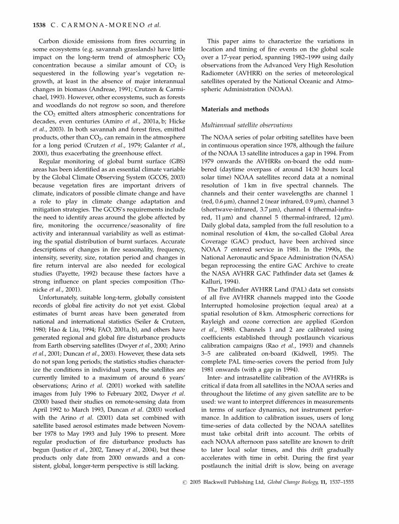
Figure 1 shows AVHRR channels 1 and 2 values

from the Libyan Desert test site for the entire PAL time-

series; Fig. 2 shows corresponding values from the

various AVHRRs’ channel 3. Channels 1 and 2 ref-

lectance values gradually increase by up to 5% during

the operational lifetime of each satellite and some

differences – in the order of 1% – are seen between the

different satellites in the series. The exception is the

data from end of 1999 where variation is much higher

(again confirming NOAAs recommendation not to use

these data). The channel 3 values vary by over 5 K over

the entire time-series. A decrease of less than 2 K is

apparent for each individual satellite in the series, with

the obvious exception of the last set of values. The large

jump of over 4 K between 1993 and 1995 is probably

because of a shift in gain on the sensor flying on the last

satellite in the NOAA series.

We recognize that the variations of around 5%

reflectance detected in channels 1 and 2 of the PAL

time-series are a potential source of error but because we

lack suitable tools for BRDF correction we left these

values unchanged. However, for channel 3 the variations

in the Pathfinder data set were too great to ignore. To

correct the trends detected in the channel 3 time-series we

assume that the degradation of the orbit and any

degradation in sensor performance during the first year

2000199819961994199219901988Year

19861984198220

22

24

26

28

30

32

34

36

38

40

42

44

Ave

rage

-CH

1 (%

)

Average-CH1

Average-CH2

CH1– CH2 Libyan Test SiteAVHRR 1982 – 2000

Fig. 1 Advanced Very High Resolution Radiometer (AVHRR)

CH1 and CH2 average values (% reflectance) for the Libyan Test

site for the period 1982–2000.

C H A R A C T E R I Z I N G I N T E R A N N U A L VA R I A T I O N S 1539


postlaunch are negligible, and we made a linear adjust-

ment to the time-series using the first year’s measure-

ments as an anchor (i.e., using a moving average with

1 year lag). Figure 2 also shows the resulting ‘detrended’

channel 3 values.

The GBS Time-Series

Using the daily PAL data set to the end of 1999 as input

(original PAL channels 1 and 2 values, detrended

channel 3 values) we generated a new weekly product

to monitor multiannual fire activity (Moreno-Ruiz et al.,

1999). The metric we use is burnt area, measured in km2,

and the final product is referred to as the GBS data set.

The algorithm for identifying burnt surfaces uses

data recorded by the AVHRRs’ channels 1–3 and is an

extension of the approach used by Barbosa et al.

(1999a, b). The algorithm consists of the sequential

application of a series of tests applied to a 7-day

minimum value composite (Barbosa et al., 1998). The

minimum value composite is created by retaining

1 day’s channels 1–3 values for each geographic

location selected on the basis of the minimum albedo

value detected during the 7-day period; the albedo

being computed according to Taylor (1990)

Albedo ¼ 0:347 rðchannel 1Þþ 0:650 rðchannel 2Þ þ 0:0746;

ð1Þ

where r(channel 1) and r(channel 2) are the Top of

Atmosphere (ToA) reflectance in channel 1 and channel

2 respectively.

The creation of minimum value albedo composites

eliminates pixels with a high albedo associated with

bright cloud tops, and is thus an approximate cloud-

screening process that is combined with the CLAVR

index of the data. Burnt surfaces are then identified

from these composites by exploiting the difference in

the spectral response over time of burned and

unburned vegetation at the wavelengths recorded by

the channels 1, 2 and 3. Vegetation indices combining

reflectance measurements at red and near-infrared

wavelengths are widely used to detect the presence

and growth of vegetation. For this purpose the GBS

uses the Global Environmental Monitoring Index

(GEMI) proposed by Pinty & Verstraete (1992). Burned

surfaces are usually darker (and warmer) than sur-

rounding unburned surfaces (Belward et al., 1993); a

linear combination of the AVHRR channels 2 and 3,

VI3T is used to emphasize this difference. VI3T is a

modified version of Vi3 (Kaufman & Remer, 1994)

where the reflective part of channel 3 is replaced by the

full channel 3 brightness temperature (BT3). The

sequence and thresholds of the test follows:

ðrðchannel 2Þ < 0:125ÞAND

ðrðchannel 3Þ > 312:0Þ AND

ðVi3t < �0:34Þ AND

ðMax ðGEMIÞ > 0:39Þ;

where Vi3t and GEMI are defined as follows:

Vi3t ¼ ðrðchannel 2Þ � BT3=1000Þðrðchannel 2Þ þ BT3=1000Þ ;

GEMI ¼Zð1� 0:25ZÞ � ðrðchannel 1Þ � 0:125Þ� ð1� rðchannel 1ÞÞ;

where

Z ¼ð2ðrðchannel 2Þ2 � rðchannel 2Þ2Þþ 1:5rðchannel 2Þ þ 0:5rðchanne 1ÞÞ=� ðrðchannel 2Þ þ rðchannel 1Þ þ 0:5Þ

and BT3 is the brightness temperature of AVHRR channel

3 and r(channel 3) is the ToA reflectance of AVHRR

channel 3. Max (GEMI) is defined as the maximum value

of the weekly GEMI data for any given pixel location.

This ‘Fixed Test’ is then followed by a ‘Temporal Test’

which uses thresholds detecting the temporal coher-

ence of the detection on a week-by-week basis.

ðVi3tw < Vi3tw�1Þ AND

ðGEMIw < GEMIw�1ÞAND

ðrðchannel 3Þw > rðchannel 3Þw�1Þ;

20011999199719951993199119891987198519831981316

317

318

319

320

321

322

Ave

rage

-CH

3 (K

)

Average-CH3Average-CH3 Detrended

Channel3 Libyan Test SiteAVHRR 1982 – 2000

Year

Fig. 2 Advanced Very High Resolution Radiometer (AVHRR)

CH3 and CH3 detrended average values (degrees Kelvin) for the

Libyan Test site in the period 1982–2000.



where wA[0, . . . , 52] and is the current week being

analyzed by the algorithm and w�1 is the precedent

week.

A third step is then an ‘Automatic Test’, which takes

into account the annual standard behavior (defined by

the mean value of the year (m) and its standard

deviation (SD)) of each pixel’s radiometry. This test

uses only Vi3t values given its better performance when

compared with other AVHRR indices and channels

(Barbosa et al., 1999a, b).

ðVi3tw < Vi3tðmÞ � LCC Vi3t ðSDÞÞ;

where LCCA[1, 2]. LCC can either be 1 or 2 depending

on the land cover class. Land cover class with low fire

ignition probability is equal to 2 (Evergreen Broadleaf

Forests, Bare and Mosses and lichens as defined by De

Fries et al. (1998)) all other land cover classes are equal

to 1.

Because an entire year’s data are needed for this test

we had to exclude partial observations from the end of

1981 and 1994, hence our GBS time-series begins 1982

and 1994 is missing. Thus, we generated a multiyear

GBS product spanning the period 1982–1999 where

burn scars are reported each 7 days for each year.

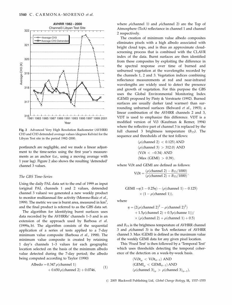
Quality assessment

Sensitivity tests. Figures 1 and 2 clearly show that the

PAL time-series is not stable over time; systematic

trends of increasing reflectance during the life-time of

each satellite are clearly visible. The amplitude of the

variation in the detrended channel 3 values over the

entire time-series is less than 1.5 K (less than 0.5% of

the channel 3 sensors’ range). The amplitude of the

variation in the channels 1 and 2 original PAL data, as

used to generate the GBS, is at least an order of

magnitude greater, being 5%. As a first step in our

quality assessment process, we model the effects of

these channel 1 and 2 changes on the performance of

the GBS algorithm.

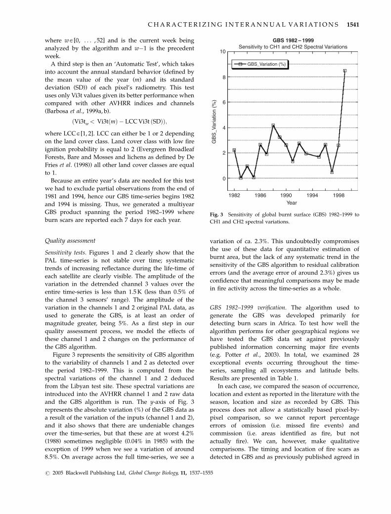
Figure 3 represents the sensitivity of GBS algorithm

to the variability of channels 1 and 2 as detected over

the period 1982–1999. This is computed from the

spectral variations of the channel 1 and 2 deduced

from the Libyan test site. These spectral variations are

introduced into the AVHRR channel 1 and 2 raw data

and the GBS algorithm is run. The y-axis of Fig. 3

represents the absolute variation (%) of the GBS data as

a result of the variation of the inputs (channel 1 and 2),

and it also shows that there are undeniable changes

over the time-series, but that these are at worst 4.2%

(1988) sometimes negligible (0.04% in 1985) with the

exception of 1999 when we see a variation of around

8.5%. On average across the full time-series, we see a

variation of ca. 2.3%. This undoubtedly compromises

the use of these data for quantitative estimation of

burnt area, but the lack of any systematic trend in the

sensitivity of the GBS algorithm to residual calibration

errors (and the average error of around 2.3%) gives us

confidence that meaningful comparisons may be made

in fire activity across the time-series as a whole.

GBS 1982–1999 verification. The algorithm used to

generate the GBS was developed primarily for

detecting burn scars in Africa. To test how well the

algorithm performs for other geographical regions we

have tested the GBS data set against previously

published information concerning major fire events

(e.g. Potter et al., 2003). In total, we examined 28

exceptional events occurring throughout the time-

series, sampling all ecosystems and latitude belts.

Results are presented in Table 1.

In each case, we compared the season of occurrence,

location and extent as reported in the literature with the

season, location and size as recorded by GBS. This

process does not allow a statistically based pixel-by-

pixel comparison, so we cannot report percentage

errors of omission (i.e. missed fire events) and

commission (i.e. areas identified as fire, but not

actually fire). We can, however, make qualitative

comparisons. The timing and location of fire scars as

detected in GBS and as previously published agreed in

19981994199019861982Year

0

2

4

6

8

10

GB

S_V

aria

tion

(%)

GBS_Variation (%)

Sensitivity to CH1 and CH2 Spectral VariationsGBS 1982 – 1999

Fig. 3 Sensitivity of global burnt surface (GBS) 1982–1999 to

CH1 and CH2 spectral variations.



Tab

le1

Lis

to

fla

rge

refe

ren

ced

wil

dfi

res

ov

erth

ep

erio

d19

82–1

999

Nu

m.

Lo

cati

on

Per

iod

Lat

itu

de/

Lo

ng

itu

de

Ref

eren

ce

Ag

reem

ent

wit

hg

lob

al

bu

rnt

surf

ace

(GB

S)

1K

alim

anta

nN

ov

emb

er19

82–A

pri

l19

8381

N–4

1S

/10

7–11

91E

Go

ldam

mer

&H

off

man

n(2

001)

Go

od

2Iv

ory

Co

ast

Dec

emb

er19

82–M

arch

1983

71N

/51

WO

ura

(199

9)G

oo

d

3A

ust

rali

aD

ecem

ber

1983

241S

/13

41E

(Ali

ceS

pri

ng

s)A

llan

&S

ou

thg

ate

(200

2)G

oo

d

4A

ust

rali

a19

8524

1S

/13

41E

(Ali

ceS

pri

ng

s)A

llan

&S

ou

thg

ate

(200

2)G

oo

d

5C

hin

a–R

uss

iaM

ay–J

un

e19

8744

–551

N/

120–

1351E

Cah

oo

net

al.

(199

1)G

oo

d

6Y

ello

wst

on

eP

ark

Su

mm

er19

8844

.61N

/11

0.71

WR

om

me

&D

esp

ain

(198

9)G

oo

d

7A

lask

aM

ay–A

ug

ust

1990

60–6

41N

/14

0–15

51W

Bo

les

&V

erb

yla

(200

0);

Kas

isch

ke

etal

.(1

995)

Ver

yP

oo

r–

per

iod

of

the

yea

rd

etec

ted

bu

tu

nd

eres

ti-

mat

ion

(o20

%)

8A

lask

aM

ay–A

ug

ust

1991

60–6

41N

/14

0–15

51W

Bo

les

&V

erb

yla

(200

0);

Kas

isch

ke

etal

.(1

995)

Ver

yP

oo

r–

per

iod

of

the

yea

r

det

ecte

db

ut

un

der

esti

mat

ion

(o20

%)

9R

uss

iaM

ay–A

ug

ust

1992

45–7

51N

/90

–150

1E

Co

nar

d&

Ivan

ov

a(1

998)

;

Co

nar

det

al.

(200

2);

Cah

oo

net

al.

(199

6)

Go

od

10C

entr

alA

fric

anR

epu

bli

cM

id-O

cto

ber

1994

–ear

lyM

arch

1995

2–13

1N

/10

–351E

Ev

a&

Lam

bin

(199

8);

Go

od

11C

anad

aM

ay–A

ug

ust

1995

50–5

81N

/65

–100

1W

Li

etal

.(2

000)

Go

od

12P

ort

ug

alJu

ne–

Oct

ob

er19

9539

.5–4

2.51

N/

6–91W

Per

eira

&D

os

San

tos

(200

3)P

oo

rP

lus

–o

ver

esti

mat

ion

bec

ause

of

ho

tsu

rfac

esin

the

sou

tho

fP

ort

ug

al(A

lmo

do

var

)

13P

atag

on

iaS

epte

mb

er19

95–e

arly

Ap

ril

1996

35–5

51S

/56

–741E

Cw

ielo

ng

(199

6)G

oo

d

14M

on

go

lia

Feb

ruar

y–J

un

e19

9647

–551

N/

97–1

201E

Sh

ulm

an(1

996)

Go

od

15C

anad

aL

ate

May

–Au

gu

st19

9647

–581

N/

65–9

51W

and

55–6

51N

/90

–130

1W

Li

etal

.(2

000)

Go

od

16M

on

go

lia

Lat

eF

ebru

ary

–Ju

ne

1997

47–5

51N

/97

–120

1E

Erd

enes

aik

han

&E

rden

etu

ya

(199

9)G

oo

d

17C

anad

aL

ate

May

–Au

gu

st19

9750

–581

N/

65–1

001W

Li

etal

.(2

000)

Go

od

18A

lask

aL

ate

May

–mid

-Au

gu

st19

9763

–641

N/

1591W

Bo

les

&V

erb

yla

(200

0)V

ery

Po

or

19N

ort

her

nA

ust

rali

aM

ay–l

ate

No

vem

ber

1997

11–2

71S

/11

8–15

21E

Ru

ssel

l-S

mit

het

al.

(200

3);

Ed

war

ds

etal

.(2

001)

Ver

yG

oo

d

20E

ast

Kal

iman

tan

Lat

eM

ay19

97–e

arly

Jun

e19

983S

–31N

/11

4–11

91E

Sie

ger

tet

al.

(200

1)G

oo

d

21N

ort

ho

fS

ou

thA

mer

ica

Jan

uar

y–A

pri

l19

9821

S–1

01N

/58

–731

W

(in

Ro

raim

a–B

razi

l)

Elv

idg

eet

al.

(200

1)V

ery

Go

od

22M

on

go

lia

Lat

eF

ebru

ary

–ear

lyJu

ne

1998

47–5

51N

/97

–120

1E

Erd

enes

aik

han

&E

rden

etu

ya

(199

9)G

oo

d

23M

exic

oA

pri

l–M

ay19

9814

–221

N/

87–1

011W

Gal

ind

oet

al(2

003)

24C

anad

aM

id-A

pri

l–la

teO

cto

ber

1998

47–5

81N

/65

–951

Wan

d

55–6

51N

/90

–130

1W

Li

etal

.(2

000)

;Jo

hn

sto

n(1

999)

Go

od

25R

uss

iaF

arE

ast

Lat

eM

ay–e

arly

No

vem

ber

1998

40–7

01N

/11

0–14

51E

Tan

imo

toet

al.

(200

0)G

oo

d

26P

ort

ug

alJu

ne–

Oct

ob

er19

9839

.5–4

2.51

N/

6–91W

Per

eira

&D

os

San

tos

(200

3)P

oo

rP

lus

–o

ver

esti

mat

ion

bec

ause

of

the

ho

tsu

rfac

esin

the

sou

tho

fP

ort

ug

al(A

lmo

do

var

)

27S

um

atra

Feb

ruar

y–D

ecem

ber

1999

31N

–61S

/98

–107

1E

An

der

son

etal

.(2

000)

Go

od

28S

iber

iaA

pri

l–A

ug

ust

1999

50–7

01N

/76

–150

1E

So

jaet

al.

(200

4)P

oo

r



all 28 cases, but the size of the fire event as measured in

GBS and independently reported varied considerably.

In Table 1, we define the agreement between previously

published documents and GBS as ‘Very Good’, where

location and timing agree and where the area

estimation from GBS is between 80% and 100% of that

independently documented. Agreement is judged

‘Good’ if location and timing agree and area estimates

from the GBS are between 60% and 80% of that

reported elsewhere. ‘Poor’ agreement is where

location and timing agree but the GBS area estimate is

only 20% to 50% of that reported, and ‘Very Poor’

agreement occurs where location and timing agree, but

GBS identifies less than 20% of the area. Those areas

where location and timing agree, but where GBS

identifies more than 100% of the area as previously

reported are judged ‘Poor Plus’.

GBS over-estimated fire area in only two out of the

28 cases. Fire area was underestimated in all of the

other 26 fire events we checked. Performance, in terms

of fire area estimation, was particularly bad at high

latitudes, which unfortunately include the extensive

and fire-prone forests of the northern boreal zone-

although the seasonal behavior of these fires was

detected.

As an additional global check we compared the GBS

maps with the monthly active fire patterns for the years

2002 and 2003 available from the Web Fire Mapper

(http://maps.geog.umd.edu/products.asp; last acces-

sed 25 November 2004). This site presents global active

fire locations as detected by the Moderate Resolution

Imaging Spectroradiometer (MODIS) instrument

(Justice et al., 2002, Davies et al., 2004). The MODIS

active fire maps again showed active fire activity

in all the regions identified as containing burn

scars in GBS, but showed far more widespread fire

activity in high northern latitudes, again suggesting

that the GBS underestimates, rather than overestimates

fire activity.

From the results of the comparisons made in Table 1

and with independently published information on

active fires we deem it inappropriate to use the GBS

time-series as a means of comparing absolute measures

of fire area across different geographical regions.

However, the good agreement concerning location

and timing does not compromise the use of GBS for

looking at inter- and intra-annual variations in regions

affected by fire and in fire calendar. And while

geographical errors are undoubtedly present these too

are consistent over time. The underestimation of fire

activity between 401 and 701 north is certainly real, but

as the same algorithm was used throughout and the

input data were all uniformly treated we can assume

the temporal variation to reflect (albeit sampled)

genuine variations in fire activity with time at these,

and indeed any other, latitudes.

Results and analysis

Fire seasons by latitude

The weekly GBS product at 8 km is the initial output. To

provide a multiannual overview of global fire seasons

we first summed each year’s weekly data into four

trimesters according to conventional seasonal group-

ings (December, January, February – DJF; March, April,

May – MAM; June, July, August – JJA; September,

October, November – SON). We then summed the 17

years record for each trimester. However, during the 17

years of our study, the trimester in which fires occur at

any given location can, and does, change. For each 8 km

grid cell we determine all dates at which burn scars are

detected and then represent the mode. Figure 4 shows

the global synthesis of all burnt areas detected over the

entire time-series. The limitations of plotting individual

features, such as burn scars, in global maps at very

small scales, such as Fig. 4, hides (or blurs) much detail.

Figures 5 and 6 complement the map and are included

as a means of showing the seasonal behavior in more

detail. These show the cumulative burnt area for each

trimester/season, and the total, as a function of

latitude. Note, that in Fig. 5 all burnt areas have been

normalized to the absolute peak in fire activity, in Fig. 6

the relative contribution of each season’s burning for

each degree of latitude is shown.

Fire season probability maps

Another important aspect in defining the global fire

regime (Payette, 1992) is the probability of fire

occurring in a particular season for any given area

(latitude i, longitude j). This can be described as the

probability for a given area at latitude i, longitude j to

burn in a given unit of time. Here, we consider that the

unit of time is a trimester and a unit area is a 0.51� 0.51

latitude–longitude cell. This is formally defined by:

PðBSpði;jÞÞ ¼P

m BSpði;jÞPp¼4p¼1

Pm BSpði;jÞ

; ð2Þ

where PðBSpði;jÞÞ is the probability of a 0.51� 0.51 cell

(latitude i and longitude j) to burn in a trimester p of the

year;P

m BSpði;jÞ is the number of burned pixels

detected in the cell (i, j) for the trimester p of the year

(p 5 {1, 2, 3, 4}); where m is the number of pixels (8 km)

in the 0.51� 0.51 cell andPp¼4

p¼1

Pm BSpði;jÞ is the total

number of burned pixels detected in the cell (i, j) along

the 17 years considered in this paper.



180°160°E140°E120°E100°E80°E60°E40°E20°E20°W40°W60°W80°W100°W120°W140°W160°W180°

120°W140°W160°W180°70

°S50

°S30

°S10

°S10

°N30

°N50

°N70

°N

70°S

50°S

30°S

10°S

10°N

30°N

50°N

70°N

0°

180°160°E140°E120°E100°E80°E60°E40°E20°E20°W40°W60°W80°W100°W 0°

December to FebruaryMarch to May

June to August

September to November

Fig. 4 Global fire activity seasonal cycle. This figure represents the seasonal distribution of the fire activity obtained from the

accumulated spatial–temporal distribution of the global burnt surface products for the period 1982–1999.

GBS 1982 – 1999Distribution by latitudes and periods of the year

0

10

20

30

40

50

60

70

80

90

100

9080706050403020100−10−20−30−40−50−60−70−80−90Latitudes

Per

cen

tag

e (%

)

SONJJAMAMDJF

Fig. 5 Accumulated and normalized fire activity distributed by latitudes for the period 1982–1999.



The outputs of this computation are four fire season

probability maps (one per trimester). These are shown

in Fig. 7(a)–(d). By definition, the sum of the prob-

abilities of the four periods is equal to 100% for those

regions where the total number of burned pixels is not

equal to 0 (no fire detected during the 17 years time-

series) in order to have a homogenous system.

We can see for instance the low probability of fire

occurring in the first trimester of the year (winter) in the

Mediterranean area and/or in high latitudes of the

boreal region. The probability strongly increases during

the second and third periods of the year (this point will

be further discussed in the Results). Peaks of prob-

ability occur in trimesters of the year in those latitudes

where fire activity reaches its maximum.

Characterizing multiannual patterns in fire occurrence

To model the spatial–temporal structure of the data for

the entire 17 years time-period, we constructed a

variogram of the GBS time-series. The variogram can

be considered as a quantitative descriptive statistic that

can be graphically represented in a manner that

characterizes the spatial and temporal continuity of

the data analyzed. The mathematical definition of the

variogram is:

gðDx;DyÞ ¼ 12e Zðxþ Dx; yþ DyÞ � Zðx; yÞf g2h i

; ð3Þ

where Z(x, y) is the value of the variable of interest

at location (x, y) and e12 is the statistical expectation

operator. It should be noted that the variogram, g(x, y),

is a function of the separation between points (Dx,Dy),

and not a function of the specific location (x, y) (Isaaks

& Srivastava, 1989).

We first took the 52 weekly global maps of burned

surface for all 17 years and summed the burned

surfaces by trimester and by latitude in 0.51 strips.

Figure 8 shows the standardized variogram where the

proportional effects (i.e. the variance value increases

with the increment of the average) are removed. A

quadratic trend has also been removed from the data.

Removing these two elements of the data that may be

considered structural perturbations does not affect the

GBS 1982 – 1999Distribution by latitudes and periods of the year

0

10

20

30

40

50

60

70

80

90

100

7770635649423528211470−7−14−21−28−35−42−49−56

Latitudes

Per

cen

tag

e o

f co

ntr

ibu

tio

n (

%)

SONJJAMAMDJF

Fig. 6 Contribution of burned surface (considered as a proxy of the fire activity) for each trimester of the year per latitude.



180°160°E140°E120°E100°E80°E60°E40°E20°E20°W40°W60°W80°W100°W120°W140°W160°W

70°S

50°S

30°S

10°S

10°N

30°N

50°N

70°N

70°S

50°S

30°S

10°S

10°N

30°N

50°N

70°N

180° 0°

180°160°E140°E120°E100°E80°E60°E40°E20°E20°W40°W60°W80°W100°W120°W140°W160°W180° 0°



70°S

50°S

30°S

10°S

10°N

30°N

50°N

70°N

70°S

50°S

30°S

10°S

10°N

30°N

50°N

70°N

0%

100%

0%

100%

% Probability

% Probability

(a)

(b)

Fig. 7 Fire seasonal probability (a) December–January–February, (b) March–April–May, (c) June–July–August and (d) September–

October–November.



180°160°E140°E120°E100°E80°E60°E40°E20°E20°W40°W60°W80°W100°W120°W140°W160°W

70°S

50°S

30°S

10°S

10°N

30°N

50°N

70°N

180° 0°




70°S

50°S

30°S

10°S

10°N

30°N

50°N

70°N

70°S

50°S

30°S

10°S

10°N

30°N

50°N

70°N

70°S

50°S

30°S

10°S

10°N

30°N

50°N

70°N

% Probability

100%

0%

% Probability

100%

0%

(c)

(d)

Fig. 7 Continued.



spatial–temporal structure we see. In other words the

variogram is highly stable.

From the analysis of the variogram, we see that there

is a low nugget effect ( �30%); thus we account for close

to �70% of the spatial–temporal correlations in our

time-series with this trimester-based model. We fit the

data with an exponential model (scale 5 1, length 5 3.5

with an anisotropy defined by a ratio 5 1 and angle 5 0).

This model shows that the range (the distance between

the origin and the point at which the variogram reaches

the sill (i.e., at the standardized variogram value of 1))

occurs after 16 trimesters, confirming a regular pattern

in the time-series with this periodicity. In the same way,

Fig. 8 also shows a pattern occurring every 4 trimesters,

i.e. a strong annual periodicity.

To provide spatial representation of the variogram

model a gridding method was used to fit the exponential

model from the variogram to the GBS data. The result is

shown in Fig. 9. This Figure shows the spatial–temporal

structure of the GBS data distributed by latitudes (y-axis),

time (x-axis, trimestrial periods), with burned surfaces

summed during each trimester and by 0.51 of latitude.

The contour interval represents 500 burned pixels.

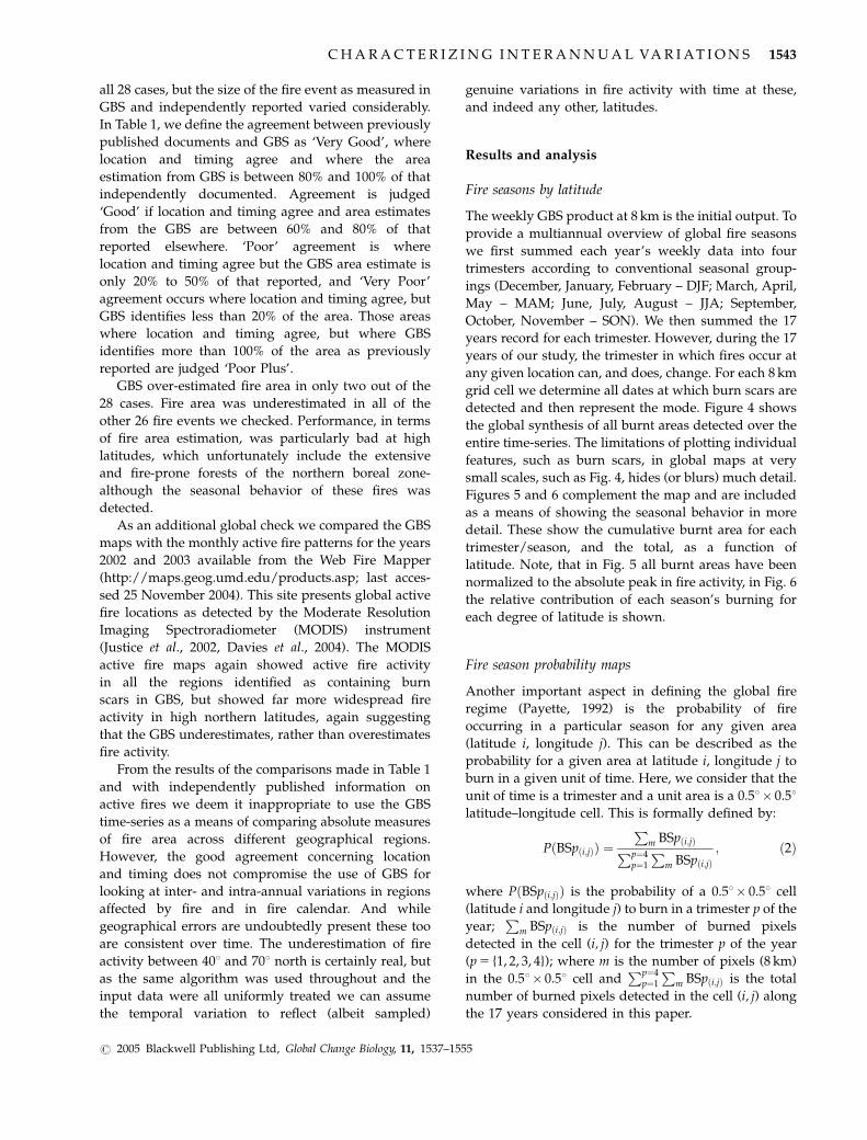
The variogram results are supported by frequency

analysis of the GBS time-series, shown in Fig. 10. This has

been computed using the Fast Fourier Transform (FFT).

Results and discussion

An overview of global fire activity

The global burnt area synthesis shown in Fig. 4

conforms to previously established geographic distri-

60565248444036322824201612840Lag distance (trimester)

0

0.1

0.2

0.3

0.4

0.5

0.6

0.7

0.8

0.9

1

Sta

ndar

dize

d va

riogr

am

Direction: 0.0 Tolerance: 90.0GBS time series (1982 – 1999)

Fig. 8 Global burnt surface (GBS) time-series 1982–1999 stan-

dardized variogram.

9998979695939291908988878685848382Years

70

60

50

40

30

20

10

0

−10

−20

−30

−40

El Ni no (warm) Index

La Ni a (cool) Index

Latit

ude

Fig. 9 Spatial–temporal distribution of global burnt surface (GBS) time-series and El Nino southern oscillation (ENSO) Index (regions

3.4 and 1–2) during the period 1982–1999. The Chichon’s (08/1982) and Mount Pinatubo’s (06/1991) eruptions (in blue), and main fire

events (in red) occurred during the period considered in this paper are also showed.



butions (e.g., Tansey et al., 2004); Australia as a ‘fire’

continent is highly evident, the almost unbroken ring of

savanna fires surrounding the largely untouched

tropical forests of central Africa, the agriculture and

savanna fires extending into the Amazon Basin (espe-

cially the southern fringes), the forest fires of the

Mediterranean Basin, the grain producing lands, range-

land and forest fires of North America and Central Asia

can all be clearly seen, as can the fires in southern Asia’s

forests and rice fields, and a scatter of fire scars across

the boreal forests of the north. Fire is at an absolute

minimum at the very high latitudes above the Arctic

and Antarctic Circles. Another major gap corresponds

to the moist humid tropical forests, with other marked

gaps in fire activity corresponding to the barren

regions, such as the Sahara, and the intensely urba-

nized, Eastern USA and Western/Central Europe. The

global seasonal synthesis shown in Figs 5 and 6 gives

further emphasis to the observation that biomass

burning is a truly global and continuous phenomenon;

burn scars are only absent at the very highest latitudes

and fires occur during all seasons on both sides of the

equator.

The northern hemisphere’s fire seasons. Northern hemis-

phere fire activity during the months of December,

January and February is principally confined to latitudes

below �351N. Fires across Africa’s northern savanna

belt, agriculture and grassland burning in the Orinoco

valley of Colombia–Venezuela and across southern India

and South East Asia contribute to the dominant peak

between �3 and �171N. The fires in Africa extend

throughout the grass and shrub savannas through to the

fringes of the humid tropical forests, and are closely

linked to the onset and advance of the dry season,

mainly between October and March (Delmas et al., 1991).

A second, less pronounced peak occurs at this time

between �17 and 351N. This is dominated by fire

activity in northern India and Asia towards the end of

the trimester. Very little burning in this season occurs

above 351N, and almost nothing above 401N.

Fire activity in March, April and May occurs

throughout the northern hemisphere, although three

distinct peaks do occur; one peak, occurring between

�3 and 171N, is mainly accounted for by late dry

season burning in Africa’s northern savannas; a second

peak between �17 and 401N can be accounted for by

fire in the tropical pine forests of Central America and

Southeast Asia – the latter are often as a result of grazing

land management fires and shifting cultivation. This

period also sees fires in Asia linked to the burning of rice

field stubble before the onset of the moist South West

Monsoon, as well as land clearance and some rangeland

management fires. Tropical pine forest fires and

agricultural crop residue clearing in Central America

and Asia add significant amounts of burn-

ing, especially in April to June, and significant burning

also occurs in India’s remaining forests (from the

temperate forests of the north to the tropical forests

along the West Coast), which come under threat from

fire each year, especially in March and April (Saha &

Hiremath, 2003). Land clearance, accidental fires from

shifting cultivation and fires used for the management of

nontimber forest products such as mahua (Madhuca

indica) flowers and kendu (Diospyros melanoxylon) leaves

account for much of this activity (Jaiswal et al., 2002;

Reddy & Venkataraman, 2002). The third peak in

burning embraces the postharvest stubble clearance

and crop residue fires of the agricultural regions

between 45 and 551N, the grassland and forest fires of

the central Eurasian steppe and, above 601N, early

summer forest fires in the boreal zone.

Very little burning occurs in the months of June, July

and August between �3 and 301N. However, this is the

season where the Mediterranean basin and Pacific

Northwestern USA experience their peak forest activity

(lightning ignition from summer convective storms is a

major factor; Rorig & Ferguson, 1999), and when

Eurasia’s more southerly steppe and forest burns. It

also represents the peak period for fire activity in the

boreal forests, where again lightning ignition is a

significant factor (Stocks, 1991).

Northern hemisphere fire activity does occur during

the autumn months of September, October, November,

but is minimal above �501N. Below this latitude the

African grasslands are a focus for much of the activity.

The northernmost savannah shrub and grasslands

GBS 1982 – 1999 – spectral density

0.000

20 000 000.000

40 000 000.000

60 000 000.000

80 000 000.000

100 000 000.000

120 000 000.000

140 000 000.000

17 8 4 2 10.

5

Sp

ectr

al d

ensi

tyGBS 1982 – 1999

Length of cycle (year)

Fig. 10 Periodogram representing the frequency component of

the global burnt surface (GBS) time-series.



between �12 and 171N burn early in the dry season – a

peak in burning occurs here between October and

November – with fire activity following the advancing

dry season south until reaching the humid forest

margins between January and March. The fire activity

between �30 and 501N during this period are mainly

late summer (September) fires in the forests of north

Africa, Central Asia and the North America – Central

America confines.

The southern hemisphere’s fire seasons. Although not on

the same scale as in the north, southern hemisphere fire

activity does occur during the months of December,

January and February. This commences at the equator,

but has a stronger presence at latitudes below 161S.

Australia, especially the southern half of the continent

(Craig et al., 2002), and South America are the main

centers of fire activity at this time, although southern

Africa also experiences some fire activity in these

months, especially in the Cape Town region (Calvin &

Wettlaufer, 2000) and South West Botswana (Brockett

et al., 2001; Dube, 2004). Argentina’s forest fires usually

occur around the month of February (Cwielong &

Rodriguez, 1993), and fire activity peaks around this

period in Chile too, (http://www.ine.cl/17-ambiente/

catastrofes.htm – last accessed 25 November 2004).

Again, in contrast with the northern hemisphere,

there is relatively little fire activity in March, April, May

in the south. Most of the fires that do occur in this

period occur in Australia, especially in the temperate

plains and agricultural regions to the south west and

south east of the continent (Williams, 2001), as well as

in the more northern parts of the arid interior.

Burning in the southern hemisphere savannas of

Africa and South America, combined with a marked

dominance of fire in the north of Australia (Craig et al.,

2002) lead to the first of two peaks in southern

hemisphere fire activity; this one occurring in the

months of June, July and August and extending from

the Equator down to �161S. This latitude belt

embraces the deforestation arc at the southern

margins of the Amazon Basin, where burning starts

around July and finishes in November with a peak at

the end of July/early September (Christopher et al.,

1998). It also encompasses the African savannas just to

the south of the central African rainforest.

The second, and larger southern hemisphere peak

occurs from September, through to November. This

dominates the more southern latitudes, extending

down from �16 to 401S. In Australia this period sees

a general swing in fire activity to the eastern tropical

costal margins and the subtropical plains. In Africa it is

the more southerly savannas that burn, and in South

America from the centre to the south (Pampa –

Patagonia regions), the fire activity is concentrated in

the summer period where the dry season occur.

Below �351S fire activity at this time is minimal, with

fires tending to occur in January to March.

Global fire calendar probability maps

In the preceding sections, we have shown that typical

fire seasons exist for each geographic location on earth.

Because fire is sensitive to prevailing climatic/meteor-

ological conditions (among other factors) these seasons

are not completely stationary over the 17 years record

we are working with. In this section, we propose global

maps showing the probability of fire occurring for any

given location for each of the four seasons. Figure 7(a)–

(d) shows each season’s probability map, where the

resolution has been degraded to 0.51 grid. These data

are freely available from http://www-gvm.jrc.it/.

Figure 7 provides a spatially explicit guide as to the

location and timing of fire on the global scale. This

information is closely linked to temperature and

precipitation, and therefore, with the prevailing climate

conditions, which have direct implications on the state

of the biomass including fuel amount and fuel moisture

content (Camberlin et al., 2001; Lyon, 2004). As we will

see in the following section, climate variability induces

temporal and spatial shifts in fire seasonality in

different parts of the world. In other regions these

shifts do not occur. This stability, and lack of it, is

evident in the 17 years fire probability maps.

The fire seasons in some regions are very stable over

the entire 17 years record. These are the areas in Fig. 7

that have either very high or very low probability

during any particular trimester. This is the case for the

high and medium latitudes in the Northern Hemi-

sphere (JJA), Far East of China–Russia (MAM), Central

Africa (JJA), and African savannas (DJF and SON). We

can hypothesize that in these areas interannual varia-

tions in climate have little or no effect on fire

seasonality, although of course may still influence the

size, intensity and efficiency of fire. However, in other

regions, even if there is always a maximum of

probability in a given trimester, the peak is less evident

(i.e., the timing of fire activity across the 17 years varies

quite widely). Thus, in Fig. 7, we see relatively high

probabilities of fire for these regions in several

trimesters. This homogeneity in the temporal prob-

ability distribution can be interpreted as particularly

fire prone areas/ecosystems, or areas that are more

sensitive to interannual climate variability. This is the

case in Indonesia, Southern Europe, Southern and East

Africa, California, Australia, Southern East Asia,

Central and Northern Latin America.



Interannual variability in fire calendar

Although the 17 years summary presented above

substantiates the concept of typical fire seasons for

specific locations across our planet, these seasons are by

no means truly stationary, as indeed confirmed by the

variogram in Fig. 9. This figure expands the view of

global fire dynamics by presenting the area burned for

each trimester of each year as a function of latitude. Size

of burned area is implied by the contour spacing (level

step 5 500 burned pixels). The fire events reported in

Table 1 have been positioned in the Figure, as have two

major volcanic eruptions and the El Nino/La Nina

events that occurred over this time-span. Although the

data are presented year-by-year, fire seasons do not

adhere to the Gregorian calendar and references to

specific years/months are made to guide the inter-

pretation; to this end January of each year is shown as a

solid vertical line.

Looked at in the latitude axis, Fig. 9 shows that each

year’s fire distribution follows much the same pattern

as described in ‘An overview of global fire activity’;

fires occur at most latitudes, maximum fire activity

occurs between the two Tropics, least fire-prone belts

are found close to the equator and between 30 and

401N; a noticeable offset occurs in the timing between

the southern and northern hemisphere burning max-

ima, and both hemispheres show maxima occurring at

more than one time within a single year.

Yet, while strong annual periodicity (and to a lesser

extent intraannual periodicity) of burning is apparent

throughout the time-series, considerable interannual

variation can be seen on both sides of the equator. This

falls into a repetitive 4-year pattern, where the various

peaks and troughs correlate well with El Nino Southern

Oscillation (ENSO) events during this period.

The apparent ENSO effects on fire calendar tend to

mirror each other across the equator. In the northern

hemisphere El Nino periods are linked to enhanced fire

activity, and fire activity gradually increases from year-

to-year as these periods persist. Manzo-Delgado et al.

(2004) have shown an increase in Central Mexico’s fire

activity during El Nino induced droughts, and fires in

the Yucatan forests of 1989 were linked to both drought

and the aftermath of Hurricane Gilbert – the storm

opened up forest and provided good fuel, the drought

‘cured’ the fuel, and run-away land clearance fires

completed the picture (Goldammer, 1992). An increase

in the frequency and extent of fires across North

America have been linked to large-scale climate

patterns in conjunction with El Nino (Swetnam &

Betancourt, 1990; Bartlein et al., 2003; McKenzie et al.,

2004) and even in Europe good correlations have been

found between increased fire activity and the El Nino

(Rodo et al., 1997). Figure 9 shows that fire activity in

the high northern latitudes is variable, both annually

(in terms of latitudes affected) and interannually (in

terms of both timing and frequency of occurrence).

Figure 9 also shows that the latitudinal limits of fire in

the north tend to spread further south during El Nino

years. The interannual variability of burning at these

latitudes and a strong agreement between the inter-

annual peaks of activity mainly occurring during El

Nino events has been reported by Conard et al. (2002),

Li et al. (2000) and Soja et al. (2004) among others.

During La Nina periods fire activity in the northern

hemisphere is not just lower, but is also more dispersed

over space and time. During these periods the fire

seasons are longer, less concentrated and less well

defined. The peak in fire activity also occurs later in the

season.

The northern hemisphere pattern of ‘strong and

symmetrical’ fire seasons coinciding with El Nino

periods and ‘weaker, more dispersed’ fire seasons

during La Nina largely inverts in the south, at least

below 51S; fire activity is more concentrated and

symmetrical during La Nina periods, more dispersed

and with longer seasons during El Nino. The southern

limits of the bulk of the southern hemisphere’s fire

activity are always greater in La Nina than El Nino

periods.

Fire activity between 51N and 51S, as depicted in Fig.

9, is always strongest during the El Nino periods. This

too, agrees well with previously published work

asserting that in Indonesia, fires occur on annual basis,

but unusually large fire events occur during El Nino

events, particularly the devastating fire activity of the

extreme 1982–1983 and 1997–1998 ENSO episodes

(Malingreau et al., 1985; Wooster et al., 1998; Legg &

Laumonier, 1999; Wooster & Strub, 2000; Siegert et al.,

2001).

Two major volcanic events also occurred during the

period of time considered in this study: the eruptions of

El Chichon and Mount Pinatubo took place, respec-

tively, between March 28 and April 4 1982 at 171230N,

931120W and between June 11 and 16 1991 at 151080N,

1201210E. In both cases effects on Earth’s climate were

detected because of the enormous ejection of volcanic

material into the stratosphere. This is mainly because of

the sulfur dioxide (SO2), which combined with water

vapor to form droplets of sulfuric acid, effectively

blocking some of the sunlight from reaching the Earth.

The consequence is a cooling effect (of ca. 0.2 1C in the

case of El Chichon and 0.4 1C for Mt Pinatubo),

although the cooling in both cases was somewhat

moderated by warming associated with ENSO events,

although far less so in the case of Pinatubo (Self et al.,

1996). The massive amounts of aerosol injected into the



stratosphere (7 million tons of SO2 for El Chichon and

22 million tons of SO2 for Pinatubo) certainly appear to

have depressed fire activity between 15 and 301N, but

we cannot discount the fact that the atmospheric

corrections used to generate the PAL data, which

formed the basis of our global estimates of burnt

surface, did not adequately deal with such aerosols,

and so the detection itself may have been compro-

mised.

Although largely substantiated by previously pub-

lished work, we further analyzed the inter/intraannual

variations in calendar shown in Fig. 10 through

frequency analysis of the entire 17 years of weekly

global burned surface measurements. Figure 10 shows

the results of the frequency analysis of the time-series.

This reveals an important yearly periodicity (i.e.

confirming there is a dominant annual burning cycle);

this can be attributed to the intense fire activity within

the tropics linked to each hemisphere’s dry season. A

less important, yet quite obvious intraannual maxima

can be attributed to one fire peak within the tropics and

a second peak at the higher latitudes corresponding to

each hemisphere’s high latitude ‘summer’ fires. And a

quadrennial component is also clearly evident; this

correlates well with ENSO events, at least for the 17

years time-period analyzed here. (It is worth recalling

here that the various NOAA satellites making up this

PAL time-series did not operate on a 4-year cycle.)

Conclusions

From analyzing a 17 years record of satellite observa-

tions, we have shown that biomass burning is unequi-

vocally a global scale phenomenon. We have also

shown that it is a perpetual process when viewed

globally, fire occurs somewhere on our planet every

week, if not every day. Furthermore, this is the case for

both hemispheres independently: they both burn all

year round.

Through constructing a spatially explicit multiannual

database documenting global burnt area we have been

able to define fire seasons and probability of fire

occurring within any season for all latitudes and all

ecosystems. Some regions show high levels of inter-

annual variability in burning period, others are stable:

they always burn at the same time each year, regardless

of shifts in the prevailing global climate. We have also

converted this information into maps showing fire

probability by season for every 0.51 grid-cell; these data

are available from http://www-gvm.jrc.it/. In this

form these data should find use for initiating and/or

validating the output from dynamic vegetation models,

trace gas emission models and general circulation

models.

Our analysis also highlights shortcomings in the

currently available processed AVHRR record and

current generation of global burn scar detection

algorithms. Improvements in both areas should lead

to more reliable measures of actual area burned, to

complement the existing capability, as reported here,

concerning characterization of location and timing of

major fire events.

While 17 years is not long enough to definitively

identify trends in biomass burning patterns, these

results do confirm a global scale influence of the ENSO

phenomena on fire activity. Long-term, reliable obser-

vations of global fire activity would be a major source of

information with which to fully confirm this. And we

share Gutman’s (1999) observation that in spite of their

problems AVHRR time-series have potential for studies

of medium-range response of ecosystems to various

weather and climate phenomena. This paper highlights

both the need for more thorough reanalysis of the GAC

record to support global fire studies, and the consider-

able value in doing so.

Acknowledgements

We wish to thank the continuous support of the GVM ComputerService and to NASA-GODDARD DAAC for providing withNOAA-AVHRR GAC 8 km data. The comments of the anon-ymous reviewers are greatly appreciated.

References

Allan GE, Southgate RI (2002) Fire regimes in spinifex land-

scapes. In: Flammable Australia: The Fire Regimes and Biodiversity

of a Continent (eds Bradstock RA, Williams JE, Gill AM), pp.

145–176. Cambridge University Press, Cambridge.

Amiro BD, Stocks BJ, Alexander ME et al. (2001b) Fire, climate

change and fuel management in the Canadian boreal forest.

International Journal of Wildland Fire, 10, 405–413.

Amiro BD, Todd JM, Logan KA et al. (2001a) Direct Carbon

emissions from Canadian forest fire, 1959 to 1999. Journal of

Forest Research, 31, 512–525.

Anderson IP, Imanda ID, Muhnandar (2000) Vegetation Fires in

Sumatra, Indonesia: Reflection on the 1999 Fires. Forest fire

prevention and Control Project, Palembag. European Union

and Ministry of Forestry and Estate Crops, Jakarta, Indonesia.

Andreae MO (1991) Biomass burning: its history, use, and

distribution and its impact on environmental quality and

global climate. In: Global Biomass Burning, Atmospheric, Climatic

and Biosphere Implication (ed. Levine JS), pp. 3–21. MIT Press,

Cambridge, MA.

Arino O, Simon M, Piccolini I et al. (2001) The ERS-2 ATSR-2

World Fire Atlas and the ERS-2 ATSR-2 World Burnt Surface Atlas

Projects. Proceedings 8th ISPRS conference on Physical

Measurement and Signatures in Remote Sensing, Aussois,

8–12 January 2001.



Barbosa PM, Gregoire JM, Pereira JMC (1999b) An algorithm for

extracting burned areas from time series of AVHRR GAC data

applied at a continental scale. Remote Sensing of Environment,

69, 253–263.

Barbosa PM, Pereira JMC, Gregoire JM (1998) Compositing criteria

for burned area assessment using multitemporal low resolution

satellite data. Remote Sensing of Environment, 65, 38–49.

Barbosa PM, Stroppiana D, Gregoire JM (1999a) An assessment

of vegetation fire in Africa (1981–1991). Burnt areas, burnt

biomass and atmospheric emissions. International Journal of

Global Biogeochemical Cycles, 13, 933–950.

Bartlein PJ, Hostetler SW, Shafer SL et al. (2003) The seasonal cycle

of wildfire and climate in the western United States. Preprints, 2nd

International Wildland Fire Ecology and Fire Management

Congress, and 5th Symposium on Fire and Forest Meteorology

American Meteorological Society, 16–20 November 2003,

Orlando, FL, Paper P3.9

Belward AS, Gregoire JM, D’Souza G et al. (1993) In-situ, real-time

fire detection using NOAA/AVHRR data, Proceedings of the 6th

AVHRR data users’ meeting, Belgirate, Italy, 28th June–2nd

July, 1993, EUMETSAT, Darmstadt, pp. 333–339.

Boles SH, Verbyla DL (2000) Comparison of three AVHRR-based

fire detection algorithms for interior Alaska. Remote Sensing of

Environment, 72, 1–16.

Brest C, Rossow WR (1992) Radiometric calibration and

monitoring of NOAA AVHRR data for ISCCP. International

Journal of Remote Sensing, 13, 235–273.

Brockett BH, Biggs HC, van Wilgen BW (2001) A patch mosaic

burning system for conservation areas in southern African

savannas. International Journal of Wildland Fire, 10, 169–183.

Cahoon DR Jr, Levine JS, Cofer WR III et al. (1991) The great

Chinese fire of 1987: a view from space. In: Global Biomass

Burning: Atmospheric, Climatic and Biospheric Implications (ed.

Levine JS), pp. 61–65. The MIT Press, Cambridge, MA.

Cahoon DR Jr., Stocks BJ, Levine JS et al. (1996) Monitoring the

1992 forest fires in the boreal ecosystem using NOAA AVHRR

satellite imagery. In: Biomass Burning and Climate Change – Vol. 2

– Biomass Burning in South America, Southeast Asia, and

Temperate and Boreal Ecosystems, and the Oil Fires of Kuwait

(ed. Levine JL), pp. 795–802. MIT Press, Cambridge, MA.

Calvin M, Wettlaufer D (2000) Fires in the Southern Cape

Peninsula, Western Cape Province, South Africa January 2000.

International Forest Fire News, 22, 69–75.

Camberlin P, Janicot S, Poccard I (2001) Seasonality and

atmospheric dynamics of the teleconnection between African

rainfall and tropical ocean surface temperature: Atlantic vs.

ENSO. International Journal of Climatology, 21, 973–1005.

Christopher SA, Wang M, Berendes TA et al. (1998) The 1985

biomass burning season in South America: satellite remote

sensing of fires, smoke, and regional radiative energy budgets.

Journal of Applied Meteorology, 37, 661–678.

Cihlar JJ, Li CZ, Huang F et al. (1998) Can interannual land

surface signal be discerned in composite AVHRR data? Journal

of Geophysical Research, 103, 23163–23172.

Conard SG, Ivanova GA (1998) Wildfire in Russian boreal forests

– potential impacts of fire regime characteristics on emissions

and global carbon balance estimates. Environmental Pollution,

98, 305–313.

Conard SG, Sukhinin AI, Stocks BJ et al. (2002) Determining

effects of area burned and fire severity on carbon cycling and

emissions in Siberia. Climatic Change, 55, 197–211.

Craig R, Heath B, Raisbeck-Brown N et al. (2002) The distribution,

extent and seasonality of large fires in Australia, April 1998–

March 2000, as mapped from NOAA–AVHRR imagery. In:

Australian Fire Regimes: Contemporary Patterns (April 1998–

March 2000) and Changes since European Settlement, Australia

State of the Environment Second Technical Paper Series (Biodiver-

sity) (eds Russell-Smith J, Craig R, Gill AM, Smith R, Williams

J), Department of the Environment and Heritage, Canberra

(http://www.ea.gov.au/soe/techpapers/index.html).

Crutzen PJ, Carmichael GR (1993) Modeling the influence

of fires on atmospheric chemistry. In: Fire in the Environ-

ment: Its Ecological, Climatic and Atmospheric Chemical Impor-

tance (ed. Goldammer JG), Wiley, John & Sons, Incorporated,

NY.

Crutzen PJ, Heidt LE, Krasnec JP et al. (1979) Biomass burning as

a source of atmospheric gases CO, H2, N2O, NO, CH3Cl and

COS. Nature, 282, 253–256.

Cwielong P (1996) The 1995–1996 Wildfire Season in Patagonia.


Cwielong P, Rodriguez N (1993) Forest fire research in the

Patagonia Region, Argentina –‘Andino Patagonico’. Interna-

tional Forest Fire News, 9, 2–5.

Davies D, Kumar S, Descloitres J (2004) Global fire monitoring

using MODIS near-real-time satellite data. GIM International,

18, 41–43.

De Fries RS, Hansen M, Townshend JRG et al. (1998) Global

land cover classifications at 8 km spatial resolution: the use of

training data derived from landsat imagery in decision trees

classifiers. International Journal of Remote Sensing, 19, 3141–

3168.

Delmas R, Loudjani P, Podaire A et al. (1991) Biomass burning in

Africa: an assessment of annually burnt biomass. In: Global

Biomass Burning (ed. Levine JS), pp. 126–133. MIT Press,

Cambridge, MA.

Dignon J, Penner JE (1991) Biomass burning: a source of nitrogen

oxides in the atmosphere. In: Global Biomass Burning (ed.

Levine JS), pp. 370–375. MIT press, Cambridge, MA.

Dube P (2004) Personal communication, Department of Envir-

onmental Science. University of Botswana.

Duncan BN, Martin RV, Staudt AC et al. (2003) Interannual and

seasonal variability of biomass burning emissions constrained

by satellite observations. Journal of Geophysical Research, 108,

4100 (doi: 10.1029/2002JD002378).

Dwyer E, Pinnok S, Gregoire J-M et al. (2000) Global spatial and

temporal distribution of vegetation fire as determined from

satellite observations. International Journal of Remote Sensing,

21, 1289–1302.

Edwards AC, Hauser P, Anderson M et al. (2001) A tale of two

parks: contempary fire regimes of Litchfield and Nitmiluk

National Parks, monsoonal northern Australia. International

Journal of Wildland Fire, 10, 79–89.

Elvidge CD, Hobson VR, Baugh KE et al. (2001) DMSP–OLS

estimation of tropical forest area impacted by surface fires in

Roraima, Brazil: 1995 versus 1998. International Journal of

Remote Sensing, 22, 2661–2673.



Erdenesaikhan N, Erdenetuya M (1999) Forest and steppe fire

monitoring in Mongolia using satellite remote sensing.


Eva H, Lambin EF (1998) Burnt area mapping in Central Africa

using ATSR data. International Journal of Remote Sensing, 19,

3473–3497.

FAO (2001a) FRA Global Forest Fire Assessment 1990–2000. Forest

Resources Assessment Programme, Working Paper 55. FAO,

Rome.

FAO (2001b) FRA Global Forest Resources Assessment 2000. Main

Report. Forest Resources Assessment Programme, FAO

Forestry paper 140, Rome.

Galanter M, Levy HII, Carmichael GR (2000) Impacts of biomass

burning on tropospheric CO, NOx and O3. Journal of

Geophysical Research, 105, 6633–6653.

Galindo I, Lopez-Perez P, Evangelista-Salazar M (2003) Real-

time AVHRR forest detection in Mexico (1998–2000). Interna-

tional Journal of Remote Sensing, 24, 9–22.

GCOS (2003) The second report on the adequacy of the global

observing systems for Climate in support of the UNFCCC, April

2003, GCOS-82, WMO Technical Document 1143, WMO,

Geneva, 74 pp.

Goldammer JG (ed.) (1992) Tropical Forest in Transition: Ecology of

Natural and Anthropogenic Disturbance Processes: An Introduc-

tion, Vol. 1. Birhauser-Verlag, Basel, Boston.

Goldammer JG, Hoffmann AA (2001) ‘Fire situation in Indonesia’

in ‘FRA 2000. Global Forest Fire Assessment, 1990–2000’. Forest

Resources Assessment Programme. Forestry Department. FAO

Working Paper 55, Rome, pp. 132–144.

Gordon HR, Brown JW, Evans RH (1988) Exact Rayleigh

scattering calculations for use with the Nimbus-7 coastal

colour scanner. Applied Optics, 27, 2111–2122.

Guenther BW, Butler J, Ardanuy P (1997) Workshop on Strategies

for Calibration and Validation of Global Change Measurements.

May 10–12, 1995, NASA Reference Publication 139. NASA/

GSFC, Greenbelt, MD, USA.

Gutman GG (1999) On the monitoring of land surface

temperatures with the NOAA/AVHRR: removing the effect

of satellite orbit drift. International Journal of Remote Sensing,

20, 3407–3413.

Hao WM, Liu MH (1994) Spatial and temporal distribution of

tropical biomass burning. Global Biogeochemical Cycles, 8, 495–

503.

Hicke JA, Asner GP, Kasischke ES et al. (2003) Post Fire response

of North American boreal Forest net primary productivity

analyzed with satellite observations. Global Change Biology, 9,

1145–1157.

Huggard CJ, Gomez AR (2001) Forest Under Fire: A Century of

Ecosystem Mismanagement in the Southwest. University of

Arizona Press, Tucson.

IPCC (2000) Land Use, Land Use Change, and Forestry. Cambridge

University Press, Cambridge, UK.

Isaaks E, Srivastava M (1989) An Introduction to Applied

Geostatistics. ISBN 0-19-505013-4. Oxford University Press,

New York.

Jaiswal RK, Mukherjee S, Raju KD et al. (2002) Forest fire risk

zone mapping from satellite imagery and GIS. International

Journal of Applied Earth Observation and Geoinformation, 4, 1–10.

James ME, Kalluri SNV (1994) The pathfinder AVHRR land data

set: an improved coarse resolution data set for terrestrial moni-

toring. International Journal of Remote Sensing, 15, 3347–3363.

Johnston T (1999) Canada Report 1998. International Forest Fire

News, 20, 40–45.

Justice CO, Giglio L, Korontzi S et al. (2002) The MODIS fire

products. Remote Sensing of Environment, 83, 244–262.

Kasischke ES, Morrissey L, Way JB et al. (1995) Monitoring seasonal

variations in boreal ecosystems using multi-temporal spaceborne

SAR data. Canadian Journal of Remote Sensing, 21, 96–109.

Kaufman YJ, Remer LA (1994) Detection of Forests using Mid-IR

reflectance: an application for aerosol studies. IEEE Transac-

tions on Geoscience and Remote Sensing, 32, 672–683.

Kidwell KD (1995) NOAA Polar Orbiter Data User’s Guide, US

Department of Commerce, National Oceanic and Atmospheric

Administration, National Environmental Satellite, Data and

Information Service (NOAA/NESDIS) 1995. Available on the

web at: http://www2.ncdc.noaa.gov/docs/podug/cover.htm).

Legg CA, Laumonier Y (1999) Fires in Indonesia, 1997: a remote

sensing perspective. Ambio, 28, 479–485.

Li Z, Nadon S, Cihlar J (2000) Satellite detection of Canadian boreal

forest fires: development and application of the algorithm.

International Journal of Remote Sensing, 21, 3057–3069.

Lyon B (2004) The strength of El Nino and the spatial extent of

tropical drought. Geophysical Research Letters, 31, L21204 (doi:

10.1029/2004GL020901).

Malingreau JP, Stephens G, Fellows L (1985) Remote sensing of

forest fires: Kalimantan and North Borneo in 1982–83. Ambio,

14, 314–321.

Manzo-Delgado L, Aguirre-Gomez R, Alvarez R (2004) Multitem-

poral analysis of land surface temperature using NOAA–AVHRR:

preliminary relationships between climatic anomalies and forest

fires. International Journal of Remote Sensing, 25, 4417–4424.

McKenzie D, Bayard AK, Kopper KE et al. (2004) A rule-based

classification of fuels for landscape modeling of fire (qualitative

coarse-scale mapping of fuels across western US using USFS

FERA’s FCCS system). Ecological Society of America Meeting,

August 1–6, 2004.

Moreno-Ruiz JA, Barbosa PM, Carmona-Moreno C et al. (1999)

GLINTS-BS–global burn scar detection system. European Union

Technical Note I.99.167.

Oura B (1999) Management and prevention of forest fires in Cote

d’Ivoire SODEFOR’s forest fire protection programme. Inter-

national Forest Fire News, 20, 50–56.

Payette S (1992) Fire as a controlling process in the North

American boreal forest. In: A Systems Analysis of the Global

Boreal Forest (ed. Shugart HH, Leemans R, Bonan GB),

Cambridge University Press, Cambridge.

Pereira JMC, Dos Santos MTN (2003) Forest Risk and Burned Area

Mapping in Portugal, ISBN 972-8097-50-6. Direccao-Geral das

Forestas, Lisboa.

Pinty B, Verstraete MM (1992) GEMI: a non-linear index to moni-

tor global vegetation from satellite. Vegetatio, 101, 1335–1372.

Potter C, Tan PN, Steinbach M et al. (2003) Major disturbance

events in terrestrial ecosystems detected using global satellite

data sets. Global Change Biology, 9, 1005–1021.

Price JC (1991) Timing of NOAA afternoon passes. International

Journal of Remote Sensing, 12, 193–198.



Rao CRN, Chen J, Staylor FW et al. (1993) Degradation of the visible

and near-infrared channels of the Advanced Very High Resolution

Radiometer on the NOAA-9 spacecraft: assessment and recommen-

dations for corrections. NOAA Technical Report NESDIS-70.

NOAA/NESDIS, Washington, DC.

Reddy MS, Venkataraman C (2002) Inventory of aerosol and

sulphur dioxide emissions from India. Part II – biomass

combustion. Atmospheric Environment, 36, 699–712.

Rodo X, Baert E, Comin FA (1997) Variations in seasonal

rainfall in Southern Europe during the present century:

relationships with the North Atlantic Oscillation and the

El Nino-Southern Oscillation. Climate Dynamics, 13,

275–284.

Romme WH, Despain DG (1989) Historical perspective on the

Yellowstone Fires of 1988. Bioscience, 39, 696–699.

Rorig ML, Ferguson SA (1999) Characteristics of lightning and

wildland fire ignition in the Pacific Northwest. Journal of

Applied Meteorology, 38, 1565–1575.

Russell-Smith J, Yates C, Edwards A et al. (2003) Contempor-

ary fire regimes of northern Australia, 1997–2001: change

since Aboriginal occupancy, challenges for sustainable

management. International Journal of Wildland Fire, 12,

283–297.

Saha S, Hiremath A (2003) Anthropogenic fires in India: a tale of

two forests. Arid Lands Newsletter, 54. Also available at http://

ag.arizona.edu/OALS/ALN/aln54/saha.html

Seiler W, Crutzen PJ (1980) Estimates of gross and net fluxes of

carbon between the biosphere and the atmosphere from

biomass burning. Climatic Change, 2, 207–247.

Self S, Zhao JX, Holasek RE et al. (1996) The Atmospheric Impact of

the 1991 Mount Pinatubo Eruption in FIRE and MUD: Eruptions

and Lahars of Mount Pinatubo, Philippines. University of

Washington Press, Seattle, WA.

Shulman D (1996) Wildfires in Mongolia 1996. International Forest

Fire News, 15, 30–35.

Siegert F, Ruecker G, Hinrichs A et al. (2001) Increased damage

from fires in logged forests during droughts caused by El

Nino. Nature, 414, 437–440.

Soja AJ, Sukhinin AI, Cahoon DR Jr et al. (2004) AVHRR-

derived fire frequency, distribution and area burned

in Siberia. International Journal of Remote Sensing, 25,

1939–1960.

Stocks BJ (1991) The extent and impact of forest fires in northern

circumpolar countries. In: Global Biomass Burning: Atmospheric,

Climatic, and Biospheric Implications (ed. Levine JS), pp. 197–

202. MIT Press, Cambridge, MA.

Swetnam TW, Betancourt JL (1990) Fire-southern oscillation

relations in the Southwestern United States. Science, 249, 1017–

1020.

Swetnam TW, Allen CD, Betancourt JL (1990) Applied historical

ecology: using the past to manage for the future. Ecological

Applications, 9, 1189–1206.

Tanimoto H, Kajii Y, Hirokawa J et al. (2000) The atmospheric

impact of boreal forest fires in far eastern Siberia on the

seasonal variation of carbon monoxide: observations at

Rishiri, a northern remote island in Japan. Geophysical Research

Letters, 27, 4073–4076.

Tansey K, Gregoire J-M, Stroppiana D et al. (2004) Vegetation

burning in the year 2000: global burned area estimates from

SPOT VEGETATION data. Journal of Geophysical Research –

Atmospheres, 109, D14S03, (doi: 10.1029/2003JD003598).

Taylor RV (1990) Implementation of reflectance models in operational

AVHRR radiation budget processing. NASA Technical Report

NESDIS – 49, NOAA, Boulder, CO.

Tilman D, Reich P, Phillips H et al. (2000) Fire suppression and

ecosystem carbon storage. Ecology, 81, 2680–2685.

Thonicke K, Venevsky S, Sitch S et al. (2001) The role of fire

disturbance for global vegetation dynamics: coupling fire into

a dynamic global vegetation model. Global Ecology and

Biogeography, 10, 661–677.

Williams J (2001) Biodiversity issues and challenges. Australia State

of the Environment Report 2001 (Theme Report). CSIRO

Publishing on behalf of the department of the Environment

and Heritage, 2001.

Wooster MJ, Ceccato P, Flasse SP (1998) Indonesian fires

observed using AVHRR. International Journal of Remote Sensing,

19, 383–386.

Wooster MJ, Strub N (2000) Study of the 1997 borneo fires:

quantitative analysis using Global Area Coverage (GAC)

satellite data. Global Biogeochemical Cycles, 16, 1–12.



Characterizing interannual variations in global fire calendar using data from Earth observing...

Documents

Transcript of Characterizing interannual variations in global fire calendar using data from Earth observing...