FRONTIERS IN OCEAN OBSERVING

DOCUMENTING ECOSYSTEMSUNDERSTANDING ENVIRONMENTAL CHANGES

FORECASTING HAZARDS

Editor: Ellen S. KappelGuest Editors: S. Kim Juniper, Sophie Seeyave, Emily Smith, and Martin Visbeck

December 2021 Supplement to Oceanography

1 Research Court, Suite 450Rockville, MD 20850 USAhttps://tos.org

Publisher

SponsorsSupport for this publication is provided by Ocean Networks Canada, the National Oceanic and Atmospheric Administration’s Global Ocean Monitoring and Observing Program, the Partnership for Observation of the Global Ocean, and the US Arctic Research Commission.

ABOUT THIS PUBLICATION

Support for this publication is provided by Ocean Networks Canada, the National Oceanic and Atmospheric Administration’s Global Ocean Monitoring and Observing Program, the Partnership for Observation of the Global Ocean, and the US Arctic Research Commission.

Editor: Ellen Kappel Assistant Editor: Vicky CullenLayout and Design: Johanna Adams

Published by The Oceanography Society

This is an open access document made available under a Creative Commons Attribution 4.0 International License, which permits use, sharing, adaptation, distri-bution, and reproduction in any medium or format as long as users cite the materials appropriately, provide a link to the Creative Commons license, and indicate the changes that were made to the original content. Users will need to obtain permis-sion directly from the license holder to reproduce images that are not included in the Creative Commons license.

Single printed copies are available upon request from info@tos.org.

ON THE COVER

Developed by scientists at the Institute for Chemistry and Biology of the Marine Environment, University of Oldenburg, the Sea Surface Scanner (S3) is a radio- controlled catamaran designed to detect biogenic and ubiquitous surface films called the sea surface microlayer (SML). The SML is typically less than 1 mm thick and controls air-sea interactions due to its unique biogeochemical properties rel-ative to the underlying water. S3 uses a set of partially submerged glass disks that continuously rotate through the sea surface, skimming and wiping the SML from the disks. The principle of this collection technique was developed several decades ago. The continuous sample stream is diverted to a set of onboard flow-through sensors (e.g., temperature, conductivity, fluorescence, pH, pCO2) and to a bottle carousel triggered by a command from the pilot. S3 is capable of mapping the SML with high temporal and spatial resolution and collecting large amounts of samples for broader biogeochemical assessment of the SML. Since 2015, S3 has been deployed in the Indian, Pacific, and Atlantic Oceans, including in open leads near the North Pole, providing a unique large data set of biogeochemical features of the ocean‘s surface. Photo credit: Alex Ingle/Schmidt Ocean Institute

PREFERRED CITATION

Kappel, E.S., S.K. Juniper, S. Seeyave, E. Smith, and M. Visbeck, eds. 2021. Frontiers in Ocean Observing: Documenting Ecosystems, Understanding Environmental Changes, Forecasting Hazards. A Supplement to Oceanography 34(4), 102 pp., https://doi.org/10.5670/oceanog.2021.supplement.02.

CONTENTS

INTRODUCTION .......................................................................................................................................................................................................................................................................................................................1Introduction to the Ocean Observing Supplement to Oceanography ...................................................................................................................................................................1

TOPIC 1. OCEAN-CLIMATE NEXUS ..........................................................................................................................................................................................................................................2The Technological, Scientific, and Sociological Revolution of Global Subsurface Ocean Observing ...................................................................2Linking Oxygen and Carbon Uptake with the Meridional Overturning Circulation Using a Transport Mooring Array...................9Climate-Relevant Ocean Transport Measurements in the Atlantic and Arctic Oceans .............................................................................................................. 10Coastal Monitoring in the Context of Climate Change: Time-Series Efforts in Lebanon and Argentina ...........................................................12Changes in Southern Ocean Biogeochemistry and the Potential Impact on pH-Sensitive Planktonic Organisms .........................14Monitoring Boundary Currents Using Ocean Observing Infrastructure ............................................................................................................................................................ 16Putting Training into Practice: An Alumni Network Global Monitoring Program ....................................................................................................................................18

TOPIC 2. ECOSYSTEMS AND THEIR DIVERSITY ..............................................................................................................................................................................20Exploring New Technologies for Plankton Observations and Monitoring of Ocean Health ............................................................................................20New Technologies Aid Understanding of the Factors Affecting Adélie Penguin Foraging .............................................................................................. 26Image Data Give New Insight into Life on the Seafloor ...........................................................................................................................................................................................................28Porcupine Abyssal Plain Sustained Observatory Monitors the Atmosphere to the Seafloor on

Multidecadal Timescales .............................................................................................................................................................................................................................................................................................. 29The Evolution of Cyanobacteria Bloom Observation in the Baltic Sea ............................................................................................................................................................30Ocean Observing in the North Atlantic Subtropical Gyre .....................................................................................................................................................................................................32EcoFOCI: A Generation of Ecosystem Studies in Alaskan Waters ..........................................................................................................................................................................34

TOPIC 3. OCEAN RESOURCES AND THE ECONOMY UNDER CHANGING ENVIRONMENTAL CONDITIONS ...........................................................................................................................................................................................36Integrating Biology into Ocean Observing Infrastructure: Society Depends on It ...........................................................................................................................36Observations of Industrial Shallow-Water Prawn Trawling in Kenya .....................................................................................................................................................................44Application of Remote Sensing and GIS to Identifying Marine Fisheries off the Coasts of Kenya and Tanzania ..............................46Quantification of the Impact of Ocean Acidification on Marine Calcifiers ....................................................................................................................................................48Upwelling Variability Offshore of Dakhla, Southern Morocco ........................................................................................................................................................................................49Valuing the Ocean Carbon Sink in Light of National Climate Action Plans ...............................................................................................................................................50

TOPIC 4. POLLUTANTS AND CONTAMINANTS AND THEIR POTENTIAL IMPACTS ON HUMAN HEALTH AND ECOSYSTEMS ................................................................................................................................................................ 52An Integrated Observing System for Monitoring Marine Debris and Biodiversity .......................................................................................................................... 52A Novel Experiment in the Baltic Sea Shows that Dispersed Oil Droplets Can Be Distinguished by Remote Sensing ........60Comparison of Two Soundscapes: An Opportunity to Assess the Dominance of Biophony Versus Anthropophony .............. 62PacIOOS Water Quality Sensor Partnership Program ............................................................................................................................................................................................................... 66An Integrated Observing Effort for Sargassum Monitoring and Warning in the Caribbean Sea, Tropical Atlantic,

and Gulf of Mexico ..................................................................................................................................................................................................................................................................................................................68

TOPIC 5. MULTI-HAZARD WARNING SYSTEMS...................................................................................................................................................................................70Long-Term Ocean Observing Coupled with Community Engagement Improves Tsunami Early Warning ..................................................70Uncrewed Ocean Gliders and Saildrones Support Hurricane Forecasting and Research ................................................................................................78Tide Gauges: From Single Hazard to Multi-Hazard Warning Systems ..............................................................................................................................................................82The California Harmful Algal Bloom Monitoring and Alert Program: A Success Story for Coordinated

Ocean Observing .....................................................................................................................................................................................................................................................................................................................84Multi-Stressor Observations and Modeling to Build Understanding of and Resilience to the Coastal Impacts

of Climate Change...................................................................................................................................................................................................................................................................................................................86

TECHNOLOGY .........................................................................................................................................................................................................................................................................................................................88Technologies for Observing the Near Sea Surface .......................................................................................................................................................................................................................88Hyperspectral Radiometry on Biogeochemical-Argo Floats: A Bright Perspective for Phytoplankton Diversity ..............................90Visualizing Multi-Hectare Seafloor Habitats with BioCam ................................................................................................................................................................................................... 92Emerging, Low-Cost Ocean Observing Technologies to Democratize Access to the Ocean ......................................................................................94Robotic Surveyors for Shallow Coastal Environments .............................................................................................................................................................................................................. 96

AUTHORS ...........................................................................................................................................................................................................................................................................................................................................98

ACRONYMS ................................................................................................................................................................................................................................................................................................................................102

INTRODUCTION

Scientists observe the ocean’s complex and interwoven physical, chemical, biological, and geological processes to understand the numerous ways in which the ocean sustains life and provides benefits to society, and to fore-cast events that affect humankind and the planet. They use a range of instruments to gather data, from simple nets and thermometers to sophisticated sensors aboard autonomous vehicles that transmit data back to labo-ratories nearly instantaneously. Some instruments are tethered to ships or moored to the seafloor, and others drift with ocean currents, move autonomously, or are controlled from land. There are also specialized satellites, aircraft, and drones that carry ocean observing sensors. Observations are made over hours to days to years in all parts of the global ocean, from the tropics to the poles, from the coasts to the open ocean, and from the seafloor to its surface waters.

The many different types of ocean observations allow scientists to detect and track pollutants and toxic sub-stances such as oil slicks, plastics, and other marine debris; to document ocean warming and acidification as well as changes in ocean circulation and ecosystem health; and to better forecast hazards such as hurricanes, earthquakes, tsunamis, ocean heatwaves, flooding, and harmful algal blooms.

In this supplement to the December issue of Oceanography, we introduce frontiers in ocean observing— the articles describe new technologies and reveal some exciting results that advance our understanding of the world ocean and its resources and support its sustain-able use and management. For this 2021 inaugural sup-plement, potential authors were invited to submit letters of interest aligned with the priorities of the UN Decade of Ocean Science for Sustainable Development (2021–2030) in the following topical areas:

TOPIC 1. Ocean-Climate Nexus. Observations related to climate monitoring, modeling, and forecasting; sea level rise; and ocean acidification.

TOPIC 2. Ecosystems and Their Diversity. Studies and observations for habitat mapping and restoration and for biodiversity monitoring, in particular, the relationship between biodiversity and climate change, as well as applica-tions for natural resource management and conservation.

TOPIC 3. Ocean Resources and the Economy Under Changing Environmental Conditions. Observations and services in support of the blue economy (e.g.,  energy, transport, tourism), sustainable use of ocean resources (e.g.,  fisheries/aquaculture, genetic resources, minerals, sand), and marine spatial planning.

TOPIC 4. Pollutants and Contaminants and Their Potential Impacts on Human Health and Ecosystems. Systems for monitoring pollutants/ contaminants (e.g., heavy metals, nutrients, plastics, and organic pollutants, as well as noise) and their dispersal, and potential links to policy frameworks.

TOPIC 5. Multi-Hazard Warning Systems. Observing systems and information services supporting disaster risk reduction and improving human health, safety, and food security.

We received 127 letters of interest from the global ocean

observing community, from which we chose the subset of articles contained in this supplement. For many of the articles, we asked authors who had never before worked together to collaborate and submit one combined article. We also chose a few articles to close the supplement with descriptions of exciting new ocean observing technologies.

We thank Ocean Networks Canada, the US National Oceanic and Atmospheric Administration’s Global Ocean Monitoring and Observing Program, the international Partnership for Observation of the Global Ocean, and the US Arctic Research Commission for generously supporting publication of this Ocean Observing supplement.

ARTICLE DOI: https://doi.org/10.5670/oceanog.2021.supplement.02-01

Introduction to the Ocean Observing Supplement to OceanographyBy Ellen S. Kappel, S. Kim Juniper, Sophie Seeyave, Emily A. Smith, and Martin Visbeck

1

TOPIC 1. OCEAN-CLIMATE NEXUS

INTRODUCTION – GLOBAL OBSERVATIONS OF THE INTERIOR OCEANThe complementary partnership of the Global Ocean Ship-based Hydrographic Investigations Program (GO-SHIP; https://www.go-ship.org/) and the Argo Program (https://argo.ucsd.edu) has been instrumental in providing sustained sub-surface observations of the global ocean for over two decades. Since the late twentieth century, new clues into the ocean’s role in Earth’s climate system have revealed a need for sustained global ocean observations (e.g., Gould et al., 2013; Schmitt, 2018) and stimulated revolutionary technology advances needed to address the societal mandate. Together, the international GO-SHIP and Argo Program responded to this need, providing insight into the mean state and variability of the physics, biology, and chemistry of the ocean that led to advance-ments in fundamental science and monitoring of the state of Earth's climate.

Historically, ocean temperature profiles have been obtained from commercial ships, although the highest quality temperature and salinity (T/S) profiles came only from research vessels (Figure 1). Global ocean hydrographic surveys, including full biogeochemistry and tracers, began in the mid-1990s under the World Ocean Circulation Experiment (WOCE) and continue now as GO-SHIP. T/S and biogeochemistry, as key variables of the climate system, began to describe variability and change in patterns of rainfall and evaporation, absorption of fossil fuel carbon dioxide into the ocean, and the pace and evolution of global warm-ing and steric sea level rise (i.e.,  due to changes

FIGURE 1. Density of profiles collected per 1° square during 10 years of (a) expendable bathythermograph (XBT), (b) shipboard T/S, and (c) Argo T/S operations. Data courtesy of World Ocean Database (WOD) 2018 (a and b) and Argo Program (c)

b

a

c

90°N

60°N

30°N

0°

30°S

60°S

90°S

90°N

60°N

30°N

0°

30°S

60°S

90°S

90°N

60°N

30°N

0°

30°S

60°S

90°S

12 to 56 to 2021 to 5051 to 100>100

12 to 56 to 2021 to 5051 to 100>100

12 to 56 to 2021 to 5051 to 100>100

60°E 120°E 180° 120°W 60°W 0°

WOD18 XBT Data 1991–2000, Density of 619,838 profiles

WOD18 Ocean Station Data 1991–2000, Density of 49,258 T/S profiles

Argo decade 2011–2020, Density of 1,612,816 profiles

The Technological, Scientific, and Sociological Revolution of Global Subsurface Ocean ObservingBy Dean Roemmich*, Lynne Talley*, Nathalie Zilberman*, Emily Osborne*, Kenneth S. Johnson*, Leticia Barbero, Henry C. Bittig, Nathan Briggs, Andrea J. Fassbender, Gregory C. Johnson, Brian A. King, Elaine McDonagh, Sarah Purkey, Stephen Riser, Toshio Suga, Yuichiro Takeshita, Virginie Thierry, and Susan Wijffels (*lead authors)

2

in ocean salinity and temperature, which affect density). However, because capturing these observations required research vessels, pre-Argo T/S data sets could not attain systematic global coverage. This changed in the 1990s with the development of autonomous profiling floats that enable high-quality T/S observations anywhere at any time. The Argo Program was designed as a global auton-omous array of over 3,000 profiling floats spread evenly over the ocean where the depth exceeds 2,000 m, and it achieved this milestone in 2007. Free-drifting Argo floats obtain T/S profiles from 2,000 m depth to the sea surface every 10 days. All Argo data are distributed freely in near-real time (12–24 hours) and as research-quality delayed-mode data (nominally in 12 months). The transformation in ocean observing brought about by Argo, from exceed-ingly sparse and regionally biased coverage to systematic and sustainable global coverage, is apparent in Figure 1.

The combination of Argo and GO-SHIP provides today’s global observations of the ocean’s interior. GO-SHIP sup-plies the highest quality global-scale multi-parameter observations, including biogeochemical as well as physi-cal properties, from the surface to the seafloor, repeated on decadal timescales. The accuracy of shipboard data makes it essential for climate change assessment, sensor development, and detection and adjustment of drift in Argo sensors (Sloyan et  al., 2019). Additionally, GO-SHIP provides a scientific foundation for expanding Argo into full-depth measurements and for investigating the ocean’s biological and biogeochemical cycling (see next section on GO-SHIP). In turn, Argo’s systematic, autonomous

sampling provides regional-to-global and seasonal-to- interannual coverage of T/S that are unattainable by con-ventional ship-based systems.

Argo has achieved and sustained global observa-tions because: (1) it provides great value in basic ocean research, climate variability and change, education, and ocean forecasting (Johnson et al., 2022); (2) it is based on effective and efficient global technologies; and (3) it com-bines with GO-SHIP to provide an ocean observing sys-tem with unprecedented accuracy and coverage. Central to Argo’s and GO-SHIP’s successes are their multinational partnerships composed of academic and government researchers, agencies charged with ocean observing, institutions having global reach, and technically proficient commercial partners.

The transformation of ocean observing brought about by Argo and GO-SHIP is not complete. GO-SHIP is expand-ing to include ocean mixing measurements and biological observations. Deep Argo floats with 6,000 m capability are increasing Argo’s reach to nearly all the ocean volume, filling key gaps in our understanding of full-depth ocean circulation and heat uptake and their relationships with cli-mate. New sensors for dissolved oxygen, pH, nitrate, and bio-optical properties have given rise to Biogeochemical (BGC)-Argo. Core Argo floats are being made more robust, long-lived, and versatile, enhancing Argo’s coverage, its sustainability, and the breadth of its applications. The inte-grated program of Core, Deep, and BGC-Argo (Figure 2), termed OneArgo, will continue the Argo revolution for sci-ence and society (Roemmich et al., 2019).

FIGURE 2. The OneArgo array design with floats color-coded for Core, Deep, and Biogeochemical (BGC) Argo. The floats are randomly distributed in regions with the intention to locate either one or two floats per 3° × 3° square. Courtesy of OceanOPS

60°N

30°N

0°

30°S

60°S

60°E 90°E 120°E 150°E 180° 150°W 120°W 90°W 60°W 30°W 0°

Core Floats (2,500)Deep Floats (1,200)BGC Floats (1,000)

OneArgo Design: 4,700 Floats

3

• The deep ocean is warming and is increasingly contrib-uting to sea level rise.

• The global ocean circulation and its physical, chemical, and biological properties are changing under changing winds and surface fluxes.

• Ocean oxygen content has declined since 1960, with loss at all depths; tropical oxygen minimum zones have expanded; upper ocean oxygen has increased in the Southern Hemisphere subtropical gyres.

• Multiple observing systems show that the ocean absorbs about 25% of excess CO2 resulting from anthropogenic inputs. From GO-SHIP, the total ocean inventory of anthropogenic carbon (Cant) has increased by 30% from 1994 to 2010. Anthropogenic carbon buildup can be detected as deep as 2,000 m and continues to acidify the ocean.

• Dissolved organic carbon distributions have been mapped globally for the first time.

While GO-SHIP’s sustained measurements have evolved conservatively for continuity, GO-SHIP provides a platform for piloting new types of observations anywhere in the world and for international collaboration on individual measure-ments and full cruises. Each GO-SHIP cruise includes mul-tiple ancillary activities, including Argo deployments, ocean mixing measurements, and some biological observations. A new expansion to include “Bio GO-SHIP” has begun to investigate the distributions and the biogeochemical and functional roles of plankton in the global ocean. Routine sampling of plankton for genetic analyses is proposed, and microbial sampling has been conducted on several cruises. As GO-SHIP continues to monitor and expand to new parameters, it will inevitably reveal new climatically signif-icant properties of the physics, chemistry, and biology of the global ocean, and inspire technological advancements in ship-based and autonomous measurements.

GO-SHIP – HIGH-QUALITY, DECADAL, GLOBAL PHYSICAL AND BIOGEOCHEMICAL OBSERVATIONS GO-SHIP’s quasi-decadal reoccupation of hydrographic transects spanning the global ocean was implemented and is sustained to quantify changes in the storage and trans-port of heat, fresh water, carbon, nutrients, and transient tracers (Talley et  al., 2016; Sloyan et  al., 2019; Figure 3). These full-depth, coast-to-coast transects measure many of the physical and biogeochemical essential ocean variables of the Global Ocean Observing System and provide the highest accuracy ocean data, attainable only with research ships and specialized, calibrated analytical methods (Figure 4). Three decades of GO-SHIP data have been cen-tral to the assessment of the state of the ocean throughout multiple IPCC reports (https://www.ipcc.ch/), and they are used in multiple climatologies (e.g., GLODAP; https://www.glodap.info/) for calibration and validation of autonomous instruments and for model initialization and validation.

Importantly, GO-SHIP provides the reference standard data central to calibrating Core, Deep, and BGC Argo sen-sors. GO-SHIP’s data sets are subject to rapid public release to maximize use as reference data and for biogeochemical assessments: preliminary data within six to eight weeks of the end of a cruise and final data within six months.

In this era of expanding autonomous observing sys-tems, GO-SHIP, supported by the research fleet, remains the backbone of sustained observing. The following climate-related results have been based on GO-SHIP data (Sloyan et al., 2019, and subsequent works) and have led to the expansion of Argo into the deep ocean and to biogeo-chemical measurements to increase our temporal and spa-tial coverage of these climatically important phenomena.

FIGURE 4. (a) Sampling for oxygen during GO-SHIP I08S on R/V Roger Revelle in 2016. Photo credit: Earle Wilson (b) A CTD/rosette package is launched during GO-SHIP I06S aboard R/V Thomas Thompson in 2019. Photo credit: Isa Rosso

FIGURE 3. Global Ocean Ship-based Hydro-graphic Investigations Program (GO-SHIP) section tracks. Credit: OceanOPS

a

b

4

CORE ARGO – SUSTAINING AND IMPROVING SYSTEMATIC GLOBAL OCEAN OBSERVATIONS FOR CLIMATE The highest priority for the OneArgo Program is to sus-tain and improve the longstanding Core Argo array (Figure 5). The sustainability of an observing system depends equally on the societal needs driving it and on its cost- effectiveness. Core Argo’s primary roles are in assess-ments of global warming, sea level rise, and the hydro-logical cycle, plus applications in seasonal- to- interannual ocean and coupled forecasting, and ocean state estimation. Other research topics that utilize Argo data include ocean circulation in interior and boundary current regions, meso-scale eddies, ocean mixing, marine heatwaves, water mass properties and formation, El Niño-Southern Oscillation, and ocean dynamics. Argo’s rapidly growing applications are well documented (e.g., Johnson et al., 2022), with about 500 research papers that use Argo data published per year.

While the scientific needs for Core Argo are strong, equally important are the technology advancements in profiling floats and sensors that are transforming the cost- effectiveness of the array while enabling new scientific missions. • Float engineering: Advances in the hydraulic system

controlling float buoyancy have contributed to sub-stantial decreases in float failure rates (Figure 6) while increasing energy efficiency for longer float missions.

• Battery technology: The use of improved (hybrid) lith-ium batteries since about 2016 is doubling the battery lifetime of some Core Argo float models from about five years to 10 years.

• Satellite communications: Around 2011, Argo com-munications transitioned from the one-way System ARGOS to the bidirectional Iridium global cellular net-work. A float’s time on the sea surface for data trans-mission was reduced from 10 hours to 15 minutes in each cycle, resulting in energy savings and avoidance of surface hazards, including grounding and biofoul-ing. New applications have emerged utilizing the rapid data turnaround, while the bidirectional transmissions enable changes in mission parameters throughout float lifetimes.

In the transition to OneArgo, Core Argo coverage require-ments (Figure 2) are increasing in key regions. Doubling of float density in the equatorial Pacific is needed by the Tropical Pacific Observing System (https://tpos2020.org). Similarly, doubling is needed in western boundary regions that exhibit high variability and in marginal seas adjacent to the continental shelves. Increasing coverage in high- latitude, seasonally ice-covered regions is accomplished by using T/S to infer ice-free conditions and by using ice-hardened antennas. The map of OneArgo coverage (Figure 2) shows that expanded coverage of 0–2,000 m T/S profiles will be accomplished even as the number of exclusively Core Argo floats decreases, because Deep and BGC Argo floats also collect 0–2,000 m (Core) T/S profiles. Core Argo will continue the technology and scientific rev-olutions that have transformed global observing from a vision to reality.

FIGURE 5. Locations of active Argo floats, including those for the Core, Deep, and Biogeochemical (BGC) programs, color-coded by national program, as of July 2021. Courtesy of OceanOPS

90°N

60°N

30°N

0°

30°S

60°S

90°S

60°E 90°E 120°E 150°E 180° 150°W 120°W 90°W 60°W 30°W 0°

Argo National Contributions: 3,894 Floats

FIGURE 6. Survival rates (%) of US Argo floats (dashed lines) and all Argo floats (solid lines) over an initial five-year period for those deployed in 2015 (blue) com-pared with those deployed in Argo’s first five years (2000–2004, red). Data cour-tesy of OceanOPS

100

80

60

40

20

0

Surv

ival

Rat

e (%

)

Year

Argo Survival Rate by Deployment Year

2000–2004

2015

Solid Lines = All ArgoDashed Lines = US Argo

0 1 2 3 4 5

5

DEEP ARGO – OBSERVING THE FULL OCEAN VOLUME Sustained measurements of ocean properties and circu-lation are needed over the full water column to provide fundamental insights into the spatial and temporal extent of deep ocean warming, sea level rise resulting from the expanded volume of deep ocean warming, and environ-mental changes that affect the growth and reproduction of deep-sea species. Deep ocean (>2,000 m) observing is sparse in space and time compared to the upper 2,000 m. Less than 10% of historical non-Argo T/S profiles extend to depths greater than 2,000 m, with current high-quality deep ocean measurements limited primarily to GO-SHIP transects repeated on decadal timescales, ocean stations located in special regions, and moored arrays set mainly near the coasts of continents.

To address the void in deep ocean observing, new Deep Argo float models are designed with high pressure toler-ance in order to extend autonomous ocean observing to the abyss. New Deep Argo CTD sensors have improved temperature, salinity, and pressure accuracies and stability to resolve deep ocean signals. Use of a bottom-detection algorithm and bottom-detecting wires enables collection of temperature, salinity, oxygen, and pressure to as close as 1–3 m above the seafloor. The implementation of an ice-avoiding algorithm on all Deep Argo floats deployed at high latitudes enables deep ocean profiling under sea ice.

The Deep Argo fleet presently consists of pilot arrays implemented in deep regions where GO-SHIP data show strong ocean warming (Figure 7). Active float models include those capable of sampling from the surface to 6,000 m depth, and others that can profile to 4,000 m (Figure 8). Observations from the pilot arrays show float life-times reaching 5.5 years and sensor accuracies approach-ing GO-SHIP quality standards. Deep Argo’s ability is well demonstrated to measure variability of deep ocean warm-ing and large-scale deep ocean circulation, both regionally and globally, at intraseasonal to decadal timescales. The international Deep Argo community is committed to imple-menting a global Deep Argo array of 1,250 floats in the next five to eight years and to sustain Deep Argo observations in the future (Zilberman et al., 2019).

With full implementation of the Deep Argo array, the temporal and spatial resolution of deep ocean observa-tions will improve by orders of magnitude, enabling new insight into how the deep ocean responds to, distributes, or influences signals of Earth’s changing climate. Deep Argo’s homogeneous coverage of the full ocean volume in all seasons will be particularly useful to constrain and increase signal-to-error ratios in global ocean reanalyses and to prevent unrealistic drift in coupled climate-ocean models. Deep Argo will therefore increase our ability to predict climate variability and change and to anticipate and reduce the impact of more frequent extreme weather events, warmer ocean temperatures, and sea level rise. These all have damaging implications for various sectors of the blue economy that nations increasingly depend upon. Low-lying coastal communities and small island developing states are especially vulnerable.

FIGURE 8. (a) Deployment of a 4,000 m capable Deep Arvor float in the North Atlantic Ocean. Photo courtesy of IFREMER/GEOVIDE (b) Deployment of a 6,000 m capable Deep SOLO float in the North Pacific Ocean. Photo credit: Richard Walsh

FIGURE 7. Location of the 191 Deep Argo floats active in October 2021, including 4,000 m capable Deep Arvor and Deep NINJA, and 6,000 m capable Deep SOLO and Deep APEX floats. The background colors indi-cate ocean bottom depth: <2,000 m (white), 2,000–3,000 m (light gray), 3,000–4,000 m (light blue), 4,000–5,000 m (blue), and >5,000 m (dark gray). Data courtesy of OceanOPS

a

b

SIO Deep SOLO (64)MRV DSeep SOLO (38)

Deep Arvor (60)Deep NINJA (1)

Deep APEX (28)

60°N

30°N

0°

30°S

60°S

60°E 120°E 180° 120°W 60°W 0°

6

Australia (7) China (4) EuroArgo (5)France (12) Germany (4) Norway (3)Italy (2) USA (131)

60°N

30°N

0°

30°S

60°S

60°E 120°E 180° 120°W 60°W 0°

FIGURE 10. Location of the 168 BGC-Argo floats with five or six sensors, in fall 2021, color coded by national program. The total number of BGC Argo floats was 425. The background colors indicate ocean bottom depth: <2,000 m (white), 2,000–3,000 m (light gray), 3,000–4,000 m (light blue), 4,000–5,000 m (blue), and >5,000 m (dark gray). Locations were obtained from the Argo GDAC in August 2021, augmented with under-ice SOCCOM floats, and five to six BGC-Argo floats known to have been deployed since August 2021.

BIOGEOCHEMICAL ARGO – SIMULTANEOUSLY OBSERVING GLOBAL OCEAN PHYSICS, CHEMISTRY, AND BIOLOGY To date, observations of global ocean biogeochemistry have relied heavily on high-quality chemical measure-ments made by GO-SHIP repeat hydrography surveys and on biological measurements extracted from satellite ocean color sensors. However, ship transects miss most years, seasons, and ocean regions, and satellites cannot sample beneath the surface, leaving the vast majority of the ocean volume unsampled. Furthermore, the minimal overlap that exists in coverage between GO-SHIP and ocean color data complicates and hampers the study of biological-chemical interactions central to ocean biogeochemistry.

BGC-Argo (https://biogeochemical-argo.org/), an emerg-ing element of the OneArgo design (Figure 2), will consist of a global fleet of 1,000 profiling floats, coordinated through the Argo national programs. The array will fill the coverage gaps described above and provide a near-real-time per-spective of ocean biogeochemistry in the upper 2,000 m (Biogeochemical-Argo Planning Group, 2016). BGC-Argo floats (Figure 9) collect nominally six ocean property mea-surements in addition to T/S, including oxygen, nitrate, chlorophyll-a concentration, pH, suspended particles, and light. These data provide useful information on air-sea gas exchange, primary productivity, net community produc-tion, carbon export, climate-driven changes in chemical properties, and biogeochemical properties, which can be assimilated into models to increase their accuracy. The BGC-Argo array will link, complement, and extend exist-ing observing programs, yielding unparalleled global-scale integration of physical, chemical, and biological measure-ments every 10 days.

Over the last decade, the number of BGC-Argo pro-files has steadily increased, with more than half a million combined sensor profiles collected to date. This is the result of increased float longevity, improved sensor accu-racy and stability, better manufacturing capability, and enhancement of data systems. Several well-established regional float arrays (Figure 10) have demonstrated excel-lent examples of scientific applications (Claustre et  al., 2020), including using (1) oxygen measurements to study biological production and respiration, (2) pH and derived carbon products in the Southern Ocean to describe the carbon cycle in critical measurement gaps during austral winter and under sea ice, and (3) integrated optical and chemical measurements to describe mechanisms that control biological carbon storage in the ocean, the global subsurface distribution of phytoplankton, and ocean photosynthetic rates.

FIGURE 9. (a) Deployment of a BGC-Argo floats with five sensors from R/V Elisabeth Mann Borgese. Photo credit: M. Naumann/IOW. (b) GO-SHIP enabled deployment of a US GO-BGC float as a contribution to the global BGC-Argo array. Photo courtesy of Ryan Woosley

a

b

7

BGC-Argo is currently transitioning from regional pilot arrays to global implementation. Multiple international programs have already begun to achieve quasi-global cov-erage (Figure 10), including the extensive North Atlantic array deployed by European partners; North Pacific arrays by Canada, Japan, China, and the United States; tropical coverage by India, France, and the United States; and Southern Ocean coverage by the United States, Australia, France, and the United Kingdom. The US-funded Southern Ocean Carbon and Climate, Observations and Modeling (SOCCOM; https://soccom.princeton.edu) project has been an important step toward a sustained system of observa-tions at the scale of an ocean basin and has deployed 200 BGC-Argo floats south of 30°S.

Moving on to global scale, the Global Ocean Biogeochemistry Array (GO-BGC; https://go-bgc.org), a sec-ond US-funded project, has begun global deployment of 500 profiling floats equipped with the full complement of six BGC sensors. The initiation of GO-BGC highlights sev-eral challenges that will come with the establishment of a global observing system. BGC float and sensor providers must scale up from relatively limited production to meet the needs of a sustained observing system. High-quality data must be delivered by multiple scientific institutions. Close collaboration between float and ship-based observ-ing systems must be maintained in a synergistic manner. Ships are needed to deploy BGC floats and collect high- quality reference data near deployment locations. GO-SHIP and similarly high-quality ship-based programs such as GEOTRACES (https://www.geotraces.org/) are strong part-ners for BGC-Argo. Access to all ocean regions necessitates international collaboration. Floats operate year-round, which enables a greater understanding of seasonal and interannual variability that builds on the framework estab-lished from GO-SHIP’s repeat hydrographic surveys.

Overcoming these challenges to build and sustain a global BGC-Argo array will be critical to understanding and managing the ocean’s role in climate, biodiversity, and society (Claustre et al., 2020). The BGC-Argo array revolu-tionizes our capability to answer important ocean climate and health questions, including tracking and predicting rates of carbon uptake, acidification, deoxygenation, and biological productivity. Answers to these science questions will significantly improve humanity’s ability to effectively manage our shared marine heritage, ocean ecosystems, fisheries, and climate in a rapidly changing world.

CONCLUSION The Argo Program and GO-SHIP together define the global subsurface elements of the Global Ocean Observing System (GOOS). Other elements of GOOS are highly

complementary to Argo and GO-SHIP, including the in situ systems for observing oceanic boundary currents, air-sea interactions, and high-latitude and coastal oceans, and satellite systems that observe many properties of the surface ocean. Despite the great breadth of GOOS, much of which is described elsewhere in this ocean observing supplement to Oceanography, the expansions described here address the major remaining gaps in global sub-surface coverage and ocean properties. The continuing revolutionary growth of OneArgo and GO-SHIP is making GOOS increasingly multidisciplinary through sampling of the global ocean’s biology and biogeochemistry, and more far-reaching by sampling the full ocean volume.

REFERENCES Biogeochemical-Argo Planning Group. 2016. The Scientific Rationale,

Design and Implementation Plan for a Biogeochemical-Argo Float Array. K. Johnson and H. Claustre, eds, https://doi.org/10.13155/46601.

Claustre, H., K.S. Johnson, and Y. Takeshita. 2020. Observing the global ocean with Biogeochemical-Argo. Annual Review of Marine Science 12(1):23–48, https://doi.org/10.1146/annurev- marine- 010419- 010956.

Gould, J., B. Sloyan, and M. Visbeck. 2013. In situ ocean observa-tions: A brief history, present status, and future directions. Pp. 59–81 in Ocean Circulation and Climate: A 21st Century Perspective. G. Siedler, S.M. Griffies, J. Gould, and J.A. Church, eds, International Geophysics Book Series, vol. 103, https://doi.org/10.1016/B978- 0- 12- 391851-2.00003-9.

Johnson, G.C., S. Hosoda, S. Jayne, P. Oke, S. Riser, D. Roemmich, T. Suga, V. Thierry, S. Wijffels, and J. Xu. 2022. Argo—Two decades: Global oceanography, revolutionized. Annual Review of Marine Science 14, https://doi.org/10.1146/annurev-marine-022521-102008.

Roemmich, D., M. Alford, H. Claustre, K. Johnson, B. King, J. Moum, P. Oke, W.B. Owens, S. Pouliquen, S. Purkey, and others. 2019. On the future of Argo: A global, full-depth, multi-disciplinary array. Frontiers in Marine Science 6:439, https://doi.org/10.3389/fmars.2019.00439.

Schmitt, R.W. 2018. The ocean’s role in climate. Oceanography 31(2):32–40, https://doi.org/10.5670/oceanog.2018.225.

Sloyan, B.M., R. Wanninkhof, M. Kramp, G.C. Johnson, L.D. Talley, T. Tanhua, E. McDonagh, C. Cusack, E. O’Rourke, E. McGovern, and others. 2019. The Global Ocean Ship-Based Hydrographic Investigations Program (GO-SHIP): A platform for integrated multidisciplinary ocean science. Frontiers in Marine Science 6:445, https://doi.org/ 10.3389/fmars.2019.00445.

Talley, L.D., R.A. Feely, B.M. Sloyan, R. Wanninkhof, M.O. Baringer, J.L. Bullister, C.A. Carlson, S.C. Doney, R.A. Fine, E. Firing, and others, 2016. Changes in ocean heat, carbon content, and ventilation: A review of the first decade of GO-SHIP global repeat hydrography. Annual Review of Marine Science 8:185–215, https://doi.org/10.1146/annurev-marine-052915-100829.

Zilberman, N.V., B. King, S. Purkey, V. Thierry, and D. Roemmich. 2019. Report on the 2nd Deep Argo Implementation Workshop. Hobart, May 13–15, 2019, https://argo.ucsd.edu/wp-content/uploads/sites/361/2020/04/DAIW2report.pdf.

ACKNOWLEDGMENTSArgo and GO-SHIP data are collected and made freely available by the International Argo Program and the International Global Ship-based Hydrographic Investigations Program, respectively, and the national programs that contribute to them (http://www.argo.ucsd.edu; http://www.go-ship.org/). The authors gratefully acknowledge support from their respective Argo and GO-SHIP national programs or national agencies, which have made these programs possible. We especially recognize the hundreds of individuals whose names do not appear in this publication but whose contributions on land and sea have brought the vision of Argo and GO-SHIP to fruition.

ARTICLE DOI: https://doi.org/10.5670/oceanog.2021.supplement.02-02

8

FIGURE 1. Schematic of the circulation in the subpolar North Atlantic (colored arrows) and the original locations of OSNAP moorings (black lines) at 53°N–60°N containing sensors that simultaneously measure salinity, tempera-ture, and depth at various depths (gray circles). The locations of added GOHSNAP and partner oxygen sensors are in yellow. The shading on the front face of the section represents oxygen concentration—white colors below 250 μM and dark purple above 300 μM—and demonstrates how ventilation enriches the water column in oxygen along the pathway of the cyclonic cir-culation. Credit: Penny Holliday, NOC

The Atlantic Meridional Overturning Circulation (AMOC) is a system of ocean currents that transports warm, salty water poleward from the tropics to the North Atlantic. Its structure and strength are monitored at several latitudes by mooring arrays installed by the international ocean sciences com-munity. While the main motivation for deploying these mooring arrays is to understand the AMOC’s influence on Northern Hemisphere climate, the circulation system also plays a crucial role in distributing oxygen (O2) and carbon dioxide (CO2) throughout the global ocean. By adding O2 sensors to several of the moorings at 53°N–60°N (Figure 1) in the western Labrador Sea, Koelling et al. (2021) demon-strated that the formation of deep water, in which the AMOC brings surface water to the deep ocean, is important for supplying the oxygen consumed by deep-ocean ecosys-tems throughout the North Atlantic. Additionally, variability in the deep-water formation has been linked to changes in the amount of anthropogenic CO2 stored in the subpolar ocean (Raimondi et  al., 2021). These studies, using data collected during research cruises and a small number of moored sensors, showed that deep-water formation and the AMOC are key to oxygen and carbon cycles in the North Atlantic. However, the common assumption that the mag-nitude and variability of O2 and CO2 uptake by the ocean are tied to the dynamics of the AMOC has never been eval-uated on the basis of direct observations.

The Gases in the Overturning and Horizontal circula-tion of the Subpolar North Atlantic Program (GOHSNAP) takes on this challenge. GOHSNAP is a US National Science Foundation funded and international collaborative effort to collect the observations necessary to relate the ocean uptake of carbon and oxygen to the ocean circulation in the Atlantic. Linking oxygen and carbon cycling to the knowl-edge of AMOC will have three important outcomes. First, it will aid in reconstructing the past variability in oxygen and carbon by leveraging decades-long multinational observa-tions of AMOC. Second, it provides an opportunity to “take

the ocean’s pulse,” record and understand the uptake and transport of O2 and CO2 right now, and more robustly pre-dict future changes. Third, supplemented by the observa-tions from the SeaCycler mooring in the central Labrador Sea (Atamanchuk et al., 2020) and the Biogeochemical Argo program in the region, GOHSNAP will provide unique infor-mation on the contemporary carbon cycle, including link-ages between the Labrador Sea and the adjacent basins.

GOHSNAP has benefited from close collaboration with international partners to add over 30 dissolved gas sen-sors to the OSNAP (Overturning in the Subpolar North Atlantic Program) mooring array, joining about 20 sensors previously deployed by a Canadian/German collaboration in the western Labrador Sea (Figure 1). In 2020, the Woods Hole Oceanographic Institution added another 25 sensors to monitor the Irminger Current. Collectively, these 70 sen-sors will enable quantification of the full-depth transport of oxygen into and out of the Labrador Sea and provide insights into the CO2 uptake and transport in the region.

The ongoing effort to expand direct observations of oxy-gen and carbon by adding to the existing mooring array is a prime example of how oceanographers can investigate interrelated oceanic processes through international col-laborations to efficiently advance research priorities that cross geographic and disciplinary boundaries.

REFERENCESAtamanchuk, D., J. Koelling, U. Send, and D.W.R. Wallace. 2020. Rapid

transfer of oxygen to the deep ocean mediated by bubbles. Nature Geoscience 13:232–237, https://doi.org/10.1038/s41561-020-0532-2.

Koelling, J., D. Atamanchuk, J. Karstensen, P. Handmann, and D.W.R. Wallace. 2021. Oxygen export to the deep ocean following Labrador Sea Water formation. Biogeosciences, https://doi.org/10.5194/bg-2021-185, in review.

Raimondi, L., T. Tanhua, K. Azetsu-Scott, I. Yashayaev, and D.W.R. Wallace. 2021. A 30-year time series of transient tracer-based estimates of anthropogenic carbon in the Central Labrador Sea. Journal of Geophysical Research: Oceans 126:e2020JC017092, https://doi.org/ 10.1029/2020JC017092.

ARTICLE DOI: https://doi.org/10.5670/oceanog.2021.supplement.02-03

Linking Oxygen and Carbon Uptake with the Meridional Overturning Circulation Using a Transport Mooring ArrayBy Dariia Atamanchuk, Jaime Palter, Hilary Palevsky, Isabela Le Bras, Jannes Koelling, and David Nicholson

RockallTrough

IcelandBasin

Hatton-Rockall Basin

LabradorSea Irminger Basin

9

Ocean circulation redistributes heat, freshwater, carbon, and nutrients all around the globe. Because of their impor-tance in regulating climate, weather, extreme events, sea level, fisheries, and ecosystems, large-scale ocean cur-rents should be monitored continuously. The Atlantic is unique as the only ocean basin where heat is, on average, transported northward in both hemispheres as part of the Atlantic Meridional Overturning Circulation (AMOC). The largely unrestricted connection with the Arctic and Southern Oceans allows ocean currents to exchange heat, freshwater, and other properties with polar latitudes.

A number of observational arrays, shown in Figure 1, together with the main circulation features, have been established across the Atlantic and in the Arctic Oceans to improve our understanding of and to monitor changes in the AMOC, as well as large-scale changes in water mass properties (e.g.,  temperature, salinity) and ocean trans-ports (how much heat or salt is transported by currents). The arrays incorporate multiple observing platforms such as ship-based hydrographic transects, submarine cable measurements, moored sensor arrays (see Figure 2) at a number of latitudes, surface drifters, satellite observations,

FIGURE 1. A schematic of the ocean transport observing systems in the Atlantic and Arctic Oceans. Circulation arrows are general representations of the warm, salty, and less dense upper limb of the Atlantic Meridional Overturning Circulation (AMOC) (red and orange arrows) and its cold, fresh, dense lower limb (blue arrows). (1) South Atlantic MOC Basin-wide Array at 34.5°S (SAMBA). (2) Tropical Atlantic Circulation and Overturning at 11°S (TRACOS). (3) Meridional Overturning Variability Experiment at 16°N (MOVE). (4) The RAPID-MOCHA-WBTS array at 26.5°N. (5) The North Atlantic Changes array at 47°N (NOAC). (6) The Overturning in the Subpolar North Atlantic Program (OSNAP) West array. (7) OSNAP East array. (8) the Greenland-Scotland Ridge (GSR) arrays. (9) Davis Strait array. (10) Svinoy mooring array. (11) Barents Sea Opening array. (12) Fram Strait array. (13) Long-term variability and trends in the Atlantic Water inflow region (ATWAIN) array. (14) Nansen and Amundsen Basin Observing System (NABOS). (15) Bering Strait array. (16) Beaufort Gyre Observing System (BGOS).

Climate-Relevant Ocean Transport Measurements in the Atlantic and Arctic OceansBy Barbara Berx, Denis Volkov, Johanna Baehr, Molly O. Baringer, Peter Brandt, Kristin Burmeister, Stuart Cunningham, Marieke Femke de Jong, Laura de Steur, Shenfu Dong, Eleanor Frajka-Williams, Gustavo J. Goni, N. Penny Holliday, Rebecca Hummels, Randi Ingvaldsen, Kerstin Jochumsen, William Johns, Steingrimur Jónsson, Johannes Karstensen, Dagmar Kieke, Richard Krishfield, Matthias Lankhorst, Karin Margetha H. Larsen, Isabela Le Bras, Craig M. Lee, Feili Li, Susan Lozier, Andreas Macrander, Gerard McCarthy, Christian Mertens, Ben Moat, Martin Moritz, Renellys Perez, Igor Polyakov, Andrey Proshutinsky, Berit Rabe, Monika Rhein, Claudia Schmid, Øystein Skagseth, David A. Smeed, Mary-Louise Timmermans, Wilken-Jon von Appen, Bill Williams, Rebecca Woodgate, and Igor Yashayaev

10

expendable bathythermographs, and Argo floats (Frajka-Williams et al., 2019; Østerhus et al., 2019).

These observational arrays contribute to the Global Ocean Observing System (GOOS) via the Observing Coordination Groups (OCG) networks. Increasingly, inter-disciplinary and international collaboration are ensuring that these arrays quantify more than solely the physi-cal ocean circulation and its transports of heat and salt. For example, sensors that can detect oxygen and nitrate concentrations, pH, the partial pressure of CO2, and sea-water optical properties have been added, along with water samplers, to a number of arrays to quantify biogeo-chemical fluxes.

While the building blocks of the arrays are nationally funded and organized (often with shorter funding periods that can jeopardize the sustained effort), it is the interna-tional collaboration and coordination that makes them truly basin-wide and allows them to bridge borders and disciplines. Moreover, the data collection efforts often bring opportunities for testing technological advances and for training early career scientists and those from developing nations.

Existing observations have greatly advanced our knowl-edge of large-scale ocean circulation variability at vari-ous timescales and provided first insights into its links to weather, ecosystems, and regional sea levels. The arrays continue to provide new and essential knowledge of oce-anic processes. This leads to better representation of the physics in ocean and coupled models and, consequently, to reduced uncertainties in climate and operational predictions. Sustained observations remain critical for

FIGURE 2. An Atlantic mooring is deployed from RRS Discovery during cruise DY129 in early 2021. Photo credit: Pete Brown, NOC

monitoring and understanding how Earth’s climate system responds to global warming and for assessing the imprints of this response on society’s development of climate adap-tation strategies. It remains important to reconcile the results from different arrays using new technologies and improved methodologies in order to reduce uncertainties in the estimates of oceanic transports. Continued global collaboration, evaluation of the different critical compo-nents of the observing system, improving visibility of the observational array components in GOOS, and engage-ment with end users will be critical to ensure the sustained effort of these arrays.

In summary, the global community has been obtaining critical environmental information by measuring ocean transports at different locations in the Atlantic and at the Arctic Ocean gateways. Continued efforts based on these observational arrays are paramount to understanding and adapting to the impacts of climate and weather on humans and Earth’s natural resources on land and in the ocean.

REFERENCESFrajka-Williams, E., I.J. Ansorge, J. Baehr, H.L. Bryden, M.P. Chidichimo,

S.A. Cunningham, G. Danabasoglu, S. Dong, K.A. Donohue, S. Elipot, and others. 2019. Atlantic Meridional Overturning Circulation: Observed transport and variability. Frontiers in Marine Science 6:260, https://doi.org/10.3389/fmars.2019.00260.

Østerhus, S., R. Woodgate, H. Valdimarsson, B. Turrell, L. de Steur, D. Quadfasel, S.M. Olsen, M. Moritz, C.M. Lee, K.M.H. Larsen, and others. 2019. Arctic Mediterranean exchanges: A consistent volume budget and trends in transports from two decades of observations. Ocean Science 15:379–399, https://doi.org/10.5194/os-15-379-2019.

ARTICLE DOI: https://doi.org/10.5670/oceanog.2021.supplement.02-04

11

COASTAL MONITORING IN LEBANON Time-series stations in the Mediterranean Sea are still scarce and not equally distributed within its sub-basins, a significant obstacle in characterizing physical, chemical, and biological trends with good temporal and geographic coverage in a sea undergoing multiple changes due to cli-mate change. We discuss two time-series stations located offshore Lebanon in the southeast Mediterranean Sea, an understudied area (Figure 1). Since 1999, stations B1 and B2, 5 km off the coast, have been sampled monthly in the upper 80 m for temperature, salinity, nitrates, nitrites, phosphates, plankton, and chlorophyll-a. Chemical vari-ables added in 2012 include total alkalinity, total dissolved inorganic carbon, pH, dissolved oxygen, and silicates. In addition, since 2012, research vessel CANA has sampled station A3, located 10 km off the coast, seasonally for the parameters listed above down to ~900 m depth.

Annual trends for the carbonate system for the period 2012–2017 demonstrate acidification in Lebanese waters (−0.0021  ±  0.001 pH units per year in the upper 80 m; Figure 2d; Hassoun et al., 2019). Further, annual variabil-ity in temperature since 1999 shows a warming trend of 0.09°C per year (Figure 2a; Ouba et al., 2016). Figure 2 also presents salinity and dissolved oxygen, although no distinct patterns are yet noted. At these stations, phytoplankton (microscopic marine algae) and zooplankton (microscopic marine organisms) populations and bottom- and water

250 km

ARGENTINA

40 km

LEBANON

A3

B2 B1

Since the beginning of the Industrial Revolution, anthro-pogenic activities have emitted greenhouse gases that are changing climate patterns worldwide, with exacerbated trends in some areas (MedECC, 2020). Climate change con-sequences are already detectable in many oceanic regions (e.g., warming, acidification, deoxygenation), and they are projected to intensify, affecting marine resources and the livelihoods of the millions of people who rely on them. Consequently, a well-equipped, multidisciplinary coastal ocean observing system is needed to monitor long-term patterns of the physical, chemical, and biological features in seawater where the most vulnerable communities and ecosystems coexist. The scientific understanding gained from such an observing system can be used to help man-agers and policymakers make informed decisions and tailor strategies and plans that would improve the resil-ience of coastal areas against climate change.

Here, we describe two coastal time-series stations, one located in the Mediterranean Sea and the other in the southwestern Atlantic Ocean, both in regions greatly impacted by climate change.

Coastal Monitoring in the Context of Climate Change: Time-Series Efforts in Lebanon and ArgentinaBy Abed El Rahman Hassoun*, Rodrigo Hernández-Moresino*, Elena S. Barbieri, Juan Cruz Carbajal, Augusto Crespi-Abril, Antonella De Cian, Lucía Epherra, Milad Fakhri, Abeer Ghanem, Houssein Jaber, Marie-Thérèse Kassab, Antonela Martelli, Anthony Ouba, Flavio Paparazzo, Juan Pablo Pisoni, Elie Tarek, and Juan Gabriel Vázquez (*equal first authors)

FIGURE 1. Locations of coastal time- series stations in the Eastern Mediterranean off Lebanon and in the south-western Atlantic off Argentina.

3127231915Te

mpe

ratu

re (°

C)

38

39

40

Salin

ity

0

5

10

15

Dis

solv

ed O

xyge

n(m

g/L)

7.4

7.9

8.4

6/29/1999

3/25/2002

12/19/2004

9/15/2007

6/11/20103/7/2013

12/2/2015

8/28/2018

5/24/2021

pH (T

25)

LEBANON ARGENTINA

a

b

d

c

Tem

pera

ture

(°C)

Pigm

ents

(mg/

m3 )

Nut

rient

s (µ

mol

/L)

201816141210

8

1.21.00.80.60.20.0

6

4

2

0

12/20119/2014

6/20173/2020

2/29/2020

1/30/2020

12/31/2019

12/1/2019

11/1/2019

10/2/20199/2/2019

7/20189/2018

12/20182/2019

4/20197/2019

9/201911/2019

8/20105/2013

1/201610/2018

a

b

c

Chl-a

NO2 + NO3

P-PO4

Silicate

Pheop.

FIGURE 2. Variability of physico- chemical parame-ters measured monthly at

station B2 off Lebanon in the Eastern Mediterranean Sea.

column- dwelling cocco-lithophores (a type of phytoplankton) are also sampled and are being studied to assess poten-tial effects of climate change on the sea’s tiniest creatures that would ultimately affect larger marine organ-isms, marine resources, and eventually coastal communities.

12

COASTAL MONITORING IN ARGENTINA At the same time and in a different hemisphere, another coastal monitoring effort is providing valuable climate change information. The Nuevo Gulf Oceanographic Station (Golfo Nuevo Estación Oceanográfica, GNEO), one of the first time-series oceanographic monitoring stations in Patagonia, Argentina, measures the temporal variability of physical, chemical, and biological processes in these waters. Sampling at Puerto Madryn’s pier sup-ports evaluation of seasonal and interannual variations in temperature, nutrients, and measured pH in the water column; the dynamics of the marine plankton community (chlorophyll-a and phytoplankton and zooplankton iden-tification); and the intensity and concentration of dust in the atmosphere. Temperature has been measured contin-uously since 2010 (Rivas et al., 2016), while measurement of other discrete variables began in 2018 when the GNEO was created. GNEO supplies data to the Argentine Marine Observatories Network (Red de Observación Marina Argentina, ROMA), the first national collaborative coastal physical and ecological time-series monitoring network, which collects measurements at several sites along the Argentine Sea and in Antarctic waters.

Preliminary results show wide annual temperature variability in Nuevo Gulf that is characteristic of temper-ate mid-latitude waters (Figure 3a). Chlorophyll-a presents a single peak of high concentration that is related to the austral spring phytoplankton bloom (Figure 3b). As the phytoplankton grow, nutrient concentration decreases in spring (Figure 3c). It will be possible to derive interannual variability and long-term trends for all parameters (tem-perature, chlorophyll, nutrients, and pH, among others) as this time series grows longer. These variables may allow us to detect changes that reflect some alterations in the local environment. Carbonate system and dissolved oxy-gen trends, variables directly connected with the anthro-pogenic CO2 emissions, will also be assessed to help gauge the health of the gulf ecosystem.

COMMON OPPORTUNITIES AND OBSTACLES: MONITORING FOR “THE OCEAN WE WANT”Participation in international networks enables scientific groups to address an important challenge of the UN Ocean Decade for Sustainable Development: to ensure a sus-tainable ocean observing system that delivers accessible, timely, and actionable data and information to all users. In this context, both time-series areas are part of the Global Ocean Acidification Observing Network (GOA-ON). In addi-tion, these stations are also part of the NANO-DOAP net-work, a global study of coastal deoxygenation, ocean acid-ification, and productivity at selected sites.

Monitoring stations are great platforms for promoting ocean literacy and public engagement. Associated training programs and capacity development activities offer oppor-tunities for students to gain experience in an integrated, multidisciplinary oceanography field. We emphasize the importance of maintaining such coastal monitoring stations and increasing their numbers to gain more insights into how marine environments are coping in a changing ocean, particularly in coastal and marginal seas where global phe-nomena are exacerbated by local human activities. Time-series studies are crucial to enabling society to understand current and future ocean conditions, to increasing commu-nity resilience to ocean hazards, and to promoting mitiga-tion strategies that protect marine ecosystems. The main challenge is to maintain the frequency of these coastal monitoring stations to guarantee production of high- quality data compatible with GOA-ON’s climatic data requirements and in line with UN Sustainable Development Goal 14.3.1 on ocean acidification data reporting.

REFERENCESHassoun, A.E.R., M. Fakhri, M. Abboud-Abi Saab, E. Gemayel, and

E.H. De Carlo. 2019. The carbonate system of the eastern-most Mediterranean Sea, Levantine sub-basin: Variations and drivers. Deep Sea Research Part II 164:54–73, https://doi.org/10.1016/ j.dsr2.2019.03.008.

MedECC. 2020. Climate and Environmental Change in the Mediterranean Basin – Current Situation and Risks for the Future. First Mediterranean Assessment Report. W. Cramer, J. Guiot, and K. Marini, eds, Union for the Mediterranean, Marseille, France, 628 pp.

Ouba, A., M. Abboud-Abi Saab, and L. Stemmann. 2016. Temporal variability of zooplankton (2000–2013) in the Levantine Sea: Significant changes associated to the 2005–2010 EMT-like event? PLoS ONE 11(7):e0158484, https://doi.org/10.1371/journal.pone.0158484.

Rivas, A.L., J.P. Pisoni, and F.G. Dellatorre. 2016. Thermal response to the surface heat flux in a macrotidal coastal region (Nuevo Gulf, Argentina). Estuarine, Coastal and Shelf Science 176:117–123, https://doi.org/ 10.1016/j.ecss.2016.04.015.

ARTICLE DOI: https://doi.org/10.5670/oceanog.2021.supplement.02-05

3127231915Te

mpe

ratu

re (°

C)

38

39

40

Salin

ity

0

5

10

15

Dis

solv

ed O

xyge

n(m

g/L)

7.4

7.9

8.4

6/29/1999

3/25/2002

12/19/2004

9/15/2007

6/11/20103/7/2013

12/2/2015

8/28/2018

5/24/2021

pH (T

25)

LEBANON ARGENTINA

a

b

d

c

Tem

pera

ture

(°C)

Pigm

ents

(mg/

m3 )

Nut

rient

s (µ

mol

/L)

201816141210

8

1.21.00.80.60.20.0

6

4

2

0

12/20119/2014

6/20173/2020

2/29/2020

1/30/2020

12/31/2019

12/1/2019

11/1/2019

10/2/20199/2/2019

7/20189/2018

12/20182/2019

4/20197/2019

9/201911/2019

8/20105/2013

1/201610/2018

a

b

c

Chl-a

NO2 + NO3

P-PO4

Silicate

Pheop.

FIGURE 3. Variability of physico-chemical parameters measured monthly at Argentina’s station in the southwestern Atlantic Ocean.

13

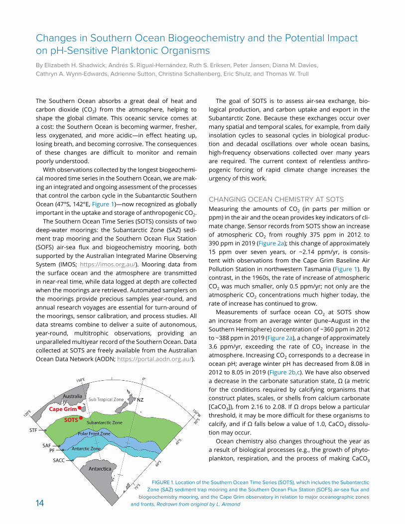
The goal of SOTS is to assess air-sea exchange, bio-logical production, and carbon uptake and export in the Subantarctic Zone. Because these exchanges occur over many spatial and temporal scales, for example, from daily insolation cycles to seasonal cycles in biological produc-tion and decadal oscillations over whole ocean basins, high-frequency observations collected over many years are required. The current context of relentless anthro-pogenic forcing of rapid climate change increases the urgency of this work.

CHANGING OCEAN CHEMISTRY AT SOTSMeasuring the amounts of CO2 (in parts per million or ppm) in the air and the ocean provides key indicators of cli-mate change. Sensor records from SOTS show an increase of atmospheric CO2 from roughly 375 ppm in 2012 to 390 ppm in 2019 (Figure 2a); this change of approximately 15 ppm over seven years, or ~2.14 ppm/yr, is consis-tent with observations from the Cape Grim Baseline Air Pollution Station in northwestern Tasmania (Figure 1). By contrast, in the 1960s, the rate of increase of atmospheric CO2 was much smaller, only 0.5 ppm/yr; not only are the atmospheric CO2 concentrations much higher today, the rate of increase has continued to grow.

Measurements of surface ocean CO2 at SOTS show an increase from an average winter (June–August in the Southern Hemisphere) concentration of ~360 ppm in 2012 to ~388 ppm in 2019 (Figure 2a), a change of approximately 3.6 ppm/yr, exceeding the rate of CO2 increase in the atmosphere. Increasing CO2 corresponds to a decrease in ocean pH; average winter pH has decreased from 8.08 in 2012 to 8.05 in 2019 (Figure 2b,c). We have also observed a decrease in the carbonate saturation state, Ω (a metric for the conditions required by calcifying organisms that construct plates, scales, or shells from calcium carbonate [CaCO3]), from 2.16 to 2.08. If Ω drops below a particular threshold, it may be more difficult for these organisms to calcify, and if Ω falls below a value of 1.0, CaCO3 dissolu-tion may occur.

Ocean chemistry also changes throughout the year as a result of biological processes (e.g., the growth of phyto-plankton, respiration, and the process of making CaCO3

120°E

150°E 0°

150°W

75°S

60°S

45°S

30°S

STF

SAFPF

SACC

Cape Grim

SOTS

FIGURE 1. Location of the Southern Ocean Time Series (SOTS), which includes the Subantarctic Zone (SAZ) sediment trap mooring and the Southern Ocean Flux Station (SOFS) air-sea flux and

biogeochemistry mooring, and the Cape Grim observatory in relation to major oceanographic zones and fronts. Redrawn from original by L. Armand

The Southern Ocean absorbs a great deal of heat and carbon dioxide (CO2) from the atmosphere, helping to shape the global climate. This oceanic service comes at a cost: the Southern Ocean is becoming warmer, fresher, less oxygenated, and more acidic—in effect heating up, losing breath, and becoming corrosive. The consequences of these changes are difficult to monitor and remain poorly understood.

With observations collected by the longest biogeochemi-cal moored time series in the Southern Ocean, we are mak-ing an integrated and ongoing assessment of the processes that control the carbon cycle in the Subantarctic Southern Ocean (47°S, 142°E, Figure 1)—now recognized as globally important in the uptake and storage of anthropogenic CO2.

The Southern Ocean Time Series (SOTS) consists of two deep-water moorings: the Subantarctic Zone (SAZ) sedi-ment trap mooring and the Southern Ocean Flux Station (SOFS) air-sea flux and biogeochemistry mooring, both supported by the Australian Integrated Marine Observing System (IMOS; https://imos.org.au/). Mooring data from the surface ocean and the atmosphere are transmitted in near-real time, while data logged at depth are collected when the moorings are retrieved. Automated samplers on the moorings provide precious samples year-round, and annual research voyages are essential for turn-around of the moorings, sensor calibration, and process studies. All data streams combine to deliver a suite of autonomous, year-round, multitrophic observations, providing an unparalleled multiyear record of the Southern Ocean. Data collected at SOTS are freely available from the Australian Ocean Data Network (AODN; https://portal.aodn.org.au/).

Changes in Southern Ocean Biogeochemistry and the Potential Impact on pH-Sensitive Planktonic OrganismsBy Elizabeth H. Shadwick, Andrés S. Rigual-Hernández, Ruth S. Eriksen, Peter Jansen, Diana M. Davies, Cathryn A. Wynn-Edwards, Adrienne Sutton, Christina Schallenberg, Eric Shulz, and Thomas W. Trull

14

bodies) and physical processes (e.g., changes in tempera-ture and salinity, the air-sea exchange of CO2). Changes in surface ocean CO2 concentration over a 12-month period at the SOTS site can be as large as 100 ppm (Figure 2a), which makes detecting the longer-term changes described above particularly challenging.

COCCOLITHOPHORE SURPRISESOcean acidification is expected to impact many organ-isms ranging from bacteria to fish, but especially calcify-ing organisms. In the Southern Ocean, this includes the coccolithophores, a group of beautifully ornate phyto-plankton that grow in the ocean’s sunlit layers (Figure 3). Observations from SOTS reveal the relationship between seasonal biogeochemical conditions and the degree of calcification in Emiliania huxleyi (Rigual-Hernández et  al., 2020a) as well as the broader composition of the cocco-lithophorid community (Figure 3) and its impacts on car-bon export (Rigual-Hernández et al., 2020b).

We found that the response of coccolithophores to changing environmental conditions is complex and not always as predicted: the more heavily calcified forms of E. huxleyi were most abundant in the winter months, when sea surface temperature, calcite saturation state, and pH are at their annual minimum (i.e.,  not the best chemical conditions for building CaCO3). It’s likely that the exten-sive genetic variability present in natural populations and the varying response of different genetic strains to sea-sonal changes in light, nutrients, and temperature under-pin this result.

Additional analyses of cocolithophores collected by the SAZ sediment trap mooring allowed the role of cocco-lithophore biodiversity in CaCO3 export to be determined.

Contrary to the prevailing notion that E. huxleyi dominates carbonate export in the Subantarctic region, we found less abundant but larger species accounted for a larger fraction of the CaCO3 flux. This nuance is important for the assessment of probable ecosystem impacts of ocean acidification as well as their feedbacks to climate change, because changing carbonate removal by organisms affects the ability of the ocean to remove atmospheric CO2.

Disentangling natural variability and climate change requires observations collected over all seasons and many years. The SOTS observatory provides an important base-line for understanding the evolution of the physical, chem-ical, and biological processes in the Subantarctic region. These observations are essential to provide advice about how climate variability is affecting us now and is likely to affect us in the future.

REFERENCESRigual-Hernández, A.S., T.W. Trull, J.A. Flores, S.D. Nodder, R. Eriksen,

D.M. Davies, G.M. Hallegraeff, F.J. Sierro, S.M. Patil, A. Cortina, and others. 2020a. Full annual monitoring of Subantarctic Emiliania huxleyi populations reveals highly calcified morphotypes in high-CO2 winter conditions. Scientific Reports 10:2594, https://doi.org/10.1038/s41598-020-59375-8.

Rigual-Hernández, A.S., T.W. Trull, S.D. Nodder, J.A. Flores, H. Bostock, F. Abrantes, R.S. Eriksen, F.J. Sierro, D.M. Davies, A.-M. Ballegeer, and others. 2020b. Coccolithophore biodiversity controls carbonate export in the Southern Ocean. Biogeosciences 17:245–263, https://doi.org/ 10.5194/bg-17-245-2020.

ACKNOWLEDGMENTSData were sourced from Australia’s Integrated Marine Observing System (IMOS)—IMOS is enabled by the National Collaborative Research Infrastructure Strategy (NCRIS). This work was supported by the Australian Antarctic Program Partnership through the Australian Government’s Antarctic Science Collaboration Initiative. This is PMEL contribution 5302. RH acknowledges funding from the European Union’s Horizon 2020 research and innovation programme under the Marie Skłodowska-Curie grant agreement number 748690 – SONAR-CO2.

ARTICLE DOI: https://doi.org/10.5670/oceanog.2021.supplement.02-06

FIGURE 3. Diversity of coccolithophorids sampled at SOTS. Clockwise from top: Syracosphaera nana, Coccolithus pelagicus, Calcidiscus leptoporous, Gephyrocapsa oceanica, Helicosphaera carteri, and Algirosphaera cucullata (collapsed). Species are scaled relative to the more lightly calcified form of Emiliania huxleyi, center, which dominates the summer populations of this species. Images taken by R. Eriksen, courtesy of Australian Antarctic Division Electron Microscopy Unit, and the Central Science Laboratory University of Tasmania

300

350

400

pCO

2 (µa

tm)

8.00

8.05

8.10

8.15

pH

2012 2013 2014 2015 2016 2017 2018 2019 2020

2.02.22.42.62.8

Ω (A

r)AtmosphereOcean

Year

FIGURE 2. Time series of (a) measured surface ocean and atmospheric CO2 partial pressure (pCO2), (b) calculated pH, and (c) calculated car-bonate saturation state (Ω) at SOTS between late 2011 and early 2020; gray shading indicates the winter (JJA) season. The black dashed line is a simple regression between the 2012 and 2019 winter pH data— quan-tification of trends in the deseasoned data is the focus of ongoing work.

a

b

c

5 µm

15

>1.2

1.1

1.0

0.9

0.8

0.7

0.6

0.5

0.4

<0.3

m/s30°N

100°E

Kar

imat

aK

arim

ata

Out

flow

Out

flow

Mak

assa

rM

akas

sar

Out

flow

Out

flow

Min

dana

oM

inda

nao

Curr

ent

Curr

ent

New Guinea Coastal Current

New Guinea Coastal Current

Sout

h So

uth

Chin

a Se

a Ch

ina

Sea

Win

ter

Win

ter

Jet

Jet

KuroshioKuroshioIntrusionIntrusion

KuroshioKuroshioIntrusionIntrusion

Kurosh

io

Kurosh

ioCurr

ent

Curren

t

EddiesEddies

North Equatorial North Equatorial CurrentCurrent

North Equatorial North Equatorial Counter CurrentCounter Current

South South Equatorial Equatorial

CurrentCurrent

110°E 130°E120°E 140°E 150°E

18°N

24°N

12°N

6°N

0°

FIGURE 2. Trajectories and near- surface velocity estimates from Global Drifter Program drifters in the western Pacific and marginal seas. Paths of various boundary currents are clearly visible. From Todd et al. (2018)

Boundary currents dominate the poleward transport of warm water and the equatorward transport of cold water and are major drivers of climate variability, extreme weather events (e.g.,hurricanes), and marine heatwaves (Figure 1). The western boundary regions have some of the most dynamic and energetic currents in the ocean and are key to the transport of mass, heat, salt, biogeo-chemical properties, and plankton. The eastern bound-ary currents are often upwelling systems that comprise some of the most biologically productive regions in the world. Boundary currents in marginal seas provide the major means of exchange with the open ocean and impact regional ecosystems. Communication between the coast and open ocean is regulated by the boundary currents that flow along the continental slopes, affecting ecosystems, sea level, flood levels, erosion, and commercial activity.

Current strategies used to monitor boundary currents vary and are composed of individual and partially coordi-nated efforts. At global scales, the Argo array of profiling floats collects a growing suite of ocean physical and biogeo-chemical parameters, providing comprehensive coverage offshore of the continental shelf. Satellite measurements of sea surface height, temperature, salinity, and ocean color clearly identify the signals of mesoscale features at the ocean surface. Surface drifters take measurements of currents (e.g., Figure 2). The need for finer spatial and temporal resolution closer to shore is addressed with more regionally focused efforts (Figure 3). Ocean gliders provide sustained or targeted observations across a few bound-ary current systems that connect the coast to the open ocean. The OceanSites network of moorings has some of the longest in situ time series at strategic locations within

Monitoring Boundary Currents Using Ocean Observing InfrastructureBy Tamaryn Morris, Daniel Rudnick, Janet Sprintall, Juliet Hermes, Gustavo J. Goni, Justine Parks, Francis Bringas, Emma Heslop, and the numerous contributors to the OCG-12 Boundary Current Workshop and OceanGliders BOON Project

boundary currents. The high- density/resolution expendable bathythermo-graph network provides repeat tempera-ture sections with fine spatial resolution across selected boundary currents along with seasonal sampling. Each network in the Global Ocean Observing System provides observations that complement each other in their efforts to monitor boundary currents. Further expansion of the suite of observing platforms may come from technologies such as autono-mous surface vehicles.

FIGURE 1. Major global ocean currents. White indicates warm western boundary currents, with the cooler eastern bound-ary currents in blue. Equatorial currents (red) and the Antarctic Circumpolar Current (purple) are shown for reference only. Potential sea surface temperature map was made available by Copernicus Marine Service through their MyOcean visualization web portal.

16

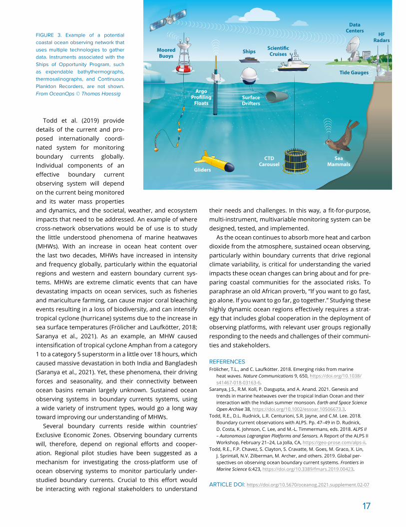
and dynamics, and the societal, weather, and ecosystem impacts that need to be addressed. An example of where cross-network observations would be of use is to study the little understood phenomena of marine heatwaves (MHWs). With an increase in ocean heat content over the last two decades, MHWs have increased in intensity and frequency globally, particularly within the equatorial regions and western and eastern boundary current sys-tems. MHWs are extreme climatic events that can have devastating impacts on ocean services, such as fisheries and mariculture farming, can cause major coral bleaching events resulting in a loss of biodiversity, and can intensify tropical cyclone (hurricane) systems due to the increase in sea surface temperatures (Frӧlicher and Laufkӧtter, 2018; Saranya et  al., 2021). As an example, an MHW caused intensification of tropical cyclone Amphan from a category 1 to a category 5 superstorm in a little over 18 hours, which caused massive devastation in both India and Bangladesh (Saranya et al., 2021). Yet, these phenomena, their driving forces and seasonality, and their connectivity between ocean basins remain largely unknown. Sustained ocean observing systems in boundary currents systems, using a wide variety of instrument types, would go a long way toward improving our understanding of MHWs.

Several boundary currents reside within countries’ Exclusive Economic Zones. Observing boundary currents will, therefore, depend on regional efforts and cooper-ation. Regional pilot studies have been suggested as a mechanism for investigating the cross-platform use of ocean observing systems to monitor particularly under-studied boundary currents. Crucial to this effort would be interacting with regional stakeholders to understand

their needs and challenges. In this way, a fit-for-purpose, multi-instrument, multivariable monitoring system can be designed, tested, and implemented.

As the ocean continues to absorb more heat and carbon dioxide from the atmosphere, sustained ocean observing, particularly within boundary currents that drive regional climate variability, is critical for understanding the varied impacts these ocean changes can bring about and for pre-paring coastal communities for the associated risks. To paraphrase an old African proverb, “If you want to go fast, go alone. If you want to go far, go together.” Studying these highly dynamic ocean regions effectively requires a strat-egy that includes global cooperation in the deployment of observing platforms, with relevant user groups regionally responding to the needs and challenges of their communi-ties and stakeholders.

REFERENCESFrölicher, T.L., and C. Laufkötter. 2018. Emerging risks from marine

heat waves. Nature Communications 9, 650, https://doi.org/10.1038/s41467-018-03163-6.

Saranya, J.S., R.M. Koll, P. Dasgupta, and A. Anand. 2021. Genesis and trends in marine heatwaves over the tropical Indian Ocean and their interaction with the Indian summer monsoon. Earth and Space Science Open Archive 38, https://doi.org/10.1002/essoar.10506673.3.

Todd, R.E., D.L. Rudnick, L.R. Centurioni, S.R. Jayne, and C.M. Lee. 2018. Boundary current observations with ALPS. Pp. 47–49 in D. Rudnick, D. Costa, K. Johnson, C. Lee, and M.-L. Timmermans, eds. 2018. ALPS II – Autonomous Lagrangian Platforms and Sensors. A Report of the ALPS II Workshop, February 21–24, La Jolla, CA, https://geo-prose.com/alps-ii.

Todd, R.E., F.P. Chavez, S. Clayton, S. Cravatte, M. Goes, M. Graco, X. Lin, J. Sprintall, N.V. Zilberman, M. Archer, and others. 2019. Global per-spectives on observing ocean boundary current systems. Frontiers in Marine Science 6:423, https://doi.org/10.3389/fmars.2019.00423.

ARTICLE DOI: https://doi.org/10.5670/oceanog.2021.supplement.02-07

Todd et  al. (2019) provide details of the current and pro-posed internationally coordi-nated system for monitoring boundary currents globally. Individual components of an effective boundary current observing system will depend on the current being monitored and its water mass properties

FIGURE 3. Example of a potential coastal ocean observing network that uses multiple technologies to gather data. Instruments associated with the Ships of Opportunity Program, such as expendable bathythermographs, thermosalinographs, and Continuous Plankton Recorders, are not shown. From OceanOps © Thomas Haessig

MooredBuoys

ShipsScientific

Cruises

DataCenters

HFRadars

Tide Gauges

ArgoProfiling

FloatsSurfaceDrifters

Gliders

CTDCarousel

Sea Mammals

17

FIGURE 1. Distribution of the 22 sampling stations involved in the alumni net-work project “A global study of coastal Deoxygenation, Ocean Acidification, and Productivity at selected sites” (NANO-DOAP) in September 2021.

The ocean benefits humankind by producing half of the global oxygen supply, absorbing a significant portion of atmospheric carbon dioxide, and providing us with food, transportation, and a means of livelihood. Nevertheless, human activities have been making the global ocean more acidic, warmer, and lower in oxygen (IPCC, 2021). Such changes and their impacts on ecosystems are highly vari-able, particularly in coastal areas where exchanges with the atmosphere and the land are more pronounced.

The capacity to collect ocean observations is insuffi-cient in many parts of the world, particularly in develop-ing countries (IOC-UNESCO, 2020). This is linked not only to a dearth of funding and instrumentation but also to a lack of scientific personnel with the capacity to collect, ana-lyze, and interpret oceanographic data. The Partnership for Observation of the Global Ocean (POGO) runs capacity development programs whose objectives are to develop key skills, capabilities, and capacities needed for world-wide ocean observations, and to nurture new genera-tions of experts and leaders in ocean affairs (see Urban and Seeyave, 2021). Since 2004, the partnership between POGO and the Nippon Foundation (NF) has offered an extensive array of training programs to nearly 500 early career scientists from 74 countries, mainly with emerging economies. The NF-POGO Alumni Network for the Ocean (NANO) was created in 2010 as a means to keep track of trainees’ career progressions, maximize the benefits from the training received, and provide further opportunities for networking and collaboration. One of NANO’s major goals is to promote joint research activities among its members, ultimately applying ocean observations for societal benefit.

Between 2012 and 2017, with the support of NF and POGO, NANO members successfully conducted five joint regional research projects that involved nearly 100 researchers from 21 countries and used coastal monitoring to study such issues as harmful algal blooms, eutrophication, coastal erosion, and invasive species.

NANO GLOBAL RESEARCH PROJECTIn 2017, NANO launched the research project “A global study of coastal Deoxygenation, Ocean Acidification, and Productivity at selected sites” (NANO-DOAP), which takes advantage of its members’ global distribution and their affiliations with institutions that can provide facilities for coastal monitoring. This project aims to advance knowl-edge and observation of the coastal ocean by consoli-dating existing, or establishing new, monitoring stations for essential ocean variables (EOVs) in the alumni loca-tions. Currently, the project encompasses 22 sampling sites in 15 countries in Asia, Africa, and Latin America (Figure 1). For more information on NANO-DOAP, visit https://nf- pogo- alumni. org/ projects/ global/).

PROJECT OUTCOMESFieldwork began in December 2018 with modest financial support from NF-POGO. Participants collect data on tem-perature, salinity, pH, dissolved oxygen, and chlorophyll-a concentration at the ocean’s surface monthly or bimonthly (Figure 2). Additional sampled parameters (e.g., total alka-linity, suspended particulate matter, plankton community structure) are not required but are welcomed and vary among sampling sites.

Putting Training into Practice: An Alumni Network Global Monitoring ProgramBy Lilian A. Krug, Subrata Sarker, A.N.M. Samiul Huda, Adriana Gonzalez-Silvera, Akinnigbagbe Edward, Carla Berghoff, Christian Naranjo, Edem Mahu, Jorge López-Calderón, Luís Escudero, Maria Tapia, Mauricio A. Noernberg, Mohamed Ahmed, Nandini Menon, and Stella Betancur-Turizo

NANO-DOAP stations are not all fully equipped and, because local conditions and resources vary, sampling frequency and instrumentation are different from station to station. Thus, data calibration is under-way to allow inter- station comparison. It is expected that the quality- controlled in situ data set, combined with satellite-derived data1, will offer insights into spatial and tem-poral variations in productivity, acidification, warming, and deoxygenation.

Promoting capacity development and outreach are also aims of NANO-DOAP. Since 2019, the project has organized reg-ular, public webinars (13 to date) where

18

NANO members and friends (mentors and instructors who contribute to NF-POGO trainings) present topics related to the scope of the project, sharing experiences and best practices. The NANO Webinar Series is increasing its live audience with every webinar.

NANO-DOAP participants are engaged in local outreach activities such as delivering seminars and conducting beach activities with school children and the general pub-lic, explaining matters of ocean acidification, microplastics, and the importance of sustained ocean observations. Furthermore, two NANO-DOAP sampling stations serve as platforms for citizen science initiatives, training local communities in using oceanographic instrumentation. The Argentinean El Veril NANO-DOAP station involves rec-reational divers interested in learning about ocean acidi-fication and climate change impacts in its sampling cam-paigns. The participants at the Kenyan Mombasa station, which is located near a community coral restoration proj-ect (REEFolution Kenya), take community members with them on the sampling campaigns and provide instruction on how to work with data-gathering instruments (Figure 3).

CONTRIBUTING TO SCIENCE AND COMMUNITYInitiatives such as NANO-DOAP can yield several benefits for the ocean sciences. Existing funding and support for early career ocean scientists and professionals are insuf-ficient, particularly in developing nations (IOC-UNESCO, 2020). This project, run by alumni, can be seen as a contin-uation of the training acquired at NF-POGO programs and serves as an opportunity to expand international collabo-ration and to acquire experience in project management. It also provides the possibility of “cascade training,” as the members use fieldwork excursions and data collected at NANO-DOAP stations to provide hands-on training to undergraduates and graduate students at their institutions, as well as valuable community outreach and ocean literacy opportunities with engaged locals. Furthermore, the finan-cial support allows the creation of new coastal monitoring stations and helps sustain others that are already estab-lished but under-resourced. It is expected that, with time,

both the institutions the alumni are affiliated with and their local governments will see the value of the participating stations of these coastal stations and help secure funding for long-term monitoring.

REFERENCES IOC-UNESCO. 2020. Global Ocean Science Report 2020—Charting Capacity for

Ocean Sustainability. K. Isensee, ed., Paris, UNESCO Publishing, 244 pp., https://gosr.ioc-unesco.org.

IPCC. 2021. Summary for policymakers. In Climate Change 2021: The Physical Science Basis. Contribution of Working Group I to the Sixth Assessment Report of the Intergovernmental Panel on Climate Change. V. Masson-Delmotte, et al., eds, Cambridge University Press. In Press.

Urban, E., and S. Seeyave. 2021. Visiting scientists provide capacity development: Lessons learned by POGO and SCOR. Oceanography 34(3):44–52, https://doi.org/10.5670/oceanog.2021.306.

ACKNOWLEDGMENTSThanks to the Nippon Foundation and the Partnership for Observation of the Global Ocean for the financial support of the NANO-DOAP project.

ARTICLE DOI: https://doi.org/10.5670/oceanog.2021.supplement.02-08

1 Satellite-derived sea surface temperature and chlorophyll-a concentration monthly time series for all sampling sites are annually acquired and processed by the NANO-DOAP participants in Mexico, members of the Phytoplankton Ecology Group at the Universidad Autonóma de Baja California.

FIGURE 3. NANO-DOAP members are involved in outreach and cit-izen science activities. In this photo, Mohamed Ahmed instructs two community members on working with a multiparameter probe and Niskin bottle at Mombasa NANO-DOAP station in Kenya. Photo credit: M. Ahmed

FIGURE 2. Average surface (0–10 m) Essential Ocean Variables: (a) tem-perature, (b) pH, (c) dissolved oxy-gen, and (d) chlorophyll-a concen-tration sampled at NANO-DOAP stations. Time series vary from station to station, with the earli-est sampling in December 2018 and the latest in September 2021. Stations in Argentina, Indonesia, Lebanon, Pakistan, and Senegal were recently added to the projeco not yet have data to contribute.

a b

c d

Chlorophyll-a(mg/m3)

Dissolved Oxygen(mg/L)

Temperature(°C)

pH(Total Scale)

19

Planktonic organisms are ubiquitous drifters in seas and oceans where they dominate life in terms of abundance and biomass (Bar-On and Milo, 2019). They are essential players in the functioning of marine ecosystems. Among them, microscopic algae called phytoplankton use sunlight to generate biomass from carbon dioxide and water, form-ing the basis of planktonic food webs, contributing about half of global primary productivity through photosynthe-sis, and producing about half of the world’s oxygen (Field et al., 1998). Phytoplankton are grazed by slightly larger, yet often still minuscule, animals called zooplankton that in turn are eaten by large predators such as fish or whales. Fish and many seabed-dwelling organisms such as corals or starfish commonly start their lives as zooplankton lar-vae. But plankton also include protists (flagellates, broadly

defined), bacteria, and viruses, far tinier organisms that may feast on zooplankton leftovers or dead cells, or may live as parasites within the bodies of larger plankton cells.

DNA analyses have revealed that less than 10% of the estimated total plankton biodiversity is known and for-mally described today—and most of the unknown spe-cies are smaller than the width of a hair (de Vargas et al., 2015). Plankton diversity is not equally distributed across the ocean. At the global scale, plankton differ from pole to pole according to temperature gradients and the degree of seasonal changes in the environment (Righetti et  al., 2019). At local scales, nutrient availability, seasonal envi-ronmental variation, and interactions among species or with anthropogenic stressors determine plankton commu-nity composition (Beaugrand, 2014).

Because plankton have short lifespans (often days or weeks) and their internal dynamics are tightly linked to global and local environmental conditions, they react quickly to environmental changes. These changes have cascading effects through the food web and significantly impact, for example, commercial fish recruitment. With the ocean under increasing stress from human activities, measuring changes in plankton communities is critical for addressing ocean health and food security and for track-ing changes in nutrient and carbon cycles (including the effectiveness or disruption of the biological carbon pump; Zhang et al., 2018).

Plankton diversity can serve as an indicator for track-ing anthropogenic environmental disturbances brought about by the maritime industry (e.g., Figure 1), eutrophi-cation, industrial wastewater, invasive species, overfishing,

TOPIC 2. ECOSYSTEMS AND THEIR DIVERSITY

Exploring New Technologies for Plankton Observations and Monitoring of Ocean HealthBy Pascal I. Hablützel, Isabelle Rombouts, Nick Dillen, Rune Lagaisse, Jonas Mortelmans, Anouk Ollevier, Michiel Perneel, and Klaas Deneudt

FIGURE 1. Wind farms in the North Sea produce renewable energy, but their effect on planktonic life is understudied.

20

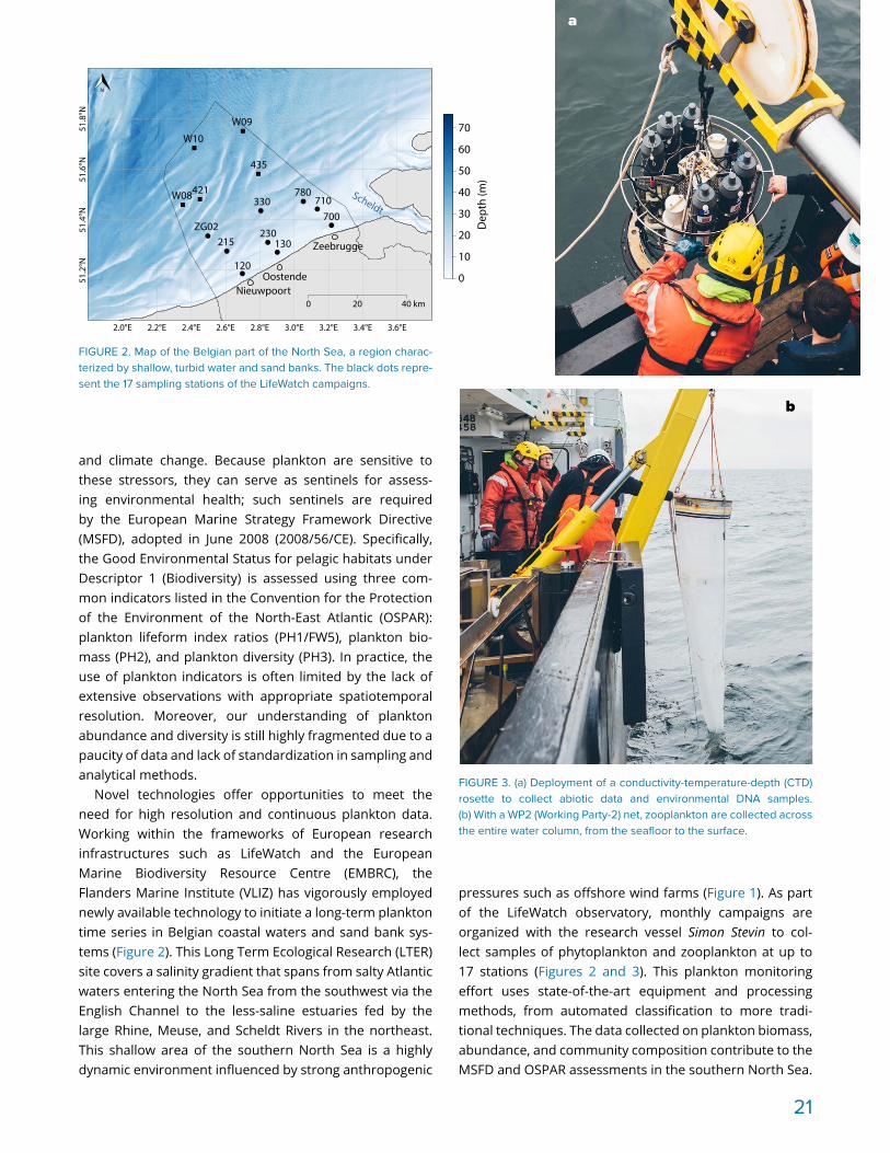
and climate change. Because plankton are sensitive to these stressors, they can serve as sentinels for assess-ing environmental health; such sentinels are required by the European Marine Strategy Framework Directive (MSFD), adopted in June 2008 (2008/56/CE). Specifically, the Good Environmental Status for pelagic habitats under Descriptor 1 (Biodiversity) is assessed using three com-mon indicators listed in the Convention for the Protection of the Environment of the North-East Atlantic (OSPAR): plankton lifeform index ratios (PH1/FW5), plankton bio-mass (PH2), and plankton diversity (PH3). In practice, the use of plankton indicators is often limited by the lack of extensive observations with appropriate spatiotemporal resolution. Moreover, our understanding of plankton abundance and diversity is still highly fragmented due to a paucity of data and lack of standardization in sampling and analytical methods.

Novel technologies offer opportunities to meet the need for high resolution and continuous plankton data. Working within the frameworks of European research infrastructures such as LifeWatch and the European Marine Biodiversity Resource Centre (EMBRC), the Flanders Marine Institute (VLIZ) has vigorously employed newly available technology to initiate a long-term plankton time series in Belgian coastal waters and sand bank sys-tems (Figure 2). This Long Term Ecological Research (LTER) site covers a salinity gradient that spans from salty Atlantic waters entering the North Sea from the southwest via the English Channel to the less-saline estuaries fed by the large Rhine, Meuse, and Scheldt Rivers in the northeast. This shallow area of the southern North Sea is a highly dynamic environment influenced by strong anthropogenic

FIGURE 3. (a) Deployment of a conductivity-temperature- depth (CTD) rosette to collect abiotic data and environmental DNA samples. (b) With a WP2 (Working Party-2) net, zooplankton are collected across the entire water column, from the seafloor to the surface.

Scheldt

0

10

20

30

40

Dep

th (m

)

50

60

70

0 20 40 km

N

2.0°E 2.2°E 2.4°E 2.6°E 2.8°E 3.0°E 3.2°E 3.4°E 3.6°E

51.2

°N51

.4°N

51.6

°N51

.8°N

120

130215230

330421

435

700710

780W08

W09

W10

ZG02

NieuwpoortOostende

Zeebrugge

FIGURE 2. Map of the Belgian part of the North Sea, a region charac-terized by shallow, turbid water and sand banks. The black dots repre-sent the 17 sampling stations of the LifeWatch campaigns.

Scheldt

0

10

20

30

40

Dep

th (m

)

50

60

70

0 20 40 km

N

2.0°E 2.2°E 2.4°E 2.6°E 2.8°E 3.0°E 3.2°E 3.4°E 3.6°E

51.2

°N51

.4°N

51.6

°N51

.8°N

120

130215230

330421

435

700710

780W08

W09

W10

ZG02

NieuwpoortOostende

Zeebrugge

pressures such as offshore wind farms (Figure 1). As part of the LifeWatch observatory, monthly campaigns are organized with the research vessel Simon Stevin to col-lect samples of phytoplankton and zooplankton at up to 17 stations (Figures 2 and 3). This plankton monitoring effort uses state-of-the-art equipment and processing methods, from automated classification to more tradi-tional techniques. The data collected on plankton biomass, abundance, and community composition contribute to the MSFD and OSPAR assessments in the southern North Sea.

a

b

21

There are many ways to collect and analyze plankton samples, because no single mesh size can effectively cap-ture the broad size spectrum of the plankton. Thus, differ-ent methods are combined in order to focus on particular size ranges (e.g.,  zooplankton, micro- or nanoplankton, bacteria), with necessary precision and accuracy. For long-term monitoring programs, it is important to keep protocols and equipment consistent for the whole time series or, if changes are needed, to have the ability to track modifications.

Once the samples are prepared for analysis, the plank-ton can be counted manually by viewing them through a microscope. In addition, to understand what is going on in the ecosystem, it is necessary to precisely identify the spe-cies present in the samples. However, because planktonic organisms are tiny and often closely resemble each other, highly skilled taxonomists are required to identify them. Although time-consuming, this taxonomic expertise will continue to be needed to advance our understanding of the marine environment, its diversity, and the risks posed by pathogenic, toxic, or otherwise harmful species, and to inform aspects of marine conservation and management.

Increasingly, manual methods are complemented by automatic and semi-automatic devices, allowing sample col-lection and analysis to be combined and speeded up. When the microscopy glass slides or counting trays are replaced by a narrow photo chamber and the manually operated pipette by thin tubing connected to dosage pumps, we can reach a throughput of several plankton individuals per sec-ond. Image recognition algorithms trained by thousands of manually identified photos can then recognize the plank-ton based on their shapes. However, some organisms, like amoebas, have no specific recognizable shape, and others, like some dinoflagellates, ciliates, and fungi, live as

parasites within other planktonic species. Identifying these organisms was very laborious, if not impossible, until the application of DNA-based techniques. Combining both high throughput microscopy and characterization of the DNA pool in bulk plankton samples (e.g., using a technique referred to as metabarcoding) provides a solution to the demands of modern plankton ecology research.

HIGH-THROUGHPUT MICROSCOPIC IMAGING OF UNICELLULAR LIFEIn recent years, a large variety of flow-through plankton imaging instruments have been developed. At VLIZ, we monitor microplankton (50–300 µm) with the help of a FlowCAM (Figure 4). This automated imaging device com-bines flow cytometry and microscopy to take traditional particle counting to the next level. An image of each particle is taken while it passes the camera’s field of view (Figure 4). From this image, more than 60 particle parameters are cal-culated, from simple metrics like length and width to more complex metrics like transparency, roughness, and edge gradient (i.e., whether the particle is in focus). In this way, the user can quantify particles, obtain valuable metrics, and create an image library for a water sample in fewer than 30 minutes.

At VLIZ, the monthly sampling campaigns have contrib-uted to the development of an extensive and validated FlowCAM image library. This library enables the use of deep learning approaches for image classification. In col-laboration with the Instituto de Física de Cantabria (IFCA), a prototype artificial intelligence (AI) classifier was devel-oped and introduced into the data workflow. Integration of this automated classification system into FlowCAM monitoring reduces time spent on image identification and facilitates faster data releases to the public. Over the past 3.5 years, FlowCAM monitoring has yielded 1.4 million particle images categorized in more than 140 taxonomic groups, with the majority of the phytoplankton groups belonging to diatoms and dinoflagellates and the majority

FIGURE 4. (a) The phytoplankton sample is stained with lugol solution before being run through the bench-top FlowCam device (background). (b) Photos of micro-eukaryotic plank-ton passing through the microscopic flow chamber of the FlowCam. Mag-nification scale differs among por-trayed organisms, which range from 50 µm to 300 µm in size.

a

b

22

of other groups belonging to ciliates. As different aspects of this FlowCAM monitoring are continuously re-evaluated and evolve, fine-tuning of protocols will lead to increased taxonomic resolution in the data set and expansion of the studied size range to better capture the patchy plankton dynamics in the Belgian part of the North Sea. One of the shortcomings of the FlowCAM and other image-based techniques is the reduced accuracy in taxonomic iden-tification compared to traditional microscopy. To better quantify plankton community composition, models for image-based classifications will need to be improved and image-based information could be combined with genetic approaches (see below).

SCANNING BIODIVERSITYNot all plankton fit through the narrow FlowCAM tub-ing. Larger zooplankton such as crustaceans or larvae of fish and seafloor-dwelling organisms can be imaged with the ZooScan. This device is essentially a high- resolution (4,800 dpi) flatbed scanner onto which the sample is poured (Figure 5). ZooScan does not distinguish among closely related species, and the identification is conducted at a higher taxonomic rank. But many zooplankton have larval stages that go through one or several metamorpho-ses until they resemble their parents, and automated anal-ysis of scanning images is effective in distinguishing among these early life stages. The ZooScan therefore informs us not only about the taxonomic composition of zooplankton communities but also about their developmental stages. In addition, image analysis can be used for standardized size measurements, providing information on growth and ecology of the scanned organisms. Upscaling image rec-ognition to the next level with the use of AI and the imple-mentation of all our 2.2 million validated images will fur-ther exploit the potential of this technique, as the accuracy of prediction will rise, whereas the time spent on manual validation will drop.

To date, 976 samples collected between January 2014 and December 2020 have been scanned, resulting in 2,218,383 scanned particles, stored into 22 taxonomic groups. These samples are both bio-archived as physical samples (enabling genomic analysis or taxonomic analy-sis by microscopy at a later stage) and stored digitally as Darwin Core Archives (DwC-A) for dissemination to other frameworks, such as the European Ocean Biodiversity Information System (EurOBIS).

UNDER THE WAVES In the new era of advanced optical techniques, it is no longer necessary to collect physical samples, as the Video Plankton Recorder (VPR) can provide direct images. This device is towed behind a ship and contains a high-speed camera that takes photos of planktonic organisms as they pass by (Figure 6). Because photos are taken in the water column, the VPR observes fragile forms of marine life with-out damaging them, enabling registration and quantifica-tion of gelatinous plankton, colony-forming species, and

FIGURE 5. A zooplankton sample is poured on the ZooScan.

FIGURE 6. (a) The Video Plank-ton Recorder (VPR) is deployed from the research vessel Simon Stevin. (b) Collage of zooplank-ton organisms captured by the VPR. Magnification scale differs among portrayed organisms, which range from a few millime-ters to centimeters in size.

a

b

23

dead organic particles (called “marine snow”) more effec-tively than net sampling. For example, the VPR can quan-tify colonies of Phaeocystis spp., a harmful algal species that can often be seen as thick layers of white foam along the Belgian coast in spring.

Because data are collected in situ, the VPR permits anal-ysis of plankton clouds at high resolution in three dimen-sions along with observations of their reactions to water quality, vertical stratification, or marine snow. Using this method, we observed that densities of certain plankton species can strongly differ between bottom and surface water layers. Furthermore, having the plankton samples in a digital format opens up the potential to accelerate the classification procedure. So far, the biggest challenge for us is to build an automated classifier that can process and validate the millions of collected images that are still vali-dated manually but that contribute to the growing image library that will serve as a learning set for future classifiers.

BARCODING BIODIVERSITYThe DNA of a plankton sample is all that is needed to iden-tify the species using a technique called metabarcoding. A short sequence of DNA—called a barcode—is rapidly cop-ied from the original DNA mixture using the polymerase chain reaction (PCR) method, and then read in a sequenc-ing apparatus. The basic premise of this approach is that each species can be identified by its unique genetic bar-code (Hebert et  al., 2003; de Vargas et  al., 2015). At this stage, no taxonomic expertise is needed to process the sample, and we can easily scale up the throughput by using liquid-handling robots and 96 well plates. Metabarcoding

has long been a cumbersome method requiring large, bulky, and expensive DNA sequencing equipment. We therefore turned to nanopore sequencing technology, which allows us to perform all analyses in our own labo-ratory with a handheld device (Figure 7), thus reducing the time to first results from weeks to days or even hours. The largest bottleneck in metabarcoding approaches is argu-ably the incompleteness of reference databases. While we can easily generate thousands of barcodes, each of them needs to be compared to a reference database that links species names with their barcode. These databases are still incomplete, so especially for microscopic species, we might obtain sequences that are unique to their species, but it is difficult or impossible to confidently assign them a taxonomic name.

An important application for which we use DNA metabarcoding is recognizing non-indigenous species. For example, using this method, we recently detected the inva-sive copepod Oithona davisae from the Indo-West Pacific for the first time in Belgian waters. This tiny zooplankton species has probably been living in the area for years, but no funding or expertise were available for microscopy- based monitoring. There is no question that more thor-ough sequencing will yield a host of such previously unde-tected invasive species in the near future.

GENETIC DATA REVEAL THE BEHAVIOR AND FUNCTION OF ORGANISMSImage and DNA-based methods identify and classify plank-tonic life, but they are not designed to answer a key ques-tion in plankton research: What are these oceanic drifters

FIGURE 7. A sample is loaded on the MinION sequencing device. In the background, a small but powerful graphics processing unit (GPU) computer is available to analyze the sequence data in real time.

doing? Evaluating how global change is affecting the plankton community is key to predicting our ocean’s future. Laboratory experiments usually infer the functional response of plankton to variations in one or two factors, for example, temperature and pH, under controlled conditions. This approach fails to describe the broad spectrum of responses that can be expected in a natural community experiencing a multitude of interactions, behaviors, and other ecological effects that occur with environmental variation. Recent advances in both molecular genetics and computational biology greatly facilitate drawing an increasingly accu-rate and detailed picture of the func-tional activity within plankton ecosys-tems (Carradec et al., 2018).

24

The functions of an organism’s individual proteins are encoded in its DNA sequence, which translates proteins via the intermediate messenger RNA. At this intermediate state, the translation can be intercepted, and the activity of gene translation can be quantified. These strings of RNA sequences will then be counted and compared with databases containing sequences of known functions. This method is easily scalable for application to mixed plankton samples, and it provides a functional profile of a plankton community. Yet, this method is still far from perfect. One reason is the incompleteness of plankton reference data-bases. In most studies, only about 50% of sequences can be assigned to genes with known functions. The remain-der is the biological “dark matter” of plankton genetics.

We recently set up a multiyear spatiotemporal sampling effort to generate environmental metatranscriptomic data. We sample surface water micro-eukaryotic plank-ton from fixed locations monthly, with additional diurnal sampling events. From a pilot sequencing run on 12 sam-ples from different seasons, 818,009 gene- containing sequences were assembled. Differential expression of these genes gave us a first insight into how the metab-olism of different North Sea plankton assemblages shift over time and space.

MAINSTREAMING AUTOMATED BIODIVERSITY OBSERVATIONSThe FlowCAM, ZooScan, VPR, and DNA-based meth-ods demonstrate that plankton data collection can be automated to a great extent. By reducing the number of expensive human work hours, more samples can be acquired and processed for the same cost, increasing spa-tial and temporal resolution of ecological observations. But improved automation and processing speed is not the only goal here. Machines do not have human subjec-tivity, which is needed to better standardize data collec-tion across countries and make data sets more useful for global analyses. Researchers worldwide are now further automating plankton data collection by mounting contin-uously operating instruments on platforms such as auton-omous underwater vehicles, drifters, or buoys, potentially reaching very remote areas of the planet.

Automated sample processors may be combined into networks not only across countries but also within the same area for detecting different organisms or assessing plankton size fractions. Ecological processes act across taxonomic groups, for example, in food webs. Deploying as many different sampling techniques as possible and combining them with sensors for abiotic measurements enables us to gain insight into relevant ecological pro-cesses such as the global carbon cycle.

Automatic collection of large data sets is pushing plank-ton research further into the field of big data science and providing systems-level insights. With such data sets, we eventually will be able to study not only the presence and abundance of plankton but also how different species interact in ecological networks. We urgently need such understanding to be able to predict and mitigate adverse effects of global environmental change, including tipping points where interactions between species and their envi-ronments change nonlinearly. We have no option but to embrace new technologies at global scale to understand our ocean in a mandatory step toward preventing further harm to its health.

REFERENCESBar-On, Y.M., and R. Milo. 2019. The biomass composition of the oceans:

A blueprint of our blue planet. Cell 179(7):1,451–1,454, https://doi.org/ 10.1016/j.cell.2019.11.018.

Beaugrand, G. 2014. Marine Biodiversity, Climatic Variability and Global Change. Routledge, London, 486 pp., https://doi.org/ 10.4324/ 9780203127483.

Carradec, Q., E. Pelletier, C. Da Silva, A. Alberti, Y. Seeleuthner, R. Blanc-Mathieu, G. Lima-Mendez, F. Rocha, L. Tirichine, K. Labadie, and others. 2018. A global ocean atlas of eukaryotic genes. Nature Communications 9, 373, https://doi.org/10.1038/s41467-017-02342-1.

de Vargas, C., S. Audic, N. Henry, J. Decelle, F. Mahé, R. Logares, E. Lara, C. Berney, N. Le Bescot, I. Probert, and others. 2015. Eukaryotic plank-ton diversity in the sunlit ocean. Science 348(6237), https://doi.org/ 10.1126/ science.1261605.

Field, C., M. Behrenfeld, J. Randerson, and P. Falkowski. 1998. Primary production of the biosphere: Integrating terrestrial and oce-anic components. Science 281:237–240, https://doi.org/10.1126/science.281.5374.237.

Hebert, P.D.N., A. Cywinska, S.L. Ball, and J.R. deWaard. 2003. Biological identifications through DNA barcodes. Proceedings of the Royal Society B: Biological Sciences 270(1512):313–321, https://doi.org/10.1098/rspb.2002.2218.

Righetti, D., M. Vogt, N. Gruber, A. Psomas, and N.E. Zimmermann. 2019. Global pattern of phytoplankton diversity driven by temperature and environmental variability. Science Advances 5(5), https://doi.org/ 10.1126/sciadv.aau6253.

Zhang, C., H. Dang, F. Azam, R. Benner, L. Legendre, U. Passow, L. Polimene, C. Robinson, C.A. Suttle, and N. Jiao. 2018. Evolving paradigms in biological carbon cycling in the ocean. National Science Review 5(4):481–499, https://doi.org/10.1093/nsr/nwy074.

ARTICLE DOI: https://doi.org/10.5670/oceanog.2021.supplement.02-09

25

The Ross Sea (Figure 1) is home to 33% of the world’s Adélie penguins (Pygoscelis adeliae), as well as substan-tial numbers of Emperor penguins (Aptenodytes forsteri), Weddell seals (Leptonychotes weddellii), and pelagic birds (Smith et al., 2014). Among these, the Commission for the Conservation of Antarctic Marine Resources (CCAMLR) has designated the Adélie penguin an “indicator species” for monitoring ecosystem structure and function in the newly designated Ross Sea Region Marine Protected Area (RSR-MPA). This penguin, among the best-known seabirds, has been studied for decades at multiple locations with investigations that have delved into its population history (both recent and through thousands of years), survival strategies, responses to environmental changes, and feed-ing ecology (summarized in Ainley, 2002, with numerous papers published thereafter).

Penguin populations are increasing in the southern Ross Sea, potentially indicating a broad response to an environ-ment being altered by climate change and increased fish-ing activity. Despite extensive research, our understanding of the species’ response to its changing habitat and food web is incomplete. Sea ice in the Ross Sea region has been increasing, at least until recent years, and this would be expected to affect populations of species that depend on the ice for predator avoidance and availability of

New Technologies Aid Understanding of the Factors Affecting Adélie Penguin ForagingBy Walker O. Smith Jr., David G. Ainley, Karen J. Heywood, and Grant Ballard

prey (crystal krill Euphausia crystallorophias and silverfish Pleuragramma antarctica, both associated with ice; Ainley, 2002). In addition, industrial fishing for Antarctic toothfish, a competitor for the same prey, has been practiced since 1997, potentially increasing prey abundance and reducing competition. Understanding the effects of these and other habitat changes on the penguin, its competitors, and prey requires further investigation.

The RSR-MPA was established in 2017 with the major goal “to conserve natural ecological structure, dynamics, and function throughout the Ross Sea region at all levels of biological organization by protecting habitats that are important to native mammals, birds, fishes, and inverte-brates.” Given that southern Ross Sea penguins live mostly within the RSR-MPA during their life cycles, ecological interactions near their nesting grounds are important to the entire MPA, and understanding the role of penguins within the continental shelf food web and biogeochemical cycles will directly facilitate achievement of RSR-MPA goals.

Ongoing advances in the use of bio-loggers on ani-mals that are near the top of the food web have provided insights into these animals’ ecology. Various devices that can be attached to penguins to quantify predatory behav-ior in time and space include simple sensors that record the conductivity (salinity) and temperature of seawater; fluorometers; “crittercams” (cameras mounted on an ani-mal to monitor diving and feeding behavior); time-depth recorders; satellite tracking tags; and accelerometers (measuring head movements, which are an indication of active feeding; Figure 2). The devices have become small enough that they have no effect on penguin behavior. Using ocean gliders in the Ross Sea (Figure 3), especially those that carry active acoustic devices for monitoring the distribution of Adélie penguin prey in the water column, has also allowed an assessment of temporal and spatial changes in prey abundance during spring and summer, as well as their changes relative to the abundance of phy-toplankton (microscopic marine algae) and water column structure (Ainley et  al., 2015). Advanced molecular tools (stable isotopes, DNA analyses) permit the diets of pen-guins to be more easily quantified. Satellite imagery and passively recording sounds in the sea have allowed deter-mination of the distribution of competing species (whales, seals) and their overlap with penguin foraging areas.

FIGURE 1. Location of foraging area (blue oval) of the Cape Crozier, Ross Sea, Adélie penguin colony superimposed on a typical late spring ice distribution map. Maximum foraging distance is ~120 km from Cape Crozier. Inset shows the location of the Ross Sea adjacent to the southern Pacific. Ice map from NASA, November 1998

Ross SeaMcMurdoSound

Ross Ice Shelf

CapeCrozier

Ross SeaMcMurdoSound

Ross Ice Shelf

CapeCrozier

Ross SeaRoss Sea

26

Penguins occupying large colonies like Cape Crozier (which has over 120,000 breeding pairs) must travel further to find food in late summer because prey availability closer to the colony has been severely depleted by penguin, seal, and whale feeding. In addition, because feeding frequency and food quality are very important to chick growth and survival, nutrition demands of their chicks increase as the ice-free season progresses (Ainley et al., 2015). Numerous additional factors affect post-fledging chick survival (pre-dation, episodic weather events), and the effects of eco-logical interactions within the “preyscape” and of oceano-graphic conditions await further investigation. Beyond the area of intense predator foraging, vertical distributions and school/swarm structures of fish and krill may be sig-nificantly different (e.g.,  larger, more cohesive, and shal-lower) from those within. These prey patches would thus be “reservoirs” available once penguins leave their central foraging area. Predation- and predator-induced changes in prey distributions could be further assessed by quan-tifying prey habitat quality and by determining the effects of oceanographic habitat attributes, such as water column characteristics and phytoplankton concentrations, on prey distributions in areas of higher predation.

To better understand and monitor the food web dynam-ics and structure of a Southern Ocean trophic hotspot, and to resolve the penguin population growth paradox, a combination of technologies and approaches is needed, including:1. Deployment of a suite of gliders with acoustic devices

in a tight grid to measure the composition and assess the size, location, and density of prey, both inside and outside of intense penguin foraging areas

2. Deployment of gliders and miniature loggers attached to penguins to quantify oceanographic patterns (such as vertical ocean characteristics, irradiance, and particu-late matter concentrations) in the ocean preyscape

3. Use of penguin bio-logging to quantify foraging areas and their seasonal changes as well as overlap with com-peting species

4. Direct and DNA stable isotope analyses of penguin diet5. Quantification of abundance and distribution of com-

peting whales and seals using satellite imagery

New technologies have revolutionized our understand-ing of numerous aspects of the ocean. By merging these techniques with new hypotheses about basic ecological processes operating in the ocean, a far greater under-standing of factors controlling mesopredator activities and distributions can be attained in harsh environments such as the Ross Sea. This enhanced knowledge will ulti-mately lead to the conservation and preservation of The Last Ocean (title of award-winning documentary film by Peter Young) and enable a new generation of marine scientists to unravel remaining unknowns.

REFERENCESAinley, D.G. 2002. The Adélie Penguin: Bellwether of Climate Change.

Columbia University Press, NY, 416 pp.Ainley, D.G., G. Ballard, R.M. Jones, D. Jongsomjit, S.D. Pierce,

W.O. Smith Jr., and S. Veloz. 2015. Trophic cascades in the western Ross Sea, Antarctica: Revisited. Marine Ecology Progress Series 534:1–16, https://doi.org/10.3354/meps11394.

Smith, W.O. Jr., D.G. Ainley, K.R. Arrigo, and M.S. Dinniman. 2014. The oceanography and ecology of the Ross Sea. Annual Review of Marine Science 6:469–487, https://doi.org/10.1146/annurev-marine-010213-135114.

ARTICLE DOI: https://doi.org/10.5670/oceanog.2021.supplement.02-10

FIGURE 3. A Kongsberg glider is shown deployed in McMurdo Sound, southern Ross Sea. Gliders can be deployed from fast ice around Ross Island, transit to their study sites, and then be recovered from vessels. Photo credit: Vernon Asper

FIGURE 2. An Adélie penguin with an attached bio-logger. The sen-sors are attached using Tesa tape and are easily removed when pen-guins return to land. Previous investigations have shown that such bio-loggers do not impede penguin foraging or survival. Photo credit: Jean Pennycook

27

Vulnerable marine ecosystems (VMEs) are typically iden-tified through detection of indicator taxa and predictive models of their distribution. In the deep sea, analysis of seafloor imagery generates quantitative data that under-pin studies of the distribution of VMEs such as cold-water coral communities. The vulnerability of cold-water corals to bottom trawling makes assessment of their distribution and biodiversity a priority for marine spatial management.

Some of the most diverse and globally significant cold-water coral communities are associated with clusters of seamounts off the coast of Tasmania, several of which are enclosed by two offshore Australian Marine Parks. These extensive reef complexes, located 950–1,350 m below the surface, are dominated by a single coral spe-cies, Solenosmilia variabilis, which supports a wide variety of soft corals, sponges, echinoderms, and other inverte-brates (Figure 1).

The seamount fauna in this region has a documented history of ecological damage from a deep-sea bottom trawl fishery. Some areas are still open to fishing, and some have been closed for 20 years. Previous studies have found substantial reductions in coral cover and sig-nificantly fewer species of bottom-dwelling organisms on heavily trawled seamounts.

During a 2018 survey aboard R/V Investigator, research-ers from Australia's National Science Agency (CSIRO) and from the Australian Government’s National Environmental Science Program (NESP) Biodiversity Hub, together with

Image Data Give New Insight into Life on the SeafloorBy Franzis Althaus, Candice Untiedt, and Kylie Maguire

marine park managers from Parks Australia, collected HD video and still images from seamounts along more than 250 km of seabed, using an advanced, towed underwater camera system developed by CSIRO.

Reviews of collected imagery documented trawl-ing damage on 45 out of a total 51 seamounts, with the most evidence of impact on shallow seamounts (peaks at <950 m depth) where recent and repeated trawling had reduced stony coral reefs to rubble (Williams et al., 2020b). However, many of the seamounts protected by Australian Marine Parks off southern Tasmania displayed few or no signs of impact.

This was the first study to examine trawling impacts in detail at a regional scale. Detecting impacts was critical to the identification of a suite of impact types and to the development of a set of indicators (Williams et al., 2020a). Analysis of image data also helped refine a method for quantifying the spatial extent of VMEs (Williams et  al., 2020b). A model prediction of suitable habitat for coral reefs in the Tasmanian area was much greater than the area of coral reef estimated from imagery.

Tasmanian coral reef VMEs range in area from 0.02 km2 to 1.16 km2, which is relatively large compared to S. variabilis reefs mapped on the typically bigger seamounts around New Zealand (Williams et  al., 2020a). Yet, the VME area is small compared to scales derived from regional model predictions of suitable habitat (typically based on 1 km2 grid cells), and much smaller than the smallest units at which spatial management is implemented (hundreds to thousands of square kilometers). The results will be used to improve predictive VME model performance at larger spatial scales and beyond single taxa. The data from the image analysis are also being incorporated into machine learning algorithms to develop automated detection of coral reef substrate from imagery.

REFERENCESWilliams, A., F. Althaus, M. Green, K. Maguire, C. Untiedt, N. Mortimer,

C.J. Jackett, M. Clark, N. Bax, R. Pitcher, and T. Schlacher. 2020a. True size matters for conservation: A robust method to determine the size of deep-sea coral reefs shows they are typically small on seamounts in the southwest Pacific Ocean. Frontiers in Marine Science 7:187, https://doi.org/ 10.33hy89/fmars.2020.00187.

Williams, A., F. Althaus, K. Maguire, M. Green, C. Untiedt, P. Alderslade, M.R. Clark, N. Bax, and T.A. Schlacher. 2020b. The fate of deep-sea coral reefs on seamounts in a fishery-seascape: What are the impacts, what remains, and what is protected? Frontiers in Marine Science 7:567002, https://doi.org/ 10.3389/fmars.2020.567002.

ARTICLE DOI: https://doi.org/10.5670/oceanog.2021.supplement.02-11

FIGURE 1. Solenosmilia variabilis is the founda-tion reef- forming species that supports a host of taxa found on Tasmania’s seamounts.

2828

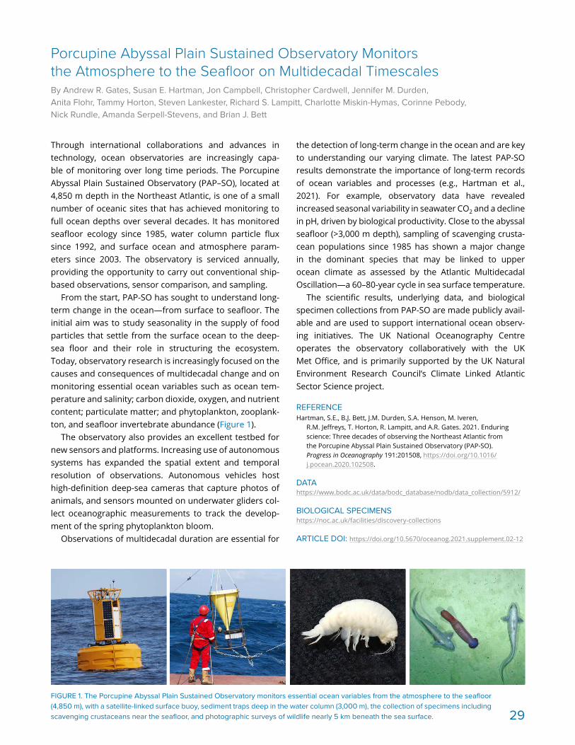
Through international collaborations and advances in technology, ocean observatories are increasingly capa-ble of monitoring over long time periods. The Porcupine Abyssal Plain Sustained Observatory (PAP–SO), located at 4,850 m depth in the Northeast Atlantic, is one of a small number of oceanic sites that has achieved monitoring to full ocean depths over several decades. It has monitored seafloor ecology since 1985, water column particle flux since 1992, and surface ocean and atmosphere param-eters since 2003. The observatory is serviced annually, providing the opportunity to carry out conventional ship-based observations, sensor comparison, and sampling.

From the start, PAP-SO has sought to understand long-term change in the ocean—from surface to seafloor. The initial aim was to study seasonality in the supply of food particles that settle from the surface ocean to the deep-sea floor and their role in structuring the ecosystem. Today, observatory research is increasingly focused on the causes and consequences of multidecadal change and on monitoring essential ocean variables such as ocean tem-perature and salinity; carbon dioxide, oxygen, and nutrient content; particulate matter; and phytoplankton, zooplank-ton, and seafloor invertebrate abundance (Figure 1).

The observatory also provides an excellent testbed for new sensors and platforms. Increasing use of autonomous systems has expanded the spatial extent and temporal resolution of observations. Autonomous vehicles host high-definition deep-sea cameras that capture photos of animals, and sensors mounted on underwater gliders col-lect oceanographic measurements to track the develop-ment of the spring phytoplankton bloom.

Observations of multidecadal duration are essential for

the detection of long-term change in the ocean and are key to understanding our varying climate. The latest PAP-SO results demonstrate the importance of long-term records of ocean variables and processes (e.g.,  Hartman et  al., 2021). For example, observatory data have revealed increased seasonal variability in seawater CO2 and a decline in pH, driven by biological productivity. Close to the abyssal seafloor (>3,000 m depth), sampling of scavenging crusta-cean populations since 1985 has shown a major change in the dominant species that may be linked to upper ocean climate as assessed by the Atlantic Multidecadal Oscillation—a 60–80-year cycle in sea surface temperature.

The scientific results, underlying data, and biological specimen collections from PAP-SO are made publicly avail-able and are used to support international ocean observ-ing initiatives. The UK National Oceanography Centre operates the observatory collaboratively with the UK Met Office, and is primarily supported by the UK Natural Environment Research Council’s Climate Linked Atlantic Sector Science project.

REFERENCEHartman, S.E., B.J. Bett, J.M. Durden, S.A. Henson, M. Iveren,

R.M. Jeffreys, T. Horton, R. Lampitt, and A.R. Gates. 2021. Enduring science: Three decades of observing the Northeast Atlantic from the Porcupine Abyssal Plain Sustained Observatory (PAP-SO). Progress in Oceanography 191:201508, https://doi.org/10.1016/ j.pocean.2020.102508.

DATA https://www.bodc.ac.uk/data/bodc_database/nodb/data_ collection/5912/

BIOLOGICAL SPECIMENS https://noc.ac.uk/facilities/discovery- collections

ARTICLE DOI: https://doi.org/10.5670/oceanog.2021.supplement.02-12

Porcupine Abyssal Plain Sustained Observatory Monitors the Atmosphere to the Seafloor on Multidecadal TimescalesBy Andrew R. Gates, Susan E. Hartman, Jon Campbell, Christopher Cardwell, Jennifer M. Durden, Anita Flohr, Tammy Horton, Steven Lankester, Richard S. Lampitt, Charlotte Miskin-Hymas, Corinne Pebody, Nick Rundle, Amanda Serpell-Stevens, and Brian J. Bett

FIGURE 1. The Porcupine Abyssal Plain Sustained Observatory monitors essential ocean variables from the atmosphere to the seafloor (4,850 m), with a satellite-linked surface buoy, sediment traps deep in the water column (3,000 m), the collection of specimens including scavenging crustaceans near the seafloor, and photographic surveys of wildlife nearly 5 km beneath the sea surface. 29

Lumi Haraguchi (2 pages)

µm0.

0000

01–0

.001

m

m1–

100

m

km1,

000–

100,

000

m

a

f g

h

b

c

Leve

l (m

V) (

103 )

Leve

l (m

V)

6,0005,0004,0003,0002,0001,000

0–1,000

141210

86420

–2 0 5 10 15 20 25 30 35

0 5 10 15 20 25 30Signal Length (µm)

d

e

50 µm

50 µm

Microscopic cyanobacteria, or blue-green algae, are found in a wide range of aquatic environments (freshwater, brack-ish, and marine). They can create a nuisance due to bio-mass accumulation and the production of toxins, which can be harmful to humans and other animals. Cyanobacteria exist in a variety of sizes and shapes (Figure  1a–c), and their blue-green coloration (some species are reddish) is attributed to the presence of phycobiliproteins that are the primary light-harvesting pigments for their photosynthesis and that are auto fluorescent (Figure 1b–e).

When the reactive forms of nitrogen needed by all pri-mary producers for growth are not available in the water, some cyanobacteria can convert free nitrogen (N2) into more reactive nitrogen forms (nitrogen fixation) to sus-tain themselves in conditions that would not support most algal growth.

Blooms of cyanobacteria are a known issue in many parts of the world. In the Baltic Sea they are commonly observed during summer, when biomass accumula-tions can cover large areas (Figure 1h). Although more than 200 species have been reported, Baltic bloom for-mation is mainly attributed to a few filamentous species (Figure 1a). As one of the largest brackish water bodies in

The Evolution of Cyanobacteria Bloom Observation in the Baltic SeaBy Lumi Haraguchi, Sirpa Lehtinen, Jenni Attila, Hanna Alasalmi, Matti Lindholm, Kaisa Kraft, Otso Velhonoja, Katri Kuuppo, Timo Tamminen, and Jukka Seppälä

the world, the unique Baltic Sea environment is sensitive to climatic and anthropogenic stressors, such as the excess nutrient loads that result from human activities and lead to eutrophication.

During summer, when reactive forms of nitrogen are scarce, the growth of cyanobacteria is favored by their capacity for fixing N2, by high inorganic phosphorus con-centrations in the waters, and by increasing water tem-peratures. Inefficient zooplankton grazing results in the accumulation of cyanobacteria and affects how nutrients, matter, and energy flow in the environment.

Increased cyanobacteria biomass and surface accumu-lations serve as indicators of Baltic Sea health. Accumulated cyanobacteria biomass often negatively affects recreation and fisheries, as it can not only be aesthetically displeas-ing but also poses a real threat for humans and domestic animals due to the potential toxicity. Thus, the detection of cyanobacteria blooms in the Baltic Sea is of paramount importance to the environment, aquatic resources, and human health, and it is needed to manage mitigation.

Systematic observations of cyanobacteria in the Baltic Sea constitute one part of monitoring activities for the larger phytoplankton community that provide environmen-tal quality indicators for the region. Baltic Sea phytoplank-ton monitoring began in Finland in 1979, with observations limited to 12 offshore locations that were sampled with a research vessel. The phytoplankton monitoring network was expanded to coastal areas in the early 1990s, and today the phytoplankton monitoring network includes 121 loca-tions in waters around Finland (Figure 2a). Phytoplankton cells larger than 2 µm, including cyanobacteria, are counted and identified using quantitative microscopy, employing the only method that is based on international standards in order to allow comparison of data between countries and provide a basis for implementing new methods. However, this method requires samples to be fixed and an expert for species identification, and it is time consuming (analysis of each sample takes a few hours).

FIGURE 1. Micrographs of different live cyanobacteria were made using (a) bright field light microscopy and (b,c) imaging flow cytometry. (d,e)  Optical properties of organisms depicted in (b) and (c) show different pigment compositions (red, yellow, and orange lines). Cyanobacteria surface accumulations are observed (f) with aerial photography, (g)  along the coast, and (h) by satellite. The arrow at left indicates the scales and size ranges in which cyanobacteria can be observed, from individual cells to biomass accumulations over extensive areas. Image sources: (a-e): L. Haraguchi. (f) I. Lastumäki. (g) E. Lehtinen. (h) J. Attila30

64°

N6

0°N

56

°N

10°E 15°E 20°E 25°E 30°E

(a)

(c) Satellite Images

FerryBoxRoute

Utö Station

PhytoplanktonMonitoring

Stations

(d) Phycobilin Fluorescence (FerryBox)May

Jun

Jul

Aug

2018

Longitude (°E) 19 20 21 22 23 24 25

(b) Phytoplankton Monitoring StationTime Series

Bio

mas

s (µ

g/L)

800

600

400

200

0 1980 1990 2000 2010 2020

Species

(f) (g)

(i)(h)

(e) Utö Station: Fixed Platform, Imaging2,0001,5001,000

500

Bio

mas

s (µ

g/L)

Jul 5 Jul 19 Aug 2 Aug 16 Aug 30 Sep 13

Species

cyanobacteria (Figure 2e–i). Although the in-flow methods allow for fast and reliable analysis of individual particles in a sample, these relatively new methods are still not stan-dardized, so experts are required to adjust the automated classifications and to manage the massive amount of data produced by the continuous measurements.

The evolution of the monitoring network and the broad-ening of its spatiotemporal coverage has only been possi-ble through the combined efforts of research institutions, international partners, and public participation, as well as the use of a variety of technologies. Multiple techniques can be used to observe cyanobacteria, each with differ-ent strengths and weaknesses, and combining techniques improves observation capacity and therefore cyanobacte-ria monitoring (Figure 2). Network observations are coor-dinated by the Finnish Environment Institute, which com-piles the information as a national summer bloom status report that is made available to the public weekly. The evo-lution of Finland’s Baltic Sea cyanobacteria observations over recent decades illustrates not only the various meth-ods available for observing the ocean but also the impor-tance of engaging diverse partners, including citizens, to accomplish observations of marine phenomena.

ARTICLE DOI: https://doi.org/10.5670/oceanog.2021.supplement.02-13

FIGURE 2. Examples of different methods used for cyanobacteria observation in the Baltic Sea. (a) Map showing Baltic Sea coastal and open sea locations of Finnish phytoplank-ton monitoring stations. (b) A time series from one of the phytoplankton monitoring stations shows biomass of different cyanobacteria species between 1979 and 2019. (c)  True color satellite imagery shows cyanobacteria surface layer accumulation over a large area in summer 2018 (the image area is shown in the black rectangle in (a). The colorful line indicates the concentration of cyanobac-teria pigments (phycobilins) recorded with the FerryBox by a ship of opportunity during the same period, with higher concentrations shown in red and lower in blue. (d) A compi-lation of all FerryBox/ship-of- opportunity trips recorded in 2018 illustrates the variability in space (x-axis) and time (y-axis) of cyanobac-teria concentrations. (e) High- resolution time series were recorded at Utö Atmospheric and Marine Research station using the Imag-ing FlowCytobot (f), an automated in-flow imaging system. Different colors depict different cyanobacteria species. Some examples of the recorded cells: (g) Aphani-zomenon flosaquae), (h) Dolichospermum/Anabaenopsis, and (i) Nodularia spumigena. Measurements at Utö and in FerryBox sys-tems are part of the Pan-European coastal observation network JERICO-RI. Panel (c) ferry photo courtesy Juha-Markku Leppänen

In the early 1990s, the Alg@line program for observations using ships of opportunity was introduced. Commercial Baltic ferry lines are equipped with automated sampling systems called FerryBoxes that collect discrete water sam-ples for laboratory analyses and have sensors for detect-ing the specific pigment fluorescence of cyanobacteria (Figure 1b–e) in high spatial resolution (Figure 2c,d).

In 1998, summertime national cyanobacterial bloom monitoring was initiated, with bloom intensity estimated visually in lakes, along coasts, and in archipelago areas. Coordinated by Finnish environmental authorities, it engages citizen volunteers and incorporates observations from routine border guard flights.

Satellite observations for detecting the cyanobacteria blooms were established in Finland in 2004, and since 2016, an open web map interface showing the areas of surface layer blooms, true color imagery (Figures 1h and 2c), and sur-face water temperatures has been available. Additionally, annual composites that show summer surface blooms detected by satellite observations are generated.

In 2015, the Utö Atmospheric and Marine Research Station was established in the outer Archipelago Sea for con-tinuous, autonomous collection of observations using fluo-rescence sensors (like those used in FerryBox) and imaging in-flow techniques for identification and quantification of

31

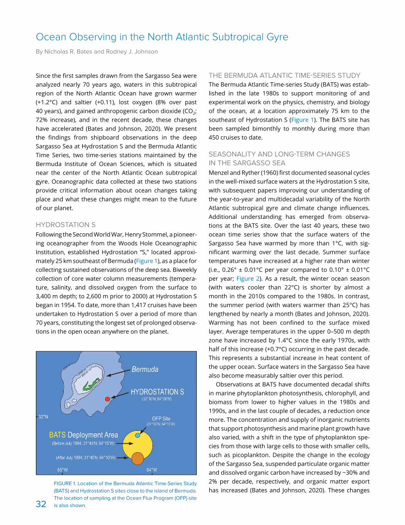
FIGURE 1. Location of the Bermuda Atlantic Time-Series Study (BATS) and Hydrostation S sites close to the island of Bermuda. The location of sampling at the Ocean Flux Program (OFP) site is also shown.

Since the first samples drawn from the Sargasso Sea were analyzed nearly 70 years ago, waters in this subtropical region of the North Atlantic Ocean have grown warmer (+1.2°C) and saltier (+0.11), lost oxygen (8% over past 40 years), and gained anthropogenic carbon dioxide (CO2; 72% increase), and in the recent decade, these changes have accelerated (Bates and Johnson, 2020). We present the findings from shipboard observations in the deep Sargasso Sea at Hydrostation S and the Bermuda Atlantic Time Series, two time-series stations maintained by the Bermuda Institute of Ocean Sciences, which is situated near the center of the North Atlantic Ocean subtropical gyre. Oceanographic data collected at these two stations provide critical information about ocean changes taking place and what these changes might mean to the future of our planet.

HYDROSTATION S Following the Second World War, Henry Stommel, a pioneer-ing oceanographer from the Woods Hole Oceanographic Institution, established Hydrostation “S,” located approxi-mately 25 km southeast of Bermuda (Figure 1), as a place for collecting sustained observations of the deep sea. Biweekly collection of core water column measurements (tempera-ture, salinity, and dissolved oxygen from the surface to 3,400 m depth; to 2,600 m prior to 2000) at Hydrostation S began in 1954. To date, more than 1,417 cruises have been undertaken to Hydrostation S over a period of more than 70 years, constituting the longest set of prolonged observa-tions in the open ocean anywhere on the planet.

THE BERMUDA ATLANTIC TIME-SERIES STUDY The Bermuda Atlantic Time-series Study (BATS) was estab-lished in the late 1980s to support monitoring of and experimental work on the physics, chemistry, and biology of the ocean, at a location approximately 75 km to the southeast of Hydrostation S (Figure 1). The BATS site has been sampled bimonthly to monthly during more than 450 cruises to date.

SEASONALITY AND LONG-TERM CHANGES IN THE SARGASSO SEA Menzel and Ryther (1960) first documented seasonal cycles in the well-mixed surface waters at the Hydrostation S site, with subsequent papers improving our understanding of the year-to-year and multidecadal variability of the North Atlantic subtropical gyre and climate change influences. Additional understanding has emerged from observa-tions at the BATS site. Over the last 40 years, these two ocean time series show that the surface waters of the Sargasso Sea have warmed by more than 1°C, with sig-nificant warming over the last decade. Summer surface temperatures have increased at a higher rate than winter (i.e., 0.26° ± 0.01°C per year compared to 0.10° ± 0.01°C per year; Figure 2). As a result, the winter ocean season (with waters cooler than 22°C) is shorter by almost a month in the 2010s compared to the 1980s. In contrast, the summer period (with waters warmer than 25°C) has lengthened by nearly a month (Bates and Johnson, 2020). Warming has not been confined to the surface mixed layer. Average temperatures in the upper 0–500 m depth zone have increased by 1.4°C since the early 1970s, with half of this increase (+0.7°C) occurring in the past decade. This represents a substantial increase in heat content of the upper ocean. Surface waters in the Sargasso Sea have also become measurably saltier over this period.

Observations at BATS have documented decadal shifts in marine phytoplankton photosynthesis, chlorophyll, and biomass from lower to higher values in the 1980s and 1990s, and in the last couple of decades, a reduction once more. The concentration and supply of inorganic nutrients that support photosynthesis and marine plant growth have also varied, with a shift in the type of phytoplankton spe-cies from those with large cells to those with smaller cells, such as picoplankton. Despite the change in the ecology of the Sargasso Sea, suspended particulate organic matter and dissolved organic carbon have increased by ~30% and 2% per decade, respectively, and organic matter export has increased (Bates and Johnson, 2020). These changes

Ocean Observing in the North Atlantic Subtropical GyreBy Nicholas R. Bates and Rodney J. Johnson

32

302826242220

+3

–3

+2

–2

0–1

+1

1980 1985 1990 1995 2000 2005 2010 2015 2020

+0.4+0.2

–0.2–0.4

0

36.936.736.536.336.1

260

240

220

200

+30

+10+20

–10–20–30

0

(c) Dissolved Oxygen

(b) Salinity

(a) Temperature

18

180

+40

–40

Tem

pera

ture

(°C)

DO

(µm

oles

/kg)

Salin

ity

FIGURE 2. Changes in (a) temperature, (b) salinity, and (c) dissolved oxygen at the BATS and Hydrostation S sites. Open blue symbols are observed data (left vertical axis) and orange symbols are seasonally detrended anomalies (right vertical axis). Modified from Bates and Johnson (2020)

in photosynthesis, marine plant biomass, and community composition have been accompanied by a rate of loss of dissolved oxygen that is notably higher than in other oce-anic areas (Bates and Johnson, 2020).

OCEAN ACIDIFICATION Over the past 40 years, the Sargasso Sea has also absorbed human-produced carbon dioxide (CO2) from the atmo-sphere, almost doubling the amount of CO2 in the upper waters (Bates and Johnson, 2020). As a consequence of the 72% increase in anthropogenic CO2 content, pH has decreased by 0.1 (and ocean acidity has increased by nearly 30%), with present-day ocean chemistry less favorable for the formation of calcium carbonate by the phytoplankton community. Over a few decades, the CO2 and pH chemical conditions have reached numbers outside of the seasonal ranges observed in the 1980s and beforehand.

DEEPER OCEAN CHANGES The deep waters of the Sargasso Sea offer a broader tem-poral and spatial perspective of long-term ocean change. Observations at Hydrostation S and BATS have revealed a slowing of the rate of formation of subtropical mode water (Stevens et  al., 2020). This water mass forms south of the Gulf Stream in wintertime and is important to setting nutrient conditions, phytoplankton growth, and biomass across the North Atlantic subtropical gyre. Such changes in the circulation of the deep-water currents flowing past Bermuda reflect reorganization of global ocean circulation patterns as well as changes in the temperature and salinity of intermediate and deep waters.

The oxygen minimum zone (i.e., <180 µmoles per kg) at Hydrostation S has also expanded, with the shallow hori-zon rising from ~600 m to ~500 m depth, particularly in the last decade, potentially reflecting changes in the time since these waters were in contact with the atmosphere and perhaps increased remineralization. Since 1970, the tem-perature and salinity properties of this water mass have not significantly changed, whereas dissolved oxygen has decreased at a rate of 2.5 µmoles per kg per decade (p-value <0.01), representing a loss of ~7% in the past 50 years.

Since the 1950s, Labrador Sea Water, found at ~2,000 m depth at Hydrostation S, has generally cooled by ~0.13°C and freshened by ~0.03. More recently, a reverse trend has been observed, with warming and increasing salinity in the last decade. These observations prompt questions about what processes operate in the North Atlantic Ocean over decadal time periods and their causes.

CONCLUSIONS AND FUTURE OCEAN OBSERVATIONS Ocean observations such as those made at Hydrostation S and BATS constitute only a handful of marine sites that have been maintained over more than a few decades. As such, they represent sentinels of ocean change for oceanogra-phers and those interested in the ocean environment. The open ocean offers few visible signs of change, but data col-lected over the past 40 years show that the ocean’s physics, chemistry, and biology have changed significantly due to human influences. With future hypothesis-testing and dis-covery, our collaborative community of scientists endeav-ors to uncover critical knowledge about the causes and future of environmental change. BATS and Hydrostation S data have been used by thousands of researchers and students and incorporated into more than 1,000 research papers. These ocean time series are also complemented by long-term observations of sinking ocean particles (Ocean Flux Program) and decade-long studies of the molecular biology of the Sargasso Sea (e.g., BIOSSCOPE, BIOS-Simons Collaboration on Ocean Processes and Ecology).

REFERENCESBates, N.R., and R.J. Johnson. 2020. Acceleration of ocean warming,

salinification, deoxygenation and acidification in the surface sub-tropical North Atlantic Ocean. Nature Communications in Earth and Environment 1:33, https://doi.org/10.1038/s43247-020-00030-5.

Menzel, D.W., and J.H. Ryther. 1960. The annual cycle of primary produc-tion in the Sargasso Sea off Bermuda. Deep Sea Research 6:351–367, https://doi.org/10.1016/0146-6313(59)90095-4.

Stevens, S.W., R.J. Johnson, G. Maze, and N.R. Bates. 2020. A recent decline in North Atlantic subtropical mode water formation. Nature Climate Change 10(4):335–341, https://doi.org/10.1038/s41558-020-0722-3.

ACKNOWLEDGMENTS The BATS and Hydrostation S programs continue due to a team of dedi-cated scientists and ship’s crew, the support of the entire institution, and the US National Science Foundation.

ARTICLE DOI: https://doi.org/10.5670/oceanog.2021.supplement.02-14

33

70ºN

70ºN

120ºW

110ºW

130ºW

130ºW

140ºW

140ºW

150º

W

150º

W

160º

W

160º

W

170º

W

170º

W

180

180º

180º

170º

E

170º

E

160ºE

60ºN

50ºN

60ºN

Arctic Circle

Arctic Circle Arctic Circle

118

Long-term monitoring and data collection provide the foundational knowledge and context for understanding how climate change impacts Alaskan marine ecosystems. A generation of ocean observing by the US National Oceanic and Atmospheric Administration (NOAA) Ecosystems and Fisheries Oceanography Coordinated Investigations (EcoFOCI) is at the forefront of detecting regional and global climate change and its impacts on ecosystems (Figure 1). Using a variety of observing tools, including research vessels and mooring arrays, and continuous integration of new technology, the program’s advances in marine science have provided contextual information to enable direct and effective management and sustainable use of fisheries resources in the Bering Sea. EcoFOCI was thus poised to address emergent physical and biological questions arising from an unprecedented loss of winter sea ice in the US Arctic in 2018 and 2019.

FROM COLD POOL TO COLD PUDDLE: SEA-ICE THICKNESS, DURATION, AND EXTENT ARE ON THE DECLINEA suite of long-term observations has shown that sea ice shapes the Bering Sea ecosystem. Ice presence in winter kick-starts the production of spring algae and zooplankton,

which in turn provides the food base for the region’s vast international fisheries. Historically, cold winter winds drove ice southward across the Bering Sea shelf, creating extensive ice that could cover an area larger than Texas and California combined. But recent shifts in wind patterns have altered the historical dynamics of ice, algae, plankton, and fisheries. In 2018, winter winds began to blow from the south and last for a month or more, allowing warm air to push against the ice and prevent its southward advance (Stabeno and Bell, 2019). Such changes were predicted to occur as part of long-term climate change—but not for another 30 years (Stabeno and Bell, 2019).

The bottom layer (~30 m deep) of the water column on the eastern Bering Sea shelf, where temperatures remain below 2°C, is known as the cold pool, and it is determined by sea ice extent. In a cold year, like 2012, it extends ~200 km (a third of the shelf width). The cold water cre-ates a barrier for commercially important fish species like Pacific cod and pollock that prefer warmer waters. As a result, the fish are usually confined to the southeastern Bering Sea and the outer shelf. The 2018 shifts in wind pat-terns resulted in the smallest cold pool on record (Stabeno and Bell, 2019), and conditions in 2019 were similar. Near-bottom temperature measurements from EcoFOCI

FIGURE 1. Map of EcoFOCI long-term observations across Alaska’s large marine ecosystems, including obser-vation types and years deployed. Uncrewed systems (e.g., gliders and floats) are not included. Ice extents in 2012 (an extensive ice year) and 2018 (the lowest ice extent on record) are indicated. EcoFOCI is a partnership between two NOAA laboratories, the Pacific Marine Environmental Labo-ratory and the Alaska Fisheries Sci-ence Center. The core of the program comprises long-term observations from the NOAA Research biophysical mooring array (25+ years) and work on the NOAA Fisheries ichthyo- and zooplankton collections (35+ years), which provide critical measurements for detecting and understanding ecosystem changes. The program was established in 1984 to examine the physical and biological factors that affect the pollock fishery in Alaska. Since that time, the program has evolved to meet emerging scien-tific questions and needs of NOAA, stakeholders, and communities.

EcoFOCI: A Generation of Ecosystem Studies in Alaskan WatersBy Heather M. Tabisola, Janet T. Duffy-Anderson, Calvin W. Mordy, and Phyllis J. Stabeno

34

FIGURE 2. Deploying the M2 “Peggy” mooring from NOAA Ship Oscar Dyson on an unusually calm spring day in the Bering Sea. The surface mooring was named after Peggy Dyson, who for many years (1965–2000) broadcast the marine weather on WBH-29 Kodiak for more than a dozen meteorological areas along Alaska’s coast. She was the voice of the north and wife to fisherman Oscar Dyson, namesake of the NOAA vessel in this photo.

moorings, while cold, were the warmest on record in 2018 (Stabeno and Bell, 2019). This revealed a “cool” pool in parts of the northern Bering Sea earlier in summer that did not last. The dynamics of how the cold pool shrinks, or becomes a puddle, are not fully understood. The lack of ice in 2018 led to the latest spring bloom on record in the northern Bering Sea, impacting the base of the food web and the commercial fisheries it supports.

INCREASED WARM TEMPERATURES COULD ALTER THE BASIC STRUCTURE AND FUNCTION OF THE FOOD WEB, BUT NOT EVERYTHING IS BEHAVING AS PREDICTEDIt was thought that ocean warming would open up the northern Bering Sea to pollock and Pacific cod, potentially supporting a larger, more productive fishery. The dramat-ically small cold pool in 2018 and 2019 did result in large numbers of adult Pacific cod and pollock emerging in the northern Bering Sea in the summer months. However, eco-system surveys showed that species of oceanic plants and animals at the base of the food web also changed, with associated lower food production and reduced food qual-ity (Duffy-Anderson et al., 2019). In addition, fish such as herring were found in low numbers. Seabirds died off, and numbers of marine mammals such as seals and whales were reduced. These impacts reach farther, to the Chukchi Sea, where local communities are feeling the changes (Huntington et al., 2020).

Physical oceanographic data such as temperature and salinity collected in the water column by moored instru-ments, and biological samples collected from ships, help demystify the connections between the distinct regions of the US Arctic. By 2020, the M2 “Peggy” mooring had been collecting oceanographic data in the Bering Sea for a quarter century, creating one of the longest time series in the world ocean (Figure 2). This mooring, coupled with three other long-term moorings (M4, 1999; M5, 2005; M8, 2005) and newly initiated observatories, cover more than 1,000  km and provide near-continuous, year-round measurements of the water column in this region (Figure 1). New technolo-gies are continually incorporated into these observing sys-tems, strengthening foundational science and improving stewardship of ocean resources in these remote and com-plex ecosystems. The real-time data from these observato-ries are also integrated into forecasts and models.

EcoFOCI provides information that supports manage-ment and sustainable use of fisheries resources. For instance, studies in 2016–2017 directly influenced decision- making by the North Pacific Fishery Management Council in determining the pollock catch and contributed to documents used by management and stakeholders to evaluate current ecosystem status and project near-future conditions. The program also predicted the collapse of the Pacific cod population in the Gulf of Alaska following the 2015 marine heatwave (the “blob”).

US Arctic waters are transforming faster than antici-pated. It is imperative that the importance of ocean observ-ing, including traditional knowledge, is at the forefront of understanding "what change is." EcoFOCI will continue to examine trends related to changing ecosystems and cli-mate and address critical topics for resource managers in this rapidly evolving system.

REFERENCESDuffy-Anderson, J.T., P. Stabeno, A.G. Andrews, K. Cieciel, A. Deary,

E. Farley, C. Fugate, C. Harpold, R. Heintz, D. Kimmel, and others. 2019. Responses of the northern Bering Sea and southeastern Bering Sea pelagic ecosystems following record-breaking low winter sea-ice. Geophysical Research Letters 46(16):9,833–9,842, https://doi.org/ 10.1029/2019GL083396

Huntington, H.P., S.L. Danielson, F.K. Wiese, M. Baker, P. Boveng, J. Citta, A. DeRobertis, D. Dickson, E. Farley, J.C. George, and others. 2020. Evidence suggests potential transformation of the Pacific Arctic ecosys-tem is underway. Nature Climate Change 10:342–348, https://doi.org/ 10.1038/s41558-020-0695-2.

Stabeno, P.J., and S.W. Bell. 2019. Extreme conditions in the Bering Sea (2017–2018): Record breaking low sea-ice extent. Geophysical Research Letters 46(15):8,952–8,959, https://doi.org/10.1029/2019GL083816.

ACKNOWLEDGMENTSThanks to S. Battle and S. Bell for the figure; and the reviewers M. Sullivan and M. Mooney-Seus. This research is supported by NOAA Research and Fisheries. Ice Extent data are from the US National Ice Center and National Snow and Ice Data Center (https://doi.org/10.7265/N5GT5K3K). This is contribution 1014 to EcoFOCI, 2021-1158 to CICOES, and 5299 to PMEL. The scientific results and conclusions, as well as any views or opinions expressed herein, are those of the author(s) and do not necessarily reflect those of OAR or the Department of Commerce.

ARTICLE DOI: https://doi.org/10.5670/oceanog.2021.supplement.02-15

35

TOPIC 3. OCEAN RESOURCES AND THE ECONOMY UNDER CHANGING

ENVIRONMENTAL CONDITIONS

INTRODUCTIONThe link between humans and life in the sea is not something most of us think about every day. However, we humans have historically built communities close to the sea, and we have studied how marine organisms grow, where they aggregate, and how their distribution changes throughout the day and with the seasons so that we can manage our activities to exploit them more effectively or protect them for other purposes. We use the sea for shipping and rec-reation, to extract energy, and to derive natural products such as medicines (Figure 1). These activities, when added to other industries, as well as research, technology, educa-tion, and governance, add up to about US$2 trillion a year. This “blue economy” is described as a knowledge-based economy in which data and information guide solutions to societal challenges (Spinrad, 2021). Similar to the way we built monitoring systems to improve global weather fore-casting over the past 100 years, sustaining a blue economy now depends on a global ocean observing system to pro-vide accurate and timely data about life in the sea.

A focus of Earth system science today is to improve fore-casts of environmental variables so that we can predict the impacts of climate change and of human uses of the ocean. We justify much of this investment in research based on the need to protect life and property and to ensure food and water security. Over 90% of Earth’s habitable space is contained in the sea, and the habitats within it are rap-idly changing. Sea surface temperatures have risen about 0.11°C per decade since the 1980s. Warming has led to sea level rise of about 3 cm per decade due to the ther-mal expansion of seawater and additional water entering the sea from melting glaciers. Warming has caused thinner

sea ice and smaller ice shelves, with the minimum summer Arctic sea ice cover decreasing by an average of about 13% per decade. Meanwhile, the ocean has absorbed about one-third of the excess carbon dioxide humans have emit-ted into the atmosphere since the Industrial Revolution, causing an average decrease in near-surface pH of about 0.1 in the last 200 years, and twice that rate since the 1980s (–0.001 to –0.002 pH units per year documented at different ocean time series locations). There is also clear evidence of changes in salinity, oxygen levels, ocean winds, severe storm patterns, and major ocean currents around the globe (IPCC, 2021).

These environmental changes have altered the distri-bution, abundance, composition, and health of marine life in ways we are only beginning to understand, and this is stressing the blue economy and associated services needed by society. We depend on the ocean for food pro-duction; for some coastal communities, the ocean is the primary source of protein as well as an integral part of their cultural heritage. Conservation and effective man-agement of marine resources are essential to ensure a sustainable blue economy. Current efforts to measure marine biodiversity and biology have neither the cover-age nor consistency of ocean physical and chemical mea-surements. Improved understanding requires improved observations—we cannot understand or manage what we don’t measure.

Our knowledge about environmental changes is based on measurements collected around the world since the 1700s (Figure 2). While observing biology and ecosystems is the only way to make informed decisions about how to balance resource use and conservation, maps such

Integrating Biology into Ocean Observing Infrastructure: Society Depends on ItBy Maurice Estes Jr., Frank Muller-Karger, Kerstin Forsberg, Margaret Leinen, Suzan Kholeif, Woody Turner, Douglas Cripe, Yana Gevorgyan, Peer Fietzek, Gabrielle Canonico, Francisco Werner, and Nicholas Bax

36

as the one in Figure 2 show that the number of biologi-cal observations in any one region, and in most locations, is nowhere near what is needed to assess the status and rates of change of biological resources. We have an oppor-tunity today to enhance the infrastructure needed to build the capacity to adequately observe marine biodiversity and biology, especially in coastal and pelagic areas of the world ocean where people most depend on these resources on a day-to-day basis.

SOCIETY’S DEPENDENCE ON INFORMATION ABOUT MARINE LIFEThe evolution of human society is intertwined with knowl-edge about marine biodiversity. Marine species shaped the ancient and current vision, culture, and heritage of many traditional and indigenous communities, from the tropics to high latitudes. Living marine resources that influence local, tribal, and national identities include the modern seafood gastronomy of Peru, the symbolic blue marlin in

WHAT IS THE BLUE ECONOMY?

Earth has an abundance of marine resources. The Blue Economy model seeks to promote economic growth, social inclusion, and the

preservation or improvement of livelihoods while ensuring environmental sustainability of

the ocean and coastal areas.

TRADE AND TRANSPORT

RENEWABLE ENERGY TOURISM AND RECREATION

MARINE PHARMACEUTICALS

SUSTAINABLE FISHERIES

BIOLOGICAL DIVERSITY

KNOWLEDGE DRIVES THE BLUE ECONOMY

Ocean observations gathered worldwide help inform decisions on

marine resources such as…

FIGURE 1. The sea and people are linked in many ways via the blue economy, including renewable energy opportunities, fisheries for food, tourism and recreation, natural sources of medicines, and conditions that support ecological diversity that is essential for healthy, sustainable marine environments. Photo credits (clockwise from top): net – iStock.com/NJPhotos; boats – iStock.com/JeerawatJ; swimmers – Fabrice Dudenhofer/Ocean Image Bank; nudibranch – Erik Lukas/Ocean Image Bank; soft coral – Renata Romeo/Ocean Image Bank; container ship – iStock.com/Tryaging; whales – François Baelen/Ocean Image Bank; plankton – Richard Kirby; wind farm – iStock.com/IanDyball. Background image: iStock.com/primo-piano 373737

the Bahamas, and the sea turtle in Antigua, Barbuda, and many Polynesian cultures. Life in the sea provides many societies with a sense of place, occupational pride, spiritu-ality, mental and bodily health, and security.

With 40% of the world’s growing population settled within 150 km of the ocean, the blue economy is expand-ing. Offshore energy, marine biotechnology, fisheries, pharmaceuticals, and tourism are growing. Global fish-eries today land approximately 80 million metric tons (mmt) every year, employing some 30.6 million people. The marine capture for 2018 was 84.4 mmt based on data from the Food and Agriculture Organization of the United Nations. Up to 10% of the global population relies on fish-eries for livelihoods. Mariculture produces over 38.6 mmt of seafood or US$67.4 billion annually, and this is growing quickly, with the potential for 700 times more production in the future. Similarly, global coral reef tourism is valued at US$35.8 billion annually and is expanding (Gaines et al., 2019). The Coral Triangle, located in parts of six countries (Indonesia, Philippines, Malaysia, Papua New Guinea, Solomon Islands, and East Timor) and the Mesoamerican Reef in parts of four countries (Belize, Guatemala, Honduras, and the Yucatán peninsula of Mexico), are esti-mated to contribute over US$20 billion to the blue econ-omy from tourism, fisheries, and coastal development

FIGURE 2. Illustration of the number of individual taxonomic observations (records) per 1,000 km2 aggregated since the late 1700s in the Ocean Biodiversity Information System (OBIS; https://obis.org/). The coverage shows large gaps in the spatial coverage of the ocean (gaps within Exclusive Economic Zones are shown in black; gaps in Areas Beyond National Jurisdiction are shown in gray). Because many records are from one-time observations, gaps in coverage over time are substantial even in coastal and continental shelf regions where most resources used by society are located. Large-scale programs typically collect observations only annually or once every few years. Many programs do not share observations with open databases such as OBIS, which limits large-scale assessments of bio-logical resources and also limits understanding of how local changes may be related to regional changes. Illustration courtesy of P. Provoost, OBIS

(Figure 3; UN Environment et al., 2018) Yet, at present, only a few locations around the world collect detailed data on the species compositions of different fisheries or the ages and life histories of fish and their prey and predators; on observations of essential habitats; or even on fish catches or socioeconomics in order to evaluate status and trends in biodiversity in the context of environmental changes or human activities (Figure 3).

Fish, other living marine resources, and the ecosystem services we depend on are sustained by many different species in coastal, shallow, and deep habitats. Seagrasses, mangroves, and macroalgal communities provide nurs-ery habitat for finfish, shellfish, and many species of megafauna. Macrophytes (aquatic plants that grow in or near water such as cattails, hydrilla, water hyacinth, and duckweed) and hard coral reefs stabilize the coast and prevent shoreline erosion from tidal energy and storms, filter nutrients and pollutants in terrestrial runoff, trap sediments, and host significant wildlife. By 2100, approx-imately 630 million people worldwide could be at risk of coastal flooding caused by climate change and sea level rise without such protection. Access to sandy beaches is essential for sea turtles to lay eggs and for horseshoe crabs to create nests near the high tide line, which is reced-ing rapidly in some areas (Figure 4).

FIGURE 3. (a) Coral reef Solomon Islands, South Pacific. Photo credit: Tracey Jennings/Ocean Image Bank (b) Estimated eco-nomic returns from coral reefs (US$20 billion in 2017 prices). Reprinted from UN Environment et al. (2018)

0 2 4 6 8 10 12 14 16

MesoamericanReef

Coral Triangle

Tourism Direct Tourism Indirect

Fisheries Direct Fisheries Indirect

Coastal Development Direct

Coastal DevelopmentIndirect

US$ Billion (2017 Prices)

Estimated Economic Returns from Coral Reefs

a

bOBIS: Number of Stations per 1,000 km2

1 10 100 1,000 10,000

38

The marine environment provides natural products that play critical roles in medicine and biotechnology. Many biochemicals have been isolated from marine species and can offer safer alternatives to cosmetics, anti-fouling agents, pharmaceuticals, and other products, including compounds with anticancer properties, and possible treat-ments for COVID-19. The blood of the common horseshoe crab, Limulus polyphemus, is the source of a compound that is used to test injectable medicines for microbial con-tamination (Sigwart et al., 2021).

Indeed, the inland economy, including the “green economy,” based on best practices intended to conserve energy and materials, is linked to the blue economy through industrial sectors, including production of fish-meal for poultry and other livestock and processing of algae used in many industries such as health, cosmetics, and renewable energy. Yet, the pollution that reaches the coast via rivers or other sources is at times unquantified in economic planning. We often use biological signals to measure downstream effects, such as microbial indica-tors for sewage contamination, or excess phytoplankton biomass or algal density to detect eutrophication. Beyond such bulk metrics, we lack biodiversity observing systems for tracking potential impacts to marine living resources and for monitoring ecosystem services around the world.

CONSERVATION AND MANAGEMENT: REQUISITES FOR SUSTAINING THE BLUE ECONOMYThe ability to sustain economic growth and jobs requires making wise investments in conservation and restoring key coastal and marine resources. We cannot afford to continue to degrade the very resources our lives depend on through unsustainable practices. So, how do we guide wise stewardship and sustainable development? Designing a sustainable economy that is based on information and knowledge requires collecting basic observations from which we can develop indicators of ecosystem health,

diversity, and productivity. The Global Ocean Observing System of the Intergovernmental Oceanographic Commission has advanced a framework for ocean observ-ing based on collecting essential ocean variables (EOVs). In addition to physical (e.g., temperature and salinity) and biogeochemical (e.g.,  oxygen, inorganic and dissolved organic carbon) EOVs, it includes a family of biology and ecosystem EOVs (e.g.,  fish abundance and distribution, phytoplankton biomass and diversity; Miloslavich et  al., 2018). This framework provides a coordinated scheme for observing the ocean and determining the fundamental indicators needed to guide decisions on sustainable devel-opment and restoration of coastal and ocean resources (Duarte et al., 2020).

Ocean financing and sustainable investing are key to developing the blue economy. Sala et al. (2021) find that protecting ~28% of the ocean could provide a net gain of 6 to 8 million metric tons of seafood, securing 35% of biodi-versity benefits and 27% of carbon benefits. The High Level Panel for a Sustainable Ocean Economy concluded in 2020 that investments in such actions as sustainable ocean-based food production and conservation and restoration of mangroves would yield a fivefold return in global ben-efits (Stuchtey et al., 2020). Such investments would also cut annual greenhouse gas emissions and help reduce the rate of global temperature rise. While marine protected areas currently conserve and sustain ocean resources for the blue economy, additional research is required to determine their optimal design (Figure 5).

FIGURE 4. An eroding coast on the southern shore of Mobile Bay, Alabama. As the shoreline recedes, trees collapse and access to the sandy beach for marine life is restricted. Photo credit: Maury Estes, University of Alabama in Huntsville

b

FIGURE 5. Average reef-fish abundance, biomass, spe-cies richness, Simpson diver-sity, and functional diversity grouped by no- take marine zones (protected) and out-side areas (unprotected) in the Florida Keys from 1999 to 2018. The unit for abundance (a) is the number of individu-als (N), and for biomass (b), grams per meter squared. (c–e) Species richness, Simpson diversity, and func-tional diversity are presented in units of effective number of species (ENS). SE = stan-dard error. Reprinted from Medina et al. (2021)

ENS

(± S

E)

(a) Abundance

(c) Species Richness

(b) Biomass

(d) Simpson Diversity

(e) Functional Diversity

N (±

SE)

g/m

2 (± S

E)

ENS

(± S

E)

ENS

(± S

E)

Year2000 2004 2008 2012 2016

800

600

400

100

50

50

45

40

35

10

9

8

71.80

1.75

1.70

1.65

UnprotectedProtected

39

Many other examples of successes show what we can do. We must focus attention on promoting sustainability and equity in ocean uses, and address factors that impact women, informal workers, indigenous peoples, local communities, youth, vulnerable and disadvantaged pop-ulations, and early career professionals. Without careful attention to our actions, global economic losses may top US$400 billion a year by 2050, and US$2  trillion by 2100 (Stuchtey et al., 2020).

MONITORING MARINE ECOSYSTEMS In order to sustain the blue economy, observations of marine life must be integrated into global ocean moni-toring of biology and ecosystem EOVs and include socio-economic indicators. For example, at the base of the food chain, the dynamics of microbes and plankton control the locations of larger animals as well as their productivity and abundance. Many plankton species are harvested for protein and are also used in emerging renewable energy technologies. In addition, they are indicators of ecosys-tem health and water quality, and they are the “bio” part in biogeochemical cycles that we need to better measure as we engineer a low-carbon economy. Effective monitor-ing of plankton is possible today through investments in genomic, optical, imaging, active and passive acoustics, and remote-sensing methods that would improve fore-casts for managing food production, water quality, and carbon sequestration (Estes et al., 2021).

At the other end of the size spectrum are marine mega-fauna (turtles, birds, mammals, and large fish are grouped in a broad category of EOVs), organisms that function as top-down controls on ecosystem structure and func-tion. Their migratory routes and associations with other multi-species networks often mark marine corridors and biodiversity hotspots. Understanding where and when these corridors and hotspots form, how they are changing, and how they are beneficial to us is key to management of shipping, fishing, mining, and land or vessel discharges.

New observing tools include sensors on satellites, air-craft, and autonomous underwater platforms. Using such “remote sensing” of biology and ecosystems expands the scope of traditional observing platforms like ships and buoys, permitting sustained and repeated synoptic map-ping of entire ocean basins.

Satellite sensors collect important measurements across the marine realm. In addition to helping to locate and track tagged animals, the many environmental parameters they collect, such as chlorophyll-a concentration and seawater color, permit definition and evaluation of phytoplankton habitats and traits. Today, remotely sensed data collected by NASA’s Moderate Resolution Imaging Spectroradiome-ter (MODIS) and the European Space Agency’s Sentinel-2 and Sentinel-3 satellite sensors, among others, provide global coverage and finer- scale data that allow obser-vations of coastal biological signals (Figure 6). New mis-sions expected to bring major advances in ocean imaging

April 8th, 2021Sentinel-2A RGB image using atmospherically corrected angular dependent water leaving reflectanceBands 4,3,1 resampled to 10-m

FIGURE 6. (a) Sentinel-2 satellite image of the Florida peninsula collected on April 8, 2021, with the Tampa Bay estuary in the west cen-tral portion of the frame. (b) Processed Sentinel-2A image focused on Tampa Bay, with colors indicating changes in water clarity. The inset (c) shows a small phytoplankton bloom that resulted from an accidental discharge from a phosphate mine retention pond (Piney Point) following heavy rains. Sentinel-2 image courtesy of Copernicus/European Space Agency; image processed by the University of South Florida College of Marine Science

a

b c

40

include NASA’s Surface Geology and Biology (SBG, expected to launch in 2027), Plankton, Aerosol, Cloud, ocean Ecosystem (PACE, scheduled for launch in 2023), and Geosynchronous Littoral Imaging and Monitoring Radiometer (GLIMR, 2026–2027). Satellite lidar systems are detecting phytoplank-ton and zooplankton deeper in the ocean at night and in winter at high latitudes and are charac-terizing the seafloor topography of coastal habitats. Combined with satellite measurements of winds, currents, sea surface topogra-phy, salinity, and temperature, a relatively coherent set of global seascapes can be visualized and analyzed nearly daily and over

conditions (e.g.,  climate variables) means that we are now able to track these changes and better understand their drivers. Combining observations requires greater collaboration among different research areas and with local stakeholders.

All of these biological observations can be incorporated into existing ocean observing programs that focus on the physics, chemistry, and geology of the ocean, includ-ing the global effort to map seafloor topography (Seabed 2030 project), the Global Ocean Ship-based Hydrographic Investigations Program (GO-SHIP), and OceanSITES. Taking Seabed 2030 as an example, its use of active acoustic sound wave reflection measurements to map the topography of the global ocean seafloor can be complemented with ini-tiatives to collect water column and seafloor acoustic back-scatter data that provide information about fish, plankton, and bottom habitats across ocean basins, repeatedly over time. Passive acoustic technology is now feasible and accessible to conduct scientific monitoring of different species, from small zooplankton to birds, and from fish to marine mammals (Figure 7), and human noise, from the bottom of the ocean to shallow reef environments. The benefits of such information for academic science, gov-ernment, the private sector, and the public are substantial. Greater collaboration will depend on multinational and national groups contributing standardized biological data to enable forecasting and global assessments, similar to what we have already accomplished with weather and cli-mate assessments. This could provide the basis for a revo-lutionary new marine biodiversity observation network to support a sustainable blue economy.

long time periods. Improved consistency and relevance in interpreted remote-sensing products requires expanded in situ calibration and validation, and greater interaction with biological sampling communities.

Monitoring of coastal nearshore environments is chal-lenging due to their dynamic nature, but necessary because the resources they contain are valuable to the blue econ-omy. Expansion of urban and agricultural land use directly affects nearshore water quality, increasing nutrient and sed-iment runoff that results in eutrophication (Boesch, 2019) and algal blooms that can harm marine life and release air-borne toxins into nearshore areas. Monitoring seagrasses, mangroves, and macroalgae (kelp, Sargassum, green and red algae) is critical because of their foundational role as habitats for many species of commercial, subsistence, and conservation interest worldwide (Estes et al., 2021). In addi-tion to the Global Coral Reef Monitoring Network, the global Mangrove Alliance, the Reef Life Survey, the Partnership for Interdisciplinary Studies of Coastal Oceans (PISCO), and other entities focused on systematic and distributed sur-veys of nearshore habitats at large scales, development of citizen scientist approaches is needed to support these and related data collection efforts.

New ways to rapidly transmit data, as well as to col-lect and process images and environmental DNA (eDNA), improve our knowledge of changes in the distribution and abundance of life in the ocean, including those caused by warming. Combining these advances in technology with improved satellite and in situ observations of pri-mary producers (e.g., phytoplankton), primary consumers (e.g.,  zooplankton, small fish), and overall environmental

Figure 7. Acoustic indices of blue and fin whale vocal activity recorded in Monterey Bay National Marine Sanctuary through the Monterey Accelerated Research System (MARS) cabled observatory. The index is a calibrated signal-to-noise ratio: signal from whale song (rhythmic repeated sequences of sound produced by males of each species) and noise from background (adjacent frequency bands). For each month, the interquartile range and median are shown. Reprinted from Ruhl et al. (2021); whale artist: Larry Foster

41

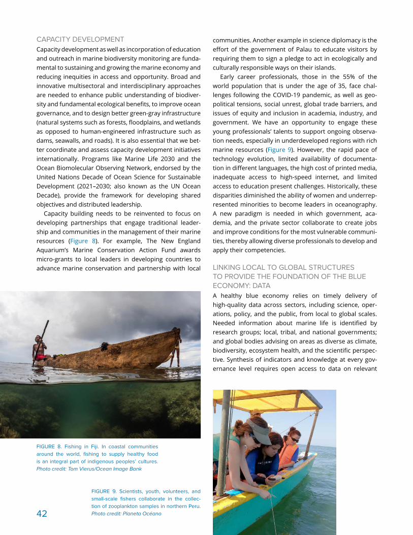
CAPACITY DEVELOPMENTCapacity development as well as incorporation of education and outreach in marine biodiversity monitoring are funda-mental to sustaining and growing the marine economy and reducing inequities in access and opportunity. Broad and innovative multisectoral and interdisciplinary approaches are needed to enhance public understanding of biodiver-sity and fundamental ecological benefits, to improve ocean governance, and to design better green-gray infrastructure (natural systems such as forests, floodplains, and wetlands as opposed to human-engineered infrastructure such as dams, seawalls, and roads). It is also essential that we bet-ter coordinate and assess capacity development initiatives internationally. Programs like Marine Life 2030 and the Ocean Biomolecular Observing Network, endorsed by the United Nations Decade of Ocean Science for Sustainable Development (2021–2030; also known as the UN Ocean Decade), provide the framework for developing shared objectives and distributed leadership.

Capacity building needs to be reinvented to focus on developing partnerships that engage traditional leader-ship and communities in the management of their marine resources (Figure 8). For example, The New England Aquarium’s Marine Conservation Action Fund awards micro-grants to local leaders in developing countries to advance marine conservation and partnership with local

communities. Another example in science diplomacy is the effort of the government of Palau to educate visitors by requiring them to sign a pledge to act in ecologically and culturally responsible ways on their islands.

Early career professionals, those in the 55% of the world population that is under the age of 35, face chal-lenges following the COVID-19 pandemic, as well as geo-political tensions, social unrest, global trade barriers, and issues of equity and inclusion in academia, industry, and government. We have an opportunity to engage these young professionals’ talents to support ongoing observa-tion needs, especially in underdeveloped regions with rich marine resources (Figure 9). However, the rapid pace of technology evolution, limited availability of documenta-tion in different languages, the high cost of printed media, inadequate access to high-speed internet, and limited access to education present challenges. Historically, these disparities diminished the ability of women and underrep-resented minorities to become leaders in oceanography. A new paradigm is needed in which government, aca-demia, and the private sector collaborate to create jobs and improve conditions for the most vulnerable communi-ties, thereby allowing diverse professionals to develop and apply their competencies.

LINKING LOCAL TO GLOBAL STRUCTURES TO PROVIDE THE FOUNDATION OF THE BLUE ECONOMY: DATAA healthy blue economy relies on timely delivery of high-quality data across sectors, including science, oper-ations, policy, and the public, from local to global scales. Needed information about marine life is identified by research groups; local, tribal, and national governments; and global bodies advising on areas as diverse as climate, biodiversity, ecosystem health, and the scientific perspec-tive. Synthesis of indicators and knowledge at every gov-ernance level requires open access to data on relevant

FIGURE 8. Fishing in Fiji. In coastal communities around the world, fishing to supply healthy food is an integral part of indigenous peoples’ cultures. Photo credit: Tom Vierus/Ocean Image Bank

FIGURE 9. Scientists, youth, volunteers, and small-scale fishers collaborate in the collec-tion of zooplankton samples in northern Peru. Photo credit: Planeta Océano42

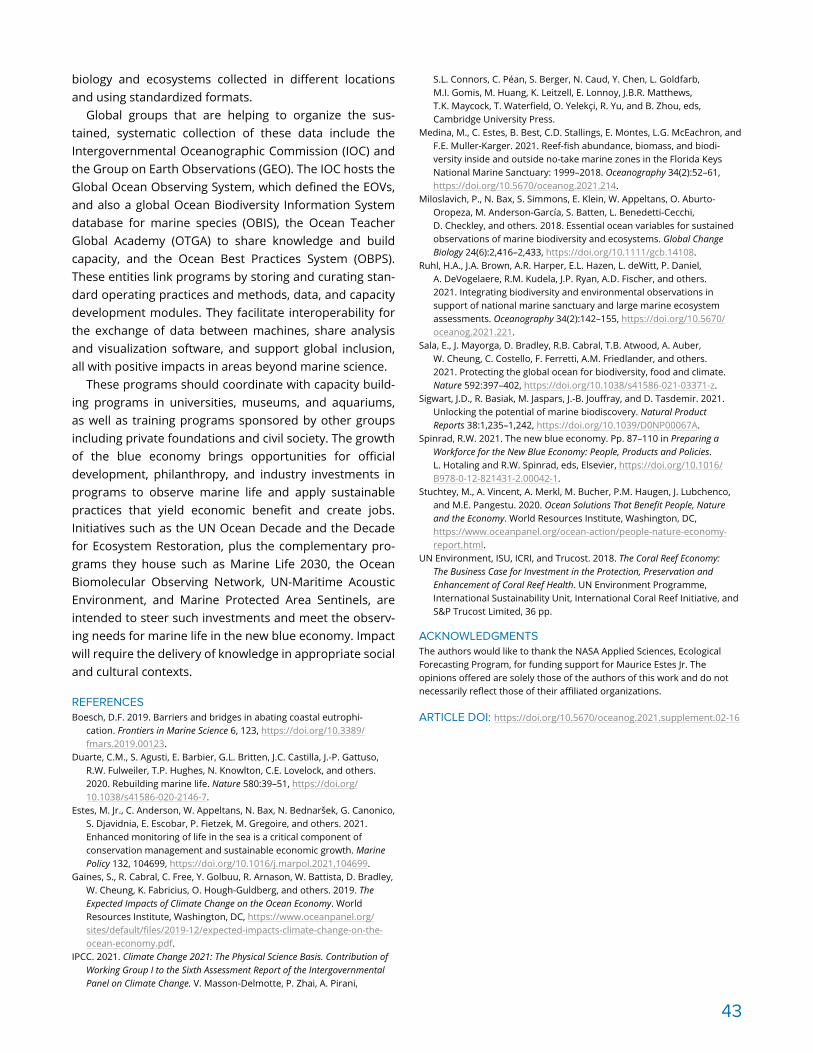
biology and ecosystems collected in different locations and using standardized formats.

Global groups that are helping to organize the sus-tained, systematic collection of these data include the Intergovernmental Oceanographic Commission (IOC) and the Group on Earth Observations (GEO). The IOC hosts the Global Ocean Observing System, which defined the EOVs, and also a global Ocean Biodiversity Information System database for marine species (OBIS), the Ocean Teacher Global Academy (OTGA) to share knowledge and build capacity, and the Ocean Best Practices System (OBPS). These entities link programs by storing and curating stan-dard operating practices and methods, data, and capacity development modules. They facilitate interoperability for the exchange of data between machines, share analysis and visualization software, and support global inclusion, all with positive impacts in areas beyond marine science.

These programs should coordinate with capacity build-ing programs in universities, museums, and aquariums, as well as training programs sponsored by other groups including private foundations and civil society. The growth of the blue economy brings opportunities for official development, philanthropy, and industry investments in programs to observe marine life and apply sustainable practices that yield economic benefit and create jobs. Initiatives such as the UN Ocean Decade and the Decade for Ecosystem Restoration, plus the complementary pro-grams they house such as Marine Life 2030, the Ocean Biomolecular Observing Network, UN-Maritime Acoustic Environment, and Marine Protected Area Sentinels, are intended to steer such investments and meet the observ-ing needs for marine life in the new blue economy. Impact will require the delivery of knowledge in appropriate social and cultural contexts.

REFERENCESBoesch, D.F. 2019. Barriers and bridges in abating coastal eutrophi-

cation. Frontiers in Marine Science 6, 123, https://doi.org/10.3389/fmars.2019.00123.

Duarte, C.M., S. Agusti, E. Barbier, G.L. Britten, J.C. Castilla, J.-P. Gattuso, R.W. Fulweiler, T.P. Hughes, N. Knowlton, C.E. Lovelock, and others. 2020. Rebuilding marine life. Nature 580:39–51, https://doi.org/ 10.1038/ s41586-020-2146-7.

Estes, M. Jr., C. Anderson, W. Appeltans, N. Bax, N. Bednaršek, G. Canonico, S. Djavidnia, E. Escobar, P. Fietzek, M. Gregoire, and others. 2021. Enhanced monitoring of life in the sea is a critical component of conservation management and sustainable economic growth. Marine Policy 132, 104699, https://doi.org/10.1016/j.marpol.2021.104699.

Gaines, S., R. Cabral, C. Free, Y. Golbuu, R. Arnason, W. Battista, D. Bradley, W. Cheung, K. Fabricius, O. Hough-Guldberg, and others. 2019. The Expected Impacts of Climate Change on the Ocean Economy. World Resources Institute, Washington, DC, https://www.oceanpanel.org/sites/default/files/2019-12/expected-impacts-climate-change-on-the-ocean-economy.pdf.

IPCC. 2021. Climate Change 2021: The Physical Science Basis. Contribution of Working Group I to the Sixth Assessment Report of the Intergovernmental Panel on Climate Change. V. Masson-Delmotte, P. Zhai, A. Pirani,

S.L. Connors, C. Péan, S. Berger, N. Caud, Y. Chen, L. Goldfarb, M.I. Gomis, M. Huang, K. Leitzell, E. Lonnoy, J.B.R. Matthews, T.K. Maycock, T. Waterfield, O. Yelekçi, R. Yu, and B. Zhou, eds, Cambridge University Press.

Medina, M., C. Estes, B. Best, C.D. Stallings, E. Montes, L.G. McEachron, and F.E. Muller-Karger. 2021. Reef-fish abundance, biomass, and biodi-versity inside and outside no-take marine zones in the Florida Keys National Marine Sanctuary: 1999–2018. Oceanography 34(2):52–61, https://doi.org/10.5670/oceanog.2021.214.

Miloslavich, P., N. Bax, S. Simmons, E. Klein, W. Appeltans, O. Aburto-Oropeza, M. Anderson-García, S. Batten, L. Benedetti-Cecchi, D. Checkley, and others. 2018. Essential ocean variables for sustained observations of marine biodiversity and ecosystems. Global Change Biology 24(6):2,416–2,433, https://doi.org/10.1111/gcb.14108.

Ruhl, H.A., J.A. Brown, A.R. Harper, E.L. Hazen, L. deWitt, P. Daniel, A. DeVogelaere, R.M. Kudela, J.P. Ryan, A.D. Fischer, and others. 2021. Integrating biodiversity and environmental observations in support of national marine sanctuary and large marine ecosystem assessments. Oceanography 34(2):142–155, https://doi.org/10.5670/oceanog.2021.221.

Sala, E., J. Mayorga, D. Bradley, R.B. Cabral, T.B. Atwood, A. Auber, W. Cheung, C. Costello, F. Ferretti, A.M. Friedlander, and others. 2021. Protecting the global ocean for biodiversity, food and climate. Nature 592:397–402, https://doi.org/10.1038/s41586-021-03371-z.

Sigwart, J.D., R. Basiak, M. Jaspars, J.-B. Jouffray, and D. Tasdemir. 2021. Unlocking the potential of marine biodiscovery. Natural Product Reports 38:1,235–1,242, https://doi.org/10.1039/D0NP00067A.

Spinrad, R.W. 2021. The new blue economy. Pp. 87–110 in Preparing a Workforce for the New Blue Economy: People, Products and Policies. L. Hotaling and R.W. Spinrad, eds, Elsevier, https://doi.org/10.1016/B978-0-12-821431-2.00042-1.

Stuchtey, M., A. Vincent, A. Merkl, M. Bucher, P.M. Haugen, J. Lubchenco, and M.E. Pangestu. 2020. Ocean Solutions That Benefit People, Nature and the Economy. World Resources Institute, Washington, DC, https://www.oceanpanel.org/ocean-action/people-nature-economy- report.html.

UN Environment, ISU, ICRI, and Trucost. 2018. The Coral Reef Economy: The Business Case for Investment in the Protection, Preservation and Enhancement of Coral Reef Health. UN Environment Programme, International Sustainability Unit, International Coral Reef Initiative, and S&P Trucost Limited, 36 pp.

ACKNOWLEDGMENTSThe authors would like to thank the NASA Applied Sciences, Ecological Forecasting Program, for funding support for Maurice Estes Jr. The opinions offered are solely those of the authors of this work and do not necessarily reflect those of their affiliated organizations.

ARTICLE DOI: https://doi.org/10.5670/oceanog.2021.supplement.02-16

43

Industrial shallow-water prawn trawling in Malindi-Ungwana Bay, located along the north coast of Kenya (Figures 1 and 2), began in the 1970s after exploratory fishing surveys identified the existence of fishable penaeid prawn stocks (Iversen, 1984). Small-scale fishers were also targeting the prawn resources in the bay. As trawlers fish-ing close to the shore destroyed nearshore habitats and the gear of small-scale fishers, resource-use conflicts arose between the trawler companies and small-scale fishers.

To reduce these conflicts, in 1991, Kenya Fisheries Act Chapter 378 limited prawn trawling to beyond 5 NM from shore, with no industrial trawling allowed within

a 0–3 NM zone. In 2010, a Prawn Fishery Management Plan recommended that trawling vessels carry a fisheries observer. However, it was not until this became a require-ment in Article 147 of the 2016 Fisheries Management and Development Act that Kenya Fisheries Service (KeFS) observers began to work aboard trawlers; this article also expanded the observer program to cover all other commercial fishing operations such as longliners, purse seiners, and deepwater trawlers. The observer program provides data and information on fish catches and their composition, on the fate of target and non-target species, and on the fishing effort to enable evaluation of the status of the fishery and to inform reviews of the regulations in management plans.

In this study, we analyzed the species composition of retained and discarded catches from 2016 to 2019 (using data collected by observers) and trawl catches between 2011 and 2019 (with fishing vessel log data provided by the trawl industry).

The first KeFS-trained scientific observers were deployed in 2016 on four Kenyan-flagged industrial trawlers licensed to fish in the Malindi-Ungwana Bay during the prawn fishing season. They observed and recorded operations between April 1 and October 31 every year from 2016 to 2019 (Figure 1) aboard trawlers that were fitted with dou-ble rigged nets of 55–60 mm and 40–45 mm at the funnel and cod ends, respectively.

Thirty-seven observer trips were executed for 168 days between 2016 and 2019 and recorded 1,371 out of 8,531 hauls. The catch composition data collected by

FIGURE 2. An industrial prawn trawler plies the fish-ing grounds of Malindi-Ungwana Bay, Kenya. Photo credit: Ben Onyango, Kenya Marine Fisheries Research Institute (KMFRI) Fisheries Observer

Observations of Industrial Shallow-Water Prawn Trawling in KenyaBy Esther N. Fondo and Johnstone O. Omukoto

FIGURE 1. Map of Malindi-Ungwana Bay, location of shallow water prawn trawling considered in this study. Observation points identify where trawl data were collected by observers from 2016 to 2019. Inset: Map of Kenya, with box indicating the location of Malindi-Ungwana Bay. Image credit: Pascal Z. Thoya

40°20'0''E

0 5 10 20 kmMalindi

Kipini

Major TownsLanding SitesMajor RiversMangrovesNo Trawl Zone

Tana River

Sabaki River

Mto Kilifi

Tanzania

KenyaSomalia

Mal

indi

Bay

Ungwana Bay

40°40'0''E

2°40

'0''S

3°0'

0''S

Observation Points2016201720182019

44

the observers followed sampling protocols adopted from Athayde (2012). The catch from each haul was emptied onto a steel sorting table on the deck, and large live animals (mainly sharks, rays, and turtles) were quickly returned to the sea to optimize their chances of survival (Figure 3). Prawns were then collected, graded, cleaned, treated, and placed into 2 kg cartons and blast frozen. The fish were sorted into retained and discarded catch. The captain kept a record of the fishing operation and the catch for each haul, and a report was sent to KeFS.

The industry data from 2011 to 2019 obtained from KeFS consisted of details of each fishing event, including start and end times and the GPS positions of each haul, and catch weights for prawns, octopus, squids, cuttlefish, lobsters, crabs, and others. Nothing at the species level was indicated. Results show a 20-fold increase in annual catches from 20 tons in 2011 to 450 tons in 2019, with a 10-fold increase in fishing effort from 437 hrs in 2011 to 5,102 hrs in 2019 (Figure 4). The catch rate for prawns varied from 8 kg/hr to 26 kg/hr. The catch rate for fin-fish was higher than that for prawns, ranging between 32 kg/hr and 88 kg/hr. Although the volume of discards (i.e.,  bycatch thrown back into the ocean, whether alive or dead, including live turtles and small, non-marketable fishes) remained high, there was a marked increase in the proportion of retained catch (prawns and finfish that were sold) over these years. The target prawn-to-bycatch ratio ranged from 1:3 to 1:9 during the four years. On average, 16% of the catch comprised target, with 59% retained and 25% discarded. The number of species identified by observers was 208 (2016), 265 (2017), 208 (2018), and 295 (2019). Multivariate analyses revealed that the spe-cies composition of retained and discarded catch differed from 2016 to 2019, and there was a significant change in

the composition of retained species over the years of this study, with Penaeus indicus (Indian prawn), Otolithes ruber (tigertooth croaker), and Panulirus homarus (scalloped spiny lobster) contributing to the differences.

This study provides a preliminary evaluation of the data collected from the Malindi-Ungwana Bay shallow- water prawn trawl fishery. The changes in prawn-to-by-catch ratio over the study period may be attributed to changes in fishing operations in accordance with the reg-ulations. Observed variation in species composition may be attributed to the effects of trawling on the ecosystem. Observers provide reliable data on catches at species level and on vessel operations that were not previously available. Observations of industrial shallow-water prawn trawling provide important basic information for guid-ing the review of the management plan to incorporate aspects of an ecosystems approach to fisheries manage-ment. Although the frequency of observer deployments on industrial vessels was affected by the COVID-19 pan-demic, efforts have been made to resume operations by establishing boarding guidelines.

REFERENCESIversen, S.A. 1984. Kenyan marine fish resources in waters deeper than

10 meters investigated by R/V Dr. Fridtjof Nansen. In Proceedings of the NORAD-Kenya Seminar to Review the Marine Fish Stocks and Fisheries in Kenya, held March 13–15 1984, Mombasa, Kenya. S.A Iversen and S. Myklevoll, eds.

Athayde, T. 2012. SWIOFP Observer Program Data Collection Guide. South West Indian Ocean Fisheries Project, 79 pp.

ARTICLE DOI: https://doi.org/10.5670/oceanog.2021.supplement.02-17

0

1,000

2,000

3,000

4,000

5,000

6,000

050

100150200250300350400450500

2011 2012 2013 2014 2015 2016 2017 2018 2019

Fish

ing

E�or

t (ho

urs)

Catc

hes

(ton

nes)

Year

PrawnsFin�shE�ort

FIGURE 4. Annual trends in trawl catches and effort in Malindi-Ungwana Bay from 2011 to 2019. These industry data were obtained from the Kenya Fisheries Service.

FIGURE 3. A trawler catch is hauled aboard one of the industrial prawn trawlers during a 2017 fishing trip. Photo credit: Ben Onyango, KMFRI Fisheries Observer

45

FIGURE 1. Pole and line fishing loca-tions (red dots) for tuna overlaid on data from AVHRR, SeaWiFS, and AVISO of (a) sea surface tempera-ture, (b) chlorophyll-a, and (c) mean sea level anomaly from August 2007. The effect of the East Africa Coastal Current is evident. Images produced by the late Dr. Nguli

(a) SST August 2007 (b) CHL August 2007 (c) MSLA August 2007

SST (°C) 24 25 26 27 28 0.0 0.1 0.2 0.3 0.4 0.5 –2 0 2 4 6 8 10 12 14

Chla (mg/m) MSLA (cm)

0°

2°S

4°S

6°S

8°S

10°S38°E 38°E 38°E42°E 42°E 42°E40°E 40°E 40°E44°E 44°E 44°E

0 100 200 300

Kilometers

Two case studies demonstrate that the application of sat-ellite remote sensing and GIS techniques can inform the development and improvement of fishing policies and fishery management in Kenya and Tanzania. Artisanal coastal fishing communities in both countries still rely on traditional methods to identify fishing grounds. The rudi-mentary techniques they use are based on conservative hunting methods that rely on recurrent experiences and evidence gathering among fisherfolk. However, multiple environmental factors determine the spatial structure and distribution of pelagic fisheries (Planque et al., 2011), and marine organisms are highly vulnerable to the rapid vari-ations in oceanographic conditions that are being acceler-ated by global changes. These changes contribute to the broad diversity in species distribution and assemblages in space and time, further complicating fishers’ quests for productive grounds. Biophysical indicators of the sea sur-face environment such as temperature and chlorophyll concentration may serve as important determinants of the presence of marine life. Physical processes in the upper ocean such as currents, waves, and tides stimulate biologi-cal processes that ultimately determine the distribution of pelagic fish (Solanki et al., 2005).

A thorough understanding of key environmental param-eters and their influence on pelagic fish distribution can inform exploration for prospective fishing zones. Chlorophyll-a (Chl-a) concentration is a measure of the

algae present in seawater and can be used as an indicator of fish production. The microscopic algae form the top of the marine food web and are consumed by zooplankton and small fish, which are then consumed by larger fish. Similarly, sea surface temperature (SST) is a significant physical factor that strongly influences the physiology and growth of ocean life, including phytoplankton and all other organisms at higher trophic levels (Tang et al., 2003), and can be used to help identify fishing grounds.

Collecting measurements of oceanographic parame-ters from boats over large areas is time consuming and expensive and can be impractical for identifying commer-cially viable fishing areas due to the dynamic nature of the ocean. Consequently, there is a need for more effective methods that can capture changes instantaneously over broad regions. Satellite sensors can be used to gather infor-mation on global ocean SST and Chl-a concentration at rel-atively high resolutions over broad regions and long time periods. Geographic Information System (GIS) techniques can then be used to integrate satellite images with spatial databases (e.g., Microsoft SQL Server, Oracle, PostgreSQL) and statistical techniques to inform fisheries management.

A pilot case study in Kenya involved the discovery of potential yellowfin tuna fishing grounds using satellite data on oceanographic parameters selected based on their relevance as descriptors of tuna habitat. SST, sea sur-face Chl-a, and mean sea level anomalies obtained from

Application of Remote Sensing and GIS to Identifying Marine Fisheries off the Coasts of Kenya and TanzaniaBy Damaris Mutia and Innocent Sailale (equal first authors)

46

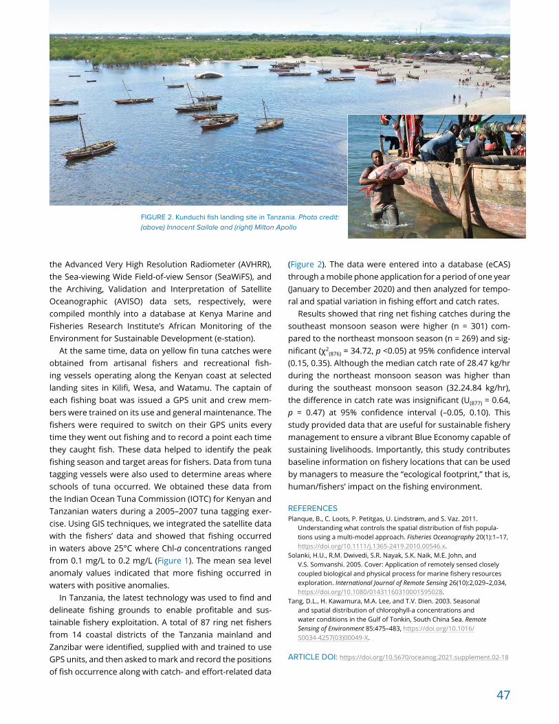
FIGURE 2. Kunduchi fish landing site in Tanzania. Photo credit: (above) Innocent Sailale and (right) Milton Apollo

the Advanced Very High Resolution Radiometer (AVHRR), the Sea-viewing Wide Field-of-view Sensor (SeaWiFS), and the Archiving, Validation and Interpretation of Satellite Oceanographic (AVISO) data sets, respectively, were compiled monthly into a database at Kenya Marine and Fisheries Research Institute’s African Monitoring of the Environment for Sustainable Development (e-station).

At the same time, data on yellow fin tuna catches were obtained from artisanal fishers and recreational fish-ing vessels operating along the Kenyan coast at selected landing sites in Kilifi, Wesa, and Watamu. The captain of each fishing boat was issued a GPS unit and crew mem-bers were trained on its use and general maintenance. The fishers were required to switch on their GPS units every time they went out fishing and to record a point each time they caught fish. These data helped to identify the peak fishing season and target areas for fishers. Data from tuna tagging vessels were also used to determine areas where schools of tuna occurred. We obtained these data from the Indian Ocean Tuna Commission (IOTC) for Kenyan and Tanzanian waters during a 2005–2007 tuna tagging exer-cise. Using GIS techniques, we integrated the satellite data with the fishers’ data and showed that fishing occurred in waters above 25°C where Chl-a concentrations ranged from 0.1 mg/L to 0.2 mg/L (Figure 1). The mean sea level anomaly values indicated that more fishing occurred in waters with positive anomalies.

In Tanzania, the latest technology was used to find and delineate fishing grounds to enable profitable and sus-tainable fishery exploitation. A total of 87 ring net fishers from 14 coastal districts of the Tanzania mainland and Zanzibar were identified, supplied with and trained to use GPS units, and then asked to mark and record the positions of fish occurrence along with catch- and effort-related data

(Figure 2). The data were entered into a database (eCAS) through a mobile phone application for a period of one year (January to December 2020) and then analyzed for tempo-ral and spatial variation in fishing effort and catch rates.

Results showed that ring net fishing catches during the southeast monsoon season were higher (n = 301) com-pared to the northeast monsoon season (n = 269) and sig-nificant (χ2

(876) = 34.72, p <0.05) at 95% confidence interval (0.15, 0.35). Although the median catch rate of 28.47 kg/hr during the northeast monsoon season was higher than during the southeast monsoon season (32.24.84 kg/hr), the difference in catch rate was insignificant (U(877) = 0.64, p = 0.47) at 95% confidence interval (–0.05, 0.10). This study provided data that are useful for sustainable fishery management to ensure a vibrant Blue Economy capable of sustaining livelihoods. Importantly, this study contributes baseline information on fishery locations that can be used by managers to measure the “ecological footprint,” that is, human/fishers’ impact on the fishing environment.

REFERENCESPlanque, B., C. Loots, P. Petitgas, U. Lindstrøm, and S. Vaz. 2011.

Understanding what controls the spatial distribution of fish popula-tions using a multi-model approach. Fisheries Oceanography 20(1):1–17, https://doi.org/10.1111/j.1365-2419.2010.00546.x.

Solanki, H.U., R.M. Dwivedi, S.R. Nayak, S.K. Naik, M.E. John, and V.S. Somvanshi. 2005. Cover: Application of remotely sensed closely coupled biological and physical process for marine fishery resources exploration. International Journal of Remote Sensing 26(10):2,029–2,034, https://doi.org/10.1080/01431160310001595028.

Tang, D.L., H. Kawamura, M.A. Lee, and T.V. Dien. 2003. Seasonal and spatial distribution of chlorophyll-a concentrations and water conditions in the Gulf of Tonkin, South China Sea. Remote Sensing of Environment 85:475–483, https://doi.org/10.1016/S0034-4257(03)00049-X.

ARTICLE DOI: https://doi.org/10.5670/oceanog.2021.supplement.02-18

47

Since the beginning of the Industrial Revolution, CO2 emis-sions into the atmosphere have been increasing continu-ously. The ocean has been taking up at least a quarter of the excess atmospheric CO2. The CO2 that dissolves in the ocean reacts with seawater and carbonate ions, leading to a decrease in seawater pH, a process called ocean acidifica-tion (OA) and is often called the “second CO2 problem.” OA could trigger remarkable changes in the ocean’s inorganic carbon system, ultimately affecting marine ecosystems. Marine organisms that have calcium carbonate skeletons such as corals, bivalves, crustaceans, and microorganisms are especially vulnerable. It is essential to understand how OA affects biological systems in order to predict future envi-ronmental impacts on organisms and ecosystem services. 

The effects of OA on marine organisms can be evalu-ated by morphological analysis of skeleton/shell surfaces using a light stereomicroscope and scanning electron microscopy (SEM). However, such observations only docu-ment surface features, limiting quantification of the degree of OA damage. Advances in X-ray Computed Tomography (XCT) have made it possible to obtain quantitative morpho-logical information such as the volume, surface area, thick-ness, and density of target objects such as marine organ-ism shells and skeletons. XCT can also be used to construct a precise, three-dimensional morphology with microme-ter to submicrometer resolution. Very small amounts of

physical damage from OA can be detected, even if the damage is inside the skeleton.

Innovative application of the latest Micro Focus XCT (μXCT) technology to low-trophic-level microzooplankton shows that the skeletal densities of shelled pteropods (sea butterflies) and planktonic foraminifera (both shown in Figure 1) are closely related to the carbonate chemis-try of the surrounding seawater (e.g., Iwasaki et al., 2019; Ofstad et al., 2021). Such quantitative measures of skele-tal density based on µXCT analyses can be used to inform marine ecosystem models and improve predictions based on future CO2 emission scenarios.

In order to accelerate this research, we recently founded a service that provides quantitative information about the morphology and density of micro-sized objects based on µXCT (http://www.jamstec.go.jp/rcgc/e/mxct/) at no cost to users. The Global Ocean Acidification Observation Network (GOA-ON) has encouraged this initiative, whose overarching goal is to provide a global map of the biologi-cal impacts of OA on marine calcifiers. To achieve this goal, cooperation and collaboration among researchers in every country are necessary, and we encourage researchers to participate in this important project.

REFERENCESIwasaki, S., K. Kimoto, O. Sasaki, H. Kano, and H. Uchida. 2019. Sensitivity

of planktic foraminiferal test bulk density to ocean acidification. Scientific Reports 9:9803, https://doi.org/10.1038/s41598-019-46041-x.

Ofstad, S., K. Zamelczyk, K. Kimoto, M. Chierici, A. Fransson, and T. Lander Rasussen. 2021. Shell density of planktonic foraminifera and pteropod species Limacina helicina in the Barents Sea: Relation to ontogeny and water chemistry. PLoS ONE, https://doi.org/10.1371/journal.pone.0249178.

ARTICLE DOI: https://doi.org/10.5670/oceanog.2021.supplement.02-19

Quantification of the Impact of Ocean Acidification on Marine CalcifiersBy Katsunori Kimoto

FIGURE 1. (left) Shelled pteropod Limacina helicina, one of the major food sources of carnivorous zooplankton, fishes, and seabirds in the polar ocean. This pteropod has a skeleton of aragonite, a form of calcium carbonate that is more soluble than calcite. (right) Three-dimensional sectional microtomography image with density map-ping of a planktic foraminifer, Globigerina bulloides, recovered from the western North Pacific. The colors show the denser (red) and less dense (blue) parts of the carbonate skeleton.

Density (g/cm3)1.00 2.71

100 µm48

To enhance oceanographic observation capacities in the Atlantic Ocean and the Mediterranean Sea, and under the project “Observation of the Marine Environment with an Operational Oceanographic Observation System,” Morocco’s National Institute of Fisheries Research (INRH) acquired and installed its first meteorological and oceanographic buoy offshore of Dakhla, southern Morocco (Figure 1). This buoy, moored at a fixed point (23°55.1208'N, 16°11.1569'W) on October 7, 2016, is a first experiment conducted by Moroccan scientists and INRH along the Moroccan Atlantic coast. The project’s intent was to allow continuous, real-time acquisition of meteo-rological and oceanographic data from the South Morocco upwelling area, which is of great scientific, oceanographic, and environmental utility for maritime decision-making, in particular, for the marine fisheries and aquaculture sector in a context of climate change.

For surface measurements, the buoy carries meteo-rological instruments, including an anemometer (wind speed and direction) and air temperature and atmo-spheric pressure sensors. Beneath the surface, the buoy is equipped with a sensor for measuring the wave swell (height, direction, and period); a profiler for measuring the current (speed and direction) in the water column; a multi- parameter sensor that includes water temperature (range 0°–40°C), salinity (0–40 psu), fluorescence, and dissolved oxygen at a single depth level. In addition, the buoy is out-fitted with a GPS system for continuous positioning and a complete data acquisition and transmission system.

When launched, the buoy recorded and transmitted data to the Laboratory of Physics and Marine Biogeochemistry of the INRH Regional Center in Casablanca. Data process-ing allowed monitoring of the different parameters every 30 minutes. The results recorded during the month of November 2016 detected the beginning of the upwelling process that brings deep, cold, and nutrient-rich waters to the surface, increasing biological activity and intensi-fying the current (Figure 2). Surface water temperatures cooled from 22.5°C to 18.5°C on November 10, predicating upwelling during the rest of the month. Salinity followed the same evolution, decreasing from 38.5 psu to 35.6 psu, then stabilizing between 36.5 psu and 37.5 psu. The profile of dissolved oxygen concentration indicates good oxygen-ation in the area, varying between 8 mg/L and 9 mg/L until upwelling begins, when it starts to decrease below 6 mg/L for three days before returning to concentrations above 7 mg/L for the rest of the month. These conditions were accompanied by phytoplankton enrichment manifested by an increase in the concentration of chlorophyll-a from 0.08 µg/L to close to 0.12 µg/L. The pH was stable at 8

Upwelling Variability Offshore of Dakhla, Southern MoroccoBy Ahmed Makaoui, Younes Belabchir, Ismail Bessa, Abedelaziz Agouzouk, Mohammed Idrissi, Omar Ettahiri, and Karim Hilmi

FIGURE 1. This moored buoy was installed on October 7, 2016, off-shore Dakhla, southern Morocco to collect meteorological and oceanographic data. It has been out of commission since early March 2017 due to vandalism.

during November. The south to southwest marine current recorded at 10 m depth increased during the period of upwelling activity and reached 35 cm/s for the southern component and more than 40 cm/s for its western com-ponent. Maximum intensity was recorded on November 9 just before upwelling began.

While vandalism five months after buoy deployment has delayed this project coming to fruition, these early data demonstrate that the selected site for the buoy was opti-mal, recording an important correlation between hydrolog-ical and meteorological parameters, especially the change in wind strength and direction, which activates upwelling. It is a constant challenge here, and in other areas of intense fishing activity, to maintain fixed observing assets and keep them safe from vandalism and accidental damage. We are optimistic that when repairs to the buoy are complete and it is redeployed, we will be able to meet our objectives.

ARTICLE DOI: https://doi.org/10.5670/oceanog.2021.supplement.02-20

FIGURE 2. Profiles show the evolution of hydrological and wind parameters collected by the buoy in November 2016. WSN = Water speed north. WSE = Water speed south.

Water Temperature

Salinity

Dissolved Oxygen

232221201918

403938373635

1098765

°Cps

um

g/l

NOVEMBER 1–30, 2016WSN 10 m & WSE 10 m

Chlorophyll-a

Wind Speed

20–10–40

20–20–60

0.140.130.120.110.100.09

141210

86420

cm/s

µg/l

m/s

0–0.50.5–11–22–44–88–1212–1616–18

Functions Analyzed: Wind Direction – Wind Speed

0

180

90270

315

225

45

135

200

100

0

49

Signatory states to the Paris Agreement are required to formulate and implement national climate action (NCA) plans to direct their nationally determined contributions (NDCs) in reducing greenhouse gases (GHGs) and in partic-ular carbon dioxide (CO2) emissions (UNFCCC, 2015). The NCA plans address CO2 management for all components of society, be it food, mobility, energy, or consumption. The extent to which NCA plans are in line with the overall tar-gets will be assessed during global stocktakings, with the first one scheduled for 2023. Limiting global temperature increase by reducing GHG and CO2 emissions will depend crucially on natural, non-anthropogenic sink efficiency. The ocean currently removes 25%–30% of the CO2 emit-ted to the atmosphere by human activities (Friedlingstein et al., 2020), thereby providing, alongside other critical eco-system services, an important societal wealth contribution via CO2 sequestration.

From the above results, it is obvious that the ocean CO2

monitoring system must be able to determine the present and future CO2 uptake with sufficient accuracy. To justify the effort involved, it is also useful to determine the mon-etary value of the oceanic sink. This can be done in three ways: a cost-benefit analysis (CBA), a cost-effectiveness analysis (CEA), or a market-based CO2 pricing approach. CBA and CEA both use shadow prices in their calculations that measure the social costs of emitting a marginal tonne of carbon1, whereas market prices are used in national accounting to compute, for example, the gross domestic product. In CBA, shadow prices are derived from estimates of costs of climate change impacts. In CEA, shadow prices are derived under a given target, such as a temperature

target as defined in the Paris Agreement. Put simply, CBA provides information on how much wealth is generated by the ocean in terms of reducing climate change, and CEA provides information on how much wealth is generated by reducing emissions abatement costs for the given target. The latter information is in most cases more reliable and can also be obtained with a market-based approach, given the regulatory framework and that a market is in place. Observed CO2 prices can also be used to assess the value of CO2 sinks, even though these sinks are not involved in trading. The market and the underlying regulatory frame-work are ideally designed to regulate anthropogenic activities, so given natural CO2 sequestration, targets like net-zero CO2 can be achieved. However, a weakening of natural sinks implies, in turn, that faster reductions and additional atmospheric CO2 removal will be required. Similarly, the market price would increase given that a weakening of CO2 sinks is expected to be considered in the underlying regulatory framework, defining the scarcity in a given CO2 market.

Hence, highly reliable information about current and future ocean CO2 sinks provides value information for policymakers to properly align the regulatory framework, and for the business community to form realistic CO2 price expectations. Furthermore, CO2 sequestration by ocean sinks varies regionally—and 38% of the global ocean com-prises territorial waters (Figure 1). Considering the regional variations in CO2 emissions and in sink activity implies that the CO2 wealth effects vary considerably for different coun-tries (Bertram et al., 2021). Although regional differences in terrestrial CO2 sinks are considered in national emissions

Valuing the Ocean Carbon Sink in Light of National Climate Action PlansBy Johannes Karstensen, Wilfried Rickels, Pierre Testor, and Maciej Telszewski

1 Marginal cost of the impacts caused by emitting one extra tonne of carbon dioxide at any point in time.

inventories, regional ocean sink con-tributions are not yet included in the determination of international bur-den sharing regarding CO2 emissions abatement. Thus, the current frame-work favors countries with large ter-restrial CO2 sinks to the disadvantage of countries with large territorial ocean sinks. However, costs of ocean CO2 fluxes are highly interconnected: vari-ability in the global ocean CO2 uptake of atmospheric CO2 will influence the CO2 uptake in territorial waters.

FIGURE 1. World Ocean territorial boundaries and Exclusive Economic Zones (EEZs).

Boundary Type

EEZ TypeEEZ

Joint Regime

Contested

200 Nautical Miles

Treaty Line

Median Line

Joint Regime

Contested

50

Therefore, improved and reliable estimates of ocean CO2 uptake are required to properly steer the ambitious levels included in the NDCs, to allow for improved burden sharing, to attribute territorial ocean CO2 uptake appropriately to countries, and to account for ocean carbon diox-ide removal (CDR). Current scenarios still focus predominantly on terrestrial CDR, mostly because economic integrated assessment models are not yet capable of properly modeling ocean CDR. Given an increasing requirement for CDR due to the weakening of CO2 sinks, the necessary net CO2 emissions path is unlikely to be achiev-able without ocean CDR solutions, for example, ocean alkalinity management. However, properly

A key aspect for use of data in the context of NCA plans is the global harmonization of error/uncertainties esti-mates that, for the ocean interior, are based on Reference Material (RM). In order to integrate the benefits of RM into a multiplatform observing system, a reference grid of long-term, sustained observations made using RM needs to be maintained. That in turn is used as a reference for sec-ondary quality control of observations that do not allow direct RM traceability (e.g., expendable sensors or devices with exceptionally long endurance under harsh conditions and impacted by biofouling). IOCCP works directly with the Surface Ocean CO2 NETwork (SOCONET) and the Global Ocean Ship-based Hydrographic Investigations Program (GO-SHIP) to assure global coordination related to data quality standards and protocols. At a regional scale, the station labeling procedure of the Ocean Thematic Center (OTC) of the European Research Infrastructure Integrated Carbon Observation System-Ocean Thematic Centre (ICOS-OTC) is a prime example of successful implementation of data management procedures that result in delivery of high-quality information with known uncertainty. ICOS-OTC also focuses on other greenhouse gases, and the OTC maintains thematic centers to coordinate atmospheric and terrestrial domains to deliver sustained, truly inte-grated observations that benefit a variety of stakeholders.

REFERENCESBertram, C., M. Quaas, T.B.H. Reusch, A.T. Vafeidis, C. Wolff, and

W. Rickels. 2021. The blue carbon wealth of nations. Nature Climate Change 11:704–709, https://doi.org/10.1038/s41558-021-01089-4.

Friedlingstein, P., M. O’Sullivan, M.W. Jones, R.M. Andrew, J. Hauck, A. Olsen, G.P. Peters, W. Peters, J. Pongratz, S. Sitch, and others. 2020. Global carbon budget 2020. Earth System Science Data 12:3,269–3,340, https://doi.org/10.5194/essd-12-3269-2020.

UNFCCC (United Nations Framework Convention on Climate Change). 2015. Adoption of the Paris Agreement, 21st Conference of the Parties, United Nations, Paris.

ARTICLE DOI: https://doi.org/10.5670/oceanog.2021.supplement.02-21

FIGURE 2. Sketch of carbon fluxes for an arbitrary EEZ bounded by a seafloor (gray).

assessing CDR via ocean-based measurements, which will be part of future NDCs, requires accounting for the feed-back of territorial ocean CO2 uptake on global CO2 uptake.

In general, the assessment of ocean CO2 sequestration must be based on understanding the processes of and monitoring both fluxes and storage of CO2 in the ocean—from regional to global scales. The processes controlling CO2 in the ocean are often separated into “solubility pump” (controlled by physics and biogeochemistry) and “biological pump” (controlled by biochemistry and biology) concepts. However, these two pumps are interlinked via underlying processes and may also counteract each other in the matter of net CO2 uptake; for example, in highly pro-ductive upwelling regions, the CO2 sink created by the bio-logical pump may compensate for the outgassing of CO2 driven by the solubility pump (Figure 2). Carbon assess-ments require determining the efficiency of both pumps and coordination of the underlying ocean observations that make use of multiple platforms (ships, underwater as well as surface autonomous vehicles, floats, moorings, and satellites) equipped with sensors and samplers employ-ing a diverse pool of sensing technology (optical, particle probes, electrochemical) and operating at varying levels of technological readiness.

Data harmonization and quality control along with FAIR (Findable, Accessible, Interoperable and Reusable) access to data permit a wide spectrum of applications across dis-ciplines and needs, and they must be ensured to enable integration of the various data streams into regional and global carbon products. Regional (and global) carbon data products with sufficient temporal and spatial res-olutions are required for assigning values to Exclusive Economic Zone CO2 sinks. Global coordination of observa-tional efforts, science approaches, and coordination with global syntheses are performed under the auspices of the International Ocean Carbon Coordination Project (IOCCP).

51

TOPIC 4. POLLUTANTS AND CONTAMINANTS AND THEIR

POTENTIAL IMPACTS ON HUMAN HEALTH AND ECOSYSTEMS

An Integrated Observing System for Monitoring Marine Debris and BiodiversityBy Nikolai Maximenko*, Artur P. Palacz*, Lauren Biermann, James Carlton, Luca Centurioni, Mary Crowley, Jan Hafner, Linsey Haram, Rebecca R. Helm, Verena Hormann, Cathryn Murray, Gregory Ruiz, Andrey Shcherbina, Justin Stopa, Davida Streett, Toste Tanhua, Cynthia Wright, and Chela Zabin (*equal first authors)

MARINE DEBRIS AND PELAGIC ECOSYSTEMSWood, pumice, drifting kelp, and other natural marine debris have long played important roles in marine eco-systems. Today, oceanic “litter” generated by human activ-ities, notably plastics, constitutes the majority of marine debris and is mostly harmful to those ecosystems. In the twentieth century, plastic became a symbol of technologi-cal development and globalization of the world’s economy. Cheap, durable, and long-lasting, with a broad variety of properties that are attractive for an array of human uses, plastic penetrated all parts of business and everyday life. In recent decades, growing demand exponentially increased plastic production. Ironically, the negative environmental impacts of plastic are in part an extension of some of the very properties that make it popular, such as its durabil-ity and wide availability. Plastic degrades with time into

microscopic particles that have been found in every corner of the natural world—on land, in lakes and rivers, and in the ocean. This phenomenon has led to a new description of the present era as the Plasticene: “an era in Earth’s his-tory, within the Anthropocene, commencing in the 1950s, marked stratigraphically in the depositional record by a new and increasing layer of plastic” (Haram et al., 2020).

A significant fraction of plastic in the ocean has sources located on land. Depending on chemical composition, some plastic entering the ocean sinks instantly, but the majority is buoyant and remains floating at the ocean’s surface for various durations. The fate of marine debris depends on ocean currents, winds, and waves, which together move floating objects and can transport them over long distances. Some debris released into the ocean transits between distant locations and pollutes remote

FIGURE 1. (a) A Hawaiian beach is covered with mixed plastic debris. (b) This large derelict fishing net was found and tagged with an Ocean Voyages Institute GPS tracker (marked with an arrow). Photo credits: (a) Sustainable Coastlines Hawai’i (https://www.sustainablecoastlineshawaii.org/), (b) Greenpeace

a

b

52

shorelines (Figure 1a). For example, many boats, floats, and other plastic items introduced into the ocean during the March 11, 2011, tsunami in Japan traveled thousands of kilometers to the shores of Hawai‘i and the west coast of North America (Carlton et al., 2017; Figure 2). Other debris (Figure 1b) gets trapped in convergence zones (so-called “garbage patches”) created by large-scale ocean currents in the five subtropical gyres (Figure 3), where it may remain for years or even decades.

Habitats around these convergence zones are charac-terized by low nutrient conditions and relatively low bio-logical activity compared to coastal zones. A potentially important source of biomass in these pelagic ecosystems is neuston, assemblages of various species that float on or live close to the ocean’s surface (Figure 4). Neuston are moved around the ocean by physical processes similar to those that move floating marine debris, and there is theo-retical expectation and observational evidence that neus-ton and debris follow similar pathways and accumulate in the same areas on the ocean’s surface. Little is known about interactions between neuston and marine debris, but we do know that larger biota, including marine mam-mals, turtles, birds, and fish that feed on neuston, can be harmed through entanglement in derelict fishing nets or by ingestion of small objects. Monitoring the status and trends of these interactions would thus benefit from an integrated monitoring approach that addresses national and/or regional policy requirements for both marine pol-lution and marine biodiversity.

Large-scale introduction of anthropogenic debris into the ocean has triggered fundamental changes in the relative

FIGURE 2. Main pathways traveled by debris from the 2011 tsunami extend from eastern Japan to Hawai‘i and North America, back to Asia, and into the North Pacific Garbage Patch. The map is the model solution for September 2011. Colors correspond to different types of debris that exhibited low (blue) to high (red) windage or buoyancy. Credit: US Navy, US Coast Guard, Randal Reeves, Jeffrey Milisen, Carlton et al. (2017), Maximenko et al. (2018)

90°N

60°N

30°N

0°

30°S

60°S

90°S0° 45°E 90°E 135°E 180° 135°W 90°W 45°W 0°

FIGURE 3. Global distribution of plastics, simulated with a numerical model. Red colors indicate the highest concentrations, while blue colors are the low-est. From van Sebille et al. (2015)

Grams per km2

1 101 102 103 104 105

FIGURE 4. Select species of neuston. Floating cnidarians (a) Porpita porpita and (b) Velella velella. (c) Floating snail Janthina sp. (d) Portuguese man-o-war Physalia sp. (e) Neustonic nudibranchs Glaucus spp. (f) Neustonic buoy bar-nacles Dosima sp. Image credits (Wikimedia commons): (a) Bruce Moravchik (NOAA). (b) Doug Beckers. (c) Peter de Lange. (d) Islands in the Sea 2002, NOAA/OER. (e) Taro Taylor. (f) Kenneth Allen

a

ed

b c

f

53

FIGURE 5. Examples of Japanese coastal species found among tsu-nami debris in North America and Hawai‘i. Photo credits: (photos of floating log and dock) Randal Reeves; Carlton et al. (2017)

abundance of different species, species interactions, and thus energy flow. Due to the slow breakdown of plastic compared to many natural debris items, floating marine debris can be adopted as a substrate for attachment by coastal species. Where formerly there were natural barriers to the dispersal and survival of coastal biota, marine debris is providing new opportunities for them to travel across ocean basins. Feasibility of such travel was demonstrated by, among others, Carlton et al. (2017) and Hansen et al. (2018), who reported at least 373 coastal Japanese species found on tsunami debris washed up on US and Canadian shorelines (Figure 5). Moreover, Haram et al. (2021) discov-ered that the high concentration of marine debris in the North Pacific Garbage Patch now allows coastal species to establish and reproduce there, creating a neopelagic eco-system. This system may then further facilitate potential biological invasions into coastal areas. It is also suggested that degrading plastic debris may release carbon accessi-ble to marine microbes that in turn could alter the entire food web (Romera-Castillo et al., 2018).

The need to significantly reduce the amount of plas-tic in the ocean is recognized by the United Nations (UN) as Sustainable Development Goal (SDG) Target 14.1: “By 2025, prevent and significantly reduce marine pollu-tion of all kinds, in particular from land-based activities, including marine debris and nutrient pollution.” The UN Environment Programme (UNEP) provides a guide for com-piling pollution indicators, including Indicator 14.1.1b on plastic debris density, whose measurements will require combining traditional monitoring techniques with new technologies and data science (UNEP, 2021). Addressing critical knowledge gaps around the fate of marine plastics and other debris and their impacts on marine ecosystems requires coordinated, multidisciplinary, large-scale obser-vations of marine debris in the ocean. This effort will be

made possible through close integration with the Global Ocean Observing System (GOOS; https://www.goosocean.org), which already coordinates a global system of ocean observing platforms (e.g.,  ships, buoys, satellites, auton-omous vehicles) that provides essential information on ocean physics and climate, biogeochemical cycles, and biological and ecosystem processes.

NOVEL APPROACHES TO MONITORING MARINE DEBRIS AND ASSOCIATED PELAGIC ECOSYSTEMSCollecting comprehensive observations of marine debris and marine life in the pelagic ocean is tremendously dif-ficult. Pelagic ecosystems contain diverse species, each having its own life cycle and each responding differently to changing environmental conditions. Interactions among species produce an even larger number of monitoring and research challenges. Similarly, marine debris objects vary broadly in their chemical (e.g.,  polymers, additives, and degree of degradation) and physical (e.g., size, geometry, and buoyancy) properties. In addition to plastic, marine debris includes other artificial materials as well as debris linked directly to human activities (e.g., logging) or natural disasters (e.g., floods, hurricanes, or tsunamis).

Given limited scientific resources available in the open ocean and patchy distributions of marine debris items and pelagic species, it is critical to develop and implement effective observational tools that target specific scientific questions or applications, including the following:• How much anthropogenic and natural debris is in the

ocean?• What are the physical and chemical compositions of the

debris?• What are the main sources, pathways, spatial patterns,

and areas of impact on marine ecosystems?

54

• What is the composition of neopelagic communities, what environmental variables control species’ life cycles, and how do they interact with plastic debris?

• What changes take place in marine ecosystems rela-tive to the distributions of marine debris and how are they related to natural variability and ongoing climate change?

• What is our capacity to predict these changes?

Water-Following (Lagrangian) InstrumentsDrifters (oceanographic instruments that are composed of a surface float tethered to a drogue) and subsurface floats are actively used to measure ocean currents, an essential ocean variable. For example, the Global Drifter Program (https://gdp. ucsd.edu/ ldl/ global- drifter- program/) main-tains a network of more than 1,300 drifters covering all ocean basins. Drifter trajectories can be used as a proxy for pathways of marine debris and neuston and to estimate drift velocities. By using standardized designs for drogued and undrogued drifters (Figure 6), their responses to var-ious ocean conditions can be understood and their data used to improve numerical ocean models, which help us to understand the many ways in which the ocean influences weather and climate. Studies establishing correspondence between the dynamics of standard drifters and different types of debris and biota are underway, and new types of drifters may be needed to reproduce pathways of particu-lar debris types, such as fishing nets. A great deal of infor-mation on ocean surface currents is also captured through

satellite measurements that allow for integration of prod-ucts from multiple satellite missions.

Some types of marine debris, such as microplastics and items that contain a lot of biological growth, have weak buoyancy. They are easily mixed downward into the water column by wind-induced turbulence and may remain below the surface. Similarly, some neustonic spe-cies may have pelagic life-cycle stages that exist below the surface waters. With the commonly strong vertical shear of near-surface currents, these vertical movements can significantly affect the horizontal transport of debris and neuston. Understanding these effects is a difficult task given that existing methods do not allow us to follow submerged objects. However, scientific instruments can be programmed to mimic the dynamics of debris or the life cycle of certain biota. For example, the buoyancy of a mixed layer float that was used in the National Aeronautics and Space Administration (NASA) funded FloatEco (Floating Ecosystem) experiment (Figure 7; https://floateco.org) could be carefully calibrated under varying ocean con-ditions. Timelines of its residence in the mixed layer of the ocean can be analyzed and compared with vertical profiles of microplastics.

FIGURE 6. These Surface Velocity Program (SVP) drifters from the Lagrangian Drifter Laboratory (https://gdp.ucsd.edu/ldl/) at the Scripps Institution of Oceanography were equipped with biological settlement panels (marked with arrows) and used for the FloatEco project. Photo credit: The Vortex Swim

FIGURE 7. NASA FloatEco subsurface Lagrangian (water-following) float outfitted for collecting physical and biological observations. The float can be programmed to alter its buoyancy to simulate the behavior of various types of marine debris or to explore the water column freely. Information on the surrounding water properties and photos of the emerging neopelagic ecosystem (inset) are relayed to shore in near-real time via a satellite uplink. The arrows in the inset mark two juvenile fish with the set-tlement panels in the background. Float imagery credit: Ocean Voyages Institute

SettlementPanels

Camera

55

New methods also allow scientists to track selected large objects. For example, since 2018, the Ocean Voyages Institute (OVI; https://www.oceanvoyagesinstitute.org/) has operated dozens of Global Positioning System (GPS) trackers (Figure 1b), the majority of them attached to der-elict fishing gear, the most harmful marine debris. The trackers have helped OVI collect hundreds of tons of derelict fishing gear and provided unique data for scientific research on the dynamics of floating debris.

Field SamplingIn situ samples are critical for monitoring marine ecosystems and marine debris distributions, validating models, and testing scientific hypotheses. To produce high-quality and timely data on marine debris and biofouling as well as neustonic biota, existing observing systems must be strength-ened and complemented with new methods and platforms. In some cases, significant progress can be achieved through coordination among exist-ing observing programs and adjustments to protocols to integrate obser-vations of debris and associated biology. For example, settlement panels (typically simple, square PVC tiles) can be attached to debris to provide information such as the rate of colonization and the community structure of colonizing species (Figure 8b). Use of such panels together with drift-ers and floats (Figures 6 and 7) opens opportunities for advanced scien-tific experiments designed to address important questions of biological- physical interactions among species, their biogeography, and how spe-cies are responding to global changes.

Citizen ScienceScientific expeditions are expensive and often have a narrow focus. At the same time, science plays an ever-increasing role in society, partly through non-scientists’ growing accessibility to cutting-edge scien-tific resources. Engagement with the public in science is supported by national and international programs (e.g.,  https://science.nasa.gov/ citizenscience; https://citizenscience.org/) and creates opportunities to fill important gaps in our observing systems. Also, as stakeholders, cit-izen scientists inspire important new applications that require support with observational data.

Recent successful cooperation with the ocean sailing community allowed for microplastic sampling over large areas of the ocean (Tanhua et al., 2020). Another remarkable example of reciprocal work between scientists and citizen scientists is the collaboration between the FloatEco team and OVI. OVI deployed and retrieved instruments operated by the FloatEco team and collected a representative set of samples of biofouled marine debris (Figure 8). In turn, FloatEco helped OVI to optimize oper-ations by using numerical models and mobilizing additional volunteers who tagged debris with OVI’s GPS trackers (Figure 9b,c). Haram et  al. (2021) highlight this collaboration, which has developed into the GO-SEA program (https://goseascience.org/), a new NASA-affiliated project that serves to expand the connections between community members and

FIGURE 8. Collection of biological and plastic samples during cleanup operations. A set-tlement panel enclosed in a protective cylindrical base is marked with an arrow in (b). Photo credits: Ocean Voyages Institute

a

b

c

d

56

scientists by including sailors and beachgoers in its network. Development of observational protocols and methods for sample collection, preserva-tion, and measurements will further increase the contributions of volun-teers to scientific studies.

The large “beachcomber” community can play an important role in documenting marine debris and biota stranded on shorelines. Reports collected through platforms such as iNaturalist (https://www.inaturalist.org/) can further reveal what is floating on the open ocean and timelines for its arrival ashore. If synthesized with numerical models and satellite images, debris observations from coastal community members can also inform our understanding of ocean circulation patterns as well as debris and neuston trajectories, yielding further insight into processes taking place far from the coast. New, exciting approaches combining citizen sci-ence macro- and microplastic sampling with simultaneous monitoring of marine debris and automatic sensor observations of physical and bio-chemical essential ocean variables have the potential for further expan-sion of interaction studies between marine plastic pollution and neuston.

Standardization and Automation of In Situ ObservationsBecause marine debris and biota have complex compositions, full proto-cols of observations and data collection are also complex, and processing of samples and data in the laboratory is labor intensive. The community needs to agree on standard protocols for sampling and laboratory ana-lytical methods to allow comparison of data collected during different campaigns. One possible way to significantly increase the data flow is by developing sensors and systems that can operate autonomously and generate large volumes of data with consistent format and quality. Once available, such sensors and systems could be used on ubiquitous plat-forms, such as commercial ships, as well as autonomous vehicles (such as drones and gliders).

Remote SensingBecause of the patchiness of floating debris and pelagic marine com-munities, satellites are the only platforms capable of capturing the “big picture.” They are critical tools for observing the most inaccessible regions of the ocean and detecting anomalies in near-real time. Space agencies and groups have expressed great interest in this new appli-cation of remote sensing. The Portugal Space Agency (https://www.moonshotchallenge.ai/) and NASA recently funded several exploratory projects, and the schedule of Sentinel-2 operated by the European Space Agency (https://sentinel.esa.int/web/sentinel/missions/ sentinel-2) was changed for July–September 2021 to include the area of the North Pacific Garbage Patch. Additionally, the International Ocean Color Coordination Group has created a Remote Sensing of Marine Litter and Debris Task Force (https://ioccg.org/rsmld-news-and-updates/). More and more proj-ects report test results, in which pre-set targets have been successfully detected by drones and/or satellites, including patches of mixed floating

FIGURE 9. Citizen scientists are pictured (a) inspecting drifting buoys, (b,c) tagging marine debris, and (d) collecting samples. Photo credits: (a) The Longest Swim, (b,d) The Vortex Swim, (c) eXXpedition

a

b

c

d

57

FIGURE 10. These photos show small-scale ocean phenomena (i.e.,  slicks, windrows, fronts, and eddies) that accumulate debris and neuston. Debris from the 2011 tsunami is shown east of Japan (a) photographed from heli-copter and (b) imaged by the Aster satellite. (c) High concentration of plastic fragments accumulating along a slick (dashed line). (d) Sentinel-1 synthetic aperture radar image of slicks trapped in ocean eddies. (e) Accumulation of the neuston species Velella velella off the coast of Washington State, USA. (f) A true color image acquired by the Sentinel-2 Multispectral Instrument (MSI) shows open-ocean slick formations within the North Pacific Garbage Patch. (g,h) Near-infrared imagery acquired by the Sentinel-2 MSI shows sea-weed aggregated and concentrated inside windrows and slicks off Ghana and UK coastlines, respectively. Scales added to the panels are approx-imate. Image credits: (a) US Navy, (b) NOAA, (c) Algalita Research and Education Foundation, (d,f,g,h) the European Space Agency and Copernicus Programme, (e) Scott Horton

) 2 km

1 km

100 m

5 km

a b

20 m

)

5 kmc d

)

10 m

e

)

2 km

g

f h

debris in coastal waters (Figure 10). Signals from marine debris and biota are often co-located in satellite images due to biofouling or concentration of debris, neuston, and/or macro algae in ocean slicks and other phenom-ena. Laboratory studies and machine learning further support the feasibility of remote-sensing applications. However, much more effort will be required to build on these early successes. Difficulties remain partly because all existing satellites were designed and built for very different applications, without marine debris or biodiversity detection in mind.

Development of new remote sensors is important because often the same technology can be replicated on many scales, from satellites to suborbital platforms, shipborne systems, drones, hand-held tools, and even in situ sensors. These sensors will generate unique opportunities for intercalibration and interscaling of data products.

THE WAY FORWARD: INTEGRATION AND COORDINATION OF OBSERVATIONAL RESOURCESThe complexity of marine debris composition and asso-ciated biological communities, as well as the diversity of tools and methods available to monitor and observe them, require coordinated approaches that harmonize regional efforts into a global system without losing the col-lection of any important indicators. At the OceanObs’19 conference (https://www.oceanobs19.net/), a large group of experts from many disciplines proposed the concept of an Integrated Marine Debris Observing System (IMDOS) that would mobilize all available resources to work together to provide a hierarchy of data products and applications needed by stakeholders (Maximenko et al., 2019). The envisioned system com-bines in situ observations and sampling, providing cali-bration of indirect information and validation for mod-els, with remote sensing yielding a big-picture view and models optimizing and interpreting field observations and forecasting future changes.

Considering that critical knowledge gaps exist around the cycling of marine debris in the ocean and the interaction of marine debris with various ecosystem components, further IMDOS development will include better integration of marine debris monitoring with biogeochemical, biological, and ecosystem observa-tions (including biodiversity and ocean health indica-tors) coordinated by GOOS and the Marine Biodiversity Observation Network (https://marinebon.org/). Suc-cessful integration depends on identifying common requirements for observed variables including accuracy

58

and spatiotemporal resolution, sharing platforms, and augmenting sampling protocols, as well as harmonizing data streams across disciplines.

GOOS coordinates a large network of ship-based, fixed-point, autonomous, and other platforms that monitor the open and coastal oceans, but its potential for measuring marine pollution remains strikingly underutilized. There is potential for co-located oceanographic (both surface and water column) observations of marine debris; co- designed environmental monitoring of marine habitats (e.g.,  seagrass and macroalgae) with seafloor debris sur-veys; or better interfacing the rapidly evolving capacity of remote-sensing detection with environmental monitoring to expand and validate modeling and scientific assess-ments toward informed decision-making.

GOOS aims to support the community in establishing IMDOS as a backbone observing system for delivering data to strengthen scientific knowledge about marine debris pollution. In particular, the aim is to establish a globally coordinated network that observes debris floating on the ocean’s surface. The envisioned observing network will build on global harmonization of monitoring meth-ods and data sharing initiatives supported by the Japan Ministry of the Environment and G20 countries. It will consider viable observing methods and platforms follow-ing GESAMP Working Group 40 (http://www.gesamp.org/work/groups/40) guidelines as well as the feasibility and cost analysis of augmenting existing standard operating protocols of relevant GOOS observing networks. The net-work’s status, progress, and performance could be visu-alized through the OceanOPS real-time dashboard and toolbox (https://www.ocean-ops.org/board). The network would also bring together different citizen science initia-tives aimed at collecting observations of debris and asso-ciated biota from non-commercial (i.e.,  sailing and other recreational) vessels. This activity will further be included in the larger cooperation effort led by OceanOPS within the UN Ocean Decade project Odyssey.

Many components of a future IMDOS are already being implemented, although global coordination of these efforts has not yet been achieved. Advances include expanding collaborations among remote-sensing and in situ monitoring groups and among scientists and environmental groups, harmonizing and standardiz-ing methods of marine debris sampling and monitoring (e.g.,  https://www.euroqcharm.eu/en for microplastics), developing global data synthesis products enabled by the growing number of international databases (e.g., Isobe et al., 2021) and experiments such as FloatEco, and implementing new sensors (e.g., https://www.oceandiagnostics.com/).

As the United Nations Decade of Ocean Science for

Sustainable Development (2021–2030) focuses attention on ocean health, the development of interdisciplinary connections between scientists, the public, and other stakeholders will allow the community to identify and act upon the most important issues associated with anthropo-genic marine debris.

REFERENCESCarlton, J.T., J.W. Chapman, J.B. Geller, J.A. Miller, D.A. Carlton,

M.I. McCuller, N.C. Treneman, B.P. Steves, and G.M. Ruiz. 2017. Tsunami-driven rafting: Transoceanic species dispersal and impli-cations for marine biogeography. Science 357(6358):1,402–1,406, https://doi.org/10.1126/science.aao1498.

Hansen, G.I., T. Hanyuda, and H. Kawai. 2018. Invasion threat of benthic marine algae arriving on Japanese tsunami marine debris in Oregon and Washington, USA. Phycologia 57:641–658, https://doi.org/ 10.2216/ 18-58.1.

Haram, L.E., J.T. Carlton, G. Ruiz, and N. Maximenko. 2020. A Plasticene lexicon. Marine Pollution Bulletin 150:110714, https://doi.org/10.1016/ j.marpolbul.2019.110714.

Haram, L.E., J.T. Carlton, L. Centurioni, M. Crowley, J. Hafner, N. Maximenko, C. Murray, A. Shcherbina, V. Hormann, C. Wright, and G.M. Ruiz. 2021. Emergence of a neopelagic community through the establishment of coastal species on the high seas. Nature Communications 12:6885, https://doi.org/10.1038/s41467-021-27188-6.

Isobe, A., T. Azuma, M.R. Cordova, A. Cózar, F. Galgani, R. Hagita, L.D. Kanhai, K. Imai, S. Iwasaki, S. Kako, and others. 2021. A multi-level dataset of microplastic abundance in the world’s upper ocean and the Laurentian Great Lakes. Microplastics and Nanoplastics 1:16, https://doi.org/ 10.1186/s43591-021-00013-z.

Maximenko, N.A., J. Hafner, M. Kamachi, and A. MacFadyen. 2018. Numerical simulations of debris drift from the 2011 tsunami in Japan, verified with boat reports. Marine Pollution Bulletin 132:5–25, https://doi.org/ 10.1016/j.marpolbul.2018.03.056.

Maximenko, N., P. Corradi, K.L. Law, E. van Sebille, S.P. Garaba, R.S. Lampitt, F. Galgani, V. Martinez-Vicente, L. Goddijn-Murphy, J.M. Veiga, and others. 2019. Toward the Integrated Marine Debris Observing System. Frontiers in Marine Science 6:447, https://doi.org/ 10.3389/fmars.2019.00447.

Romera-Castillo, C., M. Pinto, T.M. Langer, X.A. Álvarez-Salgado, and G.J. Herndl. 2018. Dissolved organic carbon leaching from plastics stim-ulates microbial activity in the ocean. Nature Communications 9:1430, https://doi.org/10.1038/s41467-018-03798-5.

Tanhua, T., S.B. Gutekunst, and A. Biastoch. 2020. A near-synoptic survey of ocean microplastic concentration along an around-the-world sailing race. PLoS ONE 15(12):e0243203, https://doi.org/10.1371/journal.pone.0243203.

UNEP (United Nations Environment Programme). 2021. Understanding the State of the Ocean: A Global Manual on Measuring SDG 14.1.1, SDG 14.2.1 and SDG 14.5.1. Nairobi, 81 pp., https://wedocs.unep.org/handle/20.500.11822/35086.

van Sebille, E., C. Wilcox, L. Lebreton, N.A. Maximenko, B.D. Hardesty, J.A. van Franeker, M. Eriksen, D. Siegel, F. Galgani, and K.L. Law. 2015. A global inventory of small floating plastic debris. Environmental Research Letters 10(12):124006, https://doi.org/ 10.1088/ 1748-9326/ 10/12/124006.

ACKNOWLEDGMENTSWe thank Martin Thiel and two anonymous reviewers for their con-structive comments that helped to improve the paper. FloatEco and GO-SEA teams are partly supported by NASA’s Biodiversity and Ecological Forecasting and Citizen Science for Earth Systems Program through Grants 80NSSC17K0559 and 80NSSC21K0857, respectively. TT and AP received funding from the European Union’s Horizon 2020 research and innovation programme under grant agreement No 862626 (EuroSea).

ARTICLE DOI: https://doi.org/10.5670/oceanog.2021.supplement.02-22

59

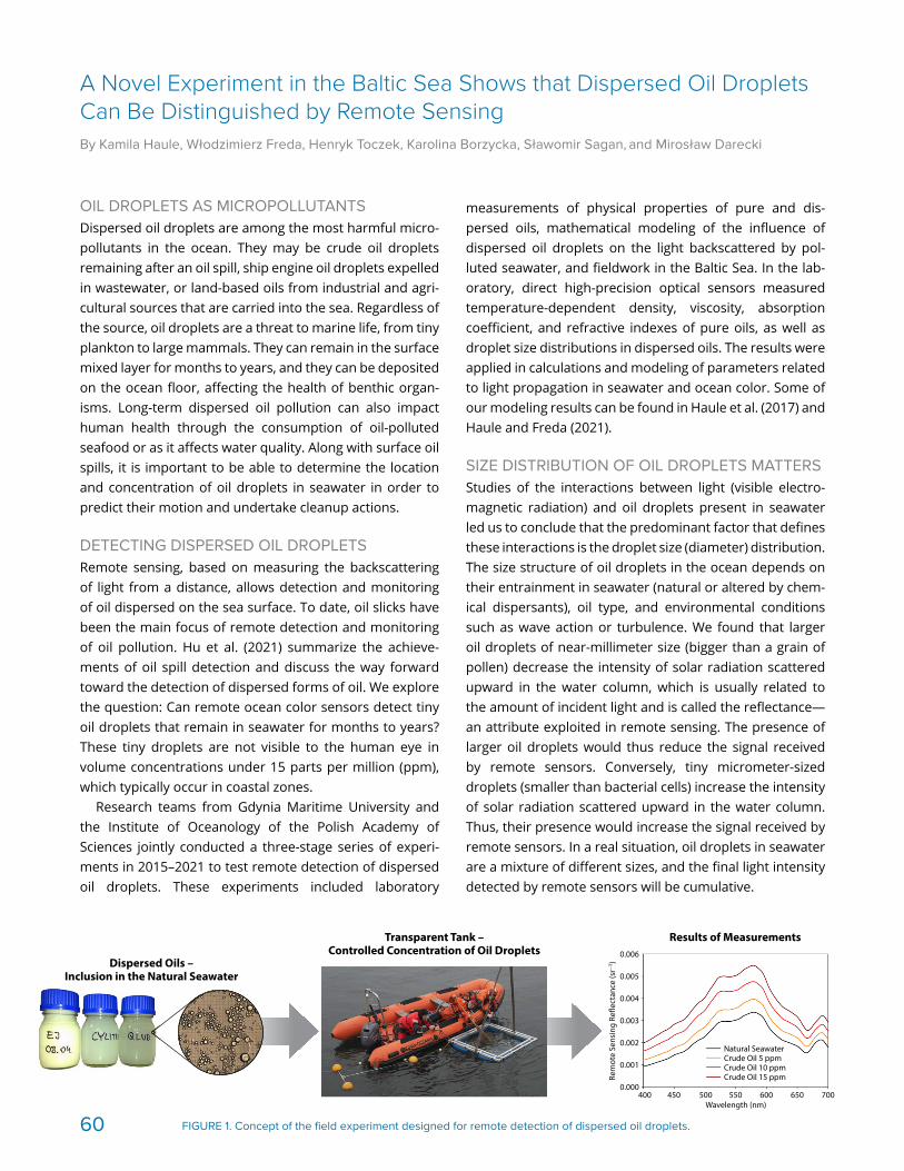
FIGURE 1. Concept of the field experiment designed for remote detection of dispersed oil droplets.

Natural SeawaterCrude Oil 5 ppmCrude Oil 10 ppmCrude Oil 15 ppm

400 450 500 550 600 650 700Wavelength (nm)

0.006

0.005

0.004

0.003

0.002

0.001

0.000

Rem

ote

Sens

ing

Refle

ctan

ce (s

r–1)

Results of MeasurementsTransparent Tank – Controlled Concentration of Oil Droplets

Dispersed Oils – Inclusion in the Natural Seawater

OIL DROPLETS AS MICROPOLLUTANTSDispersed oil droplets are among the most harmful micro-pollutants in the ocean. They may be crude oil droplets remaining after an oil spill, ship engine oil droplets expelled in waste water, or land-based oils from industrial and agri-cultural sources that are carried into the sea. Regardless of the source, oil droplets are a threat to marine life, from tiny plankton to large mammals. They can remain in the surface mixed layer for months to years, and they can be deposited on the ocean floor, affecting the health of benthic organ-isms. Long-term dispersed oil pollution can also impact human health through the consumption of oil-polluted seafood or as it affects water quality. Along with surface oil spills, it is important to be able to determine the location and concentration of oil droplets in seawater in order to predict their motion and undertake cleanup actions.

DETECTING DISPERSED OIL DROPLETSRemote sensing, based on measuring the backscattering of light from a distance, allows detection and monitoring of oil dispersed on the sea surface. To date, oil slicks have been the main focus of remote detection and monitoring of oil pollution. Hu et  al. (2021) summarize the achieve-ments of oil spill detection and discuss the way forward toward the detection of dispersed forms of oil. We explore the question: Can remote ocean color sensors detect tiny oil droplets that remain in seawater for months to years? These tiny droplets are not visible to the human eye in volume concentrations under 15 parts per million (ppm), which typically occur in coastal zones.

Research teams from Gdynia Maritime University and the Institute of Oceanology of the Polish Academy of Sciences jointly conducted a three-stage series of experi-ments in 2015–2021 to test remote detection of dispersed oil droplets. These experiments included laboratory

measurements of physical properties of pure and dis-persed oils, mathematical modeling of the influence of dispersed oil droplets on the light backscattered by pol-luted seawater, and fieldwork in the Baltic Sea. In the lab-oratory, direct high- precision optical sensors measured temperature- dependent density, viscosity, absorption coefficient, and refractive indexes of pure oils, as well as droplet size distributions in dispersed oils. The results were applied in calculations and modeling of parameters related to light propagation in seawater and ocean color. Some of our modeling results can be found in Haule et al. (2017) and Haule and Freda (2021).

SIZE DISTRIBUTION OF OIL DROPLETS MATTERSStudies of the interactions between light (visible electro-magnetic radiation) and oil droplets present in sea water led us to conclude that the predominant factor that defines these interactions is the droplet size (diameter) distribution. The size structure of oil droplets in the ocean depends on their entrainment in seawater (natural or altered by chem-ical dispersants), oil type, and environmental conditions such as wave action or turbulence. We found that larger oil droplets of near-millimeter size (bigger than a grain of pollen) decrease the intensity of solar radiation scattered upward in the water column, which is usually related to the amount of incident light and is called the reflectance—an attribute exploited in remote sensing. The presence of larger oil droplets would thus reduce the signal received by remote sensors. Conversely, tiny micrometer-sized droplets (smaller than bacterial cells) increase the intensity of solar radiation scattered upward in the water column. Thus, their presence would increase the signal received by remote sensors. In a real situation, oil droplets in seawater are a mixture of different sizes, and the final light intensity detected by remote sensors will be cumulative.

A Novel Experiment in the Baltic Sea Shows that Dispersed Oil Droplets Can Be Distinguished by Remote SensingBy Kamila Haule, Włodzimierz Freda, Henryk Toczek, Karolina Borzycka, Sławomir Sagan, and Mirosław Darecki

60

a

b

c

d

e

f

MEASUREMENTS IN THE BALTIC SEAOur Baltic Sea measurements demonstrated the possibility of remote (airborne or satellite) detection of oil droplets in seawater under real field conditions. Optical data were collected in a specially designed floating transparent tank with a volume of about 1 m3. This configuration limited the oil-polluted area and allowed us to keep the oil droplet concentration stable, with minimal disturbance from surrounding waters but maintaining near-natural conditions. Figure 1 shows the experiment concept and an example result. Figure 2 photos display each step of the field experiment.

The main field experiment was conducted from the research vessel Oceania in the coastal zone of the southern Baltic Sea. Three types of oil were dispersed in our experiment tank: crude, biodiesel, and mineral in five consecutive concentrations, from 1 ppm to 15 ppm, the concentration range permitted for the effluent and drain-age of vessels under the International Convention for the Prevention of Pollution from Ships (MARPOL 73/78 and its subsequent annexes). It is worth emphasizing that all oil types noticeably increased the intensity of solar radiation backscattered in the water column and detected by remote sensors, indicating that the signal from unpolluted seawater differs from the signal of seawater polluted by oil droplets, and that difference carries information on the presence and properties of dispersed oil.

We found that different oil dispersions tended to affect different spectral regions of visible light. Some oils made the seawater appear redder, some greener, and others bluer compared to seawater without any oil droplets. These subtle changes were complex, combined effects of oil type and size distribution. For example, a light crude oil that consisted mostly of fine submicron droplets made seawater appear bluer, and a medium-heavy crude oil that included significantly more larger drop-lets made seawater appear redder. Biodiesel added more blue and red light to the signal, while some mineral oils made seawater appear redder or greener. Moreover, we found that the modification of the remote signal by dispersed oil droplets can be enhanced or reduced depending on the state of the natural seawater being exam-ined. For example, it is easier to detect dispersed oil in clear open ocean waters than in turbid coastal zones. Seawater rich in phytoplankton or other suspended particles usually produces a lower reflectance signal than clear water, and thus the difference made by the presence of low concentrations of oil droplets may be too small to be detected. Details of the field experiment are discussed in Haule et al. (2021).

REFERENCESHaule, K., W. Freda, M. Darecki, and H. Toczek. 2017. Possibilities of optical remote sensing of dis-

persed oil in coastal waters. Estuarine, Coastal and Shelf Science 195:76–87, https://doi.org/10.1016/ j.ecss.2016.07.013.

Haule, K., and W. Freda. 2021. Remote sensing of dispersed oil pollution in the ocean—The role of chloro-phyll concentration. Sensors 21:3387, https://doi.org/10.3390/s21103387.

Haule, K., H. Toczek, K. Borzycka, and M. Darecki. 2021. Influence of dispersed oil on the remote sensing reflectance—Field experiment in the Baltic Sea. Sensors 21:5733, https://doi.org/10.3390/s21175733.

Hu, C., Y. Lu, S. Sun, and Y. Liu. 2021. Optical remote sensing of oil spills in the ocean. What is really possi-ble? Journal of Remote Sensing 2021:9141902, https://doi.org/10.34133/2021/9141902.

ACKNOWLEDGMENTS This research was funded by the National Science Centre of Poland, grant no. UMO-2012/05/N/ST10/03707 and the statutory research program of the Institute of Oceanology of the Polish Academy of Sciences.

ARTICLE DOI: https://doi.org/10.5670/oceanog.2021.supplement.02-23

FIGURE 2. Photos from the experiments: (a) Preparation of the tank on the ship deck. (b) Placing the tank on the sea surface. (c) Adding dispersed oil (visible white area below the surface). (d) Mixing dispersed oil in the tank. (e) Setting the upwelling radiance sensor. (f) Moving away to monitor measurements.

61

SOUNDSCAPE DEFINEDSound travels further through water than light and is one reason why many marine animals use sound to commu-nicate and gain information about their surroundings. Scientists collect recordings of these underwater sounds to gain information on species’ habitat use, abundance, distribution, density, and behavior. In waters where visibil-ity is severely limited or access is difficult or cost-intensive, passive acoustic monitoring is a particularly important technique for obtaining such biological information over space and time.

The “soundscape” of an ecosystem is defined as the characterization of all the acoustic sources pres-ent in a certain place (Wilford et  al., 2021). A sound-scape includes three fundamental sound source types (Figure 1): (1) anthropophony, or sounds associated with human activity; (2) biophony, or sounds produced by ani-mals; and (3) geophony, or sounds generated by physical events such as waves, earthquakes, or rain (Pijanowski et  al., 2011). Studying soundscapes can provide biologi-cal information for a specific habitat, which could then be linked to ecosystem health status and other bioindicators. This information can be used to monitor the habitat over time, allowing for rapid detection of habitat degradation, such as in response to human-driven events.

Comparison of Two Soundscapes: An Opportunity to Assess the Dominance of Biophony Versus AnthropophonyBy Maria Paula Rey Baquero*, Clea Parcerisas*, Kerri D. Seger, Christina Perazio, Natalia Botero Acosta, Felipe Mesa, Andrea Luna-Acosta, Dick Botteldooren, and Elisabeth Debusschere (*equal first authors)

SOUNDSCAPE DATA ACQUISITIONAcoustic recordings can be collected using devices that are either fixed to the ocean floor or floating/navigating in the water column; by stations cabled to a land-based laboratory; or by instruments towed from boats (i.e., hydro-phones) or attached to animals (i.e.,  bio-loggers). New technologies permit long deployments (months) that gen-erate large amounts of acoustic data. Analyses of these data are very labor and time intensive, so automation is highly desirable.

SOUNDSCAPE ANALYSESBecause the study of underwater soundscapes is relatively new, there is not yet a standardized way of processing acoustic data (Wilford et  al., 2021). Thus, given the vari-ety of instruments, mooring types, and deployment set-tings available, it can be challenging to compare results between different data sets. However, some initiatives, like the International Quiet Ocean Experiment (IQOE), are creating standards for underwater sound processing.

When analyzing acoustic habitats, different approaches can be considered. Common examples include the detec-tion and quantification of specific events or the calcula-tion of acoustic indices, which are summary statistics that describe the distribution of acoustic energy and can some-times be correlated with certain biological or ecological habitat properties. Apart from classical acoustic indices, sound ecological indices could reveal the status of marine ecosystems, but they require previous knowledge about each sound type and its characteristics. One common approach to visualizing the soundscape is to use a spec-trogram, a visual representation of a sound’s intensity and frequency over time. A spectrogram allows identification of interesting acoustic events and their timing, even for sounds outside the human hearing range.

NOISE POLLUTIONOver the last many decades, human activities at sea such as pile driving, dredging, or shipping have increased, con-tributing to and sometimes dominating underwater sound levels. When anthropophony masks biophony, marine ani-mals that rely on sound to detect predators or prey, to find or communicate with mates or offspring, and/or to navigate can be harmed (Duarte et al., 2021). Thus, it is important

Geophony Anthropo-phony

Biophony

OCEANSOUNDSCAPE

FIGURE 1. Examples of the three sources of an oceanic soundscape: anthropophony, biophony, and geophony.

62

to describe and record the soundscapes of places that are currently less and more disturbed to quantify current noise levels. Knowledge of these “baselines” will enable us to measure additional human-driven deg-radation to the oceanic soundscape and the resulting impact on marine life.

Jacques Cousteau’s first impression of the ocean was that it was silent. We now know it has always been filled with natural sounds. In 2008, the European Marine Strategy Framework Directive (MSFD) established that low underwater sound levels are one descriptor of a Good Environmental Status (GES) (MSFD 2008/56/EC), even though there is still no common description of an acoustic GES. On the other side of the Atlantic Ocean, and in the Southern Hemisphere, Colombia’s National Environmental Licensing Authority (ANLA), in charge of environmental regula-tions for infrastructure projects, stipulated in articles 2 and 3 of decree 3573 that licenses for megaprojects, such as port construction, must be approved by ANLA, which is also responsible for monitoring environmental implications.

CASE STUDIESHere, we describe two study regions with vastly different soundscapes, characterized by extremely different ship-ping densities (Figure 2). The first study region, the Gulf of Tribugá, Colombia, is “less disturbed” by undersea noise (closest to pristine). It serves as a general marine soundscape baseline for comparison with possible future disturbances from port construction and operation. By contrast, the second study region, the Belgian part of the North Sea (BPNS) is located in a “more disturbed” area of very exploited shallow waters. Its baseline is being used to monitor the effects of noise reduction policies. We chose October 16, 2020, at 12:00 until October 17, 2020, at 07:30 (local time) as the day for our soundscape comparison. Our hypothesis is that biophony dominates the Gulf of Tribugá while anthropophony dominates the BPNS.

Gulf of TribugáThe main goals of the PHySIColombia Project were to identify which sound sources exist in the Gulf of Tribugá (Figures 2a and 3); to measure the contributions of sounds from small boats, humpback whales, fish, dolphins, and storms/tides; and to establish the cycles for each source (Rey-Baquero et  al., 2021). One of the rainiest areas on Earth, Tribugá boasts high biological diversity. Due to its high ecological value, it is a newly designated Hope Spot

(an ecologically unique area of the ocean designated for protection). This area currently contains no shipping lanes, so boat noise is generated only from small- scale ecotourism and artisanal fishing. It is part of the breed-ing grounds for humpback whale (Megaptera novaeangliae) Stock G, a species whose survival relies on acoustic com-munication. The longest monitored deployment site (from 2018 to 2021) is Morro Mico (5°52'10.1''N, 77°18'40.7''W), in the north of the Gulf just south of Utría National Park, about 0.5 km from the coast. Data were collected at 25 m depth using an ecological acoustic recorder (Oceanwide Science Institute) programmed to record for 10 minutes every half hour at 15.625 kHz sampling rate.

FIGURE 3. Boats commonly used for fishing and tourism in the Gulf of Tribugá include: (a) small fiberglass outboard motorboats and (b) dugout wooden canoes. The jungle habitat along the coastline is continuous throughout the Gulf. © Felipe Mesa, Expedición Tribugá

FIGURE 2. Ship density of all boats from 2015 to 2020. (a) Study area in the Gulf of Tribugá, which is in the department of Chocó, Colombia. The star indicates the location of the acoustic recorder in Morro Mico. (b) Study area located off the coast of Belgium. The star indicates the location of the acoustic recorder.

BelgiumColombiaAcousticRecorder

Ship Density (all boats 2015–2020)

015,000,00030,000,00045,000,00060,000,000

8.0°N

6.0°N

(a) Gulf of Tribugá, Colombia (b) Belgian Part of the North Sea

52.0°N

2.0°

E78.0

°W

80.0

°W

Belgium

Colombia

a

b

63

Belgian Part of the North Sea As a part of the Belgian LifeWatch project, an acoustic network was deployed that records continuously in dif-ferent locations of the BPNS, one of the busiest ocean areas in the world. This shallow sea is characterized by sand banks and a wide variety of sediment that hosts five benthic communities.

The aim of this network is to measure underwater sound across benthic habitats. The lack of historical data prohib-its defining an unimpacted soundscape baseline. The loca-tion for the site used to compare with the Gulf of Tribugá is the Westhinder shipwreck (51°22'52.2''N, 2°27'9.72''E; Figures 2b and 4), which is next to an anchor zone for commercial ships and close to a shipping lane. Therefore, shipping and other anthropophony constitute an over-whelmingly dominant ocean sound source. It is also popu-lated with harbor porpoises (Phocoena phocoena), but their echolocation frequency is too high for the recorder used, so they cannot be seen in the acquired data. Data were collected with a SoundTrap 300 HF (Ocean Instruments) attached to a tripod at 1 m above the sea bottom at 96 kHz sampling rate, recording continuously. It was 32 m deep and about 30 km from the coastline.

SPECTROGRAM VISUALIZATIONWe identified different sounds using spectrograms gen-erated by Raven Pro 1.6 software (Figure 5). Marking the spectrograms manually when each sound type occurred allowed us to determine the schedules on which animals, natural events, and human- made noises operated. The

FIGURE 4. Aerial photo of the survey area in the Belgian part of the North Sea (Westhinder). © Thomas Verleye, VLIZ

largest contribution to the Gulf Tribugá soundscape was from singing humpback whales, then shrimp, and finally fish. Anthropophony was primarily from small boats, but occasionally from one or two larger shrimping boats. The loudest geophony sounds came from rain and wind, while the sloshing of the tide and crashing of waves onshore commonly existed in the background.

In contrast, anthropogenic noise dominates the BPNS soundscape. The identified sounds were generated by large ships, probably commercial or fishing. Another identified sound is possibly dredging or trawling, which is concentrated at about 1 kHz or below and is constant and prolonged.

SPECTRAL PROBABILITY DENSITY COMPARISONTo compare the soundscapes of both locations, we com-puted the spectral probability density (SPD) of each loca-tion using pypam (https://github.com/lifewatch/pypam). SPD is useful for computing the statistical distribution of underwater noise levels across the frequency spectrum (Merchant et  al., 2013). To compute the SPDs, the audio files were divided into one-minute samples. Frequency dis-tribution and the probability of each frequency appearing at a certain sound level (from 20 to 140 dB re 1 μPa) were computed, and both sites were processed to remove the direct current (DC) electrical noise generated by the instru-ments. The data from the BPNS location were downsam-pled to match the sampling rate used in Tribugá so that the frequency and time resolution of both SPD computa-tions would match.

The 1st, 10th, 50th, 90th, and 99th percentiles of the SPD represent the intensities and contributions of sounds in the soundscape. The 1st percentile represents sounds that occur 99% of the time but are low intensity, and the

Time (s) Iden

tified

Soun

ds Snapping ShrimpHumpback WhaleFish

Boat/ShippingRainDredging/Trawling

Gulf of Tribugá, Colombia

Freq

uenc

y (k

Hz)

5 10 15 20 25

6420

6420

6420

6420

Belgian Part of the North Sea

Time (s) 5 10 15 20 25

Soun

d Pr

essu

re L

evel

(db

re 1

µPa

)

100

80

60

40

20

0

–20

FIGURE 5. Spectrogram visualization of identified sounds in the Gulf of Tribugá and the Belgian part of the North Sea (BPNS) soundscapes. Color boxes show each type of sound’s bandwidth. NFFT is 4096. Snapping shrimp (green boxes) sounds are roughly above 4 kHz. Hump-back whale song units (blue boxes) are between about 50 Hz and 4 kHz. Fish sounds (black boxes) are usually below 1 kHz. The fundamental frequencies of boat engines are also usually up to about 1 kHz (red boxes). Raindrops (purple box in spectrogram second from bottom at left) can be 1 kHz to many kHz. Noises associated with dredging or trawling (gray boxes) can reach up to 4 kHz.

64

SPECTRAL PROBABILITY DENSITY

120

100

80

60

40

20

Frequency (Hz) Frequency (Hz)

Empi

rical

Pro

babi

lity

Den

sity

(EPD

)–0.035

–0.030

–0.025

–0.020

–0.015

–0.010

–0.005

–0.000

PSD

(dB

re 1

V 1

µPa2 /H

z)

1%10%50%90%99%

Gulf of Tribugá,Colombia

Belgian Part of the North Sea

101 102 103101 102 103

data acquisition and to develop a more general approach to establishing different ecosystems’ soundscapes. How long or how often the recorder is active also influences data analysis, so it is often not possible to compare differ-ent time periods. Because many studies focus on a single region and have budget constraints, data often come from one type of environment and deployment configuration. Several recorders spaced at intervals could capture sound-scapes in a single area with varying seafloor topography or differing sediment types.

Biophony dominated the Gulf of Tribugá, while anthro-pophony dominated the BPNS and masked any biophony. Our analysis demonstrated that different sources drove each soundscape. If the sound sources are known, SPD can be interpreted by specialists to describe the sound-scape, but unknown sources remain a limitation for soundscape studies.

REFERENCESDuarte, C.M., L. Chapuis, S.P. Collin, D.P. Costa, R.P. Devassy, V.M. Eguiluz,

C. Erbe, T.A.C. Gordon, B.S. Halpern, H.R. Harding, and others. 2021. The soundscape of the Anthropocene ocean. Science 371:eaba4658, https://doi.org/10.1126/science.aba4658.

Merchant, N.D., T.R. Barton, P.M. Thompson, E. Pirotta, D.T. Dakin, and J. Dorocicz. 2013. Spectral probability density as a tool for ambient noise analysis. Journal of the Acoustical Society of America 133:EL262–EL267, https://doi.org/10.1121/1.4794934.

Pijanowski, B.C., L.J. Villanueva-Rivera, S.L. Dumyahn, A. Farina, B.L. Krause, B.M. Napoletano, S.H. Gage, and N. Pieretti. 2011. Soundscape ecol-ogy: The science of sound in the landscape. BioScience 61:203–216, https://doi.org/10.1525/bio.2011.61.3.6.

Rey-Baquero, M.P., L.V. Huertas-Amaya, K.D. Seger, N. Botero-Acosta, A. Luna-Acosta, C.E. Perazio, J.K. Boyle, S. Rosenthal, and A.C. Vallejo. 2021. Understanding effects of whale-watching vessel noise on hump-back whale song in the North Pacific coast of Colombia with propaga-tion models of masking and acoustic data observations. Frontiers in Marine Science 8:623724, https://doi.org/10.3389/fmars.2021.623724.

Wilford, D.C., J.L. Miksis-Olds, S.B. Martin, D.R. Howard, K. Lowell, A.P. Lyons, and M.J. Smith. 2021. Quantitative soundscape analy-sis to understand multidimensional features. Frontiers in Marine Science 8:672336, https://doi.org/10.3389/fmars.2021.672336.

ARTICLE DOI: https://doi.org/10.5670/oceanog.2021.supplement.02-24

99th percentile represents the loudest sounds, which occur only 1% of the time. Depending on the soundscape, each percentile can represent different sound sources.

Biophony dominates Tribugá’s soundscape: the 1st percentile represents the sounds of snapping shrimp (sound energy above 4,000 Hz); the humpback song is represented by the 10th and 50th percentiles, especially if there are several whales singing at once. One common high- energy frequency band in song (~300 Hz) is visible as a less evident peak (when there are fewer singers) in the 90th percentile. Another peak above 1,000 Hz could repre-sent another band in humpback whale song, but because it is only in the 90th percentile for this day, it likely is due to rain (Figure 6). The 99th percentile has a predominant peak around 300 Hz, and there are several other peaks between 50 Hz and 1,000 Hz that represent bands of noise from small whale-watching and fishing boats that speed by Morro Mico quickly.

In the BPNS’s SPD, there is a clear peak between 20 Hz and 300 Hz, which is known to be the frequency band for shipping noise. Compared to Tribugá, ship noise is present for longer durations in the BPNS. Biophony present in the BPNS is mostly masked by anthropophony, and the contri-bution of marine animals to the soundscape in the BPNS is less frequent than anthropophony, so it is not obvi-ously represented in the SPD. In addition, recorded sound levels are generally louder in the BPNS than in Tribugá (Figure 6). The loudest sounds in the BPNS are lower in frequency, while in Tribugá the higher frequencies are louder. Because sound sources are more infrequent in Tribugá (i.e., no shipping lane exists to create a constant band of noise), it has greater variability in frequency and loudness, which correlates with some studies that link bio-logical sounds to greater variation of sounds in frequency and time (Wilford et al., 2021).

CONCLUSIONS AND PERSPECTIVESBy first establishing acoustic baselines in less and more noisy ocean regions, monitoring soundscapes over time can be a cost-effective method for assessing the health of marine ecosystems. Some scientists are developing acoustic indices that would link acoustic features to bio-diversity or other biological indicators (Wilford et al., 2021). Few standards exist for sensor deployment configuration, making ecosystem comparisons challenging or not feasi-ble, and no global acoustic indicator yet exists. However, various groups are working to standardize marine acoustic

FIGURE 6. Spectral probability density of the two locations. One-minute window of one day, no overlap, NFFT 4096, histogram bin size of 1 dB re 1 μPa. Boxes with dashed lines show possible boat sounds, continuous lines indicate humpback whales sounds, and dash-dot lines show shrimp sounds. Overlap in frequency with the sound of the humpback is an example of masking biophony.

65

FIGURE 1. Map of current (orange) and previous (yellow) Pacific Islands Ocean Observing System (PacIOOS) Water Quality Sensor Partnership Program (WQSPP) projects. To date, partnership deployments extend throughout the PacIOOS region, including the Hawaiian Islands (Maui, O‘ahu, and Kaua‘i); Palmyra Atoll; Pohnpei, Federated States of Micronesia; and Palau.

Ocean observing systems provide scientists, resource and conservation managers, industry, recreationists, and the general public with ocean data and information to improve decision-making (Iwamoto et al., 2016). While the need for improved open ocean data is global, data and information to address the needs of local, coastal commu-nities is increasingly important and must be identified to effectively aid decision-making by local governing bodies, stakeholders, and those mentioned above.

Initiated as a pilot project in Honolulu in 2007, the Pacific Islands Ocean Observing System (PacIOOS; https://www.pacioos.hawaii.edu/) was first certified in 2015 by the US Integrated Ocean Observing System (IOOS) as a Regional Information Coordination Entity. Its area of interest includes the State of Hawai‘i; the territories of Guam, American Samoa, and the Commonwealth of Northern Mariana Islands; the Freely Associated States of the Federated States of Micronesia (FSM); the Republic of the Marshall Islands; the Republic of Palau; and the Minor Outlying Islands of Howland, Baker, Johnston, Jarvis, Kingman, Midway, Palmyra, and Wake. PacIOOS collects ocean data from partners across the region, develops and maintains numerical models and forecasts, and integrates this information into freely accessible data services and user-friendly web interfaces (Iwamoto et al., 2016).

PacIOOS also collaborates with various organizations and individuals who need water quality data on shorter timeframes to inform their work. The Water Quality Sensor

PacIOOS Water Quality Sensor Partnership ProgramBy Shaun Wriston, Gordon Walker, Margaret Anne McManus, Simon Ellis, Fiona Langenberger, and Melissa Iwamoto

Partnership Program (WQSPP) supports scientists, nat-ural resource managers, and citizens to collect data for research, conservation, planning, and resource manage-ment projects. Accurate and reliable oceanographic param-eters are often difficult to obtain due to a lack of resources and/or technical expertise. The WQSPP aims to fill this gap by partnering with local project coordinators to increase the understanding of coastal marine ecosystems. State and government resource agencies, colleges, nongovern-mental organizations, private businesses, and citizens, as well as independent researchers within the PacIOOS region can apply to use a Sea-Bird 16plus V2 SeaCAT water quality sensor for a period ranging from six months to two years. Sensor packages autonomously measure conductivity, temperature, and pressure with high precision, and up to seven auxiliary sensors can be simultaneously deployed to measure additional parameters such as chlorophyll and turbidity. In addition to the sensor suite, participants are provided with data management and technical capacity building assistance to allow for robust data collection.

An application for the WQSPP is initiated with a con-cept paper outlining the participant’s location, eligibility, purpose, and impact; project duration; permitting require-ments; management practices; and a map of the proposed field site. Successful applicants then work with PacIOOS staff to complete a more comprehensive application, and if selected, a project agreement plan. While PacIOOS sup-plies all the equipment, training, and data management, applicants are expected to pay for all costs associated with transporting and maintaining the sensor on site.

Presently, four sensors are being deployed in the WQSPP program (Figure 1). Data from these sensor packages are used to characterize temporal variability in the water column properties at each site. After data are collected, partners receive a summary document providing specific

FIGURE 2. A diver maintains the water quality sensor at Kewalo Basin, O‘ahu, which provided valuable data to the nonprofit organization Friends of Kewalos. Photo credit: PacIOOS

Palau Federated Statesof Micronesia

PalmyraAtoll

Hawai‘i Islands

Current WQSSP ProjectsPrevious WQSSP Projects

66

FIGURE 3. Data produced by PacIOOS WQSPP sensors for Friends of Kewalos. The figure focuses on in-water construction periods (red box) during the Kewalo Basin Harbor construction project and a rain event (blue box). 

Temperature

Pressure

Chlorophyll

Turbidity

Salinity

Stream Gauge Height, Manoa-Palolo Drainage Canal

Wave Height, Pearl Harbor

Tem

pera

ture

(°C)

Salin

ity(P

SU)

Chlo

roph

yll

(µg/

L)W

ave

Hei

ght (

m)

Pres

sure

(m

)St

ream

Gau

ge

Hei

ght (

ft)

Turb

idity

(N

TU)

28.527.025.524.0

2.01.51.00.5

1.51.00.50.0

129630

34323028

6420

1.51.00.50.0

details of the project, visualizations, and descriptions of the data gathered by the sensor along with a case study addressing specific objectives of the deployment. Thus far, sensors at individual sites have provided insights into runoff patterns caused by heavy rainfall and progress in pollution cleanup, and they have clarified the impact from periods of in-water construction on local water quality.

One of the WQSPP projects was with Friends of Kewalos, based in Honolulu, Hawai‘i. Friends of Kewalos worked with the PacIOOS WQSPP to deploy and manage a sensor located on the south shore of O‘ahu in Māmala Bay, at Kewalo Basin (Figure 2). Friends of Kewalos is comprised of recreational users committed to protecting and preserving the Kewalo Basin Park and the surrounding shoreline and ocean. Their intent is to mālama (care for) Kewalo Basin, to ensure that its users will continue to have access to this site and the ability to enjoy it for generations to come.

Deployment for this partnership extended from September 2017 to May 2019, including a period of in- water construction at Kewalo Basin Harbor in October and November 2017. In September 2017, Kewalo Basin Harbor initiated an improvements project aimed at increasing harbor berth count, rehabilitating piers, and replacing a condemned loading dock and fueling system. This proj-ect included both out of water and in-water construction, and standard erosion barriers were put in place to pre-vent sediment from leaving the construction site. Friends of Kewalos and other community members were con-cerned that this construction (particularly in-water) may have adverse effects for both the surrounding marine

environment and those who enjoy it. Measurements taken by the nearshore sensor did not show any significant changes in the parameters measured over the course of each in-water construction period.

A second result from this WQSPP deployment focused on a rain event that occurred on December 26, 2017. As the neighboring stream gauge height (US Geological Survey) rose to 6.21 ft, salinity levels dropped down to 28.81 prac-tical salinity units, chlorophyll and turbidity levels rose, and temperature dropped to its lowest reading during deploy-ment, 24.27°C, showing how a single environmental event can affect many aspects of nearshore waters (Figure 3).

Through the collection of water quality information, partnerships like the PacIOOS WQSPP and Friends of Kewalos help natural resource managers and researchers to better evaluate their projects and make more informed decisions about them. PacIOOS aims to grow the number of sensor packages available and projects supported as interest and resources continue to grow.

PacIOOS would like to acknowledge and thank our part-ners at Maui Nui Marine Resource Council, Ebiil Society, Conservation Society of Pohnpei, Kaua‘i Sea Farms, The Mariana Islands Nature Alliance, US Fish and Wildlife Service, Friends of Kewalos, and Mālama Maunalua.

REFERENCEIwamoto, M.M., F. Langenberger, and C.E. Ostrander. 2016. Ocean observ-

ing: Serving stakeholders in the Pacific Islands. Marine Technology Society Journal 50(3):47–54, https://doi.org/10.4031/MTSJ.50.3.2.

ARTICLE DOI: https://doi.org/10.5670/oceanog.2021.supplement.02-25

67

tools for data distribution, information management, and visualization are critical to ensure data, and results from monitoring and predictions, are readily accessible. Such a framework would benefit essential economic, social, and environmental domains and would define the baseline needed to coordinate future science-driven monitoring and evaluation efforts, including contributions toward eventual sustainable commercial exploitation/reuse of Sargassum.

The complicated dynamics of Sargassum render routine monitoring using ships to collect in situ observations at the scale of the North Atlantic, or even the Caribbean Sea, far from practical. In contrast, satellite sensors can simulta-neously observe Sargassum across wide swaths of ocean. Detection of pelagic Sargassum by satellite sensors usually relies on the measurement of red-edge reflectance using bands in the red and near-infrared. Pioneering research by James Gower and Chuanmin Hu led to the development of indices, such as the Maximum Chlorophyll Index (MCI) and the Alternative Floating Algae Index (AFAI), for detect-ing Sargassum (Figure 2). Similar products (e.g., using the Sentinel-2 Multispectral Instrument) are being devel-oped to improve the coverage in coastal areas, where higher- resolution data are needed to monitor Sargassum). Several monitoring efforts are assessing the abundance of Sargassum in the open ocean and in coastal areas (Hu et al., 2016; Triñanes et al., 2021). Open and unrestricted access to near-real-time and historical MCI/AFAI data are provided by the University of South Florida’s Sargassum Watch System and the National Oceanic and Atmospheric

FIGURE 1. Severe coastal inundation of Sargassum is shown in Belize in August 2018. Such events usually have important con-sequences for the local economy, public health, and the coastal ecosystem. Photo credit: hat3m from Pixabay

FIGURE 2. Satellite image of Sargassum lines in the eastern Caribbean region, as observed by satellite data from Sentinel-3 OLCI between August 31 and September 1, 2021. Color-coded locations of Argo (orange), drifter (magenta), and glider (yellow) mea-surements are indicated, and in situ Sargassum (green) observations are superimposed. The inset displays temperature and salinity profiles from in situ platforms are interactive online. The map was created using OceanViewer (https://cwcgom.aoml.noaa.gov).

The floating, golden-brown algae, pelagic Sargassum, plays an important role in the marine ecosystem of the North Atlantic, and depending on its extension and impact, has the potential to be considered a pollutant. In the open sea, it provides a habitat to numerous fish and other species and represents a highly productive ecosystem in an other-wise low-nutrient environment. However, following an apparent regime shift in 2011, large amounts of Sargassum have entered the Caribbean Sea, mostly from the tropical Atlantic, washing ashore in massive amounts (Figure  1). These seasonal events have negatively affected the econo-mies of the region's island nations, which are largely driven by tourism and, to a lesser extent, fishing. The vast amounts of Sargassum may also cause problems for human health (e.g., arsenic concentration), marine navigation, and coastal ecosystems. Monitoring inundation events relies on a com-bination of in situ and remote-sensing data that have been specifically designed to detect Sargassum and are used to inform numerical models that help predict the extent, amount, and movement of these algae. Interoperable

An Integrated Observing Effort for Sargassum Monitoring and Warning in the Caribbean Sea, Tropical Atlantic, and Gulf of MexicoBy Joaquin Triñanes, Chuanmin Hu, Nathan F. Putman, Maria J. Olascoaga, Francisco J. Beron-Vera, Shuai Zhang, and Gustavo J. Goni

68

Gulf of Mexico

Greater Antilles

Central America

Lesser Antilles

South America

Risk Levels: High Medium Low No Data

0 50 100

0 50 100 0 50 100

0 50 100

0 50 100

% of Shoreline per Risk Level:

FIGURE 3. Sargassum Inundation Report (SIR) for August 31–September 6, 2021. The SIR classifies the risk of Sargassum inun-dation into three categories: low (blue), medium (orange), and high (red). Black indicates areas without enough data. SIR is the result of the collaboration between the NOAA/AOML, NOAA/CoastWatch/OceanWatch, and the University of South Florida.

Administration (NOAA) Atlantic OceanWatch. These data contribute to summaries designed to inform regional stakeholders and include the broad-scale monthly Sargassum Outlook Bulletin and a higher-resolution weekly coastal Sargassum Inundation Report (SIR) (Figure 3).

The validation of Sargassum satellite products benefits greatly from the integration of in situ data over the regions of interest. NOAA maintains a database that collects digital photos and written descriptions of Sargassum from sev-eral repositories, including citizen science projects orga-nized by NOAA, Epicollect5, and SPAW/USF. Additionally, in situ research is being conducted by NOAA’s Atlantic Oceanographic and Meteorological Laboratory to better predict how objects like Sargassum move at the ocean sur-face. GPS tracking devices have been affixed to Sargassum mats and to drifters of various shapes, sizes, and buoyan-cies (some of which were designed to mimic small patches of pelagic Sargassum), and their tracks have then been examined relative to ocean conditions (Miron et al., 2020). Analyses indicate that combining information on surface currents, winds, and the physical properties of the objects (Sargassum rafts) improve predictions of Sargassum move-ment and thus can contribute toward the development of forecast risk models.

The popularity and adoption of technologies, architec-tures, and processes linked to big data, cloud computing, machine learning, business intelligence, data integra-tion, and service-oriented architectures (SOAs) represent an opportunity for the design and implementation of a Sargassum Information Hub. The increasing availability of data (structured, semi-structured, and non-structured), the user and system requirements (in terms of, e.g., security, cost, data quality, data performance, data analytics, visual-ization, usability), the variety of technologies, and the data integration processes must be assessed and managed to ensure they align with user goals and strategies. Under the current scheme, most of the Sargassum products are avail-able through interoperable middleware, such as ERDDAP and THREDDS Data Server. Machine learning algorithms are being increasingly applied to create a new generation of products that use heterogeneous and multimodal data (e.g.,  satellite fields at different resolutions, vector and raster inputs). For visualization purposes, online mapping applications (e.g.,  OceanViewer) provide multipurpose, scalable, and easily accessible platforms for displaying and analyzing spatial data. The goal is to integrate data from

multiple sources (including models) and use SOA-based Spatial Data Infrastructure to provide services to all stake-holders across government, academia, industry, and civil society. A pilot project led by IOCARIBE (a sub-commission of UNESCO’s Intergovernmental Oceanographic Commis-sion), the Association of Caribbean States, NOAA, GEO Blue Planet, and other partners from government agencies, intergovernmental initiatives, and academia, is underway to lay the foundation for monitoring Sargassum with the goal of enhancing the response to Sargassum influxes by devel-oping an early warning system and improving forecasting.

REFERENCESHu, C., B. Murch, B.B. Barnes, M. Wang, J.-P. Marechal, J. Franks,

D. Johnson, B. Lapointe, D.S. Goodwin, J.M. Schell, and A.N.S. Siuda. 2016. Sargassum watch warns of incoming seaweed. Eos 97(22):10–15, https://doi.org/10.1029/2016EO058355.

Miron, P., M.J. Olascoaga, F.J. Beron-Vera, N.F. Putman, J. Triñanes, R. Lumpkin, and G.J. Goni. 2020. Clustering of marine-debris- and Sargassum-like drifters explained by inertial particle dynamics. Geophysical Research Letters 47:e2020GL089874, https://doi.org/ 10.1029/2020GL089874.

Triñanes, J., N. Putman., G. Goñi, C. Hu, and M. Wang. 2021. Monitoring pelagic Sargassum inundation potential for coastal communities. Journal of Operational Oceanography, https://doi.org/10.1080/1755876X. 2021.1902682.

ARTICLE DOI: https://doi.org/10.5670/oceanog.2021.supplement.02-26

69

TOPIC 5. MULTI-HAZARD WARNING SYSTEMS

Long-Term Ocean Observing Coupled with Community Engagement Improves Tsunami Early WarningBy Danielle F. Sumy, Sara K. McBride, Christa von Hillebrandt-Andrade, Monica D. Kohler, John Orcutt, Shuichi Kodaira, Kate Moran, Daniel McNamara, Takane Hori, Elizabeth Vanacore, Benoît Pirenne, and John Collins

PressureGauge

01011

1

TsunamiWarning

Center

Satellite

Long-TermSeismometer

GeodeticTransponder

AutonomousVehicle

DARTTsunameter

AUV

WaveGlider

FIGURE 1. Schematic of ocean-based geophysical instrumentation and data communications installation. A wave glider and a Deep-Ocean Assessment and Reporting of Tsunamis (DART) tsunameter communicate with a satellite. An autonomous underwater vehicle (AUV) collects data from the water col-umn for later transmission via the satellite. Other instrumentation includes a recoverable geodetic transponder, a trawl-resistant and current-protected seismometer, and a self-calibrating pressure gauge.

The 2004 magnitude (M) 9.1 Sumatra-Andaman Islands earthquake in the Indian Ocean triggered the deadliest tsunami ever, killing more than 230,000 people. In response, the United Nations Educational, Scientific, and Cultural Organization (UNESCO) established three additional Intergovernmental Coordination Groups (ICGs) for the Tsunami and Other Coastal Hazards Early Warning System: for the Caribbean and Adjacent Regions (ICG/CARIBE-EWS), for the Indian Ocean, and for the Northeastern Atlantic, Mediterranean, and Connected

Seas. Along with the ICG for the Pacific Ocean, which was established in 1965, one of the goals of the new ICGs was to improve earthquake and tsunami monitoring and early warning. This need was further demonstrated by the 2011 Great East Japan (Tōhoku-oki) earthquake and tsunami, which killed more than 20,000 people, and other destruc-tive tsunamis that occurred in the Solomon Islands, Samoa, Tonga, Chile, Indonesia, and Peru.

In response to the call to action by the UN Decade of Ocean Science for Sustainable Development (2021–2030), as well as the desired safe ocean outcome (von Hillebrandt-Andrade et al., 2021), the Intergovernmental Oceanographic Commission (IOC) of UNESCO approved the Ocean Decade Tsunami Programme in June 2021. One of its goals is to develop the capability to issue actionable alerts for tsunamis from all sources with minimum uncer-tainty within 10 minutes (Angove et al., 2019). While laud-able, this goal presents complexities. Currently, warning depends on quick detection as well as the location and initial magnitude estimates of an earthquake that may generate a tsunami. Other factors that affect tsunamis, such as the faulting mechanism (how the faults slide past each other) and areal extent of the earthquake, currently take at least 20–30 minutes to forecast and are still subject to large uncertainties. Hence, agencies charged with tsu-nami early warning need to broadcast public alerts within minutes after an earthquake occurs but may struggle to meet this 10-minute goal without further technological advances, some of which are outlined in this article.

To reduce loss of life through adequate tsunami warn-ing requires global ocean-based seismic, sea level, and geodetic initiatives to detect high-impact earthquakes and tsunamis, combined with sufficient communication and education so that people know how to respond when they receive alerts and warnings. The United Nations

70

International Strategy for Disaster Reduction defines an early warning system as “a set of capacities needed to generate and disseminate timely and meaningful warn-ing information to enable individuals, communities, and organizations threatened by a hazard to prepare and to act appropriately and in sufficient time to reduce the pos-sibility of harm or loss” (UNISDR, 2012). In short, a success-ful early warning system requires technology coupled with human factors (Kelman and Glantz, 2014).

In this article, we explore case studies from Japan and Canada, where scientists are leading the way in incorpo-rating ocean observing capabilities in their early warning systems. We also explore advancements and challenges in the Caribbean, an area with a complex tectonic envi-ronment that would benefit greatly from increased global ocean observing capabilities. We also explore physical and social science interventions necessary to reduce loss of life.

TECHNOLOGICAL CAPABILITIESSeafloor seismometers measure Earth motions in three dimensions across an extensive frequency band, from tides, earthquake-caused resonances, and seismic waves to sounds created by whales and ships (e.g., Kohler et al., 2020; Kuna and Nábelek, 2021; Figure 1). Seafloor bot-tom pressure recorders enable detection of a tsunami wave and its speed, direction, and wavelength, providing information to help forecast coastal tsunami height and duration (e.g.,  Rabinovich and Eblé, 2015). For instance, Deep-ocean Assessment and Reporting of Tsunamis

autonomous underwater vehicles, and buoys closer to or at the sea surface have helped reduce delays in delivery of data to TWCs (Figure 1). Wave gliders, which look like autonomous surfboards with collapsible propellers, use wave and solar energy for electrical power and propulsion. Within minutes, onboard communications systems access orbiting satellites in order to send data from seafloor sen-sors to onshore collection points.

In the past two decades, Japan, Canada, and the United States have also installed seismic and bottom pressure recorders onto regional ocean bottom fiber-optic cable arrays located in the Pacific Ocean. For example, in waters off southwestern Japan in the Nankai Trough, the Japan Agency for Marine-Earth Science and Technology (JAMSTEC) constructed DONET, the Dense Oceanfloor Network sys-tem for Earthquakes and Tsunamis (Aoi et  al., 2020). DONET connects various sensors to a node (a junction that connects sensors to a submarine cable) to provide data for evaluating the coupling and slip behavior along the Nankai Trough, a fault area presumed to be primed for a future earthquake and potential tsunami (Figures 2a and 3a). M8 earthquakes occur at intervals of about 100–200 years at the Nankai Trough due to the subduction of the Philippine Sea Plate beneath the Eurasian Plate. More than 75 years have elapsed since the last two M8+ earthquakes, the 1944 M8.1 and 1946 M8.3 events, ruptured the Nankai Trough. The probability of an M8 earthquake occurring in this region in the next 30 years is estimated to be more than 80% (Geological Survey of Japan, 2021).

FIGURE 2. (a) Map showing the Dense Ocean-floor Network system for Earthquakes and Tsu-namis (DONET) 1 station and borehole observato-ries (Integrated Ocean Drilling P-m/ International Ocean Discovery Program Sites C0002, C0010, and C0006) in the Nankai Trough, offshore Japan. (b) Photograph of the head of the bore-hole observatory (C0010). (c) Schematic of sen-sors within the borehole (C0002). (c) modified from Kopf et al. (2011), Figure F9

C0002

C0010C0006

C0002

Met

ers

belo

w th

e se

afloo

r

C0010

a

b

c

DONET1

(DART) seafloor pressure recorders (or tsunameters) are coupled with a sepa-rately moored buoy at the sea surface (Figure 1) to send real-time data via sat-ellite transmission to tsunami warning centers (TWCs). The real-time transmis-sion of data (on the order of minutes to tens of minutes) to TWCs helps refine the location of a potential tsunami- generating earthquake and produce more accurate tsunami forecasts and warnings. Technological improvements in acoustic data transmission from seafloor networks to wave gliders,

71

DONET contains seismometers, pressure recorders, and borehole observatories (Figure 2b,c). JAMSTEC also constructed a seafloor geodetic network by utilizing the DONET system as data transmission infrastructure. In the central part of the Nankai Trough, a sensor system for observing earthquakes, strain, tilt, and pore fluid pressure is installed in boreholes drilled by the vessel Chikyu and connected to DONET (Figure 2b,c). The pore pressure data obtained show that the plate boundary fault slips slowly (by 1–2 cm) over a duration of ~2 weeks, with a frequency of every 1 to 1.5 years, in the shallow part of the presumed earthquake fault (Araki et al., 2017). Because recent seis-mological studies reveal a possible relationship between slow slip phenomena and the timing of large earthquakes (e.g., Araki et al., 2017), the development of a seafloor net-work for real-time geodetic observations that includes a borehole observatory, seafloor tiltmeters, and fiber-optic cable strainmeters is underway to quickly identify unusual slip behavior (Aoi et al., 2020).

After the 2011 Tōhoku-Oki earthquake, the National Research Institute for Earth Science and Disaster Resilience (NIED) quickly established an earthquake and tsunami monitoring network called S-net to moni-tor aftershock activity and to detect future tsunamis for early warning purposes (Figure 3b, e.g., Mulia and Satake, 2021). S-net is characterized by seismometers and pres-sure gauges embedded in offshore submarine cables that are now used to develop and implement a tsunami inundation early warning system. In the western part of the Nankai Trough, a hybrid observation network called N-net is under construction, with the features of both S-net (i.e.,  cable- embedded sensor system) and DONET (i.e., node- connected sensor system).

a

b

FIGURE 3. (a) Distribution of DONET observatories with landing sta-tions along the Nankai Trough. (b) Distribution of S-net earthquake and tsunami monitoring observatories along the Japan Trench. S-net includes seismometers and pressure gauges embedded in offshore submarine cables. After Aoi et al. (2020), Figure 6 (a) and Figure 4 (b)

Similar to the Nankai Trough but on the other side of the Pacific Ocean, the Cascadia Subduction Zone (CSZ), runs beneath the west coast of the United States from northern California up through Washington state and then into southern Canada beneath Vancouver Island. Ocean Networks Canada (ONC) installed seafloor cabled obser-vatories, called NEPTUNE and VENUS, to measure seafloor tectonic movement on the CSZ where the Juan de Fuca Plate subducts beneath the North American Plate. In 1700, the CSZ ruptured in a large M9 earthquake and produced tsunamis both locally and across the ocean in Japan, so we know the CSZ represents a significant earthquake and tsu-nami hazard to Canada and the United States. ONC’s seabed geodesy observatory uses long-endurance acoustic sens-ing seafloor monument nodes, similar to Japan’s DONET, where the data are wirelessly transmitted to a surface autonomous vehicle that, in turn, connects with the Global Navigation Satellite System (GNSS) (Figure 4; Farrugia et al., 2019). Knowledge of the relative distance between the nodes enables scientists to calculate movement between the two converging plates with high accuracy.

To date, most seafloor cabled observatories and other infrastructure designed to make tsunami early warning a possibility are located in the Pacific Ocean. The vari-ety of earthquake and tsunami-generating sources in

72

the Caribbean dictate the location and instrument types needed for an ocean monitoring network in this region. An extensive network of coastal sea level stations, DART tsu-nameters, GNSS stations, and seismic stations contribute real-time data to ICG/CARIBE-EWS. These data are used by the Pacific Tsunami Warning Center, as the Regional Tsunami Service Provider, and national tsunami warning centers to monitor, detect, and warn of impending tsuna-mis (von Hillebrandt-Andrade, 2013).

UNESCO performance standards are carefully applied to the location of Caribbean seismic stations with the goal of reducing to within one minute the time needed to detect an earthquake and determine whether it reaches a magnitude threshold of M4.5, which could generate strong enough shaking to constitute a tsunami threat (e.g.,  McNamara et  al., 2016). In the first 10 years of

ICG/CARIBE-EWS (2006–2015), large increases in the num-ber of data-sharing seismic and sea level stations improved the performance of seismic and tsunami wave detection (Figure 5). For example, the seismic system increased from 10 stations, mostly operated by the onshore Puerto Rico Seismic Network (PRSN), to over 100 stations shared by all countries in the region (McNamara et  al., 2016). The number of sea level stations reporting in near-real time increased from 5 to 78 between 2004 and August 2017 (http://caribewave.org). However, station operation faces many challenges in a region with annual hurricanes and other hazards. In September 2017, earthquake and tsu-nami monitoring performance in the Caribbean was sig-nificantly reduced due to damage to onshore networks and regional seismic and sea level networks by Hurricanes Maria and Irma, and then Hurricane Iota in 2020 (Figure 5).

Other regional and international partners lost numer-ous pieces of equipment and data transmission capabilities due to wind and water damage. In addition, the COVID-19 pandemic has degraded performance, as all fieldwork to repair and maintain stations came to a halt, which resulted in long-term data drops. Today, station visits are beginning to occur as COVID travel restrictions are lifted throughout the region. Critically, based on the experience from the recent hurricanes, many instrumentation sites were not only repaired but also hardened to improve data conti-nuity during future meteorological events. Although field

FIGURE 4. This map of Ocean Networks Canada (ONC) networks high-lights the geographical distribution of community observatories (blue diamonds) and community partnerships (red triangles). Community observatories include an ocean-bottom instrument platform that is linked to a cable through a wharf connection and provides continu-ous, real-time monitoring in bays and estuaries along Canada’s three coasts. The inset map shows the two major seafloor cabled observato-ries, NEPTUNE and VENUS, operated by ONC. NEPTUNE and VENUS monitor the Cascadia Subduction Zone and the British Columbia coastline, respectively. Each branch of the cable (solid blue lines) is connected to a node (orange squares), which provides power and high-bandwidth Internet connections to all sensors. Other instrumen-tation such as current and wave radars are identified in the legend.

Community Observatory

Community Partnership

Node

Ocean Radar

Wave Radar (WERA) Range

Fiber-Optic Cable

Ferry Route

FIGURE 5. Evolution of sea level stations in the Caribbean and adjacent regions available in near-real time for the Intergovernmental Coordination Group for the Tsunami and Other Coastal Hazards Warning System for the Caribbean and Adjacent Regions (ICG/CARIBE-EWS) along with major events and programs that have affected data availability (blue line). The CPACC (Caribbean Planning for Adaptation to Global Climate Change) and MACC (Mainstreaming Adaptation to Climate Change) were two programs of the Caribbean Community Center for Climate Change that included installation of coastal gauges. Hurricanes Irma and Maria in 2017 and the COVID-19 pandemic and Hurricane Iota in 2020 have deeply impacted growth projections. The upswing of coastal gauges is noted after the Indian Ocean Tsunami (2004).

Year

1960

1962

1964

1966

1968

1970

1972

1974

1976

1978

1980

1982

1984

1986

1988

1990

1992

1994

1996

1998

2000

2002

2004

2006

2008

2010

2012

2014

2016

2018

2020

2022

2024

100

80

60

40

20

0

ICG/CARIBE-EWS SEA LEVEL STATIONS TREND IN THE CARIBBEAN

CPACC Indian OceanTsunami

HurricanesIrma and Maria

COVID-19 Pandemic and Hurricane Iota

MACC

Num

ber o

f Sta

tions

Sha

ring

Dat

a in

Rea

l Tim

e

73

technicians have repaired many stations and reinstalled others to contribute data to early warning and research, there are still seismic and sea level data gaps (Figure 6).

TSUNAMI EARLY WARNINGCollecting and distributing near-real-time data from long-term seafloor deployments will increase the accuracy of earthquake parameters, such as a quake’s location, the fault on which it occurred, and how large and energetic it was. Seismic waves generated by earthquakes, storms, and other environmental processes travel through all parts of Earth, and their recordings inform scientists about both the shallow and deep parts of our planet. Tying existing technologies to new ones, such as wave gliders and satel-lite and submarine cable data communications, provides a means for developing global long-term ocean observato-ries whose sustained observations will help to build coastal resilience to natural hazards. However, tsunami monitor-ing and early warning systems currently vary by country.

Japan’s 2011 M9 Tōhoku-Oki earthquake and tsunami devastated eastern Japan and led to rapid advancements in technology and tsunami early warnings. Prior to 2011, the Japan Meteorological Agency issued tsunami warn-ings based primarily on earthquake observations; this sometimes led to underestimation of other parameters, such as tsunami height (Japan Meteorological Agency, 2013). For the Nankai Trough, JAMSTEC and NIED con-structed a database of simulated tsunami waveforms that are based on tide gauge and inundation height data for more than 1,500 tsunami scenarios. When a tsunami occurs, the early warning system compares observed tsu-nami waveforms with those in the database, extracts the appropriate inundation height information, and immedi-ately issues a warning. Several local governments along the Nankai Trough (Figure 7) already operate similar sys-tems. Although the tsunami inundation early warning system is important post-earthquake, information about current plate coupling (how two tectonic plates interact) and fault slip behavior collected continuously by seafloor geodetic instruments and transmitted to shore in real time is essential to prepare for future earthquake and tsunami hazards. For this purpose, the Japanese government dis-seminates pre-earthquake advisories when unusual fault slip is observed along the Nankai Trough.

In Canada, ONC integrates inundation forecasting into planning efforts to improve awareness of earthquake and tsunami risks as part of its tsunami hazards observ-ing programs, including the development of a regional earthquake early warning system for southwest British Columbia (Schlesinger et al., 2021). ONC’s real-time obser-vations of earthquake shaking and tsunami wave heights support official tsunami alerts from the US National Tsunami Warning Center. In addition, ONC has worked collaboratively since 2016 with at-risk coastal commu-nities, including Port Alberni, Tofino, Prince Rupert, and Semiahmoo First Nation, to improve understanding of the impacts that a large tsunami could have on their unique coastlines, communities, and infrastructures.

The simulations also incorporate some amount of sea level rise, making the forecast relevant for decades to come. These simulations are essential tools in tsunami forecast-ing and water level inundation modeling, and contribute to tsunami preparedness, response, resilience, and recovery. Achieving accurate simulations requires high-resolution digital elevation models (DEMs). In 2019, ONC collaborated with the Semiahmoo First Nation, as well as national and international partners, to develop the first high- resolution DEM for British Columbia’s lower mainland (Figure 8). This cross-border model between Canada and the United States integrates 40 distinct sources of land, river, and sea

FIGURE 6. ICG/CARIBE-EWS (a) seismic and (b) sea level station data availability maps for October 2021. These maps provide a snapshot of the percent data available from the seismic and sea level stations that the NOAA Pacific Tsunami Warning Center, the Regional Tsunami Service Provider, received in a timely fashion (within 15 minutes) for tsu-nami warning. Blue lines show tectonic plate boundaries where earth-quakes are likely to occur. The colored triangles (a) and dots (b) rep-resent the percent of data available: green >90%, yellow >50%–89%, red >0%–49%, and black, no data received.

10°N

20°N

30°N

110°W 100°W 90°W 80°W 70°W 60°W

10°N

20°N

30°N

a

b

74

a

b

c

d

FIGURE 7. Screenshots of forecasted tsunami inundations during demonstration and training for the tsunami early warning system. Near the center of each figure, a blue location marker indicates the predicted point of maximum tsunami height. (a) At this moment (time 0:00 or origin time), an earthquake has occurred. The map shows the target area for the tsunami inundation forecast following a sim-ulated earthquake. (b) At 70 seconds past the origin time, an initial forecast based on DONET offshore pressure data estimates maxi-mum tsunami height (193 cm) at the predicted point (blue location marker). (c) About three minutes after the earthquake, the tsunami is forecasted to have an estimated maximum height of 400 cm at the predicted point. (d) The maximum inundation depth forecast (736 cm) is reached about 13 minutes after the earthquake. The time between the initial forecast of a tsunami >50 cm (in b) and the maxi-mum inundation depth (in d) is on the order of 10 minutes, which pro-vides an estimate of how much warning local disaster-prevention personnel will have before the tsunami impacts the coast.

elevation and bathymetric data over an area of ~7,500 km2 to reveal the complex geographic features that can influence the behavior of tsunamis and currents as they move toward and impact the densely populated Salish Sea coastline.

Many island nations, such as those in the Caribbean, are located where tsunamis can reach shores within minutes of an earthquake, volcanic eruption, or submarine land-slide. Over the past 500 years, 83 confirmed tsunamis have affected Caribbean countries, causing more than 4,500 deaths (https://www.ncei.noaa.gov/). Hundreds of thousands of peo-ple are threatened along the Caribbean coastlines, including an estimated 500,000 daily beach visitors from North America and Europe, many of whom are not aware of the tsunami and earthquake threat in the region. UNESCO has led the estab-lishment of a tsunami early warning system for the Caribbean over the past two decades. Efforts include facilitating real-time data sharing; developing standards of practice and protocols; implementing Tsunami Ready (https://www.tsunamiready.org), the IOC-UNESCO international performance-based community recognition program on tsunami preparedness; and orga-nizing the annual regional Tsunami Exercise (CARIBE WAVE; https://www.tsunamizone.org/caribewave/).

EARTHQUAKE AND TSUNAMI ALERTING STRATEGIES AND BARRIERSIn 2015, the United Nations released the Sendai Framework for Disaster Risk Reduction, which includes a goal to lower the global average number of disaster-related deaths from 2020 to 2030 compared to 2005 to 2015, noting that to meet this goal, monitoring and warning systems are required (United Nations Office for Disaster Risk Reduction, 2015). In Japan, Canada, and the Caribbean, earthquake and tsunami detection and early warning systems depend on ocean bottom infrastructure cou-pled with near-real-time acoustic and satellite data transmis-sion. A complementary requirement is that various audiences be acutely aware of what to do if they receive a warning and/or that they know the natural signs of an impending tsunami (e.g., von Hillebrandt-Andrade, 2013).

However, barriers remain in terms of access to alerts. For instance, warning systems tend to rely on mobile or smart-phone technologies to deliver alerts, a privilege available only to those who can afford these technologies. Further inequi-ties exist for communities who may struggle to understand the alerts they receive due to language comprehension, and for those with access and functional needs. Also, seasonal tourists who travel to these hazard vulnerable regions may not be aware of the risk and/or may not understand the local language. Given the many potential barriers, warning systems require messages that utilize universal design best practices, a diversity of alerting channels and modalities, and message lan-guages (e.g., McBride et al., 2021). Further, we acknowledge the

75

potential for an earthquake- or tsunami-related disaster may be compounded by other life-altering events, such as hurricanes and pandemics, which can reduce capabilities for operating and maintaining existing networks.

If people do not know what to do when a warning is issued, the value and purpose of earthquake monitor-ing and tsunami early warning systems are in question. Thus, we must ask: how do people understand the warn-ings and alerts provided to them, and do they know the best protective actions to take? McCaughey et  al. (2017) note that social influence, for example, people watch-ing others use cars to evacuate and then mirroring that behavior rather than using vertical evacuation buildings (structures built for coastal residents to escape tsunamis) was a major factor during a tsunami warning issued for the 2012 M8.6 Indian Ocean earthquake in Banda Aceh, Indonesia. Sutton et al. (2018) write that effective tsunami warning messages include more text (360 characters) that delivers information about the location of impact, threat- associated risks, and recommended protective actions. Earthquake- and tsunami-related drills and exercises, such as the international Great ShakeOut (https://www.shakeout.org/), TsunamiZone (https://www.tsunamizone.org), and IOC-UNESCO Wave Exercises, provide opportuni-ties to communicate with and educate various audiences about their hazards (Figure 9). For the Caribbean and adja-cent regions, IOC-UNESCO’s annual CARIBE WAVE involves 48 countries and territories extending from Bermuda to

Brazil. Hundreds of thousands of people have participated since 2011 when the first exercise was held. The infre-quent nature of earthquakes and tsunamis means that preparedness competes with other aspects of everyday life, but these drills offer regular opportunities to practice preparedness and evaluate the effectiveness of drills for specific countries and organizations (McBride et al., 2019).

Global risk reduction from earthquakes and tsunamis requires alert systems that address inequities in every part of the system, including data acquisition, alert deliv-ery, and education and social science strategies, so people know what to do in the event of a disaster. Recognizing the need to reduce the time and uncertainty in the first tsu-nami alerts and increase the readiness of coastal commu-nities, IOC-UNESCO approved the Global Ocean Decade Tsunami Programme as an action of the UN Decade of Ocean Science for Sustainable Development (2021–2030). The program proposes to expand existing observational systems to ensure all TWCs and Service Providers have the tools they need to effectively warn coastal and maritime communities and that all communities at risk from tsuna-mis are prepared and resilient.

These case studies argue for a global, cooperative approach to hazard monitoring, including ocean observing systems. For example, the United States conducted a short-term deployment of ocean bottom seismometers as part of the Cascadia Initiative from 2011 to 2015 (e.g., Toomey et al., 2014; Sumy et  al., 2015) and installed a long-term cabled observatory with the Ocean Observatories Initiative offshore the CSZ, just to name a couple of monitoring efforts. However, the ShakeAlert earthquake early warning system for the west coast of the United States has not yet fully incorporated seafloor-based measurements into its workflow for the CSZ.

In addition, the regional cabled arrays in Japan (DONET and S-net) and Canada (NEPTUNE and VENUS) tend to be located near the countries’ coastlines where the ends of the cables are coupled with landing stations for power and data transmission purposes, which restricts their global utility in the open ocean. To combat the issues around power and data connectivity, the Joint Task Force on Science Monitoring And Reliable Telecommunications (SMART) is working to integrate environmental sensors for ocean bot-tom temperature, pressure, and seismic acceleration into submarine telecommunications cables (e.g.,  Howe et  al., 2019). The increased number of globally distributed sta-tions will provide valuable earthquake data that will lead to more reliable and accurate tsunami warning systems, as well as provide information that will greatly enhance details of three-dimensional global structure from Earth’s outer surface all the way to its inner core.

FIGURE 8. The first high-resolution, seamless land-river-sea digital eleva-tion model of the cross-border Salish Sea region includes Vancouver, White Rock, and Surrey in Canada and Whatcom County, Washington, United States (below the dotted line marking the border). The map was calculated using

~40 distinct data sources. Charter members of the map project include Natural Resources Canada, Defence Research and Development Canada, Geological Survey of Canada, Fisheries and Oceans Canada, University of Victoria, Province of British Columbia, Indigenous Services of Canada, and Ocean Networks Canada.

2,0001,9001,8001,7001,6001,5001,4001,3001,2001,1001,0009008007006005004003002001000–100–200–300

Meters

76

REFERENCESAngove, M., D. Arcas, R. Bailey, P. Carrasco, D. Coetzee, B. Fry, K. Gledhill,

S. Harada, C. von Hillebrandt-Andrade, L. Kong, and others. 2019. Ocean observations required to minimize uncertainty in global tsunami forecasts, warnings, and emergency response. Frontiers in Marine Science 6:350, https://doi.org/10.3389/fmars.2019.00350.

Aoi, S., Y. Asano, T. Kunugi, T. Kimura, K. Uehira, N. Takahashi, H. Ueda, K. Shiomi, T. Matsumoto, and H. Fujiwara. 2020. MOWLAS: NIED obser-vation network for earthquake, tsunami, and volcano. Earth, Planets and Space 72:126, https://doi.org/10.1186/s40623-020-01250-x.

Araki, E., D.M. Saffer, A.J. Kopf, L.M. Wallace, T. Kimura, Y. Machida, S. Ide, E. Davis, and IODP Expedition 265 shipboard scientists. 2017. Recurring and triggered slow-slip events near the trench at the Nankai Trough subduction megathrust. Science 356(6343):1,157–1,160, https://doi.org/ 10.1126/science.aan3120.

Farrugia, J., E. Solomon, R. Lauer, G. West, M. Heesemann, M. Scherwath, K. Moran, E. Davis, K. Wang, Y. Jiang, and others. 2019. Northern Cascadia Subduction Zone Observatory (NCSZO): An interdisciplin-ary research initiative to assess tsunami and earthquake hazard from the Cascadia megathrust. OCEANS 2019 MTS/IEEE SEATTLE, October 27–31, 2019, Seattle, Washington, https://doi.org/10.23919/OCEANS40490.2019.8962553.

Geological Survey of Japan. 2021. For the Short to Medium Forecast of Nankai Trough Megathrust Earthquakes. Last updated April 9, 2021, https://www.gsj.jp/en/about/overview/megathrust-earthquake.html.

Howe, B.M., B.K. Arbic, J. Aucan, C.R. Barnes, N. Bayliff, N. Becker, R. Butler, L. Doyle, S. Elipot, G.C. Johnson, and others. 2019. SMART cables for observing the global ocean: Science and implementation. Frontiers in Marine Science 6:424, https://doi.org/10.3389/fmars.2019.00424.

Japan Meteorological Agency. 2013. Lessons learned from the tsunami disaster caused by the 2011 Great East Japan Earthquake and improve-ments in JMA’s tsunami warning system. 13 pp.

Kelman, I., and M.H. Glantz. 2014. Early warning systems defined. Pp. 89–108 in Reducing Disaster: Early Warning Systems for Climate Change. A. Singh and Z. Zommers, eds, Springer, Dordrecht, https://doi.org/ 10.1007/ 978-94-017-8598-3_5.

Kohler, M.D., K. Hafner, J. Park, J.C.E. Irving, J. Caplan-Auerbach, J. Collins, J. Berger, A.M. Trehu, B. Romanowicz, and B. Woodward. 2020. A plan for a long-term, automated, broadband seismic monitoring network on the global seafloor. Seismological Research Letters 91(3):1,343–1,355, https://doi.org/10.1785/0220190123.

Kopf, A., E. Araki, S. Toczko, and the Expedition 332 Scientists. 2011. Proceedings of the Integrated Ocean Drilling Program, Volume 332. Integrated Ocean Drilling Program Management International Inc., Tokyo, https://doi.org/10.2204/iodp.proc.332.104.2011.

Kuna, V.M., and J.L. Nábelek. 2021. Seismic crustal imaging using fin whale songs. Science 371(6530):731–735, https://doi.org/10.1126/science.abf3962.

McBride, S.K., J.S. Becker, and D.M. Johnston. 2019. Exploring the bar-riers for people taking protective actions during the 2012 and 2015 New Zealand ShakeOut drills. International Journal of Disaster Risk Reduction 37:101150, https://doi.org/10.1016/j.ijdrr.2019.101150.

McBride, S.K., H. Smith, M. Morgoch, D. Sumy, M. Jenkins, L. Peek, A. Bostrom, D. Baldwin, B. Reddy, R. de Groot, and others. 2021. Evidence-based guidelines for protective actions and earthquake early warning systems. Geophysics 0:1–79, https://doi.org/10.1190/geo2021-0222.1.

McCaughey, J.W., I. Mundir, P. Daly, S. Mahdi, and A. Patt. 2017. Trust and distrust of tsunami vertical evacuation buildings: Extending

protection motivation theory to examine choices under social influence. International Journal of Disaster Risk Reduction 24:462–473, https://doi.org/ 10.1016/j.ijdrr.2017.06.016.

McNamara, D.E., C. von Hillebrandt-Andrade, J. Saurel, V. Huerfano, and L. Lynch. 2016. Quantifying 10 years of improved earthquake moni-toring performance in the Caribbean region. Seismological Research Letters 87(1):26–36, https://doi.org/10.1785/0220150095.

Mulia, I.E., and K. Satake. 2021. Synthetic analysis of the efficacy of the S-net system in tsunami forecasting. Earth, Planets and Space 73:36, https://doi.org/10.1186/s40623-021-01368-6.

Rabinovich, A.B., and M.C. Eblé. 2015. Deep-ocean measurements of tsu-nami waves. Pure Applied Geophysics 172:3,281–3,312, https://doi.org/ 10.1007/s00024-015-1058-1.

Schlesinger, A., J. Kukovica, A. Rosenberger, M. Heesemann, B. Pirenne, J. Robinson, and M. Morley. 2021. An earthquake early warning system for southwestern British Columbia. Frontiers in Earth Science 9:684084, https://doi.org/10.3389/feart.2021.684084.

Sumy, D.F., J.A. Lodewyk, R.L. Woodward, and B. Evers. 2015. Ocean-bottom seismograph performance during the Cascadia Initiative. Seismological Research Letters 86(5):1,238–1,246, https://doi.org/ 10.1785/0220150110.

Sutton, J., S.C. Vos, M.M. Wood, and M. Turner. 2018. Designing effec-tive tsunami messages: Examining the role of short messages and fear in warning response. Weather, Climate, and Society 10(1):75–87, https://doi.org/ 10.1175/WCAS-D-17-0032.1.

Toomey, D.R., R.M. Allen, A.H. Barclay, S.W. Bell, P.D. Bromirski, R.L. Carlson, X. Chen, J.A. Collins, R.P. Dziak, B. Evers, and others. 2014. The Cascadia Initiative: A sea change in seismological studies of sub-duction zones. Oceanography 27(2):138–150, https://doi.org/10.5670/oceanog.2014.49.

UNISDR (United Nations International Strategy for Disaster Risk Reduction). 2012. Terminology: Early Warning System. UNaISDR, Geneva, https://www.undrr.org/terminology/early-warning-system.

United Nations Office for Disaster Risk Reduction. 2015. Sendai Framework for Disaster Risk Reduction. 32 pp., https://www.undrr.org/publication/sendai-framework-disaster-risk-reduction-2015-2030.

von Hillebrandt-Andrade, C. 2013. Minimizing Caribbean tsunami risk. Science 341(6149):966–968, https://doi.org/10.1126/science.1238943.

von Hillebrandt-Andrade, C., A. Blythe-Mallet, and E. Escobar-Briones. 2021. Co-designing a safe ocean in the Western Tropical Atlantic within the framework of the UN Decade of Ocean Science for Sustainable Development. Ocean and Coastal Research 69 (suppl):e21035, https://doi.org/ 10.1590/2675-2824069.21-027cvha.

ACKNOWLEDGMENTSAny use of trade, firm, or product names is for descriptive purposes only and does not imply endorsement by the US government. We thank Stephanie Ross, Jeff McGuire, Shane Detweiler, Mike Diggles, and two anonymous reviewers for their contributions and insights to this work. We thank Jennifer Matthews (UCSD) for her work on Figure 1.

ARTICLE DOI: https://doi.org/10.5670/oceanog.2021.supplement.02-27

(e) Venezuela

(a) British Virgin Islands

(b) Trinidad and Tobago

(c) Mexico

(d) France

(f) Caribbean

(g) Colombia

FIGURE 9. A collage from the CARIBE WAVE 2021 exercise highlights emergency operation center pro-cedures in the event of an earthquake or tsunami in (a) the British Virgin Islands, (b) Trinidad and Tobago, and (c) Mexico; drills (d) in a classroom in France and (e) with employees in Venezuela; (f) a virtual meeting between scientists and practitioners from around the Caribbean; and (g) the Tsunami Warning Center in Colombia. From https://www.weather.gov/media/ctwp/ Caribe Wave 2021/CW21_Final_presentaion_ICG.pdf

77

Uncrewed Ocean Gliders and Saildrones Support Hurricane Forecasting and ResearchBy Travis N. Miles, Dongxiao Zhang, Gregory R. Foltz, Jun A. Zhang, Christian Meinig, Francis Bringas, Joaquin Triñanes, Matthieu Le Hénaff, Maria F. Aristizabal Vargas, Sam Coakley, Catherine R. Edwards, Donglai Gong, Robert E. Todd, Matthew J. Oliver, W. Douglas Wilson, Kerri Whilden, Barbara Kirkpatrick, Patricia Chardon-Maldonado, Julio M. Morell, Debra Hernandez, Gerhard Kuska, Cheyenne D. Stienbarger, Kathleen Bailey, Chidong Zhang, Scott M. Glenn, and Gustavo J. Goni

INTRODUCTIONIn the United States alone, hurricanes have been responsi-ble for thousands of deaths and over US$1 trillion in dam-ages since 1980 (https://www.ncdc.noaa.gov/billions/). These impacts are significantly greater globally, particularly in regions with limited hurricane early warning systems and where large portions of the population live at or near sea level. The high socioeconomic impacts of tropical cyclones will increase with a changing climate, rising sea level, and increasing coastal populations. To mitigate these impacts, efforts are underway to improve hurricane track and inten-sity forecasts, which drive storm surge models and evacua-tion orders and guide coastal preparations. Hurricane track forecasts have improved steadily over past decades, while intensity forecasts have lagged until recently (Cangialosi et al., 2020). Hurricane intensity changes are influenced by a combination of large-scale atmospheric circulation, inter-nal storm dynamics, and air-sea interactions (Wadler et al., 2021, and references therein).

Components of the sustained ocean observing system (e.g., profiling floats, expendable bathythermographs, drift-ers, moorings) are useful for understanding the role of the ocean in hurricane intensity changes. However, gaps in the ocean observing system, particularly collection of data near the air-sea interface and in coastal regions, boundary currents (e.g.,  the Gulf Stream, Kuroshio, among others), and areas with complex currents and seafloor topography (e.g.,  the Caribbean Sea), have led to difficulties in accu-rately representing upper ocean features and processes in numerical ocean models. Employment of uncrewed ocean observing platforms has begun to fill these gaps by offer-ing rapid relocation and adaptive sampling of regions and ocean features of interest. These platforms include autono-mous underwater gliders (Figure 1; Testor et al., 2019) and surface vehicles (Meinig et  al., 2019). Uncrewed surface

vehicles (USVs), such as saildrones and wave gliders, are systems designed for data collection in hazardous condi-tions. Data collected by these platforms have improved our understanding of upper ocean temperature and salin-ity stratification and mixing processes and are becoming critical in improving operational ocean and coupled air-sea hurricane forecast models (Domingues et al., 2021).

This paper provides a broad overview of the ongoing US hurricane glider project and details of a new effort with the Saildrone USV during the 2021 hurricane season. While this article focuses on the US East Coast, Gulf of Mexico, and Caribbean Sea, similar efforts are underway in Korea, the Philippines, Japan, and China, among other countries.

THE OCEAN AND HURRICANESThe ocean influences hurricane development through the transfer of heat and momentum across the air-sea interface (Le Hénaff et al., 2021; Wadler et al., 2021, and references therein). Warm sea surface temperatures are conducive to hurricane intensification while cool tempera-tures often lead to weakening. Research shows that upper ocean temperature and salinity ahead of and during hurri-canes can evolve rapidly (Glenn et al., 2016). The evolution of the upper ocean depends on various factors, including wind speed and direction, wave state, upper ocean strat-ification, and interactions with the coastal ocean, among others. To accurately forecast hurricane intensity in the western Atlantic, coupled ocean and atmosphere oper-ational forecast models must resolve large-scale warm ocean currents (e.g.,  the Gulf Stream, the Gulf of Mexico Loop Current, and their associated meanders and eddies; Todd et al., 2018); freshwater layers from large rivers such as the Amazon-Orinoco and Mississippi (Domingues et al., 2021), which can inhibit ocean mixing and maintain warm upper ocean temperatures ahead of storms; and shallow

FIGURE 1. Underwater gliders: (a) Slocum. (b) Spray. (c) SeaExplorer. (d) Seaglider. For more information on gliders, go to https://ioos.noaa.gov/project/underwater-gliders/. Photo credits: (a) Matt Souza, University of Virgin Islands (b) Robert E. Todd, WHOI (c) ALSEAMAR (d) NOAA AOML

a cb d

78

continental shelf features like the Mid-Atlantic Cold Pool, a cold bottom water mass that can rapidly mix to the surface and weaken storms before landfall (Glenn et  al., 2016). New technologies such as uncrewed ocean gliders and surface vehicles, alongside more established components of the Global Ocean Observing System (e.g.,  Argo floats, air-launched expendable bathythermographs, and satel-lite sensors), will improve existing hurricane forecast and warning systems and support critical research to develop the next generation systems.

UNDERWATER GLIDERS Gliders (Figure 1) have emerged as a major component of US and international multi-hazard warning systems. Since 2014, the operation of gliders for hurricane research and forecasts has been a joint effort by the US National Oceanic and Atmospheric Administration (NOAA), the US Integrated Ocean Observing System (IOOS) Regional Associations, academic institutions, the US Navy, the National Science Foundation, private companies, and other regional and international partners. Gliders are unique in their maneuverability, able to profile through the water column as deep as 1,000 m with vertical and hor-izontal speeds of ~10–20 cm/s and ~25 cm/s, respectively. Standard glider sensor packages include temperature, salinity, and density, while some gliders also collect pro-files of water speed and direction. Biogeochemical mea-surements can include oxygen, phytoplankton, and parti-cle concentration for water quality assessment. Numerous advanced sensor packages continue to be developed and integrated. Gliders can collect data as frequently as every two seconds, providing submeter-scale measurements in the vertical, though lower sample rates are typically used to conserve power and minimize surface time.

While opportunistic glider deployments were carried out for hurricane research in the first decade of this cen-tury, coordinated regional fleets were first used for hur-ricane research and operational model development in 2014. These experiments were supported by the congres-sionally authorized Disaster Recovery Act following the devastation of Superstorm Sandy in October 2012. Studies from this time period (Glenn et al., 2016; Domingues et al., 2021, and references therein) demonstrated the unique capabilities of gliders to contribute to our understand-ing of ocean feedbacks on hurricane intensity and to the improved accuracy of coupled hurricane model forecasts.

Following the coastal impacts of Hurricanes Irma and Maria in 2017, large multi-institution fleets of gliders have now been deployed to collect data. These efforts, and other leveraged glider observations, have resulted in over 280 deployments, collecting nearly 600,000 ocean profiles during 13,000 glider days in hurricane seasons from 2018 to 2021 in the open Atlantic Ocean, the Caribbean Sea, the Gulf of Mexico, and off the US East Coast (Figure 2).

These gliders were strategically deployed in regions with high probabilities of hurricane passage, near ocean fea-tures that impact hurricane intensity, and near vulnerable coastal population centers.

Gliders have collected data in the ocean under more than 30 Atlantic tropical cyclones. These data are provided to the publicly accessible IOOS Glider Data Assembly Center (DAC; https://gliders.ioos.us), where they are accessed in real time and distributed through the World Meteorological Organization Global Telecommunication System (GTS). This distribution pathway allows NOAA to access the glider pro-files for assimilation into the operational numerical mod-els, such as the global Real Time Ocean Forecast System, used to initialize the ocean component of coupled hurri-cane forecast models such as the NOAA Hurricane Weather Research and Forecasting model.

A data impact study of Hurricane Maria (2017) showed that, out of the suite of in situ ocean observing platforms, glider data locally generate the largest error reduction in intensity forecasts within NOAA operational forecast mod-els (Domingues et  al., 2021). Additional model improve-ments were achieved when glider data were used along-side other ocean observations (Halliwell et  al., 2020). Gliders have also contributed to new understanding of hurricane-forced coastal ocean circulation (Glenn et  al., 2016), impacts on boundary currents (Todd et  al., 2018), ahead-of-eye mixing processes (Glenn et  al., 2016), and

2018–2021 Atlantic Hurricane Season Storm and Glider Tracks

FIGURE 2. Glider tracks from the 2018 (orange), 2019 (purple), 2020 (yellow), and 2021* (blue) hurricane seasons (May to November) gen-erated with data from the Integrated Ocean Observing System Glider Data Assembly Center (https://gliders.ioos.us), with an overlay of tropical cyclone tracks (black dots) from the International Best Track Archive for Climate Stewardship (IBTrACS, https://www.ncdc.noaa.gov/ibtracs/). The table in the upper left indicates the yearly breakdown of glider deployments, glider days at sea, and collected profiles. (*2021 data were extracted on 09/17/2021 prior to the completion of the Atlantic hurricane season.)

79

impacts of these processes on hurricane intensity. With the development of new sensors and public data reposi-tories, gliders additionally contribute to the understand-ing of regional ecosystems, fisheries, water quality, harm-ful algal blooms, ocean warming and climate change, and renewable energy, among other coastal processes, stressors, and solutions.

A NEW UNCREWED SURFACE VEHICLE FOR HURRICANE OPERATIONS AND RESEARCHTo continue making significant progress toward under-standing and predicting hurricane intensity changes, new technologies are being tested to provide improved esti-mates of air-sea fluxes in a hurricane environment. Efforts by public-private partnerships have rapidly advanced devel-opment of USVs into air-sea interaction observing platforms (Meinig et  al., 2019). The use of renewable wind, surface wave, and solar energy for propulsion and instrumenta-tion has increased USV endurance up to 12 months and enabled installation of more sensors (Zhang et al., 2019). Specifically, Saildrone USVs (Figure 3) are equipped with 15 sensor packages that measure 22 essential ocean and climate variables, such as sea surface temperature, salin-ity, oxygen, wave height and period, near-surface winds, air temperature, relative humidity, solar and longwave radia-tion, and barometric pressure (Zhang et al., 2019).

During the 2021 hurricane season, NOAA supported for the first time deployment and operation of five specially designed Saildrone USVs to measure air-sea interaction in regions where Atlantic tropical cyclones occur frequently. Compared to conventional Saildrone platforms, these extreme weather systems have shorter wings for increased stability, allowing them to operate in hurricane-force winds

and in the presence of large breaking waves (Figure 3). For the 2021 mission, the five extreme weather Saildrone USVs were strategically located in regions of the western tropical Atlantic, the Caribbean, and near the US East Coast to maximize the probability of encountering at least one hurricane or tropical storm. The USVs continuously mea-sured properties in the near-surface atmosphere and ocean and transmitted one-minute averaged data to the GTS and data centers in real time for assimilation into fore-cast models and for other public use.

The extreme weather Saildrone USVs travel at speeds of about 30–150 km per day, depending on winds and currents, and can be directed to locations directly in trop-ical cyclone paths. For example, during the 2021 mission, Saildrone SD-1031 traveled 35 km to the east during the 24 hours before the arrival of Hurricane Henri, bringing it within 50 km of the eye of the storm. The ability to move the USV into storm paths increases the chances of acquiring ocean-atmosphere measurements in high-wind conditions. These measurements are extremely valuable because the rates of heat and momentum exchange between the ocean and tropical cyclones, and storm dependence on the states of the ocean and atmosphere, are not well known, in part because there are so few measurements. The highlight of the mission was the passage of Category 4 Hurricane Sam directly over Saildrone SD-1045 on September 30 (Figure 4), when winds up to 56 m/s (at a height of 5 m) and waves as high as 14 m were recorded in the hurricane’s north-ern eyewall. Saildrone SD-1045 then traveled across the eastern edge of the eye and through the southern eye-wall, recording the first-ever video from the sea surface of the eyewall of a major hurricane (https://www.saildrone.com/press- release/ ocean- drone- captures- video- inside-

Extreme Weather Saildrone USV Sensor Configuration

FIGURE 3. Extreme weather (short-wing) Saildrone and its measurement capabilities (https://www.saildrone.com/news/what-is-saildrone-how-work).

category- 4- hurricane).During the August–October

2021 Atlantic hurricane mission, two other tropical storms passed close to saildrones: Grace passed directly over Saildrone SD-1048 south of Puerto Rico, and Fred passed about 140 km to the north of the same saildrone. When they were not being directed toward tropical cyclones, the mission sci-entists worked with Saildrone Inc. pilots to keep four of the Saildrone USVs close to gliders to obtain nearly collocated measurements of the upper ocean and near- surface atmosphere (Figure 4). In addition, NOAA’s hurricane reconnaissance aircraft acquired collocated profiles of atmospheric

80

temperature, humidity, and winds from dropsondes together with ocean temperature profiles collected from air-launched expendable bathythermographs in Hurricane Henri. NASA aircraft also launched dropsondes near some of the Saildrone USVs during its Convective Processes Experiment – Aerosols & Winds (CPEX-AW) field campaign. These unique data sets will be valuable for advancing knowledge of interactions between the subsurface ocean and tropical cyclones.

CONCLUSIONS Both autonomous underwater gliders and uncrewed sur-face vehicles such as saildrones represent advanced ocean observing technologies that are revolutionizing both our understanding of and ability to forecast hurricane track and intensity. To realize their full potential, these tech-nologies will continue to be more closely integrated with established regional and global ocean and atmosphere observing platforms. One of the main objectives of these projects during the 2021 Atlantic hurricane season was to obtain collocated and simultaneous measurements of the upper ocean and air-sea coupling within a hurricane. These combined observations will provide new insights into the coevolution and coupling of the ocean and atmo-sphere to better predict storm intensity. Future hurricane observations should encourage more closely coordinated deployments of underwater, near-surface, and airborne observations in order to better understand rapid hurri-cane intensity changes. As ocean, atmosphere, and cou-pled model architecture and data assimilation capabilities continue to coevolve and improve, these observing sys-tems and their shoreside cyberinfrastructure will become critical components of operational forecasting systems in the United States.

REFERENCESCangialosi, J.P., E. Blake, M. Demaria, A. Penny, A. Latto, E. Rappaport,

and V. Tallapragada. 2020. Recent progress in tropical cyclone intensity forecasting at the national hurricane center. Weather and Forecasting 35(5):1,913–1,922, https://doi.org/10.1175/WAF-D-20-0059.1.

Domingues, R., M. Le Hénaff, G.R. Halliwell, J.A. Zhang, F. Bringas, P. Chardon-Maldonado, H. Kim, J.M. Morell, and G.J. Goni. 2021. Ocean conditions and the intensification of three major Atlantic hurricanes in 2017. Monthly Weather Review 149(5):1,265–1,286, https://doi.org/ 10.1175/MWR-D-20-0100.1.

Glenn, S.M., T.N. Miles, G.N. Seroka, Y. Xu, R.K. Forney, F. Yu, H. Roarty, O. Schofield, and J. Kohut. 2016. Stratified coastal ocean interactions with tropical cyclones. Nature Communications 7:10887, https://doi.org/ 10.1038/ncomms10887.

Halliwell, G.R., G.J. Goni, M.F. Mehari, V.H. Kourafalou, M. Baringer, and R. Atlas. 2020. OSSE assessment of underwater glider arrays to improve ocean model initialization for tropical cyclone predic-tion. Journal of Atmospheric and Oceanic Technology 37(3):467–487, https://doi.org/ 10.1175/JTECH-D-18-0195.1.

Le Hénaff, M., R. Domingues, G. Halliwell, J.A. Zhang, H.S. Kim, M. Aristizabal, T. Miles, S. Glenn, and G. Goni. 2021. The role of the Gulf of Mexico ocean conditions in the intensification of Hurricane Michael (2018). Journal of Geophysical Research: Oceans 126(5):e2020JC016969, https://doi.org/10.1029/2020JC016969.

Meinig, C., E.F. Burger, N. Cohen, E.D. Cokelet, M.F. Cronin, J.N. Cross, S. de Halleux, R. Jenkins, A.T. Jessup, C.W. Mordy, and others. 2019.

Public-private partnerships to advance regional ocean observing capabilities: A Saildrone and NOAA-PMEL case study and future considerations to expand to global scale observing. Frontiers in Marine Science 6:448, https://doi.org/10.3389/fmars.2019.00448.

Testor, P., B. de Young, D.L. Rudnick, S. Glenn, D. Hayes, C.M. Lee, C. Pattiaratchi, K. Hill, E. Heslop, V. Turpin, and others. 2019. OceanGliders: A component of the integrated GOOS. Frontiers in Marine Science 6:422, https://doi.org/10.3389/fmars.2019.00422.

Todd, R.E., T.G. Asher, J. Heiderich, J.M. Bane, and R.A. Luettich. 2018. Transient response of the Gulf Stream to multiple hurricanes in 2017. Geophysical Research Letters 45(19):10,509–10,519, https://doi.org/ 10.1029/2018GL079180.

Wadler, J.B., J.A. Zhang, R.F. Rogers, B. Jaimes, and L.K. Shay. 2021. The rapid intensification of Hurricane Michael (2018): Storm structure and the relationship to environmental and air–sea interactions. Monthly Weather Review 149(1):245–267, https://doi.org/10.1175/MWR-D-20-0145.1.

Zhang, D., M.F. Cronin, C. Meinig, J.T. Farrar, R. Jenkins, D. Peacock, J. Keene, A. Sutton, and Q. Yang. 2019. Comparing air-sea flux measure-ments from a new unmanned surface vehicle and proven platforms during the SPURS-2 field campaign. Oceanography 32(2):122–133, https://doi.org/10.5670/oceanog.2019.220.

ACKNOWLEDGMENTSThe Saildrone project work was supported by NOAA’s Office of Marine and Aviation Operations (OMAO) and Office of Oceanic and Atmospheric Research (OAR): Weather Program Office (NA21OAR4590394), Atlantic Oceanographic and Meteorological Laboratory (AOML), Pacific Marine Environmental Laboratory (PMEL), Cooperative Institute for Climate, Ocean and Ecosystem Studies (CICOES/UW), and the Oceans Portfolio. The glider work was supported by NOAA (Integrated Ocean Observing System, Global Ocean Monitoring and Observing Program, IOOS Regional Associations—MARACOOS, CARICOOS, SECOORA, and GCOOS—made possible in part by supplemental funds from the Bipartisan Budget Act of 2018 and the 2019 Additional Supplemental Appropriations for Disaster Relief Act), the National Science Foundation, and Office of Naval Research. Support for the NOAA and US Navy glider partnership was made possible by NOAA OMAO. Rutgers researchers were also partially supported by NOAA (NA16NOS0120020). This is PMEL contribution # 5333.

ARTICLE DOI: https://doi.org/10.5670/oceanog.2021.supplement.02-28

30.0

29.5

29.0

28.5

28.0

27.5

SST

(°C)

0–10 kt10–20 kt20–30 kt30–40 kt40–50 kt50–60 kt60–70 kt

Trop. Storm Mindy

(30 kt)

HurricaneHenry(60 kt)

HurricaneSam

(125 kt)Tropical

Storm Peter(45 kt)

HurricaneGrace(30 kt)

TropicalStorm Fred

(35 kt)

FIGURE 4. Colored Saildrone tracks during August to October 2021 repre-sent one-hour averaged wind speed measured at a height of 5 m. Saildrone data from the mission are available at https://www.pmel.noaa.gov/saildrone- hurricane2021/. Black lines show tracks of tropical cyclones that passed close to one or more Saildrones. Storm names and their maximum sustained one-minute wind speeds at locations of closest approach to a Saildrone are also indicated. Thicker pink lines indicate repeat tracks of ocean gliders that obtained collocated measurements with Saildrones. Background shading is sea surface temperature averaged during August to September 2021.

81

Angela Hibbert (2 pages)

FIGURE 1. An example of a visual “tide gauge” engraved on a harbor wall, showing tide level markings at the entrance to Canning Half-Tide Dock, Liverpool, relative to the Old Dock Sill datum, a reference datum defined around 1715 in terms of the sill of Liverpool’s first dock. Photo credit: Philip Woodworth, National Oceanography Centre

As the name suggests, tide gauges were originally devised for the singular purpose of monitoring tidal fluctuations in sea level in order to aid safe navigation and port opera-tions. Early tide gauges, such as that used by the famous dockmaster William Hutchinson at Liverpool in the late eighteenth century, consisted of little more than graduated markers on sea walls or posts, against which the sea sur-face could be measured by eye (Figure 1). These were used to record and then forecast the times and heights of high and low water each day; printed in local tide tables, they provided rudimentary information on variations in the tide.

Within 50 years, automatic (or “self-registering”) stilling well and float systems were developed, consisting of a float housed in a large vertical tube, with an opening to the sea. The float would rise and fall with the sea surface and, by means of a pen connected to the float via a pulley sys-tem, its movements were captured on a paper chart fixed to a clock-driven chart recorder. This, for the first time, produced a continuous sea level trace, allowing other phe-nomena such as seiches, storm surges, and tsunamis to be clearly identified. Very high frequency variations in sea level, such as wave action, remained unsampled due to the damping effect of the stilling wells.

Through continued operation of these gauges over many decades, evidence of longer-term hazards emerged from their records, such as climate change-related sea level rise (SLR), a topic that is now considered in the

important regular assessments of the Intergovernmental Panel on Climate Change (IPCC). Over the past few decades, a transition to radar, acoustic, or pressure-based tide gauges, together with advances in data-logging capac-ity, has enabled high frequency sampling (~1 Hz) that is also necessary for monitoring wave action; in addition, the co-location of Global Navigation Satellite System (GNSS) receivers with tide gauges has allowed scientists to infer the contributions of vertical land motion to rates of SLR. As a result, modern tide gauge networks are better equipped to monitor a wide range of sea level phenomena and are, therefore, viewed as multi-hazard warning systems.

Of course, robust warning systems demand a com-prehensive network of monitoring stations together with coordinated and timely notifications of impending hazards. Sadly, the impetus for such developments has often been provided by natural disasters. The UK Tide Gauge Network (UKTGN), for example, was formed primarily for the pur-poses of storm surge monitoring and forecasting follow-ing the 1953 North Sea storm surge that led to the loss of ~2,400 lives. More recently, the devastating Sumatran tsunami of 2004 galvanized international cooperation, via the Intergovernmental Oceanographic Commission (IOC), to establish and augment hazard warning tide gauge net-works in high-risk areas such as the Indian Ocean and the Caribbean and Mediterranean Seas and to upgrade to mod-ern near-real-time data transmission methods such as the Inmarsat Broadband Global Area Network (BGAN) system.

The BGAN system was originally custom built to retrieve data from the remote stations of the UK’s South Atlantic Tide Gauge Network, which was established with the pri-mary scientific aim of monitoring variability in circum-polar ocean transport in the South Atlantic and Southern Ocean. However, the network is now also the primary means of tsunami detection in the remote Southwest Atlantic (Figure 2), where there is presently no coordinated international early warning system. This brings us to an important point about the role of tide gauges in hazard warning: while some gauges are embedded solely as oper-ational tools alongside numerical models within dedicated tsunami and/or storm surge early warning systems, they can never truly achieve multi-hazard status without some scientific evaluation after data collection. Design levels for sea defenses required by planners and civil engineers can only be derived thorough risk assessments, using quality- controlled observational data to estimate the combined

Tide Gauges: From Single Hazard to Multi-Hazard Warning SystemsBy Angela Hibbert, Liz Bradshaw, Jeff Pugh, Simon Williams, and Philip Woodworth

82

a periodic variation in the signal-to-noise ratio between a direct GNSS signal and one that is reflected from a relatively flat surface (such as the sea), allowing the elevation of the flat surface (i.e., sea level height) to be inferred. At present, GNSS-IR does not offer the high-frequency sampling or low latency communications needed for tsunami monitoring, but it lends itself to environments that are unsuitable for conventional tide gauge instrumentation and where the risk of tsunamis is lower. GNSS-IR is being adopted in sev-eral innovative European tide gauge networks, for exam-ple, those planned by the Horizon 2020 EuroSea project and by the National Oceanography Centre’s UK Tide Gauge Prototype project (Figure 3).

For these installations, the role of GNSS-IR extends beyond measuring sea level to monitoring significant wave height across extensive areas of bays and harbors. Other recent trials have shown that GNSS-IR can be adapted to monitor changes in beach profiles, soil moisture, sea ice, permafrost, and vegetation. This implies that a GNSS-equipped tide gauge system of the future might not only be capable of detecting multiple sea level hazards but also could be used to monitor their impacts on the surrounding environment, which would be a valuable tool indeed. Given that GNSS receivers have also been shown capable of detecting earthquakes in as little as 15 seconds after they occur, these instruments have the potential to revolution-ize the use of tide gauges in multi-hazard warning systems.

ARTICLE DOI: https://doi.org/10.5670/oceanog.2021.supplement.02-29

Aug 12

3.0

2.0

1.0

4.03.53.0

2.01.51.0

4.03.53.0

Aug 132021

Sea

Leve

l Hei

ght (

m)

Aug 14 Aug 15

a

b

c

d

FIGURE 3. The Newlyn Tidal Observatory is one of the sites for the National Oceanography Centre’s UK Tide Gauge prototype project designed to trial the use of Global Navigation Satellite System Interferometric Reflectometry (GNSS-IR) for sea level monitoring. The antenna used for these measurements can be seen on a pole to the right of the lighthouse window. Photograph credit: Les Bradley

probabilities of coinciding hazards such as storm surges, extreme wave conditions, and high tides, as well as rates of SLR, which may exacerbate such risks even further.

The major impediment to implementation is financial— tide gauge systems can be expensive to install and main-tain, particularly in hurricane-prone or remote regions. The Caribbean network (coordinated by the IOC’s Inter-governmental Coordination Group/Caribe-Early Warning System), for instance, is tasked with maintaining the oper-ational status of about 80 monitoring stations. However, given that as many as 30% of these stations may be offline at any given time for various reasons, resources must always be dedicated to their repair. In addition, there is limited financial capacity regionally for quality control and data analysis for monitoring, understanding, and predict-ing many phenomena, such as tides or SLR. Even long- established networks like the UKTGN have faced funding pressures over the last decade, resulting in increasingly poor-quality observations that are of limited use beyond flood forecasting. These financial challenges can render tide gauge data useless to local communities, scientists, planning authorities, and policymakers alike.

Thus, recent technology developments have focused on developing low-cost resilient tide gauge systems with extended functionality to observe additional hazards, increasing stakeholder interest (and, ideally, funding poten-tial). Tide gauges designed for developing economies have adopted solar- or wind-powered technology and publicly available geostationary satellite communications systems in order to minimize utility costs to local operators and promote system longevity. A novel application of GNSS systems is also being developed to monitor the sea sur-face from buildings and higher ground in hurricane prone areas, thereby minimizing the risk of damage that a con-ventional tide gauge might suffer. This technique, known as GNSS Interferometric Reflectometry (GNSS-IR), exploits

FIGURE 2. This tide gauge time series tracks sea level height (m) for the South Atlantic Tide Gauge Network locations: (a) South Georgia, (b) Stanley (Falkland Islands), (c) Vernadsky, and (d) St. Helena. It shows a tsunami generated following a magnitude 8.1 earthquake in the South Sandwich Islands on August 12, 2021. Note that the differ-ence in arrival times is consistent with the distances the tsunami must have traveled.

83

Phytoplankton, microscopic marine algae, are at the base of the food chain in most freshwater and marine systems and provide many positive benefits, including production of about half the oxygen on the planet and transforma-tion of sunlight and inorganic elements into the organic material and energy that drive productive aquatic eco-systems. A subset of the phytoplankton, referred to as harmful algal bloom (HAB) species, such as the domoic- acid- producing Pseudo-nitzschia, are persistent threats to coastal resources, local economies, and human and ani-mal health throughout US waters. HABs will likely intensify in response to anthropogenic climate change, and there is an immediate need for more effective strategies for mon-itoring and communicating the risks of HABs to human and ecosystem health.

The ocean science community has developed sev-eral novel sensors and methods for monitoring and pre-dicting this diversity of HAB events. These include the Imaging FlowCytobot (IFCB) and various biophysical mod-eling systems optimized for HAB prediction. Research efforts funded by agencies such as California Sea Grant and the NOAA competitive HAB programs have resulted in advances in understanding and monitoring HABs in California and elsewhere, but outcomes were necessar-ily focused on specific regions, organisms, and impacts. California HAB researchers, stakeholders, and monitor-ing programs identified a needed statewide capacity that encompasses existing and emerging HAB issues and more effectively leverages new technologies in a coordinated manner. This led to development of the California Harmful Algal Bloom Monitoring and Alert Program (Cal-HABMAP) with an ambitious set of goals, including studies to nor-malize the diverse methodologies used in HAB research and monitoring, development of an economic analysis of resources along the California coast and the potential impact of HABs on these resources, and design and devel-opment of an integrated network of observations and models that are accessible to all HAB stakeholders.

The California Harmful Algal Bloom Monitoring and Alert Program: A Success Story for Coordinated Ocean ObservingBy Raphael M. Kudela, Clarissa Anderson, and Henry Ruhl

Cal-HABMAP began as a grass-roots network of observ-ing sites in 2008 with eight shore stations spanning southern to central California. While predating the estab-lishment of the US Integrated Ocean Observing System (IOOS), it was quickly adopted by, and integrated with, the Central and Northern California Ocean Observing System (CeNCOOS) and the Southern California Coastal Ocean Observing System (SCCOOS) to provide robust California- wide observations. Integration into the IOOS network ensured long-term stability of both funding and products and an opportunity to leverage ongoing efforts to facilitate research-to-operations as new technologies matured and were widely adopted by the community.

Today, Cal-HABMAP has greatly expanded in research scope and geographic range, achieving the vision set forth more than a decade ago (Kudela et  al., 2015). In addi-tion to the eight original sites, shore stations have been added at Bodega Marine Lab and Humboldt Bay. Northern California has emerged as a new HAB “hotspot” for domoic acid driven by climate change and the northward expan-sion of Pseudo-nitzschia, which led to the massive disrup-tion of West Coast ecosystems, fisheries, and economies during the 2014–2015 marine heatwave; the Cal-HABMAP network effectively documented the impact and recovery of this event.

A limitation of Cal-HABMAP has been the lack of cov-erage along the coast and offshore, where sensing and sampling had historically occurred at only a small num-ber of shore stations. The development of the California Harmful Algae Risk Mapping (C-HARM) system (Anderson et  al., 2019) has largely addressed this limitation for the most common HAB events driven by the toxic diatom Pseudo-nitzschia. C-HARM generates and validates routine

FIGURE 1. Probability of cellular domoic acid exceeding 10 picograms per cell (left) and the overlap of that probabil-ity exceeding 60% with regions of high probability of bycatch (from the EcoCAST model), shown in purple (right) for May 5, 2020. Purple indicates areas with multiple risks for fishing. The merging of C-HARM and EcoCAST is an example of value- added projects that support the California Marine Protected Area networks. On the right panel, several shore stations host-ing Imaging FlowCytobots are indicated by black dots along with two mooring deployments marked by green dots.

Prob of cell DA > 10 picograms/cell

0.00.20.40.60.81.0

84

FIGURE 2. An Imaging FlowCytobot was recently deployed on a wave-powered buoy (bottom left). Photo credit: MBARI It processes 5 mL of seawater every

~30 minutes, producing high-resolution images of each particle (top). The last three plankton images show the harmful algal bloom (HAB) organisms Alexandrium, Dinophysis, and Pseudo-nitzschia. The data are processed using machine learning to identify major groups (bottom right), providing an index of the entire plankton assemblage as well as target HAB species, in this case for June 2020 from Santa Cruz Wharf, California. 0

1E^5

2E^5

3E^5

4E^5

5E^5

6E^5

Cell

Conc

entr

atio

n (c

ells

/L)

Unclassi�edNanoplankton < 10 µmDictyochaThalassiosiraThalassionemaSkeletonemaPseudo-nitzschia“Pennate”Guinardia/DactyliosolenEucampiaDetonula/Ceratulina/.LauderiaCylindrotheca/NitzschiaChaetoceros“Centric”AsterionellopsisScrippsiella/HeterocapsaProrocentrumLingulodiniumGymnodinium/PeridiniumDinophysisMargale�diniumCeratiumAmylax/Gonyaulax/ProtoceratiumAlexandriumAkashiwo

1 7 15June

23 30

nowcast and forecast products for both Pseudo-nitzschia blooms and domoic acid. Statistical ecological models rely on an understanding of the underlying mechanics of bloom formation and utilize near-real-time information from numerical model simulations, satellite imagery, and field observations from both Cal-HABMAP and marine mammal stranding programs (Anderson et  al., 2019). These maps are intended to be easily interpreted by end users; for example, a quote from the public portal notes that “as Dungeness crab fishermen, we are following these models daily.” C-HARM predictions are also combined with other IOOS data to provide value-added products such as interactive data displays where stakeholders can identify overlapping areas of risk (Figure 1).

An exciting new network of IFCBs is being brought online to complement shore station and model observa-tions with high temporal resolution (~30 minutes) plank-ton imagery. These instruments provide automated mon-itoring and classification of phytoplankton imagery at critical sites where many environmental observations are currently collected. The IFCB takes high-resolution images of fluorescing particles, primarily phytoplankton, and com-puter vision techniques provide standard morphometric data for each image, such as cell size and aspect ratio. Machine learning algorithms are then used to categorize images of taxonomic groups of interest, for example, Pseudo-nitzschia, while also providing information about the full community assemblage (Figure  2). Capturing the full assemblage is critical for understanding and predict-ing HAB events since HABs are just one component of the plankton. California leads the nation and world in creating the first such network of its size and paves the way for a National HAB Observing Network.

Cal-HABMAP’s success emerges from several core principles. First, sustained funding and a pathway from research-to-operations has allowed the HAB community to capitalize on the rich historical research and monitoring

programs in California. Second, Cal-HABMAP is compli-ant with standardization of essential ocean variables (Muller-Karger et al., 2018), and its goals are well aligned with the needs and goals of local, state, and federal agen-cies. Finally, Cal-HABMAP is responsive to the needs and requirements of end users. As noted by one stakeholder, Frances Gulland, Commissioner at the US Marine Mammal Commission and former Senior Scientist at the Pacific Marine Mammal Center, “There have been repeated calls for such capability at workshops and in publications from oceanographers, veterinarians, ecologists, and public health officials, as these blooms have dramatic effects on marine mammal health as well as on the economy and human health.” We are hopeful that Cal-HABMAP can pro-vide a successful example of how best to implement simi-lar networks regionally, nationally, and internationally.

REFERENCESAnderson, C.R., E. Berdalet, R.M. Kudela, C.K. Cusack, J. Silke, E. O’Rourke,

D. Dugan, M. McCammon, J.A. Newton, S.K. Moore, and K. Paige. 2019. Scaling up from regional case studies to a global harmful algal bloom observing system. Frontiers in Marine Science 6:250, https://doi.org/ 10.3389/fmars.2019.00250.

Kudela, R.M., A. Bickel, M.L. Carter, M.D.A. Howard, and L. Rosenfeld. 2015. The monitoring of harmful algal blooms through ocean observing: The development of the California Harmful Algal Bloom Monitoring and Alert Program. Pp. 58–75 in Coastal Ocean Observing Systems. Y. Liu, H. Kerkering, and R.H. Weisberg, eds, Elsevier.

Muller-Karger, F.E., P. Miloslavich, N.J. Bax, S. Simmons, M.J. Costello, I. Sousa Pinto, G. Canonico, W. Turner, M. Gill, E. Montes, and others. 2018. Advancing marine biological observations and data require-ments of the complementary Essential Ocean Variables (EOVs) and Essential Biodiversity Variables (EBVs) frameworks. Frontiers in Marine Science 5:211, https://doi.org/10.3389/fmars.2018.00211.

ACKNOWLEDGMENTSCal-HABMAP represents multiple organizations and partners who contrib-ute to the operation and maintenance of the network. Core funding has been provided by NOAA, including the IOOS, ECOHAB, and MERHAB pro-grams; NASA; California Sea Grant; California Ocean Protection Council; and numerous in-kind contributions from our partners and stakeholders.

ARTICLE DOI: https://doi.org/10.5670/oceanog.2021.supplement.02-30

85

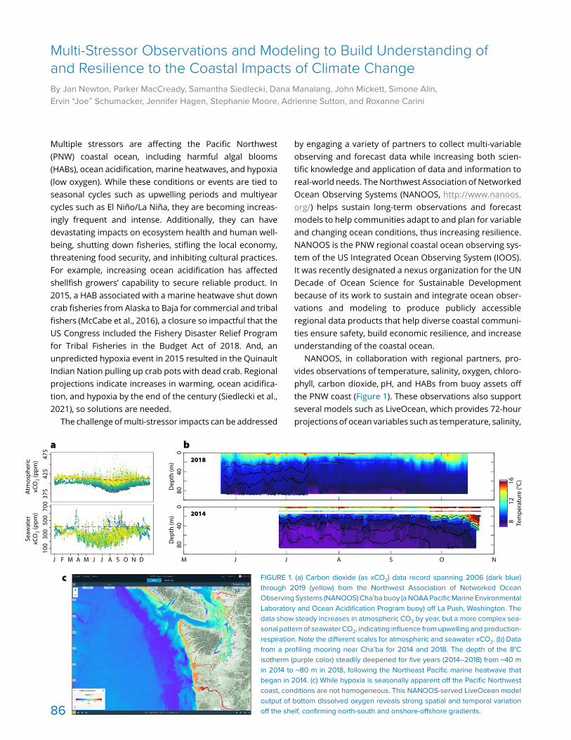
Jan Newton (2 pages)

Multiple stressors are affecting the Pacific Northwest (PNW) coastal ocean, including harmful algal blooms (HABs), ocean acidification, marine heatwaves, and hypoxia (low oxygen). While these conditions or events are tied to seasonal cycles such as upwelling periods and multiyear cycles such as El Niño/La Niña, they are becoming increas-ingly frequent and intense. Additionally, they can have devastating impacts on ecosystem health and human well- being, shutting down fisheries, stifling the local economy, threatening food security, and inhibiting cultural practices. For example, increasing ocean acidification has affected shellfish growers’ capability to secure reliable product. In 2015, a HAB associated with a marine heatwave shut down crab fisheries from Alaska to Baja for commercial and tribal fishers (McCabe et al., 2016), a closure so impactful that the US Congress included the Fishery Disaster Relief Program for Tribal Fisheries in the Budget Act of 2018. And, an unpredicted hypoxia event in 2015 resulted in the Quinault Indian Nation pulling up crab pots with dead crab. Regional projections indicate increases in warming, ocean acidifica-tion, and hypoxia by the end of the century (Siedlecki et al., 2021), so solutions are needed.

The challenge of multi-stressor impacts can be addressed

by engaging a variety of partners to collect multi-variable observing and forecast data while increasing both scien-tific knowledge and application of data and information to real-world needs. The Northwest Association of Networked Ocean Observing Systems (NANOOS, http://www.nanoos.org/) helps sustain long-term observations and forecast models to help communities adapt to and plan for variable and changing ocean conditions, thus increasing resilience. NANOOS is the PNW regional coastal ocean observing sys-tem of the US Integrated Ocean Observing System (IOOS). It was recently designated a nexus organization for the UN Decade of Ocean Science for Sustainable Development because of its work to sustain and integrate ocean obser-vations and modeling to produce publicly accessible regional data products that help diverse coastal communi-ties ensure safety, build economic resilience, and increase understanding of the coastal ocean.

NANOOS, in collaboration with regional partners, pro-vides observations of temperature, salinity, oxygen, chloro-phyll, carbon dioxide, pH, and HABs from buoy assets off the PNW coast (Figure 1). These observations also support several models such as LiveOcean, which provides 72-hour projections of ocean variables such as temperature, salinity,

Multi-Stressor Observations and Modeling to Build Understanding of and Resilience to the Coastal Impacts of Climate ChangeBy Jan Newton, Parker MacCready, Samantha Siedlecki, Dana Manalang, John Mickett, Simone Alin, Ervin “Joe” Schumacker, Jennifer Hagen, Stephanie Moore, Adrienne Sutton, and Roxanne Carini

FIGURE 1. (a) Carbon dioxide (as xCO2) data record spanning 2006 (dark blue) through 2019 (yellow) from the Northwest Association of Networked Ocean Observing Systems (NANOOS) Cha’ba buoy (a NOAA Pacific Marine Environmental Laboratory and Ocean Acidification Program buoy) off La Push, Washington. The data show steady increases in atmospheric CO2 by year, but a more complex sea-sonal pattern of seawater CO2, indicating influence from upwelling and production- respiration. Note the different scales for atmospheric and seawater xCO2. (b) Data from a profiling mooring near Cha’ba for 2014 and 2018. The depth of the 8°C isotherm (purple color) steadily deepened for five years (2014–2018) from ~40 m in 2014 to ~80 m in 2018, following the Northeast Pacific marine heatwave that began in 2014. (c) While hypoxia is seasonally apparent off the Pacific Northwest coast, conditions are not homogeneous. This NANOOS-served LiveOcean model output of bottom dissolved oxygen reveals strong spatial and temporal variation off the shelf, confirming north-south and onshore-offshore gradients.

475

425

700

500

Seaw

ater

xC

O2 (

ppm

)A

tmos

pher

ic

xCO

2 (pp

m)

300

100

J F M A M J J A S O N D

375

a

00

40

1612

8

4080

80D

epth

(m)

Dep

th (m

)

Tem

pera

ture

(°C)

2018

2014

M J AJ S O N

b

c

86

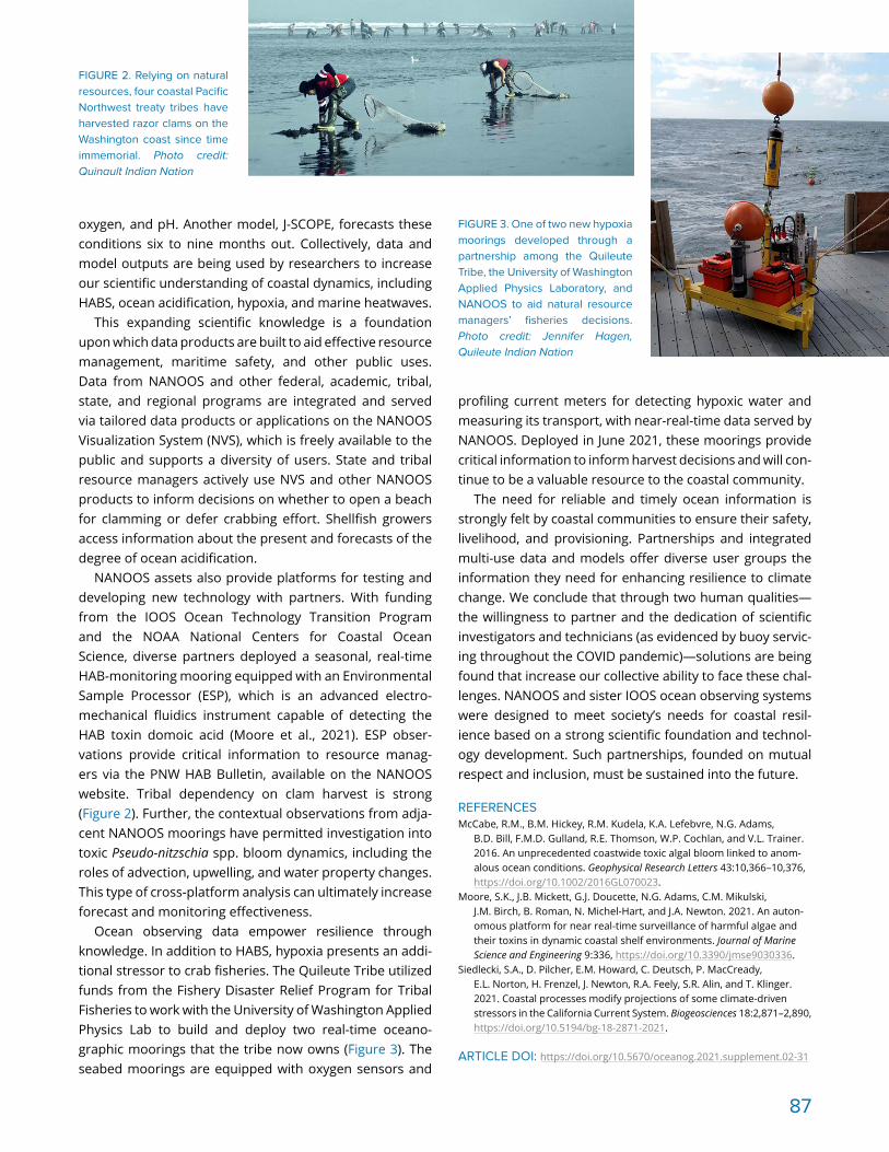
oxygen, and pH. Another model, J-SCOPE, forecasts these conditions six to nine months out. Collectively, data and model outputs are being used by researchers to increase our scientific understanding of coastal dynamics, including HABS, ocean acidification, hypoxia, and marine heatwaves.

This expanding scientific knowledge is a foundation upon which data products are built to aid effective resource management, maritime safety, and other public uses. Data from NANOOS and other federal, academic, tribal, state, and regional programs are integrated and served via tailored data products or applications on the NANOOS Visualization System (NVS), which is freely available to the public and supports a diversity of users. State and tribal resource managers actively use NVS and other NANOOS products to inform decisions on whether to open a beach for clamming or defer crabbing effort. Shellfish growers access information about the present and forecasts of the degree of ocean acidification.

NANOOS assets also provide platforms for testing and developing new technology with partners. With funding from the IOOS Ocean Technology Transition Program and the NOAA National Centers for Coastal Ocean Science, diverse partners deployed a seasonal, real-time HAB-monitoring mooring equipped with an Environmental Sample Processor (ESP), which is an advanced electro-mechanical fluidics instrument capable of detecting the HAB toxin domoic acid (Moore et  al., 2021). ESP obser-vations provide critical information to resource manag-ers via the PNW HAB Bulletin, available on the NANOOS website. Tribal dependency on clam harvest is strong (Figure 2). Further, the contextual observations from adja-cent NANOOS moorings have permitted investigation into toxic Pseudo-nitzschia spp. bloom dynamics, including the roles of advection, upwelling, and water property changes. This type of cross-platform analysis can ultimately increase forecast and monitoring effectiveness.

Ocean observing data empower resilience through knowledge. In addition to HABS, hypoxia presents an addi-tional stressor to crab fisheries. The Quileute Tribe utilized funds from the Fishery Disaster Relief Program for Tribal Fisheries to work with the University of Washington Applied Physics Lab to build and deploy two real-time oceano-graphic moorings that the tribe now owns (Figure 3). The seabed moorings are equipped with oxygen sensors and

profiling current meters for detecting hypoxic water and measuring its transport, with near-real-time data served by NANOOS. Deployed in June 2021, these moorings provide critical information to inform harvest decisions and will con-tinue to be a valuable resource to the coastal community.

The need for reliable and timely ocean information is strongly felt by coastal communities to ensure their safety, livelihood, and provisioning. Partnerships and integrated multi-use data and models offer diverse user groups the information they need for enhancing resilience to climate change. We conclude that through two human qualities—the willingness to partner and the dedication of scientific investigators and technicians (as evidenced by buoy servic-ing throughout the COVID pandemic)—solutions are being found that increase our collective ability to face these chal-lenges. NANOOS and sister IOOS ocean observing systems were designed to meet society’s needs for coastal resil-ience based on a strong scientific foundation and technol-ogy development. Such partnerships, founded on mutual respect and inclusion, must be sustained into the future.

REFERENCESMcCabe, R.M., B.M. Hickey, R.M. Kudela, K.A. Lefebvre, N.G. Adams,

B.D. Bill, F.M.D. Gulland, R.E. Thomson, W.P. Cochlan, and V.L. Trainer. 2016. An unprecedented coastwide toxic algal bloom linked to anom-alous ocean conditions. Geophysical Research Letters 43:10,366–10,376, https://doi.org/10.1002/2016GL070023.

Moore, S.K., J.B. Mickett, G.J. Doucette, N.G. Adams, C.M. Mikulski, J.M. Birch, B. Roman, N. Michel-Hart, and J.A. Newton. 2021. An auton-omous platform for near real-time surveillance of harmful algae and their toxins in dynamic coastal shelf environments. Journal of Marine Science and Engineering 9:336, https://doi.org/10.3390/jmse9030336.

Siedlecki, S.A., D. Pilcher, E.M. Howard, C. Deutsch, P. MacCready, E.L. Norton, H. Frenzel, J. Newton, R.A. Feely, S.R. Alin, and T. Klinger. 2021. Coastal processes modify projections of some climate- driven stressors in the California Current System. Biogeosciences 18:2,871–2,890, https://doi.org/10.5194/bg-18-2871-2021.

ARTICLE DOI: https://doi.org/10.5670/oceanog.2021.supplement.02-31

FIGURE 2. Relying on natural resources, four coastal Pacific Northwest treaty tribes have harvested razor clams on the Washington coast since time immemorial. Photo credit: Quinault Indian Nation

FIGURE 3. One of two new hypoxia moorings developed through a partnership among the Quileute Tribe, the University of Washington Applied Physics Laboratory, and NANOOS to aid natural resource managers’ fisheries decisions. Photo credit: Jennifer Hagen, Quileute Indian Nation

87

TECHNOLOGY

Collecting pristine observations of the sea surface from ships is challenging because research vessels destroy the integrity of the upper few meters of the ocean. This includes the sea surface microlayer (SML)—the top milli-meter of the ocean—which controls the exchange of gases between the ocean and the atmosphere and plays an essential role in the dispersal of contaminants, including plastics, oil residues, and industrial organic substances. Observations of this thin surface layer at high temporal and spatial resolutions are needed to understand the ocean-atmosphere exchanges of CO2, heat, particles, and freshwater. For these reasons, new technologies for study-ing sea surface processes are essential to advance under-standing of the ocean’s health and the ocean’s role in cli-mate (Schmitt, 2018).

In situ observations of the SML are also needed to val-idate and calibrate surface ocean observations acquired by various sensors aboard satellites. Conventional in situ methods for obtaining sea surface measurements such as Argo floats or conductivity-temperature-depth (CTD) instruments do not take measurements of the sea surface

but instead take readings at 3–5 m depth at best. Even the size of the platforms and sensors are often too big to resolve the fine scales of observation required to under-stand surface ocean processes. Similar to human skin, which has different properties than the tissues and organs underneath, the ocean has a skin with different properties than the water just below. The oceanography community has traditionally used data collected from 3–5 m depth and assumed or extrapolated similar conditions occur at the surface. This would be as if a dermatologist diagnoses your skin condition by examining an X-ray.

To resolve these issues, there have been several advance-ments in technology and sampling methods related to the SML and near-surface layer, discussed below.

REMOTE-CONTROLLED CATAMARANS. State-of-the-art research catamarans (Figure 1) permit assessment of vertical gradients of various biogeochemical parameters either by integrating onboard sensor data or by collecting discrete water samples from the SML and from additional near-surface depths. Among other parameters, onboard sensors can record temperature, conductivity (a measure of salinity), pH, partial pressure of CO2, and fluorescent dis-solved organic matter, while dissolved inorganic carbon, total alkalinity, surface active substances, and extracellular polymeric substances are determined through analysis of discrete water samples. These catamarans also include meteorological sensor packages, and the latest version can operate autonomously, with live data transmission for mission planning. By using catamarans, we overcome the disadvantages of boats and research vessels, which break the structure of the near-surface ocean and the SML.

FIGURE 1. (above) The research catamaran floats peacefully in calm Fijian waters. This remotely piloted vehicle utilizes, among other things, a "skimmer" (right)—a rotating glass disk that skims the sea surface microlayer, sampling just the top 1 mm of the ocean. Photo credit: Alex Ingle/Schmidt Ocean Institute

Technologies for Observing the Near Sea SurfaceBy Mariana Ribas-Ribas, Christopher J. Zappa, and Oliver Wurl

88

TECHNOLOGY

BUOYS. Drifting buoys are suitable for the study of the sea surface. Because they drift freely, any disturbance to the sea surface and its SML are minimal. We developed several drifting buoys for different scientific applications. There are drifting buoys that measure gas transfer veloci-ties and air-sea CO2 fluxes with high spatiotemporal reso-lution (Sniffle). Others are equipped to incubate waters at their depths of origin, including in the SML. For example, to study the metabolic contributions of microorganisms to gas exchange processes, we use light and dark bottles on the freely drifting Surface In Situ Incubator (SISI). There are surface buoys with sensors fixed at different depths to collect data on the water’s conductivity, temperature, or pH. The Surface Processes Instrument Platform 2 (SPIP-2; Figure 2) continuously profiles temperature, salinity, cur-rent velocity, and turbulence in the top meter of the ocean up to the very surface. We have also developed an SML skimmer that will be deployed on moored data buoys along shipping lanes to monitor floating soot particles.

UNCREWED AERIAL VEHICLES. We made the first fully autonomous deployment of fixed-wing, uncrewed aerial vehicles (UAVs) on R/V Falkor cruise FK191120 in November 2019 (Figure 3). The vehicles were equipped for high endur-ance (12+ hours with 6.8 kg instrument payloads) and high data bandwidth (100+ Mbs at 50 nm range), and they could take-off, hover, and land vertically. These UAVs provided “eyes over the horizon,” quickly covering more of the ocean than a ship and dramatically increased the research foot-print available for science and discovery. Moreover, these UAVs can allow those aboard research vessels to quickly and efficiently assess targets or identify events of interest, such as cyanobacteria blooms, rather than wait for the ship to encounter a phenomenon that may not occur. After the UAV discovers a physical phenomenon of interest, the research vessel party can move to sample it while the UAV monitors its temporal and spatial evolution. These UAVs can be outfitted with remote-sensing instruments typi-cally found aboard satellites, such as thermal cameras that provide sea surface skin temperature and hyperspectral imagers that yield ocean color data for identifying algal blooms. All of the imagery is telemetered in real time back to mission control on the ship, allowing real-time tasking and the reprogramming of data collection during the flight.

OUTLOOKWhile the existence of the SML has been known for many decades, we still do not have a clear understanding of how it controls air-sea interactions. It is unclear to what extent SML sampling affects the SML’s integrity and the parame-ters of interest (especially for gases). We also expect a diur-nal cycle of SML processes that we are just beginning to understand. The basic concept of the SML has also evolved. Initially, it was thought to be a separate layer that only existed during calm sea states. The SML was then shown to exist at regional to global scales and to have recurrent biofilm-like properties. Now, we are moving toward a defi-nition of the SML as a biogeochemical reactor that exhibits vertical gradients that force the air-sea exchange of heat, energy, and mass.

Our goal is to develop readily available technology that will allow collection of data on the SML to become an inte-gral part of research projects. Furthermore, we need to quantify SML processes and integrate them in ocean mod-els. For example, there are still gaps in our knowledge of the ocean carbon budget. We hypothesize that we can close (or get closer to closing) the carbon budget if we introduce the SML into ocean carbon models. We cannot continue to use data collected at 3–5 m depth and extrapolate it to describe the near-surface layer because this extrapolation may introduce significant biases that affect calculations of the global carbon budget, the validation of satellite images, and our understanding of the freshwater cycle.

REFERENCESchmitt, R.W. 2018. The ocean’s role in climate. Oceanography 31(2):32–40,

https://doi.org/10.5670/oceanog.2018.225.

ARTICLE DOI: https://doi.org/10.5670/oceanog.2021.supplement.02-32

FIGURE 2. Overhead, one of the uncrewed aerial vehicles (UAVs) passes, collecting data on the sea surface below. In the water, the Surface Processes Instrument Platform (SPIP-2) collects detailed measurements of surface dynam-ics. Photo credit: Alex Ingle/Schmidt Ocean Institute

FIGURE 3. During the 2019 R/V Falkor expedition, the team tested the new capabilities of high-endurance hybrid fixed wing vertical take-off and landing (VTOL) UAV (inset) for oceanographic applications. Pictured is the underside of one of the aircraft, making a pass of the ship. Photo credit: Alex Ingle/Schmidt Ocean Institute

89

Emanuele Organelli (2 pages)

By installing biogeochemical sensors on 1,000 autonomous Argo profiling floats across the globe, the Biogeochemical (BGC)-Argo program is the only network capable of pro-viding detailed observations of the physics, chemistry, and biology of the top 2,000 m of our ocean up to every 10 days, even in remote regions and during unfavorable conditions for manual sampling. This rapidly expanding network will yield large amounts of data that will help us understand marine ecosystems and biogeochemistry, evaluate the impact of increasing human-derived pressures on Earth’s climate, and develop science-based solutions for sustain-able ocean and climate management.

Officially established in 2016, the International BGC-Argo program has built its mission on five science pillars and two management needs. One of the grand science chal-lenges, and also a primary element for improving man-agement of all living marine resources, is observing the composition of phytoplankton communities (BGC-Argo Planning Group, 2016). These microscopic, drifting, uni-cellular algae use sunlight and seawater to transform the carbon dioxide exchanged between the atmosphere and the ocean into oxygen and complex organic compounds. Phytoplankton create enough energy to benefit the entire food chain, from zooplankton to top predators.

Phytoplankton are so diverse that collectively they main-tain a variety of biogeochemical and ecosystem functions, including carbon cycling and storage. These organisms dis-play a wide variety of types, sizes, shapes, photosynthetic efficiencies, pigmentations, and light absorption proper-ties. While various methods can be used to identify phyto-plankton, the traditional method requires water samples taken at sea and experts using microscopes to identify species, distinguishing features such as size and shape. A newer, more high-tech method employs satellite obser-vations of ocean color to provide information on cellular

Hyperspectral Radiometry on Biogeochemical-Argo Floats: A Bright Perspective for Phytoplankton DiversityBy Emanuele Organelli, Edouard Leymarie, Oliver Zielinski, Julia Uitz, Fabrizio D’Ortenzio, and Hervé Claustre

traits, which can in turn be used to identify phytoplankton types. Although they offer the highest spatial coverage of any autonomous systems, satellite observations are limited to providing information only for surface ocean waters.

In water, cellular traits are determined by measuring the amount of ultraviolet (UV) and visible (VIS) light com-ing from the sun. Water absorbs red light near the sur-face, while detrital particles and dissolved organic matter reduce the availability of light in the UV and blue spectral bands. Phytoplankton pigments absorb UV and VIS light at different wavelengths, and pigmentation is different across the various groups. Thus, changes in the colors of the light fields detected in seawater reflect various types of phytoplankton. Currently, the four color bands available on the radiometric sensors implemented on the global BGC-Argo array are not sufficient to characterize the spec-tral variability of the underwater light field, so the diver-sity of phytoplankton communities cannot be resolved by currently available sensors on the floats. Hyperspectral radiometry— capturing light over many wavelengths, enabling tens or hundreds of colors to be recognized—points the way forward (Jemai et al., 2021).

European scientists have cooperated to upgrade the BGC-Argo sensor package with a hyperspectral radiome-ter, which is mounted at the top of the float to avoid plat-form self-shading (Figure 1). This hyperspectral instrument senses the sun’s radiant energy in the water at 140 color bands, from 320 nm to 780 nm, every 3.3 nm. In 2021, the first at-sea tests of this technology involved deploy-ing five newly configured BGC-Argo floats in two different environments: the Baltic Sea and the Mediterranean Sea. During their voyages, the new floats collected data for char-acterizing the dynamics of the submarine light field down to 300 m depth, from phytoplankton bloom to post-bloom conditions and during deep chlorophyll maxima (DCM) formation. The spectral signatures captured during two high- chlorophyll DCM events show that the descending light was absorbed differently at the two sites (Figure 2). In the Baltic Sea, the most absorbed colors are blue and

FIGURE 1. Deployment of a Biogeochemical-Argo float (APEX, Teledyne Webb Research) equipped with a hyperspectral radiometer (RAMSES, TriOS GmbH). The white arrow points to the RAMSES radiometer (shiny gray instrument). Hyperspectral radiometers on APEX and PROVOR (NKE Marine Electronics) BGC-Argo floats have been imple-mented within the European Union’s HORIZON 2020 research and innovation program through the EA-RISE project (grant number 824131) and the SpectralArgo-N project funded by the German Ministry of Research (grant number 03F0825A). Image credit: Emilie Diamond Riquier, IMEV - Institut de la Mer de Villefranche (France)90

hyperspectral floats will help to build a three- dimensional view of phytoplankton diversity and a "digital twin of the ocean" to allow monitoring of ocean health and carbon and energy flows throughout the food web, and to support management actions toward maintaining ecosystem resilience.

REFERENCESBGC-Argo Planning Group. 2016. The Scientific Rationale, Design and

Implementation Plan for a Biogeochemical-Argo Float Array. K. Johnson and H. Claustre, eds, Ifremer, 65 pp., https://doi.org/10.13155/46601.

Jemai, A., J. Wollschläger, D. Voß, and O. Zielinski. 2021. Radiometry on Argo floats: From the multispectral state-of-the-art on the step to hyperspectral technology. Frontiers in Marine Science 8:676537, https://doi.org/10.3389/fmars.2021.676537.

Organelli, E., C. Nuccio, L. Lazzara, J. Uitz, A. Bricaud, and L. Massi. 2017. On the discrimination of multiple phytoplankton groups from light absorption spectra of assemblages with mixed taxonomic composi-tion and variable light conditions. Applied Optics 56(14):3,952–3,968, https://doi.org/10.1364/AO.56.003952.

ARTICLE DOI: https://doi.org/10.5670/oceanog.2021.supplement.02-33

FIGURE 2. BGC-Argo floats equipped with hyperspectral radiometers capture the optical signatures of phytoplankton communities and their compositions. The spectral bands at which light disappears provide information on pigments and thus on phytoplankton types present. Vertical profiles of hyperspectrally resolved downwelling irradiance (radiant energy from the sun) show, at the level of the deep chlorophyll maxima (DCM; thick blue line), a maximum of the remnant light around 560 nm for the brownish waters of the Baltic Sea (a), and around 480 nm for the blue Mediterranean (b).

green. While blue is mainly absorbed by substances other than phytoplankton, green is mostly absorbed by dia-toms and dinoflagellates. Indeed, diatoms and dinofla-gellates contain the highest per cell concentrations of green-light-absorbing pigments (Organelli et al., 2017). In the Mediterranean Sea, the prevailing remnant light at the DCM and below is blue-green. This color is consistent with low pigment content, and thus communities composed of cyanobacteria and other small phytoplankton.

The combination of hyperspectral radiometry and Argo technology is especially promising for monitoring ecosystem changes and for building long-term records on phytoplankton diversity through the water column. By using light bands that are specifically targeted to dis-criminate among different phytoplankton types, we can greatly improve our knowledge of oceanic carbon stocks, pathways, and fluxes. Primary production is better con-strained when BGC-Argo radiometric data are integrated into marine biogeochemical models.

The upgraded hyperspectral capability of BGC-Argo will also be beneficial for the management of living resources and ecosystem services (e.g.,  habitat suitability, fish stocks, and recruitment) and for biohazard surveillance (i.e., harmful algal blooms). Some species of phytoplank-ton are harmful due to their ability to massively proliferate or produce toxins. These toxins can affect a wide range of organisms, including fishes, seabirds, mammals, and humans. Because of specific pigments and high abun-dances, these harmful species modify the light in an easily recognizable manner. With hyperspectral radiometers, the BGC-Argo network may become a pillar for monitoring bio-hazards and the establishment of an early warning system for harmful phytoplankton (Figure 3) in the global ocean

Dep

th (m

)

100

0

50

Dep

th (m

)

300

0

150

Dow

nwel

ling

irrad

ianc

e (µ

W c

m–2

nm

–1)

Dow

nwel

ling

irrad

ianc

e (µ

W c

m–2

nm

–1)

10–4

10–4

300 400 500 600Wavelength (nm)

70010

–210

–210

–310

–310

–110

–110

010

010

110

110

2

a

b

FIGURE 3. Use of hyperspectral radiometry on BGC-Argo floats provides opportunities to improve surveillance of harmful algal blooms. Examples of two toxin-producing species found in Mediterranean waters are shown: (a) the dinoflagellate Gonyaulax cf. spinifera, and (b) the diatom Pseudo-nitzschia pungens. Image credit: Caterina Nuccio, University of Florence (Italy)

a

b 91

as well as in regional seas. This capability could be expanded to monitor toxic spe-cies by developing synergies with other optical observations from BGC-Argo or remote-sensing technologies (e.g., lidar).

BGC-Argo radiometry extends space-based observations of ocean color into the water column, and synergies have already been developed for validating satellite products. A novel synergy with

Range or resolution? We often get asked this question when mapping the seafloor. And it is important because the type of data we choose to collect fundamentally changes the science that can follow. Photos taken by camera- equipped autonomous underwater vehicles (AUVs) rep-resent one extreme of the range/resolution trade-off, where sub-centimeter resolutions can be achieved, but typically only from close ranges of 2 m to 3 m. Taking images from higher altitudes increases the area mapped during visual surveys in two ways. First, a larger footprint can be observed in each image, and second, the lower risk of collision with rugged terrains when operating at higher altitudes allows use of flight-style AUVs (e.g., Autosub6000 shown in Figure 1), which are faster and more energy effi-cient than the hover-capable vehicles typically used for visual surveys. Combined, these factors permit several tens to more than a hundred hectares of the seafloor to be mapped in a single AUV deployment.

BioCam is a high-altitude three-dimensional (3D) imaging system that uses a stereo pair of high- dynamic- range scien-tific complementary metal- oxide semiconductor (sCMOS) cameras, each with 2,560 × 2,160 pixel resolution, that are mounted in a 4,000 m rated titanium housing. The housing has domed windows to minimize image distortion and also includes low-power electronics for communication, data storage, and control of the dual LED strobes and dual line

lasers BioCam uses to acquire 3D imagery. The LED strobes each emit 200,000 lumens of warm hue white light for 4 milli seconds. The lasers each project a green line (525 nm, 1 W Class 4) onto the seafloor at right angles to the AUV’s direction of travel to measure the shape of the terrain. The optical components are arranged along the bottom of the AUV, with an LED and a laser each mounted fore and aft of the cameras (Figure 1). A large distance between these illumination sources and the cameras ensures high-quality images, and high-resolution bathymetry data can be gath-ered from target altitudes of 6 m to 10 m.

The large dynamic range of the sCMOS cameras is nec-essary for high-altitude imaging because red light attenu-ates much more strongly than green and blue light in water (Figure 2). A large dynamic range allows detection of low intensity red light with sufficient bit resolution to restore color information, while simultaneously detecting the more intense light of the other color channels without saturation. Range information from the dual lasers allows the distance light travels from the strobes to each detected pixel to be calculated for accurate color rectification (see Figure 2). Rectified color is projected onto the laser point cloud and fused with AUV navigation data to generate texture- mapped, 3D visual reconstructions (Bodenmann et  al., 2017). The BioCam processing pipeline calibrates the dual laser setup so that quantitative length, area, and volumet-ric measurements can be made together with estimates of dimensional uncertainty, without the need for artificial field calibration targets (Leat et al., 2018).

Although 3D reconstructions are useful for studying detailed seafloor information, exploring them is both time-consuming and subjective. To help plan more effec-tive data acquisition during research expeditions, it is valu-able to be able to rapidly understand large georeferenced image data sets in expedition-relevant timeframes. For this, we have developed location-guided unsupervised learning methods (Yamada et al., 2021) that can automatically learn the features that best describe images in a georeferenced

Visualizing Multi-Hectare Seafloor Habitats with BioCamBy Blair Thornton, Adrian Bodenmann, Takaki Yamada, David Stanley, Miquel Massot-Campos, Veerle Huvenne, Jennifer Durden, Brian Bett, Henry Ruhl, and Darryl Newborough

FIGURE 1. BioCam consists of a central unit with a stereo pair of cameras and control electronics, fore and aft dual LED strobes, and line lasers that are used to generate 3D color reconstructions of the seafloor.

Range Map

Near Far

Corrected ImageRaw Image

FIGURE 2. Laser-derived 3D range information is used to rectify the color information in the images. Physics-based image formation models use the range maps to compensate for the wavelength- dependent attenuation of light in water. This allows the darkening effects and the blue-green hue seen in the raw images to be rectified even over rugged terrains.

AUV

Cameras and Electronics

LineLasers

LED Strobes

92

FIGURE 3. Three-dimensional visual mapping data gathered at the Darwin Mounds marine protected area (59°54'N, 7°39'W). The top left panel shows a 30 ha area mapped using BioCam mounted on the autonomous underwater vehicle overlaid on side-scan sonar data. The expanded detail (indicated by red lines) shows a micro-mound (~5 m diameter, 20 cm high). The smaller, individual protrusions that form a ring around the mound are cold- water- coral colonies consisting mainly of Desmophyllum pertusum and Madrepora oculata. These can be seen more clearly in the expanded isometric view indicated by blue lines. The individual colonies have diameters of between 20 cm and 50 cm and are between 10 cm and 30 cm high in the area shown.

FIGURE 4. Unsupervised clustering outputs (left) and examples of automat-ically identified cluster representative images (right) show the distribution of cold-water coral and coral rubble (red), xenophyophores (green), and rippled sand (blue). The light green, green, and dark green clusters show dense dis-tributions of xenophyophores in the tails of the mounds where the mounds themselves are characterized by the presence of coral and coral rubble (red). The content-based query ranks images in order of their similarity to an input image (orange).

data set without needing any human input for interpreta-tion. These features are used to cluster images into groups with similar appearances, identifying the most represen-tative images in each cluster and also allowing scientists to flexibly query data sets by ranking all images in order of their similarity to any input image, where the ranked outputs for different query images can be generated in milliseconds. Both the clustering and query returns can be visualized using georeference information to identify spa-tial patterns in the data sets.

Figure 3 shows an example of a 3D visual reconstruction collected during a survey of the Darwin Mounds marine protected area, 160 km northwest of Cape Wrath, Scotland, at ~1,000 m depth. BioCam was mounted on the flight-style Autosub6000 AUV, which operated at 6 m altitude and 1 m/s forward speed to cover 30,000 m2/h. The setup achieved a resolution of 3.3 mm across track and 2 mm in depth. The closeup in Figure 3 shows individual colonies of cold- water-corals forming a ring around the base of a micro-mound. Figure 4 shows the results of clustering, rep-resentative image identification, and content- based query. Cold-water coral colonies were most densely distributed around the bases of mounds, several of which are signifi-cantly larger (up to 75 m wide and 5 m high) than the micro-mound in Figure 3, forming ring patterns more broadly throughout the 30 ha region mapped during the dive. The clustering results also show that xenophyophores, large single-cell organisms recognized as a vulnerable marine ecosystem indicator species, are most densely distributed in the tails of the mounds. The ability to recognize biolog-ical zonation associated with mounds, in particular micro-mounds that are difficult to observe in lower resolution acoustic data, illustrates how combining subcentimeter resolution 3D visual mapping with methods developed to

summarize observations and flexibly answer queries can generate rapid human insight and so help focus efforts in observation and downstream analysis.

REFERENCESBodenmann, A., B. Thornton, and T. Ura. 2017. Generation of high-

resolution three-dimensional reconstructions of the seafloor in color using a single camera and structured light. Journal of Field Robotics 34(5):833–851, https://doi.org/10.1002/rob.21682.

Leat, M., A. Bodenmann, M. Massot-Campos, and B. Thornton. 2018. Analysis of uncertainty in laser-scanned bathymetric maps. In 2018 IEEE/OES Autonomous Underwater Vehicle Workshop, November 6–9, 2018, Porto, Portugal, https://doi.org/10.1109/AUV.2018.8729747.

Yamada, T., A. Prügel-Bennett, and B. Thornton. 2021. Learning features from georeferenced seafloor imagery with location guided auto-encoders. Journal of Field Robotics 38:52–67, https://doi.org/10.1002/rob.21961.

ACKNOWLEDGMENT This research is funded by the UK Natural Environment Research Council’s Oceanids program, grant NE/P020887/1. The data used in this article are available on the benthic imaging repository Squidle+ (www.soi.squidle.org).

ARTICLE DOI: https://doi.org/10.5670/oceanog.2021.supplement.02-34

93

Jack Butler and Camille Pagniello (2 pages)

TABLE 1. Examples of different low-cost, open-source ocean sensors and platforms with step-by-step assembly guides.

NAME TYPE STEP-BY-STEP GUIDE

OpenCTD CTD

https://github.com/ Oceanographyfor Everyone/OpenCTD/ blob/master/ OpenCTD_Feather_ Adalogger/OpenCTD_ConstructionOperation.pdf

PiCTD CTD https://github.com/haanhouse/pictd

CTDDizzle CTD https://github.com/IanTBlack/CTDizzle

Open-Source-

Underwater-Glider

Gliderhttps://hackaday.io/project/20458- osug- open- source- underwater-glider

Aruna ROV ROV https://hackaday.io/project/172364-aruna-rov

LoCO-AUV AUV https://loco-auv.github.io

AusOcean’s “Rig” Mooring http://www.ausocean.

org/s/doc/rig.html

Maker Buoy Buoy https://github.com/wjpavalko/Maker-Buoy

IPAX Camera https://github.com/plertvilai/IPAX

FishOASIS Camera https://github.com/cpagniel/FishOASIS

AudioMothPassive Acoustic Recorder

https://www.openacoustic-devices.info/audiomoth

The rise of low-cost, small, and efficient microcontrollers and single-board computers (e.g.,  Arduino1, Raspberry Pi2, Nvidia Jetson3) has catalyzed a vibrant, user-led com-munity that focuses on the development of useful or fun “do-it-yourself” (DIY) projects. The utility of these “tiny computers” as backbones for low-cost oceanographic sensor systems has not been lost on the marine science community, particularly for applications that do not need the endurance, accuracy, or ruggedness provided by com-mercial oceanographic products. Additionally, open-source oceanographic tools bolster the goals of the United Nation’s Decade of Ocean Science for Sustainable Development to encourage a more inclusive and participative approach to ocean science, to better predict ocean phenomena, and to democratize access to the ocean. Though there has been a recent increase in peer-reviewed, published step-by-step guides on how to build some marine sensors and systems (e.g.,  see the recurring “DIY Oceanography” sec-tion in Oceanography magazine or the journal HardwareX), most of the resources detailing custom-built, user- designed oceanographic instrumentation remain in the “gray literature.” Here, we highlight a few projects that pro-vide step-by-step guides on how to construct some of the most common types of ocean sensor systems or platforms (Figure 1; Table 1). Lastly, we provide budding DIY oceanog-raphers with some useful resources.

Perhaps the most widely used oceanographic instru-ment is the conductivity-temperature-depth (CTD) logger; however, even the most economical commercial CTDs can

cost over US$5,000. This high acquisition cost can be pro-hibitive for many ocean scientists and managers, especially those in developing nations. OpenCTD is an open-source, Arduino-based system designed by Oceanography for Everyone’s marine scientists that is intended to be built by the end user at a cost of around US$600 (Figure 2). For researchers who do not require the accuracy of com-mercial units and/or are working in coastal environments (i.e., where the water depth is typically less than 140 m), this instrument offers a low-cost alternative that could allow them to extend monitoring over larger spatiotempo-ral scales. Others have been inspired by OpenCTD to create their own low-cost CTDs (e.g., PiCTD, CTDizzle) using differ-ent types of microcomputers and oceanographic sensors.

Mobile, moored, and autonomous platforms have also seen an influx of end-user-built, open-source hardware. These types of platforms collect invaluable data for oceanic and atmospheric forecasting. Yet, commercial versions of these platforms tend to be very expensive (i.e., tens to hun-dreds of thousands of dollars per unit). Examples of low-cost platforms include the Open-Source Underwater Glider (OSUG), an open-source, user- constructed alternative

Emerging, Low-Cost Ocean Observing Technologies to Democratize Access to the OceanBy Jack Butler and Camille M.L.S. Pagniello

FIGURE 1. An ocean filled with low-cost, open-source, DIY ocean observing tech-nologies. AusOcean “rig” image provided courtesy of AusOcean. Maker Buoy image courtesy of Wayne Pavalko. All other images used under MIT and GNU Public License v3.0 CC-BY

AusOcean “Rig”

IPAX

OpenCTD

Maker Buoy

OSUG

FishOASISLoCO-AUV

94

to oceanic glider platforms that can be equipped with a suite of oceanographic sensors. There are also many examples of open-source tethered and untethered pow-ered underwater vehicles (such as the Aruna remotely operated vehicle [ROV] and the LoCO autonomous under-water vehicle [AUV]) that allow marine scientists to build their own underwater vehicles tailored to their research needs. Furthermore, open-source moorings and surface vehicles like AusOcean’s “rig” and Maker Buoy provide long-duration, real-time data acquisition platforms that support a wide variety of sensors for research in coastal waters with mobile data network access.

Additionally, many low-cost instruments have been developed to directly monitor animal biodiversity and habitat quality. Ongoing developments in consumer-grade cameras have improved the price performance of opti-cal imaging systems such as IPAX (Lertvilai, 2020) and FishOASIS (Pagniello et  al., 2021; Figure 3), which allow researchers to explore the dynamics of marine communi-ties, from plankton to fish, for extended periods. Passive acoustic systems have also benefited from the prolifera-tion of low-cost, off-the-shelf components (e.g.,  Caldas-Morgan et  al., 2015) and the increasing ease in printing custom circuit boards (e.g., AudioMoth).

These are just a handful of the many projects that aim to incorporate developments from the "Maker Movement" into oceanography and marine science. The proliferation of low-cost alternatives to commercial ocean observing platforms and the increasing availability of step-by-step guides to build DIY instrumentation will allow the collec-tion of more oceanographic data around the globe. In the face of global climate change, incorporating these low-cost systems to better estimate population densities and abun-dances, as well as habitat health, has become increas-ingly important.

For those who feel inspired and wish to start their own DIY oceanography journey, many online resources and communities are available to get you started. WILDLABS4 is a global online community of researchers, engineers,

technologists, and entrepreneurs, boasting more than 4,000 active users dedicated to the use of technology to address conservation issues around the world. They host resources (e.g.,  Tech Tutors) to aid conservation technologists in seeing their projects through to fruition. Hackaday.io5 is a worldwide, collaborative hardware devel-opment community that hosts project build pages (like many featured in this article) and troubleshooting forums. For example, there are 12 projects on Hackaday.io tagged with the keyword “ocean” aimed at creating open-source hardware for monitoring the ocean, many of which have robust bills-of-materials and build guides. We also main-tain a list of open-source, ocean science tools and low-cost, ocean sensor vendors on GitHub6 that readers can use as a source for existing projects or to find a project to cus-tomize to their needs. We hope that the continued devel-opment of low-cost ocean tools, such as those highlighted here, will open the world of marine science to a broader, global audience and increase the footprint of data col-lected within the world’s ocean.

REFERENCESCaldas-Morgan, M., A. Alvarez-Rosario, and L. Rodrigues Padovese.

2015. An autonomous underwater recorder based on a single board computer. PLoS ONE 10(6):e0130297, https://doi.org/10.1371/journal.pone.0130297.

Lertvilai, P. 2020. The In situ Plankton Assemblage eXplorer (IPAX): An inexpensive underwater imaging system for zooplankton study. Methods in Ecology and Evolution 11(9):1,042–1,048, https://doi.org/ 10.1111/2041-210X.13441.

Pagniello, C.M.L.S., J. Butler, A. Rosen, A. Sherwood, P.L.D. Roberts, P.E. Parnell, J.S. Jaffe, and A. Širović. 2021. An optical imaging system for capturing images in low-light aquatic habitats using only ambient light. Oceanography 34(3):71–77, https://doi.org/10.5670/oceanog.2021.305.

ARTICLE DOI: https://doi.org/10.5670/oceanog.2021.supplement.02-35

1 https://www.arduino.cc/; 2 https://www.raspberrypi.org/; 3 https://www.nvidia.com/en-us/autonomous-machines/embedded- systems/; 4 https://www.wildlabs.net/; 5 https://hackaday.io/; 6 https://github.com/jack-butler/open-ocean

FIGURE 2. Fully assembled OpenCTDs (left) and com-parison of data collected via OpenCTD to a commercial CTD (right). Images and data used under MIT license, copyright Oceanography for Everyone

Dep

th (m

)

0102030405060708090

100110120130140150

Temperature (°C)

West Mooring – Descent

2 4 6 8 10 12 14

OpenCTDComCTD

FIGURE 3. Fish Optical-Acoustic Sensor Identification System (FishOASIS) deployed in the kelp forest off La Jolla, California (left), and an example image taken by FishOASIS during a deployment.

95

Coastal ecosystems are suffering immediate and detri-mental consequences of a warming global climate. Ocean heating, rising sea level, and increasing coastal storm fre-quency and intensity are imposing stresses on coastal environments that historically were less frequent and less severe. At the same time, human population within 100 km of the coast is projected to nearly double by mid-century, increasing pressure on a variety of marine services includ-ing fisheries and recreation. Shallow water environments are key components of healthy coastal ecosystems as they provide feeding grounds and nurseries for fish and crus-taceans and act to buffer the impacts of coastal storms on adjacent land areas. But they are also susceptible to rapid degradation because stresses are distributed within a compressed water volume. To address these challenges, policymakers and natural resource managers increasingly rely on more accurate and timely environmental data.

The past two decades of robotic and sensor technology development have resulted in ocean observing systems that can monitor and survey water column properties autonomously at temporal and spatial scales and in envi-ronmental conditions that exceed what is possible with traditional human-based operations involving ships and divers (Chai et al., 2020). Most recently, new system con-cepts are providing more complete environmental descrip-tions of shallow water environments, including water qual-ity and the shape and composition of the seafloor.

In 2017, the US Naval Research Laboratory (NRL) began developing robotic surveying approaches that support remote sensing of shallow coastal environments (Ackleson et al., 2017). The initial approach was to use a modified,

FIGURE 1. (a) This robotic kayak was used to tow an instrumented buoy that measured water reflectance and bottom depth and photographed the shallow seafloor in high definition. (b) A refinement of the robotic kayak concept, the Autonomous Coastal Color Environmental Survey System (ACCESS) consists of an instrumented outrigger that can be attached to any recreational kayak. ACCESS provides propulsion and navigation while measuring an expanded suite of environmen-tal parameters, including water clarity, phytoplankton concentration, water currents, bottom depth, and organisms inhabiting the seafloor.

Robotic Surveyors for Shallow Coastal EnvironmentsBy Steven G. Ackleson

self-navigating kayak towing an instrumented buoy to sur-vey water depth, photograph the shallow bottom in high definition, and simultaneously record how different colors of light are reflected from the water column (Figure 1a). Field surveys conducted in Kane’ohe Bay, Hawai’i, provided high-resolution maps of bottom depth and coral cover (Figure 2). The data were used to assess how well sensors on aircraft and satellites are able to map water depth and bottom cover on coral reefs.

Following the successful Kane’ohe Bay surveys, NRL began designing a new robotic system capable of provid-ing more complete descriptions of shallow water environ-ments, including water clarity, phytoplankton (microscopic marine algae) concentration, water currents, bottom depth, and organisms inhabiting the seafloor. In addition to providing environmental sensing, the system had to be easily managed with a minimal workforce and inexpen-sively transported to remote locations. The final design, the Autonomous Coastal Color Environmental Survey System (ACCESS; Figure 1b), is essentially an instrumented outrigger system that can be attached to any recreational kayak and powered with standard 12 V marine batteries. The outrigger design offers increased stability, and the kayak provides housing for heavy batteries. For distant field deployments where a kayak and batteries can be

Recreational Kayak

Batteries

Communicationsand GPS

Outrigger Equippedwith Environmental

Sensor Suite

Control Electronicsand Data Storage

ObstacleAvoidance Camera

Spectral Light Sensors

Bottom MappingSonar

Depth Sounder

Downward-Looking

GoPro CameraArticulating

Electric Motor

Deck Aft-Looking

GoPro Camera

Navigation and SensorControl Electronics

a b

Recreational Kayak

Batteries

Communicationsand GPS

Outrigger Equippedwith Environmental

Sensor Suite

Control Electronicsand Data Storage

ObstacleAvoidance Camera

Spectral Light Sensors

Bottom MappingSonar

Depth Sounder

Downward-Looking

GoPro CameraArticulating

Electric Motor

Deck Aft-Looking

GoPro Camera

Navigation and SensorControl Electronics

a b

96

sourced locally, only the outrigger components need to be transported, thus reducing shipping costs. ACCESS is easily disassembled and stored or transported in a small num-ber of protective boxes, each of which can be managed by one or two people.

ACCESS surveys can be conducted in waters as shal-low as 0.5 m. The operator communicates with ACCESS remotely across maximum distances of 1–2 km using a hand-held computer pad. Survey missions are either planned in advance or controlled manually onsite using open-source software commonly used to control general purpose drones. Map-based graphics show the platform location and speed, and separate windows display user- selected data streams in real time. An infrared camera continuously scans the forward sea surface for any obsta-cles that could impede the survey. Propulsion is provided with an array of four independently controlled thrusters that can be easily replaced in the field. Survey speed is user selected and generally ranges between 2 km/hr and 8 km/hr, and surveys can last up to 6 hours. ACCESS may be deployed from a shoreline using a light-weight custom cart or from a small research vessel.

ACCESS represents an important step in the evolution of robotic ocean survey systems, enabling detailed sur-veys of important shallow water habitats that support

remote-sensing operations and aid in monitoring environ-mental changes in response to climate and human activi-ties. However, survey needs, such as the mix of sensors and navigation attributes, are not all the same for each user, and requirements frequently change with user knowledge and experience. The good news for potential users is that highly capable and cost-effective systems can be built and customized using readily available components and open-source software, and how-to instructions and videos are easily found on the internet. Aside from the various envi-ronmental sensors, ACCESS makes use of 80/20 aluminum building components (https://8020.net/), Blue Robotics plug-and-play T200 thrusters (https://bluerobotics.com/), and Robotic Operating Software (https://www.ros.org/).

REFERENCESAckleson, S.G., J.P. Smith, L.M. Rodriguez, W.J. Moses, and B.J. Russell.

2017. Autonomous coral reef survey in support of remote sens-ing. Frontiers in Marine Science 4:325, https://doi.org/10.3389/fmars.2017.00325.

Chai, F., K.S. Johnson, H. Claustre, X. Xing, Y. Wang, E. Boss, S. Riser, K. Fennel, O. Schofield, and A. Sutton. 2020. Monitoring ocean biogeochemistry with autonomous platforms. Nature Reviews Earth & Environment 1:315–326, https://doi.org/10.1038/s43017-020-0053-y.

ARTICLE DOI: https://doi.org/10.5670/oceanog.2021.supplement.02-36

Bottom Roughness

Go Pro Image: Coral CoverGoPro Image: Soft Sediment

0.0 0.5

km

Bottom Depth Coral Cover

1 2 3 4 5Depth (m)

Red

Edge

Hei

ght

1.4

1.2

1.0

0.8

0.6

0.4

0.2

0.0

Survey Path

CoconutPatch Reef

0123456789101112131415

Dep

th (m

)

Kane’ohe Bay

Moku o Lo’e

a b

cd

g

e f

FIGURE 2. Autonomous survey systems provide more complete descriptions of shallow water environments compared with traditional ship and diver approaches. In Kane’ohe Bay, Hawai’i, (a) a robotic kayak and towed instrument buoy were used to provide detailed surveys of a patch reef (b) located southeast of Moku o lo’e island. The survey included bottom depth (c), bottom roughness (d), high-definition bottom photography (e and f), and water reflectance. The reflectance was used to detect and quantify coral coverage using a vegetation index (g).

97

AUTHORS

*Equal first authors

PAGE 1. Ellen S. Kappel (ekappel@geo-prose.com), Geosciences Professional Services Inc., USA. S. Kim Juniper, Ocean Networks Canada (ONC). Sophie Seeyave, Partnership for Observation of the Global Ocean (POGO), Plymouth Marine Laboratory, UK. Emily A. Smith, National Oceanic and Atmospheric Administration, Global Ocean Monitoring and Observing Program (NOAA/GOMO), USA. Martin Visbeck, GEOMAR Helmholtz Centre for Ocean Research Kiel, Germany.

PAGE 2. Dean Roemmich* (droemmich@ucsd.edu), Lynne Talley* (ltalley@ucsd.edu), Nathalie Zilberman* (nzilberman@ucsd.edu), and Sarah Purkey, Scripps Institution of Oceanography, University of California San Diego, USA. Emily Osborne* (emily.osborne@ noaa.gov) and Leticia Barbero, NOAA Atlantic Oceanographic and Meteorological Laboratory, USA. Kenneth S. Johnson* (johnson@mbari.org) and Yuichiro Takeshita, Monterey Bay Aquarium Research Institute, USA. Henry C. Bittig, Leibniz Institute for Baltic Sea Research Warnemünde, Germany. Nathan Briggs and Brian A. King, National Oceanography Centre, Southampton, UK. Andrea J. Fassbender and Gregory C. Johnson, NOAA Pacific Marine Environmental Laboratory, USA. Elaine McDonagh, Norwegian Research Centre and Bjerknes Centre for Climate Research, Norway, and National Oceanography Centre, Southampton, UK. Stephen Riser, School of Oceanography, University of Washington, USA. Toshio Suga, Tohoku University, Japan. Virginie Thierry,

IFREMER, Plouzané, France. Susan Wijffels, Woods Hole Oceanographic Institution, USA.

PAGE 9. Dariia Atamanchuk (dariia.atamanchuk@dal.ca), Department of Oceanography, Dalhousie University, Canada. Jaime Palter, Graduate School of Oceanography, University of Rhode Island, USA. Hilary Palevsky, Department of Earth and Environmental Sciences, Boston College, USA. Isabela Le Bras, Woods Hole Oceanographic Institution, USA. Jannes Koelling, Department of Oceanography, Dalhousie University, Canada. David Nicholson, Woods Hole Oceanographic Institution, USA.

PAGE 10. Barbara Berx (b.berx@marlab.ac.uk), Marine Scotland Science, UK. Denis Volkov, NOAA Atlantic Oceanographic and Meteorological Laboratory (NOAA/AOML), and University of Miami, USA. Johanna Baehr, Universität Hamburg, Germany. Molly O. Baringer, NOAA/AOML, USA. Peter Brandt, GEOMAR Helmholtz Centre for Ocean Research Kiel, Germany. Kristin Burmeister and Stuart Cunningham, Scottish Association for Marine Science, UK. Marieke Femke de Jong, Royal Netherlands Institute for Sea Research, Netherlands. Laura de Steur, Norwegian Polar Institute, Norway. Shenfu Dong, NOAA/AOML, USA. Eleanor Frajka-Williams, National Oceanography Centre, Southampton, UK. Gustavo J. Goni, NOAA/AOML, USA. N. Penny Holliday, National Oceanography Centre, Southampton, UK. Rebecca Hummels, GEOMAR Helmholtz Centre for Ocean Research Kiel, Germany. Randi Ingvaldsen, Institute of Marine Research, Norway. Kerstin Jochumsen, Bundesamt für Seeschifffahrt und Hydrographie, Germany. William Johns, Rosenstiel School of Marine and Atmospheric Science, University of Miami, USA. Steingrimur Jónsson, University of Akureyri, Iceland. Johannes Karstensen, GEOMAR Helmholtz Centre for Ocean Research Kiel, Germany. Dagmar Kieke, University of Bremen, Germany. Richard Krishfield, Woods Hole Oceanographic Institution (WHOI), USA. Matthias Lankhorst, Scripps Institution of Oceanography, University of California San Diego, USA. Karin Margetha H. Larsen, Faroe Marine Research Institute, Faroe Islands. Isabela Le Bras, WHOI, USA. Craig M. Lee, Applied Physics Laboratory, University of Washington, USA. Feili Li, Xiamen University, China. Susan Lozier, Georgia Institute of Technology, USA. Andreas Macrander, Marine and Freshwater Research Institute, Iceland. Gerard McCarthy, Maynooth University, Ireland. Christian Mertens, University of Bremen, Germany. Ben Moat, National Oceanography Centre, Southampton, UK. Martin Moritz, Bundesamt für Seeschifffahrt und Hydrographie, Germany. Renellys Perez, NOAA/AOML, USA. Igor Polyakov, University of Alaska Fairbanks, USA. Andrey Proshutinsky, WHOI, USA. Berit Rabe, Marine Scotland Science, UK. Monika Rhein, University of Bremen, Germany. Claudia Schmid, NOAA/AOML, USA. Øystein Skagseth, Institute of Marine Research, Norway. David A. Smeed, National Oceanography Centre, Southampton, UK. Mary-Louise Timmermans, Yale University, USA. Wilken-Jon von Appen, Alfred Wegener Institute, Germany. Bill Williams, Institute of Ocean Sciences, Canada. Rebecca Woodgate, Applied Physics Laboratory, University of Washington, USA. Igor Yashayaev, Department of Fisheries and Oceans and Bedford Institute of Oceanography, Canada.

PAGE 12. Abed El Rahman Hassoun* (abedhassoun@cnrs.edu.lb), Milad Fakhri, Abeer Ghanem, Houssein Jaber, Marie-Thérèse Kassab, Anthony Ouba, and Elie Tarek, National Council for Scientific Research, National Center for Marine Sciences, Lebanon. Rodrigo Hernández-Moresino* (rodrigo@cenpat- conicet.gob.ar), Elena S. Barbieri, Juan Cruz Carbajal, Augusto Crespi-Abril, Antonella De Cian, Lucía Epherra, Antonela Martelli, Flavio Paparazzo, Juan Pablo Pisoni, and Juan Gabriel Vázquez, Laboratorio de Oceanografía Biológica (LOBio), Centro para el Estudio de Sistemas Marinos (CESIMAR), Consejo Nacional de Investigaciones Científicas y Técnicas (CONICET), Argentina.

98

PAGE 14. Elizabeth H. Shadwick (elizabeth.shadwick@csiro.au), CSIRO Oceans and Atmosphere, Australia, and Australian Antarctic Program Partnership, University of Tasmania, Australia. Andrés S. Rigual-Hernández, Área de Paleontología, Departamento de Geología, Universidad de Salamanca, Spain. Ruth S. Eriksen (ruth.eriksen@csiro.au), CSIRO Oceans and Atmosphere, Australia, and Australian Antarctic Program Partnership and Institute of Marine and Antarctic Studies, University of Tasmania, Australia. Peter Jansen, CSIRO Oceans and Atmosphere, Australia. Diana M. Davies, CSIRO Oceans and Atmosphere, Australia, and Australian Antarctic Program Partnership, University of Tasmania, Australia. Cathryn A. Wynn-Edwards, CSIRO Oceans and Atmosphere, Australia, and Australian Antarctic Program Partnership and Institute of Marine and Antarctic Studies, University of Tasmania, Australia. Adrienne Sutton, NOAA Pacific Marine Environmental Laboratory, USA. Christina Schallenberg, Australian Antarctic Program Partnership and Institute of Marine and Antarctic Studies, University of Tasmania, Australia. Eric Shulz, Centre for Australian Weather and Climate Research, Bureau of Meteorology, Australia. Thomas W. Trull, CSIRO Oceans and Atmosphere, Australia, and Australian Antarctic Program Partnership, University of Tasmania, Australia.

PAGE 16. Tamaryn Morris (tamaryn.morris@weathersa.co.za), South African Weather Service (SAWS), South Africa. Daniel Rudnick, Janet Sprintall, and Justine Parks, Scripps Institution of Oceanography, University of California San Diego, USA. Juliet Hermes, South African Environmental Observation Network (SAEON), South Africa. Gustavo J. Goni and Francis Bringas, NOAA Atlantic Oceanographic and Meteorological Laboratory, USA. Emma Heslop, IOC/UNESCO, France. And the numerous contributors to the OCG-12 Boundary Current Workshop and OceanGliders BOON Project.

PAGE 18. Lilian A. Krug (lakrug@ualg.pt), Partnership for Observation of the Global Ocean (POGO), UK, and Centre for Marine and Environmental Research, University of the Algarve, Portugal. Subrata Sarker and A.N.M. Samiul Huda, Department of Oceanography, Shahjalal University of Science and Technology, Bangladesh. Adriana Gonzalez-Silvera and Jorge López-Calderón, Universidad Autónoma de Baja California, Mexico. Akinnigbagbe Edward, Nigerian Institute for Oceanography and Marine Research, Nigeria. Carla Berghoff, National Institute of Fisheries and Development, Argentina. Maria Tapia and Christian Naranjo, Oceanographic Institute of the Navy, Ecuador. Edem Mahu, University of Ghana, Ghana. Luís Escudero, Maritime Institute of Peru, Peru. Mauricio A. Noernberg, Center for Marine Studies, Federal University of Paraná, Brazil. Mohamed Ahmed, Kenya Marine and Fisheries Research Institute, Kenya. Nandini Menon, Nansen Environmental Research Centre, India. Stella Betancur-Turizo, Ministry of Defence, General Maritime Directorate, Colombia.

PAGE 20. Pascal I. Hablützel (pascal.hablutzel@vliz.be), Isabelle Rombouts, Rune Lagaisse, Jonas Mortelmans, and Klaas Deneudt,

Flanders Marine Institute (VLIZ), Belgium. Nick Dillen, VLIZ, Belgium, and Protistology and Aquatic Ecology, Biology Department, Ghent University, Belgium. Anouk Ollevier, VLIZ, Belgium, and Marine Biology Research Group, Ghent University, Belgium. Michiel Perneel, VLIZ, Belgium, and Department of Plant Biotechnology and Bioinformatics, Ghent University, Belgium.

PAGE 26. Walker O. Smith Jr. (wos@vims.edu), Virginia Institute of Marine Science, College of William & Mary, USA, and School of Oceanography, Shanghai Jiao Tong University, Shanghai, PRC. David G. Ainley, H.T. Harvey & Associates Ecological Consultants, USA. Karen J. Heywood, Centre for Ocean and Atmospheric Sciences, School of Environmental Sciences, University of East Anglia, UK. Grant Ballard, Point Blue Conservation Science, USA.

PAGE 28. Franzis Althaus (franzis.althaus@csiro.au), Candice Untiedt, and Kylie Maguire, CSIRO, Australia.

PAGE 29. Andrew R. Gates (arg3@noc.ac.uk) and Susan E. Hartman, National Oceanography Centre, Southampton, UK. Jon Campbell, Campbell Ocean Data, UK. Christopher Cardwell, Jennifer M. Durden, Anita Flohr, and Tammy Horton, National Oceanography Centre, Southampton, UK. Steven Lankester, Met Office, UK. Richard S. Lampitt, National Oceanography Centre, Southampton, UK. Charlotte Miskin-Hymas, British Oceanographic Data Centre, National Oceanography Centre, Southampton, UK. Corinne Pebody, Nick Rundle, Amanda Serpell-Stevens, and Brian J. Bett, National Oceanography Centre, Southampton, UK.

PAGE 30. Lumi Haraguchi (lumi.haraguchi@syke.fi), Sirpa Lehtinen, Jenni Attila, Hanna Alasalmi, Matti Lindholm, Kaisa Kraft, Otso Velhonoja, Katri Kuuppo, Timo Tamminen, and Jukka Seppälä, Finnish Environment Institute (SYKE), Finland.

PAGE 32. Nicholas R. Bates (nick.bates@bios.edu), Bermuda Institute of Ocean Sciences, Bermuda, and Department of Ocean and Earth Sciences, University of Southampton, UK. Rodney J. Johnson, Bermuda Institute of Ocean Sciences, Bermuda.

PAGE 34. Heather M. Tabisola (heather.tabisola@noaa.gov), NOAA Cooperative Institute for Climate, Ocean, and Ecosystem Studies (CICOES), University of Washington, USA, and NOAA Pacific Marine Environmental Laboratory (PMEL), USA. Janet T. Duffy-Anderson, NOAA Alaska Fisheries Science Center, USA. Calvin W. Mordy, NOAA CICOES, University of Washington, USA, and NOAA PMEL, USA. Phyllis J. Stabeno, NOAA PMEL, USA.

PAGE 36. Maurice Estes Jr. (maury.estes@nsstc.uah.edu), University of Alabama in Huntsville/NASA Ecological Forecasting Program, USA. Frank Muller-Karger, College of Marine Science, University of South Florida, USA. Kerstin Forsberg, Planeta Océano, Peru, and Migramar, USA. Margaret Leinen, Scripps Institution of Oceanography, University of California San Diego, USA. Suzan Kholeif, National Institute of Oceanography and Fisheries (NIOF), Egypt. Woody Turner, Earth Science Division, NASA Headquarters, USA. Douglas Cripe and Yana Gevorgyan, Group on Earth Observations, Switzerland. Peer Fietzek, Kongsberg Maritime Germany GmbH, Germany. Gabrielle Canonico, NOAA, US Integrated Ocean Observing System, USA. Francisco Werner, NOAA Fisheries, USA. Nicholas Bax, CSIRO Oceans and Atmosphere, Tasmania, Australia, and Institute for Marine and Antarctic Science, University of Tasmania, Australia.

*Equal first authors 99

PAGE 44. Esther N. Fondo (efondo@yahoo.com) and Johnstone O. Omukoto, Kenya Marine and Fisheries Research Institute, Kenya.

PAGE 46. Damaris Mutia* (dmutia@kmfri.go.ke), Kenya Marine and Fisheries Research Institute, Kenya. Innocent Sailale* (innocentsailale@tafiri.go.tz), Tanzania Fisheries Research Institute, Tanzania.

PAGE 48. Katsunori Kimoto (kimopy@jamstec.go.jp), Japan Agency for Marine-Earth Science and Technology, Japan.

PAGE 49. Ahmed Makaoui, Younes Belabchir, Ismail Bessa, Abedelaziz Agouzouk, Mohammed Idrissi (idrissi@inrh.ma), Omar Ettahiri, and Karim Hilmi, Laboratoire de Physique et Bio-géochimie Marine, Institut National de Recherche Halieutique (INRH), Morocco.

PAGE 50. Johannes Karstensen (jkarstensen@geomar.de), GEOMAR Helmholtz Centre for Ocean Research Kiel, Germany. Wilfried Rickels, Kiel Institute for the World Economy, Germany. Pierre Testor, CNRS – Sorbonne Université, Laboratoire d’Océanographie et de Climatologie, Institut Pierre Simon Laplace, Observatoire Ecce Terra, France. Maciej Telszewski, International Ocean Carbon Coordination Project, Institute of Oceanology, Polish Academy of Sciences, Poland.

PAGE 52. Nikolai Maximenko* (maximenk@hawaii.edu), Jan Hafner, and Justin Stopa, University of Hawai‘i, USA. Artur P. Palacz* (a.palacz@ioccp.org), Institute of Oceanology, Polish Academy of Sciences, Poland. Lauren Biermann, Plymouth Marine Laboratory, UK. James Carlton, Williams College, USA. Luca Centurioni and Verena Hormann, Lagrangian Drifter Laboratory, Scripps Institution of Oceanography, University of California San Diego, USA. Mary Crowley, Ocean Voyages Institute, USA. Linsey Haram, Gregory Ruiz, and Chela Zabin, Smithsonian Environmental Research Center, USA. Rebecca R. Helm, University of North Carolina Asheville, and Smithsonian Institution National Museum of Natural History, USA. Cathryn Murray and Cynthia Wright, Fisheries and Oceans Canada. Andrey Shcherbina, Applied Physics Laboratory, University of Washington, Seattle, USA. Davida Streett, NOAA National Environmental Satellite, Data, and Information Service, USA. Toste Tanhua, GEOMAR Helmholtz Centre for Ocean Research Kiel, Germany.

PAGE 60. Kamila Haule (k.haule@wm.umg.edu.pl), Włodzimierz Freda, and Henryk Toczek, Department of Physics, Gdynia Maritime University, Poland. Karolina Borzycka, Sławomir Sagan, and Mirosław Darecki, Department of Marine Physics, Institute of Oceanology, Polish Academy of Sciences, Poland.

PAGE 62. Maria Paula Rey Baquero* (rey_m@javeriana.edu.co), Departamento de Ecología y Territorio, Facultad de Estudios Ambientales y Rurales, Pontificia Universidad Javeriana, Colombia. Clea Parcerisas* (clea.parcerisas@vliz.be), Flanders Marine Institute, Belgium, and WAVES Department, Ghent University, Belgium. Kerri D. Seger, Applied Ocean Sciences, USA, and Fundación Macuáticos Colombia, Colombia. Christina Perazio, Neural and Cognitive Plasticity Lab, Evolution, Ecology, & Behavior Program, State University of New York at Buffalo, USA, and Fundación Macuáticos Colombia, Colombia. Natalia Botero Acosta, Fundación Macuáticos Colombia, Colombia. Felipe Mesa, Expedición Tribugá, Colombia. Andrea Luna-Acosta, Departamento de Ecología y Territorio, Facultad de Estudios Ambientales y Rurales, Pontificia Universidad Javeriana, Colombia. Dick Botteldooren, WAVES Department, Ghent University, Belgium. Elisabeth Debusschere, Flanders Marine Institute, Belgium.

PAGE 66. Shaun Wriston (swriston@hawaii.edu), Department of Oceanography, University of Hawai‘i at Mānoa, USA. Gordon Walker, Pacific Islands Ocean Observing System, and Department of Oceanography, University of Hawai‘i at Mānoa, USA. Margaret Anne McManus, Department of Oceanography, University of Hawai‘i at Mānoa, USA. Simon Ellis, Pacific Islands Ocean Observing System, and University of Hawai‘i Sea Grant, USA. Fiona Langenberger and Melissa Iwamoto, Pacific Islands Ocean Observing System, USA.

PAGE 68. Joaquin Triñanes (joaquin.trinanes@noaa.gov), Department of Electronics and Computer Science, Universidade de Santiago de Compostela, Spain; NOAA Atlantic Oceanographic and Meteorological Laboratory (AOML), USA; and Cooperative Institute for Marine and Atmospheric Studies, Rosenstiel School of Marine and Atmospheric Science (RSMAS), University of Miami, USA. Chuanmin Hu, College of Marine Science, University of South Florida (USF), USA. Nathan F. Putman, LGL Ecological Research Associates Inc., USA. Maria J. Olascoaga, Department of Ocean Sciences, RSMAS, University of Miami, USA. Francisco J. Beron-Vera, Department of Atmospheric Sciences, RSMAS, University of Miami, USA. Shuai Zhang, College of Marine Science, USF, USA. Gustavo J. Goni, NOAA/AOML, USA.

PAGE 70. Danielle F. Sumy (danielle.sumy@iris.edu), Incorporated Research Institutions for Seismology, USA. Sara K. McBride, United States Geological Survey. Christa von Hillebrandt-Andrade, National Oceanic and Atmospheric Administration, USA. Monica D. Kohler, California Institute of Technology, USA. John Orcutt, Scripps Institution of Oceanography, University of California San Diego, USA. Shuichi Kodaira and Takane Hori, Japan Agency for Marine-Earth Science and Technology. Kate Moran and Benoît Pirenne, Ocean Networks Canada. Daniel McNamara, Independent. Elizabeth Vanacore, University of Puerto Rico/Puerto Rico Seismic Network. John Collins, Woods Hole Oceanographic Institution, USA.

*Equal first authors100

*Equal first authors

PAGE 78. Travis N. Miles (tnmiles@marine.rutgers.edu), Sam Coakley, and Scott M. Glenn, Rutgers, The State University of New Jersey, Department of Marine and Coastal Sciences, USA. Dongxiao Zhang, NOAA Pacific Marine Environmental Laboratory, and Cooperative Institute for Climate, Ocean, and Ecosystem Studies, University of Washington, USA. Gregory R. Foltz, Francis Bringas, and Gustavo J. Goni, NOAA Atlantic Oceanographic and Meteorological Laboratory (AOML), USA. Jun A. Zhang, Cooperative Institute for Marine and Atmospheric Studies (CIMAS), University of Miami, USA. Joaquin Triñanes, Department of Electronics and Computer Science, Universidade de Santiago de Compostela, Spain. Christian Meinig and Chidong Zhang, NOAA Pacific Marine Environmental Laboratory, USA. Matthieu Le Hénaff, CIMAS, University of Miami, and NOAA/AOML, USA. Maria F. Aristizabal Vargas, IM Systems Group at NOAA Environmental Modeling Center, USA. Catherine R. Edwards, Skidaway Institute of Oceanography, University of Georgia, USA. Donglai Gong, Virginia Institute of Marine Science, College of William & Mary, USA. Robert E. Todd, Woods Hole Oceanographic Institution, USA. Matthew J. Oliver, School of Marine Science and Policy, University of Delaware, USA. W. Douglas Wilson, Ocean and Coastal Observing, Virgin Islands. Kerri Whilden and Barbara Kirkpatrick, Gulf of Mexico Coastal Ocean Observing System Regional Association, Texas A&M University, USA. Patricia Chardon-Maldonado and Julio M. Morell, Caribbean Coastal Ocean Observing System, Puerto Rico. Debra Hernandez, Southeast Coastal Ocean Observing Regional Association, USA. Gerhard Kuska, Mid Atlantic Regional Association Coastal Ocean Observing System, USA. Cheyenne D. Stienbarger, NOAA Global Ocean Monitoring and Observing Program, USA. Kathleen Bailey, NOAA US Integrated Ocean Observing System Office, USA.

PAGE 82. Angela Hibbert (anhi@noc.ac.uk), Jeff Pugh, Simon Williams, and Philip Woodworth, National Oceanography Centre, Liverpool, UK. Liz Bradshaw, National Oceanography Centre and British Oceanographic Data Centre, Liverpool, UK.

PAGE 84. Raphael M. Kudela (kudela@ucsc.edu), Ocean Sciences Department and Institute of Marine Sciences, University of California Santa Cruz, USA. Clarissa Anderson, Southern California Coastal Ocean Observing System, Scripps Institution of Oceanography, University of California San Diego, USA. Henry Ruhl, Central and Northern California Ocean Observing System, Monterey Bay Aquarium Research Institute, USA.

PAGE 86. Jan Newton (janewton@uw.edu), Northwest Association of Networked Ocean Observing Systems (NANOOS); Applied Physics Laboratory, University of Washington; and School of Oceanography, University of Washington, USA. Parker MacCready, School of Oceanography, University of Washington, USA. Samantha Siedlecki, University of Connecticut, USA. Dana Manalang and John Mickett, Applied Physics Laboratory, University of Washington USA. Simone Alin, NOAA Pacific Marine Environmental Laboratory, USA. Ervin “Joe” Schumacker, Quinault Indian Nation. Jennifer Hagen, Quileute Indian Tribe. Stephanie Moore, Conservation Biology Division, NOAA Northwest Fisheries Science Center, National Marine Fisheries Service, USA. Adrienne Sutton, NOAA Pacific Marine Environmental Laboratory, USA. Roxanne Carini, NANOOS and Applied Physics Laboratory, University of Washington, USA.

PAGE 88. Mariana Ribas-Ribas (mariana.ribas.ribas@uol.de), Center for Marine Sensors, Institute for Chemistry and Biology of the Marine Environment, Carl von Ossietzky Universität Oldenburg, Germany. Christopher J. Zappa, Lamont-Doherty Earth Observatory, Columbia University, USA. Oliver Wurl, Center for Marine Sensors, Institute for Chemistry and Biology of the Marine Environment, Carl von Ossietzky Universität Oldenburg, Germany.

PAGE 90. Emanuele Organelli (emanuele.organelli@cnr.it), National Research Council (CNR), Institute of Marine Sciences (ISMAR), Italy. Edouard Leymarie, CNRS – Sorbonne Université, Laboratoire d’Océanographie de Villefranche, Villefranche sur mer, France. Oliver Zielinski, Center for Marine Sensors (ZfMarS), Institute for Chemistry and Biology of the Marine Environment (ICBM), Carl von Ossietzky Universität Oldenburg, Germany, and German Research Center for Artificial Intelligence (DFKI), Marine Perception Research Department, Germany. Julia Uitz, Fabrizio D’Ortenzio, and Hervé Claustre, CNRS – Sorbonne Université, Laboratoire d’Océanographie de Villefranche, Villefranche sur mer, France.

PAGE 92. Blair Thornton (b.thornton@soton.ac.uk), Centre for In situ and Remote Intelligent Sensing, University of Southampton, UK, and Institute of Industrial Science, The University of Tokyo, Japan. Adrian Bodenmann, Takaki Yamada, David Stanley, Miquel Massot-Campos, Centre for In situ and Remote Intelligent Sensing, University of Southampton, UK. Veerle Huvenne, Jennifer Durden, Brian Bett, National Oceanography Centre, Southampton, UK. Henry Ruhl, Monterey Bay Aquarium Research Institute, USA. Darryl Newborough, Sonardyne International Ltd, UK.

PAGE 94. Jack Butler (jbutler@fiu.edu), Institute of Environment, Department of Biological Sciences, Florida International University, USA. Camille M.L.S. Pagniello, Hopkins Marine Station, Stanford University, USA.

PAGE 96. Steven G. Ackleson (steve.ackleson@nrl.navy.mil), Naval Research Laboratory, USA.

101

ACRONYMS

AMOC ........................Atlantic Meridional Overturning Circulation

AUV ..............................Autonomous Underwater Vehicle

BGC-Argo ..............Biogeochemical Argo

BPNS ..........................Belgian Part of the North Sea

Chl-a ...........................Chlorophyll-a

CO2 ...............................Carbon Dioxide

CSZ ...............................Cascadia Subduction Zone

CTD ..............................Conductivity-Temperature-Depth

DONET .....................Dense Oceanfloor Network system for Earthquakes and Tsunamis

eDNA .........................Environmental DNA

EEZ ...............................Exclusive Economic Zone

EOV ..............................Essential Ocean Variable

GEO .............................Group on Earth Observations

GNSS ..........................Global Navigation Satellite System

GOOS.........................Global Ocean Observing System

GO-SHIP..................Global Ocean Ship-based Hydrographic Investigations Program

GPS ..............................Global Positioning System

GTS...............................Global Telecommunication System

HAB .............................Harmful Algal Bloom

IGC ................................Intergovernmental Coordination Group

IOC ...............................Intergovernmental Oceanographic Commission of UNESCO

IOOS ...........................Integrated Ocean Observing System

LTER ............................Long Term Ecological Research

MHW ..........................Marine Heatwave

MPA .............................Marine Protected Area

NOAA .........................National Oceanic and Atmospheric Administration

OBIS ............................Ocean Biodiversity Information System

ONC.............................Ocean Networks Canada

POGO ........................Partnership for Observation of the Global Ocean

SDG..............................Sustainable Development Goal

R/V ................................Research Vessel

SML ..............................Sea Surface Microlayer

SST ................................Sea Surface Temperature

T/S .................................Temperature/Salinity

TWC .............................Tsunami Warning Center

UNESCO..................United Nations Educational, Scientific, and Cultural Organization

USD..............................US Dollars

USV ..............................Uncrewed Surface Vehicle

102

ABOUT THIS PUBLICATION

Support for this publication is provided by Ocean Networks Canada, the National Oceanic and Atmospheric Administration’s Global Ocean Monitoring and Observing Program, the Partnership for Observation of the Global Ocean, and the US Arctic Research Commission.

Editor: Ellen Kappel Assistant Editor: Vicky CullenLayout and Design: Johanna Adams

Published by The Oceanography Society

This is an open access document made available under a Creative Commons Attribution 4.0 International License, which permits use, sharing, adaptation, distri-bution, and reproduction in any medium or format as long as users cite the materials appropriately, provide a link to the Creative Commons license, and indicate the changes that were made to the original content. Users will need to obtain permis-sion directly from the license holder to reproduce images that are not included in the Creative Commons license.

Single printed copies are available upon request from info@tos.org.

ON THE COVER

Developed by scientists at the Institute for Chemistry and Biology of the Marine Environment, University of Oldenburg, the Sea Surface Scanner (S3) is a radio- controlled catamaran designed to detect biogenic and ubiquitous surface films called the sea surface microlayer (SML). The SML is typically less than 1 mm thick and controls air-sea interactions due to its unique biogeochemical properties rel-ative to the underlying water. S3 uses a set of partially submerged glass disks that continuously rotate through the sea surface, skimming and wiping the SML from the disks. The principle of this collection technique was developed several decades ago. The continuous sample stream is diverted to a set of onboard flow-through sensors (e.g., temperature, conductivity, fluorescence, pH, pCO2) and to a bottle carousel triggered by a command from the pilot. S3 is capable of mapping the SML with high temporal and spatial resolution and collecting large amounts of samples for broader biogeochemical assessment of the SML. Since 2015, S3 has been deployed in the Indian, Pacific, and Atlantic Oceans, including in open leads near the North Pole, providing a unique large data set of biogeochemical features of the ocean‘s surface. Photo credit: Alex Ingle/Schmidt Ocean Institute

PREFERRED CITATION

Kappel, E.S., S.K. Juniper, S. Seeyave, E. Smith, and M. Visbeck, eds. 2021. Frontiers in Ocean Observing: Documenting Ecosystems, Understanding Environmental Changes, Forecasting Hazards. A Supplement to Oceanography 34(4), 102 pp., https://doi.org/10.5670/oceanog.2021.supplement.02.

FRONTIERS IN OCEAN OBSERVING

DOCUMENTING ECOSYSTEMSUNDERSTANDING ENVIRONMENTAL CHANGES

FORECASTING HAZARDS

Editor: Ellen S. KappelGuest Editors: S. Kim Juniper, Sophie Seeyave, Emily Smith, and Martin Visbeck

December 2021 Supplement to Oceanography

1 Research Court, Suite 450Rockville, MD 20850 USAhttps://tos.org

Publisher

SponsorsSupport for this publication is provided by Ocean Networks Canada, the National Oceanic and Atmospheric Administration’s Global Ocean Monitoring and Observing Program, the Partnership for Observation of the Global Ocean, and the US Arctic Research Commission.