National Oceanography Centre Cruise Report No. 45

National Oceanography Centre

Cruise Report No. 45

RRS Discovery Cruise DY050 18 APR - 08 MAY 2016

Cruise to the Porcupine Abyssal Plain sustained observatory

Principal Scientist

M Stinchcombe

2017

National Oceanography Centre, Southampton University of Southampton Waterfront Campus European Way Southampton Hants SO14 3ZH UK Tel: +44 (0)23 8059 6340 Email: [email protected]

mailto:[email protected]

DOCUMENT DATA SHEET

AUTHOR

STINCHCOMBE, M et al PUBLICATION DATE 2017

TITLE RRS Discovery Cruise DY050, 18 Apr - 08 May 2016. Cruise to the Porcupine Abyssal Plain sustained observatory.

REFERENCE Southampton, UK: National Oceanography Centre, Southampton, 189pp.

(National Oceanography Centre Cruise Report, No. 45) ABSTRACT

The Porcupine Abyssal Plain Observatory is a sustained, multidisciplinary observatory in the

North Atlantic coordinated by the National Oceanography Centre, Southampton. For over 20

years the observatory has provided key time-series datasets for analysing the effect of climate

change on the open ocean and deep-sea ecosystems.

More information on PAP can be found in NOC’s website at: http://projects.noc.ac.uk/pap/

where the most current data can be found: http://projects.noc.ac.uk/pap/pap-april-2017

PAP is one of the 23 fixed-point open ocean observatories included in the Europe-funded

project FixO3, coordinated by Professor Richard Lampitt at NOC: http://www.fixo3.eu/

This 4-year project started in September 2013 with the aim to integrate the open ocean

observatories operated by European organizations and is a collaboration of 29 partners from 10

different countries.

KEYWORDS

ISSUING ORGANISATION National Oceanography Centre University of Southampton Waterfront Campus European Way Southampton SO14 3ZH UK Tel: +44(0)23 80596116 Email: [email protected]

A pdf of this report is available for download at: http://eprints.soton.ac.uk

This page intentionally left blank

5

Contents 1 Cruise Personnel ............................................................................................................................. 7

1.1 Scientific Personnel ................................................................................................................ 7

1.2 Ships Personnel ....................................................................................................................... 8

2 Narrative ....................................................................................................................................... 11

3 Cruise Events Log ......................................................................................................................... 17

4 Scientific Systems Cruise Report .................................................................................................. 30

4.1 Overview ............................................................................................................................... 30

4.1.1 Itinerary & Maps…………………………………………………………………………………………………….31

4.2 Deployed Equipment ............................................................................................................ 35

4.3 Instrumentation ..................................................................................................................... 38

4.4 Hydroacoustics ...................................................................................................................... 39

4.5 Third Party Equipment .......................................................................................................... 46

5 PAP Mooring Instrumentation ...................................................................................................... 47

5.1 SeaBird 37 ............................................................................................................................. 47

5.2 Norteks .................................................................................................................................. 47

5.3 Sediment traps ....................................................................................................................... 48

5.4 Acoustic releases ................................................................................................................... 48

5.5 PAP1 Mooring Schematic ..................................................................................................... 49

5.6 PAP3 Mooring Schematic ..................................................................................................... 50

6 PAP1 Observatory ........................................................................................................................ 51

6.1 General Description .............................................................................................................. 51

6.2 Power Incident ...................................................................................................................... 52

6.3 Deployed Observatory Description ....................................................................................... 56

6.4 Deployed PAP1 Sensors ....................................................................................................... 62

6.5 PAP1 Recovered Data Hub and Telemetry Systems ............................................................ 76

6.6 PAP1 Recovered Sensors ...................................................................................................... 82

7 PAP3 Mooring ............................................................................................................................ 108

7.1 Sediment Traps ................................................................................................................... 108

7.2 BioOptical Platform ............................................................................................................ 109

7.3 Larval Traps ........................................................................................................................ 113

8 Zooplankton Net Sampling ......................................................................................................... 115

8.1 Future Work ........................................................................................................................ 116

9 Marine Snow Catchers ................................................................................................................ 118

9.1 Objectives and Aims ........................................................................................................... 119

6

9.2 Methods............................................................................................................................... 119

9.3 Preliminary Results ............................................................................................................. 121

9.4 Marine snow catcher maintenance issues ........................................................................... 125

10 Microplastics sampling ........................................................................................................... 127

10.1 Sampling microplastics with large volume in situ pumps (SAPs). ..................................... 127

10.2 Microplastics collection with megacorer ............................................................................ 130

11 PELAGRA Cruise Report ....................................................................................................... 131

11.1 Deployment 1 ...................................................................................................................... 131

11.2 Deployment 2 ...................................................................................................................... 134

11.3 Deployment 3 ...................................................................................................................... 138

11.4 Deployment 4 ...................................................................................................................... 140

12 PELAGRA Cam ...................................................................................................................... 146

12.1 Introduction ......................................................................................................................... 146

12.2 Methods............................................................................................................................... 147

12.3 The Red Camera Frame (RCF) ........................................................................................... 148

12.4 PELAGRA Cam and gel traps on the PELAGRAs ............................................................ 150

13 Holographic imaging of particles ............................................................................................ 152

14 CTD sampling ......................................................................................................................... 155

14.1 Oxygen analysis on-board ................................................................................................... 157

15 Underway sampling ................................................................................................................ 160

16 Benthic Biology ...................................................................................................................... 161

16.1 Megacorer ........................................................................................................................... 161

16.2 Trawls ................................................................................................................................. 168

16.3 Trawl specimen measurement ............................................................................................. 175

16.4 Amphipod Traps ................................................................................................................. 183

17 Molecular Ecology .................................................................................................................. 187

17.1 Megacore ............................................................................................................................. 187

17.2 CTD..................................................................................................................................... 187

17.3 Trawl ................................................................................................................................... 187

7

1 Cruise Personnel

1.1 Scientific Personnel

Surname First Name Affiliation E-mail

1 Stinchcombe Mark NOC - OBE (Principal

Scientist)) [email protected]

2 Belcher Anna NOC - OBE [email protected]

3 Benoist Noelie NOC - OBE [email protected]

4 Bett Brian NOC - OBE [email protected]

5 Brown Robin NOC - OTEG [email protected]

6 Charcos-

Llorens Miguel NOC - OTEG [email protected]

7 Flintrop Clara Max Planck Institute [email protected]

8 Gates Andrew NOC - OBE [email protected]

9 Hartman Sue NOC - OBE [email protected]

10 Iversen Morten MARUM [email protected]

11 Konrad Christian MARUM [email protected]

12 Laguionie-

Marchais Claire NOC - OBE

claire.laguionie-

[email protected]

13 Morris Andrew NOC - OTEG [email protected]

14 Nealova Lenka Natural History Museum [email protected]

15 Pabortsava Katsia NOC - OBE [email protected]

16 Pebody Corinne NOC - OBE [email protected]

17 Pfeifer Simone NOC - OBE [email protected]

18 Ruhl Henry NOC - OBE [email protected]

19 Saw Kevin NOC - OTEG [email protected]

20 Spencer Marla NOC - OBE [email protected]

21 Young Rob NOC - OBE [email protected]

22 Rundle Nick NMF - Sensor Systems [email protected]

23 Craft Robin NMF - Mooring Systems [email protected]

24 McLachlan Rob NMF - Mooring Systems [email protected]

25 Nemeth Zoltan NMF - Ship Systems [email protected]

26 Poole Ben NMF - Ocean Engineering [email protected]

27 Shepherd Owain NMF - Ocean Engineering [email protected]

28 Whittle Steve NMF - Mooring Systems [email protected]






























8

1.2 Ships Personnel

Surname First Name Rank

1 Gatti Antonio Captain

2 Voaden Evelyn Chief Officer

3 Williams Tom 2nd Mate

4 O’Brien Matthew 3rd Mate

5 Cook Stuart Chief Petty Officer, Deck

6 Gregory Nathan Chief Petty Officer, Science

7 Moore Mark Petty Officer, Deck

8 Crabb Gary Seaman Grade 1A

9 Cantlie Ian Seaman Grade 1A

10 Edwards Barry Seaman Grade 1A

11 Macneil Seamus Seaman Grade 1A

12 Bills James Chief Engineer

13 Uttley Chris 2nd Engineer

14 Franklin Nicholas 3rd Engineer (Fwd)

15 Hamilton Angus 3rd Engineer (Aft)

16 Lawes Duncan Engine Room Petty Officer

17 Brazier Tom Electro-Technical Officer

18 Lynch Peter C. Cadet

19 Watterson Ian Purser

20 Lynch Peter A. Head Chef

21 Waterhouse Jacqui Chef

22 Dooherty Tom Steward

23 Mason Kevin Assistant Steward

11

2 Narrative

18.04.2016 – We departed Southampton at 09:00hrs and headed towards Sandown Bay on the east

coast of the Isle of Wight for DP trials. These took approximately 16 hours but finally, at 04:00hrs,

after dropping the engineer off, we turned west and sailed towards the PAP site.

19.04.2016 – We continued to sail west, towards the PAP1 mooring site. There was a science briefing

in the morning, where the different cruise operations were discussed, and further discussion were held

afterwards by the benthic team, and those interested in sampling the CTD. The first station was

planned for the following morning, nominally a test CTD, but it would also be used to calibrate the

PAP1 sensors.

20.04.2016 – At 08:00 we stopped for our first station, a CTD test to check the firing of the Niskin

bottles and the sensors on the frame. It was also decided to use this dip as a calibration cast for the

PAP1 mooring instruments. As we had lost so much on day 1, this would at least save us a bit of time

in the future. During the cast there was an issue with some of the temperature sensors but this was

traced back to incorrect cabling. All the Niskins fired correctly and on inspection of the PAP1

mooring instruments there was enough data to use to calibrate. After the cast we continued to steam

towards PAP1.

21.04.2016 – A problem with the ODAS buoy battery was confirmed during the morning. Despite all

the best efforts of Rob Craft and Miguel Charcos-Llorens, there didn’t appear to be an easy way to fix

the issue. Communications back to base were unable to shed light on the issue and the decision was

made to feed power from the NAV light on the buoy. This was deemed a risky solution but the only

one that could easily be completed on board the ship. Communications with the NOC continued to

make sure the new system was tested thoroughly.

We also arrived at the PAP site. The first station was a CTD and the wire jumped off the sheath. This

resulted in us switching to steaming to the coring stations and we began with a couple of megacores.

The first of these was completed successfully, the second was not so successful.

22.04.2016 – After completing the coring work we steamed back to attempt to collect PAP1.

Unfortunately the swell was too much for us to collect PAP1 so instead we headed to the bathysnap

location. This was released and then ascended at a rate of 30m/min. It was spotted quickly at the

surface and was then collected with ease. Steaming off, we readied ourselves for a CTD, marine

12

snow catchers SAPs, and a PELAGRA deployment before heading off to the next coring location.

The first core was highly successful.

23.04.2016 – The second core of the night was not so successful, but it still returned 6 out of 10 cores

intact. Overnight it had become apparent that one PELAGRA had surfaced early so after the coring

was finished we headed to the last know location. After a brief search Henry spotted the PELAGRA

and we moved in to collect it at about 10:00hrs. However it sank again before we were able to collect

it. It resurfaced 5 minutes later and we tried again. This time it sank and after nearly 2 hours it hadn’t

resurfaced so we moved off to the safe sampling site. On arrival the winch broke down and so did the

crane so there was period where we were unable to do any over the side work. The winch was

quickly fixed and we started a deep SAPs deployment. The crane was fixed later in the afternoon but

it still gave us time to complete a red camera frame dip and three marine snow catcher deployments.

After this we moved off to the next coring location. The first core was unsuccessful so it was

repeated. This time it was successful, and included a nice amphipod.

24.04.2016 – This morning there was enthusiasm and excitement as we had planned to deploy the

new PAP3 and then recover the old PAP3 in one day. Initially though, during the final preparations,

there was just enough time for a CTD to 500m and 4 marine snow catcher deployments. After that

PAP3 was successfully deployed. An hour or so later, the old PAP 3 was released. It took a little bit

of steaming to find it as the old position was slightly incorrect, but it was found and recovered. Then

we steamed off to recover the two PELAGRAs which had both come to the surface again. They were

spotted and collected with relative ease which allowed us to head off to the coring sight earlier than

expected.

25.04.2016 – After one megacore we steamed to PAP1. The sea state was extremely calm which

made this a perfect day to recover the ODAS buoy. It was hooked on and recovered by midday, the

mooring team working very effectively and efficiently to bring the buoy on board quickly, but safely.

It had a lot of biofouling on it, as expected. Samples of barnacles were collected by Brian and Sue

and Miguel started looking at the sensors on the frame. Then there was a quick turnaround so that we

could deploy the amphipod trap and move the new PAP1 ODAS buoy into position on the aft deck,

ready for deployment at a later date. When this was completed we set to doing a SAPs deployment to

1,000m as well as the red camera frame and marine snow catchers. Finally, once everything was out

of the water we deployed three PELAGRAs and then steamed off for the next set of megacores.

26.04.2016 – Both megacores were a success, with only a few core tubes not firing. After steaming

back to the sampling site, we set about deploying the SAPs again, this time to a shallow depth. Next

we attempted a deep deployment of the CTD, down to 3,000m. However at approximately 250m

13

there was a cable error and we lost communication with the CTD. It had to be hauled back up and a

re-termination was done. During this time we deployed the marine snow catchers and the red camera

frame. This time the red camera frame was on P-frame, not off the aft starboard quarter, which

allowed us to do a very high resolution deployment. The frame was slowly lowered, stopping for ever

increasing time intervals every 10m or so. Towards the end of this period we released the amphipod

trap which unfortunately has a slower than expected ascent rate. It was finally on the surface at 20:30

and was collected and recovered by 21:30, just in time to deploy another PELAGRA. Once that was

over the side we steamed back to the coring site.

27.04.2016 – We arrived at the coring site later than expected, but there was still time to get two cores

completed before steaming back to the sampling site. The cores were deployed with 10 large tubes

this time, instead of 8 large and 2 small, which had been the case on all the previous deployments.

They both came up with 5 or 6 tubes out of 10 complete. Once finished we steamed back to the

sampling site and proceeded with a deep SAPs deployment to 2,250m. At the same time we

completed a couple of marine snow catcher deployments, the red camera frame for a normal

deployment and for the first time this cruise, a plankton net was also deployed. After a 1,500m CTD

we steamed off to recover the PELAGRAs that we deployed 2 days ago. We recovered two of them

with ease, however the third one refused to communicate. We waited at the location of the second

PELAGRA in the hope that the third one would have surfaced nearby. We stayed until it was totally

dark but could not locate it so we started steaming back to the core site. On route we had a fantastic

piece of luck. The errant PELAGRA was spotted directly in front of us. Its light shining in the dark.

So we stopped and collected this one and headed off again, a little late but at least we had all three

PELAGRA.

28.04.2016 – Once at the core site we completed a net and then deployed the megacore before

heading back to PAP1. Today was deployment day. The deployment was completed with relative

ease, the syntactic float being retrieved, the sensor cage connected to the mooring line and then that

and the ODAS buoy being released. It was confirmed that the data was being sent back to base and

everyone was pleased that the main objective of the cruise was complete. There wasn’t a lot of time

to rest though. We steamed back to the sampling site and did a couple of nets as well as a deep

(3,000m) CTD to test a nitrate sensor which had never been that deep before. There was just enough

time for a couple of marine snow catchers before we needed to start steaming to the start of the trawl

run. This was 18nm away from a central point, roughly south by south-east. The trawl was then

towed behind the ship, slowly being lowered until it hit the seafloor.

29.04.2016 – The trawl was slowly brought back to the surface again. The whole process takes from

12 to 16 hours. Near the end of the trawl on the bottom there was a large spike in the tension on the

14

wire, the trawl hit something. On recovery it was obvious that the trawl had become tangled and the

trawl doors were wrapped around each other. The trawl recovery was a slow process because of this

but finally, after an hour or so it was brought on deck. The net was full of mud but a number of

animals had been brought to the top. These were easily collected but then it was a long slow process

sieving the huge volume of abyssal mud. After the trawl was on deck we headed back to the sampling

site where we completed a full depth CTD to push the nitrate sensor even deeper. Marine snow

catchers and a red camera frame deployment were also completed before the ship turned north east to

go and recover the PELAGRA we deployed two days ago. It was about this time that we received

some bad news. The ODAS buoy had stopped communicating. We would monitor this over the next

12 hours or so. PELAGRA was found quickly and on route to the sampling site we stopped for a

couple of nets.

30.04.2016 – The nets were followed by 5 red camera frame deployments in a row. Then we steamed

off to get back to the sampling site by 08:00hrs, ready to deploy 4 of the 5 PELAGRA. The fifth was

due to be deployed by it stopped communicating just as it was going to be deployed. During the

course of the day we completed a shallow SAPs deployment as well as 3 marine snow catchers, 2 red

camera frames, 2 nets and a shallow CTD to calibrate the old PAP1 mooring sensors. During the

course of the day we got further information from the ODAS buoy. It turned out it was not just a

communication error. It looked like the batteries failed shortly after deployment. There was

communication with base to try to confirm our suspicions. Discussions continued on what the best

course of action was but due to the weather closing in we would be unable to recover the buoy within

the next few days. For the time being science would continue as normal. So this meant steaming off

to the start of the next trawl run. This was started at approximately 18:00. However this did not go to

plan either. After 2,000m of cable had been paid out, several alarms came on and cut the power to the

winches. The alarms were from systems not even being used so there was a problem with the

communication system of the winches somewhere. This continued for the next hour or so until a

decision was made to stop the trawl. It took a few hours to get all the cable back in. So instead we

headed off to do our last megacore using the general purpose wire.

01.05.2016 – Before reaching the megacore site we stopped to complete a couple more plankton nets

and then continued to the final planned core site. Unfortunately the winch alarms started again after

about 1,500m and so the decision was made to cancel this core as well. It took a long time to recover

the cable. We steamed back to the sampling site whilst the ships engineers looked at what they

thought was causing the problems. Once this was complete a test of the system was done using some

lump weights. In the mean time we continued to deploy marine snow catchers and the red camera

frame from the aft deck on the Romica winch. Once the winch issues were resolved we deployed the

SAPs followed by a CTD.

15

02.05.2016 – During the course of the night we had to stop all operations due to the weather, the wind

and swell had picked up and the ship couldn’t hold position on DP. This meant we were unable to

complete a megacore. Operations started again at around midday when we deployed the amphipod

trap for the second time this cruise. We were also able to have a deep SAPs deployment and a deep

CTD deployment with prolonged stops. As the wind was still quite strong we could no longer do two

deployments at the same time so the marine snow catcher and red camera frame deployments had to

fit in and around the SAPs and CTD. Finally a couple of nets were completed at around midnight

before steaming off to the final megacore location.

03.05.2016 – RP12 was finally completed after 2 failed attempts and then we steamed back to the safe

sampling site. We were still only able to do one deployment at a time so over the course of the

morning we completed another deep SAPs. At midday we released the amphipod trap and did a few

marine snow catcher deployments while we waited the expected 2 and a half hours for the amphipod

trap to ascend. At around 16:30 it was clear that the trap had reached the surface but we couldn’t see

it. We had to steam around and get ranges from it to try and track it down. After 4 hours we

eventually did and brought it on board. Then we headed off to track down the PELAGRAs. Two of

the four deployed had given us positions. The swell was still quite high and the wind was quite

strong. The first recovery was completed successfully just before midnight.

04.05.2016 – The second PELAGRA was recovered two hours later. Spotting them in the haze and

the swell had not been easy. We had given up on the other two when one of the suddenly signalled to

say it was at the surface. We turned around again and steamed off to collect it. It was eventually

brought on board at 05:00hrs, at this time the wind and swell had died down a lot and visibility was

very good. The fourth PELAGRA (P8) still had not given us a position so we turned and steamed

back to the safe sampling site. Once back on site we completed another SAPs, three marine snow

catchers and a red camera frame deployment before steaming off to the start of the trawl run. The

trawl deployment went unhindered.

05.05.2016 – Over night the trawl had continued and shortly after breakfast it was ready to be brought

on deck. The catch was good, although some human artefacts had also affected the quality of some of

it. There were two barrels, beer cans and more clinker. In amongst this though were numerous

holothurians, pycnogonids, fish and cnidarians. After the trawl there was a meeting to discuss the

issue with the ODAS buoy. The forecast was that the weather was improving and so we were

gathered to discuss what we could do to track the buoy. It had previously been identified that we

might be able to get the tracking beacon on the buoy working by attaching a battery to the buoy

somewhere and running a cable up to it. Exactly how this would be done was unclear at the time.

16

Following in depth discussions it was decided that the operation was too risky. The most we would

get out of it would be 100 days of positional data, but the risk of damaging the buoy and/or the sensor

frame was too high as the weather conditions were not going to be good enough to complete the task

with minimal risk. We instead turned our attentions to completing the last day of science before

heading home. A final deep CTD was completed with prolonged stops again, 3 marine snow catchers,

1 red camera frame and a final megacore (Station number 124 for the cruise) were completed. The

ship was then turned for home.

06.05.2016 – The process of packing up was started, cruise reports started to be written and the cruise

summary report and post-cruise assessment were written.

07.05.2016 – We had the post-cruise wash up meeting. There were only a few items to discuss, the

issues with the winches and cranes that we had had during the cruise as well as a few domestic issues

but there were no real problems other than these.

08.05.2016 – DY050 arrived in Southampton.

MS

17

3 Cruise Events Log

Table 1: Full cruise events log for DY050

Event

No. Date Jday Station

Latitude

(N)

Longitude

(W)

Uncorr.

Sea

Floor

Depth

(m)

Time

IN

(UTC)

Time

Bottom

(UTC)

Time

OUT

(UTC)

Activity Comments

1 20.04.2016 111 DY050-001 49° 36.102 8° 21.633 139 08:25 08:36 09:35 CTD001 CTD test, calibration

of PAP1 sensors

2 21.04.2016 112 DY050-002 48° 50.055 16° 31.312 4807 19:30 21:26 23:16 MgC08+2 Site RP01

3 22.04.2016 113 DY050-003 48° 50.387 16° 31.174 4810 00:17 02:14 04:10 MgC08+2 Site RP02

4 22.04.2016 113 N/A 49° 01.641 16° 24.150 4810 N/A N/A 13:11 Bathysnap

(2015)

Recovery of

Bathysnap

(Station DY032-103)

5 22.04.2016 113 DY050-004 49° 00.375 16° 23.848 4813 14:03 14:43 18:40 CTD002

Full depth, testing of

releases, dodgy

fluorescence

6 22.04.2016 113 DY050-005 49° 00.375 16° 23.848 4813 14:37 14:50 MSC001 20m

18

7 22.04.2016 113 DY050-006 49° 00.375 16° 23.848 4813 15:05 15:10 MSC002 20m, leaking, O-ring

caught

8 22.04.2016 113 DY050-007 49° 00.375 16° 23.848 4813 15:20 15:45 MSC003 120m

9 22.04.2016 113 DY050-008 49° 00.375 16° 23.848 4812 48:50 N/A N/A PELAGRA

P2 deployed (200m)

*recovered on the

24.04.2016

10 22.04.2016 113 DY050-009 49° 00.457 16° 23.540 4812 19:07 N/A N/A PELAGRA

P7 deployed (200m)

*recovered on the

24.04.2016

11 22.04.2016 113 DY050-010 49° 00.457 16° 23.540 4811 19:52 21:38 SAPs001 3 deployed, maximum

depth 150m

12 23.04.2016 114 DY050-011 48° 50.255 16° 31.084 4808 23:55 01:43 04:00 MgC08+2 Site RP03

13 23.04.2016 114 DY050-012 48° 50.016 16° 31.086 4809 04:35 06:26 08:16 MgC08+2 Site RP04

14 23.04.2016 114 DY050-013 49° 00.318 16° 23.846 4811 14:13 13:35 18:51 SAPs002

4 deployed, maximum

depth 2,000m. 1

flooded and 1 had

battery issues.

15 23.04.2016 114 DY050-014 49° 00.338 16° 23.808 4812 17:46 18:15 18:57 RCF001 300m

16 23.04.2016 114 DY050-015 49° 00.338 16° 23.808 4812 19:08 19:20 MSC004 60m

19

17 23.04.2016 114 DY050-016 49° 00.338 16° 23.808 4812 19:25 19:45 MSC005 160m

18 23.04.2016 114 DY050-017 49° 00.338 16° 23.808 4812 19:49 20:00 MSC006 80m

19 23.04.2016 114 DY050-018 48° 50.277 16° 31.270 4809 21:57 23:44 01:30 MgC08+2 Site RP05

20 24.01.2016 115 DY050-019 48° 50.296 16° 31.262 4810 01:50 03:42 05:45 MgC08+2 Site RP05 (repeated)

21 24.01.2016 115 DY050-020 49° 00.488 16° 27.184 4810 08:15 08:30 10:28 CTD003 500m, 30 minute stops

22 24.01.2016 115 DY050-021 49° 00.488 16° 27.184 4810 08:58 09:08 MSC007 80m

23 24.04.2016 115 DY050-022 49° 00.488 16° 27.184 4810 09:16 09:35 MSC008 180m

24 24.04.2016 115 DY050-023 49° 00.488 16° 27.184 4810 09:39 09:48 MSC009 Failed to close

25 24.04.2016 115 DY050-024 49° 00.488 16° 27.184 4810 09:50 10:00 MSC010 80m

26 24.04.2016 115 DY050-025 49° 00.443 16° 29.539 4810 13:31 N/A N/A PAP3

(2016)

PAP3 mooring

deployed

27 24.04.2016 115 N/A 49° 01.460 16° 22.210 4811 N/A N/A 18:36 PAP3

(2015)

Recovery of PAP3

(Station DY032-046)

28 24.04.2016 115 N/A 49° 00.350 16° 13.470 4811 N/A N/A 19:35 PELAGRA P7, recovery of

DY050-010


DY050-009

20

30 25.04.2016 116 DY050-026 48° 50.171 16° 31.526 4807 23:04 00:51 02:45 MgC08+2 RP06

31 25.04.2016 116 N/A 49° 02.431 16° 17.875 4837 N/A N/A 10:59 PAP1

(2015)

Recovery of DY032-

084

32 25.04.2016 116 DY050-027 49° 00.789 16° 23.850 4812 13:52 N/A N/A ATRAP Recovered on

26.04.2016

33 25.04.2016 116 DY050-028 49° 00.417 16° 23.864 4812 14:48 18:14 SAPs003 Maximum depth

1,000m

34 25.04.2016 116 DY050-029 49° 00.417 16° 23.864 4812 15:37 16:55 RCF002 300m

35 25.04.2016 116 DY050-030 49° 00.417 16° 23.864 4812 17:09 17:17 MSC011 60m

36 25.04.2016 116 DY050-031 49° 00.417 16° 23.864 4812 17:26 17:40 MSC012 160m

37 25.04.2016 116 DY050-032 49° 00.417 16° 23.864 4812 17:51 18:00 MSC013 80m

38 25.04.2016 116 DY050-033 49° 00.417 16° 23.864 4812 19:09 N/A N/A PELAGRA

P2 deployed

*recovered on

27.04.2016

39 25.04.2016 116 DY050-034 49° 00.417 16° 23.864 4812 19:38 N/A N/A PELAGRA

P6 deployed

*recovered on

27.04.2016

40 25.04.2016 116 DY050-035 49° 00.697 16° 23.853 4811 20:10 N/A N/A PELAGRA

P8 deployed

*recovered on

27.04.2016

21

41 25.04.2016 116 DY050-036 48° 50.270 16° 30.999 4807 21:56 23:43 01:35 MgC08+2 RP07

42 26.04.2016 117 DY050-037 48° 50.477 16° 31.344 4810 02:07 03:56 05:45 MgC08+2 RP08

43 26.04.2016 117 DY050-038 49° 00.325 16° 23.855 4811 08:28 10:58 SAPs004 Maximum depth 150m

44 26.04.2016 117 DY050-039 49° 00.324 16° 23.852 4811 11:43 12:18 CTD004

Cable error at ~250m,

pulled back in, re-

termination

45 26.04.2016 117 DY050-040 49° 00.344 16° 23.860 4811 13:20 13:30 MSC014 60m

46 26.04.2016 117 DY050-041 49° 00.344 16° 23.860 4811 13:37 13:52 MSC015 Leaking, so

redeployed

47 26.04.2016 117 DY050-042 49° 00.344 16° 23.860 4811 13:37 17:23 RCF003 300m, stopping at

intervals on descent.

48 26.04.2016 117 DY050-043 49° 00.344 16° 23.860 4811 14:00 14:20 MSC016 160m

49 26.04.2016 117 DY050-044 49° 00.344 16° 23.860 4811 14:24 14:35 MSC017 60m, tap open so lost

~5 litres

50 26.04.2016 117 N/A 49° 01.300 16° 21.700 4810 N/A N/A 21:28 ATRAP Recovery of station

DY050-027

51 26.04.2016 117 DY050-045 49° 01.400 16° 21.200 4810 21:35 N/A N/A PELAGRA

P7 deployed 400m

*recovered on

29.04.2016

22

52 27.04.2016 118 DY050-046 48° 50.075 16° 31.223 4807 23:36 01:22 03:15 MgC10 RP09

53 27.04.2016 118 DY050-047 48° 50.263 16° 31.622 4810 03:43 05:37 07:25 MgC10 RP10

54 27.04.2016 118 DY050-048 49° 00.327 16° 23.842 4811 09:29 13:20 SAPs005 Maximum depth

2,250m

55 27.04.2016 118 DY050-049 49° 00.327 16° 23.842 4811 09:56 10:03 MSC018 60m

56 27.04.2016 118 DY050-050 49° 00.327 16° 23.842 4811 10:14 10:27 MSC019 160m

57 27.04.2016 118 DY050-051 49° 00.327 16° 23.842 4811 10:30 11:15 12:01 RCF004 300m

58 27.04.2016 118 DY050-052 49° 00.327 16° 23.842 4811 12:09 12:51 WP2NET0

01 200m

59 27.04.2016 118 DY050-053 49° 00.327 16° 23.842 4811 12:53 13:30 WP2NET0

02 200m

60 27.04.2016 118 DY050-054 49° 00.327 16° 23.842 4811 14:05 16:49 CTD005 1500m


DY050-035


DY050-034


DY050-033

23

64 28.04.2016 119 DY050-055 48° 50.250 16° 31.200 4807 01:41 02:07 WP2NET0

03 200m

65 28.04.2016 119 DY050-056 48° 50.281 16° 31.139 4807 02:27 04:56 05:43 MgC10 RP11

66 28.04.2016 119 DY050-057 49° 02.830 16° 18.070 4709 10:26 N/A N/A PAP1 Deployment of PAP1

mooring

67 28.04.2016 119 DY050-058 49° 00.314 16° 23.817 4810 11:30 12:16 WP2NET0

04 200m

68 28.04.2016 119 DY050-059 49° 00.314 16° 23.817 4810 12:17 13:07 WP2NET0

05 200m

69 28.04.2016 119 DY050-060 49° 00.314 16° 23.817 4810 12:22 13:25 15:44 CTD006 3,000m

70 28.04.2016 119 DY050-061 49° 00.314 16° 23.817 4810 15:04 15:11 MSC020 60m

71 28.04.2016 119 DY050-062 49° 00.314 16° 23.817 4810 15:18 15:27 MSC021 60m

72 28.04.2016 119 DY050-063 48° 58.800 16° 05.600 18:51 11:01* OTSB14 *recovered on

29.04.2016

73 29.04.2016 120 DY050-064 49° 00.321 16° 23.847 4846* 14:00 15:55 18:38 CTD007 4,827m

*corrected water depth

74 29.04.2016 120 DY050-065 49° 00.321 16° 23.847 4846* 14:22 14:37 MSC022 90m


75 29.04.2016 120 DY050-066 49° 00.321 16° 23.847 4846* 14:48 15:15 MSC023 160m


24

76 29.04.2016 120 DY050-067 49° 00.321 16° 23.847 4844* 16:05 18:16 RCF005 300m


77 29.04.2016 120 DY050-068 49° 00.321 16° 23.847 4844* 18:24 18:35 MSC024 60m



DY050-045

79 29.04.2016 120 DY050-069 49° 10.600 16° 05.400 4804 23:17 23:54 WP2NET0

06 200m

80 30.04.2016 121 DY050-070 49° 10.600 16° 05.400 4804 00:00 00:35 WP2NET0

07 200m

81 30.04.2016 121 DY050-071 49° 10.600 16° 05.400 4804 01:01 01:28 01:55 RCF006 300m

82 30.04.2016 121 DY050-072 49° 10.600 16° 05.400 4804 02:13 02:38 03:05 RCF007 300m

83 30.04.2016 121 DY050-073 49° 10.600 16° 05.400 4804 03:17 03:40 04:06 RCF008 300m

84 30.04.2016 121 DY050-074 49° 10.600 16° 05.400 4804 04:18 04:42 05:04 RCF009 300m

85 30.04.2016 121 DY050-075 49° 10.600 16° 05.400 4804 05:14 05:39 06:03 RCF010 300m

86 30.04.2016 121 DY050-076 49° 00.567 16° 23.232 4810 08:13 N/A N/A PELAGRA

P2 deployed

*recovered on

04.05.2016

25

87 30.04.2016 121 DY050-077 49° 00.567 16° 23.232 4810 08:16 N/A N/A PELAGRA

P4 deployed

*recovered on

03.05.2016

88 30.04.2016 121 DY050-078 49° 00.567 16° 23.232 4810 08:19 N/A N/A PELAGRA

P6 deployed

*recovered on

04.05.2016

89 30.04.2016 121 DY050-079 49° 00.567 16° 23.232 4810 08:27 N/A N/A PELAGRA P8 deployed

*not recovered

90 30.04.2016 121 DY050-080 49° 00.324 16° 23.805 4810 09:30 10:59 RCF011 300m, holo-cam only

91 30.04.2016 121 DY050-081 49° 00.324 16° 23.805 4810 09:58 12:23 SAPs006

92 30.04.2016 121 DY050-082 49° 00.324 16° 23.805 4810 11:09 11:21 MSC025 90m

93 30.04.2016 121 DY050-083 49° 00.324 16° 23.805 4810 11:30 11:50 MSC026 160m

94 30.04.2016 121 DY050-084 49° 00.324 16° 23.805 4810 12:00 12:10 MSC027 60m

95 30.04.2016 121 DY050-085 49° 00.324 16° 23.805 4810 12:16 13:28 WP2NET0

08 200m

96 30.04.2016 121 DY050-086 49° 00.324 16° 23.805 4810 13:02 13:16 13:42 CTD008 200m

97 30.04.2016 121 DY050-087 49° 00.324 16° 23.805 4810 13:31 14:15 WP2NET0

09 200m

26

98 30.04.2016 121 DY050-088 49° 00.324 16° 23.805 4810 14:31 16:04 RCF012 300m

99 30.04.2016 121 DY050-089 49° 00.689 16° 04.154 18:16 23:27 OTSB14 ABORTED mid water,

winch issues

100 01.05.2016 122 DY050-090 48° 53.260 16° 28.200 00:24 01:10 WP2NET0

10 200m

101 01.05.2016 122 DY050-091 48° 53.260 16° 28.200 01:14 02:01 WP2NET0

11 200m

102 01.05.2016 122 DY050-092 48° 50.192 16° 31.210 4807 03:42 09:20 MgC10 ABORTED mid water,

winch issues

103 01.05.2016 122 DY050-093 49° 00.331 16° 23.812 4809 11:14 11:24 MSC028 50m

104 01.05.2016 122 DY050-094 49° 00.331 16° 23.812 4809 11:33 11:52 MSC029 150m

105 01.05.2016 122 DY050-095 49° 00.331 16° 23.812 4809 12:00 12:08 MSC030 40m

106 01.05.2016 122 DY050-096 49° 00.331 16° 23.812 4809 12:20 14:03 RCF013 300m

107 01.05.2016 122 DY050-097 49° 00.331 16° 23.812 4809 14:11 15:57 RCF014 300m

108 01.05.2016 122 DY050-098 49° 00.331 16° 23.812 4809 16:03 18:19 SAPs007 70m

109 01.05.2016 122 DY050-099 49° 00.331 16° 23.812 4809 19:13 19:20 20:04 CTD009 100m

110 02.05.2016 123 DY050-100 49° 00.205 16° 23.851 4810 11:59 ATRAP

27

111 02.05.2016 123 DY050-101 49° 00.708 16° 23.848 4810 12:20 15:18 SAPs008 1,000m

112 02.05.2016 123 DY050-102 49° 00.708 16° 23.848 4810 15:26 15:33 MSC031 30m

113 02.05.2016 123 DY050-103 49° 00.708 16° 23.848 4810 15:43 17:23 RCF015 300m

114 02.05.2016 123 DY050-104 49° 00.708 16° 23.848 4810 17:47 19:39 23:20 CTD010 4,800m

115 02.05.2016 123 DY050-105 49° 00.708 16° 23.848 4810 23:54 00:36 WP2NET0

12 200m

116 03.05.2016 124 DY050-106 49° 00.708 16° 23.848 4810 00:39 01:20 WP2NET0

13 200m

117 03.05.2016 124 DY050-107 48° 50.210 16° 31.222 4806 03:10 04:59 MgC10 RP12

118 03.05.2016 124 DY050-108 49° 00.323 16° 23.812 4810 09:00 11:32 SAPs009 500m

119 03.05.2016 124 DY050-109 49° 00.323 16° 23.812 4810 10:48 11:03 MSC032 160m

120 03.05.2016 124 DY050-110 49° 00.323 16° 23.812 4810 11:13 11:20 MSC033 Failed

121 03.05.2016 124 DY050-111 49° 00.323 16° 23.812 4810 14:35 14:44 MSC034 60m

122 03.05.2016 124 DY050-112 49° 00.323 16° 23.812 4810 14:53 14:55 MSC035 30m

123 03.05.2016 124 N/A 49° 06.300 16° 19.900 4805 N/A 20.29 ATRAP Recovery of DY050-

100

28

124 03.05.2016 124 N/A 49° 26.521 15° 56.673 N/A N/A 23.42 PELAGRA P4, recovery of

DY050-077

125 04.05.2016 125 N/A 49° 29.255 15° 53.370 N/A N/A 01:53 PELAGRA P2, recovery of

DY050-076

126 04.05.2016 125 N/A 49° 38.390 15° 41.599 N/A N/A 05:06 PELAGRA P6, recovery of

DY050-078

127 04.05.2016 125 DY050-113 49° 00.299 16° 23.597 4811 11:05 13:18 SAPs010

128 04.05.2016 125 DY050-114 49° 00.299 16° 23.597 4811 13:40 MSC036 30m

129 04.05.2016 125 DY050-115 49° 00.299 16° 23.597 4811 14:00 MSC037 60m

130 04.05.2016 125 DY050-116 49° 00.299 16° 23.597 4811 14:30 MSC038 160m

131 04.05.2016 125 DY050-117 49° 00.299 16° 23.597 4811 14:37 16:23 RCF016 300m

132 04.05.2016 125 DY050-118 49° 48.275 16° 03.188 4697 18:34 08:50 OTSB14

133 05.05.2016 126 DY050-119 49° 00.319 16° 23.821 4808 11:25 12:16 15:13 CTD011 2,500m

134 05.05.2016 126 DY050-120 49° 00.319 16° 23.821 4808 12:43 13:03 MSC039 150m

135 05.05.2016 126 DY050-121 49° 00.319 16° 23.821 4808 13:11 13:37 MSC040 300m

136 05.05.2016 126 DY050-122 49° 00.319 16° 23.821 4808 13:43 13:51 MSC041 50m

29

137 05.05.2016 126 DY050-123 49° 00.319 16° 23.821 4808 14:07 15:58 RCF017 300m

138 05.05.2016 126 DY050-124 48° 50.165 16° 31.362 4805 17:33 MgC10 RP13

30

4 Scientific Systems Cruise Report

By Zoltan Nemeth

4.1 Overview

PAP - Porcupine Abyssal Plain cruise.

The Porcupine Abyssal Plain (PAP) Observatory is a sustained, multidisciplinary observatory in the

North Atlantic coordinated by the National Oceanography Centre, Southampton. For over 25 years the

observatory has provided key time-series datasets for analysing the effect of climate change on the

open ocean and deep-sea ecosystems. Historically the term ‘abyss’ characterizes the dark, apparently

bottomless ocean under extreme static pressure far beyond coastal and shelf areas. Today this ancient

definition remains still rather unfocused in earth sciences. Geographers, marine biologists, and

geologists use abyss for deep-sea regions with water depths exceeding 1000 or 4000 m. In physical

oceanography a widely accepted definition of the abyss denotes the water column that ranges from the

base of the main thermocline down to the seabed.

31

4.1.1 Itinerary & Maps

Figure 1: Map of North Atlantic showing the position of the PAP site in relation to the UK.

32

Table 2: Summary of events for DY050.

Event Date:YYYYMMDD/Day:hhhh Summary Lat. & Lon.

Start Date: 20160415/Fri: Mobilisation

Sail Date: 20160418/Mon:0800UTC Departed from Empress Dock,

Southampton at 09.00BST

53° 26.79' N,

003° 00.81' W

Transit: 20160418/Mon Transit to PAP

Station:001 20160420/Wed CTD001 (100m) Test 49° 36.10' N,

008° 21.63' W

Station:002-

003

20160421/Thu CTD002(aborted), MgC 1 49° 01.18' N,

016° 08.46' W

Station:004-

011

20160422/Fri Bsnap, CTD002, MSC01-03,

PELAGRA (P2,P7 dep.), SAPS1,

MgC 2

49° 01.65' N,

016° 25.51' W

Station:012-

018

20160423/Sat MgC 3-4, SAPS2, RCF 1,

MSC04-06

48° 50.00' N,

016° 31.14' W

Station:019-

029

20160424/Sun PAP3 rec., CTD003, MSC 7-9,

MgC 5, PELAGRA (P7, P2 rec.)

48° 50.28' N,

016° 31.33' W

Station:030-

041

20160425/Mon MgC 6-7, MSC 10-12, SAPS 2,

A-Trap 1,RFC2, PELAGRA

(P2;P6;P8 dep.)

48° 50.18' N,

016° 31.58' W

Station:042-

052

20160426/Tue CTD004(aborted) MSC 14-17, A-

TRAP rec., RCF 3, SAPS 3,

PELAGRA(), MgC 8-9

48° 50.45' N,

016° 31.39' W

Station:053-

063

20160427/Wed ZooP 1-2, MgC 10, CTD005, RCF

4, SAPS 4, MSC 18-19,

PELAGRA (P8;P6;P2 rec.)

48° 50.23' N,

016° 31.68' W

Station:064-

072

20160428/Thu MgC 11, MSC 20-21, CTD006,

Zoop 4-5, TRAWL 1

48° 50.26' N,

016° 31.19' W

Station:073-

080

20160429/Fri RCF 5, MSC 22-23, ZooP 6-7,

CTD007

48° 53.01' N,

016° 31.06' W

Station:081-

099

20160430/Sat SAPS 6, MSC 25-27, RCF 11-12,

OTSB14 Trawl 2 (aborted), Zoop

8-9, PELAGRA (P2;P4;P6;P8

dep.)

49° 00.57' N,

016° 23.24' W

Station:100-

109

20160501/Sun MgC12 (aborted), Zoop 10-11,

MSC 28-30, RCF 13-14, SAPS 7,

48° 54.56' N,

016° 26.55' W

33

CTD009, GENP winchtest

Station:110-

114

20160502/Mon A-Trap dep., SAPS 8, MSC 31,

RCF 15, CTD010

49° 00.61' N,

016° 23.56' W

Station:115-

124

20160503/Tue ZooP 12-13, MgC 12, SAPS 9,

MSC 32-35, A-Trap rec.,

PELAGRA (P4 rec.)

48° 50.19' N,

016° 31.22' W

Station:125-

132

20160504/Wed PELAGRA (P2;P6 rec.), SAPS

10, MSC 36-38, RCF 6, Trawl 3

49° 29.22' N,

015° 53.40' W

Station:133- 20160505/Thu MSC 39-41, RCF 7, MgC 13 48° 53.07' N,

016° 30.63' W

Transit: 20160506/Fri:2120UTC Set off to Southampton

Dock Date: 20160508/Sun:1100 Berthed in Southampton

Alongside NOC

End Date: Preparation to DY051.

4.1.2 Abbrevations

• MSC – Marine Snow Catcher. The marine snow catcher (MSC) is essentially a large (95 L)

water bottle. It is deployed open to the desired depth, often in the upper 500 m of the water

column, and closed via a mechanical messenger/release system. Once closed it is brought

immediately back to deck and left to stand full of water for 2 hours. During this time organic

particles in the MSC sink towards the base. Particles will have different sinking times depending

on their size, shape and density. Particles sat on the base of the MSC will be the fastest sinking

particles, which have reached the bottom in 2 hours. Slightly higher up in the base will be slowly

sinking particles, which are often smaller than the fast sinking particles. Finally in the top of the

MSC are suspended particles with neutral buoyancy therefore they do not sink. Collecting fresh

particles in this manner is useful for a whole suite of experimental analyses to further aid our

understanding of the biological carbon pump.

• BSnap – Bathysnap. Bathysnap is a free-fall mooring / lander equipped with a digital still

camera (Imenco) operated in time-lapse mode, capable of long-term (1-year+) full ocean depth

(6000m) operations.

• OTSB14 Trawl - Hydraulic winches bolted to the deck matrix will be used for the deployment

and recovery of the OTSB trawl system. The trawl net is deployed over the stern and controlled

via the trawl doors, which are connected to the outboard winches. The doors and pennants fitted

to the winches are then deployed simultaneously using the winches. The inboard ends of the

34

pennant wires are then connected to the main winch trawl wire via the stern gantry main sheave

block. This is then payed out to the seabed. Recovery is the opposite of deployment with the end

of the net connected to another winch situated in the centre of the deck. This allows the ‘full’ net

to be recovered and sat on deck. All winches and wires are tested and certified. When deploying

and recovering the stern rails are removed. Therefore safety harnesses to be worn during

deployment and recovery. Trawling for megafauna (large animals) on the abyssal plain is a

lengthy process. The net we use is a modified Louisiana shrimp net, which is small enough to

catch most of the animals we are interested in without being too big to handle. This net is

attached to a staggering 12 km of cable, and takes about 4 hours to reach the seafloor. Once we

think it's got to the seabed, we let it fish for about 2-3 hours before recovering it back to the ship.

Providing everything goes smoothly, the whole process takes about 12 hours from start to finish,

and until we get the net back on board, we have absolutely no idea if we're going to catch

anything at all...

• ZooP – Zooplankton Net – This system uses a WP2 net, 200 μm mesh size. Each vertical haul

was lowered as quickly as the lightness of the net allowed down to 200m then brought up at

10metres/ minute. Samples were either preserved in formalin or sieved and frozen at -80°C.

• PAP1 - The PAP telemetry system comprises a buoy telemetry electronics unit and a data

concentrator hub in the sensor frame. Data are transmitted via the Iridium satellite system every

4 hours (typically) and are automatically displayed on the EuroSITES website:

http://www.eurosites.info/pap/data.php Short status messages are also sent via the Iridium SBD

(Short Burst Data) email system every 4 hours (typically). The SBD email system is also used to

send commands to the buoy to change sampling intervals, disable/enable sensors and to vary

other settings. The buoy also houses an entirely separate system provided by the UK Met Office

which has its own Iridium telemetry system and a suite of meteorological sensors measuring

wind velocity, wave spectra and atmospheric temperature, pressure and humidity. Data from

these sensors are telemetered to the Met Office every hour.

• RCF – Red Camera Frame (Holocam) Scientists love to see what they’re studying and the Red

Camera Frame records both holographic image and traditional optical images. A typical

deployment will take over ???? images from depths down to 150m. These pictures illuminate the

plankton and the particles in the water column, allowing us to study critical pathways for carbon

export from the surface to deeper waters.

• SAPS – Stand-alone Pumps Top filter 50μ (micron), bottom filter 1μ, A stand alone pump is used

to filter sea water at various depths and collects any particles on the special filers. Deployment

of SAP’s is usually done on the stbd gantry using one of the ships’ main warps. A weight (approx

100kg) is connected to the main warp via a swivel. This is then deployed using the stbd gantry

and winch. At a certain depth the winch is stopped and the gantry is recovered so that the main

http://www.eurosites.info/pap/data.php

35

warp is vertical and near the stbd gunnel. Using the rexroth winch, pennant and via a stbd

gantry sheaveblock a SAPS (70kg) is lifted and clamped to the main warp. A safety line is then

fitted around main warp and saps. The pennant is uncoupled from SAPS, gantry moved outboard

and main warp is lowered. Recovery is the opposite of deployment.

• MgC – Mega Corer (Bowers and Connelly) The Mega corer is deployed from the starboard deck

using the general purpose winch and wire and the starboard gantry/P-frame. It can take up to

twelve 0.5m long sediment cores, at 100mm diameter.

• PELAGRA - PELAGRA sediment traps are neutrally buoyant sediment traps. They are deployed

as free-drifting instruments that are carefully ballasted to maintain neutral buoyancy at some

pre-determined depth between 50 and 1000 m. They are built around APEX profiling floats that

have the facility to adjust their buoyancy to counteract minor changes in ocean temperature and

in situ density that may otherwise conspire to move the traps away from the ideal drift depth.

Each PELAGRA carries four sediment collection pots that can be opened and closed at

predetermined times. Deployments typically last from one to three days. At the end of the mission

an abort weight is released that makes the traps positively buoyant and they return to the

surface. Once at the surface, position is obtained via GPS and that is then transmitted to the

Internet via the Iridium satellite telephone service.

4.2 Deployed Equipment

The equipment deployed for is as follows:

• Networking:

o Servers, Computers, Displays, Printers,, Network Infrastructure

o A public network drive for scientists, updated via Syncback

• Datasystems:

o IFREMer TechSAS logged data and converted it to NetCDF format

o NetCDF Format given in: dy050_netcdf_file_descriptions.docx

o Logged Instruments given in: dy050_instrument_logging.docx

o Data was also logged to NERC/RVS Level-C format, also described in:

dy050_netcdf_file_descriptions.doc

o NERC software: Level-C; SurfMet Python; CLAM 2016; SSDS3

o Olex

• Hydroacoustics

o Kongsberg echosounders (EM122, EM710, EA640, SBP120)

• Telecommunications

o GPS & DGPS (POS MV, PhINS; KB Seapath 330; CNAV 3050)

36

o OceanWaves WaMoS II Wave Radar

o DartCom Polar Ingester

o NESSCo V-Sat; Thrane & Thrane Sailor 500 Fleet BroadBand

• Instrumentation

o SWS Underway & Met Platform instrumentation

4.2.1 Requested Services

• 150 kHz hull mounted ADCP system

• SBP120 system

• EM122, EM710 multi-beam echosounders

• Wave Radar

• Meteorology monitoring package

• Pumped sea water sampling system

• Sea surface monitoring system

• Ship scientific computing systems

4.2.2 Data Acquisition Performance

All times given are in UTC.

4.2.3 Ship Scientific Datasystems

Data was logged and converted into NetCDF file format by the TechSAS datalogger.

The format of the NetCDF files is given in the file dy032_netcdf_file_descriptions.docx.

The instruments logged are given in dy032_ship_instrumentation_overview.docx.

Data was additionally logged in the RVS Level-C format, which is also described in

dy032_netcdf_file_descriptions.docx.

NetCDF data available in /scientific_systems/TechSAS/NetCDF/

ASCII data available in /scientific_systems/Level-C/raw_data/dy050/

4.2.4 TechSAS

TechSAS started by 2016.04.18 05:00:10 and running until the NOC. Gaps in data streams:

gyro_s:

time gap : 16 109 08:40:11 to 16 109 08:44:56 (4.8 mins)

time gap : 16 111 18:32:21 to 16 111 19:38:42 (66.3 mins)

time gap : 16 114 03:27:17 to 16 114 06:42:20 (3.3 hrs)

37

time gap : 16 129 06:35:23 to 16 129 06:48:54 (13.5 mins)

ea640: (longer than 5 minutes)

time gap : 16 111 21:06:49 to 16 111 21:19:19 (12.5 mins)

time gap : 16 113 15:51:24 to 16 113 16:19:17 (27.9 mins)

time gap : 16 117 16:50:21 to 16 117 17:09:45 (19.4 mins)

time gap : 16 119 15:53:40 to 16 119 16:00:33 (6.9 mins)

time gap : 16 124 13:29:28 to 16 124 18:57:45 (5.5 hrs)

em120cb: (longer than 5 minutes)

time gap : 16 113 08:29:13 to 16 113 08:50:55 (21.7 mins)

time gap : 16 113 09:04:51 to 16 113 12:12:40 (3.1 hrs)

time gap : 16 113 15:50:44 to 16 113 16:19:53 (29.1 mins)

time gap : 16 116 15:46:03 to 16 116 15:59:25 (13.4 mins)

time gap : 16 117 15:52:37 to 16 117 16:01:51 (9.2 mins)

time gap : 16 117 16:49:44 to 16 117 20:35:05 (3.8 hrs)

time gap : 16 118 11:04:44 to 16 118 11:14:17 (9.6 mins)

time gap : 16 119 15:05:13 to 16 119 15:10:28 (5.2 mins)

time gap : 16 119 15:19:27 to 16 119 15:21:34 (2.1 mins)

time gap : 16 119 20:22:40 to 16 119 20:38:55 (16.2 mins)

time gap : 16 124 12:59:31 to 16 124 13:04:19 (4.8 mins)

time gap : 16 124 13:28:50 to 16 124 20:14:01 (6.8 hrs)

time gap : 16 126 08:30:53 to 16 126 08:35:52 (5.0 mins)

spathpos:

time gap : 16 112 17:09:20 to 16 112 17:28:28 (19.1 mins)

4.2.5 Position & Attitude

The main GNSS and attitude measurement system, Applanix POS MV was run throughout the cruise.

POSMV position and attitude was used by the EM (echosounders) System.

4.2.6 Kongsberg Seapath 330

The Seapath is the vessel’s primary GPS, it outputs the position of the ship’s common reference point

in the gravity meter room. Seapath position and attitude was used by the EM (echosounders) System.

Data ailable in /scientific_systems/TechSAS/NetCDF/GPS/

38

4.2.7 Applanix POSMV

The POSMV is the secondary scientific GPS, and is used on the SSDS displays around the vessel. A

TechSAS data logging module for the iXSea PHINS and Seapath 330 is under development. Data

available in /scientific_systems/TechSAS/NetCDF/GPS/

4.2.8 PhINS

PhINS supplies the ADCP OS75 and OS150 with position and attitude data. Lost ascii log between

2016.04.25 13:54:58 – 2016.04.26 11:09:20. Data is available in

/scientific_systems/Attitude_and_Position/phins_ph-832/

4.3 Instrumentation

4.3.1 SurfMet

Following changes to the serial connections, SurfMet ran without any problems.

dy032_surfmet_sensor_information.docx for details of the sensors used and the calibrations that

need to be applied. Calibration sheets are included in the directory

\scientific_systems\MetOcean\SurfMet_metocean_system\SurfMet_calibration_sheets\fitted\

Data is available in NetCDF format in /scientific_systems/TechSAS/NetCDF/SURFMETV2/

4.3.2 SurfMet: Surface Water System

The system cleaned on 2016.04.17 13:30 and rinse with freshwater.

The non-toxic water supply was ON from 2016.04.18 11:15 to 2016.05.07 17:15

The transmissometer optic cleaned on jd129 08:10-09:10

The fluorimeter cleaned on jd129 08:10-09:10

The whole system cleaned after end of the cruise on jd129 2016.05.08 08:10-09:10

4.3.3 SurfMet: Met Platform System

Light sensors glass covers cleaned during the ports of call at Southampton and 01/05/2016 12:00.

4.3.4 SurfMet: PYTHON

No issues.

39

4.3.5 WaMoS II Wave Radar

Logged locally. When data is logged, a summary of its output is given in the PARA*.ems files also in

NetCDF format. The water depth set to fix rate 500m.

4.3.6 Gravity Meter

Not installed on the ship for this cruise.

4.4 Hydroacoustics

Generally worked well. Raw data is available in \scientific_systems\Hydroacoustics

During the Mooring release and tests all sounders switched off.

4.4.1 Kongsberg EA640

10kHz run at most of the times with uncorrected 1500m/s Sound Velocity. The History function is

used to store echograms on bitmap format. Data is available in

\scientific_systems\Hydroacoustic\EA640\history. The raw data recorded on this cruise is in

\scientific_systems\Hydroacoustic\EA640\raw

40

4.4.3 Kongsberg EM710

Not requested, but during the transit from Southampton to PAP it is tested, some data logged. Data is available in

\scientific_systems\Hydroacoustic\EM710. No problems.

Table 3: Summary of Kongsberg EM710 data

startdate start

JD

start

time

sounder survey

name

draught motion motion Z

pos

water

line

Cell

size

Total

LogTime

h:m:s

Lines

2016.04.18 109 07:58 EM710

Em710-

dy050

soton to

drift 6.6 Pos MV 7.841 1.34 1.1 16:28:49 11

2016.05.06 126 05:36 EM710

dy050

em710

posmv

cdrift to

soton 6.6 Pos MV 7.841 1.34 1.5

4.4.4 Kongsberg EM122

When the ship was in DP mode in station, most of the time I started a new line, also started a new line when the ship was in transit between two station. Data

is available in \scientific_systems\Hydroacoustic\EM122. No problems.

41

Table 4: Summary of Kongsberg EM122 data

startdate start

JD

start

time

sounder survey name draught motion motion Z

pos

water

line

Cell

size

Total

LogTime

h:m:s

Lines

2016.04.18 109 08:20 EM122

Em122-dy050

soton to ridge 6.6 Pos MV 7.841 1.34 6.0 58:22:34 28

2016.04.20 111 22:20 EM122

Dy050 em122

great sole

bank to pap 6.6 Pos MV 7.841 1.34 6.0 77:18:32 39

2016.04.24 115 07:45 EM122

Dy050 em122

PAP 6.6 Pos MV 7.841 1.34 50.0 67:03:03 41

2016.04.27 118 11:17 EM122

Dy050 em122

posmv pap

cs200m 6.6 Pos MV 7.841 1.34 200 203:40:18 106

2016.05.06 127 08:09 EM122

dy032 em122

posmv over

cdrift

csize200m 6.6 Pos MV 7.841 1.34 200 47:11:05 18

4.4.5 Kongsberg SBP120

Requested, just a short test recorded on 5th of May, 2016. Data is available in \scientific_systems\Hydroacoustic\SBP120.

42

4.4.6 Kongsberg EK60

Not requested. A short test run on 6th of May, 2016

4.4.7 Sound Velocity Profiles

SVP was taken at several stations. Data is available in \scientific_systems\Hydroacoustics\Sound_Velocity_Profiles.

Table 5: Summary of Sound Velocity Profiles

Date St cast

number

time in

water

time at

botto

m

pos at bottom time

on

deck

max depth

(m)

Water

depth (m)

SVP

16111 001 CTD001 08:30 08:39

49°36.10N,

008°21.63W 09:33 100 138

22356SV

P

16113 004 CTD002 14:08 15:43

49°00.33N,

016°23.83W 18:38 4790 4827

From

CTD

15118 060 CTD005 14:05 14:50

49°00.35N,

016°23.85W 16:49 1500 4843

From

CTD

15119 069 CTD006 12:20 13:25

49°00.31N,

016°23.82W 15:40 3000 4840

22563SV

P+CTD

15123 114 CTD010 17:47 19:39

49°00.71N,

016°23.85W 23:25 4800 4838

From

CTD

15126 133 CTD011 11:25 12:16

49°00.32N,

016°23.82W 15:13 2500 4840

22563SV

P+CTD

43

4.4.8 Teledyne RDI Ocean Surveyor ADCPs

Ocean Surveyor 75kHz

During the transit between Southampton to PAP, until the edge of deep water running in Bottom Tracking mode and after the continental drift to back to

Southampton. Data is available in \scientific_systems\Hydroacoustics\OS75kHz.

Table 6: Summary of Ocean Survey 75kHz data

Date starttime enddate endtime Os75 mode Os75 file number Remarks

2016.04.18 13:51:29 2016.04.19 08:33:33 Bt 0

Binsize: 16m, No. Bins:

60, Pings/Ens: 29,

Time/Ping 00:01:50

2016.04.19 08:36:25 2016.04.20 10:20:28 Bt 1 Pings/Ens: 29

2106.04.20 09:36:08 2016.04.20 23:00:10 Bt 2 Pings/Ens: 29

2016.04.20 23:01:05 2016.04.21 10:49:05 nobt 3 Pings/Ens: 40

2016.04.21 10:49:20 2016.04.22 08:29:20 nobt 4 Pings/Ens: 40

2016.04.22 08:51:19 2016.04.22 09:39:19 nobt 5 Pings/Ens: 40

2016.04.22 12:17:38 2016.04.22 15:49:38 nobt 6 Pings/Ens: 40

2016.04.22 16:20:25 2016.04.23 17:38:25 nobt 7 Pings/Ens: 40

2016.04.23 17:38:51 2016.04.24 20:06:51 nobt 8 Pings/Ens: 40

2106.04.24 20:07:13 2016.04.25 17:07:13 nobt 9 Pings/Ens: 40

2016.04.25 17:07:40 2016.04.26 19:01:40 nobt 10 Pings/Ens: 40

2016.04.26 19:02:02 2016.04.27 07:52:02 nobt 11 Pings/Ens: 40

44

Ocean Surveyor 150kHz.

During the transit between Southampton to PAP, until the edge of deep water running in Bottom Tracking mode. Data is available in

\scientific_systems\Hydroacoustics\OS150kHz.

2016.04.27 19:42:37 2016.04.29 12:38:37 nobt 12 Pings/Ens: 40

2016.04.29 12:38:53 2016.04.30 16:58:53 nobt 13 Pings/Ens: 40

2016.04.30 16:59:13 2016.05.01 18:05:13 nobt 14 Pings/Ens: 40

2016.05.01 18:05:30 2016.05.03 07:03:30 nobt 15 Pings/Ens: 40

2016.05.03 07:03:55 2016.05.04 07:51:55 nobt 16 Pings/Ens: 40

2016.05.04 07:53:10 2016.05.05 07:01:10 nobt 17 Pings/Ens: 40

2016.05.05 07:01:56 2016.05.06 06:19:56 nobt 18 Pings/Ens: 40

2016.05.06 06:20:13 2016.05.06 13:44:13 nobt 19 Pings/Ens: 40

2016.05.06 13:45:06 2016.05.07 06:49:07 bt 20 Pings/Ens: 28

2016.05.07 06:49:28 2016.05.08 06:59:28 bt 21 Pings/Ens: 29

45

Table 7: Summary of Ocean Survey 150kHz data

date starttime enddate endtime os150 mode os150 file number remarks

2016.04.18 13:09:50 2016.04.19 07:49:52 bt 1

Binsize: 8m, No. Bins: 60,

Pings/Ens: 46, Time/Ping

00:01:00

2016.04.19 07:50:10 2016.04.20 09:34:13 bt 2 Pings/Ens: 46

2016.04.20 09:36:06 2016.04.20 23:00:09 bt 3 Pings/Ens: 42

2016.04.20 23:01:02 2016.04.21 10:49:02 nobt 4 Pings/Ens: 60

2016.04.21 10:49:18 2016.04.22 08:29:18 nobt 5 Pings/Ens: 60

2016.04.22 08:51:26 2016.04.22 09:37:26 nobt 6 Pings/Ens: 60

2016.04.22 12:17:34 2016.04.22 15:49:35 nobt 7 Pings/Ens: 57

2016.04.22 16:20:30 2016.04.23 17:38:30 nobt 8 Pings/Ens: 60

2016.04.23 17:38:46 2016.04.24 20:06:46 nobt 9 Pings/Ens: 60

2016.04.24 20:07:19 2016.04.25 17:07:19 nobt 10 Pings/Ens: 60

2016.04.25 17:07:32 2016.04.26 19:01:32 nobt 11 Pings/Ens: 60

2016.04.26 19:01:53 2016.04.27 19:41:53 nobt 12 Pings/Ens: 60

2016.04.27 19:42:26 2016.04.29 12:38:26 nobt 13 Pings/Ens: 60

2016.04.29 12:38:40 2016.04.30 16:58:40 nobt 14 Pings/Ens: 60

2016.04.30 16:58:58 2016.05.01 18:04:58 nobt 15 Pings/Ens: 60

2016.05.01 18:05:15 2016.05.03 07:03:15 nobt 16 Pings/Ens: 60

2016.05.03 07:04:38 2016.05.04 07:52:38 nobt 17 Pings/Ens: 60

46

4.4.9 Sonardyne USBL

Data logged. The MF-DIR WMT 6G beacon (acoustic address 2004, s/n: 290249-001) was fixed to the MegaCorer frame, and logged data downwards.

Data is available in \scientific_systems\TechSAS\NetCDF\GPS.

4.4.10 CLAM – Cable Logging And Management System

No problem. Data is available in \specific_equipment\CLAM.

4.5 Third Party Equipment

4.5.1 NMFSS Sensors & Moorings: CTD, LADCP, Salinometer

Nick RUNDLE has provided a CTD cruise report in the following location in the Data Disc \specific_equipment\CTD\documents.

4.5.2 DartCom Live PCO2

Used, and looked after by me on this cruise. Standard Cylinder 1 (250ppm was empty). 2016.04.23 the blocked equilibrator pipe cleaned.

2016.05.04 07:52:52 2016.05.05 07:00:52 nobt 18 Pings/Ens: 60

2016.05.05 07:01:36 2016.05.06 06:19:36 nobt 19 Pings/Ens: 60

2016.05.06 06:19:52 2016.05.06 13:43:52 nobt 20 Pings/Ens: 60

2016.05.06 13:44:43 2016.05.07 06:48:45 bt 21 Pings/Ens: 42

2016.05.07 06:49:03 2016.05.08 06:59:05 bt 22 Pings/Ens: 46

2016,07.08 07:00:55 2016.05.08 Xx:xx:xx bt sync 23 Pings/Ens: 27

47

5 PAP Mooring Instrumentation

By Rob McLachlan

5.1 SeaBird 37

5 SBE 37’s were sent out for the cruise:

SN 10315 (ODO)

SN 9030 (ODO)

SN 6915

SN 9469

SN 9475

The first shallow calibration dip was carried out on 20th April 2016. Three SBE’s were dipped at this

time – SN’s 10315, 9030 and 6915, all for PAP1. They were set up to sample at 10 seconds starting at

08:00. Once the cast had finished and the data looked at, SN 9030 showed no pressure readings.

Initial investigations showed that the instrument recognizes that the sensor is installed and that were

no error codes associated with the pressure sensor.

We hope to try this instrument on another cast at some point. It has been removed from service.

The next cast was deep, approximately 4800m. Two SBE’s went down on this one, SN’s 9469 and

9475, one for PAP3, the other spare. Both were set up to sample at 10 seconds starting at 07:00 on the

22nd April 2016. Both were recovered with good data.

We will use SN 6975 on PAP3 and SN 9469 will replace SN 9030 (bad pressure) on PAP1.

SN 6975 has been set up to sample at 1800 second intervals starting at 10:00 on the 24th April 2016.

SN 6975 has also been set up to sample at 1800 second intervals. The ID has been changed to 01 so

that it is easier to integrate in to the PAP1 telemetry system.

The SBE’s recovered from PAP3 (SN 9976) and PAP1 keel (SN 13397) both worked well with full

data.

5.2 Norteks

Both Norteks, SN’s 8420 and 9969, have been set up to sample every 1800 seconds starting at 09:00

on the 24th April 2016. Before deployment a compass calibration was carried out and the internal

memory cleared.

48

Both recovered Norteks, SN’s 9968 and 8449, had worked well with good data.

5.3 Sediment traps

Four traps were sent out for the deployment, three 21 way and one 13 way. The battery pack sent out

for the 13 way was dead. A replacement was quickly built. To conserve battery power the motor was

removed and the rotor turned by hand to fill the bottles. Three of the four recovered traps all worked

well, the inverted trap worked but appeared to have little if any matter in the bottles.

5.4 Acoustic releases

All of the acoustic releases worked as expected with good acoustics throughout.

The drop keel mounted unit was used with limited success. My recommendation is that a

comprehensive testing procedure is drafted and carried out to prove the system.

49

5.5 PAP1 Mooring Schematic

Figure 2: Diagram of the full PAP1 mooring. Only the top sensor frame and ODAS buoy is

recovered and swapped.

50

5.6 PAP3 Mooring Schematic

Figure 3: Diagram of the full PAP3 mooring to be deployed.

51

6 PAP1 Observatory

By Miguel Charcos Llorens , Katsia Pabortsava, Andrew Morris, Susan Hartman and Corinne

Pebody

6.1 General Description

The PAP0003 system comprises a buoy telemetry electronics unit and a frame data concentrator hub.

Sensors in the frame and buoy connect to PAP003 and their data is sent using Iridium to our server at

NOC. The telemetry communication is intended to provide remote quasi-real time data. Schematic

drawings of these two units as configured for the latest deployment are shown in Error! Reference

source not found. and Error! Reference source not found.. The buoy also hosts an entirely separate

system provided by the UK Met Office which has its own Iridium telemetry unit and a suite of

meteorological sensors measuring wind velocity, wave spectra and atmospheric temperature, pressure

and humidity.

The goal during this cruise is to recover the data from the sensors of the frame and the buoy as well as

the PAP0003 system that were deployed on July 2015. Then, deploy the new set of electronics and

sensors that will be taking data for a year between 2016 and 2017. The PAP1 mooring rope will be re-

used but the Met Office is providing a newly refurbished buoy (including flotation, mast, power

system and keel) with new equipment. The frame of the PAP0003 system hosting the sensors at 30m

was refurbished and new clamps were provided by NMF. The clamps in the buoy and the frame were

reused from last recovery of the system that was deployed in 2014-2015. All science sensors were

replaced with serviced and calibrated sensors except for the Star-Oddis on the chain.

The previous PAP1 Observatory system was deployed on July 1st 2015 on cruise DY032. The

recovery and results of PAP1 were highly successful. The system deployed last year has been

recording data internally on the sensors for the entire duration of the deployment. It has also been the

most complete deployment of PAP1 providing real-time data along the entire 10 months mission

except for some sensors that failed mostly due to large biofouling as we will explain in detail in the

section about recovery.

Unfortunately, this year the power system provided by Met Office in the buoy failed to provide the

necessary power to the PAP0003 and Met Office systems and therefore there is no real time data in

the current deployment. As we will explain later in this document, only self-logging sensors with

autonomous power are recording data. For this reason, we will emphasize in the sensor deployment

section 6.4 the details about the power that is supplied to each of the sensors. In fact, the issue with

the buoy batteries has a high impact in the 2016-2017 operations. A mission for repairing the system

52

is recommended in the shortest possible term in order to provide a successful science operation and

for safety reasons. More details are explained in the power incident section 6.2.

In section 6.2 we describe the power incident, the consequences for the PAP1 observatory and

recommendations to mitigate the consequences. Then, section 6.3 describes the systems that were

deployed in 2016. It describes the deployed PAP1 observatory including the changes to the telemetry

and data hub systems as well as the status after the power issues. Section 6.4 is devoted to the

calibration and configuration of the deployed sensors. Section 6.5 includes an analysis of the status of

the PAP0003 system that was recovered from the deployment in 2015. Finally, section 6.6 includes a

description and post-deployment calibration of the sensors that were deployed in 2014 and recovered

during this cruise.

6.2 Power Incident

6.2.1 Power System Description

The PAP buoy has 6 batteries of 12V and 180Ah that are charged by 6 solar panels. There are 2 sets

of 3 solar panels providing up to 55W and 70W to the batteries. The typical efficiency of the solar

panels is about 15-20%. The power system is separated in two independent subsystems of 3 batteries

and 3 solar panels that bring power to the Met office and PAP0003 systems through two independent

loops. The configuration between the set of batteries is unknown and we do not know what type of

solar panels power which set of batteries. We assume for the subsequence diagrams a particular

configuration for the sake of clarity.

Concerning the PAP0003 system, some sensors are powered internally or with external batteries

providing a way to be functioning autonomously without depending in the power of the buoy. When

the power is functional, we usually power them from the buoy since these batteries are charged by the

solar panels. The Met Office sensors work with the batteries from inside the buoy. Figure 4 shows a

block diagram of the main components powering the PAP0003 and MetOffice systems. Notice that

the components inside the buoyancy were not accessible with the on-board equipment because we did

not have the lifting equipment to disassemble the buoy.

53

Figure 4: Block diagram of the power provided to PAP0003 and MetOffice systems. The points

A, B and C are referenced in the text. The red line represents the slice that was performed to

provide power to the PAP0003 as a solution.

In normal operations, PAP0003 data are transmitted via the Iridium satellite system every 4 or 6 hours

and are automatically displayed on the PAP website: http://www.noc.ac.uk/pap/. Short status

messages are typically sent via the Iridium SBD (Short Burst Data) email system every 4 hours. The

SBD email system is also used to send commands to the buoy to change sampling intervals,

disable/enable sensors and to vary other settings. The frequency of the data transmission and SBD

emails can be changed remotely using an SBD command. Data from the Met office sensors are

telemetered to the Met Office every hour. Both Iridium communication systems are powered directly

from the buoy batteries.

Inside Buoyancy

Battery 1 (12V,180Ah) d h



Solar Panel 55W

Solar Panel 55W

Solar Panel 70W

Regulator

Bulkhead connectors in buoy hull

Electric box on mast

Fuse

5A Fuse




Solar Panel 55W

Solar Panel 70W

Solar Panel 70W

Regulator

Bulkhead connectors in buoy hull

PAP0003 +

Science Sensors

MetOffice Sensors

NAV Light

Sensor Internal batteries +

External batteries

B

A

C

Slice added to solve lack of power during the cruise (not in original system)

http://www.noc.ac.uk/pap/

54

6.2.2 Incident Description

During the cruise we discovered a lack of power from the battery set that powers the PAP0003 system

at point A. Our assessment indicated that there was not a problem with the connections between the

outside of the flotation and the electrical box where the cable to the telemetry system is connected at

any of points A or B. The conclusion of this assessment was that the buoy needed to be disassembled

in order to fix the problem with the battery set. We decided not to follow that path because of the lack

of equipment, the limitations of resources and time as well as the high risk involved in this solution.

Instead, we spliced the cable providing power to the NAV light at point C where we measured full

power (>12V). The risk involved in that solution was that we could potentially blow up a 5A fuse.

Our calculations show that the sensors and telemetry systems usually provide up to 2A and there is a

large safety margin. In addition, according to the information from the Met Office, this solution would

not compromise their system that does not rely on the same fuse except if the batteries were drained.

Figure 5: Voltage from buoy power system as measured from the input of the telemetry system

of PAP0003

PAP0003 was tested on deck with the power new setup to confirm the expectations of the

performance of the system. The system functioned normally with 30min interval Iridium modem

communications (dialup + SBD emails) and all sensors that could be tested dry were powered from

the buoy. No result from this test indicated a potential failure from the system and no flag was raised

55

stopping the deployment. In fact, the system worked fine for a day after deployment until it suddenly

stopped communicating on April 29th around 12:30. Our latest data show a sudden drop in the voltage

from the batteries at the time when they should be charging from the solar panels (Figure 5). At about

13:00, the Met Office also stopped receiving data. The most likely explanations would be either the

batteries were drained or there is a problem with system inside the buoyancy similar to the one for the

PAP0003 set. In order to identify the source of the failure, it will be necessary to disassemble the

buoy and asses the system inside the buoyancy. It is likely that the same problem caused the failure in

the second set of batteries. In fact, since the Met Office sensors stopped working, according to the

information we gathered in our communications to the Met Office, the batteries are likely drained. It

is unlikely that PAP0003 suddenly drained the batteries. A short circuit would probably blow the 5A

fuse before that happens. In addition, the system was running wet for an entire day and no power

hungry sensors were expected to run at the time of the failure. It will not be possible any final

conclusion until we recover an asses the system carefully since a combination of various problems

may have added to the failure of the power. Another possibility is that the cables connecting the two

battery pods to the Met Office electronics pod have been damaged when assembling the buoy.

6.2.3 Consequences and Recommendations

The current situation of the observatory is that there is not rechargeable power from the buoy into the

Met Office sensors or PAP0003. Therefore, no positioning system, communications or lights are left

in the buoy. The weather conditions and equipment did not allow any recovery, swap or fix in PAP1

and the observatory was left with no facility to monitor its condition or position. It was recommended

not to deploy the old buoy due to its conditions and the recovery of the entire mooring was not an

option. We considered the option of adding the Oceansonics batteries at the keel of the buoy and use

the CO2 harness to bring the power up to the telemetry system in order to have the position of the

buoy remotely. Although this was a plausible technical solution the operation was risky. In fact, the

chances of damaging the current system in the actual weather were non-negligible. The operation

would likely require working on the buoy on deck while attached to the sea bed which would

compromised the security of the personnel. The consequence for the science sampling is that the

following sensors will not be functional:

• Buoy:

o Pro-Oceanus CO2

o pH senslab

o OCR

• Frame:

o GTD

o OCRs

56

The rest of the sensors will probably survive a year deployment since they are powered as follow:

• Buoy:

o SeaFET: Pro-Oceanus battery 15V, 268 Ah + Internal battery

o SBO Microcat: Internal lithium batteries

• Frame:

o Pro-Oceanus CO2: 2 Oceansonics batteries of 14.4V 2x168Ah=336Ah

o SeaFET: Oceansonics batteries of 18V 168Ah + interal batteries

o SUNA: 2xSatlantic batteries 14V 2x102Ah = 204Ah

o 2 SBE MicroCats: Internal lithium batteries

o Wetlabs FLNTUSB: internal batteries

o Wetlabs P-cycle: External battery pack

The impact to the sampling of the sensors will be detailed in section 6.4 for each of the sensors. This

section will estimate the lifetime of operation for each of the science sensors. The recovery of the

buoy in the near term must be a priority. The information from the Met Office is that the refurbishing

of the old buoy at NOC will take about 3 months and the cost would be around £17000.

Another recommendation is that integration testing prior to the cruise must be a priority in future

deployments since it could mitigate this type of failures. Identifying these type of problems early in

the process can save large unexpected costs and provide reliable systems and successful missions.

This early integration if planned ahead could be performed with no extra cost since the work time of

each group would not change but just moved earlier in the schedule. In the contrary, it would help the

coordination of the different groups and save development costs.

This experience also shows the importance of having a technical lead coordinating the efforts from the

different teams involved in this project. Having an engineer with decision power to coordinate the

groups and oversee the developments would help smoothing the schedule plans and integration of the

systems.

6.3 Deployed Observatory Description

6.3.1 Technical Configurations

The previously deployed PAP0003 system demonstrated being a good solution for the two previous

years of deployment at PAP. This year, we deployed the same system that was recovered in 2015. We

57

used the same printed circuit boards (PCB) that were designed by Jon Campbell for the 2014

deployment and manufactured to fit in the Develogic housing. This board carries new Persistor CF2

microcomputers, two 8-channel UART (Universal Asynchronous Receiver transmitter) devices

providing 16 serial communication ports and switched power supplies for some of the sensors. A

small compass, pitch and roll board is mounted on the main PCB, along with temperature and

humidity sensors. The electronics also include a triaxial accelerometer. However, the accelerometer

and the compass were often causing the data hub to fail when schedule. Because it is not critical to

have these data the attitude system of the data hub was turned off providing more reliability to the

system. The deployed version will be tagged as v1.1. See

http://twiki.noc.soton.ac.uk/twiki/bin/view/PAP/PapTechDevelopment for more information about the

content of this version release.

Figure 6: Ocean Sonics batteries

for CO2 and SeaFET sensors

Figure 7: SeaFET, SUNA and Satlantic batteries

There were upgrades providing power and remote control of 3 more sensors: the Aanderaa Seaguard,

the WetLabs fluorometer and the WetLabs Phosphate Cycle-P. They allow these sensors to last for a

longer deployment since they were previously dependent only of their internal batteries or a separate

pack for the Cycle-P. Three new Oceansonics battery housings were purchased to replace the one that

were deployed (see Figure 6). The batteries were received the week before the cruise with the wrong

electronics configuration. Fortunately, we were able to receive the necessary components to change

the electronic boards of the batteries for the new configuration. The connectors of the new battery

housings were also different compared to those deployed in 2015. We managed to get the wright

connectors to modify the harness to fit the battery specifications.

http://twiki.noc.soton.ac.uk/twiki/bin/view/PAP/PapTechDevelopmentM

58

Figure 8: Frame and buoy before 2016 deployment

Two complete PAP0003 systems are now available that can be swapped every year. Battery packs

will need to be replaced and sensors serviced between the recovery and a new deployment. The

harnesses were made in house to fit the new configuration of the sensors in the frame. These were

carefully tested at NOC by Miguel Charcos Llorens for each of the sensors. The setup was similar to

the one deployed.

Figure 9: PAP Telemetry Buoy Schematic as Deployed in 2015

Buoy Controller Persistor CF2 data

logger/controller and power switching circuits

Satlantic OCR-507 ICSA s/n 201 Upward looking with Bioshutter

1 x 200Ah 12V batteries charged by 3 x 55W solar panels provided

by Met Office

Data Concentrator Hub Located in Sensor Frame hanging

30 m under buoy

Pro-Oceanus CO2-Pro s/n 34-201-45 with Seabird 5T pump

Seabird SBE-37IMP-ODO MicroCAT s/n 10315

(on buoy keel)

30V supply and RS-232 comms to Data Hub

18 mm plastic coated cable

SeaBird Inductive Modem Module

EZ3 Compass, pitch, roll

Iridium 9522B satellite

Trimble GPS

Satlantic SeaFET pH sensor s/n

Sensor Lab SP101-Sm pH sensor

59

Figure 10: PAP Frame Schematic as Deployed in 2015

A few systems had to be tested again on board due mainly to some modifications before the cruise.

The major modification was the data logger of one of the CO2 sensors that arrived the last week

before the cruise (see description of the CO2 sensor). We also added an extra Satlantic battery to the

SUNA nitrate sensor to provide more autonomous life time. We kept two Ocean Sonics batteries for

the CO2 sensor. These two decisions for the battery configuration will be especially useful this year

since the power from the buoy will not be available. We used the SUNA sensor instead of the ISUS

sensor for nitrate measurements. One of the oxygen MicroCats had to be replaced by a regular SBE

sensor as explained in the section 6.4.4.

Figure 9 and Figure 10 show the configuration of these sensors within the buoy and frame of the

PAP0003 system. The configuration of the sensors is shown in Table 8.

6.3.2 Deployment and initial performance

The PAP1 deployment started at 9:00 on 28th April 2016 and proceeded smoothly until 10:30. Data

telemetered to NOC from the buoy were accessed via FTP using the ship’s Internet connection and

indicated that all the sensors were functioning. Email commands were sent to switch on the Data Hub,

the Satlantic OCR irradiance sensors, the CO2 and Sensor Lab pH sensor on the keel and the GTD

sensor in the frame. The sampling regimes of these sensors may be altered by sending further email

Pro Oceanus logging CO2-Pro s/n 33-143-45 with Seabird pump

Pro Oceanus GTD-Pro s/n 29-099-15

Satlantic OCR-507 ICSW s/n 95 upward looking with Bioshutter

Satlantic OCR-507 R10W s/n 200 downward looking with

Bioshutter

Aanderaa Seaguard s/n 1130 with Oxygen Optode, current

meter and Turner Cyclops

Satlantic SUNA s/n 391 Two Satlantic 102Ah battery packs

Satlantic SeaFET s/n 105

OceanSonics 200Ah battery pack

WETLabs FLNTUSB s/n 269

Data Concentrator Hub

with Persistor CF2 data

logger/controller and power

switching circuits.

Seabird SBE-37IMP MicroCAT s/n 9469

Seabird SBE-37IMP MicroCAT s/n 6915

Two OceanSonics 200Ah battery

60

commands. Because of the failure of the power from the buoy the communication from PAP0003

lasted until 29th April at 12:30. The observatory is currently in autonomous configuration using the

batteries of sensors and frame to take samples. Data are logged internally for the sensors that have this

capability.

Sensor

Serial

Number

Intervals

(hours)

Minutes

after hour

BUOY

Pro-Oceanus CO2-Pro 34-201-45 12 19

SeaBird SBE-37-ODO-IMP MicroCAT 10315 0.5 0

Satlantic OCR-507 ICSA (buoy) with

bioshutter

201

0.5 17

Satlantic SeaFET pH 111 0.5 27

Sensor Lab SP101-Sm pH sensor Loan 3 26

FRAME

SeaBird SBE-37IMP MicroCAT 9469 0.5 0

SeaBird SBE-37IMP MicroCAT 6915 0.5 0

WETLabs FLNTUSB Fluorometer 269 4 0

Satlantic SUNA Nitrate sensor 391 1 20

Satlantic SeaFET pH sensor 105 0.5 23

Aanderaa 4430H Seaguard 1130 1 30

Aanderaa 4330 optode in Seaguard 1339 1 30

Turner Cyclops Fluorometer in

Seaguard (4808 Chlorophyll??)

2102108

1 30

ZebraTech Wiper for Cyclops NA 6 0

Satlantic OCR-507 ICSW irradiance 200 0.5 17

61

with Bioshutter

Satlantic OCR-507 R10W radiance with

bioshutter

95

0.5 17

Pro-Oceanus Logging CO2-Pro 33-146-45 12 59

Pro-Oceanus GTD-Pro 29-099-15 6 56

WETLabs CYCL-P Phosphate Analyser 177 (Loan) 6 40

Table 8: Sensors fitted on buoy and sensor frame for April 2016 deployment

62

6.4 Deployed PAP1 Sensors

6.4.1 Aanderaa Seaguard s/n1130

A RCM Seaguard with Oxygen optode (Aanderaa 4330, S/N 1339) and fluorometer (Turner cyclops,

S/N 2102108) was prepared for deployment as part of the PAP1 sensor frame. The Seaguard and its

devices were serviced between the recovery in 2015 and the current deployment. Initial set-up and

preliminary checks in the lab and whilst on board showed the Seaguard to be in proper working order

and correctly communicating with the central Hub of PAP1.

Pre-Deployment Calibration on a CTD Frame 6.4.1.1

Figure 11: Pre-deployment calibration CTD

with Seaguard in place of one of the 20 l

Niskin bottles, please note the Turner

Cyclops fluorometer mounted on the top bar

facing out of the CTD rosette.

The Seaguard was placed on CTD cast 001, which

went to a depth of 100 m (see Figure 11). Waters

were collected by Niskin and later analysed

through Winkler titration for Oxygen to calibrate

the Aanderaa optode. The Turner Cyclops

fluorometer was also calibrated against water

samples that were analysed by a lab based Turner

Triology unit. The RCM was not tested.

The oxygen data from the Seaguard was corrected

for pressure and salinity using the equations

provided in the optode manual and the pressure

and salinity readings from the CTD’s SBE911+,

the temperature data was taken from the optode as

it was closest to the sensing membrane.

The pressure and salinity corrected oxygen data

was then compared to the levels read from

Winkler. The result of this comparison is the

calibration presented in Figure 12.

Whilst the calibration dip did not span a large oxygen concentration the relationship appears to be

linear across the range that is sampled. The result is also within Aanderaa’s accuracy specification of

5%. It is therefore likely that this correction is suitable for the PAP deployment (NB correction only

valid after first applying pressure and salinity corrections to Seaguard data).

63

Figure 12: Corrected Seaguard vs Winkler.

Figure 13: Chlorophyll Seaguard (turner fluorimeter) calibration.

Figure 13 illustrates the comparison of chlorophyll measurements between the Seaguard mounted

Turner fluorometer and the bottle samples collected on the same CTD and analysed on board.

y = 0.9746x + 9.7923 R² = 0.9711

274

276

278

280

282

284

286

270 272 274 276 278 280 282 284

Win

kler

oxy

gen

/(uM

/l)

Sal and Pressure corrected Seaguard /(uM/l)

y = 0.3794x - 0.0058 R² = 0.6077

0.000.200.400.600.801.001.201.401.601.80

0 0.5 1 1.5 2 2.5 3 3.5

chlo

roph

yll c

td sa

mpl

es (u

g/l)

chlorophyll seaguard (ug/l)

seaguard chlorophyll cals

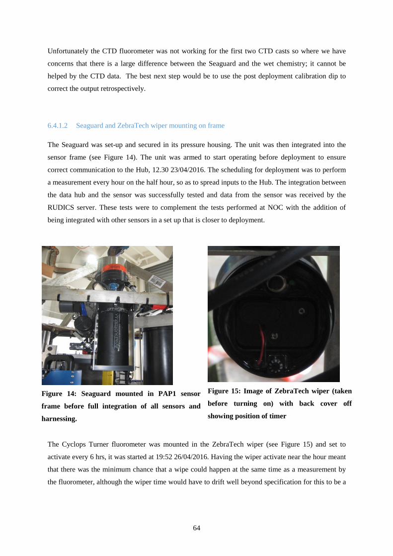
64

Unfortunately the CTD fluorometer was not working for the first two CTD casts so where we have

concerns that there is a large difference between the Seaguard and the wet chemistry; it cannot be

helped by the CTD data. The best next step would be to use the post deployment calibration dip to

correct the output retrospectively.

Seaguard and ZebraTech wiper mounting on frame 6.4.1.2

The Seaguard was set-up and secured in its pressure housing. The unit was then integrated into the

sensor frame (see Figure 14). The unit was armed to start operating before deployment to ensure

correct communication to the Hub, 12.30 23/04/2016. The scheduling for deployment was to perform

a measurement every hour on the half hour, so as to spread inputs to the Hub. The integration between

the data hub and the sensor was successfully tested and data from the sensor was received by the

RUDICS server. These tests were to complement the tests performed at NOC with the addition of

being integrated with other sensors in a set up that is closer to deployment.

Figure 14: Seaguard mounted in PAP1 sensor

frame before full integration of all sensors and

harnessing.

Figure 15: Image of ZebraTech wiper (taken

before turning on) with back cover off

showing position of timer

The Cyclops Turner fluorometer was mounted in the ZebraTech wiper (see Figure 15) and set to

activate every 6 hrs, it was started at 19:52 26/04/2016. Having the wiper activate near the hour meant

that there was the minimum chance that a wipe could happen at the same time as a measurement by

the fluorometer, although the wiper time would have to drift well beyond specification for this to be a

65

problem. Extra tubing was added to the cable arms from the Seaguard in an attempt to better protect it

from flexing while deployed (see Figure 14).

6.4.2 SUNA Nitrate Sensor (S/N: 391)

In lab-calibration 6.4.2.1

The SUNA nitrate sensor was calibrated in the lab at NOC (12.03.2016) using one point calibration

method with a set of nitrate calibration standards (5.9 µM, 11.8 µM, 29.5 µM). The standards were

prepared using a nitrate standard stock of 5900 µM and ultra-pure deionised water (Milli-Q DIW).

The exact concentrations of the calibration solutions will be determined using a Nutrient

AutoAnalyser at the National Oceanography Centre Southampton. The in-lab and Satlantic calibration

curves are presented in Figure 16.

Figure 16: In-lab calibration of the SUNA nitrate sensor

Nitrate = 1.0631×∙SUNA value - 1.1148 R² = 0.9998

Nitrate = 1.036 × SUNA value) - 0.145 R² = 1

0

5

10

15

20

25

30

35

40

45

0.00 10.00 20.00 30.00 40.00 50.00

Nitr

ate

stan

dard

(µM

)

SUNA Nitrate (µM)

SUNA Nitrate sensor in lab calibration

in lab cal 10.03.2016

Satlantic calibration

Linear (in lab cal10.03.2016)Linear (Satlanticcalibration )

66

Pre-deployment calibration on a CTD 6.4.2.2

The pre-deployment calibration of the SUNA sensor took place on 20.04.2016 during CTD

DY050_001 deployment to 100 m depth. The connection with the sensor was established through

SUNACom 3.0.6 software downloaded on a 64-bit PC. The sensor was mounted horizontally onto the

CTD rosette frame and powered to a battery pack. The SUNA was set to sample in a PERIODIC

mode recording EACHEVENT of sampling to its internal memory. Upon recovery, raw data and log

files were downloaded. The SUNA nitrate values will be corrected against Total Oxidised Nitrogen

measurements (TON=NO3- +NO2

-) from the Niskin bottles sampled at 10 discrete depths (5, 10, 15,

20, 25, 30, 40, 50, 60, 80, and 100 m).

After CTD deployment, the instrument drift was checked using DIW. NB: ‘Sampling Fresh Water’

was checked in ‘Advanced’ options of the SUNACom set up menu). The measured nitrate

concentrations drifted to an average of 2.64 µM, which is higher than the allowed range of ±2.0 µM

for DIW. The calibration of the instrument was therefore updated using ‘Update Calibration’ option in

the SUNACom main menu. The concentrations in DI water after recalibration were -0.34 µM on

average. We suggest subtracting the drift value from the measured nitrate concentration during CTD

deployment DY050-001.

Deployment on the PAP sensor frame 6.4.2.3

On the sensor frame deployed at 30 m, the SUNA Nitrate sensor was configured to sample in a

periodic mode/frame based operation. The sampling interval was set to 1 hour with 1200 sec (20 min)

offset past the hour. Within the sampling interval, the acquisition duration was given by the number of

frames. For this deployment, the chosen 1 frame operation outputs 1 dark frame then 1 light frame

which is the average of 10 samples. This gives an estimated frame rate of 0.1587 frames per second

(6.3 sec/frame). The integrated wiper was enabled.

6.4.3 WETLabs Fluorometer

The Wetlabs fluorimeter was tested on the bench and found to working well. It was then deployed on

CTD 1 to 100m to calibrate the chlorophyll reading prior to deployment. The CTD fluorometer was

not working on either ctd 1 or 2, as we are unable to compare the measurements against the CTD.

This is unfortunate as the r2 is only 0.69. One of the higher values in Figure 17 is probably incorrect

but we cannot be sure which one. The calibration generated by this dip can be used for initial

correction, but the post deployment calibration should be applied once this instrument is recovered

and re calibrated.

67

Figure 17: Chlorophyll calibration measurements on CTD cast

6.4.4 Sea-Bird SBE 37 MicroCATs

The SBE sensors s/n 10315, 9030 and 6915 were attached to the CTD and calibrated down to 100m

with sampling intervals of 10s. All the SBE sensors were serviced prior to the cruise. The result

showed that the SBE 37-ODO s/n 9030 sensor did not measure pressure and we decided to replace it

with the SBE 37-IMP s/n 9469 MicroCAT. Because the latest does not provide oxygen measurements

the configuration of the sensors on the frame was changed compared to the initial plans.

A Sea-Bird SBE 37-ODO (s/n 10315) was attached to the buoy keel and set to sample temperature,

pressure, conductivity and oxygen concentration every 30 minutes. It was assigned an inductive ID of

01. The initial plan was to clamp the SBE 37-ODO s/n 9030 on the keel and SBE 37-ODO s/n 10315

to the frame. By replacing the SBE 37-ODO s/n 9030 with SBE 37-IMP s/n 9469 the keel would be

left with no oxygen measurements. Since the Aanderaa optode provides oxygen measurements in the

frame we decided to swap them and install the SBE 37-IMP s/n 9469 and 6915 on the frame.

6.4.5 Pro-Oceanus dissolved gas sensors

CO2 sensor on the buoy 6.4.5.1

A non-logging CO2-Pro CO2 sensor (s/n 34-201-45) was attached to the buoy keel and is powered

and controlled by the buoy Telemetry Unit. It was serviced in 2015 after its recovery on July. This

sensor was supposed to be powered from the buoy and is planned to switched on every 12 hours (at

11:20 and 23:30). However, because of the lack of power from the buoy it will not be sampling.

y = 0.8126x - 0.0182 R² = 0.6932

00.20.40.60.8

11.21.41.61.8

0 0.5 1 1.5 2

chlo

roph

yll (

CTD

sam

ples

via

turn

er

fluor

omet

er)

chlorophyll ( flnt usb)

flnt usb chlorophyll cal

flnt usb chlorophyll cal

Linear (flnt usbchlorophyll cal)

68

The expected configuration was as follow. The start time, warm-up minutes, equilibration minutes

and sampling minutes can all be varied by email command and for this deployment a total on time of

37 minutes was used. A Sea-Bird pump pushes water through the sensor head and is powered directly

from the buoy during the equilibration and sampling phases. This sensor is not configurable and

performs an Auto Zero Point Calibrations (AZPC) every time it would be powered on.

CO2 sensor on the frame 6.4.5.2

A self-logging CO2-Pro (s/n 33-146-45) was attached to the sensor frame and was configured to

sample every 12 hours at midnight and noon producing 4 samples per record and performing an

AZPC every 4 sampling sessions. The real time clock battery was fully charged shortly before

deployment. This sensor is powered by two, 168Ah OceanSonics battery connected in parallel to

provide a voltage of approximately 14.4V and 336Ah. The average power consumption during

warmup for the CO2-Pro CV is 9 W, 643 mA at 14 VDC. The warming time in the context of PAP is

less than 5min. After warmup, the sensor power consumption is ~3 W, 214 mA at 12 VDC. The

sampling time is less than 5min for 4 samples. The internal controller requires ~30 μA of current

during sleep, 263mAh for a year which is negligible in the battery lifetime calculation. Thus, the

consumption during a year for 2 times a day sampling is 365*2*(5*0.643+5*0.214) = 3128Ah. The

consumption increases of about 25% with the pump according to the values from the sensor manual.

The consumption for a year would be 10160Ah. According to the manual, a battery of 268Ah would

allow 833 days of sampling. The values of the consumption are all from the manual and we believe

that they are inconsistent.

The ascarite CO2 absorbent in this sensor was replaced when serviced after the recovery of the sensor

on July. The data logger of this sensor was changed shortly before the cruise by a new data logger

provided by Pro-Oceanus. The previous data logger did not allow changing the sampling time. The

Pro-Oceanus sensors with the tubular interface are slower at depth. By the time the sensor warms up

and takes a zero, there was not enough time left in the 20 minute sampling cycle to fully equilibrate.

This created lower values during the samples with automatic zeroing due to the lack of complete

equilibration. The new logger can be configured to a range of sampling times. However, it was not

able to wake up the MAX3244 component on the electronics of the data hub. This conclusion was

reached after performing tests on board with various configurations. The sensor was communicating

with the data hub only if it was previously woken up with a character from the PC within 30 seconds.

The component also connects to the OCRs, the GTD and the Cycle-P sensor that did not have any

trouble communicating with the data hub. In fact, the previous logger of the CO2 sensor did not seem

to have any problem when tested at NOC. These results points out to a problem of incompatibility

between the MAX3244 and the new data logger that needs to be investigated further. In the current

69

context, this issue lacks of importance since the data hub is not functional due to the lack of power

from the Buoy. The CO2 sensor will be recording data internally.

GTD sensor on the frame 6.4.5.3

A GTD-Pro gas tension sensor (s/n 29-099-15) was also attached to the sensor frame and is only

powered and recorded by the Data Hub. Therefore, it will not be sampling data due to the lack of

power.

The expected configuration was as follow. The sampling time and duration is controlled by email

command and was for this deployment the sensor sampled for 6 minutes every 6 hours. This sensor

gave normal readings of pressure while on deck and the first day of deployment before the power shut

down.

6.4.6 pH SensLab sensors

The set of pH sensors at PAP1 deployment include a Sensor Lab SP101-Sm pH sensor on loan from

Melchor González Dávila at ULPGC on Gran Canaria along with two Satlantic SeaFET pH sensors

(s/n 105 and 111). The SP101 was calibrated before being received by NOC and checked and serviced

in Southampton before the cruise began by Melchor. However, it is also powered through the

telemetry system from the batteries of the buoy. Therefore, it will not be operational during this

deployment.

6.4.7 SeaFET pH sensors (s/n 105 and 111)

In-lab calibration 6.4.7.1

The SeaFET pH sensors (S/N 105 and 111) were calibrated in the lab at NOC and on-board RRS

Discovery using a set of Certified Reference Materials (CRMs) of known pH values (Batch 128, 146,

and 151). The sensors were sampling in the CONTINUOUS mode during calibration. The sensors

were warmed up for approximately 2 hours (to stabilise internal temperature of the sensor) before the

steady readings were logged. Temperature was recorded with a thermometer at the beginning and end

of the calibration test and the pH of CRM was calculated using CO2Sys_v2.1 macro. The results of

the calibration test are summarised in Table 9. The offsets between the aim CRM values and pH

measured by the SeaFETs 105 and 111 are shown in Figure 19.

70

Test SeaFET S/N pH internal pH external Temperature

(ºC) CRM pH

Pre-deployment calibration 10.02.2016

CRM Batch 140 105 7.864±0.001 7.932±0.001 20.1 7.929

CRM Batch 128 105 7.956±0.001 8.085±0.001 20.3 7.999

CRM Batch 140 111 7.859±0.008 7.936±0.009 20.4 7.929

CRM Batch 128 111 7.955±0.008 8.105±0.009 20.6 7.995

On-board pre-deployment calibration 19.04.2016

CRM Batch 128 105 7.862±0.001 7.9812±0.002 21.6 7.98

CRM Batch 146 105 7.922±0.001 8.088±0.002 21.1 7.963

CRM Batch 151 105 7.865±0.0004 8.059±0.001 21.2 7.915

CRM Batch 128 111 7.950±0.006 8.039±0.008 20.1 8.002

CRM Batch 146 111 7.986±0.002 8.141±0.004 20.3 7.975

CRM Batch 151 111 7.928±0.001 8.111±0.001 20.5 7.963

On-board post -deployment calibration 1 25.05.2016

CRM Batch 128 63 8.256±0.007 7.639±0.007 22.7 7.964

CRM Batch 146 63 8.468±0.012 7.862±0.041 22.8 7.938

CRM Batch 151 63 8.499±0.002 7.898±0.025 22.9 7.890

CRM Batch 128 257 7.772±0.014 7.724±0.016 22.9 7.961

CRM Batch 146 257 7.878±0.010 7.888±0.010 22.7 7.939

CRM Batch 151 257 7.854±0.011 7.881±0.013 23.1 7.887

71

On-board post -deployment calibration 2 28.05.2016

CRM Batch 128 63 8.540±0.014 7.917±0.001 22.3 7.970

CRM Batch 146 63 8.619±0.001 8.007±0.001 22.6 7.940

CRM Batch 151 63 8.571±0.002 7.963±0.002 22.3 7.899

CRM Batch 128 63 8.061±0.054 8.083±0.060 22.5 7.967

CRM Batch 146 63 7.929±0.013 7.991±0.013 22.8 7.938

CRM Batch 151 63 7.859±0.012 7.938±0.010 22.7 7.893

Table 9: Summary of pre- and post-deployment calibration tests for Satlantic SeaFET pH

sensors

Figure 18: Results of the calibration tests for (A) SeaFET-105 and (B) SeaFET-111 pH sensors

conducted in the land laboratory. The columns show the difference between the pH of certified

reference materials (CRMs) and the values measured by internal (red) and external (blue) pH

sensors of the SeaFETs.

72

Figure 19: Results of the pre-deployment calibration tests for (A) SeaFET-105 and (B) SeaFET-

111 pH sensors. The columns show the difference between the pH of CRMs and the values

measured by internal (red) and external (blue) pH sensors of the SeaFETs.

Deployment of SeaFETs on the sensor frame and the buoy. 6.4.7.2

The SeaFET sensors are programmed to take samples every 30min. They are connected to internal

batteries and external batteries. At the frame, the SeaFET 105 is connected to an Ocean Sonics battery

with 150Ah and at the buoy the SeaFET 111 is also powered by a Pro-Oceanus 268Ah.

The internal battery compartment holds 12 Alkaline D-Cell batteries. A distinctive characteristic of

the SeaFET is that it requires an uninterrupted and isolated source of power to keep the sensing

element conditioned and the battery pack is split into two packs, the main pack with 8 batteries (12V)

and the isolated pack with 4 batteries (6V). The 'Main battery pack' and the external batteries are used

to power the instrument control electronics when the instrument is in active mode. Because the power

consumption of the isolated battery power is 10uA in operation and 1.1mA in standby, the isolated

battery will last more than 15/0.0011 = 13636h = 568d and thus the consumption for keeping the

elements conditioned is not a limitation.

The main circuit consumes 340-400mW in operation and 70uA in standby. The consumption in

standby of a year deployment is 70x10-6x24*365 = 600mAh which is negligible in this context.

Assuming that the sensor stays on 15min for each sample, it would be in sampling mode half of the

time in a day. The batteries provide 14V-18V which correspond in the worst case scenario to a

consumption in sampling mode of 400/18-400/14 = 22mA-29mA. The consumption for an entire year

would be 22*(24/2)*365 = 96Ah to 29*(24/2)*365 = 127Ah and therefore, our external batteries

should provide power for a year deployment.

73

On the frame, SeaFET was set up to sample in periodic mode with a sampling interval of 30 min and

1380 sec offset (23 min past the hour), producing 3 Frames per burst (output of 3 samples, each is an

average of 10 readings) and creating a DAILY log ASCII file (Figure 20). On the buoy, SeaFET was

set up to sample in PERIODIC mode with a sampling interval of 30 min and 1620 sec offset (27 min

past the hour), producing 3 Frames per burst (output of 3 samples, each is an average of 10 readings)

and creating a DAILY log ASCII file. Note that the sampling regimes cannot be changed remotely.

Figure 20: SeaFET 105 pH sensor configuration for the deployments on the frame.

6.4.8 WETLabs Cycle phosphate sensor (s/n CYCL-P-177)

The WETlabs CYCLE phosphate sensor was deployed on the PAP sensor frame at 30m. The sensor

was calibrated in the lab at NOC. Because of the failure during the previous deployment, the company

loaned one of their sensors to be installed during the current deployment.

The cycle was set up the day before deployment after testing a few days earlier that the sensor would

continue to operate if power was interrupted. There are several issues to review the cycle. It needs to

be vertical when sampling but must be horizontal on the sensor frame prior to deployment. Priming on

land is achieved by drawing the three solutions through thin diameter tubing under a gentle vacuum.

74

Once the sensor is on the frame, there is no access to any internal tubing. The tubes are then left for

several days so could develop bubbles. The instrument doesn’t prime until in position at 30m it should

then be at a pressure which should help the reagents to be drawn through.

The cycle was programmed on deck using a small power source because using a mains type power

supply on deck is problematic. The instrument communicated for programming and the deployment

report below was normal, but the cycle failed to output any data late on 28/04/16 when the first

sample was due to be telemetered back. It is not clear whether it is still working and self logging but

not communicating or whether it is not working. It was communicating well on the tests made on the

frame when still on deck and was sampling and outputting correctly until it entered the water.

Figure 21: Set-up of the WETLabs Cycle phosphate sensor



Asynchronous Slave mode

Output initiated by external control

Sync to host clock

Reset sample counter

Reset power consumption

Data dir to existing dir: DY050DEP - NOT RECOMMENDED

Instrument units to uM

Setting cal deployment volume to 250.0

Setting reagent 1 deployment volume to 250.0

Setting reagent 2 deployment volume to 250.0

Priming to start at 18:45:00 on 04/28/16

(1444.6) minutes from now

Sampling to start at 19:15:00 on 04/28/16

(1474.6) minutes from now

Number of samples = 300000

Sample interval = 6:00:00

Calibration frequency = 6



Awake

PO4>$WKM

2

75

PO4>$WKM 2

2

PO4>$CLK

04/27/16 18:41:00

PO4>$CLK 04/27/16 18:40:55

04/27/16 18:40:55

PO4>$VOL

117.124 6.900 7.718 7.560

PO4>$VOL 0.00 0.00 0.00 0.00 /S

0.000 0.000 0.000 0.000

PO4>$CNT

3

PO4>$CNT 0 /S

0

PO4>$ONT

1:27:04

PO4>$ONT 0 /S

0:00:00

PO4>$DSD

DY050DEP

PO4>$DSD DY050DEP

DY050DEP

PO4>$EUF

uM

PO4>$EUF 0

uM

PO4>$DCA

250.000 250.000 250.000

PO4>$DCA 250.00 250.00 250.00 /S

250.000 250.000 250.000

PO4>$SUD 04/28/16 18:45:00 /P

04/28/16 18:45:00 P

PO4>$CSF

6 0

PO4>$CSF 6

6 0

76

PO4>$INT

1:00:00

PO4>$INT 21600

6:00:00

PO4>$IDT

120

PO4>$NOS

3 3

PO4>$NOS 300000

-27680 -27680

PO4>$SUD

Figure 22: The Cycle with cables attached correctly, the exhaust tubes and intakes are free

6.4.9 Satlantic OCR-507 Irradiance sensors

A Satlantic OCR-507 ICSA irradiance sensor (s/n 201) was fitted to the buoy mast and is controlled

by the Telemetry Unit. The Data Hub controls an OCR-507 ICSW upward-looking irradiance sensor

(s/n 200) and an OCR-507 R10W downward-looking radiance sensor (s/n 95). All 3 sensors were

commanded to sample every 30 minutes at the same time so that their data are coincident. The

sampling intervals can be changed remotely using SBD commands. All sensors were serviced before

the deployment and they are paired with a bioshutter to avoid biofouling. They will not be working

since they should be powered from the batteries of the buoy through the telemetry or data hub

systems.

6.5 PAP1 Recovered Data Hub and Telemetry Systems

The recovered PAP Observatory system was deployed on 1st July 2015 on RRS Discovery cruise

DY050 and the PAP0003 system was fully operational until its recovery. The buoy and sensor frame

77

were recovered without difficulty on the morning of 25th April 2016. The mooring rope was

disconnected from the bottom of the sensor frame and attached to a large buoy which was then

released. This allowed the vessel to continue with other work until the system was finally re-attached

to the mooring and deployed on 28th April.

Sensor Performance

Recommendations and

Actions

Telemetry

Worked and communicate for entire

deployment.

Test system at NOC.

Copy data from drive.

Pro-Oceanus CO2-Pro

Failed to collect data during

deployment since 2016/03/03 but

sensor worked when connected to

PC after recovery. Extreme

biofouling of sensor and pump.

Check harness. Assess

if servicing is needed.

Need new pump and its

copper guard.

SeaBird SBE-37-ODO-

IMP MicroCAT Worked along deployment.

Assess need of

servicing.

Satlantic OCR-507

ICSA (buoy) with

bioshutter

Sensor sampled successfully to the

end of deployment. Copper

protection was absent.

Copy data from

telemetry system.

Asses if servicing is

needed

Satlantic SeaFET pH

The sensor was sampling data for the

entire deployment but the internal-

external measurement diverged when

checked in lab probably due to

extreme biofouling. Data was

uploaded from sensor. Servicing.

Sensor Lab SP101-Sm

pH sensor

It failed intermittently through

winter. On 2016/01/13 failed to take

sensible pH data but was still

sending good MicroCAT data.

Found extreme biofouling on keel

explaining the failure.

Extract data.

Return to Melchor

Table 10: Summary of status of sensors in the buoy

78

In comparison to previous years the system was extremely biofouled after 10 months of deployment,

especially at the buoy (see Figure 23). This caused sensors to fail working properly or not at all. On

the other hand, the orange cable, the protective hydraulic hosing over the cable and the sensors did not

show any obvious damage (see Figure 24).

The operation observations and commands were logged in the wiki at

http://twiki.noc.soton.ac.uk/twiki/bin/view/PAP/Papdep2015OpNotes. Table 10 shows the

performance and the status of the data extraction for the sensors that are located on the buoy. The

sensors located at the frame are shown in Table 11.

Sensor Performance

Recommendations and

Actions

SeaBird SBE-37IMP

MicroCAT

Real time data stopped around mid-

March due to problem of frame-buoy

inductive link. Data was stored

internally and uploaded from sensor.

Check inductive link.

Service sensor.

SeaBird SBE-37IMP

MicroCAT

Real time data stopped around mid-

March due to problem of frame-buoy

inductive link. Data was stored

internally and uploaded from sensor.

Check inductive link.

Service sensor.

WETLabs FLNTUSB

Fluorometer

Sampling successfully to the end of

the deployment. Data was uploaded

from sensor. Assess servicing

Satlantic ISUS Nitrate

sensor

External battery failed intermittently.

The sensor sampled for the entire

deployment although the level raised

considerably at the end of 2016

probably due to biofouling. Data was

uploaded from sensor.

Servicing but not

urgent since it will be

replaced by SUNA.

Satlantic SeaFET pH

sensor

Data started to scatter on March

2015. Some biofouling but probably

mainly due to need of calibration. Servicing.

Aanderaa 4430H Sensors sampled data along the Asses if servicing is

http://twiki.noc.soton.ac.uk/twiki/bin/view/PAP/Papdep2015OpNotes

79

Seaguard entire deployment. Data diverged at

the end of the deployment due to

biofouling on the sensors. Wiper was

not working when recovered. Data

was uploaded from sensor.

needed. Paint work to

fix scratches.

Satlantic OCR-507

ICSW irradiance with

Bioshutter

Sensor sampled successfully to the

end of deployment. Data was lower

than usual for a period of time may

be due to biofouling. Copper

protection was absent.


needed.

Satlantic OCR-507

R10W radiance with

bioshutter

Failed on 2016/10/29 likely due to

failure of harness.


needed

Pro-Oceanus Logging

CO2-Pro

2016/01/8 sensor started to

misbehave and stopped sampling a

few days later. It shows assembling

failures after recovery. Data was

extracted from SD card inside. In

addition, there was a problem with

the logger as explained in the

deployment section.

Servicing and

discussions with

company about

improving assembling

design. Need new

pump and its copper

guard.

Pro-Oceanus GTD-Pro

Showed signs of failure just after

deployment on 2016/07/01 but it was

working normally after recovery

which indicates that we turned it off

too soon

Servicing since it is an

old sensor and the

increase of values was

probably due to need

of inspection.

WETLabs CYCL-P

Phosphate Analyser

Stopped working soon after

deployment probably due to

blocking of out tube. Data was

uploaded from sensor.

Assess if servicing is

needed.

Table 11: Summary of status of sensors in the frame

80

Figure 23: Picture of buoy keel after the recovery from deployment 2015-2016

81

Figure 24: Orange cable near the frame-chain connection

The PAP0003 system has

proven very reliable

during the entire

deployment. There was

no failure of the

communication Figure

25 shows the efficiency

of the data transfer. The

power of the system was

also very successful

except for some

shutdowns of the data

hub unit at the end of the

deployment. As

mentioned earlier, the

orange cable was intact

after the recovery and

even the hose was not

damage. The tubing

around the cable was

sliced near the chain (see

Figure 24).

There was a recurrent restart of the data hub at the end of the deployment when the OCR started to

take measurements. This problem went away after a command was sent to stop the OCR sampling.

82

Figure 25: Time versus Data bytes transferred by Iridium dial-up

6.6 PAP1 Recovered Sensors

6.6.1 Satlantic SeaFET sensors (s/n 063 and 257)

The SeaFET sensors S/N 063 (frame) and 257 (buoy) deployed during DY032 in June 2015 were

successfully recovered on 25.04.2016. The sensor slot of both instruments was covered with biofilm

(Figure 27).

83

Figure 26: pH and temperature data collected by (A) SeaFET-063 (B) and SeaFET-257. The pH

value measured by internal and external sensors are in red and blue, respectively. Temperature

values are shown in green.

Figure 27: Biofouling on the ensor

probe of SeaFET 257

The data collected over a year of deployment was

successfully downloaded from the internal memory of

both instruments. The SeaFET-063 was recording data

from 22.05.2015 till 25.04.2015, while the SeaFET-257

was recording from 19.05.2015 to 25.04.2016.

Upon recovery, the performance of the sensors was tested

using the same set of CRMs as for SeaFETs deployed

during DY050 and following the procedure described in

Section 6.4.7. The results of post-deployment calibration

are summarised in Error! Reference source not found..

The offset between the measured pH and CRM values are

shown in Figure 28 (A, C). Due to a relatively large

offset observed for both SeaFETs, a repeated test with

CRMs was conducted (see Table 9 and Figure 28 (B, D).

The uncorrected data collected by SeaFETs is shown in

84

Figure 26.

Figure 28: Results of the post-deployment calibration tests for (A,B) SeaFET 063 and (B, C)

SeaFET 257. The columns show the difference between the pH of CRMs and the values

measured by internal (red) and external (blue) pH sensors of the SeaFETs.

6.6.2 Nitrate ISUS sensor (s/n 059)

ISUS nitrate sensor deployed on a frame in June 2015 during DY032 cruise was successfully

recovered on 25.04.2016. The data from internal memory of the instrument was downloaded

immediately. ISUS was recording data from 20.06.2015 to 24.04.2016. The copper guard of ISUS

corroded significantly over the deployment period (Figure 30), which might have affected the

performance of the sensor.

85

A post-deployment calibration test was performed on 27.04. 2016 using DIW, low nutrient sea water

(LNSW), and a set of nitrate standards (0.6 µM, 2.5 µM, 5 µM, 11 µM) prepared from 5900 µM

nitrate stock solution. The exact concentrations of these standards will be determined using Nutrient

AutoAnalyser at National Oceanography Centre Southampton. The initial calibration test revealed a

lot of noise in the nitrate data and a large offset in nitrate concentrations (3.41±1.88µM) measured in

DIW and LNSW samples. The real-time data observed along the year (see Figure 29) also showed a

shift of the concentration data consistent with the first calibration.

For the second calibration run (29.04.2016), the sensor probe was cleaned with DIW and a tissue, and

the test in DIW was performed again. The offset however persisted, indicating an overall drift in the

accuracy of the sensor. The calibration update procedure was then conducted using DIW and ‘Update

Calibration’ option in the ISUSCom main menu. DIW sample and nitrate standards (5.9 µM, 11.8

µM, 23.5 µM) were subsequently tested (Figure 31).

Figure 29: ISUS real time data during deployment 2015-2016

86

Figure 25: Corroded copper guard of ISUS nitrate sensor

87

Figure 31: ISUS nitrate sensor post-deployment calibration results

Nitrate = 0.9806x (ISUS value) - 4.6594 R² = 0.9478

Nitrate = 1.0402 × (ISUS value) + 1.6065 R² = 0.9999

0

5

10

15

20

25

-5 0 5 10 15 20 25

Nitr

ate

stan

dard

(µM

)

ISUS Nitrate (µM)

ISUS nitrate sensor post-deployment calibration

PD Cal 1 (27.04.2016)

PD Cal 2 (29.04.2016)

Linear (PD Cal 1(27.04.2016))Linear (PD Cal 2(29.04.2016))

88

Figure 32: Uncorrected (blue) and corrected (red) nitrate data collected with ISUS sensor.

Although the average nitrate value for DIW (-1.67±1.15) was within the Satlantic recommended value

of 0±2 µM, we note a persistent large standard error regardless the calibration update. The cause of

this problem will be investigated with the Satlantic team.

The nitrate concentrations measurements that we recovered from the ISUS are shown in Figure 32.

The uncorrected values are shown in blue. In red are nitrate values corrected for an average offset of

3.41±1.88µM determined during post-calibration tests. Note, that it is unknown at which point during

the deployment this offset developed.

6.6.3 Pro-Oceanus CO2-Pro s/n 29-097-45 at the buoy keel

This sensor was powered from the buoy and was switched on every 12 hours (at 11:20 and 23:30).

The start time, warm-up minutes, equilibration minutes and sampling minutes can all be varied by

email command and for this deployment a total on time of 37 minutes was used. A Sea-Bird pump

pushes water through the sensor head and is powered directly from the buoy during the equilibration

and sampling phases. Figure shows the data during the deployment period. The sensor stopped

sending data at the beginning of March. When recovered we did not see any sign of damage and it

was operational when connected to the PC. This indicates a failure of the harness that connects the

sensor to the telemetry unit. The sensor was covered with biofouling as shown by Figure 23.

However, this is unlikely to stop the sensor providing data and we would expect at least non-sense

data received through PAP0003. A first assessment of the cable indicates a possible failure in the

89

junction between the pump and the sensor. It is recommended a more careful assessment of the

location of the harness failure to provide more information for future deployments.

Pro-Oceanus logging CO2-Pro s/n 34-200-45 at the frame 6.6.3.1

Figure 33: Uncorrected CO2 concentration data from the sensors on the buoy (blue) and the

sensor frame at 30m (red)

This sensor ran autonomously and was powered from two OceanSonics battery housings each

containing around 150Ah of lithium cells. The real time clock battery was fully charged shortly before

deployment and the sensor was configured to record every 12 hours producing 4 samples per record.

The sensor ran successfully throughout the deployment until the end of December (see Figure 33). At

that time the data started to diverge and it stopped sending any data at the beginning of March with

intermittent stops. After recovery, we discovered that the electronics inside was loose which explains

the failure during the deployment.

Pro-Oceanus GTD-Pro s/n 33-152-16 at the frame 6.6.3.2

A GTD-Pro gas tension sensor (s/n 33-152-16) was also attached to the sensor frame and is powered

and recorded by the Data Hub. This allows the sampling time and duration to be controlled by email

command, and for this deployment the sensor sampled for 6 minutes every 6 hours. The data during

the first few days is not showing reasonable pressures but we should have waited to see if it stabilise.

90

This sensor gave normal readings of pressure while on deck. The increasingly high and unfeasible

readings as soon as it entered the water made us believe that there was some kind of malfunction. The

sensor was turned off after reaching to the conclusion that it was leaking. However, after recovery the

sensor does not have any indication of water inside the tube and it is sampling data and

communicating to the PC. The sensor would probably be sampling if we have not have send the

command but the samples would probably not be reasonable. The sensor should be sent for inspection

to the company, especially considering that we use an old sensor that was in the shelves for a long

time.

6.6.4 Sea-Bird SBE 37 MicroCATs

Three Microcats were recovered from the 2015-2016 deployment. The Sea-Bird SBE 37-ODO (s/n

13397) was attached to the buoy keel and set to sample temperature, pressure, conductivity and

oxygen concentration every 30 minutes. Sea-Bird sensors SBE 37-ODO (s/n 10535) and SBE 37-IMP

(s/n 6904) were attached to the frame. The SBE 37-ODO was set to sample temperature, pressure,

conductivity and oxygen concentration every 30 minutes, while the 37-IMP samples temperature,

pressure and conductivity every 15 minutes. On March 2015, the SBE 37-ODO (s/n 13397) sensor

was purchased and the SBE 37-ODO (s/n 10535) was serviced and recalibrated by Sea-Bird.

The sensors on the frame stopped the inductive communications with the telemetry system on mid-

March 2016 indicating a problem with the inductive cable. In fact, the sensor on the buoy continued to

send the data and therefore the problem and all three sensors recorded the data internally until they

were recovered. The sensors recorded for 302 days since they were started on 2015/06/28 and

recorded 14502 samples at the buoy and 14725 samples (ODO) and 29490 samples (ODE). The

problem with the real time data was likely to come from a failure of the harness.

The data from the buoy is consistent with the values from the SensLab for temperature and

conductivity. The values of oxygen are also consistent with the Seaguard measurements although the

latest was biofouled and showed large scattering. The results from the MicroCAT on the buoy are

surprising considering the large amount of biofouling. However, all these sensors were probably

affected in same degree by biofouling.

6.6.5 Satlantic OCR-507 Radiance and Irradiance Sensors

A Satlantic OCR-507 ICSA irradiance sensor (s/n 226) was fitted to the buoy mast and is controlled

by the Telemetry Unit. The Data Hub controlled an OCR-507 ICSW upward-looking irradiance

sensor (s/n 287) and an OCR-507 R10W downward-looking radiance sensor (s/n 113). All 3 sensors

were commanded to sample every 30 minutes at the same time so that their data are coincident.

Sensor operation was suspended during hours of darkness according to a monthly look-up table in the

91

buoy controller. The irradiance sensors on the buoy and frame were covered of biofouling and have

lost their copper Bioshutter (see Figure 35). The radiance sensor in the frame (see Figure 34) looked

physically fine.

Figure 34: Upward-looking irradiance sensor

s/n 113

Figure 35: Upward-looking irradiance

sensor s/n 287

The irradiance sensors in the frame and the buoy sampled and sent the data via iridium through the

telemetry unit for the entire deployment. However, the looking downwards radiance sensor in the

frame failed to send data in 29th October 2015. The cable seems to fail at the level of the sensor-

bioshutter junction and the meter indicates a connection between pins 4, 5 and 6 which are the serial

pins. In fact, the assessment was performed a week after recovery and the harness may have dried in

between. Other wires probably started short-circuiting explaining why the data hub re-started at the

time when OCRs were scheduled to turn on.

6.6.6 Wet Labs flnt usb fluorimeter

On recovery the instrument has some biofouling but the optical window was successfully kept clean

by the copper shutter

92

Figure 36: wetlabs s/n 3050 effective copper wiper

The recovered wetlabs fluorimeter was cleaned down with fresh water and deployed on a calibration

cast to 200m.

93

Figure 37: wetlabs s/n 3050 chlorophyll calibration

The post deployment calibration was reasonably successful with an r2 of 0.8. This calibration can be

retrospectively applied to the data generated since deployment in June 2015.

6.6.7 Recovery of Seaguard s/n 1614

Recovery Status 6.6.7.1

A RCM Seaguard with oxygen optode (Aanderaa 4330, S/N 2001) and fluorometer (Turner cyclops,

S/N 2103960) were part of the sensor frame of the PAP1 that was recovered in 25/04/2016.

Data had been continuously received from the Seaguard since deployment, only occasionally lost

through a separate issue with shore side servers, but all data is also stored locally to the sensor so full

data sets were available upon recovery.

y = 1.8331x - 2.5077 R² = 0.8046

y = 1.2465x + 0.0387 R² = 0.9324

0

0.1

0.2

0.3

0.4

0.5

0.6

0.7

0.8

0.9

0 0.5 1 1.5 2

chlo

roph

yll f

rom

wet

che

mis

try

(ug/

l\)

chlorophyl from instruments (ug/l)

flnt usb 3050 post deployment calibration 30/04/16

wetlabs vs on boardanlaysis

CTD vs on board analysis

Linear (wetlabs vs onboard anlaysis)

Linear (CTD vs on boardanalysis)

94

Figure 38: Image of flurometer and optode post deployment. Biofouling covers nearly all

surfaces equally, including the sensing surfaces.

First impressions upon recovery were that the Seaguard had fared well. Biofouling was noticeable

across all surfaces but did not appear to be debilitating. A partial success was the fluorometer sensing

window that was serviced on deployment by a ZebraTech wiper (set to activate every 6 hrs). It

appears that the operation failed at some point as there was slight biofouling on the surface of the

fluorometer, Error! Reference source not found.. Manually passing the wiper across the fluorometer

completely cleared the biofouling, indicating it had been out of operation for probably a few weeks.

Another site of concern was the optode window that had biofouling across the membrane, Figure 38.

The sacrificial anode had performed its role and was noticeably corroded but approximately 50 % of

its bulk remained. Its integrity is severely impaired and now crumbles easily. Some corrosion was

noted around the G-clamps used to keep the instrument sealed within its pressure casing. The

corrosion appear to match wear scratches in paintwork had occurred and around the bolts of the G-

clamps.

Once removed from the PAP1 sensor frame the Seaguard was washed down with plain cold water and

wiped with blue roll to remove as much of the growth on the unit as possible. Care was taken around

the optode and fluorometer sensor windows, using kimwipes and MilliQ - and no scrubbing.

The Seaguard was still powered when removed from its pressure housing; no water ingress beyond

the o-ring seal was noticed. Recording was halted and the two alkaline batteries reported a voltage of

6.9 V (7.6 V is considered the lowest level to be used by the instrument).

With the spare capacity of the SD card it is likely if future deployments employed lithium batteries for

the Seaguard an increase in the sampling rate could be easily accommodated by the SD card.

95

An operational check was conducted with the Seaguard and it took readings at the expected intervals,

without checking the accuracy of the readings the Seaguard appeared in good health.

Full data sets from Seaguard deployment

Figure 39 is the deployed data from the fluorometer and Figure 40 the deployment data from the

oxygen optode. Both data sets do not have the pre-deployment calibrations applied.

Figure 39: Screenshot of chlorophyll data collected by fluorometer during deployment, please

note this data does not have pre-deployment calibrations applied.

0

2

4

6

8

10

12

14

16

18

20

05/ 01-00:00 07/ 01-00:00 09/ 01-00:00 11/ 01-00:00 01/ 01-00:00 03/ 01-00:00 05/ 01-00:00 07/ 01-00:00

Da te & T ime [Gmt]

Line Graph

Chlorophyll # 2103960 [ug/ L]

Moving average: 1

96

Figure 40: Screenshot of oxygen data collected by optode during deployment, please note this

data assumes zero salinity and sea level pressure and does not have pre-deployment calibrations

applied.

Post deployment calibration check of Seaguard 6.6.7.2

The deployment batteries were replaced and the Seaguard was mounted on a CTD frame for a cast to

200 m. Waters were collected by Niskin and later analysed through Winkler titration. The fluorometer

was compared with chlorophyll readings, also analysed on board from the collected waters.

260

280

300

320

340

360

380

400

420

440

05/ 01-00:00 07/ 01-00:00 09/ 01-00:00 11/ 01-00:00 01/ 01-00:00 03/ 01-00:00 05/ 01-00:00 07/ 01-00:00

Da te & T ime [Gmt]

Line Graph

O2Conc entration [uM]

Moving average: 1

97

Figure 41: Seaguard pre-deployment calibration from 2015.

Figure 42: Seaguard post deployment calibration from 2016.

y = 0.8675x + 44.487 R² = 0.9942

245

250

255

260

265

270

235 240 245 250 255 260

Win

kler

oxy

gen

/(uM

/l)

Sal and Pres corrected Seaguard oxygen /(uM/l)

y = 0.8876x + 42.523 R² = 0.9609

255

260

265

270

275

280

240 245 250 255 260 265

Win

kler

oxy

gen

/(uM

/l)

Sal. and Pressure corrected Seaguard oxygen /(uM/l)

98

The Seaguard was cleaned post deployment, removing any biofouling. Therefore if biofouling has

been the cause of drift whilst on deployment it is not directly revealed in the post calibration cast.

The resulting difference between the two calibrations is equivalent to ≈ 2.8 μM/l at 250 μM/l.

Figure 43: chlorophyll calibrations for turner fluorimeter

Chlorophyll samples were collected on the CTD cast and analysed on board using a Turner bench top

fluorimeter courtesy of Alex Poulton. Whilst the comparison in Figure 43 with the fluorimeter on the

CTD was close there was a greater difference with the Seaguard fluorimeter reflected in the r2 of

0.263. This can now be applied to correct data collected over 2015/16.

6.6.8 Wetlabs CYCLE phosphate sensor sn 164

We learned from the previous year deployment that the reason of failing taking measurements was

likely to be related to the compression of the outlet tubes (see recovery section for more details).

Therefore, we decided to cut the tubes instead of tying them to the frame.

y = 1.2465x + 0.0387 R² = 0.9324

y = 0.091x + 0.2148 R² = 0.2623

0

0.1

0.2

0.3

0.4

0.5

0.6

0.7

0.8

0.9

0 2 4 6

wet

che

mis

try

chlo

roph

yll (

ug/l

)

instrument chlorophyll (ug/l)

seaguard 1614 calibrations

wet chemistry vs ctd

wet chemistry vs seaguard

Linear (wet chemistry vsctd)

Linear (wet chemistry vssea guard)

99

Figure 44: Measured phosphate (umol/l) from the cycle, which gave data for approximately

three weeks after deployment then read zero

The deployment totalled 74 files which translates on the summary file to 37 readings, each file

1640001-16400025 looks OK, but after this there is a ‘low power fault’ on every file (aside from

16400026, 16400028, 16400029 and 16400058). This is thought to be due to the drain from trying to

push the chemicals throught the over tight exhaust tube.

Figure 45: Measured phosphate standards on the Cycle

The recovered cycle was bench calibrated using a Phosphate standard. After each set of readings the

standard was approximately halved in concentration. Exact concentration will be confirmed by

running sub samples of the serial dilutions at NOC. The uncorrected standards were plotted against

y = 1.1116x + 0.0803 R² = 0.9819

0

0.5

1

1.5

2

2.5

3

0 1 2 3

Phos

phat

e st

anda

rd (u

M)

Cycle Phosphate (uM)

CAPO4

CAPO4

Linear (CAPO4)

100

the cycles reading below and showed a good level of accuracy from the instrument. This suggests

there has been no lasting damage from the problem with the waste tube.

6.6.9 Star-Oddi sensors: Recovery and Re-deployment

Recovery of Staroddis from PAP1 6.6.9.1

The recovery of PAP1 in 2016 was of the buoy and sensor frame only. The line down to the acoustic

release is not scheduled for recovery until 2017 (was originally planned for 2016 but has now been

deferred) and so not all of the Staroddis that have been deployed were recovered. Of the six Staroddis

expected for recovery this year all returned although one no longer communicated, a summary is

provided in Table 12.

Table 12: Summary of Star-Oddi status upon PAP1 recovery

Staroddi Type Deployment

depth /m

Position Interval

type

Interval Status

6788 DST

CTD

5 Below buoy Fixed 30 min Recovered,

data collected

6782 DST

CTD


data collected

7728 DST

CTD


data collected

6792 DST

CTD

20 Below buoy Fixed 30 min Recovered but

loss of

communication

6784 DST

CTD


data collected

H454 DST tilt 30 Sensor frame Multiple

Interval

Tilt: 1 s x 60

measurements;

Temperature:

30 min x 48

measurements

Recovered,

data collected

7561 DST

CTD

50 Below frame Fixed 30 min Not scheduled

for recovery

7562 DST

CTD


for recovery

101

7563 DST

CTD


for recovery

7564 DST

CTD


for recovery

7565 DST

CTD


for recovery

7566 DST

CTD


for recovery

H457* DST tilt 1000 Sub-surface

buoy

Fixed

interval

45 min Not scheduled

for recovery

*rated to 3000 m

Please note that the sum of the measurements made by H454 does not equal 24 hrs, this is so the one

minutes burst of tilt measurements do not occur at the same time of day.

Figure 46 is an image of the six recovered StarOddis after removing any fixings (e.g. mounting block,

cable ties or tape) that bound them to the cable hose or to the frame. H454 was the only one of the six

recovered units that was in a mounting block as it was also the only one mounted on the frame. The

remaining retrieved Staroddis had all been secured to the cable hose running alongside the chain and

held in place by cable ties and amalgamated tape near a raised bolt on the bracket (leaving the tip and

base of each unit to sense the ocean).

102

Figure 46: Image of the five recovered Staroddis; all have been removed

from the fixings that bound them to the hose/frame and have been cleaned

of any biofouling.

2015-2016 Deployment Data 6.6.9.2

The recovered data was treated with the pre-deployment calibration coefficients found from last

year’s preparation. Initial inspection suggests the results are sensible. Taking temperature as an

example all units closely agree in colder months where the surface layers of the ocean are well

mixed and in warmer months the temperature recorded separates in accordance to how deep the

StarOddi was mounted (deeper units recorded colder temperatures).

Figure 47: Complete temperature data set of StarOddis mounted at various depths.

When recovering the units it was noticeable how much more biofouling there was closer to the

surface (Figure 48).

181 231 281 331 34 84 134

11

12

13

14

15

16

17

Day of year

Tem

pera

ture

/C

5 m10 m15 m25 m30 m

103

Figure 48: (left) Staroddi at 5 m depth (right) Staroddi at 25 m depth.

It is likely that this has affected the output from the StarOddis such as shown in the pressure data

(Figure 49).

Figure 49: Complete pressure data set of StarOddis mounted at depths.

181 231 281 331 34 84 134

-1

0

1

2

3

Day of year

Pre

ssur

e /b

ar

5 m10 m15 m25 m30 m

104

The pressure data in Figure 49 shows drift in sensor output, which appears worse depending on how

close to the surface the StarOddi was placed. Since the StarOddis nearer the surface experienced

greater levels of biofouling this drift could be attributed to that cause.

Post-deployment calibration 6.6.9.3

The StarOddis recovered that were not re-deployed or were no longer communicating underwent a

post-deployment calibration. All biofouling had to be removed to download data and restart running,

as a consequence the post-deployment calibration cannot be used to understand the effect biofouling

may have had on readings taken.

Table 13: Pre-deployment and post-deployment calibration comparison

StarOddie Pre-deployment

calibration 2015

Post-deployment

calibration 2016

Test value

(2015-2016)

S6782

Temperature

Pressure

1.000x+0.03529

0.97849x+12.9

0.9838x+0.2083

0.9863x+13.46

-0.011 °C (@ 10 °C)

-0.580 bar (@ 2.5 bar)

S6784

Temperature

Pressure

1.005x-0.02085

0.9975x-0.8931

0.9879x+0.1709

0.9945x-0.8756

-0.021 °C (@ 10 °C)

-0.01 bar (@ 2.5 bar)

S7728

Temperature

Pressure

0.9929x+0.1279

0.9781x-0.01775

0.9907x+0.1239

0.9781x+0.01375

+0.026 °C (@ 10 °C)

-0.032 bar (@ 2.5 bar)

The largest change was in the pressure measurement of S6782. This change closely matches the drift

of the sensor from the deployment data.

Note that salinity has not been compared as there was not enough of a variation in the shallow CTD

casts to enable a calibration.

Deployment of Staroddis from PAP1 6.6.9.4

For the DST CTD type Staroddis that were located on the chain direct replacements were made with

units that had greater battery capacity, an exception being S6788 which was immediately redeployed.

The DST tilt that had been fixed to the frame was also re-used as a newer replacement was not

available.

105

Table 14: Summary of Staroddis deployed at PAP1 following re-deployment of frame and buoy

Staroddi Type Deployment

depth /m

Position Interval

type

Interval Date memory

will be full

(and battery

life at that

time)

6788 DST

CTD

5 Below buoy Fixed 30 min 28/12/2019

Mem. 73%

Batt. 45%

7724 DST

CTD


Mem. 73%

Batt. 45%

7725 DST

CTD


Mem. 73%

Batt. 45%

7727 DST

CTD


Mem. 73%

Batt. 45%

7729

DST

CTD


Mem. 73%

Batt. 45%

H454 DST tilt 30 Frame Multiple

Interval

Tilt: 1 s x 60

measurements;

Temperature: 30

min x 48

measurements

09/09/2017

Mem. 100%

Batt. 57.7%

7561 DST

CTD

50 Below frame Fixed 30 min Deployed

2014

7562 DST

CTD


2014

7563 DST

CTD


2014

7564 DST

CTD


2014

7565 DST

CTD


2014

106

7566 DST

CTD


2014

H457* DST tilt 1000 Sub-surface

buoy

Fixed

interval

45 min Deployed

2014

*rated to 3000 m

All units being deployed this year were set to start at 12:00 28th April 2016.

As mentioned H454 was re-used and replaced on to the frame in the block holder, Figure 50. The

orientation of H454 was modified to what it was last year. This year the z-axis of the tilt sensor is

aligned to the vertical line of the frame when deployed – this is in line with the guidelines set out by

the manufacturer.

Figure 50: H454 being secured to cross bar of sensor frame before PAP1 deployment.

The remaining StarOddis being deployed were spaced 5 m apart from the bottom of the water line in

accordance with the information in Table 14. The StarOddis on the hose were always placed on one of

the brackets used to keep the hose and chain together. In the past a number of these brackets had split

in the middle so the Staroddis were placed to one side and next to one of the bolts that stand proud of

the bracket. The bolt of the bracket should protect the Staroddis as the chain and hose slip over the

deck on deployment and recovery. This methodology has proven successful with all units mounted in

this way returning after deployment with no obvious physical damage.

Once again the Staroddis on the hose were first wrapped in self-amalgamating tape then secured with

cable ties and further tape. Finally electrical tape was used to highlight there placement for care

107

during deployment and easier identification upon recovery, Figure 51. The tip and base of each

Staroddi was kept free to allow full operation.

Figure 51: Staroddi secured on bracket along cable hose at 15 m mark.

108

7 PAP3 Mooring

7.1 Sediment Traps

By Corinne Pebody

The 2016/17 PAP#3 sediment trap moorings were deployed and the 2015/6 traps recovered on 24th

April 2016. Traps A, B, C and D were recovered successfully. On recovery, the bottles were removed

and lids screwed on before removing to the general purpose lab. The bottles were photographed (see

Figures 52, 53 and 54) and the pH checked. Then 1ml of formalin was added before the bottles, an

extra layer of parafilm was added then the lids replaced and samples stored in the chill room.

Figure 52: Bottles from 3000m 2015 – 2016 with bottle 14 showing the spring bloom has started

to export material already.

Figure 53: Bottles from 100mab showing the export has reached the seabed.

109

Figure 54: Bottles from the 3000m inverted trap. The bottles were empty except for 14 which

had a medusa.

Figure 55: Estimated volume flux 2015/16

The bottles were measured to estimate volume flux (a quick bit reasonable measure of the particle

flux) over the deployment year. Figure 55 illustrates the summer bloom of 2015, the drop off over

winter and the 2016 bloom. This was suspected before the cruise as the instruments at PAP 1 were

showing a spikey fall in nitrate and a similarly spikey increase in chlorophyll.

7.2 BioOptical Platform

By Christian Konrad, Clara Flintrop, Morten Iversen

0123456789

EVF

(ml/

m2/

day)

mid day open date

PAP 3 EVF 20014/16

Trap A 3000M

Trap B 3000M

Trap C 100MAB

110

7.2.1 Using the BioOptical Platform (BOP) to study long-term aggregate dynamics as

part of the PAP3 Mooring

We developed a new method to follow aggregate dynamics throughout a whole year by combining in

situ optics with gel traps. The BioOptical Platform (BOP) uses an optical system to determine size-

distribution, abundance and size-specific sinking velocities of settling particles every day throughout a

whole year. Additionally, it collects the settling particles in a viscous gel over different time intervals

throughout the year. The BOP system is based on a modified sediment trap (Fa. KUM GmbH) where

we have replaced the collection funnel with a polycarbonate cylinder to avoid that the settling

particles are sliding down the sides of the funnel, which would change the physical structure. The

polycarbonate cylinder has an inner diameter of 35 mm and functions as a settling column and allows

us to measure the settling velocities and sizes of the particles without interference from ocean currents

(Figure 1). This is done with a camera system that is placed at the lower part of the settling column.

The camera system consists of an industrial camera (Fa. Basler), a fixed focal length lens (Fa.

Edmund Optics) and the system electronics consisting of single board computer including a SSD hard

disc and custom made power and time management circuitry. The images are illuminated by a custom

made visible light source providing backlight. The whole camera system is powered by a Li-Ion

battery (24V, 1670Wh, Fa. SubCTech GmbH) (2). The camera system makes 5 min of recordings

every day. Once the particles have settled through the settling column they are collected in cups filled

with a viscous gel that preserves their size and physical structure. The gel cups are placed on two

rotation tables capable of carrying 40 gel cups (Figure 56).

Figure 56: The BOP system with the polycarbonate settling column (left image) and the two

rotation tables (right image).

111

Figure 57: Camera System on BOP with the camera housing (for camera, lens and system

electronics), the VIS light source and the Li-Ion battery

7.2.2 System configuration, measurements and deployment

The geometrical configuration of the camera system enables daily recordings of shadow images of the

particles within the settling column throughout a whole year. It is programmed to take one image per

second for five minutes every day throughout one year (Table 5).

The system was deployed at as part of the PAP3 mooring at 2930m. See the final position and layout

of the mooring is given in the PAP3 report. During the deployment of the trap the top polycarbonate

plate got damaged and due to that the measurement might be influenced by this event.

112

Table 15: Programming of the BOP system. Periodical measurements of the camera system for

5 minutes every day and changing of 40 gel cups in the sediment trap every 3 / 15.5 days

alternately.

Date [YYYY-

MM-DD]

Time

[HH:MM:SS]

Remarks

2016-04-21 12:00:00 Camera: auto start, 1 image per second for 5

minutes, auto shutdown,

THIS PROCEDURE WILL BE REPEATED

EVERY DAY WITHOUT END DATE

2016-04-26 00:01:00 Trap: Next bottom bottle





















2016-08-31 00:02:00 Trap: Next top bottle






113














2017-05-17 00:01:00 Trap: Last bottle out; System open

7.3 Larval Traps

By Mark Stinchcombe

A number of larval traps were supplied by Luciana Génio, Marina Cunha, Ana Hilário and Clara

Rodrigues from the Universidade de Aveiro, Nikoleta Bellou from the Hellenic Centre for Marine

Research and Craig Young from the Oregan Institute of Marine Biology. They were attached to the

PAP3 mooring and deployed with it. These were in the form of 4 settlement traps which were

attached to the uprights of one of the sediment traps on PAP3 and colonisation and settlement traps

which were attached to the rope of PAP3 above the anchor.

The settlement traps consisted of PVC pipe which contained 50ml centrifuge tubes with fixative

inside. To ensure the fixative stayed inside the tube until the traps were in position, they were sealed

with parafilm pulled taught with an elastic band connected to a galvanic release. After 2f hours the

galvanic release would let go of the parafilm which would come clear of the tube.

The colonisation traps were a wide diameter plastic pipe with large holes in it. Within were cages

containing different substrates. They were bone, wood and oyster shells. These were placed in

different orders in the two traps. One of these traps also had a repeat of the settlement traps attached

to the top. These traps were attached to the rope of PAP3 using clamps which were made onboard

(Figure 58).

114

Figure 58: Colonisation traps with smaller larval settlement traps being attached to the PAP3

rope.

115

8 Zooplankton Net Sampling

By Corinne Pebody

The WP2, 200µm net was deployed to 200m in a series of paired vertical hauls. Prior to each haul, the

net was checked for twists and that the tap was closed, then the net was lowered over the side using

either the Rozler (Rexroth) winch over the starboard side or the Romica with the crane over the aft

starboard side. There were strong currents running on some occasions and the rope was put over the

roller when using the Rexroth to keep the net clear of the ship (thanks Stuart and Barry). This also

seemed to improve the vertical line of the net, except for the last deployment where even the addition

of extra weight failed to keep the angle to less than 30 degrees. Maximum depth was 200 metres

where the deployment was paused for a minute to allow the net to hang straight before the being

brought up at approx. 10 metres per minute.

Figure 59: Deployed Net

116

On recovery the net was hosed down from the outside with seawater and the cod end emptied into a

white bucket. Hosing was repeated and time allowed for zooplankton to settle into the bottom of the

cod end. Samples were then either, transferred to 2 litre bottles and preserved by adding borax

buffered formalin to an approximate concentration of 5%. Alternatively the sample was sieved

through a series of meshes, 2mm, 1mm, and 200µm and transferred to cryo vials and stored in the -

80°C freezer.

8.1 Future Work

At NOC, formalin preserved samples will be split with a Folsom splitter. A sub sample will be picked

to remove zooplankton greater than 2mm. Remaining meso-zooplankton will be analysed using flow

cam technology to ascertain size and abundance distribution

Figure 60: Pteropod and Salp (?) dominated nets 12 and 13.

Table 16: Summary of zooplankton net deployments.

Station

ID

DY050-

052

NET #1

noon

sample preserved in formalin 2litre bottles

Water

depth

net shot 27/04/16 12:09

ucm

at surface 27/04/16 12:47 ucm

DY050-

053

NET #2

noon

sample

Sieved into >2mm; ,<2mm; >1mm;

<1mm>200µm; <200µm>63 µm

Nb due to oil leak and orders from bridge,

net hauled up at 60m a minute to get away

frozen at

- 80°C

117

from azipods. Part way up we were allowed

to go back to 102m/min.

net shot 27/04/16 12:53 49 02.00 N 16 15.00 W 4810

at surface 27/04/16 13:26

ucm

DY050-

055

NET #3

midnight

sample

preserved in formalin 2 litre bottles

net shot 28/04/16 01:49 48 50.2462 N 16 31.2201 W 4806

at surface 28/04/16 02:09

DY050-

058

NET #4

noon

sample preserved in formalin 2litre bottles

Water

depth

net shot 28/04/16 11:30 49 0.31416 N 16 23.81724 W 4810


DY050-

059

NET #5

noon

sample


<1mm>200µm; <200µm>63 µm frozen at

- 80°C

net shot 28/04/16 12:17 49 0.31434 N 16 23.81766 W 4809

at surface 28/04/16 13:07

ucm

DY050-

069

NET #6

midnight

sample



- 80°C

Water

depth

net shot 29/04/16 23:39 49 10.5208 N 16 5.58828 W 4806

at surface 29/04/16 23:53 Ucm

DY050-

070

NET #7

midnight

sample


net shot 29/04/16 23:59 49 10.64322 N 16 5.4234 W 4804

at surface 30/04/16 00:32

Ucm

DY050-

085

NET #8

noon

sample



- 80°C

Water

depth

net shot 30/04/16 12:17 49 0.32508 N 16 23.8056 W 4809


DY050-

087

noon

sample preserved in formalin 2 litre bottles

118

NET #9

net shot 30/04/16 13:31 49 0.32466 N 16 23.80554 W 4809

at surface 30/04/16

ucm

DY050-

90 NET

#10

midnight

sample



- 80°C

Water

depth

net shot 01/05/16 00:25 48 53.26968 N 16 28.18164 W 4808


DY050-

91 NET

#11

midnight

sample


net shot 01/05/16 01:14 48 53.269610 N 16 28.18170 W 4807

at surface 01/05/16 02:04

Ucm

DY050-

105

NET

#12

midnight

sample



- 80°C

Water

depth

net shot 02/05/16 23:53 49 0.70930 N 16 23.84860 W 4811


DY050-

106

NET

#13

midnight

sample


net shot 03/05/16 00:40 49 0.70974 N 16 23.84784 W 4811

at surface 03/05/16 01:??

Ucm

Thank you to Brian, Ben, Owain, Stuart, Barry, Seamus and Ian.

9 Marine Snow Catchers

By Anna Belcher, Clara Flintrop, Christian Konrad, Morten Iversen

We used the MSC to determine the sinking particle flux, particle composition, size-specific settling

velocity of in situ collected particles, and bacterial colonization of marine particles.

119

9.1 Objectives and Aims

The aim of the cruise was to investigate temporal changes in sinking particle flux over the duration of

the cruise at the PAP site, with the hope to capture the spring bloom. Marine snow catchers (MSC)

were utilised to collect marine snow particles from the water column and examine the size,

composition and abundance of material at different depths and make estimates of particle flux. We

further used the collected marine snow to determine bacterial colonization processes via laboratory

incubations. As such it was aimed to use the MSC to:

1) Measure any variation in the sinking particles (in terms of magnitude, particle size and

composition) with depth and over the course of the cruise

2) Measure the sinking velocities of particles to calculate particle fluxes

3) Collect water from the MSC to measure the particulate organic carbon (POC) and size

fractionated chlorophyll (Chl) in the slow sinking and suspended carbon pool

4) Determine how bacteria colonize marine aggregates and how different motility strategies

influence the colonization efficiency.

9.2 Methods

95 litres of water were collected in each marine snow catcher (a PVC closing water bottle designed to

minimise turbulence), deployed at a range of depths below the chlorophyll maximum at base of the

mixed layer (determined from the most recent CTD profile). A RBR Concerto CTD with fluorescence

and turbidity sensors was attached to each MSC to record the vertical profile during deployment. As

soon as the MSCs were on deck, an initial two litre sample was taken from the bottom tap on the

MSC. The MSCs were then left upright for two hours to allow the marine snow particles to sink to the

bottom. One litre of the initial sample (Time zero - T0 sample) was filtered immediately for POC and

represents the homogenous water column. The remaining litre was left to stand for two hours before

also being filtered for POC (T2 sample).

After standing for two hours, a 1.5L sample was taken from the top section of the MSC (the

suspended fraction) before draining the remaining water. The bottom section of the MSC containing 7

litres of water and settled particles was then removed. A 1.5L sample was siphoned out of the base

section (representing the slow sinking pool), before removing the particle collector tray from the base

and storing in a 10°C temperature controlled laboratory. Water samples collected from both the top

and the base sections of the MSC were filtered for POC and Chl (size fractionated).

Particles that had settled to the base (the fast sinking pool) of the bottom chamber and collected in the

collector try were photographed with a Canon EOS DSLR camera and a 105 mm macro lens. These

images enable us to determine the sizes, types, and abundance of the particles collected in each of the

four compartments in the collector tray and will make it possible to relate different particle types and

120

abundance to the POC measurements done for two of the compartments for each deployment.

Following this sinking velocity measurements were carried out on 5-15 particles from a number of

MSC. Sinking velocity measurements were conducted using a flow chamber containing water

collected from MSC 004 (stn 15) which was filtered (GF/F) and maintained at a temperature of 12 °C.

Each particle was carefully placed in a 10 cm high Plexiglas tube (5 cm diameter), on a net extended

across middle of the tube. Flow was supplied from below the net, adjusted using a needle valve,

resulting in a uniform flow field across the upper chamber. The flow was adjusted so that the particle

is suspended one particle diameter above the net. At this point the sinking velocity is balanced by the

upward flow velocity, and can be calculated by dividing the flow rate by the area of the flow chamber.

Three measurements of the sinking velocity were made for each particle and the x, y, and z

dimensions of the particle measured using a horizontal dissection microscope with a calibrated ocular.

Two splits were taken from each marine snow catcher and put on ashed GF/F filters for measurement

of POC. High resolution microscope photos were taken of particles in one split, and one final split

frozen for future analysis. All particles were collected from one collector tray compartment and

placed in an Utermöhl chamber for investigations of the individual aggregates using an inverted

microscope. We used magnifications ranging between 100x and 400x in a brightfield and phase

contrast microscope. Pictures were taken of aggregates and wherever interesting grazing behaviour

occurred, a video recording was. Special attention was devoted to grazing activity in marine snow by

ciliates and nanoflagellates to answer questions such as where and at which components of the

aggregates have the highest abundance of grazers? How does this correlate with the compactness and

the content of the aggregate? How does grazing activity differ between aggregates collected from

different depths? Some of the particles were stained with Alcian Blue to qualitatively assess TEP

content within aggregates. The microscopic investigations of the particles will be used to determine

changes in the settling particles both vertically and over time during the cruise period.

121

9.2.1 Filter Sample Preparation, Preservation and Analysis

POC 9.2.1.1

1L was filtered through a 25mm diameter, ashed GF/F filter, rinsed with milliQ

water, placed in a Petri dish, air dried and stored at room temperature for later

analysis.

Total Chlorophyll 9.2.1.2

200 ml was filtered through a 0.8μm pore size, 25mm diameter, MPF300 filter,

rinsed with milliQ water, placed in an eppendorf tube and stored at -20°C for later

analysis.

Chl >20 µm 9.2.1.3

200ml was filtered through a 20µm pore size, 25mm diameter nucleopore

polycarbonate membrane filter, rinsed with milliQ water, placed in an eppendorf

tube and stored at -20°C for later analysis.

9.3 Preliminary Results

A total of 41 marine snow catcher deployments were made to support this study (Table 17).

Table 17: Details of MSC deployments during DY050 utilised for this study.

Date Time on

deck

(GMT)

MSC

#

Statio

n #

Latitude

(°N)

Longitude

(°W)

Depth

(m)

Notes

22/04/16 14:50 001 5 49° 00.375 16° 23.848 20 Contaminated with

ship’s rust

22/04/16 15:10 002 6 49° 00.375 16° 23.848 20 Leaked – no usable

sample

22/04/16 15:45 003 7 49° 00.375 16° 23.848 120 Leaked a little, but

stopped once secured on

deck

23/04/16 19:20 004 15 49° 00.338 16° 23.808 60

23/04/16 19:45 005 16 49° 00.338 16° 23.808 160

23/04/16 20:00 006 17 49° 00.338 16° 23.808 80

24/04/16 09:10 007 21 49° 00.488 16° 27.184 80 Deployed without tray

for particles for CF

122

24/04/16 09:35 008 22 49° 00.488 16° 27.184 180

24/04/16 009 23 49° 00.488 16° 27.184 MSC didn’t fire

24/04/16 10:00 010 24 49° 00.488 16° 27.184 80

25/04/16 17:20 011 30 49° 00.417 16° 23.864 60

25/04/16 17:40 012 31 49° 00.417 16° 23.864 80

25/04/16 18:00 013 32 49° 00.417 16° 23.864 160



26/04/16 015 41 49° 00.344 16° 23.860 160 Leaking so redeployed

(MSC017)

26/04/16 14:20 016 43 49° 00.344 16° 23.860 160

26/04/16 14:35 017 44 49° 00.344 16° 23.860 60

27/04/16 10:02 18 49 49° 00.327 16° 23.842 60

27/04/16 10:27 19 50 49° 00.327 16° 23.842 160



28/04/16 15:27 21 62 49° 00.314 16° 23.817 60

29/04/16 14:40 22 65 49° 00.321 16° 23.847 90 *benthic trawl had just

come up and lots of mud

being washed into

water. But mostly on

port side, MSC

deployed off starboard

side

29/04/16 15:15 23 66 49° 00.321 16° 23.847 160 Dripping a little on deck

29/04/16 18:35 24 68 49° 00.321 16° 23.847 60

30/04/16 11:25 25 82 49° 00.324 16° 23.805 90

30/04/16 11:55 26 83 49° 00.324 16° 23.805 160

30/04/16 12:10 27 84 49° 00.324 16° 23.805 60

01/05/16 11:25 28 93 49° 00.331 16° 23.812 60

01/05/16 11:55 29 94 49° 00.331 16° 23.812 160

01/05/16 12:10 30 95 49° 00.331 16° 23.812 30

02/05/16 15:35 31 102 49 00.708 16 23.848 30 Deployed without tray


03/05/16 11:07 32 109 49 00.323 16 23.812 160

03/05/16 33 110 49 00.323 16 23.812 60 Knocked against ship as

123

came aboard and started

to leak, so aborted

03/05/16 14:45 34 111 49 00.323 16 23.812 60

03/05/16 14:55 35 112 49 00.323 16 23.812 30

04/05/16 13:40 36 114 49 00.299 16 23.597 30

04/05/16 14:00 37 115 49 00.299 16 23.597 60

04/05/16 14:30 38 116 49 00.299 16 23.597 160

05/05/16 13:03 39 120 49 00.319 16 23.821 150

05/05/16 13:37 40 121 49 00.319 16 23.821 300

05/05/16 13:51 41 122 49 00.319 16 23.821 50

The RBR CTD showed a change in the mixed layer depth over the course of the cruise as well as in

the magnitude and depth of the chlorophyll maximum. The chlorophyll maximum shallowed from 50

to 30m, becoming a more defined peak (Figure 61). The RBR CTD has not been fully calibrated for

temperature, salinity, fluorescence and turbidity and hence data should be considered relative but not

absolute.

124

Figure 61: Example profiles of chlorophyll and temperature from the RBR attached to the

marine snow catcher. A) for MSC 3, B) for MSC 28

Further results will be worked up following laboratory analysis of sample filters (POC, Chl) obtained

from filtration of slow sinking and suspended water fractions from the MSCs. These data will be

accompanied by measurements from the CTD as well as PELAGRA trap samples, SAPS samples and

holocam and PELAGRA Cam profiles to support investigation of changing export flux over the

spring bloom at the PAP site.

The microscopic investigations of the particles collected with the MSC showed that there was a shift

in the particles types at the 1st of May. Before this period we had mainly collected compact and dense

particles consisting of small phytoplankton – too small to identify with 400x magnification, though

some indications of the presence of coccolithophores were observed. After the 1st of May we observed

0

50

100

150

200

250

0 0.5 1 1.5 2

Dept

h (m

)

Chlorophyll (mg/L - uncalibrated)

0

50

100

150

200

250

11.5 12 12.5 13

Dept

h (m

)

Temperature (°C)

0

50

100

150

200

0 0.5 1 1.5 2

Dept

h (m

)

Chlorophyll (mg/L - uncalibrated)

0

50

100

150

200

11.5 12 12.5 13

Dept

h (m

) Temperature (°C)

A)

B)

125

a shift toward a higher presence of mucous aggregates. We stained those aggregates with Alcian Blue

and found that large proportions of the particles contained polysaccharides that were stained by

Alcian Blue (Figure 62).

Figure 62: Alcian Blue stained aggregate. The blue-green colour is due to the Alcian blue

staining and suggests the presence of polysaccharides within the aggregate. This aggregate with

photographed on an inverted microscope at a 100x magnification. The total width of the image

is 1.14 mm and diameter of the aggregate is around 1 mm.

9.4 Marine snow catcher maintenance issues

One MSC (MSC Tom) was se 0rviced before the first deployment as the pole through the plunger in

the base was not secure and slipped up and down preventing the MSC from sealing. The inner pole

was secured to the plunger with a pin and no further problems occurred (Figure 2). There was a

problem of contamination of the first samples (MSC 001-003) which may have been due to material

trapped inside the MSC or material falling in when the MSC made contact with the side of the ship.

The MSCs were thoroughly hosed again before redeployment and no further contamination issues

occurred. Following the initial deployment, MSCs Tom and Jerry were leaking from the base. This

problem was rectified by tightening the nuts on the clasps that secure the base to the top. Additionally

the MSC bases were marked with tape to help line up the top and the base of the MSC for the most

water tight fit. MSC Tom has continued to drip slightly from the base and may need some additional

silicon applied to the pole at the base of the plunger where the fix was made.

MSC Tom in particular has a very tight fitting top plunger making it difficult to attach the base and

the top. This problem was exacerbated by the o-rings falling out or becoming misaligned when trying

to clasp the base to the top. Thicker and/or flat o-rings that would sit more securely in the groove

126

are recommended to be purchased for future deployments. The problem of the tight plunger can

be solved by rigging the snow catchers upright (either manually or using the crane), however the use

of the crane eats into valuable ship time. The option to sand back part of the plunger was not carried

out on board for fear of causing further damage and preventing the snow catcher from sealing.

However, this should be investigated further to create a more permanent solution.

Figure 63: Schematic to highlight fix that was carried out on MSC Tom.

Inner pole Base plunger

Additional pin added here

127

10 Microplastics sampling

By Katsia Pabortsava

10.1 Sampling microplastics with large volume in situ pumps (SAPs).

Microplastics and biogenic particles in the water column were collected with large-volume stand-

alone in situ pumps (SAPs; Figure 64A). Over the course of the cruse, SAP 03-06 was flooded and

fell out of action, while SAP 03-07 had an internal fault, the nature of which could not be identified

and fixed. During the last SAPs deployment on 04.05.2016 we also discovered a leak in SAP 03-03.

Nevertheless, the instrument still pumped a substantial volume of water.

The SAPs were deployed at 2-3 discrete depths (Table 18) collecting particles onto acid-washed (10%

HCl) 53 µm (pre-filter) and 1 µm (main filter) NITEX© nylon meshes. Filter loading, sample

preparation, and processing were always carried out under the laminar flow hood in a clean laboratory

on board of the ship. The SAPs were set to pump for 90 min, filtering up to 2000 L of seawater (Table

18). Each SAP was equipped with a SeaBird Temperature-Depth sensor, recording the data every 10

min. Upon recovery, NITEX© meshes were carefully removed from filter holders. Particles collected

onto a 53 µm mesh were immediately rinsed into a beaker with exactly 1 L of artificial sea water

(ASW; 35 g NaCl per 1 L of ultra-pure water) and split into 4 sub-samples using Folsom splitter (Fig.

64B, C, D). Splits designated for POC analysis were filtered onto pre-ashed (450°C for 24 hrs) 25 mm

Whatman GF/F filters (0.8 µm nominal pore size). Splits for microplastic analysis were filtered onto

25 mm Whatman cyclopore polycarbonate filter (0.4 µm nominal pore size). All filters were stored

frozen at -20°C until analysis. For POC and microplastic sample blanks, 100 ml of ASW was filtered

through unused GFF and polycarbonate filters. The microplastic contamination level during sample

processing was accessed by keeping polycarbonate filters exposed in the laminar flow hood for the

duration of particle rinse-off and splitting. The remaining particle-ASW splits were spiked with 12.5

mL of concentrated formalin (5% v/v final concentration) buffered with 5g/L di-sodium tetraborate

and stored at 4°C until analysis. One micron mesh with particles was carefully folded, wrapped into

aluminium foil, and frozen at -20°C until processing and analysis in the land laboratory. For blanks,

unused acid-washed 53 µm and 1 µm NITEX© meshes were processed in exactly the same way as the

samples.

128

Figure 64: A. Large volume in situ Stand Alone Pump (SAP) used to collect microplastics and

marine particles; B. SAPs sample processing under the laminar flow hood; C. NITEX© pre-

filter (53 µm) with collected particles; D. Set-up for rinsing particles off the NITEX© mesh.

129

Table 18: SAPs deployment log during DY050 cruise

Date Station # Latitude

ºN

Longitude

ºW

SAPS

S/N

Depth

(m)

Volume

pumped

(L)

Remarks

22.04.2016 DY050-10 49.008 16.392 03-03 10 1174

22.04.2016 DY050-10 49.008 16.392 03-06 70 781

22.04.2016 DY050-10 49.008 16.392 03-06 150 1178

23.04.2016 DY050-13 49.005 16.397 03-04 250 1027

23.04.2016 DY050-13 49.005 16.397 03-06 500 85 leaked

23.04.2016 DY050-13 49.005 16.397 03-03 1000 1924

23.04.2016 DY050-13 49.005 16.397 03-07 2000

failed

25.04.2016 DY050-28 49.007 16.398 03-04 1000 1785

25.04.2016 DY050-28 49.007 16.398 03-03 500 1985

26.04.2016 DY050-38 49.005 16.398 03-07 150 62 failed

26.04.2016 DY050-38 49.005 16.398 03-04 70 766

26.04.2016 DY050-38 49.005 16.398 03-03 10 1902

27.04.2016 DY050-48 49.005 16.397 03-03 250 1421

27.04.2016 DY050-48 49.005 16.397 03-04 500 1649

27.04.2016 DY050-48 49.005 16.397 03-07 2000 1 failed

30.04.2016 DY050-81 49.005 16.397 03-03 150 2002

30.04.2016 DY050-81 49.005 16.397 03-04 10 896

01.05.2016 DY050-97 49.006 16.397 03-03 70 455

01.05.2016 DY050-97 49.006 16.397 03-04 10 779

02.05.2016 DY050-101 49.012 16.397 03-04 1000 783

02.05.2016 DY050-101 49.012 16.397 03-03 250 973

03.05.2016 DY050-108 49.005 16.386 03-03 500 1056

03.05.2016 DY050-108 49.005 16.386 03-04 250 1054

04.05.2016 DY050-113 49.005 16.393 03-03 150 691 leaked

04.05.2016 DY050-113 49.005 16.393 03-04 70 834

130

10.2 Microplastics collection with megacorer

Sediment core samples were collected by Brian

Bett’s benthic team to investigate the abundance of

microplastics in the deep marine sediments at PAP.

Upon recovery, the cores were removed from the

megacorer one by one. The core designated for

microplastics was immediately covered with foil to

prevent any airborne microplastics contamination.

The surface water was siphoned through a 250 μm

sieve and the sediment remaining on the sieve was

collected in a pre-weighed, ashed, acid-clean, glass

sampling jar (250 ml). The top 1 cm was sliced off

using a metal cutter and added to the sampling jar.

Plastics are only likely to be found on the surface

sediments since plastic is a modern product. Hence,

for control sample, the next 5 cm of mud sample

was discarded and the following 1 cm of mud was collected into a separate jar. The sampling

procedure is described in section 16. The layer of foil was placed between the jar and lid. The wet

sample was then weighted wet and dried at 50°C in the oven. The weight of a dry sample was also

determined. All core samples will be analysed for microplastics in the land laboratory.

Table 19: Log of cores samples for microplastics

Core ID Site Date Latitude

(ºN)

Longitude

(ºW)

Depth

(m) Thickness

Wet

weight

(g)

MgC08+2 RP02 22.04.2016 48.840 16.520 4810 0-1 cm 657.5

MgC08+2 RP03 23.04/2016 48.838 16.518 4808 0-1 cm 826

MgC08+2 RP03 23.04/2016 48.838 16.518 4808 6-7 cm 958

MgC08+2 RP07 26.04.2016 48.838 16.517 4807 0-1 cm 705

MgC08+2 RP07 26.04.2016 48.838 16.517 4807 6-7 cm 606.5

MgC10 RP09 27.04.2016 48.835 16.520 4807 0-1 cm 734.5

MgC10 RP09 27.04.2016 48.835 16.520 4807 6-7 cm 621.5

MgC10 RP11 28.04.2016 48.838 16.519 4807 0-1 cm 566.8

MgC10 RP11 28.04.2016 48.838 16.519 4807 6-7 cm 591.4

MgC10 RP13 05.05.2016 48.836 16.522 4805 0-1 cm 746.5

MgC10 RP13 05.05.2016 48.836 16.522 4805 6-7 cm 862.5

Figure 65: Diagram of microplastic sampling of a sediment core (not to scale; figure credits: E. Cavan)

131

11 PELAGRA Cruise Report

By Kevin Saw and Robin Brown

The purpose of including the PELAGRA sediment traps on DY050 was to carry out engineering trials

in preparation for the COMICS science program scheduled for 2017 and 2018.

Following various issues experienced on the previous cruise (JC087, 2013), the traps have undergone

a number of modifications:

• The sample pot rotation carousel has been upgraded from the original four-roller system to a

full complement slew-ring type ball race arrangement utilising acetal balls. This has also

allowed the drive motor to be re-mounted with its axis tangential to the worm wheel which

removes the need for the original bevel gear arrangement.

• The 1000 m emergency abort releases have been redesigned to replace the original disc

springs with a conventional coil spring to improve reliability.

• The LED flashing light beacons have been modified to replace the original rubber pressure

switch membrane with a waspaloy metal foil membrane.

• Four polypropylene feet have been added to the base ring to enable moving the traps with a

pallet truck and lifting the attached weights clear of the deck without the need for the

existing wooden deck stands.

All five existing traps (P2, P4, P6, P7 and P8) were present for the cruise. P4 and P7 were rigged with

particle cameras as described in the cruise report for JC087. All traps were re-weighed and re-

ballasted prior to the cruise.

Apart from testing the mechanical alterations, it was intended that data from these deployments could

be used to confirm ballasting calculations and any adjustments needed and to gain a better

understanding of the coefficients for compressibility and thermal expansion. To help with the latter it

was hoped that successful (i.e. stable) deployments could be achieved for each trap at two distinct

depths, e.g. around 200 m and 600 m.

11.1 Deployment 1

Initially, for least risk, it was decided to deploy one of each trap type (i.e. one ‘standard’ trap and one

camera trap with gels, P2 and P7 respectively) to check accuracy of ballasting. Both traps were set up

for 200 m deployments with ballast added as calculated by the ballast spreadsheets with no

adjustments. In situ temperature and salinity data were obtained from the CTD cast made at station

DY050-004.

132

P2 (standard trap)

Station: DY050-008

Target depth: 200 m

Target temp: 11.86°C

In situ density: 1027.924 kg m-3

Added ballast: 4123 g

Deployment time: 22.04.16 18:50

Deployment posn: 49° 00.375’ N

16° 23.848’ W

Figure 66: P2, deployment 1

As is evident from the above plot, P2 was over-ballasted and descended to 400 m before recovering to

the intended 200 m. It then underwent a number of oscillations before stabilising (as evidenced by

stable sigma-theta) around 03:00 on 24 April. The APEX buoyancy engine needed to increase

displacement by about 60 counts to achieve this suggesting that the trap was over-ballasted by c. 60 g.

The depressor weight was released at 100 m as expected.

On recovery, all four sample pots had collected particles, the carousel was positioned as expected and

the burn wire released at the expected time, all indicating proper function of the timer and the new

carousel bearing.

133

P7 (camera trap)

Station: DY050-009

Target depth: 200 m






16° 23.848’ W


P7 was under-ballasted. The APEX buoyancy engine attempted to correct for this but had no chance

of doing so before the trap reached the surface and went into recovery mode. No quantitative

assessment can be made from this deployment of the degree of ballast error.


On recovery, although no particles had been collected, swimmers were found in the pots indicating

that they had been open, the carousel was positioned as expected and the burn wire released at the

expected time, all indicating proper function of the timer and the new carousel bearing. As the ship

134

approached P7 for recovery the LED flash beacon was not working (although it appeared to be

working prior to the close approach). After investigation it was concluded that the switch plunger was

a bit too tight. This was rectified and the light functioned normally for later deployments.

Figure 68: Deployment 1 drift plot (including surface drift for P7)

11.2 Deployment 2

For deployment 2, it was decided to carry out a deployment of all three ‘standard’ traps to 200 m

again. Due to the findings from P2 deployment 1, a -50 g adjustment was made to the calculated

ballast for all three traps based on the assumption that being similar in construction, P6 and P8 would

be similarly over-ballasted. Temperature and salinity data recorded during deployment 1 was used as

it differed somewhat from the original CTD data recorded at station 004.

135

P2 (standard trap)

Station: DY050-033

Target depth: 200 m



Added ballast: 4111- 50 = 4061 g



16° 23.864’ W


Here, P2 is ballasted about as well as can be expected. The initial stable period was achieved with just

9 counts adjustment of the APEX buoyancy engine. The trap was fully stable well before the first

sample collection period.


136



carousel bearing.

P6 (standard trap)

Station: DY050-034

Target depth: 200 m



Added ballast: 4123 – 50 = 4073 g



16° 23.864’ W


Here, P6 is ballasted almost perfectly. Despite an initial adjustment in response to the trap ascending

just after the depressor weight released and the slight over-depth situation caused by that, stability was

achieved with just 4 counts adjustment of the APEX buoyancy engine. The trap was fully stable well

before the first sample collection period.

The -50 g ballast adjustment was correct for this trap.

137




carousel bearing.

P8 (standard trap)

Station: DY050-035

Target depth: 200 m



Added ballast: 4053 – 50 = 4003 g



16° 23.853’ W


P8 was under-ballasted and returned to the surface after the depressor weight had released at 100 m

and quicker than the APEX could adjust to compensate. The APEX aborted and entered recovery

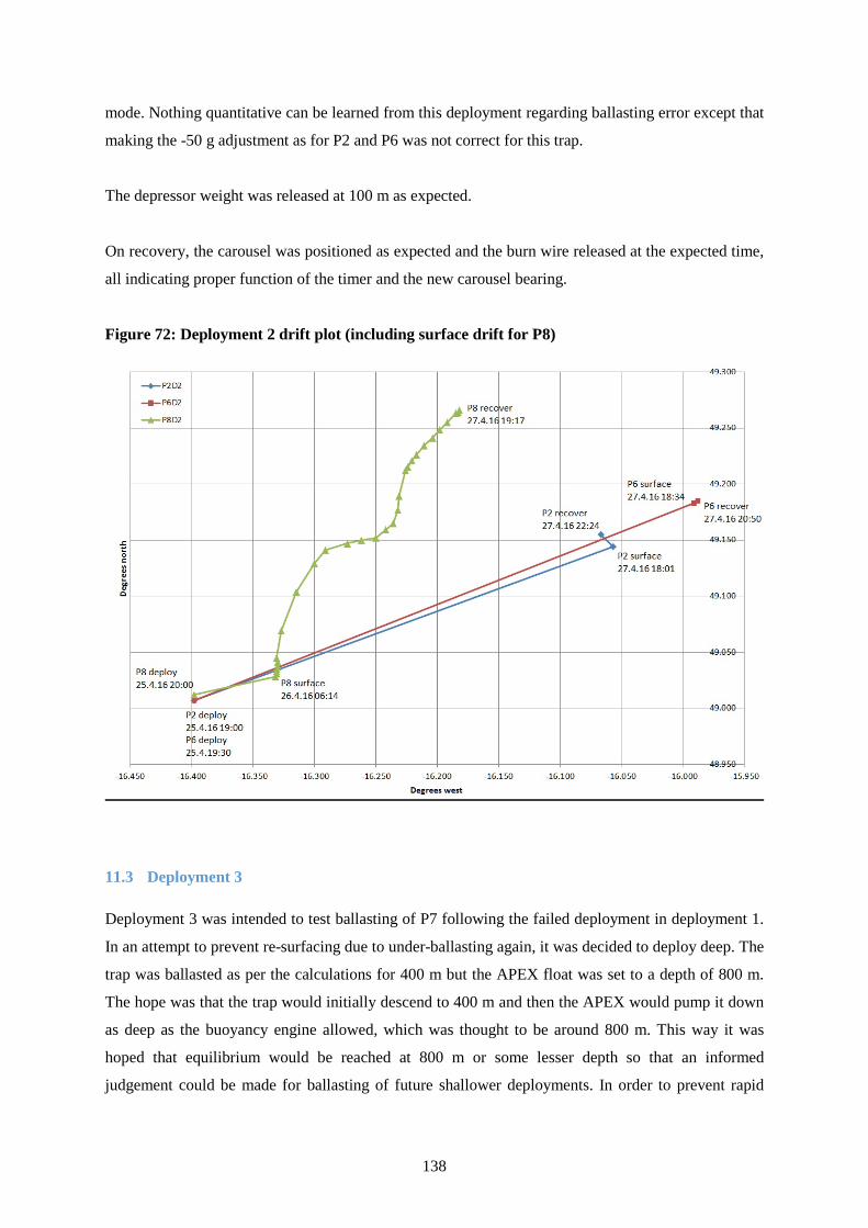
138

mode. Nothing quantitative can be learned from this deployment regarding ballasting error except that

making the -50 g adjustment as for P2 and P6 was not correct for this trap.


On recovery, the carousel was positioned as expected and the burn wire released at the expected time,

all indicating proper function of the timer and the new carousel bearing.

Figure 72: Deployment 2 drift plot (including surface drift for P8)

11.3 Deployment 3

Deployment 3 was intended to test ballasting of P7 following the failed deployment in deployment 1.

In an attempt to prevent re-surfacing due to under-ballasting again, it was decided to deploy deep. The

trap was ballasted as per the calculations for 400 m but the APEX float was set to a depth of 800 m.

The hope was that the trap would initially descend to 400 m and then the APEX would pump it down

as deep as the buoyancy engine allowed, which was thought to be around 800 m. This way it was

hoped that equilibrium would be reached at 800 m or some lesser depth so that an informed

judgement could be made for ballasting of future shallower deployments. In order to prevent rapid

139

descent that may carry the risk of descending to 1000 m or more and thus aborting, the APEX float

was set to a piston adjust period of 15 minutes instead of the usual 5 minutes.

P7 (camera trap)

Station: DY050-045

Target depth: 400 m (ballast), 800 m (APEX)

Target temp: 11.23°C (400 m), 8.94°C (800 m)

In situ density: 1028.923 kg m-3 (400 m), 1031.022 kg m-3 (800 m)




16° 21.180’ W


As can be seen, P7 did just about achieve equilibrium at 800 m with the APEX buoyancy engine at its

minimum adjustment of 9 counts but only for the final 4 hours. It also appears to have begun to

equilibrate at about 350 m just before the APEX began adjusting. Changing the piston adjust period to

15 minutes was unnecessary as the trap wouldn’t have descended deeper than 800 m and, had the

adjustments been quicker, it is clear that equilibrium would have been achieved much sooner.

140

Based on this result, a further deployment would be made using the as-calculated ballast but for 600

m depth.




carousel bearing.

Figure 73: Deployment 3 drift plot

11.4 Deployment 4

Deployment 4 was intended as a deep (600 m) deployment of all five traps. This would complement

the successful shallow deployments of P2 and P6 and obtain equilibrium data for P4, P7 and P8

without the risk of premature surfacing.

141

In the event, P7 suffered a malfunction during mission prelude that caused its air bladder to not inflate

so it wasn’t deployed. Subsequent investigations revealed a ‘modem registration’ failure also. The

causes of this will be investigated on our return to NOC.

P2 (standard trap)

Station: DY050-076

Target depth: 600 m






16° 23.220’ W


142

P2 was correctly ballasted using the previous adjustment from the calculated value of -50 g. Initial

equilibrium was achieved with an adjustment of just 10 piston counts and the maximum adjustment

throughout the mission was 21 counts.

For this deployment two pot cams were fitted with pots 1 & 3 and 2 & 4 opening in pairs.




carousel bearing.

P4 (camera trap)

Station: DY050-077






16° 23.220’ W

143


P4 was slightly under-ballasted with a piston adjustment of 23 counts needed to reach initial

equilibrium at just over 600 m. With no other data to go on, P4 was ballasted as calculated with no

adjustments.

Two adjacent cams were fitted in order for one gel pot and one standard formalin pot to open

simultaneously for subsequent comparison of particles. Positioning of the cams was such that pot 2

(labelled wrongly as 1 on the trap funnel) opened with gel 3 and pot 4 (wrongly labelled as 3 on the

trap funnel) opened with gel 1.




carousel bearing.

P6 (standard trap)

Station: DY050-078

Target depth: 600 m






16° 23.220’ W

144


P6 was ballasted perfectly with just 3 piston counts needed to reach its initial equilibrium period.

Further adjustments were made but only in response to changing sigma-theta values as expected.

Ballasting was made with a -50 g adjustment on the calculated value as in the previous deployment.

All four cams were fitted such that all four pots opened simultaneously for one single aggregated

sample.




carousel bearing.

P7 (camera trap)

P7 was not deployed as the air bladder failed to inflate during mission prelude and a ‘modem

registration’ error was encountered. This will be investigated when back at NOC.

P8 (standard trap)

Station: DY050-079

Target depth: 200 m

145



Added ballast: 4053 – 50 = 4003 g



16° 23.220’ W

P8 was set up and deployed in the same manner as P2, P4 and P6 but appears to have failed to surface.

No Iridium transmissions have been received to date (6.5.16 11:05). All setup records have been

checked and all appear to be in order so it is not clear what has gone wrong with this deployment. A

search was carried out in the vicinity of the expected position assuming it had surfaced at the

programmed time and followed the other traps’ course but nothing was found. Possible scenarios

include:

• Trap descended too deep and the emergency abort weight failed to release at 1000 m. (All

releases have been refurbished and fully tested at NOC).

• Trap is on the surface but the APEX telemetry has failed. (Telemetry on P8 has worked up

until now and P8 did successfully telemeter its position whilst on deck during mission

prelude).

• Trap is on the surface and APEX telemetry is working but messages are not being received on

the Iridium server at NOC. (All other traps have been able to log in and upload/download

successfully. The modem at NOC has been power cycled to rule out any problem with that).

• The timer and/or burnwire have failed in some way so the end-of-mission weight hasn’t

released. This may cause the trap to be neutrally buoyant at some depth below the surface and

so telemetry is impossible. (This is a possibility. If this is the case, the burnwire may

eventually corrode through and the trap may yet surface and communicate – this may take

several weeks or months).

• Something may have flooded; APEX float, Idronaut logger, buoyancy hoop. (This is always a

possibility).

146

Figure 77: Deployment 4 drift plot (including surface drift)

12 PELAGRA Cam

By Morten Iversen, Christian Konrad, Kev Saw, Clara Flintrop, Richard Lampitt

Deployment of the PELAGRA Cam on the RCF and on the PELAGRAs

12.1 Introduction

We deployed the PELAGRA Cam in the upper water column to determine the abundance and size-

distribution of particles larger than ~100 µm. We deployed the PELAGRA Cam both as a profiling

system to capture an image of the particles in the upper 300 m of the water column at five seconds

intervals and as neutrally buoyant systems on the PELAGRA sediment traps. The PELAGRA Cam

was time to take ten images with two seconds intervals every 30 minutes while on the PELAGRA

sediment traps. While it is difficult to determine if a particle is settling or suspended from the images

obtained with the profiling system, the PELAGRA sediment trap deployments offers the opportunity

to determine settling velocity of the particles in situ, as well as estimating the proportion of settling

versus suspended particles. Further, due to the high resolution of illumination of the PELAGRA cams,

147

it is possible to determine particle types and colours and thereby quantify abundance and size-

distribution of different particle types (e.g. marine snow versus zooplankton faecal pellets). We can

even determine size-specific settling velocities of the different particles types from the deployments

on the neutrally buoyant PELAGRA sediment traps.

12.2 Methods

The PELAGRA Cam consisted of a Canon EOS 6D digital SLR camera equipped with a 50 mm

macro lens and a Canon Speedlite 600EX RT flash gun. The camera and the flash gun were places

perpendicular to each other provide illumination from the right side of the captured images (see

Figure 78). We used a Hahnel Giga T Pro II remote timer to capture an image every five seconds. The

camera was put in manual mode and the settings were adjusted to have an ISO of 2500, a shutter

speed of 1/160 seconds, an aperture of f/32, and the lens focus was put to 1.5 feet. The flash was also

in manual mode and put for straight flash direction and a flash output of 1/8.

Figure 78: Overview figure of the PELAGRA Cam configuration. The pressure housing in the

lower right part of the image contained the camera and the upper left pressure housing

contained the flash gun.

148

We were able to capture individual particles through the water column in a water volume of 2.15 L for

each captured image. The pixel size of the images changed depending on whether the particles were in

the front of back of the field of depth. We determined a pixel size of 33 µm per pixel in the front of

the depth of field (as seen from the camera) and a pixel size of 61 µm per pixel at the back of the

depth of field. This suggested an average pixel size of 54 µm per pixel. The field of view for each

image was 157 mm width, 101 mm height, and 135 mm depth. The width and height of the images

were determined by the cropping of each image to compensate for uneven flash illumination and

might change when we do the final image processing.

12.3 The Red Camera Frame (RCF)

The PELAGRA Cam deployments were done as vertical profiles on the Red Camera Frame (RCF) in

combination with the LISST HOLO (Holocam) and an Idronaut CTD (Figure 79). The Holocam

captured images every five seconds, which was the same frequency as the PELAGRA Cam. The

Idronaut CTD was programmed to obtain depth, temperature, and conductivity (salinity) every 125

ms. We made 16 vertical profiles with the RCF from the surface to 300 m depth (see Table 20).

Figure 79: The Red Camera Frame (RCF) with the PELAGRA Cam, the Idronaut CTD, and

the LISST HOLO (Holocam). Image provided by Richard Lampitt.

Table 20: Overview of deployments of the Red Camera Frame (RCF). Station No is the ship’s

station number, RCF No. is the deployment number of the RCF.

149

Station

No.:

RCF

No.: Date

Maximu

m wire

out (m)

No of

Images

taken

Latitude

N

Longitude

W

DY050-

014

RCF_00

1

2016-04-

23

300 287 49°00,33' 16°23,81'

DY050-

029

RCF_00

2

2016-04-

25

300 914 49°00,42' 16°23,86'

DY050-

042

RCF_00

3

2016-04-

26

300 450 49°00,33' 16°23,86'

DY050-

051

RCF_00

4

2016-04-

27

300 933 49°00,33' 16°23,84'

DY050-

067

RCF_00

5

2016-04-

29

300 1403 49°00,32' 16°23,85'

DY050-

071

RCF_00

6

2016-04-

30

300 647 49°10,82' 16°05,29'

DY050-

072

RCF_00

7

2016-04-

30

300 625 49°10,82' 16°05,29'

DY050-

073

RCF_00

8

2016-04-

30

300 592 49°10,82' 16°05,29'

DY050-

074

RCF_00

9

2016-04-

30

300 560 49°10,82' 16°05,29'

DY050-

075

RCF_01

0

2016-04-

30

300 588 49°10,82' 16°05,29'

DY050-

088

RCF_01

2

2016-04-

30

300 1082 49°00,21' 16°23,45'

DY050-

096

RCF_01

3

2016-05-

01

300 1214 49°00,33' 16°23,81'

DY050-

097

RCF_01

4

2016-05-

01

300 1263 49°00,33' 16°23,81'

DY050-

103

RCF_01

5

2016-05-

02

300 1180 49°00,71' 16°23,85'

DY050-

117

RCF_01

6

2016-05-

04

300 1249 49°00,30' 16°23,59'

DY050-

125

RCF_01

7

2016-05-

05

300 1243 49°48.28' 16°03,19'

total count of images 14230

150

12.4 PELAGRA Cam and gel traps on the PELAGRAs

We deployed the PELAGRA Cam on the PELAGRAs three times (Figure 80); on P7 deployment 1,

P7 deployment 3, and P4 deployment 4. The first deployment (P7 deployment 1) was under-ballasted

and never made it to depth (see cruise report on the PELAGRAs, Section 11). Additionally the horse

shoe connected for the flash on the camera had slipped out during mounting of the camera in the

pressure housing and no illumination was provided for the images. The second deployment (P7

deployment 3) provided well illuminated images with particles in focus. However, since the

PELAGRA did not reach its target depth until at the end of the deployment period (see Cruise Report

for PELAGRAs), all image sequences were obtained while the PELAGRA was descending. This

means that we cannot use the images to determine size-specific settling velocities, but the images are

very useful for determinations of particle size-distribution and abundance through the upper 800 m of

the water column. The last deployment (P4 deployment 4) was successful both in terms of the

PELAGRA reaching its target depth within a few hours and in terms of focus and illumination of the

images and we have several image sequences that provide settling velocities of the captured particles.

Figure 80: PELAGRA with the PELAGRA Cam mounted (the two green pressure housings).

The left side pressure housing is for the camera and the right side pressure housing is for the

flash gun.

12.4.1 Preliminary results

We still need to quantify the particle sizes and abundance via image processing of the captured

particles. From the first qualitative observations of the images we observed a change in the marine

snow particles on the 1st of May. The profiles made before the 1st of May showed mainly small and

151

compact particles (Figure 81, left panel) while the particles captured from the 1st of May and onward

suggested that the particles were more loosely structured and contained high amounts of gel-like

substances (Figure 81, right panel). We could confirm this observation from the microscopic

observations of the individual particles collected with the Marine Snow Catcher. This seemed to

coincide with indications of increasing abundances of pteropods in the vertical hauls of zooplankton

nets, suggesting that the gel-like substances in the marine snow aggregates could be caused by

mucous feeding structures produced by pteropods.

Figure 81: Examples of particles captured in the upper 50 m of the water from the 30th of April

2016 (left panel) and from the 5th of May 2016 (right panel). The white line in the lower right

corner of both images is a scale bar showing 5 mm.

152

13 Holographic imaging of particles

We deployed a LISST-Holo (Sequoia Scientific, Inc.) holographic imager. The system was run on the

same “Red Camera Frame” as the pelagic particle camera operated by Morten Iversen et al (Section

12). The system uses a laser and 1600 x 1200 pixel image sensor to image a small volume of water

1.86 cm3 at full frame (see also region of interest). The system was run over 17 deployments of

varying length including 4 night-time deployments. All deployments were run over the full

operational depth of the instrument, 300 m depth (Table 21). This system was frequently operated

before or after the marine snow catcher. The instrument was oriented such that there was unobstructed

flow in the viewed volume in both the upward and downward casts. The system was deployed by

running the Romica winch wire through a block on the starboard aft crane over the starboard side.

Winch wire speed was generally between 3-5 rpm on the winch, equating to <10 m s-1 in water

vertical speed. The only exception was DY050-042, where stops every 10 m depth of between 2-8

min. were added, with longer stops at deeper depths. The holographic system was set at its maximum

image capture rate of 1 image every 5 s. The viewed volume can be sub-sampled as needed to

generate size-volume distributions of particles from ~25-2500 µm in equivalent spherical diameter.

The software Holo Batch v3.0 was used to process the images into the size distribution data with the

“LISST-100x RANDOM type C” size class output. A reduced region of interest (ROI) was used to

avoid an apparent errant object in the optical path, where the right ~20% of the image was removed.

As an additional adjustment to avoid errant particle detection, we only considered the volume from 5

to 45 mm in the 0 to 50 mm optical path length, avoiding volume adjacent to the windows.

153

Figure 82: Red camera frame with the LISST-Holo instrument (foremost housing), battery

housing (backmost black housing), as well as the macro camera and flash (green housings).

Figure 83: Screen grabs of the Holo Batch settings, including the adjusted ROI area.

154

Table 21: Station log of LISST-Holo deployments.

In water times (instrument clock)

Station

Year Month Day Start

time End time

Useful

holograms

(count)

Maximum

wire out

(m)

Comments

DY050-014 2016 4 23 17:46:39 18:56:16 577 300

DY050-029 2016 4 25 15:39:26 16:54:21 624 300

DY050-042 2016 4 26 13:37:56 17:22:38 1858 300

Longer

time at

deeper

depths

DY050-051 2016 4 27 10:40:06 11:57:38 637 300

DY050-067 2016 4 29 16:07:14 18:16:07 1048 300

Mud being

washed

overboard

DY050-071 2016 4 30 01:01:31 01:55:06 438 300

DY050-072 2016 4 30 02:14:20 03:05:12 425 300

DY050-073 2016 4 30 03:18:05 04:06:34 407 300

DY050-074 2016 4 30 04:18:55 05:04:14 384 300

DY050-075 2016 4 30 05:15:52 06:03:35 400 300

DY050-080 2016 4 30 09:30:12 10:58:34 723 300

No macro

camera on

Red

Camera

Frame

DY050-088 2016 4 30 14:33:41 16:02:40 736 300

DY050-096 2016 5 1 12:20:51 14:00:49 832 300

DY050-097 2016 5 1 14:11:38 15:56:41 863 300

DY050-103 2016 5 2 15:45:40 17:22:23 800 300

After

weather

hold

DY050-117 2016 5 4 14:38:53 16:22:04 842 300

DY050-123 2016 5 5 14:08:54 15:52:00 1012 300

Total count of useful images 12606

155

14 CTD sampling

By Sue Hartman, Corinne Pebody, Andrew Morris

CTD casts on DY050 were primarily for testing sensors and releases. The first cast was shallow and

was used for pre deployment validation of the wetlabs and Cyclops fluorometer on the Aanderra

Seaguard, to be deployed at PAP1. Unfortunately there was a problem with the CTD fluorometer

cable so we do not have this measurement for comparison. The sensors were tested against each other

and also the extracted chlorophyll samples. The star oddis, optode, SUNA nitrate and PAP1

microcats were also tested at CTD001.

CTD002 was the first deep station and was used to test the PAP3 microcats and releases. The post

deployment validation check of PAP1 sensors was CTD008, with the testing of microcats on

CTD009. The PAP3 microcat was tested on CTD010.

Table 22: A summary of sensors (additional to the CTD sensors) attached to the rosette

CTD Cast Sensor type Serial number

001 Pre deployment sensors:

Suna nitrate

Seaguard Turner fluorometer

Seaguard optode

Wetlab fluorometer FLNTSUB

Oxygen microcat 37imp odo (for buoy PAP1)

Microcat 37im (for 30m PAP1)

Oxygen microcat 37 imp ido (pressure sensor fail)

698

2102108

1339

269

10315

6915

9030

002 Pre deployment sensors: PAP 3 microcats & releases

Microcat sbe37-im

Microcat sbe77-im

09469

09475

008 Post deployment sensors:

Seaguard Turner fluorometer

Seaguard optode 44330

Wetlab fluorometer FLNTSUB

2103960

2001

3050


Oxygen microcat odo (from buoy PAP1)

Oxygen microcat odo (from frame PAP1)

Microcat (from buoy PAP1)

Pre deployment sensors:

13397

10535

6904

156

Oxygen microcat 37 imp ido (pressure sensor fail) 9030


PAP3 microcat 37-imp-66262

9476

In total we had 11 CTD stations (with no bottle samples from CTD004). The station positions are

shown in Table 23 (which shows that the first shallow CTD station was not near the PAP site area). In

retrospect the pre deployment calibration should have been repeated on a later cast, once the CTD

sensors were working properly.

Table 23: CTD station positions, seabed and cast depth

Station Latitude (N) Longitude (W) Seabed depth (m) Cast depth (m)

CTD001

CTD002

CTD003

CTD004

CTD005

CTD006

CTD007

CTD008

CTD009

CTD010

CTD011

49 36.102

49 0.33

49 0.488

49 0.32

49 0.347

49 0.314

49 0.321

49 0.325

49 0.334

49 0.708

49 0.319

08 21.633

16 23.82

16 27.184

16 23.85

16 23.846

16 23.817

16 23.847

16 23.8

16 23.813

16 23.85

16 23.82

138

4812

4811

4811

4811

4809

4849

4810

4810

4810

4808

100

4790

500

N/A

1500

3000

4828

200

100

4800

2500

Aside from sensor validation the stations were used to collect water for analysis, to validate the CTD

sensors and to test NOC sensors that are in development (for T, S and nitrate). On each occasion

samples were taken in the following order: Dissolved oxygen, Dissolved Inorganic Carbon (DIC),

inorganic nutrients, salinity and associated parameters from the top 200m. The associated parameters

from the surface samples were chlorophyll, size fractionated chlorophyll, PIC, POC and biogenic

silica. These surface samples were filtered and frozen as appropriate for analysis ashore.

Occasionally Lugols samples were also taken (from CTD001,002, 003 and 005), for analysis at NOC.

Table 24: Summary of the CTD log sheets showing the depth sampled for DIC, nutrients and

oxygen, then depths sampled for surface parameters such as chlorophyll.

depth

(m)

CTD stations

with DIC,

oxygen and

CTD stations with

surface

parameters

depth (m)

CTD stations

with DIC,

oxygen and

157

nutrients Eg: Chlorophyll nutrients

10 2,3,5,6,7,8,9,10,11 2,3,5,6,7,8,9,10,11

900 6,7,10

20 1,2,5,6,7,9,10,11 1,2,5,6,7,8,9,10,11

1000 2,5,6,7,10

30 2,3,5,6,7,8,9,10,11 2,3,5,6,7,8,9,10,11

1200 7

50 2,8,10,11 1,8,10,11

1500 5,7,10

60 1,2,3,5,6,7,8,9 5,6,7,8,9

1600 11

70 1 1

2000 2,6,7,10

80 2,3,5,6,7,8,9,10,11 2,3,5,6,7,8,9,11

2500 11

100 1,2,3,5,6,7,8,9,10,11 1,3,5,6,7,8,9,10,11

3000 2,6,7,10

150 8,11 11

3500 10

200 2,6,8,10 2,10

4000 2,7,10

250 3,5 3

4300 10

300 10

4700 2

400 2,6,7

4760 2

500 2,3,5,6,7,10 3

4790 2,7

600 2,6,7,10

4800 7

750 2,5,6,7,10,11 4828 7

DIC samples were preserved with mercuric chloride and will be analysed on Vindta24 at NOC for

Dissolved Inorganic Carbon (DIC) and Total Alkalinity (TA). Duplicates were taken from each

station (usually 2). Nutrient samples were collected in centrifuge tubes and frozen for analysis of

inorganic nutrients (NO2+NO3, phosphate and silicate) using the Quattro auto-analyser at NOC.

Sufficient sample was taken for duplicate analysis.

Generally 2-3 salinity bottle samples were taken from each cast, for analysis on-board at the end of

DY050. Chlorophyll samples were filtered and frozen for analysis in batches on DY050. The oxygen

bottle samples were fixed on deck, returned to the deck laboratory and analysis was started within 2 to

7 hours of collection.

14.1 Oxygen analysis on-board

By Sue Hartman

In total 140 samples were analysed for dissolved oxygen using a modified Winkler technique. An

amperometric end point method was used, following the titration using an electrode to a set end point.

Thiosulphate titrant was delivered using a Titrino 794. The method was standardised using 5ml

additions of 0.01N OSIL iodate (3 bottles were used during DY050). The normality of the

thiosulphate ranged from 0.0992-0.0996 (a constant 0.0995 was used to calculate each cast).

158

Duplicate samples were taken on each cast (between 2 and 4 each time). The average duplicate

difference was 0.38 umol/l. The CTD temperature was used for the fixing temperature to account for

any changes in bottle volume (as the probe that was used initially was not thought to be reliable

enough). Density from the CTD processed files was then used to convert to umol/kg units so the

oxygen bottle data could be compared with the CTD sensors (Figure 84).

Figure 84: Oxygen data from the three deep casts (CTD002, 007 and 010) with associated bottle

oxygen data.

As seen in Figure 84 the bottle oxygen agreed reasonably well on the deep casts. Figure 2 however

shows that there is a potentially high offset between bottle oxygen and CTD seabird oxygen

measurements in the shallow water (Figure 85). This was reasonably linear and could be used to

correct the sensor data to the bottle samples.

159

Figure 85: The offset between bottle data (minus CTD oxygen data) for the three deep stations,

CTD002 (in red), 007 (in blue) and 010 (in green) was linear with depth, with larger offsets in

shallow water.

Figure 86: Tthe overall relationship between the bottle and CTD oxygen data

This equation can be applied to the CTD oxygen data however this will not improve data agreement at

depth (Figure 87). The final merged bottle oxygen data are available in a file called: ‘All-Final-Oxy-

data-DY050’.

CTD 010 y = 0.0016x - 7.6218

R² = 0.7983 CTD 007 y = 0.0016x - 8.8765

R² = 0.822

CTD 002 y = 0.0016x - 5.6678

R² = 0.943

-12

-10

-8

-6

-4

-2

0

2

4

0 1000 2000 3000 4000 5000

Diffe

renc

e bo

t-sb

e (u

mol

/kg)

CTD 010 CTD 007 CTD 002

y = 1.0042x - 4.8171 R² = 0.9301

190

210

230

250

270

290

310

200 220 240 260 280 300

160

Figure 87: Corrected CTD oxygen data (in grey) along with the bottle data (blue) and

uncorrected CTD oxygen data (red crosses).

15 Underway sampling

By Sue Hartman

Bottle samples were taken from the non-toxic supply seawater at the sampling point next to the

thermo-salino-graph (TSG) on the main deck, one deck down from the CTD sampling. Samples were

taken 1-2 times a day for DIC, salinity and chlorophyll. 250ml aliquots of the chlorophyll samples

were immediately filtered onto GF/F filters and frozen for analysis on-board. Likewise salinity

analysis was done on-board, at the end of DY050.

The DIC samples were preserved for analysis on Vindta 24 at NOC. These samples will be analysed

for DIC and TA and calculations made of pCO2 for comparison with the PML underway pCO2

system. At the start of DY050 the PML system was found to have only two of the three calibrant

gases. The system was also initially blocked at the equilibrator but was soon fixed. The dataset will be

assessed and made available via PML.

0

500

1000

1500

2000

2500

3000

3500

4000

4500

5000

180 230 280

dept

h (m

)

Oxygen (umol/kg)

final oxybot-umol/kg

CTD-Sbeox umol/kg

corrected CTD data

161

Chlorophyll concentration was greatest in the western English Channel, but once at the PAP

observatory site, the chlorophyll concentration increased throughout the cruise. The drop at the end

may be due to poor weather that blew through.

Figure 88: Location and quantity of chlorophyll from the underway sampling.

16 Benthic Biology

By Brian Bett, Henry Ruhl, Andrew Gates, Rob Young, Claire Laguionie-Marchais , Lenka

Nealova, Noelie Benoist, Simone Pfeifer and Marla Spencer

16.1 Megacorer

The NOC-OBE Bowers & Connelly megacorer was used on 14 occasions at 13 stations during the

cruise for collection of sediment for biological analysis (Table 25). If sufficient cores were available

samples were also collected to analyse for microplastics. The deployment at RP-05 was repeated

because the first attempt at that station only recovered one good sample. The first 9 deployments used

8 large core tubes and 2 small (MgC-08+2). On subsequent deployments 10 large tubes were used

(MgC-10).

16.1.1 On deck

Once megacorer was recovered to deck the cores were examined for overlying water clarity,

disturbance and cracks in the core and notable layers or patches in the sediment. The length of core

162

sediment retention was measured and example core profiles were photographed. They were then

removed from the megacorer and allocated to analysis type randomly.

16.1.2 Lab processing

Once the cores were removed from the megacorer they were processed by three teams of two with

assistance from others if available. One person held the core in position while the other sliced the

sediment. Details of slicing procedures to acquire the necessary sediment horizons are detailed in

Table 26 and summarised below.

16.1.3 Macrofauna

Macrofauna samples were the priority for the megacorer deployments. A minimum of four large

tubes per deployment were allocated to macrofauna. If fewer than four were available macrofauna

samples were not taken. If four were available the remaining cores were allocated to other analyses

with any additional cores allocated to macrofauna.

To process the cores the overlaying top water was siphoned into a 250 µm sieve and then transferred

into the bottle for 0-1 cm sediment layer (syringes were used when necessary to extract the small

volume of remaining water). Slicing rings were used to measure the following horizons: 0.0 – 1.0 cm

(if the top layer was not flat, the lower part of a slope was used to define the 0-1 cm layer), 1.0 – 3.0

cm, 3.0 – 5.0 cm, 5.0 – 10.0 cm, 10.0 – 15.0 cm. Each layer was cut with slicing plate, which was

then rinsed (the upper side on the current layer and the downside side used as the top side for the next

slice). The top three layers were usually transferred into the bottle with the help of funnel, the 5cm

thick layers were sliced with knife and then put directly into the bottle. Rings, funnels and knives

were rinsed into appropriate bottle in filtered seawater.

The 0-1, 1-3 and 3-5 cm were put in 500 ml UN bottles and 1500 ml UN bottles were used for the 5-

10 and 10-15 cm layers. Each bottle was labelled on the cap and one side and a paper label was

placed inside the bottle. Samples were preserved in 4% formaldehyde (½ 8% formaldehyde with

borax (5 g l-1) ½ sediment/filtered seawater). If the sample filled more than half the volume of a

bottle, the overlying water was passed through a 250 µm mesh sieve and the material washed back

into the bottle to ensure the correct formaldehyde concentration.

16.1.4 eDNA & Phosphlipids

One large core was used for eDNA. All slicing equipment was sterilised in bleach prior to sample

processing and washed with Milli-Q between each slice. Nitrile gloves were worn at all stages (new

pair for each core). The overlying water was discarded and the following horizons were sliced: 0.0-

163

1.0 cm, 1.0-2.0 cm, 2.0-3.0 cm, 3.0-4.0 cm, 4.0-5.0, 10.0-15.0 and 15.0-20.0. For each 1 cm slice

samples of sediment were placed in 3 small sterile aliquots for DNA (stored at -80°C), 3 small

aliquots for RNA Later (-80°C after 4°C for few hours) and the remainder of slice in a 50 ml Falcon

tube at -80°C for phospholipids analysis. For the 5.0-10.0, 10.0-15.0 and 15.0-20.0 cm slices

sediment was placed in 50 ml Falcon tubes at stored at -80°C using spatula. In all cases sediment near

the edge of the core was discarded. New sterile spatulas were used for each slice. In between the

slices, the slicing plate was rinsed with Milli-Q. More details in section 17.

16.1.5 Biomarkers

One large core was used as a replicate for biomarkers. The top water was discarded. Before slicing

and between slices the equipment was rinsed with milli-Q water. Four sections were taken at 0.5 cm

horizons to 2 cm. Sediment in contact with the core tube was removed using a knife rinsed in Milli-Q

water and the remaining material preserved in muffled foil (preserving as much as possible the

integrity of the slice) held inside labelled petri dishes, placed inside a single labelled bag per sample

and frozen at -80°C straight away. Nitrile gloves were worn at all stages

16.1.6 Quantitative protozoan meiofauna (Foraminifera):

A small core was used. Before processing and between slices the slicing equipment was washed with

filtered seawater. The top 1cm of overlaying sea water was passed through 250 µm sieve and added

to the 0-0.5 cm sample. The samples were then sliced at 0.5 cm intervals to 2 cm then at 1 cm interval

from 2-3 cm. The sediment was preserved in 4% formaldehyde (½ 8% formaldehyde with borax (5 g

l-1) ½ sediment/filtered seawater) and placed into 500 ml UN bottles (blue lids, one for each slice).

Metazoan meiofauna: A small core was used. Before processing and between slices the slicing

equipment was washed with filtered seawater. The top five cm of sediment and 2 cm of sieved top

water were retained in 1.5 l plastic bottles and preserved in 4% formaldehyde (½ 8% formaldehyde

with borax (5 g l-1) ½ sediment/filtered seawater).

Microplastics: As soon as the sample was removed from the megacorer, the large core allocated for

microplastics analysis was covered with aluminium foil (instead of a rubber bung, to avoid plastic

contamination). Before processing and between slices the slicing equipment was washed with filtered

seawater. Two 1 cm slices were retained: the 0-1 cm (including the overlaying water) and the 6-7 cm.

Each sliced was placed in a glass jar with a plastic top covered in foil to avoid plastic contamination

from the cap. The overlying water was filtered with a 250 µm mesh sieve and added to the 0-1 cm jar.

For both slices, as little as possible water was added to the samples. Samples were provided to Katsia

Pabortsava who then dried them at 60°C on board RRS Discovery.

164

Labelling

All samples were labelled with Cruise ID (DY050), Station number, Date of the megacorer at the

bottom, core letter (for macrofauna only), sediment horizon, analysis type and type of preservative.

The outside of every container was labelled (top and side if possible) and a paper label was placed

inside the container.

165

Table 25: Summary of megacorer samples collected at the PAP central coring station during DY050 St

atio

n

Site

Sam

pler

Lat

itude

(N)

Lon

gitu

de (W

)

Dep

th (m

) (U

SBL

)

Mac

rofa

una

eDN

A/P

hosp

holip

ids

Bio

mar

kers

Met

azoa

n M

eiof

auna

Fora

min

ifera

Mic

ropl

astic

s

DY050-

002

RP-01 MgC-

08+2

48°

50.055'

016°

31.312'

4850 5 1 1 1 1

DY050-

003

RP-02 MgC-

08+2

48°

50.387'

016°

31.174'

4850

1 1

1

DY050-

011

RP-03 MgC-

08+2

48°

50.255'

016°

31.084'

4849 5

1 1 1 1

DY050-

012

RP-04 MgC-

08+2

48°

50.016'

016°

31.086'

4850 5

1

DY050-

018

RP-05 MgC-

08+2

48°

50.277'

016°

31.270'

4849

1

DY050-

019

RP-05

repeat

MgC-

08+2

48°

50.296'

016°

31.262'

4851 4 1

1 1

166

DY050-

026

RP-06 MgC-

08+2

48°

50.171'

016°

31.526'

4849 4 1

1 1

DY050-

36

RP-07 MgC-

08+2

48°

50.270'

016°

30.999'

4849 4 1

1 1 1

DY050-

37

RP-08 MgC-

08+2

48°

50.477'

016°

31.344'

4850 4

1 1 1

DY050-

46

RP-09 MgC-10 48°

50.075'

016°

31.223'

4849 4 1

1

DY050-

47

RP-10 MgC-10 48°

50.263'

016°

31.622'

4851 4

DY050-

56

RP-11 MgC-10 48°

50.281'

016°

31.139'

4850 7

1

DY050-

107

RP-12 MgC-10 48°

50.210'

016°

31.222'

4848 5

DY050-

124

RP-13 MgC-10 48°

50.183'

016°

31.377'

4850 5

1

TOTAL

REPLICATES 12 6 5 6 7 6

Total cores 56 6 5 6 7 6

167

Table 26: Summary of the megacore processing protocols

Large core (10 cm diameter) Small core (7 cm diameter)

eDN

A

&

phos

phol

ipid

s

Mic

ropl

astic

Mac

rofa

una

Bio

mar

kers

Fora

min

ifera

Met

azoa

n

mei

ofau

na

Number of core

per megacore 1 1 At least 4 1 1 1

Preservation

RNA

Later, -

80°C dried

4% buffered

formaldehyde

frozen

-80°C

4% buffered

formaldehyde

4% buffered

formaldehyde

Surface water Discard

300

micron

sieve +

added to

first

layer

300 micron

sieve + added

to first layer

In

sample

300 micron

sieve + added

to first layer

Top 1 cm

retained and

added to first

layer

0-1 0-1 0--1

0-0.5 0-0.5

0-5

0.5-1 0.5-1

1-2

1-3

1-1.5 1-1.5

1.5-2 1.5-2

2-3 2-3

3-4 3-5

4-5

5-10

5-10

6-7

10-15

10-15

15-20

168

16.2 Trawls

16.2.1 DY050-063 OTSB14

When the trawl came on deck there was a large amount of mud in the net. In front of the mud there

was a clean selection of specimens which were removed before attempting to deal with the mud.

These specimens were cleaned in filtered seawater and brought to the 5°C chill room for further

sorting. Once these specimens were removed the haul was initially hosed with the fire hose. The mud

was then spilled on deck and shovelled in to grey crates for washing through the sieving table. Thick

gloves were used during the washing to avoid injury with glass and clinker. Clinker was put aside and

photograph for the records as were any waste found in the trawl.

Specimens were regularly transferred to the 5°C chiller room for further sorting. Owing to the length

of time required to process the mud on deck the specimens were broadly sorted in the chill room (one

broad category, one container Table 27) and added to preservative as batches were available. A

category of unedified taxa was added as some specimens were too damaged to be quickly identified.

Crustaceans were preserved in 100 % ethanol, while other taxa were preserved in 4% formaldehyde

(½ 8% formaldehyde with borax (5 g l-1) ½ sediment/filtered seawater). All samples were labelled

with Cruise ID (DY050), Station number, Date of the trawl, taxa and type of preservative. The outside

of every container was labelled (top and side if possible) and a paper label was placed inside the

container.

Noelie Benoist took photos, measurements, volume and weight for 47 specimens (see section

Specimen Measurements by Noelie, Table 28 and 29). These animals are in separate bags within the

main preservation container for future identification. Rob Young took tissue samples for DNA from

most of the specimens examined by Noelie. (Further details of RY and NB’s work elsewhere).

The catch comprised fairly typical haul of megabenthic invertebrates from PAP. Holothurians such as

Psychropotes sp., actiniarians and asteroids (Styracaster sp.) were the most abundant. The specimens

were preserved and the catch is stored in 20 containers labelled with the station number and listed in

Table 27.

169

Figure 89: DY050-063 OTSB14, the trawl as it came on deck. Note the large quantity of mud

Figure 90: Example images of the catch from DY050-063 a) holothurians, b) arthropods,

molluscs and asteroids c) fishes

170

Figure 91: Example artefacts from the otter trawl DY050-063. a) Left, litter including cans,

bottles, broken plate, fishing line, b) clay pipe, c) clinker and other hard substrate

16.2.2 DY050-118 OTSB14

The second successful trawl arrived on deck with considerably less mud in the net. The catch

contained two large barrels/drums (Figure 92), one painted white and blue and labelled “FLOATING”

(Figure 94). The trawl was opened and specimens were spilled in to grey crates and washed with

filtered seawater at the sieving table while wearing thick gloves to avoid injury with broken glass,

rusty metal and clinker. Specimens were transferred to the 5°C chiller room for further sorting.

Clinker, litter and artefacts were put aside and photographed. The catch comprised a fairly typical

haul of megabenthic invertebrates from PAP. Holothurians (Psychropotes sp.), actiniarians and

asteroids (resembling Styracaster sp.) were the most abundant. Several macrourid fish were also

caught, the two largest of which were discarded at sea.

In the chill room, the samples were quickly sorted to the broad groups based on the main taxa present

(see table 27) then separated into different containers. For crustaceans, 100% ethanol was added in the

chill room. Other taxa were preserved in 4% formaldehyde outside on the back deck (½ 8%

formaldehyde with borax (5 g l-1) ½ sediment/filtered seawater). There were 25 containers in total

(Table 27).

All samples were labelled with Cruise ID (DY050), Station number, Date of the trawl, taxa and type

of preservative (Table XX). The outside of every container was labelled (top and side if possible) and

a paper label was placed inside the container.

Noelie Benoist took photos, measurements, volume and weight for 42 specimens. These animals

were placed in separate bags within the main preservation container for identification by Discovery

Collections (see section 16.3 by Noelie Benoist, Table 28 and 29). Rob Young took gut contents of

two broad morphologies of holothurian. These dissected specimens were preserved in formaldehyde

for identification (see section 17 by Rob Young).

171

Figure 92: Otter Trawl arriving on deck, note the drums in the catch

Figure 93: examples of the catch from DY050-118, a) & b) mixed catch direct from emptying

the net, c) specimens examined by Noelie Benoist & d) two large macrourids.

172

Figure 94: Examples of litter from DY050-118, a) Drinks cans, glass, lifting strop, plastic

wrapping and a (Dutch?) shipping manifest, b) coal, c) one of two large drums, this one was

marked “Floating” and d) clinker and chipped paint (blue and white presumably from the

drum).

Table 27: Samples retain from trawls DY050-063 and DY050-118

Station

number Container label Container type Preservation Notes

DY050-063 Paroriza Blue barrel Formaldehyde Not only Paroriza

DY050-063 Deima/Oneirophanta Blue barrel Formaldehyde

DY050-063 Mixed holothurians Blue barrel Formaldehyde

DY050-063 Psychropotes Blue barrel Formaldehyde

DY050-063 Asteroids Large white

bucket

Formaldehyde

DY050-063 Fish Large white

bucket

Formaldehyde

DY050-063 Actiniaria Large white

bucket

Formaldehyde

DY050-063 Others 1500 ml UN -

red lid

Formaldehyde

DY050-063 "Mixed Noelie stuff" 1500 ml UN -

red lid

Formaldehyde

DY050-063 "Noelie unknown" 1500 ml UN -

red lid

Formaldehyde

DY050-063 Mixed arthropods 1500 ml UN -

red lid

Formaldehyde

DY050-063 Ophiuroidea 1500 ml UN - Formaldehyde

173

red lid

DY050-063 Molluscs 1500 ml UN -

red lid

Formaldehyde

DY050-063 Sipuncula 1500 ml UN -

red lid

Formaldehyde

DY050-063 Tubes 1500 ml UN -

red lid

Formaldehyde

DY050-063 Polychaeta

Laetmonice sp.

500 ml UN - red

lid Ethanol ID by Lenka Nealova.

DY050-063 Munida/Munidopsis Small white

bucket

Ethanol

DY050-063 Pycnogonida 1500 ml UN -

red lid

Ethanol

DY050-063 Cirripedia (barnacles) 1500 ml UN -

red lid

Ethanol Took time to get

preserved

DY050-063 Cirripedia 500 ml UN - blue

lid

Ethanol Preserved almost

straight away in

ethanol

DY050-118 Holothurian smooth Blue barrel Formaldehyde Pseudostichopus?

DY050-118 Fish Blue barrel Formaldehyde 2 large grenadiers

discarded



DY050-118 Deima/Oneirophanta Blue barrel Formaldehyde spikey holothurians

DY050-118 Psychropotes Large white

bucket

Formaldehyde

DY050-118 Mixed holothurians Small white

bucket

Formaldehyde

DY050-118 Actiniaria Small white

bucket

Formaldehyde

DY050-118 Asteroids Small white

bucket

Formaldehyde

DY050-118 Jelly/blobby Small white

bucket

Formaldehyde

DY050-118 Encrusting polychaete 500 ml UN Formaldehyde A small number of

serpulids removed

174

from a drum

DY050-118 Mixed to be sorted 500 ml UN

Formaldehyde last minute extras

(mostly crustactean

appendages)

DY050-118 Porifera spicules 500 ml UN Formaldehyde

DY050-118 Scale

worms/Polychaete 500 ml UN

Formaldehyde

DY050-118 Polychaete Eunice

morph 500 ml UN

Formaldehyde

DY050-118 Unidentified taxa 500 ml UN Formaldehyde

DY050-118 Transparent 500 ml UN Formaldehyde mid water?

DY050-118 Jellyfish 1500 ml UN -

red lid

Formaldehyde

DY050-118 Gastropod 1500 ml UN -

red lid

Formaldehyde

DY050-118 Cephalopod 1500 ml UN -

red lid

Formaldehyde Dumbo octopods

DY050-118 Mixed Animalia Large white

bucket

Formaldehyde Noelie's samples

DY050-118 Munida/Munidopsis 1500 ml UN -

red lid

Ethanol

DY050-118 Cirripedia 1500 ml UN -

red lid

Ethanol

DY050-118 Pycnogonida 1500 ml UN -

red lid

Ethanol

DY050-118 Mixed crustaceans Small white

bucket

Ethanol

175

16.3 Trawl specimen measurement

By Noelie M.A. Benoist

Body measurement data – body length, fresh wet weight, and volume – were obtained from trawled

benthic megafauna specimen during RRS Discovery DY050 cruise.

16.3.1 Specimen measurement

A subset of the benthic megafauna collected from the OTSB14, spanning various shapes (e.g.

vermiform, star-shaped, with appendages, etc.) and sizes within taxa (i.e. at least one ‘small’ and one

‘big’ of a kind when possible), were sampled for individual body measurement (Figure 95, Table 28

and 29). Only those complete and intact specimens (i.e. not punctured, including all ‘legs’ /

appendages) were selected.

16.3.2 Photography

Each individual was photographed in their in situ position (i.e. as if they were observed using a

downward-orientated camera (e.g. the tail of squat lobsters remained underneath their body, shrimps

and anemones were sited to view their dorsal side and oral disc, respectively), in a tray next to a ruler,

using a Fine Pix F550EXR FUJIFILM camera (photograph dimension: 4608 x 3456 pixels, focal

length: 4 mm, max aperture: 3.6), Nikon D800 camera (photograph dimension: 7360 x 4912 pixels,

focal length: 24 mm, max aperture: 3.6), Canon PowerShot SX100 IS camera (photograph dimension:

3264 x 2448 pixels, focal length: 6 mm, max aperture: 2.9).

16.3.3 Body weight measurement

Excess of water was quickly absorbed with tissue, and fresh body wet weight (fwwt, g) of each

specimen was measured using a Marine Scale S/V-182 (Program ver.3.58). Note the body weight of

the fish specimen (i.e. DY050-118-noe_89) wasn’t recorded.

16.3.4 Body volume measurement

Each specimen was placed in a measuring cylinder containing sea water permitting measurement of

their body volume (ml) (i.e. volume including individual – initial volume without individual). Note

the body volume of the fish specimen (i.e. DY050-63-noe_43 and angler fish DY050-118-noe_89)

weren’t recorded.

176

Figure 95. Photo example of the trawled benthic megafauna collected in the Porcupine Abyssal

Plain (PAP) during RRS Discovery DY050-063. (a) ?Laetmonice sp.; (b) Cirripedia; (c) Caridea;

(d) ?Colossendeis colosea; (e) ?Munidopsis spp.; (f) Anthozoa; (g) ?Styracaster sp.; (h)

Holothurian_c; (i) Psychropotes sp.; (j) ?Oneirophanta mutabilis; (k) Holothurian_a; (l)

Ophiuroidea; (m) Bivalvia. Individuals with label ending with ‘noe_X’ were those used for body

measurement and ‘cry_X’ for DNA sample (Table 28 and 29). Scale bars represent 1 cm.

Table 28: Subset of the trawled benthic megafauna collected in the Porcupine Abyssal Plain

(PAP) during RRS Discovery DY050-063. (a) Individual body measurements of forty-six

specimen: fresh wet weight (fwwt, g) and volume (ml), (b) samples collected for DNA by Rob

Young.

177

Table 28

1/2 (a) Body measurement

(b) DNA

sampling

Station

Number Taxa Comment Sample label

Weight

(fwwt,

g)

Volume

(ml)

Sample

label

DY050-

063

?Munidopsis

spp.

with eggs DY050-63-noe_1 54.8 60.0 DY050-

63-cry_1

DY050-

063

?Munidopsis

spp.

DY050-63-noe_2 27.2 20.0 DY050-

63-cry_2

DY050-

063

anthozoa DY050-63-noe_3 8.0 6.0 DY050-

63-cry_3

DY050-

063

anthozoa DY050-63-noe_4 3.0 2.0 DY050-

63-cry_4

DY050-

063

?Munidopsis

spp.

DY050-63-noe_5 4.1 2.0 DY050-

63-cry_9

DY050-

063

?Actinauge

abyssorum

attached to

sponge glass

DY050-63-noe_6 7.8 8.0 DY050-

63-cry_5

DY050-

063

?Styracaster

sp.

DY050-63-noe_7 2.2 2.0 DY050-

63-cry_6

DY050-

063

?Styracaster

sp.

DY050-63-noe_8 15.8 10.0 DY050-

63-cry_7

DY050-

063

bivalve DY050-63-noe_9 4.4 20.0 DY050-

63-cry_8

DY050-

063

cirripedia DY050-63-noe_10 4.2 6.0 n/a

DY050-

063


DY050-

063

?Colossendeis

colosea

DY050-63-noe_12 1.0 0.5 DY050-

63-cry_10

DY050-

063

?Colossendeis

colosea

DY050-63-noe_13 1.8 2.0 DY050-

63-cry_11

DY050-

063

Psychropotes

sp.

DY050-63-noe_14 407.4 375.0 DY050-

63-cry_12

DY050-

063

holothurian_a DY050-63-noe_15 247.2 225.0 DY050-

63-cry_13

DY050- holothurian_a DY050-63-noe_16 311.0 275.0 DY050-

178

063 63-cry_14

DY050-

063

?Oneirophanta

mutabilis

DY050-63-noe_17 98.8 80.0 DY050-

63-cry_15

DY050-

063

?Oneirophanta

mutabilis

DY050-63-noe_18 107.2 100.0 DY050-

63-cry_16

DY050-

063

holothurian_c DY050-63-noe_19 47.0 32.0 DY050-

63-cry_17

DY050-

063

?Oneirophanta

mutabilis

DY050-63-noe_20 31.2 28.0 DY050-

63-cry_18

DY050-

063


63-cry_19

DY050-

063

?Oneirophanta

mutabilis

DY050-63-noe_22 55.2 38.0 DY050-

63-cry_20

DY050-

063


63-cry_21

DY050-

063


63-cry_22

DY050-

063

Psychropotes

sp.

punctured? DY050-63-noe_25 417.4 400.0 DY050-

63-cry_23

DY050-

063


63-cry_24

DY050-

063


63-cry_25

DY050-

063


63-cry_26

DY050-

063


63-cry_27

DY050-

063


63-cry_28

DY050-

063

anthozoa DY050-63-noe_31 26.4 20.0 n/a

DY050-

063

?Styracaster

sp.

DY050-63-noe_32 5.0 2.0 n/a

DY050-

063

?Laetmonice

sp.

DY050-63-noe_33 1.8 2.0 n/a

DY050- shrimp DY050-63-noe_34 6.6 6.0 n/a

179

063

DY050-

063

shrimp DY050-63-noe_35 4.8 14.0 n/a

DY050-

063

?Laetmonice

sp.

DY050-63-noe_36 2.0 1.0 n/a

DY050-

063

shrimp DY050-63-noe_37 3.2 4.0 n/a

DY050-

063

opiuroid DY050-63-noe_38 0.4 1.0 n/a

DY050-

063

indeterminate DY050-63-noe_39 6.0 40.0 n/a

DY050-

063

?Styracaster

sp.

DY050-63-noe_40 4.8 4.0 n/a

DY050-

063

shrimp DY050-63-noe_41 2.2 2.0 n/a

DY050-

063

anthozoa ?Parasicyonis

biotrans

DY050-63-noe_42 162.6 150.0 n/a

DY050-

063

fish_a DY050-63-noe_43 11.0 n/a

DY050-

063

Psychropotes

sp.

smashed DY050-63-noe_44 17.6 16.0 n/a

DY050-

063


DY050-

063

holothurian_a DY050-63-noe_46 418.2 400.0 n/a

Table 29. Subset of the trawled benthic megafauna collected in the Porcupine Abyssal Plain

(PAP) during RRS Discovery DY050-118. (a) Individual body measurements of forty-six

specimen: fresh wet weight (fwwt, g) and volume (ml), (b) samples collected for DNA by Rob

Young

Table 29

2/2 (a) Body measurement

(b) DNA

sampling

Station

Number Taxa Comment Sample label

Weight

(fwwt,

g)

Volume

(ml)

Sample

label

180

DY050-

118

holothurian_d DY050-118-noe_48 60.0 55.0 n/a

DY050-

118

?Oneirophanta

mutabilis

DY050-118-noe_49 103.0 100.0 n/a

DY050-

118

Psychropotes

sp.

DY050-118-noe_50 515.2 450.0 n/a

DY050-

118

shrimp DY050-118-noe_51 7.6 5.0 n/a

DY050-

118

isopod DY050-118-noe_52 5.2 5.0 n/a

DY050-

118

fish_b DY050-118-noe_53 584.3 570.0 n/a

DY050-

118

jelly fish DY050-118-noe_54 42.8 40.0 n/a

DY050-

118

?Oneirophanta

mutabilis

DY050-118-noe_55 54.6 53.0 n/a

DY050-

118

?Colossendeis

colosea

DY050-118-noe_56 1.8 5.0 n/a

DY050-

118

?Colossendeis

colosea

DY050-118-noe_57 1.4 1.0 n/a

DY050-

118

?Styracaster

sp.

DY050-118-noe_58 1.6 5.0 n/a

DY050-

118

Paroriza sp. DY050-118-noe_59 434.0 400.0 n/a

DY050-

118

Paroriza sp. DY050-118-noe_60 217.6 175.0 n/a

DY050-

118

anthozoa ?Actinauge

abyssorum

DY050-118-noe_61 8.0 5.0 n/a

DY050-

118

anthozoa attached to

plastic sachet

DY050-118-noe_62 8.2 7.0 n/a

DY050-

118

anthozoa ?Parasicyonis

biotrans

DY050-118-noe_63 142.4 110.0 n/a

DY050-

118

?Colossendeis

colosea

DY050-118-noe_64 2.8 2.0 n/a

DY050-

118

Psychropotes

sp.

?punctured tail DY050-118-noe_65 281.2 250.0 n/a

181

DY050-

118

holothurian_d DY050-118-noe_66 69.6 60.0 n/a

DY050-

118

arthropoda DY050-118-noe_67 11.4 5.0 n/a

DY050-

118

?Dytaster

grandis grandis

DY050-118-noe_68 64.4 50.0 n/a

DY050-

118

Psychropotes

sp.

DY050-118-noe_69 361.2 320.0 n/a

DY050-

118

anthozoa ?Actinauge

abyssorum

DY050-118-noe_70 2.0 1.0 n/a

DY050-

118

anthozoa ?Actinauge

abyssorum

DY050-118-noe_71 8.2 20.0 n/a

DY050-

118


DY050-

118


DY050-

118

?Laetmonice

sp.

DY050-118-noe_74 1.4 1.0 n/a

DY050-

118

?Oneirophanta

mutabilis

DY050-118-noe_75 25.6 25.0 n/a

DY050-

118

Psychropotes

sp.

DY050-118-noe_76 312.0 275.0 n/a

DY050-

118

Psychropotes

sp.

DY050-118-noe_77 136.0 100.0 n/a

DY050-

118

Psychropotes

sp.

DY050-118-noe_78 25.2 30.0 n/a

DY050-

118

?Peniagone sp. DY050-118-noe_79 63.4 60.0 n/a

DY050-

118


DY050-

118

jelly fish DY050-118-noe_81 52.8 50.0 n/a

DY050-

118

?Dytaster

grandis grandis

DY050-118-noe_82 54.2 50.0 n/a

DY050-

118

?Dytaster

grandis grandis

DY050-118-noe_83 13.6 13.0 n/a

182

DY050-

118


DY050-

118

gastropoda DY050-118-noe_85 8.2 7.0 n/a

DY050-

118

anthozoa attached to red

soft plastic

DY050-118-noe_86 2.4 12.0 n/a

DY050-

118


DY050-

118


DY050-

118

angler fish DY050-118-noe_89 n/a

183

16.4 Amphipod Traps

By Marla Spencer

16.4.1 Sample processing

Each trap was photographed with the Station ID and Sample ID number and then subsequently

removed from the frame and taken to the cold room (~10°C) for processing. Each trap was marked

with location (e.g. Top 1, Top 2, Bottom 1, or Bottom 2), this was to ensure that we kept everything

straight. Gloves were used at all times. All amphipods were removed from the trap using Ethanol into

labelled 0.5L UN certified plastic bottles and kept in the refrigerator at 4° C. To remove the

amphipods, the net and remains of fishes are removed first and placed in a bucket labelled with the

trap ID. The fish is then carefully examined and rinsed in ethanol to ensure that all amphipods are

taken from the bait. The net is then carefully rinsed with ethanol and any amphipod placed on the

0.5L UN bottle. Then the first funnel of the trap is carefully removed and rinsed with ethanol, putting

every individual within the 0.5L UN bottle. The rest of the trap (the cylinder and second funnel) are

then rinsed. Individuals trapped between the funnel edge and the cylinder trap were removed using

tweezers or spraying ethanol with a syringes on them. At the end, all individuals are placed in the

0.5L UN bottle. The trap is then washed in filtered seawater and reassembled for future use.

16.4.2 Deployment 1: Station DY050_027 25/04/2016

The (double parlour acrylic) Amphipod traps were loaded with one standard mackerel (~0.5 kg each).

One mackerel was attached to the base of the trap (nearest the mesh bottom) securely with cable ties.

The traps were then reassembled, checked that they were fastened securely, and then placed onto the

frame (securely holding all four traps).The pins were placed through the handle locking it onto the

frame. The frame was deployed at 13:52 (GMT) on 25/04/2016 with an estimated time of arrival to

the seabed (~97 minutes later) at 14:24 (GMT) and was released on 26/04/2016 at ~16:45, travelling

at ~15-20 m per min-1. The estimated soak time was approximately 26 hours. Once it had arrived to

the surface, it was recovered on deck at approximately 20:30 GMT.

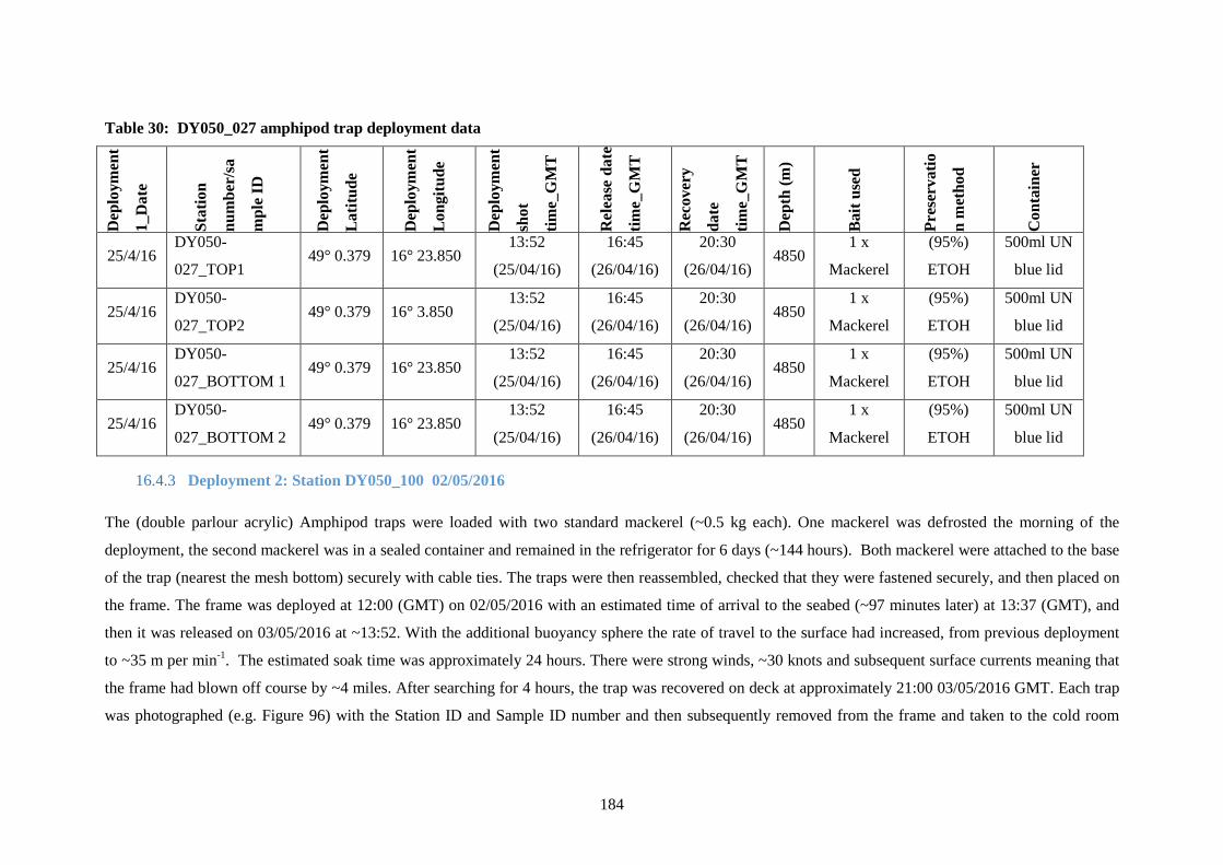
184

Table 30: DY050_027 amphipod trap deployment data D

eplo

ymen

t

1_D

ate

Stat

ion

num

ber/

sa

mpl

e ID

Dep

loym

ent

Lat

itude

Dep

loym

ent

Lon

gitu

de

Dep

loym

ent

shot

time_

GM

T

Rel

ease

dat

e

time_

GM

T

Rec

over

y

date

time_

GM

T

Dep

th (m

)

Bai

t use

d

Pres

erva

tio

n m

etho

d

Con

tain

er

25/4/16 DY050-

027_TOP1 49° 0.379 16° 23.850

13:52

(25/04/16)

16:45

(26/04/16)

20:30

(26/04/16) 4850

1 x

Mackerel

(95%)

ETOH

500ml UN

blue lid

25/4/16 DY050-

027_TOP2 49° 0.379 16° 3.850

13:52

(25/04/16)

16:45

(26/04/16)

20:30

(26/04/16) 4850

1 x

Mackerel

(95%)

ETOH

500ml UN

blue lid

25/4/16 DY050-

027_BOTTOM 1 49° 0.379 16° 23.850

13:52

(25/04/16)

16:45

(26/04/16)

20:30

(26/04/16) 4850

1 x

Mackerel

(95%)

ETOH

500ml UN

blue lid

25/4/16 DY050-

027_BOTTOM 2 49° 0.379 16° 23.850

13:52

(25/04/16)

16:45

(26/04/16)

20:30

(26/04/16) 4850

1 x

Mackerel

(95%)

ETOH

500ml UN

blue lid

16.4.3 Deployment 2: Station DY050_100 02/05/2016

The (double parlour acrylic) Amphipod traps were loaded with two standard mackerel (~0.5 kg each). One mackerel was defrosted the morning of the

deployment, the second mackerel was in a sealed container and remained in the refrigerator for 6 days (~144 hours). Both mackerel were attached to the base

of the trap (nearest the mesh bottom) securely with cable ties. The traps were then reassembled, checked that they were fastened securely, and then placed on

the frame. The frame was deployed at 12:00 (GMT) on 02/05/2016 with an estimated time of arrival to the seabed (~97 minutes later) at 13:37 (GMT), and

then it was released on 03/05/2016 at ~13:52. With the additional buoyancy sphere the rate of travel to the surface had increased, from previous deployment

to ~35 m per min-1. The estimated soak time was approximately 24 hours. There were strong winds, ~30 knots and subsequent surface currents meaning that

the frame had blown off course by ~4 miles. After searching for 4 hours, the trap was recovered on deck at approximately 21:00 03/05/2016 GMT. Each trap

was photographed (e.g. Figure 96) with the Station ID and Sample ID number and then subsequently removed from the frame and taken to the cold room

185

(~10°C) for processing. Each trap was marked with location (e.g. Top 1, Top 2, Bottom 1, or Bottom 2), this was to ensure that we kept everything straight.

All amphipods were removed from the trap using Ethanol into labelled 0.5L and 1.5 L UN certified plastic bottles and kept in the refrigerator at 4° C.

Table 31: DY050_100 amphipod trap deployment data

Dep

loym

ent

2_D

ate

Stat

ion

num

ber/

Sam

pl

e ID

Dep

loym

ent

Lat

itude

Dep

loym

ent

Lon

gitu

de

Dep

loym

ent

shot

time_

GM

T

Rel

ease

da

te

time_

GM

T

Rec

over

y da

te

time_

GM

T

Dep

th (m

)

Bai

t use

d*

Pres

erva

tion

met

hod

Con

tain

er

02/05/2016 DY050-

100_TOP1 49° 0.647 16° 23.769

12:00

(02/05/16)

16:15

(03/05/16)

21:00

(03/05/16) 4850

2 x

Mackerel

(95%)

Ethanol

500 ml UN

blue

02/05/2016 DY050-

100_TOP2 49° 0.647 16° 23.769

12:00

(02/05/16)

16:15

(03/05/16)

21:00

(03/05/16) 4850

2 x

Mackerel

(95%)

Ethanol

500 ml UN

blue

02/05/2016

DY050-

100_BOTTO

M 1

49° 0.647 16° 23.769 12:00

(02/05/16)

16:15

(03/05/16)

21:00

(03/05/16) 4850

2 x

Mackerel

(95%)

Ethanol

1500 ml

UN red

02/05/2016

DY050-

100_BOTTO

M 2

49° 0.647 16° 23.769 12:00

(02/05/16)

16:15

(03/05/16)

21:00

(03/05/16) 4850

2 x

Mackerel

(95%)

Ethanol

500 ml UN

blue

*1 x out freezer 144hours, 1 X 24 hours

186

Figure 96: Images of the traps with greatest catch from deployment a) DY050-027 and b)

DY050-100.

187

17 Molecular Ecology By C. R. Young

Genetic samples were collected from the megacore, trawl, and CTD.

17.1 Megacore

All megacore samples were sectioned by 1cm intervals up to 5cm, and by 5cm intervals up to 20cm when possible. Spatulas, slicer, and rings were sterilized between cores. A different, sterile, spatula was used for each slice. Slicer and ring was rinsed in Milli-Q water between slices. Three replicate DNA and RNA samples were taken from each slice and archived in 2ml tubes. The bulk of the slices were stored in 50ml falcon tubes and frozen at -80C. Replicate DNA samples were immediately frozen at -80C, and RNA samples were preserved in RNALater, left in the cold room (10-12C) for 24 hours, and then frozen at -80C.

17.2 CTD

Three CTD samples were filtered (1.3L) from the CTD cast, preserved in RNALater, left in the cold room for 24 hrs., then stored at -80C. In addition, one negative control was filtered from the MilliQ water supply (1.3 L) and processed in the same manner.

17.3 Trawl

Tissue samples were taken from select taxa collected from the trawl, and samples were preserved in EtOH. Due to recovery issues with DY050-063 (twisted leader lines and a larger than usual amount of sediment in the net), samples were exposed to ambient sea temperatures for an extended period of time, and time to processing of tissue samples once on deck was considerably longer than optimal. Recovery was scheduled for 8am, however the last tissue sample that I took was processed around 3:30 pm. Table 32 summarizes samples taken or attempted during the cruise. Samples taken during DY050-118 included 10 holothurians from two different species.

Figure 97: Holothurians samples from DY050-118. Body wall tissue and gut along with contents were dissected and stored at -80°C

188

STN

NO LAT (N) LONG (W)

SCIENCE

EVENT Sampled COMMENTS

002 48 50.055 16 31.342 Megacorer Y 0-5cm by 1cm, 5-10cm, 10-15cm; frozen at -

80C

003 48 50.387 16 31.174 Megacorer Y 0-5cm by 1cm, 5-10cm, 10-15cm, 15-20cm;

frozen at -80C

004 49 0.375 16 23.848 CTD Y CTD to 4800m; Sampled depths: 4300m,

4700m, 4760m, 4790m (all 1.3L)

018 48 50.277 16 31.270 Megacorer N failed deployment


frozen at -80C

026 48 50.171 16 31.526 Megacorer Y 0-3cm by 1cm; slippage in core, 0-2cm OK,

2-3cm questionable; frozen at -80C

036 48 50.270 16 30.999 Megacorer Y *0-5cm by 1cm, 5-10cm, 10-15cm, 15-

20cm; frozen at -80C


frozen at -80C

063 48 58.800 16 05.600 Otter Trawl Y

See trawl sample list for details; tissue in

EtOH; 28 samples taken: munidopsis,

anemones, asteroids, bivalve, pyncogonids,

holothurians. Rest of sample individually

bagged and preserved in formalin, labels

cry-1 to cry-28.

118 48 48.275 16 03.188 Otter Trawl Y

10 individuals from two holothurian taxa (5

each) were sampled. Body wall and gut +

contents were dissected out and stored at -

80C. Remainder of sample preserved in

formalin, labels cry-29 to cry-38.

Table 32: Samples taken for Molecular Ecology during DY050. * Standard sample taken, some core

slippage after/at 3-4cm but not much, Some MilliQ water transfer to the core that changed consistency

of sediment

189

Figure 98: Winston, the DY050 curlew

National Oceanography Centre Cruise Report No. 45

Documents

Transcript of National Oceanography Centre Cruise Report No. 45