Ocean Sci., 8, 11–18, 2012www.ocean-sci.net/8/11/2012/doi:10.5194/os-8-11-2012© Author(s) 2012. CC Attribution 3.0 License.

Ocean Science

Mapping turbidity layers using seismic oceanography methods

E. A. Vsemirnova1,*, R. W. Hobbs1, and P. Hosegood2

1Department of Earth Sciences, Durham University, Durham, DH1 3LE, UK2School of Marine Science and Engineering, Plymouth University, Plymouth PL4 8AA, UK* now at: Geospatial Research Ltd, Durham University, Durham DH1 3LE, UK

Correspondence to:R. W. Hobbs (r.w.hobbs@durham.ac.uk)

Received: 25 May 2011 – Published in Ocean Sci. Discuss.: 18 August 2011Revised: 12 December 2011 – Accepted: 22 December 2011 – Published: 10 January 2012

Abstract. Using a combination of seismic oceanographicand physical oceanographic data acquired across the Faroe-Shetland Channel we present evidence of a turbidity layerthat transports suspended sediment along the western bound-ary of the Channel. We focus on reflections observed on seis-mic data close to the sea-bed on the Faroese side of the Chan-nel below 900 m. Forward modelling based on independentphysical oceanographic data show that thermohaline struc-ture does not explain these near sea-bed reflections but theyare consistent with optical backscatter data, dry matter con-centrations from water samples and from seabed sedimenttraps. Hence we conclude that an impedance contrast in wa-ter column caused by turbidity layers is strong enough to beseen in seismic sections and this provides a new way to visu-alise this type of current and its lateral structure. By invert-ing the seismic data we estimate a sediment concentrationin the turbidity layers, present at the time of the survey, of45± 25 mg l−1. We believe this is the first direct observationof a turbidity current using Seismic Oceanography.

1 Introduction

Turbidity layers are some of the largest sediment-laden un-derflows that occur in ocean basins. In a geological context,these layers play an important role in transporting fluvial,littoral and shelf sediments into deep ocean environments.They may be sourced from sediment-laden river flow cas-cading down submarine canyons, slope failure, or by the re-mobilisation of unconsolidated sediment by strong currents.Turbidity layers are typically defined as relatively diluteflows in which particles are dominantly supported by fluidturbulence with sediment volume concentrations of<∼10 %.At higher sediment concentrations grain collision is morefrequent and the flow dynamics are changed (Sumner et al.,2009). A large number of experimental studies on turbid-ity layers are available (e.g. Middleton, 1966; Sumner et al.,

2009), however natural turbidity layers and other sediment-laden transient currents are hard to observe and study, due totheir irregular occurrence and often destructive nature (Hay,1987). Hence our knowledge of the turbidity layers is basedlargely on indirect observations of the modern seafloor frommultibeam bathymetry surveys (Kuijpers et al., 2002), high-resolution seismic surveys especially those designed for ob-servations of geohazards (Bulat and Long, 2001; Meiburgand Kneller, 2010) and the study of contourites (Masson etal., 2010; Koenitz et al., 2008); together with direct obser-vation of suspended sediment of the neptheloid layer fromoptical backscatter or transmissometer and sampling eitherin Niskin bottles or sediment traps (Bonnin et al., 2002; vanRaaphorst et al., 2001; Hosegood and van Haren, 2004).

2 Turbidity layers in the Faroe-Shetland Channel

The Faroe-Shetland Channel (FSC) (60◦ N, 6◦ W–63◦ N,1◦ W) is an elongate basin that trends NE–SW betweenthe West Shetland Shelf and the Faroe Shelf (Fig. 1c). Itis one of the major conduits of the global thermohalinesystem as it connects the deep waters of the NorwegianBasin with the Iceland Basin and Atlantic ocean. Turrellet al. (1999) identify five major water masses in the FSCdefined by differences in temperature, salinity and prove-nance. These are North Atlantic Water (NAW), ModifiedNorth Atlantic Water (MNAW), Arctic Intermediate/NorthIcelandic Water (AI/NIW), Norwegian Sea Arctic Intermedi-ate Water (NSAIW) and Faroe Shetland Channel Bottom Wa-ter (FSCBW). The classification can be simplified into twogroups based on transport direction and water depth, whichwe will refer to as surface water and bottom water. Thesurface water (NAW, MNAW and AI/NIW) are essentiallywarmer, higher salinity water masses and have a transport di-rection from the south-west to the north-east, with a base inthe FSC at approximately 500 m below sea-level. The bottom

Published by Copernicus Publications on behalf of the European Geosciences Union.

12 E. A. Vsemirnova et al.: Mapping turbidity layers

West East

(a)

(b)

(c)

Fig. 1. (a)a depth converted stacked seismic section of the FAST profile (England et al., 2005) reprocessed to recover the reflectivity in thewater layer. The seabed reflection is the high amplitude event that can be traced from the centre of the trough at about 1.2 km depth onto themargins. The band of reflectivity at a depth of about 500 m is caused by mixing of the North Atlantic Water with the Faroe-Shetland ChannelBottom Water.(b) the inset in rectangle focuses on the near-bed reflections between 65 and 82 km of the profile which we investigate in thispaper. The red line shows the section of data used to compute the histograms in Fig. 4.(c) a map showing the location of profiles used inthis study: black line: the FAST seismic profile; red dots: locations of CTD and moorings (Bonnin et al., 2002; Hosegood et al., 2005) crosssignifies location used for modelling sound-speed and density profiles (see Fig. 2).

Ocean Sci., 8, 11–18, 2012 www.ocean-sci.net/8/11/2012/

E. A. Vsemirnova et al.: Mapping turbidity layers 13

water (NSAIW and FSCBW) are cold, low salinity, watermasses flowing from the north-east to the south-west entirelycontained within the FSC. The boundary zone between thesetwo water types is a complex mix of waters and will varyseasonally and over time (Sherwin et al., 2006, 2008).

The shape of the Faroe-Shetland Channel and the orienta-tion of the Wyville-Thomson Ridge effects on the strength ofthe bottom currents, firstly funnelling these waters togetherand then deflecting most of the water mass by ninety degreesinto the Faroe bank Channel. Hansen and Østerhus (2000)estimate the average flow of bottom water in the FSC to be3 Sv. Direct measurements at 1000 m depth on the Shetlandside of the FSC show a variable current speed with a meanof 0.25 m s−1 with an M2 period with occasional peaks inspeed of over 0.5 m s−1 (Bonnin et al., 2002). These bottomcurrents have sufficient strength to mould and rework the sea-floor sediments within the FSC (Stoker et al., 1998; Bonninet al., 2002).

The emergence of 3-D seismic acquisition as a tool for re-gional reconnaissance for the hydrocarbons industry as wellas oil field development has resulted in nearly complete cov-erage of the FSC area by seismic reflection imaging. High-resolution seismic profiles acquired by the British Geolog-ical Survey in the FSC area, were integrated with the 3-Ddata to produce a regional image of the sea floor with an aimto identify seabed hazards (Bulat and Long, 2001; Massonet al., 2010). These detailed images of the seabed reveal anumber of sedimentary processes at work adjacent to andwithin the FSC. Of particular interest is an extensive net-work of long mounds that run sub-parallel to the strike ofthe slope between the 900 m and 1400 m isobaths. The net-work is restricted to the slope area but appears to cover itcompletely (Bulat and Long, 2001, their Fig. 2). One of theproposed mechanisms for generating these features are sedi-ment waves produced by turbidity-layers creating a series ofchannels and levees. The irregular character and internal ge-ometry of the mounds are indicative of erratic and turbulentflow.

3 Data sets

To date there has not been an integrated physical oceanog-raphy and seismic imaging survey with coincident and co-located sampling to examine turbidity layers. So we draw ontwo surveys, described below, that provide evidence of sus-pended particulate matter (SPM) that were acquired at dif-ferent times but in the same region of the Faroe-Shetlandchannel (Fig. 1). Seismic data (FAST) were obtained duringsummer 1994, with near ideal weather conditions with windspeeds of less than force 3 (England et al., 2005). Physicaloceanography data comes from an array of four moorings(PROCS-Processes at the Continental Slope) which was de-ployed during spring (April–May) and late summer (Septem-ber) 1999 (Bonnin et al., 2002). The dynamics that dominate

large resuspension events, and a possible mechanism for theformation of turbidity layers is the passage of solibores upthe continental slope (Hosegood et al., 2004; Hosegood andvan Haren, 2005). Long-term moorings deployed betweenthe two PROCS cruises showed that these events occurredwith a 3–5 day periodicity. Other observations of highly non-linear waves near the sea bed that could also promote resus-pension at depth were attributed to the internal tide (Hall etal., 2011). Thus, the hydrodynamics that drive the resuspen-sion events observed in the 1994 FAST data appear to beubiquitous throughout the FSC, implying that a comparisonbetween the FAST and PROCS data is valid despite the dif-ferent periods of observation.

3.1 Seismic reflection

The seismic line (FAST) which traverses the whole width ofthe Faroe-Shetland Trough (Fig. 1c) (England et al., 2005)was acquired with the original objective to map the struc-ture of the sedimentary basin and underlying basement. Theacquisition used a 147 l (8970 cu in) air-gun source opti-mised for low frequencies (bandwidth 6–60 Hz) and a 6 km240-channel hydrophone receiver array towed at 18 m depth.Though the acquisition configuration and the source weredesigned specifically for deep seismic profiling, the repro-cessed section presented here can still produce an image ofthe overlying water column (Fig. 1a) as demonstrated byHolbrook et al. (2003). The processing sequence for seismicdata was modified to include an eigenvector filter to suppressthe direct-wave between the seismic source and receiver ar-ray which obscures the weak reflectivity from the water col-umn. This reprocessing reveals a band of seismic reflectiv-ity centred around 500 m which correlates with the boundarybetween the warmer surface waters and the colder bottomwaters (Turrell et al., 1999). In addition, a discontinuous re-flection can be traced as a thin layer on the western slopeand along the base of the channel. Figure 1b shows an ex-panded section focused on the near sea-bed. The amplitudevariations along the reflection are indicative of the complex3-D nature of this boundary (Hobbs et al., 2006). Below thisreflection, for the bandwidth of 6–60 Hz, there is a lack ofreflectivity in the interval immediately overlying the seabed.

3.2 Physical oceanography datasets

In this study we used data from Optical Back-Scatter (OBS)measurements of suspended sediment, using a Seapoint STMsensor, and water samples taken during Conductivity Tem-perature Depth (CTD) casts during the PROCS programmein 1999, together with measurements from sediment traps at-tached to moorings deployed on a transect across the Shet-land side of the channel (Bonnin et al., 2002; Hosegood et al.,2005) (Fig. 1c). The CTD data (Fig. 2a, b) shows no signifi-cant changes in either temperature or salinity in the proximityof the seabed suggesting the deeper reflections observed on

www.ocean-sci.net/8/11/2012/ Ocean Sci., 8, 11–18, 2012

14 E. A. Vsemirnova et al.: Mapping turbidity layers

°C)

3)

-1)4)

(a) (b) (c)

(d) (e)

(f) (g)

Fig. 2. (a) temperature,(b) salinity and(c) optical back-scatter from the CTD cast (crossed red dot Fig. 1c).(d) corresponding sound-speedand(e) the density profiles without (blue) and with (red) the addition of suspended sediment (assumed to be quartz). The intrusion at 750 mshown in insert.(f) and(g) the vertical gradient of sound-speed and density respectively again without and with suspended sediment. Theeffects of intrusion at 750 m and near seabed sediment load are highlighted by arrows.

the seismic image (Fig. 1b) are wholly within the FSCBW.However, there is evidence of a change in suspended sed-iment, both dry matter from water samples and high OBSreadings close to the sea-bed (Fig. 2c; Bonnin et al., 2002,their Fig. 2). The addition of suspended sediment will changethe bulk average sound-speed and density which we proposecauses the change in impedance necessary to produce the ob-served seismic reflection which we can verify through mod-elling.

4 Modelling

To test our hypothesis that measurable reflections can be gen-erated by suspended sediment we perform forward modellingof seismic response based on the temperature, salinity andoptical back-scatter measurements from a CTD cast (Fig. 2a,b and c). Initially, we compute the background sound-speedand density profiles using the UNESCO equations of state(Fofonoff and Millard, 1983) assuming no suspended sedi-ment (Fig. 2d, e blue line). From these profiles we can cal-culate the vertical derivatives (Ruddick et al., 2009) which,

Ocean Sci., 8, 11–18, 2012 www.ocean-sci.net/8/11/2012/

E. A. Vsemirnova et al.: Mapping turbidity layers 15

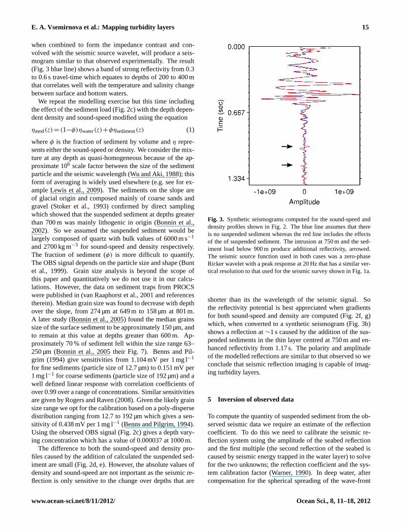
when combined to form the impedance contrast and con-volved with the seismic source wavelet, will produce a seis-mogram similar to that observed experimentally. The result(Fig. 3 blue line) shows a band of strong reflectivity from 0.3to 0.6 s travel-time which equates to depths of 200 to 400 mthat correlates well with the temperature and salinity changebetween surface and bottom waters.

We repeat the modelling exercise but this time includingthe effect of the sediment load (Fig. 2c) with the depth depen-dent density and sound-speed modified using the equation

ηmod(z) = (1−φ)ηwater(z)+φηsediment(z) (1)

whereφ is the fraction of sediment by volume andη repre-sents either the sound-speed or density. We consider the mix-ture at any depth as quasi-homogeneous because of the ap-proximate 106 scale factor between the size of the sedimentparticle and the seismic wavelength (Wu and Aki, 1988); thisform of averaging is widely used elsewhere (e.g. see for ex-ample Lewis et al., 2009). The sediments on the slope areof glacial origin and composed mainly of coarse sands andgravel (Stoker et al., 1993) confirmed by direct samplingwhich showed that the suspended sediment at depths greaterthan 700 m was mainly lithogenic in origin (Bonnin et al.,2002). So we assumed the suspended sediment would belargely composed of quartz with bulk values of 6000 m s−1

and 2700 kg m−3 for sound-speed and density respectively.The fraction of sediment (φ) is more difficult to quantify.The OBS signal depends on the particle size and shape (Buntet al., 1999). Grain size analysis is beyond the scope ofthis paper and quantitatively we do not use it in our calcu-lations. However, the data on sediment traps from PROCSwere published in (van Raaphorst et al., 2001 and referencestherein). Median grain size was found to decrease with depthover the slope, from 274 µm at 649 m to 158 µm at 801 m.A later study (Bonnin et al., 2005) found the median grainssize of the surface sediment to be approximately 150 µm, andto remain at this value at depths greater than 600 m. Ap-proximately 70 % of sediment fell within the size range 63–250 µm (Bonnin et al., 2005 their Fig. 7). Benns and Pil-grim (1994) give sensitivities from 1.104 mV per 1 mg l−1

for fine sediments (particle size of 12.7 µm) to 0.151 mV per1 mg l−1 for coarse sediments (particle size of 192 µm) and awell defined linear response with correlation coefficients ofover 0.99 over a range of concentrations. Similar sensitivitiesare given by Rogers and Raven (2008). Given the likely grainsize range we opt for the calibration based on a poly-dispersedistribution ranging from 12.7 to 192 µm which gives a sen-sitivity of 0.438 mV per 1 mg l−1 (Benns and Pilgrim, 1994).Using the observed OBS signal (Fig. 2c) gives a depth vary-ing concentration which has a value of 0.000037 at 1000 m.

The difference to both the sound-speed and density pro-files caused by the addition of calculated the suspended sed-iment are small (Fig. 2d, e). However, the absolute values ofdensity and sound-speed are not important as the seismic re-flection is only sensitive to the change over depths that are

Fig. 3. Synthetic seismograms computed for the sound-speed anddensity profiles shown in Fig. 2. The blue line assumes that thereis no suspended sediment whereas the red line includes the effectsof the of suspended sediment. The intrusion at 750 m and the sed-iment load below 900 m produce additional reflectivity, arrowed.The seismic source function used in both cases was a zero-phaseRicker wavelet with a peak response at 20 Hz that has a similar ver-tical resolution to that used for the seismic survey shown in Fig. 1a.

shorter than its the wavelength of the seismic signal. Sothe reflectivity potential is best appreciated when gradientsfor both sound-speed and density are computed (Fig. 2f, g)which, when converted to a synthetic seismogram (Fig. 3b)shows a reflection at∼1 s caused by the addition of the sus-pended sediments in the thin layer centred at 750 m and en-hanced reflectivity from 1.17 s. The polarity and amplitudeof the modelled reflections are similar to that observed so weconclude that seismic reflection imaging is capable of imag-ing turbidity layers.

5 Inversion of observed data

To compute the quantity of suspended sediment from the ob-served seismic data we require an estimate of the reflectioncoefficient. To do this we need to calibrate the seismic re-flection system using the amplitude of the seabed reflectionand the first multiple (the second reflection of the seabed iscaused by seismic energy trapped in the water layer) to solvefor the two unknowns; the reflection coefficient and the sys-tem calibration factor (Warner, 1990). In deep water, aftercompensation for the spherical spreading of the wave-front

www.ocean-sci.net/8/11/2012/ Ocean Sci., 8, 11–18, 2012

16 E. A. Vsemirnova et al.: Mapping turbidity layers

from a point source, the amplitude of the primary reflectionfrom sea bed is given by

AP= cR (2)

whereR is the unknown reflection coefficient andc is therequired calibration factor. The amplitudeAM of the corre-sponding first sea bed multiple is

AM = −cR2. (3)

By taking the ratio of the primary to multiple amplitude, thereflection coefficient of the sea bedR can be determined.

To make the calculation robust, we used the ratio ofmean values and standard deviations from distributions of theseabed primary and multiple from 900 traces from a sectionof the profile where we observe the turbidity layer. The se-lected data were processed to suppress low frequency noise,corrected for spherical divergence and normal move-out thenstacked with a maximum aperture of 1000 m. This limits themaximum incident angle for reflections from the base of thechannel to less than 24◦, which is sufficient to increase theamplitude of the reflection from the turbidity layer above theambient noise while minimises the effect of any amplitude orphase distortion of the reflections caused by the angle of in-cidence of the seismic energy or processing. The histogramsfor the seabed reflection and multiple are shown in Fig. 4a,b. The computed ratio ofAM/AP gives a value for the re-flection coefficient at the sea-bed ofR = 0.20± 0.05 whichis a reasonable value for an interface between sea-water andunconsolidated sediment (Warner, 1990). Substituting backinto (2) or (3) we can compute the calibration factor,c, of18± 3. We can now invert amplitudes on the seismic datato reflection coefficients provided we only use data with thesame processing applied as used for the calibration and, asis the case for sea-water at these frequencies, we ignore anyadditional transmission losses.

The top of the reflectivity interpreted as the turbidity layeris sampled at 900 locations and the mean and standard de-viation are used to estimate the reflection coefficient (Eq. 2,Fig. 4c) to give a value ofR = 0.00004± 0.00002. We can in-vert this value to estimate the sediment loading. Provided theimpedance contrast is small the reflection coefficientR canbe approximated toδZ/2Z where the impedanceZ =ρν; ρ isthe density andν is the sound-speed (Ruddick et al., 2009).Using Eq. (1),δZ is equal to

δZ = ((1−φ)vw +φvs)((1−φ)ρw +φρs)−vwρw (4)

which can be expanded to give

δZ = φvwρs+φvsρw −2φvwρw +O(φ2

). (5)

Ignoring the higher order terms and substituting in the val-ues of sound-speed and density for water (1470 m s−1 and1033 kg m−3 respectively) and quartz, we arrive at the re-lationship for the volume fraction of sediment. This is fi-nally converted back into sediment loading to give a value of45± 25 mg l−1.

2.8

2.9

3 3.1

3.2

3.3

3.4

3.5

3.6

3.7

3.8

3.9

4 4.1

0.00

50.00

100.00

150.00

200.00

250.00

Reflection amplitude of seabed

Amplitude

Pop

ulat

ion

­0.2

­0.3

­0.4

­0.5

­0.6

­0.7

­0.8

­0.9

­1 ­1.1

­1.2

­1.3

0

40

80

120

160

200

Reflection amplitude of multiple

AmplitudeP

opul

atio

n

0.00E+00

1.00E­04

2.00E­04

3.00E­04

4.00E­04

5.00E­04

6.00E­04

7.00E­04

8.00E­04

9.00E­04

1.00E­03

1.10E­03

1.20E­03

0

20

40

60

80

100

120

140

Reflection amplitude of tubiditic current

Amplitude

Pop

ulat

ion

(b)

(a)

(c)

Fig. 4. Histograms of the peak amplitude of reflections picked from900 traces from the seismic section (Fig. 1).(a) the seabed;(b) themultiple of the seabed (not shown on figure); and(c) the top of theturbidity layer. The shape of the histogram is indicative of the con-sistency of the reflection coefficient, the rugosity of the reflectionsurface in 3-D and the signal-to-noise ratio.

6 Discussions and conclusions

Benns and Pilgrim (1994) discussed the response of opti-cal backscatter devices to variations in suspended particu-late matter (SPM) and conclude that the particle size is themost influential physical characteristic of SPM on the in-strument response; Bunt et al. (1999) also mention that de-viations from sphericity in particle shape and the existence

Ocean Sci., 8, 11–18, 2012 www.ocean-sci.net/8/11/2012/

E. A. Vsemirnova et al.: Mapping turbidity layers 17

of radial projections can both increase scattering by 20 %.Using the calibration for medium size particles from Bennsand Pilgrim (1994) who suggest that the sediment load forthe observed SPM data could be 75–100 mg l−1 which is ofthe same order as estimated from the seismic data. As theseismic wavelength is much larger than the size of the par-ticulate matter, this method is not sensitive to the geome-try of the particles and the suspended sediment/water mix-ture can be considered as an equivalent homogeneous me-dia with properties determined by Eq. (1). Compared to dryweight of total particulate matter estimated from PROCS ex-periment, which is given as not exceeding 10 mg l−1 (vanRaaphorst et al., 2001), our value for the sediment load israther high. However they mention that the design of the fil-ters used in the experiment was changed to avoid overload-ing and to match the filter parameters for particulate organicmatter. Hence the results from the PROC experiment are notdiagnostic for the analysis of turbidity layer. Furthermore,our estimation is in a good agreement with sediment loadfound in other areas of the Ocean: Ashley and Smith (2000)give values of 8–15 mg l−1 of suspended solids in ephemeralturbid horizons, and 25–36 mg l−1 for “quasipermanent” tur-bidity layer; and Larcombe and Carter (2004) provide valuesof 10–100 mg l−1.

A potential error is the assumption that the suspended mat-ter is wholly composed of quartz. Stoker et al. (1998) esti-mates that in the FSC 8–16 % of the seabed is composed of ofmuddy sand facies. Assuming a similar fraction is present inthe suspend matter with a lower density ofρ = 2350 kg m−3

(Sumner et al., 2009) gives us an error of 2 % in our resultwhich is well below level of error we estimated for reflectioncoefficient. Error due to the motion of the sediment particlesis also negligible for the seismic survey. Furthermore, the re-gion within which we observed the seismic reflection is espe-cially homogeneous in terms of water density and thus speedof sound (Hosegood et al., 2005), with values for the Brunt-Vaisala frequency,N , <10−3.5 s−1. Specifically, the water atthis depth is vertically homogeneous FSCBW as confirmedby the data available from CTD profiles. The accuracy of theSPM concentration computed from seismic data is limited bythe signal-to-noise ratio of the data and the effects on reflec-tion amplitude caused by the local 3-D rugosity of the topof the current (Drummond et al., 2004; Hobbs et al., 2006).Further, we have assumed the upper boundary of the turbidityflow is sharp. If the boundary is gradational with a thicknessof more than 10 m the amplitude of the reflection is reducedhence our method will tend to produce an underestimate.

From this investigation we conclude that an impedancecontrast in the water column caused by turbidity layers isstrong enough to be seen in seismic sections and this pro-vides a new way to visualise this type of current to assessits dimensions and lateral structure. Further, it is possible toderive reasonable estimates of SPM in turbidity layers whichare consistent with other observation methods and, becauseof the longer seismic wavelength, maybe more robust.

Acknowledgements.Acknowledgements to the NOIZ PROCSprogramme (1999–2004) for the physical oceanographic data andthe FAST consortium for the seismic data. The seismic data wereprocessed using ProMAX software provided to Durham Universityby Halliburton under their University Scholarship Program.Final plots were made using Octave, Seismic Unix (Cohen andStockwell, 2010) and Generic Mapping Tools (GMT).

Edited by: O. Zielinski

References

Ashley, G. M. and Smith, N. D.: Marine sedimentation at a calvingglacier margin, Bull. Geol. Soc. Am., 112, 657–667, 2000.

Benns, E. J. and Pilgrim, D. A.: The effect of particle characteris-tics on beam attenuation coefficient and output from an opticalbackscatter sensor, Neth. J. Aquat. Ecol., 28, 245–248, 1994.

Bonnin, J., van Raaphorst, W., Brummer, G.-J., van Haren, H., andMalschaert, H.: Intense mid-slope resuspension of particulatematter in the Faeroe-Shetland Channel: Short-term deploymentof near-bottom sediment traps, Deep-Sea Res., Part I, 49, 1485–1505, 2002.

Bonnin, J., Koning, E., Epping, H. G., Brummer, G. J. A., and Grut-ters, M.: Geochemical characterization of resuspended sedimenton the SE slope of the Faeroe-Shetland Channel, Mar. Geol., 214,215–233, 2005.

Bonnin, J., van Haren, H., Hosegood, P. J., and Brummer, G.-J.:Burst resuspension of seabed material at the foot of the conti-nental slope of the Rockall Channel, Mar. Geol., 226, 167–184,2006.

Bulat, J. and Long, D.: Images of the seabed in Faroe-ShetlandChannel from commercial 3D seismic data, Mar. Geophys. Res.,22, 345–367, 2001.

Bunt, J. A. C., Larcombe, P., and Jago, C.: Quantifying the re-sponse of optical back scatter devices and transmittometers tovariations in suspended particulate matter, Cont. Shelf Res., 19,1199–1220, 1999.

Cohen, J. K. and Stockwell Jr., J. W.: CWP/SU: Seismic Unix Re-lease 42: a free package for seismic research and processing,Center for Wave Phenomena, Colorado School of Mines, 2010.

Drummond, B. J., Hobbs, R. W., and Goleby, B. R.: The effectsof out-of-plane seismic energy on reflections in crustal-scale 2Dseismic sections, Tectonophysics, 388, 213–224, 2004.

England, R. W., McBridge, J. H., and Hobbs, R. W.: The role ofMesozoic rifting in the opening of the NE Atlantic: evidencefrom deep seismic profiling across the Faroe-Shetland Trough, J.Geol. Soc., 162, 661–673, 2005.

Fofonoff, P. and Millard Jr., R. C.: Algorithms for computation offundamental properties of seawater, Unesco Technical Papers inMarine Science, 44, Unesco, 1983.

Hansen, B. and Østerhus, S.: North Atlantic – Nordic Seas ex-changes, Prog. Oceanogr., 45, 109–208, 2000.

Hay, A. E.: Turbidity currents and submarine channel formation inRupert inlet, J. Geophys. Res., 92, 2883–2900, 1987.

Hobbs, R. W, Drummond, B. J., and Goleby, B. R.: The effectsof three-dimensional structure on two-dimensional images ofcrustal seismic sections and on the interpretation of shear zonemorphology, Geophys. J. Int., 164, 490–500, 2006.

www.ocean-sci.net/8/11/2012/ Ocean Sci., 8, 11–18, 2012

18 E. A. Vsemirnova et al.: Mapping turbidity layers

Holbrook, W. S., Paramo, P., Pearse, S., and Schmitt, R. W.: Ther-mohaline fine structure in an oceanographic front from seismicreflection profiling, Science, 301, 821–824, 2003.

Hosegood, P. and van Haren, H.: Near-bed solibores over the conti-nental slope in the Faroe-Shetland Channel, Deep-Sea Res., 51,2943–2971, 2004.

Hosegood, P., van Haren, H., and Veth, C.: Mixing within the inte-rior of the Faeroe-Shetland Channel, J. Mar. Res., 63, 529–561,2005.

Koenitz, D., White, N., McCave, I. N., and Hobbs, R.: Inter-nal structure of a contourite drift generated by the AntarcticCircumpolar Current, Geochem. Geophy. Geosy., 9, Q06012,doi:10.1029/2007GC001799, 2008.

Kuijpers, A., Hansen, B., Huhnerbach, V., Larsen, B., Nielsen,T., and Werner, F.: Norwegian Sea overflow through the Faroe-Shetland gateway as documented by its bedforms, Mar. Geol.,188, 147–164, 2002.

Larcombe, P. and Carter, R. M.: Cyclone pumping, sediment parti-tioning and the development of the Great Barrier Reef shelf sys-tem: a review, Quaternary Sci. Rev., 23, 107–135, 2004.

Lewis, S. E., Sherman, B. S., Bainbridge, Z. T., Brodie, J. E.,and Cooper, M.: Modelling and monitoring the sediment trap-ping efficiency and sediment dynamics of the Burdekin FallsDam, Queensland, Australia, 18th, World IMACS/MODSIMCongress, Cairns, Australia, 13–17 July, 2009.

Masson, D. G., Plets, R. M. K., Huvenne, V. A. I., Wynn, R. B., andBett, B. J.: Sedimentology and depositional history of Holocenesandy contourites on the lower slope of the Faroe-Shetland Chan-nel, northwest of the UK, Mar. Geol., 268, 85–96, 2010

Meiburg, E. and Kneller, B.: Turbidity currents and their deposits,Annu. Rev. Fluid Mech., 42, 135–156, 2010.

Middleton, G. V.: Experiments on density and turbidity currents,Can. J. Earth Sci., 3, 523–546, 1966.

Rogers, A. L. and Ravens, T. M.: Measurement of Longshore Sed-iment Transport Rates in the Surf Zone on Galveston Island,Texas, J. Coastal Res., 2, 62–73,doi:10.2112/05-0564.1, 2008.

Ruddick, B., Song, H., Dong, C., and Pinheiro, L.: Water col-umn seismic images as smoothed maps of temperature gradient,Oceanography, 22, 192–205, 2009.

Sherwin, T. J., Williams, M. O., Turrell, W. R., Hughes, S. L., andMiller, P. I.: A description and analysis of mesoscale variabilityin the Faroe-Shetland Channel, J. Geophys. Res., 111, C03003,doi:10.1029/2005JC002867, 2006.

Sherwin, T. J., Hughes, S. L., Turrell, W. R., Hansen, B., and Øster-hus, S.: Wind driven variations in transport and the flow field inthe Faroe-Shetland Channel, Polar Res., 27, 7–22, 2008.

Stoker, M. S., Hitchen, K., and Graham, C. C.: The geology of theHebrides and West Shetland shelves, and adjacent deep waterareas, United Kingdom Offshore Regional Report, British Geo-logical Survey, London, 1993.

Stoker, M. S., Ackhurst, M. C. Howe, J. A., and Stow, D. A. V.: Sed-iment drifts and contourites on the continental margin off north-west Britain, Sediment. Geol., 15, 33–51, 1998.

Sumner, E. J., Talling, P. J., and Amy, L. A.: Deposits of flowstransitional between turbidity current and debris flow, Geology,37, 991–994, 2009.

Turrell, W. R., Slesser, G., Adams, R. D., Payne, R., and Gillibrand,P. A.: Decadal variability in the composition of Faroe ShetlandChannel bottom water, Deep Sea Res., Part I, 46, 1–25, 1999.

van Raaphorst, W., Malschaert, H., van Haren, H., Boer, W., andBrummer, G.-J.: Cross-slope zonation of erosion and depositionin the Faeroe-Shetland Channel, North Atlantic Ocean, Deep-SeaRes., Part I, 48, 567–591, 2001.

Warner, M.: Absolute reflection coefficients from deep seismic re-flections, Tectonophysics, 173, 15–23, 1990.

Wu, R.-S. and Aki, K.: Introduction: Seismic wave scattering inthree-dimensionally heterogeneous earth, Pure Appl. Geophys.PAGEOPH, 128, 1–6, 1988.

Ocean Sci., 8, 11–18, 2012 www.ocean-sci.net/8/11/2012/