www.elsevier.com/locate/epsl

Earth and Planetary Science Le

The role of chemical boundary layers in regulating the thickness

of continental and oceanic thermal boundary layers

Cin-Ty Aeolus Lee*, Adrian Lenardic, Catherine M. Cooper, Fenglin Niu, Alan Levander

Department of Earth Science, MS-126, Rice University, 6100 Main St., Houston, TX 77005, United States

Received 6 July 2004; received in revised form 10 November 2004; accepted 23 November 2004

Available online 13 January 2005

Editor: S. King

Abstract

An important feature of continents and oceans is that they are underlain by chemically distinct mantle, made intrinsically

buoyant and highly viscous by melt depletion and accompanying dehydration, respectively. Of interest here are the influences of

these preexisting chemical boundary layers on small-scale convective processes (as opposed to large-scale processes, which

govern the drift of continents and the eventual fate of oceanic thermal boundary layers, e.g., subduction) at the base of the oceanic

and continental thermal boundary layers. This manuscript explores the endmember in which dehydrated and melt-depleted

boundary layers are assumed to be strong (in the viscous sense) and chemically buoyant enough that they do not partake in any

secondary convection, that is, vertical heat transfer through these lids occurs purely by conduction. This assumption implies that

the only part of the thermal boundary layer that participates in secondary convection resides beneath the strong chemical boundary

layer. For oceans, this leads to the condition that the onset time of convective instability is suppressed until after the thermal

boundary layer has cooled through the base of the strong chemical boundary layer, whose thickness is defined at the outset by the

depth at which the solid mantle adiabat crosses the anhydrous peridotite solidus. A scaling law is presented that accounts for the

presence of a preexisting strong chemical boundary layer and predicts that the onset time of convective instability beneath oceans

correlates with the thickness of the chemical boundary layer, which itself correlates with the potential temperature of the mantle at

the time ofmelting. Estimated paleo-potential temperatures required to generate old oceanic crust in the Pacific andAtlantic may in

fact be correlated with onset time of seafloor flattening, but more data are needed to confirm these preliminary observations.

Finally, for continents, recent numerical models suggest that the thickness of the convective sublayer, hence the total thermal

boundary layer thickness, is also controlled by the thickness of a preexisting strong chemical boundary layer. Xenolith data from

cratons are shown to be largely consistent with the model-predicted relationship between the thicknesses of the chemical and

thermal boundary layers beneath continents. The conclusion of this study is that the nature of both oceanic and continental thermal

boundary layers is likely to be linked to preexisting strong chemical boundary layers.

D 2004 Elsevier B.V. All rights reserved.

Keywords: craton; peridotite; chemical boundary layer; dehydration; flattening

0012-821X/$ - s

doi:10.1016/j.ep

* Correspon

E-mail addr

tters 230 (2005) 379–395

ee front matter D 2004 Elsevier B.V. All rights reserved.

sl.2004.11.019

ding author. Tel.: +1 713 348 5084; fax: +1 713 348 5214.

ess: ctlee@rice.edu (C.-T.A. Lee).

C.-T.A. Lee et al. / Earth and Planetary Science Letters 230 (2005) 379–395380

1. Introduction

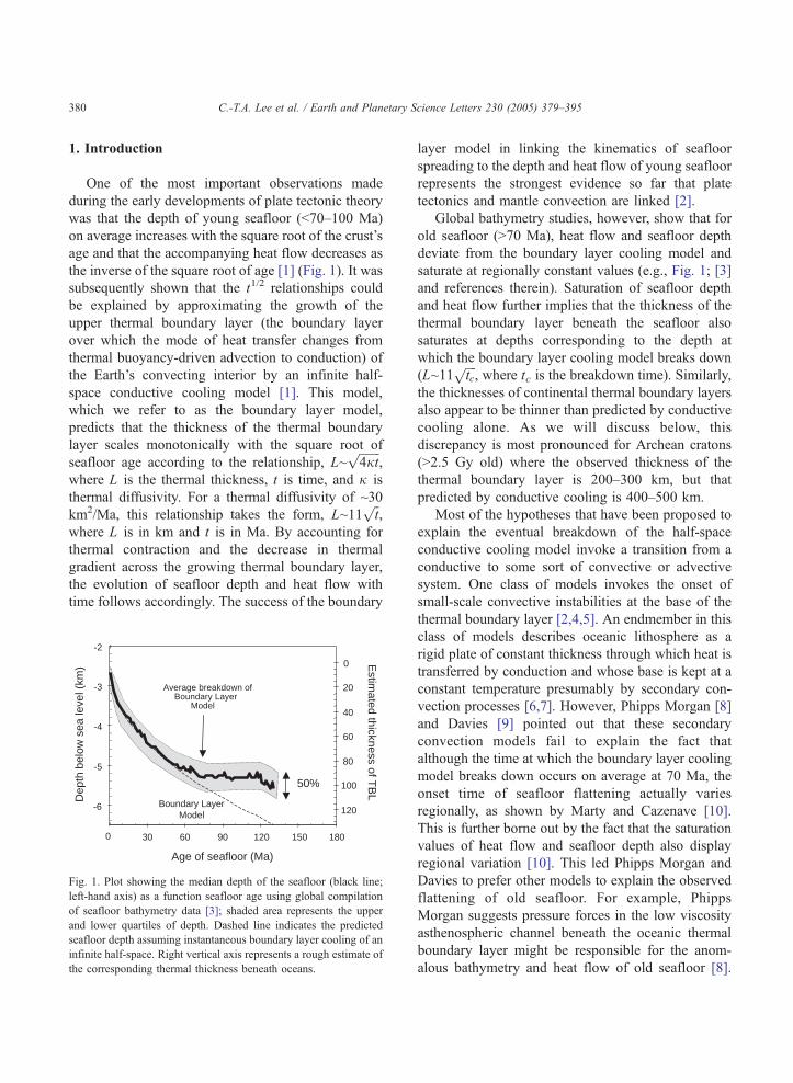
One of the most important observations made

during the early developments of plate tectonic theory

was that the depth of young seafloor (b70–100 Ma)

on average increases with the square root of the crust’s

age and that the accompanying heat flow decreases as

the inverse of the square root of age [1] (Fig. 1). It was

subsequently shown that the t1/2 relationships could

be explained by approximating the growth of the

upper thermal boundary layer (the boundary layer

over which the mode of heat transfer changes from

thermal buoyancy-driven advection to conduction) of

the Earth’s convecting interior by an infinite half-

space conductive cooling model [1]. This model,

which we refer to as the boundary layer model,

predicts that the thickness of the thermal boundary

layer scales monotonically with the square root of

seafloor age according to the relationship, L~ffiffiffiffiffiffiffi4jt

p,

where L is the thermal thickness, t is time, and j is

thermal diffusivity. For a thermal diffusivity of ~30

km2/Ma, this relationship takes the form, L~11ffiffit

p,

where L is in km and t is in Ma. By accounting for

thermal contraction and the decrease in thermal

gradient across the growing thermal boundary layer,

the evolution of seafloor depth and heat flow with

time follows accordingly. The success of the boundary

0 30 60 90 120 150 180

Dep

th b

elow

sea

leve

l (km

)

Age of seafloor (Ma)

0

20

40

60

80

100

120

Estim

ated thickness of TB

L

Boundary LayerModel

-6

-5

-4

-3

-2

Average breakdown ofBoundary Layer

Model

50%

Fig. 1. Plot showing the median depth of the seafloor (black line;

left-hand axis) as a function seafloor age using global compilation

of seafloor bathymetry data [3]; shaded area represents the upper

and lower quartiles of depth. Dashed line indicates the predicted

seafloor depth assuming instantaneous boundary layer cooling of an

infinite half-space. Right vertical axis represents a rough estimate of

the corresponding thermal thickness beneath oceans.

layer model in linking the kinematics of seafloor

spreading to the depth and heat flow of young seafloor

represents the strongest evidence so far that plate

tectonics and mantle convection are linked [2].

Global bathymetry studies, however, show that for

old seafloor (N70 Ma), heat flow and seafloor depth

deviate from the boundary layer cooling model and

saturate at regionally constant values (e.g., Fig. 1; [3]

and references therein). Saturation of seafloor depth

and heat flow further implies that the thickness of the

thermal boundary layer beneath the seafloor also

saturates at depths corresponding to the depth at

which the boundary layer cooling model breaks down

(L~11ffiffiffiffitc

p, where tc is the breakdown time). Similarly,

the thicknesses of continental thermal boundary layers

also appear to be thinner than predicted by conductive

cooling alone. As we will discuss below, this

discrepancy is most pronounced for Archean cratons

(N2.5 Gy old) where the observed thickness of the

thermal boundary layer is 200–300 km, but that

predicted by conductive cooling is 400–500 km.

Most of the hypotheses that have been proposed to

explain the eventual breakdown of the half-space

conductive cooling model invoke a transition from a

conductive to some sort of convective or advective

system. One class of models invokes the onset of

small-scale convective instabilities at the base of the

thermal boundary layer [2,4,5]. An endmember in this

class of models describes oceanic lithosphere as a

rigid plate of constant thickness through which heat is

transferred by conduction and whose base is kept at a

constant temperature presumably by secondary con-

vection processes [6,7]. However, Phipps Morgan [8]

and Davies [9] pointed out that these secondary

convection models fail to explain the fact that

although the time at which the boundary layer cooling

model breaks down occurs on average at 70 Ma, the

onset time of seafloor flattening actually varies

regionally, as shown by Marty and Cazenave [10].

This is further borne out by the fact that the saturation

values of heat flow and seafloor depth also display

regional variation [10]. This led Phipps Morgan and

Davies to prefer other models to explain the observed

flattening of old seafloor. For example, Phipps

Morgan suggests pressure forces in the low viscosity

asthenospheric channel beneath the oceanic thermal

boundary layer might be responsible for the anom-

alous bathymetry and heat flow of old seafloor [8].

C.-T.A. Lee et al. / Earth and Planetary Science Letters 230 (2005) 379–395 381

Alternatively, hotspots have been called upon to

convectively thin the lithosphere [11].

Here, we explore the possibility that preexisting

chemical/rheologic boundary layers beneath oceans

and continents might dictate the thickness of thermal

boundary layers by influencing secondary convective

processes at the base of the thermal boundary layer.

We are not concerned with large-scale convective

processes, which govern the drift of continents and the

eventual fate of oceanic thermal boundary layers, i.e.,

subduction. Our paper is largely motivated by recent

advances in the community’s understanding of the

deep thermal and compositional structure of con-

tinents, particularly beneath their ancient tectonically

quiescent cores (cratons). Cratons are typically under-

lain by thick mantle keels, which are highly depleted

in meltable components [12]. Oceanic mantle has also

experienced melt extraction although not to the very

high extents seen in cratonic mantle. Importantly, melt

depletion results in a mantle residue that is not only

chemically buoyant but also dehydrated, the latter

which results in an increase in intrinsic viscosity,

possibly by more than two orders of magnitude

[13,14]. The effects of enhanced chemical buoyancy

and viscosity are to compete against the development

of convective instabilities. Such chemical boundary

layers may thus be expected to a play a role in the

development and preservation of continental and

oceanic thermal boundary layers. At least beneath

continents, radiogenic isotopic studies indicate that

these chemical boundary layers have remained iso-

lated and largely undeformed over billion year time-

scales [15,16].

The effects of chemical buoyancy on the develop-

ment and preservation of thermal boundary layers

have recently been investigated by Zaranek and

Parmentier [17] and Sleep [18], respectively.

Although the effects of temperature-dependent vis-

cosity have already been investigated (e.g., [19,20]),

the influence of depth-dependent viscosity, specifi-

cally, intrinsic depth-variations in viscosity, have only

recently been investigated by Korenaga and Jordan

[4]. The purpose of our paper is to assess the

endmember in which the chemical boundary layer,

as a consequence of dehydration and chemical buoy-

ancy, can be considered a purely (vertically) con-

ductive lid such that it effectively does not participate

in secondary convection. We consider how a preex-

isting and rheologically strong chemical boundary

layer influences the thickness of thermal boundary

layers beneath continents and oceans. We begin with a

review of the main properties of cratonic mantle that

are likely to influence its long-term stability and

strength: density, water content, and thermal state. We

then show that saturation thicknesses of thermal

boundary layers predicted by the recent numerical

models of Cooper et al. [21] are broadly consistent

with xenolith data. In the case of oceans, we present a

scaling analysis that provides qualitative predictions

on the relationship between the onset time of

convective instabilities and the thickness of the

chemical boundary layer.

2. The cratonic perspective: long-lived chemical

boundary layers

We begin by reviewing the most relevant character-

istics of cratonic mantle. A distinct feature of cratonic

mantle keels is that their major-element composition,

as inferred from mantle xenoliths, differs from that of

the shallow part of the convecting mantle from which

mid-ocean ridge basalts derive [12,22,23]. Compared

to convecting mantle, mantle keels are highly depleted

in Ca and Al and to a lesser extent Fe. Ca and Al are

the elements that stabilize clinopyroxene and garnet,

both of which are the first minerals to be exhausted

during progressive partial melt extraction. The deple-

tion in Ca and Al is believed to be the result of

extensive melt extraction (20–40 wt.% partial melt). A

common index of melt extraction is the Mg# (the

molar ratio Mg/(Mg+Fe)), which is a measure of the

relative proportion of Fe to Mg. Convecting mantle is

more bfertileQ in terms of meltable components and is

characterized by Mg#s of ~0.88–0.89. Cratonic

mantle keels are largely depleted of meltable compo-

nents (clinopyroxene and garnet) and are character-

ized by average Mg#s of ~0.92–0.93. Fertile (low

Mg#) peridotites found in cratonic xenolith suites

appear to originate from a distinct narrow zone below

the chemically depleted layer.

There are two important consequences of high

degrees of melt extraction. The first is that the

residue becomes intrinsically less dense because the

dense minerals, garnet and clinopyroxene, are

exhausted and the proportion of Fe relative to Mg

C.-T.A. Lee et al. / Earth and Planetary Science Letters 230 (2005) 379–395382

decreases (e.g., Mg# increases) [12,22,24,25]. Jor-

dan suggested that this decrease in intrinsic density

may offset the increase in density of mantle keels

due to thermal contraction associated with the cooler

thermal state of cratons relative to the convecting

mantle [26]. Using the South African craton as an

example, he proposed that mantle keels are in fact

neutrally buoyant because the compositional buoy-

ancy exactly offsets the negative thermal buoyancy

of cratons at every depth, a condition that Jordan

termed bisopycnic.Q The large amount of data since

accumulated for other cratonic mantle keels [23,27–

29] has confirmed that high Mg# peridotite indeed

characterizes the bulk of cratonic mantle. Although

it now appears that cratonic mantle may not be

strictly isopycnic at every depth (see Fig. 2), the

depth-integrated density of cratonic mantle indeed

roughly offsets the craton’s total negative thermal

buoyancy.

fert

ile

65 Ma

Continents

B

Dep

th (

km)

FertileMantle

CratonicMantle

A

1600

400

600

800

1000

1200

1400

50

100

150

200

250

250 150 100 65 Ma

25

3300

3320

3340

3360

3380

T (oC) ρ1 bar

Base ofCBL?

dep

lete

d

Base ofTBL?

100

150

South AfricaSiberiaCanadaTanzania

Fig. 2. (A) Thermal state of Archean cratonic mantle based on xenolith the

shallower than ~175 km are mostly highly depleted (open symbols; chemi

than ~175 km are mostly fertile (gray symbols). Curved lines represent h

times. (B) Pressure-normalized density structure of cratonic mantle as a fu

shown in panel (A). Dotted lines represent the density of cratonic and fertile

different transient geotherms. Viscosities are calculated following Hirth

exp((E+PV)/(RT)) where P is pressure (Pa), T is temperature (K), A is th

mol), V is the activation volume (m3/mol), n is the exponent (assumed to b

rheology was assumed (dry: A=4.85�104, E=535; wet: A=4.89�106, E=5

15�10�6 at 1 bar to 7.5�10�6 at 8 GPa following [14]. Solid curves repre

represent the viscosities for cratonic and fertile mantle at TP.

The second consequence of melt extraction is the

progressive dehydration of the solid residue due to the

incompatible nature of H2O during partial melting

[14]. At the high degrees of melting required to

generate the high Mg#s of cratonic mantle peridotites

(N30% melting), the residual peridotites should have

been completely dehydrated. Estimates of the amount

of H2O in different parts of the mantle range from

~100 to 750 ppm ([30–32] and references therein).

According to Hirth and Kolhstedt [14], such dehy-

dration can lead to a 500-fold increase in intrinsic

viscosity. Assuming subsequent metasomatism did

not pervasively reintroduce water to the dehydrated

mantle keel, the chemically depleted boundary layer

then represents a layer of low intrinsic density and

increased intrinsic viscosity (c.f., [13,33]).

The precise thickness of the chemical boundary layer

(dCBL) and/or thermal boundary layer (dTBL) beneath

cratons is debated. Seismic tomographic studies show

convectivelyunstable

strong chemicalboundary

layer

250150

0

3400

3420

3440

3460

3480

3500

Log η (kg/m3)

252015

C

65 Ma

100

150

250

250

150

TP = 1450 oC TP = 1450 oC

rmobarometric data from various cratons [28,29,40]. Xenoliths from

cal boundary layer; chemical boundary layer), whereas those deeper

ypothetical transient boundary layer cooling geotherms at different

nction of different thermal states defined by the transient geotherms

mantle at 25 8C. C. Log viscosity (g; Pa s) as a function of depth forand Kohlstedt [14] for non-Newtonian fluids using g=A�1 rn�1

e preexponential factor (s�1MPa�n), E is the activation energy (kJ/

e 3.5) and r is the background deviatoric stress (~0.3 MPa); olivine

15). The activation volume V was assumed to change linearly from

sent viscosities for the transient geotherms in panel (A). Dotted lines

C.-T.A. Lee et al. / Earth and Planetary Science Letters 230 (2005) 379–395 383

that the high velocities beneath cratons extend to depths

anywhere from 200 to 400 km [34–37]. This large

uncertainty may be due to the lack of good vertical

resolution in the teleseismic data used in tomographic

studies [38,39]. In addition, seismic velocities are most

sensitive to temperature, and therefore, high-velocity

anomalies at great depth may simply reflect local

thermal disturbances rather than the presence of a thick

chemical boundary.

Xenolith thermobarometric data provide an inde-

pendent constraint on the thickness of the chemical and

thermal boundary layers provided the xenoliths were in

chemical equilibrium up until the time they were

sampled by their host volcanics. The thermobarometric

data of xenoliths indicate that chemically depleted

mantle extends to depths of ~175 km [23,29,40,41]

(open symbols in Fig. 2A). Beyond this depth, there

appears to be a pronounced increase in the fertility of

mantle xenoliths (gray symbols in Fig. 2A). The

equilibration temperatures of these deep and fertile

xenoliths range between 1300 and 1450 8C, approach-ing the temperature defined by the solid mantle adiabat

at equivalent depths. Several interpretations for the

origin of these deep, fertile xenoliths have been

suggested: high Mg# peridotites that have been

reenriched (refertilized) in Fe, Ca, and Al (some show

disequilibria in the form of chemically zoned minerals

and high strain deformation textures) [15,42], sub-

ducted oceanic lithospheric mantle [43], and/or sam-

ples from the top of the fertile convecting mantle [42].

Whatever their origin, the deep, fertile xenoliths appear

to derive from just below the chemically depleted layer.

If we interpret them to derive from the lower part of the

thermal boundary layer, their near-adiabatic temper-

atures suggest that the base of the thermal boundary

layer cannot be much deeper than their maximum

depths of origin (~250 km). These observations suggest

that the chemical boundary layer beneath cratons

extends to ~175 km, and that the thermal boundary

layer (which includes the chemical boundary layer)

extends to greater depths, but not significantly exceed-

ing ~250 km. These depth constraints are consistent

with the results of more recent seismic studies. Gung et

al. showed that there is pronounced radial seismic

anisotropy beneath continents in the depth range of

250–400 km, which they attribute to the presence of a

low viscosity asthenospheric channel [44]. Niu et al.

showed that there are no detectable deflections at the

410- and 670-km discontinuities beneath the Kaapvaal

craton in south Africa, which they argue limit the

thickness of the Kaapvaal craton to less than ~300 km

[45]. The consistent results from independent techni-

ques provide some affirmation that our interpretations

may be robust.

3. Dynamic effects of a preexisting chemical

boundary layer beneath continents

We now address the dynamic effects of a composi-

tionally and rheologically stratified thermal boundary

layer beneath cratons. Fig. 2B shows the density

structure of the cratonic mantle as a function of depth

relative to the fertile convecting mantle (Mg#=0.89)

and time since the initiation of boundary layer cooling

(Fig. 2A). The density–Mg# scalings of Lee [25] were

used. Cratons are assumed to be underlain by a

uniformly depleted (Mg#=0.925) chemical boundary

layer, which has a lower intrinsic density than the

fertile convecting mantle; gray line in Fig. 2B). The

thickness of the chemical boundary layer, dCBL, isinferred from the transition from depleted to fertile

peridotites shown in Fig. 2A (170 km). Superimposed

on Fig. 2A are hypothetical transient half-space

conductive cooling curves. These are shown only to

illustrate that the xenolith-defined geotherm matches

an apparent 250 Ma transient geotherm, which is

much younger than the cratons themselves. The high

Mg#s characteristic of the cratonic chemical boundary

layer imply such high degrees of melting that the

chemically depleted boundary layer would be

expected to be initially completely dehydrated (meta-

somatic reintroduction of H2O is discussed below).

Fig. 2C shows the viscosity structure of the mantle as

a function of depth and time after the onset of

conductive cooling. The viscosities of the chemical

boundary layer and the underlying fertile mantle were

calculated using the viscosity laws of Hirth and

Kohlstedt [14] for wet and dry olivine and assuming

complete dehydration of a fertile mantle at depths

above the intersection between the adiabat and the dry

peridotite solidus (Fig. 4).

The discontinuity in composition at dCBL~175 km is

accompanied by discontinuities in intrinsic density and

viscosity. Two features are apparent from Fig. 2B and

C. First, because the deepest part of the thermal

C.-T.A. Lee et al. / Earth and Planetary Science Letters 230 (2005) 379–395384

boundary layer (N170 km) is fertile, this sublayer is

intrinsically denser than the overlying material in the

chemical boundary layer. This fertile sublayer becomes

negatively buoyant once the transient conductive

boundary layers in Fig. 2A pass through the base of

the chemical boundary layer. The melt-depleted upper

layer, on the other hand, will be positively or neutrally

buoyant and provide a resisting force to convective

downwelling. Second, the hydrated character of fertile

mantle renders it over 2 orders of magnitude less

viscous [14] than the chemically depleted and dehy-

drated mantle lying directly above it (Fig. 2C).

According to Lenardic and Moresi [46] and Sleep

[18], the combination of chemical buoyancy and

enhanced viscosity in the chemical boundary layer is

sufficient to keep the chemical boundary layer from

being entrained into convective downwellings. How-

ever, the fertile and wetter sublayer is likely to be

available for convection. For these reasons, we suggest

that the chemical boundary layer itself is viscous (due

to dehydration) and buoyant enough to act as a strong

conductive lid over long timescales while the under-

lying fertile part represents the actively convecting part

of the thermal boundary layer, which we term here the

δ TB

L/δ C

BL

δ CBL

δ CSL

δTBL

δC

Radiogenically Depleted

Radiogenically Undepleted Root

4.5

4

3.5

3

2.5

2

1.5

40 60 80 100 11

Fig. 3. The ratio of thermal boundary layer thickness to chemical boundary

and depleted (light gray line) cratonic root. Based on numerical simulati

relationship between the thicknesses of the chemical boundary layer (rCB

The chemical boundary layer consists of the crust and depleted mantle ro

convective sublayer. The thermal boundary layer

therefore consists of a strong upper lid (chemical

boundary layer) and the convectively active lower

portion (e.g., the convective sublayer; Fig. 3), i.e.,

dTBL=dCBL+dCSL.The thickness of the convective sublayer dCSL is

linked to the thermal state of the cratonic thermal

boundary layer due to the temperature-dependency of

viscosity. If we assume that cratonic chemical

boundary layers are so long-lived that their thermal

structures have reached statistical steady state, dCSLmust depend on the convective vigor in the interior of

the Earth (as represented by the bottom and internally

heated Rayleigh numbers) and any sources of heat

generation within the cratonic chemical boundary

layer as both parameters dictate the thermal state of

the chemical boundary layer. Cooper et al. [21]

conducted numerical simulations to explore the

thermal coupling between strong chemical boundary

layers and the convecting mantle at statistically

steady-state conditions. They showed that the thick-

ness of strong, preexisting chemical boundary layers

dictate the nature of the thermal boundary layer

beneath cratons. Fig. 3 shows that the ratio of thermal

Depleted Mantle Root

CSL

Cont. crust

BL(km)

CB

L t

hic

knes

sb

enea

th c

rato

ns

Root

20 140 160 180 200

layer thickness for both a radiogenically undepleted (solid black line)

ons of Cooper et al. [21]. Inset shows schematic illustration of the

L), convective sublayer (rCSL), and thermal boundary layer (rTBL).

ot, which together serve as a strong conductive lid.

C.-T.A. Lee et al. / Earth and Planetary Science Letters 230 (2005) 379–395 385

boundary layer thickness to chemical boundary layer

thickness dTBL/dCBL decreases as dCBL increases. For

a dCBL~175 km, such as beneath Siberia and South

Africa (Fig. 2A), the numerical simulations predict a

steady-state dCSL of ~50 km, which corresponds to

dTBL~220 km. This is remarkably close to dTBLestimated from thermobarometric studies of mantle

xenoliths (Fig. 2A), which supports the idea that the

chemical boundary layer beneath a craton represents a

strong, long-lived lid.

4. The chemical boundary layer beneath oceanic

crust

Wenow address whether oceanic crust might also be

underlain by a chemical boundary layer and whether

this boundary layer influences the evolution of the

oceanic thermal boundary layer. Unlike cratonic

mantle, which can be characterized using mantle

xenoliths, there are no xenolith samples of oceanic

mantle. Ophiolites and abyssal peridotites provide a

window to the oceanic mantle, but sample only the

shallow veneer lying just beneath the Moho. We thus

infer the chemical structure of oceanic mantle by

assuming that it forms as the residue of partial melting

beneath mid-ocean ridges, which are driven by passive

upwelling (Fig. 4). Schematic streamlines of passive

corner flow are shown in Fig. 4A. The intersection of

A

P (

GP

a)

0

1

2

3

4

5

6

7

Dry meltingregime

Mid-ocean Ridge

Fig. 4. (A) Schematic diagram showing how a triangular melting regim

(arrowed lines represent schematic streamlines). Due to corner flow, this r

Pressure–temperature diagram illustrating the geometry of adiabatic mantle

solidus for peridotite having ~700 ppm H2O [48]. Ascent paths for two diffe

gradient of 0.5 8C/km assumed). The intersections of the adiabats and the

Dashed and solid horizontal lines represent the thicknesses of the resulti

chemical boundary layer as shown in panel (A).

the mantle adiabat and the mantle solidus represents the

depth at which dry melting initiates and the peridotite

residue can be said to be completely dehydrated.

Using the parameterizations of the mantle solidus

taken from Hirschmann [47], it can be seen from

Fig. 4 that the depth of dry melting initiates at 50 km

and 110 km for solid mantle adiabats having

respective potential temperatures TP of 1300 8Cand 1450 8C (TP is defined as the temperature of the

solid upper mantle if it were decompressed adiabati-

cally to the surface), which spans the range the range

of upper mantle TP (see Section 5). The density

structure of the oceanic mantle due to partial melting

can also be estimated. Assuming passive upwelling

and a linear melting function, the cumulative fraction

of melt extracted per unit depth, dF/dz, is approx-

imately 0.0035/km [48]. The Mg# of the mantle

residue as a function of depth can be estimated by

plugging F(z) into an equation relating Mg# to F

determined from the thermodynamically based

pMELTS program (dMg#/dF ~0.0794) [49]. We can

then use density–Mg# relationships [25] to infer the

intrinsic density structure of the schematized oceanic

mantle in Fig. 4A.

Figs. 5A–C show the density and viscosity

structure of oceanic mantle for different transient

geotherms (Fig. 5A). By construct of our partial

melting model for mid-ocean ridges, the Mg# of the

oceanic mantle decreases gradually with depth so that

Temp (oC)

Dep

th (km

)

B

500

1000

1500

2000

2500

0

50

100

150

200

Dry solidus

Liquidus

e forms beneath a mid-ocean ridge undergoing passive upwelling

esults in a chemically depleted and dehydrated boundary layer. (B)

ascent paths and the dry peridotite solidus. Dotted line represents the

rent potential temperatures (1300 and 1450 8C) are shown (adiabaticdry solidus [47] represent the depth at which dry melting initiates.

ng dehydrated and melt-depleted residuum. This leads to a strong

0

200

400

600

800

1000

1200

1400

1600

0

25

50

75

100

125

150

3320

3340

3360

3380

3400

3420

3440

3460

3480

3500

convectivelyunstable

strong chemicalboundary

layer

CA

2 Ma

10

75

2 Ma

OceanicMantle

FertileMantle

B

10

75

252015

2 Ma

10

75

0

25

50

75

100

125

150

TP = 1300 oC

TP = 1450 oC

T (oC) Log η(Pa s)

ρ1 bar(kg/m3)

TP = 1375 oC

TP = 1375 oC TP = 1375 oC

Z (

dept

h)

Oceans

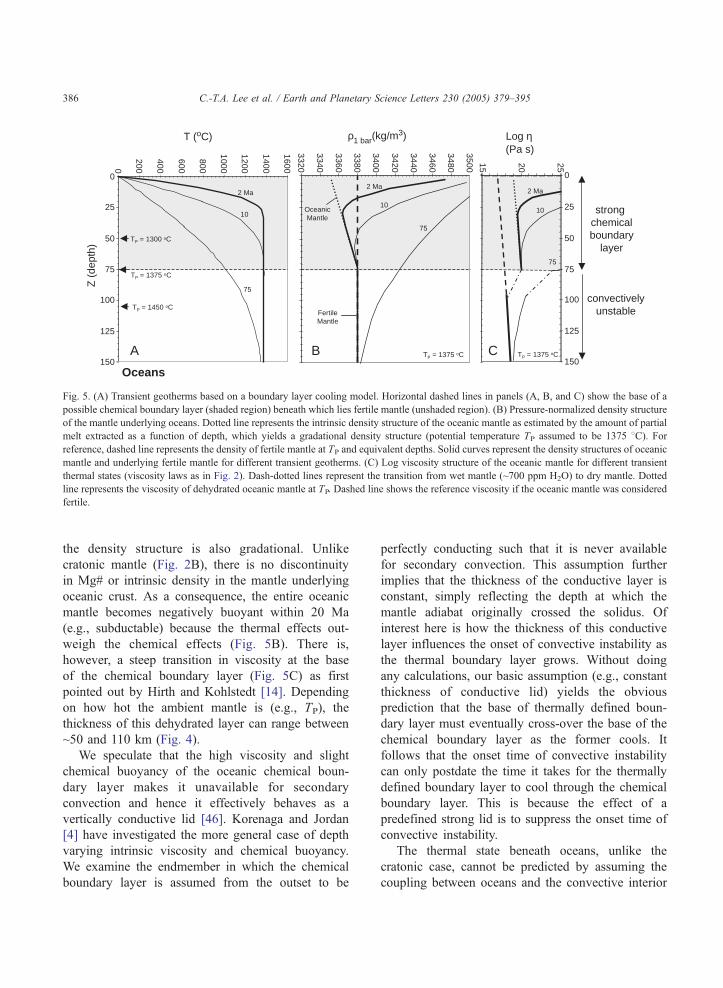
Fig. 5. (A) Transient geotherms based on a boundary layer cooling model. Horizontal dashed lines in panels (A, B, and C) show the base of a

possible chemical boundary layer (shaded region) beneath which lies fertile mantle (unshaded region). (B) Pressure-normalized density structure

of the mantle underlying oceans. Dotted line represents the intrinsic density structure of the oceanic mantle as estimated by the amount of partial

melt extracted as a function of depth, which yields a gradational density structure (potential temperature TP assumed to be 1375 8C). Forreference, dashed line represents the density of fertile mantle at TP and equivalent depths. Solid curves represent the density structures of oceanic

mantle and underlying fertile mantle for different transient geotherms. (C) Log viscosity structure of the oceanic mantle for different transient

thermal states (viscosity laws as in Fig. 2). Dash-dotted lines represent the transition from wet mantle (~700 ppm H2O) to dry mantle. Dotted

line represents the viscosity of dehydrated oceanic mantle at TP. Dashed line shows the reference viscosity if the oceanic mantle was considered

fertile.

C.-T.A. Lee et al. / Earth and Planetary Science Letters 230 (2005) 379–395386

the density structure is also gradational. Unlike

cratonic mantle (Fig. 2B), there is no discontinuity

in Mg# or intrinsic density in the mantle underlying

oceanic crust. As a consequence, the entire oceanic

mantle becomes negatively buoyant within 20 Ma

(e.g., subductable) because the thermal effects out-

weigh the chemical effects (Fig. 5B). There is,

however, a steep transition in viscosity at the base

of the chemical boundary layer (Fig. 5C) as first

pointed out by Hirth and Kohlstedt [14]. Depending

on how hot the ambient mantle is (e.g., TP), the

thickness of this dehydrated layer can range between

~50 and 110 km (Fig. 4).

We speculate that the high viscosity and slight

chemical buoyancy of the oceanic chemical boun-

dary layer makes it unavailable for secondary

convection and hence it effectively behaves as a

vertically conductive lid [46]. Korenaga and Jordan

[4] have investigated the more general case of depth

varying intrinsic viscosity and chemical buoyancy.

We examine the endmember in which the chemical

boundary layer is assumed from the outset to be

perfectly conducting such that it is never available

for secondary convection. This assumption further

implies that the thickness of the conductive layer is

constant, simply reflecting the depth at which the

mantle adiabat originally crossed the solidus. Of

interest here is how the thickness of this conductive

layer influences the onset of convective instability as

the thermal boundary layer grows. Without doing

any calculations, our basic assumption (e.g., constant

thickness of conductive lid) yields the obvious

prediction that the base of thermally defined boun-

dary layer must eventually cross-over the base of the

chemical boundary layer as the former cools. It

follows that the onset time of convective instability

can only postdate the time it takes for the thermally

defined boundary layer to cool through the chemical

boundary layer. This is because the effect of a

predefined strong lid is to suppress the onset time of

convective instability.

The thermal state beneath oceans, unlike the

cratonic case, cannot be predicted by assuming the

coupling between oceans and the convective interior

C.-T.A. Lee et al. / Earth and Planetary Science Letters 230 (2005) 379–395 387

of the Earth has reached statistical steady state.

Because of the short timescales involved (b200 Ma),

we assume that the development of local convective

instabilities at the base of the growing oceanic

thermal boundary layer is largely independent of the

length scale of convection in the Earth’s whole

mantle. We assume that the onset of convective

instability can be estimated by considering a local

boundary layer Rayleigh number (Ra). We further

assume that all of the thermal boundary layer lying

deeper than the base of the strong chemical

boundary layer is potentially available for secondary

convection, but none of the chemical boundary layer

is available. If these assumptions hold, then the

length scale of interest is the thickness of the entire

sublayer, which we define as the convective sub-

layer dCSL. We note that for strongly temperature-

dependent viscosity, not all of the sublayer can

participate in secondary convection. This is because

if the chemical boundary layer is very thin (or

nonexistent), then the upper part of the convectively

active sublayer would be too cold and hence too

viscous to participate in secondary convection. Our

model is thus only valid for the case in which all of

the sublayer participates in convection.

δ CBL

B

δ CB

Lδ CS

L

To

0.9T

o

TC

BL

∆TCSL

Z

T

A

δT

BL

tx

tc

X

Z

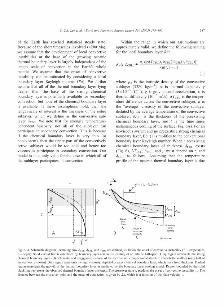
Fig. 6. A. Schematic diagram illustrating how dCBL, dCSL, and dTBL are de

Z—depth). Solid curved line is calculated by boundary layer conductive

chemical boundary layer. (B) Schematic and exaggerated cartoon of the th

the seafloor is shown). Gray region represents the high viscosity, depleted o

region represents the growth of the thermal boundary layer as predicted b

black line represents the observed thermal boundary layer thickness. The c

distance between the crossover point and the onset of convection is given

Within the range in which our assumptions are

approximately valid, we define the following scaling

for the local boundary layer Ra:

Raðt; dCBLÞcqoagDTCSLðt; dCBLÞ½dCSLðt; dCBLÞ�3

jlðt; dCBLÞð1Þ

where qo is the intrinsic density of the convective

sublayer (3380 kg/m3), a is thermal expansivity

(3�10�5 8C�1), g is gravitational acceleration, j is

thermal diffusivity (10�6 m2/s), DTCSL is the temper-

ature difference across the convective sublayer, l is

the baverageQ viscosity of the convective sublayer

dictated by the average temperature of the convective

sublayer, dCBL is the thickness of the preexisting

chemical boundary layer, and t is the time since

instantaneous cooling of the surface (Fig. 6A). For an

isoviscous system and no preexisting strong chemical

boundary layer, Eq. (1) simplifies to the conventional

boundary layer Rayleigh number. When a preexisting

chemical boundary layer of thickness dCBL exists

(Fig. 6), DTCSL, dCSL, and l must depend on tc and

dCBL as follows. Assuming that the temperature

profile of the oceanic thermal boundary layer is due

Cross-overTime

tx

δCBL

δ CSL

δTBL

Onset ofconvectiveinstability

tc

Boundarylayer

cooling

Not to scale

∆X = V (tc – δ CBL2/4κ)

fined just before the onset of convective instability (T—temperature,

cooling of an infinite half-space. Gray region represents the strong

ermal and compositional structure beneath the seafloor (only half of

ceanic chemical boundary layer, which has a fixed thickness. Dashed

y the boundary layer cooling model. Region bounded by the solid

rossover time tx predates the onset of convective instability tc. The

by Dx, which is a function of the plate velocity v.

t c (

Ma)

100 kJ/mol

200 kJ/mol

300 kJ/mol

tx

A

Medianseafloor

flattening time

δCBL (km)

0

20

40

60

80

100

120

140

160

180

200

0 50 100 150

δCBL (km)

B

δTBL(tc)

δCBL

1

1.1

1.2

1.3

1.4

1.5

1.6

1.7

1.8

1.9

2

0 50 100 150

Fig. 7. (A) The critical time tc (Ma) for the onset of convective

instability as a function of chemical boundary layer thickness dCBL

(km) determined by solving Eq. (1) for Rac=1500. Curves denoted

with symbols represent Newtonian temperature-dependent viscos-

ities assuming a A0 of 1018 Pa s and activation energies E of 100,

200 and 300 kJ/mol. The l0 of 1018 Pa s is consistent with the

viscosity of the convecting mantle shown in Figs. 2C and 5C.

Horizontal bar represents the median onset time for seafloor

flattening; arrow shows total range of observed onset times for

seafloor flattening. (B) The ratio of the thermal boundary layer and

chemical boundary layer thickness at the onset of convective

instability as a function of chemical boundary layer thickness.

Symbols as in panel (A).

C.-T.A. Lee et al. / Earth and Planetary Science Letters 230 (2005) 379–395388

solely to boundary layer cooling up until tc, the

temperature difference across the convective sublayer

can then be defined as the difference between the

temperature at the base of the chemical boundary

layer (TCBL) and the temperature of the convecting

interior of the mantle (To):

DTCSLðtc; dCBLÞTo

¼ To � TCBLðtc; dCBLÞTo

¼ erfc

�dCBLffiffiffiffiffiffiffiffiffi4jtc

p�

ð2Þ

Defining the base of the thermal boundary layer dTBLas the depth at which the temperature equals 0.9 To, we

can express the thickness of the convective sublayer as

dCSLðtc; dCBLÞ ¼ dTBLðtcÞ � dCBL ¼ 2:32ffiffiffiffiffiffijtc

p� dCBL

ð3Þ

Assuming Newtonian viscosity, the average viscosity

of the convective sublayer is taken as

lðtc; dCBLÞ ¼ loexp

�E

R

�1

T aveCSLðtc; dCBLÞ

� 1

To

��

ð4Þ

where lo is the viscosity (Pa s) at To, E is the

activation energy (kJ/mol), R is the gas constant, and

TCSLave is the average temperature across the con-

vective sublayer (TCSLave ~To�0.5DTCSL).

Convective instability initiates when Ra approaches

Rac, the critical Rayleigh number, e.g.,

Racðtc; dCBLÞcqoagDTCSLðtc; dCBLÞ½dCSLðtc; dCBLÞ�3

jlðtc; dCBLÞð5Þ

where tc represents the onset time of convective

instability. Substituting Eqs. (2) (3) (4) into Eq. (1), it

can be seen that the onset time of convection tc must

depend on the thickness of the chemical boundary

layer, dCBL. For a given dCBL, Eq. (5) can be solved

for tc by assuming an appropriate value of Rac. Since

we do not know the exact value of Rac , an

approximate value of 1500 was assumed. As

expected, Fig. 7A shows that tc increases as dCBL

increases since the preexisting lid suppresses the onset

of convective instability.

We note that Eq. (5) (or 1) breaks down as dCBL

approaches zero (Fig. 7A). Under these conditions and

for a temperature-dependent viscosity, not all of the

sublayer is available for secondary convection

because the upper part of the sublayer is cold and

hence highly viscous. Because our definition of TCSLave

assumes that all of the sublayer is available for

convective instability, the average temperature of the

true convective part of the sublayer is underestimated

and viscosity overestimated when the thickness of the

chemical boundary layer approaches zero. Thus, when

dCBL approaches zero, we generate an artifact of

unusually high onset times of convective instability as

C.-T.A. Lee et al. / Earth and Planetary Science Letters 230 (2005) 379–395 389

can be seen from the breakdown of the curves in Fig.

7A. The artifact is most pronounced for highly

temperature-dependent viscosities (e.g., high activa-

tion energy), and, as can be seen from Fig. 7A, the

breakdown of our curves depend accordingly on E.

However, for the conditions (thick dCBL) in which our

scalings are approximately valid, it can be seen that

the dependency of tc on activation energy E is small.

The low dependency on E in this endmember scenario

follows from the fact that for thick chemical boundary

layers, the average sublayer temperature is high and

the temperature variation within the sublayer (and

hence viscosity variation) is small. The small depend-

ency with E is similar to the results of recent

numerical simulations [4,5,20].

We recognize that scaling analyses by construct

cannot provide absolute predictions. Nevertheless,

scaling analyses can provide qualitative and relative

predictions. The significance of our model is that it

makes simple predictions on the relative magnitudes

of potentially observable parameters, such as the

thickness of the chemical boundary layer (dCBL),

thickness of the thermal boundary layer (dTBL), andonset time of convective instability (tc). First, the base

of the thermally defined boundary layer should cross

the base of the chemical boundary layer at a time

equivalent to the time it takes for the conductive

geotherm to cool just past the base of the chemical

boundary layer (e.g., tx in Fig. 6B); the distance of the

cross-over point from the mid-ocean ridge should be

correlated with plate velocity. Second, the onset time

of convective instability, tc, should depend on dCBL asshown in Fig. 7A. Third, the ratio of the thicknesses

of the thermal boundary layer to the chemical

boundary layer dTBL(tc)/dCBL at the onset time of

convective instability should correlate with dCBL

(Fig. 7B). Finally, the thickness of the oceanic

chemical boundary layer, dCBL, should increase as a

function of potential temperature TP at the time the

chemical boundary layer formed (see Fig. 4), which

can be estimated from major-element geochemistry

and/or olivine thermometry of primary mid-ocean

ridge basalts (cf. [50]). This means that all of the

above quantities (dCBL, dTBL, and tc) should also

correlate with TP. Assuming that the rheologic proper-

ties of the actively convecting part of the upper mantle

are globally similar (since the dependency on activa-

tion energy is small, this is not a bad assumption), our

model further predicts that a plot of dTBL(tc)/dCBL

versus onset time of convective instability throughout

the seafloor should yield a negative correlation as

shown in Fig. 7B. What our model cannot predict is

the absolute seafloor bathymetry because our model

does not explicitly account for changes in the thermal

state of the underlying asthenosphere as a conse-

quence of secondary convection [51].

Recently, Korenaga and Jordan [52] argued that the

presence of a rheologically strong dehydrated boun-

dary layer should not have any effect on the onset

time of convective instabilities because it is much

thinner (50–60 km) than the thickness of the rigid

(highly viscous) layer at the onset time of convective

instability predicted by their numerical models (~80–

120 km for E=300 kJ/mol). We note, however, that

the thickness of their assumed chemical boundary

layer (50–60 km) was calculated for a single mantle

potential temperature of 1350 8C. A higher mantle

potential temperature, e.g., 1400–1450 8C, would

predict chemical boundary layer thicknesses up to

~100 km. Indeed, the temperatures of the mantle

source regions to mid-ocean ridge basalts have been

argued previously to vary by ~250 8C [50]. In Section

5, we show that potential temperatures beneath mid-

ocean ridges can be as high as ~1450 8C.

5. Testing the predictions

5.1. Continents

The predictions we make for continents and oceans

can be tested only if dCBL and dTBL can be measured.

For continents, we have shown above that these

quantities can be estimated from thermobarometric

studies of mantle xenoliths (Fig. 2) and that model

predictions of Cooper et al., assuming the chemical

boundary layer is intrinsically strong [21], are con-

sistent with the observations from xenoliths. Another

approach is to use seismology. A recent study on the

compositional dependencies of peridotite seismic

velocities at standard temperature and pressure con-

ditions (STP) suggests that the ratio of compressional

to shear wave velocity (VP/VS) is sensitive to Mg# but

not so sensitive to temperature, provided anelastic

effects are small and there is no partial melt [25]. This

is because of the opposite signs of dln(VP/VS)/dT for

C.-T.A. Lee et al. / Earth and Planetary Science Letters 230 (2005) 379–395390

orthopyroxene and olivine, the dominant minerals in

melt-depleted peridotites. If these STP composition–

velocity relationships hold at elevated pressure and

temperature, one can use VP/VS variations to infer

compositional structure. In contrast, because VP and

VS alone are more sensitive to temperature than

composition, it may be possible to use VP, VS, and

or surface wave seismology to infer the thermal

structure. In a recent study of VP/VS ratios using S-

P travel time residuals in the South African craton, we

have shown that the regional differences in VP/VS

may in fact be correlated with differences in mantle

fertility [45].

5.2. Oceans

For oceanic mantle, the degree of depletion is less

than that seen in cratonic mantle, and the compositional

and mineralogic transition at the base of the chemical

boundary layer is much more gradational than beneath

cratons. For these reasons, it will be difficult to

seismically separate the base of the chemical and

thermal boundary layers beneath the oceans.

Another way to estimate dCBL beneath oceans is

from the intersection depth of the mantle adiabat with

the dry peridotite solidus. The depth of intersection

can be calculated from the mantle’s paleo-potential

temperature (e.g., the temperature at the surface of the

Earth if the laterally averaged upper mantle were

isentropically decompressed) and solid adiabat. Con-

straints on the potential temperature can be estimated

from the compositions of primary magmas [50,53,54].

One caveat is that the liquidus temperatures of mid-

ocean ridge basalts are undoubtedly minimum esti-

mates of mantle potential temperature because they

have cooled along nonadiabatic paths, as evidenced

by the fact they have already undergone significant

crystallization of olivine (and in some cases, clino-

pyroxene and plagioclase) by the time they are

sampled. The temperature of magma segregation from

the mantle can only be had by estimating primary

magma compositions after correcting for differentia-

tion effects. This is done by incrementally adding

equilibrium olivines back into a magma (e.g., revers-

ing fractional crystallization) with the constraint that

KD=(Fe/Mg)ol/(Fe/Mg)melt=0.31. The assumption is

that olivine is the only crystallizing phase. For mid-

ocean ridge basalts having MgO contents greater than

8 wt.% MgO, this is generally a reasonable assump-

tion because crystallization takes place at low pressure

where the olivine liquidus surface is greatly expanded.

When the Mg# of the magma reaches equilibrium

with an olivine having typical upper mantle compo-

sitions (in this case, Mg# of 0.89–0.90 was assumed),

it is assumed that the primary magma composition has

been attained. The MgO and SiO2 content of this

primary magma is then used to respectively calculate

the average temperature [55] and pressure [56] of the

magma when it was last equilibrated with the mantle.

For temperature, this means that both FeO and MgO

are important parameters. For those mid-ocean ridge

basalts having high FeO for a given MgO content

(hence low Mg#s), larger amounts of olivine must be

added to reach equilibrium with typical upper mantle

olivines (Mg#=0.89–0.90), giving rise to primary

magma compositions having higher MgO contents

and accordingly, higher magmatic temperatures due to

the proportionality of magmatic temperature with

MgO [55].

The potential temperature is then calculated in two

steps. First, the P-T path of the primary magma is

back-tracked to the solidus along an isentropic

decompressional melting path (under reversible con-

ditions, this is equivalent to an adiabatic melting

path). The approach requires simultaneous numerical

integration of (dX/dP)S and (dT/dP)S, which represent

the differentials of melt fraction X and T as a function

of P at constant entropy (S) using the formulas

presented in McKenzie [57] and the updated solidus

and liquidus P-T relations in Hirschmann [47] and

Katz et al. [58]. The intersection of the melting

adiabat with the dry peridotite solidus is then used as

an anchor point for the solid mantle adiabat, and the

potential temperature of the solid mantle is then

calculated by integrating (dT/dP)S following McKen-

zie and Bickle [54].

As a preliminary test of our oceanic hypothesis, we

have examined the compositions of old oceanic crust

(N50 Ma) in the western Pacific Ocean (Pacific plate

only) and the western half of the northern Atlantic

(North American plate only; north of equator; Fig. 8A).

According to Marty and Cazenave [10], seafloor depth

begins to deviate from the half-space cooling model

between 70 and 100 Ma in the western Pacific and

between 100 and 150 Ma in the northern Atlantic. In

Fig. 8B–D, we have plotted FeO and MgO contents

MgO (wt. %)

6

7

8

9

10

11

12

13

14

6 6.5 7 7.5 8 8.5 9 9.5 10

.

Active Ridges

FeO

T(w

t. %

)

B

Western Pacific

MgO (wt. %)

FeO

T(w

t. %

)

C

6 6.5 7 7.5 8 8.5 9 9.5 106

7

8

9

10

11

12

13

14

6

7

8

9

10

11

12

13

14

6 6.5 7 7.5 8 8.5 9 9.5 10

Northern Atlantic (west)

MgO (wt. %)

FeO

T(w

t. %

)D

60 ºN

A

30 ºN

30 ºS

60 ºS

0 º 30ºE 60ºE 90ºE 120ºE 150ºE 180º 150ºW 120ºW 90ºW 60ºW 30ºW 0º

0 º

Fig. 8. (A) Sample localities. (B) FeO and MgO contents of whole-rock (open symbols) and glass (solid symbols) mid-ocean ridge basalt

samples from active ridges (Juan de Fuca, East Pacific Rise, mid-Atlantic, Indian; [59]). Vertical bars (with arrowed ends) show estimated range

of FeO at MgON8.5 wt.%. (C) and (D) FeO and MgO contents of old oceanic crust (N50 Ma) in the western Pacific and western half of the

northern Atlantic (e.g., north of the equator) using data from [59]. Symbols as in panel (B).

C.-T.A. Lee et al. / Earth and Planetary Science Letters 230 (2005) 379–395 391

from active ridges and old oceanic crust (N50Ma) in the

two regions of interest using the data from RidgePetDB

[59]. Both fresh glass and whole-rock data are

represented. Fresh glass is considered superior to

whole-rock data because the latter have been chemi-

cally modified by seawater alteration. The effects of

seawater alteration are most pronounced for old

oceanic crust.

For MgON8 wt.%, the FeO contents of basaltic

glasses from active ridges (mid-Atlantic, East Pacific

Rise, Juan de Fuca, and Southeast Indian) range

between 7.5 and 10 wt.% (Fig. 8B). There are no new

data for glasses having MgON8 wt.% in the western

Pacific (Fig. 8C). However, if we take the few western

Pacific whole-rock data points at face value, it appears

that their FeO contents overlap the range of active

ridges. In contrast, for old oceanic crust in the

northern Atlantic, the glasses have FeO contents

ranging between 9 and 10 wt.% (Fig. 8D), which

falls in the upper end of the compositional range seen

in active ridges (and old Pacific crust). The average

segregation pressures and temperatures of the primary

magma compositions inferred from the basaltic data

are shown in Fig. 9A along with their corresponding

mantle potential temperatures (Fig. 9A and B). It can

be seen that active ridges and old Pacific crust yield

potential temperatures between 1330 and 1450 8C,whereas old oceanic crust in the northern Atlantic

crust yields paleo-potential temperatures of 1410–

1450 8C.

δCBL (km)

0.0

0.5

1.0

1.5

2.0

2.5

3.0

3.5

4.01250 1300 1350 1400 1450 1500 1550 1600

Dry solidus

Cpx-outB C

A. Active ridgeB. w. PacificC. n. Atlantic (W)

P (

GP

a)

T (oC)

A

0

20

40

60

80

100

120

Z (depth)

Active ridges & w. Pacific

A

1300 1350 1400 1450 1500

t C (

Ma)

Paleo-Potential Temperature (oC)

n. Atlantic

60 70 80 90 100 110 120 130

40

60

80

100

120

140

160

180

theory

w. Pacific

B

Fig. 9. (A) Pressure (GPa) versus temperature (8C) diagram showing

the estimated mantle segregation temperatures and pressures (.) ofthe primary parental magmas to the basaltic compositions shown in

Fig. 8B–D. Lines connecting each solid circle to the dry peridotite

solidus [58] represent anhydrous melting adiabats; lines connecting

the intersection of the melting adiabat with the dry solidus to the

surface represent solid mantle adiabats; the temperature at the

surface of the Earth is the potential temperature. Horizontal shaded

bar represents the range of potential temperatures seen in modern

mid-ocean ridge basalts. Line labeled Cpx-out represents the point

at which clinopyroxene is completely exhausted from the residue

[58]. (B) Plot of the range of paleo-potential temperatures (8C)estimated for old oceanic crust in the western Pacific and western

half of the northern Atlantic (shaded boxes) versus the range of

onset times tc for seafloor flattening in the respective regions [10].

Large open box encompassing the shaded boxes for the western

Pacific and western half of the northern Atlantic represents the

global range of tc and modern mantle potential temperature. Top

horizontal axis represents the equivalent thickness of the dehydrated

chemical boundary layer. Curves represent relative dependency of

onset time for convective instability versus thickness of the

preexisting chemical boundary layer from Fig. 7.

C.-T.A. Lee et al. / Earth and Planetary Science Letters 230 (2005) 379–395392

In Fig. 9B, we plot the potential temperatures (with

estimated uncertainties) of active ridges, old oceanic

crust in the western Pacific and western part of the

northern Atlantic versus the total range in onset times

of observed seafloor flattening in the respective

regions. On the top axis of Fig. 9B, the corresponding

chemical boundary layer thickness is plotted. The

large range in potential temperature for old Pacific

crust is due to the large scatter in the data. However, it

can be seen that the northern Atlantic falls in the upper

right hand corner of the total range of seafloor

flattening times and modern potential temperature. If

the onset time of seafloor flattening represents the

onset time of convective instability, then the high

mantle potential temperatures and long onset times for

seafloor flattening are consistent with the predictions

of our scaling arguments. This can be seen from Fig.

9B, where we have superimposed our theoretical

prediction. We reemphasize that the absolute position

of this curve is meaningless, but the relative sense of

the curve is meaningful.

We readily admit that these preliminary observa-

tions are not extremely convincing. Clearly, more

fresh glass data from old oceanic crust are needed. We

also recognize that another uncertainty in our inter-

pretation of old oceanic crust data rests on the

assumption that the mantle source composition to

mid-ocean ridge basalts is constant. If it is not, then an

alternative explanation is that the FeO contents of the

mantle sources to old Pacific and Atlantic oceanic

crust are different, rendering our estimates of paleo-

potential temperature meaningless. This means that, in

addition to more major-element data on fresh glasses,

complementary trace-element and isotopic data are

needed to track variations in source heterogeneity. If

these data can become available in the near future,

geochemical constraints on chemical boundary layer

thicknesses can be combined with seismic constraints

on the thickness of oceanic thermal boundary layers

(e.g., surface wave seismology [60]). This would

allow for an estimate of the ratio dTBL(tc)/dCBL for a

given region of oceanic lithosphere, providing yet

another approach for testing our model.

6. Conclusions and implications

Our analyses suggest that chemical boundary

layers play a significant role in dictating the thickness

of thermal boundary layers beneath oceans and

continents. For continents, the thermal boundary layer

C.-T.A. Lee et al. / Earth and Planetary Science Letters 230 (2005) 379–395 393

thickness at statistical steady state is limited by the

thickness of a preexisting chemical boundary layer,

which represents a highly melt-depleted, dehydrated

mantle layer. For oceans, a new model is presented

that relates the transition between a vertically con-

ductive heat transfer regime and a convection-domi-

nated regime to the thickness of a preexisting

chemical boundary layer. The chemical boundary

layer beneath oceans originates by melt extraction at

mid-ocean ridges, which yields a melt-depleted (but

not as depleted as most cratonic mantle) and

dehydrated mantle layer that is consequently strong

from the outset like that beneath continents. The

thickness of the oceanic chemical boundary layer is a

function of potential temperature and therefore, the

proposed model makes specific predictions on the

relationships between the onset of seafloor flattening

and various geochemical indices that indirectly track

potential temperature (e.g., FeO and MgO).

If our models are correct, the thermal and structural

evolution of continents and oceans must be controlled

in part by the presence of preexisting chemical

boundary layers. This implies further that chemical

boundary layers may indirectly dictate the strength of

continental and oceanic thermal boundary layers

because the integrated strength of any thermal

boundary layer depends on its intrinsic viscosity

(hypothesized here to be primarily controlled by

water content) and average temperature, which itself

depends on its thickness (as well as the distribution of

radiogenic heat production). Thick, dehydrated and

melt-depleted chemical boundary layers would be

expected to give rise to strong lithosphere, while thin,

wetter, and more fertile chemical boundary layers

would be expected to give rise to weaker lithosphere

[68]. It thus follows that there may be a relationship

between the degree of intraplate deformation (e.g.,

diffuse plate deformation) and the thickness and

composition of preexisting chemical boundary layers.

One important point that we did not discuss was

how chemical boundary layers actually form beneath

continents. While the formation of a dehydrated layer

beneath mid-ocean ridges can be explained by a

relatively simple model, how cratonic mantle formed

is still open to debate. On one hand, the thicker and

more depleted nature of the chemical boundary layer

beneath cratons might imply formation by melting of

upwelling mantle characterized by significantly higher

temperatures than the present (e.g., [13,61,62]). This

process allows for the generation of a thick and

dehydrated chemical boundary layer in one relatively

short geologic event. However, it has been suggested

that cratonic peridotites may have actually melted at

pressures significantly less (b3 GPa) than their present

equilibration pressures (N3 GPa) as they do not show

the tell-tale trace-element signatures of garnet [63,

64]. In addition, it is not clear if mantle potential

temperature was significantly hotter in the late

Archean [65], and finally, the presence of dipping

seismic reflectors within cratonic mantle are highly

suggestive of trapped oceanic lithosphere [66]. These

observations can be reconciled if cratonic mantle is

formed by amalgamation or thickening of oceanic

lithosphere (as well as arc lithosphere). However, if

these lithospheric segments are initially dry, a paradox

arises because they should be strong and not easily

deformed. If they are wet or rehydrated to make them

weak enough to deform and make cratons, another

paradox arises because a chemically buoyant boun-

dary layer, without being intrinsically stronger, would

eventually thin out gravitationally (e.g., in the spirit of

[67]).

Acknowledgments

This work was supported by the Department of

Earth Science at Rice University and NSF grants to

Lee (EAR-0309121) and Lenardic (EAR-0001029). J.

Dixon and J. Korenaga are thanked for their reviews.

Informal discussions with J. Korenaga, S. Zhong, and

W. Leeman are greatly appreciated.

References

[1] J.G. Sclater, B. Parsons, Oceans and continents: similarities

and differences in the mechanisms of heat loss, J. Geophys.

Res. 86 (1981) 11535–11552.

[2] B. Parsons, D.P. McKenzie, Mantle convection and the

thermal structure of the plates, J. Geophys. Res. 83 (1978)

4485–4495.

[3] W.H.F. Smith, D.T. Sandwell, Global sea floor topography

from satellite altimetry and ship depth soundings, Science 277

(1997) 1956–1962.

[4] J. Korenaga, T.H. Jordan. Onset of convection with temper-

ature- and depth-dependent viscosity, Geophys. Res. Lett. 29,

(2002).

C.-T.A. Lee et al. / Earth and Planetary Science Letters 230 (2005) 379–395394

[5] J. Huang, S.J. Zhong, J. van Hunen, Controls on sub-litho-

spheric small-scale convection, Journ. Geophys. Res. (2003).

[6] C.A. Stein, S. Stein, A model for the global variation in

oceanic depth and heat flow with lithospheric age, Nature 359

(1992) 123–129.

[7] C.A. Stein, S. Stein, Comparison of plate and asthenospheric

flow models for the thermal evolution of oceanic lithosphere,

Geophys. Res. Lett. 21 (1994) 709–712.

[8] J. Phipps Morgan, W.H.F. Smith, Flattening of the seafloor

depth-age curve as a response to asthenospheric flow, Nature

359 (1992) 524–527.

[9] G.F. Davies, Dynamic Earth, Plates, Plumes and Mantle

Convection, Cambridge University Press, Cambridge, UK,

1999, 458 pp.

[10] J.C. Marty, A. Cazenave, Regional variations in subsidence

rate of oceanic plates: a global analysis, Earth Planet. Sci. Lett.

94 (1989) 301–315.

[11] R.T. Heest, S.T. Crough, The effect of hot spots on the oceanic

age-depth relation, J. Geophys. Res. 86 (1981) 6107–6114.

[12] T.H. Jordan, Composition and development of the continental

tectosphere, Nature 274 (1978) 544–548.

[13] H.N. Pollack, Cratonization and thermal evolution of the

mantle, Earth Planet. Sci. Lett. 80 (1986) 175–182.

[14] G. Hirth, D.L. Kohlstedt, Water in the oceanic upper mantle;

implications for rheology, melt extraction and the evolution

of the lithosphere, Earth Planet. Sci. Lett. 144 (1–2) (1996)

93–108.

[15] R.J. Walker, R.W. Carlson, S.B. Shirey, F.R. Boyd, Os, Sr, Nd,

and Pb isotope systematics of southern African peridotite

xenoliths: implications for the chemical evolution of subcon-

tinental mantle, Geochim. Cosmochim. 53 (1989) 1583–1595.

[16] D.G. Pearson, R.W. Carlson, S.B. Shirey, F.R. Boyd, P.H.

Nixon, Stabilisation of Archaean lithospheric mantle: a Re–Os

isotope study of peridotite xenoliths from the Kaapvaal craton,

Earth Planet. Sci. Lett. 134 (1995) 341–357.

[17] S.E. Zaranek, E.M. Parmentier, Convective cooling of an

initially stably stratified fluid with temperature-dependent

viscosity: implications for the role of solid-state convection

in planetary evolution, J. Geophys. Res. 109 (2004).

[18] N.H. Sleep, Survival of Archean cratonal lithosphere, J.

Geophys. Res. 108 (2003).

[19] A. Davaille, C. Jaupart, Onset of thermal convection in fluids

with temperature-dependent viscosity: application to the

oceanic mantle, J. Geophys. Res. 99 (1994) 19853–19866.

[20] J. Korenaga, T.H. Jordan, Physics of multiscale convection in

Earth’s mantle: onset of sublithospheric convection, J. Geo-

phys. Res. 108 (B7) (2003) 2333.

[21] C.M. Cooper, A. Lenardic, L. Moresi, The thermal structure of

stable continental lithosphere within a dynamic mantle, Earth

Planet. Sci. Lett. 222 (2004) 807–817.

[22] F.R. Boyd, Compositional distinction between oceanic and

cratonic lithosphere, Earth Planet. Sci. Lett. 96 (1989) 15–26.

[23] W.L. Griffin, S.Y. O’Reilly, C.G. Ryan, The composition

and origin of sub-continental lithospheric mantle, Mantle

Petrology: Field Observations and High Pressure Exper-

imentation: A Tribute to R. (Joe) Boyd 6, Geochemical

Society, 1999, pp. 13–45.

[24] F.R. Boyd, R.H. McAllister, Densities of fertile and sterile

garnet peridotites, Geophys. Res. Lett. 3 (1976) 509–512.

[25] C.-T.A. Lee, Compositional variation of density and seismic

velocities in natural peridotites at STP conditions: implications

for seismic imaging of compositional heterogeneities in the

upper mantle, J. Geophys. Res. 108 (2003) 2441.

[26] T.H. Jordan, Structure and formation of the continental

tectosphere, J. Petrol. 1988 (1988) 11–37.

[27] S.Y. O’Reilly, W.L. Griffin, Y.H. Djomani, P. Morgan, Are

lithospheres forever? Tracking changes in subcontinental

lithospheric mantle through time, GSA Today 11 (4) (2001)

4–10.

[28] F.R. Boyd, N.P. Pokhilenko, D.G. Pearson, S.A. Mertzman,

N.V. Sobolev, L.W. Finger, Composition of the Siberian

cratonic mantle: evidence from Udachnaya peridotite xeno-

liths, Contrib. Mineral. Petrol. 128 (1997) 228–246.

[29] M.G. Kopylova, J.K. Russell, H. Cookenboo, Petrology of

peridotite and pyroxenite xenoliths from Jericho Kimberlite;

implications for the thermal state of the mantle beneath the

Slave Craton, northern Canada, J. Petrol. 40 (1) (1999)

79–104.

[30] D.R. Bell, Water in mantle minerals, Nature 357 (1992)

646–647.

[31] D.R. Bell, G.R. Rossman, Water in Earth’s mantle: the role

of nominally anhydrous minerals, Science 255 (1992)

1391–1397.

[32] J.E. Dixon, L. Leist, C. Langmuir, J.-G. Schilling, Recycled

dehydrated lithosphere observed in plume-influenced mid-

ocean-ridge basalt, Nature 420 (2002) 385–389.

[33] J.E. Dixon, T.H. Dixon, D.R. Bell, R. Malservisi, Lateral

variation in upper mantle viscosity: role of water, Earth Planet.

Sci. Lett. 222 (2004) 451–467.

[34] S.P. Grand, R. van der Hilst, S. Widiyantoro, Global seismic

tomography; a snapshot of convection in the Earth, GSA

Today 7 (1997) 1–7.

[35] D.E. James, M.J. Fouch, J.C. VanDecar, S. van der Lee,

Tectospheric structure beneath Southern Africa, Geophys. Res.

Lett. 28 (2001) 2485–2488.

[36] S.B. Shirey, J.W. Harris, S.R. Richardson, M.J. Fouch, D.E.

James, P. Cartigny, P. Deines, F. Viljoen, Diamond genesis,

seismic structure, and evolution of the Kaapvaal–Zimbabwe

craton, Science 297 (2002) 1683–1686.

[37] J. Polet, D.L. Anderson, Depth extent of cratons as inferred

from tomographic studies, Geology 23 (1995) 205–208.

[38] C.J. Wolfe, I.T. Bjarnason, J.C. Van Decar, S.C. Solomon,

Assessing the depth resolution of tomographic models of

upper mantle structure beneath Iceland, Geophys. Res. Lett. 29

(2002).

[39] W.R. Keller, D.L. Anderson, R.W. Clayton, Resolution of

tomographic models of the mantle beneath Iceland, Geophys.

Res. Lett. 27 (2000) 3993–3996.

[40] R.L. Rudnick, W.F. McDonough, R.J. O’Connell, Thermal

structure, thickness and composition of continental litho-

sphere, Chem. Geol. 145 (1998) 395–411.

[41] C.-T. Lee, R.L. Rudnick, Compositionally stratified cratonic

lithosphere: petrology and geochemistry of peridotite xenoliths

from the Labait tuff cone, Tanzania, in: B.J. Dawson volume,

C.-T.A. Lee et al. / Earth and Planetary Science Letters 230 (2005) 379–395 395

J.J. Gurney, J.L. Gurney, M.D. Pascoe, S.R. Richardson

(Eds.), Proc. VIIth International Kimberlite Conference,

1999, pp. 503–521.

[42] F.R. Boyd, High- and low-temperature garnet peridotite

xenoliths and their possible relation to the lithosphere-

asthenosphere boundary beneath southern Africa, in: P.H.

Nixon (Ed.), Mantle Xenoliths, John Wiley and Sons, 1987,

pp. 403–412.

[43] M.J. Walter, Melting residues of fertile peridotite and the

origin of cratonic lithosphere, in: Y. Fei, C.M. Bertka, B.O.

Mysen (Eds.), Mantle Petrology: Field Observations and

High Pressure Experimentation: A Tribute to Francis R.

(Joe) Boyd, Geochemical Society Special Publication, vol.

6, 1999, pp. 225–239.

[44] Y. Gung, M. Panning, B. Romanowicz, Global anisotropy and

the thickness of continents, Nature 422 (2003) 707–711.

[45] F. Niu, A. Levander, C.M. Cooper, C.-T.A. Lee, A. Lenardic,

D.E. James, Seismic constraints on the depth and composition

of the mantle keel beneath the Kaapvaal craton, Earth Planet.

Sci. Lett. 224 (2004) 337–346.

[46] A. Lenardic, L.N. Moresi, Some thoughts on the stability of

cratonic lithosphere; effects of buoyancy and viscosity, J.

Geophys. Res. B, Solid Earth Planets 104 (6) (1999)

12,747–12,759.

[47] M.M. Hirschmann, Mantle solidus: experimental constraints

and the effects of peridotite composition, Geochem. Geophys.

Geosys. 1 (2000) (2000GC000070).

[48] P.D. Asimow, C.H. Langmuir, The importance of water

to oceanic mantle melting regimes, Nature 421 (2003)

815–820.

[49] M.S. Ghiorso, M.M. Hirschmann, P.W. Reiners, V.C. Kress,

The pMELTS: a revision of MELTS for improved calculation

of phase relations and major element partitioning related to

partial melting of the mantle to 3 GPa, Geochem. Geophys.

Geosys. 3 (2002).

[50] E.M. Klein, C.H. Langmuir, Global correlations of ocean ridge

basalt chemistry with axial depth and crustal thickness, J.

Geophys. Res. 92 (B8) (1987) 8089–8115.

[51] R.J. O’Connell, B.H. Hager, On the thermal state of the earth,

in: A. Dziewonski, E. Boschi (Eds.), Physics of the Earth’s

interior, 1980, pp. 270–317.

[52] J. Korenaga, T.H. Jordan, On dsteady-stateT heat flow and the

rheology of oceanic mantle, Geophys. Res. Lett., 29 (2002).

[53] E. Humler, C. Langmuir, V. Daux, Depth versus age: new

perspectives from the chemical compositions of ancient crust,

Earth Planet. Sci. Lett. 173 (1999) 7–23.

[54] D. McKenzie, M.J. Bickle, The volume and composition of

melt generated by extension of the lithosphere, J. Petrol. 29

(1988) 625–679.

[55] T. Sugawara, Empirical relationships between temperature,

pressure, and MgO content in olivine and pyroxene saturated

liquid, J. Geophys. Res. 105 (2000) 8457–8472.

[56] F. Albarede, How deep do common basaltic magmas form and

differentiate? J. Geophys. Res. 97 (1992) 10997–11009.

[57] D. McKenzie, The generation and compaction of partially

molten rock, J. Petrol. 25 (3) (1984) 713–765.

[58] R.F. Katz, M. Spiegelman, C.H. Langmuir, A new paramete-

rization of hydrous mantle melting, Geochem. Geophys.

Geosys., 4 (2003).

[59] K. Lehnert, Y. Su, C.H. Langmuir, B. Sarbas, U. Nohl, A

global geochemical database structure for rocks, Geochem.

Geophys. Geosys. 1 (2000) (1999GC000026).

[60] M.H. Ritzwoller, N.M. Shapiro, S.-J. Zhong, Cooling history

of the Pacific lithosphere, Earth Planet. Sci. Lett. 226 (2004)

69–84.

[61] M.J. Walter, Melting of garnet peridotite and the origin of

komatiite and depleted lithosphere, J. Petrol. 39 (1998) 29–60.

[62] C. Herzberg, Phase equilibrium constraints on the formation of

cratonic mantle, in: Y. Fei, C.M. Bertka, B.O. Mysen (Eds.),

Mantle Petrology, Field Observations and High Pressure

Experimentation, A Tribute to Francis R. (Joe) Boyd, Geo-

chem. Soc. Spec. Pub., vol. 6, 1999, pp. 241–257.

[63] D. Canil, Mildly incompatible elements in peridotites and the

origins of mantle lithosphere, Lithos 77 (2004) 375–393.

[64] S. Bernstein, P.B. Kelemen, C.K. Brooks, Depleted spinel

harzburgite xenoliths in Tertiary dykes from East Greenland:

restites from high degree melting, Earth Planet. Sci. Lett. 154

(1998) 221–235.

[65] T.L. Grove, S.W. Parman, Thermal evolution of the Earth as

recorded by komatiites, Earth Planet. Sci. Lett. 219 (2004)

173–187.

[66] M. Bostock, Mantle stratigraphy and evolution of the Slave

province, J. Geophys. Res. 103 (1998) 21183–21200.

[67] P. Bird, Lateral extrusion of lower crust from under high

topography, in the isostatic limit, J. Geophys. Res. 96 (1991)

10275–10286.

[68] C.-T. Lee, Q. Yin, R.L. Rudnick, S.B. Jacobsen, Preservation

of ancient and fertile lithospheric mantle beneath the south-

western United States, Nature 411 (2001) 69–73.