Where Can Seismic Anisotropy Be Detected in the Earth's Mantle? In Boundary Layers

Pure appl. geophys. 151 (1998) 223–2560033–4553/98/040223–34 $ 1.50+0.20/0

Where Can Seismic Anisotropy Be Detected in the Earth’s Mantle?In Boundary Layers . . .

JEAN-PAUL MONTAGNER1

Abstract—During the last 30 years, considerable evidence of seismic anisotropy has accumulateddemonstrating that it is present at all scales, but not in all depth ranges. We detail which conditions arenecessary to detect large-scale seismic anisotropy. Firstly, minerals must display a strong anisotropy atthe microscopic scale, and/or the medium must be finely layered. Secondly, the relative orientations ofsymmetry axes in the different crystals must not counteract in destroying the intrinsic anisotropy of eachmineral, and there must be efficient mechanisms of orientation of minerals and aggregates. Finally, thestrain field must be coherent at large scale in order to preserve long wavelength anisotropy. Part ofshallow anisotropy can be related to the past strain field (frozen-in anisotropy), however the deepanisotropy is due to the present strain field. All these conditions are fulfilled only in boundary layers ofconvective mantle.

We review in this paper, the seismic data sets which provide insight into the location at depth oflarge-scale anisotropy from the D�-layer up to the lithosphere. In addition to the well-documentedseismic anisotropy in the lithosphere and asthenosphere, there is new evidence of seismic anisotropy inthe upper (400–660 km) and lower (660–900 km) transition zones and in the D�-layer. Nonetheless thebulk of the lower mantle seems close to isotropy. If we assume the hypothesis that seismic anisotropyis associated with boundary layers in convective systems, these observations strongly suggest that thetransition zone is a boundary layer which makes the pasage of matter between the upper and the lowermantle difficult. However, this general statement does not rule out flow circulation between the upperand lower mantles. Finally, the geophysical, mineral physics and geological applications are brieflyreviewed. An intercomparison between surface wave anisotropy and body-wave anisotropy data sets ispresented. We discuss the scientific potential of seismic anisotropy and how it makes it possible to gainmore insight into continental root, deformation and geodynamics processes.

Key words: Seismic anisotropy, mantle convection, boundary layers.

1. Introduction

For theoretical and practical reasons, the earth was long considered as com-posed of isotropic and laterally homogeneous layers. When an isotropic elasticmedium can be described by two independent elastic parameters (� and � Lameparameters), the simplest anisotropic medium (transverse isotropy with verticalsymmetry axis) necessitates five independent parameters (LOVE, 1927; ANDERSON,

1 Seismological Laboratory, CNRS URA 195, Institut Universitaire de France, Institut de Physiquedu Globe, Paris, France.

Jean-Paul Montagner224 Pure appl. geophys.,

1961). To date, seismic observations have been explained in terms of isotropiclateral heterogeneities instead of manifestations of anisotropy. However, since, the1960s, it was recognized that most parts of the earth are not only laterallyheterogeneous but also anisotropic. Though the lateral heterogeneities of seismicvelocities were long used for geodynamical applications, the importance of an-isotropy for understanding geodynamic processes is only recently recognized. Theearly evidence of seismic anisotropy was the discrepancy between Rayleigh andLove wave dispersions (ANDERSON, 1961; AKI and KAMINUMA, 1963) and theazimuthal dependence of Pn velocities (HESS, 1964). These first observations werefollowed by many in the 1970s and 1980s (see CRAMPIN, 1984; MONTAGNER andNATAF, 1986; BABUS� KA and CARA, 1991 for references).

Different geophysical fields are involved in the investigation of the manifesta-tions of anisotropy of earth materials, mineral physics and geology for the study ofthe microscopic scale, and seismologists for scales larger than typically one kilome-ter. It is evident that it is present in most depth ranges of the earth. But the originof seismic anisotropy is nonunique. In the crust, the crack distribution seems toplay a major role (CRAMPIN and BOOTH, 1985). In the lithosphere, it is usuallyexplained by the preferred orientation of olivine (NICOLAS and CHRISTENSEN,1987) and is related to plate tectonics processes. The intrinsic anisotropy ofminerals (olivine and to a less extent orthopyroxene and clinopyroxene) associatedwith lattice-preferred orientation induces large-scale observable and unambiguouseffects, either on body waves (S-wave splitting observed on SKS (VINNIK et al.,1984); P-wave anisotropy (BABUSKA et al., 1984) or surface waves through theazimuthal anisotropy (FORSYTH, 1975) and the ‘polarization’ anisotropy (SCHLUE

and KNOPOFF, 1977). Both kinds of observable anisotropy can be simultaneouslyexplained by the theoretical developments of MONTAGNER and NATAF (1986).Most of the lower mantle seems to be isotropic (MEADE et al., 1995) except theD�-layer (VINNIK et al., 1989; MAUPIN, 1994). It recurs in the inner core, whereanisotropy was discovered about 10 years ago from free oscillations (WOODHOUSE

et al., 1986) and from the P-wave travel times reported in the ISC bulletins(MORELLI et al., 1986). However the origin and mechanisms creating the an-isotropy in the core are still the subject of controversy.

Since these early observations of seismic anisotropy, numerous studies haveconfirmed the existence of anisotropy in different depth ranges of the earth and willnot be reviewed in this paper. From the global geodynamics point of view, seismicanisotropy has many applications. We will show that it makes it possible to definethe root of continents and to investigate the coupling between the lithosphere andthe rest of the mantle (MONTAGNER and TANIMOTO, 1991; SILVER, 1996), andmore generally to gain insight into mantle convection. Due to the high Rayleighnumber, mantle convection is highly chaotic and numerical modeling demonstratesthat most of the deformation takes place in boundary layers. Since seismicanisotropy is closely related to large-scale deformation (NICOLAS and CHRIS-

Where Can Seismic Anisotropy Be Detected 225Vol. 151, 1998

TENSEN, 1987; KARATO, 1989), we suggest that, conversely, boundary layers canbe detected by the existence of seismic anisotropy. We will present in this paper,the different depth ranges in the mantle, where seismic anisotropy was detected,i.e., D�-layer, transition zone and uppermost mantle. In this top boundary layer,seismic anisotropy can be directly compared to geological results, and it providesfundamental information on processes involved in mountain building and colli-sion between continents such as in Central Asia. The robust features of thesedifferent investigations in different depth ranges are presented in this paper andthe enormous scientific potential of seismic anisotropy is underlined.

2. E�idence of Anisotropy in the Different Layers of the Mantle

2.1 Conditions for Obser�ing Seismic Anisotropy

The observations of seismic anisotropy usually involve a very large spatialrange from the microscopic wavelength extending to the thousands of kilometers.Different geophysical fields are involved in the investigation of the manifestationsof anisotropy of earth materials, mineral physics and geology for the study ofthe microscopic scale, and seismology for scales larger than typically one kilome-ter. At least four conditions are necessary to detect large-scale mantle seismicanisotropy and they are quite severe.

Intrinsic anisotropy of minerals. The different minerals present in the uppermantle are anisotropic (PESELNICK et al., 1974). The main constituent, olivine, isstrongly anisotropic; the difference of velocity between the fast axis and the slowaxis is larger than 20%. Other important minerals such as orthopyroxene orclinopyroxene are anisotropic as well (�10%) (see for example CHRISTENSEN

and LUNDQUIST, 1982 and ANDERSON, 1989, for a review). Other constituentssuch as garnet display a cubic crystallographic structure which presents a smalleranisotropy.

As depth increases, the minerals undergo phase transformations. There issome tendency (though not systematic) that with increasing pressure and temper-ature, the crystallographic structure evolves towards a more closely packed struc-ture, more isotropic, such as cubic structure. For example, olivine transformstowards �-spinel and then �-spinel in the upper transition zone (410–660 km ofdepth) and towards perovskite and magnesiowustite in the lower mantle. Theideal structure of perovskite is cubic, but it can display some important distor-tion which can induce large anisotropy at least in the uppermost lower mantle.Therefore, at microscopic scales, earth materials in the upper mantle are stronglyanisotropic, although the anisotropy tends to decrease as depth is increasing,with some exceptions such as MgO (KARATO, 1997).


Efficient mechanisms of orientation of crystals. In order to observe seismicanisotropy the crystals must be sensitive to the strain field, slip systems must beactivated, and a lattice-preferred orientation can develop from dislocation creep(KARATO, 1989). Through the mechanisms of lattice-preferred orientation, it isfound that the anisotropy of many minerals (NICOLAS and CHRISTENSEN, 1987)can be very large.

Anisotropy of assemblages of minerals. Mantle rocks are assemblages of differ-ent minerals. All of them are less anisotropic than pure olivine. The amount ofanisotropy is largely dependent on the percentage of these different minerals. Therelative orientations of symmetry axes in the different minerals must not counteractin destroying the intrinsic anisotropy of each mineral. Consequently, the resultinganisotropy will depend on the mechanisms which align the crystallographic axes ofdifferent minerals. For example, the anisotropy of the pyrolitic model, mainlycomposed of olivine and orthopyroxene (RINGWOOD, 1975), is affected by therelative orientation of their crystallographic axes (CHRISTENSEN and LUNDQUIST,1982). According to their results, the fast axis of olivine is parallel to theintermediate axis of orthopyroxene in the shear plane and parallel to the flowdirection, however the fast axis of orthopyroxene is orthogonal to the shear plane.The resulting anisotropy, however, will be larger than 10% (ESTEY and DOUGLAS,1986; MONTAGNER and ANDERSON, 1989a). For competing petrological modelssuch as piclogite (ANDERSON and BASS, 1984, 1986), where the percentage ofolivine is smaller, and of garnet larger than in pyrolite, the amount of anisotropywill be smaller (about 5%). At slightly larger scales, the scale of rock samples,several studies of anisotropy were undertaken (NICOLAS et al., 1973). Dunite, whichis also pure olivine, displays a large anisotropy (PESELNICK and NICOLAS, 1978).Moreover, this anisotropy is coherent in whole massifs of ophiolites over severaltens of kilometers (NICOLAS, 1993; VAUCHEZ and NICOLAS, 1991).

Coherent strain field. At large scale, the deformation due to mantle convectionmust be large enough (MCKENZIE, 1979), and the principal directions of the straintensor must be parallel or subparallel in order to preserve long wavelengthanisotropy (RIBE, 1989). From Pn studies and models of the formation of theoceanic lithosphere, it is possible to infer that anisotropy remains homogeneous onhorizontal length sales in excess of 1000 km.

However, it must be noted that there is one case in which anisotropy is observedwithout microscopic anisotropic minerals: If a medium is finely layered, with anaverage thickness of layer smaller than the wavelength, the equivalent mediumbehaves like a transversely isotropic solid (BACKUS, 1962). This condition can bemet for example in a laminated structure, such as marble cake (ALLEGRE andTURCOTTE, 1986), and this kind of anisotropy is often referred to as SPO(shape-preferred orientation) anisotropy (KARATO, 1997). Therefore, though themedium is effectively equivalent to an anisotropic medium from the seismic point ofview, it can lead to invalid interpretations (LEVSHIN and RATNIKOVA, 1984). That


is a very important statement: the observation of large-scale anisotropy does notlead to a unique interpretation, and necessitates additional information in order todiscriminate between the different origins of anisotropy.

If one of these conditions is not satisfied, the overall seismic anisotropy effectwill be close to zero. Fortunately, the necessary conditions for observing seismicanisotropy are satisfied in many geological and geodynamical contexts. Let us nowconsider the evidence of anisotropy at very large wavelengths (�100 km), whichhave been investigated from seismic observations. Different and independent seis-mic data sets evidence that the effect of anisotropy is not negligible for explainingthe propagation of seismic waves inside the earth. Most of this anisotropy is thusfar attributed to the upper mantle but we will see that there is new evidence thatseismic anisotropy is not only confined to the upper mantle but that it is present inother depth ranges of the mantle as well.

2.2 Reference Earth Models

Before considering measurements of anisotropy at global, regional or localscales, let us consider the laterally averaged earth or equivalently, the sphericallysymmetric reference earth models. The last ten years have seen the rapid develop-ment of seismic tomographic models from the surface down to the center of theearth. It might therefore be considered that there is no need for inversion for radialreference earth models. However, tomographic models are derived from a referencemodel by linearized inversion schemes applying first-order perturbation theory. Thequality of the reference model will strongly condition the outcome of inversions for3-D models. As pointed out by ANDERSON and DZIEWONSKI (1982), an inappro-priate theory might lead to biased models and such a statement motivated theintroduction of anisotropy down to 220 km depth in the derivation of thePreliminary Reference Earth Model (hereafter referred as PREM, DZIEWONSKI andANDERSON, 1981).

The most general case of anisotropy for a spherically symmetric earth is thetransverse isotropy with vertical symmetry axis (also termed radial anisotropy).Such a medium can be described using six functions of radius r, the density �, thewave velocities, VPH=�A/�, VSV=�L/�, and the anisotropic parameters �=N/L, �=C/A, �=F/(A−2L), where A, C, F, L, N are the five elastic modulineeded to describe the transversely isotropic medium (LOVE, 1927). In the case ofisotropy, VPH and VSV are the P- and S-wave velocities and �, �, � are unity.

PREM introduced for the first time the radial anisotropy in the uppermost 220km of the mantle. However, some aspects of the normal mode data are not wellexplained by PREM (MONTAGNER and ANDERSON, 1989a), for example fundamen-tal toroidal mode. A modified version of PREM was derived ACY (MONTAGNER

and ANDERSON, 1989b), with a smaller anisotropy in the layer 24–220 km and withevidence of small anisotropy down to 400 km discontinuity. Recently, WIDMER


(1991) proposed a new model CORE11 which incudes radial anisotropy in theentire mantle. MONTAGNER and KENNETT (1996) showed that these differentreference earth models do not explain body-wave observations and conversely thatthe eigenperiods calculated from reference models derived from body wave IASP91(KENNETT and ENGDAHL, 1991); SP6 (MORELLI and DZIEWONSKI, 1993); AK135and AK303 (KENNETT et al., 1996) differ significantly from the observed eigenperi-ods. They proposed to reconcile body-wave and normal-mode approaches byinverting for free parameters which cannot be extracted from body waves, in thecontext of a radially anisotropic medium, but which can be derived from eigenperi-ods, i.e., the density �, the quality factor Q� and the anisotropy parameters�, �, �.

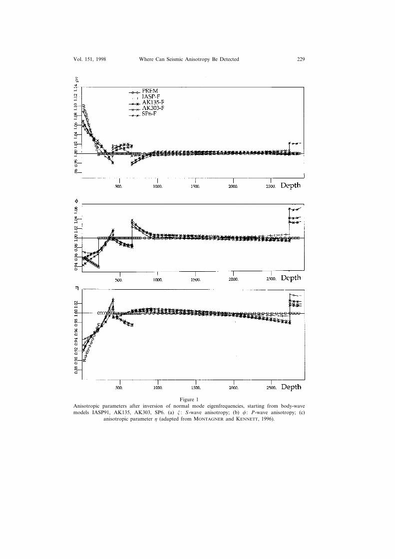
Several robust features have been found from the inversions, based on thedifferent body-wave models, regarding the radial anisotropy. First of all, anisotropyis significant in the whole upper mantle with a minimum value in the depth range300–500 km. It is very small in the whole lower mantle except in the lowertransition zone (between 660 km discontinuity and 1000 km depth) and in theD�-layer. The corresponding models for �, �, � are plotted in Figure 1. Aninteresting feature of these models is the existence of radial anisotropy in the upper(410–600 km) and lower (660–1000 km) transition zones with opposite signs.KARATO (1997) proposed an explanation to this reversal by estimating the lattice-preferred oreintations of the main constituents of the upper and lower transitionzones. The behavior of anisotropy in the D�-layer seems robust as well, but is morecomplex with a small S-wave anisotropy but large P wave and � anisotropies.

Therefore, these new reference earth models provide some indication of theexistence of anisotropy in two boundary layers; the first one in D�-layer at thecore-mantle boundary and the second one in upper and lower transition zones atthe ULM (upper-lower mantle boundary around the 660 km discontinuity). Inde-pendent seismological studies tend to corroborate these findings in the D�-layer andin the transition zone, as will be seen in the next section.

2.3 Anisotropy in the D�-Layer

During recent years, the structure of the mysterious D�-layer has been exten-sively investigated. It is not the goal of this paper to review these different studieswhich make use of different kinds of body waves but only to draw attention torecent studies which make evident the presence of anisotropy in the D�-layer(VINNIK et al., 1989; LAY and YOUNG, 1991). By studying Sd waves (S-diffractedwaves at the core-mantle boundary), VINNIK et al. (1995) found that SVd waves aredelayed relative to SHd waves by 3 s (Fig. 2). That is an unambiguous observationin the sense that the authors present a careful comparison of their waveforms withSKS and SKKS waveforms. Their observations are characteristic of a transverselyisotropic medium with vertical symmetry axis with VSH�VSV. Other seismic


Figure 1Anisotropic parameters after inversion of normal mode eigenfrequencies, starting from body-wavemodels IASP91, AK135, AK303, SP6. (a) � : S-wave anisotropy; (b) � : P-wave anisotropy; (c)

anisotropic parameter � (adapted from MONTAGNER and KENNETT, 1996).


Figure 2Radial (thick line) and transverse (thin line) components of records in WFM and HRV station forearthquakes located in the Tonga subduction zone. Seismogram s starts at the theoretical arrival time of

Sdiff for model IASP91 (after Fig. 2 of VINNIK et al., 1995).

observations such as anomalous diffraction of body waves (MAUPIN, 1994) confirmthis kind of anisotropy and its lateral variation in the Caribbean Sea (KENDALL

and SILVER, 1996) or North America (MATZEL et al., 1996; GARNERO and LAY,1996). The anisotropy observed in D�-layer is most probably due to horizontallayering or aligned inclusions inducing different velocities for SV and SH (SPOanisotropy).

2.4 Anisotropy in the Transition Zone

The transition zone plays a key role in mantle dynamics, particularly the 660 kmdiscontinuity which might inhibit the passage of matter between the upper and thelower mantle. Its seismic investigation is made difficult on a global scale by thepoor sensitivity of fundamental surface waves in this depth range and by the factthat teleseismic body waves recorded in continental stations from earthquakesprimarily occurring along plate boundaries have their turning point below thetransition zone. However, MONTAGNER and KENNETT (1996), by using eigenfre-quency data, display evidence of radial anisotropy in the upper and lower transitionzones. Another important feature of transition zone is that, contrary to the rest ofthe upper mantle, the upper transition zone is characterized by a large degree 2


pattern (MASTERS et al., 1982). MONTAGNER and ROMANOWICZ (1993) explainedthis degree 2 pattern by the predominance of a simple large-scale flow patterncharacterized by two upwellings in the Central Pacific Ocean and Eastern Africaand two downwellings in the Western and Eastern Pacific Oceans. This scheme iscorroborated by the existence in the upper transition zone of a slight but significantradial anisotropy displayed by MONTAGNER and TANIMOTO (1991) and ROULT etal. (1990). The distribution of radial anisotropy at a depth of 470 km is presentedin Figure 3. We will explain in section 3.1 why the pattern of radial anisotropy isdominated by degree 4 in agreement with the prediction by this model.

The existence of anisotropy close to the 660 km discontinuity is also confirmedby VINNIK and MONTAGNER (1996) below Germany. By studying P-to-S con-verted waves at GRF network, they observed that part of the initial P wave isconverted into SH wave. This signal can be observed on the transverse componentin Figure 4. The amplitude of this wave cannot be explained by a dipping 660 kmdiscontinuity and this constitutes sound evidence for the existence of anisotropy justabove this discontinuity. However, there is evidence of lateral variation of an-isotropy in the transition zone as found by the investigation of several subductionzones (FISCHER and YANG, 1994; FISCHER and WIENS, 1996). FOUCH andFISCHER (1996) present a synthesis of these different studies and demonstrate thatsome subduction zones such as Sakhalin Islands require deep anisotropy in thetransition zone, whereas others such as Tonga need no anisotropy. However, theyconclude that their data might be reconciled by considering the upper transition

Figure 3Radial �-anisotropy map for degree 4 at a depth of 470 km. Isolines 0.25%. Four zones of dominantradial flow can be observed and associated with Central Pacific and Africa for upgoing flow, WesternPacific and America for downgoing flow. They are therefore in agreement with the degree 2 pattern of

the transition zone.


Figure 4SV and T components of the mantle P-to-S phases at GRF (VINNIK and MONTAGNER, 1996). Thesesignals have been obtained by stacking many records of teleseismic events recorded in the GRF

(Grafenberg array).

zone (410–520 km) intermittently anisotropic, and the rest of the transition zoneisotropic. Moreover, they make a very strong assumption that the orientation andstrength of anisotropy does not vary with depth, which is not supported by surfacewave studies (MONTAGNER and TANIMOTO, 1991).


2.5 E�idence of Anisotropy in the Upper 410 km of the Mantle

The upper 410 km of the mantle is the depth range where the existence ofseismic anisotropy is now widely recognized and well documented. The earlyevidence was the discrepancy between Rayleigh and Love wave dispersion (ANDER-

SON, 1961; AKI and KAMINUMA, 1963) and the azimuthal dependence of Pn

velocities (HESS, 1964). Azimuthal variations have been found for different areas inthe world as well as for body waves and surface waves.

Body wa�es. For body waves the evidence of anisotropy results from theinvestigation of the splitting in teleseismic shear waves such as SKS (VINNIK et al.,1984, 1989a,b, 1992; SILVER and CHAN, 1988; ANSEL and NATAF, 1989), ScS(ANDO, 1984; FUKAO, 1984) and S (ANDO and ISHIKAWA, 1983; BOWMAN andANDO, 1987; FISCHER and WIENS, 1996; GAHERTY and JORDAN, 1995). There isalso evidence of P-wave anisotropy (BABUSKA et al., 1984, 1993). These waves areshown to provide an excellent lateral resolution. Among these different observa-tions, the splitting information derived from SKS is probably the less ambiguousand has been extensively used in teleseismic anisotropy investigations (see SILVER,1996 for a review). The drawbacks of this technique are that it is almost impossibleto locate at depth the anisotropic area, that it cannot take account for a dippingsymmetry axis, and that only continental areas can be extensively investigated. Therapid variation of directions of fast velocity which can be observed in somecontinental regions on a short spatial scale (VINNIK et al., 1989a; HIRN et al.,1995), cannot be explained by a very deep anisotropy and the origin of anisotropyat depth is confined to the first 410 km, either in the lithosphere or in the top of theasthenosphere.

Surface wa�es. Surface waves are also well suited for investigating upper mantleanisotropy. Two kinds of observable anisotropy can be considered. The first oneresults from the well-known discrepancy between Love and Rayleigh waves, oftenreferred to as ‘‘polarization’’ anisotropy (SCHLUE and KNOPOFF, 1977) or radialanisotropy. In order to remove this discrepancy, it is necessary to consider atransversely isotropic medium with a vertical symmetry axis (also termed radialanisotropic medium). This kind of anisotropy is characterized by five anisotropicparameters plus density (ANDERSON, 1961). On a global scale, NATAF et al. (1984,1986) derived by the simultaneous inversion of Rayleigh and Love wave dispersion,the geographical distributions of S-wave anisotropy at different depths, assumingradial anisotropy.

The second kind of observable anisotropy is the azimuthal anisotropy, directlyderived from the azimuthal variation of phase velocity of surface waves. It wasobserved initially on Rayleigh waves by FORSYTH (1975) in Nazca plate. Sincethese pioneering studies, global and regional models have been derived for bothkinds of anisotropy (MITCHELL and YU, 1980; MONTAGNER, 1985). TANIMOTO

and ANDERSON (1985) obtained a global distribution of the Rayleigh wave


azimuthal anisotropy at different periods. On a regional scale, several tomographicinvestigations report the existence of azimuthal anisotropy in the Indian Ocean(MONTAGNER, 1986a), in the Pacific Ocean (SUETSUGU and NAKANISHI, 1987;NISHIMURA and FORSYTH, 1987, 1988) and in Africa (HADIOUCHE et al., 1988).LEVEQUE and CARA (1985), CARA and LEVEQUE (1988) used higher mode data todisplay radial anisotropy under the Pacific Ocean and North America to at least300 km.

The radial anisotropy (or ‘‘polarization’’ anisotropy) and the azimuthal an-isotropy are two different manifestations of the same phenomenon, the anisotropyof the upper mantle. MONTAGNER and NATAF (1986) derived a technique whichmakes it possible to simultaneously explain these two forms of seismically observ-able anisotropy. The principles of this technique will be only briefly described, forthe most general case of anisotropy (on the condition that it is small). A completedescription of the whole procedure can be found in MONTAGNER (1996). Thenumber of independent anisotropic parameters is 13 for surface waves. This highnumber of independent parameters explains the difficulty in implementing such atechnique, from a practical point of view. However, the method can be slightlysimplified by assuming that the medium displays a symmetry axis with anyorientation. In that case, 7 independent anisotropic parameters are necessary, 5related to the transverse isotropy plus 2 angles to express the orientation in spaceof the symmetry axis. This simplified technique was coined ‘‘vectorial tomography’’(MONTAGNER and NATAF, 1988), and was applied to the 3-D anisotropic investiga-tion of the Indian Ocean (MONTAGNER and JOBERT, 1988). Moreover, this latterstudy showed that, paradoxically, in order to explain their data on the IndianOcean, a parameterization with anisotropy requires less parameters than a parame-terization with only isotropic terms. This can be explained by the fact that theincrease in the number of physical parameters in the case of anisotropy is largelycompensated by a reduced number of spatial parameters. A first global 3-Danisotropic tomography (with 13 anisotropic parameters) was derived by MONTAG-

NER and TANIMOTO (1990, 1991). Therefore, contrarily to body waves, surfacewaves enable location of anisotropy at depth but, so far, its lateral resolution(several thousands of kilometers) is very poor.

From a theoretical point of view, a general slight elastic anisotropy in aplane-layered medium gives rise to an azimuthal dependence of the local phase orgroup velocities of Love and Rayleigh waves of the form (SMITH and DAHLEN,1973, 1975):

�(, �)−�0(, �)=0()+1() cos 2�+2() sin 2�

+3() cos 4�+4() sin 4� (1)

where is the frequency of the wave and � is the azimuth along the path.


MONTAGNER and NATAF (1986), following the same approach, displayed thesimple linear combinations of the elastic tensor components Cij sufficient to describethe two seismically observable effects of anisotropy, the ‘‘polarization’’ anisotropyand the azimuthal anisotropy. The 0–� term corresponds to the average over allazimuths and involves five independent parameters, A, C, F, L, N, which expressthe equivalent transversely isotropic medium with vertical symmetry axis. The otherazimuthal terms (2–� and 4–�) depend on 4 groups of 2 parameters, B, G, H,respectively describing the 2–� azimuthal variation of A, L, F, and E describingthe 4–� azimuthal variation of A and N. Therefore, the different azimuthal terms0, 1, 2, 3, 4, depend on 13 three-dimensional parameters, which are assumedindependent:

Constant term (0 �-azimuthal term)(0)A=��2

PH=38(C11+C22)+1

4C12+12C66

C=��2PV=C33

F=12(C13+C23)

L=��2SV=1

2(C44+C55)

N=��2SH=1

8(C11+C22)−14C12+

12C66

2 �-azimuthal term:

(1) cos 2� (2) sin 2�Bc=

12(C11−C22) Bs=C16+C26

Gc=12(C55−C44) Gs=C54

Hc=12(C13−C23) Hs=C36

4 �-azimuthal term:

(3) cos 4� (4) sin 4�

Ec=18(C11+C22)−1

4C12−12C66 Es=

12(C16−C26)

where indices 1 and 2 refer to horizontal coordinates (1: North; 2: East) and index3 refers to vertical coordinates. � is the density, �PH, �PV are respectively horizontaland vertical P-wave velocities, �SH, �SV horizontal and vertical S-wave velocities.Therefore, the different parameters present in the different azimuthal terms aresimply related to elastic moduli Cij and the corresponding kernels are detailed andtheir variation at depth is plotted in MONTAGNER and NATAF (1986). Therefore, inthe most general case for a slight anisotropy, thirteen combinations of elasticmoduli are necessary to describe the total effect of anisotropy on seismic surface


waves. That means that, from a theoretical point of view, seismic surface waveshave the ability to provide 13 tomographic models. However, from a practical pointof view, data does not have the resolving power to invert for so many parameters.MONTAGNER and ANDERSON (1989a) proposed the usage of constraints frompetrology in order to reduce the parameter space. Actually, they ascertained thatsome of these parameters display large correlations independent of the petrologicalmodel used. Two extreme models were used to derive these correlations: thepyrolite model (RINGWOOD, 1975) and the piclogite model (ANDERSON and BASS,1984, 1986; BASS and ANDERSON, 1984). In the depth inversion process, theslightest correlations between parameters of both models are kept. This approachwas already followed by MONTAGNER and ANDERSON (1989b) to derive anaverage reference earth model, and by MONTAGNER and TANIMOTO (1991) for thefirst global 3-D anisotropic model. The complete tomographic technique (regional-ization+ inversion at depth) has been applied to investigate either regional struc-tures of the Indian Ocean (MONTAGNER and JOBERT, 1988), of the Atlantic Ocean(MOCQUET et al., 1989; SILVEIRA et al., 1997), of Africa (HADIOUCHE et al., 1989),of the Pacific Ocean (NISHIMURA and FORSYTH, 1988), of Antarctica (ROULT etal., 1994) and Central Asia (GRIOT et al., 1996) or global structure (MONTAGNER

and TANIMOTO, 1990, 1991).Figure 5 presents some maps which illustrate the two kinds of anisotropy which

can be retrieved by simultaneous inversion of Rayleigh and Love waves constantand azimuthal terms of equation (1). The map of Figure 5a is the distribution of theG parameter which is related to the azimuthal variation of SV-wave velocity. The

Figure 5a


Figure 5Result of the simultaneous inversion of Rayleigh and Love waves dispersion and their azimuthalvariations. (a) Distribution of the G parameter at 200 km (adapted from MONTAGNER and TANIMOTO,1991). G is related to the azimuthal variation of �SV velocity. (b) � distributions at two depths (100 kmand 300 km) in % with respect to ACY400 (MONTAGNER and ANDERSON, 1989b). Be aware that �

anomalies are plotted at the 2 depths with respect to a reference value different from 0.


maximum amplitude of G is around 2% and rapidly decreasing as depth isincreasing. On Figure 5b, the equivalent radial anisotropy of the medium for Swave expressed by the � parameter is displayed for 2 different depths, 100 km and310 km. The distribution of anisotropy has completely different patterns andamplitudes at these two depths. We will investigate the geodynamical consequenceof such a behavior in section 3.1.

Consequently, the evidence of anisotropy is now quite robust, but its completeinterpretation and utilization for geophysical purposes are ongoing. In the nextsection, we will present examples of geodynamical applications of three-dimensionalmodels of anisotropy derived from surface waves. In the fourth section, we willrelate two independent seismic data sets, on one hand, phase velocity data setderived from surface waves, on the other hand, differential travel times as derivedfrom SKS body waves.

3. Geophysical Applications of Seismic Anisotropy

The seismic anisotropy in the earth can therefore be retrieved by differentmethods. Since it represents a new dimension in the interpretation of seismic data,its scientific potential is enormous, and still largely unexploited. We will onlypresent examples of interesting applications of anisotropy in geodynamics andtectonics.

3.1 Geodynamics

The application of seismic anisotropy to geodynamics is straightforward, sincethe seismic anisotropy in the mantle generally reflects the strain field prevailing inpast (frozen-in anisotropy) or present convective processes. Therefore, it becomespossible to map convection in the mantle. TANIMOTO and ANDERSON (1985)presented the first maps of azimuthal anisotropy at different periods. NATAF et al.(1984) displayed the first global model of radial anisotropy (0–� term). However,when only the radial anisotropy is retrieved, its interpretation is nonunique becausea fine layering of the mantle can also generate such a kind of anisotropy. In orderto simultaneously explain azimuthal anisotropy and radial anisotropy, MONTAG-

NER and JOBERT (1988) by applying the method of Vectorial Tomography (MON-

TAGNER and NATAF, 1988) have been able to plot for the first time, the 3-Ddistribution of the fast axis in the Indian Ocean. That means that, if this axis iseffectively related to the strain induced by plate motion and convective processes,it is possible to visualize convection cells. A quite similar technique has been appliedon a global scale by MONTAGNER and TANIMOTO (1990, 1991). When both kindsof observable anisotropy (azimuthal and radial anisotropies) are retrieved, the mostlikely interpretation is the presence of large-scale flow which can align the symmetry


axes of the different anisotropic minerals of the mantle; primarily olivine and to aless extent the ortho- and clino-pyroxenes.

For the upper mantle, the �= (N−L)/L parameter (radial S anisotropy) can besimply interpreted as a tendency for a horizontal or subhorizontal flow when � ispositive, and a radial (or very steep) flow when it is negative. The simultaneousexistence of azimuthal anisotropy for example through the G parameter (SV-waveazimuthal anisotropy) will provide in addition the horizontal orientation of theflow, but not its vectorial direction because surface waves are insensitive to thesense of propagation: In the expression of the phase velocity (equation 1), thetransformation of the azimuth � into �+� does not change the value of phasevelocity. In order to define the actual direction of flow, it is necessary to addinformation such as plate velocity directions or numerical modeling strain principaldirections. Though surface wave tomography enables simultaneous retrieval ofthirteen anisotropic parameters, we will only focus on the best resolved anisotropicparameters, the G parameter (related to azimuthal variations of SV-wave velocity)and the � parameter which expresses the relative importance of the azimuthallyaverages of �SH and �SV or in other words the radiality of the flow.

The distribution of the G parameter is plotted on Figure 5a at 200 km depth. Itshows that the agreement of directions of maximum velocity with plate tectonics isreasonable in the depth range 100–300 km (MONTAGNER, 1994). However, theazimuth of G parameter can largely vary as a function of depth (MONTAGNER andTANIMOTO, 1991). For instance, at shallow depths (to 60 km), the maximumvelocity is very often parallel to mountain belts (VINNIK et al., 1992; SILVER, 1996;BABUSKA et al., this issue). This means that, at a given place, the orientation of fastaxis is a function of depth. Contrary to seismic anisotropy derived from SKS, theanisotropy inferred from surface waves can be located at detph, and both measure-ments must be combined in order to provide a complete understanding of theprocesses prevailing in a given tectonic context.

The simultaneous inversion of Rayleigh, Love wave dispersion curves and theirazimuthal variations provides better estimates of the second kind of observableseismic anisotropy, i.e., the radial anisotropy expressed through the parameter�= (N−L)/L. The � parameter is retrieved through the inversion of the 0–�azimuthally averaged term of the expansion of the local phase velocity and thus isnot biased by an imperfect azimuthal coverage of the criss-crossing paths in thearea under investigation. It results that a close inspection of the three-dimensionaldistribution of � displays different patterns below continents and oceans (Fig. 5b).Whereas � is primarily positive in most oceanic areas (except near ridges) at 100 kmdepth, the pattern is reversed at large depths (310 km), where positive � is nowassociated with continents. However, the amplitude of � is rapidly decreasing inaverage at depth below 200 km and is less resolved.


Continents. � is usually very heterogeneous below continents in the first 150–200 km of depth with positive or negative areas according to geology. However, itseems to display a systematic tendency to be positive at larger depth (down to300–400 km), whereas it is very large in the oceanic lithosphere in the depth range50–200 km and decreases rapidly at larger depths (Fig. 6). Conversely, radialanisotropy displays a maximum (though smaller than in oceanic lithosphere) belowvery old continents (such as the Siberian and Canadian Shields) in the depth range200–400 km. Contrary to the assertion of GAHERTY and JORDAN (1995), seismicanisotropy below continents is not necessarily limited to the upper 220 km. A morequantitative comparison of radial anisotropy between different continentalprovinces is presented in this issue by BABUSKA et al. (1997), and it demonstratessystematic differences according to the tectonic context. The existence of positivelarge-scale radial anisotropy below continents at depth might be a good indicator ofthe continental root which has been largely debated since the presentation of thecontroversial model of tectosphere by JORDAN (1978, 1981). If we assume that thismaximum of anisotropy is related to an intense strain field in this depth range, itmight be characteristic of the boundary between continents and ‘‘normal’’ uppermantle material. Our results show that the root of continents is located between 200and 300 km.

It must be emphasized that the anisotropy near the surface is probably differentfrom the deep one. Part of the observed anisotropy might be related to the fossilestrain field prevailing during the setting of materials and the other deeper part isrelated to the present strain field. If we bear in mind that the anisotropy displayedfrom surface waves is the long wavelength filtered anisotropy (approximately 1500km), it can be easily understood that the average anisotropy displayed from surfacewaves in the first 200 km might be very different from the one found from bodywaves. The tectonics of continents is the result of a long and complex history. Thecharacteristic length scale under continents is related to the size of blocks succes-sively accreted to existing initial cores and probably smaller than 1500 km. Thisstatement is supported by different studies of SKS body waves which demonstratethat the direction of maximum velocity can change on scales smaller than 100 km(VINNIK et al., 1992; SILVER, 1996). This difference of characteristic scales canexplain the apparent contradictions between surface wave and body wave an-isotropy measurements. The fact that we do not observe a systematic behavior inthe first hundreds of kilometers for similar continental geological zones, does notmean that anisotropy is not present but only that its characteristic scale is differentfrom one region to another. Due to the low-pass filtering effect of our technique, itslong wavelength signature is diluted.

The fossile shallow anisotropy (first hundred of kilometers) that reflects the paststrain field, should be very useful for understanding the processes involved insurficial tectonics. If we were able to determine the age of this shallow anisotropy,the measurement of this kind of anisotropy should open wide a new field in Earth


Sciences: the Paleo-Seismology which might provide fundamental information ofStructural Geology. We will return to the scientific applications of shallow an-isotropy in the next section.

Figure 6a


Figure 6Radial cross-sections of the � parameter at latitudes: a) −20S and b) +20N (same color scale).

Oceans. Since convective flow below oceans is dominated by large-scale platemotions, the long wavelength anisotropy found in oceanic plates should be similarto the smaller-scale anisotropy which should be measured from body waves. One ofthe first evidence of anisotropy was found in the Pacific Ocean by HESS (1964) forPn waves. Since that time there have been many measurements of the subcrustal


anisotropy (see BABUSKA and CARA, 1991 for a review). Unfortunately, to date,there are very few measurements of deep anisotropy by SKS splitting in the oceans.Due to the absence of a seismic station on the sea floor, the only measurementsavailable for SKS were performed in stations located on ocean islands (ANSEL andNATAF, 1989; KUO and FORSYTH, 1992; RUSSO and OKAL, 1997), which are bynature anomalous objects, such as hotspots where the strain field is perturbed bythe ascending material and not necessarily representative of the main flow field.There were other attempts to determine anisotropy for other kinds of body wavessuch as ScS and multiple ScS (ANDO, 1984; FARRA and VINNIK, 1994; GAHERTY

et al., 1997), PS waves (SU and PARK, 1994), or differential times of sS-S, or SS-Swaves (KUO et al., 1987; SHEEHAN and SOLOMON, 1991; FISCHER and YANG,1994; GAHERTY et al., 1996; FOUCH and FISCHER, 1996; YANG and FISCHER,1994). However, the two cross-sections of Figure 6 illustrate that the � parameteris negative and small, where flow is primarily radial (mid-ocean ridges andsubducting zones). Between plate boundaries, oceans display vast areas with apositive radial anisotropy, characteristic of an overall horizontal flow field. Oceanicplates are zones where the comparison between directions of plate velocities(MINSTER and JORDAN, 1978) and directions of G parameter is the most successfulin the entire lithosphere and asthenosphere beneath 250–300 km (MONTAGNER,1994). Conversely, such a comparison is more controversial below plates bearing alarge proportion of continents, such as the European-Asian plate, characterized bya very small absolute motion in the hotspot coordinate system. Another interestingapplication of the � parameter can be found in the process of understanding theconvection pattern in the transition zone. Recent tomographic models of seismicvelocity, anisotropy and anelasticity obtained from GEOSCOPE and IRIS datademonstrate that at depth larger than 410 km�100 km, the degree 2 and to a lessextent the degree 6 arise as the most important features. These models also displaya large degree 4 for radial anisotropy at large depths (ROULT et al., 1990;MONTAGNER and TANIMOTO, 1991). A simple flow pattern with two upgoing flowsbelow central Pacific and Africa and two downgoing flows below western Pacificand America can explain the predominance of these different degrees 2 and 6.MONTAGNER and ROMANOWICZ (1993) demonstrate that the degree-2 patterncorrectly predicts the predominance of degree 4 of �-anisotropy because � is notaffected by the sense of flow but only by its radiality or horizontality. Moreover,the geographical distribution of radial anisotropy is in agreement with the degree-2pattern as it is displayed in Figure 3. Therefore, the observations of the geograph-ical distributions of degrees 2, 4, 6 in the transition zone are coherent and spatiallydependent. MONTAGNER (1994) compared these different degrees to the corre-sponding degrees of the hotspot and slab distribution. In this simple framework thedistribution of plumes and slabs is merely a byproduct of the large-scale simple flowin the transition zone.


3.2 Tectonics

The measurement of seismic anisotropy can provide fundamental informationfor the understanding of tectonic processes. SILVER (1996) presents a review ofthe information provided by shear-wave splitting beneath continents. The poorlateral resolution of global scale anisotropic tomography can be considered as astrong limitation in continental areas. This technique can only be efficientlyapplied in areas where large-scale tectonic forces are implied. The best candidatewhere this condition is fulfilled in continents is the collision zone between Indiaand Asia. GRIOT et al. (1996) undertook such an investigation in Central Asia.The primary goal of this study is the discrimination between two competingextreme models of deformations, the heterogeneous model of AVOUAC and TAP-

PONNIER (1993) and the homogeneous model of ENGLAND and HOUSEMAN

(1986). It was necessary to use shorter wavelength surface waves (40–200 s) inorder to obtain a lateral resolution of 350 km. Synthetic models of seismicanisotropy can be inferred from the heterogeneous and homogeneous models. Inorder to perform correct and quantitative comparisons between observed seismicanisotropy and the deformation models, the short wavelengths of the syntheticmodels (spatial scale smaller than 350 km) were filtered out (Fig. 7).

The statistical comparison between observed and synthetic azimuthal an-isotropies for both models enables a determination in different depth ranges ofwhich the deformation model dominates. GRIOT et al. (1997) show that theheterogeneous model is in better agreement with observations in the first 200km, whereas the homogeneous model better fits the deep anisotropy below 200km. We must be aware that such a comparison is only valid from a statisticalpoint of view and that a comparison at a more local scale (the scale of body-wave measurements) might display some differences with the observed SKS an-isotropy. This kind of investigation only underlines large-scale ongoing andprevailing active processes and is not devoted to a precise measurement of an-isotropy at any specific place.

4. Discussion

In the previous sections we have illustrated by different examples that theeffect of anisotropy (though small) is significant and must be taken into accountto correctly explain independent data sets related to the propagation of seismicwaves inside the earth. Nonetheless, we must wonder whether these data sets areconsistent, and which general statement regarding mantle convection can be putforward when considering the different depth ranges in which seismic anisotropyhas been observed.

246 Jean-Paul Montagner Pure appl. geophys.,

4.1 Comparison between Surface-wa�e Anisotropy and SKS Delay Times

For simplicity only two data sets are considered in this section. The first oneconcerns the global distribution of anisotropy as inferred from surface waves. Thesecond one is composed of local measurements of delay times and directions ofmaximum velocities as obtained from SKS-splitting measurements. We will onlypresent the qualitative comparison between both data sets. The theory whichenables such a comparison is detailed in MONTAGNER et al. (in preparation). It isimportant to note that the anisotropic parameters, linear combinations of elasticmoduli Cij, which can be derived from the surface waves, also come up when youconsider the propagation of body waves in symmetry planes for a slightly an-isotropic medium (see for instance, BACKUS, 1965; CRAMPIN, 1984; MONTAGNER

and NATAF, 1986). However, attention must be directed to the orientation of thecoordinates’ system. A global investigation of anisotropy inferred from SKSbody-wave data has been undertaken by different authors (VINNIK et al., 1992;SILVER, 1996). Actually, most SKS measurements have been performed in conti-nental parts of the earth. A direct comparison of both data sets is now necessaryand possible. If we assume that the anisotropic medium is characterized by ahorizontal symmetry axis with any orientation, a synthetic data set of SKS delaytimes and azimuths can be calculated by using the following equations:

�tSKS=� h

0

dz��

h�Gc (z)

L(z)cos (2�(z))+

Gs (z)L(z)

sin (2�(z))�

(2)

where �tSKS is the integrated travel time for the depth range 0–h, where theanisotropic parameters Gc (z), Gs (z) and L(z) are the elastic parameters retrievedfrom surface waves at different depths. It is remarkable to realize that only the Gparameter (expressing the SV-wave azimuthal variation) is present in this equation.From equation (2) we can infer the maximum value of delay time �tmax

SKS and thecorresponding azimuth �SKS :

�tmaxSKS=

�� h

0

dz��

LGc (z)L(z)

�2

+�� h

0

dz��

LGs (z)L(z)

�2

(3)

tan (2�SKS )=

� h

0

dzGs (z)L(z)� h

0

dzGc (z)L(z)

. (4)

However, equation (2) is approximate and only valid when the wavelength is muchlarger than the thickness of layers. It should be possible to make more precisecalculations by using the technique derived for two layers by SILVER and SAVAGE

(1994). The resulting map is presented in Figure 8.

Vol. 151, 1998 When Can Seismic Anistropy Be Detected 245

Figure 7Distributions of azimuthal anisotropy at different depths (after GRIOT et al., 1997). Top—Syntheticanisotropic models. Left: Heterogeneous model. Right: Homogeneous model. Bottom figures: G parame-

ter at different depths derived from surface-wave data.


Initially the map illustrates that both data sets are compatible in magnitudealthough not necessarily in directions. Some contradictions between measurementsderived from surface waves and from body waves can be noted. The agreement ofdirections is correct in tectonically active areas but not in old cratonic zones. Thediscrepancy in these areas results from the rapid change of directions of anisotropyat a small scale and that the hypothesis of horizontal symmetry axis is not valid(PLOMEROVA et al., 1996). These changes stem from the complex history of theseareas, which have been built by successive collages of continental pieces. Thepositive consequence of this discrepancy is that a small-scale mapping of anisotropyin such areas might provide clues to understand the processes of growth ofcontinents and mountain building.

Contrary to surface waves, body waves have a good lateral resolution butno vertical resolution. They are sensitive to the short wavelength anisotropy justbelow and around the stations. On the other hand, global anisotropy tomographyderived from surface waves only provides long wavelength anisotropy (poorlateral resolution) although it enables location at depth of anisotropy. Thereforethe long wavelength anisotropy derived from surface waves will display thesame direction as the short wavelength anisotropy inferred from body wavesonly when large-scale geodynamic processes are dominating. In some continentalareas, short-scale anisotropy, the result of a complex history, might be importantand even mask the large-scale anisotropy more related to present convectiveprocesses.

4.2 Location of Anisotropy in Boundary Layers

The review of the presence of anisotropy in different layers of the earthdemonstrated that the anisotropy is a very general feature but that it is not presentin whole depth ranges nor at all scales. As discussed in section 2.1, the observationof seismic anisotropy at large scales requires several redhibitory conditions, startingwith the presence of anisotropic crystals extending to the existence of an efficientlarge-scale present or past strain field. Theoretical studies suggest that, whenanisotropic minerals such as olivine or pyroxene are subjected to strain, theircrystallographic axes develop a systematic relationship to the principal axes of finitestrain (MCKENZIE, 1979; RIBE, 1989). Many numerical modelings of the convectivemantle show that in a convective system, the strain field is not spatially uniform.Streamlines are substantially more concentrated in boundary layers than centrallyin the cells. Consequently, the amplitude of the strain field is very heterogeneousand the largest in boundary layers. Conversely, we can assume that the observationof mantle seismic anisotropy is an indication of a strong present-day strain field(excepting crust, topmost oceanic and continental lithospheres where fossile an-isotropy may be present), associated with boundary layers. In the previous sectionswe noted sound evidence of the presence of seismic anisotropy in the D�-layer, in


Fig

ure

8a

Where

Can

Seismic

Anisotropy

Be

Detected

249V

ol.151,

1998

Figure 8Top: Distributions of synthetic delay time �tmax

SKS and azimuth �SKS at the surface of the earth, such as derived from AUM anisotropic tomographic model(MONTAGNER and TANIMOTO, 1991). Bottom: Map of distribution of observed SKS maximum directions and delay times (SILVER, 1996). On both figures

the length of lines is proportional to �tSKS.


the transition zone and in the uppermost mantle. These findings are summarized inFigure 9. The D�-layer and the uppermost mantle were long related to boundarylayers of the mantle convective system. The D�-layer above the core-mantleboundary is characterized by a large degree of seismic heterogeneities and an-isotropy with �SH larger than �SV. It might be simultaneously the graveyard ofsubducted slabs and the source of megaplumes. D� anisotropy can be related eitherto horizontal layering of cold material or the presence of aligned inclusions owingto the presence of melt (KENDALL and SILVER, 1996). For the uppermost oceanicmantle, seismic anisotropy is present in both the lithosphere and the asthenosphere,and for oceans some finite-element models can quantitatively relate lithospheric andasthenospheric strain to anisotropy (TOMMASI et al., 1996). However the presenceof anisotropy in the transition zone is fundamental and problematic because itprovides a new clue that the transition zone is acting as a boundary layer. The firstevidence of anisotropy in the transition zone tends to favor the predominance ofhorizontal flow over vertical flow. The major consequence of this finding is that thetransition zone is dividing the mantle, on average, into two convective systems, theupper mantle and the lower mantle. This general statement does not rule out thepossibility that flow circulation between the upper and the lower mantle is occur-ring. Nonetheless it does mean that the exchange of matter between the upper andthe lower mantle is difficult. It is premature to assess the amount of mattercirculating from measurements of seismic anisotropy.

Figure 9Cross-section of the earth from the core-mantle boundary extending to the surface. The hatched(respectively dotted) areas show where there is robust evidence of (resp. fossile) anisotropy. B.L. stands

for Boundary Layer.


5. Conclusions

We have presented in this paper different observations of seismic anisotropy andtheir applications in geology and geodynamics. Seismic anisotropy defines continen-tal roots so as to discriminate different competing convective models. Threeboundary layers as yet have been detected by seismic anisotropy: the uppermostmantle, the transition zone (though new work is necessary to confirm it) and theD�-layer. Other applications of seismic anisotropy can be easily found. Forexample, MONTAGNER and ANDERSON (1989a) demonstrate that different an-isotropic parameters might be used to discriminate competing petrological modelssuch as pyrolite or piclogite. Some seismologists claim that the temporal variationof anisotropy in the crust might be an efficient tool to investigate the earthquakecycle. It is now used routinely in seismic exploration. Therefore the scientificpotential of seismic anisotropy is enormous and largely unexploited. In conclusion,seismic anisotropy provides a new dimension in the investigation of processes ofour dynamic earth.

Acknowledgments

I am grateful to Lev Vinnik, Alessandro Forte, Vlada Babuska, Jarka Plom-erova, and Bob Liebermann for fruitful discussions. I thank Shun-Ichiro Karatoand an anonymous reviewer for their critical review of the paper, and Daphne-Anne Griot for providing some of the figures.

REFERENCES

AKI, K., and KAMINUMA, K. (1963), Phase Velocity of Lo�e Wa�es in Japan (Part 1): Lo�e Wa�es fromthe Aleutian Shock of March 1957, Bull. Earthq. Res. Inst. 41, 243–259.

ALLEGRE, C. J., and TURCOTTE, D. L. (1986), Implications of a Two-component Marble-cake Mantle,Nature 323, 123–127.

ANDERSON, D. L. (1961), Elastic Wa�e Propagation in Layered Anisotropic Media, J. Geophys. Res. 66,2953–2963.

ANDERSON, D. L., Theory of the Earth (Blackwell Scientific Publications, Oxford 1989).ANDERSON, D. L., and BASS, J. D. (1984), Mineralogy and Composition of the Upper Mantle, Geophys.

Res. Lett. 11, 637–640.ANDERSON, D. L., and BASS, J. D. (1986), Transition Region of the Earth ’s Upper Mantle, Nature 320,

321–328.ANDERSON, D. L., and DZIEWONSKI, A. M. (1982), Upper Mantle Anisotropy: E�idence from Free

Oscillations, Geophys. J. R. Astron. Soc. 69, 383–404.ANDERSON, D. L., and REGAN, J. (1983), Upper Mantle Anisotropy and the Oceanic Lithosphere,

Geophys. Res. Lett. 10, 841–844.ANDO, M. (1984), ScS Polarization Anisotropy around the Pacific Ocean, J. Phys. Earth 32, 179–196.ANDO, M., ISHIKAWA, Y., and YAMAZAKI, F. (1983), Shear-wa�e Polarization Anisotropy in the Upper

Mantle beneath Honshu, Japan, J. Geophys. Res. 88, 5850–5864.


ANSEL, V., and NATAF, H.-C. (1989), Anisotropy beneath 9 Stations of the Geoscope Broadband Networkas Deduced from Shear-wa�e Splitting, Geophys. Res. Lett. 16, 409–412.

AVOUAC, J.-P., and TAPPONNIER, P. (1993), Kinematic Model of Acti�e Deformation in Central Asia,Geophys. Res. Lett. 20, 895–898.

BABUSKA, V., and CARA, M., Seismic Anisotropy in the Earth (Kluwer Academic Press, Dordrecht, TheNetherlands 1991), 217 pp.

BABUSKA, V., PLOMEROVA, J., and SILENY, J. (1984), Large-scale Oriented Structures in the SubcrustalLithosphere of Central Europe, Ann. Geophys. 2, 649–662.

BABUSKA, V., PLOMEROVA, J., and SILENY, J. (1993) Models of Seismic Anisotropy in the DeepContinental Lithosphere, Phys. Earth Planet. Int. 78, 167–191.

BABUSKA, V., MONTAGNER, J.-P., PLOMEROVA, J., and GIRARDIN, N. (1997), Age-dependent Large-scale Fabric of the Mantle Lithosphere as Deri�ed from Surface-wa�e Velocity Anisotropy, Pure appl.geophys. 151, 257–280.

BACKUS, G. E. (1962), Long-wa�e Elastic Anisotropy Produced by Horizontal Layering, J. Geophys. Res.67, 4427–4440.

BACKUS, G. E. (1965), Possible Forms of Seismic Anisotropy of the Upper Mantle under Oceans, J.Geophys. Res. 70, 3249–3439.

BARRUOL, G., and MAINPRICE, D. (1993), A Quantitati�e E�aluation of the Contribution of CrustalRocks to the Shear-wa�e Splitting of Teleseismic SKS Wa�es, Phys. Earth Planet. Int. 78, 281–300.

BARRUOL, G., SILVER, P. G., and VAUCHEZ, A. (1997), Shear-wa�e Splitting in the Eastern U.S.: DeepStructure of a Complex Continental Plate, J. Geophys. Res. 102, 8329–8348.

BASS, J., and ANDERSON, D. L. (1984), Composition of the Upper Mantle: Geophysical Tests of 2Petrological Models, Geophys. Res. Lett. 11, 237–240.

BOWMAN, J. R., and ANDO, M. (1987), Shear-wa�e Splitting in the Upper Mantle Wedge abo�e theTonga Subduction Zone, Geophys. J. R. Astron. Soc. 88, 25–41.

CARA, M., and LEVEQUE, J.-J. (1988), Anisotropy of the Asthenosphere: The Higher Mode Data of thePacific Re�isited, Geophys. Res. Lett. 15, 205–208.

CHRISTENSEN, N. I., and LUNDQUIST, S. (1982), Pyroxene Orientation within the Upper Mantle, Bull.Geol. Soc. Am. 93, 279–288.

CRAMPIN, S. (1984), An Introduction to Wa�e Propagation in Anisotropic Media, Geophys. J. R. Astron.Soc. 76, 17–28.

CRAMPIN, S., and BOOTH, D. C. (1985), Shear-wa�e Polarizations near the North Anatolian Fault, II.Interpretation in Terms of Crack-induced Anisotropy, Geophys. J. R. Astron. Soc. 83, 75–92.

DZIEWONSKI, A. M., and ANDERSON, D. L. (1981), Preliminary Reference Earth Model, Phys. EarthPlanet. Int. 25, 297–365.

ENGLAND, P., and HOUSEMAN, G. (1986), Finite Strain Calculations of Continental Deformation, 2.Comparison with the India-Asia Collision Zone, J. Geophys. Res. 91, 3664–3676.

ESTEY, L. H., and DOUGLAS, D. J. (1986), Upper Mantle Anisotropy: A Preliminary Model, J. Geophys.Res 91, 11,393–11,406.

FARRA, V., and VINNIK, L. (1994), Shear-wa�e Splitting in the Mantle of the Pacific, Geophys. J. Int.119, 195–218.

FISCHER, K. M., and YANG, X. (1994), Anisotropy in Kuril-Kamtchatka Subduction Zone Structure,Geophys. Res. Lett. 21, 5–8.

FISCHER, K. M., and WIENS, D. A. (1996), The Depth Distribution of Mantle Anisotropy beneath theTonga Subduction Zone, Earth Planet. Sci. Lett. 142, 253–260.

FORSYTH, D. W. (1975), The Early Structural E�olution and Anisotropy of the Oceanic Upper Mantle,Geophys. J. R. Astron. Soc. 43, 103–162.

FOUCH, M. J., and FISCHER, K. M. (1996), Mantle Anisotropy beneath Northwest Pacific SubductionZones, J. Geophys. Res. 101, 15,987–16,002.

FUKAO, Y. (1984), E�idence from Core-reflected Shear Wa�es for Anisotropy in the Earth ’s Mantle,Nature 309, 695–698.

GAHERTY, J. B., and JORDAN, T. H. (1995), Lehmann Discontinuity as the Base of an Anisotropic Layerbeneath Continents, Science 268, 1468–1471.

GAHERTY, J. B., JORDAN, T. H., and GEE, L. S. (1997), Seismic Structure of the Upper Mantle in aCentral Pacific Corridor, J. Geophys. Res., in press.


GARNERO, E. J., and LAY, T. (1996), Lateral Variations in Lowermost Mantle Shear-wa�e Anisotropybeneath the North Pacific and Alaska, J. Geophys. Res., 102, 8121–8135.

GRIOT, D.-A., MONTAGNER, J.-P., and TAPPONNIER, P. (1996), Surface Wa�e Phase Velocity andAzimuthal Anisotropy in Central Asia, J. Geophys. Res.

GRIOT, D.-A., MONTAGNER, J.-P., and TAPPONNIER, P. (1997), Heterogeneous �ersus HomogeneousStrain in Central Asia, Geophys. Res. Lett.

HADIOUCHE, O., JOBERT, N., and MONTAGNER, J.-P. (1989), Anisotropy of the African ContinentInferred from Surface Wa�es, Phys. Earth Planet. Int. 58, 61–81.

HESS, H. (1964), Seismic Anisotropy of the Uppermost Mantle under the Oceans, Nature 203, 629–631.HIRN, A. et al. (1995), Seismic Anisotropy as an Indicator of Mantle Flow beneath the Himalayas and

Tibet, Nature 375, 571–574.JORDAN, T. H. (1978), Composition and De�elopment of the Continental Tectonosphere, Nature 274,

544–548.JORDAN, T. H. (1981), Continents as a Chemical Boundary Layer, Philos. Trans. R. Soc. London, Ser.

A, 301, 359–373.KANESHIMA, S., and SILVER, P. G. (1992), A Search for Source-side Anisotropy, Geophys. Res. Lett. 19,

1049–1052.KARATO, S.-I., Seismic anisotropy: mechanisms and tectonic implications. In Rheology of Solids and of the

Earth (eds. S. Karato, and M. Toriumi) (Oxford University Press, Oxford 1989) pp. 393–342.KARATO, S.-I. (1997), Seismic Anisotropy in the Deep Mantle, Boundary Layers and the Geometry of

Mantle Con�ection, Pure appl. geophys. 151, 565–587.KENDALL, J.-M., and SILVER, P. G. (1996), Constraints from Seismic Anisotropy on the Nature of the

Lowermost Mantle, Nature 381, 409–412.KENNETT, B. L. N., and ENGDAHL, E. R. (1991), Tra�el Times for Global Earthquake Location and

Phase Identification, Geophys. J. Int. 105, 429–465.KENNETT, B. L. N., ENGDAHL, E. R., and BULAND, R. (1995), Constraints on Seismic Velocities in the

Earth from Tra�el Times, Geophys. J. Int., 122, 108–124.KUO, B.-Y., and FORSYTH, D. W. (1992), A Search for Split SKS Wa�eforms in the North Atlantic,

Geophys. J. Int. 108, 557–574.KUO, B.-Y., FORSYTH, D. W., and WYSESSION, M. (1987), Lateral Heterogeneity and Azimuthal

Anisotropy in the North Atlantic Determined from SS-S Differential Tra�el Times, J. Geophys. Res. 92,6421–6436.

LAY, T., and YOUNG, C. J. (1991), Analysis of Seismic SV Wa�es in the Core ’s Penumbra, Geophys. Res.Lett. 18, 1373–1376.

LEVEQUE, J. J., and CARA, M. (1985), In�ersion of Multimode Surface Wa�e Data: E�idence forSub-lithospheric Anisotropy, Geophys. J. R. Astron. Soc. 83, 753–773.

LEVSHIN, A., and RATNIKOVA, L. (1984), Apparent Anisotropy in Inhomogeneous Media, Geophys. J. R.Astron. Soc. 76, 65–69.

LOVE, A. E. H., A Treatise on the Theory of Elasticity, 4th ed. (Cambridge University Press 1927) 643pp.

MASTERS, G., JORDAN, T. H., SILVER, P. G., and GILBERT, F. (1982), Aspherical Earth Structure fromFundamental Spheroidal-mode Data, Nature 298, 609–613.

MATZEL, E., SEN, M. K., and GRAND, S. P. (1996), E�idence for Anisotropy in the Deep Mantle beneathAlaska, Geophys. Res. Lett. 23, 2417–2420.

MAUPIN, V. (1994), On the Possibility of Anisotropy in the D� Layer as Inferred from the Polarization ofDiffracted S Wa�es, Phys. Earth Planet. Int. 87, 1–32.

MCKENZIE, D. (1979), Finite Deformation during Fluid Flow, Geophys. J. R. Astron. Soc. 58, 689–715.MEADE, C., SILVER, P. G., and KANESHIMA, S. (1995), Laboratory and Seismological Obser�ations of

Lower Mantle Anisotropy, Geophys. Res. Lett. 22, 1293–1296.MINSTER, J. B., and JORDAN, T. H. (1978), Present-day Plate Motions, J. Geophys. Res. 83, 5331–5354.MITCHELL, B. J., and YU, G.-K. (1980), Surface Wa�e Dispersion, Regionalized Velocity Models and

Anisotropy of the Pacific Crust and Upper Mantle, Geophys. J. R. Astron. Soc. 63, 497–514.MONTAGNER, J.-P. (1985), Seismic Anisotropy of the Pacific Ocean Inferred from Long-period Surface

Wa�e Dispersion, Phys. Earth Planet. Int. 38, 28–50.


MONTAGNER, J.-P. (1986a), First Results on the Three-dimensional Structure of the Indian Ocean Inferredfrom Long-period Surface Wa�es, Geophys. Res. Lett. 13, 315–318.

MONTAGNER, J. P. (1986b), Regional Three-dimensional Structures Using Long-period Surface Wa�es,Ann. Geophys. 4, B3, 283–294.

MOCQUET, A., ROMANOWICZ, B., and MONTAGNER, J.-P. (1989), Three D Structure of the UpperMantle beneath the Atlantic Ocean From Long-period Rayleigh Wa�es. I: Group and Phase VelocityDistributions, J. Geophys. Res. 94, 7449–7468.

MONTAGNER, J. P. (1994), What Can Seismology Tell us about Mantle Con�ection? Rev. Geophys. 32,2, 115–137.

MONTAGNER, J. P., (1996), Surface wa�es on a global scale—Influence of anisotropy and anelasticity,Summer School of Erice, Seismic Modeling of the Earth ’s Structure (eds. E. Boschi, G. Ekstrom, A.Morelli), pp. 81–148.

MONTAGNER, J. P., and ANDERSON, D. L. (1989a), Constraints on Elastic Combinations Inferred fromPetrological Models, Phys. Earth Planet. Int. 54, 82–105.

MONTAGNER, J. P., and ANDERSON, D. L. (1989b), Constrained Reference Mantle Model, Phys. EarthPlanet. Int. 58, 205–227.

MONTAGNER, J.-P., and JOBERT, N. (1988), Vectorial Tomography II: Application to the Indian Ocean,Geophys. J. R. Astron. Soc. 94, 309–344.

MONTAGNER, J.-P., and NATAF, H.-C. (1986), On the In�ersion of the Azimuthal Anisotropy of SurfaceWa�es, J. Geophys. Res. 91, 511–520.

MONTAGNER, J.-P., and NATAF, H.-C. (1988), Vectorial Tomography. I: Theory, Geophys. J. R. Astron.Soc. 94, 295–307.

MONTAGNER, J.-P., and TANIMOTO, T. (1990), Global Anisotropy in the Upper Mantle Inferred from theRegionalization of Phase Velocities, J. Geophys. Res. 95, 4797–4819.

MONTAGNER, J.-P., and TANIMOTO, T. (1991), Global Upper Mantle Tomography of Seismic Velocitiesand Anisotropies, J. Geophys. Res. 96, 20,337–20,351.

MONTAGNER, J.-P., and ROMANOWICZ, B. (1993), Degrees 2, 4, 6 Inferred from Seismic Tomography,Geophys. Res. Lett. 20, 631–634.

MORELLI, A., DZIEWONSKI, A. M., and WOODHOUSE, J. H. (1986), Anisotropy of Inner Core InferredPKIKP Tra�el Times, Geophys. Res. Lett. 13, 1545, 1548.

MORELLI, A., and DZIEWONSKI, A. M. (1993), Body Wa�e Tra�el Times and a Spherically Symmetric P-and S-wa�e Velocity Model, Geophys. J. Int. 112, 178–194.

NATAF, H.-C., NAKANISHI, I., and ANDERSON, D. L. (1984), Anisotropy and Shear Velocity Hetero-geneities in the Upper Mantle, Geophys. Res. Lett. 11, 109–112.

NATAF, H.-C., NAKANISHI, I., and ANDERSON, D. L. (1986), Measurement of Mantle Wa�e Velocitiesand In�ersion for Lateral Heterogeneity and Anisotropy, III. In�ersion, J. Geophys. Res. 91, 7261–7307.

NICOLAS, A. (1993), Why Fast Polarization Directions of SKS Seismic Wa�es are Parallel to MountainBelts? Phys. Earth Planet. Int. 78, 337–342.

NICOLAS, A., BOUDIER, F., and BOULLIER, A. M. (1973), Mechanisms of Flow in Naturally andExperimentally Deformed Peridotites, Am. J. Sci. 273, 853–876.

NICOLAS, A., and CHRISTENSEN, N. I., Formation of anisotropy in upper mantle peridotites : A re�iew. InComposition, Structure and Dynamics of the Lithosphere/Asthenosphere System (eds K. Fuchs, and C.Froidevaux) (American Geophysical Union, Washington, D.C. 1987) pp. 111–123.

NISHIMURA, C. E., and FORSYTH, D. W. (1987), Rayleigh Wa�e Phase Velocities in the Pacific withImplications for Azimuthal Anisotropy and Lateral Heterogeneities, Geophys. J. R. astr. Soc.

NISHIMURA, C. E., and FORSYTH, D. W. (1989), The Anisotropic Structure of the Upper Mantle in thePacific, Geophys. J. 96, 203–229.

PESELNICK, L., NICOLAS, A., and STEVENSON, P. R. (1974), Velocity Anisotropy in a Mantle Peridotitefrom I�rea Zone: Application to Upper Mantle Anisotropy, J. Geophys. Res. 79, 1175–1182.

PESELNICK, L., and NICOLAS, A. (1978), Seismic Anisotropy in an Ophiolite Peridotite. Application toOceanic Upper Mantle, J. Geophys. Res. 83, 1227–1235.

PLOMEROVA, J., SILENY, J., and BABUSKA, V. (1996), Joint Interpretation of Upper-Mantle AnisotropyBased on Teleseismic P-tra�el Time Delay and In�ersion of Shear-wa�e Splitting Parameters, Phys.Earth Planet. Int. 95, 293–309.


RIBE, N. M. (1989), Seismic Anisotropy and Mantle Flow, J. Geophys. Res. 94, 4213–4223.RICARD, Y., NATAF, H.-C., and MONTAGNER, J.-P. (1996), The 3S-Mac Model: Confrontation with

Seismic Data, J. Geophys. Res. 101, 8457–8472.RINGWOOD, A. E., Composition and Petrology of the Earth ’s Mantle (McGraw-Hill, New York 1975)

618 pp.ROULT, G., ROULAND, D., and MONTAGNER, J.-P. (1994), Antarctica II: Upper Mantle Structure from

Velocity and Anisotropy, Phys. Earth Planet. Int. 84, 33.ROULT, G., ROMANOWICZ, B., and MONTAGNER, J.-P. (1990), 3D Upper Mantle Shear Velocity and

Attenuation from Fundamental Mode-free Oscillation Data, Geophys. J. Int. 101, 61–80.RUSSO, R. M., and OKAL, E. A. (1997), Shear-wa�e Splitting in French Polynesia, Geophys. J. Int., in

press.SCHLUE, J. W., and KNOPOFF, L. (1977), Shear-wa�e Polarization Anisotropy in the Pacific Ocean,

Geophys. J. R. Astron. Soc. 49, 145–165.SHEEHAN, A. F., and SOLOMON, S. C. (1991), Joint In�ersion of Shear-wa�e Tra�el-time Residuals and

Geoid and Depth Anomalies for Long-wa�elength Variations in Upper Mantle Temperature andComposition along the Mid-Atlantic Ridge, J. Geophys. Res. 96, 19,981–20,351.

SILVER, P. G. (1996), Seismic Anisotropy beneath the Continents: Probing the Depths of Geology, Ann.Rev. Earth Planet. Sci. 24, 385–432.

SILVER, P. G., and CHAN, W. W. (1988), Implications for Continental Structure and E�olution fromSeismic Anisotropy, Nature 335, 34–39.

SILVER, P. G., and CHAN, W. W. (1991), Shear-wa�e Splitting and Subcontinental Mantle Deformation,J. Geophys. Res. 96, 16,429–16,454.

SILVER, P. G., and SAVAGE, M. K. (1994), The Interpretation of Shear-wa�e Splitting Parameters in thePresence of Two Anisotropic Layers, Geophys. J. Int. 119, 959–963.

SILVEIRA, G., STUTZMANN, E., MONTAGNER, J.-P., and MENDES-VICTOR, L. (1997), AnisotropicTomography of the Atlantic Ocean from Rayleigh Surface Wa�es, Phys. Earth Planet. Int., submitted.

SMITH, M. L., and DAHLEN, F. A. (1973), The Azimuthal Dependence of Lo�e and Rayleigh Wa�ePropagation in a Slightly Anisotropic Medium, J. Geophys. Res. 78, 3321–3333.

SMITH, M. L., and DAHLEN, F. A. (1975), Correction to ‘The Azimuthal Dependence of Lo�e andRayleigh Wa�e Propagation in a Slightly Anisotropic Medium ’, J. Geophys. Res. 80, 1923.

SU, L., and PARK, J. (1994), Anisotropy and the Splitting of PS Wa�es, Phys. Earth Planet. Int. 86,263–276.

SUETSUGU, D., and NAKANISHI, I. (1987), Regional and Azimuthal Dependence of Phase Velocities ofMantle Reyleigh Wa�es in the Pacific Ocean, Phys. Earth Planet. Int. 47, 230–245.

TANIMOTO, T., and ANDERSON, D. L. (1985), Lateral Heterogeneity and Azimuthal Anisotropy of theUpper Mantle: Lo�e and Rayleigh Wa�es 100–250 s, J. Geophys. Res. 90, 1842–1858.

TARANTOLA, A., and VALETTE, B. (1982), Generalized Non-linear In�erse Problems Sol�ed Using theLeast-squares Criterion, Rev. Geophys. Space Phys. 20, 219–232.

TOMMASI, A., VAUCHEZ, A., and RUSSO, R. (1996), Seismic Anisotropy in Oceanic Basins: Resisti�eDrag of the Sublithospheric Mantle, Geophys. Res. Lett. 23, 2991–2994.

TRAMPERT, J., and WOODHOUSE, J. H. (1996), Global Phase Velocity Maps of Lo�e and Rayleigh Wa�esbetween 40 and 150 Seconds, Geophys. J. Int. 212, 675–690.

VAUCHEZ, A., and NICOLAS, A. (1991), Mountain Building: Strike-parallel Motion and Mantle An-isotropy, Tectonophys. 185, 183–191.

VINNIK, L., FARRA, F., and ROMANOWICZ, B. (1989), Obser�ational E�idence for Diffracted SV in theShadow, of the Earth ’s Core, Geophys. Res. Lett. 16, 519–522.

VINNIK, L. P., KOSAREV, G. L., and MAKEYEVA, L. I. (1984), Anisotropiya litosfery po nablyudeniyam�oln SKS and SKKS, Doklady Akademii Nauk USSR 278, 1335–1339.

VINNIK, L. P., KIND, R., KOSAREV, G. L., and MAKEYEVA, L. I. (1989a), Azimuthal Anisotropy in theLithosphere from Obser�ations of Long-period S Wa�es, Geophys. J. Int. 99, 549–559.

VINNIK, L. P., FARRA, V., and ROMANOWICZ, B. (1989b), Azimuthal Anisotropy in the Earth fromObser�ations of SKS at GEOSCOPE and NARS Broadband Stations, Bull. Seismol. Soc. Am. 79,1542–1558.


VINNIK, L., FARRA, V., and ROMANOWICZ, B. (1989c), Obser�ational E�idence for Diffracted SV in theShadow of the Earth ’s Core, Geophys. Res. Lett. 16, 519–522.

VINNIK, L., MAKEYEVA, L. I., MILEV, A., USENKO, A. Y. (1992), Global Patterns of AzimuthalAnisotropy and Deformations in the Continental Mantle, Geophys. J. Int. 111, 433–447.

VINNIK, L., ROMANOWICZ, B., LE STUNFF, Y., and MAKEYEVA, L. I. (1995), Seismic Anisotropy inD�-layer, Geophys. Res. Lett. 22, 1657–1660.

VINNIK, L., and MONTAGNER, J.-P. (1996), Shear-wa�e Splitting in the Mantle from Ps Phases,Geophys. Res. Lett. 23, 2449–2452.

WIDMER, R. (1991), The Large-scale Structure of the Deep Earth as Constrained by Free OscillationsObser�ations, Ph.D. Thesis, 149 pp., University of California, San Diego.

WIDMER, R., MASTERS, G., and GILBERT, F. (1993), Spherically Symmetric Attenuation within the Earthfrom Normal Mode Data, Geophys. J. Int. 104, 541–553.

WOODHOUSE, J. H., GIARDINI, D., and LI, X. D. (1986), E�idence for Inner Core Anisotropy from FreeOscillations, Geophys. Res. Lett. 13, 1549–1552.

YANG, X., and FISCHER, K. M. (1994), Constraints on North Atlantic Upper Mantle Anisotropy from Sand SS Phase, Geophys. Res. Lett. 21, 309–312.

(Received December 30, 1996, revised/accepted October 8, 1997)

.

Where Can Seismic Anisotropy Be Detected in the Earth's Mantle? In Boundary Layers

Documents

Transcript of Where Can Seismic Anisotropy Be Detected in the Earth's Mantle? In Boundary Layers