Tubular Anisotropy for 2D Vessel Segmentation

Fethallah Benmansour, Laurent D. CohenCEREMADE, UMR CNRS 7534, Universite Paris Dauphine,

Place du Marechal De Lattre De Tassigny,75775 PARIS CEDEX 16 - FRANCE

benmansour,cohen@ceremade.dauphine.fr

Max W.K. Law and Albert C.S. ChungLo Kwee-Seong Medical Image Analysis Laboratory,Department of Computer Science and Engineering,

The Hong Kong University of Science and Technology, Hong Kongmaxlawwk,achung@cse.ust.hk

Abstract

In this paper, we present a new approach for segmenta-tion of tubular structures in 2D images providing minimalinteraction. The main objective is to extract centerlines andboundaries of the vessels at the same time. The first step isto represent the trajectory of the vessel not as a 2D curvebut to go up a dimension and represent the entire vessel asa 3D curve, where each point represents a 2D disc (two co-ordinates for the center point and one for the radius). The2D vessel structure is then obtained as the envelope of thefamily of discs traversed along this 3D curve. Since this2D shape is defined simply from a 3D curve, we are ableto fully exploit minimal path techniques to obtain globallyminimizing trajectories between two or more user suppliedpoints using front propagation. The main contribution ofour approach consists on building a multi-resolution metricthat guides the propagation in this 3D space. We have cho-sen to exploit the tubular structure of the vessels one wantsto extract to built an anisotropic metric giving higher speedon the center of the vessels and also when the minimal pathtangent is coherent with the vessel’s direction. This measureis required to be robust against the disturbance introducedby noise or adjacent structures with intensity similar to thetarget vessel. Indeed, if we examine the flux of the projectedimage gradient along a given direction on a circle of a givenradius (or scale), one can prove that this flux is maximal atthe center of the vessel, in its direction and with its exact ra-dius. This approach is called optimally oriented flux. Com-bining anisotropic minimal paths techniques and optimallyoriented flux we obtain promising results on noisy syntheticand real data.

1. Introduction

In this paper we deal with the problem of finding a com-plete segmentation of tubular structures like vessels. Themain objective is to extract at the same time the centerlineof the tubular structure and its boundary. During the last twodecades, the extraction of vascular objects such as the bloodvessel, coronary arteries, or other tube-like structures hasattracted the attention of more and more researchers. Vari-ous methods such as vascular image enhancement methods[15, 8, 14, 6], or others were proposed, see [5, 13] for acomplete survey. Some of these methods extract the vesselboundary directly, and then use thinning methods to find itscenterline. Other methods extract only the centerline andthen estimate the vessel width to extract its boundary. De-schamps and Cohen [3] proposed to use the minimal pathmethod to find the centerline as well as a rough estimate ofthe vessel. The minimal path technique introduced by Co-hen and Kimmel [2] captures the global minimum curve be-tween two points given by the user. This leads to the globalminimum of an active contour energy. Since then, the min-imal path method has been improved by many researchers,and adapted to anisotropic media as done by Jbabdi et alfor tractography [7]. Unfortunately, despite their numerousadvantages, classical minimal path techniques exhibit somedisadvantages. First, precise vessel boundary extraction canbe very difficult, even in 2D where the vessel’s boundarycan be completely described by two curves. Second, thepath given by the minimal path technique does not alwaysyield to the centerline of the vessel. A readjustment step isrequired to obtain a central trajectory. Third, the minimalpath technique provides only a trajectory and does not giveinformation about the vessel boundary and local width.

12286978-1-4244-3991-1/09/$25.00 ©2009 IEEE

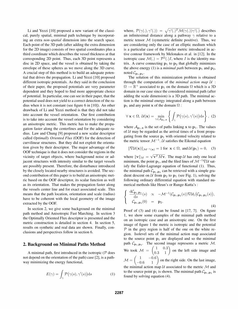
Li and Yezzi [10] proposed a new variant of the classi-cal, purely spatial, minimal path technique by incorporat-ing an extra non-spatial dimension into the search space.Each point of the 3D path (after adding the extra dimensionfor the 2D image) consists of two spatial coordinates plus athird coordinate which describes the vessel thickness at thatcorresponding 2D point. Thus, each 3D point represents adisc in 2D space, and the vessel is obtained by taking theenvelope of these spheres as we move along the 3D curve.A crucial step of this method is to build an adequate poten-tial that drives the propagation. Li and Yezzi [10] proposeddifferent isotropic potentials. As they said in the conclusionof their paper, the proposed potentials are very parameterdependent and they hoped to find more appropriate choiceof potential. In particular, one can see in their paper, that thepotential used does not yield to a correct detection of the ra-dius when it is not constant (see figure 6 in [10]). An otherdrawback of Li and Yezzi method is that they did not takeinto account the vessel orientation. Our first contributionis to take into account the vessel orientation by consideringan anisotropic metric. This metric has to make the propa-gation faster along the centerlines and for the adequate ra-dius. Law and Chung [9] proposed a new scalar descriptorcalled Optimally Oriented Flux (OOF) for the detection ofcurvilinear structures. But they did not exploit the orienta-tion given by their descriptor. The major advantage of theOOF technique is that it does not consider the regions in thevicinity of target objects, where background noise or ad-jacent structures with intensity similar to the target vesselsare possibly present. Therefore, the disturbance introducedby the closely located nearby structures is avoided. The sec-ond contribution of this paper is to build an anisotropic met-ric based on the OOF descriptor, its scalar function as wellas its orientation. That makes the propagation faster alongthe vessels center line and for exact associated scale. Thismeans that the path location, orientation and scale (radius)have to be coherent with the local geometry of the imageextracted by the OOF.

In section 2, we give some background on the minimalpath method and Anisotropic Fast Marching. In section 3the Optimally Oriented Flux descriptor is presented and themetric construction is detailed in section 4. In section 5,results on synthetic and real data are shown. Finally, con-clusions and perspectives follow in section 6.

2. Background on Minimal Paths Method

A minimal path, first introduced in the isotropic (P doesnot depend on the orientation of the path) case [2], is a path-way minimizing the energy functional,

E(γ) =∫

γ

P(γ(s), γ′(s)

)ds (1)

where, P(γ(.), γ′(.)) =√

γ′(.)TM(γ(.))γ′(.) describesan infinitesimal distance along a pathway γ relative to ametric tensor M (symmetric definite positive). Thus, weare considering only the case of an elliptic medium whichis a particular case of the Finsler metric introduced in ac-tive contour framework by Melonakos et al. in [12]. In theisotropic case M(.) = P2(.)I , where I is the identity ma-trix. A curve connecting p1 to p2 that globally minimizesthe above energy (1) is a minimal path between p1 and p2,noted Cp1,p2 .

The solution of this minimization problem is obtainedthrough the computation of the minimal action map U :Ω → R+ associated to p1 on the domain Ω which is a 3Ddomain in our case since the considered minimal path (afteradding the scale dimension) is a 3D path. The minimal ac-tion is the minimal energy integrated along a path betweenp1 and any point x of the domain Ω :

∀ x ∈ Ω, U(x) = minγ∈Ap1,x

∫γ

P(γ(s), γ′(s)

)ds

, (2)

where Ap1,x is the set of paths linking x to p1. The valuesof U may be regarded as the arrival times of a front propa-gating from the source p1 with oriented velocity related tothe metric tensor M−1. U satisfies the Eikonal equation

‖∇U(x)‖M−1(x) = 1 for x ∈ Ω, and U(p1) = 0, (3)

where ‖v‖M =√

vT Mv. The map U has only one localminimum, the point p1, and the filed lines of M−1∇U sat-isfy the Euler-Lagrange equation of functional (1). Thus,the minimal path Cp1,p2 can be retrieved with a simple gra-dient descent on U from p2 to p1 (see Fig. 1), solving thefollowing ordinary differential equation with standard nu-merical methods like Heun’s or Runge-Kutta’s :

dCp1,p2

ds(s) ∝ −M−1(Cp1,p2(s))∇U1

(Cp1,p2(s)

),

Cp1,p2(0) = p2.(4)

Proof of (3) and (4) can be found in [17, 7]. On figure1, we show some examples of the minimal path methodon an isotropic case and an anisotropic one. On the firstimage of figure 1 the metric is isotropic and the potentialP in the grey region is half of the one on the white re-gion. Isolevel sets of the minimal action map associatedto the source point p1 are displayed and so the minimalpath Cp1,p2 . The second image represents a metric M.

We took M =(

1 0.30.3 1

)on the left side image and

M =(

1 −0.6−0.6 1

)on the right side. On the last image,

the minimal action map U associated to the metric M andto the source point p1 is shown. The minimal path Cp1,p2 isfound by solving equation (4).

2287

p1

p2

Figure 1. Minimal path examples on an isotropic case on the firstimage. On the second image, visualization by small ellipses ofeigenvalues of a metric constant on each half side of the image.On the last one, the minimal action map associated to the sourcepoint p1 with the minimal path Cp1,p2 .

The Fast Marching Method (FMM) is a numericalmethod introduced by Sethian in [16] and Tsitsiklis in [18]for efficiently solving the isotropic Eikonal equation on acartesian grid. The central idea behind the FMM is to visitgrid points in an order consistent with the way wavefrontsof constant action propagate. It leads to a single-pass algo-rithm for solving equation (3) and computing the minimalaction map U . Tsitsiklis’s method relies on minimizing di-rectly the energy functional of equation (1) while Sethian’smethod uses the Eikonal equation. Both methods are suit-able for isotropic metric, but they fail for anisotropic metric[1]. To deal with anisotropy, Sethian and Vladimirsky [17]proposed an update scheme that converges to the viscos-ity solution of the anisotropic Eikonal equation. A simpli-fied scheme, based on the original Tsitsiklis’s method [18],was proposed by Lin in [11] to approximate the solution ofthe anisotropic Eikonal equation. Contrary to Sethian andVladimirsky’s ordered upwind method (OUM) [17], Lin’salgorithm does not converge to the viscosity solution ofthe Eikonal equation. In this paper we used Lin’s schemeto solve the anisotropic Eikonal equation, since it is muchfaster than OUM and the introduced errors do not affectmuch the extracted geodesics.

The FMM is a front propagation approach that computesthe values of U in increasing order, and the structure ofthe algorithm is almost identical to Dijkstra’s algorithm forcomputing shortest paths on graphs [4]. In the course of the

algorithm, each grid point is tagged as either Alive (point forwhich U has been computed and frozen), Trial (point forwhich U has been estimated but not frozen) or Far (pointfor which U is unknown). The set of Trial points formsan interface between the set of grid points for which U hasbeen frozen (the Alive points) and the set of other grid points(the Far points). This interface may be regarded as a frontexpanding from the source until every grid point has beenreached. Let us denote by NM(x) the set of M neighbors ofa grid point x, where M = 2 × 3 since the dimension ofΩ is equal to 3. Initially, all grid points are tagged as Far,except the source point p1 that is tagged as Trial with es-timate value 0. At each iteration of the FMM one choosesthe Trial point with the smallest U value, denoted by xmin.Then, xmin is tagged as Alive and the value of U is updatedfor each point of the set NM(xmin) which is either Trial orFar. In order to satisfy a causality condition, the way U isupdated in the vicinity of xmin requires special care. The it-eration ends by tagging every Far point of the setNM(xmin)as Trial. The algorithm (see Table 1) automatically stopswhen all grid points are Alive. The key to the speed of theFMM is the use of a priority queue to quickly find the Trialpoint with the smallest U value. If Trial points are orderedin a min-heap data structure, the computational complexityof the FMM is O(N logN), where N is the total number ofgrid points.

Table 1 : Fast Marching Method for solving equation (3).

• Notation.NM(x) is the set of M neighbors of a grid point x,where M = 6 in 3D.

• Initialization.For each grid point x, do

Set U(x) := +∞.Tag x as Far.

For the source point p1, doSet U(p1) := 0.Tag p1 as Trial.

• Marching loop.While the set of Trial points is non-empty, do

Find xmin, the Trial point with the smallest U value.Tag xmin as Alive.For each point xm ∈ NM(xmin) which is not Alive, do

u :=UpdateScheme`xm,NM(xm)

´(see text).

Set U(xm) := u.If xn is Far, tag xm as Trial.

A crucial step of the Fast Marching algorithm is the com-putation of the weighted distance between the front and theneighbouring voxels in the Trial set. Here, we present away to estimate this weighted distance in the anisotropiccase and only in 3D. Since the distance is anisotropic, wecannot use the standard upwind methods, because they relyon the fact that the geodesics are perpendicular to the levelsets of U . To take into account the anisotropy Jbabdi et al

2288

[7] and Lin [11] considered a set of simplexes that coverthe whole neighborhood around a voxel of the narrow band.The choice they made reduces errors on the obtained mini-mal path but does not guarantee the convergence to the vis-cosity solution of the Eikonal equation. The definition of asimplex neighboring a point x is simply a set of three points(x1,x2,x3) that are among the 26 neighbours of x, defin-ing a triangle1 that we denote x1x2x3. There are 48 suchtriangles around x for the 26 connexity. To make the up-date procedure faster, we propose to consider only the sim-plexes2 defined by a t-uple of three points of the 6-neighborsof x. There are 8 such triangles (see Fig. 2), and by makingthis modification, the precision of the algorithm is lower butthe algorithm is six times faster. To estimate U(xm), in rou-

x1

xm

x3

x⋆

x2

Figure 2. On the left Position of the optimal point on a simplexsuch as to minimize the geodesic distance to x. On the right theconsidered simplexes.

tine UpdateScheme of Table 1, we say that the geodesicpassing by xm comes from a triangle x1x2x3 and then thetime of arrival is given by:

U(xm) = minx∈x1x2x3

U(x) +

∫ xm

x

P (γ, γ′)

(5)

The term one wants to minimize is approximated by :

f(α) =3∑

i=1

αiU(xi) +∥∥∥x− 3∑

i=1

αixi

∥∥∥M(x)

, (6)

where α = (α1, α2, α3), with∑3

i=1 αi = 1 since thepoint x is in the triangle (see figure 2). This equation fol-lows Tsitsiklis’s approximation [18]. The first term approx-imates the value of the minimal action map at the pointx =

∑3i=1 αixi by a simple linear interpolation. And the

second term approximates the remaining distance by con-sidering the metric constant along the segment [x,xm] equalto its value at point xm. The function f is convex and theconstraints on α, i.e

∑3i=1 αi = 1 and αi ≥ 0, define a con-

vex subset. Thus the minimization of f can be done usingclassical optimization tools. See [7] for more details.

For each of the eight triangles, we get a value u. Finally,we choose the triangle giving the smallest value of u. This

1Such that x1 is a 6-connectivity neighbor, x2 is a 18-connectivtyneighbor on the same face as x1, and x3 is a 26-connectivity neighboron the same edge as x2.

2This time, all xi are 6-connectivity neighbors, but on a same face ofthe cube surrounding x, see figure 2.

is the estimate returned by routine UpdateScheme in theFast Marching algorithm described in table 1. Note that inorder to approximate ∇U , computing the derivatives of Uin the triangle using the estimate U(xm) gives a consistentapproximation of ∇U(xm) by the following:

∇U(xm) = (U(xm)− U(x?))xm − x?

‖xm − x?‖,

where x? is the minimizer of function f , see figure 2 left,and ‖.‖ is the Euclidean norm. The computation of the gra-dient is very useful since it is used to solve the gradientdescent described by equation (4).

3. Optimally Oriented Flux : an AnisotropyDescriptor

We are interested in the construction of a metric that ex-tracts from the image the geometric information leading toreconstruction of vessels. This means that we wish to findan estimate for the local orientation and scale and a criterionon the local geometry to distinguish the presence of vesselsfrom the background.

At the position x on a 2D image I , the amount of theimage gradient projected along the axis v flowing out froma 2D circle ∂Dr is measured as in [9],

f(x,v; r) =∫

∂Dr

((∇(G ∗ I(x + h)) · v)v

)· h|h|

da,

(7)where G is a Gaussian function with a scale factor of 1pixel, r is the circle radius, h is the position vector along∂Dr and da is the infinitesimal length on ∂Dr. To de-tect vessels having higher intensity than the background re-gion, one would be interested in finding the vessel directionwhich minimizes f(x,v; r), i.e. we are looking for:

arg minv

f(x,v; r).

Using the divergence theorem, it can be shown thatf(x,v; r) can be calculated using a simple convolution [9],

f(x,v; r) = vT (∂i,jG) ∗ I ∗ 1Dr v, (8)

where (∂i,jG) is the Hessian matrix of function G and 1Dr

is the indicator function of the disc Dr. By differentiatingthe above equation with respect to v, minimization of func-tion f is in turn acquired as solving a generalized eigenvaluedecomposition problem.

Solving the aforementioned generalized eigen decompo-sition problem gives two eigenvalues, λ1(x; r) and λ2(x; r)where λ1(·) ≤ λ2(·) and two eigenvectors v1(x; r) andv2(x; r), i.e. λ1(x; r) = f(x,v1(x; r); r) and λ2(x; r) =f(x,v2(x; r); r). v1 is perpendicular to the vessel direc-tion and v2 is parallel to it when the chosen point x is on

2289

x

x

x

x

Local disc A

Local disc B

Local disc D

Local disc C

Local disc E

x

x

Image gradients

Vesselboundaries

Local discs

Center pixels

Figure 3. Five examples of computing OOF using different radiiat various positions inside a vessel. Local discs A and B have theexact radius of the vessel. Local discs C and E have an undersizedradius and Local disc D has an oversized radius.

the centerline and the scale r is equal to the vessel radius.Along the vessel direction, v2(·), it is obvious that the mag-nitude of the eigenvalue λ2(·) is small inside the vessel asimage gradient magnitudes are minor along the vessel di-rection. Meanwhile, along the first eigenvector v1(·), themagnitudes of λ1(·) varies according to the radius of the lo-cal disc and also the positions where OOF is evaluated. Toillustrate this idea, five examples are presented in Figure 3.

For Local disc A, OOF is computed at the center of thevessel with its exact radius. As the evaluation of equa-tion (7) is grounded on analyzing image gradients along theboundary of the disc, the OOF detection results are onlyinduced when the disc boundary touches the object bound-ary. In equation (7), when r is the vessel radius and the im-age gradients are projected along v1, the projected imagegradients at the contacting positions between the bound-ary of Local disc A and the vessel boundaries are alignedalong the orientation of the disc outward normal h

|h| . Assuch, the contacting positions between the disc boundaryand the boundaries at the both side of the vessel contributeto the computation of equation (7). Consequently, a neg-ative eigenvalue λ1(·) with a large magnitude can be ob-tained.

It is worth mentioning that the magnitudes of λ1(·) forLocal discs B, C, D and E are smaller than that of Localdisc A. For Local disc B, at the contacting positions be-tween the disc boundary and the vessel boundary, the imagegradients that point to the center line of the vessels are notaligned along the disc outward normal. It therefore sup-presses the resultant magnitude of the dot product betweenthe projected image gradient and the disc outward normalin equation (7).

On the other hand, for Local disc C, the disc boundaryand the vessel boundary have only one contacting positionthat restraints the magnitude of λ1(·). It is in contrast tothe case of Local disc A where the disc touches the vesselboundaries on the both sides of the vessel. The Local discD also returns a small magnitude eigenvalue λ1(·) with thereasons similar to those of Local discs B and C. The magni-tude of λ1(·) for Local disc E is insignificant and random asthere is no overlapping between Local disc E and the vesselboundaries. Considering the small magnitudes of the first

Figure 4. The OOF’s eigenvalues computed on a 2D tubular struc-ture. Top row: The synthetic image consists of a 10 pixels radiustube, where the intensity inside the structure is 255 and 0 for thebackground. Additive Gaussian noise with standard deviation 10is added. The second and the third row: The second and the firsteigenvalues extracted by the OOF method using different valuesof r (radii).

eigenvalues in the cases of Local discs B, C, D and E, thefirst eigenvalue of OOF can attain the maximum negativevalue on Local disc A, where OOF is evaluated at the cen-ter of the vessel with its exact radius. Figure 4 shows theOOF’s eigenvalues computed on a synthetic tube. In which,strong detection responses are acquired along the center lineof the tube when OOF is evaluated with the same radius asthe vessel radius (see the sub-image of r = 10 in the bottomrow of Figure 4). At four different positions of the synthetictube (see figure 5a), the computation result of equation (7)using various values of r and different projection axes vare shown in figures 5c-f. As λ2(x; r) = f(x,v2; r), thesefigures clearly demonstrate second eigenvalue of OOF onlyattains its negative maximal at the center of the vessel withits exact radius.

To handle the vessels having various radii, a multi-scaleapproach should be used along with the OOF method.In [9], Law and Chung have proposed to normalize theOOF’s eigenvalues by the sphere surface area when theOOF method is incorporated in a multi-scale approach for3D image volumes. In the 2D case the eigenvalues are nor-malized by the circle perimeter 2πr.

It is important to point out that the flux introduced byLaw and Chung in [9] is completely different than the flux-based approach introduced by Vasilevskiy and Sidiqqi in[19] which is included in a global energy to minimize alongthe shape to find (for tubular structures segmentation), whileour flux is a local feature which allows to define a localmetric in order to minimize a path energy.

4. How to construct the metric?

Li and Yezzi [10] proposed a new variant of the classical,purely spatial, minimal path technique by incorporating an

2290

Figure 5. The plots of the values of f(x,v; r) as a function of projection axis v and radius r, obtained from the synthetic image shown inFigure 4, at four different positions with various radii and projection axes. (a) Four interest positions, denoted as x1, x2, x3 and x4 areshown along with the original synthetic image presented in Figure 4. (b) An illustration regarding the polar coordinate system used fordirection v in (c)-(f). (c)-(f) The plots of the values of f(·) and the corresponding eigenvectors, computed at the four different positionsshown in (a), using various values of r and different projection axes (cos θ sin θ)T .

extra non-spatial dimension into the search space. The cru-cial step of this method is to build an adequate metric thatdrives the propagation. Li and Yezzi [10] proposed differentisotropic potentials. The main drawback, as they mention,is that these potentials are very parameter dependent andthey do not exploit the vessel orientation. Our main con-tribution is to improve Li and Yezzi method by adding toit an anisotropic formulation, and the anisotropic metric isconstructed by extension of the OOF descriptor presentedby Law et al. [9].

The 3D minimal path is found by minimizing the follow-ing energy: ∫

γ

√γ′(s)TM(γ(s))γ′(s)

ds, (9)

where M is the anisotropic metric we want to construct. Itis not natural to consider orientations on the 3rd dimension,i.e. the radii dimension. Thus one can decompose by blockthe metric M as follows:

M(x, r) =(M(x, r) 0

0 Pradius(x, r)

)(10)

where M(x, r) is a 2×2 symmetric definite positive matrixgiving the spatial anisotropy and Pradius(x, r) is the radiuspotential (also strictly positive).

Since the result given by the anisotropic minimal pathmethod is very dependent on the metric, results inherit ad-vantages and drawbacks of the constructed metric, thus weshould be very careful with its construction. First, let usfix conditions on the desired metric. The spatial metric Mhas to be well oriented along the vessel centerline. Andthe radius potential Pradius has to be small for the adequatescale for any point of the image.

√Pradius corresponds to

the inverse speed for the radii dimension. Since M is sym-metric definite positive, we can decompose it as follows:M(.) =

∑2i=1 mi(.)ui(.)ui(.)T , where 0 < m1 ≤ m2 are

the eigenvalues and ui are the associated eigenvectors. Thevelocity of the propagating front along direction ui is equalto 1/

√mi, for i = 1, 2.

As presented in section 3, for a point on the center line ofthe vessel, and when r is equal to the exact vessel scale, theeigenvector v2 is parallel to the vessel, see figure 5. Thusthe associated speed should be higher than the speed alongthe perpendicular direction v1. But the obtained eigenval-ues satisfy λ1 ≤ λ2 and they may be negative. Since themetric M should be positive, we took:

M(.) = eαλ2(.)v1(.)v1(.)T + eαλ1(.)v2(.)v2(.)T , (11)

Pradius(.) = β exp(α

λ1(.) + λ2(.)2

). (12)

The constant α is controlled by an intuitive parame-ter, which is the maximal spatial anisotropy ratio: µ =

maxx,r

exp(αλ2(x, r))exp(αλ1(x, r))

. By choosing the maximal spatial

anisotropy ratio µ, the constant α is fixed. And by doingso, the anisotropy descriptor M becomes contrast invariantbecause the OOF is linear on the image. The parameter βcontrols the radius speed. If Pradius ≤ exp(αλ1) then theFast Marching propagation is faster for the radii than thespatial dimensions. If Pradius ≥ exp(αλ2) then the propaga-tion is slower. One can tune parameter β depending on thetubular structure one wants to extract. If its radius changesa lot then β should be chosen such that the propagation onthe radius dimension is faster. If not, β is chosen such thatthe propagation is less sensitive on the radius dimension.

On figure 6 the constructed metric of figure 4 at somedifferent scales is shown. Since we chose the same colorrange for the visualization, we can see that the directionsare well detected, and that the optimal values are obtainedalong the centerline of the tube when the scale is equal tothe tube radius. For our experiments, we took µ = 10 andβ such that max

(eαλ1

Pradius

)= 5, this means that in the worst

case, the speed along the radii dimension is√

5 times fasterthan the spatial dimensions. We did so, because we wantedour algorithm to be sensitive to the radii dimension.

2291

Figure 6. The constructed metric for different scales r = 1, 5, 10, 15, 20 from left to right. The original image is shown in figure 5 (a), theradius of the structure is equal to 10. We used the same color range for all images, so one can see that the optimal anisotropy is obtainedalong the centerline of the tubular structure when the scale r is equal to the exact radius of the tube. On the top, we show a display ofM(x, r)−1 using small ellipses of eigenvalues. On the bottom, responses of Pradius are shown.

Figure 7. The red cross points are source points given by the user, and the blue ones are end points. On each case the segmented centerlinesare displayed as well as the envelope of the moving discs. We show results on synthetic, medical and aerial images. In the middle, theassociated minimal action map U as well as the 3D minimal path between the two selected points are shown (transparent visualization).

2292

5. Experimental ResultsOur method is minimally interactive. First, the user

has to precise if the desired vessels are darker or brighterthan the background. So, we can consider different crite-ria on the signs of the eigenvalues. Then the scale range[rmin, rmax], which corresponds to the range of radii of thevessel one wants to extract, is given by the user. Finallyfew points are required as source points or end points of theFast Marching algorithm. We used the metric described inthe previous section to find the minimal anisotropic path (asdescribed in section 2) between two or more selected points(see figure 7). For any selected point, the associated radiusis equal to the minimal radius rmin given by the user.

On figure 7, segmentation results on synthetic and realnoisy 2D images are shown. On the first synthetic image,the source point and destination are selected on the center-line. The obtained tube is perfectly detected as well as thecenterline. On the second image, the initial points are notcentered. But the centerline given by our algorithm goesback fast to the real centerline. This makes our algorithmrobust to initialization. The third synthetic image shows thatour approach is robust to scale changing. On the last line offigure 7, segmentation results are shown on real noisy im-ages. Obviously, these early experiments are not sufficient,and we are working on a quantitative comparison of our ap-proach with existing ones like Siddiqi’s [19] and others.

6. ConclusionIn this paper we have proposed a new general method for

tubular structure extraction in 2D images. Our method ex-ploit the orientation of the vessels by using the optimallyoriented flux to construct a multi-resolution anisotropicmetric that extracts from the image the local geometry anddescribes the vessels orientation and scales. Combining thismetric with anisotropic minimal path technique, we wereable to find a complete description of the tubular structure,i.e the centerline as well as the boundary. To summarize,our method is minimally interactive, robust to initialization,scale variations and bifurcations. In the future, we will ex-tend our method to 3D vessels, and we will also work onthe medical validation on coronary arteries.

Acknowledgements

We would like to thank Professor Anthony J. Yezzi for in-teresting discussions. This work was partially supported byANR grant SURF -NT05-2 45825, and from the K S LoFoundation and RGC612308.

References[1] D. L. Chopp. Replacing iterative algorithms with single-pass

algorithms. Proceedings of the National Academy of Sci-

ences of the United States of America, 98(20):10992–10993,2001.

[2] L. D. Cohen and R. Kimmel. Global minimum for activecontour models: a minimal path approach. InternationalJournal of Computer Vision, 24:57–78, 1997.

[3] T. Deschamps and L. Cohen. Fast extraction of minimalpaths in 3D images and applications to virtual endoscopy.Medical Image Analysis, 5(4), Dec. 2001.

[4] E. W. Dijkstra. A note on two problems in connection withgraphs. Numerische Mathematic, 1:269–271, 1959.

[5] J. Duncan and N. Ayache. Medical image analysis: Progressover two decades and the challenges ahead. PAMI, 22(1):85–106, January 2000.

[6] R. F. Frangi, W. J. Niessen, K. L. Vincken, and M. A.Viergever. Multiscale vessel enhancement filtering. pages130–137. Springer-Verlag, 1998.

[7] S. Jbabdi, P. Bellec, R. Toro, J. Daunizeau, M. Pelegrini-Issac, and H. Benali. Accurate anisotropic fast marching fordiffusion-based geodesic tractography. Journal of Biomedi-cal Imaging, 2008(1):1–12, 2008.

[8] K. Krissian. Flux-based anisotropic diffusion applied toenhancement of 3-D angiogram. TMI, 21(11):1440–1442,2002.

[9] M. W. K. Law and A. C. S. Chung. Three dimensionalcurvilinear structure detection using optimally oriented flux.ECCV, 4:368–382, 2008.

[10] H. Li and A. Yezzi. Vessels as 4D curves: Global minimal 4-D paths to extract 3-D tubular surfaces and centerlines. IEEETransactions on Medical Imaging, 26(9):1213–1223, 2007.

[11] Q. Lin. Enhancement, extraction, and visualization of 3Dvolume data. PhD thesis, Linkopings Universitet, 2003.

[12] J. Melonakos, E. Pichon, S. Angenent, and A. Tannenbaum.Finsler active contours. IEEE Trans Pattern Anal Mach In-tell, 30(3):412–423, 2008.

[13] D. L. Pham, C. Xu, and J. L. Prince. Current methods inmedical image segmentation. Annual Review of BiomedicalEngineering, 2(1):315–337, 2000.

[14] W. N. R. Manniesing, M.A. Viergever. Vessel enhancing dif-fusion a scale space representation of vessel structures. Me-dIA, 10(6):815–825, 2006.

[15] Y. Sato, S. Nakajima, N. Shiraga, H. Atsumi1, S. Yoshida,T. Koller, G. Gerig, and R. Kikinis. Three-dimensionalmulti-scale line filter for segmentation and visualization ofcurvilinear structures in medical images. MedIA, 2(2):143–168, 1998.

[16] J. A. Sethian. A fast marching level set for monotonicallyadvancing fronts. Proceedings of the National Academy ofSciences, 93:1591–1595, 1996.

[17] J. A. Sethian and A. Vladimirsky. Fast methods for theeikonal and related hamilton- jacobi equations on unstruc-tured meshes. Proceedings of the National Academy of Sci-ences, 97(11):5699–5703, May 2000.

[18] J. N. Tsitsiklis. Efficient algorithms for globally opti-mal trajectories. IEEE Transactions on Automatic Control,40:1528–1538, 1995.

[19] E. Vasilevskiy and K. Siddiqi. Flux maximizing geometricflows. IEEE TPAMI, 24:1565–1578, 2002.

2293