1

VALIDATION / EVALUATION OF A MODEL

2

Validation or evaluation?

• Treat model as a scientific hypothesis– Hypothesis: does the model imitate the way the real

world functions?

– We want to validate or invalidate hypothesis -validation

• Treat model as engineering tool– The question is how good the tool is

– We want to evaluate the quality of the model

3

The model as a scientific hypothesis

4

• Does the model behave in the same way as the real world for a set of conditions C.– “behaves like”: Each process gives results

similar to measurements (within experimental error)

M behaves like R

for C

hypothesis

5

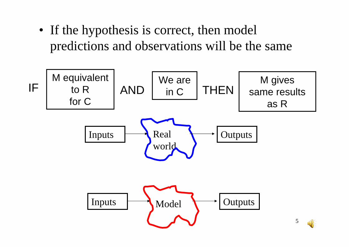
M equivalent to Rfor C

We are in C

M givessame results

as R

IF AND THEN

• If the hypothesis is correct, then model predictions and observations will be the same

Real world

OutputsInputs

Model OutputsInputs

6

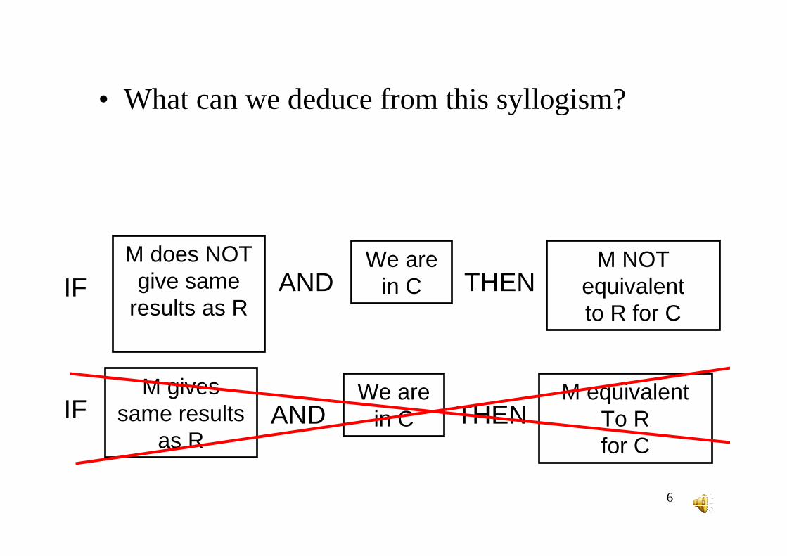
M does NOT give same

results as R

We are in C

M NOT equivalent to R for C

AND THEN

M gives same results

as R

We are in C

M equivalentTo R for C

IF AND THEN

IF

• What can we deduce from this syllogism?

7

• We can invalidate a model

• We cannot validate a model – The model may be right for the wrong reasons

• e. g. even if aphid densities are correct, models of individual processes may e wrong

Real world

OutputsInputs

Model OutputsInputs

8

• Logically, we can’t validate a model

• In any case, we know that all models are false– A model is a simplification of reality

• e.g. aphid-ladybeetle model is extreme simplification, ignores other populations, plant growth, etc. etc. etc.

– It is not meant to be exactly the same as reality

9

So a model as theory is useless?

• NO– Show that unlikely hypotheses are possible

– Show that accepted hypotheses are wrong

– Compare alternative hypotheses

10

Example of comparison of hypotheses

• Respiration of wheat during grain filling. Does the C for respiration come directly from photosynthesis, or from reserves?

11

• Hypothesis 1 : C for respiration comes fromphotosynthesis if possible.

photosynthesis

Grain fill

reserves

respiration1

2

3

12

• Hypothesis 2: C for respiration comes fromreserves

photosynthesis

grain fill

reserves respiration

1

2

13

• Do experiments using pulses of14C markedair. Measure14C concentrations in grain andreserves.

• Develop 2 models, corresponding to above2 hypotheses. Models predict14C concentrations in grain and reserves.

• Model based on hypothesis 1 is more consistent with data.

14

photosynthesis

Grain fill

reserves respiration

1

2

photosynthesis

Grain fill

reserves

respiration1

2

3

15

• Hypothesis 1 is more apt to reproduce observedresults.

• We don’t accept it as exactly true, but as betterworking hypothesis– So this is like engineering model?

– Yes and no. • Yes because we look at how well model reproduces results.

• No because we have drawn conclusions about mechanisms.

Conclusions?

16

Engineering model

17

Evaluation

• We don’t treat the model as a hypothesisbut as a tool.

• We want it to reproduce important aspects of reality (e. g. predict yield, predictresponse to fetilizer)

• How well does model do that? That’s whatwe evaluate.

18

The role of evaluation

• At the start of a modelling project– Define objectives and therefore evaluation

criteria

• During the project– To choose between alternatives, evaluate each– Evaluation may give indication of how to

improve model

• At the end of the project (or of a cycle)– Evaluation provides measure of quality of

model

19

The practice of evaluation

• Compare model to data, measure model quality

• Estimate how well model will predict for new cases

• Evaluation applies to all models. Both simple linear models and complex dynamic system models.– So we can use simple linear models to illustrate

– We will point out specific aspects of dynamic system models

20

Examples of data and models

• Dynamic system models. – We have seen several examples

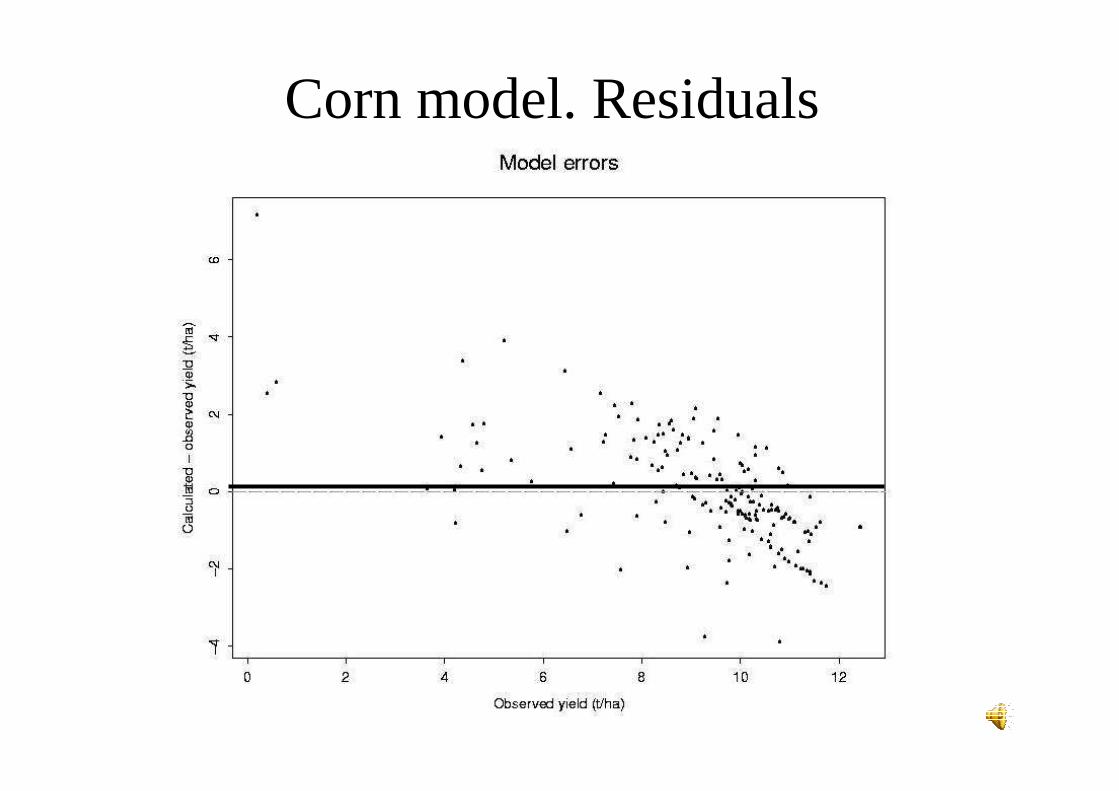
– Dynamic system model for corn. Model is used to compare different irrigation strategies. We don’t present model, just measured and calculated values.

• Static models– Predicting yield in a Polish region. To show that same

problems arise for static and dynamic models.

– An invented example, used to illustrate methods.

21

Spring wheat yield in the Zachodnie Pomorze Province 1970-1998.

22

Rainfall and mean air temperature from March 11 to August 20 in the Zachodnie Pomorze Province 1970-1998.

23

Relationship between spring wheat yield (t.ha-1) in the Zachodnie PomorzeProvince and weather components 1970-1998

Regression equations R2

Till April 30

y = 1.40129 + 0.2396x1 - 0.0448x2+ 0.130222x3- 0.002306x4 67.84

Till May 31

y = 2.25358 + 0,2837x1 - 0.01490x2 + 0.15782x3 - 0.01039x5 - 0.020279x679.31

Till June 30

y = 3.77033 + 0.2557x1-0.01218x2+ 0.13753x3- 0.01265x5- 0.0235x7-0,00273x888.85

Till July 31

y = 3.61260 + 0.02643x1-0.01126x2+0.13129x3-0.01291x5-0.02982x7 + 0.03687x9-0.00215x10 + 0.03107x11 90.5

24

Artificial data and model• Invent formula for generating data. This is « real

world ». Generate sample of 8 data values. Thoseare « measurements ».

• Model has same form (linear model with 5 explanatory variables)

• Use data to estimate model parameters• Estimate 0,2,3,4, or 6 parameters. Others have

default values that are different than true values.

1 1 1 2 2 3 3 4 4 5 5Y x x x x xθ θ θ θ θ θ ε= + + + + + +

1 1 1 2 2 3 3 4 4 5 5ˆ ˆ ˆ ˆ ˆ ˆY x x x x xθ θ θ θ θ θ= + + + + +

25

Data for artificial example

x(1) x(2) x(3) x(4) x(5) Y Y

-1.6339 0.7977 0.4416 -0.4463 -0.4728 -9.3896 -9.3144

-0.9485 1.0700 0.5047 0.5308 -0.3257 -3.2312 -3.0994

-0.2512 0.1952 0.5099 0.8226 0.4495 0.3732 0.7236

0.3789 1.0193 -0.2185 0.8163 -1.9263 7.1024 6.1808

0.1464 1.1373 1.0657 1.6325 -0.5528 5.8245 5.4485

-1.1984 -1.7925 0.3530 -0.2601 0.2617 -11.2130 -11.8425

-0.9720 -0.1533 0.1113 1.1251 0.1019 -5.8110 -5.9035

0.3931 -1.2031 2.0132 -0.7947 -1.4396 2.8158 0.4690

)5()5()4()4()3()3()2()2()1()1()0( *ˆ*ˆ*ˆ*ˆ*ˆˆ)ˆ;( xxxxxXf θθθθθθθ +++++=

26

Graphs

27

Artificial model

Residuals (observed – calculated)

observed value

obse

rved

-pre

dict

ed

-10 -5 0 5

0.0

0.5

1.0

1.5

2.0

Observed values

resi

dual

28

-10 -5 0 5

observed value

-10

-50

5

pred

icte

d va

lue

Observed values

Cal

cula

ted

valu

es

Artificial example

Calculated vs observed values

29

Corn model. Residuals

30

Corn model. Observed vs calculated

31

Measures of error

• Summarize information about differencesbetween measured and calculated values

32

MSE

• Mean Squared Error (the most common measure)

2ˆ(1/ ) ( )1

NMSE N Y Y

i ii

= −∑=

Y

1 1Y Y−

2 2Y Y−

3 3Y Y−4 4Y Y−

resi

dual

s

33

RMSE and MAE

2ˆ( )0.88(t/ha)²

0.94(t/ha)

ˆ0.62(t/ha)

i i

i i

Y YMSE

N

RMSE MSE

Y YMAE

N

−=

=

−=

∑

∑

mean squared error

root mean squared error

mean absolute error

value for exampleequationname

34

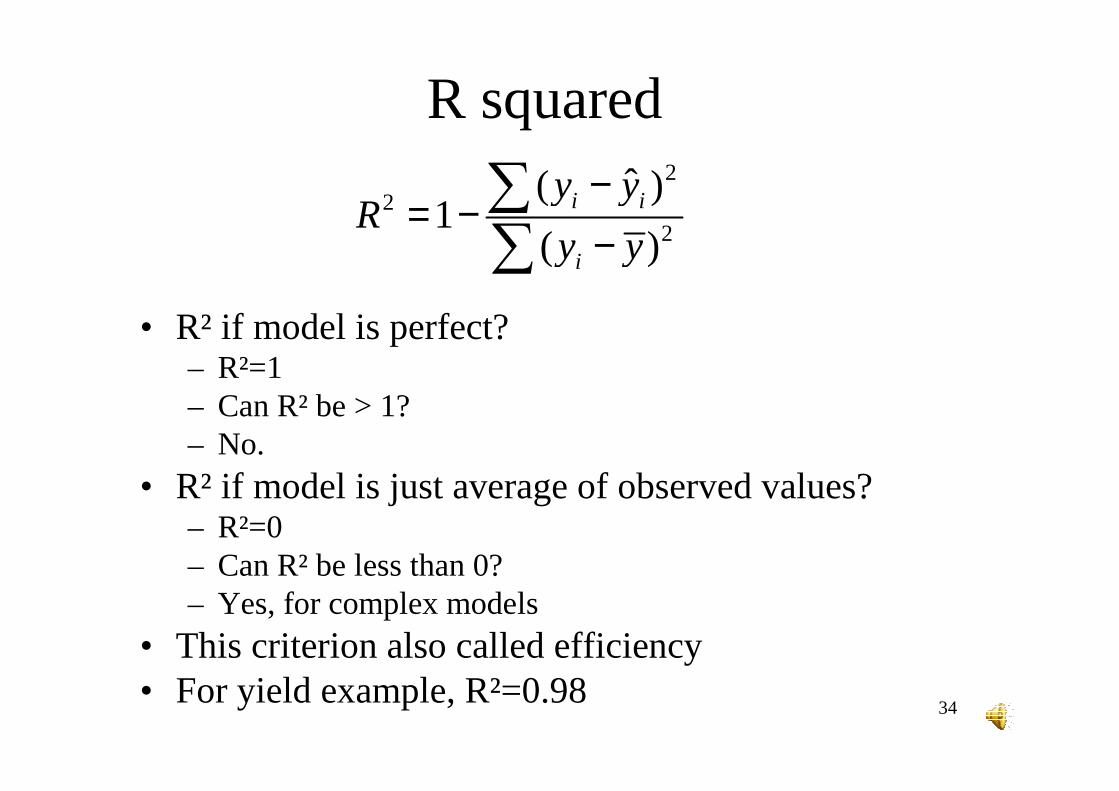
R squared

• R² if model is perfect? – R²=1– Can R² be > 1? – No.

• R² if model is just average of observed values? – R²=0– Can R² be less than 0? – Yes, for complex models

• This criterion also called efficiency• For yield example, R²=0.98

22

2

ˆ( )1

( )i i

i

y yR

y y

−= −

−∑∑

35

R²=1 Yi=Ŷi

R²=0 Yi=Ŷi

Calculated vs. observed Residuals

R² and graphs

36

Components of model error

• To better understand origin of error

• May give ideas of how to improve model

37

Components of MSE

MSE=bias² + variability difference + remainder

38

ˆ( )²bias²

Y Yi iN

−=∑

Small bias Large bias

Bias termresiduals

• If bias is large– Left out or underestimated a factor that systematically

increases or decreases response– For example, underestimated harvest index (relation of

yield to total biomass)– In example, bias²=0.23 (MSE=0.88)

39

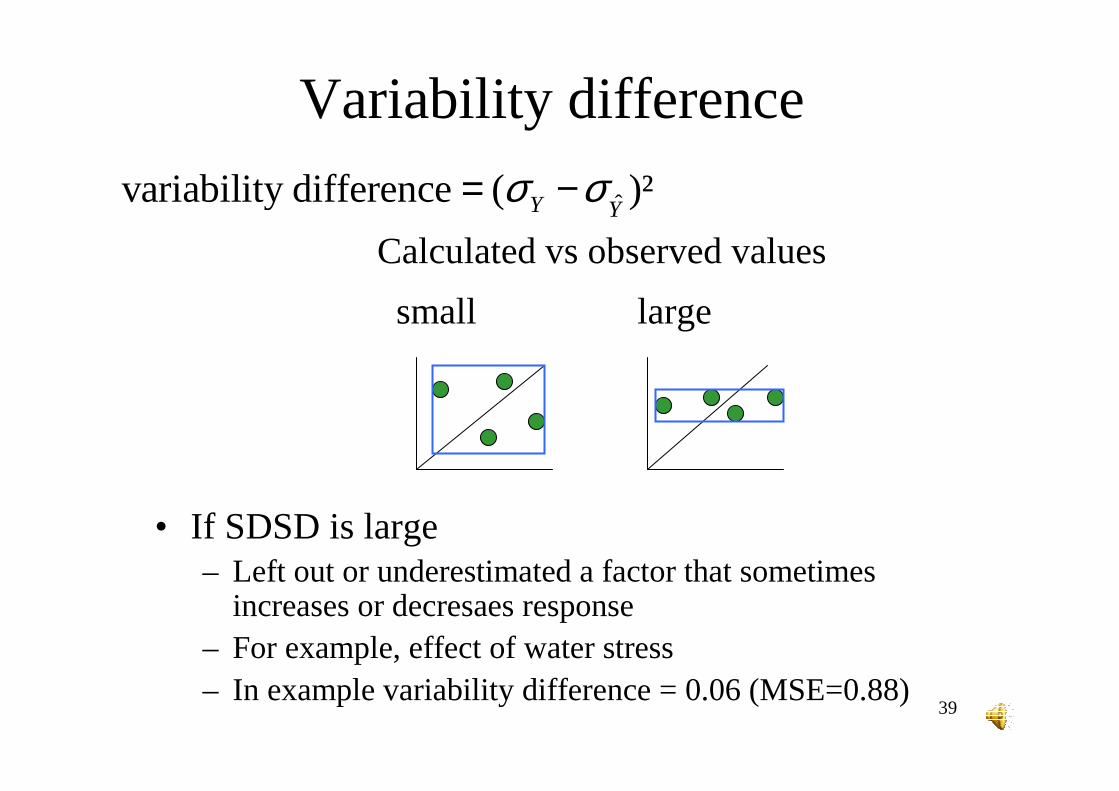
Variability difference

ˆvariability difference ( )²Y Yσ σ= −

small large

Calculated vs observed values

• If SDSD is large– Left out or underestimated a factor that sometimes

increases or decresaes response– For example, effect of water stress– In example variability difference = 0.06 (MSE=0.88)

40

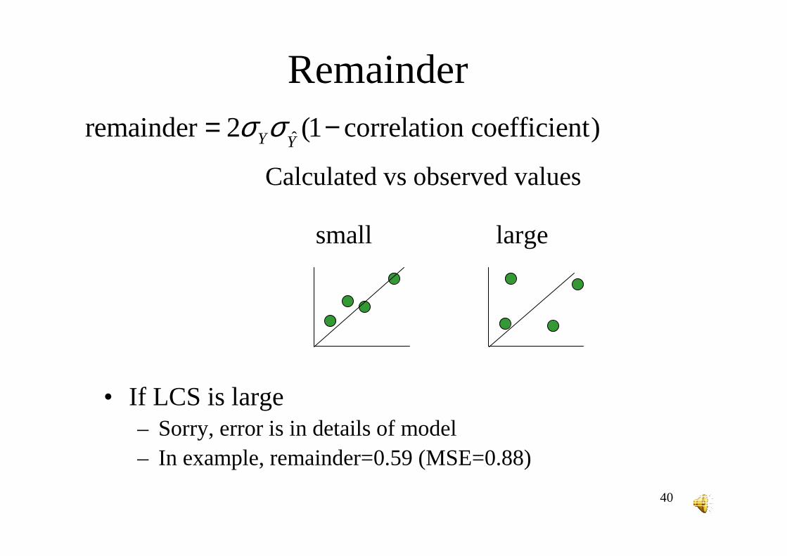
Remainder

ˆremainder 2 (1 correlation coefficient)Y Yσ σ= −

Calculated vs observed values

small large

• If LCS is large– Sorry, error is in details of model– In example, remainder=0.59 (MSE=0.88)

41

Criteria for model comparison

• Can we use criteria we have seen? – Graphs, MSE, R²

42

MSE and R²

• What will be effect of adding extra variables to model, and estimating their parameters, on MSE and R²?– MSE will decrease, R² will increase

– Because adding extra terms allows better fit

– MSE=0.16 (was 0.21)

– R²=0.56 (was 0.45)

43

• Should we add extra variables in this case?• Should we always add extra variables?

– Is a more complex model always better than a simpler model?

– Should we always put all our knowledge of the system into a model?

• The answer is no. Next we explain why. – Note that this implies that MSE and R² are not good for

comparing models of different complexity.

44

Summary to here

• Common methods of evaluation– Graphs

– MSE, R²

• Decomposition of MSE can give indication of source of errors

• MSE and R² are not suited for comparing models of different complexity

45

EVALUATING PREDICTIONS

46

• Often, the goal is to predict for different situations– Could be future (prediction) or could be past (unobserved

situations)– So we need to compare prediction errors of models. That is topic

of this section. – (In other cases, we are interested in using a model to make

decisions. In that case, we need to compare the qualityofdecisions based on different models. That is another lecture).

• In this case we are not really interested in MSE or R²perse.– We have data, don’t need model for those situations– We would be interested in MSE if it gave information about

predictions. Does it?

47

• First, define prediction quality

48

Prediction for what situations?

• Define target population = situations wherewe want to use model.– For model of animal metabolism rate, random

selection of animals (of given race, age).

– Corn yield in southwestern France. Randomfields in region, random climate for region, certain management practices

49

Prediction of what variables?

• Prediction quality depends on what wepredict. Define target variables. – e. g. Aphid-ladybeetle model may have

different error for prey population in margins, aphid population in wheat, ladybeetlepopulation, total predation, etc.

50

A criterion of prediction error

–A common measure of predictionerror is MSEP=mean squared errorof prediction.

–Expectation over target population. Y is target variable.

( ) 2ˆMSEP E Y Y = −

Y

51

The difference MSE, MSEP

• MSE is adjustment error (based on measurements)

• MSEP is prediction error (for full target population)

target population

measurements

2

1

2ˆ

ˆ(1/ ) ( )N

i ii

MSEP E Y Y

MSE N Y Y

=

= −

= −∑

52

• The difference between MSE and MSEP is very important.– Conceptually.

– Practically. MSE and MSEP can be very different.

53

Estimate value of MSEP

• MSEP measures average squared error over target population. At best, we only have measurements for a sample.

• How can we measure MSEP?– We can’t

• How can we estimate MSEP? – Based on measurements (no other choice)

54

2

1

2ˆ

ˆ(1/ ) ( )N

i ii

MSEP E Y Y

MSE N Y Y

=

= −

= −∑

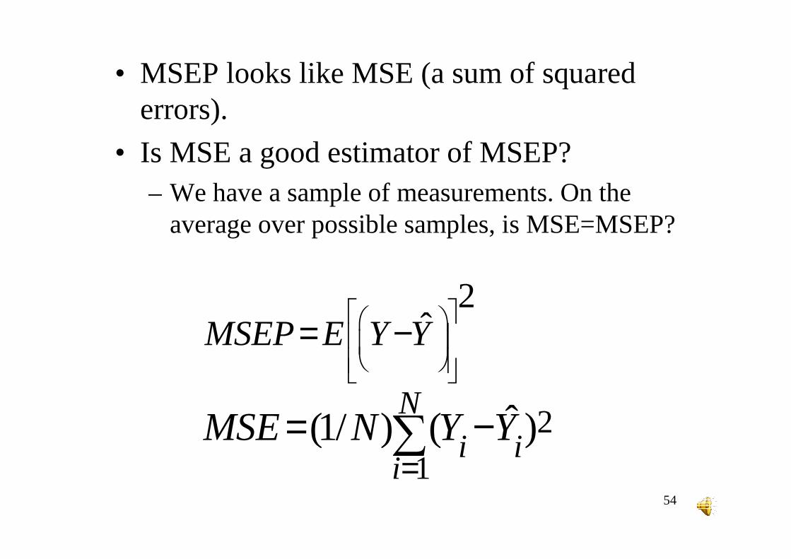
• MSEP looks like MSE (a sum of squared errors).

• Is MSE a good estimator of MSEP? – We have a sample of measurements. On the

average over possible samples, is MSE=MSEP?

55

MSE estimates MSEP if…

• Our measurements are representative of the targetpopulation

• The measurements weren’t used to develop the model • Often, measurements used to estimate parameter values• But could also be used to choose form of function etc.

56

Representative sample

• If data are not representative of target population, of course MSE is not a good measure of MSEP

57

• Insure by random sampling– For complex systems, random sampling may

not be possible. • e.g. agronomy experiments at field stations, not

farmer fields.

– With many explanatory variables, even random sample may not be representative

• e.g. climate. With only a few years sampled, hard to say if this is representative sample.

58

If sample from target population unavailable

• Can estimate error in each part off model, and use model to get overall error– In particular, parameter error

– If we know possible distribution of parametervalues, run model to get distribution of responses

• See uncertainty analysis, Bayesian estimation

59

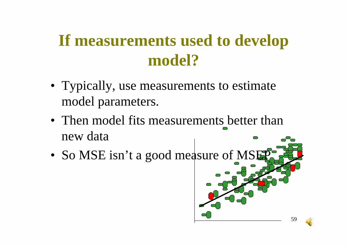
If measurements used to developmodel?

• Typically, use measurements to estimatemodel parameters.

• Then model fits measurements better thannew data

• So MSE isn’t a good measure of MSEP

60

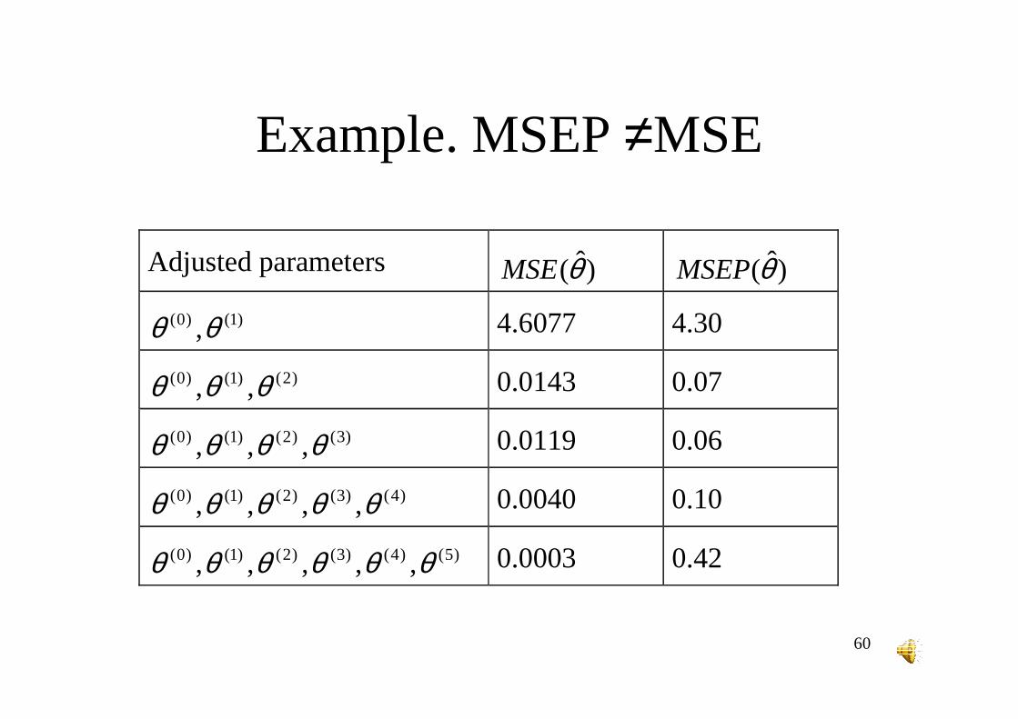
Adjusted parameters )ˆ(θMSE )ˆ(θMSEP

)1()0( ,θθ 4.6077 4.30

)2()1()0( ,, θθθ 0.0143 0.07

)3()2()1()0( ,,, θθθθ 0.0119 0.06

)4()3()2()1()0( ,,,, θθθθθ 0.0040 0.10

)5()4()3()2()1()0( ,,,,, θθθθθθ 0.0003 0.42

Example. MSEP ≠MSE

61

Conclusions about MSE and MSEP

MSEP≠MSEFor large p/n, MSEP>>MSEMSE always decreases as model complexity increasesMSEP has a minimum for somenumber of parameters

62

How can we estimate MSEP if data is used in model development?

• This is important practical question

• We need estimate of error

63

Data splitting

64

All data

Part of data to estimate parameters

Apply model to rest of data. Can we use fit to

estimate MSEP?

same model

65

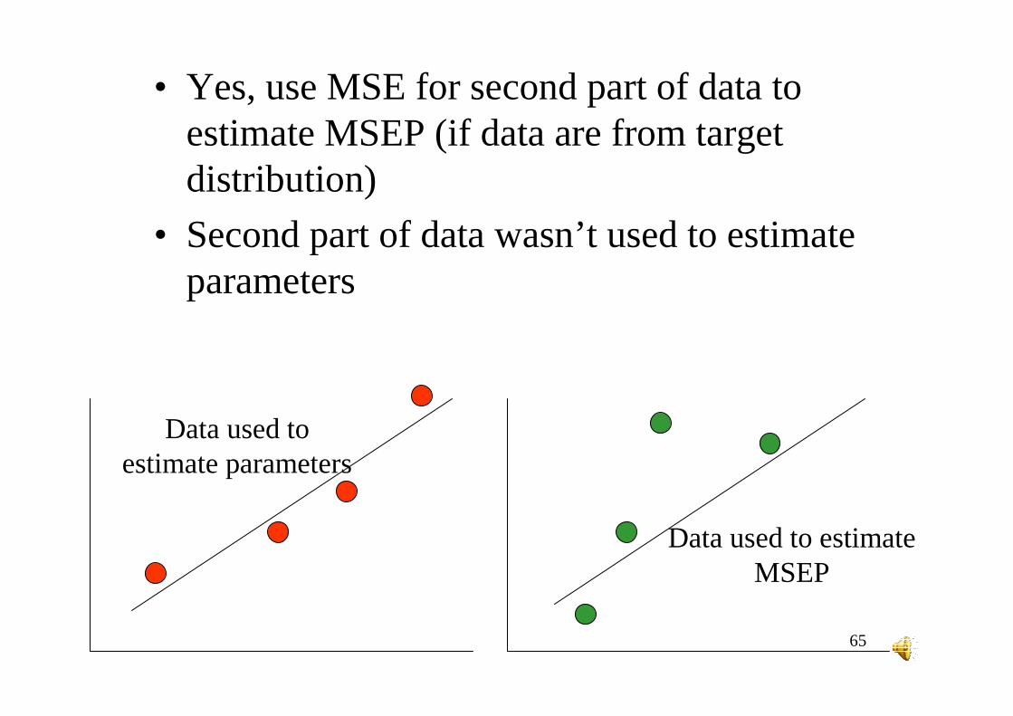
• Yes, use MSE for second part of data to estimate MSEP (if data are from target distribution)

• Second part of data wasn’t used to estimate parameters

Data used to estimate parameters

Data used to estimate MSEP

66

Data used to estimate parameters

Data used to estimate MSEP

• What are disadvantages of data splitting?– Arbitrary division of data into two parts

– Use only part of data to estimate parameters

– Use only part of data to estimate MSEP

67

Other strategy

• Use all data to estimate parameters, then data splitting to estimate MSEP

68

Proposed parameters based on all data

Estimate of MSEP based on data splitting

69

• What do you think of that?• We want two things: parameter estimates

for model and estimate of MSEP. • This way, get best parameter estimates (use

all data)• And MSEP is correctly estimated.

– The only problem is that MSEP refers to model based on half the data.

– This probably overestimates MSEP for model based on all data.

70

Other strategy• As above, but do data splitting twice. Then use

average MSEP.

Model based on these data

Model based on these data

Estimate MSEP using these data

Estimate MSEP using these data

71

• What do you think of that?

• Less arbitrary – But split into two groups is still arbitrary

• Use all data to estimate MSEP

• But model for calculating MSEP isn’t model that is proposed.

• Could we do better?

72

Cross validation

• Similar to above ideas.

73

Develop model using only green data. Estimate MSEP using red data. (Estimate is squared error)

For N data values, repeat N times. Final estimate of MSEP is average of N MSEP estimates.

74

Y1 Y2 Y3 ……. YN Y1-f-1(U1)

Y1 Y2 Y3 ……. YN Y2-f-2(U2)

Y1 Y2 Y3 ……. YN YN-f-N(UN)

$ / ( )MSEP n Y f Ui i i= − −∑12

Calculation with cross validation

75

• What do you think of that?

• Proposed model based on all data.

• Evaluation based on model that uses all data but 1. So should be close to proposedmodel.

76

Decompose MSEP

77

• MSEP can be written as the sum of twoterms

• To help understand what determinespredictive quality

78

Y

X

First term

• Model has some explanatory variables

• They do not explain all the variability in Y– e.g. Temp, geometry, initial values don’t

explain all aphid-ladybeetle dynamics

• What is relation between unexplained variability and MSEP?

79

• For each value of explanatory variables X, model has unique prediction. Can’t be exact for all

• What is best possible model?

Y

X

80

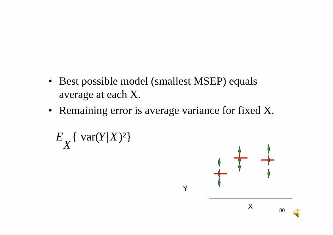
• Best possible model (smallest MSEP) equals average at each X.

• Remaining error is average variance for fixed X.

Y

X

{ var( | )²}E Y XX

81

• Average variance for fixed X is lower limit for MSEP. Just depends on choice of explanatory variables.

• What is effect of adding more explanatory variables (more detailed model)?– Adding explanatory variables always reduces

average variance for fixed X. – But some explanatory variables are important,

others less important or irrelevent.

• What is second term in MSEP?

82

Second contribution to MSEP

ˆ { [ ( | ) - ( )]²}E E Y X Y XX Y

Y

X

• Actual model will not be best model– Equations not exactly “correct”.

– Parameters not exactly “correct”.

• Second term, model error for fixed X, measures difference between actual model and best model .

error

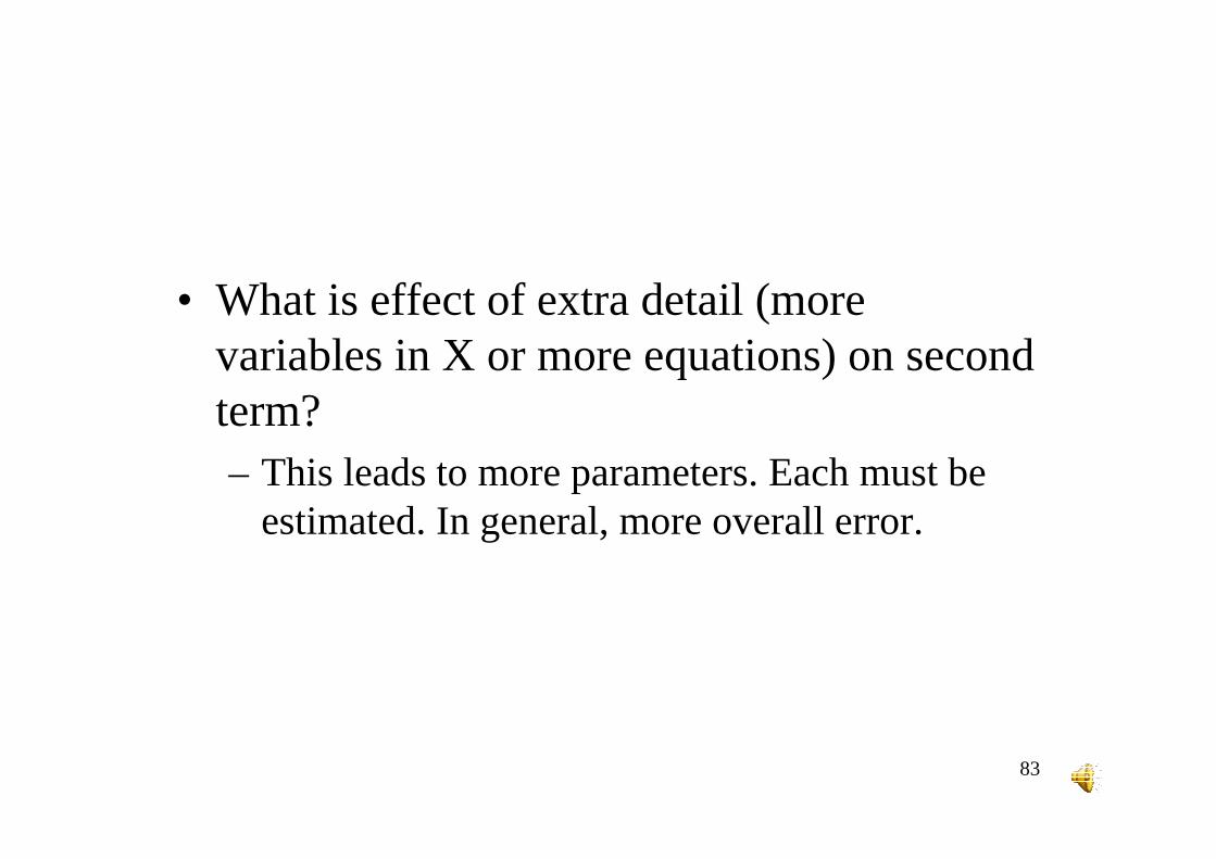
83

• What is effect of extra detail (more variables in X or more equations) on second term?– This leads to more parameters. Each must be

estimated. In general, more overall error.

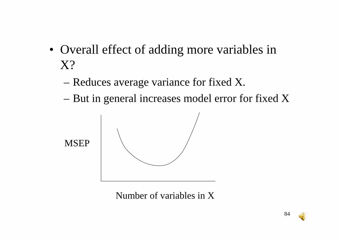
84

• Overall effect of adding more variables in X?– Reduces average variance for fixed X.

– But in general increases model error for fixed X

MSEP

Number of variables in X

85

• What is good strategy?– Add important variables, that reduces average

variance for fixed X a lot.– Don’t add unimportant variables.– Appropriate model complexity will depend on

amount of data for estimating parameters. – This is particularly important for dynamic

system models, where very complex models are possible

86

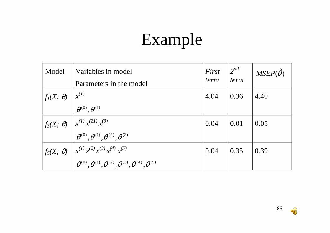
Model Variables in model

Parameters in the model

First term

2nd term

)ˆ(θMSEP

f1(X; θ) x(1)

)1()0( ,θθ

4.04 0.36 4.40

f3(X; θ) x(1) x(21) x(3)

)3()2()1()0( ,,, θθθθ

0.04 0.01 0.05

f5(X; θ) x(1) x(2) x(3) x(4) x(5)

)5()4()3()2()1()0( ,,,,, θθθθθθ

0.04 0.35 0.39

Example

87

Summary• Common criterion of prediction error is MSEP

– Specify target population, target variables

• MSE is not in general a good estimator of MSEP– In particular if measured sample is not representative of

target population, or if sample is used for parameter estimation

– The difference between MSE and MSE depends on p/n

• MSEP is the result of two contributions– Variation due to fact that explanatory variables don’t

explain all variability– Differences between model and best model

• MSEP has a minimum for some intermediate level of complexity

88

Evaluating decisions based on a model

• Not exactly the same as a good model for prediction.

• See David Makowski lecture.

89

THE END

90

References for examples

• Gent, M. P. N., 1994, PhotosynthateReserves during Grain Filling in Winter Wheat, Agron J 86:159-167

• Michalska, B. and Witos, A. 2000. Weather-based spring wheat yielding forecasting. EJPAU online. http://www.ejpau.media.pl/volume3/issue2/agronomy/art-04.html