EU-ClueScanner100m; model description and validation results
91
Commissioned by: European Commission JRC Project reference: IES/H/2008/01/11/NC EU-ClueScanner100m; model description and validation results
-
Upload
independent -
Category
Documents
-
view
3 -
download
0
Transcript of EU-ClueScanner100m; model description and validation results

Commissioned by:
European Commission JRC Project reference: IES/H/2008/01/11/NC
EU-ClueScanner100m; model description and validation results

Authors Eric Koomen, Vasco Diogo, Maarten Hilferink, Martin van der Beek Date July 16, 2010 Version 1.0 Status External document Reference VU FEWEB/RE
VU University Amsterdam
www.feweb.vu.nl/gis

Report EU-ClueScanner tutorial Reference FEWEB/RE
3 / 91
Table of contents
1 Introduction .................................................................................................................. 5
1.1 The EU-ClueScanner in a multi-model framework ........................................................ 5
1.2 Main model components................................................................................................ 6
1.3 DG environment application with 1km resolution .......................................................... 8
1.4 JRC application with 100m resolution ......................................................................... 10
1.5 Getting started ............................................................................................................. 15
2 Viewing existing policy alternatives ........................................................................ 19
2.1 Tree view and main GUI elements .............................................................................. 19
2.2 Land-use data.............................................................................................................. 21
2.3 Factor data................................................................................................................... 22
2.4 Demand ....................................................................................................................... 22
2.5 Runs............................................................................................................................. 22
2.6 Indicators ..................................................................................................................... 23
3 Defining new policy alternatives .............................................................................. 27
3.1 Replacing spatial data sets.......................................................................................... 29
3.2 Editing current demand specification........................................................................... 29
3.3 Combining existing scenario components ................................................................... 30
3.4 Adding a new demand specification ............................................................................ 32
3.5 Adding new spatial data sets ....................................................................................... 35
4 Adjusting the EU-ClueScanner model ..................................................................... 37
4.1 Replacing land-use base data ..................................................................................... 37
4.2 Revise calibration ........................................................................................................ 38
4.3 Edit or add indicator definitions.................................................................................... 39
4.4 Link EU-ClueScanner to other models ........................................................................ 39
4.5 Adjust land-use typology.............................................................................................. 40
5 Validating the JRC version at 100m resolution ...................................................... 41
5.1 Validation methodology ............................................................................................... 41
5.2 Validation results ......................................................................................................... 42
5.3 Conclusion ................................................................................................................... 45
Appendix 1 Overview of original CLC2000 classes.................................................................... 47
Appendix 2 Overview of spatial data sets ................................................................................... 48
Appendix 3 Spatial data set format details.................................................................................. 51
Appendix 4 Model specification files ........................................................................................... 53
Appendix 5 Calibration steps........................................................................................................ 63
Appendix 6 Observed land-use change....................................................................................... 65
Appendix 7 Validation results....................................................................................................... 88
References ..................................................................................................................................... 90

Report EU-ClueScanner tutorial Reference FEWEB/RE
4 / 91

Report EU-ClueScanner tutorial Reference FEWEB/RE
5 / 91
1 Introduction
The EU-ClueScanner model is part of a multi-model framework that aims to produce policy-relevant information related to land-use change. It can support the creation of ex-ante assessments of policies that impact spatial developments. The framework is thus relevant to many different DGs of the Commission to help answer questions such as: what spatial developments are likely to occur in the coming decades? what possible impacts would a foreseen policy have on land-use patterns in Europe and how will these affect issues such as biodiversity for instance? how will specific environmental protection policies and/or climate change adaptation measures influence spatial patterns? The final report documenting the development of the EU-ClueScanner model discusses the initial applications of the model for DG Environment to answer this type of questions (Perez-Soba et al., 2010). The purpose of this report is to help those who will operate the EU-ClueScanner get started with the model. In addition it will explain the basic functionalities of the model and specify how specific components of the model can be adjusted to define new policy alternatives. The tutorial also points at relevant documents for background information and more advanced manipulation of the model. This first chapter provides an initial introduction to the model in general and the applications for DG Environment and Joint Research Centre (JRC) in particular. It helps users getting started with the model and describes the most important model components. Chapter 2 describes how existing policy alternatives can be viewed and explains the main elements of the graphical user interface (GUI). It discusses how various types of data can be viewed, how the calculation process can be traced and how land-use results and indicator values can be retrieved. Chapter 3 helps the user to define new policy alternatives. First through describing relative simple operations, such as the replacing of spatial data sets and the editing of the current demand specification, and then by highlighting more complex modelling tasks such as the manipulation of basic simulation settings. Chapter 4 briefly discusses how possible improvements can be made to the EU-ClueScanner model. Chapter 5 describes the validation of the 100m version of the model that was performed especially for EC-JRC. The appendices at the end of this tutorial contain in-depth information on various model elements and include amongst others, an overview of the basic land-use classes and included spatial data sets.
1.1 The EU-ClueScanner in a multi-model framework
The EU-ClueScanner is a land allocation model positioned at the heart of a multi-scale, multi-model, framework. It bridges sector models and indicator models and connects Global and European scale analysis to the local level of environmental impacts, see Figure 1. External, global models account for interactions between Europe and other world regions. The dynamics of the global economy are typically described by GTAP or derived LEITAP model, whereas global climate-land use interactions are incorporated in an integrated assessment model (IMAGE). This configuration was used in the EURURALIS project (Eickhout et al., 2007; Van Meijl et al., 2006) and the applications created for the DG Environment. Results from the global level models relate to the demand for goods and commodities and are, in Europe, delivered at Member State level. The output of the global-level models is translated into a land demand in km
2 for the specific land-use types distinguished in the EU-ClueScanner model.
This translation is performed in a newly developed demand module that is implemented in the GeoDMS model script and thus part of the EU-ClueScanner model.

Report EU-ClueScanner tutorial Reference FEWEB/RE
6 / 91
Land allocation in the EU-ClueScanner model is based on the approach taken in the well-known Dyna-CLUE model (Verburg et al., 2006; Verburg and Overmars, 2009). Especially for DG Environment this approach has now been programmed in the GeoDMS environment using the numerical algorithm of the Land Use Scanner model to optimize its performance for use on desktop computers. The Land Use Scanner is another well-established land use model with many applications within Europe (Dekkers and Koomen, 2007; Koomen et al., 2008). Combining the strengths of both models ensures a consistent, state-of-the-art and flexible modelling core. In addition, a series of indicator models corresponding to the demands of the policy alternatives are implemented. Indicator models use information derived from economic models (e.g. LEITAP) and the land allocation models to arrive at a balanced set of indicators focussing on the land-use and environmental domains. To assess specific issues (such as, for example, flood risk) additional detailed spatial data sets are used in the implemented indicators. Another interesting option for many ex-ante assessments is the possibility to link the pan-European analysis at 1 km
2 resolution
to more detailed models for specific case studies that either focus on specific regions or on specific policy domains.
Figure 1 The EU-ClueScanner as the the core of a multi model framework.
1.2 Main model components
The EU-ClueScanner model has the following main components: - a demand module that specifies the amount of land that has to be allocated per land-use
type, normally following scenario conditions; - location specific characteristics (locspecs) that influence the suitability of a location for a
land-use type, typically reflecting scenario-specific restrictions or stimulating policies that are added to the statistically derived suitability definition;
- conversion settings that specify which land-use conversions are allowed and, optionally,
Graphical
User Interface
Demand module
(meta-model integrating sector-specific goods and commodities demand into national-level land demand)
Land allocation module
(Dyna-CLUE implementation in GeoDMS environment)
Indicator models (meta-models/ simple models)
Complex indicator models (needed for specific policy cases)
External models
LEITAP (Global Economy Model) / IMAGE(Global Environment)
EU
-Clu
eS
ca
nn
er
mo
de
l
Spatial databaseGraphical
User Interface
Demand module
(meta-model integrating sector-specific goods and commodities demand into national-level land demand)
Land allocation module
(Dyna-CLUE implementation in GeoDMS environment)
Indicator models (meta-models/ simple models)
Complex indicator models (needed for specific policy cases)
External models
LEITAP (Global Economy Model) / IMAGE(Global Environment)
EU
-Clu
eS
ca
nn
er
mo
de
l
Spatial database
Report EU-ClueScanner tutorial Reference FEWEB/RE
7 / 91
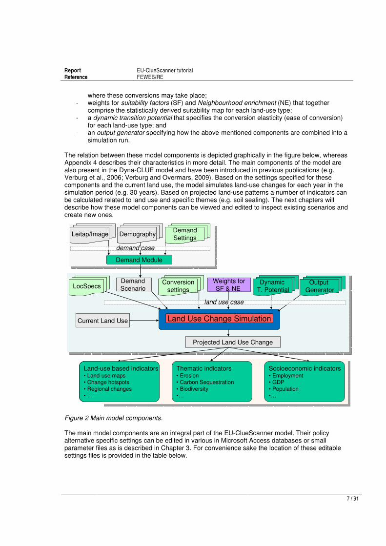
where these conversions may take place; - weights for suitability factors (SF) and Neighbourhood enrichment (NE) that together
comprise the statistically derived suitability map for each land-use type; - a dynamic transition potential that specifies the conversion elasticity (ease of conversion)
for each land-use type; and - an output generator specifying how the above-mentioned components are combined into a
simulation run. The relation between these model components is depicted graphically in the figure below, whereas Appendix 4 describes their characteristics in more detail. The main components of the model are also present in the Dyna-CLUE model and have been introduced in previous publications (e.g. Verburg et al., 2006; Verburg and Overmars, 2009). Based on the settings specified for these components and the current land use, the model simulates land-use changes for each year in the simulation period (e.g. 30 years). Based on projected land-use patterns a number of indicators can be calculated related to land use and specific themes (e.g. soil sealing). The next chapters will describe how these model components can be viewed and edited to inspect existing scenarios and create new ones.
Figure 2 Main model components. The main model components are an integral part of the EU-ClueScanner model. Their policy alternative specific settings can be edited in various in Microsoft Access databases or small parameter files as is described in Chapter 3. For convenience sake the location of these editable settings files is provided in the table below.
Projected Land Use Change
Demand Module
Demand
Scenario Weights for
SF & NE
demand case
land use case
Land-use based indicators• Land-use maps• Change hotspots
• Regional changes• …
Leitap/Image DemographyDemand
Settings
Conversion
settings
Dynamic
T. PotentialOutput
Generator
Land Use Change Simulation
Thematic indicators• Erosion• Carbon Sequestration
• Biodiversity•…
Current Land Use
LocSpecs
Socioeconomic indicators• Employment• GDP
• Population•…

Report EU-ClueScanner tutorial Reference FEWEB/RE
8 / 91
Table 1 Location of main model components in the EU-ClueScanner 100m version. Appendix 4 describes most of the files mentioned below in more detail.
Component Editable settings files and their storage location1
Demand module Demand.mdb in projects\EuClueScanner\data\demand normally specifies how the demand should be calculated per land per year; the results of these calculations are stored in demand.in1 files in the \projects\EuClueScanner\Demand\ PolicyAlternativeName (e.g. Validation2000MNL)\CountryName folder
Locspecs LocspecX.asc (when present) in \projects\EuClueScanner\Paramsets\ PolicyAlternativeName. Note that these are currently not used in the100m version.
Conversion settings Main.1 in \projects\EuClueScanner\Paramsets\PolicyAlternativeName2 (e.g.
ReferenceJRC) specifies, amongst other basic model settings, a land-use type specific conversion elasticity (resistance to transition). Allow.txt in \projects\EuClueScanner\Paramsets\PolicyAlternativeName
2 defines
which transitions are allowed; this definition can be location specific by referring to spatially-explicit allow driver maps (e.g. X1.tif) stored in \SourceData\ EuClueScanner\Drivers
Weights for suitability factors (SF) and neighbourhood enrichment (NE)
Alloc1.reg and alloc2.reg in \projects\EuClueScanner\Paramsets\ PolicyAlternativeName\CountryName specify the results of the statistical calibration of the model. The relative weight of each of these components in defining local suitability is specified in the neighmat.txt file in \projects\EuClueScanner\Paramsets\PolicyAlternativeName
Dynamic transition potential
Main.1 in \projects\EuClueScanner\Paramsets\PolicyAlternativeName2, this file
may refer to spatially explicit dynamic driver maps (e.g. sc1gr33.1) that describe changing conditions over time. These maps are stored in \SourceData\EuClueScanner\DynamicDrivers
Output generator Part of a crucial land-use allocation GeoDMS script (\Projects\EuClueScanner\cfg\ Default\JrcClueWrap.dms) that determines which intermediate results of the simulation should be processed and how this should be done..
Notes: 1Please note the JRC-model model version still contains reference to elements of the 1km version. So for
specific elements of that model version (e.g. the location of model components) it may be wise to also consult the tutorial related to the 1km application developed for DG Environment. 2The main.1 and other parameters files are normally stored in the policy-alternative folder, but when country-
specific conditions apply they can also be placed in country-specific folders. The model will first look in these folder and the country-specific settings will then apply.
1.3 DG environment application with 1km resolution
The EU-ClueScanner model is a very flexible environment that allows the construction of many different applications. These applications can differ on the initial land use that is used as starting point for simulation, the land-use types that are simulated, the demand that is specified for each type of land use, the location characteristics that are included and other model-specific setting relating to, for example, the possible conversions of specific land-use types. This section lists the most important characteristics of the EU-ClueScanner application developed for DG Environment. It specifies the included land-use typology and included policy alternatives.
Thematic resolution
The Corine Land Cover database for the year 2000 (CLC2000) was selected as base data for the DG Environment application as it is the most recent, consistently developed and available pan-European source of land-use related information. The CLC2000 data was aggregated to a 1km
2
spatial resolution representing 18 main land-use types for inclusion in the land-use model. Table 2 describes the thematic integration of the initial land-cover classes in CLC2000 to this set of 18 main classes. The table, furthermore, lists for which land-use types future patterns are simulated. For the remaining land-use types the location is kept stable.

Report EU-ClueScanner tutorial Reference FEWEB/RE
9 / 91
Although the CLC data technically refer to land cover we use the more common term ‘land use’ in this report as it better corresponds to phenomena such as abandoned farmland that are simulated by the model. The latter type of land use, for example, allows for the simulation of forest regeneration and is not based on the CLC data. It arises from simulation when agricultural demand is insufficient to maintain agricultural use. Based on the conversion settings specific locations may develop into semi-natural vegetation (3) or forest (10). Table 2 Thematic resolution of the model and their relation with the Corine Land Cover types.
Nr.1 CLC (main) class
2 Description Simulated
3
0 1.1/1.2/1.3/1.4 Built-up area Yes (0) 1 2.1.1/2.4.2p(50%)/
2.4.3p(25%) Arable land (non-irrigated) Yes (1)
2 2.3/ 2.4.2p(50%)/ 2.4.3p (45%)
Pasture Yes (2)
3 3.2.1/3.2.3/ 3.2.4/2.4.3p (30%)
(semi-) Natural vegetation (including natural grasslands, scrublands, regenerating forest below 2 m, and small forest patches within agricultural landscapes)
Yes (3)
4 4.1 Inland wetlands No (9) 5 3.3.5 Glaciers and snow No (9) 6 2.1.2/2.1.3 Irrigated arable land No (4) 7 New Recently abandoned arable land (i.e. “long fallow”; includes
very extensive farmland not reported in agricultural statistics, herbaceous vegetation, grasses and shrubs below 30 cm)
Yes (5)
8 2.2/2.4.1/2.4.4 Permanent crops Yes (6) 10 3.1 Forest Yes (7) 11 3.3.2/ 3.3.3/3.3.4 Sparsely vegetated areas No (9) 12 3.3.1 Beaches, dunes and sands No (9) 13 4.2.2 Salines No (9) 14 4.1/4.2.1/4.2.3/
5.1/5.2 Water and coastal flats No (9)
15 3.2.2 Heather and moorlands No (9) 16 New Recently abandoned pasture land (includes very extensive
pasture land not reported in agricultural statistics, grasses and shrubs below 30cm)
Yes (8)
Notes: 1This column shows the individual land-use types distinguished in the DG Environment application. Please
note that the model can contain up to 18 classes depending on its application, but in this case 16 land-use types are distinguished (the numbers 9 and 17 are not present in this model version). 2For reference purposes the corresponding (main) land-cover classes from the CLC2000 dataset are shown.
See Appendix 1 for a complete overview of these land cover classes. The ‘p’ after certain CLC-classes denotes that only part of it is assigned to the DG Environment class. This partial assignment has been done randomly according to the mentioned probabilities. So each cell with CLC type 2.4.2 (representing complex cultivation patterns) has a probability of 50% to be classified as arable land and a probability of 50% to be classified as pasture. A random selection was chosen as that corresponds well with actual land-use patterns that can be observed from aerial photographs. 3The numbers between brackets refer to the coding generally used within the model (referred to as Clue10).
Policy alternatives
European policies can be relevant for land use change in two ways. First, there is a group of policies that influences the demand for land, e.g. stimulation of different types of agriculture through the Common Agricultural Policy. A second group of policies influence land-use configurations, for example by excluding or favouring some regions for a specific type of land use. For the development of these policy alternatives one future scenario is selected as reference: the Global Co-operation (B1) scenario. This well-known scenario originating from the IPCC-SRES framework sketches the climatic and socio-economic boundary conditions within which the policy alternatives are developed.

Report EU-ClueScanner tutorial Reference FEWEB/RE
10 / 91
Within the DG Environment application seven policy alternatives are included next to a baseline (see the summary in Table 3). The first set of policy alternatives deals with different implementation options of the proposed Renewable Energy Directive (Directive 2009/28/EC) and considers potential changes in the demand of land (through biofuel production) that can be associated with this policy. In addition, several spatial policy alternatives are defined that influence land-use configuration, each focusing on a separate important policy theme relevant for the environment:
- Biodiversity alternative: strengthening the green environment (i.e. nature and landscape); - Soil and climate change alternative: protecting soil and adapting to climate change.
The chosen policy packages fit within the proposed modelling framework and are able to illustrate key policy issues and trade-offs for the EU. The policy options selected are not necessarily likely to be implemented in reality. Their inclusion in the land-use simulations merely aims to show the potential of the modelling framework to assess the impact of such explicit policies. Thus answering what-if? type of questions. An extensive description of the reference scenario and policy alternatives can be found in the final report of that project (Perez-Soba et al., 2010). Table 3 Overview of the included land-use simulations following the reference scenario and supplemented policy alternatives and their short names used in the model.
Nr. Characteristic Short name
1 Reference scenario: Global Co-operation (B1) ReferenceB1 2 Biofuel mandate in OECD countries without EU (unrestricted land
conversion of forests into agricultural land) BFP5nonEU
3 same as 2) with EU BFP5nonEUandEU 4 same as 3) with full protection of all existing forests BFP5nonEUandEU_noF 5 Biodiversity alternative BiodiversityB1 6 Biodiversity alternative with alternative 3 as reference BiodiversityB1_high 7 Soil and climate change alternative SoilCCB1 8 Soil and climate change alternative with alternative 3 as reference SoilCCB1_high
1.4 JRC application with 100m resolution
Specifically for the JRC application a new set of land-use base data was constructed based on the original Corine Land Cover database for the years 1990 and 2000. These data originate from the European Environment Agency (EEA) and were provided by EC-JRC as grid versions at a 100 metre resolution and contained the complete set of Corine land-cover classes (see Appendix 1). Initial attempts to use a more extensive land-use data set covering ‘some of the ‘white spots’ enclosed in the CLC2000 territory such as Switzerland and Norway failed due to problems with projections and inconsistencies between the subsequent years. This process has been described in the interim technical report related to this project (Koomen and Hilferink, 2009). To prevent the introduction of inaccuracies it was decided to use the CLC data in the original Lambert equal area projection that is also prescribed by the INSPIRE guidelines. To allow the use of this projection the EU-ClueScanner model was extended with a specification of this projection and the definition of a lookup matrix that relates the cells of the 100m grid on Lambert coordinates to the cells of the 1km grid on Albers coordinates. This matrix is used to reproject 1km factor data for use in the model application at a 100m grid (see Appendix 3 for more details on this issue). In addition to 100m resolution land-use data, the JRC application also contains thematic datasets at this fine resolution to enhance the calibration of the model and allow the calculation of specific indicators. These data relate to elevation, slope, Natura-2000 areas and water depths for the 100-year return period floods under current climate conditions. Appendix 2 lists the 100m resolution data sets that are used in the calibration of the JRC model version.

Report EU-ClueScanner tutorial Reference FEWEB/RE
11 / 91
Thematic resolution
As thematic resolution (land-use typology) the set of land-use types indicated in the table below is selected. JRC has expressed the wish that as much urban land-use types are simulated as possible. The model will have the flexibility to introduce new or more refined land-use types should this be deemed necessary in future especially when higher resolution data (e.g. from the MOLAND database or acquired from regional institutions) are available. The land-use typology has, furthermore, been harmonized with the land-use model that will be developed for EC-DG Environment. This has led to the inclusion of several natural land-use types that allow for more specific allocation rules and the assessment of changes in biodiversity. In addition to this typology based on Corine Land Cover (CLC) it is possible to include additional land-use types in model simulation to account for anticipated developments related to, for example, land for biofuels or recently abandoned pasture land. The latter land-use type allows the simulation forest regeneration. It is apparent from Table 2 that the land-use typologies in the JRC and DG Environment projects are different. For clarity’s sake these differences are shortly discussed below:
• The JRC-model has a finer resolution (100m versus 1km) and potentially also slightly different origin (more recent version of CLC). The coarser resolution may lead to a structural underestimate of some classes and an overestimate of others.
• The JRC application uses the Lambert equal area projection whereas the DG environment application uses the WGS-1972 Albers projection
• The random reassignment of the CLC-classes 2.4.2 and 2.4.3 will cause local differences. The initial reassignment for EURURALIS was also done randomly, but the randomness of this process and the difference in spatial resolution will obviously lead to a different spatial representation.
• The JRC application is calibrated to simulate changes in six land-use types (those JRC9 types that are indicated to be simulated in the table below), whereas the DG Environment application is calibrated to simulate seven types of land use. The JRC version distinguishes two urban classes (DG Environment: one) and two agricultural classes (DG Environment: four). It does not (yet) distinguish the additional abandoned farmland classes that are used in the DG Environment application and that are governed fully by transition rules that are applied in subsequent modelling step. These land-use types can be, however, be added by including the appropriate conversion settings.
• The JRC application contains the extensive JRC22 typology to represent specific spatial phenomena (e.g. specific types of infrastructure or water). These land-use types are not simulated, but allow for more visualisation and analysis options. They can, for example, be used to add extra thematic detail to simulation results with types of land use that are not likely to change (such as glaciers or wetlands). This type of information may be valuable for ecological impact assessments. The DG Environment application has a similar approach with a more limited set of land-use types. Figure 3 and Figure 4 provide examples of the representation of the CLC data in the DMS environment. The former shows the land-use typology of the JRC-project at a 100m resolution, the latter that of the DG Environment project at a 1 km resolution.

Report EU-ClueScanner tutorial Reference FEWEB/RE
12 / 91
Table 4 Thematic resolution of the JRC model and its relation with the DG Environment model and initial Corine Land Cover types.
JRC221 JRC9
1 DG.Env
2 CLC-class CLC-code Name Simulated
0 0 0 1.1.1 1 Continuous_Urban_fabric Yes 1 0 0 1.1.2 2 Discontinuous_Urban_fabric Yes 2 1 0 1.2.1 3 Industrial_or_commercial_units Yes 3 7 0 1.2.2 4 Road_and_rail_networks No 4 7 0 1.2.3 5 Port_areas No 5 7 0 1.2.4 6 Airports No 6 1 0 1.3 7/8/9 Mine_dump_and_construction_sites Yes 7 0 0 1.4 10/11 Artificial_non_agricultural_vegetated_areas Yes 8 2 1 2.1.1/
2.4.2p(50%)/ 2.4.3p(25%)
12/20p/21p Arable_land (non-irrigated) Yes
9 2 6 2.1.2/2.1.3 13/14 Arable_land (irrigated) Yes 10 2 8 2.2/2.4.1/2.4.4 15/16/17/
19/22 Permanent_crops Yes
11 3 2 2.3/ 2.4.2p(50%)/ 2.4.3p (45%)
18/20p/21p Pastures Yes
12 4 10 3.1 23/24/25 Forests Yes 13 5 3 3.2.1/3.2.3/
3.2.4/2.4.3p (30%)
26/28/29/ 21p
Semi natural vegetation Yes
14 6 15 3.2.2 27 Heather and moorlands No 15 6 12 3.3.1 30 Beaches, dunes and sands No 16 6 11 3.3.2/
3.3.3/3.3.4 31/32/33 Sparsely vegetated areas No
17 6 5 3.3.5 34 Glaciers and snow No 18 6 4 4.1 35/36 Inland_wetlands No 19 6 13/ 14
3 4.2 37/38/39 Coastal_wetlands No
20 8 14 5.1 40/41 Inland_waters No 21 8 14 5.2 42/43/44/
50 Marine_waters No
Notes: 1The JRC columns show the individual land-use types distinguished in the model developed for JRC. JRC22
denotes the basic classification available in the land-use maps for 1990 and 2000; JRC9 the classification used for the calibration. 2For reference purposes the land-use types of the model developed for DG Environment are included in the
third column. These correspond to the EURURALIS application. The ‘p’ after certain Corine Land Cover classes and codes denotes that only part of this type is to the mentioned class. This partial assignment has been done randomly within the quantitative constraints mentioned here. So a random selection of 50% of the grid cells belonging to CLC-class 2.4.2 has been assigned to arable land, the other half has been assigned to pastures. A random selection was chosen as that corresponded well with the actual land-use patterns that can be observed from aerial photographs (verbal comment Peter Verburg, 2009). As this artificial reclassification is not considered to be realistic at a 100 metre resolution JRC is considering to change this approach for future applications. 3The DG Environment application separates Salines (13) from the other coastal wetlands (salt marshes and
intertidal flats). The latter are combined with all sweet and salt water classes (14).

Report EU-ClueScanner tutorial Reference FEWEB/RE
13 / 91
Figure 3 The 100m CLC grid data inserted in the GeoDMS environment shown as the 22 basic land-use types defined for current land use in the JRC application.
Figure 4 The 1km CLC grid data inserted in the GeoDMS environment shown as the 18 land-use types defined for the DG Environment application.

Report EU-ClueScanner tutorial Reference FEWEB/RE
14 / 91
Model runs
To demonstrate the potential of the 100m version of the EU-ClueScanner several model runs are included. These do not relate to policy alternatives as is the case with the DG Environment, but reflect the results of the calibration of this new model version. The model runs make use of the new JRC9 typology and follow the results of the multinomial logistic regression that was applied to estimate the probability of occurrence of each simulated land-use type. This analysis was performed separately for each individual country, based on a set of explanatory variables representing different driving forces. The current statistical calibration used Corine Land Cover data for 1990 and thus describes the importance of various driving forces in explaining the land-use patterns of that year. We assume, however, that the observed relations also hold true for the simulation of future land use. It should, furthermore, be noted that the importance of the factor data was estimated separately from the importance of the neighbourhood-related variables. Appendix 5 lists the mains steps of the applied calibration methodology. The results of the statistical analysis are used to describe the importance of different driving forces and are stored in files called alloc1.reg (for factor data) and alloc2.reg (for neighbourhood-related data) in the \Projects\EuClueScanner\Paramsets\ReferenceJRC directory. See Appendix 4 for a more extensive description of the layout and content of these files. All these model specification files will normally be the same for different scenarios, but they are stored in scenario specific folders to allow for the inclusion of different calibration values per scenario. The model contains one set of validation runs and several sets of reference alternatives (see Table 5). The validation runs are intended to show how well the model is able to simulate the year 2000 based on 1990 land use and the statistical calibration. In fact, a very informative quantitative validation has been performed by comparing these simulation results with observed land use in 2000 (see Chapter 5). The reference alternatives use the same specification of local suitability as the validation runs, but apply this to the period 2000-2030 using a different base year (2000) and different demands for future land use. The available reference alternatives have the following characteristics:
- the basic Reference alternatives allow the simulation of future land use in 2030 based on an extrapolation of past (1990-2000) land-use developments. Appendix 6 describes how this demand is obtained.
- the Nuts2 alternatives are created especially for JRC to allow them to run the model at NUTS2 level. At this moment these runs do not contain a demand for land and thus use the current amounts of land in simulation. The results will therefore only show a shift in land-use patterns based on the underlying definition of local suitability. JRC will add a demand to specific NUTS2 regions in the future as part of upcoming regional studies.
- the RefernceB1OrgClue alternative uses the same land-use typology and specification of demand and suitability as the reference alternative in the DG environment application. It is included here to allow a comparison between the different resolutions, although especially the definition of neighbourhood relations is known to be unsuitable.
For all validation and reference alternatives (except ReferenceB1OrgClue) three different methods to define local suitability (called: ’Suitability traits’) are included to analyse their performance:
- The split100 trait uses the original local suitability definition used in the Dyna-Clue model and DG Environment application. This option is meant to incorporate a binomial logistic regression of suitability factors and neighbourhood enrichment. In this case the associated alloc1.reg and alloc2.reg files are rescaled separately for each individual land-use type using the standard logistic expression: exp(x)/(1+exp(x)). By definition this function results in a value between 0 and 1, expressing the probability a location will be allocated to a specific type of land use. Please note that the rescaled local suitability based suitability factors (following alloc1.reg) and neighbourhood enrichment (following alloc2.reg) is

Report EU-ClueScanner tutorial Reference FEWEB/RE
15 / 91
subsequently combined into one value using the relative weight of neighbourhood enrichment specified in the neighbourhood settings file (neighmat.txt).
- The mnl100 trait uses multinominal logit functions for calculating the two components of the local suitability definition and thus estimates the probability of occurrence of one land-use type at a certain location in relation to the total probability of occurrence of all land-use types at that location. This approach has the basic expression: exp(x) / sum exp(s) and best resembles the performed multinomial logistic regression. After applying the logit function the two components (based on alloc1 and alloc2) are then combined using the using the relative weight of neighbourhood enrichment specified in the neighbourhood settings file.
- The linear100 trait first combines the local suitability definitions following the suitability factors and neighbourhood enrichment linearly (without rescaling) and then applies a multinominal logit function on the combined result. This linear specification is still subject to investigation and validation, as especially the impact of combining the logit-based rescaling with the discrete allocation is fairly novel.
Table 5 Overview of model runs available in JRC model version
Model run1 SuitabilityTrait
2 ParamName
3 DemandName
4 PeriodSet
5
Validation2000Clue Split100 ReferenceJRC Validation2000 P1990_2000 Validation2000MNL Mnl100 ReferenceJRC Validation2000 P1990_2000 Validation2000Linear Linear100 ReferenceJRC Validation2000 P1990_2000 ReferenceClue Split100 ReferenceJRC JrcRegion2030 P2000_2030 ReferenceMNL Mnl100 ReferenceJRC JrcRegion2030 P2000_2030 ReferenceLinear Linear100 ReferenceJRC JrcRegion2030 P2000_2030 Nuts2Clue Split100 ReferenceJRC To be created P2000_2030 Nuts2MNL Mnl100 ReferenceJRC To be created P2000_2030 Nuts2Linear Linear100 ReferenceJRC To be created P2000_2030 ReferenceB1OrgClue Split100 B1 ReferenceB1 P2000_2030
Notes: 1Name of the model run in the tree view, under runs -> EuClueScanner100m.
2Describes the way in which local suitability is defined from the combination of suitability factors and
neighbourhood enrichment; see discussion in text below. 3Name of the parameter set (stored in Projects/EuClueScanner/Paramsets) that contains the main allocation
settings (main.1, alloc1.reg etc). As the Nuts2 model runs currently do not have specific parameter sets, the appropriate NUTS0 parameter sets are selected from ReferenceJRC. The original parameter set related to the B1 scenario of DG Environment project is stored in SourceData/EuClueScanner/B1. 4The demand set that is used; these are normally stored in the Projects/EuClueScanner/Demand directory.
Only the original demand files related to the DG Environment project are stored in a different directory (LocalData/EuClueScanner/Demand). Please note that no demand has yet been specified for the NUTS2 model runs. 5The simulation period. For the validation runs this is the 1990-2000 period. The other reference alternatives
cover the 2000-2030 period.
1.5 Getting started
Before installing first please check the system requirements. The following hard- and software components are needed to successfully install and run the model. You need to have local administrator rights to be able to do the installation yourself. If you do not have these rights you should ask your system administrators to assist with the installation procedure.
Hardware requirements
1. Processor: Intel Pentium or Pentium compatible; 2. Internal RAM: 1GB (4 GB recommended) for 1km version; 4GB (24 GB recommended) for
100m version;
Report EU-ClueScanner tutorial Reference FEWEB/RE
16 / 91
3. Internal hard disk with at least 20 GB (30 GB for 100m version) free for the GeoDMS Program Files and data files;
4. Screen: High resolution with supporting video card (dual-screen recommended)
Software requirements
1. Win32 Operating System: XP or Vista; Windows 7 (64 bit) recommended for 100m version; 2. To edit meta info and claim data: GUI for working with Microsoft Access database files
(*.mdb, version 2003 or later); 3. To edit configuration (*.DMS) files: an ASCII text editor (the Crimson Editor 3.70 is
recommended).
Downloading and installing the four components
To install the software and project data, you need to download and install 4 folders: 1. GeoDms585 or recent update (by default C:\Program Files\ObjectVision\GeoDms586)
contains the compiled GeoDMS software. The software can be installed by running the file: http://svn.objectvision.hosting.it-rex.nl/public/geodms/trunk/distr/GeoDms586-SetupW32.exe This can be done directly from this web location, or after downloading the file to a temporary location on your PC. Info on this installation can be found at http://www.objectvision.nl/geodms/ under the menu item Software -> Installation Instructions. To check for more recent updates of the GeoDMS (that are provided frequently): http://svn.objectvision.hosting.it-rex.nl/public/geodms/trunk/distr/
2. SourceData (by default assumed to be located in C:\SourceData\EuClueScanner) contains external data that is read-only in the context of the EuClueScanner project. Download http://www.objectvision.nl/OutGoing/EuClueScanner/SD-EUCS-2010-07-16.rar and extract its contents in C:\SourceData or any other read-only location. Additional Sourcedata for JRC should be located in C:\SourceData\EUCS_100m (next to C:\SourceData\EuClueScanner) and can be downloaded from: http://www.objectvision.nl/OutGoing/EuClueScanner/SD-EUCS_100m-2010-05-26.rar Enable file compression to save disk space before extracting. See the Getting started section below for more information on extracting files and enabling file compression. Without file compression, the SourceData takes 10 GB. File compression reduces this size to 1.4 GB on disk.
3. ProjectData (choose any location, for example C:\Users\XXX\projects\EuClueScanner, further referred at by ‘%projdir%) contains data and model scripts that are created and changed within the context of the project. Download this from: http://www.objectvision.nl/OutGoing/EuClueScanner/PRJ-EUCS-2010-07-16.rar and extract its contents in your project base folder (in this example: in C:\Users\XXX\projects).
4. LocalData (by default assumed to be located in C:\LocalData\EuClueScanner) contains intermediate and final results of the calculations, including the ‘CalcCache’ storage location that the GeoDMS creates. Precalculated results for all configured scenarios are provided here to enable you to request Indicator values without having to (re)calculate a scenario. Also the precalculated results of the demand model runs are provided. Download http://www.objectvision.nl/OutGoing/EuClueScanner/V1/LD-EUCS-v1.rar and extract its contents in C:\LocalData or any other read-only location.
As the model is continuously being improved new versions of especially the ProjectData may be available. These will normally be provided by email, but users can look for available updates with a subversion (svn) client at http://svn.objectvision.hosting.it-rex.nl/public/EuClueScanner/trunk The software tool TortoiseSvn (http://tortoisesvn.tigris.org/) is recommended for this purpose.

Report EU-ClueScanner tutorial Reference FEWEB/RE
17 / 91
Folder sizes and their advised management
The system components have been classified into these four groups on the basis of advised management policies in order to minimize the tasks of version control, exchange and synchronization. Table 6 Main folder characteristics
Folder Approximate size on disc (compressed)
Required rights Advised Management
ProgramFiles 18 MB Read/Execute Secure installation procedure SourceData \EuClueScanner \EUCS_100m
1.2 GB (1km data) 4.5 GB (100m data)
ReadOnly Secure installation procedure. Compression on.
ProjectData 8.8 MB ReadWriteCreate Incremental Backup / version control
LocalData and \CalcCache
350 MB and several GB depending on model operations
ReadWriteCreate Compression on. Remove old files during disk cleanup. Manage CalcCache like a Downloads Cache folder
Additional tips and tricks
1. In order to save disk space it is strongly recommended to enable file compression in the LocalData and SourceData folders before extracting the .rar files. This can be done in the Windows Explorer by right-clicking on the created (and still empty) folder, selecting ‘Properties’, clicking the ‘Advanced’ options on the ‘General’ tab and then ticking the ‘Compress contents to save disk space’ box. For additional instructions on how to enable FileCompression, see ‘Keep files Compressed’ at http://www.objectvision.nl/geodms/docs/CalcCache.htm#h6
2. You can extract .rar files with WinRar (WinRar 3.80 was used for compressing the data). 3. You can start the GeoDMS software from the Start button or execute
%ProgramFiles%/ObjectVision/GeoDms<<version number>>/GeoDmsGui.exe. The first time you start this, the program doesn’t know which configuration to load and will present a File Open Dialog (also accessible from the MainMenu->File->Open Configuration File). You’ll have to select %projdir%/cfg/default.dms to open the default model configuration. When you close a modelling session you normally should not save any changes into the current default.dms unless you are absolutely sure you have added valuable new elements to the model. Otherwise you create barely changed copies of the original model and loose disk space.
4. If you choose to extract the SourceData or the LocalData in a different folder than C:\SourceData resp. C:\LocalData, you have to tell the GeoDMS where to look in the general settings. These and other more complex settings are managed from the ‘Tools’ option in the main EU-ClueScanner menu by selecting ‘Options’ and then the ‘General Settings’ tab (see below). Here you can provide the chosen location in the Paths section. Close and restart the GeoDmsGui.exe to make the changed values effective. These settings are stored in a config ini file, which is part of the project configuration.
5. General information on how to use the GeoDMS user interface can be found at http://www.objectvision.nl/geodms/ under the menu item User Guide -> GeoDMS GUI. For details on the Declarative Model Script (the .dms files) look at the menu item Modelling.
Report EU-ClueScanner tutorial Reference FEWEB/RE
18 / 91
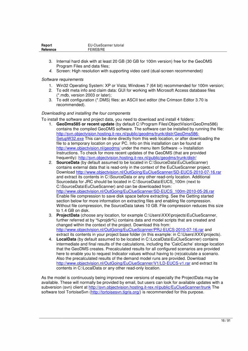
Figure 5 General settings tab in the Main menu.
Advanced options
The GeoDms executes a configurable external editor when you double-click on messages that refer to model scripts or press Ctrl-E. By default, the Crimson Editor is configured. The appropriate line number and file name are provided to the editor by means of the parameters added to the reference to the editor in general setting tab in the Main menu ( /L:%L “%F”). The Crimson Editor is downloadable from http://www.crimsoneditor.com/; please check whether the pathname included in the ‘General Settings’ tab corresponds to the location where the editor is installed). You can download and install. DMS syntax highlight files for this editor from: https://geodms.svn.sourceforge.net/svnroot/geodms/dev/res/Crimson Editor with subversion, or from http://geodms.svn.sourceforge.net/viewvc/geodms/dev/res/Crimson%20Editor/ You can also configure your own favourite editor as an external program under the ‘General Settings’ tab.

Report EU-ClueScanner tutorial Reference FEWEB/RE
19 / 91
2 Viewing existing policy alternatives
This chapter helps the modeller to get familiar with the main components of the EU-ClueScanner model. First the main elements of the Graphical User Interface (GUI) are explained. Subsequently the main components of the model are described. These relate to the available spatial data (land-use and factor data) and policy alternatives (claim data, runs, results, tracing calculation process and indicators). Note that this chapter is partially based on an adaptation of the first two chapters of the GeoDMS GUI user guide (van der Beek, 2009), which can be found at http://www.objectvision.nl/GeoDMS/ under User Guide -> GeoDMS GUI. More in-depth information on the concepts and the syntax of the GeoDMS configuration language is available at the same website under Modelling- > Modeller’s guide.
2.1 Tree view and main GUI elements
The graphical user interface (GUI) provides the modeller with a range of windows to view data layers, look-up background information, inspect simulation results and follow the simulation process. Figure 6 presents an overview of the many different windows in a typical application. Which windows are shown in a session depends on the options that are selected (ticked) in the main menu under View.
Figure 6 Tree view and main components of the GeoDMS interface. The GUI contains the following elements:
- the Menu bar with several pull down menus; - an initially empty dark-grey Tool bar that contains window-specific tools; - on the left hand side a Tree view that allows navigation through the available data sets and
model result;
Data view
Event log
Tree view Optional details pages
Legend
Tool bar
Status bar
Menu bar

Report EU-ClueScanner tutorial Reference FEWEB/RE
20 / 91
- a Data view that displays data as tables or maps; - a map Legend that appears with map in the Data views; - various Details pages containing technical and background information that appear or
disappear by simultaneously clicking the ALT and 1 keys - an Event log that presents information on the processed steps. This event log
appears/disappears by simultaneously clicking the ALT and 2 keys - a Status bar that presents hints and status information about ongoing processes.
The Tree view is the main navigation component within the application. It is comparable to the Windows Explorer in Windows and allows easy access to the huge collection of data and model result items that are available in the model. The Tree view presents the hierarchical structure of the EU-ClueScanner configuration. By default the root and the first level items are shown (the root item is expanded). Each item in the tree (called a tree item) is presented with a name and an icon. The icons are related to the default viewer for the corresponding tree item. In section 2.2.1 these icons are explained. The selected item in the Tree view is the active item in the application. This is an important concept, as many functions of the application work on the active tree item. By clicking the right mouse button a pop-up menu can be activated, with a set of menu options that work on this active tree item. This also applies to most main menu options and to the Detail pages. The pop-up menu options, most main menu options and the details pages are described in Chapter 4 and 5 of the GeoDMS user guide.
Icons used in the Tree view
The main purpose of the icons is to show which default viewer is used for an item. Double clicking or pressing the enter key on a selected tree item activates this viewer. The following icons are used to indicate this default viewer:
Data item that can be viewed in a map. This implies the domain of the data item has a geographic relation (see GeoDMS modeller’s guide for how to configure a geographic domain unit). Dependent on the geographic domain, the data is visualized in a grid, point, arc or polygon layer.
Data item that cannot be visualized in map (has no geographic relation) but can be viewed in a Datagrid.
Data item that contains a classification (a set of classes). A classification can be made or edited with the classification and palette composer, see GeoDMS user guide Chapter 10
Not all tree items are data items. For the non-data items (these items cannot be viewed with a primary data viewer), the following icons are in use:
A tree item with no data item and subitems that also have no data items. The icon is used for containers grouping other containers or units.
A tree item with no data item, but with data items as subitems. All subitems of this item with the same domain unit can be viewed in a Datagrid.
A tree item with no data item and no subitems, e.g. a unit
The next sections explore the five main components of the tree view: land-use data, other spatial (factor) data sets, the demand specification, models runs and indicators.

Report EU-ClueScanner tutorial Reference FEWEB/RE
21 / 91
2.2 Land-use data
The land-use data can be viewed by browsing through the Tree view. Start by clicking on the + in front of the container (directory) called “LandUseData”. For the DG Environment version 1km resolution, the 2000 land use is shown in two different thematic aggregations: one using 18 classes and one using 10 classes (see Section 1,2,1). The container ‘Çorine’ includes the Corine Land Cover (CLC) data-layers that describe the land use at a 100m resolution in the years 1990 and 2000. A more detailed account on the different land-use typologies can be found by browsing to EuCluescanner->Classifications->LU in the Tree view. The small globes indicate that the data item can be visualised in a map view. Maps can be drawn in the data view area in three different ways:
1. by double-clicking on any of the data layer names. This option allows multiple data layers to be drawn in the same map view window.
2. by activating (clicking on) the data layer and then simultaneously pressing the Ctrl-M key combination. This option will open a new map view window for every data layer.
3. by giving a right mouse-click on the data layer and selecting the Map View or the Default option from the appearing menu. The other options allow showing the data as a table (which does not make sense here) or histogram. The latter option shows the frequency distribution of the different land-use types.
The included classes are described in the legend that appears on the right hand side of the map. The last column in this legend contains the count for each class. As the application has a 100x100 m resolution the count values can be read as surface areas in hectares. More background information on the data is available in a meta-data sheet that can be retrieved as one of the Details pages. Right mouse-clicking on the legend area allows the user to select, amongst others, the statistics function. This option provides some basic statistics on the selected dataset, e.g. minimum and maximum value per grid cell and the total area (sum) covered by this land-use type. The edit palette pop-up menu option allows you to change the classification and colour as is explained in more detail in the GeoDMS user guide. The tool-bar now contains several standard GIS-functions such as:
zoom in, zoom out, pan, get info, zoom to full extent, copy visible area to clipboard, toggle scale bar.
The objective of these and other functions is indicated with a mouse-over text. For a full description of all tools, including options to export specific views and datasets as bitmaps or other data formats, see the GeoDMS user guide. Please note that the Corine data sets are stored as tif files in the EUCS_100m\landuse folder in the SourceData directory. This data set can be copied from here to be used in, for example, a GIS environment. Alternatively all data items that can be viewed in a map, such as the land-use data sets, can be exported by right-clicking on the attribute in the tree view and selecting the option export primary data. The user can then choose to export data in various formats, such as ascii grid or bitmap (bmp) with world file (reference to a coordinate system). It is necessary to first draw the map in the map window before this option is selected. These export options will create a copy of the whole data set, using its full extent. When the user only wants to export the part of the map that is visible in the map window, the tool bar option ‘copy visible area to clipboard’ should be selected.
Report EU-ClueScanner tutorial Reference FEWEB/RE
22 / 91
2.3 Factor data
The EU-ClueScanner also contains a wide range of spatial data sets that describe specific themes such as accessibility, geomorphology, climate and land use in neighbouring cells. These datasets were collected for the EURURALIS project (Eickhout et al., 2007; Van Meijl et al., 2006) and are used as independent factors in the statistical calibration of the model. The factor data are stored as tif files in the ‘Drivers’ folder in the SourceData directory. The data can be requested in the EU-ClueScanner from the FactorData container and can be shown as indicated above. They are shown with a corresponding legend file and meta data (a standardised description) in the details pages. In addition, datasets at a 100 metre resolution are also included. These datasets are related to features such as elevation, slope, south slope and Natura2000 areas. These are stored as tif files in the folder EUCS_100m in the Source data container and can be visualized by browsing to the container JrcFactorData in the Tree view. Appendix 2 provides an overview of the included datasets.
2.4 Demand
The container Demand normally specifies the total amount of land (in hectares for the model version at 100m resolution, in km
2 for the 1km resolution version) that has to be allocated per year,
per land-use type, per region. These land-use claims or demands can be calculated in the demand module based on the information from external sources such as the LEITAP model and can be viewed in the Demand container. Demands are calculated per demand scenario and specified for each of the claim regions. These regions normally consist of individual countries, only the Belgium and Luxemburg are aggregated in the JRC application. The functioning of the demand module is explained in Section 3.2. Please note that different from previous model versions it is no longer needed to specify the exact demand per land-use type per year for each region needs to be specified. The model is now able to allocate land when more (or less) land is claimed than is available in a region. When no land is claimed at all (i.e. when a demand specification is lacking) the allocation is unconstrained and fully governed by the conversion settings, transition potential and other model parameters. In the initial 100 metre version of the model the Demand module is not directly used. The demand for the Reference (B1) alternative from the DG Environment application is used by way of example in the 100 metre model runs. This application thus also uses the Clue10 typology applied for DG Environment. In addition a demand for the year 2000 is calculated to allow for a validation of the model. This demand is obtained by comparing the total amounts of land the JRC9 land-use classes that are simulated by the model and thus prescribes the actual (observed) amounts of land for 2000. Appendix 6 lists how this demand is derived for each country. These demand data are stored as text files (with a .in1 extension) in the folder projects\EuClueScanner\Demand\Validation2000\ Country name. Appendix 4 explains the layout of these files. The demand files related to the original 1km model can be found in the Demand folder in the LocalData directory. This folder contains a subfolder per demand scenario (e.g. ReferenceB1) that in turn contains subfolders per demand region.
2.5 Runs
The term runs refers to individual simulation runs. These represent a unique combination of claims (demand) and local suitability settings and in our case correspond to the eight policy alternatives that are included in the model. The definition of the runs can be inspected in runs ->

Report EU-ClueScanner tutorial Reference FEWEB/RE
23 / 91
EuClueScanner100m -> runs -> PolicyAlternativeName (e.g. Validation2000MNL) -> CountryName (e.g. Austria). This is a reflection of all possible model settings and may be a bit confusing at first. The most important components of the case definition are described in Chapter 3. It is clear from these folders that the model is essentially specified at the level of individual countries. To actually produce and view intermediate and final simulation results several options exist in the country-specific policy alternative folder:
- DynaClue -> TimeSteps -> Year (e.g. P2000) -> ResultingState -> LandUse starts the simulation of land use in a specific year. Obviously this simulation process takes longer when a longer period is selected. This TimeSteps folder contains also many other important dynamic model settings per individual simulation year.
- simulation_results -> LandUse shows land use in the final year and all preceding years (in the PerYear container). The visual representation is explained in the legend file and meta data in the details pages. Once this item is activated the allocation process starts. Upon completion the resulting land use is stored as a .TIFF file in the LocalData\EuClueScanner\PolicyAlternativeName folder. Please note that the second time an item is calculated, the old version will not directly be overwritten. The new version will receive a .tmp extension instead. When model is opened again the old version will get a .old extension and the new version will takes its place. This procedure allows the user to rename and store previous simulation results for a policy alternative.
- The simulation_results -> Indicators folder allows the user to inspect the results with different land-use based and thematic indicators. This folder contains several indicators that help interpret the (impacts of) simulated land-use patterns at a 100m resolution. Especially soil sealing and river flood risk indicators are interesting as these use highly detailed additional data sets. The individual indicators are described in more detail the factsheets that can be viewed in the model by opening the details pages.
- The endstate folder shows the final-year simulation result (discr_result) and allows the inspection of locations that have changed since the initial year: changed_to shows the new land use of changed locations, changed_from shows their intial land use.
The Event log shows the progress of calculations during simulation. It lists, amongst others, the amount of data items that still have to be calculated and thus gives an indication of the additional time needed to complete a calculation. Pre-processed results from model runs that have already been stored can be viewed in the indicators folder in the tree view. Please note that this has only been done for the policy alternatives of the 1km application for DG Environment. The indicators in this folder are designed specifically for the land-use types and resolution of this application and can not readily be applied to results from the JRC version of the model. The tutorial for the 1km version of the model describes how these simulation results can be made available for indicator calculations. Temporary results that are produced by updating data items during a modelling session are stored in the LocalData\EuClueScanner\CalcCache directory. This is the storage facility for all (intermediate) results that are produced during simulation. The results stored here will automatically be retrieved when an attribute is called upon from the tree view. Please note that this directory can become extremely voluminous, so it is advisable to delete files not recently used in the CalcCache when the model becomes too slow or after the model has crashed.
2.6 Indicators
The indicators folder contains, for each pre-calculated policy alternative of the 1km application for DG environment, the land-use results in various representations, derived thematic indicator maps

Report EU-ClueScanner tutorial Reference FEWEB/RE
24 / 91
(related to specific policy themes) and a set of socio-economic indicators that originate from the LEITAP and demographic models that feed into the EU-ClueScanner. The latter type of indicators is derived from the LEITAP model and only available at the National level. This extensive set of indicators helps the user interpret simulation results. A full overview of the available indicators is presented in the final report of this project (Perez-Soba et al., 2010) and can be obtained by opening the indicators subfolders for a policy alternative. Indicators can either be viewed as maps and tables. Regional aggregations usually exist at the national level and lower Nuts2 and Nuts3 statistical regions. The indicators can be viewed by selecting them in the tree view. Background information on the origin, input data and applied methodology can be found in the associated meta-data sheets that can be viewed by clicking Alt+1 and selecting the MetaData tab in the Details pages. Figure 7 shows an example of an indicator map retrieved within the user interface. The simulated land-use patterns for the different policy alternatives are essential input for the calculation of the various indicators. This input is read from the pre-calculated results folder (Results.use) in the the LocalData\EuClueScanner\ EuClueScanner1km directory. It is thus a prerequisite for indicator calculation to first perform the land-use simulation for any new policy alternatives and copy the results to the Results.use folder.
Figure 7 Example of a land-use based indicator (hot-spot of agricultural abandonment). A comparison of land-use maps can be created with the ExploreTools/CompareLanduse template. It allows the user to compare two individual land-use maps that can be selected from pull-down lists. The ExploreTools can be activated by clicking Ctrl+A when the administrator mode is switched on. A so-called case generator window appears that first asks the user to specify a name

Report EU-ClueScanner tutorial Reference FEWEB/RE
25 / 91
for this map comparison and then (after clicking next) to select two land-use maps from two pull-down menus that will be compared on a pixel-by-pixel basis. The resulting maps are available in a new folder in the tree view under runs -> CompareLandUse that contains four maps:
- map1 is the land-use map that was selected first - map2 is the land-use map that was selected subsequently - diff1 is a map showing the initial (map1) land use for those locations where land use
changed between the two years. - diff2 is a map showing the final (map2) land use for those locations where land use
changed between the two years. Please note that the created difference maps are created temporarily within a modelling session. They are not stored when the model is closed. Should you wish to store specific maps you created you can do so by exporting them through the various options in the Tool bar. If you have specific map comparison you want to evaluate in each session it may be wise to define that comparison option as an indicator in the appropriate GeoDMS script file (see Section 4.3).

Report EU-ClueScanner tutorial Reference FEWEB/RE
26 / 91

Report EU-ClueScanner tutorial Reference FEWEB/RE
27 / 91
3 Defining new policy alternatives
Creating a new model application to simulate land use according to, for example, a new reference scenario or policy alternative normally requires the following steps:
1. specification of the application in terms of land-use related themes, thus answering the question how the proposed policy alternative may influence land-use patterns;
2. specification of the application in terms of model inputs, thus define which model components should be used to simulate the anticipated spatial processes;
3. implementation of the new settings and data in the model and simulation; 4. visualisation and interpretation of the model results.
The development of a new policy alternative is an iterative process that requires intensive cooperation between policy makers and scientists with a good overview of data and model potentials (i.e. land-use modelling experts). This is especially important in the specification of the application (step 1 and 2), but also for the evaluation of initial simulation outcomes (step 4); policy makers should evaluate whether or not the results are in line with their expectations. They may request alternative model specifications when the simulated land-use patterns conflict their anticipations or other policy objectives. The implementation of a proposed new policy alternative should start with obtaining a clear understanding of its land-use related impacts. Initial discussions between policy makers and modellers/scientists should thus focus on clarifying the intentions and likely consequences of proposed policy alternatives in terms of land-use change. When these cause-effect relations are clear, specification in terms of model inputs can be proposed by the modeller. A basic question in this respect is: will the policy influence the demand for land (e.g. through intervention in the macro-economic processes as is the case with a reform of the Common Agricultural Policy) or will it mainly affect the locations of future developments. The former case will normally require the application of a regional economic model such as LEITAP, whereas the latter types of spatial policy can be represented in spatial data sets (e.g. maps of areas where specific land-use restrictions will apply). The policy alternatives that were developed for DG Environment also resulted from several discussion sessions that focussed on the objectives of specific policies and the potential of the land-use modelling framework to accommodate their likely consequences. The actual implementation of the final set of policy alternatives has been extensively documented in an appendix to the final report (Perez-Soba et al., 2010). This description is essential reading for those who consider developing a new policy alternative. New applications request a modification of the modelling set-up in some form or other. Roughly ranging from simple to complex, these may include:
- adding new thematic data (e.g. policy maps, revised accessibility); - adding new land-use datasets, e.g. CLC 2006 when it becomes available; - developing and adding new indicators; - extending the study area with, for example, Switzerland, Balkan or Turkey; - link the land-use model with other models (transport, hydrology, economics); - changing the resolution (e.g. 100m grid); - revise the calibration based on the new land-use data or other additional data sets;
The table below organises the main tasks related to the implementation of new model applications under two main headings: 1) defining and running new policy alternatives; and 2) more extensive improvements of the modelling framework required for specific new applications. It indicates the complexity of these tasks and lists the model components that should be edited and the profile of the user that is likely to be involved. Most of the basic tasks needed to modify or implement a new

Report EU-ClueScanner tutorial Reference FEWEB/RE
28 / 91
scenario are feasible by an experienced user within reasonable time (depending on the type of scenario between 1 hour and 10 days). It is important to note that new and more complex applications may involve additional relevant partners (e.g. to run hydrological or global agro-economic models). Please note that the complexity of the tasks only refers to the work involved in adjusting the EU-ClueScanner model. In many cases the most substantial part of the work will have to be performed outside the actual model. Collection and preparation of pan-European datasets is, for example, an extremely time consuming issue. Even the collection of base data for a single new member state and harmonising it with the currently available datasets can easily take several months for a GIS-expert. Table 7 Indication of complexity (*=simple, ** = advanced, *** = complex) of various tasks related to the application of the EU-ClueScanner framework.
Tasks Complexity Model component
User profile
1. Defining and running new policy alternatives Replacing spatial data sets (adding pre-processed data relating to e.g. policy, accessibility)
* file manager programmer
Editing current demand specification * Dbase programmer Combining existing scenario components (demands, transition potential definitions, etc.) into new policy alternative
* Dbase/ DMS-script
policy maker
Adding new demand specification (e.g. adding new external LEITAP or demographic projections)
* Dbase/ DMS-script
programmer
Adding new spatial data sets (adding pre-processed data and referring to it in policy alternatives)
* DMS-script/ DMS-script
programmer
Edit basic simulation settings (e.g. Conversion Settings Matrices)
* DMS-script/ parameter files
programmer/ scientist
2. Improving the EU-ClueScanner model Replacing land-use base data (e.g. inserting CLC2006) and adjusting demand settings
* DMS-script scientist
Revise calibration, renew specification of weights of suitability factors and neighbourhood enrichment, based on pre-processed data for one country
** e.g. SPSS/ DMS-script
scientist (with expertise in statistics)
Add/edit indicator definitions including graphic representation (strongly dependent on the type of indicator)
** DMS-script programmer
Link model to other models e.g. to assess specific impacts (strongly dependent on type of linking)
** programmer
Edit allocation process: - change Transition Potential definitions - change rules of Neighbourhood enrichment - adjust post-processing rules (succession) - edit Output Generation Definition
*** DMS-script programmer/ scientist
Change set of land use classes, including revision of demand and other simulation settings
*** DMS-script programmer/ scientist
Extend study area (e.g. include Switzerland or Balkan), including adding of demand and other model settings
*** DMS-script programmer/ scientist
Change resolution including respecification of model settings *** DMS-script programmer/ scientist
This chapter aims to introduce the relatively simple tasks related to the defining and running of new policy alternatives, whereas the subsequent chapter discusses some of the advanced tasks involved in improving the modelling framework. The complex tasks listed in the table are beyond the scope of this tutorial as they require a thorough knowledge of the modelling environment. The same goes for adaptations to the modelling shell (GeoDMS) such as: adding new spatial analytical

Report EU-ClueScanner tutorial Reference FEWEB/RE
29 / 91
or other functionality, supporting new file formats or updating the model to a new windows version. Such changes will normally have to be programmed in the GeoDMS-source code (in C++) and are thus the domain of software programmers. To define new policy alternatives a relatively small set of files can be manipulated relating to:
- the spatial data sets describing policy maps or driving forces; - the regional land demand associated with the policy alternatives; and - model settings (including the statistically calibrated suitability factors, transition potential
and location specific characteristics). This chapter first explains how existing spatial data sets can be replaced. Subsequently the editing and adding of new elements (demand specifications, data sets) is explained. Finally more complex issues such as the changing of the basic model settings and the creation of completely new policy options are discussed.
3.1 Replacing spatial data sets
The simplest way to include new information in the existing policy alternatives is through replacing existing spatial data sets. This may be necessary to include revised policy maps or updated accessibility maps. To replace an existing dataset, a number of actions have to be taken as is described below. First the to-be replaced data set needs to be identified and located. Appendix 2 provides an overview of the included factor data sets. These are stored as TIFF files in the SourceData\EuClueScanner\DRIVERS folder on your computer. The exact location of the Sourcedata folder can be found by in the ‘General setting’ tab (see Section 1.5). Alternatively the location (Source description) of a specific file can be retrieved by opening the details pages (by selecting this option from the ‘View’ menu or by pressing the ‘alt’ and the ‘1’ buttons), while viewing the dataset. In the viewer on the right you can read the source of the dataset. It is necessary that the new data set has the same grid specifications (extent, location, and cell size) and is created in the same projection (see Appendix 3) as the old data set it is replacing. It should also have the same values units (e.g. kilometres or per cent) as the old file to make sure that it has an equivalent impact. When the units are, for example, accidentally specified as meters instead of kilometres the data set will have 1000 times stronger impact. When the replacing data set has exactly the same name as the original file it will be directly used in calculation. The adding of new data sets is discussed in Section 3.5.
3.2 Editing current demand specification
The demand for land is calculated in the model with the demand module. This module translates base data related to demographic development and the demand for agricultural commodities into a demand for land in hectares or km
2 per land-use type. The base data comes from external sources
and is stored in a Microsoft Access database (demand.mdb) located in projects\EuClueScanner\data\ demand. This database consists of collection of different tables related to demographic data, agricultural commodities, and additional demand settings. The demographic data is derived from scenario-based projections of the PHOENIX model (Hilderink, 2004) and stored in four scenario-specific tables in the database (demography_A1, demography_A2, demography_B1, demography_B2). The demand for agricultural commodities is taken from the LEITAP/IMAGE combination (Van Meijl et al., 2006) and stored in several scenario-specific tables (using the original names of the files coming from the LEITAP modellers, e.g. GTAP_CLUE_090615_DGEnv_Ref). The demand database also contains scenario-specific

Report EU-ClueScanner tutorial Reference FEWEB/RE
30 / 91
demand settings (e.g. the amount of land in m2 per inhabitant) that are used to translate the base
data into land demand. These settings may differ for different scenarios and the DG Environment application contains 7 different variants that are included as separate tables in (with the prefix demand_settings) in the demand.mdb. Table 8 briefly explains the demand setting parameters. The demographic and agricultural demand base data and demand settings are stored at the national level. The current demand settings can be edited fairly easily in Microsoft Access to, for example, test the impact of changes in agricultural policy. This should, however, be done with great caution as the current settings have been made by a wide range of experts in the EURURALIS project. Note also that changes in Microsoft Access cannot be undone. It is thus advisable to save a copy of the original database. Ideally, revised demand settings should be stored in a new table with a meaningful new name within the demand.mdb. A new policy alternative can then be created that makes use of this new demand specification (see Section 3.4). Table 8 Demand setting parameters
Demand setting Explanation
isEU15 Parameter indicating whether or not the other demand settings parameters apply to EU15 countries. The demand settings for the new accession states are specified in the second row of the column and may differ on all of the following demand settings.
RatioPermanentRotationalCrop Ratio of permanent crops to arable land, used to calculate the demand for permanent crops
CeasingSubsSetAside Starting year of decrease in set aside subsidies (or 0 when decrease is absent)
PeriodSubsSetAsideDiminishing Period in years over which set-aside subsidies are diminishing IncreasingSubsSetAside Starting year of increase (or 0 when decrease is absent) PeriodIncreaseSpread Period in years over which increase is spread MaxPercentSetAside Maximum percentage of land set aside PercentIncrease Percentage of the increase MaxFallowPastures Percentage of maximum fallow for pastures MinFallowPastures Percentage of minimum fallow for pastures BiofuelSetAside_2000_2010 Percentage of biofuel allowed on set-aside land in 2000-2010 BiofuelSetAside_2010_2020 Percentage of biofuel allowed on set-aside land in 2010-2020 BiofuelSetAside_2020_2030 Percentage of biofuel allowed on set-aside land in 2020-2030 TrendDensity Yearly increase in the amount of urban land in m
2 used per
inhabitant corrPasture Minimum percentage used to define a lower limit to the area
including fallow (areaInclFallow)
3.3 Combining existing scenario components
Individual simulation runs consist of a socio-economic scenario and superimposed policy alternatives. These are defined in the table Scenarios that is stored as part of a Microsoft Access database (metadata.mdb) located in \projects\EUClueScanner\data. This table can be viewed and edited with Microsoft Access (see the example in Figure 8). You can add runs (new simulation alternatives) by inserting new rows into the Scenarios table. Changes to the contents of this table become effective after reloading the model configuration from the GeoDmsGUI (File->Open). A case definition consists of several components that are discussed below. The column ItemName contains a name given by the user to characterise the new alternative. This is the name that will appear in the tree view of the model. The IsActive and IsActive100m columns denote whether the new case is part of the DG
Report EU-ClueScanner tutorial Reference FEWEB/RE
31 / 91
Environment application (with a 1km grid) or the JRC application (with a 100m resolution) and should be ticked accordingly. The IsCalculated and IsCalculated100m columns indicate whether pre-calculated results already exist. These should be stored in the LocalData\EuClueScanner\ EuClueScanner1km\Results.use folder when available. Please note that this folder name should correspond exactly to the ItemName in the Scenarios table to be found. Section 2.5 describes how results for a new case can be obtained and stored. The column SuitabilityTraits indicates which method will be used to combine the different components related to local suitability. Three different options exist that differ in the way the statistical calibration results from the alloc1.reg and alloc2.reg files are used in the definition of local suitability. These methods were developed and tested for the 100m version of the model and consist of the following options:
- Split100 contains a method that fits best with binomial logistic regression results, this method was part of the original dyna-Clue model;
- Mnl100 contains a method that fits best with multinomial logistic regression results; - Linear100 contains a first attempt at a method to combine the results of alloc1 and alloc2
files first before rescaling them with a multinominal logit function. This method is included here for test purposes.
Section 1.4 shortly describes the application of these methods in the model runs developed for JRC. The column ParamName links to the separate ParamSets table in the metadata.mdb (see also Figure 9) that specifies which parameter sets are chosen (e.g. ReferenceJRC), which land-use typology is used (Clue10 for 1km applications of DG Environment or JRC9 for 100m version of JRC), which regional division is selected (e.g. Country or Nuts2) and which basic land-use data set is used as starting point. The parameters sets of the 100m version of the model are stored in the projects/EuClueScanner/Paramsets folder and contain the scenario specific parameter files are read. These files include:
- alloc1.reg, which relates Suitability Factors to land-use types; - alloc2.reg, which relates Neighbourhood Enrichment factors to land-use types; - neighmat.txt, which defines the size and shape of the neighbourhoods and the weight
assigned to the neighbourhood function; - allow.txt, which specifies succession and/or refers to succession maps; - locspecX.asc, which refer to location-specific characteristics (e.g. spatial policies) per land-
use type when applicable (only in specific policy alternatives). See Appendix 4 for descriptions of these file formats. The files may differ per country and policy alternatives to reflect local conditions or specific policies or anticipated spatial developments. The Column DemandName in the Scenario table identifies for each case which demand set to use. The DemandName is read from the separate DemandSets table in the metadata.mdb. This link has been defined with the relationships option in Microsoft Access. The PeriodSet item in the table specifies the period of simulation, this is normally 2000 to 2030, but in case of the validation refers to the 1990 to 2000 period. Finally the OutputGenerator specifies the way output is generated based on the simulation results. This refers back to the inclusion of the non-simulated (static) land-use types in maps with future land use that was discussed in Section 1.4. Currently options exist to create maps in the Clue18 typology (for simulations using the Clue10 typology, see Table 2) or the JRC22 typology (for simulations using the JRC9 classification, see Table 4).

Report EU-ClueScanner tutorial Reference FEWEB/RE
32 / 91
New runs can be created by combining the above components. It is, for example, possible to combine the spatial policy alternatives (e.g. the parameter sets related to Biodiversity and Climate Change) with a different demand scenario than is currently implemented (e.g. by selecting the BFP5nonEU demand scenario).
Figure 8 Screenshot of the Scenarios table in the metadata.mdb.
3.4 Adding a new demand specification
To be able to understand how a new demand specification can be added it is important to understand the way the relations between the different tables in the metadata.mdb are defined. Figure 9 provides an overview of these relations that can be shown and edited in Microsoft Access with the option tools -> relationships. The figure makes clear that policy alternatives (called Scenarios in the metadata.mdb) rely on demand sets that combine information from both the GTapSets and DemandSettingSets tables. This section describes different ways to make new demand specifications: add new demand sets, add new demand settings sets or add new demand base data (such as the LEITAP demand sets stored in the GTapSets table).
Figure 9 Relationships in the metadata.mdb.
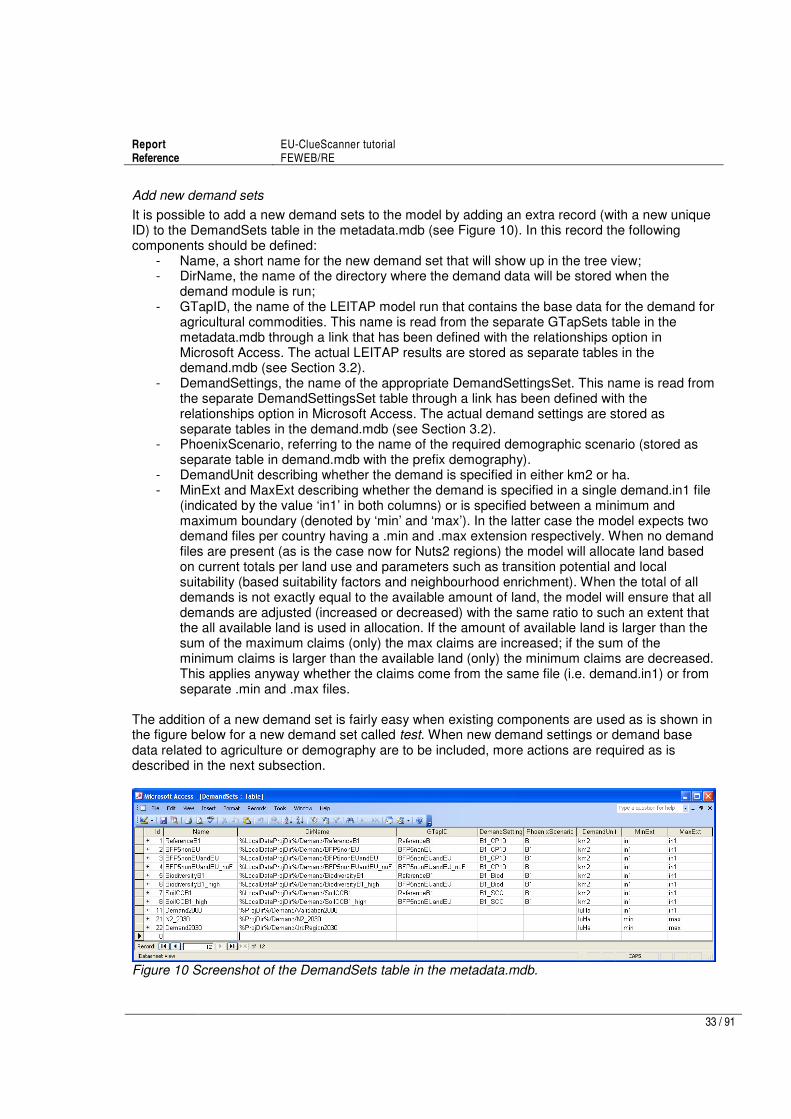
Report EU-ClueScanner tutorial Reference FEWEB/RE
33 / 91
Add new demand sets
It is possible to add a new demand sets to the model by adding an extra record (with a new unique ID) to the DemandSets table in the metadata.mdb (see Figure 10). In this record the following components should be defined:
- Name, a short name for the new demand set that will show up in the tree view; - DirName, the name of the directory where the demand data will be stored when the
demand module is run; - GTapID, the name of the LEITAP model run that contains the base data for the demand for
agricultural commodities. This name is read from the separate GTapSets table in the metadata.mdb through a link that has been defined with the relationships option in Microsoft Access. The actual LEITAP results are stored as separate tables in the demand.mdb (see Section 3.2).
- DemandSettings, the name of the appropriate DemandSettingsSet. This name is read from the separate DemandSettingsSet table through a link has been defined with the relationships option in Microsoft Access. The actual demand settings are stored as separate tables in the demand.mdb (see Section 3.2).
- PhoenixScenario, referring to the name of the required demographic scenario (stored as separate table in demand.mdb with the prefix demography).
- DemandUnit describing whether the demand is specified in either km2 or ha. - MinExt and MaxExt describing whether the demand is specified in a single demand.in1 file
(indicated by the value ‘in1’ in both columns) or is specified between a minimum and maximum boundary (denoted by ‘min’ and ‘max’). In the latter case the model expects two demand files per country having a .min and .max extension respectively. When no demand files are present (as is the case now for Nuts2 regions) the model will allocate land based on current totals per land use and parameters such as transition potential and local suitability (based suitability factors and neighbourhood enrichment). When the total of all demands is not exactly equal to the available amount of land, the model will ensure that all demands are adjusted (increased or decreased) with the same ratio to such an extent that the all available land is used in allocation. If the amount of available land is larger than the sum of the maximum claims (only) the max claims are increased; if the sum of the minimum claims is larger than the available land (only) the minimum claims are decreased. This applies anyway whether the claims come from the same file (i.e. demand.in1) or from separate .min and .max files.
The addition of a new demand set is fairly easy when existing components are used as is shown in the figure below for a new demand set called test. When new demand settings or demand base data related to agriculture or demography are to be included, more actions are required as is described in the next subsection.
Figure 10 Screenshot of the DemandSets table in the metadata.mdb.

Report EU-ClueScanner tutorial Reference FEWEB/RE
34 / 91
To apply the new demand sets in land-use simulation, the following steps are necessary: 1. A (new) policy alternative (model run) should be defined in the Scenarios table that refers
to the new demand set (see Section 3.3); 2. The new or revised policy alternative should be applied in the demand module in the EU-
ClueScanner to calculate the demand per land-use type, per year for each country following the changed settings and existing demand base data. This calculation starts after activating the Result data item in the Tree view under Demand -> runs -> PolicyAlternativeName -> FileGenerator. A demand file for an individual country can be created by activating the data item demandFile in Demand -> runs -> PolicyAlternativeName -> per_country -> CountryName -> Results.
The demand specification resulting from running the demand module is stored as a Demand.in1 text file in the folder \LocalData\EuClueScanner\Demand\PolicyAlternativeName\CountryName. Please note that existing demand specification files are not directly replaced when the demand for an already existing policy alternative is calculated anew. In this case a new Demand.in1.tmp file is created, that will only replace the initial file when the EU-ClueScanner model is closed. Upon closing the model, the initial files are renamed to Demand.in1.old to allow the user to recover the initial demand settings when necessary. Appendix 4 provides a short description of the format of the demand files. When the demand files have been generated for a new policy alternative, the simulation of future land use can be started as was described in Section 2.5.
Adding new demand settings
New demand settings can be added by creating a new table in the demand.mdb. To make sure that the right structure is used, it is best to copy an existing demand settings table and paste it (with structure and data) as new table within the demand.mdb. The copied table should be given a sensible short name with the prefix demand_settings. Please note that certain characters (e.g. spaces, slashes are not allowed as tree item names in the GeoDMS and should thus be avoided. The demand settings of the new table can then be adjusted to, for example, change the amount of urban land per inhabitant (see also Section 3.2). To be able to use the new demand settings created in the demand.mdb in the specification of a new demand set the following steps are necessary:
1. First it is necessary to create a reference to the new demand settings in the metadata.mdb. This should be done by adding a new record to the DemandSettingsSet table in the metadata.mdb with the exact name of the new demand settings table excluding its demand_settings prefix. When these names do not match the demand module in the EU-ClueScanner will not be able to combine data from the two databases and produce an error.
2. The new settings can then be combined with the other demand base data sets (e.g. a demographic scenario from Phoenix model) in the DemandSets table to create a (new) demand set. Please note that the DemandSets table has to be reopened in order to read the newly defined DemandSettingsSet. The new or revised demand sets can then be used to define a new policy alternative as was explained above.
Adding new demand base data
New base data referring to demographic developments or the demand for agricultural commodities can be added to the demand.mdb. Such new demographic or agricultural projections can be created with the PHOENIX or LEITAP/IMAGE runs or be inferred from other sources. To be able to directly use the new demand input it is necessary that exactly the same table format is used as in the current demand base data. This means that, for example, the same regional division (mostly countries) and units (inhabitants) are used.
Report EU-ClueScanner tutorial Reference FEWEB/RE
35 / 91
For the LEITAP/IMAGE model a structured file format is agreed upon. The results of a LEITAP/IMAGE run are delivered as .csv files (comma separated value files commonly used for data export that in this case use a semicolon as separator) with the following attributes:
- Country; - Year; - PermanentPasture; - AreaArableLand; - AreaArableBiofuels; - AreaPerennialBiofuels.
New LEITAP model run results should be stored as .csv files in the \projects\EUClueScanner\data\ Demand folder. They can be imported in the demand.mdb (through the options external data -> textfile) as one table for each .csv file. The .csv filename should correspond with the name of the table. In the GtapSets table in the metadata.mdb a record is then added for each imported csv table in the demand.mdb. In this GtapSets table, each Gtap set has an ID (autonumber), a name, a tablename (which needs to match with the name of the table in the demand.mdb) and a SocEconDbName. This last attribute refers to additional databases for these LEITAP results with economic indicators, stored in the \projects\EUClueScanner\data\indicator_econ folder. In the DemandSets table the name of the GtapSet is selected to specify which LEITAP model run results are used. After the .csv files are imported in the existing structure in the demand.mdb database they can be used to calculate new demand specification files when they are referred to in a new demand set specification (i.e. a new record in the DemandSets table as was described above). In this version of the EU-ClueScanner the demands are calculated at the national level. The module could also function at sub- or supra-national level. This implies the data used in the module is available or can be (des)aggregated to the requested level. Technically it is possible to calculate the demands at other regional levels (as long as the number of regions does not become too large). But some adaptations to the basic model configuration are needed for which some technical support may be required for non-expert users.
3.5 Adding new spatial data sets
New spatial data sets (with a new name) referring to, for example, accessibility or spatial policy can be added to the model. Typically, these will be created in a GIS environment. They should have the same grid specifications (extent, location, and cell size) and be created in the same projection (see Appendix 3) as the other data sets available in the model. They can be stored together with all other datasets in SourceData\EuClueScanner\Drivers. After placing data in this location, references have to be made to it in the EU-ClueScanner. In the Microsoft Access-database ‘Metadata.mdb’, which can be found in the Projects\EuClueScanner\data directory, a row can be added to the FactorData table specifying the correct FileName and other characteristics. The data set can now be included in the definition of simulation runs (e.g. as factor in the calibration of the model, see Section 4.2, or as a new allow driver map, see Appendix 4) or be used in indicator calculations. Note that spatial datasets that are used to increase or decrease the local suitability values for a land-use type in the context of a policy alternative are applied in simulation as part of a single locspec file (see Appendix 4).

Report EU-ClueScanner tutorial Reference FEWEB/RE
36 / 91

Report EU-ClueScanner tutorial Reference FEWEB/RE
37 / 91
4 Adjusting the EU-ClueScanner model
Before discussing possible adjustments to the existing EU-ClueScanner model configuration, it is good to highlight two specific model characteristics: the administrator mode and the GeoDMS script files that comprise the model. For more advanced users a specific administrator mode exists that allows the inspection of basic model settings (e.g. units, standard regional divisions, classification schemes for the visualisation of data), many in-between steps in simulation, auxiliary data files and templates used for the creation of indicator values etcetera. This mode is active when the administrator mode tick box is clicked in the General Settings tab in the Options window that appears by clicking Ctrl+Alt+O (see Figure 5). By now you may be expert enough to use this mode. Most of EU-ClueScanner components are programmed in the GeoDMS script files that can be edited with any text editor. The user interface only offers limited functionality to edit these files, as previous experience has learnt that direct editing of the underlying script files offers more flexibility, a more compact and robust programming environment and a better overview of the context of these files and their relation with other model components. The GeoDMS files define the actual modelling application and offer an open and flexible environment to manipulate its many components. The definition of indicator calculations, the inclusion of new spatial datasets and model run characteristics are also defined in the GeoDMS files. For a complete description of the naming conventions, available operators and functions, potential configuration errors and many other aspects of GeoDMS scripting, see the modellers guide at http://www.objectvision.nl/GeoDMS/ under modelling.
4.1 Replacing land-use base data
The current EU-ClueScanner model uses the CLC2000 data to represent current land use. In the near future a revised version (CLC2006) is expected to be released, that would allow the incorporation of a more recent starting year for simulation. To replace the current land use data set a few steps are necessary. First a reclassified version of the new land-use dataset must be created that uses the same land-use classification and has exactly extent and projection as the current land-use base data set. Table 2 specifies how the current, extensive set of CLC types is reclassified to the classification used in the model. It is important that this reclassification scheme is followed closely to prevent the introduction of inconsistencies with previous simulation results. The reclassified data should then be stored in the SourceData folder, closely following the projection and data file format specifications listed in Appendix 3. This new data set can then replace the current version stored in \SourceData\EUCS_100m\landuse. A second, more complex step is adjusting the demand settings (see also Section 3.2). This calls for a thorough analysis of the current specification and a revision of those settings that are not appropriate anymore in the demand_settings tables in the demand.mdb. This may, for example, relate to the year set aside subsidies cease. Exactly which settings should be changed and how this should be done, depends on the year the new base data refer to and the scenario and policy alternative under consideration. Then, the the simulation period (start and end year of simulation) have to be specified in the PeriodSet column in the Scenarios table of the metadata.mdb. A new period may have to be

Report EU-ClueScanner tutorial Reference FEWEB/RE
38 / 91
referred to with a new name in this column. When this is done, the characteristics of this new period have to be specified in the default.dms script file in the folder \Projects\EuClueScanner\cfg\default. This new specification can be based on already existing examples. In fact, copying the lines of script relating to an existing period and editing these may the most efficient strategy. Finally, the spatial data sets related to the age of land use and dynamic simulation should be considered carefully. The age of land use is stored in the age0.asc file in the folder \SourceData\EuClueScanner\LandUse and may have to be updated. Ideally this calls for a detailed transition analysis comparing land use in the initial base year (2000) and the new base year. Based on this, locations where land use remained the same will increase in age (with the difference in years between the two observation moments), whereas changed locations will receive a new age of 0 years. Also the dynamic driver files (stored in \SourceData\EuClueScanner\DynamicDrivers) contain explicit mentioning of specific years and may have to be adjusted. Again this depends on the new period of simulation and the characteristics of the policy alternative under consideration. When new land-use base data become available, the user can also to consider updating the calibration. However, as the driving forces that influence land-use patterns are considered to be relatively stable over time this is not essential.
4.2 Revise calibration
Calibration is the process of tuning a model in such a way that sensible results can be obtained. This is normally done through a statistical (logistic regression) analysis that describes the relation between a number of spatially explicit explanatory variables (e.g. accessibility, soil type and climatic variables) and an observed (to be explained) land-use pattern (Pontius Jr. et al., 2008). These explanatory variables are called factor data in the model. In case of the EU-ClueScanner a separate calibration was performed for each individual country, to reflect the fact that driving forces behind land-use change may differ between countries in specification and explanatory power. This means that different factors are used to explain land-use patterns per country; in general about 10 different factors are used for a country from the total list of over 60 factors described in Appendix 2. In addition, explanatory variables are used that describe land use in the direct environment (or neighbourhood) of a grid cell. A revision of the calibration becomes necessary when new land-use or factor data are added to the model, or when a land-use type is introduced. In this case a new statistical analysis should be performed that uses an observed land-use (e.g. of the new base year) as to be explained variable and a set of explanatory variables. Standard statistical software such as SPSS can be used to do this type of analysis. To keep calculation times within reasonable bounds it is advised to limit the number of observations, depending on the calculation power and available internal memory in the computer. The sample should preferably be structured with a minimum distance between the observations to limit spatial autocorrelation. In addition it is suggested to limit the number of to be explained variable values (land-use types) to about 9 and to make sure that all land-use types have sufficient observations (at least 2% of the total amount of observations) to prevent the creation of statistically insignificant results. A thorough statistical background is required to perform such analyses and assess the value of their outcomes. For the JRC version of the EU-ClueScanner multinomial logistic regression was applied using SPSS. Appendix 5 lists the main steps in this approach. In multinomial regression the probability of occurrence of a certain land-use types is estimated in relation to the probability that other land-use types will occur. This implies that when a single new land-use type is added to the model the

Report EU-ClueScanner tutorial Reference FEWEB/RE
39 / 91
statistical analysis should be performed for the complete set of land-use types. It is not sound to only analyse the occurrence of a single land-use type using, for example, binomial logistic regression and use that in combination with previous multinomial regression results.
4.3 Edit or add indicator definitions
The indicators are defined in a set of GeoDMS script files that are stored in the folder \projects\EuClueScanner\cfg\Default. Initial reference to the indicators is made in the IndicatorData.dms file. This file also defines some of the units and legends that are used in their calculation and representation. Their actual calculations are defined in the indicator-specific GeoDMS files in the IndicatorData subfolder. Additional spatial data sets that are needed for the calculation of the indicator values are stored in the \SourceData\EuClueScanner\Indicators folder. These data sets are independent of the policy alternatives and are thus stored in this general folder that also contains the factsheets describing, for example, the origin and methodology of the indicators. The definition of the indicators can be edited by manipulating the corresponding GeoDMS files. Obviously this requires a thorough understanding of the current indicator definitions and the basics of the GeoDMS scripting language. Straightforward changes can, however, already be made by relatively novel users of the GeoDMS language. New indicators can be added by defining them in separate GeoDMS files and referring to them in the IndicatorData.dms file through an include statement (e.g. #include <NewIndicator.dms>, see similar references in IndicatorData.dms). The GeoDMS language offers a large set of operators that allow the user to define new quantitative evaluation measures. The operators include more complex spatial analysis options generally found in more advanced GIS-packages that relate to, for example, combining, comparing and overlaying individual data layers, defining contiguous areas with the same raster values, calculating distances or network analysis. A full list of these operators is available in the GeoDMS Modeller’s guide that can be found under modelling on: http://www.objectvision.nl/GeoDMS/. Examples of other indicators developed within the same modelling environment are described elsewhere (Bubeck and Koomen, 2008).
4.4 Link EU-ClueScanner to other models
The EU-ClueScanner model can be linked with other spatial models related to either derive more specific input for simulation (e.g. changed regional agricultural demand from CAPRI, or revised accessibility maps from TRANSTOOLS) or provide additional impact assessments (e.g. through coupling with a hydrologic model). These model couplings require a clear vision on the anticipated level of integration and a careful consideration of the thematic, temporal and spatial resolution of the involved models. A model coupling can be a straightforward exchange of output and input data when the considered land-use types (thematic resolution), time period (temporal resolution) and regional divisions or grid cell size (spatial resolution) are aligned. Substantial efforts are, however, required when the models need to be adjusted. This would, for example, be the case when additional agricultural land-use types have to be inserted in the land-use model to allow the input from an agro-economic model such as CAPRI. Although coupling of the modelling framework to alternative detailed indicator models is possible it may not always be recommended. Many indicator models are based on detailed understanding of processes at the micro-level (e.g. causing greenhouse gas emissions) and are therefore subject to scaling errors when applied to a 1 km spatial resolution. It is thus important to choose indicator models that are suited for and sensitive to the information provided by the EU-ClueScanner framework at the spatial and temporal scale of analysis. Also a good fit with the thematic content of

Report EU-ClueScanner tutorial Reference FEWEB/RE
40 / 91
the different land-use classes is necessary. For example, due to the limited differentiation currently possible in land-use intensity, no specific indicator on the agricultural biodiversity is included in the modelling system given the dependence of this indicator on detailed changes in land-use intensity.
4.5 Adjust land-use typology
Adjusting the land-use typology to, for example, include new types of land use is a complex task that involves several of the activities described above. It involves the steps mentioned below. First the new land-use types have to be defined spatially. This will most likely be a refinement of the existing types of land use (e.g. a distinction in high and low density urban fabric). In that case it is necessary that the land-use base data will be updated (see Section 4.1). Care should be taken the new land-use types completely overlap the existing land-use types it replaces. This type of data preparation will typically take place in an ArcGIS environment. A next step consists of the definition of the most suitable locations for the new land-use types. This implies a revision of the statistical calibration that defines the most likely locations for land-use types according to suitability factors (alloc1.reg) and neighbourhood enrichment (alloc2.reg). See Section 4.2 for this step. In some cases it may be possible to skip the statistical calibration, for example when a new land-use type is expected to have the same basic spatial behaviour as another type of land use. Subsequently, it is important to consider which other factors influence the future location of the new land-use type and how this relates to the main model parameters. Will it be strongly related to neighbouring land use (in which case the weight for the neighbourhood enrichment should be set at a high value in neighmat.txt)? Will it have a strong resistance to change (specified in main.1)? Are specific transition allowed or impossible (specified in allow.txt)? Will certain location characteristics (e.g. spatial policies) influence the location of the land use type (to be included in locspecx.asc)? Please note that it is essential that reference to the new land-use type is made in the main.1 file. This file specifies amongst others the total amount of land-use types that are simulated and their internal codes. Especially the main.1, neighmat.txt and allow.txt files should be checked on their proper treatment of the new land-use types. As usual Appendix 4 provides info on the exact characteristics of these files. Finally a future demand for land for the new type of use should be specified in the demand.in1 files. These list the expected total amount of land per year and can be created with the demand module or other tools.

Report EU-ClueScanner tutorial Reference FEWEB/RE
41 / 91
5 Validating the JRC version at 100m resolution
This section describes the way the 100m version of the EU-ClueScanner was validated by comparing simulated land use for 2000 with observed land use in CLC2000. Firstly, an account on the applied methodology is provided, followed by the validation results. Based on that, the ability of the model to produce sensible land-use patterns will be discussed.
5.1 Validation methodology
The method applied to evaluate the model’s performance was a pixel-by-pixel comparison between simulated land use for 2000 and observed land use in CLC1990 and CLC2000. The simulated land use maps for 2000 resulted from the model runs described in Section 1.4 that follow the calibration method documented in Appendix 5. In these model runs suitability for each land-use class is defined according to the statistical analysis of the observed land-use patterns in CLC1990. More specifically we chose to use the validation2000MNL model runs that follow closely the multinomial logit specification that was also used in the statistical analysis. In this validation effort, the claims per land-use type for 2000 were specified by assigning the exact quantities corresponding to the observed amount of land for these land-use types in CLC2000. For the validation we followed a similar approach to that carried out in a previous assessment of contemporary land-use change models (Pontius Jr. et al, 2008). That study distinguished three possible two-map comparisons:
- CLC1900-CLC2000, which characterises the observed land-use change (Appendix 6); - CLC1990-MNL2000, which refers to the land-use change predicted by the model; - CLC2000-MNL2000, which permits to determine the accuracy of the prediction.
Based on the available maps it is also possible to perform a three-map comparison that allows distinguishing the correct prediction due to persistence of land use from well-predicted changes in land use. This is an important distinction as the amount of change is normally limited. Comparison methods that compare the complete simulation map with the complete observation map are strongly influenced by the static patterns and tend to overestimate the predictive power of land-use models. Therefore it is more meaningful to focus on the amount of correctly predicted change. Based on the comparisons of the three available maps we can determine both quantity and location agreement between observed and simulated land use patterns. Quantity agreement is obtained by comparing the aggregate totals of all land-use classes in the simulated and observerd land use. To describe location agreement we first create the following maps:
- well-predicted change (A); - observed change predicted, but as a wrong gaining class (B) - observed change predicted as persistence (C) - observed persistence predicted as change (D)
Based on that, location agreement was quantified using the following three statistic measurements:
- figure of merit = A / (A+B+C+D), which measures the accuracy of the model in predicting land-use change;
- producer accuracy = A / (A+B+C), which gives the proportion of pixels that the model predicts accurately as change, given the observed change;
- user accuracy = A / (A+B+D), which calculates the proportion of pixels predicted accurately as change, given the model predicted change,

Report EU-ClueScanner tutorial Reference FEWEB/RE
42 / 91
5.2 Validation results
By way of example, the results of the validation method introduced above are described here for the simulation of land use for 2000 in the Netherlands. From Table 9, it can be concluded that there is a strong agreement between the quantities of observed and predicted land-use change. This is exactly what we expect since the simulated amounts of land per land-use class were derived from the CLC2000. There is a small disagreement, however, that can be explained by the fact that the classes that we consider static in the model (Infrastructures, Other Nature and Water) did change between the observed years. The approximately 7000 hectares increase in the classes that we do not simulate is therefore added to the classes that are simulated. This correction, that was already applied in the demand.in1 files that were used as input for these model runs, will cause an overestimate of the amount of change for these classes and thus a somewhat poorer performance in the validation. Table 9 Observed and predicted land use change per land use type for 1990-2000 in the Netherlands
Aggregated land use classes
Urban Fabric 55565 18,9% 56308 19,1% 743 0,2%
Industry and related uses 24611 46,2% 24773 46,5% 162 0,2%
Arable land and permanent crops -27755 -2,5% -25411 -2,3% 2344 0,2%
Pastures -75033 -5,1% -72004 -4,9% 3029 0,2%
Forests 8195 2,7% 8871 2,9% 676 0,2%
Semi natural vegetation 7325 12,7% 7463 12,9% 138 0,2%
Infrastructures 2842 13,1% 0 0,0% -2842 -11,6%
Other Nature 777 0,2% 0 0,0% -777 -0,2%
Water 3473 1,0% 0 0,0% -3473 -1,0%
Observed Change Predicted ChangeDifference between predicted
and observed change
Note: the percentages relate the amount of change to the total amount of land for a land-use class in 1990. Figure 11 shows that location agreement between the simulated and observed land use in 2000 is mostly related to well-predicted persistence of land use. Indeed, well-predicted change occurs so infrequently that it can be hardly perceived in the map. This becomes even clearer from Table 10. This table further indicates that almost all (94%) of the change predicted by the model was observed persistence. The enormous overestimate of change essentially results from the way the model deals with the locations classified as Heterogeneous Agriculture Areas in the original Corine typology and that were subsequently randomly assigned to Arable Land and Pastures. As a matter of fact, this outcome could be almost entirely explained by interchanges between these two classes: while a transition of 23,572 ha from Pastures to Arable land and an opposite transition of 3,108 ha was observed in 1990-2000, the model simulated for the same period 151,481 ha and 146,616 ha respectively (see the transition matrices for CLC1990-CLC2000 and CLC1990-MNL2000 in Appendix 6 and 7 for more detailed results). The overestimation of change is exemplified in Figure 12 and Figure 13. These figures show that in some regions where ‘chess-board’ patterns exist (that reflect the random assignment), many land-changes are simulated where the observed patterns remain the same. Nevertheless, it should be noted that the landscape structure is maintained, even though land-use change is overestimated.

Report EU-ClueScanner tutorial Reference FEWEB/RE
43 / 91
Figure 11 Three-map comparison for simulated and observed land use change in 1990-2000 in the Netherlands. Table 10 Pixel-by-pixel comparison between simulated and observed land use change in 1990-2000 in the Netherlands
Persistance well
predicted
Observed persistance
predicted as changeWell predicted change
Observed change
predicted as wrong
gaining class
Observed change
predicted as
persistance
2726474 422752 9933 18131 116653

Report EU-ClueScanner tutorial Reference FEWEB/RE
44 / 91
Figure 12 Detail of an area previously classified as Heterogenous Agricultural Land in the original Corine typology in CLC2000.
Figure 13 Outcome of the model simulation for 2000 in the same area.
Hence, it can be concluded that the model predicts much more land-use change than is desirable. This is confirmed by the statistical measurements of the models performance (Table 11). Both the Figure of Merit, that measures the overall accuracy of the model in predicting land-use change, and User Accuracy, that relates the well-predicted change to the total amount of change predicted by the model, are extremely low. The Producer Accuracy that relates well-predicted change to the observed amount of change is slightly higher. Table 11 Statistical measurements of the model’s performance for simulation of land-use change in 1990-2000 in the Netherlands
Figure of Merit Producer Accuracy User Accuracy
1,75% 6,86% 2,20% It must be mentioned, however, that these statistical indices can be misleading in assessing the ability of model in predicting sensible land use patterns. Actually, they provide an indication of the location agreement between observed and simulated land-use change, which can prove to be a deceptive issue while dealing with a model using such a fine resolution for a large area. Pontius Jr. et al (2008) state that Figures of Merit tend to be larger when the amount of net change in the reference maps is higher. Since the total amount of net observed change accounts for less than 4% of the Netherlands total area, it is not surprising that a small value for the Figure of Merit was obtained. It is more difficult to correctly predict such a rare feature than a more common phenomenon. In fact, for countries such as Austria where land-use change accounted for only 0.3% the total area, a Figure of Merit as low as 0.12% was obtained (see Appendix 7). Similar patterns have been encountered while simulating land-use change in other countries, showing that the model performs

Report EU-ClueScanner tutorial Reference FEWEB/RE
45 / 91
consistently for different regions. Therefore, it is recommendable for future research to carry on additional validation steps, making a distinction between near-location and far-location disagreement by converting the maps to a coarser resolution (Pontius Jr. et al, 2008), to better understand the performance of the model.
5.3 Conclusion
Calibration and validation are continuous processes that aim to improve the performance of land-use change models. It is very hard, if not impossible, to define the ultimate calibration for a model. Proper model settings depend on the type of application and associated time period and objective of the study. For shorter time period it is normally wise to create an application that shows little change (limited conversion elasticity, strong importance of neighbouring cells), whereas scenario-based studies for longer time periods may call for more freedom in the allocation process. Based on the calibration and validation efforts undertaken for this study we have several suggestions for further improvement. These are introduced with reference to some general observations that were made while validating the EU-ClueScanner model. Figure 14 depicts these observations for a small part of the Netherlands. The blocky appearance that sometimes appears in simulated land-use patterns indicates the coarseness of part of the underlying datasets. Not only are these data available at a 1km resolution, but most of these pan-European maps (related to for example soil characteristics or climatic variables) typically describe the landscape in large homogenous areas of hundreds of square kilometres. The performance of the model would greatly improve with more detailed spatial data. Especially for distance relation maps it is not so difficult to create these for European territory. The scattered pattern related to the reclassification of heterogeneous CLC classes was discussed extensively above. This can be solved simply by assigning these classes to one aggregated class (e.g. arable land) only. Alternatively, the reclassification can be followed by a post-processing step to generate larger spatial units. Ideally the model should be recalibrated after this, since the spatial relations will change. But as these classes only take up a small proportion of the pastures and arable farming classes this may be necessary. The spatial mismatch between the relatively coarse NUTS2 delineations and the 100m resolution can be solved by creating a more refined spatial data set describing NUTS2 regions. The initial simulation problems at the very edges of the countries have, however, been solved through a different way of dealing with no-data areas. Any no-data location in the land-use base map is now excluded from the allocation process. The strong link with initial land use in the simulation process can either be caused by land-use specific conversion elasticities or by the demand. In the figure below it is especially the strong decrease in pastures that causes the new urban areas to follow former pastures. These may indeed very well be preferable locations for development. To correctly simulate these processes it is important to distinguish between profitable and marginal agricultural areas. In addition spatial policy constraints should be added to incorporate local regulations. Inclusion of such data sets, in addition to predominantly biophysical data sets included now, would enhance model performance. The strong influence of neighbourhood relations may also reflect actual spatial processes, but for longer simulation periods other location factors may become more important. Here again inclusion of more detailed spatial data related to the full range of potential biophysical, economic and planning-related driving forces should help the model to better capture the most important spatial processes.

Report EU-ClueScanner tutorial Reference FEWEB/RE
46 / 91
Figure 14 General Observations made while validating the EU-ClueScanner model.
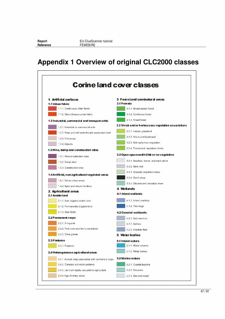
Report EU-ClueScanner tutorial Reference FEWEB/RE
47 / 91
Appendix 1 Overview of original CLC2000 classes

Report EU-ClueScanner tutorial Reference FEWEB/RE
48 / 91
Appendix 2 Overview of spatial data sets
This appendix provides an overview of two types of spatial data sets: - the 52 factor data sets that are used as independent factors in the statistical calibration of
the model. These are called upon in the alloc1.reg and alloc2.reg files. The datasets are made available from the EURURALIS 2.0 project and are described in more detail in the meta data sheets (adapted from: Overmars et al., 2006) that are included as part of the details pages in the model.
- the 13 allow driver maps (X1-X13) that specify the spatially explicit settings for the conversion matrix. These maps are called upon in the allow.txt files. The meta data sheets that are included as part of the details pages in the model describe these maps in more detail.
- the 100m resolution factor data sets that are used in the calibration of the JRC model version.
ID Name Description Coverage
Factor data sets used in calibration of the model (1km resolution)
1 ACCESS1_06M Timecost to cities > 100.000 (seconds) missing Turkey (Cyprus and Malta are reasonably ok)
2 ACCESS2_06M Timecost to cities > 500.000 (seconds) missing Turkey and Cyprus and Malta
3 ACCESS3_06M Timecost to ports > 15.000 kTon/year (seconds)
missing Turkey and Cyprus and Malta
4 ACCESS4_06M Timecost to cities > 650.000 (seconds) missing Turkey and Cyprus and Malta
5 ACCESS5_06M Euclidean distance to nearest road of level 0 or 1 (metres)
missing Turkey and Cyprus and Malta
6 ACCESS6_06M Timecost to major airports (seconds) missing Turkey and Cyprus and Malta
7 ACCESS7_06M Timecost to airports & ports (seconds) missing Turkey and Cyprus and Malta
8 claycont_06pc Soil clay content (%) missing Iceland, Turkey, Cyprus and Malta
9 ddw_shortage Water deficit growing season (mm) ALL
10 dem_final Elevation based on SRTM3 NASA-data (m) ALL
11 envmap01 ALN: Alpine north (0/1) missing Iceland, Turkey, Cyprus
12 envmap02 BOR: Boreal (0/1) missing Iceland, Turkey, Cyprus
13 envmap03 NEM: Nemoral (0/1) missing Iceland, Turkey, Cyprus
14 envmap04 ATN: Atlantic north (0/1) missing Iceland, Turkey, Cyprus
15 envmap05 ALS: Alpine south (0/1) missing Iceland, Turkey, Cyprus
16 envmap06 CON: Continental (0/1) missing Iceland, Turkey, Cyprus
17 envmap07 ATC: Atlantic central (0/1) missing Iceland, Turkey, Cyprus
18 envmap08 PAN: Pannonian (0/1) missing Iceland, Turkey, Cyprus
19 envmap09 LUS: Lusitanian (0/1) missing Iceland, Turkey, Cyprus
20 envmap10 ANO: Anotolian (0/1) missing Iceland, Turkey, Cyprus
21 envmap11 MDM: Mediterranean mountains (0/1) missing Iceland, Turkey, Cyprus
22 envmap12 MDN: Mediterranean north (0/1) missing Iceland, Turkey, Cyprus
23 envmap13 MDS: Mediterranean south (0/1) missing Iceland, Turkey, Cyprus
24 EUAC120_2006 # of people that reach a location from their home within 120 minutes (persons)
EU15
25 EUAC30_2006 # of people that reach a location from their home within 30 minutes (persons)
EU15
26 EUAC60_2006 # of people that reach a location from their home within 60 minutes (persons)
EU15
27 Geomorf01 Average height difference of 0-20 m: flat (0/1)
missing Turkey
28 Geomorf02 Average height difference of 20-80 m: rolling missing Turkey
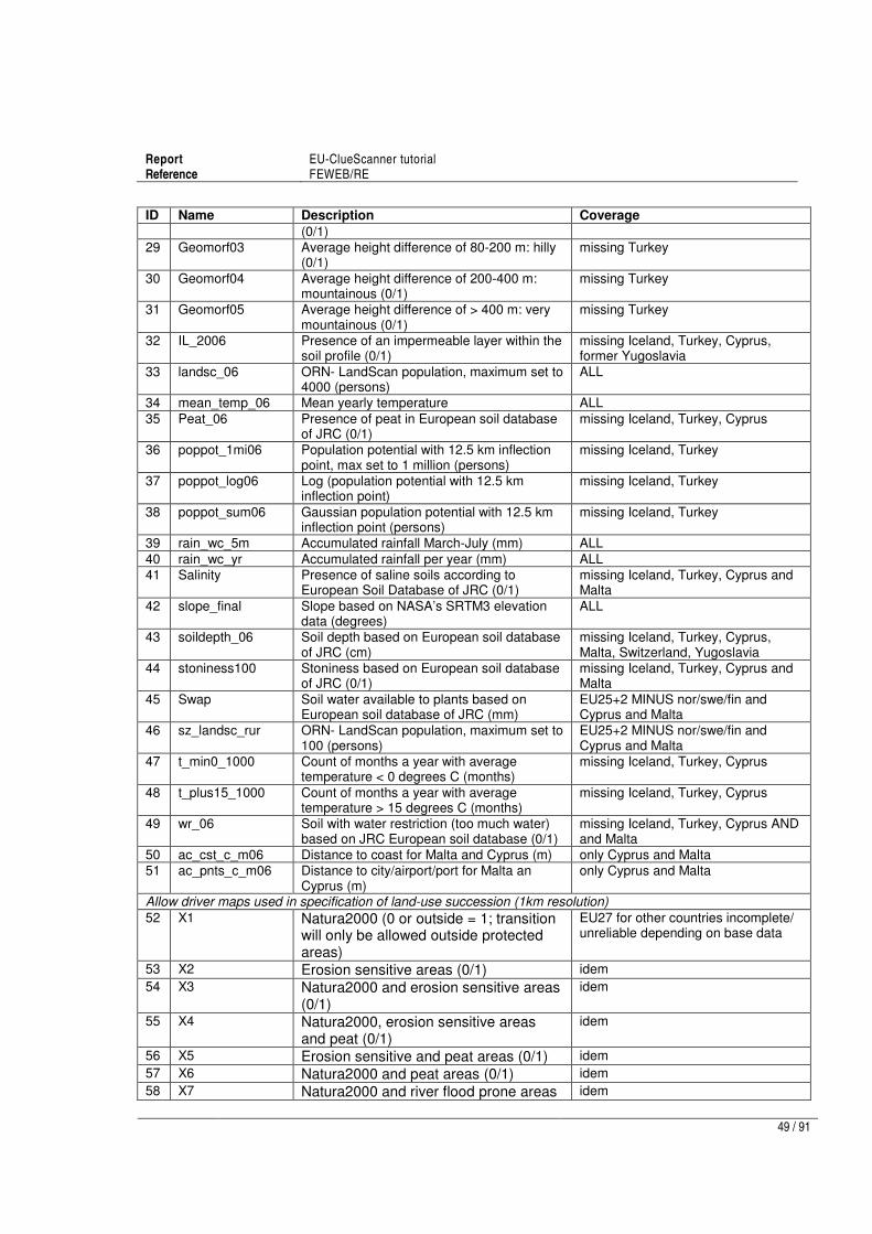
Report EU-ClueScanner tutorial Reference FEWEB/RE
49 / 91
ID Name Description Coverage
(0/1)
29 Geomorf03 Average height difference of 80-200 m: hilly (0/1)
missing Turkey
30 Geomorf04 Average height difference of 200-400 m: mountainous (0/1)
missing Turkey
31 Geomorf05 Average height difference of > 400 m: very mountainous (0/1)
missing Turkey
32 IL_2006 Presence of an impermeable layer within the soil profile (0/1)
missing Iceland, Turkey, Cyprus, former Yugoslavia
33 landsc_06 ORN- LandScan population, maximum set to 4000 (persons)
ALL
34 mean_temp_06 Mean yearly temperature ALL
35 Peat_06 Presence of peat in European soil database of JRC (0/1)
missing Iceland, Turkey, Cyprus
36 poppot_1mi06 Population potential with 12.5 km inflection point, max set to 1 million (persons)
missing Iceland, Turkey
37 poppot_log06 Log (population potential with 12.5 km inflection point)
missing Iceland, Turkey
38 poppot_sum06 Gaussian population potential with 12.5 km inflection point (persons)
missing Iceland, Turkey
39 rain_wc_5m Accumulated rainfall March-July (mm) ALL
40 rain_wc_yr Accumulated rainfall per year (mm) ALL
41 Salinity Presence of saline soils according to European Soil Database of JRC (0/1)
missing Iceland, Turkey, Cyprus and Malta
42 slope_final Slope based on NASA’s SRTM3 elevation data (degrees)
ALL
43 soildepth_06 Soil depth based on European soil database of JRC (cm)
missing Iceland, Turkey, Cyprus, Malta, Switzerland, Yugoslavia
44 stoniness100 Stoniness based on European soil database of JRC (0/1)
missing Iceland, Turkey, Cyprus and Malta
45 Swap Soil water available to plants based on European soil database of JRC (mm)
EU25+2 MINUS nor/swe/fin and Cyprus and Malta
46 sz_landsc_rur ORN- LandScan population, maximum set to 100 (persons)
EU25+2 MINUS nor/swe/fin and Cyprus and Malta
47 t_min0_1000 Count of months a year with average temperature < 0 degrees C (months)
missing Iceland, Turkey, Cyprus
48 t_plus15_1000 Count of months a year with average temperature > 15 degrees C (months)
missing Iceland, Turkey, Cyprus
49 wr_06 Soil with water restriction (too much water) based on JRC European soil database (0/1)
missing Iceland, Turkey, Cyprus AND and Malta
50 ac_cst_c_m06 Distance to coast for Malta and Cyprus (m) only Cyprus and Malta
51 ac_pnts_c_m06 Distance to city/airport/port for Malta an Cyprus (m)
only Cyprus and Malta
Allow driver maps used in specification of land-use succession (1km resolution)
52 X1 Natura2000 (0 or outside = 1; transition will only be allowed outside protected areas)
EU27 for other countries incomplete/ unreliable depending on base data
53 X2 Erosion sensitive areas (0/1) idem
54 X3 Natura2000 and erosion sensitive areas (0/1)
idem
55 X4 Natura2000, erosion sensitive areas and peat (0/1)
idem
56 X5 Erosion sensitive and peat areas (0/1) idem
57 X6 Natura2000 and peat areas (0/1) idem
58 X7 Natura2000 and river flood prone areas idem

Report EU-ClueScanner tutorial Reference FEWEB/RE
50 / 91
ID Name Description Coverage
(0/1) 59 X8 Succession abandoned arable to semi-
natural (succession code denoting that this transition is enforced after a specified number of years; coded as 1000+number of years).
idem
60 X9 Succession abandoned pasture to semi-natural (succession code)
idem
61 X10 Succession semi-natural to forest (succession code)
idem
62 X11 Succession abandoned arable to semi-natural for Biodiversity scenario (succession code)
idem
63 X12 Succession abandoned pasture to semi-natural for Biodiversity scenario (succession code)
idem
64 X13 Succession semi-natural to forest for Biodiversity scenario (succession code)
idem
Factor data sets used in calibration of the model (100m resolution)
65 Slope_100 Slope in 6 classes: - Flat to gently sloping (0-3
o)
- Gently sloping (3-8o)
- Sloping (8-15o)
- Moderately steep (15-30o)
- Steep (30-60o)
- Very steep (60o)
Based on Elevation_100
EU-27
66 Sosl_100 Presence of south-facing slope (0/1) EU-27
67 Natura2000_100 Presence of Natura_2000 areas (0/1) EU-27
68 Elevation_100 Elevation (m) based on EU-27
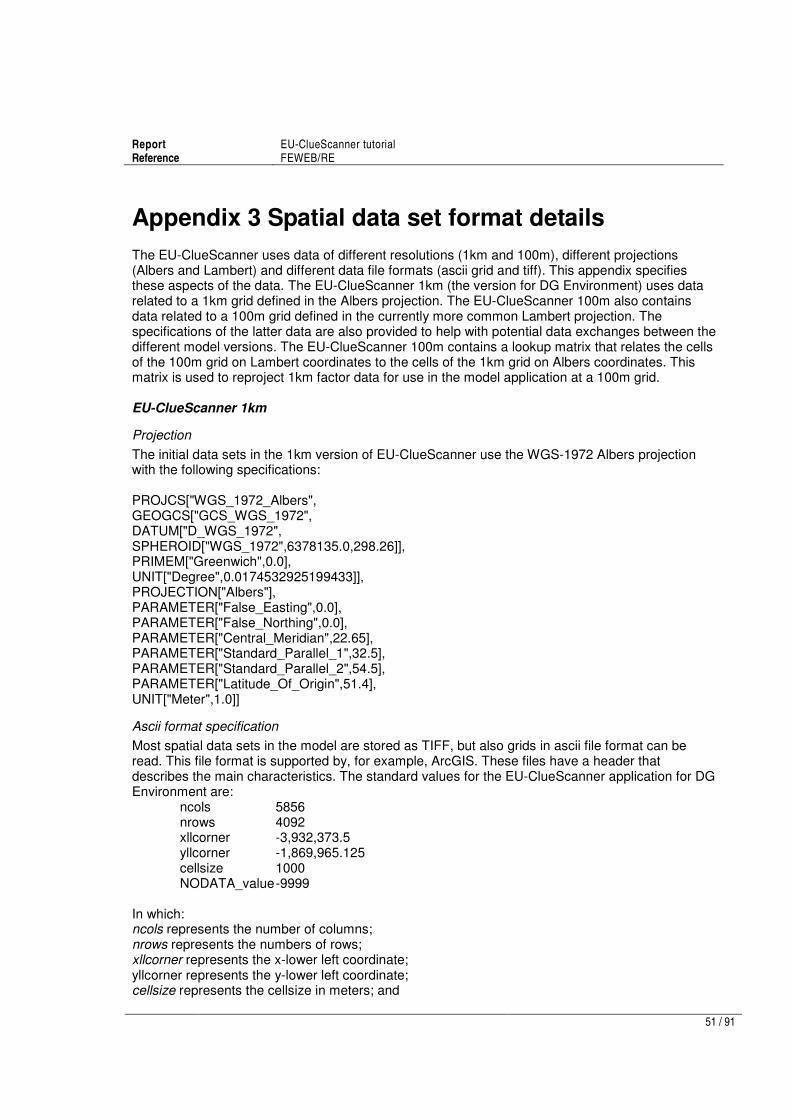
Report EU-ClueScanner tutorial Reference FEWEB/RE
51 / 91
Appendix 3 Spatial data set format details
The EU-ClueScanner uses data of different resolutions (1km and 100m), different projections (Albers and Lambert) and different data file formats (ascii grid and tiff). This appendix specifies these aspects of the data. The EU-ClueScanner 1km (the version for DG Environment) uses data related to a 1km grid defined in the Albers projection. The EU-ClueScanner 100m also contains data related to a 100m grid defined in the currently more common Lambert projection. The specifications of the latter data are also provided to help with potential data exchanges between the different model versions. The EU-ClueScanner 100m contains a lookup matrix that relates the cells of the 100m grid on Lambert coordinates to the cells of the 1km grid on Albers coordinates. This matrix is used to reproject 1km factor data for use in the model application at a 100m grid. EU-ClueScanner 1km
Projection
The initial data sets in the 1km version of EU-ClueScanner use the WGS-1972 Albers projection with the following specifications: PROJCS["WGS_1972_Albers", GEOGCS["GCS_WGS_1972", DATUM["D_WGS_1972", SPHEROID["WGS_1972",6378135.0,298.26]], PRIMEM["Greenwich",0.0], UNIT["Degree",0.0174532925199433]], PROJECTION["Albers"], PARAMETER["False_Easting",0.0], PARAMETER["False_Northing",0.0], PARAMETER["Central_Meridian",22.65], PARAMETER["Standard_Parallel_1",32.5], PARAMETER["Standard_Parallel_2",54.5], PARAMETER["Latitude_Of_Origin",51.4], UNIT["Meter",1.0]]
Ascii format specification
Most spatial data sets in the model are stored as TIFF, but also grids in ascii file format can be read. This file format is supported by, for example, ArcGIS. These files have a header that describes the main characteristics. The standard values for the EU-ClueScanner application for DG Environment are:
ncols 5856 nrows 4092 xllcorner -3,932,373.5 yllcorner -1,869,965.125 cellsize 1000 NODATA_value -9999
In which: ncols represents the number of columns; nrows represents the numbers of rows; xllcorner represents the x-lower left coordinate; yllcorner represents the y-lower left coordinate; cellsize represents the cellsize in meters; and

Report EU-ClueScanner tutorial Reference FEWEB/RE
52 / 91
NODATA_value represents the value that the model interprets as a cell with no value. EU-ClueScanner 100m
Projection
In the 100m model, all datasets use the ETRS 1989 Lambert projection with the following specifications: PROJCS["ETRS_1989_LAEA_L52_M10", GEOGCS["GCS_ETRS_1989", DATUM["D_ETRS_1989", SPHEROID["GRS_1980",6378137.0,298.257222101]], PRIMEM["Greenwich",0.0], UNIT["Degree",0.0174532925199433]], PROJECTION["Lambert_Azimuthal_Equal_Area"], PARAMETER["False_Easting",4321000.0], PARAMETER["False_Northing",3210000.0], PARAMETER["Central_Meridian",10.0], PARAMETER["Latitude_Of_Origin",52.0], UNIT["Meter",1.0]]
Data format specifications
Due to size constraints, the 100m model only supports TIFF files stored with smallest possible bit size (i.e. 1 bit for binary data, 8 bits for other types) and LZW compressed, with the following specifications:
Cell size: 100 m Size: 60,000 columns * 45,300 rows
Pixel Size = (100;-100) Corner Coordinates: Upper Left (1,500,000; 5,430,000) Lower Left (1,500,000; 900,000) Upper Right (7,500,000; 5,430,000) Lower Right (7,500,000; 900,000)
It is possible to store grid data as TIFF with ArcGIS software package, using ArcToolbox
TM Data
Management Tools -> Raster -> Raster Dataset -> Copy Raster. The file extension (.tif) must be specified while naming the file. The projection and format specifications referred above can be defined using the Environments options, namely General Settings (Output coordinate system and Extent) and Raster Analysis Settings (Cell size). The most straightforward way to define the projection is using the file ETRS_1989_LAEA_L52_M10.prj, which can be found e.g. in the folder SourceData/JRC/landuse. After this, the created TIFF file has to be exported using File -> Export map, in order to define the bit size and compression mode. To export from ArcGIS as TIFF in a compressed (LZW) format may turn out to be difficult. We solved this by specifying LZW as the default option in the ArcGIS preference definition file for TIFF files (C:\Program Files\Common Files\ESRI\Raster\defaults\tiffs.pdf). Notwithstanding its name this is a plain text file that can be edited in any text editor. When importing the dataset to the model, be sure to include a copy of the projection file in the folder.
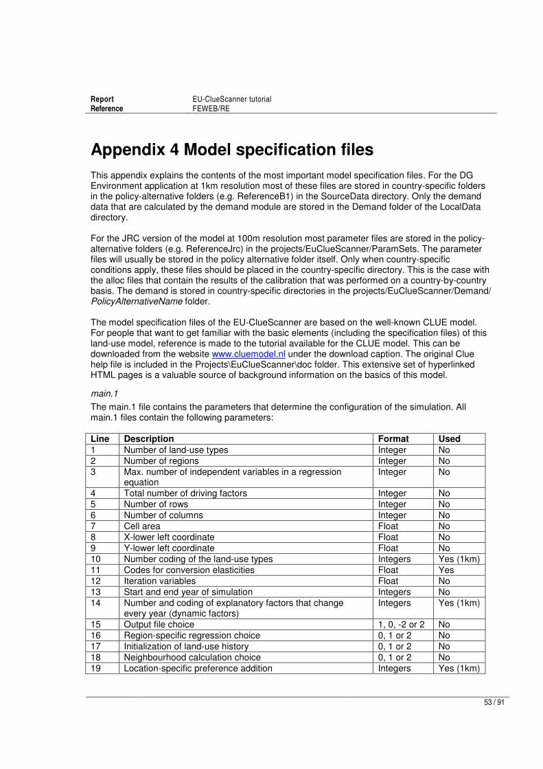
Report EU-ClueScanner tutorial Reference FEWEB/RE
53 / 91
Appendix 4 Model specification files
This appendix explains the contents of the most important model specification files. For the DG Environment application at 1km resolution most of these files are stored in country-specific folders in the policy-alternative folders (e.g. ReferenceB1) in the SourceData directory. Only the demand data that are calculated by the demand module are stored in the Demand folder of the LocalData directory. For the JRC version of the model at 100m resolution most parameter files are stored in the policy-alternative folders (e.g. ReferenceJrc) in the projects/EuClueScanner/ParamSets. The parameter files will usually be stored in the policy alternative folder itself. Only when country-specific conditions apply, these files should be placed in the country-specific directory. This is the case with the alloc files that contain the results of the calibration that was performed on a country-by-country basis. The demand is stored in country-specific directories in the projects/EuClueScanner/Demand/ PolicyAlternativeName folder. The model specification files of the EU-ClueScanner are based on the well-known CLUE model. For people that want to get familiar with the basic elements (including the specification files) of this land-use model, reference is made to the tutorial available for the CLUE model. This can be downloaded from the website www.cluemodel.nl under the download caption. The original Clue help file is included in the Projects\EuClueScanner\doc folder. This extensive set of hyperlinked HTML pages is a valuable source of background information on the basics of this model.
main.1
The main.1 file contains the parameters that determine the configuration of the simulation. All main.1 files contain the following parameters: Line Description Format Used
1 Number of land-use types Integer No
2 Number of regions Integer No
3 Max. number of independent variables in a regression equation
Integer No
4 Total number of driving factors Integer No
5 Number of rows Integer No
6 Number of columns Integer No
7 Cell area Float No
8 X-lower left coordinate Float No
9 Y-lower left coordinate Float No
10 Number coding of the land-use types Integers Yes (1km)
11 Codes for conversion elasticities Float Yes
12 Iteration variables Float No
13 Start and end year of simulation Integers No
14 Number and coding of explanatory factors that change every year (dynamic factors)
Integers Yes (1km)
15 Output file choice 1, 0, -2 or 2 No
16 Region-specific regression choice 0, 1 or 2 No
17 Initialization of land-use history 0, 1 or 2 No
18 Neighbourhood calculation choice 0, 1 or 2 No
19 Location-specific preference addition Integers Yes (1km)

Report EU-ClueScanner tutorial Reference FEWEB/RE
54 / 91
With the recoding of the original Clue model to the GeoDMS environment most parameters of the main.1 file have lost their importance as they are defined in other parts of the model or read directly from other input files. This last column in the table above lists which parameters are actually used in the allocation process. With the exception of the conversion elasticity these parameters are only used in the 1km application for DG Environment. It is possible, however, to also apply these parameters in applications at a 100m resolution. If possible, the parameters that are not used are set to 0 in the main.1 file for the current 100m application. However, for some parameters (e.g. number of land-use types) the model checks the values in the main.1 file. In these cases sensible values were maintained. A more extensive description of the original use of the parameters is provided below: 1. The number of land-use types that are distinguished in simulation. A maximum of 12
different land-use types can be identified. 2. The number of regions, default is 1 and the maximum number of regions is 3. Normally a
study area consists of only one region, but for study areas that are divided in parts with a very different behaviour of land-use types, more regions can be used. Please note that in the EU-ClueScanner separate models are specified for individual countries that are not subdivided in smaller regions.
3. The maximum number of independent variables in a regression equation. This is the number of driving factors of the regression equation with most variables.
4. The total number of driving factors that are addressed, this means the number of driving factor files per year.
5. Number of rows of the input grids. 6. Number of columns of the input grids. 7. The cell area of the grid cells, this should be in the same units as in the demand file. In our
case this is 1 km2.
8. X-coordinate of the lower left corner, this is also indicated in the header of the ArcView and ArcGIS ASCII files.
9. Y-coordinate of the lower left corner, this is also indicated in the header of the ArcView and ArcGIS ASCII files.
10. The internal number coding of the land-use types used in the simulation process. This should start with 0 for the first land-use type (= Clue10-type 0 introduced in Table 2), 1 for the second land-use type, etc. This line of script is also used to state which land-use types are simulated together (i.e. have the same demand for land). This is the case with the recently abandoned arable land (Clue10-type 5), forest (Clue10-type 7) and recently abandoned pasture land (Clue10-type 8) in the example below that are all treated as natural vegetation (Clue10-type 3).
11. The codes for the allowed changes and behaviour of the land-use types (conversion elasticities) have to be indicated for each land-use type, following the order of line 10. This must be a value between 0 and 1. 0: Means that all changes for that land-use type are allowed, independent from the current land use of a location. This means that a certain land-use type can be removed at one place and allocated at another place at the same time, e.g. shifting cultivation. >0...<1: Means that changes are allowed, however, the higher the value, the higher the preference that will be given to locations that are already under this land-use type. This setting is relevant for land-use types with high conversion costs. 1: Means that grid cells with one land-use type can never be added and removed at the same time. This is relevant for land-use types that are difficult to convert, e.g., urban settlements and primary forests. A value of one stabilizes the system and should thus be used with care.
12. Iteration variables: three numbers should be specified: Iteration mode: with the options: 0, which means that convergence criteria are expressed as a percentage of the demand; or 1, meaning that these criteria are expressed as

Report EU-ClueScanner tutorial Reference FEWEB/RE
55 / 91
absolute values (units of demand) First convergence criterium: average deviation between demanded changes and actually allocated changes (default for %: 0.35; otherwise minimal 1 grid cell divided by the number of land-use types). Second convergence criterium: maximum deviation between demanded changes and actually allocated changes (default for %: 3; otherwise should minimally be the percentage of 1 cell change of the land-use type with the smallest demand, e.g. for a land-use type with a demand of 200 ha and a cell area of 4 ha, the value should be minimally 4/(200/100) = 2).
13. Start year and end year of the simulation. 14. Number of dynamic driving factors (e.g. population density or climate related variables).
This number should be followed by the coding of these explanatory factors. The example below mentions 5 dynamic factors (numbers: 33 34 39 40 46) that thus should have input files for each year in simulation. These file codes correspond to the numbers listed in the FactorData table in the metadata.mdb. Appendix 2 also lists these numbers. Note that these files are currently ascii grids at a 1km resolution in Albers projection. When no dynamic drivers are used a ‘0’ should be paced on this line.
15. Choice for the type of output file: 1. ArcView-ArcGIS headers will be printed in output files; 0. No headers in output files (suited for e.g., Idrisi). -2. No headers in output files, suppress information in log-file on iteration procedure. 2. ArcView-ArcGIS headers will be printed in output files, suppress information in log-file on iteration procedure. Note: If the ArcView-ArcGIS file type is chosen, all input grid files should contain an ArcView-ArcGIS header.
16. Choice for a region specific regression: 0. No different regressions for different regions 1. Different regressions for different regions; demands for each region specifically defined 2. Different regressions for different regions; demand for all regions aggregated. The default is value 0.
17. When temporal dynamics are taken into account it is necessary to know the land-use history. Often this is not known and a random number has to be assigned. One can choose between three options: 0. The initial land-use history will be read from file age.0, which should contain a grid with, for every pixel, the number of years that the pixel is used for the current land-use type. 1. A random number will be assigned to all pixels to represent the number of years that the current land use is already found at that location according to the standard seed for the random number generator. With this option two runs will result in the same random number, which is useful for comparison. 2. A random number will be assigned to all pixels to represent the number of years that the current land use is already found at that location with a different random number generator. Two consecutive runs will start with different land-use histories. For option 1 or 2 an additional number should be added that indicates the maximum number of years that can be generated by the randomizer.
18. Choice for using the neighbourhood function: 0. Neighbourhood function is not used. 1. Neighbourhood function is used in simulation. 2. Only the influences are calculated, the influence files are saved directly, no simulation.
19. Variables for location specific preference addition. The first number is a switch: activate the function (1) or not (0). If the switch is set to 1, it should be followed by, for each land-use type, the fraction of the preference addition that is added to the probability as calculated in the regression.

Report EU-ClueScanner tutorial Reference FEWEB/RE
56 / 91
Below is an example of a main.1 file used in the 100m version of the EU-ClueScanner model.
line 1
line 2
line 3
line 4
line 5
line 6
line 7
line 8
line 9
line 10
line 11
line 12
line 13
line 14
line 15
line 16
line 17
line 18
line 19
6
1
0
0
0
0
0
0.0
0.0
0 1 2 3 4 5
1 0.8 0.5 0.5 0.5 0.5
1 0 0
0 0
0
2
0
0
1
0

Report EU-ClueScanner tutorial Reference FEWEB/RE
57 / 91
demand.in1
The required amount of land (demand) per year, per land-use type, per region is stored in demand.in1 text files. These files contain for each year that needs to be simulated the demand in either km
2 for the version with a 1km resolution (see example below), or hectares for the version at
a 100m resolution. The first line specifies the number of years for which demand is included in this file. In our case this is 31 (the initial year and 30 subsequent simulation years). After that, every line contains the demands for the respective land-use types for one year. The order of the land-use types should be the same as in the main parameter file (main.1) and the second line of the file contains the demands for year 0. Note: the total demand for all land-use types together should be equal to the total land area from the region file and should remain constant for each year. Below is an example of the first 7 lines of a demand.in1 file for one demand region (normally country) in the 100m version of the model. The demand for land-use type 0, for example, increases, every year with about 800 ha.
Remember, these files are calculated within the EU-ClueScanner by the demand module. The files are not intended to be edited by the user. Instead the input parameters of the Microsoft Access demand database (demand.mdb) located in projects\EuClueScanner\data\demand should be edited.
11
317581.0 17137.0 1520974.0 1196644.0 3758362.0 586994.0
318363.1 17352.8 1520186.9 1196330.6 3758386.2 587072.5
319145.2 17568.6 1519399.7 1196017.2 3758410.4 587150.9
319927.3 17784.5 1518612.5 1195703.8 3758434.6 587229.4
320709.4 18000.3 1517825.3 1195390.3 3758458.8 587307.8
321491.6 18216.1 1517038.1 1195076.9 3758483.0 587386.3
322273.8 18432.0 1516250.9 1194763.5 3758507.2 587464.8
323056.0 18647.8 1515463.6 1194450.0 3758531.4 587543.2
323838.2 18863.7 1514676.3 1194136.5 3758555.6 587621.7
324620.4 19079.5 1513889.0 1193823.1 3758579.8 587700.2
325402.7 19295.4 1513101.7 1193509.6 3758604.0 587778.6

Report EU-ClueScanner tutorial Reference FEWEB/RE
58 / 91
alloc1.reg
The alloc1.reg file contains the part of logistic regression results that relate to the importance of the suitability factors in explaining observed land-use patterns. This file has the following format (see also the example below): Line 1: Number code for land-use type (here 0 = urban land use). Line 2: Constant of regression equation for this land-use type. Line 3: Number of explanatory factors in the regression equation for that land-use type. Line 4 and further: On each line the beta coefficients (-0.00043 etc.) for the explanatory factor and the number code of the explanatory factor. The number codes of these factors can be found in the FactorData table in the metadata.mdb. Appendix 2 also lists these numbers. In the example below, line 4 refers to ACCESS1_06M: the timecost to cities > 100.000 (seconds).
0
5.964
8
-0.00043 1
-0.00007 3
-0.004 39
0.001 45
-1.482 65
-0.333 32
-1.599 67
0.490 66
1
6.303
8
-0.00073 1
-0.00010 3
-0.007 39
etc.

Report EU-ClueScanner tutorial Reference FEWEB/RE
59 / 91
alloc2.reg
The alloc2.reg file contains the part of logistic regression results that relate to the importance of the neighbourhood enrichment factors in explaining observed land-use patterns. This file has the same format as alloc1.reg: Line 1: Number code for land-use type. Line 2: Constant of neighbourhood regression equation for land-use type (ß0). Line 3: Number of explanatory factors (land-use types) in the regression equation for that land-use type. For example the presence of urban area and arable land in the neighbourhood are explanatory factors for the land-use type urban area, so the number of explanatory factors is 2. Line 4 and further: On each line the beta coefficients (ß1, ß2, etc.) for the explanatory factors and the number code of the explanatory factor. In using the neighbourhood function, the explanatory factors are the land-use types and therefore the number codes are the number codes for the land-use types. Land-use conversions can be explained partly by the occurrence of land uses in the neighbourhood. For example, new urban area is more likely to develop at the fringe of existing urban area than elsewhere. Especially in the context of urban growth, it is useful to include neighbourhood interactions as a driving factor (Verburg et al., 2004). To characterise the neighbourhood of a location the enrichment factor is often used. This measure is defined by the occurrence of a land-use type in the neighbourhood of a location relative to the occurrence of this land-use type in the study area. The weight that is assigned to the neighbourhood characteristics is assigned in the neighbourhood settings file (neighmat.txt).

Report EU-ClueScanner tutorial Reference FEWEB/RE
60 / 91
neighmat.txt
In this file the size and shape of the neighbourhoods and the weight assigned to the neighbourhood function is indicated for each land-use type individually. The file has the following format: Line 1 Weight (0-1) assigned to the neighbourhood function for each land-use type. Line 2 and further. For each land-use type: - The radius of the neighbourhood (1 = 1 grid cell on each side of the central cell). - Followed by the shape of the neighbourhood (with weights (0-1) for individual cells). Below is an example of the first part of such a file for the 1km version of the EU-ClueScanner model. It shows that for the first land-use type only the first ring of cells surrounding the central cell is selected as neighbourhood. The second reference to this first land-use type indicates that each cell receives an equal weight.
0.3 0.3 0.3 0.3 0.3 0.3
3
1 1 1 1 1 1 1
1 2 2 2 2 2 1
1 2 4 4 4 2 1
1 2 4 0 4 2 1
1 2 4 4 4 2 1
1 2 2 2 2 2 1
1 1 1 1 1 1 1
etc.

Report EU-ClueScanner tutorial Reference FEWEB/RE
61 / 91
1 0 0 0 0 0 0 0 0 0
52 1 1 0 0 1 52 0 0 0
52 61 1 0 0 0 52 0 1 0
0 61 52 1 0 0 52 60 0 0
0 0 0 0 1 0 0 0 0 0
52 61 52 58 0 1 52 0 0 0
52 61 52 0 0 1 1 0 0 0
0 61 52 0 0 0 52 1 0 0
52 61 52 59 0 0 52 0 1 0
0 0 0 0 0 0 0 0 0 1
allow.txt
The allow.txt file specifies how succession of land-use types takes place. It may refer to succession maps that specify locations where certain successions may take place. It is a Y x Y matrix where Y equals the number of land-use types. So when 10 land-use types are simulated by the model it will be a 10x10 matrix. Rows denote the present land-use type and columns the potential future land-use type. A value of 1 indicates that the conversion is allowed, a value of 0 indicates that the conversion is not allowed. Other codes refer to maps that specify whether succession is allowed for individual (1x1 km) locations. The example below shows a typical allow.txt file used in the DG environment application. For clarity’s sake the related Clue10 land-use type codes (0-9) are included next to the file. The value 52 in row 1 on line 2 in this example denotes that the conversion of the second land-use type (arable land) into the first (urban) is conditional on allow driver map 52. This map represents the Natura2000 areas with a value of 0, indicating that urbanisation is not allowed here (see the FactorData table in the metadata.mdb or Appendix 2 for a complete list of all allow driver maps). The remaining areas contain a value of 1 indicating that conversion is allowed. The conversion settings for the different policy alternatives in the DG-Environment application of the EU-ClueScanner are provided in a separate annex to the final report. to: 0 1 2 3 4 5 6 7 8 9
from
land use 0
1
2
3
4
5
6
7
8
9
Please note that this option has not yet been used in 100m version of the model, although this is technically possible. Take care, however, that the allow driver maps should be stored as ascii grids in the Albers projection at 1km resolution. A lookup matrix ensures that these dataset are used properly. When needed the allow driver definition can also be implemented at the level of countries, or be adjusted to ingest 100m resolution data in Lambert projection.

Report EU-ClueScanner tutorial Reference FEWEB/RE
62 / 91
locspecX.asc
The implementation of policy themes is, to some extent, done by location specific modification of the suitability of the land for a specific land-use type. The suitabilities reflect an index of the potential land rent that can be attained at a specific location for a specific land-use type. Scenario settings (subsidies and taxes) influence these suitabilities. Financial support may, for example, be considered for maintaining agriculture in mountainous areas. This leads to a higher probability that agricultural land use is conserved in these areas than could be expected from the statistical regression between land use and (biophysical and socio-economic) driving factors that apply for the study area as a whole. Such modifications are reflected in the location-specific addition factors (locspec). These location-specific addition factors for different policies are combined in one map for each land-use type. See the appendix to the final report for an overview of the way various policies are combined in the current application. When this option is used, for each land-use type a file named locspec#.asc (# indicates the land-use type number) should be supplied in the relevant policy-alternative folders (e.g. ReferenceJRC) in the Projects/EuClueScanner/ParamSets directory. These additions are stored in maps that provide a value in each grid cell that should preferably lie between 0-1 in order to fit the range of the regression results. Note that the switch on line 19 in the main.1 file should be set to 1 and weight factors should be specified. The function is not active when the switch in main.1 has the value 0. Please note that this option has not yet been used in 100m version of the model, although this is technically possible. Take care, however, that the locspec files should be stored as ascii grids in the Albers projection at 1km resolution. A lookup matrix ensures that these dataset are used properly. As opposed to the previous 1km version the locspec files are now expected to be stored in the Projects/ EuClueScanner/Paramsets directory at the policy-alternative level and not in SourceData/EuClueScanner/PolicyAlternativeName at the country level. When needed the locspec definition can also be implemented at the level of countries, or be adjusted to ingest 100m resolution data in Lambert projection.

Report EU-ClueScanner tutorial Reference FEWEB/RE
63 / 91
Appendix 5 Calibration steps
This appendix describes the main steps in the calibration of the JRC version of the EU-ClueScanner. It is basically an internal working document that is included to provide JRC with some background information on how to calibrate the model using mulitinomial logistic regression. The main idea is to calibrate the suitability map definition for the new JRC-land use model based on observed land-use patterns in 1990 (thus a static approach). This is based on the actual amount of change from 1990-2000 from our own CLC comparison and the calibrated suitability maps to simulate land-use in 2000 and validate the thus obtained simulation results with observed 2000 land use. A first introduction to Multinomial Logistics can be found at the following informative website: http://www.ats.ucla.edu/stat/Spss/output/mlogit.htm
Main steps
1. Collect the relevant data per country (a NUTS-0 region that normally consists of one country, but, in case of very small ones, more. See further on in document) in ArcGIS: 1990-land use in 9 classes, neighbourhood-land use, additional explanatory variables at 1km (selection of 52 datasets from WUR, based on their statistical results in alloc1.reg files) and several own 100m data sets.
2. The land-use types are reclassified in the JRC-9 typology. 3. Export data to x,y,z-text file. First a mask is applied on the land-use raster to make sure
that only the country itself is analysed (and not the neighbouring countries in the NUTS0-rectangle). Then, through the SAMPLE command (using the Multi Output Map Algebra feature), the explanatory and neighbourhood variables are exported as z variables with the land-use data as mask and source of the x,y coordinates. The resulting file gets the name of the country and a .sav extension.
4. import data in SPSS - note that the file contains a header - specify the types of the variables in Variable view as being either scale (continuous),
ordinal (range) or nominal (for categorical or binary dummy variables). Almost all variables are scale, except for natura2000 regions, southslope, Geomorf etc.
- check the dataset descriptive statistics (Analyze -> Descriptive Statistics-> Descriptive) and then set the width (number of decimal cases) of each variable in Variable view, according to the maximum value (e.g. maximum value 1000, thus set width as 4).
- apply a filter on the static land-use types (water, infrastructures and other nature – thus classes 7, 8 and 9) that are not simulated by the model (data -> select cases –> if: jrc9_1990 ne 7 and jrc9_1990 ne 8 and jrc9_1990 ne 9)
5. run multinomial regression (analyse -> regression -> MNL) taking into account: - dependent is land use (jrc9) - increase the stephalving from 5 to 10 for better results (under criteria) - specify as reference category a land-use type according to the name of the dataset
file, e.g. Netherlands_refclass4 –means that class 4 should be specified as reference category.
- factors are dummy and other categorical (nominal) variables - co-variates are continuous variables (scale) - Basically we try three separate regression models:
o one using all factors from the WUR; o one using the WUR-factors and the relevant new 100metre grid data (not
population); o one using the rings (neighbourhood variables);
Each step is refined based on an analysis of the correlation between the independent

Report EU-ClueScanner tutorial Reference FEWEB/RE
64 / 91
(explanatory) variables as is discussed below. Eventually we end up with about 15 independent variables as is documented in files such as: summary JRC9Belgium.rtf in the G:/0301.../calibration directory. Such neat output files are generated by giving File -> Export in the spss outputfile (.spo).
- Check correlation between factors with Pearson test (Analyze -> Correlate -> BiVariate). This is done for the following groups of similar and potentially correlated variables:
o population and accesses variables (e.g. access1_06min, access6_06min, euac60_1000, landsc_06, poppot_1000 and population density);
o geophysical variables (e.g. geomorf0, mean_temp_06, rain_wc_5m , t_plus15_1000, slope, elev and sosl)
o soil variables (e.g. claycont_06pc, soildepth_06 and swap) o neighbourhood variables
There is strong correlation if correlation coefficient > 0.5 or < -0.5. In this case one of the correlated variables should be dropped. We prefer to keep the 100metre versions and strive to maintain at least one accessibility measure, one climate and one soil variable.
- Consider also dropping some of the neighbourhood variables based on the average value in the Descriptives (drop when this is very close to 0) or the significance in the statistical regression.
- Labels can be added to the output in spss by adding this bit of script to the syntax: VALUE LABELS jrc9_1990 1 'Urban fabric' 2 'Industry and related uses' 3 'Arable land and permanent crops' 4 'Pastures' 5 'Forests' 6 'Semi natural vegetation' 7 'Other nature' 8 'Infrastructure' 9 'Water'.

Report EU-ClueScanner tutorial Reference FEWEB/RE
65 / 91
Appendix 6 Observed land-use change
This appendix list the observed land-use change between CLC1990 and CLC2000 for all 27 member states based on the reclassified Corine Land Cover data. The changes are described as aggregate changes (relating to the total amounts of land taken be each type of use) and land-use transitions based on a pixel-by-pixel comparison of the two data sets performed in GIS. Such transitions are helpful in highlighting the ongoing land-use change processes (see for example: Diogo and Koomen, 2010; Pena et al., 2007). The observed aggregate changes were used to define the demand for the land-use types that were simulated in the validation2000 runs of the 100m version of the model. The amount of change observed was also used to estimate the amount of change between 2000 and 2030 for the Reference alternatives in the JRC application. In this case the observed amount of change between CLC1990 and CLC2000 was divided by the observation period to obtain a yearly increase per land-use type. This was then used as additional demand per land-use type for each year until 2030. This calculation corrected for the fact that the actual time period between CLC1990 and CLC2000 differs per country, as is shown below.
Country CLC1990 CLC2000 Comments
start end start end
Austria 1985 1986 1999 2001
Belgium 1989 1990 1999 2000
Bulgaria 1989 1992 2000 2001
Cyprus1 x x 2000 2000 no CLC1990 available
Czech Republic 1989 1992 1999 2001
Denmark 1989 1990 1999 2001
Estonia 1993 1995 1999 2001
Finland1 1986 1994 1999 2002 no CLC1990 version 9/2007 available
France (Incl. Monaco) 1987 1994 1999 2001
Germany 1989 1992 1999 2001
Greece 1987 1991 2000 2001
Hungary 1990 1992 2000 2000
Ireland 1989 1990 2000 2001
Italy (Incl. San Marino & the Vatican) 1990 1993 1999 2002
Latvia 1994 1995 1999 2001
Lithuania 1994 1995 1999 2001
Luxembourg 1991 1991 2000 2000
Malta1 x x 2001 2001 no CLC1990 available
The Netherlands 1986 1988 1999 2000
Poland 1989 1992 1999 2001
Portugal 1985 1987 1999 2002
Romania 1989 1992 2000 2001
Slovak Republic 1989 1992 2000 2001
Slovenia 1995 1996 1999 2000
Spain 1984 1990 1999 2002
Sweden1 x x 1999 2002 no CLC1990 available
United Kingdom 1989 1990 1999 2002 no CLC1990 version 9/2007 available; a 1990 version was constructed based on
the CLC-change data set
Note: 1For the countries that lack CLC1990 data no change analysis could be performed.

Report EU-ClueScanner tutorial Reference FEWEB/RE
66 / 91
Austria
Aggregated land use classes 1990 2000 Change
Urban fabric 317581 325362 7781
Industry and related uses 17137 19293 2156
Arable land and permanent crops 1520974 1512912 -8062
Pastures 1196644 1193360 -3284
Forests 3758362 3758133 -229
Semi natural vegetation 586994 587705 711
Infrastructures 5567 6172 605
Other Nature 921253 921030 -223
Water 69744 70289 545
Total 8394256 8394256 0
Observed land-use change in Austria based on CLC1990 and CLC2000.
Urb
an
fa
bri
c
Ind
ust
ry a
nd
re
late
d u
ses
Ara
ble
lan
d a
nd
pe
rma
ne
nt
cro
ps
Pa
stu
res
Fo
rest
s
Se
mi n
atu
ral v
eg
eta
tio
n
Infr
ast
ruct
ure
s
Oth
er
Na
ture
Wa
ter
Urban fabric 317455 78 2 8 6 0 32 0 0
Industry and related uses 234 15239 184 345 590 67 156 0 322
Arable land and permanent crops 4148 2635 1512278 842 522 163 312 0 74
Pastures 2881 301 250 1191703 1311 143 12 0 43
Forests 440 878 178 431 3751930 4322 11 117 55
Semi natural vegetation 185 162 0 15 3669 582875 82 6 0
Infrastructures 0 0 0 0 0 0 5567 0 0
Other Nature 19 0 11 0 105 129 0 920907 82
Water 0 0 9 16 0 6 0 0 69713
CLC
19
90
CLC2000
Transition matrix for observed land-use change in Austria based on CLC1990 and CLC2000.

Report EU-ClueScanner tutorial Reference FEWEB/RE
67 / 91
Belgium and Luxemburg
Aggregated land use classes 1990 2000 Change
Urban fabric 550378 557787 7409
Industry and related uses 55115 64633 9518
Arable land and permanent crops 1068440 1060361 -8079
Pastures 792989 782356 -10633
Forests 697322 701456 4134
Semi natural vegetation 89938 84712 -5226
Infrastructures 20789 23490 2701
Other Nature 29938 29253 -685
Water 19917 20778 861
Total 3324826 3324826 0
Observed land-use change in Belgium and Luxemburg based on CLC1990 and CLC2000.
Urb
an
fa
bri
c
Ind
ust
ry a
nd
re
late
d u
ses
Ara
ble
lan
d a
nd
pe
rma
ne
nt
cro
ps
Pa
stu
res
Fo
rest
s
Se
mi n
atu
ral v
eg
eta
tio
n
Infr
ast
ruct
ure
s
Oth
er
Na
ture
Wa
ter
Urban fabric 549389 819 23 49 8 0 81 0 9
Industry and related uses 183 51999 125 114 22 426 799 1110 337
Arable land and permanent crops 3963 5785 1054515 1940 505 168 1140 142 282
Pastures 3250 3266 5331 779813 633 192 228 189 87
Forests 353 843 146 243 687819 7481 95 223 119
Semi natural vegetation 476 685 131 156 11867 76411 28 103 81
Infrastructures 0 13 31 0 0 0 20712 21 12
Other Nature 173 1121 55 30 602 34 357 27465 101
Water 0 102 4 11 0 0 50 0 19750
CLC2000
CLC
19
90
Transition matrix for observed land-use change in Belgium and Luxemburg based on CLC1990 and CLC2000. Please note that these two countries have been combined into one demand region in the model.

Report EU-ClueScanner tutorial Reference FEWEB/RE
68 / 91
Bulgaria
Aggregated land use class 1990 2000 Change
Urban fabric 424612 424782 170
Industry and related uses 108237 111140 2903
Arable land and permanent crops 4479194 4477440 -1754
Pastures 960400 959106 -1294
Forests 3481200 3491133 9933
Semi natural vegetation 1438023 1429267 -8756
Infrastructures 8424 8424 0
Other Nature 101837 100576 -1261
Water 95548 95607 59
Total 11097475 11097475 0
Observed land-use change in Bulgaria based on CLC1990 and CLC2000.
Urb
an
fa
bri
c
Ind
ust
ry a
nd
re
late
d u
ses
Ara
ble
lan
d a
nd
pe
rma
ne
nt
cro
ps
Pa
stu
res
Fo
rest
s
Se
mi n
atu
ral v
eg
eta
tio
n
Infr
ast
ruct
ure
s
Oth
er
Na
ture
Wa
ter
Urban fabric 424603 6 2 1 0 0 0 0 0
Industry and related uses 0 107788 394 10 0 0 0 0 45
Arable land and permanent crops 88 1798 4468566 7796 383 474 0 60 29
Pastures 66 721 7910 950629 417 614 0 0 43
Forests 0 315 112 157 3450575 29026 0 967 48
Semi natural vegetation 25 511 324 229 37640 1399132 0 89 73
Infrastructures 0 0 0 0 0 0 8424 0 0
Other Nature 0 0 45 284 2051 0 0 99146 311
Water 0 1 87 0 67 21 0 314 95058
CLC
19
90
CLC2000
Transition matrix for observed land-use change in Bulgaria based on CLC1990 and CLC2000.

Report EU-ClueScanner tutorial Reference FEWEB/RE
69 / 91
Czech Republic
Aggregated land use classes 1990 2000 Change
Urban fabric 377511 383191 5680
Industry and related uses 87841 86755 -1086
Arable land and permanent crops 3789061 3499380 -289681
Pastures 578213 857937 279724
Forests 2490003 2555103 65100
Semi natural vegetation 490126 428316 -61810
Infrastructures 10596 11062 466
Other Nature 11972 11889 -83
Water 53784 55474 1690
Total 7889107 7889107 0
Observed land-use change in Czech Republic based on CLC1990 and CLC2000.
Urb
an
fa
bri
c
Ind
ust
ry a
nd
re
late
d u
ses
Ara
ble
lan
d a
nd
pe
rma
ne
nt
cro
ps
Pa
stu
res
Fo
rest
s
Se
mi n
atu
ral v
ege
tati
on
Infr
ast
ruct
ure
s
Oth
er
Na
ture
Wa
ter
Urban fabric 377220 246 12 33 0 0 0 0 0
Industry and related uses 1422 80056 760 1020 180 4144 82 0 177
Arable land and permanent crops 3764 4065 3492084 286068 136 1993 270 0 681
Pastures 448 538 6117 569656 210 729 89 0 426
Forests 21 355 18 89 2434586 54816 0 20 98
Semi natural vegetation 316 1491 367 1054 119947 366452 25 71 403
Infrastructures 0 0 0 0 0 0 10596 0 0
Other Nature 0 0 5 11 44 153 0 11672 87
Water 0 4 17 6 0 29 0 126 53602
CLC
19
90
CLC2000
Transition matrix for observed land-use change in Czech Republic based on CLC1990 and CLC20000.

Report EU-ClueScanner tutorial Reference FEWEB/RE
70 / 91
Denmark
Aggregated land use classes 1990 2000 Change
Urban fabric 251804 259532 7728
Industry and related uses 26065 30954 4889
Arable land and permanent crops 2939050 2918121 -20929
Pastures 270048 270218 170
Forests 408803 383133 -25670
Semi natural vegetation 178644 209381 30737
Infrastructures 11738 11883 145
Other Nature 191420 193930 2510
Water 82454 82874 420
Total 4360026 4360026 0 Observed land-use change in Denmark based on CLC1990 and CLC2000.
Urb
an
fa
bri
c
Ind
ust
ry a
nd
re
late
d u
ses
Ara
ble
lan
d a
nd
pe
rma
ne
nt
cro
ps
Pa
stu
res
Fo
rest
s
Se
mi n
atu
ral v
ege
tati
on
Infr
ast
ruct
ure
s
Oth
er
Na
ture
Wa
ter
Urban fabric 251444 356 0 0 0 0 4 0 0
Industry and related uses 33 25513 164 52 5 151 59 88 0
Arable land and permanent crops 6918 4217 2917725 1872 473 6441 82 1272 50
Pastures 520 296 225 268254 23 303 0 180 247
Forests 144 202 7 5 382161 26188 0 96 0
Semi natural vegetation 436 288 0 35 465 176138 0 1198 84
Infrastructures 0 0 0 0 0 0 11738 0 0
Other Nature 37 75 0 0 6 160 0 191096 46
Water 0 7 0 0 0 0 0 0 82447
CLC
19
90
CLC2000
Transition matrix for observed land-use change in Denmark based on CLC1990 and CLC2000.

Report EU-ClueScanner tutorial Reference FEWEB/RE
71 / 91
Estonia
Aggregated land use classes 1990 2000 Change
Urban fabric 53148 54532 1384
Industry and related uses 29315 29797 482
Arable land and permanent crops 837389 847642 10253
Pastures 524832 513048 -11784
Forests 2133239 2093230 -40009
Semi natural vegetation 509576 548202 38626
Infrastructures 6358 6393 35
Other Nature 217630 218735 1105
Water 221327 221235 -92
Total 4532814 4532814 0 Observed land-use change in Estonia based on CLC1990 and CLC2000.
Urb
an
fa
bri
c
Ind
ust
ry a
nd
re
late
d u
ses
Ara
ble
lan
d a
nd
pe
rma
ne
nt
cro
ps
Pa
stu
res
Fo
rest
s
Se
mi n
atu
ral v
eg
eta
tio
n
Infr
ast
ruct
ure
s
Oth
er
Na
ture
Wa
ter
Urban fabric 53142 0 2 3 1 0 0 0 0
Industry and related uses 39 28692 1 0 8 69 0 506 0
Arable land and permanent crops 384 33 814212 22572 41 142 4 1 0
Pastures 662 75 33225 490219 63 581 0 7 0
Forests 50 242 149 161 2088786 43499 25 322 5
Semi natural vegetation 246 664 53 93 4326 503667 6 521 0
Infrastructures 0 0 0 0 0 0 6358 0 0
Other Nature 9 91 0 0 5 244 0 217281 0
Water 0 0 0 0 0 0 0 97 221230
CLC
19
90
CLC2000
Transition matrix for observed land-use change in Estonia based on CLC1990 and CLC2000.

Report EU-ClueScanner tutorial Reference FEWEB/RE
72 / 91
France
Aggregated land use classes 1990 2000 Change
Urban fabric 2080408 2144434 64026
Industry and related uses 372058 419105 47047
Arable land and permanent crops 20131305 20119019 -12286
Pastures 12433222 12341987 -91235
Forests 14491461 14510117 18656
Semi natural vegetation 3347396 3321298 -26098
Infrastructures 78866 90462 11596
Other Nature 1779079 1754752 -24327
Water 445554 458175 12621
Total 55159349 55159349 0
Observed land-use change in France based on CLC1990 and CLC2000.
Urb
an
fa
bri
c
Ind
ust
ry a
nd
re
late
d u
ses
Ara
ble
lan
d a
nd
pe
rma
ne
nt
cro
ps
Pa
stu
res
Fo
rest
s
Se
mi n
atu
ral v
eg
eta
tio
n
Infr
ast
ruct
ure
s
Oth
er
Na
ture
Wa
ter
Urban fabric 2078629 1574 38 18 5 0 95 6 43
Industry and related uses 5110 347613 3334 2711 758 3610 3602 1589 3731
Arable land and permanent crops 30065 36164 20006139 44969 3049 2137 4922 511 3349
Pastures 22620 18896 93165 12284187 4971 3526 1580 445 3832
Forests 4513 8118 6319 4413 14146448 314891 1430 3889 1440
Semi natural vegetation 2722 4313 8533 4490 350145 2971129 276 5294 494
Infrastructures 0 327 8 0 0 0 78451 0 80
Other Nature 760 1564 1406 1071 4714 25954 66 1742595 949
Water 15 536 77 128 27 51 40 423 444257
CLC
19
90
CLC2000
Transition matrix for observed land-use change in France based on CLC1990 and CLC2000.

Report EU-ClueScanner tutorial Reference FEWEB/RE
73 / 91
Germany
Aggregated land use classes 1990 2000 Change
Urban fabric 2267868 2381891 114023
Industry and related uses 393661 436651 42990
Arable land and permanent crops 15473094 15172992 -300102
Pastures 5862762 5958103 95341
Forests 10408672 10392037 -16635
Semi natural vegetation 603582 647304 43722
Infrastructures 74632 76167 1535
Other Nature 542947 543265 318
Water 495971 514779 18808
Total 36123189 36123189 0
Observed land-use change in Germany based on CLC1990 and CLC2000.
Urb
an
fa
bri
c
Ind
ust
ry a
nd
re
late
d u
ses
Ara
ble
lan
d a
nd
pe
rma
ne
nt
cro
ps
Pa
stu
res
Fo
rest
s
Se
mi n
atu
ral v
eg
eta
tio
n
Infr
ast
ruct
ure
s
Oth
er
Na
ture
Wa
ter
Urban fabric 2263858 3265 250 47 259 87 38 38 26
Industry and related uses 1758 344672 5742 1847 1408 12391 320 15178 10345
Arable land and permanent crops 90801 65789 15086815 205596 12328 3071 1929 1396 5369
Pastures 22914 8182 76767 5746968 3360 1330 130 1068 2043
Forests 1175 9170 1189 996 10326173 68121 162 944 742
Semi natural vegetation 1088 3307 548 829 47031 547928 116 2003 732
Infrastructures 121 699 103 17 53 110 73426 0 103
Other Nature 176 1409 1470 1663 1425 14048 0 522045 711
Water 0 158 108 140 0 218 46 593 494708
CLC
19
90
CLC2000
Transition matrix for observed land-use change in Germany based on CLC1990 and CLC2000.

Report EU-ClueScanner tutorial Reference FEWEB/RE
74 / 91
Greece
Aggregated land use classes 1990 2000 Change
Urban fabric 178291 184186 5895
Industry and related uses 52059 74711 22652
Arable land and permanent crops 3751335 3740097 -11238
Pastures 1084759 1080460 -4299
Forests 2430740 2374598 -56142
Semi natural vegetation 5097256 5128075 30819
Infrastructures 11009 20020 9011
Other Nature 349425 353832 4407
Water 127821 126716 -1105
Total 13082695 13082695 0
Observed land-use change in Greece based on CLC1990 and CLC2000.
Urb
an
fa
bri
c
Ind
ust
ry a
nd
re
late
d u
ses
Ara
ble
lan
d a
nd
pe
rma
ne
nt
cro
ps
Pa
stu
res
Fo
rest
s
Se
mi n
atu
ral v
eg
eta
tio
n
Infr
ast
ruct
ure
s
Oth
er
Na
ture
Wa
ter
Urban fabric 178179 57 16 1 0 2 36 0 0
Industry and related uses 221 49293 13 123 0 421 1842 15 131
Arable land and permanent crops 2931 12631 3725628 4052 203 825 4507 81 477
Pastures 2236 3436 5616 1071163 201 952 897 41 217
Forests 16 1272 639 744 2339743 85912 210 1427 777
Semi natural vegetation 569 7540 6207 4048 34344 5033453 1588 8237 1270
Infrastructures 0 24 7 9 0 40 10929 0 0
Other Nature 34 263 409 171 99 6380 10 341239 820
Water 0 195 1562 149 8 90 1 2792 123024
CLC
19
90
CLC2000
Transition matrix for observed land-use change in Greece based on CLC1990 and CLC2000.

Report EU-ClueScanner tutorial Reference FEWEB/RE
75 / 91
Hungary
Aggregated land use classes 1990 2000 Change
Urban fabric 452082 454466 2384
Industry and related uses 59069 63043 3974
Arable land and permanent crops 5392710 5368266 -24444
Pastures 918365 899530 -18835
Forests 1682445 1737428 54983
Semi natural vegetation 518191 494449 -23742
Infrastructures 9912 11309 1397
Other Nature 106393 107265 872
Water 169848 173259 3411
Total 9309015 9309015 0 Observed land-use change in Hungary based on CLC1990 and CLC2000.
Urb
an
fa
bri
c
Ind
ust
ry a
nd
re
late
d u
ses
Ara
ble
lan
d a
nd
pe
rma
ne
nt
cro
ps
Pa
stu
res
Fo
rest
s
Se
mi n
atu
ral v
eg
eta
tio
n
Infr
ast
ruct
ure
s
Oth
er
Na
ture
Wa
ter
Urban fabric 451352 473 16 67 116 35 23 0 0
Industry and related uses 305 56642 271 1180 190 414 6 0 61
Arable land and permanent crops 2020 3803 5301719 54207 12237 15632 1237 325 1530
Pastures 588 1615 62539 842078 2410 7293 47 1043 752
Forests 98 271 891 749 1623701 56492 65 108 70
Semi natural vegetation 53 208 2760 1002 98626 414307 31 947 257
Infrastructures 0 0 0 0 0 0 9900 0 12
Other Nature 22 31 0 118 56 243 0 104469 1454
Water 28 0 70 129 92 33 0 373 169123
CLC
19
90
CLC2000
Transition matrix for observed land-use change in Hungary based on CLC1990 and CLC2000.

Report EU-ClueScanner tutorial Reference FEWEB/RE
76 / 91
Ireland
Aggregated land use classes 1990 2000 Change
Urban fabric 87500 110565 23065
Industry and related uses 10671 17317 6646
Arable land and permanent crops 563677 706032 142355
Pastures 4052274 3869195 -183079
Forests 302365 293324 -9041
Semi natural vegetation 432882 554818 121936
Infrastructures 3280 5187 1907
Other Nature 1407977 1305281 -102696
Water 166129 165036 -1093
Total 7026755 7026755 0
Observed land-use change in Ireland based on CLC1990 and CLC2000.
Urb
an
fa
bri
c
Ind
ust
ry a
nd
re
late
d u
ses
Ara
ble
lan
d a
nd
pe
rma
ne
nt
cro
ps
Pa
stu
res
Fo
rest
s
Se
mi n
atu
ral v
eg
eta
tio
n
Infr
ast
ruct
ure
s
Oth
er
Na
ture
Wa
ter
Urban fabric 87154 278 0 29 0 1 35 0 3
Industry and related uses 372 9805 0 0 0 0 493 0 1
Arable land and permanent crops 3681 2320 487352 67853 716 1447 283 5 20
Pastures 18437 4690 217821 3798691 4238 7207 1067 40 83
Forests 98 21 20 100 232505 69524 0 45 52
Semi natural vegetation 582 89 562 959 31359 399195 29 63 44
Infrastructures 0 0 0 0 0 0 3280 0 0
Other Nature 241 114 271 1524 24506 76111 0 1305081 129
Water 0 0 6 39 0 1333 0 47 164704
CLC
19
90
CLC2000
Transition matrix for observed land-use change in Ireland based on CLC1990 and CLC2000.

Report EU-ClueScanner tutorial Reference FEWEB/RE
77 / 91
Italy
Aggregated land use classes 1990 2000 Change
Urban fabric 1042963 1094501 51538
Industry and related uses 244088 273140 29052
Arable land and permanent crops 12726080 12626151 -99929
Pastures 2442015 2410878 -31137
Forests 7813500 7897245 83745
Semi natural vegetation 4001361 3961629 -39732
Infrastructures 42196 43309 1113
Other Nature 1442126 1446562 4436
Water 311517 312431 914
Total 30065846 30065846 0
Observed land-use change in Italy based on CLC1990 and CLC2000.
Urb
an
fa
bri
c
Ind
ust
ry a
nd
re
late
d u
ses
Ara
ble
lan
d a
nd
pe
rma
ne
nt
cro
ps
Pa
stu
res
Fo
rest
s
Se
mi n
atu
ral v
eg
eta
tio
n
Infr
ast
ruct
ure
s
Oth
er
Na
ture
Wa
ter
Urban fabric 1042854 61 22 0 26 0 0 0 0
Industry and related uses 599 241958 54 4 48 924 239 0 262
Arable land and permanent crops 34344 24286 12612498 17263 3568 31649 770 399 1303
Pastures 12742 4145 7821 2392549 3545 20881 90 127 115
Forests 716 772 1644 372 7792490 12914 7 4474 111
Semi natural vegetation 3107 1412 3840 556 96329 3892976 15 3035 91
Infrastructures 0 43 0 0 0 0 42153 0 0
Other Nature 139 283 173 98 1087 2119 35 1437574 618
Water 0 180 99 36 152 166 0 953 309931
CLC
19
90
CLC2000
Transition matrix for observed land-use change in Italy based on CLC1990 and CLC2000.

Report EU-ClueScanner tutorial Reference FEWEB/RE
78 / 91
Latvia
Aggregated land use classes 1990 2000 Change
Urban fabric 61263 61263 0
Industry and related uses 18773 18894 121
Arable land and permanent crops 1298552 1303584 5032
Pastures 1404276 1399193 -5083
Forests 2840781 2712137 -128644
Semi natural vegetation 557944 686517 128573
Infrastructures 4599 4599 0
Other Nature 160163 159938 -225
Water 120848 121074 226
Total 6467199 6467199 0
Observed land-use change in Latvia based on CLC1990 and CLC2000.
Urb
an
fa
bri
c
Ind
ust
ry a
nd
re
late
d u
ses
Ara
ble
lan
d a
nd
pe
rma
ne
nt
cro
ps
Pa
stu
res
Fo
rest
s
Se
mi n
atu
ral v
eg
eta
tio
n
Infr
ast
ruct
ure
s
Oth
er
Na
ture
Wa
ter
Urban fabric 61263 0 0 0 0 0 0 0 0
Industry and related uses 0 18773 0 0 0 0 0 0 0
Arable land and permanent crops 0 4 1238535 59993 9 10 0 0 1
Pastures 0 0 65041 1339199 10 26 0 0 0
Forests 0 111 7 1 2711945 128717 0 0 0
Semi natural vegetation 0 6 1 0 173 557764 0 0 0
Infrastructures 0 0 0 0 0 0 4599 0 0
Other Nature 0 0 0 0 0 0 0 159938 225
Water 0 0 0 0 0 0 0 0 120848
CLC
19
90
CLC2000
Transition matrix for observed land-use change in Latvia based on CLC1990 and CLC2000.

Report EU-ClueScanner tutorial Reference FEWEB/RE
79 / 91
Lithuania
Aggregated land use classes 1990 2000 Change
Urban fabric 157865 158653 788
Industry and related uses 47040 46805 -235
Arable land and permanent crops 2733488 2784118 50630
Pastures 1127691 1076231 -51460
Forests 1953242 1896182 -57060
Semi natural vegetation 325058 382059 57001
Infrastructures 9360 9376 16
Other Nature 67816 67880 64
Water 171218 171474 256
Total 6592778 6592778 0 Observed land-use change in Lithuania based on CLC1990 and CLC2000.
Urb
an
fa
bri
c
Ind
ust
ry a
nd
re
late
d u
ses
Ara
ble
lan
d a
nd
pe
rma
ne
nt
cro
ps
Pa
stu
res
Fo
rest
s
Se
mi n
atu
ral v
eg
eta
tio
n
Infr
ast
ruct
ure
s
Oth
er
Na
ture
Wa
ter
Urban fabric 157852 0 11 1 1 0 0 0 0
Industry and related uses 646 46258 7 38 0 11 0 23 57
Arable land and permanent crops 70 236 2717501 15349 5 246 0 0 81
Pastures 70 129 66357 1060624 11 331 0 3 166
Forests 0 77 102 68 1894608 58361 16 10 0
Semi natural vegetation 15 105 140 85 1557 323004 0 123 29
Infrastructures 0 0 0 0 0 0 9360 0 0
Other Nature 0 0 0 0 0 106 0 67694 16
Water 0 0 0 66 0 0 0 27 171125
CLC
19
90
CLC2000
Transition matrix for observed land-use change in Lithuania based on CLC1990 and CLC2000.

Report EU-ClueScanner tutorial Reference FEWEB/RE
80 / 91
The Netherlands
Aggregated land use classes 1990 2000 Change
Urban fabric 294516 350081 55565
Industry and related uses 53234 77845 24611
Arable land and permanent crops 1111501 1083746 -27755
Pastures 1471212 1396179 -75033
Forests 305688 313883 8195
Semi natural vegetation 57792 65117 7325
Infrastructures 21701 24543 2842
Other Nature 320665 321442 777
Water 332539 336012 3473
Total 3968848 3968848 0
Observed land-use change in the Netherlands based on CLC1990 and CLC2000.
Urb
an
fa
bri
c
Ind
ust
ry a
nd
re
late
d u
ses
Ara
ble
lan
d a
nd
pe
rma
ne
nt
cro
ps
Pa
stu
res
Fo
rest
s
Se
mi n
atu
ral v
eg
eta
tio
n
Infr
ast
ruct
ure
s
Oth
er
Na
ture
Wa
ter
Urban fabric 293521 880 13 17 43 0 0 1 41
Industry and related uses 3959 45206 292 27 207 725 2162 225 431
Arable land and permanent crops 21798 13705 1059088 3108 6397 4329 336 1502 1238
Pastures 28679 15793 23572 1392705 2926 1824 405 3275 2033
Forests 1154 609 135 167 302477 241 33 765 107
Semi natural vegetation 583 286 65 3 571 56229 7 3 45
Infrastructures 1 221 1 1 0 0 21370 95 12
Other Nature 322 515 332 108 1247 1744 57 314897 1443
Water 64 630 248 43 15 25 173 679 330662
CLC
19
90
CLC2000
Transition matrix for observed land-use change in the Netherlands based on CLC1990 and CLC2000.

Report EU-ClueScanner tutorial Reference FEWEB/RE
81 / 91
Poland
Aggregated land use classes 1990 2000 Change
Urban fabric 839544 847598 8054
Industry and related uses 150470 156579 6109
Arable land and permanent crops 15341257 15324205 -17052
Pastures 4330953 4315648 -15305
Forests 9261319 9229603 -31716
Semi natural vegetation 690466 743213 52747
Infrastructures 35635 36342 707
Other Nature 156511 144794 -11717
Water 517886 526059 8173
Total 31324041 31324041 0
Observed land-use change in Poland based on CLC1990 and CLC2000.
Urb
an
fa
bri
c
Ind
ust
ry a
nd
re
late
d u
ses
Ara
ble
lan
d a
nd
pe
rma
ne
nt
cro
ps
Pa
stu
res
Fo
rest
s
Se
mi n
atu
ral v
eg
eta
tio
n
Infr
ast
ruct
ure
s
Oth
er
Na
ture
Wa
ter
Urban fabric 839184 237 0 0 0 0 123 0 0
Industry and related uses 3982 141319 922 1048 17 790 112 1482 798
Arable land and permanent crops 3127 10424 15300541 15738 4986 5165 264 26 986
Pastures 1059 1807 22025 4296072 2380 2831 45 1206 3528
Forests 155 1284 533 283 9173595 84766 163 255 285
Semi natural vegetation 91 1041 120 160 48498 638891 0 1568 97
Infrastructures 0 0 0 0 0 0 35635 0 0
Other Nature 0 341 46 2282 127 10749 0 140003 2963
Water 0 126 18 65 0 21 0 254 517402
CLC
19
90
CLC2000
Transition matrix for observed land-use change in Poland based on CLC1990 and CLC2000.

Report EU-ClueScanner tutorial Reference FEWEB/RE
82 / 91
Portugal
Aggregated land use classes 1990 2000 Change
Urban fabric 138459 183258 44799
Industry and related uses 24442 46759 22317
Arable land and permanent crops 3434149 3403476 -30673
Pastures 694219 655523 -38696
Forests 2471391 2435603 -35788
Semi natural vegetation 1470493 1548403 77910
Infrastructures 5721 8165 2444
Other Nature 573420 525745 -47675
Water 102831 108193 5362
Total 8915125 8915125 0 Observed land-use change in Portugal based on CLC1990 and CLC2000.
Urb
an
fa
bri
c
Ind
ust
ry a
nd
re
late
d u
ses
Ara
ble
lan
d a
nd
pe
rma
ne
nt
cro
ps
Pa
stu
res
Fo
rest
s
Se
mi n
atu
ral v
eg
eta
tio
n
Infr
ast
ruct
ure
s
Oth
er
Na
ture
Wa
ter
Urban fabric 137792 560 0 0 11 0 96 0 0
Industry and related uses 1091 22186 4 8 106 331 504 161 51
Arable land and permanent crops 23180 6111 3336786 14966 18291 29712 531 1319 3253
Pastures 8822 2160 32675 632031 4619 11376 269 1470 797
Forests 5607 8500 14103 3550 2152638 278307 595 7614 477
Semi natural vegetation 5655 5915 16052 3964 238767 1183738 342 14560 1500
Infrastructures 51 0 0 0 0 0 5670 0 0
Other Nature 1049 1294 3663 1004 21159 44186 57 500191 817
Water 11 33 193 0 12 753 101 430 101298
CLC
19
90
CLC2000
Transition matrix for observed land-use change in Portugal based on CLC1990 and CLC2000.

Report EU-ClueScanner tutorial Reference FEWEB/RE
83 / 91
Romania
Aggregated land use classes 1990 2000 Change
Urban fabric 1313507 1316926 3419
Industry and related uses 167247 170414 3167
Arable land and permanent crops 9669809 9661981 -7828
Pastures 3480609 3482395 1786
Forests 6992116 7013968 21852
Semi natural vegetation 1333989 1312473 -21516
Infrastructures 12564 12615 51
Other Nature 517167 516050 -1117
Water 395475 395661 186
Total 23882483 23882483 0 Observed land-use change in Romania based on CLC1990 and CLC2000.
Urb
an
fa
bri
c
Ind
ust
ry a
nd
re
late
d u
ses
Ara
ble
lan
d a
nd
pe
rma
ne
nt
cro
ps
Pa
stu
res
Fo
rest
s
Se
mi n
atu
ral v
eg
eta
tio
n
Infr
ast
ruct
ure
s
Oth
er
Na
ture
Wa
ter
Urban fabric 1313296 0 95 63 1 25 0 12 15
Industry and related uses 571 165379 39 96 13 86 51 757 255
Arable land and permanent crops 2207 2018 9633341 28694 100 2980 0 223 246
Pastures 723 1506 24519 3448982 95 4381 0 21 382
Forests 9 987 224 1005 6923545 66158 0 22 166
Semi natural vegetation 35 470 1597 2587 90179 1238701 0 127 293
Infrastructures 0 0 0 0 0 0 12564 0 0
Other Nature 59 42 1746 305 35 107 0 513614 1259
Water 26 12 420 663 0 35 0 1274 393045
CLC
19
90
CLC2000
Transition matrix for observed land-use change in Romania based on CLC1990 and CLC2000.

Report EU-ClueScanner tutorial Reference FEWEB/RE
84 / 91
Slovakia
Aggregated land use classes 1990 2000 Change
Urban fabric 234554 237862 3308
Industry and related uses 37636 34380 -3256
Arable land and permanent crops 1828892 1823741 -5151
Pastures 511353 496433 -14920
Forests 1940184 1939070 -1114
Semi natural vegetation 299445 316160 16715
Infrastructures 4270 4482 212
Other Nature 31899 29866 -2033
Water 22860 29099 6239
Total 4911093 4911093 0
Observed land-use change in Slovakia based on CLC1990 and CLC2000.
Urb
an
fa
bri
c
Ind
ust
ry a
nd
re
late
d u
ses
Ara
ble
lan
d a
nd
pe
rma
ne
nt
cro
ps
Pa
stu
res
Fo
rest
s
Se
mi n
atu
ral v
eg
eta
tio
n
Infr
ast
ruct
ure
s
Oth
er
Na
ture
Wa
ter
Urban fabric 234424 48 8 8 0 6 0 0 60
Industry and related uses 221 32322 47 109 10 907 60 0 3960
Arable land and permanent crops 2223 1138 1808712 13607 750 2062 146 3 251
Pastures 490 324 13438 480756 1909 14040 3 0 393
Forests 188 440 94 213 1883464 55679 0 0 106
Semi natural vegetation 307 97 1409 1596 52930 242889 3 0 214
Infrastructures 0 0 0 0 0 0 4270 0 0
Other Nature 2 0 33 125 0 566 0 29741 1432
Water 7 11 0 19 7 11 0 122 22683
CLC
19
90
CLC2000
Transition matrix for observed land-use change in Slovakia based on CLC1990 and CLC2000.

Report EU-ClueScanner tutorial Reference FEWEB/RE
85 / 91
Slovenia
Aggregated land use classes 1990 2000 Change
Urban fabric 43361 43392 31
Industry and related uses 8584 8347 -237
Arable land and permanent crops 315969 315632 -337
Pastures 336947 337149 202
Forests 1139460 1138807 -653
Semi natural vegetation 118675 119708 1033
Infrastructures 2138 2606 468
Other Nature 54811 54394 -417
Water 8105 8015 -90
Total 2028050 2028050 0
Observed land-use change in Slovenia based on CLC1990 and CLC2000.
Urb
an
fa
bri
c
Ind
ust
ry a
nd
re
late
d u
ses
Ara
ble
lan
d a
nd
pe
rma
ne
nt
cro
ps
Pa
stu
res
Fo
rest
s
Se
mi n
atu
ral v
eg
eta
tio
n
Infr
ast
ruct
ure
s
Oth
er
Na
ture
Wa
ter
Urban fabric 43361 0 0 0 0 0 0 0 0
Industry and related uses 0 8161 4 6 0 0 382 0 31
Arable land and permanent crops 20 30 315553 208 44 61 15 0 38
Pastures 7 55 41 336705 80 53 4 0 2
Forests 0 97 30 71 1138623 549 62 0 28
Semi natural vegetation 4 4 4 9 60 118583 5 0 6
Infrastructures 0 0 0 0 0 0 2138 0 0
Other Nature 0 0 0 150 0 462 0 54199 0
Water 0 0 0 0 0 0 0 195 7910
CLC
19
90
CLC2000
Transition matrix for observed land-use change in Slovenia based on CLC1990 and CLC2000.

Report EU-ClueScanner tutorial Reference FEWEB/RE
86 / 91
Spain
Aggregated land use classes 1990 2000 Change
Urban fabric 463771 545784 82013
Industry and related uses 139160 217361 78201
Arable land and permanent crops 20800930 20845017 44087
Pastures 3673127 3663243 -9884
Forests 9182476 9197008 14532
Semi natural vegetation 13051135 12835093 -216042
Infrastructures 23276 27960 4684
Other Nature 2216945 2182426 -34519
Water 284105 321033 36928
Total 49834925 49834925 0
Observed land-use change in Spain based on CLC1990 and CLC2000.
Urb
an
fa
bri
c
Ind
ust
ry a
nd
re
late
d u
ses
Ara
ble
lan
d a
nd
pe
rma
ne
nt
cro
ps
Pa
stu
res
Fo
rest
s
Se
mi n
atu
ral v
eg
eta
tio
n
Infr
ast
ruct
ure
s
Oth
er
Na
ture
Wa
ter
Urban fabric 461417 1486 395 183 0 41 241 0 8
Industry and related uses 6860 126411 1693 611 153 2247 261 584 340
Arable land and permanent crops 43225 48455 20537574 66721 9249 78514 2147 1494 13551
Pastures 10324 10379 68309 3564183 4404 12216 861 977 1474
Forests 4927 5211 21245 2866 8815490 293890 170 34484 4193
Semi natural vegetation 18273 21888 203180 25368 353462 12364924 835 45871 17334
Infrastructures 9 40 0 0 0 0 23227 0 0
Other Nature 737 3210 12013 3305 14151 83099 170 2098836 1424
Water 12 281 608 6 99 162 48 180 282709
CLC
19
90
CLC2000
Transition matrix for observed land-use change in Spain based on CLC1990 and CLC2000.

Report EU-ClueScanner tutorial Reference FEWEB/RE
87 / 91
United Kingdom
Aggregated land use classes 1990 2000 Change
Urban fabric 1508230 1533966 25736
Industry and related uses 201153 208028 6875
Arable land and permanent crops 6723304 6701866 -21438
Pastures 7466254 7449206 -17048
Forests 1812058 1982571 170513
Semi natural vegetation 2419810 2317115 -102695
Infrastructures 64464 65116 652
Other Nature 4180787 4117765 -63022
Water 319418 319845 427
Total 24695478 24695478 0
Observed land-use change in the United Kingdom based on CLC1990 and CLC2000.
Urb
an
fa
bri
c
Ind
ust
ry a
nd
re
late
d u
ses
Ara
ble
lan
d a
nd
pe
rma
ne
nt
cro
ps
Pa
stu
res
Fo
rest
s
Se
mi n
atu
ral v
eg
eta
tio
n
Infr
ast
ruct
ure
s
Oth
er
Na
ture
Wa
ter
Urban fabric 1507637 582 0 2 0 0 9 0 0
Industry and related uses 1854 196021 429 1390 106 964 235 41 113
Arable land and permanent crops 14748 5926 6700906 9 864 248 240 1 362
Pastures 9002 4248 3 7445800 6283 742 112 7 57
Forests 329 657 517 1867 1742099 62005 17 4566 1
Semi natural vegetation 316 529 8 48 169646 2248618 0 635 10
Infrastructures 36 43 0 75 0 0 64310 0 0
Other Nature 11 22 1 7 63573 4538 118 4112515 2
Water 33 0 2 8 0 0 75 0 319300
CLC
19
90
CLC2000
Transition matrix for observed land-use change in the United Kingdom based on CLC1990 and CLC2000.

Report EU-ClueScanner tutorial Reference FEWEB/RE
88 / 91
Appendix 7 Validation results
By way of example this appendix contains the validation results for two countries. Other results are available on request. Note that when the CLC1990 data set is lacking it is not possible properly validate the model. In that case the statistical analysis for the calibration is performed on the 2000 land-use data and no attempt was made to validate the resulting simulation outcomes.
Austria
Urb
an
fa
bri
c
Ind
ust
ry a
nd
re
late
d u
ses
Ara
ble
lan
d a
nd
pe
rma
ne
nt
cro
ps
Pa
stu
res
Fo
rest
s
Se
mi n
atu
ral v
eg
eta
tio
n
Infr
ast
ruct
ure
s
Oth
er
Na
ture
Wa
ter
Urban fabric 317326 75 0 162 18 0 0 0 0
Industry and related uses 715 16422 0 0 0 0 0 0 0
Arable land and permanent crops 1545 37 1323715 171189 16261 8227 0 0 0
Pastures 436 63 160786 1006062 14397 14900 0 0 0
Forests 5079 1656 21222 88 3724721 5596 0 0 0
Semi natural vegetation 301 1042 7379 16008 3208 559056 0 0 0
Infrastructures 0 0 0 0 0 0 5567 0 0
Other Nature 0 0 0 0 0 0 0 921253 0
Water 0 0 0 0 0 0 0 0 69744
Validation_MNL
CLC
19
90
Transition matrix for simulated land-use change in Austria based on CLC1990 and Validation2000.
Land use classPersistance well
predicted
Observed persistance
predicted as changeWell predicted change
Observed change
predicted as wrong
gaining class
Observed change
predicted as
persistance
Urban Fabric 317200 7844 68 164 126
Industry and related uses 14542 2643 180 50 1880
Arable land and permanent crops 1315800 188715 32 640 7915
Pastures 1001767 186683 147 617 4295
Forests 3718645 33686 152 46 6076
Semi natural vegetation 555389 28566 0 157 3667
Total 6923343 448137 579 1674 23959 Three-map comparison per simulated land-use type in Austria.

Report EU-ClueScanner tutorial Reference FEWEB/RE
89 / 91
Netherlands
Urb
an
fa
bri
c
Ind
ust
ry a
nd
re
late
d u
ses
Ara
ble
lan
d a
nd
pe
rma
ne
nt
cro
ps
Pa
stu
res
Fo
rest
s
Se
mi n
atu
ral v
eg
eta
tio
n
Infr
ast
ruct
ure
s
Oth
er
Na
ture
Wa
ter
Urban fabric 294516 0 0 0 0 0 0 0 0
Industry and related uses 0 53234 0 0 0 0 0 0 0
Arable land and permanent crops 12749 7967 926778 146616 8049 9342 0 0 0
Pastures 36833 13129 151481 1239424 12319 18026 0 0 0
Forests 5954 3577 118 433 293447 2159 0 0 0
Semi natural vegetation 772 100 7713 12735 744 35728 0 0 0
Infrastructures 0 0 0 0 0 0 21701 0 0
Other Nature 0 0 0 0 0 0 0 321038 0
Water 0 0 0 0 0 0 0 0 332539
Validation_MNL
CLC
19
90
Transition matrix for simulated land-use change in the Netherlands based on CLC1990 and Validation2000.
Land use classPersistance well
predicted
Observed persistance
predicted as changeWell predicted change
Observed change
predicted as wrong
gaining class
Observed change
predicted as
persistance
Urban Fabric 293521 47224 4827 4257 995
Industry and related uses 45206 17865 4337 2571 8028
Arable land and permanent crops 884674 153736 445 5131 42104
Pastures 1177614 155112 25 4647 61810
Forests 290751 20155 94 863 2696
Semi natural vegetation 34708 28660 205 662 1020
Total 2726474 422752 9933 18131 116653 Three-map comparison per simulated land-use type in the Netherlands.

Report EU-ClueScanner tutorial Reference FEWEB/RE
90 / 91
References
Bubeck, P. and Koomen, E. (2008) The use of quantitative evaluation measures in land-use change projections; An inventory of indicators available in the Land Use Scanner. Spinlab Research Memorandum SL-07. Vrije Universiteit Amsterdam/ SPINlab, Amsterdam.
Dekkers, J.E.C. and Koomen, E. (2007) Land-use simulation for water management: application of the Land Use Scanner model in two large-scale scenario-studies. Chapter 20. In: Koomen, E., Stillwell, J., Bakema, A. and Scholten, H.J. (eds.), Modelling land-use change; progress and applications. Springer, Dordrecht, pp. 355-373.
Diogo, V. and Koomen, E. (2010) Explaining land-use changes in Portugal 1990-2000. In: Painho, M., Santos, M.Y. and Pundt, H. (eds.) Geospatial Thinking; Proceedings of AGILE 2010.The 13th AGILE International Conference on Geographic Information Science, Guimarães, Portugal.
Eickhout, B., Van Meijl, H., Tabeau, A. and Van Rheenen, T. (2007) Economic and ecological consequences of four European land use scenarios. Land Use Policy 24: 562-575.
Hilderink, H.B.M. (2004) Populations and Scenarios: Worlds to Win? RIVM report 550012001/2004. RIVM
Koomen, E., Loonen, W. and Hilferink, M. (2008) Climate-change adaptations in land-use planning; a scenario-based approach. In: Bernard, L., Friis-Christensen, A. and Pundt, H. (eds.), The European Information Society; Taking Geoinformation Science One Step Further. Springer, Berlin, pp. 261-282.
Koomen, E. and Hilferink, M. (2009) Development of modelling tools for land use projections for large European areas; interim technical report May 15, 2009. Vrije Universiteit Amsterdam
Overmars, K., Verburg, P.H., Bakker, M., Staritsky, I., Hellman, F. and Schulp, N. (2006) EURURALIS 2.0; Technical documentation CLUE-s. Wageningen University research, Wageningen.
Pena, J., Bonet, A., Bellot, J., Sanchez, J.R., Eisenhuth, D., Hallett, S. and Aledo, A. (2007) Driving Forces Of Land-Use Change in a Cultural Landscape Of Spain. Chapter 6. In: Koomen, E., Stillwell, J., Scholten, H.J. and Bakema, A. (eds.), Modelling land-use change; progress and applications. Springer, Dordrecht, pp. 97-115.
Perez-Soba, M., Verburg, P.H., Koomen, E., Hilferink, M., Benito, P., Lesschen, J.P., Banse, M., Woltjer, G., Eickhout, B., Prins, A.-G. and Staritsky, I. (2010) Land use modelling - implementation; Preserving and enhancing the environmental benefits of "land-use services". Final report to the European Commission, DG Environment. Alterra Wageningen UR/ Geodan Next/ Object Vision/ BIOS/ LEI and PBL, Wageningen.
Pontius Jr., R.G., Boersma, W., Castella, J.-C., Clarke, K., De Nijs, T., Dietzel, C., Duan, Z., Fotsing, E., Goldstein, N., Kok, K., Koomen, E., Lippitt, C.D., McConnell, W., Pijanowski, B.C., Pithadia, S., Sood, A.M., Sweeney, S., Trung, T.N., Veldkamp, T.A. and Verburg, P.H. (2008) Comparing the input, output, and validation maps for several models of land change. Annals of Regional Science 42(1): 11-37.

Report EU-ClueScanner tutorial Reference FEWEB/RE
91 / 91
van der Beek, M. (2009) User guide Ruimtescanner; version 5.64. Object Vision bv, Amsterdam.
Van Meijl, H., Van Rheenen, T., Tabeau, A. and Eickhout, B. (2006) The impact of different policy environments on agricultural land use in Europe. Agriculture, Ecosystems & Environment 114(1): 21-38.
Verburg, P.H., De Nijs, T.C.M., Ritsema van Eck, J., H.Visser and de Jong, K. (2004) A method to analyse neighbourhood characteristics of land use patterns. Computers, Environment and Urban Systems 28(6).
Verburg, P.H. and Overmars, K. (2009) Combining top-down and bottom-up dynamics in land use modeling: exploring the future of abandoned farmlands in Europe with the Dyna-CLUE model. Landscape ecology 24(1167): 1181.
Verburg, P.H., Rounsevell, M.D.A. and Veldkamp, A. (2006) Scenario-based studies of future land use in Europe. Agriculture, Ecosystems & Environment 114(1): 1-6.