All-weather model for sky luminance distribution-preliminary configuration and validation

Solar Energy Vol. 50, No, 3, pp. 235-245, 1993 0038-092X/93 $6.00 + .00 Printed in the U.S.A. Copyright @ 1993 Pergamon Press Ltd.

ALL-WEATHER MODEL FOR SKY LUMINANCE DISTRIBUTION--PRELIMINARY CONFIGURATION

A N D VALIDATION

R. PEREZ, R. SEALS, and J. MICHALSKY Atmospheric Sciences Research Center, State University of New York,

100 Fuller Road, Albany, NY 12205, U.S.A.

Abstract--This article reports the development and evaluation of a new model for describing, from routine irradiance measurements, the mean instantaneous sky luminance angular distribution patterns for all sky conditions from overcast to clear, through partly cloudy, skies.

1. INTRODUCTION

Skylight is a nonuniform extended light source whose intensity and angular distribution pattern varies as a function of insolation conditions. In addition to direct sunlight, sky luminance angular distribution is the necessary and sufficient information required for cal- culating daylight penetration into any properly described environment (e.g., a daylit space in a structure [1,2 ] ). Because actual sky luminance distribution data are available only in a handful of locations, it is essential to be able to estimate skylight distribution from routine measurements such as irradiance[3 ].

In a recent s tudy[4] , we evaluated six existing models [ 3,5-9 ] designed to account for changing light spatial distribution as a function of insolation conditions. This study concluded that 1. The best possible performance of any of these mod-

els, i.e., the models" ability to recreate observed lu- minances at any point in the sky at any point in time, was found to be limited by the random nature of cloud luminance patterns superimposed on mean luminance distribution patterns for any given insolation condition.

2. The best models tested[3,5 ]were found to approach this best possible performance, that is, to account for mean luminance distributions at given insolation conditions. However, some room for systematic improvement was noted.

3. The performance of empirically based models was found to be satisfactory [ 5 ].

4. The key to a model 's performance was its ability to adequately parameterize insolation conditions. In this paper we present a new model that is con-

sistent with points 2, 3, and 4 above: the model at- tempts to account for systematic directional bias errors remaining with existing models (e.g., see Table 1 in[4]) , it is experimentally derived from a large pool of data (3 million data points) covering a wide range of insolation conditions, albeit at a unique site. How- ever, the model does rely on a parameterization of insolation conditions that has proven to be versatile and largely site independent [ 3 ]. The random cloudiness issue is addressed in a separate paper[10], with the goal of developing a working model capable ofrecreat-

ing random but physically sound cloud luminance patterns to be superimposed on the mean sky model presented here.

2. M E T H O D S

Like many other transposition models, this model can be logically divided into three basic building blocks: (a) the model mathematical framework, that is, the analytical expression relating the luminance of any sky element to the selected input data: this expression should be able to account for all possible luminance profiles for any conditions by adjusting selected coefficients; (b) the input quantities to the models and the parameters delineating insolation conditions; and (c) the functional form of the coefficients that relate the framework to the insolation condition parameters: these functions may be based on either physical grounds[ 7 ] or experimental data; in the present case the functions are derived statistically from a large bank of sky scan data described at the end of this section.

2.1 Model tmmework We retained a mathematical expression that is a

generalization of the CIE standard clear sky formula[l 1]. This general expression includes five critical coefficients that can be adjusted to account for luminance distributions ranging from totally overcast to very clear. The relative luminance, Iv, defined as the ratio between the luminance of the considered sky element, Lv, and the luminance of an arbitrary reference sky element is given by

Iv : f(~-,-y) : [1 + aexp(b/cos ~')]

x [1 +cexp(d'~)+ecos2"y], (1)

where ~" is the zenith angle of the considered sky element and 3' is the angle between this sky element and the position of the sun. The coefficients a, b, c, d, and e are adjustable coefficients, functions of insolation conditions.

Lv may be obtained from Iv as follows, if zenith luminance Lvz is known, either measured or modeled[3]:

235

236 R. PEREZ, R. SEALS, and J. MICHALSKY

~ = a = 0.75

~'~ ~ a = -0.75

I ~ 4 I I I d I I I I F F I I I I

ZENITH ANGLE OF CONSIDERED SKY ELEMENT

Fig. 1. Influence of coefficient a on luminance distribution.

Lv = Lvz f(~', ~y)/f(0, Z) , (2)

where Z is the zenith angle of the sun (solar zenith angle). More generally, we recommend that Lv be obtained after normalization of the modeled sky to diffuse illuminance Evd, where Evd is either a measured quan- tity or modeled from irradiance [ 3 ]:

Lv= lvEvd/( f [lv(~,'y)cos ~]d¢o], (3) \ t / s k y hemisphere = 2~ sr /

where ¢o is the solid angle differential element. The relative intensity and width of the circumsolar

region, the sign and shape of the horizon-zenith gradient, and the relative importance of backscattering may be specified by adjusting the coefficients a, b, c, d, and e. The effect of each coefficient on the model's skylight distribution pattern is briefly described below.

Coefficienl a. Depending on the sign of this coefficient, the model will exhibit either a darkening (a > 0) or a brightening (a < 0) of the horizon region with respect to the zenith, corresponding respectively to overcast and clear sky conditions. The magnitude of the horizon-zenith gradient is proportional to the absolute value of a. Figure 1 displays three luminance patterns corresponding to a = 0.75, a = -0.75, and a = -1.5.

Coefficient b. The luminance gradient near the horizon may be modulated by adjusting this coefficient. This is illustrated in Fig. 2, where two luminance profiles have been reported, one with b = -0.2, corresponding to a narrow bright band near the horizon, and the other, with b = -0.7, corresponding to a more gradually varying luminance from horizon to zenith. For the reader's information, the CIE standard clear sky model uses a value of-0 .32.

Coefficient c. The magnitude of this coefficient is proportional to the relative intensity of the circumsolar region or solar aureole. In Fig. 3, we illustrate this effect by showing two luminance profiles in the plane of the sun, with values ofc separately equal to 4 and 10. Note that we have eliminated any horizon-zenith effect in this example by taking the coefficient a equal to zero. This pattern would typically correspond to intermediate skies. In the standard CIE clear sky model, this coefficient is 10.

Coefficient d. This coefficient accounts for the width of the circumsolar region. The two examples shown in Fig. 4 correspond to values of d equal to - 2 and -6 , with a = 0 and c = 4. In the standard CIE clear sky model, this coefficient is equal to -3 .

Co~,fficient e. This coefficient accounts for the relative intensity of backscattered light received at the earth's surface. The two illustrative examples in Fig. 5 correspond to standard ClE clear sky conditions, but with values ofe separately equal to zero and one. The

UJ r l"

, - I I P I I I I ~ I I I I I 4 I J I


• - - b = -0.2

b = -0.7

Fig. 2. Influence of coefficient b on luminance distribution.

All-weather model for sky luminance 237

m

--1 sun

1 1 1 1 1 1 1 1 1 1 1 1 1 1 1 1 1


: C = 4

[] c = 1 0

Fig. 3. Influence of coefficient c on luminance distribution in the plane of the sun.

standard CIE sky backscattering coefficient is equal to 0.45.

2.2 Model input and parameterization o f insolation conditions

This model is designed to use hourly or shorter time step global and direct irradiance to predict sky luminance angular distribution. If measured direct irradiance is not available, the model could be used in con- junct ion with an additional model developed by the authors to generate hourly direct irradiance from global [ 12 ].

In its operational form the model consists of a primary model to extrapolate horizontal diffuse illuminance or zenith luminance from global, direct irradiance and if available, dew point temperature-- this model is described in detail in[3 ]. The primary model is used to normalize the luminance patterns per eqns (2) or (3).

The relative sky luminance distribution is modeled with eqn ( 1 ). This model makes use of direct and global irradiance to parameterize insolation conditions. This parameterization is identical to that reported in [ 3 ] wherein insolation conditions are described as a three-dimensional space, including the solar zenith angle Z, the sky's clearness ~, and the sky's brightness A, where Z is given in radians and obtained from time of day, time of year, and location, and ~ and 2x are obtained from direct and global irradiance and are specified respectively in eqns (4) and (5). Note that the term sky brightness, originally introduced by Perez et al. [ 13 ], is unrelated to the standard CIE definition of brightness.

= [ ( E e d + E e s ) / E e d + 1.041Z3]/[1 + 1.041Z 3]

(4)

= mEed/Eeso . ( 5 )

sun I I I I I I I I [ I I I I h q I - - - ~


-- d = - 2

[] d = - 6

Fig. 4. Influence of coefficient d on luminance distribution in the plane of the sun.


U,I U.I o _ z

sun,?


-- e=O

m e=1

Fig. 5. Influence of coefficient e on luminance distribution in the plane of the sun.

The term Eed refers to horizontal diffuse irradiance, Ees to normal incident direct irradiance, m to the optical air mass[14], and Eeso to the normal incident extraterrestrial irradiance. Note that this parameterization has proven to be largely site independent for models concerned with skylight anisotropy [ 3,15,16 ].

2.3 Derivation q[ilhnctions relating the model~' co~,fficients to insolation conditions

The five coefficients of the model are treated as functions of A, ~, and Z. The functions are derived via nonlinear least-squares fitting of eqn (1) to a large number of experimental data points. The functions have a structure similar to that of the irradiance and daylight availability models described in [ 3 ]. That is, the functions are analytical in terms of A and Z and discrete in terms of ~. For each coefficient, a total of eight functions of A and Z corresponding to eight intervals are derived. The eight sky clearness intervals are given in Table 1. These intervals are identical to those used in[3] . For all but two cases the A, Z analytical form is the same for each coefficient for each ~. This analytical form is given below, using coefficient a as an example:

a = al(~) + a2(~)Z + A[a3(~) + a4(~)Z]. (6)

The terms ai(¢) are discrete functions of the parameter represented by eight-term vectors corresponding to

each ~ interval. The two exceptions are for the coefficients c and d

in the first ~ interval. These functions are

c = exp[(A(ct + c2Z)) r3] - c4 (7)

d = - exp [A(d , + d2Z)] + d3 + Ad4. (8)

2.4 Experimental data base The experimental set of data includes over 16,000

all-sky scans recorded in Berkeley, California, between June 1985 and December 1986117]. Data were ac-

quired with a 15-min nominal time step and used in- discriminately in this project, including a broad range of insolation conditions from overcast to clear through intermediate skies. This may be seen in Fig. 6, where the distribution of observations as a function of sky clearness and sky brightness has been reported. The distribution is typically bimodal but features a broad range of brightness levels for overcast skies and exhibits a widely distributed range of clear skies from turbid/ partly cloudy (¢ ~ 3) to very clear (~ > 8).

Each all-sky scan consists of 186 luminance measurements, amount ing to a total number of almost 3 million data points. Measurements were performed using a multipurpose scanning photometer developed by Pacific Northwest Laboratories. This instrument is well characterized tbr the current research applica- t ion[ l 8 ]. In addition to sky scans, we also have time- coincident measurements of direct illuminance. Un- fortunately, measurements for the primary input to the model, global, and direct irradiance are not available directly. However, using both direct i l luminance and diffuse illuminance (through sky-scan integration ) allows us to adequately parameterize insolation conditions as specified above by back-modeling the corresponding direct and global irradiance from[ 3].

3. RESULTS

3.1 Model derivation The coefficients derived via least-squares fitting of

the model to the data are reported in Table I. In its operational form, the model will first access coefficients a~ to ei as a function of ~. The coefficients a, b, c, d, and e will then be calculated on the basis of A and Z using eqns (6), (7), or (8). A luminance pattern will be derived using eqn (1) and normalized using eqn (3). Typical values of the coefficients a, b, c, d, and e extracted from Table 1 for each of the eight sky clearness categories at midrange solar zenith angles have been plotted in Figs. 7, 8, 9, 10, and I I.

All-weather model for sky luminance

Table 1. Model coetficients

239

For sky clearness ranging

From To al a2 a3 a4 bl b2 b3 b4

1.000 1.065 1.3525 -0.2576 -0.2690 -1.4366 -0.7670 0.0007 1.2734 -0.1233 1.065 1.230 -1.2219 -0.7730 1.4148 1.1016 -0.2054 0.0367 -3.9128 0.9156 1.230 1.500 -1.1000 -0.2515 0.8952 0.0156 0.2782 -0.1812 -4.5000 1.1766 1.500 1.950 -0.5484 -0.6654 -0.2672 0.7117 0.7234 -0.6219 -5.6812 2.6297 1.950 2.800 -0.6000 -0.3566 -2.5000 2.3250 0.2937 0.0496 -5.6812 1.8415 2.800 4.500 -1.0156 -0.3670 1.0078 1.4051 0.2875 -0.5328 -3.8500 3.3750 4.500 6.200 -1.0000 0.0211 0.5025 -0.5119 -0.3000 0.1922 0.7023 -1.6317 6.200 - - -1.0500 0.0289 0.4260 0.3590 -0.3250 0.1156 0.7781 0.0025

cl c2 c3 c4 dl d2 d3 d4

1.000 1.065 2.8000 0.6004 1.2375 1.0000 t 1.8734 0.6297 0.9738 0.2809* 1.065 1.230 6.9750 0.1774 6.4477 -0.1239 -1.5798 -0.5081 -1.7812 0.1080 1.230 1.500 24.7219 -13.0812 -37.7000 34.8438 -5.0000 1.5218 3.9229 -2.6204 1.500 1.950 33.3389 -18.3000 -62.2500 52.0781 -3.5000 0.0016 1.1477 0.1062 1.950 2.800 21.0000 -4.7656 -21.5906 7.2492 -3.5000 -0.1554 1.4062 0.3988 2.800 4.500 14.0000 -0.9999 -7.1406 7.5469 -3.4000 -0.1078 -1.0750 1.5702 4.500 6.200 19.0000 -5.0000 1.2438 -1.9094 -4.0000 0.0250 0.3844 0.2656 6.200 - - 31.0625 -14.5000 -46.1148 55.3750 -7.2312 0.4050 13.3500 0.6234

el e2 e3 e4

1.000 1.065 0.0356 -0.1246 -0.5718 0.9938 1.065 1.230 0.2624 0.0672 -0.2190 -0.4285 1.230 1.500 -0.0156 0.1597 0.4199 -0.5562 1.500 1.950 0.4659 -0.3296 -0.0876 -0.0329 1,950 2.800 0.0032 0.0766 -0.0656 -0.1294 2.800 4.500 -0.0672 0.4016 0.3017 -0.4844 4.500 6.200 1.0468 -0.3788 -2.4517 1.4656 6.200 - - 1.5000 -0.6426 1.8564 0.5636

For x = a, b, c, d, and e x = x ~ + x2Z + ~[x3 + x4Z], except for first sky clearness bin,

t c = exp[(2x(cj + c2Z)) c3] - 1 * d = -exp[A(d. + d2Z)] + d3 + ~xd4.

where

Coefficient a is positive for overcast condit ions (first in terval) but becomes rapidly negative for interme-

diate and clear condit ions, indicat ing a d isplacement of the nonc i rcumsolar luminance e n h a n c e m e n t from the zenith to the horizon. The effect of a can be assessed by compar ing the overcast and clear luminance profiles in Figs. 12 and 13. It is interesting to note in Fig. 12 that the dark overcast zenith br ightening is found to be somewhat less significant than that suggested in the CIE s tandard overcast sky [ 19 ]. This finding, which is consistent with several recent (yet u n d o c u m e n t e d ) observations in the central Uni ted States and Nor thern Europe [ 20,21 ], will have to be corroborated with data from other sites.

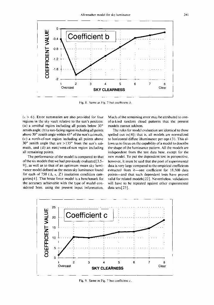
Coefficient b exhibits a gradual decrease in absolute value from the second ~ interval ( in te rmedia te condi t ions) on. This indicates that the model will go from no noticeable hor izon br ightening for in termediate condi t ions to a well-defined hor izon band with a steep luminance gradient for clear condit ions. This can be visualized on Fig. 13 where luminance profiles corresponding to bright overcast (first ~ interval, dark horizon ), in termediate ( th i rd e interval ), turbid (sixth

interval ), and very clear condi t ions (eighth ~ interval) have been plotted.

The c i rcumsolar intensity coefficient, c, exhibits a marked increase from overcast to partly cloudy condi t ions before gradually increasing toward clear conditions. Note tha t the overcast value of c reported here corresponds to moderately dark skies ( A = 0.1 ). Coef- ficient c would approach zero for dark overcast skies and exceed five for bright overcast skies; this effect can be visualized in Fig. 12 where luminance profiles for bright and dark overcast skies are compared.

Coefficient d, which accounts for the width of the c i rcumsolar region, decreases exponential ly with clearness. This is indicative of the well-known obser- vat ion that the solar aureole is considerably narrower for clear skies than turbid skies. It is interesting to note tha t the value o f - 3 found in the C1E clear sky model appears to be an upper l imit value for all condit ions; however, the aureoles modeled here for clear condit ions are found to be substantially narrower than the CIEs. The cumula t ive effect of coefficients c and d results in a total a m o u n t of modeled c i rcumsolar light tha t is m a x i m u m for the fifth and sixth ~ categories, which is

240

1 0

0 . ~ 5 3

0 . 6

R. PEREZ, R. SEALS, and J. MICHALSKY

0 . , , 4 -

O . 2 -

O . O

Fig. 6. Distribution of experimental sky scans as a function of sky clearness (~) and sky brightness (~).

consistent with the findings of earlier studies concerned with irradiance and il luminance on tilted surfaces (see Fig. 14 in [3] ) .

Finally, the backscattering coefficient e becomes significant only for the three highest ~ categories where it exhibits an exponential increase with clearness. This observation is physically sound, because backscattering effect should be maximum in a molecular (Rayleigh) atmosphere.

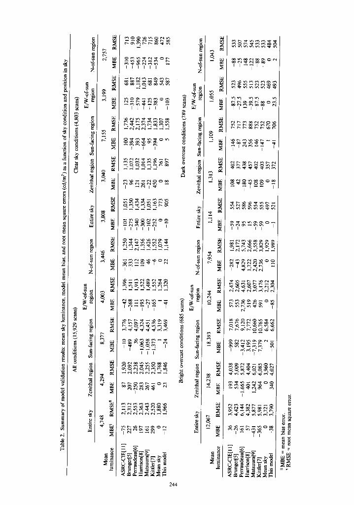
3.2 Model validation The model is validated using the mean bias error

(MBE) and root mean square error (RMSE) bench- marks computed after comparison of 3 million modeled and measured luminance values. All-sky error summaries are provided for the entire experimental data set and for three distinct sky conditions: (a) dark overcast conditions (~ = 1, A < 0.1 ), (b) bright overcast conditions (~ = 1, A > 0.4), and (c) clear conditions

0.8

. . I 0.4

0

-0.4

E -0.8

-1.2

-1.6 1 2 3 4 5 6 7 8 Overcast SKY CLEARNESS Clear

Fig. 7. Variations of coefficient a with sky clearness, ~, obtained from the equation for Z = 45 ° and A corresponding to the mean brightness value in each ~ bin.


0 I l l

-0.4

~ -0.8

-1.2

E (~) -1.6

-2 , i

2 3 4 5 6 7 8 Overcast Clear

SKY CLEARNESS

Fig. 8. Same as Fig. 7 but coefficient b.

(~ > 6). Error summaries are also provided for four regions in the sky vault relative to the sun's position: (a) a zenithal region including all points below 30 ° zenith angle, (b) a sun-facing region including all points above 30 ° zenith angle within 45 ° of the sun's azimuth, (c) a north-of-sun region including all points above 30 ° zenith angle that are >135 ° from the sun's azimuth, and (d) an east/west-of-sun region including all remaining points.

The performance of the model is compared to that of the six models that we had previously evaluated [ 3,5- 9], as well as to that of an optimum mean sky luminance model defined as the mean sky luminance found for each of 750 (A, ~, Z) insolation condition categories[4]. This brute force model is a benchmark for the accuracy achievable with the type of model considered here, using the present input information.

Much of the remaining error may be attributed to one- of-a-kind random cloud patterns that the present models cannot address.

The rules for model evaluation are identical to those spelled out in[4]; that is, all models are normalized to horizontal diffuse illuminance per eqn (3). This allows us to focus on the capability of a model to describe the shape of the luminance pattern. All the models are independent from the test data base, except for the new model. To put the dependent test in perspective,

however, it must be said that the pool of experimental data is very large compared to the empirical coefficients extracted from it--one coefficient for 18,500 data points--and that such dependent tests have proved valid for related models[22]. Nevertheless, validations will have to be repeated against other experimental data sets [ 23 ].

25 IdJ

=' t Coefficient c cl~ 20

I - - Z klJ N

m

i i i i klJ O

15

10

5

I ' . . . . i

1 Overcast

2 3 4 5 6 7 8 Clear

SKY CLEARNESS

Fig. 9. Same as Fig. 7 but coefficient c.


-2 UJ

3

F-- Z UJ -4 m

(J D i1 I I -5 W 0 ¢ j

-6

Coefficientd

2 3 4 5 Overcast

SKY CLEARNESS Clear

Fig. 10. Same as Fig. 7 but coefficient d.

Validation results are reported in Table 2. The performance of the new model approaches that of the op t imum mean sky model for all conditions and ori- entations and constitutes a systematic gain over the two models that had posted the best performance in our preliminary evaluation [4,5 ]. As explained in [ 3 ], it should be noted that the Harrison [8]algori thm is at a slight disadvantage in this comparison, as we did not have access to the opaque cloud cover data required as input for this model.

The performance gain of the new model is most noticeable in terms of directional mean bias errors, because the capability of this type model to minimize RMSEs is limited by random cloud/haze distributions. In order to best gauge this systematic performance improvement, we defined a distortion index as the sum

of the model absolute bias errors in each of the four sky vault regions described above. This index illustrates the ability of a model to generate prevailing skylight distribution patterns representative of observations. In Fig. 14, we have plotted the distortion index found for each model for the entire data base and for the three sets of insolation conditions of Table 2. Note that the indexes have all been normalized to one.

Although these results do not constitute a definitive proof of the new model 's precision because the model was statistically derived from this site-dependent data set, some validity may be drawn from the fact that the Brunger [ 5 ] model also derived statistically from a distinct data set scores rather well in the distortion test. Validation with new data sets is of course recom- mended as they become available.

1.4 IJJ

1.2

Z~ 0.8

0.6

E .4

(~ 0.2

(J o

overcast

- - - - - c o e f f i c i e n t e t" . . . . . : . . . . . . . : . . . . . .

- - I ~ I I I

2 3 4 5 6 7 8 clear SKY CLEARNESS

Fig. 11. Same as Fig. 7 but coefficient e.


• dark overcast

W

SUR l t l 4 1 1 1 1 t l l l - - I l t l ~


Fig. 12. Modeled luminance in the plane of the sun for dark and bright overcast conditions.

4 . C O N C L U S I O N S

The model presented here combines a simple mathematical framework that can assume most prevailing sky luminance patterns with a set of coefficients derived from a large, high-quality experimental set of sky-scan data. The coefficients act on the model's framework to account for the relative effects of forward scattering, backscattering, multiple scattering, and air mass on luminance distribution. They are treated as a function of three insolation condition parameters-- solar elevation, sky clearness, and brightness--which may be derived from standard irradiance time series. These functions are consistent with the physics of ra- diative transfer and the findings of earlier studies concerned with diffuse irradiance anisotropy.

Validation results show that the performance of the model approaches optimum level for this type of model. That is, the model accounts for most mean

anisotropic effects, but not random, one-of-a-kind cloud effects (an upgrade to this model incorporating random cloud patterns will be presented in a later paper). Of course, the validation performed here is dependent and will have to be repeated on independent data. It is possible that the model may require adjust- ment to account for this data base site specificity. The International Daylighting Measurement Program ini- tiated by the CIE and WMO[23]will provide such a climatically diverse data base. To the credit of the present work, however, it must be said that in our preliminary assessment of luminance distribution models, the best performers were empirical models, derived from site-specific data [ 3,5 ] ; the key to a model's performance was found to be its parameterization of insolation conditions; the insolation condition parameterization used here has been shown to be site independent, particularly when used to account for diffuse light anisotropy [ 3 ].

LU

Z .,:¢ z ~E

_,J uJ ~>

UJ Pr"

-- = bright overcast / / ~

=-,o,or=o0,a=

-- clear turbid /~///~ ~ l ~

s u n I I I I [ I I i i [ I I I I I I I


Fig. 13. Modeled luminance in the plane of the sun for different levels of sky clearness.

= 0

0

,...,

0

e~

8

e~

e,i

E

E

0

E

e-i

0

8 <

e , o .#

u ~ ?

Z

! .#

e~ "i .i I e~ 0

e~

. ,= =

ct~

e n U.

r,¢l

~ m

I I I I I I

T ? ? I T ? T

, I ?

• - q q q , - - t , - ~-. ~

T ? ~ ? T ? I I

I I

I I I

I

I ~ ~

~ E

2 4 4

O :'-2." I=

8

O

=

O

"13 =

8

,u

O

.v,

O

e!

? Z

f=

O #

!

f=

O

? Z

r"

#

exl

l i ~ I I

I I - J l l

i r t l

~ I ~

I ~ ~

° -

I l r l

i

I I

e~

r= _=

~ 2 H

II

F


1

0.9

0.8

0.7

0.6

0.5

0.4

0.3

0.2

0.1

0 This

model

NORMALIT I=D DI~;TORRION INDEX

ASRC- Brunger Matsuura Harrison CIE

KJttler Perraude

Fig. 14. Model relative distortion index.

Acknowledgments--This work was supported by the U.S. Na- tional Science Foundation under grant MSM 8915165. Dis- cussions with several members of IEA-SHCP Task 17E and with Mojtaba Navvab were helpful.

REFERENCES

1. M. Fontoynont, P. Barral, and R. Perez, Indoor daylighting frequencies computed as a function of outdoor solar radiation data, Proceedings ~[ 22nd CIE Cmdbrence. Melbourne, Australia. Div. 3, 100-105 ( 1991 ).

2. Y. Uetani and K. Matsuura, A mathematical model of the reflected directional characteristics for the luminance calculation in a non-isotropic diffuse reflecting interior, Proceedings ~122nd CIE Conlerence. Melbourne, Aus- tralia, Div. 3, 94-99 ( 1991 ).

3. R. Perez, P. Ineichen, R. Seals, J. Michalsky, and R. Stewart, Modeling daylight availability and irradiance components, Solar Ener~v 44, 271-289 (1990).

4. R. Perez, J. Michalsky, and R. Seals, Modeling sky luminance angular distribution from real sky conditions: Experimental evaluation of existing algorithms, Proceed- ings of lSES Worm Congress, Denver, CO 1049-1054 ( 1991 ). See Journal of the IES 21(2), 84-92 (1992).

5. A. P. Brunger, The magnitude, variability, and angular characteristics of the shortwave sky radiance at Toronto, Ph.D. Thesis, University of Toronto ( 1987 ).

6. M. Perraudeau, Luminance models, National Lighting ('on/i,rence and Daylighting Colloquium. Robinson Col- lege, Cambridge, UK (1988).

7. R. Kittler, Luminance models of homogeneous skies for design and energy performance predictions, Proceedings 01 Second International Daylighting Con lerence, Long Beach, CA, American Society of Heating, Refrigerating, and Air Conditioning Engineers, Atlanta, GA (1986).

8. A. W. Harrison, Directional luminance versus cloud cover and solar position, Solar Energy 46, 13-20 ( 1991 ).

9. K. Matsuura and T. lwata, A model of daylight source for the daylight illuminance calculations on the all weather

conditions, In: A. Spiridonov (ed.), Proceedings of Third International Daylighting Conlerence. Moscow, NIISF, Moscow (1990).

10. R. Perez, R. Seals, and J, Michalsky, Geostatistical prop- erties of random cloud patterns in real skies. (in press).

1 t. Standardization of luminous distribution on clear skies, International Conli'rence on Illumination, CIE Publication No. 22, Paris (1973).

12. R. Perez, P. Ineichen, E. Maxwell, R. Seals, and A. Ze- lenka, Dynamic global-to-direct irradiance conversion models, Proceedings q[ ISES H'orld Congress, Denver, CO ( 1991 ).

13. R. Perez, R. Stewart. and J. T. Scott, A two-parameter description of the sky hemisphere, Proceedings *?fAMS Fi#h Conlerence on Atmospheric Radiation, Baltimore, MD, 322-325 (1983).

14. F. Kasten and A. Young, Revised optical air mass tables and approximation formula, Applied Optics 28, 4735- 4738 (1989).

15. International Energy Agency Solar Heating and Cooling Program, Task 9-B: Validation of solar irradiance sim- ulation models, lEA Report. Paris (1987).

16. D. Feuermann and A. Zemel, Validation of models for global irradiance on inclined planes, Solar Energy 48( 1 ), 59-66 (1992).

17. Lawrence Berkeley Labs, Windows and Daylighting Group, LBL, Berkeley, CA.

18. E. W. Kleckner and J. J. Michalsky, A multipurpose computer-controlled scanning photometer, PNL-4081, Pacific Northwest Lab, Richland, WA ( 1981 ).

19. P. Moon and D. Spencer, Illumination from a nonuniform sky, Illuminating Eng. 37, 707-726 ( 1942 ).

20. M. Navvab, Personal communication, University of Michigan. Ann Arbor, MI ( 1991 ).

21. T. Rutten, Personal communication, Eindhoven Uni- versity, Eindhoven, The Netherlands ( 1991 ).

22. R. Perez, An anisotropic hourly diffuse radiation model for sloping surfaces, Solar Energy 36(6), 481-497 (1986).

23. The International Daylighting Measurement Program-- IDM P ( 199 I - 1995 ), International Illumination Com- mission, (IE), Wien, Austria (1991).

All-weather model for sky luminance distribution-preliminary configuration and validation

Documents

Transcript of All-weather model for sky luminance distribution-preliminary configuration and validation