The Egyptian Journal of Remote Sensing and Space Sciences (2011) 14, 81–89

National Authority for Remote Sensing and Space Sciences

The Egyptian Journal of Remote Sensing and Space

Sciences

www.elsevier.com/locate/ejrswww.sciencedirect.com

ORIGINAL ARTICLE

Using SPOT data and leaf area index for rice

yield estimation in Egyptian Nile delta

M. Aboelghar a,*, S. Arafat a, M. Abo Yousef b, M. El-Shirbeny a, S. Naeem b,

A. Massoud a, N. Saleh a

a National Authority for Remote Sensing and Space Sciences (NARSS), P.O. Box 1564, Alf Maskan, Cairo, Egyptb Rice Research Center, Agricultural Research Center (ARC),Giza, Egypt

Received 20 June 2011; revised 8 September 2011; accepted 21 September 2011Available online 22 October 2011

*

Se

15

E

na

11

Sc

Pe

Se

do

KEYWORDS

SPOT;

Leaf area index;

Vegetation Indices;

Statistical models

Corresponding author. Ad

nsing and Space Sciences (N

64 Alf Maskan, El-Nozha E

-mail addresses: mohamed

rss.sci.eg (M. Aboelghar).

10-9823 � 2011 National Au

iences. Production and hosti

er review under responsibili

nsing and Space Sciences.

i:10.1016/j.ejrs.2011.09.002

Production and h

dress: Na

ARSS),

l-Gedida,

.aboelgha

thority f

ng by Els

ty of Na

osting by E

Abstract The objective of the current work is to generate statistical empirical rice yield estimation

models under the local conditions of the Egyptian Nile delta. The methodology is based on regress-

ing measured yield with satellite derived spectral information or leaf area index (LAI). LAI field

measurements and spectral information from SPOT data collected during two crop seasons are

examined against measured yield to generate the yield models. Near-infrared and red bands, six veg-

etation indices and LAI of 100 points are used as the main inputs for the modeling process while 20

points of the same are used for validation process. Nine models are generated and tested against the

observed yield. Comparing the generated models show relatively higher superiority of (LAI-yield)

and (infrared-yield) models over the rest of the models with (0.061) and (0.090) as a standard error

of estimate and (0.945) and (0.883) as coefficient of determinations between modeled and observed

yield. The models are applicable a month before harvest for similar regions with same conditions.� 2011 National Authority for Remote Sensing and Space Sciences.

Production and hosting by Elsevier B.V. All rights reserved.

tional Authority for Remote

23 Joseph Tito St., P.O. Box,

Cairo, Egypt.

r@gmail.com, maboelghar@

or Remote Sensing and Space

evier B.V. All rights reserved.

tional Authority for Remote

lsevier

1. Introduction

Accurate and timely assessment of crop yield is an essential pro-cess to ensure the adequacy of a nation’s food supply. It providespolicy makers, governmental agencies and commodity traders

with the necessary information to better manage harvest, stor-age, import/export, transportation and marketing activities.The sooner this information is available, the lower the economic

risk, the greater the efficiency and the increased return on invest-ments Salazar et al., 2007). Synoptic observation and repetitivecoverage of the satellite remote sensing data is considered to bean effective methodology for real-time crop monitoring and

crop yield prediction on both local and regional scales. Spectralempirical modeling of such data is an important approach for

Figure 1 Location map of Sakha area.

82 M. Aboelghar et al.

crop yield estimation. This approach has the advantage of beingsimple with all the required data either readily available on a re-gional or global scale or easy to collect (Prasad et al., 2007). The

basis of this modeling process is generating statistical relation-ships between spectral variables and crop yield or estimatingcrop yield through measurable bio-physical parameters that

are highly correlated with crop canopy vigor and structureand hence, correlated with the spectral characteristics of thecrops. The normalized difference vegetation index (NDVI) is

known to be able to respond to changes in the amount of greenbiomass, chlorophyll content, and canopy water stress. It iseffective in predicting surface properties when the vegetation

canopy is not too dense or too sparse (Liang, 2004). The rela-tionship between NDVI and production has been confirmedby various field experiments (Prince and Justice, 1991; Rasmus-sen, 1992). It has a direct strong correlation with leaf area index

(LAI), biomass and vegetation cover (Tucker, 1979; Holbenet al., 1980; (Ahlrichs and Bauer, 1983; Nemani and Running,1989; Wiegand et al., 1990). These parameters drive the crop

production, and are largely influenced by variations in soil fertil-ity (Hinzman et al., 1986), soil moisture (Daughtry et al., 1980;Teng, 1990), planting date (Crist, 1984) and crop density (Aase

and Siddoway, 1981). They are also related to the crop yieldassuming the absence of significant stresses during the head-ing/filling stages (Hartfield, 1983; Wiegand and Richardson,

1990). The general drawback of most methods using statisticalrelationships between vegetation indices (VI), leaf area index(LAI) and crop yield is that they have a strong empirical charac-

ter (Groten, 1993; Sharma et al., 1993). Nomodels unless devel-oped and tested locally are suitable for local use (Shresthan andNaikaset, 2003). Therefore, the main objective of the currentstudy is to use SPOT satellite imagery and LAI field measure-

0

10

20

30

40

50

60

70

80

May-08

Jun-08

Jul-08 Aug-08

Sep-08

Oct-08

Nov-08

Dec-08

Jan-09

Feb-09

Mar-09

Apr-09

May-09

Jun-09

Jul-09 Aug-09

Sep-09

Average Air temp Average RH%

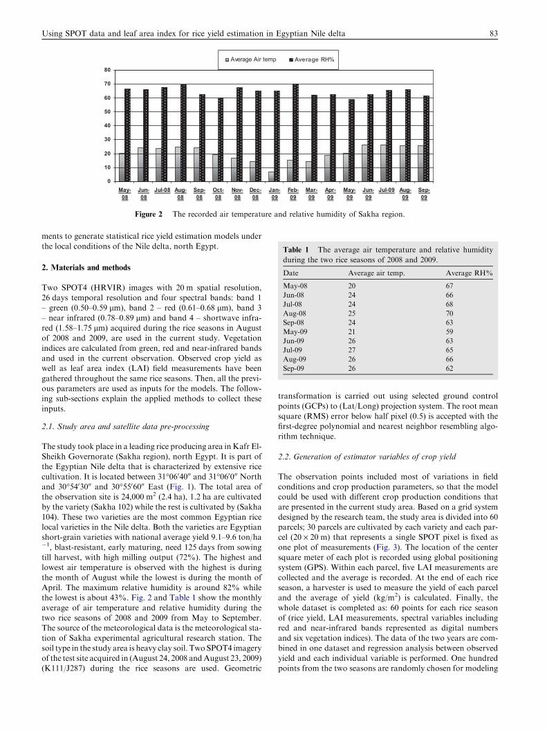
Figure 2 The recorded air temperature and relative humidity of Sakha region.

Table 1 The average air temperature and relative humidity

during the two rice seasons of 2008 and 2009.

Date Average air temp. Average RH%

May-08 20 67

Jun-08 24 66

Jul-08 24 68

Aug-08 25 70

Sep-08 24 63

May-09 21 59

Jun-09 26 63

Jul-09 27 65

Aug-09 26 66

Sep-09 26 62

Using SPOT data and leaf area index for rice yield estimation in Egyptian Nile delta 83

ments to generate statistical rice yield estimation models under

the local conditions of the Nile delta, north Egypt.

2. Materials and methods

Two SPOT4 (HRVIR) images with 20 m spatial resolution,26 days temporal resolution and four spectral bands: band 1– green (0.50–0.59 lm), band 2 – red (0.61–0.68 lm), band 3

– near infrared (0.78–0.89 lm) and band 4 – shortwave infra-red (1.58–1.75 lm) acquired during the rice seasons in Augustof 2008 and 2009, are used in the current study. Vegetation

indices are calculated from green, red and near-infrared bandsand used in the current observation. Observed crop yield aswell as leaf area index (LAI) field measurements have been

gathered throughout the same rice seasons. Then, all the previ-ous parameters are used as inputs for the models. The follow-ing sub-sections explain the applied methods to collect these

inputs.

2.1. Study area and satellite data pre-processing

The study took place in a leading rice producing area inKafr El-Sheikh Governorate (Sakha region), north Egypt. It is part ofthe Egyptian Nile delta that is characterized by extensive rice

cultivation. It is located between 31�0604000 and 31�060000 Northand 30�5403000 and 30�5506000 East (Fig. 1). The total area ofthe observation site is 24,000 m2 (2.4 ha), 1.2 ha are cultivated

by the variety (Sakha 102) while the rest is cultivated by (Sakha104). These two varieties are the most common Egyptian ricelocal varieties in the Nile delta. Both the varieties are Egyptianshort-grain varieties with national average yield 9.1–9.6 ton/ha�1, blast-resistant, early maturing, need 125 days from sowingtill harvest, with high milling output (72%). The highest andlowest air temperature is observed with the highest is during

the month of August while the lowest is during the month ofApril. The maximum relative humidity is around 82% whilethe lowest is about 43%. Fig. 2 and Table 1 show the monthly

average of air temperature and relative humidity during thetwo rice seasons of 2008 and 2009 from May to September.The source of the meteorological data is the meteorological sta-

tion of Sakha experimental agricultural research station. Thesoil type in the study area is heavy clay soil. Two SPOT4 imageryof the test site acquired in (August 24, 2008 andAugust 23, 2009)(K111/J287) during the rice seasons are used. Geometric

transformation is carried out using selected ground control

points (GCPs) to (Lat/Long) projection system. The root meansquare (RMS) error below half pixel (0.5) is accepted with thefirst-degree polynomial and nearest neighbor resembling algo-rithm technique.

2.2. Generation of estimator variables of crop yield

The observation points included most of variations in fieldconditions and crop production parameters, so that the modelcould be used with different crop production conditions that

are presented in the current study area. Based on a grid systemdesigned by the research team, the study area is divided into 60parcels; 30 parcels are cultivated by each variety and each par-cel (20 · 20 m) that represents a single SPOT pixel is fixed as

one plot of measurements (Fig. 3). The location of the centersquare meter of each plot is recorded using global positioningsystem (GPS). Within each parcel, five LAI measurements are

collected and the average is recorded. At the end of each riceseason, a harvester is used to measure the yield of each parceland the average of yield (kg/m2) is calculated. Finally, the

whole dataset is completed as: 60 points for each rice seasonof (rice yield, LAI measurements, spectral variables includingred and near-infrared bands represented as digital numbers

and six vegetation indices). The data of the two years are com-bined in one dataset and regression analysis between observedyield and each individual variable is performed. One hundredpoints from the two seasons are randomly chosen for modeling

Figure 3 Gridding system for field measurements and data collection.

84 M. Aboelghar et al.

process while 20 points from the two seasons are used to val-idate the models.

LAI-2000 plant canopy analyzer is used to measure LAI foreach point during the two seasons. This device calculates LAI

and other canopy structure attributes from radiation measure-ments made with a (fish-eye) optical sensor (148� field-of-view). Measurements made above the canopy and below

the canopy are used to determine canopy light interception atfive angles, fromwhich LAI is computed using amodel of radio-active transfer in vegetative canopy.Measurements are made by

positioning the optical sensor and pressing a button; data areautomatically logged into the control unit for storage and LAIcalculations. Multiple below-canopy readings and the fish-eyefield-of-view assure that LAI calculations are based on a large

sample of the foliage canopy. After collecting above and be-low-canopy measurements, the control unit performs all calcu-lations and the results are available for immediate on-site

inspection.Six vegetation indices are tested in the current study; nor-

malized difference vegetation index (NDVI), soil adjusted veg-

etation index (SAVI), green vegetation index (GVI), infraredpercentage vegetation Index (IPVI), ratio vegetation index(RVI) and difference vegetation Index (DVI). NDVI is deter-

mined using the red (R) and near-infrared (NIR) bands of agiven image (Rouse et al., 1973) and is expressed as follows:

NDVI ¼ qir � qr

qir þ qr

ð1Þ

where qr and qir are spectral reflectance from the red and NIR-band images, respectively. The green vegetation index (GVI) is

determined using

GVI ¼qir � qg

qir þ qg

ð2Þ

where qg and qir are spectral reflectance from the Green and

NIR-band images, respectively (Panda et al., 2010). Soiladjusted vegetation index (SAVI) is determined as

SAVI ¼ qir � qr

qir þ qr þ L

� �� ð1þ LÞ ð3Þ

where qr and qir are spectral reflectance from the red andNIR-band images, respectively and L is an optimal adjustmentfactor. Huete (1988) defined the optimal adjustment factor of

L = 0.25 to be considered for higher vegetation density inthe field, L = 0.5 for intermediate vegetation density, andL = 1 for the low vegetation density. He suggested that SAVI

(L = 0.5) successfully minimized the effect of soil variations ingreen vegetation compared to NDVI. Based on our observa-tions, we considered canopy cover of the rice crop in the field

as high dense during the satellite images acquisition time in2008 and 2009. Thus, 0.25 is used as the (L) factor using theHuete strategy of selecting the (L) factor, which is also sup-

ported by Thiam and Eastmen (1999). IPVI is the infrared per-centage vegetation index which was first described by Crippen(1990). He found that the subtraction of the red in the numer-ator as is done with SAVI to be irrelevant, and proposed this

index as a way of improving calculation speed. It is restrictedto values between 0 and 1 and eliminates the conceptualstrangeness of negative values for vegetation indices. It is cal-

culated as explained in the following equation:

IPVI ¼ NIR

NIRþ Rð4Þ

Using SPOT data and leaf area index for rice yield estimation in Egyptian Nile delta 85

RVI is the ratio vegetation index which is first described by

Jordan (1969). It is used to eliminate various albedo effects andit is calculated as shown in the following equation:

RVI ¼ NIR

Redð5Þ

DVI is the difference vegetation index, which is describedby Richardson and Everitt (1992) as follows:

DVI ¼ NIR�Red ð6Þ

All VI values and LAI are considered for the regressionanalysis and integrated yield prediction models of the two riceseasons are produced. The explanatory power of the indepen-

dent variables in the model and eventual prediction accuracyof the generated models can be assessed with statistical param-eters such as standard error of estimate (SEE), (t) test, andcoefficient of determination (R2).

3. Results and discussion

Nine statistical yield prediction models are produced. Figs. 4–12 show the trendline and the correlation coefficients for allgenerated models. Basically, linear regression is the best model

that represents the relation between observed yield and eachindividual estimator. It is found that the coefficient of determi-nation (R2) of all models is around (0.8) except for (GVI-yield)

model that showed relatively low ones. The models are exam-ined and the relative superiority over the generated models isdecided through computing Standard Error of Estimate

(SEE) and (t) test and the squared coefficient of determinationsbetween modeled and observed yield (R2). Table 2 shows thegenerated models and the validation results and Figs. 13–21show the trendline and the squared coefficient of determina-

tion between observed and modeled yield.The main objective of the current study is to generate rice

yield prediction models for the most common rice local varie-

ties in the Egyptian Nile delta (Sakha 102) and (Sakha 104).The data of the two seasons were combined in one dataset,part of this dataset was used to generate the models while

the other part was used to validate these models. The idea ofcombining the two rice seasons of the two varieties in one data-set is to generate applicable rice yield prediction models that

could be applied through satellite remote sensing data withacceptable accuracy. The first step of yield prediction is to iso-late the investigate crop from the other land cover types. Clas-sifying different crop types in Egyptian Nile delta is still

problematic and classifying different crop varieties within the

Table 2 The generated models and the validation results.

Variable Regression equation

NIR Yield = 0.0129IR�0.236Red Yield = �0.0923R+ 3.5717

NDVI Yield = 2.3606NDVI�0.2713RVI Yield = 0.2522RVI + 0.1131

IPVI Yield = 4.721IPVI�2.632DVI Yield = 0.0116DVI + 0.21

GVI Yield = 1.3675GVI + 0.468

SAVI Yield = 1.8899SAVI�0.2697

LAI Yield = 0.2846LAI�0.0764*Yield kg/m2.

same crop type is almost not possible under the current agri-

cultural conditions in Egyptian Nile delta using available satel-lite imagery. The models were generated using two seasons andtwo varieties to cover all possible minimal variations and to benot limited to the conditions of one season. It is expected that

these models could be applicable in future through any type ofhigh resolution satellite data. The generated models could beapplied to predict the yield of these two common rice varieties

under normal agricultural practices and common environmen-tal conditions in Egyptian Nile delta. Concerning the results ofthe models, it is found that the statistical relationship between

middle infrared, green bands and yield showed low accuracy,so, these two variables are excluded from further analysis.Among the rest of the examined variables, LAI is the best esti-

mator that gave the highest (R2) and the lowest (SEE). The cal-culated yields from all variables are comparable except for(GVI) that showed lowest validation result. This may be be-cause of the calculation of (GVI) as a ratio between green band

and (IR) and as mentioned above that green band showed rel-atively low correlation with yield. Among spectral variables,(IR) band is the best estimator with the highest validation re-

sult. The calculated (t) is less than the tabeled (t) with all vari-ables that reflects insignificant difference between modeled andobserved yields. (Table 1). Among the three statistical method

that are used to validate the generated models. SEE and R2 aremore powerful than (t) test method for showing the differencein prediction ability among the generated models.

The generated models are site specific and limited to the

area and environment as well as to the date of the experiment.Following the rice growing circle, milking stage (when waterycontent of the grain turn to thick milky ones) is selected as the

best crop growing stage that is closely related to LAI and riceyield. This assumption is proved by the author after one-sea-son experiment during rice season of 2007 using LAI measure-

ments that were gathered using (LAI-2000 plant canopyanalyzer device) and NDVI measurements that were gatheredfrom SPOT data and gathered also using (PlantPen NDVI

300 m) device (Aboelghar et al., 2010). NDVI-meter measuresNDVI comparing the reflected light at two distinct wave-lengths, 660 and 740 nm. NDVI data collected by NDVI-meterduring different growing stages of rice were examined against

the yield and against LAI. It is found that the NDVI of themilking stage of rice is the most correlated growing stage toyield and LAI. This is consistent with other results from the lit-

erature (Murthy et al., 1996; Labus et al., 2002; Royo et al.,2003). The models are produced under the common soil, cli-matic and crop conditions of Egyptian Nile delta and could

R2 SEE t values

0.883 0.090 0.454

0.720 0.123 �0.0940.850 0.099 0.381

0.823 0.098 0.307

0.850 0.099 0.372

0.874 0.090 0.506

0.786 0.210 0.037

0.850 0.099 0.369

0.945 0.061 �0.419

y = -0.0923x + 3.5717

R2 = 0.8004

0.000

0.200

0.400

0.600

0.800

1.000

1.200

1.400

1.600

0 5 10 15 20 25 30 35 40Red

Yie

ld K

g/m

2

Figure 5 Rice yield statistical modeling using red band.

y = 2.3606x - 0.2713

R2 = 0.8298

0.000

0.200

0.400

0.600

0.800

1.000

1.200

1.400

1.600

0.000 0.100 0.200 0.300 0.400 0.500 0.600 0.700 0.800

NDVI

Yie

ld K

g/m

2

Figure 6 Rice yield statistical modeling using NDVI.

Yie

ld K

g/m

2

y = 4.7213x - 2.632

R2 = 0.8298

0.000

0.200

0.400

0.600

0.800

1.000

1.200

1.400

1.600

0.000 0.100 0.200 0.300 0.400 0.500 0.600 0.700 0.800 0.900

IPVI

Figure 8 Rice yield statistical modeling using IPVI.

y = 0.0116x + 0.21

R2 = 0.8676

0.000

0.200

0.400

0.600

0.800

1.000

1.200

1.400

1.600

0.000 20.000 40.000 60.000 80.000 100.000 120.000

DVI

Yie

ld K

g/m

2

Figure 9 Rice yield statistical modeling using DVI.

y = 0.2846x - 0.0764

R2 = 0.82

0.000

0.200

0.400

0.600

0.800

1.000

1.200

1.400

1.600

0 1 2 3 4 5 6

LAI

Yie

ld K

g/m

2

Figure 10 Rice yield statistical modeling using LAI.

y = 0.0129x - 0.2355

R2 = 0.8512

0.000

0.200

0.400

0.600

0.800

1.000

1.200

1.400

1.600

0 20 40 60 80 100 120 140

Infrared

Yie

ld k

g/ m

2

Figure 4 Rice yield statistical modeling using near-infrared

band.

Yie

ld K

g/m

2

y = 0.2522x + 0.1131

R2 = 0.8824

0.000

0.200

0.400

0.600

0.800

1.000

1.200

1.400

1.600

0.000 1.000 2.000 3.000 4.000 5.000 6.000

RVI

Figure 7 Rice yield statistical modeling using RVI.

y = 1.3675x + 0.468

R2 = 0.3189

0.000

0.200

0.400

0.600

0.800

1.000

1.200

1.400

1.600

0.000 0.050 0.100 0.150 0.200 0.250 0.300 0.350 0.400 0.450 0.500

GVI

Yie

ld K

g/m

2

Figure 11 Rice yield statistical modeling using GVI.

86 M. Aboelghar et al.

be applied under similar conditions. The applicability of themodels with high accuracy is limited to the experiment date

and the type of the used satellite data. Precautions should be

taken when using these empirical relationships for otherspace-borne or air-borne sensors because of NDVI differencebetween sensors is often substantial (Spanner et al., 1994 and(Kim et al., 2010). Generation of new models might be neces-

y = 1.242x - 0.2879

R2 = 0.8499

0.000

0.200

0.400

0.600

0.800

1.000

1.200

1.400

1.600

0.000 0.200 0.400 0.600 0.800 1.000 1.200 1.400 1.600

Predicted yield (NDVI)

Obs

erve

d yi

eld

Figure 15 Correlation between observed yield and NDVI based

model.

y = 0.8778x + 0.1363

R2 = 0.7203

0.000

0.200

0.400

0.600

0.800

1.000

1.200

1.400

1.600

0.000 0.200 0.400 0.600 0.800 1.000 1.200 1.400 1.600

Predicted yield (R)

Obs

erve

d yi

eld

Figure 14 Correlation between observed yield and red based

model.

y = 1.8899x - 0.2697

R2 = 0.8299

0.000

0.200

0.400

0.600

0.800

1.000

1.200

1.400

1.600

0.000 0.100 0.200 0.300 0.400 0.500 0.600 0.700 0.800 0.900 1.000

SAVI

Yie

ld K

g/m

2

Figure 12 Rice yield statistical modeling using SAVI.

y = 1.2021x - 0.2504

R2 = 0.883

0.000

0.200

0.400

0.600

0.800

1.000

1.200

1.400

1.600

0.000 0.200 0.400 0.600 0.800 1.000 1.200 1.400 1.600

Predicted yield (IR)

Obs

erve

d yi

eld

Figure 13 Correlation between observed yield and near infrared

based model.

y = 0.9738x + 0.0079

R2 = 0.8225

0.000

0.200

0.400

0.600

0.800

1.000

1.200

1.400

1.600

0.000 0.200 0.400 0.600 0.800 1.000 1.200 1.400 1.600

Predicted yield (RVI)

Obs

erve

d yi

eld

Figure 16 Correlation between observed yield and RVI based

model.

y = 1.2422x - 0.2874

R2 = 0.8499

0.000

0.200

0.400

0.600

0.800

1.000

1.200

1.400

1.600

0.000 0.200 0.400 0.600 0.800 1.000 1.200 1.400 1.600

Predicted yield (IPVI)

Obs

erve

d yi

eld

Figure 17 Correlation between observed yield and IPVI based

model.

y = 1.135x - 0.181

R2 = 0.8742

0.000

0.200

0.400

0.600

0.800

1.000

1.200

1.400

1.600

0.000 0.200 0.400 0.600 0.800 1.000 1.200 1.400 1.600

Predicted yield (DVI)

Ob

serv

ed y

ield

Figure 18 Correlation between observed yield and DVI based

model.

y = 1.0681x - 0.0429

R2 = 0.9453

0.000

0.200

0.400

0.600

0.800

1.000

1.200

1.400

1.600

0.000 0.200 0.400 0.600 0.800 1.000 1.200 1.400 1.600

Predicted yield (LAI)

Obs

erve

d yi

eldj

Figure 19 Correlation between observed yield and LAI based

model.

Using SPOT data and leaf area index for rice yield estimation in Egyptian Nile delta 87

y = 10.681x - 10.373

R2 = 0.7855

0.000

0.200

0.400

0.600

0.800

1.000

1.200

1.400

1.600

1.030 1.040 1.050 1.060 1.070 1.080 1.090 1.100 1.110

Predicted yield (GVI)

Obs

erve

d yi

eld

Figure 20 Correlation between observed yield and GVI based

model.

y = 1.2421x - 0.2871

R2 = 0.8501

0.000

0.200

0.400

0.600

0.800

1.000

1.200

1.400

1.600

0.000 0.200 0.400 0.600 0.800 1.000 1.200 1.400 1.600

Predicted yield (SAVI)

Ob

serv

ed y

ield

Figure 21 Correlation between observed yield and SAVI based

model.

88 M. Aboelghar et al.

sary to estimate rice yield in middle Egypt region that has dif-ferent conditions.

4. Conclusion

A combined dataset through two rice seasons of the year 2008

and 2009 is used to produce statistical empirical rice yield pre-diction in a test site in Egyptian Nile delta. The planting dateswere May 24, 2008 and May 23, 2009. Various yield models

containing different number of predictor variables are gener-ated. The basic idea is the simpler the model, the easier andquicker will be the estimation process as fewer variables are ta-ken into account for data collection and computation process.

The spectral variables considered in the current study are redand near-infrared bands either alone or in the form of vegeta-tion indices and LAI as a bio-physical parameter that is related

to crop yield. LAI and infrared models showed higher accu-racy over the rest of the models as shown by the statisticalanalysis. The generated LAI and IR based models could be ap-

plied yearly to predict rice yield in Egyptian Nile delta and canbe also applied for rice yield estimation in any rice producingarea with similar conditions as the study area more than amonth before harvest. Similar studies could be also the basis

for a yield prediction and early warning system for the othermain crops of the country. The available satellite imagery dur-ing crop seasons and multi-temporal measurements of LAI

and infrared using field devices in selected sites of each cropcould be the main sources for the inputs of the models. Apply-ing the generated models on satellite imagery will produce

yield maps for the main crops month/s before harvest.

References

Aase, J.K., Siddoway, F.H., 1981. Spring wheat yield estimates from

spectral reflectance measurements. IEEE Transactions on Geosci-

ence and Remote Sensing 19 (2), 78–84.

Aboelghar, M., Arafat, S., Saleh, A., Naeem, S., Shirbeny, M., Belal,

A., 2010. Retrieving leaf area index from SPOT-4 satellite data.

Egyptian Journal of Remote Sensing 13, 121–127.

Ahlrichs, J.S., Bauer, M.E., 1983. Relation of agronomic and

multispectral reflectance characteristics of spring wheat canopies.

Agronomy Journal 75, 987–993.

Crippen, R.E., 1990. Calculating the vegetation index faster. Remote

Sensing of Environment 34, 71–73.

Crist, E.P., 1984. Effects of cultural and environmental factors of

corn and soybean spectral development pattern. Remote Sensing of

Environment 14, 3–13.

Daughtry, C.S.T., Bauer, M.E., Cresclius, D.W., Hixon, M.M., 1980.

Effects of management practices on reflectance of spring wheat

canopies. Agronomy Journal 72, 1055–1060.

Groten, S.M.E., 1993. NDVI – crop monitoring and early yield

assessment of Burkina Faso. International Journal of Remote

Sensing 148, 1495–1515.

Hartfield, J.L., 1983. Remote sensing estimators of potential and

actual crop yield. Remote Sensing of Environment 13, 301–311.

Hinzman, L.D., Bauer, M.E., Daughtry, C.S.T., 1986. Effects of

nitrogen fertilization on growth and reflectance characteristics of

winter wheat. Remote Sensing of Environment 19, 47–61.

Holben, B.N., Tucker, C.J., Fan, C.J., 1980. Spectral assessment of

soybean leaf area and leaf biomass. Photogrammetric Engineering

and Remote Sensing 46 (5), 651–656.

Huete, A.R., 1988. Soil adjusted vegetation index (SAVI). Remote

Sensing of Environment 25, 295–309.

Jordan, C.F., 1969. Derivation of leaf area index from quality of light

on the forest floor. Ecology 50, 663–666.

Kim, Y., Huete, A.R., Miura, T., Jiang, Z., 2010. Spectral compat-

ibility of vegetation indices across sensors: a band decomposition

analysis with hyperion data. Journal of Applied Remote Sensing 4.

Labus, M.P., Nielsen, R.L., Lawrence, R.L., Engel, R., Long, D.S.,

2002. Wheat yield estimates using multi-temporal NDVI satellite

imagery. International Journal of Remote Sensing 23 (20), 4169–

4180.

Liang, S., 2004. Quantitative Remote Sensing of Land Surfaces. Wiley,

New Jersey, 479-501.

Murthy, C.S., Thiruvengadachari, S., Raju, P.V., Jonna, S., 1996.

Improved ground sampling and crop yield estimation using satellite

data. International Journal of Remote Sensing 17 (5), 945–956.

Nemani, R.R., Running, S.W., 1989. Testing a theoretical climate-soil-

leaf area hydrological equilibrium of forests using satellite data and

ecosystem simulation. Agriculture and Forest Meteorology 44,

245–260.

Panda, S.S., Ames, D.P., Panigrahi, S., 2010. Application of vegetation

indices for agricultural crop yield prediction using neural network

techniques. Remote Sensing 2, 673–696.

Prasad, A.K., Singh, R.P., Tarem, V., Kafatos, M., 2007. Use of

vegetation index and meteorological parameters for the prediction

of crop yield in India. International Journal of Remote Sensing 28

(23), 5207–5235.

Prince, S.D., Justice, C.O., 1991. Coarse resolution remote sensing of

the Sahelian environment. International Journal of Remote Sensing

12, 1133–1421.

Rasmussen, M.S., 1992. Assessment of millet yields and production in

northern Burkina Faso using integrated NDVI from the AVHRR.

International Journal of Remote Sensing 13, 3431–3442.

Richardson, A.J., Everitt, J.H., 1992. Using spectra vegetation indices

to estimate rangeland productivity. Geocarto International, 63–69.

Using SPOT data and leaf area index for rice yield estimation in Egyptian Nile delta 89

Rouse, J.W., Haas, R.H., Schell, J.A., Deering, D.W., 1973. Moni-

toring vegetation systems in the great plains with ERTS. In: Third

ERTS Symposium, NASA SP-351, vol. 1, pp. 309–317.

Royo, C., Apaticio, N., Villegas, D., Casadesus, J., Monneveux, P.,

Araus, J.L., 2003. Usefulness of spectral reflectance indices as

durum wheat yields predictors under contrasting Mediterranean

conditions. International Journal of Remote Sensing 24 (22), 4403–

4419.

Salazar, L., Kogan, F., Roytman, L., 2007. Use of remote sensing data

for estimation of winter wheat yield in the United States.

International Journal of Remote Sensing 28 (17), 3795–3811.

Sharma, T., Sudha, K.S., Ravi, N., Navalgund, R.R., Tomar, K.P.,

Chakravarty, N.V.K., 1993. Procedures for wheat yield prediction

using Landsat MSS and IRS-1A data. International Journal of

Remote Sensing 14 (13), 2509–2518.

Shresthan, R.P., Naikaset, S., 2003. Agro-spectral models for estimat-

ing dry season rice yield in the Bangkok Plain of Thailand. Asian

Journal of Geoinformatics 4, 11–19.

Spanner, M.A., Johnson, L., Miller, J., 1994. Remote sensing of

seasonal leaf area index across the Oregon transect. Ecological

Applied 4, 258–271.

Teng, W.L., 1990. AVHRR monitoring of U.S. crops during the 1988

drought. Photogrammetric Engineering and Remote Sensing 56 (8),

1143–1146.

Thiam, S., Eastmen, R.J., 1999. Chapter on vegetation indices. In:

Guide to GIS and Image Processing, vol. 2, Idrisi Production,

Clarke University, Worcester, MA, USA, pp. 107–122.

Tucker, C.J., 1979. Red and photosynthetic infrared linear combina-

tion for monitoring vegetation. Remote Sensing of Environment 8,

127–150.

Wiegand, C.L., Richardson, A.J., 1990. Use of spectral vegetation

indices to infer leaf area, evapotranspiration and yield: I. rationale.

Agronomy Journal 82, 623–629.

Wiegand, C.L., Gerbermann, A.H., Gallo, K.P., Blad, B.L., Dusek,

D., 1990. Multisite analyses of spectral – biophysical data for corn.

Remote Sensing of Environment 33, 1–16.