Use of the Robust Design to Estimate Seasonal Abundance and Demographic Parameters of a Coastal...

Use of the Robust Design to Estimate SeasonalAbundance and Demographic Parameters of a CoastalBottlenose Dolphin (Tursiops aduncus) PopulationHolly C. Smith1,2*, Ken Pollock1,3, Kelly Waples2,1, Stuart Bradley1, Lars Bejder1

1 Murdoch University Cetacean Research Unit, Centre for Fish, Fisheries and Aquatic Ecosystems Research, School of Veterinary and Life Sciences, Murdoch University,

Perth, Australia, 2 Marine Science Program, Nature Conservation Division, Department of Environment and Conservation, Perth, Australia, 3 North Carolina State

University, Department of Biology, Raleigh, North Carolina, United States of America

Abstract

As delphinid populations become increasingly exposed to human activities we rely on our capacity to produce accurateabundance estimates upon which to base management decisions. This study applied mark–recapture methods followingthe Robust Design to estimate abundance, demographic parameters, and temporary emigration rates of an Indo-Pacificbottlenose dolphin (Tursiops aduncus) population off Bunbury, Western Australia. Boat-based photo-identification surveyswere conducted year-round over three consecutive years along pre-determined transect lines to create a consistentsampling effort throughout the study period and area. The best fitting capture–recapture model showed a population witha seasonal Markovian temporary emigration with time varying survival and capture probabilities. Abundance estimates wereseasonally dependent with consistently lower numbers obtained during winter and higher during summer and autumnacross the three-year study period. Specifically, abundance estimates for all adults and juveniles (combined) varied from alow of 63 (95% CI 59 to 73) in winter of 2007 to a high of 139 (95% CI 134 to148) in autumn of 2009. Temporary emigrationrates (c’) for animals absent in the previous period ranged from 0.34 to 0.97 (mean = 0.54; 6SE 0.11) with a peak duringspring. Temporary emigration rates for animals present during the previous period (c’’) were lower, ranging from 0.00 to0.29, with a mean of 0.16 (6 SE 0.04). This model yielded a mean apparent survival estimate for juveniles and adults(combined) of 0.95 (6 SE 0.02) and a capture probability from 0.07 to 0.51 with a mean of 0.30 (6 SE 0.04). This studydemonstrates the importance of incorporating temporary emigration to accurately estimate abundance of coastaldelphinids. Temporary emigration rates were high in this study, despite the large area surveyed, indicating the challenges ofsampling highly mobile animals which range over large spatial areas.

Citation: Smith HC, Pollock K, Waples K, Bradley S, Bejder L (2013) Use of the Robust Design to Estimate Seasonal Abundance and Demographic Parameters of aCoastal Bottlenose Dolphin (Tursiops aduncus) Population. PLoS ONE 8(10): e76574. doi:10.1371/journal.pone.0076574

Editor: Patrick J. O. Miller, University of St Andrews, United Kingdom

Received April 25, 2013; Accepted August 26, 2013; Published October 9, 2013

Copyright: � 2013 Smith et al. This is an open-access article distributed under the terms of the Creative Commons Attribution License, which permitsunrestricted use, distribution, and reproduction in any medium, provided the original author and source are credited.

Funding: This project was financially and logistically supported by the partners of the South West Marine Research Program. These include Bemax Cable Sands,BHP Billiton Worsley Alumina Pty Ltd, Bunbury Dolphin Discovery Centre, Bunbury Port Authority, the City of Bunbury, Cristal Global, Department of Environmentand Conservation, Iluka, Millard Marine, Naturaliste Charters, Newmont Boddington Gold, South West Development Commission and WA Plantation Resources. HSwas supported by a Murdoch University scholarship. The funders had no role in study design, data collection and analysis, decision to publish, or preparation ofthe manuscript.

Competing Interests: Bemax Cable Sands, BHP Billiton Worsley Alumina Pty Ltd, Bunbury Dolphin Discovery Centre, Cristal Global, Iluka, Millard Marine,Naturaliste Charters, Newmont Boddington Gold, South West Development Commission and WA Plantation Resources. The authors declare that this does notalter their adherence to all the PLOS ONE policies on sharing data and materials and will provide the MARK data files or other supplementary information tocomply with PLOS ONE policies on sharing data and materials on request and will do so when advised on the preferred file format.

* E-mail: [email protected]

Introduction

Coastal bottlenose dolphins (Tursiops spp) are one of the most

studied cetacean species mainly due to their widespread distribu-

tion and ease of accessibility. Much is known about their biology,

social behaviour and population dynamics [1,2,3,4,5]. Various

methods for estimating the abundance of dolphin populations have

been developed and used routinely [1,6,7,8,9]. However, methods

should be continuously refined based on the growing understand-

ing of dolphin biology and behaviour to ensure that abundance

estimates and population parameters are reliable and accurate

[10,11].

It is becoming clear that many coastal bottlenose dolphin

populations include individuals with varying patterns of residency

and ranging size. In some cases, individuals reside permanently in

an area [12], while others transit through only occasionally

[7,9,10]. In contrast, others temporarily emigrate leaving an area

for a period of time (e.g. seasonally) but return more frequently

than transients [13]. The varying degrees of individual residency

have a large influence on abundance estimates at any given time

and need to be incorporated into study designs and data analysis

through statistical models.

Resident individuals may be particularly vulnerable to anthro-

pogenic pressures such as habitat degradation, poor water quality,

marine debris, anthropogenic noise, food provisioning from

humans, competition with fisheries for prey and entanglement in

fishing gear [14,15,16,17]. Accurate assessments of abundance,

distribution and life history parameters (such as survival and

recruitment) are critical to understanding a population and its

PLOS ONE | www.plosone.org 1 October 2013 | Volume 8 | Issue 10 | e76574

habitat use as well as identifying potential impacts of anthropo-

genic or natural pressures.

Estimating abundance using capture-recapturetechniques

For most delphinid species, particularly Tursiops, photographs of

the dorsal fin are used for individual identification [18]. Fin shape

and distinguishing marks, nicks and scars allow for their long-term

identification, while markings on the surface of the fin and body

are used for short-term identification [19]. Initial cataloguing of an

identified individual is called the capturing process, and later

resightings are defined as the recapture events. As identifying marks

may change over time, it is necessary to record these changes and

track modifications to avoid mis-identification [20].

While capture-recapture methods have remained the standard

for identifying animals, there are a variety of sampling protocols

for collecting the captures. These involve boat-based surveys

conducted throughout zones of the study area while using varying

temporal and spatial sampling designs. To take into account

varying residency patterns and the opportunities available to

capture all individuals within the population, careful thought must

be given to the sampling regime, including sampling periods for

and between captures and recaptures.

Population modelsStatistical models used in capture-recapture studies are designed

to calculate abundance estimates over multiple sampling periods

[21]. Models are useful because they allow for population estimate

calculations under complex parameterisations. Sampling designs

must meet model assumptions, and the parameters must make

sense biologically. Model parameters, e.g. survival and recruitment

rates, should be customised as either constant or time-varying

according to the characteristics and life history of the study

population. A traditional definition of a population is ‘‘a group of

organisms of the same species occupying a particular space at the

same time’’ [22]. In this study, we considered the study population

to include any bottlenose dolphins within our defined study area

(Figure 1) at any time during the study.

Closed versus open models. There are two general types of

models that have been used to describe bottlenose dolphin

populations: closed and open. Closed population models are used

when there are no population losses (through emigration or death)

during the sampling period. To avoid violation of this assumption,

closed models are best suited to studies where sampling can be

conducted over a short period (e.g. a week). Open population

models have been used more recently in cetacean studies

[10,23,24]. They allow for permanent emigration, i.e. increases

(births, immigration) and losses (mortality, emigration) to the

population [21]. However, multiple movements in or out of the

population, known as temporary emigration, is best accommodat-

ed in the Robust Design which combines characteristics of both

open and closed population models [25,26,27]. Temporary

emigration is defined as: (1) completely random; or (2) Markovian,

where the probability of being unavailable for detection in primary

period i depends on whether the animal was available (y") or

unavailable (y’) for detection in primary period i – 1.Standard

open models give rise to biased estimates if there is Markovian

temporary emigration [21,26].

The Robust Design incorporates open sampling events called

‘‘primary periods’’, within which are a number of closed

‘‘secondary periods’’ [27]. Closure is assumed within primary

periods but not between them. To fulfil this assumption, the

Robust Design relies on secondary periods being close together,

temporally [28]. Bottlenose dolphins have different sized home

ranges (based on age and sex) that may result in unequal capture

probabilities between individuals in the study area [29,30].

Therefore, the capacity for the Robust Design to allow for

temporary emigration is a very useful feature when estimating

abundance for species that exhibit movement in and out of a study

area.

The Robust Design has been used to estimate abundance and

demographic parameters of other taxa, including multiple species

of Plethodontid salamanders [31], Asian elephants (Elephas

maximus) [32] and tigers (Panthera tigris) [33]. Similar to dolphins,

these taxa may be available for capture in some sampling periods

but not in others, as they move in and out of a study area.

Likewise, the Robust Design has been used to estimate population

abundance and parameters of several cetacean species, e.g. long-

finned pilot whales (Globicephala melas) [34] Guiana dolphins (Sotalia

guianensis) [35] and Irrawaddy dolphins (Orcaella brevirostris) [36].

This approach is particularly recommended for monitoring

bottlenose dolphin populations because the model incorporates

temporary emigration [10,11,13,37,38] which allows for the

seasonal movements of this species [13,39].

The aim of this study was to use a sampling design and

population model that address the complexity posed by a coastal

dolphin population comprised of both resident animals and

temporary emigrants. In this study, we employed the Robust

Design with two main objectives: (1) to examine seasonal

abundances and demographic parameters of a coastal bottlenose

dolphin population and (2) to explore the implications that

residency and temporary emigration have on demographic

parameter estimates.

Materials and Methods

Ethics statementThis study was carried out in strict accordance to the Murdoch

University Animal Ethics Committee approval (W2009/06) and

licensed as scientific research by the Department of Environment

and Conservation (SF005811).

Study areaThe study was located next to the city of Bunbury, which is the

fastest growing regional centre in Australia with a human

population of 35,000 and is expected to increase to 100,000 by

2030 (Australian Bureau of Statistics 2010). Bunbury has one of

the largest ports in Western Australia and plays a significant role in

the State’s economy and trade (Department of Transport 2010).

The port is the only export facility for local industry and produce

from the surrounding rural areas. The study area covered 120 km2

of coastal waters around the city of Bunbury extending from

Peppermint Beach to Buffalo Beach (Figure 1). The exposed

coastal area was typified by open sandy beaches interspersed with

limestone reef and an adjoining estuary. The inner-waters of

Bunbury included the Leschenault Inlet, Leschenault Estuary,

Bunbury Inner Harbour, Bunbury Outer Harbour, and the Collie

River. The coastal study area covered 100 km2 and extended to

approximately 1.5 km offshore, to a maximum water depth of

15 m, and with a linear distance of 50 km. The remaining area

comprised inshore waters including the estuary, inlet, inner and

outer harbours (20 km2). The benthic habitat in the study area was

typical of temperate environments, including seagrasses, limestone

reef, macroalgae communities and sand.

Sampling methodsPhoto-identification capture-recapture technique. Be-

tween March 2007 and November 2009, photo-identification was

Abundance of Coastal Bottlenose Dolphins


used during boat-based surveys as a capture-recapture method for

estimating abundance, demographic parameters and movements

of bottlenose dolphins. One field day of effort was defined as a

survey, with each dolphin group encounter during a survey termed

a sighting. Using a Nikon D 200 with Nikkor zoom lens 70–

300 mm, photographs were taken of individual dolphins encoun-

Figure 1. A map of the 120km2 study area in the near-shore environment around Bunbury, Western Australia. The extent of the threezones of transect lines (dashed zigzag line). Both Zone 1 (Buffalo Beach) and Zone 2 (Peppermint Beach) were coastal waterways, while Zone 3(Bunbury Inner) consisted of inner waters including the Leschenault Inlet and Estuary, Inner and Outer Harbour, Koombana Bay and the lower reachesof the Collie River.doi:10.1371/journal.pone.0076574.g001

Table 1. Sample sizes of the two-tiered data structure consisting of primary (seasons) and secondary sampling periods (no. oftimes all three zones of the study area were surveyed) of the Robust Design.

Year Sampling Period 2007 2008 2009

Seasons Primary Aut Win Spr Sum Aut Win Spr Sum Aut Win Spr

No. of times the studyarea was surveyed

Secondary 3 3 2 9 5 6 4 9 7 4 2

doi:10.1371/journal.pone.0076574.t001



tered along pre-determined transect lines (Figure 1). A sighting

commenced when a dolphin or dolphin group were encountered

along the transect line. A zone was defined as a pre-determined

route that consisted of zig-zag transect lines that were followed

during surveys. Surveys were conducted from a 5 m centre console

research vessel driven at a speed of 8 to 12 kn with two to five

observers (median = 4) present during each survey.

Sampling designLine Transects. Surveys were conducted year-round during

three consecutive years and used repeated effort in three zones

with pre-determined transects lines (Table 1; Figure 1). The

transect lines within the three zones totalled 120 km with a strip

width of approximately 250 m either side of the vessel. Zones 1

and 2 followed a zig-zag pattern to maximise coverage of the study

area. However, this was not possible for Zone 3, where designated

channels and shallow water governed the path of the transect lines.

The aim of each field day was to complete all transect lines within

one zone (Figure 1). Due to weather and time constraints, it was

not possible to survey all three zones in a single day. A sampling

period was defined as the time required to complete all three zones.

A sampling period took a minimum of three days and a maximum

of three weeks. This is equivalent to one secondary sampling period of

the Robust Design. This study sampled year-round to account for

possible seasonal temporary emigration, maximising the capture

probability of all individuals in each sampling occasion and the

likelihood of each individual being resighted annually.

All surveys were conducted in Beaufort sea state # 3. When a

dolphin group was sighted, the research vessel would break away

from the transect line to approach the dolphin(s) at which time the

location (GPS coordinates) and dolphin group size were recorded.

Sightings lasted for a minimum of five minutes (to allow

determination of predominant activity) and until all the dorsal

fins were photographed. Known individuals were photographed

regardless of familiarity. Once all dolphins had been photo-

graphed, the vessel was repositioned on the transect line at the

point where it was left and the search for other dolphin groups

resumed.

Data processingPhotographs were assessed according to their sharpness,

contrast, angle and size of the dorsal fin in relation to the frame.

Using these measures, only images of excellent and good quality

were used for analyses [40,41]. Images that could not reliably be

used for individual identification were discarded. Individual

dolphins were primarily identified based on the nicks and scars

on the leading and trailing edges of the dorsal fin. Secondary

features (such as pigmentation, natural fin shape, and scarring on

the surface of the fin and peduncle) were also used for

identification. The sampling regime allowed for the tracking of

temporary/secondary markings (e.g. rake marks and/or lesions)

that tended to fade after approximately six months.

Characterisation of study subjectsAge and sex. The age of population members is an important

consideration in abundance modelling, as it may influence the

likelihood of individuals having distinguishable marks, capture

probability and demographic and dispersal factors. In this study,

the exact age of many individuals was unknown, therefore

individuals were assigned to one of three mutually exclusive age

classes (adults, juveniles and calves) according to body length.

Calves were excluded from the analysis for two reasons: (1)

because they lacked identifying marks and; (2) the natural

mortality of calves is assumed to be high based on mortality of

calves in the bottlenose dolphin population in Shark Bay, Western

Australia (Mann et al. 2000). Juveniles were included in the analysis

along with adults as they were sufficiently marked for recognition

and recapture. Abundance estimates presented here refer to all

juveniles and adults of both sexes combined.

Sex determination of adult female dolphins was usually based

on a series of consistent sightings with a dependent calf.

Confirming the sex of males and non-mother females was more

challenging and relied on visual observation of the genital area or

the genetic analysis from biopsy samples that were collected as part

of a separate research project.

Description of modelsRobust Design assumptions. Many assumptions of the

Robust Design are the same as for the standard open models

(Williams et al. 2002), while also allowing for temporary

emigration and with no requirement for population closure

between primary periods. Specifically, the Robust Design allows

a population to be open to immigration, emigration, births, and

deaths between the primary periods, and assumes population

closure over all the secondary periods within a primary period.

Also, unlike standard models, the Robust Design allows for

Table 2. Summary of annual survey effort across months and number of zones surveyed between March 2007 and November2009.

Year No. of surveys No. of months No. of zones surveyed No. of dolphin group sightings

2007 48 10 (Mar-Dec) 43 157

2008 100 12 (Jan-Dec) 85 137

2009 69 9 (Jan-Sept) 73 250

Dolphin group encounters are included as number of ‘sightings’ along transect lines.doi:10.1371/journal.pone.0076574.t002

Table 3. Total number of transect replicates per seasons foreach zone.

Summer Autumn Winter Spring

Dec-Jan-Feb Mar-Apr-May June-July-Aug Sept-Oct-Nov

Zone 1 21 21 20 12

Zone 2 25 19 18 10

Zone 3 30 20 22 13

Zone 1: Buffalo Beach; Zone 2: Back Beach; and Zone 3: Bunbury Inner; Figure 1.doi:10.1371/journal.pone.0076574.t003



heterogeneity of capture probabilities because the secondary

sampling periods occur close together.

The Robust Design allows for estimating: the probability of first

capture ‘p’; the probability of recapture ‘c’; and the number of

animals that are in the sampling area [N(i)]. For the intervals

between primary sampling periods, the model also allows for

parameter estimation of the: probability of apparent survival [S(i)],

and two temporary emigration parameters which are the

probability of emigration from the study area given that the

animal was present in the last period [c’’ (i)], and the probability of

staying away from the study area given that the animal has left the

survey area before this period [c’(i)].

A Robust Design procedure within the software MARK [42]

was chosen for analysis as it has the most flexibility in setting

sampling occasions, parameters and incorporating unequal time

intervals between sampling. Conventional methods of dolphin

photo-identification use only permanent marks on the edge of the

dorsal fin [18,43]. In this study, all juveniles and adults were

considered identifiable as each dorsal fin was distinct when the

natural dorsal fin shape was used in conjunction with temporary

marks on the surface of the dorsal fin and body, i.e. lesions and

tooth rake marks [19]. Therefore, no adjustment was made for an

unmarked proportion of the population.

Robust Design structure. Primary periods were based on

the Australasian seasons: Summer (December-February), Autumn

(March-May), Winter (June-August); and Spring (September-

November). There were 11 primary periods (seasons) and 54

secondary periods in this three-year study (Table 1). The time it

took to complete the secondary sampling periods varied and the

intervals between secondary periods varied. Ideally, the time

duration to complete a full secondary sampling period (i.e. all three

zones within the entire study area) would have been shorter than

we achieved (i.e., quicker (within days rather than weeks) but

survey effort was constrained by weather. Again, we assumed that

the population was closed within seasons (primary periods).

Data analysis was performed on the data available on juveniles

and adults of both sexes. We used the Akaike Information

Criterion (AIC) to evaluate model fit. The best fitting model was

identified as having the lowest AICc [44].

Results

Survey effort and summary statisticsA total of 201 surveys were completed over the three years,

resulting in 544 dolphin group sightings (Tables 2 and 3). A total of

108, 219 and 357 dolphin groups were encountered along Zones

1, 2 and 3, respectively. In total, 172 individual dolphins were

identified of which 39 and 133 were juveniles and adults,

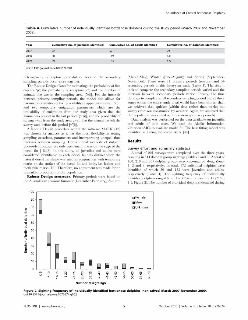
respectively (Table 4). The sighting frequency of individually

identified dolphins ranged from 1 to 67 with a mean of 15 (6 SE

1.3; Figure 2). The number of individual dolphins identified during

Figure 2. Sighting frequency of individually identified bottlenose dolphins (non-calves) March 2007-November 2009.doi:10.1371/journal.pone.0076574.g002

Table 4. Cumulative number of individually identified bottlenose dolphins during the study period (March 2007 and November2009).

Year Cumulative no. of juveniles identified Cumulative no. of adults identified Cumulative no. of dolphins identified

2007 22 57 79

2008 30 119 149

2009 39 133 172

doi:10.1371/journal.pone.0076574.t004



each secondary sampling period ranged from 10–90 (mean = 40;

6SE 2.0) (Figure 3).

Of the 172 individuals identified, 21 were documented as males

(12%), 66 as females (39%) and 85 (49%) were of unknown sex.

Forty one dolphins were sexed as females based on the presence of

a dependent calf. Two male dolphins were confirmed through

direct observation of the genitals. Biopsy and subsequent genetic

analysis confirmed the sex of the additional 25 females and 19

males.

Adult females were sighted more often than adult males in all

seasons (except during spring). Individual females were sighted, on

average, on 7.33 (6 SE 0.86) occasions while individual males

were sighted, on average, on 4.55 (6 SE 0.59) occasions in

summer seasons. Spring was an exception where the reverse was

observed: each adult male and female was, on average, observed

on 3.80 (6 SE 0.52) and 2.57 (6 SE 0.31) occasions, respectively

(Table 5).

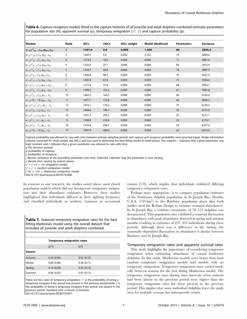
Abundance, temporary emigration and survival estimatesThe study population could not be considered geographically

closed between seasons as some individuals were captured

inconsistently across sampling seasons. Therefore, models that

incorporated temporary emigration were included in the tested

model sets. As assumed, models that did not incorporate a

parameter for temporary emigration fit the data poorly (Table 6).

Unfortunately, sex specific abundance estimates and demographic

parameters could not be modelled separately because of the large

proportion individuals that were of unknown sex. The best fitting

model (Q(t)c’’(s) ?c’(s) pt = ct Nt), based on the lowest AICc, had

apparent survival varying with time (rather than constant),

seasonal Markovian temporary emigration (with time variation

in emigration parameters c’’ and c’) and a different capture

probability for each primary sampling occasion (Table 6). The

temporary emigration rates of being absent based on the previous

period state also being absent (c’) were high and ranged from 0.34

to 0.97 with a peak in spring and a mean value of 0.546SE 0.11

(Table 7). The temporary emigration rates of being absent based

on the previous period state being present (c’’) were lower, ranging

0.00–0.29, with a mean of 0.166SE 0.04 (Table 7) and showed a

strong seasonal effect with an estimated value of 0 during winter

(Table 7) compared to 0.29 in autumn. Our model yielded a mean

apparent survival estimate for juveniles and adults (combined) of

0.956SE 0.02 and a capture probability of from 0.07 to 0.51 with a

mean of 0.30 (6 SE 0.04). Mean seasonal dolphin abundance

estimates (juveniles and adults combined) varied according to season

with consistently lower abundance estimated during winter and

higher during summer and autumn across the three year study

period (Figure 4). Specifically, abundance estimates ranged from a

low of 63 (6 SE 3.32; 95% CI 59 to 73) in winter 2007 to a high of

139 (6 SE 3.39; 95% CI 134 to148) in autumn 2009 (Figure 4). This

seasonal trend in abundance was apparent in all years (Figure 4).

Discussion

Abundance estimates are seasonally dependentOne of the most interesting results was the seasonal differences

in abundance estimates of juveniles and adults combined, with

consistently lower abundance estimated during winter months and

higher during summer and autumn months. Specifically, abun-

dance estimates varied from a low of 63 (95% CI 59-73) in winter

2007 to a high of 139 (95% CI 134-148) in autumn 2009.

Elsewhere, the abundance of coastal bottlenose dolphins in

study areas of comparable size to this study (120 km2) have

reported similar population estimates [1,7,9,45,46,47,48,49]. For

example, abundance of bottlenose dolphins in Port Stephens

(140 km2), Jervis Bay (102 km2) and Clarence River (89 km2)

ranged between 61 and 160 individuals [7,9]. However, compar-

ison of dolphin abundance estimates between studies should be

treated with caution, particularly when sampling approaches vary.

Figure 3. Number of individual dolphins (juveniles and adults) identified in each secondary period March 2007-November 2009.doi:10.1371/journal.pone.0076574.g003

Table 5. The mean number of sightings of individual adultmale and adult female bottlenose dolphins for eachAustralasian season (March 2007 and November 2009).

Autumn Winter Spring Summer

Males (n = 21) 5.05 (60.60) 2.30 (60.61) 3.80 (60.52) 4.55 (60.59)

Females(n = 66) 5.03 (60.49) 4.55 (60.61) 2.57 (60.31) 7.33 (60.86)

Standard error is shown in brackets.doi:10.1371/journal.pone.0076574.t005



In contrast to our research, the studies noted above used closed

population models which did not incorporate temporary emigra-

tion into their abundance estimates. However, these studies

highlighted that individuals differed in their sighting frequency

and classified individuals as resident, transient or occasional

visitors [7,9], which implies that individuals exhibited differing

temporary emigration rates.

Perhaps more appropriate, is to compare population estimates

of the bottlenose dolphin population in St Joseph Bay, Florida,

U.S.A. (150 km2) to the Bunbury population given that both

studies used the Robust Design to estimate seasonal abundances.

In St Joseph Bay a resident community of 78–152 dolphins was

documented. This population also exhibited a seasonal fluctuation

in abundance with peak abundance detected in spring and autumn

months resulting in estimates of 237–410 individuals during these

periods. Although there was a difference in the timing, the

seasonally-dependent fluctuation in abundance is similar between

Bunbury and St Joseph Bay.

Temporary emigration rates and apparent survival ratesThis study highlights the importance of considering temporary

emigration when estimating abundance of coastal bottlenose

dolphins. In this study, Markovian models were better than both

random temporary emigration models and models with no

temporary emigration. Temporary emigration rates varied mark-

edly between seasons for the best fitting Markovian model. The

temporary emigration rates during time intervals when animals

had been absent in the previous period were higher than the

temporary emigration rates for those present in the previous

period. This implies that some individual dolphins leave the study

area for multiple seasons but subsequently return.

Table 6. Capture-recapture models fitted to the capture histories of all juvenile and adult dolphins combined estimate parametersfor population size (N), apparent survival (Q), temporary emigration (c’’, c’) and capture probability (p).

Models Rank AICc dAICc AICc weight Model likelihood Parameters Deviance

Q (t)c’’(s) ?c(s) p(t) = c(t) 1 1297.9 0.0 0.908 1.000 83 5845.3

Q (.)c’’(s) ?c’(s) p(t) = c(t) 2 1302.5 4.6 0.092 0.102 74 5869.6

Q (.)c’’(s) ?c’(.) p(t) = c(t) 3 1313.9 16.0 0.000 0.000 71 5887.6

Q (.)c’’(t) ?c’(t) p(t) = c(t) 4 1325.0 27.1 0.000 0.000 83 5872.4

Q (.)c’’(t) ?c’(.) p(t) = c(t) 5 1334.7 36.8 0.000 0.000 76 5897.5

Q (.)c’’(t) =c’(t) p(t) = c(t) 6 1356.6 58.7 0.000 0.000 75 5921.5

Q (.)c’’(.) ?c’(t) p(t) = c(t) 7 1365.6 67.8 0.000 0.000 75 5930.6

Q (.)c’’(.) ?c’(.) p(t) = c(t) 8 1373.5 75.6 0.000 0.000 68 5953.7

Q (.)c’’(.) =c’(.) p(t) = c(t) 9 1399.5 101.6 0.000 0.000 67 5981.8

Q (.)c’’(t) ?c’(t) p(.) = c(.) 10 1462.2 164.3 0.000 0.000 40 6102.0

Q (.)c’’0 = c’0 p(t) = c(t) 11 1471.7 173.8 0.000 0.000 66 6056.2

Q (.)c’’ (t) ?c’(.) p(.) = c(.) 12 1472.1 174.2 0.000 0.000 33 6126.5

Q (.)c’’(t) =c’(t) p(.) = c(.) 13 1494.6 196.7 0.000 0.000 32 6151.0

Q (.)c’’ (.)?c’(t) p(.) = c(.) 14 1501.2 203.3 0.000 0.000 32 6157.7

Q (.)c’’(.) ?c’(.) p(.) = c(.) 15 1508.8 210.9 0.000 0.000 25 6179.7

Q (.)c’’(.) = c’(.) p(.) = c(.) 16 1534.6 236.7 0.000 0.000 24 6207.6

Q (.)c’’0 = c’0 p(.) = c(.) 17 1597.9 300.0 0.000 0.000 23 6272.9

Capture probability was allowed to vary with time between primary sampling periods and capture and recapture probability were assumed equal. Akaike informationcriterion corrected for small sample size (AICc) and was used to determine the best fitting model (in bold below). The notation ‘.’ indicates that a given parameter waskept constant and t indicates that a given parameter was allowed to vary with time.Q Phi denotes survival.p probability of capture.c probability of recapture.. denote constancy of the preceding parameter over time. Subscript t denotes that the parameter is time varying.s denote time varying by austral season.c’’ = c’ = 0 = no emigration model.c’’ = c’ = random emigration model.c’’(t) ? c’(t) = Markovian emigration model.doi:10.1371/journal.pone.0076574.t006

Table 7. Seasonal temporary emigration rates for the bestfitting Markovian model using the overall dataset thatincluded all juvenile and adult dolphins combined.

Temporary emigration rates

(c’’) (c’)

Season

Autumn 0.29 (0.05) 0.52 (0.10)

Winter 0.00 (0.00) 0.34 (0.11)

Spring 0.14 (0.03) 0.35 (0.13)

Summer 0.06 (0.02) 0.97 (0.13)

There are two rates of temporary emigration: c’’ is the probability of being atemporary emigrant if the animal was present in the previous period while c’ isthe probability of being a temporary emigrant if the animal was absent in theprevious period. Standard error is shown in brackets.doi:10.1371/journal.pone.0076574.t007



Other studies have also used the Robust Design to estimate

temporary emigration rates of bottlenose dolphins [10,38]. The

rates of temporary emigration calculated for the Azores archipel-

ago (,5400 km2) were reportedly high between consecutive years

0.42 (6 0.12 SE) and 0.76 (6 0.05 SE) [10]. Similarly in the

smaller coastal area of Shark Bay (226 km2), temporary emigration

rates were relatively high: 0.33 (6 0.07 SE) – 0.66 (6 0.05 SE))

[38]. The temporary emigration rates estimated in these studies

are similar to those for Bunbury (c’) 0.34–0.97 (6 SE 0.11) which

varied seasonally. Apparent survival rates were high and

comparable between these three bottlenose dolphin studies:

apparent adult survival rates for the Azores dolphins were slightly

higher (0.9760.02 SE) [10] than that that of juveniles and adults

combined in Shark Bay (0.9560.02 SE) and Bunbury (0.9560.02

SE).

Biological interpretationThe seasonally-dependent fluctuation in abundance is likely

explained by the polygynous mating system typical of coastal

bottlenose dolphins (Tursiops sp.). Long-term studies indicate that

bottlenose dolphins live in mixed sex communities with looser

bonds between adult females than adult males [50,51] and,

compared to males, females have smaller home ranges and

stronger site fidelity [29,30,52]. For females, particularly mothers

with calves, sheltered waters may be favoured over open coastal

waters as they provide more protection from predation as well as

more predictable prey resources [53]. In contrast, adult males

range more widely, have lower site fidelity and larger home

ranges, most likely as a result of optimising the number of

encounters with adult females for mating opportunities [52]

coupled with the dynamics of their social network which relies on

bonds with fewer individuals than adult females [50]. The

seasonally-dependent fluctuation in dolphin abundance observed

in this study may be the result of an influx of adult males into the

study area during the breeding season (summer/autumn season)

and their subsequent departure during the non-breeding months.

This is consistent with the documented peak calving and mating

season in Bunbury spanning the summer and autumn months

(unpublished data) and a twelve month gestation period.

The probability of being a temporary emigrant was estimated at

zero during winter months when the population estimate was

smallest. Furthermore, temporary emigration rates were higher

during warmer seasons when males were in the study area for

mating opportunities.These sex differences in ranging have been

confirmed for bottlenose dolphins inhabiting other coastal waters

in the USA [36,49]. Therefore it may be expected in this study

that some individuals, most likely males and non-reproductive

females have home ranges much larger than the study area,

resulting in temporary emigration when searching for prey and

mating opportunities. In contrast, females, most likely mothers

with calves, may have smaller home ranges and show more site

fidelity by not emigrating and instead residing entirely within the

study area year-round.

Future researchFuture research efforts should strive to document the sex of a

larger proportion of the individuals in the study population than

we achieved, as this information would allow for sex-specific

estimation of abundance, survival probabilities and temporary

emigration rates. The sampling regime used in this study was

restricted by weather and could be improved by having shorter

secondary sampling periods to ensure population closure. Specif-

ically, the assumption of population closure within secondary

periods could be optimised by completing these sampling periods

in more closely-spaced time periods and with more temporally

spaced primary periods, if weather conditions are favourable [11].

Conclusions

The presented abundance, survival and temporary emigration

estimates of the local dolphin population serve as an important

baseline for future comparisons. As such, this research is the first

Figure 4. Seasonal abundance estimates of juvenile and adult (combined) bottlenose dolphins 2007-November 2009. 95%confidence intervals indicated by vertical bars.doi:10.1371/journal.pone.0076574.g004



step in science-informed management of the dolphins inhabiting

the waters of the rapidly expanding city of Bunbury. Results

highlight that mark-recapture models must accommodate the

complexities of an animal’s life history and biology in order to

produce meaningful and accurate abundance estimates. We have

demonstrated that the Robust Design is suitable for estimating the

population size and determining the apparent survival rates for

coastal bottlenose dolphins that emigrate seasonally.

Acknowledgments

HS would like to acknowledge the numerous volunteers that assisted with

data collection in the field and Murdoch University. Sincere thanks to

Lyndon Brooks for constructive comments on the analysis and Amanda

Hodgson for helpful suggestions on the manuscript.

Author Contributions

Conceived and designed the experiments: HS SB LB. Performed the

experiments: HS. Analyzed the data: HS KP. Wrote the paper: HS KP

KW LB.

References

1. Wilson B, Hammond PS, Thompson PM (1999) Estimating Size and assessing

trends in a coastal bottlenose dolphin population. Ecological Applications 9:288–300.

2. Reynolds JE, Wells RS, Eide SD (2000) The bottlenose dolphin: biology and

conservation. GainsvilleFL: University Press of Florida. 288 p.

3. Connor RC, Wells RS, Mann J, Read AJ (2000) The bottlenose dolphin: socialrelationships in a fission-fusion society. In: Mann J, Connor RC, Tyack PL,

Whitehead H, editors. Cetacean societies: field studies of dolphins and whales.

Chicago, IL: University of Chicago Press. pp. 91–126.

4. Mann J, Connor RC, Barre LM, Heithaus MR (2000) Female reproductivesuccess in bottlenose dolphins (Tursiops sp.): life history, habitat, provisioning, and

groupsize effects. Behavioural Ecology 11: 210–219.

5. Moller LM, Beheregaray LB, Allen SJ, Harcourt RG (2006) Association patternsand kinship in female Indo-Pacific bottlenose dolphins (Tursiops aduncus) of

southeastern Australia. Behav Ecol Sociobiol 61: 109–117.

6. Currey RJC, Rowe LE, Dawson SM, Slooten E (2008) Abundance and

demography of bottlenose dolphins in Dusky Sound, New Zealand, inferredfrom dorsal fin photographs. New Zealand Journal of Marine and Freshwater

Research 42: 439–449.

7. Fury CA, Harrison PL (2008) Abundance, site fidelity and range patterns ofIndo-Pacific bottlenose dolphins (Tursiops aduncus) in two Australian subtropical

estuaries. Marine and Freshwater Research 59: 1015–1027.

8. Lukoschek V, Chilvers BL (2008) A robust baseline for bottlenose dolphin

abundance in coastal Moreton Bay: a large carnivore living in a region ofescalating anthropogenic impacts. Wildlife Research 35: 593–605.

9. Moller LM, Allen SJ, Harcourt RG (2002) Group characteristics, site fidelity and

seasonal abundance of bottlenose dolphins Tursiops aduncus in Jervis Bay and

Port Stephens, southeastern Australia. Australian Mammalogy 24: 11–22.

10. Silva MA, Magalhaes S, Prieto R, Santos RS, Hammond PS (2009) Estimatingsurvival and abundance in a bottlenose dolphin population taking into account

transience and temporary emigration. Marine Ecology Progress Series 392: 263–276.

11. Rosel PE, Mullin KD, Garrison LP, Schwacke L, Adams J, et al. (2011) Photo-

identification captire-mark-recapture techniques for estimating abundance of

Bay, Sound and Estuary Populations of Bottlenose dolphins along the U.S. EastCoast and Gulf of Mexico: A workshop report NOAA Technical Memorandum

NMFS-SEFSC-621. Lafayette, LA: National Oceanic and AtmosphericAdministration, National Marine Fisheries Service. pp. 38.

12. Frere C, Krutzen M, Mann J, Watson-Capps J, Connor R, et al. (2010) Home

range overlap, matrilineal, and biparental kinship drive female associations in

East Shark Bay bottlenose dolphins. Animal Behaviour 80: 481–486.

13. Balmer BC, Wells RS, Nowacek DP, Schwacke LH, McLellan WA, et al. (2008)Seasonal abundance and distribution patterns of common bottlenose dolphins

(Tursiops truncatus) near St. Joseph Bay, Florida, USA. Journal of CetaceanResearch and Management 10: 157–167.

14. Wells RS, Allen JB, Hofmann S, Bassos-Hull K (2008) Consequences of injuries

on survival and reproduction of common bottlenose dolphins (Tursiops truncatus)

along the west coast of Florida. Marine Mammal Science 24: 774–794.

15. Bejder L, Samuels A, Whitehead H, Gales N, Mann J, et al. (2006) Decline inRelative Abundance of Bottlenose Dolphins Exposed to Long-Term Distur-

bance. Conservation Biology 20: 1791–1798.

16. Watson-Capps JJ, Mann J (2005) The effects of aquaculture on bottlenosedolphin (Tursiops sp.) ranging in Shark Bay, Western Australia. Biological

Conservation 124: 519–526.

17. Donaldson R, Finn H, Bejder L, Lusseau D, Calver M (2012) The social side of

human-wildlife interaction: wildlife can learn harmful behaviours from eachother. Animal Conservation. doi: 10.1111/j.1469-1795.2012. 00548.x.

18. Wursig B, Wursig M (1977) The photographic determination of group size,

composition and stability of coastal porpoises (Tursiops truncatus). Science 198:755–756.

19. Scott EM, Mann J, Watson-Capps JJ, Sargeant BL, Connor RC (2005)Aggression in bottlenose dolphins: evidence for sexual coercion, male-male

competition, and female tolerance through analysis of tooth-rake marks andbehaviour. Behaviour 142: 21–44.

20. Yoshizaki J, Pollock K, Brownie C, Webster R (2009) Modeling misidentification

errors in capture–recapture studies using photographic identification of evolvingmarks. Ecology 90: 3–9.

21. Williams KB, Nichols DJ, Conroy JM (2002) Introduction to Population

ecology. Analysis and Management of Animal Populations. San Diego, CA:

Academic Press. pp. 3–9.

22. Krebs (2001) Ecology. San FranciscoCA: Benjamin Cummings. 695 p.

23. Straley JM, Quinn TJ II, Gabriele CM (2009) Assessment of mark–recapture

models to estimate the abundance of a humpback whale feeding aggregation in

Southeast Alaska. Journal of Biogeography 36: 427–438.

24. Wade PR, Kennedy A, LeDuc R, Barlow J, Carretta J, et al. (2011) The world’s

smallest whale population? Biology Letters 7: 83–85.

25. Kendall WL, Nichols JD (1995) On the use of secondary capture-recapture

samples to estimate temporary emigration and breeding proportions. Journal of

Applied Statistics 22: 751–762.

26. Kendall WL, Nichols JD, Hines JE (1997) Estimating temporary emigration

using capture-recapture data with Pollock’s robust design Ecology 78: 563–578.

27. Pollock KH (1982) A Capture-Recapture Design Robust to Unequal Probability

of Capture. Journal of Wildlife Management 46: 752–757.

28. Kendall WL (2004) Coping with unobservable and mis–classified states in

capture–recapture studies. Animal Biodiversity and Conservation 27: 97–107.

29. Urian K, Hofmann S, Wells RS (2009) Fine-scale population structure of

bottlenose dolphins (Tursiops truncatus) in Tampa Bay, FL. Marine Mammal

Science 25: 619–638.

30. Gubbins C (2002) Use of home ranges by resident bottlenose dolphins (Tursiops

truncatus) in a South Carolina Estuary. Journal of Mammalogy 83: 178–187.

31. Bailey LL, Simons TR, Pollock KH (2004) Comparing Population Size

Estimators for Plethodontid Salamanders. Journal of Herpetology 38: 370–380.

32. de Silvaa S, Ranjeewab ADG, Weerakoond D (2011) Demography of Asian

elephants (Elephas maximus) at Uda Walawe National Park, Sri Lanka based on

identified individuals. Biological Conservation 144: 1742–1752.

33. Ullas KK, Nichols JD, Kumar NS, Hines JE (2006) Assessing tiger population

dynamics using photographic capture-recapture sampling. Ecology 87: 2925–

2937.

34. Verborgh P, De Stephanis R, Perez S, Jaget Y, Barbraud C, et al. (2009)

Survival rate, abundance, and residency of long-finned pilot whales in the Strait

of Gibraltar. Marine Mammal Science 25: 523–536.

35. Cantor M, Wedekin LL, Daura-Jorge FG, Rossi-Santos MR, Simoes-Lopes PC

(2011) Assessing population parameters and trends of Guiana dolphins (Sotalia

guianensis): An eight-year mark-recapture study. Marine Mammal Science 28:

63–83.

36. Beasley I, Pollock KH, Jefferson TA, Arnold P, Morse L, et al. (2012) Likely

future extirpation of another Asian river dolphin: The critically endangered

population of the Irrawaddy dolphin in the Mekong River is small and declining.

Marine Mammal Science. doi: 10.1111/j.1748-7692.2012.00614.x.

37. Mansur RM, Strindberg S, Smith BD (2012) Mark-resight abundance and

survival estimation of Indo-Pacific bottlenose dolphins, Tursiops aduncus, in the

Swatch-of-No-Ground, Bangladesh. Marine Mammal Science 28: 561–578.

38. Nicholson K, Bejder L, Allen SJ, Kruetzen M, Pollock KH (2012) Abundance,

survival and temporary emigration of bottlenose dolphins (Tursiops sp.) off

Useless Loop in the western gulf of Shark Bay, Western Australia. Marine and

Freshwater Research 63: 1059–1068.

39. Toth JL, Hohn A, Able KW, Gorgone AM (2011) Defining bottlenose dolphin

(Tursiops truncatus) stocks based on environmental, physical, and behavioral

characterist ics. Marine Mammal Science. doi: 10.1111/j.1748-

7692.2011.00497.x.

40. Urian K, Hohn AA, Hansen LJ (1999) Status of the photo-identification catalog

of coastal bottlenose dolphins of the western North Atlantic: Report of a

workshop of catalog contributors Technical Memorandum NMFS-SEFSC 425.

National Oceanic and Atmospheric Administration. p. 22.

41. Gowans S, Whitehead H (2001) Photographic identification of northern

bottlenose whales (Hyperoodon ampullatus): Sources of heterogeneity from natural

marks. Marine Mammal Science 17: 76–93.

42. White GC, Burnham KP (1999) MARK: Survival estimation from populations

of marked animals. Bird Study 46 Supplement: 120–138.

43. Wursig B, Jefferson TA (1990) Methods of Photo-identification for small

cetaceans. Report to International Whaling Commission: 43–52.

44. Burnham KP, Anderson DR (2004) Multimodel Inference Understanding AIC

and BIC in Model Selection. Sociological Methods & Research 33: 261–304.



45. Moller LM, Wiszniewski J, Allen SJ, Beheregaray LB (2007) Habitat type

promotes rapid and extremely localised genetic differentiation in dolphins.

Marine and Freshwater Research 58: 640–648.

46. Wilson B, Thompson PM, Hammond PS (1997) Habitat use by bottlenose

dolphins: seasonal distribution and stratified movement patterns in the Moray

Firth, Scotland. Journal of Applied Ecology 34: 1365–1374.

47. Bearzi G, Agazzi S, Bonizzoni S, Costa M, Azzellino A (2008) Dolphins in a

bottle: abundance, residency patterns and conservation of bottlenose dolphins

Tursiops truncatus in the semi-closed eutrophic Amvrakikos Gulf, Greece. Aquatic

Conservation: Marine and Freshwater Ecosystems 18: 130–146.

48. Genov T, Kotnjek P, Lesjak J, Hace A, Fortuna CM (2008) Bottlenose dolphins

(Tursiops truncatus) in Slovenian and adjacent waters (Northern Adriatic Sea).

Annales Ser hist nat 18: 227–244.

49. Vermeulen E, Cammareri A (2009) Residency Patterns, Abundance, and Social

Composition of Bottlenose Dolphins (Tursiops truncatus) in Bahıa San Antonio,Patagonia, Argentina. Aquatic mammals 35: 379–386.

50. Connor RC, Heithaus MR, Barre LM (2001) Complex social structure, alliance

stability and mating access in a bottlenose dolphin ‘super-alliance’. Proceedingsof the Royal Society London B 268: 263–267.

51. Wells RS (1991) The role of long-term study in understanding the socialstructure of a bottlenose dolphin community. In: Pryor K, Norris KS, editors.

Dolphin Societies: Discoveries and Puzzles. Berkeley, CA: University of

California Press. pp. 199–225.52. Wells RS (2003) Dolphin social complexity: Lessons from long-term study and

life history. Cambridge, MA: Harvard University Press. pp. 32–56.53. Heithaus MR, Dill LM (2002) Food availability and tiger shark predation risk

influence bottlenose dolphin habitat use. Ecology 83: 480–491.



Use of the Robust Design to Estimate Seasonal Abundance and Demographic Parameters of a Coastal...

Documents

Transcript of Use of the Robust Design to Estimate Seasonal Abundance and Demographic Parameters of a Coastal...