us army research office - DTIC
535
US ARMY RESEARCH OFFICE Report i40. 76-3 September 1976 PROCEEDINGS OF THE 1976 ARMY NUMERICAL AND COMPUTERS ANALYSIS CONFERENCE Sponsored by the Army Mathematics Steering Committee TECHNlCALRE~RtS SECtlOft; HOST STlNFO BRANCH --- BtBE. 308 d/&&&j US Awty Research Office Research Triangle Park, North Carolina 11-12 February 1976 Approved for public release; distribution unlimited. The findings in this report are not to be construed as an official Department of the Army position, un- less so designated by other authorized documents. US Army Research Office PO Box 12211 Research Triangle Park, 14orth Carol ina
-
Upload
khangminh22 -
Category
Documents
-
view
1 -
download
0
Transcript of us army research office - DTIC

US ARMY RESEARCH OFFICE
Report i40. 76-3
September 1976
PROCEEDINGS OF THE 1976 ARMY NUMERICAL
AND COMPUTERS ANALYSIS CONFERENCE
Sponsored by the Army Mathematics Steering Committee
TECHNlCALRE~RtS SECtlOft;
HOST STlNFO BRANCH --- BtBE. 308 d/&&&j
US Awty Research Office
Research Triangle Park, North Carolina
11-12 February 1976
Approved for public release; distribution unlimited. The findings in this report are not to be construed as an official Department of the Army position, un- less so designated by other authorized documents.
US Army Research Office
PO Box 12211
Research Triangle Park, 14orth Carol ina


FOREWORD
The first in this series of conferences had as its host the Office OF Ordnance Research (now the Army Research Office), It was held in Durham, North Carolina, in late 1962, and was entitled the "AR0 Working Group on Computers." It retained this title for only two meetings; then the name was changed to the "Army Numerical Analysis Conference." Re- cently the name received a modification. The title is now the "Army Numerical Analysis and Computers Conference." This new designation emphasizes both phases of these meetings.
The host for the initial conference also served as host for the present conference-- the thirteenth in this series of meetings. The Army Mathematics Steering Committee (AMSC) continues to be their spon- sor. Members of this committee would like to thank Dr. Paul Boggs for serving as Chairman on Local Arrangements. He did an outstanding job in carrying out the many tasks associated with conducting a conference of this size,
"The Impact of Mini-Computers and Micro-Processors on Scientific Computation in Army Research and Development" was the theme of the 1976 conference. A Panel Discussion in this area was one of the outstanding features of this meeting. It was chaired by Professor David J, Farber of the University of California at Irvine. The four members of his panel were Dr. E. David Crockett, tlewlett-Packard's Data Systems Division, Professor E. J. Desautels, University of Wisconsin, Dr. Ivan Sutherland, Rand Corporation and Mr. Eric Wolf, Bolt Beraneck Newman.
The keynote address was delivered by Dr. E. David Crockett. He titled his talk “Is the Mini-Computer the Next Dinosaur?" Another address which was also closely related to the theme of the conference had as its title the "Evolution of Micro-Computer Technology." It was delivered by Dr. Evan Sutherland, Two other featured speakers were Dr. Achi Brandt, IBM Thomas 3, Watson Research Center, and Professor Gene H. Golub, Stanford University. The respective titles for their addresses were "Multi-Level Adaptive Techniques (MLAT) for Discretizing and Solving Partial Differential Boundary Value Problems" and "Least Square and Robust Regression." Members of the AMSC would like to extend their thanks to the above-mentioned panelists and invited speakers for sharing with members of the audience their knowledge about new numerical analysis techniques and new developments in the computer field. Also, they wish to thank those scientists presenting the thirty-three con- tributed papers. Without their input to this meeting it could not have fulfilled its full significance as an Army conference.
The responsibility for organizing these symposia rests in the hands of the AMSC Subcommittee on Nmerical Analysis and Computers. Its chair-
,man, Dr. Ronald P. tJh1 iq , held an up?rr rrror!tinl;l of this subcommittee on the last diry of l.hi< syrrtpoc,ium. Among the topics brought up for discussion was the theme for the 1977 conference. After considerable interplay of ideas and many suggestions, the theme receiving the strongest indorse- merits was entitled "Numerical Techniques for Solutions of Nonlinear Partial Differential Equations," We are pleased to be able to announce that the Mathematics Research Center, University of Wisconsin at Madison, Wisconsin, will serve as the host of this coming conference.
iii

TABLE OF CONTENTS*
Title
Foreword.........., ., . . . . . . . . . . . . . . . . .
Table of Contents , . . . . . . . . . . . . . . . . . . . . . . .
Agenda......................... . . . . .
A Case History Exploring the Transportability of a Mathematical Algorithm from a Large-scale Computer to a Microcomputer
S. Kravitz and J. A. Hauser , . , . , . . . . . . . . . . . .
High Speed, Quality Computing on a Minicomputer Edouard J. Desautels . . . . . . . . . . . . . . . . . . . .
The Yuma Proving Ground Distributed Computer Ring Network Edward Goldstein , . . , , . . . . . , . , . . . . . . s . .
Linearized Least Squares Larry M. Sturdivan and John W. Jameson . . . . , . , . . + .
Nonlinear Spline Regression on Mini-Computers Philip W. Smith and Stanley Hrncir . . . . , . . . . . . , .
Some Novel Rootfinding Methods Charles E. Gray , . . . . . , . . . . . . . . . . . . . . . .
An Improved Iterative Method for Optimizing Symmetric Successive Overrelaxation
Vitalius Benokraitis . . . . . . . . . . , . . . . . . . . .
VP-Splines, An Extension of Twice Differentiable Interpolation RoyceW.Soanes,Jr. . . . . . . . . . . . . . . , . . . . .
Iterative Solution of the Transonic Potential Equation D. C. Adams and Gary Vander Roest . . . . . . . . . . . . . .
Utilizing Real-Time Test Data Analysis in System Monitoring and Checkout
E.H.Gamble . . . . . . . . . . . . . . . . . . . . . . . .
Lethality of a Spectrum of Shaped Charge Projectile Anti-Tank Firepower-Kill Effects Evaluated by the AVVAM-1 Computer Model
Donald F. Haskell . . . . . . . . . . . . . . . . . . . . . .
Page
iii
iv
vi
1
21
29
49
53
91
133
141
153
163
187
*This Table of Contents lists only the papers that are published in this technical manual. For a list of the papers presented at the 1976 Arrrly Numerical Analysis and Computers Conference, see a copy of the Agenda.
iV

Development and Optimization of Signal Processing Utilized in a Mine Detection System
AbramLeff..........................
Automated Control, Data Acquisition, and Analyses for Hydraulic Models of Tidal Inlets
D. L. Durham; H. C. Greer; III, and R. W. Whalin . . . . . . .
Optimal Instrumentation Planning Using and LDLT Factorization William S. Agee, Robert H. Turner, and Jerry L. Meyer . . . .
A Computer Solution of the Buckingham PI Theorem Using SYMBOLANG, a Symbolic Manipulation Language
Morton A. Hirschberg . . . . . a l . . . . . . . . . . . . . .
PIPS - An Interactive Graphics Program for Determination of Mass Properties of Irregular Planar Solids
R. I. IsaFower and F. R. TFpper . . + . . . . . . , . . . . .
Testing Algorithms for a Mini-Computer on a Maxi F.D.Crary . . . . . . . . . . . . . . . . . . . . . . . . .
Use of a Mini-Computer for On-Line Real-Time Processing of Mass Spectral Data from Multiple Mass Spectrometers
D. H. Robertson and C. Merrit, Jr. . . , . . . . . . . . . . .
Recursive Digital Filtering Applied to a Mini-Computer Data Acquisition System Proposed for Army Wind Tunnels
R. P.Reklis.......... . . . . . . . . . . . . . . .
Finite Difference Schemes for Simulating Flow in an Inlet-Wetlands System
H. Lee Butler and Donald C. Raney . . . . . . . . . . . . . .
Model for Landslide Generated Water Waves Donald C. Raney and H. Lee Butler , , . . . . . . . . . . . .
Automatic Euler-Maclaurin Integration Julia H. Gray and L. B. Rall . . . . . . . . . . . . . . . . .
Cancellation and Rounding Errors 3. Barkley Rosser and J. Michael Yohe . . . . . . . . . . . .
Applications of Numerical Modeling to Coastal Engineering Problems H. Lee Butler and D, L. Durham . . . . . . . . . . . . . . . ,
Automated Data Acquisition and Control Systems for Hydraulic Wave Model
Don L. Durham and Homer C. Greer, III . . . . . . . . . , . .
Attendees.............................
213
223
249
259
275
333
343
363
393
413
431
445
471
509
521
V

AGENDA
1976 ARMY NUMERICAL ANALYSIS AND COMPUTERS CONFERENCE US Army Research Office
Research Triangle Park, North Carolina
All sessions will be held in the Ramada Inn-Downtown, 600 Willard Street, Durham, North Carolina.
0800-0830
0830-0845
0845 -0945
0945 -1000
1000-1215
Wednesday Morning, 11 February 1976
REGISTRATION - Triangle Ballroom
OPENING OF CONFERENCE - Triangle Ballroom
WELCOMING REMARKS - COL Lothrop Mittenthal, Commander, US Army Research Office, Research Triangle Park, North Carolina
LOCAL ARRANGEMENTS - Paul Boggs, US Army Research Office, Research Triangle Park, North Carolina
KEYNOTE ADDRESS - Triangle Ballroom
CHAIRMAN - Ronald Uhlig, Hqs., US Army Materiel Command, Alexandria, Virginia
SPEAKER - E. David Crockett, Hewlett-Packard, Data Systems, Cupertino, California
TITLE - Is the Mini-Computer the Next Dinosaur?
BREAK
TECHNICAL SESSION I - Central Carolina Room
CHAIRMAN- Thomas Dames, Manaqement Information Systems Office, US Army Electronics Command, Ft. Monmouth, New Jersey
A LARGE CAPACITY CIRCUIT ANALYSIS CODE PROGRAMMED ON PDP-11/40
J. C. Ingram, Harry Diamond Laboratories, Adelphi, Maryland
MINI-COMPUTER EXPERIENCE OF A STUDY AGENCY Michael E. Gilbertson, Engineer Studies Group, Washington, DC
vi

A CASE HISTORY EXPLORING THE TRANSPORTABILITY OF MATHEMATICAL ALGORITHM FROM A LARGE-SCALE TO A MICROCOMPUTER
S. Kravitz, Aeronutronic Ford Corporation, Palo Alto, California
HIGH-SPEED, QUALITY COMPUTING ON A MINI-COMPUTER E. J, Desautels, University of Wisconsin-Madison, Computer Sciences Department, Madison, Wisconsin
USE OF MICROPROCESSORS AND MINI-COMPUTERS FOR TARGET LOCATION
Alan Weinberger and Raymond Coakley, USA Mobility Equipment R&D Center, Ft. Belvoir, Virginia
SUMMARY OF PRESENTATION OF THE YUMA PROVING GROUND DISTRIBUTED COMPUTER RING NETWORK
Edward Goldstein, USA Test ahd Evaluation Command, Aberdeen Proving Ground, Maryland
1000-1215 TECHNICAL SESSION II - Duke Room
CHAIRMAN - William S. Agee, National Range Operations Directorate, US Army White Sands Missile Range, White Sands Missile Range, New Mexico
LINEARIZED LEAST SQUARES Larry M, Sturdivan and John W. Jameson, Biomedical Laboratory, Edgewood Arsenal, Aberdeen Proving Ground, Maryland
NONLINEAR SPLINE REGRESSION ON MINICOMPUTERS Philip W. Smith, Texas A&M University, College of Science, College Station, Texas
SOME NOVEL ROOTFINDING METHODS Charles E. Gray, Aeronutronic Ford Corporation, Palo Alto, California
AN IMPROVED ITERATIVE METHOD FOR OPTIMIZING SYMMETRIC SUCCESSIVE OVERRELAXATION
Vitalius Benokraitis, US Army Ballistic Research Laboratories, Aberdeen Proving Ground, Maryland
VP SPLINE, AN EXTENSION OF TWICE DIFFERENTIABLE INTERPOLATION Royce Soanes, Computer Science Branch, Benet Weapons Laboratories, Watervliet Arsenal, Watervliet, New York
ITERATIVE SOLUTION OF THE TRANSONIC POTENTIAL EQUATION D. C. Adams and Gary Vander Roest, US Army Air Mobility R&D Laboratory, Ames Directorate, Moffett Field, California
vii

Wednesday Afternoon, 71 February 1976
1215-1315 LUNCHEON
1315-1530 TECHNICAL SESSION III - Central Carolina Room
CHAIRMAN - David Grobstein, Management Information Systems Office, Picatinny Arsenal, Dover, New Jersey
IMPROVED MISSILE SIMULATION DEVELOPMENT USING A HIGHER LEVEL SIMULATION LANGUAGE
Willard M. Holmes, US Army Missile Command, G&C Directorate, Redstone Arsenal, Alabama
UTILIZING REAL-TIME TEST DATA ANALYSIS IN SYSTEM MONITORING AND CHECKOUT
E. H. Gamble, US Army Test and Evaluation Command, Aberdeen Proving Ground, Maryland
LETHALITY OF A SPECTRUM OF SHAPED CHARGE PROJECTILE ANTI- TANK FIREPOWER-KILL EFFECTS EVALUATED EY THE AVVAM-1 COMPUTER MODEL
Donald F. Haskell, US Army Ballistic Research Laboratories, Aberdeen Proving Ground, Maryland
DEVELOPMENT AND OPTIMIZATION OF SIGNAL PROCESSING UTILIZED IN A MINE DETECTION SYSTEM
Abram Leff, US Army Mobility Equipment R&D Center, Ft. Belvoir, Virginia
TRANSIENT THERMAL ANALYSIS OF TRANSCALENT POWER SEMICON- DUCTING DEVICES
Russell Eaton, US Army Mobility Equipment R&D Center, Ft. Belvoir, Virginia
1315-1530 TECHNICAL SESSION IV - Duke Room
CHAIRMAN - Sylvan H. Eisman, US Army Frankford Arsenal, Philadelphia, Pennsylvania
FLAT: A FOURIER TRANSFORM Alfred C. Brandstein, Harry Diamond Laboratories, Adelphi, Maryland
AUTOMATED CONTROL, DATA ACQUISITION AND ANALYSES AND HYDRAULIC MODELS OF TIDAL INLETS
Don L. Durham and Robert W. Whalin, US Army Engineer Waterways Experiment Station, Vicksburg, Mississippi
viii

OPTIMAL INSTRUMENTATION PLANNING USING LDLT FACTORIZATION William S. Agee, National Range Operations Directorate, US Army White Sands Missile Range, White Sands Missile Range, New Mexico
A COMPUTER SOLUTION TO THE BUCKINGHAM Pi THEOREM USING SYMBOLANG, A SYMBOLIC MANIPULATION LANGUAGE
Morton A. Hirschberg, US Army Ballistic Research Laboratories, Aberdeen Proving Ground, Maryland
PIPS - AN INTERACTIVE GRAPHIC PROGRAM FOR DETERMINATION OF MASS PROPERTIES OF IRREGULARLY SHAPED PLANAR SOLIDS
Robert I. Isakower and Frederick R. Tepper, Picatinny Arsenal, Dover, New Jersey
TESTING ALGORITHMS FOR A MINI COMPUTER ON A MAXI Fred Crary, Mathematics Research Center, University of Wisconsin-Madison, Madison, Wisconsin
1530-1545 BREAK
1545-1645. GENERAL SESSION I - Triangle Ballroom
CHAIRMAN - Alan S. Galbraith, Durham, North Carolina
SPEAKER - Achi Brandt, Mathematical Sciences, IBM Thomas J. Watson Research Center, Yorktown Heights, New York
TITLE - Multi-Level Adaptive Techniques (MLAT) for Discretizing and Solving Partial Differential Boundary Value Problems
Wednesday Evening, 11 February 1976
1930-2130 PANEL SESSION ON THEME OF MEETING - Triangle Ballroom
PANEL MODERATOR - David J. Farber, Information and Computer Science Department, University of California, Irvine, California
PANEL MEMBERS - E. J. Desautels, Computer Sciences Department, University of Wisconsin-Madison, Madison, Wisconsin; Ivan Sutherland, Rand Corporation, Santa Monica, California; E. David Crockett, Hewlett-Packard, Data Systems, Cupertino, California; and Eric Wolf, Bolt Beraneck Newman> Arlington, Virginia
************
ix

Thursday Morning, 12 February 1976
0830-1030 TECHNICAL SESSION V - Central Carolina Room
CHAIRMAN - Stan Taylor, Ballistic Research Laboratories, Aberdeen Proving Ground, Maryland
A MINICOMPUTER CONTROLLED BINARY DATA ACQUISITION AND CONTROL SYSTEM
J. C. Ingram, Harry Diamond Laboratories, Adelphi, Maryland
USE OF A MINI-COMPUTER FOR ON-LINE REAL-TIME PROCESSING OF MASS SPECTRAL DATA FROM MULTIPLE MASS SPECTROMETERS
D. H. Robertson and C. Merritt, Jr ,, US Army Natick Development Center, Food Sciences Laboratory, Natick, Massachusetts
ON LINE, ACQUISITION, PROCESSING, AND PLOTTING OF HELMET IMPACT TEST DATA
Thomas L. Nichols, US Army Natick Development Center, Natick, Massachusetts
RECURSIVE DIGITAL FILTERING APPLIED TO A MINI-COMPUTER DATA ACQUISITION SYSTEM PROPOSED FOR ARMY WIND TUNNELS
Robert P. Reklis, US Army Ballistic Research Laboratories, Aberdeen Proving Ground, Maryland
APPLICATIONS OF THE MICRO-COMPUTER SYSTEMS FOR IMPROVED ARTILLERY TARGET ACQUISITION
Daniel J. Ramer, Picatinny Arsenal, Dover, New Jersey
0830-l 030 TECHNICAL SESSION VI - Duke Room
CHAIRMAN - Paul Boggs, US Army Research Office, Research Triangle Park, North Carolina
FINITE DIFFERENCE SCHEMES FOR SIMULATING FLOW IN AN INLET- WETLANDS SYSTEM
H. Lee Butler and Donald C. Raney, US Army Engineer Waterways Experiment Station, Vicksburg, Mississippi
A NUMERICAL MODEL FOR PREDICTING THE EFFECTS OF LANDSLIDE- GENERATED WATER WAVES
Donald C. Raney and H. Lee Butler, US Army Engineer Waterways Experiment Station, Vicksburg, Mississippi
X

A NUMERICAL METHOD FOR DETERMINING THE STABILITY CHARACTER- ISTICS OF HINGELESS ROTORS
William F. White, Jr., Langley Directorate, US Army Air Mobility R&D Laboratory, Hampton, Virginia
AUTOMATIC EULER-MACLAURIN INTEGRATION L. B. Rail and Julia H. Gray, Mathematics Research Center, University of Wisconsin-Madison, Madison, Wisconsin
CANCELLATION AND ROUNDING ERRORS 3. Barkley Rosser, Mathematics Research Center, University of Wisconsin-Madison, Madison, Wisconsin
1030-1045 BREAK
1045-1145 GENERAL SESSION II - Triangle Ballroom
CHAIRMAN - J, Barkley Rosser, Mathematics Research Center, University of Wisconsin-Madison, Madison, Wisconsin
SPEAKER - Gene H. Golub, Department of Computer Science, Stanford University, Stanford California
TITLE - Least Square and Robust Regression
1145-1300 LUNCHEON
Thursday Afternoon, 12 February 1976
1300-1430 OPEN MEETING OF NUMERICAL ANALYSIS SUBCOMMITTEE - Triangle Ballroom
ADDENDUM
An invited general lecture entitled,
"Evolution of Micro-Computer Technology"
will be delivered by Dr. Ivan Sutherland
of the Rand Corporation, Santa Monica,
California at 1930 on Wednesday evening.
This talk will be followed by the panel
session as announced.
xi


A CASE HISTORY EXPLORING THE TRANSPORTABILITY OF A MATHEMATICAL ALGORITHM FROM A LARGE-SCALE COMPUTER TO A MICRCCOMPUTER
S. Kravitz and J.A. Hauser
Aeronutronic Ford CoToration Western Development Laboratories Division
Pald Alto, California
Abstract
Problem-solving techniques as adapted to microcomputers compare in varying degrees with those used with large-scale computers and minicomputers. The latest hardware technology has re-exposed some
of the same numerical and programming problems that were attendant upon the introduction of minicomputers in replacement of ,large-scale computers. A case history of a typical microprocessor
application is presented, with emphasis on algorithm transport- , . ability and microprocessor restrictions and capabilities. The illustrative example is a Graphics Plotter controlled by an Intel-8080
microprocessor. Recommendations for future studies in algorithm standardization are presented,
A. INTRODUCTION
Technological developments in the field of microprocessors within the past few years have revolutionized the electronics industry. Microprocessor prices have been drastically reduced recently, making it virtually impossible to ignore them as cost-effective alterna-
tives to minicomputers and, in some applications, large-scale computers.
Use of a digital computer for problem solving is typically divided into the formulation, algorithm development, and programming phases. Problem solving can be viewed as a team effort involving a numerical analyst, programmer, and electronic engineer, Micro- processor-based applications generally involve some electronic fabrication which includes
circuit design and integration of input/output sensors.
1

‘The computer architecture must be taken into account in each development Stage. Micro
precessor applications differ from large-scale or minicomputer applications in the areas oi limited arithmetic capability, lack of adequate support software, and in the require- ments of solving real-time data acquisition problems.
The use of large-scale computers for microprocessor software development is an accepted technique. Proofing and simulating algorithms before developing them for the more difficult microprocessor environment is made possible through the use of cross soft- ware, such as compilers, assemblers and simulators, which operate on a host computer.
However, transporting these algorithms, or those already in use on large-scale computers, c&Ill presents numerical and Software-language difficulties.
The present day use of large computers to solve engineering problems in general is im- plemented in high-level languages such as FORTRAN, The use of a high-level language hae certain drawbacks, not the least of which is an abstraction (or transparency effect)
which masks the nature of the actual computer arithmetic operations. In using micrt>- computers, however, the practitioner must be keenly aware of the hardware implementa- tion of the arithmetic operations and the numerical problems attendant on small word
sizes.
A typical microprocessor system generally consists of the following system components:
CPU - The Central Processing. Unit controls the communication8 between
memory and the input/output, keeps track of the program, and operates on instructions via the ALU (Arithmetic Logic Unit).
MCU - The Memory Control Unit controls which memory chip is accessed by the CPU. A decoder is often uS8d for this purpose.
DCU - The Device Control Unit selects the input/output accessed by the CPU.
lb general, these are the selected port addresses.
MYemory - Most microprocessors employ both ROM (Road Only Memory) and RAM (Random Access Memory).
System Clock - Although some micros now have on-chip clocks, many still require an external clock chip for system timing.
2

Interface chip - The interface chip is a register (either programmable or not), cm&rolled by the CPU, and is used to interke to the outs:dc world.
Microprocessor applications fall into the following general categories: controllers,
terminals, communication equipment; and consumer products. Specifically, micrck processors are being used in point-of-sale terminals, onboard vehicle control, banking, recreational games, industrial controls, time-sharing, remote batch, and numerous other
applications.
B, ALGORITHM TRANSPORTABILITY CONCEPTS
B. 1 Algorithm Development
For this discussion, algorithms are those numerical methods which are used to solve problems on digital computers, By definition, they are completely unambiguous, and should include an error analysis. The error analysis includes accuracy requirements, estimation of round-off and ciiscretization error, step-size and iteration counts, and
non-convergence allowances. For the context of this paper, algorithms include pro- gramming considerations which are necessary for software implementation.
A much-sought-after objective in scientific computer applications is transportability of
algorithms, Transporting an algorithm involves conversion and translation of the computer- dependent features so that the algorithm can be implemented in software on a different computer. Computer algorithms have been developed during the last two decades at great cost and unfortunately, with duplication of effort in conversion to newer and different hard- ware. Some earlier large computers used’for technical problem soKn.g had 36-bit word
architecture (with some exceptions, notably the Philco 2000 series, 48-bit word); 32-bit and 60-bit word machines were adapted later. Mlnicommters, arriving somewhat later on the scientific-applications scene generally used 16-bit words, although this also varied.
More recently, microcomputers became popular. These include 2, 4., 8, 12, and 16-bit architectures. In general, the use of floating-point arithmetic hardware has been confined to large-scale computers and some minicomputers.
With a diversity in number representation, arithmetic capability, and software languages, it is no wonder that the goal of algorithmic transportability seems no closer in the micro- computer era than it did in the minicomputer era. The practical development of n nvunerical algorithm involves an analysis which considers not only computer word size ani, zVrithtnetic;
3

but also vagaries of software languages, software library functions, and, in the case of
microcomputers, the pecularities of real-time data acquisition - notably digitization.
Ths use of numerical analysis techniques for real-time microcomputer usage differs in some respects from that used in defining a large-scale computer algorithm. Memory and speed constraints restrict the use of extended-word arithmetic and floating-point software.
ti trade-offs are not always simple nor are the alternatives clearly defined.
The extensive algorithmic and software literature (‘* 293) represents a treasure house of ingenious techniques developed with great effort and expense. The future usefulness of microcomputers to solve problems heretofore reserved for larger and more expensive
machines, depends upon the conversion techniques adopted. They also depend on the s&Ware aids developed to emulate, if necessary, the larger-word machines for which
the algorithms were originally developed.,
]B. 2 Software Development
The general acceptance of FORTRAN as the standard in technical software development has been aided by the efforts of the X3J3 FORTRAN committeet4). Unfortunately for users of mathematical algorithms, standardization is an objective still to be attained. The
dIff’erences in machine architecture must be taken into account in defining an algorithm. This is especially true in the use of microprocessors. The relative newness of this technology and its application in general problem solving indicates that little in the way of software support tools are available. The first-time user is cautioned against assuming
the existence of any extensive mathematical library supplied by the manufacturer.
A purchaser of a microcomputer system can obtain a manufacturer-supplied operating system, assembler programs, and, in some cases, higher-level-language compilers.
Unlike the minicomputer environment, suppliers generally do not furnish a compre- hen&e mathematical library which is fully tested and warranted. However, user groups are being formed, and programs are being exchanged on an informal basis, Faced with the task of implementing an algorithm on a microprocessor, the development team
must plan to convert, or transport and implement, existmg algorithms (sin, COB, etc. ) from larger machines.
High-level-language compilers have been developed as an alternative to machine language.
Programs take less time and are easier to write than their assembly language cour!erparts.
4

The Intel PL/M cross compiler (5) is an early example. Other support programs are being announced in technical publications; (6) however. there appears to be little in the way of standardization.
Figure 1 illustrates a typical microprocessor software development cycle. The develop- ment team of numerical analyst, programmer, and electronic engineer must interface
throxhout the cycle to ensure a valid and verifiable implementation.
Develop
Aleorithm
1 Fcrmulate
Program Specification ‘ 4
1
Program Algortthm in Assembly Code or Higher Level Language
HOST I RESIDENT
COMPUTE COMPUTER 1
Assemble Via Cross Alternately Assemble Vie Assembler or Cross Compiler
Resident Asscmbhr , 4 1
Y I
Checkout Vte Checkout Via MiCrOprOCeS8Or Developnent
4 Simulator A system
Program ROM Chips From Awembled or Compiled
Code
1
Lxternal Inputs
Pro totypc Mictocompurer
I System
Load program into ROM manwry by physically ‘burning’ in chip
Program is executed on Hictoproceesot hardware
Resulta ere displayed a) on console b) via ASB terminal
Figure 1. Microprocessor SofWare Development Cycle
5

‘C. MICROPROCESSOR RESTRICTIONS AND IMPLICATIONS FOR ALGORITHM DEVELOPMENT
C. 1 Hardware Restrictions
unlike the large scale computer, the microprocessor is restricted in its operation by various inherent parameters. Although nomenclature differences exist between micros,
minis and large-scale units, a meaningful comparison can be made,
Word size - The standard microprocessor word lengths vary from 2 bits to 16 bits. However, 8 bits seems to have become the industry standard. Compared to 32-bit or 36-bit words used in many large-scale computers, the limitations are clear. Although multiword definitions increase microprocessor software capability and accuracy, coding, memory,
and speed restrictions limit their use.
Speed - The instruction time of microprocessor commands depends primarily on the
technology of the unit. Whereas the more popular microprocessors, such as the Intel 8080 and Motorola M6800, use NMOS technology and, therefore, have slow instruction times (approximately 2 vs.), bipolar microprocessors are becoming more popular and less expensive. These units offer much faster instruction times (approximately 10 to 100 times) at the expense of more power and a larger number of chips per system.
Memory restrictions - The amount of memory a microcomputer system can handle is restricted by the amount of addressing available. Many micros use a 16-bit address bus,
enabling a micm to have a capacity of 65K memory. In addition to memory restriction, semiconductor memory access-time restrictions can become important in real-time
applications.
Digital to Analog Converter - The restrictions due to Digital-to-Analog Converters (DAC’s) are mentioned here because of their implications in the design example. DAC’s are specified by resolution (number of bits being converted) as well as type of technology. The higher the
resolution the smaller the increment of output voltage each bit represents.
V out = (2-n Vref)
where n represents the resolution in bits for unipolar operation.
6

The design must also take into account the settling time of the DAC. This is the time re- quired for the output function to settle within l/2 LSB for a given digital input stimulus.
Various other specifications are important in the determination of the accuracy of the converted number.
C. 2 Software Restrictions
Microprocessor software can be subdivided into two major categories: microprogramming, and fixed instruction set programming. Nearly all bipolar microprocessors are micro-
programmable (a user-defined instruction set, utilized at the fun&mental register transfer level). Most MOS microprocessors are not microprogrammable and have a fixed instruction set. The more popular Intel 8080 and Motorola M6800 Bll into this later category, .Due to general size and speed constraints, microprocessor instruction sets are not as extensive as their large-scale computer counterparts.
Many microprocessor vendors are now making available a higher level language. The more
popular ones are PL/M and FORTRAN, with newer ones such as MPL (Motorola) soon to be released. Although these languages alleviate some of the problems of assembly language
programming, they create a lot of their own. Some of the problems of assembly language
and higher level language are as follows:
Multiply/Divide - Most fixed instruction microprocessors do not have a multiply or divide
instruction. Some newer microprocessors consider this problem and either have such instructions, or have a hardware multiply/divide circuit; however, many algorithms have
been written to compensate for this oversight.
Fixed Point Arithmetic - Several higher level languages such as PL/M do not incorporate floating-point arithmetic. Although floating-point subroutines have been written and can be called as part of the program, a definite disadvantage both in flexibility and time is
recognized.
Unsigned Arithmetic - An annoyance one must keep track of in PL/M is the minus sign in
comparisons. In the case of an A>B check, a negative A which has an absolute value greater than B would appear to be greater than B, whereas it is really less than B.
IKI real-time data acquisition, the special purpose data gathering hardware is usually designed and constructed simultaneously with the algorithm development. Thus,
7

sinud.atlon tools must be used to verify the algo *ithms. Especially useful are simulation programs that run on large-scale computers an 1 that allow software to be checked out before final checkout on the candidate hardware Testing on the candidate hardware will
then verify that sensors and conversion devices are correct and adequate. The Intel
Ibtellec microcomputer system permits Wut/oa@ut through a straightforward PL/M command that directly connects the application rrogram to a designated hardware input
port. To output a specific value, the followfng command is used:
OUTPUT (PORT NUMBER) = OU TPUT VALUE
D. ILLUSTRATIVE EXAMPLE
The development of a microprocessor-controlled plotter to draw Iwo-dimensional ellipses, although simple, is illustrative of some of the problem areas in algorithm transportability.
D. 1 Problem Statement
Given the major, minor axis lengths (a, b), draw a smooth ellipse using a microprocessor- controlled analog plotter. This problem is trivial given a modern computer and supporting software. However, as will be shown, the microcomputer solution is not trivial, certainly
not for a first-time microprocessor user who has become accustomed to large machine
euppo~*
Figure 2 is an artist’s rendition of the final objective, a portable microprocessor based,
plotting system.
D. 2 System Design
Figure 3 illustrates the system solution to the ellipse plotter between algorithm, software, hardware, and human factors,
problem. The interactions
influenced the design,
D.3 Hardware
The hardware required for the Graphics Plotter can be divided into two sections: (1) the development hardware, and (2) the prototype hardware. The development hardware consists of a system such as the Intel Intellec S/Mod 80 with the I/o connected to two IO-bit DACts
8

and, subsequently through appropriate amplification, to the X and Y inputs of an X-Y
~~urder. Data entry is handled through a teletype.
The portable prototype systim employs an Intel 8080A microprocessor connected to several 256 X 8 ROW s and 256 X 4 RAM’% In addition, a programmable I/O interface
obip handles the input and output, a clock generator and crystal handle the system timing, a l-d-8 decoder does the device control selection, and a USART is used for data
cummunications through a current loop or RS232 me interface. A system-controller chip Undone the proper timing signals to the rest of the system.
The prototype system also employs a keyboard for data entry and an alphanumeric display for information verification and data interchange.
Figure 2, Portable Microprocessor-Based Plotting System
9

Figure 3. Microprocessor-Controlled Graphics Plotter-Systems Block Diagram
D.4 Algorithm
The following discussion traces the algorithm development in solving the equation of the ellipse on a microprocessor.
Cartesian Approach
Solve for x and y, given a and b
2 2 l/2 y=(b2-b;)
a
where x ranges from -b to +b in steps of 0.01 inches
altmmatively y= (b -p,Y2(b +bxp B
Eq. D4-1
E4, D4-2
10

Parametric Approach
xfac0sQ pbsine
Eq. m-93
Where 9 ranges from 0 to 28in steps of& Olrd&m,s.
The cosine fuaction (7) was initially approximated by the three-term economized Chebyshev
series
Where
cos(x) = I+ a2x2 f a4x4
a2= -0.49670
ad= 0.03705
Eq. w-4
The series wae rewritten, replacing the decimal representation with
CO8 (x) = 1000
where K=x=lOO
A more accurate six-term seriestrl) currently being implemented is
where a2 = -0.4999999963
a4 = 0.0416666418
'6 = -0.0013888397
aa = 0.0000247609
%o = -0.0000002605
Eq. D4-5
Eq. D4-6
The number of multiplications was reduced by factoring,and the decimal constants xi11 be
replaced by their reciprocal integer counterparts.
11

D.6 Ekror Analysis
The rwndaff error@)in solving the equation of the ellipse is represented by the function E.
IEI 5 IEpI + IEgI Eq. D&l
Ep is tie error due to the finite machine repreaexitition of
real numbers; it includes the propagation errOr dm to the arithmetic operations.
Eg represents the generated error, introduced as 8 -result of imperfect machine
atihmetic operations.
An eXSlnp18 of geWXat8d 8mOr is tb8 tIuIu%tion caused by integer ditiSioa III th8 micro-
c#vmplter environment, E will depend upon the range of the parameters, the accuracy of
&e function approximations, word size, scaling, and th8 fixed or floating-point mathema-
iid Op8=tiOII.S. Although not shown, a statistical approach can be used to estimate E.
aopagated error may be aPproximat8d by Taylor’s theorem:
F(u, v, w,. . . , t) - F(u:v,*w: . . . t*) (V-Z)
+ 8F &w-w*)+ . . . + s e-t*, Eq. D5-2
wbere
Jy* WV l . . t are the true values of the function parameters
u ,v*,w*, . l l t* are machine approximations
EP z AF EJ 8F E
au pu + @ E
a.v pv + a E
aw pw + l l l Bt E E
pt
E pu
= u-u*
E pv =‘17-
V*
E PW
= w-w*
E Pt
= t-t*
Eq. IX-3

For the Cartesian approach, where
F(& a, b) = (b2 -$fb
+ Epb
Eq” m-4
Eq. IX-5
E Epa and Epb are assumed to be zero, the Cartesian error may be expressed as:
E PY = Epxx Eq. DS-6
For the parametric approach, where
F(i, 8)” a cos8 Eq. DS-7
F@, @)=bsinO Eq. DS-8
EgndZ PY’
the parametric error terms are evaluakd’as
Em-z ms9 E pa
- a sind E PB Eq. D5-9
E PY
t sin9 E Pb
+ b cos8 E P8 Eq. D5-10
Where E and E pa Pb
are assumed to be zero, the parametric error may be expressed as:
Eq. D5-11
13

The Castesian error, Eg, is evaluated in functional form as:
E g = fl (Eglv Epzs E@’ Eg41 Eg5’ *gS* Eg7’
EtIl = Error introduced by squaring a
Eg2 = Error introduced by squaring b
= Eg3
Error introduced by squaring x
Eg4 = Error introduced by dividing b2 by a2
Eg5 b2
= Error introduced by multiplying - by x2 a2
Et16 b?x2
= Error introduced by subtracting - from b2 a2
57 = -Error introduced by the square root function
The parametric generated error Fg is evaIuated.in functional form as
Eq. Ix-12
Eq. JX-13
where
F t31
= Error introduced by sin or COB series approximation
E g2
= Error introduced by a or b multiplication
The Intel microcomputer implementation of the Cartesian formulation was made difficult by the following factors:
a. The limited integer range of 0 to 255 for single-length words and 0 to 65025 for double-length words caused overflow in multipkation, re-
quiring scaling. b. Truncation caused by integer division required scaling.
c. Truncation caused by the integer square root algorithm required scaling.
14

Extended arithmetic or floating-point arithmetic c&d have been used to alleviate the
above diBicUt@. This approach is being pursued.
Iti a similar manner, implementition of the parametric formulation w~ta made difficult by ths requirements for an accurate Wgonometric approximation and by the scaling required to represent the inditidual 5ctors and the product of their muWplicatLon,
D.6 Software
The PI/M language was utilized to implement the elI.ipss soh~ffon(~). The Intel cross-
mpiler was used on a large scale Honeywell 6060 compter to produce a loadable
object paper tape. The simulator program was run later to verify the proper operation
of the object program. Using a high level language reduced training and program develop- ment the, although the resulting program used more memory resources than anticipated.
A ilow ohart of the program code is shown in Figure 4.
D. 7 Problem Areas
When implemented in PL/M code the Cartesian approach revealed the following problems:
a. A lack of supplied mathematical library routines, The original square-root 5nction did not satisfy the accuracy requirements.
b. Division and multiplication worked properly on positive (unsigned) numbers only.
C. Integer division truncated the results’, making accuracy difficult.
d. Single and double precision word arithmetic was not sufficient to avoid overflow.
e. The resulting error in the x,y coordinates was too large to present visually
smooth ellipses.
The parametric approach solved some of the above problems and the resulting’graph was smoother than the Cartesian results. However, a new series expansion for the trigonometric sine function had to be derived.
15

Keyboard Input/
COSINE SUBROIRINE
HIILTIPW SuBROIJTfm
output Subtautine
Subroutine
Ngure 4. PL/M Program Flowchart for Ellipse
&me of the system and hardware problems weret
a. The original design used an S-bit DAC, which was expanded to IO bits when it was realized that more precision was required.
b. The classic problem of deciding whether a problem was hardware or software
was approached by using the Intellec development system to step through the sofkvare as well as by probing the hardware circuitry.
16

E. CONCLUSIONS
Problem solving with microcomputers is likely to increase in tie uear future. In some cases,
microcomputers will replace minicomputers because of price, size, and low power require-
ment& Dl&&3:
a.
b.
C.
d.
8.
0.
43.
h.
To expedite development and reduce redundancy, the following recommendations are
Use a development team for microprocessor applications. Include a numerical analyst, programmer, and electronic engineer.
Encourage the development of mathematical libraries, and obtain access to manufacturers’ libraries.
Encourage language standardization.
Use host software tc check and simula-‘d’ codes.
Anticipate requirements for multiword and floating-point arithmetic through a thorough error analysis before algorithm implementation,
Debug hardware and software on a development candidate unit such as an Intel
MCS or MDS, or a Motorola EXORciser,
Consider the accuracy of the hardware (DACls, A/D’s, etc) before determining stire accuracy. There is no need for software to be more accurate than the
hardware.
Employ scaling techniques that are appropriate for the individual application.
F. XMPLICATIONS FOR ARMY RESEARCH AND DEVELQPMENT
The acceptance and use of microcomputers by the military will pace usage in the commercial world. High reliability and qualification testing are proceeding, and some
acceptance is assumed during 1976.
17

~~icrocomputers are viewed not only as a direct replacement for minicomputers but, be- cause of their small size and lower power requirements, a8 new devices for various tactical applications. The use of minicomputers in radar and fire control systems is already well established. In the future, micros will likely be found on board tanks
(automatic turret positioning and fire control, computer-aided fuel injection systems, vehicle communication and display); in guided missiles; in electronic surveillance systems; in navigation aids; and in field-portable communication, process control, and logistics systems. In any instance where digital circuitry is applicable, the use of a microcomputer is suggested, based on,lower design costs as well as increased capacity
cmlaerations*
The cost factors in using microcomputers are weighed heavily in the ma&me costs ncceasary to prepare software. In a recent article w, the adoption of standardized processor algorithms to solve problems in electronic warfare is recommended. The
author relates the high We cycle costs of custom-designed software as compared to the lower costs incurred by using proven building block modules. Such an approach could result in libraries of algorithms stored on the disks of large-scale computers with -port software that would allow the burning in of read-only-memories with those
programs of interest. In this style, microcomputer software applications would involve integrating proven modules and preparing only the necessary high-level executive program and if necessary, problem-dependent algorithms.
For future Army application of microprocessors, a study of useful common algorithms and preparation of guidelines for language standardization may be cost-effective in reducing software development and redundancy costs.
18

The authors wish to acknowledge the contributions of Messrs F. P. Tatar, and B. G. Stewart.
1.
2.
3.
4.
5.
6.
7.
8
9.
REFERENCES
Computer Subroutine Libraries in Mathematics and Statistics, International Mathematical and Statistical I&r&es, Inc. , September 1975.
BMD Biomedical Computer Programs, University of California, 1 Jarnlary 1973
COSMIC, Computer Software Management and Information Center, University of Georgia.
FORTRAN Revision, proposed draft ANS X3.9-19xX, American National Standards Institute.
Intel 8008 and 8080 PL/M Programming Manual, Revision A, Intel Corporation, 1975.
Electronics Design, 20 December 1975 and 5 January 1976.
Handbook of Mathematical Functions, ed. M. Abramowitz and
of Commerce, National Bureau of Standards, May 1968.
Elementary Numerical Analysis, S. D. Conte, 1965
LA. Stegun, TJ. S. Dept.
Standardized EW Software - A Method of Improving Life Cycle Costs, H. I. Hylton,
Air Force Electronic Warfare, May/June 1975
19


HIGH SPEED, QUALITY COMPUTING ON A MINICOMPUTER
Edouard J. Desautels Computer Sciences Department
University of Wisconsin Madison, Wisconsin 53706
ABSTRACT. Factors which should allow the current generation of mini- computers to run large scale scientific computations cost-effectively in comparison to current large systems are discussed. The obstacles to lower-cost software conversion from large systems will decrease due to the advent of minicomputers with large physical memories and large address spaces. Initiation of the development of a numerical analysis problem solving system on a dedicated minicomputer is proposed as a means of exploiting recent hardware and software advances.
1. INTRODUCTION. The title for this paper may be interpreted by some as a statement of the obvious. It is intended to raise the following questions. To what extent can one today conveniently solve large scientific problems quickly and as reliably on minicomputers as on large shared systems such as the CDC 6000, IBM 370/158+ and UNIVAC 1110 series computers? What are the obstacles in reaping the full potential of minicomputers in the mathematical software area? This paper attempts to address these and related questions.
As a preliminary, let us agree that minicomputers for our purposes are general-purpose computer systems deemed sufficiently inexpensive to avoid the need for concurrent sharing via a multiprogramming operating system. Thus a minicomputer would either be dedicated to a single job or it would run a simple batch system, or it would be turned over to single users for hands-on use, etc, Using this defini- tion, what might be considered a minicomputer at one site (e.g. a $100,000 PUP-11/45) might be used as a shared central facility at another site.
As we proceed with our discussion, the characteristics of mini- computers will also be assumed to change with time. We have to be thinking of the potential uses of minicomputers as they may be 3 to 5 years from now, and what efforts have to be undertaken now in order to be able to fully exploit them as the new generation of minicomputers becomes available.
21

2. HIGH SPEED. The measures of speed we have in mind are the raw speed usually measured in millions of instructions executed per second (MIPS), sometimes refined as a Gibson mix index (the sum of the products of instruction speeds and instruction frequencies for an assumed characteristic instruction mix). We are also concerned with the perceived speeds as measured by turnaround times under actual operating conditions,
Considering this second aspect first, many times we have heard undocumented allegations as to the overhead associated with large operating systems, Schneck in [9] discusses the factors which can lead to a multiprogramming system consuming an excessive fraction of a system's resources. He advocates monoprogramming as a method of achieving high performance which yields advantages in turnaround time, efficiency and equipment configuration.
Returning to the raw hardware speed, in spite of the small word size of most minicomputers (e.g. 16 bits), single-precision floating point hardware, for 32 bit operands, for $5,000 - $10,000.
is now available on many systems Many minicomputers have memory cycle times
of one microsecond or less. Thus when dealing with memory reference instructions, a rate of 0,5 MIPS or better is attained. Since some minicomputers are equipped with cache memories (a user-transparent high-speed program and data buffer), rates of 1 to 2.5 MIPS are achievable.
In a mathematical problem solving situation, one may wish to distinguish the speeds for two distinct phases of problem-solving. The first phase involves experimentation, program development and trial and error until a suitable approach is found. Interractive computing is the natural mode of computing in this phase, When a suitable approach is found, one enters phase two, the production phase (sometimes called number-crunching).
One can sometimes rather easily cost-justify using a minicomputer for the production phase. For instance, suppose one has access to a shared facility charging $200 per CPU hour, which typically pro- vides its users with only one tenth of its effective power (because it multiprograms 10 - 15 programs simultaneously to maximize resource utilization). One can imagine a $100,000 minicomptuer system with a speed equivalent to the perceived speed of the large system (a 1 MIPS minicomputer vs a 10 MIPS large computer). The breakeven point for hardware purchase occurs after 500 hours. Since a minicomputer system entails other costs, supporting costs equal to the initial capital investment bring the breakeven point to 1,000 hours (25 weeks at 40 hours/week). Schaefer [8] reports on the use of a mini- computer (a Datacraft 6024/4) for computations in theoretical chemistry as a realistic alternative to machines such as the CDC 7600 or IBM 360/l 95. He reports that the cost of operating and capitalizing a
22

minicomputer system can be significantly lower than the cost of operating a very large system which has already been amortized, on the basis of computations per dollar. He concludes that as a theoretical chemist he was able to get three times more computing per dollar using a 1973 vintage minicomputer, and that the technology forecasts point to the price-performance bias towards minicomputers increasing.
Justification for a dedicated minicomputer used for the inter- active phase may be more difficult. If one amortizes the equipment over 4 years, then the $25,000 per year may be equivalent to the cost of a scientific prograrmler with his overhead. On this basis, the justification may not be so difficult, especially if the system is also used for the production phase, as would be expected. The inter- active phase is labor intensive, and any convenient interactive capability suffices, provided it is somehow linked to and software compatible with the production system.
Q Quality mathematical software is being produced by l?rojecFt':zh as the the National Activity to Text Software (NATS) 111, and organizations such as the International Mathematical and Statistical Library (IMSL) [3], in addition to efforts put forth by computer equipment manufacturers. As might be expected, these products run on large computers (e.g. CDC 6000/7000 series, UNIVAC 1100 series, IBM 370/360 series, etc.).
Assuming one has access to a high quality library of mathematical software, it is more likely than not written in Fortran, and one has the initial problem of selecting the appropriate subroutines, then mastering the calling sequences and providing for the data handling requirements. This work can be simplified by providing a framework or a coherent working environment for the user.
In attempts to do so, a number of experimental systems were developed in the mid and late 1960's, as described in the Klerer and Reinfelds book [4]. One in particular focussed on providing the user with a means of having a natural notation for problem definition (e.g. mathematical notation), providing for selection of appropriate algorithms (e.g. using polyalgorithms), and using a natural representa- tion of results (e.g. graphical). This was the Numerical Analysis Problem Solving System (NAPSS). The paper by Rice [7] is a retrospective view of the problems and prospects of NAPSS-like systems. Co-existing with the multiprogrammed operating system of a large scale machine was a non-trivial difficulty in the implementation of NAPSS.
NAPSS-like systems do not seem to be available for the current generation of minicomputers. This may in part be due to the fact that it was difficuit to fit NAPSS into a system as large as a CDC6500. What efforts might be undertaken at this time?
23

4. APPROACHES. One can imagine using a minicomputer as a program generator (PG). One would present to the minicomputer a description of a problem in a suitable problem-description-language (PDL) which presumably has the appealing aspects of NAPSS-like languages. The PDL interpreter checks the description for consistency and a limited notion of "correctness". After a dialogue with the problem originator, it generates a series of calls on a mathematical software library, and transmits this collection to a large system, as a remotely-submitted batch job.
The program generator approach is attractive, but it probably is the least effective use of a dedicated minicomputer system. It is an attractive application for a minicomputer-based timesharing system, but it may be equally cost-effective on a large-scale system.
The second approach we will discuss assumes that, if it is almost cost-effective to perform both phases of problem solving on a mini- computer today, it will be more so within three to five years. The second approach involves dedicating a minicomputer to the support of a NAPSS-like system. Instead of having to co-exist with a general purpose multiprogram operating system, we can assume the operating system will be designed to meet the needs of its one and only user. Thus it does not suffer the depletion of resources which seems to characterize multiprogram resource sharing systems, it does not have to contend with protection problems either for security or as protection against unreliable concurrent users. Nor does it need expend much time in detailed cost accounting for resource utilization.
Of course we realize that some protection services are useful as debugging and program checkout tools, and that some accounting information can be used to identify performance bottlenecks. However, instead of supporting services for the primary benefit of the sytem (e.g. protection, accounting), we would prefer supporting services of direct benefit to the user (e.g. debugging, performance measurements).
5. CURRENT LIMITATIONS. With a few exceptions, most current mini- computers are restricted to directly addressing 64KB (8 bit bytes). In a mathematical software context, this would provide for a maximum of 16K floating point 32 bit words, or a square matrix of 126 by 126. In most systems this would exhaust all of memory. In some, another 32KW (16 bits) would be available for program storage. In a few systems, one could have perhaps1 MB of physical memory, while still being restricted to the small address space described above. The report by Poppendieck and Desautels [6] describes the range of memories and restrictions available on current minicomputers, and their implications.
24

As mentioned previously, floating point arithmetic of suitable speed and precision is now available on many minicomputers. The availability of sufficient mass storage (e.g. disk) used to be a problem with minicomputers. Fortunately relatively inexpensive drives (80 MB) are available for under $20,000.
One additional consequence of operating a dedicated system is the possibility of exploiting the microprogramming option which is available on some minicomputers. It is very difficult to support user microprogramming on a shared system, and it is simpler on a dedicated system. In some cases this can yield a performance increase of a factor of 2-5 or better.
6, A POSSIBLE APPROACH. The mathematical software written for large computers might be adapted for use on the current generation of minicomputers. Much of this software is written in Fortran, and adaption might appear to be straightforward. However since most current minicomputers have difficulty handling even 16K floating point operands, much of the code would have to be rewritten to implement in software the virtual memory hardware support for large direct addressing found on some large computers. Even after an expensive adaption process, performance would leave much to be desired.
Recognizing that some minicomputers now support direct addressing spaces comparable to current large computers, and assuming that technological forecasts indicating the cost of logic and memory decreasing by a factor of two every two to three years, we would propose to initiate development of a NAPSS-like system on a dedicated minicomputer with a direct addressing capability of at least 1 MB (20 bits). This is equivalent to a floating point word capacity of 256 KW (32 bit words) which exceeds the direct addressing capability of large systems such as the CDC 6000 series and UNIVAC 1100 series (restricted to 65KW each). By the time efforts to convert large machine code into 16-bit minicomputers might begin to bear fruit, minicomputer technology is likely to have advanced to the point where large memories and large direct addresses would have invalidated most of the conversion effort. The recent interview on the design of the PDP-11 is illuminating in this respect [lo].
One can argue that the benefits of improved technology apply to large and small systems equally, yet it appears to be the case that the smaller systems increase in capability while decreasing in price much more rapidly than the large systems.
A very attractive development approach would involve beginning software development on a minicomputer which has the appearance from the programming viewpoint of having a 32 bit word. The Interdata 7/32 has the logical characteristics of a 32 bit-word computer, but it
25

provides this at a low cost by using 16 bit internal data paths. Having developed software on this "slow" system, one can then upgrade into a faster system, the Interdata 8/32, which is upward compatible with the 7/32, The 8/32 provides 32 bit data paths and other enhancements such as an instruction cache, so that its performance is claimed to equal that of an IBM 370/158.
A computer such as the 8/32 is attr;tctive in that it also supports a writeable-control store, with which one can write micro- code tuned to support the current application. This can provide performance increases and opportunities for monitoring arithmetic errors.
Further performance increases can be obtained through the addition of outboard arithmetic units such as the one manufactured by Floating Point Systems [2]. In principle it is capable of a maximum of 12 million floating point instructions per second, on 38 bit operands. The problem of course is how to keep it busy [5].
7. PRACTICAL CONSIDERATIONS, Developing software is an expensive activity, and it is not likely to decrease in cost. The prospects for transporting software ("software portability") with little effort are not too promising for mathematical software, because of the consequences of minute differences in arithmetic, as well as the usual difficulties.
Since the cost of main storage continues to decrease, it would seem foolish to expend much software conversion effort to adaptation of quality mathematical software developed for large machines so that it can run on minicomputers with minute direct addressing capabilities,
8. CONCLUSIONS AND RECOMMENDATIONS. Current minicomputers are in some instances as cost-effective for scientific computations as large scale systems. Within the next few years, minicomputers are likely to be much more cost-effective, provided one funds a way to minimize the cost of adapting quality mathematical software which has been developed for large scale systems,
Such adaptationsshould be performed for the newer generation of minicomputers with larger direct addressing capabilities (1 MB or greater), so that conversion costs remain reasonable.
REFERENCES
1. CODY, W. 3. The FUNPACK package of special function subroutines. ACM Trans on Math Software 1, 1 (March 1975), 13-25.
2. Floating Point Systems, Inc., Portland, Oregon
3. International Mathematical and Statistical Libraries, Inc., Houston, Texas.
26

4. KLERER, M. and J. REINFELDS, eds. Interactive systems, for experimental applied mathematics, Academic Press, New York, 1968.
5. LYNCH, W. C. How to stuff an array processor. Proc. of Third Texas Conf. on Computing Systems, Nov. 7-8, 1974, pp. 3-Z-l-3-2-2.
6. POPPENDIECK, M. and E. J. DESAUTELS. Memory extension techniques for mini-computers. Univ. of Wisconsin, Computer Sciences TR #270, March 1976.
7. RICE, J. R. NAPSS-like systems - problems and prospects. Proc. AFIPS NCC Conf., 1973, pp. 43-47.
8. SCHAEFER III, H. F. Are minicomputers suitable for large scale scientific computation?- Proc. IEEE Compcon, Sept. 1975, pp. 61-63.
9. SCHNECK, P. B. The myth of multiprogramming. Software-Practice and Experience, 4 (1974), pp. 59-62,
10. SCRUPSKI, S. E. Designing the PDP-11: trials, triumphs. Electronics, Jan. 22, 1976, pp. 75-76.
27


THE YUMA PROVING GROUND DISTRIBUTED COMPUTER RING NETWORK
Edward Goldstein U. S. Army Test & Evaluation Command
Directorate for Management Information Systems Aberdeen Proving Ground, Maryland 21005
ABSTRACT.
Most present day real-time data systems at test ranges have been implemented using large scale computers such as the UNIVAC 1108's at White Sands Missile Range. In selecting a new real-time system for Yuma Proving Ground (YPG), the US Army Test and Evaluation Command is applying a new approach - Think Small! With the increasing sophistication and capability of minicomputers rapidly approaching those of large scale computers, it is possible, by separating the various processing elements used in a real-time system and substituting inter- connected minicomputers, to do the same job for much less cost. This is the Distributed Computing System approach.
Several distributed computer configurations now in existence are examined in this presentation as well as the YPG proposed system. Included are the Carnegie- Mellon Multi-Processor (C.mmp) System, the Bell Labs Distributed Network and the University of California at Irvine (LJCI) System.
INTRODUCTION.
The paper I am to deliver covers in part a subject on which one of the acknowledged experts is present. However it is not a treatise on the subject but an information brief concerning Yuma Proving Ground and how Yuma intends to implement a distributed computer network. This paper, originally a briefing prepared for the DOD Research & Engineering Directorate (DDRE), contrasts some of the known current distributed computer systems with the type which Yuma intends to install. We tried to show the practicality, desirability, and feasibility of a ring type distributed network for Yuma without getting too bogged down in technical details, since those briefed were management oriented rather than ADPE technically oriented. Nothwithstanding, these DDRE managers are at a policy making level influencing the entire scope of ADPE within the DOD. Prior to this briefing their ADPE orientation was towards large stand alone computers, which is diametrically opposed to the ring concept planned for YPC. This is the briefing paper substantially as it was presented. The purpose was to sell a concept and it succeeded in that objective.
29

At TECOM we have a diversity of weapon systems to be tested. Formost among these are the Army's big five developments.
*Mechanized Infantry Combat Vehicle (MICV) *Advanced Attack Helicopter (AAH) *Utility Tactical Transport Aircraft System (UTTS) *Surface-to-Air Missile Development (SAM-D) *xMI Tank
Both instrumentation and ADPE must be able to react to the testing requirements of these items as tie11 as all other Army materiel in a timely and economical manner.
At YPG for example, these requirements are prompted by testing application ranging from ground vehicles, such as MICV & the XM1 Battle Tank, to Artillery such as the XM204 Howitzer; to Aircraft-Armament; and most recently the Global Positioning System, A Tri-Service Responsibility of the Air Force.
Figure 1 depicts the Global Positioning System (GPS) concept. When complete, GPS will provide time and positioning data for any receiving unit at any location on earth. The initial Yuma testing will constist of: (1) A simulated or inverted range, & (2) Testing with up to nine satellites which will be within the reception area of YPG approximately four hours per day.
During both the Aircraft Armament tests and the Global Positioning System tests, large amounts of data will be collected within short time frames. It is essential to do as much processing in real time as possible, in order to speed the analysis of the data collected and to prepare reports in the shortest possible time frame.
Recognizing that a large increase in ADPE workload would result from these testing requirements, TECOM initiated action to review all ADPE at YPG. As a result several alternatives were identified which were then studied, in full recognition of the following dynamic technological thrusts which impact ADP today:
1. Hardware costs are decreasing by a factor of 100 each ten years, with every indication of continuation for the next ten years,
2. Software costs are decreasing by a factor of 10 each ten years, with every indication of continuation for the next ten years.
3. Data communication costs are decreasing by a factor of 10 each ten years, with reasonable expectations of continuation for the next ten years.
4. Personnel costs are essentially stable, after accounting for inflation.
30

The consequences are that overall - personnel costs are looming larger relative to all other costs, with hardware diminishing as a cost factor.
But most present-day real time data systems have been implemented using large scale computer systems such as at White Sands Missile Range where large UNIVAC 1108's are used in the real time tracking of missiles. These systems effectively control input, output and processing of all data for real time systems. (Fig 2) As you are aware, the cost of.these large scale computers is always high, usually several millions of dollars or more.
On the other hand the ever increasing sophistication and capabilities of minicomputers, are rapidly approaching those of large scale computers. This is accomplished by separating the various processing elements used in a real time system and substituting interconnected minicomputers for each, The result- ing multi-processor system, using a number of minicomputers, can do the same real time job as a large scale system and for much less cost.
As a result, the thrust of our current thinking is more in terms of small minicomputers. (Fig 3) For this reason new practical and cost effective solutions for meeting the future ADPE requirements of YPG were considered along with the traditional approach.
With the most recent availability of low-cost minicomputers a computer trend toward localized computing at the site of the user is developing in industry and in Government as well. For example, here in TECOM the computer has become an integral part of instrumentation, test chambers, and data acquisition and control systems, This requires that at least part of the computing facility be at the application site. The minicomputer has been ideally suited to such real-time applications. This leads us to a concept of integrating a number of mini- computers into a computing system. (Fig 4)
In effect this is an information utility made up of a number of minis rather than one or two maxi-computers. This concept is known as a distrihuted computing system. The goal of distributed computing is an integrated hardware system which provides reliable service at low cost.
There are several different kinds of distributed mini-computer networks in existence today - all of which are in various stages of development. Rep- resentative of these are:
*The Carnegie-Mellon Multi-Mini Processor *The Bell Labs Spider Network *The University of California at Irvine Ring Network
Figure 5 is a schematic of the ADPE contained in the Carnegie-Mellon Multi- Mini-Processor or C.mmp. This system will contain up to sixteen mini-processors, five of which are shown. These are connected through a switch to memory boxes.
31

The switch allows any processor to access any of the memory boxes.
The processors are not permanently attached to a memory box, rather each time a processor wishes to access a particular memory a connection is established through the switch for that access, sixteen separate processor-memory connections will be possible simultaneously.
Peripheral devices are connected to buses associated with each processor and gain access through these buses to the shared memory. Each processor can intercept each of the other processors at several priority levels and can start and stop other processors. This enables one processor to task another to perform an operation for a program running on the first processor, Thus user programs are not restricted to execute on any particular processor.
Figure 6 illustrates the techniques used to keep the highest priority jobs in processing. If a new user program enters the queue and is a higher priority than the job in "A" then the priority will be compared with the priority of the job in processor "10". If the new job is a higher priority it will take the place of the job in processor "10" and that job will be returned to the waiting queue as the highest priority in the queue.
An algorithm stored in the memory controls the matching of priority jobs and processors, and insures that those jobs with the highest priority are processed first.
There are several benefits to the C.mmp - (1) by having multiple processor units, the failure of any one will not crash the total system. Removal of one processor from the system will affect the system so little that it may hardly be noticed.
(2) Minicomputers are produced in large quantities at low cost, and as it turns out the C.mmp system costs less than one half of what a single machine of similar power would cost.
(3) Interconnected minis allow user organizations to start at a level using only the number of minis needed and, as requirements and usage grows, expansion can be achieved by adding processors as required, This technique is much more cost effective than replacing a large processor.
(4) In the C.mmp configuration, if required all the processors may cooperate to solve a single problem or each processor may be dedicated to a different user or any combination in between,
The C.mmp is not a geographically distributed network. All processors are in the same room. It is however, an alternative to a large maxi-computer.
Figure 7 shows a Bell Labs type Distributed Network. This network has a central control known as "Spider". All communication must first go to Spider for messages to be routed to the appropriate network member. This creates a
32

central decision point facilitating workload distribution and resource sharing. Depicted are different configuration sets consisting of three mini's each. (The Bell Lab system actually links eleven mini-computers of five different types.) Each machine connects to Spider through a terminal interface unit (TN). The basic idea for this system involves the transmission of data between minicomputer terminals in packets, or bursts, rather than a uniform stream. Each mini- computer terminal is associated with a buffer, Each buffer is large enough to hold at least one data packet. This method provides the time periods needed for making effective routine decisions by Spider which operates as a data switch.
Spider is the central component of the system and switches data between the various minicomputers. Each of the minicomputer terminals sends out data bursts in response to encoded control signals generated by a Spider controlled interface technique. Data transmitted from a mini terminal is picked out by a multiplixer at intervals determined by the encoded interface control signals,
In doing this, the multiplixer assembles the data into the proper packet format prior to sending it to Spider on one of the network transmission lines. Packets of data are transmitted by placing messages into an open time slot on a conveyor belt-like channel. Input messages are received similarly.
The advantages of the Spider Network are the same as for the C.mmn. However, this system is distributed over a larger area, being specifically designed to support different laboratories conducting experiments and research.
One potential shortcoming of the system is the switch communication computer, the Spider, thru which all traffic flows. Failure of this component causes a failure in the total network.
Figure 8 depicts the University of California (WI) type system, which has a number of minis connected to a single transmission line in a ring configuration. Each mini interfaces with the line via a device called a ring interface, or RI. Each of the RI units is programmed to impart outgoing and incoming computer information.
Each RI recognizes information on the line addressed to its associated mini and passes it on to that mini while rejecting information not so addressed. The transmission line is designed so that all information flows in one direction. Since all RI's continually reject or accept information from the line, they can spot available time slots in which outgoing information can be inserted without interfering with other data.
Thus, control of data flow and destination is time distributed around the ring. If one or more of the minis or RI’5 breaks down, the rest of the system continues to function.
33

The RI's are equipped with self-monitoring circuits that detect any malfunctioning of normal operations. Since RI or mini failure could cause road blocking of the transmission line, the self-monitoring circuit acts as a circuit breaker to take the RI and its mini off the line if appropriate.
The only store-and forward message switching technique required in the system is that between each mini and its RI. Besides greatly reducing trans- mission time, this simplifies the RI design, thus the RI's can be built for much less than any other type of communications processor - less than five hundred dollars. This further enhances cost effectiveness when the ring is expanded by hooking up an additional RI to the line and connecting it to a mini.
Each RI contains a multi address code. When a message from another RI passes it.on the line, the destination code is compared to the stored addresses. If a match results, the message is accepted and the information transferred to the minicomputer. If the minicomputer cannot accept the message because it is occupied, the message is transmitted to the next appropriate computer in the ring.
Figure 9 depicts the completed UC1 ring network including its associated peripherals, (i.e., printers, plotters, & disks). Low cost is achieved here in several ways. Each of the component computers of the network is relatively small and inexpensive. The system software is a modest programming effort, existing other software can be integrated readily, and finally standardized interfaces to the communication ring are available at low cost as previously indicated.
The same benefits apply here as in the previous networks. However it is even more reliable because no central control computer is required as in the Bell Lab's system. Also the ring concept has the advantage of allowing for greater geographical dispersion than the C.mmp.
Having examined 3 examples of minicomputer distributed networks, let us turn now to TECOM.
Profiting from the R&D efforts of others, TECdM at Yuma Proving Ground is moving into this new technology with the expansion of the real-time data acquisition network on the Aircraft Armament Range. This will be the first non-laboratory application of the ring concept. The ADPE (some now in operation) to be included in this distributed network will range from programmable calculators, to minicomputers, to a large-scale central real-time and batch processing system.
Shown schematically in Figure 10 is the existing instrumentation/ADPE for the Aircraft Armament Range for Puma's Cibola Range.
Two computers (an EMR 6130 and an IBM 7044/7094 Direct Coupled System) comprise the main computer site. A real-time cinethedolite data system (CINE), located at three separate sites tracks a target and transmits position data to the main computer site in real-time. A precision aircraft tracking system(PATS),
34

which is a Laser Tracker, also tracks and transmits position data to the central site. The data flow illustrated occurs five times/set. Total computation time for all processors in the central computer takes under one hundred eighty milliseconds.
Figure 11 is a schematic of how the range will look with the ADPE instrumentation system now in procurement. The two additional laser trackers (PATS 2 & 3) each have a minicomputer for control, data logging, and formatting. The position locating system at site 7 (PLS) also contains a minicomputer. All data from these data collection systems will be transmitted to the main computer site for real-time data reduction with output then being sent back to the test site for analysis and control by the test officer. The output displays (DID) also contain minicomputers.
In addition to the instrumentation and ADPE currently in procurement; the central real-time computers at YPG are also expected to be replaced. The re- placement will take the form as shown in Figure 12 and represents the new technology in software and hardware which we referred to earlier as a distributed computer network. The net will incorporate key minicomputers at the test sites for data reduction and processing. In this net execution of programs both real- time and batch, will automatically be performed on the optimum system available.
Benefits which are expected to accrue from the YPG distributed computing network are: a higher level of performance; increased reliability and availability because of the redundant nature of the network; and since the net is fundamentally a complex of minicomputers - expandability. In the case of YPG, the capital investment for the basic mini-ring network is much less than it would be for a new stand alone-system. That alone would make it worthwhile. Additionally, by taking advantage of some minis currently at YPG the capital cost of this network will be even less, while operating expense for this system will be approximately seventy-eight thousand dollars per year less than the current systems.
Since the new quipment will cost three hundred thirty thousand dollars it will pay for itself in a little over four years, primarily from the savings in maintenance cost.
In conclusion, a real challenge we face at TECOM is the increasing sophistication of Doll materiel and the demand this places on testing technology. The YPG distributed computer system is but one example of what we are doing in TECOM to enhance our testing capability in a cost effective manner.
35


37

38

c . u
I WE CHALLENGE YOU / 0
FIGURE 4

tn
40 .
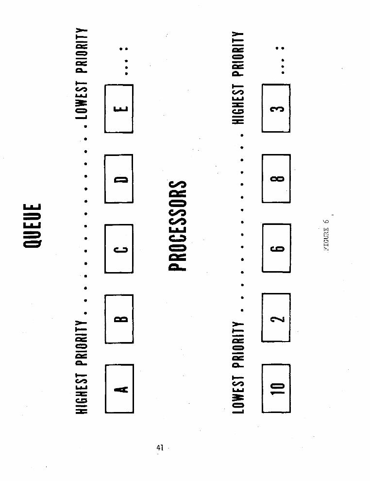
. - mm -
l
l
l
l
l
l
a
l
l
l
l
l
l
l
l
l l
H El El H Eil
mm
a l .
F-l
Ll CA
E 41

BELL LAB’S SPIDER NETWORK MINICOMPUTER SET USING CONCENTRATOR CONFIGURATION
1 MtIItCUMPUTER 1 1 MtWtCUMPUTER 1 1 TERMtWAL 1
I 1 b 1 r 1 I 1
1 MUkTtPLEXER 1 MUlTtqtEXER 1 1 MULTtPLEXER 1 1 MULTIPLEXER 1 I 1 l_- 5
MINICOMPUTER SET USING LOOP CONFIGURATtON FIGURE 7

RING NETWORK
FIGURE 8
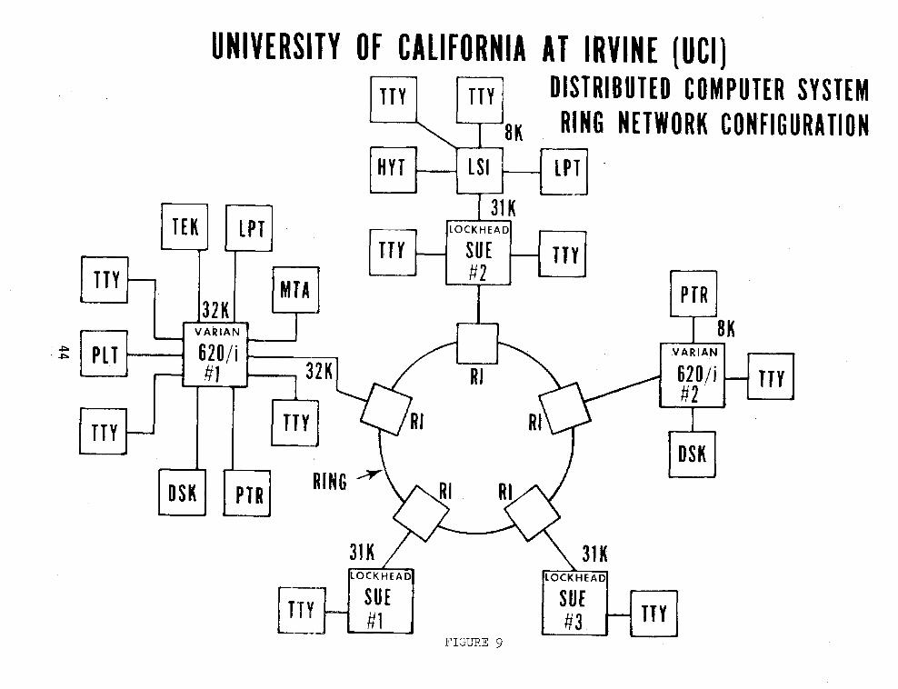
UNIVERSITY OF CALIFORNIA AT IRVINE (UCI) 1
TTY TTY DISTRIBUTED COMPUTER SYSTEM
I _ 3jK RING NETWORK CO----- - HYT 1 LSI LPI
A 1 31K
LOCKHEAD t
TTY - SUE - TTY t #2 ~ l r
PTR b i 8K
VARIAN
620/i - #2
I
0 DSK
El TTY

45


47
I Y


LINEARIZED LEAST SQUARES
Larry M. Sturdivan and John W. Jameson Biomedical Laboratory
Edgewood Arsenal Aberdeen Proving Ground, Maryland 21010
ABSTRACT. The paper discusses iterative methods for fitting linear- izable functions by weighted least squares. Starting values of the coefficients are derived from data. The method is adaptable for some desk top programmable calculators. The effect of various weighting schemes on the residual sum of squares is discussed. Two methods are presented for making the residuals in the dependent variable sum to zero.
1. INTRODUCTION. Since the early 19th century the method of least squares has been the most widely used mathematical tool for determining the values of constant parameters in linear functions (linear with respect to the parameters to be determined). The general, nonlinear least squares problem, by contrast , remains a largely unsolved problem. There is, however, a class of nonlinear functions, which some authors call "intrinsically linear", for which good estimates of the least square values of the fitted parameters may be easily and reliably obtained.
2. STATEMENT OF PROBLEM. Let us assume that we have a dependent variable y which may be expressed as an explicit function of a set of independent variables and constant parameters whose values are to be estimated.
y=F(x iy bj) ;i=l, . * * , n ; j = 1, . . . m 0) 'y = dependent variable
Xi= set of n indep. variables
bj= set of m constant parameters
The following algorithm may be used to determine the bj if F may be made linear with respect to the bj by suitable mathematical transformation, i.e. if there is some function h(y) such that
h(y) = ; bj gj (Xi); i = 1, . . . , n j=l
(2)
and dh(y)/dy is defined
The functions F and g. may involve known constants which are not members of be; e.g. the fourt
$ il of the following examples of intrinsically linear
func ions:
49

y = In (bx)
y = arctan (bx)
y = 'I*" x _ b j i=l 1
y= Ko K1 f "Xp (biXi) Ko, K, Known
Of course conventional least squares could be used directly on equation 2. The result, however, is the minimization of squared errors in h, not y.
3. THE ALGORITHM. We designate the difference between the actual and predicted value of y for the kth data point as:
AYk = Yk - F (bj, Xik) k = 1, . . . . P and
Expanding h(y - 4y) in a Taylor series with a remainder term, we get
h(y - AY> = h(y) - Ayh’(y) + Ay2 h"(y) + m.. + l-Ay)qh(q)(y) 2! q!
where h(O) (y) is the qth derivative of h(y) with respect to y, evaluated at 7, and where i is in the interval between y and y + Ay. Let q = 1, then
Ah -= h'(y) AY
Now we want to minimize
E (AY,)2 = ,I, (Ahk12 k=l
[h’ (7,) 1’
(3)
This is equivalent to weighted least squares on equation 2 with weights
Uk2 = [l/h'(jk)12; k = 1, ,.., p
Initially we do not know the value of the Ayk, much less the position of yk in the interval, ‘k.
so we use the data points yk to approximate the We may then use the Ayk from the first pass to calculate improved
weights and make a second, etc., continuing the iteration until stability is reached. Several methods of obtaining improved estimates Of the uk of equation 4 have been tried. Some authors have used regression line values
50

for 7, in equation 4; in effect using the opposite end of the interval from the data point. This method improves the fit (decreases the sum of deviations in equation 3) most of the time, but if j is closer to the data point than the regression value the fit thus o tained Is is actually worse than the results of the first iteration, Other methods tried include:
a) The first q terms of the Taylor expansion about the data values.
b) The first q terms of the Taylor expansion about the regression values.
c) Uk2 = ( h' ;y,)) (hi (y; + ayk) ) '~;~;;;;;,;~~; ;;,$$
d) uk2 = (Ayk/Ahk)2 (A’s from previous iteration)
Methods a and b have the serious drawback of requiring the first q derivatives of h, almost always an unpleasant task whatever the form of h. It is wasted labor in most cases, as well, for method d usually gives results as good as, or better than any other. In fact, intuitively one might think that method d would lead to convergence on "the" least squares answer. However, we must remember that we are determining m weights and n b's from just m data points, an underdetermined system. Thus as long as the weights are determined from the data, as they must be, one cannot guarantee convergence on the global minimum. Indeed, we have observed intermediate iterations in which the sum of squared deviations in y was slightly smaller than the "converged" value.
Unlike the linear least squares case, the above algorithm does not produce a zero sum of deviations in y:
i.e. CAy = CuAh # o
Although, cu'nh = o
If one has an overriding reason for desiring a zero sum of deviations in y, it may be obtained by minimizing
Cu(dh)* = ZAyAh (5)
wh ich, of course does not minimize the sum of squared deviations in y. In many cases the increase in squared deviations is tolerably minimization of equation 5 (i.e. using weights u rather than u 3
mall with ) if zero
sum of deviations is desired. A second method of obtaining a zero sum of deviations is to force the fitted line to pass through the weighted mean h*, xi*. i.e. fit the model
51

m-l h - h” = C b- ge (xi - xi*)
j=l J J i = 1, . . . . n
where h* = cub ni-
and A.* = cux. 1 1
cu
using weights I.?. The summation running to m-l indicates the absence of an intercept; i.e. one of the b's, say bf, for which gf = 1. Both methods of obtaining CAy = o work best when the u's are calculated by method (d) above.
4. AN APPLICATION. An example of an intrinsically linear function is the Logistic (probability distribution) function
y= 1 1 f a/xbl
The linearized form is 2
h(y) = ln(y/l-y) = lna f b,ln x = C b g*(x) i=l i '
where g, = lnx
92 = 1
b2 = lna
Also 1 1
u = h'(y) = jqt-7)
The following table shows how much improvement in the root mean square error was gained by using the iterative algorithm on the Logistic function over an unweighted fit. As expected, the fit is perfect when the data all lie right on the fitted line, whether the least square fit is weighted or not. As the data get more scattered (i.e. with a correlation coefficient significantly less than 1.00) the reduction in root mean square error is marked (Case III).
Correl. Root Mean Sq. Error % Case Coeff. Unweighted Weighted Improvement
I 1.00 II .98 0” 0496
0 0 0.0488
III .94 0:0419 0.0368 1;
52

NONLINEAR SPLINE REGRESSION ON MINI-COMPUTERS
Philip W. Smith*
Appendix
Stanley Hrncir and Philip W. Smith*
Department of Mathematics Texas A&M University
College Station, Texas
1. Introduction. -- In this paper we will present our experiences in artcq3ting to solve certain nonlinear regression problems on a mini-computer. More specifically, we used spline curves of a specified order and treated the knots as nonlinear parameters,
Section 2 contains the relevant notation and theory. In seqtion 3 we make some final remarks. At the end is an appendix with a listing of the programs and an abbreviated description of their use with examples. The reader who is unfamiliar withsplines should first glance through the examples in the appendix.
7 C . Description of Numerical Solution. Throughout this section and the
IlPX f ihe following notation will be used. Let k be a positive integer and & be a knot vector satisfying
t: =a=t = 1 =..,=t .qt
k k+l 5 I 1 * 2 tn < tn+l = . " . = tn+k = b
WhC!l:C! t.i+k > t . Given a k and a knot vector
H-splines N j . 9 ," by [ll ,
g one forms the normali:r.e?rl
k-l Nj,k(&/d = ctj+k - tj>[tj,...,tjlkl('-')+ 1
where [t 1
,,,T3tj+k] denotes the k-th divided difference operator. A
spline of order k with knot vector k is any function of the form
*This author supported by the U.S. Army Research Office under Grant Number DAHC 04-75-G-0186.
Note: k-l
(s--v)+ = (s-v)k-l if s > v and is zero otherwise.
53

Given data {(xi,yi)]~=l one can attempt to find &* and &* so that
min 'r :,; i=l
M&&) - Y,lZ = k Is(g*,q*,x,) - Yi12 1 i=l
It is in general Jmpossible to find &* and hence b*; however, given a knot vector f and linear parameters $ one can attempt to decrease the error sum of squares by some sort of descent algorithm.
The method of descent which we use is essentially that of deRoor and Rir.e [2].
Alg:orithlTl: Given $ and j = k + 1
step 1: Find 4 which minimizes
Step 2: With & fixed, move 9
between tjcl and tj+3. so as to de-
crease the error sum of squares, Call this new knot sequence $.
Step 3: If j < n set j = j + 1, otherwise set j = k f 1. *
step 4: Go to 1.
This algorithm is described in more detail ;in the appendix, We remark that Step 1 consists of solving a linear system and that in Step 2 we use a quadratic interpolation to obtain an approximation to the minimum.
We originally had a Fortraa version of the above algorithm and "trans- cribed" this program into Basic when implementing it on an HP 9830A. Same of the characteristics of the HP 9830A are detailed in the appendix. Oper- ating time on the HP 9830A was quite long. A typical problem with 20 data points and k = 4 with 2 fnterior knots might easily take thirty minutes.
We discovered that most of the time was being spent in evaluating the error sum of squares,
This term must be evaluated quite often during Step 2 of the algorithm. Additional time was being spent filling out the matrix to solve for the linear parameters. The two routines which were being used to evaluate the spline or fill out the matrfx had the following form:
54

Given 5 - <T't: i+1:
620
630
640
650
660
670
680
690
700
710
720
730
This
N[l,l] = 1
FOR S =lToK-1
P[S] = T[l+S] - T MIS] = T - T[Ifl-S]
N[l,S+l] - 0 FOR R = 1 TO S
29 = N[R,S]/(P[R] + M[S+l-R] K[R,S+l] = N[R,S+l] + P[R,j * 29
N[R+tl,S+l] = M[S+l-R] * Z9 NEXT R NEXT S RETURN
computes simultaneously the values of all the non-zero normalized B- * splines at the point T, for the matrix computations.
880 FOR R = 1 TO K
890 P[Rl = T[I+R] - T
900 M[R] = T - T[I-K+R]
910 DIR,11 = A[I-K+R]
920 NEXT R
930 FOR S = 1 TO K - 1
940 FOR R = S+lTOK
950 D[R,S+l] = (M[R] * D[R,S] + P[R-S] * DW-LSI)/(NRI + P[R-SlI 960 NEXT R
970 NEXT S 980 RETLJti
This computes s&&T) for the error sum of squares.
The parameter K is set at the first of the program and determines the order of the spline, Since K does not change throughout the program we decided to rewrite these routines in such a way that no loops were
0 55

j nvo i ved , This simple expediant reduced the running time by a factor of twr, or. thrt?c:. We list below the corresponding changes in the k = 2 (Tinpar spl.lnc) program and the k - 4 (cubic spline) program. Given
1892 PI =I T[I-+l] - T 1894 Ml 2 T -' T[I] 1896 Z9 = l/(Pl + Ml)
1897 Sl = Pl * 29 1898 S2 = Ml * 29
This cc?my~tes simultaneously the values of all the ponzero normalized B- splines at the point T and stores them in Sl and S2.
2788 Pl = T[I+l] - T
2792 M2 = 'IT - T(I] 2802 CI = (M2 * A[I] + Pl * A[Icl])/(M2 f Pl)
This cmputes s(&,&,T) for the error sum of squares, For k = 4 we have
56

Sl = Pl * z9
CL! = M3 * z9
29 = $%/(I?2 + M2)
52 = C% + P2 * 29
c’! 3 M2 * z9
209 = S3/(P3 -t Ml) s3 = c3 f P3 * z9
* 54 = Ml * z9
This computes simultaneously the values of all the nonzero normalized B- splines at the point T and store6 them in Sl through S4.
2490 Pl = T[I+l] y T
2500
2505 2510 2520 2530
2s40 25.50 2560
cl i" (M:! * A[?s-21 + Pl * A[I-3])/(M2 + Pl) ~2 = (M3*A[I-l] + P2 * A[I-2])/(M3 + P2)
C3 = (M4 fi A[I] + P3 * A[I-l])/ (M4 f P3) 2562 Cl = .@3 * c2 f Pl * Cl)/(M3 + Pl) 2564 ~7, = (FI4 * 63 + P2 * C2)/(M4 I- P2) 2566 ci -- (pi4 * C2 -f- Pl * Cl)/(MC + Pl) 2570 RETURN
This CQmputc~ s($,&,T) for the error sum of squares,
7.t is easi:y seen that as K2
K increases the length of these new routines increases by a factor of ,
3 CONrLuDING R~S, ,A---.-rt+.- When writing programs on mini-computers one has to be extremely careful not to write the programs in full generality, at least for this generation7 mini-computers, due to their slow execution t he I) For our particular problem we found it necessary to write a special program for each order. Initially this takes more time, but In the long run much tim is saved,
57

concCrnin~~ our specific problem we found that most of the computer time w;I:; spent in the spline evaluation routine. This occurred quite often dr~rirq; the computation of the error stun of squares. Noti, originally the sjl)li.nc: evaluation was accomplished in two nested do-loops where the outer par;~mcter was K - 1 where K is the order of the spline, Since in our applications K was fixed throughout the entire program, it made sense to rewrite the program for a fixed K, thus eliminating the loops and lineariz- ing the execution. The details are in Section 2.
REFERENCES
1. C, d&oor, On Calculating with B-splines, J. of Approximation Theory 6(X972), 50-62.
2. G. deBoar and J. R. Rice, Least Squares Cubic Spline Approximation fJ-- Vari.abPe Knots, CSD TR 21, Purdue University, 1968,
3. e. deBoor, ‘“Package for Calculating with IMplines”, The University of IJiscansin-Madison, Mathematics Research Center, Technical Summary Report 1333, October 1973,
58

APPENDIX
Stanley Hrrncir and Philip W. Smith
USER'S GUIDE
TABLE OF CONTENTS
I. Marr.iMachJ.ne Interface
A., BASIC Computer Language od HP 9830. B. Cassette Storage Capability.
If. M&l hmgram
A” Xnput of Data and Knot Sequence. B I, Calculation of Initial Error. c r; :
Execution of Knot Moving Routine. Pm)-3;~=am Li+mitations.

I w -achine Interface
A, . The program presented in this paper was written in the EASIC computer language for the Hewlett Packard Model 9830A digital com- puter q The BASIC language is very similar to FORTRAN.
1. Xn using the HR9830, the user 1. ‘s provided with a man/macIline interface capabIlity, With this interface capability, the pro-~ gram pauses at various points in its execution co allow the user to exercLse differen”r: optJ.ons .ruch as pl.ot:rp~~g the spline, i?lo2.-- ting the data points, cdxulating the derivative., etc,,
cassette magnetic tapes, Progrlms as weli as data poixlts can he maintained on these tapes. Having this peripheral capability is a tremendous asset especiillly when dealing with large programs nnd/ar large volumes of data.
Currently, there are three scperate versions of the Spline 1, oi,r:rm being maintained on three seperat@ files. The user can
~:i~!.t,ct from any of these depending on which degree Spline pro-- ~:r;uri he wi3hes to run (Linear, Quadratic, or Cubic] ,I
A. lllrnt. Datz,. The u3ex ia provi.ded the wprioa of h.putr,irrg dara through ehe 'keybuard ox having thr, program read pr~ious~y sto%red data. from a casserte tapem With eAther aptian, the user musr pro- u-uyI1 v:Rdc the program with two fil.e lmTlhe.rs, I,f the data is being input through the keyboard p the program will bui1.d two new fXles on the CaF~ette ta.pA.
1 I* After the program is loaded and xunn?x~g, the program wXl request the u5er to input the number of delta points, The request will be displayed on the display panel. and the user simply types in the number and then hits the execute switch, 2. The next program request is for the Iiz~8nli by whick ti:c dara Is ta be input --either keyboard or cassel”tc ttlp”e. The jlrogrlllri Will. diE@d.)- the mesnage: %'ANT TO LOAD DATE FRCiM TAI'~~'", rT( .?, ,.) * !‘k. u3erts response is either "Y" or "N" for yes or no, If no, the progrilm wiu expect the dam to he loadrxl through the, keyboard, and if yes, from files on the cassette tape. 3, Wit:.11 either option in 2 above, the prO~~r&Tl will. XIC!Xt l+e$UPSt two tape file numbers--where the data 2s to be found or where to store the data, The first number gives the file location where tbs variable X is (will be) stored and the second number gives the file location where the dependent variable Y .is (will be) stored, - _--. _ 4. The next program request will be displayed aa: “IWMDER OF EQUATXONS? “a The value of this variable (called N) depends on the number of internal knots the user proposes to use in his xm ~19~3 the order of the Spline (degree f I> he is using. POT exampls .a if the UEW is runalng the Cubic Spline Program with I.i internal knots, then the value of N would be 14.
60

5. The next program request is for input of the knots. All knows are input in order from 1 through N f K, where K is the Spllne order. The program requires that K knots be stacked at each end of the interval over which the Spline is being fit,
B. As soon as the knots have all been input, the program im?cdiately calls subroutine EQUATE to find the unique Spline function that mini- mizes the error or difference between the input data and the Spline curve calculated for the knot sequence as initialized. The progrem next calls a subroutine to calculate the error and this error value is printed when returned to the main routine. At this poir,t, th& ;)r'u- gram pauses for 3 seconds to allow the user to halt the program if he wishes to branch to some special subroutine. If the user fails to halt the program at this point* control is given to the knot moving routine which starts the optimization process of moving knots to re- duce the error. C. The program will remain in the knot moving routine until the user halts the program. The knot moving routine will pause periodically to allow the user to branch to another subroutine if he wishes. This pause will occur at the end of each cycle through the knot moving rou- tine, i.e,, after all interior knots have been considered as candidstcs for moving. D, Program Limitations. The program is currently set up to handle a maximum of 50 data points and a max value of 30 for N ('number of equations as described in II.A.4.). This restriction is a program limitation where array lengths are currently set at 50 and 30 respec- tively. By increasing the dimension of certain arrays, the user can increase the max number of data points and value of N--machine limit for dimension size is 256. However, the program run time on this machine, for large values of N and large data sets is tremendous, The program assumes the values stored in the independent variable array X and the knot sequence T are in increasing order,
III. Subroutine Descriptions,
A. EQUATE. -- For all three versions of the Spline progralr,, the :xb-- routine EQUATE can be found starting at instruction number 550 in t;),c program listings, The structure for the routine was taken from the technical report by C. deBoor, [3].
1. In order to decrease the program run time, a number of changes were made to the subroutine as presented by deBoor (page 38 of 131). The major changes include the following:
a. The number of DO loops was reduced. b. Cholesky's decomposition method was added to solve the system of equations, C. Linear arrsys are used to store the diagonal elements of the band matrix instead of two dimensional arrays as done by deBoor, d. Since the matrix being generated is symmetric, only the main and upper diagonals are generated and stored.
61

2. For all three versions of the program, the main diagonal and first off-diagonal vector of the coefficient matrix are stored in arrays C and P respectively, The constant vector is stored in array B for the system, The second off-diagonal vector is stored in M for the quadratic and Cubic versions and the third off-diagonal vector is stored in ;array Q for the Cubic, The system of equations in matrix notation has the following form: (for Quadratic only)
Cl p1 M1 />
p1 C2 p2 M2
5 P2, C3,,,Pt M3
A\ \ \‘\’ ’ \,
‘1, \ \ \‘\ ,\ \
a. ‘i \
“, \ :
I’,Mrne2
or simply, Ax = B, Since the matrix A is real, symmetric and positive definite, then it is possible to factor A as LLT where L is a real lower-triangular matrix, Then Ax = B becomes LLTX = B. Letting y = LTx, then we can solve for y in Ly = B by for- ward substitution and finally we can solve for x in LTx = y by back substitution. This scheme is known as Cholesky’s Decom- position method and is programmed directly into the EQUATE sub-- routine.
B. Plotting Routines. The plotting routines are seperate subrou- tines and are not called by the main program or any other routine, Powever, they do require that the spline coefficients be generated before being called. Also, before they can be used, the plotter must be brought on-line and properly adjusted,
I, Spline Graph, This routine provides the user with a graph of the spline function based on the spline coefficients that are currently in memory. The user will be asked to specify the scaling to use for the graph and step size (distance between calculated points-- the smaller the step size the smoother the graph) e
62

a. The first program request reads; "4 SCALE VALUES?". The user inputs 4 values: First two are the limits on the x-axis of the graph and the second two are the limits on the y-axis of the graph, For example, if we know that our input data for the x-axis spans values from 0 to 100 and we expect our spline function to not vary outside the limits of -10 to -t 10, we might input the following values: 0, 100, -10, 10. b. The second program request reads: "2 VALUES X-CROSS AND XTIC?". The user inputs the point he wants the x-axis to cross the y-axis and the spacing for the Tic marks on the x-axis 0 An input, for the example given above, might be: 0, 10. c. The next program request reads: "2 VALUES FOR Y-CROSS AND YTIC?". The user inputs the point he wants the y-axis to cross the x-axis and the spacing of the Tic marks on the y-axis l For the example given above, an input might be: 0, 1. With the example inputs given in a, b, and c above, the program would sketch the x and y axis as follows:
d. After having the axis plotted, the program will next ask for the step size (Quadratic and Cubic version only). The display simply reads: "STEP 4 ?". If the user requires a smooth curve, the step size should be small compared to the overall length of the curve. Usually 100 to 200 points pro- vides a very smooth graph, For the example given above, a step size of one would provide 100 graph points of the spline function connxcd by straight lines which should provide the appearance of a fairly smooth curve, For the linear spline Pwv~ 9 a step size is not required because the program sim- ply joins the knats with straight lines, e. After the spline graph is completed, the program will next automatically sketch in the locations of all interior knots,
2, Data Point Plot, To plot the data points is an option that is usually exercised after the Spline Graph has been completed. This plot provides an "overlay" of where the input data lie with respect to the Spline graph, The routine simply steps through each data poPnt and plots a small “x" at the coordinates of the pofnt. 3. Error.Plat. This routine provides a graphical representation of the error at each data point, The error is the difference be- tween the input data point value and Spline Function value for the same point. The routine does its own scaling based on input data and on the square root of the sum of squares of the error taken over all data points. Tic marks are provided for each axis and the value of each is printed on the printer.
63

C. Knot Moving Routine. Once the Main routine transfers control to the knot moving rozine, this routinz will stay in an endless loop constantly trying to reduce the error. The only way the pro- gram will stop is by operator intervention. The program allows such intervention at the end of each cycle through the knot sequence, i.e., after all knots have been considered as candidates for moving. At the end of each cycle, the program pauses for three seconds dis- playing the message "PLOT". If the user fails to stop the program at this point, the routine branches to the beginning and starts the cycle all over again in moving knots.
1, Logic of Knut Moving Routine. This routine considers each knot, in order, as a possible candidate for moving, The routine will not change the position of a knot unless the new position -- decreases the overall sum of squares of the errors.
a. The routine starts at t:le current position of the knot and steps in the direction of decreasing error. The step size El is determined by the variable H8 which is set to 128 by default {user can adjust this value if he wishes--set in instruction 120 of all versions of the pro- gram). El is initially set to l/H8 of the distance between candidate knot X5 and adjacent knot. Call the interval Z. b. The candidate knot's new position, X4, is determined by
,X4 = X5 + El. El can be positive or negative depending on which interval-- left or right of current knot--is considered. c. If position X4 yields an improved error value over X5, then El is doubled and a third candidate position X3 is examined (X3 = X4 + El). d. If position X3 gives a smaller error value, we then con- tinue stepping through the interval Z toward the adjacent knot until we either step outside 2 or until a candidate position X3 produces an error greater than the error at position X4. If this happens, graphically, we have the following condition:
i lL As' \ A ;
Error A31
'\\,, I<*'
/d
4 i. .."_ - -__ x5 xh x3 Positio
We know that WC are in the v.icinity of a minimum. EC! can approximate the position of that minimum by simply fitting a quadratic through the points ()15,A5), (X4,A4), (X3,A3) and solving for the minimum. e. After having found a new location for a knot, we call EQUATE, calculate the new sum of squares for the errors, and loop on next knot.
D., Derivative Routine. This routine calculates and prints the zeroth through the second derivative of the Spline Function for 60 equally spaced points along the x-axis for the entire span of data. The value 60 is set by default in the program and the user may change the value if he wishes (instruction 9050 of all versions of the program). This routine is based onthe formulae in [l].
64

IV, Examples of Output from the Program. Output from two seperare runs _.- are presented.
A. The first run uses the Quadratic version of the Spline program. Twenty data points are used and two internal knots. The spline was graphed before any knots were moved and again after three cycles through the knot moving routine. The error plot routine was also run after the knots were -moved. Figure 1 shows output to the printer,
1, When the Quadratic version of the program was executed, the first two messages printed were:
"QUADRATIC SPLINE PROGRAM" "K EQUALS 3" .
2. The program next requested the number of data points, The number 20 was input and the program printed:
"L9 EQUALS 20". (I,9 is a program variable used for storing data point count). 3 . . The data was loaded via cassette tape and printed. 4. The next request was for the number of equations; the number 5 was input and "N = 5" was printed. 5. The program next requested the input of knots and each was printed by the program when input. 6. After all knots were input, the program calculated the in-i.-- tial sum of squares of the error and printed the message: "'SUM OF SQUARES = 10.24179658". At this point, the program was halted and control transferred to the Spline Graph Routine. The first graph (labeled Plot 1 in fig. 2.a) was accomplished. The Data Point Plot was also accomplished at this point. 7. Control was then given to the knot moving routine. As each knot was moved, the new location'and the new sum of squares of the error were printed. As can be seen in figure 1., the two internal knots were moved from 2.1 and 7.0, as input, to 3.213337131 and 6.893706417 with a 10 fold reduction in the error. Three cycles through the knot moving routine were requfred to accomplish this reduction. 8, The program was halted at this point and control transferred to the Spline Graph routine again. The new Spline Graph {Plot 2 of fig. 2.a) was accomplished and the results show a much bet*- ter fit to the input data. 9. After the Spline Graph was completed, an error plot was done (fig. 2.b). The scaling was done automatically and the message:
"XTIC = 0.855 YTIC = 0.458175936" provides the user with the value of the X and Y tic marks.
Pi , The second example used the same data set but was run using chr! Linear Spline program and six internal knots.
1. The output from the printer is shown in figure 3 and the plotted output in figure 4. 2. The program was again allowed to cycle three times througll the knot moving sequence. The plots were made after the third cycle.
c. Figure 5 provides an example of output for the derivative rou-* tine. The routine calculates and prints the zeroth, first, and second derivative for twenty equally*spaced points along the Quad- ratic Spline curve generated for example 1 above. I
65

0.4-5 Q*9 1 l 35 1.8 2.25 2.7 3115 3.6 4.05
t:;5 5.4 5.85 6.3 6.75 7.2 7,65 8,1 8.55 9
FOR EXAMPLE 1
0.532832779 1 l 135824019
1.674336624 I*850310499 1.653405543 1.004342719
-0.021648662 -1.23905724.1 -2.385288895 -3.176972882 -3.377363166 -2.859228 04 -1.64757377
0.069777687 1.968942823 3.650872173. 4.724967051 4.897943545 4.04801103 2.266651669
2 l 705905’7 t-10 5.776486574 7.023652237 3a765599501
3,026696625 ?,836770835 6.964153151 1.763237007
3.243337154 1.055100397 6293706417 0.951943319
66

4
3
2
1
0
-1
-2
-3
-4
Fii
Figure 2a: Example 1 SPLINjZ PLOT 1, SPLINT PLOT 2, and DATA POINT PLOT
e 2b: BmOB PLOT FOR DATA POINT VS SPLINE 2 VALUE
.XTIC= 0.855 YTIC= 0.109083874
67

LINEAR :;IJLIN13 PROGRAM K EQUALS 2 Lg EQUALS 20
N= 8
1 2 :s 4
z 7 8 9 10
SUM OF SQUARES = 0.508496390
2.312506664 0.507836829
;::30897345 0.507836829 0.494072159
5.514309408 0.487454070 7.508981167 0.484908316 8.468580843 0.450663854
2.312506664 0.450663854
;:;62157505 0.450663854 0.437636837
5.524269999 0.434330461 7.508981167 0.434330461 8.439467487 0.408240592
2.312506664 0.408240592 3.3 0.408240592 4.590545267 0.398339792 5.532Go7619 0.395976608 7.508981167 0.395976608 8.41376275 0.3778665422
68

i*igurc da,: Example 2 LINEAR SPLINE PLOT AND DATA POINT PLOT
4
3
2
1
0
-1
-2
-3
-4
Figure 4b: ERROR PLOT FOR DATA POINT VS SPLINE VALUE
0 1 f I
I I
.
XTIC= 0.855 YTIC= 0.068726398
69 *

Figure 5: EXAMPLE OF OUTPUT FROM DERIVATIVE ROUTINE FOR 20 EVENLY SPACED POINTS
X-VALUE SPLINE FIRST SECOND VALUE DERIVATIVE DERIVATIVE
0 -1.276456667 3.851459424 -2.240811742 0.465 0.272212206 2.809481963 -2.240811742 0.93 1.336361559 1.767504503 -2.240811742 1.395 'I -915991394 0.725527043 -2.240811742 1.86 2.011101709 -0.316450417 -2.240811742 2.725 1.621692505 -1.358427878 -2.240811742 2.79 0.747763783 -2.400405338 -2.240811742 3.255 -0.610305260 -3.383637786 2.309543558 3.72 -1.g34006303 -2.30g700031 2.309543558 4.185 -2.758326289 -1.235762277 2.309543558 4.65 -3,08326522 -0,161824522 2.309543558 5.115 -2.908823095 0.912113232 2.309543558 5.58 -2.234999914 1.986050987 2.309543558 6.045 -1 a061795678 3.05998874 2,309543558 6.51 0.610789615 4.133926495 2.309543558 6.375 2.759180793 4.62786348 -4.825100395 7.44 4.389483645 2.384191797 -4.825100395 7.905 c 4.976479164 0.140520113 -4.825100395 8.37 4,520167350 -2.lO3151571 -4.825100395 8.835 3.020548203 -4.346823255 -4.825100395 9.3 0.477621723 -6.590494939 -4.825100395
70

loo 110 120 130 740 150 160 170 180 190 200 210 220 230
40 250 260 270 280 290 300 310 320 330 340 350 360 370 380 390 400 410 r, 2 0 /5. go 440 450 460 470 480
K=Z RSM **ss H8 USED IN KNOT MOVING ROUTINE *** H8=1 28 I.!RINT "LINI$AR S LINE PROG,;AM" I'RINT "K EQUALS"K D&Z/N$JBER OF DATA PTS";
/ 1 I'RINT "L9 EQUALS'%9 DISI' "WANT TO LOAD DATA FROM TAPE"; INPUT Hi$ IF H$="Y" THEN 300 DISP "2 FILE #S WHERE DATA GOES"; 1NU.R" A8,A9 FOH T=l TO L9 DISI' "INrUT X Y"1' INI-'UT X[I.;,G[t] ' NXXT I :;TOHiz: DATA A8,X ;;TORZ DATA A9,G GOT0 370 DISf' "2 FILE #S WHERE DATA IS"; INPUT A8, A9 LOAD DATA A8,X LOAD DATA A9,G DISI' "TRINT DATA"; INPUT H:$ IF H.;:#"Y" THEN 400 FOR I=1 TO L9 IIRINT I,X[I],G[I] NEXT I
DI Al "KNOT IN !lJ( I)=?"1 ;
NX i:T I 30 GOSUR 550 500 GOSUl.3 8070 510 I'IIINT "L3lJ-M OF SQUARES ="Sl 520 DISf' "i'LOT?"; 530 'AIT 3000 5:0 GOT'0 7640
l-l 71
di ( 1. ?c:~ **UN* T,INEhR :;I)LINT: PROGRAM ***** 2() [<'qq x*-s* :;URROUTINF JUMl' ADDRESSES *****-**XX************************ $0 ;j ; ,;"Jy 1 4 0 lti;iY 50 Hi5M ii
;;.i'J,IN+; G]<;Il'II -----------e---e--- 7000 2 .l~II?i-~Oh GIURII! --HHH-*HH3c--LH----- 7380
,3 DATA ?OINT T'LOT "HHHHH-HHH--H--- 7290 cs 0 IIXM (4) II:i<TUIfN TO KNOT MOVING ROUTINII: --- 7640

550 ;z:: 610 620 630 :I: 660 670 680 690 700 710 720 730 740
;z: 770 780 790 800 819 820 830 840 850 860 870 880 8’30 900 910 920 930 940 ‘950 960
;iEl 990
‘:b;M +- :,~***~,~*+u+*SUBROUTINE EQUATE*“““~“*“~~~~““~~~~~~~*~~~~~~*~~~*j
FOR 11-l TO N l3[11]=c[11]~P[11]=0 NJSXT 11 I-K Il=O FOR I;=1 TO L9 IF I=N THEN 700 IF X[L]cT[I+l] THEN 700 I=I+l 11=1-H GOT0 650 T=X[L] Pl=T[ I-cl
3 -T
Ml=T-T[I ZS=l/(Pl+Ml) ~l=l?l*zg 52=Ml*Z9 ~;:I"l[~l]
p[iii:~~;z~;[Ej
12-121; B 12
1 3 =S2*Gl+B 12
c 12 E 3 =s2*s2+c 12 l
NEXT L
R3M -x-k********+**+* BAND&Q) MATRIX Rouq’1-J’~ +***t+W~WW**W*~~~~****~~*~
REM SOLVES SYSTEM USING CHOLESKY'S DECOMPOSITION METHOD FOR J=l TO Nl Jl=J+l E Jl=b=S&R(C[J]) P Jl=Dl=P[J]/D
i C Jl)=C[Jl]-Dl+Dl NEXT J :[y]:;yy\gq 3 FOR J=2 TO N Jl=J-1 C[J]=(B[J]-=P[Jl]*C[Jl])/E[J] NEXT J ACNl=C[N]/E[N]
1000 FOR J=Nl TO 1 STEP -1 1010 Jl=Jf+l 1020 A[J3=iC[JJla[JJ+A[~1J)/~[~] 1030 NEXT J 1040 RETURN
l-2
72

“(-;(I0 \i;;D’” X-H-X -XX-XX K;;J’I,IN]( GI~Ap~~~*~“W*W~++ww~~~~*****~~~**~*******~~~~~~~~~**~
:IblO .iu:;,F "4 =;CALE VALtJJiS”; 20?0 INI:UT Q9,(@,Q7,&6 7030 :.i(:Alll< 'XLQ4QLQ6 '7040 jjl.:;J, “2 VALUES X-CROSS AND XTIC"; 7050 INJ'UT Q7,Q6 7060 X,'I;(IS Q7,Q6 7070 DISP "2 VALUES FOR Y-CROSS AND YTIC"; 7080 INI'UT Q7,&6 7090 YAXIS &7,&6 7110 It=K 7120 FOE! J=2 TO Ni-d 7130 T='?[J] 7140 GOSUB 8930 7150 GC',SUB '7550 :‘160 :ZO’1’ T, Cl 7170 NVT J 7180 :=E: ;;;o" "i;:7; &6=K+l TO N
<,lk 7210 T=T[Q6] 7’20 GOZUB 8930 7230 GOSUB 7550 7240 FI,O" T,Cl 7250 CPLOT -0.3,-0.3 7?60 LABEL (* ) “0” 7270 NUT Q6 e 7280 STOP 7290 R;<pj -K***-X-* DATA POINT PLOT W~**~*t~~*~+*Y~~C*~~~~~~~~~*~~*~~***~~*~- 7300 FOR 11~1 TO I&j 7310 PLOT X[Il],G[Il] 7'520 CI'LOT -0.3@-013 7330 LABEL (*)"X" 7350 I'EN 7360 NEXT II 7370 ;TOI‘ 7380 RxM ,+**** EmOR PLOT R0UTIN-E *~**+**~++*+~~++*Y**~*~**~***~~~*~*~ 7390 7400
Y=T*SQR I Sl/L9) SCALI;: X 11 X[Lg] -Y,Y
7410 XAXIS 0 (X[L9]-xt1 J)/lO 7420 YA:(TS X[l],Y/6 7L30 PRINT "XTIC 7440 1=x
=I’(x[Lg J-x[ 1])/10wIc=~~~/6
7450 FOR J=1 TO L9 7460 T=j:[J] 7470 GOSUB 8930 7480 GOJUB 75 50 71190 PLOT T,G[J]-Cl 7435 I'LOT T,O 7 500 7-'EN 7510 IWXT J 7520 STOP
l-3
73

7530 "!550 7570 7600 7630 7640 7650 7660 7670 7690 7690 7700 7710 7720 7730 7740
;;zo” 770
7780 7790 7800 7SlO 7820 7830 7840 7050 7860 7870 7880 7890 7900 7910 7920 7930 .7940 7950 7c36') 7970 7980 7990 no: io 8010 m20 8030 8040 8050 8060
I:~<M -X*-*+X** CALCULATE SPLINE VALUE FROM SFLINE COEFFICIENTS *c3c**3t** Pl=T[I+lj-T MZ=T-T[I Cl=(WU I]+Pl*A[I-13)/@2+Pl) [' RGTU i{N R~:r,lX-X,~*X~~,~*-*CJC*~+KNOT MOVING SUBROUTINE , *****************++******* * FOX I?=3 TO N .;~l=(!rCIS+l]-T[I5])/H8 A5=;71 :1;5df'15] T[I5\=-4=T[I5]+El G&UB 8070 IP Sl<A5 THEN 7770 I~I=(T[I~-~]-x~)/H~ T[I5]=xJ=X5+El GOSIJB 8070 IF SlcA5 THEN 7770 GO'_70 7990 ii4=Sl ~l=~j+El T[15]=X3=X&+El IF (x3cT[I5-l] OR X3=-T[I5+1)) THEN 7990 GO:;UB 8070 A3=sl IF (A3>A4) THEN 7890 A5=A4 x5=x4 A4=A3 :;4=:;3 GOT0 7780 X6=X3*X3 x7=x4*x4 X&x5”Q Rl=A5*(X6-X7)+A4*(Xs-x6)+A3*(X7-X8) R2=(A5*(X3-X4)+A4*(X+X3)+AP(X4-X5))*2 T[I5]=R1/R2 EOSUB 8070 IF (SlcA4) THEN 8000 T[I5]=,14 GOT 8000 T[I5]=T[15]-E'i GOSlJii 550 c;O:;UB 8070 mINT r[15],si ~XT 15 DI3P "PLOT?"; WAIT 3000 GOT0 7650
1-4
74

$070 R~~M*~***~“*~*COMPUTES SUM OF SQUARES~*~***~~“““*+~~***~***~*
8080 21-O 8090 I=K 8100 FOR I,==1 TO L9 8110 T=X[L] 8120 IF T[I+l] >= T THFnN 8170 8130 I=Icl 8140 IF I <= N+l THEN 8120 8150 PRINT "RANGE" 8160 STOP 8170 Pl=T[I+l -T 8190 M2=T-TII 8220 8250
Cl=(M2*A i I]+Pl*A[I-l])/(M2+Pl) S=Cl-G[L
5260 Sl=S1+S*S 8270 NE>:T I; 8280 RETURN 8930 REM"** FIN S I SUCH THAT T(I)<=T<T(I+l) USING FORWARD SEARCH ONLY** 8940 IF T[I+l] === T THEN 8990 8950 I=I+i 8960 IF I (= N+l THEN 8940 8970 PRINT s'RANGE"; 8980 STOP 8990 RETURN
l-5
75

]<sM *X**YfWt~f** DERIVATIVES*~“*~~~“~~**~~~,~**~~*
RE:M THIS ROUTINE CALCULATES THE ZEROTH THROUGH Dl DERIVATIVES OF REM AND PLACES THEM IN P(1) THROUGH p(Dl+l) RESP. SPUN REM THE DERIVATIVES ARE AT T Dl=3
9000 go10 9020 9030 9040
;z /
9070 9080 9090 9100 9110 9120 9130 9140 9150 9160 9170 9180 9190 9200 9210 9220 9230 B240 9250 9260 ,927o 9280 9290 9300 9310 9320 9330 9340 9350 9360 9370 9380 9390 3400 9500 9510 9520
I=K GOSUB 8930 nEM*~-*"~~"~""*"**"~"~*** N[l,l]=l
CALCULATES N(I,K) AT T""***************.
FOR S=l TO K-l
ii N FOR R=l TO S 29=N[H,S]/ P[R]+M[S+l-RI)
R,S+l]=N R t S+l]+P[R]*Z9 i+l,S+l]=M[S+l-RI+29
NEXT R NEXT S FOR S-l TO K D[S,i]=A[I-Scl] NEXT S FOR S=2 TO K FOR R=S TO If ~[R,S~=(D[R~~~S-~]-D[R~S~I])/(T[I~K~~+~]-T~I-R~$]) e NEXT R NEXT S Ml=1 FOR I=1 TO Dltl Sl=O FOR J=l TO K-I+1 S1=S1+D[K-+J,1]*N[J,X+1-1] NEXT J P[I]=Sl*Ml Ml=Ml*(K4) NEXT I PRINT T,P[l],P[2]&3] NEXT T STOP R3-M -ES-K SpJJ-~ Jj'UNCTI()N -j'NS (T) ~*****Y~*~+~~W~~~+***~***~~~~~~**~~ DLW FNS(T) I=K
9530 GosuB 8930 9540 GWJJB 7550 9;; ;;;URN Cl
l-6
76

1C ;,:>:TP*'*". QUADRATIC SPLINE I'ROGRAM **** 2(-J ;;:%y x*-n** SIJBROUTINX JUMP ADDRZSSES *~~***~~tt*****~*~~*~~~***~~~~~ jG Ri~M (1 sI'I;Im G&yJq 3-11 ---I-----**-*-- 7000 ‘1 9 Rim (2 1 ERROR GluI'IJ ----e--------c------ 7380 50 REM (3) DATA POINT PLOT -l-"--c--------l 7290 60 R M (4) RETURN TO KNOT MOVING ROUTINE --- 7640
110 iIEM"*" HR USED IN KNOT MOVING ROUTINE *** 170 Hf3=1%8 130 i'TiIN? "QUADRATIC SPLINx PROGRAM" 140 !'R.INT "K tiQUALS K 150 DI\?ll "NUMBER OF DATA PTS"; 160 IN?UT L9 17 I:RINT "L9 %QUALS++Lg 130 D%Si; "I/ANT TO LOAD DATA FROM TAPE++; 190 INrUT H.$ 200 IF H,$="Y++ THEN 300 210 ;31s.i "2 PIId j/S WHERE DATA GOES++; 220 INWT A8,Ag 230 FOR i=l TO I&I .;O Xi " IWUT X,Y"I ; 250 INlUll >L[I],G[I] 260 N.i:::;T I 270 ,;!p(jl;l_;?: DATA h8,X 280 ,;wiit< DATA A9,G '290 (XT0 370 300 .DIL;1: "2 FILE #S 'ti%ER% DATA IS++; 310 PNi'UT A8,Ag 3 0 LOAD DATA A8,X 330 LOAD DATA Ag,G 340 DISI' "PRINT DATA"; 31;O INf'UT Hqj 360 IP H,;#++Y'+ THEN 400 370 FOR I=1 TO Lg '280 PRINT I,X[I],G[I] 390 NE:<T I 400 ;3T:;I: "NUMBER OF EQUATIONS=?'+; 11 ri INPUT N n20 Nl =X-l d 25 )J2=I::-? 430 J‘RINT "N=+'N
N+K IN T(I)=?'+I;
440 F(i;: -i=l TO 450 1jISP "KNOT 469 IN'UT T[I] 4.'0 PRINT "T(1 480 Nil:'iT I 490 GOXJR 550 5,IO GO3UB 8070
)='+T[I],I
510 I'RINT "SUM OF SQUARES =+'Sl 5?O DI:;T "I'LOT? " ; 5 ii) wri T'I' 3000

550 l’\::K ,1(x -)I *xu.~~*~~w*SUBROUTIN EQUATE ‘~*JC*~*******JCXJC*~tJt**t~*~SC**-K**-***~-.
560 t"Oli 11-l TO N 570 n[rl~]=c[Il]=P[Il]=M[Il]=O 610 NUT Xl 620 I=K 630 X1=0 640 FOX L-1 TO L9 650 IP I=N THEN 700 660 IF X[L]<T[I+l] THEN 700 670 I=I+l 600 11=1-K 690 GOT0 650
750 29=1/(Pl+Ml) 760 Sl=Pl*Z9
800 Sl=Pl*Zg 8 0 C2=M2*CLg 820 Zg=S2/(P2+Ml) 830 d2==C2+P2*Zg 840 33=Ml"Zg 850 Gl=G[Ll 860 IZ=Il+l
950 12=12+1 -33*Gl+B 12 =sg*s3+c E 12 3
980 N3XT Ii
2-2 78

:]go l{;;l’i XX*-***++*X**Y**-W BAN-J)E,JJ ~“JRIX ROUT NE fv**Y-X~**~**-X*tw**~~*~~~**~
1000 R15FI SOLVES SYSTEM USING CHOLESKY'S DECOMPOSITION MFTHOD 1010 POil J=l TO N.2 1020 Jl=J-tl 1030 J2=J+
1100 NEXT J
1160 PO3 J=3 TO N 1170 51=5-l Il.80 J2=J-2 1190 1:00
C[J1=(B[J)-M[J2]*C[J2]~~[Jl]*C[J~])/E[S] NEXT J
1210 A[N]=C[Nt/E\N] 1220 A Nl]= C Nl -P[Nl]*A[N])/E[Nl] 1230 FOR J=N2 TO 1 STEP -1 1240 Jl=J+l 1250 J2=J+2 1260 A[J]=(CCJ]-P[J]“A[Jl]~M[J]WACJ2])/E[J] 1270 INEXT J 1280 RETURN
2-3
79

7000 RX 7 -Yf3C*C.-X-XK SJ'I;INi$ GFU1PH*"~*"*"*~"~*""*******~~~~~*~*~~*~~~~~~~~*~~ 7010 Ill.;.:, "4 SCAIJ VAT,UES" ; 702r, TNTtJT Q9,90,&7,QG 7030 .iC,ZJ,E &9,98,Q7,Q6 7040 DISP "2 VALUES X-CROSS AND XTIC"; 7050 INI'UT 47 ,Q6 7060 THIS &7,&6 7070 DIS'P "2 iVhJES FOR Y-CROSS AND YTIC!"; 7080 INPUT Q7,&6 7030 YAXIS Q7,Q6 7100 DISI' "STEP ='I; 7110 INI'UT Q5 7120 I=K 7130 FOR T=Q9 TO Q8 STEP Q5 7140 GOSUB 8930 7150 GOSUB 7550 7160 :i'l.,OT T,Cl 7170 NUXT T 7180 I=K 7190 FOR Q6=K+l TO N 7200 PF,N 7210 T=T[Q6] 7220 GOSUB 8930 7230 GOSUB 7550 7240 I'LOT T,Cl 7250 CI'LOT -0.3,-O. 3 I 7260 LABEL (*)"O" 7270 NEXT Q6 7280 e;TOP 7230 RK:M Jc***** DATA POINT PLOT ~~~***#+~Y+*~*X~*~***~*~*~~**~***~~~***~ 7700 I'OK II=1 TO I,9 7510 7320
PLOT X[Il],G[Il] CPLOT -0.3,-0.3
7330 LABEL (*)"X" 7350 PEN 7360 NEXT 11 7370 .;TOP 738', REM ***** ERROR PLOT ROUTINE ***************+******************** 7390 Y=3*SQ2 76cm ~.;CAL~~ x l],X[I&] -Y Y t
Sl/L9)
7410 ::;1:J,-rs 0 (X[L91-X[l]j/lO 7420 YBXIS X[l],Y/G 7v0 3Iwr IfxTIc =~~(x[Lg]-x[l])/i0"~~1c=~~y/6 7440 ?=K 7450 POR J=l TO L,g 7460 T=X[J] 7/17q GOSUB 8930 74r30 GOSUB 7550 7490 I'LOT T&J]-Cl 7495 PLOT T,O 7500 ;'dN 7 5 1 0 N i--t; T J 7520 i;TOP
2-4 80

7530 ;:z:: El:: 7590 7600 7610 7670 76-50 7640 7650 7660 7670 7680 7690 7700 7710 7720 7740 7740 ;;2: 7770 7780 7790 7800 7810 7820 7830 7840 7850 7860 7870 7880 7090 7900 7910 7920 7930 7940 7950 7360 7970 7980 7390 8000 8010 BO20 8030 GO40 SO50
Ri<ib] ****-K-K* (JAI;CmATE: Sj?LINE VALUE FROM SPLINE COEFFICIENTS *****'* :i?j=TrI+l -T I-;?=?'[I+2 -T I M2=T-T I-l]
F MS=T-T I W=h[I-1 3 Cl=(M2*C2+Pl*A[I-2])/(M2+P1) W=(Pl3*A[I1+P2*C2)/(Ms+y2) cl-(~3*C2+Pl*Cl)/(M3+Pl) :~1;:Tt.J~~N I!I,:FI*C"~~***J~**~~**~YKNOT MOVING SUBROUTINE *w+~*++*~+****~~~**~~~****~~~ FOX 15=4 TO N j~l=(T[I5+1]-T[I5))/H8
g;'I5] T[I5 =X4=T[I5]+El 5 GOSU13 8070 IF SI-=A5 THZN 7770 .b;l=(T[I5-1]-X5)/H8 T[I5]=X4=X%El GOSUB 8070 IF Sl<A5 THEN 7770 GOT0 7990 A/I=Sl 2l=El+El T[ 15]=X3=X4+El IF (X3cT[I5-l] OR Xj>T[I5+1]) THEN 7990 Nmy 8070
Iv-(k3>A4) THEN 7890 A5=A4 ;<5=.:4 A4 =A3 X4=X3 GOT0 7780 X6=X3"l.X3 ;c7=x/l*x4-
GOSU3 8070 IT (S 1 iA4) THEN 8000 T[I5]=:44 GOT0 8000 T[I5]=T[I5]-El GOSUH 550 GOSUB 8070 YIIINT, T[I5],Sl NEXT 15 DISI' "YIJOT?'~; NAIT 3000
8060 GOT0 7650
2-5 81

f3070 ~~~W~"*u~"""~""COMPU'~ES SUM ()Jj' sQUA~S”*““~~“*“*~*~*~*~~~~~~~~
8000 Sl=O 8090 1-E; 8100 FOH L=l TO II9
110 T=>;[L] 8120 IF T[I+l] )= T THEN 8170 8130 1=1-t-l 8140 IF I <= Ntl THEN 8120 8150 PI!INT "OUT OF RANGE"; 0160 STOY 8170 Pl=T E 11-l 3 -T 8180 Pz=T I+2 -T 8190
8200
M2=T-T 1 I-l]
8210 M3=T-T I 3 C2=A[I-1 8220 Cl= M2*C2+Pl+A[I-2])/(M2+Pl) 8230 C2= I M3*A[I]+P2*C2)/(M3+P2) 8240 Cl=(M3*C2+Pl*Cl)/(M3+P1) 8250 S=Cl-G[L] 82GO I;l=Sl+S"S 8270 NXXT L 8280 X?,TUdN 8930 RXM** FINDS I SUCH THAT T(I)<=T<T(I+l) 8940 IF T[I+l] >= T THEN 8990
USING FORWAD SEARCH ONLY
8950 I=I+l 8960 IF I <= N+i THEN 8940 8970 PRINT "RANGE"; * 8980 STOI, 8990 RETKiN
2-6 82

9000 9010 9020 9030 9040 9050 9060 9070 9080 9090 9100 9110 9120 9130 9140 9150 91 63 9170 9180 9190 9200 9210 9220 9230 9240 9250
p;yJj * 44 **w-xX*X*, DERIVATIVES”**“*w~**~********~**
,‘(ll:M THIS ROUTINE CALCULAT.ZS THE ZEROTH THROUGH 131 IN7RTVA’t’TVI;l.S nB ;PT,T RX4 i1N.1) PLACES THEM IN P(1) THROUGH p(Dl+l) RESP.
--_- .---1 , Y . , VL u 1 J,L
XWi THE DERIVATIVES ARE AT T Dl=3
1=x GOi;UB. 8930 H~~~~x*~~~~*+********~~~** N[l,l]=l
CALCUI#J'ES N&K) AT 'J******+*******+***~
FOR S=l TO K-l ? S]=T[I+S]-T M
i 5 ;=T-T[ 1+-t-~ J
N,l,S+l]=O FOR R=l TO S %%N[R,S]/ P[R]+M[S+l-R]) N
t R,Z+l]=-N R S+l]+P[R]*Zg t
N R+l,S+l]=MfS+l-RI"29 NXCT R NEXT S FOR S=l TO K D[S,l]=A[I-S+1] NEXT S FOR S=2 TO K FOR !i=S TO K
9260 D:n,~~~=(D[R-l,S-l]-D~R,S-l])/(TCI+K-R+l]-T[I~R~S]) * 3270 NEXT 11 9280 N'GXT S 9290 Ml=1 9300 FOR I=1 TO Dl+l 9310 ::;1=0 ‘3720 FOR J=l TO K-I+1 9330 ~~1=,l~,D[K+1-JTI]*N[J,g+l-I] 9340 NEXT J 9350 P[I]=Sl*M1 9360 M-t=Pll*(K-I) 9370 NhXT I 9380 ERIBT 9390 N-EXT T
T,P[l],P[2],P[3]
9400 ST02 9500 R3iil ** * SPLINE FUNCTION FNS(T) 9510 DEP FNS(T)
*********+**********************+.**
. ' 9520 1-K 9530 GOSUB 8930 9540 GOSUB 7550 3550 RETURN Cl 9560 ZND
2-7 a3

I(1 T#M+** **** CUBIC SI%INE I'lIOGRAM ***** 20 i{is;M Y*** SUBR0UTIN.I;; JUMt' ADDR13SSES *~a***C***********~**~~~~~~~~~~.~ 70 RlSN 40 REM I
1 SPIJNE GlW'H -I---l--ll-I-c-,-l-~l 7000 2 1 ERROR GRAFH c-----------L-------- 7380
50 RiSTI DATA I'OINT PLOT e--------------c- 7290 60 REM RETURN TO KNOT MOVING ROUTINE --- 7640 7 0 RX4 (5) DERIVATIVE ROUTINE: -------------- 9000 81’) DIM 13 301 F:[%o] xc503 G[501 Hs ll, 90 DIPI 7; 6,6],~[30j,1)[30j,M[3Oj,D t E 3
[3O] 696 ,A~303~C~301~S[6~
100 K-4 110 Rl?M*--* H8 USED IN KNOT MOVING ROUTINE *** 120 H8=128 138 PRINT '"CUBIC SPLINE PROGRAM" 140 PRINT "K I<QUALS"K 150 3IST "NUMBER OF DATA PTS"; 160 IN.1‘UT L9 770 PRINT "Id9 EQUAjW'L9 180 ;)I:;? ":/ANT TO LOAD DATA FROM TAPE"; 190 IIII,UT H11: 200 13 H$="Y" THEN 300 210 Dl'S!-‘ "2 FILE #S WHERE DATA GOES"; 220 IPiPUT A8,Ag 230 FOIi I=1 TO II9 240 DISI‘ "INPUT x,Y"I; 250 INPUT X[I],G[I] 260 NEXT I 270 STO;lE DATA A8,X * 280 ST0li.Z DATA A9,G 290 GOT0 370 330 DISl "2 FILE #S WHiZRE DATA IS"; 310 INPUT A8,A9 320 LOAD DATA A8,X 770 LOAD DATA A9,G 340 DISP "PRINT DATA". Y 750 INI'UT HG; 360 IF H&#"Y" TPKEN $00 770 FOR I=1 TO L9 38C PRINT I,X[I],G[I] 390 NEXT I 400 DISI, "NUMBZR OF EQUATIONS=?"; 410 INPUT N 420 Nl=N-1 425 N2=:J-2 /!30 ?RINT "N="N
N-1-K IN T(I)=?"I;
440 FOR I=1 TO 450 DISP "KNOT 46rl INPUT T[I] 470 l'?iINT "T(1 180 NEXT I 490 GOSUB 550 500 GOSUB 8100
)="T[I],I
510 ?RINT "SUM OF SQUARES ="Sj 520 DISP "PLOT?"; 530 WAIT 3000 540 GOT0 7640
51 84

570 B[11]=C[Il]=P[Il]=M[Il]=Q[Il]=O 620 NEST 11 630 I=K 640 El=0 650 FOH L=l TO L9 660 12' I=N THEN 710 670 IF X[L]<T[I+l] THEN 710 680 I=I-tl 690 11=1-K 700 GOT0 660
780 Z~=l:(Pl+Ml) 790 sl=Pl*zg 800 SF?=Ml*Zg 810 29=Sl/(Pl+M2) 820 ;;1=2)lCi;g 830 c2=m*z9 840 Zg=S2/(F2+Ml) 850 s2=C?+i'2*Zg 360 s;4=)11*~9 870 Z9=~l/(Pl+M3) 880 Sl=i'l*Cg 890 C2=FI3*23 900 Zg=S2/(P2+M2) 910 S2=C2+P2*29 920 c3=rJiz* 29 930 Zg=S3/@'3+Ml) 940 sg=c3+23*zg 950 SJ=Ml*Zg 960 Gl=G[L] 970 IZ=Il+l
1150 NZXT L P2 85

116~) yr:l -x~~~~t~f+*~~*+E*G+* BANDED MATRIX R()jJTI~J *~~~~***~*~+*~~-~*+3*~~*~
1 170 RiZ'! sGLv~:s SYSTEM USING CHOLESKY'S DECOMPOSITION METHOD 1180 FC;R J=l TO N-3 1190 Jl=J+1 1230 J2=Jt2 1210 J3=J+3
1273 P Jl" =P Jl.-Dl*DZ 1280 M Jl &I Jl--D1*D3 1290 C J2 =C J2/D2*D2 1300 P J2 =I' J2--DZ*D'-S 1310 C;JS_=C,J?_-bS*DS 1320 NEXT J
1460 FOR J=4 TO N 1470 Jl=J-9 1480 J2=J-2 1490 J3=J- 1500 C[J]= 1 510 NZLT
1550 FOR J
'3 IB[J3-M[J2l~C[J23-P[Jl]~C~Jl]~Q[J3]~C[J3]~/E[J]
1560 Jl=J+l 1570 J2=5+2 1580 J3=J+3 1590 1600
h[JI=(C[J]-r[J]*A[Jl~-M[J!wACJ23-&CJI”AtJ3])/~[J] NEXT J
1610 RETURN
3-3 86

7000 7010 7020 7030 7040 7050 7060 7070 7080 7090 7100 7110 7120 7130 7140 7150 7160 7170 7180 7190 7200 7210 7220 7230
:g 7260 7270 7280 7290 7300 7310 7320 7330 7350 7360 7370 7380
REM*********SPLINE GRAPH ********************************************** DISP "4 SCALE VALUES"; INWT &9,&8,47,96 SCALE &9,&8,&7,Q6 \ DISP "2 VALUES X-CROSS AND XTIC"; INPUT &7,&6 XAXIS &7,&6 DISF "2 VALUES FOR Y-CROSS AND YTIC"; INPUT Q7,Q6 YAXIS &7,Q6 DISP "STEP ="* 9 INPUT 45
;;: T=Qg TO Q8 STEP Q5 GOSUB 8930 GOSUB 7540 PLOT TIC1 NEXT T I=K FOR Q6=K+l TO N
K$Q~] GOSUB 8930 GOSUB 7540 FLOT T,Cl CPLOT -o.g,-0.3 LABEL (*)"O" NEXT Q6 STOP REM -X-~-W--KU DATA PO-j-NT PLO'11 UUfUUUUUU+U++UUUUUUUUUUUUU~UUUUUUUUUUUUU FOR X1=1 TO L9 PLOT X[Il],G[Il] CPLOT -0.3,-0.3 LABEL (*)"X" PEN NEXT I1 STOP REM ***** .ERBOR PLOT ROUTINE *********************************~**
7390 Y=3"SQR(Sl/Lg) 400 SCALE X[l ,X[Lg],-Y Y 7410 XAXIS 0, i X[L9]-X[lj)/lO 7420 YAxzs x[ 1],Y/6 7430 PRINT "XTIC ="(x[Lg]-~[?])/~o"YTIc="Y/~ 7440 I=K 7450 FOR J=l TO L9 7460 T=X[ J-j 7470 GOSUB 8930 7480 GOSUB 7540 7490 BLOT T,G[J]-Cl 7495 PLOT.T,O 7500 PEN 7510 NEXT J 7520 STOP
3-4 87

;;c 7550 7560 7570 7580 ;290: 7610
615 7620 7625 7630 7635 7640 7680 7690 7700 7710 7720 7730 7740 7750 7760 7770 7780
$90: 7810 7820 7830 7840
;% 7870 7880
;;z: 7910 7920 7930
77;;: 7960 7970 7980 7990 8000 8010 8020 8030 8040 8050 8060 8070 8080
REM SC****** C!ALCULATE SPLINE VALUE FROM SPLINE COEFFICIENTS ****+**
FOR 15=5 TO N El=(T[I5+1]-T[I5])/H8 A5=Sl X5=T 151 '??[I5 -X4=T[I5]+El 5 GOSUB 8100 IF Sl<A5 THEN 7aOO El=(T[I5-l]-~5)/H8 T[I5]=X4=X5+El GOSUB 8100 ;;T;lzAoTHEN 7800
A4=Sl El-El+El T[I5]=X3=X&El IF (X%T[I+l] OR X3>T[15+1]) THEN 8q20 GOSUB 8100 A3=S1 IF (AS>A4) TlHEN 7920 :'5=A4 x5-x4 A4=A3 X4=X3 GOT0 7810 X6=X3*X3 x7=x4*x4 X8=X5*X5 RkA5*(~6-X7)+A4"(X8-X6)+A3*(X71X8) R2=(A5*(XS-X4)+A4*(X5-X3)+A3*(X4-x5))*2 T[l5]=Rl/R2 GOSUB 8100 IF (SWA4) THEN 8030 T[I5]=X4 GOT0 8030 T[I5]=T[I5]-El GOSUB 550 GOSUB 8100 PRINT T[I5],Sl NEXT 15 DISP "PLOT"'; WAIT 3000 '
man txwn 7mn - - nn

8100 ~M”*~*t”~~C~*~COMPUTES SUM OF sQUARES”““~*~~““““““~~~~~~~~~~
8110 Sl=O 8120 I=K $130 FOR L=l TO L9 8540 T=X[L] 8150 IF T[I+l] T= T THEN 8200 8160 I=I+l 8170 IF I <= N+l TIIEN 8150 8180 PRINT "RANGE" 8190 STOP 8200 GOSUB 7530 8210 S=Cl-G[L] 8220 Sl=Sl+S"S 8230 NEXT L 8240 RETURN 8930 REM*+ FINDS I SUCH THAT T(I)<&T(I+l) USING F'ORWARD SEARCH OnY*** 8940 IF T[I+l] >* T THEN 8990 8950 I=I+l 8960 IF I <= N+l THEN 8940 8970 SRINT "MNGE"; 8980 STOP 8990 RETURN
3-6 89

9000 9010 9020 9030 9040
%E 9070 9080 9090 9100 9110 9120 9130 9140 9150 3160 9170 9180 9190 9200 9210 9220 9230 9240 9250 9260 9270 9280 9290 9300 9310 9320 9330 9340 9350 9360 9370
REM *-XS-Kk-ES-kS+*S DERIVATIYES~~““*““~“~~***~*~~~~
REM THIS ROUTINE CALCULATES THE ZEROTH THROUGH Dl DERXVATXVE3 OF REM AND PLACES THEM IN P(1) THROUGH p(Dl+l) RESP, SPLlrJ R3,M THE: DERIVATIV3S ARE AT T
/ Dl-3
STEP Hl I=K GOSUB 8930 REM**~*~**t~*t~jt*CY*"Y++~ CALCULATES N( 1,K) AT T***+***********! ' N[i,l]=l FOR S=l TO K-1 P S =T[I+S]-T
i'
\ M S =T-T[I+l-S] N l,S+l]=O FOR R=l TO S 29=N[R,S]/ P[R]+M[S+l-R]) N R,S+l]=N R N R+l,S+l]=M[S+l-R]+Z9 E
t S+l]+P[R]*Zg
NEXT R NEXT S FOR S=l TO K D[S,l]=A[I-Si-I] NEXT S FOR S=2 TO K FOR R=S TO K D[R,S]=(D[R-l,S-l]-D[R,S~l])/(T~I~K-R~l]-T[I~R~S]) NEXT R NEXT S Ml =1 FOR I=1 TO Dl+l Sl=O FOR J=i TO K-I+1 S1=S1+D[K~l-J,I]~N[J,K~l~I] NEXT J P[I]=Sl*Ml Ml=Ml* (K-I) NEXT I
9380 PRINT T,P[l],P[2],P[3] 9390 NEXT T 9500 REM *** SPLINE FUNCTION FNS(T) *w*wY~+~***~~~*~~+*+~~***~~*~*~~~~ ;;N& I"; FNS(T) d
9530 GbUB 8930 9540 GOSUB 7540 9550 RETURN Cl 9560 END
90

Charles E. Gray
Aeronutronic Ford Corporation
&lo Alto,Califosnia
This paper devcl.ops some methods for computing the real root-s of
a rcaal valued function in a finite infcrval. This classirnl problem is
treated by mctl:ods that are novel in the following respects: the con-
vcrgencc dots not dcpcnd on the customary “initial guess;” one can con-
clude that the function has no roots, if that be the case; if that is
not the case, one can compute al1 real roots of the function in the in-
tcr-val to witl1i.n a preassigned accuracy. It is assumed that the func-
tion is Lipscllitz and that a value for the Lipschitz constant is known.
These assu:nptior?s arc mild enough so that methods are applicable to a
variety 0T problems, notably in optimal control. From the basic method
two other algorithms are derived: one computes the maximum of a func-
tion on an interval; the other computes the roots oE a function, but
with improved speed of convergence similnr to that af Newton’s method.
Numerical results are presented which illustrate the properties dis-
cussed abova.
91
*,

Introduction
A classical problem Ln numerical analysis is that of finding in a
given interval (which w@ -assume to be closed and finite) a real root
of a continuous, real-valued function. Many algorithms have been proposed
to solve this problem (I1 1*l44 W[4 +I)*
In one way or another, they all require an initial guess at the value
of the root; it is hoped that this guess is improved by an iterative
.application of the algorithm. This hope may be disappointed for a number
of reasons. It may happen that an initial guess appropriate to the algo-
rithm does not exist, even though a root exists. Or, if an initial guess
and a root both exist, the algorithm may nevertheless fail to converge,
because the initial guess is not close enough to the root. Of course, if
there are no roots, no convergence is possible. Unfortunately, it is not
possible to determine whether lack of convergence is due to the first or the
second of these alternatives. The only recourse then is: if at first you
don't converge, pick a new initial guess and try, try again.
By contrast, the method which we present be':cw (first proposed in II
1)
does not require an initial guess at the value of the root. If there is no
root of the function in the given interval, the algorithm reveals this fact.
Otherwfse, the algorithm computes all roots of the function in the interval.
TO illustrate the problems that can beset ciassical methods, we consider
two of them: the bisection method and Newton's method. We denote the func-
tion whose roots are sought by f(x) and the interval of interest by a,b . f I
The problem then is to find an x E [a,b] such that
f(x) = 0
92

The BiSeCtiCI~‘lc tiled
In the bisection method it is assumed that WC know two numbers u. f [a,b]
and voE p .q , such th.4t f ( uo) and f (vo) are of opposite sign.
Since f (x) is continuous, there is at least one x E [uo,vo] such that
f (x) = 0. (See Figure 1.) The bisection method will compute one root,
as foil ow5 :
Step 0 Guess uo,vo such that f ( uo)a f ( vo) < 0. Set f = 0
step 1 set xi = l/2 (Ui t Vi)
- If f (Xi) * f (ui)<O Set vi+l-xi
Go to Step 2
- If f (xi) f (ui) = 0 stop: xi is the solution,
- If f (Xi) f (u,) b 0 set ui-tl-xi
Go to Step 2
Step 2 set it--i-!-l and go to Step 1
However, it may happen that there are no u and v ; in the example 0 0
of Figure 2, f (x)20 V x c [a,b] hence f (uo) f (v,) >_ 0
VUo~[~,b] ,v c 0
b&j
Newton's EIethac! --_.
In Newton's method, it is assumed that an initial guess x0 is given.
This guess is then updated according to the formula
f(x. >
Lfke the little girl, who had a little curl, right in the middle of
her forehead, when Newton's method is good, it is very, very good, but when
it is bad it is horrid (See Figures 4, 5, 6).
93

A New Root Finding Method.
Concept
' Suppose that f (x) is Lipschitz on [a,b] , Thus for some i-4':
I f (x1) - f (X2) I
C M' Ix1 - x2 t
V x1, x2 E [a,b]
Assume that M' is known and consider the following algorithm:
Algorithm --I
step 0 Set i-0, xi-a.
Step 1 Compute f (x i ).
Go to Step 2, .
Step 2 Set Xi + ,!zY"!- +a XFS1 M'
Go to Step 3
Step 3 of yb, stop.
Otherwise set i-i+1 and go to Step 1.
The geometric interpretation of the algorithm is the following (cf.
Figure 7):
To obtain xi+l, araw from the point with coordinates (xi, f(xi)) the
line L whose slope is M’ Ln magnitude and which intersects the x-axis ta the
right of xi; the point of intersection is x~+~.
Convergence Proverties I-,- --w-m--
The algorithm generates a monotonically increasing sequence 1x 1 i , 1
. If
this sequence is finite, then the algorithm stops in Step 3 with xi> b.
If the sequence is infinite 1x1 UJ ( ij i=O then it has a limit in [a,b] ,
say x* (because is a sequence bounded from above by b).
Then: 1Lm lim *
xis1 = *i = x i---W i-w
94

Because f (x) is Lipschitz, it is continuous so that.
iFa 1 f (Xi) 1 = ] f (x*) 1
From Step 2 of the algorithm WC conclude
* k 1 J- X = xf-
M' I I f (x 1
Hence : f (x*) = 0
Thus the al::orithm either converges to a root in an infinite number
of steps or it reaches the end of the interval ( xi > b) in a finite -
number of steps without computing a root. Note that this conclusion holds
for any positive value of Ml.
But M' is a Lipschitz constant. This key fact allows us to strengthen
OUT conclusions, which we now state in the form of a theorem.
Theorem
Let f Ix) . be a real valued function on bl such that
Consider a sequencelui,i=O generated by applying Algorithm 1 to f (x).
Then either
(1) The sequence is finite, in which case E (x) has no roots in [a,b]
or
(2) The sequence is infinite, in which case it conrerges to the
smallest x < ca ?b3 such that f (x) = 0.
Geometrical Sketch of Proof
Refer to Figure 7. Since M' is a Lipschitz constant, it is greater
than the magnitude of the slope of f (xl anywhere on [a,b] . Hence the
95

line I, so to sReak,goes to zero faster than the function. Consequently
if f (xi) > 0, then f (x)> 0 V x c
Therefore if f (a) > 0 then f (x)>O V c ra,xi] for every i = 1, 2,..*..
If the sequence xi "jams up" at x* E [a,b] then f (x*) = 0 while
f (x)> 0 V x E [a,x*j . Otherwise, f (x)> 0 V x~[a,b] as in Figure 8.
For a formal proof see the appendix.
,Realization
Introduction ------
Algorithm 1 allows us to determine the first root of f (x) to *
the right of x = a, say x1 ; by applying Algorithm 1 again we can
* compute the first root to the right of xl , say x2*. i.e., the second root
to the right of x = a and so on until &I& the roots of f (x) in [a,b]
have been computed.
Note that, as stated,Algorithm 1 requires in general an infinite
* number of steps to compute x1 ' and therefore will not be able to compute
* x2'
in finite time. In order to complete the computation in finite time,
we must modify Algorithm 1; the result is Algorithm 2, which we call ROOT-
FINDER.
Algorithm 2 is obtained by relaxing the requirement that we corn-
pute the set So= [xc[a,b] 1 f (9 1 = 0 i to the requirement that we s
compute some set SC of the form % = xc[a,b] /f(x)/ ,< c/ t I
where E
is a preassigned number. Clearly Se contains So* Also, as E- 0,
% - so so that S s is an approximation to the set of roots of f (x),
so; the closeness of the approximation c, can be preassigned, (See Figure 11).
96

$teD 4
5 Step
Step 6
step 7
step 8
step 9
Step 10
step 11
Step 12
Step 13
ROOTFINDEK -1---
set NC* - 1, i-+-o, NR--0, .yi- a, j+l.r,et E> 0 be give~\
Compute f (x,)
If If $1 I< c go tlosrep 5;
Otherwise go to step 6,
If NE =I go tostep4;
Otherwise go to :i~ep 5 I
Set (j+,--Xi, go to Step 5 f
set NC*- 0, h*--- +- , NK* 1
Go to Step 9.
If NC = 1, go ?o Step S;
Otherwise go to Step 7.
Go to Sten 9.
set xi+ 1+-- xi + h
i*-- i+1
If xi ( b go to step 1;
ott1rrwise go to :;tep 11 l
If NC = 1 go I.0 step 13;
Otherwise go to ::tep 12 .
Set. b--r qj j t 1 ---c j, go to s1.,>p 12.
If NR = 0, rep01 t “Thrle arc’ nr: roots;” and stop. Otherwise,
Set j-l-+-.r, repo’-t: “Rou .s 1 ic ii the inrPrv.lls
and stop,

Referring to tl~e flow chart nt F’igul-e <) we see that xi is updated
in one of two ways:
1) If 1 f (Xi) 1 ' E
xi+1 2 'i +
Cl1 ,
f XT.l M,
as in Algorithm 1. The jeep sf::c xi+l- xi is variable, being
proportional to
2) If f (x,> *= c then
-
Xn this case the step si:re ~f+~-xf i.~ constant.
The flag NC takes on the value 0 if at tire previous :c
and takes on the value 1 otrerwfse.
To understand algorFthrn 2 refer to Fij;ttre 10 whLch depicts the function
f (x) in the vicinfty of ;r ,zero crossing, The path follor,ted through the
algorithm is analyzed in Table 1.
The key paints are the following:
1) If NE = 1 then, because of tile pruoerty of the variable step size
of Algorithm 1 the function does not vanish in [xieVl, xi].
2) If NE = 0, Xf is incremented by the constant step size which is
chosen small enough so that in one step I I f(x) cannot exceed E (due
to the bound on the 51ope of 1 1
f(x) ). "
3) If NC = 1 and 1 I
f(x) i6 the algorithm enters an interval --
IQ* ql where by 2) above 1 f (x)1 dot:5 not l:xceed c .
4) If NC e 0 and I I
f (x) > 6 the algorft:hm Xcayres an interval -I

In summary, Algorith91 2 computes a set of E-intervals ll
[ f (x) 1
<j"j J(
in which dots not exceed E and outside of which (as shown in the
discussion of Algorithm 1) I 1
f (4 does not vanish (See Figure II). The
flag NR is initialiycd at 0; it is set to 1 when the first E-interval
is entered (i.e., when x z tl). If when the algorithm stops h'R is 0,
then at no point in [a,b] is 1 f (x)1 < E , so that f(x) has no roots in
[a,b] . In temls of the discussion in the introduction we have
Remark:-
Considering the simplicity o-f the concep t underlying ROOTFINDER and
CNEw'fCN, it seems remarkab1.e that these algorithms have remained undis-
covered until. now , yet such seems to be the casc. This is not to say there
haven't been some near misses.
Thus, for exampLe, Milne [2] discusses algcrithms of the form
1 x i+l.
=x -- i m f lx,>
Various choices for m are considered but the choice of a Lipschitz con-
stant is not amcng them. Also, the use of the absolute value of the second
term on the right hand side is not considered; this would ensure that the
search always proceeds t0 the right, as in ROOTFINDER.
99

Application
Introduction -I----
Algorithm 2 can be modified to find approximately the maximum of the
function f(x) on [a,b]. The idea is to find the zeros of f(x)-c,
where c is a constant; then, by some search procedure, increase c until
the algorithm indicates that f(x)-c is non-positive but not strictly neg-
ative on [a,b] .
Algorithm 3 which we call MAXFINDER described below, computes a
value c + E which exceeds the maximum of f(x) on [a,b] by no more than
4 (where E is a preassigned number) together with intervals
where f(x) lies in the band c-E , c+C [See Figure 12).
100

Ugorittm 3: - - --
0 step
step 1
2 Step
Step 3
Step 4
5 Step
step 6
step 7
s tTJ8 -
9 step
step 10
Step 11
Step 12
Step 13
Step 24
15 Step
MAXFISDER ---A-
Set 0 ,--, Nl l->N, . O+i 13 j 3 -3x i -A 4.
3 go to step 1.
Compute f (Xi>. Go to step 2.
If N1=O go to step 3.
Otherwise go to Step 4.
Set f (x,) + c l- N1 Go to srep 4. I
If f $1 < c + -5 Go to Step 8.
Othcrwisc, go to step 5.
Set f (Xi) 4 c 1 j. -7 Go to Step 6.
Set xi i ~j Go to Step 7.
*
Set: E + h, O -=? NE. Go to Step 13. M'
If f (x)'c -C, i
go to step 9.
Otherwise, go to Step 10.
If NE = 0, go to Step 7.
Otherwise go to Step 6.
If N, = 0, gb to step 11.
Otherwise go to Step 12.
Set 1 -3 N, , xiv1 j rlj, j+l -3 j
Go to Step 12.
Set + ii h* I Go to Step 13. M
Set Xi +h+x r+1,
i + 1 -7 i Go ?o Step 14.
IExi> b, got0 Step 15. Otherwise go to Step 1.
IfN, =0 , go to step 16. Otherwise go to Step 17.
101

Step 16 Set b+ rl 1'
j+l ,+ j. Go to Step 17.
Step 17 Set j-l + J-
Report: c - 6 < Max f (x) < c-l- E
c -E < f (x) < c I- c f 4 in intervals( I
17 )J k, k I ) k=l
stop.
102

Dis_cussion *- -
Algorithm 3 can be understood by referring to the flow chart of Figure II: ad
to Figure 15, which represents a sample f(x) to be maximized.
As long as f(x) increases E the algorithm steps along in steps of I , M
updating c to f(xi) whenever f(xi) exceeds the previous c by more than
E ; at the same time f j
is updated to xi. When f(xi) starts to decrease,
the value of xi at which the decrease is noted, i.e., the xi previous tr t_he cnc
such that f (xi) - c < - 6 , is retained as n. J. The current approximation
to the maximum is tllen the current c while the location of the naximum is
approximated by I I., v 1 3 j'
men f(x) decreases, the algorithm steps along in variable steps pro-
portional to c - f(x) in the manner of Algorithm 1.
In Figure 15, 12 successive approximations tc* the maximum are c , c ,*a..
c . After c6 6 the function starts to decrease so c6 is taken to be c, the
approximation to the maximum. Likewise, t16 Is taken to he the approximation
to the left hand end of the E- interval around the maximum. When f(xi) <
C-6, x i-is taken to be ?f
and the algorithm starts stepping in vari-
able steps proportional to c--f(x) in the manner of Algorithm 1. The pro-
cedure may be likened to plotting f(x) on the side of an aquarium, then
703

filling the aquarium with water until the maxi&m of the curve f(x) just
touches the surface of the water. Notice that this is a direct search,
which yields the global maximum. This is in contrast to the method of
searching for the set of roots of the derivative of f(x), which may or
may not contain the global maximum (See Figure 13).
&cceleration of Convergence
&n&oduction ----
One of the virtues of Newton's method is that it exhibits very rapid
convergence when "close enough" to a root of ,f(x). It is possible to com-
bine Algorithm 2 and Algorithm 3 to give a new algorithm, Algorithm 4, which
we call GNEWTON, which has the convergence properties of Newton's method in
the vicinity of a root but, in the manner of Algorithm 2, computes all roots
of f(x) in the interval [a,b] ( or indicates that there are none) without
requiring an Fnitfal guess. This, Newton's method cannot do.
Algorithm 4 is based on two ideas: the first i.s to introduce an
iteration on e: the interval [a,b] is scanned by ROOTFINDER with a coarse
value of E, ROOTFINDER computes E-intervals [ x1, y, I,......[&, yk ] .
Then E is refined so that,say,new E = E' <old c; As we saw above
f(x) + 0 outside of [xl7 ~~1. l l [xk) Y,J , so on the next pass KOOTFINDER
need only scan [x1, yl] I . . . , [ \ . YJ l The algorithm then computes 6' -
intervals x;, YJ , 9a.e [<, yi ]. Again < is refined, the 6' inter-
vals are scanned and so on until * c is less than some preassigned E .
Signfficant improvements in computational efficiency result when this idea
is combined with the following one: prior to scanning an e-interval
PI.2 ylcl* with ROOTFINDER, MAXFINDER is used to estimate the maximum value
of the slope of f(x) on [ \s Yk] - The result is then used as M' in
ROOTFINDER.
104

Sfx!~ set a-x, - b-y, Choose f:c and c -> 6:". Set 1-K-k.
step 1. Apply MtZXFIXDER to the function f'(x) on the interval[x,yJ
to compute M'.
Step 2 Using M' computed in Step 1, apply ROOTFINDER to f(x) on
the interval [x,13
Store the resulting E-intervals '[
11 I 'j' 'j Jj
in Stack B
(Number these sequentially as they are computed).
Step 3 If k < K go to Step 6. Otherwise go to Step 4.
Step 4 If f < E" Report results.
Otherwise go to step 5.
Step 5 Refine 6 .
Note K, the total number of E-intervals just computed
Transfer {['k, 'k]j I the E-intervals just computed, from
Stack B to Stack A, which contains the intervals to be scanned
on the next pass; label them
Clear Stack B.
set 1-k
Go to Step 7.
6, step set k + l-k. Go to Step 7.
step 7 set Xk'X 3s - Y-
Go to Step 1.
Algorithm 4 can be understood by referring to the flowchart of Figure 16
and the discussion in the introduction. Some further discussion of the entries
in Stack b is appropriate: the intervals [tj> "j] arc numbered sequentially
in the order in which they are computed. For example, suppose that in scanning
105

c 1 x1' y1 three intervals are computed; these are numbered 1, 2, 3 from left
to right. Then in scanning two more intervals arc computed; these
would then be numbered 4 and 5; and SO on, An example is given in Figure 17.
As mentioned before, when close enough to a root, Newton's method ex-
hibits very rapid convergence. To see why this is so, let us consider
Newton's tk
Lteration formula in the Vicinity of a simple root x V
X i+l = xi - ' (ki)
. f'(Xi)
using Taylor's expansion around x* for f(xi) and f'(xi) there follows: 2
* k % (de) + f' (X"')( X."Xqf 0 ((x 1 + i
-x';) ) Xifl. - x = xi - x -
f'(x*) f 0 (x -x") i
where 0 (*I denotes any function such that:
Noting that f(x*) = o and f'(x;k) c 0 (because x* is a simple root) there
follows:
xi+p = 0 ( (xi-xq2)
Hence the speed of convergence [7 ] of the method is at least quadratic.
Notice that the same result would be obtained with any iteration scheme
of the form:
xi+l = xi - '(Xi)
4 (Xi)
provided only that:
'$(Xi) = f'(x*) + 0 (xi-x*)
106

In fat t , GIE!~~~RV4 3ppcars to he just such nn iteration scheme. This
is suggested by the following argument. Consider (for
simplicity) the case of 3 single, simple root x k
of f(x). Denote by
c 1. tiJi the strcccssivc C-intervals around it computed by GNXWTOFJ and by
M' (ti,?') the corresponding value of M computed by MAXFTNDER. Then :
Max f' (x) - E < M' (ti, $- ) < Mnx r'(x) -I- 6
If the seyuencc C converges to 0, we obtain
M' ($7 - x*)
It then seems plausible to assert t.ll:lt, for sm:~ll 1:' - XT? 1 the
iteration scheme is of the form:
which, by what was said above, assures NlTwton convergence. This con-
jecture is supported by the numerical br*itav~or of GNE~JTON, as will be
discussed below.
Discussion --*--- -
marison of ;Issumnions ---1.- -
jet us cornpar: first the assumpti.n\:; ~lnde in using bisection and in
using ROOTFINDER. In both cases f(x) fs assumed to be continuous. In
addition, ROOTFINDER assumes that the ::l,~pc of f(x) is bounded and that a
bound M ' is known, while the bisecti,jl\ method assumes that E(x) changes
sign on [a,b] .
Among the questions that we might .:::k at this point are the following.
Are these ass~mpti.onS ~r,duly restricti\)tb :I Are they easy to vcrlfy? Thcsc
are rather vague questions, SO the answcI-s will likewise bc somewhat vague.
107

In many applf.cations the functions of interest are continuous. The
class of band limited functions, for example, are not only continuous but
have bounded slope and the maximum value of the slope can bc predicted on
the basis of the bandwidth. In other cases, the assumptions can be verified
by inspection of the analytical expression for f(x) together with a few
rough numerical. calculations.
It is worth notFng that the assumptions underlying ROOTFmDER buy some-
'what more than those underlying bisection, since ROOTFINDER provides informa-
tion about all the roots of f(x), including none if there are none.
If we now compare GN'EWTON and NEWTON, we find that both assume
that f(x) is continuously differentiable. In addition GNEWTON assumes
that the slope of I I f 'Cd is bounded and that a bound M" is known. This
additional assumption buys, as above, information about all the roots of f(x),
SLnce these assumptions are stronger than those made for ROOTFIh9ER or
bIsection, the class of functions to which GNEWTON or NEWTON can be applied
is more restricted. This class is by no means empty, as the following non-
trivial example will show.
In solving a certain linear optimal control. problem ([7] ,[9] ) Ft is
necessary to find the roots in [a,b] of a funct:on f(x) of the form
f(x) = 4 (4 - /9
where B is a constant and 4 (x) is a given functton of the form:
4 (x) = g a. e 'ix i=l '
(A, real, $ 0 )
Thus, the derivative 4' (4 is given by:
4'(x) = r" ai Ai ehi x i=l
108

The upper bound M" on the slope of 4'can bc crudely estimated from
the SCCOII~ deriva ~LVE d, "(X) :
n
Such an estimate is: hi
a
A, 2 x i" if Ai < ' (Note that i, bib if hi > 0 a<b >
This problem musr be solved for a sequence of values of /?, so that it
is important to have the fastest convergence possible. It is also important
to compute a11 the roots of f(x) in [a,b]. Thus, GNJZWTON appears to be
made to order for this application.
Comparison of Nurncrical Performnnce
Newton's method, CNEWTON and ROOTFEKER were applied to the problem of
finding the roots of f(x) on [a,b] for the particular case where:
f(x) = k+ sin2xx
[a&l = Lo, 11
The constant k was chosen successively to be 0, 1 and 2, thus ilXus-
trating the case There f(x) has several sfmple roots, one double root and no
roots at a11 (See Figure 18).
The termination criterion was
1 f(x) ( < E
Three values of 6 were used, 10 -2, 10-4, 10%
Also, to illustrate the effect of overestimating M' (for ROOTFINIYIEE:) or
M" (for GNWTON) three values were considered:
109

M’ zz M” = M =2Tr 0
M ' = M” = 5 MO
M ' = M" = lo Mo
Here MO is the optimum value of the Lipschitz constant M' or M".
The measure of efficiency of a method was taken to be the total number
of function evaluations of f(x) and f'(x) required to meet the termination
criterion.
To compare two methods, the relative efficiency was computed by divid-
ing the number of function evaluationsfor one method by the number of func-
tion evaluation for the other. If one method could not converge (as for
example, when the bisection method was applied to a non-negative function)
the number of steps was taken to be infinite.
The results are presented in Tables III, IV, V, VI, and VII. The data
on which they are based is presented in Table II.
Table III compares the performance of GNE:JTON and ROOTFINDER. Because
of the overhead involved in evaluating the slope GNEWION is less efficient
than ROOTFINDER when M' is equal to the value of the slope of f(x) at the
root (M' = 2;TT,f(x) = sin 2rrx i.e. k = 0).
As M' increases ROOTFINDER takes smaller and smaller steps and its ef-
ficiency decreases. As M" increases the efficiency of the slope estimations
in GNWTON decreases because of the smaller steps; howe%,--r, the improved slope
estimates accelerate the zero searching phase of GNEwTQN so that overall, its
efficiency relative to ROOTFINDER increases.
Likewise, in the case (M' = 2~, f(x) = 1 + sin 27rx, i. e. k= 1) the
value of M' is much greater than the value of the slope at the root (which
110

is 0). Thus ROOTFINDER must take Small Steps to avoid overstepping the
root, while GNEVT(IIJ can adapt its step size. The result is that GNKVTON
becomes significantly more efficient.
Tables IV and V sl~ow the degradation in efficiency of th.e algorithms as a
function of M' or If" relative to their own performance when M' or M" are
chosen optimally (M' = M" = 2n). The degradation of GNEWTON is slight,
while ROOTFINDER degrades by an order of magnitude when M' is overestimated
by an order of magnitude.
Table VI comptires ROOTFINDER to NEWTON. When M' is well chosen (PI' = 27-r)
and the slope of the function near the root is close to M' (k = 0) ROOTFINDER
is only slightly less efficient than NEWTON. As these conditions are departed
from, its efficiency decreases. (The table illustrates only the result of varying k!.
However, for k>l NEWTON does not converge while ROOTFINDER does, so its
relative efficiency is infinite.
Table VI also compares ROOTFJNDER to RISFXTION. If ~I>~wR that RO@TFfNDER,is
uniformly more efficient (i.e. for every k and 6 , when M’ = 2T).
Table VII similarly compares GTU'EKTON to BE'!MK and l3ISE:CTIO;~:.
The method is somewhat less efficient than either of the.se methods except
in the cases where they fail to converge (k = 1. 2 for BISECTION, k = 2 for
NEWTON) .
Finally Table VIII summarizes these results by tabulating the Efficiencies
of GNEWTON, NEWTON and BISECTION relative to that of ROOTFINDER for M' = 2 'IT
which was chosen because it converges in every case).
It is to be noted that these comparisons are overly favorable to NEWTON
and BISECTION as they do not take into account the computarional effort neces-
sary to obtain an initial guess, which necessarily degrades the efficiency.
111

Advantages and limitations of GNETJTON and ROOTFINDER
The distinguishing feature of GNEWTON and ROOTFINDER is that their
convergence does not depend on an"initial guess". This is especially im-
portant if they are to be used as a subalgorithm within a larger program,
where human supervision of a trial and error search is impractical.
The logic of ROOTFINDER is simple enough that it can be programmed on
a commercially available 8 register, 49 program step pocket calculator with 19
steps and 4 registers left for programming the function whose roots are
sought. This is sufficient to solve non-trivfal problems. On the other
hand it can, in some cases, be prohibitively inefficient. This shortcoming
is overcome to a degree by GNEWTON at the cost of a somewhat more limited
applicability and more algorithm complexity.
A second shortcoming of these methods is that it is difficult to extend
them.to several dimensions. Indeed, in order to preserve the feature that
all roots are computed, the computational effort must increase at least ex-
ponentially with the dimension of the space. For the same reason it is dif- '
ficult to extend MAXFINDER to many dimensions.
Conclusions
We have developed some methods for computing the real roots of a real
valued function in a finite interval. These methods are novel in that their
convergence does not depend on the customary "initial guess"; one can conclude
that the function has no roots, if that be the case; and if it is not, one can
compute all the roots of the function in the interval. On the opposite side
of the coin, these methods appear to be substantially less efEicient than the
notably efficient but erratic method of Newton. This penalty in efffciency may
112 .

be a reasonable price to pay Eor the definitive nature of the results obtained.
This is particularly true if these algorithms are to be used as subalgorithms
within a larger program, in which case human supervision of a trial and error
search would not be practical.
References:
R. W. Hamming, "Numerical Methods for Scientists and Engineers"
I I 4
I I 5
I I 6
I I 7
I 1 9
McGraw fill 1962
W. E. Milnc, 'Wumerical Calculus", Princeton University Press 1949
Wendell L. Grove, 'brief Numerical Methods" Prentice-Hall Inc.
A. S. Householder, "Principles of Numerical Analysis" McGraw- Hill, 1953
Forman S. Acton, "Numerical Methods that Work" Harper & Row 1970
Jon M. Smith, "Scientific Analysis on the Pocket Calculator" John Wiley 1975
C. E. Gray, "Optimal Control of Systems with combined pulse width and pulse frequency modulation". Doctoral ~Jissertation Department of Electrical Engineering and Computer Sciences, University of California, Berkeley, California, March 1971
J. F. Traub, "Iterative Methods for the Solution of Equations" Prentice-Hall Inc.
C. E. Gray, "Optimal Control of Systems Using N-State Controls" IEEE Transactions on Automatic Control Vol, K-19, No. 4 AugusK 1974
113

APPENDIX
Proof of Theorem
Suppose first that f(a) = 0, Then from Step 2 of Algorithm 1:
i 1 = ' la, a, a, . . ..I
Suppose now that f(a)>0 (to fix ideas). For any
xi1 if E(xQ>0, then f(x)> 0 V x E [Xi> xi+l] l
Indeed from Step 2 of Algorithm 1:
M’ (x i+l-xi) =f (Xi)> 0
From the LLpschitz condition
(1) f(x) - f$) > - M' (x .. xi)2 - M (xi+l-xi) vx < x [ Pi+1]
Hence: f(x) 3 0 V x d[ii, xi+11 i = 0, 1, 2,.,,.
I i Thus the sequence (xij is strictly monotonically increasing. If it is
finite, it must be true that for some k, “k > b since only this condition
leads to a Stop command in the algorithm, In this case:
Since b, Xt&&+] d(X) h as no roots in [a,b ] ,
Conversely, if the sequence is infinite, then for every i :
Hence the sequence has a least upper bound x*(_b, Since the sequence is
monotonic, it converges to x*, Therefore, as was shown above, f(x*) = 0
on the other hand from (1) there follows:
f(x) > 0 Y xE [a,x*)
Hence H is the smallest x* in [a,b] such that f(x+) = 0.
114

X
X 0
COhXIITIONS PATH THROUGH ALGORITHM
1 (>r j 1-2-6-8-9-10-l -
l-2-6-8-9-10-1
1 <E p F-2-3-4-5-9-10-1
I
1-2-6-7-8-9-10-l
i
REMRKS -j
I i
--/ -!
-
N, initialized to I
NE comptlted as 1 -._ .--_ .-_I_ -- ._.. --__.--- - -I
Transition of f(x) from I I
>E to <c
tj is left hand end of interval
There is
at least one such interval, ficnce
N is set to 0. _- _ --_- .._. -- _ll.l--_ .-
-- - ----.-I_ ~-~
Transition of f(x) from I I
<c to >e -
q3 is Right hand end of interval
where f I t
(E. Set value of j I
to j + 1 as index of next such I
I
1
interval.

TABLE II
- - ”
Algorithm
ROOTPINDER(27: >
ROOTFINDER(10 TT )
ROOTFINDER(2Oz-)
GNEWTON(2 TT )
-
GNEWTON(L0 TT )
GNEWTON (20n)
BISECTION
NEWTON
k
0
1
2
0
1
2 --
0
1
2
0
1
2
0
1
2 I-
O
1
2
0
1
2
0
1
2
t-l0-2 *j <=lo4 --
7.7 12.3
56 565
4 4
42 72.7
283 2825
19 19
84 145.3
566 5650
37 37
18.7 1 I 25.7
46 92
7 7
22.3 ] 30
95 " 153
15 I 15
24.7 i
33
115 /
218
18 ‘18 !
10 j
17
-c *
I !
z‘ m
S 7
7 13
'55 DC
6 ;: 10 -6
17
5656
4
103.3
28280
19
206.7
56560
37
33.3
161
7
37
211
Remarks -*-^. -
(*) (See below)
(*> (See below)
PI_
(*> (See below)
(*) (See below)
(*) (See below)
15 1 -
4o i (*) 3 roots To get total funct+on eval-
325 I uations multiply; entry by 3.
18
23
*
.I '
BISECTION cannot LI converge
m
7
21
m NEWTON cannot converge
Average Number of function evaluations per root for various algorithms.
116

TABLE ITI
2n 0
1
2
0
1
2 --
0
1
2
.41
1.22
.57
1.88
2.98
1.27
3.4
4.92
2.06
2.42
.57
2.79
18.46 134.03
5X degraded
Lipschitz Constant
1.27 1.27
4.4 5.17 10 x degraded
25.92 174.03 Lipschitz constant
2.06 2.06 -
Efficiency of GNEWTON relative to R.OOTFI?DEK as a function of Lipschitz constant
-.---, ---
k -2
E =lO
--- -4
fz =lO
.48
6.14 35.13
.57
-6 c= 10
l 51
----
REMARK
Optirrmn Lipshcitz
Constant
(M ' , M") , accuracy ( E ) and function (fk (x) = k + Sin 2ZX ).
117
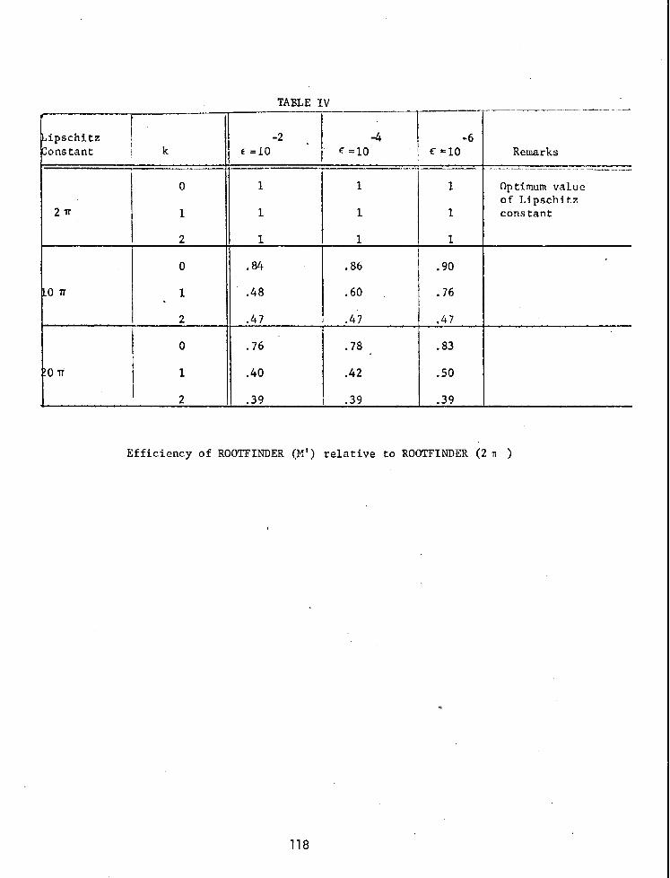
TABLE IV
pschitz ; Instant k
,+.--
0
2r 1
0
1 ,
0
1 si 1
es
-2 * E =lO
----
1
1
1
.84
.48
.47
-76
.40
.39
-4 E=lO
1
1
.86
.60
.47
.78
.42
.39
--.
-6 cc10
_.--II_ I
1
1
1
.90
.76
.47
.83
*SO
-39
__.--“___-..-.-- _- ,...,.. .-
Remarks -- , .._..." . . . . ----.., --- -., - ,-_ ,,..,, __ . . . . .._. _,
Optimum value of Lipschitz constant
Efficiency of ROOTFINDER (Ml) relative to ROOTFINDER (2 n )
118
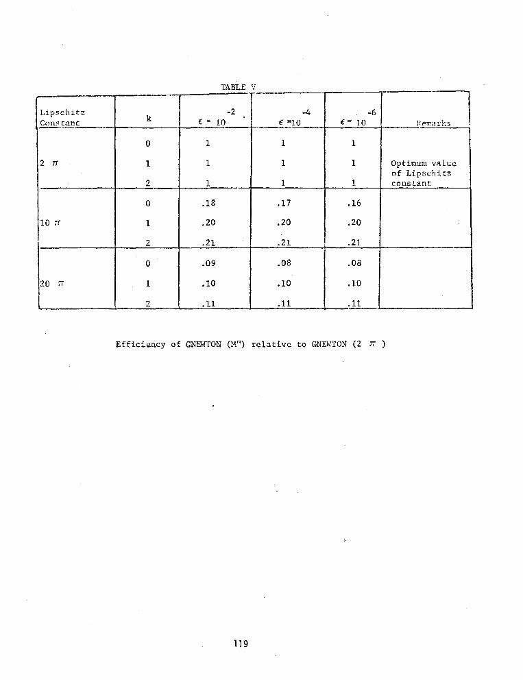
Lipschitz Constant --
TABLE V *-.--
K
0
1
_- r 1 1
1 1 Opticrum value
of 1,ipscllirz
1 1 constrnt --
.17 .16
.20 .20
.21
I
i .21 1 --
.08 -08
.lO. .lO
.ll .11
Efficiency of GNEWIION (M”) relative to GNEhTON (2 7i >
119

TABLE VI I
.-.---
:OOTFINDER :ompared to
ZSECTION
EWTON
k
0
0
1
2
E = 10 -2
~~-
1.3
co
%
.65
.13
w
-
-4 -6 c= lb 6 =lO
1.38
fx
cc
.57
.02
x
I.35
OS
SC
.41.
.004
oc)
Remarks
Optimum Lipschitz constant used.for ROOTFINQER
Bisection cannot converge
Optimum Lipschitz constant used for ROOTFINDER
Newton cannot converge
Efficiency of ROOTFINDER relative to BISECTION and NEWTON.
120

k --
0
1
2
0
1
2
E=lO -2 E -10 -4 "
.54 .56
co
t --
co
m co
.26 .27
.15 -14
m 03
c =10 -6
.69
w
03
.21
.13
cc
Optimum Lipschitz constant 1Ased for GNEWTON
BISECTION cannot converge
Optimum Lipschirz " Constant usccl for GNEWTON
NEWTON cannot converge
Efficiency of GNEW.ON relative to BISECTION and NEWTON
121

. .
TABLE VIII
.,^-. .-_ 111* , Algorithm Compared to ROOTFINDER (2 7 > k =o kc1
ROOmINDER (2 x )
ROOflINDER (XI T: )
GNEWTON (2 7.r )
GNEWTON (20 x >
BISECTION
NEWTON
-0: / .I I .41
I 1.22
.31. .49
+-----
.77 0
1.53 I
8
k=2 / Remarks
.57 I
.22 GNEWTON's perfar- mance degrades Sy a factor 1~2s than S ,
0 BISECTION cannot converge for k 1 1
0 NEWTON cannot converge for k = 2
Efficiency of varigus algorithms relative to the optimum ROOTFINDER algo- rithm for f =lO
122

r 8L 1 ,
I
“0 b
fb,) < 0
Figure 1. The bisection method works
Root,
Figure 2. The bisection method fails (there do not exist ,uO , vO e [ a,b ] such that f(uO) f(vo) < 0)
8 b
Figure 3. The bisection method fails (there is no root)
123

b
Figure 4. Newtou’s method is very. very good
‘Figure 5. Newtou’s method is horrid (because of an irlflectiori point near the root)
Figure 6. Newtons’s method is horrid (because there is uo root)
124

125

xi -+ 5 1 [
.*,,. ,z._ I., ,, ( ^,I_, ,... ^,. ,.r I
x ‘ii <-. 1
j--l ,j .,,-, +,%.” l._,l_,, ’ i ,, -.“. --~*,“,.
Y
-1

Figure 11. Example of a set SE = {(!, , rl, 1, (5, I ‘$)I
I- ‘\ I
IfI < e :. Xi -, pi
N- +* .
c \
Figure 10. Analysis of Algorithm 2
127

J
COMPUTE flx,l
Figure 14. Flow chw of Algorithm 3
128

I .
129 .

01 0 l-k-+K a+XbdY I
XK’YK l r l ‘k “I,
l l
:
x2’y2
x1 ‘Yl
0 Y SCAN MORE r INTERVALS?
k<K
syAdK A . - . I - -
F-INTERVALS CURRENTLY BEING SCANNED
lo 6
k+l-+!i 5-l REFINE f
1 l-l REPORT
RESULTS
Figure 16. Flow chart of Algorithm 4 : GNEWTON
130

Figure 17. Rootfinding using GNEWTON
73 roots
1 root
0 (b) 1
Figure 18. The function fk = k + sin 2nX on [O,i j
g :I; (c) k = 2
?31

M’large - small steps
Figure 19. Effect of M’on step size of ROOTFINDER
132 *
AN IMPROVED ITERATIVE METHOD FOR OPTIMIZING
SYMMETRIC SUCCESSIVE OVERRELAXATION
Vitalius Benokraitis Applied Mathematics and Sciences Laboratory
U.S. Army Ballistic Research Laboratories Aberdeen Proving Ground, Maryland 21005
ABSTRACT. An algorithm is proposed to determine the optimum relaxation parameter wo as well as the spectral radius of the iteration matrix S
wO corresponding to the symmetric successive overrelaxation method. The algorithm is based on the work of Evans and Forrington and Young. Computa- tional results indicate that the improved algorithm converges to the optimum parameter even when the scheme of Evans and Forrington fails.
1. INTRODUCTION. Consider the linear system
(1) - Au = b
where A is a real, symmetric, positive definite matrix of order N. The real N-vector b is given and the N-vector u is to be determined.
Systems of the form (1) arise in the finite difference solution of boundary value problems involving elliptic partial differential equations. In particular, we shall be concerned with the generalized Dirichlet problem involving the differential equation
L[u] = & (Ag) +$ (C$+ Fu = T
where* A = A(x,y) > 0, C = C(x,y) > 0, and F = F(x,y) c 0 in R u S. Here R is a bounded connected plane region and S is its bouKdary. Given a function g(x,y) continuous on S, we 'seek a function u(x,y) twice continuously differentiable in R and continuous on S such that L[u] = T in R and u = g on S.
In order to apply the method of finite differences, we superimpose over the region R a grid consisting of a network of horizontal and vertical lines spaced at intervals of h = Ax = Ay units apart. For simplicity, we assume the spacing to be uniform, although this is not a necessary requirement.
Now for some h0 and some (x0, yo) in R, we consider the set "h 0
which contains all points of the form (x + iho, y0 + jho) for integers i and j. Following Young [1974], we assum that for any point of n
h0 which
lies in R, the four adjacent points lie in R or on S. Furthermore, this property is assumed to hold for all h such that ho/h is an integer. More- over, we define Rh = "h n R and Sh = fib n S.
*The coefficient A = A(x,y) should not be confused with the matrix A of the system (1).
133

= 52 n R, the differential equation given by (2) i~"r~~a,P~d"~y(X,~~)s~~~~ric bifference equation
(3) L~[u] = + {A(X + 5, Y) [u b + h, Y) - u (x3 Y)I
- A (x - ;, y) Cu(x, Y) - u (x .. hs ~11
+ c (x5 y + +) [u b, Y + h) - u (~9 Y)]
- c(x, Y - ;)h lx, Y) - u (x, Y - h)l
+ F (x, Y) u 1x3 Y) = T (x, Y).
Thus we have transformed the continuous problem to a discrete generalized Dirichlet problem. That is, we now seek to determine a function u defined On Rh U Sh such that Lh[u] = T(x, y) On Rh and U = g On sh.
Multiplying (3) by -h* and bringing the known boundary values to the right-hand side yields a system of the form (1) where the order of the matrix A, assumed to be N, is the number of mesh points in Rh. Besides being positive definite the matrix A can be shown to have Property A. Also it can be verified that the matrix A is an L-matrix, irreducible, and weakly diagonally dominant(Young [19711).
Another property of the matrix A, which naturally (but not exclusively) points to iterative techniques as a mode of s that A is large (the order is about 103 to 10 8
lution for the system (1) is ) and sparse (i.e., the number
of nonzero elements is small compared to the total number of elements in A).
The iterative scheme on which we shall focus our attention is the symmetric successive overrelaxation (SSOR) method. In particular, we shall be interested in obtaining certain parameters of an accelerated SSOR method.
2. THE SSOR METHOD. In order to define the SSOR method it is con- venient rewrite (1) ln the form
(4) u=Bu+c
where I B=I -D-'A=L+U
(5) C = D-lb
and where D = diag (A) and L and U are strictly lower and upper triangular matrices,respectively,
134
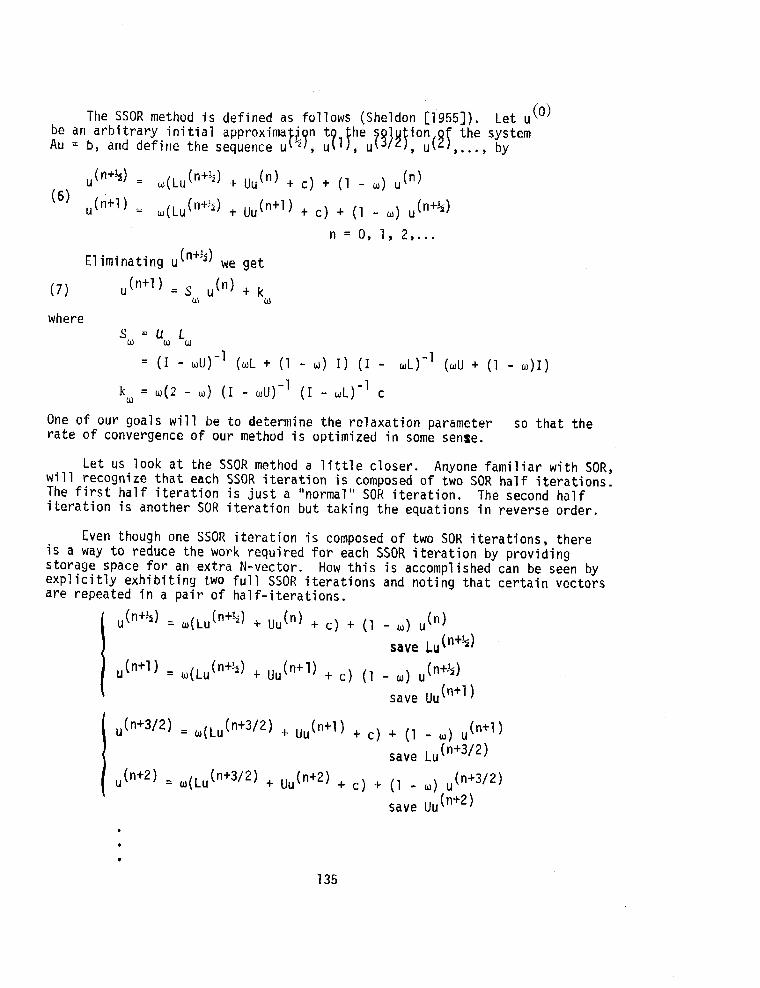
The SSOR method is defined as follows (Sheldon [1955]). Let u(O) be an arbitrary initial approxima i n t Au = b, and define the sequence u M, ,,Pl~teu~~lz~lo,(,,,the,s~~tem
,(n++) =
(6) ,(Lu(""+) t "J") t c) + (1 - w) u(n)
u(i+1) z w(Lu(n+Jd + Uu(n+l) + c) + (1 I w) ,h+Q
n = 0, 1, 2,...
Eliminating u (WI we get
(7) ,(n+l) = s ,b-d + k w w
where SW = uw L
= (I -wu")-l (WL + (1 - w) I) (I - wL)-' (WU + (1 - w)I)
ku = ~(2 - w) (I - wU)-' (I - wL)*' c
One of our goals will be to determine the relaxation parameter so that the rate of convergence of our method is optimized in some sense.
Let us look at the SSOR method a little closer. Anyone familiar with SOR, will recognize that each SSOR iteration is composed of two SOR half iterations. The first half iteration is just a "normal" SOR iteration. The second half iteration is another SOR iteration but taking the equations in reverse order.
Even though one SSOR iteration is composed of two SOR iterations, there is a way to reduce the work required for each SSOR iteration by providing storage space for an extra N-vector. How this is accomplished can be seen by explicitly exhibiting two full SSOR iterations and noting that certain vectors are repeated in a pair of half-iterations.
,h+4) = w(Lu("+J") + U"(") t c) f (1 - w) u(n)
save Lu("+~)
,(n+l) = &u("+4) + u&n+') + c) (1 - w) ,(n+&)
save Uu("+')
I ,h+W ) = w(Luh+W + uuh+l ) + c) + (1 - &) Jn+')
I
save Lu("+~'~)
Jn+2) = 4Lu(n+3/2) + uu(n+2) + c) + (1 - ti) u (n+3/2)
save UU("+~)
135

This scheme is due to Niethammer [1964]. The work required per this technique is approximately the same as with the SOR method.
iteration using
We noted that the SSOR method can be written as
u(n+l) = s ,tn) + k
with SW and kw appro;riately deyined.
Evidently, SSOR is a stationary iterative method of first degree. It is stationary because Syn$fy k are fixed from iteration to iteratio of first degree since u dgpends only on one preceding iterate u n . 2)
It is
It is well known (Young [1971]) that we must have S(S,) <lin order to guarantee convergence. Flere S(S,) denotes the spectral radius of S,. This conditions holds if 0 c w c 2 and A is positive definite. Also, if we define the error
&n) = ,(d _ u
where u is the exact solution of Au = b, appropriate norm)
we have approximately (in some
I/m I I = S@& I I An-‘) I I and
1 p 11 = CS(~Jl”l IE(“)l I
To reduce 1 IS(~) 11 to a fraction, say F, of I we must have
,h)
i-b+ E O II = IS(SJJ” < r
and we must iterate n times, where
We define R(S,) = -log S(So) as the rate of convergence of the SSOR method.
As indicated, we suspect that the rate of convergence of the SSOR method
R(S,) = -log S(S,)
depends on w. Not evident from our notation, the rate of convergence is also governed by the ordering of the equations. Given an ordering, the optimum w will be considered to be the w which minimizes S(S,) or maximizes R(S,). Assuming the "natural ordering", for a certain "good" choice of w = w , which depends on upper bounds of S(B) and S(LU), Young [1974] has shown tha the i
136

number of iterations necessar to solve the discrete generalized Dirichlet problem is proportional to h- s( . This is the same order of magnitude required by the SOR method with optimum W.
Thus, even if Niethammer's work-saving techniques are employed, there seems to be little justification to choose SSOR over SOR.
However, what is nice about the SSOR method is that the eigenvalues of the iteration matrix S, are real and nonnegative (Young,[l971]). Under these conditions, it is possible to accelerate SSOR by an order of magnitude by means of semi-iteration. (This is not possible for the SOR method, since many of the eigenvalues of its iteration matrix L, are complex for the optimal ti.)
3. SSOR SEMI-ITERATION. Semi-iteration was studied by Varga (1957) and Golub and Varga (1961). The optimum semi-iterative method based on SSOR, denoted by SSOR-SI,is defined by
Jn+l) = P,,+~ { &SW utn) + k,) + (1 - ;r) I,#, + (1 - Pn+l) u(~-')
Here
z-
Pl
P2
=&T-J = 1
= (1 - u2/2) -1
2 0 P, -1
Pn+l = (1 - y ) , n = 2, 3, ..*
where (5
Wu) = mq-
S(S,) We see that in order to apply SSOR-SI, we must estimate the parameter
along with W. Using estimates derived, again, by Young [1974], the required number of iterations is proportional to h-4, an order of magnitude better than SOR.
4. OPTIMAL PARAMETERS. The parametersw and S(S,) determined by Young are not optimal. Habetler and Wachspress (1961) determined what they pre- sumed were the optimum parameters:
w. = 2
1 + n - 2a + 46
137

‘- ‘-a
S(Suo) = Jl - 2a f 48
1+ l-a
Jl - 2a + 48
where
and where v is a vector such that S v = S(S wO
)v. However, these formulas are wO
not usable directly, since these are implicit relationships. Thus we are unable to determine w. and S(Sw ) from the formulas since the formulas imply that we
know the eigenvector v (ind therefore S(Swo) and wo).
Evans and Forrington [1963] used an iterative technique based on these formulas to determine the optimum w and corresponding S(S,). Starting with an initial guess of w, the power method on the matrix S was used to determine an approximation to the eigenvector associated wit! S(S,). Then, via c1 and 8, w and S(S ) were updated by the formulas, and the procedure was repeated until w and Sysw) settled down.
This procedure worked quite well for Laplace's equation. However, our numerical results indicate that for certain cases where S(LU) < $, the Habetler-Wachspress formulas do not hold, and in turn, the Evans-Forrington procedure fails. It was found that the optimum parameters seem to be
loo = 2
1+-
1-m s(swo) = - 1+/P--O
Incorporating these formulas into the Evans-Forrington scheme we have a new method for determining the optimum parameters w. and S(S ) for the SSOR-SI method. The algorithm follows wO
1. v # 0.
Choose convergence tolerances cl and ~~ and initial values of w and
2. Iterate with the power method to obtain S(S@) and a vector v such that
suv q S(s)
138

3. Compute
a = (VI ~DBv)/(v. Dv) 6 = (v, DLUv)/(v, Dv)
4. Compute
I
2
1+n -2cl+46 w ' al
2
1+-
ffaf48
ifa>
it l- 1 - $I - 20 -0 + 4s w lt n-2 1-U a + 46 > if a 148
5. Terminate process if
lo - w'l < E'
Is&)) - S' I < 9
and choose
w. = w'
s(s40) = 5'
Othemfse set w = W' and go to Step 2.
5. NUMERICAL EXAMPLE. Ue now apply generalized Dfrlchlet prob'lem of the form
WY) - C(X.Y) = e 1OWY)
F(x.Y) - Thy) = 0
the algorithm to a specific dfscrete (3). In particular, ltt
dnd let the region be the unit square with zero boundary values txctpt unity on side y = 0. Inltlrlly, t "good* w (Young 119741) wts chostn. Tht toltrrncts El =c2= 10-4 were specified. Rtsultr art glvtn in Tablt 1.
139

TABLE 1
h-'
OPTIMUM PARAMETERS w. AND S@o) OBTAINED BY ALGORITHM
Number of wO S(Swo) Iterations S(LU)
20 1.5866 .5866 1;
.2329 40 1.7653 .7653 .2455 80 1.8742 .8742 35 .2489
The Evans-Forrington algorithms did not converge in this case. For a more detailed discussion of this example and a number of other problems, see Benokraitis [1974].
6. ACKNOWLEDGEMENT. This is a small part of a thesis written under the direction of Professor David M. Young, whose guidance is gratefully acknowledged.
7. REFERENCES.
Benokraitis, V.J. [1974] "On the Adaptive Acceleration of Syn-unetric Successive Qverrelaxation", Doctoral Thesis, University of Texas, Austin.
Evans, D.J. and C.V.D. Forrington [1963], "An Iterative Process for Optimizing Symmetric Successive Overrlaxation", m L, 6, 271-273.
Golub, G.H. and R. S. Varga [1961], "Chebyshev Semi-Iterative Methods, Successive Overrelaxation Iterative Methods, and Second-Order Richardson Iterative Methods", Numer. Math., Parts I and II, 3, 147-168.
Habetler, G.J., and E.L. Wachspress [1961], "Symmetric Successive Overrelaxation in Solving Diffusion Difference Equations", Math. Camp. 15, 356-362.
Niethamner, W. [1964], "Relaxation bei Komplexen Matrizen", Math. Zeitsch 86, 34-40.
Sheldon, J.W. [1955], "On the Numerical Solution of Elliptic Difference Equations", Math, Tables Aids Comput. 9, 101-112. --
Varga, R.S. [1957], "A Comparison of the Successive Overrelaxation Method and Semi-Iterative Methods Using Chebyshev Polynomials", 2. Sot. Indus. u. Math. 5, 39-46.
Young, O.M. [1971], Iterative Solution of Large Linear Systems, Academic Press, New York.
Young, D.M. [1974], "On the Accelerated SSOR Method for Solving Large Linear Systems", Report CNA-92, Center for Numerical Analysis, University of Texas, Austin.
140

VP - SPLINES, AN EXTENTION OF TWICE DIFFERENTIABLE INTERPOLATION
Royce W. Soanes Jr. Watervliet Arsenal, Watervliet, New York
1. Introduction. Since the cubic spline is a special case
of the Variable Power - splines presented here, the latter may be
regarded as a generalization of the former. This generalization
does not take place in the direction of obtaining higher degrees
of differentiability, however, but rather in the more practical
direction of obtaining greater flexibility and better local be-
havior while retaining two orders of differentiability. The
cubic spline has the optimal property of being the interpolater
of smallest quadratic mean second derivative; this is a global
property, however, and as such may conflict with the curve
fitter’s desire for certain local behavior. Specifically, the
cubic spline has a tendency to misrepresent the behavior of a
function which passes from a region of low curvature through a
region of high curvature. The cubic may underestimate the high
curvature and overestimate the low, This tendency may be mani-
fested in the cubic interpolater by the presence of inflection
points where none are desired. VP - splines make it possible to
develop a more aesthetically pleasing functional curve from a
given set of data by eliminating or at least diminishing undesir-
able local behavior when it is encountered.
141

NOMENCLATURE
xl<x2<...‘XN is a sequence of nodes over an interval on which
we desire to interpolate the function y.
Ri = Xi+l-Xi = length of the ith subinterval.
yi = known function value at the ith node.
yi,yy = unknown first and second derivatives at the ith node,
yi (x) , y; (x) , yy (x) = interpolating function, derivative and
second derivative at any point in the ith subintexval.
r- 1 = (X-Xi)/ai
2. The Basic Form. Consider the following interpolatory
function defined on the ith subinterval.
m- n. (11 kiyi(X) = ai+biri+ciri’+di(l-xi) ’
The parameters mi and ni are positive real numbers and ki = mi
+ni-mini. ‘To insure a bounded second derivative, mi and ni
should both be greater than 2. The functions yi (x) and Y;(x)
can be evaluated at Xi and Xi+1 to obtain ai,bi,ci and di in
terms of Yi>Yi+lSY; and Y;+~.
C23 ai = kiyi+~i(miqi-(mi-l)yr-yl+l)
142

(3) bi = ei(-miniqi'*iY~+"iY1+11
(4) =i = Ri(niqi-yl-(ni-l)y;+l)
(5) di = Ili(-miqi+(mi-l)yl+yi,l)
The interpolater is only once differentiable at this juncture,
. SO we enforce continuity of its second derivative at the ith node
by setting yy(xi) = ~y-~(xi) and obtaining Eq. (6).
(61 [aimi-lki(l-ki-1)+~i-lniki-l(l-ki)lYf
Qi,lki-lniCni-1) (miqi-yl+l)
Once mi and ni are set for each subinterval, we may solve
the linear system represented by Eq. (6) (plus end conditions)
and obtain the nodal derivatives which insure the continuity of
the second derivative of the interpolater. Setting mi = ni*= 3
on each subinterval would give us the cubic spline formula.
3. Effect of Large m's and n's. Some insight into the
effect of increasing the m's and n's may be obtained from the
consideration of a special case. Equation (7) may be obtained
from Eq. (6) by setting mi = ni = m on each subinterval.
(7) (m-l)(Q+"i-llyi = Qi Cmqi-l-Y~-ll+Qi-l Imqi-YI+l)
143

It is apparent from Eq. (7) that the corresponding linear system
will become increasingly more diagonally dominant as m becomes
large, and in the limit as m approaches infinity, yi will be
given by Eq. (8).
At the same time, Equations (1) through (5) show that yi(x)
approaches yi*riQiqi (the linear interpolater) as m approaches
infinity. 'l'his example indicates that we should obtain a well
conditioned set of linear equations as we judiciously increase
the m's and n's to obtain the flattening effect which will pro-
duce desirable local behavior in the VP interpolater.
4. Elimination of Improper Inflection Points. When the
cubic spline is used for interpolation, the curve fitter may
be faced with the undesirable situation of having yiyi+l<O
while (qi-y~)(qi-y1,1)<0. These conditions indicate the presence
of an inflection point in the interior of the ith subinterval
when qi is between yi and yi+l. This is an aesthetically dis-
pleasing situation created by the average curvature diminishing
property of the cubic spline. The cubic is trying to deny the
existence of a point of high curvature in the function. In
order to eliminate the undesirable inflection point, of which
there can be at most one per subinterval, we must insure that II It
YiYi+lL"* This is equivalent to having CidiO. We therefore
want to enforce condition (9) in the event that qi is between
144

1 But since Cqi-Yi> (qi-Yi+l ' )<O, condition (9) can obviously be
enforced by insuring that mi and ni obey conditions (10) and
Cl13 -
(101 miZ_CYi+l-Yfll (CLi-Yfl
(111 niL(Y~+l-Yfl/ (Yf+l”qi)
Conditions (10) and (11) must naturally be enforced in an itera-
tive manner if two orders of differentiability are desired, since
mi and ni must be set before y; and ~f+~ are obtained.
5. A Local Consideration. A local VP - spline over the
restricted node set [Xi-l,Xi, Xi*l] will be found useful in the
initial setting of the m's and n's. If We Set yy(Xi*l) = 0 =
Yy-1 Cxi,13 I we obtain the following end conditions.
Equations (12) and (13) can then be used to eliminate yf+l and
rim1 from Eq. (6) to yield Eq. (14).
Equation (14) can now be solved for the ratio of ni to mi-1,
145

If we now set y; at each node according to some preferred local
formula, we may set the m's and n's according to the following
rule.
(163 miml = L and ni = LRi if Ri>l
n. 1 = L and mi-1 = L/Ri if Ri'_f
Rule (16) sets a lower bound of L on the m's and n's and assumes
that Ri is positive and finite. If Eq. (15) and Rule (16), are
used to initialize the m's and n's, Conditions (10) and (11) can
be used in conjunction with Eq. (6) to iteratively eliminate any
unwanted inflection points.
A simple local formula which has been found effective in practice
for initial setting of the nodal derivatives is given by Eq. (17).
Cl71 Yi = Clmwi) (Ii-1 + ‘i9i
where wi = l/f1 + J[(l + q,?)/(l + q;_l)J}
This derivative is obtained from the slope of the line through
cx. 1 , yi) which makes equal angles with the left and right chords.
When this formula is used, it is usually unnecessary to increase the
m's and n's gradually in order to enforce conditions (10) and (11).
146

6. A Simple Computational Procedure. An abbreviated procedure
which can be followed in most cases is:
I. Set L equal to a value between 2 and 3. Values
greater than 3 may flatten the curve too much
between the nodes. Values closer to 2 will produce
more roundedness in the interpolater.
XI. Compute the initial nodal derivatives according to
Eq. (17) for 2 2 i 2 N - 1.
III. Set nl = L = mNl and calculate R i
for 2 < i < N - 1 - -
using Eq. (15).
IV. Compute the rest of the m’s and n’s using Rule (16).
V. Solve the tridiagonal set of equations represented
by Equations (6), (12) and (13) for the final nodal
derivatives.
7. Examples. The following drawings, which were produced on
a graphic display CRT, illustrate the more stable behavior of the
VP-spline as compared with the oscillatory behavior of the cubic
spline. Each of the VP-spline curves was computed using the
abbreviated procedure previously outlined [not making use of
conditions (10) and (1131.
147

x
148

149

.
,
150
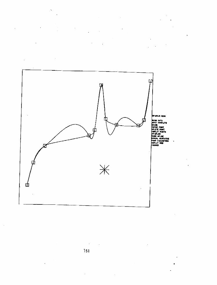
151

REFERENCES
1. Ahlberg, J. H., Nilson, E. N., and Walsh, J. L., 1967, The Theory
of Splines and Their Applications, Academic Press, New York.
2. Barnhill, R. E., and Riesenfeld, R. F., 1974, Computer -Aided
Geometric Design, Academic Press, New York.
3. Cline, A. K., April 1974, "Scalar- and Planar-Valued Curve Fitting
Using Splines Under Tension," Comm. ACM, Vol. 17, No. 4, pp* 218-
z'20.
4. Prenter, P. M., 1975, Splines and Variational Methods, John Wiley
4 Sons, New York.
5. Schweikert, D. G., 1966, "An Interpolation Curve Using a Spline
in Tension," J. Math. and Physics, Vol. 45, pp. 312-317.
152

ITERATIVE SOLUTION OF THE TRANSONIC POTENTIAL EQUATION
D. I:. Adams and Gary Vander Roest U.S. Army Air Mobility R&D Laboratory
Ames Directorate Moffett Field, California 94035
ABSTPACT. The unsteady, transonic small-disturbance equation is a suit- able model for the flow on advancing rotor tips. This paper discusses the rela- tive efficiency of two implicit iterative techniques used in the solution of this nonlinear equation; namely, the point SOR technique and the Douglas-Gunn A31I technique. While the two-dimensional calculations of both methods demon- strate the effect of varying lift and incident Mach number on a high-speed heli- copter rotor, the ADZ technique proved to be the more efficient method.
1. INTRODUCTION. The advancing blade of a helicopter in high-speed for- ward flight often enters the transonic flow regime. This type of flow is marked by the presence of local pockets of supersonic flow which are usually terminated by a shock. A feature of transonic flow which is beginning to be considered is that these flows are intrinsically unsteady. This is especially important for the helicopter in forward flight, since the rotor sees a con- stantly varying incident Mach number and angle of attack.
The first treatment of this problem was the paper of Caradonna and Isom (ref. 1) where nonlifting three-dimensional flows were considered. It was shown that the Mach number variation alone is a considerable source of unsteadi- ness. "his treatment used a point SOR scheme to solve the set of nonlinear difference equations derived from a mixed differencing of the small-disturbance potential equation. However, SOR is often not the fastest technique at our disposal. In this paper, an iterative AD1 scheme to solve the nonlinear system of difference equations is devised and then compared with the SOR method.
2. STATEMENT OF PROBLEM. The second-order nonlinear partial differential equation to be solved is
A%t + Wxt = Wxx + 9 YY
(1)
where
A = Mf+Q2S2/~ )
B = [2Mp!F&3)1 (1 + p sin $J)
C 1 - Mi(l + p sin 11)~
z
[ ,r2/3
- (1 -I- ~)%(l + 1~ sin *)$x
a
$ = disturbance potential
t = time
2 = chordwise coordinate
153

7 = normal coordinate
x = Ix/c
y = (y/c)d3
and where
AR= aspect ratio = r/c
c = blade chord
MR = blade tncident Mach number due to rotation
r = blade radius
:,y z!F physical coordinates
y = specific heat ratio
6 = thickness ratio
u = ratio of forward flight speed to rotational speed, Vw/mr
$ = blade azimuth angle (measured from the downwind direction)
The linearized body boundary conditions are given by
~y(x’o”) = -& [f,,+LY)l (2)
where f, R given by '
(x,y), the equation for the upper and lower airfoil surface, is
(3)
where T, a. is the thickness distribution and ~1 is the blade angle of attack. '
The far-field boundary conditions are gjven by
G(X,Y) = - 4n::,3 tan-l(:y $ , X2 4 y2.+m (4)
where
C L
= lift per unit length [ (1/2)P~JJC
and where
v = total velocity of the rotor
p = air density
154

The right-hand side of cq. (1) is of mixed type, being elliptic when flow is subsonic (ML c 1) and hyperbolic when flow is supersonic (ML > 1).
Equation (1) is differenced as follows:
N+l N+l N-t-1 Nfl N+l N+l N-t-1
= &.C M 6xx$M+l li f (1 - YY
$M+1 (5)
where
N = time level
M = iteration level
WI" 1 M+l
6YY4
M-t1 =L$
[
( Ay2 j+l )
N+1
- 2+j + 4. M-t1
J-1 i N+l
cy = l- % 2Cl + p sin $J)~
&2/X - (1 + y)$(l + u sin $)
E. = 1, E 1 1 i-1 = for ML < 1
E z!!E i 0, Ei. 1 = 0 for ML > 1
E = i 0, LBl=l for ML = 1
E = i 1, EiBl = 0 for shock point
The epsilon notation denotes that backward and central differences in the x-direction are used in supersonic and subsonic regions, respectively. The use of mixed differences is required for stability. Also, this notation indicates that the sum of the central and backward operators are used at a shock point. This is necessary in order to satisfy the equations in the global sense and insure proper shock jump conditions.
155

The differencing of 4 YY
is modified on the body as follows:
+ YY
= -?-- (LQ 2 - @i,l - AY+~) Ay?. I
For the lifting problem, the potential must be discontinuous in the wake of the rotor. The difference in potential at this discontinuity is equal to the circulation, r. In order to difference across this discontinuity, 9 dif- ferencing is modified as follows: YY
where
cL r =I--- +I3 s
+ 2 +
= i,2 - 2$ 1 + (9.
1 -1 r4 r>
, YY Ay2
Differencing, as above, yields a set of nonlinear algebraic equations which must be solved by iteration. In the course of iteration, one can specify either CL and iterate to find the angle of attack (u), or specify u and iterate to find C . In the former case, ~1 at the &railing edge equals r.
must be updated until the jump in potential This is done using
.N+ 1 =c1 N - X[$T(X*e,o) - P(x,,,O) - r] (7)
where A is a relaxation factor (usually equal to one).
3. SOR METHOD OF SOLUTION. For the SOR scheme, the potential of each iteration is updated using
N
N
N N M-i-1 RM
$. l,j = 4fj - w +
Lj (9)
where i,* KM i
is the residual that is defined by eq. (5), with all terms grouped on the rig t-hand side. Dij is the sum of the diagonal elements of the residual:
2EiCi (1 - EJ
'i 2 A B
D. l,j =-+ Ax2 ---i-z- Ay2 AxAt (i0)
The relaxation factor w is less than 1 in supersonic regions and between 1 and 2 for subsonic regions.
In order to start the problem, the first two time steps are assumed to be quasi.-steady (A and B are set equal to zero). This procedure causes no problems as long as the starting Mach number is subcritical.

4. DOUGLAS-GUNN ADI METHOD OF SOLUTION. With this method, it has been found necessary to include an artificial $--like term in eq. (5) for stability purposes. We now have the modified differehce equation
N+1 N+l N-i-1 N-l-1 N+l
'xx+ M-!-l +(1-E: (11)
We have not determined the optimal value of F. However, F = 4OB seems to work well for most uses. For convenience, eq. (11) is rewritten in an operator nota- tion as N-l-l
(KI + n&x + Sl+S,>$"+" + $" T#N-a = gN+-' (12)
where N+l N-l-1 F M
g =- /It 9
I = identify operator
F A K = nt: + at2
M = iteration index
N = time index
Sl = spatial operator in the x-direction =
N-+1 N+l N+l N-l-1 M+l
- cybl (1 - E N+l
S2 = spatial operator in the y-direction = -Avv$ M+l
BN+l ,I
T - 211 o--s- -6 axnt x
A Tl = - At2
6 X
= $ .- $Jivl
BN+l
' = AxAt
The Douglas-Gunn scheme (ref. 2) is employed to generate the ADI routine because it is generalizable to any number of dimensions. Note that the term (KI + nu + S1 + S2) contains all the unknowns. does notXinclude the 6,
The original Douglas-Gunn scheme operator because they did not consider equations that
157

had mixed spatial-time derivatives. The general Douglas-Gunn recursion rel;l- tion for generating AD1 schemes for any number of dimensions is
N41 I, (KI + n6x + (13)
wlacrt! f4 i:; the ni.lmhcr 01 dimensions, which is 2 for our case, and Cp* is some extrapolation from previous time steps. Generally, we have let $* equal the previous iterant. The first step of the two-dimensional case is as follows:
1 (KX + n&x + S,)i f SF+* + c T,$N-" = gNfl
R=O 04)
The coefficient of i, having both central and backward differences, gives rise to either a central or lower tridiagonal matrix. This matrix is solved by a combination of the Thomas algorithm and direct elimination. Substituting in eq, (13) for the second step (q = 2), we get
(15)
Subtracting eq. (14) from eq. (15), yields a simplified step 2, which is as follows:
N+l
(16)
KI and S2 generate a tridiagonal matrix. However, n6 adds a term which is on a previous column. This column must be solved beforeXwe can move to the next column. This imposes a necessary order on the process and the tridiagonal inversions march across the grid from left to right. To get started, we let the first two time steps be quasi-steady by setting the time index (n) equal to the iteration index (m).
5. RESULTS. Numerous cases were run by both the SOR and AD1 methods, using various Mach number and lift variations. The greatest difference between these calculations and the results of ref. 1 is the inclusion of lift. It was noted in ref. 1 that upstream wave propagation necessitated placing the upstream boundary at least 10 chords upstream. With lift, however, this situ- ation becomes much more acute, and it was necessary to place the boundaries 20 chords away (upstream and downstream) in order to obtain stable solutions. The ADI method was generally more reliable, as the SOR method often failed to converge at higher values of lift and Mach number. However, when the SOR method did converge, it agreed almost exactly with the AD1 method. In these situations, however, the AD1 method appeared to be about twice as fast as the SOR.
A case, from which identical results were obtained from both methods, is shown in fig. 1. In this case, we specify a si.nusoidal CL and find the angle of attack. The rotor in the center of fig. 1 indicates the various azimuth angles for the CR plots.
158

Unsteadiness is indicated by the effect of flow history on th.' f'low. For example, at 111~ rotor posi t inns A and I, the Mirc11 number, ;~ngl.c oI ;Itt;lclc and lift <are the same. Also, the solutions obtained are so identical that they are plotted on top of each other. Clearly, the flow history plays no role at these points and the flows are essentially steady. At blade position D, the lift is specified to be zero, and the solution obtained has identical flows on the top and bottom surfaces. This is what one expects from steady flows. How- ever, one would also expect a zero angle of attack from a steady solution instead of the slightly negative angle that was actually obtained. The nega- tive angle implies that the flow, up to this point, is unsteady but only slightly so.
In the subsequent blade locations, the flow is decelerating and the lift is again increasing. The shock is seen to move forward but does not'diminish much in strength. In fact, on the bottom surface, the shock does not go to zero strength at all. Instead, it appears at position G to be on the verge of popping off the leading edge and proceeding out into space. This effect was First noted in ref. 1 for nonlifting cases and is seen with great clarity in ref. 3, which uses an AD1 technique very similar to this one. On the top surface, the increasing lift allows for the sustenance of the supersonic region, and there is no shock popping. However, the shocks are substantially stronger than at their corresponding azimuths in the accelerating flow region. For example, position H is the mirror image of position B, but the CP dis- tributions for the upper surface are quite different.
Clearly, the effect of unsteadiness is large in a decelerating transonic flow. In addition, where there is lift, the difference in unsteadiness can be quite different on the top and bottom surfaces.
6. CONCLUDING REMARKS. The modified Douglas-Gunn ADI is &bout twice as fast as SOR and generally more reliable. Present computing times are about 20 minutes on a CDC 7600 for a two-dimensional lifting problem. This can be greatly improved with more efficient programming, a less rigid convergence cri- terion, and the use of a variable time step. An interesting approach is taken in ref. 3, where the nonlifting two-dimensional problem is treated, using a Douglas-Gunn scheme. In this approach, the difference equation is linearized in time, thus eliminating the iterations, but requiring a smaller time step. It appears that with a combination of the above approaches, unsteady three- dimensional calculations would be a practical proposition. We are now working toward this end.
It appears that the inclusion of unsteadiness in transonic flow predic- tion is at least as important (and likely more important) than the effect of three dimensionality. Decelerating flows are altogether different from their quasi-steady counterparts. Also, lift raises the possibility of very unusual loads in the second rotor quadrant.
AcknowLedgnent
The authors gratefully acknowledge the valuable contributions of Francis X. Caradonna to this work.
159

REFERENCES
1. Caradonna, F. X., and Tsom, M. P,: Numerical Calculations of Unsteady Transonic Potential Flow Over Helicopter Rotor Blades, AIAA Paper 75-168, presented at AMA 13th Aerospace Sciences Meeting, Pasadena, Calif., .Jan. 20-22, 1975.
2. Douglas, J., and Gunn, J. E.: A General Formulation of Alternating Direc- tion Methods, Numer. Math., Vol. 6, 1964, pp. 428-453.
3. Gallhaus, W, F., and Stager, J. L.: NASA TM X-73,082, Nov. 1975.
160

CALCULATED TWO-DIMENSIONAL PRESSURE DISTRIBUTIONS ON A ROTOR
B
X/C NACA 0012
C -1.0 ,
I $ =49.5”
-. 5 CP -
a
-1 .o
-. 6 CP -
f
MAXIMUM TIP MACH NO. = 0.906 A3 = 13.7
$ = 116.5”
D $I =SO” tvl = 0.84 c,= 0.0 a =-0.008”
X/C
ADVANCE RATIO = 0.25 CL = 0.4 (l-sin $4 Fig. 1
161


UTILIZING REAL-TIME TEST DATA ANALYSIS IN SYSTEM MONITORING AND CHECKOUT
E. H. Gamble U. S. Army Test and Evaluation Command
Deputy to the CG for Analysis Aberdeen Proving Ground, Maryland 2 1005
ABSTRACT. For the proper utilization of equipment needed for test data on-line acquisition, display, and comparative analysis, some novel data management techniques are in the process of development.
For on-line analysis of test display data, the recognition of changing values in the inherent uncontrolled design parameters and system output variables must be basic. Also, the display technique must accommodate a reasonable number of sets of operating and envi- ronmental conditions.
We must be able to identify shifts in the values of the parameters and variables as well as shifts in the weighted contributions of each parameter to the output system variable value. Each contribution is the product of the quantified parameter value under a given condition set and the corresponding influence coefficient. This coefficient reflects the sensitivity of the output variable to a nominal change in the pa- rameter when measured at the given condition set. In addition, we must identify any changes in the gains of the functional equipment components and variations in the transmission characteristics of the test data trans- port and management system. An observation matrix of the coefficients, parameter values, or contributions provides the display vehicle.
The study adopts a model consisting of seven parameters and five sets of conditions. Variations of all quantities are demonstrated and companion computations made to show the significance of the variations and their identification.
163

I. INTRODUCTION.
One of the significant developments in process to be applied to the test analysis and evaluation of Army materiel systems is the real time use of the computer for the:
1. On-line acquisition and analysis of data.
2. Display of the test data while the system is under test.
3. Making comparisons of this test data with stored data from a developed reservoir of historical data about similar and current systems. Knowledge of the testing subsystem equipment should be available for ready reference (see Figure 1).
One such testing system is in the design and planning stage and called project ADAPT (Automatic Data Acquisition and Processing Technology). This program is under the direction of the Materiel Testing Directorate of the Aberdeen Proving Ground.
A practical technique for on-the-spot analysis of test display data is needed. For such on-line analysis, not only central or “expected” values for the parameters must be displayed at the centralized control and display area. We must identify shifts in the values of the uncon- trolled parameters of the system under test and the testing and instru- mentation system. In addition, we must identify any changes in the gains of the functional components of equipment and the variations in the trans- mission characteristics of the data transport and management system.
To assist in the understanding of utility and potential application for such a system, a study is described where the data display is eval- uated as a means for both real time system monitoring and confidence status or checkout. A display model for the test item and the testing equipment will be applied to a planned group of activities. These activities are defined as the set of subtests planned and executed as a part of the Test Plan and defined by a Test Directive. One approach to this model is the adoption of a Data Observation Matrix as the display vehicle. This model has found use wherever one applied techniques such as systems modeling by functions (see Reference 1) on parameter-sensitivity coefficients (see Reference 2). Figure 2 describes a general form for such an observation matrix.
164
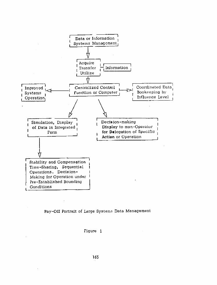
71 , Improved I Centralized Control 1-i Coordinated Data: ,4 , Systems , Function or Compuy , Bookeeping by , 1 Operation Influence Level
/ \
1 1 , Simulation, Display ,
1 of Data in Integrated ,
Form I I
I-- , Decision-making
1
Display to man-Operator I ,
, for Delegation of Specific , , Action or Operation I
’ Stability and Compensation ; Time-Sharing, Sequential I Operations. Decision- Making for Operation under I Pre-Established Bounding Conditions
Pay-Off Portrait of Large Systems Data Management
Figure 1
165
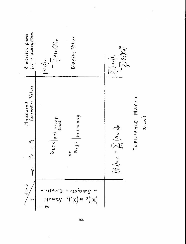
166

It will be our purpose to illustrate the application of analysis techniques for a matrix model of seven parameters and five condition sets of grouped activities. The complete study of this model involves the display for the time variations in the participating parameters and their dimensionalized contributions and changes in the parametric sensitivities.
II. DISCUSSION.
A. Mathematical Background.
Utility of Observation Matrix for Data Display:
One evaluation criterion for usefulness for any method of information identification and cataloging is that the variationals of all system parameters be recognizable, definable, and predictable. We have suggested that the mathematical and informational system model for a given influence level be described by the coefficients array for the ap- plicable engineering equipment and physical. constraints.
The influence level is defined by the operating subsystem or data system gross functions, g or mission phase, the data functional model subfunction or component, activity and agency, etc. The (pi) are the measured values for the XJ parameters or the set of values found as the set to maximize or minimize the criterion - our measure of adequacy/excellence.
Two cases are of immediate interest. For a change in system time of magnitude (At) :
(1) A shift occurs in the system parameter measurable values (polarity included).
(2) The shift occurs in the influence coefficients, which represent either the compatibility potentials or sensitivity potentials of the equipment. Transfer or data transmittal characteristics are the inter- dependency factors for the variables and the system conditions.
In both cases, the display integrated parameters and contributions to the system objective functions are changed in magnitude. A dependable tech- nique must be established for determining whether the shift is made up
167

of type (11, (2), or some combination of these. Variation with system condition/configuration (J) should be identifiable.
A numerical example with seven parameters and five conditions or configurations which define the Interdependence relationships will be used to Illustrate both cases (1) and (2). The example will also show a variation with (J) for one of the seven parameters. We will study these for a system time, t = tl , and a time change A tl I a second time t2 and time change A t2. The data are available for a consideration of the variations consistent with the time interval (t2 - tl), as well as those mentioned.
For Case (1) , where the shift occurs in the parameter values, the supporting analysis follows:
The change in objective criterion equals --
C” - c =B1 (XT- Xl) + m a a + Bn (Xn* - Xn) (. 01)
The corresponding change in subsystem capacity potential or integrated parameter is
wilt - WKi = alfli (Xl* - Xl) + . . . a,Ki (lx: - x,)
C” .“c= c
i t Wl;i - WKi
)
m n T=c c 1 aiKJ (Xy - XJ) =
i J c “J (x; - XJ) J
m n E c c
i=l Jz1 (aiKJ) (6PJ) =
(. 02)
( l 03)
t.041
t.051
168

(Note: The starred quantities (previous page) are values for variables at (t1 f A t) and unstarred those at tl .J
A check test is performed in which all the stimuli parameters XJ are set at a fixed constant value (normalized,this is equivalent to unity, 11. If this will give a zero change in the objective function c = cs I the valid conclusion is that there have been no changes in the
influence coefficients ( k %KJ * Superscript (1) identifies check values.
If both ( c * - c ) and c (B:K - BJK) have a value which is
J J J non-zero for the test of fixed constant values for the parameters, then the variations are in the (?iiKJ) . Mathematically, for the change in the
coefficients, we state tha
2*-f $2
J J
t: “~JK - “iJK (.OS:l
= ‘; - ‘<J ‘0 < ; XJ = p; = p J
= 1 C.07)
J
For a shift in the parameter values, we 9ta)te that:
At
for X; # X3’ = PJ = 1
The time sensitivity potential for the parameter XJ is found by dividing the expression and value for A XJ for the time shift At
169

by the time interval A t. This sensitivity is identical to the time rate of change of the variable XI.
axJ = I 3-c t,K
change
" (Ad
(q X,=J, t K
(. 09)
I.111
When the change is in the influence coefficients and not in the XT parameters, we must answer the selection question regarding equipment deterioration. “Do we need to determine the individual change A(aiTK) or the resultant effect?” Let us consider the mathe- matical forms needed to answer this question.
*(; "iJ2J jK,F *( pJxJ ), =
A c a.
Aw = I.J~J Ki J
* c, -(c”-qK For the particular case where XJ = 1,
for AaiJK = 0
C.12)
i’ 22 c I A qpD$ i. 13) J
for AX,= 0
(.14)
(. 15)
(. 16) if AaiSK # 0
170

The individual ( AaiJ~j are needed in order to determine or verify the change in the subsystem output variable to be derivable from the summed weighted influence of the parameters (see Equation 13). Fortunately, our matrix technique displays all these quantities and they are recognizable.
For our Case (2), where the shift is in the coefficients and not the parameters, we know these facts:
I*- 1 = C ( 'ii - WKi ) (. 17) i i
"CJK - ai,rK (. 18)
( h aiJKK)
= c ( xJ 6; - eJ d ) K
(. 19)
= c XJ (A& . J
Since our variations with A t are in aiJK, we set XJ equal to plus one, then we find:
= 2 z(a?JK-aiJK )K ,J i
= 2 7 (Aai,JK) . J i
(. 21)
171
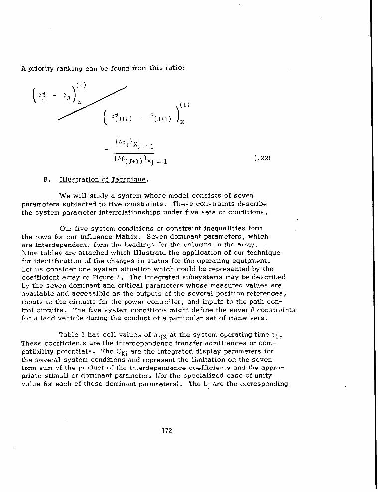
A priority ranking can be found from this ratio:
(A%-)xJ = , xz
(Afq,+,) )XJ = 1 (. 22)
B. Illustration of Technique.
We will study a system whose model consists of seven parameters subjected to five constraints. These constraints describe the system parameter interrelationships under five sets of conditions.
Our five system conditions or constraint inequalities form the rows for our Influence Matrix. Seven dominant parameters, which are interdependent, form the headings for the columns in the array. Nine tables are attached which illustrate the application of our technique for identification of the changes in status for the operating equipment. Let us consider one system situation which could be represented by the coefficient array of Figure 2. The integrated subsystems may be described by the seven dominant and critical parameters whose measured values are available and accessible as the outputs of the several position references, inputs to the circuits for the power controller, and inputs to the path con- trol circuits. The five system conditions might define the several constraints for a land vehicle during the conduct of a particular set of maneuvers.
Table 1 has cell values of aiJK at the system operating time tl. These coefficients are the interdependence transfer admittances or com- patibility potentials. The CKi are the integrated display parameters for the several system conditions and represent the limitation on the seven term sum of the product of the interdependence coefficients and the appro- priate stimuli or dominant parameters (for the specialized case of unity value for each of these dominant parameters). The bJ are the corresponding
172

SENSITIVITY - fNFLUENCE TABLE FUR SHIFT IN PARAMETERVALUES WITH (At)
J-r
'4 Xl X2
Al 853 450
A2 804 450
A3 960 675
A4 450 450
A5 720 450
bJ tl at 3797 2475 - ;=: PJ It21 1.903 0.641
PJ (tz +dtz) 2.135 0.898
APJ (Atz) 0.230 0.257 Aq [. t2 + ttz - tlq
0.128 0.311
‘J tq> 2.007 0.587
bJ P, at tl 7592 1452
x4
130 445
130 445
155 525
104 195
86 455
605 2075
1 I 000 0.738
0.593 0.896
0.407 0.158
0.385 0.014
0.208 0,882
126 7829
X5 x6 x7 CKi(PJ’r>
180
180
180
72
151
771
0.406
0.056
0.350
550 190 2808
95 190 2124
120 200 2623
50 100 1385
100
915
180 1925
940 c, bj j(PJ = I) 1(= It574 =zCKi
0.166 0.095
-0.695 - 0.420
-0.365
0.421
322
- 0.682 + 0.428
0.848 0,523 , _
776 491 = 12588 Kat tl
TABLE 1

capacity potentials for the unity measured parameter values. This table gives the parameter values for three system times-- (tl), (t2), and (t2 + At2).
Table 2 gives the array of cell values at system time (t2) and each is the contribution at the corresponding I_ system condition to the display parameter. In addition, an optimization study was performed for the given array to find the set of weighting coefficients or optimal set (pJ*) for amaximization-minimization of the criterion. This set has significance for an overall performance evaluation of the operating subsystem rather than a status or diagnosis study.
Table 3 provides the array of display contributions at time tl . These values present rather obvious changes in cell values from those shown in Table 2.
Table 4 portrays the contributions at system time (t2 + A t2) in contrast with those identified asa part of Table 2 at (t2).
An optimization study was also performed at this system time to find the set (p J) * .
Table 5 gives the variations in the display contributions for the time change of ( A tl) . This array is used to illustrate our Case (1) where the shift occurs in the parameter measured values with no changes in bi JK) - The change in the integrated display parameter wKi is given for each i system condition. The percentage change in the parameter value measured at tl is also determined. This set of values shows the sig- nificant dominance of XJ for J = 1, 2, and 4.
Table 6 gives the variations in the display contributions for the time change of ( A t2). fixed. The change in
The pJ corresponding to the XJ are considered CiA wIci is a positive quantity 282. H-owever,
the summation 1 (AB,) is the negative quantity (-561). J
Table 7 is a companion array to Table 6, but givinq the changes in aiv rather than 6 [aiK(pJ)l,the variation,or (pJ) 6 [aiK ] . The sum- mation of the variations in aiJK first with respect to i, and then J is a negative quantity (-540). This array is numerically identical with the test
174

TABLE OF CONTRIBUTIONS Ia iK PJ) AT t = t2
i J -, 5
Xl x2 x3
Al 1644 289 130
A2 1531 289 130
A3 1826 433 155
4 857 287 104
A5 1371 289 86
$J 7231 1589 405
I, 346 0.650 1.312 - bJ1*
’ (6~ pi)* 9732 1032 794
x4 x5 X6
328 73 473
336 73 82
387 77 103
144 31 43
336 61 86
1531 316 787
0.738 0.612 0.880
1129 193 692
Individual contribution to w
*
x7
98
98
103
52
93
444
0.490
WKi fKi 3035 3322
2539 2832
3084 3418
1618 1666
232 2 2553
‘J = 12’ 03 J 125 OO= c WKi
218 f Ki
i
( PJ) are optimum values of parameters for the matrix array having individudl cell
designations “iK ‘J tt2) - The result from an interative , convergent
process maximizing-minimizing the criterion xi fKi =s[ ST PJ )*
TABLE 2

T-+ Xl x2
‘t Al 1724 264
A2 lb06 264
A3 1920 396
4 900 264
A5 1440 264
K III 7592 1452
5 2 (agK PJ>** at t = tl = K III i=l
VALUES OF ( aiw pJ)** AT (t = tl)
x3 x4
27 392
27 401
32 463
22 172
18 401
124 1829
x5 X6 x7 IWKiJk
76 466 99 3050
76 81 99 2554
76 102 105 3094
30 42 94 1524
64 85 94 2366
322 776 491 c IWKi)k = 12588
TABLE 3

J-, ‘+ Al
A2 A3
Aq
A5
bJ*
=: BJ*pJ*** PJ
***
1 2
1042 405
1716 405
2048 607
960 405
1546 405
8102 2227
9641 2062 217 903 4 93 121
I. 1899
TABLE OF CONTRlBUTJONS AT + m t2 + At2
Values at t n t2 + At2
3 4 5 6 7 wlti
77 398 10 91 17 2840
77 408 10 16 17 2649
92 470 10 20 18 3265
62 175 4 8 9 1620
51 408 8 17 16 2441
359 1859 42 152 84 c
J ( B*J& = 12815 =xi WK~
0.926 0.605 0.486 0.0846 0.613 I.437
Individual contribution to WKi is I 1 "iE k PJ ***(t2+At2 1
$?i
2911
2720
3349
1672
2481
c *** i F~jz 13027, Bi q
to F& is ( "iJK PJ & \ + AQ)} q***
*** I pJ I = the parameter value set resulting from optimizing 1 FKi = g; q*‘), i
TABLE 4

VARIATION IN DISPLAY PARAMETERS
c i AI A2
A3
A4
A5
Element is +m Pr) Q aiJK APJ t 1
for &I
J4 *I *2 *3 x4 *5 *6 *7 (&ki )
116 141 50 6 -66 -375 -82 -210
110 141 50 7 -66 -65 -82 + 95
128 211 60 7 -66 -82 -87 +I71
60 141 40 3 -26 -34 -78 +106
96 141 33 7 -56 -68 -78 -75 * \?
(AK)- (KJ-KJ) 510 775 233 30 -280 -624 -407 z P 237
bJ 3797 2475 605 2075 767 915 940
iii (&P, ) =(P; - P,) 0.128 0.311 0.385 0.014 -0.682 0.428 -.033
cc * WKi i J
No change assumed in aiK from tr to kl +&I)
Data obtained as differences in Tables 3 and 4
0.53 1.85 0.016 -0.87 -0.804 +O. 82
53% 185% 1.6% -87% -80.4% +82%
TA3LE 5

VARIATIONS IN EQUIPMENT INFLUENCE COEFFICIENTS. Element is
Change for (&2) from Tables 2 and 4 .
= (‘2 + A t2) - t2
J-F
i4 Al
Xl x2 x3 x4 x5 % x7
198 116 -53 70 -63 -382 -81
A2 185 116 -53 72 -63 -66 -81
A3 220 174 -63 83 -67 -83 -85
A4 103 116 -42 31 -27 -35 -77
2 A5 165 116 -35 72 -53 -69 -77
K; -“J =&K (&) 871 638 -246 328 -273 -635 -401
pJ (tz to t,+&) I.905 0.641 I.000 0.738 0.406 0.861 0.515
Assume that total shift during (At21 is due to changes in a_ip
(AK), 457 995 -246 430 -672
PJ
-737 -778
nwi llWKi
PJ It2 )
-195 -428
+110 - 66
+179 -61
+ 69 +47
+119 - 31
c JAM =281.= c( nwKi ] i
1 A WKi = - 555
‘J lt2 1
c A “J = -5621 1 PJ J
TABLE 6

i J+ Xl t 4 104
*2 97
A3 115
Aq 54
A5 86
K; - KJ 1 = ( & JJ 871
(piJK) = *aKJ 456
s i
PJ lt2 I 1.905
TABLE OF EQUIPMENT VARIATIONS
pJ fixedj changes in zaF Period = at2)
x2 x3 x4 X5 X6- x7
181 -53 95 -155 -44,3 -157
181 -53 98 -155 -77 -157
271 -63 42 -164 - 97 -165
181 -42 111 - 66 - 41 -150
181 -35 98 -131 -80 -150
638 -246 328 -273 -635 -401
995 -246 444 -672 -738 -779
0.641 1.000 0.738 0.406 0.861 0.515
Values of Table 6 contributions changes divided by pJ to form ( 6aiJK )
Priority 5 1 7 6 4 3 2 Ranking of Deterioration
c 6 aiJK A WKi J -428 -195 -66 +l 10
- 61 +1t9
147 +(59
- 31 +119
UE 6 aiJK J i
1-540
Equals (By - B$ /
($+I - B,J++I)
nWKi
El 1 6 aijX 0.45
-1.66
-2.93
+1.47
-3.84
TABLE 7

condition of setting all of the parameter measured values to the zame constant -- unity. The criterion value (-540) is then the zs(BJ - BJ). A priority rankin% can be found from the ratio of each (B; - BJ) to the next parameter BJ + 1 - BJ + 1.
Table 8 gives the data of Table 7 now with the cell value as the percentage change which has occurred in { aiJK ) for the time change
nt2. These are the shifts or deterioration in the operating characteristics of the equipment defined for their influence corresponding to XJ.
Table 9 records the array of aiK i b coefficients for their values after the A t2 shift has occurred. .These are the total deteriorated values for each interdependence cell. Of some significance are the % change in the display parameters (for PJ = 1). These cover a percentage change from -18% to + 3.3%. The corresponding changes in the true display parameters with PJ(t$ actual values show a range of -6 e 8% to +5.5%. The change in criterion value z J bJ for PJ = 1, t = t2 is from 11,574 to 10,326. The data indicates a consrant percentage change in equipment transfer characteristics with varying system conditions, except for the one case of (J = 4). This latter variation would provide a basis for forecasting a nonlinear type of deterioration with system operating conditions. Such a variation does not lend itself easily to malfunction isolation, identification, and corrective action.
111. CONCLUSIONS.
The study is a first cut at enlarging our knowledge concerning the applicability and limitations of the Observation Matrix Technique for Data System Cataloging. What we have learned from this study:
1. The matrix technique will permit the identification of variations in display integrated parameters (system quantities WKi) and the individual contributions due to each selected dominant equipment or software parameter. These parameters may be functional in origin -- hence an activity or action.
2. It will permit the separation of the variations into changes in values of the influence or interdependence (interface) coefficients or po- tentials or changes in the measured values of the parameters. The parameters can also be equipment signals inputs or stimuli.
181

‘Xp!~Dulay~Dw ‘=I fde
L ‘9 ‘s ‘I ‘z “I: =I103 0 = IT- ‘(p = r) ~oj qdwxa ‘suo!~!puo~
cu uo!~~rn6!juo~/!lnur!+s +uaurd!nba u! y!ys ay I#!M s3~~sya+3~.my:, ~ajsu~q Juaurd!nba u! a8utay3 ~uo4suo3 D s! aJay1 2
! L)I!M a6my~ ti?‘i? ay$ U! UO!+D!JDA fMylDlU D SMOqS ‘p n j- +t()
X=Y
I JO P=G3 I
I 1 >rlfFQ
*ti8- %i8- %88- %8*91+ %uv- %!# %z1 ati3aAV
%28- %08- W8- %9’lZ %,a’op- %z’op %zL FV
%ZS- %18- %!G’Lb- %a %z’oP %z’W %zL PV
%Z8- %18- %L6- %Q’8 %lP- %z’W %I1 %
%28- %18- %98- %ZZ %8 ‘OF %m %zl ZV
*X328- %S8- %98- %c’iZ o/d3 ‘OP- %z ‘OP %zl Iv +
Lx 9X SX PX &X ZX 1X 4-r r
(‘67) 3S)NVH3 3WllkIOJ Cl3XIJ ‘d ! x[b NI 33NVH3 %

J-t
; 4
A2
A3
A4
A5
(&‘bJ
XI
967 631
901 631
1075 946
504 631
806 631
456
3797
12%
995
2475
40.2%
INFLUENCE MATRIX FOR %fi@Q I
X3 x4 X5
77 540 25
77 543 25
92 567 16
62 306 6
51 553 20
-246 444 -672
605 2075 771
-40.6% +21.4% -87%
% x7 cKi AcKi A Wi --
PJ = 1 cKi WKi
107 33 2380 -18% -6.8%
18 33 2058 -3.2% +4.1%
23 35 2562 -2.4% +5.5%
9 30 1432 +3.% +4.2%
20 30 1894 -1.6% +4.9%
1 bJ(t2) q 10,326 J PJ=l
-738 -779 - -540
915 940
-81% -83%
= ZT GSJK
J i
TABLE 9
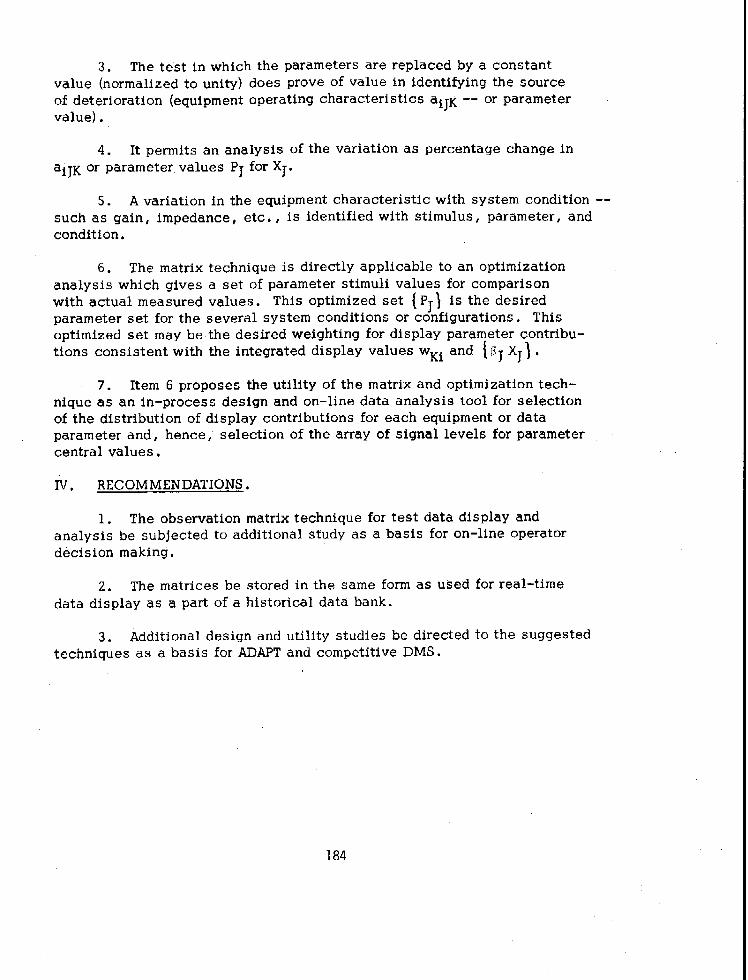
3. The test in which the parameters are replaced by a constant value (normalized to unity) does prove of value in identifying the source of deterioration (equipment operating characteristics aiJK -- or parameter value).
4. It permits an analysis of the variation as percentage change in aiJK OI” parameter Values PJ for XJ.
5. A variation in the equipment characteristic with system condition -- such as gain, impedance, etc. , is identified with stimulus, parameter, and condition.
6. The matrix technique is directly applicable to an optimization analysis which gives a set of parameter stimuli values for comparison with actual measured values. This optimized set ( PJ) is the desired parameter set for the several system conditions or configurations. This optimized set may be the desired weighting for display parameter contribu- tions consistent with the integrated display values wKi and { 6 J XJJ ,
7. Item 6 proposes the utility of the matrix and optimization tech- nique as an in-process design and on-line data analysis tool for selection of the distribution of display contributions for each equipment or data parameter and, hence, selection of the array of signal levels for parameter central values,
Iv, RECOMMENDATIONS.
1. The observation matrix technique for test data display and analysis be subjected to additional study as a basis for on-line operator decision making.
2. The matrices be stored in the same form as used for real-time data display as a part of a historical data bank.
3. Additional design and utility studies be directed to the suggested techniques as a basis for ADAPT and competitive DMS.
184

REFERENCES
Gamble, Edward H. , “Systems Modeling via Functions, ” Technical Report CS-A-74-1, May 1974.
Gamble, Edward H. , “Design Analysis of Large-Scale Systems, ” Proceedinqs of the 1975 Army Numerical Analysis and Computers Conference, AR0 Report 75-3, December 1975.
Gamble, Edward H. , “Utilization of Computer Analyses for Major Design Decisions for Large-Scale Systems, ” Proceedinqs of the 1975 Army Numerical Analysis and Computers Conference, AR0 Report 75-3, December 1975.
Gamble, Edward H . , “A Function Modeling Technique for Estimating Computer Traffic for a Data Management System,” DA 75-3, 15 July 1975.
Gamble, Edward H. , “A Critique on the Design of Complex Systems, ” Copyright #A927900, 1967.
185


LETHALITY OF A SPECTRlM OF SHAPED CHARGE PROJECTILE ANTI-TANK FIREPOWER-KILL EFFECTS EVALUATED BY
THE AWAM-1 COMPUTER MODEL
Donald F. Haskell OS Army Ballistic Research Laboratories
Aberdeen Proving Gxound, Maryland 21005
ABSTRACT. This papes describes an anti-tank lethality study pex- formed by the use of AVVAM-1, the first version of a new armored vehicle vulnerability analysis computer model developed at the Ballistic Research Laboratories. In this study the vulnerability of a Russian T55 tank to a spectrum of anti-tank shaped charge projectile terminal ballistic effects is calculated and analyzed. This is done to illuminate the behind-armor effects characteristics and their combinations that axe most lethal. The measure of lethality employed in this study is the probability of achieving a firepower kill given a hit on a specific point on the tank.
Lethality of the various projectile effects is calculated for direct frontal attack of the tank. It is assumed that there is an equal proba- bil,i.ty of hitting any point on the vehicle attack aspect. In this manner the individual projectile effects may be separated from weapons systems hit probability. Typical shaped charge projectile spatial distributions are employed for the mass, speed and numbers of fragments produced behind the armor. The end product of the study is a ranking of the damage p.ro- ducing effects of the various projectile types according to their lethality in causing a firepower kill. This was obtained by a sensitivity study of the effects of the various parameters. The conclusions of the study are:
1. Over the range of the variables (noxmalized to the standard HRL 3.3 inch cone diameter precision shaped charge) from 0.6 to 1.2, firepower-kill lethality of the shaped charge jet projectile in direct frontal attack of the Russian 1'55 tank is most sensitive to changes in cone diameter and the number and speed of behind-the-axmor fxag- ments (given in decreasing order of influence on lethality of the seven variables studied in this investigation).
2. Over the range of the standard charge noxmalized variables between 1.2 and 1.8, lethality is most sensitive to changes in jet velocity, cone diameter and the number of behind-the-armor fragments (given in decreasing order of influence). Here again, 1ethaIity is least sensitive to jet breakup time.
3. On the other hand, jet breakup time exerts the highest effect on lethality over the standard charge normalized variable range from 1.8 to 2.0. This is followed by jet velocity and cone diameter. Mass of the behind-the-armor fragments has the least influence on shaped charge lethality over this range.
187

4. A marked functional dependence of P K/H
upon the behind-the-
armor fragment spray total kinetic energy was found. This informa- tion should be very useful in the design of new shaped-charge anti- tank projectiles. it should also provide guidance in the vulnerability reduction of tanks.
1. INTRODUCTION. The object of this investigation was to determine which of seven selected shaped charge munition parameters exert the most influence on the probability of achieving a firepower kill of the Russian T55 tank given a random hit on the tank in a direct frontal attack. The seven parameters are: the liner cone base diameter, munition standoff distance from the target, jet velocity, and jet break-up time as well as the number, mass and speed of the fragments generated behind the tank armor by the jet. Each parameter was varied independently over a pre- selected range of values to assess its effect on the firepower capability of the tank. In addition, the effects on kill probability caused by varia- tion of combinations of these parameters was also studied.
AVVAM-ll was used to perform the study, AVVAM-1 (Armored Vehicle Vulnerability Analysis Model, first version) is a conceptual model and associated digital computer code developed at BRL to analytically assess the vulnerability of armored vehicles. AVVAM-1 can be employed to per- form both armored vehicle vulnerability and anti-armor weapons design and analysis studies. This first version of AVVAM treats components and per- sonnel subjected to penetration and/or perforation damage mechanisms. The attacking munition may be a shaped charge or kinetic energy projec- tile, or a shaped charge or Misznay-Schardin land mine. With additional effort the present model may be extended to include other damage mechan- isms. Although originally developed for armored vehicles, the code is not restricted to armored vehicles - it may be employed to assess the vulnerability of any structure.
AWAM-1 is an outgrowth of an exjsting digital computer code devel- oped by H. Ege of the Surface Targets Branch, Vulnerability Laboratory, BRL. Ege’s code is based on relations between the characteristics of certain weapons and vehicle damage observed from the res-ults of antitank tests conducted under the auspices of the UK, Canada and the IJS in Canada during 1959.2
1 D. F. Haskell and M. J. Reisinger, “Armored Vehicle Vulnerability Analysis Model - First Version,” US Army Ballistic Research Laboratories Interim Memorandum Report No. 85, February 1973.
2 Canadian Armament Research and Development Establishment Report Q-21, “Tripartite Anti-Tank Trials and Lethality Evaluation (U) ,‘I-Final Report Part I, November 19S9, (SECRET).
188

AWAM-1 is based on analytical evaluations of the damage inflicted on individual critical components and the aggregate effect of these damaged components on compartment and overall vehicle vulnerability. To do this, AWAM-1 accounts for not only the damage inflicted on com- ponents in the direct line of fire, or shotline, of the attacking muni- tion but also the damage inflicted by armor spa11 and/or munition fragment sprays on components located away from the munition shotline. In addi- tion, AWAM-1 accounts for the degrading (or possible enhancing) effects on the spa11 and/or fragment sprays caused by components positioned between the armor and the critical components. Thus, the potential pro- tection afforded critical components by intervening components is included in the AWAM-1 calculational procedure.
2. DESCRIPTION OF AWAM-1. AVVAM-1 is composed of two major computer codes. One of these characterizes the target. The other code characterizes the munition-target interaction and pesforms the vulnerability evaluation. The target characterization code describes the target and identifies, locates and determines the presented area of critical components. It also provides information concerning components that are located between the vehicle armor and the critical components.
To generate the target description information, AWAM-I employs the GIFT (Geometric Information for a Target) code.3 The GIFT code is an improved version of the existing MAGIC code.4 The identification, loca- tion and presented area determinations of critical components and the intervening component information is generated by a subcode within the GIFT code called RIP (Rays Initiated at a Point).
The second major code employed in AVVAM-1 encompasses the terminal ballistics of the attacking munition and the post-plate-perforation characteristics of plate spa11 OY munition fragment sprays. In addition, this second code calculates the vulnerability of selected components within the vehicle as well as compartment vulnerability and overall
vehicle vulnerability. Because of its functions, it is called the P3 and
C3PKH (Post-Plate-Perforation and Component, Compartment and Combat Vehicle Probability of a Kill given a Hit) code.
In operation, AVVAM-1 selects critical components within the target and then evaluates the extent of damage and kill probability for each selected munition aim point in a given view of the target. It does this
‘Lawrence W. Bain, Jr., and Mathew J. Reisinger, “The GIFT Code User Manual, Volume I Introduction and Input Requirements,” BRL Report No. 1802, July 1975.
4 Armament Systems, Incorporated and Propulsion Development Department, “MAGIC Computer Simulation,” Volumes I and II, Naval Weapons Center Technical Note 4565-X-71, Volume I and Volume II, May 1971.
189

by determining the armor thickness in the direction of the shotline of the attacking munition and the number of intervening components between the vehicle armor and critical component. It then utilizes the behind- the-plate characterization of a specific munition to calculate kill probabilities given a hit for all or selected critical components within the vehicle, This whole process is accomplished by firing a large number of parallel rays at a given attack angle and azimuth into the target. Each individual parallel ray then spawns new rays that are initiated at the munition exit point on the armor interior surface. These new rays are used to search out the critical components, define their position, shielding, and presented area. Then the post-plate,-perforation subcode converts terminal ballistics input data into an expected number of hits
into each of the critical components and finally the C’PKH subcode determines the probability of a kill of these components for the expected number of hits. The kill probabilities for all the critical components within a given compartment may be combined into compartment mobility (M), firepower (F), and complete or catastrophic (K) kills. Values for M, F, and K kills of the whole vehicle may also be determined.
A flow chart summarizing the operations of AVVAM-1 is presented by Figure 1. In this figure Box 1 represents the target input, Box 2 is
the RIP-section of the GIFT code, Box 3 is the P3 section and Box 4 is
the C3PKH section. The C3PK11 section provides the output in terms of probability of a kill given a hit. Also indicated in the figure- is Box 5 which indicates an iteration scheme that may be employed for multiple views. Since the sections represented by Boxes 1, 2, 3, and 4 provide the PK/H output for a single view, results for multiple views may be obtained by iterating through Boxes 2, 3, and 4 fox each view desired.
The code operates as follows: The particular target description is input through Box 1 on cards and the specific munition is input by cards
through Box 3. Information for the P3 section is handled by card input. After the target is described and the critical components identified, for a single vehicle view, RTP selects a starting point on the vehicle, fires a main ray at the starting point, and essentially determines the position, shielding, and presented area of all the critical components
in the vehicle in relation to the shotline of the main ray. The C3PKH code calls on the Post-Plate-Perforation code to supply the behind the plate spa11 data and main munition shotline information to include number of fragments, size, and speed of fragments. Next, it calculates the expected number of fragments to hit a given critical component, and then the probability of killing that component given a hit. It does this for each critical component identified by the RIP code for the particular shotline selected. All the critical components axe evaluated for the first shotline. The RIP code then moves to a new shotline (or shotpoint)
190

and the probabilities of a kill given a hit are calculated for all the components in the view of the new shotline. This process is continued until the whole view of the vehicle is completed. At this point the out- put of the AWAM code is the following: Probability of a kill for each critical component in the vehicle, a set of compartment M, F, and K kill probabilities and overall vehicle view probability of M, F, and K kill
values. During these calculations the C3PKH code in conjunction with the
I’ 3 code account fox the mass and velocity attrition of the shotline and spa11 fragments as they perforate intervening components between the exit point on the armor and the specific critical component under evaluation at that time.
3. STUDY CONDITIONS. As described previously, the object of this investigation was to determine which of the following parameters has the most effect on the firepower kill lethality of a shaped charge projectile used in a direct frontal attack of the TSS tank: liner cone base diameter, standoff distance, jet velocity, jet breakup time, and the number, mass and speed of the behind-the-armor fragments produced by the jet. Each of these parameters was varied independently over a selected range of values and AWAM-1 was used to calculate and follow the attendant variation in firepower kill probability given a hit on the tank (PK,H). The effect on
‘K/H of certain combinations of parameters was also calculated. To do this,
equal variations in each of the parameters in the combination were employed.
Those parameters used to characterize the shaped charge jet itself were varied over the following range of values:
. Liner cone base diameter = 0.0508 m -0.2032 m
. Munition-target standoff distance = 0.08382 m -2.0955 m
. Jet velocity = 2,000 m/set -20,000 m/set
. Jet break-up time = 25 microsecs -200 microsecs
The behind-the-armor fragment characteristics produced by the above range of conditions were automatically calculated internally by AWAM-1. In addition, other calculations were made in which the behind-the-armor fragment characteristics (number of fragments, fragment mass and fragment speed) were varied independently of the normally expected values that would otherwise be governed by the jet parameters. In these cases, the number of fragments, their mass and speed were made proportional to those produced by a standard shaped charge and were varied over the range from 0.01 to 10 times the particular standard charge behind-the-armor charac- teristic value. That is, the numbex of fragments-to-number of fragments from the standard charge ratio, fragment mass-to-standard charge fragment
191

mass ratio, and the fragment speed-to-standard charge fragment speed ratio were varied from 0.01 to 10.
The standard shaped charge5 is a 42', apex angle, copper cone loaded with octal explosive in a light confining wall of aluminum. A diagram of this charge is shown in Figure 2. All linear dimensions in the diagram axe in inch units. It will be referred to as the "standard charge." The nominal liner wall thickness is .081 inch 1.206 mm) and the outside diameter at the base of the cone is 3.3 inches (84 mm), The total liner weight is .61 lb C.277 kg), the explosive weight is 1.93 lbs (.875 kg), and the aluminum body weight is 1.14 lbs (.517 kg). The standard cone diameter and standoff as well as the jet constants of this standard charge obtained experimentally from flash radiographs are as follows:
Cone diameter = 0.0832 m Standoff = 0.16764 m Jet velocity = 8,300 m/set Break-up time = 103 microseconds
The 4'55 tank was assumed to be Sully combat loaded and directly attacked in the front (zero azimuth and elevation) by the shaped charge projectile. A planar gridwork of GO.96 cm square cells was erected over the front of the tank normal to the attack direction. A shotline, to simulate a projectile flight path, was fired in the attack direction at a random point within each cell. measured by the firepower P
In this manner the projectile lethality,
K/H' was evaluated for strike points over the whole front of the tank. Then these individual cell (or shotline) PK,llts were averaged together to obtain a single firepower kill P K/H' represen- tative of the particular set of parameter values being evaluated.
The GIFT description of the T5S tank consisted of approximately 6.70 components. Of this total about 400 were considered critical components. About half of these were considered critical to the tank's firepower. In this AVVAM-1 analysis, 5 rays to simulate behind-the-armor fragments were fired at each of these 200 firepower critical components.
4. RESULTS AND DISCUSSION. The study results obtained by use of AVVAM-1 are illustrated in Figures 3 through 14 and Tables I and II. Figures 3 through 6 show the effects on average firepower kill P K/H Of independent variations in the basic shaped charge projectile jet charac- terization parameters. In these figures the ordinate corresponds to P K/H and the abscissa corresponds to the jet parameter. The jet parameters are
5 R. DiPersio, J. Simon and A. B. Merendino, "Penetration of Shaped-Charge Jets Into Metallic Targets," BRL Report No. 1296, September 1965, pp. 16-17.
192

displayed as a ratio of the actual parameter value-to-the value of that parameter exhibited by the “‘standard charge.” For example, in Figure 3, at the abscissa value equal to 2, the cone diameter under investigation is twice the size of the standard charge cone diameter, ox .0168 m (6.6 in.). Each parameter was varied while the remaining parameters were kept constant at the value exhibited by the standard charge. In the cone diameter case the standoff was maintained equal to that of the standard charge i..e., equal to two cone diameters.
As to be expected, the figures show that average P K/H
increases with
increasing cone diameter, jet velocity and breakup time and that P K/H
decreases as standoff is increased. The ‘K/H and its slope vary contin-
uously with cone diameter. On the othex hand, both P K/H
and its slope
vary irregularly (almost discontinuously) with jet velocity and bxeak- up time. Figure 5 depicts a plateau in PK,H over the jet velocity-to-
standard charge jet velocity ratio from 0.6 to 1.3. A wider plateau exists in the relationship between P
K/H and breakup time as shown by Figure 6.
In this case the plateau extends from breakup time-to-standard charge breakup time ratio equal to 0.4 to approximately 1.6.
The relationship between PK,H and standoff illustrated in Figure 4
is interesting. As to be expected, P K/H
decreases with standoff over the
range studi ed. However, this decrease is less than would be expected- the functional dependence of P
K/H on standoff is quite weak. It is much
less than it is wi.th the other jet parameters. The jet lethality is not significantly degraded at standoffs much greater than standard.
Figure 7 illustrates the effect on P K/H
of simultaneous and equal
variation of the jet parameters. As before, the abscissa represents the value of the parameter relative to its value exhibited by the standard charge. Although here it represents the value of all four jet parameters relative to the standard charge case. For example, at the parameter value-to-parameter value of standard charge ratio equal to 0.5, the P K/H computation was performed with the cone diameter, standoff, jet velocity and jet breakup time all set equal to one-half the parameter values cor- responding to the standard charge, As indicated by the figure, PK,H is a
smooth, increasing function of the four jet parameters. Its rate of increase with these four parameters is higher, as to be expected, than its variati.on with change in the parameters individually, although the combined effect is not the sum of the effects of the individual parameters.
193

Figure 8 SIIOWS the effect of individual and combined change in the behind-the-armor fragment parameters on PK,H. The functional relation-
ship between P K/H
and the fragment parameters is similar for all three:
number of fragments, fragment mass and speed. PK,H increases rapidly as
the fragment parameter-to-standard charge parameter value ratio increases from zero to 1 ox 2. Beyond this region, the PK.,” rise levels off. As
indicated, equal variation of all three fragment parameters at the same time yields higher P
K/H than individual variation of these parameters.
However, the combined effects do not show as high an increase over the individual fragment parameter variations as may be expected beforehand.
The slopes of the curves from Figures 3 to 6 and 8 in which the jet and fragment parameters axe varied independently are plotted in Figures 9 and 10. Figures 9 and 10 exhibit the P
K/H sensitivity to the various para-
meters over a range of these parameters. As indicated, there is no single parameter that has the most influence on P K/H over the range of independ-
ent parameters shown. Between normalized variable from 0.6 to about 1.2,
pK/H is most sensitive to cone diameter. Above 1.2 and below about 1.8
jet velocity has the most effect on P K/H *
Between normalized variable
equal to 1.8 and 2.0, the jet velocity displays the highest influence on
pK/H. The effect of standoff, as described earlier, is minimal- over the
whole range. In regard to the fragment effects, the number and speed of the fragments show ahout the same influence on P
K/H which, over most of
parameter range shown, is considerably higher than the fragment mass influence.
The slopes of the curves in Figures 9 and 10 over the range of para- meter-to-standard charge ratio from 0.6 to 2.0 at discrete points within this range axe listed in Table I. The slopes are normalized to that of the cone diameter. In this manner those parameters that have higher, or lower, inf luencc on P
K/H than the cone diameter axe easily distinguished,
Table II lists the parameters according to their decreasing order of influence on PK,H over the variable value normalized to standard charge
range from .6 to 2. As indicated, cone diameter, jet velocity and jet breakup time exhibit the highest influence on PK,H over the range of
variables shown.
Figures 11 to 14 are log-log plots of P K/H
versus behind-the-armor
fragment total kinetic energy. These figures axe included hexe to illus- trate the relationship between behind-the-armor fragment kinetic energy
194

and average kill probability. Figures 11, 12 and 13 show the calculation results for i,ndependent variations in the fragment parameters. In Figure 11 the total fragment kinetic energy was increased by increasing the number of fragments with their mass and speed held constant and equal to the mass and speed exhibited by the standard charge. In Figure 12 the mass of the fragments was varied while the number and speed were main- tained equal to those characteristic of the standard charge. The fragment speed was varied in Figure 13, and in Figure I4 all three parameters were varied simultaneously and equally. The lines in these figures were drawn in by “eye.” These figures indicate that there appears to be a definite relationship between behind-the-armos fragment total kinetic energy and resultant l’K/He In each figure, PK,H increases with total fragment
kinetic energy, Furthermore, there axe two distinct regions of fragment
influence, with kinetic energy of the osdar of lo4 to 105 joules as the demarcation zone between these two regions. Fragment kinetic energy has a much larger effect on PK,H in the lower kinetic energy region than in
the higher region.
5 .:.. - CONCLUSIONS.
1. Over the range of the variables (normalized to the standard BRI. 3.3 inch cone diameter preci.sion shaped charge) from 0.6 to 1.2, firepower-kill lethality of the shaped charge jet projectile in direct fxontal attack of the Russian T5.5 tank is most sensitive to changes in cone diameter and the number and speed of behind-the-armor fragments (given in decreasing order of influence). Over this same range, jet breakup time exerts the least influence on lethaIi.ty of the seven vaxi- ables studied in this investigation.
2. Over the range of the standard cha,rge normalized variables between 1.2 and 1.8, lethality is most sensitive to changes in jet veloc- ity, cone diameter and the number of behind-the-armor fragments (given in decreasing order of influence). Ilero again, lethality is least sen- sitive to jet breakup time.
3. On the other hand, jet breakup time exerts the highest effect on lethality over the standard charge normalized variable range from 1.8 to 2.0. This is followed by jet velocity and cone diameter. Mass of the behind-the-armor fragments has the least influence on shaped charge lethality over this range.
4. A marked functional dependence of P K/H
upon the behind-the-
armor fragment spray total kinetic energy was found.
195
REFERENCES
1. D. F. Haskell and M. J. Reisinger, "Armored Vehicle Vulnerability Analysis Model - First Version," US Army Ballistic Research Labora- tories Interim Memorandum Report NO. 85, February 1973.
2. Canadian Armament Research and Development Establishment Report Q-21, "Tripartite Anti-Tank Trials and Lethality Evaluation (U],ff Final Report Part I, November 1959, (SECRET).
3. Lawrence W. Bain, Jr., and Mathew J. Reisingex, "The GIFT Code User Manual, Volume I Introduction and Input Requirements," BRL Report No. 1802, July 1975.
4. Armament Systems, Incorporated and Propulsion Development Department, "MAGIC Computer Simulation" Volumes I and II, Naval Weapons Center Technical Note 4565-3-71, Volume I and Volume II, May 1971.
5. R. DiPexsio, J. Simon and A. 6, Mexendino, "Penetration of Shaped- Charge Jets Into Metallic Targets," BRL Report No. 1296, Sep 65.
196

1. /TARGET INPUT
I TARGET DESCRIPTION
CRITICAL COMPONENT IDENTtFlCATlON
2. RIP CODE
SINGLE VEHICLE VIEW I---
1 CRITICAL COfAPONENT
POSITION, SHIELDING, AND
PEkFORATION INFOI:F~‘IATIOIJ -----
a
I PK,H OUTPUT FOR L--.-J
VEHICLE M. F AND K KILLS
Figure 1. AVVAM-I Code Summary Flow Chart
197

SW&E FOR BOOSTER AND JNlTiATOR
.----..,_-.- BODY
?8.%&COPPER LINER
Figure 2. Diagram of Standard Shaped Charge
198

1.0
.a
.6
.4
.2
0 L
0
I I I I 1 1 I 1 1 1 1 1
1 2
CONE DIAMETER CONE DIAMETER OF STANDARD CHARGE
Figure 3. Effect of Liner Cone Diameter

I I I I I I I I I
200

1.0 - 1
.8
.6
.4
.2
JET VELUCI7Y STANDARD CHARGE JET VELOCITY
Figure 5. Jet Velocity Influence

1.0
.8
.6
-4
.2
0 I I 1 I I I 1 I I
Figure 6. Jet Breakup Time Influence
202

1 . 0
.8
.6
P K/l1 .4
.2
D
0 1 2
Figure 7, Effect of Simultaneous and Equal Variation in Cone Diameter, Standoff, .Jet Velocity and Jet Breakup Time on 1’
K/H
203

1 . 0
.8
.6
.4
.2
0
Figure 8.
- - -
- - - -
3----a--
I I I I
0 2 4 h 8
Effect of Behind-the-Armor Fragment. Parameters on P K/H
1 0
204

1.2
1.0
.2
0
-.2
0
I I 1 I I I I I 1
1
VARIABLE NORMALIZED TO STANDARD CHARGE
2
Figure 9. Sensitivity to Shaped Charge Variables
205

0 1 2
VAR IAt3I.I:. NORMAl, ILLI) ‘I’0 STANDARI) CtIARGE
Figure 10. Sensitivity to Fragment Variables
206
.6
a P -$x
.4
.2
0 ---.- r

207

--___ “ . I I . _ , - -_ - . . - . . . . _-_-_-^“.- - - - . , - . “ - - , - , - - - - - , - - “ , -> - -
208

C’
209

.6
pK/H
.4
lo4 lo5 lo6 10' i08
TOTAL FRAGMENT KINETIC ENERGY, joules
Figure 14. PK,H Variation with Total Fragment Kinetic Energy for Simultaneous and Equal Variations in Fragment Number, Mass and Speed
210

Table T. pK/Il Sensitivities Relative to Cone Diameter
VAHIAHl,E VAHIAHl,E -6 -6 .8 .8 1 1 1.2 1.2 1.4 1.4 1.6 1.6 1.8 1.8 2.0 2.0
CONE DIA. CONE DIA. 1 1 1 1 1 1 1 1 1 1 1 1 1 1 1 1
STANDOFF STANDOFF .OOS .OOS -,008 -,008 -.024 -.024 -.057 -.057 -.079 -.079 -.I74 -.I74 -.203 -.203 -.217 -.217
JET VELOCITY JET VELOCITY .172 .172 0 0 0 0 0 0 6,263 6,263 2,333 2,333 1,855 1,855 1.681 1.681
BREAKUP TIME BREAKUP TIME 0 0 0 0 0 0 0 0 0 0 0 0 2.203 2.203 14.493 14.493
NUMBER OF FRAGS. NUMBER OF FRAGS. .211 .211 .236 .236 ,246 ,246 .359 .359 .351 .351 .435 .435 .319 .319 .304 .304
t4ASS OF FRAGS. t4ASS OF FRAGS. .072 .072 ,098 ,098 ,114 ,114 .156 .156 .316 .316 .261 .261 .145 .145 .058 .058
FRAGMENT SPEED FRAGMENT SPEED .187 .187 .226 .226 .237 .237 .286 .286 ,202 ,202 .319 .319 .261 .261 ,116 ,116
211

Table II. PK,H Sensitivities in Descending Order of Influence
INFLUENCE r HIGHEST
LOWEST
NOTE:
CD: VJET :
Tl: s:
NF: SF: MF:
.6
CD
NF
SF ---
VJET
MF
S --I
Tl
VARIABLE VALUE NORMALIZED TO STANDARD CHARGE
MF MF MF MF
S s S S
VJET VJET VJET VJET --------- ---
Tl Tl Tl Tl
Cone diameter Jet velocity Jet breakup time Shaped charge standoff distance Number of behind-the-armor fragments Speed of behind-the-armor fragments Mass of behind-the-armor fragments
212
VJET
CD
NF ---
MF
SF
S ---
Tl
1.6
VJET
CD
NF ---
SF
MF
S --I
Tl
1.8
Tl
VJET
CD ---
NF
SF
S --* MF
Tl
VJET
CD --- NF
S
SF .-- MF

DEVELOPMENT AND OPTIMIZATION OF SIGNAL PROCESSING UTILIZED IN A MINE DETECTION SYSTEM
Abram Leff U.S. Army Mobility Equipment R&D Command
Fort Belvoir, Virginia 22060
ABSTRACT. Based upon an extensive R&D program a broadband microwave technique has evolved which can be utilized to rapidly scan roads and reliably detect both metallic/non-metallic cased AT mines. In order to optimize mine detection capability and minimize false alarms, processing algorithms had to be developed and evaluated. field data was initially recorded on analog tape for off-site processing. This data was utilized to develop potential processing algorithms.
To permit the evaluation of algorithms in real-world conditions, a mobile real-time feasibility system was designed and fabricated. This system incorporated a CDC 469 minicomputer which allowed storage in memory of up to six algorithms, as well as the control programs for the system. Flexibility incorporated in the design and the addition of a keyboard unit provided the capability to utilize any one of the six algorithms or vary most test parameters in the field, by simply changing an address in the System Control Unit or CPU.
This paper will discuss utilization of a minicomputer in the development of an optimized processing algorithm for mine detection.
1. INTRODUCTION. Considerable data processing and analysis effort has been expended with the objective of developing target discrimination techniques for detecting road mine responses in the presence of normal background responses. The goal of this effort was the development of field-operable software that optimizes the probability of detecting AT/AV mines under field conditions while concurrently minimizing the false alarm rate.
The inherent nature of the data analysis problem dictates a tradeoff between the probability of target detection vs. the false alarm rate. This relationship in a specific situation depends upon the particular field conditions encountered; therefore, large amounts of test data had to be gathered from a considerable variety of test site conditions in order to optimize detection vs. false alarms.
Initially, field data was recorded on a four channel analog tape recorder and was off-line converted to digital data format and recorded on IBM-compatible magnetic tape which then could be played back in various ways to produce plots of the desired data parameters. This digitized data also formed the basis for the development of the processing algorithms by means of computer analysis.
213

2. STATEMENT OF PROBLEM. To attack the basic data analysis problem, which was to develop a field-operable software system maximizing target detection while minimizing false alarms, a methodical investigation was initiated to (a) define the general target responses, (b) select the most favorable processing methods, (c) find the best way to represent the data, (d) identify the decision rules for discrimination between mine signature and background data, and (e) minimize the computational complexity needed to perform the task.
Based upon the results of the various analysis and processing schemes which were applied to test data, it was concluded that two initial processes were essential: (a) calculation of a background estimate based on preceding data inputs, and (b) normalization of the input data with respect to the background estimate. The latter is required because of the large differences in absolute amplitude levels in the various frequency channels caused by frequency roll-off of the antennas, and because of different attenuation levels in the soil.
3. ALGORITHM DEVELOPMENT. The first useful algorithm developed was named Target Amplitude Descriptor, or TAD, where for each channel and at each consecutive position the ratio between the input data and the background estimate was established, after which these ratios were averaged for all channels of a particular antenna pair.
Logarithmic TAD plots were made from the recorded test data using the amplitude information Rij ( ratio between receive and transmit signal levels in dB as measured at position i and frequency j) in the following manner:
j=n
Log TADi =201Og {~ z: Aij/Bij 1 (in dB) j=l
where: A,. = ‘J linear value of Rij (by using: Aij z.10 Rij'20)
n = number of frequency channels
B ij = linear value of background estimate at position i and frequency j, determined as follows:
B ij = (1 * ~1 1 xB~-1 ,j + ~1 x Ai- ,j
where c1 is a constant chosen such that the background estimate relates to a selected distance:
214

-2AXj
a= 1 _ e-Dziiy
where AXi = position increment in meters
"Decay" can be defined also as the trailing distance where the relative weight of the background contribution is equal to 13,5%. This process is known as exponential smoothing (i.e. gives greater weight to most recent data), with the decay analogous to two time constants in an R-C filter network. Expressed in terms of ~1:
2AXj Decay = - ln (1-o)
Initially all mines responses were differentiated on TAD plots because the target data was not excluded from the background estimate, in essence reducing the target responses. To correct this, a threshold condition was initially inserted in the determination of the weighting factor ~1. In test areas with large background fluctuations, however, the background peaks would also be excluded from the background estimate when the threshold was exceeded.
Average (ASUM) although originally developed as a modifier for the weighting factor to dynamically exclude target responses from the background estimate, the process designated ASUM proved to be a most successful algorithm. ASUM is defined as follows:
n 1
ASUMi = n C Anij j=l
where:
n = number of frequency channels
Anij = the normalized data at position i and frequency j
Aij - B ij Anij '
uij
and
A.. = 13
linear value of amplitude data for position i and frequency j
‘215

B** 13 = exponentially smoothed background estimate for position i and frequency j.
oij = standard deviation, obtained from the exponentially smoothed estimate of the variance.
Bij and oij are determined by:
B** 1J =B i-1,j (lwa) + +-l ,j
oij 2 2 = ui-l,j (1-a) + a(Ai-l,j - Bi-l,j)2
where the weighting factor a was initially:
= , 7 -
,-ZAXildecay
where
AXi = position increment between samples at i and i-l
Decay = the distance prior to position i where the relative weight of the contribution to the background estimate is down to 13%.
The weighting factor was later modified to:
a2= { ~11; if ASUMi IO.9
0; otherwise
and finally to:
“3 = al/(1 + ASDMi4)
The weighting factor was modified in order to compensate for the effects of varying background levels as a function of soil conditions and moisture conditions.
Many more attempts were made to further improve target discrimination by evaluating statistical methods and methods using magnitude and/or duration of target responses. As a result, six algorithms were developed for evaluation in real-time, real-world field tests with the feasibility model.
216

4. FEASIBILITY MODEL. To provide real-time test results and flexibility in the selection of test parameters (position and frequency sample intervals, frequency range, etc.), a mine detection feasibility model incorporating advanced discrimination techniques was designed and fabricated. (See block diagram, Figure 4-l). A programmable minicomputer (CDC Model 649) was incorporated into the system to increase the data processing capabilities, an X-Y recorder was added to provide real-time plots of test results, and a four-channel analog instrumentation recorder was employed to record the test data for off-site processing and analysis.
This feasibility s tractor (G.E. Model E-15 J
stem was installed on an electrically powered as shown in Figure 4-2. Field tests were
conducted (and continue to be conducted) at various field sites, with the purpose of evaluating the real-time discrimination techniques that were previously developed utilizing an off-line system.
The electronic components of the feasibility model consist primarily of a transmitter, a receiver, a System Control Unit (SCU) and the data processing subsystem (CDC 469). As described in the subparagraphs that follow, the receiver compares the phase and amplitude of received signals to the transmitted signal. The resulting phase and amplitude data are examined by the data processing subsystem for indications of the presence of a mine under the detector heads.
4.1 FEASIBILITY SYSTEM OPERATION. The major system components -- transmitter, receiver, system control unit, processor and power supplies -- are housed in an equipment enclosure which mounts to the front of the tractor. The antenna switches mount near the search head at the end of the frame, and the shaft encoder that correlates mine detector data to search head position and operating speed is driven by a rear wheel on the tractor.
The System Control Unit (SCU) responds to synchronizing pulses from the position encoder and control commands generated via the keyboard unit, producing sweep control signals for use by the transmitter. The transmitter signal originates in a voltage-controlled oscillator (VCO) whose output frequency is proportional to input sweep voltage. The VCO output is power-amplified to approximately 1 watt and supplied via a directional coupler and solid-state switch to the transmit antennas, with a -20 dB output of the coupler supplied as a reference to the receiver.
The receive antennas connect via another solid-state switch to the receiver. The SCU synchronously controls the two antennas switches, providing the scanning sequence that selects each transmit-receive antenna pair in turn. The receiver contains a synchronous detector that yields an amplitude output and a phase detector that yields the
217

phase data signal. Receiver outputs are digitized and processed by the SCU and CPU.
4.1.1 SYSTEM CONTROL UNIT. In addition to generating scan sequence commands in response to position encoder pulses, and generating sweep control voltages and antenna switching commands, the SCU processes amplitude data supplied by the receiver, detects target responses in the processed data, and activates the target alarm and identifies the position of a detected target. In particular, the SCU produces control signals for system operation.
Various computer operational commands and any one of the processing algorithms stored in the computer memory can be addressed via the SCU by means of appropriate keyboard entries. The keyboard is also employed to set up the SCU control circuits which establish the test parameters for a particular operation, as follows:
(1) Frequency Increment - Amplitude data supplied by the receiver is sampled at intervals as the frequency range is swept, and the frequency change during a sample is defined as the frequency increment. The frequency increment is selectable over a range from 10 MHz to 150 MHz in mu.ltiples of 10 MHz.
(2) Start Frequency - The start frequency is defined as the frequency chosen for the low end of the swept frequency range, and is selectable in multiples of 10 MHz from 300 to 990 MHz.
(3) Sample Interval - The sample interval is a measure of the duration between each frequency sample, and is selectable over a range from 0.1 ins to 1.5 ms in multiples of 0.1 ms.
(4) Number of Sample Intervals - The number of sample intervals per sweep (up or down) is selectable over a range from 1 to 15 intervals per sweep.
(5) Transition Time - When a sweep reaches the end frequency (either high or low), it dwells at this frequency for a selected time period to allow the antenna switches to select the next antenna pair. This transition time is selectable from 0.1 to 1.5 ms in multiples of 0.1 ms.
(6) Number of Sweeps - The number of sweeps per scan normally corresponds to the number of antenna pairs in the search head array, thus allowing one sweep per pair. The number of sweeps per scan is selectable over a range from 1 to 16.
(7) Scan Rate - The scan rate is the number of complete scans (sweeping all antenna pairs) per unit of travel, The selectable rates are 25, 50, 100 and 200 scans/meter.
218

4.1.2 CENTRAL PROCESSOR UNIT (CPU). The processor employed in the feasibility model is a CDC Model 469 minicomputer with 8K words of plated wire memory. Word length is 16 bits, and the cycle time is 1 vs. There are 42 instructions, and the CPU responds to direct, indexed direct and indirect addressing modes.
The function of the processor is to analyze the digitized data supplied by the SCU and determine, with a high degree of certainty, whether a received response is caused by a mine or some other anomaly in the ground. If the presence of a mine is indicated, an output signal is generated far use in sounding an alarm.
The 8K memory in the processor stores and protects all the processing algorithms, and also contains the operational programs for the SCU. Thus, by means of the control keyboard, any of the various algorithms can be selected, and parameter changes to both processing algorithms and SCU programs can be entered at any time, as desired.
Through use of the computer peripherals, the contents of the memory can be changed as desired by connecting the system to the programmer's console. Changes can then be entered using magnetic tape, paper type, or via the teleprinter. A monitor oscilloscope is available for displaying the contents of the memory.
5. CONCLUSIONS. Utilizing the feasibility model, a test program was performed in order to evaluate the developed algorithms as well as several detector head configurations. Six algorithms were stored in memory in the CDC 469 minicomputer and could be selected with the keyboard, for operation in the system. Nominal default values were included for the variable test parameters such as decay and position increment as well as for threshold values or conditions applicable to certain algorithms. All these could be changed by addressing a defined location in the CPU by means of the keyboard. In addition, two versions of ASUM were included to establish accuracy requirements: one in floating point and one in 6-place fixed point. The latter provided insufficient accuracy and was later dropped.
From the start it was apparent that performance of any algorithm using one or more thresholds hinged on the margin over which these threshold values could be used at any location and with any soil composition or moisture content. Obviously, under operational conditions, it would not be feasible to obtain a specific threshold value for the encountered soil conditions. One could hardly be expected to operate over a road to establish the required threshold value, then go back over it to detect any possible mines.
After a lengthy, time consuming series of tests at several test sites, it was found that threshold values varied widely with different soil conditions. With the need for a priori knowledge of soil conditions established, the
219

further use of threshold dependent algorithms were abandoned for the practical reasons stated above.
Real Time field evaluation of the TAD and ASUM algorithms indicated that best performance could be achieved with ASUM (floating-point version).
220


AUTOMATED CONTROL, DATA ACQUISITION, AND ANALYSES FOR HYDRAULIC MODELS OF TIDAL INLETS
D. L. Durham; H. C. Greer, III; and R. W. Whalin U. S. Army Engineer Waterways Experiment Station
P. 0. Box 631, Vicksburg, Miss. 39180
ABSTRACT. An Automated Data Acquisition and Control System (ADACS), which was developed (Durham and Greer, 1975) at the Waterways Experiment
Station (WES) during the past two years, has been expanded to provide automated control, data acquisition and analyses for hydraulic models
of tidal inlets. ADACS configuration consists of a minicomputer with 32K 16-bit words of memory, an interval timer (1 psec), an analog to digital 12-bit converter with 64 analog inputs (+ 10 volts) and 45 kHz
multiplexer, 96 sense/control lines, a magnetic tape controller with
two g-track tape drives, a moving head disk controller with one dual disc drive (removable and non-removable platters), one matrix electro-
static printer/plotter, and an ASR 33 teletype unit. ADACS controls the hydraulic generation of the tide in the tidal
inlet model by providing a programmable analog voltage to the hydraulic
tide generator. The programmable tide controller can simulate a tide composed of one to N tidal constituents for as many tidal cycles as
required. Model tidal elevations are recorded by ADACS using a bubbler
system which measures small hydrostatic pressure changes associated with changes in tidal elevations in the model. The bubbler system consists
of a high precision pressure transducer, a scanivalve device for sequencing input ports, and 48 pressure inputs. The pressure transducer can be calibrated prior to and at selected time intervals during each tidal
test to provide accurate, updated calibration data for scaling voltage (pressure) data to tidal elevations. In addition to collecting tidal elevation data, tide velocities at specific model locations are monitored by using miniature, electromagnetic current meters. Besides controlling
the tide generator during a tidal test, ADACS acquires the above tidal data (elevations and velocities) including calibration information and
223

test parameters and records these data on magnetic tape for future
analyses and permanent storage. Data analyses include scaling and editing of original data, least
squares harmonic analyses of tidal data (elevation and velocity) for amplitude and phase of various tidal constituents, plots of original
data and superimposed harmonic constituents, and analyses of residual
variances. Verification of hydraulic tidal inlet models, which are geometrically distorted models scaled on the Froude model law, requires
artificially simulating in the model the frictional effects associated
with prototype roughness of bottom and sides of channels and ovexbank
and marsh land roughness. The relative phase lags of major tidal constituents from one specific location to another in the prototype and the measurement
of these phase lags in the model provide a means for estimating the amount of roughness and specific model areas requiring artificial roughness
in order to achieve model verification.
These procedures for spatial definition of roughness, full. model verification, and model testing using ADACS and associated automation
procedures have been successfully applied in hydraulically modeling
Muxxells Inlet, South Carolina. The required time for model verification and testing, as well as data analyses, has been significantly reduced.
In addition, the quality,and quantity of model data has increased with minimal cost increases. Thus, better information can be made available
on which to make sound engineering decisions regarding the planning and
design of proposed engineering changes in tidal inlets. 1. Introduction. Over the past decade, automated processing techno-
logy has evolved from large, expensive computers to minicomputers and
microprocessors. With this evolution, the physical size and cost of
automated processing systems have greatly decreased with a minimal decrease in system capabilities. Cost reductions for such systems have resulted in economic justification of the use of minicomputer and micro-
processors to a specific task or group of specific operations; whereas,
large computers can be justified economically only for multiple operations
224

and tasks. The automation of physical, hydraulic modeling techniques has lagged automation efforts in many othe? fields mainly because of
cost justification and the requirements of highly specialized instrumentation
(e-g. sensors), However, needs for such automation have existed for many years. These needs are the result of requirements for (1) real-time model control decisions, (2) quasi real-time data analyses, and (3) mOre
accurate and reliable model data for engineering and environmental
interest studies. One mission of the Hydraulics Laboratory of the U. S. Army Engineer
Waterways Experiment Station is the physical modeling of hydraulic prob-
lems associated with the activities of the Corps of Engineers, as well as
other government and private agencies. Hydraulic problems associated with wave phenomena and the effects of these phenomena in harbors, tidal
inlets, and along the open coast are the primary modeling interests of
the Wave Dynamics Division (WDD) of Hydraulics Laboratory. Over the last three years, WDD has been very successful in automating 132 the major
aspects of its physical models for wave and tidal inlet studies. Major
automation efforts were devoted to (1) model control, (2) model data
acquisition, and (3) model data reduction and analyses. The subject of this paper is a description of the automated system, which has been given
the name "Automated Data Acquisition and Control System" (whose acronym is
ADACS), for wave and tidal models and its general application to tidal
inlet model studies. 2. SYSTEM CONFIGURATION. The automated system for wave and tidal
inlet models has two primary functions: (1) automated acquisition of
wave and tide data in a format (magnetic tape or disc) compatible for digital reduction and analyses and (2) automated control of model sensor
calibration and of the wave and tide generators. The design, development,
and configuration of automated systems to perform these functions with particular applications to wave models were presented in Reference 1.
System configuration (Fig. 1) of ADACS consists basically of the following
four subsystems:
225


a. Digital data recording and controls.
b. Analog recorders and channel selection circuits.
c. Wave/tide sensors and interfacing equipment. d. Wave/tide generators and control equipment.
The first subsystem is basically a 32 K, l&bit word minicomputer
with I/O and storage devices, analog/digital packages, and a timing package. Details of this subsystem were presented by Durham and Gxeer
(1975). The analog recording subsystem is (1) a backup for the digital
data recording subsystem and (2) a visual display fox operator in-
spection of analog signals from model sensors. This subsystem has manual/
automated selection and control of five, 12-channel oscillographs and a
test point center fox manually monitoring a selected channel as to system
setup, calibration, and signal condition. The model sensor subsystem includes instrumentation for both wave
and tide sensors. Details of the wave sensor subsystem and calibration
procedures were presented in Reference 1. The wave sensor subsystem consists basically of the following four components:
a. Wave height sensoxs and stands.
b. Power supplies and signal conditioning equipment.
C. Manual and automatic calibration equipment.
The sensox subsystem for tidal heights includes the following major
components:
a. Bubble tubes, stands, and high pressure supply.
b. Scanivalve with manual and automated controls.
C. Precision pressure transducer.
d. Power supplies and signal conditioning equipment.
The last subsystem includes controls for both wave and tide generators.
Controls for both mechanical and electxohydraulic wave generators can
be provided by ADACS. Start/stop commands axe available for mechanically gear-driven wave generators; however, controls for wave period and
227

amplitude must be supplied manually. For the electrohydraulic wave
generator, ADACS provides a programmable analog voltage as a command
signal to the servocontroller of the electrohydxaulic actuators. The
wave period and amplitude for these wave generators are controlled by
ADACS.
The command signal to the tide generator is a programmable analog
voltage which is supplied by ADACS through one channel of the digital to
analog converter. The tide generator has the option of receiving this
command signal from ADACS or accepting an analog voltage from a pro-
grammable cam and reference potentiometer arrangement. This Latter
control scheme is used as a back-up ox alternate control to the ADACS
control and until recently has been the primary control of the tide
generator prior to installation of ADACS. In addition to the command
signal, the tide generator has four other major components which are
(a) differential amplifier and power supply, (b) bubble tube positioner,
(c) hydraulic-pneumatic amplifier, and (d) hydraulic cyclinder and flow-
control gate assembly.
Basically, the tide in a physical model is generated from cyclic
exchanging by controlled flow a predetermined volume of water between
the physical model and a tidal reservoir (sump). Figure 2 is a schematic
of the tide generator and controls. The programmed command signal causes
a change in the vertical position of the bubble tube relative to the
water level in the model. This position change perturbs the equilibrium
position of the pneumatic-hydraulic amplifier and results in a differential
hydraulic pressure applied to the hydraulic cyclinder activating the
flow-control gate. The movement of the flow-control gate is in a direction
to correct the perturbed equilibrium condition of the pneumatic-hydraulic
amplifier by changing the water-surface elevation in the tide model. A
feedback circuit from the hydraulic cyclindex to the differential
amplifier/bubble tube positioner provides a “damping effect” to prevent
gate overshoot and unstable oscillations. Thus, any tidal constituent or
progressive tide can be used as the forcing function for the tide
228

PROGRAM CAM
ELECTRIC DIFFERENTIAL ----I---
AMPLIFIER
t
1 AND
POWER I I I----I
1 1 ELECTRIC LINE
I I i i FEEDBACK 1 1
I
POTENTIOMETER I
I TO AIR SUPPLY
1 NEEDLEVALVE > I
r-
P"P'TlONER
CONSTANT INFLOW
ROLLERGATE
Figure 2. TIDE GENERATOR AND CONTROLS
229

model by progxamming ADACS to produce a command signal harmonically
representing the appropriate forcing function. 3. TIDAL HEIGHT SENSORS. Data, which are acquired by ADACS from
tidal inlet models, consist of time histories of water surface variations
relative to some reference water level. For specified tide conditions
at the generator, tidal elevations are collected at selected locations
within the tidal model. These data are used to calculate mean tide levels, tidal ranges, arrival times of high and low water, and the phases
and amplitudes of specific tidal constituents. Al though various types
of tidal height sensors are used by the Hydraulics Laboratory, a tide sensor system developed and implemented within the last year for use
in tidal inlet models is presented in this paper. For lack of a better
name, this sensor subsystem has been labeled the “bubbler system.” This
system measures small hydrostatic pressure changes associated with changes in tidal elevations in the model and consists of a high precision, pressure
transducer, a scanivalve device for sequencing input ports, and 48 pressure
inputs . To employ the bubbler system (Fig. 33, a small plastic tube is
inserted some small distance into the water. The outside diameter of
this bubble tube is required to be small to minimize blockage of tidal
flow, etc. The tube is connected through a throttling valve to a regulated pressure supply. This valve or restriction serves to regulate
air‘flow and isolate the bubble tube from other bubble tubes and the supply pressure. Each bubble tube is connected to a common pressure
transducer, which is parallel with the throttling valve and high pressure
source, of suitable pressure range to accurately detect the tube’s internal pressure changes associated with changes of water surface elevation.
To allow many bubble tubes to share a common pressure transducer, a
multiplexing device, which is called a scanivalve, is used. This device
multiplexes sequentially many pressure inputs’to a common output port.
A high precision pressure transducer is included as an integral part of the output port. A controller is used to advance the unidirectional
230

AIR SUPPLY TRUNK LINE : 6 z+ p:
Y ul -' SCANIVALVE 100 PSI SHELTER MODEL AIR PRESSURE
REGULATOR REGULATOR FILTER 15 PSI 5 PSI
GAGE
MODEL BASIN
Figure 3. BUBBLER SYSTEM

stepping motor which increments the scanivalve. By contact clsoures or
commands from ADACS, the valve can be advanced sequentially to any input
port or to a Ithornet (reference) position without intermediate stops.
The system presently used by the Wave Dynamics Division is capable of
accepting up to 48 pressure inputs and includes a +0.25 psid pressure
transducer with a nonlinearity and hystexsis (best straight line) of
0.05 percent full scale. The pressure transducer output is an analog
voltage of +10 volts full scale. The pressure cell is interfaced through
appropriate signal conditioning equipment to the analog multiplexer of
the digital. recording subsystem. The valve accepts both home and step
commands from the ADACS and has a BCD position feedback to the ADACS. The
system can be complete1 y controlled by either ADACS or manual controls.
To install the bubbler system in the rrrodel, the water level in the
tidal model is raised to mean higher high water (MHHW). At this still
water level, the orifice of the bubbler is inserted into the watex to a
depth which is slightly greater than the maximum expected tidal range
(hydrostatic head) . At this elevation, the pressure supply must be set
high enough to cause the emission of air bubbles from the tube. Fox
these conditions, the tube’s internal pressure is equal to the hydrostatic
pressure of the water column above the orifice of the bubble tube. The
tube orifice is cut diagonally to aid in the bubble’s escape. It is
important that the system bubble freely at this depth because the tube’s
internal pressure ceases to be equal to the hydrostatic head with bubble
cessation. At this point, the bubble tubes should be observed over
several tidal cycles to be certain there is a continuous stream of
bubbles.
The bubbler system with the arrangement of bubble tubes, scanivalve,
and a high precision pressure transducer provides a very economical system
of obtaining precise measurements of water surface elevations at a large
number of locations in a tidal model. Tidal elevation measurements by
this system are accurate to 0.001 feet. The sampling sequence of the
scanivalve is rated at a maximum of 10 samples per second. This method
of detecting changes of water surface elevation is limited only by the
232

three constant pressure values over the tidal range. These values are
obtained by setting a bubble tube at each of the following three tide
levels: mean lower low water, mean tide level, and mean higher high water. The three bubble tubes are positioned to these levels in a stilling basin which is connected to the tidal model by a cut-off
valve. Prior to each tidal test, the water level in the model and
stilling basin are raised to mean higher high water. The stilling basin
is then isolated from the model by closing the cut-off valve. Finally, the three bubble tubes are adjusted to their appropriate water depth.
Throughout the tidal test these bubble tubes are monitored at every scan to provide update calibration data. During data analysis, cali-
bration information can be updated by calculating calibration coefficients
for each scan or any multiple of scans.
A limited number of channels of tidal velocity can be measured by miniature, electromagnetic current meters which are monitored by
ADACS. The collection of tidal velocities using ADACS has not been fully implemented at this time and is pending the completion of trans-
ducer evaluation which should be completed within the next year. Until
such time, the majority of tidal velocity measurements are obtained
manually by using a modified version of the miniature Price meters. In addition to tide data, many tidal inlet studies require wave
information as well. The generation of waves and collection of wave data at specific tidal phases (normally high, low, and mean tide levels)
are provided by ADACS. While controlling the tide generator and collecting
tidal data, ADACS uses in-core timers to determine the occurrence of specified
tidal phases at which times (1) the wave generators are turned on,
(2) wave data at a specified sampling rate for a predetermined number of wave periods are collected at various locations in the model, (3) the
completion of wave test for that tidal phase is detected, (4) the wave
generators are turned off, and (5) in-core timers initialized to determine
the next specified tidal phase for wave tests. These wave tests are
performed normally during the middle cycle of a three-cycle tidal test.
The instrumentation and procedure for collecting wave data are the same
as described in Reference 1.
234

frequency response of the system and the accuracy of the pressure trans- ducer. Application of this system to tidal models has resulted in large
dollar savings when 5 or more locations in a model are instrumented. 4. DATA ACQUISITION. During the acquisition mode, tidal data for
a programmed tidal condition at the generator are collected from a specified number of tide sensors, digitized, and recorded on magnetic
tape or disc for further analyses. The sampling scheme is flexible
and can be tailored for different applications with maximum thru-put
rates theoretically limited by the multiplexing rate of the scanivalve. The present sampling scheme is to (a) increment the scanivalve to the
first data channel, (b) delay a specified time interval (normally 0.5
set) to allow input pressure to stabilize, (c) collect a specified number (normally 10) of samples, (d) average these voltage samples,
(e) store the discrete sample in memory, (f) increment to the next channel, (g) repeat the above procedure, and (h) continue sequentially through remaining channels. For each tide sensor, 100 discrete voltage
samples are collected at equally spaced intervals over each tidal cycle
for a predetermined number of cycles (normally 3 to 5), The minicom- puter calculates from input parameters (1) the required timing interval
between multiplexing scans of the scanivalve to provide the correct
sampling rate, (2) the delay interval at each channel, and (33 the number of voltage samples to be digitized and averaged and initializes
counters for determining completion of tidal tests. In addition, it
provides an analog command signal through the digital to analog con- verter to the tide generator and lags the beginning of data acquisition
by a specified number of tide cycles after starting the generator.
Due to thermal effects (zero drift) on the transducer output over a tidal test of 2 to 3 hours duration, the pressure transducer is cali- brated prior to and at selected time intervals during each tidal test to
provide accurate, update calibration data for scaling voltage (pressure)
to tidal elevations. The calibration data are obtained by monitoring
233

At completion of the acquisition mode, the calibration, wave, and
tide data have been recorded in binary form on magnetic tape or disc.
These data with a header for test identification and pertinent param-
eters are available from disc or magnetic tape for analyses.
5. DATA ANALYSES. Analyses of the elevation and velocity data
from tidal model are performed by either the minicomputer subsystem or
a Honeywell G635 of the Automated Data Processing Center at WES.
Schematically, the automated procedures for analyzing tidal data are
as follow:
I. Program Initialization
(1) Input test parameters and option flags.
(2) Read and decode data tape or disc file.
(3) Demultiplex data files and scale data.
II. Tidal Data Analyses
(1) Harmonic analysis using Least Squares techniques.
(a) Amplitude and phases of tidal constituents.
(b) Relative phases between gages.
(2) Analyses of residual variances.
(a) Original versus Least Square estimate.
(b) Prototype tide versus model tide.
(c) Model base test versus model plans.
(3) Graphic output of above results.
In addition to the above automated procedures, manual and photo-
graphic techniques are employed in tidal models to study general patterns
of tidal, circulation and to define qualitatively littoral transport
and deposition patterns.
The analyses of data from wave models are presented by Durham and
Greer (1975) and are basically auto-spectral and cross-spectral analyses,
statistical analyses for wave heights and periods of wave signals at
selected locations throughout the model, and computation of response
functions or amplification factors from wave energy within the harbor
or tidal inlet relative to incoming wave energy. In addition to
235

analyzing data from wave models, these procedures axe used also in
analyzing wave data which are generated and acquired (refer to previous
section) at selected tidal phases and/or tidal ranges during specific
tide/wave tests in the tidal model.
6. MODEL APPLICATION. The hydraulic tidal model is used as an
engineering tool in predicting the effects of proposed engineering changes
(channel dredging, inlet geometry changes, and construction of coastal
structures) and in planning and designing the proposed changes in a
cost effective and environmentally compatible manner. For physical
models of tidal inlets to be most effective as a predictive tool,
verification of such models is desirable. Verification of hydraul ic
tidal inlet models requixes the hydraulic model to reproduce observed
prototype conditions of tidal elevations, tidal phases, and average
mass distributions at specified locations and/or cross sections in
the model. Hydraulic tidal inlet models are scaled on the Fxoude model
law and are usually geometrically distorted models in which the hori-
zontal length scale is not the same as the vertical length scale. Such
modeling procedures require artifically simulating in the model- the
frictional effects associated with prototype roughness of bottom and
sides of channels and overbank and marshland roughness.
Various procedures are available fox inducing artifically the frictional
effects 3’4 in the hydraulic tidal model. One such procedure is the use
of roughness (drag) elements which are small strips of metal that are
attached vertically to the model bottom. The practice of using such
roughness strips for simulating frictional effects in tidal inlet models
is a standard and accepted procedure in physical modeling. The
successful application (required number and horizontal distribution of
roughness strips) of this procedure most frequently depends upon the
modeling experience of the hydraulic engineer and requires lengthy
testing programs. A means of estimating theoretically and/or empirically
the required number of roughness elements and their horizontal distribution
236

is a needed capability in physical modeling. One method of estimating
the uniform horizontal distribution (number of elements per square foot)
of roughness elements in a distorted hydraulic model has been proposed
by Multer. 5
Although this procedure is based on one-dimensional tidal
flow, it warrants additional laboratory investigation and study. One
desirable refinement is to be able to define the variation in the horizontal
distribution of roughness elements from an idealized uniform horizontal
distribution. The relative phase of the tide at different locations
along a tidal channel relative to a reference location in the channel
can be used as one parameter to estimate the horizontal distribution
of roughness elements. Having placed a uniform horizontal distribution
of roughness elements in a tidal hydraulic model, comparison of the
model and prototype relative phases of a dominant tidal constituent
between two locations along a specific channel can provide information
as to the change in the amount of model roughness required to reproduce
correctly the prototype tidal phase along the specific reach of channel
between the two chosen points. Thus, the relative phase lags or leads
of major tidal constituents between selected locations throughout the
tidal inlet can provide similar information for the various channel
reaches in the model. If sufficient prototype data (amplitudes and phases
of various tidal constituents) are available, much information and
guidance as to the horizontal distribution of roughness elements in
the tidal hydraulic model can be obtained from the above procedure.
These procedures fox defining the horizontal distribution of model
roughness, full model verification, and model testing using ADACS and
associated automation procedures were successfully applied in hydraulically
modeling-Muxrells Inlet, South Carolina. A fixed-bed tidal model study
was conducted to estimate the effects of proposed engineering changes
in the mouth of the inlet on the tide and wave regime in the inlet.
The prototype area of interest was approximately 1.5 miles inland and
6.5 miles along shore. A distorted physical model with an area of
approximately 21,800 sq ft was scaled at 1 to 60 vertically and
1 to LOO horizontally and constructed with molded topography reproduced
237

to -25 Et offshore and +lO ft on land- Good prototype data was available
from National Ocean Survey of NOAA for 8 tide gages within the tidal
inlet. Figure 4 is a schematic of the model and the locations of the
various tide gages. The tidal regime of this inlet is dominated by
the principal lunar semidiurnal constituent, M2 , whose variance repre-
sents over 85 percent of the tidal variance in the inlet.
In the verification of Murrells Inlet model, the major tidal con- stituent, M 2 , and its overtides, M4 , M6 , and M8 were used in the
initial verification tests. After estimating and placing a quasi-
uniform distribution of roughness strips in the model, the tide generated
in the model was composed of the M2 , M4 , M6 , and MS tidal con- stituents. The tidal coefficients (amplitudes and phases) for these and 20 other tidal constituents were calculated by National Ocean Survey
from prototype data collected at the 7 tidal gages within Murrells Inlet
and one tide gage just outside the mouth of the inlet. The instantaneous
height (elevation) of the prototype tide at a specific location in the
inlet can be represented by the following equation. TIDAL HEIGHT:
N h(t) = 'Ho + c fiHi cos [ait + (V, + uIi - Ki ]
i=l
WHERE h = Tidal height at time ti .
Ho = Mean height above reference datum.
Hi = Mean amplitude of i th constituent.
fi = Factor to reduce mean amplitude to year of prediction a. = Angular speed of i th constituent. 1
t = Time reckoned from some initial epoch. (Vo+u)i = Equilibrium argument of ith constituent for t=O.
th K.
1 = Local epoch of i constituent.
N = Total number of constituents.
Harmonic analysis performed by National Ocean Survey on prototype data provide Ho , H., and Q for each tidal gage.
1 The other coefficients,
238

LEGEND 0 TIDE G*GE
M URRELL’S I N LET SCHEMATIC
TIDE GAGE LOCATIONS
Figure 4. Schematic of Model and Gage Locations

f. , a. I 1' and (Vo+uji , can be obtained from appropriate tables. ' The
preceeding equation can be rewritten in the following form:
N h(t) =uo+ 1
i=l Ai COS (wit i- &)
WHERE
h = Tidal height at time t.
*cl = Mean height above reference datum
Ai = fiHi .tll = Amplitude of 1 constituent.
$i = (Vo+u). - K. = Phase of ith 1 constituent. I
This form of the instantaneous tidal height is used in model control
and data analyses of the hydraulic tidal model, For Murrells Inlet, the harmonic function composed of the M2 , M4 , M6, and M8 tidal
(constituents at Gage 8 was used as a command signal to the tide
generator in producing the model tide forcing function for the initial
verification tests. At each of the gage locations, the instantaneous tidal heights were
recorded simultaneously for several tidal cycles. The instantaneous
tidal height, hM(t), at each gage location in the model can be represented as follows:
hM(t) = G(t) + E[t) I ao + N C [ai COS(u,t) + bi SIN (wit)] + ~[t)
i=l
where j;,(t) is the calculated tidal height, which is represented by a harmonic series of known frequencies, and a[t) is noise associated with the transfer function of the hydraulic model, etc. in the tidal
record. With an undetermined noise level in the tidal height record,
the principal of least squares can be used to solve for the unknown
coefficients (amplitudes and phases) for the M2 , M4 , M6 , and Mg
tidal constituents by minimizing the variance or the sum of the squared
differences between the measured model tidal height and the assumed
form of the model tidal height. The application of the principal of least squares is as follows:
240

E z - r J T c2 (t)dt = I T bMW - iM(t)] ‘dt + MINIMAL
T = RECORD LENGTH
REQUIRES
aE 0. aE aE TIT0 = ' zi
= O’ AND =i = 0
Thus, have 2N+l normal equations for ao, ai, and bi where i=l, . . . , N
[‘A [Al = [Fl
C = Real, symmetric matrix of sine and cosine products
A = Vector of coefficients
I: = Vector of products of observed signal and sine or cosine terms
N = Total number of constituents
The above set of equations can be solved by routine procedures of
matrix inversion. With the model data in digital form from ADACS, this
method of analysis is very easily performed by ADACS.
Having obtained the harmonic coefficients for the model tidal
height at each tide gage, the relative phases of the tidal constituents
at each gage relative to the tidal gage (Gage #8) at the inlet mouth
and the differences in these relative phases in the model and the proto-
type can be determined. Tables 1 and 2 give the amplitudes and model
to prototype differences in relative phases of the M2 tidal constituent
for model tests #I, #36, and #73. In addition, the relative phases between
any two tidal gages can be obtained, and the difference of these relative
phases in prototype and model can be calculated. Table 3 gives the
model to prototype differences of the relative phases of the M2 tidal
constituent fox appropriate gages for model tests #l, #36, and 873.
In model test #l, quasi-uniform horizontal distribution of roughness
elements was placed in the hydraulic model of Murrells Inlet. From
Tables 2 and 3, the channel reaches (model area between two gages)
requiring more or less roughness elements can be determined by considering
the magnitude and sign of the model to prototype differences in relative
241

Table 1
Y2 CONSTITUENT TIDAL AMPLITUDES (FT)
RUNNO. RUN NO. 36 RUN NO. 73
STATION PROTOTWE YODEL DIFFERENCE MODEL DIFFERENCE MODEL DIFFERENCE
1 1,786 2.150 t 0.362 1,804 t 0.016 1.716 -0,072
2 1.834 2,140 t 0.306 1.922 t 0.088 1.789 - 0.045 3 1.866 2.070 t 0.204 1,916 + 0.050 1.797 -0.069
4 1,919 2,260 + 0,341 1,974 + 0,055 1,878 - O.OQI
5 l,BB5 2,220 to,335 1.957 + 0.072 1.838 -0.047
6 1,936 2,270 + 0,334 1,986 -c 0.050 1.872 -0.064 7 I.865 1,950 t 0.085 1.885 t 0.020 1.819 -0.066
8 2.402 2.430 t 0.028 2,412 + 0.010 2.396 - 0.006
Table 2
1112 CONSTITUENT PHASE DIFFERENCES (DEG+)
STATION TO
STATION
8-1 8-2
8-3 8-4
8-5 B-6
8-7
PROTOTYPE
48,23
33All 19.52 20.69
32.66 33.23
47J9
RUN ND. 1
MODEL DIFFERENCE
3030 - 17.73 26.50 - 6.90
13,M - 5.72 13.80 - 6.89
23.90 - 0.76 21.20 - 12.03
41m - 6109
RUN ND. 36
MODEL DIFFERENCE
45.14 -3,09
32.20 - 1.20 19,m -0.32 21AO to.71
32.30 -0.36 32.00 -1.23
44,46 - 2.63
RUN NO. 13
YODEL DIFFERENCE
49,24 + LO1
34.20 tam 20.20 t 0.68
2iLM -039 33.10 t 0.44
32.5u -iI, 46.80 -a.29
l 1 DEGREE = 2.07 MINUTES OF PROTOTYPE TIME
242

Table 3
M2 CONSTITUENT PHASE DIFFERENCES (DEG.)
STATION
STiflON
2-l 3-l
3-2 4-5
4-6
4-l
5-6 6-7
PROTOTYPE
14.83 26.71
13.88
11.98 12.54
26.38 0.57
13.84
RUN NO. 1 RUN NO. 36
MODEL DIFFERENCE MODEL DIFFERENCE
4.60 - 10.23 12.94 - 1.89 17JO - 11.41 25.94 - 2877 12.70 - 1.18 13.00 -0.88 lo.10 - 1.88 10.90 - 1.08 7.40 - 5.14 10.60 -1.94
27.20 t 0.82 23.06 -3.32 -2.70 - 3.27 -0.30 -0.87 19.70 t 5.86 u46 - 1.38
* 1 DEGREE = 2.07 MINUTES OF PROTOTYPE TIME
Table 4
M2 CONSTITUENT MEAN TIDE LEVELS (FEET ABOVE MLW)
STATION PROTOTYPE
1 2.668
2 2.674 3 2.696
4 2.715
5 2.696 6 2.680
1 2.676
0 2.344
RUN NO. 1 MODEL DIFFERENCE
2.833 t 0.165
2.831 (0.157 2.632 - 0.062
2.733 t 0.018
2.794 fO.098
2,755 t 0.075
3.012 to.336
2.557 + 0.213
RUN NO. 36 MODEL DIFFERENCE
2.499 -0.169
2.427 -0.247
2.249 -0.447
2.380 -0.335 2.423 -0.273
2.381 -0.293
2.523 -0.153
2.128 -0.216
RUN NO. 73
MODEL DIFFERENCE
15.04 + 0.21
29,04 + 0,33
14.00 to.12
12.80 + 0.82
12.20 -0.34
26.50 t 0.12
-0.60 -1.17
14.30 t 0.46
RUN NO. 73 MODEL DIFFERENCE
2.734 + 0.046
2.695 + 0.020 2.546 -0.150
2.663 - 0.052
2.682 -0.014
2.655 - 0.025
2.762 + 0.086 2.365 t 0.021
243

phases between specific gages. In addition to relative phase differences,
the tidal amplitudes (Table 1) and mean tide levels (Table 4) must be
considered in adjusting the model forci.ng function and the model rough-
ness during verification. After model test #73, the hydraulic model is
considered verified fox the M2 tidal constituent and its overtides.
Tidal amplitudes and mean tidal levels in the model agree to within
0.1 feet of prototype measurements and relative phase differences have
been reduced to one degree or less. gigures 5 and 6 show plots of
model and prototype M2 tidal heights before and after model verification
at Gages 8 and 2, respectively. These plots show that corrections for
mean tide levels, tidal ranges, and tidal phases were performed during
verification in getting the hydraulic tidal model to reproduce prototype
conditions,
The above verification procedure is repeated using a progressive
tide as the model tidal forcing function. Since the M2 tidal constituent
represents more than 85 percent of the tidal variance in Murrells Inlet,
minimum adjustments to the model roughness are required for model veri-
fication using a progressive tide. The harmonic analyses of a progressive
tide requires a much longer tide record (approximately 15 days) than
the harmonic analyses of the M2 tidal constituent and its overt ides.
Thus, verifying initially with the M2 tide (dominant tidal constituent)
reduces the total time required fox model verification. In addit ion,
using the relative phase differences to isolate model areas requiring
changes in roughness elements has decreased the total time required to
verify a hydraulic tidal model.
Velocity verification can be performed in the hydrtiulic model using
the same procedure as presented above for the tidal heights. Frequently,
insufficient data exist for the tidal velocity regime to be analyzed
for the various tidal constituents. In most cases, twenty-four hours
of tidal velocity data exist for appropriate cross sections in the various
channels of the tidal inlet e For such cases, a progressive tide can be
generated in the model after tidal height verification. This progressive
244

BEFORE VERIFICATION MURRELLS INLET RUN NWEER 1 GRGE NUMBER ~-88
0.00 5.00 IQ.00 15.80 20.80 TIME PROTOTYP&OiRS )30’80 35.00 w.4ro
AFTER VERIFICATION NURRELLS 1NLET RUN NUMBER 73 GRGE NUMBER H-08
:t7 0.00 5.00 18.W 15.00
TIME PR:OT.&P:5’?iRS ?- 35.80 w.!m
Figure 5. M2 Tidal Elevation Near Mouth of Murrells Inlet.
245

BEFORE VERIFICATION MURRELLS INLET RUN NUMBER I FRGE NUMSEI: M-02
-8.00 5.00 10.08 15.09 20.80 25.00 38.00 35.00 ' TIME PROTOTYPE (HRS)
AFTER VERIFICATION MURRELLS INLET RUN NUMBER 73 GRGE NUflBER M-02
. . . . . . . . . . ..l.j.......l....~ .j............ i ...........i.......... T i ~ i T . . . . . . . . . . . . . . . . . . . . . . . . . ;...
j ; i / ; ; / i / i j i / j
i : : : i 4 i . . . . . . . . . . . . j
: : . . . . . i . . . . . . . . . . . . . j . . . . . . / ......... i ........,,. i,,.
Pa 5.00 10.0B 15.00 20.00 25.00 30.00 35.00 TIME PROTOTYPE (FIRS)
Figure 6. M2 Tidal Elevation in Back Reach of Estuary.
246

tide can be made to correspond to the appropriate progressive tide for
the particular twenty-four hours of interest. Then, tidal velocity
measurements and required model adjustments can be performed to obtain model reproduction of prototype tidal velocity.
The first application of the verification procedure, which is presented in this paper, to a hydraulic tide model of Murrells Inlet,
South Carolina, was quite successful and demonstrated that a reduction
of required time fox tidal model verification can be obtained by quali- tative procedures of defining required model roughness and model areas
requiring such roughness. The present procedure with its complex method of analyses requires the services of an ADACS for practical application
within the time frame of typical hydraulic model studies. Although
the methodology presented in this paper has shown much promise, additional model applications and laboratory experiments are needed to refine
the appiication of the technique and to provide improved procedures for quantitative estimates of the horizontal distribution of model
roughness in distorted, hydraulic tidal models.
7. SUMMARY. Application of ADACS to physical modeling techniques
fox tidal inlet studies has (1) reduced the required time for model
verification and testing with a related cost reduction in model studies, (2) increased the quality and quantity of model data, and (3) allowed
more sophisticated procedures for model control and data analyses with
an improvement in information from model tests on which can be based
engineering decisions regarding the planning and design of proposed channel dredging, inlet geometry changes, and the height, length,
alignment, and orientation of coastal structures (e.g., jetties' and
breakwaters). Initial efforts in attempting to quantify the artificial simulation of prototype frictional effects in geometrically distorted
hydraulic tidal models have shown much promise in the first application
of the relative phase difference procedure, reported in this paper, to
the tidal model of Murrells Inlet, South Carolina. Additional refine-
ments to this procedure are required, and future model applications and/or
247

laboratory studies are desirable to define such improvements. The
automation efforts, described in this paper, of physical hydraulic models
for wave and tidal inlet studies has been highly successful in improving
modeling techniques, enhancing modeling capabilities, and increasing
the efficiency of such procedures through time and cost savings.
Proposed future efforts in model automation at WES include improved sensors, spectral wave generation, and an expansion of these automated
capabilities to other model facilities.
REFERENCES
1. Durham, D. L. and Ii. C. Greer, III, "Automated Data Acquisition and Control Systems for Hydraulic Wave Models." Paper presented at 1975 Army Numerical Analysis Conference, St. Louis, Missouri, Feb 1975.*
2. Whalin, R. W., Chatham, C. E., Durham, D. L., and Pickett, E. B., "A Case History of Los Angeles-Long Beach Harbors," ASCE Proc. of International Symposium on Ocean Wave Measurement and Analysis Vol 1, Sep 1974.
3. 'tRoughness Standards for Hydraulic Models, Report 1, Study of Finite Boundary Roughness in Rectangular Flumes," Tech. Memo. No. 2-364, U. S. Army Engineer Waterways Experiment Station, Vicksburg, Miss., 1953.
4. de Vries, M., Conference on "Selected Problems from the Theory of Simulation of Hydrodynamic Phenomena" at Jablouna, Jun 1969, Polish Academy of Sciences, Institue of Hydro-Engineering, Gdonsk.
5. Multer, Roger, "Artificial Roughness in Distorted Hydraulic Models of Estuaries," Unpublished Memorandum (HM) on Chesapeake Bay Study, U. S. Army Engineer Waterways Experiment Station, Vicksburg, Miss., 1975.
6. Schureman, Paul, "Manual of Harmonic Analyses and Prediction of Tides," Special Publication No. 98, Ll. S. Dept. of Commerce, 1958.
*This ax-tide q-peam near the end of these Proceedings.
248

OPTIMAL INSTRUMENTATION PLANNING USING AN LDLT FACTORIZATION
N c = 1 w;trcov(xi) c: >o
i.=.l i--
249

The r~umber of surveyed ~.rJ:~tr!lrIW~l~ sites for each of the instrumentation systems is appror,irnately: (a) raddr - 3.5, (b) dovap - 650, and (c) cinctheo- dolite - 230. It is obvious tha.L the spl.cction of F siyes frc~~ the large number of avaiLable sites would ~~;m-illy be cornpu-tationally prollihitive if a procedure of enumeration and exiimination of al.1 possible combinations of E sites is used to achieve a global minimum o? C. Rather than pursuing a global minimum, we have satisfied oursolves wi,th ob-Laining a Local minimum of C through the u:;e of an i.nstrumentaCion plan improvement algorithm.
Instrumentation Plan Improvement Algori~thm --
a. Given an arsbitrary ini.tid IP having E instruments construct a modified IP having F+l instruments by addinf2 f the instrument site from those available in an instrumentation pl.anning pool (IF?) which results in tht: great- est decrease of C.
b. Delete the instrument site from the modified LP which results in tha smallest increase of C.
c. Repeat the exchange procedure between the IPP and the IP given i.n steps a. and b. until no far-ther i.mproverncnt is possible.
The minimum achieved by the II? improvement algorithm is local in the sense that i-t is dependent on the initial 11' with which the algorithm started.
The IPP is a set oE instrument sites considered feasible to use for the geometry of the! given r'l.ight path. 'The IPP is obtained from the se-t of a11 existing sites by placing some basic constrai.n-l‘s on site selection. The con- siderations which go into these basic constrarints me:
(1) Dovap:
(a> Reference signal streng.th available at the receiver sites.
(b) Antenna nulls at low and high elevation angles.
(2) Kadar: Ground clut-ter at Low elevation angles.
(3) Cinetheodolite:
(a) Ninimum irrqe size read&l<: on film.
(b) Faicimum tracking rates.
(c) Sun angle.
(d) Plight safety cvacuat-ion areaS
250

The effect of- -(:!I!- ad~li-:ion and deletion of instrument ~itr!s on tile ubjccti*Jc: lunctibi! f; p6:qLli.i'c.d i.n step:: ;1. and l>, of The IP im~rovemcnt alp,o- rithm rcqui.rc:; il ;:xmc2;lt deal of- COIII;!U~.~?:~OII evr:n though the number of :<ii.es to be cons.idrred li;is l,c:cn rcduccc-1 through the USC: 01' basic constraints in forming TT.1'. Cach time a :; tci tion .is adt1L.d 011 dcl.eted the entire 311"3N 11' covariance matrix must be up4;1 ~:r;d. In a Pr'eviOULi ripproach to updating the IP covariance mat-ri x a direct upc;~-l-e wds used. The USC of this direct update required ex- ccr.5i.W cornpu~taticin kiTne . Al.:;o, scvcrc numerical instabili-ty was encountered when using this updat:? for' radar site selection. Because of these probl.etns the dir,ecl: update was discardci-1 in favor of a method which updates the IP inCou9ilC3.tion ma-crix e Zn all. cases -the IP information matrix has a special, spar::c structure tiisr‘ci'ore requiring muc:h less computation for an update. The numerica.l instabilities WC also elimjnated using irhis update procedure.
The remaindnr of the paper is devoted .to describing the implementation of the iF' improvement algori-tllm using the information matrix update. Fir4s.t measurement models for the .instrumenta-Lion system:; wi13. be described. &ow- ing this , the batch processors used to estimate the trajectory and their information and covariancc matrices will be briefly described. Finally, the numerl.cal procedures for upclati.ng the information matrices will be given.
2. MEASLllXMYWT !X)DI:l,S . --.---'-" Each dovap receiver measmes a loop range change
be-t:ween suc&ri,ve trajectory points. Thus, the measurement function for the cttl' receiver is a function o1 the posiTion vector Xi and Xi.+1 to the trajectory. Denote tile measurement function by g&xi ,Gi+l). The dovap observation, for the ith trajectory intervaIL, denoted by %u(ti,ti+l) is
(J-1
where n,(ti+l) is a zero mean measurement noise term having variance R,(~.+L).
jet ga(Gi) be a p-vector of measurement funcrions for the .th radar or tine site at the ith trajectory point. Then the p-vector of radar or cinu observations at the ith trajec-t-01-y time is
za(ti> ,= g,(xi) + ba f n,(ti) (2)
whore b, :is p-vector of zero-set measurement biases for the .th site and na(t;) is a, zero-mean mcasurcmcr1.t noise vector having diagonal covarianc,e Ra(i.). for cirie measurcmenl;s pz2 and the components of ga(*) are azimuth and elevation angles. FOP r;ldar p=3 and the comp0neni.s of pa(.) are range, azimuth, and elevation.
The information matrix of Zrhis ba-tch processor is a 3Nx314 block tridi‘1guna.L matilix
251

‘*r;-l,N *N
(4)
where the Ai's and A"' 13 s are vectors,
3x3 and are functions of the trajectory pos:tion the measurement noise variance:;, and the partial derivative vectors,
cal(xi)=ae~(xi,~i+l>/axi Zdld ca2(xi+l)"~sa(~i,xi+l)/aPi+l. matrix A is factored as A=LDLT where L k
The information
onal. The special structure of A allows L unit lower triangular and II is diag-
to be chosen as
(5) L= \
L32 \
0 \ 1 \ ’
L’ ‘L N,N-1 h 11
where the Li are 3x3 unit lower triangular and the Lij are 3x3. The matrix IJ is partitioned into 3x3 diagonal blocks Di. The Li, from
Lij, and Di are computed
LIDLL; q AL (6a)
LiDiL; = Ai - L i , 1 (6b)
LiDiL;+l i = Ai i+L I 3
Adding or deleting the Bth receiver site during the Kth observation inter- val yields the information matrix update equation
A, = A +_ JB(i$1 x,<) J% - , p K-1’“K) (7)
where A +I is the information mal:rix after adding a measurement (+) or dekting a measurement C-1. J~CXK-~,XK) is a BN-vector of the form
252

J&&) = [O 0 - - - OCB1(~E-l) G&1()0 - - - 01 \ (8) (K-l)“t Kth block block
J;(~K-1,"~) is partitioned into 3-vectors with the only nonzero entries being in the (k-l)st and kth positions. If A? is factored as L'DkLST then
(9)
Equating block elements on both sides of the last equation gives the update equa-tions for Li, Lij, arid Di as
(lOa) Li = Li
I); = Ri i-X-1 (lob)
L4 i+l,i =L itl,i (1oc)
LS $ L&T T T - K-l K-l K-L = LK-lDK-lLK-l j" G&,&,(x,*,) (11)
(12)
T T L+ LKDKLK + '~K,K-lDK-lLK,K-1 -
$ $T Li,K-l K-l K&-l
(13)
LfD4LtT i i i+l,i = LiDiL;+l i K<icN-1
I -- (14)
L;D>tT = LiDiLt t L T i,i-lDi-lLi,i-l K<i<N -
(15)
Some manipulation of the above equations reduces (13) and (15) to a rank one modification form SO that the update equations become
L; = L. 1
Dk = i
D i i-x-1
L+ ,i+l,i =L i+l,i 1
253

with
4. l-l
= x i-l(Li-lDi-lLT-l)-lXT_l
(11)
(12)
(16)
(17)
(18)
(19)
(20)
(22)
Equations (ll), (161, and (20) me solved for the updated factors using methods cl and c2 of Gill, Golub, Furray, and Sanders [l]. Method cl. is used for addjtion (+> because there arc many more adds than deletes and cl is the most computationally efficient of the update methods. Method c7 is used fur delete (-> since sttibility can be a problem in this case. (10) are sol.vtd for the rows of Lki+, i.
Equations (12) and
, After applying the above update equations sequentially to add or delete
the @h ~ecciver from all observation intervals, the effect of the Bth receiver on the objcct.ive function C must be computed. The new objective func-tion C is easily computed by obtaining the new values of cov(xi) from the available L and D fact-ors of the information matrix.
(23)
(24)
254

(25)
where b is the composite bias vector
bT = [blb2---$3 I (26)
and
Sab = b a (27)
The information mayrix of this batch processor is a (BN+pF)x(BNi-pF) bordered block diagonal matrix
A=
jT AT T 1,Ntl 2 ,N+l.- - - -'%,lj+lAg-l
(28)
The Ai. jzI,N ape 3x3, A)J+i is pWpE and the A<,N+~ are 3xpM. These matrices are functions- of the trajectory position vectors, the mizasurement noise variances and .the par$tial derivative matrices aea(G<>/axi=G,(xi), A is factored as A=LULT where L i:; unit lower triangular and D is Gagon& The simple :;-tructure of A allows L to be chosen as
255

L= (29)
1 L Ntl,l LN+1,2 lJN+l ,N LN+&
The Li are 3x3 unit lover triangular, LN+l,i are pW3, and LN+~ is pPpF unit lower triangular. The matrix D is partitioned into N 3x3 diagonal blocks Di and one pKxpM diagonal block DN+~. The Li, LN+l,i, and Di are computed from
LiDiLT = Ai i=I,N (30a)
LiDiL;,.l i = *i Ntl (30b) , ,
L T N+lDN+lLN+L = AN+l - i=l ! $+l iDiLi+l i , ,
(3Oc)
Adding or deleting the 8th instrument site at the Kth time point yields the information matrix update equation
Ak = A+ J&$J;f$) (31)
where A? is the information, matrix after adding a measurement (+) or deleting a measurement (-). Jg(x~) is a (3NtpM)xp matrix which is partitioned as
J&) = [O --- OGB(xK) 0 --~- CI Sg] (32)
Kth (Ntl)st block block
If A& is factored as L%4L'CT
I,fD+LfT = L DLT t J&+ J&) (33)
Equating block elements on both sides of the last equation gives the updaTe equa-tions for Li, L N+l , i. ' and D
i as
256

L i
I i#K
L!: NtL,i = I"N+l i , I
-t, 3- +T LKDKLK =
I *&‘T T ‘IK K N+1,K = LK"KLN+l, K
(34a)
(34b)
(34c)
(35)
(36)
(37)
The above update equat?'ons are solved by reducing (35) and (37) to a sequence
of p rank one modificatjons. t~ie j '~11 co~urnn of ST a
Let Cz*(GK) be the jth column of I$(+) and SJj
B Then (35)-(373 reduce to
with XT 5
q = Ggj(XK)(LKDKL~)-'~~j(xK)
(40)
(4-l")
(42)
In i-he above LK+Li, DK+$, modifica-tion.
IJI.~+I,K~+L,K, LN+~~-~J~+~ after the jth rank one
factors. Ikthods ~1 and ~2 of C11 are again used to solve for the updated
After applying the above update tzquations sequentially to add or delete the pi:h i.nstrumcntr site at all trajectory time points, tile effect of the fit11 jnstrument on the objcctivc funciion c il~ust: be computed. The new objc!ctive fuUCi.i.011 c is CaS'i~y C0K1putCd by obtainj.ng the ne7.q valUes of cov(xj-) fro]?) the
av;liLhlc L and D factor:; of the information matri>:.
2i7

i-1,N (43)
1. Gill, P. c., G. II. Ccluh, W. krray, and I+?. A, Sanders; "flethods for Modifying Matrix Pactorizations"; Math of Cornp, VO1 28, No. 126, p 505-535, April 1.9'74.
258

A COMPUTER SOLUTION OF THE BUCKINGHAM PI THEOREM USING SYMBOLANG, A SYMBOLIC MANIPULATION LANGUAGE*
Morton A. Hirschberg US Army Ballistic Research Laboratories Aberdeen Proving Ground, Maryland 21005
ABSTRACT
Among the theories of similitude, application of the Buckingham Pi Theorem allows one to find meaningful relationships among variables, check the formulation of a system of equations , and allow prediction from scaled parameters. Simply stated, the Pi Theorem asserts that if there are n variables involving N fundamental units, these may be combined to form n-N dimensionless parameters each containing N+l variables.
SYMBOLANG is a FORTRAN-based symbol manipulator using a list structure. Symbol manipulators operate on strings of symbols rather than numbers. As an example, a symbol manipulator allows multiplication of N+l by N-l to obtain N2-1. A list structure allows data to be stored and manipulated by relationships rather than sequentially or by some other scheme.
Th,e solution of the Pi Theorem involves forming Pi Terms. This is done by the investigator ordering the equations of the system in order of impor- tance. The equations are then exponentiated and multiplied together in groups depending upon the sizes of n and N. Once a Pi Term is formed, the dimensionless set is solved for by setting the exponents of the parameters to zero and using any routine which will solve a linear set of equations. The numeric solution is then paired wjth the parameter to which it belongs.
Planned extensions of this work involve tabling well known dimension- less numbers andchecking generated solutions against the tabled set. Furthermore, data for the parameters can be input and full numeric answers obtained.' In addition, the computer can generate a large number of solu- tions by permutting the equations. Permutted solutions can be factor- analyzed and a regression fit made to determine a "best-solution."
*This article appeared as BRL Report No, 1824.
259

The method of dimensions is somewhat dangerous but when used with proper care, it is unquestionably of great powar and value. 1
I. INTRODUCTION
The theory of dimensions has a long history of development dating back to the ancient Greeksq2 Galileo, Newton, Fourier, Lord Rayleigh, Vaschy, Buckingham, and Bridgeman are a few of the men instrumental in the development of dimensional analysis.
The theory of dimensions is important when we wish to compare results for two arbitrarily selected systems of units. It is useful in areas where knowledge is developing through an intermediate stage, when basic laws are already known but problem solutions are lacking. Its application may yield interesting conclusions based upon general physical assumptions which are themselves uninterestinga
The theory of dimensions has three important applications4:
1. It supplies one with useful checks against errors made in calculations.
2. It suggests forms of physical laws.
3. It allows the prediction of behavior of a full-scale system from the behavior of a model.
The rest of this paper will deal with all three applications: however, the very nature of the method employed guarantees the first application, and planned extensions of the model will form the basis for a future report of the third application.
‘Strutt, J.W., Baron Rayleigh, The Theory of Sound, Vol. I, New York, Dover Publications, 1945.
2 Macagno, E.O., Historico-Critical Review of Dimensional Analysis, Journal of the Franklin Institute, 292, 391-402, 1971.
3 Sedov, L.I., Similarity and Dimensional Methods in Mechac, New York, Academic Press, 1959.
4Synge, J.L ,, 6 Griffith, B.A., Principles of Mechanics, New York, McGraw-Hill, 1942.
260

II. THE BUCKINGHAM PI THEOREM
In dealing with the equations of physical phenomena, one often multiplies and divides various quantities and/or parameters. The rules of combination are essentially inherent in the parameters at hand. If two physical quantities possess the same dimensionality, we say their quotient is dimensionless ox non-dimensional. Pi terms axe the names given to such non-dimensional products ox quotients of the original pararrleters.5
As a general rule; it takes N+l variables to form a dimension- less term with N fundamental units. This leads one to a simple statement of the Pi Theorem:
If there are n variables involving N fundamental units, they can be combined to form n-N dimensionless parameters, each contain- ing N*l variables."
The Pi Theorem was first proved by Buckingham and is often referred to as the Buckingham Pi Theorem,
As an example, all the quantities in mechanics can be expressed using three fundamental units, e.g. force (F), length (I,), and time CT) . All quantities in mechanics can be expressed in the form
Pa LB Ty where a, B, and y are positive, zero, ox negative powers which are not necessarily integers. The following is a list of a few of the dimensions which can be formed:
'Baker, W.E., Westine,P.S., 6 Dodge, F.T., Similarity Methods in' Engineering Dynamics: Theory and Practice of Scale Modeling, New Jersey, Spartan Books, 1973.
6 Housnex, C.W., & Hudson, D.E., Applied Mechanics Dynamics, New York, van Nostrand, 1950.
7 Buckingham, E., On Physically Similar Systems: Illustrations of the Use of Dimensional Equations, Physical Review, 2, 345-376, 1914.
261

[Velocity] = LT-’
[Acceleration] = LTS2
[Force] = F
[Moment of a Force] = FL
[Linear momentum] = FT
[Angular momentum] = FLT
[Density] = FT2 Lm4
[Power] = FLT-1
[Pressure] = FLe2
[viscosity] = FL-2T
where the “=” is a true equality.
The solution of a dimensional set of equations involves forming Pi Terms and solving the system of equations formed by the resulting coefficients of Pi Terms. That is, one solves equations of the form
Gil + ci2cL + CifB + ci4y = 0 i = 1,2,3
where each equation is the coefficient of L, F, and T respectively, One solution is formed for each possible Pi Term.
A computer program, described in a later section, has been developed to form the Pi Terms and solve the resulting equations which render the system dimensionless,
III. FORMULA MANIPULATION
Formula manipulation (or symbolic manipulation) is primarily processin
fl of non-numeric data. Several languages exist for such
purposes. Basically, a formula manipulator is written as a specific list processing language, or language which processes strings of symbols.
‘Sammet, J.L., Survey of Formula Manipulation, Communications of the Association for Computing Machinery, 2, 555-569, 1966.
262

The language selected to form Pi Terms and solve the system of coefficient equations was SYMBOLANG. g*lo SYMBOLANG is written almost completely in FORTRAN and is itself an extension of SLlP,11’12,13 a list-processing language also written in FORTRAN.
The combined SYMBOLANG-SLIP system comprises nearly 180 sub- programs and allows for arithmetic operations (addition, subtraction, multiplication, division), exponentiations, substitutions, evaluations, and differentiations.
Lists may be created, manipulated, and destroyed, with storage of destroyed lists being reusable. In addition, recursive or repetitive processing is permitted in a limited sense (using the computed GO TO statement). In toto, the SYMBOLANG-SLIP system is powerful and easily extendable. No new language is required to use the system. One need be familiar with FORTRAN and acquainted with the subprograms comprising SYMBOLANG and SLIP.
IV, METHOD OF SOLUTION
The number of parameters and the parameters of the system are input and’ displayed. This is done for completeness. Next, the number of equations, n, and the equations of the system are input. The latter are input as SYMBOLANG lists and are assumed to be ordered with those equations deemed most important first. That is, earlier entered equations are more likely to produce fruitful results. The equations are displayed. The number of fundamental units, N, is also an input. From n and N, the number of Pi Terms to be produced is calculated.
The equations are then partitioned into new SYMBOLANG lists (herein called factors) containing the portion to the right of the equal sign. Similarly, the portion to the left of the equation is also retained (this will now be referred to as a variable). Factors involve fundamental units of the system.
9 Finder, N.V., Pfaltz, J.L., f, Bernstein, H.J., Pour High-Level Extensions of FORTRAN IV: SLIP, AMPPL-II, TREETRAN, SYMBOLANG; New York, Spartan Books, 305-387, 1972.
“Hirschberg, M.A., SYMBOLANG-A SLIP Extension for Albegraic Manipu- lation, Ballistic Research Laboratories Report No. 1749, Nov 1974.
, 1 (AD #AOO3190) “Weizenbaum, J., Symmetric List Processor, Communications of the
Association fox Computing Machinery, 6, 524-544, 1963.
12 Reference 9, pp 1-82.
13 Hirschberg, M.A., SLIP for the BRLESC II COMPUTER, Ballistic Research Laboratories Report No. 1731, July 1974. (AD #A000653j
263

Pi Terms are formed by systematically raising each newly created factor to a power (powers are expressed as variables for solution, that is A, B, C, etc.) and then multiplying the exponentiated factors together.
There is always one factor in each Pi Term that has as its exponent 1. That is, it is not raised to a power, but is used as is, while all the other factors are exponentiated. This selection of primary factors is made systematically.
Once the product term has been formed (all exponentiated factors multiplied together), the product is displayed. It is of the form
FACTORlo’ FACTOR2o* FACTOR3a3 . ..FACTORnan
whereui=Cl i
+C2 A+C3 i i
B+C4 C... i
and C.. 1 f & etc. 31 is a signed integer 0, 1, 2, 3,
The equations are solved by setting the ai’s to zero and then evaluating the resulting set of simultaneous linear equations (this can be done using any matrix inversion routine where the solution vector is calculated).
The solutions of the simultaneous set of equations are then paired with their proper variable. This completes both the symbolic and numerical portions of the solution of the Pi Theorem.
Appendix I contains the computer listings for solving the Buckingham Pi Theorem.
V. A SAMPLE PROBLEM
The following problem is adapted from Housner and Hudson. Let us consider the drag force F acting upon a body moving through a fluid. Let us assume a constant velocity v through a fluid of density P and viscosity p. The analysis is to apply to bodies of a specified shape, so the cross-sectional area A may be used as a measure of the body’s size. The following variables and fundamental units enter into the problem:
264

Variable Fundamental Unit
F = F
v = FL-2 T
A = L2
P = FL-’ T2
v = LT-’
Two Pi Terms can be formed from this set. Using Force and Viscosity as the unique variables for solution, we arrive at
% = F AA pB vc and II2 = I.IA~ pB vc.
Expanding these equations in terms of the fundamental units and solving the exponential equations, we arrive at the following solution:
F n, = - A PI’*
and n* = -.l-- * wP2p
Table I shows the computer inputs and outputs for the problem above. Each Pi Term is developed and displayed. Following the Pi Term is the numerical solution of the exponents giving rise to the dimensionless set,
VI. DISCUSSION
The presented computer solution of the Buckingham Pi Theorem provides one solution for a ph sical system. It is not necessarily an optimum or “best” solution. y4$15 Similarly the computer solution
14Blau, G.E., Optimization of Models Derived by Dimensional Analysis Using Generalized Polynomial Programming, Journal of the Franklin Institute, 292, 519-526, 1971.
15 Chen, W.K., Algebraic Theory of Dimensional Analysis, Journal of the Franklin Institute, 292 403-422, 1971. -’
265

TABLE I INPUTS AND OUTPUTS FOR THE
COMPUTER SOLUTION OF THE BUCKINGHAM PI THEOREM
pR1 MI T I VES f’lblLY LlSEn FOR CDMPLETENESS FnRCElrS VrRCnSftY~ ARFASl IIFNSITYS INPUTS VFLOCITY~
FrlQCE% LENGTHS
TIHFS
THERF ARE H FnRMIJLAS ?NVnLVING 3 VARIARI F*
I INPUTS
THFRF ARF 3 PI TERMS LTV * FlrRCF,**f 1 + R)*LENfiTH**f2*A
l TIrlF**17*i? - C) s smn flF EXPH~QSInN
soL~lT!nN FOR Pf TFRn FORCFn l * . innnnnanL 01 AREA l * -. 1 nnonnonE ni DENSITY ** -.innnonnftE 171 VELnClTY l * -,2nnnnannE 01
L,ty l FnRCF**ll + 9)*l,FNGTH**f-2 *R + c)*TlME**(l + 2*0
5 SEND f!F FXPRFSSIn”r
L 4*9 + r:
266

might need to have a transformation applied to it to put it in a form where it proves more usable (i.e. cubing the terms of one of the Pi Terms, etc.].
If the user’s insight was good, the numerical solution (results obtained by using values for the parameters) one would obtain would be the same as those for an optimum or “best” solution.
The planned extension of this work is to provide data for the variables and calculate a Buckingham Pi Theorem solution, Next apply numerical values and save the results. Next calculate a new Buckingham Pi Theorem solution and again apply numerical values to this, saving the results. The computer can be programmed to do this for a great many of the total possible Pi solutions. The numerical results can then be factor-analyzed and a regression fit made. The numerical data can then be fed back through each Pi solution and solutions closest to the regression can be saved for later analysis. In this manner, a quasi-empirical best solution can be obtained for further study and use in later analysis of the system under consideration.
Furthermore, common non-dimensional numbers16 may be tabled and as computed solutions are formed, these may be compared to the tabled values. If a match is found this can be noted, as it is of considerable use to know if a computed Pi Term is one of the common dimensionless numbers.
16 Land, N.S., A Compilation of Non-dimensional Numbers, Washington, D.C.) U.S. Government Printing Office, NASA SP-274, 1972.
267

APPENDIX I
Computer Listing of the Buckingham Pi Theorem Solution
268

PRORRAH RUCKY [: C THIS IS TYE PI THPoREH SOLVER C WRITTEN BY MA HtRQCHBERG c OcTnRER 1974 C
r: nFF I NE’ FXPONFYTS A-7rA1-71,92372 nATA IZFF/lHA, lHMr lHC, iHnr lHF, lHF,jHQ, !HH, jNl,!UJ, IHY, lH(., IIY, l-jq,
1 lcln,IHP,IH~,1HR,lHS,lHT,lH~I,1HV,1~N,~HX,lHY,~H7, 23~A1,2~~1,2~C112H01,2HE!,ZYf1,2HGi,2YHl,2~tt,2~.~t,~~~l,~~l.t,?H~~~, ~~H~~~~~H~~,~HP~,~HQ~,~HR~,~H~~,~HT~,~HI~~,~H~~,~H~~,?HX~,?NY~,~~~~, 42HA7,?HR7,2YC3,2Hn2r 2HE3,2HF7,3HB2,2HY2, PWl2,3YJ2,?M~3, PHl.2e?HV~r
Fi?HN7, ?nfl?r 7HP3,2H~2,2HR?,?HS?, 2Hf2,3H112,2HV2,2H~‘7,7HXi?, ?HY3,3HT3/ c C SFTUP wnRK!NG STnHABE
CALL INlTASISP,l~i-!On~ C REAn NUHHER nF PRtHITIvEs
UEAn (5,ln) YPRHS in FPRHAT (IS)
WRITE (6,12\ NPRMS 13 FnH~AfflHl,~!SX,I8Y PI THEOREM $flLVER/
1 2lH ‘JUHHER nF PRIMITfVF~,4X,IS~ WRITE l&,14)
14 FORMAT (~RH~PRIHITIvES nNLY I,tSEn Ftlu CnNPLFTFUFRSI C REA~I PRIMITIVFS
00 i?fl I+l,tlPRHS LPRIMSIl~~tNLl$T~LPH~NS~l~,5~lNP~]~,999~
2n cnNT t YuF C OllTPUT PRIHITIVFA C PO 30 f=l,NPRHS
: CALL LS~pNT~~pRIHs~I~,l~HPRIM~TIVEg,999~~,TE~p~.
3n CnNTINlJF
: REAn NIIHRER OF FnRMllLAS REAn (5,101 NFRMS
C REAn NlrHBEf? OF INnEPEYDENT vARIARLES REAlI (5,111) lVAf?S WRITE (6,32) NfHMS,IVARd
33 FnRHAJ (1nHnTHERE ARE,lX,l5,lX,RHFf’IRMI)LASI 1 1%,9~1NVOLVING,IX,IS,~X,9HVARlA~L~~~
C READ FnRHuLAs no 40 IM~,NFHMS CALL INI” f$TfLFORNS( I),SHlNPUT,3HVAL,TFYPI
411 CONTINUF
269

: CALCULATE THE NlJMflER OF PI TERYS IPIrNFRMS-IVARS WRlTF (6,421 IPI
47 FORMAT IlnHntHERE ARE,~~,Is,Ix,RHPI TFRMS;)
C I-IUTPIIT FORHULAS C nn ‘SKI t=l,NFvHS C CAL.1 LSfjpNTfLFORMSf I ),RHFnRnllLAS,99c).rTEHPl
C 5n CONTfWllF C c STRIP EOIJALS nFF A~11 StTUP NEW SYMRnLArrG LISTS
1XllTlKl no 2nn I-l,NFPnS
C C SET UP READFR FnR FflRHULAS
LRn=LRURnVfI FnHMSll) I C C StRlP FIRST PART OF FoRHULA
nn fin rt=t,d ~ATllH=A~VSFR(LHD,FLAG~ IF fII.NF.31 GO f0 h0 IXnTmtXDt*l
C C SAVF: VARIAR1.F NAME IN FnHMlJ1.A FnR LATER USE f9~l.ilS yrltl 1
FFnRn( IXIIT)~~ATIJH 6n CONT I NUF
I-wan
C ADVANCF TnRnUr.,r LlST nAflJM=AFVSFA(LRn,FLA~)
IF (FLAR.NF.0.) Go Tfl 70 C C JET IIP TFMPnRARV LIST AND CnllbT FLFnENTS
1C*IC+l CALL NEWROT ( nATllH, LW, TEMP 1 Grl TO 65
7n CONTINUF
.C C SET C[IIINT AND FORM NEW NEW SYWRnl ANG LjqT
LNEW( I)*11 LFIFW( I )mLIST(LNEw( I) 1 LRn-LRDRnv(LW) LTEMPt I )mL.tST(Y) CALL ~EWR~T~LTEHp~~~,LYEw~I~~TF~Pl L,CmIC*2 IF ~LC.LE.O) GO Tn 2nnn no 80 J=l,LC IIATIJH~AnVSER( I.RD,FLAG) CALL ~EWROT~~ATlJH,LTEMPfI)rtFHP~
an CflNfIYUF
: ERASF TFbPORARV LIST ANI) PRINT NEW LIST CALL IRALSTfLWl
C CALL LSOPNTfLNEWf~),IHLNE~,~99.,T~~~P) 2Iln CONTINUF
KmNFRMS-1
270

I’n 710 l=l,K C C SFfllP EXPnNFNtR
~,.~xP~~)+~~~Q~~~~LSY~Y~~~.,~~E~~~),~~))
21n CONTINUE c C SETUP PI TERMS
LFRMS-LSoMNlcLSoHNi(l.)) nn 36ll I=t,lPI ~fV=LsQYNi~LS~HNl~l.)~ KK=n
C Cyr:),F THROUGH FnRMoLAS HDST IHpflRTANt ANn SKIP F~RHIILAS $0 A9 c Tn INCLIJDF ONLY THE 1HPnRTAUT FORHIILAQ nYE AT 4 TIlrlF
no 345 .I=l,UFRYS
c C RAlSE POWFR
LPnwER(KK)=lSnRA~(LNEwo,LEXplKK)) I..TII=LSDMFX f I.fvt LPO*EA( KK 1 ) CAI.1.. LSQnF$(Ltv,fEHP) fLGn=sEi)unRfLfu) L TVmLSuCPY I TLGli) CALL 1 S~~IE$~LTUITE~‘P) GO TO 245
215 CON’TINUE CALL LSUlrESI LTV, TEHp) L..TV=LSObiFX (ILFRHS, LNFlJ t J I )
246 C(lhlT I YUF CAL.L LSOPNT(LTV,3HLTV1999.,TFMP)
C CAL... PRL~TSfLTV~4) C c S(7l.VF FRLIPT~~LIS
CALL SUCKSVILTV,IZ~E,SOLT~,lC~lJ~T) CA).1 LSODF$fLTV,TEMp) lln 751-I .f=i,vK CALL LSO~fS~LPnwER(J),TFHP)
25n CON1 I YLIF
C
C PRINT SnLllTInY FOR P1 TERM WHITE 16,351)
25t FDRYAff 2lHfISnLUTtON FIlR PI TERY) KK=r) Dt-I 25H J=l,NFPMS IF tJ.EQ,t) WRITE f(ir2531 FFbRM(fl,OYf
253 FORMAT (1H , A~o,IX~~H*~,~X,~~~.RI IF (J+IVARQ.LE.NFRHS) t31-1 1f1 258
KK=KK+I WRITE (6,253) FFORh(J),!3nLTNfKK)
25R CONTINUE 2m CON1 1 NUF
CALL EXIT 201-1n CONY I UIIE
WRlTE fh,2nlo) 2010 FORMAT (7H YQ Nfl 1
CALL EXlT END SURROUTINJE RUCKSVtLIST, ZEE,SnLtY,ICOUNT)
C
271

C THIS SIIHROUTI~~F SETS UP THE SDLUTIDN FOR TMF PI TwEnb?Fr C wRlTTEN RY HA HIRSCHBERG C JANIIARY 197!5 C
DIYENSInFl 7EEf78) nIttENSION Si3LTN(241 nIMENSInN AHAT(24,24) DIHENSII-JN AwnRrbt31
. L C CL,FAH STORARF
II0 5 falr24 SOLTNltl=n.fl Da 4 Jm1,34 AHATt1,J)rfl.D
4 Cl”lNTIqUF: 5 CON1 1 YIIF
c C SFT UP RE40FR FnR LIST
LR=LRDROV(LlST) c 3ET FLAGS
LFvEL=n 1 CnUNTal IFlrlnrn I wnf?n-n 1 no-0
.f E N 0 = 1 in CnNTlYUE
lGn”IGO+l JGn=Il
C AnVANCF THHnllRH LlST x=AnvswRfLw,ul IF IK) iDn,?n,100
2n IF (LEVFI,-LCNTH(LR)) irin,lrn,7n 3n IF INAHTST1X)) bO,rln,dfl 4n IF ILISTMT~X~~ 50,1n,50
C WE HIT A SuRLfQT Sn CON1 I rJIIE
LEVEL=LEVFI +1 vEND*n 1 WnRlJ*O Go Tn in
c WE HIT A nATllM FLEHENY 8t-t CtINTlNUF
IENn-0 IF (IGO.LE.31 60 Tn 10 VF f JGO.FO.1 1 ICOuNT-lCnirNt+l IF fJG0,FO.f) GO TO 10 IwnRo=rwnaD*i
C SToRE IIATIJH AwnRDtIwnRn)=x no to In
C WE HIT AN END OF SIJBLIST 7fI CONTlNUE
LEVFLILEVFL -1 fENll~IEND+l IF fIEHn,Lt,2) Go TO 7s JOO= 1 a0 To 213
7’5 CONT 1 NLIE tF (IWORU,f?T,ib GD TO 8ll
272

IF (1~ORD.LF.n) So Tn 20 c sTnf?E NIIMERICAL CnEFFlClFNT fCnNSTANT TERM)
Sf’ILTN( ICOIIYT)m*4~ORll( 1) IwnRb-0 80 TQ 20
Rn CCIMT~NUE C STI)RF MATRIX COFFFICIEkT
nn 90 I*1078 1F (AWOHn(3).NE. EEElII) Rll Tn 90 A~AT~ICntl~lf,I~-~~fl~D(I) 1 lunRn=n 60 To (Pn,lfinI, JEhn
Pn Cnfi:T I NUE 95 CONTINUF
CA1.L QLPFRR I InH RlJCKSV ) inn IF (LEVFL-lC~TR(LH)I i!5n,l2n,llo 110 Cf~rJTIYUE
l.EVFL=LFVEL-I En fn Ino
12n C~NfINUt: l:l.L RCFlLtI R)
1Cin CnNTtVUF Jw-2 Gil TI> Sn
ldn CflMTIY(lF C c INVFRT MATRIX Tn FINn NllMERtCAL $n/l,TIf)u
273


- PIPS -
AN INTERACTIVE GRAPHICS PROGRAM FOR OETERMlNATlON OF MASS
PROPERTIES OF IRREGULAR PLANAR SOLIDS
R. I, ISAKOWER AND
F. R. TEPPER
PICATINNY ARSENAL, DOVER, N.J.
ABSTRACT
PIPS is an interactive computer graphics program for the calculation of the mass properties of irregular planar solids. This program utilizes the graphics terminal to determine the mass, center of gravity, mass moments of inertia, products of inertia, principal axes and center of percussion of assemblies of irregularly shaped parts (not necessarily touching nor in the same plane) with respect to arbitarily selected 3-axis coordi- nate systems. The solids may either be drawn at the graphics screen, or described and read in on punched cards, or generated by attaching (and modifying) an existing file of parts. The inputted solids may be accumulated with other solids and their combined properties calculated.
This paper describes the techniques used in, and operation of, the PIPS program along with examples of the successful application of PIPS to provide engineering support to the design analysis of problems associated with hardware components and assemblies.
275

PROPERTIES OF IRREGULAR PLANAR SOLIDS
- n

THE PROBLEM
A. Background
PIPS is an interactive computer graphics program for the calculation of the mass properties of generalized shaped planar solids. The applications of this program at Picatinny support the dynamic evaluations of fuze components and assemblies and missile and shell warhead sections. The need for this program illustrates the fact that even theoretically basic and familiar engineering calculations are at times, not only difficult, but nearly impossible to accurately and expeditiously accomplish in a design room environment. Calculations for mass, CG, and inertial terms are familiar to engineers, designers, and students, but since actual design components perversely do not conform to "nice" uniform shapes, determining these properties of munition parts is a difficult and imposing job. This program offers a considerable savings in development time (and expense) and permits the analyst to "stay on top" of the changing design, thus optimizing final hardware performance.
There are no restrictions to the contours, materials, assemblies of the planar solids, and combinations of com- plicated convoluted shapes and materials that are routinely handled by the PIPS program.
Any discussion of a computer program should rightfully include a description of the computer system upon which- it operates. There are two graphics systems in use at Picatinny Arsenal: a Control Data Corporation 274/1700/6500 refresh graphics facility (fig.2) and a network of Tektronix 4014 storage tube graphics stations (fig.4).
PIPS was originally written for the Control Data Corpora- tion (CDC) facility operating under Scope 3.4.1, IGS Version 2, employing 30 overlays and 46K octal of 60 bit words of storage. The program was later rewritten for the Tektronix Terminal Control System (TCS) package, and required 13 over- lays and 56K octal storage. The CDC 274 refresh graphics terminal is a twenty inch diameter screen with a light pen and alphanumeric and function keyboards. It is driven by a mini-computer, a CDC 1700, which is a satellite to the main or host computer, the CDC 6500, which "houses" the problem programs. The problem programs are those programs (stress analysis, circuit design, etc.. ) to which graphical techniques are being implemented.
The Arsenal's network of Low Cost Graphics Terminals (LCGT) are Tektronix 4014 storage tubes driven directly by the CDC 6000, They feature a nineteen inch diagonal screen, a thumb wheel controlled cross-hair cursor, and an alpha- numeric keyboard. Work at the tube is supported by 30"x40" data tablets for digitizing input and "quick look" electro- static copying devices,
277

PRESENT LARGE SCALE IG SYSTEM
CDC 274/1700/6500 FACI LlTY
l 274 DIGIGRAPHICS CRT CONSOLE
l 20 INCH DIAMETER SCREEN (REFRESH)
l 4096 UNITS OVER 20 INCHES
l LIGHT PEN
l ALPHANUMERIC KEYBOARD
l FUNCTION KEYBOARD
@ 1700 DIGITAL COMPUTER
l SATELLITE
l ITEM IDENTI FfCATION HANDLER
a GRAPHIC DRIVERS
@ CARD READER, LINE PRINTER, CARD PCH
e 6500 (HOST) DIGITAL COMPUTER
@ PROBLEM PROGRAM
FlGURE 1.


PIPS’ SLICE METHOD
FfGURE 5.

add nothing to engineering understanding of the problem - and add tremendously to programming complexity. Thus, four displacement vectors (three linear and one angular) are permitted for the User Reference System out of a possible six.
It is convenient to initially confine the discussion of the PIPS' algorithm to two-dimensional (plane) polygons and later, by adding thickness to the polygons, extend the ex- planation to solid bodies.
The outer and inner contours of any shape input to PIPS may be described as contiguous straight line and circular arc segments. The program drops perpendiculars from the end points of the line segments to a base line below. The area enclosed by the line segment, the two perpendiculars, and the base line is automatically partitioned into right triangles, rectangles, and circular segments. The section properties of these well known BASIC SHAPES (fig.6) are in the literature.
All contour lines are developed: that is, drawn from initial paint to end point, PIPS establishes the X (hori- zontal) development of the first line segment as what is called the "ADD" direction. The section properties of the areas under all line segments developed in that direction are added together. The section properties of areas under all line segments developed in the opposite or "SUBTRACT" direction are subtracted from this total. The summation of all this addition and subtraction produces the section properties of the anclosed area of the plane polygon. This is illustrated in the figure entitled SUMMING CONVENTION. (fig.7), To ensure positive values for axea and section prop- erties the code uses the absolute values of the summation re- suits. (This over simplified explanation does not, of course, hold for product of inertia calculations, Mare detailed com- puter logic is employed to produce the properly signed result). Needless to say, all the bookkeeping of adding, subtracting, re-adding, etc of section properties poses no.strain to the user as it is transparently, automatically performed for him by the code.
When thickness of the areas is introduced, the line segments become edges. The areas under the line segments are extrapolated from triangles, rectangles, and circular segments to wedges, rectangular parallelopipeds (boxes), and cylindrical segments. The mass properties of these basic solids are also available in the literature or may be derived, and it is these equations that are coded into the PIPS algorithm (fig-14).
284

m -- -- -4 W
I
I
I
I
--
<
7 P
I co I
0 I
-- 4 W
s' i I


287

W
c
N X
/
288

WEDGE (B)
P= MASS DENSITY
M= MASS= f Pxyz
C.G. ;2!L 3
,=t 2
MASS MOMENTS OF INERTIA ABOUT AXES THROUGH C.G.
I xx = f M fy2 + 2z2)
GY = GM (x2.2z2)
I 22
= &M (x2+y2)
PRODUCTS OF INERTIA A30UT PLANES CONTAINING C.G.
I XV = $ Px2y22= $Mxy
IV2 = 0.0
I X2
= 0.0
FIGURE IO.

BOX
z FIGURE 11.
P = MASS DENSITY
M=MAiS= pxyz
CENTER OF GRAVITY: X=x/2
v = y/2
7 = 212
MOMENTS OF INERTIA ABOUT AXES THROUGH C.G.
lxx= AM (z2+y2)
1 YY = &M (x2+z2)
‘zz = &M Ix2 + y21
PRODUCTS OF tNERTIA WITH RESPECT TO THE PLANES CONTAtNfNG THE C.G.
f xy = 0.0
‘YZ = 0.0
Ixz = 0.0
Y CYLINDER
P = MASS DENSITY
M= MASS = Prrr2z
C.G. % = CENTER OF CIRCLE
7 = CENTER OF CIRCLE
I= Z/2
MOMENTS OF INERTIA ABOUT AXES THROUGH C.G.
I xx = $M (3 r2 + z2)
IYY - 12 - LM (3 r2 + z2)
I zz = +M (6 r2)
PRODUCTS OF INERTIA ABOUT PLANES CONTAlNlNG C.G.
I xy = 0.0
IYZ = 0.0
I I xz = 0.0
FIGURE 12.

SEGMENT CYLINDER
v = 0.
7 = =/2
P = MASS DENSITY
FIGURE 13. M= MASS = pz r2 Ia -SINaCOSa)
2/3 r SIN3 a ‘C.G. = a - StNa COSa
MASS MOMENTS OF THE tNERTtA ABOUT AXES THROUGH C.G. OF THE CYLINDER CONTAINING THE SEGMENT
I,,= +(a-COSaSINa) + ‘$ ( a-sINacosa-2/3SIN3a COSa)
IYY = P r223 4 Pr z
12 Ia-CosaSlNa )+ 4 ! CY- StNa COSa +2SIN3a cosa 1
Pr 2 4 Izz = 2
(a-SINacOSa + 2/3SlN3a COSa )
PRODUCTS OF LNERTIA ABOUT PLANES THROUGH C.G. OF THE CYLINDER THAT CONTAINS THE SEGMENT
I I xy= xz= 92 = 0.0


The solid arrows are the X and a__ ~~ Y axes or the User Reference Sys- tem. The two pair of dashed vec- tors are the priticipal axes drawn through the CG of the piece and through the User Reference Origin.
FIGURE 20. CLOSE-UP OF SINGLE SLICE RESULTS

The effect of any change (con- tour, material, thickness, etc.) to the piece may be immediately seen. Here the User Reference Origin is "attached" with the light pen and, towed (translated) to another location. All prop- erties are recalculated.

Here, the User Reference Sys- tem is rotated about the 2 axis to a new orientation. The coor- dinate system can be relocated (and reorientated) with the light pen or via the keyboard. Again, the displayed results are newly calculated.
FIGURE 22. ROTATION OF USER REFERENCE SYSTEM

The User Reference System can even be repositioned off the screen - desired.
out of the building, if
scales PIPS automatically re-
the picture to fit within the boundaries of the CRT.


= -
rc I
i -
J 1
u 1 1 -1 -
The slices are not necessarily in the same plane.
FIGURE 26. SIDE VIEW OF ASSEMBLY


It is possible at any time to return to the electronic drafting board portion of PIPS to redesign a piece or create an entirely new item. As an example, the contour of the recently examined piece is used as the inner contour of an irregular hole in a newly designed circular disk, The four holes in the original piece are now small circular disks of different diameters located within the irregularly shaped inner contour. The new configuration is now a cluster of five solids with all of the PIPS graphics and calculation capabilities (change of contour , material and reference axes, automatic scaling, etc..) available - a cluster can be handled as if it were a single entity.
Finally, a file of any display of a piece or assembly of pieces may be catalogued for use by a plotter program to produce a hard copy of what appears on the screen. (Slide and Poloroid cameras also provide reproductions of the screen contents but their proper utilization require addi- tional skills).
307

I
\ 411
1* f
I
\ I I
i I ;’
I i
\
FIGURE 28. NEW DESIMI


-
1 . . .
0 E ii! i Y
,w a s ‘8 9 5 P
L
311

.
Hard copy of one page of the FIGURE 32.
library of slices. Selections are made by locating the CRT's cross-hairs over any portion of the item desired.
!


EQUATION OF MOTION OF FIRST LEAF
OF SAFING AND ARMING MECHANISM OF M509 FUZE .
Ipl et = Ml r,.l ii COS(c3 + 01) + PIVOT FRICTION TORQUE
+ SPRING TORQUE + FRtCTfON TORQUE DUE TO SPRING
+ TORQUE DUE TO FORCE FROM LEAF 2 EXERTED ON LEAF 1 (INCLUDING FRICTION)
FIGURE 35.

(2) Proposed Safing and Arming Mechanism of TOW Missile
(a) Description of System
This mechanism is similar to the previous device with the exception that only two leaves are currently used.
(b) Problem
A study was undertaken to evaluate the possibility of replacing the present system with a single leaf. A drawing of one of the three proposed leaves is depicted in Fig. 36.
(c) Application of PIPS
A relationship was derived expressing the "g" level required to initiate motion of the leaf as a function of the leaf geometry and mass properties, leaf and rotor spring torques,forces due to leaf and rotor interaction, and friction. The expression for this g-level is given in Fig. 37. The nomenclature for this equation is as follows:
FR = force exerted by the rotor on the leaf
MR,M~ = spring torques on the rotor and leaf, respectively
W = weight of leaf (determined by PIPS)
x3 = location of e.g. (determined by PIPS)
P = coefficient of friction
The other parameters are geometric constants which are defined in Fig. 38. (Note: x,=o for this contour.)
The PIPS program was utilized to locate the position of the c.g. for each of the three candidate designs. It is estimated that approximately one week of engineer- ing time was saved by applying PIPS.
With the help of PIPS, the mathematical simulation was able to demonstrate the feasibility of the single leaf design.
378

SINGLE LEAF CONFIGURATION FOR SAFING AND ARMING MECHANISM
FOR TOW MISSILE
35030’
/ r .370 R
FIGURE 36.

IA a w I w I- a 3 + 0 a 0 I- n w a w w z 4 w > W I
z a r 0 W z
cs 2
W I u) cn
r a a P z a (3 z
E 3 0 I- LL 0
320

X
LL
321

Timing Mechanism of M577 Fuze
(a) Description of System
Two views of the timer of the MS77 fuze are shown in Figs. 39a and 39b. Fig. 40 is a schematic diagram of the functioning sequence of this mechanism. In the safe position, the setback pin, which is spring loaded, blocks the path of motion of the spin detent, which is also spring loaded (spring not shown in Fig.40). The spin detent engages the balance wheel of the timer, thus preventing it from operating. Under the influence of the acceleration of the projectile in the gun tube, the setback pin retracts against the setback spring, releasing the spin detent. As the projectile progresses through the gun bore, rotation causes the spin detent to move radially outward against its spring until stopped by the fuze body. This movement frees the balance wheel and sets the timer mechanism into motion, eventually arming the fuze.
(b) Problem
An unacceptable dud rate was experienced during lot acceptance testing of the fuze, It was hypothesized that the setback pin had returned to its original position be- fore the spin detent had released the balance wheel, which, of course, would result in a dud. Such an event is possible since, due to friction torques induced by the projectile acceleration, the spin detent does not move for a con- siderable portion of the acceleration pulse. It is only when the acceleration level has decayed sufficiently that the spin detent can move and disengage the balance wheel. By that time, the force exerted on the setback pin by the setback spring may be greater than that due to the acceleration, This makes it possible for the setback pin to return and obstruct the path of motionof the spin de- tent.
322


FUNCTIONING SEQUENCE SETBACK PIN SETBACK PIN
POSITION 1 BALANCE IS LOCKED
8=0
POSITION 2 WALL REACHED
8 =er
OF M577 FUZE TIMING MECHANlSM
(A) SAFE POSlTfON
SETBACK SPA ING
POSITION 1 REST POSITION AGAINST DETENT
(RI ARMED POSITfON
POSfTlON 2 FULLY RETRACTED
FIGURE 40.

(cl PIPS Application
In order to verify or disprove this hypothesis, a mathematical model of the behavior of this system was developed. The differential equation given in Fig. 41 was derived to describe the motion of the spin detent (see Pig. 42) q In that equation:
I = moment of inertia of detent (determined by PIPS)
If, = additional effective moment of inertia due to frictional effects
8, 6, e = angular displacement, velocity and acceleration of detent, respectively
Md = mass of detent (determined by PIPS and verified by weighing)
L = distance from projectile spin axis to pivot of spin detent
k = location of c.g. of detent with respect to pivot (determined by PIPS)
. w*w = angular velocity and acceleration of
projectile
Q = initial angular orientation of spin detent
The use of the PIPS program to compute the mass, moment of inertia and c.g. location of the detent resulted in a savings of approximately three days of engineering time. (To verify the validity of the calculated values, the spin detent was weighed, and the measured mass differed only negligibly from the calculated mass.)
The analysis showed that the motion of the spin detent is very sensitive to friction: a dud is quite likely to occur whenever the coefficient of friction is of the order of .35. The dud problem was eventually alleviated when the setback pin/setback spring system was modified.
326


E. Development Plans and Conclusions
There are other programs, batch and graphics, that perform similar calculations on different shapes: solids of revolution and asymmetrical systems of bodies (with major axes at skew angles). It is intended to incorporate the special features and strengths of these other programs into the next version of the PIPS code along with the coding to use the tablet as a digitizing device to permit rapid input of contours directly from drawings or lofting templates.
As a final reflection - the development of batch pro- cessing computer programs to solve problems of this type has proved inadequate to satisfy the analysis needs of the designers who must use them. The perceptual augmenta- tion that graphics provides has proved to be an essential ingredient in the design - analysis process, and to insure maximum usefullness, a substantial amount of human engineer- ing must go into the development of the graphics procedures.
329

DEVELOPMENT PLANS
COM8lNE CAPABILITIES: % Q l PtPS” (PLANAR SOLIDS)
l PROMS: PHASOR: WEtGHT (AXISYMMETR tCAL SHAPES)
l SOS, MOMENTS (ASYMMETRICAL SYSTEM Of BOOtES)
* GRAPHtCS PROGRAMS
FIGURE 43.


TESTING ALGORITHMS FOR A MINI-COMPUTER ON A MAXI
F. D. Crary The Mathematics Research Center
The University of Wisconsin-Madison
ABSTRACT. A common problem in the development or testing of algorithms to be run on minicomputers is the lack of access to the eventual target machine. In such cases, development is done on other equipment. Occasionally the success (or failure) of the development effort may directly influence the choice of minicomputer to be used in the application.
An obvious approach to this problem is to simulate the target minicomputer on available large scale equipment, This approach poses certain difficulties. Even if a package of subroutines to simulate the minicomputer arithmetic is accessible from a high-level language, the programming problems are difficult. Since calling upon such subroutines usually amounts to coding in assembly language disguised in the syntax of a high-level language, nearly all of the problems of assembly language coding face the programmer: the programming time is excessive, the programs are difficult to comprehend and correct, etc,
A solution to these difficulties is the use of an appropriate preprocessor. The input to the preprocessor is the desired program expressed in a high-level programming language. The output of the preprocessor is the same program expressed in terms of references to the subroutines simulating the minicomputer. Thus the preprocessor has done the “dirty work” of preparing the disguised assembly language version of the program.
A desirable capability of such a preprocessor is to be able to accept a description of the supporting subroutine package and produce a program accord- ing to that description. This can be useful if a number of different simulations must be made--neither the input program nor the preprocessor need be changed, only the description.
Such a preprocessor to extend Fortran (called AUGMENT) is available from the Mathematics Research Center. The input language is Fortran extended by user-defined data types, operators, and functions. AUGMENT’s output is an ANSI Standard Fortran program with nonstandard operations replaced by calls to appropriate subroutines + The language extension capabilities of AUGMENT make it suitable for an application needing nonstandard arithmetics. Some other applications are mentioned in the text.
Sponsored by the United States Army under Contract No. DAAG29-75-C-0024.
333

1. INTRODUCTION. The initial problem that we address is the develop- ment of software for minicomputer applications on large scale computers. This development may be required for a number of reasons:
Algorithms may be destined for a number of different computers, more than can conveniently be made available to the developer.
Algorithms may be of varying sophistication for different applications.
The requirements of the algorithm may determine the minicomputer to be used in the application; that is, the algorithm development must precede acquisition of the minicomputer.
The file storage and editing capabilities of the large system may offer an attractive development environment.
Any number of these reasons (and possibly others) may combine to make software development and/or maintenance on large scale equipment desirable or necessary.
An obvious means of performing such development begins with the development or acquisition of a package of subroutines that allows the simulation of the essential aspects of the arithmetic on the minicomputer to be used for the application. The proposed algorithms are then tested in the large machine by coding references to the routines in the simulation package.
This approach to development has several difficulties. First, consider the kind of code that must be written. In Fig. I (a), we have a well-known algebraic expression. We assume that a straightforward evaluation of this expression is desired (the proper choice of numerical method is a very important subject, but we do not concern ourselves with it in this paper). If we were to evaluate this expression by references to a collection of three argument subroutines, we would obtain code of the form shown in Fig. l(b) e If the simulating routines supported a simulated accumulator, Fig. l(c) could result + Finally, simulating routines implemented as functions could yield Fig. l(d).
334

r x=
-b t b - 4ac 2a
(a) original expression
CALL MUL (B, B, TMP(l)) CALL MUL (FOUR, A, TMP(Z)) CALL MUL (TMP(~), c, TMP(P)) CALL su6 (TMP(~), TMP 2), TMP(~)) CALL RT2 (TMP(2), TMP 2)) I CALL SUB (TMP(P), B, TMP(2)) CALL ADD (A, A, TMP(l)) CALL DIV (TMP(2), TMP(l), X)
(b) subroutine package
CALL LOAD (FOUR)
&: M":: It,' CALL STORE (TMP(~)) CALL LOAD (B) ;;:: ;;; (B)
(TMP(l)) CALL RT2
(c) simulated accumulator
x = QUIT (DIFF (RT~ (DIFF (PROD (B, B), PROD (FOUR, PROD (A, Cl))), B), SUM (A, A))
( d) functions
Figure 1.
Code generated by calling on simulating packages
335

The point of Fig. 1 is that the resulting code to be used to test the algorithm is essentially assembly language code. The use of a high-level language and compiler serve only to disguise that fact, and not very well since more code might be written than would be required by a true assembly language program. Programs written in this form suffer from almost all the faults of assembly language programs:
programming time and effort are excessive programs are difficult to comprehend and maintain debugging is more difficult algorithm testing is more difficult because it is harder
to make changes
An additional difficulty can occur if more than one machine is to be simulated in this fashion. If the simulating packages for the various machines are obtained from different sources, they may have different calling conventions b Thus several different versions of the same program may need to be written, debugged, and maintained during the development process.
2. AUGMENT. The Mathematics Research Center has developed the AUGMENT precompiler to solve problems of the sort discussed above. AUGMENT is a flexible preprocessor that extends the Fortran language to include nonstandard data types, operators, and functions. Its operation is summarized in Figure 2. The input to AUGMENT is a source program written in the extension to Fortran, accompanied by a Description Deck.
The Description Deck contains information about the extension to the Fortran language and how the extension is implemented by the simulating package, A portion of a Description Deck with an explanation of its contents is contained in the Appendix.
To test an algorithm for a minicomputer using AUGMENT, one would need a simulating package that supported the minicomputer data types to be used in the algorithm (INTEGER, REAL, and perhaps DOUBLE PRECISION), and a Description Deck for the package. Then the algorithm is written in Fortran with the various quantities declared as nonstandard data types as specified by the Description Deck. A pass through AUGMENT generates a Fortran program which makes calls on the simulating package (see Fig. 3). From that point, compilation, linking/loading, and testing proceed as usual.
AUGMENT eliminates the need to program in disguised assembly language by creating that form automatically. AUGMENT also eliminates the need for several versions of the same algorithm if more than one machine is to be simulated. In this case, only the Description Deck need be changed to change simulated machine and adapt to different calling conventions.
336

[--is-]
Figure 2.
Summary of AUGMENT use
337

3. OTHER APPLICATIONS. AUGMENT can be applied in any application where nonstandard data types or operations are needed. Some of these applications are:
-instruction counts. To obtain an estimate of the amount of work performed by a subroutine, one can prepare a simulating package which performs the usual machine arithmetic opera- tions with the side effect of counting the number of opera- tions that are performed. This may, of course, be combined with a minicomputer simulation.
-multiple precision arithmetic. On those occasions when one requires greater accuracy than is provided by the machine, a software multiple precision may be easily employed with the aid of AUGMENT.
-interval arithmetic. Interval arithmetic is a tool for obtaining valid results in spite of the inherent inaccuracies of machine computation * The method computes with closed intervals rather than single numbers. See [ 31 for more information.
-Taylor series. In a package under development, a truncated Taylor series is maintained for each variable. When an operation is performed, the Taylor series for the result iS computed.
AUGMENT input:
X = (-B + SQRT (B*B - 4.*A*C)) / (2.*A)
AUGMENT output:
CALL NEG (B, TMP(l)) CALL MUL (B, B, TMPIP)) CALL CNV (4., TMP(3)) CALL MUL (TMP(S), A, TMP(3)) CALL MUL (TMP(3), C, TMP(3)) CALL SUB (TMP(2), TMP(3), TMP CALL RT2 (TMP(3), TMP(3)) CALL ADD (TMP(l), TMP(3), TMP CALL CNV (Z., TMP(l)) CALL MUL (TMP(~), A, TMP(~)) CALL DIV (TMP(3), TMP(l), X)
(3))
(3))
Figure 3.
Sample of AUGMENT translation
338

4. AVAILABILITY. AUGMENT is currently (March 1976) available for the following systems:
UNIVAC 1100 IBM 370 CDC 7600 Honeywell 6 3 5
Copies of AUGMENT have been supplied to persons intending to implement it on the following systems:
MULTICS DEC PDP-IO
Portability of AUGMENT has been found to be very good (in one week, both the IBM and CDC versions were brought up). The precompiler is written in ANSI Standard Fortran except for
(1) eight machine dependent primitive routines which require about 150 lines (total) to implement, and
(2) some minor oversights which are documented in [ 21.
5. CONCLUSION. The AUGMENT precompiler is a tool which simplifies the programming process when nonstandard arithmetics and data types are required. The applications for AUGMENT include simulation of minicomputers, word length sensitivity analysis, multiple precision arithmetic, operation counting, and interval arithmetic.
AUGMENT will not cure all world’s programming problems, but can be of great assistance in dealing with some problems. One user of AUGMENT put it this way: “AUGMENT isn’t a program that you need all the time--but when you need it, you really need it. ‘I
6. REFERENCES e
1. Crary, F. D., The Augment Precompiler, I. User Information, The University of Wisconsin-Madison, Mathematics Research Center, Technical Summary Report #1469, December 197 4.
2. Crary, F. D., The Augment Precompiler, II. Technical Documentation, The University of Wisconsin-Madison, Mathematics Research Center, Technical Summary Report #I 470, October 197 5.
3. Moore, Ramon E. , Interval Analysis, Prentice-Hall, Inc., Englewood Cliffs, N. J., 1966.
References [ 1 ] and [ 21 are updated as changes are made to AUGMENT. Current versions are available on COM microfiche from the author.
339

APPENDIX
This Appendix presents a portion of a Description Deck for AUGMENT with a brief explanation of its contents. A portion of a Description Deck for a double precision complex data type is presented in Figure 4. The line numbers in the Figure are added for easy reference from the text. The explanation below is by line number.
Line 1. The first line of the description of a data type specifies the name of the type. A program translated under this description may use the data type name DBLCOMPLEX in the same way that INTEGER, REAL, etc. are used in a standard Fortran program. In the lines following, the character “$” is an abbreviation for “DBLCOMPLEX”. This abbreviation is built into AUGMENT to reduce the size of the Description Deck.
1. 2.
43: 5. 6.
;:
*DESCRIBE DBLCOMPLEX DECLARE DOUBLE PRECISION (2), KIND SAFE SUBROUTINE,
PREFIX DPC OPERATOR - (NEG, UNARY, PREVIOUS, $) OPERATOR -c (, NULL UNARY, PREVIOUS, $) OPERATOR + (ADD, BINARY 1, PREVIOUS, $), - (SUB),
* (MUL(SUBR~UTINE)), / (DIV(SUB)) OPERATOR .EQ. (EQ, BINARY 2, PREVIOUS, $, LOGICAL),
.NE. (NE) FUNCTION CLOG (LN, ($), $), LN () CONVERSION CTDC (CFI, INTEGER, $, UPWARD), CTDC (CFR, REAL)
Figure 4.
Portion of Description Deck for Double Precision Complex Arithmetic
(Line numbers are not part of the Description Deck + )
340

Line 2. The second line gives the general information about the data type and its supporting package of subprograms. The first clause (DECLARE DOUBLE PRECISION (2)) specifies the way in variables of type DBLCOMPLEX are to be represented in the translated program. A declaration of the form
DBLCOMPLEX A, B( 10)
would be translated to the form
DOUBLE PRECISION A(Z), B( 2,lO)
The second clause indicates the nature of the supporting routines. Three choices are available: function, subroutine (three argument), and simulated accumulator. The clause SAFE SUBROUTINE specifies that the routines are three argument subroutines and that it is safe to allow the output argument to be one of the operand arguments. This specification may be overridden for specific routines (see Line 5). The last clause (PREFIX DPC) specifies the manner in which the routines are named. Unless overridden, all routine names will begin with the letters “DPC” as will the names of all temporary locations generated by AUGMENT.
Line 3. Beginning with Line 3, we describe the operators that may have DBLCOMPLEX operands. Line 3 describes the unary minus (negation) operator. It is implemented by the subroutine DPCNEG (the “DPC”. is not written since it is the prefix--AUGMENT adds it). The remaining information in the line specifies that the operator is unary, that its position in the operator hierarchy is previously defined (the hierarchy position is attached to the symbol used in the source program), and that this description of the operator is for operands of type DBLCOMPLEX (the result is also of type DBLCOMPLEX since unary operators do not change type).
Line 4 describes the unary + operator. Since the description contains the phrase “NULL UNARY”, AUGMENT will discard all unary + operators with an operand of type DBLCOMPLEX. Since it is to be discarded, no routine name need be specified.
Line 5. Next come the arithmetic operators. The notation “BINARY 1 ‘I specifies that the operator being described is binary (has two operands) and that both operands and the result for this description have the same type (DBLCOMPLEX). This line also indicates the “drop out” rules allowed by AUGMENT. The subtraction operator has exactly the same description as the addition operator except for subroutine name, hence only the subroutine name need be specified. For the multiplication and division operators, the routines are such that it is not safe for the result argument to be one of the operand arguments, Hence the “SAFE SUBROUTINE” specification of Line 2 is overridden by the specification ttSUBROUTINEtt which may be abbreviated “SUB”.
341

Line 6. The relational operators . EQ. and .NE. are also meaningful for complex types. The “BINARY 2” specification means that the description will contain two data type names: the first is the type of the operands; and the second, the type of the result. Since none of the other relational operators are defined for DBLCOMPLEX operands, their use will cause AUGMENT to diagnose an error.
Line 7. Next we describe two of the functions which may operate on DBLCOMPLEX operands. Functions for AUGMENT are generic. The logarithm function is described as being implemented by the routine DPCLN when it appears with the argument list ‘I( $) I’, (that is, when it appears with a single argument of type DBLCOMPLEX), and yields a result of type DBLCOMPLEX. This function may also be called by the name LN with the same description.
Line 8 describes two conversion functions. Conversion functions are applied automatically in certain cases of mixed mode operands or may be coded in the program. The function CTDC (Convert To DblComplex) is defined for INTEGER and REAL arguments with DBLCOMPLEX results. In each case, the conversion is “upward” meaning that DBLCOMPLEX is the preferred type if automatic conversion is applied. That is, the expression “I+D” is equivalent to “CTDC(I)fD” if I is INTEGER and D is DBLCOMPLEX. “Downward” conversion functions are applied automatically only across the replacement operator.
Other features and options are available which are not illustrated by this example. The user documentation [ 1 ] describes these cases.
342

USE OF A MINI-COMPUTER FOR ON-LINE REAL-TIME
PROCESSING OF' MASS SPECTRAL DATA FROM MULTIPLE MflSS SPECTROMETERS
D,H, Robertson and C, Merritt, Jr,
U,S, Army Natick Research and Development Command
Natick, Massachusetts 01760
I
ABSTIQV,T
343

The primary function of the computer system in the Analytical Chemistry
Laboratories at the Natick B&D Command, has been to automate the instrumen-
tation used to perform chemical analyses. The most challenging aspects
of automation are presented by on-line real-time acquisition, reduction
and interpretation of mass spectrometer output. In the area of interpre-
tation, several mathematical data treatments, in succession, have been
developed which have been used in sequence as the size of the data base
has increased. The hardware and software specifications of our system
are described herein followed by a review of the mathematical treatments
and presentation of some applications of the overall system,
The basic system is a PDP15/76, manufactured by Digital Equipment
Corporation. It is equipped with 48K of core memory in the central
processor configuration and 2 PDPll memories respectively, controlling
the UNIBUS access to the 15 memory and the I/O operations for the GT40, a
graphic display system. The 15 memory directly controls a fixed head disc
with a 250,000 word capacity i.e, 218 (262,144); a cartridge disc system
operates through the peripheral processor, which allows the 15 memory to
access the 11 memory associated with the unibus.
Figure 1 depicts the basic units of our system as well as some of the
experiments which are interfaced with the system. The slave computer is
a HP 2116B which was the original venture into computer technology in the
Analytical Chemistry Laboratories. Simply because the acquisition and
reduction routines were fully developed for this disc-oriented system,
it has been kept in the link, handling output from a medium resolution
mass spectrometer, the output of which is digitized directly with a PAD
(pulse amplifier discriminator).
344

The TOF Mass Spectrometer is equipped with a CSI 260 high speed
digitizer as a front end prior to direct data transmission to the 15/76
system. The high resolution mass spectrometer is simularly front-,ended
with a high speed digitizer unit custom built for the Laboratories by
Adage.
It is possible to effect compound identification from first principles,
an approach whereby the structure of each unknown is assigned as a function
of characteristic mass peaks in a spectrum which refer directly to the
presence of specific bonding and/or chemical functionality. As such,
a library is not necessary.
In most cases, however, the identification of an unknown compound
from its mass spectrum by automatic data processing assumes the existence
of a file of data for a large number of known compounds and the capability
for searching that file in a manner which will provide component identi-
fication. The conventional approach uses tables of mass vs, intensity
values that constitute digitized mass spectra. By comparing the unknown
to each known spectrum in the library, it is possible to achieve identifi-
cation from the best match of the unknown to a known spectrum in the
library file.
Because of the large number of spectra to be searched in a typical
application, that of combined gc/ms operation for instance, the computer
configuration required for identification of unknown based on use of
all their mass and intensity data i.e., the complete spectrum, is normally
345

quite large and counter to the best interests of efficient on-l+lne
real-time handling of mass spectral data. In particular, there is a
need in the average analytical laboratory for searches on small,
relatively inexpensive computers which remain inexpensive only if their
peripheral units are confined to modest size and capability.
Historically, three methods were developed for encoding spectra as
compressed data:
1. Calculation of entropy function
2. Calculation of divergence
3. Selected binary encoding
The first two approaches to the classification of mass spectral
data, namely the calculation of the Khjnchine entropy function and of the
divergence function, are derived from set theory and are based on the
statistical distribution of peaks in a mass spectrum, These as well as
the selected binary encoding which is described below, have in common the
reduction of the mass spectrum to a single-valued number which is diagnostic
within some range for the compound with which it is associated. ( Fig. 2.)
The entropy function is calculated by summing the products of
individual ion abundances p and their respective logarithms, 1, I, p
thus represents the ion abundance in terms of the percent of total ioni-<
zation of the molecule in question or in another sense, more germane
here, the probability of occurrence of that ion fragment in the spectrum.
Mass spectra are thus converted to a single valued number and in this
way a data file can be constructed consisting of these numbers. An
example is shown in Table 1. These compounds have been selected to show
the typical variation in the "entropy" value which is expected for the
346

variation in the degree of unsaturation in the molecule, In searching a
file of precalculated Khinchine values, a matching index is used to
establish correspondence of the value for an unknown with the library
value. In the early work with Khinchine values, the construction of the
reference file was limited to a few hundred compounds which are normally
encountered in the analysis of the volatile components of natural products,
most especially of foodstuffs. .
When applied to large libraries, in the order of 7000 compounds, the
range of values of the Khinchine function was not sufficiently unique.
An example of this situation is shown in Table 2.
To provide differentiation between two compounds, the Khinchine
functions of which are too nearly alike to be diagnostic, the second
function on our list; namely, the divergence calculation was invoked,
The formula for this calculation appears jn Figure 3: here N, and N 2
represent, respectively the total number of ions in each of the 2 compounds
being compared and "p" has the same meaning as in the Khinchine function
calculation* In practice it has been found convenient to refer the
calculation of divergence of a given compound in the aliphatic hydrocarbon
series for instance, to the normal straight- chained alkane of the same
carbon number. In Table 3 arelisted the divergence values for
several C6 hydrocarbons referred to N-hexane. For example, in the case
of two compounds such as hexene and methylpentene, the divergence values
are markedly different. 7
Considering the fact that the final format in which data are handled
in a digital computer is in the binary world we were led to develop an
347

approach which we call selected binary coding. This code allows compresv
sion of the library file through selective binary coding of characteristic
peaks and use of variable length logical records,
The coding procedure is illustrated in Figure 4.. A hypothetical
mass spectrum is shown with a representation of a 16 bit computer word
at the top. Selective binary coding is accomplished by dividing the mass
range of interest into multiple groups of seven. The number corresponding
to the peak in the spectrum in each group which has the highest intensity
is then coded as a three bit binary number. In this example the fourth
position is encoded in the first grouping, the seventh in the second
and so on; zero is used to denote the absence of a peak within the group-
ing, thereby giving a total of eight possible values, hence the term
octal coding by which we have designated this scheme,
Representation of an octal number within the computer requires
three bits; thus, in a 16-bit machine such as the HP 2116B used in setting
up this system, five octal characters can be stored in each computer word
with one bit left over. A single computer word is capable of storing
information which spans a range of 35 amu. Compounds with a greater
mass range require additional computer words. As many as needed are used;
the last word is designated by setting a flag in the 16th bit. A further
illustration of this system of encoding is shown in Table 4.
Since 15 bit positions allow 215 or 32768 unique representations, it
is possible to encode that many compounds in a unique manner.
The octal code for a mass spectrum may be easily obtained from
digitized mass and intensity data acquired on-line and stored for subsequent
348

processing. A flow chart of the procedure is shown in Figure 4, A
normal sequence of data processing involves the following on-line
operations.
1. Conversion of analog output to digital i,e,, mass and intensity
data.
2. Condensation of the data to octal format utilizing the routine
in this slide, thus providing the binary equivalent of the "spectrum"
for which the library is being searched.
3. When binary "1" is sensed in the 16th bit, the number of words
to encode the "spectrum" is known, then it is not necessary to search
the entire library but only the subset or sub-library collection which
requires that number of words for coding.
The subdivision into subfiles of variable record length and creation
of a name file were designed to make maximum use of random access mass
storage devices.
For each unknown compound being searched, a matching index is cal-
culated; the five best matches are printed out, thereby anticipating
the possibility for identical or nearly identical matching indices.
The usefulness of selective binary coding for search and retrieval from
large data files has been well illustrated in the literature and for this
purpose it actually matters little what size window one uses. If,
however, one is to make use of the diagnostic information which is
contained in a mass spectrum, the size of the window and the starting
masses for each window become vitally important. Consider Table 5.
The vertical column at the left refers to the number of the window under
349

consideration and the horizontal sequence across the top of the table
consists of the octal digits below each of which appear the masses
corresponding to the octal code. The first window,for example,will
contain the masses coded octally from 23 to 29. A series of masses
corresponding to a series of ions such as 29, 43, 57 and 71 etc,
represents alkyl fragments and will each be encoded as the 7th digit
in an odd-numbered window.
A pattern of codes is seen in Table 6 which demonstrates the recur-
ring octal digit pattern for various series of ions which correspond to
several common functional groups. The hydrocarbon fragments will always
be coded in odd-numbered windows, and when the skeletal structure is a
saturated aliphatic hydrocarbon, one would expect the most abundant peaks
to be a series of alkyl fragments which would be coded as octal 7.
If the compound is unsaturated, the octal code would be a 5. Moreover,
ions which are still more unsaturated, such as the alkynyl series having
the formula CnH2nF3 and consisting of the series 39, 53, 67 etc,,
will be represented by octal digit 3 in odd-numbered windows. It should
be noted that oxygen containing peaks such as those arising from ketones
and aldehydes are isometric with the alkyl ion fragments and will be
coded n octal 7 in odd-numbered windows. The code pattern, which
occurs in the even-numbered windows and produces the series of ions
which i s characteristic for alcohols etc., is seen in the bottom left
row of the table.
Additional octal code patterns which are characteristic of functional
group type compounds are seen in the right hand column. Thus, the

appearance of a particular digit as a series in an even-numbered window
may be correlated with a particular structural feature. Generally
speaking, octal patterns from the odd-numbered windows are less specific,
whereas the patterns for ions encoded in even-numbered windows are more
closely related to functionality. In order to achieve the accurate
identification for an unknown spectrum as created on-line from a GS/MS run,
it is necessary to use a combination of odd and even numbered windows.
Some examples taken from real data coded from compounds selected
at random from a file of mass spectral data are seen in Table 7. The
top left shows some patterns for alcohols. Compounds A-Dcorrespond
to ethanol, isopropanol, n-propanol and 2-ethyl-1-butanol. The first
column of digits corresponds to the first odd-numbered window contain9
masses 23-29. The successive odd-numbered windows contain, for all the
compounds, digits representing hydrocarbon series of fragment ions. The
corresponding even-numbered windows all contain the octal digit 2 which is
characteristic of rearrangement ions for alcohols and other oxygenated
species. In the case of the isopropanol and ethylbutanol the octal digit 5,
rather than 7, appears, suggesting the possibility of branching. The 6
which appears in the 3rd window for compound C is an error in coding;
normally a 7 would be expected to appear.
At the top right patterns for various esters are shown. As with
alcohols the octally encoded digit in the odd-numbered windows is a 7
which corresponds to the series of alkyl fragment ions. In the even-
numbered windows the 2s appear, representing oxygenated species. In this
case the pattern at the end of the code is found to be diagnostic for esters.
351

Most important in the overall is the success of this technique of
coding when used with real data as obtained on-line and in real-time
from a standard GC/MS system. Moreover, experience with the technique
adds further support to the choice of coding one mass in 7 as opposed
to one mass in every 14 amu. This choice provides greater success in
identification of functional group character when the compound for which
one is searching is not in the library.
The most demanding aspect of the operat ions within the Analyt ical
Chemistry Group is associated with monitoring the volatile components
in irradiated-preserved foods. A study has already been completed to
indicate that there are no toxic substances produced during this preserva-
tion process; the current study of volatile components is being conducted
in conjunction with an animal feeding study to determine the alteration
in nature, if any, of the nutritional quality of the food stuff. As
such, large numbers of samples are produced from the rapid scanning mass
spectrometric monitoring of the eluent from a gas chromatograph, by
means of which the volatile components are separated subsequent to vacuum
distillation into rough fractions based on b.p. of component.
The pattern for aldehydes is similar. Again, sevens occur in odd-
numbered windows representing alkyl fragments. In this case there is a
contribution to these ions from the isometric ion containing CO. Compounds
C and II are actually 2 different spectra for 3-methylbutanal. These
again suggest the possibility for detecting branching by the appearance
of 5 in one of the odd-numbered windows. The succession of Is is found
to be characteristic for both aldehydes and ketones.
352

There are two aspects of computer applications to thjs work. The
first is the automatic acquisition, reduction and interpretation of
mass spectrometric data based on the principles of octal codification which
have been presented earlier. The repetitive nature of this application
allows high accuracy in identification insomuch as one is looking for
differences among samples which relate to nutritional value.
The second aspect of this deals with statistical analysis of the
quantitative data which are produced from the studies, i.e., a study of
the variation in quantitative values for the various components determined
as a function of sample treatment, method used for irradiation and storage
time. It is customary to plot time of storage after irradiation vs.
concentration of component(s) for the various procurements or lots of
meat, thereby indicating scatter of the data. Included in this plot
are usually the ji and 2 sigma lines for each collection of data. The
previously described investigations have been conducted on output from
low resolution mass spectrometers. At the time of this writing the
addition of high resolution capability is nearing completion; it is based
on electrical processing of the signal from a CEC 21-110 high resolution
mass spectrometer operating via a high speed digitizing unit which was
custom built for these laboratories by Adage. The Adage device inter-
faces through traditional links, directly with the computer where the data
are processed with standard routines to provide exact mass values.
Although in-house requirements have not yet dictated the interface
of our standalone gas chromatographs to the system, the multi-programming
aspects of the PDP 15/76 system will readily allow the addition of many
slow devices such as these, liquid-liquid chromatographs and standard
spectroscopic devices, viz I.R., U.V. and visible spectrophotometry.
353

_ComppI+
n-butane
P-methylpropene
t-2-butene
3-methyl-1,2-butadiene
l$,5-hexatriene
1,5phexadiyne
3-heptyne
TABLE ‘i
Khinchine Function
0.926614
0.812125
l"O41750
1.215960
1.339620
1,605300
1.379110
TABLE 2
Use of Divergence to Resolve Non-unique Khlnchine Functions
Compound E?tW?py
2,4-hexadiene 0.473
3-methyl-1,3-pentadiene 0.474
P-ethyl-1,3Fbutadiene 0.497
1,3-hexadiene 0,498
Divergence I, . .."T.._
IO,97
26.19
7,79
9.17
354

TABLE 3
Reference Compound for the Series is Hexane
Comparison Compound Divergence(J)
n-hex-1-ene 4.2269
2-methylpent-2-ene 7.7805
cyclohexane 10.0238
3-hexyne 11,8302
2-methylpentene 12.5054
l-hexyne 18.7163
2-hexyne 25.8092
TABLE 4
Example of Octal Coding
Positlon m/e to be of m/e in Binary Octal
Mass ranges encoded octet- Code Code
23-29 24 2 010 2
30-36 32 3 011 3
37-43 43 7 111 7
44-50 0 0 000 0
355

Grow Numb&-
1
2
3
4
5
6
7
8
9
10
11
TABLE 5
Array of Masses According to Position In Spectrum Grouping*
Position in Group**
1 2 3 4 5
23 24 25 26 27
30 0 31 32 33 34
37 38 39 40 41
44 0 45 46 47 48
51 52 53 54 55
58 0 59‘ 60 61 62
65 66 67 68 69
72 0 73 74 75 76
79 80 81 82 83
86 0 87 88 89 90
93 94 95 96 97
6
28
35
42
49
56
63
70
77
84
91
98
7
0 29
36
43
50
0 57
64
0 71
78
0 85
92
99
*Circled masses indicate characteristic ion series,
**See Figure 6.
356

c V 1:ifc 31 45 f,!l 7.7 etc.
i l code 1 1 1
e v dc 33 l! 7 Cl 7i; etc. c 11 code 4 (1 4 4
357

TABLE 7
PATTERN FOR ALCOHOLS
Compd,
A 7272
E 5272 7262 02 72 D 7272 52
PATTERN FOR ALDEHYDES
Compd,
A 7131 c" 7251 7271
:071 71717
D 7051 71707
PATTERN FOR ESTERS
Compd,
A 7202 03 B 7271 0203 C 7272 04620 D 7272 04620 3"
1 1
358

FIG. 1
FOOD SCIENCES LABORATORY Muss Spectral Data Acquisition System
EXECUTIVE 16K
I CORE PARTITIONS ( 1 I c
GC /MS (quad)
32 K
A r I/O
(I8 bit)
0 8US
C 1
IX-J Jl I(elec scon)~ I MSD 1
‘7’ J SATELLITE I- COMPUTER
I 4 J I

Fig. 2
-Tj =it, Pi lOg Pi
Fig. 3
J(1,2) = N, ; (PI, - P,) @I, pli P2i -p- + N2 f (Pzi - pi) log, -
1 pi
‘Ii + ‘Zi Pi =
2
360


References:
1. C. Merritt, Jr., D.H. Robertson, R.A. Graham and T.L. Nichols, Proceedings of the 20th Annual Conference, ASMS, page 355.
2. D.H. Robertson, J. Cavagnaro, J.B. Holz and C. Merritt, Jr., Proceedings of the 20th Annual Conference, ASMS, page 359,
3. D.H. Robertson and C. Merritt, Jr., Proceedings of the 21st Annual Conference, ASMS, page 65,
4. S.L. Grotch, Anal. Chem. 45, 3(1973).
362
Recursive Digital Filtering Applied to a Mini-Computer Data Acquisition System Proposed for Army Wind Tunnels
R. P. Reklis U.S. Army Ballistic Research Laboratories
Aberdeen Proving Ground, Maryland
A recursive digital filtering scheme designed for use with wind
tunnel data will be discussed. The filter has been designed in such
a fashion that it will not distort low order polynomial data. This
filter is to be used in a proposed mini-computer based data acquisition
system. This system will automate several functions required in wind
tunnel data taking and will gather and display data graphically. Its
design will be discussed briefly.
363

INTRODUCTION
Wind tunnel data are composed of a series of data sets. Each set is made
up of several runs. A run is composed of data taken while a spinning model
slows down or while a model is swept through angle of attack. Data are often
linear with spin rate or angle of attack and are generally fit with a low
order polynomial. At the end of a run calibration is checked and another run
is made at an altered angle bf attack or roll position. A data set is ended
when it is necessary to stop the flow of air in the tunnel in order to make
further alterations in the test.
A data system has been proposed that will automate all of the action
which takes place during a set of runs. When the set is complete data will
be plotted for use by the test engineer. Data will be processed in the
following manner. A tape will be made of digitized data in nearly the form
they are produced by the analog to digital converter. This tape will be made
on line for future analysis on the main BRL computer and for possible playback
through the data acquisition system. Data will be simultaneously filtered
digitally and stored in core buffers. At the end of each run data will be
taken from these core buffers and written on disc. At the end of a series of
runs data will be plotted. The system will allow data‘from any run in the
entire series to be plotted. It will be possible to overlay graphs and to
alter the scale of plots from the keyboard. The hardware for this mini-
computer system is diagramned in Figure 1. It consists of a Harris 6024/5 CPU
which is currently owned together with various peripherals.. The Astrodata
seen in Figure 1 refers to the data acquisition system currently in use.
It is a hard wired system that writes data on magnetic tape, The fifty
instrumentation amplifiers, multiplexer wiring, and A/D converter contained
364

in this system will be carried over. The tunnel control subsystem sets
switches which control tunnel operation. Al 1 other peripherals are standard.
The Astrodata amplifiers described above include switch selectable
Butterworth filters. It is desirable to increase the variety of filtering
available and to allow the selection of filtering after test data are
collected. This last feature in particular suggests digital filtering.
The scheme selected must use a minimum amount of both memory and time.
A recursive scheme seems best suited. It is in addition necessary that the
filter not distort data that may be fit with a low order polynomial.
This paper begins with a review of some background material. Digital
filtering is developed on this background that fits the needs described
above. Random noise effects, start up effects, numerical accuracy, and
deviation from the limiting continuous behavior are then discussed. Further
background material is available from several references. Reference 1
contains reprints of important papers and provides a good review of the
subject. The paper by C. M. Rader and B. Gold* is of particular interest.
A related discussion of polynomial smoothing is given by Blackman3.
365

SOME USEFUL CONCEPTS
Filtering Properties of Derivatives
It is, of course, obvious that the derivative of a jittery function is
likely to be even more jittery. It should not be surprising, therefore,
that the analysis of many filters leads to differential equations in which
the derivatives are taken of the filter output, which is to be smoothed to
obtain the filter input, which is rough. For example, the differential
equation that describes the common resistor-capacitor filter is,
Such an equation descr ibes a method by which the filter input may be obta ined
from the output. Clearly it is desirable to invert this equation to a form
that gives the filter output from the filter input. Such an inversion leads
to the Green's function and to the transfer function of the problem.
C d Vout/dt + Vout/R = Vin/R .
.Transfer Function and Green's Function
The differential equations that describe many filters have the form
N
' an d"V dt"
V n=O out= in' (1)
where the an's are constants and the zeroth derivative is taken to be one.
The operator in Eq. (1) applied to Vout is linear and for this reason
solution pairs Vout, Vin have the property that Vout 1
+ V,,t , Vin + Vin 2 1
is a solution pair if Vout , Vin ) and Vout , Vin are. Thus, Eq. (1) caf 11 2 2
be rewritten by expressing Vout and Vin in terms of some complete set
of functions and solving for each component. This is usually done by
366

expressing Vout and V. In as Fourier transforms since this procedure
diagonalizes the problem, that is,
N ,iwt =
N C a d"
n=O "dt" I c
n=O an (iw)n 1 ,idz
N in which c an (iw)n is the eigenvalue for the cigen function e iwt
n=O .
The expression,
l/ z n=O
an.(iw)" ,
is known as the transfer function since if a signal eiwt is input to the
filter the output will be,
eiwt/ ,R an (iw)n , =
and, thus, Eq. (1) has been inverted in frequency space.
A return from frequency to time space can be made by carrying through
the inverse Fourier transforms. Defining the Fourier transform pair as:
F (t) = l/G p f (w) eiwt dw -m .I
m
f (w) = l/K J
F (t' ) ,-id' dt
-m
367
(2)
(3)

gives,
V out (t) = (ll2n) j dt' Vi,., . -0D
(.t;' ) { 7 dw [ eiw(t-t'-) 1.1, an (iti)n]} . -m
This expression is of the form
V out (t) = J de’ Vin w 1 9 (t - t’> , ,m
where the Green's function g (t - t' ) is given by
Cl (t - t’ ) = (l/h) 7, dti[eiw(t-t' )/ ! 3(P n=O
a, (i.)"] .
The integral in Eq. (4) can be readily evaluated by use of the‘ residue
thereon if the zeros of the polynomial,
N PN = nfo an Xn ,
are known.
(4)
(5)
For a physic-ally realizable filter the Green's function must be zero
for t c t' as the filter cannot exhibit a response to events in the future.
It is worthwhile noting that this will only be the case if the polynomial in
Eq. (5) has no zeros in the right half plane.
The Aliasing Problem
A digital filtering scheme acts on a finite number of discretely spaced
data points to which the continuous analysis developed above does not
368
l

directly apply and it is necessary to carry over the various equations to the
discrete case. Equation (1) for example can be rewritten in terms of finite
differences or, in general, as,
N c
m=D am H (n - m) = 0 (n),
where H is the output of the filter, D is the data set and the am's are
constants. Such an equation is linear and Fourier analysis applies. The
transform pair becomes,
M D (n) = (l/m) c ‘d (k) exp [2Trikn/(2Mtl)] ,
k=-M
(6)
(7)
M d (k) = (l/m) c D (n') exp [-2~ikn'/(211+1)] , 03)
n' Z-M
for 2M+l data points.
This form should be very familiar to anyone with solid state experience;
a crystal lattice is a discrete space and simildr forms are used. Just as
the finite nature of the lattice folds momentum space in upon itself giving
rise to the Brillouin zone, frequency space is folded in the digital filter
problem. For example, there is no way to distinguish sixty Hz noise from a
D.C. signal if data are sampled at sixty Hz (see Figure 2) as sixty Hz is
folded into DC at this sample rate. This phenomenon is known as aliasing
and implies that a data rate must be selected with care.
The relationship between the continuous and discrete Fourier transforms
is obtained by sampling a continuous function whose transform is known and
369

calculating the discrete transform Eq. (9) , by combining Eq, (2) with
Eq. (8).
d(k) = (l/m C n~-M{[(l/dZQ f f(w) eiwnr dw] exp I2Ttikn/(2!4+1)} , (9) -0D
where ;r is the sampling period. This equation simplifies to:
m
d(k) = (l//m)) J {
dw f(w) sin [(2M+l)(wT - -a
2-M(2M+l> > /21/
(10)
sin [(UT - Zak/(ZM+l)/Z] .
The implications of Eq.'(lO) are that the discrete coefficient samples
the continuous coefficients in a window of half width 2~/(2Fl+l) about
w = 2mk/T(2M+l). A word of caution is urged in this interpretation, however.
A noisy signal with components at frequencies much higher than the data
sampling rate will p.roduce an essentially random data component. Clearly, if
the 0 (n) in Eq, (8) are random the Fourier components d (k) will also
be random. The problem of obtaining useful numerical frequency spectra is
discussed in reference 4, As long as the Green's function is broad enough to
include many data points and as long as the band pass is much wider than
2n/(2M+l) statistical effects will average out. This is demonstrated below.
Linearity
These filters are designed for use with data that approximates a low
order polynomial in addition noise at particular frequencies may be present
as well as a random variation in the data points. Finally, the solution to
the equations that describe these filters is an initial value problem and
370

the response depends on starting conditions. Fortunately, these equations
are linear and the rrisponse to each of those signal components may be
treated separately.
SHIFT FILTERS
The result of applying the operator 0,
! .(a"/,,!) d"/dt" , n=O 1
to a polynomial in t of order N is to shift the polynomial, without
distortion, by an amount a along the t axis; that is, .
0 [ .!, Cm t”] 3 .!, Cm (t + alrn ,
whore a and the cm are constants.
The transfer function for this operator is,
A N 1 C (ia,)"/n!) ,
n=O 1 (12)
which for small aw is just e -iUW , and has magnitude one. The band pass for
a filter described by Eq. (11) will, therefore, be flat for small U. For
large u only the last term in the polynomial in Eq. 12 need be kept and the
filter will cut out high frequency as N!/(W)'. A filter described by this
operator will have the desirable property of a flat band pass and will shift
without distortion a data signal that approximates a low-order polynomial.
Unfortunately, only filters N = 1, 4 are realizable as the polynomial,
N p/.&x) = c X"/n! , (13)
n=O
has zeros in the right half plane for N > 4.
371

in Fi
have
The band pass curves of the first four filters in this series are shown
gure 3. These have been adjusted, by proper choice of ~1, so that they
the same 3 db. cut off frequency. The relationship between u and the
3 db. cut off frequency is given in Table I.
The Green's functions of the first four filters can be obtained from
the residue theorem and Eq. 4 as stated above and can be shown to be,
9 (t - r ),=I ~ - (N!/a) ! exp [Z_ (t - I! )/al /Z/ ,tar;
(14) rt<r,
where the Zn 's are the zeros of the polynomia
plotted in F igure 4.
> Eq. 13. These zeros are
Note should be made that the fjlters for N = 1 and 2 are Buttemlorth
filters; however, the filters for N = 3 and 4 are not.
NUMERICAL SIMULATION
The desirable i'eature of this series of filters is that low order
polynomial data is not distorted. This is the feature that led to the
development of the operator in Eq. 11 and it can be used to simulate the
operator numerically. Rearranging Eq. 6 to solve for.the last output of
the filter H(n) in terms of the previous outputs and the current datum
point D(n) gives,
N H(n) = A0 D(n) + c A, H(n-m) .
m=l (15)
372

This is the useful form of the filter algorithm and gives the current
filter output in terms of past filter outputs and current data. The A's
can be solved for by insisting that,
when
D(n) = H(n+a) , (16)
N H(n) =, C aa nR .
!L=O (17)
Equations 16 and 17 imply that the filter algorithm given by Eq. 15 will
have the appropriate shifting property for polynomial data. Applying
Eq. 16 and Eq. 17 to Eq. 15 leads to the set of equations,
1 = A0 (l*a)& + mtl A~ (1-m)' , t
1, . . . . N,
which can be solved for the Am 's giving,
(18)
A0 = N!/[(l+a)(Z+a)...(N+a)] , (19)
Am = - [a/(m+a)] (-1')" N!/[m!. (N-m) !].. (20)
The connection between the discrete operator, Eq. 15, and the continuous
operator, Eq. 11, can be seen by writing Eq. 15 with the coefficients given
in Eq. 19 and Eq. 20 in terms of difference operators as,
N D(n) = H(n-N) + c [(N+a)(N-l+a)...(N-c+l+a)/a!3 vk H(n-N+a),
a=1
373

where
Va H(n) = a c (") (-l)k H(n-k).
k=O .k
For large a this becomes,
D(n) = ,!, [(a-r)L/n!) vR H(n-N+a)/T' .
Let H sample the function F(t) at increments of T and fix aT = a a constant,
then by definition the right hand side of the above equation becomes,
N C (a'/&!) ‘d' F(t)/di? ,
J!=O
as T approaches zero.
Thus, the discrete filter given in Eq. 15 with coefficients given by
Eq. 19 and Eq. 20 is equivalent to the continuous operator given in Eq. 11
in the limit of small sampling period with u = aT.
Such equivalence is often shown by fitting the discrete data points
with a continuous function of some specific form that eases the translation
from continuous to discrete equations maintaining the band pass characteristics
of the fi1ter5. This was not done in translating the shift filter, since the
property that remains constant in this translation is the shift property
and not the band pass.
RANDOM NOISE
The average response, IH(n), of the filter given in Eq, 15 to random
data of distribution,
374

,-(D/d* /u J;; , ‘.
is zero. The average squared response gives a measure of the randomness of
the filtered data and is given by,
- - H(n)2 = D(n)2 1 9* (n-d ,
a=0 1 where g (n-e) is the discrete Green's function, i.e. the response H(n) to
D(n-e) = 1 and D otherwise zero. The random noise attenuation factor,
c g2 (4 I a=0
can be calculated in the large a limit from the continuous Green's functions
and becomes,
- (W2/a ,4, kLz, [l/Z: zFk (zk [ 1 + 'kk) ] .
The value of these factors are given in Table II while Figure 5 shows a plot
for small a.
(21)
of the attenuation factors
START UP
As mentioned previously the filter output depends on starting conditions.
As may be seen in Eq. 14 the magnitude of the Green's functions >damps out
exponentially and consequently starting conditions may be ignored after a
certain startup time that goes as u divided by the real part-of the zero of
the polynomial in Eq. 13 that is closest to the imaginary axis. These
damping factors are given in Table III. Clearly, some improvement may be
375

made if some sT*heme can be used to start the filter algorithm by assigning
H(l-m), M = 1, -2...N some appropriate values. This may be,done by setting
all H(l-m) equal to D(1) or by curve fitting the first few data points and
extrapolating backwards, etc.
NUMERICAL ACCURACY
The response of the digital shift filters to a signal D(n) = 1 may be
calculated from Eq. 15 as,
H(n) = Ao.+ 'd A,,, , m=l
(22)
which, by Eq. 18, is H(n) = 1. Clearly, the sum in Eq. 22 represents the
D.C. gain of the filter. It can be shown that the values,
G,,k = A0 aaWk f m!l. (-m)R-k Am a!/k! (a-k)! , k Q II ,
give a measure of the distortion in the form of an nk term present in the
filter output when nR is input. Note that the G, R's reduce to the gain *
calculated from Eq. 22. The calculation of these distortion terms gives a
measure of the numerical accuracy to be expected from 'the algorithm.
SMALL SHIFT BEHAVIOR
Due to the aliasing problem the band passes of digital filters are
periodic in w with period ~s/T. It is, therefore, necessary to use them
in conjunction with some electronic filtering to insure that signal
components of frequency w > n/r are minimal. The data acquisition system
376

used with the wind tunnel application uses a second order Butter-worth filter
with a cut off frequency set at w = T/T. A choice of a > 1 will then
insure that final filter output is predominantly controlled by the digital
filter. The question then arises as to whether the large a approximation
is appropriate for a > 1. The random noise attenuation factor being the
integral of the square of the Green's function serves as a good single
parameter for a study of the,closeness to which the behavior of the filter
is approximated by the large a formulas. As can be seen from Figure 5
differences can be expected and the small a band passes and Green's functions
must be calculated.
The band pass may be obtained from the numerical transfer function,
N l- C A, exp (-i,,m) /A0 ,
m=l 1 w = 2 IT i k/-r (ZMtl), k = -m,...m
The attenuation curves are plotted in Figure 6 for a = 1 and in Figure,
iplied by a to show the approach to the large a limit.
7 for a = 5.
W; it is mult
The smal
to the filter
when applying
Figure 8 shows the 3 db. roll off frequency as a function of
1 a Green's functions are easily obtained by applying a pulse
, i.e. D(1) = 1, D(n) = 0, n # 1. The variable of interest
the filters is the width of this Green's function‘since this
determines the time necessary for errors in the initial conditions to damp
out. These widths are plotted in Figure 9. The criterion used in calculating
them is that integral of the square of the Green's function has reached
ninty percent of its limiting value. For practical purposes the width of
377

the Green's function is about twice the value calculated by this criterion,
the factor of two arising from the fact that the Green's function was
-squared.
The 3 db. roll off frequency and random noise factors for small a are
given in Tables IV and V.
CONCLUSION
The filter algorithms discussed in this paper have been linear in
nature. That is the action of the filters on various data components
may be analyzed separately. As has been shown the main data signal will
be preserved without distortion if it is in the form of a small order
polynomial. The attenuation of noise at particular frequencies has been
discussed. In general, the band pass becomes wider with increasing filter
order and a particularly noticeable spike or resonance is observed in the
fourth order filter which may pose a problem if noise is present at this
frequency. The fourth order filter will also pass more random noise than
the others, and it is also true that the fourth order filter will require
a greater amount of time to damp out starting effects or noise spikes.
All four filter types are useful if consideration is taken of the
peculiarities found in order four, however. Figure 10 shows the effects of
all -four orders on a sample of wind tunnel data containing a large 60 Hz
noise component. Note that this component appears at 20 Hz due to the
40 Hz sampling rate and is eliminated by the filtering.
ACKNObJLEDGMENTS
The author would like to acknowledge the help of Mr. Michael Conboy
of the University of Massachusetts in finding references;
378

Table I
Attenuation factors and 3 db. Cut Off Frequencies for Shift Filters
Order Attenuation Factor 3 db, Frequency (HZ)
1 1/n + (Ua)* f3 = .276/a
2 l/J1 f (wa)4/4 ,296/a
5
3 l/J1 - (~a)~/12 + (wc&36 .390/a
4 l/n - (wa)6/72 + (~a)~/576 .499/a
Table II
Random Noise Attenuation Factors for Large a Filters
Filter Order
1
2
3
4
Attenuation Factor
.5 /a
.5 /a
.75/a
1.5 /a
Table III
Green's Function Damping Factor
!! Factor
1 -1
2 -1
3 - 1.42
4 - 3.69
379

Table IV
Band Edge Frequencies (Hz) for Small a Filters (3 db)
Data Rate = 40 Hz for(120 Hz multiply by 3)
Filter Order
a 1
2
3
4 5
6
8
10 12
14
16 18
20
8.40 4.62
3.23
2.48
2.02 1.71
1.31 1.32 1.66 2.01
1.05 1.08 1.36 1.67. 0.89 0.91 1.16 1.43 0.76 0.79 1.01 1.25
0.67 0.70 0.89 1.11
0.60 0.63 9.80 1.00
0.54 0.56 0.73 0.91
2. 3 --
6.68 7.07 4.14 4.71
3.03 3.59
2.40 2.90 2.00 2.43
1.71 2.10
4 7.64
5.35
4.18
3.42
2.92
2.54
380

Table V
Random Noise Attenuation for Small a Filters
Filter Order
a 1 z 3 4 1 .33 .29 .33 .47
2 .2D .18 l 22 .36
3 .14 "13 .17 .29
4 .ll .lO .14 .24
5 -091 -087 .12 .21
6 .077 0072 .lO .19
8 .059 ., .056 .079 .15
10 .048 .046 .066 .12
FOOTNOTES
1. Lawrence R. Rabiner and Charles M. Rader, Digital Signal Processing,
(IEEE Press, N.Y., 1972).
2. Charles M. Rader and Bernard Gold, Proc. IEEE, 55, 149 (1967).
3. R. B. Blackman, Linear Data-Smoothing and Prediction in Theory and
Practice, (Addison-Wesley, Reading, Mass., 1965).
4. J. W. Cooley, A. W. Lewis, and P. 0, Welch, The Fast Fourier Transform
Algorithm and Its Applications, (IBM, Yorktown Heights, N.Y., 1967).
5. K. Steiglitz, Inform. Co&r. 8, 455 (1965).
. 381


Figure 2. A Sine Wave of Frequency l/r Sampled at I/r. Note that the result may be interpreted as a D.C. signal.

2x
I.8
1.6
1.4
1.2
b z 1.0 e
.6
.4
.2
0.0
k-
I-
I-
‘1 I : : ’ I
Filter Order I 2 --- 3 --- 4 --*-
I
i
I
Frequency /f,,,
384
.

Fi Her Order X
I 0 -2i 2+ 0
3 0 4x
x + - i
n h I v Y -2 -I
X .+ - -i
0 -, -2i
X
N Figure 4. Zeros of c X"/m!
m=l
385

L 0
?3
lz
C 0 .-
i Q
x
1.5
I .u
.5
to 20 Shift (a)
30 40
- l 75
- .5u
Ffgure 5. Random. Noise Attenuation Factors Multiplfed by a to Show the Approach to the Large a Asymptote

0
l-l Fi lter Order I
1 : n
I\
2 . 1 --e l I
3---
Frequency
‘I.5
-1.0
- .5
Figure 6. Attenuation Curves for a = 1
387

C
1.5
I .o
5
--I : I : I : 4 ‘a
Filter Order
Frequency
-1.5
-1.0
’ l 5
Figure 7. Attenuation Curvks for a = 5
388

N ‘3 %P . . --

‘
5
4
3
2
I
0
Fi I ter Order
I 3 -I-
2- -- 4 -aI m
lb .- 2-o - 30 40 0
Figure 9. kfidth of the Small a Green's Functions Divided b a to Show the Approach to the Large a Asym tote.
E The criterion used to determine wldt z is that the*integral at the square of
the rem's function has obtained ninety percent of its limi tlng Value.

l -
2; 0’ .
I 1 0 u3 - 8 - 5:
( s+unoj) D+Da
391


I:! Nl'l'li I)II~l~lil~l.NCli SCIlliMliS FOR SlMIlI.AI'~NG l;l,O\i TN AN INl.li'l'-WETLANI)S SYS'I'IiM
II. Lee Butler U. S. Army Wotcrways lixpcriment Station
tlydraulics Iaboratory, Wave Dynamics Division Vicksburg, Missj ssippi 39180
Donald C. Raney AME Dcpnrtment
University of Alabama University, Alabama 35486
ABSTRACT. Two numerical models for simulating the tidal hydrodynamics
of an inlet, bay or harbor are compared. An implicit finite difference
solution to the basic equations of hydrodynamic flow has been developed
at the Waterways Experiment Station. This implicit model is compared with
an explicit formulation as applied by Masch, 1973. Both models calculate
depth avcragcd velocity components and ti.dal elevations as a function of
position and time during a specified tidal cycle. In addition to the
actual bathymetry, the two models include variable bottom roughness, non-
linear advcctive terms in the momentum equations, treatment of regions
which are inundated during a portion of the tidal cycle, exposed anb
submerged barriers, wind stress, and other physical features of the region
to be modeled. A discussion of the mathematical formulation and associated
finite difference approximations is included. The comparison consists in
applying both models to Masonboro Inlet, North Carolina, with identical
b:lthymctric data, boundary conditions, and spatial step size. The hydro-
dynamic solutions obtained are compared as well as the economics associated
with the two models. Wh i 1 c , in general, the solutions obtained from the
two schemes arc comparable, the explicit solution has a considerably more
stringent stabi 1 j ty criterion 1imi.ting the time step. Remedial actions
rcqui reel t,o ovc~‘como stability problems inherent in imp1 icit schemes arc
di.scusscd,
1 NTIux"I~JpTON. 1 * Most numerical simul:ltions of tidal hydro-
dyn:lmics associated with inlets and bays have been performed using
393

finite diffcrcncc schcmrs ha~cd upon an cxpl icit formulation. A
code employing such a schcmc was dcvclopcd by Reid 6 Bodine (1968)
and used cxtcnsivcly in treating problems which include possible flooding
of low-lying a.rcas and subgrid topographic Eeaturcs. An extension of
this work was carried out by Masch, Brandes, and Reagan (1973) for
the U. S. Army Coastal Engineering Research Center to help evaluate
the degree to which mathematical models can be used to predict the tidal
hydrodynamics (exclusive of sediment transport) of an inlet system.
The Wave Dynamics Division, WES Hydraulics Laboratory, has applied
implicit finite difference schemes to a variety of problems such as
tsunami propagation, simplified tidal models, landslide generated water
waves and storm surge calculations (Butler and Durham, 1975). Implicit
schemes have been appl.ied successfully by Leendertse (1970, 1971) to
regions which include areas that are inundated only during a portion
.of the tidal cycle. The present work is an extension of the ideas
expressed by Leendertse but differs in that the basic equations are
written in terms of vertically integrated flows per unit of width
rather than velocity, and subgrid features, such as exposed,submerged,
and overtopping barriers, are treated.
The principal reason for using the implicit formulation is
economic. Explicit schemes are generally hampered by a stringent
restriction on the time step used in the computational procedure. For
large regions simulation may be infeasible. Normally, implicit schemes
do not have such restrictions and, therefore, can be applied using
a significantly larger time step.
The method of comparison consists in applying both implicit
and explicit codes to a seven and one half square mile arca at
Masonboro Inlet, North Carolina. Comparisons of surface elevations
and depth averaged flows with prototype data are made for each scheme.
394
.

2. 'I'tlc!ory--liclu;lC iorls of I:luid I:IOw. --,------ l’hc hydrodynamic equations
used in this work are dcrivcd from the standard three-dimensional
Nzvicr-Stokes equ:ltions. By assuming the vertical accclcrations are
snw 11 and the fluid is well mixed, and integrating the flow from
the sea bottom to the wntcr surface, the usual two-dimcnsionnl depth-
avcrngcd form of the equations of momentum and continuity are obtained:
MOMENTUM
u au :+7x
v au a, +dTy -fV+gd$g -
$ (U2 + V2)'/2 t F,
34 u av v av a, ,,+,,+,qfUtgdy
$ (U* f V2J1/* t Fy
CONTINUITY
12)
(33
U,V: FLOW/UNITWlOTH n: SURFACE ELEVATION
In these equations, U and V are the vertically integrated flows per unit
of width at time t in the x and y directions, respcctivolyt n is the wntcr
surface elevation with respect to the given datum; d is the w:ltcr
depth at (x,y, t) ; other terms are defined in the table of notations.
As evident in the equations of motion, advcction, coriolis force, bottom
friction, rainfall, and wind forces arc included. Two forms of finite
diffcrcncc solutions to equations (I), (2), and (3) arc considcrcd: an
explicit and implicit fOrmul:ltion. ‘l’hc computational grid used in both
395

formulations is idciitiuill. A roctl incar mesh is placed over the study
axca, and within each gri.d ccl1 the followjng assumptions are made:
(1) the value of n is consjdcrcd to be an average over a grid ccl1 ’
CCntCrCd at x = IdAx and y = N Ay and at time: kAt; (2) the value of
U N , M is given at the center of the lower cell face; and (3 ) the value
of VN M is given at the center of t;~c right-hand cell face (Figure 1) a ,
I -- d M --
L&A -Y
I
c x
N
II - FLOW/UNIT WIDTH IN X * OIRECTION (U)
A - FLOW/UNIT WIDTH IN Y *DIRECTION (‘4,
o - SURFACE ELEVATION (,,)I WATER DEPTH (d), FRICTIONAL COEFFICIENT (C or II)
Figure 1. Cell definition
In addition, the water depth d and Chezy frictional coefficient C are
also defined at the center of grid cells.
Explicit Solution Scheme. The explicit solution method used by
Reid is a time-centered difference scheme involving a procedure of the
“leap frog” t ype for computation of flow and water levels. The follow-
ing notation will be used: k = kAt; angle brackets, ( iox I ), ’ to
indicate that terms maintained in differential form arc evaluated with
centered difference expressions over one or two grid cells, respectively.
Quantities which are not specified at a given spatial location are
replaced by averaged values indicated by a bar, such as vN b,+!,.q Using .?
these notations, applying centered differences in time and’space, and
396

MOMENTUM
- &d*($ + &!]/C,x Af (N, M t l/Z)
+ n t$-‘12.
- A tgd* (2);” + AV;]/ C,, AT (N t K!,M)
WHERE
d’=Fk-F;
CONTINUITY
14)
(5)
(i))
(11)
AT (N, M)
The calculati.ons for each time step ar’c Jividcd into two halves;
the flows nrc computed during the first h:llf of the time st.cp, and the
results arc used in the continuity cqunt ion to calculate the surface
el cvat ions during the second h:il f.
397

Implicit Solution S~hcmc. -___-_ --I ‘I’0 Sol vc tho governing equations
implicitly, the same sp:tcr:-staggcrcd schcmc is used. The implicit
code employs an alternating-direction tcchniquc whose calculations
arc divided into two parts. The first step, or !i-cycle, consists in
solving for n and U implicitly; the second &cycle computes n and V
implicitly. The omitted transport in each $-cycle is assumed constant
for that step. Employing a centered difference operator to the
momentum equation (1) and the continuity equation (3) along a grid
line parallel to the x-axis, results in a system of linear algebraic
equations whose coefficient matrix is tridiagonal. The form of the
equations for the first $-cycle is given by:
MOMENTUM au k-1/2
0 ax*
AT (N, M + l/2)
CONTINUITY
AT N Ml WHERE d* = yk - ii (14)
Notations used in equations (7) and (8) arc the some as those given
in the dcscri.ption of the explicit formulation, The oquntions for the
second %-cycle arc similar to the above and 31-c not prcscnted.
I~oundary Conditions. Various types of hounda.ry conditions are
permissible in the prcscnt system of cornput:ltion for both explicit and
398

impli.cit co&s. In t~otll COJCS, IIOLJI~I~~ conditions at the tide computa-
tion boundary (open bound:Iry conditions) are nccomplishcd by setting the
water lcvcls, rlN b,, as prcscribcd by input tables. Flow rates may be
specified instc;Gl of water lcvcls. Al 1 additional boundary conditions
rclatc the normal component of flow at the boundary to the state of the
water level at the boundary.
Water-hand Yound:~ries. Such boundaries are prescribed along
ccl 1 faces, hence this condition is handled by specifying U = 0 or
V = 0 for those cells where impermeable boundaries exist. In estuarine
systems with large areas of low-lying terrain and a significant tidal
range, many areas alternately dry and flood with each tidal cycle.
Thj.s behavior is simulated by making the location of the land-water
boundary a function of the current. value of the total water depth.
By checking the water level in adjacent cells relative to the ground
elevation, a determination is made as to the possibility of inundation.
If flooding is possible, the boundary face is treated as open and compu-
tations for n, U, and V are made for that cell. The drying of cells
is simply the inverse process.
Subgrid Barriers. Subgrid barriers are defined along cell faces
and are of three types: exposed, submerged, and overtopping. One
characteristic of such barriers is that the surface elevation is
computed at the center of cells on either side of the barrier. The
treatment of these barriers in the explicit code can be found in
Masch (1973). The following discussion is limited to the way in which
these conditions are simulated in the implicit code. Exposed barriers
are handled by simply specifying a no-flow condition across the cell
face. This type of barrier is used to describe dykes, jetties, and
similar features which are impermeable and usually of width much less than
!2 the spatial grid step. Submerged barriers are used to simulate flows
across such barriers as submcrgcd reefs, spoil banks, pipe lines, etc.
The water level on each side of a submerged barrier must always exceed
the b:irricr crest clcvation. The flow over a submcrgcd barrier can be
controlled in n rn:lwwx- similar to that used by Masch, but cxpericnce
399

has shown that by dc~l’ining a special Chczy cocfficicnt for tbc barri.er
f:Icc, the El.ow over the barrier can bc simulated without introduci.ng
unwanted transients due to the USC of the submerged weir equation.
Overtopping bnrrics is a terminology used to distinguish a
bayricr which can bc submerged during one portion of the tidal cycle
and totally exposed in another. blasch used a broad-crested weir
formula to describe the overtopping nature of the flow and then the
submerged weir formula when appropriate. Since a larger time step
is used in the implicit code and the duration time of overtopping
is short, a Chezy formulation is again used to simulate the flow
across the barrier. When the barrier is exposed a very small Chezy
coefficient (high friction) is used to “stop” the flow. When overtopping
occuxs, the coefficient is increased to a specified maximum as a function
of the water-level over the barrier. As the water level decreases at a
later ti.me, the coefficient is decreased accordingly.
Numerical Stability. Fox an explicit solution scheme, the grid
size and computation’al time step are related through a stability
criterion. The criterion associated with the explicit scheme presented
here is given by the relation
where As is the mesh si.zc and d ~~~ is the maximum water depth used
in the model. This approximate condition was derived from expressions
obtained by linearizing the problem. When the non-li.near terms are in-
cluded, it can be cxpcctcd that the time step will require further reduction.
Considering the linearized implicit equations, it can be shown that
the difference scheme is uncondi.tionaIly stable. In other words the
space and time steps may be chosen to meet required accuracy in
rcprcscnting topogr:iphic features and cxtcrnal forcing functions. The
inclusion of the non-linear advcctivc terms (of the form U 2, V z) ay
400

into t,iic imp1 icit r;chomc rchsults i 11 i nhcrcnt install i 1 it i cs, All derivatives
in tlic lxtsic equation:; arc approximated with ccntcrcd Jiffcrcnccs over
a single grid Sl>ilCC with the exception of the advectivc terms, which
arc computed over two grid ccl 1s. Oscillations of the water lcvcl at
a grid point (period 4At) may occur and grow unbounded.
A scheme which proved capable of eliminating these instabilities
was the USC of a recursive digital filter of the form
nk+l = an(c) k+l + bqk t cqk-l (16)
where n(‘) rcprescnts the computed water level and T\, the water level
value used in further computations; coefficients a,b,c are chosen to
filter out oscillations of period 4At (corresponds to 4 the Nyquist
frequency) and smaller, while permitting the longer period wave motion
to remain undisturbed. The coefficients of the digital filter must
also be chosen in such a way as to maintain stability of the filter.
By applying the linearized system with and without a filter it was
demonstrated that filtering does not affect the results. For applica-
tions presented jn thi.s paper, values of a = 0.6, b = 0.3, and c = 0.1
were selcctcd.
An additional instability, which is termed a “secondary flow”
phenomena, may also occur. A discussion of this problem was presented
by Vreugdenhil (1973). The scheme normally employed to eliminate
this instability is the inclusion of terms in the momentum equations of
the form -
Such a form is referred to as an eddy-viscosity term and is generally
tahcn as 3 rcprcscntntion of thu effective-stress in vertical plants.
l’hcs~ terms arc usually ncglcct cd hut are very important when the
flow has a strong tcndcnry to converge or diverge at various locations
within the system.
401
Cl73

7 . . /yyl i~;l1ioll to M:l!anlmro Inlet North --__---A.-- Carolirl~i--Conlputntional
Grid. --- A 111;l~) of the M:Isorll,oro Inlet sy5ttum is shown in Fig. 2. A grid
size of 300 I‘cct was adapted resulting in a mesh of dimensions 41 X 57.
‘I’hc computational water points arc 1721 in number. Tidal elevations
obtained from prototype data taken in a survey on 32 September 1969
arc imposed at boundary lines donoted by circled numbers. The bathemctry
at Masonboro Inlet for this period of time was also surveyed; available
boat sheets were digitized for the computational arca. The frictional
coefficients are dcfincd by assigning number codes to the various
types of terrain and applying known values of Manning’s n and the
relationship: c = 1.49 d1/6
n (181 Since the prototype data was taken on a calm day, no wind stress was
applied in the numerical model.
The jetty system protruding from the outer barrier island is
composed of a weir section, elevation 2’ above datum and 1000’ in
length, extending from the outer island to near the bend in the jetty.
The remainder of the structure is impermeable. Exposed barriers were
used to represent very narrow strips of high land in the marsh area
behind the barrier islands. The outer model boundaries are set at
a distance of 10,000 feet from the inlet throat to minimize effects
from inherent problems in handling all the terms in the equations
at the input boundaries.
Comparison of Results. -“_ Although excellent results were obtained
by both codes at gages located throughout the system, for brevity,
only results at the three locations depicted in Fig. 2 will be presented
for comparison. Figure 3 shows the degree to which the numerical codes
simulate the prot.otypc tides. The computations were begun at 1330 EST
and 3 fold-over occurred at 2000 EST, equating data at this hour with
that taken at 0730 13T. This proccdurc may cause some discrepancy in
the results but is rcquircd since the models must spin up from rest
at low tide. Roth ndcls Jcscribc the tides equally well. The
di.scrcpncy at gage 2 in the obb phase may have resulted from two
402

- SHORELINE MLW
lssl SHADED AREA MHW
a INPUT TIDAL ELEVATIONS
A TIDAL STATIONS AND VELOCITY RANGES
NOTE: GRID SIZE 300’
a
403

q 9 n N -
P P I N -
404

~‘l’“l,lcnl!~ : tllc ~)rr)~otyl~c t i JC gage W;IS loc:l.tcd within 3. tn;lriIln t)chind
1 tic riorthcrw Ix-rricr island :~nd thcrc was soac question as to the phasing
of the t.idal input specified ut bounrlary 2.
~igurc 4 shows the tidal voloci,tics calculated in the numerical
models rclntivc to prototype velocity mensurcments taken at three depths:
SUl+f:ICC, mid-depth and bottom. Recalling that the models produce a depth
averaged flow rate, velocities arc obtained by dividing the flow by
the local water depth. Again, good agreement is obtained in both models.
Figures 5-6 display sample circulation patterns at flood stage
(5 Hrs = 1830 EST) and ebb stage (10 Hrs = 1100 EST), The arrowheads
indicate direction of flow and their length is proportional to the
magnitude of the flow rate.
4. Comparison Statistics and Conclusions.
the computer run time requixcd for the Masonboro
numerical models .
Table 1 below relates
simulation for both
TABLE 1. COMPARISON STATISTICS
GRID
NUMBER OF WATER POINTS 1721
SPATlAL STEPSIZE (FT) 300
SOLUTION
RUN*
At TIME
(SEC) (MIN) - - EXPLICIT 3 60
IMPLICIT 90 4
* BASl:D ON 18 PROTOTYPE IIOUR SlClULATION ON A Cl)C 7600.
The stability criterion :lssoci.atcd with the explicit schcmc predicts a
5.2 second time step is necessary for the xangc of water depths appearing
in the system. tlowcvor, time steps of 5 see and 4 see were tried and
405

Figure 4. Comparison of velocity agreement with prototype

. . . . . . . . . . . . .
. . . . . . . - . . , I .
. . . . . . . . . . . / +
. . . . . . . . . . . . .
. . . . . . . . . . . . .
. . . . . . . . . . . . .
. . . . . . . . . . . . .
. . . . . . . . . . . . .
. * . .
I .
. .
. . .
. .
.
* .
.
.
*
I . . *
. . . .
. . . .
. . . * .
. . . . .
407
.

. . . . . . . . . . . . . . . . r r? f I r r r , . , . . . . . . . . . . .
. . . . . . . . . . . . . . . . t t t r r r r r r r , . . . . . . . . . . .
100 SO.FT./SEC I - 100 SQ.FT./SEC = -
Figure 6. Circulation patterns at ebb stage

jnstabi 1 itics rosul tctl. A ?;tcpsiL~ of’ 3 sw was found to be stable
for the: cnt ire simul:~tion, ‘I’hc impI i c it schcmc was run for time stops
of 45, 90, nntl 180 seconds. Results for the two smaller time steps
wore pract i c;rl ly i.dcnt. i cnl . I<csult,s for At = 180 compared favorably
wi.th the prototype but some discrepancies in phasing were noted.
I<cr;ults for At = 90 seconds have been prcsentcd. Note that At for
the imp1ici.t scheme is the time for a complete cycle, that i.s, U and V
are computed once and 11, twice. In the exp1ici.t scheme, U, V and rl
arc computccl once in a time step of 3 seconds. The speed of the implicit
sc]lemc CZLII bc cxprcsscd by the relationship
I= 3% *% (19)
where Ati and Ate are the time steps of the implicit and explicit schemes,
respectively, and I is the execution speed of the implicit model relative
to the explicit model. In this application a 15:1i ratio in execution time
was noted.
The results of this study demonstrate that the implicit schem,c
presented herein can reliably simulate the ti.dal hydrodynamics of
a complicated inlet system. The W13S implicit model is considerably
more economical to apply and should prove to be most beneficial in
applications to estuarine systems as well as other problems which
require simulation of long period wave motion.
409

1. Butler, II. Lee and Durham, I). L., (1.975), "Applications of Numerical Modeling to Coastal Engineering I~roblcms," presented at the 1975 Army Numerical Analysis and Computers Conference, St. Louis, MO., Fcb 1975 (to be published in 1976 proceedings).
2. Lccndcrtse, J. J., (1970), "A Water-Quality Simulation Model for Well-Mixed Estuaries and Coastal Seas: Volume I, Principals of Computation," 'The Rand Corporation, RM-6230-RC, Feb 1970.
3. Leendertse, J. ,J., (1971), "A Water-Quality Simulation Model for Well-Mixed Estuaries and Coastal Seas: Volume 11, Computational Procedures," The Rand Corporation, R-70&-NYC, Aprl 1971.
4. Masch, I:. D., Brandes, R. J. and Reagan, J. D., (19733, "Simulation of Hydrodynamcis in a Tidal inlet, I' Water Resources Engineers, Inc., Technical Report to the Army Coastal Engineering Research Center, Feb 1973.
5. Reid, R. 0. and Bodine, B. R., (1968), "Numerical Model for Storm Surges in Galveston Bay," Journal of Waterways and Harbors Division, Proceedings, ASCE, Vol. 94, No. WWl, Feb 1968.
6. Vreugdenhil, C. B. (19733, "Secondary-Flow Computations,." nelft Hydraulics Laboratory, Publication No. 114, Nov 1973.
410
.

NO’I‘AT IONS --
C
d
d MAX
f
Fx,F Y
g
h
k
M,N
n
9 *Y
t
U,V
X,Y
E
rl
5
AxsAy
AS
At:
Cl~czy fri ctionnl cocff’icicnt
Total water tlcpth
Maximum water depth at any locatian and time in the system
Coriolis paramctcr
External forcing functions
Acceleration of gravity
Land surface elevation
Time increment counter
Indicics denoting spatial increments in the x and y
Manning Frictional coefficient
Averaged Manning’s coefficient
Time
Integrated horizontal velocity components
Cartesian coordinates
Eddy-viscosity coefficient
Water surface elevation with respect to given datum
Rainfall minus evaporation
Spatail increment
General spatial increment
Time incrcmcnt
direction
411

A MODEL FOR LANDSLIDE GENERATED WATER WAVES
Donald C. Raney AME Department
University of Alabama University, Alabama 35486
H. Lee Butler U. S. Army Waterways Experiment Station
Hydraulics Laboratory, Wave Dynamics Division Vicksburg, Mississippi 39180
ABSTRACT. A numerical model is developed for simulating the development and propagation of landslide generated water waves in reservoirs. The numerical model is based upon a finite difference representation of the depth averaged hydro- dynamic equations. The landslide is formulated as a moving boundary condition, propagating into the reservoir and accelerating the fluid due to physical displacement and viscous drag. Arbitrary reservoir geometry and landslide parameters can be considered. The numerical model results are compared with experimental results obtained on a 1:120 undistorted scale physical model of Libby Dam and Lake Koocanusa in Montana. Landslides were considered reflecting a wide range of landslide volumes and velocities. The wave heights predicted by the numerical model are in good agree- ment with the wave heights observed in the physical model.
1. INTRODUCTION. There are many serious problems associated with rockfalls or landslides into bays, lakes, reservoirs, fjords and rivers. These problems are becoming increasingly important due to expanded use of these bodies for recreational purposes and the increased industrial and residential development along the shores. Some areas of concern created by potential slide areas are: loss of life, damage to shoreside structures and boats, overtopping of dams by surge or waves with resulting damage to the dam and spillways, failure of dams with resulting large scale flooding, upstream flooding due to river blockage and loss of usage of the water body due to restrictions imposed by the final position of the slide material, Examples of the occurence of each of these can be found in the literature and vividly indicate the extent of the potential problem.
2. BACKGROUND REVIEW. Some attention has previously been directed toward obtaining a qualitative and quantitative understanding of the probability of occurrence and the characteristics of water waves generated by rockfalls or landslides into reservoirs. Most laboratory and theoretical
413

investigations, however, have been two dimensional studies in an attempt to determine the fundamental relationships between the geometry and speed of a rockfall or landslide and the characteristics of the water waves generated by this mechanism (5, 7, 8).
In 1972 the Hydraulics Laboratory at the U. S. Army Corps of Engineers Waterways Experiment Station (WES) constructed a 1:120 undistorted model of Libby Dam and Lake Koocanusa and conducted tests to determine generated wave heights and characteristics resulting from the sliding of individual rock ribs into the reservoir (1). Libby Dam, a 420 ft. (128 m) high concrete gravity structure on the Kootenai River in western Montana, is flanked by high rock slopes extending several thousand feet upstream from the structure. The rock is predominately bedded and jointed. Several prominent rock ribs form possible rock slide zones.
The present study was directed toward developing numerical methods for predicting the effects of landslide generated water waves in reservoirs. The previous physical model tests were used to provide comparative data.
3 THE NUMERICAL MODEL. which iossesses
A two dimensional approach a pseudo three dimensional effect was utilized
in the numerical investigation. The vertical component of velocity is neglected and the governing hydrodynamic equations are integrated over the water depth. An average two dimen- sional flow field is obtained but three dimensional geometry can be considered. This basic approach has been used by several authors such as Hansen (2), Leendertse (4) and Platzman (6).
The rectangular coordinate system used is located in the plane of the undisturbed water surface as shown in Figure 1. The equations of motion and the equation of continuity are written as follows:
au+ua!+v~ an at ay + 63 E = Rx * 'X
&x+&fvav.gari= aY aY
Rx + L Y
and an 2 at - at -t & [(h srl) u] +g[(h +-rl ) v]= 0.
(1)
In these equations u and v are velocity components, rl is the water level displacement relative to the initial reservoir
414

Figure 1. Coordinate system for problem formulation
:Y
k-l k k+l
I
X
0 WATER DEPTH, h X WATER LEVEL DISPLACEMENT TJ: BOTTOM DISPLACEMENT, s 0 VELOCITY IN THE X DIRECTION, u V VELOCITY IN THE Y DIRECTION, V
Figure 2. Grid system and variable definttion location
415
.

surface, h is the undisturbed reservoir depth, <is the vertical bottom deformation created by the landslide material, R is the bottom friction and L is a direct acceleration effect of the landslide on the fluid. Additional terms, Coriolis effect, horizontal diffusion, and wind stress could be considered in the equations of motion; however, these terms were neglected in this investigation. The continuity equation has been obtained by integrating across the water depth and applying kinematic and dynamic boundary conditions at the surface and bottom of the reservoir. The bottom friction terms are represented using a modification of the normal formulation of friction in terms of the Chezy coefficient. This formula- tion is necessary to properly account for the bottom friction where the moving landslid represents the bottom boundary.
Rx = g (Vx - u)[(Vx - u12 -t (V - v12j2
C2(h +rl)
R = g(V - v)[(Vx - uJ2 -t (v - v,*$
Y C2(h -I- n>
(4)
The velocity components Vx landslide velocity.
and Vy are the components of the
To solve the governing equations a finite difference approximation of the equations and an implicit-explicit alternating direction technique is employed. A space stag- gered scheme is used in which velocities, water level dis- placement, bottom displacement, and water depth are described at different locations within a grid cell as shown in Figure 2. A double-time-step operation is used in such a manner that the terms containing space derivatives are generally taken as alternating forward and backward, The first step in the calculation consists of computing u and rl implicitly and v explicity, advancing from time n At to (n f 3) At. The second step computes n and v implicitly and u explicitly, advancing from time (n -t 3) At to (n + 1) At. Central differences are used for evaluating all derivatives in the governing equations. This method of solution has been dis- cussed in detail by Leendertse (4).
Three types of boundaries are involved in the calcula- tions. These are the solid boundaries at fixed coastlines, the fictitious open boundaries arising from the need to truncate the region of computation and the time dependent boundary between the landslide surface and the water in the reservoir.
416

A condition of complete reflection is adopted at solid boundaries. The condition can be written as
7 . n=o
at solid boundaries, where the n denotes a unit vector normal to the boundary.
The applicable condition at fictitious open boundaries is more difficult to specify. The total transmission of the wave is the physical requirement at this boundary: how- ever, this cannot be rigorously achieved without computation beyond the boundary. As an approximation to the desired physical requirement, the wave profile is simply assumed to travel without change of form across the last interior grid cell.
The landslide is represented by a time dependent vertical deformation of the bottom of the reservoir plus additional terms to represent the effect of the landslide due to viscous and inertia forces. The bottom deformation propagates into specified regions of the reservoir at the average speed of the landslide with the deformation at any particular location increasing from zero to a maximum value according to a specified time-displacement relationship. For those portions of the bottom of the reservoir through which the landslide passes but which do not experience a net change in ground elevation, the deformation is allowed to return to zero at a specified rate. The handling of the landslide condition is illustrated in Figure 3. The direc- tion, extent, and magnitude of the bottom deformation is ,determined by knowledge of assumptions concerning the path and final disposition of the particular landslide. The water in the reservoir experiences an acceleration due to the force exerted by the landslide at the time dependent boundary between the water and landslide. This force per unit mass consists of a component due to the vertical displacement of the water by the slide, a component due to the bottom friction between the landslide and the water, and.a pressure drag exerted on the water by the front of the moving landslide. The pressure drag at the leading edge of the slide can be represented by
(Fp) x = CD (& )(Vx - u>[(V X
- u)~ f (Vy - v)~]+ A Z (7)
where CD is a pressure drag coefficient and A, is an effective vertical cross-sectional area of the slide. The force per unit mass can then be considered as:
417

-- --- i
-t
Y
X
1
‘.- --- -4
TOP VIE’&
A 2
U#DLSTUR8EO WAJER SURFACE X
SIDE VIEW
Figure 3. Position of the landslide at arbitrary times
418
.

(*P)x 9 (CD AZ )(vx - u)[(vx - u12 + (v - v12]+ iiixss-= *c h
where Ac is the grid cell area and h is the water depth. The pressure drag contribution per unit mass can then be considered as:
Lx = p (vx - u)[(vx - u12 -I- NY - d21Q
23’ = p (vy - v>[(v X
- u)2 - (Vy - v)q$
'I) *Z where B = z (g) (10)
A representation of the landslide is allowed to propagate into the numerical representation of the reservoir, acceler- ating the fluid due to physical displacement, viscous effects, and pressure drag effects. The resulting waves propagate across the reservoir in accordance with the governing equations. The wave height and velocity components are calculated for each grid cell at the end of each one half time step.
4. BRIEF DISCUSSION OF PHYSICAL MODEL TESTS. The num- erical results were compared with experimental data from a physical model of Libby Dam and Lake Koocanusa (1). A site map in Figure 4 shows the topography of the steep rock slopes upstream of Libby Dam. Potential landslide zones upstream of the left abutment are denoted as rock ribs 909, 914, 923, 927 with reference to the stationing along Montana State Highway 37. The area covered by the hydraulic model study is shown by heavy dotted lines. The locations of two prehistoric landslides denoted as 925 slide and 930 slide are also shown in Figure 4. The Libby Dam hydraulic model was constructed to a linear scale of 1:120, model to prototype. An undistorted scale was used to insure accurate reproduction of wave heights, wave period and runup. The dimensions of the model were 57 ft (17.4 m) long, 40 ft (12.2 m) wide and about 5 ft (1.5 m) deep. The maximum elevation reproduced in the model was 2700 ft (823 m) msl with an adjustable mechanical inclined plane to support the landslide material above this elevation. A range of possible landslide velocities was con- sidered at each potential slide location, These velocities ;z;;ed between 37 fps (11.3 m/set) and 192 ft/sec (58.5 m/
.
419

Figure 4. Site map 420 <. .

Wave heights at selected locations in the model were measured using direct contact electrical wave-height gages. The gage locations are shown in Figure 5. The runup dis- tances on the sides of the model were observed and the water overtopping the dam was collected and measured.
Figure 6 shows the physical model ready for a test run. The landslide material used in the model tests was l/18 cu. ft. (0.028 cu m) bags filled with lead and iron ore. Photographs showing the final position of the slide were taken and the approximate final contours of the reservoir were determined after each test. A typical set of these data are shown in Figures 7 and 8 for Run 87.
5 THE NUMERICAL CALCULATIONS. The numerical model requir;?d that a rectangular grid of mesh cells be established as well as the computational boundaries be established, and appropriate information be defined at discrete points in the reservoir. The grid size is selected to obtain the desired spatial resolution. Initial data include defining the reser- voir depth and a Chezy coefficient at each grid line. The time step is chosen using as a general requirement:
Ax At < - (gh)"
(11)
This relation restricts movement of the water wave to 'less than one grid space per time step.
Defining the landslide characteristics is the most critical aspect of the model. It is necessary to know or assume the volume of the slide material, the average velocity at which it moves, its path through the water, the general shape of its leading face, a time-vertical displacement relationship for the slide and the final dis- position of the slide in the reservoir. In a general investigation the use of this model would require a para- metric study. Available for this study were experimental data from a physical model study so that these parameters were known or could be approximated to a reasonable degree of accuracy. This study then reflects the degree to which the mathematical model can represent the reservoir conditions if the slide characteristics are reasonably well defined.
A time step of 1 set and a spatial grid size of 80 ft (24.2 m) were used in the calculations. The pressure drag parameter 13 was varied between 0.005 and 0.0005 ft-1.
421

+ +
\ + .*’
\ + -I-
+@I4 +
\ I ) I I f r I I 1
FIgure 5. Location of wave gages
422


L’) \ \ I I \ I a” L ----- 4 , MODEL d r ------- 1 I \ i
\ / \ II I Ii ---- I
1 4 ------ ----d
Figure 8. Final position of landslide material for run 87
425
.

I I R P
426

knowledge concerning prototype conditions or how to model certain phenomena. The results indicate that the numerical model is capable of modeling landslide generated water waves sufficiently accurate to allow overall engineering decisions to be made concerning the possible effects of a potential landslide.
For small landslide velocities the viscous drag and pressure drag contributions to wave heights and velocities are small and the physical displacement of the water by the landslide is the predominate factor. The water waves pro- duced by the slide will generally be propagating faster than the slide is moving and thus the initial phase of the land- slide must be accurately defined if good numerical results are to be obtained.
For large landslide velocities significant contribu- tions to wave heights and propagation velocities are pro- duced by the viscous drag and pressure drag. Viscous drag and pressure drag contributions to wave heights and velocities are focused in the direction of the landslide to a greater degree than the contributions from the physical displacement of water. If the landslide is moving faster than the normal propagation velocity for the water waves it produces, the entire path and time history of the landslide becomes of importance in obtaining an accurate prediction of the first wave crest.
Additional experimental work is needed in which the landslide parameters, numerical program,
which are required as input to the
detail. are observed and measured in greater
The initial physical model study of Libby Dam and Lake Koocanusa was an end in itself and not designed to pro- vide information to verify a numerical model. Fortunately, most of the required information was observed but not in the detail that would be desirable for use in detailed veri- fication of a numerical model.
0. ACKNOWLEDGEMENTS. The work upon which this paper is based was performed while the first writer was working as a Research Engineer with the U.S. Army Engineer Waterways Experi- ment Station (WES), Vicksburg, Mississippi under an Inter- governmental Personnel Exchange agreement between WES and The University of Alabama. Funds for this investigation were authorized by the Office, Chief of Engineers under the Civil Works Research Program.
427

Gage Location
1 2
TABLE 1
RUN 87 - RIB 92’7
MAXIMUM SLIDE VELOCITY = 84 fps (25.6 m/see)
First Wave Crest, Ft (m> Arrival Time of First Crest, sec. Physical Model Numerical Model Physical Model Numerical Model
16.9 10.7 11.6 15.3 18.0 10.7 25.1 11.1 11.6
5.7 19.2
8.3 10.1 ---- ----
;z 35:5 38.5 41.0
42.5 36.0 32.0 30.0 20.0 23*5 18.0
21.5 ---- m-m-
Average difference in wave heights between numerical and experimental values 23%
Average difference in time of arrival between numerical and experimental values 6.2%

REFERENCES
1. Davidson, D. D. and R. W. Whalin. "Potential Land- slide-Generated Water Waves, Libby Dam and Lake Koocanusa, Montana", Technical Report H-75-15, U. X. Army Engineer Waterways Experiment Station, Vicksburg, Mississippi, December 1974.
2. Hansen, W. "Hydrodynamical Methods Applied to Oceano- graphic Problems", Proceedings of the Symposium on Mathematical-Hydrodynamical Methods of Physical Oceanography, Institut fur Meereskunde der Universitat, Hamburg 1962.
3m Hwang, X-San, H. Lee Butler, and D. J. Divoky. "Tsunami Model: Generation and Open-Sea Characteristics", Bulletin of the Se.ismological Society of America, vol. 62,No. December 1972.
4. Leendertse, J. J. "Aspects of a Computational Model for Long-Period Water-Wave Propagation", Memorandum Rm-5294- PR, The Rand Corporation, Santa Monica, California, May 1967.
5. Noda, E.K. "Theory of Water Waves Generated by a Time Dependent Boundary Displacement", Hydraulic Engineering Laborator
7 Report HEL 16-5, University of California
(Berkeley , October 1969.
6. Platzman, G. W. "A Numerical Computation of the Surge of 26 June 1954 on Lake Michigan", Geophysics, Vol. 6, No. 3-4, 1959, pp. 407-38.
7. Whalin, Robert W. "The Linear Theory of Water Waves Generated by Explosions", National Engineering Science Co. Report s-256-1, Pasadena, California, October 1965.
8. Wiegel, R. L., E. K. Noda, E. M. Kuba, D. M. Gee and G. F. Thornberg. "Water Waves Generated by Landslides in Reservoirs", Hydraulic Engineering Laboratory Report HEL 19-1, University of California (Berkeley), April 1968.
429

NOTATION
*c = grid cell area
AZ = cross-sectional area of landslide
C = Chezy coefficient
cD = pre::sure drag coefficient
$7 = acceleration of gravity
h = depth of the undisturbed water surface
Lx' Ly = x and y component of the acceleration effect of the landslide on the water
. Jl k = indices for finite difference grid locations
n = indices indicating multiples of the time step
n = unit vector normal to boundary
Rx' Ry = x and y component of the bottom roughness effect
t
U
= time
= depth-averaged water velocity component in the x direction
V
‘;:
5
vY W
XI Y
B
tl
D = density of water
= depth-averaged water velocity component in the y direction
= velocity vector with components u and v
= x component of the landslide velocity
= y component of the landslide velocity
= water velocity in the z direction
= rectangular coordinate variables
= pressure drag parameter
= water level displacement with respect to still water elevation
vertical bottom deformation created by landslide material
430

AUTOMATIC EULER-MACLAURIN INTEGRATION
Julia H. Gray
and
I,. B. Rall
Mathematics Research Center University of Wisconsin-Madison
Madison, Wisconsin 53706
ABSTRACT. The Euler-Maclaurln formula for numerical integration is
b Zk-1 h”B
s f(x)dx = Tn - 2 +[f(m*l)(b) - f(m-l)(a)] - a m=2
hZk -(Zk)!
(b - a) B2k f(2k)(c) ,
where T n is the trapezoidal rule
n-l Tn = z [f(a) f f(b)] t h c f(a t ih) ,
i=l
h = (b - a)/n, B2, B3, . . . , BZk are Bernoulli numbers, and a< 5 < b m The application of this formula can be automated by using software developed at MRC for analytic differentiation and interval analysis. The use of interval techniques permits rigorous bounding of the error due to roun off, and also the truncation error by calculating an interval containing f (2e)(5) . By use of observed values of the time required for evaluation of the integrand and experimental results on differentiation time, optimal values for n, k are calculated to give a required accuracy in minimum time, or an estimate of the ultimate accuracy of the Euler-Maclaurin integration method may be com- puted. The theory is illustrated by results obtained using a UNIVAC 1108/1110 program.
AMS (MOS) Classifications (1970): 65D30, 65G05.
Key Words: Numerical integration, Euler-Maclaurin formulas, Automatic error estimation, Interval integrals.
Research sponsored by the U. S. Army under Contract No. DAAG29-75-C-0024.
431

1. BACKGROUND. With the aid of software for interval analysis [4] and automatic differentiation, various methods for numerical integration with rigorous error estimation [I, 31 have been implemented as a program for the UNIVAC 1108/1110 [2]. To be more specific, the program described in [2] provides the user with the capability of finding intervals containing the value of the integral
(1.1, b
z = j- f(x)dx a
by the use of Riemann sums, various open and closed Newton-Cotes integration formulas, or standard Gaussian integration formulas. The latter types of inte- gration formulas (Newton-Cotes and Gaussian) are of the form
(1. 2, 2 = r(f) + e(f) ,
where the rule r(f) of numerical integration is a linear combination
(1. 3) r(f) = E, f(xi)wi i=l
of values of the integrand at the nodes x19 X2’ - * * , xn7 with weights w w 1’ -p***47-p and the (truncation) error (or remainder) term
(1.4) e(f) = c,(a, b) f(k)(f)
k! ’ a<E<b ,
is a multiple of the kth Taylor coefficient of f, evaluated at some point 5 in the open interval (a, b) . In (l-4), the constant c (a, b) is independent of f . A numerical integration formula of this type will brie said to be of order n and degree k, and is valid for integrands which are sufficiently smooth. As a typical example, one has the (extended) trapezoidal formula [5, p. 1701
(1. 5) Ibf(x)dx = a
3f”o -,y. 2, , a<g<b,
which is of order n f 1, n a positive integer, and degree two.
As the program has facilities for analytic differentiation, it is also possible to implement formulas for numerical integration in which the rule involves values of derivatives (or, equivalently, Taylor coefficients) of the integrand. A class of formulas of this type may be obtained from the Euler-Maclaurin formula for numerical
432

integration, in which the order (> 2) and (even) degree may be specified by the user. This formula and its implezentation for automatic computation are described in the following sections.
As in [Z], the present program is applicable only to integrands f(x) which may be written in ordinary FORTRAN notation. In addition to the variable of integration, the integrand may contain one or more parameters to be specified by the user.
2. THE EULER-MACLAURIN FORMULA. Using the fact that the Bernoulli numbers B ,B B ..e of odd order > 3 all vanish (5, p. 2181, the Euler-Maclaurin ir?teg?~ti~~ formula of order n’+ 1 and degree 2k may be written in terms of values of the integrand and its Taylor coefficients as
(29 1) b
f(a)+f(b) n-l
s f(x)dx = h 2 + 2 f(a+ih) - a i=l 3
k-l hZmB
-r 2m
mil 2m
- hZk(b-a)BZk a<c<b,
where
It should be noted that the values of 5 for which formula (2.1) holds depend in general on a, b, f, k, and n; however, this dependence is suppressed for simplicity of notation, and will be inconsequential in the interval version of the formula.
For practical reasons, the computer program is limited to calculation of Taylor coefficients of orders less than twenty, hence the maximum degree of the integration formula (2.1) permitted without modification of the program is 2k = 18 . The even-order Bernoulli numbers B2, B4, . . . , Bl8 are given in Table 2.1 [5, p. 2181.
433

B4 = - $ , B6 = 1
42j
B12 = 691
-27’
TABLE 2.1. THE BERNOULLI NUMBERS
B2, B4, - - - , B18 .
The first term of (2. l),
(2. 3) tn = t,(f) = h f(atih) 3
is simply the trapezoidal rule from the integration formula (1. 5). Hence, the use in the second term of (2.1) of values of the Taylor coefficients of f(x) at the endpoints a, b can be viewed as a method for increasing the order of accuracy of the trapezoidal integration formula.
3. THE INTERVAL VERSION OF THE EULER-MACLAURIN FORMULA. In order to make use of the integration formula (2.1) and take into account the effects of round-off error, uncertainties in the coefficients of f(x) and perhaps the limits of integration, and the unknown value of 6, an interval extension of the right- hand side of (2.1) is calculated by the program. As defined in [Z], an interval extension of a set of numbers is any interval containing that set. (Of course, the set being extended could consist of a single number. ) Interval extensions of numbers and functions will generally be denoted by the corresponding capital letters, exceptions being small integers and the Bernoulli numbers. Taking
(3.1) X 3 [a, b]
and
(3.2) H=B-A n ’
434

one computes the interval version
[
n-l (3, 3) In k = H E(A); E(B) t c F(A + iH) -
, i=l 3
k-l H 2m
B
-2 2m
m=l 2m [ F(2m-1)(B) I F WWtA) (2m-1) ! 1 (Zm-l)! *
(2k) - H2k(B-A)B2k w
of the Euler-Maclaurin integration formula.
For
(3.4) b
z= I f(xW , a
one has that
(3. 5) ZE I n, k
for all positive integers k, n . If In k = [c, d], then one may take the midpoint ,
(3.6) *
z = p[In 9
J = F
as an approximation to z, with absolute error
(3.7) Iz - zy 2 E =; 6[1,, k] =q .
If the minimum bound for the relative (or percentage) error is desired instead, then, provided 0 $ In k, the corresponding estimate for z is the harmonic point
,
(3. 8) *;*
z = q&v, kl = $f , ,
435

with relative error
(3.9)
The percentage error is, of course, bounded by 100~ . The 2 posteriori error bounds (3.7) and (3. 9) are rigorous, as follows from the theory of interval analysis [3,4].
4. THE INTERSECTION PRINCIPLE. As the computer program calculates Taylor coefficients recursively (21, the values of In 1, In 2, . . . , In k 1 can be obtained in the course of the computation of effort .
in ,
k &th very little additional For
(4.1) k
1=n I j=l n? j ’
it follows from (3. 5) that
(4.2) b
Z= I f(x) E I . a
The estimates
(4. 3) z ‘k = p[I], + WI ,
or, if 0 $ I ,
** (4.4) z = dI1, p = 2 p[I] I I iILL
’
are at lgast as good as those obtained from (3.6)-(3.9), and are the ones actually calculated by the program. This is a simple application of the intersection principle of interval analysis; which states that results belonging to several intervals are contained in their intersection.
For example, for
436

(4. 5) 1 -1
s sinx+tan x
.Z= dx f 0 ln(2 + eX)
one has
(4.6) z c r1 7
1 = [o. 43180767, l-08392931 ,
the interval form of the trapezoidal formula, and
(4.7) ZE I 1 ?
2 = [0.41804086, 0. 813632831 ,
and thus
(4.8) zEI=I IlI I,1 1,2
= [0.43180767, 0.813632831 ,
which gives a more accurate result.
5. OPTIMIZATION. If the values of n and k are given by the user of the Euler-Maclaurin integration program, then the results given by (4. 3) or (4.4) are obtained directly. On the other hand, one or both of these parameters may be determined by the program in order to achieve a prescribed or maximum possible accuracy with the use of the minimal amount of computational effort. This type of optimization of performance of the program makes use of an extension of the strategy outlined previously for k fixed and n arbitrary [Z, pp. 12-163 to the case that both the order and degree of the integration rule may vary.
First of all, for n fixed, it has been found expedient simply to compute
(5.1)
until
(5.2)
,(j) =A Ini i=l ’
437

or j = 9 . Once the optimal value j = j* is determined, one sets
and obtains approximate values for the integral and error estimates from (4. 3) or (4.4). For example, for the integral (4. 5),
(5.4) I(‘) = rO.43180767, 0. 813632831
is optimum for n = 1, while
(5. 5) I(3) = [O. 65189380, 0.66617152]
is optimum for n = 2, and
(s-6) I(@ = [O. 6 5887 366, 0.658907181
is the optimal value for n = 4 .
In the second case of fixed k and arbitrary n, the procedure is similar to optimization of integration rules of degree k done previously [Z, pp. 12-161. In order to discuss the analysis, write
(5.7)
where
(5.8)
I “3 k
=Tn+S n, k
fRnk , 9
c n-l Tn=H =+=-+c F(A+iH) ,
i=l 1 the interval version of the trapezoidal rule,
(5.9) k-l HZmB
S zrn
n,k=- c c
F(2m-1)(Q F(zm-‘)(A)
m=l 2m 3 (Zm-1) I - (2m-l)! ’
the correction term, and
438

(5.10) R 2k F(2k’(X)
n, k = -H (B-A)B2k (2k)! ,
the interval remainder term. The error bound
(5.11) n, k] = ; 6[T,l + ; s[sn , k] f ; s[R n , k]
will thus depend on the way in which the widths of the intervals (5.8)-(5.10) vary with n, or, more conveniently, as functions of
(5.12) h=6[Xl. n
The quantity 6[T ] turns out to be essentially constant as a function of n, as T is the averagE of interval evaluations of the integrand f(x), the widths of thnese intervals depending on round-off and imprecision in the data involved in the definition of f(x) . Thus,
(5.13) r = 6[Tl]
is computed, and is taken as a measure of the potential accuracy of the numerical integration procedure. If an error bound E is prescribed such that
1 E< -r , = 2
this accuracy will be considered to be unattainable, and the program will print an error message (2, p. 551. If an error bound E is not specified in advance, then the value of r is used to obtain an estimate of the maximum number p of decimal places of accuracy that can be guaranteed for the approximate value of the integral. One takes p to be the largest positive integer such that
(5.15) 10-p > r ,
and sets
(5.16) E = 5 . 10-+-l
as the desired error bound [2, p. 15). In the program, (5.16) is computed if the input value EPS = 0 is specified.
439

Define
’ m = 1,2,, . . , k-l ,
and
(5.18) t = 6 c
(B-A)B2k
One has
(5.19) 6 [I, k] <= p(h) = r + rlh’ + . . . f rk 1 h2k-2 f thZk , ,
and thus
(5.20) ; ‘[In kl< ’ ,
if n is chosen large enough so that
(5.21) p(h) < 2~ .
In order to conserve computer time, the optimal solution is taken to be the smallest positive integer n for which (5.21) is satisfied. This value is determined by a simple iteration, taking into account the fact that ordinarily much larger than the values of r, rl, . . initial approximation the least positive integer n
the coefficient t in (5.19) is One uses as an
(5.22)
and, if necessary, increases n by one until (5.19) is satisfied by the correspond- ing value of h .
440

In the final case, the values of both n and k are to be determined in order to satisfy the error bound E with minimal computational effort. To do this, some assumptions are made concerning the dependence upon k of the width
(5.23) t k
of the kth interval Taylor coefficient of the integrand f(x), and the time
(5.24)
required for its computation. Knowing these relationships, one could determine if a given accuracy is best obtained by increasing n or k .
A heuristic argument indicates that the values of t of an arithmetic progression, while the 0 are obtained ‘r
are given by the sums n the same way from a
geometric progression. These observationks are borne out experimentally, as illustrated in Table 5.1 for
(5.25) f(x) = sinx t tan-lx
ln(2 + eX) , x = [o, l] l
The program computes
(5.26) e. = OIT1] = 8 [,(A,:WYj ,
from which the estimate
(5.27)
is obtained for E$Tn] . Similarly, the values of e[Lie] and b[*] are
obtained initially for k = 0,1,2 , Suppose that nk denotes the least value of n satisfying inequality (5. 22). The corresponding estimate for @I taken to be nkY
kl is
441

k ed.g [: .I 0 0. 130 sec.
1 0.259 11
2 0. 397 I’
3 0. 546 ”
4 0.701 ”
5 0. 865 ”
6 1. 038 ”
7 1.220 ”
8 1.409 ”
9 1.609 ”
10 1. 817 ”
11 2.034 ”
12 2.261 ”
13 2.498 ”
14 2.745 ”
15 3. 000 ”
16 3.266 ”
17 3. 541 ”
18 3. 828 ”
19 4. 124 ”
+l [ .I 1.4809
2.0949
3.9133
6.5944
1. 1868 x 10
2. 1230 x 10
3.8380 x 10
7.0895 X 10
2.6012 x 10’
2.6012 x 10’
5. 1869 X lo2
1.0605 x lo3
2.2173 X lo3
4.7251 X 10³
1.0231 x lo4
2.2448 X lo4
4.977 1 x lo4
1.1131 x lo5
2.5068 x lo5
5,678O X lo5
TABLE 5. 1. COMPUTATION TIMES AND WIDTHS
OF INTERVAL TAYLOR COEFFICIENTS OF (5.25).
442

(5.28) 8 = nk, k Oo ’
for the additional time to compute T nk
. Using the numbers
(5.29)
where
(5. 30)
t = B2k+2 ‘;k6k-1 ’
an estimate L k+l for nk+l can also be obtained by using the value of t’
in (5.22) in place of t . Similarly, one estimates
(5. 31)
Now, if
(5. 32)
the program computes
(5.33)
8 nk? k
2k I= n I
j=l nk9j ;
otherwise, the above process is continued with k replaced by k t 1 until (5. 32) is satisfied or k = 9 ,
443

REFERENCES
1. Gray, Julia H. and L. B. Rail. A computational system for numerical integration with rigorous error estimation, Proceedings of the 1974 Army Numerical Analysis Conference, pp. 341-355. AR0 Report 74-2, U. S. Army Research Office, Research Triangle Park, N. C., 1974.
2. Gray, Julia H. and L. B. Rall. INTE: A UNIVAC 1108/1110 Program for numerical integration with rigorous error estimation, MRC Technical Summary Report #1428, Mathematics Research Center, University of Wisconsin- Madison, 197 5.
3. Moore, R. E. The automatic analysis and control of error in digital computation based on the use of interval numbers, Error in Digital Computation, Vol. I, ed. by L. B. Rall, pp. 61-130. John Wiley &Sons, New York, 1965.
4. Moore, R. E. Interval analysis, Prentice-Hall, Englewood Cliffs, N. J., 1966.
5. Mysovskih, I. P. Lectures on numerical methods, Tr. from ,Russian by L. B. Rall, Wolters-Noordhoff, Gronigen, The Netherlands, 1969,
444

UNIVI:RSITY OF WISCONSIN - MADISON MATHEMATICS RESEARCH CENTER
CANCELLATION AND ROUNDING ERRORS
J. Barkley Rosser and J. Michael Yohe
Technical Summary Report #1588
ABSTRACT
The fact that a calculating machine can usually hold only an
approximation to the number that one is concerned with leads to
cancellation errors and rounding errors. These concepts are defined
precisely and examples are given. Suggestions are given for reducing
(when possible) the size of errors arising from these two effects,
AMS(MOS) Subject Classifications - 68-01, 68A05, 68AlO
Key Words - Computer arithmetic, Rounding errors, Cancellation, Numerical algorithms.
Sponsored by the United States Army under Contract No. DAAGZC)-75-C-0024.
445
,

CANCELLATION AND ROUNDING ERRORS
J. Barklcy Rosser and J. Michael Yohe
1. Definition of terms. We assume that all real numbers
with which we will be dealing are represented on the calculating
machine in floating point positional notation with a fixed radix. If
two such numbers are nearly equal, then the calculated difference
between them will have more leading zeros than either of the original
numbers. This will usually cause no trouble if it happens that the
numbers are exactly representable on the calculating machine, though
even in this case imperfections in machine architecture can result in
a botched answer. However, in the usual case, when both numbers are
only approximated on the calculating machine, this phenomenon will
commonly cause appreciable relative error in the answer.
As most real numbers can only be approximated on a calculating machine,
this danger is always present, and steps should be taken to minimize
the effect.
Suppose we are given two real numbers a and b and a binary
operation 0 , and suppose also that we have a machine M with the
corresponding binary operation 0 M’ Suppose further that we have a
rounding operation p from the real numbers to the set of machine
numbers; we shall assume that p rounds a real number to its closest
approximation on the machine.
Sponsored by the United States Army under Contract No. DAAG29-75-C-0024.
446
_ , , . . . . -_ , . . . . - - . _ . . . - . . - - - . - . - . - . - - - - - - “ . __-I-

We are interested in how well the machine answer,
p(a) oM p(b), will approximate the true answer, a 0 b: that is,
we wish information on the value of
(1.1) Ip(a)o Mp(b) - sob t .
There are actually three different considerations involved in
this expression; we shall call them machine error (or error due to
architectural deficiencies in the machine), accumulated error
(which is due to performing arithmetic operations on approximate
numbers), and rounding error (which results only from the fact that
most real numbers must be approximated). We shall now define these
types of error precisely.
Machine error is the amount by which the machine result
fails to be the best possible result derivable from the rounded numbers
being given, including the fact that the result must be rounded; i.e.,
machine error is defined to be
(1. 2) Ip(a)o, p(b) - p(p(a)op(b)) 1 .
In a well-designed machine, (1. 2) can be made to vanish: see [ 9) for
details. Thus this type of error is completely avoidable. Unfortunately,
it is often not avoided; we have even seen a calculating machine on
which, for a large class of real numbers, a, we have a Xhn. 1 - a X 1 + 0
in spite of the fact that p(a) = a for this class!
447

Accumulated error is the amount by which the rounded result
of performing the real operation using rounded operands differs from
the rounded result using the original operands: i.e.,
(1. 3) Ip(p(aPpW - p(a”b) 1 .
In general, accumulated error can not be avoided, but it can be
controlled to a certain extent by selecting computational formulas
judiciously, as we shall see in the sequel.
Roundinq error is simply the amount by which the rounded
result differs from the true result, i. e. ,
(1.41 (p(aOb) - sob 1 .
Rounding error must be regarded as totally unavoidable in the context
in which we are working.
We observe that
IP (a) OM p(b) - sob 12
lp (a) oM p(b) - p(p(a)“p(b)) 1 + (1.51
+ Ip(pWp(b)) - p(aob1 1 +
t lp(aob) - aobl .
448

Hence, by (1. 2) - (l-4), the t t 1 b 1 t o a a so u e error is not greater than
the sum of machine error, accumulated error, and rounding error.
Since machine error is avoidable, we shall not treat it here,
even though it will be exhibited in some of our discussions: we shall
concentrate on accumulated error and rounding error. These can be
lumped together and called “error of approximation”; a fuller
discussion of approximation generally can be found in Yohe
[lo, p. 101. However, since rounding error is totally unavoidable,
the major thrust of this paper will be in dealing with accumulated
error.
In most cases the relative error associated with an instance
of accumulated error behaves rather predictably. That is, the relative
error of a result in a case of accumulated error is related in a rather
straightforward manner to the relative errors in the operands. In one
case, however, the relative error can grow catastrophically: the
subtraction of two nearly equal quantities can cause the relative
error to grow by many orders of magnitude, This particular instance
of accumulated error is so serious that we give it a special name:
cancellation error.
As an example, consider
(1.6)
We have
449
D

22 ;;I M 3.142857142857
T = 3.141592653590
22 - - rr 2 0.00126448926735, 7
However, suppose the calculation is done on the g-place decimal
machine belonging to one of the authors. We enter the approximations
(1.7) y s 3.1428571
(1.8) T = 3.1415927.
Subtracting these gives
(1.9) 22 - n 2 0 0012644 , 7
.
The value of (1.6) is calculated by the machine to only five
significant decimals, of which the last is incorrectly rounded. Thus
we have lost at least three decimal places of accuracy.
The cause of cancellation error is the fact that when the
calculating machine is called upon to subtract two nearly equal
numbers, the early digits cancel, and fewer significant digits will result,
as shown.
Rounding error usually occurs as soon as a number is
entered into the calculating machine. Thus, in (1.7)) the value given
is too small, though it is the best possible on an 8 -place machine. In
(1.8 1, the value given is too large, though it is the best possible on an
8 -place machine. When one performs arithmetic operations on such
450

- A * approximate numbers, the errors already present can accumulate.
Thus, in (1.9), not only arc we giving only five significant digits (due
to cancellation error), but we are not even giving the five best digits,
A more accurate five digit value would be
;
22 - TV GZ o 0012645 m 7 .
The additional discrepancy (getting 0.0012644 instead of 0.00 12645)
was due to accumulation of rounding errors.
Although we will not discuss it in this report, we should
recognize yet one other source of error in using a calculating machine,
This is numerical instability, which arises when the method of computation
is such that the percent error at one step is multiplied by a constant greater
than unity in making the next step.
If one can use double or triple precision arithmetic, so that one
has a superfluity of digits, losing a few digits by cancellation errors or
rounding errors will likely do no harm. However, one should give thought
to the details of the calculation, since occasions can arise in which
double precision (or even triple precision ! ) will not suffice to avoid
serious errors, or even complete nonsense.
2. Cancellation errors, As noted, cancellation errors arise
when one subtracts two nearly equal numbers. Addition, of positive numbers
causes no appreciable cancellation errors, Likewise for addition of negative
numbers. Also, the way most calculating machines are built, multiplying or dividing
two numbers produces no appreciable cancellation error.
451

Many tlmcs when one has a formula involving subtraction that
leads to cancellation errors, one can find a mathematically equivalent
formula for which there is no cancellation error. A classic illustration
arises in solving quadratic equations. Suppose one wishes both roots of
(2.1) x2 - 200x-t 1 = 0.
The formula for the roots is
2a
With the coefficients shown, this gives
200 * d40000 - 4 2
We have
~40000 - 4 E 199.9899997499875 .
To get the larger root, we enter 200 into the machine, and
the best possible eight digit approximation for the square root, namely
199.99000. When we add and divide by 2, we get 199.99500, which is
correct to eight digits. When we subtract and divide by 2, we get
0.0050000000 .
To eight places, the answer should be
0.0050001250 .
Here we have a cancellation error.
452

In this case, one can find a mathematically equivalent formula
for the roots by multiplying both top and bottom of the quadratic formula
F-- -b F b - 4ac .
This gives
Then for the small root, we have
2 200 f 199.99000
e 0.0050001250 .
As a matter of fact, the situation could have been considerably
worse * Suppose we had tried to get the roots of
2 x - 100x+ 1 =o ,
This gives the roots
100 *d-imFi 2
.
We have
di5-iEZ g 99.9799979996 .
We enter 100 into the machine and the best possible eight digit approxima-
tion for the square root, namely 99.979998. As the calculator is an eight
digit machine, it must reduce these to the same number of decimals before
adding or subtracting. It shows 100 as 100.00000; to get the other number
to match, it truncates the final 8, so that it gives
453
---_ ._-.

100 + 99.37799 = 99 989995 2 . .
To eight places the larger root should be approximated by 99.989999.
This is not a cancellation error. This is poor machine architecture,
We should note that some very large and very expensive calculating
machines make the same sorts of blunders. For instance, the UNIVAC 1108
and 1110 do so. Other vagaries of calculating machines are discussed in
Kahan [b]. A discussion of hew to improve calculating machines in
matters of this sort is given in Yohe [ 91.
It is fairly common that, with a little ingenuity, one can find
for a formula that produces cancellation error another, mathematically
equivalent, formula that does not. Thus, in Rosser [ l] , we had the
formula numbered ( 2.44)
C n+l
= $3 n - y-J,
which in Table 2.6 did not even give the right order of magnitude for
51 ’ However, the formula turns out to be mathematically equivalent
to the formula numbered (2.88)
2 C n
C z- ntl 4a ,
ntt
which clearly has no cancellation error. Or in the same report, the
formula numbered (2.9 5) involved a difference, and gave disastrous
results; the mathematically equivalent formula numbered (2.98) involved
454

a sum, and gave quite satisfactory results. Of course, just having an
algebraic sum won’t guarantee avoidance of cancellation error; one
summand could be nearly the negative of the other, However, the
formula numbered (2.98) involved a sum of siuares, and hence could
be relied on not to give a cancellation error.
So, for purposes of calculation, close attention should be paid
to trying to replace formulas that could produce cancellation errors by
mathematically equivalent formulas which do not. Sometimes, this does
not seem possible. Thus in the formula numbered (3.27) in Rosser and
Papamichael [ 21, we are undertaking to compute the AN recursively
from
(2.2) Nt1
L E A(2r-l )
r NtZ-r ’ r=2
The Er are known, with E, P 2.4. The value (-1) Nf
BODN is approximately
1. 5. The AFi;-‘r can be calculated from A ,, ..‘I AN ’ Now the AN
decrease in absolute value; A2O G -10 -8
. So obviously use of the
formula shown will have to involve serious cancellation errors for the
larger values of N, However, we were not able to find any other way to
calculate that AN. By using double precision, we were able to get about
two significant digits for AzO. To have gone appreciably further would
have required a triple precision calculation.
455

Incidentally, this also disclosed a clearly marked case of
numerical instability. If one works out the coefficient of AN on the
right side of (2. 2)) it is of the order of 3, In other words, whatever
absolute error we make in A N’ we are guaranteed to make an absolute
error about 3 times as large in AN+,.
3. Rounding errors. As we indicated, rounding errors
originate from the fact that usually a calculator can hold only an
approximation to a given number. When operations are performed on these
approximate numbers, the errors tend to accumulate. A classic treatise on
this subject is Wilkinson [ 31.
Roughly speaking, if one multiplies or divides two numbers, the
percent error in the product or quotient can be as large as the sum of the
absolute percent errors in each of the participating numbers. It need not
be that large, and often will not be. When it comes to adding or subtracting
two numbers, the situation is much more complex. In subtracting, the
absolute error of the difference might be expected not to be more than the
sum of the absolute errors of the participating terms (this is not always so)
but if there is cancellation error, the percent error could make a sensational
jump.
Thus, in our early example, we had an approximation for 22/7
with about (1 B 4 X 10 -6
)% error and an approximation for TI with about
(1.5 X 10S6)% error, but got an approximation for (22/7) - v with about
(7.1 X 10 -3
)% error.
456

Even in addition of positive numbers, the situation is murky,
It might seem obvious that if one has approximations a,, . . . ,aN on the
machine, eachofwhichis not more than E percent less than the true value,
then the sum a,ta2+. . . +aN will not be more than E percent less than the sum
of the true values. This seems merely to be a special case of the
distributive law of algebra. However, it is not so. See page 11 of
Yohe [ lo].
Consider the divergent series
(3.1) I+ it Lb . . . . 3 4
Let us propose to sum this (or parts of it) on an eight decimal digit
calculating machine which can accept or handle numbers down to an
underflow limit of about 10 -100
. Each term of the series (down to the
underflow limit) can be entered on the calculator to within E percent
accuracy. Suppose we do this successively, and add. With an 8-place
decimal calculating machine, after fewer than !08 terms the terms will be
so small that when they dre added they will make no change in the calculated
sum, From that point on the calculated sum will remain the same, though
the true sum will rise gradually into the hundreds until we come to terms
so small that underflow limitations prevent us from entering them into
the machine, and the summation is perforce terminated.
Of course, this is a very contrived situation, but it illustrates
why it is difficult to make any general remarks about rounding errors for
addition, and even less for subtraction. However, in general, a group
457
of numbers to be added will not bc too disparate in size, and something
like the distributive law can be invoked, but with caution.
Usually, with ideal rounding, the errors from rounding are
reasonably random. This tends to hold down the accumulation of errors.
A rather simplistic statistical model is often invoked; see Henrici [ 41 ,
page 305, ff. Even more elaborate discussions can be found, as in
Rademacher [ 73 . For the simplistic model, the argument is roughly
as follows. If an error of S could occur at each operation, and if the
error should occur in the same direction each time, then in n operations
a total error of nS would accumulate. However, if the errors should
fluctuate randomly between positive and negative, then in n operations
a total error of k& S would (usually) occur. People even try to
determine a suitable value to assign to k. However, this is hardly
justified.
Consider, if we have n positive summands all about the same
size, and all too small by 6, the error after. n additions should be
nS; the sum will also be about n times each individual term, so that
the percent of error has not increased (the distributive law again).
Actually, the way most calculators work, the error after n additions
could be much more than nS for very large n. Review again the example
with the divergent series. If n is large enough, one can reach the point
where adding another number makes no change. Then the error increases
much faster than by 6 at each step. However, if the addition is properly
458

arranged (see discussion below), the distributive law will be reasonably
well approximated, and the error will indeed be about nS, to be com-
pared with a sum about n times the individual summands,
Suppose that, because of randomness, the error is claimed to
be k& 6 . Suppose that a value has been assigned to k, so that with
the given value of n the error is claimed to be only nd/lO . If the
summands are all about the same size, the sum is about n times an
individual term, So we claim an accuracy for the sum ten times as good
as for the individual terms. If each summand was entered to maximum
accuracy on an S-place calculator, then it would have the sum correct
to 9 places, which is obviously impossible.
However, there are many cases where the general distribution of
errors is random enough that the predictions of the statistical theory seem
reasonably well fulfilled. The total error (in some sense) grows at a
rate proportional to 4; rather than to n. For additional exceptions,
see the next section.
In Crary and Rosser [ 51, power series coefficients for 41 functions
were calculated to high accuracy: between 40 and 50 coefficients were
computed for each function. In the report, these coefficients were uniformly
rounded to considerably fewer decimals at print out than were carried in the
calculation. Among the checks of accuracy of transcription, the sum of
the coefficients for each function was also computed to high accuracy.
459

For each function, the transcribed and rounded coefficients were added
to see how their sum compared with the true sum (see page 48 of Crary
and Rosser [ 5] ). The results are shown in Table I. This is a reasonable
approximation to a Gaussian distribution,
Sum too high by Number of cases
t4 2
t-2 3
+I 9
0 12
-1 9
-2 2
-3 4
We might remark that in summing (3.1) we used the worst possible
Table 1.
procedure. It is standard doctrine that, in summing a series, rounding error
will accumulate more slowly if one adds starting with the small numbers.
The reason for this is that if one adds the large terms first, then when
a small term is added in, one must truncate it or round it to bring it to
the right number of decimals, and information is lost. If one adds several
small terms together first, this information is used (in part) to form an
accurate partial sum of a size more comparable to the large terms. Still
460

better, if the series is suitably graduated, would be to keep the partial
sums more nearly of a size with each other. In the series (3.1), this
could be done very nicely by adding the terms in pairs, then adding
the pairs in pairs, etc. With this system, one could possibly get a
sum of any part of the series (3.1) to about the full accuracy which the
machine could accomodate.
If one wishes to calculate the determinant of a large matrix,
one can be subject to both cancellation and rounding errors. By definition,
the determinant involves a large number of differences, so that there is
great opportunity for cancellation errors, It involves a large number of
terms, so that rounding errors can accumulate badly. Closely related is
the problem of solving a large number of simultaneous linear equations.
With proper techniques, one can sidestep some of the difficulties.
However, it remains a problem in which even the best methods can
occasionally fail disastrously. A very full discussion is given in Kahan
PI.
4. A particular example. Define
(4.1)
Then
(4.2)
E = 0.000013516 (octal),
s FE 0.0000 44450 16384 (decimal) .
461

Let us enter & into a calculating machine with 9-place octal
accuracy (floating), compute r=l- E I and then erase the value
of E. How well can the computer recover E from r ?
As an 8 -place decimal machine is nearly equivalent to a 9 -place
octal machine, we will write much of our discussion as though for an8-place
decimal machine; this machine is assumed to be designed in such a manner as
to truncate prior to addition, so that machine error also occurs.
The first thing is to make sure we subtract E properly from 1 ,
The machine will hold 1 as
1.0000000,
being an 8-place machine. To subtract E, it will truncate it to
0.0000444 .
Subtracting will give r g 0.9999 5560. Already, we have lost valuable
information.
What we do is to calculate
r = (+ - E) t f .
This will give
(4.3) r E 0.99995555.
462

From this, how good a value of E can we compute ? If we
carelessly take
E=l -r,
we will get the approximation 0.445 X 10 -4 . If we remember to take
& = (0.99999 - r) t (0.00001)
we can get the approximation 0.4445 X IO -4
. This ought to be the
best we can do. However, note that
(4.4) l-r
N l-r=
1tr+r2t .* N-l ’
. tr
Take N large, say N = 262,144. Then, with the given value of r, we
N -5 have r < IO , So, if we can give an approximation for r
N good to 3
significant decimal digits, we will have the numerator good to 8 significant
digits: that is, if we remember to take
N 1 -r = ($ - rN) t f .
There is no cancellation in the denominator of (4.4). So we should
be able to get it accurate to about 8 significant digits. So then (4.4)
should give E good to nearly 8 significant digits !
Of course, one has to be smart about summing the denominator,
as discussed near the end of the previous section. We carried out a
number of calculations on the UNIVAC 1108, which has 9-place octal
463

accuracy (floating). In each case, just to compare results, we summed
the denominator of (4.4) in three different ways: summing from the left,
summing from the right, and iterated summing by pairs,
N The first question is about the calculation of r . The analysis
given in Wilkinson [ 3] applies perfectly to this calculation. If the
rounding is biased, the accumulation of rounding errors could be so severe
that we would get an approximation for r N
correct to only two significant
decimal digits. In fact, after multiplying, the UNIVAC 1108 truncates instead
of rounding, thus introducing machine error. After 262,144 multiplications by r,
wegot rN*8.684x10 -6 , as contrasted with the more accurate value of
(4.5) rN = 8.696 3885 X10 -6
(got by a double precision calculation). However, even this poor value
would give l-r N with an error of only 2 units in the 8-th decimal digit.
However, one cannot expect the denominator of (4.4) to be very
good, with truncation instead of rounding at each step. We got the
results shown in Table 2. Considering the bias in the rounding, these
are not too bad.
Methods of summing 5 the denominator
& x IO
true value 4.445 0164 summing from the left 4.450 5777 summing from the right 4.446 0810 iterated summing by pairs 4.445 5325
Table 2.
464

In Yohe [ 9] , it is shown how various sorts of rounding, including
various types of “ideal” rounding, could be accomplished by simple
hardware or simulated by software on most computers. We programmed
the UNIVAC; for ordinary rounding, thus eliminating machine error as defined
by (1 . 2). Presumably the statistical theory should have some validity in
this case. N -6
Indeed, we did far better. We got r E 8.696 3897 X IO .
So we have full accuracy for the numerator of (4. 4). We got the results shown
in Table 3. It appears that we have recovered 7 of the 8 digits of E, and
are off only 3 units in the 8 -th place.
Methods of summing 5 the denominator E x 10
true value 4,445 0164 summing from the left 4.445 3544 summing from the right 4.445 01 77 iterated summing by pairs 4.445 0167
Table 3.
As long as we are looking for convenient forms for the calculation
of E, we might note that since N = 2 18
, we can write 18
(4.6) l-r= 1 - r2
(l+r)(l+r2)(ltr4)(1+r8). . . (l+r2 17 *
)
465

This involves very few multiplications and additions, and should be
still better. However, it is not. It gives 4.445 1465 as an approximation
for EX,O?
The reason for this appears if we give a little thought to the
matter. 2 4 8 We computed r , r , r , - . . by successive squarings. If
A = (l+.z)r M M
is an approximation for r , then
2 2M A2 = (1 -I- 2~ + E )r .
Of course, in general, A2 will not be a number that can be stored in
the machine. The result of multiplying A by A on the machine will be
B, where
B = (1 t &)A2 .
So the approximation B for r 2M is related to r
2M by
B = (It6)(lt2E+E2)r2M .
If 6 and E have opposite signs, B could be as good an
approximation for r 2M
as A was for r M
, possibly even better.
However, with reasonable randomness of rounding errors, there will
come a time when 6 and E have the same sign. So we will from
time to time get a fairly large E, and eventually the 2~ term will
become overriding. From then on, we essentially double the percent
466
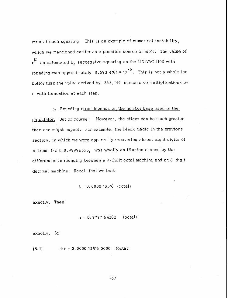
error at each squaring. This is an example of numerical instability,
which we mentioned earlier as a possible source of error, The value of
rN as calculated by successive squaring on the UNIVAC 1108 with
rounding was approximately 8.69 3 4141 X 10 -4
, This is not a whole lot
better than the value derived by 262,144 successive multiplications by
r with truncation at each step.
5. Rounding error depends on the number base used in the
calculator. But of course! However, the effect can be much greater
than one might expect. For example, the black magic in the previous
section, in which we were apparently recovering almost eight digits of
E from I-E e 0.99995555, was wholly an illusion caused by the
differences in rounding between a 9 -digit octal machine and an 8 -digit
decimal machine. Recall that we took
& = 0.0000 13516 (octal)
exactly. Then
exactly. So
r = 0.7777 64262 (octal)
(5.1) j-r = 0.0000 13516 0000 (Octal)
467

exactly. The formula (4.4), when applied properly, will give this
value to nearly 9 significant octal digit accuracy. Converted to decimal,
this means we were getting close to
0.0000 4445 0164
for E; the illusion was created that we were recovering nearly 8
decimal digits of E.
As another illustration of a startling divergence due to differences
of rounding, recall that when we calculated r N
by successive squaring,
using octal rounding, we got
8.693 4161X 10 -6
as compared with a more accurate value of
rN E 8.696 3885x10 -6 ,
However, if we start with the decimal equivalent of r,
r 4 0.99995555,
and perform successive squarings with decimal rounding, we get
N f = 8.696 0578.
If used in (4.6), this would have given
468

&E 4.445 0305x10 -5 l
If this paper has a moral, it is that cancellation and rounding
errors are more serious than is generally believed, especially if one
runs into some numerical instability. Mitigation of these effects
due to randomness of errors is not as trustworthy as one might believe
from the statistical theories that have been propounded. However, the
remedy used by many people, of going to a double precision calculation
if any suspicion of unreliability appears, will probably be entirely
adequate in all but an extremely small minority of cases. Nonetheless,
even with double precision, it is worthwhile giving thought to whether,
of several mathematically equivalent forms, one has chosen the one
least likely to produce cancellation errors, Also, if one has a sum involving
a large number of summands, it is worthwhile, and not much trouble, to
give thought to the best order of performing the summation.
REFERENCES
VI
[ 21
J. Barkley Rosser, “Potentials of charged plates, Part I, ”
MRC-TSR #1318, April 1973.
J. Barkley Rosser and N. Papamichael, “A power series
solution of a harmonic mixed boundary value problem, ”
MRC-TSR #1405, January 1975 and Technical Report TR/35,
Brunel University , December 19 7 3.
469

[ 31
141
[ 51
W
PI
183
r91
PO1
J. H, Wilkinson, “Rounding errors in algebraic processes, ”
National Physical Laboratory Notes on Applied Science, no. 32,
London, HMSO, 1963.
Peter Henrici, “Elements of numerical analysis, ” John Wiley
and Sons, Inc., New York, 1964.
Fred D. Crary and J. Barkley Rosser, “High precision coefficients
related to the zeta function, ” Mathematics Research Center
Technical Summary Report #1344, May 1, 1973.
W. Kahan, “A survey of error analysis, ” pp. 1214-1239,
Information Processing 71, Proceedings of International
Federation of Information Processing Congress 1971, Ed. C. V.
Freiman, ed., vol. II, North Holland Publishing Company, 1972.
Hans A. Rademacher, “On the accumulation of errors in
processes of integration on high-speed calculating machines, ”
pp. 176-187, Annals of the Computation Laboratory of Harvard
University, vol. XVI, Harvard University Press, 1948.
W. Kahan, “Numerical linear algebra, ” Canadian Mathematical
Bulletin, vol. 9 (1966), pp. 757-801.
J. Michael Yohe, “Roundings in floating -point arithmetic, ”
IEEE Transactions on Computers, vol. C-22 (1973), pp. 577-586.
J. Michael Yohe, “Implementing a nonstandard data type, ”
MRC-TSR #1545, June, 1975.
470

APPLICATIONS OF NUMERICAL MODELING TO COASTAL ENGINEERING PROBLEMS
H. Lee Butler and D. L. Durham Il. S. Army Engineer Waterways Experiment Station
F. 0. Box 631, Vicksburg, Miss. 39180
ABSTRACT. -- A review of the numerical modeling efforts within the Wave Dynamics Division, Hydraulic Laboratory at the Waterways Experiment Station is presented. Numerical modeling has progressed rapidly in the last several years and is now generally recognized as a useful tool capable of yielding valuable information on alternative solutions to many coastal engineering problems. Present efforts include models for application to: Wind-driven circulation; storm surge on a lake; tsunami generation and transoceanic propagation; tidal hydraulics of bays, harbors, and inlets; generation and propagation oE landslide generated water waves; and harbor oscillations, both free and forced. A discussion of the mathematical formulations and applications is given herein. Future efforts are dis- cussed which include stratified lake circulation and both deep and shallow water wind wave generation.
1. INTRODUCTION. The advent of large scale computer systems has made itpossible to use hydrodynamic theory based upon rational physical approximations rather than the dictates of mathematical tractability. Constraints still exist due to computer limitations and lack of basic understanding of certain phenomena; however, numerical modeling has progressed rapidly in the last several years. The mathematical model is now generally recognized as a tool capable of yielding valuable information on the particular phenomenon under investigation.
All of the models discussed in this paper are based on long wave theory approximations. There are many problems to which long wave theory can be applied and the degree of validity of each application is dependent on the particular approximation made and must be carefully evaluated. Long wave theory is a valid approximation when the ratio of water depth to wave length is small and the vertical component of motion does not significantly influence the pressure distribution which is assumed to be hydrostatic.
A wide range of applications together with model formulations are presented. It is not the intent of this paper to present detailed descrip- tions of models, but, instead, to indicate the level of effort being undertaken by various members of the staff at the Waterways Experiment Station. The reader is asked to consult the appropriate reference to obtain details of the model formulations.
This paper nas preserlted at the 1.975 Army Numeric:il Analysis and Computers Conference.
471

2 SCOPE OF MODELING EFFORTS. 1_-. Dynamic prediction equations based on the fundamental differential equations of hydrodynamics can be applied with minor variations to provide data on wave motion where the depth of water is small relative to the wave length. A linearized version of the model expressed in a spherical coordinate system has been used to calculate the propagation of tsunamis (originating from seismic disturbances in 12 segments of the Aleutian Trench) from their source to the west coast of the United States. The results were used to evaluate the relative vul- nerability of an area along the west coast to tsunami inudation as a function of seismic location.
A model based on the same fundamental equations, but cast into a Cartesian coordinate system, has been applied in analyzing the tidal hydraulics associated with harbors and inlets. Additional terms including non-linear inertial forces (convective forces) and bottom stress were con- sidered. The numerical tidal model has been used as a complementary tool in the operation of a physical model of the Los Angeles and Long Beach harbor complex. Such a numerical model can provide valuable information for use in the design and operation of physical models. Some of the areas to which the numerical model can be of assistance are documented below:
a. Establishing appropriate boundaries during design of the physical model which are sufficiently removed from the influence of regions to be investigated.
b. Indicating regions where data collection may be more critical or desirable.
c. Indicating possible problem areas in advance of physical model tests.
d. Providing assistance in the general interpretation of physical model results for certain phenomena.
e. Providing a "quick look" at a number of possible configurations indicating the more promising plans,
f. Providing a mechanism for investigating certain phenomena such as wind which cannot be easily introduced into the physical model.
The integration of the numerical and physical wave models allows for a more complete and comprehensive test program.
Under a project entitled, "General Investigation of Tidal Inlets" an attempt has been made to construct an idealized inlet in order to investi- gate the effects of inlet geometry, friction, and bay and tidal heights. An effort was undertaken to investigate the ability of the numerical model to reproduce localized velocity patterns. The results bore out the fact that many details of the velocity patterns seen in the physical model were reproduced in the numerical model. Applications to actual inlets have been made and comparisons with prototype elevation and velocity data obtained.
472
With minor variations the tidal model has been applied in the investi- gation of !;rndsli.de gl,eneratrd water waves. In 1971, the Hydraulics Laboratory at WRS constructed a l:I20 undistorted scale model of Libby Dam and Lake Koocanusa, Montana, and conducted tests to determine wave heights, runup and amount of overtopping resulting from the sliding of individual rock ribs into the reservoir. Subsequently a study was initi- ated at WES and directed toward developing numerical methods for predicting the effects of landslide generated water waves in reservoirs. The agree- ment between the physical and numerical mode1.s was very good considering that each set of results (f-ivc separate slides with different slide velocities) were subject to certain inherent l.imitations imposed by the model theory and otbrrs imposed by l.ack of knowledge concerning prototype conditions or how to model certain phenomena.
The Lake Erie Regional Transportation Authority is conducting a feasibility and site selection study for a ma:jor hub airport in Lhe Cleveland service area. One of the possibl.e sites being evaluated is an offshore site near Cleveland. Ohio. As a part of the feasibility analysis of an offshore site, WES is conducting a model feasibility investigation and a part of this study is to determine the effrcts of the jetport on the hydrodynamics of the surrounding area. Two of the numerical models applied so far in chc pro.ject have been used to define the effects of the jetport: on the following phcnomcna:
a. Near-field and far-field definition of the wind-driven cir- culatlon for constant density, well mixed lake conditions.
b. Storm surge at the shoreline from Lorain to Fairport, Ohio.
For many coastal engineering problems, particularly in the design of harbors, the capability of estimating the response of partially enclosed bodies of water suc:h as harbors, hays, etc., to long wave excitation can be a useful tool for preliminary investigations as well as a guide to physical model studies. The geometric shape of the harbor and the wave reflections nssociared with its boundariss produce amplification or attenuation of the incident:c? wave regi.me. This phenomenon is after refer- red to as harbor resonance or seiching and can excite adverse motion of moored ships and produce currents which may bc. hazardous to navigation. New harbors or modifications to existing harbors can be designed to minimize the effects of harbor resonance by mismatching the frequencies at which a harbor has t~laximum response and the frequencies of the pre- duminant long wave energy which is characteristic of the wave regime at the harbor site.
The major problem is how to determine accurately the amplitude distribution function and frequencies of the resonance characteristics oE a harbor. One approach is the application of numerical techniques. Two methods have been applied at WES:
473

n . A finite element method for obtaining the two-dimensional amplitude distribution and frequencies of undamped, natural modes of oscillations.
b. The solution of a boundary value problem for Long wave- induced oscillations (forced oscillations).
These methods were applied to the harbor at Port Hueneme, California, in conjunction with a physical long wave model study of the harbor. An additional application of the free oscillation model was made to l,ake Erie in order to determine the effects of a jetport structure on the free oscillations of Lake Erie.
7. TSUNAMI MODEL, A computational scheme rel.ating arbitrary sea- floor displacements and the consequent surface-wave history was developed by Hwang, Butler, and Divoky (1972). In order to permit more reliable estimates of far-field surface displacements as well as ease of including the effects of the earth's curvature, the problem was cast into a spherical. grid covering the area of interest.
The governing equations can be written as:
Momentum Equations
(1)
(2)
aLJ -.. = _ 2% at re ae av _,“_ ,_ = _ L-3 at resin6 a$
Continuity Equation
au at= ((h+q)UsinB) + g ((h+rl)V)} + g
where the spherical coordinate system is described in Figure la.
To sol.ve these equations an alternating direction technique is employed similar to that of I,eendertse (1967). A space-staggered scheme is used in which velocities, water Level, and depth are described at different points within a grid cell (Fig, lb). The first half cycle of the calculation consists of computing U and n implicitly and V explicity, advancing from time nAt to (n -I- g) At. The second half cycle computes rl and V implicitly and U explicitly, advancing from time (n f $) At to (n -I- 1) At.
By continutng these processes one can determine the values of U , V , and rl as functions of time. The finite difference equations involved in the first half cycle of the calculation are:
474
,

Fig. la. Spherical cnordinatc system
j-l
J i
j+l
k-l k ktl
0 WATER DEPTH h
X WATER LEVEL 7
- u VELOCITY IN THE DIRECTION 8
I v VELOCITY IN THE DIRECTION 4
Fig. Lb. Space-staggered grid definition
4‘J!,

(4)
(5)
n++ 'j+&k
11 = 'j+$,k
- Atg ($1: k - II;+;) 2r,A8 ' '
I-,“+‘” rln j,k = j,k - 2r ,$n6 rh( ((h+n)U sinB}?$ k - {(h-J-n)IJsit~ei~!~ k) e j
A, ,
-- +& (l(h+Wl; k++ - {(h+ri)V1;,-$} + At/, (gjn
,
These equations can be solved for U Il+$ and nn++ where terms noted with a bar are computed by averaging values of h and n to determine the barred quantities at the specific points. The explicit expression for Vn++ is
(6) Vn-t$ = v"
Atg _ --1,-.- j,k+k J.k-6 2reA[tsinBj , crl; k+l - n; k)
I
The difference equations for the second half cycle are similar with IJ and V exchanging roles.
TWO types of boundary conditions are involved in the computations. These are the solid boundaries at coastlines and the open sea boundaries arising from the need to truncate the region of computation to minimize computer core and processing time requirements. A condition of-complete reflection is adopted at solid boundaries. No dissipative factor is considered in the model at present to account for loss of tsunami energy due to shorcl.ine interaction. This condition is accomplished by settinp U=O or V-O at the appropriate boundary.
The open sea condition must simulate a total transmission of the wave through the boundary. This cannot be rigorously achieved without computation beyond the boundary and thus an artifice is adopted which assumes that the wave profile travels without change of form across the last interi.or cell of the grid at the shallow-water wave speed. This leads to the expression
(7)
where R refers to an exterior face of a boundary cell, B-l, the cor- responding interior face of the same cell, and AS the dimension of the cell normal to the boundary face.
The derivative of the ground motion term appearing in the continuity equation accounts for the time dependent vertical bottom displacement measured from a pre-quake bottom topography. If far-field results are the major interest, an initial water surface deformation is assumed instead
476

of allowing the numerical code to simulate the time dependent vertical motion. This initial surface condition conforms to the topographic features of the ocl:an floor which experiences permanent vertical displ~scement resulting from a quake disturbance. Since the characteristic time for vertical ground movement is small when compared to the long periods of tsunami waves, it is suffiriont to assume an instantaneous uplift over the entire disturbance area.
The tsunami model was verified by hindcasting the 1964 Alaskan Tsunami (Hwang, et al; 1972). With obsc?-rvations of genernted bottom di.splaccmcnts and distant wave histories available, the computed and observed waves compared well in amplitude and phase of the dominant lead- i r1g wave.
Results of the Aleutian Trench study (Whalin, Garcia, and Butler; 1974) indicate that the tsunami generated hy the 1964 Alaskan quake may not be a t-arc event at all. Further, a tsunami of equal intensity result- ing from a seismic disturbance located elsewhere in the Aleutian Trench could cause significantly higher runup at particular west coast locations. Figure 2 di.splays a sample plot of surface elevation contours at a time of 4 hours following a hypothetical disturbance in segment 7 of the
Aleutian Trench (a source location south of Shumagin Island).
4 TIDAL MODEL. -:....-. A numerical tidal model, based upon the original formulation by Leendertse (1967), has been applied at WES to analyze the tidal hydraulics of harbors and inlets, Again the fundamental equations are averaged over the vertical dimension and expressed in a Cartesian coordinate system to yield
Momentum Eqrlations
(9)
(10)
Continuity Equation
where the stress terms
Bottom stress
{(h+rl)Ul + g {(h+n)Vj = 0
are defined as
(11)
,--_-_.- T; = @ &+V2
c2
477


and -“-
(12) TY = BV Jt12+v2
B c2 Wind stress
(13) -r 1‘ w
= c&y
The major assumptions involved along with the consequence of each assumption are outlined below:
a. Internally the fluid is inviscid (horizontal and vertical eddy viscosity terms are considered to be negligible).
h. 'The fluid is incompressible (continuity equation and gravity term are simpliEied).
c. The vertical component of the fluid acceleration is negligible (momentum equation in the vortiral. direction reduces to the hydrostatic pressure variation).
d. 'The fluid 4s we.11 mixed so that the variations of flow in the vertical direction are small (allowing the averaging of flow quantities over the vertical).
'To solve the above system of equations numerically the differential equaLions must be discretized and replaced by a system of finite diffcrcnce equations using central differences on a space-staggered grid as in the case with the tsunami model, Again, Leendertsc's implicit-explicit mult.i- operational method is employed in determining the solution for IJ , V , and n it s functions of time.
The difference equations for the second half cycle are written as:
(14)
(15)
V IlSl = Vtl+" gAt - 7jg~ <rly> d-1
- 4rix" At = n+$V >n+$
X
At - ---v 4Ay
n+lCV >r& At p y' -2-y at j, k+$
n-t-1 rl =rl
11+45 - $; i.(h+rl)U> X
n++ _ at <(hfrl)v,yn+l 2Ay at j, k
‘I’hes~ equations are solved for V"+l and r)n+l along a grid line j . For simplicity of notation some terms have been maintained in differential form within angle brackets < >. Central differences are used in evaluat- ing these terms. The additional velocity component ~n+l can be determined explicitly irom the equation

The expressions fur the forcing terms I: ant F :1rc written as x Y
In addition the terms signified by a singl.c bar are not defined at the point whcrc the equation is written and are determined by averaging two neighboring values. The terms signified by a doubie bar require four neighboring values to obtain an average.
Three types of boundaries arc+ tnvolved in the calculations:
a. A condition of complete reflection is considered at solid boundaries.
h. Tidal elevations are input data at artificial ocean boundaries.
c. Tidal elevations or average fluid velocities are input data at artificial boundaries in the inlet, harbor or bay.
Sufficient prototype data must be available to operate and/or verify the model. Along these lines, it should be emphasized that tidal elevations or average fluid velocities must he defined at all artificial boundaries in the inlet, harhor or boy.
From a consideration of the assumptions involved in the development of the model, it is apparent that it should be most applicable for consider- ing long period waves in non-stratified regions where vertical accelerations arc small.. The model provides no indication of the vertical distribution of velocity. Phenomena which depend on the. detailed velocity distribution as a function of the depth cannot be investigated.
As mentioned previously, applications of the model at WES include the Los Angeles-Long Beach Harbor area and an idealized inlet model. Figure 3 illustrates the tidal velocity field for a portion of the LA-LB harbor. The treatment of breakwaters and piers on piles are of particular interest in this application. The frictional coefficients were varied to simulate the resistance of these structures to the flow. Approximately 1600 grid points were used in the computational grid.
.5 - LANDSLLDE MODEL. A numerical. model for the generation and propagation of landslide-generated water waves in reservoirs was developed at WES (Raney and Butler; 1975) as part of an effort directed toward
480

. - , I . . - - . ~ 1 3 I . . “ ” , . - .
/
/
L _ -".-.- / .' / . ) r-----, ..^- 1 f L---L--- -_-- * I’-““ -----I
_._,“._ -.. ,.. J
* .‘I
Fig. 3. Illustration of a tidal velocity flow field for a portion of the Los Angeles-Long Beach Harbor Complex

finding analytical and/or numerical methods for predicting the effects of these waves. It was decided that a promising i.nitial approach for the investigation involved using a depth averaged formuJ.ation of the fluid mechanics equations.
The tidal model as discussed previously can be adopted with appropriate modifications to eval.uatc the arrival time and height of the first wave crest which may result from a landslide. Results from the physical model study conducted at WlZS (Davidson and Whalin; 1974) indicated that in most cases the first wave crest was the largest measured at each of the model gauges. The pertinent modifications to the tidal model are:
a. A vertical bottom deformation term representing the passage and settling of landslide material is introduced into the continuity equation in a manner similar to the ground motion term appearing in the tsunami model.
b . The acceleration effect of the l.andslide on the fluid with which it is in contact is introduced into the momentum equations as part of the forcing terms.
Thus the equations can be written as:
Momentum Equations
(19)
(20) av av av an T< t L& + ~~~ I- gay = Ry + Ly
Continuity Equation
The method of solution is identical to that used in the tidal model..
Boundary conditions are similar to those adopted in the tsunami model. The fictitious open boundaries arise from the need to truncate the region of computation (in order to minimize computational time requirements). Also considered is a time dependent boundary between the landslide surface and the water in the reservoir.
The landslide is represented by a time dependent deformation of the bottom of the reservoir plus additional terms to represent the effect of the landslide on the reservoir due to viscous and inertia forces. The bottom deformation propagates into specified regions of the reservoir at
482

the average speed of the landslide with the deformation at any particular location increasing from zero to a maximum value according to a specified time-displac:ement relationship. For those .portions of the bottom of the reservoir through which the landslide passes but which do not experience n net change in ground elevation 3s a result of the ffnal slide deposi- t i 0 n I the deformation is allowed to return to zero at a specified rate. Th(‘ handling of the landslide condition is illustrated in Fig. 4* The direction, cxrent, and magnitude of the botrom deformation is .detertnincd by knowledge or assumptions concerning the path and f'inal disposition of the particular landslide.
The water in the reservoir experiences an acceleration due to the rorce exerted by the landslide at the time dependent boundary between rhe water and the landslide. This force per unit mass is considcrcd to consist of a component due to the displacement oi the water hy the slide plus two components which act on fluid elements in contact with the landslide:
(22) 5 = cx(V X
- u>2 f D (V - u)* X
(23) L = tx(V Y Y
- VJ2 + a (V - ")' Y
where
vx =the x component of the landslide velocity
V Y
= the y component of the landslide velocity
Yy = viscous drag paramtr,ter
fi = pressure drag parameter
The first component of L and L is related to the viscous drag exerted by the slide upon the fluid wYth which it is in contact. The second component of L and I, expresses a pressure drag exerted on the water by the front ofXthe slyde. The viscous drag is considered to act at all points of contact between the slide and the water. The pressure drag acts only at the leading face of the landslide.
The landslide is thus represented numerically by a combination of terms whose net effect in the numerical model. should be a reasonable representation of the large scale physical effects produced by a landslide entering a reservoir. A representation of the landsl.idc propagates into the numerical representation of the reservoir, accelerating the fluid due to physical displacement, viscous effects, and pressure drag effects. The resulting waves propagate across the reservoir in accordance with the governing equations. The wave height and velocity components are calculated for each grid cell at the end of each time step.
483

----- 1 / /’ / / Y t= t, I y-I t=t,
X
TOP VIEW
A Z
UNDLTURBED WATER SURFACE X / /=-; -- -- _ -- 1 -
SIDE VIEW
Fig. 4. Landslide model
4e4